IBM Visualization Data Explorer User's Guide - Theochem ...

IBM

IBM Visualization Data Explorer

User’s Guide

Version 3 Release 1 Modification 4

SC38-0496-06

IBM IBM Visualization Data Explorer

User’s Guide

Version 3 Release 1 Modification 4

SC38-0496-06

Note!

Before using this information and the product it supports, be sure to read the general information under “Notices” on page xiii.

Seventh Edition (May 1997)

This edition applies to IBM Visualization Data Explorer Version 3.1.4, to IBM Visualization Data Explorer SMP Version 3.1.4, and toall subsequent releases and modifications thereof until otherwise indicated in new editions. Make sure you are using the correctedition for the level of the product. Order publications through your IBM representative or the IBM branch office serving your locality.Publications are not stocked at the address given below.

A form for readers’ comments appears at the back of this publication. If the form has been removed, address your comments to:

IBM CorporationThomas J. Watson Research Center/HawthorneData Explorer DevelopmentP.O. Box 704Yorktown Heights, NY 10598-0704

USA

If you send information to IBM, you grant IBM a nonexclusive right to use or distribute that information, in any way it believesappropriate, without incurring any obligation to you.

Copyright International Business Machines Corporation 1991-1997. All rights reserved.Note to U.S. Government Users — Documentation related to restricted rights — Use, duplication or disclosure is subject torestrictions set forth in GSA ADP Schedule Contract with IBM Corp.

Contents

Figures . . . . . . . . . . . . . . . . . . . . . . . . . . . . . . . . . . . . . . . . . . ix

Tables . . . . . . . . . . . . . . . . . . . . . . . . . . . . . . . . . . . . . . . . . . . xi

Notices . . . . . . . . . . . . . . . . . . . . . . . . . . . . . . . . . . . . . . . . . xiiiProducts, Programs, and Services . . . . . . . . . . . . . . . . . . . . . . . . . . xivTrademarks and Service Marks . . . . . . . . . . . . . . . . . . . . . . . . . . . xivCopyright notices . . . . . . . . . . . . . . . . . . . . . . . . . . . . . . . . . . . . xv

About This Guide . . . . . . . . . . . . . . . . . . . . . . . . . . . . . . . . . . . xxiWho Should Use It . . . . . . . . . . . . . . . . . . . . . . . . . . . . . . . . . . . xxiiHow To Use It . . . . . . . . . . . . . . . . . . . . . . . . . . . . . . . . . . . . . xxiiTypographic Conventions . . . . . . . . . . . . . . . . . . . . . . . . . . . . . . xxiiiRelated Publications and Sources . . . . . . . . . . . . . . . . . . . . . . . . . xxiii

IBM Publications . . . . . . . . . . . . . . . . . . . . . . . . . . . . . . . . . . xxiiiNon-IBM Publications . . . . . . . . . . . . . . . . . . . . . . . . . . . . . . . xxivOther sources of information . . . . . . . . . . . . . . . . . . . . . . . . . . . xxiv

New Features in Data Explorer Version 3.1.4 . . . . . . . . . . . . . . . . . xxviiUser Interface . . . . . . . . . . . . . . . . . . . . . . . . . . . . . . . . . . . . . xxviii

New Startup Behavior . . . . . . . . . . . . . . . . . . . . . . . . . . . . . . xxviiiNew Save Image Dialog in Image Window . . . . . . . . . . . . . . . . . . xxviiiNew Data Prompter . . . . . . . . . . . . . . . . . . . . . . . . . . . . . . . . xxviiiPages . . . . . . . . . . . . . . . . . . . . . . . . . . . . . . . . . . . . . . . . xxviiiAnnotation . . . . . . . . . . . . . . . . . . . . . . . . . . . . . . . . . . . . . xxviiiOptimizing Caching . . . . . . . . . . . . . . . . . . . . . . . . . . . . . . . . xxviii

Changes to Get and Set modules . . . . . . . . . . . . . . . . . . . . . . . . . xxixNew Window Management Functionality . . . . . . . . . . . . . . . . . . . . . xxixHardware Rendering . . . . . . . . . . . . . . . . . . . . . . . . . . . . . . . . . xxixDXLink . . . . . . . . . . . . . . . . . . . . . . . . . . . . . . . . . . . . . . . . . xxixChanged Modules . . . . . . . . . . . . . . . . . . . . . . . . . . . . . . . . . . . xxxNew Modules . . . . . . . . . . . . . . . . . . . . . . . . . . . . . . . . . . . . . xxxiBackward Incompatibilities . . . . . . . . . . . . . . . . . . . . . . . . . . . . . xxxiiiHTML Documentation . . . . . . . . . . . . . . . . . . . . . . . . . . . . . . . . xxxivFixes . . . . . . . . . . . . . . . . . . . . . . . . . . . . . . . . . . . . . . . . . . xxxiv

Chapter 1. Overview . . . . . . . . . . . . . . . . . . . . . . . . . . . . . . . . . . 11.1 Overview of Data Explorer . . . . . . . . . . . . . . . . . . . . . . . . . . . . . 21.2 System Structure . . . . . . . . . . . . . . . . . . . . . . . . . . . . . . . . . . 3

Graphical User Interface . . . . . . . . . . . . . . . . . . . . . . . . . . . . . . . 3Executive . . . . . . . . . . . . . . . . . . . . . . . . . . . . . . . . . . . . . . . . 4Modules . . . . . . . . . . . . . . . . . . . . . . . . . . . . . . . . . . . . . . . . 4Data Management . . . . . . . . . . . . . . . . . . . . . . . . . . . . . . . . . . . 4How the Data Model Facilitates Interoperability . . . . . . . . . . . . . . . . . . 4

Chapter 2. Introduction to Visualization . . . . . . . . . . . . . . . . . . . . . . 72.1 Terminology . . . . . . . . . . . . . . . . . . . . . . . . . . . . . . . . . . . . . 8

Rendering . . . . . . . . . . . . . . . . . . . . . . . . . . . . . . . . . . . . . . . 8Positions and Connections Dependence . . . . . . . . . . . . . . . . . . . . . . 8Connections and Interpolation . . . . . . . . . . . . . . . . . . . . . . . . . . . . 9

Copyright IBM Corp. 1991-1997 iii

Identifying Connections . . . . . . . . . . . . . . . . . . . . . . . . . . . . . . . 11Invalid Data . . . . . . . . . . . . . . . . . . . . . . . . . . . . . . . . . . . . . 12Fields . . . . . . . . . . . . . . . . . . . . . . . . . . . . . . . . . . . . . . . . . 12

2.2 Visual Programming: The Basics . . . . . . . . . . . . . . . . . . . . . . . . 13

Chapter 3. Understanding the Data Model . . . . . . . . . . . . . . . . . . . 153.1 Introduction to the Data Model . . . . . . . . . . . . . . . . . . . . . . . . . 163.2 Object Types . . . . . . . . . . . . . . . . . . . . . . . . . . . . . . . . . . . 17

Fields . . . . . . . . . . . . . . . . . . . . . . . . . . . . . . . . . . . . . . . . . 17Arrays . . . . . . . . . . . . . . . . . . . . . . . . . . . . . . . . . . . . . . . . . 28Groups . . . . . . . . . . . . . . . . . . . . . . . . . . . . . . . . . . . . . . . . 34

Chapter 4. Data Explorer Execution Model . . . . . . . . . . . . . . . . . . . 374.1 Data Flow . . . . . . . . . . . . . . . . . . . . . . . . . . . . . . . . . . . . . 384.2 Iterative Execution and Caching of Intermediate Results . . . . . . . . . . 404.3 Conditional Execution: Route and Switch . . . . . . . . . . . . . . . . . . . 414.4 Iteration using the Sequencer . . . . . . . . . . . . . . . . . . . . . . . . . . 434.5 Iteration using Looping . . . . . . . . . . . . . . . . . . . . . . . . . . . . . . 444.6 Preserving Explicit State . . . . . . . . . . . . . . . . . . . . . . . . . . . . . 454.7 Advanced Looping Constructs . . . . . . . . . . . . . . . . . . . . . . . . . . 504.8 External Asynchronous Data Sources . . . . . . . . . . . . . . . . . . . . . 544.9 Parallelism using Distributed Processing . . . . . . . . . . . . . . . . . . . . 554.10 Parallelism for Data Explorer SMP . . . . . . . . . . . . . . . . . . . . . . 56

Chapter 5. Graphical User Interface: Basics . . . . . . . . . . . . . . . . . . 575.1 Starting Data Explorer . . . . . . . . . . . . . . . . . . . . . . . . . . . . . . 58

Using Environment Variables . . . . . . . . . . . . . . . . . . . . . . . . . . . 595.2 Understanding Data Explorer Windows . . . . . . . . . . . . . . . . . . . . 60

Looking at Window Structure . . . . . . . . . . . . . . . . . . . . . . . . . . . 61Using the Mouse . . . . . . . . . . . . . . . . . . . . . . . . . . . . . . . . . . 62Moving and Resizing Windows . . . . . . . . . . . . . . . . . . . . . . . . . . 62Selecting Pull-Down Menus and Pull-Down Menu Options . . . . . . . . . . 62Selecting and Deselecting Items with the Mouse . . . . . . . . . . . . . . . . 63Selecting a Choice in an Option Box . . . . . . . . . . . . . . . . . . . . . . . 63Editing Text Fields . . . . . . . . . . . . . . . . . . . . . . . . . . . . . . . . . 64Working with Windows . . . . . . . . . . . . . . . . . . . . . . . . . . . . . . . 65

5.3 Using Online Help . . . . . . . . . . . . . . . . . . . . . . . . . . . . . . . . . 65User-Defined Help Files . . . . . . . . . . . . . . . . . . . . . . . . . . . . . . 67

5.4 Executing a Visual Program . . . . . . . . . . . . . . . . . . . . . . . . . . . 67Using the Sequencer . . . . . . . . . . . . . . . . . . . . . . . . . . . . . . . . 68Using a Data-Driven Sequencer . . . . . . . . . . . . . . . . . . . . . . . . . . 70Error Messages . . . . . . . . . . . . . . . . . . . . . . . . . . . . . . . . . . . 71

Chapter 6. Graphical User Interface: Important Windows . . . . . . . . . . 736.1 Using the Image Window . . . . . . . . . . . . . . . . . . . . . . . . . . . . 74

Controlling the Image: View Control... . . . . . . . . . . . . . . . . . . . . . . 74Undo, Redo, and Reset . . . . . . . . . . . . . . . . . . . . . . . . . . . . . . 87AutoAxes... . . . . . . . . . . . . . . . . . . . . . . . . . . . . . . . . . . . . . 88Set Background Color... . . . . . . . . . . . . . . . . . . . . . . . . . . . . . . 89Display Rotation Globe . . . . . . . . . . . . . . . . . . . . . . . . . . . . . . . 91Rendering Options... . . . . . . . . . . . . . . . . . . . . . . . . . . . . . . . . 91Image Depth . . . . . . . . . . . . . . . . . . . . . . . . . . . . . . . . . . . . . 93Changing the Rate of Frame Display: Throttle... . . . . . . . . . . . . . . . . 93Changing the Title of an Image Window . . . . . . . . . . . . . . . . . . . . . 93

iv IBM Visualization Data Explorer: User’s Guide

Control Panel Access... . . . . . . . . . . . . . . . . . . . . . . . . . . . . . . 94Saving an Image . . . . . . . . . . . . . . . . . . . . . . . . . . . . . . . . . . 94Printing an Image . . . . . . . . . . . . . . . . . . . . . . . . . . . . . . . . . . 97

6.2 Using the VPE . . . . . . . . . . . . . . . . . . . . . . . . . . . . . . . . . . . 99Creating a Visual Program . . . . . . . . . . . . . . . . . . . . . . . . . . . . 100Specifying Values for a Tool's Inputs . . . . . . . . . . . . . . . . . . . . . . 103Creating, Deleting, and Moving Tab Connections . . . . . . . . . . . . . . . 104Moving and Copying Tools . . . . . . . . . . . . . . . . . . . . . . . . . . . . 105Using Transmitters and Receivers . . . . . . . . . . . . . . . . . . . . . . . 106Adding and Removing Input and Output Tabs . . . . . . . . . . . . . . . . 106Entering Values in a Configuration Dialog Box . . . . . . . . . . . . . . . . 107Revealing and Hiding Input Tabs . . . . . . . . . . . . . . . . . . . . . . . . 110Using the Compute Module Configuration Dialog Box . . . . . . . . . . . . 111Locating Tools: The Find Tool Dialog Box . . . . . . . . . . . . . . . . . . . 111Customizing the VPE Window . . . . . . . . . . . . . . . . . . . . . . . . . . 113Adding Comments to a Visual Program . . . . . . . . . . . . . . . . . . . . 114Adding Annotation to a Visual Program . . . . . . . . . . . . . . . . . . . . 115Creating pages in the VPE . . . . . . . . . . . . . . . . . . . . . . . . . . . . 115Saving and Restoring a Visual Program . . . . . . . . . . . . . . . . . . . . 115

6.3 Using the Colormap Editor . . . . . . . . . . . . . . . . . . . . . . . . . . . 119Entering Values in a Colormap Editor . . . . . . . . . . . . . . . . . . . . . 121Using Data-Driven Colormap Editors . . . . . . . . . . . . . . . . . . . . . . 125

Chapter 7. Graphical User Interface: Control Panels, Interactors, andMacros . . . . . . . . . . . . . . . . . . . . . . . . . . . . . . . . . . . . . . . . 127

7.1 Using Control Panels and Interactors . . . . . . . . . . . . . . . . . . . . 128Building Control Panels . . . . . . . . . . . . . . . . . . . . . . . . . . . . . . 129Placing Interactors in a New Control Panel . . . . . . . . . . . . . . . . . . 130Adding Interactors to an Existing Control Panel . . . . . . . . . . . . . . . . 130Selecting, Moving, and Deleting Interactors . . . . . . . . . . . . . . . . . . 131Changing the Size of an Interactor . . . . . . . . . . . . . . . . . . . . . . . 132Locating Interactor Stand-ins . . . . . . . . . . . . . . . . . . . . . . . . . . 132Deleting Control Panels . . . . . . . . . . . . . . . . . . . . . . . . . . . . . 132Saving and Restoring Control Panels . . . . . . . . . . . . . . . . . . . . . 132Customizing a Control Panel . . . . . . . . . . . . . . . . . . . . . . . . . . 133Control Panels as Dialog Boxes . . . . . . . . . . . . . . . . . . . . . . . . . 138Control Panel Access, Groups, and Hierarchies . . . . . . . . . . . . . . . 138Creating, Modifying, and Deleting Control Panel Groups . . . . . . . . . . 139Restricting Control Panel Access . . . . . . . . . . . . . . . . . . . . . . . . 140Specifying a Startup Control Panel . . . . . . . . . . . . . . . . . . . . . . . 141Opening Existing Control Panels . . . . . . . . . . . . . . . . . . . . . . . . 141Using Interactors . . . . . . . . . . . . . . . . . . . . . . . . . . . . . . . . . 142Using Data-Driven Interactors . . . . . . . . . . . . . . . . . . . . . . . . . . 147

7.2 Creating and Using Macros . . . . . . . . . . . . . . . . . . . . . . . . . . 149Creating Macros . . . . . . . . . . . . . . . . . . . . . . . . . . . . . . . . . . 149Loading Macros . . . . . . . . . . . . . . . . . . . . . . . . . . . . . . . . . . 152Using Macros in a Visual Program . . . . . . . . . . . . . . . . . . . . . . . 153Viewing and Changing Macros . . . . . . . . . . . . . . . . . . . . . . . . . 154

Chapter 8. Graphical User Interface: Menus, Options, and the MessageWindow . . . . . . . . . . . . . . . . . . . . . . . . . . . . . . . . . . . . . . . 155

8.1 Using the Primary Window Pull-Down Menus and Options . . . . . . . . 156VPE Window Menu Bar . . . . . . . . . . . . . . . . . . . . . . . . . . . . . 156Control Panel Menu Bar . . . . . . . . . . . . . . . . . . . . . . . . . . . . . 162

Contents v

Image Window Menu Bar . . . . . . . . . . . . . . . . . . . . . . . . . . . . 165Colormap Menu Bar . . . . . . . . . . . . . . . . . . . . . . . . . . . . . . . 168Menu Bar Menu Bar . . . . . . . . . . . . . . . . . . . . . . . . . . . . . . . 170Message Window Menu Bar . . . . . . . . . . . . . . . . . . . . . . . . . . . 172

8.2 Using the Message Window . . . . . . . . . . . . . . . . . . . . . . . . . . 174

Chapter 9. Graphical User Interface: For Advanced Users . . . . . . . . 1779.1 Using Distributed Computation . . . . . . . . . . . . . . . . . . . . . . . . 178

Creating, Modifying, and Deleting Execution Groups . . . . . . . . . . . . . 178Displaying the Tools in an Execution Group . . . . . . . . . . . . . . . . . . 180Assigning Execution Groups to Workstations . . . . . . . . . . . . . . . . . 181Restrictions . . . . . . . . . . . . . . . . . . . . . . . . . . . . . . . . . . . . . 182

9.2 Loading and Using Outboard and Runtime-Loadable Modules . . . . . . 1839.3 Connecting to the Server . . . . . . . . . . . . . . . . . . . . . . . . . . . 183

Resetting the Server . . . . . . . . . . . . . . . . . . . . . . . . . . . . . . . 185

Chapter 10. Data Explorer Scripting Language . . . . . . . . . . . . . . . 18710.1 Starting Data Explorer in Script Mode . . . . . . . . . . . . . . . . . . . 188

Setting Environment Variables . . . . . . . . . . . . . . . . . . . . . . . . . . 18910.2 Understanding the Script Structure . . . . . . . . . . . . . . . . . . . . . 18910.3 Language Delimiters . . . . . . . . . . . . . . . . . . . . . . . . . . . . . 191

Commenting Scripts . . . . . . . . . . . . . . . . . . . . . . . . . . . . . . . 191Naming Variables and Macros . . . . . . . . . . . . . . . . . . . . . . . . . . 192Specifying Values in a Script . . . . . . . . . . . . . . . . . . . . . . . . . . 193

10.4 Building Expressions and Statements . . . . . . . . . . . . . . . . . . . 197Arithmetic Expressions . . . . . . . . . . . . . . . . . . . . . . . . . . . . . . 197Assignment Statements . . . . . . . . . . . . . . . . . . . . . . . . . . . . . 198Function Call Assignments . . . . . . . . . . . . . . . . . . . . . . . . . . . . 199

10.5 Invoking Data Explorer Macros and Modules . . . . . . . . . . . . . . . 200Function Call Arguments . . . . . . . . . . . . . . . . . . . . . . . . . . . . . 200Function Call Attributes . . . . . . . . . . . . . . . . . . . . . . . . . . . . . . 202

10.6 Defining Macros . . . . . . . . . . . . . . . . . . . . . . . . . . . . . . . . 204Macro Header . . . . . . . . . . . . . . . . . . . . . . . . . . . . . . . . . . . 204Macro Body . . . . . . . . . . . . . . . . . . . . . . . . . . . . . . . . . . . . 205Macro Examples . . . . . . . . . . . . . . . . . . . . . . . . . . . . . . . . . . 205

10.7 Using Data Explorer Script Commands . . . . . . . . . . . . . . . . . . . 206Sequencer . . . . . . . . . . . . . . . . . . . . . . . . . . . . . . . . . . . . . 206File Inclusion . . . . . . . . . . . . . . . . . . . . . . . . . . . . . . . . . . . . 207Prompts . . . . . . . . . . . . . . . . . . . . . . . . . . . . . . . . . . . . . . . 207

10.8 Understanding the Script Execution Model . . . . . . . . . . . . . . . . . 208Top-level Environment . . . . . . . . . . . . . . . . . . . . . . . . . . . . . . 208Function Execution . . . . . . . . . . . . . . . . . . . . . . . . . . . . . . . . 208Macro Expansion . . . . . . . . . . . . . . . . . . . . . . . . . . . . . . . . . 208Variables Used in Macros . . . . . . . . . . . . . . . . . . . . . . . . . . . . 208Assignment and Function Call Semantics . . . . . . . . . . . . . . . . . . . 209Execution Example . . . . . . . . . . . . . . . . . . . . . . . . . . . . . . . . 210

10.9 Running .net files in script mode . . . . . . . . . . . . . . . . . . . . . . 210

Appendix A. Using Data Explorer: Some Useful Hints . . . . . . . . . . . 211A.1 Using Data Explorer Effectively . . . . . . . . . . . . . . . . . . . . . . . . 212

Common Problems . . . . . . . . . . . . . . . . . . . . . . . . . . . . . . . . 212What is the Difference Between Image and Display? . . . . . . . . . . . . 212How do I get more information? . . . . . . . . . . . . . . . . . . . . . . . . . 213Memory Use . . . . . . . . . . . . . . . . . . . . . . . . . . . . . . . . . . . . 213

vi IBM Visualization Data Explorer: User’s Guide

A.2 Visualization Techniques . . . . . . . . . . . . . . . . . . . . . . . . . . . 217Animation . . . . . . . . . . . . . . . . . . . . . . . . . . . . . . . . . . . . . . 217Annotation . . . . . . . . . . . . . . . . . . . . . . . . . . . . . . . . . . . . . 218Color Mapping . . . . . . . . . . . . . . . . . . . . . . . . . . . . . . . . . . . 219Contours and Isosurfaces . . . . . . . . . . . . . . . . . . . . . . . . . . . . 221Mapping . . . . . . . . . . . . . . . . . . . . . . . . . . . . . . . . . . . . . . 223Normals and Shading . . . . . . . . . . . . . . . . . . . . . . . . . . . . . . . 224Plots and Histograms . . . . . . . . . . . . . . . . . . . . . . . . . . . . . . . 227Rubbersheet . . . . . . . . . . . . . . . . . . . . . . . . . . . . . . . . . . . . 227Transformations and Structuring . . . . . . . . . . . . . . . . . . . . . . . . 228Vector Fields . . . . . . . . . . . . . . . . . . . . . . . . . . . . . . . . . . . . 229Volume Rendering . . . . . . . . . . . . . . . . . . . . . . . . . . . . . . . . 231

A.3 Design for Interactive Use . . . . . . . . . . . . . . . . . . . . . . . . . . . 232Interactors and Control Panels . . . . . . . . . . . . . . . . . . . . . . . . . 232Transmitters and Receivers . . . . . . . . . . . . . . . . . . . . . . . . . . . 234Documentation . . . . . . . . . . . . . . . . . . . . . . . . . . . . . . . . . . . 235

A.4 Design for Video Output . . . . . . . . . . . . . . . . . . . . . . . . . . . . 236TV Line Resolution . . . . . . . . . . . . . . . . . . . . . . . . . . . . . . . . 236TV Color Resolution . . . . . . . . . . . . . . . . . . . . . . . . . . . . . . . 237Animation and Frame Rates . . . . . . . . . . . . . . . . . . . . . . . . . . . 237

A.5 Presentation: Issues and Techniques . . . . . . . . . . . . . . . . . . . . 238

Appendix B. Importing Data: File Formats . . . . . . . . . . . . . . . . . . 241B.1 General Array Importer: Keyword Information from Data Files . . . . . . 242B.2 Data Explorer Native Files . . . . . . . . . . . . . . . . . . . . . . . . . . . 244

Overview of the Native File Format . . . . . . . . . . . . . . . . . . . . . . . 244Examples . . . . . . . . . . . . . . . . . . . . . . . . . . . . . . . . . . . . . . 246Syntax of the Native File Format . . . . . . . . . . . . . . . . . . . . . . . . 268Objects . . . . . . . . . . . . . . . . . . . . . . . . . . . . . . . . . . . . . . . 269Group Objects . . . . . . . . . . . . . . . . . . . . . . . . . . . . . . . . . . . 270Series Objects . . . . . . . . . . . . . . . . . . . . . . . . . . . . . . . . . . . 271Multigrid Objects . . . . . . . . . . . . . . . . . . . . . . . . . . . . . . . . . . 271Composite Field Objects . . . . . . . . . . . . . . . . . . . . . . . . . . . . . 271Field Objects . . . . . . . . . . . . . . . . . . . . . . . . . . . . . . . . . . . . 272Array Objects . . . . . . . . . . . . . . . . . . . . . . . . . . . . . . . . . . . 272Constant Array Objects . . . . . . . . . . . . . . . . . . . . . . . . . . . . . . 273gridpositions Keyword . . . . . . . . . . . . . . . . . . . . . . . . . . . . . . 274Regular Array Objects . . . . . . . . . . . . . . . . . . . . . . . . . . . . . . 274Product Array Objects . . . . . . . . . . . . . . . . . . . . . . . . . . . . . . 275gridconnections Keyword . . . . . . . . . . . . . . . . . . . . . . . . . . . . . 275Path Array Objects . . . . . . . . . . . . . . . . . . . . . . . . . . . . . . . . 276Mesh Array Objects . . . . . . . . . . . . . . . . . . . . . . . . . . . . . . . . 276Xform Objects . . . . . . . . . . . . . . . . . . . . . . . . . . . . . . . . . . . 277String Objects . . . . . . . . . . . . . . . . . . . . . . . . . . . . . . . . . . . 277Light Objects . . . . . . . . . . . . . . . . . . . . . . . . . . . . . . . . . . . . 277Camera Objects . . . . . . . . . . . . . . . . . . . . . . . . . . . . . . . . . . 278Clipped Objects . . . . . . . . . . . . . . . . . . . . . . . . . . . . . . . . . . 278Screen Objects . . . . . . . . . . . . . . . . . . . . . . . . . . . . . . . . . . 278Data Mode Clause . . . . . . . . . . . . . . . . . . . . . . . . . . . . . . . . 278Default Clause . . . . . . . . . . . . . . . . . . . . . . . . . . . . . . . . . . . 279End Clause . . . . . . . . . . . . . . . . . . . . . . . . . . . . . . . . . . . . . 279

B.3 CDF Files . . . . . . . . . . . . . . . . . . . . . . . . . . . . . . . . . . . . 279B.4 netCDF Files . . . . . . . . . . . . . . . . . . . . . . . . . . . . . . . . . . 281

Regular Grids . . . . . . . . . . . . . . . . . . . . . . . . . . . . . . . . . . . 281

Contents vii

B.5 netCDF Files: Complex Fields . . . . . . . . . . . . . . . . . . . . . . . . 282Irregular Arrays . . . . . . . . . . . . . . . . . . . . . . . . . . . . . . . . . . 282Series Data . . . . . . . . . . . . . . . . . . . . . . . . . . . . . . . . . . . . 284Examples . . . . . . . . . . . . . . . . . . . . . . . . . . . . . . . . . . . . . . 286

B.6 HDF Files . . . . . . . . . . . . . . . . . . . . . . . . . . . . . . . . . . . . 288

Appendix C. Environment Variables and Command Line Options . . . . 291C.1 Environment Variables . . . . . . . . . . . . . . . . . . . . . . . . . . . . . 292

Path Variables . . . . . . . . . . . . . . . . . . . . . . . . . . . . . . . . . . . 292Other Environment Variables . . . . . . . . . . . . . . . . . . . . . . . . . . 292

C.2 Command Line Options . . . . . . . . . . . . . . . . . . . . . . . . . . . . 295

Appendix D. User Interface Configuration . . . . . . . . . . . . . . . . . . 299

Appendix E. Data Explorer Fonts . . . . . . . . . . . . . . . . . . . . . . . . 307

Appendix F. Data Explorer Colors . . . . . . . . . . . . . . . . . . . . . . . 313

Appendix G. Accelerator Keys . . . . . . . . . . . . . . . . . . . . . . . . . 315

Glossary . . . . . . . . . . . . . . . . . . . . . . . . . . . . . . . . . . . . . . . 317

Index . . . . . . . . . . . . . . . . . . . . . . . . . . . . . . . . . . . . . . . . . . 323

viii IBM Visualization Data Explorer: User’s Guide

Figures

1. Examples of Data Dependency . . . . . . . . . . . . . . . . . . . . . . . . 102. Example of a Field Object . . . . . . . . . . . . . . . . . . . . . . . . . . . 183. Shared Components among Different Fields . . . . . . . . . . . . . . . . . 194. Order of Vertices in Triangles and Tetrahedra . . . . . . . . . . . . . . . . 215. Order of Vertices in Quads and Cuboids . . . . . . . . . . . . . . . . . . . 216. Examples of Grid Types . . . . . . . . . . . . . . . . . . . . . . . . . . . . 227. Use of Faces, Loops, and Edge Components . . . . . . . . . . . . . . . . 268. Example of an Irregular Array . . . . . . . . . . . . . . . . . . . . . . . . . 299. Example of a Regular Array . . . . . . . . . . . . . . . . . . . . . . . . . . 29

10. Example of a Product Array . . . . . . . . . . . . . . . . . . . . . . . . . . 3011. Product Array of Two Regular Arrays . . . . . . . . . . . . . . . . . . . . . 3112. Example of a Path Array . . . . . . . . . . . . . . . . . . . . . . . . . . . . 3113. Example of a Mesh Array . . . . . . . . . . . . . . . . . . . . . . . . . . . . 3214. Mesh Array of Two Path Arrays (with Regular Connections) . . . . . . . 3315. Example of a Constant Array . . . . . . . . . . . . . . . . . . . . . . . . . . 3316. Example of a Group . . . . . . . . . . . . . . . . . . . . . . . . . . . . . . . 3417. Example of a Series Group . . . . . . . . . . . . . . . . . . . . . . . . . . . 3518. Example 1 . . . . . . . . . . . . . . . . . . . . . . . . . . . . . . . . . . . . 3919. Example 2 . . . . . . . . . . . . . . . . . . . . . . . . . . . . . . . . . . . . 4120. Example 3 . . . . . . . . . . . . . . . . . . . . . . . . . . . . . . . . . . . . 4321. Example 4 . . . . . . . . . . . . . . . . . . . . . . . . . . . . . . . . . . . . 4422. Example 5 . . . . . . . . . . . . . . . . . . . . . . . . . . . . . . . . . . . . 4623. Example 6 . . . . . . . . . . . . . . . . . . . . . . . . . . . . . . . . . . . . 4824. Example 7 . . . . . . . . . . . . . . . . . . . . . . . . . . . . . . . . . . . . 4925. Example 8 . . . . . . . . . . . . . . . . . . . . . . . . . . . . . . . . . . . . 5126. Example 9 . . . . . . . . . . . . . . . . . . . . . . . . . . . . . . . . . . . . 5227. Example 10 . . . . . . . . . . . . . . . . . . . . . . . . . . . . . . . . . . . . 5328. Example 11 . . . . . . . . . . . . . . . . . . . . . . . . . . . . . . . . . . . . 5429. Example 12 . . . . . . . . . . . . . . . . . . . . . . . . . . . . . . . . . . . . 5530. Visual Program Editor Window . . . . . . . . . . . . . . . . . . . . . . . . . 6131. Example of an Option Box . . . . . . . . . . . . . . . . . . . . . . . . . . . 6432. Sample Help Window . . . . . . . . . . . . . . . . . . . . . . . . . . . . . . 6633. Sequence Control Panel . . . . . . . . . . . . . . . . . . . . . . . . . . . . 6834. Sequencer Frame Control Dialog Box . . . . . . . . . . . . . . . . . . . . 6935. View Control Dialog Box . . . . . . . . . . . . . . . . . . . . . . . . . . . . 7536. View Control Modes with Accelerator Keys . . . . . . . . . . . . . . . . . 7537. Set View Option Box . . . . . . . . . . . . . . . . . . . . . . . . . . . . . . 7638. Navigate Portion of the View Control Dialog Box . . . . . . . . . . . . . . 8139. Camera Settings Portion of the View Control Dialog Box . . . . . . . . . 8340. 3-D Cursor with a Selected Point . . . . . . . . . . . . . . . . . . . . . . . 8641. AutoAxes Configuration dialog box . . . . . . . . . . . . . . . . . . . . . . 8942. Expanded AutoAxes Configuration Dialog Box . . . . . . . . . . . . . . . 9043. Rendering Options Dialog Box . . . . . . . . . . . . . . . . . . . . . . . . . 9244. Throttle Dialog Box . . . . . . . . . . . . . . . . . . . . . . . . . . . . . . . 9445. Save Image Dialog Box . . . . . . . . . . . . . . . . . . . . . . . . . . . . . 9546. Print Image Dialog Box . . . . . . . . . . . . . . . . . . . . . . . . . . . . . 9847. VPE Window . . . . . . . . . . . . . . . . . . . . . . . . . . . . . . . . . . 10048. Example of a Tool Icon . . . . . . . . . . . . . . . . . . . . . . . . . . . . 10149. How Tabs Work . . . . . . . . . . . . . . . . . . . . . . . . . . . . . . . . 10450. Typical Configuration Dialog Box . . . . . . . . . . . . . . . . . . . . . . 108

Copyright IBM Corp. 1991-1997 ix

51. Typical Dialog Box for the Compute Module . . . . . . . . . . . . . . . . 11152. Find Tool Dialog Box . . . . . . . . . . . . . . . . . . . . . . . . . . . . . 11253. Grid Dialog Box . . . . . . . . . . . . . . . . . . . . . . . . . . . . . . . . 11454. Save As Dialog Box . . . . . . . . . . . . . . . . . . . . . . . . . . . . . . 11655. Open Dialog Box . . . . . . . . . . . . . . . . . . . . . . . . . . . . . . . . 11856. Fragment of Visual Program Using Colormap . . . . . . . . . . . . . . . 12057. Colormap Editor . . . . . . . . . . . . . . . . . . . . . . . . . . . . . . . . 12158. Colormap's Add Control Points Dialog Box . . . . . . . . . . . . . . . . . 12359. Generate Waveforms Dialog Box . . . . . . . . . . . . . . . . . . . . . . 12560. Control Panel Window . . . . . . . . . . . . . . . . . . . . . . . . . . . . . 12961. Set Attributes Dialog Box . . . . . . . . . . . . . . . . . . . . . . . . . . . 13562. Set Attributes Dialog Box for a Selector Interactor . . . . . . . . . . . . 13663. Set Interactor Label Dialog Box . . . . . . . . . . . . . . . . . . . . . . . 13764. Control Panel Group Dialog Box . . . . . . . . . . . . . . . . . . . . . . . 13965. Control Panel Access Dialog Box . . . . . . . . . . . . . . . . . . . . . . 14066. Stepper Style . . . . . . . . . . . . . . . . . . . . . . . . . . . . . . . . . . 14267. Dial Style . . . . . . . . . . . . . . . . . . . . . . . . . . . . . . . . . . . . 14368. Slider Style . . . . . . . . . . . . . . . . . . . . . . . . . . . . . . . . . . . 14369. Text Style . . . . . . . . . . . . . . . . . . . . . . . . . . . . . . . . . . . . 14470. String Interactor . . . . . . . . . . . . . . . . . . . . . . . . . . . . . . . . 14471. Sample Vector List Interactor . . . . . . . . . . . . . . . . . . . . . . . . 14572. Selector Interactor (Radio-button Style) . . . . . . . . . . . . . . . . . . . 14673. FileSelector Interactor . . . . . . . . . . . . . . . . . . . . . . . . . . . . . 14774. File Selection Dialog Box . . . . . . . . . . . . . . . . . . . . . . . . . . . 14875. Example of a Macro . . . . . . . . . . . . . . . . . . . . . . . . . . . . . . 15076. Input Configuration Dialog Box . . . . . . . . . . . . . . . . . . . . . . . . 15177. Macro Name Dialog Box . . . . . . . . . . . . . . . . . . . . . . . . . . . 15278. MapAndDeform Macro Icon . . . . . . . . . . . . . . . . . . . . . . . . . 15479. Execution Group Dialog Box . . . . . . . . . . . . . . . . . . . . . . . . . 17980. Execution Group Assignment Dialog Box . . . . . . . . . . . . . . . . . . 18281. Start Server Dialog Box . . . . . . . . . . . . . . . . . . . . . . . . . . . . 18482. Start Server Options Dialog Box . . . . . . . . . . . . . . . . . . . . . . . 18483. Data Imbedded in a Header Section . . . . . . . . . . . . . . . . . . . . 24584. Header Referring to Data in Another File . . . . . . . . . . . . . . . . . . 24585. Header and Data in the Same File . . . . . . . . . . . . . . . . . . . . . 24686. Regular Grid Example . . . . . . . . . . . . . . . . . . . . . . . . . . . . . 24887. Regular Skewed Grid Example . . . . . . . . . . . . . . . . . . . . . . . 24988. Warped Regular Grid Example . . . . . . . . . . . . . . . . . . . . . . . . 25089. Irregular Grid Example . . . . . . . . . . . . . . . . . . . . . . . . . . . . 25290. Product Array Example with Irregular Points in the XY Plane . . . . . . 25691. Product Array Example with Irregular Points in the Z Direction . . . . . 25792. Example of Faces, Loops, and Edges . . . . . . . . . . . . . . . . . . . 26393. Example of Faces, Loops, and Edges with a Hole . . . . . . . . . . . . 26394. Example of a Surface Using Faces, Edges, and Loops . . . . . . . . . 266

x IBM Visualization Data Explorer: User’s Guide

Tables

1. Standard Field Components . . . . . . . . . . . . . . . . . . . . . . . . . . 192. Component attributes . . . . . . . . . . . . . . . . . . . . . . . . . . . . . . 253. Object attributes . . . . . . . . . . . . . . . . . . . . . . . . . . . . . . . . . 254. Look Option Menu . . . . . . . . . . . . . . . . . . . . . . . . . . . . . . . . 815. Data Explorer Command Line Options . . . . . . . . . . . . . . . . . . . 2956. Command Line Options for Developers . . . . . . . . . . . . . . . . . . . 2977. Resource Configuration Table . . . . . . . . . . . . . . . . . . . . . . . . 2998. roman_ext Font Characters (Part 1) . . . . . . . . . . . . . . . . . . . . . 3099. roman_ext Font Characters (Part 2) . . . . . . . . . . . . . . . . . . . . . 310

10. Additional Symbols \001 - \035 . . . . . . . . . . . . . . . . . . . . . . . . 31011. European National Language Symbols and Characters \200 to \255 . . 31112. Summary of Data Explorer Accelerator Keys . . . . . . . . . . . . . . . 315

Copyright IBM Corp. 1991-1997 xi

xii IBM Visualization Data Explorer: User’s Guide

Notices

Products, Programs, and Services . . . . . . . . . . . . . . . . . . . . . . . . . . xivTrademarks and Service Marks . . . . . . . . . . . . . . . . . . . . . . . . . . . xivCopyright notices . . . . . . . . . . . . . . . . . . . . . . . . . . . . . . . . . . . . xv

Copyright IBM Corp. 1991-1997 xiii

Products, Programs, and ServicesReferences in this publication to IBM* products, programs, or services do not implythat IBM intends to make these available in all countries in which it operates. Anyreference to an IBM product, program, or service is not intended to state or implythat only IBM’s product, program, or service may be used. Any functionallyequivalent product, program, or service that does not infringe any of IBM’sintellectual property rights may be used instead. Evaluation and verification ofoperation in conjunction with other products, except those expressly designated byIBM, is the user’s responsibility.

IBM may have patents or pending patent applications covering subject matter inthis document. The furnishing of this document does not give the user any licenseto those patents. License inquiries should be sent, in writing, to:

International Business Machines CorporationIBM Director of Licensing500 Columbus AvenueThornwood, New York 10594USA

Trademarks and Service MarksThe following terms, marked by an asterisk (*) at their first occurrence in thispublication, are trademarks or registered trademarks of the IBM Corporation in theUnited States and/or other countries.

AIXIBMIBM Power Visualization SystemRISC System/6000Visualization Data Explorer

The following terms, marked by a double asterisk (**) at their first occurrence in thispublication, are trademarks of other companies.

AViiON Data General CorporationDEC Digital Equipment CorporationDGC Data General CorporationGraphics Interchange Format (GIF) CompuServe, Inc.Hewlett-Packard Hewlett-Packard CompanyHP Hewlett-Packard CompanyiFOR/LS Apollo Computer, Inc.Motif Open Software FoundationNetLS Apollo Computer, Inc.Network Licensing Software Apollo Computer, Inc.OpenWindows Sun Microsystems, Inc.OSF Open Software Foundation, Inc.PostScript Adobe Systems, Inc.X Window System Massachusetts Institute of Technology

xiv IBM Visualization Data Explorer: User’s Guide

Copyright noticesIBM Visualization Data Explorer contains software copyrighted as follows:

E. I. du Pont de Nemours and Company

Copyright 1997 E. I. du Pont de Nemours and Company

Permission to use, copy, modify, distribute, and sell this software and itsdocumentation for any purpose is hereby granted without fee, provided that theabove copyright notice appear in all copies and that both that copyright noticeand this permission notice appear in supporting documentation, and that thename of E. I. du Pont de Nemours and Company not be used in advertising orpublicity pertaining to distribution of the software without specific, written priorpermission. E. I. du Pont de Nemours and Company makes no representationsabout the suitability of this software for any purpose. It is provided “as is”without express or implied warranty.

E. I. du Pont de Nemours and Company disclaims all warranties with regard tothis software, including all implied warranties of merchantability and fitness, inno event shall E. I. du Pont de Nemours and Company be liable for anyspecial, indirect or consequential damages or any damages whatsoeverresulting from loss of use, data or profits, whether in an action of contract,negligence or other tortious action, arising out of or in connection with the useor performance of this software.

National Space Science Data Center

Copyright 1990-1994 NASA/GSFC

National Space Science Data CenterNASA/Goddard Space Flight CenterGreenbelt, Maryland 20771 USA(NSI/DECnet -- NSSDCA::CDFSUPPORT)(Internet -- [email protected])

University Corporation for Atmospheric Research/Unidata

Copyright 1993, University Corporation for Atmospheric Research

Permission to use, copy, modify, and distribute this software and itsdocumentation for any purpose without fee is hereby granted, provided that theabove copyright notice appear in all copies, that both that copyright notice andthis permission notice appear in supporting documentation, and that the nameof UCAR/Unidata not be used in advertising or publicity pertaining todistribution of the software without specific, written prior permission. UCARmakes no representations about the suitability of this software for any purpose.It is provided “as is” without express or implied warranty. It is provided with nosupport and without obligation on the part of UCAR Unidata, to assist in its use,correction, modification, or enhancement.

NCSA

NCSA HDF version 3.2r4March 1, 1993

NCSA HDF Version 3.2 source code and documentation are in the publicdomain. Specifically, we give to the public domain all rights for future licensingof the source code, all resale rights, and all publishing rights.

Notices xv

We ask, but do not require, that the following message be included in allderived works:

Portions developed at the National Center for Supercomputing Applications atthe University of Illinois at Urbana-Champaign, in collaboration with theInformation Technology Institute of Singapore.

THE UNIVERSITY OF ILLINOIS GIVES NO WARRANTY, EXPRESSED ORIMPLIED, FOR THE SOFTWARE AND/OR DOCUMENTATION PROVIDED,INCLUDING, WITHOUT LIMITATION, WARRANTY OF MERCHANTABILITYAND WARRANTY OF FITNESS FOR A PARTICULAR PURPOSE

Gradient Technologies, Inc. and Hewlett-Packard Co.

Copyright Gradient Technologies, Inc. 1991,1992,1993 Copyright Hewlett-Packard Co. 1988,1990

June, 1993

UNIX is a registered trademark of UNIX Systems Laboratories, Inc.

Gradient is a registered trademark of Gradient Technologies, Inc.

NetLS and Network Licensing System are trademarks of Apollo Computer, Inc.,a subsidiary of Hewlett-Packard Co.

Sam Leffler and Silicon Graphics

Copyright 1988-1996 Sam Leffler Copyright 1991-1996 Silicon Graphics, Inc.

Permission to use, copy, modify, distribute, and sell this software and itsdocumentation for any purpose is hereby granted without fee, provided that (i)the above copyright notices and this permission notice appear in all copies ofthe software and related documentation, and (ii) the names of Sam Leffler andSilicon Graphics may not be used in any advertising or publicity relating to thesoftware without the specific, prior written permission of Sam Leffler and SiliconGraphics.

THE SOFTWARE IS PROVIDED “AS-IS” AND WITHOUT WARRANTY OFANY KIND, EXPRESS, IMPLIED OR OTHERWISE, INCLUDING WITHOUTLIMITATION, ANY WARRANTY OF MERCHANTABILITY OR FITNESS FOR APARTICULAR PURPOSE.

IN NO EVENT SHALL SAM LEFFLER OR SILICON GRAPHICS BE LIABLEFOR ANY SPECIAL, INCIDENTAL, INDIRECT OR CONSEQUENTIALDAMAGES OF ANY KIND, OR ANY DAMAGES WHATSOEVER RESULTINGFROM LOSS OF USE, DATA OR PROFITS, WHETHER OR NOT ADVISEDOF THE POSSIBILITY OF DAMAGE, AND ON ANY THEORY OF LIABILITY,ARISING OUT OF OR IN CONNECTION WITH THE USE ORPERFORMANCE OF THIS SOFTWARE.

Compuserve Incorporated

The Graphics Interchange Format is the copyright property of CompuserveIncorporated. GIF(SM) is a Service Mark property of Compuserve Incorporated.

Integrated Computer Solutions, Inc.

Motif Shrinkwrap License

READ THIS LICENSE AGREEMENT CAREFULLY BEFORE USING THEPROGRAM TAPE, THE SOFTWARE (THE “PROGRAM”), OR THEACCOMPANYING USER DOCUMENTATION (THE “DOCUMENTATION”).

xvi IBM Visualization Data Explorer: User’s Guide

THIS AGREEMENT REPRESENTS THE ENTIRE AGREEMENTCONCERNING THE PROGRAM AND DOCUMENTATION POSAL,REPRESENTATION, OR UNDERSTANDING BETWEEN THE PARTIES WITHRESPECT TO ITS SUBJECT MATTER. BY BREAKING THE SEAL ON THETAPE, YOU ARE ACCEPTING AND AGREEING TO THE TERMS OF THISAGREEMENT. IF YOU ARE NOT WILLING TO BE BOUND NY THE TERMSOF THIS AGREEMENT, YOU SHOULD PROMPTLY RETURN THECONTENTS, WITH THE TAPE SEAL UNBROKEN; YOUR MONEY WILL BEREFUNDED.

1. License: ISC remains the exclusive owner of the Program and theDocumentation. ICS grant to Customer a nonexclusive, nontransferable (exceptas provided herein) license to use, modify, have modified, and prepare andhave prepared derivative works of the Program as necessary to use it.

2. Customer Rights: Customer may use, modify and have modified and prepareand have prepared derivative works of the Program in object code form as isnecessary to use the Program. Customer may make copies of the Program upto the number authorized by ICS in writing, in advance. There shall be no feefor Statically linked copies of the Motif libraries. Statically linked copies areobject code copies integrated within a single application program andexecutable only with that single application. Run Time copies require paymentof ICS' then applicable fee. Run Time copies are copies which include anyportion of a linkable object file (“.o” file), library file (“.a” file), the windowmanager (mwm manager), the U.I.L. compiler, a shared library, or any tool ormechanism that enables generation of any portion of such components; othercopies will require payment of ICS' applicable fees. TRANSFERS TO THIRDPARTIES OF COPIES OF THE LICENSED PROGRAMS, OR OFAPPLICATIONS PROGRAMS INCORPORATING THE PROGRAM (OR ANYPORTION THEREOF), REQUIRE ICS' RESELLER AGREEMENT. Customermay not lease or lend the Program to any party. Customer shall not attempt toreverse engineer, disassemble or decompile the program.

3. Limited Warranty: (a) ICS warrants that for thirty (30) days from the deliveryto Customer, each copy of the Program, when installed and used inaccordance with the Documentation, will conform in all material respects to thedescription of the Program's operations in the Documentation. (b) Customer'sexclusive remedy and ICS' sole liability under this warranty shall be for ICS toattempt, through reasonable efforts, to correct any material failure of theProgram to perform as warranted, if such failure is reported to ICS within thewarranty period and Customer, at ICS' request, provides ICS with sufficientinformation (which may include access to Customer's computer system for useof Customer's copies of the Program by ICS personnel) to reproduce the defectin question; provided, that if ICS is unable to correct any such failure within areasonable time, ICS may, at its sole option, refund to the Customer the licensefee paid for the Product. (c) ICS need not treat minor discrepancies in theDocumentation as errors in the Program, and may instead furnish correction tothe Program. (d) ICS does not warrant that the operation of the Program will beuninterrupted or error-free, or that all errors will be corrected. (e) THEFOREGOING WARRANTY IS IN LIEU OF, AND ICS DISCLAIMS, ALL OTHERWARRANTIES, EXPRESS OR IMPLIED, INCLUDING BUT NOT LIMITED TOTHE WARRANTIES OF MERCHANTABILITY AND FITNESS FOR ANYPARTICULAR PURPOSE. IN NO EVENT WILL ICS BE LIABLE FOR ANYINCIDENTAL OR CONSEQUENTIAL DAMAGES, INCLUDING WITHOUT

Notices xvii

LIMITATION LOST PROFITS, ARISING OUT OF THE USE OR INABILITY TOUSE THE PROGRAM OR DOCUMENTATION.

4. Term and Termination: The term of this agreement shall be indefinite;however, this Agreement may be terminated by ICS in the event of a materialdefault by Customer which is not cured within thirty (30) days after the receiptof notice of such breech by ICS. Customer may terminate this Agreement atany time by destruction of the Program, the Documentation, and all othercopies of either of them. Upon termination, Customer shall immediately ceaseuse of, and return immediately to ICS, all existing copies of the Program andDocumentation, and cease all use thereof. All provisions hereof regardingliability and limits thereon shall survive the termination of this the Agreement.

5. U.S. GOVERNMENT LICENSES. If the Product is provided to the U.S.Government, the Government acknowledges receipt of notice that the Productand Documentation were developed at private expense and that no part ofeither of them is in the public domain. The Government acknowledges ICS'representation that the Product is “Restricted Computer Software” as defined inclause 52.227-19 of the Federal Acquisition Regulations (the “FAR” and is“Commercial Computer Software” as defined in Subpart 227.471 of theDepartment of Defense Federal Acquisition Regulation Supplement (the“DFARS”). The Government agrees that (i) if the software is supplied to theDepartment of Defense, the software is classified as “Commercial ComputerSoftware” . and that the Government is acquiring only “Restricted Rights” in thesoftware and its documentation as that term is defined in Clause252.227-7013(c)(1) of the DFARS and (ii) if the software is supplied to any unitor agency of the Government other than the Department of Defense, thennotwithstanding any other lease or license agreement that may pertain to, oraccompany the delivery of, the computer software and accompanyingdocumentation, the rights of the Government regarding its use, reproductionand disclosure are as set forth in Clause 52.227-19(c)(2) of the FAR. All copiesof the software and the documentation sold to or for use by the Governmentshall contain any and all notices and legends necessary or appropriate toassure that the Government acquires only limited right in any suchdocumentation and restricted rights in any such software.

6. Governing Law: This license shall be governed by and construed inaccordance with the laws of the Commonwealth of Massachusetts as a contractmade and performed therein.

OMRON Corporation, NTT Software Corporation, and MIT

Copyright 1990, 1991 by OMRON Corporation, NTT Software Corporation,and Nippon Telegraph and Telephone Corporation Copyright 1991 by the Massachusetts Institute of Technology

Permission to use, copy, modify, distribute, and sell this software and itsdocumentation for any purpose is hereby granted without fee, provided that theabove copyright notice appear in all copies and that both that copyright noticeand this permission notice appear in supporting documentation, and that thenames of OMRON, NTT Software, NTT, and M.I.T. not be used in advertisingor publicity pertaining to distribution of the software without specific, writtenprior permission. OMRON, NTT Software, NTT, and M.I.T. make norepresentations about the suitability of this software for any purpose. It isprovided “as is” without express or implied warranty.

xviii IBM Visualization Data Explorer: User’s Guide

OMRON, NTT SOFTWARE, NTT, AND M.I.T. DISCLAIM ALL WARRANTIESWITH REGARD TO THIS SOFTWARE, INCLUDING ALL IMPLIEDWARRANTIES OF MERCHANTABILITY AND FITNESS, IN NO EVENT SHALLOMRON, NTT SOFTWARE, NTT, OR M.I.T. BE LIABLE FOR ANY SPECIAL,INDIRECT OR CONSEQUENTIAL DAMAGES OR ANY DAMAGESWHATSOEVER RESULTING FROM LOSS OF USE, DATA OR PROFITS,WHETHER IN AN ACTION OF CONTRACT, NEGLIGENCE OR OTHERTORTIOUS ACTION, ARISING OUT OF OR IN CONNECTION WITH THEUSE OR PERFORMANCE OF THIS SOFTWARE.

Notices xix

xx IBM Visualization Data Explorer: User’s Guide

About

About This Guide

Who Should Use It . . . . . . . . . . . . . . . . . . . . . . . . . . . . . . . . . . . xxiiHow To Use It . . . . . . . . . . . . . . . . . . . . . . . . . . . . . . . . . . . . . xxiiTypographic Conventions . . . . . . . . . . . . . . . . . . . . . . . . . . . . . . xxiiiRelated Publications and Sources . . . . . . . . . . . . . . . . . . . . . . . . . xxiii

IBM Publications . . . . . . . . . . . . . . . . . . . . . . . . . . . . . . . . . . xxiiiNon-IBM Publications . . . . . . . . . . . . . . . . . . . . . . . . . . . . . . . xxivOther sources of information . . . . . . . . . . . . . . . . . . . . . . . . . . . xxiv

Copyright IBM Corp. 1991-1997 xxi

This manual is a guide to using IBM Visualization Data Explorer\ for:

manipulating and controlling data visualizations importing various kinds of data for visualization creating and customizing visual programs with the Visual Program Editor using the Data Explorer scripting language to create visual programs.

Who Should Use ItThis Guide is intended for users of different degrees of knowledge and experiencewith graphical programs:

Non-programmers The non-programmer can learn how to use previouslycreated visual programs to examine data sets (e.g.,modifying one or more inputs to a visual program andsaving and restoring the results).

Programmers The programmer can learn how to use:

the visual programming interface to create visualprograms and applications.

the scripting language to create visualizations.

This Guide assumes that you have some knowledge of the operating system andthe X Window System** being used, as well as of OSF**/Motif**. For moreinformation, see IBM AIXwindows User’s Guide or the appropriate window systemdocumentation.

In this Guide, any reference to the X Window System means any window serverthat supports the X11 protocol, including Sun’s OpenWindows**.The Motif window manager, mwm, has been used in many figures and examples inthis Guide. Please use the appropriate window manager for your system, such asvuewm (Hewlett-Packard), 4dwm (SGI), or olwm (Sun). Since title bars andwindow borders are features of a window manager, the appearance of yourwindows may differ slightly from those in the figures and examples.

How To Use It Chapter 1, “Overview” on page 1, describes IBM Visualization Data

Explorer—an integrated visualization environment—and its main features. Chapter 2, “Introduction to Visualization” on page 7 introduces the basic

terminology and working principle of Data Explorer. Chapter 3, “Understanding the Data Model” on page 15, presents a formal

description of Data Explorer’s underlying data model. (Users who do notrequire such a description, however, should find the informal treatment inChapter 2, “Introduction to Visualization” on page 7 sufficient for theirpurposes.)

Chapter 4, “Data Explorer Execution Model” on page 37 describes the DataExplorer execution model.

The next five chapters deal with various aspects of the Data Explorer graphicaluser interface:

– Chapter 5, “Graphical User Interface: Basics” on page 57– Chapter 6, “Graphical User Interface: Important Windows” on page 73– Chapter 7, “Graphical User Interface: Control Panels, Interactors, and

Macros” on page 127

xxii IBM Visualization Data Explorer: User’s Guide

About

– Chapter 8, “Graphical User Interface: Menus, Options, and the MessageWindow” on page 155

– Chapter 9, “Graphical User Interface: For Advanced Users” on page 177

If you intend to use only existing visual programs, see– 5.4, “Executing a Visual Program” on page 67– 6.1, “Using the Image Window” on page 74– 6.3, “Using the Colormap Editor” on page 119.– 7.1, “Using Control Panels and Interactors” on page 128

Chapter 10, “Data Explorer Scripting Language” on page 187 presents a moretraditional approach to creating data visualizations. In this connection, see alsoChapter 1, “Data Explorer Tools” on page 1 in IBM Visualization Data ExplorerUser’s Reference.

Appendix A, “Using Data Explorer: Some Useful Hints” on page 211 describessome of the ways to use Data Explorer more effectively.

Appendix B, “Importing Data: File Formats” on page 241 discusses variousdata formats that Data Explorer can import, including Data Explorer’s nativeformat.

The remaining appendixes contain information of varying interest to differentusers:

– Appendix C, “Environment Variables and Command Line Options” onpage 291

– Appendix D, “User Interface Configuration” on page 299– Appendix E, “Data Explorer Fonts” on page 307– Appendix F, “Data Explorer Colors” on page 313– Appendix G, “Accelerator Keys” on page 315.

Typographic ConventionsBoldface Identifies commands, keywords, files, directories, messages from the

system, and other items whose names are defined by the system.

Italic Identifies parameters with names or values to be supplied by the user.

Monospace Identifies examples of specific data values and text similar to what youmight see displayed or might type at a keyboard or that you might writein a program.

Related Publications and Sources

IBM Publications IBM Visualization Data Explorer User’s Guide, SC38-0496

Details the main features of Data Explorer, including the data model, dataimport, the user interface, the Image window, and the visual program editor.and the scripting language. Of particular interest to programmers: chapters onthe data model and the scripting language.

IBM Visualization Data Explorer User’s Reference, SC38-0486

Contains detailed descriptions of Data Explorer’s tools.

Note: Consult this reference if you are creating visual programs or scripts.

IBM Visualization Data Explorer Programmer’s Reference, SC38-0497

About This Guide xxiii

Contains detailed descriptions of the Data Explorer library routines.

Note: Consult this reference if you are writing your own modules for DataExplorer.

Non-IBM PublicationsThe following treat various aspects of computer graphics and visualization:

Adobe Systems Incorporated, PostScript Language Reference Manual, 2ndEd., Addison-Wesley Publishing Company, Massachusetts, 1990.

Aldus Corporation and Microsoft Corporation, Tag Image File FormatSpecification, Revision 5.0, Aldus Corporation, Washington, 1988.

Arvo, Jim, ed., Graphics Gems II, Academic Press, Inc., Boston,Massachusetts, 1991.

Foley, J.D., van Dam, A., Feiner, S.K., Hughes, J.F., Computer Graphics:Principles and Practice, Addison-Wesley Publishing Company; Massachusetts,1990.

Friedhoff, Richard M., and Benzon, William, Visualization: The SecondComputer Revolution, New York, Harry N. Abrams, Inc., 1989.

Glassner, Andrew, ed., Graphics Gems, Academic Press, Inc., Boston,Massachusetts, 1990.

Hill, F.S., Jr., Computer Graphics. Macmillan Publishing Company, New York,1990.

Kirk, David, ed., Graphics Gems III, Academic Press, Inc., Boston,Massachusetts, 1992.

Robin, Harry, The Scientific Image: from cave to computer, Harry N. Abrams,Inc., New York, 1992.

Rogers, David F., Procedural Elements for Computer Graphics, McGraw-HillBook Company, New York, 1985.

Rogers, David F. and Adams, J.Alan, Mathematical Elements for ComputerGraphics, 2nd Ed., New York, McGraw-Hill Book Company, 1990.

SIGGRAPH Conference Proceedings, Association for Computing Machinery,Inc.: A Publication of ACM SIGGRAPH, New York, various years.

Tufte, Edward, The Visual Display of Quantitative Information, Graphics Press,Cheshire, Connecticut, 1983.

Other sources of informationFor additional ideas, consult the “DX Repository,” available through anonymousFTP (ftp.tc.cornell.edu. in directory pub/Data.Explorer), and gopher(ftp.tc.cornell.edu. port 70). This public software resource includes informationand visual programs contributed by Data Explorer users from around the world.We encourage you to contribute your innovations and ideas to the Repository, inthe form of new modules, macros, visual programs, and tips and tricks you discoveras you learn and master Data Explorer.

On the Internet, the newsgroup comp.graphics.apps.data-explorer is used bycustomers around the word to share information and ask questions. Thisnewsgroup is also followed by Data Explorer developers.

xxiv IBM Visualization Data Explorer: User’s Guide

About

If you have access to the World Wide Web, you can find the Data Explorer homepage at http://www.almaden.ibm.com/dx/.

About This Guide xxv

xxvi IBM Visualization Data Explorer: User’s Guide

New

New Features in Data Explorer Version 3.1.4

User Interface . . . . . . . . . . . . . . . . . . . . . . . . . . . . . . . . . . . . . xxviiiNew Startup Behavior . . . . . . . . . . . . . . . . . . . . . . . . . . . . . . xxviiiNew Save Image Dialog in Image Window . . . . . . . . . . . . . . . . . . xxviiiNew Data Prompter . . . . . . . . . . . . . . . . . . . . . . . . . . . . . . . . xxviiiPages . . . . . . . . . . . . . . . . . . . . . . . . . . . . . . . . . . . . . . . . xxviiiAnnotation . . . . . . . . . . . . . . . . . . . . . . . . . . . . . . . . . . . . . xxviiiOptimizing Caching . . . . . . . . . . . . . . . . . . . . . . . . . . . . . . . . xxviii

Changes to Get and Set modules . . . . . . . . . . . . . . . . . . . . . . . . . xxixNew Window Management Functionality . . . . . . . . . . . . . . . . . . . . . xxixHardware Rendering . . . . . . . . . . . . . . . . . . . . . . . . . . . . . . . . . xxixDXLink . . . . . . . . . . . . . . . . . . . . . . . . . . . . . . . . . . . . . . . . . xxixChanged Modules . . . . . . . . . . . . . . . . . . . . . . . . . . . . . . . . . . . xxxNew Modules . . . . . . . . . . . . . . . . . . . . . . . . . . . . . . . . . . . . . xxxiBackward Incompatibilities . . . . . . . . . . . . . . . . . . . . . . . . . . . . . xxxiiiHTML Documentation . . . . . . . . . . . . . . . . . . . . . . . . . . . . . . . . xxxivFixes . . . . . . . . . . . . . . . . . . . . . . . . . . . . . . . . . . . . . . . . . . xxxiv

Copyright IBM Corp. 1991-1997 xxvii

User Interface

New Startup BehaviorWith this release, when you type dx, a different initial panel will appear, giving youaccess to various parts of Data Explorer, such as the Data Prompter, the Tutorial,the Visual Program Editor, etc.

To bypass the Startup window and go directly to the Visual Program Editor (as inprevious versions of Data Explorer) either type dx -edit at the prompt or set yourDXARGS environment variable to -edit.

New Save Image Dialog in Image WindowThe Save Image dialog has been improved to make it easier for users to saveimages at a specific size on the printed page.

New Data PrompterThe Data Prompter has a new initial window, which allows you to specify what kindof data you have (dx format, image format, ...). You can access the Data Browserfrom this window to view your data before attempting to import it. If you have“general array” format data, then choose the “Grid or Scattered file” button, whichwill lead to the interface which was called the Data Prompter in previous versions ofData Explorer.

Once your data has been imported, there is an option to either describe or visualizeyour data. If you choose the “Test Import” option, then the data will be importedand characteristics about it (such as dimensionality, number of points, ...) will bereported to you. If you choose the “Visualize Data” option, then a general purposevisual program will be run on your data. You can then inspect and modify thisvisual program.

PagesIn the VPE, you can now segment your visual program into “pages”, which aredisconnected sets of modules. Modules in one page communicate with modules inother pages using transmitters and receivers. You can name pages and control theordering of pages. See the Edit menu of the VPE.

AnnotationYou can add comments directly onto the canvas of the VPE. This option isavailable from the Edit menu of the VPE.

Optimizing CachingThere is now an option in the Edit menu of the VPE called Output Cacheability ->Optimize Cache. If you choose this option, Data Explorer will use a heuristic tooptimally set the caching behavior of each tool in the visual program.

xxviii IBM Visualization Data Explorer: User’s Guide

New

Changes to Get and Set modulesIn this release, the Get and Set modules have been replaced by GetLocal/SetLocaland GetGlobal/SetGlobal. Briefly, the difference between these pairs of modules isthat the Global pair maintains state between executions, while the Local pair donot. (Remember that a single loop in the visual program is considered a singleexecution). If you do not do anything to modify your visual program, any Get/Setpairs which you have will be replaced by GetGlobal and SetGlobal, and the visualprogram will run as it did before. However, in many cases you can replace yourGet/Set pair by GetLocal and SetLocal for performance advantages. One way toknow if you can do this is if you are using the First module to reset Get on eachexecution. If so, then you can certainly replace your Get and Set by GetLocal andSetLocal (and the First module is no longer necessary, as GetLocal automaticallyresets on each new execution).

See “GetLocal” on page 151, “SetLocal” on page 300, “GetGlobal” on page 149,and “SetGlobal” on page 299 in IBM Visualization Data Explorer User’s Referencefor more detailed information.

Assign Get/Set Scope → Convert All modules under the Edit pulldown in the VPEis available for helping change Get/Set modules to the new GetGlobal/SetGlobal,GetLocal/SetLocal options.

New Window Management FunctionalityThe SuperviseWindow and SuperviseState modules (see “SuperviseState” onpage 332 and “SuperviseWindow” on page 336 in IBM Visualization Data ExplorerUser’s Reference) implement important new functionality for users, allowing youmuch more control over the effect of mouse and keyboard actions in a Displaywindow. This allows you not only to define the behavior for given mouse orkeyboard events, but also allows you to implement direct interaction without the useof the Image tool. Thus direct interaction is now possible without the Data ExplorerUser Interface.

Hardware RenderingTrue transparency is now supported for OpenGL platforms (previously onlyscreen-door transparency was supported).

Anti-aliasing of lines, and multiple-pixel-width lines is now supported in OpenGLand GL. To specify anti-aliasing of lines, pass the object to be rendered through theOptions module, setting an attribute of “antialias” with a value of “lines”. To specifymultiple pixel width lines, pass the object to be rendered through Options, settingan attribute of “line width”, with value set to the number of pixels.

DXLinkA number of new routines which allow execution of named macros, and controlover window management (e.g. opening and closing image windows) have beenadded. See Chapter 16, “DXLink Developer's Toolkit” on page 157 in IBMVisualization Data Explorer Programmer’s Reference.

New Features in Data Explorer Version 3.1.4 xxix

Changed ModulesThis section contains only summaries. See IBM Visualization Data Explorer User’sReference for details.

AutoAxesThere are new inputs to AutoAxes which allow you to explicitly specifytick locations, and optionally, to specify labels to be associated withthose locations. Thus for example, if one of your axes represents themonths, with integers 1 to 12, you could indicate to AutoAxes to placeticks at each integer from 1 to 12 and to label them “jan”, “feb”, .... Plotand ColorBar similarly now allow you to specify tick location and label.

AutoAxes no longer scales the input object. This should make usingprobes in an image which includes axes easier. There is a break withbackward compatibility in that for some viewpoints the axes may not liecompletely within the image; you will need to change the viewpoint to beslightly farther away from the object.

AutoGlyph, Glyph “cube” and “square” glyphs have been added.

ColorBarHas new inputs which allow you to specify precise tick locations andlabels for the ticks (see AutoAxes).

Compute, Compute2 Now perform string operations, such as strcmp, strlen, strstr, etc.Compute also provides a “random” function.

DisplayNow has output called “where”. This is the identifier for the window intowhich the image was displayed. See ReadImageWindow on page xxxii.

ExportNow exports VRML 2.0 data.

Get/SetAre replaced by GetLocal/SetLocal and GetGlobal/SetGlobal. See“Changes to Get and Set modules” on page xxix.

HistogramNow will create 2- and 3-dimensional histograms for vector data.

ImageNow has new output called “where”. This is the identifier for the windowinto which the image was displayed. See ReadImageWindow onpage xxxii. Also, if you choose the Rerender Image option to render theimage at a higher (or lower) resolution, screen objects such as captionsand color bars will now be WYSIWYG. See ScaleScreen on page xxxii.

IncludeHas a new input called “pointwise”. If this input is set, then Include willremove the connections of the input before removing points. Thus onlythose positions with data values outside the specified range will beremoved. The default behavior (and previous behavior) is to alsoremove all connections (and positions referenced by those connections)containing at least one invalid point.

xxx IBM Visualization Data Explorer: User’s Guide

New InquireHas several new inquiries: “is image”, “is connection”, “object tag”,“connection type”, “valid count”, “invalid count”

Integer, IntegerList, Scalar, ScalarList, Vector, VectorListEach of these data-driven interactors now has a “refresh” input. Thisinput resets the interactor, as if it is running for the first time, regardlessof the current output value with respect to the range of the current inputto the interactor.

PickHas new inputs locations and camera. These inputs are intended foruse when picking is done in an image window created usingSuperviseWindow, rather than the Image tool.

PlotHas new inputs which allow you to specify precise tick locations andlabels for the ticks (see AutoAxes on page xxxiii).

ReadImageReadImage supports miff images. If the .miff file contains a sequence ofimages, they will be read in as an image series. ReadImage has a newinput, “colortype”, which allows control over the pixel format usedinternally to represent the loaded image. It also has a new input,delayed, which specifies whether images stored in image-with-colormapformat should be imported as a delayed colors image.

WriteImageSupports MIFF output, which is a run-length-encoded format thatsupports image sequences. Supports GIF output of any image.

New ModulesThis section contains only summaries. See IBM Visualization Data Explorer User’sReference for details.

AutoGridThis module provides much of the function of the existing moduleRegrid. However it automatically will construct a grid for you rather thanrequiring you to create one.

CategorizeCategorizes data, replacing the categorized component by a list ofindices into a lookup component. Among other things, allows string datato be categorized.

CategoryStatisticsComputes statistics on categorical data.

ChangeGroupMemberAllows you to insert a new member into a group, or replace a memberof a group.

ChangeGroupTypeAllows you to change the type of a group (for example from a genericgroup to a series)

New Features in Data Explorer Version 3.1.4 xxxi

CopyContainerAllows you to copy the header of an object.

DescribeThis module is used to “describe” an input object. For example, it will tellyou the structure of the object (how many data points, the bounding box,etc.) It can also tell you whether or not it is ready to be rendered (i.e., isa valid input to the image tool).

DXLInputNamedSimilar to DXLInput, but allows you to specify the name of the DXLinkvariable by passing it into the module rather than via the configurationdialog box for the module.

ImportSpreadsheetImports tabular (spreadsheet) data.

LegendCreates a legend bar, which is similar to a color bar, but whichassociates colors with strings.

The Legend module also accepts a colormap for the second parameter(colorlist). If a colormap is given, then the colors corresponding to theintegers 0, ..., n-1, where n is the number of items in the stringlist (firstparameter) are assumed.

LookupUse one object to lookup the value of another object in a field. Thismodule is especially useful with categorical data.

QuantizeImageAllows you to create a “delayed colors” image from any image. Youspecify the number of colors to use and the module will choose the bestset of colors to represent the image.

ReadImageWindowAllows you to obtain the image (that is, the field of pixels) from a Displayor Image window. (ReadImageWindow is called internally by the Imagetool, when necessary to save a displayed image)

ScaleScreenScales all screen objects (i.e. captions, color bars, text glyphs) by aspecified amount. Used internally by the Image tool to make sure thatrerendered images remain WYSIWYG.

SimplifySurfaceReduces the number of triangles in a surface.

SuperviseStateUsed with SuperviseWindow to create and manage windows. This pairof modules allows you to directly specify what actions should take placefor a given mouse or keyboard event in the window. This is in contrastto the use of the Image window, where mouse actions are predefined byData Explorer (i.e. rotation or pan/zoom mode).

SuperviseWindowSee SuperviseState on page xxxii.

xxxii IBM Visualization Data Explorer: User’s Guide

New

Backward IncompatibilitiesThere are a few backward incompatibilities with previous versions of Data Explorer.

AutoAxesNo longer scales the object to be smaller. This means that you mayneed to zoom out a bit in order to see all of the axes labels.

DXLinkBecause of the new startup behavior (see “New Startup Behavior” onpage xxviii), DXLink programs may need to add “-edit” or “-image” to thestartup command string.

Get and SetHave been replaced by GetGlobal, GetLocal, SetGlobal, and SetLocal.See “Changes to Get and Set modules” on page xxix.

PlotThere is a backward incompatibility with regard to the aspect parameterof Plot. This parameter now defaults to 1.0, meaning that the ratio of they to x axis length will be made equal to one. Previously, no scaling wasautomatically done if aspect was not set. The previous default behaviorcan be obtained by specifying aspect as “inherent”.

ReadImageThe ReadImage module now will store all images read in as three bytes,rather than than three floating point numbers. This will only affect visualprograms in which the colors themselves are expected to be floats. Thisdefault behavior can be overridden either with an environment variableor an input parameter. In addition, images which are stored in a formatsuch that the colors are specified as lookups into a table will be read inas “delayed colors”. (Some modules may not perform properly ondelayed colors images.) This default behavior may also be overriddenwith either an environment variable or an input parameter. See“ReadImage” on page 250 in IBM Visualization Data Explorer User’sReference for more information.

Transmitters and ReceiversVersion 3.1.4 prevents Transmitter and Output nodes, and Receiver andInput nodes from sharing names. These name collisions were permittedin earlier versions and could lead to incorrect behavior. Now, collidingnodes will be renamed automatically and you will be notified.

Save Image from Image WindowBy default, SaveImage in PostScript format will now nearly fill the page,and will automatically choose portrait or landscape orientation.

WriteImage (and Image)A gamma correction factor of 2 is applied to all images when they arewritten out. This can be changed if desired by using the formatparameter of WriteImage or the SaveImage dialog of the Image tool.Previously, images were not gamma corrected when saved.

DXSHMEM environment variableIn versions of Data Explorer prior to 3.1.4, DXSHMEM, if set to anything,would force shared memory to be used. In version 3.1.4, DXSHMEMmust be set to anything other than -1 for shared memory to be used; if

New Features in Data Explorer Version 3.1.4 xxxiii

set to -1, then the data segment will be extended, for architectures forwhich this is permissible.

HTML DocumentationFor the HTML version of the complete Data Explorer documentation, point yourweb browser at $DXROOT/html/index.htm.

FixesCreating an outboard module on an SGI will no longer fail due to lack of resourcesresulting from fork.

SelectorList interactors can now contain more entries.

Cache management has been improved.

It is now possible to save texture-mapped images, both from the Image window andby capturing the output of Display. See ReadImageWindow on page xxxii.

xxxiv IBM Visualization Data Explorer: User’s Guide

Chapter 1. Overview

Overview 1.1 Overview of Data Explorer . . . . . . . . . . . . . . . . . . . . . . . . . . . . . 21.2 System Structure . . . . . . . . . . . . . . . . . . . . . . . . . . . . . . . . . . 3

Graphical User Interface . . . . . . . . . . . . . . . . . . . . . . . . . . . . . . . 3Executive . . . . . . . . . . . . . . . . . . . . . . . . . . . . . . . . . . . . . . . . 4Modules . . . . . . . . . . . . . . . . . . . . . . . . . . . . . . . . . . . . . . . . 4Data Management . . . . . . . . . . . . . . . . . . . . . . . . . . . . . . . . . . . 4How the Data Model Facilitates Interoperability . . . . . . . . . . . . . . . . . . 4

Copyright IBM Corp. 1991-1997 1

This book describes the IBM Visualization Data Explorer\, which you can use in aworkstation environment. Data Explorer is a visualization system that can be usedin many application areas and with a variety of data representations to extractuseful information from complex data.

1.1 Overview of Data ExplorerThe Data Explorer graphical user interface allows end users to perform tasks atvarious levels of sophistication. For example, a user can use the user interface toapply data and adjust input values to an existing visualization process. A slightlymore advanced user can construct a new visualization process, called a visualprogram, by connecting a network of Data Explorer’s modules. An expertprogrammer can create new modules, using C or FORTRAN, for use with thesystem modules. Besides the user interface, Data Explorer also provides ascripting language interface, for users who want to build their own visualizationfunctions in a more traditional programming style.

Data Explorer’s graphical user interface provides an integrated online help facility.This facility provides users with online access to the Data Explorer user manuals,as well as with context-sensitive help information. In addition to the helpinformation provided with Data Explorer, the online help facility allows users todocument various aspects of their particular visual programs. Other users of thesevisual programs then have online access to this program-specific documentation.

Data Explorer provides an extensive set of modules that you can use to visualizeyour data. For example, the Isosurface, Streamline, and AutoColor modulesperform the standard visualization functions of creating constant-value surfaces,tracing particle paths through velocity fields, and coloring objects based on a datavalue, respectively.

In addition to these expected functions, Data Explorer also provides tools toperform more sophisticated manipulation of data. The Map module is a generalpurpose module that can map a data field onto an arbitrary object—whether it is astreamline, an isosurface, or even another data field’s computational mesh. TheCompute module can perform arithmetic or trigonometric operations point-by-pointnot only on your data but also on the grid itself. Thus warping a grid, for example,is a simple matter of entering an expression.

Even standard tools, such as Isosurface, operate on multiple types of input grids.For example, if the input field to Isosurface is 2-dimensional, the moduleautomatically creates contour lines.

The Data Explorer renderer can handle opaque or translucent surfaces, translucentvolumes, and opaque or translucent lines or points—all in the same image. Inaddition, data on different computational or observational grids can be visualizedtogether, allowing you to correlate disparate data fields without requiring you toforce the data onto the same grid.

The power and interoperability of the modules is possible because of the underlyingdata model, which is capable of describing a wide variety of types of input data.Because the data itself is self-describing, modules can be flexible in the types ofdata they accept, and can perform their actions appropriately based on their input.

2 IBM Visualization Data Explorer: User’s Guide

1.2 System Structure Overview

Data Explorer is designed as a client-server model. The Data Explorer client-serverarchitecture incorporates system components such as TCP/IP, sockets, X WindowSystem, and Motif.

In this client-server model, the user interface is the client. The executive, modules,and data management components, often referred to collectively as the executive,make up the server portion. The user interface client can be on a different platformfrom the server (executive), and the executive can run on multiple platformssimultaneously (distributed processing). Data Explorer allows you to switch amongservers running on different hardware platforms.

The Data Explorer system can be thought of as consisting of four “layers,” eachwith its own defined interface. These layers are described in the order in which youare likely to encounter them:

Graphical user interface Executive Modules Data management.

Graphical User InterfaceThe graphical user interface is built upon the X Window and Motif standards.These tools manage multiple application windows that allow a user to create andcontrol the visualization process easily and effectively. The graphical user interfaceprovides two levels of service. First, non-programmers or users with fixedrequirements can execute previously created visual programs. These visualprograms may consist of various menus, dials, sliders, and other interactors thatprovide fixed functions. Second, programmers can create customized visualizationsby using the interface to interconnect modules in flexible ways, and to create newcombinations of modules in the form of macros.

The Data Explorer graphical user interface lets you create or work with a visualprogram to easily realize sample, select, and transform data during visualization.You can use the Visual Program Editor (VPE) to create new scenarios by simplyconnecting module icons on the screen in any logical sequence.

Data Explorer provides the following primary windows:

Visual Program Editor Lets you create and alter visual programs.

Control Panel Lets you set and control the variable input parameters ofthe tools used in a visual program.

Image Window Displays the image created by a visual program andallows direct interaction with the visualized image.

Help Window Provides online access to the Data Explorer user manualand context-sensitive help information.

Data Explorer provides a Colormap Editor window that lets you map colors tospecified data values and display the results in the visual image. The system alsoprovides a Sequencer window, which has many uses, including controlling how asequence of images is displayed (with forward and backward direction, repetition,and so on).

Chapter 1. Overview 3

These windows are discussed in detail in Chapter 5, “Graphical User Interface:Basics” on page 57. In addition, Data Explorer provides two stand-alone utilities:

Data Prompter: a point-and-click interface for describing a data set for importing.(See IBM Visualization Data Explorer QuickStart Guide.)

Module Builder: a point-and-click interface for describing the interface to auser-written module. The Module Builder creates the necessary makefilesand a template .c file for the module. (See IBM Visualization Data ExplorerProgrammer’s Reference.)

ExecutiveThe executive is the component of the system that manages the execution of themodules specified in the scripting language. This scripting language is generatedby the graphical user interface to invoke visualization functions for visual programs.Users can also use the scripting language to write their own programs, asdescribed in Chapter 10, “Data Explorer Scripting Language” on page 187.

ModulesData Explorer provides an extensive, powerful set of highly interoperablevisualization modules. The modules used for visualization functions are available:

As nodes, through the use of their icons in a visual programming network.

As function calls, available in the scripting language interface provided by theexecutive layer.

For integrated applications, as part of the visualization library programminginterface. (See 12.10, “Module Access” on page 127 in IBM Visualization DataExplorer Programmer’s Reference for information on this use of modules.)

Data ManagementThe data management layer is the portion of the programming interface thatprovides modules with access to the data model, which is discussed in Chapter 3,“Understanding the Data Model” on page 15. This layer includes general systemservices as well as routines for creating and managing the set of data objects. Thedata management layer also provides an application programming interface (API)for adding new modules to Data Explorer and for accessing the power and flexibilityof the data model.

Detailed information on this API can be found in IBM Visualization Data ExplorerProgrammer’s Reference.

How the Data Model Facilitates InteroperabilityThe Data Explorer data model is not simply a convenient way to represent dataobjects. It also allows Data Explorer tools to be more powerful than they would beotherwise.

Tools can be used in multiple ways, because the components of the data set aredescribed using a common structure. There is no distinction between “data,”“positions,” and “colors” in how they are represented within a Data Explorer fieldobject. (For more information on Data Explorer fields, see Chapter 3,“Understanding the Data Model” on page 15.) For example, you can use theCompute module to operate on the data to extract the magnitude, or x componentof a vector (e.g., operate on the positions of a grid to warp the grid or on the colors

4 IBM Visualization Data Explorer: User’s Guide

of a field to negate an image). This also means that the user has the capability ofmodifying or inspecting all aspects of a data object.

Tools can be used on any object in Data Explorer; there is no distinction between“data objects” and “geometry objects.” An isosurface or an image is represented inthe same way in which an imported data field is represented. So for example, youcan:

create an isosurface (contour lines) of a mapped isosurface create an isosurface from an image map onto glyphs, streamlines, isosurfaces, etc.

The Data Model also ensures that the fidelity of the original data is maintainedthroughout the visualization process. In particular, all of the following are preservedthroughout:

the original coordinate space of the data the original range of data values (not scaled to 0 to 255, for example) attributes of the data (dependency on positions or connections) the presence of missing or invalid data.

Finally, the data model ensures that Data Explorer users and developers can addnew components or new attributes without modifying current modules.

Overview

Chapter 1. Overview 5

6 IBM Visualization Data Explorer: User’s Guide

Chapter 2. Introduction to Visualization

2.1 Terminology . . . . . . . . . . . . . . . . . . . . . . . . . . . . . . . . . . . . . 8Rendering . . . . . . . . . . . . . . . . . . . . . . . . . . . . . . . . . . . . . . . 8Positions and Connections Dependence . . . . . . . . . . . . . . . . . . . . . . 8Connections and Interpolation . . . . . . . . . . . . . . . . . . . . . . . . . . . . 9Identifying Connections . . . . . . . . . . . . . . . . . . . . . . . . . . . . . . . 11Invalid Data . . . . . . . . . . . . . . . . . . . . . . . . . . . . . . . . . . . . . 12Fields . . . . . . . . . . . . . . . . . . . . . . . . . . . . . . . . . . . . . . . . . 12

2.2 Visual Programming: The Basics . . . . . . . . . . . . . . . . . . . . . . . . 13

Visualization

Copyright IBM Corp. 1991-1997 7

This chapter is not a substitute for the detailed information in the rest of this Guide,but it does summarize some important terms and concepts that may be new to youif you have not used a scientific visualization application before. So we suggest thefollowing:

Read this section first, concentrating on topics that are unfamiliar. Follow the tutorials in IBM Visualization Data Explorer QuickStart Guide. Start using Data Explorer. A good place to begin is the set of example

“networks” (or “visual programs”) in the directory/usr/lpp/dx/samples/programs. You can open up any visual program file andstudy how the different modules are interconnected and then run the visualprograms to observe the visual output.

Use the online Help system to get more information about these example visualprograms and Data Explorer tools. This system also contains hypertextreferences to additional information.

The printed documentation contains detailed information, including graphics,sample code, and data examples.

2.1 TerminologyMany of the terms used in Data Explorer are borrowed from traditional scientificdisciplines, others come from computer graphics, and a few have been coined bythe Data Explorer software developers for lack of any widely accepted term.Important Data Explorer terms are defined in the Glossary.

RenderingThe process of rendering an image involves a computer calculation of the amountof light falling on each visible surface of the objects in the “scene,” as seen fromthe point of view of the computer “camera” (the viewer's eye point). During therendering process, surface properties of objects are taken into account as are thecolors of both the objects and the “lights” shining on them. In other words, acomputer graphics renderer samples the scene in front of the camera at theresolution of the computer monitor on which the scene is to be displayed. Itssample space is the 3-dimensional “world” containing the objects. But the imagerenderer does not create a 3-dimensional picture; it only calculates the colors of thedots that can be seen on the 2-dimensional monitor screen from the chosen pointof view. Any parts of objects that cannot be seen from that point of view areneither sampled nor rendered, nor are they stored in the image file or displayed onthe monitor. This 2-dimensional image may appear 3-dimensional to our eyesbecause of shading, occlusion of distant objects by closer ones, and other visualcues that, in the real world, indicate dimensionality. Like any image, it is arepresentation, however real it may appear.

Positions and Connections DependenceThe concept of sampling should be familiar to anyone who has ever collected dataon some kind of grid. For example, a botanist may lay down a series of squaregrid markers over an area of interest then count the numbers of species of grassesgrowing inside each grid square. The number so collected becomes a samplevalue or datum associated with that grid marker. A single number like this, whetherfloating point or integer, is called a scalar. If the wind velocity and direction at, say,the center of each grid square is also measured, the botanist would record a vector

8 IBM Visualization Data Explorer: User’s Guide

quantity as a second datum sampled at the same place. A vector encodes bothdirection and magnitude with two or more numeric “vector components.”

In this example, the locations of the corners of each grid marker are recorded as anarray of 2-dimensional coordinates that define the sampling area dimensions andthe sampling resolution. In computer graphics terms, these spatial location pointsare called vertices (singular: vertex); in Data Explorer, they are referred to as“positions”. Loosely, everyone calls them “points.”

Four coordinate positions can be connected by a quadrilateral to define a gridelement. The quadrilateral itself is called a connection in Data Explorer (we willdiscuss other connection types in a moment). Since the botanist collected one setof data per grid element, such data are termed connection-dependent data. Thisimplies that the data value is assumed by Data Explorer to be constant within thatelement.

Consider another technique for data sampling: on a larger scale, remote-sensingsatellites can resolve various features of the Earth down to some finite level ofresolution. In this case, the grid positions are identified by a latitude-longitudecoordinate pair, and the data values may encode such things as surface reflectancein the ultraviolet. By associating each data value with a latitude-longitude position,we produce position-dependent data.

This implies that data values should be interpolated between positions, using theconnections (grid) if one is present. Data Explorer works equally well withposition-dependent and connection-dependent data (see Figure 1 on page 10).Generally, the decision about which dependency the data has is made by you atthe time of data collection or simulation. (There is a simple way in Data Explorer toconvert either dependency to the other. See “Post” on page 242 in IBMVisualization Data Explorer User’s Reference.)

We can extend our data sampling into three dimensions where appropriate. In thatcase, we identify each grid position with three coordinates. These coordinates formthe corners of “volumetric” elements and the entire sample space is called avolume. A volumetric element may be a rectangular prism (like a cube) or atetrahedron (a solid with four triangular faces, not necessarily equilateral).

Visualization

Connections and InterpolationIn the cases just discussed, we made the implicit assumption that there is a logicalconnectivity between adjacent members of our 2-dimensional or 3-dimensional gridpositions. The path connecting grid positions is called a connection in DataExplorer. For a surface (2- or 3-dimensional positions connected by 2-dimensionalconnections), we could choose to make triangular or quadrilateral connections (i.e.,triangles or quads). Quads require four positions for each connection and trianglesthree. Data Explorer supports these element types as well as cubes, tetrahedra,and lines.

Suppose we first choose to link adjacent positions in the botanist’s sample areawith line connections. The grid markers were 1 meter on a side. Given a samplingarea of 5 meters by 3 meters, the entire sample would be 15 meters square; therewould be 24 positions (6 in X, and 4 in Y). On such a plot, we see that a positionlocated at [x=0,y=0] is connected to its neighbor at [x=1,y=0]. We can imagine thatit is meaningful to draw associations between data values at adjacent grid positionsconsidering that so many natural phenomena are continuous rather than discrete.

Chapter 2. Introduction to Visualization 9

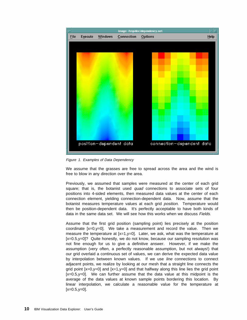
Figure 1. Examples of Data Dependency

We assume that the grasses are free to spread across the area and the wind isfree to blow in any direction over the area.

Previously, we assumed that samples were measured at the center of each gridsquare; that is, the botanist used quad connections to associate sets of fourpositions into 4-sided elements, then measured data values at the center of eachconnection element, yielding connection-dependent data. Now, assume that thebotanist measures temperature values at each grid position. Temperature wouldthen be position-dependent data. It's perfectly acceptable to have both kinds ofdata in the same data set. We will see how this works when we discuss Fields.

Assume that the first grid position (sampling point) lies precisely at the positioncoordinate [x=0,y=0]. We take a measurement and record the value. Then wemeasure the temperature at [x=1,y=0]. Later, we ask, what was the temperature at[x=0.5,y=0]? Quite honestly, we do not know, because our sampling resolution wasnot fine enough for us to give a definitive answer. However, if we make theassumption (very often, a perfectly reasonable assumption, but not always!) thatour grid overlaid a continuous set of values, we can derive the expected data valueby interpolation between known values. If we use line connections to connectadjacent points, we realize by looking at our mesh that a straight line connects thegrid point [x=0,y=0] and [x=1,y=0] and that halfway along this line lies the grid point[x=0.5,y=0]. We can further assume that the data value at this midpoint is theaverage of the data values at known sample points bordering this location. Bylinear interpolation, we calculate a reasonable value for the temperature at[x=0.5,y=0].

10 IBM Visualization Data Explorer: User’s Guide

We need to define polygonal connections over the 2-D grid if we wish to find thevalue at the point [x=0.2,y=0.7]. With line connections between adjacent pairs ofgrid points, we can only reasonably perform interpolations along those linearboundaries but not into the middle of our grid elements. By defining areas boundedby three or more points, we can perform interpolation across the area (the polygonsurface) using weighting functions that take into account the data values at allpoints surrounding the area. In fact, this is the same process used by animage-rendering program: it interpolates from known values (at the vertices) acrossthe faces of polygons and computes the appropriate color at all visible points on thesurface, at the resolution allowed by the output device (digital file, computermonitor, etc.).

Visualization

Identifying ConnectionsIn Data Explorer, we identify connections in the following way. List the samplepoint location vertices in any order: that list is called the “positions” as wediscussed above. Consider each point in the positions list to have an ordinalnumber, starting at 0 for the first point in the list (these ordinal numbers are notexplicitly listed in a Data Explorer file). A connection is denoted by a “list of lists” ofnumbers in which each entry represents the ordinal values of the points that are tobe connected, listed in the order they are to be connected. So for example, if thefirst point in the positions list is “0.0 0.0” and the second point is “1.0 0.0”, wedenote a line connection between these two points by “0 1”, indicating that a linejoins point 0 (first point in the positions list) to point 1 (the second point in the list).

As mentioned above, a triangle connection must reference three positions and aquad references four positions. For complete examples of position and connectionlists, see Chapter 3, “Understanding the Data Model” on page 15.

As a direct extension of this concept, when we define volumetric elements likecubes and tetrahedra, we can perform 3-dimensional interpolation and derive areasonable data value for any point in a sample volume. The good news about allof this interpolation is that Data Explorer already knows how to do the necessarycalculations. As a researcher, your job is to define your data space to DataExplorer—its positions, connections, and data-dependency—but you do not have toworry about the details of how the interpolation is actually performed.

The connections list is optional if it makes no sense to connect your sample points;for example, if you are studying gas molecules, there may be no meaningfulinterconnecting lines between separate molecules. Nevertheless, you may wish todefine “line” connections linking the atoms within each molecule, in order tovisualize interatomic bonds or protein backbones; or you may define cubicvolumetric elements in the space around the nucleus if you wish to visualizeelectronic potential fields, for instance.

In any case, you must define a set of connections before you can performinterpolation operations between sampled data values. This is true both forposition-dependent data and for connection-dependent data. Once again, positionsare discrete points in space, and connections are logical paths between thosepoints representing reasonable interpolation paths between the sampled datavalues. If you do not have connection information available, you can use theConnect or Regrid modules to create connections for scattered point data.

If you work with regular grids, the “connections” can be defined in a simple way byData Explorer regardless of the import format you are using. See Chapter 3,

Chapter 2. Introduction to Visualization 11

“Understanding the Data Model” on page 15 in this Guide and Chapter 5,“Importing Data” on page 61 in IBM Visualization Data Explorer QuickStart Guide.

If your work requires irregular grids, you will need to carefully read the section ofthis manual that describes the format of Data Explorer element types. You mayneed to write a filter program to convert the connection list output from your finiteelement program to the format required by Data Explorer before you can importand visualize data sampled on arbitrary structures.

Invalid DataSometimes in the process of collecting or analyzing data, certain regions orpositions have no data value associated with them. For example, an instrumentmay have a “data drop-out” or a simulation may (for whatever reason) produce aninvalid entry. Of course, if you are explicitly listing your positions or connections,you can simply leave those positions out when you create your data file. However,if you have a regular grid (for which you simply list the origin of the grid and thedelta in each dimension), this is not convenient. Data Explorer has a way to easilyhandle this situation, using “invalid positions” and “invalid connections” components.These components are discussed in Chapter 3, “Understanding the Data Model” onpage 15, but briefly, when present in a Field, they instruct any module processingthat Field to completely ignore any position or connection identified in thatcomponent. For example, an “invalid positions” component may list the integers 0,15, and 23. This instructs Data Explorer to ignore the positions 0, 15, and 23 (andthe data associated with those positions).

You can create these components in a Data Explorer format file (see Appendix B,“Importing Data: File Formats” on page 241) or, often more easily, using theInclude module. For example, suppose in your data file drop-outs are indicatedwith a data value of 9999, while all valid data lies in the range 0–100. Then set themax parameter of Include to 9998. Include will then remove or invalidate all of thepositions with the value 9999. Note that it is usually preferable to set the cull flagof Include to 0 so that the data values are invalidated rather than actually removed(see Include in IBM Visualization Data Explorer User’s Reference).

All Data Explorer modules know to ignore invalid data. For example, Streamlineswill stop when they reach an invalid element, and Statistics will ignore data valuesassociated with invalid elements.

FieldsGiven the sets of numbers, “positions,” “connections,” and “data”, we can define aField, as it is called in Data Explorer. The positions identify locations in space, the(optional) connections define logical continuities (interpolation paths) betweenpositions, and the data are the values measured either at each position or withineach connection element. Data Explorer calls each of these sets of numbers(positions, connections, data) a Field component. Components are represented asarrays of numbers with some auxiliary information specifying attributes (e.g., type ofdependency). In addition, there are many other types of Field components. TheField is the basic unit of information in Data Explorer, so it is important tounderstand how to express your data in these terms.

A Field can only have one “positions” and one “connections” component. A Fieldcan have only one component actually named “data”, but you may assign names ofyour choosing to additional components representing other data sets that are also

12 IBM Visualization Data Explorer: User’s Guide

mapped to the same grid. So you can name a “data” component “temperature” andanother “wind velocity”, or you can just use the default name “data” if you only haveone “data” component.

The “.dx” file format provides the most flexibility for describing data sets to DataExplorer. But many researchers produce fairly straightforward arrays of numbersmapped onto regular or deformed regular grids. If your data are already written outin such a form, you may not need to convert your data files into the native “.dx” fileformat. Instead, Data Explorer's General Array Importer can read your datadirectly, given a small “header” file that you create to tell the General Array Importerthe name of your data file and its dimensions (see Chapter 5, “Importing Data” onpage 61 in IBM Visualization Data Explorer QuickStart Guide).

This shorthand description is enough for Data Explorer to convert your datastructure into a Field when it reads your raw data file. You will still find it valuableto understand the components of a Field, because once you begin using the DataExplorer visual programming language, you will have direct access to thesecomponents. Much of the power and flexibility of the visual programming languageis derived from our ability to access and manipulate Field components in a varietyof ways.

Visualization

2.2 Visual Programming: The BasicsThe Field description represents a mapping between your actual data samplingspace and the Data Explorer graphics system used to make images of that dataspace. Given such a mapping, the next step is to learn how to visualize your datain meaningful ways. Data Explorer provides both a visual programming languageand a text-based scripting language. The scripting language is described inChapter 10, “Data Explorer Scripting Language” on page 187. The visualprogramming language uses a graphically oriented editor instead of a traditionaltext-based editor as in C or Pascal. You will be using this graphical programmingenvironment to generate graphic images as output; this distinction betweengraphics as program and graphics as output is subtle, but we do not want toconfuse the two.

To build a visual program, you physically select, place, and connect functionalmodules; these are represented graphically as labeled rectangular boxes with tabssticking out of them. Each module can be thought of as a subroutine in atext-based programming system. You can place multiple instances of the samemodule, analogous to calling a subroutine several times in a program. Moduleshave inputs and outputs (those little tabs sticking out) just like the arguments andreturn values in a text language. The inputs and outputs of modules are connectedtogether into a network, which in some ways resembles a flow-chart diagram.(Unlike a flow-chart, you cannot loop back a wire to an earlier input in a DataExplorer visual program) Note that many modules have “hidden” tabs for lesscommonly used parameters. You can expose hidden parameters by using theExpand button in the module’s Configuration dialog box.

Generally speaking, you use Data Explorer to visualize your data in the followingway. First, bring in the data from a disk file as a Field (the Import module can readin a Data Explorer format file, a General Array Importer file, or netCDF, CDF, orHDF files). Next, run the imported data Field through one or more modules foundin the Realization category. Each of these produces a visual object. You may alsowant to process these Realizations through Transformation modules to modify the

Chapter 2. Introduction to Visualization 13

visual or other characteristics of an object. Either one or a collection of visualobjects is then displayed in an Image window. The Image window provides anumber of convenient tools for interactively rotating your visual objects, zooming infor a closer look at them, and so on. There are many different variations of theabove scheme: for example, modules like Construct allow you to create simpleFields without having to import data; Structuring category modules permit you tomodify Field components in many ways; other types of output are provided so youcan write image files to disk, and so on. But the concept ofImport-Realize-Transform-Image is the basic and most common approach to usingData Explorer.

So what happens inside a visual program? The Field with its components flowsthrough one module after another. Some modules add new components, othersremove or change components. However, an essential point to keep in mind is thatunless a module is designed to operate on a specific component, it does not affectany other part of a Field. That is to say, if you feed a Field into a module thatdoes not operate on the “positions” component, then from the output of that modulewill come a Field with the identical (unchanged) positions component. And thatmeans that another module further “downstream” in the visual program can operateon that “positions” component if need be. This differs in a critical way fromtraditional languages, which explicitly specify all return values from a function. InData Explorer, assume that everything that goes into a module comes out (thoughoften changed), whereas in a traditional language, ignoring side-effects (badprogramming practice, usually), only those values specifically indicated as returnvalues are returned when the function exits. The descriptions in IBM VisualizationData Explorer User’s Reference identify the components that are changed, deleted,or added by each module.

It is also very often useful to “branch” a visual program. Any module input can onlyhave one wire (“tab connection”) attached to it at a time. However, any moduleoutput can feed several different module inputs. This allows you to run copies ofthe same Field through different “subnets” to perform several different operationson it. To see all of these visual outputs in the same scene, you use the Collectmodule to gather all the “subnet” output wires back together. The single outputfrom Collect (called a Group) can be attached to the input of the Image module.The Collect module shares a handy feature with some other modules in that youcan easily add new inputs to it if you need more than the two default input tabs.

See Appendix A, “Using Data Explorer: Some Useful Hints” on page 211 fordiscussions of the following:

Visualization techniques (including animation, color mapping, and shading). Creating good visualization programs for interactive use. Creating good visualizations for video.

14 IBM Visualization Data Explorer: User’s Guide

Chapter 3. Understanding the Data Model

3.1 Introduction to the Data Model . . . . . . . . . . . . . . . . . . . . . . . . . 163.2 Object Types . . . . . . . . . . . . . . . . . . . . . . . . . . . . . . . . . . . 17

Fields . . . . . . . . . . . . . . . . . . . . . . . . . . . . . . . . . . . . . . . . . 17Arrays . . . . . . . . . . . . . . . . . . . . . . . . . . . . . . . . . . . . . . . . . 28Groups . . . . . . . . . . . . . . . . . . . . . . . . . . . . . . . . . . . . . . . . 34

Data Model

Copyright IBM Corp. 1991-1997 15

This chapter describes the concepts and terminology of the data model for datastored in the Data Explorer system, whether in memory or on disk.

A complete understanding of this chapter is not required for the effective use ofData Explorer, and the brief discussion of a Field in Chapter 2, “Introduction toVisualization” on page 7 should get you started. However, the more detailedinformation here is useful when you have specific questions about the data model.

3.1 Introduction to the Data ModelThe Data Explorer data model supports various types of simulation andobservational data. Data structures that can be represented include:

Data defined on a regular orthogonal grid Data defined on a deformed regular or curvilinear grid Data defined on various irregular grids, such as triangular, quadrilateral, and

tetrahedral meshes Unstructured data with no connections between the data samples.

The data samples can be defined over spaces of any dimensionality, and,independently, can also be connected by primitives of various dimensionalities(allowing, for example, triangular and quadrilateral meshes defined over 2- or3-dimensional points). The data values can be associated either with the samplepoints or with the connections between the sample points. Available data typesinclude:

Real and complex data Scalar, vector and tensor data Byte, short, integer (signed and unsigned), and floating-point data

Data are stored in the form of Objects for use by Data Explorer modules. AnObject is a data structure stored in memory that contains an indication of theObject’s type, along with additional type-dependent information. The bulk of thedata is encapsulated in Array Objects.

The data model centers on the notion of a sampled field. The next sectiondescribes the Field, Array, and Group Objects that implement sampled fields inData Explorer. In addition to these basic Object types, other types are used toconstruct models for rendering (e.g., Transforms, Clipped Objects, Lights, andCameras). These are described in B.2, “Data Explorer Native Files” on page 244and in IBM Visualization Data Explorer Programmer’s Reference.

Data are also stored in permanent file storage in the form of the same Objects.Although Data Explorer supports the creation of Objects from data stored in otherfile formats (such as netCDF), the Data Explorer file format offers significantadditional functionality and flexibility.

Note that the Data Explorer file format is versatile, allowing for future expansion ofthe capabilities of the system without requiring changes to the file format. It ispossible to represent data types in a Data Explorer file that cannot be processed bythe current version of Data Explorer. For example, in the current release of DataExplorer, only single-precision floating-point positions are universally supported.Also, most modules support only 1-, 2-, or 3-dimensional positions.

16 IBM Visualization Data Explorer: User’s Guide

3.2 Object TypesField, Array, and Group Objects implement sampled fields in Data Explorer.Additional Object types, used to construct models for rendering, are described inAppendix B, “Importing Data: File Formats” on page 241.

FieldsField Objects are the fundamental Objects in the Data Explorer data model. AField represents a mapping from some domain to some data space. The domain ofthe mapping is specified by a set of positions and (generally) a set of connectionsthat allow interpolation of data values for points in the domain between specifiedpositions. The mapping at all points in the domain is represented implicitly byspecifying data that are dependent on (located at) the sample points or on theconnections between the sample points (cell-centered data).

This simple abstraction is sufficient for representing a wide range of things. Forexample, you can describe 3-dimensional volumetric data, whose domain is theregion specified by the positions, and whose data space is the value associatedwith each position. Two-dimensional images have a domain that is the set of pixellocations, and a data space that consists of the pixel color. Two-dimensionalsurfaces imbedded in 3-space (that is, traditional graphical models) can have adomain that is the set of positions on the surface, and a data space that is, forexample, the set of data values on that surface.

If the data are dependent on the given positions, then a data value at a point otherthan those given is found by interpolation within the connection in which the pointresides. If the data is dependent on connections, then the data value is assumedto be constant within each connection. If no connections are specified, then thereis no implied information about data values at positions other than those given.

The information in a Field is represented by some number of named components.Each component has a value, that is an Object. In general, components are ArrayObjects (described in more detail in the next section). For example, the “positions”component is an Array specifying the set of sample points; the “connections”component is an Array specifying a means to interpolate between the positions;and the “data” component is an Array specifying the data values.

Data Model

Chapter 3. Understanding the Data Model 17

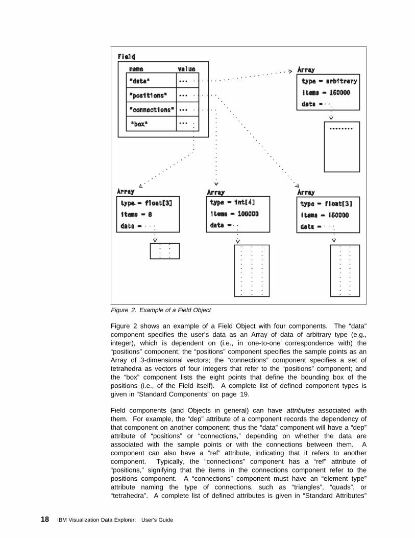
Figure 2. Example of a Field Object

Figure 2 shows an example of a Field Object with four components. The “data”component specifies the user’s data as an Array of data of arbitrary type (e.g.,integer), which is dependent on (i.e., in one-to-one correspondence with) the“positions” component; the “positions” component specifies the sample points as anArray of 3-dimensional vectors; the “connections” component specifies a set oftetrahedra as vectors of four integers that refer to the “positions” component; andthe “box” component lists the eight points that define the bounding box of thepositions (i.e., of the Field itself). A complete list of defined component types isgiven in “Standard Components” on page 19.

Field components (and Objects in general) can have attributes associated withthem. For example, the “dep” attribute of a component records the dependency ofthat component on another component; thus the “data” component will have a “dep”attribute of “positions” or “connections,” depending on whether the data areassociated with the sample points or with the connections between them. Acomponent can also have a “ref” attribute, indicating that it refers to anothercomponent. Typically, the “connections” component has a “ref” attribute of“positions,” signifying that the items in the connections component refer to thepositions component. A “connections” component must have an “element type”attribute naming the type of connections, such as “triangles”, “quads”, or“tetrahedra”. A complete list of defined attributes is given in “Standard Attributes”

18 IBM Visualization Data Explorer: User’s Guide

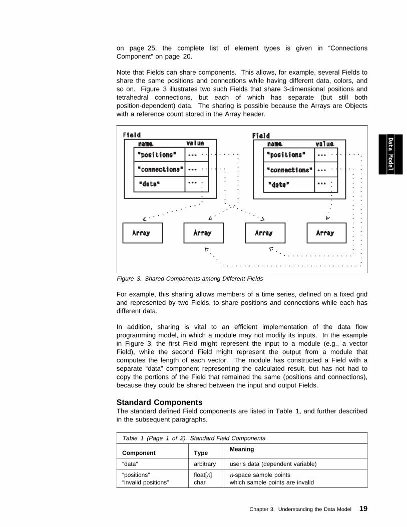
on page 25; the complete list of element types is given in “ConnectionsComponent” on page 20.

Note that Fields can share components. This allows, for example, several Fields toshare the same positions and connections while having different data, colors, andso on. Figure 3 illustrates two such Fields that share 3-dimensional positions andtetrahedral connections, but each of which has separate (but still bothposition-dependent) data. The sharing is possible because the Arrays are Objectswith a reference count stored in the Array header.

Figure 3. Shared Components among Different Fields

Data Model

For example, this sharing allows members of a time series, defined on a fixed gridand represented by two Fields, to share positions and connections while each hasdifferent data.

In addition, sharing is vital to an efficient implementation of the data flowprogramming model, in which a module may not modify its inputs. In the examplein Figure 3, the first Field might represent the input to a module (e.g., a vectorField), while the second Field might represent the output from a module thatcomputes the length of each vector. The module has constructed a Field with aseparate “data” component representing the calculated result, but has not had tocopy the portions of the Field that remained the same (positions and connections),because they could be shared between the input and output Fields.

Standard ComponentsThe standard defined Field components are listed in Table 1, and further describedin the subsequent paragraphs.

Table 1 (Page 1 of 2). Standard Field Components

Component TypeMeaning

“data” arbitrary user’s data (dependent variable)

“positions”“invalid positions”

float[n]char

n-space sample pointswhich sample points are invalid

Chapter 3. Understanding the Data Model 19

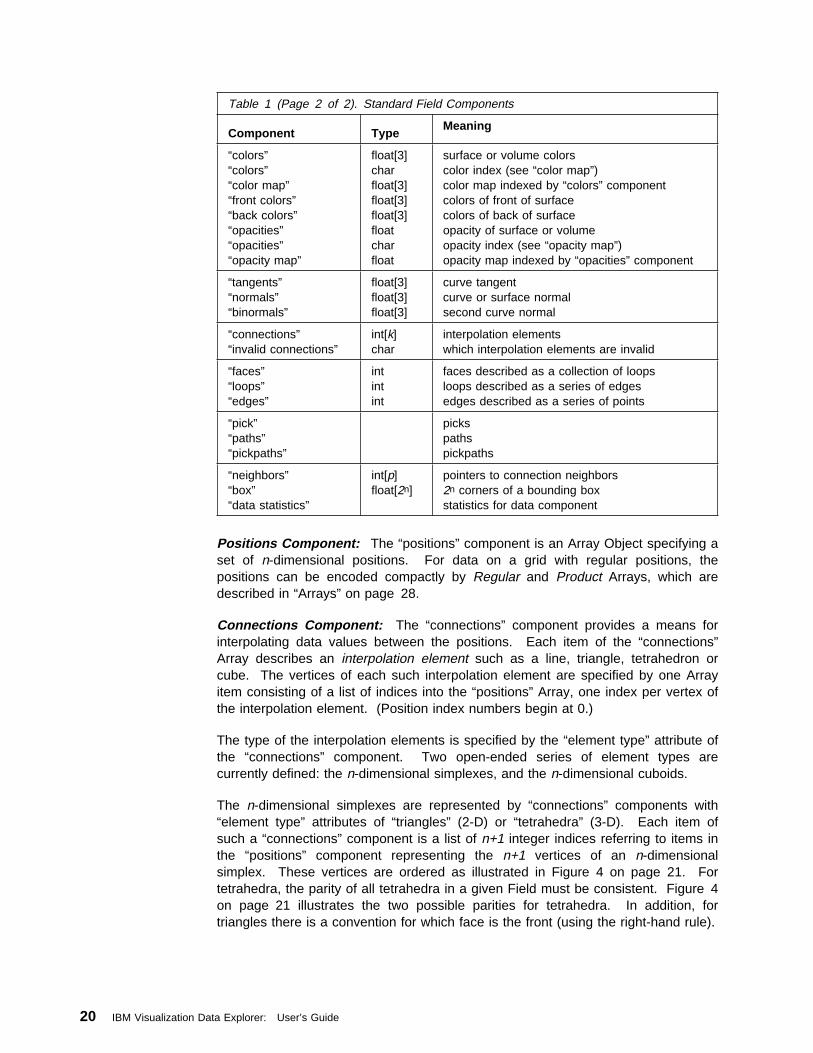
Positions Component: The “positions” component is an Array Object specifying aset of n-dimensional positions. For data on a grid with regular positions, thepositions can be encoded compactly by Regular and Product Arrays, which aredescribed in “Arrays” on page 28.

Connections Component: The “connections” component provides a means forinterpolating data values between the positions. Each item of the “connections”Array describes an interpolation element such as a line, triangle, tetrahedron orcube. The vertices of each such interpolation element are specified by one Arrayitem consisting of a list of indices into the “positions” Array, one index per vertex ofthe interpolation element. (Position index numbers begin at 0.)

The type of the interpolation elements is specified by the “element type” attribute ofthe “connections” component. Two open-ended series of element types arecurrently defined: the n-dimensional simplexes, and the n-dimensional cuboids.

The n-dimensional simplexes are represented by “connections” components with“element type” attributes of “triangles” (2-D) or “tetrahedra” (3-D). Each item ofsuch a “connections” component is a list of n+1 integer indices referring to items inthe “positions” component representing the n+1 vertices of an n-dimensionalsimplex. These vertices are ordered as illustrated in Figure 4 on page 21. Fortetrahedra, the parity of all tetrahedra in a given Field must be consistent. Figure 4on page 21 illustrates the two possible parities for tetrahedra. In addition, fortriangles there is a convention for which face is the front (using the right-hand rule).

Table 1 (Page 2 of 2). Standard Field Components

Component TypeMeaning

“colors”“colors”“color map”“front colors”“back colors”“opacities”“opacities”“opacity map”

float[3]charfloat[3]float[3]float[3]floatcharfloat

surface or volume colorscolor index (see “color map”)color map indexed by “colors” componentcolors of front of surfacecolors of back of surfaceopacity of surface or volumeopacity index (see “opacity map”)opacity map indexed by “opacities” component

“tangents”“normals”“binormals”

float[3]float[3]float[3]

curve tangentcurve or surface normalsecond curve normal

“connections”“invalid connections”

int[k]char

interpolation elementswhich interpolation elements are invalid

“faces”“loops”“edges”

intintint

faces described as a collection of loopsloops described as a series of edgesedges described as a series of points

“pick”“paths”“pickpaths”

pickspathspickpaths

“neighbors”“box”“data statistics”

int[p]float[2n]

pointers to connection neighbors2n corners of a bounding boxstatistics for data component

20 IBM Visualization Data Explorer: User’s Guide

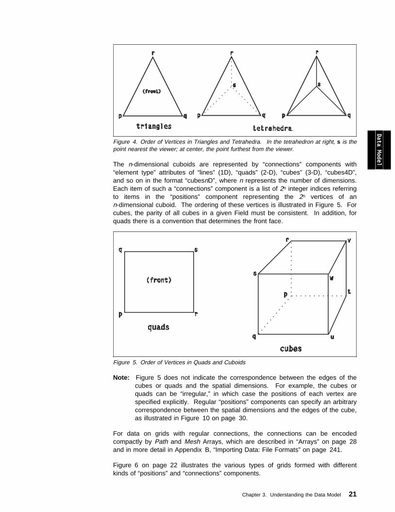
Figure 4. Order of Vertices in Triangles and Tetrahedra. In the tetrahedron at right, s is thepoint nearest the viewer; at center, the point furthest from the viewer.

Data Model The n-dimensional cuboids are represented by “connections” components with“element type” attributes of “lines” (1D), “quads” (2-D), “cubes” (3-D), “cubes4D”,and so on in the format “cubesnD”, where n represents the number of dimensions.Each item of such a “connections” component is a list of 2n integer indices referringto items in the “positions” component representing the 2n vertices of ann-dimensional cuboid. The ordering of these vertices is illustrated in Figure 5. Forcubes, the parity of all cubes in a given Field must be consistent. In addition, forquads there is a convention that determines the front face.

Figure 5. Order of Vertices in Quads and Cuboids

Note: Figure 5 does not indicate the correspondence between the edges of thecubes or quads and the spatial dimensions. For example, the cubes orquads can be “irregular,” in which case the positions of each vertex arespecified explicitly. Regular “positions” components can specify an arbitrarycorrespondence between the spatial dimensions and the edges of the cube,as illustrated in Figure 10 on page 30.

For data on grids with regular connections, the connections can be encodedcompactly by Path and Mesh Arrays, which are described in “Arrays” on page 28and in more detail in Appendix B, “Importing Data: File Formats” on page 241.

Figure 6 on page 22 illustrates the various types of grids formed with differentkinds of “positions” and “connections” components.

Chapter 3. Understanding the Data Model 21

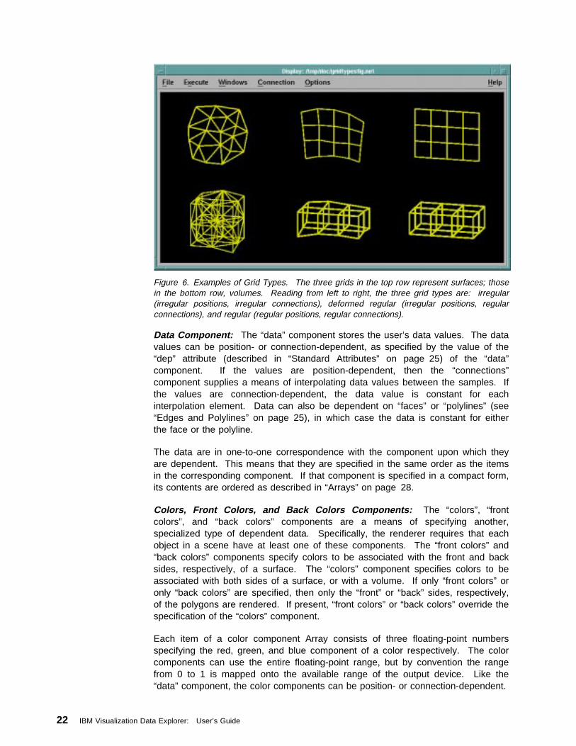
Figure 6. Examples of Grid Types. The three grids in the top row represent surfaces; thosein the bottom row, volumes. Reading from left to right, the three grid types are: irregular(irregular positions, irregular connections), deformed regular (irregular positions, regularconnections), and regular (regular positions, regular connections).

Data Component: The “data” component stores the user’s data values. The datavalues can be position- or connection-dependent, as specified by the value of the“dep” attribute (described in “Standard Attributes” on page 25) of the “data”component. If the values are position-dependent, then the “connections”component supplies a means of interpolating data values between the samples. Ifthe values are connection-dependent, the data value is constant for eachinterpolation element. Data can also be dependent on “faces” or “polylines” (see“Edges and Polylines” on page 25), in which case the data is constant for eitherthe face or the polyline.

The data are in one-to-one correspondence with the component upon which theyare dependent. This means that they are specified in the same order as the itemsin the corresponding component. If that component is specified in a compact form,its contents are ordered as described in “Arrays” on page 28.

Colors, Front Colors, and Back Colors Components: The “colors”, “frontcolors”, and “back colors” components are a means of specifying another,specialized type of dependent data. Specifically, the renderer requires that eachobject in a scene have at least one of these components. The “front colors” and“back colors” components specify colors to be associated with the front and backsides, respectively, of a surface. The “colors” component specifies colors to beassociated with both sides of a surface, or with a volume. If only “front colors” oronly “back colors” are specified, then only the “front” or “back” sides, respectively,of the polygons are rendered. If present, “front colors” or “back colors” override thespecification of the “colors” component.

Each item of a color component Array consists of three floating-point numbersspecifying the red, green, and blue component of a color respectively. The colorcomponents can use the entire floating-point range, but by convention the rangefrom 0 to 1 is mapped onto the available range of the output device. Like the“data” component, the color components can be position- or connection-dependent.

22 IBM Visualization Data Explorer: User’s Guide

The front of a triangle is defined to be the side such that the path traversing thevertices in the order that they are listed for the triangle appears to gocounterclockwise. The front of a quad is the side from which the vertex numberingappears (Figure 5 on page 21).

The interpretation of colors differs between surfaces and volumes. For surfaces,the color values in the range from 0 to 1 are mapped onto the range of colorsvalues possible for the display. For volumes, the interpretation of colors follows the“dense emitter” model described in the next section.

Opacities Component: The “opacities” component plays a role similar to that ofcolors components, except that it specifies a floating-point opacity for rendering. Itsinterpretation differs depending on whether the connections represent a surface(triangles or quads), or a volume (tetrahedra, cubes, and so on). In the surfacecase, the opacity is a number from 0 to 1 specifying the opacity of the surface. Inthe volume case, the opacity represents the instantaneous attenuation of light perunit distance traveled. Like the colors components, it can be position- orconnection-dependent.

The interpretation of “colors” and “opacities” differs between surfaces and volumes.For surfaces, a surface of color cf and opacity o is combined with the color cb of theobjects behind it resulting in a combined color cfo + cb(1 − o).

For volumes, the “dense emitter” model is used, in which the opacity represents theinstantaneous rate of absorption of light passing through the volume per unitthickness, and the color represents the instantaneous rate of light emission per unitthickness. If c(z) represents the color of the object at z and o(z) represents itsopacity at z, then the total color of a ray passing through the volume is given by:

c = ∫∞

−∞c(z) exp ( − ∫

z

−∞o(ζ)dζ) dz

Color Map and Opacity Map Components: There is an alternative to having the“colors” component and “opacities” component explicitly list the color and opacityassociated with each position or connection element. If each element of the“colors” and “opacities” components is a single byte, then it is interpreted as anindex into the “color map” or “opacity map” component. The “color map”component is a 256-element table of three floating-point values (representing red,green, and blue, typically with values between 0 and 1). The “opacity map”component is a 256-element table of floating-point values between 0 and 1.

Invalid Positions and Invalid Connections Components: The “invalid positions”and “invalid connections” components allow positions or connections to be markedas not having valid data. This is useful, for example, for observational data definedon a regular grid but with occasional missing observations, or for simulation datadefined on a regular grid but with a “hole” covered by another grid, perhaps at ahigher resolution. The “invalid positions” component can be an Array of bytes orunsigned bytes, one for each position, where the component is dependent onpositions (i.e., has a “dep” attribute of “positions.”). In that case, the value 1indicates that the corresponding position is invalid, and 0 that the correspondingposition is valid. Alternatively, the “invalid positions” component can be an Array ofsigned or unsigned integers, where the component references the positions (i.e.,has a “ref” attribute of “positions”). In that case, the component contains a list ofthe indices of the invalid positions. The first method is more space-conserving

Data Model

Chapter 3. Understanding the Data Model 23

when there are a large number of invalid elements; the second, when there are arelatively small number. See “Compute” on page 86 in IBM Visualization DataExplorer User’s Reference for a way to convert from the “ref” type to the “dep” type.

The “invalid connections,” “invalid faces,” and “invalid polylines” components can bedefined in an analogous way.

Tangents, Normals, and Binormals Components: The “normals” component isused to specify a local surface normal for rendering purposes. The “tangents”,“normals” and “binormals” components specify a local reference frame on a path;this is useful, for example, for twisted-ribbon representations of streamlines.

Normals are used for, among other things, surface shading. By convention, thenormals are expected to point out from the front of a surface, as defined in “Colors,Front Colors, and Back Colors Components” on page 22. Normals are expected tohave unit length.

Neighbors Component: The “neighbors” component represents information aboutthe neighbors of each connection element. The number of items in this componentmust match the number of items in the “connections” component. The number ofentries in each item must match the number of faces (for 3-D) or edges (for 2-D) inthe connection element. For example, each item in the “neighbors” component fortriangle connections has three entries, while each item in the “neighbors”component for tetrahedral connections has four entries.

For simplexes in n dimensions (for example, triangles and tetrahedra), each item ofthe neighbors Array consists of n+1 integer indices into the connections Arrayidentifying the n+1 neighbors of the simplex; the ith of the n+1 indices correspondsto the face opposite the ith vertex of the simplex. For quads, cubes, and so on,each item of the neighbors Array contains 2n integer indices into the connectionsArray identifying the 2n neighbors of the polyhedron. The pointers are in the order-x1+x1-x2+x2 ... -xn+xn, meaning that the first index points to the neighbor in the −x1direction, the second to the neighbor in the +x1 direction, and so on, where the xndimension varies fastest in the representation of the point indices in theinterpolation element. Faces without neighbors are indicated by an index of −1.

Box Component: The “box” component consists of 2n n-dimensional points,where n is the dimensionality of the positions component, identifying the corners ofa bounding box that contains the positions of this Field.

Data Statistics Component: The “data statistics” component contains statistics ofthe “data” component. The information in this component should be accessedusing the Statistics module or the DXStatistics() function, as the exact contentsare undefined. If DXStatistics is called on other components (e.g., “positions”), ananalogous component (in this case “positions statistics”) will be created.

Faces, Loops, and Edges Components: The “faces”, “loops”, and “edges”components are used for special-purpose applications, such as fonts or geometricmodels. The “faces” component represents a set of faces, each described as a setof loops. Each entry in the face Array is a single integer index into the “loops”Array identifying the first of a consecutive set of loops for this face. The loops arelisted in order of the faces they are associated with, so that the list of loops for facei ends in the loops Array just before the first loop for face i+1. Each entry in the“loops” Array is a single integer index into the “edges” Array, identifying the first of

24 IBM Visualization Data Explorer: User’s Guide

a consecutive set of edges for this loop. The edges are listed in order of the loopsthey are associated with, so that the list of edges for loop i in the edges Array endsjust before the first edge for loop i+1. Each entry in the edges Array is a singleinteger index into the “points” Array identifying one vertex of an edge; the othervertex of an edge is the next entry in the “edges” Array, except that the last edge ina loop that connects the last point to the first point is not listed explicitly. This isillustrated in Figure 7 on page 26.

It is assumed that the first loop for each face is the enclosing loop, and thatsubsequent loops, if any, are holes in the face. If this is not true, then set theDX_NESTED_LOOPS environment variable (see “Other Environment Variables” onpage 292). However, setting this environment variable will cause a decrease inperformance when processing faces, loops, and edges data.

Edges and Polylines: “Polylines” are a way of collecting a set of line segmentsinto a single object with which data can be associated. They are implementedmuch as faces, loops, and edges are (see above). An “edges” component containsthe indices of the vertices along polylines. A “polylines” component contains theindices of the first element in the “edges” component of each polyline sequence. Inother words, the ith element of the “polylines” component is the index in the “edges”component at which the sequence of vertex indices of polyline i starts. Thesequence corresponding to polyline[i] continues to the beginning of the next polylinesequence (or to the end of the “edges” component). Polyline data may bedependent on either “polylines” or “positions”.

Pokes, Picks, and Pick Paths Components: The pokes, picks, and pick pathscomponents are created as part of the picking process, as implemented by the Picktool. A user writing a module that uses the pick structure output by the Pick tool isexpected to use the pick structure manipulation routines (as described in IBMVisualization Data Explorer Programmer’s Reference) rather than accessing thepick structure directly. The contents of the pick structure are not defined.

Data Model

Standard AttributesThe standard defined attributes are listed in Table 2 and Table 3, and are furtherdescribed in the subsequent paragraphs. Attributes associated with renderingproperties are described under the Display module in Chapter 1, “Data ExplorerTools” on page 1 in IBM Visualization Data Explorer User’s Reference.

Table 2. Component attributes

Attribute Meaning

“dep” component that this component depends on

“ref” component that this component refers to

“der” component that this component is derived from

“element type” interpolation method for connections component

Table 3 (Page 1 of 2). Object attributes

Object Relevant module

label Plot

scatter Plot

mark Plot

Chapter 3. Understanding the Data Model 25

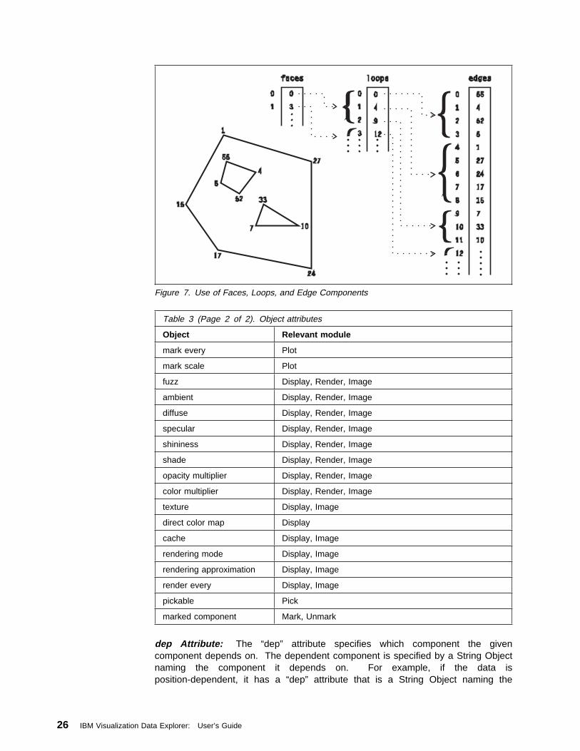
Figure 7. Use of Faces, Loops, and Edge Components

dep Attribute: The “dep” attribute specifies which component the givencomponent depends on. The dependent component is specified by a String Objectnaming the component it depends on. For example, if the data isposition-dependent, it has a “dep” attribute that is a String Object naming the

Table 3 (Page 2 of 2). Object attributes

Object Relevant module

mark every Plot

mark scale Plot

fuzz Display, Render, Image

ambient Display, Render, Image

diffuse Display, Render, Image

specular Display, Render, Image

shininess Display, Render, Image

shade Display, Render, Image

opacity multiplier Display, Render, Image

color multiplier Display, Render, Image

texture Display, Image

direct color map Display

cache Display, Image

rendering mode Display, Image

rendering approximation Display, Image

render every Display, Image

pickable Pick

marked component Mark, Unmark

26 IBM Visualization Data Explorer: User’s Guide

“positions” component. A component with a this attribute is expected to be in aone-to-one correspondence with the component named in the attribute.

ref Attribute: The “ref” attribute specifies which component the given componentrefers to. The referent component is specified by a String Object naming thecomponent it refers to. For example, the “connections” component generally has a“ref”attribute that is a String Object naming the “positions” component. Acomponent with this attribute consists of indices into the component named in theattribute.

der Attribute: The “der” attribute specifies that a component is derived fromanother component, and so should be recalculated or deleted when the componentit is derived from changes. For example, the “box” component has a “der” attributethat is a String Object naming the “positions” component.

element type Attribute: The “element type” attribute is an attribute of the“connections” component. It is a String Object naming the type of the interpolationprimitives. See “Connections Component” on page 20 for a list of the possiblevalues of the “element type” attribute.

label, scatter, mark, mark every, mark scale Attributes Specifies characteristicsof a plotted line. Affects the behavior of the Plot module. See “Plot” on page 237in IBM Visualization Data Explorer User’s Reference for more information.

fuzz, ambient, diffuse, specular, shininess, shade Attributes Specifies variousrendering characteristics of an object. Affects the behavior of the rendering modules(Display, Render, and Image). See “Display” on page 109 in IBM VisualizationData Explorer User’s Reference for more information.

opacity multiplier, color multiplier Attributes Specifies opacity and color valuesfor volume rendering. Affects the behavior of the rendering modules (Display,Render, and Image). See “Display” on page 109 in IBM Visualization DataExplorer User’s Reference for more information.

texture Attribute Specifies a texture map which is to be applied to an object.Affects the behavior of Display and Image. See “Display” on page 109 in IBMVisualization Data Explorer User’s Reference for more information.

direct color map Attribute Specifies whether or not a direct color map should beused when displaying images. Affects the behavior of the Display module. See“Display” on page 109 in IBM Visualization Data Explorer User’s Reference formore information.

cache Attribute Specifies whether the rendered image should be cached. Affectsthe behavior of Display and Image modules. See “Display” on page 109 in IBMVisualization Data Explorer User’s Reference for more information.

rendering mode Attribute Specifies the rendering mode to be either hardware orsoftware. Affects the behavior of Display and Image modules. See “Display” onpage 109 in IBM Visualization Data Explorer User’s Reference for moreinformation.

Data Model

Chapter 3. Understanding the Data Model 27

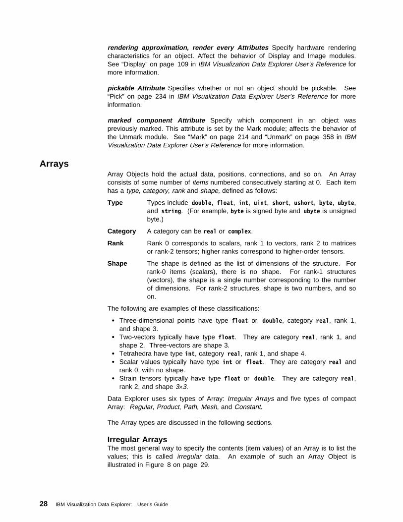
rendering approximation, render every Attributes Specify hardware renderingcharacteristics for an object. Affect the behavior of Display and Image modules.See “Display” on page 109 in IBM Visualization Data Explorer User’s Reference formore information.

pickable Attribute Specifies whether or not an object should be pickable. See“Pick” on page 234 in IBM Visualization Data Explorer User’s Reference for moreinformation.

marked component Attribute Specify which component in an object waspreviously marked. This attribute is set by the Mark module; affects the behavior ofthe Unmark module. See “Mark” on page 214 and “Unmark” on page 358 in IBMVisualization Data Explorer User’s Reference for more information.

ArraysArray Objects hold the actual data, positions, connections, and so on. An Arrayconsists of some number of items numbered consecutively starting at 0. Each itemhas a type, category, rank and shape, defined as follows:

Type Types include double, float, int, uint, short, ushort, byte, ubyte,and string. (For example, byte is signed byte and ubyte is unsignedbyte.)

Category A category can be real or complex.

Rank Rank 0 corresponds to scalars, rank 1 to vectors, rank 2 to matricesor rank-2 tensors; higher ranks correspond to higher-order tensors.

Shape The shape is defined as the list of dimensions of the structure. Forrank-0 items (scalars), there is no shape. For rank-1 structures(vectors), the shape is a single number corresponding to the numberof dimensions. For rank-2 structures, shape is two numbers, and soon.

The following are examples of these classifications:

Three-dimensional points have type float or double, category real, rank 1,and shape 3.

Two-vectors typically have type float. They are category real, rank 1, andshape 2. Three-vectors are shape 3.

Tetrahedra have type int, category real, rank 1, and shape 4. Scalar values typically have type int or float. They are category real and

rank 0, with no shape. Strain tensors typically have type float or double. They are category real,

rank 2, and shape 3×3.

Data Explorer uses six types of Array: Irregular Arrays and five types of compactArray: Regular, Product, Path, Mesh, and Constant.

The Array types are discussed in the following sections.

Irregular ArraysThe most general way to specify the contents (item values) of an Array is to list thevalues; this is called irregular data. An example of such an Array Object isillustrated in Figure 8 on page 29.

28 IBM Visualization Data Explorer: User’s Guide

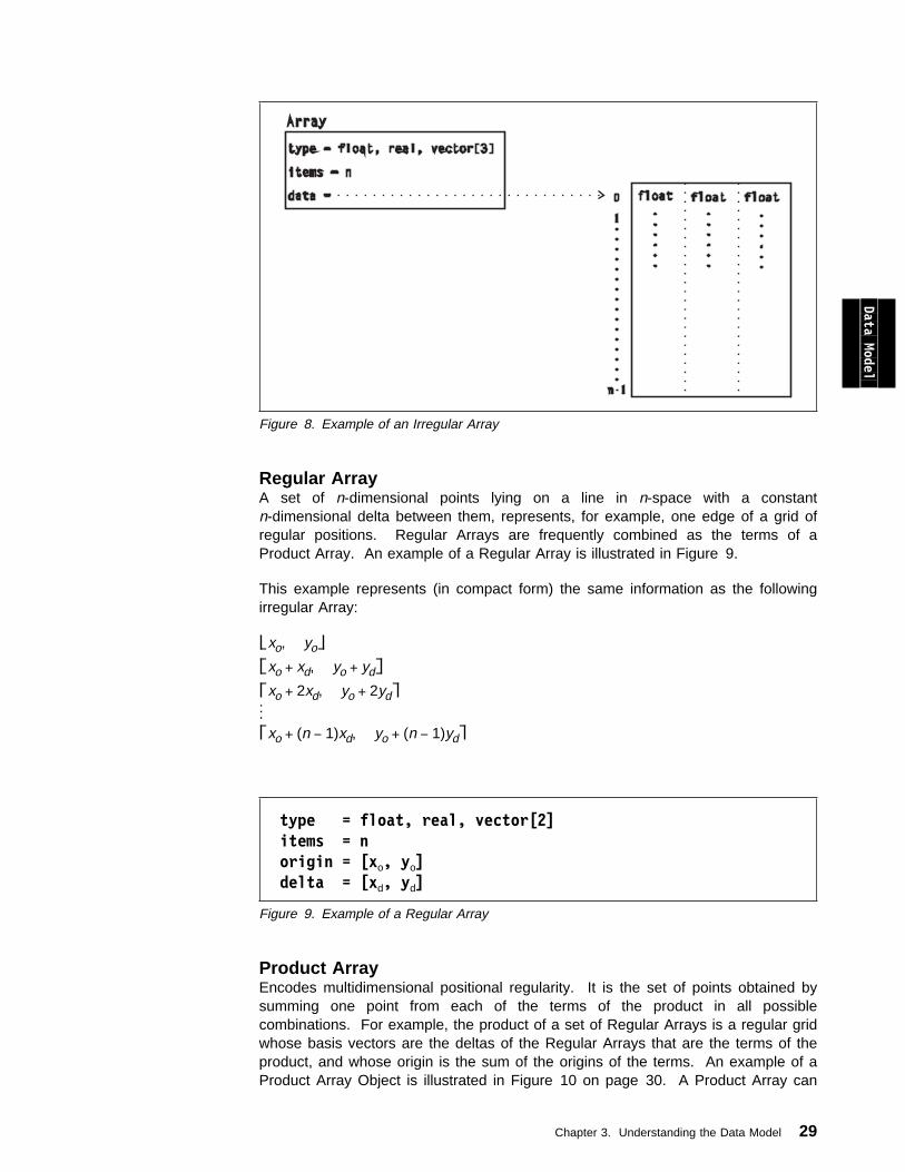
Figure 8. Example of an Irregular Array

Data Model

Regular ArrayA set of n-dimensional points lying on a line in n-space with a constantn-dimensional delta between them, represents, for example, one edge of a grid ofregular positions. Regular Arrays are frequently combined as the terms of aProduct Array. An example of a Regular Array is illustrated in Figure 9.

This example represents (in compact form) the same information as the followingirregular Array:

xo, yo

xo + xd, yo + yd

xo + 2xd, yo + 2yd

... xo + (n − 1)xd, yo + (n − 1)yd

type = float, real, vector[2] items = n origin = [xo, yo] delta = [xd, yd]

Figure 9. Example of a Regular Array

Product ArrayEncodes multidimensional positional regularity. It is the set of points obtained bysumming one point from each of the terms of the product in all possiblecombinations. For example, the product of a set of Regular Arrays is a regular gridwhose basis vectors are the deltas of the Regular Arrays that are the terms of theproduct, and whose origin is the sum of the origins of the terms. An example of aProduct Array Object is illustrated in Figure 10 on page 30. A Product Array can

Chapter 3. Understanding the Data Model 29

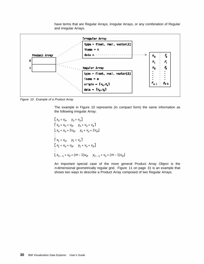
have terms that are Regular Arrays, irregular Arrays, or any combination of Regularand irregular Arrays.

Figure 10. Example of a Product Array

The example in Figure 10 represents (in compact form) the same information asthe following irregular Array:

xo + uo, yo + vo

xo + uo + ud, yo + vo + vd

xo + uo + 2ud, yo + vo + 2vd

... x1 + uo, y1 + vo

x1 + uo + ud, y1 + vo + vd

... xn − 1 + uo + (m − 1)ud, yn − 1 + vo + (m − 1)vd

An important special case of the more general Product Array Object is then-dimensional geometrically regular grid. Figure 11 on page 31 is an example thatshows two ways to describe a Product Array composed of two Regular Arrays.

30 IBM Visualization Data Explorer: User’s Guide

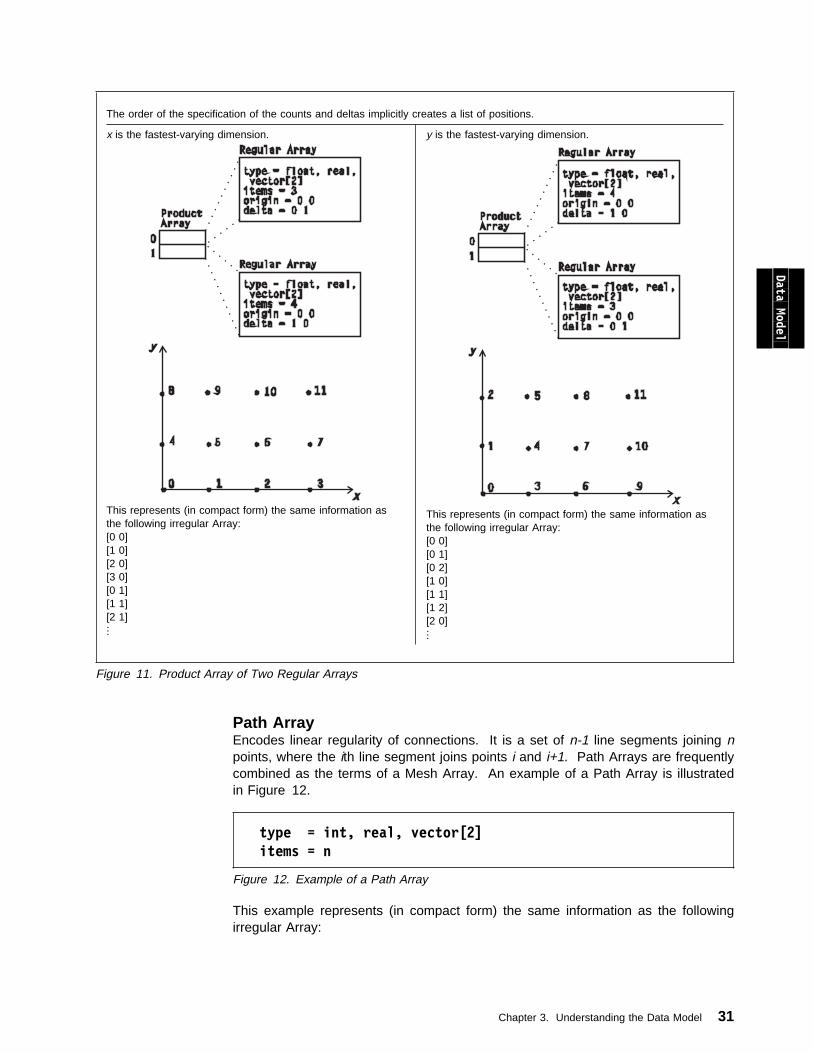
Figure 11. Product Array of Two Regular Arrays

The order of the specification of the counts and deltas implicitly creates a list of positions.

x is the fastest-varying dimension.

This represents (in compact form) the same information asthe following irregular Array:[0 0][1 0][2 0][3 0][0 1][1 1][2 1]...

y is the fastest-varying dimension.

This represents (in compact form) the same information asthe following irregular Array:[0 0][0 1][0 2][1 0][1 1][1 2][2 0]...

Data Model

Path ArrayEncodes linear regularity of connections. It is a set of n-1 line segments joining npoints, where the ith line segment joins points i and i+1. Path Arrays are frequentlycombined as the terms of a Mesh Array. An example of a Path Array is illustratedin Figure 12.

type = int, real, vector[2]items = n

Figure 12. Example of a Path Array

This example represents (in compact form) the same information as the followingirregular Array:

Chapter 3. Understanding the Data Model 31

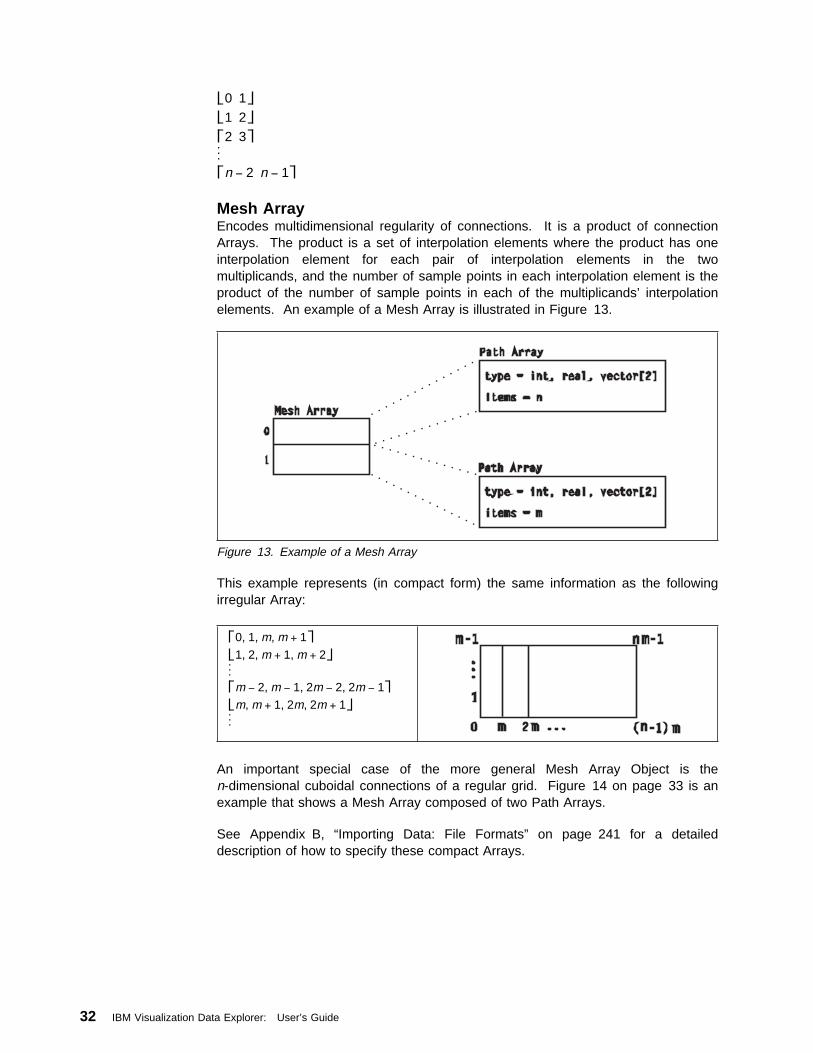
0 1

1 2

2 3 ... n − 2 n − 1

Mesh ArrayEncodes multidimensional regularity of connections. It is a product of connectionArrays. The product is a set of interpolation elements where the product has oneinterpolation element for each pair of interpolation elements in the twomultiplicands, and the number of sample points in each interpolation element is theproduct of the number of sample points in each of the multiplicands’ interpolationelements. An example of a Mesh Array is illustrated in Figure 13.

Figure 13. Example of a Mesh Array

This example represents (in compact form) the same information as the followingirregular Array:

An important special case of the more general Mesh Array Object is then-dimensional cuboidal connections of a regular grid. Figure 14 on page 33 is anexample that shows a Mesh Array composed of two Path Arrays.

See Appendix B, “Importing Data: File Formats” on page 241 for a detaileddescription of how to specify these compact Arrays.

0, 1, m, m + 1

1, 2, m + 1, m + 2 ... m − 2, m − 1, 2m − 2, 2m − 1

m, m + 1, 2m, 2m + 1 ...

32 IBM Visualization Data Explorer: User’s Guide

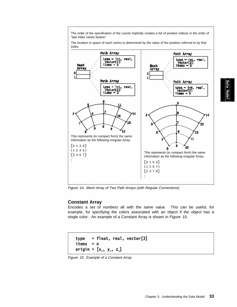
Figure 14. Mesh Array of Two Path Arrays (with Regular Connections)

The order of the specification of the counts implicitly creates a list of position indices in the order of“last index varies fastest.”

The location in space of each vertex is determined by the value of the position referred to by thatindex.

This represents (in compact form) the sameinformation as the following irregular Array:

0 1 3 4

1 2 4 5

3 4 6 7

...

This represents (in compact form) the sameinformation as the following irregular Array:

0 1 5 6

1 2 6 7

2 3 7 8

...

Data Model

Constant ArrayEncodes a set of numbers all with the same value. This can be useful, forexample, for specifying the colors associated with an object if the object has asingle color. An example of a Constant Array is shown in Figure 15.

type = float, real, vector[3] items = norigin = [xo, yo, zo]

Figure 15. Example of a Constant Array

Chapter 3. Understanding the Data Model 33

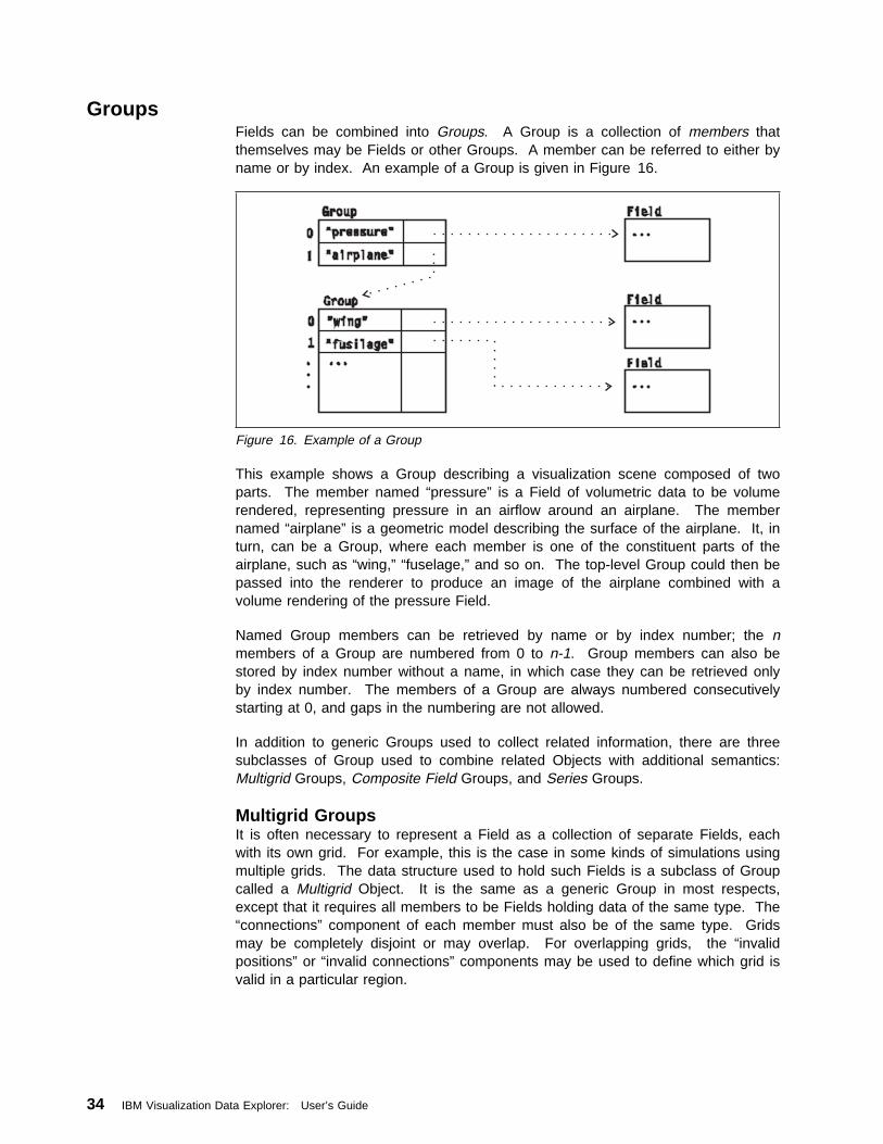
GroupsFields can be combined into Groups. A Group is a collection of members thatthemselves may be Fields or other Groups. A member can be referred to either byname or by index. An example of a Group is given in Figure 16.

Figure 16. Example of a Group

This example shows a Group describing a visualization scene composed of twoparts. The member named “pressure” is a Field of volumetric data to be volumerendered, representing pressure in an airflow around an airplane. The membernamed “airplane” is a geometric model describing the surface of the airplane. It, inturn, can be a Group, where each member is one of the constituent parts of theairplane, such as “wing,” “fuselage,” and so on. The top-level Group could then bepassed into the renderer to produce an image of the airplane combined with avolume rendering of the pressure Field.

Named Group members can be retrieved by name or by index number; the nmembers of a Group are numbered from 0 to n-1. Group members can also bestored by index number without a name, in which case they can be retrieved onlyby index number. The members of a Group are always numbered consecutivelystarting at 0, and gaps in the numbering are not allowed.

In addition to generic Groups used to collect related information, there are threesubclasses of Group used to combine related Objects with additional semantics:Multigrid Groups, Composite Field Groups, and Series Groups.

Multigrid GroupsIt is often necessary to represent a Field as a collection of separate Fields, eachwith its own grid. For example, this is the case in some kinds of simulations usingmultiple grids. The data structure used to hold such Fields is a subclass of Groupcalled a Multigrid Object. It is the same as a generic Group in most respects,except that it requires all members to be Fields holding data of the same type. The“connections” component of each member must also be of the same type. Gridsmay be completely disjoint or may overlap. For overlapping grids, the “invalidpositions” or “invalid connections” components may be used to define which grid isvalid in a particular region.

34 IBM Visualization Data Explorer: User’s Guide

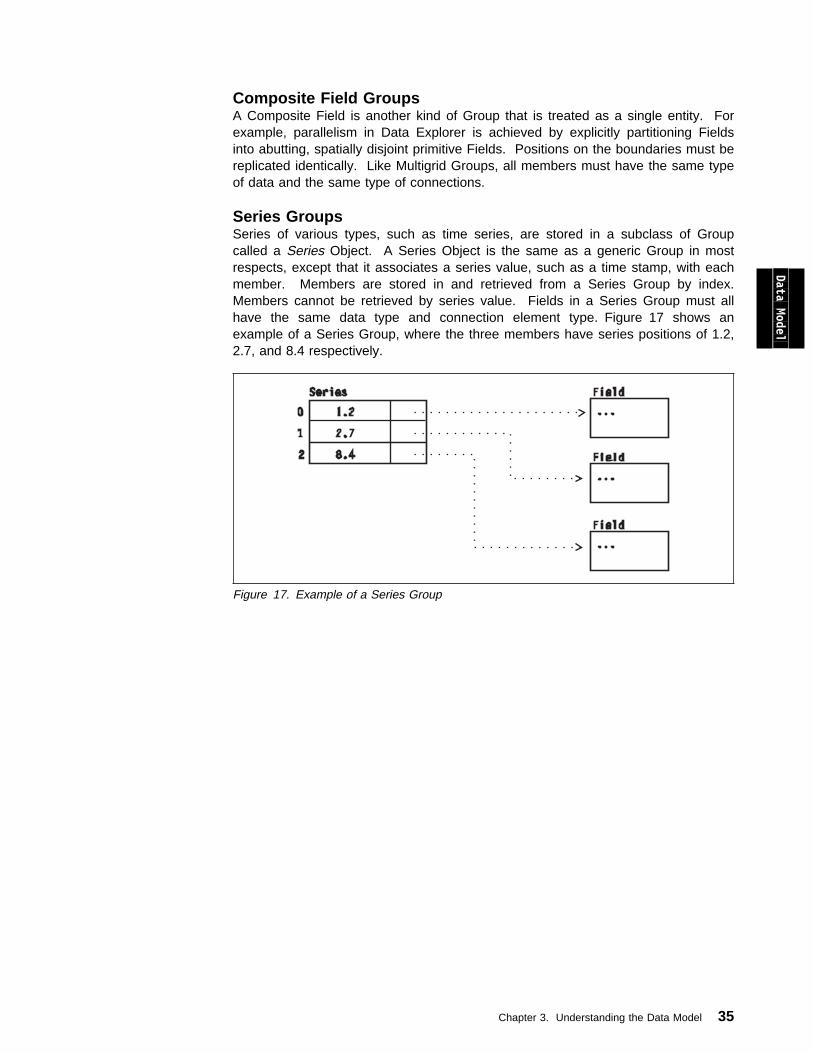
Composite Field GroupsA Composite Field is another kind of Group that is treated as a single entity. Forexample, parallelism in Data Explorer is achieved by explicitly partitioning Fieldsinto abutting, spatially disjoint primitive Fields. Positions on the boundaries must bereplicated identically. Like Multigrid Groups, all members must have the same typeof data and the same type of connections.

Series GroupsSeries of various types, such as time series, are stored in a subclass of Groupcalled a Series Object. A Series Object is the same as a generic Group in mostrespects, except that it associates a series value, such as a time stamp, with eachmember. Members are stored in and retrieved from a Series Group by index.Members cannot be retrieved by series value. Fields in a Series Group must allhave the same data type and connection element type. Figure 17 shows anexample of a Series Group, where the three members have series positions of 1.2,2.7, and 8.4 respectively.

Data Model

Figure 17. Example of a Series Group

Chapter 3. Understanding the Data Model 35

36 IBM Visualization Data Explorer: User’s Guide

Chapter 4. Data Explorer Execution Model

4.1 Data Flow . . . . . . . . . . . . . . . . . . . . . . . . . . . . . . . . . . . . . 384.2 Iterative Execution and Caching of Intermediate Results . . . . . . . . . . 404.3 Conditional Execution: Route and Switch . . . . . . . . . . . . . . . . . . . 414.4 Iteration using the Sequencer . . . . . . . . . . . . . . . . . . . . . . . . . . 434.5 Iteration using Looping . . . . . . . . . . . . . . . . . . . . . . . . . . . . . . 444.6 Preserving Explicit State . . . . . . . . . . . . . . . . . . . . . . . . . . . . . 454.7 Advanced Looping Constructs . . . . . . . . . . . . . . . . . . . . . . . . . . 504.8 External Asynchronous Data Sources . . . . . . . . . . . . . . . . . . . . . 544.9 Parallelism using Distributed Processing . . . . . . . . . . . . . . . . . . . . 554.10 Parallelism for Data Explorer SMP . . . . . . . . . . . . . . . . . . . . . . 56

Execution Model

Copyright IBM Corp. 1991-1997 37

Data Explorer's execution model is based on the data flow concept. However,features are provided that extend the data flow concept to allow you to create avisual program that could not be supported by simple data flow. For example,there are tools that allow you to explicitly save partial results of a visual program tobe used in a subsequent execution. Data Explorer also provides you with varioustools to control the flow of execution of your visual programs. Most of these toolsare analogous to constructs found in commonly used programming languages. Forexample, tools are provided that perform the function of IF statements, CASEstatements and FOR (or DO) loops. This chapter discusses flow-control tools (withseveral examples of their use) both individually and in combination.

Although it is not necessary to understand all the details of the Data Explorerexecution model in order to build and run visual programs, you may find it helpfulas you build visual programs. Other topics in this chapter include caching ofintermediate results, conditional execution using the Route and Switch modules,iteration using the Sequencer, simple iteration using the looping modules,preservation of state using the pairs GetLocal/SetLocal or GetGlobal/SetGlobal,creating advanced looping constructs using combinations of tools, asynchronousdata sources, and parallelism. The tools that control the flow of execution of avisual program are found in the Data Explorer category Flow Control.

4.1 Data FlowIn a true data-flow implementation, all modules are pure functions (i.e., their outputsare fully defined by their inputs). Hence, processes are stateless with no sideeffects. When a module's inputs are received, it runs, and when finished itdistributes its results to modules waiting downstream. Note that in Data Explorer,results are communicated between modules by passing pointers to data objects,not by copying. Of course, when running in distributed mode or when usingoutboard modules, data must be sent by socket since the processing may occur onanother host.

Consider the example illustrated in Figure 18 on page 39.

38 IBM Visualization Data Explorer: User’s Guide

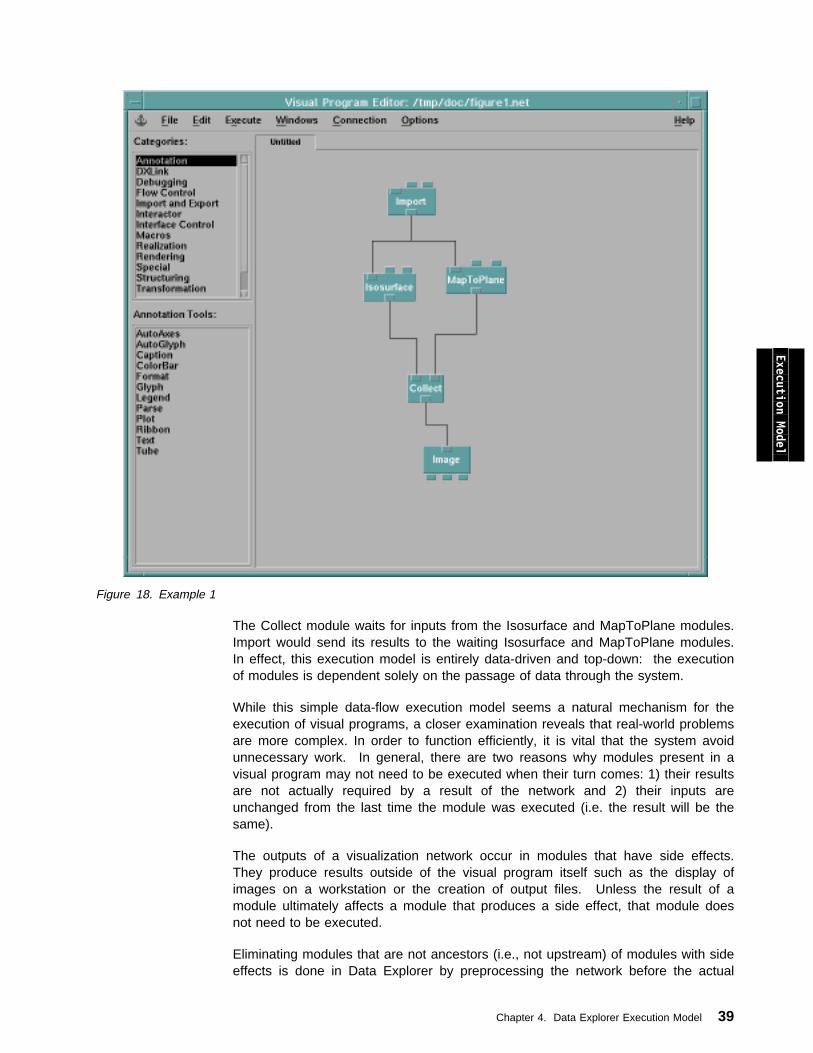
Figure 18. Example 1

Execution Model

The Collect module waits for inputs from the Isosurface and MapToPlane modules.Import would send its results to the waiting Isosurface and MapToPlane modules.In effect, this execution model is entirely data-driven and top-down: the executionof modules is dependent solely on the passage of data through the system.

While this simple data-flow execution model seems a natural mechanism for theexecution of visual programs, a closer examination reveals that real-world problemsare more complex. In order to function efficiently, it is vital that the system avoidunnecessary work. In general, there are two reasons why modules present in avisual program may not need to be executed when their turn comes: 1) their resultsare not actually required by a result of the network and 2) their inputs areunchanged from the last time the module was executed (i.e. the result will be thesame).

The outputs of a visualization network occur in modules that have side effects.They produce results outside of the visual program itself such as the display ofimages on a workstation or the creation of output files. Unless the result of amodule ultimately affects a module that produces a side effect, that module doesnot need to be executed.

Eliminating modules that are not ancestors (i.e., not upstream) of modules with sideeffects is done in Data Explorer by preprocessing the network before the actual

Chapter 4. Data Explorer Execution Model 39

data-flow network evaluation commences. This is done by traversing the graphbottom-up, beginning at each module known to have side effects and flagging eachmodule as it is encountered. Once this is complete, modules that have not beenflagged do not have to be executed.

Note that the exact order in which modules will be executed cannot be controlledby the user; for example, modules in two parallel branches may execute in anyorder with respect to one another; it is only guaranteed that a module that dependson the results of one or more modules will wait for them to be complete before it isexecuted.

4.2 Iterative Execution and Caching of Intermediate ResultsUnlike the simple example in Figure 18 on page 39 most real visualizationproblems involve some form of iteration. This may either be direct interaction,where the user is adjusting parameters of the visualization and observing theireffect on the resulting images, or animation, in which one or more inputs to thenetwork may vary from frame to frame.

In iterative applications, there are often major parts of the network that areunaffected when input parameters are modified. In Figure 18 on page 39 if theisovalue input to the Isosurface module is changed, only the affected module andits descendents need to be executed. The output of Import is not affected by thechange. Hence, it can be reused, which avoids a superfluous access of data ondisk. The MapToPlane module also does not need to be executed, since its inputsdid not change.

One way to implement this capability is via a caching mechanism for partial results.Instead of immediately reexecuting when its inputs arrive, a module may firstdetermine whether its inputs have changed. If they have not changed, it can simplyretrieve its results from the cache. Otherwise, the module reexecutes, placing itsnew result into the cache.

Data Explorer extends this notion by incorporating a cache (implemented by themodule scheduler rather than by the modules themselves) for all partial results.This cache retains results from not only the previous execution of the network, butfrom all prior executions (this is the default behavior; the user can also controlcache settings for modules). The saving of objects in the cache is subject tomemory limitations and a least-recently-used cache eviction strategy (items usedthe longest time ago are first to be discarded from the cache). The cachingbehavior for each output of a module may also be explicitly set by a user tooptimize memory utilization. (See A.1, “Using Data Explorer Effectively” onpage 212.)

The caching of partial results means that in general, the output of Import is held inthe cache. Usually, this is highly desirable, as it avoids needing to reimport the dataevery time the visual program is run. However if you modify your file on disk (e.g.,by editing it), Data Explorer will not know that the file has been changed, and willcontinue to use the cached version. To force Data Explorer to reimport the data,use the Reset Server option of the Connection menu. This will cause all items inthe cache to be discarded, and Import will reaccess the file on disk. You may alsoset Import to cache no results by using the Cache option of Import’s Configurationdialog box; note, however, that this will not necessarily cause Import to run everytime unless modules downstream from Import are also set to cache no results.

40 IBM Visualization Data Explorer: User’s Guide

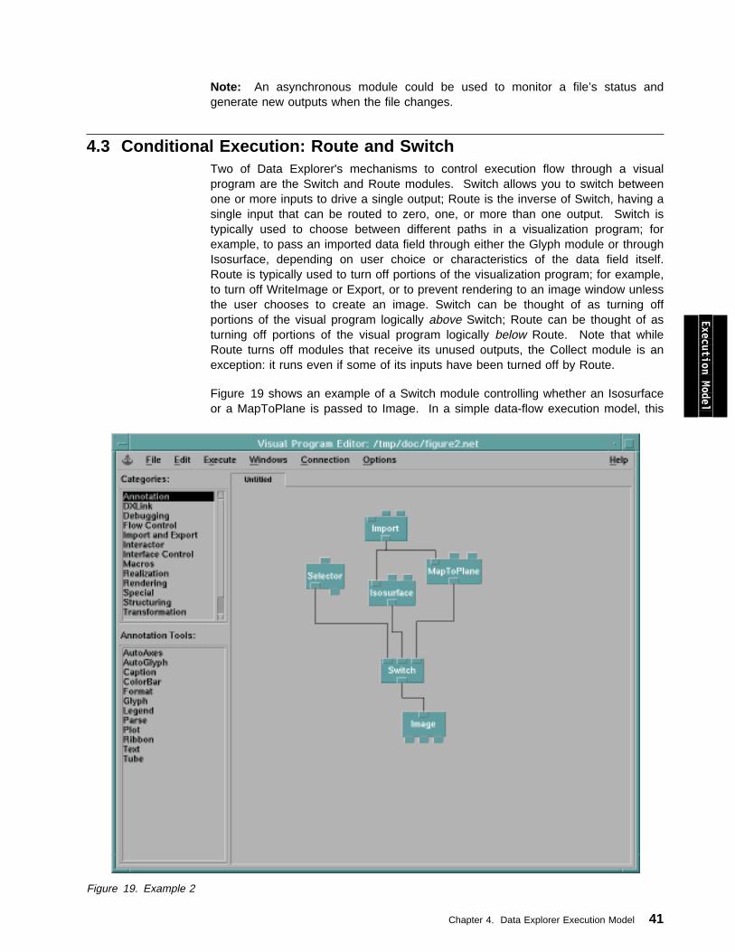
Note: An asynchronous module could be used to monitor a file’s status andgenerate new outputs when the file changes.

4.3 Conditional Execution: Route and SwitchTwo of Data Explorer's mechanisms to control execution flow through a visualprogram are the Switch and Route modules. Switch allows you to switch betweenone or more inputs to drive a single output; Route is the inverse of Switch, having asingle input that can be routed to zero, one, or more than one output. Switch istypically used to choose between different paths in a visualization program; forexample, to pass an imported data field through either the Glyph module or throughIsosurface, depending on user choice or characteristics of the data field itself.Route is typically used to turn off portions of the visualization program; for example,to turn off WriteImage or Export, or to prevent rendering to an image window unlessthe user chooses to create an image. Switch can be thought of as turning offportions of the visual program logically above Switch; Route can be thought of asturning off portions of the visual program logically below Route. Note that whileRoute turns off modules that receive its unused outputs, the Collect module is anexception: it runs even if some of its inputs have been turned off by Route.

Figure 19 shows an example of a Switch module controlling whether an Isosurfaceor a MapToPlane is passed to Image. In a simple data-flow execution model, this

Execution Model

Figure 19. Example 2

Chapter 4. Data Explorer Execution Model 41

Switch module will be executed when its inputs are available (i.e., the results of theIsosurface and MapToPlane modules, and the value of the selector). On execution,the Switch module chooses whether to pass the Isosurface or MapToPlane result tothe output based on the selection input to Switch. In the case of a pure data-flowmodel both the Isosurface and MapToPlane modules execute before the decisionas to which will actually be used is known. Since both operations can becomputationally expensive, the execution of both of them is very inefficient.

Again, this problem is handled in Data Explorer within the simple data-flowexecution module by an examination of the graph prior to execution. If theselection value comes from an external source (e.g., an interactor) and is known apriori, the selection may be performed by a simple transformation of the graph:excising the Switch module altogether, and substituting arcs from the selectedsource (either Isosurface or MapToPlane) to each of the modules that, in theoriginal network, received the result of the Switch module. This leaves theunselected module dangling. It and any of its ancestors that are therefore madeunnecessary will not be executed.

A different procedure is used if the controlling value is not static (e.g., if it isdetermined elsewhere in the network), as shown in Figure 20 on page 43.Suppose either an isosurface or a set of vector glyphs is selected depending onwhether the data are scalar or vector. The determination of the type of the data ismade using the Inquire module (i.e. at run time). In this case, the selection valuefor the Switch module cannot be determined before the execution of the graph.Instead, the graph must be evaluated in stages: 1) determine the selection value, 2)determine the necessary input to the Switch module and 3) evaluate the remainderof the graph. Since dynamic inputs may themselves be descended from othernon-static inputs (e.g., computed in the network), this process may have to beperformed repeatedly.

42 IBM Visualization Data Explorer: User’s Guide

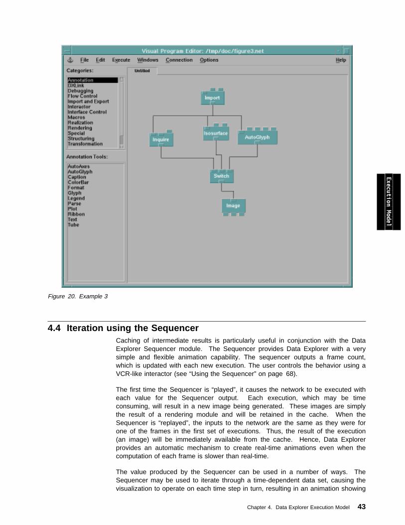
Figure 20. Example 3

Execution Model

4.4 Iteration using the SequencerCaching of intermediate results is particularly useful in conjunction with the DataExplorer Sequencer module. The Sequencer provides Data Explorer with a verysimple and flexible animation capability. The sequencer outputs a frame count,which is updated with each new execution. The user controls the behavior using aVCR-like interactor (see “Using the Sequencer” on page 68).

The first time the Sequencer is “played”, it causes the network to be executed witheach value for the Sequencer output. Each execution, which may be timeconsuming, will result in a new image being generated. These images are simplythe result of a rendering module and will be retained in the cache. When theSequencer is “replayed”, the inputs to the network are the same as they were forone of the frames in the first set of executions. Thus, the result of the execution(an image) will be immediately available from the cache. Hence, Data Explorerprovides an automatic mechanism to create real-time animations even when thecomputation of each frame is slower than real-time.

The value produced by the Sequencer can be used in a number of ways. TheSequencer may be used to iterate through a time-dependent data set, causing thevisualization to operate on each time step in turn, resulting in an animation showing

Chapter 4. Data Explorer Execution Model 43

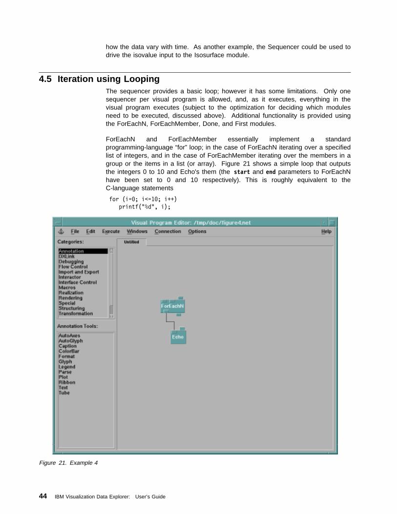
how the data vary with time. As another example, the Sequencer could be used todrive the isovalue input to the Isosurface module.

4.5 Iteration using LoopingThe sequencer provides a basic loop; however it has some limitations. Only onesequencer per visual program is allowed, and, as it executes, everything in thevisual program executes (subject to the optimization for deciding which modulesneed to be executed, discussed above). Additional functionality is provided usingthe ForEachN, ForEachMember, Done, and First modules.

ForEachN and ForEachMember essentially implement a standardprogramming-language “for” loop; in the case of ForEachN iterating over a specifiedlist of integers, and in the case of ForEachMember iterating over the members in agroup or the items in a list (or array). Figure 21 shows a simple loop that outputsthe integers 0 to 10 and Echo's them (the start and end parameters to ForEachNhave been set to 0 and 10 respectively). This is roughly equivalent to theC-language statements

for (i=ð; i<=1ð; i++)

printf("%d", i);

Figure 21. Example 4

44 IBM Visualization Data Explorer: User’s Guide

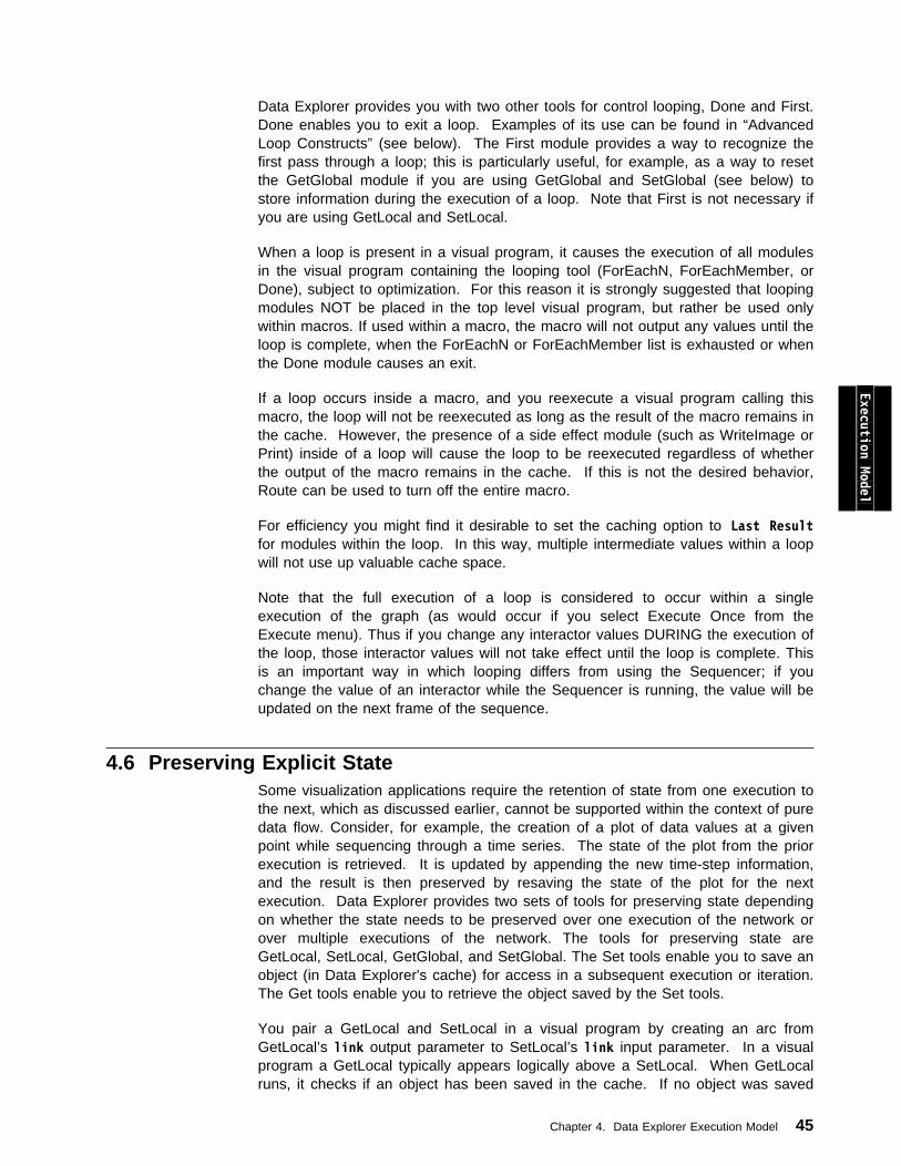
Data Explorer provides you with two other tools for control looping, Done and First.Done enables you to exit a loop. Examples of its use can be found in “AdvancedLoop Constructs” (see below). The First module provides a way to recognize thefirst pass through a loop; this is particularly useful, for example, as a way to resetthe GetGlobal module if you are using GetGlobal and SetGlobal (see below) tostore information during the execution of a loop. Note that First is not necessary ifyou are using GetLocal and SetLocal.

When a loop is present in a visual program, it causes the execution of all modulesin the visual program containing the looping tool (ForEachN, ForEachMember, orDone), subject to optimization. For this reason it is strongly suggested that loopingmodules NOT be placed in the top level visual program, but rather be used onlywithin macros. If used within a macro, the macro will not output any values until theloop is complete, when the ForEachN or ForEachMember list is exhausted or whenthe Done module causes an exit.

If a loop occurs inside a macro, and you reexecute a visual program calling thismacro, the loop will not be reexecuted as long as the result of the macro remains inthe cache. However, the presence of a side effect module (such as WriteImage orPrint) inside of a loop will cause the loop to be reexecuted regardless of whetherthe output of the macro remains in the cache. If this is not the desired behavior,Route can be used to turn off the entire macro.

For efficiency you might find it desirable to set the caching option to Last Resultfor modules within the loop. In this way, multiple intermediate values within a loopwill not use up valuable cache space.

Note that the full execution of a loop is considered to occur within a singleexecution of the graph (as would occur if you select Execute Once from theExecute menu). Thus if you change any interactor values DURING the execution ofthe loop, those interactor values will not take effect until the loop is complete. Thisis an important way in which looping differs from using the Sequencer; if youchange the value of an interactor while the Sequencer is running, the value will beupdated on the next frame of the sequence.

Execution Model

4.6 Preserving Explicit StateSome visualization applications require the retention of state from one execution tothe next, which as discussed earlier, cannot be supported within the context of puredata flow. Consider, for example, the creation of a plot of data values at a givenpoint while sequencing through a time series. The state of the plot from the priorexecution is retrieved. It is updated by appending the new time-step information,and the result is then preserved by resaving the state of the plot for the nextexecution. Data Explorer provides two sets of tools for preserving state dependingon whether the state needs to be preserved over one execution of the network orover multiple executions of the network. The tools for preserving state areGetLocal, SetLocal, GetGlobal, and SetGlobal. The Set tools enable you to save anobject (in Data Explorer's cache) for access in a subsequent execution or iteration.The Get tools enable you to retrieve the object saved by the Set tools.

You pair a GetLocal and SetLocal in a visual program by creating an arc fromGetLocal’s link output parameter to SetLocal’s link input parameter. In a visualprogram a GetLocal typically appears logically above a SetLocal. When GetLocalruns, it checks if an object has been saved in the cache. If no object was saved

Chapter 4. Data Explorer Execution Model 45

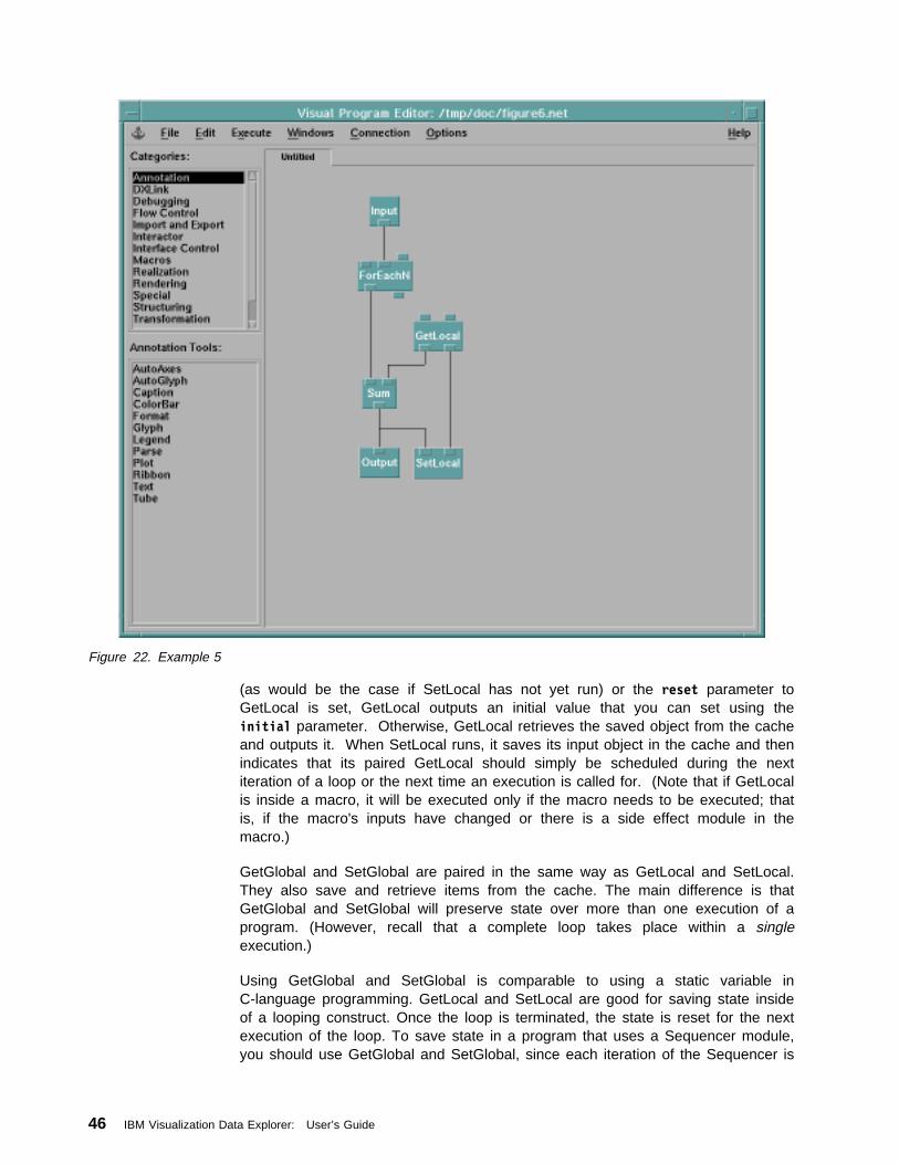
Figure 22. Example 5

(as would be the case if SetLocal has not yet run) or the reset parameter toGetLocal is set, GetLocal outputs an initial value that you can set using theinitial parameter. Otherwise, GetLocal retrieves the saved object from the cacheand outputs it. When SetLocal runs, it saves its input object in the cache and thenindicates that its paired GetLocal should simply be scheduled during the nextiteration of a loop or the next time an execution is called for. (Note that if GetLocalis inside a macro, it will be executed only if the macro needs to be executed; thatis, if the macro's inputs have changed or there is a side effect module in themacro.)

GetGlobal and SetGlobal are paired in the same way as GetLocal and SetLocal.They also save and retrieve items from the cache. The main difference is thatGetGlobal and SetGlobal will preserve state over more than one execution of aprogram. (However, recall that a complete loop takes place within a singleexecution.)

Using GetGlobal and SetGlobal is comparable to using a static variable inC-language programming. GetLocal and SetLocal are good for saving state insideof a looping construct. Once the loop is terminated, the state is reset for the nextexecution of the loop. To save state in a program that uses a Sequencer module,you should use GetGlobal and SetGlobal, since each iteration of the Sequencer is

46 IBM Visualization Data Explorer: User’s Guide

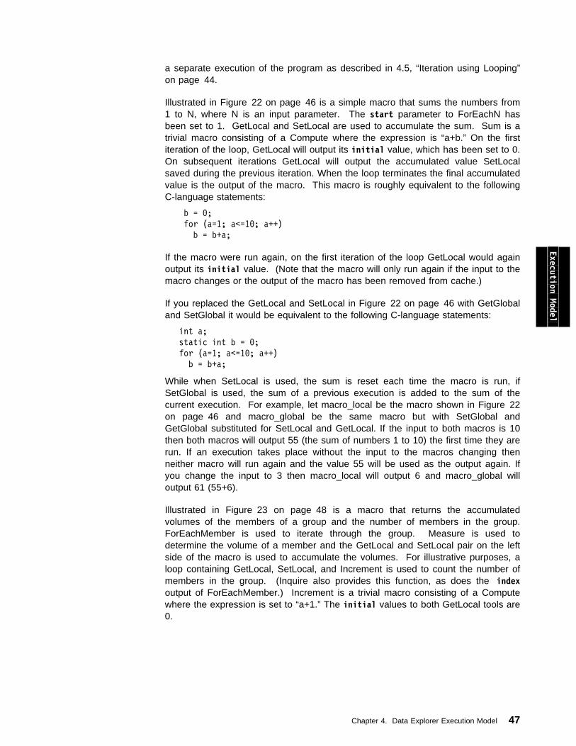
a separate execution of the program as described in 4.5, “Iteration using Looping”on page 44.

Illustrated in Figure 22 on page 46 is a simple macro that sums the numbers from1 to N, where N is an input parameter. The start parameter to ForEachN hasbeen set to 1. GetLocal and SetLocal are used to accumulate the sum. Sum is atrivial macro consisting of a Compute where the expression is “a+b.” On the firstiteration of the loop, GetLocal will output its initial value, which has been set to 0.On subsequent iterations GetLocal will output the accumulated value SetLocalsaved during the previous iteration. When the loop terminates the final accumulatedvalue is the output of the macro. This macro is roughly equivalent to the followingC-language statements:

b = ð;

for (a=1; a<=1ð; a++)

b = b+a;

If the macro were run again, on the first iteration of the loop GetLocal would againoutput its initial value. (Note that the macro will only run again if the input to themacro changes or the output of the macro has been removed from cache.)

If you replaced the GetLocal and SetLocal in Figure 22 on page 46 with GetGlobaland SetGlobal it would be equivalent to the following C-language statements:

int a;

static int b = ð;

for (a=1; a<=1ð; a++)

b = b+a;

While when SetLocal is used, the sum is reset each time the macro is run, ifSetGlobal is used, the sum of a previous execution is added to the sum of thecurrent execution. For example, let macro_local be the macro shown in Figure 22on page 46 and macro_global be the same macro but with SetGlobal andGetGlobal substituted for SetLocal and GetLocal. If the input to both macros is 10then both macros will output 55 (the sum of numbers 1 to 10) the first time they arerun. If an execution takes place without the input to the macros changing thenneither macro will run again and the value 55 will be used as the output again. Ifyou change the input to 3 then macro_local will output 6 and macro_global willoutput 61 (55+6).

Illustrated in Figure 23 on page 48 is a macro that returns the accumulatedvolumes of the members of a group and the number of members in the group.ForEachMember is used to iterate through the group. Measure is used todetermine the volume of a member and the GetLocal and SetLocal pair on the leftside of the macro is used to accumulate the volumes. For illustrative purposes, aloop containing GetLocal, SetLocal, and Increment is used to count the number ofmembers in the group. (Inquire also provides this function, as does the indexoutput of ForEachMember.) Increment is a trivial macro consisting of a Computewhere the expression is set to “a+1.” The initial values to both GetLocal tools are0.

Execution Model

Chapter 4. Data Explorer Execution Model 47

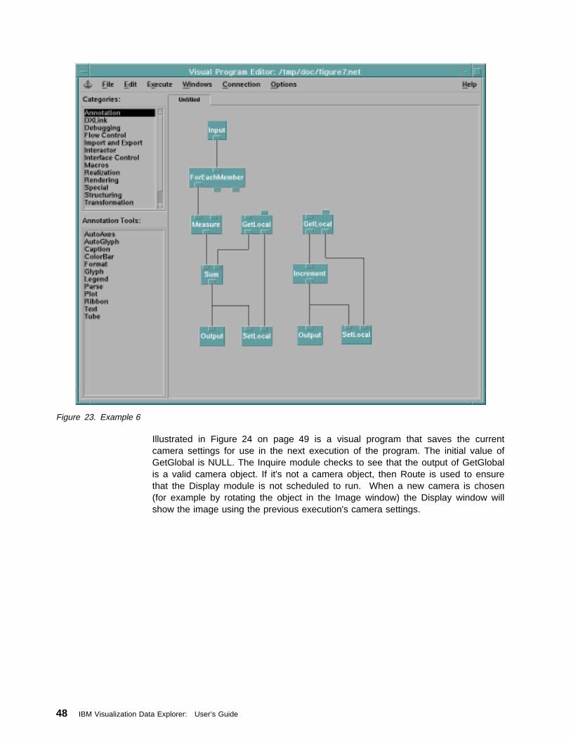
Figure 23. Example 6

Illustrated in Figure 24 on page 49 is a visual program that saves the currentcamera settings for use in the next execution of the program. The initial value ofGetGlobal is NULL. The Inquire module checks to see that the output of GetGlobalis a valid camera object. If it's not a camera object, then Route is used to ensurethat the Display module is not scheduled to run. When a new camera is chosen(for example by rotating the object in the Image window) the Display window willshow the image using the previous execution's camera settings.

48 IBM Visualization Data Explorer: User’s Guide

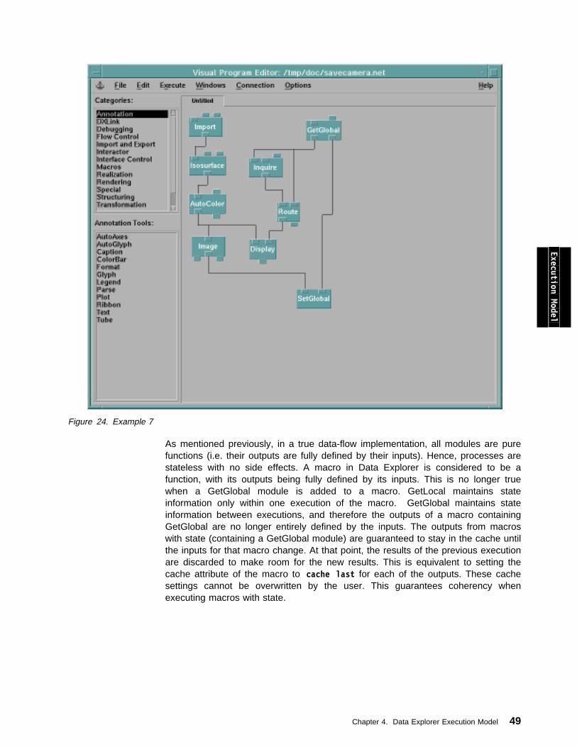
Figure 24. Example 7

Execution Model

As mentioned previously, in a true data-flow implementation, all modules are purefunctions (i.e. their outputs are fully defined by their inputs). Hence, processes arestateless with no side effects. A macro in Data Explorer is considered to be afunction, with its outputs being fully defined by its inputs. This is no longer truewhen a GetGlobal module is added to a macro. GetLocal maintains stateinformation only within one execution of the macro. GetGlobal maintains stateinformation between executions, and therefore the outputs of a macro containingGetGlobal are no longer entirely defined by the inputs. The outputs from macroswith state (containing a GetGlobal module) are guaranteed to stay in the cache untilthe inputs for that macro change. At that point, the results of the previous executionare discarded to make room for the new results. This is equivalent to setting thecache attribute of the macro to cache last for each of the outputs. These cachesettings cannot be overwritten by the user. This guarantees coherency whenexecuting macros with state.

Chapter 4. Data Explorer Execution Model 49

4.7 Advanced Looping ConstructsCombinations of the modules described above enable you to create advancedlooping constructs. These constructs are equivalent to C-language constructs suchas “do while” or “for” loops containing “break” and “continue” statements. In thefollowing figures the Sum and Increment macros, as described above, are used aswell as a macro named Equals that consists of a Compute where the expression is“a==b?1:0” (if the inputs are equal output 1 otherwise output 0).

Illustrated in Figure 25 on page 51 is a macro that computes the sum of numbersfrom 1 to N. If a number in the sequence from 1 to N is equal to an external input,x, the loop terminates and returns the sum from 1 to x. Done, in combination withEquals, is used to cause early termination of the loop. Done causes the loop toterminate after all the modules in the macro have executed if the input to Done isnonzero. The macro illustrated in Figure 25 on page 51 is equivalent to theC-language statements:

sum = ð;

i = ð;

do

i++;

sum = sum+i;

while (i<=n && i!=x);

Now consider a macro in which the sum of numbers from 1 to N is computed, but ifa number is equal to an external input value, x, it is excluded from the sum. Toachieve this result using C-language statements, you would use a conditional with a“continue” statement:

sum = ð;

for (i=1; i<=n; i++)

if (i==x) continue;

sum = sum+i;

50 IBM Visualization Data Explorer: User’s Guide

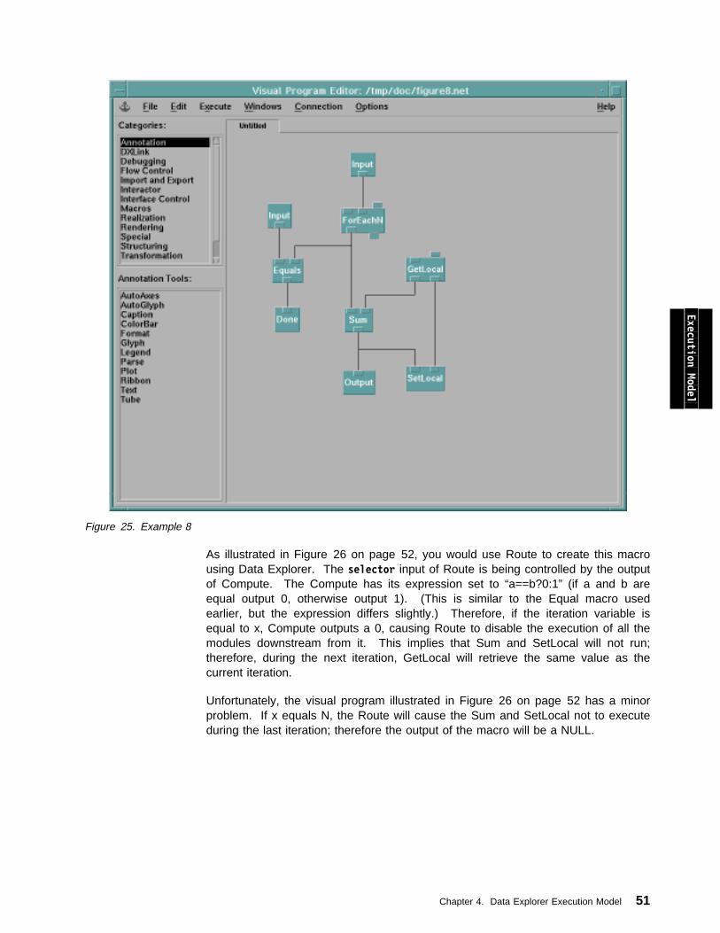
Figure 25. Example 8

Execution Model

As illustrated in Figure 26 on page 52, you would use Route to create this macrousing Data Explorer. The selector input of Route is being controlled by the outputof Compute. The Compute has its expression set to “a==b?0:1” (if a and b areequal output 0, otherwise output 1). (This is similar to the Equal macro usedearlier, but the expression differs slightly.) Therefore, if the iteration variable isequal to x, Compute outputs a 0, causing Route to disable the execution of all themodules downstream from it. This implies that Sum and SetLocal will not run;therefore, during the next iteration, GetLocal will retrieve the same value as thecurrent iteration.

Unfortunately, the visual program illustrated in Figure 26 on page 52 has a minorproblem. If x equals N, the Route will cause the Sum and SetLocal not to executeduring the last iteration; therefore the output of the macro will be a NULL.

Chapter 4. Data Explorer Execution Model 51

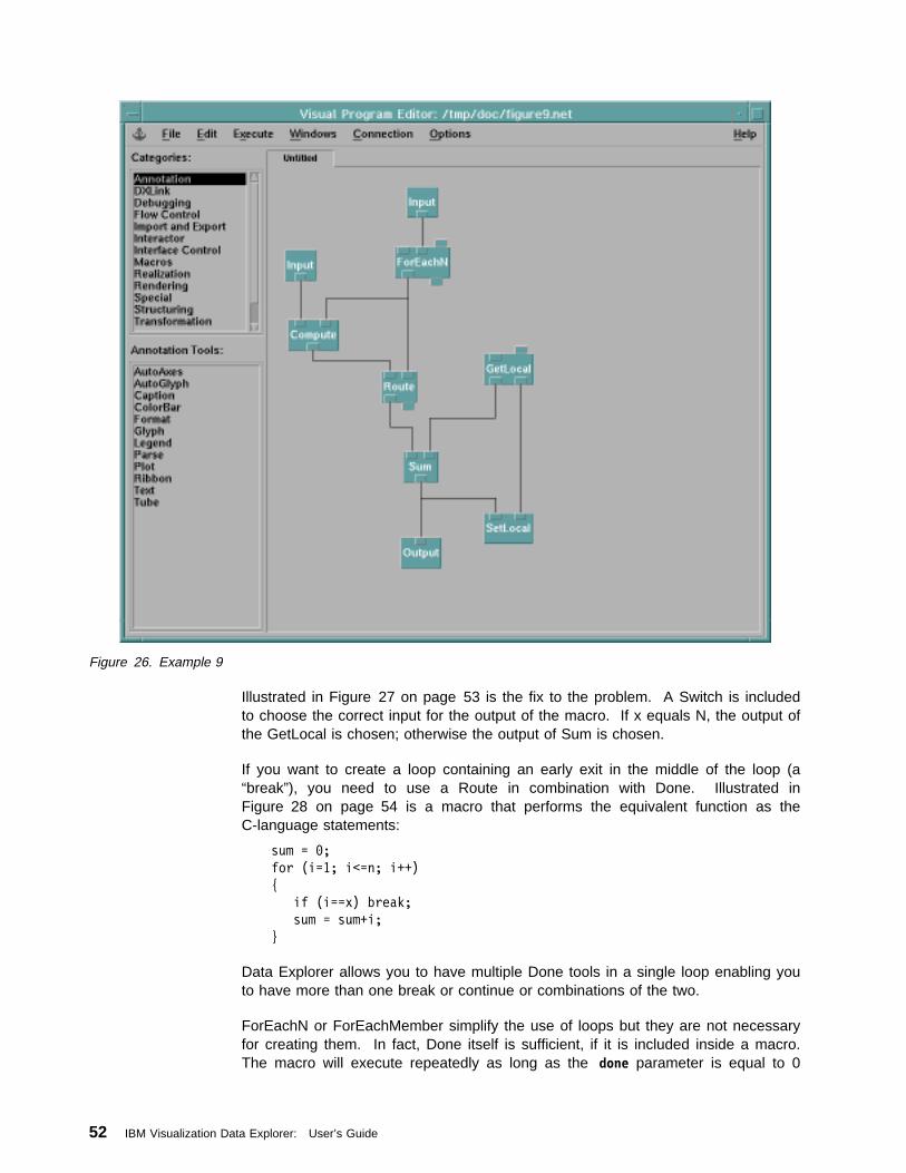
Figure 26. Example 9

Illustrated in Figure 27 on page 53 is the fix to the problem. A Switch is includedto choose the correct input for the output of the macro. If x equals N, the output ofthe GetLocal is chosen; otherwise the output of Sum is chosen.

If you want to create a loop containing an early exit in the middle of the loop (a“break”), you need to use a Route in combination with Done. Illustrated inFigure 28 on page 54 is a macro that performs the equivalent function as theC-language statements:

sum = ð;

for (i=1; i<=n; i++)

if (i==x) break;

sum = sum+i;

Data Explorer allows you to have multiple Done tools in a single loop enabling youto have more than one break or continue or combinations of the two.

ForEachN or ForEachMember simplify the use of loops but they are not necessaryfor creating them. In fact, Done itself is sufficient, if it is included inside a macro.The macro will execute repeatedly as long as the done parameter is equal to 0

52 IBM Visualization Data Explorer: User’s Guide

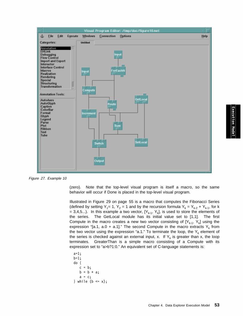
Figure 27. Example 10

Execution Model

(zero). Note that the top-level visual program is itself a macro, so the samebehavior will occur if Done is placed in the top-level visual program.

Illustrated in Figure 29 on page 55 is a macro that computes the Fibonacci Series(defined by setting Y1= 1, Y2 = 1 and by the recursion formula Yk = Yk-2 + Yk-1, for k= 3,4,5...). In this example a two vector, [Yk-1, Yk], is used to store the elements ofthe series. The GetLocal module has its initial value set to [1,1]. The firstCompute in the macro creates a new two vector consisting of [Yk-1, Yk] using theexpression “[a.1, a.0 + a.1].” The second Compute in the macro extracts Yk fromthe two vector using the expression “a.1.” To terminate the loop, the Yk element ofthe series is checked against an external input, x. If Yk is greater than x, the loopterminates. GreaterThan is a simple macro consisting of a Compute with itsexpression set to “a>b?1:0.” An equivalent set of C-language statements is:

a=1;

b=1;

do

c = b;

b = b + a;

a = c;

while (b <= x);

Chapter 4. Data Explorer Execution Model 53

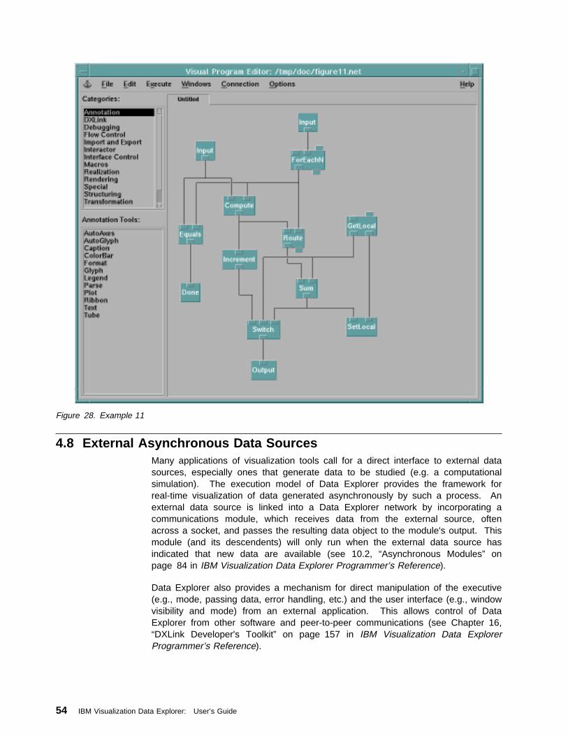
Figure 28. Example 11

4.8 External Asynchronous Data SourcesMany applications of visualization tools call for a direct interface to external datasources, especially ones that generate data to be studied (e.g. a computationalsimulation). The execution model of Data Explorer provides the framework forreal-time visualization of data generated asynchronously by such a process. Anexternal data source is linked into a Data Explorer network by incorporating acommunications module, which receives data from the external source, oftenacross a socket, and passes the resulting data object to the module's output. Thismodule (and its descendents) will only run when the external data source hasindicated that new data are available (see 10.2, “Asynchronous Modules” onpage 84 in IBM Visualization Data Explorer Programmer’s Reference).

Data Explorer also provides a mechanism for direct manipulation of the executive(e.g., mode, passing data, error handling, etc.) and the user interface (e.g., windowvisibility and mode) from an external application. This allows control of DataExplorer from other software and peer-to-peer communications (see Chapter 16,“DXLink Developer's Toolkit” on page 157 in IBM Visualization Data ExplorerProgrammer’s Reference).

54 IBM Visualization Data Explorer: User’s Guide

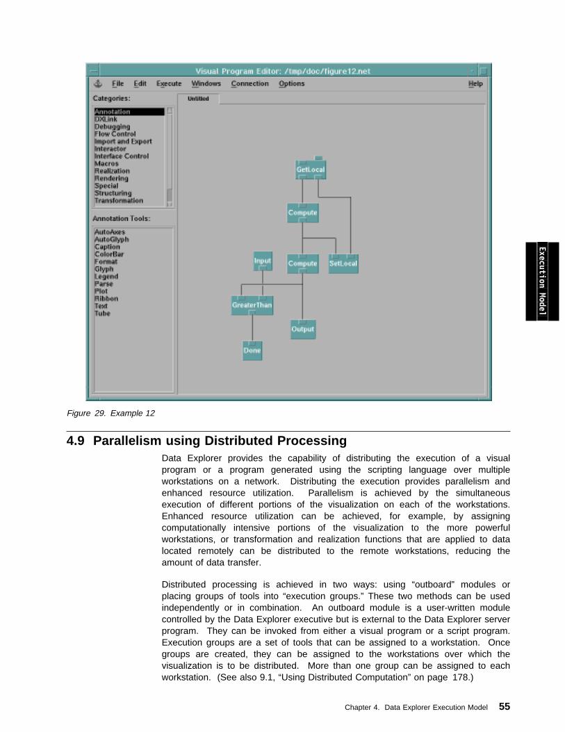
Figure 29. Example 12

Execution Model

4.9 Parallelism using Distributed ProcessingData Explorer provides the capability of distributing the execution of a visualprogram or a program generated using the scripting language over multipleworkstations on a network. Distributing the execution provides parallelism andenhanced resource utilization. Parallelism is achieved by the simultaneousexecution of different portions of the visualization on each of the workstations.Enhanced resource utilization can be achieved, for example, by assigningcomputationally intensive portions of the visualization to the more powerfulworkstations, or transformation and realization functions that are applied to datalocated remotely can be distributed to the remote workstations, reducing theamount of data transfer.

Distributed processing is achieved in two ways: using “outboard” modules orplacing groups of tools into “execution groups.” These two methods can be usedindependently or in combination. An outboard module is a user-written modulecontrolled by the Data Explorer executive but is external to the Data Explorer serverprogram. They can be invoked from either a visual program or a script program.Execution groups are a set of tools that can be assigned to a workstation. Oncegroups are created, they can be assigned to the workstations over which thevisualization is to be distributed. More than one group can be assigned to eachworkstation. (See also 9.1, “Using Distributed Computation” on page 178.)

Chapter 4. Data Explorer Execution Model 55

4.10 Parallelism for Data Explorer SMPFor completeness, the notion of module parallelism is discussed here. If you aredeveloping visualizations or modules exclusively for use with the IBM VisualizationData Explorer running on a single-processor workstation, then these concepts arenot applicable. However, if your visualizations or modules are to be run on boththe IBM Visualization Data Explorer and IBM Visualization Data Explorer SMP, thenthese concepts are important for achieving higher performance.

Every module that performs any significant amount of processing is “parallelized”;that is, the module makes use of all processors made available to Data Explorer tooperate on the data.

Data Explorer uses explicit data partitioning as the primary framework forparallelism. Data Explorer partitions the data into local, self-contained regions. Ingeneral, visualization modules then generate subtasks corresponding to partitions.For more information about partitioning, see Partition in IBM Visualization DataExplorer User’s Reference.

In general, parallel programming is complex. To help manage it, Data Explorersimplifies the process by providing a simple fork-join parallelism model toimplement coarse-grain shared memory parallelization (data parallel). Using datapartitions, read-only objects, and a single-fork join mode simplifies the modulewriting task by avoiding the explicit use of locks in modules, thereby reducing thepossibility of deadlock. For information about adding modules to the Data Explorersystem, see IBM Visualization Data Explorer Programmer’s Reference.

56 IBM Visualization Data Explorer: User’s Guide

Chapter 5. Graphical User Interface: Basics

5.1 Starting Data Explorer . . . . . . . . . . . . . . . . . . . . . . . . . . . . . . 58Using Environment Variables . . . . . . . . . . . . . . . . . . . . . . . . . . . 59

5.2 Understanding Data Explorer Windows . . . . . . . . . . . . . . . . . . . . 60Looking at Window Structure . . . . . . . . . . . . . . . . . . . . . . . . . . . 61Using the Mouse . . . . . . . . . . . . . . . . . . . . . . . . . . . . . . . . . . 62Moving and Resizing Windows . . . . . . . . . . . . . . . . . . . . . . . . . . 62Selecting Pull-Down Menus and Pull-Down Menu Options . . . . . . . . . . 62Selecting and Deselecting Items with the Mouse . . . . . . . . . . . . . . . . 63Selecting a Choice in an Option Box . . . . . . . . . . . . . . . . . . . . . . . 63Editing Text Fields . . . . . . . . . . . . . . . . . . . . . . . . . . . . . . . . . 64Working with Windows . . . . . . . . . . . . . . . . . . . . . . . . . . . . . . . 65

5.3 Using Online Help . . . . . . . . . . . . . . . . . . . . . . . . . . . . . . . . . 65User-Defined Help Files . . . . . . . . . . . . . . . . . . . . . . . . . . . . . . 67

5.4 Executing a Visual Program . . . . . . . . . . . . . . . . . . . . . . . . . . . 67Using the Sequencer . . . . . . . . . . . . . . . . . . . . . . . . . . . . . . . . 68Using a Data-Driven Sequencer . . . . . . . . . . . . . . . . . . . . . . . . . . 70Error Messages . . . . . . . . . . . . . . . . . . . . . . . . . . . . . . . . . . . 71

GUI: Basics

Copyright IBM Corp. 1991-1997 57

This chapter describes how to use the graphical user interface provided with DataExplorer. This interface enables you to create and control the visualization of data.An image is created by applying data, as input, to a visual program. The visualprogram is a sequence of interconnected functions acting on one or more inputsand producing one or more outputs. Typically, input is user data and output is arealization of that data in the form of an image.

Data Explorer consists of the following windows:

Startup WindowYou can use the Startup window to access other windows in DataExplorer.

Visual Program EditorYou can use the Visual Program Editor (VPE) to create and alter visualprograms and macros.

Control PanelYou can use Control Panel windows to set and control the inputparameters of visual program tools.

ImageYou can use the Image window to view an image created by DataExplorer.

Colormap EditorYou can use the Colormap Editor to map colors and opacity to specifieddata.

SequencerYou can use the Sequencer to advance through a data series or to stepthrough a changing sequence of input parameters.

Message WindowYou can use the Message window to access error and workinginformation about your execution.

HelpYou can use the Help window to access online documentation.

Data PrompterA graphical user interface that simplifies the import of data.

Module BuilderA graphical user interface that simplifies the process of adding modulesto Data Explorer.

For information on the Data Prompter, see IBM Visualization Data ExplorerQuickStart Guide; on the Module Builder, IBM Visualization Data ExplorerProgrammer’s Reference.

5.1 Starting Data ExplorerTo run Data Explorer using a workstation, you must have:

An account on the workstation If the executive portion of Data Explorer is to be executed on a remote

workstation, then a .rhosts file in your home directory should contain the nameof the machine on which the user interface will run. The permissions for the.rhosts file should be set to 600 (read and write only by the owner).

58 IBM Visualization Data Explorer: User’s Guide

You can start Data Explorer in any of several modes. In all cases, you must firstdo the following:

1. Log on to your workstation.2. Start an X Window System running with the Motif or the appropriate window

manager.

If you are going to create, modify, and execute visual programs, start Data Explorerinitially in the Visual Program Editor and connect to the executive (server) bytyping:

dx -edit [program]

where program (which is optional) names an existing visual program.

If you plan to execute a previously created visual program, start Data Explorerinitially in the Image window and connect to the executive (server) by typing:

dx -image program

or

dx -menubar program

where program is the name of an existing visual program.

You may want to start the user interface without connecting to the executive. Forexample, you may want to work on a visual program or macro, but may not plan toexecute it until some later time. In that case, you can start Data Explorer with thefollowing command:

dx -edit -uionly

Once the user interface is started, you can connect to the executive portion of DataExplorer by following the procedures described in 9.3, “Connecting to the Server”on page 183.

All of the command line options for Data Explorer are described in C.2, “CommandLine Options” on page 295.

GUI: Basics

Using Environment VariablesThere are several environment variables that you may find useful to customize DataExplorer. These can be set in your login profile, or set as required.

DXMACROS: The DXMACROS environment variable is a list of the directories inwhich Data Explorer will look for macros. If you do not specify DXMACROS, youwill need to load macros individually, using the process described in 7.2, “Creatingand Using Macros” on page 149. The directories are searched in the order inwhich they are specified in the environment variable. If multiple macros with thesame name are encountered, the first macro found is used.

An example of the statement setting the DXMACROS environment variable (in theC shell environment) is the following:

setenv DXMACROS /usr/mydirectory/projectAmacros:/usr/mydirectory/projectBmacros

where /usr/mydirectory/projectAmacros and /usr/mydirectory/projectBmacrosare two directories in which macros will be sought. Multiple directories can belisted, with directory names separated by a colon.

Chapter 5. Graphical User Interface: Basics 59

DXDATA: The DXDATA environment variable specifies a list of directories inwhich Data Explorer will search for data files. If the data you wish to import are inone of the directories specified in the DXDATA environment variable, then you donot need to specify the complete path name to the data in the Configuration dialogbox for the Import tool. You can simply specify the file name, and the Importmodule will look in the specified directories for the data file. The directories aresearched in the order in which they are listed in the environment variable; and thefirst occurrence of the data file is used.

An example of a statement that sets the DXDATA environment variable (in the Cshell environment) is the following:

setenv DXDATA /usr/mydirectory/mydata:/usr/group/groupdata

where /usr/mydirectory/mydata and /usr/group/groupdata are two directories thatcontain data files. Multiple directories can be listed, with directory names separatedby a colon.

DXHOST: The DXHOST environment variable is the initial machine name of theworkstation on which to run the executive. If DXHOST is not specified, then adefault of “localhost” is used. See 9.3, “Connecting to the Server” on page 183 formore information on how to connect to the server. The host name should be thename that results when you issue the uname -n shell command.

The rest of the environment variables and start-up options are discussed inAppendix C, “Environment Variables and Command Line Options” on page 291.

5.2 Understanding Data Explorer WindowsThe Data Explorer user interface is built on the X Window System and Motifstandards. These tools manage the windows used with Data Explorer. Thewindows you use depends upon how you choose to use the system.

The primary windows are listed and described at the start of this chapter. Theprimary window in which you begin a Data Explorer session (either the VisualProgram Editor or Image window) is called the anchor window. (You can also havea menu bar as your anchor window by specifying -menubar on the command line.)This is the window that, if closed, ends the Data Explorer session. The anchorwindow is identified by a symbol resembling a ship’s anchor located in the top leftcorner, as illustrated in Figure 30 on page 61.

Descriptions of the primary window pull-down menu options are located in Section8.1, “Using the Primary Window Pull-Down Menus and Options” on page 156.

Secondary windows, such as dialog boxes or informational boxes, appear whenthey are needed to complete a task. You can move secondary windows, but youcannot put them behind the primary window from which they came. See IBMAIXwindows User’s Guide or the appropriate window system overview for moreinformation on how to manipulate windows.

In this chapter, when references are made to the X Window System it means anywindow server that supports X11 protocol, including Sun’s OpenWindows. TheMotif window manger, mwm, has been used in many figures and examples in thischapter. Please use the appropriate window manager for your system, such asvuewm for Hewlett-Packard, 4dwm for SGI, and olwm for Sun. Since title bars and

60 IBM Visualization Data Explorer: User’s Guide

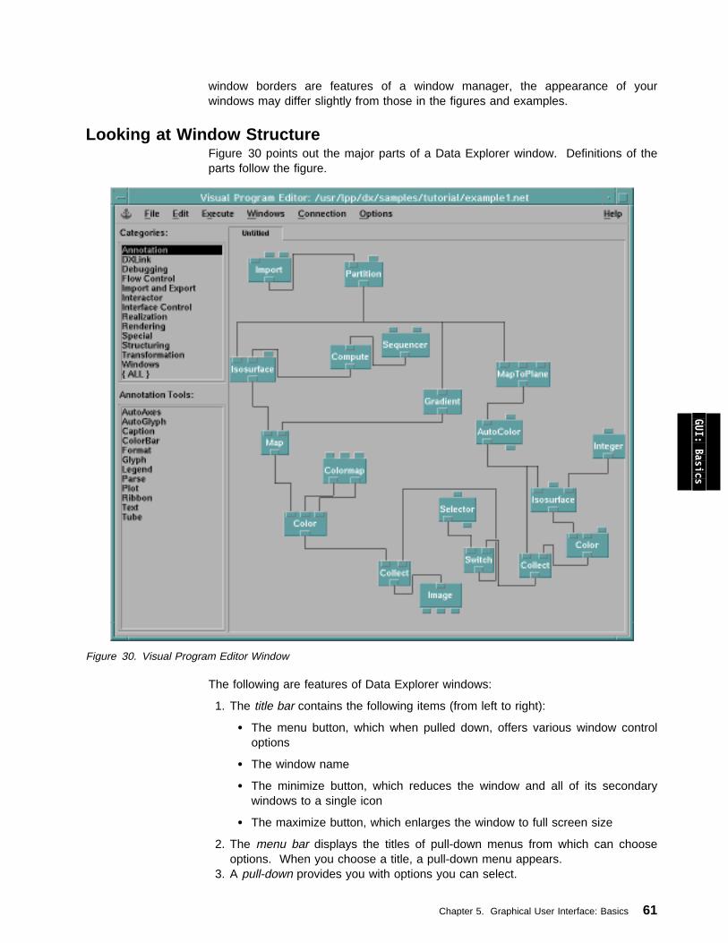
window borders are features of a window manager, the appearance of yourwindows may differ slightly from those in the figures and examples.

Looking at Window StructureFigure 30 points out the major parts of a Data Explorer window. Definitions of theparts follow the figure.

Figure 30. Visual Program Editor Window

GUI: Basics

The following are features of Data Explorer windows:

1. The title bar contains the following items (from left to right):

The menu button, which when pulled down, offers various window controloptions

The window name

The minimize button, which reduces the window and all of its secondarywindows to a single icon

The maximize button, which enlarges the window to full screen size

2. The menu bar displays the titles of pull-down menus from which can chooseoptions. When you choose a title, a pull-down menu appears.

3. A pull-down provides you with options you can select.

Chapter 5. Graphical User Interface: Basics 61

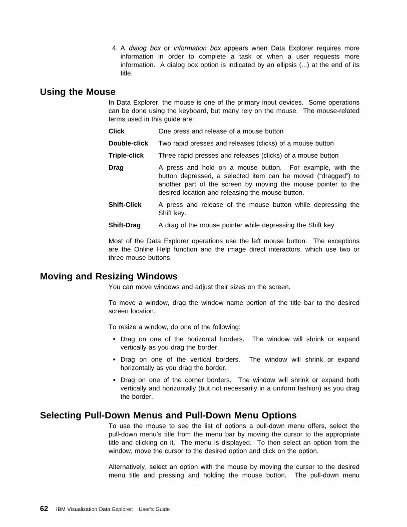
4. A dialog box or information box appears when Data Explorer requires moreinformation in order to complete a task or when a user requests moreinformation. A dialog box option is indicated by an ellipsis (...) at the end of itstitle.

Using the MouseIn Data Explorer, the mouse is one of the primary input devices. Some operationscan be done using the keyboard, but many rely on the mouse. The mouse-relatedterms used in this guide are:

Click One press and release of a mouse button

Double-click Two rapid presses and releases (clicks) of a mouse button

Triple-click Three rapid presses and releases (clicks) of a mouse button

Drag A press and hold on a mouse button. For example, with thebutton depressed, a selected item can be moved (“dragged”) toanother part of the screen by moving the mouse pointer to thedesired location and releasing the mouse button.

Shift-Click A press and release of the mouse button while depressing theShift key.

Shift-Drag A drag of the mouse pointer while depressing the Shift key.

Most of the Data Explorer operations use the left mouse button. The exceptionsare the Online Help function and the image direct interactors, which use two orthree mouse buttons.

Moving and Resizing WindowsYou can move windows and adjust their sizes on the screen.

To move a window, drag the window name portion of the title bar to the desiredscreen location.

To resize a window, do one of the following:

Drag on one of the horizontal borders. The window will shrink or expandvertically as you drag the border.

Drag on one of the vertical borders. The window will shrink or expandhorizontally as you drag the border.

Drag on one of the corner borders. The window will shrink or expand bothvertically and horizontally (but not necessarily in a uniform fashion) as you dragthe border.

Selecting Pull-Down Menus and Pull-Down Menu OptionsTo use the mouse to see the list of options a pull-down menu offers, select thepull-down menu’s title from the menu bar by moving the cursor to the appropriatetitle and clicking on it. The menu is displayed. To then select an option from thewindow, move the cursor to the desired option and click on the option.

Alternatively, select an option with the mouse by moving the cursor to the desiredmenu title and pressing and holding the mouse button. The pull-down menu

62 IBM Visualization Data Explorer: User’s Guide

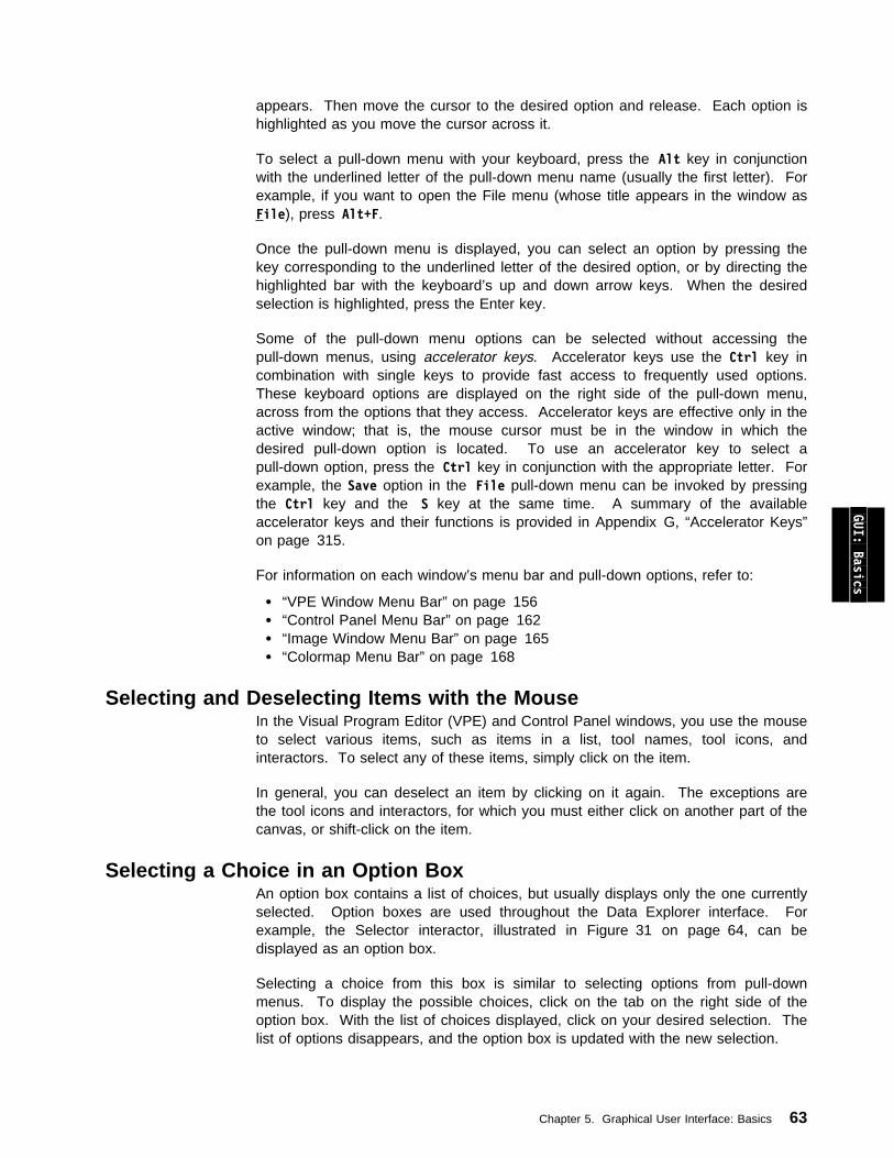
appears. Then move the cursor to the desired option and release. Each option ishighlighted as you move the cursor across it.

To select a pull-down menu with your keyboard, press the Alt key in conjunctionwith the underlined letter of the pull-down menu name (usually the first letter). Forexample, if you want to open the File menu (whose title appears in the window asFile), press Alt+F.

Once the pull-down menu is displayed, you can select an option by pressing thekey corresponding to the underlined letter of the desired option, or by directing thehighlighted bar with the keyboard’s up and down arrow keys. When the desiredselection is highlighted, press the Enter key.

Some of the pull-down menu options can be selected without accessing thepull-down menus, using accelerator keys. Accelerator keys use the Ctrl key incombination with single keys to provide fast access to frequently used options.These keyboard options are displayed on the right side of the pull-down menu,across from the options that they access. Accelerator keys are effective only in theactive window; that is, the mouse cursor must be in the window in which thedesired pull-down option is located. To use an accelerator key to select apull-down option, press the Ctrl key in conjunction with the appropriate letter. Forexample, the Save option in the File pull-down menu can be invoked by pressingthe Ctrl key and the S key at the same time. A summary of the availableaccelerator keys and their functions is provided in Appendix G, “Accelerator Keys”on page 315.

For information on each window’s menu bar and pull-down options, refer to:

“VPE Window Menu Bar” on page 156 “Control Panel Menu Bar” on page 162 “Image Window Menu Bar” on page 165 “Colormap Menu Bar” on page 168

GUI: Basics

Selecting and Deselecting Items with the MouseIn the Visual Program Editor (VPE) and Control Panel windows, you use the mouseto select various items, such as items in a list, tool names, tool icons, andinteractors. To select any of these items, simply click on the item.

In general, you can deselect an item by clicking on it again. The exceptions arethe tool icons and interactors, for which you must either click on another part of thecanvas, or shift-click on the item.

Selecting a Choice in an Option BoxAn option box contains a list of choices, but usually displays only the one currentlyselected. Option boxes are used throughout the Data Explorer interface. Forexample, the Selector interactor, illustrated in Figure 31 on page 64, can bedisplayed as an option box.

Selecting a choice from this box is similar to selecting options from pull-downmenus. To display the possible choices, click on the tab on the right side of theoption box. With the list of choices displayed, click on your desired selection. Thelist of options disappears, and the option box is updated with the new selection.

Chapter 5. Graphical User Interface: Basics 63

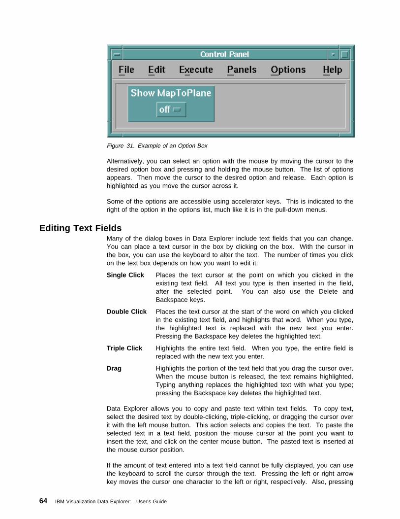
Figure 31. Example of an Option Box

Alternatively, you can select an option with the mouse by moving the cursor to thedesired option box and pressing and holding the mouse button. The list of optionsappears. Then move the cursor to the desired option and release. Each option ishighlighted as you move the cursor across it.

Some of the options are accessible using accelerator keys. This is indicated to theright of the option in the options list, much like it is in the pull-down menus.

Editing Text FieldsMany of the dialog boxes in Data Explorer include text fields that you can change.You can place a text cursor in the box by clicking on the box. With the cursor inthe box, you can use the keyboard to alter the text. The number of times you clickon the text box depends on how you want to edit it:

Single Click Places the text cursor at the point on which you clicked in theexisting text field. All text you type is then inserted in the field,after the selected point. You can also use the Delete andBackspace keys.

Double Click Places the text cursor at the start of the word on which you clickedin the existing text field, and highlights that word. When you type,the highlighted text is replaced with the new text you enter.Pressing the Backspace key deletes the highlighted text.

Triple Click Highlights the entire text field. When you type, the entire field isreplaced with the new text you enter.

Drag Highlights the portion of the text field that you drag the cursor over.When the mouse button is released, the text remains highlighted.Typing anything replaces the highlighted text with what you type;pressing the Backspace key deletes the highlighted text.

Data Explorer allows you to copy and paste text within text fields. To copy text,select the desired text by double-clicking, triple-clicking, or dragging the cursor overit with the left mouse button. This action selects and copies the text. To paste theselected text in a text field, position the mouse cursor at the point you want toinsert the text, and click on the center mouse button. The pasted text is inserted atthe mouse cursor position.

If the amount of text entered into a text field cannot be fully displayed, you can usethe keyboard to scroll the cursor through the text. Pressing the left or right arrowkey moves the cursor one character to the left or right, respectively. Also, pressing

64 IBM Visualization Data Explorer: User’s Guide

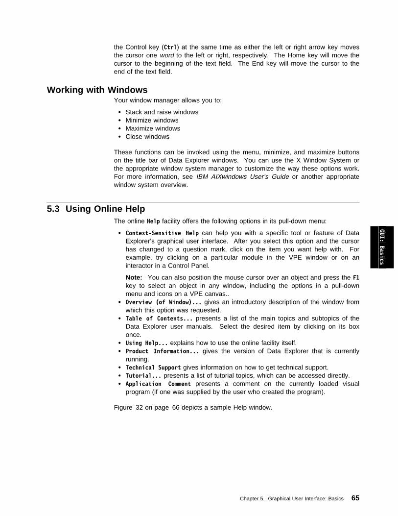
the Control key (Ctrl) at the same time as either the left or right arrow key movesthe cursor one word to the left or right, respectively. The Home key will move thecursor to the beginning of the text field. The End key will move the cursor to theend of the text field.

Working with WindowsYour window manager allows you to:

Stack and raise windows Minimize windows Maximize windows Close windows

These functions can be invoked using the menu, minimize, and maximize buttonson the title bar of Data Explorer windows. You can use the X Window System orthe appropriate window system manager to customize the way these options work.For more information, see IBM AIXwindows User’s Guide or another appropriatewindow system overview.

5.3 Using Online HelpThe online Help facility offers the following options in its pull-down menu:

Context-Sensitive Help can help you with a specific tool or feature of DataExplorer’s graphical user interface. After you select this option and the cursorhas changed to a question mark, click on the item you want help with. Forexample, try clicking on a particular module in the VPE window or on aninteractor in a Control Panel.

Note: You can also position the mouse cursor over an object and press the F1key to select an object in any window, including the options in a pull-downmenu and icons on a VPE canvas..

Overview (of Window)... gives an introductory description of the window fromwhich this option was requested.

Table of Contents... presents a list of the main topics and subtopics of theData Explorer user manuals. Select the desired item by clicking on its boxonce.

Using Help... explains how to use the online facility itself. Product Information... gives the version of Data Explorer that is currently

running. Technical Support gives information on how to get technical support. Tutorial... presents a list of tutorial topics, which can be accessed directly. Application Comment presents a comment on the currently loaded visual

program (if one was supplied by the user who created the program).

Figure 32 on page 66 depicts a sample Help window.

GUI: Basics

Chapter 5. Graphical User Interface: Basics 65

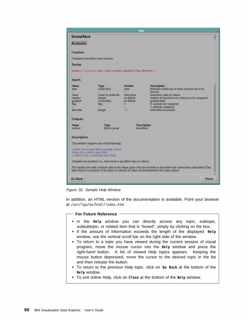
Figure 32. Sample Help Window

In addition, an HTML version of the documentation is available. Point your browserat /usr/lpp/dx/html/index.htm.

For Future Reference

In the Help window you can directly access any topic, subtopic,subsubtopic, or related item that is “boxed”, simply by clicking on the box.

If the amount of information exceeds the length of the displayed Helpwindow, use the vertical scroll bar on the right side of the window.

To return to a topic you have viewed during the current session of visualprogram, move the mouse cursor into the Help window and press theright-hand button: A list of viewed Help topics appears. Keeping themouse button depressed, move the cursor to the desired topic in the listand then release the button.

To return to the previous Help topic, click on Go Back at the bottom of theHelp window.

To exit online Help, click on Close at the bottom of the Help window.

66 IBM Visualization Data Explorer: User’s Guide

User-Defined Help FilesVisual programmers can create online documentation for their visual programs andControl Panels. A user can access the comments for the visual program from anyprimary window, and can access the comments for a Control Panel from theControl Panel with which the comments are associated. For information on how toadd this documentation to your own visual program, see “Adding Comments to aVisual Program” on page 114 and “Customizing a Control Panel” on page 133.

To access comments for the visual program, select the Application Comment optionfrom the Help pull-down menu. A dialog box opens with the comments.

Note: If there are no comments associated with the visual program, this menuoption is grayed-out. Also, you cannot modify the comments when usingthis option—only view them.

The user can also access the comments for the visual program from the Open... orLoad Macro... file selection dialog boxes, even before the visual program isopened. For information on how to do this, see “Restoring a Previously CreatedProgram” on page 118.

To access comments for a specific Control Panel, select the On Control Paneloption from the Help pull-down menu in the Control Panel about which you want tolearn. A dialog box opens with the comments.

Note: If there are no comments associated with the Control Panel, this menuoption is grayed-out. Also, you cannot modify the comments when usingthis option—only view them.

GUI: Basics

5.4 Executing a Visual ProgramAfter you set up a visual program in the VPE window and build any desired ControlPanels (or after you open an existing visual program file), you can execute thevisual program program. The resulting image appears in the Image window. Thissection explains how to execute a visual program. Section 6.1, “Using the ImageWindow” on page 74 describes how to manipulate images in the Image window byusing direct interactors. You can also manipulate images in the Image windowusing interactors in the Control Panels, the Colormap Editor, and the Sequencer.(For more information on these tools, see 7.1, “Using Control Panels andInteractors” on page 128, “Colormap” on page 84, and “Sequencer” on page 297in IBM Visualization Data Explorer User’s Reference.)

You can execute the visual program from the Execute menu of a VPE window, aControl Panel, an Image window, or a Message window. The options are the samein all four windows. When a visual program is executed, an Image window iscreated if one is not already open. (You can also control execution using theExecute module. See IBM Visualization Data Explorer User’s Reference.)

Note: If the Execute options are grayed-out, your workstation may not beconnected to the server. For information about connecting to the server,see 9.3, “Connecting to the Server” on page 183.

Although you can initiate execution from the Control Panel, VPE, Image, andMessage windows, you may find it more efficient to execute your visual programthrough the Control Panel menu (if you are using a Control Panel). This efficiency

Chapter 5. Graphical User Interface: Basics 67

is due to the ease with which you can change inputs with interactors and initiateexecution.

You can choose one of four options from the Execute menu when executing avisual program. Select the first option, Execute Once, to execute the program once,using the values currently set in the interactors. If you change any interactorvalues after execution, the visual program does not automatically execute; youmust again choose an option from the Execute menu to execute the alteredprogram.

Choosing the Execute on Change option causes the visual program to executeevery time you change an interactor setting. If you change values faster than DataExplorer can generate images, the system executes the program as quickly aspossible, always using the current settings at the time an execution cycle begins. Ifyou modify your visual program while Execute on Change is enabled, then theoption automatically becomes disabled. After the changes are made, you canreenable it.

Choosing End Execution while the visual program is executing causes execution tostop after the currently executing module.

The final Execute menu option is Sequencer. If you select this option, and aSequencer tool is present in the visual program, the Sequencer appears (see“Using the Sequencer” for more information). While the Sequencer runs, you canchange interactor settings, and those changes are reflected in subsequent framesgenerated by the Sequencer. The Execute Once and Execute on Change optionsare grayed out when the Sequencer is running, but when you pause theSequencer, you can use those two options to explore the particular frame theSequencer paused on.

While the visual program is executing, the Execute option on the menu bar ishighlighted. It remains highlighted until execution is finished. If Execute on Changeis selected, the Execute option on the menu bar is highlighted with one color duringexecution, and another color outside of execution cycles.

Using the SequencerThe Sequencer allows you to “animate” a visual image and is very easy to use.The process is rather like running a video cassette tape: You can play it forward orbackward, stop it, pause, and so on. The Sequencer Control panel consists of 8buttons as shown in Figure 33.

Figure 33. Sequence Control Panel. The first two buttons at top left are Loop andPalindrome. The others are: Step (%||5), Counter (...), Back (%), Forward (5), Stop (), andPause (||).

68 IBM Visualization Data Explorer: User’s Guide

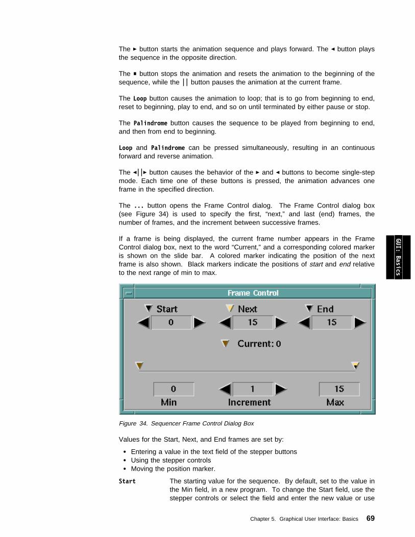
The 5 button starts the animation sequence and plays forward. The % button playsthe sequence in the opposite direction.

The button stops the animation and resets the animation to the beginning of thesequence, while the || button pauses the animation at the current frame.

The Loop button causes the animation to loop; that is to go from beginning to end,reset to beginning, play to end, and so on until terminated by either pause or stop.

The Palindrome button causes the sequence to be played from beginning to end,and then from end to beginning.

Loop and Palindrome can be pressed simultaneously, resulting in an continuousforward and reverse animation.

The %||5 button causes the behavior of the 5 and % buttons to become single-stepmode. Each time one of these buttons is pressed, the animation advances oneframe in the specified direction.

The ... button opens the Frame Control dialog. The Frame Control dialog box(see Figure 34) is used to specify the first, “next,” and last (end) frames, thenumber of frames, and the increment between successive frames.

If a frame is being displayed, the current frame number appears in the FrameControl dialog box, next to the word “Current,” and a corresponding colored markeris shown on the slide bar. A colored marker indicating the position of the nextframe is also shown. Black markers indicate the positions of start and end relativeto the next range of min to max.

GUI: Basics

Figure 34. Sequencer Frame Control Dialog Box

Values for the Start, Next, and End frames are set by:

Entering a value in the text field of the stepper buttons Using the stepper controls Moving the position marker.

Start The starting value for the sequence. By default, set to the value inthe Min field, in a new program. To change the Start field, use thestepper controls or select the field and enter the new value or use

Chapter 5. Graphical User Interface: Basics 69

the Start marker. If you change the value in the Min field, then theStart field is set to that new value. If you are working with a savedprogram, then the Min and Start fields are set to the values thatwere saved.

End The ending value for the sequence. By default, set to the value inthe Max field, in a new program. To change the End field, use thestepper controls or select the field and enter the new value or usethe End marker. If you change the value in the Max field, then theEnd field is set to that new value. If you are working with a savedprogram, then the Max and End fields are set to the values thatwere saved.

Current Displays the current frame number.

Increment By default, set to 1. To change the increment, use the steppercontrols or select the field and enter the new value.

Next By default, set to the value in the Start field, in a new program.You can set the Next field to any value between the Start and Endvalues: the Sequencer will begin running at that value. (When theSequencer is in loop mode, subsequent loops begin at the value inthe Start field.)

Min and Max Specify the allowed range of sequence values. These are textfields that can be altered. Data Explorer ensures that the value inthe Start field is greater than or equal to the Min value, and thevalue in the End field is less than or equal to the Max value.

Note: If the images change more quickly than you would like, use theThrottle... option (see “Changing the Rate of Frame Display: Throttle...”on page 93).

Using a Data-Driven SequencerThe Sequencer can be data driven, meaning that its minimum, maximum, and stepvalues can be set by connecting the output of a tool to the input of a Sequencer inthe VPE or by a value typed into the Sequencer’s Configuration dialog box, ratherthan by using the Frame Control panel.

If the Sequencer is data driven, then the information transmitted by connection orset in the Configuration dialog box overrides values set in the Frame Control panel.

A data-driven Sequencer allows you to create visual programs that will work with avariety of input data sets without your having to reset Sequencer attributes. Forexample, if the Sequencer minimum is set to zero and its maximum to the numberof steps in a series, it can be used to drive the Select module to select eachmember of the series in turn.

The inputs are summarized in the corresponding module description in IBMVisualization Data Explorer User’s Reference.

Each time an input to a data-driven Sequencer is changed (for example, byimporting a new data set) the Sequencer is reexecuted, updating its attributes.

70 IBM Visualization Data Explorer: User’s Guide

Error MessagesIf Data Explorer encounters an error in your visual program while executing it, anerror message is displayed in the Message window (see 8.2, “Using the MessageWindow” on page 174). The name of the tool in which the error occurred is shownin the window. Pull-down menu options enable you to quickly locate the tool thatcaused the error.

The title of the tool icon in the visual program that caused the error is displayed ina different color in the VPE until you execute the program again. When the erroroccurs, execution stops only in the path where the error is; other paths continue.

GUI: Basics

Chapter 5. Graphical User Interface: Basics 71

72 IBM Visualization Data Explorer: User’s Guide

Chapter 6. Graphical User Interface: Important Windows

6.1 Using the Image Window . . . . . . . . . . . . . . . . . . . . . . . . . . . . 74Controlling the Image: View Control... . . . . . . . . . . . . . . . . . . . . . . 74Undo, Redo, and Reset . . . . . . . . . . . . . . . . . . . . . . . . . . . . . . 87AutoAxes... . . . . . . . . . . . . . . . . . . . . . . . . . . . . . . . . . . . . . 88Set Background Color... . . . . . . . . . . . . . . . . . . . . . . . . . . . . . . 89Display Rotation Globe . . . . . . . . . . . . . . . . . . . . . . . . . . . . . . . 91Rendering Options... . . . . . . . . . . . . . . . . . . . . . . . . . . . . . . . . 91Image Depth . . . . . . . . . . . . . . . . . . . . . . . . . . . . . . . . . . . . . 93Changing the Rate of Frame Display: Throttle... . . . . . . . . . . . . . . . . 93Changing the Title of an Image Window . . . . . . . . . . . . . . . . . . . . . 93Control Panel Access... . . . . . . . . . . . . . . . . . . . . . . . . . . . . . . 94Saving an Image . . . . . . . . . . . . . . . . . . . . . . . . . . . . . . . . . . 94Printing an Image . . . . . . . . . . . . . . . . . . . . . . . . . . . . . . . . . . 97

6.2 Using the VPE . . . . . . . . . . . . . . . . . . . . . . . . . . . . . . . . . . . 99Creating a Visual Program . . . . . . . . . . . . . . . . . . . . . . . . . . . . 100Specifying Values for a Tool's Inputs . . . . . . . . . . . . . . . . . . . . . . 103Creating, Deleting, and Moving Tab Connections . . . . . . . . . . . . . . . 104Moving and Copying Tools . . . . . . . . . . . . . . . . . . . . . . . . . . . . 105Using Transmitters and Receivers . . . . . . . . . . . . . . . . . . . . . . . 106Adding and Removing Input and Output Tabs . . . . . . . . . . . . . . . . 106Entering Values in a Configuration Dialog Box . . . . . . . . . . . . . . . . 107Revealing and Hiding Input Tabs . . . . . . . . . . . . . . . . . . . . . . . . 110Using the Compute Module Configuration Dialog Box . . . . . . . . . . . . 111Locating Tools: The Find Tool Dialog Box . . . . . . . . . . . . . . . . . . . 111Customizing the VPE Window . . . . . . . . . . . . . . . . . . . . . . . . . . 113Adding Comments to a Visual Program . . . . . . . . . . . . . . . . . . . . 114Adding Annotation to a Visual Program . . . . . . . . . . . . . . . . . . . . 115Creating pages in the VPE . . . . . . . . . . . . . . . . . . . . . . . . . . . . 115Saving and Restoring a Visual Program . . . . . . . . . . . . . . . . . . . . 115

6.3 Using the Colormap Editor . . . . . . . . . . . . . . . . . . . . . . . . . . . 119Entering Values in a Colormap Editor . . . . . . . . . . . . . . . . . . . . . 121Using Data-Driven Colormap Editors . . . . . . . . . . . . . . . . . . . . . . 125

GUI: Windows

Copyright IBM Corp. 1991-1997 73

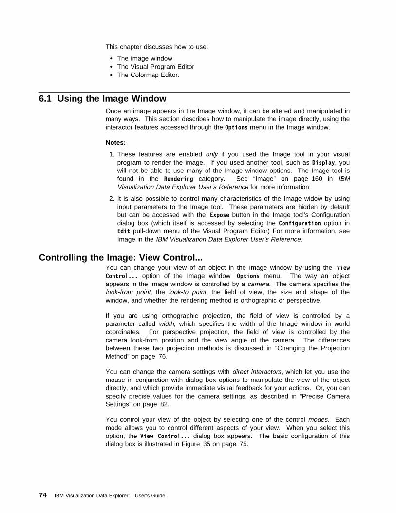
This chapter discusses how to use:

The Image window The Visual Program Editor The Colormap Editor.

6.1 Using the Image WindowOnce an image appears in the Image window, it can be altered and manipulated inmany ways. This section describes how to manipulate the image directly, using theinteractor features accessed through the Options menu in the Image window.

Notes:

1. These features are enabled only if you used the Image tool in your visualprogram to render the image. If you used another tool, such as Display, youwill not be able to use many of the Image window options. The Image tool isfound in the Rendering category. See “Image” on page 160 in IBMVisualization Data Explorer User’s Reference for more information.

2. It is also possible to control many characteristics of the Image widow by usinginput parameters to the Image tool. These parameters are hidden by defaultbut can be accessed with the Expose button in the Image tool’s Configurationdialog box (which itself is accessed by selecting the Configuration option inEdit pull-down menu of the Visual Program Editor) For more information, seeImage in the IBM Visualization Data Explorer User’s Reference.

Controlling the Image: View Control...You can change your view of an object in the Image window by using the ViewControl... option of the Image window Options menu. The way an objectappears in the Image window is controlled by a camera. The camera specifies thelook-from point, the look-to point, the field of view, the size and shape of thewindow, and whether the rendering method is orthographic or perspective.

If you are using orthographic projection, the field of view is controlled by aparameter called width, which specifies the width of the Image window in worldcoordinates. For perspective projection, the field of view is controlled by thecamera look-from position and the view angle of the camera. The differencesbetween these two projection methods is discussed in “Changing the ProjectionMethod” on page 76.

You can change the camera settings with direct interactors, which let you use themouse in conjunction with dialog box options to manipulate the view of the objectdirectly, and which provide immediate visual feedback for your actions. Or, you canspecify precise values for the camera settings, as described in “Precise CameraSettings” on page 82.

You control your view of the object by selecting one of the control modes. Eachmode allows you to control different aspects of your view. When you select thisoption, the View Control... dialog box appears. The basic configuration of thisdialog box is illustrated in Figure 35 on page 75.

74 IBM Visualization Data Explorer: User’s Guide

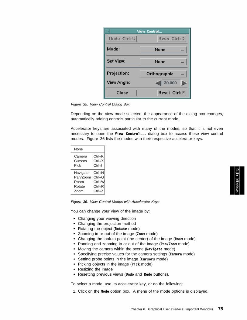
Figure 35. View Control Dialog Box

Depending on the view mode selected, the appearance of the dialog box changes,automatically adding controls particular to the current mode.

Accelerator keys are associated with many of the modes, so that it is not evennecessary to open the View Control... dialog box to access these view controlmodes. Figure 36 lists the modes with their respective accelerator keys.

Figure 36. View Control Modes with Accelerator Keys

None

Camera Ctrl+KCursors Ctrl+XPick Ctrl+I GUI: Windows

Navigate Ctrl+NPan/Zoom Ctrl+GRoam Ctrl+WRotate Ctrl+RZoom Ctrl+Z

You can change your view of the image by:

Changing your viewing direction Changing the projection method Rotating the object (Rotate mode) Zooming in or out of the image (Zoom mode) Changing the look-to point (the center) of the image (Roam mode) Panning and zooming in or out of the image (Pan/Zoom mode) Moving the camera within the scene (Navigate mode) Specifying precise values for the camera settings (Camera mode) Setting probe points in the image (Cursors mode) Picking objects in the image (Pick mode) Resizing the image Resetting previous views (Undo and Redo buttons).

To select a mode, use its accelerator key, or do the following:

1. Click on the Mode option box. A menu of the mode options is displayed.

Chapter 6. Graphical User Interface: Important Windows 75

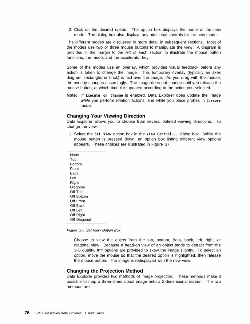
2. Click on the desired option. The option box displays the name of the newmode. The dialog box also displays any additional controls for the new mode.

The different modes are discussed in more detail in subsequent sections. Most ofthe modes use two or three mouse buttons to manipulate the view. A diagram isprovided in the margin to the left of each section to illustrate the mouse buttonfunctions, the mode, and the accelerator key.

Some of the modes use an overlay, which provides visual feedback before anyaction is taken to change the image. This temporary overlay (typically an axesdiagram, rectangle, or brick) is laid over the image. As you drag with the mouse,the overlay changes accordingly. The image does not change until you release themouse button, at which time it is updated according to the action you selected.

Note: If Execute on Change is enabled, Data Explorer does update the imagewhile you perform rotation actions, and while you place probes in Cursorsmode.

Changing Your Viewing DirectionData Explorer allows you to choose from several defined viewing directions. Tochange the view:

1. Select the Set View option box in the View Control... dialog box. While themouse button is pressed down, an option box listing different view optionsappears. These choices are illustrated in Figure 37.

Figure 37. Set View Option Box

NoneTopBottomFrontBackLeftRightDiagonalOff TopOff BottomOff FrontOff BackOff LeftOff RightOff Diagonal

Choose to view the object from the top, bottom, front, back, left, right, ordiagonal view. Because a head-on view of an object tends to detract from the3-D quality, Off options are provided to skew the image slightly. To select anoption, move the mouse so that the desired option is highlighted, then releasethe mouse button. The image is redisplayed with the new view.

Changing the Projection MethodData Explorer provides two methods of image projection. These methods make itpossible to map a three-dimensional image onto a 2-dimensional screen. The twomethods are:

76 IBM Visualization Data Explorer: User’s Guide

Perspective Perspective projection simulates normal camera and human visualsystems, thereby providing realistic rendering of objects. While itis realistic, it does not preserve the exact shape andmeasurements of the object, and parallel lines usually do notproject as being parallel.

Orthographic Orthographic projection provides a less realistic view of an objectthan perspective projection. However, orthographic projectiondoes preserve exact scale measurements and parallel lines. Oneway to think about orthographic projection is that it is as if thedistance between the front and back of an object is small, relativeto the distance between the object and the camera. Orthographicis the default projection method. It is quicker to render an object inorthographic projection than in perspective.

The differences between these two methods become evident when using the viewcontrols in certain modes. For example, the Zoom mode behavior depends on theprojection method, as does the behavior of the 3-D cursor (Roam and Cursorsmodes). The differences are discussed in the sections that discuss these modes.For more information about these projection methods, consult a computer graphicstext.

You can select the projection method by using the Projection option box on theView Control... dialog box.

Setting the View Angle: If you select Perspective, then you can also specify theview angle (in degrees). The vertex of the view angle is located at your camera,and the end points are the left and right sides of the image area. Thus, the widerthe viewing angle, the more image space you can fit in your viewing area.

Specify the view angle by adjusting the View Angle stepper in the View Control...dialog box. Unless you are in Navigate mode, the camera position is adjusted sothat the size of the object in the image area remains unchanged. While in Navigatemode, changing the view angle does not change the camera position.

While you are using orthographic projection, the View Angle stepper is disabled. Inorthographic projection, you can specify the camera width. This is discussed in“Precise Camera Settings” on page 82.

Note: Changing the projection method or view angle does not automatically initiatereexecution of the visual program. To see the effects of your changes, youmust select Execute Once or Execute on Change.

GUI: Windows

Rotating the ObjectTo rotate the object you are viewing:

1. Select Rotate from the Mode pull-down box or use the Ctrl+R accelerator key.2. A set of 3-D axes appears in the lower right corner of the Image window. Also,

if you have enabled the Display Rotation Globe option (in the Optionspull-down menu), or you do so now, a wire-frame globe appears in the lowerleft corner. If you press the right mouse button, you can drag the mouse torotate the object clockwise (CW) and counter-clockwise (CCW), with the imagecenter as the point of rotation. If you press the left or center mouse button, youcan use the mouse as a track ball and rotate the object in all three dimensions.The mode of rotation is determined by the mouse button you use.

Chapter 6. Graphical User Interface: Important Windows 77

As you rotate the object, the set of axes and the wire-framed globe (if enabled)also rotate, providing instant feedback to your actions.

Note: If you do not have Execute on Change enabled, only the set of axes andthe globe are updated as you move the mouse, providing preliminaryfeedback to your rotation actions. If Execute on Change is enabled, thenthe object rotates as you move the mouse.

3. When you release the mouse button, the object is rotated according to the newposition of the axes and globe.

Note: You can also enable Rotate mode by using the intrctnMode parameterto the Image tool (see Image in IBM Visualization Data Explorer User’sReference).

The point around which the object rotates is the look-to point, which you canchange by selecting Roam (see “Changing the Look-to Point” on page 79).Alternatively, you can select Pan/Zoom in the Mode pull-down menu (see “Zoominginto and out of the Image”).

Zooming into and out of the ImageTo zoom in or out (relative to the center of the Image window):

1. Select the Zoom mode in the Mode option box, or use the Ctrl+Z accelerator key.2. To zoom in, press the left mouse button; to zoom out, press the right mouse

button. Drag the mouse in the image area. This causes an overlay image of arectangle to appear. As you move the mouse pointer away from the center ofthe window, the rectangle enlarges. As you move the mouse pointer towardsthe center of the window, the rectangle shrinks. Releasing the mouse buttoncauses the image to zoom in or out, depending on which mouse button ispressed. If the left button (zoom in) is pressed, the portion of the image insidethe rectangle is enlarged to fill the Image window. If the right button is pressed(zoom out), the image displayed in the Image window is reduced to the size ofthe rectangle.

Note: You can also enable Zoom mode by using the intrctnMode parameter tothe Image tool (see Image in IBM Visualization Data Explorer User’sReference).

For both orthographic and perspective projection, zooming in makes the objectappear larger in the Image window, while zooming out makes it appear smaller.However, the way that this is accomplished is different depending on whichprojection method is selected:

While using perspective projection, zooming in or out changes the view angle,without changing the look-from point.

While using orthographic projection, zooming in or out adjusts width of theimage. The camera look-from point does not change, because withorthographic projection the look-from parameter merely specifies a direction, nota location in space.

For more information about the projection methods, see “Changing the ProjectionMethod” on page 76.

78 IBM Visualization Data Explorer: User’s Guide

Changing the Look-to PointData Explorer maintains the look-to point at the center of the Image window. Youcan use the Roam mode to change the look-to point.

To change the look-to point:

1. Select the Roam mode by using the Mode option box or the Ctrl+W acceleratorkey.

2. A wire-frame box appears around the image. The current look-to point ismarked by a small square box. To move the look-to point, select the point bypressing the left mouse button and holding the mouse pointer on it. You canthen move the cursor by dragging the selected point inside the box. When theleft mouse button is depressed on the point, the mouse cursor disappears (thelook-to point remains) and the three projections (one for each axis) appearinside the wire-framed box as dots, similar to the 3-D cursor function illustratedin Figure 40 on page 86. When you release the mouse button, the location ofthe point becomes the new look-to point, and the image view is updated.

Alternatively, double-clicking on a point in the Image window changes thelook-to point to the position on which you double-click. You can set the look-topoint to a location outside the current boundary box of the object using thismethod.

Note: You can also enable Roam mode by using the intrctnMode parameter tothe Image tool (see Image in IBM Visualization Data Explorer User’sReference).

The directions of the axes are indicated by a wire-frame 3-D axes diagram in thelower right-hand corner of the Image window. To move the look-to point, themovement of the mouse must be along the same direction as one of the axes. Ifyou move the mouse in a direction that does not correspond to any of the axesdirections, the point does not move. Because of this, the movement of the look-topoint is constrained to six directions (i.e., the positive and negative directions foreach of the three axes).

Note that since perspective projection does not preserve parallel lines, thedirections in the axes diagram do not necessarily correspond to the direction thatthe point moves in the Image window. However, these axes do correspond withthe values of the coordinates.

While using orthographic projection, the movement of the point in the Imagewindow corresponds with the directions of the axes diagram.

The Constraints option appears in the View Control... dialog box when youselect Roam mode.

You can further restrict the movement of the look-to point by using the Constraintsoption. This allows you to constrain movement of the point to two directions (i.e.,the positive and negative directions of a particular axis). Select an axis to restrictmovement to by clicking on the Constraints option box and selecting the desiredaxis (X, Y, or Z). Once this is done, you are able to move the look-to point alongonly the selected axis, while the values of the other two axes remain constant.

You may want to position the cursor in two steps, using different views for eachstep. For example, you can position the x and y coordinates using the front view,and the z coordinate using the side view.

GUI: Windows

Chapter 6. Graphical User Interface: Important Windows 79

To release the constraints on an axis, choose the None option.

While in Roam mode, the center and right mouse buttons have the same functionsas they do in Rotate mode.

Panning and Zooming into and out of the ImageYou can zoom into or out of the image and change the look-to point at the sametime, using the Pan/Zoom mode. In this mode, the left and right mouse buttons workthe same as they do in Zoom mode, except that the point on the image where youinitially click becomes the new look-to point, and therefore the center of your zoomaction. As you move the mouse pointer away from the point where you initiallyclicked, the rectangle enlarges. As you move the mouse pointer towards the pointwhere you initially clicked, the rectangle shrinks. For information about the Zoommode, see “Zooming into and out of the Image” on page 78.

To select Pan/Zoom mode, select its option from the Mode option box, or use theCtrl+G accelerator key.

Note: You can also enable Pan/Zoom mode by using the intrctnMode parameter tothe Image tool (see Image in IBM Visualization Data Explorer User’s Reference).

Navigating in a SceneYou can move your camera within the scene in all directions using the Navigatemode. As well as being able to change your view direction like the other modes,Navigate also lets you move through an object and view it from the inside out.

When you use Navigate mode, the camera is automatically changed to perspectiverendering.

You can also move your camera in one direction while looking in another direction.For instance, you can move forward past the left side of an object while looking tothe right, enabling you to see the object as you move past it.

Unlike the Roam and Rotate modes, which appear to adjust the object to changeyour view, or the Zoom mode, which appears to adjust the camera lens to changeyour view, the Navigate mode appears to actually move your camera around thescene, while the objects you are viewing remain stationary.

Note: Because Data Explorer does not support perspective rendering of volumes,you cannot navigate software-rendered volumes.

To move your camera within the scene:

1. Select the Navigate mode from the Mode option box. This adds some controls,illustrated in Figure 38 on page 81, to the View Control... dialog box.

2. The mouse buttons control the navigate motion of the camera, while the settingof the Look option box controls the direction the camera is pointing. The Lookoptions are illustrated in Table 4 on page 81.

Note: You can also enable Navigate mode by using the intrctnModeparameter to the Image tool (see Image in IBM Visualization Data ExplorerUser’s Reference).

With Look set to Forward, you have more control over the trajectory the cameramoves along in the scene. To move forward, click on the left mouse button.To move backward, click on the right mouse button. The position of the mousepointer on the image indicates the angle at which you travel; that is, the point

80 IBM Visualization Data Explorer: User’s Guide

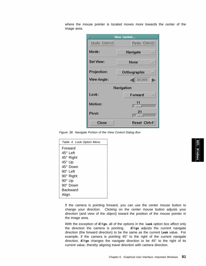
where the mouse pointer is located moves more towards the center of theimage area.

Figure 38. Navigate Portion of the View Control Dialog Box

If the camera is pointing forward, you can use the center mouse button tochange your direction. Clicking on the center mouse button adjusts yourdirection (and view of the object) toward the position of the mouse pointer inthe image area.

With the exception of Align, all of the options in the Look option box affect onlythe direction the camera is pointing. Align adjusts the current navigatedirection (the forward direction) to be the same as the current Look value. Forexample, if the camera is pointing 45° to the right of the current navigatedirection, Align changes the navigate direction to be 45° to the right of itscurrent value, thereby aligning travel direction with camera direction.

GUI: Windows

Table 4. Look Option Menu

Forward45° Left45° Right45° Up45° Down90° Left90° Right90° Up90° DownBackwardAlign

Chapter 6. Graphical User Interface: Important Windows 81

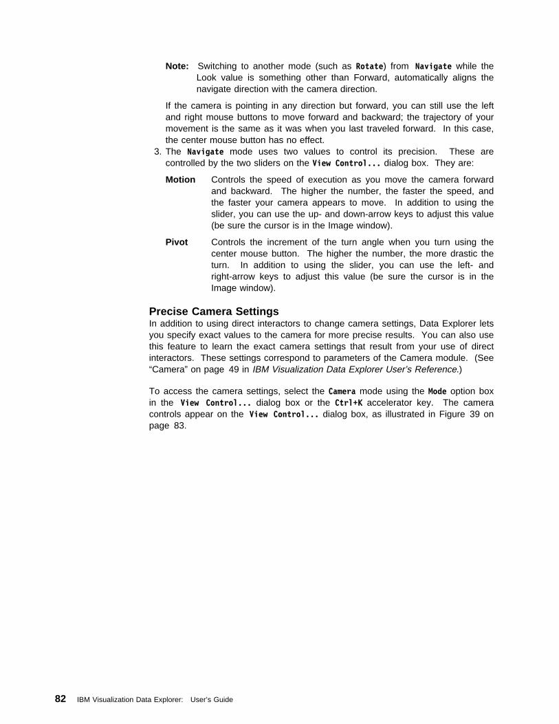
Note: Switching to another mode (such as Rotate) from Navigate while theLook value is something other than Forward, automatically aligns thenavigate direction with the camera direction.

If the camera is pointing in any direction but forward, you can still use the leftand right mouse buttons to move forward and backward; the trajectory of yourmovement is the same as it was when you last traveled forward. In this case,the center mouse button has no effect.

3. The Navigate mode uses two values to control its precision. These arecontrolled by the two sliders on the View Control... dialog box. They are:

Motion Controls the speed of execution as you move the camera forwardand backward. The higher the number, the faster the speed, andthe faster your camera appears to move. In addition to using theslider, you can use the up- and down-arrow keys to adjust this value(be sure the cursor is in the Image window).

Pivot Controls the increment of the turn angle when you turn using thecenter mouse button. The higher the number, the more drastic theturn. In addition to using the slider, you can use the left- andright-arrow keys to adjust this value (be sure the cursor is in theImage window).

Precise Camera SettingsIn addition to using direct interactors to change camera settings, Data Explorer letsyou specify exact values to the camera for more precise results. You can also usethis feature to learn the exact camera settings that result from your use of directinteractors. These settings correspond to parameters of the Camera module. (See“Camera” on page 49 in IBM Visualization Data Explorer User’s Reference.)

To access the camera settings, select the Camera mode using the Mode option boxin the View Control... dialog box or the Ctrl+K accelerator key. The cameracontrols appear on the View Control... dialog box, as illustrated in Figure 39 onpage 83.

82 IBM Visualization Data Explorer: User’s Guide

Figure 39. Camera Settings Portion of the View Control Dialog Box

Note that these camera controls are not direct interactors, so changing their valuesdoes not cause the visual program to reexecute automatically. To see the effect ofyour changes, you must specify Execute or Execute on Change in the VPE, ControlPanel, or Image window.

Changing the Look-to Point, Look-from Point, and the Up Vector: You canadjust your view of the image by specifying values for these settings:

look-to point vector The point around which the displayed image is centered.The point is specified as a vector in world coordinates.

look-from point vector The position of the camera. The point is specified as avector in world coordinates.

up vector The rotation (tilt) of the camera. Only the direction of thisvector is important, not the magnitude. For instance, ifyou are looking at the object from a positive z direction,an up vector with a negative value for x tilts the cameracounterclockwise.

The option box near the center of the View Control... dialog box (displaying To:by default and in Figure 39) allows you to select the vector values to be displayed.

To change the value of one of the vectors, do the following:

1. Select the vector to change using the option box. The choices in the optionmenu are To, From, and Up. The current values for the vector you choose aredisplayed in the X, Y, and Z fields to the right of the options.

GUI: Windows

Chapter 6. Graphical User Interface: Important Windows 83

2. Change each field to the new value. Do this by clicking on the field, typing inthe new number, and pressing the enter key.

3. Repeat these steps for each vector you want to change.

Remember, to see the results of your changes, you must specify Execute orExecute on Change.

Changing the Size of the Image Window: Data Explorer lets you specify theexact height and width of the image display area in the Image window, in pixels.When you change the size of the image display area, the image is resizedaccordingly.

To change the width and height of the image display:

1. Click on the Window Width field of the View Control... dialog box illustrated inFigure 39 on page 83.

2. Type a new value, specified in pixels, for the width. Press the enter key.3. Repeat steps 1 and 2 for the Window Height field.

To see effect of the changes, specify Execute or Execute on Change.

Setting the Camera Width: If you select Orthographic projection, then you canalso specify the width of the field of view. The larger the width, the smaller theobject appears.

Specify the width by clicking on the Camera Width field, typing a new value (in worldcoordinates), and pressing the Enter key.

While you are using perspective projection, the Width field is grayed out.

Resizing the ImageTo resize the image, simply resize the image window by dragging its borders toshrink or expand the window. The image displayed inside the window is resizedaccordingly. Note that the size of the object in the Image window is controlled onlyby the width of the window.

You can specify an exact Image window size by using Camera mode, as describedin “Precise Camera Settings” on page 82.

For more information on resizing windows, see “Moving and Resizing Windows” onpage 62.

Restoring ImagesData Explorer remembers the 10 most recent camera configurations. You canundo the most recent actions in the View Control... dialog box by selecting theUndo option box or by using its accelerator key, Ctrl+U. You can continue to revertto previous configurations until you have reached the first configuration in memory;after that, the Undo option is disabled (grayed out).

As you revert to previous camera configurations (by Undoing actions), you can stillrestore them by using the Redo button, providing that you have not performed anyother actions since the last Undo. The accelerator key for Redo is Ctrl+D.

Note: The Redo button is disabled as soon as you change the cameraconfiguration by a means other than Undo. Any configurations that havebeen stored and “undone” are discarded.

84 IBM Visualization Data Explorer: User’s Guide

Resetting the Camera: To return the image to a “front” view that includes theentire object, select the Reset option of the View Control... dialog box, or use theCtrl+F accelerator key.

You can also use this option if you bring in a new data set and want to create anew camera appropriate for the data.

Note: You can also reset the camera by using the resetCamera parameter to theImage tool (see Image in IBM Visualization Data Explorer User’s Reference).

Using Probes (Cursors)A probe is a list of one or more vectors that represent points in the image. Youcan use them with Data Explorer modules that accept vectors as input, such asClipPlane and Streamline.

After you execute a visual program and have an image in the Image window, youcan modify the visual program to include a Probe or ProbeList tool from theSpecial category. The probe tool accepts input from the 3-D cursor tool, specifyingthe points to use as vectors for input into another tool. The Probe tool accepts onepoint as its input; the ProbeList tool accepts multiple points as input.

To use probes to select points for input into tools:

1. Execute a visual program to produce an image in the Image window.2. In the VPE, place one or more probe tools from the Special category in the

visual program, connecting them to the tools for which you want to provideinput.

The probe icons are numbered as you place them on the canvas. Forexample, the first probe icon you place is labeled “Probe_1,” the second“Probe_2,” and so on. You can change the label of the icon by using itsConfiguration dialog box.

3. In the View Control... dialog box, select Cursors mode from the Mode optionbox, or use the Ctrl+X accelerator key. A wire frame appears around theobject. The dialog box changes to add the Probe controls. Select the probeyou want to set by choosing the Probe(s) option box. This opens an optionsmenu with a list of the available probes, from which you can select the desiredprobe.

4. Use the mouse to select a point or points to use as input to the tool connectedto the Probe or ProbeList icon.

To add a point, double-click on the left mouse button inside the wire-frame box.A small square box appears, marking the point.

Note: The Probe tool allows only one point, while the ProbeList allowsseveral.

To move a point, select the point by pressing the left mouse button with themouse pointer positioned on it. When the left mouse button is depressed onthe point, the three projections (one for each axis) appear inside the wire-framebox as dots, and the values for the x, y, and z coordinates are displayed on theright side of the Image window menu bar, as illustrated in Figure 40 onpage 86. You can move the point by dragging the selected point inside thebox along the same direction as any of the axes. When you have moved thepoint to the desired area, release the left mouse button.

Note that since perspective projection does not preserve parallel lines, thedirections in the axes diagram do not necessarily correspond with the direction

GUI: Windows

Chapter 6. Graphical User Interface: Important Windows 85

Figure 40. 3-D Cursor with a Selected Point

that the point moves in the Image window. However, these axes docorrespond with the values of the coordinates.

While using orthographic projection, the movement of the point in the Imagewindow corresponds to the directions of the axes diagram.

To delete a point, double click on it with the left mouse button.

You can restrict the movement of the 3-D cursor with the Constraints option.Selecting the Constraints option box reveals an options menu that lets youchoose which of the three axis projections to that movement is constrained.For example, if the x axis is selected from the cascade menu, you are able tomove only the x projection in the 3-D cursor box. When cursor movement isconstrained, the portion of the wire-frame box that corresponds to the selectedaxis is highlighted. To remove movement constraints on the cursors, selectNone from the options menu.

Constraining is useful for more precise positioning of the cursor. Note thatexact positioning is not possible with the 3-D cursor tool.

5. Repeat the previous three steps for each probe icon in your visual program.

Reexecute the visual program to implement the probes.

While in Cursors mode, the center and right mouse buttons have the samefunctions as they do in Rotate mode.

Note: You can also enable Probe (cursors) mode by using the intrctnModeparameter to the Image tool (see Image in IBM Visualization Data Explorer User’sReference).

86 IBM Visualization Data Explorer: User’s Guide

Using PickPicking consists of choosing a location on an object in an image using the mouse.A chosen location is called a “poke”. Each poke may intersect the object in theimage in one or more places (the intersections are called “picks”) or may notintersect the object at all. For example, a poke on a spherical isosurface results intwo “picks”: one on the front of the sphere and one on the back. Picking differsfrom using probes, in which probes may be present anywhere in a 3-dimensionalspace, while picks always exist on the surface of an object.

After you execute a visual program and have an image in the Image window, youcan modify the visual program to include a Pick tool from the Special category.The Pick tool accepts input from the mouse and outputs a field that specifies thepicked point or points. The “positions” component of this field identifies eachpicked point on the object in the image. The field can be used, for example, toidentify all picked points with a glyph, or to start streamlines at each picked point.In addition, the field output by the Pick tool can be used by a user-written moduleto perform a variety of operations on the object in the image (e.g., coloring eachpicked object a particular color). IBM Visualization Data Explorer Programmer’sReference includes a sample module that uses the pick structure in this way.

To use picking to select points on objects:

1. Execute a visual program to produce an image in the Image window.2. In the VPE, place one or more pick tools from the Special category in the

visual program, connecting them to the tools for which you want to provideinput.

The pick icons are numbered as you place them on the canvas. For example,the first pick icon you place is labeled “Pick_1”, the second “Pick_2”, and so on.You can change the label of the icon by using its Configuration dialog box.

3. In the View Control... dialog box, select Pick mode from the Mode option boxor use the Ctrl+I accelerator key. The dialog box changes to add the Pickcontrols.

Select the pick tool you want by choosing the Pick(s) option box. This opensan options menu with a list of the available picks from which to select.

4. Select a point or points as input to the tool connected to the Pick icon.

To choose a point, click on a point in the image. A small square box appears,marking the point.

Depending on whether you have the persistent parameter to the Pick tool set to 0or 1, subsequent executions may or may not use the last pick point or pointschosen. If persistent is set to 0, then pick points are not saved betweenexecutions; if persistent is set to 1, then pick points are saved betweenexecutions.

Note: You can also enable Pick mode by using the intrctnMode parameter to theImage tool (see Image in IBM Visualization Data Explorer User’s Reference).

GUI: Windows

Undo, Redo, and ResetThese options are almost self-explanatory. Undo and Redo both restore images,either by “undoing” the current image or by “redoing” the image that has just been“undone”.

The Reset option returns the Image window to its initial state (i.e., before the imagewas first modified). See also “Restoring Images” on page 84.

Chapter 6. Graphical User Interface: Important Windows 87

AutoAxes...This option generates an axes box around an image:

Select AutoAxes...from the Options pull-down menu. The AutoAxesConfiguration... dialog box appears, as illustrated in Figure 41 on page 89.

The dialog box consists of eight parts:

Enabled The first “part” consists of a single toggle button—AutoAxesenabled. This button must be activated (depressed) to makean axes box appear the next time the visual program isexecuted. (The button is automatically activated wheneverone or more of the AutoAxes options are changed.)Releasing (deactivating) the button prevents the appearancesof an axes box.

Input groups The second part of the dialog box displays six (6) of theavailable configuration options shown below. Depressing(enabling) any of these option buttons automatically expandsthe window appropriately to reveal the relevant options.Releasing (disabling) any of these option buttons removesthe relevant options.

Axes' Labels Allows you to individually specify a label for each of the threeaxes:

X, Y, Z

Miscellaneous Contains the following specifications:

Frame allows you to turn on or off a frame for the axes(that is, lines which complete the cube, in additionto the back three faces which are drawn bydefault).

Grid allows you to turn on or off grid lines along majorticks.

Font allows you to choose a font for the labels. Theellipses button allows you to choose from the setof predefined fonts.

Label Scaleallows you to change the size of the labels fromthe default size. For example, specifying a labelsscale of 2 will make the labels twice as large.

Annotation Colors allows you to specify a color for each part of the axes: thegrid (if drawn), ticks, labels, and background. The colors canbe any of the defined colors (see “Color” on page 75 in IBMVisualization Data Explorer User’s Reference), and inaddition, the background can be drawn as “clear” (invisible).

Corners / Cursor The Corners section allows you to explicitly set the range ofthe axes in each dimension. The Cursor section allows youto place a cursor (marker) at a specific location in the axesbox.

Ticks Allows you to specify number or locations of ticks. If theoption menu to the right of “Ticks” is set to “All”, then you canspecify the approximate total number of ticks in the “All” field.

88 IBM Visualization Data Explorer: User’s Guide

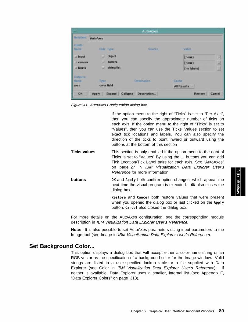
Figure 41. AutoAxes Configuration dialog box

If the option menu to the right of “Ticks” is set to “Per Axis”,then you can specify the approximate number of ticks oneach axis. If the option menu to the right of “Ticks” is set to“Values”, then you can use the Ticks' Values section to setexact tick locations and labels. You can also specify thedirection of the ticks to point inward or outward using thebuttons at the bottom of this section

Ticks values This section is only enabled if the option menu to the right ofTicks is set to “Values” By using the ... buttons you can addTick Location/Tick Label pairs for each axis. See “AutoAxes”on page 27 in IBM Visualization Data Explorer User’sReference for more information.

buttons OK and Apply both confirm option changes, which appear thenext time the visual program is executed. OK also closes thedialog box.

Restore and Cancel both restore values that were presentwhen you opened the dialog box or last clicked on the Applybutton. Cancel also closes the dialog box.

For more details on the AutoAxes configuration, see the corresponding moduledescription in IBM Visualization Data Explorer User’s Reference.

Note: It is also possible to set AutoAxes parameters using input parameters to theImage tool (see Image in IBM Visualization Data Explorer User’s Reference).

GUI: Windows

Set Background Color...This option displays a dialog box that will accept either a color-name string or anRGB vector as the specification of a background color for the Image window. Validstrings are listed in a user-specified lookup table or a file supplied with DataExplorer (see Color in IBM Visualization Data Explorer User’s Reference). Ifneither is available, Data Explorer uses a smaller, internal list (see Appendix F,“Data Explorer Colors” on page 313).

Chapter 6. Graphical User Interface: Important Windows 89

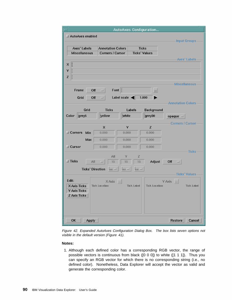
Figure 42. Expanded AutoAxes Configuration Dialog Box. The box lists seven options notvisible in the default version (Figure 41).

Notes:

1. Although each defined color has a corresponding RGB vector, the range ofpossible vectors is continuous from black ([0 0 0]) to white ([1 1 1]). Thus youcan specify an RGB vector for which there is no corresponding string (i.e., nodefined color). Nonetheless, Data Explorer will accept the vector as valid andgenerate the corresponding color.

90 IBM Visualization Data Explorer: User’s Guide

2. Data Explorer supplies double quotation marks for color-name strings, andbrackets, commas, and terminal zeros for vectors. For example, either green orð 1 ð is sufficient to specify the color green.

3. It is also possible to set the background color using the bkgrdColor parameterto the Image tool (see Image in IBM Visualization Data Explorer User’sReference).

Display Rotation GlobeThe rotation globe can be displayed only in the Roam and Rotate modes of the ViewControl... dialog box (see “Controlling the Image: View Control...” on page 74).In either mode, activation (depression) of the Display Rotation Globe toggle buttongenerates a globe in the lower left-hand corner of the Image window. Theorientation of this globe changes in parallel with that of the axes in the lowerright-hand corner of the window, or vice versa, depending on which object youmanipulate.

Hold down the left mouse button to rotate the objects in two dimensions (Rotatemode) and the middle button to orient them in three (Roam mode).

Rendering Options...You can choose between software and hardware rendering if you are running DataExplorer on a workstation with a graphics card that supports hardware rendering.Approximations in both types of rendering help the user to see the effect of rotation,roam, or navigation interactions before rendering and display are complete.

To set the rendering options, select Rendering Options... in the Options pull-downmenu in the Image window. This causes the Rendering... dialog box to appear,as illustrated in Figure 43 on page 92.

The Rendering... dialog box allows you to select the rendering mode with a togglebutton. If you select hardware, this means “use hardware if available” at the timeData Explorer is run. If a graphics card which supports hardware rendering is notavailable, software rendering will be used instead.

You can specify the approximation method that Data Explorer uses for each of twoexecution states—button-up execution and button-down execution. Button-downexecution is applicable in execute-on-change mode and in navigation.

For example, you might specify None for the approximation method for button-upexecution, and Dots for the approximation method for button-down execution.When holding the mouse button down in Rotate mode (with Execute on Changeenabled), these rendering methods display a dot representation of the object, givingyou quick feedback on your camera position, until you release the mouse button, atwhich point the object is rendered normally. The following is a brief description ofthe rendering methods you can specify with this dialog box. For detailedinformation about the rendering options, see “Display” on page 109 in IBMVisualization Data Explorer User’s Reference.

NoneNo approximation method is specified, so a complete rendering of the image isdone.

GUI: Windows

Chapter 6. Graphical User Interface: Important Windows 91

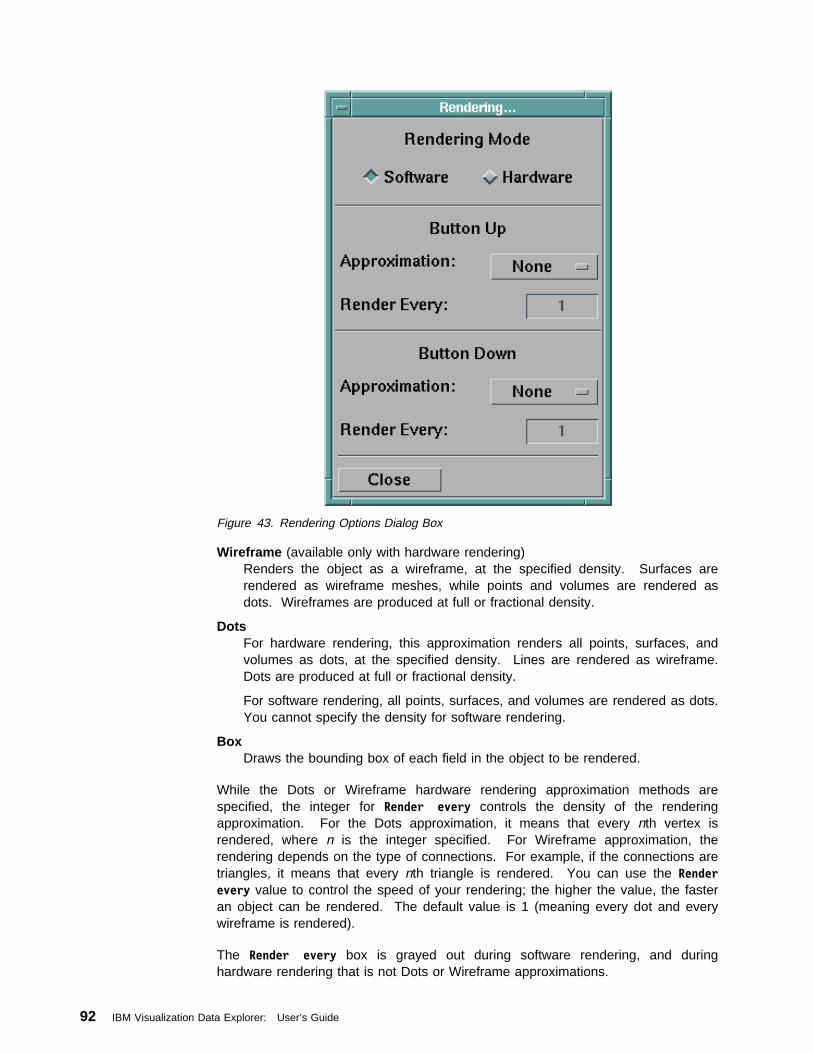
Figure 43. Rendering Options Dialog Box

Wireframe (available only with hardware rendering)Renders the object as a wireframe, at the specified density. Surfaces arerendered as wireframe meshes, while points and volumes are rendered asdots. Wireframes are produced at full or fractional density.

DotsFor hardware rendering, this approximation renders all points, surfaces, andvolumes as dots, at the specified density. Lines are rendered as wireframe.Dots are produced at full or fractional density.

For software rendering, all points, surfaces, and volumes are rendered as dots.You cannot specify the density for software rendering.

BoxDraws the bounding box of each field in the object to be rendered.

While the Dots or Wireframe hardware rendering approximation methods arespecified, the integer for Render every controls the density of the renderingapproximation. For the Dots approximation, it means that every nth vertex isrendered, where n is the integer specified. For Wireframe approximation, therendering depends on the type of connections. For example, if the connections aretriangles, it means that every nth triangle is rendered. You can use the Renderevery value to control the speed of your rendering; the higher the value, the fasteran object can be rendered. The default value is 1 (meaning every dot and everywireframe is rendered).

The Render every box is grayed out during software rendering, and duringhardware rendering that is not Dots or Wireframe approximations.

92 IBM Visualization Data Explorer: User’s Guide

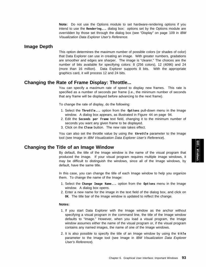
Note: Do not use the Options module to set hardware-rendering options if youintend to use the Rendering... dialog box: options set by the Options module areoverridden by those set through the dialog box (see “Display” on page 109 in IBMVisualization Data Explorer User’s Reference.

Image DepthThis option determines the maximum number of possible colors (or shades of color)that Data Explorer can use in creating an image. With greater numbers, gradationsare smoother and edges are sharper. The image is “clearer.” The choices are thenumber of bits available for specifying colors: 8 (256 colors), 12 (4096) and 24(more than 16 million). Data Explorer supports 8 bits. With the appropriategraphics card, it will process 12 and 24 bits.

Changing the Rate of Frame Display: Throttle...You can specify a maximum rate of speed to display new frames. This rate isspecified as a number of seconds per frame (i.e., the minimum number of secondsthat any frame will be displayed before advancing to the next frame).

To change the rate of display, do the following:

1. Select the Throttle... option from the Options pull-down menu in the Imagewindow. A dialog box appears, as illustrated in Figure 44 on page 94.

2. Edit the Seconds per Frame text field, changing it to the minimum number ofseconds you want any given frame to be displayed.

3. Click on the Close button. The new rate takes effect.

You can also set the throttle value by using the throttle parameter to the Imagetool (see Image in IBM Visualization Data Explorer User’s Reference). GUI: Windows

Changing the Title of an Image WindowBy default, the title of the Image window is the name of the visual program thatproduced the image. If your visual program requires multiple image windows, itmay be difficult to distinguish the windows, since all of the Image windows, bydefault, have the same title.

In this case, you can change the title of each Image window to help you organizethem. To change the name of the Image:

1. Select the Change Image Name... option from the Options menu in the Imagewindow. A dialog box opens.

2. Enter a new name for the image in the text field of the dialog box, and click onOK. The title bar of the Image window is updated to reflect the change.

Notes:

1. If you start Data Explorer with the Image window as the anchor withoutspecifying a visual program in the command line, the title of the Image windowdefaults to “Image.” However, when you load a visual program, the Imagewindow assumes either the name of the visual program or, if the visual programcontains any named images, the name of one of the Image windows.

2. It is also possible to specify the title of an Image window by using the titleparameter to the Image tool (see Image in IBM Visualization Data ExplorerUser’s Reference).

Chapter 6. Graphical User Interface: Important Windows 93

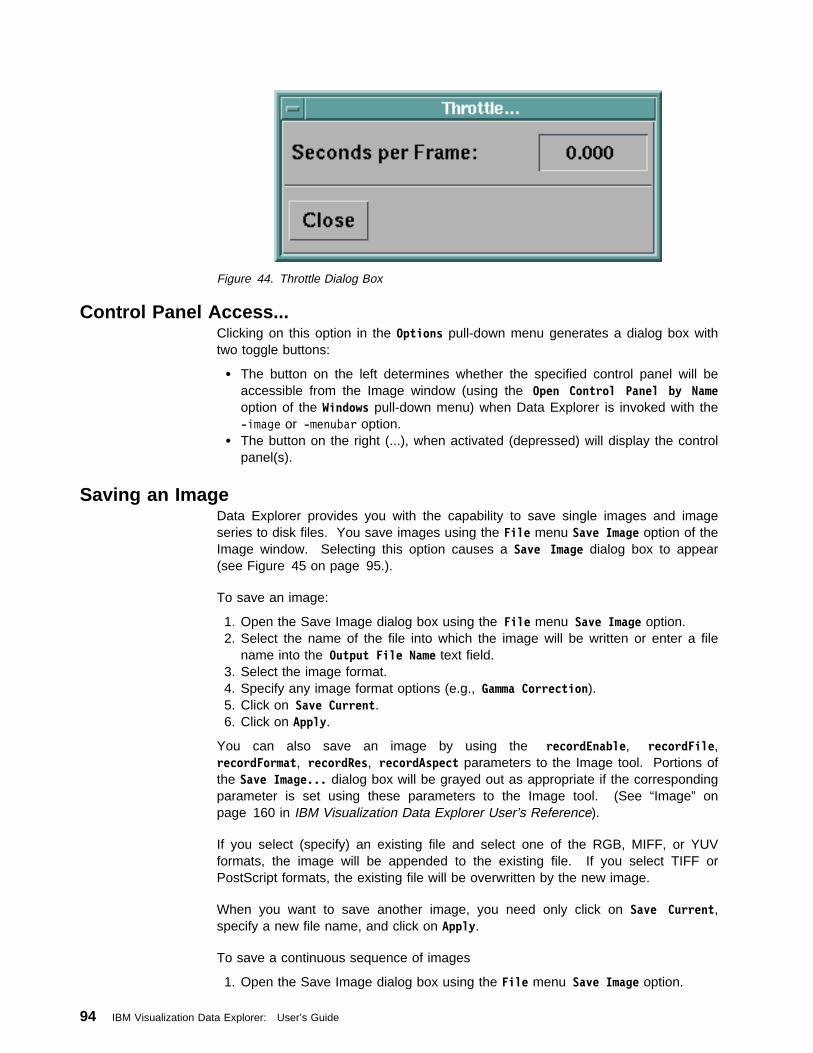
Figure 44. Throttle Dialog Box

Control Panel Access...Clicking on this option in the Options pull-down menu generates a dialog box withtwo toggle buttons:

The button on the left determines whether the specified control panel will beaccessible from the Image window (using the Open Control Panel by Nameoption of the Windows pull-down menu) when Data Explorer is invoked with the-image or -menubar option.

The button on the right (...), when activated (depressed) will display the controlpanel(s).

Saving an ImageData Explorer provides you with the capability to save single images and imageseries to disk files. You save images using the File menu Save Image option of theImage window. Selecting this option causes a Save Image dialog box to appear(see Figure 45 on page 95.).

To save an image:

1. Open the Save Image dialog box using the File menu Save Image option.2. Select the name of the file into which the image will be written or enter a file

name into the Output File Name text field.3. Select the image format.4. Specify any image format options (e.g., Gamma Correction).5. Click on Save Current.6. Click on Apply.

You can also save an image by using the recordEnable, recordFile,recordFormat, recordRes, recordAspect parameters to the Image tool. Portions ofthe Save Image... dialog box will be grayed out as appropriate if the correspondingparameter is set using these parameters to the Image tool. (See “Image” onpage 160 in IBM Visualization Data Explorer User’s Reference).

If you select (specify) an existing file and select one of the RGB, MIFF, or YUVformats, the image will be appended to the existing file. If you select TIFF orPostScript formats, the existing file will be overwritten by the new image.

When you want to save another image, you need only click on Save Current,specify a new file name, and click on Apply.

To save a continuous sequence of images

1. Open the Save Image dialog box using the File menu Save Image option.

94 IBM Visualization Data Explorer: User’s Guide

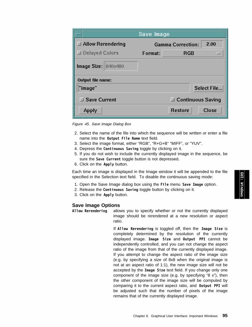
Figure 45. Save Image Dialog Box

2. Select the name of the file into which the sequence will be written or enter a filename into the Output File Name text field.

3. Select the image format, either “RGB”, “R+G+B” “MIFF”, or “YUV”.4. Depress the Continuous Saving toggle by clicking on it.5. If you do not wish to include the currently displayed image in the sequence, be

sure the Save Current toggle button is not depressed.6. Click on the Apply button.

Each time an image is displayed in the Image window it will be appended to the filespecified in the Selection text field. To disable the continuous saving mode:

1. Open the Save Image dialog box using the File menu Save Image option.2. Release the Continuous Saving toggle button by clicking on it.3. Click on the Apply button.

GUI: Windows

Save Image OptionsAllow Rerendering allows you to specify whether or not the currently displayed

image should be rerendered at a new resolution or aspectratio.

If Allow Rerendering is toggled off, then the Image Size iscompletely determined by the resolution of the currentlydisplayed image. Image Size and Output PPI cannot beindependently controlled, and you can not change the aspectratio of the image from that of the currently displayed image.If you attempt to change the aspect ratio of the image size(e.g. by specifying a size of 8x8 when the original image isnot at an aspect ratio of 1:1), the new image size will not beaccepted by the Image Size text field. If you change only onecomponent of the image size (e.g. by specifying “8 x”), thenthe other component of the image size will be computed bycomparing it to the current aspect ratio, and Output PPI willbe adjusted such that the number of pixels of the imageremains that of the currently displayed image.

Chapter 6. Graphical User Interface: Important Windows 95

If Allow Rerendering is toggled on, then the currentlydisplayed image will be rerendered at a new resolution basedon the settings of Output PPI and Image Size, which cannow be independently controlled. You can use this option, forexample, to save or print an image at a much higherresolution than is displayed on the screen. You can alsospecify the number of pixels directly by setting the units ofImage Size to pixels (note that in this case it is meaninglessto set the Output PPI).

Gamma Correction Allows you to specify gamma correction applied to the outputimage. The default is 2.

Delayed Colors For TIFF, MIFF, and PostScript image formats, allows you tospecify whether the image is saved in animage-with-colormap format. For GIF image format, thisoption is required by the format.

Format Allows you to choose from the set of available imageformats.

Output file name Allows you to specify the file name to which the imageshould be written. An appropriate extension for the chosenformat will be added if you do not provide one.

Select File Allows you to use a File Selection dialog to specify the outputimage file name.

Save Current Allows you to specify that the current image should be savedwhen the Apply button is pressed.

Continuous Saving Allows you to save a series of images. If you do not want thecurrent image to be saved, be sure the Save Current buttonis not set before pressing Apply. When Continuous Saving isactivated, each image displayed in the image window will besaved to the specified file. This option is useful only forimage formats which support series: RGB, R+G+B, YUV, andMIFF.

For all formats other than the Postscript formats, the following field is available:

Image Size If the Allow Rerendering button is set, this field allows you toset the resolution of the output image to something otherthan that of the image displayed to the screen.

If one of the Postscript formats is selected then the following fields are displayed:

Image Dimensions Allows you to specify the size of the image on the page (bydefault in inches).

Orientation Allows you to specify the orientation of the image to portraitor landscape, or automatic, which chooses the best for thegiven image.

Input Image Size Specifies the resolution of the image to be saved. This fieldis enabled only if the Allow Rerendering button is toggled on.

Page Dimensions Specifies the size of the page. By default this is specified ininches.

96 IBM Visualization Data Explorer: User’s Guide

Output PPI Specifies the “pixels per inch” of the output image.

Note: Unless you specifically care to set the precise pixelsper inch, you do not typically need to set this.

Margin Width Specifies a margin width of white space on the page.

For PostScript formats, the printed image will, by default, fill the page to withinMargin Width of the edge of the page. If Allow Rerendering is off, the pixels in theimage will be sized appropriately to scale the image to fill the page, but the samenumber of pixels as in the currently displayed image will be used. If this results in agrainy image, set Allow Rerendering on, and enter a different Input image size.For example, if the displayed image is 640x480, and you want to double theresolution, just enter 1280 in the Input image size field and Data Explorer willrecalculate the new value of y (960) and the new (higher) value for Output PPI.

By default, Image Dimensions, Page Dimensions, and Margin Width are specified ininches However, you can use the DX\metric resource or the -metric command lineoption to use centimeters instead. See Table 7 on page 299.

Pushbuttons Apply causes the currently displayed image to be saved if theSave Current toggle button is depressed.

Restore restores settings in the dialog to what they were thelast time the Apply button was depressed.

Close causes the dialog to be closed without saving animage.

Note: If you are not using the Image window, this functionality is available with theWriteImage module. See “WriteImage” on page 374 in IBM Visualization DataExplorer User’s Reference.

GUI: Windows

Printing an ImageYou can print images displayed in the Image window by choosing the PrintImage... option from the File menu of the Image window. Selecting this optioncauses a Print Image dialog box to be opened (see Figure 46 on page 98). Notethat portions of the Print Image dialog box will be grayed out as appropriate if thecorresponding parameter is set using the recordFormat, recordRes, orrecordAspect parameters to the Image tool.

Print Image OptionsAllow Rerendering allows you to specify whether or not the currently displayed

image should be rerendered at a new resolution or aspectratio.

If Allow Rerendering is toggled off, then the Image Size iscompletely determined by the resolution of the currentlydisplayed image. Image Size and Output PPI cannot beindependently controlled, and you can not change the aspectratio of the image from that of the currently displayed image.If you attempt to change the aspect ratio of the image size(e.g. by specifying a size of 8x8 when the original image isnot at an aspect ratio of 1:1), the new image size will not beaccepted by the Image Size text field. If you change only onecomponent of the image size (e.g. by specifying “8 x”), thenthe other component of the image size will be computed by

Chapter 6. Graphical User Interface: Important Windows 97

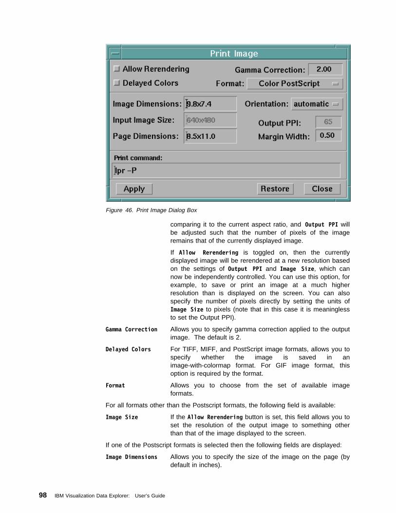
Figure 46. Print Image Dialog Box

comparing it to the current aspect ratio, and Output PPI willbe adjusted such that the number of pixels of the imageremains that of the currently displayed image.

If Allow Rerendering is toggled on, then the currentlydisplayed image will be rerendered at a new resolution basedon the settings of Output PPI and Image Size, which cannow be independently controlled. You can use this option, forexample, to save or print an image at a much higherresolution than is displayed on the screen. You can alsospecify the number of pixels directly by setting the units ofImage Size to pixels (note that in this case it is meaninglessto set the Output PPI).

Gamma Correction Allows you to specify gamma correction applied to the outputimage. The default is 2.

Delayed Colors For TIFF, MIFF, and PostScript image formats, allows you tospecify whether the image is saved in animage-with-colormap format. For GIF image format, thisoption is required by the format.

Format Allows you to choose from the set of available imageformats.

For all formats other than the Postscript formats, the following field is available:

Image Size If the Allow Rerendering button is set, this field allows you toset the resolution of the output image to something otherthan that of the image displayed to the screen.

If one of the Postscript formats is selected then the following fields are displayed:

Image Dimensions Allows you to specify the size of the image on the page (bydefault in inches).

98 IBM Visualization Data Explorer: User’s Guide

Orientation Allows you to specify the orientation of the image to portraitor landscape, or automatic, which chooses the best for thegiven image.

Input Image Size Specifies the resolution of the image to be printed. This fieldis enabled only if the Allow Rerendering button is toggled on.

Page Dimensions Specifies the size of the page. By default this is specified ininches.

Output PPI Specifies the “pixels per inch” of the output image.

Note: Unless you specifically care to set the precise pixelsper inch, you do not typically need to set this.

Margin Width Specifies a margin width of white space on the page.

For PostScript formats, the printed image will, by default, fill the page to withinMargin Width of the edge of the page. If Allow Rerendering is off, the pixels in theimage will be sized appropriately to scale the image to fill the page, but the samenumber of pixels as in the currently displayed image will be used. If this results in agrainy image, set Allow Rerendering on, and enter a different Input image size.For example, if the displayed image is 640x480, and you want to double theresolution, just enter 1280 in the Input image size field and Data Explorer willrecalculate the new value of y (960) and the new (higher) value for Output PPI.

Print command Contains a text field where you can enter a command to printthe image, for example:

lpr -P myPrinter

Pushbuttons Apply Causes the command specified by Print Command tobe executed.

Restore Restores settings in the dialog to what they were thelast time that Apply was depressed.

Close Causes the dialog to be closed without printing animage.

GUI: Windows

6.2 Using the VPEA visual program is a collection of interconnected tools that acts upon one or moreinputs to create one or more outputs (for example, an image). You derive programinputs from the output of tools in the program, or by setting the input values toconstants. Tools that provide output values as input to other tools are (inalphabetical order):

Colormap Editors (see 6.3, “Using the Colormap Editor” on page 119) Interactors (see “Using Interactors” on page 142) Macros (see 7.2, “Creating and Using Macros” on page 149) Modules (see Chapter 1, “Data Explorer Tools” on page 1 in IBM Visualization

Data Explorer User’s Reference) Picks (see “Using Pick” on page 87) Probes (see “Using Probes (Cursors)” on page 85) Sequencers (see “Using the Sequencer” on page 68) Transmitters and Receivers (see “Using Transmitters and Receivers” on

page 106).

Chapter 6. Graphical User Interface: Important Windows 99

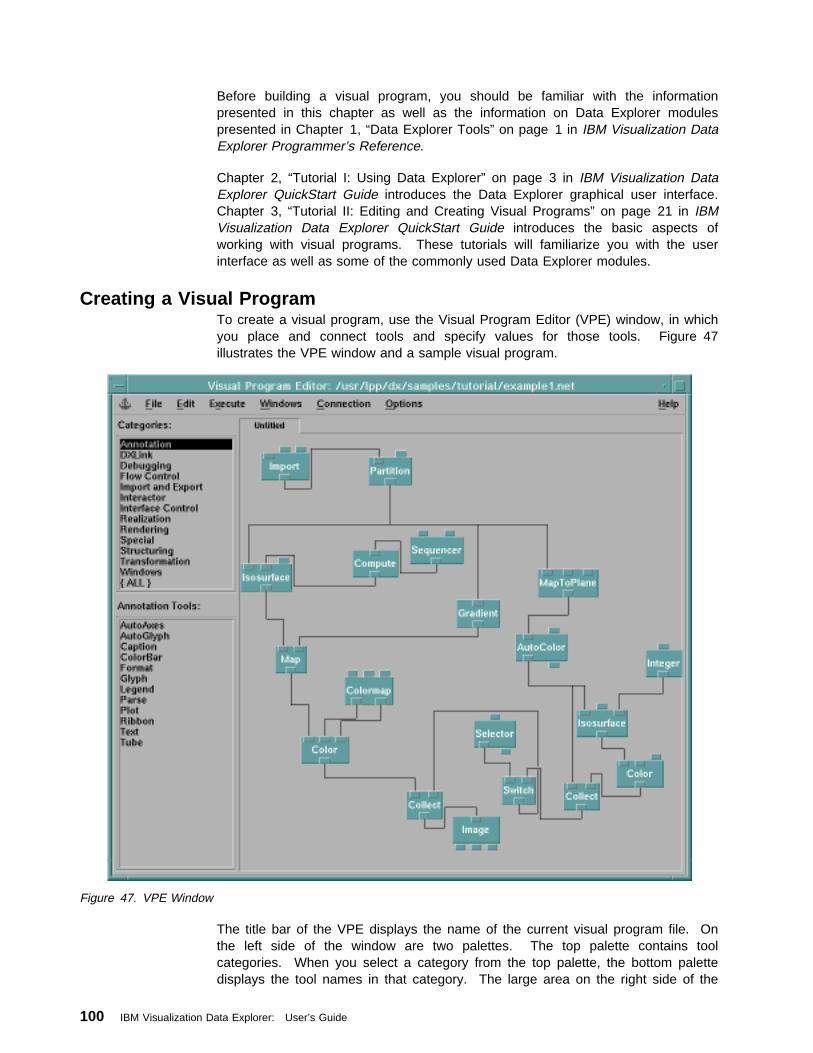
Before building a visual program, you should be familiar with the informationpresented in this chapter as well as the information on Data Explorer modulespresented in Chapter 1, “Data Explorer Tools” on page 1 in IBM Visualization DataExplorer Programmer’s Reference.

Chapter 2, “Tutorial I: Using Data Explorer” on page 3 in IBM Visualization DataExplorer QuickStart Guide introduces the Data Explorer graphical user interface.Chapter 3, “Tutorial II: Editing and Creating Visual Programs” on page 21 in IBMVisualization Data Explorer QuickStart Guide introduces the basic aspects ofworking with visual programs. These tutorials will familiarize you with the userinterface as well as some of the commonly used Data Explorer modules.

Creating a Visual ProgramTo create a visual program, use the Visual Program Editor (VPE) window, in whichyou place and connect tools and specify values for those tools. Figure 47illustrates the VPE window and a sample visual program.

Figure 47. VPE Window

The title bar of the VPE displays the name of the current visual program file. Onthe left side of the window are two palettes. The top palette contains toolcategories. When you select a category from the top palette, the bottom palettedisplays the tool names in that category. The large area on the right side of the

100 IBM Visualization Data Explorer: User’s Guide

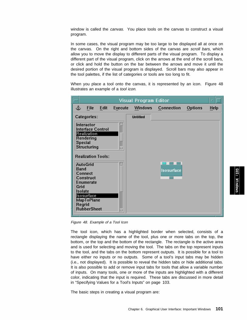
window is called the canvas. You place tools on the canvas to construct a visualprogram.

In some cases, the visual program may be too large to be displayed all at once onthe canvas. On the right and bottom sides of the canvas are scroll bars, whichallow you to move the display to different parts of the visual program. To display adifferent part of the visual program, click on the arrows at the end of the scroll bars,or click and hold the button on the bar between the arrows and move it until thedesired portion of the visual program is displayed. Scroll bars may also appear inthe tool palettes, if the list of categories or tools are too long to fit.

When you place a tool onto the canvas, it is represented by an icon. Figure 48illustrates an example of a tool icon.

Figure 48. Example of a Tool Icon

GUI: Windows

The tool icon, which has a highlighted border when selected, consists of arectangle displaying the name of the tool, plus one or more tabs on the top, thebottom, or the top and the bottom of the rectangle. The rectangle is the active areaand is used for selecting and moving the tool. The tabs on the top represent inputsto the tool, and the tabs on the bottom represent outputs. It is possible for a tool tohave either no inputs or no outputs. Some of a tool’s input tabs may be hidden(i.e., not displayed). It is possible to reveal the hidden tabs or hide additional tabs.It is also possible to add or remove input tabs for tools that allow a variable numberof inputs. On many tools, one or more of the inputs are highlighted with a differentcolor, indicating that the input is required. These tabs are discussed in more detailin “Specifying Values for a Tool's Inputs” on page 103.

The basic steps in creating a visual program are:

Chapter 6. Graphical User Interface: Important Windows 101

1. Select and place the desired tools on the canvas.2. Connect tool outputs to inputs.3. Set values for the tools.4. If you plan to change input parameters frequently while viewing an image (e.g.,

an isosurface value), then you should build a Control Panel and set interactors(see “Building Control Panels” on page 129 and “Using Interactors” onpage 142).

Placing Tools on the CanvasThe tools are divided into categories, and a list of these categories appears in thetop palette on the left side of the VPE window. To locate a tool:

1. Click on a desired category. The names of the tools in that category appear inthe lower tool palette. All palette lists are presented in alphabetic order.

2. Select the appropriate tool name from the bottom palette by clicking on thetool’s name. Clicking on an already selected tool deselects that tool.

To place one instance of the selected tool on the canvas:

1. Move the cursor to where you want to position the tool on the canvas. Notethat the style of the cursor changes when you move it onto the canvas. Exactplacement of the tool depends on the grid settings (see “Customizing the VPEWindow” on page 113).

2. Click the mouse. The tool icon appears at the specified location. When youhave placed the tool, its name is no longer highlighted in the lower palette.

To place multiple instances of the tool:

1. Double click on the tool name in the lower tool palette.2. Click the mouse on the canvas to place one instance of the tool. Repeat this

step for further instances of the tool.3. To stop placing the same tool, deselect the tool’s name in the palette by

clicking on any tool name.

Note: After you place a tool, its icon stays selected until you place another tool, ordeselect the tool as described in “Selecting, Moving, and Deleting ToolIcons”.

If you place one tool icon on top of another, the bottom tool icon is pushedto the right to allow room for the new one. To avoid the displacement oftool icons, allow enough space for each tool icon you plan to use.

To deselect a tool name in the lower palette, do one of the following:

Click on the tool name. Select another tool name. Select another category.

Selecting, Moving, and Deleting Tool IconsTo select a tool icon, click on it.

To select a group of tool icons, use one of these methods:

Hold down the Shift key and click on each tool icon in turn.

Position the cursor on the canvas near a corner of the group and drag themouse to draw a selection box around the tool icons you want. To select thetool icon, you must completely enclose it in the selection box. As a tool icon is

102 IBM Visualization Data Explorer: User’s Guide

encompassed by the selection box, it is highlighted (indicating that it isselected).

Note: If you have tools selected already and you want to select more, holddown the Shift key and either click on a single icon, or drag theselection box over several icons to select them. To select all icons onthe canvas, use the Select All option of the Edit pull-down menu.

To deselect an icon, shift-click on it.

To deselect a group of tools, use one of these methods:

Shift-click on each icon.

Shift-drag to draw a box around the tools you want to deselect. As a selectedtool is encompassed in the box, it becomes unhighlighted. Release the buttonto deselect the tools.

Note: Clicking on an empty part of the canvas deselects all selected tools.

To move a tool icon:

1. Press and hold the left mouse button on the tool icon and drag it to the desiredlocation. While you are dragging the tool, an outline of the tool icon follows themotion of the mouse, but the tool icon remains in the original location.

2. Release the mouse button at the desired location. The tool icon moves to thatlocation. Any lines connecting to other tools are rerouted to the tool’s newlocation.

To move a group of tool icons:

1. Select a group of tool icons to be moved.2. Position the cursor on any member of the group and drag it. An outline of each

tool icon follows the motion of the mouse.3. Release the mouse button. The icons representing the tools move to the new

location. Any affected connections are rerouted.

To delete tool icons:

1. Select the tool icon or group to be deleted.2. Press the Ctrl+Delete accelerator key or click on the Delete option of the Edit

menu.

GUI: Windows

Specifying Values for a Tool's InputsTo provide the values of a given input for a tool, use one of these methods:

Connect the output tab of another tool to the desired input tab. or Use the tool’s Configuration dialog box.

When you specify an input value for a tool, the corresponding tab on the tool’s iconautomatically folds in. If you do not specify an input value, the input tab remainsfolded out, indicating that the input is unbound and the tool uses its default for thatinput. The default values are given in the Configuration dialog box. The tabs thatare folded in give you a visual representation of the inputs that have user-specifiedvalues. Some tabs require an input; those tabs remain highlighted in a differentcolor until you specify an input with a connection or through a Configuration dialogbox. Some of the tabs are not displayed, termed hidden. The hidden tabs can be

Chapter 6. Graphical User Interface: Important Windows 103

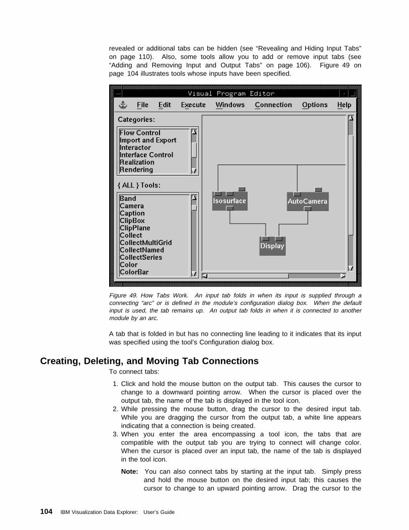
revealed or additional tabs can be hidden (see “Revealing and Hiding Input Tabs”on page 110). Also, some tools allow you to add or remove input tabs (see“Adding and Removing Input and Output Tabs” on page 106). Figure 49 onpage 104 illustrates tools whose inputs have been specified.

Figure 49. How Tabs Work. An input tab folds in when its input is supplied through aconnecting “arc” or is defined in the module’s configuration dialog box. When the defaultinput is used, the tab remains up. An output tab folds in when it is connected to anothermodule by an arc.

A tab that is folded in but has no connecting line leading to it indicates that its inputwas specified using the tool’s Configuration dialog box.

Creating, Deleting, and Moving Tab ConnectionsTo connect tabs:

1. Click and hold the mouse button on the output tab. This causes the cursor tochange to a downward pointing arrow. When the cursor is placed over theoutput tab, the name of the tab is displayed in the tool icon.

2. While pressing the mouse button, drag the cursor to the desired input tab.While you are dragging the cursor from the output tab, a white line appearsindicating that a connection is being created.

3. When you enter the area encompassing a tool icon, the tabs that arecompatible with the output tab you are trying to connect will change color.When the cursor is placed over an input tab, the name of the tab is displayedin the tool icon.

Note: You can also connect tabs by starting at the input tab. Simply pressand hold the mouse button on the desired input tab; this causes thecursor to change to an upward pointing arrow. Drag the cursor to the

104 IBM Visualization Data Explorer: User’s Guide

desired output tab. When the cursor enters the area encompassing atool icon, the output tabs that are compatible with the input tab willchange color.

4. Place the pointer over the input tab you want and release the mouse button. Ifyou release the mouse button in the rectangle area of the icon, the lineautomatically connects to the leftmost of the newly colored tabs.

When you release the mouse button, the white temporary line is replaced witha black line, and the corresponding tabs fold in.

Note: Sometimes, when tools are placed too close together on the canvas, aconnection that you made is not visible. In this case, the affected inputtabs are still folded in, and a dark line is visible on each one, but theconnecting line is not visible. To correct this, move one of the affectedtools to another spot on the canvas.

You can connect an output tab to more than one input tab (either on different toolicons or on the same tool icon). Therefore, you can make a connection from anoutput tab even though the output tab is folded in.

An input tab can receive a value from only one source, either from a connection toan output tab or from a value entered in a Configuration dialog box. Once an inputtab folds in, you cannot make a new connection to the tab until the tab is released.

Because output tabs can have multiple destinations, connections can only bemoved or deleted from an input tab.

To delete a tab connection:

1. Depress the mouse button on the input tab.2. Drag the cursor to an empty space on the canvas (away from the active area of

the tool). A white line from the output tab follows the mouse pointer. If youdecide at this point not to break the connection, you must place the cursor backon the input tab where the connection was, and release the mouse button.

3. Release the mouse button. The connection is deleted and the input tabreleased.

To move a tab connection:

1. Depress the mouse button on the input tab.2. Drag the cursor to an empty input tab (one that has not already been folded in).3. Release the mouse button. The connection is rerouted to the new input tab.

GUI: Windows

Moving and Copying ToolsThe Drag and Drop capability provided by Data Explorer allows you to move orcopy selected tools within a Data Explorer window (e.g., the VPE or a controlpanel) or between different Data Explorer windows (i.e., between two different VPEwindows). You can also drag interactor stand-ins to control panels to createinteractors.

To initiate a drag and drop, first select the tools you want to move or copy, eitherby rubber-band or shift selection. Then place the mouse cursor over one of theselected tools and press the middle mouse button. Keeping the button pressed,move the cursor to an empty spot on the canvas and release the button. A copy of

Chapter 6. Graphical User Interface: Important Windows 105

the selected tool will be placed where the mouse button was released. To do a cutand drop (move), use Shift-middle mouse button.

When dragging and dropping tools from the VPE, you may drop the tools on a VPEin another Data Explorer session or in another VPE (i.e., macro editor) of the sameData Explorer session. Interactors in control panels can only be dragged anddropped between panels in the same visual program.

If you drag a set of tools to an inappropriate window (e.g., from a control panel to aVPE), no action will occur. If you drag a set of tools that includes transmitters, thelatter (along with their corresponding receivers) will be renamed to wireless-1,wireless-2, and so on.

Note: To include an existing .net file in the VPE, use the Insert Visual Programoption of the Edit pull-down menu in the VPE. The inserted visual program isplaced to the right of the rightmost tool in the existing network.

Using Transmitters and ReceiversIt is possible to create large visual programs in Data Explorer. Data Explorerprovides two tools, Transmitter and Receiver, to maintain the modularity andreadability of large programs. These tools allow connections between input andoutput tabs without using a visible connecting line. Using the Transmitter andReceiver tools allows you to separate visual programs into logical blocks. Forexample, the output of several logical blocks can be transmitted to another blockthat receives them, collects them, and produces the image. Macros, described in7.2, “Creating and Using Macros” on page 149, provide another way to structurevisual programs into logical blocks.

To remotely connect input and output tabs:

1. Select the Transmitter tool, which appears under the Special category in thetool palette, and place it near the output tab.

2. Connect the tool’s output tab to the input tab of the Transmitter.3. Select the Receiver tool (also in the Special category), and place it near the

input tab to be connected to the output tab above.4. Connect the Receiver’s output tab to the receiving tool icon’s input tab.

The Receiver automatically assumes the same name as the Transmitter. Therecan be multiple instances of a Receiver corresponding to a single Transmitter.These Receivers assume the same name until a new Transmitter is selected.

The name of a Transmitter and Receiver can be changed using the notationfield of the Configuration dialog box (as described in “Entering Values in aConfiguration Dialog Box” on page 107). When you change the name of theTransmitter, all Receivers that share a name with that Transmitter also changetheir names. However, when you change the name of a particular Receiver,the associated Transmitter and the other Receivers are not affected.

Adding and Removing Input and Output TabsMost of the tools have a fixed number of inputs and outputs, but some, such asCollect and Compute, allow the number of inputs to vary. For example, the defaultnumber of inputs for Compute is two, but you may want to use the output from anexpression that has six inputs. Data Explorer lets you change such tools toaccommodate the extra inputs.

106 IBM Visualization Data Explorer: User’s Guide

To add input tabs to a tool on the canvas:

1. Select the tool icon by clicking on it.2. Select the Add Input Tab option from the Input/Output Tabs option from the

Edit pull-down menu. (You can also use the Ctrl+A accelerator key.)

Note: If the tool you selected has a fixed number of inputs, the Add Input Taboption is grayed out.

The appropriate number of input tabs are added to the tool icon. Typically, the AddInput Tab option adds one tab to the icon. In the case of some tools, such asCollectNamed, that require inputs in pairs, two input tabs are added. To addmultiple tabs, repeat the previous steps.

When you change the number of input tabs on the tool icon, the tool’sConfiguration dialog box is updated to reflect the change.

To remove input tabs from a tool on the canvas:

1. Select the tool by clicking on it.2. Select the Remove Input Tab option from the Input/Output Tabs option from

the Edit pull-down menu. (You can also use the Ctrl+R accelerator key.)

Note: If the tool you selected has a fixed number of inputs, or if the icon hasonly the minimum number of tabs required for that tool, the RemoveInput Tab option is grayed out.

The appropriate number of input tabs are removed from the right-side tool icon.If the tabs that are removed previously had connections to them, thoseconnections are broken. It is possible for some tools to have zero input tabs.For example, you may want the Compute module to contain only an expression,with no inputs. The output would be the result of the expression.

GUI: Windows

Entering Values in a Configuration Dialog BoxThe Configuration dialog box displays the current state of a tool’s inputs. You canmodify the contents of the box directly. The contents are also automaticallyupdated when changes in the visual program or in interactors in a Control Panelaffect a tool’s inputs. In general, specifying input values using the Configurationdialog box should be reserved for those values that remain constant during avisualization session. Use an interactor set in a Control Panel to specify valuesthat are likely to be changed frequently.

This section describes a typical Configuration dialog box, illustrated in Figure 50 onpage 108. The Configuration dialog box for the Compute module, which is unlikethe other Configuration dialog boxes, is described in “Using the Compute ModuleConfiguration Dialog Box” on page 111.

Chapter 6. Graphical User Interface: Important Windows 107

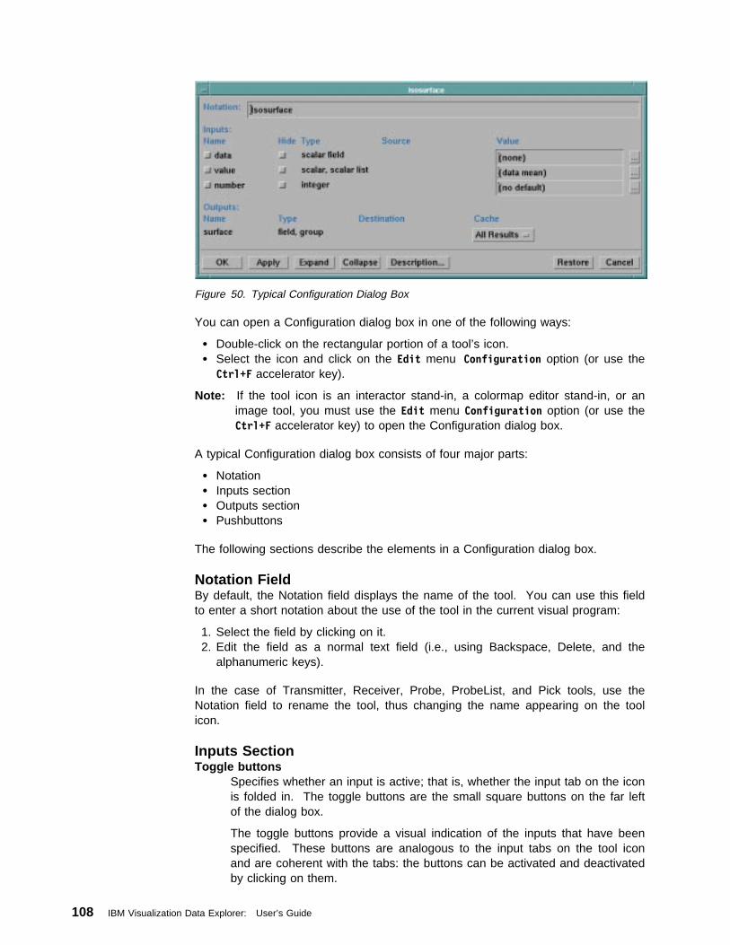
Figure 50. Typical Configuration Dialog Box

You can open a Configuration dialog box in one of the following ways:

Double-click on the rectangular portion of a tool’s icon. Select the icon and click on the Edit menu Configuration option (or use the

Ctrl+F accelerator key).

Note: If the tool icon is an interactor stand-in, a colormap editor stand-in, or animage tool, you must use the Edit menu Configuration option (or use theCtrl+F accelerator key) to open the Configuration dialog box.

A typical Configuration dialog box consists of four major parts:

Notation Inputs section Outputs section Pushbuttons

The following sections describe the elements in a Configuration dialog box.

Notation FieldBy default, the Notation field displays the name of the tool. You can use this fieldto enter a short notation about the use of the tool in the current visual program:

1. Select the field by clicking on it.2. Edit the field as a normal text field (i.e., using Backspace, Delete, and the

alphanumeric keys).

In the case of Transmitter, Receiver, Probe, ProbeList, and Pick tools, use theNotation field to rename the tool, thus changing the name appearing on the toolicon.

Inputs SectionToggle buttons

Specifies whether an input is active; that is, whether the input tab on the iconis folded in. The toggle buttons are the small square buttons on the far leftof the dialog box.

The toggle buttons provide a visual indication of the inputs that have beenspecified. These buttons are analogous to the input tabs on the tool iconand are coherent with the tabs: the buttons can be activated and deactivatedby clicking on them.

108 IBM Visualization Data Explorer: User’s Guide

When you activate a toggle button, the value of the input is either theoutput of another module (specified in the Source field of the dialog box),or the value specified in the Value field.

When you deactivate a toggle button, the input parameter is unboundand the tool uses its default value for the input.

NameSpecifies the name of an input parameter. You cannot modify this field.This field is grayed out if the name is specified with tab connections.

HideIndicates whether an input tab is to be hidden. When you activate the Hidetoggle button, the corresponding tab on the tool icon is removed. If a tab isconnected to another tool it cannot be hidden. Once a tab is hidden, it canbe removed from display in the Configuration dialog box by using theCollapse button.

To reveal individual input tabs, first click on the Expand button. This willcause the Configuration dialog box to resize, displaying all of the tool’sinputs. Then deactivate the Hide toggle buttons of the desired inputs byclicking on the toggle buttons. As the inputs are revealed, the tool icon isupdated to reflect the additional inputs. Once you have revealed all thedesired tabs, you can click on the Collapse button to remove the remaininghidden tabs from being displayed in the Configuration dialog box.

See also “Revealing and Hiding Input Tabs” on page 110.

TypeSpecifies the type of an input parameter. You cannot modify this field.

SourceDisplays the name of the tool connected to the input, if a connection exists.If the name of a tool is displayed in the source field, the toggle button isactivated and the name field is grayed out, and this input cannot be modifieduntil the connecting line is deleted.

ValueYou use the Value field to specify a value for an input. Initially the fieldcontains the default value for an input. To modify the Value field, select thefield by clicking on it. Then, edit it as a normal text field. The value must bespecified in the syntax described in Chapter 10, “Data Explorer ScriptingLanguage” on page 187. After you change the field, do one of the following:

Press Enter (which automatically activates the toggle button if it is notalready activated).

Activate the toggle button by clicking on it.

Click on either the OK pushbutton or the Apply button at the bottom ofthe box (see button descriptions in “Pushbuttons” on page 110).

Data Explorer automatically adds the appropriate delimiters for the type ofvalue entered. For instance, if you specified a string parameter in theConfiguration dialog box, Data Explorer automatically adds the quotesaround it. If you specified a scalar list, Data Explorer adds braces.

Note: If a source is displayed, you cannot modify the Value field. If youhave modified the Value field and you want to use the default value,release the toggle button. With the toggle button, you can flipbetween the modified value and the default value.

GUI: Windows

Chapter 6. Graphical User Interface: Important Windows 109

...This button, when enabled, brings up a list of possible values for theparameter. This list is for convenience only; you may enter values otherthan those listed as long as they are valid inputs for that parameter. Forexample, the ... button for the color parameter to the Color module listsred, green, and blue.

Outputs SectionName Specifies the name of an output parameter. You cannot modify this

field.

Type Specifies the type of an output parameter. You cannot modify thisfield.

Destination Displays the name of the tool (or tools) to which the output tabs areconnected.

Cache Specifies the number of results for this output of the tool that areeligible for caching. Cache can be “All Results”, in which all resultsare eligible for cache, “Last Result”, in which only the last value of theoutput is eligible, or “No Results”, in which no results from the moduleshould be cached. (See “Cache Control: Executive” on page 215.)

PushbuttonsThe seven buttons at the bottom of the Configuration dialog box are labeled boxesthat perform an action when you click on them. The buttons are:

OK Applies new values and closes the box.

Apply Saves newly entered values. Once you click on the Apply button, youcan no longer restore previous values.

Expand Causes all hidden inputs to be displayed in the Configuration dialogbox. You can then unhide hidden tabs using the Hide toggle button.

Collapse Causes all hidden input tabs to be removed from display in theConfiguration dialog box.

Description Displays a window with descriptions of the input and outputparameters of the tool.

Restore Restores previous values that were present when you opened the boxor when you last clicked on the Apply button.

Cancel Restores previous values that were present when you opened the boxor when you last clicked on the Apply button, and then closes thebox.

Revealing and Hiding Input TabsMost of the tools have more input tabs than are displayed when a tool icon isinitially displayed. For example, the Isosurface module has six inputs, but when anIsosurface tool icon is initially placed on the canvas, only three input tabs aredisplayed. The displayed tabs represent those that are most frequently used.

To reveal the hidden input tabs:

1. Select the tool icon by clicking on it.2. Select the Reveal All Tabs option from the Edit pull-down menu. (You can

also use the Ctrl+L accelerator key.)

110 IBM Visualization Data Explorer: User’s Guide

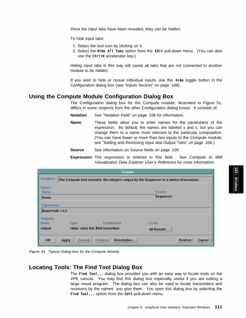
Once the input tabs have been revealed, they can be hidden.

To hide input tabs:

1. Select the tool icon by clicking on it.2. Select the Hide All Tabs option from the Edit pull-down menu. (You can also

use the Ctrl+H accelerator key.)

Hiding input tabs in this way will cause all tabs that are not connected to anothermodule to be hidden.

If you wish to hide or reveal individual inputs, use the hide toggle button in theConfiguration dialog box (see “Inputs Section” on page 108).

Using the Compute Module Configuration Dialog BoxThe Configuration dialog box for the Compute module, illustrated in Figure 51,differs in some respects from the other Configuration dialog boxes. It consists of:

Notation See “Notation Field” on page 108 for information.

Name These fields allow you to enter names for the parameters of theexpression. By default, the names are labeled a and b, but you canchange them to a name more relevant to the particular computation.(You can have fewer or more than two inputs to the Compute module;see “Adding and Removing Input and Output Tabs” on page 106.)

Source See information on Source fields on page 109.

Expression The expression is entered in this field. See Compute in IBMVisualization Data Explorer User’s Reference for more information. GUI: Windows

Figure 51. Typical Dialog Box for the Compute Module

Locating Tools: The Find Tool Dialog BoxThe Find Tool... dialog box provides you with an easy way to locate tools on theVPE canvas. You may find this dialog box especially useful if you are editing alarge visual program. The dialog box can also be used to locate transmitters andreceivers by the names you give them. You open this dialog box by selecting theFind Tool... option from the Edit pull-down menu.

Chapter 6. Graphical User Interface: Important Windows 111

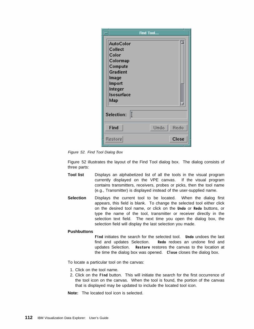
Figure 52. Find Tool Dialog Box

Figure 52 illustrates the layout of the Find Tool dialog box. The dialog consists ofthree parts:

Tool list Displays an alphabetized list of all the tools in the visual programcurrently displayed on the VPE canvas. If the visual programcontains transmitters, receivers, probes or picks, then the tool name(e.g., Transmitter) is displayed instead of the user-supplied name.

Selection Displays the current tool to be located. When the dialog firstappears, this field is blank. To change the selected tool either clickon the desired tool name, or click on the Undo or Redo buttons, ortype the name of the tool, transmitter or receiver directly in theselection text field. The next time you open the dialog box, theselection field will display the last selection you made.

PushbuttonsFind initiates the search for the selected tool. Undo undoes the lastfind and updates Selection. Redo redoes an undone find andupdates Selection. Restore restores the canvas to the location atthe time the dialog box was opened. Close closes the dialog box.

To locate a particular tool on the canvas:

1. Click on the tool name.2. Click on the Find button. This will initiate the search for the first occurrence of

the tool icon on the canvas. When the tool is found, the portion of the canvasthat is displayed may be updated to include the located tool icon.

Note: The located tool icon is selected.

112 IBM Visualization Data Explorer: User’s Guide

If you wish to find another occurrence of the same tool, simply click on Find again.This can be repeated as many time as you desire. When no more occurrences ofthe tool can be found, a message is displayed. If you click on the Find buttonagain, the search will be reset and the first occurrence of the tool icon will belocated.

If the selected tool is a transmitter, receiver, probe, or pick, occurrences of the toolwill be found independently of the user-supplied name. To locate a transmitter,receiver, probe, or pick tool by name:

1. Enter the name of the transmitter, receiver, pick or probe in the Selection: textfield.

2. Click on the Find button.

You can initiate the search for a different tool at any point. If you wish to retraceyour steps, the Find dialog provides an Undo button, allowing you to undo up to 10previous searches. When you click on the Undo pushbutton, the name of the tool(or transmitter or receiver) that was previously located will appear in the Selection:text field and the canvas is updated to reflect the location of the tool icon.

The dialog box also provides a Redo button. This enables you to repeat a searchthat was undone with the Undo button.

If you wish to return the canvas to its former “state” (i.e., to the set of tool icons itdisplayed) prior to the first search, click on Restore button.

Note: Clicking on Undo, Redo, or Restore will deselect the tool that is selected inthe Tools palette.

Customizing the VPE Window

GUI: Windows

Under the Options menu bar category are selections for customizing the window:

Tool Palettes Use as a toggle by clicking to close the palettes and make theworking area on the canvas larger.

Grid... A dialog box, illustrated in Figure 53 on page 114, appears for youto enter new values.

Chapter 6. Graphical User Interface: Important Windows 113

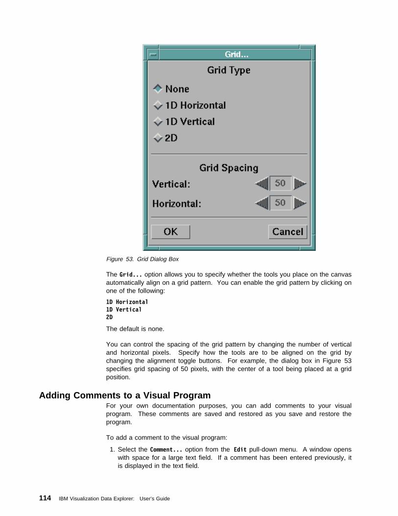
Figure 53. Grid Dialog Box

The Grid... option allows you to specify whether the tools you place on the canvasautomatically align on a grid pattern. You can enable the grid pattern by clicking onone of the following:

1D Horizontal1D Vertical2D

The default is none.

You can control the spacing of the grid pattern by changing the number of verticaland horizontal pixels. Specify how the tools are to be aligned on the grid bychanging the alignment toggle buttons. For example, the dialog box in Figure 53specifies grid spacing of 50 pixels, with the center of a tool being placed at a gridposition.

Adding Comments to a Visual ProgramFor your own documentation purposes, you can add comments to your visualprogram. These comments are saved and restored as you save and restore theprogram.

To add a comment to the visual program:

1. Select the Comment... option from the Edit pull-down menu. A window openswith space for a large text field. If a comment has been entered previously, itis displayed in the text field.

114 IBM Visualization Data Explorer: User’s Guide

2. Enter the desired comment in the text field. Edit the field the same way youedit any text field. This text field has multiple lines; you can generate linebreaks using the Enter key, or type continuously and have the line breaksadded automatically.

You can view these comments by using the Comment... option of the Editpull-down menu in the VPE, or by using the Application Comment option of theHelp pull-down menu in any primary window.

Adding Annotation to a Visual ProgramYou can also add annotation directly to the canvas. Select the Add Annotationoption from the Edit pull-down menu. A cursor appears. Click on the canvas whereyou would like to place annotation. You can modify the text in the annotation bydouble-clicking on the annotation. A text-entry dialog appears.

By default, the annotation text is visible on the canvas. You can choose the HideText option on the text-entry dialog, in which case only a “marker” appears on thecanvas.

Creating pages in the VPEYou can structure your visual program to make it more readable by using pages. Avisual program can consist of a number of pages. Each page contains a set ofmodules completely disconnected from modules on other pages. Receivers andtransmitters are used to connect modules on different pages.

To use pages, select the Pages... option in the Edit menu of the VPE. A cascademenu allows you to create an empty page, create a page containing the currentlyselected tools, delete the currently displayed page, or configure the page, that is,change its name or position.

GUI: Windows

Saving and Restoring a Visual ProgramThe Save As... and Open... options of the File pull-down menu use similar dialogboxes. A sample Save As... dialog box is illustrated in Figure 54 on page 116.

Chapter 6. Graphical User Interface: Important Windows 115

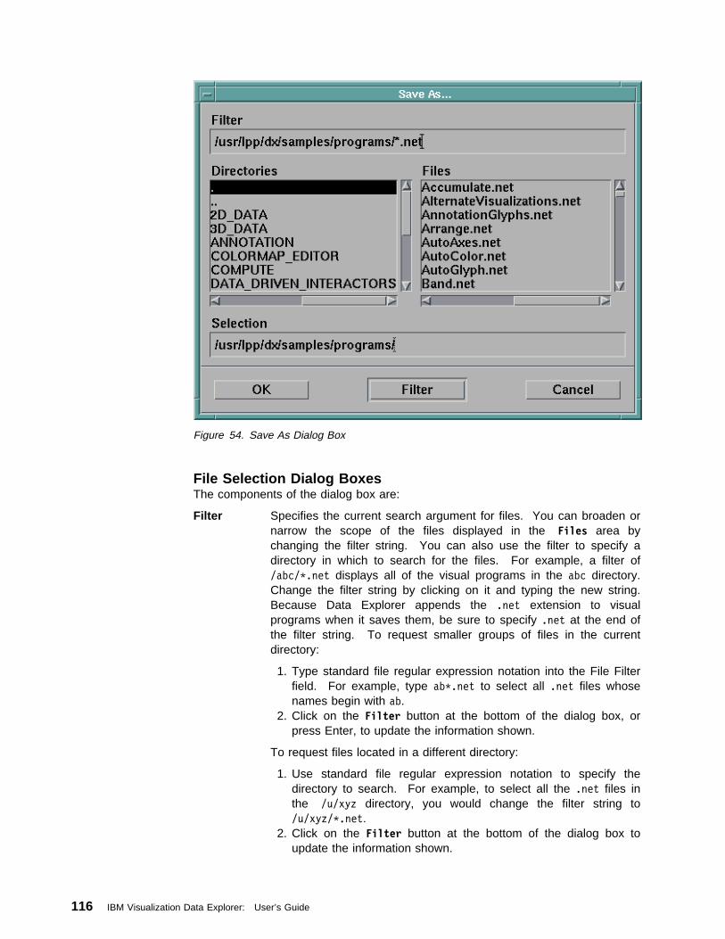
Figure 54. Save As Dialog Box

File Selection Dialog BoxesThe components of the dialog box are:

Filter Specifies the current search argument for files. You can broaden ornarrow the scope of the files displayed in the Files area bychanging the filter string. You can also use the filter to specify adirectory in which to search for the files. For example, a filter of/abc/\.net displays all of the visual programs in the abc directory.Change the filter string by clicking on it and typing the new string.Because Data Explorer appends the .net extension to visualprograms when it saves them, be sure to specify .net at the end ofthe filter string. To request smaller groups of files in the currentdirectory:

1. Type standard file regular expression notation into the File Filterfield. For example, type ab\.net to select all .net files whosenames begin with ab.

2. Click on the Filter button at the bottom of the dialog box, orpress Enter, to update the information shown.

To request files located in a different directory:

1. Use standard file regular expression notation to specify thedirectory to search. For example, to select all the .net files inthe /u/xyz directory, you would change the filter string to/u/xyz/\.net.

2. Click on the Filter button at the bottom of the dialog box toupdate the information shown.

116 IBM Visualization Data Explorer: User’s Guide

Directories Displays the directories in the current filter path. When you click ona directory, its name is displayed in the filter field; pressing the Enterkey then applies that filter. You can traverse through the availablepaths by double-clicking on the paths displayed in this portion of thedialog box. The parent directory of the filter path can be reached byselecting and applying the directory name that ends with two periods(..) as a filter. As you change directories this way, the Selectionbox and Files section are updated accordingly.

Files Displays the files specified by the File Filter and the directoryshown in the Selection area.

Clicking on a file name once will change the current selection.Double-clicking on a file name will select that file and proceed withthe Open, Save As, or Load Macro operation.

Selection Displays the current file selection. When the dialog box firstappears, Selection displays the current directory. To change thecurrent selection, either click on the desired file in the File area orclick on the Selection area and type the desired file name. Thenext time you open the dialog box, the Selection field displays thedirectory you most recently specified.

Pushbuttons OK approves the file name in the Selection area and proceeds withthe Open, Save As, or Load Macro operation. Filter applies thefilter string specified in the File Filter area. Cancel closes thedialog box. In the Open... and Load Macro... file selection dialogboxes, the Comments button lets you view any comments associatedwith the selected visual program file.

You can use the scroll bars provided on the right side and the bottom of thedirectories and file listings to view file and path names that are either too long ortoo numerous to fit in the available space.

GUI: Windows Saving a Visual ProgramWhen saving a visual program, Data Explorer saves the following files:

The visual program, with a .net extension The configuration settings, with a .cfg extension

Data Explorer automatically appends .net, .cfg to the name you enter in the SaveAs... dialog box. However, if you enter your file name with a .net extension, DataExplorer does not add another .net. If you end the file name with any otherextension, Data Explorer appends the .net extension to the extension you havespecified. For example, a file named abc.xyz would be renamed abc.xyz.net.

An existing file can be saved in the following ways:

Under the same name, replacing the previous version of the file

Under a new name or directory, thus creating a new file and preserving theprevious version.

Replacing a Previously Saved File: To save a program that has been namedand saved previously, press Ctrl+S or select the File menu Save option. Thisreplaces the previous version of the file. A named visual program has its namedisplayed in the title bar of the VPE window.

Chapter 6. Graphical User Interface: Important Windows 117

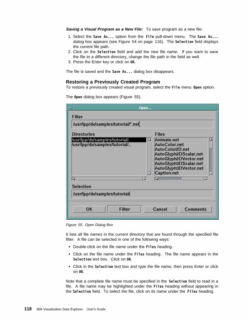
Saving a Visual Program as a New File: To save program as a new file:

1. Select the Save As... option from the File pull-down menu. The Save As...dialog box appears (see Figure 54 on page 116). The Selection field displaysthe current file path.

2. Click on the Selection field and add the new file name. If you want to savethe file to a different directory, change the file path in the field as well.

3. Press the Enter key or click on OK.

The file is saved and the Save As... dialog box disappears.

Restoring a Previously Created ProgramTo restore a previously created visual program, select the File menu Open option.

The Open dialog box appears (Figure 55).

Figure 55. Open Dialog Box

It lists all file names in the current directory that are found through the specified filefilter. A file can be selected in one of the following ways:

Double-click on the file name under the Files heading.

Click on the file name under the Files heading. The file name appears in theSelection text box. Click on OK.

Click in the Selection text box and type the file name, then press Enter or clickon OK.

Note that a complete file name must be specified in the Selection field to read in afile. A file name may be highlighted under the Files heading without appearing inthe Selection field. To select the file, click on its name under the Files heading.

118 IBM Visualization Data Explorer: User’s Guide

To see any comments that might be associated with a visual program before youload it, select a file by clicking on its name once or by entering its name in theSelection text box, then click on the Comments button. If the visual program hascomments associated with it, they are displayed; otherwise, a message appearstelling you that there are no comments.

To see a different list of files, change either the file filter or the file directory (“FileSelection Dialog Boxes” on page 116).

When you open a file, its name is displayed in the title bar of the VPE.

6.3 Using the Colormap EditorThe Colormap Editor is a window that enables you to map colors to specified datavalues, the results of which are displayed in the visual image. In addition to color,the Colormap Editor also controls the mapping of opacity to data, which is thedegree of the image’s transparency in relation to its background. Maximum opacityshows the color calculated by the hue, saturation, and value fields; minimumopacity calculates colors so that the image is faintly visible in front of thebackground. In summary, the Colormap Editor enables you to:

Control the range of data values over which the mapping occurs. Select the colors that are mapped to the range of values. Select the opacities that are mapped to the range of values.

When the Colormap stand-in from the Special category is connected to the Colortool as shown in the visual program fragment in Figure 56 on page 120, thecombination can be used in place of the AutoColor tool.

GUI: Windows

Chapter 6. Graphical User Interface: Important Windows 119

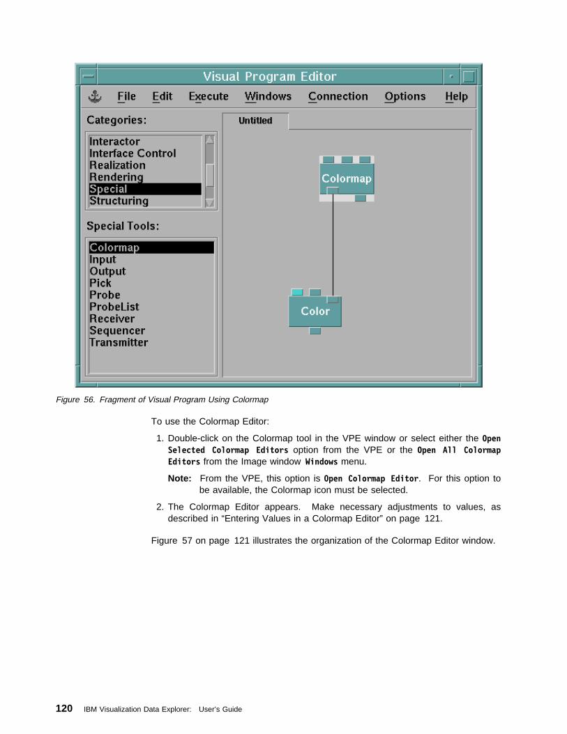
Figure 56. Fragment of Visual Program Using Colormap

To use the Colormap Editor:

1. Double-click on the Colormap tool in the VPE window or select either the OpenSelected Colormap Editors option from the VPE or the Open All ColormapEditors from the Image window Windows menu.

Note: From the VPE, this option is Open Colormap Editor. For this option tobe available, the Colormap icon must be selected.

2. The Colormap Editor appears. Make necessary adjustments to values, asdescribed in “Entering Values in a Colormap Editor” on page 121.

Figure 57 on page 121 illustrates the organization of the Colormap Editor window.

120 IBM Visualization Data Explorer: User’s Guide

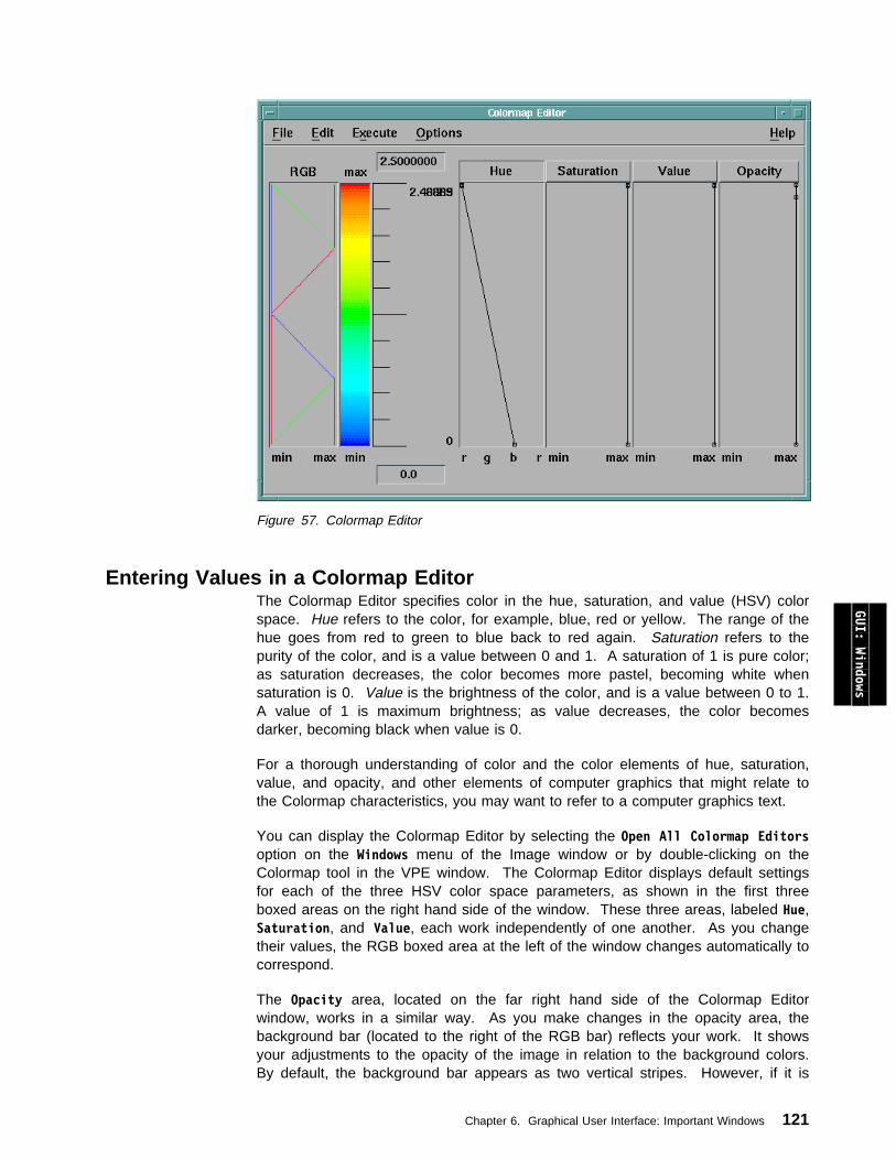
Figure 57. Colormap Editor

Entering Values in a Colormap EditorThe Colormap Editor specifies color in the hue, saturation, and value (HSV) colorspace. Hue refers to the color, for example, blue, red or yellow. The range of thehue goes from red to green to blue back to red again. Saturation refers to thepurity of the color, and is a value between 0 and 1. A saturation of 1 is pure color;as saturation decreases, the color becomes more pastel, becoming white whensaturation is 0. Value is the brightness of the color, and is a value between 0 to 1.A value of 1 is maximum brightness; as value decreases, the color becomesdarker, becoming black when value is 0.

For a thorough understanding of color and the color elements of hue, saturation,value, and opacity, and other elements of computer graphics that might relate tothe Colormap characteristics, you may want to refer to a computer graphics text.

You can display the Colormap Editor by selecting the Open All Colormap Editorsoption on the Windows menu of the Image window or by double-clicking on theColormap tool in the VPE window. The Colormap Editor displays default settingsfor each of the three HSV color space parameters, as shown in the first threeboxed areas on the right hand side of the window. These three areas, labeled Hue,Saturation, and Value, each work independently of one another. As you changetheir values, the RGB boxed area at the left of the window changes automatically tocorrespond.

The Opacity area, located on the far right hand side of the Colormap Editorwindow, works in a similar way. As you make changes in the opacity area, thebackground bar (located to the right of the RGB bar) reflects your work. It showsyour adjustments to the opacity of the image in relation to the background colors.By default, the background bar appears as two vertical stripes. However, if it is

GUI: Windows

Chapter 6. Graphical User Interface: Important Windows 121

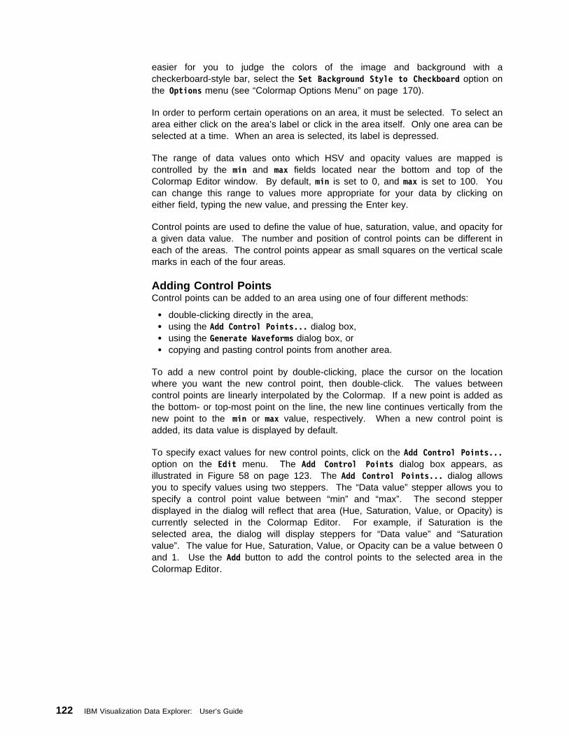
easier for you to judge the colors of the image and background with acheckerboard-style bar, select the Set Background Style to Checkboard option onthe Options menu (see “Colormap Options Menu” on page 170).

In order to perform certain operations on an area, it must be selected. To select anarea either click on the area’s label or click in the area itself. Only one area can beselected at a time. When an area is selected, its label is depressed.

The range of data values onto which HSV and opacity values are mapped iscontrolled by the min and max fields located near the bottom and top of theColormap Editor window. By default, min is set to 0, and max is set to 100. Youcan change this range to values more appropriate for your data by clicking oneither field, typing the new value, and pressing the Enter key.

Control points are used to define the value of hue, saturation, value, and opacity fora given data value. The number and position of control points can be different ineach of the areas. The control points appear as small squares on the vertical scalemarks in each of the four areas.

Adding Control PointsControl points can be added to an area using one of four different methods:

double-clicking directly in the area, using the Add Control Points... dialog box, using the Generate Waveforms dialog box, or copying and pasting control points from another area.

To add a new control point by double-clicking, place the cursor on the locationwhere you want the new control point, then double-click. The values betweencontrol points are linearly interpolated by the Colormap. If a new point is added asthe bottom- or top-most point on the line, the new line continues vertically from thenew point to the min or max value, respectively. When a new control point isadded, its data value is displayed by default.

To specify exact values for new control points, click on the Add Control Points...option on the Edit menu. The Add Control Points dialog box appears, asillustrated in Figure 58 on page 123. The Add Control Points... dialog allowsyou to specify values using two steppers. The “Data value” stepper allows you tospecify a control point value between “min” and “max”. The second stepperdisplayed in the dialog will reflect that area (Hue, Saturation, Value, or Opacity) iscurrently selected in the Colormap Editor. For example, if Saturation is theselected area, the dialog will display steppers for “Data value” and “Saturationvalue”. The value for Hue, Saturation, Value, or Opacity can be a value between 0and 1. Use the Add button to add the control points to the selected area in theColormap Editor.

122 IBM Visualization Data Explorer: User’s Guide

Figure 58. Colormap's Add Control Points Dialog Box

Selecting Control PointsControl points can be selected by doing one of the following:

Select a single control point by simply clicking on it once.

Select a group of control points by clicking on a point in the selected area anddragging the cursor around the desired points.

Select all of the control points in an area by using the Select All ControlPoints option under the Edit menu.

Note: A control point is selected automatically when it is created. When onecontrol point is created, all other previously selected points in that area areautomatically deselected.

Deleting Selected Control Points: To delete selected control points, you can doone of the following:

Double-click on each of them, one at a time. Choose the Edit menu, then click on the Delete Selected Control Points

option.

GUI: Windows

Moving Control PointsTo move a control point, simply drag it to the desired location. Control pointscannot be moved past each other; this facilitates the creation of step functions.They can be moved as a group by doing the following:

1. Draw a selection box around the points you want in the group.2. Position the mouse pointer on any one of them and drag it to the desired

location.

All of the control points move together within the constraints of the unselectedpoints above and below.

The movement of control points can be constrained either horizontally or verticallyby selecting the Constrain Horizontal or Constrain Vertical option from theColormap Edit menu (see “Colormap Edit Menu” on page 169). By constraininghorizontally after adding a precise control point, you can move the point to changethe color or opacity mapped to specific value, without changing the value itself.

Chapter 6. Graphical User Interface: Important Windows 123

Creating WaveformsTo create waveforms, select the Generate Waveforms option from the Editpull-down menu. The Generate Waveforms dialog box appears (Figure 59 onpage 125).

This dialog box allows you to:

Choose the shape of the waveform from an options box. Waveforms can bestep, square, or sawtooth.

Choose the range of the waveform from an options box. “Full” creates awaveform that runs the full length of the selected area. “Selected” creates awave that runs the distance between two selected control points in thespecified area.

Specify the number of steps to be created in the range of the waveform byusing the stepper. The number of steps specified can be between 2 and 100.

Copying and Pasting Control PointsControl points can be copied and pasted from one Colormap area to another, usingthe Copy and Paste options of the Edit window.

1. Select the control point or control points you wish to copy.2. Click on Copy.3. Select the area to which you wish to copy the control points and then click on

Paste.

Display Control Point ValuesThe data values of control points are displayed by default. You can control whichdata values are displayed, using the Display Control Point Data Value cascademenu in the Options menu. If “off” is specified, no data values are shown. If“selected” is chosen, only the data values for the selected control points are shown,and if “all” is selected, the data values for all control points in the selected area areshown.

Axis DisplayYou can control how the Colormap Editor axis is displayed by using the Optionsmenu Axis Display... option. You have three choices for the display: Ticks (thedefault), Histogram, and Log Histogram. Histogram will cause the histogram of thedata to be displayed. Log Histogram will cause the log of the histogram to bedisplayed. If the Colormap Editor is not data-driven, these two options will begrayed-out. The number of histogram bins can be controlled using the Edit menuNumber of histogram bins... option.

Changing the name of the Colormap EditorEvery Colormap Editor is given the default name of “Colormap Editor” in the boxacross the top of the window. If you want to customize the name of the ColormapEditor, you can do so by clicking on the Options menu Change Colormap Name...option and entering a new name in the dialog box that appears.

Note: You can also change the name of the Colormap Editor by using the titleparameter in the Colormap tool.

124 IBM Visualization Data Explorer: User’s Guide

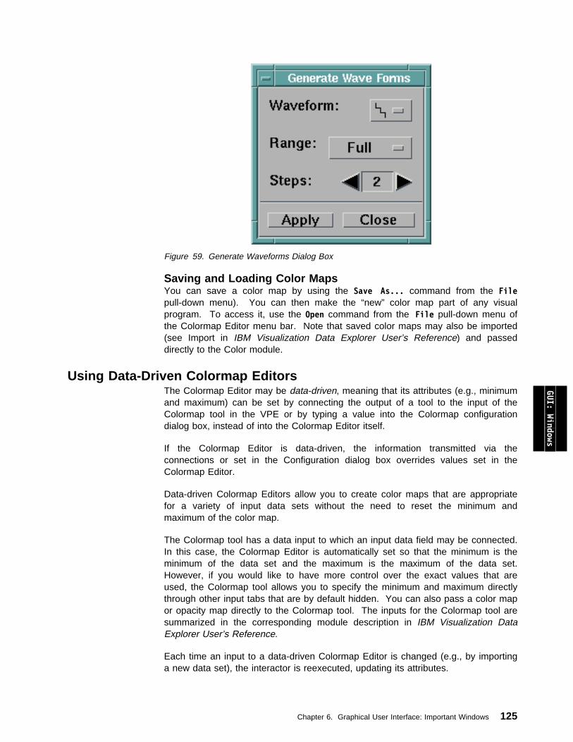
Figure 59. Generate Waveforms Dialog Box

Saving and Loading Color MapsYou can save a color map by using the Save As... command from the Filepull-down menu). You can then make the “new” color map part of any visualprogram. To access it, use the Open command from the File pull-down menu ofthe Colormap Editor menu bar. Note that saved color maps may also be imported(see Import in IBM Visualization Data Explorer User’s Reference) and passeddirectly to the Color module.

Using Data-Driven Colormap EditorsThe Colormap Editor may be data-driven, meaning that its attributes (e.g., minimumand maximum) can be set by connecting the output of a tool to the input of theColormap tool in the VPE or by typing a value into the Colormap configurationdialog box, instead of into the Colormap Editor itself.

If the Colormap Editor is data-driven, the information transmitted via theconnections or set in the Configuration dialog box overrides values set in theColormap Editor.

Data-driven Colormap Editors allow you to create color maps that are appropriatefor a variety of input data sets without the need to reset the minimum andmaximum of the color map.

The Colormap tool has a data input to which an input data field may be connected.In this case, the Colormap Editor is automatically set so that the minimum is theminimum of the data set and the maximum is the maximum of the data set.However, if you would like to have more control over the exact values that areused, the Colormap tool allows you to specify the minimum and maximum directlythrough other input tabs that are by default hidden. You can also pass a color mapor opacity map directly to the Colormap tool. The inputs for the Colormap tool aresummarized in the corresponding module description in IBM Visualization DataExplorer User’s Reference.

Each time an input to a data-driven Colormap Editor is changed (e.g., by importinga new data set), the interactor is reexecuted, updating its attributes.

GUI: Windows

Chapter 6. Graphical User Interface: Important Windows 125

126 IBM Visualization Data Explorer: User’s Guide

Chapter 7. Graphical User Interface: Control Panels,Interactors, and Macros

7.1 Using Control Panels and Interactors . . . . . . . . . . . . . . . . . . . . 128Building Control Panels . . . . . . . . . . . . . . . . . . . . . . . . . . . . . . 129Placing Interactors in a New Control Panel . . . . . . . . . . . . . . . . . . 130Adding Interactors to an Existing Control Panel . . . . . . . . . . . . . . . . 130Selecting, Moving, and Deleting Interactors . . . . . . . . . . . . . . . . . . 131Changing the Size of an Interactor . . . . . . . . . . . . . . . . . . . . . . . 132Locating Interactor Stand-ins . . . . . . . . . . . . . . . . . . . . . . . . . . 132Deleting Control Panels . . . . . . . . . . . . . . . . . . . . . . . . . . . . . 132Saving and Restoring Control Panels . . . . . . . . . . . . . . . . . . . . . 132Customizing a Control Panel . . . . . . . . . . . . . . . . . . . . . . . . . . 133Control Panels as Dialog Boxes . . . . . . . . . . . . . . . . . . . . . . . . . 138Control Panel Access, Groups, and Hierarchies . . . . . . . . . . . . . . . 138Creating, Modifying, and Deleting Control Panel Groups . . . . . . . . . . 139Restricting Control Panel Access . . . . . . . . . . . . . . . . . . . . . . . . 140Specifying a Startup Control Panel . . . . . . . . . . . . . . . . . . . . . . . 141Opening Existing Control Panels . . . . . . . . . . . . . . . . . . . . . . . . 141Using Interactors . . . . . . . . . . . . . . . . . . . . . . . . . . . . . . . . . 142Using Data-Driven Interactors . . . . . . . . . . . . . . . . . . . . . . . . . . 147

7.2 Creating and Using Macros . . . . . . . . . . . . . . . . . . . . . . . . . . 149Creating Macros . . . . . . . . . . . . . . . . . . . . . . . . . . . . . . . . . . 149Loading Macros . . . . . . . . . . . . . . . . . . . . . . . . . . . . . . . . . . 152Using Macros in a Visual Program . . . . . . . . . . . . . . . . . . . . . . . 153Viewing and Changing Macros . . . . . . . . . . . . . . . . . . . . . . . . . 154

GUI: Control Panels

Copyright IBM Corp. 1991-1997 127

7.1 Using Control Panels and InteractorsAs you create a visual program, you may have inputs whose values are subject tofrequent change. You can use interactors as an easy method for controlling thoseinput values. Interactors, which appear only in Control Panels, are the interactivedevices that you use to manipulate inputs to a visual program in order to changethe image that is produced (see “Using Interactors” on page 142 for detaileddescriptions).

Interactor stand-ins are used to indicate which input to a module a given interactoris to control. While you are building the network in the VPE, you select interactorstand-ins from the tool palettes and place them on the canvas, as you do with othertools. Like any tool, the output of an interactor stand-in can be connected to morethan one input. Interactor stand-ins are named, in general, after the type of datathey output:

Integer stand-insRepresent interactors that output whole numbers.

Scalar stand-insRepresent interactors that output real numbers.

String stand-insRepresent interactors that output text strings.

Value stand-insRepresent interactors that output scalars, vectors, and tensors.

Vector stand-insRepresent interactors that output vectors.

Integer list stand-insRepresent interactors that output integer lists.

Scalar list stand-insRepresent interactors that output scalar lists.

String list stand-insRepresent interactors that output string lists.

Value list stand-insRepresent interactors that output value lists (e.g., vector and scalarlists).

Vector list stand-insRepresent interactors that output vector lists.

Selector stand-insRepresent interactors that output values and strings, representing achoice of one from many.

Selector list stand-insRepresent interactors that output values and strings, representing achoice of none, one, or more among many.

FileSelector stand-insRepresent interactors that output both a fully qualified path name and anindividual file name.

128 IBM Visualization Data Explorer: User’s Guide

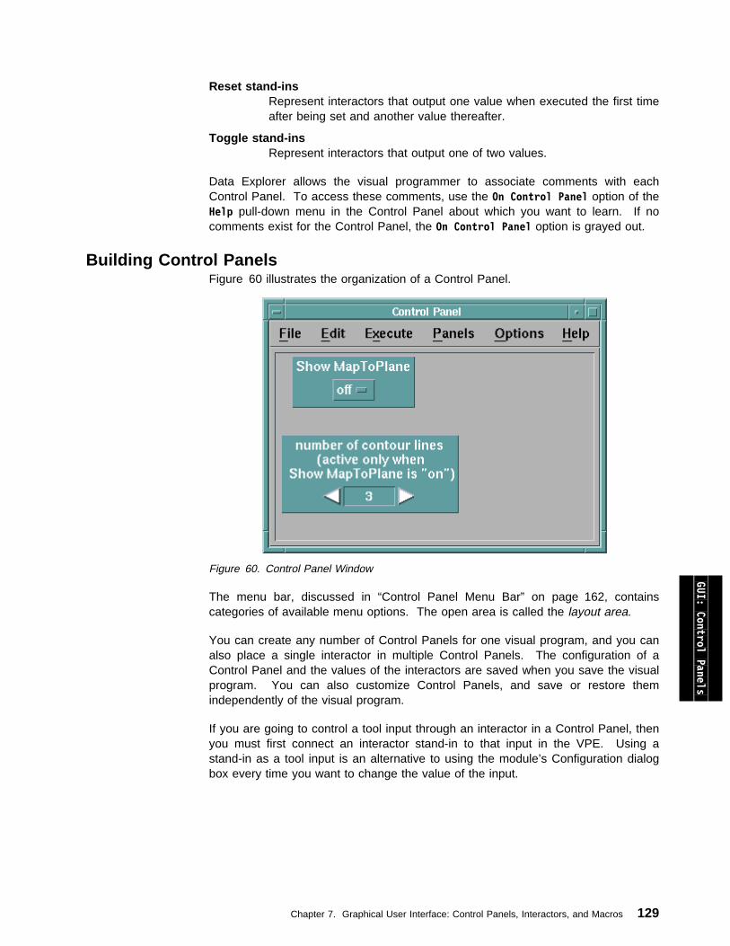
Reset stand-insRepresent interactors that output one value when executed the first timeafter being set and another value thereafter.

Toggle stand-insRepresent interactors that output one of two values.

Data Explorer allows the visual programmer to associate comments with eachControl Panel. To access these comments, use the On Control Panel option of theHelp pull-down menu in the Control Panel about which you want to learn. If nocomments exist for the Control Panel, the On Control Panel option is grayed out.

Building Control PanelsFigure 60 illustrates the organization of a Control Panel.

Figure 60. Control Panel Window GUI: Control Panels

The menu bar, discussed in “Control Panel Menu Bar” on page 162, containscategories of available menu options. The open area is called the layout area.

You can create any number of Control Panels for one visual program, and you canalso place a single interactor in multiple Control Panels. The configuration of aControl Panel and the values of the interactors are saved when you save the visualprogram. You can also customize Control Panels, and save or restore themindependently of the visual program.

If you are going to control a tool input through an interactor in a Control Panel, thenyou must first connect an interactor stand-in to that input in the VPE. Using astand-in as a tool input is an alternative to using the module’s Configuration dialogbox every time you want to change the value of the input.

Chapter 7. Graphical User Interface: Control Panels, Interactors, and Macros 129

Placing Interactors in a New Control PanelTo place interactors in a new Control Panel:

1. On the VPE canvas, select the interactor stand-ins you want in the ControlPanel (other tools can be selected as well).

2. Click on the New Control Panel option of the Windows menu. This causes anew Control Panel to appear with the selected interactors in the layout area.Each interactor is labeled with the name of the tool to which its output isconnected, unless its output is connected to more than one tool or notconnected to any tool, in which case the interactor is labeled with the interactortype (e.g., an integer interactor is labeled with “Integer”). You can alsodouble-click on one of the selected interactor stand-ins to create a new ControlPanel automatically.

When a new Control Panel is created with the selected interactors, the interactorsare placed in a vertical column in the order in which their stand-ins were placed onthe VPE canvas.

Note: If you select a group that includes tools other than interactor stand-ins, onlythe interactors appear in the Control Panel. Therefore, the quickest way to placeall the visual program’s interactors in one Control Panel is to use the Select Alloption of the Edit pull-down, then select the New Control Panel option of theWindows pull-down menu.

Adding Interactors to an Existing Control PanelTo add an interactor to an existing Control Panel:

1. Open the Control Panel.2. Select the interactor stand-in on the VPE canvas.3. In the Control Panel window, click on the Add Selected Interactor(s) option

of the Edit menu.4. Move the cursor to where you want to position the tool in the Control Panel.

Note that the style of the cursor changes when you move it onto the panel.This is similar to how tool icons are placed on the VPE canvas. Exactplacement of the interactor depends on the grid settings (see “Changing theAlignment of Interactors in the Control Panel” on page 134).

5. Click the mouse. The interactor appears at the specified location.

Alternatively, you can use “drag and drop” to add an interactor to an existingControl Panel:

1. Select the interactor stand-in on the VPE canvas.2. Press the middle mouse button while the cursor is positioned on the stand-in

icon.3. Drag the cursor to the Control Panel and release the mouse button.4. The interactor appears at the new location.

You can add more than one interactor at a time to a Control Panel. To do this,select multiple interactor stand-ins on the VPE canvas, then select Add SelectedInteractor(s) in the desired Control Panel. After doing this, you can use themouse to place the interactors in the Control Panel one at a time. They are placedin the Control Panel in the same order that they were placed initially onto the VPEcanvas. Similarly, you can drag and drop multiple stand-ins from the visualprogram to a Control Panel. You can also drag and drop interactors from oneControl Panel to another, as long as both are associated with the same Data

130 IBM Visualization Data Explorer: User’s Guide

Explorer session. For more information on drag and drop, see “Moving andCopying Tools” on page 105.

You can put the same interactor in more than one Control Panel and in the sameControl Panel more than once. For example, you may want to have one ControlPanel that contains all the interactors for a visual program, and another thatcontains only the most frequently used interactors. You can also place multipleinstances of an interactor, with different styles or step size increments, in oneControl Panel. This provides both coarse and fine control over a parameter value.The user interface ensures that each instance of the interactor is consistent. If youchange a value in one instance, it changes in the others.

Selecting, Moving, and Deleting InteractorsTo select an interactor, click on it.

To select a group of interactors, use one of the following methods:

Hold down the Shift key and click on each interactor in turn.

Position the mouse pointer on the canvas near a corner of the group and dragthe mouse to draw a selection box around the interactor you want. To selectan interactor, you must completely enclose it in the selection box. As aninteractor is encompassed by the selection box, it is highlighted (indicating thatit is selected).

To deselect an interactor, shift-click on it.

To deselect a group of interactors, use one of these methods:

Shift-click on each interactor.

Shift-drag to draw a box around the interactors you want to deselect. As aselected interactor is encompassed in the box, it becomes unhighlighted.Release the button to deselect the interactors.

Note: Clicking on an empty part of the layout area deselects all selectedinteractors.

To move an interactor:

1. Depress the mouse button on the interactor and drag it to the desired location.While the mouse button is depressed, an outline of the interactor follows themotion of the mouse, but the interactor remains in the original location.

2. Release the mouse button. The interactor moves to that location.

To move a group of interactors:

1. Select a group of interactors to be moved.2. Position the mouse pointer on any member of the group and drag it. An outline

of each interactor appears and follows the mouse.3. Release the mouse button. The interactors move to the new location.

To delete one or more interactors:

1. Select one or more interactors to delete.2. Press the Ctrl+Delete accelerator key or click on the Delete option of the Edit

menu.

GUI: Control Panels

Chapter 7. Graphical User Interface: Control Panels, Interactors, and Macros 131

If you delete an interactor stand-in from the VPE, the interactor in the Control Panelis also deleted. However, deleting the interactor in the Control Panel does notaffect what is displayed in the VPE.

Changing the Size of an InteractorYou can change the size of interactors in a Control Panel. Some interactors (e.g.,Selector) resize automatically, depending on their contents, but others (e.g., String)do not. You can resize any interactor by pressing the control key (Ctrl) and the leftmouse button.

Locating Interactor Stand-insAs you are building and modifying visual programs and Control Panels, you mayfind it desirable to locate that interactor in a Control Panel that corresponds to aspecific interactor stand-in. To locate an interactor corresponding to a stand-in:

1. Select the desired stand-in in the VPE by clicking on it.2. Select the Edit menu Show Selected Interactor(s) option in the Control

Panel.

The interactor corresponding to the stand-in will become selected. If no interactorsin the Control Panel are associated with the selected stand-in, the Show SelectedInteractor(s) option will be grayed-out. If you have more than one Control Paneland you are unsure which of them contains the interactor corresponding to thestand-in, Step 2 (above) can be applied to each Control Panel. Alternatively, youcan double-click on the stand-in. This will highlight the corresponding interactor.

To locate a stand-in corresponding to an interactor:

1. Select the interactor in a Control Panel by clicking on it.2. Select the Edit menu Show Selected Tool option in the Control Panel.

The stand-in corresponding to the interactor will be selected. If the stand-in is notin the currently displayed portion of the visual program, the display will be updatedso the selected stand-in is visible.

Deleting Control PanelsTo delete a Control Panel:

1. Delete the interactors in the Control Panel.2. Click on the Close option of the File menu.

Saving and Restoring Control PanelsThe Program Settings... option of the anchor window allows you to save your ownconfiguration of the Control Panel(s) independently of the rest of the network. Youcan save the values of the Control Panels as well as the configuration of all of thestored Control Panels for the current visual program.

Select the Program Settings...Save As option on the File menu anchor windowbar. You can retrieve Control Panels in the anchor window by using the ProgramSettings...Load option.

If you have made changes that you do not want to keep, click on the ProgramSettings...Load option of the File menu, and select the file again without saving.This procedure restores the original configuration.

132 IBM Visualization Data Explorer: User’s Guide

Customizing a Control PanelThis section describes the customization that can be done while building theControl Panel from the VPE window or while actually viewing the image in theImage window.

The Control Panel Options menu provides several possibilities for furthercustomizing the Panel and its interactors, as described in “Control Panel OptionsMenu” on page 164.

Changing the Name of a Control PanelEvery Control Panel is given the default name of “Control Panel,” as shown in thetitle box across the top of the window. If you want to customize the name in anyparticular Control Panel, you can do so by clicking on the Change Control PanelName... option on the Options menu and entering a new name in the dialog boxthat appears. The new name can contain any number of characters including anyletter, number, symbol, or space that you find on the keyboard.

If you have several Control Panels in your visual program, you should assignnames to them. Data Explorer allows you to open each one individually, by name,from a Control Panel, Image window, and VPE. To open a Control Panel by namefrom any of these three primary windows, do the following:

1. Select the Open Control Panel by Name option from the Windows pull-downmenu in the VPE and Image window, or from the Panels pull-down menu in theControl Panel. This reveals a cascade menu with a list of the existing ControlPanels.

2. Click on the name of the Control Panel you wish to open. The desired ControlPanel appears.

Adding Comments to a Control PanelIf other people are going to use the visual programs you create, it may be desirableto document how the interactors are used. You can associate comments with theControl Panel to describe how it uses the interactors to control input values in thevisual program.

To add comments to a Control Panel:

1. Select the Comment... option from the Edit pull-down menu in the ControlPanel. A dialog box appears, with a large text field in which you can type thecomments. If a comment has been entered previously for this Control Panel, itis displayed in the text field.

2. Enter your comments in the text field, editing the same way as with any textfield. This text field has multiple lines; you can break the lines using the Enterkey, or allow them to flow automatically as you type.

3. Click on OK to store the comments.

These comments can be viewed, but not edited, by using the On Control Paneloption of the Help pull-down menu in the Control Panel. To edit the comments, youmust use the Comment... option of the Options pull-down menu.

GUI: Control Panels

Chapter 7. Graphical User Interface: Control Panels, Interactors, and Macros 133

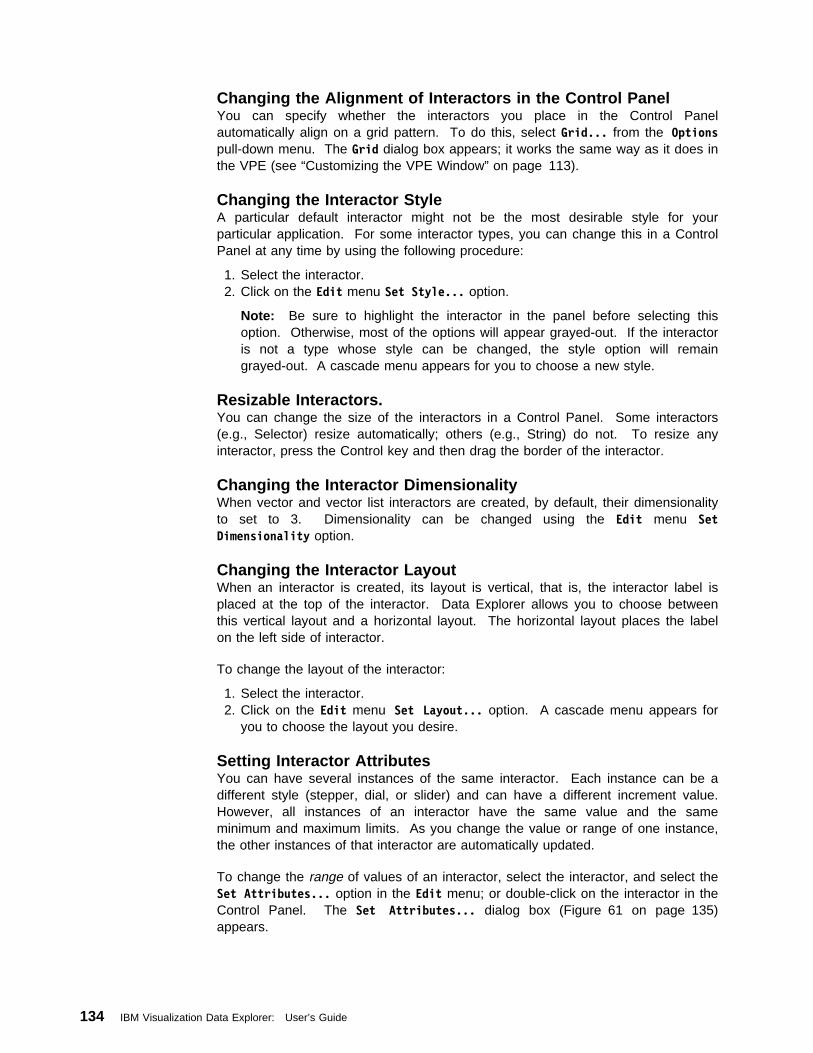
Changing the Alignment of Interactors in the Control PanelYou can specify whether the interactors you place in the Control Panelautomatically align on a grid pattern. To do this, select Grid... from the Optionspull-down menu. The Grid dialog box appears; it works the same way as it does inthe VPE (see “Customizing the VPE Window” on page 113).

Changing the Interactor StyleA particular default interactor might not be the most desirable style for yourparticular application. For some interactor types, you can change this in a ControlPanel at any time by using the following procedure:

1. Select the interactor.2. Click on the Edit menu Set Style... option.

Note: Be sure to highlight the interactor in the panel before selecting thisoption. Otherwise, most of the options will appear grayed-out. If the interactoris not a type whose style can be changed, the style option will remaingrayed-out. A cascade menu appears for you to choose a new style.

Resizable Interactors.You can change the size of the interactors in a Control Panel. Some interactors(e.g., Selector) resize automatically; others (e.g., String) do not. To resize anyinteractor, press the Control key and then drag the border of the interactor.

Changing the Interactor DimensionalityWhen vector and vector list interactors are created, by default, their dimensionalityto set to 3. Dimensionality can be changed using the Edit menu SetDimensionality option.

Changing the Interactor LayoutWhen an interactor is created, its layout is vertical, that is, the interactor label isplaced at the top of the interactor. Data Explorer allows you to choose betweenthis vertical layout and a horizontal layout. The horizontal layout places the labelon the left side of interactor.

To change the layout of the interactor:

1. Select the interactor.2. Click on the Edit menu Set Layout... option. A cascade menu appears for

you to choose the layout you desire.

Setting Interactor AttributesYou can have several instances of the same interactor. Each instance can be adifferent style (stepper, dial, or slider) and can have a different increment value.However, all instances of an interactor have the same value and the sameminimum and maximum limits. As you change the value or range of one instance,the other instances of that interactor are automatically updated.

To change the range of values of an interactor, select the interactor, and select theSet Attributes... option in the Edit menu; or double-click on the interactor in theControl Panel. The Set Attributes... dialog box (Figure 61 on page 135)appears.

134 IBM Visualization Data Explorer: User’s Guide

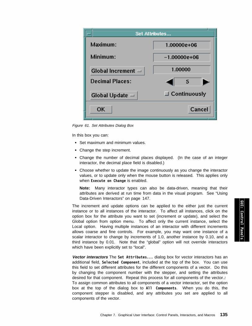
Figure 61. Set Attributes Dialog Box

In this box you can:

Set maximum and minimum values.

Change the step increment.

Change the number of decimal places displayed. (In the case of an integerinteractor, the decimal place field is disabled.)

Choose whether to update the image continuously as you change the interactorvalues, or to update only when the mouse button is released. This applies onlywhen Execute on Change is enabled.

Note: Many interactor types can also be data-driven, meaning that theirattributes are derived at run time from data in the visual program. See “UsingData-Driven Interactors” on page 147.

The increment and update options can be applied to the either just the currentinstance or to all instances of the interactor. To affect all instances, click on theoption box for the attribute you want to set (increment or update), and select theGlobal option from option menu. To affect only the current instance, select theLocal option. Having multiple instances of an interactor with different incrementsallows coarse and fine controls. For example, you may want one instance of ascalar interactor to change by increments of 1.0, another instance by 0.10, and athird instance by 0.01. Note that the “global” option will not override interactorswhich have been explicitly set to “local”.

Vector interactors The Set Attributes... dialog box for vector interactors has anadditional field, Selected Component, included at the top of the box. You can usethis field to set different attributes for the different components of a vector. Do thisby changing the component number with the stepper, and setting the attributesdesired for that component. Repeat this process for all components of the vector.:To assign common attributes to all components of a vector interactor, set the optionbox at the top of the dialog box to All Components. When you do this, thecomponent stepper is disabled, and any attributes you set are applied to allcomponents of the vector.

GUI: Control Panels

Chapter 7. Graphical User Interface: Control Panels, Interactors, and Macros 135

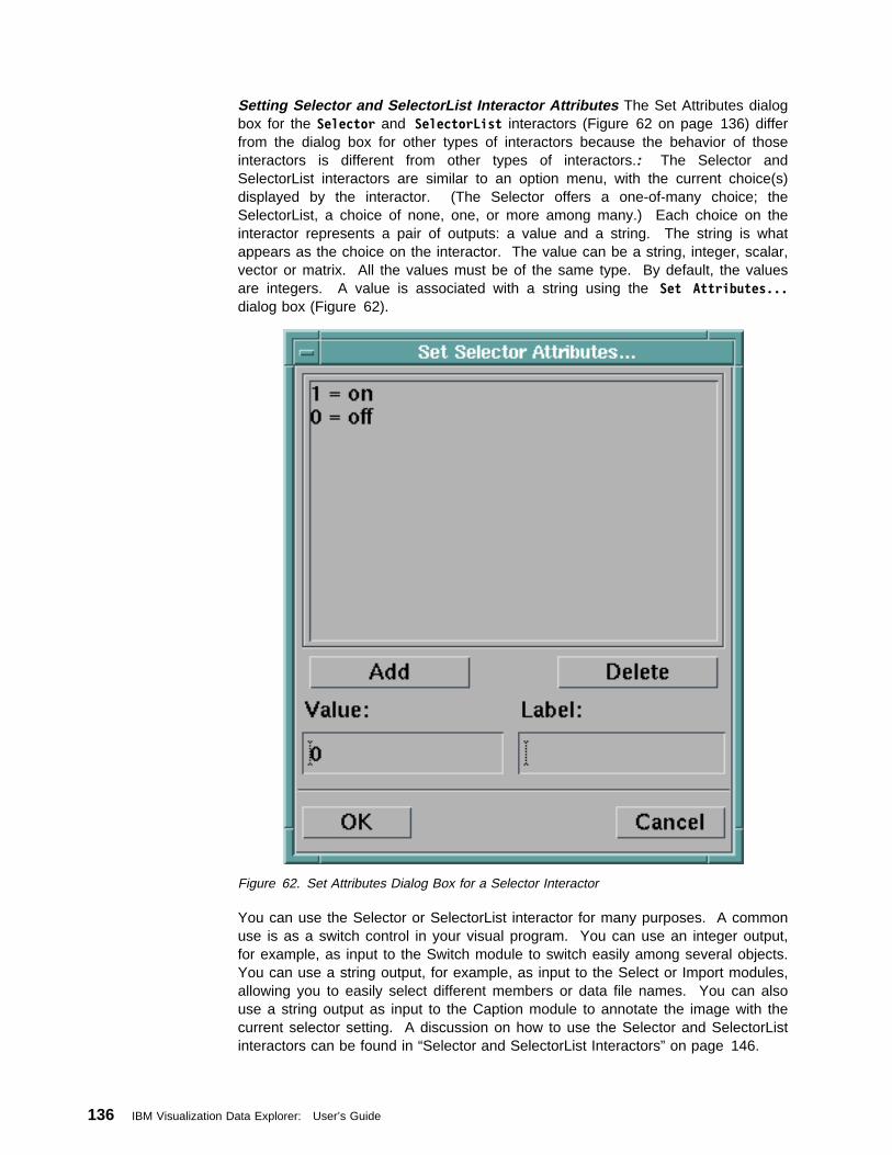
Setting Selector and SelectorList Interactor Attributes The Set Attributes dialogbox for the Selector and SelectorList interactors (Figure 62 on page 136) differfrom the dialog box for other types of interactors because the behavior of thoseinteractors is different from other types of interactors.: The Selector andSelectorList interactors are similar to an option menu, with the current choice(s)displayed by the interactor. (The Selector offers a one-of-many choice; theSelectorList, a choice of none, one, or more among many.) Each choice on theinteractor represents a pair of outputs: a value and a string. The string is whatappears as the choice on the interactor. The value can be a string, integer, scalar,vector or matrix. All the values must be of the same type. By default, the valuesare integers. A value is associated with a string using the Set Attributes...dialog box (Figure 62).

Figure 62. Set Attributes Dialog Box for a Selector Interactor

You can use the Selector or SelectorList interactor for many purposes. A commonuse is as a switch control in your visual program. You can use an integer output,for example, as input to the Switch module to switch easily among several objects.You can use a string output, for example, as input to the Select or Import modules,allowing you to easily select different members or data file names. You can alsouse a string output as input to the Caption module to annotate the image with thecurrent selector setting. A discussion on how to use the Selector and SelectorListinteractors can be found in “Selector and SelectorList Interactors” on page 146.

136 IBM Visualization Data Explorer: User’s Guide

The default choices for the Selector and SelectorList interactors are:

1, “on” 0, “off”

To modify the choices, do the following:

1. Open a Control Panel with the selector interactor in it.2. Open the selector’s Set Attributes... dialog box by double-clicking on the

interactor, or by selecting the interactor and then choosing the SetAttributes... option in the Edit pull-down menu. A dialog box appears,similar to the one shown Figure 62 on page 136.

3. The procedure for modifying the choices in this list is similar to that formodifying the list elements in a list interactor (see “List Interactors” onpage 145). To enter a value in this interactor click on the Value box, enter avalue, and press the Enter key. Then click on the Label box, type a string, andpress the Enter key. For more information about how to modify, add, anddelete elements, see “List Interactors” on page 145.

Note: If you wish to change the type of the values in the value field, forexample, entering values other than integers when initially configuringthe interactor, you must first delete all the entries in the SetAttributes... dialog before entering new ones. This is required sincethe type of all values must be the same.

4. When you are finished modifying the choices, click on OK to apply the changes.

Because the selector interactor yields both the value and the string as outputs, youcan use either output, or both, in a visual program. In the selector stand-in, theoutput on the left is the value, while the output on the right represents the string.

Changing the Label on the Interactor: The default label on any unconnectedinteractor is the name of the interactor stand-in. If the interactor is connected toone input, the default name of the interactor is the name of the tool followed by theinput parameter name. If the interactor is connected to more than one input, itsdefault name is the name of the interactor stand-in. You can change the defaultname by doing the following:

1. Click on the Set Interactor Label... option on the Control Panel Edit menu.2. Enter a new name in the dialog box that appears (Figure 63).

GUI: Control Panels

Figure 63. Set Interactor Label Dialog Box

Chapter 7. Graphical User Interface: Control Panels, Interactors, and Macros 137

The new name can contain any number of characters, including any letter, number,symbol, or space that you find on the keyboard. (If you want a blank label, enter“\0” for the name.)

The interactor label can have multiple lines: type “\n” where you want a line tobreak. For example,

First Line\nSecond Line

Setting Toggle and Reset Attributes: You can set the output of Toggle andReset interactors for both their “button down” (set) and “button up” (unset) states..The output value can be string, integer, scalar, or vector, and the set and unsetoutputs do not have to be of the same type.

Control Panels as Dialog BoxesIt is possible to customize Control Panels so that they appear as dialog boxes.This is intended for building applications to be used in -image or -menubar mode(i.e., with the Image window or menu bar as the anchor window). The appearanceof the dialog box can be modified with the options Label and Separator under AddElement in the Edit pull-down menu of the Control Panel. These will add thespecified element to the panel at the point where the mouse cursor is positioned.Separators can be made vertical using the Set Layout option of the Edit menu.The size of the separator can be controlled using the mechanism described in“Resizable Interactors.” on page 134. The color and font of labels can be specifiedusing the dialog box that appears when the label is created. These can bechanged by selecting the label and choosing Set Attributes from the Edit menuof the Control Panel.

Once the Control Panel has been created, select Dialog Style in the Optionspull-down menu to create the dialog box. The size of the box will vary toaccommodate the interactors. The empty canvas to the right of the interactors willbe truncated. The placement of the interactors will also change if the box size ischanged, to maintain the same relative positions. In -editor mode, the Closebutton returns to an editable Control Panel. In -image or -menubar mode the,Close button closes the dialog box. To enable a “dialog style” dialog box, save thevisual program with the Control Panel in dialog-style format.

Control Panel Access, Groups, and HierarchiesYou may wish to organize your Control Panels into groups or hierarchies dependingon how the interactors in the Control Panels relate. For example, you may have afew Control Panels that are tightly related and wish to have them treated as agroup. Data Explorer provides you with the means of placing these Control Panelsinto a group so that they can be opened together.

If you have a master Control Panel that should be open before any other controls,Data Explorer provides you with the capability of restricting access to these ControlPanels from any Data Explorer window except the master Control Panel. Access toControl Panel groups can be done in a similar fashion. Restricting access toControl Panels in this way allows you to build Control Panels into hierarchicalstructures.

A special type of Control Panel access can be achieved by specifying whichControl Panels are automatically opened when Data Explorer is started with theImage window or menu bar as the anchor (using the -image or -menubar option).

138 IBM Visualization Data Explorer: User’s Guide

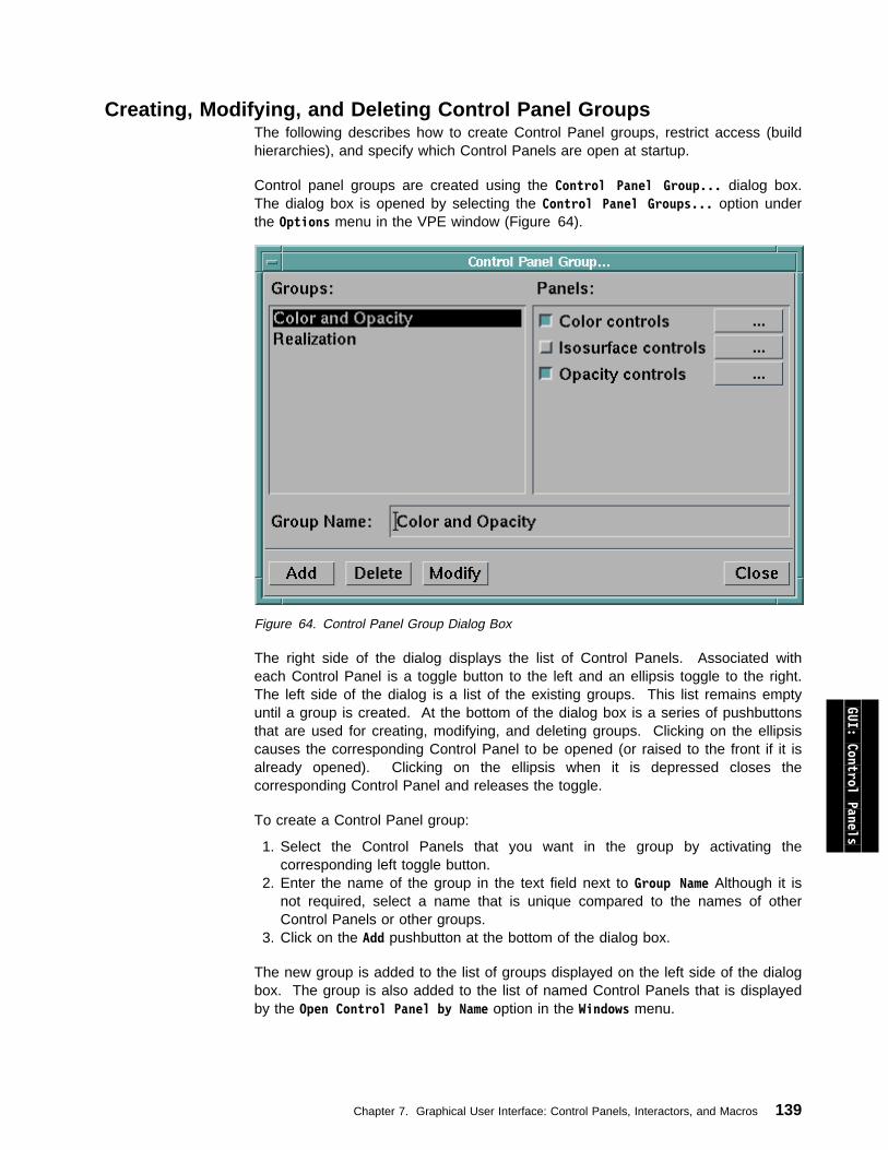
Creating, Modifying, and Deleting Control Panel GroupsThe following describes how to create Control Panel groups, restrict access (buildhierarchies), and specify which Control Panels are open at startup.

Control panel groups are created using the Control Panel Group... dialog box.The dialog box is opened by selecting the Control Panel Groups... option underthe Options menu in the VPE window (Figure 64).

Figure 64. Control Panel Group Dialog Box

The right side of the dialog displays the list of Control Panels. Associated witheach Control Panel is a toggle button to the left and an ellipsis toggle to the right.The left side of the dialog is a list of the existing groups. This list remains emptyuntil a group is created. At the bottom of the dialog box is a series of pushbuttonsthat are used for creating, modifying, and deleting groups. Clicking on the ellipsiscauses the corresponding Control Panel to be opened (or raised to the front if it isalready opened). Clicking on the ellipsis when it is depressed closes thecorresponding Control Panel and releases the toggle.

To create a Control Panel group:

1. Select the Control Panels that you want in the group by activating thecorresponding left toggle button.

2. Enter the name of the group in the text field next to Group Name Although it isnot required, select a name that is unique compared to the names of otherControl Panels or other groups.

3. Click on the Add pushbutton at the bottom of the dialog box.

The new group is added to the list of groups displayed on the left side of the dialogbox. The group is also added to the list of named Control Panels that is displayedby the Open Control Panel by Name option in the Windows menu.

GUI: Control Panels

Chapter 7. Graphical User Interface: Control Panels, Interactors, and Macros 139

Once a Control Panel group is created, it can be modified. Modifying a ControlPanel group can include changing its name, adding new Control Panels, andremoving Control Panels from the group.

To modify a Control Panel group:

1. Click on the Control Panel group name that is to be modified. This causes thename of the Control Panel group to be displayed in the group name text fieldand causes the toggle buttons of the Control Panels that are members of thegroup to be activated. All other Control Panel buttons are released.

2. You may now change the name of the group by editing the text field. Add anew Control Panel by clicking on its toggle button (this causes the toggle buttonto be activated). To remove a Control Panel from the group, click on its togglebutton to release it.

3. Once you have made the desired changes to the Control Panel group, click onthe Modify button at the bottom of the dialog box. This causes the change totake effect.

To delete a Control Panel group:

1. Select the group by clicking on its name.2. Click on the Delete button at the bottom of the dialog box.

Restricting Control Panel AccessAccess to Control Panels is restricted using the Control Panel Access... dialogbox. This dialog box is opened by selecting the Control Panel Access in theOption menu of the VPE, Image, or Control Panel windows. The Control PanelAccess dialog is used to restrict certain Control Panel names or Control Panelgroups names from appearing in the Open Control Panel by Name option in theWindows window.

A Control Panel Access dialog box appears in Figure 65.

Figure 65. Control Panel Access Dialog Box

140 IBM Visualization Data Explorer: User’s Guide

Each Control Panel and Control Panel group is listed. To the left of each is atoggle button. This toggle button is used to select which Control Panels or groupscan be accessed from the window in which the dialog box was opened. To theright of the Control Panel names is an ellipsis toggle. (Note that Control Panelgroups do not have the ellipsis.) The ellipsis toggle is used to open (or raise) thecorresponding Control Panel when the button is activated. Once activated,selecting the button again closes the Control Panel and pops up the button.

To restrict Control Panel access:

1. Click on each Control Panel access toggle button that you wish to exclude sothat those toggle buttons are deactivated. (Initially, all the toggle buttons areactivated.)

2. Once you have indicated which Control Panels and Control Panel groups youwish to exclude, click on OK.

Selecting the Cancel pushbutton causes the dialog box to be closed and anychanges to be canceled.

Specifying a Startup Control PanelData Explorer allows you to choose whether a Control Panel opens automaticallywhen you start the system with the Image window or menu bar as the anchor(using the -image or -menubar option). Using this option, you can have theappropriate Control Panels be immediately available to a user running your visualprogram. The Startup Control Panel option in the Options pull-down menu is atoggle button, and is toggled on by default. If you do not want a particular ControlPanel to open automatically, toggle the option off by clicking on it in that ControlPanel.

The automatic startup feature can be suppressed by using the -suppress startupflag when you run Data Explorer. See C.2, “Command Line Options” on page 295for more information.

Opening Existing Control Panels GUI: Control Panels

You can open existing Control Panels associated with a visual program in thefollowing ways:

Select the Open All Control Panels option from the Windows menu in the VPEor Image window, or from the Panels menu in an already open Control Panel.

Select the Open Control Panel by Name option from the Windows menu in theVPE or Image window, or from the Panels menu in an already open ControlPanel. From the list of Control Panel names, click on the one you want toopen. (If there are no accessible Control Panels, no names are displayed.)

Double-click on the interactor stand-in in the VPE whose Control Panel youwant to open. All Control Panels that contain that interactor are opened. If theselected interactor does not currently have a Control Panel, Data Explorercreates one for it.

Alternatively, you can select one or more interactor stand-ins in the VPE, thenchoose Open Control Panel from the Windows menu in the VPE. All ControlPanels associated with the selected interactors are opened.

When Data Explorer is started with the Image window or menu bar as the anchorwindow, some Control Panels may be opened automatically as a visual program is

Chapter 7. Graphical User Interface: Control Panels, Interactors, and Macros 141

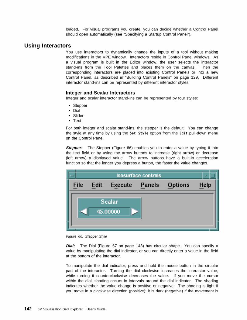
loaded. For visual programs you create, you can decide whether a Control Panelshould open automatically (see “Specifying a Startup Control Panel”).

Using InteractorsYou use interactors to dynamically change the inputs of a tool without makingmodifications in the VPE window. Interactors reside in Control Panel windows. Asa visual program is built in the Editor window, the user selects the interactorstand-ins from the Tool Palettes and places them on the canvas. Then thecorresponding interactors are placed into existing Control Panels or into a newControl Panel, as described in “Building Control Panels” on page 129. Differentinteractor stand-ins can be represented by different interactor styles.

Integer and Scalar InteractorsInteger and scalar interactor stand-ins can be represented by four styles:

Stepper Dial Slider Text

For both integer and scalar stand-ins, the stepper is the default. You can changethe style at any time by using the Set Style option from the Edit pull-down menuon the Control Panel.

Stepper: The Stepper (Figure 66) enables you to enter a value by typing it intothe text field or by using the arrow buttons to increase (right arrow) or decrease(left arrow) a displayed value. The arrow buttons have a built-in accelerationfunction so that the longer you depress a button, the faster the value changes.

Figure 66. Stepper Style

Dial: The Dial (Figure 67 on page 143) has circular shape. You can specify avalue by manipulating the dial indicator, or you can directly enter a value in the fieldat the bottom of the interactor.

To manipulate the dial indicator, press and hold the mouse button in the circularpart of the interactor. Turning the dial clockwise increases the interactor value,while turning it counterclockwise decreases the value. If you move the cursorwithin the dial, shading occurs in intervals around the dial indicator. The shadingindicates whether the value change is positive or negative. The shading is light ifyou move in a clockwise direction (positive); it is dark (negative) if the movement is

142 IBM Visualization Data Explorer: User’s Guide

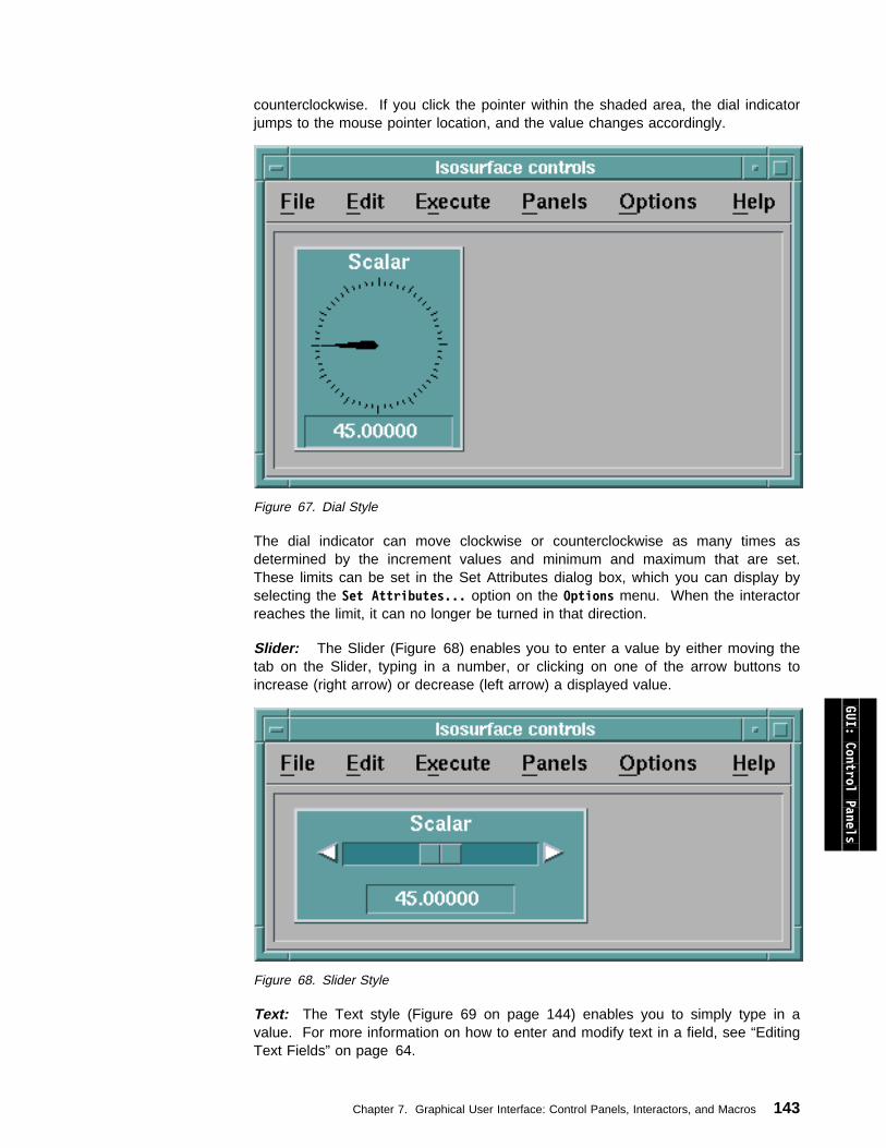
counterclockwise. If you click the pointer within the shaded area, the dial indicatorjumps to the mouse pointer location, and the value changes accordingly.

Figure 67. Dial Style

The dial indicator can move clockwise or counterclockwise as many times asdetermined by the increment values and minimum and maximum that are set.These limits can be set in the Set Attributes dialog box, which you can display byselecting the Set Attributes... option on the Options menu. When the interactorreaches the limit, it can no longer be turned in that direction.

Slider: The Slider (Figure 68) enables you to enter a value by either moving thetab on the Slider, typing in a number, or clicking on one of the arrow buttons toincrease (right arrow) or decrease (left arrow) a displayed value.

GUI: Control Panels

Figure 68. Slider Style

Text: The Text style (Figure 69 on page 144) enables you to simply type in avalue. For more information on how to enter and modify text in a field, see “EditingText Fields” on page 64.

Chapter 7. Graphical User Interface: Control Panels, Interactors, and Macros 143

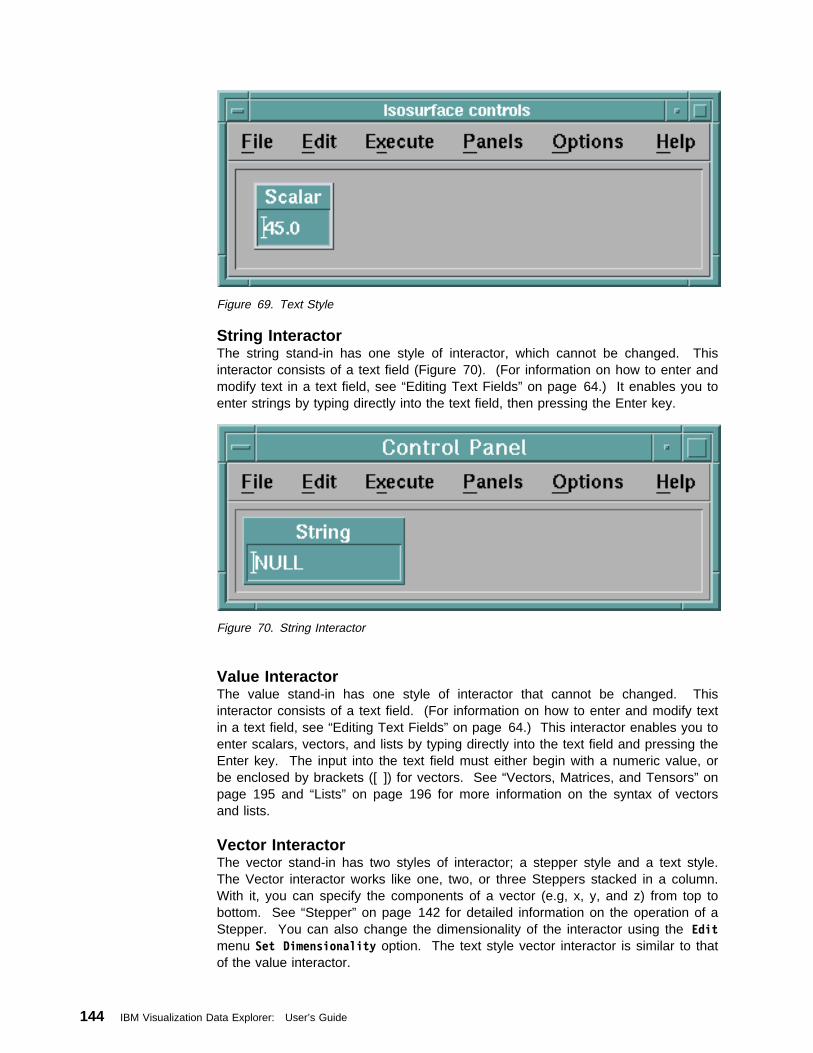
Figure 69. Text Style

String InteractorThe string stand-in has one style of interactor, which cannot be changed. Thisinteractor consists of a text field (Figure 70). (For information on how to enter andmodify text in a text field, see “Editing Text Fields” on page 64.) It enables you toenter strings by typing directly into the text field, then pressing the Enter key.

Figure 70. String Interactor

Value InteractorThe value stand-in has one style of interactor that cannot be changed. Thisinteractor consists of a text field. (For information on how to enter and modify textin a text field, see “Editing Text Fields” on page 64.) This interactor enables you toenter scalars, vectors, and lists by typing directly into the text field and pressing theEnter key. The input into the text field must either begin with a numeric value, orbe enclosed by brackets ([ ]) for vectors. See “Vectors, Matrices, and Tensors” onpage 195 and “Lists” on page 196 for more information on the syntax of vectorsand lists.

Vector InteractorThe vector stand-in has two styles of interactor; a stepper style and a text style.The Vector interactor works like one, two, or three Steppers stacked in a column.With it, you can specify the components of a vector (e.g, x, y, and z) from top tobottom. See “Stepper” on page 142 for detailed information on the operation of aStepper. You can also change the dimensionality of the interactor using the Editmenu Set Dimensionality option. The text style vector interactor is similar to thatof the value interactor.

144 IBM Visualization Data Explorer: User’s Guide

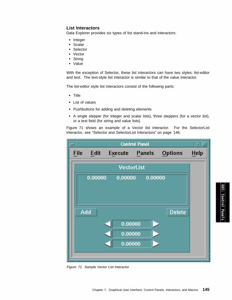
List InteractorsData Explorer provides six types of list stand-ins and interactors:

Integer Scalar Selector Vector String Value

With the exception of Selector, these list interactors can have two styles: list-editorand text. The text-style list interactor is similar to that of the value interactor.

The list-editor style list interactors consist of the following parts:

Title

List of values

Pushbuttons for adding and deleting elements

A single stepper (for integer and scalar lists), three steppers (for a vector list),or a text field (for string and value lists).

Figure 71 shows an example of a Vector list interactor. For the SelectorListinteractor, see “Selector and SelectorList Interactors” on page 146.

Figure 71. Sample Vector List Interactor

GUI: Control Panels

Chapter 7. Graphical User Interface: Control Panels, Interactors, and Macros 145

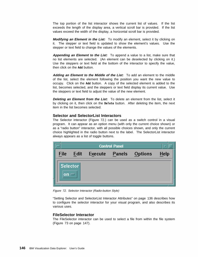
The top portion of the list interactor shows the current list of values. If the listexceeds the length of the display area, a vertical scroll bar is provided. If the listvalues exceed the width of the display, a horizontal scroll bar is provided.

Modifying an Element in the List: To modify an element, select it by clicking onit. The stepper or text field is updated to show the element’s values. Use thestepper or text field to change the values of the elements.

Appending an Element to the List: To append a value to a list, make sure thatno list elements are selected. (An element can be deselected by clicking on it.)Use the steppers or text field at the bottom of the interactor to specify the value,then click on the Add button.

Adding an Element to the Middle of the List: To add an element to the middleof the list, select the element following the position you want the new value tooccupy. Click on the Add button. A copy of the selected element is added to thelist, becomes selected, and the steppers or text field display its current value. Usethe steppers or text field to adjust the value of the new element.

Deleting an Element from the List: To delete an element from the list, select itby clicking on it, then click on the Delete button. After deleting the item, the nextitem in the list becomes selected.

Selector and SelectorList InteractorsThe Selector interactor (Figure 72.) can be used as a switch control in a visualprogram. It can appear as an option menu (with only the current choice shown) oras a “radio button” interactor, with all possible choices shown, and only the currentchoice highlighted in the radio button next to the label. The SelectorList interactoralways appears as a list of toggle buttons.

Figure 72. Selector Interactor (Radio-button Style)

“Setting Selector and SelectorList Interactor Attributes” on page 136 describes howto configure the selector interactor for your visual program, and also describes itsvarious uses.

FileSelector InteractorThe FileSelector interactor can be used to select a file from within the file system(Figure 73 on page 147).

146 IBM Visualization Data Explorer: User’s Guide

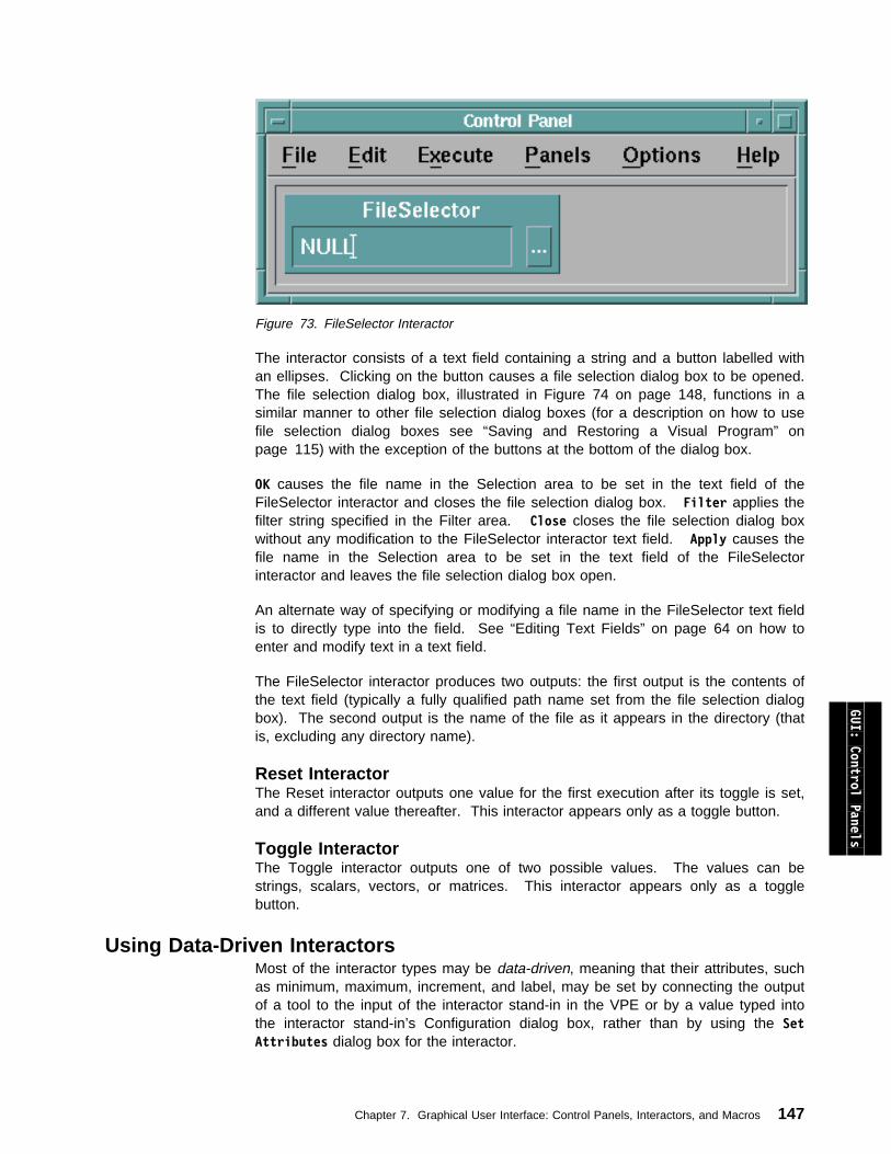
Figure 73. FileSelector Interactor

The interactor consists of a text field containing a string and a button labelled withan ellipses. Clicking on the button causes a file selection dialog box to be opened.The file selection dialog box, illustrated in Figure 74 on page 148, functions in asimilar manner to other file selection dialog boxes (for a description on how to usefile selection dialog boxes see “Saving and Restoring a Visual Program” onpage 115) with the exception of the buttons at the bottom of the dialog box.

OK causes the file name in the Selection area to be set in the text field of theFileSelector interactor and closes the file selection dialog box. Filter applies thefilter string specified in the Filter area. Close closes the file selection dialog boxwithout any modification to the FileSelector interactor text field. Apply causes thefile name in the Selection area to be set in the text field of the FileSelectorinteractor and leaves the file selection dialog box open.

An alternate way of specifying or modifying a file name in the FileSelector text fieldis to directly type into the field. See “Editing Text Fields” on page 64 on how toenter and modify text in a text field.

The FileSelector interactor produces two outputs: the first output is the contents ofthe text field (typically a fully qualified path name set from the file selection dialogbox). The second output is the name of the file as it appears in the directory (thatis, excluding any directory name).

GUI: Control Panels

Reset InteractorThe Reset interactor outputs one value for the first execution after its toggle is set,and a different value thereafter. This interactor appears only as a toggle button.

Toggle InteractorThe Toggle interactor outputs one of two possible values. The values can bestrings, scalars, vectors, or matrices. This interactor appears only as a togglebutton.

Using Data-Driven InteractorsMost of the interactor types may be data-driven, meaning that their attributes, suchas minimum, maximum, increment, and label, may be set by connecting the outputof a tool to the input of the interactor stand-in in the VPE or by a value typed intothe interactor stand-in’s Configuration dialog box, rather than by using the SetAttributes dialog box for the interactor.

Chapter 7. Graphical User Interface: Control Panels, Interactors, and Macros 147

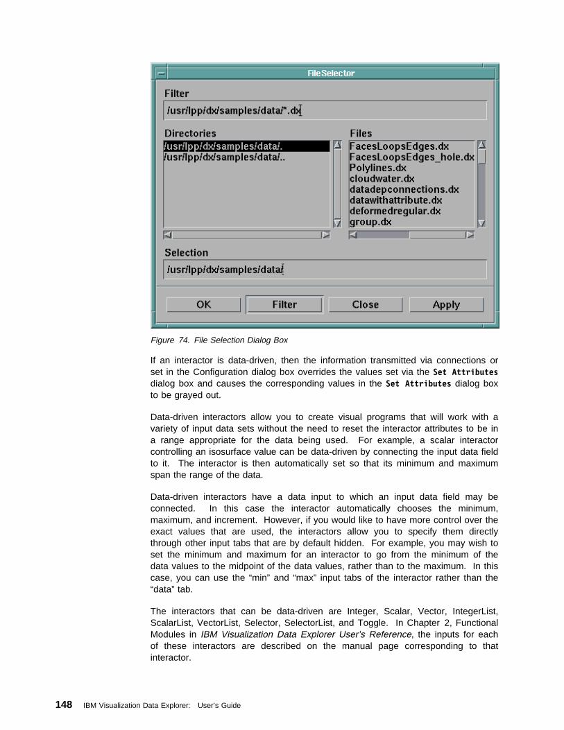
Figure 74. File Selection Dialog Box

If an interactor is data-driven, then the information transmitted via connections orset in the Configuration dialog box overrides the values set via the Set Attributesdialog box and causes the corresponding values in the Set Attributes dialog boxto be grayed out.

Data-driven interactors allow you to create visual programs that will work with avariety of input data sets without the need to reset the interactor attributes to be ina range appropriate for the data being used. For example, a scalar interactorcontrolling an isosurface value can be data-driven by connecting the input data fieldto it. The interactor is then automatically set so that its minimum and maximumspan the range of the data.

Data-driven interactors have a data input to which an input data field may beconnected. In this case the interactor automatically chooses the minimum,maximum, and increment. However, if you would like to have more control over theexact values that are used, the interactors allow you to specify them directlythrough other input tabs that are by default hidden. For example, you may wish toset the minimum and maximum for an interactor to go from the minimum of thedata values to the midpoint of the data values, rather than to the maximum. In thiscase, you can use the “min” and “max” input tabs of the interactor rather than the“data” tab.

The interactors that can be data-driven are Integer, Scalar, Vector, IntegerList,ScalarList, VectorList, Selector, SelectorList, and Toggle. In Chapter 2, FunctionalModules in IBM Visualization Data Explorer User’s Reference, the inputs for eachof these interactors are described on the manual page corresponding to thatinteractor.

148 IBM Visualization Data Explorer: User’s Guide

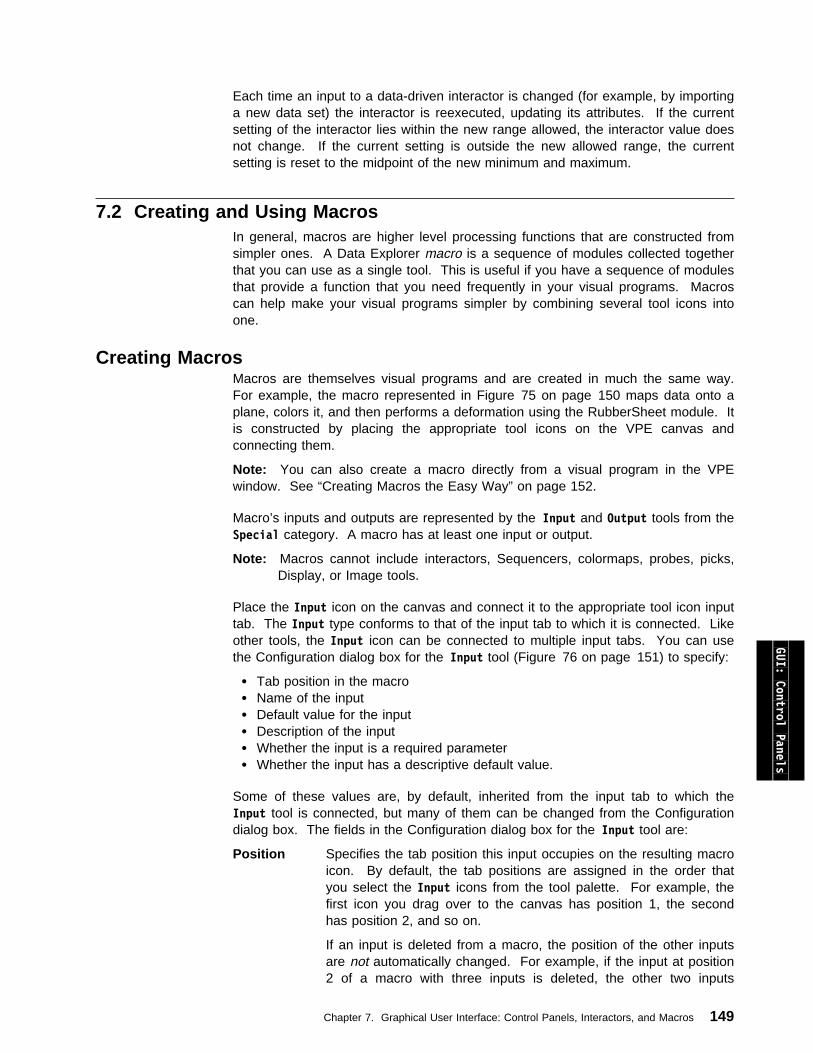
Each time an input to a data-driven interactor is changed (for example, by importinga new data set) the interactor is reexecuted, updating its attributes. If the currentsetting of the interactor lies within the new range allowed, the interactor value doesnot change. If the current setting is outside the new allowed range, the currentsetting is reset to the midpoint of the new minimum and maximum.

7.2 Creating and Using MacrosIn general, macros are higher level processing functions that are constructed fromsimpler ones. A Data Explorer macro is a sequence of modules collected togetherthat you can use as a single tool. This is useful if you have a sequence of modulesthat provide a function that you need frequently in your visual programs. Macroscan help make your visual programs simpler by combining several tool icons intoone.

Creating MacrosMacros are themselves visual programs and are created in much the same way.For example, the macro represented in Figure 75 on page 150 maps data onto aplane, colors it, and then performs a deformation using the RubberSheet module. Itis constructed by placing the appropriate tool icons on the VPE canvas andconnecting them.

Note: You can also create a macro directly from a visual program in the VPEwindow. See “Creating Macros the Easy Way” on page 152.

Macro’s inputs and outputs are represented by the Input and Output tools from theSpecial category. A macro has at least one input or output.

Note: Macros cannot include interactors, Sequencers, colormaps, probes, picks,Display, or Image tools.

Place the Input icon on the canvas and connect it to the appropriate tool icon inputtab. The Input type conforms to that of the input tab to which it is connected. Likeother tools, the Input icon can be connected to multiple input tabs. You can usethe Configuration dialog box for the Input tool (Figure 76 on page 151) to specify:

Tab position in the macro Name of the input Default value for the input Description of the input Whether the input is a required parameter Whether the input has a descriptive default value.

Some of these values are, by default, inherited from the input tab to which theInput tool is connected, but many of them can be changed from the Configurationdialog box. The fields in the Configuration dialog box for the Input tool are:

Position Specifies the tab position this input occupies on the resulting macroicon. By default, the tab positions are assigned in the order thatyou select the Input icons from the tool palette. For example, thefirst icon you drag over to the canvas has position 1, the secondhas position 2, and so on.

If an input is deleted from a macro, the position of the other inputsare not automatically changed. For example, if the input at position2 of a macro with three inputs is deleted, the other two inputs

GUI: Control Panels

Chapter 7. Graphical User Interface: Control Panels, Interactors, and Macros 149

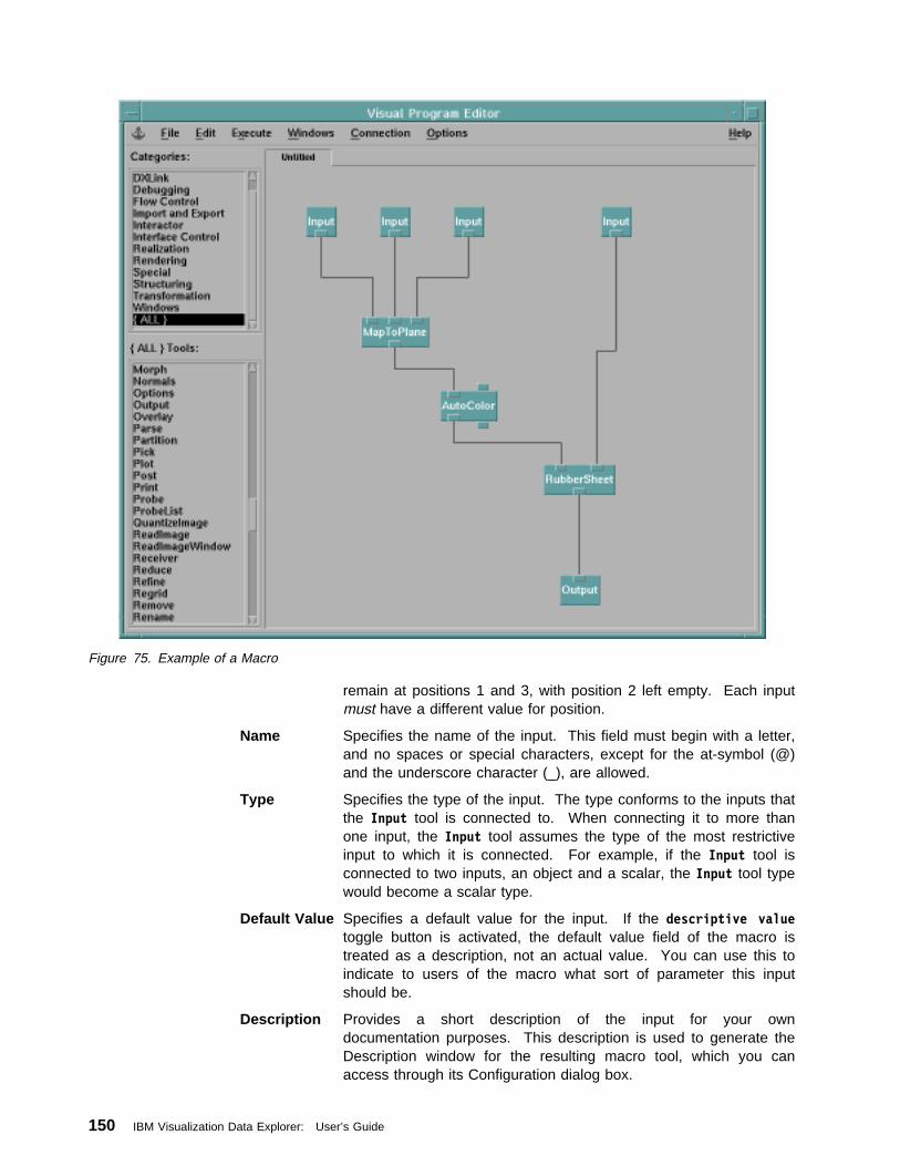
Figure 75. Example of a Macro

remain at positions 1 and 3, with position 2 left empty. Each inputmust have a different value for position.

Name Specifies the name of the input. This field must begin with a letter,and no spaces or special characters, except for the at-symbol (@)and the underscore character (_), are allowed.

Type Specifies the type of the input. The type conforms to the inputs thatthe Input tool is connected to. When connecting it to more thanone input, the Input tool assumes the type of the most restrictiveinput to which it is connected. For example, if the Input tool isconnected to two inputs, an object and a scalar, the Input tool typewould become a scalar type.

Default Value Specifies a default value for the input. If the descriptive valuetoggle button is activated, the default value field of the macro istreated as a description, not an actual value. You can use this toindicate to users of the macro what sort of parameter this inputshould be.

Description Provides a short description of the input for your owndocumentation purposes. This description is used to generate theDescription window for the resulting macro tool, which you canaccess through its Configuration dialog box.

150 IBM Visualization Data Explorer: User’s Guide

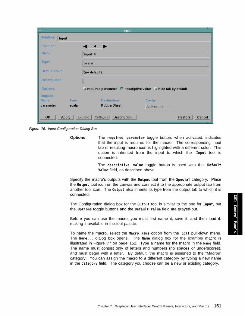
Figure 76. Input Configuration Dialog Box

Options The required parameter toggle button, when activated, indicatesthat the input is required for the macro. The corresponding inputtab of resulting macro icon is highlighted with a different color. Thisoption is inherited from the input to which the Input tool isconnected.

The descriptive value toggle button is used with the DefaultValue field, as described above.

Specify the macro’s outputs with the Output tool from the Special category. Placethe Output tool icon on the canvas and connect it to the appropriate output tab fromanother tool icon. The Output also inherits its type from the output tab to which it isconnected.

The Configuration dialog box for the Output tool is similar to the one for Input, butthe Options toggle buttons and the Default Value field are grayed-out.

Before you can use the macro, you must first name it, save it, and then load it,making it available in the tool palette.

To name the macro, select the Macro Name option from the Edit pull-down menu.The Name... dialog box opens. The Name dialog box for the example macro isillustrated in Figure 77 on page 152. Type a name for the macro in the Name field.The name must consist only of letters and numbers (no spaces or underscores),and must begin with a letter. By default, the macro is assigned to the “Macros”category. You can assign the macro to a different category by typing a new namein the Category field. The category you choose can be a new or existing category.

GUI: Control Panels

Chapter 7. Graphical User Interface: Control Panels, Interactors, and Macros 151

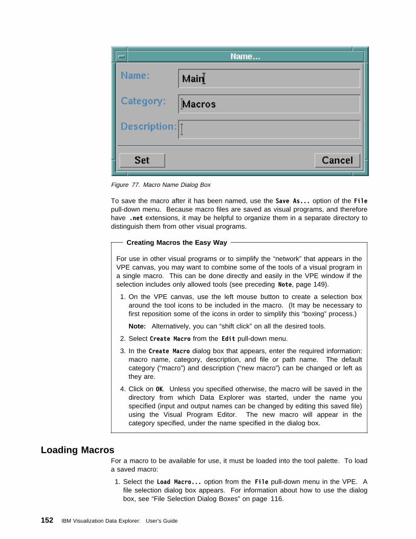
Figure 77. Macro Name Dialog Box

To save the macro after it has been named, use the Save As... option of the Filepull-down menu. Because macro files are saved as visual programs, and thereforehave .net extensions, it may be helpful to organize them in a separate directory todistinguish them from other visual programs.

Creating Macros the Easy Way

For use in other visual programs or to simplify the “network” that appears in theVPE canvas, you may want to combine some of the tools of a visual program ina single macro. This can be done directly and easily in the VPE window if theselection includes only allowed tools (see preceding Note, page 149).

1. On the VPE canvas, use the left mouse button to create a selection boxaround the tool icons to be included in the macro. (It may be necessary tofirst reposition some of the icons in order to simplify this “boxing” process.)

Note: Alternatively, you can “shift click” on all the desired tools.

2. Select Create Macro from the Edit pull-down menu.

3. In the Create Macro dialog box that appears, enter the required information:macro name, category, description, and file or path name. The defaultcategory (“macro”) and description (“new macro”) can be changed or left asthey are.

4. Click on OK. Unless you specified otherwise, the macro will be saved in thedirectory from which Data Explorer was started, under the name youspecified (input and output names can be changed by editing this saved file)using the Visual Program Editor. The new macro will appear in thecategory specified, under the name specified in the dialog box.

Loading MacrosFor a macro to be available for use, it must be loaded into the tool palette. To loada saved macro:

1. Select the Load Macro... option from the File pull-down menu in the VPE. Afile selection dialog box appears. For information about how to use the dialogbox, see “File Selection Dialog Boxes” on page 116.

152 IBM Visualization Data Explorer: User’s Guide

2. Use the dialog box to locate the macro you want to load, and select the desiredfile. The macro name appears on the tool palette under its assigned category.

3. You can also load all the macros in a selected directory by clicking on Load AllMacros in the dialog box.

Note: If the macro you loaded has the same name as a macro previouslyloaded, the “new” macro replaces the earlier one, whether or not theywere assigned to the same category.

When the new macro is available for use, it is listed in the tool palette as a memberof the category you assigned it to. For example, the MapAndDeform macro wouldbe listed under the MyMacros category.

When you save a visual program which uses a macro, the path to the macro issaved in the visual program. When you reload the visual program, the macro willautomatically be loaded for you from the same location, so it will only be necessaryto explicitly load the macro if it has been moved to a new location. You can alsoeasily see what macros need to be included with a visual program, if for example,you are sending a visualization program to another user. Simply look at the top ofthe .net file for the list of referenced macros.

You can configure Data Explorer to automatically load macros from a specifieddirectory when you begin the Data Explorer program. To do this, use the -macrospathlist option when starting Data Explorer, where pathlist specifies one or morepaths where the macros can be found. Alternatively, you can use the DXMACROSenvironment variable. For more information on how to do this, see “UsingEnvironment Variables” on page 59, and C.1, “Environment Variables” onpage 292.

Using Macros in a Visual ProgramAfter you have created and loaded a macro, you can use it the same way you useother Data Explorer tools. Simply select it from the tool palette and place the iconon the canvas. Figure 78 on page 154 shows the new icon created for theMapAndDeform macro.

GUI: Control Panels

Chapter 7. Graphical User Interface: Control Panels, Interactors, and Macros 153

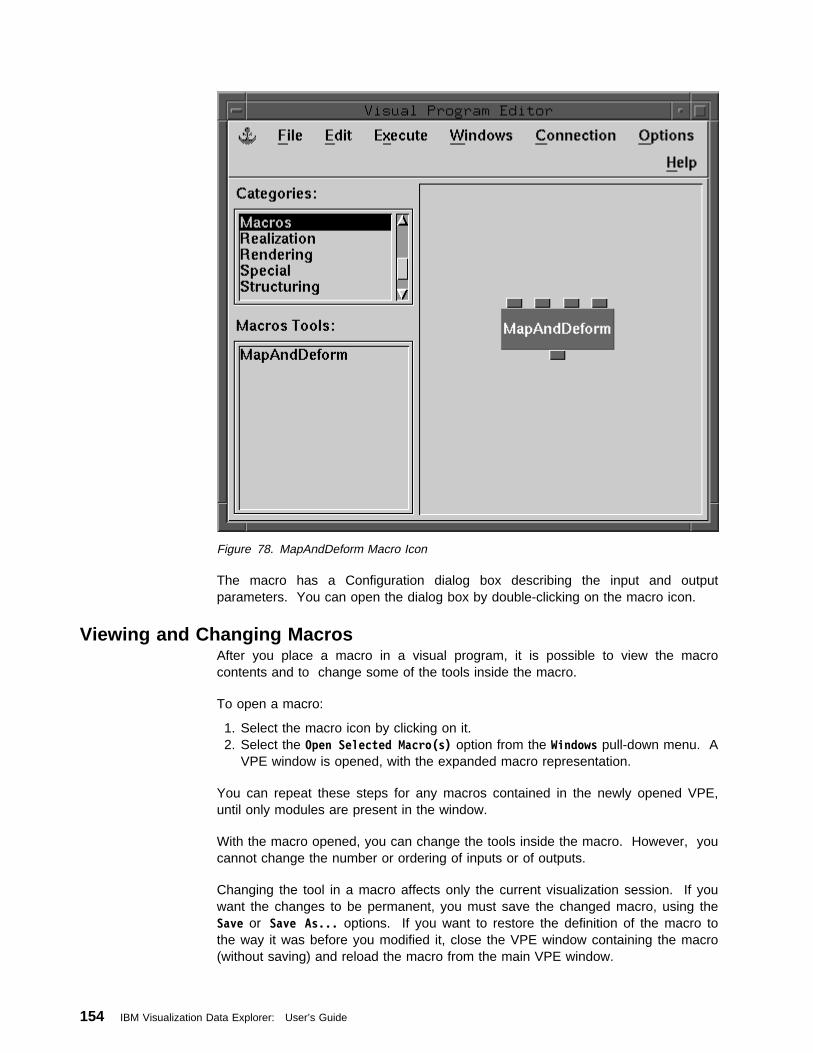
Figure 78. MapAndDeform Macro Icon

The macro has a Configuration dialog box describing the input and outputparameters. You can open the dialog box by double-clicking on the macro icon.

Viewing and Changing MacrosAfter you place a macro in a visual program, it is possible to view the macrocontents and to change some of the tools inside the macro.

To open a macro:

1. Select the macro icon by clicking on it.2. Select the Open Selected Macro(s) option from the Windows pull-down menu. A

VPE window is opened, with the expanded macro representation.

You can repeat these steps for any macros contained in the newly opened VPE,until only modules are present in the window.

With the macro opened, you can change the tools inside the macro. However, youcannot change the number or ordering of inputs or of outputs.

Changing the tool in a macro affects only the current visualization session. If youwant the changes to be permanent, you must save the changed macro, using theSave or Save As... options. If you want to restore the definition of the macro tothe way it was before you modified it, close the VPE window containing the macro(without saving) and reload the macro from the main VPE window.

154 IBM Visualization Data Explorer: User’s Guide

Chapter 8. Graphical User Interface: Menus, Options, and theMessage Window

8.1 Using the Primary Window Pull-Down Menus and Options . . . . . . . . 156VPE Window Menu Bar . . . . . . . . . . . . . . . . . . . . . . . . . . . . . 156Control Panel Menu Bar . . . . . . . . . . . . . . . . . . . . . . . . . . . . . 162Image Window Menu Bar . . . . . . . . . . . . . . . . . . . . . . . . . . . . 165Colormap Menu Bar . . . . . . . . . . . . . . . . . . . . . . . . . . . . . . . 168Menu Bar Menu Bar . . . . . . . . . . . . . . . . . . . . . . . . . . . . . . . 170Message Window Menu Bar . . . . . . . . . . . . . . . . . . . . . . . . . . . 172

8.2 Using the Message Window . . . . . . . . . . . . . . . . . . . . . . . . . . 174

GUI: Menus

Copyright IBM Corp. 1991-1997 155

8.1 Using the Primary Window Pull-Down Menus and OptionsThis section provides illustrations of the primary windows with explanations of thepull-down menu options on their menu bars. The discussions include:

“VPE Window Menu Bar” “Control Panel Menu Bar” on page 162 “Image Window Menu Bar” on page 165 “Colormap Menu Bar” on page 168 “Menu Bar Menu Bar” on page 170 “Message Window Menu Bar” on page 172

The Sequencer and Help primary windows have no pull-down options, so they arenot discussed here. See “Using the Sequencer” on page 68 for information aboutthe Sequencer, and 5.3, “Using Online Help” on page 65 for information on theHelp window and Help menu options.

VPE Window Menu BarThe menu bar displays the titles of seven menus:

File Edit Execute Windows Connection Options Help.

The following sections describe the menus and their options. For many of themenu options, one or more tools on the canvas must be selected in order for theoption to be applied. If a menu option is grayed out, it is unavailable and cannot beselected.

VPE File MenuThe File menu displays the options you can use to create new programs, view oredit previously created programs, load macros, and save programs. You musthave write permission for a file to save changes directly to that file.

The following options appear on the File menu:

New Initializes the VPE for a new program and clears the canvas. If youhave opened Control Panels and Image windows from the VPE, theyare closed. If a program you changed but did not save currently existson the canvas, a dialog box appears so you can save changes. If youopened the VPE using Open Macro or Open Visual Program Editor, thisoption is grayed out.

Open Program...Opens an existing visual program. A dialog box appears for you tospecify the desired program name. If a program you changed but didnot save currently exists on the canvas, a dialog box appears asking ifyou want to save changes. If you opened the VPE using Open Macro,this option is grayed out. See “File Selection Dialog Boxes” onpage 116 for more information.

156 IBM Visualization Data Explorer: User’s Guide

Save ProgramSaves the current visual program, and associated Control Panels. Thisoption saves the following files: filename.net (for network; that is, aData Explorer visual program); filename.cfg (for configuration).

Save Program As...Saves the current visual program and all associated Control Panelsunder a name you type into the dialog box. This option saves thefollowing files: filename.net (for network; that is, a Data Explorer visualprogram), filename.cfg (for configuration).

Program SettingsBrings up a cascade menu with two choices:

Save As saves the current settings for the visual program (e.g.,window placement, interaction mode, camera viewpoint, interactorsetup, etc. The settings are saved in a .cfg file.

Load loads previously saved settings from a .cfg file.

Load Macro...Loads a macro and makes it available in a tools palette. A file selectiondialog box appears for you to specify the desired macro file name. Seealso “Loading Macros” on page 152

Load Module Definition(s)...Loads a module definition and makes it available in a tool palette. A fileselection dialog box appears for you to specify the desired module filename. The executable you are using must either include this module, orthis module definition must refer to an outboard or run-time loadablemodule. See 9.2, “Loading and Using Outboard and Runtime-LoadableModules” on page 183.

Print Program...Prints or saves to a file a representation of a visual program.

If the Label Set Input toggle button is activated, then any parametervalue(s) set in the configuration module’s Configuration dialog box willalso be printed next to the corresponding tab(s), if scale allows.

Quit or CloseCloses all windows created from the current VPE window. If you havemade changes since the last save, a dialog box appears so you cansave changes. If you opened the VPE from the Image window or withthe Open Macro option, Close appears as an option instead of Quit.Quit is grayed out if the Execute menu title is highlighted. You mustselect the End Execution option in the Execute pull-down menu; or if theSequencer is running, you must stop it or pause before quitting.

GUI: Menus

VPE Edit MenuThe Edit menu lists options for manipulating tools on the canvas.

Configuration...Displays a Configuration dialog box for setting and changing the valuesof the selected tool. See “Entering Values in a Configuration DialogBox” on page 107.

Find tool...Opens a dialog box that lists the tools in the visual network displayed onthe canvas. Double-click on the tool name (or type the name in the

Chapter 8. Graphical User Interface: Menus, Options, and the Message Window 157

Selection field) to highlight the corresponding icon in the canvas. If theicon falls outside the canvas, the canvas will automatically scroll todisplay the part of the network in which it lies.

See “Locating Tools: The Find Tool Dialog Box” on page 111.

Input/Output TabsBrings up a cascade menu with the following options:

Add Input Tab Adds input tabs to the selected tool.

Remove Input Tab Removes input tabs from the selected tool.

Add Output Tab Adds output tabs to the selected tool.

Remove Output TabRemoves output tabs from the selected tool.

Reveal All Tabs Reveals all tabs of the selected tool.

Hide All Tabs Hides all unconnected tabs of the selected tool.

Assign Get/Set ScopeBrings up a cascade menu with the following options:

Convert All ModulesBrings up a dialog which allows you tointeractively change all of the Get and Set tools inyour visual program to either the Local or Globalvariety.

Set Selected Gets/Sets LocalSets all of the selected Get and Set modules tothe Local variety

Set Selected Gets/Sets GlobalSets all of the selected Get and Set modules tothe Global variety

For additional information on the Get/Set tools see 4.6, “PreservingExplicit State” on page 45.

Select/Deselect ToolsBrings up a cascade menu with the following options:

Select All Selects all tools on the canvas.

Select Connected Selects all tools connected to the currentlyselected tool.

Select UnconnectedSelects all tools not connected to the currentlyselected tool.

Select Upward Selects all tools (modules) that directly orindirectly provide input to the selected tool.

Select Downward Selects all tools (modules) that directly orindirectly accept output from the currently selectedtool.

Deselect All Deselects all selected tools.

Select Unselected Selects all unselected tools.

158 IBM Visualization Data Explorer: User’s Guide

Output CacheabilityBrings up a cascade menu with the following options:

Optimize CacheabilityUses a heuristic for automatically selecting theoptimal cache setting for each module in a visualprogram.

Set Output CacheabilityBrings up a cascade menu with the followingoptions:

Cache All Results Caches all results of theselected tool(s)

Cache Last Result Caches only the last result ofthe selected tool(s)

Cache No Results Caches no results.

Show Output CacheabilityBrings up a cascade menu with the followingoptions:

All Results Highlights all tools for which allresults are cached

Last Result Highlights all tools for which only thelast result is cached

No Results Highlights all tools for which noresults are cached

See “Cache Control: Executive” on page 215.

DeleteDeletes the selected tools and connections to other tools.

CutDeletes the selected tools but places them into a buffer so they can bepasted.

CopyCopies the selected tools and places them into a buffer so they can bepasted.

PastePastes the tools from the buffer into a selected location

Add AnnotationAdds annotation text to the canvas (see “Adding Annotation to a VisualProgram” on page 115).

Insert Visual ProgramBrings up a file selection dialog box for selecting a visual program. Theselected program will be inserted to the right of all the tools in thecurrent program.

Create MacroCreates a macro from the currently selected tools. See “CreatingMacros” on page 149 for more information.

GUI: Menus

Chapter 8. Graphical User Interface: Menus, Options, and the Message Window 159

PageBrings up a cascade menu with the following options:

Create Empty Page creates an empty pageCreate with Selected Tools

creates a new page containing the currentlyselected tools

Delete deletes the currently displayed page (availableonly if there is more than one page)

Configure brings up a dialog which allows you to specify thename of the page, specify whether or not thepage is included in PostScript output (through thePrint Program option of the File menu), andspecify the tab position of the page.

Macro Name ...Displays a Configuration dialog box for naming a visual program as amacro. See “Creating Macros” on page 149 for more information.

Execution Groups...Displays a dialog box for creating and modifying execution groups. (See9.1, “Using Distributed Computation” on page 178.)

Comment ...Displays a dialog box for documenting the function of a visual programor macro. (See “Adding Comments to a Visual Program” on page 114.)

VPE Execute MenuYou can use the Execute menu to execute the current visual program in variousways. This menu is the same as the Execute menus in control panels, the Imagewindow, the Colormap Editor, and the Message window. The options in theExecute pull-down menu are grayed out when there is no connection to the server.

The Execute menu lists the following options:

Execute OnceCauses the visual program to execute only once, using current valuesand configuration settings. Subsequent interactor value changes do notcause program reevaluation until this command is reexecuted. Thisoption is grayed out if the Sequencer is running.

Execute on ChangeCauses the visual program to execute each time a value or configurationsetting is changed. If you are changing values faster than Data Explorercan generate images, the program executes as fast as possible, alwaysusing the current settings at the time an execution cycle begins. Thisoption is grayed out if the Sequencer is running.

End ExecutionCauses the visual program to stop executing.

SequencerCauses the Sequencer to display. This option is grayed out if there isno Sequencer in the visual program. While the Sequencer is running,you can change interactors, and those changes are reflected insubsequent frames. You can pause the Sequencer on a particularframe and explore that frame using the Execute Once and Execute onChange options.

160 IBM Visualization Data Explorer: User’s Guide

“Using the Sequencer” on page 68 discusses the Sequencer in detail.

While the visual program is executing, the Execute label in the menu bar ishighlighted and remains so until execution is completed. If Execute on Change isselected, the Execute label in the menu bar is highlighted with one color duringexecution, and another color the rest of the time.

For more information, see 5.4, “Executing a Visual Program” on page 67.

VPE Windows MenuThe Windows menu allows a user to open and create control panels, openpreviously defined macros included in the visual program, open the Image window,and open the Colormap Editor.

These options appear on the Windows menu:

New Control PanelOpens a new Control Panel. If you have selected one or moreinteractor stand-ins on the VPE canvas, the new Control Panel containsthose interactors. If you have not selected anything on the canvas, thepanel is empty.

Open Selected Control Panel(s)Opens all Control Panels containing selected (highlighted) interactorstand-ins. Control Panels that are already open are unaffected.

Open All Control PanelsOpens all the Control Panels for the current visual program.

Open Control Panel by NameOpens a cascade menu with the names of the existing control panels.Using this, you can open a particular control panel.

Open Selected Macro(s)Opens a VPE window containing the expanded representation of theselected macro icon. From this newly opened window, you can openthe macros contained in the currently opened macro. You can repeatthis operation until only modules are contained in the window. See“Using Macros in a Visual Program” on page 153 for more information.This options is grayed out if no macro is selected.

Open Selected Image Window(s)Opens an Image window for each selected Display or Image tool icon inthe current visual program. This option is grayed out if no Display orImage icons are selected.

Open Selected Colormap Editor(s)Opens a window where you can map colors and opacities to datavalues, the results of which are displayed in the visual image. Thisoption is grayed out if a Colormap icon is not selected. Features of theColormap Editor allow you to:

Control the range of data values over which the mapping occurs.

Select the colors and opacities that are mapped to that range ofvalues.

The Colormap Editor is discussed in detail in 6.3, “Using the ColormapEditor” on page 119.

GUI: Menus

Chapter 8. Graphical User Interface: Menus, Options, and the Message Window 161

Open Message WindowOpens a window where you can access error and warning messagesand working information about your execution. See 8.2, “Using theMessage Window” on page 174.

VPE Connection MenuThe Connection menu lists the following options:

Start Server Connects the user workstation to the server. For moreinformation, see 9.3, “Connecting to the Server” on page 183.

Disconnect from ServerDisconnects the user workstation from the server.

Reset Server Flushes the cache, forcing the visual program to reaccess thedata on the server the next time it executes.

See “Resetting the Server” on page 185.

Execution Group Assignment...Displays a dialog box that allows you to assign execution groupsto specific machine host names.

See “Assigning Execution Groups to Workstations” on page 181.

VPE Options MenuThe Options menu allows you to customize tools and window features.

The Options menu lists the following options:

Tool PalettesToggles between displaying the tool palettes and not displaying them.You can also use the Ctrl+T accelerator key.

Control Panel Access...Allows you to specify which controls panels and control panel groupsare accessible from the VPE. (See “Control Panel Access, Groups, andHierarchies” on page 138.)

Control Panel Groups...Displays a dialog box that allows you to create, modify and deletecontrol panel groups. (See “Control Panel Access, Groups, andHierarchies” on page 138.)

Grid ... Allows you to select the grid type you want to use on the canvas. Adialog box displays the choices. See “Customizing the VPE Window” onpage 113 for more information about the Grid... option.

Help MenuThe options in this menu are discussed in 5.3, “Using Online Help” on page 65.

Control Panel Menu BarThe Control Panel menu bar (Figure 60 on page 129) displays the names of sixmenus you can use within the Control Panel window:

File Edit Execute Panels

162 IBM Visualization Data Explorer: User’s Guide

Options Help.

The following sections describe the options available on these menus.

Control Panel File MenuThe File menu lists the following options:

Close Closes the current Control Panel.

Close All Control PanelsCloses all control panels.

Control Panel Edit MenuThe Edit menu lists the options you can use to edit and delete interactors in theControl Panel.

Set Style...Allows you to change the type of selected interactors on the layout area.See “Changing the Interactor Style” on page 134.

Set Dimensionality...Allows you to set the dimensionality of the selected interactors in thelayout area. See “Changing the Interactor Dimensionality” on page 134.

Set Layout...Allows you to set the layout of the selected interactors in the layoutarea. You can specify horizontal or vertical. See “Changing theInteractor Layout” on page 134.

Set Attributes...for integer, scalar, and vector values, allows you to specify:

The minimum and maximum limits for the interactor values

The number of decimal places displayed for scalar values

The increment of change in value when using stepper, slider, dial, ortext style interactors

Whether the specified increment applies to all instances of theinteractor or is local to the current interactor.

Vector interactors allow you to modify these attributes for eachcomponent of the vector. Specify that component to modify by changingthe Component field at the top of the vector interactor’s Set Attributesdialog box.

You can also open the Set Attributes window by double clicking on theborder area of the interactor inside the Control Panel.

See “Setting Interactor Attributes” on page 134 for detailed information.

Set LabelAllows you to change the title of the interactor. See “Changing theLabel on the Interactor” on page 137.

Delete Deletes selected interactors.

Add ElementBrings up a cascade menu with the choices Label and Separator.These can then be added to the control panel. See “Control Panels asDialog Boxes” on page 138.

GUI: Menus

Chapter 8. Graphical User Interface: Menus, Options, and the Message Window 163

Add Selected Interactor(s)Adds an interactor to the Control Panel for each stand-in that is selectedin the VPE window. See “Adding Interactors to an Existing ControlPanel” on page 130.

Show Selected Interactor(s)Shows the relation between a selected interactor stand-in in the VPEand the interactors in the Control Panels. See “Locating InteractorStand-ins” on page 132.

Show Selected ToolShows the relation between a selected interactor stand-in in a controlpanel and interactor stand-ins in the VPE.

Comment...Opens a dialog box with a text field. You can use this text field todocument the use of the Control Panel. See “Adding Comments to aControl Panel” on page 133.

Control Panel Execute MenuThis execute menu is identical to that of the Visual Program Editor window. See“VPE Execute Menu” on page 160 for descriptions of the Execute options. Seealso 5.4, “Executing a Visual Program” on page 67.

Control Panel Panels MenuThe Panels menu allows you to open one or all existing control panels.

The Panels menu has the following options:

Open All Control PanelsOpens all existing control panels.

Open Control Panel by NameOpens a cascade menu, from which you can select the name of thecontrol panel to open.

Control Panel Options MenuThe Options menu allows you to customize the Control Panel.

The Options menu contains the following options:

Change Control Panel Name...Displays a dialog box where you can enter a new name for the currentControl Panel.

Control Panel Access...Allows you to specify which control panels and control panel groups areaccessible from the Control Panel’s Open All Control Panels optionunder the Windows menu. See “Restricting Control Panel Access” onpage 140.

Grid... Allows you to select the grid type you want to use on the layout area. Adialog box displays the choices. See “Customizing the VPE Window” onpage 113 for more information about the Grid... option. See“Changing the Alignment of Interactors in the Control Panel” onpage 134.

164 IBM Visualization Data Explorer: User’s Guide

Dialog StyleChanges a control panel to “dialog style” (see “Control Panels as DialogBoxes” on page 138).

Startup Control PanelAllows you to specify whether the Control Panel is opened automaticallywhen Data Explorer is started with the Image window or menu bar asthe anchor window. See “Specifying a Startup Control Panel” onpage 141.

Help MenuThe options in this menu are discussed in 5.3, “Using Online Help” on page 65.

Image Window Menu BarThe Image window menu bar displays the names of six menus:

File Execute Windows Connection Options Help.

Image Window File MenuThe File menu displays the options you use to open, save, and close visualprograms, and load macros.

The File menu lists the following options:

Open ... Displays a dialog box for specifying a file path name to load a visualprogram or, if the path name ends in a directory, to show a list of visualprograms in that directory. To select a program, click on the name.See “File Selection Dialog Boxes” on page 116 for more information.

Save ProgramSaves the current visual program and associated Control Panels. Thisoption saves the following files: filename.net (for network; that is, aData Explorer visual program) and filename.cfg (for configuration). Thisoption is grayed out unless Data Explorer was started in -image mode.

Save Program As...Saves the current visual program and all associated Control Panelsunder a name you type in the dialog box. This option saves thefollowing files: filename.net (for network; that is, a Data Explorer visualprogram) and filename.cfg (for configuration). This option is grayed outunless Data Explorer was started in -image mode.

Program SettingsBrings up a cascade menu with two choices:

Save As saves the current settings for the visual program (e.g.,window placement, interaction mode, camera viewpoint, interactorsetup, etc. The settings are saved in a .cfg file.

Load loads previously saved settings from a .cfg file.

GUI: Menus

Chapter 8. Graphical User Interface: Menus, Options, and the Message Window 165

Load Macro...Loads a macro for use, making it available in the tool palette. A fileselection dialog box appears for you to specify the desired macro filename. See “Loading Macros” on page 152.

Load Module Definition(s)...Loads a module definition for use, making it available in the tool palette.A file selection dialog box appears for you to specify the desired modulefile name. The executable you are using must also include this module.See 9.2, “Loading and Using Outboard and Runtime-Loadable Modules”on page 183.

Save Image...Displays a dialog box that allows you to save the image and specify theformat, layout, resolution, and page size of the image. See “Saving anImage” on page 94.

Print Image...Displays a dialog box that allows you to specify the format, layout,resolution, and page size of the print. See “Printing an Image” onpage 97.

Close or QuitCloses the Image window. If you opened the Image window from theVPE, Close appears is the option. If you started Data Explorer with theImage window as the anchor, Quit is the option. Quit is grayed out ifthe Execute menu title is highlighted. You must select the EndExecution option in the Execute pull-down menu; or if the Sequencer isrunning, you must stop it or pause before quitting.

Image Window Execute MenuThis execute menu is identical to that of the Visual Program Editor window. See“VPE Execute Menu” on page 160 for descriptions of the Execute options. Seealso 5.4, “Executing a Visual Program” on page 67.

Image Window Windows MenuThe Windows menu allows you to open a VPE window containing the programlayout or the Control Panels associated with the visual program. All windowscreated from this Image window become its children. Quitting the Image windowcauses all of its child windows to close. Before the window closes, a dialog boxappears to request confirmation.

The Windows menu offers the following options:

Open Visual Program EditorOpens a VPE window containing the current visual program. Thisoption is disabled if you have not loaded a visual program or if the VPEis the anchor window.

Open All Control PanelsOpens all the Control Panels and macro Control Panels for the currentvisual program unless the macro Control Panels are already containedin another Control Panel. This option is disabled if you have not loadeda visual program.

166 IBM Visualization Data Explorer: User’s Guide

Open Control Panel by NameOpens a cascade menu, from which you can select the name of thecontrol panel to open.

Open All Colormap EditorsOpens all the Colormap Editors for the current visual program.

See 6.3, “Using the Colormap Editor” on page 119.

Open Message WindowOpens the Message Window that displays error and warning informationabout your execution.

See 8.2, “Using the Message Window” on page 174.

Image Window Connection MenuThe Connection menu allows you to monitor and control communication functionsbetween the workstation and the server.

The Connection menu lists the following options:

Start Server... Connects the user workstation to the server. For moreinformation, see 9.3, “Connecting to the Server” on page 183.

Disconnect from ServerDisconnects the user workstation from the server.

Reset Server Flushes the cache, forcing the visual program to reaccess the dataon the server the next time it executes.

See “Resetting the Server” on page 185.

Execution Group Assignment...Displays a dialog box that allows you to assign execution groupsto specific machine host names.

See “Assigning Execution Groups to Workstations” on page 181.

Image Window Options MenuThe Options menu provides the following options, which are available only whenthe Image tool is used in a visual program:

View Control ...Opens a dialog box with various view control options. For moreinformation on this menu option, see “Controlling the Image: ViewControl...” on page 74.

Undo Returns to the view of the image that was displayed before the mostrecent action (effectively undoing the action). See “Restoring Images”on page 84.

Redo Restores the view of the image that was displayed before the last Undoaction. See “Restoring Images” on page 84.

Reset Resets the camera to its initial position and direction. See “RestoringImages” on page 84.

AutoAxes...Places axes around the image the next time you execute the visualprogram. See “AutoAxes...” on page 88.

GUI: Menus

Chapter 8. Graphical User Interface: Menus, Options, and the Message Window 167

Set Background Color...Sets the background color of the image. See “Set Background Color...”on page 89.

Display Rotation GlobeEnables and disables the wire-framed globe display in many of the viewcontrol options. While the toggle button is pressed in, the globe displayis enabled. See “Rotating the Object” on page 77.

Rendering Options...Displays a dialog box, allowing you to choose hardware or softwarerendering options. See “Rendering Options...” on page 91.

Image DepthSpecifies the number of bits (8, 12 or 24) per color. See “Image Depth”on page 93.

Throttle...Specifies the minimum number of seconds to display each frame. See“Changing the Rate of Frame Display: Throttle...” on page 93.

Change Image Name...Opens a dialog box in that you can specify a new title for the Imagewindow. See “Changing the Title of an Image Window” on page 93.

Control Panel Access...Allows you to specify which control panels and control panel groups areaccessible from the Image Window’s Open All Control Panels optionunder the Windows menu. See “Control Panel Access...” on page 94.

Help MenuThe options in this menu are discussed in 5.3, “Using Online Help” on page 65.

Colormap Menu BarThe Colormap menu bar displays the name of five menus you can use:

File Edit Execute Options Help.

Colormap File MenuThe Colormap File menu provides the following options:

New Replaces Colormap Editor values with default values.

Open... Opens an existing Colormap as specified in the dialog boxthat appears. If a current Colormap is on display andchanges have been made, a dialog box appears forapplying wanted changes.

Save As... Saves the current Colormap configuration as the nametyped into the dialog box that appears.

Close Closes the Colormap window.

168 IBM Visualization Data Explorer: User’s Guide

Colormap Edit MenuThe Colormap Edit menu displays the options used to edit the current color map.

The following options appear on the Edit menu:

UndoReturns an operation to its previous value. Undo retains a stack of 10operations.

CopyCopies selected control points to a buffer so that they can be pasted toanother field. See “Copying and Pasting Control Points” on page 124.

PastePastes selected control points to a different field. See “Copying andPasting Control Points” on page 124.

Use Application DefaultIf the Colormap Editor is data-driven, it is still possible to override itsdata-driven values by explicitly setting them in the Colormap Editor. TheUse Application Default option restores the data-driven values. Itgenerates a cascade menu with four suboptions:

Color (HSV) Map If a color map was provided to the color-map tab of theColormap tool, and was subsequently modified by the user(i.e, adding, moving, or deleting control points), selection ofthis suboption restores the original color map.

Opacity Map If an opacity map was provided to the opacity tab of theColormap tool, and was subsequently modified by the user(i.e, adding, moving, or deleting control points), selection ofthis suboption restores the original opacity map.

Minimum If the minimum was set either by a field passed to the datatab of the Colormap tool or by a value passed to or set forthe min parameter of Colormap, and was subsequentlymodified by the user in the Colormap Editor, this suboptionrestores the original value.

Maximum If the maximum was set either by a field passed to the datatab of the Colormap tool or by a value passed to or set forthe max parameter of Colormap, and was subsequentlymodified by the user in the Colormap Editor, this suboptionrestores the original value.

All Restores all values to their data-driven settings.Minimum & Maximum Restores both the minimum and the maximum

values of the original color map.

Add Control Points...Brings up a dialog box in which you can enter the exact numericallocation for control points to be added as the data value and as thevalue for either the Hue, Saturation, Value, or Opacity area of the colormap. See “Adding Control Points” on page 122.

Constrain HorizontalConstrains the horizontal movement of all control points in all areas ofthe Colormap. See “Moving Control Points” on page 123.

Constrain VerticalConstrains the vertical movement of all control points in all areas of thecolor map.

GUI: Menus

Chapter 8. Graphical User Interface: Menus, Options, and the Message Window 169

Generate WaveformsDisplays a dialog box that allows you to select from a menu ofwaveforms. The waveforms can be applied to the full range of hue,saturation, value or opacity or to a selected range. See “CreatingWaveforms” on page 124.

Delete Selected Control PointsDeletes selected control points in the selected area of the Colormap.

Select All Control PointsSelects all the control points in the selected area of the Colormap.

Colormap Execute MenuThis execute menu is identical to that of the Visual Program Editor window. See“VPE Execute Menu” on page 160 for descriptions of the Execute options. Seealso 5.4, “Executing a Visual Program” on page 67.

Colormap Options MenuThe Colormap Options menu displays the options used to edit the current colormap.

The Colormap Options menu lists the following options:

Set Background Style to Checkerboard (or Stripes)Changes the background bar from two vertical stripes to acheckerboard.

Note: The opacity must be less than 1 to make this pattern visible.

Axis DisplayAllows you to choose between Ticks, Histogram, and Log(Histogram).See “Axis Display” on page 124.

Number of histogram bins...Allows you to select the number of histogram bins. See “Axis Display”on page 124.

Display Control Point Data ValueAllows you to specify which control point values will be displayed. See“Display Control Point Values” on page 124

Change Colormap NameSets the name of the Colormap Editor. See “Changing the name of theColormap Editor” on page 124.

Help MenuThe options in this menu are discussed in 5.3, “Using Online Help” on page 65.

Menu Bar Menu BarA menu bar is displayed as the anchor window when the user specifies the-menubar option on the command line to Data Explorer. The menu bar displays thetitles of five menus:

File Execute Connection Windows Help.

170 IBM Visualization Data Explorer: User’s Guide

Menu Bar File MenuThe File menu lists the following options:

Open ... Displays a dialog box for specifying a file path name to load a visualprogram or, if the path name ends in a directory, to show a list of visualprograms in that directory. To select a program, click on the name.See “File Selection Dialog Boxes” on page 116 for more information.

Program SettingsBrings up a cascade menu with two choices:

Save As saves the current settings for the visual program (e.g.,window placement, interaction mode, camera viewpoint, interactorsetup, etc. The settings are saved in a .cfg file.

Load loads previously saved settings from a .cfg file.

Load Macro...Loads a macro for use, making it available in the tool palette. A fileselection dialog box appears for you to specify the desired macro filename. See “Loading Macros” on page 152.

Load Module Definition(s)...Loads a module definition for use, making it available in the tool palette.A file selection dialog box appears for you to specify the desired modulefile name. The executable you are using must also include this module.See 9.2, “Loading and Using Outboard and Runtime-Loadable Modules”on page 183.

Quit Closes the Menu Bar window

Menu Bar Execute MenuThis execute menu is identical to that of the Visual Program Editor window. See“VPE Execute Menu” on page 160 for descriptions of the Execute options. Seealso 5.4, “Executing a Visual Program” on page 67.

Menu Bar Connection MenuThe Connection menu allows you to monitor and control communication functionsbetween the workstation and the server.

The Connection menu lists the following options:

Start Server... Connects the user workstation to the server. For moreinformation, see 9.3, “Connecting to the Server” on page 183.

Disconnect from ServerDisconnects the user workstation from the server.

Reset Server Flushes the cache, forcing the visual program to reaccess the dataon the server the next time it executes.

See “Resetting the Server” on page 185.

Execution Group Assignment...Displays a dialog box that allows you to assign execution groupsto specific machine host names.

See “Assigning Execution Groups to Workstations” on page 181.

GUI: Menus

Chapter 8. Graphical User Interface: Menus, Options, and the Message Window 171

Menu Bar Windows MenuThe Windows menu allows you to open a VPE window containing the programlayout or the Control Panels associated with the visual program. All windowscreated from this Image window become its children. Quitting the Image windowcauses all of its child windows to close. Before the window closes, a dialog boxappears to request confirmation.

The Windows menu offers the following options:

Open Visual Program EditorOpens a VPE window containing the current visual program. Thisoption is disabled if you have not loaded a visual program or if the VPEis the anchor window.

Open All Control PanelsOpens all the Control Panels and macro Control Panels for the currentvisual program unless the macro Control Panels are already containedin another Control Panel. This option is disabled if you have not loadeda visual program.

Open Control Panel by NameOpens a cascade menu, from which you can select the name of thecontrol panel to open.

Open All Colormap EditorsOpens all the Colormap Editors for the current visual program.

See 6.3, “Using the Colormap Editor” on page 119.

Open Message WindowOpens the Message Window that displays error and warning informationabout your execution.

See 8.2, “Using the Message Window” on page 174.

Help MenuThe options in this menu are discussed in 5.3, “Using Online Help” on page 65.

Message Window Menu BarThe Message window menu bar displays the names of five menus:

File Edit Execute Options Help

Message Window File MenuThe Message window File menu provides the following options:

Clear Clears the Message window.

Log... Allows you to designate a file that will receive all subsequentmessages displayed in the Message window.

Save As... Saves the current contents of the Message window to the filenamed in the dialog box that appears.

Close Closes the Message window.

172 IBM Visualization Data Explorer: User’s Guide

Message Window Edit MenuThe Message window Edit menu displays the options used to edit the currentMessage window.

The following options appear on the Edit menu:

Next ErrorDisplays and highlights the next error in the Message window andhighlights the tool that reported it.

Previous ErrorDisplays and highlights the previous error in the Message window andhighlights the tool that reported it.

Message Window Execute MenuThis execute menu is identical to that of the Visual Program Editor window. See“VPE Execute Menu” on page 160 for descriptions of the Execute options. Seealso 5.4, “Executing a Visual Program” on page 67.

Message Window Commands MenuThe Message window Commands menu displays the options for running specificcommands. The following options appear on the Commands menu:

Debug TracingWhen enabled, displays instance numbers on each tool in a visualprogram (to distinguish between multiple instances of a tool) and turnson tracing in the message window so that as each module is run itsname and instance number is displayed.

Execute Script CommandAllows commands to be issued directly to the server (see “Executive” onpage 126 in IBM Visualization Data Explorer User’s Reference).

Show Memory UseDisplays the current memory usage (see “Usage” on page 362 in IBMVisualization Data Explorer User’s Reference).

Message Window Options MenuThe Message window Options menu displays the options used to edit the currentMessage window.

The Message Window Options menu lists the following options: See also 8.2,“Using the Message Window” on page 174.

Information MessagesAllows you to either display or not display Information messages.

Warning MessagesAllows you to either display or not display Warning messages.

Error MessagesAllows you to either display or not display Error messages.

GUI: Menus

Chapter 8. Graphical User Interface: Menus, Options, and the Message Window 173

8.2 Using the Message WindowThe Message window allows you to monitor the progress of a visual program as itexecutes. It displays information, warning and error messages from the executiveand output from the Print and Echo modules (if you include them in your visualprogram).

You can use the Print module, for example, to print the contents of an object. SeePrint in IBM Visualization Data Explorer User’s Reference for more information.You can use the Echo module to print values or strings. See Echo in IBMVisualization Data Explorer User’s Reference.

To open the Message window, select the Open Message Window option from theWindows pull-down menu of either the Image window or the VPE window. TheMessage window consists of a text window and various pull-down menus. When avisual program is running, any information, warnings, or errors sent by the server tothe user interface are shown in the display area. (See also “Error Messages” onpage 71.)

The Message window allows users to save the contents of the text window in twodifferent ways. The Save As... command of the Message window’s File menubrings up a File Selection dialog box that allows the user to designate a file towhich the current contents of text window are to be saved. Alternatively, theLog... command of the File menu brings up a File Selection dialog box thatallows the user to designate a file that will receive all subsequent messagesdisplayed in the text window.

The Message window provides a number of techniques to help the user locate thesource of errors and warnings. Before each successful execution of the visualprogram, the string “Begin execution” is placed in the text window. This allows theuser to more easily determine whether messages are the result of the most recentexecution. Also, any line in the text window can be highlighted before execution.Highlighted lines remain highlighted over executions, making it easy to locate amarker indicating the beginning of execution. This technique is particularly usefulwhen a large amount of information (from Print or Echo) is being displayed in theMessage window. Alternatively, the contents of the text window can be removedwith the Clear option of the Message window’s File menu.

When an error occurs during the execution of a module, the errant module can belocated in the VPE by double-clicking on the line in the Message window’s textwindow containing the error message. This selection causes the VPE’s canvas toshift so that the indicated module is within the canvas’s scrolled viewing area.Errors for the last execution can also be located using the Next Error and PreviousError commands of the Message window’s Edit menu. These commands exposeand highlight errors that occurred before or after the currently highlighted error. Ifno error is currently highlighted, then Previous Error indicates the last error duringexecution and Next Error indicates the first error.

The Message window can be configured so that it does not display certainmessage types in the text window (by using the Error Messages, Warning Messages,and Information Messages buttons in the Message window’s Options pull-downmenu). If a toggle button is activated (colored), the corresponding message type isdisplayed. The default behavior is to display all error, warning, and informationmessages. You can change this default behavior with the infoEnabled,

174 IBM Visualization Data Explorer: User’s Guide

warningEnabled, and errorEnabled configuration options described in Appendix D,“User Interface Configuration” on page 299. By default, the Message window popsup when an error is displayed in the text window and does not automatically pop upwhen information or warning messages are displayed. You can also change thisdefault behavior with the infoOpensMessage, warningOpensMessage, anderrorOpensMessage configuration options described in Appendix D, “User InterfaceConfiguration” on page 299.

Lastly, when connected to the server, the Execute Script Command... command ofthe Message window’s Options menu allows commands to be issued directly to theserver. However, only advanced users should use this feature, as the results of thecommands entered can upset the state of the visual program. This commandbrings up the Execute Script Command dialog box, which will accept a singlecommand in a 1-line text window. Any messages that result from this commandappear in the Message window’s text window.

GUI: Menus

Chapter 8. Graphical User Interface: Menus, Options, and the Message Window 175

176 IBM Visualization Data Explorer: User’s Guide

GUI: For Advanced Users

Chapter 9. Graphical User Interface: For Advanced Users

9.1 Using Distributed Computation . . . . . . . . . . . . . . . . . . . . . . . . 178Creating, Modifying, and Deleting Execution Groups . . . . . . . . . . . . . 178Displaying the Tools in an Execution Group . . . . . . . . . . . . . . . . . . 180Assigning Execution Groups to Workstations . . . . . . . . . . . . . . . . . 181Restrictions . . . . . . . . . . . . . . . . . . . . . . . . . . . . . . . . . . . . . 182

9.2 Loading and Using Outboard and Runtime-Loadable Modules . . . . . . 1839.3 Connecting to the Server . . . . . . . . . . . . . . . . . . . . . . . . . . . 183

Resetting the Server . . . . . . . . . . . . . . . . . . . . . . . . . . . . . . . 185

Copyright IBM Corp. 1991-1997 177

9.1 Using Distributed ComputationData Explorer provides you with the capability to distribute your visual programacross a network of heterogeneous workstations. Distributing your visual programprovides you with parallelism and enhanced resource utilization. Parallelism isachieved by the simultaneous execution of different portions of the visual programon each of the workstations. The amount of parallelism that you can achieve isdependent on the organization of your visual program and the number of availableworkstations.

Enhanced resource utilization can be achieved, for example, by assigningcomputationally intensive portions of the visual program to the more powerfulworkstations. If the data you are visualizing is located on one or moreworkstations, then performing some of the data realization and transformation onthe workstations containing the data can reduce data transfer overheads.

Distributed processing in Data Explorer is achieved in two ways: by using“outboard” modules (user supplied) or by placing groups of tools to “executiongroups”. These two methods can be used independently or in combination. For adiscussion of outboard modules see 10.3, “Inboard, Outboard, andRuntime-loadable Modules” on page 85 in IBM Visualization Data ExplorerProgrammer’s Reference. Execution groups can be created and modified using theVisual Program Editor or by using attributes if you are using the Data Explorerscripting language (see Chapter 10, “Data Explorer Scripting Language” onpage 187). Once the execution groups are created, you assign each group to theworkstations over which you wish to distribute the visual program. You can assignmore than one group per workstation. Note that if more than one group is assignedto a given workstation, the groups will not be run as separate processes.

Data Explorer uses this two part approach of creating groups and assigning groupsto make it easier for you to change the set of workstations over which you distributeyour visual programs. This utility is especially convenient if you share visualprograms with other users.

When you execute a visual program for the first time, the Data Explorer executiveis started on each workstation over which the program is to be distributed. Eachexecutive “plans” the execution and executes each of the execution groupsassigned to it. This means that not only is the computation and data flowdistributed, but the control flow is distributed as well. One of the workstations is a“master”—the workstation to which the user interface is connected. The mastercreates and initiates the communication between the other workstations anddistributes commands from the user interface to all the workstations. The masteralso executes any execution group that is not assigned to another workstation inaddition to its own assigned groups.

Creating, Modifying, and Deleting Execution GroupsBy default, all tools in a visual program belong to a single unnamed executiongroup. This group is executed on the master workstation. New execution groupsare created and existing execution groups are modified and deleted using theExecution Group dialog box (Figure 79 on page 179).

The dialog box consist of three parts:

178 IBM Visualization Data Explorer: User’s Guide

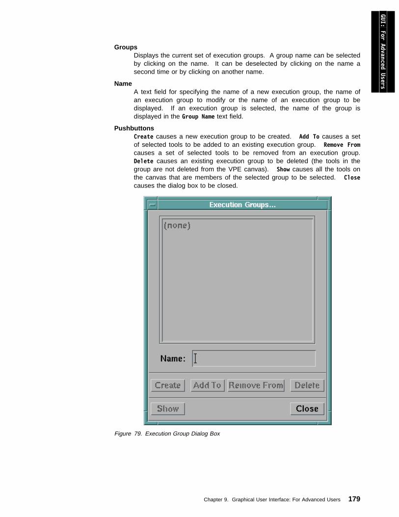
GUI: For Advanced Users

GroupsDisplays the current set of execution groups. A group name can be selectedby clicking on the name. It can be deselected by clicking on the name asecond time or by clicking on another name.

NameA text field for specifying the name of a new execution group, the name ofan execution group to modify or the name of an execution group to bedisplayed. If an execution group is selected, the name of the group isdisplayed in the Group Name text field.

PushbuttonsCreate causes a new execution group to be created. Add To causes a setof selected tools to be added to an existing execution group. Remove Fromcauses a set of selected tools to be removed from an execution group.Delete causes an existing execution group to be deleted (the tools in thegroup are not deleted from the VPE canvas). Show causes all the tools onthe canvas that are members of the selected group to be selected. Closecauses the dialog box to be closed.

Figure 79. Execution Group Dialog Box

Chapter 9. Graphical User Interface: For Advanced Users 179

Creating an Execution GroupTo create an execution group

1. Select the tools on the VPE canvas that are to be placed in a single executiongroup. This can be done by a rubber-band selection or using a shift-clickselection or a combination of both.

2. Open the Execution Group... dialog box by selecting the Edit menu ExecutionGroup... option.

3. In the Group Name text field, enter a name for the execution group.4. Click on the Create button.

The newly created execution group will appear in the list of execution groups.

Note: If a tool is a member of an existing execution group and it is placed into anew group, the tool is automatically deleted from the existing group. Asingle tool can not be a member of two execution groups.

Modifying Execution GroupsExecution groups can be modified by adding new tools to the group or removingtools from the group.

To add tools to an Execution Group:

1. Select the tool or tools to be added to a group.2. Open the Execution Groups... dialog box by selecting the Edit menu

Execution Groups... option.3. Select the name of the execution group to which the tool(s) are to be added.4. Click on the Add To button.

To remove tools from an Execution Group:

1. Select the tool or tools to be removed from a group.2. Open the Execution Groups... dialog box by selecting the Edit menu

Execution Groups... option.3. Select the name of the execution group from which the tool(s) are to be

removed.4. Click on the Remove From button.

Deleting an Execution GroupTo delete an execution group:

1. Open the Execution Groups... dialog box by selecting the Edit menuExecution Groups... option.

2. Select the name of the execution group to be deleted.3. Click on the Delete button.

Displaying the Tools in an Execution GroupData Explorer provides you with the ability to display all the tools that are membersof an execution group. To display the tools:

1. Open the Execution Groups... dialog box by selecting the Edit menuExecution Groups... option.

2. Select the name of the execution group to be displayed.3. Click on the Show button.

180 IBM Visualization Data Explorer: User’s Guide

GUI: For Advanced Users

The tools that are members of the execution group become selected. If theselected tools are not part of the currently displayed portion of the visual program,the VPE will be updated so that the selected tools will be displayed.

Assigning Execution Groups to WorkstationsOnce you have decomposed your visual program into execution groups, you canassign these groups to workstations (or hosts). If you do not specify a host for aparticular execution group, the group will be executed on the master. Executiongroups are assigned to a host using the Execution Group Assignment... dialog box(Figure 80 on page 182).

The dialog box consists of three parts:

Groups and HostsDisplays the name of an execution group and the host on which thegroup is executed. If a host name is not given, then “localhost” isdisplayed as the host name.

Host Name A text field for specifying the name of a host on which an executiongroup is to be executed.

PushbuttonsOK causes the assignments of executions groups to host names andcloses the dialog box. Options... opens a dialog box that allowsyou to specify startup options (e.g., memory size, or the DataExplorer executive that will be started on the host.

Chapter 9. Graphical User Interface: For Advanced Users 181

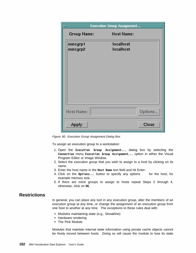
Figure 80. Execution Group Assignment Dialog Box

To assign an execution group to a workstation:

1. Open the Execution Group Assignment... dialog box by selecting theConnection menu Execution Group Assignment... option in either the VisualProgram Editor or Image Window.

2. Select the execution group that you wish to assign to a host by clicking on itsname.

3. Enter the host name in the Host Name text field and hit Enter.4. Click on the Options... button to specify any options for the host, for

example memory size.5. If there are more groups to assign to hosts repeat Steps 2 through 4,

otherwise, click on OK.

RestrictionsIn general, you can place any tool in any execution group, alter the members of anexecution group at any time, or change the assignment of an execution group fromone host to another at any time. The exceptions to these rules deal with:

Modules maintaining state (e.g., Streakline) Hardware rendering The Pick Module.

Modules that maintain internal state information using private cache objects cannotbe freely moved between hosts. Doing so will cause the module to lose its state

182 IBM Visualization Data Explorer: User’s Guide

GUI: For Advanced Users

information or obtain old state information. If you do reassign a module maintainingstate to another host, you should reset the server using the Connection menuReset Server option to ensure correct execution. The only Data Explorer moduleprovided with the system that maintains state information is Streakline.

When you are using the hardware rendering option with either the Display or Imagetools, the tool should be assigned to execution on the host physically connected toyour display.

The Pick module must be run on the same host as the Image tool.

9.2 Loading and Using Outboard and Runtime-Loadable ModulesData Explorer allows the following types of user-written module:

inboard modules are compiled and linked into the Data Explorer Executive.

outboard modules are run as separate processes.

runtime-loadable modules are loaded at runtime and effectively become inboardmodules.

For an outboard or runtime-loadable to be available for use, its module descriptionfile must be loaded into the tool palette. To load a module description file:

1. Select the Load Modules Description(s)... option from the File pull-downmenu in the VPE. A file selection dialog box appears. For information abouthow to use the dialog box, see “File Selection Dialog Boxes” on page 116.

2. Use the dialog box to locate the description file for the module you want toload, and select the desired file. The module name appears on the tool paletteunder its assigned category.

Note: If the module description you loaded has the same name as an moduledescription loaded previously, the more recent description replaces theless recent, regardless of whether they were assigned to the samecategory.

When the new module is available for use, it is listed in the tool palette as amember of the category you assigned it to.

You can configure Data Explorer to automatically load module descriptions whenyou begin the Data Explorer program. To do this, use the -mdf filename optionwhen starting Data Explorer, where filename specifies one or more moduledefinitions. Alternatively, you can use the DXMDF environment variable. For moreinformation on how to do this, see “Using Environment Variables” on page 59 andC.1, “Environment Variables” on page 292.

9.3 Connecting to the ServerBefore you can execute a visual program, your workstation must have establishedconnection to the server. When you start Data Explorer, the program automaticallystarts the server connection, unless you specified that only the user interface wasto be started. However, if for some reason your workstation becomes disconnectedbetween the time you start Data Explorer and the time you are ready to run aprogram, you must reestablish connection with the server.

Chapter 9. Graphical User Interface: For Advanced Users 183

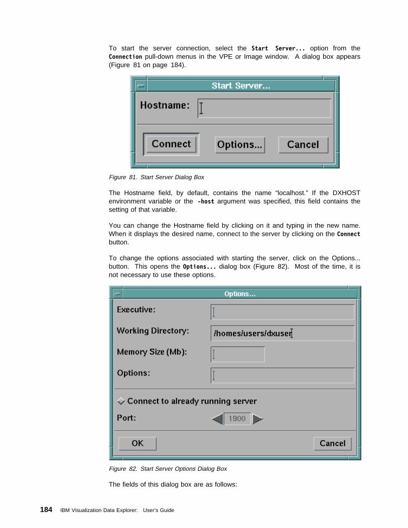
To start the server connection, select the Start Server... option from theConnection pull-down menus in the VPE or Image window. A dialog box appears(Figure 81 on page 184).

Figure 81. Start Server Dialog Box

The Hostname field, by default, contains the name “localhost.” If the DXHOSTenvironment variable or the -host argument was specified, this field contains thesetting of that variable.

You can change the Hostname field by clicking on it and typing in the new name.When it displays the desired name, connect to the server by clicking on the Connectbutton.

To change the options associated with starting the server, click on the Options...button. This opens the Options... dialog box (Figure 82). Most of the time, it isnot necessary to use these options.

Figure 82. Start Server Options Dialog Box

The fields of this dialog box are as follows:

184 IBM Visualization Data Explorer: User’s Guide

GUI: For Advanced Users

ExecutiveSpecifies the name of the executive to run. You might change this field if youwant to run a customized version of Data Explorer.

Working DirectorySpecifies the default directory to search for files.

Memory SizeSpecifies the amount of memory to use, in megabytes.

OptionsSpecify options in this text box as you would on the command line wheninvoking Data Explorer; that is, each option must be preceded by a dash.

-cache on saves the state of the visual program in memory after anexecution. If the visual program changes, Data Explorer reexecutes only theportion of the program affected by the change. If -cache off is specified,Data Explorer must reexecute the entire program for each change. (Thedefault setting is on.)

-trace on displays each execution step, as it happens, in the Debug window.It is mainly used for debugging purposes. (The default setting is off.)

-log on saves all communication between the server and the user interface toa file. (The default setting is off.)

Other options are listed in C.2, “Command Line Options” on page 295.

Connect to already running server radio buttonSpecifies that the user interface should connect with a server that was startedearlier.

You might use this option to set up a connection to a debugging session for acustomized version of the Data Explorer executable. You can specify the portnumber in using the stepper below the button. Note that when this button istoggled on, all other fields in this dialog box become disabled.

Resetting the ServerIf the data set your visual program is using changes (e.g., by being edited) duringyour Data Explorer session, and the cache is enabled (the default condition), it maybe necessary to force Data Explorer to reinitialize the server executive to accessthe new data. To do this, select the Reset Server option from the Connectionspull-down menu.

The action of resetting the server flushes the executive cache. The next time youexecute the visual program, it executes the entire network, not just the portionsaffected by changes internal to the Data Explorer session, and will thus reaccessthe data set.

Chapter 9. Graphical User Interface: For Advanced Users 185

186 IBM Visualization Data Explorer: User’s Guide

Chapter 10. Data Explorer Scripting Language

10.1 Starting Data Explorer in Script Mode . . . . . . . . . . . . . . . . . . . 188Setting Environment Variables . . . . . . . . . . . . . . . . . . . . . . . . . . 189

10.2 Understanding the Script Structure . . . . . . . . . . . . . . . . . . . . . 18910.3 Language Delimiters . . . . . . . . . . . . . . . . . . . . . . . . . . . . . 191

Commenting Scripts . . . . . . . . . . . . . . . . . . . . . . . . . . . . . . . 191Naming Variables and Macros . . . . . . . . . . . . . . . . . . . . . . . . . . 192Specifying Values in a Script . . . . . . . . . . . . . . . . . . . . . . . . . . 193

10.4 Building Expressions and Statements . . . . . . . . . . . . . . . . . . . 197Arithmetic Expressions . . . . . . . . . . . . . . . . . . . . . . . . . . . . . . 197Assignment Statements . . . . . . . . . . . . . . . . . . . . . . . . . . . . . 198Function Call Assignments . . . . . . . . . . . . . . . . . . . . . . . . . . . . 199

10.5 Invoking Data Explorer Macros and Modules . . . . . . . . . . . . . . . 200Function Call Arguments . . . . . . . . . . . . . . . . . . . . . . . . . . . . . 200Function Call Attributes . . . . . . . . . . . . . . . . . . . . . . . . . . . . . . 202

10.6 Defining Macros . . . . . . . . . . . . . . . . . . . . . . . . . . . . . . . . 204Macro Header . . . . . . . . . . . . . . . . . . . . . . . . . . . . . . . . . . . 204Macro Body . . . . . . . . . . . . . . . . . . . . . . . . . . . . . . . . . . . . 205Macro Examples . . . . . . . . . . . . . . . . . . . . . . . . . . . . . . . . . . 205

10.7 Using Data Explorer Script Commands . . . . . . . . . . . . . . . . . . . 206Sequencer . . . . . . . . . . . . . . . . . . . . . . . . . . . . . . . . . . . . . 206File Inclusion . . . . . . . . . . . . . . . . . . . . . . . . . . . . . . . . . . . . 207Prompts . . . . . . . . . . . . . . . . . . . . . . . . . . . . . . . . . . . . . . . 207

10.8 Understanding the Script Execution Model . . . . . . . . . . . . . . . . . 208Top-level Environment . . . . . . . . . . . . . . . . . . . . . . . . . . . . . . 208Function Execution . . . . . . . . . . . . . . . . . . . . . . . . . . . . . . . . 208Macro Expansion . . . . . . . . . . . . . . . . . . . . . . . . . . . . . . . . . 208Variables Used in Macros . . . . . . . . . . . . . . . . . . . . . . . . . . . . 208Assignment and Function Call Semantics . . . . . . . . . . . . . . . . . . . 209Execution Example . . . . . . . . . . . . . . . . . . . . . . . . . . . . . . . . 210

10.9 Running .net files in script mode . . . . . . . . . . . . . . . . . . . . . . 210

Scripting Language

Copyright IBM Corp. 1991-1997 187

When you create a visual program with the graphical user interface, Data Explorersaves the program in a .net file. This saved version is actually a set ofscripting-language commands. You do not need to understand the script languageunless you are running Data Explorer in script mode.

In Data Explorer script mode you can also perform tasks that would be awkwardwith a visual program (e.g., facilitation of batch processing or debugging of amodule).

10.1 Starting Data Explorer in Script ModeTo run Data Explorer in script mode on a workstation, you must have an accounton that workstation.

To start Data Explorer, follow these steps:

1. Start the X Window System session on the workstation.

2. Type:

dx -script

When script mode starts, you will see a prompt symbol (dx>), indicating thatData Explorer is ready to accept input. (If you want to change the promptsymbol, see 10.7, “Using Data Explorer Script Commands” on page 206.)

(All of the command line options for Data Explorer are described in C.2, “CommandLine Options” on page 295.)

You can type commands directly at the command line, but you may find it moreconvenient to create a script and submit it to Data Explorer for execution. Tosubmit a script, type:

include "scriptname"

at the prompt, where scriptname is the name of the script.

Once you have submitted a script, Data Explorer will process the commands itcontains. Note that none of the direct interactor options are available in scriptmode: you must use the Image tool in the graphical user interface to takeadvantage of those options.

After the included script has been processed, you can include another script. Toterminate your Data Explorer session, type:

quit

You can also include a script name directly in the script command: add the name ofthe script after the -script option. Data Explorer will terminate automatically whenit has executed the script. For example, type:

include "/usr/lpp/dx/samples/scripts/scriptexample"

You will see a sequence of images created with sequencer commands. Thedirectory /usr/lpp/dx/samples/scripts contains examples for many modules. Youmay find it helpful to experiment with them to learn how they function.

Note: To ensure that an example program does not exit before you want it to,invoke script mode first and then “include” the program. Otherwise, some programswill execute and disappear so quickly that you won’t be able to identify the image.

188 IBM Visualization Data Explorer: User’s Guide

Setting Environment VariablesThere are several environment variables that you may find useful to customize DataExplorer. These can be set in your login profile.

DXDATA: The DXDATA environment variable specifies a list of directories inwhich Data Explorer will search for data files. If the data you wish to import is inone of the directories specified in the DXDATA environment variable, you do notneed to provide the complete path name to the Import tool. Specify the file name,and the Import module will look in the specified directories for the data file. Thedirectories will be searched in the order in which they are listed in the environmentvariable; and the first occurrence of the data file will be used.

An example of a statement that sets the DXDATA environment variable (in the Cshell environment) is the following:

setenv DXDATA /usr/mydirectory/mydata:/usr/group/groupdata

where /usr/mydirectory/mydata and /usr/group/groupdata are two directories thatcontain data files. Multiple directories can be listed, with each directory nameseparated by a colon.

DXHOST: The DXHOST environment variable is the initial machine name of theserver on which to run the executive. If DXHOST is not specified, then a default of“localhost” is used. See 9.3, “Connecting to the Server” on page 183 for moreinformation on how to connect to the server. The host name should be the namethat results when you issue the uname -n shell command.

DXINCLUDE: If this environment variable is set, Data Explorer looks for includedscripts first in the current directory, and then in each of the directories specified inthe colon-separated list specified by this variable.

DXMACROS: The DXMACROS environment variable is a list of the directories inwhich Data Explorer will look for macros.

Scripting Language

10.2 Understanding the Script StructureThe following example illustrate some of the more important characteristics ofscripts; a detailed description of each of the elements follows. However, you mayprefer to simply study these examples (and perhaps those in/usr/lpp/dx/samples/scripts) and then begin writing your own scripts.

Example 1. A Simple ScriptIn this example, the data found in /usr/...cloudwater is imported and assigned to thevariable data. Then the Isosurface module is called on data (with no otherparameters set) and the result is assigned to iso. A Camera is created usingAutoCamera, and the isosurface is displayed using Display (note that the Imagetool is not available in the scripting language.

data = Import("/usr/lpp/dx/samples/data/cloudwater");

iso = Isosurface(data);

camera = AutoCamera(iso);

Display(iso, camera);

Chapter 10. Data Explorer Scripting Language 189

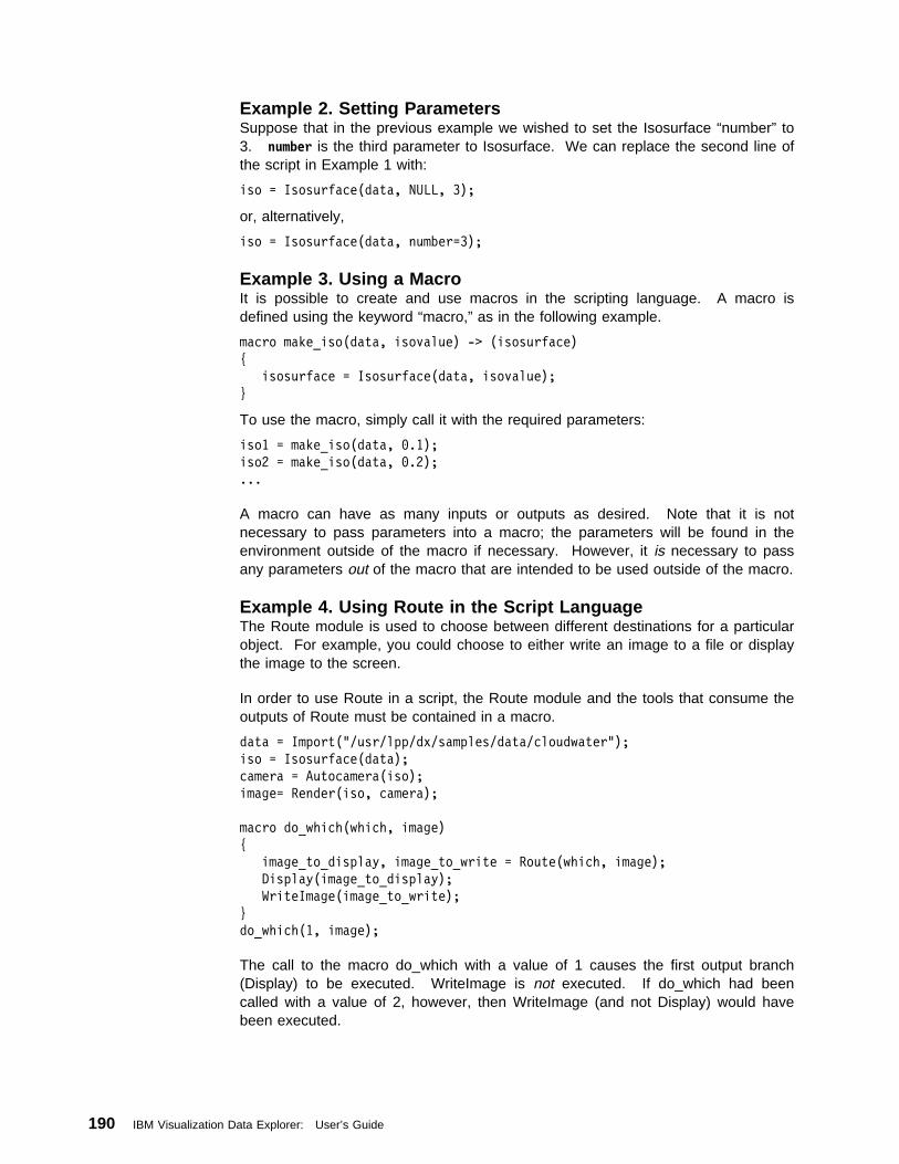
Example 2. Setting ParametersSuppose that in the previous example we wished to set the Isosurface “number” to3. number is the third parameter to Isosurface. We can replace the second line ofthe script in Example 1 with:

iso = Isosurface(data, NULL, 3);

or, alternatively,

iso = Isosurface(data, number=3);

Example 3. Using a MacroIt is possible to create and use macros in the scripting language. A macro isdefined using the keyword “macro,” as in the following example.

macro make_iso(data, isovalue) -> (isosurface)

isosurface = Isosurface(data, isovalue);

To use the macro, simply call it with the required parameters:

iso1 = make_iso(data, ð.1);

iso2 = make_iso(data, ð.2);

...

A macro can have as many inputs or outputs as desired. Note that it is notnecessary to pass parameters into a macro; the parameters will be found in theenvironment outside of the macro if necessary. However, it is necessary to passany parameters out of the macro that are intended to be used outside of the macro.

Example 4. Using Route in the Script LanguageThe Route module is used to choose between different destinations for a particularobject. For example, you could choose to either write an image to a file or displaythe image to the screen.

In order to use Route in a script, the Route module and the tools that consume theoutputs of Route must be contained in a macro.

data = Import("/usr/lpp/dx/samples/data/cloudwater");

iso = Isosurface(data);

camera = Autocamera(iso);

image= Render(iso, camera);

macro do_which(which, image)

image_to_display, image_to_write = Route(which, image);

Display(image_to_display);

WriteImage(image_to_write);

do_which(1, image);

The call to the macro do_which with a value of 1 causes the first output branch(Display) to be executed. WriteImage is not executed. If do_which had beencalled with a value of 2, however, then WriteImage (and not Display) would havebeen executed.

190 IBM Visualization Data Explorer: User’s Guide

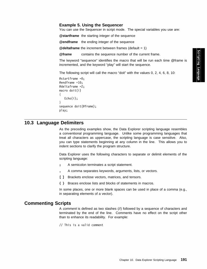
Example 5. Using the SequencerYou can use the Sequencer in script mode. The special variables you use are:

@startframe the starting integer of the sequence

@endframe the ending integer of the sequence

@deltaframe the increment between frames (default = 1)

@frame contains the sequence number of the current frame.

The keyword “sequence” identifies the macro that will be run each time @frame isincremented, and the keyword “play” will start the sequence.

The following script will call the macro “doit” with the values 0, 2, 4, 6, 8, 10:

@startframe =ð;

@endframe =1ð;

@deltaframe =2;

macro doit(i)

Echo(i);

sequence doit(@frame);

play;

Scripting Language

10.3 Language DelimitersAs the preceding examples show, the Data Explorer scripting language resemblesa conventional programming language. Unlike some programming languages thattreat all characters as uppercase, the scripting language is case sensitive. Also,you can type statements beginning at any column in the line. This allows you toindent sections to clarify the program structure.

Data Explorer uses the following characters to separate or delimit elements of thescripting language:

; A semicolon terminates a script statement.

, A comma separates keywords, arguments, lists, or vectors.

[ ] Brackets enclose vectors, matrices, and tensors.

Braces enclose lists and blocks of statements in macros.

In some places, one or more blank spaces can be used in place of a comma (e.g.,in separating elements of a vector).

Commenting ScriptsA comment is defined as two slashes (//) followed by a sequence of characters andterminated by the end of the line. Comments have no effect on the script otherthan to enhance its readability. For example:

// This is a valid comment

Chapter 10. Data Explorer Scripting Language 191

Naming Variables and MacrosYou can name the variables and macros with identifiers. Identifiers are sequencesof characters selected from the following:

Uppercase alphabetic characters (A-Z) Lowercase alphabetic characters (a-z)

Numerals (ð-9) Special characters:

– Underscore (_)– Single quote (’)– “At” sign (@)

All identifiers must start with either an alphabetic character, an underscore (_), oran “at” sign (@). Remember that the Data Explorer script language is casesensitive: identifiers that differ in the case of at least one character are consideredto be different identifiers. Identifiers are currently limited to a length of 200characters.

Note: IBM reserves the definition and use of most identifiers that begin with @.However, there are some built-in @ variables that you can set; these arediscussed in 10.7, “Using Data Explorer Script Commands” on page 206.

The following are valid, unique identifiers:

ComputeSine

Compute_Sine

cðmpute_sine

compute_s1ne

compute_sine'

Identifiers can be used as:

variable names function names.

Some identifiers are reserved and cannot be used as a variable or a function name.Every other identifier can be used both as a variable and as a function name. Theproper use of the identifier is determined by its context.

Reserved WordsThe identifiers in the following list cannot be used for variable or function names.Those marked with asterisks are reserved for use in future releases.

The identifier NULL is a reserved variable name. It can be used to initialize othervariables or function arguments to have no value assigned to them.

and\backwardcancel\else\false\for\forwardif\include

loopmacronot\offonpalindromepauseplayquit

repeat\or\sequencestepstopthen\true\until\while\

192 IBM Visualization Data Explorer: User’s Guide

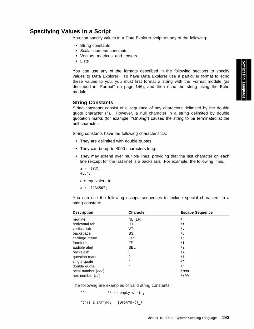
Specifying Values in a ScriptYou can specify values in a Data Explorer script as any of the following:

String constants Scalar numeric constants Vectors, matrices, and tensors

Lists

You can use any of the formats described in the following sections to specifyvalues to Data Explorer. To have Data Explorer use a particular format to echothese values to you, you must first format a string with the Format module (asdescribed in “Format” on page 146), and then echo the string using the Echomodule.

Scripting Language

String ConstantsString constants consist of a sequence of any characters delimited by the doublequote character ("). However, a null character in a string delimited by doublequotation marks (for example, “str\0ing”) causes the string to be terminated at thenull character.

String constants have the following characteristics:

They are delimited with double quotes.

They can be up to 4000 characters long.

They may extend over multiple lines, providing that the last character on eachline (except for the last line) is a backslash. For example, the following lines,

a = "123\

456";

are equivalent to

a = "123456";

You can use the following escape sequences to include special characters in astring constant:

The following are examples of valid string constants:

"" // an empty string

"this a string: ˜!@#$%^&\()_+"

Description Character Escape Sequence

newline NL (LF) \nhorizontal tab HT \tvertical tab VT \vbackspace BS \bcarriage return CR \rformfeed FF \faudible alert BEL \abackslash \ \\question mark ? \?single quote ' \'double quote " \"octal number (ooo) \ooohex number (hh) \xhh

Chapter 10. Data Explorer Scripting Language 193

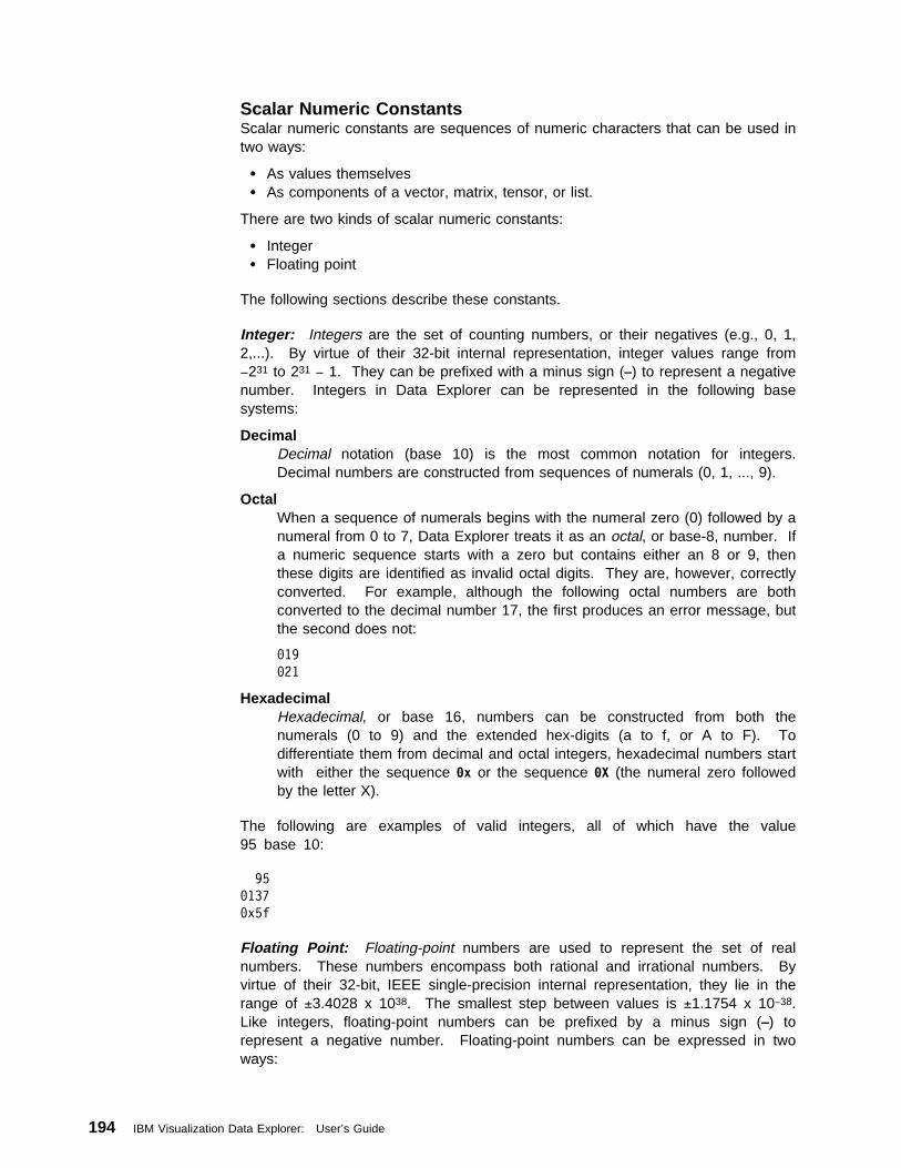
Scalar Numeric ConstantsScalar numeric constants are sequences of numeric characters that can be used intwo ways:

As values themselves As components of a vector, matrix, tensor, or list.

There are two kinds of scalar numeric constants:

Integer Floating point

The following sections describe these constants.

Integer: Integers are the set of counting numbers, or their negatives (e.g., 0, 1,2,...). By virtue of their 32-bit internal representation, integer values range from−231 to 231 − 1. They can be prefixed with a minus sign (–) to represent a negativenumber. Integers in Data Explorer can be represented in the following basesystems:

DecimalDecimal notation (base 10) is the most common notation for integers.Decimal numbers are constructed from sequences of numerals (0, 1, ..., 9).

OctalWhen a sequence of numerals begins with the numeral zero (0) followed by anumeral from 0 to 7, Data Explorer treats it as an octal, or base-8, number. Ifa numeric sequence starts with a zero but contains either an 8 or 9, thenthese digits are identified as invalid octal digits. They are, however, correctlyconverted. For example, although the following octal numbers are bothconverted to the decimal number 17, the first produces an error message, butthe second does not:

ð19

ð21

HexadecimalHexadecimal, or base 16, numbers can be constructed from both thenumerals (0 to 9) and the extended hex-digits (a to f, or A to F). Todifferentiate them from decimal and octal integers, hexadecimal numbers startwith either the sequence ðx or the sequence ðX (the numeral zero followedby the letter X).

The following are examples of valid integers, all of which have the value95 base 10:

95

ð137

ðx5f

Floating Point: Floating-point numbers are used to represent the set of realnumbers. These numbers encompass both rational and irrational numbers. Byvirtue of their 32-bit, IEEE single-precision internal representation, they lie in therange of ±3.4028 x 1038. The smallest step between values is ±1.1754 x 10−38.Like integers, floating-point numbers can be prefixed by a minus sign (–) torepresent a negative number. Floating-point numbers can be expressed in twoways:

194 IBM Visualization Data Explorer: User’s Guide

Standard representationThe standard representation of a floating-point number consists of a decimalnumber followed by a decimal point (.), followed by another decimal number.The first decimal number represents the whole part of the floating-pointnumber. The second represents the fractional part. Either the first or thesecond of the numbers surrounding the decimal point can be omitted, but notboth. If the first is omitted, then the number is purely fractional. If the secondis omitted, then the number does not contain a fractional part. This secondalternative is useful for representing integer values that lie outside of therange representable by the integer format.

Scientific notationScientific notation is an alternative means of representing floating-pointnumbers. A number in scientific notation has the form xey (or xEy). Thenumber x can be either a standard floating-point number or a decimal integer.The number y must be a decimal integer. It can be prefixed by a minus sign.This scientific notation is simply shorthand for writing x×10y. The effect of thedecimal value y is to specify the number of places the decimal point shouldbe shifted to the right, or if y is negative, to the left.

The following are examples of valid floating-point numbers, all of which have thevalue 95.0:

95.

95.ð

95eð

9.5E1

95ðe–1

9.5ðe+1

Scripting Language

Vectors, Matrices, and TensorsVectors, matrices, and tensors are higher dimensional mathematical entities thatare used for the representation of specific kinds of data.

Vectors: A vector is a quantity that has both magnitude and direction inn-dimensional space. It corresponds to a directed line segment whose lengthrepresents the magnitude of the vector and whose orientation corresponds to itsdirection.

Vectors are composed of a sequence of scalar values enclosed by square brackets[ ]. The scalar values can be separated by commas if desired, although this is notnecessary. If the elements of a vector are not homogeneous, (e.g., if they are bothinteger and floating-point elements), then the integer elements are converted tofloating point. The following are all valid vectors:

[ð.ð ð.ð ð.ð] // the origin of a 3-D space

[ð, ð, 1] // an axis in a 3-D coordinate system

[1, 1.ð 1, 1.ð 1] // a vector in a 5-D space

Matrices: Matrices are 2-dimensional collections of scalars. They are used torepresent, among other things, the coefficients of a set of simultaneous equationsor a transformation of a vector.

Chapter 10. Data Explorer Scripting Language 195

Matrices are constructed from a sequence of vectors enclosed by square brackets.Each of the vectors contained in a matrix must have the same length as all of theothers. The following are all valid matrices:

[[1 ð ð ð][ð 1 ð ð][ð ð 1 ð][ð ð ð 1]] // a 4x4 identity matrix

[[ ð.7ð7 ð.7ð7 ð.ððð] // a 45-degree rotation

[–ð.7ð7 ð.7ð7 ð.ððð] // about the Z axis

[ ð.ððð ð.ððð 1.ððð]]

[[1 1 1 1][2 2 2 2]] // a 2x4 matrix

Tensors: Tensors are a generalization of the concept of vectors. On one hand,the elements in a tensor have meanings that are independent of the coordinatesystem in which they are embedded. On the other hand, one can associate certainmetrics to them that vary among coordinate systems.

In general, a rank n tensor can be formed by surrounding k rank n−1 tensors withsquare brackets. (Note that scalars, vectors, and matrices are rank 0, 1, and 2tensors, respectively.) As with the matrices, all of the subtensors must have thesame shape.

The following are valid tensors:

[[[[[ðxabcd]]]]] // a 1x1x1x1x1 rank 5 tensor

[[[1 ð ð] // a 3x3x3 rank 3 tensor with

[ð ð ð] // 1’s on the diagonal

[ð ð ð]]

[[ð ð ð]

[ð 1 ð]

[ð ð ð]]

[[ð ð ð]

[ð ð ð]

[ð ð 1]]]

ListsUnlike the vector, matrix, and tensor constructions that aggregate several lowerdimensional data elements into a single higher one; the list construction collectsseveral homogeneous elements together so that they can be handled as a singleentity while still retaining their individuality.

Lists are constructed by enclosing a sequence of scalars, vectors, matrices, rank ntensors, or string constants in braces ( ). The elements of a list can beseparated by commas, although they need not be. In Data Explorer, a list is thesame as an Array (see “Arrays” on page 28).

The following are examples of valid lists:

196 IBM Visualization Data Explorer: User’s Guide

1.ð 2.ð 3.ð // 3 scalar values (for isovalues)

[ð.ð ð.ð ð.ð], // 4 vector values for use as

[1.ð ð.ð ð.ð], // streamline seed points

[2.ð ð.ð ð.ð],

[3.ð ð.ð ð.ð]

“a” “list” “of” “string”

“constants”

Lists of scalars can also be defined with a convenient shorthand notation thatspecifies the following:

The list’s starting value The list’s ending value A stepping increment (optional).

If you do not specify a stepping increment, then the default is 1. If any of thevalues in the list constructor (including the stepping increment) are specified asfloating point numbers, then the generated list contains floating-point numbers;otherwise, it contains integers. If the starting value is smaller than the endingvalue, the list elements are generated in increasing order; otherwise they aregenerated in decreasing order. Also, only the magnitude of the stepping incrementis important, not the sign. A negative stepping increment produces the sameresults as a positive one.

The values included in the list are generated by continually adding the value of thestepping increment to the starting value until the resultant value passes the endingvalue. Each of the following produces the same list:

-1 1 3 5 7 9

-1 .. 9 : 2

-1 .. 9 : -2

-1 .. 1ð : 2

Note: Spaces are required around the .. operator.

Lists specified using this notation will be represented as a Regular Array of1-vectors. See “Arrays” on page 28 for a discussion of Array types.

Scripting Language

10.4 Building Expressions and StatementsYou can use the basic elements of the Data Explorer scripting language to buildexpressions and assignment statements. Most statements in the scripting languageare assignment statements; however, a special group of script commands with theiroptions can form a statement. These commands are described in 10.7, “UsingData Explorer Script Commands” on page 206. The following sections tell you howto write Data Explorer script expressions and statements.

Arithmetic ExpressionsYou can combine scalar values and variables that contain values with the arithmeticoperators listed below to derive new values. Lists of scalars can also be combinedif the lists have the same cardinality (number of elements), or if one of the lists hasjust a single element. If the two lists being operated upon have the same numberof elements, then the operator is applied to the corresponding element pairs ineach list to produce a new list of the same cardinality. If one of the lists has just a

Chapter 10. Data Explorer Scripting Language 197

single element, then the operator is applied, in turn, to each of the elements of thelarger list and to that single element to produce a list whose size is the same as thelarger list.

If both of the elements in an operation are the same type, either integer or floatingpoint, then the result of the operation is also of the same type. If, however, one ofthe elements is an integer and the other is a floating-point value, then the result isa floating-point value. Given this automatic type conversion, a simple way toconvert an integer value to a floating-point value is to add 0.0 to it.

OperatorsThe operators listed in the following table can be used in arithmetic expressions. Inthe table, a horizontal line separates each precedence level and the higher levelsare placed above the lower ones. Operators with higher precedence are evaluatedbefore those with lower precedence. Operators with the same precedence areevaluated from left to right. Because expressions in parentheses are evaluatedfirst, you can use parentheses to alter the grouping of operands, thereby changingthe precedence levels.

The following expressions all have the value 2.0 4.0 8.0:

3.ð 5.ð 9.ð − 1.ð 1.ð 1.ð2 4 8 + ð.ð

8 \ .25 .5ð 1eð

2 ^ 1.ð 2.ð 3.ð

(2 2 2 – 1.ð) \ 2 4 8

Operator Description

– Unary minus

^ Exponentiation\\ Exponentiation (alternate form)

\ Multiplication/ Division

+ Addition

– Subtraction

Assignment StatementsAssignment statements store values in variables. The general form of anassignment statement is:

left-side[attribute_name:value,...] =right-side[attribute_name:value,...]

The left-side portion of an assignment statement is a sequence of one or moreidentifiers separated by commas. The [attribute_name:value,...] value pair listsand the brackets are optional, and are discussed in “Function Call Attributes” onpage 202. The equal sign (=) is the assignment operator. It stores the valuesspecified in the right-side portion of the statement in the variables named by theidentifiers specified in the left-side portion of the statement. You can specify thevalues in the right-side portion of the statement as a sequence of expressions or asthe result of a single function call.

198 IBM Visualization Data Explorer: User’s Guide

You can also use either of two additional symbols, <– or :=, as the assignmentoperator. An assignment statement is terminated with a semicolon, indicating theend of the right-side portion of the statement.

The values specified to the right of the assignment operator are assigned to theidentifiers to the left of the assignment operator. If the number of values equals thenumber of identifiers, the first value is stored in the first identifier, the second in thesecond, the third in the third, and so on. If the number of values is greater than thenumber of identifiers, the extra rightmost values are ignored. If the number ofvalues is less than the number of identifiers, the values are assigned in order to theleftmost identifiers.

Those identifiers not receiving a value from the right-side list are set to the valueNULL. In addition, if an identifier is repeated in the left-side list, then the right-sideassociated with that identifier is the value associated with its rightmost instance.

All identifiers that have not had a value explicitly assigned to them have the valueNULL.

Scripting Language

Expression AssignmentsThe values for the right-side portion of an expression assignment statement consistof a sequence of constant values, variables, arithmetic expressions, and the valueNULL, separated by commas. The various values need not be of the same kind,data type, or dimension.

The following examples all assign the value “A string” to the variable a, the value2.0 to the variable b, and the value NULL to the variable c.

a = "A string"; // These 3 lines

b := 2 \ (2 – 1eð); // constitute a single

c <– NULL; // example.

a, b, c = "A string", 2.ð, NULL;

a, b, c <– "A string", 5 / 2.5, NULL;

a, b, c = "A string", 2.ð;

a, b, c, d = "A string", 2.ð;

a, b, c, a = [[1 ð][ð 1]], 2.ð, NULL, "A string", [1 2 3];

The following example illustrates a simple way to swap values:

a = 2;

b = 4;

c = 6;

d = 8;

e = 1ð;

a, b = b, a; // Values are swapped, so a = 4, b = 2

c, d, e = e, c, d; // c = 1ð, d = 6, e = 8

Function Call AssignmentsA function call can refer either to a function defined as a module (a functioncompiled into the system), or to a macro (a function defined in the scriptinglanguage itself). The values for the right-side portion of a function call assignmentstatement are the values returned by a single function call.

The Statistics function, which is used in the following examples, returns five values:

Chapter 10. Data Explorer Scripting Language 199

Mean of the data Standard deviation of the data Variance of the data The minimum value in the data The maximum value in the data

In the first example, all of these values are assigned to variables for later use. Inthe second example, the minimum and maximum values are ignored. In the thirdexample, only the minimum and maximum values are being saved for later use.

(1) mean, sd, var, min, max = Statistics (data);

(2) mean, sd, var = Statistics (data);

(3) min, min, min, min, max = Statistics (data);

10.5 Invoking Data Explorer Macros and ModulesThis section describes the procedures and features for invoking macros andmodules. It describes function call arguments and attributes.

Function Call ArgumentsData Explorer provides a flexible function-calling mechanism for invoking macrosand modules.

A macro’s definition includes a list of identifiers that are used as its input formalparameters. The formal parameters act as names and place holders for thearguments that you supply when the macro is called.

Modules (functions that are compiled into the system) have named formalparameters. The general form of a function (macro or module) call, whether usedas the right hand side of an assignment statement or on its own, is:

Name (arglist)[attribute_name:value,...]

where Name is the name of the function being called and arglist is a list ofarguments that are separated by commas (the list can be empty). Following thefunction may optionally be a list of attribute_name:value pairs enclosed in squarebrackets. Each argument’s value can be either a variable identifier, a constantvalue, an expression, or the special identifier NULL. Note that nested function callscannot be passed as arguments. The argument values can be passed either byposition or by name, as described in the following sections.

Positional ArgumentsThe positional argument-passing mechanism is similar to the mechanism found inmost programming languages that use subroutines. Given a function declared withn input formal parameters, the first n values supplied in the function call areassigned to the first n formal parameters. If you supply i < n values in the functioncall, then only the first i of the function’s formal parameters are assigned thesupplied values.

The missing arguments are assigned the value of NULL.

200 IBM Visualization Data Explorer: User’s Guide

By-Name ArgumentsThe “by name” argument-passing mechanism provides more flexibility in specifyingarguments. When an argument is passed by name, the following syntax is used forthe argument:

Fname = value

Fname is an identifier that corresponds to one of the function’s input formalparameters. Value is one of the types of values that are valid for that argument tothe function. If the function is a macro, the arguments are named in the definitionof the macro in the script. If the function is a module, the argument names areprovided in the description of the module in Chapter 2, “Functional Modules” onpage 15 in IBM Visualization Data Explorer User’s Reference.

Notes:

1. Positional arguments can be supplied only prior to by-name arguments,because the positional context is lost once a name has been supplied.

2. If an argument is supplied both by position and by name, then the value givenby name takes precedence.

3. If an argument is supplied by name more than once in a given function call,then the value associated with the last (rightmost) instance of the input formalparameter is used.

4. A name that does not correspond to one of the function’s formal parametersand its associated values is considered a semantic error.

Scripting Language

Missing ArgumentsAny formal parameter of a module that has not had a value passed to it, either byposition or by name, is initialized to the value NULL. If NULL is explicitly passed intothe module, the module may still use the default value, provided it is designed to doso. The NULL value allows modules to use internal defaults for those values thatare not specified in a function call. The default value must be specified in the codeof the module (see IBM Visualization Data Explorer Programmer’s Reference forinformation).

If the function is a macro, a missing argument or an argument explicitly specified asNULL causes the default value to be used. If no default is specified, the parameteris set to NULL.

ExampleThe module Camera takes the following arguments:

to The position in space to which the camera is pointed. The default is[0, 0, 0].

from The position in space where the camera is located. The default is [0,0, 1].

width The width, in user units, of the camera’s view. The default is 100.

resolution The horizontal resolution, in pixels, of the image generated by thecamera. The default is 640.

aspect The aspect ratio of the image generated by the camera (i.e., its heightdivided by its width). The default is 0.75.

Chapter 10. Data Explorer Scripting Language 201

up The direction, in the world coordinate system, that the cameraconsiders “up” The default is [0, 1, 0].

perspective The projection method. The default is 0, indicating orthographicprojection.

view angle The viewing angle. This applies only in perspective projection, andthe default is 30.

background The image background color. The default is “black”.

The following function calls are all equivalent and construct the default CameraObject:

c1 = Camera ([ð, ð, ð], [ð, ð, 1], 1ðð, 64ð, ð.75, [ð, 1, ð], ð, "black");

c2 = Camera (NULL, NULL, NULL, NULL, NULL, NULL, NULL, NULL, NULL);

c3 = Camera ();

c4 = Camera (NULL, NULL, NULL, NULL, NULL, [ð, 1, ð], NULL, NULL);

c5 = Camera (up = [ð, 1, ð]);

c6 = Camera ([5, 5, 5], [ð, ð, 1], NULL, to = [ð, ð, ð]);

c7 = Camera (width = 512, width = 64ð);

Function Call AttributesFunctions may optionally have attributes associated with each invocation of thefunctions, and attributes may also be associated with specific outputs of a module.The Data Explorer scripting language provides three function call attributes:

instance Identifies the instance of a function call. This can help you locate errorsin scripts. To use the instance attribute, follow the function call withinstance and the instance number separated by a colon and enclosed inbrackets. For example:

out1 = Color(surface,"blue") [instance:1];

out2 = Color(surface,"green") [instance:2];

In this example, each instance of the Color module is identified uniquely.If an error occurs, the error message will report the module name, in thiscase Color, plus its instance number. If the instance numbering was notused, the error message will only report the name of the module.

cache Specifies whether the system writes the outputs of a module into thecache. The cache is a portion of memory in which results of previouslyexecuted functions are stored. If the inputs to a module do not changethe module will not be invoked in subsequent executions, rather themodule results are retrieved from the cache. If the module results arenot found in the cache, because they were purged in order to makeroom for some other result or they were never stored in the cache, themodule will be reexecuted.

The cache attribute can have one of three values:

[cache:0] - Do not cache the module outputs

[cache:1] - Cache all the results of the modules outputs

[cache:2] - Cache only the results of the modules outputs for thelast execution of the module

The cache attribute can be associated with the individual outputs of amodule, with the entire module (affecting all the outputs) or acombination of both. When output-associated and module-associated

202 IBM Visualization Data Explorer: User’s Guide

cache attributes are used in combination the output-associated attributesoverride the effects of the module-associated attributes.

The following two examples illustrate how the cache attribute can beused. In the first example the attribute is associated with the module.In the second example the attribute is associated with the moduleoutput. The results of both of these examples are identical sinceIsosurface has only one output.

iso = Isosurface(data,value) [cache:ð];

iso [cache:ð] = Isosurface(data,value);

The following examples look similar to those above, but there is adifference because DivCurl produces two outputs. In the first example,only the last result of both outputs of DivCurl are stored in the cache. Inthe second example the last result of div is placed in the cache, but allresults of curl are placed in the cache.

div, curl = DivCurl(data) [cache:2];

div [cache:2], curl = DivCurl(data);

In the following example all outputs of Statistics are not cached exceptfor min. Since a cache attribute with a value of 2 was associated withmin, the last result of the min output of Statistics will be stored in thecache.

mean, sd, var, min [cache:2], max = Statistics(data) [cache:ð]

If no cache attribute is associated with the module, all results of theoutputs will be cached unless an individual output has a cache attributeassociated with it. The following example is similar to the one above,except that all results of module outputs are cached with the exceptionof min. Since a cache attribute with a value of 2 was associated withmin only the last result of the min output of Statistics will be stored inthe cache.

mean, sd, var, min [cache:2], max = Statistics(data);

group Identifies which execution group a module belongs to. This attribute isused to distribute parts of a visualization across multiple workstations.This attribute does not bind a module to a specific workstation, butidentifies it to be a member of a group that may be assigned to aworkstation. The assignment of an execution group to a workstation isdone using the Executive module (see “Executive” on page 126 in IBMVisualization Data Explorer User’s Reference).

The following example illustrates how the group attribute can be used.

cwater = Import("cloudwater");

iso = Isosurface(cwater);

wind = Import("wind") [group: "group2"];

x = Compute("$ð.x",wind) [group: "group2"];

mapped = Map(iso,x);

colored = Color(mapped);

camera = Camera(colored);

Display(colored,camera);

The second Import and the Compute will be placed into an executiongroup called “group2”. All other modules will be placed into one defaultexecution group.

Scripting Language

Chapter 10. Data Explorer Scripting Language 203

You can combine the various attributes for a single function call byseparating them with commas, as in the following examples:

wind = Import("wind") [instance:2, group: "group2"];

Colored = Color(iso,"blue") [instance:1, cache:2];

Colored = Color(iso,"green") [instance:2, cache:2, group:"group"];

one shot Represents the script language implementation of the Reset interactor inthe user interface. It sets the value of a variable to one value for thefirst execution and a different value (resetvalue) there after. The syntaxis:

x[oneshot:resetvalue] = value;

10.6 Defining MacrosMacros are higher level processing functions that are constructed from simplerones. A macro definition consists of two parts:

A macro header A macro body

The following sections define these parts.

Macro HeaderThe macro header defines the macro’s name, its formal parameters, and the namesof values that it returns. The syntax of a macro header is

macro MacroName (inputs) [ -> (outputs) ]

where:

The keyword macro indicates that a new macro definition has started.

MacroName is an identifier of the name that is being associated with the macrodefinition.

The inputs portion of a macro header is a list of identifiers separated bycommas. The list may be empty. These identifiers act as place holders for thearguments passed to the macro when it is called. If the macro does not requireany arguments, then you can omit the list (but not the enclosing parentheses).The right-arrow symbol is needed only for macros with outputs. The followingare examples of valid headers for macros without outputs:

macro MyMacro(x,y)

macro MyMacro()

You can also specify default values for the inputs. Consider the followingexample:

macro X (a = "no input", b = 4)

Echo (a, b);

The values of the arguments a and b vary, depending how the macro isinvoked. For example:

204 IBM Visualization Data Explorer: User’s Guide

X(); // a and b are set to the defaults, "no input" and 4

X("new value", 3); // a is set to "new value", b is set to 3

X(NULL); // a and b are set to the defaults, "no input" and 4

X(b = 6); // a gets default of "no input", b is set to 6

See 10.5, “Invoking Data Explorer Macros and Modules” on page 200 forfurther explanation of the function-calling mechanism.

The outputs portion of a macro’s header is a list of identifiers separated bycommas.

These identifiers act as place holders for the values returned by the macrowhen the macro is executed. If the macro does not return any values, then theright-arrow portion, -> (), is not necessary.

Scripting Language Macro BodyThe macro body consists of a sequence of assignment statements and functioncalls surrounded by braces . The functions referred to in these statements neednot exist when a macro is defined; however, they must exist when it is executed.

Recursive and mutually recursive macro invocations are detected and preventedfrom executing. Statements are not guaranteed to execute in the order given in themacro’s declaration, although some partial ordering is always preserved. Calls tomodules that cause external side effects (such as Display) are always executed inthe order in which they were specified.

Macro ExamplesThe first example macro, Sum, takes two arguments. The macro computes andreturns their sum.

macro Sum (arg1, arg2) -> (sum)

sum = arg1 + arg2;

The second example macro, PrintSum, also takes two arguments and computestheir sum. However, unlike the macro Sum, it does not return the computed value.Instead, it prints out using the Echo module. This example illustrates a function call(to Echo) that either does not return a value or whose return values are ignored.

macro PrintSum (arg1, arg2)

sum = arg1 + arg2;

Echo (sum);

The third example macro, VectorManip, implements a function to compute the crossproduct, dot product, and cosine of two 3-vectors. Note that the returned values donot need to be computed in the order in which they are declared.

macro VectorManip (vectlist1, vectlist2) -> (dot, cross, cos)

cross = Compute("cross($ð, $1)", vectlist1, vectlist2);

dot = Compute("dot($ð, $1)", vectlist1, vectlist2);

cos = Compute("$ð/(mag($1)/mag($2))", dot, vectlist1, vectlist2);

Chapter 10. Data Explorer Scripting Language 205

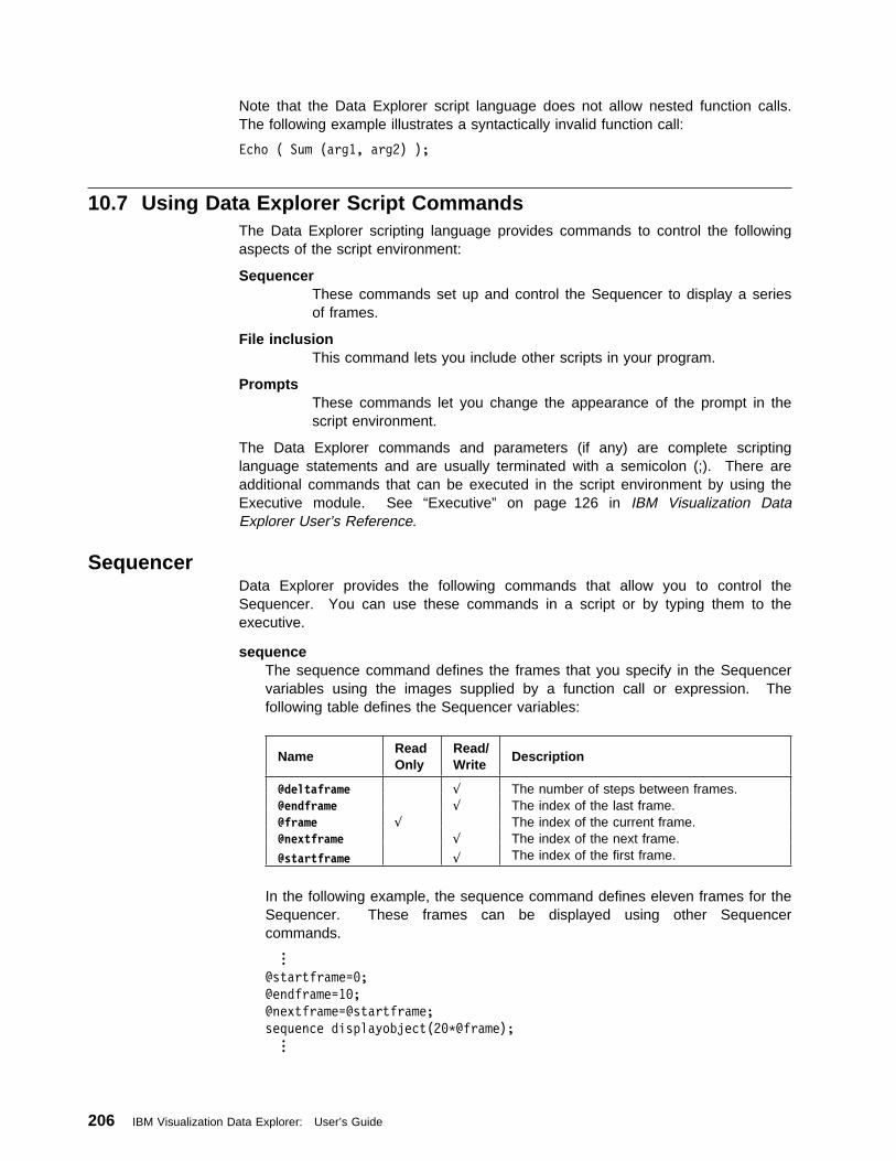
Note that the Data Explorer script language does not allow nested function calls.The following example illustrates a syntactically invalid function call:

Echo ( Sum (arg1, arg2) );

10.7 Using Data Explorer Script CommandsThe Data Explorer scripting language provides commands to control the followingaspects of the script environment:

SequencerThese commands set up and control the Sequencer to display a seriesof frames.

File inclusionThis command lets you include other scripts in your program.

PromptsThese commands let you change the appearance of the prompt in thescript environment.

The Data Explorer commands and parameters (if any) are complete scriptinglanguage statements and are usually terminated with a semicolon (;). There areadditional commands that can be executed in the script environment by using theExecutive module. See “Executive” on page 126 in IBM Visualization DataExplorer User’s Reference.

SequencerData Explorer provides the following commands that allow you to control theSequencer. You can use these commands in a script or by typing them to theexecutive.

sequenceThe sequence command defines the frames that you specify in the Sequencervariables using the images supplied by a function call or expression. Thefollowing table defines the Sequencer variables:

In the following example, the sequence command defines eleven frames for theSequencer. These frames can be displayed using other Sequencercommands....

@startframe=ð;

@endframe=1ð;

@nextframe=@startframe;

sequence displayobject(2ð\@frame);...

NameReadOnly

Read/Write

Description

@deltaframe √ The number of steps between frames.@endframe √ The index of the last frame.@frame √ The index of the current frame.@nextframe √ The index of the next frame.

@startframe √ The index of the first frame.

206 IBM Visualization Data Explorer: User’s Guide

playThis command begins execution on the frames that have been defined with thesequence command.

pauseThis command stops the sequence at the current frame.

stepThis command displays the next frame in the current sequence direction.

stopThis command stops the sequence display and returns to the first frame in thesequence.

forwardThis command sets the forward direction of the sequence.

backwardThis command sets the backward direction of the sequence.

'palindrome on' | offThe palindrome command with its parameters sets or unsets the palindromemode. When you display frames in the palindrome mode, the current directionchanges at the first or last frame in the series.

'loop on' | offThe loop command with its parameters sets or unsets the loop mode. Whenyou display frames in the loop mode, the series of frames repeats using thesettings of the forward, backward, and palindrome commands.

Scripting Language

File Inclusioninclude

The include command is used to interpose the contents of a file into the inputstream being sent to Data Explorer. The file being included can contain bothscripting language constructs and executive commands. This means anincluded file can, in turn, include other files.

There is currently a limit of 32 nested levels of inclusion, after which theinclude commands are ignored.

To include the file my.script, issue the following command:

include "my.script"

Prompts@prompt and @cprompt

There are two at-sign (@) variables that you can set in the executive (or in ascript) to customize the Data Explorer script prompt (@prompt) and continuationprompt (@cprompt). (The continuation prompt appears when you enter anincomplete command in the script environment. It indicates that you mustcomplete the command before it can be acted upon.)

The default prompt and continuation prompt are dx> and > respectively.

The following example show how to set these variables. Note that thisexample shows the Data Explorer prompts as they would be displayed in theexecutive.

Chapter 10. Data Explorer Scripting Language 207

dx> @prompt = "DATA EXPLORER>";

DATA EXPLORER> @cprompt = " more>";

If, after these commands, an incomplete statement was entered, Data Explorerwould respond as follows:

DATA EXPLORER> a =

more> 3 \ 5;

10.8 Understanding the Script Execution ModelAn execution model is applied to the constructs defined by the Data Explorerscripting language. This model consists of the environment structure that ismaintained during function calls, the behavior associated with macro expansions,the scope rules used for locating the value associated with a variable, and thesemantics associated with assignment statements and function calls.

Top-level EnvironmentAll global assignment statements and initial function invocations occur in thetop-level environment. This environment is special in that all assignmentstatements and function invocations initiated in this environment are alwaysexecuted.

Function ExecutionWhen either a macro or a module function is executed, a new dynamically scopedenvironment specific to that function call is created. Variables that correspond tothe function’s input and output formal parameters are created in this newenvironment. The variables corresponding to the output formal parameters areinitialized to NULL. Those variables corresponding to the input formal parametersare initialized in the manner described in the preceding section. If an input and anoutput formal parameter both have the same name, then they share a singleparameter and are initialized to the value passed as input when the function iscalled.

Macro ExpansionWhen the function being called is a macro, the macro is effectively expanded in-lineafter first constructing the necessary environment for its input and outputparameters. This guarantees that the partial orderings defined by macros aremaintained.

Variables Used in MacrosThe Data Explorer allows you to use variables on both the left and right sides of afunction assignment; that is, as both left-side and right-side.

Variables as Left-Side ValuesAll assignments in a macro’s environment affect variables that are local to themacro. These variables, if they do not already exist, are created in the macro’senvironment when they are first used on the left-hand side of an assignmentexpression. Thus, a variable outside of a macro cannot be modified with thatmacro.

208 IBM Visualization Data Explorer: User’s Guide

The only way to make such a change is to propagate a new value out of the macrousing its output formal parameters, and to use this returned value in an assignmentstatement in the enclosing environment.

Given these semantics, it is possible for a local version of a variable to come intoexistence and obscure a more global version of a variable, midway through amacro’s execution.

Scripting Language

Variables as Right-Side ValuesThe values of variables used in a macro in expressions and as function argumentsare found according to standard dynamic scoping rules. If the variable exists in themacro’s local environment, then its value is used. Otherwise, the enclosingenvironments, all the way to the top-level environment, are searched to locate thevariable. The value used is the value associated with the first instance of thevariable. If the variable is not found in any environment, then the value NULL isused.

ExampleThe following is a sample script that illustrates how variables are treated in macros:

// This is a complete sample script

macro add(a, b) -> (sum)

c = a + b; // c is created and given the value a+b

c = a + x; // x is found in the top level, and used in this expression

c = a + z; // z does not exist anywhere; NULL is used

sum = a + b; // sum is created local to the macro, separate from the

// version of sum in the top level

x = 7;

sum = 1ð;

total = add(4, 4); // total = 8, sum stays at 1ð

Assignment and Function Call SemanticsAs stated earlier, all assignment statements and function calls initiated at thetop-level environment are executed. In a macro, the process is slightly different.When a macro is expanded, its statements are first analyzed to determine whetherthey need to be executed. The rule of thumb for determining if a statement will beexecuted is that it must contribute, either directly or indirectly, to:

One of the values passed into a module that has a side effect A value assigned to a top-level variable, using a macro’s formal output

parameters.

There are two kinds of “side effect” modules:

Those that do not produce any Object outputs. Display and WriteImage areexamples of this kind of module because they modify things such as monitorsand files, which are outside of the language’s domain and control. This type ofmodule is represented in the graphical user interface as having no output tabs.

Those that make use of internal executive features. These modules arespecially marked in their .mdf (module description) files as ones that can causeside effects.

Chapter 10. Data Explorer Scripting Language 209

Side effect modules are always executed. (For information on the SIDE_EFFECTflag, see 10.1, “Module Description Files” on page 80 in IBM Visualization DataExplorer Programmer’s Reference.)

Execution ExampleThe macro sum3 in the following example computes both the sum of its first twoarguments and the sum of all three of its arguments. When the top-levelassignment statement on line 7 is executed, the statements in lines 3 and 4 areboth executed, resulting in the values 11 and 111 being assigned to the top-levelvariables x and y respectively. When the top-level assignment statement on line 8is executed, only the statement on line 3 is executed. Since the value in the outputvariable e is not assigned to anything in the calling environment, the statement online 4 need not be executed.

macro sum3 (a, b, c) -> (d, e) // 1

// 2

d = a + b; // 3

e = d + c; // 4

// 5

// 6

x, y = sum3 (1, 1ð, 1ðð); // 7

x = sum3 (1, 1ð, 1ðð); // 8

10.9 Running .net files in script modeWhen you create a visual program using the User Interface, the .net file saved is ascript, so you can run it in script mode. (User Interface-specific information, such asplacement of tools on the canvas, is saved as comments in the script.) If you havea sequencer in your visual program, the User Interface adds a “play” command asthe last line of the .net file. Thus you can edit this line out and add your ownoptions if you want to do something other than play forward through the sequenceonce (see “Sequencer” on page 206). If you do not have a sequencer in yourvisual program, the User Interface adds a call to “main()”, the main macro which isdefined to be your top level visual program. If you do not want the program toautomatically execute when you read it in as a script, remove or comment out thecall to “main()”.

If your visual program uses macros, the user interface will add an “include” line sothat the macros will be included when the visual program is run as a script. Youcan look at the top of the .net file to see which macros are referenced by theprogram. Thus if you need to send a collection of visual programs and macros toanother person, this can help you to make sure you have sent all the necessarytools.

210 IBM Visualization Data Explorer: User’s Guide

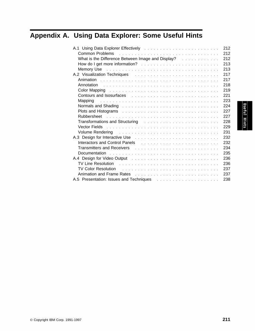
Appendix A. Using Data Explorer: Some Useful Hints

A.1 Using Data Explorer Effectively . . . . . . . . . . . . . . . . . . . . . . . . 212Common Problems . . . . . . . . . . . . . . . . . . . . . . . . . . . . . . . . 212What is the Difference Between Image and Display? . . . . . . . . . . . . 212How do I get more information? . . . . . . . . . . . . . . . . . . . . . . . . . 213Memory Use . . . . . . . . . . . . . . . . . . . . . . . . . . . . . . . . . . . . 213

A.2 Visualization Techniques . . . . . . . . . . . . . . . . . . . . . . . . . . . 217Animation . . . . . . . . . . . . . . . . . . . . . . . . . . . . . . . . . . . . . . 217Annotation . . . . . . . . . . . . . . . . . . . . . . . . . . . . . . . . . . . . . 218Color Mapping . . . . . . . . . . . . . . . . . . . . . . . . . . . . . . . . . . . 219Contours and Isosurfaces . . . . . . . . . . . . . . . . . . . . . . . . . . . . 221Mapping . . . . . . . . . . . . . . . . . . . . . . . . . . . . . . . . . . . . . . 223Normals and Shading . . . . . . . . . . . . . . . . . . . . . . . . . . . . . . . 224Plots and Histograms . . . . . . . . . . . . . . . . . . . . . . . . . . . . . . . 227Rubbersheet . . . . . . . . . . . . . . . . . . . . . . . . . . . . . . . . . . . . 227Transformations and Structuring . . . . . . . . . . . . . . . . . . . . . . . . 228Vector Fields . . . . . . . . . . . . . . . . . . . . . . . . . . . . . . . . . . . . 229Volume Rendering . . . . . . . . . . . . . . . . . . . . . . . . . . . . . . . . 231

A.3 Design for Interactive Use . . . . . . . . . . . . . . . . . . . . . . . . . . . 232Interactors and Control Panels . . . . . . . . . . . . . . . . . . . . . . . . . 232Transmitters and Receivers . . . . . . . . . . . . . . . . . . . . . . . . . . . 234Documentation . . . . . . . . . . . . . . . . . . . . . . . . . . . . . . . . . . . 235

A.4 Design for Video Output . . . . . . . . . . . . . . . . . . . . . . . . . . . . 236TV Line Resolution . . . . . . . . . . . . . . . . . . . . . . . . . . . . . . . . 236TV Color Resolution . . . . . . . . . . . . . . . . . . . . . . . . . . . . . . . 237Animation and Frame Rates . . . . . . . . . . . . . . . . . . . . . . . . . . . 237

A.5 Presentation: Issues and Techniques . . . . . . . . . . . . . . . . . . . . 238

Useful Hints

Copyright IBM Corp. 1991-1997 211

A.1 Using Data Explorer EffectivelyFollowing are some hints for using Data Explorer more effectively, debugging visualprograms, and using memory efficiently.

Common Problems

DebuggingOne of the most useful tools for debugging visual programs is the Print module.For example, if you are getting an error from a module that a particular field isinappropriate for processing, you can print out the object to see if it is what youexpect it to be. Print can be used to see the structure of and data values in anyobject. The options parameter is used to set the level of detail printed: the default“o” prints just the top level object: for example “Field with 4 (four) components.” Ifoptions is set to “r,” more information about each component is printed, forexample, how many items in each component, and the data type. You can alsoprint out some or all of the values in the components.

The output of Print appears in the Message window.

Stopping ExecutionThere are two ways to stop execution of a visual program:

End Execution in the Execute menu stops execution after the currentlyexecuting module has finished.

Disconnect from Server in the Connection menu kills the Data Explorerexecutive (not the user interface) immediately. You can restart, using StartServer in the Connection menu.

In addition, modifying a visual program (for example by disconnecting an arc oradding a new tool) will cause execution to stop after the currently executingmodule.

How to orient yourself in the Image windowIf you find yourself “lost” in the Image window; for example, you have a blackpicture and don't know where your data object is, you can always “reset thecamera” by using the Reset Camera option in the View Control dialog box of theImage window. This zooms out so that you can see all of your object, from a “frontand center” view.

It is also often helpful to use ShowBox to display the bounding box of your entiredata set. Collect this with the rest of your visualization, and then you will be able tosee how the part you are looking at relates to the entire data set.

What is the Difference Between Image and Display?Image, Display, and Render all render an object (i.e. create an image).

Render, given an object and a camera, creates as output an image. This imagecan be sent directly to Display for display to the screen, sent to WriteImage to bewritten to a file, or collected with other images into a single window using Arrange.

Display, given an object and a camera, both renders the object (using the camera)and displays it to the screen.

212 IBM Visualization Data Explorer: User’s Guide

Display, given only an image, simply displays it to the screen.

Image, given an object, renders it and displays it to the screen. The camerainformation is provided via direct interactors (rotate, zoom, etc.) or through thecamera mode option in the View Control dialog box. Image has two outputs: theobject to be rendered (including any AutoAxes that may have been added via menuchoices) and the camera used.

You would use Render if you needed the image itself, for example, for the Arrangeor Filter modules, or if you wanted to use WriteImage. (For the Image tool, theWriteImage function is available through the Save Image and Print Imagecommands in the Image window, or through the hidden recordEnable,recordFormat, and recordFile parameters to the Image tool).

You would use Display without a camera if your object is already an image, andyou simply want to display it. You do not need (or want) to render it. You wouldalso use Display without a camera to display a set of Arranged images.

You would use Display with a camera if you wanted to directly control the camera,for example, for a computed fly-through path. You would also use Display if youwanted to define your own direct interaction modes (see “SuperviseWindow” onpage 336 and “SuperviseState” on page 332 in IBM Visualization Data ExplorerUser’s Reference), rather than using the predefined direct interaction modes of theImage tool.

Useful Hints

How do I get more information? In the Help Menu:

– Application Comment presents comments (if provided) on the current visualprogram.

– Table of Contents presents the table of contents of the userdocumentation. You can use hypertext links to go to a particular topic.

– Context-Sensitive Help presents a “?” cursor: just click on a tool icon orother feature to learn more.

Samples:– Sample Visual Programs: /usr/lpp/dx/samples/programs. See also the

subdirectories there, grouped by topic.– Sample Scripts: /usr/lpp/dx/samples/scripts.

Information available electronically:– Data Explorer user group on the internet

(comp.graphics.apps.data-explorer)– DX Home Page on world wide web (http://www.almaden.ibm.com/dx/).– Data Explorer Repository at Cornell: anonymous ftp:

ftp.tc.cornell.edu. (look for directory pub/Data.Explorer).– gopher: ftp.tc.cornell.edu. port 70.

Memory Use

Appendix A. Using Data Explorer: Some Useful Hints 213

Data Explorer Object CacheData Explorer uses an object cache to store intermediate results of modules.Caching systems are intended to fill up and then reclaim memory by throwingthings out of the cache. The size of the cache defaults to a large percentage of thephysical memory on the machine. You can control the size of the cache with the-memory command line option to the dx command. The minimum cache sizeneeded is on the order of the maximum amount of memory required for a programexecution.

The Data Explorer “executive” schedules module execution. It does detailed graphanalysis, implements distributed processing of the modules, and implements theSwitch and Route modules. It also provides optimization by caching theintermediate outputs of modules. For example, if you run Import twice in a row withthe same inputs, Import will not actually run the second time, and instead theexecutive will use the cached output from the previous execution. The Image andDisplay tools also cache their images internally.

To implement the caching scheme, Data Explorer will allocate memory up to somefixed size. This memory is referred to as the arena. When the arena fills up andmore memory is required, Data Explorer looks for objects to discard from thecache. When it does this it may mean that subsequent executions will have toexecute larger portions of the program.

The arena is of fixed size for any one instance of Data Explorer. The size of thisarena is chosen by default based on the size of the physical memory in the system.

For some data sets, the default arena size will not be sufficient. In those cases,one can use the -memory option to increase the size of the arena, with the limitationthat your can't increase the arena size to be larger than the amount of real plusvirtual memory (page or swap space) on your machine. Talk to your systemadministrator if you think you need to increase the amount of swap space on yoursystem.

Reducing Memory RequirementsIf, after using the -memory option as described above, you find you still lacksufficient memory to perform your visualization, there are a number of strategiesthat can be used to reduce the amount of memory that is required by your program.

Do Not Render Images: A common mistake is to render image data (i.e.2-dimensional grids) using Render, Image, or Display with a camera input. Thisresults in Data Explorer interpreting the image as a very large number of quads, inwhich case much memory and CPU is used.

Instead, one can AutoColor or Color the image and pass it directly to Display(without a camera input), or for even more memory savings, convert the data tounsigned bytes (see below) and AutoColor or Color the data with delayed colors(see below).

Delayed Colors: If you are coloring your objects (using AutoColor,AutoGrayScale, or Colormap/Color), you might want to use “delayed” colors.

To do this, convert the data component to unsigned bytes and set the “delayed”parameter of the coloring module to 1. Using delayed colors means that rather

214 IBM Visualization Data Explorer: User’s Guide

than a 3-vector being used for each data point, a single scalar byte is used to indexinto a color table with 256 entries.

If you are using ReadImage, you may want to set the DXDELAYEDCOLORSenvironment variable. See “ReadImage” on page 250 in IBM Visualization DataExplorer User’s Reference.

Converting Data Types: In many cases it may be acceptable to convert yourdata components to smaller sized types using Compute. For example, you mightchange your floating point data to bytes. This has the advantage that alldownstream modules will require less memory.

Working with Series Data: When working with series data, if you are importingthe entire series and then selecting members out of the series, it may be that yourprogram can be changed so that you only import one member at a time. Do thisusing the start and end parameters to Import.

This reduces memory requirements by not having the whole series in memory atonce.

Glyphs: If you are using glyphs (AutoGlyph or Glyph), you may want to use less“spiffy” glyphs. A less spiffy glyph is one that has fewer positions and connections(facets), and therefore consumes less memory. To use less spiffy glyphs, use thetype parameter of either AutoGlyph or Glyph, and set it to “speedy” or to a smallfraction of 1.

Reducing Grid Resolution: If you can sacrifice resolution in your data set, youmay want to use the Reduce module (usually just after Import) to reduce thenumber of points in your data set. Reduce filters the data set before reducing thenumber of points. Remember that it is of little use to process 5000x5000 points ifyour final image is only 1000x1000 pixels.

24-Bit Images: You can create 24-bit images (instead of the default 96-bitimages) by setting the environment variable DXPIXELTYPE to DXByte. See“ReadImage” on page 250 and “Render” on page 264 in IBM Visualization DataExplorer User’s Reference.

Cache Control: Executive: In general, it is not necessary to change how theexecutive caches intermediate results. However, in a few cases, it may beadvantageous to do so. For example, if you are reading a live data feed into yourprogram, it is probably not necessary to cache the downstream outputs.

You can change how and if the executive caches intermediate output values byopening the Configuration dialog box of a module and changing the option menu tothe right of each output. You can also choose Output Cacheability from the Editmenu of the VPE, and set the cacheability of a group of modules, show thecacheability of a group of modules, or ask Data Explorer to use a heuristic toautomatically optimize the caching for the current visual program.

In general, it is most efficient to cache only the results of the last module in a singlefile line of modules; for example to cache the output of Isosurface, but not Import.Note that if you do this, however, if you need to change the isosurface value, thedata file will need to be reimported, slowing execution.

Useful Hints

Appendix A. Using Data Explorer: Some Useful Hints 215

If you want to turn off caching altogether you can use the -cache off

command-line option to Data Explorer.

Cache Control: Display: Some modules use the caching system to cache theirown data. The Display and Image tools are such tools. When using softwarerendering, they cache the images they display in the X windows. This is anoptimization that can be seen when using the Sequencer. When this tool startsrepeating itself (in loop or palindrome mode), the images are displayed much faster.That is, Display (or Image) is pulling them out of the cache instead of rerenderingthe input objects each time. You can observe this effect by running the exampleprogram MovingCamera.net with software rendering.

Most of the time this caching behavior is desirable, but in some cases it is betterturned off. To do that, use the Options module to add a “cache” attribute with theinteger value of 0 (zero), as follows:

o = Options(o, "cache", ð);

Display(o, camera);

The Image tool’s Configuration dialog box has an option menu that lets you controlits caching. This can be useful when one is running a batch job to generate ananimation in which none of the frames will be displayed a second time.

Note that the -cache off command line option mentioned above has no effect onthe internal caching that modules themselves perform.

Note: You can use the Data Explorer command line option -optimize memory,which will automatically set the DXDELAYEDCOLORS and DXPIXELTYPEenvironment variable to the options that consume the least memory. Thealternative is -optimize precision.

System TuningDefault Memory Size: Except where noted in the architecture-specific README(in /usr/lpp/dx), by default Data Explorer will be allowed to grow to use all but 8megabytes of the physical memory when there is less than 64 megabytes ofphysical memory.

If there are more than 64 megabytes of physical memory, then Data Explorer will,by default, be allowed to grow to 7/8 of the amount of physical memory.

Users may wish to alter this default amount of memory by using the -memory optionto the dx command, or the “Memory” field of the Connect to Server Options dialogbox.

Paging Space: Since it is possible for Data Explorer to use a large amount ofvirtual memory, users should configure systems with paging space at least two orthree times the total physical memory in their system.

If you do not have enough paging space, the operating system may kill DataExplorer (or other processes), sometimes without warning, depending on thearchitecture. Your system administrator can increase your paging space.

Per Process Limits: Some systems may enforce per process limits on suchthings as data segment size, stack size and so forth. These may need to beadjusted to run Data Explorer with large amounts of memory to avoid paging. Yoursystem administrator can adjust your per-process limits.

216 IBM Visualization Data Explorer: User’s Guide

A.2 Visualization TechniquesNow we have our data in a Field Object inside Data Explorer. What can we dowith it? This section discusses some common visualization techniques and theData Explorer modules associated with them:

“Animation” “Annotation” on page 218 “Color Mapping” on page 219 “Contours and Isosurfaces” on page 221 “Mapping” on page 223 “Normals and Shading” on page 224 “Plots and Histograms” on page 227 “Rubbersheet” on page 227 “Transformations and Structuring” on page 228 “Vector Fields” on page 229 “Volume Rendering” on page 231.

Useful Hints AnimationThe Sequencer tool is the primary device used in Data Explorer to produceanimation or motion control. There are two basic types of animation: show a seriesof steps one after another, or, cause an object to move or rotate or change scale inorder to study it from different points of view.

Since many data sets are measured at a series of different times, your data mayhave a “time value” associated with each measurement set. There are two ways toread in these time step data files in order to study the dynamic process you havemeasured.

In one scheme, you can collect all your data files into a Series, a special Group ofFields understood by Data Explorer. Each Series member can represent a datacollection event at a certain time. Series do not have to be based on time; youmay have a set of experimental measurements made at different voltages (e.g., avoltage series). Each series member is assumed to have the same type (scalar,vector, etc.) and the same dimensionality (2-D, 3-D, etc.), but the data and eventhe grid size or number of connections and positions may be different for eachSeries member. The Series Field is described in detail in “Series Groups” onpage 35. Series “values” do not have to be continuous but may represent usefulinformation like the actual voltage setting for that Series entry (0.04, 2.3, 13.4).Series members are accessed by their ordinal position, starting at 0, regardless oftheir “value.”

Another way to organize a collection of associated data files is to create individualfiles for each time step (or voltage measurement, etc.). Give each file a filenamecontaining an ordinal number so you can access them easily with a computerprogram (e.g., myfield.001.dx, myfield.002.dx, and so on). Each file will contain theField to be imported at each time step.

In either case (Series Field or separately numbered files), you can control when aparticular time step is visualized in a visual program using the Sequencer tool. Thistool emits a series of integers. You set the minimum, maximum, and increment, aswell as choosing to start at a specific number (so you can jump ahead in the seriesif you like). The Sequencer can be connected to the Import module to specifywhich Series member to read in from the specified input file at the next iteration.

Appendix A. Using Data Explorer: Some Useful Hints 217

Alternately, you could Import the Series Group file with Import, then use the Selectmodule. Select takes an integer input (from Sequencer, for example) to choose theappropriate series member.

If you choose to use separate files for separate data samples, you would likelywant to use the Sequencer as an input to a Format module. The Format modulecould construct the filename with a format string like %s%ð3d%s along with threeinputs, “myfield.”, the output of the Sequencer, and “.dx”. Then, when theSequencer emits the integer “2”, the output string from Format becomes“myfield.002.dx”. This can be fed into Import as the name of the .dx file to read.The result is that you can use the Sequencer to specify either any specific file or awhole series of files to import and image one after another.

Another common type of animation is to use the Sequencer to control objectmotion. Usually, this requires that you run the output of Sequencer through at leastone Compute module. For instance, you can rotate an object around the Y-axisone full revolution by employing the Rotate module. The smaller the angularincrement, the smoother the animation will appear, but there is a trade-off inapparent motion rate if your graphics workstation is not very fast. So you mayhave to adjust the incremental angular amount to your liking.

You will find the technique of wiring Interactors to Compute modules useful forconverting the output of Sequencer to arbitrary floating-point values. If you wantedto vary the Scale of your object using the Scale module, it might be moreconvenient to adjust the scale in increments of 0.01. With a little thought, you canextend this idea so that the same (one and only) Sequencer integer series can beconverted into several different series of numbers that can simultaneously rotate,scale, and read in different time steps of data. Just a caution, though: too muchchanging at the same time will probably not help you visualize your data, butinstead will cause confusion. Is the object getting bigger because the data valuesare increasing, or because you are changing the scale, or because you are movingthe object closer to you with Translate? When you start out, keep your animationssimple and they will be much more effective.

AnnotationIt is imperative that good visualizations contain sufficient annotation for a viewer toderive appropriate information from the imagery. A colored height field orstreamline set with no supporting labeling can make perfectly beautiful, utterlymeaningless computer graphics.

Annotating a scene can be done in several ways using Data Explorer modules.You can, for example, provide a ColorBar with numeric values automatically labelednext to the related colors, show Text or Caption information to provide textualdescriptions of objects, or turn on AutoAxes to show neatly labeled and numberedaxes around the perimeter of your data space.

Using the Format module, it is possible to create “clocks” or other “meters.” Formatcreates a formatted string of text suitable for Caption or Text modules to display.Format takes a “template” and text strings and/or numbers as value inputs andassembles an informative text string as output. For example, inputting theminimum value of your data to the first value input (the second input tab) of aFormat module, you could create a Caption that reads:

Minimum temperature = ð.ð deg.

218 IBM Visualization Data Explorer: User’s Guide

To do this, the “template” inside the Format module would read:

Minimum temperature = %1.1f deg.

In this template, the “%1.1f” serves as a place holder for the first value (which mustbe floating point) provided to Format; consequently, the minimum value argument issubstituted into the string when the visual program is executed. The “1.1” meansthat the floating-point number should display at least one number to the left of thedecimal point but should round off to only one decimal place to the right of thedecimal. By tying the data Field to Statistics (Transformation category), you caneasily extract the minimum value of the data; use this as the second input toFormat. If you later input a different data set with a different minimum, Caption willautomatically change to reflect the new minimum value.

One trick for showing text together with numbers that are changing is to use a“fixed width” font instead of a “variable” or “proportional” font. Variable text looksbetter when making Captions that do not include changing values, but fixed widthtext maintains the same width regardless of the numeric characters currently beingdisplayed. Try both ways and you will see that the variable text has an annoyingshrinking-expanding effect as your clock or time step meter changes value. To getthe fixed text clock to behave correctly, you must use a Format template like“%03.2f” that allows for enough numbers to the left of the decimal point. In thisexample, we have predetermined that we will never create a number greater than999.99 (note that if we do go over 1000, the text will expand to show the wholenumber, causing the Caption string to expand: the very thing we are trying toavoid!). The “%03.2f” format makes floating-point numbers with 3 numerals beforethe decimal, including left side zero padding, and 2 numerals after the decimal.

Useful Hints

Color MappingData Explorer provides an automatically generated color map (AutoColor), anautomatically generated grayscale (AutoGrayScale), and a user-definable color map(the Colormap module that attaches to the Color module). A color map representsa relationship between a continuous range of floating point numeric data values anda set of color values. Frequently, you will encounter color maps with continuous(“spectral”) color tones like a rainbow, but there is no requirement that color mapsappear continuous. Each color map has associated with it a minimum and amaximum scalar value. You can either specify the minimum and maximum orconnect the data Field to the Colormap module and have these valuesautomatically extracted.

We can describe “color” to a computer in a number of ways. One of the moreintuitive is the “hue-saturation-value” model used by Data Explorer's Colormap tool.Hue is the color’s “name”, like blue, red, and so on. Hue is considered to form acircle from red through yellow, green, cyan, blue, magenta, and back to red; thinkof Hue as an “angle” around this color wheel (scaled from 0.0 to 1.0). Saturation isthe “richness” of a color. Decreasing the Saturation of a color from 1.0 to 0.0makes the color progressively more pastel, so for example, bright red becomeslight red, then pink, finally turning white. You can think of decreasing the Saturationas adding “white paint” to paint of a pure hue. At Saturation 0.0, any colorbecomes white (assuming Value is held at 1.0). Similarly, Value is a measure ofthe amount of “black paint” mixed with a color. As you decrease the color’s Valuefrom 1.0 to 0.0, you add more “black”, so bright red becomes progressively darkerred, and finally black. Any color becomes black at a Value of 0.0. All three of

Appendix A. Using Data Explorer: Some Useful Hints 219

these parameters interact, so you can adjust Hue and decrease Saturation andValue to get a “dark pastel blue.”

Another scheme for describing color is RGB (Red-Green-Blue). As in the HSVmodel just described, you specify a color as a triplet (a 3-vector). Each componentcan have a value from 0.0 to 1.0. If all three are 0.0, the resulting color is black; ifall three are 1.0, you get white. Given Red = 1.0, Green = 0.0, Blue = 0.0, thecolor is fully saturated bright red. You can observe a graph of RGB lines at the farleft of the Colormap tool as you manipulate the colors using theHue-Saturation-Value (HSV) controls. You can specify an RGB vector in the Colormodule in place of connecting a Colormap if you want the output object to have asingle color (or you can specify one of the X Window System color names). Andyou can convert from RGB to HSV or back using the Convert module. See “Color”on page 75 and “Colormap” on page 84 in IBM Visualization Data Explorer User’sReference for more details about these different specification schemes.

Let us assume that we have set the Colormap minimum and maximum to equal theminimum and maximum of the temperature data we collected in the atmosphere(this is done automatically if you connect the data Field to the input on Colormap).Recall that we collected position-dependent data, one temperature value at eachgrid position. For this example, assume the minimum temperature measured was 0degrees Centigrade and the maximum 20. What color is 10? That dependsentirely on the color map used. If we have a standard spectral (rainbow) map withblue at 0 and red at 20, then 10 would have a color halfway between blue and red.On the default color map, this would be green. When we ask Data Explorer tocolor-map our data, it examines each data value, performs a linear interpolationbetween the minimum and maximum values to find the color associated with thatinterpolated value in the color map and “colorizes” the object at all points containingthat data value with that color.

If we change the maximum value in the color map to 30, the measured data valueof 10 (taken from the same data set as above) will now map to a cyan color, partway between blue and green. On the other hand, we could keep our sameextreme values but manipulate the color map’s color distribution in such a way thatany value has any color we like. You can learn the details about this capability in6.3, “Using the Colormap Editor” on page 119.

The best way to learn about the power of color mapping is to take some sampledata, color-map it, then manipulate the settings in the Colormap Editor you haveconnected to the Color module your data Field passes through.

Note: Choose Execute on Change from the Colormap Editor Execute menu andyou will see the data change colors as soon as you make a change in theColormap Editor.)

For instance, you can create sharp color discontinuities by placing two controlpoints close together vertically on the Hue control line, then dragging onehorizontally away from the other. This can be used to indicate a sharp edgetransition in your data. It is sometimes useful to place a special contrasting color inthe middle of an otherwise continuous color map. For example, to highlight thevalue of 12 degrees C in our temperature data, we could insert a sharply definedred notch or band into the middle of our smooth rainbow color map. This wouldhighlight that particular value or range for someone examining the scene. You canautomatically generate a number of control point patterns by choosing GenerateWaveforms... from the Edit menu in the Colormap window. To make a notch,

220 IBM Visualization Data Explorer: User’s Guide

choose one of the “S” shaped curves from the pop-up menu in the GenerateWaveforms dialog box. Set the number of Steps to 4 to make a single notch, or 3 tomake a single step. Click Apply to place control points on the currently chosencurve (Hue, Saturation, Value, or Opacity). You can then drag the new controlpoints where you like.

If you use a red color notch in the middle of your data range, you probably will notwant to use red elsewhere in your color map or it will be difficult for a viewer to tellthe 12-degree specially highlighted red area from the 20-degree red maximumvalues (assuming 20 is the maximum). In fact, it might be safer to use a white orgray color to mark the special value of 12 degrees. Do this by creating a notch onthe Saturation or Value curves instead of on the Hue curve.

Similarly, you can change the opacity of objects. Opacity is the inverse oftransparency: that is, the more opaque the object, the less transparent. You canset opacity to a value between 0.0 and 1.0. Opacities less than 1.0 allow you tosee through an object to reveal objects inside or behind the transparent object. Forall objects except volumes, an Opacity of 0.0 will make the object disappearcompletely. Since Data Explorer uses an emissive volume rendering technique,you must set the color of a volume to “black” (RGB of [0, 0, 0]), as well as settingthe Opacity to 0.0, to make the volume disappear. You will notice that when youview slightly transparent objects through each other, the colors of each objectcombine, making it very difficult to accurately assess the color of any one object.Used sparingly, opacity is a very powerful tool for examining the insides of objectsor volumes and gauging the physical relationships between intersecting objects.

You can create a variable opacity on an object by manipulating the opacity curve inColormap. This can make parts of an object trail off to transparency, useful if somedata values are not of interest. Be aware that “hiding” data in this way maymislead someone viewing your results. But in some data sets, there may be alarge number of “noisy” data values that you would like to exclude in order to seethe “signal” data values of interest. In that case, setting an Opacity notch to hidethe noisy values may be the best visualization technique.

When you lower opacity below 1.0, you will see two stripes, one white and oneblack, or a checkerboard pattern of black and white behind the sample color strip inthe Colormap Editor. These are useful when you manipulate Opacity to check theapparent color against both a light and dark background. As with the color tools,you can turn on Execute On Change and interactively play with the Opacity of theselected object until you get the effect you want.

Useful Hints

Contours and IsosurfacesGiven a set of samples taken over a presumably continuous region, it is meaningfulto consider drawing smooth lines connecting together the locations on the gridcontaining the same data values. You are probably familiar with topographic mapsthat show contour lines connecting together the same values of elevation of theEarth’s surface features, such as hills and valleys. These lines are called “contourlines” or “isolines” (iso means “same” or “equal”). In most cases, the places on thesurface of the sample grid that have identical data values will not coincide with thegrid sample points. This is another case where the “connections” component isrequired for Data Explorer to determine where on the grid the same value occurs(say the value 5.2) in order to create lines connecting together all these locations.

Appendix A. Using Data Explorer: Some Useful Hints 221

To return to our 3-dimensional data set taken from the atmosphere. Since we havecollected data throughout a 3-dimensional space, we can identify volumetricelements defined by connecting adjacent grid sample points in three dimensionsusing a “connections” component like cubes. It now becomes possible to draw“isosurfaces” rather than “isolines.” An isosurface is that surface cutting through avolume on which all data values are equal to a specified value. Depending on theactual distribution of the data, isosurfaces may look more or less like flat sheets(the isosurface of “sea level” in a data set of elevations would look like this); itmight enclose a portion of our space or appear as a whole set of smalldisconnected surfaces or enclosed spaces.

To create an isosurface, we pick a value of interest. Suppose that according to ourknowledge of meteorology, we know that the dew point (at which water condensesfrom vapor to liquid) is 12 degrees C in our sample. Although we measuredtemperatures at only a fixed number of grid points, we are interested in seeingwhere rain formation may begin throughout the atmosphere. We could show onlythe sample points highlighted by themselves, but once again, we make areasonable assumption that we have taken discrete samples from a continuousnatural volume. In other words, rain formation will not simply occur at the limitedset of discrete points where we have sampled temperatures of 12 degrees C, but atall the points in between that are also at 12 degrees. How do we find all thosein-between points? By interpolating through the volumetric elements betweenadjacent sample points. And in fact, the Isosurface module will do thisautomatically.

The resulting isosurface will represent all values of 12 degrees C throughout ourvolume of sampled space. The actual image depends on the distribution of thedata, of course. If the outside of a rain cloud were at exactly 12 degrees C, wewould see a shape resembling a cloud in the sky. But if rain formed at an altitudewhere the temperature was 12 degrees C, we would instead expect to see a flatsheet. Or we may not know what to expect: that is one of the uses of visualization,as well—for discovery, not just for verification.

Generally, the vertices that describe the mesh positions of an isosurface will notcoincide with the original grid points. It is important to realize that an Isosurface isa new and valid Data Explorer Field with positions and connections and a datacomponent (in which all data values are identical). You can treat this Field just likeany data Field you have imported. Color mapping such a Field is not particularlyuseful since all the data values are identical, so you will get the same color forevery point.

To draw contour lines on a 2-dimensional grid, you also use the Isosurface module.Data Explorer figures out the dimensionality of the visualization by looking at theinput data. Thus, a biologist’s 2-D grid can be easily contour-mapped with thesame tool as a meteorologist’s 3-D volume, but the visual output will beappropriately different for the different inputs. Similar to Isosurface’s contour linesis the output of the Band module. This yields filled regions between contours;these bands can be colored by a color map or AutoColor to yield the kind of imagefrequently used to show temperature distributions on a weather map.

222 IBM Visualization Data Explorer: User’s Guide

MappingThere is a very useful module called Map in Data Explorer that permits you to“map” one data set onto a Field defined by another data set. For example, in ourrain cloud data, we have measured temperature and cloud-water density throughouta volume. We learned earlier how to make an isosurface of temperature equal to12 degrees C. Now it may be instructive to observe the cloud-water densityassociated with this temperature isosurface.

The operation we wish to perform is to use our temperature isosurface with itsarbitrary (data-defined) shape as a sampling surface to pick out the values ofcloudwater density as they occur throughout the volume. That is, conceptually, wewill dip the temperature isosurface into the cloudwater volume. Wherever theisosurface comes in contact with the cloudwater volume, the values that stick to theisosurface represent the values of cloudwater density that occur at that intersection.But remember that the isosurface was created using temperature data. Theisosurface of temperature (the input Field to Map in this example) had only onedata value (12 degrees C) at every position, but the mapped isosurface (the outputof Map) will contain arbitrary patches of data corresponding to the distribution ofcloudwater density. If we AutoColor this output isosurface, we will see an arbitrarygeometric surface with a patchy color scheme. The surface is the location of all 12degree temperatures, and the patchy color corresponds to the distribution ofdifferent cloudwater densities sampled on that surface. (Of course, if cloudwaterdensity happened to have the same value at all points on the 12-degreetemperature surface, we would see only one color.)

Naturally, you can do the opposite! First, make an isosurface of cloudwaterdensity, say at the mean value of density. The mean value of a Field is taken asthe default value by the Isosurface module: this is convenient when you startexploring a new data set and do not know what the extreme values are. Now mapthe temperature data onto the cloudwater isosurface. Run the output throughAutoColor. The result will look very different. This time, you have “dipped” thecloudwater isosurface into a “bucket” of temperature data. Once again, this servesas a reminder that you must indicate to an observer exactly what kind of operationyou performed if your visualization is to bear any meaning.

You can also dip the cloudwater isosurface into the temperature colors. To do this,first AutoColor the temperature data set. Then use Mark to “mark” the colors asdata (this temporarily renames the colors component to data, while saving theoriginal data component). Then use Map to map this marked Field into thecloudwater isosurface colors component. (It is necessary to mark the colors asdata before mapping because Map always maps from the data component). Anexample visual program that performs each of these mapping operations can befound in /usr/lpp/dx/samples/programs/UsingMap.net.

Note that we changed the order of the modules slightly in the third example. In thesecond case, we Mapped data values from the “map” Field (cloudwater density)onto the “input” Field (the temperature isosurface), then AutoColored the resultingField. In the third case, we AutoColored the “map” Field (temperature), thenmapped color values onto the “input” Field (cloudwater density). This illustratessome of the flexibility of both the Map module itself and Data Explorer in general.In this case, the output image would be similar whether you colored by temperaturethen mapped, or mapped temperature first, then colored by temperature. There willbe color differences if the range of values that mapped onto the isosurface isdifferent from the entire data range used to AutoColor the entire temperature Field.

Useful Hints

Appendix A. Using Data Explorer: Some Useful Hints 223

You could avoid this problem by substituting a Color and Colormap pair in place ofAutoColor, then connecting the original temperature Field to the input of theColormap. This would automatically lock the minimum and maximum to the entirerange of temperature, not just to the range of values that happened to fall on theisosurface.

But there are other cases in which commutative ordering of modules will yield aquite different visual output. For example, suppose we have a volumetric Fieldcontaining both vector data and a scalar data set. We can generate a series ofStreamlines through the vector Field, Map the scalar data from the volume throughwhich the Streamlines pass onto these lines, then AutoColor the lines according tothe scalar data. To make the lines easier to see, we employ the Tube module tocreate cylinders along the path of each streamline. The radius of the Tubes can beadjusted until we get the look we like. By performing the operations in that order,the original colors are carried from the lines out to the outside of the cylinders,resulting in distinct circumferential bands of color on the Tube surfaces.

Now, change the order: create Streamlines, then Tube the lines. This yieldsuncolored cylinders. At this point, we Map the scalar data values from thevolumetric Field in which the cylinders are embedded onto the surfaces of thecylinders, then AutoColor. This time, we will have patches of color on the cylinders,since it is highly unlikely that the volumetric data would lie in perfect rings aroundthe outside of the tubes.

Which of the above two representations is “correct”? Both are accurate. Whichyou choose to show depends on the point you are trying to make. In the first case,you are illustrating the values of data precisely as they occur along the Streamlines:the Tubes are used to make these very thin lines more visible. In the second case,you wish to sample the data volume at a specified radius away from a givenStreamline. By varying the radius of the Tubes, you can investigate phenomenasuch as the rate of change of the data Field as you move further away from theStreamline itself.

Normals and ShadingAnother Field component used in Data Explorer is the “normals” component.normals are unit vectors that tell the computer graphics program and the imagerenderer which direction is “up” or “out.” Several tools, like Isosurface,automatically create a normals component so you do not have to calculate thesenumbers yourself.

There are two types of normals provided in Data Explorer, “connections normals”and “positions normals”. Connection-based normals are vectors perpendicular toeach connection element on the surface. They are created by the Normals modulewhen you set the method input to “connections”. The resulting surface reveals theunderlying polygonal grid structure of your sample grid. Frequently, this is avaluable way to show your data, as any observer can then see the grid resolutiondirectly. At the same time, this surface can be colored or color mapped either byconnection-dependent or position-dependent data.

The other type of normals are created by the Normals module when you enter“positions” as the method (this is the default method, in fact). In this case, thesurface will be much smoother in appearance yielding a more aesthetically pleasingsurface at the expense of being able to directly perceive the grid resolution. It issometimes less confusing to use position normals in place of connection normals

224 IBM Visualization Data Explorer: User’s Guide

because the object is less “busy” looking. You must be the judge of what is theappropriate way to observe your own data. You can also show your data first withconnection normals, to illustrate the sample resolution, then switch to positionnormals in order to better show some other aspect of your data.

Normals are used by various modules in Data Explorer. One use of thisinformation is that it is required by the image renderer (the Image, Render, andDisplay modules all incorporate the image renderer) to calculate the amount anddirection of light falling on an object’s surface (we will discuss this in more detailbelow). Rubbersheet assumes that the input grid or line is flat (if there is no“normals” component in the input Field) and projects the values in a perpendiculardirection. However, you may wish to create your own normals or modify anexisting “normals” component (using the Compute module, for example) andRubbersheet will then use the modified normals to control the direction of projectionof the surface or line. After performing the Rubbersheet projection, you may wantto insert another Normals module. This will take the projected object and generatereal surface normals before rendering, resulting in better-looking shading on youprojected surface. See “RubberSheet” on page 277 in IBM Visualization DataExplorer User’s Reference for a full description.

Isosurface will also generate normals automatically; to do so, Isosurface eithercalculates or reads the previously calculated Field gradient (depending on thesetting of the gradient input flag). Therefore, the normals generated by Isosurfaceare not necessarily perpendicular to the connection elements generated by theIsosurface module, but better indicate the actual Field direction than simpleperpendicular normals.

If you wish to understand Normals better, you can use the Glyph module tovisualize them. First use Mark to mark the “normals” component. This makes DataExplorer treat the “normals” component as if it were the “data” component. Then,Glyph the Field. Finally, Unmark the normals to restore the previous datacomponent to its proper place. By showing the normals as vector glyphs inconjunction with a surface, you should be able to see how different modules, likeRubbersheet and Isosurface, deal with these vectors.

Normals are also useful in helping you determine the “inside” and “outside” of anobject. In addition to a “colors” component, which holds the color-mappedinformation for each data point in a Field, you can specify a “front colors” and a“back colors” component. Which is front and which is back is determined by thedirection of the normal for that vertex (position normals) or polygon (connectionnormals). By setting different colors for the inside and outside of a complicatedobject, you may be able to understand its shape better. This technique can also behelpful when you are trying to convert a connection list like a finite element meshinto Data Explorer form. If you accidentally describe the “winding” (rhymes with“binding”) of a polygonal face in the wrong order, the normal for that face will pointin the wrong direction. Setting “back colors” to red and “front colors” to white willclearly indicate which faces are pointing the wrong way.

The Shade module employs the “normals” component; it will make a “normals”component if it does not already exist. Shade allows you to set up the lighting ofyour objects to make them more “realistic” in appearance. That is to say, when weobserve a 3-dimensional object, the way light falls on the object is an important cueto our eyes that helps us understand the shape of the object. We expect thesurfaces of the object that are generally facing a light source to be brighter than

Useful Hints

Appendix A. Using Data Explorer: Some Useful Hints 225

those that face away. Data Explorer, like other computer graphics renderingprograms, takes the normal directions of the object surfaces into account whencalculating the angle between the object, the light(s) in the scene, and the viewer’seye point (the camera in the scene).

In the real world, different materials react to incident light differently. For example,many metals scatter light causing the “specular” reflection to be more spread outthan it is on shiny plastic surfaces. The specular highlight is the highlight (manytypes of cloth and other dull surfaces have no specular brightest spot on a shinysurface. Think of how the sun sometimes bounces off the hood of your car at justthe right angle and makes a bright sharp reflection. By adjusting the “specular” and“shininess” inputs to the Shade module, you can make your object appear moremetallic or more plastic. If you turn the specular value all the way to 0.0, youeliminate the specular reflection). This can be important if you are trying to makesense of color-mapped data, since the specular highlight will be a bright white areaon the surface of the object (assuming the incident light color is white). This whitespot or area could confuse a viewer who is trying to interpret the color mapping ofthe data.

Two other inputs in the Shade module (diffuse and ambient) are also used byData Explorer when it lights an object. Diffuse light is light emanating from a directlight source, like the default Light in any Data Explorer network, or from Lightmodules you place in your network. Think of diffuse light as the light coming froma light bulb and falling on an object surface, like a light in your office shining directlyon your desk. This property is called “diffuse” because it represents the way lightbounces off a surface, depending on the “roughness” of the surface. The rougherthe surface, the more the light rays are scattered (“diffused”). An extremely smoothsurface tends to bounce light more uniformly to the eye. Ambient light is light thatis indirect: for example, daylight coming through a window, bouncing off white wallsand then impinging on your desk. Data Explorer automatically places anAmbientLight value in any scene, or you can override this value by placing yourown AmbientLight module in a network. Ambient light is best thought of as a sortof “glow” emanating from a non-point source of light and therefore illuminating eventhe parts of objects that face away from the point light sources in a scene. If youremove the ambient light, the apparent “shadows” on an object lit only by a pointsource of light are much harsher.

Like Normals, the Shade module can light an object in two fundamentally differentways. If you enter “smooth” in the how input to Shade, the surface will appearsmoothly rounded (assuming it is not completely flat to start with). This isequivalent to setting “positions” in a Normals module. Shade will, if necessary,create position normals, then light the object accordingly. Any point on aconnection between positions will be lit by calculating an interpolated normal valuebetween the position normals. If you choose faceted in Shade, the effect is thesame as selecting “connections” in the Normals module. In this case, eachconnection element has one normal direction over the entire face. As a result,every point on a connection element reflects light exactly the same way. Theimage that you see will thus show faceted polygons. Once again, while this maymake the object look less “realistic,” it does more accurately reflect the samplingresolution of your data and may therefore be a more desirable image to show otherviewers.

226 IBM Visualization Data Explorer: User’s Guide

Plots and HistogramsData Explorer provides a Plot module that will give you a simple 2-D graphics plotof your data. This can be convenient for showing one parameter plotted“traditionally” while you show a colored 3-D height Field illustrating the same orother parameters, in the same scene.

Histogram regroups your data into a specified number of bins (it acts like a form offilter on your data). The output of Histogram is a new Field withconnection-dependent data. The connections are the bars on the histogram (whichcan be plotted). The height of each histogram bar is proportional to the number ofsamples of original data that occur in the range covered by that bar. You can feedthe output of Histogram through AutoColor then Plot to get a colored plot of thedata distribution.

If the aspect ratio of the Plot is distorted, you can correct it in the Plot module.This will stretch the Plot out in either the X or the Y direction until you achieve thelook you want. Visual designers recommend an aspect ratio of approximately 4units wide to 3 units high; since this is also the aspect ratio of television, yourimage will be ready both for video and for print.

Be aware that “binning” your data with Histogram can sometimes create ratherarbitrary distributions. It is important to make this clear to the viewer of yourvisualization. For example, by carefully selecting bin size, you may turn a unimodaldistribution into a bimodal one. Which distribution is correct for the phenomenonunder study must be determined by the underlying science, not by the arbitrarypicture you create.

On the other hand, if you wish to actually redistribute your data rather than justshow a histogram of its distribution, you can use the Equalize module. The outputof this module is essentially the same scalar Field you fed into it, but the datavalues have been changed to fit the specified distribution. By default, the datavalues are changed to approximate a uniform distribution, but you can create yourown custom distribution, like a normal Gaussian curve. Equalize is useful to reduceextreme values back to a range similar to the majority of data values. You mayalso wish to experiment with other data “compression” and “expansion” techniquesby connecting your data Field to Compute and applying a function like “ln(a)” or“a^2”, where “a” is the input Field.

Useful Hints

RubbersheetAnother technique used to visualize data collected on a 2-dimensional grid issometimes called a “height map.” In Data Explorer, the Rubbersheet module willgenerate this for you. Conceptually, a height map is drawn by elevating the 2-Dgrid into the third dimension. Call it the Z dimension, with our original grid lying inthe X-Y plane. The height or Z-value given to each vertex of the original grid isproportional to the specified scalar data value at that vertex. If the data werevector data, you could elevate the grid by the magnitude of the vector, sincemagnitude is a scalar value. The result usually resembles something akin to arelief map of the surface of the Earth with hills and valleys.

However, this brings up an important point that will occur elsewhere in DataExplorer (and visualization in general). Remember that the original data werecollected on the X-Y plane (for example, our grass-counting botanist’s data). It isone thing to indicate the different distributions of grass species by showing a 3-D

Appendix A. Using Data Explorer: Some Useful Hints 227

plot of the numbers using a height map. But it is not correct to say, then, that thedata values so shown were collected from these 3-dimensional positions: thatwould imply the botanist counted grass species growing in mid-air! This might betrue in the Amazon, but not in Kansas.

That is, we may have counted 2 species at the grid point [x=0, y=0]. If weRubbersheet using the species count as the Z deflection value, our 3-D height mapwill now have a point at [x=0,y=0, z=2] (if the Rubbersheet “scale” is 1.0 and theminimum count in our data set is 0). The data was not collected at that point butrather at [x=0,y=0, (z=0)]. For our convenience, Data Explorer maintains theoriginal data values as if they were attached to the original grid. It is yourresponsibility to remember and, if necessary, make it clear to other viewers that therepresentation of the data in 3-D is not a “realistic” image of the original 2-Dsampling space. Rather, Rubbersheet is used to visualize the “ups and downs” inthe data Field as actual differences in height. This is a very powerful visualizationtechnique because of our familiarity with actual heights in everyday experience.One simple way to show viewers the difference is to make two copies of the Fieldby taking two wires from the output tab of the Import module you use to import thedata Field. Connect one wire to a Color module with a Colormap attached, butleave the Field 2-dimensional. Arrange the 2-D colored grid such that the viewer islooking straight down on it. Connect the second wire from Import to Rubbersheetand then use a second Color module, but run wires from the same Colormap asyou used to color the first copy. The second copy, a 3-D colored “height Field”,can then be rotated into a “perspective” view. The result will be a Field bothcolorized according to the data values and also elevated into the third dimensionaccording the same data values. This redundancy is often more instructive thaneither visualization technique used alone.

Transformations and StructuringRotate, Scale, Translate, and Transform are all special types of operations thatchange the location, orientation, or size of objects in your scene. These operationscan be performed anywhere in a visual program. You can create “hierarchical”motion by attaching Rotates and Translates to individual objects, then Collect theseobjects together and attach another Rotate and Translate to the Group (output ofCollect). In this fashion, you can individually rotate members of the groupindependently of each other, or you can rotate the entire group as one.

By default, many modules operate on the “data” component. We have beentreating “data” as a special kind of numeric Array, separate from “positions” and“connections”. We mentioned earlier that you can have several different “data”components, but each must have a unique name; for example, your input data filecan contain “positions”, “connections”, “temperature” (data), and “wind” (data). Forthis example, assume that “wind” is a 3-D vector.

Using the Structuring category tools Mark and Unmark, you can convert any Fieldcomponent into the “data” component. When you Mark “wind” for example, the old“data” component (if any) is moved into a safe place called “saved data” and the“wind” values are copied into the “data” component. Since “wind” is a 3-D vector,the new (current) data component becomes a 3-D vector also. The Computemodule is used to make changes in the data component of a Field. So bymultiplying the first (x) component of our 3-D “data” we are, in effect, scaling in X.For example, the Compute expression in this case would be “[a.x * 2.0, a.y, a.z]” todouble the size of each x component of each “data” point while leaving the y and z

228 IBM Visualization Data Explorer: User’s Guide

components the same. Any module connected to the output of Compute will seethe scaled “wind” values as the “data” component of the Field. However, the oldunscaled “wind” values are still kept in memory, also. By connecting other modulesto the originally imported “wind” values, you still have access to those originalvalues, at the same time. To operate on the “temperature” data, first use Unmarkto return the “data” to the “wind” component. The result will be to place the scaled“wind” values into the “wind” component for all modules connected to the output ofUnmark. Unmark also copies back all values from “saved data” into the “data”component. Then, you can Mark “temperature” as “data” and perform operationson it, if you like.

Since “positions” are also 2-D or 3-D vectors, you can Mark “positions”, performoperations on the grid itself, then Unmark “positions” to perform operations on the“data”. With a little knowledge of the correct matrix operations, it is possible tosimulate the effects of rotations, translations, and scalings using this Marktechnique. You can warp flat grids into cylinders or polar coordinate systems orcreate more complex objects like cones. In fact, there are already many macrosavailable in the Data Explorer Repository that handle these types of operationsusing this technique, which you may wish to download and use yourself. (For theData Explorer Repository, see “Other sources of information” on page xxiv.)

Useful Hints

Vector FieldsVector-valued data sets occur very frequently in visualization. Data Explorer offersthree ways to visualize vector Fields: vector glyphs, streamlines, and streaklines.For this example, assume that we acquired data on wind velocity and direction inthe atmosphere.

Recall that a “glyph” is a visual object; a Field of glyphs is made by copying ageneric object, positioning each copy appropriately, and scaling or coloring eachcopy according to the data associated with that sample point. Vector glyphsresemble arrows or rockets and are generated for you by the Glyph or AutoGlyphmodules. A vector Field, like any Field, must have a positions component toidentify where the vector-valued data was sampled (even if the data isconnection-dependent, it still requires positions). For Glyph realizations, a“connections” component is not required, but it may exist if the Field contained it forother purposes. Of course, a data component containing a vector quantity isneeded. Each vector glyph will point in the direction of the vector given by thedatum at that point, with the base of the vector fixed at the vertex position (samplepoint) for position-dependent data. The base of the vector is located at the centerof the connection element for connection-dependent data. The length of eachvector glyph is scaled based on the vector “magnitude”, relative to all the othervectors in the data Field. Glyph and AutoGlyph offer a number of modifications youcan make to achieve the appearance you desire. The effect of glyphing a vectorField is to create a “porcupine” plot with lots of arrows sticking out in variousdirections. This can become hard to interpret if there are many vector data pointsor, if one area of your data has very large values, the vectors may intersect orocclude each other. You can use the Reduce module (in the Import and Exportcategory) to downsample the original data Field and thereby decrease the numberof vectors in the image. Picking a reasonable reduction factor will permit the viewerto see the overall vector Field direction(s) while reducing the visual clutter.

You can also use the Sample module to extract a subset of points of the data Field.For example, you can select a subset of points lying on an isosurface; these data

Appendix A. Using Data Explorer: Some Useful Hints 229

points can then be fed to Glyph. The effect in this case is to show the vector Fielddirection and magnitude sampled at the surface of constant value. This is anothertechnique to reduce the number of vectors glyphed at the same time and maymake it easier to perceive the structure of the vector Field.

Another technique for visualizing a vector Field relies on the concept that thereexists a potential flow direction through the Field. Imagine releasing some verylight styrofoam balls into our wind Field; each ball has a streamer attached to it.(Gravity and friction are ignored by the visualization tool; of course, you may haveaccounted for these forces in the simulation that modeled the vector Field, if theseforces are relevant to your science.) We release the balls at one instant on oneside of our Field and after they have passed through the Field, we take a snapshotof the streamers. This type of image is essentially what you get with theStreamline module. Streamline is used to visualize a flow Field at an instant intime; it assumes that you have a particular measure of a vector Field and wish tostudy the “shape” of that static Field.

Streamline produces a set of lines that show the flight path of each “ball andstreamer.” You can indicate the starting positions of these paths in a number ofways: essentially, any kind of object with positions can be the designated start pointor points for Streamline. For example, you can use the Sample module to extractan arbitrary subset of positions from an isosurface, then treat this subset ofpositions as valid starting points for Streamline. You would see a set ofstreamlines that began on an isosurface and then traversed your vector Field. Ifyou want to visualize the streamers’ associated “twist,” use the Ribbon module anduse the curl and flag parameters of Streamline to force computation of the vorticityfield. Streamlines can also start from a Grid, a list of positions, or a Probe. TheProbe is a handy way to interactively investigate a vector Field; Probe tools areselected from the Special category. They are manipulated in the Image window;select View Control... from the Image window’s Options menu, then chooseCursors from the Mode pop-up menu. Any Probes that you have placed in yourvisual program will be listed in another pop-up menu, so you can pick the one youwish to interactively manipulate. By dragging the probe through the vector Field,the Streamline starting point will follow the mouse pointer (again use Execute onChange to see this happen interactively).

Streakline is used to study a dynamic vector Field. Streakline is equivalent totaking a series of snapshots as our styrofoam balls and streamers (or just the ballswithout streamers if you like) fly through the vector Field, but with the additional factthat each time we take a snapshot, we import the next time step of our Field. Thatis, at each moment, we provide new data for vector direction and intensity at eachsample point. As a result, you would expect the direction and speed of the ballsand streamers to change as their flight is affected by the changing Field. Thistechnique is often referred to as “particle advection.”

Note that both Streamline and Streakline perform interpolation, so both modulesrequire that your input vector Field has positions, data, and a “connections”component.

230 IBM Visualization Data Explorer: User’s Guide

Volume RenderingAnother way to examine data collected throughout a volume of space is calledvolume rendering. Imagine a glass bowl full of lemon gelatin. Holding it up to alight, you can see through the gelatin because it is somewhat translucent. Nowimagine that you have added strawberries to the bowl of gelatin before it set up.You can see the strawberries embedded in the gelatin. What is really happening,visually? Light shines through the mass of gelatin “accumulating” color. If you lookthrough the top corner, it will appear somewhat less yellow than if you look throughthe thickest part. If the light strikes a strawberry as it passes through the gelatin,your eyes will detect an orange object with a distinct outline, which of courseenables us to find the location of the strawberries in the volume of gelatin. Thestrawberry appears orange because its red color is partly occluded by the yellowgelatin: nevertheless, our brains convert the strawberry color back to red because itis a familiar object. If someone has added a fruit unfamiliar to you, you will have ahard time identifying the true color of the fruit, since our brains are not good atperforming subtractive color calculations.

Volume rendering a data space yields an image something like our bowl of gelatin.By default, a volume rendering appears somewhat transparent. As light passesthrough from behind the volume toward your eye, it is absorbed more in areas ofdensely concentrated values. These areas will appear to be more “opaque.” If youcolor-map your volume according to the data component, you will see indistinctcolored areas in their relation to each other. For more detail on the “dense emitter”model used by Data Explorer, see “Opacities Component” on page 23.

If we are looking for those areas of rain formation within a rain cloud data volume,we do not have a built-in conception of the “correct” color for such an area. Thecolors assigned will come from the color map we construct. If we map the 12degree C area to red, as in the example above, the red-colored rain-forming areasseen through a yellow cloud will, in fact, be perceived as orange areas. We cantemporarily hide the yellow cloud (by changing its opacity to 0.0 and its color toblack) and entrain ourselves to see the red regions by themselves.

This is a fine point of perception, but it is important to be aware of. Perception ofnatural objects is greatly modified by psychological memories and judgementsabout their “correctness” in size, color, mass, and relationship to each other. Oncewe move into the abstract world of visualization, we have no firm psychologicalconstructs on which to base our perceptions. While this may imply that we areworking with a “clean slate”—no preconceptions, and an unbiased scientificviewpoint—just the opposite happens: we seek to impose interpretation on thescene and may ascribe invalid attributes to objects as we try to derive “meaning”from the scene. On one hand, this is precisely why we imaged the volume in thefirst place! We want to derive patterns or shape and then figure out why they exist.On the other hand, we can be fooled by our own eyes if we are not very careful tocomprehend and explain to others exactly the assumptions we make as we convertour sample numbers into colored images.

By the way, you won’t find a specific module named VolumeRendering. As ithappens, any volumetric Field can be directly rendered by the Image module or theRender or Display modules. So if you simply Import your volumetric data, run itthrough AutoColor, and attach it to Image, you will get a colored volume renderingof your data space.

Useful Hints

Appendix A. Using Data Explorer: Some Useful Hints 231

A.3 Design for Interactive UseData Explorer is first and foremost designed for interactive exploration using dataas the raw material for creating, modifying, and understanding imagery. As such,the system is designed to permit operation at several different levels of expertise:“exploring”, “authoring”, and “programming.” You can engage in exploring byopening previously created visual programs (e.g., the visual programs provided withData Explorer) and changing values of the Interactors found in Control Panels,changing values in the Image window controls, or by manipulating the Sequencer (ifone is provided). You author a visual program when you place and interconnectadditional modules on the VPE or reorganize connections between modules alreadypresent, or when you create a new visual program from scratch. At the advancedlevel, you can learn how to write and add your own custom modules to DataExplorer. This involves writing in a traditional programming language like C, takingadvantage of a rich function library provided, compiling your new module, andrunning your customized version of Data Explorer. While it is nice to know you cando this, do not worry if you are not a programmer, because you may never find aneed to write your own module considering how powerful the “stock” Data Explorertool set is.

The next section addresses those who want to create new visual programs, Sohere are a few tips on design for interactive use.

Interactors and Control PanelsInteractors are special two-part modules. To incorporate an interactor into yourvisual program, you select the preferred type of interactor from the Interactorcategory, place it on the VPE canvas just like any other module, and connect it tothe appropriate input tab or tabs on other modules. The interactor module thatappears on the canvas is called a “stand-in.” To use the interactor interactively, youalso place an instance of the interactor in a Control Panel window. The interactorin the control panel represents the actual manipulator used by the user exploringthe data. When a value is set by a user, it becomes the new output of theinteractor stand-in and is thereby fed to the modules connected to the stand-in’soutput. Interactors have different appearances depending on its type; numeric(integer or scalar) interactors can be made to look like dials or sliders, while stringinteractors give you a place to type in a string. List interactors let you keep a list ofitems: there are lists of strings, vectors, values, integers, and scalars.

It is good “programming” practice to set interactor minima, maxima, and incrementsto reasonable values. For example, a Scale module will accept a value of 0.0, butthe effect will be to make the scaled object disappear! That is usually notdesirable; set the minimum permitted scale value to be a positive value greaterthan 0.0 if you do not want to confuse users of your visual program.

Some interactors can be used in a different mode than interactive: these are calleddata-driven interactors. Scalar, Integer, and Vector interactors, (and theirrespective List types) all have input tabs of their own. By default, all the numericinteractors have arbitrary ranges preset to −1,000,000 to +1,000,000. Clearly,these will rarely be the appropriate ranges for your data. As part of goodinteractive visual program design, you, the visual program author, would like torestrict these ranges to the “correct” values for the input data sets. But if you arebuilding a visual program for use by others, you won’t know in advance the rangesof data sets the user will import. If you build your visual program such that the data

232 IBM Visualization Data Explorer: User’s Guide

Field (the output of Import, for example) connects to the input tab on one of theseinteractors, the correct maximum and minimum values will be automatically set thefirst time the visual program is executed, and they will be updated appropriately asthe input data set changes. Thereafter, the user cannot accidentally exceed therange of values by turning a dial or sliding a slider too far in one direction or theother.

Data-driven interactors can be directly driven by Compute functions that might inturn be connected to a Sequencer or other data Fields or data components in aField. As just a simple example, a Sequencer could emit a series of integers from0 to 360; a Compute can turn the integers into floating-point angles in the rangefrom 0.0 to 1.0 then make this new number the first component of a 3-vector(“[a/360.0, 1.0, 1.0]”); then Convert can change this HSV vector into RGB. Connectthe output of Convert to a Vector Interactor and feed the interactor output to Color.The result is that the Sequencer will make the color of an object attached to thisColor module pass through the entire spectrum of hues; simultaneously, you canwatch the RGB values change on the Vector interactor in the Control Panel.

You can have as many Control Panels associated with a visual program as youlike. Furthermore, a handy feature is that the same “stand-in” (the Interactormodule that appears in the visual program) can have multiple interactor instancesassociated with it. This means you can have both simple Control Panels andelaborate Control Panels with commonly needed interactors appearing in both.When you do set things up like this, you will notice that the multiple instances ofthe interactors will always maintain the same value: as you change the value inone Control Panel(s), the associated interactor(s) in the other Control Panel willstay in perfect agreement.

Control Panels can be named and accessed by name. This allows you to set uphierarchies or even rings of Control Panels. You might choose to make a simplepanel with only the most commonly used interactors, then create additional panelswith less-used interactors. The main panel can then be set up to access thesubpanels by name, using the Control Panel’s Panels menu. Select Open ControlPanel by Name to see the list of other Control Panels accessible by the currentpanel.

It is very important to create sensible labels for the interactors in your ControlPanels. Data Explorer will automatically assign a name to a new interactor thatreflects the name of the module and input to which you have attached the interactorstand-in in the visual program. However, this name tends to be too generic,especially if you have several interactors connected to several similar modules. Forexample, you connect a Scalar Interactor to the “value” input of an Isosurfacemodule. The interactor label in your control panel will acquire the title Isosurfacevalue. But if you also place another Scalar connected to a different Isosurface, youwill end up with two interactors with identical names. So it is incumbent upon you,the visual program author, to change the names of your interactors to reflect theirfunction in your visual program. See 7.1, “Using Control Panels and Interactors” onpage 128 and “Using Interactors” on page 142 for the instructions on using ControlPanels and Interactors.

A very handy interactor is the Selector. This interactor lets you construct a pop-upmenu containing one or more string items each associated with a value, either ascalar (including integer scalar), vector or a string. Selector has two outputs, thevalue and the string you have entered. This allows you to present a menu that

Useful Hints

Appendix A. Using Data Explorer: Some Useful Hints 233

describes clearly what choices the user has, and when the user picks an item,Selector outputs both the value (through its left-hand output tab) and the stringchoice (through the right-hand output tab). The right-hand output can be attachedto modules that accept string input. Remember Format? You can use thistechnique to change a caption depending on the user’s current Selector choice.

If you use integers as the “values” in your Selector, the left-hand output will be thecurrently selected integer. You can direct this numeric output of Selector to anymodule that takes an integer; a common use is to connect the integer output ofSelector to a Switch module.

The Switch module (in the Structuring category) uses a number to pick which ofseveral inputs to pass to its output. Suppose you have connected an Isosurface tothe first “input” (the second tab) of Switch and a ShowConnections to the second“input” (third tab). You have also constructed a Selector menu to offer the threechoices: 0 = Both off; 1 = Show Isosurface; and 2 = Show Connections. Theleft-hand output of Selector is connected to the first tab (the “selector”) of Switch.Now when the user chooses item 1 on the menu in the Selector interactor (locatedon a control panel, of course), the number 1 is emitted and received by Switch.Switch then lets the isosurface pass through. One more trick: you may want toallow both the Isosurface and the ShowConnections images to appear at the sametime. Use a Collect module just before the Switch. Attach the Isosurface outputboth to Switch input 1, and to Collect; similarly, attach the ShowConnections outputto Switch input 2 and to the Collect. Now add a fourth choice to the Selectormenu: 3 = Show both. Attach the output of Collect to “input” 3 of Switch, and youhave provided this new capability to the user. By the way, the value “0” will alwaysturn off all output from the Switch; you do not need to provide a “0” valued choice ifthat is not appropriate; in other words, if you always want Switch to pass at leastone item.

The default settings for Selector are 0 = off, 1 = on. You may find this handy asyou begin to develop more complicated visual programs containing a number ofobjects in the Image window. As you develop each “subnet” (that is, a branch ofthe visual program that yields a particular visual object), attach it to a Switch andadd an on-off Selector. Change the label of the Selector interactor in the ControlPanel to identify the object it controls. Run the output of each Switch to a Collect(add inputs to Collect as needed), then to Image. This way, you have a wholepanel of Switches, allowing you to turn off and on each object in the scene. Thiswill decrease the amount of time you wait for all objects to be rendered if you knowthat certain ones are OK but wish to test new ones in the scene. This technique iseasier than connecting and breaking wires, too.

Transmitters and ReceiversIn the Special category, there are two modules, Transmitter and Receiver, thatshould be used in larger visual programs. Each Transmitter can “broadcast” to anynumber of identically named Receivers. The name you choose for the Transmitteris analogous to a radio station’s broadcast frequency. Receivers with the identicalname are like radios tuned to that channel. Like radios, more than one Receivercan receive from a single Transmitter; more than one Transmitter can broadcast,each on a different frequency, requiring differently named (“tuned”) Receivers. Thismeans you reduce the clutter of wires looping all over the screen in the VPE. Butthe real advantage of Transmitters and Receivers is that you, the visual programauthor, can provide meaningful names that then appear on the modules in the

234 IBM Visualization Data Explorer: User’s Guide

visual program. This is a handy way to provide some visual documentation of theway the visual program is wired.

Although you can add Transmitters and Receivers to your net at any time, and donot have to add them in pairs, you will find it is easier to add one or moreReceivers to a net right after you place and name the corresponding Transmitterbecause Data Explorer automatically gives Receivers the same name as the mostrecently placed Transmitter. However, if you decide to add a Receiver later, just besure to double-click the Receiver module and set its name to the name of theTransmitter you wish it to receive from. Changing the name of any Transmitter willautomatically change the names of all associated Receivers, but changing thename of a Receiver affects only that specific module.

A good way to use Transmitters is to broadcast “global variables”, to use theterminology of traditional programming. For example, you are allowed only oneSequencer per visual program, but, as discussed earlier, the output of Sequencermay be used by many “subnets” to perform various functions. You may find it mostconvenient to place the Sequencer connected to a Transmitter you name“sequencer” near the top of your visual program (the lowercase “s” helps remindyou of the function of this Transmitter, but you may use any name you like). Then,wherever in the net that you need to receive the current value of the Sequencer,attach a Receiver named “sequencer.”

Another global that you may want available is the path name of your current workdirectory. Attach a String Interactor to a Transmitter. Then pick up this “channel”with Receivers throughout the visual program, for instance, as an input to a Formatmodule (the Format template must include a “%s” as a place-holder for a stringinput). You will find this especially convenient when you give your visual programto a colleague who will naturally place the visual program and data files in adifferently named subdirectory on your colleague’s workstation. By simply changingthe name in the Interactor to identify the name of the work directory on the newmachine, the visual program will be back in business. If you had “hard-coded” thename of the path into several modules on your visual program, the new user wouldhave to hunt down all these references and do a lot of extra typing.

Useful Hints

DocumentationWhen you author a visual program or create a macro (a special kind of visualprogram, discussed in “Creating Macros” on page 149), you should describe itsfunction using the Comment capability (found on the Edit menu in the VPE). ThisComment will be viewable by other users (or yourself) when they run your visualprogram and choose the Help menu item Application Comment.

Another brief kind of documentation is available in each module. Double-click amodule, and its default name is shown in the “Notation” box at the top of themodule description dialog box. You can add to or change this notation. This isparticularly helpful in Compute modules to describe the meaning of the expression,for example, “square root of pressure per cubic inch.” And any time you dosomething “tricky” with a module, enter a note to yourself in the Notation box forlater reference.

Compute also offers a useful way to document the terms of an expression. Eachinput to Compute can be given a meaningful name (the default names are simply aand b). If you like, you can change the input letter names to words, like “pressure”and “scale”, then use an expression like sqrt(pressure / scale) \ ð.5. You may

Appendix A. Using Data Explorer: Some Useful Hints 235

add more inputs to Compute by simply pressing Ctrl+A when you have selectedthe Compute module.

You can also add annotation text directly to the canvas using the Add Annotationoption of the Edit menu of the VPE (see “Adding Annotation to a Visual Program”on page 115). And you can segment your visual program with pages (see“Creating pages in the VPE” on page 115).

A.4 Design for Video OutputVideo production is only one useful output from a Data Explorer visual program.Videotape has the advantage of portability: you can send a video to almost anyonethese days because of the proliferation of consumer VCRs. But video has thegreat disadvantage that you can no longer make interactive changes in the images:you cannot “explore” any more once you have committed your images to videotape.

Unfortunately, high-definition digital television is not widely available yet. It is veryimportant to be aware of the technical limitations of standard analog television,especially as it differs from workstation monitors.

The two biggest problems encountered in moving images created on ahigh-resolution workstation to a consumer television (monitor or VCR) are the lossof resolution and the inability of consumer TV to accurately render color. (Theseremarks are basically true for both the American NTSC TV system and theEuropean PAL system. This is not meant to be a technical description of eithersystem.)

TV Line ResolutionResolution losses are most evident if you use single-width lines. Workstations haveboth a higher number of vertical and horizontal lines on the screen, and a muchhigher “refresh” rate than consumer TV. However, on TV, the alternating lines (oddnumbered, even numbered) are “refreshed” or painted on the monitor at slightlydifferent times. As long as the scene contains objects that span more than one ofthese lines, our eye-brain system is fooled into believing that the entire object isalways present, due to the phenomenon of “persistence of vision.” But when youuse single-line width horizontal lines, the lines will visibly flash, clearly showing thatthey are being drawn only half of the time.

Related to this problem is the condition in which you rotate a grid of single-widthlines slightly away from horizontal. This will generate an optical effect called a“moire pattern”, in which curved lines appear where none are actually present, and,this frequently causes colors to appear that are not in the original signal. Both ofthese effects can be very distracting.

Finally, single-width vertical lines will not have the same color! Because of the wayconsumer TV color phosphors are aligned, a vertical line at one location may beblue, but if you move it slightly it will become red. A grid with single-width verticallines will appear to change color as you translate the grid in a horizontal direction.

So what is the solution to all these problems? Do not use single-width lines, ever.Data Explorer's Tube module is the easiest way to fix most of these problems.Tube generates cylinders around any kind of field with line connections. If youhave created a mesh of lines with ShowConnections, for example, you can run this

236 IBM Visualization Data Explorer: User’s Guide

visual object through Tube to “fatten” up the lines. Tube permits you to choose adiameter that looks right. As long as you make the tubed lines bigger than one TVline width, you will have solved the problem.

Be aware that single-width line text or captions will become virtually illegible on TV.To get better-looking results using the “stroke” fonts (originally designed forplotters), you can use Tube. Another technique is to use a multiple-line font, suchas the “roman_d” font supplied with Data Explorer. The best solution is to use an“area” font that is made up of characters containing polygonal faces rather thansingle lines. Data Explorer provides a font called “area”, or “pitman”, which usespolygonal faces.

Another tip about text is that due to the much lower resolution of TV, you must becareful to keep text large! Ideally, use a size that permits only about 30 to 40characters to fit across the width of the screen. Fine detailed text annotations maylook good on the workstation, but will become blurry little globs on TV, defeatingthe whole purpose of annotating your video for your viewers. Try making some textin different sizes, then dub to VHS videotape. Can you still read the text? If so,the size is probably sufficient for general use. If it is too mushy to read, increasethe size. For best legibility use white or yellow colored text.

Useful Hints

TV Color ResolutionStandard TV is simply not capable of correctly rendering fully saturated colors, likered (in particular) or blue. Large areas of fully saturated colors will pulse and“bleed”; that is, they will smear to the right (due to the direction the TV raster scanis moving). This smears any sharp edges on your objects and will severelydegrade the quality of your visualization. The color problem can best be dealt withby never using fully saturated colors. Instead, when building your color maps,lower the entire Saturation curve to about 0.8. Although this will look much morepastel than you might prefer, once you have converted the images to TV, thesecolors will brighten up again. What looks kind of pink on the RGB workstationmonitor will usually be much redder on TV. Of course, if you are producing imagesfor another medium, like a color printer, you can set the color saturationsappropriately (fully saturated may be correct in that case: the tips in this section areto help you make better video recordings).

Animation and Frame RatesIn making animation for TV, you must be aware of “frame rate.” Just like all theother references to sampling in the discussion above, TV “samples” time at 30frames per second (25 in PAL). That means that at most you can have 30time-step changes per second of video (unless you choose to skip some time stepsin your data). Generally, you may want to show many fewer changes than that orthe phenomenon may go by too quickly for the viewer to comprehend. On theother hand, when you rotate an object you want to make as many small changesas you can afford. The result will be smooth animation rather than jerkycartoon-like movement. One rule of thumb is to rotate no faster than 3 degrees perframe. That means that your object would rotate 90 degrees in one second, or 360degrees in 4 seconds. Like any rule of thumb, this can be adjusted depending onthe case at hand. For example, it is often useful to record the rotation at more thanone speed. The human visual system will detect different levels of detail in anobject depending on its motion rate. This can be used to your advantage, to getdouble-duty out of your visualization. Record and play it at one rate, and viewerswill see one aspect of your data; play it faster or slower, and different details will be

Appendix A. Using Data Explorer: Some Useful Hints 237

noticed. And often, it is good practice to let an animation “loop” a few times,allowing the viewer to observe the entire process from beginning to end.

The Sequencer also can generate “palindromic” motion in which the object swingsback and forth rather than jumping from the end of a series back to the beginning.Be sure that you use this feature in a meaningful way: time steps shown in reverseorder imply time running backward. Annotation is definitely required in this case!

A.5 Presentation: Issues and TechniquesVisualization is used to represent natural phenomena that are inherently visualthemselves, but probably more often, it is used to “visualize” non-visualphenomena. The process of making something visual means making choices onthe part of the program author or designer. Clearly, without a sound scientific basisfor these choices, this can become a purely artistic venture. While computergraphics can be used to make beautiful artwork, that is presumably not the point ofusing visualization to help study, analyze, or understand data. This does not meanthat you should forego good design in making your visualization sceneunderstandable. Remember and use the “rules” of design mentioned above,including proper, legible annotation, reasonable choices for colors, and so on.These things are determined partly by the medium you are working in and partly bythe rules of good layout and design.

But what color is a magnetic field? What color is hot? What color is high? Howfast should molecules vibrate? How quickly should a metallic surface move as itchanges phase? These decisions must be made by the program author. Probablythe three most critical choices are color, scale, and speed.

In visualization, color is used precisely because it is not realistic. That is, toemphasize an area of interest, red is commonly used. Or, a strong contrast colorcan be used against a field of fairly neutral colors. However, there are somecultural color choices that you may find inappropriate to violate. For historical andto some degree natural reasons, we tend to make color gamuts that indicate red asthe “highest” and blue the “lowest.” Particularly with temperature, we can associateblue with “cool” or water/ice color, and red with “hot” or flame/sun color. To somedegree, this gamut is related to the color of heated metal, but of course, the metalcolor does not pass through green at the midway point, and the color scale doesnot end at white like white-hot metal, so this too is only a loose analogy. But tryinverting a color map of temperature to make red cool and blue hot and you willprobably find you have to perform mental gymnastics to interpret it “correctly.” Ifyou are mapping altitude, however, red is not necessarily best associated with the“high” point: after all, the highest altitudes are snow-covered and lower altitudedeserts are frequently “red-hot”! Actually, color-mapping altitude is almost purelyan artistic endeavor, but at least it has a long history and literature in cartography.Consulting the “traditional” textbooks for a field may indicate how users in thatdiscipline “prefer” things to be mapped. It is generally unwise to start a newschema for your visualization if you wish it to be immediately accessible to otherviewers familiar with the discipline. But relating new ways of visualizing data to theold methods may be a good way to provide new insights for everyone involved.

Remember that to use interpolation, the basis of your assumptions is that thephenomenological space studied is continuous and linear. If you have reason tobelieve the sampling was not done over a domain that can be linearly interpolated,you should certainly not be using linear interpolated images to understand the data.

238 IBM Visualization Data Explorer: User’s Guide

You may need to collect more data on a finer grid to resolve such problems. SinceData Explorer supports irregular grids, this is not a problem for the software, aslong as you provide the correct data sampling. Also, be aware that trying to readtoo much detail out of an image is an error. You cannot accurately assess detail ata resolution equal to or less than your sampling rate (the Nyquist law states thatyou cannot derive valid signal from noisy information at less than twice your samplerate). For example, occasionally, you will see peculiar color artifacts that arisewhen data and therefore interpolated colors change rapidly at the scale of thesampling mesh. In those cases, the best bet is to “zoom out” to see only the bigpicture: do not try to read between the lines!

Related to sampling rate in space is sampling in time. Be sure you have collectedenough time step detail to ensure you have not completely missed some importanttransitional state that might have occurred in the middle of an animated sequence.It is acceptable to skip through the entire range of time steps during thedevelopment of your animation, but be sure to fill in the gaps before the finalpresentation is analyzed.

As in traditional statistical plotting, a computer can all too easily permit the author toscale objects or graphs into wildly distorted aspects. In charting, there are somesimple rules of thumb: it is often suggested that the aspect ratio (height/width) beabout 0.75 to 1.00 for a 2-dimensional chart. This may require rescaling one axis,and naturally, both axes and their scales must be shown. It is also bad form tostart an axis at one point then create a break part way along, causing a visualforeshortening. And it is also inappropriate to start an axis at a point other than theorigin if the intent of the chart is to represent absolute amounts of quantities beingcompared side by side. All of these rules of thumb are employed to make “good”charts; nevertheless, these rules are too often violated even in the mainstreammedia.

Unfortunately, these traditional rules of scale do not help us much when we create3-dimensional objects of arbitrary shape. So it becomes incumbent upon you tomake sensible decisions in depicting objects never before seen by any viewer. Itwill be very easy to exaggerate a 3-D height field by changing the scale factor inRubbersheet. You can make the one high point in the data leap as high as Mt.Everest. If that point is in fact a special value in your data, this may be anappropriate thing to do. If not, you may wish to choose a scale better suited todepicting the entire surface. On the other hand, if there are peaks, you must avoid“crushing” the entire surface to lessen the high points. Doing so could lead topotential misinterpretation of your results.

For many researchers, Data Explorer will be the first program they have used thatpermits them to create and view animation or motion playback of their data. Thisnew temporal dimension is often a source of problems until the author gets thehang of things. Here are a few tips as you develop your own “moving pictures.”

First, remember that your viewers have never seen this phenomenon before. Givethem a chance to absorb it: looping the entire sequence is usually helpful. You donot want to bore the viewer to death, but visualization is not a TV commercial:cutting to a new scene every two seconds is not a good editing technique forcommunicating difficult visual information. As we discussed in the section onAnimation, showing the same sequence at more than one speed helps a viewernotice different information in the very same scene.

Useful Hints

Appendix A. Using Data Explorer: Some Useful Hints 239

Visualization allows users (fortunately) to wildly distort time scales. One video mayshow the movement of tectonic plates, another the gyrations of atoms in a gas.One scale is millions of years, the other billionths of seconds, but both are broughtinto the “video” scale of one frame every thirtieth of a second. Clearly, you mustuse some kind of clock annotation, especially if you plan to change playback rates,and even more importantly, if you plan to show different data sets using the sametype of animation. The user must be given a proper sense of how two animationscompare in their duration if sense is to be made of these animated sequences.

However, humans are not particularly good at visual comparison from memory. Weare good at pattern recognition and comparison, but we have inadequate temporalrate memories; we do not remember detail in relation to time because we do nothave good time-keeping reference systems in our brain. That implies that you musteither choose to show comparisons based on precisely the same time duration andplayback rate (thus factoring out the time dimension), or, much better, show twomotion sequences at the same time in the same picture. One way to accomplishthis is to render two sets of images, then use the Arrange module to construct ananimation showing the two sequences side by side. This technique is important ifthe two phenomena vary in a scientifically critical way during the process; forexample, if one phase change event is virtually complete after 40% of the entiretime step series and another phase change after 60%, this may represent one ofthe important findings of your research. But if you show the viewer first onesequence, then the other, very few people will be able to make a solid visualcomparison from their memory. It is much more visually impressive to show thetwo phase change simulations side by side, starting at the same time, andproceeding for the same number of time steps.

Animation must also proceed quickly enough for the mind’s eye to perceive it asanimation. Imagine taking each time step of your simulation, making a 35mm slide,and loading up a slide carousel with ninety slides. A viewer who is shown eachslide for 5 seconds is unlikely to perceive the “motion.” Put on videotape, the samesequence of images takes only 3 seconds. This may be too fast: the entire eventmay flash by too fast for the viewer to see any change. You may need todouble-record each image (i.e., slowing things down by one-half) making the videotake 6 seconds. Another way (more computationally expensive) is to generatetwice as many raw data files and twice as many images. This will yield smootheranimation, but may be too costly for your resources. Of course, some events canbe shown in 3 seconds: maybe everything stays the same for 1.5 seconds, then“pops” into a new configuration. Slowing this down too much might hide theimportance of the sudden transition to a new state. Again, you, the user familiarwith the field and with the phenomenon become a judge and a designer. You haveto make wise decisions based on a desire to accurately and honestly depict thebehavior under study with the purpose of illuminating other viewers, not impressingthem with spectacular computer graphics displays.

240 IBM Visualization Data Explorer: User’s Guide

Appendix B. Importing Data: File Formats

B.1 General Array Importer: Keyword Information from Data Files . . . . . . 242B.2 Data Explorer Native Files . . . . . . . . . . . . . . . . . . . . . . . . . . . 244

Overview of the Native File Format . . . . . . . . . . . . . . . . . . . . . . . 244Examples . . . . . . . . . . . . . . . . . . . . . . . . . . . . . . . . . . . . . . 246Syntax of the Native File Format . . . . . . . . . . . . . . . . . . . . . . . . 268Objects . . . . . . . . . . . . . . . . . . . . . . . . . . . . . . . . . . . . . . . 269Group Objects . . . . . . . . . . . . . . . . . . . . . . . . . . . . . . . . . . . 270Series Objects . . . . . . . . . . . . . . . . . . . . . . . . . . . . . . . . . . . 271Multigrid Objects . . . . . . . . . . . . . . . . . . . . . . . . . . . . . . . . . . 271Composite Field Objects . . . . . . . . . . . . . . . . . . . . . . . . . . . . . 271Field Objects . . . . . . . . . . . . . . . . . . . . . . . . . . . . . . . . . . . . 272Array Objects . . . . . . . . . . . . . . . . . . . . . . . . . . . . . . . . . . . 272Constant Array Objects . . . . . . . . . . . . . . . . . . . . . . . . . . . . . . 273gridpositions Keyword . . . . . . . . . . . . . . . . . . . . . . . . . . . . . . 274Regular Array Objects . . . . . . . . . . . . . . . . . . . . . . . . . . . . . . 274Product Array Objects . . . . . . . . . . . . . . . . . . . . . . . . . . . . . . 275gridconnections Keyword . . . . . . . . . . . . . . . . . . . . . . . . . . . . . 275Path Array Objects . . . . . . . . . . . . . . . . . . . . . . . . . . . . . . . . 276Mesh Array Objects . . . . . . . . . . . . . . . . . . . . . . . . . . . . . . . . 276Xform Objects . . . . . . . . . . . . . . . . . . . . . . . . . . . . . . . . . . . 277String Objects . . . . . . . . . . . . . . . . . . . . . . . . . . . . . . . . . . . 277Light Objects . . . . . . . . . . . . . . . . . . . . . . . . . . . . . . . . . . . . 277Camera Objects . . . . . . . . . . . . . . . . . . . . . . . . . . . . . . . . . . 278Clipped Objects . . . . . . . . . . . . . . . . . . . . . . . . . . . . . . . . . . 278Screen Objects . . . . . . . . . . . . . . . . . . . . . . . . . . . . . . . . . . 278Data Mode Clause . . . . . . . . . . . . . . . . . . . . . . . . . . . . . . . . 278Default Clause . . . . . . . . . . . . . . . . . . . . . . . . . . . . . . . . . . . 279End Clause . . . . . . . . . . . . . . . . . . . . . . . . . . . . . . . . . . . . . 279

B.3 CDF Files . . . . . . . . . . . . . . . . . . . . . . . . . . . . . . . . . . . . 279B.4 netCDF Files . . . . . . . . . . . . . . . . . . . . . . . . . . . . . . . . . . 281

Regular Grids . . . . . . . . . . . . . . . . . . . . . . . . . . . . . . . . . . . 281B.5 netCDF Files: Complex Fields . . . . . . . . . . . . . . . . . . . . . . . . 282

Irregular Arrays . . . . . . . . . . . . . . . . . . . . . . . . . . . . . . . . . . 282Series Data . . . . . . . . . . . . . . . . . . . . . . . . . . . . . . . . . . . . 284Examples . . . . . . . . . . . . . . . . . . . . . . . . . . . . . . . . . . . . . . 286

B.6 HDF Files . . . . . . . . . . . . . . . . . . . . . . . . . . . . . . . . . . . . 288

File Formats

Copyright IBM Corp. 1991-1997 241

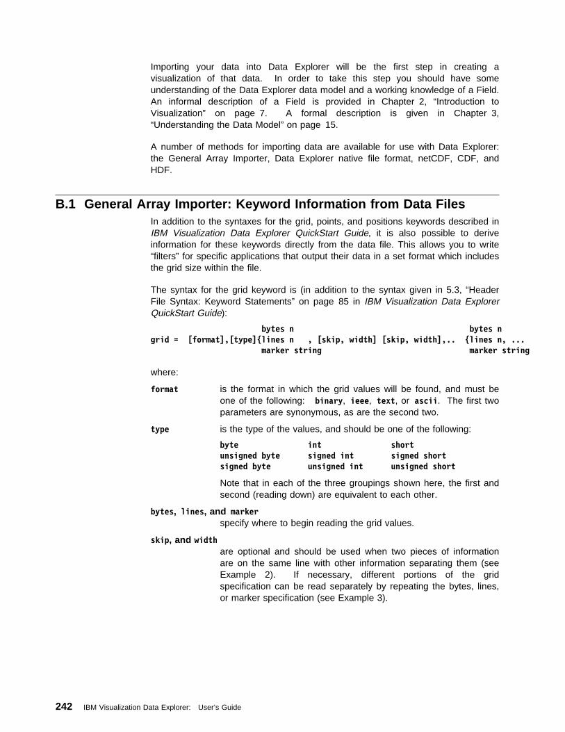
Importing your data into Data Explorer will be the first step in creating avisualization of that data. In order to take this step you should have someunderstanding of the Data Explorer data model and a working knowledge of a Field.An informal description of a Field is provided in Chapter 2, “Introduction toVisualization” on page 7. A formal description is given in Chapter 3,“Understanding the Data Model” on page 15.

A number of methods for importing data are available for use with Data Explorer:the General Array Importer, Data Explorer native file format, netCDF, CDF, andHDF.

B.1 General Array Importer: Keyword Information from Data FilesIn addition to the syntaxes for the grid, points, and positions keywords described inIBM Visualization Data Explorer QuickStart Guide, it is also possible to deriveinformation for these keywords directly from the data file. This allows you to write“filters” for specific applications that output their data in a set format which includesthe grid size within the file.

The syntax for the grid keyword is (in addition to the syntax given in 5.3, “HeaderFile Syntax: Keyword Statements” on page 85 in IBM Visualization Data ExplorerQuickStart Guide):

bytes n bytes ngrid = [format],[type]lines n , [skip, width] [skip, width],.. lines n, ... marker string marker string

where:

format is the format in which the grid values will be found, and must beone of the following: binary, ieee, text, or ascii. The first twoparameters are synonymous, as are the second two.

type is the type of the values, and should be one of the following:

byte int shortunsigned byte signed int signed shortsigned byte unsigned int unsigned short

Note that in each of the three groupings shown here, the first andsecond (reading down) are equivalent to each other.

bytes, lines, and markerspecify where to begin reading the grid values.

skip, and widthare optional and should be used when two pieces of informationare on the same line with other information separating them (seeExample 2). If necessary, different portions of the gridspecification can be read separately by repeating the bytes, lines,or marker specification (see Example 3).

242 IBM Visualization Data Explorer: User’s Guide

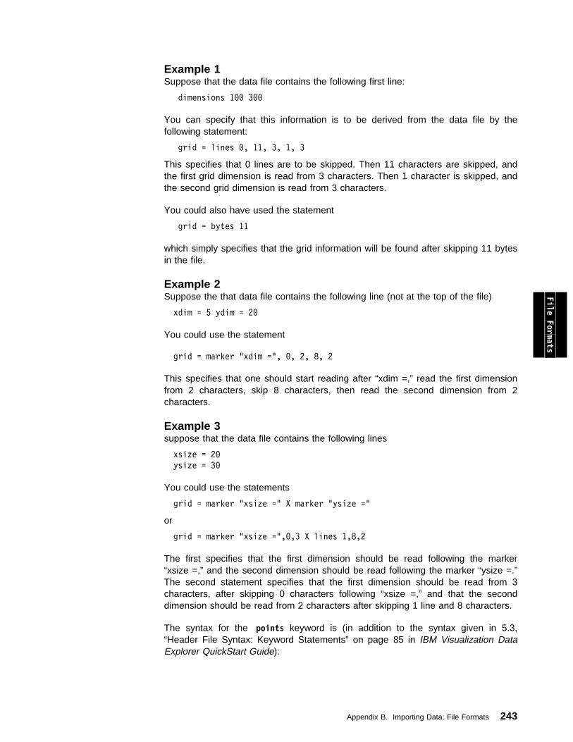
Example 1Suppose that the data file contains the following first line:

dimensions 1ðð 3ðð

You can specify that this information is to be derived from the data file by thefollowing statement:

grid = lines ð, 11, 3, 1, 3

This specifies that 0 lines are to be skipped. Then 11 characters are skipped, andthe first grid dimension is read from 3 characters. Then 1 character is skipped, andthe second grid dimension is read from 3 characters.

You could also have used the statement

grid = bytes 11

which simply specifies that the grid information will be found after skipping 11 bytesin the file.

Example 2Suppose the that data file contains the following line (not at the top of the file)

xdim = 5 ydim = 2ð

You could use the statement

grid = marker "xdim =", ð, 2, 8, 2

This specifies that one should start reading after “xdim =,” read the first dimensionfrom 2 characters, skip 8 characters, then read the second dimension from 2characters.

File Formats

Example 3suppose that the data file contains the following lines

xsize = 2ð

ysize = 3ð

You could use the statements

grid = marker "xsize =" X marker "ysize ="

or

grid = marker "xsize =",ð,3 X lines 1,8,2

The first specifies that the first dimension should be read following the marker“xsize =,” and the second dimension should be read following the marker “ysize =.”The second statement specifies that the first dimension should be read from 3characters, after skipping 0 characters following “xsize =,” and that the seconddimension should be read from 2 characters after skipping 1 line and 8 characters.

The syntax for the points keyword is (in addition to the syntax given in 5.3,“Header File Syntax: Keyword Statements” on page 85 in IBM Visualization DataExplorer QuickStart Guide):

Appendix B. Importing Data: File Formats 243

bytes npoints = [format],[type] lines n , [skip, width] marker string

where:

format is the format in which the grid values will be found, and must be one of thefollowing: binary, ieee, text, or ascii. The first two parameters aresynonymous, as are the second two.

For type and the other parameters, see the preceding description of grid.

The syntax for the positions keyword is (in addition to the syntax given in 5.3,“Header File Syntax: Keyword Statements” on page 85 in IBM Visualization DataExplorer QuickStart Guide):

bytes npositions =[format],[type] lines n , [skip, width] | ?, ... marker string

(This syntax may be used only if you are specifying regular positions: origin anddelta pairs for each dimension. As described in IBM Visualization Data ExplorerQuickStart Guide, the origins and deltas are specified as origin1, delta1, origin2,delta2, etc.)

format is the format in which the grid values will be found, and must be one of thefollowing: binary, ieee, text, or ascii. The first two parameters aresynonymous, as are the second two.

For type and the other parameters, see the description of grid above. Aquestion mark (?) signifies that the default should be used (origin=0 ordelta=1) for a particular origin or delta value. This would be used if only theorigins or only the deltas are to be found in the file.

B.2 Data Explorer Native FilesThe Data Explorer native file format encapsulates the Data Explorer data model ondisk (or on standard output as the result of an external conversion program). Thisfile format is comprehensive and flexible in that it can represent any of the Objectscreated in Data Explorer. Thus, any Object can be exported at any point. A datafile in this format can be imported into a Data Explorer session by specifying “dx”as the value of the format parameter for the Import module. For more information,see “Import” on page 165 in IBM Visualization Data Explorer User’s Reference.

Overview of the Native File FormatA Data Explorer file consists of a header section followed by an optional datasection. The header section consists of a textual description of a collection ofObjects. The data section contains the Array Object data, either as text or inbinary, and is referred to by the header section. A header section can refer toObjects and data either in the current file or in other files.

Figure 83 on page 245 shows data imbedded in its header. Another file cannotrefer to data in this file because there is no specified data section. However,header sections in this file can refer to data sections in other files. This method issometimes more convenient when creating data files with simple programs.

244 IBM Visualization Data Explorer: User’s Guide

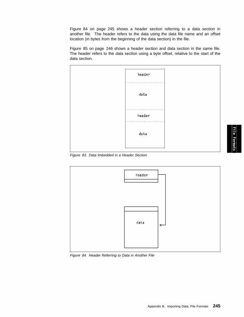
Figure 84 on page 245 shows a header section referring to a data section inanother file. The header refers to the data using the data file name and an offsetlocation (in bytes from the beginning of the data section) in the file.

Figure 85 on page 246 shows a header section and data section in the same file.The header refers to the data section using a byte offset, relative to the start of thedata section.

Figure 83. Data Imbedded in a Header Section

File Formats

Figure 84. Header Referring to Data in Another File

Appendix B. Importing Data: File Formats 245

Figure 85. Header and Data in the Same File

These configurations can be used in conjunction with each other. For example, afile can contain both a header and data and can refer to data both in the same fileand in another file. A file can also have only a header and refer to data in either adata-only file or in a file that contains both a header and data. This flexibility allowsyou to construct a header that points to data in existing files, and lets you view andedit the header information (if necessary), using standard tools.

The following examples illustrate some of the ways you can import data using theData Explorer native file format. You may wish to refer to the full specification ofthe syntax (see “Syntax of the Native File Format” on page 268).

ExamplesThe basic way to create a data file is to first define the Arrays, or components,contained in a Field and to then describe how to collect the components together.To define a higher level structure, such as a series, first define the components,then the Fields, and then how to collect the Fields to make a series. The examplesin this section illustrate the process.

In the first six examples, the data Objects can be viewed by the script shown here.Other scripts are shown with the later examples.

data = Import("filename.dx", format = "dx");

connections = ShowConnections(data);

connections = AutoColor(connections);

tubes = Tube(connections, ð.ð8);

camera = AutoCamera(tubes, "off diagonal");

image = Render(tubes, camera);

Display(image);

Note: For Figure 86 on page 248 and Figure 87 on page 249, the argument “offfront” is used instead of “off diagonal.”

246 IBM Visualization Data Explorer: User’s Guide

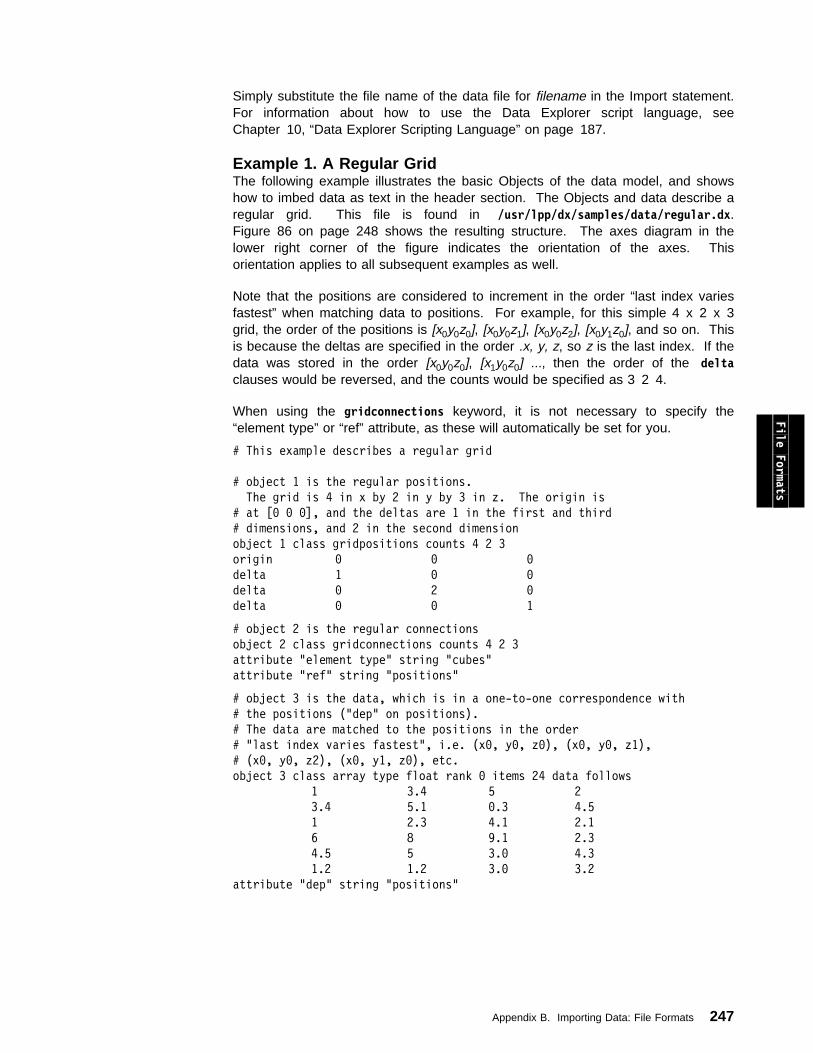
Simply substitute the file name of the data file for filename in the Import statement.For information about how to use the Data Explorer script language, seeChapter 10, “Data Explorer Scripting Language” on page 187.

Example 1. A Regular GridThe following example illustrates the basic Objects of the data model, and showshow to imbed data as text in the header section. The Objects and data describe aregular grid. This file is found in /usr/lpp/dx/samples/data/regular.dx.Figure 86 on page 248 shows the resulting structure. The axes diagram in thelower right corner of the figure indicates the orientation of the axes. Thisorientation applies to all subsequent examples as well.

Note that the positions are considered to increment in the order “last index variesfastest” when matching data to positions. For example, for this simple 4 x 2 x 3grid, the order of the positions is [x0y0z0], [x0y0z1], [x0y0z2], [x0y1z0], and so on. Thisis because the deltas are specified in the order .x, y, z, so z is the last index. If thedata was stored in the order [x0y0z0], [x1y0z0] ..., then the order of the deltaclauses would be reversed, and the counts would be specified as 3 2 4.

When using the gridconnections keyword, it is not necessary to specify the“element type” or “ref” attribute, as these will automatically be set for you.

# This example describes a regular grid

# object 1 is the regular positions.

The grid is 4 in x by 2 in y by 3 in z. The origin is

# at [ð ð ð], and the deltas are 1 in the first and third

# dimensions, and 2 in the second dimension

object 1 class gridpositions counts 4 2 3

origin ð ð ð

delta 1 ð ð

delta ð 2 ð

delta ð ð 1

# object 2 is the regular connections

object 2 class gridconnections counts 4 2 3

attribute "element type" string "cubes"

attribute "ref" string "positions"

# object 3 is the data, which is in a one-to-one correspondence with

# the positions ("dep" on positions).

# The data are matched to the positions in the order

# "last index varies fastest", i.e. (xð, yð, zð), (xð, yð, z1),

# (xð, yð, z2), (xð, y1, zð), etc.

object 3 class array type float rank ð items 24 data follows

1 3.4 5 2

3.4 5.1 ð.3 4.5

1 2.3 4.1 2.1

6 8 9.1 2.3

4.5 5 3.ð 4.3

1.2 1.2 3.ð 3.2

attribute "dep" string "positions"

File Formats

Appendix B. Importing Data: File Formats 247

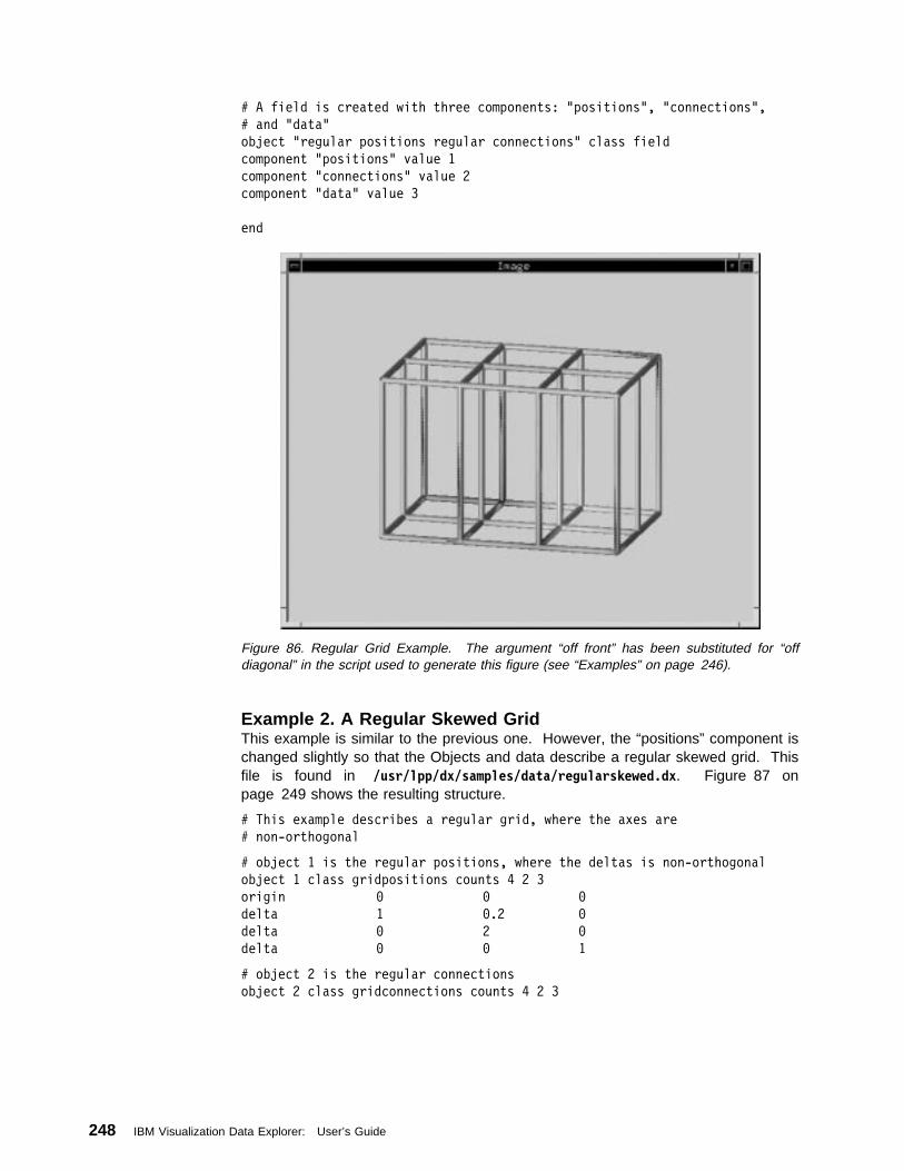
# A field is created with three components: "positions", "connections",

# and "data"

object "regular positions regular connections" class field

component "positions" value 1

component "connections" value 2

component "data" value 3

end

Figure 86. Regular Grid Example. The argument “off front” has been substituted for “offdiagonal” in the script used to generate this figure (see “Examples” on page 246).

Example 2. A Regular Skewed GridThis example is similar to the previous one. However, the “positions” component ischanged slightly so that the Objects and data describe a regular skewed grid. Thisfile is found in /usr/lpp/dx/samples/data/regularskewed.dx. Figure 87 onpage 249 shows the resulting structure.

# This example describes a regular grid, where the axes are

# non-orthogonal

# object 1 is the regular positions, where the deltas is non-orthogonal

object 1 class gridpositions counts 4 2 3

origin ð ð ð

delta 1 ð.2 ð

delta ð 2 ð

delta ð ð 1

# object 2 is the regular connections

object 2 class gridconnections counts 4 2 3

248 IBM Visualization Data Explorer: User’s Guide

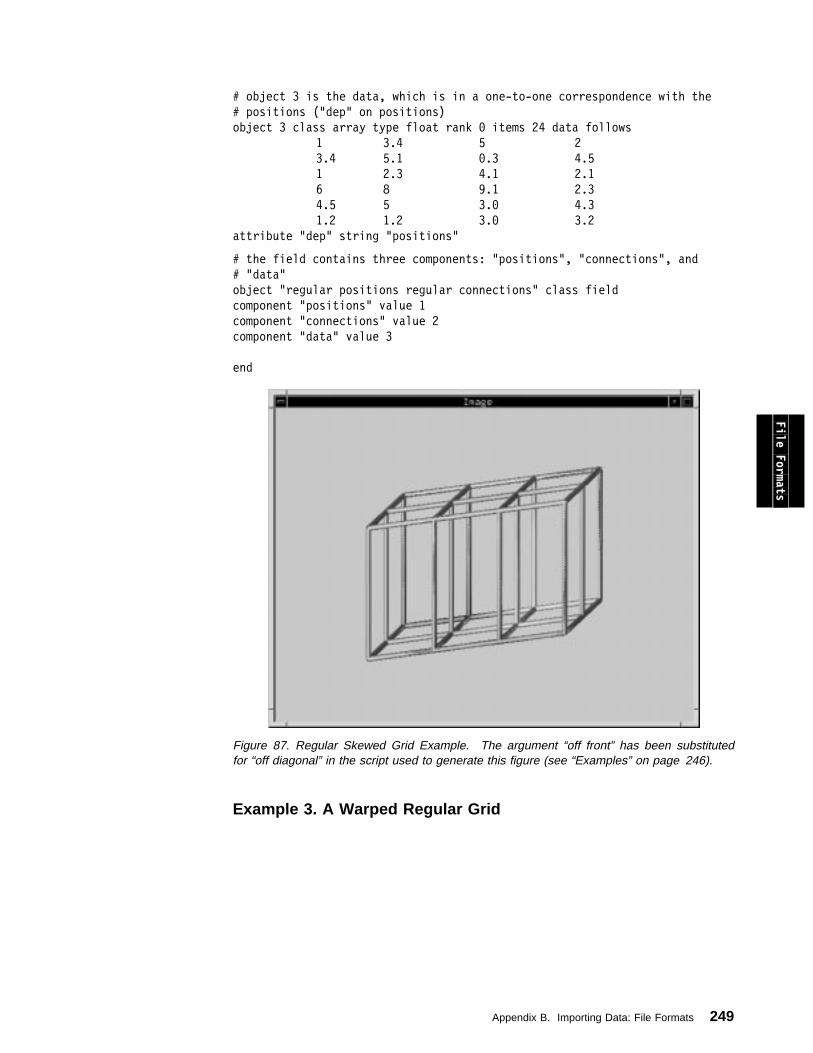
# object 3 is the data, which is in a one-to-one correspondence with the

# positions ("dep" on positions)

object 3 class array type float rank ð items 24 data follows

1 3.4 5 2

3.4 5.1 ð.3 4.5

1 2.3 4.1 2.1

6 8 9.1 2.3

4.5 5 3.ð 4.3

1.2 1.2 3.ð 3.2

attribute "dep" string "positions"

# the field contains three components: "positions", "connections", and

# "data"

object "regular positions regular connections" class field

component "positions" value 1

component "connections" value 2

component "data" value 3

end

Figure 87. Regular Skewed Grid Example. The argument “off front” has been substitutedfor “off diagonal” in the script used to generate this figure (see “Examples” on page 246).

File Formats

Example 3. A Warped Regular Grid

Appendix B. Importing Data: File Formats 249

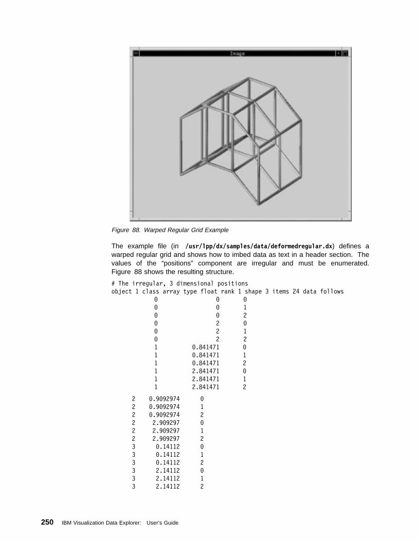
Figure 88. Warped Regular Grid Example

The example file (in /usr/lpp/dx/samples/data/deformedregular.dx) defines awarped regular grid and shows how to imbed data as text in a header section. Thevalues of the “positions” component are irregular and must be enumerated.Figure 88 shows the resulting structure.

# The irregular, 3 dimensional positions

object 1 class array type float rank 1 shape 3 items 24 data follows

ð ð ð

ð ð 1

ð ð 2

ð 2 ð

ð 2 1

ð 2 2

1 ð.841471 ð

1 ð.841471 1

1 ð.841471 2

1 2.841471 ð

1 2.841471 1

1 2.841471 2

2 ð.9ð92974 ð

2 ð.9ð92974 1

2 ð.9ð92974 2

2 2.9ð9297 ð

2 2.9ð9297 1

2 2.9ð9297 2

3 ð.14112 ð

3 ð.14112 1

3 ð.14112 2

3 2.14112 ð

3 2.14112 1

3 2.14112 2

250 IBM Visualization Data Explorer: User’s Guide

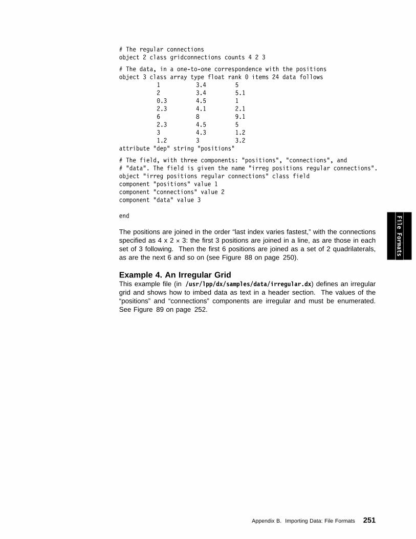
# The regular connections

object 2 class gridconnections counts 4 2 3

# The data, in a one-to-one correspondence with the positions

object 3 class array type float rank ð items 24 data follows

1 3.4 5

2 3.4 5.1

ð.3 4.5 1

2.3 4.1 2.1

6 8 9.1

2.3 4.5 5

3 4.3 1.2

1.2 3 3.2

attribute "dep" string "positions"

# The field, with three components: "positions", "connections", and

# "data". The field is given the name "irreg positions regular connections".

object "irreg positions regular connections" class field

component "positions" value 1

component "connections" value 2

component "data" value 3

end

The positions are joined in the order “last index varies fastest,” with the connectionsspecified as 4 x 2 × 3: the first 3 positions are joined in a line, as are those in eachset of 3 following. Then the first 6 positions are joined as a set of 2 quadrilaterals,as are the next 6 and so on (see Figure 88 on page 250).

File Formats

Example 4. An Irregular GridThis example file (in /usr/lpp/dx/samples/data/irregular.dx) defines an irregulargrid and shows how to imbed data as text in a header section. The values of the“positions” and “connections” components are irregular and must be enumerated.See Figure 89 on page 252.

Appendix B. Importing Data: File Formats 251

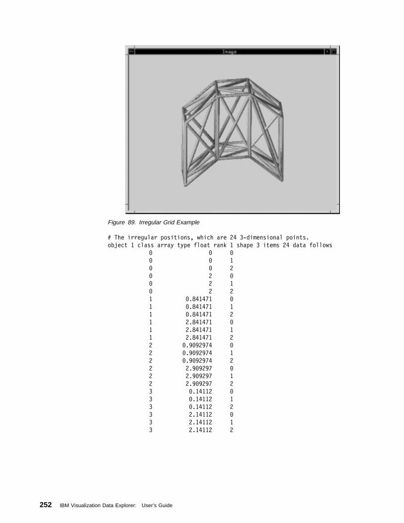
Figure 89. Irregular Grid Example

# The irregular positions, which are 24 3-dimensional points.

object 1 class array type float rank 1 shape 3 items 24 data follows

ð ð ð

ð ð 1

ð ð 2

ð 2 ð

ð 2 1

ð 2 2

1 ð.841471 ð

1 ð.841471 1

1 ð.841471 2

1 2.841471 ð

1 2.841471 1

1 2.841471 2

2 ð.9ð92974 ð

2 ð.9ð92974 1

2 ð.9ð92974 2

2 2.9ð9297 ð

2 2.9ð9297 1

2 2.9ð9297 2

3 ð.14112 ð

3 ð.14112 1

3 ð.14112 2

3 2.14112 ð

3 2.14112 1

3 2.14112 2

252 IBM Visualization Data Explorer: User’s Guide

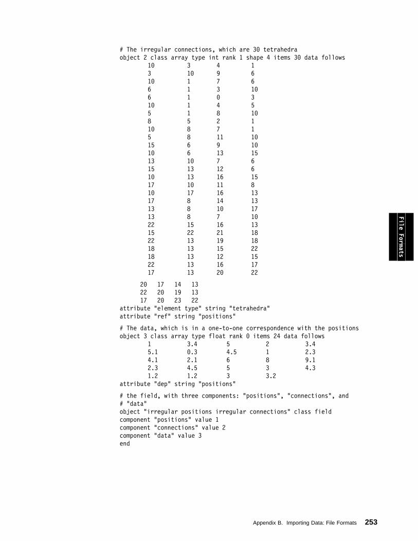
# The irregular connections, which are 3ð tetrahedra

object 2 class array type int rank 1 shape 4 items 3ð data follows

1ð 3 4 1

3 1ð 9 6

1ð 1 7 6

6 1 3 1ð

6 1 ð 3

1ð 1 4 5

5 1 8 1ð

8 5 2 1

1ð 8 7 1

5 8 11 1ð

15 6 9 1ð

1ð 6 13 15

13 1ð 7 6

15 13 12 6

1ð 13 16 15

17 1ð 11 8

1ð 17 16 13

17 8 14 13

13 8 1ð 17

13 8 7 1ð

22 15 16 13

15 22 21 18

22 13 19 18

18 13 15 22

18 13 12 15

22 13 16 17

17 13 2ð 22

2ð 17 14 13

22 2ð 19 13

17 2ð 23 22

attribute "element type" string "tetrahedra"

attribute "ref" string "positions"

# The data, which is in a one-to-one correspondence with the positions

object 3 class array type float rank ð items 24 data follows

1 3.4 5 2 3.4

5.1 ð.3 4.5 1 2.3

4.1 2.1 6 8 9.1

2.3 4.5 5 3 4.3

1.2 1.2 3 3.2

attribute "dep" string "positions"

# the field, with three components: "positions", "connections", and

# "data"

object "irregular positions irregular connections" class field

component "positions" value 1

component "connections" value 2

component "data" value 3

end

File Formats

Appendix B. Importing Data: File Formats 253

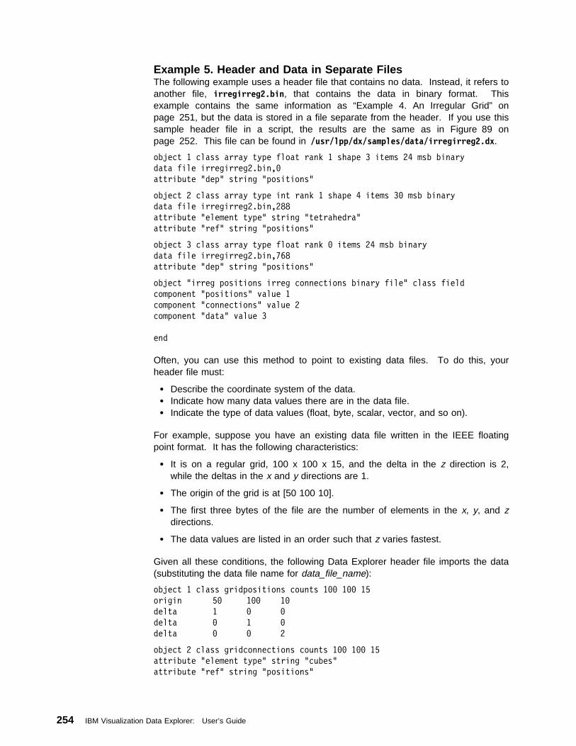
Example 5. Header and Data in Separate FilesThe following example uses a header file that contains no data. Instead, it refers toanother file, irregirreg2.bin, that contains the data in binary format. Thisexample contains the same information as “Example 4. An Irregular Grid” onpage 251, but the data is stored in a file separate from the header. If you use thissample header file in a script, the results are the same as in Figure 89 onpage 252. This file can be found in /usr/lpp/dx/samples/data/irregirreg2.dx.

object 1 class array type float rank 1 shape 3 items 24 msb binary

data file irregirreg2.bin,ð

attribute "dep" string "positions"

object 2 class array type int rank 1 shape 4 items 3ð msb binary

data file irregirreg2.bin,288

attribute "element type" string "tetrahedra"

attribute "ref" string "positions"

object 3 class array type float rank ð items 24 msb binary

data file irregirreg2.bin,768

attribute "dep" string "positions"

object "irreg positions irreg connections binary file" class field

component "positions" value 1

component "connections" value 2

component "data" value 3

end

Often, you can use this method to point to existing data files. To do this, yourheader file must:

Describe the coordinate system of the data. Indicate how many data values there are in the data file. Indicate the type of data values (float, byte, scalar, vector, and so on).

For example, suppose you have an existing data file written in the IEEE floatingpoint format. It has the following characteristics:

It is on a regular grid, 100 x 100 x 15, and the delta in the z direction is 2,while the deltas in the x and y directions are 1.

The origin of the grid is at [50 100 10].

The first three bytes of the file are the number of elements in the x, y, and zdirections.

The data values are listed in an order such that z varies fastest.

Given all these conditions, the following Data Explorer header file imports the data(substituting the data file name for data_file_name):

object 1 class gridpositions counts 1ðð 1ðð 15

origin 5ð 1ðð 1ð

delta 1 ð ð

delta ð 1 ð

delta ð ð 2

object 2 class gridconnections counts 1ðð 1ðð 15

attribute "element type" string "cubes"

attribute "ref" string "positions"

254 IBM Visualization Data Explorer: User’s Guide

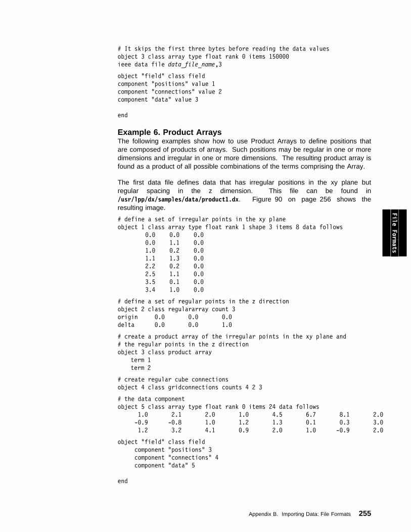
# It skips the first three bytes before reading the data values

object 3 class array type float rank ð items 15ðððð

ieee data file data_file_name,3

object "field" class field

component "positions" value 1

component "connections" value 2

component "data" value 3

end

Example 6. Product ArraysThe following examples show how to use Product Arrays to define positions thatare composed of products of arrays. Such positions may be regular in one or moredimensions and irregular in one or more dimensions. The resulting product array isfound as a product of all possible combinations of the terms comprising the Array.

The first data file defines data that has irregular positions in the xy plane butregular spacing in the z dimension. This file can be found in/usr/lpp/dx/samples/data/product1.dx. Figure 90 on page 256 shows theresulting image.

# define a set of irregular points in the xy plane

object 1 class array type float rank 1 shape 3 items 8 data follows

ð.ð ð.ð ð.ð

ð.ð 1.1 ð.ð

1.ð ð.2 ð.ð

1.1 1.3 ð.ð

2.2 ð.2 ð.ð

2.5 1.1 ð.ð

3.5 ð.1 ð.ð

3.4 1.ð ð.ð

# define a set of regular points in the z direction

object 2 class regulararray count 3

origin ð.ð ð.ð ð.ð

delta ð.ð ð.ð 1.ð

# create a product array of the irregular points in the xy plane and

# the regular points in the z direction

object 3 class product array

term 1

term 2

# create regular cube connections

object 4 class gridconnections counts 4 2 3

# the data component

object 5 class array type float rank ð items 24 data follows

1.ð 2.1 2.ð 1.ð 4.5 6.7 8.1 2.ð

-ð.9 -ð.8 1.ð 1.2 1.3 ð.1 ð.3 3.ð

1.2 3.2 4.1 ð.9 2.ð 1.ð -ð.9 2.ð

object "field" class field

component "positions" 3

component "connections" 4

component "data" 5

end

File Formats

Appendix B. Importing Data: File Formats 255

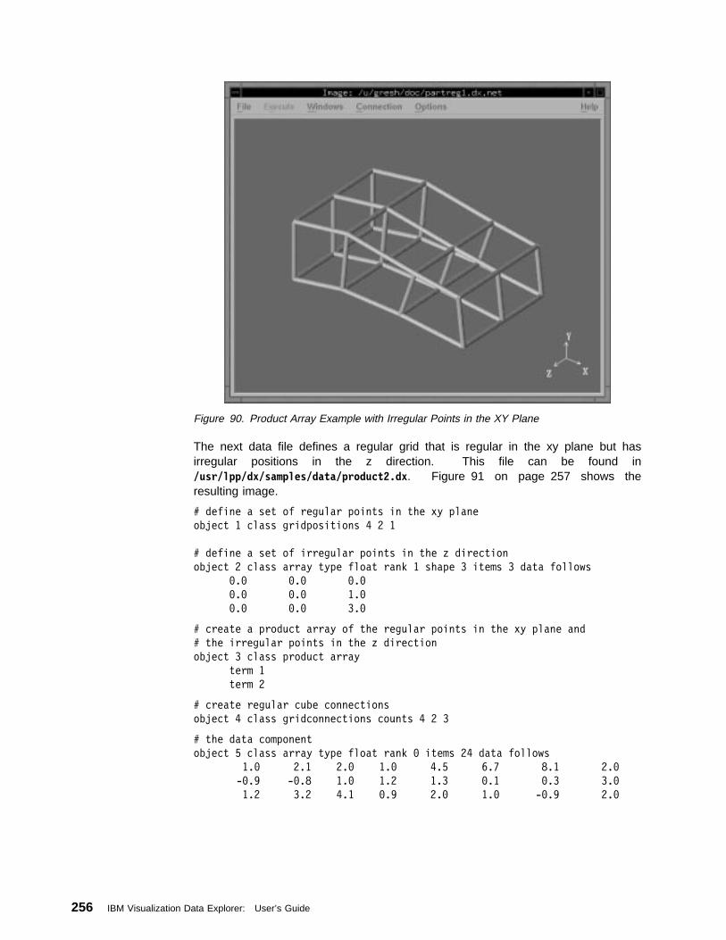
Figure 90. Product Array Example with Irregular Points in the XY Plane

The next data file defines a regular grid that is regular in the xy plane but hasirregular positions in the z direction. This file can be found in/usr/lpp/dx/samples/data/product2.dx. Figure 91 on page 257 shows theresulting image.

# define a set of regular points in the xy plane

object 1 class gridpositions 4 2 1

# define a set of irregular points in the z direction

object 2 class array type float rank 1 shape 3 items 3 data follows

ð.ð ð.ð ð.ð

ð.ð ð.ð 1.ð

ð.ð ð.ð 3.ð

# create a product array of the regular points in the xy plane and

# the irregular points in the z direction

object 3 class product array

term 1

term 2

# create regular cube connections

object 4 class gridconnections counts 4 2 3

# the data component

object 5 class array type float rank ð items 24 data follows

1.ð 2.1 2.ð 1.ð 4.5 6.7 8.1 2.ð

-ð.9 -ð.8 1.ð 1.2 1.3 ð.1 ð.3 3.ð

1.2 3.2 4.1 ð.9 2.ð 1.ð -ð.9 2.ð

256 IBM Visualization Data Explorer: User’s Guide

object "field" class field

component "positions" 3

component "connections" 4

component "data" 5

end

Figure 91. Product Array Example with Irregular Points in the Z Direction

File Formats

Example 7. SeriesThe following file defines the data for a series. It defines three data Array Objects,and then three Field Objects that are associated with the data. The grid definitionsare in a separate file (pos_conn.data). This first file can be found in/usr/lpp/samples/data/regseries.dx.

# This example describes a data series with three member fields

# Object 1 is the data associated with the first frame in the

# series. The data is "dep" positions, or in a one-to-one

# correspondence with positions.

object 1 class array type float rank 1 shape 3 items 18 data follows

1.ð ð.1 ð.ð

1.4 ð.2 ð.ð

1.ð ð.ð ð.ð

2.2 ð.1 ð.2

1.ð ð.ð ð.ð

2.ð ð.ð ð.1

ð.9 ð.1 ð.ð

1.1 -ð.4 ð.ð

1.ð ð.1 ð.ð

1.2 ð.1 ð.1

ð.3 ð.ð ð.ð

Appendix B. Importing Data: File Formats 257

1.ð ð.1 ð.1

1.1 -ð.4 ð.2

1.1 ð.2 ð.ð

1.1 ð.1 ð.ð

1.2 ð.1 ð.1

1.1 ð.ð ð.ð

ð.9 ð.ð ð.1

attribute "dep" string "positions"

# Object 2 is the data associated with the second frame in the series.

object 2 class array type float rank 1 shape 3 items 18 data follows

ð.ð 1.1 ð.ð

ð.1 2.2 ð.ð

ð.ð 1.ð ð.ð

ð.2 1.1 -ð.2

ð.ð ð.8 ð.ð

ð.ð 1.9 ð.4

ð.1 1.1 ð.ð

ð.1 1.2 ð.ð

ð.ð 1.1 ð.ð

ð.2 2.1 ð.1

ð.1 1.ð ð.ð

ð.ð ð.8 ð.1

ð.1 ð.9 -ð.2

ð.1 1.2 ð.ð

ð.1 1.1 ð.ð

ð.2 1.1 -ð.4

ð.1 ð.9 ð.ð

ð.2 ð.9 ð.1

attribute "dep" string "positions"

# Object 3 is the data associated with the third frame in the series.

object 3 class array type float rank 1 shape 3 items 18 data follows

ð.ð ð.1 1.ð

ð.1 ð.2 1.ð

ð.ð ð.ð 2.ð

-ð.2 ð.1 2.2

ð.ð ð.1 ð.9

ð.ð ð.2 ð.8

-ð.4 ð.1 ð.9

ð.1 ð.2 1.9

ð.ð ð.1 ð.7

ð.2 ð.1 1.1

-ð.1 ð.ð 2.ð

ð.ð ð.3 1.1

ð.1 ð.1 1.2

-ð.5 ð.2 1.ð

ð.1 ð.1 2.ð

ð.2 ð.1 1.4

ð.1 -ð.3 ð.9

ð.2 ð.3 1.1

attribute "dep" string "positions"

258 IBM Visualization Data Explorer: User’s Guide

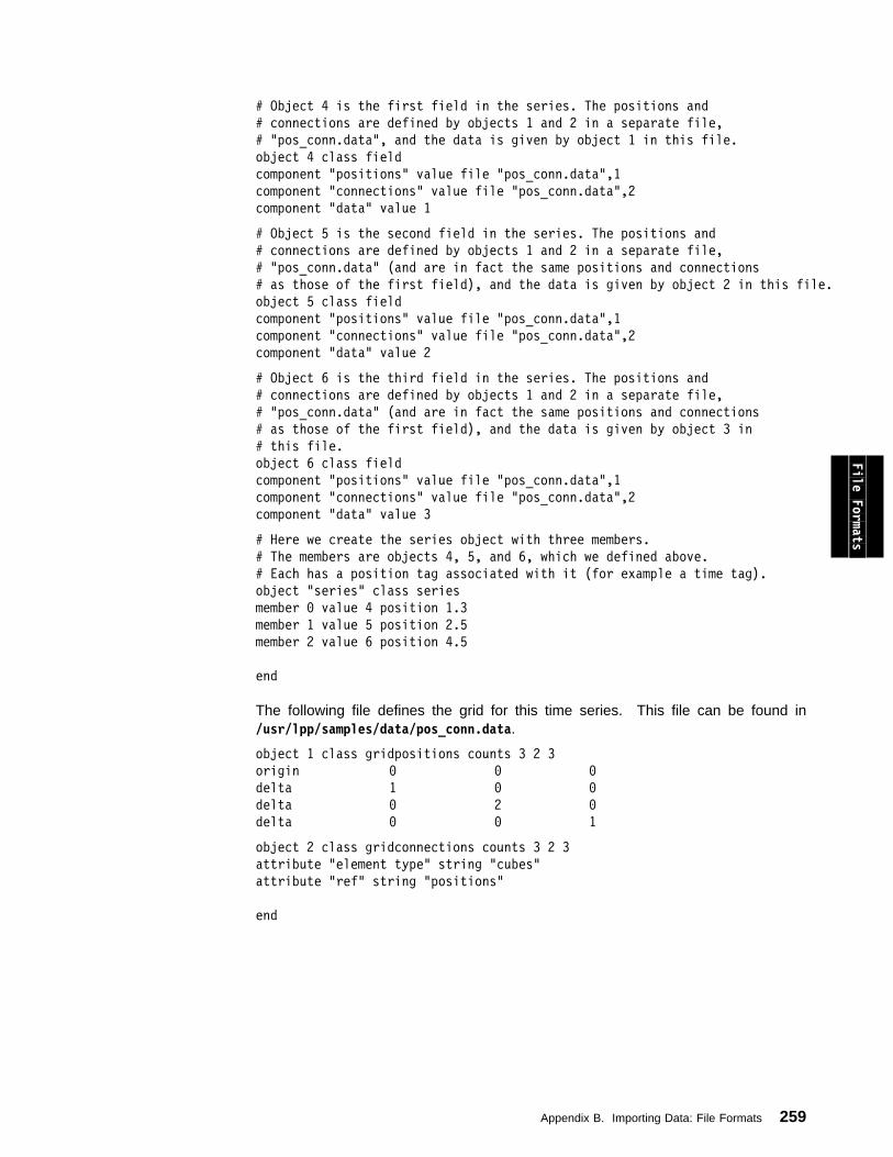
# Object 4 is the first field in the series. The positions and

# connections are defined by objects 1 and 2 in a separate file,

# "pos_conn.data", and the data is given by object 1 in this file.

object 4 class field

component "positions" value file "pos_conn.data",1

component "connections" value file "pos_conn.data",2

component "data" value 1

# Object 5 is the second field in the series. The positions and

# connections are defined by objects 1 and 2 in a separate file,

# "pos_conn.data" (and are in fact the same positions and connections

# as those of the first field), and the data is given by object 2 in this file.

object 5 class field

component "positions" value file "pos_conn.data",1

component "connections" value file "pos_conn.data",2

component "data" value 2

# Object 6 is the third field in the series. The positions and

# connections are defined by objects 1 and 2 in a separate file,

# "pos_conn.data" (and are in fact the same positions and connections

# as those of the first field), and the data is given by object 3 in

# this file.

object 6 class field

component "positions" value file "pos_conn.data",1

component "connections" value file "pos_conn.data",2

component "data" value 3

# Here we create the series object with three members.

# The members are objects 4, 5, and 6, which we defined above.

# Each has a position tag associated with it (for example a time tag).

object "series" class series

member ð value 4 position 1.3

member 1 value 5 position 2.5

member 2 value 6 position 4.5

end

The following file defines the grid for this time series. This file can be found in/usr/lpp/samples/data/pos_conn.data.

object 1 class gridpositions counts 3 2 3

origin ð ð ð

delta 1 ð ð

delta ð 2 ð

delta ð ð 1

object 2 class gridconnections counts 3 2 3

attribute "element type" string "cubes"

attribute "ref" string "positions"

end

File Formats

Appendix B. Importing Data: File Formats 259

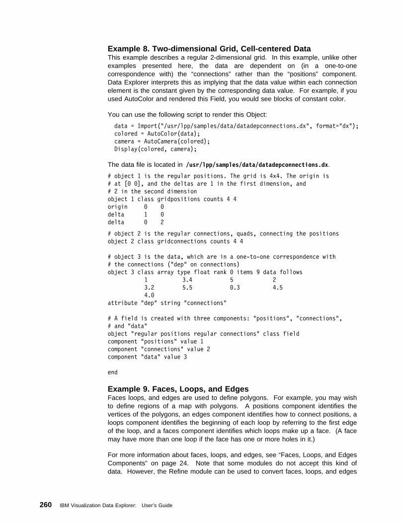
Example 8. Two-dimensional Grid, Cell-centered DataThis example describes a regular 2-dimensional grid. In this example, unlike otherexamples presented here, the data are dependent on (in a one-to-onecorrespondence with) the “connections” rather than the “positions” component.Data Explorer interprets this as implying that the data value within each connectionelement is the constant given by the corresponding data value. For example, if youused AutoColor and rendered this Field, you would see blocks of constant color.

You can use the following script to render this Object:

data = Import("/usr/lpp/samples/data/datadepconnections.dx", format="dx");

colored = AutoColor(data);

camera = AutoCamera(colored);

Display(colored, camera);

The data file is located in /usr/lpp/samples/data/datadepconnections.dx.

# object 1 is the regular positions. The grid is 4x4. The origin is

# at [ð ð], and the deltas are 1 in the first dimension, and

# 2 in the second dimension

object 1 class gridpositions counts 4 4

origin ð ð

delta 1 ð

delta ð 2

# object 2 is the regular connections, quads, connecting the positions

object 2 class gridconnections counts 4 4

# object 3 is the data, which are in a one-to-one correspondence with

# the connections ("dep" on connections)

object 3 class array type float rank ð items 9 data follows

1 3.4 5 2

3.2 5.5 ð.3 4.5

4.ð

attribute "dep" string "connections"

# A field is created with three components: "positions", "connections",

# and "data"

object "regular positions regular connections" class field

component "positions" value 1

component "connections" value 2

component "data" value 3

end

Example 9. Faces, Loops, and EdgesFaces loops, and edges are used to define polygons. For example, you may wishto define regions of a map with polygons. A positions component identifies thevertices of the polygons, an edges component identifies how to connect positions, aloops component identifies the beginning of each loop by referring to the first edgeof the loop, and a faces component identifies which loops make up a face. (A facemay have more than one loop if the face has one or more holes in it.)

For more information about faces, loops, and edges, see “Faces, Loops, and EdgesComponents” on page 24. Note that some modules do not accept this kind ofdata. However, the Refine module can be used to convert faces, loops, and edges

260 IBM Visualization Data Explorer: User’s Guide

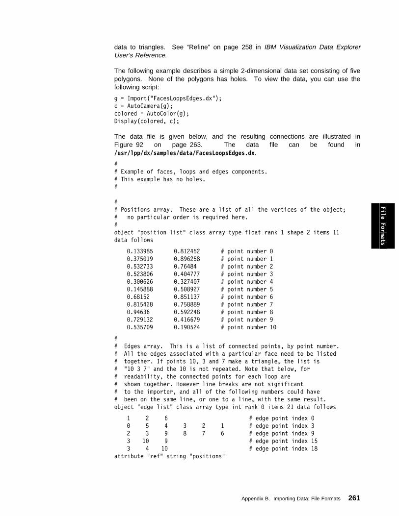
data to triangles. See “Refine” on page 258 in IBM Visualization Data ExplorerUser’s Reference.

The following example describes a simple 2-dimensional data set consisting of fivepolygons. None of the polygons has holes. To view the data, you can use thefollowing script:

g = Import("FacesLoopsEdges.dx");

c = AutoCamera(g);

colored = AutoColor(g);

Display(colored, c);

The data file is given below, and the resulting connections are illustrated inFigure 92 on page 263. The data file can be found in/usr/lpp/dx/samples/data/FacesLoopsEdges.dx.

#

# Example of faces, loops and edges components.

# This example has no holes.

#

#

# Positions array. These are a list of all the vertices of the object;

# no particular order is required here.

#

object "position list" class array type float rank 1 shape 2 items 11

data follows

ð.133985 ð.812452 # point number ð

ð.375ð19 ð.896258 # point number 1

ð.532733 ð.76484 # point number 2

ð.5238ð6 ð.4ð4777 # point number 3

ð.3ðð626 ð.3274ð7 # point number 4

ð.145888 ð.5ð8927 # point number 5

ð.68152 ð.851137 # point number 6

ð.815428 ð.758889 # point number 7

ð.94636 ð.592248 # point number 8

ð.729132 ð.416679 # point number 9

ð.5357ð9 ð.19ð524 # point number 1ð

#

# Edges array. This is a list of connected points, by point number.

# All the edges associated with a particular face need to be listed

# together. If points 1ð, 3 and 7 make a triangle, the list is

# "1ð 3 7" and the 1ð is not repeated. Note that below, for

# readability, the connected points for each loop are

# shown together. However line breaks are not significant

# to the importer, and all of the following numbers could have

# been on the same line, or one to a line, with the same result.

object "edge list" class array type int rank ð items 21 data follows

1 2 6 # edge point index ð

ð 5 4 3 2 1 # edge point index 3

2 3 9 8 7 6 # edge point index 9

3 1ð 9 # edge point index 15

3 4 1ð # edge point index 18

attribute "ref" string "positions"

File Formats

Appendix B. Importing Data: File Formats 261

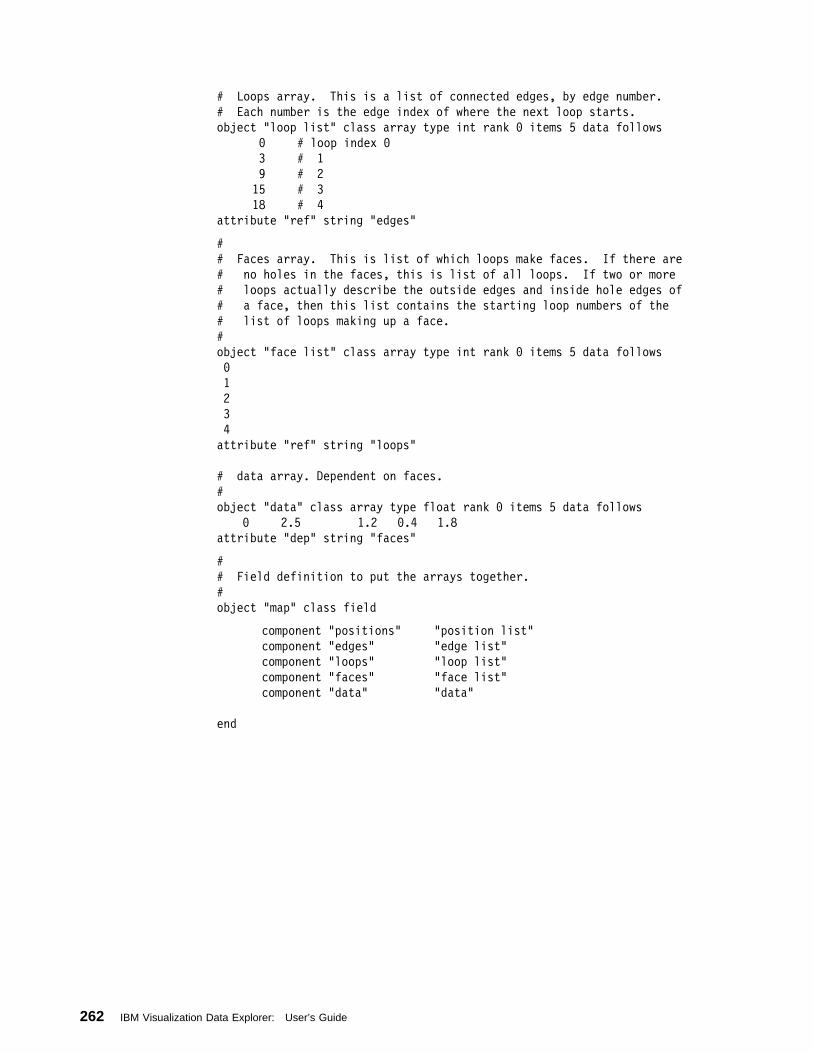
# Loops array. This is a list of connected edges, by edge number.

# Each number is the edge index of where the next loop starts.

object "loop list" class array type int rank ð items 5 data follows

ð # loop index ð

3 # 1

9 # 2

15 # 3

18 # 4

attribute "ref" string "edges"

#

# Faces array. This is list of which loops make faces. If there are

# no holes in the faces, this is list of all loops. If two or more

# loops actually describe the outside edges and inside hole edges of

# a face, then this list contains the starting loop numbers of the

# list of loops making up a face.

#

object "face list" class array type int rank ð items 5 data follows

ð

1

2

3

4

attribute "ref" string "loops"

# data array. Dependent on faces.

#

object "data" class array type float rank ð items 5 data follows

ð 2.5 1.2 ð.4 1.8

attribute "dep" string "faces"

#

# Field definition to put the arrays together.

#

object "map" class field

component "positions" "position list"

component "edges" "edge list"

component "loops" "loop list"

component "faces" "face list"

component "data" "data"

end

262 IBM Visualization Data Explorer: User’s Guide

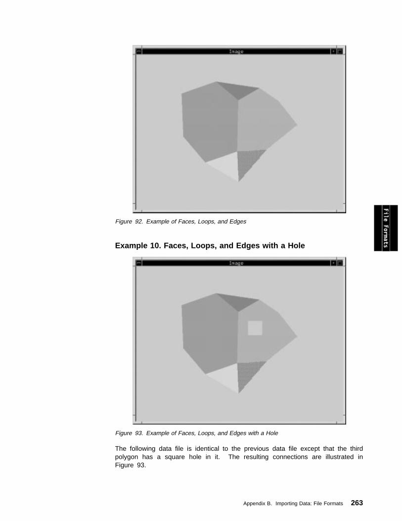
Figure 92. Example of Faces, Loops, and Edges

File Formats Example 10. Faces, Loops, and Edges with a Hole

Figure 93. Example of Faces, Loops, and Edges with a Hole

The following data file is identical to the previous data file except that the thirdpolygon has a square hole in it. The resulting connections are illustrated inFigure 93.

Appendix B. Importing Data: File Formats 263

#

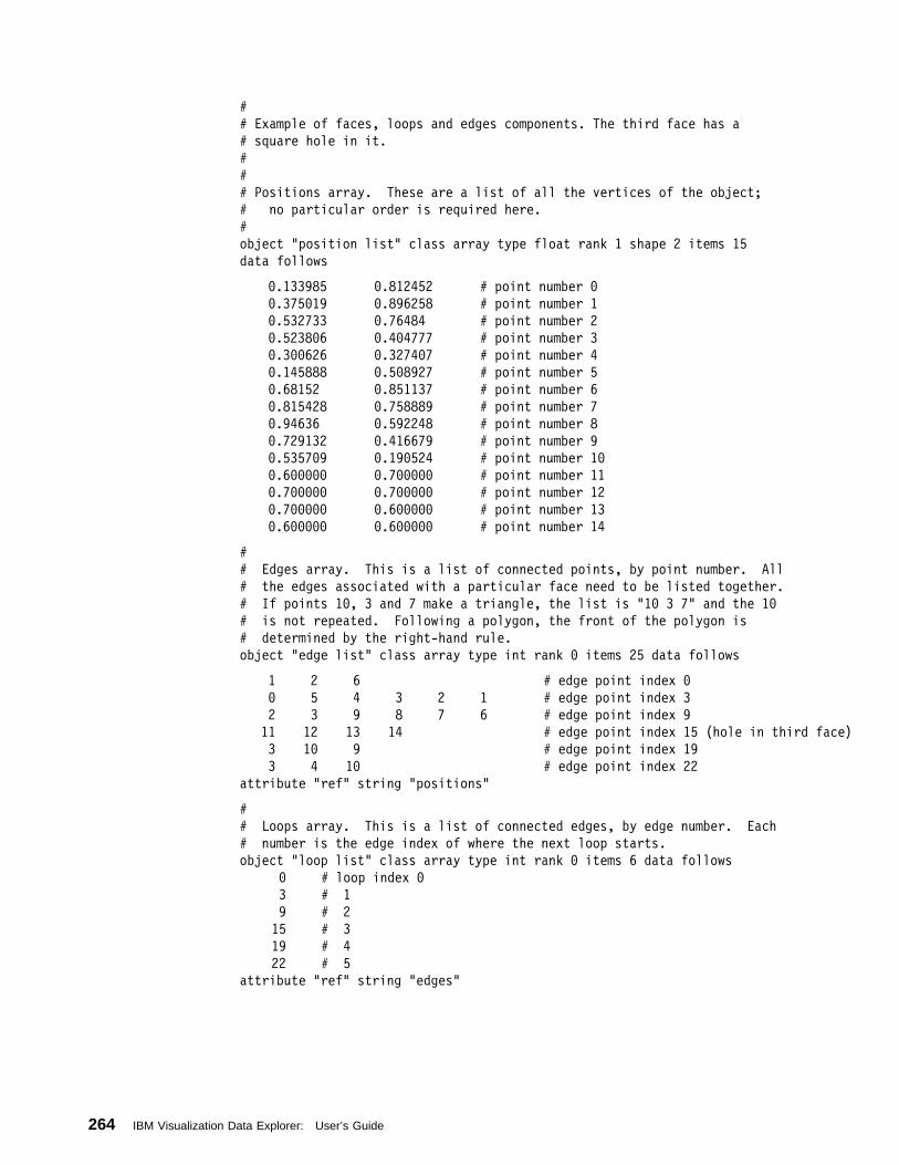
# Example of faces, loops and edges components. The third face has a

# square hole in it.

#

#

# Positions array. These are a list of all the vertices of the object;

# no particular order is required here.

#

object "position list" class array type float rank 1 shape 2 items 15

data follows

ð.133985 ð.812452 # point number ð

ð.375ð19 ð.896258 # point number 1

ð.532733 ð.76484 # point number 2

ð.5238ð6 ð.4ð4777 # point number 3

ð.3ðð626 ð.3274ð7 # point number 4

ð.145888 ð.5ð8927 # point number 5

ð.68152 ð.851137 # point number 6

ð.815428 ð.758889 # point number 7

ð.94636 ð.592248 # point number 8

ð.729132 ð.416679 # point number 9

ð.5357ð9 ð.19ð524 # point number 1ð

ð.6ððððð ð.7ððððð # point number 11

ð.7ððððð ð.7ððððð # point number 12

ð.7ððððð ð.6ððððð # point number 13

ð.6ððððð ð.6ððððð # point number 14

#

# Edges array. This is a list of connected points, by point number. All

# the edges associated with a particular face need to be listed together.

# If points 1ð, 3 and 7 make a triangle, the list is "1ð 3 7" and the 1ð

# is not repeated. Following a polygon, the front of the polygon is

# determined by the right-hand rule.

object "edge list" class array type int rank ð items 25 data follows

1 2 6 # edge point index ð

ð 5 4 3 2 1 # edge point index 3

2 3 9 8 7 6 # edge point index 9

11 12 13 14 # edge point index 15 (hole in third face)

3 1ð 9 # edge point index 19

3 4 1ð # edge point index 22

attribute "ref" string "positions"

#

# Loops array. This is a list of connected edges, by edge number. Each

# number is the edge index of where the next loop starts.

object "loop list" class array type int rank ð items 6 data follows

ð # loop index ð

3 # 1

9 # 2

15 # 3

19 # 4

22 # 5

attribute "ref" string "edges"

264 IBM Visualization Data Explorer: User’s Guide

#

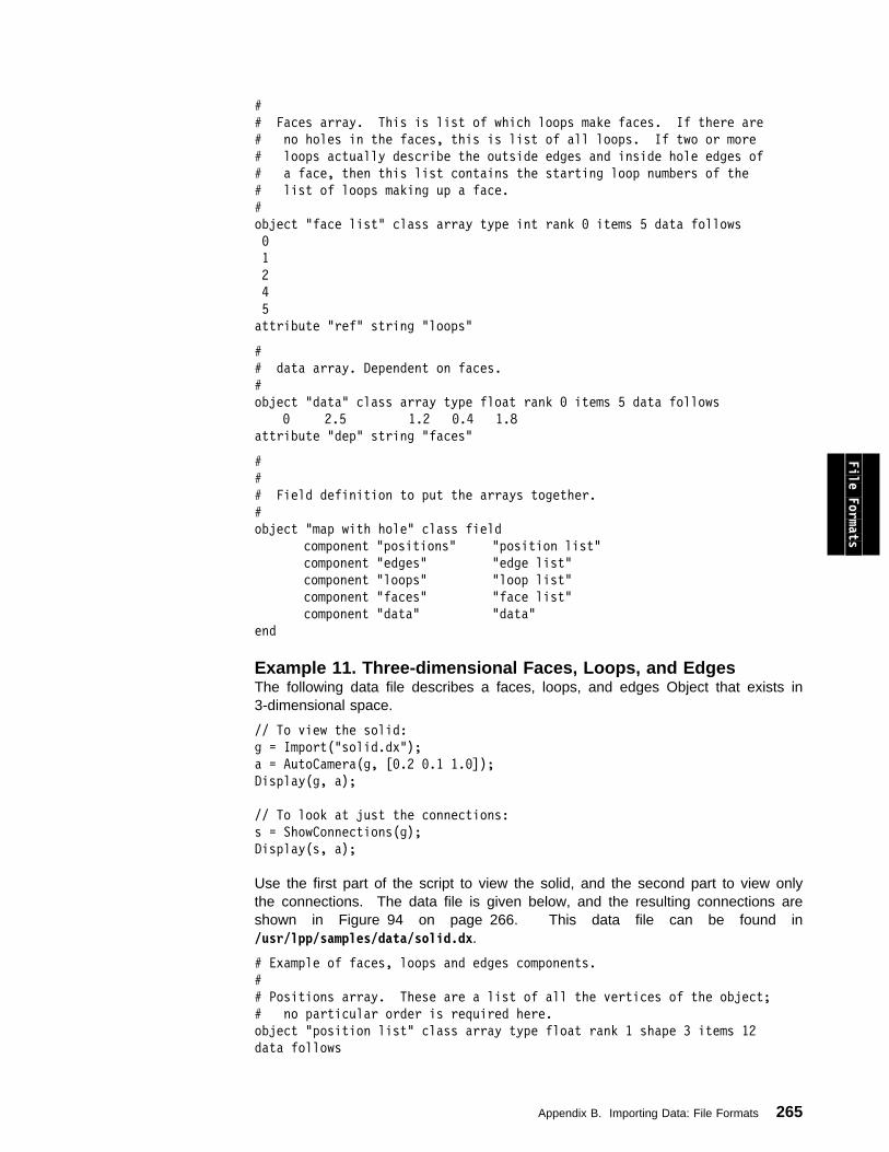
# Faces array. This is list of which loops make faces. If there are

# no holes in the faces, this is list of all loops. If two or more

# loops actually describe the outside edges and inside hole edges of

# a face, then this list contains the starting loop numbers of the

# list of loops making up a face.

#

object "face list" class array type int rank ð items 5 data follows

ð

1

2

4

5

attribute "ref" string "loops"

#

# data array. Dependent on faces.

#

object "data" class array type float rank ð items 5 data follows

ð 2.5 1.2 ð.4 1.8

attribute "dep" string "faces"

#

#

# Field definition to put the arrays together.

#

object "map with hole" class field

component "positions" "position list"

component "edges" "edge list"

component "loops" "loop list"

component "faces" "face list"

component "data" "data"

end

File Formats

Example 11. Three-dimensional Faces, Loops, and EdgesThe following data file describes a faces, loops, and edges Object that exists in3-dimensional space.

// To view the solid:

g = Import("solid.dx");

a = AutoCamera(g, [ð.2 ð.1 1.ð]);

Display(g, a);

// To look at just the connections:

s = ShowConnections(g);

Display(s, a);

Use the first part of the script to view the solid, and the second part to view onlythe connections. The data file is given below, and the resulting connections areshown in Figure 94 on page 266. This data file can be found in/usr/lpp/samples/data/solid.dx.

# Example of faces, loops and edges components.

#

# Positions array. These are a list of all the vertices of the object;

# no particular order is required here.

object "position list" class array type float rank 1 shape 3 items 12

data follows

Appendix B. Importing Data: File Formats 265

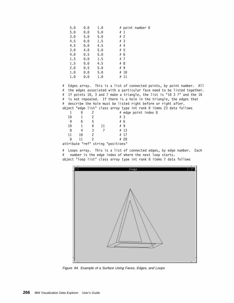
5.ð ð.ð 1.ð # point number ð

5.ð ð.ð 5.ð # 1

3.ð 5.ð 5.ð # 2

4.5 ð.ð 1.5 # 3

4.5 ð.ð 4.5 # 4

3.ð 4.ð 5.ð # 5

4.ð ð.5 5.ð # 6

1.5 ð.ð 1.5 # 7

1.5 ð.ð 4.5 # 8

2.ð ð.5 5.ð # 9

1.ð ð.ð 5.ð # 1ð

1.ð ð.ð 1.ð # 11

# Edges array. This is a list of connected points, by point number. All

# the edges associated with a particular face need to be listed together.

# If points 1ð, 3 and 7 make a triangle, the list is "1ð 3 7" and the 1ð

# is not repeated. If there is a hole in the triangle, the edges that

# describe the hole must be listed right before or right after.

object "edge list" class array type int rank ð items 23 data follows

1 ð 2 # edge point index ð

1ð 1 2 # 3

9 6 5 # 6

1ð 1 ð 11 # 9

8 4 3 7 # 13

11 1ð 2 # 17

ð 11 2 # 2ð

attribute "ref" string "positions"

# Loops array. This is a list of connected edges, by edge number. Each

# number is the edge index of where the next loop starts.

object "loop list" class array type int rank ð items 7 data follows

Figure 94. Example of a Surface Using Faces, Edges, and Loops

266 IBM Visualization Data Explorer: User’s Guide

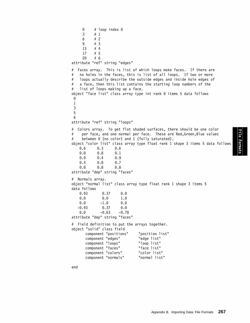
ð # loop index ð

3 # 1

6 # 2

9 # 3

13 # 4

17 # 5

2ð # 6

attribute "ref" string "edges"

# Faces array. This is list of which loops make faces. If there are

# no holes in the faces, this is list of all loops. If two or more

# loops actually describe the outside edges and inside hole edges of

# a face, then this list contains the starting loop numbers of the

# list of loops making up a face.

object "face list" class array type int rank ð items 5 data follows

ð

1

3

5

6

attribute "ref" string "loops"

# Colors array. To get flat shaded surfaces, there should be one color

# per face, and one normal per face. These are Red,Green,Blue values

# between ð (no color) and 1 (fully saturated).

object "color list" class array type float rank 1 shape 3 items 5 data follows

ð.6 ð.3 ð.6

ð.8 ð.8 ð.1

ð.9 ð.4 ð.9

ð.4 ð.8 ð.7

ð.8 ð.8 ð.8

attribute "dep" string "faces"

# Normals array.

object "normal list" class array type float rank 1 shape 3 items 5

data follows

ð.93 ð.37 ð.ð

ð.ð ð.ð 1.ð

ð.ð -1.ð ð.ð

-ð.93 ð.37 ð.ð

ð.ð -ð.63 -ð.78

attribute "dep" string "faces"

# Field definition to put the arrays together.

object "solid" class field

component "positions" "position list"

component "edges" "edge list"

component "loops" "loop list"

component "faces" "face list"

component "colors" "color list"

component "normals" "normal list"

end

File Formats

Appendix B. Importing Data: File Formats 267

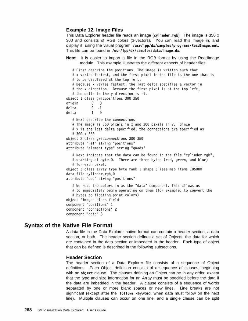
Example 12. Image FilesThis Data Explorer header file reads an image (cylinder.rgb). The image is 350 x300 and consists of RGB colors (3-vectors). You can read this image in, anddisplay it, using the visual program /usr/lpp/dx/samples/programs/ReadImage.net.This file can be found in /usr/lpp/dx/samples/data/image.dx.

Note: It is easier to import a file in the RGB format by using the ReadImagemodule. This example illustrates the different aspects of header files.

# First describe the positions. The image is written such that

# x varies fastest, and the first pixel in the file is the one that is

# to be displayed at the top left.

# Because x varies fastest, the last delta specifies a vector in

# the x direction. Because the first pixel is at the top left,

# the delta in the y direction is -1.

object 1 class gridpositions 3ðð 35ð

origin ð ð

delta ð -1

delta 1 ð

# Next describe the connections

# The image is 35ð pixels in x and 3ðð pixels in y. Since

# x is the last delta specified, the connections are specified as

# 3ðð x 35ð

object 2 class gridconnections 3ðð 35ð

attribute "ref" string "positions"

attribute "element type" string "quads"

# Next indicate that the data can be found in the file "cylinder.rgb",

# starting at byte ð. There are three bytes (red, green, and blue)

# for each pixel.

object 3 class array type byte rank 1 shape 3 ieee msb items 1ð5ððð

data file cylinder.rgb,ð

attribute "dep" string "positions"

# We read the colors in as the "data" component. This allows us

# to immediately begin operating on them (for example, to convert the

# bytes to floating point colors)

object "image" class field

component "positions" 1

component "connections" 2

component "data" 3

Syntax of the Native File FormatA data file in the Data Explorer native format can contain a header section, a datasection, or both. The header section defines a set of Objects, the data for whichare contained in the data section or imbedded in the header. Each type of objectthat can be defined is described in the following subsections.

Header SectionThe header section of a Data Explorer file consists of a sequence of Objectdefinitions. Each Object definition consists of a sequence of clauses, beginningwith an object clause. The clauses defining an Object can be in any order, exceptthat the type and size information for an Array must be specified before the data ifthe data are imbedded in the header. A clause consists of a sequence of wordsseparated by one or more blank spaces or new lines. Line breaks are notsignificant (except after the follows keyword, when data must follow on the nextline). Multiple clauses can occur on one line, and a single clause can be split

268 IBM Visualization Data Explorer: User’s Guide

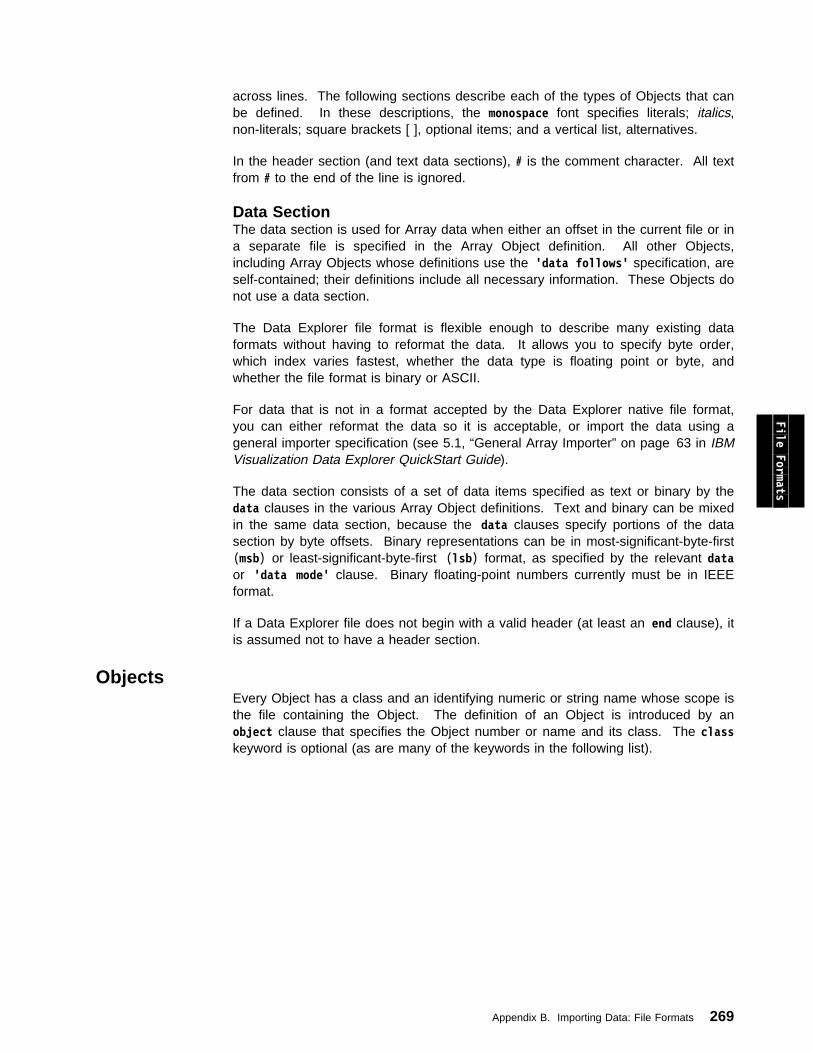
across lines. The following sections describe each of the types of Objects that canbe defined. In these descriptions, the monospace font specifies literals; italics,non-literals; square brackets [ ], optional items; and a vertical list, alternatives.

In the header section (and text data sections), # is the comment character. All textfrom # to the end of the line is ignored.

Data SectionThe data section is used for Array data when either an offset in the current file or ina separate file is specified in the Array Object definition. All other Objects,including Array Objects whose definitions use the 'data follows' specification, areself-contained; their definitions include all necessary information. These Objects donot use a data section.

The Data Explorer file format is flexible enough to describe many existing dataformats without having to reformat the data. It allows you to specify byte order,which index varies fastest, whether the data type is floating point or byte, andwhether the file format is binary or ASCII.

For data that is not in a format accepted by the Data Explorer native file format,you can either reformat the data so it is acceptable, or import the data using ageneral importer specification (see 5.1, “General Array Importer” on page 63 in IBMVisualization Data Explorer QuickStart Guide).

The data section consists of a set of data items specified as text or binary by thedata clauses in the various Array Object definitions. Text and binary can be mixedin the same data section, because the data clauses specify portions of the datasection by byte offsets. Binary representations can be in most-significant-byte-first(msb) or least-significant-byte-first (lsb) format, as specified by the relevant dataor 'data mode' clause. Binary floating-point numbers currently must be in IEEEformat.

If a Data Explorer file does not begin with a valid header (at least an end clause), itis assumed not to have a header section.

File Formats

ObjectsEvery Object has a class and an identifying numeric or string name whose scope isthe file containing the Object. The definition of an Object is introduced by anobject clause that specifies the Object number or name and its class. The classkeyword is optional (as are many of the keywords in the following list).

Appendix B. Importing Data: File Formats 269

object number [class] group “name” series

multigrid compositefield field array constantarray gridpositions regulararray productarray gridconnections patharray mesharray xform string light camera clipped screen

The numeric or string name of an Object is used to refer to that Object in thedefinitions of other Objects. In general such references can take one of severalforms:

number “name” file file file file,number file file,“name”

An Object that has a string name can be imported with the Import module byspecifying that string as the variable parameter of Import.

All Objects can have any number of named attributes specified by attributeclauses. The value of an attribute is an Object. The value can be specified as astring or list of strings by using the string keyword (in which case a String Objectis created to hold the string), as a number by using the number keyword (in whichcase an Array Object is created to hold the number), or as an Object reference.

attribute "attribute-name" [value] string "string" ... number number

number “name”

file file file file,number file file,“name”

Group ObjectsA Group Object has any number of named or numbered members specified bymember clauses. The value of the member is specified as an Object name ornumber in the current file or as an Object name or number in another file. Membernumbers must be sequential, starting at 0, with no gaps in the numbering.

270 IBM Visualization Data Explorer: User’s Guide

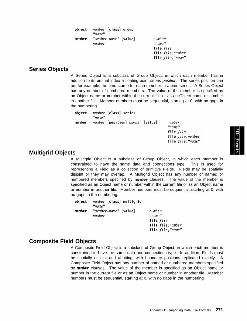
object number [class] group “name”member "member-name" [value] number

number “name” file file file file,number file file,“name”

Series ObjectsA Series Object is a subclass of Group Object, in which each member has inaddition to its ordinal index a floating-point series position. The series position canbe, for example, the time stamp for each member in a time series. A Series Objecthas any number of numbered members. The value of the member is specified asan Object name or number within the current file or as an Object name or numberin another file. Member numbers must be sequential, starting at 0, with no gaps inthe numbering.

object number [class] series "name"member number [position] number [value] number

“name” file file file file,number file file,“name”

File Formats Multigrid ObjectsA Multigrid Object is a subclass of Group Object, in which each member isconstrained to have the same data and connections type. This is used forrepresenting a Field as a collection of primitive Fields. Fields may be spatiallydisjoint or they may overlap. A Multigrid Object has any number of named ornumbered members specified by member clauses. The value of the member isspecified as an Object name or number within the current file or as an Object nameor number in another file. Member numbers must be sequential, starting at 0, withno gaps in the numbering.

object number [class] multigrid “name”member "member-name" [value] number

number “name” file file file file,number file file,“name”

Composite Field ObjectsA Composite Field Object is a subclass of Group Object, in which each member isconstrained to have the same data and connections type. In addition, Fields mustbe spatially disjoint and abutting, with boundary positions replicated exactly. AComposite Field Object has any number of named or numbered members specifiedby member clauses. The value of the member is specified as an Object name ornumber in the current file or as an Object name or number in another file. Membernumbers must be sequential, starting at 0, with no gaps in the numbering.

Appendix B. Importing Data: File Formats 271

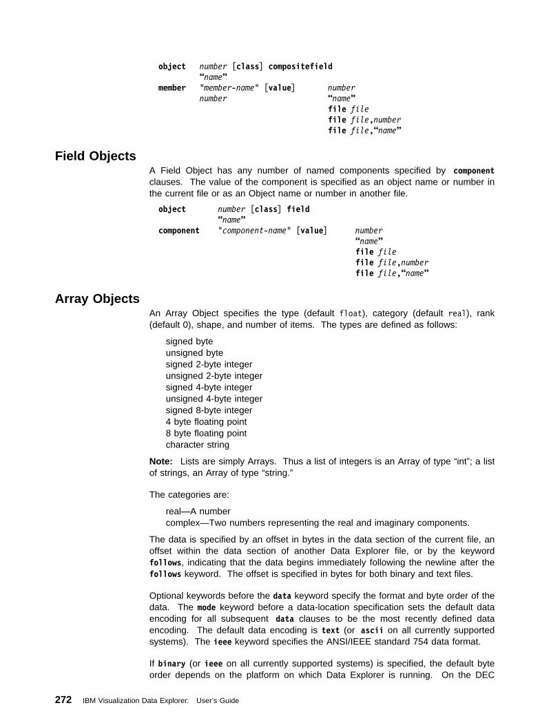
object number [class] compositefield “name”member "member-name" [value] number

number “name” file file file file,number file file,“name”

Field ObjectsA Field Object has any number of named components specified by componentclauses. The value of the component is specified as an object name or number inthe current file or as an Object name or number in another file.

object number [class] field “name”component "component-name" [value] number

“name” file file file file,number file file,“name”

Array ObjectsAn Array Object specifies the type (default float), category (default real), rank(default 0), shape, and number of items. The types are defined as follows:

signed byte unsigned byte

signed 2-byte integerunsigned 2-byte integersigned 4-byte integerunsigned 4-byte integersigned 8-byte integer4 byte floating point8 byte floating point

character string

Note: Lists are simply Arrays. Thus a list of integers is an Array of type “int”; a listof strings, an Array of type “string.”

The categories are:

real—A numbercomplex—Two numbers representing the real and imaginary components.

The data is specified by an offset in bytes in the data section of the current file, anoffset within the data section of another Data Explorer file, or by the keywordfollows, indicating that the data begins immediately following the newline after thefollows keyword. The offset is specified in bytes for both binary and text files.

Optional keywords before the data keyword specify the format and byte order of thedata. The mode keyword before a data-location specification sets the default dataencoding for all subsequent data clauses to be the most recently defined dataencoding. The default data encoding is text (or ascii on all currently supportedsystems). The ieee keyword specifies the ANSI/IEEE standard 754 data format.

If binary (or ieee on all currently supported systems) is specified, the default byteorder depends on the platform on which Data Explorer is running. On the DEC

272 IBM Visualization Data Explorer: User’s Guide

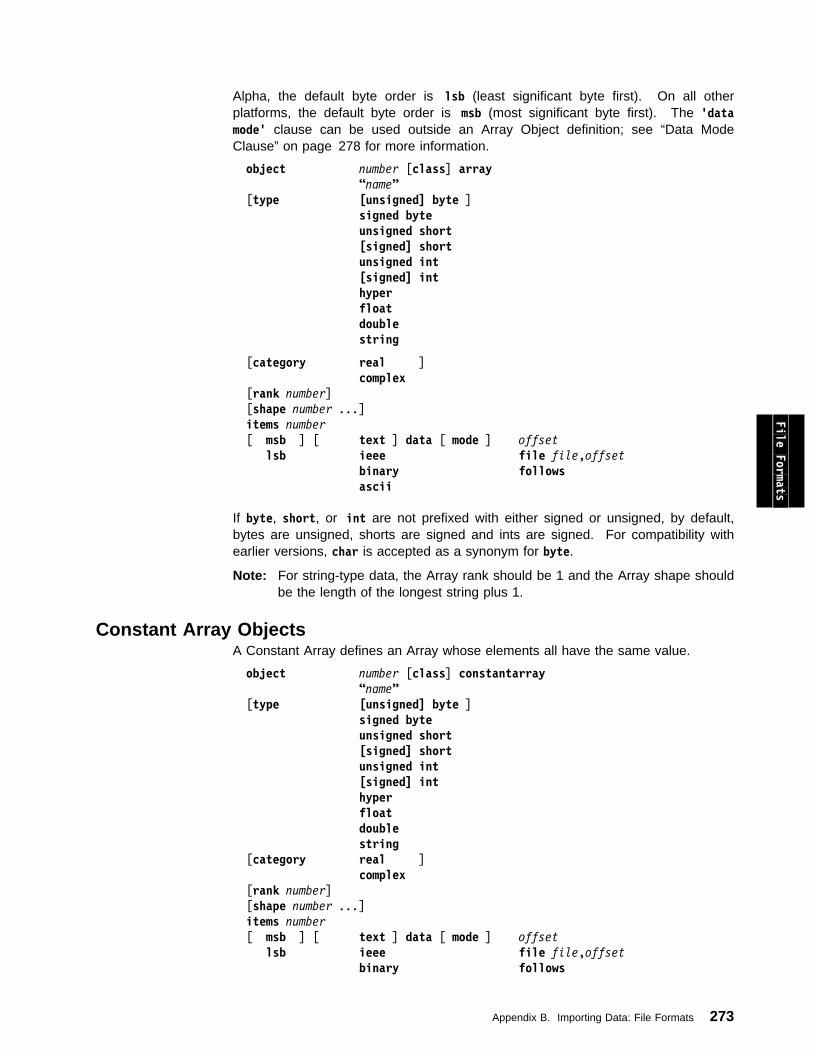
Alpha, the default byte order is lsb (least significant byte first). On all otherplatforms, the default byte order is msb (most significant byte first). The 'datamode' clause can be used outside an Array Object definition; see “Data ModeClause” on page 278 for more information.

object number [class] array “name”[type [unsigned] byte ]

signed byte unsigned short [signed] short unsigned int [signed] int

hyper float double string

[category real ]

complex [rank number]

[shape number ...] items number [ msb ] [ text ] data [ mode ] offset lsb ieee file file,offset binary follows ascii

If byte, short, or int are not prefixed with either signed or unsigned, by default,bytes are unsigned, shorts are signed and ints are signed. For compatibility withearlier versions, char is accepted as a synonym for byte.

Note: For string-type data, the Array rank should be 1 and the Array shape shouldbe the length of the longest string plus 1.

File Formats

Constant Array ObjectsA Constant Array defines an Array whose elements all have the same value.

object number [class] constantarray “name”[type [unsigned] byte ]

signed byte unsigned short [signed] short unsigned int [signed] int

hyper float double string [category real ]

complex [rank number]

[shape number ...] items number [ msb ] [ text ] data [ mode ] offset lsb ieee file file,offset binary follows

Appendix B. Importing Data: File Formats 273

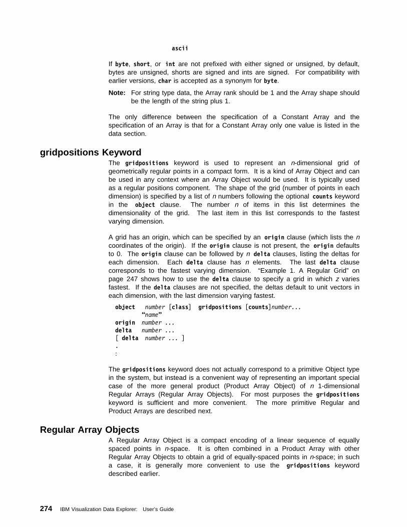
ascii

If byte, short, or int are not prefixed with either signed or unsigned, by default,bytes are unsigned, shorts are signed and ints are signed. For compatibility withearlier versions, char is accepted as a synonym for byte.

Note: For string type data, the Array rank should be 1 and the Array shape shouldbe the length of the string plus 1.

The only difference between the specification of a Constant Array and thespecification of an Array is that for a Constant Array only one value is listed in thedata section.

gridpositions KeywordThe gridpositions keyword is used to represent an n-dimensional grid ofgeometrically regular points in a compact form. It is a kind of Array Object and canbe used in any context where an Array Object would be used. It is typically usedas a regular positions component. The shape of the grid (number of points in eachdimension) is specified by a list of n numbers following the optional counts keywordin the object clause. The number n of items in this list determines thedimensionality of the grid. The last item in this list corresponds to the fastestvarying dimension.

A grid has an origin, which can be specified by an origin clause (which lists the ncoordinates of the origin). If the origin clause is not present, the origin defaultsto 0. The origin clause can be followed by n delta clauses, listing the deltas foreach dimension. Each delta clause has n elements. The last delta clausecorresponds to the fastest varying dimension. “Example 1. A Regular Grid” onpage 247 shows how to use the delta clause to specify a grid in which z variesfastest. If the delta clauses are not specified, the deltas default to unit vectors ineach dimension, with the last dimension varying fastest.

object number [class] gridpositions [counts]number... “name”

origin number ... delta number ...[ delta number ... ]

.

:

The gridpositions keyword does not actually correspond to a primitive Object typein the system, but instead is a convenient way of representing an important specialcase of the more general product (Product Array Object) of n 1-dimensionalRegular Arrays (Regular Array Objects). For most purposes the gridpositionskeyword is sufficient and more convenient. The more primitive Regular andProduct Arrays are described next.

Regular Array ObjectsA Regular Array Object is a compact encoding of a linear sequence of equallyspaced points in n-space. It is often combined in a Product Array with otherRegular Array Objects to obtain a grid of equally-spaced points in n-space; in sucha case, it is generally more convenient to use the gridpositions keyworddescribed earlier.

274 IBM Visualization Data Explorer: User’s Guide

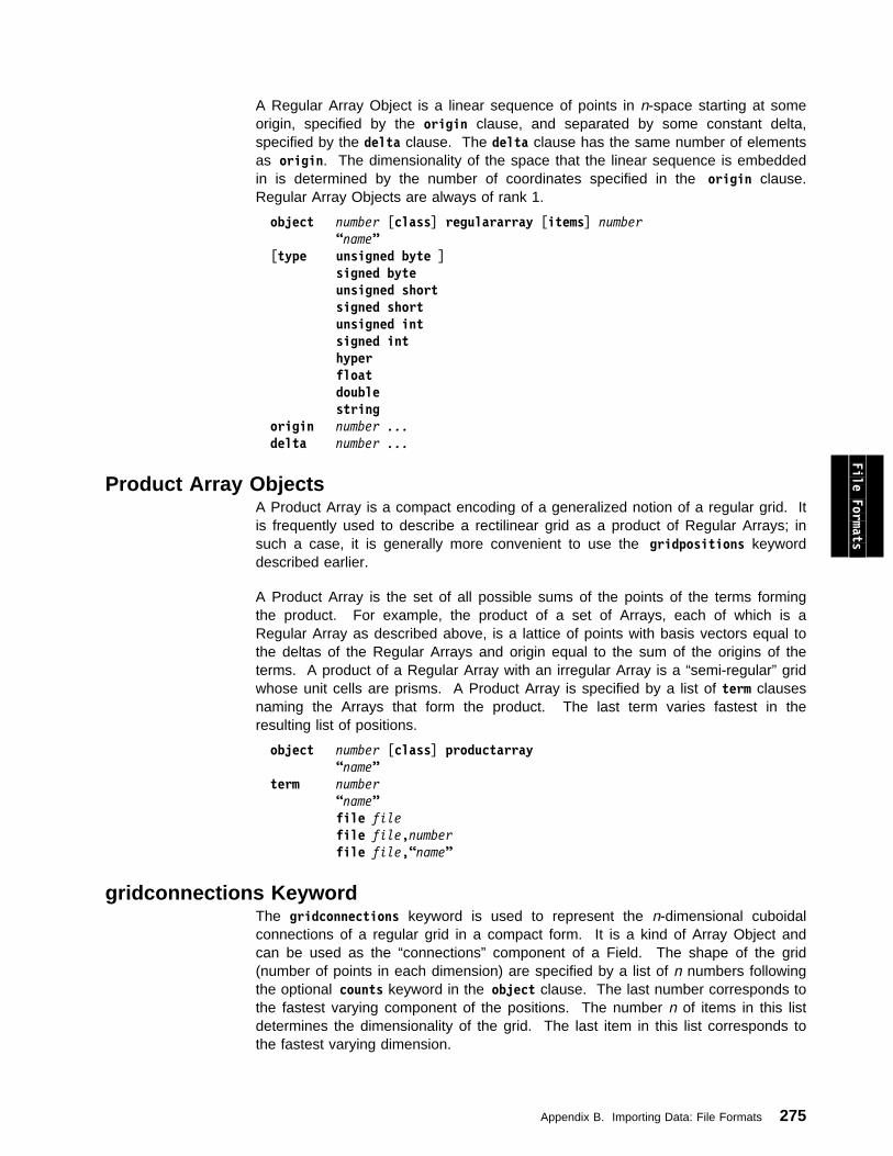
A Regular Array Object is a linear sequence of points in n-space starting at someorigin, specified by the origin clause, and separated by some constant delta,specified by the delta clause. The delta clause has the same number of elementsas origin. The dimensionality of the space that the linear sequence is embeddedin is determined by the number of coordinates specified in the origin clause.Regular Array Objects are always of rank 1.

object number [class] regulararray [items] number “name”[type unsigned byte ]

signed byte unsigned short signed short unsigned int signed int

hyper float double string origin number ...delta number ... File Formats

Product Array ObjectsA Product Array is a compact encoding of a generalized notion of a regular grid. Itis frequently used to describe a rectilinear grid as a product of Regular Arrays; insuch a case, it is generally more convenient to use the gridpositions keyworddescribed earlier.

A Product Array is the set of all possible sums of the points of the terms formingthe product. For example, the product of a set of Arrays, each of which is aRegular Array as described above, is a lattice of points with basis vectors equal tothe deltas of the Regular Arrays and origin equal to the sum of the origins of theterms. A product of a Regular Array with an irregular Array is a “semi-regular” gridwhose unit cells are prisms. A Product Array is specified by a list of term clausesnaming the Arrays that form the product. The last term varies fastest in theresulting list of positions.

object number [class] productarray “name” term number “name” file file file file,number file file,“name”

gridconnections KeywordThe gridconnections keyword is used to represent the n-dimensional cuboidalconnections of a regular grid in a compact form. It is a kind of Array Object andcan be used as the “connections” component of a Field. The shape of the grid(number of points in each dimension) are specified by a list of n numbers followingthe optional counts keyword in the object clause. The last number corresponds tothe fastest varying component of the positions. The number n of items in this listdetermines the dimensionality of the grid. The last item in this list corresponds tothe fastest varying dimension.

Appendix B. Importing Data: File Formats 275

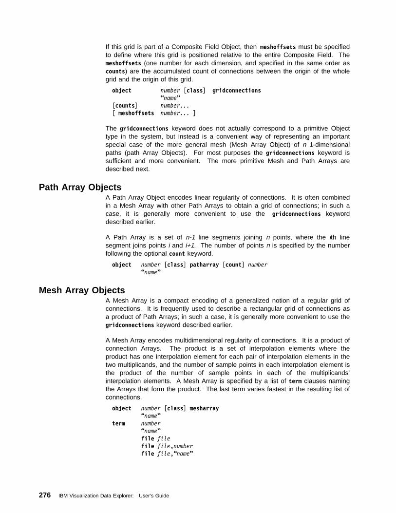
If this grid is part of a Composite Field Object, then meshoffsets must be specifiedto define where this grid is positioned relative to the entire Composite Field. Themeshoffsets (one number for each dimension, and specified in the same order ascounts) are the accumulated count of connections between the origin of the wholegrid and the origin of this grid.

object number [class] gridconnections “name” [counts] number...

[ meshoffsets number... ]

The gridconnections keyword does not actually correspond to a primitive Objecttype in the system, but instead is a convenient way of representing an importantspecial case of the more general mesh (Mesh Array Object) of n 1-dimensionalpaths (path Array Objects). For most purposes the gridconnections keyword issufficient and more convenient. The more primitive Mesh and Path Arrays aredescribed next.

Path Array ObjectsA Path Array Object encodes linear regularity of connections. It is often combinedin a Mesh Array with other Path Arrays to obtain a grid of connections; in such acase, it is generally more convenient to use the gridconnections keyworddescribed earlier.

A Path Array is a set of n-1 line segments joining n points, where the ith linesegment joins points i and i+1. The number of points n is specified by the numberfollowing the optional count keyword.

object number [class] patharray [count] number “name”

Mesh Array ObjectsA Mesh Array is a compact encoding of a generalized notion of a regular grid ofconnections. It is frequently used to describe a rectangular grid of connections asa product of Path Arrays; in such a case, it is generally more convenient to use thegridconnections keyword described earlier.

A Mesh Array encodes multidimensional regularity of connections. It is a product ofconnection Arrays. The product is a set of interpolation elements where theproduct has one interpolation element for each pair of interpolation elements in thetwo multiplicands, and the number of sample points in each interpolation element isthe product of the number of sample points in each of the multiplicands’interpolation elements. A Mesh Array is specified by a list of term clauses namingthe Arrays that form the product. The last term varies fastest in the resulting list ofconnections.

object number [class] mesharray “name” term number “name”

file file file file,number file file,“name”

276 IBM Visualization Data Explorer: User’s Guide

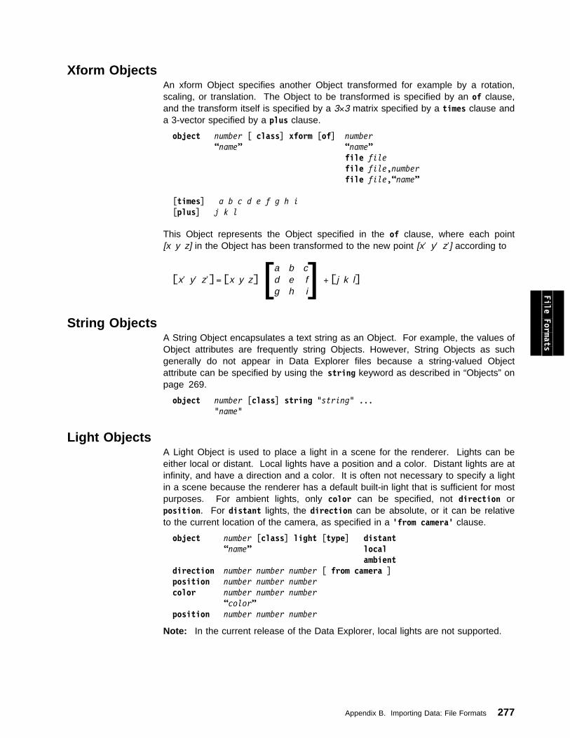
Xform ObjectsAn xform Object specifies another Object transformed for example by a rotation,scaling, or translation. The Object to be transformed is specified by an of clause,and the transform itself is specified by a 3×3 matrix specified by a times clause anda 3-vector specified by a plus clause.

object number [ class] xform [of] number “name” “name”

file file file file,number file file,“name”

[times] a b c d e f g h i[plus] j k l

This Object represents the Object specified in the of clause, where each point[x y z] in the Object has been transformed to the new point [x′ y′ z′] according to

x′ y′ z′ =

x y z [a

dg

beh

cfi] +

j k l

File Formats

String ObjectsA String Object encapsulates a text string as an Object. For example, the values ofObject attributes are frequently string Objects. However, String Objects as suchgenerally do not appear in Data Explorer files because a string-valued Objectattribute can be specified by using the string keyword as described in “Objects” onpage 269.

object number [class] string "string" ... "name"

Light ObjectsA Light Object is used to place a light in a scene for the renderer. Lights can beeither local or distant. Local lights have a position and a color. Distant lights are atinfinity, and have a direction and a color. It is often not necessary to specify a lightin a scene because the renderer has a default built-in light that is sufficient for mostpurposes. For ambient lights, only color can be specified, not direction orposition. For distant lights, the direction can be absolute, or it can be relativeto the current location of the camera, as specified in a 'from camera' clause.

object number [class] light [type] distant “name” local

ambientdirection number number number [ from camera ]

position number number numbercolor number number number

“color” position number number number

Note: In the current release of the Data Explorer, local lights are not supported.

Appendix B. Importing Data: File Formats 277

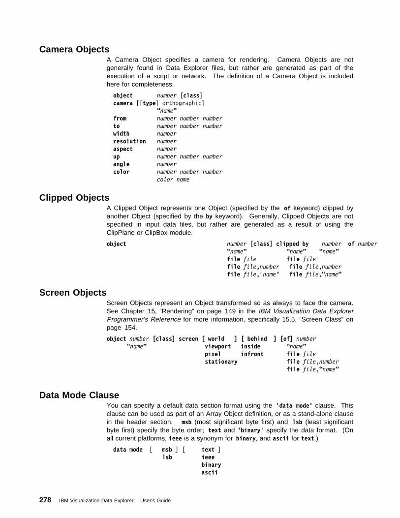
Camera ObjectsA Camera Object specifies a camera for rendering. Camera Objects are notgenerally found in Data Explorer files, but rather are generated as part of theexecution of a script or network. The definition of a Camera Object is includedhere for completeness.

object number [class]camera [[type] orthographic]

“name”from number number numberto number number number

width number resolution number aspect numberup number number number

angle numbercolor number number number

color name

Clipped ObjectsA Clipped Object represents one Object (specified by the of keyword) clipped byanother Object (specified by the by keyword). Generally, Clipped Objects are notspecified in input data files, but rather are generated as a result of using theClipPlane or ClipBox module.

object number [class] clipped by number of number “name” “name” “name” file file file file file file,number file file,number file file,"name" file file,“name”

Screen ObjectsScreen Objects represent an Object transformed so as always to face the camera.See Chapter 15, “Rendering” on page 149 in the IBM Visualization Data ExplorerProgrammer’s Reference for more information, specifically 15.5, “Screen Class” onpage 154.

object number [class] screen [ world ] [ behind ] [of] number“name” viewport inside “name”

pixel infront file file stationary file file,number

file file,“name”

Data Mode ClauseYou can specify a default data section format using the 'data mode' clause. Thisclause can be used as part of an Array Object definition, or as a stand-alone clausein the header section. msb (most significant byte first) and lsb (least significantbyte first) specify the byte order; text and 'binary' specify the data format. (Onall current platforms, ieee is a synonym for binary, and ascii for text.)

data mode [ msb ] [ text ] lsb ieee binary ascii

278 IBM Visualization Data Explorer: User’s Guide

Default ClauseYou can specify the default Object to be imported using the default clause. Whena Data Explorer data file contains more than one Object (which is the usual case),the Import module (see “Import” on page 165 in IBM Visualization Data ExplorerUser’s Reference) decides which Object to import based on the value of thevariable parameter (Object name or names) of the Import module, and thedefault clause (if specified). If variable is specified to Import, then those Objectsspecified are imported. If variable is not specified, but a default Object is specifiedwith the default clause, then the default Object is imported. If variable is notspecified, and no Object has been defined as the default, then the last Object in thefile is imported.

default number "name"

End ClauseThe end of the header section is indicated by an end clause. The data sectionbegins with the byte immediately following the first newline after the end clause.

end File Formats

B.3 CDF FilesCDF is a data abstraction for self-describing multidimensional Arrays. It representsa simpler data model than that of Data Explorer, one similar to that of the ArrayObject. Data are accessed in CDF through an applications programming interface,available as C and FORTRAN libraries from the National Space Science DataCenter, NASA/Goddard Space Flight Center, Greenbelt, MD. Data in CDF may bestored in a number of physical formats (e.g., native or portable binary, single ormultiple files, row or column majority), but the interface is the same. Hence, data ina CDF written in a format “foreign” to the workstation on which Data Explorer isrunning are converted automatically during the Import process.

Data Explorer provides support for importing Fields stored as CDF r-variables. Toimport data from a CDF, specify the CDF name as the name parameter in the ImportConfiguration dialog box (not the file name, since the CDF may be in multiple-fileformat). If the CDF has more than one variable, which is typical, Data Explorercategorizes each variable as positions, series, or data as appropriate. Variablesthat vary in one dimension only and are not record-variant are considered positions,and become the positions component in a Field Object. In many cases, thesevariables may have the CDF variable mnemonics of LATITUDE and LONGITUD,which are mapped to the first (x) and second (y) components of the positionsvector, if they exist. This mapping permits direct use of these data withcartographic and other tools for the earth and space sciences that are publiclyavailable for use with Data Explorer. Otherwise, the first n variables categorized aspositions (where n is the dimensionality of the CDF dimensions) are used to formthe positions component. Any additional such variables are treated as datavariables. If there are no positions-type variables, the positions component will bea regular grid with origin of 0 and increments of 1 in each axis, where the numberof axes corresponds to the dimensionality of the imported CDF r-variable.

If there are records in the CDF, each record is imported as a series member. Inmany cases there is a variable with the mnemonic EPOCH, which corresponds to atime stamp for each record in the CDF. If so, the double representing msec since

Appendix B. Importing Data: File Formats 279

0 AD in each value of EPOCH is stored as the series position attribute. If not, thefirst variable that is record-variant and nondimensional-variant is considered theseries variable. This variable is imported as the series position attribute. If there isno time variable, the series position starts at 1 and increments by 1 per seriesmember, so that there is one member for each record in the CDF. The seriesposition attribute, containing the time stamp, may be accessed with the Attributemodule.

You can specify the name or names of the data variable in the variable parameterof the Import tool and the corresponding variable(s) will be imported. In the sameway, you can use start, end, and delta to import a subset of CDF records.

Variable and global attributes present in the CDF are imported as Object attributes.These attributes may be accessed through the Attribute and Inquire modules (e.g.,to build metadata-driven applications).

Variables that vary in all dimensions and are record-variant are considered datavariables. Any variable that is not a position or time variable is also considered adata variable, allowing every variable to be imported. If you want the positions tobe a variable other than the one chosen by Data Explorer, you can use Replace orRename to switch the components (e.g., two or more sets of positions informationare stored for different coordinate systems). Each data variable becomes a datacomponent in a Field Object. Hence, there is one Field for each data variable inthe Group imported. Since Data Explorer can handle data more flexibly than CDF,some assumptions are imposed upon certain classes of data that may be imported:

Since data stored in CDF are not distinguished as cell-centered or node-based,all data components are treated as the latter, (i.e., data dep positions). ThePost module may be used to transform a Field to cell-centered (i.e., data depconnections).

Since CDF does not “natively” support Fields other than rank=0, all datavariables are treated as scalars. The Compute module can be used toconstruct the appropriate vector representation from multiple scalar Fields.

The connections component depends on the dimensionality of the data variablesuch that 0 = none, 1 = lines, 2 = quads, 3 = cubes, and so on.

Each positions variable is considered a term of a Product Array to form thepositions component.

All variables of 0 dimension are imported as the data component of a Field withno positions and no connections. If the LATITUDE and/or LONGITUDvariables exist, the other variables are considered data components of Fieldswith positions and no connections, where the positions are those latitude andlongitude variables. You can construct an appropriate Field with positions andconnections from the variables that are imported through modules likeConstruct, Regrid, and Connect.

All variables of 1 dimension are imported as the data component of a Field oflines, where the positions would typically be a scalar (i.e., the one independentvariable). If the LATITUDE and LONGITUD variables exist, then the positionsare a 2-vector constructed from the latitude and longitude Arrays, but still a line.

One-dimensional variables in CDF may be of one of three distinct classes,which are NOT distinguished in the way they are stored in a CDF file: 1) true1-dimensional or line data; 2) indexed point data; or 3) indexed mesh data.You must know which class the variable belongs to in order to ensure that DataExplorer processes the data in an appropriate fashion. The first class ishandled correctly. For the second and third class, the connections component

280 IBM Visualization Data Explorer: User’s Guide

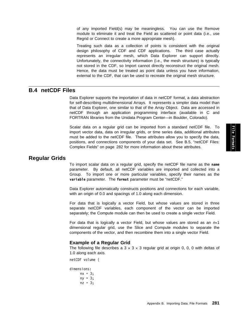
of any imported Field(s) may be meaningless. You can use the Removemodule to eliminate it and treat the Field as scattered or point data (i.e., useRegrid or Connect to create a more appropriate mesh).

Treating such data as a collection of points is consistent with the originaldesign philosophy of CDF and CDF applications. The third case actuallyrepresents an irregular mesh, which Data Explorer can support directly.Unfortunately, the connectivity information (i.e., the mesh structure) is typicallynot stored in the CDF, so Import cannot directly reconstruct the original mesh.Hence, the data must be treated as point data unless you have information,external to the CDF, that can be used to recreate the original mesh structure.

B.4 netCDF FilesData Explorer supports the importation of data in netCDF format, a data abstractionfor self-describing multidimensional Arrays. It represents a simpler data model thanthat of Data Explorer, one similar to that of the Array Object. Data are accessed innetCDF through an application programming interface (available in C andFORTRAN libraries from the Unidata Program Center—in Boulder, Colorado).

Scalar data on a regular grid can be imported from a standard netCDF file. Toimport vector data, data on irregular grids, or time series data, additional attributesmust be added to the netCDF file. These attributes allow you to specify the data,positions, and connections components of your data set. See B.5, “netCDF Files:Complex Fields” on page 282 for more information about these attributes.

File Formats

Regular GridsTo import scalar data on a regular grid, specify the netCDF file name as the nameparameter. By default, all netCDF variables are imported and collected into aGroup. To import one or more particular variables, specify their names as thevariable parameter. The format parameter must be “netCDF.”

Data Explorer automatically constructs positions and connections for each variable,with an origin of 0.0 and spacings of 1.0 along each dimension.

For data that is logically a vector Field, but whose values are stored in threeseparate netCDF variables, each component of the vector can be importedseparately; the Compute module can then be used to create a single vector Field.

For data that is logically a vector Field, but whose values are stored as an n+1dimensional regular grid, use the Slice and Compute modules to separate thecomponents of the vector, and then recombine them into a single vector Field.

Example of a Regular GridThe following file describes a 3 × 3 × 3 regular grid at origin 0, 0, 0 with deltas of1.0 along each axis.

netCDF volume

dimensions:

nx = 3;

ny = 3;

nz = 3;

Appendix B. Importing Data: File Formats 281

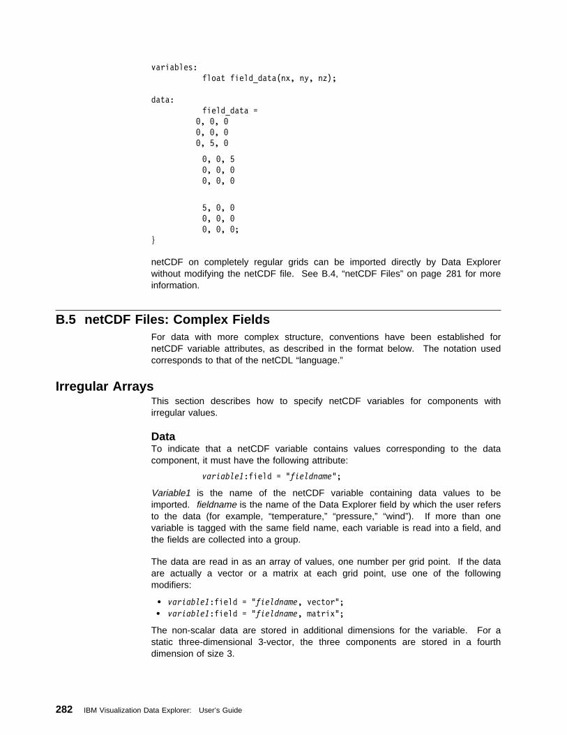
variables:

float field_data(nx, ny, nz);

data:

field_data =

ð, ð, ð

ð, ð, ð

ð, 5, ð

ð, ð, 5

ð, ð, ð

ð, ð, ð

5, ð, ð

ð, ð, ð

ð, ð, ð;

netCDF on completely regular grids can be imported directly by Data Explorerwithout modifying the netCDF file. See B.4, “netCDF Files” on page 281 for moreinformation.

B.5 netCDF Files: Complex FieldsFor data with more complex structure, conventions have been established fornetCDF variable attributes, as described in the format below. The notation usedcorresponds to that of the netCDL “language.”

Irregular ArraysThis section describes how to specify netCDF variables for components withirregular values.

DataTo indicate that a netCDF variable contains values corresponding to the datacomponent, it must have the following attribute:

variable1:field = "fieldname";

Variable1 is the name of the netCDF variable containing data values to beimported. fieldname is the name of the Data Explorer field by which the user refersto the data (for example, “temperature,” “pressure,” “wind”). If more than onevariable is tagged with the same field name, each variable is read into a field, andthe fields are collected into a group.

The data are read in as an array of values, one number per grid point. If the dataare actually a vector or a matrix at each grid point, use one of the followingmodifiers:

variable1:field = "fieldname, vector"; variable1:field = "fieldname, matrix";

The non-scalar data are stored in additional dimensions for the variable. For astatic three-dimensional 3-vector, the three components are stored in a fourthdimension of size 3.

282 IBM Visualization Data Explorer: User’s Guide

If the data have both regular connections and regular positions, no other attributesare required. A regular grid is assumed, with the origin at 0.0, and a spacing of 1.0along each axis. The number of axes will be determined from the number ofdimensions in the data array.

PositionsIf the locations of the data values in variable1 do not form a regular lattice (withorigins at 0.0 and spacings of 1.0), the name of a netCDF variable that contains theposition information must be specified as an attribute for variable1.

There are five different types of position specifications: none, completely regular,completely irregular, and two types of partially regular.

Completely irregular is assumed if the following attribute is specified:

variable1:positions = "variable2";

where variable2 is an array of vectors, one for each grid point, defining its location.The dimensionality of the data space is determined by the number of items in avector.

Regular positions can be specified with just the origin and spacing between gridpoints along each axis in compact form. The following attribute is used:

variable1:positions = "variable2, compact";

where variable2 is the name of a n×2 array containing origin, delta pairs for thespacing and location of positions along each axis. The number of positions alongeach axis is determined from the shape of variable1.

Positions that can be specified as the product of arrays containing the location ofpoints along each axis can be input in product form. Use the following attribute:

variable1:positions = "variable2a, product; variable2b, product;

.

.

.

variable2x, product";

where the variable2's are each the name of an array containing a list of positionsalong that axis. The number of items in each array must match the length of thecorresponding axis in the original variable1 data array.

If any of the axes in an partially regular product array are actually regular, they canbe specified in compact form:

variable1:positions = "variable2a, product, compact; variable2b, product;

.

.

.

variable2x, product";

where variable2a is the name of an origin, delta array, and the rest are position listsas before.

File Formats

Appendix B. Importing Data: File Formats 283

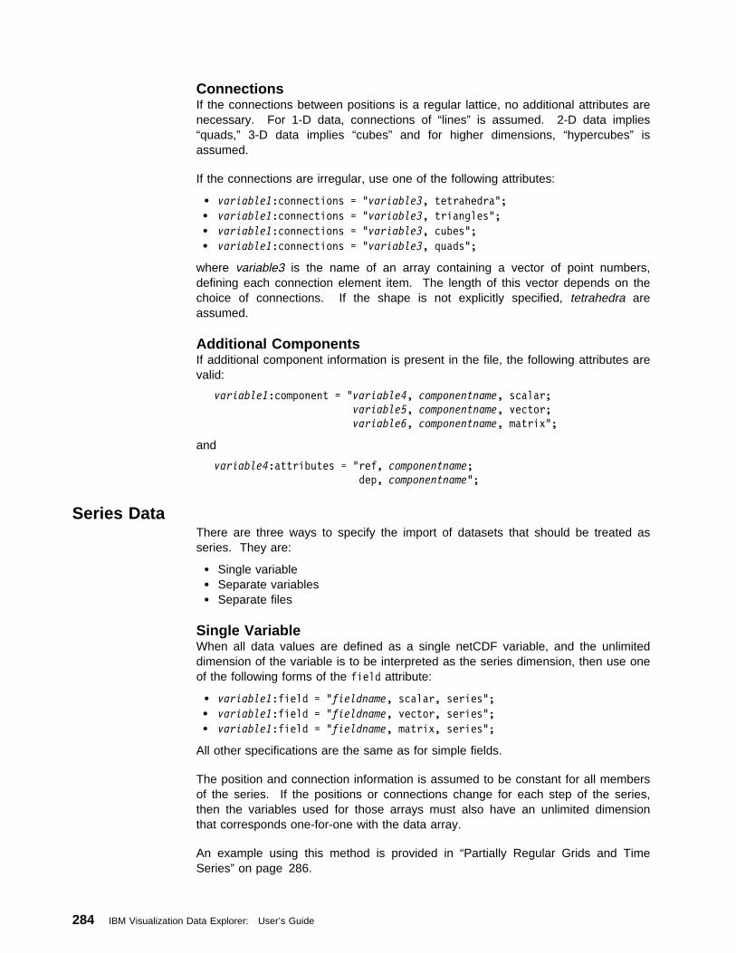
ConnectionsIf the connections between positions is a regular lattice, no additional attributes arenecessary. For 1-D data, connections of “lines” is assumed. 2-D data implies“quads,” 3-D data implies “cubes” and for higher dimensions, “hypercubes” isassumed.

If the connections are irregular, use one of the following attributes:

variable1:connections = "variable3, tetrahedra"; variable1:connections = "variable3, triangles"; variable1:connections = "variable3, cubes"; variable1:connections = "variable3, quads";

where variable3 is the name of an array containing a vector of point numbers,defining each connection element item. The length of this vector depends on thechoice of connections. If the shape is not explicitly specified, tetrahedra areassumed.

Additional ComponentsIf additional component information is present in the file, the following attributes arevalid:

variable1:component = "variable4, componentname, scalar;variable5, componentname, vector;variable6, componentname, matrix";

and

variable4:attributes = "ref, componentname; dep, componentname";

Series DataThere are three ways to specify the import of datasets that should be treated asseries. They are:

Single variable Separate variables Separate files

Single VariableWhen all data values are defined as a single netCDF variable, and the unlimiteddimension of the variable is to be interpreted as the series dimension, then use oneof the following forms of the field attribute:

variable1:field = "fieldname, scalar, series"; variable1:field = "fieldname, vector, series"; variable1:field = "fieldname, matrix, series";

All other specifications are the same as for simple fields.

The position and connection information is assumed to be constant for all membersof the series. If the positions or connections change for each step of the series,then the variables used for those arrays must also have an unlimited dimensionthat corresponds one-for-one with the data array.

An example using this method is provided in “Partially Regular Grids and TimeSeries” on page 286.

284 IBM Visualization Data Explorer: User’s Guide

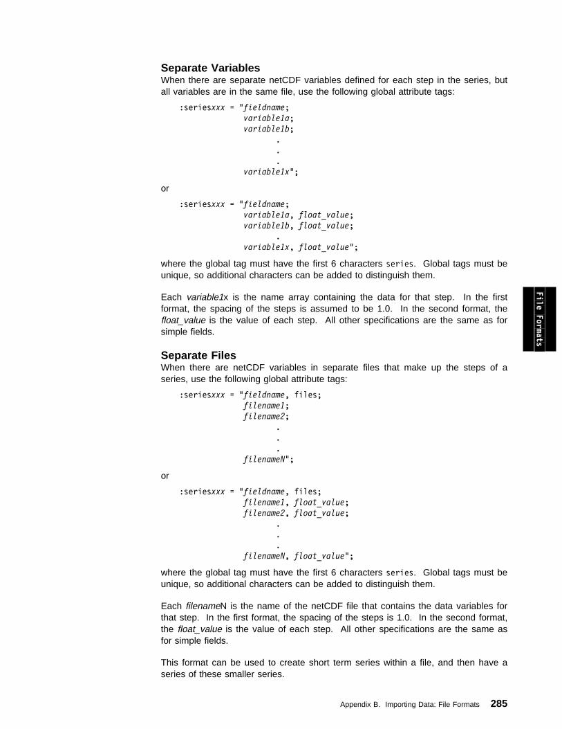
Separate VariablesWhen there are separate netCDF variables defined for each step in the series, butall variables are in the same file, use the following global attribute tags:

:seriesxxx = "fieldname; variable1a; variable1b; .

.

.

variable1x";

or

:seriesxxx = "fieldname; variable1a, float_value; variable1b, float_value; .

variable1x, float_value";

where the global tag must have the first 6 characters series. Global tags must beunique, so additional characters can be added to distinguish them.

Each variable1x is the name array containing the data for that step. In the firstformat, the spacing of the steps is assumed to be 1.0. In the second format, thefloat_value is the value of each step. All other specifications are the same as forsimple fields.

File Formats

Separate FilesWhen there are netCDF variables in separate files that make up the steps of aseries, use the following global attribute tags:

:seriesxxx = "fieldname, files; filename1; filename2; .

.

.

filenameN";

or

:seriesxxx = "fieldname, files; filename1, float_value; filename2, float_value; .

.

.

filenameN, float_value";

where the global tag must have the first 6 characters series. Global tags must beunique, so additional characters can be added to distinguish them.

Each filenameN is the name of the netCDF file that contains the data variables forthat step. In the first format, the spacing of the steps is 1.0. In the second format,the float_value is the value of each step. All other specifications are the same asfor simple fields.

This format can be used to create short term series within a file, and then have aseries of these smaller series.

Appendix B. Importing Data: File Formats 285

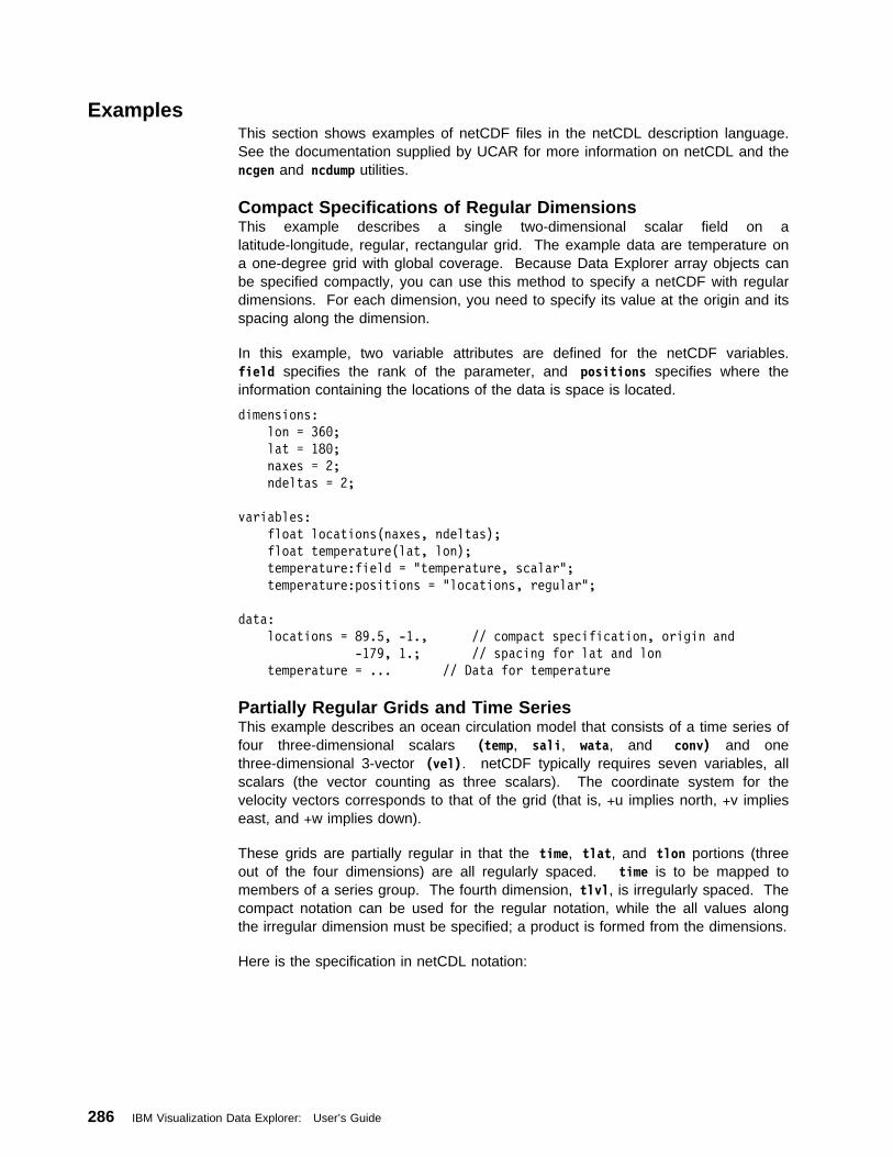
ExamplesThis section shows examples of netCDF files in the netCDL description language.See the documentation supplied by UCAR for more information on netCDL and thencgen and ncdump utilities.

Compact Specifications of Regular DimensionsThis example describes a single two-dimensional scalar field on alatitude-longitude, regular, rectangular grid. The example data are temperature ona one-degree grid with global coverage. Because Data Explorer array objects canbe specified compactly, you can use this method to specify a netCDF with regulardimensions. For each dimension, you need to specify its value at the origin and itsspacing along the dimension.

In this example, two variable attributes are defined for the netCDF variables.field specifies the rank of the parameter, and positions specifies where theinformation containing the locations of the data is space is located.

dimensions:

lon = 36ð;

lat = 18ð;

naxes = 2;

ndeltas = 2;

variables:

float locations(naxes, ndeltas);

float temperature(lat, lon);

temperature:field = "temperature, scalar";

temperature:positions = "locations, regular";

data:

locations = 89.5, -1., // compact specification, origin and

-179, 1.; // spacing for lat and lon

temperature = ... // Data for temperature

Partially Regular Grids and Time SeriesThis example describes an ocean circulation model that consists of a time series offour three-dimensional scalars (temp, sali, wata, and conv) and onethree-dimensional 3-vector (vel). netCDF typically requires seven variables, allscalars (the vector counting as three scalars). The coordinate system for thevelocity vectors corresponds to that of the grid (that is, +u implies north, +v implieseast, and +w implies down).

These grids are partially regular in that the time, tlat, and tlon portions (threeout of the four dimensions) are all regularly spaced. time is to be mapped tomembers of a series group. The fourth dimension, tlvl, is irregularly spaced. Thecompact notation can be used for the regular notation, while the all values alongthe irregular dimension must be specified; a product is formed from the dimensions.

Here is the specification in netCDL notation:

286 IBM Visualization Data Explorer: User’s Guide

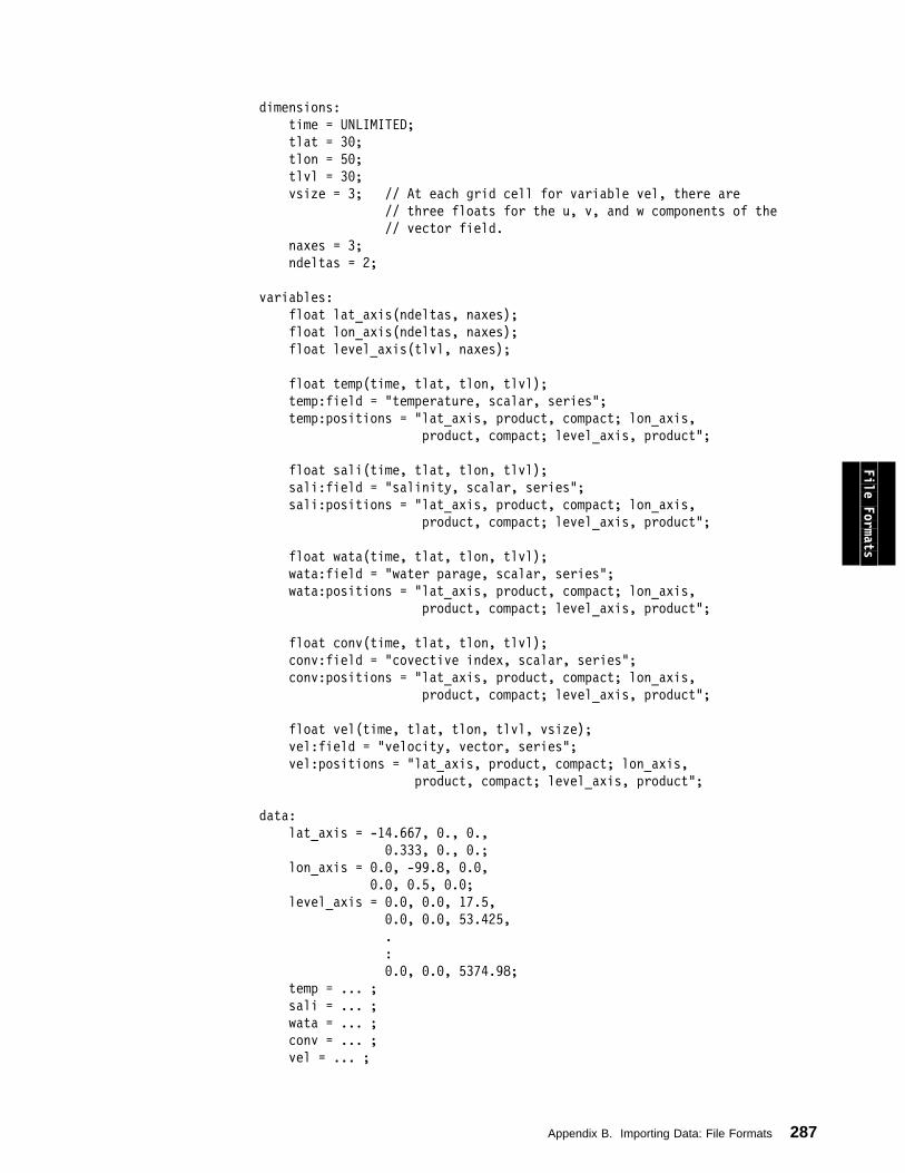
dimensions:

time = UNLIMITED;

tlat = 3ð;

tlon = 5ð;

tlvl = 3ð;

vsize = 3; // At each grid cell for variable vel, there are

// three floats for the u, v, and w components of the

// vector field.

naxes = 3;

ndeltas = 2;

variables:

float lat_axis(ndeltas, naxes);

float lon_axis(ndeltas, naxes);

float level_axis(tlvl, naxes);

float temp(time, tlat, tlon, tlvl);

temp:field = "temperature, scalar, series";

temp:positions = "lat_axis, product, compact; lon_axis,

product, compact; level_axis, product";

float sali(time, tlat, tlon, tlvl);

sali:field = "salinity, scalar, series";

sali:positions = "lat_axis, product, compact; lon_axis,

product, compact; level_axis, product";

float wata(time, tlat, tlon, tlvl);

wata:field = "water parage, scalar, series";

wata:positions = "lat_axis, product, compact; lon_axis,

product, compact; level_axis, product";

float conv(time, tlat, tlon, tlvl);

conv:field = "covective index, scalar, series";

conv:positions = "lat_axis, product, compact; lon_axis,

product, compact; level_axis, product";

float vel(time, tlat, tlon, tlvl, vsize);

vel:field = "velocity, vector, series";

vel:positions = "lat_axis, product, compact; lon_axis,

product, compact; level_axis, product";

data:

lat_axis = -14.667, ð., ð.,

ð.333, ð., ð.;

lon_axis = ð.ð, -99.8, ð.ð,

ð.ð, ð.5, ð.ð;

level_axis = ð.ð, ð.ð, 17.5,

ð.ð, ð.ð, 53.425,

.

:

ð.ð, ð.ð, 5374.98;

temp = ... ;

sali = ... ;

wata = ... ;

conv = ... ;

vel = ... ;

File Formats

Appendix B. Importing Data: File Formats 287

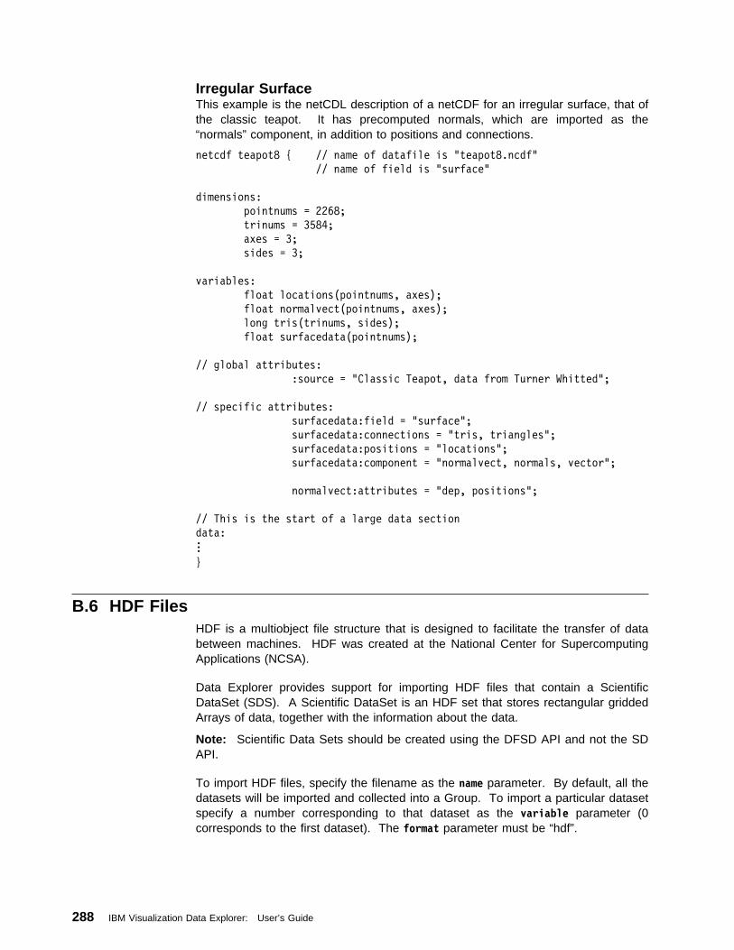
Irregular SurfaceThis example is the netCDL description of a netCDF for an irregular surface, that ofthe classic teapot. It has precomputed normals, which are imported as the“normals” component, in addition to positions and connections.

netcdf teapot8 // name of datafile is "teapot8.ncdf"

// name of field is "surface"

dimensions:

pointnums = 2268;

trinums = 3584;

axes = 3;

sides = 3;

variables:

float locations(pointnums, axes);

float normalvect(pointnums, axes);

long tris(trinums, sides);

float surfacedata(pointnums);

// global attributes:

:source = "Classic Teapot, data from Turner Whitted";

// specific attributes:

surfacedata:field = "surface";

surfacedata:connections = "tris, triangles";

surfacedata:positions = "locations";

surfacedata:component = "normalvect, normals, vector";

normalvect:attributes = "dep, positions";

// This is the start of a large data section

data:...

B.6 HDF FilesHDF is a multiobject file structure that is designed to facilitate the transfer of databetween machines. HDF was created at the National Center for SupercomputingApplications (NCSA).

Data Explorer provides support for importing HDF files that contain a ScientificDataSet (SDS). A Scientific DataSet is an HDF set that stores rectangular griddedArrays of data, together with the information about the data.

Note: Scientific Data Sets should be created using the DFSD API and not the SDAPI.

To import HDF files, specify the filename as the name parameter. By default, all thedatasets will be imported and collected into a Group. To import a particular datasetspecify a number corresponding to that dataset as the variable parameter (0corresponds to the first dataset). The format parameter must be “hdf”.

288 IBM Visualization Data Explorer: User’s Guide

If dimension scales are specified, Data Explorer uses these to construct positions;otherwise positions have an origin of 0.0 and deltas of 1.0 along each dimension.Data Explorer automatically constructs regular connections for either case.

File Formats

Appendix B. Importing Data: File Formats 289

290 IBM Visualization Data Explorer: User’s Guide

Appendix C. Environment Variables and Command LineOptions

C.1 Environment Variables . . . . . . . . . . . . . . . . . . . . . . . . . . . . . 292Path Variables . . . . . . . . . . . . . . . . . . . . . . . . . . . . . . . . . . . 292Other Environment Variables . . . . . . . . . . . . . . . . . . . . . . . . . . 292

C.2 Command Line Options . . . . . . . . . . . . . . . . . . . . . . . . . . . . 295

Variables/Options

Copyright IBM Corp. 1991-1997 291

C.1 Environment VariablesThe environment variables described in this section can be set in your login profileto customize Data Explorer. Note also that these variables can be overridden onthe command line (see C.2, “Command Line Options” on page 295).

Path VariablesPath variables specify a directory or directories to be searched for files. Directoriesare searched in the order of their appearance in the variable, reading from left toright, with successive path names separated by a colon (:). Thus when a fileappears in more than one directory, Data Explorer will choose the first copy it finds(i.e., in the leftmost directory containing a copy).

DXDATA specifies directories to be searched for importable data files. If the datato be imported is in your current directory or one of the specified directories, you donot need to enter the complete path name in the Configuration dialog box for theImport tool: given just the file name, the Import module will search all of thesedirectories.

DXINCLUDE specifies directories to be searched for include scripts. Data Exploreruses include scripts in script mode. It is not necessary to specify this variable inEdit mode.: See “File Inclusion” on page 207 for more information.

DXMACROS specifies directories to be searched for macros when Data Explorerstarts up. If DXMACROS is not specified, you will have to load macros individually(see 7.2, “Creating and Using Macros” on page 149).

DXMODULES specifies the directories to be searched for outboard modules.

Setting a Path Variable: ExamplesNote the colon (:) separating successive path names.

To set DXMACROS for both the Bourne (sh) and the Korn (ksh) shells:

DXMACROS=/usr/mydirectory/projectAmacros:/usr/mydirectory/projectBmacros

export DXMACROS

To set DXDATA for the Korn shell (ksh) only:

export DXDATA=/usr/mydirectory/mydata:/usr/group/groupdata

To set DXDATA for the C shell (csh):

setenv DXDATA /usr/mydirectory/mydata:/usr/group/groupdata

Other Environment VariablesDX8BITCMAP sets the level at which the change to using a private color map ismade. The allowed values are -1 and the range from 0 (zero) to 1 (one) andrepresent the Euclidean distance in RGB color space, normalized to 1 (one) for themaximum allowed discrepancy. The default value is 0.1. If this variable is set to 1,a private color map will never be used; conversely, if it is set to -1, a private colormap will always be used. (See Display in IBM Visualization Data Explorer User’sReference.)

DXARGS specifies the default set of arguments for Data Explorer start-up. Anoption specified on the command line will override the corresponding setting in thevariable.

292 IBM Visualization Data Explorer: User’s Guide

DXAXESMAXWIDTH sets the number of digits in axes tick labels at which a switchto scientific notation is made. The default is 7.

DXNO_BACKING_STORE if set to anything, disables framebuffer readbacks.Setting this environment variable will improve performance of interaction withhardware rendered images, especially for machines for which readback is slow.However, some of the interactions in the image window (such as zoom) will resultin a black image while interaction is taking place. If you are not planning on usingthe Image tool, then it is strongly recommended that this environment variable beset. The default is that framebuffer readbacks are enabled.

DXCOLORS specifies a file name containing string and RGB value pairs as analternate for /usr/lpp/dx/lib/colors.txt. The string name can be used by any DataExplorer tool where a color can be specified by name (for example, Color). TheRGB value specifies the specific numeric value for the color.

DXDELAYEDCOLORS enables ReadImage to create delayed color images if theimage is a tiff format image saved in a byte-with-colormap format or a GIF format.This feature is enabled if this variable is set to any value. Delayed colors use lessmemory.

DXEXEC specifies an executive to be run at start-up. You should set this variableonly for a customized version of Data Explorer.

DXFLING If DXFLING is set to 1, then for hardware-rendered images, in rotationmode and execute-on-change mode, if you drag the mouse across the image, andrelease the mouse button outside the image, the object in the image will begin torotate, and will continue to rotate until you click inside the image. The direction andspeed of the mouse motion before release will affect the rotation direction androtation speed of the object in the window.

DXGAMMA sets the gamma correction for software-rendered images displayed tothe screen by a Display or Image tool. On many display devices a given change inthe digital brightness of the image is not reflected in a corresponding change inscreen brightness. A gamma correction is a nonlinear adjustment of the pixelvalues to compensate for this difference and produce a more accuraterepresentation on the screen. By default (except for 8-bit windows on the sgiarchitecture), the correction factor (exponent) is 2 (two), on the assumption that thedisplay is not otherwise gamma corrected. The DXGAMMA variable allows you tooverride this default. In particular, if the display device is already gamma corrected,set the variable to 1 (one). (See Display in IBM Visualization Data Explorer User’sReference, and README_sgi in /usr/lpp/dx.)

DXGAMMA_8BIT, DXGAMMA_12BIT, and DXGAMMA_24BIT set the gammacorrection for software-rendered images displayed to the screen in 8-, 12-, or 24-bitwindows by a Display or Image tool. This variable overrides the value set byDXGAMMA.

DXHOST specifies the machine name of the server on which the executive is to berun. The default is “localhost”. (See 9.3, “Connecting to the Server” on page 183for information on how to connect to the server.) To determine the host name,enter the command:

uname -n

Variables/Options

Appendix C. Environment Variables and Command Line Options 293

DXHWGAMMA sets the gamma correction for hardware-rendered images displayedto the screen by a Display or Image tool. On many display devices a given changein the digital brightness of the image is not reflected in a corresponding change inscreen brightness. A gamma correction is a non-linear adjustment of the pixelvalues to compensate for this difference and produce a more accuraterepresentation on the screen. By default, the correction factor is 2, on theassumption that the display is not otherwise gamma corrected. The DXHWGAMMAvariable allows you to override this default. In particular, if the display device isalready gamma corrected, set the variable to 1.

DXHWMOD if both GL and OpenGL are supported, you can override the defaultlibrary (which is platform-specific; please see the appropriate README file for yourarchitecture in /usr/lpp/dx) by using this environment variable. It should be set toeither DXhwdd.o (for GL) or DXhwddOGL.o (for OpenGL).

DXMDF specifies the name of the .mdf file that contains custom-added modules forcustomized versions of Data Explorer.

DXMEMORY sets the amount of memory (in megabytes) that can be used by theexecutive.

DX_NESTED_LOOPS for faces, loops, and edges data, if set, allows loops otherthan the enclosing loop for a face to be listed first. However, there is a consequentdecrease in performance if this environment variable is set.

DXPIXELTYPE sets the image type to either 24-bit color images orfloating-point-based 96-bit images (the default). This affects the behavior of Renderand ReadImage. This variable can be set to either DXByte (24 bits) or DXFloat (96bits). Setting this variable to DXByte will result in images taking up less memory.

DXPROCESSORS sets the number of processors for Data Explorer SMP.

DXROOT specifies the top-level directory for all the files and directories needed byData Explorer. The default is /usr/lpp/dx.

DXSHMEM specifies whether or not shared memory should be used. The amountof memory allocated by Data Explorer for its data and object management can beset at runtime with the -memory command line option. At startup, Data Explorereither allocates a shared memory segment or expands the existing data segment tocreate this space.: SMP (multiprocessor) systems are required to use sharedmemory so each processor can share a common data space. SGI systems alsouse shared memory for space. IBM systems use shared memory if the size to beallocated is larger than 256 MB. In all other cases Data Explorer extends theexisting data segment using the brk() system call.

Each architecture (SGI, IBM, HP, ...) has a different way of configuring themaximum user data segment size, and a different way of setting the limit on themaximum size of a single shared memory segment. Consult your systemadministrator or system documentation if you have problems getting Data Explorerto use the amount of memory which should be available to you.

If you have problems using a large data segment, you can force Data Explorer touse shared memory by setting the DXSHMEM environment variable to any value otherthan -1. This will override the defaults and use shared memory for space.

294 IBM Visualization Data Explorer: User’s Guide

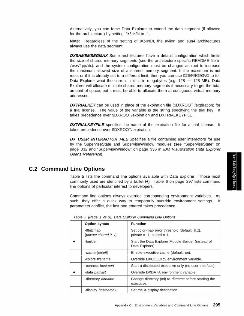
Alternatively, you can force Data Explorer to extend the data segment (if allowedfor the architecture) by setting DXSHMEM to -1.

Note: Regardless of the setting of DXSHMEM, the aviion and sun4 architecturesalways use the data segment.

DXSHMEMSEGMAX Some architectures have a default configuration which limitsthe size of shared memory segments (see the architecture specific README file in/usr/lpp/dx), and the system configuration must be changed as root to increasethe maximum allowed size of a shared memory segment. If the maximum is notreset or if it is already set to a different limit, then you can use DXSHMEMSEGMAX to tellData Explorer what the current limit is in megabytes (e.g. 128 == 128 MB). DataExplorer will allocate multiple shared memory segments if necessary to get the totalamount of space, but it must be able to allocate them at contiguous virtual memoryaddresses.

DXTRIALKEY can be used in place of the expiration file ($DXROOT /expiration) fora trial license. The value of the variable is the string specifying the trial key. Ittakes precedence over $DXROOT/expiration and DXTRIALKEYFILE.

DXTRIALKEYFILE specifies the name of the expiration file for a trial license. Ittakes precedence over $DXROOT/expiration.

DX_USER_INTERACTOR_FILE Specifies a file containing user interactors for useby the SuperviseState and SuperviseWindow modules (see “SuperviseState” onpage 332 and “SuperviseWindow” on page 336 in IBM Visualization Data ExplorerUser’s Reference).

Variables/Options

C.2 Command Line OptionsTable 5 lists the command line options available with Data Explorer. Those mostcommonly used are identified by a bullet (Á). Table 6 on page 297 lists commandline options of particular interest to developers.

Command line options always override corresponding environment variables. Assuch, they offer a quick way to temporarily override environment settings. Ifparameters conflict, the last one entered takes precedence.

Table 5 (Page 1 of 3). Data Explorer Command Line Options

Option syntax Function

-8bitcmap[private|shared|0–1]

Set color-map error threshold (default: 0.1).private = -1; stored = 1.

Á -builder Start the Data Explorer Module Builder (instead ofData Explorer).

-cache [on|off] Enable executive cache (default: on).

-colors filename Override DXCOLORS environment variable.

-connect host:port Start a distributed executive only (no user interface).

Á -data pathlist. Override DXDATA environment variable.

-directory dirname Change directory (cd) to dirname before starting theexecutive.

-display hostname:0 Set the X-display destination.

Appendix C. Environment Variables and Command Line Options 295

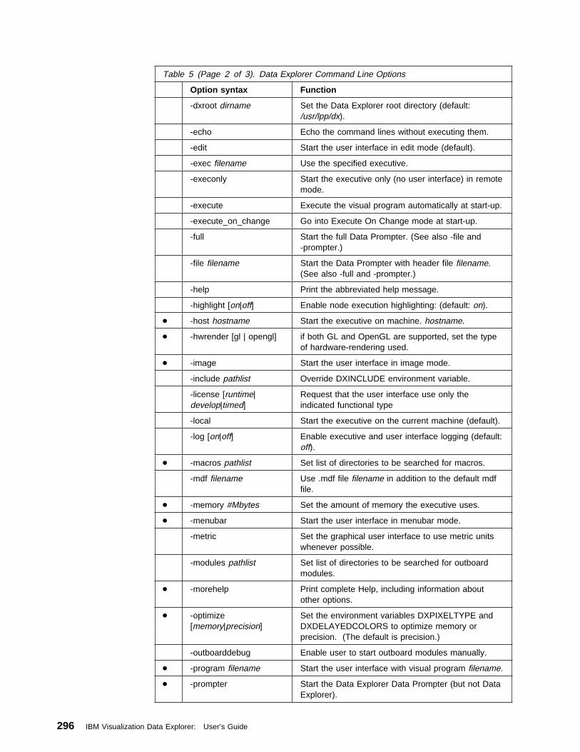
Table 5 (Page 2 of 3). Data Explorer Command Line Options

Option syntax Function

-dxroot dirname Set the Data Explorer root directory (default:/usr/lpp/dx).

-echo Echo the command lines without executing them.

-edit Start the user interface in edit mode (default).

-exec filename Use the specified executive.

-execonly Start the executive only (no user interface) in remotemode.

-execute Execute the visual program automatically at start-up.

-execute_on_change Go into Execute On Change mode at start-up.

-full Start the full Data Prompter. (See also -file and-prompter.)

-file filename Start the Data Prompter with header file filename.(See also -full and -prompter.)

-help Print the abbreviated help message.

-highlight [on|off] Enable node execution highlighting: (default: on).

Á -host hostname Start the executive on machine. hostname.

Á -hwrender [gl | opengl] if both GL and OpenGL are supported, set the typeof hardware-rendering used.

Á -image Start the user interface in image mode.

-include pathlist Override DXINCLUDE environment variable.

-license [runtime|develop|timed]

Request that the user interface use only theindicated functional type

-local Start the executive on the current machine (default).

-log [on|off] Enable executive and user interface logging (default:off).

Á -macros pathlist Set list of directories to be searched for macros.

-mdf filename Use .mdf file filename in addition to the default mdffile.

Á -memory #Mbytes Set the amount of memory the executive uses.

Á -menubar Start the user interface in menubar mode.

-metric Set the graphical user interface to use metric unitswhenever possible.

-modules pathlist Set list of directories to be searched for outboardmodules.

Á -morehelp Print complete Help, including information aboutother options.

Á -optimize[memory|precision]

Set the environment variables DXPIXELTYPE andDXDELAYEDCOLORS to optimize memory orprecision. (The default is precision.)

-outboarddebug Enable user to start outboard modules manually.

Á -program filename Start the user interface with visual program filename.

Á -prompter Start the Data Explorer Data Prompter (but not DataExplorer).

296 IBM Visualization Data Explorer: User’s Guide

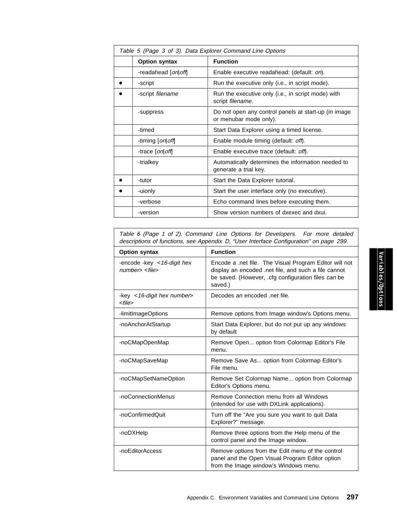
Table 5 (Page 3 of 3). Data Explorer Command Line Options

Option syntax Function

-readahead [on|off] Enable executive readahead: (default: on).

Á -script Run the executive only (i.e., in script mode).

Á -script filename Run the executive only (i.e., in script mode) withscript filename.

-suppress Do not open any control panels at start-up (in imageor menubar mode only).

-timed Start Data Explorer using a timed license.

-timing [on|off] Enable module timing (default: off).

-trace [on|off] Enable executive trace (default: off).

-trialkey Automatically determines the information needed togenerate a trial key.

Á -tutor Start the Data Explorer tutorial.

Á -uionly Start the user interface only (no executive).

-verbose Echo command lines before executing them.

-version Show version numbers of dxexec and dxui.

Table 6 (Page 1 of 2). Command Line Options for Developers. For more detaileddescriptions of functions, see Appendix D, “User Interface Configuration” on page 299.

Option syntax Function

Variables/Options

-encode -key <16-digit hexnumber> <file>

Encode a .net file. The Visual Program Editor will notdisplay an encoded .net file, and such a file cannotbe saved. (However, .cfg configuration files can besaved.)

-key <16-digit hex number><file>

Decodes an encoded .net file.

-limitImageOptions Remove options from Image window's Options menu.

-noAnchorAtStartup Start Data Explorer, but do not put up any windowsby default

-noCMapOpenMap Remove Open... option from Colormap Editor's Filemenu.

-noCMapSaveMap Remove Save As... option from Colormap Editor'sFile menu.

-noCMapSetNameOption Remove Set Colormap Name... option from ColormapEditor's Options menu.

-noConnectionMenus Remove Connection menu from all Windows(intended for use with DXLink applications).

-noConfirmedQuit Turn off the “Are you sure you want to quit DataExplorer?” message.

-noDXHelp Remove three options from the Help menu of thecontrol panel and the Image window.

-noEditorAccess Remove options from the Edit menu of the controlpanel and the Open Visual Program Editor optionfrom the Image window's Windows menu.

Appendix C. Environment Variables and Command Line Options 297

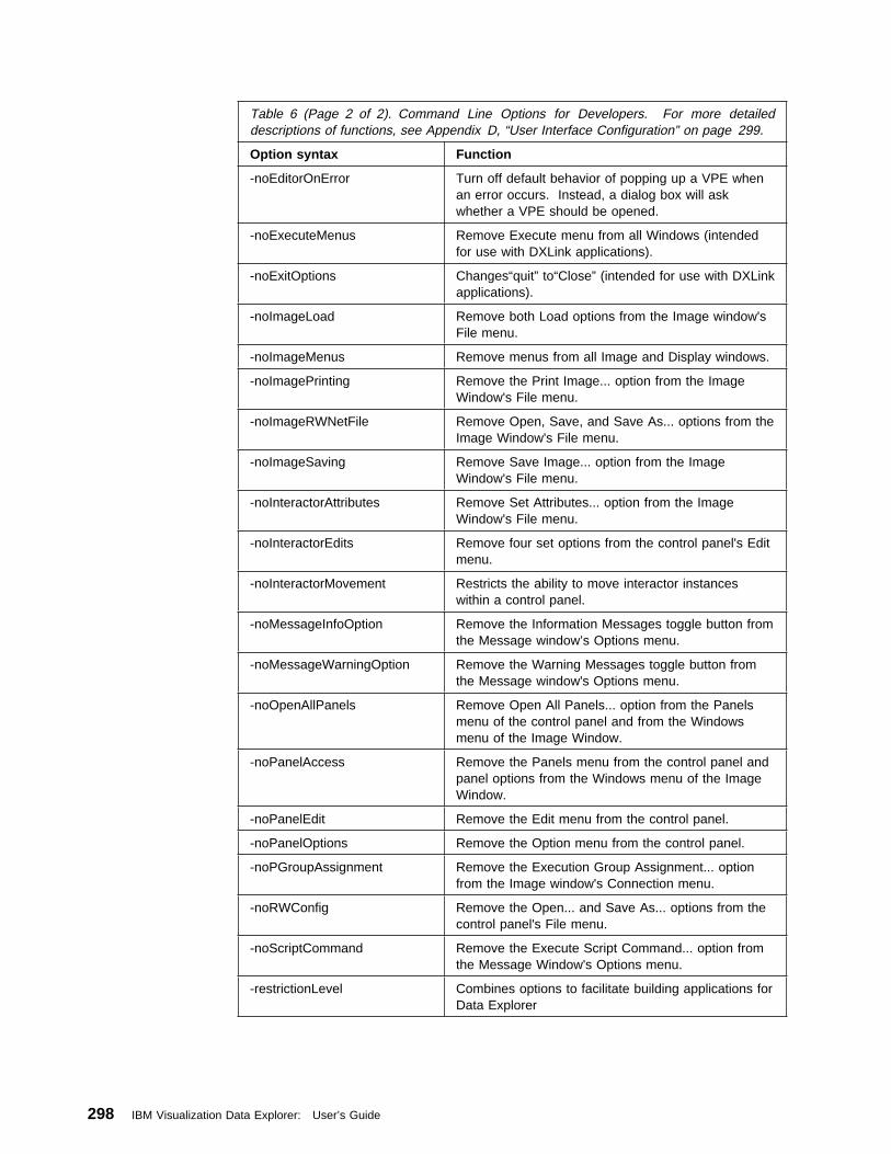
Table 6 (Page 2 of 2). Command Line Options for Developers. For more detaileddescriptions of functions, see Appendix D, “User Interface Configuration” on page 299.

Option syntax Function

-noEditorOnError Turn off default behavior of popping up a VPE whenan error occurs. Instead, a dialog box will askwhether a VPE should be opened.

-noExecuteMenus Remove Execute menu from all Windows (intendedfor use with DXLink applications).

-noExitOptions Changes“quit” to“Close” (intended for use with DXLinkapplications).

-noImageLoad Remove both Load options from the Image window'sFile menu.

-noImageMenus Remove menus from all Image and Display windows.

-noImagePrinting Remove the Print Image... option from the ImageWindow's File menu.

-noImageRWNetFile Remove Open, Save, and Save As... options from theImage Window's File menu.

-noImageSaving Remove Save Image... option from the ImageWindow's File menu.

-noInteractorAttributes Remove Set Attributes... option from the ImageWindow's File menu.

-noInteractorEdits Remove four set options from the control panel's Editmenu.

-noInteractorMovement Restricts the ability to move interactor instanceswithin a control panel.

-noMessageInfoOption Remove the Information Messages toggle button fromthe Message window’s Options menu.

-noMessageWarningOption Remove the Warning Messages toggle button fromthe Message window's Options menu.

-noOpenAllPanels Remove Open All Panels... option from the Panelsmenu of the control panel and from the Windowsmenu of the Image Window.

-noPanelAccess Remove the Panels menu from the control panel andpanel options from the Windows menu of the ImageWindow.

-noPanelEdit Remove the Edit menu from the control panel.

-noPanelOptions Remove the Option menu from the control panel.

-noPGroupAssignment Remove the Execution Group Assignment... optionfrom the Image window's Connection menu.

-noRWConfig Remove the Open... and Save As... options from thecontrol panel's File menu.

-noScriptCommand Remove the Execute Script Command... option fromthe Message Window's Options menu.

-restrictionLevel Combines options to facilitate building applications forData Explorer

298 IBM Visualization Data Explorer: User’s Guide

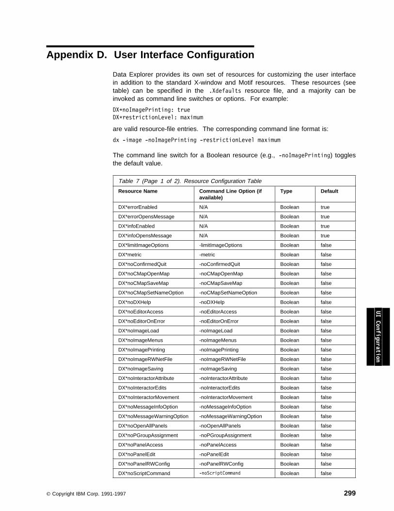
Appendix D. User Interface Configuration

Data Explorer provides its own set of resources for customizing the user interfacein addition to the standard X-window and Motif resources. These resources (seetable) can be specified in the .Xdefaults resource file, and a majority can beinvoked as command line switches or options. For example:

DX\noImagePrinting: true

DX\restrictionLevel: maximum

are valid resource-file entries. The corresponding command line format is:

dx -image -noImagePrinting -restrictionLevel maximum

The command line switch for a Boolean resource (e.g., -noImagePrinting) togglesthe default value.

Table 7 (Page 1 of 2). Resource Configuration Table

Resource Name Command Line Option (ifavailable)

Type Default

DX*errorEnabled N/A Boolean true

DX*errorOpensMessage N/A Boolean true

DX*infoEnabled N/A Boolean true

DX*infoOpensMessage N/A Boolean true

DX*limitImageOptions -limitImageOptions Boolean false

DX*metric -metric Boolean false

DX*noConfirmedQuit -noConfirmedQuit Boolean false

DX*noCMapOpenMap -noCMapOpenMap Boolean false

DX*noCMapSaveMap -noCMapSaveMap Boolean false

DX*noCMapSetNameOption -noCMapSetNameOption Boolean false

DX*noDXHelp -noDXHelp Boolean false

DX*noEditorAccess -noEditorAccess Boolean false

UI Configuration

DX*noEditorOnError -noEditorOnError Boolean false

DX*noImageLoad -noImageLoad Boolean false

DX*noImageMenus -noImageMenus Boolean false

DX*noImagePrinting -noImagePrinting Boolean false

DX*noImageRWNetFile -noImageRWNetFile Boolean false

DX*noImageSaving -noImageSaving Boolean false

DX*noInteractorAttribute -noInteractorAttribute Boolean false

DX*noInteractorEdits -noInteractorEdits Boolean false

DX*noInteractorMovement -noInteractorMovement Boolean false

DX*noMessageInfoOption -noMessageInfoOption Boolean false

DX*noMessageWarningOption -noMessageWarningOption Boolean false

DX*noOpenAllPanels -noOpenAllPanels Boolean false

DX*noPGroupAssignment -noPGroupAssignment Boolean false

DX*noPanelAccess -noPanelAccess Boolean false

DX*noPanelEdit -noPanelEdit Boolean false

DX*noPanelRWConfig -noPanelRWConfig Boolean false

DX*noScriptCommand -noScriptCommand Boolean false

Copyright IBM Corp. 1991-1997 299

DX\errorEnabled

Specifies the default value of the Error Messages toggle button in theMessage window’s Option menu.

DX\errorOpensMessage

Specifies whether or not the Message window pops up when an errormessage is printed in the Message window.

DX\infoEnabled

Specifies the default value of the Information Messages toggle button inthe Message window’s Option menu.

DX\infoOpensMessage

Specifies whether or not the Message window pops up when aninformational message is printed in the Message window.

DX\limitImageOptions

Removes the Image Depth, Throttle, Change Image Name..., and PanelAccess... menu commands from the Image window’s Options menu.

DX\metric

Specifies that Data Explorer use the metric system (centimeters) whenset to “true”. The default is the English system (inches). The PrintImage and Save Image dialog boxes option menus are affectedaccordingly.

Table 7 (Page 2 of 2). Resource Configuration Table

Resource Name Command Line Option (ifavailable)

Type Default

DX*printImageCommand N/A String “lpr”

DX*printImageFormat N/A String “PSCOLOR”

DX*printImagePageSize N/A String NULL

DX*printImageResolution N/A int 0

DX*printImageSize N/A String NULL

DX*restrictionLevel -restrictionlevel String NULL

DX*saveImageFormat N/A String “PSCOLOR”

DX*saveImagePageSize N/A String NULL

DX*saveImageResolution N/A int 0

DX*saveImageSize N/A String NULL

DX*vpeCanvas.lineThickness N/A int 1

DX*warningEnabled N/A Boolean true

DX*warningOpensMessage N/A Boolean true

300 IBM Visualization Data Explorer: User’s Guide

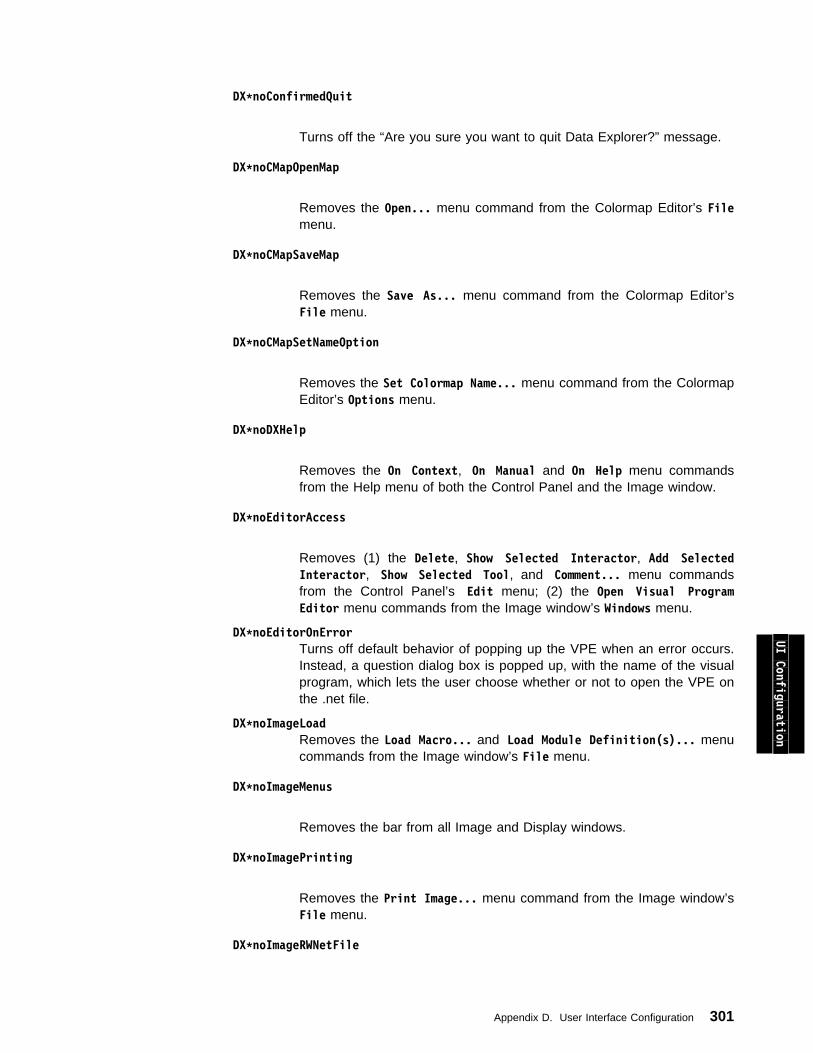
DX\noConfirmedQuit

Turns off the “Are you sure you want to quit Data Explorer?” message.

DX\noCMapOpenMap

Removes the Open... menu command from the Colormap Editor’s Filemenu.

DX\noCMapSaveMap

Removes the Save As... menu command from the Colormap Editor’sFile menu.

DX\noCMapSetNameOption

Removes the Set Colormap Name... menu command from the ColormapEditor’s Options menu.

DX\noDXHelp

Removes the On Context, On Manual and On Help menu commandsfrom the Help menu of both the Control Panel and the Image window.

DX\noEditorAccess

Removes (1) the Delete, Show Selected Interactor, Add SelectedInteractor, Show Selected Tool, and Comment... menu commandsfrom the Control Panel’s Edit menu; (2) the Open Visual ProgramEditor menu commands from the Image window’s Windows menu.

DX\noEditorOnErrorTurns off default behavior of popping up the VPE when an error occurs.Instead, a question dialog box is popped up, with the name of the visualprogram, which lets the user choose whether or not to open the VPE onthe .net file.

DX\noImageLoadRemoves the Load Macro... and Load Module Definition(s)... menucommands from the Image window’s File menu.

DX\noImageMenus

Removes the bar from all Image and Display windows.

DX\noImagePrinting

Removes the Print Image... menu command from the Image window’sFile menu.

DX\noImageRWNetFile

UI Configuration

Appendix D. User Interface Configuration 301

Removes the Open, Save, and Save As... menu commands from theImage window’s File menu.

DX\noImageSaving

Removes the Save Image... menu command from the Image window’sFile menu.

DX\noInteractorAttribute

Removes the Set Attributes... menu command from the ControlPanel’s Edit menu.

DX\noInteractorEdits

Removes the Set Style, Set Layout, Set Dimensionality, and SetInteractor Label... menu commands from the Control Panel’s Editmenu.

DX\noInteractorMovement

Restricts the ability to move interactor instances within a Control Panel.

DX\noMessageInfoOption

Removes the Information Messages toggle button from the Messagewindow’s Options menu.

DX\noMessageWarningOption

Removes the Warning Messages toggle button from the Messagewindow’s Options menu.

DX\noOpenAllPanels

Removes the Open All Panels... menu command from the Panelsmenu of the Control Panel and the Windows menu of the Image window.

DX\noPGroupAssignment

Removes the Execution Group Assignment... menu command from theImage window’s Connection menu.

DX\noPanelAccess

Removes (1) the Control Panel’s Panels menu and all its menucommands; (2) the Open All Control Panels and Open Control Panelby Name menu commands from the Image window’s Windows menu.

DX\noPanelEdit

302 IBM Visualization Data Explorer: User’s Guide

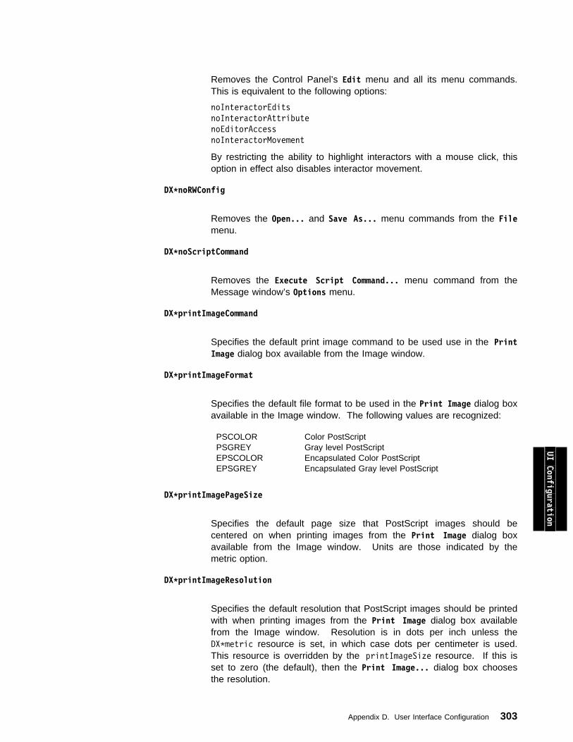
Removes the Control Panel’s Edit menu and all its menu commands.This is equivalent to the following options:

noInteractorEdits

noInteractorAttribute

noEditorAccess

noInteractorMovement

By restricting the ability to highlight interactors with a mouse click, thisoption in effect also disables interactor movement.

DX\noRWConfig

Removes the Open... and Save As... menu commands from the Filemenu.

DX\noScriptCommand

Removes the Execute Script Command... menu command from theMessage window’s Options menu.

DX\printImageCommand

Specifies the default print image command to be used use in the PrintImage dialog box available from the Image window.

DX\printImageFormat

Specifies the default file format to be used in the Print Image dialog boxavailable in the Image window. The following values are recognized:

DX\printImagePageSize

Specifies the default page size that PostScript images should becentered on when printing images from the Print Image dialog boxavailable from the Image window. Units are those indicated by themetric option.

DX\printImageResolution

Specifies the default resolution that PostScript images should be printedwith when printing images from the Print Image dialog box availablefrom the Image window. Resolution is in dots per inch unless theDX\metric resource is set, in which case dots per centimeter is used.This resource is overridden by the printImageSize resource. If this isset to zero (the default), then the Print Image... dialog box choosesthe resolution.

PSCOLOR Color PostScriptPSGREY Gray level PostScript UI Configuration

EPSCOLOR Encapsulated Color PostScriptEPSGREY Encapsulated Gray level PostScript

Appendix D. User Interface Configuration 303

DX\printImageSize

Specifies the default size of PostScript images printed from the PrintImage dialog box available from the Image window. If specified thisoption overrides the printImageResolution option. The value is a stringin the same format as that accepted by the dialog box (for example, “8”,“8x”, “x10”, “8x10”). Units are those indicated by the metric option. Thedefault value is determined by printImageResolution option.

DX\restrictionLevel

Combines options to make it easier to build applications on top of DataExplorer. The string value must be one of the following:

DX\saveImageFormat

Specifies the default file format to be used in the Print Image dialog boxavailable in the Image window. The following values are recognized:

DX\saveImagePageSize

Specifies the default page size that PostScript images should be

minimum Combines the restrictions implied by the following options:

noEditorAccess

noInteractorEdits

noInteractorMovement

limitImageOptions

noScriptCommand

noCMapSetNameOption

intermediate Combines the restrictions implied by minimum restrictionlevel plus the following options:

noImageRWNetFile

noOpenAllPanels

noImageLoad

noPanelEdit

noPanelOptions

noPGroupAssignment

maximum Combines the restrictions implied by the intermediaterestriction level plus the following options:

noPanelRWConfig

noImageSaving

noPanelAccess

noCMapOpenMap

noCMapSaveMap

PSCOLOR Color PostScriptPSGREY Gray level PostScriptEPSCOLOR Encapsulated Color PostScriptEPSGREY Encapsulated Gray level PostScriptRGB “rgb” formatR+G+B “r+g+b” formatTIFF TIFF format

304 IBM Visualization Data Explorer: User’s Guide

centered on when saving images from the Save Image dialog boxavailable from the Image window. Units are those indicated by themetric option.

DX\saveImageResolution

Specifies the default resolution that PostScript images should be savedwith when saving images from the Save Image dialog box available fromthe Image window. Resolution is in dots per inch unless the DX\metricresource is set, in which case dots per centimeter is used. Thisresource is overridden by the saveImageSize resource. If this is set tozero (the default), then the Save Image dialog box chooses theresolution, which may be specified inside the visual program.

DX\saveImageSize

Specifies the default size of PostScript images saved from the PrintImage dialog box available from the Image window. If specified thisoption overrides the saveImageResolution option. The value is a stringin the same format as that accepted by the dialog box (for example, “8”,“8x”, “x10”, “8x10”). Units are those indicated by the metric option. Thedefault value is determined by saveImageResolution option.

DX\vpeCanvas.lineThickness

Specifies the thickness of the lines that connect module outputs tomodule inputs in the VPE.

DX\warningEnabled

Specifies the default value of the Warning Messages toggle button in theMessage window’s Option menu.

DX\warningOpensMessage

Specifies whether or not the Message window pops up when a warningmessage is printed in the Message window.

UI Configuration

Appendix D. User Interface Configuration 305

306 IBM Visualization Data Explorer: User’s Guide

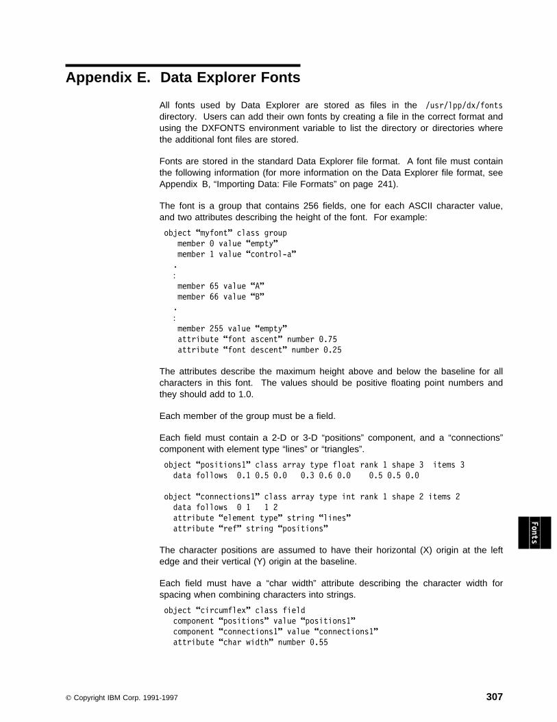
Appendix E. Data Explorer Fonts

All fonts used by Data Explorer are stored as files in the /usr/lpp/dx/fonts

directory. Users can add their own fonts by creating a file in the correct format andusing the DXFONTS environment variable to list the directory or directories wherethe additional font files are stored.

Fonts are stored in the standard Data Explorer file format. A font file must containthe following information (for more information on the Data Explorer file format, seeAppendix B, “Importing Data: File Formats” on page 241).

The font is a group that contains 256 fields, one for each ASCII character value,and two attributes describing the height of the font. For example:

object “myfont” class group

member ð value “empty”

member 1 value “control-a”

.

:member 65 value “A”

member 66 value “B”

.

:member 255 value “empty”

attribute “font ascent” number ð.75

attribute “font descent” number ð.25

The attributes describe the maximum height above and below the baseline for allcharacters in this font. The values should be positive floating point numbers andthey should add to 1.0.

Each member of the group must be a field.

Each field must contain a 2-D or 3-D “positions” component, and a “connections”component with element type “lines” or “triangles”.

object “positions1” class array type float rank 1 shape 3 items 3

data follows ð.1 ð.5 ð.ð ð.3 ð.6 ð.ð ð.5 ð.5 ð.ð

object “connections1” class array type int rank 1 shape 2 items 2

data follows ð 1 1 2

attribute “element type” string “lines”

attribute “ref” string “positions”

The character positions are assumed to have their horizontal (X) origin at the leftedge and their vertical (Y) origin at the baseline.

Each field must have a “char width” attribute describing the character width forspacing when combining characters into strings.

object “circumflex” class field

component “positions” value “positions1”

component “connections1” value “connections1”

attribute “char width” number ð.55

Fonts

Copyright IBM Corp. 1991-1997 307

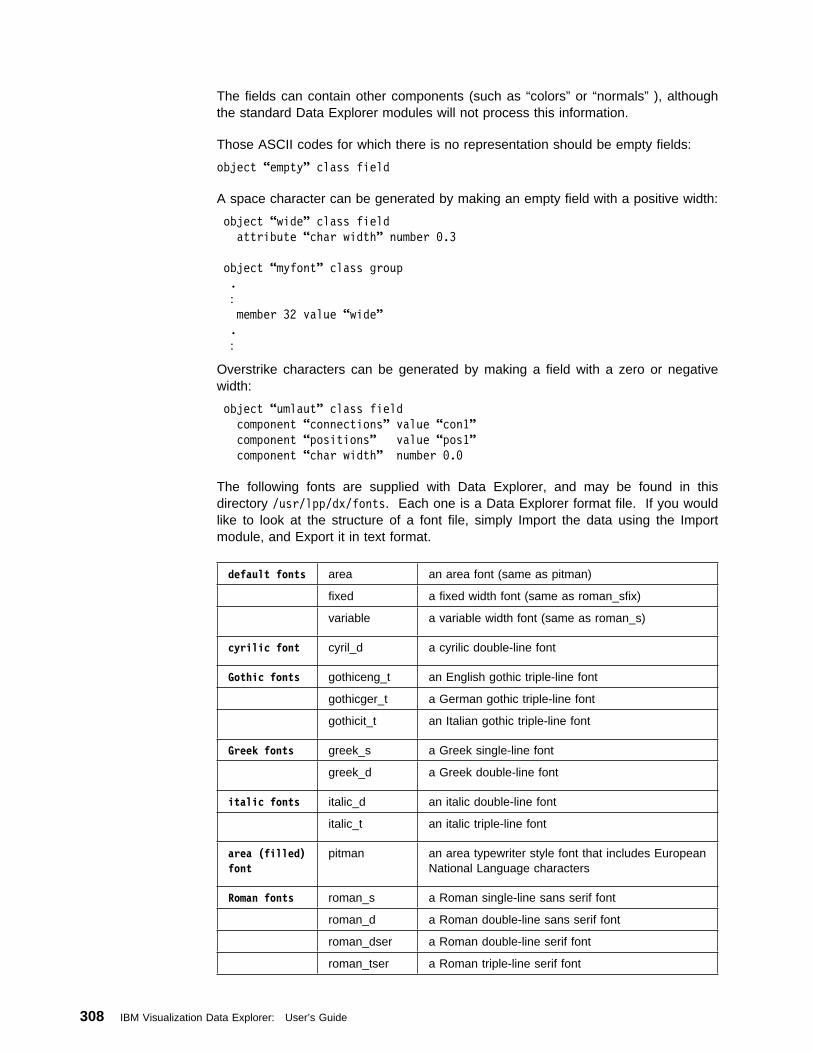
The fields can contain other components (such as “colors” or “normals” ), althoughthe standard Data Explorer modules will not process this information.

Those ASCII codes for which there is no representation should be empty fields:

object “empty” class field

A space character can be generated by making an empty field with a positive width:

object “wide” class field

attribute “char width” number ð.3

object “myfont” class group

.

:member 32 value “wide”

.

:

Overstrike characters can be generated by making a field with a zero or negativewidth:

object “umlaut” class field

component “connections” value “con1”

component “positions” value “pos1”

component “char width” number ð.ð

The following fonts are supplied with Data Explorer, and may be found in thisdirectory /usr/lpp/dx/fonts. Each one is a Data Explorer format file. If you wouldlike to look at the structure of a font file, simply Import the data using the Importmodule, and Export it in text format.

default fonts area an area font (same as pitman)

fixed a fixed width font (same as roman_sfix)

variable a variable width font (same as roman_s)

cyrilic font cyril_d a cyrilic double-line font

Gothic fonts gothiceng_t an English gothic triple-line font

gothicger_t a German gothic triple-line font

gothicit_t an Italian gothic triple-line font

Greek fonts greek_s a Greek single-line font

greek_d a Greek double-line font

italic fonts italic_d an italic double-line font

italic_t an italic triple-line font

area (filled)font

pitman an area typewriter style font that includes EuropeanNational Language characters

Roman fonts roman_s a Roman single-line sans serif font

roman_d a Roman double-line sans serif font

roman_dser a Roman double-line serif font

roman_tser a Roman triple-line serif font

308 IBM Visualization Data Explorer: User’s Guide

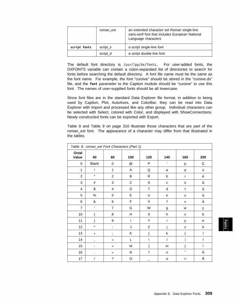
The default font directory is /usr/lpp/dx/fonts. For user-added fonts, theDXFONTS variable can contain a colon-separated list of directories to search forfonts before searching the default directory. A font file name must be the same asthe font name. For example, the font “cursive” should be stored in the “cursive.dx”file, and the font parameter to the Caption module should be “cursive” to use thisfont. The names of user-supplied fonts should be all lowercase.

Since font files are in the standard Data Explorer file format, in addition to beingused by Caption, Plot, AutoAxes, and ColorBar, they can be read into DataExplorer with Import and processed like any other group. Individual characters canbe selected with Select, colored with Color, and displayed with ShowConnections.Newly constructed fonts can be exported with Export.

Table 8 and Table 9 on page 310 illustrate those characters that are part of theroman_ext font. The appearance of a character may differ from that illustrated inthe tables.

roman_ext an extended character set Roman single-linesans-serif font that includes European NationalLanguage characters

script fonts script_s a script single-line font

script_d a script double-line font

Table 8. roman_ext Font Characters (Part 1)

OctalValue 40 60 100 120 140 160 200

0 Blank 0 @ P ‘ p Ç

1 ! 1 A Q a q ü

2 " 2 B R b r é

3 # 3 C S c s â

4 $ 4 D T d t ä

5 % 5 E U e u à

6 & 6 F V f v å

7 ' 7 G W g w ç

10 ( 8 H X h x ê

11 ) 9 I Y i y ë

Fonts 12 * : J Z j z è

13 + ; K [ k ï

14 , < L \ l ¦ î

15 - = M ] m ì

16 . > N ↑ n ˜ Ä

17 / ? O _ o Ø Å

Appendix E. Data Explorer Fonts 309

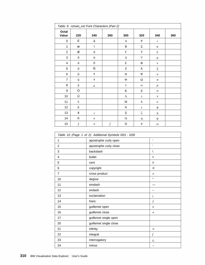
Table 9. roman_ext Font Characters (Part 2)

OctalValue 220 240 260 300 320 340 360

0 É á Α Ρ ι

1 æ í Β Σ κ

2 Æ ó Γ Τ λ

3 ô ú ∆ ϒ µ

4 ö ñ Ε Φ ν

5 ò Ñ Ζ Χ ξ

6 û ª Η Ψ ο

7 ù º Θ Ω π

8 ÿ ¿ Ι α ρ

9 Ö Κ β σ

10 Ü Λ γ τ

11 ¢ Μ δ υ

12 £ Ν ε φ

13 ¥ ¡ Ξ ζ χ

14 | « Ο η ψ

15 ƒ » ∫ Π θ ω

Table 10 (Page 1 of 2). Additional Symbols \001 - \035

1 apostrophe curly open ‘

2 apostrophe curly close ’

3 backslash \

4 bullet

5 cent ¢

6 copyright

7 cross product ×

10 degree °

11 emdash —

12 endash –

13 exclamation ¡

14 franc ƒ

15 guillemet open «

16 guillemet close »

17 guillemet single open

20 guillemet single close

21 infinity ∞

22 integral ∫

23 interrogatory ¿

24 minus −

310 IBM Visualization Data Explorer: User’s Guide

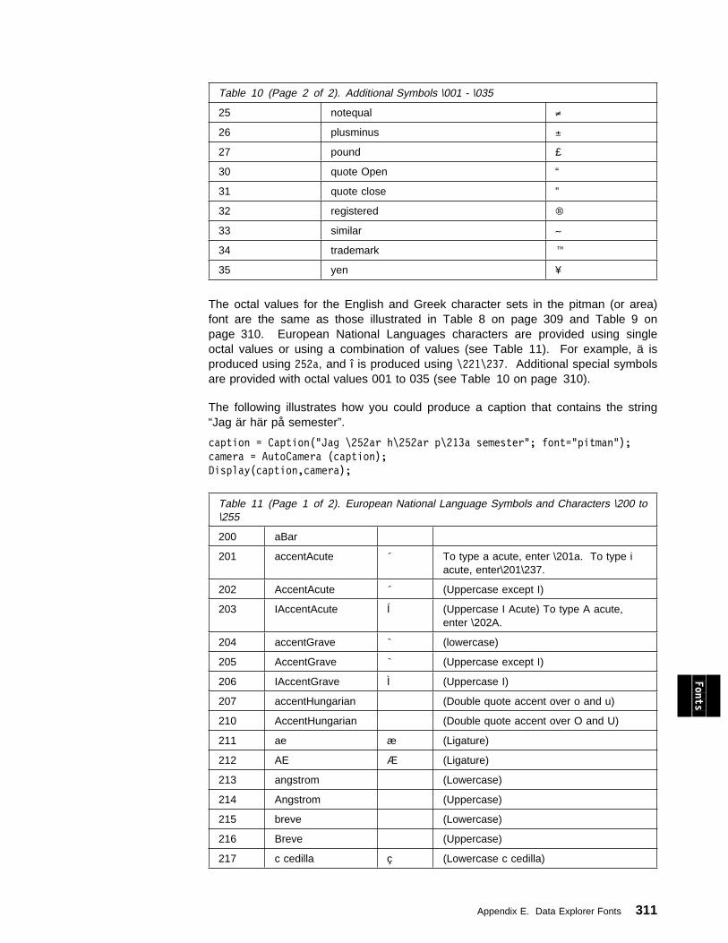
The octal values for the English and Greek character sets in the pitman (or area)font are the same as those illustrated in Table 8 on page 309 and Table 9 onpage 310. European National Languages characters are provided using singleoctal values or using a combination of values (see Table 11). For example, ä isproduced using 252a, and î is produced using \221\237. Additional special symbolsare provided with octal values 001 to 035 (see Table 10 on page 310).

The following illustrates how you could produce a caption that contains the string“Jag är här på semester”.

caption = Caption("Jag \252ar h\252ar p\213a semester"; font="pitman");

camera = AutoCamera (caption);

Display(caption,camera);

Table 10 (Page 2 of 2). Additional Symbols \001 - \035

25 notequal ≠

26 plusminus ±

27 pound £

30 quote Open “

31 quote close ”

32 registered

33 similar ∼

34 trademark

35 yen ¥

Table 11 (Page 1 of 2). European National Language Symbols and Characters \200 to\255

200 aBar

201 accentAcute ´ To type a acute, enter \201a. To type iacute, enter\201\237.

202 AccentAcute ´ (Uppercase except I)

203 IAccentAcute Í (Uppercase I Acute) To type A acute,enter \202A.

204 accentGrave ` (lowercase)

205 AccentGrave ` (Uppercase except I)

206 IAccentGrave Ì (Uppercase I)

Fonts 207 accentHungarian (Double quote accent over o and u)

210 AccentHungarian (Double quote accent over O and U)

211 ae æ (Ligature)

212 AE Æ (Ligature)

213 angstrom (Lowercase)

214 Angstrom (Uppercase)

215 breve (Lowercase)

216 Breve (Uppercase)

217 c cedilla ç (Lowercase c cedilla)

Appendix E. Data Explorer Fonts 311

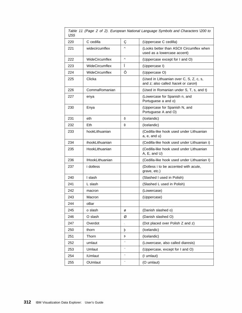
Table 11 (Page 2 of 2). European National Language Symbols and Characters \200 to\255

220 C cedilla Ç (Uppercase C cedilla)

221 widecircumflex ^ (Looks better than ASCII Circumflex whenused as a lowercase accent)

222 WideCircumflex ^ (Uppercase except for I and O)

223 WideCircumflex Î (Uppercase I)

224 WideCircumflex Ô (Uppercase O)

225 Clicka (Used in Lithuanian over C, S, Z, c, s,and z; also called hacek or caron)

226 CommaRomanian (Used in Romanian under S, T, s, and t)

227 enya (Lowercase for Spanish n, andPortuguese a and o)

230 Enya (Uppercase for Spanish N, andPortuguese A and O)

231 eth ð (Icelandic)

232 Eth Ð (Icelandic)

233 hookLithuanian (Cedilla-like hook used under Lithuaniana, e, and u)

234 ihookLithuanian (Cedilla-like hook used under Lithuanian i)

235 HookLithuanian (Cedilla-like hook used under LithuanianA, E, and U)

236 IHookLithuanian (Cedilla-like hook used under Lithuanian I)

237 i dotless (Dotless i to be accented with acute,grave, etc.)

240 l slash (Slashed l used in Polish)

241 L slash (Slashed L used in Polish)

242 macron (Lowercase)

243 Macron (Uppercase)

244 oBar

245 o slash ø (Danish slashed o)

246 O slash Ø (Danish slashed O)

247 Overdot . (Dot placed over Polish Z and z)

250 thorn þ (Icelandic)

251 Thorn Þ (Icelandic)

252 umlaut ¨ (Lowercase, also called diaresis)

253 Umlaut ¨ (Uppercase, except for I and O)

254 IUmlaut ¨ (I umlaut)

255 OUmlaut ¨ (O umlaut)

312 IBM Visualization Data Explorer: User’s Guide

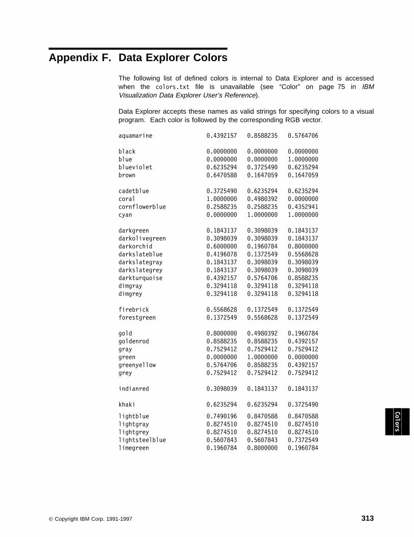
Appendix F. Data Explorer Colors

The following list of defined colors is internal to Data Explorer and is accessedwhen the colors.txt file is unavailable (see “Color” on page 75 in IBMVisualization Data Explorer User’s Reference).

Data Explorer accepts these names as valid strings for specifying colors to a visualprogram. Each color is followed by the corresponding RGB vector.

aquamarine ð.4392157 ð.8588235 ð.57647ð6

black ð.ððððððð ð.ððððððð ð.ððððððð

blue ð.ððððððð ð.ððððððð 1.ððððððð

blueviolet ð.6235294 ð.372549ð ð.6235294

brown ð.647ð588 ð.1647ð59 ð.1647ð59

cadetblue ð.372549ð ð.6235294 ð.6235294

coral 1.ððððððð ð.498ð392 ð.ððððððð

cornflowerblue ð.2588235 ð.2588235 ð.4352941

cyan ð.ððððððð 1.ððððððð 1.ððððððð

darkgreen ð.1843137 ð.3ð98ð39 ð.1843137

darkolivegreen ð.3ð98ð39 ð.3ð98ð39 ð.1843137

darkorchid ð.6ðððððð ð.196ð784 ð.8ðððððð

darkslateblue ð.4196ð78 ð.1372549 ð.5568628

darkslategray ð.1843137 ð.3ð98ð39 ð.3ð98ð39

darkslategrey ð.1843137 ð.3ð98ð39 ð.3ð98ð39

darkturquoise ð.4392157 ð.57647ð6 ð.8588235

dimgray ð.3294118 ð.3294118 ð.3294118

dimgrey ð.3294118 ð.3294118 ð.3294118

firebrick ð.5568628 ð.1372549 ð.1372549

forestgreen ð.1372549 ð.5568628 ð.1372549

gold ð.8ðððððð ð.498ð392 ð.196ð784

goldenrod ð.8588235 ð.8588235 ð.4392157

gray ð.7529412 ð.7529412 ð.7529412

green ð.ððððððð 1.ððððððð ð.ððððððð

greenyellow ð.57647ð6 ð.8588235 ð.4392157

grey ð.7529412 ð.7529412 ð.7529412

indianred ð.3ð98ð39 ð.1843137 ð.1843137

khaki ð.6235294 ð.6235294 ð.372549ð

lightblue ð.749ð196 ð.847ð588 ð.847ð588

lightgray ð.827451ð ð.827451ð ð.827451ð

lightgrey ð.827451ð ð.827451ð ð.827451ð

lightsteelblue ð.56ð7843 ð.56ð7843 ð.7372549

limegreen ð.196ð784 ð.8ðððððð ð.196ð784

Colors

Copyright IBM Corp. 1991-1997 313

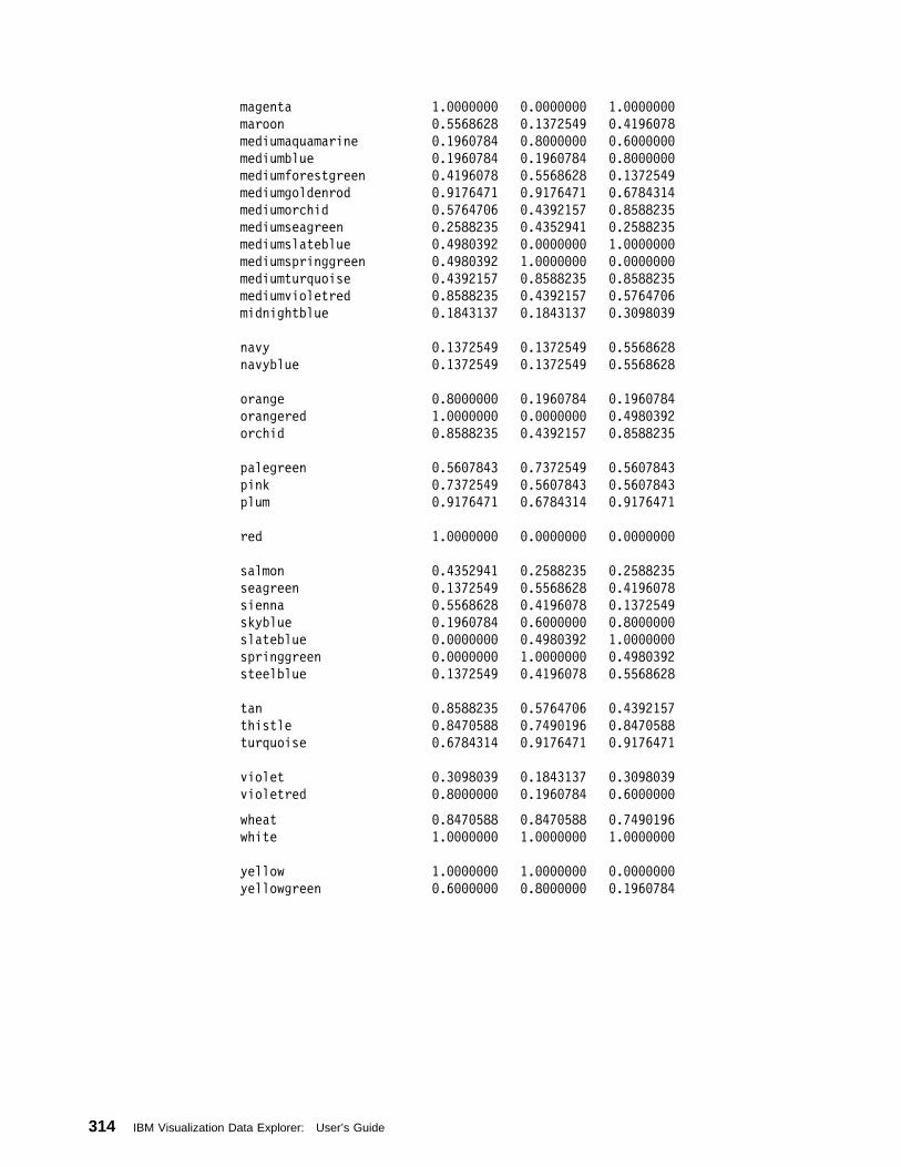
magenta 1.ððððððð ð.ððððððð 1.ððððððð

maroon ð.5568628 ð.1372549 ð.4196ð78

mediumaquamarine ð.196ð784 ð.8ðððððð ð.6ðððððð

mediumblue ð.196ð784 ð.196ð784 ð.8ðððððð

mediumforestgreen ð.4196ð78 ð.5568628 ð.1372549

mediumgoldenrod ð.9176471 ð.9176471 ð.6784314

mediumorchid ð.57647ð6 ð.4392157 ð.8588235

mediumseagreen ð.2588235 ð.4352941 ð.2588235

mediumslateblue ð.498ð392 ð.ððððððð 1.ððððððð

mediumspringgreen ð.498ð392 1.ððððððð ð.ððððððð

mediumturquoise ð.4392157 ð.8588235 ð.8588235

mediumvioletred ð.8588235 ð.4392157 ð.57647ð6

midnightblue ð.1843137 ð.1843137 ð.3ð98ð39

navy ð.1372549 ð.1372549 ð.5568628

navyblue ð.1372549 ð.1372549 ð.5568628

orange ð.8ðððððð ð.196ð784 ð.196ð784

orangered 1.ððððððð ð.ððððððð ð.498ð392

orchid ð.8588235 ð.4392157 ð.8588235

palegreen ð.56ð7843 ð.7372549 ð.56ð7843

pink ð.7372549 ð.56ð7843 ð.56ð7843

plum ð.9176471 ð.6784314 ð.9176471

red 1.ððððððð ð.ððððððð ð.ððððððð

salmon ð.4352941 ð.2588235 ð.2588235

seagreen ð.1372549 ð.5568628 ð.4196ð78

sienna ð.5568628 ð.4196ð78 ð.1372549

skyblue ð.196ð784 ð.6ðððððð ð.8ðððððð

slateblue ð.ððððððð ð.498ð392 1.ððððððð

springgreen ð.ððððððð 1.ððððððð ð.498ð392

steelblue ð.1372549 ð.4196ð78 ð.5568628

tan ð.8588235 ð.57647ð6 ð.4392157

thistle ð.847ð588 ð.749ð196 ð.847ð588

turquoise ð.6784314 ð.9176471 ð.9176471

violet ð.3ð98ð39 ð.1843137 ð.3ð98ð39

violetred ð.8ðððððð ð.196ð784 ð.6ðððððð

wheat ð.847ð588 ð.847ð588 ð.749ð196

white 1.ððððððð 1.ððððððð 1.ððððððð

yellow 1.ððððððð 1.ððððððð ð.ððððððð

yellowgreen ð.6ðððððð ð.8ðððððð ð.196ð784

314 IBM Visualization Data Explorer: User’s Guide

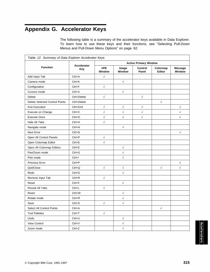
Appendix G. Accelerator Keys

The following table is a summary of the accelerator keys available in Data Explorer.To learn how to use these keys and their functions, see “Selecting Pull-DownMenus and Pull-Down Menu Options” on page 62.

Table 12. Summary of Data Explorer Accelerator Keys

FunctionAccelerator

Key

Active Primary Window

VPEWindow

ImageWindow

ControlPanel

ColormapEditor

MessageWindow

Add Input Tab Ctrl+A √

Camera mode Ctrl+K √

Configuration Ctrl+F √

Cursors mode Ctrl+X √

Delete Ctrl+Delete √ √

Delete Selected Control Points Ctrl+Delete √

End Execution Ctrl+End √ √ √ √

Execute on Change Ctrl+C √ √ √ √

Execute Once Ctrl+O √ √ √ √

Hide All Tabs Ctrl+H √

Navigate mode Ctrl+N √

Next Error Ctrl+N √

Open All Control Panels Ctrl+P √

Open Colormap Editor Ctrl+E √

Open All Colormap Editors Ctrl+E √

Pan/Zoom mode Ctrl+G √

Pick mode Ctrl+I √

Previous Error Ctrl+P √

Quit/Close Ctrl+Q √ √ √ √

Redo Ctrl+D √

Remove Input Tab Ctrl+R √

Reset Ctrl+F √

Reveal All Tabs Ctrl+L √

Roam Ctrl+W √

Rotate mode Ctrl+R √

Save Ctrl+S √ √

Select All Control Points Ctrl+A √

Tool Palettes Ctrl+T √

Undo Ctrl+U √ Accelerators

View Control Ctrl+V √

Zoom mode Ctrl+Z √

Copyright IBM Corp. 1991-1997 315

316 IBM Visualization Data Explorer: User’s Guide

Glossary

Some of the definitions in this glossary are taken fromthe IBM Dictionary of Computing, SC20-1699.

Aaccelerator . A “shortcut” that minimizes the number ofkeystrokes or mouse clicks required to complete a task.

anchor window . The window in which a Data Explorersession starts (either the Visual Program Editor or theImage window). The window is identified by an anchorsymbol in the top left corner. When this window isclosed, the Data Explorer session ends.

architecture . The organizational structure of acomputer system, including hardware and software.

array . In Data Explorer, an array structure containingan ordered list of data items of the same type alongwith additional descriptive information. Arrays are eithercompact or irregular. See compact array, irregulararray.

assembly . An object representing a collection ofobjects.

attribute . A characteristic of an object. Objects canhave attributes that are indexed by a string name andhave a value that is an object. See also componentattribute.

Ccamera . An object that describes the viewingparameters of an image (e.g., width of the viewport,viewer’s location relative to the object, and theresolution and aspect ratio of the image). A cameramay be explicitly defined and passed as a parameter tothe Render or Display module. It may also be implicitlydefined in the use of interactive, mouse-driven options(such as zoom or rotate) in the Image window.

canvas . The area of a VPE window used in buildingand editing visual programs.

cell-centered data . Connection-dependent data.

clipping plane . A plane that divides athree-dimensional object into a rendered and anunrendered region, making the object’s interior visible.

colormap . A map that relates colors to data values.The colors are carried in the map’s “data” componentand the data values to which each color applies in its“positions” component.

colormap editor . A special tool for mapping precisecolors to specified data values, the results of which aredisplayed in a visual image.

compact array . Any of five types of compact encodingof array data:

constant array mesh array path array product array regular array

component . A basic part of a field (such as“positions,” “data,” or “colors”); each component isindexed by a string (e.g., “positions”), and its value istypically an array object (e.g., the list of position values).See also component attribute.

component attribute . A characteristic of acomponent. Components of a field can have attributesthat are indexed by a string name and have a value thatis an object.

composite field . A grouping of like fields forprocessing a single spatial entity. See also partitionedfield.

connection . Component of an IBM Data Explorer datafield that specifies how a set of points are joinedtogether. Also controls interpolation.

connection-dependent data . Cell-centered data. Thedata value is interpreted as constant throughout theconnection element.

contour . On a surface, a line that connects pointshaving the same data value (e.g., pressure, depth,temperature).

control panel . An IBM Data Explorer window thatfacilitates setting and changing the parameters of visualprograms.

cube . A volumetric connection element that connectseight positions in a data field.

cutting plane . An arbitrary plane, in three-dimensionalspace, onto which data are mapped.

Glossary

Copyright IBM Corp. 1991-1997 317

Ddata-driven interactors . Interactors whose attributes(such as minimum and maximum) are set by an inputdata field.

Data Prompter . An interface that enables a user todescribe the format of the data in a file. The promptercreates a General Array Format header file that is usedby the Import module to import the data.

dependence . A component attribute. One componentis said to be dependent (“dep”) on another if the itemsin their component arrays are in one-to-onecorrespondence to each other.

dialog box . The “window” displayed when the userselects a pull-down option that offers or requires moredetailed specification.

display . (1) To present information for viewing, usuallyon a terminal screen or a hard-copy device. (2) Adevice or medium on which information is presented,such as a terminal screen. (3) Deprecated term forpanel.

Eelement . Connection item.

element type . An attribute that describes the type ofconnection element, for example, “cubes”, “tetrahedra”,or “lines”.

executive . The component of the Data Explorersystem that manages the execution of specifiedmodules. The term often refers to the entire serverportion of the Data Explorer client-server model,including the executive, modules, anddata-management components.

Fface . (1) Any planar surface that bounds athree-dimensional object. (2) A polygon.

field . A self-contained collection of data items. A DataExplorer field typically consists of the data itself (the“data” component), a set of sample points (the“positions” component), a set of interpolation elements(the “connections” component), and other information asneeded.

flat shading . A shading model in which each face ofan object is shaded with a single intensity value.Contrast with Gouraud shading.

fork . An operation that causes a program to branchinto two or more parallel concurrent paths.

fork-join parallelism . A programming mechanism thatsupports parallel processing: The fork statement splitsa single computation into multiple independentcomputations. The join statement recombines two ormore concurrent computations into one.

Ggeneral array format . A data-importing method thatuses a header file to describe the data format of a datafile. This “format” makes it possible to import data in avariety of formats.

glyph . A graphical figure used to represent values of aparticular variable. The length, angle, or other attributeof the glyph is some function of the value of thatvariable. Each occurrence of a glyph represents asingle value of the variable.

Gouraud shading . Also called intensity interpolationshading. A shading model in which the intensity ofvalues of incident illumination on a polygon areinterpolated from intensity values at the vertices of thepolygon. Contrast with flat shading.

graphical user interface . A set of panels and dialogsfor interacting with an application.

group . A collection of objects.

Iicon . A displayed symbol that a user can point to witha device such as a mouse to select a particularoperation or software application.

image window . IBM Data Explorer window thatdisplays the image generated by a visual program.Associated with the Image window are specialinteractors for 3-D viewing.

interactor . A Data Explorer device used to manipulatedata in order to change the visual image produced by aprogram. See also data-driven interactor, interactorstand-in.

interactor stand-in . An icon used in the VPE windowto represent an interactor. Stand-ins are named afterthe type of data they generate:

integer scalar selector (outputs a value and a string)

string value vector

interpolation element . An item in the connectionscomponent array. Each interpolation element provides

318 IBM Visualization Data Explorer: User’s Guide

a means for interpolating data values at locations otherthan the specified set of sample points. See positionscomponent.

invalid . A classification of an array item (typicallypositions or connections). An invalid item is not to berendered or realized.

irregular array . In contrast to a compact array, anarray in which the data is stored explicitly.

isosurface . A surface in three-dimensional space thatconnects all the points in a data set that have the samevalue.

isovalue . The single value that characterizes each andevery point constituting an isosurface. By default, thisvalue is the average of all the data values in the setbeing visualized.

item . A single piece of data in an array.

Jjoin . An operation that merges two or morecomputation paths.

Lline . An element that connects two positions in a field.

Mmacro . In IBM Data Explorer, a sequence of modulesthat acts as a functional unit and is displayed as asingle icon. Macros can also be defined in the DataExplorer scripting language.

member . An individual unit or object in a group. Acollection of members makes a group.

menu bar . In windows, a horizontal bar that displaysthe names of one or more menus (or tasks). When theuser selects a menu, a pull-down list of options for thatmenu is displayed.

mesh array . A compact array that encodesmultidimensional regularity of connections. It is aproduct of path arrays. In a mesh array, whichpositions are connected to one another is implicitlyrather than explicitly defined.

module . (1) In IBM Data Explorer, a primitive function,such as Isosurface. (2) In a VPE window, the icon fora module. (3) A program unit that is functionallydiscrete and identifiable (i.e., it can be assembled,compiled, combined with other units, and so on).

Nnavigate . To move the camera (changing the “to” and“from” points) around the image scene, using themouse.

netCDF . Network Common Data Form.

network . In Data Explorer the set of tool modules,interactor stand-ins, and connections that constitute avisual program. In the VPE window, a network appearsas a set of icons connected by arcs.

Network Common Data Form (netCDF) . A dataformat that stores and retrieves scientific data inself-describing, multidimensional blocks (netCDF is nota database management system, however). netCDF isaccessible with C and FORTRAN.

normal . (1) Perpendicular to a surface. (2) In IBMData Explorer, a vector that is perpendicular to a faceor surface of an object. A normal may depend onconnections or positions. A connection-dependentnormal results in flat shading; a position-dependentnormal results in Gouraud shading.

Oobject . In IBM Data Explorer, any discrete andidentifiable entity; specifically, a region of globalmemory that contains its own type-identification andother type-specific information.

opacity . The capacity of matter to prevent thetransmission of light. For a surface, an opacity of 1means that it is completely opaque; an opacity of 0, thatit is completely transparent. For volume, opacity isdefined as the amount of attenuation (of light) per unitdistance.

Ppage . (1) That portion of a panel displayed by a userinterface. (2) To move back and forth through thepages of a multipage panel. See also scroll.

palette . A displayed grouping of available selections(such as functions, modules, or colors) in auser-interface window.

palindrome . In Data Explorer, a mode of running anentire sequence, first in one direction, then in theopposite direction.

panel . A formatted display of information on a displayscreen. See also window. Synonymous with display. Glossary

Glossary 319

partitioned field . A composite field, created bypartitioning a single field into a collection of separatefields; used for parallel processing anddata-management purposes.

path array . A compact array that encodes linearregularity of connections. It is a set of n−1 linesegments, where the ith line segment joins points i andi + 1.

pixel . Picture element. In computer graphics, thesmallest element of a display surface that can beindependently assigned color and intensity.

polygon . (1) Any multisided planar figure. (2) A faceof a three-dimensional object.

position-dependent data . Data that are in one-to-onecorrespondence with positions.

positions component . A component that consists of aset of dimensional points in a field.

probe . A list of one or more vectors that representpoints in a graphical image. Probes can be used withData Explorer tools that accept vectors as input (suchas ClipPlane and Streamline) or to control the view ofan image.

product array . A compact array that encodesmultidimensional positional regularity. It is the set ofpoints obtained by summing one point from each of theterms in all possible combinations. In the simplestcase, each term is a regular array.

pull-down . In windows, the list of options displayedwhen a task is selected from the menu bar.

Qquad . An element that connects four positions in afield.

Rrank . The number of dimensions in an array. Rankzero corresponds to scalars (e.g., the number 3). Rankone corresponds to vectors (e.g, [1.5 3.7] and[2.9 4.0 6.0]). Rank two corresponds to matrices orrank-two tensors (e.g., the matrix[[1 3 8][5 7 2][1 0 1]]). Higher ranks correspond tohigher-order tensors. See also shape.

realization . A description of how raw data is to berepresented in terms of boundaries, surfaces,transparency, color, and other graphical, image, andgeometric characteristics.

reference . A component attribute. One component issaid to refer to another (“ref”) if the items in the firstarray are integer indices into the second array. Theconnections component references the positionscomponent.

regular array . A compact array that is a set of npoints lying on a line, with constant spacing betweenthem, which can represent one-dimensional regularpositions.

rendering . The generation of an image from somerepresentation of an object, such as a surface, or fromvolumetric information.

ribbon . A figure derived from lines (e.g., fromstreamlines and streaklines). Ribbons may twist toindicate vorticity.

Ssample point . A point that represents user data. Datais interpolated between sample points by interpolationelements (connections).

scalar . A non-vector value characterized by a single,real number.

scatter data . A collection of sample points withoutconnections.

screen . An illuminated display surface (e.g., thedisplay surface of a CRT or plasma panel).

scripting language . The IBM Data Explorer commandlanguage. Used for writing visual programs, to managethe execution of modules, and to invoke visualizationfunctions.

scroll . To move all or part of the display imagevertically or horizontally to display data that cannot beobserved in a single display image.

secondary window . Any window generated byanother window. A secondary window always appearson top of its parent window and is automaticallyminimized or closed when the parent window isminimized or closed. Synonymous with child window.

sequencer . An IBM Data Explorer tool for creating“animated” sequences of images.

series . In IBM Data Explorer, used to represent asingle field sampled across some parameter (e.g., asimulation of a CMOS device across a temperaturerange). Members of a series have a position. A copyof the position is found in the “series position” attribute.

320 IBM Visualization Data Explorer: User’s Guide

shape . A list of the dimensions of a structure (the listcontains nothing for scalars, one entry for vectors, twofor rank-two tensors, and so on). See also rank.

shared . A term used to indicate the availability of aresource for use by more than one program at thesame time.

specular reflection . A reflection from a shiny object.

stand-in . See interactor stand-in.

streaklines . Lines that represent the path of particlesin a changing vector field. Also called rakes.

streamlines . Lines that represent the path of particlesin a vector field at a particular time. Also called flowlines.

Ttask . A basic unit of work to be accomplished by acomputer.

tetrahedron . A volumetric connection element thatconnects four positions in a field.

tool . In IBM Data Explorer, a general term for any iconused to build a visual program (specifically, module,macro, or interactor stand-in).

triangle . A connection element that connects threepoints in a field.

tube . A surface centered on a deriving line (e.g., astreamline or streakline). Tubes may twist to indicatevorticity.

Uuser . Anyone who uses the services of a computersystem. See also user display station.

Vvalue . An instance of an attribute (for example, “blue”as the value of the attribute “color”).

vector . A quantity characterized by more than onecomponent.

visual program . A user-specified interconnected set ofData Explorer modules that performs a sequence ofoperations on data and typically produces an image asoutput.

vertex . One of the positions that define a connectionelement.

visual program editor . IBM Data Explorer windowused to create and edit visual programs and macros.See also canvas.

volume . The amount of three-dimensional spaceoccupied by an object or substance (measured in cubicunits). To be distinguished from an object’s surface,which is a mathematical abstraction.

volume rendering . A technique for using color andopacity to visualize all the data in a 3-dimensional dataset. The internal details visualized may be physical(such as the structure of a machine part) or they maybe other characteristics (such as fluid flow, temperature,or stress).

vorticity . Mathematically defined as the curl of avelocity field. A particle in a velocity field with nonzerovorticity will rotate.

Wwindow . On a visual display terminal, information in aframed area on a panel that overlies part of the panel.See also anchor window, primary window, secondarywindow.

wireframe . Connected lines that represent a surface.

Glossary

Glossary 321

322 IBM Visualization Data Explorer: User’s Guide

Index

Index

Special Characters@ variables 192, 206, 207

Numerics3-D cursor 79, 85

Aaccelerator keys 63adding comments to a visual program 114adding input tabs 106advanced looping constructs 50align (for navigating) 80aligning interactors in a Control Panel 134aligning tools in the VPE window 113anchor symbol 60angle for perspective rendering 77animation 68, 217, 237arithmetic expressions in scripting language 197Array items

category 28rank 28shape 28type 28

Array Objects in Data Explorer file format 272Array types 28Arrays

compactconstant 33in Data Explorer file format 244mesh 31path 31product 29regular 29

irregular 28items in 28

assignment statements in scripting languageexpression assignments 199function call assignments 199general description 198

at (@) variables in scripting language 192, 206, 207attributes

color multiplier 27dependence (dep) 26derived (der) 27element type 27opacity multiplier 27reference (ref) 27

attributes, function call in scripting language 202attributes, setting interactor

See interactor attributes

AutoAxes 88axes box 88

Bback colors component 22binormals component 24box component 24by-name arguments in scripting language 201

Ccache attribute 202cache in memory use 214cache, object 214cacheability, setting output 214Camera

getting precise settings 82resetting 85

Camera Objects in Data Explorer file format 278category of an Array item 28changing the look-to point 79changing the size of interactors 132changing your view direction 76Clipped Objects in Data Explorer file format 278closing windows 65color map component 23color mapping 219color multiplier attribute 27Colormap Editor

adding control points 122entering values 121menus

Edit 169Execute 170File 168Options 170

moving control points 123selecting control points 123using 119

colors component 22comments

adding to a visual program 114in a Control Panel 67in a data file 269in a script 191in a visual program 67user-defined 67

Compact Arrays 29component attributes 26component sharing 19

Copyright IBM Corp. 1991-1997 323

component, definition 17Composite Field Groups 35Composite Field Objects in Data Explorer file

format 271configuration dialog box

buttons 110entering values in 107for Compute module 111notation field 108toggle button 108value field 109

connecting to the server 183connection dependence 8, 20connections 9, 20Constant Array in Data Explorer file format 273Constant Arrays 33constants in scripting language

scalar numeric 194string 193

constraints on 3-D cursor tool 79, 85constructs, advanced looping 50contours 221Control Panels 232

access 138adding interactors 130building 129customizing 133deleting 132Groups 138, 139menus

Edit 163Execute 164File 163Options 164Panels 164

placing interactors 130saving and restoring 132

Control Panels, dialog-style 135controlling view of an image

See image, controlling view ofcopying tools 105cuboid vertices ordering 21cursor constraints 79, 85customizing the VPE window 113

Ddata component 22Data Explorer

Data Model 16environment variables 59, 292file format examples

See examples of Data Explorer file formatoverview 2scripting language 188starting Data Explorer 58

Data Explorer (continued)system structure 3windows

Colormap Editor 119Image 74pull-down options 62structure 61using on-line help 65VPE 99working with windows 65

data flow 38data mode clause in Data Explorer file format 278Data Model, Data Explorer 16data section of Data Explorer file format 269data statistics component 24data structures supported 16data-driven interactors 147debugging visual programs 212decimal notation in scripting language 194default values

in configuration dialog box 109in scripting language 204

deforming a surface field 227dependence (dep) attribute 27dependence, data 8, 17derivative (der) attribute 26description button in configuration dialog box 110dialog-style Control Panels 135distributed computation 3, 178drag and drop 105

Eedges component 24element type attribute 27end clause of the Data Explorer file 279environment variables 59, 292error messages 71examples of Data Explorer file format

faces, loops, edges, and polylines 25, 260, 263,265

header and data in separate files 254image files 268irregular grid 251Product Arrays 255regular grid 247regular skewed grid 248series 257two-dimensional grid 260warped grid 249

executing a visual program 67execution Groups 178

assigning Groups to workstations 181creating 178, 180deleting 178, 180modifying 178, 180

324 IBM Visualization Data Explorer: User’s Guide

Index

execution model 38execution, stopping 212explicit state, preserving 45expression assignments in scripting language 199

Ffaces component 24Field attributes

color multiplier 27opacity multiplier 27

Field Objects 17, 18, 272Fields

Data Explorer file format 244Data Model 16general discussion 12

file formatCDF 279Data Explorer 244HDF 288netCDF 281

Find Tool dialog box 111flow control 38flow, data 38frame display rate 93, 237front colors component 22function call assignments in scripting language 199function call attributes 202function call conventions in scripting language

by-name arguments 201function call example 201introduction to 200missing arguments 201positional arguments 200

GGetGlobal (preserving state) 45GetLocal (preserving state) 45graphical user interface 58, 74, 128, 156, 178graphics card hardware rendering options 91grid types 21gridconnections keyword in Data Explorer file

format 275gridpositions keyword in Data Explorer file format 274Groups 34

Composite Field 35general description 34in Data Explorer file format 270Multigrid 34, 271Series 35

Hheader section of the Data Explorer file format 268

helpContext-Sensitive Help 65in a Control Panel 67, 133in a visual program 67Overview (of Window) 65Table of Contents 65Technical Support 65Tutorial 65user-defined 67Using Help 65

hexadecimal numbers in scripting language 194hiding input tabs 110hints for using Data Explorer 212Histogram 227

in Colormap Editor 124

Iidentifiers in scripting language 192Image Window

changing the name of 93menus

Connection 167, 171Execute 166, 171File 165, 171Options 167Windows 166, 172

organization 165image, controlling view of

changing look-to point (roaming) 79changing view direction 76navigating 80panning 80resizing 84rotating 77selecting view mode 74zooming 78

import, changing data 185importing data 242include command 207input tabs, adding and removing 106input tabs, revealing and hiding 110instance attribute in scripting language 202interactive use 232interactor attributes

in general 134incrementing 135label 137layout 134style 134updating 135

interactor stand-ins 128interactors

adding and moving to existing Control Panel 130and Control Panels 232changing the label 137

Index 325

interactors (continued)changing the layout 134changing the size of 132changing the style 134deleting 131Dial 142Integer 142List 145moving a group 131moving single interactor 131placing in Control Panel 130radio-button 146Reset 147Scalar 142selecting a group 131Selector 136, 146SelectorList 146Slider 143Stepper 142String 144Toggle 147use of 130—147Value 144Vector 144

interface, user 58, 74, 128, 156, 178interpolation 9invalid-positions and invalid-connections

components 23irregular Arrays in Data Explorer file format 28isosurfaces 221issues of visualization presentation 238iteration using looping 44

Llight object in Data Explorer file format 277lists in scripting language 196loading modules 183locating tools 111look direction (for navigating) 80look-to point 79looping

constructs, advanced 50iteration using 44

loops component 24

Mmacros

in scripting languagebody 205definition of 204example of macro execution 210examples 205expansion 208header 204variables in 208

macros (continued)in visual programs

creating 149loading 152naming 151opening 154

Map 223matrices in scripting language 195maximizing windows 65memory, use of 213Mesh Array Objects in Data Explorer file format 276

in data model 32Message window 174

menusCommands 173Edit 173Execute 173File 172Options 173

minimizing windows 65missing arguments in scripting language 201modules, loading 183mouse, use in Data Explorer 62moving tools 105Multigrid Groups 34Multigrid Objects 34, 271

Nnamed arguments 201naming the image 93navigating around the image 80neighbors component 24netCDF file format

complex Fields 282description 281examples 286series data 284simple Fields 281

networks 13normals component 24notation field in a configuration dialog box 108

Oobject attributes 27object cache 214Objects

Array 28definition of 16Field 17Group 34in Data Explorer files 244

Objects, Arraycompact

constant 33in Data Explorer file format 244

326 IBM Visualization Data Explorer: User’s Guide

Index

Objects, Array (continued)compact (continued)

mesh 31path 31product 29regular 29

irregular 28items in 28

octal numbers in scripting language 194on-line help

Context-Sensitive Help 65in a Control Panel 67, 133in a visual program 67Overview (of Window) 65Table of Contents 65Technical Support 65Tutorial 65user-defined 67Using Help 65

opacities component 23opacity map component 23opacity multiplier attribute 27operators in scripting language 198options box 63ordering of vertices 20, 21orthographic projection method 76outboard modules, loading 183output cacheability, setting 214

Ppanning 80

See also look-to pointparallelism 55, 56Path Array Objects

in Data Explorer format 276in the Data Model 31

paths component in the Data Model 25perspective projection method 76pick paths component 25picking 25, 87Plot 227pokes component 25positional arguments in scripting language 200positions component 20positions dependence 8, 17positions, definition 17preserving explicit state 45printing an image 97probes 85Product Array Objects

in Data Explorer format 275in the Data Model 29

projection methods 76pull-down menus, selecting 62

Rrank of an Array item 28Receiver tool 106, 234Redo action 84reference (ref) attribute 27Regular Array Objects

in Data Explorer format 274in the Data Model 29

remote tab connections 106removing input tabs 106render options 91rendering, volume 231required inputs 103reserved words in scripting language 192Reset interactor 147resetting the camera 85resetting the server 185resizing the image 84restoring a camera setting 84restoring a visual program file 115revealing input tabs 110roaming in the image scene 79rotating the image 77RubberSheet 227runtime modules, loading 183

Ssaving a visual program file 115saving an image 94scalar numeric constants in scripting language

definition of 194floating-point numbers

scientific notation 195standard representation 195

integersdecimal notation 194hexadecimal numbers 194octal numbers 194

scientific notation in scripting language 195Screen Objects in Data Explorer file format 278script execution model

executing macro or module 208macro expansion 208top level environment 208

scripting language, Data Explorer 188scroll bars 101selecting options with an options box 63Selector interactor 136SelectorList interactor 146separate files

for Data Explorer header and data 254for netCDF variables 285

Sequencerframe controls 69

Index 327

Sequencer (continued)script commands 206sequence controls 68using 68

Seriesfor Data Explorer file format 271for netCDF file format 284

Series in the Data Model 35server

connecting to 183resetting 185

SetGlobal (preserving state) 45SetLocal (preserving state) 45setting interactor attributes

See interactor attributessetting output cacheability 214setting render options 91shape of an Array item 28shared components 19simplex vertices ordering 20standard attributes

color multiplier 27dependence (dep) 26derived (der) 27element type 27opacity multiplier 27reference (ref) 27

standard componentsattributes

dependence (dep) 26derivative (der) 27element type 27reference (ref) 27

box 24color map 23colors, front colors, and back colors 22connections 20data 22data statistics 24edges and polylines 25faces, loops, and edges 24invalid positions and invalid connections 23neighbors 24opacities 23opacity map 23pokes, paths, and pick paths 25positions 20tangents, normals, and binormals 24

Start Server option 183state, preserving explicit 45stopping execution 212string constants in scripting language 193String Objects in Data Explorer file format 277structuring in modules 228

Ttabs

connecting 104deleting 105moving 105

tangents component 24techniques for presentation 238techniques, visualization 217television

color resolution 237line resolution 236

tensors in scripting language 196Throttle option 93Toggle interactor 147tool icons 101tools

deleting 103icons 101moving 103moving a group 103placing 102requesting general information 65selecting 102selecting a group 102special 218specifying values for inputs 103

transformation modules 228Transmitter tool 106, 234type of an Array item 28types of Arrays 28

UUndo action 84use of memory 213user interface 58, 74, 128, 156, 178using the Sequencer 68

Vvector Fields 229vectors in scripting language 195vertex ordering 20, 21video output 236video output design 236view angle for perspective rendering 77view direction, changing 76view of an image, controlling

See image, controlling view ofVisual Program Editor (VPE)

customizing 113finding tools 111menus

Connection 162Edit 157Execute 160File 156

328 IBM Visualization Data Explorer: User’s Guide

Index

Visual Program Editor (VPE) (continued)menus (continued)

Options 162Windows 161

tool palette 100visual program (definition) 99

visual programming 13visual programs

creatingSee tools

executing 67restoring previously created programs 118saving

a previous file 117in general 115to a different directory 118

visualization techniques 217volume rendering 231

Wwaveforms in the Colormap Editor 124

Xxform Objects in Data Explorer file format 277

Zzooming into and out of an image 78

Index 329

Readers' Comments — We'd Like to Hear from You

IBM Visualization Data ExplorerUser’s GuideVersion 3 Release 1 Modification 4

Publication No. SC38-0496-06

Overall, how satisfied are you with the information in this book?

How satisfied are you that the information in this book is:

Please tell us how we can improve this book:

Thank you for your responses. May we contact you? Ø Yes Ø No

When you send comments to IBM, you grant IBM a nonexclusive right to use or distribute your commentsin any way it believes appropriate without incurring any obligation to you.

Name Address

Company or Organization

Phone No.

Very

Satisfied Satisfied Neutral DissatisfiedVery

Dissatisfied

Overall satisfaction Ø Ø Ø Ø Ø

Very

Satisfied Satisfied Neutral DissatisfiedVery

Dissatisfied

Accurate Ø Ø Ø Ø ØComplete Ø Ø Ø Ø ØEasy to find Ø Ø Ø Ø ØEasy to understand Ø Ø Ø Ø ØWell organized Ø Ø Ø Ø ØApplicable to your tasks Ø Ø Ø Ø Ø

Cut or FoldAlong Line

Cut or FoldAlong Line

Readers' Comments — We'd Like to Hear from YouSC38-0496-06 IBM

Fold and Tape Please do not staple Fold and Tape

NO POSTAGENECESSARYIF MAILED IN THEUNITED STATES

BUSINESS REPLY MAILFIRST-CLASS MAIL PERMIT NO. 40 ARMONK, NEW YORK

POSTAGE WILL BE PAID BY ADDRESSEE

IBM CorporationThomas J. Watson Research Center/HawthorneData Explorer DevelopmentP.O. Box 704YORKTOWN HEIGHTS, NYUSA 10598-0704

Fold and Tape Please do not staple Fold and Tape

SC38-0496-06

IBM

Printed in U.S.A.

Printed in the United States of Americaon recycled paper containing 10%recovered post-consumer fiber

SC38-ð496-ð6