316 Fatma el Zahraa St., New Cairo, Egypt, Postal Code 19111 T: +2-025378542 F: +2-025378541 W: www.smartvision-me.com A SELECT INTERNATIONAL COMPANY IBM SPSS Forecasting 19

Welcome message from author
This document is posted to help you gain knowledge. Please leave a comment to let me know what you think about it! Share it to your friends and learn new things together.
Transcript

316 Fatma el Zahraa St., New Cairo, Egypt, Postal Code 19111
T: +2-025378542 F: +2-025378541 W: www.smartvision-me.com A SELECT INTERNATIONAL COMPANY
IBM SPSS Forecasting 19

316 Fatma el Zahraa St., New Cairo, Egypt, Postal Code 19111
T: +2-025378542 F: +2-025378541 W: www.smartvision-me.com A SELECT INTERNATIONAL COMPANY
Note: Before using this information and the product it supports, read the general information
under Notices on p. 108. This document contains proprietary information of SPSS Inc, an IBM Company. It is provided under a license agreement and is protected by copyright law. The information contained in this publication does not include any product warranties, and any statements provided in this manual should not be interpreted as such. When you send information to IBM or SPSS, you grant IBM and SPSS a nonexclusive right to use or distribute the information in any way it believes appropriate without incurring any obligation to you. © Copyright SPSS Inc. 1989, 2010.

316 Fatma el Zahraa St., New Cairo, Egypt, Postal Code 19111
T: +2-025378542 F: +2-025378541 W: www.smartvision-me.com A SELECT INTERNATIONAL COMPANY
Preface
IBM® SPSS® Statistics is a comprehensive system for analyzing data. The Forecasting optional
add-on module provides the additional analytic techniques described in this manual. The
Forecasting add-on module must be used with the SPSS Statistics Core system and is completely
integrated into that system.
About SPSS Inc., an IBM Company
SPSS Inc., an IBM Company, is a leading global provider of predictive analytic software
and solutions. The company’s complete portfolio of products — data collection, statistics,
modeling and deployment — captures people’s attitudes and opinions, predicts outcomes of future customer interactions, and then acts on these insights by embedding analytics into business
processes. SPSS Inc. solutions address interconnected business objectives across an entire
organization by focusing on the convergence of analytics, IT architecture, and business
processes. Commercial, government, and academic customers worldwide rely on SPSS Inc.
technology as a competitive advantage in attracting, retaining, and growing customers, while
reducing fraud and mitigating risk. SPSS Inc. was acquired by IBM in October 2009. For more
information, visit http://www.spss.com.
Technical support
Technical support is available to maintenance customers. Customers may contact
Technical Support for assistance in using SPSS Inc. products or for installation help for
one of the supported hardware environments. To reach Technical Support, see the SPSS
Inc. web site at http://support.spss.com or find your local office via the web site at http://support.spss.com/default.asp?refpage=contactus.asp. Be prepared to identify yourself,
your organization, and your support agreement when requesting assistance.
Customer Service
If you have any questions concerning your shipment or account, contact your local office, listed
on the Web site at http://www.spss.com/worldwide. Please have your serial number ready for
identification.
Training Seminars
SPSS Inc. provides both public and onsite training seminars. All seminars feature hands-on
workshops. Seminars will be offered in major cities on a regular basis. For more information on these
seminars, contact your local office, listed on the Web site at http://www.spss.com/worldwide. © Copyright SPSS Inc. 1989, 2010 iii

316 Fatma el Zahraa St., New Cairo, Egypt, Postal Code 19111
T: +2-025378542 F: +2-025378541 W: www.smartvision-me.com A SELECT INTERNATIONAL COMPANY
Additional Publications
The SPSS Statistics: Guide to Data Analysis, SPSS Statistics: Statistical Procedures Companion,
and SPSS Statistics: Advanced Statistical Procedures Companion, written by Marija Norušis and
published by Prentice Hall, are available as suggested supplemental material. These publications
cover statistical procedures in the SPSS Statistics Base module, Advanced Statistics module and
Regression module. Whether you are just getting starting in data analysis or are ready for
advanced applications, these books will help you make best use of the capabilities found within
the IBM® SPSS® Statistics offering. For additional information including publication contents
and sample chapters, please see the author’s website: http://www.norusis.com
iv

316 Fatma el Zahraa St., New Cairo, Egypt, Postal Code 19111
T: +2-025378542 F: +2-025378541 W: www.smartvision-me.com A SELECT INTERNATIONAL COMPANY
Contents
Part I: User’s Guide
1 Introduction to Time Series 1
Time Series Data . . . . . . . . . . . . . . . . . . . . . . . . . . . . . . . . . . . . . . . . . . . . . . . . . . . . . . . . . . . . . 1
Data Transformations . . . . . . . . . . . . . . . . . . . . . . . . . . . . . . . . . . . . . . . . . . . . . . . . . . . . . . . . . . 2
Estimation and Validation Periods . . . . . . . . . . . . . . . . . . . . . . . . . . . . . . . . . . . . . . . . . . . . . . . . . 2
Building Models and Producing Forecasts . . . . . . . . . . . . . . . . . . . . . . . . . . . . . . . . . . . . . . . . . . 2
2 Time Series Modeler 3
Specifying Options for the Expert Modeler . . . . . . . . . . . . . . . . . . . . . . . . . . . . . . . . . . . . . . . . . . 6
Model Selection and Event Specification . . . . . . . . . . . . . . . . . . . . . . . . . . . . . . . . . . . . . . . . 7
Handling Outliers with the Expert Modeler . . . . . . . . . . . . . . . . . . . . . . . . . . . . . . . . . . . . . . . 8
Custom Exponential Smoothing Models . . . . . . . . . . . . . . . . . . . . . . . . . . . . . . . . . . . . . . . . . . . . 9
Custom ARIMA Models. . . . . . . . . . . . . . . . . . . . . . . . . . . . . . . . . . . . . . . . . . . . . . . . . . . . . . . . . 10
Model Specification for Custom ARIMA Models. . . . . . . . . . . . . . . . . . . . . . . . . . . . . . . . . . . 11
Transfer Functions in Custom ARIMA Models . . . . . . . . . . . . . . . . . . . . . . . . . . . . . . . . . . . . 12
Outliers in Custom ARIMA Models . . . . . . . . . . . . . . . . . . . . . . . . . . . . . . . . . . . . . . . . . . . . . 14
Output . . . . . . . . . . . . . . . . . . . . . . . . . . . . . . . . . . . . . . . . . . . . . . . . . . . . . . . . . . . . . . . . . . . . . 15
Statistics and Forecast Tables . . . . . . . . . . . . . . . . . . . . . . . . . . . . . . . . . . . . . . . . . . . . . . . . 16
Plots . . . . . . . . . . . . . . . . . . . . . . . . . . . . . . . . . . . . . . . . . . . . . . . . . . . . . . . . . . . . . . . . . . . 18
Limiting Output to the Best- or Poorest-Fitting Models . . . . . . . . . . . . . . . . . . . . . . . . . . . . . . 20
Saving Model Predictions and Model Specifications. . . . . . . . . . . . . . . . . . . . . . . . . . . . . . . . . . . 21
Options. . . . . . . . . . . . . . . . . . . . . . . . . . . . . . . . . . . . . . . . . . . . . . . . . . . . . . . . . . . . . . . . . . . . . 23
TSMODEL Command Additional Features . . . . . . . . . . . . . . . . . . . . . . . . . . . . . . . . . . . . . . . . . . . 24
3 Apply Time Series Models 25
Output . . . . . . . . . . . . . . . . . . . . . . . . . . . . . . . . . . . . . . . . . . . . . . . . . . . . . . . . . . . . . . . . . . . . . 28
Statistics and Forecast Tables . . . . . . . . . . . . . . . . . . . . . . . . . . . . . . . . . . . . . . . . . . . . . . . . 28
Plots . . . . . . . . . . . . . . . . . . . . . . . . . . . . . . . . . . . . . . . . . . . . . . . . . . . . . . . . . . . . . . . . . . . 30
Limiting Output to the Best- or Poorest-Fitting Models . . . . . . . . . . . . . . . . . . . . . . . . . . . . . . 32
Saving Model Predictions and Model Specifications. . . . . . . . . . . . . . . . . . . . . . . . . . . . . . . . . . . 33
v

316 Fatma el Zahraa St., New Cairo, Egypt, Postal Code 19111
T: +2-025378542 F: +2-025378541 W: www.smartvision-me.com A SELECT INTERNATIONAL COMPANY
Options. . . . . . . . . . . . . . . . . . . . . . . . . . . . . . . . . . . . . . . . . . . . . . . . . . . . . . . . . . . . . . . . . . . . . 34
TSAPPLY Command Additional Features . . . . . . . . . . . . . . . . . . . . . . . . . . . . . . . . . . . . . . . . . . . . 35
4 Seasonal Decomposition 36
Seasonal Decomposition Save . . . . . . . . . . . . . . . . . . . . . . . . . . . . . . . . . . . . . . . . . . . . . . . . . . . 37
SEASON Command Additional Features . . . . . . . . . . . . . . . . . . . . . . . . . . . . . . . . . . . . . . . . . . . . 38
5 Spectral Plots 39
SPECTRA Command Additional Features. . . . . . . . . . . . . . . . . . . . . . . . . . . . . . . . . . . . . . . . . . . . 41
Part II: Examples
6 Bulk Forecasting with the Expert Modeler 43
Examining Your Data . . . . . . . . . . . . . . . . . . . . . . . . . . . . . . . . . . . . . . . . . . . . . . . . . . . . . . . . . . . 43
Running the Analysis . . . . . . . . . . . . . . . . . . . . . . . . . . . . . . . . . . . . . . . . . . . . . . . . . . . . . . . . . . 45
Model Summary Charts . . . . . . . . . . . . . . . . . . . . . . . . . . . . . . . . . . . . . . . . . . . . . . . . . . . . . . . . 51
Model Predictions . . . . . . . . . . . . . . . . . . . . . . . . . . . . . . . . . . . . . . . . . . . . . . . . . . . . . . . . . . . . 52
Summary . . . . . . . . . . . . . . . . . . . . . . . . . . . . . . . . . . . . . . . . . . . . . . . . . . . . . . . . . . . . . . . . . . . 53
7 Bulk Reforecasting by Applying Saved Models 54
Running the Analysis . . . . . . . . . . . . . . . . . . . . . . . . . . . . . . . . . . . . . . . . . . . . . . . . . . . . . . . . . . 54
Model Fit Statistics . . . . . . . . . . . . . . . . . . . . . . . . . . . . . . . . . . . . . . . . . . . . . . . . . . . . . . . . . . . . 57
Model Predictions . . . . . . . . . . . . . . . . . . . . . . . . . . . . . . . . . . . . . . . . . . . . . . . . . . . . . . . . . . . . 58
Summary . . . . . . . . . . . . . . . . . . . . . . . . . . . . . . . . . . . . . . . . . . . . . . . . . . . . . . . . . . . . . . . . . . . 58
8 Using the Expert Modeler to Determine Significant Predictors59
Plotting Your Data . . . . . . . . . . . . . . . . . . . . . . . . . . . . . . . . . . . . . . . . . . . . . . . . . . . . . . . . . . . . . 59
Running the Analysis . . . . . . . . . . . . . . . . . . . . . . . . . . . . . . . . . . . . . . . . . . . . . . . . . . . . . . . . . . 61
vi

316 Fatma el Zahraa St., New Cairo, Egypt, Postal Code 19111
T: +2-025378542 F: +2-025378541 W: www.smartvision-me.com A SELECT INTERNATIONAL COMPANY
Series Plot . . . . . . . . . . . . . . . . . . . . . . . . . . . . . . . . . . . . . . . . . . . . . . . . . . . . . . . . . . . . . . . . . . 67
Model Description Table . . . . . . . . . . . . . . . . . . . . . . . . . . . . . . . . . . . . . . . . . . . . . . . . . . . . . . . . 67
Model Statistics Table . . . . . . . . . . . . . . . . . . . . . . . . . . . . . . . . . . . . . . . . . . . . . . . . . . . . . . . . . 68
ARIMA Model Parameters Table. . . . . . . . . . . . . . . . . . . . . . . . . . . . . . . . . . . . . . . . . . . . . . . . . . 68
Summary . . . . . . . . . . . . . . . . . . . . . . . . . . . . . . . . . . . . . . . . . . . . . . . . . . . . . . . . . . . . . . . . . . . 69
9 Experimenting with Predictors by Applying Saved Models 70
Extending the Predictor Series . . . . . . . . . . . . . . . . . . . . . . . . . . . . . . . . . . . . . . . . . . . . . . . . . . . 70
Modifying Predictor Values in the Forecast Period . . . . . . . . . . . . . . . . . . . . . . . . . . . . . . . . . . . . 74
Running the Analysis . . . . . . . . . . . . . . . . . . . . . . . . . . . . . . . . . . . . . . . . . . . . . . . . . . . . . . . . . . 76
10 Seasonal Decomposition 80
Removing Seasonality from Sales Data . . . . . . . . . . . . . . . . . . . . . . . . . . . . . . . . . . . . . . . . . . . . . 80
Determining and Setting the Periodicity . . . . . . . . . . . . . . . . . . . . . . . . . . . . . . . . . . . . . . . . . 80
Running the Analysis . . . . . . . . . . . . . . . . . . . . . . . . . . . . . . . . . . . . . . . . . . . . . . . . . . . . . . . 84
Understanding the Output . . . . . . . . . . . . . . . . . . . . . . . . . . . . . . . . . . . . . . . . . . . . . . . . . . . 85
Summary . . . . . . . . . . . . . . . . . . . . . . . . . . . . . . . . . . . . . . . . . . . . . . . . . . . . . . . . . . . . . . . . 87 Related Procedures . . . . . . . . . . . . . . . . . . . . . . . . . . . . . . . . . . . . . . . . . . . . . . . . . . . . . . . . . . . 87
11 Spectral Plots 88
Using Spectral Plots to Verify Expectations about Periodicity . . . . . . . . . . . . . . . . . . . . . . . . . . . . 88
Running the Analysis . . . . . . . . . . . . . . . . . . . . . . . . . . . . . . . . . . . . . . . . . . . . . . . . . . . . . . . 88
Understanding the Periodogram and Spectral Density . . . . . . . . . . . . . . . . . . . . . . . . . . . . . . 90
Summary . . . . . . . . . . . . . . . . . . . . . . . . . . . . . . . . . . . . . . . . . . . . . . . . . . . . . . . . . . . . . . . . 91
Related Procedures . . . . . . . . . . . . . . . . . . . . . . . . . . . . . . . . . . . . . . . . . . . . . . . . . . . . . . . . . . . 92
vii

316 Fatma el Zahraa St., New Cairo, Egypt, Postal Code 19111
T: +2-025378542 F: +2-025378541 W: www.smartvision-me.com A SELECT INTERNATIONAL COMPANY
Appendices
A Goodness-of-Fit Measures 93
B Outlier Types 94
C Guide to ACF/PACF Plots 95
D Sample Files 99
E Notices 108
Bibliography 110
Index 112
vii

316 Fatma el Zahraa St., New Cairo, Egypt, Postal Code 19111
T: +2-025378542 F: +2-025378541 W: www.smartvision-me.com A SELECT INTERNATIONAL COMPANY
Part I:
User’s Guide

316 Fatma el Zahraa St., New Cairo, Egypt, Postal Code 19111
T: +2-025378542 F: +2-025378541 W: www.smartvision-me.com A SELECT INTERNATIONAL COMPANY
316 Fatma el Zahraa St., New Cairo, Egypt, Postal Code 19111
T: +2-025378542 F: +2-025378541 W: www.smartvision-me.com A SELECT INTERNATIONAL COMPANY
Chapter
1
Introduction to Time Series
A time series is a set of observations obtained by measuring a single variable regularly over a
period of time. In a series of inventory data, for example, the observations might represent daily
inventory levels for several months. A series showing the market share of a product might consist
of weekly market share taken over a few years. A series of total sales figures might consist of one
observation per month for many years. What each of these examples has in common is that some
variable was observed at regular, known intervals over a certain length of time. Thus, the form of
the data for a typical time series is a single sequence or list of observations representing
measurements taken at regular intervals.
Table 1-1 Daily inventory time series
Time Week Day Inventory level
t1 1 Monday 160 t2 1 Tuesday 135
t3 1 Wednesday 129 t4 1 Thursday 122
t5 1 Friday 108
t6 2 Monday 150 ...
t60 12 Friday 120
One of the most important reasons for doing time series analysis is to try to forecast future
values of the series. A model of the series that explained the past values may also predict
whether and how much the next few values will increase or decrease. The ability to make such
predictions successfully is obviously important to any business or scientific field.
Time Series Data
When you define time series data for use with the Forecasting add-on module, each series
corresponds to a separate variable. For example, to define a time series in the Data Editor, click
the Variable View tab and enter a variable name in any blank row. Each observation in a time series
corresponds to a case (a row in the Data Editor). If you open a spreadsheet containing time series data, each series should be arranged in a
column in the spreadsheet. If you already have a spreadsheet with time series arranged in rows,
you can open it anyway and use Transpose on the Data menu to flip the rows into columns.
© Copyright SPSS Inc. 1989, 2010 1
316 Fatma el Zahraa St., New Cairo, Egypt, Postal Code 19111
T: +2-025378542 F: +2-025378541 W: www.smartvision-me.com A SELECT INTERNATIONAL COMPANY
2 Chapter 1
Data Transformations
A number of data transformation procedures provided in the Core system are useful in time
series analysis. „ The Define Dates procedure (on the Data menu) generates date variables used to establish
periodicity and to distinguish between historical, validation, and forecasting periods.
Forecasting is designed to work with the variables created by the Define Dates procedure.
„ The Create Time Series procedure (on the Transform menu) creates new time series
variables as functions of existing time series variables. It includes functions that use
neighboring observations for smoothing, averaging, and differencing.
„ The Replace Missing Values procedure (on the Transform menu) replaces system- and user-missing values with estimates based on one of several methods. Missing data at the
beginning or end of a series pose no particular problem; they simply shorten the useful length
of the series. Gaps in the middle of a series (embedded missing data) can be a much more
serious problem.
See the Core System User’s Guide for detailed information concerning data transformations
for time series.
Estimation and Validation Periods
It is often useful to divide your time series into an estimation, or historical, period and a
validation period. You develop a model on the basis of the observations in the estimation
(historical) period and then test it to see how well it works in the validation period. By forcing the
model to make predictions for points you already know (the points in the validation period), you
get an idea of how well the model does at forecasting. The cases in the validation period are typically referred to as holdout cases because they are
held-back from the model-building process. The estimation period consists of the currently
selected cases in the active dataset. Any remaining cases following the last selected case can be
used as holdouts. Once you’re satisfied that the model does an adequate job of forecasting, you
can redefine the estimation period to include the holdout cases, and then build your final model.
Building Models and Producing Forecasts
The Forecasting add-on module provides two procedures for accomplishing the tasks of creating
models and producing forecasts. „ The Time Series Modeler procedure creates models for time series, and produces forecasts. It
includes an Expert Modeler that automatically determines the best model for each of your
time series. For experienced analysts who desire a greater degree of control, it also provides
tools for custom model building.
„ The Apply Time Series Models procedure applies existing time series models—created by
the Time Series Modeler—to the active dataset. This allows you to obtain forecasts for series
for which new or revised data are available, without rebuilding your models. If there’s reason
to think that a model has changed, it can be rebuilt using the Time Series Modeler.
316 Fatma el Zahraa St., New Cairo, Egypt, Postal Code 19111
T: +2-025378542 F: +2-025378541 W: www.smartvision-me.com A SELECT INTERNATIONAL COMPANY
Chapter
2
Time Series Modeler
The Time Series Modeler procedure estimates exponential smoothing, univariate Autoregressive
Integrated Moving Average (ARIMA), and multivariate ARIMA (or transfer function models)
models for time series, and produces forecasts. The procedure includes an Expert Modeler that
automatically identifies and estimates the best-fitting ARIMA or exponential smoothing model
for one or more dependent variable series, thus eliminating the need to identify an appropriate
model through trial and error. Alternatively, you can specify a custom ARIMA or exponential
smoothing model.
Example. You are a product manager responsible for forecasting next month’s unit sales and
revenue for each of 100 separate products, and have little or no experience in modeling time
series. Your historical unit sales data for all 100 products is stored in a single Excel spreadsheet.
After opening your spreadsheet in IBM® SPSS® Statistics, you use the Expert Modeler and
request forecasts one month into the future. The Expert Modeler finds the best model of unit sales
for each of your products, and uses those models to produce the forecasts. Since the Expert
Modeler can handle multiple input series, you only have to run the procedure once to obtain
forecasts for all of your products. Choosing to save the forecasts to the active dataset, you can
easily export the results back to Excel.
Statistics. Goodness-of-fit measures: stationary R-square, R-square (R2
), root mean square
error (RMSE), mean absolute error (MAE), mean absolute percentage error (MAPE), maximum
absolute error (MaxAE), maximum absolute percentage error (MaxAPE), normalized Bayesian
information criterion (BIC). Residuals: autocorrelation function, partial autocorrelation function,
Ljung-Box Q. For ARIMA models: ARIMA orders for dependent variables, transfer function
orders for independent variables, and outlier estimates. Also, smoothing parameter estimates for
exponential smoothing models.
Plots. Summary plots across all models: histograms of stationary R-square, R-square (R2
),
root mean square error (RMSE), mean absolute error (MAE), mean absolute percentage error (MAPE), maximum absolute error (MaxAE), maximum absolute percentage error (MaxAPE), normalized Bayesian information criterion (BIC); box plots of residual autocorrelations and
partial autocorrelations. Results for individual models: forecast values, fit values, observed
values, upper and lower confidence limits, residual autocorrelations and partial autocorrelations.
Time Series Modeler Data Considerations
Data. The dependent variable and any independent variables should be numeric.
Assumptions. The dependent variable and any independent variables are treated as time
series, meaning that each case represents a time point, with successive cases separated by a
constant time interval. © Copyright SPSS Inc. 1989, 2010 3

316 Fatma el Zahraa St., New Cairo, Egypt, Postal Code 19111
T: +2-025378542 F: +2-025378541 W: www.smartvision-me.com A SELECT INTERNATIONAL COMPANY
4 Chapter 2
„ Stationarity. For custom ARIMA models, the time series to be modeled should be
stationary. The most effective way to transform a nonstationary series into a stationary one
is through a difference transformation—available from the Create Time Series dialog box.
„ Forecasts. For producing forecasts using models with independent (predictor) variables,
the active dataset should contain values of these variables for all cases in the forecast
period. Additionally, independent variables should not contain any missing values in the
estimation period.
Defining Dates
Although not required, it’s recommended to use the Define Dates dialog box to specify the date
associated with the first case and the time interval between successive cases. This is done prior to
using the Time Series Modeler and results in a set of variables that label the date associated with
each case. It also sets an assumed periodicity of the data—for example, a periodicity of 12 if the
time interval between successive cases is one month. This periodicity is required if you’re
interested in creating seasonal models. If you’re not interested in seasonal models and don’t
require date labels on your output, you can skip the Define Dates dialog box. The label associated
with each case is then simply the case number.
To Use the Time Series Modeler
E From the menus choose:
Analyze > Forecasting > Create Models...
316 Fatma el Zahraa St., New Cairo, Egypt, Postal Code 19111
T: +2-025378542 F: +2-025378541 W: www.smartvision-me.com A SELECT INTERNATIONAL COMPANY
5
Time Series Modeler
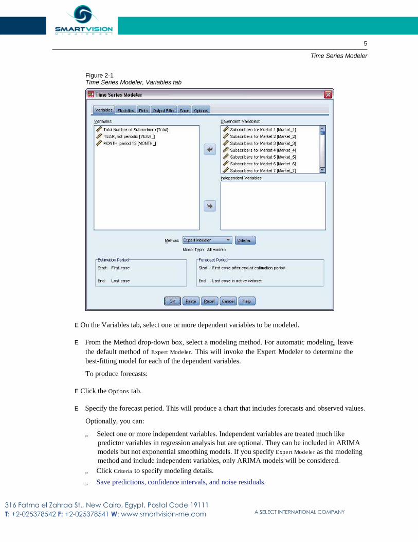
Figure 2-1 Time Series Modeler, Variables tab
E On the Variables tab, select one or more dependent variables to be modeled. E From the Method drop-down box, select a modeling method. For automatic modeling, leave
the default method of Expert Modeler. This will invoke the Expert Modeler to determine the
best-fitting model for each of the dependent variables.
To produce forecasts:
E Click the Options tab. E Specify the forecast period. This will produce a chart that includes forecasts and observed values.
Optionally, you can:
„ Select one or more independent variables. Independent variables are treated much like
predictor variables in regression analysis but are optional. They can be included in ARIMA
models but not exponential smoothing models. If you specify Expert Modeler as the modeling
method and include independent variables, only ARIMA models will be considered.
„ Click Criteria to specify modeling details.
„ Save predictions, confidence intervals, and noise residuals.

316 Fatma el Zahraa St., New Cairo, Egypt, Postal Code 19111
T: +2-025378542 F: +2-025378541 W: www.smartvision-me.com A SELECT INTERNATIONAL COMPANY
6 Chapter 2
„ Save the estimated models in XML format. Saved models can be applied to new or revised
data to obtain updated forecasts without rebuilding models. This is accomplished with the
Apply Time Series Models procedure.
„ Obtain summary statistics across all estimated models.
„ Specify transfer functions for independent variables in custom ARIMA models.
„ Enable automatic detection of outliers.
„ Model specific time points as outliers for custom ARIMA models.
Modeling Methods
The available modeling methods are:
Expert Modeler. The Expert Modeler automatically finds the best-fitting model for each dependent
series. If independent (predictor) variables are specified, the Expert Modeler selects, for inclusion in
ARIMA models, those that have a statistically significant relationship with the dependent series.
Model variables are transformed where appropriate using differencing and/or a square root or natural
log transformation. By default, the Expert Modeler considers both exponential smoothing and
ARIMA models. You can, however, limit the Expert Modeler to only search for ARIMA models or to only search for exponential smoothing models. You can also specify
automatic detection of outliers.
Exponential Smoothing. Use this option to specify a custom exponential smoothing model.
You can choose from a variety of exponential smoothing models that differ in their treatment of
trend and seasonality.
ARIMA. Use this option to specify a custom ARIMA model. This involves explicitly specifying
autoregressive and moving average orders, as well as the degree of differencing. You can include
independent (predictor) variables and define transfer functions for any or all of them. You can
also specify automatic detection of outliers or specify an explicit set of outliers.
Estimation and Forecast Periods
Estimation Period. The estimation period defines the set of cases used to determine the model.
By default, the estimation period includes all cases in the active dataset. To set the estimation
period, select Based on time or case range in the Select Cases dialog box. Depending on available
data, the estimation period used by the procedure may vary by dependent variable and thus differ
from the displayed value. For a given dependent variable, the true estimation period is the period
left after eliminating any contiguous missing values of the variable occurring at the beginning or
end of the specified estimation period.
Forecast Period. The forecast period begins at the first case after the estimation period, and
by default goes through to the last case in the active dataset. You can set the end of the
forecast period from the Options tab.
Specifying Options for the Expert Modeler The Expert Modeler provides options for constraining the set of candidate models, specifying the
handling of outliers, and including event variables.

316 Fatma el Zahraa St., New Cairo, Egypt, Postal Code 19111
T: +2-025378542 F: +2-025378541 W: www.smartvision-me.com A SELECT INTERNATIONAL COMPANY
7
Time Series Modeler
Model Selection and Event Specification
Figure 2-2 Expert Modeler Criteria dialog box, Model tab
The Model tab allows you to specify the types of models considered by the Expert Modeler and
to specify event variables.
Model Type. The following options are available:
„ All models. The Expert Modeler considers both ARIMA and exponential smoothing models.
„ Exponential smoothing models only. The Expert Modeler only considers exponential
smoothing models.
„ ARIMA models only. The Expert Modeler only considers ARIMA models.
Expert Modeler considers seasonal models. This option is only enabled if a periodicity has
been defined for the active dataset. When this option is selected (checked), the Expert Modeler
considers both seasonal and nonseasonal models. If this option is not selected, the Expert
Modeler only considers nonseasonal models.
Current Periodicity. Indicates the periodicity (if any) currently defined for the active dataset.
The current periodicity is given as an integer—for example, 12 for annual periodicity, with each
case representing a month. The value None is displayed if no periodicity has been set. Seasonal
models require a periodicity. You can set the periodicity from the Define Dates dialog box.

316 Fatma el Zahraa St., New Cairo, Egypt, Postal Code 19111
T: +2-025378542 F: +2-025378541 W: www.smartvision-me.com A SELECT INTERNATIONAL COMPANY
8 Chapter 2
Events. Select any independent variables that are to be treated as event variables. For event
variables, cases with a value of 1 indicate times at which the dependent series are expected to be
affected by the event. Values other than 1 indicate no effect.
Handling Outliers with the Expert Modeler
Figure 2-3 Expert Modeler Criteria dialog box, Outliers tab
The Outliers tab allows you to choose automatic detection of outliers as well as the type of
outliers to detect.
Detect outliers automatically. By default, automatic detection of outliers is not performed.
Select (check) this option to perform automatic detection of outliers, then select one or more of
the following outlier types: „ Additive
„ Level shift
„ Innovational
„ Transient
„ Seasonal additive

316 Fatma el Zahraa St., New Cairo, Egypt, Postal Code 19111
T: +2-025378542 F: +2-025378541 W: www.smartvision-me.com A SELECT INTERNATIONAL COMPANY
9
Time Series Modeler
„ Local trend
„ Additive patch
For more information, see the topic Outlier Types in Appendix B on p. 94.
Custom Exponential Smoothing Models
Figure 2-4 Exponential Smoothing Criteria dialog box
Model Type. Exponential smoothing models (Gardner, 1985) are classified as either seasonal
or nonseasonal. Seasonal models are only available if a periodicity has been defined for the
active dataset (see “Current Periodicity” below). „ Simple. This model is appropriate for series in which there is no trend or seasonality. Its
only smoothing parameter is level. Simple exponential smoothing is most similar to an
ARIMA model with zero orders of autoregression, one order of differencing, one order of
moving average, and no constant.
„ Holt’s linear trend. This model is appropriate for series in which there is a linear trend
and no seasonality. Its smoothing parameters are level and trend, which are not constrained
by each other’s values. Holt’s model is more general than Brown’s model but may take
longer to compute for large series. Holt’s exponential smoothing is most similar to an
ARIMA model with zero orders of autoregression, two orders of differencing, and two
orders of moving average.
„ Brown’s linear trend. This model is appropriate for series in which there is a linear trend
and no seasonality. Its smoothing parameters are level and trend, which are assumed to be
equal. Brown’s model is therefore a special case of Holt’s model. Brown’s exponential smoothing is most similar to an ARIMA model with zero orders of autoregression, two
orders of differencing, and two orders of moving average, with the coefficient for the second
order of moving average equal to the square of one-half of the coefficient for the first order.

316 Fatma el Zahraa St., New Cairo, Egypt, Postal Code 19111
T: +2-025378542 F: +2-025378541 W: www.smartvision-me.com A SELECT INTERNATIONAL COMPANY
10 Chapter 2
„ Damped trend. This model is appropriate for series with a linear trend that is dying out and
with no seasonality. Its smoothing parameters are level, trend, and damping trend. Damped
exponential smoothing is most similar to an ARIMA model with 1 order of autoregression, 1
order of differencing, and 2 orders of moving average.
„ Simple seasonal. This model is appropriate for series with no trend and a seasonal effect
that is constant over time. Its smoothing parameters are level and season. Simple seasonal exponential smoothing is most similar to an ARIMA model with zero orders of autoregression,
one order of differencing, one order of seasonal differencing, and orders 1, p, and p + 1
of moving average, where p is the number of periods in a seasonal interval (for monthly
data, p = 12).
„ Winters’ additive. This model is appropriate for series with a linear trend and a seasonal
effect that does not depend on the level of the series. Its smoothing parameters are level,
trend, and season. Winters’ additive exponential smoothing is most similar to an ARIMA
model with zero orders of autoregression, one order of differencing, one order of seasonal
differencing, and p + 1 orders of moving average, where p is the number of periods in a
seasonal interval (for monthly data, p = 12).
„ Winters’ multiplicative. This model is appropriate for series with a linear trend and a seasonal
effect that depends on the level of the series. Its smoothing parameters are level, trend, and
season. Winters’ multiplicative exponential smoothing is not similar to any ARIMA model.
Current Periodicity. Indicates the periodicity (if any) currently defined for the active dataset.
The current periodicity is given as an integer—for example, 12 for annual periodicity, with each
case representing a month. The value None is displayed if no periodicity has been set. Seasonal
models require a periodicity. You can set the periodicity from the Define Dates dialog box.
Dependent Variable Transformation. You can specify a transformation performed on each
dependent variable before it is modeled. „ None. No transformation is performed.
„ Square root. Square root transformation.
„ Natural log. Natural log transformation.
Custom ARIMA Models
The Time Series Modeler allows you to build custom nonseasonal or seasonal ARIMA
(Autoregressive Integrated Moving Average) models—also known as Box-Jenkins (Box,
Jenkins, and Reinsel, 1994) models—with or without a fixed set of predictor variables. You can
define transfer functions for any or all of the predictor variables, and specify automatic detection
of outliers, or specify an explicit set of outliers. „ All independent (predictor) variables specified on the Variables tab are explicitly included in the
model. This is in contrast to using the Expert Modeler where independent variables are only
included if they have a statistically significant relationship with the dependent variable.

316 Fatma el Zahraa St., New Cairo, Egypt, Postal Code 19111
T: +2-025378542 F: +2-025378541 W: www.smartvision-me.com A SELECT INTERNATIONAL COMPANY
11
Time Series Modeler
Model Specification for Custom ARIMA Models
Figure 2-5 ARIMA Criteria dialog box, Model tab
The Model tab allows you to specify the structure of a custom ARIMA model.
ARIMA Orders. Enter values for the various ARIMA components of your model into the
corresponding cells of the Structure grid. All values must be non-negative integers. For
autoregressive and moving average components, the value represents the maximum order. All
positive lower orders will be included in the model. For example, if you specify 2, the model
includes orders 2 and 1. Cells in the Seasonal column are only enabled if a periodicity has been
defined for the active dataset (see “Current Periodicity” below). „ Autoregressive (p). The number of autoregressive orders in the model. Autoregressive
orders specify which previous values from the series are used to predict current values. For
example, an autoregressive order of 2 specifies that the value of the series two time periods in
the past be used to predict the current value.
„ Difference (d). Specifies the order of differencing applied to the series before estimating models.
Differencing is necessary when trends are present (series with trends are typically nonstationary
and ARIMA modeling assumes stationarity) and is used to remove their effect. The order of
differencing corresponds to the degree of series trend—first-order differencing accounts for linear
trends, second-order differencing accounts for quadratic trends, and so on.
„ Moving Average (q). The number of moving average orders in the model. Moving
average orders specify how deviations from the series mean for previous values are used to
predict current values. For example, moving-average orders of 1 and 2 specify that
deviations from the mean value of the series from each of the last two time periods be
considered when predicting current values of the series.

316 Fatma el Zahraa St., New Cairo, Egypt, Postal Code 19111
T: +2-025378542 F: +2-025378541 W: www.smartvision-me.com A SELECT INTERNATIONAL COMPANY
12 Chapter 2
Seasonal Orders. Seasonal autoregressive, moving average, and differencing components play
the same roles as their nonseasonal counterparts. For seasonal orders, however, current series
values are affected by previous series values separated by one or more seasonal periods. For
example, for monthly data (seasonal period of 12), a seasonal order of 1 means that the current
series value is affected by the series value 12 periods prior to the current one. A seasonal order of
1, for monthly data, is then the same as specifying a nonseasonal order of 12.
Current Periodicity. Indicates the periodicity (if any) currently defined for the active dataset.
The current periodicity is given as an integer—for example, 12 for annual periodicity, with each
case representing a month. The value None is displayed if no periodicity has been set. Seasonal
models require a periodicity. You can set the periodicity from the Define Dates dialog box.
Dependent Variable Transformation. You can specify a transformation performed on each
dependent variable before it is modeled. „ None. No transformation is performed.
„ Square root. Square root transformation.
„ Natural log. Natural log transformation.
Include constant in model. Inclusion of a constant is standard unless you are sure that the overall
mean series value is 0. Excluding the constant is recommended when differencing is applied.
Transfer Functions in Custom ARIMA Models
Figure 2-6 ARIMA Criteria dialog box, Transfer Function tab

316 Fatma el Zahraa St., New Cairo, Egypt, Postal Code 19111
T: +2-025378542 F: +2-025378541 W: www.smartvision-me.com A SELECT INTERNATIONAL COMPANY
13
Time Series Modeler
The Transfer Function tab (only present if independent variables are specified) allows you to
define transfer functions for any or all of the independent variables specified on the Variables tab.
Transfer functions allow you to specify the manner in which past values of independent
(predictor) variables are used to forecast future values of the dependent series.
Transfer Function Orders. Enter values for the various components of the transfer function into the
corresponding cells of the Structure grid. All values must be non-negative integers. For numerator and
denominator components, the value represents the maximum order. All positive lower orders will be
included in the model. In addition, order 0 is always included for numerator components. For example,
if you specify 2 for numerator, the model includes orders 2, 1, and 0. If you specify 3 for denominator,
the model includes orders 3, 2, and 1. Cells in the Seasonal column are only enabled if a periodicity
has been defined for the active dataset (see “Current Periodicity” below). „ Numerator. The numerator order of the transfer function. Specifies which previous values
from the selected independent (predictor) series are used to predict current values of the
dependent series. For example, a numerator order of 1 specifies that the value of an
independent series one time period in the past—as well as the current value of the
independent series—is used to predict the current value of each dependent series. „ Denominator. The denominator order of the transfer function. Specifies how deviations
from the series mean, for previous values of the selected independent (predictor) series, are
used to predict current values of the dependent series. For example, a denominator order of 1
specifies that deviations from the mean value of an independent series one time period in the
past be considered when predicting the current value of each dependent series. „ Difference. Specifies the order of differencing applied to the selected independent
(predictor) series before estimating models. Differencing is necessary when trends are
present and is used to remove their effect. Seasonal Orders. Seasonal numerator, denominator, and differencing components play the
same roles as their nonseasonal counterparts. For seasonal orders, however, current series values
are affected by previous series values separated by one or more seasonal periods. For example,
for monthly data (seasonal period of 12), a seasonal order of 1 means that the current series value
is affected by the series value 12 periods prior to the current one. A seasonal order of 1, for
monthly data, is then the same as specifying a nonseasonal order of 12. Current Periodicity. Indicates the periodicity (if any) currently defined for the active dataset.
The current periodicity is given as an integer—for example, 12 for annual periodicity, with each
case representing a month. The value None is displayed if no periodicity has been set. Seasonal
models require a periodicity. You can set the periodicity from the Define Dates dialog box. Delay. Setting a delay causes the independent variable’s influence to be delayed by the number
of intervals specified. For example, if the delay is set to 5, the value of the independent variable
at time t doesn’t affect forecasts until five periods have elapsed (t + 5). Transformation. Specification of a transfer function, for a set of independent variables,
also includes an optional transformation to be performed on those variables. „ None. No transformation is performed. „ Square root. Square root transformation. „ Natural log. Natural log transformation.
316 Fatma el Zahraa St., New Cairo, Egypt, Postal Code 19111
T: +2-025378542 F: +2-025378541 W: www.smartvision-me.com A SELECT INTERNATIONAL COMPANY
14 Chapter 2
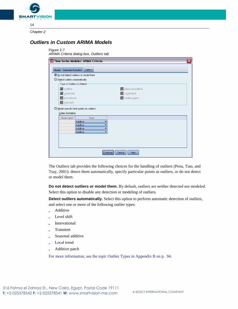
Outliers in Custom ARIMA Models
Figure 2-7 ARIMA Criteria dialog box, Outliers tab
The Outliers tab provides the following choices for the handling of outliers (Pena, Tiao, and
Tsay, 2001): detect them automatically, specify particular points as outliers, or do not detect
or model them.
Do not detect outliers or model them. By default, outliers are neither detected nor modeled.
Select this option to disable any detection or modeling of outliers.
Detect outliers automatically. Select this option to perform automatic detection of outliers,
and select one or more of the following outlier types: „ Additive
„ Level shift
„ Innovational
„ Transient
„ Seasonal additive
„ Local trend
„ Additive patch
For more information, see the topic Outlier Types in Appendix B on p. 94.

316 Fatma el Zahraa St., New Cairo, Egypt, Postal Code 19111
T: +2-025378542 F: +2-025378541 W: www.smartvision-me.com A SELECT INTERNATIONAL COMPANY
15
Time Series Modeler
Model specific time points as outliers. Select this option to specify particular time points
as outliers. Use a separate row of the Outlier Definition grid for each outlier. Enter values for
all of the cells in a given row. „ Type. The outlier type. The supported types are: additive (default), level shift,
innovational, transient, seasonal additive, and local trend.
Note 1: If no date specification has been defined for the active dataset, the Outlier Definition grid
shows the single column Observation. To specify an outlier, enter the row number (as displayed
in the Data Editor) of the relevant case.
Note 2: The Cycle column (if present) in the Outlier Definition grid refers to the value of the
CYCLE_ variable in the active dataset.
Output
Available output includes results for individual models as well as results calculated across all
models. Results for individual models can be limited to a set of best- or poorest-fitting models
based on user-specified criteria.

316 Fatma el Zahraa St., New Cairo, Egypt, Postal Code 19111
T: +2-025378542 F: +2-025378541 W: www.smartvision-me.com A SELECT INTERNATIONAL COMPANY
16 Chapter 2
Statistics and Forecast Tables
Figure 2-8 Time Series Modeler, Statistics tab
The Statistics tab provides options for displaying tables of the modeling results.
Display fit measures, Ljung-Box statistic, and number of outliers by model. Select
(check) this option to display a table containing selected fit measures, Ljung-Box value, and the
number of outliers for each estimated model.
Fit Measures. You can select one or more of the following for inclusion in the table containing
fit measures for each estimated model: „ Stationary R-square
„ R-square
„ Root mean square error
„ Mean absolute percentage error
„ Mean absolute error
„ Maximum absolute percentage error
„ Maximum absolute error
„ Normalized BIC

316 Fatma el Zahraa St., New Cairo, Egypt, Postal Code 19111
T: +2-025378542 F: +2-025378541 W: www.smartvision-me.com A SELECT INTERNATIONAL COMPANY
17
Time Series Modeler
For more information, see the topic Goodness-of-Fit Measures in Appendix A on p. 93. Statistics for Comparing Models. This group of options controls display of tables containing
statistics calculated across all estimated models. Each option generates a separate table. You can
select one or more of the following options: „ Goodness of fit. Table of summary statistics and percentiles for stationary R-square, R-
square, root mean square error, mean absolute percentage error, mean absolute error,
maximum absolute percentage error, maximum absolute error, and normalized Bayesian
Information Criterion. „ Residual autocorrelation function (ACF). Table of summary statistics and
percentiles for autocorrelations of the residuals across all estimated models. „ Residual partial autocorrelation function (PACF). Table of summary statistics and
percentiles for partial autocorrelations of the residuals across all estimated models. Statistics for Individual Models. This group of options controls display of tables containing
detailed information for each estimated model. Each option generates a separate table. You can
select one or more of the following options: „ Parameter estimates. Displays a table of parameter estimates for each estimated model.
Separate tables are displayed for exponential smoothing and ARIMA models. If outliers
exist, parameter estimates for them are also displayed in a separate table. „ Residual autocorrelation function (ACF). Displays a table of residual autocorrelations by lag
for each estimated model. The table includes the confidence intervals for the autocorrelations.
„ Residual partial autocorrelation function (PACF). Displays a table of residual partial
autocorrelations by lag for each estimated model. The table includes the confidence intervals
for the partial autocorrelations. Display forecasts. Displays a table of model forecasts and confidence intervals for each
estimated model. The forecast period is set from the Options tab.

316 Fatma el Zahraa St., New Cairo, Egypt, Postal Code 19111
T: +2-025378542 F: +2-025378541 W: www.smartvision-me.com A SELECT INTERNATIONAL COMPANY
18 Chapter 2
Plots
Figure 2-9 Time Series Modeler, Plots tab
The Plots tab provides options for displaying plots of the modeling results.
Plots for Comparing Models
This group of options controls display of plots containing statistics calculated across all estimated
models. Each option generates a separate plot. You can select one or more of the following options:
„ Stationary R-square
„ R-square
„ Root mean square error
„ Mean absolute percentage error
„ Mean absolute error
„ Maximum absolute percentage error
„ Maximum absolute error
„ Normalized BIC

316 Fatma el Zahraa St., New Cairo, Egypt, Postal Code 19111
T: +2-025378542 F: +2-025378541 W: www.smartvision-me.com A SELECT INTERNATIONAL COMPANY
19
Time Series Modeler
„ Residual autocorrelation function (ACF) „ Residual partial autocorrelation function (PACF) For more information, see the topic Goodness-of-Fit Measures in Appendix A on p. 93.
Plots for Individual Models Series. Select (check) this option to obtain plots of the predicted values for each estimated
model. You can select one or more of the following for inclusion in the plot: „ Observed values. The observed values of the dependent series. „ Forecasts. The model predicted values for the forecast period. „ Fit values. The model predicted values for the estimation period. „ Confidence intervals for forecasts. The confidence intervals for the forecast period. „ Confidence intervals for fit values. The confidence intervals for the estimation period. Residual autocorrelation function (ACF). Displays a plot of residual autocorrelations
for each estimated model. Residual partial autocorrelation function (PACF). Displays a plot of residual partial
autocorrelations for each estimated model.

316 Fatma el Zahraa St., New Cairo, Egypt, Postal Code 19111
T: +2-025378542 F: +2-025378541 W: www.smartvision-me.com A SELECT INTERNATIONAL COMPANY
20 Chapter 2
Limiting Output to the Best- or Poorest-Fitting Models
Figure 2-10 Time Series Modeler, Output Filter tab
The Output Filter tab provides options for restricting both tabular and chart output to a subset of
the estimated models. You can choose to limit output to the best-fitting and/or the poorest-
fitting models according to fit criteria you provide. By default, all estimated models are included
in the output.
Best-fitting models. Select (check) this option to include the best-fitting models in the
output. Select a goodness-of-fit measure and specify the number of models to include.
Selecting this option does not preclude also selecting the poorest-fitting models. In that case,
the output will consist of the poorest-fitting models as well as the best-fitting ones. „ Fixed number of models. Specifies that results are displayed for the n best-fitting models.
If the number exceeds the number of estimated models, all models are displayed.
„ Percentage of total number of models. Specifies that results are displayed for
models with goodness-of-fit values in the top n percent across all estimated models.

316 Fatma el Zahraa St., New Cairo, Egypt, Postal Code 19111
T: +2-025378542 F: +2-025378541 W: www.smartvision-me.com A SELECT INTERNATIONAL COMPANY
21
Time Series Modeler
Poorest-fitting models. Select (check) this option to include the poorest-fitting models in the
output. Select a goodness-of-fit measure and specify the number of models to include. Selecting
this option does not preclude also selecting the best-fitting models. In that case, the output will
consist of the best-fitting models as well as the poorest-fitting ones. „ Fixed number of models. Specifies that results are displayed for the n poorest-fitting
models. If the number exceeds the number of estimated models, all models are displayed.
„ Percentage of total number of models. Specifies that results are displayed for
models with goodness-of-fit values in the bottom n percent across all estimated models.
Goodness of Fit Measure. Select the goodness-of-fit measure to use for filtering models.
The default is stationary R square.
Saving Model Predictions and Model Specifications
Figure 2-11 Time Series Modeler, Save tab The Save tab allows you to save model predictions as new variables in the active dataset and
save model specifications to an external file in XML format.

316 Fatma el Zahraa St., New Cairo, Egypt, Postal Code 19111
T: +2-025378542 F: +2-025378541 W: www.smartvision-me.com A SELECT INTERNATIONAL COMPANY
22 Chapter 2
Save Variables. You can save model predictions, confidence intervals, and residuals as new
variables in the active dataset. Each dependent series gives rise to its own set of new variables,
and each new variable contains values for both the estimation and forecast periods. New cases are
added if the forecast period extends beyond the length of the dependent variable series. Choose to
save new variables by selecting the associated Save check box for each. By default, no new
variables are saved. „ Predicted Values. The model predicted values.
„ Lower Confidence Limits. Lower confidence limits for the predicted values.
„ Upper Confidence Limits. Upper confidence limits for the predicted values.
„ Noise Residuals. The model residuals. When transformations of the dependent variable
are performed (for example, natural log), these are the residuals for the transformed series.
„ Variable Name Prefix. Specify prefixes to be used for new variable names, or leave the
default prefixes. Variable names consist of the prefix, the name of the associated dependent
variable, and a model identifier. The variable name is extended if necessary to avoid variable
naming conflicts. The prefix must conform to the rules for valid variable names.
Export Model File. Model specifications for all estimated models are exported to the specified
file in XML format. Saved models can be used to obtain updated forecasts, based on more
current data, using the Apply Time Series Models procedure.

316 Fatma el Zahraa St., New Cairo, Egypt, Postal Code 19111
T: +2-025378542 F: +2-025378541 W: www.smartvision-me.com A SELECT INTERNATIONAL COMPANY
23
Time Series Modeler
Options
Figure 2-12 Time Series Modeler, Options tab
The Options tab allows you to set the forecast period, specify the handling of missing values, set
the confidence interval width, specify a custom prefix for model identifiers, and set the number
of lags shown for autocorrelations.
Forecast Period. The forecast period always begins with the first case after the end of the
estimation period (the set of cases used to determine the model) and goes through either the last
case in the active dataset or a user-specified date. By default, the end of the estimation period is
the last case in the active dataset, but it can be changed from the Select Cases dialog box by
selecting Based on time or case range. „ First case after end of estimation period through last case in active dataset. Select this
option when the end of the estimation period is prior to the last case in the active dataset, and you
want forecasts through the last case. This option is typically used to produce forecasts for a
holdout period, allowing comparison of the model predictions with a subset of the actual values.
„ First case after end of estimation period through a specified date. Select this option
to explicitly specify the end of the forecast period. This option is typically used to produce
forecasts beyond the end of the actual series. Enter values for all of the cells in the Date grid.

316 Fatma el Zahraa St., New Cairo, Egypt, Postal Code 19111
T: +2-025378542 F: +2-025378541 W: www.smartvision-me.com A SELECT INTERNATIONAL COMPANY
24 Chapter 2
If no date specification has been defined for the active dataset, the Date grid shows the single
column Observation. To specify the end of the forecast period, enter the row number (as
displayed in the Data Editor) of the relevant case.
The Cycle column (if present) in the Date grid refers to the value of the CYCLE_ variable
in the active dataset.
User-Missing Values. These options control the handling of user-missing values.
„ Treat as invalid. User-missing values are treated like system-missing values.
„ Treat as valid. User-missing values are treated as valid data.
Missing Value Policy. The following rules apply to the treatment of missing values (includes
system-missing values and user-missing values treated as invalid) during the modeling procedure:
„ Cases with missing values of a dependent variable that occur within the estimation period
are included in the model. The specific handling of the missing value depends on the
estimation method.
„ A warning is issued if an independent variable has missing values within the estimation period.
For the Expert Modeler, models involving the independent variable are estimated without the
variable. For custom ARIMA, models involving the independent variable are not estimated.
„ If any independent variable has missing values within the forecast period, the procedure
issues a warning and forecasts as far as it can.
Confidence Interval Width (%). Confidence intervals are computed for the model
predictions and residual autocorrelations. You can specify any positive value less than 100. By
default, a 95% confidence interval is used.
Prefix for Model Identifiers in Output. Each dependent variable specified on the Variables tab
gives rise to a separate estimated model. Models are distinguished with unique names consisting of a
customizable prefix along with an integer suffix. You can enter a prefix or leave the default
of Model.
Maximum Number of Lags Shown in ACF and PACF Output. You can set the maximum
number of lags shown in tables and plots of autocorrelations and partial autocorrelations.
TSMODEL Command Additional Features
You can customize your time series modeling if you paste your selections into a syntax window
and edit the resulting TSMODEL command syntax. The command syntax language allows you to: „ Specify the seasonal period of the data (with the SEASONLENGTH keyword on the AUXILIARY
subcommand). This overrides the current periodicity (if any) for the active dataset.
„ Specify nonconsecutive lags for custom ARIMA and transfer function components (with the
ARIMA and TRANSFERFUNCTION subcommands). For example, you can specify a custom
ARIMA model with autoregressive lags of orders 1, 3, and 6; or a transfer function with
numerator lags of orders 2, 5, and 8.
„ Provide more than one set of modeling specifications (for example, modeling method,
ARIMA orders, independent variables, and so on) for a single run of the Time Series
Modeler procedure (with the MODEL subcommand). See the Command Syntax Reference for complete syntax information.
316 Fatma el Zahraa St., New Cairo, Egypt, Postal Code 19111
T: +2-025378542 F: +2-025378541 W: www.smartvision-me.com A SELECT INTERNATIONAL COMPANY
Chapter
3
Apply Time Series Models
The Apply Time Series Models procedure loads existing time series models from an external file
and applies them to the active dataset. You can use this procedure to obtain forecasts for series
for which new or revised data are available, without rebuilding your models.Models are generated
using the Time Series Modeler procedure.
Example. You are an inventory manager with a major retailer, and responsible for each of
5,000 products. You’ve used the Expert Modeler to create models that forecast sales for each
product three months into the future. Your data warehouse is refreshed each month with actual
sales data which you’d like to use to produce monthly updated forecasts. The Apply Time Series
Models procedure allows you to accomplish this using the original models, and simply
reestimating model parameters to account for the new data.
Statistics. Goodness-of-fit measures: stationary R-square, R-square (R2
), root mean square
error (RMSE), mean absolute error (MAE), mean absolute percentage error (MAPE), maximum absolute error (MaxAE), maximum absolute percentage error (MaxAPE), normalized Bayesian information criterion (BIC). Residuals: autocorrelation function, partial autocorrelation function, Ljung-Box Q.
Plots. Summary plots across all models: histograms of stationary R-square, R-square (R2
),
root mean square error (RMSE), mean absolute error (MAE), mean absolute percentage error (MAPE), maximum absolute error (MaxAE), maximum absolute percentage error (MaxAPE), normalized Bayesian information criterion (BIC); box plots of residual autocorrelations and
partial autocorrelations. Results for individual models: forecast values, fit values, observed
values, upper and lower confidence limits, residual autocorrelations and partial autocorrelations.
Apply Time Series Models Data Considerations
Data. Variables (dependent and independent) to which models will be applied should be numeric.
Assumptions. Models are applied to variables in the active dataset with the same names as the
variables specified in the model. All such variables are treated as time series, meaning that each
case represents a time point, with successive cases separated by a constant time interval. „ Forecasts. For producing forecasts using models with independent (predictor) variables, the
active dataset should contain values of these variables for all cases in the forecast period. If
model parameters are reestimated, then independent variables should not contain any missing
values in the estimation period.
© Copyright SPSS Inc. 1989, 2010 25

316 Fatma el Zahraa St., New Cairo, Egypt, Postal Code 19111
T: +2-025378542 F: +2-025378541 W: www.smartvision-me.com A SELECT INTERNATIONAL COMPANY
26 Chapter 3
Defining Dates
The Apply Time Series Models procedure requires that the periodicity, if any, of the active
dataset matches the periodicity of the models to be applied. If you’re simply forecasting using the
same dataset (perhaps with new or revised data) as that used to the build the model, then this
condition will be satisfied. If no periodicity exists for the active dataset, you will be given the
opportunity to navigate to the Define Dates dialog box to create one. If, however, the models
were created without specifying a periodicity, then the active dataset should also be without one.
To Apply Models
E From the menus choose:
Analyze > Forecasting > Apply Models...
Figure 3-1 Apply Time Series Models, Models tab
E Enter the file specification for a model file or click Browse and select a model file (model files
are created with the Time Series Modeler procedure).
Optionally, you can:
„ Reestimate model parameters using the data in the active dataset. Forecasts are created using
the reestimated parameters.
„ Save predictions, confidence intervals, and noise residuals.
„ Save reestimated models in XML format.

316 Fatma el Zahraa St., New Cairo, Egypt, Postal Code 19111
T: +2-025378542 F: +2-025378541 W: www.smartvision-me.com A SELECT INTERNATIONAL COMPANY
27
Apply Time Series Models
Model Parameters and Goodness of Fit Measures Load from model file. Forecasts are produced using the model parameters from the model file
without reestimating those parameters. Goodness of fit measures displayed in output and used to
filter models (best- or worst-fitting) are taken from the model file and reflect the data used when
each model was developed (or last updated). With this option, forecasts do not take into account
historical data—for either dependent or independent variables—in the active dataset. You must
choose Reestimate from data if you want historical data to impact the forecasts. In addition,
forecasts do not take into account values of the dependent series in the forecast period—but they
do take into account values of independent variables in the forecast period. If you have more
current values of the dependent series and want them to be included in the forecasts, you need to
reestimate, adjusting the estimation period to include these values. Reestimate from data. Model parameters are reestimated using the data in the active dataset.
Reestimation of model parameters has no effect on model structure. For example, an
ARIMA(1,0,1) model will remain so, but the autoregressive and moving-average parameters
will be reestimated. Reestimation does not result in the detection of new outliers. Outliers, if
any, are always taken from the model file. „ Estimation Period. The estimation period defines the set of cases used to reestimate the
model parameters. By default, the estimation period includes all cases in the active dataset.
To set the estimation period, select Based on time or case range in the Select Cases dialog box. Depending on available data, the estimation period used by the procedure may vary by model
and thus differ from the displayed value. For a given model, the true estimation period is the
period left after eliminating any contiguous missing values, from the model’s dependent
variable, occurring at the beginning or end of the specified estimation period.
Forecast Period The forecast period for each model always begins with the first case after the end of the
estimation period and goes through either the last case in the active dataset or a user-specified
date. If parameters are not reestimated (this is the default), then the estimation period for each
model is the set of cases used when the model was developed (or last updated). „ First case after end of estimation period through last case in active dataset.
Select this option when the end of the estimation period is prior to the last case in the
active dataset, and you want forecasts through the last case. „ First case after end of estimation period through a specified date. Select this option to
explicitly specify the end of the forecast period. Enter values for all of the cells in the Date grid.
If no date specification has been defined for the active dataset, the Date grid shows the single
column Observation. To specify the end of the forecast period, enter the row number (as
displayed in the Data Editor) of the relevant case.
The Cycle column (if present) in the Date grid refers to the value of the CYCLE_ variable
in the active dataset.

316 Fatma el Zahraa St., New Cairo, Egypt, Postal Code 19111
T: +2-025378542 F: +2-025378541 W: www.smartvision-me.com A SELECT INTERNATIONAL COMPANY
28 Chapter 3
Output
Available output includes results for individual models as well as results across all models.
Results for individual models can be limited to a set of best- or poorest-fitting models based
on user-specified criteria.
Statistics and Forecast Tables
Figure 3-2 Apply Time Series Models, Statistics tab
The Statistics tab provides options for displaying tables of model fit statistics, model parameters,
autocorrelation functions, and forecasts. Unless model parameters are reestimated (Reestimate
from data on the Models tab), displayed values of fit measures, Ljung-Box values, and model
parameters are those from the model file and reflect the data used when each model was
developed (or last updated). Outlier information is always taken from the model file.
Display fit measures, Ljung-Box statistic, and number of outliers by model. Select
(check) this option to display a table containing selected fit measures, Ljung-Box value, and the
number of outliers for each model.
Fit Measures. You can select one or more of the following for inclusion in the table containing
fit measures for each model: „ Stationary R-square
„ R-square
„ Root mean square error

316 Fatma el Zahraa St., New Cairo, Egypt, Postal Code 19111
T: +2-025378542 F: +2-025378541 W: www.smartvision-me.com A SELECT INTERNATIONAL COMPANY
29
Apply Time Series Models
„ Mean absolute percentage error „ Mean absolute error „ Maximum absolute percentage error „ Maximum absolute error „ Normalized BIC For more information, see the topic Goodness-of-Fit Measures in Appendix A on p. 93. Statistics for Comparing Models. This group of options controls the display of tables
containing statistics across all models. Each option generates a separate table. You can select one
or more of the following options: „ Goodness of fit. Table of summary statistics and percentiles for stationary R-square, R-
square, root mean square error, mean absolute percentage error, mean absolute error,
maximum absolute percentage error, maximum absolute error, and normalized Bayesian
Information Criterion. „ Residual autocorrelation function (ACF). Table of summary statistics and percentiles
for autocorrelations of the residuals across all estimated models. This table is only
available if model parameters are reestimated (Reestimate from data on the Models tab). „ Residual partial autocorrelation function (PACF). Table of summary statistics and
percentiles for partial autocorrelations of the residuals across all estimated models. This table
is only available if model parameters are reestimated (Reestimate from data on the Models tab). Statistics for Individual Models. This group of options controls display of tables containing
detailed information for each model. Each option generates a separate table. You can select one
or more of the following options: „ Parameter estimates. Displays a table of parameter estimates for each model. Separate
tables are displayed for exponential smoothing and ARIMA models. If outliers exist,
parameter estimates for them are also displayed in a separate table. „ Residual autocorrelation function (ACF). Displays a table of residual autocorrelations
by lag for each estimated model. The table includes the confidence intervals for the
autocorrelations. This table is only available if model parameters are reestimated (Reestimate
from data on the Models tab). „ Residual partial autocorrelation function (PACF). Displays a table of residual partial
autocorrelations by lag for each estimated model. The table includes the confidence
intervals for the partial autocorrelations. This table is only available if model parameters are
reestimated (Reestimate from data on the Models tab). Display forecasts. Displays a table of model forecasts and confidence intervals for each model.
316 Fatma el Zahraa St., New Cairo, Egypt, Postal Code 19111
T: +2-025378542 F: +2-025378541 W: www.smartvision-me.com A SELECT INTERNATIONAL COMPANY
30 Chapter 3
Plots
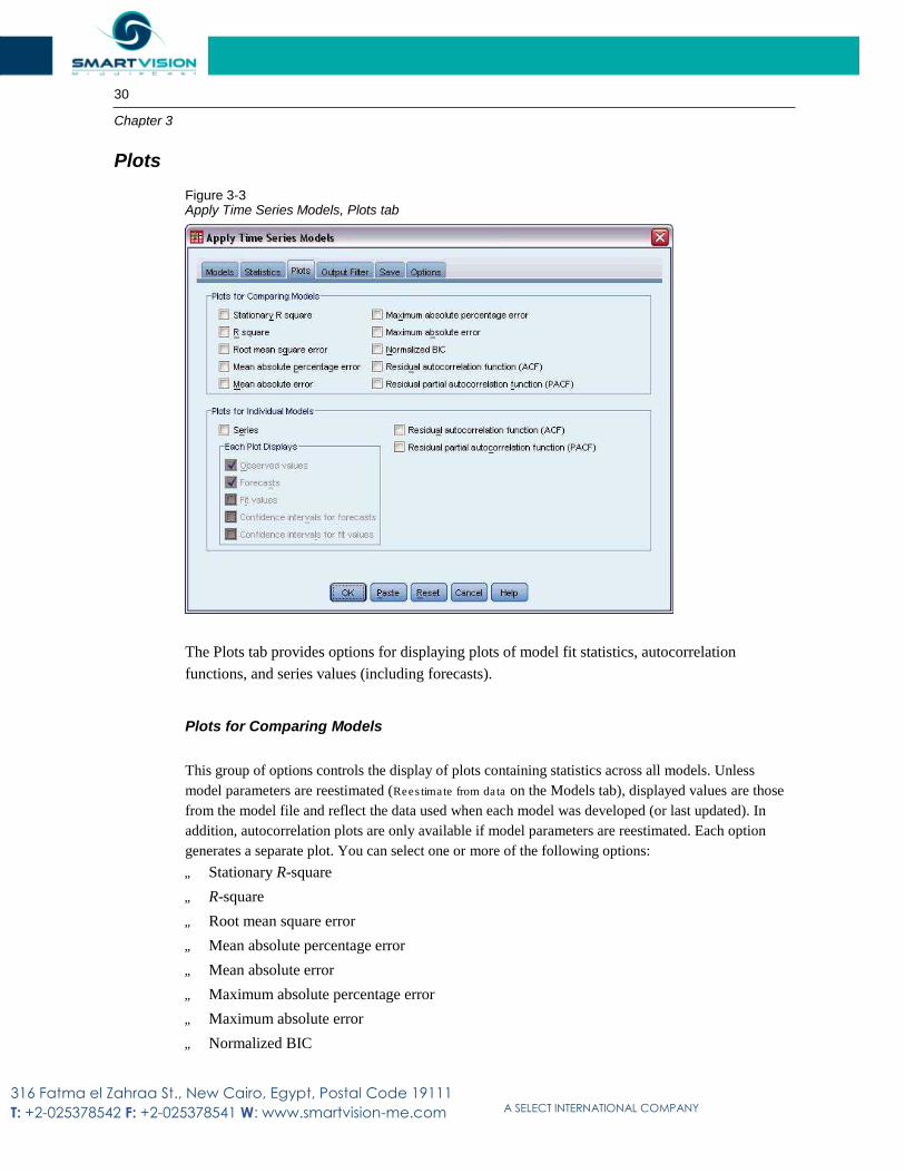
Figure 3-3 Apply Time Series Models, Plots tab
The Plots tab provides options for displaying plots of model fit statistics, autocorrelation
functions, and series values (including forecasts).
Plots for Comparing Models
This group of options controls the display of plots containing statistics across all models. Unless
model parameters are reestimated (Reestimate from data on the Models tab), displayed values are those
from the model file and reflect the data used when each model was developed (or last updated). In
addition, autocorrelation plots are only available if model parameters are reestimated. Each option
generates a separate plot. You can select one or more of the following options: „ Stationary R-square
„ R-square
„ Root mean square error
„ Mean absolute percentage error
„ Mean absolute error
„ Maximum absolute percentage error
„ Maximum absolute error
„ Normalized BIC

316 Fatma el Zahraa St., New Cairo, Egypt, Postal Code 19111
T: +2-025378542 F: +2-025378541 W: www.smartvision-me.com A SELECT INTERNATIONAL COMPANY
31
Apply Time Series Models
„ Residual autocorrelation function (ACF) „ Residual partial autocorrelation function (PACF) For more information, see the topic Goodness-of-Fit Measures in Appendix A on p. 93.
Plots for Individual Models Series. Select (check) this option to obtain plots of the predicted values for each model.
Observed values, fit values, confidence intervals for fit values, and autocorrelations are only
available if model parameters are reestimated (Reestimate from data on the Models tab). You can
select one or more of the following for inclusion in the plot: „ Observed values. The observed values of the dependent series. „ Forecasts. The model predicted values for the forecast period. „ Fit values. The model predicted values for the estimation period. „ Confidence intervals for forecasts. The confidence intervals for the forecast period. „ Confidence intervals for fit values. The confidence intervals for the estimation period. Residual autocorrelation function (ACF). Displays a plot of residual autocorrelations
for each estimated model. Residual partial autocorrelation function (PACF). Displays a plot of residual partial
autocorrelations for each estimated model.
316 Fatma el Zahraa St., New Cairo, Egypt, Postal Code 19111
T: +2-025378542 F: +2-025378541 W: www.smartvision-me.com A SELECT INTERNATIONAL COMPANY
32 Chapter 3
Limiting Output to the Best- or Poorest-Fitting Models
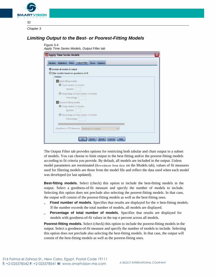
Figure 3-4 Apply Time Series Models, Output Filter tab
The Output Filter tab provides options for restricting both tabular and chart output to a subset
of models. You can choose to limit output to the best-fitting and/or the poorest-fitting models
according to fit criteria you provide. By default, all models are included in the output. Unless model parameters are reestimated (Reestimate from data on the Models tab), values of fit measures
used for filtering models are those from the model file and reflect the data used when each model
was developed (or last updated).
Best-fitting models. Select (check) this option to include the best-fitting models in the
output. Select a goodness-of-fit measure and specify the number of models to include.
Selecting this option does not preclude also selecting the poorest-fitting models. In that case,
the output will consist of the poorest-fitting models as well as the best-fitting ones. „ Fixed number of models. Specifies that results are displayed for the n best-fitting models.
If the number exceeds the total number of models, all models are displayed.
„ Percentage of total number of models. Specifies that results are displayed for
models with goodness-of-fit values in the top n percent across all models.
Poorest-fitting models. Select (check) this option to include the poorest-fitting models in the
output. Select a goodness-of-fit measure and specify the number of models to include. Selecting
this option does not preclude also selecting the best-fitting models. In that case, the output will
consist of the best-fitting models as well as the poorest-fitting ones.

316 Fatma el Zahraa St., New Cairo, Egypt, Postal Code 19111
T: +2-025378542 F: +2-025378541 W: www.smartvision-me.com A SELECT INTERNATIONAL COMPANY
33
Apply Time Series Models
„ Fixed number of models. Specifies that results are displayed for the n poorest-fitting
models. If the number exceeds the total number of models, all models are displayed.
„ Percentage of total number of models. Specifies that results are displayed for
models with goodness-of-fit values in the bottom n percent across all models.
Goodness of Fit Measure. Select the goodness-of-fit measure to use for filtering models.
The default is stationary R-square.
Saving Model Predictions and Model Specifications
Figure 3-5 Apply Time Series Models, Save tab
The Save tab allows you to save model predictions as new variables in the active dataset and
save model specifications to an external file in XML format.
Save Variables. You can save model predictions, confidence intervals, and residuals as new
variables in the active dataset. Each model gives rise to its own set of new variables. New cases
are added if the forecast period extends beyond the length of the dependent variable series
associated with the model. Unless model parameters are reestimated (Reestimate from data on the
Models tab), predicted values and confidence limits are only created for the forecast period.
Choose to save new variables by selecting the associated Save check box for each. By default,
no new variables are saved. „ Predicted Values. The model predicted values.
„ Lower Confidence Limits. Lower confidence limits for the predicted values.
„ Upper Confidence Limits. Upper confidence limits for the predicted values.

316 Fatma el Zahraa St., New Cairo, Egypt, Postal Code 19111
T: +2-025378542 F: +2-025378541 W: www.smartvision-me.com A SELECT INTERNATIONAL COMPANY
34 Chapter 3
„ Noise Residuals. The model residuals. When transformations of the dependent variable
are performed (for example, natural log), these are the residuals for the transformed series.
This choice is only available if model parameters are reestimated (Reestimate from data on
the Models tab).
„ Variable Name Prefix. Specify prefixes to be used for new variable names or leave the
default prefixes. Variable names consist of the prefix, the name of the associated dependent
variable, and a model identifier. The variable name is extended if necessary to avoid variable
naming conflicts. The prefix must conform to the rules for valid variable names.
Export Model File Containing Reestimated Parameters. Model specifications, containing
reestimated parameters and fit statistics, are exported to the specified file in XML format. This option
is only available if model parameters are reestimated (Reestimate from data on the Models tab).
Options
Figure 3-6 Apply Time Series Models, Options tab
The Options tab allows you to specify the handling of missing values, set the confidence interval
width, and set the number of lags shown for autocorrelations.
User-Missing Values. These options control the handling of user-missing values.
„ Treat as invalid. User-missing values are treated like system-missing values.
„ Treat as valid. User-missing values are treated as valid data.

316 Fatma el Zahraa St., New Cairo, Egypt, Postal Code 19111
T: +2-025378542 F: +2-025378541 W: www.smartvision-me.com A SELECT INTERNATIONAL COMPANY
35
Apply Time Series Models
Missing Value Policy. The following rules apply to the treatment of missing values
(includes system-missing values and user-missing values treated as invalid): „ Cases with missing values of a dependent variable that occur within the estimation period
are included in the model. The specific handling of the missing value depends on the
estimation method.
„ For ARIMA models, a warning is issued if a predictor has any missing values within the
estimation period. Any models involving the predictor are not reestimated.
„ If any independent variable has missing values within the forecast period, the procedure
issues a warning and forecasts as far as it can.
Confidence Interval Width (%). Confidence intervals are computed for the model
predictions and residual autocorrelations. You can specify any positive value less than 100. By
default, a 95% confidence interval is used.
Maximum Number of Lags Shown in ACF and PACF Output. You can set the maximum
number of lags shown in tables and plots of autocorrelations and partial autocorrelations. This option
is only available if model parameters are reestimated (Reestimate from data on the Models tab).
TSAPPLY Command Additional Features
Additional features are available if you paste your selections into a syntax window and edit the
resulting TSAPPLY command syntax. The command syntax language allows you to: „ Specify that only a subset of the models in a model file are to be applied to the active dataset
(with the DROP and KEEP keywords on the MODEL subcommand).
„ Apply models from two or more model files to your data (with the MODEL subcommand). For
example, one model file might contain models for series that represent unit sales, and
another might contain models for series that represent revenue.
See the Command Syntax Reference for complete syntax information.
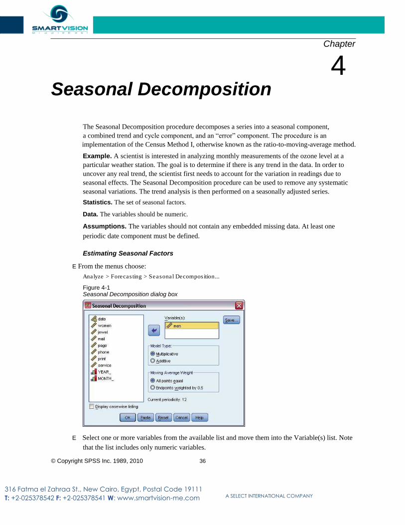
316 Fatma el Zahraa St., New Cairo, Egypt, Postal Code 19111
T: +2-025378542 F: +2-025378541 W: www.smartvision-me.com A SELECT INTERNATIONAL COMPANY
Chapter
4
Seasonal Decomposition
The Seasonal Decomposition procedure decomposes a series into a seasonal component,
a combined trend and cycle component, and an “error” component. The procedure is an implementation of the Census Method I, otherwise known as the ratio-to-moving-average method.
Example. A scientist is interested in analyzing monthly measurements of the ozone level at a
particular weather station. The goal is to determine if there is any trend in the data. In order to
uncover any real trend, the scientist first needs to account for the variation in readings due to
seasonal effects. The Seasonal Decomposition procedure can be used to remove any systematic
seasonal variations. The trend analysis is then performed on a seasonally adjusted series.
Statistics. The set of seasonal factors.
Data. The variables should be numeric.
Assumptions. The variables should not contain any embedded missing data. At least one
periodic date component must be defined.
Estimating Seasonal Factors
E From the menus choose:
Analyze > Forecasting > Seasonal Decomposition...
Figure 4-1 Seasonal Decomposition dialog box
E Select one or more variables from the available list and move them into the Variable(s) list. Note
that the list includes only numeric variables. © Copyright SPSS Inc. 1989, 2010 36
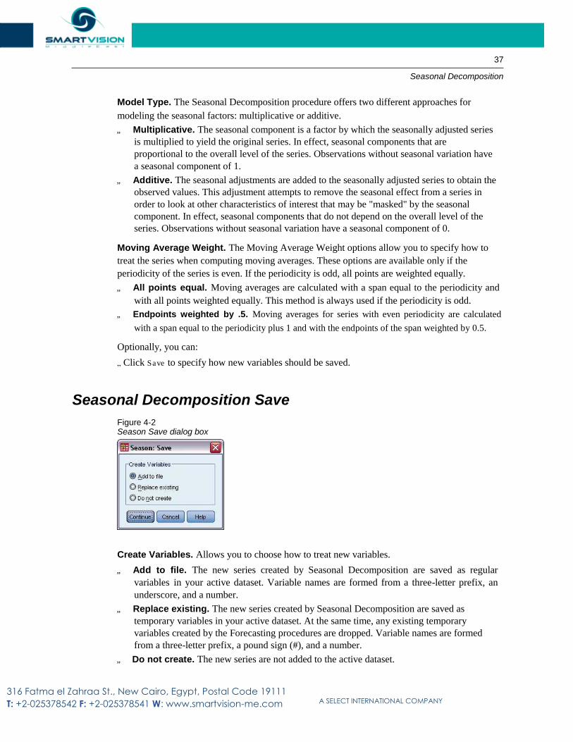
316 Fatma el Zahraa St., New Cairo, Egypt, Postal Code 19111
T: +2-025378542 F: +2-025378541 W: www.smartvision-me.com A SELECT INTERNATIONAL COMPANY
37
Seasonal Decomposition
Model Type. The Seasonal Decomposition procedure offers two different approaches for
modeling the seasonal factors: multiplicative or additive. „ Multiplicative. The seasonal component is a factor by which the seasonally adjusted series
is multiplied to yield the original series. In effect, seasonal components that are
proportional to the overall level of the series. Observations without seasonal variation have
a seasonal component of 1.
„ Additive. The seasonal adjustments are added to the seasonally adjusted series to obtain the
observed values. This adjustment attempts to remove the seasonal effect from a series in
order to look at other characteristics of interest that may be "masked" by the seasonal
component. In effect, seasonal components that do not depend on the overall level of the
series. Observations without seasonal variation have a seasonal component of 0.
Moving Average Weight. The Moving Average Weight options allow you to specify how to
treat the series when computing moving averages. These options are available only if the
periodicity of the series is even. If the periodicity is odd, all points are weighted equally. „ All points equal. Moving averages are calculated with a span equal to the periodicity and
with all points weighted equally. This method is always used if the periodicity is odd.
„ Endpoints weighted by .5. Moving averages for series with even periodicity are calculated
with a span equal to the periodicity plus 1 and with the endpoints of the span weighted by 0.5.
Optionally, you can:
„ Click Save to specify how new variables should be saved.
Seasonal Decomposition Save
Figure 4-2 Season Save dialog box
Create Variables. Allows you to choose how to treat new variables.
„ Add to file. The new series created by Seasonal Decomposition are saved as regular
variables in your active dataset. Variable names are formed from a three-letter prefix, an
underscore, and a number.
„ Replace existing. The new series created by Seasonal Decomposition are saved as
temporary variables in your active dataset. At the same time, any existing temporary
variables created by the Forecasting procedures are dropped. Variable names are formed
from a three-letter prefix, a pound sign (#), and a number.
„ Do not create. The new series are not added to the active dataset.

316 Fatma el Zahraa St., New Cairo, Egypt, Postal Code 19111
T: +2-025378542 F: +2-025378541 W: www.smartvision-me.com A SELECT INTERNATIONAL COMPANY
38 Chapter 4
New Variable Names
The Seasonal Decomposition procedure creates four new variables (series), with the following
three-letter prefixes, for each series specified:
SAF. Seasonal adjustment factors. These values indicate the effect of each period on the
level of the series.
SAS. Seasonally adjusted series. These are the values obtained after removing the
seasonal variation of a series.
STC. Smoothed trend-cycle components. These values show the trend and cyclical
behavior present in the series.
ERR. Residual or “error” values. The values that remain after the seasonal, trend, and
cycle components have been removed from the series.
SEASON Command Additional Features
The command syntax language also allows you to:
„ Specify any periodicity within the SEASON command rather than select one of the alternatives
offered by the Define Dates procedure.
See the Command Syntax Reference for complete syntax information.

316 Fatma el Zahraa St., New Cairo, Egypt, Postal Code 19111
T: +2-025378542 F: +2-025378541 W: www.smartvision-me.com A SELECT INTERNATIONAL COMPANY
Chapter
5
Spectral Plots
The Spectral Plots procedure is used to identify periodic behavior in time series. Instead of
analyzing the variation from one time point to the next, it analyzes the variation of the series as a
whole into periodic components of different frequencies. Smooth series have stronger periodic
components at low frequencies; random variation (“white noise”) spreads the component
strength over all frequencies.
Series that include missing data cannot be analyzed with this procedure.
Example. The rate at which new houses are constructed is an important barometer of the state of the
economy. Data for housing starts typically exhibit a strong seasonal component. But are there longer
cycles present in the data that analysts need to be aware of when evaluating current figures?
Statistics. Sine and cosine transforms, periodogram value, and spectral density estimate for
each frequency or period component. When bivariate analysis is selected: real and imaginary
parts of cross-periodogram, cospectral density, quadrature spectrum, gain, squared coherency,
and phase spectrum for each frequency or period component.
Plots. For univariate and bivariate analyses: periodogram and spectral density. For bivariate
analyses: squared coherency, quadrature spectrum, cross amplitude, cospectral density, phase
spectrum, and gain.
Data. The variables should be numeric.
Assumptions. The variables should not contain any embedded missing data. The time series to be
analyzed should be stationary and any non-zero mean should be subtracted out from the series.
„ Stationary. A condition that must be met by the time series to which you fit an ARIMA
model. Pure MA series will be stationary; however, AR and ARMA series might not be. A
stationary series has a constant mean and a constant variance over time.
Obtaining a Spectral Analysis
E From the menus choose:
Analysis > Time Series > Spectral Analysis...
© Copyright SPSS Inc. 1989, 2010 39
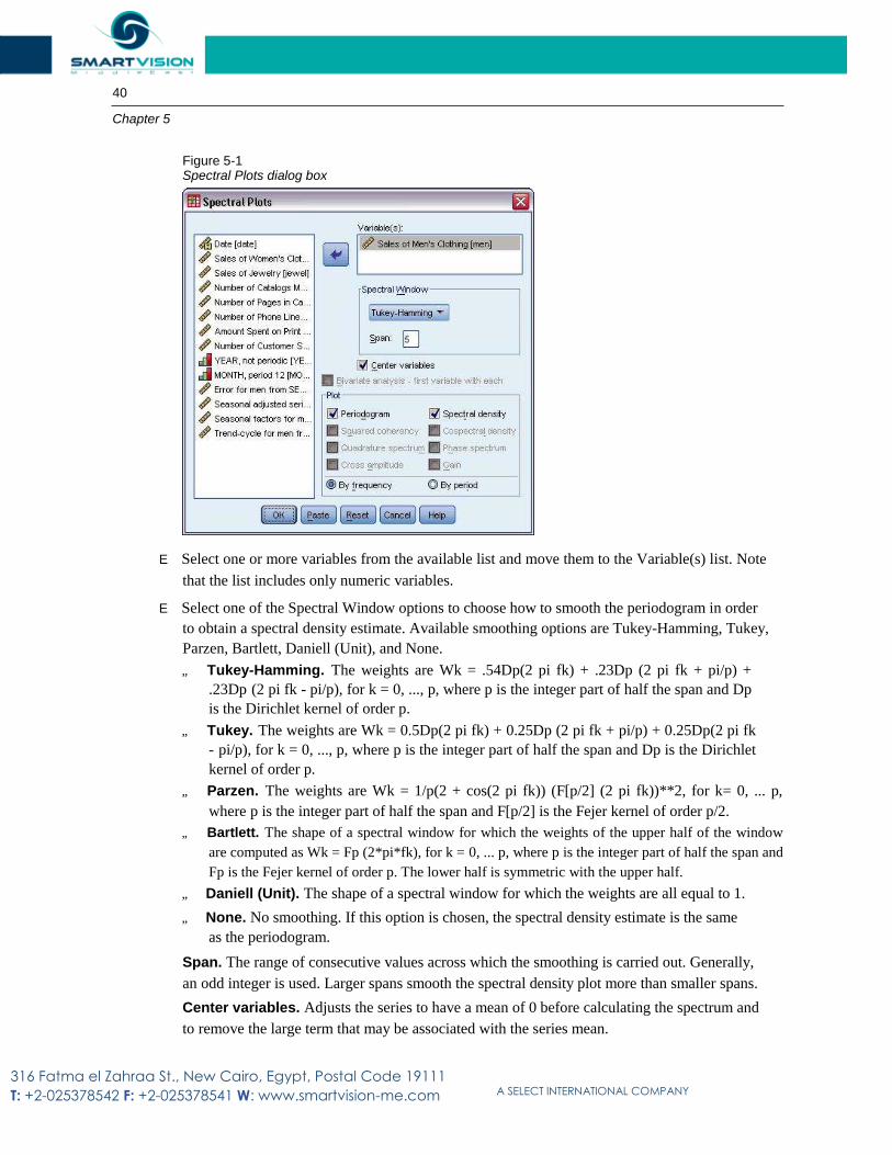
316 Fatma el Zahraa St., New Cairo, Egypt, Postal Code 19111
T: +2-025378542 F: +2-025378541 W: www.smartvision-me.com A SELECT INTERNATIONAL COMPANY
40 Chapter 5
Figure 5-1 Spectral Plots dialog box
E Select one or more variables from the available list and move them to the Variable(s) list. Note
that the list includes only numeric variables.
E Select one of the Spectral Window options to choose how to smooth the periodogram in order
to obtain a spectral density estimate. Available smoothing options are Tukey-Hamming, Tukey,
Parzen, Bartlett, Daniell (Unit), and None. „ Tukey-Hamming. The weights are Wk = .54Dp(2 pi fk) + .23Dp (2 pi fk + pi/p) +
.23Dp (2 pi fk - pi/p), for k = 0, ..., p, where p is the integer part of half the span and Dp
is the Dirichlet kernel of order p.
„ Tukey. The weights are Wk = 0.5Dp(2 pi fk) + 0.25Dp (2 pi fk + pi/p) + 0.25Dp(2 pi fk
- pi/p), for k = 0, ..., p, where p is the integer part of half the span and Dp is the Dirichlet
kernel of order p.
„ Parzen. The weights are Wk = 1/p(2 + cos(2 pi fk)) (F[p/2] (2 pi fk))**2, for k= 0, ... p,
where p is the integer part of half the span and F[p/2] is the Fejer kernel of order p/2.
„ Bartlett. The shape of a spectral window for which the weights of the upper half of the window
are computed as Wk = Fp (2*pi*fk), for k = 0, ... p, where p is the integer part of half the span and
Fp is the Fejer kernel of order p. The lower half is symmetric with the upper half.
„ Daniell (Unit). The shape of a spectral window for which the weights are all equal to 1.
„ None. No smoothing. If this option is chosen, the spectral density estimate is the same as the periodogram.
Span. The range of consecutive values across which the smoothing is carried out. Generally,
an odd integer is used. Larger spans smooth the spectral density plot more than smaller spans.
Center variables. Adjusts the series to have a mean of 0 before calculating the spectrum and
to remove the large term that may be associated with the series mean.

316 Fatma el Zahraa St., New Cairo, Egypt, Postal Code 19111
T: +2-025378542 F: +2-025378541 W: www.smartvision-me.com A SELECT INTERNATIONAL COMPANY
41
Spectral Plots
Bivariate analysis—first variable with each. If you have selected two or more variables,
you can select this option to request bivariate spectral analyses. „ The first variable in the Variable(s) list is treated as the independent variable, and all
remaining variables are treated as dependent variables.
„ Each series after the first is analyzed with the first series independently of other series
named. Univariate analyses of each series are also performed.
Plot. Periodogram and spectral density are available for both univariate and bivariate analyses.
All other choices are available only for bivariate analyses. „ Periodogram. Unsmoothed plot of spectral amplitude (plotted on a logarithmic scale)
against either frequency or period. Low-frequency variation characterizes a smooth series.
Variation spread evenly across all frequencies indicates "white noise."
„ Squared coherency. The product of the gains of the two series.
„ Quadrature spectrum. The imaginary part of the cross-periodogram, which is a measure
of the correlation of the out-of-phase frequency components of two time series. The
components are out of phase by pi/2 radians.
„ Cross amplitude. The square root of the sum of the squared cospectral density and the
squared quadrature spectrum.
„ Spectral density. A periodogram that has been smoothed to remove irregular variation.
„ Cospectral density. The real part of the cross-periodogram, which is a measure of
the correlation of the in-phase frequency components of two time series.
„ Phase spectrum. A measure of the extent to which each frequency component of one
series leads or lags the other.
„ Gain. The quotient of dividing the cross amplitude by the spectral density for one of the
series. Each of the two series has its own gain value.
By frequency. All plots are produced by frequency, ranging from frequency 0 (the constant or
mean term) to frequency 0.5 (the term for a cycle of two observations).
By period. All plots are produced by period, ranging from 2 (the term for a cycle of two
observations) to a period equal to the number of observations (the constant or mean term). Period
is displayed on a logarithmic scale.
SPECTRA Command Additional Features
The command syntax language also allows you to:
„ Save computed spectral analysis variables to the active dataset for later use.
„ Specify custom weights for the spectral window.
„ Produce plots by both frequency and period.
„ Print a complete listing of each value shown in the plot.
See the Command Syntax Reference for complete syntax information.

316 Fatma el Zahraa St., New Cairo, Egypt, Postal Code 19111
T: +2-025378542 F: +2-025378541 W: www.smartvision-me.com A SELECT INTERNATIONAL COMPANY
Part II:
Examples

316 Fatma el Zahraa St., New Cairo, Egypt, Postal Code 19111
T: +2-025378542 F: +2-025378541 W: www.smartvision-me.com A SELECT INTERNATIONAL COMPANY
Chapter
6
Bulk Forecasting with the Expert Modeler
An analyst for a national broadband provider is required to produce forecasts of user subscriptions in
order to predict utilization of bandwidth. Forecasts are needed for each of the 85 local markets that
make up the national subscriber base. Monthly historical data is collected in broadband_1.sav. For
more information, see the topic Sample Files in Appendix D in IBM SPSS Forecasting 19. In this example, you will use the Expert Modeler to produce forecasts for the next three months for
each of the 85 local markets, saving the generated models to an external XML file. Once you are
finished, you might want to work through the next example, Bulk Reforecasting by Applying Saved
Models in Chapter 7 on p. 54, which applies the saved models to an updated dataset in order to extend
the forecasts by another three months without having to rebuild the models.
Examining Your Data
It is always a good idea to have a feel for the nature of your data before building a model. Does
the data exhibit seasonal variations? Although the Expert Modeler will automatically find the
best seasonal or non-seasonal model for each series, you can often obtain faster results by
limiting the search to non-seasonal models when seasonality is not present in your data. Without
examining the data for each of the 85 local markets, we can get a rough picture by plotting the
total number of subscribers over all markets.
E From the menus choose:
Analyze > Forecasting > Sequence Charts...
© Copyright SPSS Inc. 1989, 2010 43

316 Fatma el Zahraa St., New Cairo, Egypt, Postal Code 19111
T: +2-025378542 F: +2-025378541 W: www.smartvision-me.com A SELECT INTERNATIONAL COMPANY
44 Chapter 6
Figure 6-1 Sequence Charts dialog box
E Select Total Number of Subscribers and move it into the Variables list.
E Select Date and move it into the Time Axis Labels box.
E Click OK.
Figure 6-2 Total number of broadband subscribers across all markets

316 Fatma el Zahraa St., New Cairo, Egypt, Postal Code 19111
T: +2-025378542 F: +2-025378541 W: www.smartvision-me.com A SELECT INTERNATIONAL COMPANY
45
Bulk Forecasting with the Expert Modeler
The series exhibits a very smooth upward trend with no hint of seasonal variations. There might
be individual series with seasonality, but it appears that seasonality is not a prominent feature of
the data in general. Of course you should inspect each of the series before ruling out seasonal
models. You can then separate out series exhibiting seasonality and model them separately. In the
present case, inspection of the 85 series would show that none exhibit seasonality.
Running the Analysis
To use the Expert Modeler:
E From the menus choose:
Analyze > Forecasting > Create Models...
Figure 6-3 Time Series Modeler dialog box
E Select Subscribers for Market 1 through Subscribers for Market 85 for dependent variables.
E Verify that Expert Modeler is selected in the Method drop-down list. The Expert Modeler will
automatically find the best-fitting model for each of the dependent variable series.

316 Fatma el Zahraa St., New Cairo, Egypt, Postal Code 19111
T: +2-025378542 F: +2-025378541 W: www.smartvision-me.com A SELECT INTERNATIONAL COMPANY
46 Chapter 6
The set of cases used to estimate the model is referred to as the estimation period. By default,
it includes all of the cases in the active dataset. You can set the estimation period by selecting
Based on time or case range in the Select Cases dialog box. For this example, we will stick with
the default. Notice also that the default forecast period starts after the end of the estimation period and
goes through to the last case in the active dataset. If you are forecasting beyond the last case, you
will need to extend the forecast period. This is done from the Options tab as you will see later on
in this example.
E Click Criteria.
Figure 6-4 Expert Modeler Criteria dialog box, Model tab
E Deselect Expert Modeler considers seasonal models in the Model Type group.
Although the data is monthly and the current periodicity is 12, we have seen that the data does
not exhibit any seasonality, so there is no need to consider seasonal models. This reduces the
space of models searched by the Expert Modeler and can significantly reduce computing time.
E Click Continue.
E Click the Options tab on the Time Series Modeler dialog box.
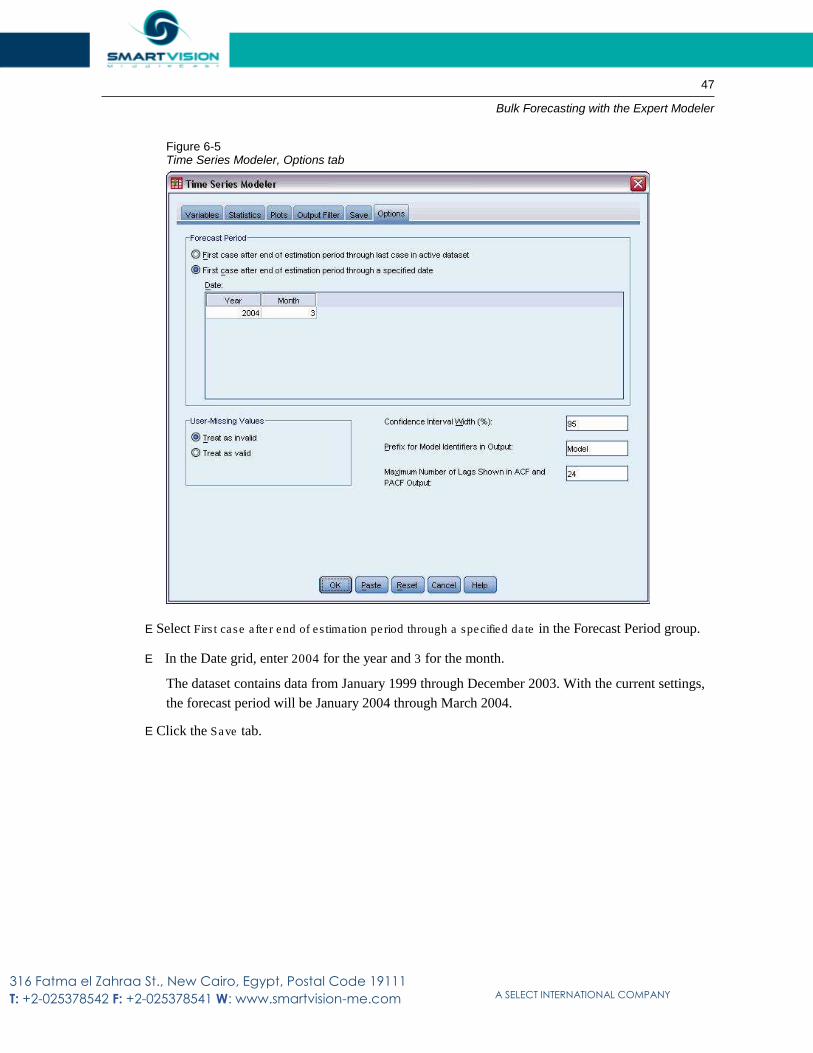
316 Fatma el Zahraa St., New Cairo, Egypt, Postal Code 19111
T: +2-025378542 F: +2-025378541 W: www.smartvision-me.com A SELECT INTERNATIONAL COMPANY
47
Bulk Forecasting with the Expert Modeler
Figure 6-5 Time Series Modeler, Options tab
E Select First case after end of estimation period through a specified date in the Forecast Period group. E In the Date grid, enter 2004 for the year and 3 for the month.
The dataset contains data from January 1999 through December 2003. With the current settings,
the forecast period will be January 2004 through March 2004. E Click the Save tab.
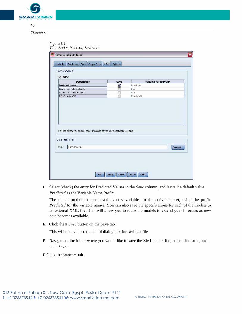
316 Fatma el Zahraa St., New Cairo, Egypt, Postal Code 19111
T: +2-025378542 F: +2-025378541 W: www.smartvision-me.com A SELECT INTERNATIONAL COMPANY
48 Chapter 6
Figure 6-6 Time Series Modeler, Save tab
E Select (check) the entry for Predicted Values in the Save column, and leave the default value
Predicted as the Variable Name Prefix.
The model predictions are saved as new variables in the active dataset, using the prefix
Predicted for the variable names. You can also save the specifications for each of the models to
an external XML file. This will allow you to reuse the models to extend your forecasts as new
data becomes available.
E Click the Browse button on the Save tab.
This will take you to a standard dialog box for saving a file.
E Navigate to the folder where you would like to save the XML model file, enter a filename, and
click Save. E Click the Statistics tab.

316 Fatma el Zahraa St., New Cairo, Egypt, Postal Code 19111
T: +2-025378542 F: +2-025378541 W: www.smartvision-me.com A SELECT INTERNATIONAL COMPANY
49
Bulk Forecasting with the Expert Modeler
Figure 6-7 Time Series Modeler, Statistics tab
E Select Display forecasts.
This option produces a table of forecasted values for each dependent variable series and provides
another option—other than saving the predictions as new variables—for obtaining these values.
The default selection of Goodness of fit (in the Statistics for Comparing Models group) produces
a table with fit statistics—such as R-squared, mean absolute percentage error, and normalized
BIC—calculated across all of the models. It provides a concise summary of how well the models
fit the data. E Click the Plots tab.

316 Fatma el Zahraa St., New Cairo, Egypt, Postal Code 19111
T: +2-025378542 F: +2-025378541 W: www.smartvision-me.com A SELECT INTERNATIONAL COMPANY
50 Chapter 6
Figure 6-8 Time Series Modeler, Plots tab
E Deselect Series in the Plots for Individual Models group.
This suppresses the generation of series plots for each of the models. In this example, we are
more interested in saving the forecasts as new variables than generating plots of the forecasts.
The Plots for Comparing Models group provides several plots (in the form of histograms)
of fit statistics calculated across all models.
E Select Mean absolute percentage error and Maximum absolute percentage error in the Plots for
Comparing Models group.
Absolute percentage error is a measure of how much a dependent series varies from its model-
predicted level. By examining the mean and maximum across all models, you can get an
indication of the uncertainty in your predictions. And looking at summary plots of percentage
errors, rather than absolute errors, is advisable since the dependent series represent subscriber
numbers for markets of varying sizes. E Click OK in the Time Series Modeler dialog box.
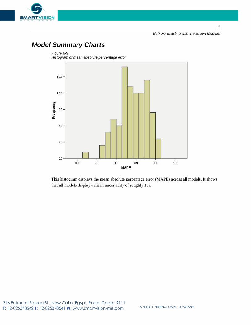
316 Fatma el Zahraa St., New Cairo, Egypt, Postal Code 19111
T: +2-025378542 F: +2-025378541 W: www.smartvision-me.com A SELECT INTERNATIONAL COMPANY
51
Bulk Forecasting with the Expert Modeler
Model Summary Charts
Figure 6-9 Histogram of mean absolute percentage error
This histogram displays the mean absolute percentage error (MAPE) across all models. It shows
that all models display a mean uncertainty of roughly 1%.

316 Fatma el Zahraa St., New Cairo, Egypt, Postal Code 19111
T: +2-025378542 F: +2-025378541 W: www.smartvision-me.com A SELECT INTERNATIONAL COMPANY
52 Chapter 6
Figure 6-10 Histogram of maximum absolute percentage error
This histogram displays the maximum absolute percentage error (MaxAPE) across all models
and is useful for imagining a worst-case scenario for your forecasts. It shows that the largest
percentage error for each model falls in the range of 1 to 5%. Do these values represent an
acceptable amount of uncertainty? This is a situation in which your business sense comes into
play because acceptable risk will change from problem to problem.
Model Predictions
Figure 6-11 New variables containing model predictions
The Data Editor shows the new variables containing the model predictions. Although only two
are shown here, there are 85 new variables, one for each of the 85 dependent series. The variable
names consist of the default prefix Predicted, followed by the name of the associated dependent
variable (for example, Market_1), followed by a model identifier (for example, Model_1).

316 Fatma el Zahraa St., New Cairo, Egypt, Postal Code 19111
T: +2-025378542 F: +2-025378541 W: www.smartvision-me.com A SELECT INTERNATIONAL COMPANY
53
Bulk Forecasting with the Expert Modeler
Three new cases, containing the forecasts for January 2004 through March 2004, have been
added to the dataset, along with automatically generated date labels. Each of the new variables
contains the model predictions for the estimation period (January 1999 through December 2003),
allowing you to see how well the model fits the known values.
Figure 6-12 Forecast table
You also chose to create a table with the forecasted values. The table consists of the predicted values
in the forecast period but—unlike the new variables containing the model predictions—does not
include predicted values in the estimation period. The results are organized by model and identified by
the model name, which consists of the name (or label) of the associated dependent variable followed
by a model identifier—just like the names of the new variables containing the model predictions. The table also includes the upper confidence limits (UCL) and lower
confidence limits (LCL) for the forecasted values (95% by default). You have now seen two approaches for obtaining the forecasted values: saving the forecasts
as new variables in the active dataset and creating a forecast table. With either approach, you will have a number of options available for exporting your forecasts (for example, into an
Excel spreadsheet).
Summary
You have learned how to use the Expert Modeler to produce forecasts for multiple series, and
you have saved the resulting models to an external XML file. In the next example, you will learn
how to extend your forecasts as new data becomes available—without having to rebuild your
models—by using the Apply Time Series Models procedure.
316 Fatma el Zahraa St., New Cairo, Egypt, Postal Code 19111
T: +2-025378542 F: +2-025378541 W: www.smartvision-me.com A SELECT INTERNATIONAL COMPANY
Chapter
7
Bulk Reforecasting by Applying Saved Models
You have used the Time Series Modeler to create models for your time series data and to
produce initial forecasts based on available data. You plan to reuse these models to extend your
forecasts as more current data becomes available, so you saved the models to an external file.
You are now ready to apply the saved models. This example is a natural extension of the previous one, Bulk Forecasting with the Expert
Modeler in Chapter 6 on p. 43, but can also be used independently. In this scenario, you are an
analyst for a national broadband provider who is required to produce monthly forecasts of user
subscriptions for each of 85 local markets. You have already used the Expert Modeler to create
models and to forecast three months into the future. Your data warehouse has been refreshed
with actual data for the original forecast period, so you would like to use that data to extend the
forecast horizon by another three months. The updated monthly historical data is collected in broadband_2.sav, and the saved models
are in broadband_models.xml. For more information, see the topic Sample Files in Appendix D
in IBM SPSS Forecasting 19. Of course, if you worked through the previous example and saved
your own model file, you can use that one instead of broadband_models.xml.
Running the Analysis
To apply models:
E From the menus choose:
Analyze > Forecasting > Apply Models...
© Copyright SPSS Inc. 1989, 2010 54
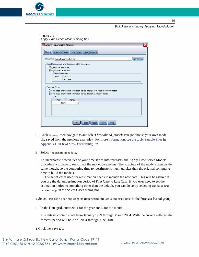
316 Fatma el Zahraa St., New Cairo, Egypt, Postal Code 19111
T: +2-025378542 F: +2-025378541 W: www.smartvision-me.com A SELECT INTERNATIONAL COMPANY
55
Bulk Reforecasting by Applying Saved Models
Figure 7-1 Apply Time Series Models dialog box
E Click Browse, then navigate to and select broadband_models.xml (or choose your own model
file saved from the previous example). For more information, see the topic Sample Files in
Appendix D in IBM SPSS Forecasting 19.
E Select Reestimate from data.
To incorporate new values of your time series into forecasts, the Apply Time Series Models
procedure will have to reestimate the model parameters. The structure of the models remains the
same though, so the computing time to reestimate is much quicker than the original computing
time to build the models.
The set of cases used for reestimation needs to include the new data. This will be assured if
you use the default estimation period of First Case to Last Case. If you ever need to set the
estimation period to something other than the default, you can do so by selecting Based on time
or case range in the Select Cases dialog box.
E Select First case after end of estimation period through a specified date in the Forecast Period group.
E In the Date grid, enter 2004 for the year and 6 for the month.
The dataset contains data from January 1999 through March 2004. With the current settings, the
forecast period will be April 2004 through June 2004.
E Click the Save tab.
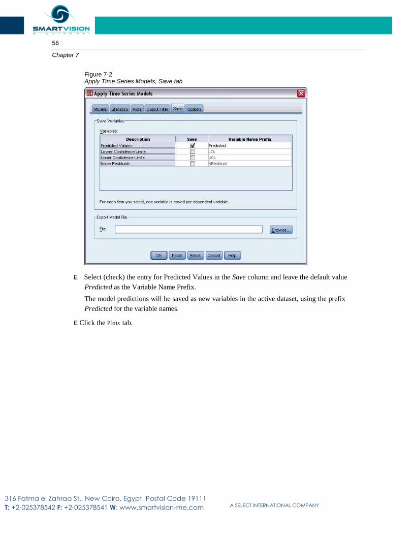
316 Fatma el Zahraa St., New Cairo, Egypt, Postal Code 19111
T: +2-025378542 F: +2-025378541 W: www.smartvision-me.com A SELECT INTERNATIONAL COMPANY
56 Chapter 7
Figure 7-2 Apply Time Series Models, Save tab
E Select (check) the entry for Predicted Values in the Save column and leave the default value
Predicted as the Variable Name Prefix.
The model predictions will be saved as new variables in the active dataset, using the prefix
Predicted for the variable names.
E Click the Plots tab.
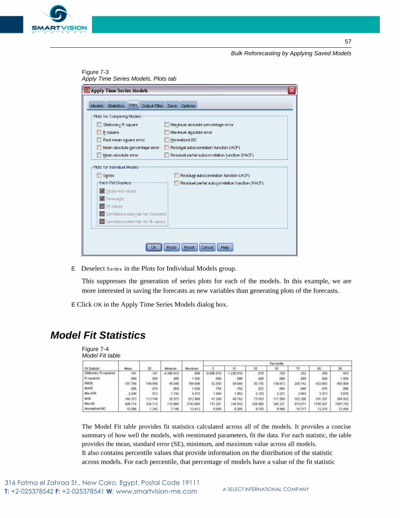
316 Fatma el Zahraa St., New Cairo, Egypt, Postal Code 19111
T: +2-025378542 F: +2-025378541 W: www.smartvision-me.com A SELECT INTERNATIONAL COMPANY
57
Bulk Reforecasting by Applying Saved Models
Figure 7-3 Apply Time Series Models, Plots tab
E Deselect Series in the Plots for Individual Models group.
This suppresses the generation of series plots for each of the models. In this example, we are
more interested in saving the forecasts as new variables than generating plots of the forecasts.
E Click OK in the Apply Time Series Models dialog box.
Model Fit Statistics
Figure 7-4 Model Fit table
The Model Fit table provides fit statistics calculated across all of the models. It provides a concise
summary of how well the models, with reestimated parameters, fit the data. For each statistic, the table
provides the mean, standard error (SE), minimum, and maximum value across all models. It also contains percentile values that provide information on the distribution of the statistic
across models. For each percentile, that percentage of models have a value of the fit statistic
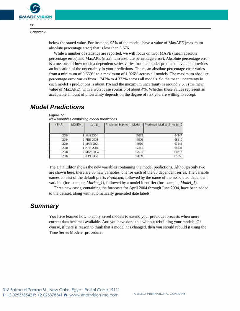
316 Fatma el Zahraa St., New Cairo, Egypt, Postal Code 19111
T: +2-025378542 F: +2-025378541 W: www.smartvision-me.com A SELECT INTERNATIONAL COMPANY
58 Chapter 7
below the stated value. For instance, 95% of the models have a value of MaxAPE (maximum
absolute percentage error) that is less than 3.676. While a number of statistics are reported, we will focus on two: MAPE (mean absolute
percentage error) and MaxAPE (maximum absolute percentage error). Absolute percentage error
is a measure of how much a dependent series varies from its model-predicted level and provides
an indication of the uncertainty in your predictions. The mean absolute percentage error varies
from a minimum of 0.669% to a maximum of 1.026% across all models. The maximum absolute
percentage error varies from 1.742% to 4.373% across all models. So the mean uncertainty in
each model’s predictions is about 1% and the maximum uncertainty is around 2.5% (the mean
value of MaxAPE), with a worst case scenario of about 4%. Whether these values represent an
acceptable amount of uncertainty depends on the degree of risk you are willing to accept.
Model Predictions
Figure 7-5 New variables containing model predictions
The Data Editor shows the new variables containing the model predictions. Although only two
are shown here, there are 85 new variables, one for each of the 85 dependent series. The variable
names consist of the default prefix Predicted, followed by the name of the associated dependent
variable (for example, Market_1), followed by a model identifier (for example, Model_1). Three new cases, containing the forecasts for April 2004 through June 2004, have been added
to the dataset, along with automatically generated date labels.
Summary
You have learned how to apply saved models to extend your previous forecasts when more
current data becomes available. And you have done this without rebuilding your models. Of
course, if there is reason to think that a model has changed, then you should rebuild it using the
Time Series Modeler procedure.

316 Fatma el Zahraa St., New Cairo, Egypt, Postal Code 19111
T: +2-025378542 F: +2-025378541 W: www.smartvision-me.com A SELECT INTERNATIONAL COMPANY
Chapter
8
Using the Expert Modeler to Determine Significant Predictors
A catalog company, interested in developing a forecasting model, has collected data on monthly sales
of men’s clothing along with several series that might be used to explain some of the variation in sales.
Possible predictors include the number of catalogs mailed, the number of pages in the catalog, the
number of phone lines open for ordering, the amount spent on print advertising, and the number of
customer service representatives. Are any of these predictors useful for forecasting? In this example, you will use the Expert Modeler with all of the candidate predictors to find
the best model. Since the Expert Modeler only selects those predictors that have a statistically
significant relationship with the dependent series, you will know which predictors are useful, and
you will have a model for forecasting with them. Once you are finished, you might want to work
through the next example, Experimenting with Predictors by Applying Saved Models in Chapter
9 on p. 70, which investigates the effect on sales of different predictor scenarios using the model
built in this example. The data for the current example is collected in catalog_seasfac.sav. For more information,
see the topic Sample Files in Appendix D in IBM SPSS Forecasting 19.
Plotting Your Data
It is always a good idea to plot your data, especially if you are only working with one series:
E From the menus choose:
Analyze > Forecasting > Sequence Charts...
© Copyright SPSS Inc. 1989, 2010 59

316 Fatma el Zahraa St., New Cairo, Egypt, Postal Code 19111
T: +2-025378542 F: +2-025378541 W: www.smartvision-me.com A SELECT INTERNATIONAL COMPANY
60 Chapter 8
Figure 8-1 Sequence Charts dialog box
E Select Sales of Men’s Clothing and move it into the Variables list.
E Select Date and move it into the Time Axis Labels box.
E Click OK.

316 Fatma el Zahraa St., New Cairo, Egypt, Postal Code 19111
T: +2-025378542 F: +2-025378541 W: www.smartvision-me.com A SELECT INTERNATIONAL COMPANY
61
Using the Expert Modeler to Determine Significant Predictors
Figure 8-2 Sales of men’s clothing (in U.S. dollars)
The series exhibits numerous peaks, many of which appear to be equally spaced, as well as a
clear upward trend. The equally spaced peaks suggests the presence of a periodic component to
the time series. Given the seasonal nature of sales, with highs typically occurring during the
holiday season, you should not be surprised to find an annual seasonal component to the data. There are also peaks that do not appear to be part of the seasonal pattern and which represent
significant deviations from the neighboring data points. These points may be outliers, which can
and should be addressed by the Expert Modeler.
Running the Analysis
To use the Expert Modeler:
E From the menus choose:
Analyze > Forecasting > Create Models...
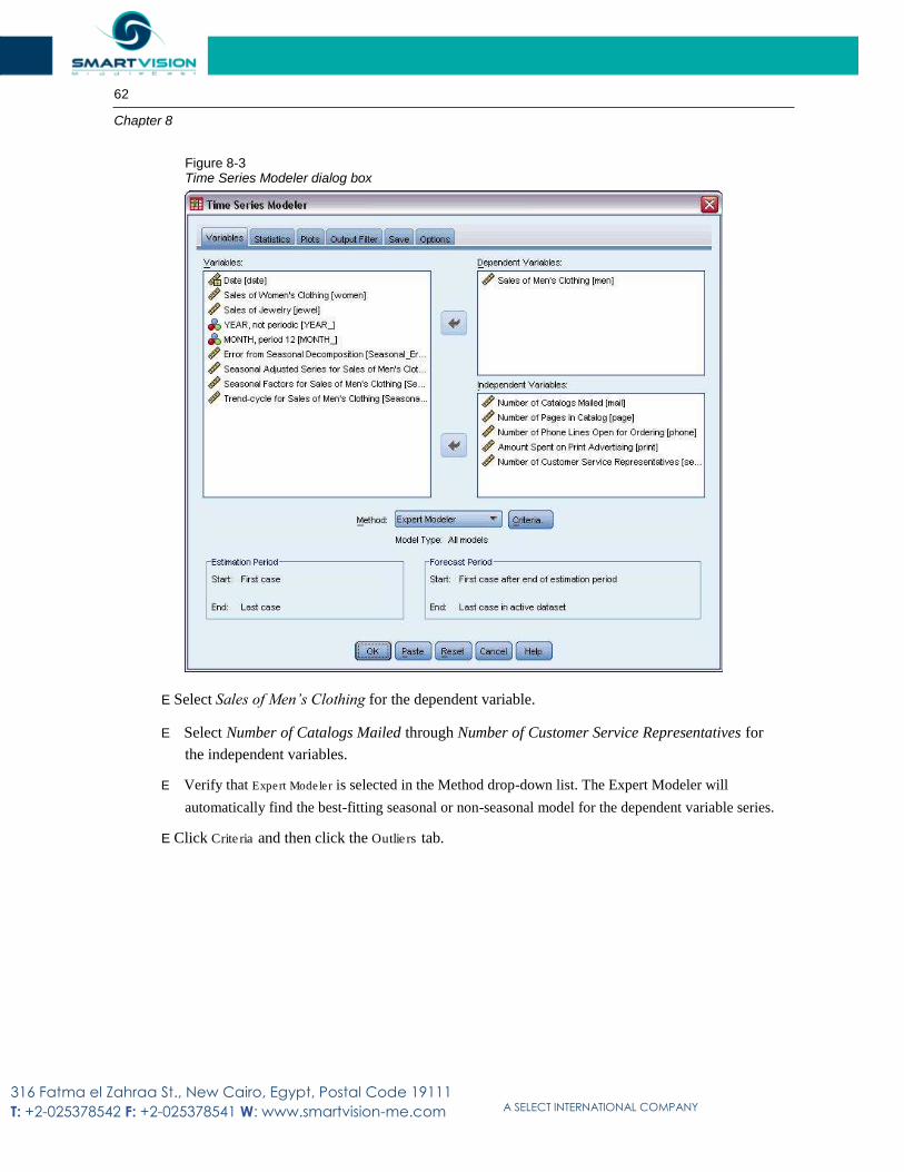
316 Fatma el Zahraa St., New Cairo, Egypt, Postal Code 19111
T: +2-025378542 F: +2-025378541 W: www.smartvision-me.com A SELECT INTERNATIONAL COMPANY
62 Chapter 8
Figure 8-3 Time Series Modeler dialog box
E Select Sales of Men’s Clothing for the dependent variable.
E Select Number of Catalogs Mailed through Number of Customer Service Representatives for
the independent variables.
E Verify that Expert Modeler is selected in the Method drop-down list. The Expert Modeler will
automatically find the best-fitting seasonal or non-seasonal model for the dependent variable series.
E Click Criteria and then click the Outliers tab.

316 Fatma el Zahraa St., New Cairo, Egypt, Postal Code 19111
T: +2-025378542 F: +2-025378541 W: www.smartvision-me.com A SELECT INTERNATIONAL COMPANY
63
Using the Expert Modeler to Determine Significant Predictors
Figure 8-4 Expert Modeler Criteria dialog box, Outliers tab
E Select Detect outliers automatically and leave the default selections for the types of outliers to detect.
Our visual inspection of the data suggested that there may be outliers. With the current choices,
the Expert Modeler will search for the most common outlier types and incorporate any outliers
into the final model. Outlier detection can add significantly to the computing time needed by the
Expert Modeler, so it is a feature that should be used with some discretion, particularly when
modeling many series at once. By default, outliers are not detected. E Click Continue. E Click the Save tab on the Time Series Modeler dialog box.

316 Fatma el Zahraa St., New Cairo, Egypt, Postal Code 19111
T: +2-025378542 F: +2-025378541 W: www.smartvision-me.com A SELECT INTERNATIONAL COMPANY
64 Chapter 8
Figure 8-5 Time Series Modeler, Save tab
You will want to save the estimated model to an external XML file so that you can experiment
with different values of the predictors—using the Apply Time Series Models procedure—
without having to rebuild the model.
E Click the Browse button on the Save tab.
This will take you to a standard dialog box for saving a file.
E Navigate to the folder where you would like to save the XML model file, enter a filename, and
click Save.
E Click the Statistics tab.

316 Fatma el Zahraa St., New Cairo, Egypt, Postal Code 19111
T: +2-025378542 F: +2-025378541 W: www.smartvision-me.com A SELECT INTERNATIONAL COMPANY
65
Using the Expert Modeler to Determine Significant Predictors
Figure 8-6 Time Series Modeler, Statistics tab
E Select Parameter estimates.
This option produces a table displaying all of the parameters, including the significant
predictors, for the model chosen by the Expert Modeler. E Click the Plots tab.

316 Fatma el Zahraa St., New Cairo, Egypt, Postal Code 19111
T: +2-025378542 F: +2-025378541 W: www.smartvision-me.com A SELECT INTERNATIONAL COMPANY
66 Chapter 8
Figure 8-7 Time Series Modeler, Plots tab
E Deselect Forecasts.
In the current example, we are only interested in determining the significant predictors and
building a model. We will not be doing any forecasting.
E Select Fit values.
This option displays the predicted values in the period used to estimate the model. This period
is referred to as the estimation period, and it includes all cases in the active dataset for this
example. These values provide an indication of how well the model fits the observed values, so
they are referred to as fit values. The resulting plot will consist of both the observed values and
the fit values.
E Click OK in the Time Series Modeler dialog box.

316 Fatma el Zahraa St., New Cairo, Egypt, Postal Code 19111
T: +2-025378542 F: +2-025378541 W: www.smartvision-me.com A SELECT INTERNATIONAL COMPANY
67
Using the Expert Modeler to Determine Significant Predictors
Series Plot
Figure 8-8 Predicted and observed values
The predicted values show good agreement with the observed values, indicating that the model
has satisfactory predictive ability. Notice how well the model predicts the seasonal peaks. And
it does a good job of capturing the upward trend of the data.
Model Description Table
Figure 8-9 Model Description table
The model description table contains an entry for each estimated model and includes both a
model identifier and the model type. The model identifier consists of the name (or label) of the
associated dependent variable and a system-assigned name. In the current example, the dependent
variable is Sales of Men’s Clothing and the system-assigned name is Model_1. The Time Series Modeler supports both exponential smoothing and ARIMA models.
Exponential smoothing model types are listed by their commonly used names such as Holt
and Winters’ Additive. ARIMA model types are listed using the standard notation of ARIMA(p,d,q)(P,D,Q), where p is the order of autoregression, d is the order of differencing (or
integration), and q is the order of moving-average, and (P,D,Q) are their seasonal counterparts.

316 Fatma el Zahraa St., New Cairo, Egypt, Postal Code 19111
T: +2-025378542 F: +2-025378541 W: www.smartvision-me.com A SELECT INTERNATIONAL COMPANY
68 Chapter 8
The Expert Modeler has determined that sales of men’s clothing is best described by a seasonal
ARIMA model with one order of differencing. The seasonal nature of the model accounts for the
seasonal peaks that we saw in the series plot, and the single order of differencing reflects the upward trend that was evident in the data.
Model Statistics Table
Figure 8-10 Model Statistics table
The model statistics table provides summary information and goodness-of-fit statistics for each
estimated model. Results for each model are labeled with the model identifier provided in the
model description table. First, notice that the model contains two predictors out of the five
candidate predictors that you originally specified. So it appears that the Expert Modeler has
identified two independent variables that may prove useful for forecasting. Although the Time Series Modeler offers a number of different goodness-of-fit statistics, we
opted only for the stationary R-squared value. This statistic provides an estimate of the proportion
of the total variation in the series that is explained by the model and is preferable to ordinary R-
squared when there is a trend or seasonal pattern, as is the case here. Larger values of stationary
R-squared (up to a maximum value of 1) indicate better fit. A value of 0.948 means that the
model does an excellent job of explaining the observed variation in the series. The Ljung-Box statistic, also known as the modified Box-Pierce statistic, provides an
indication of whether the model is correctly specified. A significance value less than 0.05 implies
that there is structure in the observed series which is not accounted for by the model. The value of
0.984 shown here is not significant, so we can be confident that the model is correctly specified. The Expert Modeler detected nine points that were considered to be outliers. Each of these points
has been modeled appropriately, so there is no need for you to remove them from the series.
ARIMA Model Parameters Table
Figure 8-11 ARIMA Model Parameters table
The ARIMA model parameters table displays values for all of the parameters in the model, with
an entry for each estimated model labeled by the model identifier. For our purposes, it will list all
of the variables in the model, including the dependent variable and any independent variables that
the Expert Modeler determined were significant. We already know from the model statistics table

316 Fatma el Zahraa St., New Cairo, Egypt, Postal Code 19111
T: +2-025378542 F: +2-025378541 W: www.smartvision-me.com A SELECT INTERNATIONAL COMPANY
69
Using the Expert Modeler to Determine Significant Predictors
that there are two significant predictors. The model parameters table shows us that they are the Number of Catalogs Mailed and the Number of Phone Lines Open for Ordering.
Summary
You have learned how to use the Expert Modeler to build a model and identify significant
predictors, and you have saved the resulting model to an external file. You are now in a position
to use the Apply Time Series Models procedure to experiment with alternative scenarios for the
predictor series and see how the alternatives affect the sales forecasts.
316 Fatma el Zahraa St., New Cairo, Egypt, Postal Code 19111
T: +2-025378542 F: +2-025378541 W: www.smartvision-me.com A SELECT INTERNATIONAL COMPANY
Chapter
9
Experimenting with Predictors by Applying Saved Models
You’ve used the Time Series Modeler to create a model for your data and to identify which predictors
may prove useful for forecasting. The predictors represent factors that are within your control, so
you’d like to experiment with their values in the forecast period to see how forecasts of the dependent
variable are affected. This task is easily accomplished with the Apply Time Series Models procedure,
using the model file that is created with the Time Series Modeler procedure. This example is a natural extension of the previous example, Using the Expert Modeler
to Determine Significant Predictors in Chapter 8 on p. 59, but this example can also be used independently. The scenario involves a catalog company that has collected data about monthly
sales of men’s clothing from January 1989 through December 1998, along with several series
that are thought to be potentially useful as predictors of future sales. The Expert Modeler has
determined that only two of the five candidate predictors are significant: the number of catalogs
mailed and the number of phone lines open for ordering. When planning your sales strategy for the next year, you have limited resources to print
catalogs and keep phone lines open for ordering. Your budget for the first three months of 1999
allows for either 2000 additional catalogs or 5 additional phone lines over your initial projections.
Which choice will generate more sales revenue for this three-month period? The data for this example are collected in catalog_seasfac.sav, and catalog_model.xml contains the
model of monthly sales that is built with the Expert Modeler. For more information, see the topic Sample Files in Appendix D in IBM SPSS Forecasting 19 . Of course, if you
worked through the previous example and saved your own model file, you can use that file
instead of catalog_model.xml.
Extending the Predictor Series
When you’re creating forecasts for dependent series with predictors, each predictor series needs to be
extended through the forecast period. Unless you know precisely what the future values of the
predictors will be, you’ll need to estimate them. You can then modify the estimates to test different
predictor scenarios. The initial projections are easily created by using the Expert Modeler.
E From the menus choose:
Analyze > Forecasting > Create Models...
© Copyright SPSS Inc. 1989, 2010 70

316 Fatma el Zahraa St., New Cairo, Egypt, Postal Code 19111
T: +2-025378542 F: +2-025378541 W: www.smartvision-me.com A SELECT INTERNATIONAL COMPANY
71
Experimenting with Predictors by Applying Saved Models
Figure 9-1 Time Series Modeler dialog box
E Select Number of Catalogs Mailed and Number of Phone Lines Open for Ordering for the
dependent variables. E Click the Save tab.

316 Fatma el Zahraa St., New Cairo, Egypt, Postal Code 19111
T: +2-025378542 F: +2-025378541 W: www.smartvision-me.com A SELECT INTERNATIONAL COMPANY
72 Chapter 9
Figure 9-2 Time Series Modeler, Save tab
E In the Save column, select (check) the entry for Predicted Values, and leave the default value
Predicted for the Variable Name Prefix.
E Click the Options tab.
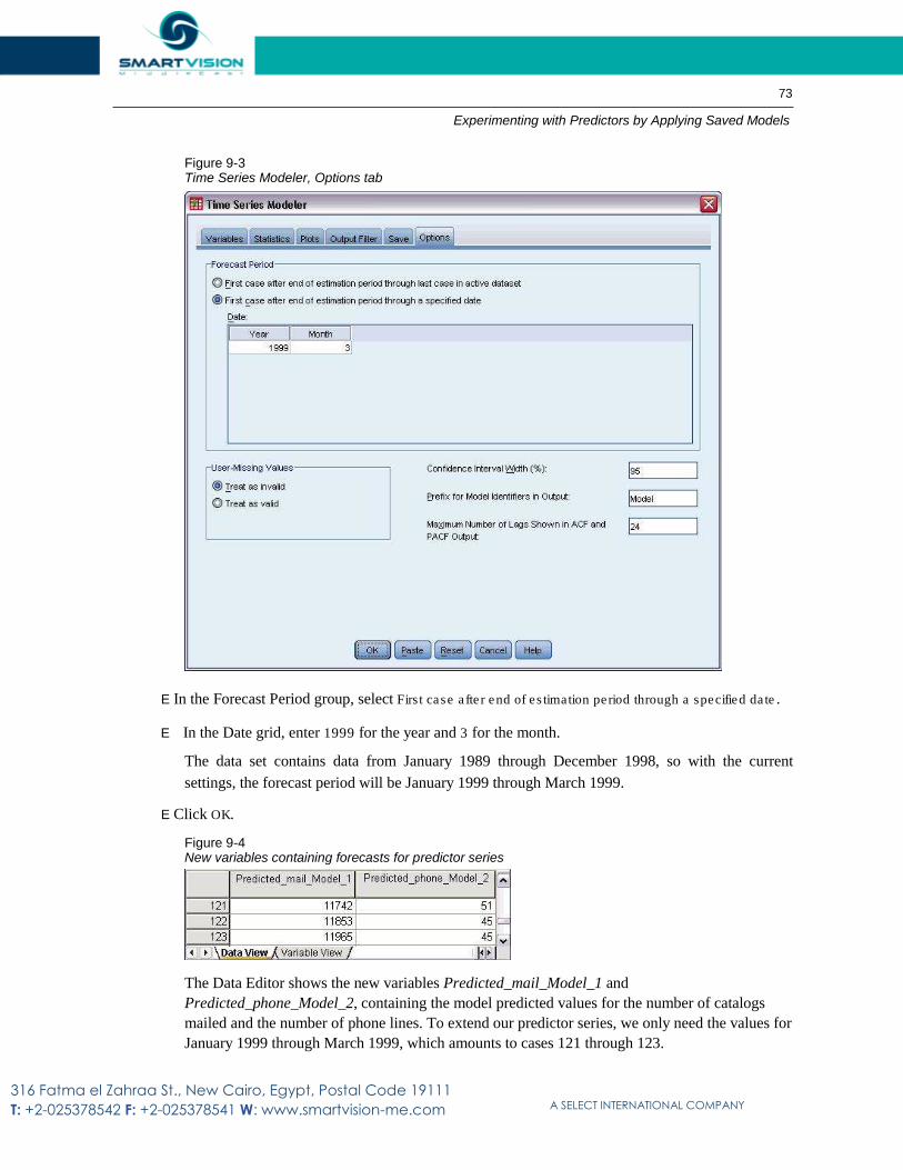
316 Fatma el Zahraa St., New Cairo, Egypt, Postal Code 19111
T: +2-025378542 F: +2-025378541 W: www.smartvision-me.com A SELECT INTERNATIONAL COMPANY
73
Experimenting with Predictors by Applying Saved Models
Figure 9-3 Time Series Modeler, Options tab
E In the Forecast Period group, select First case after end of estimation period through a specified date. E In the Date grid, enter 1999 for the year and 3 for the month.
The data set contains data from January 1989 through December 1998, so with the current
settings, the forecast period will be January 1999 through March 1999. E Click OK.
Figure 9-4 New variables containing forecasts for predictor series
The Data Editor shows the new variables Predicted_mail_Model_1 and
Predicted_phone_Model_2, containing the model predicted values for the number of catalogs
mailed and the number of phone lines. To extend our predictor series, we only need the values for
January 1999 through March 1999, which amounts to cases 121 through 123.

316 Fatma el Zahraa St., New Cairo, Egypt, Postal Code 19111
T: +2-025378542 F: +2-025378541 W: www.smartvision-me.com A SELECT INTERNATIONAL COMPANY
74 Chapter 9
E Copy the values of these three cases from Predicted_mail_Model_1 and append them to the
variable mail.
E Repeat this process for Predicted_phone_Model_2, copying the last three cases and appending
them to the variable phone.
Figure 9-5 Predictor series extended through the forecast period
The predictors have now been extended through the forecast period.
Modifying Predictor Values in the Forecast Period
Testing the two scenarios of mailing more catalogs or providing more phone lines requires
modifying the estimates for the predictors mail or phone, respectively. Because we’re only
modifying the predictor values for three cases (months), it would be easy to enter the new values
directly into the appropriate cells of the Data Editor. For instructional purposes, we’ll use the
Compute Variable dialog box. When you have more than a few values to modify, you’ll
probably find the Compute Variable dialog box more convenient.
E From the menus choose:
Transform > Compute Variable...

316 Fatma el Zahraa St., New Cairo, Egypt, Postal Code 19111
T: +2-025378542 F: +2-025378541 W: www.smartvision-me.com A SELECT INTERNATIONAL COMPANY
75
Experimenting with Predictors by Applying Saved Models
Figure 9-6 Compute Variable dialog box
E Enter mail for the target variable. E In the Numeric Expression text box, enter mail + 2000. E Click If.

316 Fatma el Zahraa St., New Cairo, Egypt, Postal Code 19111
T: +2-025378542 F: +2-025378541 W: www.smartvision-me.com A SELECT INTERNATIONAL COMPANY
76 Chapter 9
Figure 9-7 Compute Variable If Cases dialog box
E Select Include if case satisfies condition.
E In the text box, enter $CASENUM > 120.
This will limit changes to the variable mail to the cases in the forecast period.
E Click Continue.
E Click OK in the Compute Variable dialog box, and click OK when asked whether you want to
change the existing variable.
This results in increasing the values for mail—the number of catalogs mailed—by 2000 for each
of the three months in the forecast period. You’ve now prepared the data to test the first
scenario, and you are ready to run the analysis.
Running the Analysis
E From the menus choose:
Analyze > Forecasting > Apply Models...
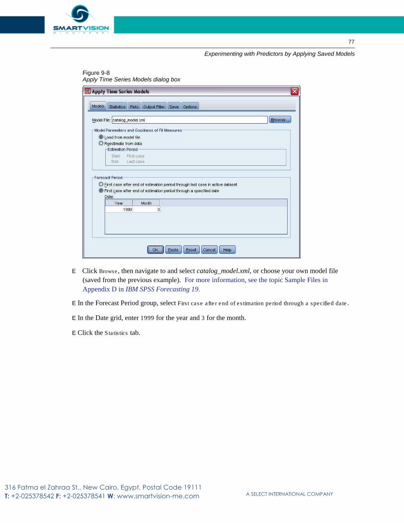
316 Fatma el Zahraa St., New Cairo, Egypt, Postal Code 19111
T: +2-025378542 F: +2-025378541 W: www.smartvision-me.com A SELECT INTERNATIONAL COMPANY
77
Experimenting with Predictors by Applying Saved Models
Figure 9-8 Apply Time Series Models dialog box
E Click Browse, then navigate to and select catalog_model.xml, or choose your own model file
(saved from the previous example). For more information, see the topic Sample Files in
Appendix D in IBM SPSS Forecasting 19. E In the Forecast Period group, select First case after end of estimation period through a specified date. E In the Date grid, enter 1999 for the year and 3 for the month. E Click the Statistics tab.

316 Fatma el Zahraa St., New Cairo, Egypt, Postal Code 19111
T: +2-025378542 F: +2-025378541 W: www.smartvision-me.com A SELECT INTERNATIONAL COMPANY
78 Chapter 9
Figure 9-9 Apply Time Series Models, Statistics tab
E Select Display forecasts.
This results in a table of forecasted values for the dependent variable.
E Click OK in the Apply Time Series Models dialog box.
Figure 9-10 Forecast table
The forecast table contains the predicted values of the dependent series, taking into account the
values of the two predictors mail and phone in the forecast period. The table also includes the
upper confidence limit (UCL) and lower confidence limit (LCL) for the predictions. You’ve produced the sales forecast for the scenario of mailing 2000 more catalogs each month.
You’ll now want to prepare the data for the scenario of increasing the number of phone lines, which
means resetting the variable mail to the original values and increasing the variable phone by 5. You
can reset mail by copying the values of Predicted_mail_Model_1 in the forecast period and pasting
them over the current values of mail in the forecast period. And you can increase the number of phone
lines—by 5 for each month in the forecast period—either directly in the data editor or using the
Compute Variable dialog box, like we did for the number of catalogs.
To run the analysis, reopen the Apply Time Series Models dialog box as follows:
E Click the Dialog Recall toolbar button.

316 Fatma el Zahraa St., New Cairo, Egypt, Postal Code 19111
T: +2-025378542 F: +2-025378541 W: www.smartvision-me.com A SELECT INTERNATIONAL COMPANY
79
Experimenting with Predictors by Applying Saved Models
E Choose Apply Time Series Models.
Figure 9-11 Apply Time Series Models dialog box
E Click OK in the Apply Time Series Models dialog box.
Figure 9-12 Forecast tables for the two scenarios
Displaying the forecast tables for both scenarios shows that, in each of the three forecasted
months, increasing the number of mailed catalogs is expected to generate approximately $1500
more in sales than increasing the number of phone lines that are open for ordering. Based on the
analysis, it seems wise to allocate resources to the mailing of 2000 additional catalogs.

316 Fatma el Zahraa St., New Cairo, Egypt, Postal Code 19111
T: +2-025378542 F: +2-025378541 W: www.smartvision-me.com A SELECT INTERNATIONAL COMPANY
Chapter
10
Seasonal Decomposition
Removing Seasonality from Sales Data
A catalog company is interested in modeling the upward trend of sales of its men’s clothing line
on a set of predictor variables (such as the number of catalogs mailed and the number of phone
lines open for ordering). To this end, the company collected monthly sales of men’s clothing for
a 10-year period. This information is collected in catalog.sav. For more information, see the topic
Sample Files in Appendix D in IBM SPSS Forecasting 19. To perform a trend analysis, you must remove any seasonal variations present in the data. This
task is easily accomplished with the Seasonal Decomposition procedure.
Determining and Setting the Periodicity
The Seasonal Decomposition procedure requires the presence of a periodic date component in the
active dataset—for example, a yearly periodicity of 12 (months), a weekly periodicity of 7
(days), and so on. It’s a good idea to plot your time series first, because viewing a time series plot
often leads to a reasonable guess about the underlying periodicity.
To obtain a plot of men’s clothing sales over time:
E From the menus choose:
Analyze > Forecasting > Sequence Charts... © Copyright SPSS Inc. 1989, 2010 80

316 Fatma el Zahraa St., New Cairo, Egypt, Postal Code 19111
T: +2-025378542 F: +2-025378541 W: www.smartvision-me.com A SELECT INTERNATIONAL COMPANY
81
Seasonal Decomposition
Figure 10-1 Sequence Charts dialog box
E Select Sales of Men’s Clothing and move it into the Variables list.
E Select Date and move it into the Time Axis Labels list.
E Click OK.
Figure 10-2 Sales of men’s clothing (in U.S. dollars)

316 Fatma el Zahraa St., New Cairo, Egypt, Postal Code 19111
T: +2-025378542 F: +2-025378541 W: www.smartvision-me.com A SELECT INTERNATIONAL COMPANY
82 Chapter 10
The series exhibits a number of peaks, but they do not appear to be equally spaced. This output
suggests that if the series has a periodic component, it also has fluctuations that are not
periodic—the typical case for real-time series. Aside from the small-scale fluctuations, the
significant peaks appear to be separated by more than a few months. Given the seasonal nature of
sales, with typical highs during the December holiday season, the time series probably has an
annual periodicity. Also notice that the seasonal variations appear to grow with the upward series
trend, suggesting that the seasonal variations may be proportional to the level of the series, which
implies a multiplicative model rather than an additive model.
Examining the autocorrelations and partial autocorrelations of a time series provides a more
quantitative conclusion about the underlying periodicity.
E From the menus choose:
Analyze > Forecasting > Autocorrelations...
Figure 10-3 Autocorrelations dialog box
E Select Sales of Men’s Clothing and move it into the Variables list.
E Click OK.

316 Fatma el Zahraa St., New Cairo, Egypt, Postal Code 19111
T: +2-025378542 F: +2-025378541 W: www.smartvision-me.com A SELECT INTERNATIONAL COMPANY
83
Seasonal Decomposition
Figure 10-4 Autocorrelation plot for men The autocorrelation function shows a significant peak at a lag of 1 with a long exponential tail—
a typical pattern for time series. The significant peak at a lag of 12 suggests the presence of an
annual seasonal component in the data. Examination of the partial autocorrelation function will
allow a more definitive conclusion. Figure 10-5 Partial autocorrelation plot for men
The significant peak at a lag of 12 in the partial autocorrelation function confirms the presence
of an annual seasonal component in the data.

316 Fatma el Zahraa St., New Cairo, Egypt, Postal Code 19111
T: +2-025378542 F: +2-025378541 W: www.smartvision-me.com A SELECT INTERNATIONAL COMPANY
84 Chapter 10
To set an annual periodicity:
E From the menus choose:
Data > Define Dates...
Figure 10-6 Define Dates dialog box
E Select Years, months in the Cases Are list.
E Enter 1989 for the year and 1 for the month.
E Click OK.
This sets the periodicity to 12 and creates a set of date variables that are designed to work with
Forecasting procedures.
Running the Analysis
To run the Seasonal Decomposition procedure:
E From the menus choose:
Analyze > Forecasting > Seasonal Decomposition...

316 Fatma el Zahraa St., New Cairo, Egypt, Postal Code 19111
T: +2-025378542 F: +2-025378541 W: www.smartvision-me.com A SELECT INTERNATIONAL COMPANY
85
Seasonal Decomposition
Figure 10-7 Seasonal Decomposition dialog box
E Right click anywhere in the source variable list and from the context menu select Display Variable
Names.
E Select men and move it into the Variables list.
E Select Multiplicative in the Model Type group.
E Click OK.
Understanding the Output
The Seasonal Decomposition procedure creates four new variables for each of the original
variables analyzed by the procedure. By default, the new variables are added to the active data
set. The new series have names beginning with the following prefixes:
SAF. Seasonal adjustment factors, representing seasonal variation. For the multiplicative
model, the value 1 represents the absence of seasonal variation; for the additive model, the
value 0 represents the absence of seasonal variation.
SAS. Seasonally adjusted series, representing the original series with seasonal variations
removed. Working with a seasonally adjusted series, for example, allows a trend component to be
isolated and analyzed independent of any seasonal component.
STC. Smoothed trend-cycle component, which is a smoothed version of the seasonally
adjusted series that shows both trend and cyclic components.
ERR. The residual component of the series for a particular observation.

316 Fatma el Zahraa St., New Cairo, Egypt, Postal Code 19111
T: +2-025378542 F: +2-025378541 W: www.smartvision-me.com A SELECT INTERNATIONAL COMPANY
86 Chapter 10
For the present case, the seasonally adjusted series is the most appropriate, because it represents
the original series with the seasonal variations removed.
Figure 10-8 Sequence Charts dialog box
To plot the seasonally adjusted series:
E Open the Sequence Charts dialog box.
E Click Reset to clear any previous selections.
E Right click anywhere in the source variable list, and from the context menu select Display Variable
Names.
E Select SAS_1 and move it into the Variables list.
E Click OK.

316 Fatma el Zahraa St., New Cairo, Egypt, Postal Code 19111
T: +2-025378542 F: +2-025378541 W: www.smartvision-me.com A SELECT INTERNATIONAL COMPANY
87
Seasonal Decomposition
Figure 10-9 Seasonally adjusted series
The seasonally adjusted series shows a clear upward trend. A number of peaks are evident, but
they appear at random intervals, showing no evidence of an annual pattern.
Summary
Using the Seasonal Decomposition procedure, you have removed the seasonal component of a
periodic time series to produce a series that is more suitable for trend analysis. Examination of
the autocorrelations and partial autocorrelations of the time series was useful in determining the
underlying periodicity—in this case, annual.
Related Procedures
The Seasonal Decomposition procedure is useful for removing a single seasonal component
from a periodic time series. „ To perform a more in-depth analysis of the periodicity of a time series than is provided by
the partial correlation function, use the Spectral Plots procedure. For more information,
see Chapter 11.

316 Fatma el Zahraa St., New Cairo, Egypt, Postal Code 19111
T: +2-025378542 F: +2-025378541 W: www.smartvision-me.com A SELECT INTERNATIONAL COMPANY
Chapter
11
Spectral Plots
Using Spectral Plots to Verify Expectations about Periodicity
Time series representing retail sales typically have an underlying annual periodicity, due to the
usual peak in sales during the holiday season. Producing sales projections means building a
model of the time series, which means identifying any periodic components. A plot of the time
series may not always uncover the annual periodicity because time series contain random
fluctuations that often mask the underlying structure. Monthly sales data for a catalog company are stored in catalog.sav. For more information,
see the topic Sample Files in Appendix D in IBM SPSS Forecasting 19. Before proceeding with
sales projections, you want to confirm that the sales data exhibits an annual periodicity. A plot of
the time series shows many peaks with an irregular spacing, so any underlying periodicity is not
evident. Use the Spectral Plots procedure to identify any periodicity in the sales data.
Running the Analysis
To run the Spectral Plots procedure:
E From the menus choose:
Analyze > Forecasting > Spectral Analysis...
© Copyright SPSS Inc. 1989, 2010 88
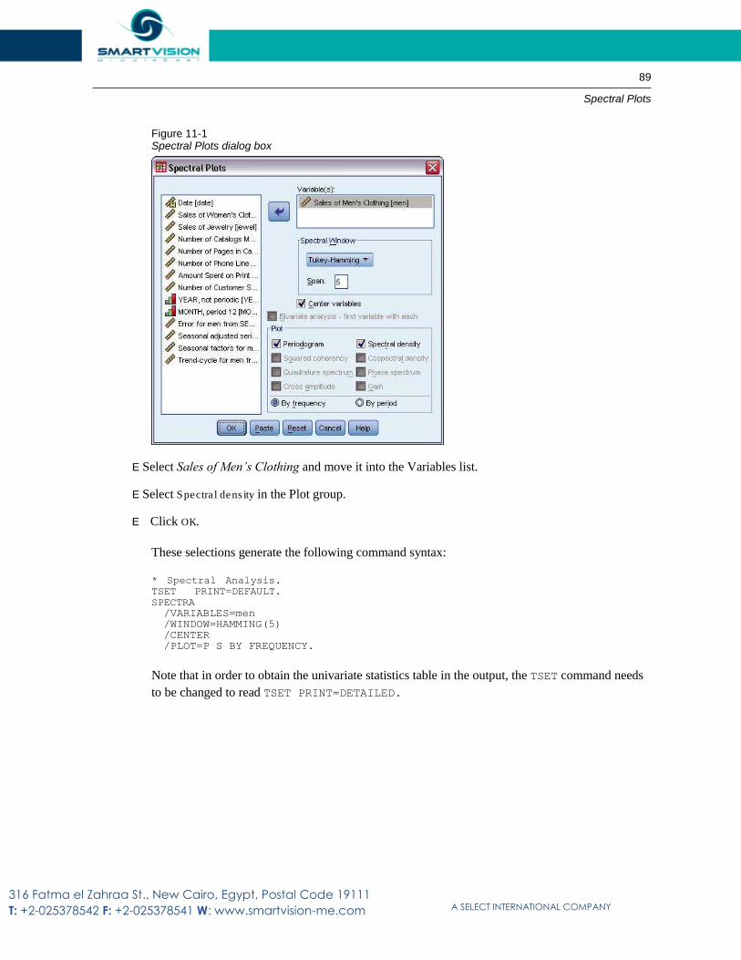
316 Fatma el Zahraa St., New Cairo, Egypt, Postal Code 19111
T: +2-025378542 F: +2-025378541 W: www.smartvision-me.com A SELECT INTERNATIONAL COMPANY
89
Spectral Plots
Figure 11-1 Spectral Plots dialog box
E Select Sales of Men’s Clothing and move it into the Variables list. E Select Spectral density in the Plot group. E Click OK.
These selections generate the following command syntax:
* Spectral Analysis.
TSET PRINT=DEFAULT.
SPECTRA /VARIABLES=men /WINDOW=HAMMING(5) /CENTER /PLOT=P S BY FREQUENCY.
Note that in order to obtain the univariate statistics table in the output, the TSET command needs
to be changed to read TSET PRINT=DETAILED.
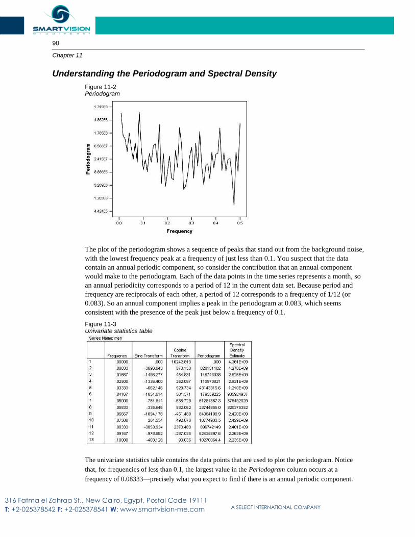
316 Fatma el Zahraa St., New Cairo, Egypt, Postal Code 19111
T: +2-025378542 F: +2-025378541 W: www.smartvision-me.com A SELECT INTERNATIONAL COMPANY
90 Chapter 11
Understanding the Periodogram and Spectral Density
Figure 11-2 Periodogram
The plot of the periodogram shows a sequence of peaks that stand out from the background noise,
with the lowest frequency peak at a frequency of just less than 0.1. You suspect that the data
contain an annual periodic component, so consider the contribution that an annual component
would make to the periodogram. Each of the data points in the time series represents a month, so
an annual periodicity corresponds to a period of 12 in the current data set. Because period and
frequency are reciprocals of each other, a period of 12 corresponds to a frequency of 1/12 (or
0.083). So an annual component implies a peak in the periodogram at 0.083, which seems
consistent with the presence of the peak just below a frequency of 0.1.
Figure 11-3 Univariate statistics table
The univariate statistics table contains the data points that are used to plot the periodogram. Notice
that, for frequencies of less than 0.1, the largest value in the Periodogram column occurs at a
frequency of 0.08333—precisely what you expect to find if there is an annual periodic component.

316 Fatma el Zahraa St., New Cairo, Egypt, Postal Code 19111
T: +2-025378542 F: +2-025378541 W: www.smartvision-me.com A SELECT INTERNATIONAL COMPANY
91
Spectral Plots
This information confirms the identification of the lowest frequency peak with an annual
periodic component. But what about the other peaks at higher frequencies?
Figure 11-4 Spectral density
The remaining peaks are best analyzed with the spectral density function, which is simply a smoothed
version of the periodogram. Smoothing provides a means of eliminating the background noise from a
periodogram, allowing the underlying structure to be more clearly isolated. The spectral density consists of five distinct peaks that appear to be equally spaced. The lowest
frequency peak simply represents the smoothed version of the peak at 0.08333. To understand the
significance of the four higher frequency peaks, remember that the periodogram is calculated by
modeling the time series as the sum of cosine and sine functions. Periodic components that have
the shape of a sine or cosine function (sinusoidal) show up in the periodogram as single peaks.
Periodic components that are not sinusoidal show up as a series of equally spaced peaks of
different heights, with the lowest frequency peak in the series occurring at the frequency of the
periodic component. So the four higher frequency peaks in the spectral density simply indicate
that the annual periodic component is not sinusoidal. You have now accounted for all of the discernible structure in the spectral density plot and
conclude that the data contain a single periodic component with a period of 12 months.
Summary
Using the Spectral Plots procedure, you have confirmed the existence of an annual periodic
component of a time series, and you have verified that no other significant periodicities are
present. The spectral density was seen to be more useful than the periodogram for uncovering the
underlying structure, because the spectral density smoothes out the fluctuations that are caused
by the nonperiodic component of the data.

316 Fatma el Zahraa St., New Cairo, Egypt, Postal Code 19111
T: +2-025378542 F: +2-025378541 W: www.smartvision-me.com A SELECT INTERNATIONAL COMPANY
92 Chapter 11
Related Procedures
The Spectral Plots procedure is useful for identifying the periodic components of a time series.
„ To remove a periodic component from a time series—for instance, to perform a trend
analysis—use the Seasonal Decomposition procedure. See Chapter 10 for details.

316 Fatma el Zahraa St., New Cairo, Egypt, Postal Code 19111
T: +2-025378542 F: +2-025378541 W: www.smartvision-me.com A SELECT INTERNATIONAL COMPANY
Appendix
A
Goodness-of-Fit Measures
This section provides definitions of the goodness-of-fit measures used in time series modeling.
„ Stationary R-squared. A measure that compares the stationary part of the model to a simple
mean model. This measure is preferable to ordinary R-squared when there is a trend or seasonal
pattern. Stationary R-squared can be negative with a range of negative infinity to 1. Negative
values mean that the model under consideration is worse than the baseline model. Positive
values mean that the model under consideration is better than the baseline model.
„ R-squared. An estimate of the proportion of the total variation in the series that is
explained by the model. This measure is most useful when the series is stationary. R-
squared can be negative with a range of negative infinity to 1. Negative values mean that
the model under consideration is worse than the baseline model. Positive values mean that
the model under consideration is better than the baseline model.
„ RMSE. Root Mean Square Error. The square root of mean square error. A measure of how
much a dependent series varies from its model-predicted level, expressed in the same units
as the dependent series.
„ MAPE. Mean Absolute Percentage Error. A measure of how much a dependent series varies
from its model-predicted level. It is independent of the units used and can therefore be used
to compare series with different units.
„ MAE. Mean absolute error. Measures how much the series varies from its model-
predicted level. MAE is reported in the original series units.
„ MaxAPE. Maximum Absolute Percentage Error. The largest forecasted error, expressed as a
percentage. This measure is useful for imagining a worst-case scenario for your forecasts.
„ MaxAE. Maximum Absolute Error. The largest forecasted error, expressed in the same
units as the dependent series. Like MaxAPE, it is useful for imagining the worst-case
scenario for your forecasts. Maximum absolute error and maximum absolute percentage
error may occur at different series points–for example, when the absolute error for a large
series value is slightly larger than the absolute error for a small series value. In that case,
the maximum absolute error will occur at the larger series value and the maximum absolute
percentage error will occur at the smaller series value.
„ Normalized BIC. Normalized Bayesian Information Criterion. A general measure of the
overall fit of a model that attempts to account for model complexity. It is a score based upon
the mean square error and includes a penalty for the number of parameters in the model and
the length of the series. The penalty removes the advantage of models with more parameters,
making the statistic easy to compare across different models for the same series.
© Copyright SPSS Inc. 1989, 2010 93

316 Fatma el Zahraa St., New Cairo, Egypt, Postal Code 19111
T: +2-025378542 F: +2-025378541 W: www.smartvision-me.com A SELECT INTERNATIONAL COMPANY
Appendix
B
Outlier Types
This section provides definitions of the outlier types used in time series modeling.
„ Additive. An outlier that affects a single observation. For example, a data coding error
might be identified as an additive outlier.
„ Level shift. An outlier that shifts all observations by a constant, starting at a particular
series point. A level shift could result from a change in policy.
„ Innovational. An outlier that acts as an addition to the noise term at a particular series
point. For stationary series, an innovational outlier affects several observations. For
nonstationary series, it may affect every observation starting at a particular series point.
„ Transient. An outlier whose impact decays exponentially to 0.
„ Seasonal additive. An outlier that affects a particular observation and all subsequent
observations separated from it by one or more seasonal periods. All such observations are
affected equally. A seasonal additive outlier might occur if, beginning in a certain year, sales
are higher every January.
„ Local trend. An outlier that starts a local trend at a particular series point.
„ Additive patch. A group of two or more consecutive additive outliers. Selecting this outlier
type results in the detection of individual additive outliers in addition to patches of them.
© Copyright SPSS Inc. 1989, 2010 94

316 Fatma el Zahraa St., New Cairo, Egypt, Postal Code 19111
T: +2-025378542 F: +2-025378541 W: www.smartvision-me.com A SELECT INTERNATIONAL COMPANY
Appendix
C
Guide to ACF/PACF Plots
The plots shown here are those of pure or theoretical ARIMA processes. Here are some general
guidelines for identifying the process: „ Nonstationary series have an ACF that remains significant for half a dozen or more lags,
rather than quickly declining to 0. You must difference such a series until it is stationary
before you can identify the process.
„ Autoregressive processes have an exponentially declining ACF and spikes in the first one or
more lags of the PACF. The number of spikes indicates the order of the autoregression.
„ Moving average processes have spikes in the first one or more lags of the ACF and an
exponentially declining PACF. The number of spikes indicates the order of the moving
average.
„ Mixed (ARMA) processes typically show exponential declines in both the ACF and the PACF.
At the identification stage, you do not need to worry about the sign of the ACF or PACF, or
about the speed with which an exponentially declining ACF or PACF approaches 0. These
depend upon the sign and actual value of the AR and MA coefficients. In some instances, an
exponentially declining ACF alternates between positive and negative values. ACF and PACF plots from real data are never as clean as the plots shown here. You must
learn to pick out what is essential in any given plot. Always check the ACF and PACF of the
residuals, in case your identification is wrong. Bear in mind that: „ Seasonal processes show these patterns at the seasonal lags (the multiples of the seasonal
period).
„ You are entitled to treat nonsignificant values as 0. That is, you can ignore values that lie
within the confidence intervals on the plots. You do not have to ignore them, however,
particularly if they continue the pattern of the statistically significant values.
„ An occasional autocorrelation will be statistically significant by chance alone. You can
ignore a statistically significant autocorrelation if it is isolated, preferably at a high lag, and if
it does not occur at a seasonal lag. © Copyright SPSS Inc. 1989, 2010 95
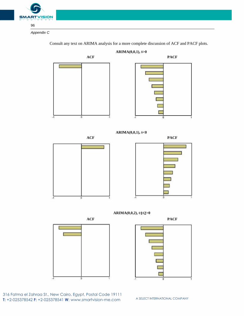
316 Fatma el Zahraa St., New Cairo, Egypt, Postal Code 19111
T: +2-025378542 F: +2-025378541 W: www.smartvision-me.com A SELECT INTERNATIONAL COMPANY
96 Appendix C
Consult any text on ARIMA analysis for a more complete discussion of ACF and PACF plots.
ARIMA(0,0,1), θ>0
ACF PACF
ARIMA(0,0,1), θ<0
ACF PACF
ARIMA(0,0,2), θ1θ2>0
ACF PACF

316 Fatma el Zahraa St., New Cairo, Egypt, Postal Code 19111
T: +2-025378542 F: +2-025378541 W: www.smartvision-me.com A SELECT INTERNATIONAL COMPANY
97
Guide to ACF/PACF Plots
ARIMA(1,0,0), φ>0
ACF PACF
ARIMA(1,0,0), φ<0
ACF PACF
ARIMA(1,0,1), φ<0, θ>0
ACF PACF
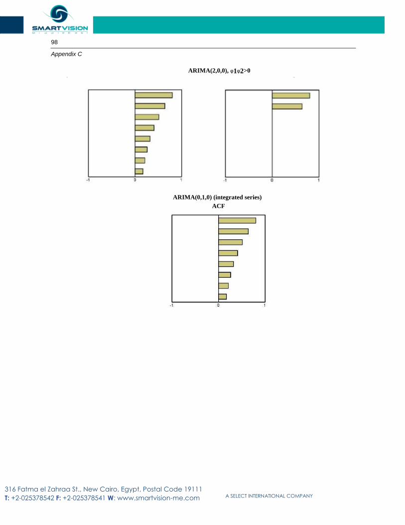
316 Fatma el Zahraa St., New Cairo, Egypt, Postal Code 19111
T: +2-025378542 F: +2-025378541 W: www.smartvision-me.com A SELECT INTERNATIONAL COMPANY
98 Appendix C
ARIMA(2,0,0), φ1φ2>0
ACF PACF
ARIMA(0,1,0) (integrated series) ACF

316 Fatma el Zahraa St., New Cairo, Egypt, Postal Code 19111
T: +2-025378542 F: +2-025378541 W: www.smartvision-me.com A SELECT INTERNATIONAL COMPANY
Appendix
D
Sample Files
The sample files installed with the product can be found in the Samples subdirectory of the
installation directory. There is a separate folder within the Samples subdirectory for each of
the following languages: English, French, German, Italian, Japanese, Korean, Polish, Russian,
Simplified Chinese, Spanish, and Traditional Chinese.
Not all sample files are available in all languages. If a sample file is not available in a language,
that language folder contains an English version of the sample file.
Descriptions
Following are brief descriptions of the sample files used in various examples throughout the
documentation. „ accidents.sav. This is a hypothetical data file that concerns an insurance company that is
studying age and gender risk factors for automobile accidents in a given region. Each case
corresponds to a cross-classification of age category and gender.
„ adl.sav. This is a hypothetical data file that concerns efforts to determine the benefits of a
proposed type of therapy for stroke patients. Physicians randomly assigned female stroke patients
to one of two groups. The first received the standard physical therapy, and the second received an
additional emotional therapy. Three months following the treatments, each patient’s abilities to
perform common activities of daily life were scored as ordinal variables.
„ advert.sav. This is a hypothetical data file that concerns a retailer’s efforts to examine
the relationship between money spent on advertising and the resulting sales. To this end,
they have collected past sales figures and the associated advertising costs..
„ aflatoxin.sav. This is a hypothetical data file that concerns the testing of corn crops for aflatoxin, a poison whose concentration varies widely between and within crop yields. A
grain processor has received 16 samples from each of 8 crop yields and measured the
alfatoxin levels in parts per billion (PPB). „ anorectic.sav. While working toward a standardized symptomatology of anorectic/bulimic
behavior, researchers (Van der Ham, Meulman, Van Strien, and Van Engeland, 1997) made
a study of 55 adolescents with known eating disorders. Each patient was seen four times over
four years, for a total of 220 observations. At each observation, the patients were scored for
each of 16 symptoms. Symptom scores are missing for patient 71 at time 2, patient 76 at time
2, and patient 47 at time 3, leaving 217 valid observations.
„ bankloan.sav. This is a hypothetical data file that concerns a bank’s efforts to reduce the rate of loan defaults. The file contains financial and demographic information on 850 past
and prospective customers. The first 700 cases are customers who were previously given © Copyright SPSS Inc. 1989, 2010 99

316 Fatma el Zahraa St., New Cairo, Egypt, Postal Code 19111
T: +2-025378542 F: +2-025378541 W: www.smartvision-me.com A SELECT INTERNATIONAL COMPANY
100 Appendix D
loans. The last 150 cases are prospective customers that the bank needs to classify as good
or bad credit risks. „ bankloan_binning.sav. This is a hypothetical data file containing financial and
demographic information on 5,000 past customers.
„ behavior.sav. In a classic example (Price and Bouffard, 1974), 52 students were asked to
rate the combinations of 15 situations and 15 behaviors on a 10-point scale ranging from
0=“extremely appropriate” to 9=“extremely inappropriate.” Averaged over individuals,
the values are taken as dissimilarities.
„ behavior_ini.sav. This data file contains an initial configuration for a two-dimensional
solution for behavior.sav.
„ brakes.sav. This is a hypothetical data file that concerns quality control at a factory that
produces disc brakes for high-performance automobiles. The data file contains diameter
measurements of 16 discs from each of 8 production machines. The target diameter for the
brakes is 322 millimeters.
„ breakfast.sav. In a classic study (Green and Rao, 1972), 21 Wharton School MBA
students and their spouses were asked to rank 15 breakfast items in order of preference with
1=“most preferred” to 15=“least preferred.” Their preferences were recorded under six
different scenarios, from “Overall preference” to “Snack, with beverage only.”
„ breakfast-overall.sav. This data file contains the breakfast item preferences for the
first scenario, “Overall preference,” only.
„ broadband_1.sav. This is a hypothetical data file containing the number of subscribers,
by region, to a national broadband service. The data file contains monthly subscriber
numbers for 85 regions over a four-year period.
„ broadband_2.sav. This data file is identical to broadband_1.sav but contains data for
three additional months.
„ car_insurance_claims.sav. A dataset presented and analyzed elsewhere (McCullagh and
Nelder, 1989) concerns damage claims for cars. The average claim amount can be modeled
as having a gamma distribution, using an inverse link function to relate the mean of the
dependent variable to a linear combination of the policyholder age, vehicle type, and vehicle
age. The number of claims filed can be used as a scaling weight.
„ car_sales.sav. This data file contains hypothetical sales estimates, list prices, and physical
specifications for various makes and models of vehicles. The list prices and physical
specifications were obtained alternately from edmunds.com and manufacturer sites.
„ car_sales_uprepared.sav. This is a modified version of car_sales.sav that does not
include any transformed versions of the fields.
„ carpet.sav. In a popular example (Green and Wind, 1973), a company interested in
marketing a new carpet cleaner wants to examine the influence of five factors on consumer
preference—package design, brand name, price, a Good Housekeeping seal, and a money-
back guarantee. There are three factor levels for package design, each one differing in the
location of the applicator brush; three brand names (K2R, Glory, and Bissell); three price
levels; and two levels (either no or yes) for each of the last two factors. Ten consumers rank
22 profiles defined by these factors. The variable Preference contains the rank of the average
rankings for each profile. Low rankings correspond to high preference. This variable reflects
an overall measure of preference for each profile.

316 Fatma el Zahraa St., New Cairo, Egypt, Postal Code 19111
T: +2-025378542 F: +2-025378541 W: www.smartvision-me.com A SELECT INTERNATIONAL COMPANY
101
Sample Files
„ carpet_prefs.sav. This data file is based on the same example as described for carpet.sav,
but it contains the actual rankings collected from each of the 10 consumers. The consumers
were asked to rank the 22 product profiles from the most to the least preferred. The variables
PREF1 through PREF22 contain the identifiers of the associated profiles, as defined in
carpet_plan.sav. „ catalog.sav. This data file contains hypothetical monthly sales figures for three products
sold by a catalog company. Data for five possible predictor variables are also included. „ catalog_seasfac.sav. This data file is the same as catalog.sav except for the addition of a
set of seasonal factors calculated from the Seasonal Decomposition procedure along with
the accompanying date variables. „ cellular.sav. This is a hypothetical data file that concerns a cellular phone company’s
efforts to reduce churn. Churn propensity scores are applied to accounts, ranging from 0 to
100. Accounts scoring 50 or above may be looking to change providers. „ ceramics.sav. This is a hypothetical data file that concerns a manufacturer’s efforts to
determine whether a new premium alloy has a greater heat resistance than a standard alloy.
Each case represents a separate test of one of the alloys; the heat at which the bearing failed
is recorded. „ cereal.sav. This is a hypothetical data file that concerns a poll of 880 people about their
breakfast preferences, also noting their age, gender, marital status, and whether or not they
have an active lifestyle (based on whether they exercise at least twice a week). Each case
represents a separate respondent. „ clothing_defects.sav. This is a hypothetical data file that concerns the quality control
process at a clothing factory. From each lot produced at the factory, the inspectors take a
sample of clothes and count the number of clothes that are unacceptable. „ coffee.sav. This data file pertains to perceived images of six iced-coffee brands (Kennedy,
Riquier, and Sharp, 1996) . For each of 23 iced-coffee image attributes, people selected all
brands that were described by the attribute. The six brands are denoted AA, BB, CC, DD,
EE, and FF to preserve confidentiality. „ contacts.sav. This is a hypothetical data file that concerns the contact lists for a group of
corporate computer sales representatives. Each contact is categorized by the department of
the company in which they work and their company ranks. Also recorded are the amount of
the last sale made, the time since the last sale, and the size of the contact’s company. „ creditpromo.sav. This is a hypothetical data file that concerns a department store’s efforts
to evaluate the effectiveness of a recent credit card promotion. To this end, 500 cardholders
were randomly selected. Half received an ad promoting a reduced interest rate on purchases
made over the next three months. Half received a standard seasonal ad. „ customer_dbase.sav. This is a hypothetical data file that concerns a company’s efforts to
use the information in its data warehouse to make special offers to customers who are most
likely to reply. A subset of the customer base was selected at random and given the special
offers, and their responses were recorded. „ customer_information.sav. A hypothetical data file containing customer mailing
information, such as name and address. „ customer_subset.sav. A subset of 80 cases from customer_dbase.sav.

316 Fatma el Zahraa St., New Cairo, Egypt, Postal Code 19111
T: +2-025378542 F: +2-025378541 W: www.smartvision-me.com A SELECT INTERNATIONAL COMPANY
102 Appendix D
„ debate.sav. This is a hypothetical data file that concerns paired responses to a survey from
attendees of a political debate before and after the debate. Each case corresponds to a
separate respondent.
„ debate_aggregate.sav. This is a hypothetical data file that aggregates the responses in
debate.sav. Each case corresponds to a cross-classification of preference before and after
the debate.
„ demo.sav. This is a hypothetical data file that concerns a purchased customer database,
for the purpose of mailing monthly offers. Whether or not the customer responded to the
offer is recorded, along with various demographic information.
„ demo_cs_1.sav. This is a hypothetical data file that concerns the first step of a company’s
efforts to compile a database of survey information. Each case corresponds to a different
city, and the region, province, district, and city identification are recorded.
„ demo_cs_2.sav. This is a hypothetical data file that concerns the second step of a
company’s efforts to compile a database of survey information. Each case corresponds to a
different household unit from cities selected in the first step, and the region, province,
district, city, subdivision, and unit identification are recorded. The sampling information
from the first two stages of the design is also included.
„ demo_cs.sav. This is a hypothetical data file that contains survey information collected
using a complex sampling design. Each case corresponds to a different household unit, and
various demographic and sampling information is recorded.
„ dmdata.sav. This is a hypothetical data file that contains demographic and purchasing
information for a direct marketing company. dmdata2.sav contains information for a subset
of contacts that received a test mailing, and dmdata3.sav contains information on the
remaining contacts who did not receive the test mailing.
„ dietstudy.sav. This hypothetical data file contains the results of a study of the “Stillman
diet” (Rickman, Mitchell, Dingman, and Dalen, 1974). Each case corresponds to a separate
subject and records his or her pre- and post-diet weights in pounds and triglyceride levels in
mg/100 ml.
„ dvdplayer.sav. This is a hypothetical data file that concerns the development of a new
DVD player. Using a prototype, the marketing team has collected focus group data. Each
case corresponds to a separate surveyed user and records some demographic information
about them and their responses to questions about the prototype.
„ german_credit.sav. This data file is taken from the “German credit” dataset in the Repository of
Machine Learning Databases (Blake and Merz, 1998) at the University of California, Irvine.
„ grocery_1month.sav. This hypothetical data file is the grocery_coupons.sav data file with
the weekly purchases “rolled-up” so that each case corresponds to a separate customer. Some
of the variables that changed weekly disappear as a result, and the amount spent recorded is
now the sum of the amounts spent during the four weeks of the study.
„ grocery_coupons.sav. This is a hypothetical data file that contains survey data collected by a grocery store chain interested in the purchasing habits of their customers. Each customer
is followed for four weeks, and each case corresponds to a separate customer-week and
records information about where and how the customer shops, including how much was
spent on groceries during that week.

316 Fatma el Zahraa St., New Cairo, Egypt, Postal Code 19111
T: +2-025378542 F: +2-025378541 W: www.smartvision-me.com A SELECT INTERNATIONAL COMPANY
103
Sample Files
„ guttman.sav. Bell (Bell, 1961) presented a table to illustrate possible social groups.
Guttman (Guttman, 1968) used a portion of this table, in which five variables describing
such things as social interaction, feelings of belonging to a group, physical proximity of
members, and formality of the relationship were crossed with seven theoretical social
groups, including crowds (for example, people at a football game), audiences (for example,
people at a theater or classroom lecture), public (for example, newspaper or television
audiences), mobs (like a crowd but with much more intense interaction), primary groups
(intimate), secondary groups (voluntary), and the modern community (loose confederation
resulting from close physical proximity and a need for specialized services). „ health_funding.sav. This is a hypothetical data file that contains data on health care
funding (amount per 100 population), disease rates (rate per 10,000 population), and visits
to health care providers (rate per 10,000 population). Each case represents a different city. „ hivassay.sav. This is a hypothetical data file that concerns the efforts of a
pharmaceutical lab to develop a rapid assay for detecting HIV infection. The results of the
assay are eight deepening shades of red, with deeper shades indicating greater likelihood
of infection. A laboratory trial was conducted on 2,000 blood samples, half of which were
infected with HIV and half of which were clean. „ hourlywagedata.sav. This is a hypothetical data file that concerns the hourly wages of
nurses from office and hospital positions and with varying levels of experience. „ insurance_claims.sav. This is a hypothetical data file that concerns an insurance company
that wants to build a model for flagging suspicious, potentially fraudulent claims. Each case
represents a separate claim. „ insure.sav. This is a hypothetical data file that concerns an insurance company that is
studying the risk factors that indicate whether a client will have to make a claim on a 10-year
term life insurance contract. Each case in the data file represents a pair of contracts, one of
which recorded a claim and the other didn’t, matched on age and gender. „ judges.sav. This is a hypothetical data file that concerns the scores given by trained
judges (plus one enthusiast) to 300 gymnastics performances. Each row represents a
separate performance; the judges viewed the same performances. „ kinship_dat.sav. Rosenberg and Kim (Rosenberg and Kim, 1975) set out to analyze 15 kinship
terms (aunt, brother, cousin, daughter, father, granddaughter, grandfather, grandmother, grandson,
mother, nephew, niece, sister, son, uncle). They asked four groups of college students (two
female, two male) to sort these terms on the basis of similarities. Two groups (one female, one
male) were asked to sort twice, with the second sorting based on a different criterion from the
first sort. Thus, a total of six “sources” were obtained. Each source corresponds to a
proximity matrix, whose cells are equal to the number of people in a source minus the number of
times the objects were partitioned together in that source. „ kinship_ini.sav. This data file contains an initial configuration for a three-dimensional
solution for kinship_dat.sav. „ kinship_var.sav. This data file contains independent variables gender, gener(ation), and
degree (of separation) that can be used to interpret the dimensions of a solution for
kinship_dat.sav. Specifically, they can be used to restrict the space of the solution to a linear
combination of these variables. „ marketvalues.sav. This data file concerns home sales in a new housing development in
Algonquin, Ill., during the years from 1999–2000. These sales are a matter of public record.

316 Fatma el Zahraa St., New Cairo, Egypt, Postal Code 19111
T: +2-025378542 F: +2-025378541 W: www.smartvision-me.com A SELECT INTERNATIONAL COMPANY
104 Appendix D
„ nhis2000_subset.sav. The National Health Interview Survey (NHIS) is a large, population-
based survey of the U.S. civilian population. Interviews are carried out face-to-face in a
nationally representative sample of households. Demographic information and observations
about health behaviors and status are obtained for members of each household. This data
file contains a subset of information from the 2000 survey. National Center for Health
Statistics. National Health Interview Survey, 2000. Public-use data file and documentation.
ftp://ftp.cdc.gov/pub/Health_Statistics/NCHS/Datasets/NHIS/2000/. Accessed 2003.
„ ozone.sav. The data include 330 observations on six meteorological variables for
predicting ozone concentration from the remaining variables. Previous researchers
(Breiman and Friedman, 1985), (Hastie and Tibshirani, 1990), among others found
nonlinearities among these variables, which hinder standard regression approaches.
„ pain_medication.sav. This hypothetical data file contains the results of a clinical trial for anti- inflammatory medication for treating chronic arthritic pain. Of particular interest is
the time it takes for the drug to take effect and how it compares to an existing medication. „ patient_los.sav. This hypothetical data file contains the treatment records of patients who were
admitted to the hospital for suspected myocardial infarction (MI, or “heart attack”). Each case
corresponds to a separate patient and records many variables related to their hospital stay.
„ patlos_sample.sav. This hypothetical data file contains the treatment records of a sample of patients who received thrombolytics during treatment for myocardial infarction (MI, or
“heart attack”). Each case corresponds to a separate patient and records many variables
related to their hospital stay. „ poll_cs.sav. This is a hypothetical data file that concerns pollsters’ efforts to determine the
level of public support for a bill before the legislature. The cases correspond to registered
voters. Each case records the county, township, and neighborhood in which the voter lives.
„ poll_cs_sample.sav. This hypothetical data file contains a sample of the voters listed in
poll_cs.sav. The sample was taken according to the design specified in the poll.csplan plan
file, and this data file records the inclusion probabilities and sample weights. Note, however,
that because the sampling plan makes use of a probability-proportional-to-size (PPS)
method, there is also a file containing the joint selection probabilities (poll_jointprob.sav).
The additional variables corresponding to voter demographics and their opinion on the
proposed bill were collected and added the data file after the sample as taken.
„ property_assess.sav. This is a hypothetical data file that concerns a county assessor’s
efforts to keep property value assessments up to date on limited resources. The cases
correspond to properties sold in the county in the past year. Each case in the data file records
the township in which the property lies, the assessor who last visited the property, the time
since that assessment, the valuation made at that time, and the sale value of the property.
„ property_assess_cs.sav. This is a hypothetical data file that concerns a state assessor’s
efforts to keep property value assessments up to date on limited resources. The cases
correspond to properties in the state. Each case in the data file records the county, township,
and neighborhood in which the property lies, the time since the last assessment, and the
valuation made at that time.
„ property_assess_cs_sample.sav. This hypothetical data file contains a sample of the properties
listed in property_assess_cs.sav. The sample was taken according to the design specified in the
property_assess.csplan plan file, and this data file records the inclusion probabilities

316 Fatma el Zahraa St., New Cairo, Egypt, Postal Code 19111
T: +2-025378542 F: +2-025378541 W: www.smartvision-me.com A SELECT INTERNATIONAL COMPANY
105
Sample Files
and sample weights. The additional variable Current value was collected and added to the
data file after the sample was taken. „ recidivism.sav. This is a hypothetical data file that concerns a government law
enforcement agency’s efforts to understand recidivism rates in their area of jurisdiction.
Each case corresponds to a previous offender and records their demographic information,
some details of their first crime, and then the time until their second arrest, if it occurred
within two years of the first arrest. „ recidivism_cs_sample.sav. This is a hypothetical data file that concerns a government law
enforcement agency’s efforts to understand recidivism rates in their area of jurisdiction. Each case
corresponds to a previous offender, released from their first arrest during the month of June, 2003,
and records their demographic information, some details of their first crime, and the data of their
second arrest, if it occurred by the end of June, 2006. Offenders were selected from sampled
departments according to the sampling plan specified in recidivism_cs.csplan; because it makes
use of a probability-proportional-to-size (PPS) method, there is also a file containing the joint
selection probabilities (recidivism_cs_jointprob.sav). „ rfm_transactions.sav. A hypothetical data file containing purchase transaction data,
including date of purchase, item(s) purchased, and monetary amount of each transaction. „ salesperformance.sav. This is a hypothetical data file that concerns the evaluation of
two new sales training courses. Sixty employees, divided into three groups, all receive
standard training. In addition, group 2 gets technical training; group 3, a hands-on tutorial.
Each employee was tested at the end of the training course and their score recorded. Each
case in the data file represents a separate trainee and records the group to which they were
assigned and the score they received on the exam. „ satisf.sav. This is a hypothetical data file that concerns a satisfaction survey conducted by
a retail company at 4 store locations. 582 customers were surveyed in all, and each case
represents the responses from a single customer. „ screws.sav. This data file contains information on the characteristics of screws, bolts,
nuts, and tacks (Hartigan, 1975). „ shampoo_ph.sav. This is a hypothetical data file that concerns the quality control at a
factory for hair products. At regular time intervals, six separate output batches are measured
and their pH recorded. The target range is 4.5–5.5. „ ships.sav. A dataset presented and analyzed elsewhere (McCullagh et al., 1989) that
concerns damage to cargo ships caused by waves. The incident counts can be modeled as
occurring at a Poisson rate given the ship type, construction period, and service period. The
aggregate months of service for each cell of the table formed by the cross-classification of
factors provides values for the exposure to risk. „ site.sav. This is a hypothetical data file that concerns a company’s efforts to choose new
sites for their expanding business. They have hired two consultants to separately evaluate
the sites, who, in addition to an extended report, summarized each site as a “good,” “fair,”
or “poor” prospect. „ smokers.sav. This data file is abstracted from the 1998 National Household
Survey of Drug Abuse and is a probability sample of American households. (
http://dx.doi.org/10.3886/ICPSR02934) Thus, the first step in an analysis of this data file
should be to weight the data to reflect population trends.
316 Fatma el Zahraa St., New Cairo, Egypt, Postal Code 19111
T: +2-025378542 F: +2-025378541 W: www.smartvision-me.com A SELECT INTERNATIONAL COMPANY
106 Appendix D
„ stroke_clean.sav. This hypothetical data file contains the state of a medical database
after it has been cleaned using procedures in the Data Preparation option.
„ stroke_invalid.sav. This hypothetical data file contains the initial state of a medical
database and contains several data entry errors.
„ stroke_survival. This hypothetical data file concerns survival times for patients exiting a
rehabilitation program post-ischemic stroke face a number of challenges. Post-stroke, the
occurrence of myocardial infarction, ischemic stroke, or hemorrhagic stroke is noted and the
time of the event recorded. The sample is left-truncated because it only includes patients who
survived through the end of the rehabilitation program administered post-stroke.
„ stroke_valid.sav. This hypothetical data file contains the state of a medical database after
the values have been checked using the Validate Data procedure. It still contains potentially
anomalous cases.
„ survey_sample.sav. This data file contains survey data, including demographic data and
various attitude measures. It is based on a subset of variables from the 1998 NORC General
Social Survey, although some data values have been modified and additional fictitious
variables have been added for demonstration purposes.
„ telco.sav. This is a hypothetical data file that concerns a telecommunications company’s
efforts to reduce churn in their customer base. Each case corresponds to a separate customer
and records various demographic and service usage information.
„ telco_extra.sav. This data file is similar to the telco.sav data file, but the “tenure” and log-transformed customer spending variables have been removed and replaced by
standardized log-transformed customer spending variables. „ telco_missing.sav. This data file is a subset of the telco.sav data file, but some of
the demographic data values have been replaced with missing values.
„ testmarket.sav. This hypothetical data file concerns a fast food chain’s plans to add a new
item to its menu. There are three possible campaigns for promoting the new product, so the
new item is introduced at locations in several randomly selected markets. A different
promotion is used at each location, and the weekly sales of the new item are recorded for the
first four weeks. Each case corresponds to a separate location-week.
„ testmarket_1month.sav. This hypothetical data file is the testmarket.sav data file with the
weekly sales “rolled-up” so that each case corresponds to a separate location. Some of the
variables that changed weekly disappear as a result, and the sales recorded is now the sum of
the sales during the four weeks of the study.
„ tree_car.sav. This is a hypothetical data file containing demographic and vehicle
purchase price data.
„ tree_credit.sav. This is a hypothetical data file containing demographic and bank loan
history data.
„ tree_missing_data.sav This is a hypothetical data file containing demographic and bank
loan history data with a large number of missing values.
„ tree_score_car.sav. This is a hypothetical data file containing demographic and
vehicle purchase price data.
„ tree_textdata.sav. A simple data file with only two variables intended primarily to show
the default state of variables prior to assignment of measurement level and value labels.

316 Fatma el Zahraa St., New Cairo, Egypt, Postal Code 19111
T: +2-025378542 F: +2-025378541 W: www.smartvision-me.com A SELECT INTERNATIONAL COMPANY
107
Sample Files
„ tv-survey.sav. This is a hypothetical data file that concerns a survey conducted by a TV
studio that is considering whether to extend the run of a successful program. 906 respondents
were asked whether they would watch the program under various conditions. Each row
represents a separate respondent; each column is a separate condition. „ ulcer_recurrence.sav. This file contains partial information from a study designed to
compare the efficacy of two therapies for preventing the recurrence of ulcers. It provides a
good example of interval-censored data and has been presented and analyzed elsewhere
(Collett, 2003). „ ulcer_recurrence_recoded.sav. This file reorganizes the information in ulcer_recurrence.sav
to allow you model the event probability for each interval of the study rather than simply the end-
of-study event probability. It has been presented and analyzed elsewhere (Collett et
al., 2003). „ verd1985.sav. This data file concerns a survey (Verdegaal, 1985). The responses of 15
subjects to 8 variables were recorded. The variables of interest are divided into three sets. Set
1 includes age and marital, set 2 includes pet and news, and set 3 includes music and live. Pet is scaled as multiple nominal and age is scaled as ordinal; all of the other variables are
scaled as single nominal. „ virus.sav. This is a hypothetical data file that concerns the efforts of an Internet service
provider (ISP) to determine the effects of a virus on its networks. They have tracked the
(approximate) percentage of infected e-mail traffic on its networks over time, from the
moment of discovery until the threat was contained. „ wheeze_steubenville.sav. This is a subset from a longitudinal study of the health effects of air
pollution on children (Ware, Dockery, Spiro III, Speizer, and Ferris Jr., 1984). The data contain
repeated binary measures of the wheezing status for children from Steubenville, Ohio, at ages 7,
8, 9 and 10 years, along with a fixed recording of whether or not the mother was a smoker during the first year of the study.
„ workprog.sav. This is a hypothetical data file that concerns a government works program
that tries to place disadvantaged people into better jobs. A sample of potential program
participants were followed, some of whom were randomly selected for enrollment in the
program, while others were not. Each case represents a separate program participant.

316 Fatma el Zahraa St., New Cairo, Egypt, Postal Code 19111
T: +2-025378542 F: +2-025378541 W: www.smartvision-me.com A SELECT INTERNATIONAL COMPANY
Appendix
E
Notices
Licensed Materials – Property of SPSS Inc., an IBM Company. © Copyright SPSS Inc. 1989,
2010.
Patent No. 7,023,453
The following paragraph does not apply to the United Kingdom or any other country where
such provisions are inconsistent with local law: SPSS INC., AN IBM COMPANY, PROVIDES
THIS PUBLICATION “AS IS” WITHOUT WARRANTY OF ANY KIND, EITHER EXPRESS OR
IMPLIED, INCLUDING, BUT NOT LIMITED TO, THE IMPLIED WARRANTIES OF NON-INFRINGEMENT, MERCHANTABILITY OR FITNESS FOR A
PARTICULAR PURPOSE. Some states do not allow disclaimer of express or implied
warranties in certain transactions, therefore, this statement may not apply to you.
This information could include technical inaccuracies or typographical errors. Changes are
periodically made to the information herein; these changes will be incorporated in new editions of
the publication. SPSS Inc. may make improvements and/or changes in the product(s) and/or the
program(s) described in this publication at any time without notice.
Any references in this information to non-SPSS and non-IBM Web sites are provided for
convenience only and do not in any manner serve as an endorsement of those Web sites. The
materials at those Web sites are not part of the materials for this SPSS Inc. product and use of
those Web sites is at your own risk.
When you send information to IBM or SPSS, you grant IBM and SPSS a nonexclusive right
to use or distribute the information in any way it believes appropriate without incurring any
obligation to you.
Information concerning non-SPSS products was obtained from the suppliers of those products,
their published announcements or other publicly available sources. SPSS has not tested those
products and cannot confirm the accuracy of performance, compatibility or any other claims
related to non-SPSS products. Questions on the capabilities of non-SPSS products should be
addressed to the suppliers of those products.
This information contains examples of data and reports used in daily business operations.
To illustrate them as completely as possible, the examples include the names of individuals, companies, brands, and products. All of these names are fictitious and any similarity to the names
and addresses used by an actual business enterprise is entirely coincidental.
COPYRIGHT LICENSE:
This information contains sample application programs in source language, which illustrate
programming techniques on various operating platforms. You may copy, modify, and distribute these
sample programs in any form without payment to SPSS Inc., for the purposes of developing, © Copyright SPSS Inc. 1989, 2010 108

316 Fatma el Zahraa St., New Cairo, Egypt, Postal Code 19111
T: +2-025378542 F: +2-025378541 W: www.smartvision-me.com A SELECT INTERNATIONAL COMPANY
109
Notices
using, marketing or distributing application programs conforming to the application
programming interface for the operating platform for which the sample programs are written.
These examples have not been thoroughly tested under all conditions. SPSS Inc., therefore,
cannot guarantee or imply reliability, serviceability, or function of these programs. The sample
programs are provided “AS IS”, without warranty of any kind. SPSS Inc. shall not be liable for
any damages arising out of your use of the sample programs.
Trademarks IBM, the IBM logo, and ibm.com are trademarks of IBM Corporation, registered in many
jurisdictions worldwide. A current list of IBM trademarks is available on the Web at
http://www.ibm.com/legal/copytrade.shmtl. SPSS is a trademark of SPSS Inc., an IBM Company, registered in many jurisdictions worldwide. Adobe, the Adobe logo, PostScript, and the PostScript logo are either registered trademarks or
trademarks of Adobe Systems Incorporated in the United States, and/or other countries. Intel, Intel logo, Intel Inside, Intel Inside logo, Intel Centrino, Intel Centrino logo, Celeron, Intel
Xeon, Intel SpeedStep, Itanium, and Pentium are trademarks or registered trademarks of Intel
Corporation or its subsidiaries in the United States and other countries. Linux is a registered trademark of Linus Torvalds in the United States, other countries, or both. Microsoft, Windows, Windows NT, and the Windows logo are trademarks of Microsoft
Corporation in the United States, other countries, or both. UNIX is a registered trademark of The Open Group in the United States and other countries. Java and all Java-based trademarks and logos are trademarks of Sun Microsystems, Inc. in the
United States, other countries, or both. This product uses WinWrap Basic, Copyright 1993-2007, Polar Engineering and Consulting,
http://www.winwrap.com. Other product and service names might be trademarks of IBM, SPSS, or other companies. Adobe product screenshot(s) reprinted with permission from Adobe Systems Incorporated. Microsoft product screenshot(s) reprinted with permission from Microsoft Corporation.

316 Fatma el Zahraa St., New Cairo, Egypt, Postal Code 19111
T: +2-025378542 F: +2-025378541 W: www.smartvision-me.com A SELECT INTERNATIONAL COMPANY
Bibliography
Bell, E. H. 1961. Social foundations of human behavior: Introduction to the study of sociology.
New York: Harper & Row. Blake, C. L., and C. J. Merz. 1998. "UCI Repository of machine learning databases." Available at
http://www.ics.uci.edu/~mlearn/MLRepository.html. Box, G. E. P., G. M. Jenkins, and G. C. Reinsel. 1994. Time series analysis: Forecasting and
control, 3rd ed. Englewood Cliffs, N.J.: Prentice Hall. Breiman, L., and J. H. Friedman. 1985. Estimating optimal transformations for multiple
regression and correlation. Journal of the American Statistical Association, 80, 580–598. Collett, D. 2003. Modelling survival data in medical research, 2 ed. Boca Raton: Chapman &
Hall/CRC. Gardner, E. S. 1985. Exponential smoothing: The state of the art. Journal of Forecasting, 4, 1–28.
Green, P. E., and V. Rao. 1972. Applied multidimensional scaling. Hinsdale, Ill.: Dryden Press. Green, P. E., and Y. Wind. 1973. Multiattribute decisions in marketing: A measurement
approach. Hinsdale, Ill.: Dryden Press. Guttman, L. 1968. A general nonmetric technique for finding the smallest coordinate space for
configurations of points. Psychometrika, 33, 469–506. Hartigan, J. A. 1975. Clustering algorithms. New York: John Wiley and Sons. Hastie, T., and R. Tibshirani. 1990. Generalized additive models. London: Chapman and Hall. Kennedy, R., C. Riquier, and B. Sharp. 1996. Practical applications of correspondence analysis
to categorical data in market research. Journal of Targeting, Measurement, and Analysis for
Marketing, 5, 56–70. McCullagh, P., and J. A. Nelder. 1989. Generalized Linear Models, 2nd ed. London: Chapman &
Hall. Pena, D., G. C. Tiao, and R. S. Tsay, eds. 2001. A course in time series analysis. New York:
John Wiley and Sons. Price, R. H., and D. L. Bouffard. 1974. Behavioral appropriateness and situational constraints as
dimensions of social behavior. Journal of Personality and Social Psychology, 30, 579–586. Rickman, R., N. Mitchell, J. Dingman, and J. E. Dalen. 1974. Changes in serum cholesterol
during the Stillman Diet. Journal of the American Medical Association, 228, 54–58. Rosenberg, S., and M. P. Kim. 1975. The method of sorting as a data-gathering procedure in
multivariate research. Multivariate Behavioral Research, 10, 489–502. Van der Ham, T., J. J. Meulman, D. C. Van Strien, and H. Van Engeland. 1997. Empirically
based subgrouping of eating disorders in adolescents: A longitudinal perspective. British Journal
of Psychiatry, 170, 363–368. Verdegaal, R. 1985. Meer sets analyse voor kwalitatieve gegevens (in Dutch). Leiden:
Department of Data Theory, University of Leiden.
© Copyright SPSS Inc. 1989, 2010 110

316 Fatma el Zahraa St., New Cairo, Egypt, Postal Code 19111
T: +2-025378542 F: +2-025378541 W: www.smartvision-me.com A SELECT INTERNATIONAL COMPANY
111
Bibliography
Ware, J. H., D. W. Dockery, A. Spiro III, F. E. Speizer, and B. G. Ferris Jr.. 1984. Passive
smoking, gas cooking, and respiratory health of children living in six cities. American Review of
Respiratory Diseases, 129, 366–374.

316 Fatma el Zahraa St., New Cairo, Egypt, Postal Code 19111
T: +2-025378542 F: +2-025378541 W: www.smartvision-me.com A SELECT INTERNATIONAL COMPANY
ACF
in Apply Time Series Models, 28, 30 in Time Series Modeler, 16, 18 plots for pure ARIMA processes, 95
additive outlier, 94 in Time Series Modeler, 8,
14 additive patch outlier, 94 in Time Series Modeler, 8, 14
Apply Time Series Models, 25, 54, 70 best- and poorest-fitting models, 32 Box-Ljung statistic, 28 confidence intervals, 30, 34 estimation period, 27 fit values, 30 forecast period, 27, 55, 77 forecast table, 78 forecasts, 28, 30, 78 goodness-of-fit statistics, 28, 30, 57 missing values, 34 model fit table, 57
model parameters, 28 new variable names, 33, 58
reestimate model parameters, 27, 55 residual autocorrelation function, 28, 30 residual partial autocorrelation function, 28, 30 saving predictions, 33, 56 saving reestimated models in XML, 33
statistics across all models, 28, 30, 57 ARIMA model parameters table
in Time Series Modeler, 68 ARIMA models, 6
autoregressive orders, 11 constant, 11 differencing orders, 11 moving average orders, 11 outliers, 14 seasonal orders, 11
transfer functions, 12
autocorrelation function in Apply Time Series Models, 28, 30 in Time Series Modeler, 16, 18 plots for pure ARIMA processes, 95
autoregression ARIMA
models, 11
Box-Ljung statistic
in Apply Time Series Models, 28
in Time Series Modeler, 16, 68 Brown’s exponential smoothing model, 9
Index
confidence intervals
in Apply Time Series Models, 30,
34 in Time Series Modeler, 18, 23
damped exponential smoothing model,
9 difference transformation ARIMA models, 11
estimation period, 2
in Apply Time Series Models, 27
in Time Series Modeler, 6, 46 events, 8
in Time Series Modeler, 7 Expert Modeler, 6, 43
limiting the model space, 7, 46 outliers, 8, 63
exponential smoothing models, 6, 9
fit values
in Apply Time Series Models, 30 in Time Series Modeler, 18,
66 forecast period in Apply Time Series Models, 27, 55, 77
in Time Series Modeler, 6, 23, 46–47 forecast table
in Apply Time Series Models, 78 in Time Series Modeler, 53
forecasts in Apply Time Series Models, 28, 30, 78 in Time Series Modeler, 16, 18, 49
goodness of fi t
definitions, 93 in Apply Time Series Models, 28, 30,
57 in Time Series Modeler, 16, 18, 49
harmonic analysis,
39 historical data in Apply Time Series Models, 30 in Time Series Modeler, 18
historical period, 2 holdout cases, 2 Holt’s exponential smoothing model, 9
innovational outlier, 94
in Time Series Modeler, 8, 14 integration
ARIMA models, 11
112

316 Fatma el Zahraa St., New Cairo, Egypt, Postal Code 19111
T: +2-025378542 F: +2-025378541 W: www.smartvision-me.com
113
legal notices, 108
level shift outlier, 94 in Time Series Modeler, 8,
14 local trend outlier, 94 in Time Series Modeler, 8,
14 log transformation in Time Series Modeler, 9, 11–12
MAE, 93
in Apply Time Series Models, 28, 30 in Time Series Modeler, 16, 18
MAPE, 93 in Apply Time Series Models, 28, 30, 58 in Time Series Modeler, 16, 18, 50
MaxAE, 93 in Apply Time Series Models, 28, 30 in Time Series Modeler, 16, 18
MaxAPE, 93 in Apply Time Series Models, 28, 30, 58 in Time Series Modeler, 16, 18, 50
maximum absolute error, 93 in Apply Time Series Models, 28, 30 in Time Series Modeler, 16, 18
maximum absolute percentage error, 93 in Apply Time Series Models, 28, 30, 58 in Time Series Modeler, 16, 18, 50
mean absolute error, 93 in Apply Time Series Models, 28, 30 in Time Series Modeler, 16, 18
mean absolute percentage error, 93 in Apply Time Series Models, 28, 30, 58 in Time Series Modeler, 16, 18, 50
missing values in Apply Time Series Models, 34 in Time Series Modeler, 23
model description table in Time Series Modeler,
67 model fit table in Apply Time Series Models,
57 model names in Time Series Modeler,
23 model parameters in Apply Time Series Models, 28 in Time Series Modeler, 16,
65 model statistics table in Time Series Modeler,
68 models ARIMA, 6, 11
Expert Modeler, 6 exponential smoothing, 6,
9 moving average ARIMA models, 11
natural log transformation
in Time Series Modeler, 9, 11–12 normalized BIC (Bayesian information criterion),
93 in Apply Time Series Models, 28, 30
Index
in Time Series Modeler, 16, 18
outliers
ARIMA models, 14 definitions, 94 Expert Modeler, 8, 63
PACF
in Apply Time Series Models, 28, 30 in Time Series Modeler, 16, 18 plots for pure ARIMA processes, 95
partial autocorrelation function in Apply Time Series Models, 28, 30 in Time Series Modeler, 16, 18 plots for pure ARIMA processes, 95
periodicity in Time Series Modeler, 7, 9, 11–12
R2
, 93 in Apply Time Series Models, 28, 30 in Time Series Modeler, 16, 18
reestimate model parameters in Apply Time Series Models, 27,
55 residuals in Apply Time Series Models, 28, 30 in Time Series Modeler, 16, 18
RMSE, 93 in Apply Time Series Models, 28, 30 in Time Series Modeler, 16, 18
root mean square error, 93 in Apply Time Series Models, 28,
30 in Time Series Modeler, 16, 18 sample files
location, 99 save
model predictions, 21, 33 model specifi cations in XML, 21 new variable names, 21, 33 reestimated models in XML, 33
seasonal additive outlier, 94 in Time Series Modeler, 8, 14
Seasonal Decomposition, 36–38 assumptions, 36 computing moving averages, 36 create variables, 37 models, 36 new variables, 85 periodic date component, 80 related procedures, 87 saving new variables, 37
seasonal difference transformation ARIMA models, 11
seasonal orders
ARIMA models, 11 simple exponential smoothing model, 9

316 Fatma el Zahraa St., New Cairo, Egypt, Postal Code 19111
T: +2-025378542 F: +2-025378541 W: www.smartvision-me.com A SELECT INTERNATIONAL COMPANY
114 Index
simple seasonal exponential smoothing model,
9 Spectral Plots, 39, 41 assumptions, 39 bivariate spectral analysis, 40 centering transformation, 40 periodogram, 90 related procedures, 92
spectral density, 90
spectral windows, 39 square root transformation
in Time Series Modeler, 9, 11–12
stationary R2
, 93 in Apply Time Series Models, 28, 30 in Time Series Modeler, 16, 18, 68
Time Series Modeler,
3 ARIMA, 6, 11 ARIMA model parameters table, 68 best- and poorest-fitting models, 20 Box-Ljung statistic, 16 confidence intervals, 18, 23 estimation period, 6, 46 events, 7 Expert Modeler, 6, 43, 59 exponential smoothing, 6, 9 fit values, 18, 66 forecast period, 6, 23, 46–47 forecast table, 53 forecasts, 16, 18, 49 goodness-of-fit statistics, 16, 18, 49, 68 missing values, 23 model description table, 67 model names, 23 model parameters, 16, 65 model statistics table, 68 new variable names, 21, 52 outliers, 8, 14, 63 periodicity, 7, 9, 11–12 residual autocorrelation function, 16, 18 residual partial autocorrelation function, 16, 18 saving model speci fications in XML, 21, 48, 64 saving predictions, 21, 48 series transformation, 9, 11–12 statistics across all models, 16, 18, 49, 51 transfer functions, 12
trademarks, 109
transfer functions, 12 delay, 12 denominator orders, 12 difference orders, 12 numerator orders, 12 seasonal orders, 12
transient outlier, 94 in Time Series Modeler, 8, 14
variable names
in Apply Time Series Models,
33 in Time Series Modeler, 21
Winters’ exponential smoothing model
additive, 9 multiplicative, 9
XML
saving reestimated models in XML, 33 saving
time series models in XML, 21, 48, 64
validation period, 2
Related Documents