www.ib.academy SL MATH AA STUDY GUIDE

Welcome message from author
This document is posted to help you gain knowledge. Please leave a comment to let me know what you think about it! Share it to your friends and learn new things together.
Transcript

www.ib.academy
SLM A T H A A
S T U D Y G U I D E
Mathematics Analysis and Approaches SLStudy Guide
Available on www.ib.academy
Author: Nikita Smolnikov, Alex BarancovaContributing Authors: Laurence Gibbons
Design Typesetting
TEX Academy
Special thanks: Robert van den Heuvel
This work may be shared digitally and in printed form,but it may not be changed and then redistributed in any form.
Copyright © 2020, IB AcademyVersion: MathAASL.1.0.200507
This work is published under theCreative Commons BY-NC-ND 4.0 International License.To view a copy of this license, visitcreativecommons.org/licenses/by-nc-nd/4.0
This work may not used for commercial purposes other than by IB Academy, orparties directly licenced by IB Academy. If you acquired this guide by paying forit, or if you have received this guide as part of a paid service or product, directlyor indirectly, we kindly ask that you contact us immediately.
Daltonlaan 4003584 BK UtrechtThe Netherlands
[email protected]+31 (0) 30 4300 430

Welcome to the IB.Academy guide for Mathematics Analysis andApproaches SL.
Our Study Guides are put together by our teachers who worked tirelessly with studentsand schools. The idea is to compile revision material that would be easy-to-follow forIB students worldwide and for school teachers to utilise them for their classrooms.Our approach is straightforward: by adopting a step-by-step perspective, students caneasily absorb dense information in a quick and efficient manner. With this format,students will be able to tackle every question swiftly and without any difficulties.
For this guide, we supplement the new topics with relevant sections from our previousMath Studies, SL and HL study resources, and with insights from our years of experienceteaching these courses. We illustrate theoretical concepts by working through IB-stylequestions and break things down using a step-by-step approach. We also include detailedinstructions on how to use the TI-Nspire™ to solve problems; most of this is also quiteeasily transferable to other GDC models.
The best way to apply what you have learned from the guides is with a study partner.We suggest revising with a friend or with a group in order to immediately test theinformation you gathered from our guides. This will help you not only process theinformation, but also help you formulate your answers for the exams. Practice makesbetter and what better way to do it than with your friends!
In order to maintain our Study Guides and to put forth the best possible material, we arein constant collaboration with students and teachers alike. To help us, we ask that youprovide feedback and suggestions so that we can modify the contents to be relevant forIB studies. We appreciate any comments and hope that our Study Guides will help youwith your revision or in your lessons. For more information on our material or courses,be sure to check our site at www.ib.academy.
IB.Academy Team
If you would like to consider supporting our materials and be recognised for it,send us an email to [email protected].

0PRIOR KNOWLEDGE
Before you start make sure you have a firm grasp of the following. Many marks are lostthrough errors in these fundamentals.
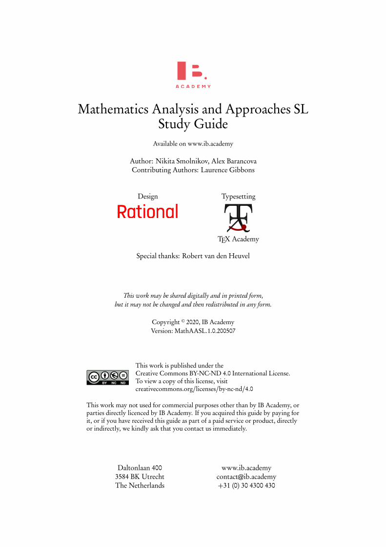
0.1 NumberNumbers can be grouped in to a number of sets. From the diagram you see that allrational numbers are also real numbers; i.e.Q is a subset of R.
N naturals
0,1,2,3, . . .
Z integers. . . ,−4,−3,−2,−1, . . .. . . , 1, 2, 3,4, . . .
Q rational numbers
13
−251267
irrational numbers
p2 π
p102
R real numbers
Positive integers Z+ = {1,2,3, . . .}Positive integers and zero N= {0,1,2,3, . . .}Integers Z= {. . . ,−3,−2,−1,0,1,2,3, . . .}Rational numbers Q= any number that can be written as the ratio
pq
of any two integers, where q 6= 0
0.2 Signs+ and − signs describe positive and negative numbers. Remember they work theopposite way with negative integers. In maths two wrongs do make a right.
1−−1= 1+ 1= 2 −1×−1= 1
5
PRIOR KNOWLEDGE Standard form
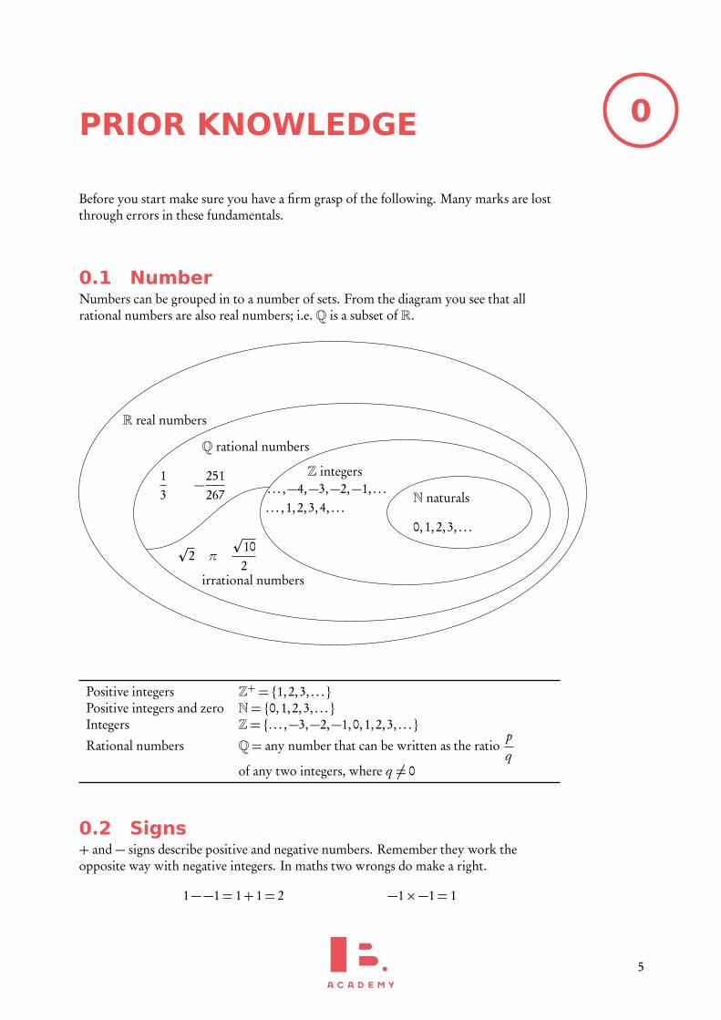
0.3 Standard form
Standard form is just a way of rewriting any num-ber, sometimes also referred to as ‘scientificnotation’. This should be in the form a× 10k ,where a is between 1 and 10, and k is an integer.
10 1× 101
1000 1× 10³
3280 3.28× 10³
4582000 4.582× 10⁶
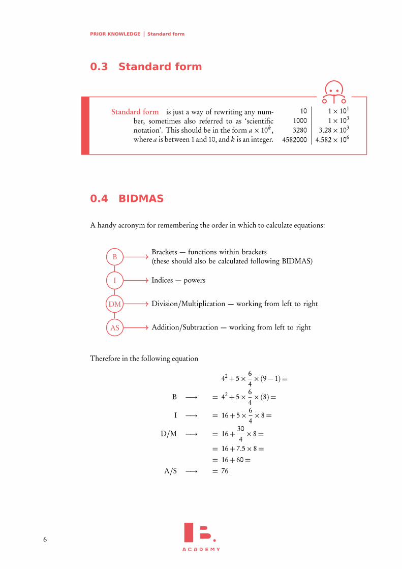
0.4 BIDMAS
A handy acronym for remembering the order in which to calculate equations:
B
I
DM
AS
Brackets — functions within brackets(these should also be calculated following BIDMAS)
Indices — powers
Division/Multiplication — working from left to right
Addition/Subtraction — working from left to right
Therefore in the following equation
42+ 5× 64× (9− 1) =
B −→ = 42+ 5× 64× (8) =
I −→ = 16+ 5× 64× 8=
D/M −→ = 16+304× 8=
= 16+ 7.5× 8== 16+ 60=
A/S −→ = 76
6
PRIOR KNOWLEDGE Solving simultaneous equations 0
0.5 Solving simultaneous equations
If we have two unknowns, for example x and y, and two equations, then we can solve forx and y simultaneously.
(
(1) y = 3x + 1(2) 2y = x − 1
There are 3 methods to solve simultaneous equations.
Elimination
Multiply an equation and then subtractit from the other in order to eliminateone of the unknowns.
3× (2)⇒ (3) 6y = 3x − 3(3)− (1)⇒ 6y − y = 3x − 3x − 3− 1
5y =−4
y =−45
Put y in (1) or (2) and solve for x
−45= 3x + 1
3x =−95
x =− 915=−3
5
Substitution
Rearrange and then substitute one in toanother.
Substitute (1) into (2)
2(3x + 1) = x − 16x + 2= x − 1
5x =−3
x =−35
Put x in (1) or (2) and solve for x
y = 3�
−35
�
+ 1
y =−45
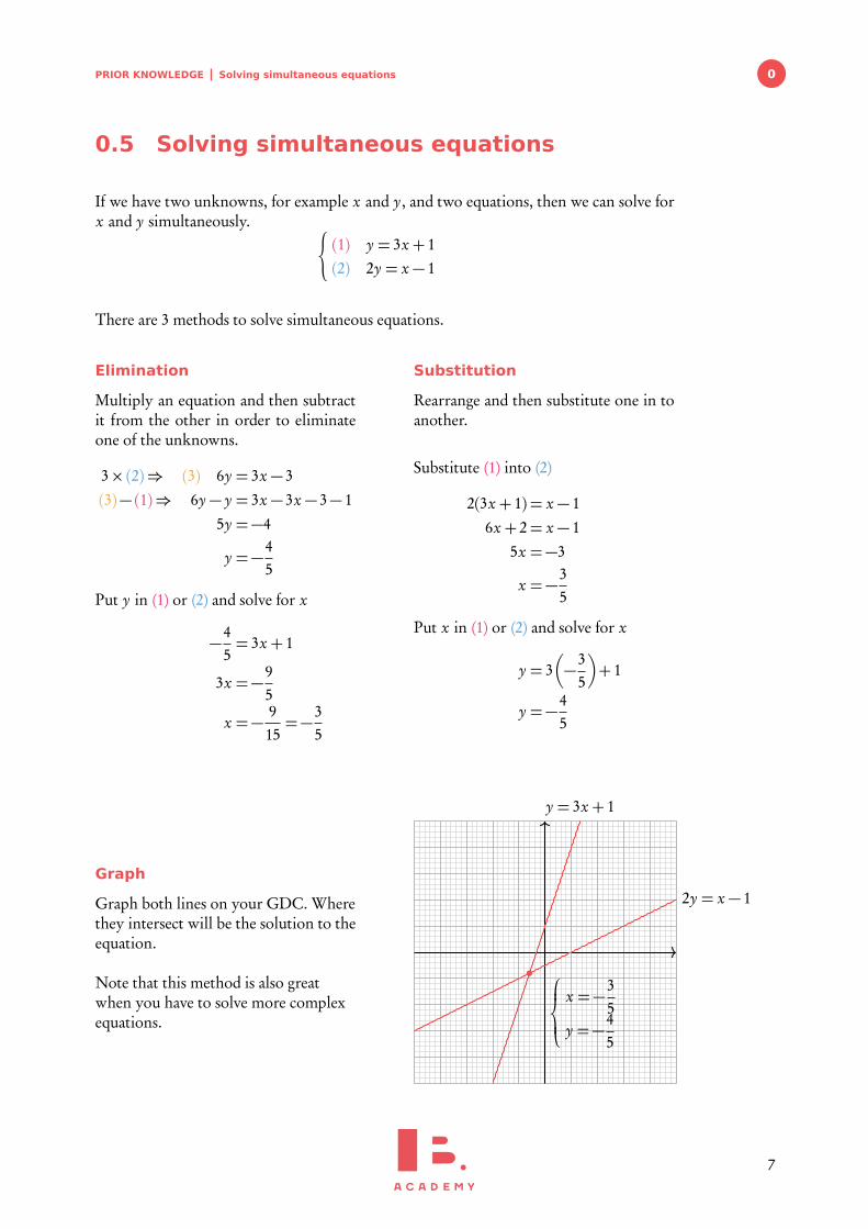
Graph
Graph both lines on your GDC. Wherethey intersect will be the solution to theequation.
Note that this method is also greatwhen you have to solve more complexequations.
y = 3x + 1
2y = x − 1
x =−35
y =−45
7
PRIOR KNOWLEDGE Geometry
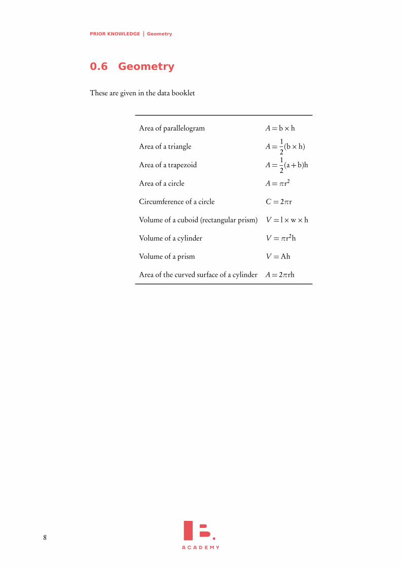
0.6 Geometry
These are given in the data booklet
Area of parallelogram A= b×h
Area of a triangle A=12(b×h)
Area of a trapezoid A=12(a+ b)h
Area of a circle A=πr2
Circumference of a circle C = 2πr
Volume of a cuboid (rectangular prism) V = l×w×h
Volume of a cylinder V =πr2h
Volume of a prism V =Ah
Area of the curved surface of a cylinder A= 2πrh
8
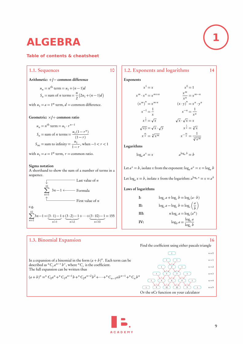
1ALGEBRATable of contents & cheatsheet
1.1. Sequences 10
Arithmetic: +/− common difference
un = nth term= u1+(n− 1)d
Sn = sum of n terms=n2
�
2u1+(n− 1)d�
with u1 = a = 1st term, d = common difference.
Geometric: ×/÷ common ratio
un = nth term= u1 · rn−1
Sn = sum of n terms=u1 (1− r n)(1− r )
S∞ = sum to infinity=u1
1− r, when −1< r < 1
with u1 = a = 1st term, r = common ratio.
Sigma notationA shorthand to show the sum of a number of terms in asequence.
10∑
n=13n− 1
Last value of n
Formula
First value of n
e.g.10∑
n=13n−1= (3 · 1)− 1
︸ ︷︷ ︸
n=1
+(3 · 2)− 1︸ ︷︷ ︸
n=2
+ · · ·+(3 · 10)− 1︸ ︷︷ ︸
n=10
= 155
1.2. Exponents and logarithms 14
Exponents
x1 = x x0 = 1
x m · xn = x m+n x m
xn= x m−n
(x m)n= x m·n (x · y)n = xn · yn
x−1 =1x
x−n =1
xn
x12 =p
xp
x ·p
x = xp
xy =p
x ·py x1n = npx
xmn = npx m x−
mn =
1npx m
Logarithms
loga ax = x aloga b = b
Let ax = b , isolate x from the exponent: loga ax = x = loga b
Let loga x = b , isolate x from the logarithm: aloga x = x = ab
Laws of logarithms
I: logc a+ logc b = logc (a · b )
II: logc a− logc b = logc
� ab
�
III: n logc a = logc (an)
IV: logb a =logc alogc b
1.3. Binomial Expansion 16
In a expansion of a binomial in the form (a+ b )n . Each term can bedescribed as nCr an−r b r , where nCr is the coefficient.The full expansion can be written thus
(a+ b )n =n C0an+n C1an−1b+n C2an−2b 2+ · · ·+n Cn−1ab n−1+n Cn b n
Find the coefficient using either pascals triangle
1
1 1
1 2+
1
1 3+
3+
1
1 4+
6+
4+
1
1 5+
10+
10+
5+
1
n = 0
n = 1
n = 2
n = 3
n = 4
n = 5
Or the nCr function on your calculator
9
ALGEBRA Sequences
1.1 Sequences
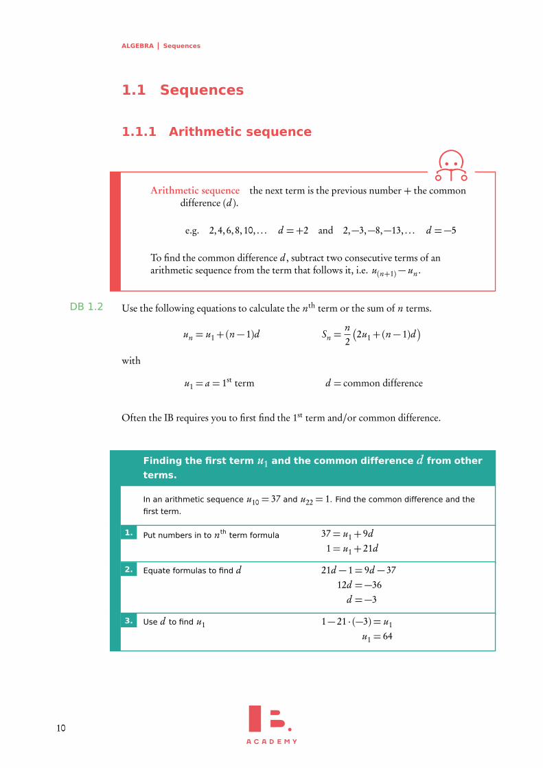
1.1.1 Arithmetic sequence
Arithmetic sequence the next term is the previous number + the commondifference (d ).
e.g. 2,4,6,8,10, . . . d =+2 and 2,−3,−8,−13, . . . d =−5
To find the common difference d , subtract two consecutive terms of anarithmetic sequence from the term that follows it, i.e. u(n+1)− un .
Use the following equations to calculate the nth term or the sum of n terms.DB 1.2
un = u1+(n− 1)d Sn =n2
�
2u1+(n− 1)d�
with
u1 = a = 1st term d = common difference
Often the IB requires you to first find the 1st term and/or common difference.
Finding the first term u1 and the common difference d from other
terms.
In an arithmetic sequence u10 = 37 and u22 = 1. Find the common difference and the
first term.
1. Put numbers in to nth term formula 37= u1+ 9d1= u1+ 21d
2. Equate formulas to find d 21d − 1= 9d − 3712d =−36
d =−3
3. Use d to find u1 1− 21 · (−3) = u1
u1 = 64
10
ALGEBRA Sequences 1
1.1.2 Geometric sequence
Geometric sequence the next term is the previous number multiplied by thecommon ratio (r ).
To find the common ratio, divide any term of an arithmetic sequence by the
term that precedes it, i.e.second term (u2)
first term (u1)e.g. 2,4,8,16,32, . . . r = 2
and 25,5,1,0.2, . . . r =15
Use the following equations to calculate the nth term, the sum of n terms or the sum toinfinity when −1< r < 1. DB 1.3 & 1.8
un = nth term Sn = sum of n terms S∞ = sum to infinity
= u1 · rn−1 =
u1 (1− r n)(1− r )
=u1
1− r
again with
u1 = a = 1st term r = common ratio
Similar to questions on Arithmetic sequences, you are often required to find the 1st termand/or common ratio first.
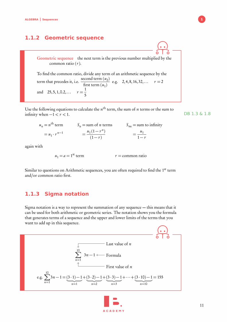
1.1.3 Sigma notation
Sigma notation is a way to represent the summation of any sequence — this means that itcan be used for both arithmetic or geometric series. The notation shows you the formulathat generates terms of a sequence and the upper and lower limits of the terms that youwant to add up in this sequence.
10∑
n=13n− 1
Last value of n
Formula
First value of n
e.g.10∑
n=13n− 1= (3 · 1)− 1
︸ ︷︷ ︸
n=1
+(3 · 2)− 1︸ ︷︷ ︸
n=2
+(3 · 3)− 1︸ ︷︷ ︸
n=3
+ · · ·+(3 · 10)− 1︸ ︷︷ ︸
n=10
= 155
11
ALGEBRA Sequences
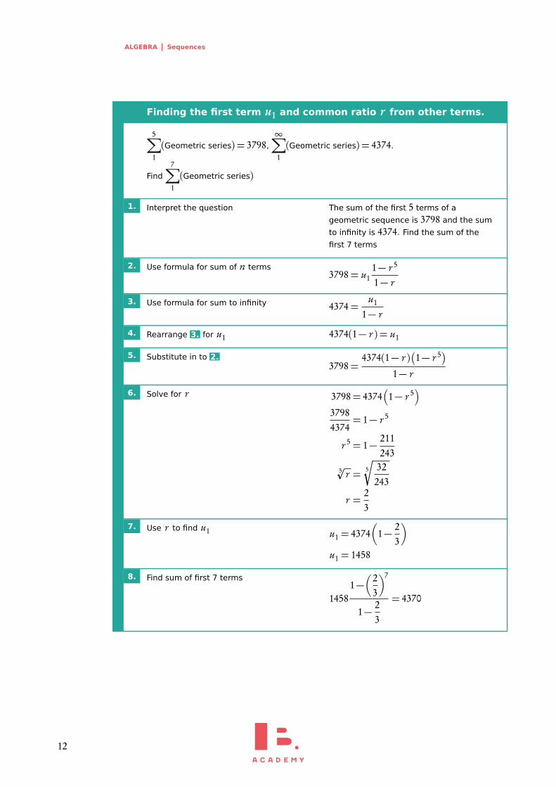
Finding the first term u1 and common ratio r from other terms.
5∑
1(Geometric series) = 3798,
∞∑
1(Geometric series) = 4374.
Find7∑
1(Geometric series)
1. Interpret the question The sum of the first 5 terms of a
geometric sequence is 3798 and the sum
to infinity is 4374. Find the sum of the
first 7 terms
2. Use formula for sum of n terms3798= u1
1− r 5
1− r
3. Use formula for sum to infinity 4374=u1
1− r
4. Rearrange 3. for u1 4374(1− r ) = u1
5. Substitute in to 2.3798=
4374(1− r )�
1− r 5�
1− r
6. Solve for r 3798= 4374�
1− r 5�
37984374
= 1− r 5
r 5 = 1− 211243
5pr = 5
s
32243
r =23
7. Use r to find u1 u1 = 4374�
1− 23
�
u1 = 1458
8. Find sum of first 7 terms
14581−
�
23
�7
1− 23
= 4370
12
ALGEBRA Sequences 1
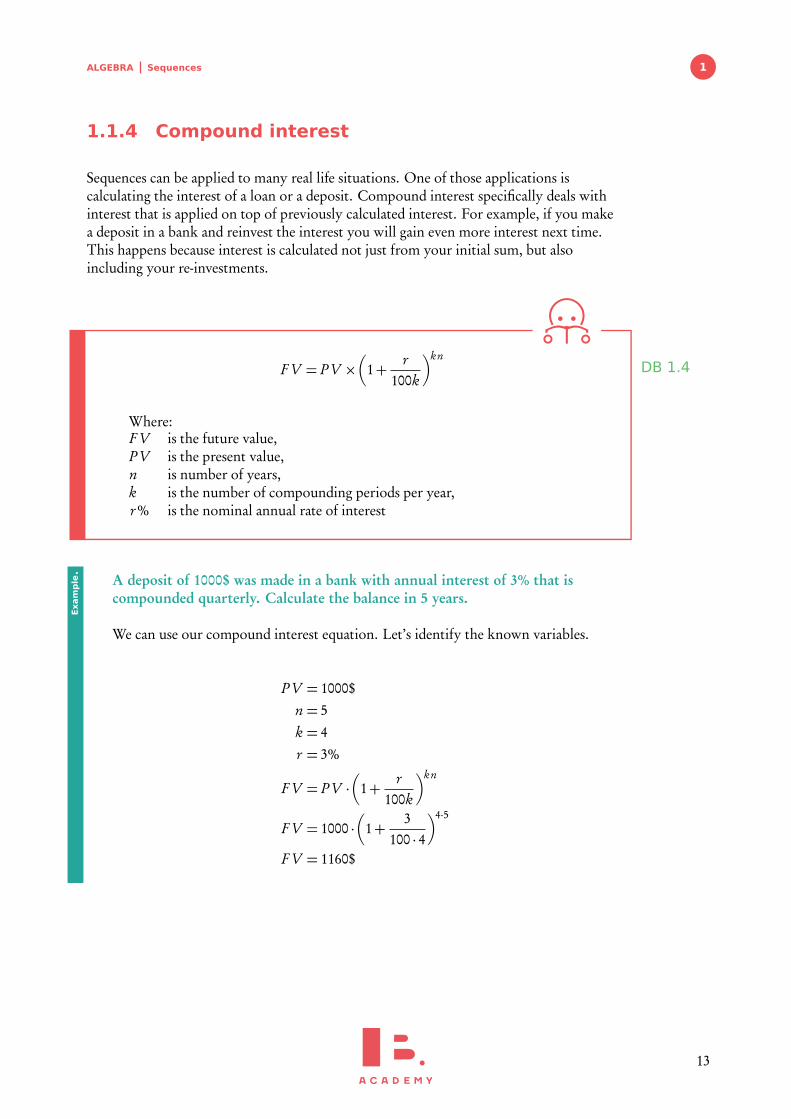
1.1.4 Compound interest
Sequences can be applied to many real life situations. One of those applications iscalculating the interest of a loan or a deposit. Compound interest specifically deals withinterest that is applied on top of previously calculated interest. For example, if you makea deposit in a bank and reinvest the interest you will gain even more interest next time.This happens because interest is calculated not just from your initial sum, but alsoincluding your re-investments.
F V = PV �
1+r
100k
�knDB 1.4
Where:F V is the future value,PV is the present value,n is number of years,k is the number of compounding periods per year,r % is the nominal annual rate of interest
A deposit of 1000$ was made in a bank with annual interest of 3% that iscompounded quarterly. Calculate the balance in 5 years.
We can use our compound interest equation. Let’s identify the known variables.
PV = 1000$n = 5k = 4r = 3%
F V = PV ·�
1+r
100k
�kn
F V = 1000 ·�
1+3
100 · 4
�4·5
F V = 1160$
Exam
ple.
13
ALGEBRA Exponents and logarithms
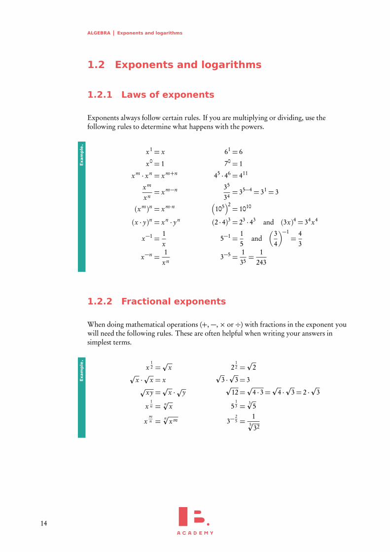
1.2 Exponents and logarithms
1.2.1 Laws of exponents
Exponents always follow certain rules. If you are multiplying or dividing, use thefollowing rules to determine what happens with the powers.
x1 = x 61 = 6
x0 = 1 70 = 1
x m · xn = x m+n 45 · 46 = 411
x m
xn= x m−n 35
34= 35−4 = 31 = 3
(x m)n = x m·n�
105�2= 1010
(x · y)n = xn · yn (2 · 4)3 = 23 · 43 and (3x)4 = 34x4
x−1 =1x
5−1 =15
and�
34
�−1=
43
x−n =1
xn3−5 =
135=
1243
Exam
ple.
1.2.2 Fractional exponents
When doing mathematical operations (+, −, × or ÷) with fractions in the exponent youwill need the following rules. These are often helpful when writing your answers insimplest terms.
x12 =p
x 212 =p
2p
x ·p
x = xp
3 ·p
3= 3p
xy =p
x ·pyp
12=p
4 · 3=p
4 ·p
3= 2 ·p
3
x1n = npx 5
13 = 3p5
xmn = npx m 3−
25 =
15p
32
Exam
ple.
14
ALGEBRA Exponents and logarithms 1
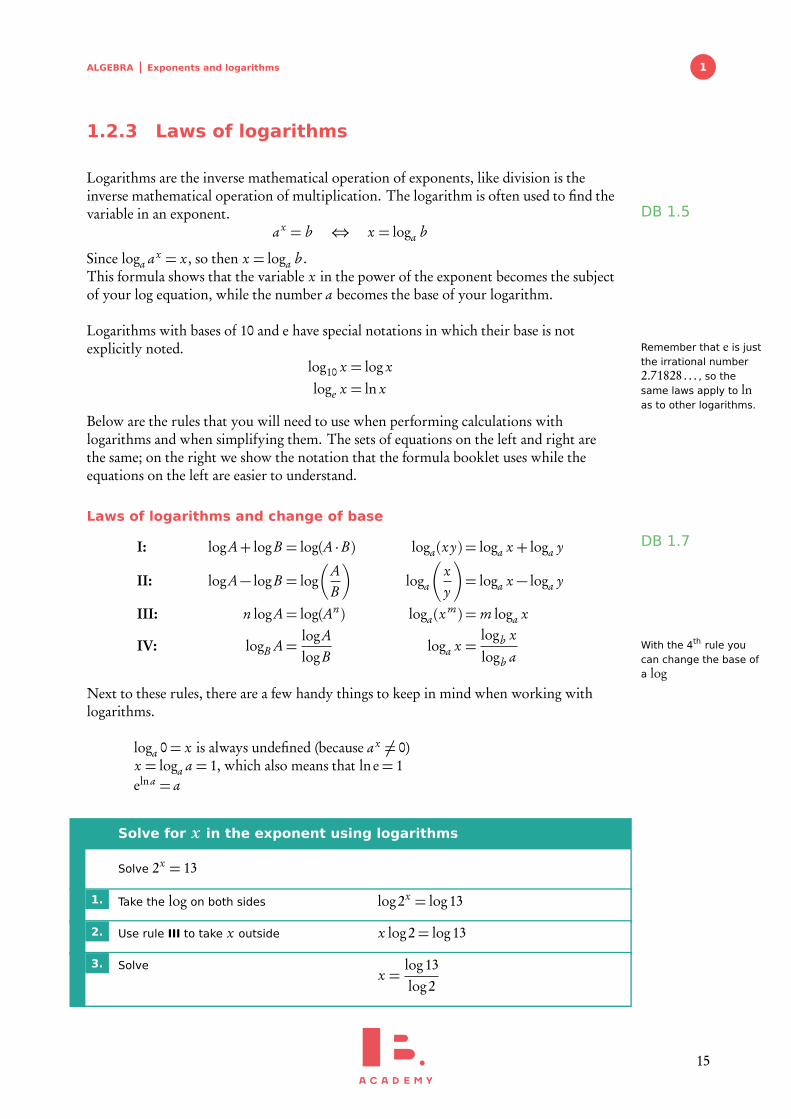
1.2.3 Laws of logarithms
Logarithms are the inverse mathematical operation of exponents, like division is theinverse mathematical operation of multiplication. The logarithm is often used to find thevariable in an exponent. DB 1.5
ax = b ⇔ x = loga b
Since loga ax = x, so then x = loga b .This formula shows that the variable x in the power of the exponent becomes the subjectof your log equation, while the number a becomes the base of your logarithm.
Logarithms with bases of 10 and e have special notations in which their base is notexplicitly noted. Remember that e is just
the irrational number2.71828 . . . , so thesame laws apply to lnas to other logarithms.
log10 x = log xloge x = ln x
Below are the rules that you will need to use when performing calculations withlogarithms and when simplifying them. The sets of equations on the left and right arethe same; on the right we show the notation that the formula booklet uses while theequations on the left are easier to understand.
Laws of logarithms and change of base
DB 1.7I: logA+ logB = log(A ·B) loga(xy) = loga x + loga y
II: logA− logB = log�
AB
�
loga
�
xy
�
= loga x − loga y
III: n logA= log(An) loga(xm) = m loga x
With the 4th rule youcan change the base ofa log
IV: logB A=logAlogB
loga x =logb xlogb a
Next to these rules, there are a few handy things to keep in mind when working withlogarithms.
loga 0= x is always undefined (because ax 6= 0)x = loga a = 1, which also means that lne= 1elna = a
Solve for x in the exponent using logarithms
Solve 2x = 13
1. Take the log on both sides log2x = log13
2. Use rule III to take x outside x log2= log13
3. Solvex =
log13log2
15
ALGEBRA Binomial expansion
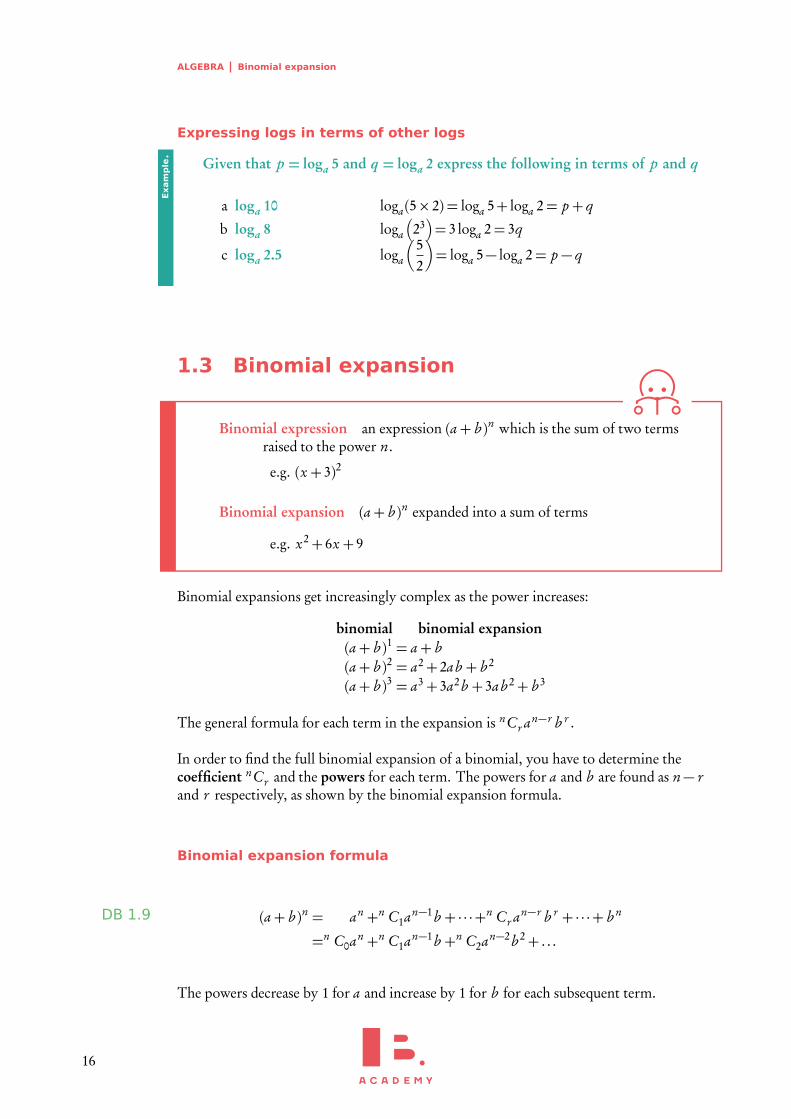
Expressing logs in terms of other logs
Given that p = loga 5 and q = loga 2 express the following in terms of p and q
a loga 10 loga(5× 2) = loga 5+ loga 2= p + q
b loga 8 loga
�
23�
= 3 loga 2= 3q
c loga 2.5 loga
�
52
�
= loga 5− loga 2= p − q
Exam
ple.
1.3 Binomial expansion
Binomial expression an expression (a+ b )n which is the sum of two termsraised to the power n.
e.g. (x + 3)2
Binomial expansion (a+ b )n expanded into a sum of terms
e.g. x2+ 6x + 9
Binomial expansions get increasingly complex as the power increases:
binomial binomial expansion(a+ b )1 = a+ b(a+ b )2 = a2+ 2ab + b 2
(a+ b )3 = a3+ 3a2b + 3ab 2+ b 3
The general formula for each term in the expansion is nCr an−r b r .
In order to find the full binomial expansion of a binomial, you have to determine thecoefficient nCr and the powers for each term. The powers for a and b are found as n− rand r respectively, as shown by the binomial expansion formula.
Binomial expansion formula
DB 1.9 (a+ b )n = an +n C1an−1b + · · ·+n Cr an−r b r + · · ·+ b n
=n C0an +n C1an−1b +n C2an−2b 2+ . . .
The powers decrease by 1 for a and increase by 1 for b for each subsequent term.
16
ALGEBRA Binomial expansion 1
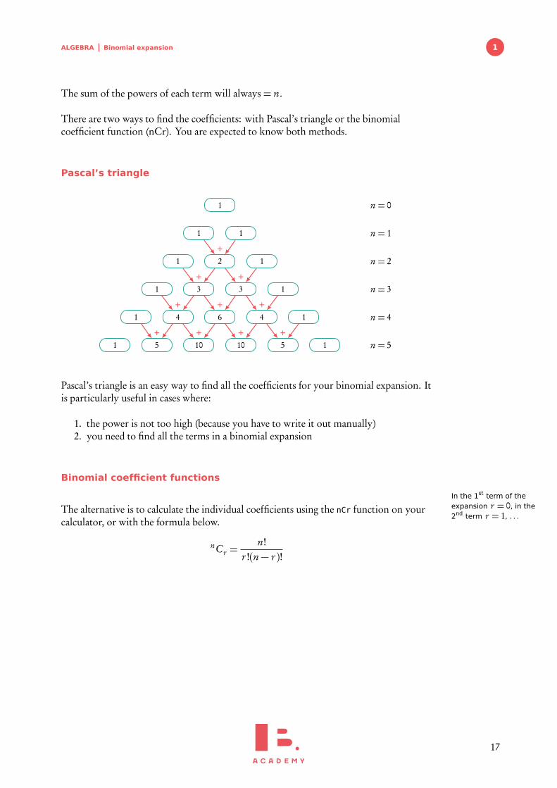
The sum of the powers of each term will always = n.
There are two ways to find the coefficients: with Pascal’s triangle or the binomialcoefficient function (nCr). You are expected to know both methods.
Pascal’s triangle
1
1 1
1 2+
1
1 3+
3+
1
1 4+
6+
4+
1
1 5+
10+
10+
5+
1
n = 0
n = 1
n = 2
n = 3
n = 4
n = 5
Pascal’s triangle is an easy way to find all the coefficients for your binomial expansion. Itis particularly useful in cases where:
1. the power is not too high (because you have to write it out manually)2. you need to find all the terms in a binomial expansion
Binomial coefficient functions
In the 1st term of theexpansion r = 0, in the2nd term r = 1, . . .
The alternative is to calculate the individual coefficients using the nCr function on yourcalculator, or with the formula below.
nCr =n!
r !(n− r )!
17
ALGEBRA Binomial expansion
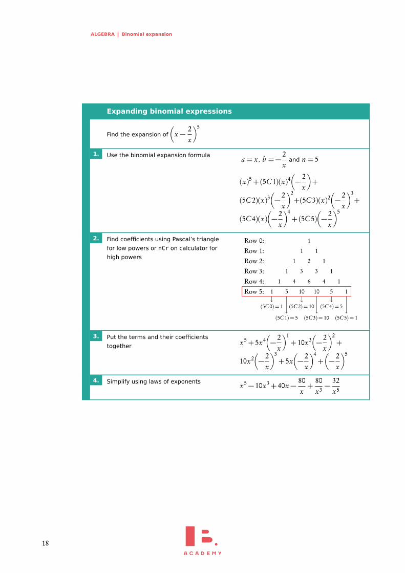
Expanding binomial expressions
Find the expansion of
�
x − 2x
�5
1. Use the binomial expansion formula a = x , b =− 2x
and n = 5
(x)5+(5C 1)(x)4�
− 2x
�
+
(5C 2)(x)3�
− 2x
�2+(5C 3)(x)2
�
− 2x
�3+
(5C 4)(x)�
− 2x
�4+(5C 5)
�
− 2x
�5
2. Find coefficients using Pascal’s triangle
for low powers or nCr on calculator for
high powers
1
1 1
1 2 1
1 3 3 1
1 4 6 4 1
1 5 10 10 5 1
Row 0:Row 1:Row 2:Row 3:Row 4:Row 5:
(5C 0) = 1
(5C 1) = 5
(5C 2) = 10
(5C 3) = 10
(5C 4) = 5
(5C 5) = 1
3. Put the terms and their coefficients
together x5+ 5x4�
− 2x
�1+ 10x3
�
− 2x
�2+
10x2�
− 2x
�3+ 5x
�
− 2x
�4+�
− 2x
�5
4. Simplify using laws of exponents x5− 10x3+ 40x − 80x+
80x3− 32
x5
18
ALGEBRA Binomial expansion 1
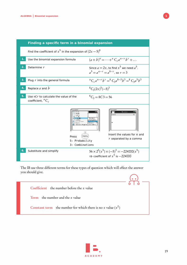
Finding a specific term in a binomial expansion
Find the coefficient of x5 in the expansion of (2x − 5)8
1. Use the binomial expansion formula (a+ b )n = · · ·+n Cr an−r b r + . . .
2. Determine r Since a = 2x , to find x5 we need a5.
a5 = an−r = a8−r , so r = 3
3. Plug r into the general formula nCr an−r b r =8 C3a8−3b 3 =8 C3a5b 3
4. Replace a and b 8C3(2x)5(−5)3
5. Use nCr to calculate the value of the
coefficient, nCr
8C3 = 8C 3= 56
IB ACADEMY
Press menu
5: Probability
3: Combinations
IB ACADEMY
Insert the values for n and
r separated by a comma
6. Substitute and simplify 56× 25(x5)× (−5)3 =−224000(x5)⇒ coefficient of x5 is −224000
The IB use three different terms for these types of question which will effect the answeryou should give.
Coefficient the number before the x value
Term the number and the x value
Constant term the number for which there is no x value (x0)
19

2FUNCTIONSTable of contents & cheatsheet
Definitions
Function a mathematical relationship where each input has a single output. It is often written as f (x)where x is the input
Domain all possible x values, the input. (the domain of investigation)
Range possible y values, the output. (the range of outcomes)
Coordinates uniquely determines the position of a point, given by (x, y)
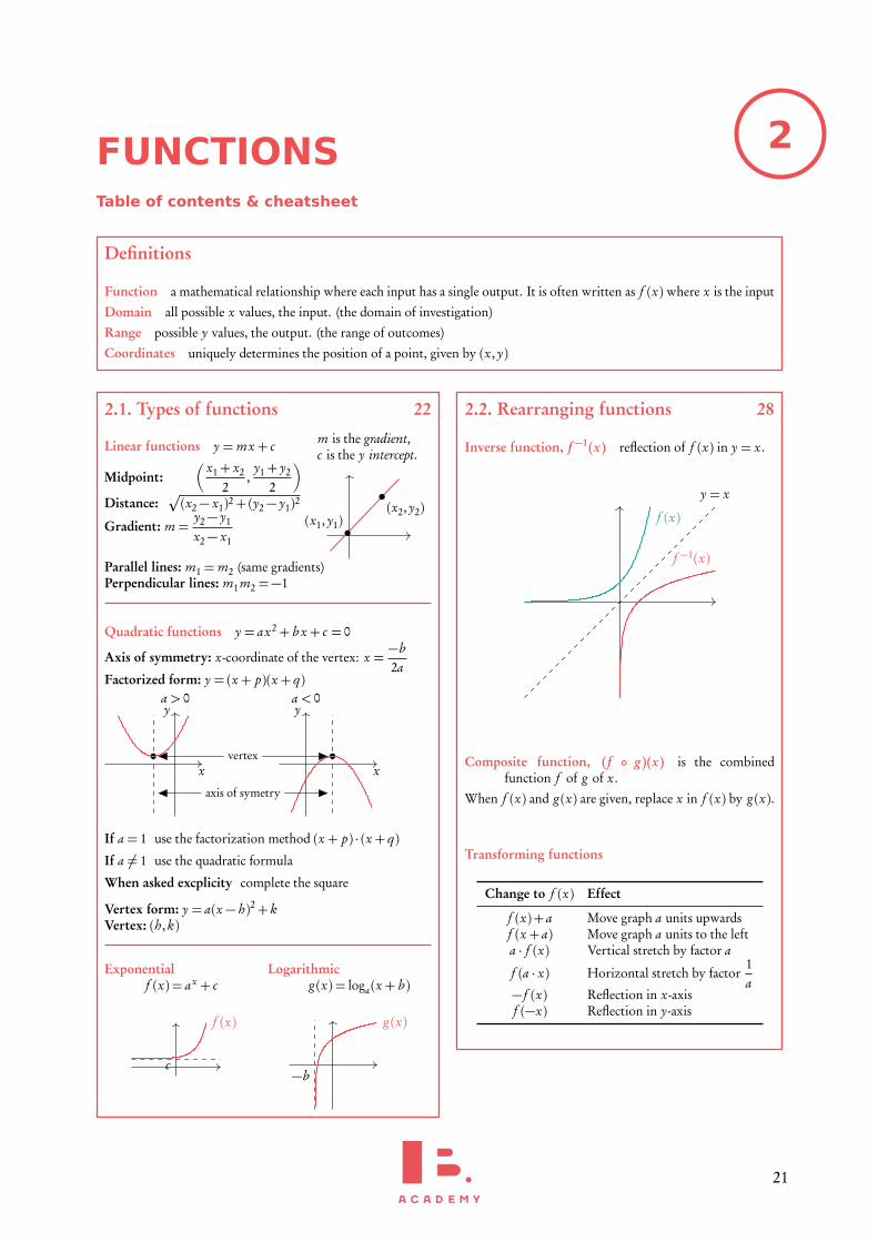
2.1. Types of functions 22
Linear functions y = mx + c m is the gradient,c is the y intercept.
Midpoint:� x1+ x2
2,
y1+ y2
2
�
Distance:p
(x2− x1)2+(y2− y1)2
Gradient: m =y2− y1
x2− x1
(x1, y1)(x2, y2)
Parallel lines: m1 = m2 (same gradients)Perpendicular lines: m1m2 =−1
Quadratic functions y = ax2+ b x + c = 0
Axis of symmetry: x-coordinate of the vertex: x =−b2a
Factorized form: y = (x + p)(x + q)
x
ya > 0
x
ya < 0
vertex
axis of symetry
If a = 1 use the factorization method (x + p) · (x + q)
If a 6= 1 use the quadratic formula
When asked excplicity complete the square
Vertex form: y = a(x − h)2+ kVertex: (h, k)
Exponentialf (x) = ax + c
f (x)
c
Logarithmicg (x) = loga(x + b )
g (x)
−b
2.2. Rearranging functions 28
Inverse function, f −1(x) reflection of f (x) in y = x.
y = x
f (x)
f −1(x)
Composite function, (f ◦ g)(x) is the combinedfunction f of g of x.
When f (x) and g (x) are given, replace x in f (x) by g (x).
Transforming functions
Change to f (x) Effect
f (x)+ a Move graph a units upwardsf (x + a) Move graph a units to the lefta · f (x) Vertical stretch by factor a
f (a · x) Horizontal stretch by factor1a
− f (x) Reflection in x-axisf (−x) Reflection in y-axis
21
FUNCTIONS Types of functions
2.1 Types of functions
Functions are mathematical relationships where each input has a single output. You haveprobably been doing functions since you began learning maths, but they may havelooked like this:
16 +10 26 Algebraically this is:f (x) = x + 10,here x = 16, y = 26.
We can use graphs to show multiple outputs of y for inputs x, and therefore visualize therelation between the two. Two common types of functions are linear functions andquadratic functions.
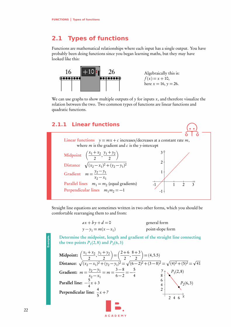
2.1.1 Linear functions
Linear functions y = mx + c increases/decreases at a constant rate m,where m is the gradient and c is the y-intercept
Midpoint� x1+ x2
2,
y1+ y2
2
�
DistanceÆ
(x2− x1)2+(y2− y1)2
Gradient m =y2− y1
x2− x1
Parallel lines m1 = m2 (equal gradients)Perpendicular lines m1m2 =−1
-1
-1
1
1
2
2
3
3
Straight line equations are sometimes written in two other forms, which you should becomfortable rearranging them to and from:
ax + b y + d = 0 general formy − y1 = m(x − x1) point-slope form
Determine the midpoint, length and gradient of the straight line connectingthe two points P1(2, 8) and P2(6, 3)
Midpoint:� x1+ x2
2,
y1+ y2
2
�
=�
2+ 62
,8+ 3
2
�
= (4,5.5)
Distance:p
(x2− x1)2+(y2− y1)2 =p
(6− 2)2+(3− 8)2 =p
(4)2+(5)2 =p
41
Gradient: m =y2− y1
x2− x1= m =
3− 86− 2
=−54
Parallel line: −54
x + 3
Perpendicular line:45
x + 7x
y
2 4 6
2468
P1(2,8)
P2(6,3)
Exam
ple.
22
FUNCTIONS Types of functions 2
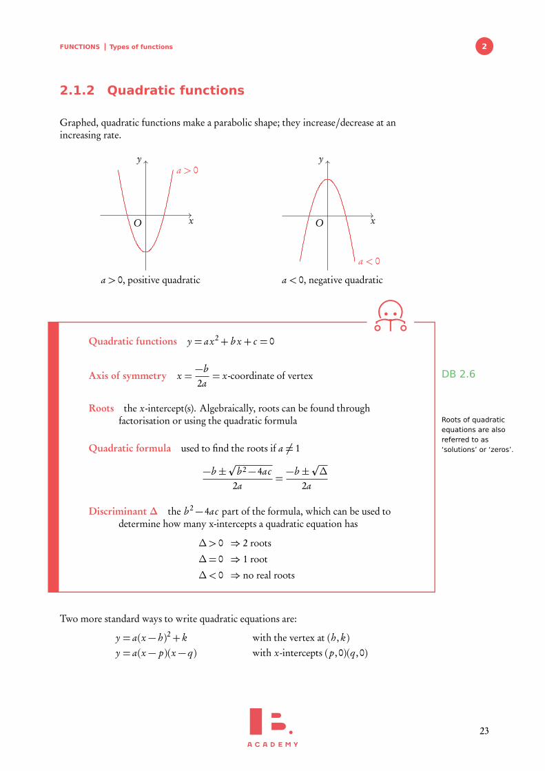
2.1.2 Quadratic functions
Graphed, quadratic functions make a parabolic shape; they increase/decrease at anincreasing rate.
x
y
O
a > 0
a > 0, positive quadratic
x
y
O
a < 0
a < 0, negative quadratic
Quadratic functions y = ax2+ b x + c = 0
Axis of symmetry x =−b2a= x-coordinate of vertex DB 2.6
Roots the x-intercept(s). Algebraically, roots can be found throughfactorisation or using the quadratic formula Roots of quadratic
equations are alsoreferred to as‘solutions’ or ‘zeros’.Quadratic formula used to find the roots if a 6= 1
−b ±p
b 2− 4ac2a
=−b ±
p∆
2a
Discriminant ∆ the b 2− 4ac part of the formula, which can be used todetermine how many x-intercepts a quadratic equation has
∆> 0 ⇒ 2 roots
∆= 0 ⇒ 1 root
∆< 0 ⇒ no real roots
Two more standard ways to write quadratic equations are:
y = a(x − h)2+ k with the vertex at (h, k)y = a(x − p)(x − q) with x-intercepts (p, 0)(q , 0)
23
FUNCTIONS Types of functions
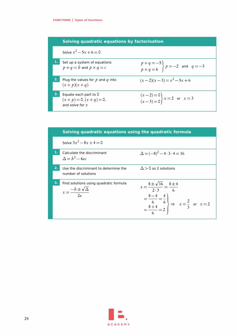
Solving quadratic equations by factorisation
Solve x2− 5x + 6= 0
1. Set up a system of equations
p + q = b and p × q = cp + q =−5p × q = 6
«
p =−2 and q =−3
2. Plug the values for p and q into
(x + p)(x + q)(x − 2)(x − 3) = x2− 5x + 6
3. Equate each part to 0(x + p) = 0, (x + q) = 0,
and solve for x
(x − 2) = 0(x − 3) = 0
«
x = 2 or x = 3
Solving quadratic equations using the quadratic formula
Solve 3x2− 8x + 4= 0
1. Calculate the discriminant
∆= b 2− 4ac∆= (−8)2− 4 · 3 · 4= 16
2. Use the discriminant to determine the
number of solutions
∆> 0 so 2 solutions
3. Find solutions using quadratic formula
x =−b ±
p∆
2a
x =8±p
162 · 3
=8± 4
6
=8− 4
6=
46
=8+ 4
6= 2
⇒ x =23
or x = 2
24
FUNCTIONS Types of functions 2
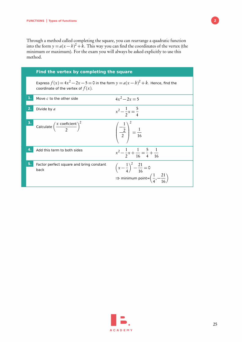
Through a method called completing the square, you can rearrange a quadratic functioninto the form y = a(x − h)2+ k. This way you can find the coordinates of the vertex (theminimum or maximum). For the exam you will always be asked explicitly to use thismethod.
Find the vertex by completing the square
Express f (x) = 4x2− 2x − 5= 0 in the form y = a(x − h)2+ k . Hence, find the
coordinate of the vertex of f (x).
1. Move c to the other side 4x2− 2x = 5
2. Divide by a x2− 12
x =54
3.Calculate
� x coeficient
2
�2
−12
2
2
=116
4. Add this term to both sides x2− 12
x +116=
54+
116
5. Factor perfect square and bring constant
back
�
x − 14
�2− 21
16= 0
⇒ minimum point=
�
14
,−2116
�
25
FUNCTIONS Types of functions
2.1.3 Functions with asymptotes
Asymptote a straight line that a curve approaches, but never touches.
A single function can have multiple asymptotes: horizontal, vertical and in rare casesdiagonal. Functions that contain the variable (x) in the denominator of a fraction andexponential and logarithmic functions will always have asymptotes.
Vertical asymptotes
Vertical asymptotes occur when the denominator is zero, as dividing by zero isundefinable. Therefore if the denominator contains x and there is a value for x for whichthe denominator will be 0, we get a vertical asymptote.
In the function f (x) =x
x − 4the denominator is 0 when x = 4, so this line forms the
a vertical asymptote.Exam
ple.
Horizontal asymptotes
Horizontal asymptotes are the value that a function tends to as x becomes really big orreally small; technically speaking to the limit of infinity, x→∞. The general idea is thenthat when x is large, other parts of the function not involving x become insignificant andso can be ignored.
In the function f (x) =x
x − 4, when x is small the 4 is important.
x = 10 10− 4= 6But as x gets bigger the 4 becomes increasingly insignificant
x = 100 100− 4= 96x = 10000 10000− 4= 9996
Therefore as we approach the limits we can ignore the 4.lim
x→∞f (x) =
xx= 1
So there is a horizontal asymptote at y = 1.
Exam
ple.
26
FUNCTIONS Types of functions 2
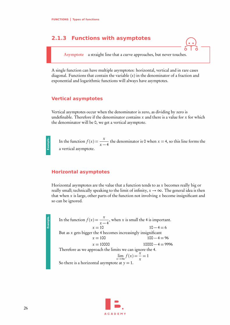
Exponential and logarithmic functions
Exponential functions will always have a horizontal asymptote and logarithmicfunctions will always have a vertical asymptote, due to the nature of these functions. Theposition of the asymptote is determined by constants in the function.
Exponential
f (x) = ax + c asymptote at y = c
where a is a positive number (often e)f (x)
c
Logarithmic
g (x) = loga(x+b ) asymptote at x =−b
g (x)
−b
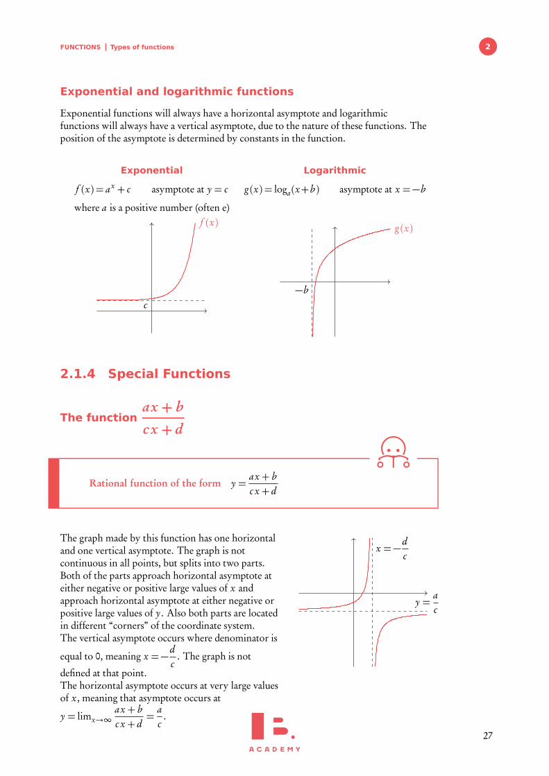
2.1.4 Special Functions
The functionax + b
c x + d
Rational function of the form y =ax + bc x + d
The graph made by this function has one horizontaland one vertical asymptote. The graph is notcontinuous in all points, but splits into two parts.Both of the parts approach horizontal asymptote ateither negative or positive large values of x andapproach horizontal asymptote at either negative orpositive large values of y. Also both parts are locatedin different “corners” of the coordinate system.The vertical asymptote occurs where denominator is
equal to 0, meaning x =−dc
. The graph is not
defined at that point.The horizontal asymptote occurs at very large valuesof x, meaning that asymptote occurs at
y = limx→∞ax + bc x + d
=ac
.
x =−dc
y =ac
27
FUNCTIONS Rearranging functions
2.2 Rearranging functions
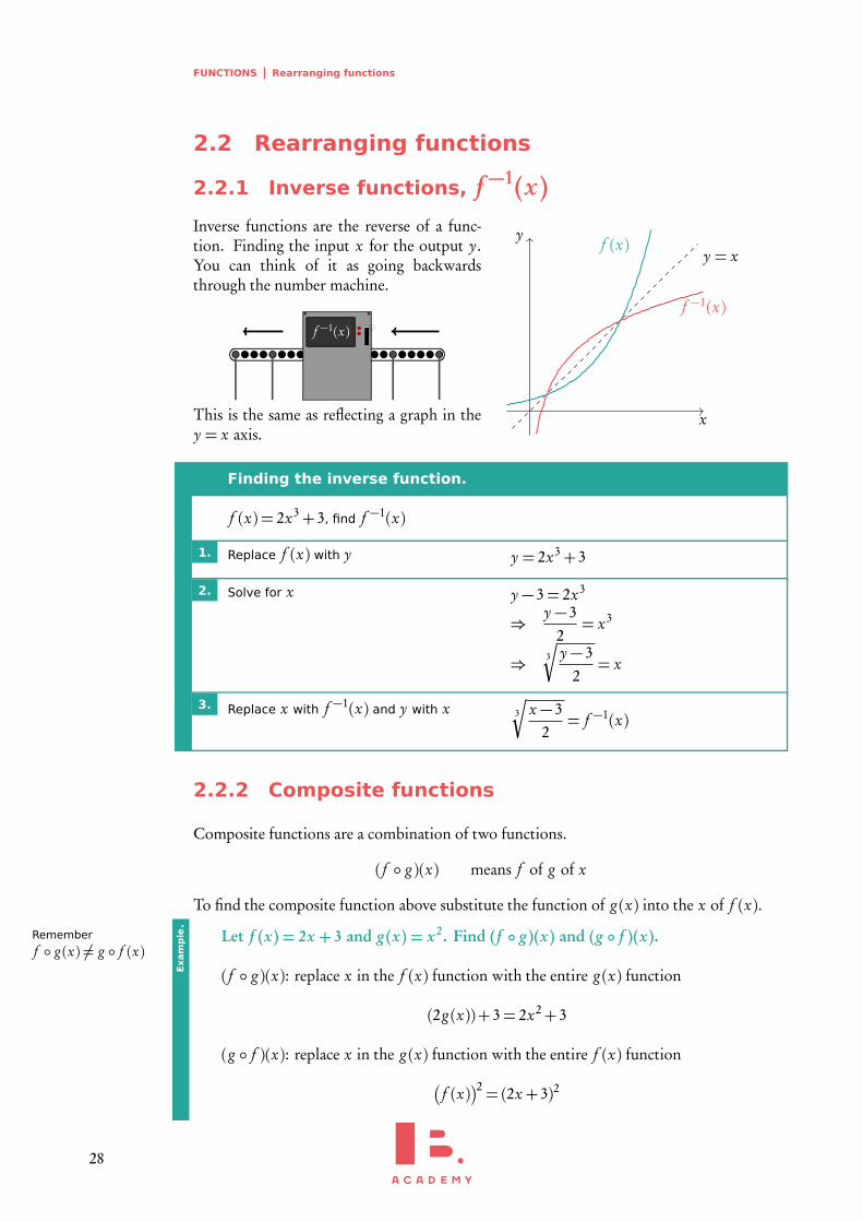
2.2.1 Inverse functions, f −1(x)Inverse functions are the reverse of a func-tion. Finding the input x for the output y.You can think of it as going backwardsthrough the number machine.
f −1(x)
This is the same as reflecting a graph in they = x axis.
x
yy = x
f (x)
f −1(x)
Finding the inverse function.
f (x) = 2x3+ 3, find f −1(x)
1. Replace f (x) with y y = 2x3+ 3
2. Solve for x y − 3= 2x3
⇒y − 3
2= x3
⇒ 3
s
y − 32= x
3. Replace x with f −1(x) and y with x 3
s
x − 32= f −1(x)
2.2.2 Composite functions
Composite functions are a combination of two functions.
( f ◦ g )(x) means f of g of x
To find the composite function above substitute the function of g (x) into the x of f (x).
Let f (x) = 2x + 3 and g(x) = x2. Find (f ◦ g)(x) and (g ◦ f )(x).Remember
f ◦ g (x) 6= g ◦ f (x)
( f ◦ g )(x): replace x in the f (x) function with the entire g (x) function
(2g (x))+ 3= 2x2+ 3
(g ◦ f )(x): replace x in the g (x) function with the entire f (x) function
�
f (x)�2 = (2x + 3)2
Exam
ple.
28
FUNCTIONS Rearranging functions 2
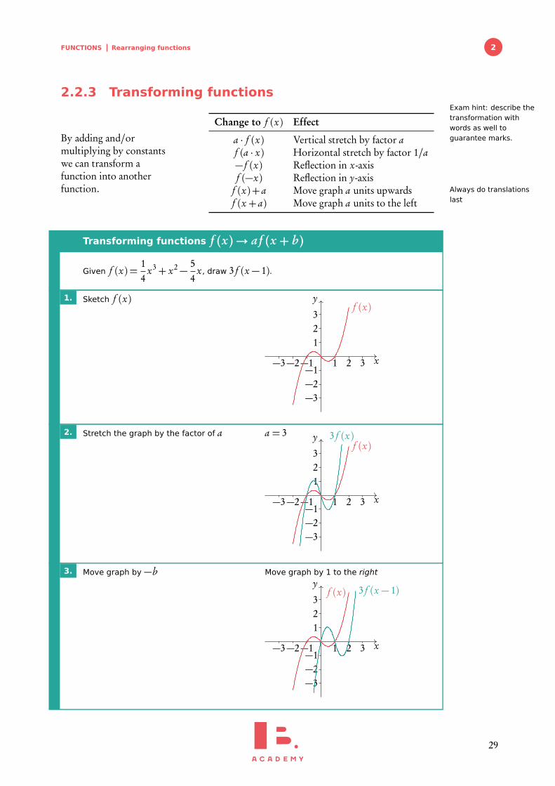
2.2.3 Transforming functionsExam hint: describe thetransformation withwords as well toguarantee marks.By adding and/or
multiplying by constantswe can transform afunction into anotherfunction.
Change to f (x) Effect
a · f (x) Vertical stretch by factor af (a · x) Horizontal stretch by factor 1/a− f (x) Reflection in x-axisf (−x) Reflection in y-axis
f (x)+ a Move graph a units upwards Always do translationslastf (x + a) Move graph a units to the left
Transforming functions f (x)→ a f (x + b)
Given f (x) =14
x3+ x2− 54
x , draw 3 f (x − 1).
1. Sketch f (x)
x
y
−3
−3
−2
−2
−1−11
1
2
2
3
3f (x)
2. Stretch the graph by the factor of a a = 3
x
y
−3
−3
−2
−2
−1−11
1
2
2
3
3f (x)
3 f (x)
3. Move graph by −b Move graph by 1 to the right
x
y
−3
−3
−2
−2
−1−11
1
2
2
3
3f (x) 3 f (x − 1)
29
FUNCTIONS Intersection
2.3 Intersection
When functions intersect the x and y-values are equal, so at the point of intersectionf (x) = g (x).
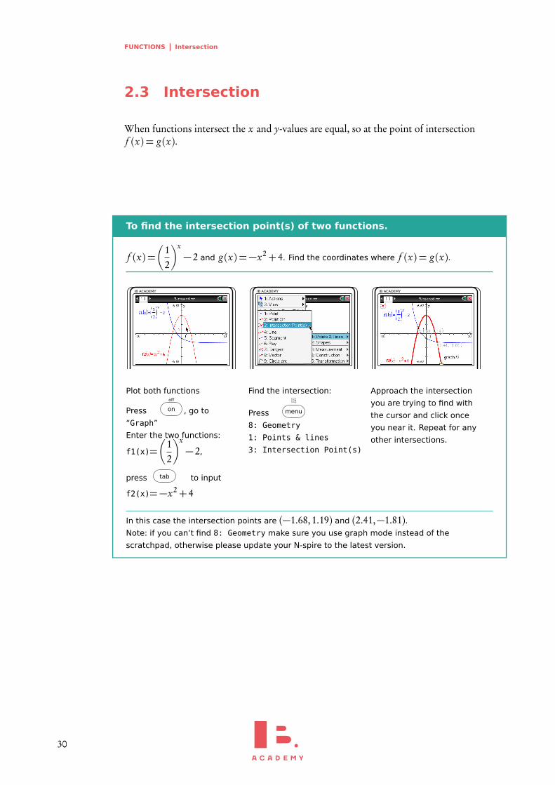
To find the intersection point(s) of two functions.
f (x) =�
12
�x− 2 and g (x) =−x2+ 4. Find the coordinates where f (x) = g (x).
IB ACADEMY
Plot both functions
Press
off
on , go to
“Graph”
Enter the two functions:
f1(x)=�
12
�x− 2,
press tab to input
f2(x)=−x2+ 4
IB ACADEMY
Find the intersection:
Press menu
8: Geometry
1: Points & lines
3: Intersection Point(s)
IB ACADEMY
Approach the intersection
you are trying to find with
the cursor and click once
you near it. Repeat for any
other intersections.
In this case the intersection points are (−1.68,1.19) and (2.41,−1.81).Note: if you can’t find 8: Geometry make sure you use graph mode instead of the
scratchpad, otherwise please update your N-spire to the latest version.
30
3TRIGONOMETRY AND
CIRCULAR FUNCTIONSTable of contents & cheatsheet
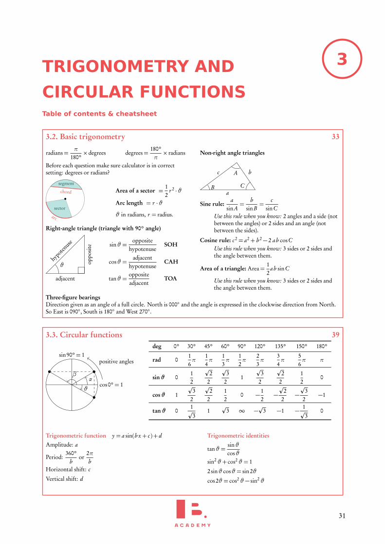
3.2. Basic trigonometry 33
radians=π
180°× degrees degrees=
180°π× radians
Before each question make sure calculator is in correctsetting: degrees or radians?
chord
segment
arc
sector
Area of a sector =12
r 2 ·ϑ
Arc length = r ·ϑ
ϑ in radians, r = radius.
Right-angle triangle (triangle with 90° angle)
adjacent
hypo
tenus
e
ϑ oppo
site sinϑ =
oppositehypotenuse
SOH
cosϑ =adjacent
hypotenuseCAH
tanϑ =oppositeadjacent
TOA
Non-right angle triangles
a
bc
B C
A
Sine rule:a
sinA=
bsinB
=c
sinCUse this rule when you know: 2 angles and a side (notbetween the angles) or 2 sides and an angle (notbetween the sides).
Cosine rule: c2 = a2+ b 2− 2 ab cosCUse this rule when you know: 3 sides or 2 sides andthe angle between them.
Area of a triangle: Area=12
ab sinC
Use this rule when you know: 3 sides or 2 sides andthe angle between them.
Three-figure bearingsDirection given as an angle of a full circle. North is 000◦ and the angle is expressed in the clockwise direction from North.So East is 090◦, South is 180◦ and West 270◦.
3.3. Circular functions 39
sin90°= 1
cos0°= 1
positive angles
αβ
ϑ
deg 0° 30° 45° 60° 90° 120° 135° 150° 180°
rad 016π
14π
13π
12π
23π
34π
56π π
sinϑ 012
p2
2
p3
21
p3
2
p2
212
0
cosϑ 1
p3
2
p2
212
0 −12
−p
22
−p
32
−1
tanϑ 01p
31
p3 ∞ −
p3 −1 − 1
p3
0
Trigonometric function y = a sin(b x + c)+ d
Amplitude: a
Period:360°
bor
2πb
Horizontal shift: c
Vertical shift: d
Trigonometric identities
tanϑ =sinϑcosϑ
sin2ϑ+ cos2ϑ = 1
2sinϑ cosϑ = sin2ϑ
cos2ϑ = cos2ϑ− sin2ϑ
31
TRIGONOMETRY AND CIRCULAR FUNCTIONS Properties of 3D shapes
3.1 Properties of 3D shapes
3.1.1 Points in 3D space
When you are learning about the points on a 2-dimensional plane, you also learn how tofind distances between those two points. One of the easiest ways to derive that formula isby constructing a triangle and using Pythagoras. In the same way it is possible to derive avery similar expression for distance between two points in a 3D space:
d =Æ
(x1− x2)2+(y1− y2)2+(z1− z2)2
You have also learnt how to find the midpoint between the two points (x1, y1) and(x2, y2): add those individual coordinates together and divide the sum by two. One canfind the midpoint between two points in 3D space in almost exact same way:
� x1+ x2
2,
y1+ y2
2,
z1+ z2
2
�
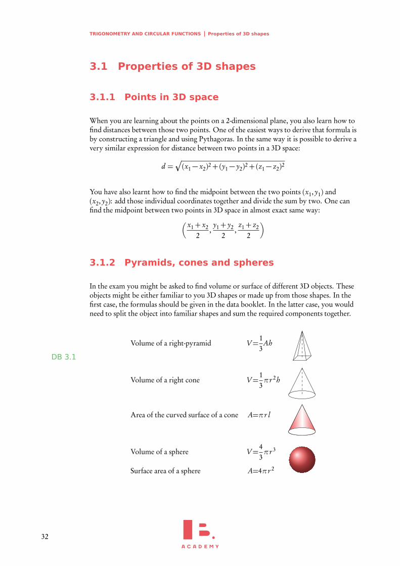
3.1.2 Pyramids, cones and spheres
In the exam you might be asked to find volume or surface of different 3D objects. Theseobjects might be either familiar to you 3D shapes or made up from those shapes. In thefirst case, the formulas should be given in the data booklet. In the latter case, you wouldneed to split the object into familiar shapes and sum the required components together.
Volume of a right-pyramid V=13
Ah
DB 3.1
Volume of a right cone V=13πr 2h
Area of the curved surface of a cone A=πr l
Volume of a sphere V=43πr 3
Surface area of a sphere A=4πr 2
32
TRIGONOMETRY AND CIRCULAR FUNCTIONS Basic trigonometry 3
3.2 Basic trigonometry
This section offers an overview of some basic trigonometry rules and values that willrecur often. It is worthwhile to know these by heart; but it is much better to understandhow to obtain these values. Like converting between Celsius and Fahrenheit; you canremember some values that correspond to each other but if you understand how toobtain them, you will be able to convert any temperature.
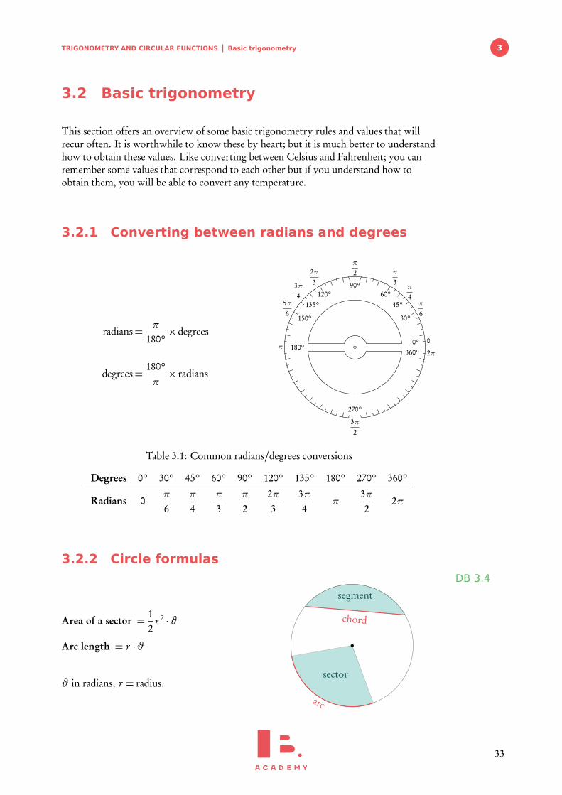
3.2.1 Converting between radians and degrees
radians=π
180°× degrees
degrees=180°π× radians
30°
π
645°
π
460°
π
390°
π
2
120°
2π3
135°
3π4
150°
5π6
180°π
270°
3π2
0° 0
360° 2π
Table 3.1: Common radians/degrees conversions
Degrees 0° 30° 45° 60° 90° 120° 135° 180° 270° 360°
Radians 0π
6π
4π
3π
22π3
3π4
π3π2
2π
3.2.2 Circle formulasDB 3.4
Area of a sector =12
r 2 ·ϑ
Arc length = r ·ϑ
ϑ in radians, r = radius.
chord
segment
arc
sector
33
TRIGONOMETRY AND CIRCULAR FUNCTIONS Basic trigonometry
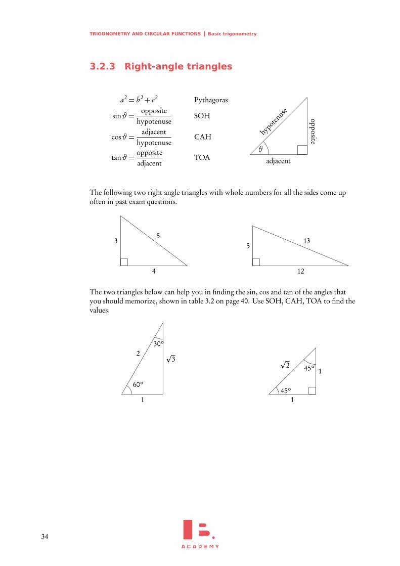
3.2.3 Right-angle triangles
a2 = b 2+ c2 Pythagoras
sinϑ =opposite
hypotenuseSOH
cosϑ =adjacent
hypotenuseCAH
tanϑ =oppositeadjacent
TOA adjacent
hypo
tenus
e
θ
opposite
The following two right angle triangles with whole numbers for all the sides come upoften in past exam questions.
4
53
12
135
The two triangles below can help you in finding the sin, cos and tan of the angles thatyou should memorize, shown in table 3.2 on page 40. Use SOH, CAH, TOA to find thevalues.
60°
30°
1
p3
2
45°
45°
1
1
p2
34
TRIGONOMETRY AND CIRCULAR FUNCTIONS Basic trigonometry 3
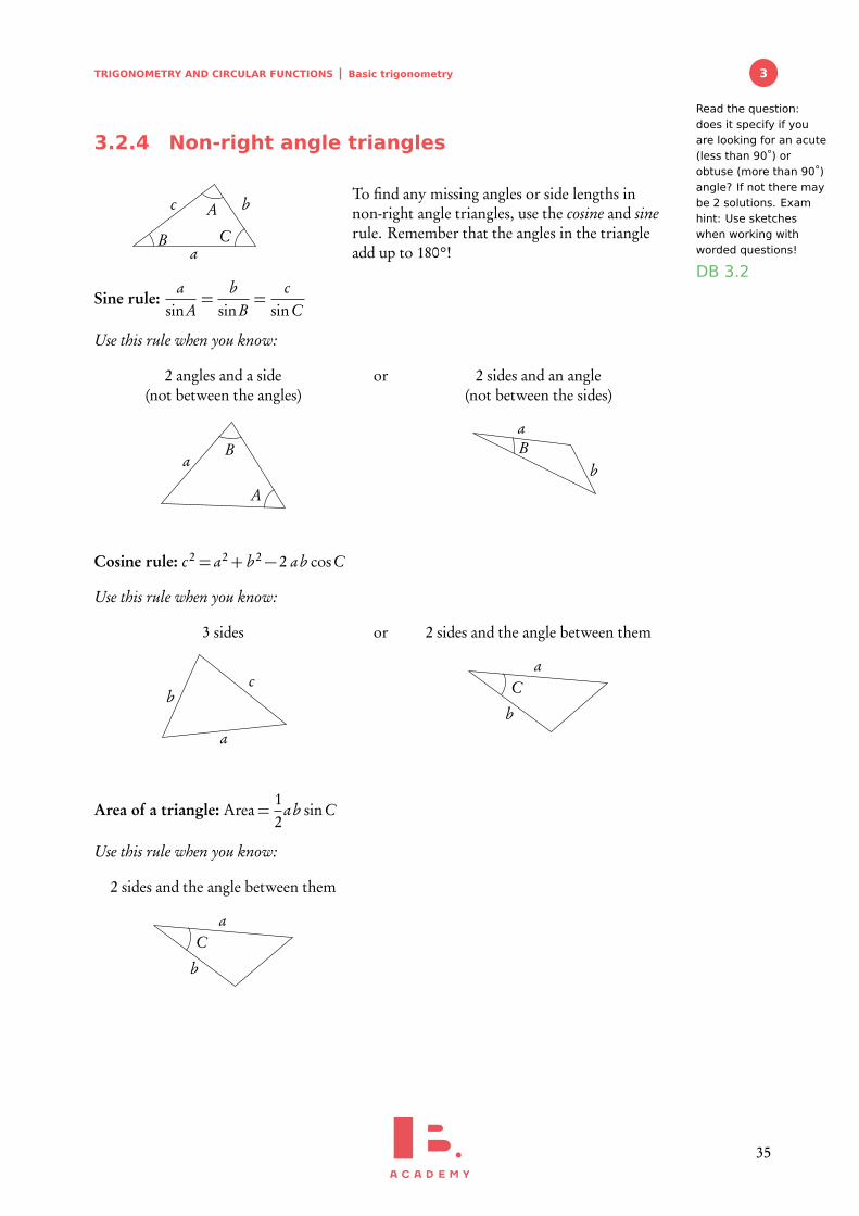
3.2.4 Non-right angle triangles
a
bc
B C
ATo find any missing angles or side lengths innon-right angle triangles, use the cosine and sinerule. Remember that the angles in the triangleadd up to 180°!
Read the question:does it specify if youare looking for an acute(less than 90°) orobtuse (more than 90°)angle? If not there maybe 2 solutions. Examhint: Use sketcheswhen working withworded questions!
DB 3.2
Sine rule:a
sinA=
bsinB
=c
sinC
Use this rule when you know:
2 angles and a side(not between the angles)
a
A
B
or 2 sides and an angle(not between the sides)
b
aB
Cosine rule: c2 = a2+ b 2− 2 ab cosC
Use this rule when you know:
3 sides
a
cb
or 2 sides and the angle between them
b
aC
Area of a triangle: Area=12
ab sinC
Use this rule when you know:
2 sides and the angle between them
b
aC
35
TRIGONOMETRY AND CIRCULAR FUNCTIONS Basic trigonometry
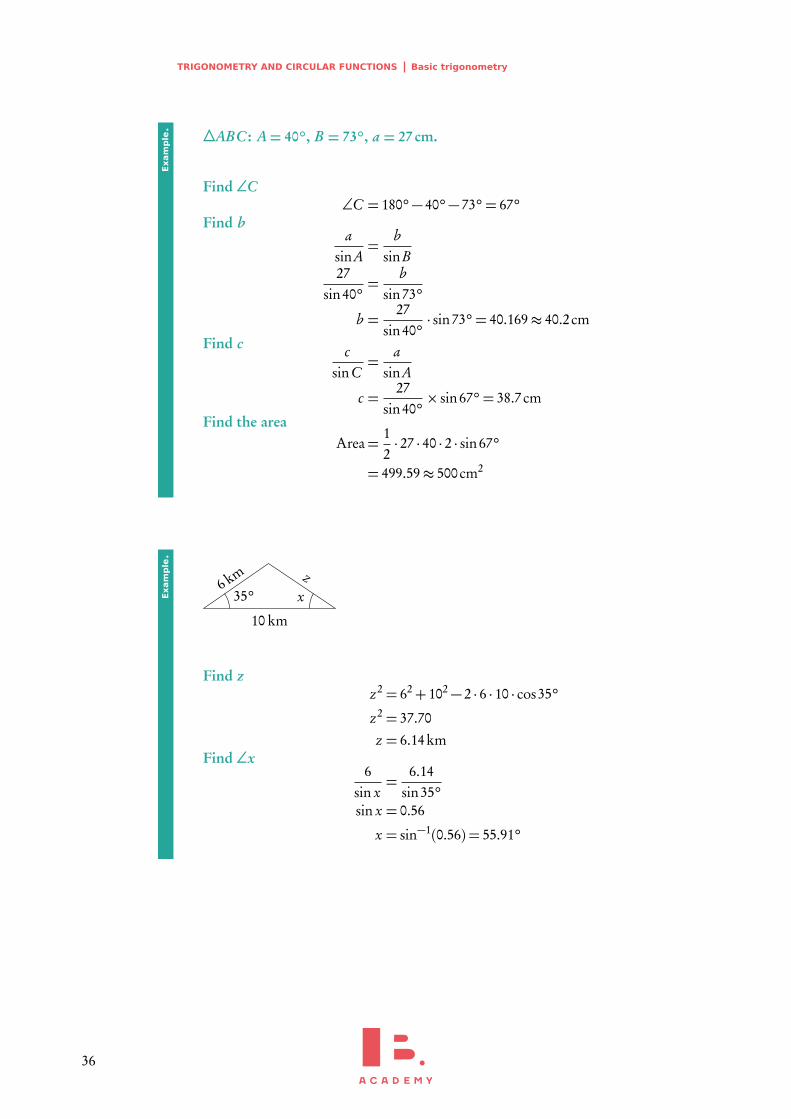
4ABC: A= 40°, B = 73°, a = 27 cm.
Find ∠C∠C = 180°− 40°− 73°= 67°
Find ba
sinA=
bsinB
27sin40°
=b
sin73°
b =27
sin40°· sin73°= 40.169≈ 40.2cm
Find c csinC
=a
sinA
c =27
sin40°× sin67°= 38.7cm
Find the areaArea=
12· 27 · 40 · 2 · sin67°
= 499.59≈ 500cm2
Exam
ple.
10 km
6 km z35° x
Find zz2 = 62+ 102− 2 · 6 · 10 · cos35°
z2 = 37.70z = 6.14km
Find ∠x6
sin x=
6.14sin35°
sin x = 0.56
x = sin−1(0.56) = 55.91°
Exam
ple.
36
TRIGONOMETRY AND CIRCULAR FUNCTIONS Basic trigonometry 3
3.2.5 Ambiguous case
Ambiguous case, also known as an angle-side-side case, is when the triangle is not uniquefrom the given information. It happens when you are given two sides and an angle notbetween those sides in a triangle.
You have to use a sine rule to solve a problem in this case. However, one needs toremember that sin x = sin(180°− x), meaning that your answer for an angle is not just x,but also 180°− x.
In other words, we might get two different possible angles as an answer and thus twodifferent possible triangles that satisfy the information given.
However, that is not always the case, if the sum of the two known angles becomes biggerthan 180°. So if you are required to calculate the third angle or total area of a triangle, youmight have to do the calculations for two different triangles using both of your angles.
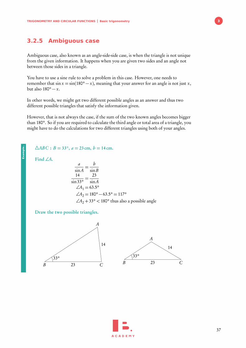
4ABC : B = 33°, a = 23 cm, b = 14 cm.
Find ∠A.a
sinA=
bsinB
14sin33°
=23
sinA∠A1 = 63.5°∠A2 = 180°− 63.5°= 117°∠A2+ 33°< 180° thus also a possible angle
Draw the two possible triangles.
23
14
A
B C33°
23
14
A
B C33°
Exam
ple.
37
TRIGONOMETRY AND CIRCULAR FUNCTIONS Basic trigonometry
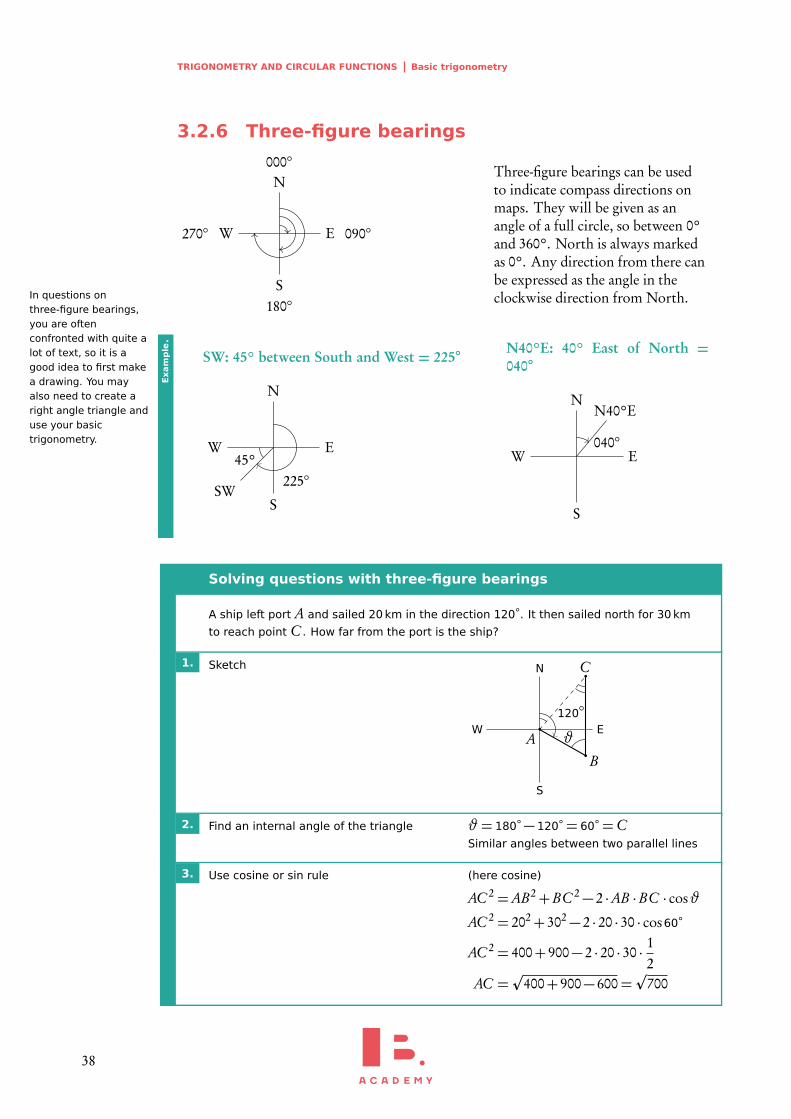
3.2.6 Three-figure bearings
N000◦
E 090◦
S180◦
W270◦
Three-figure bearings can be usedto indicate compass directions onmaps. They will be given as anangle of a full circle, so between 0°and 360°. North is always markedas 0°. Any direction from there canbe expressed as the angle in theclockwise direction from North.In questions on
three-figure bearings,you are oftenconfronted with quite alot of text, so it is agood idea to first makea drawing. You mayalso need to create aright angle triangle anduse your basictrigonometry.
SW: 45° between South and West = 225◦
N
E
S
W
SW
45°225◦
N40°E: 40° East of North =040◦
N
E
S
W
N40°E
040◦
Exam
ple.
Solving questions with three-figure bearings
A ship left port A and sailed 20 km in the direction 120°. It then sailed north for 30 km
to reach point C . How far from the port is the ship?
1. Sketch N
E
S
W
C
BA
120◦
ϑ
2. Find an internal angle of the triangle ϑ = 180°− 120°= 60°=CSimilar angles between two parallel lines
3. Use cosine or sin rule (here cosine)
AC 2 =AB2+BC 2− 2 ·AB ·BC · cosϑ
AC 2 = 202+ 302− 2 · 20 · 30 · cos60°
AC 2 = 400+ 900− 2 · 20 · 30 · 12
AC =p
400+ 900− 600=p
700
38
TRIGONOMETRY AND CIRCULAR FUNCTIONS Circular functions 3
3.3 Circular functions
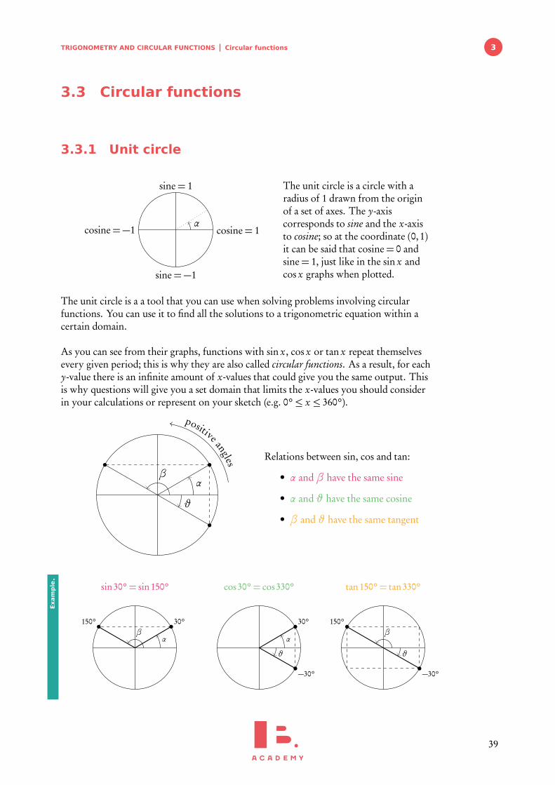
3.3.1 Unit circle
sine=−1
sine= 1
cosine=−1 cosine= 1α
The unit circle is a circle with aradius of 1 drawn from the originof a set of axes. The y-axiscorresponds to sine and the x-axisto cosine; so at the coordinate (0,1)it can be said that cosine= 0 andsine= 1, just like in the sin x andcos x graphs when plotted.
The unit circle is a a tool that you can use when solving problems involving circularfunctions. You can use it to find all the solutions to a trigonometric equation within acertain domain.
As you can see from their graphs, functions with sin x, cos x or tan x repeat themselvesevery given period; this is why they are also called circular functions. As a result, for eachy-value there is an infinite amount of x-values that could give you the same output. Thisis why questions will give you a set domain that limits the x-values you should considerin your calculations or represent on your sketch (e.g. 0°≤ x ≤ 360°).
positive angles
αβ
ϑ
Relations between sin, cos and tan:
• α and β have the same sine
• α and ϑ have the same cosine
• β and ϑ have the same tangent
sin30°= sin150°
30°150°
−30°
αβ
cos30°= cos330°
30°
−30°
150°
α
ϑ
tan150°= tan330°
30°
−30°
150°
ϑ
β
Exam
ple.
39
TRIGONOMETRY AND CIRCULAR FUNCTIONS Circular functions
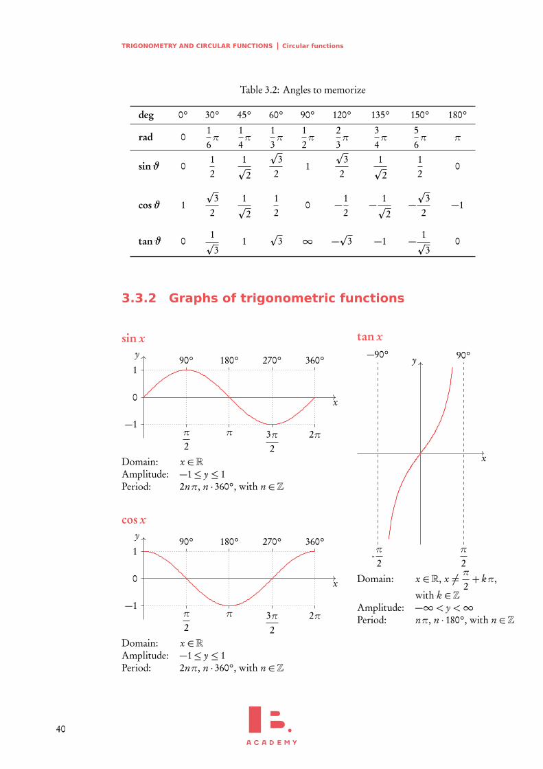
Table 3.2: Angles to memorize
deg 0° 30° 45° 60° 90° 120° 135° 150° 180°
rad 016π
14π
13π
12π
23π
34π
56π π
sinϑ 012
1p
2
p3
21
p3
21p
2
12
0
cosϑ 1
p3
21p
2
12
0 −12
− 1p
2−p
32
−1
tanϑ 01p
31
p3 ∞ −
p3 −1 − 1
p3
0
3.3.2 Graphs of trigonometric functions
sin x
x
y
π
2
90°
π
180°
3π2
270°
2π
360°
−1
1
0
Domain: x ∈RAmplitude: −1≤ y ≤ 1Period: 2nπ, n · 360°, with n ∈Z
cos x
x
y
π
2
90°
π
180°
3π2
270°
2π
360°
−1
1
0
Domain: x ∈RAmplitude: −1≤ y ≤ 1Period: 2nπ, n · 360°, with n ∈Z
tan x
x
y
-π
2
−90°
π
2
90°
Domain: x ∈R, x 6= π2+ kπ,
with k ∈ZAmplitude: −∞< y <∞Period: nπ, n · 180°, with n ∈Z
40
TRIGONOMETRY AND CIRCULAR FUNCTIONS Circular functions 3
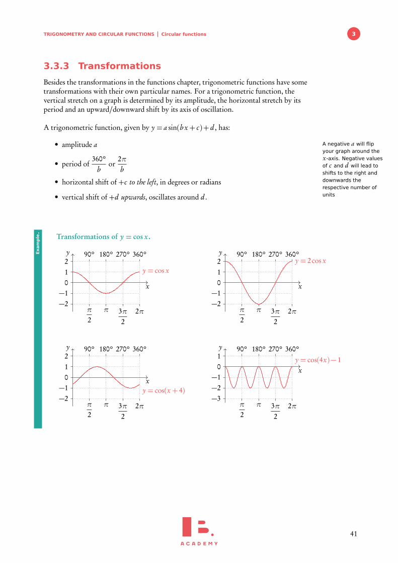
3.3.3 Transformations
Besides the transformations in the functions chapter, trigonometric functions have sometransformations with their own particular names. For a trigonometric function, thevertical stretch on a graph is determined by its amplitude, the horizontal stretch by itsperiod and an upward/downward shift by its axis of oscillation.
A trigonometric function, given by y = a sin(b x + c)+ d , has:
• amplitude a A negative a will flipyour graph around thex-axis. Negative valuesof c and d will lead toshifts to the right anddownwards therespective number ofunits
• period of360°
bor
2πb
• horizontal shift of +c to the left, in degrees or radians
• vertical shift of +d upwards, oscillates around d .
Transformations of y = cos x .
x
y
π
2
90°
π
180°
3π2
270°
2π
360°
−2−1
12
0
y = cos x
x
y
π
2
90°
π
180°
3π2
270°
2π
360°
−2−1
12
0
y = 2cos x
x
y
π
2
90°
π
180°
3π2
270°
2π
360°
−2−1
12
0
y = cos(x + 4)
x
y
π
2
90°
π
180°
3π2
270°
2π
360°
−3−2−1
10
y = cos(4x)− 1
Exam
ple.
41
TRIGONOMETRY AND CIRCULAR FUNCTIONS Circular functions
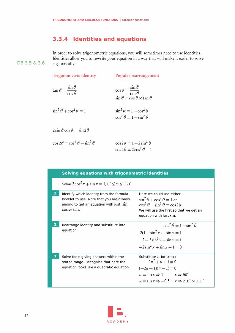
3.3.4 Identities and equations
In order to solve trigonometric equations, you will sometimes need to use identities.Identities allow you to rewrite your equation in a way that will make it easier to solvealgebraically.DB 3.5 & 3.6
Trigonometric identity Popular rearrangement
tanϑ =sinϑcosϑ
cosϑ =sinϑtanϑ
sinϑ = cosϑ× tanϑ
sin2ϑ+ cos2ϑ = 1 sin2ϑ = 1− cos2ϑ
cos2ϑ = 1− sin2ϑ
2sinϑ cosϑ = sin2ϑ
cos2ϑ = cos2ϑ− sin2ϑ cos2ϑ = 1− 2sin2ϑ
cos2ϑ = 2cos2ϑ− 1
Solving equations with trigonometric identities
Solve 2cos2 x + sin x = 1, 0°≤ x ≤ 360°.
1. Identify which identity from the formula
booklet to use. Note that you are always
aiming to get an equation with just, sin,
cos or tan.
Here we could use either
sin2ϑ+ cos2ϑ = 1 or
cos2ϑ− sin2ϑ = cos2ϑ.
We will use the first so that we get an
equation with just sin.
2. Rearrange identity and substitute into
equation.cos2ϑ = 1− sin2ϑ
2(1− sin2 x)+ sin x = 1
2− 2sin2 x + sin x = 1
−2sin2 x + sin x + 1= 0
3. Solve for x giving answers within the
stated range. Recognise that here the
equation looks like a quadratic equation.
Substitute u for sin x:
−2u2+ u + 1= 0(−2u − 1)(u − 1) = 0u = sin x⇒ 1 x⇒ 90°u = sin x⇒−0.5 x⇒ 210° or 330°
42
4DIFFERENTIATIONTable of contents & cheatsheet
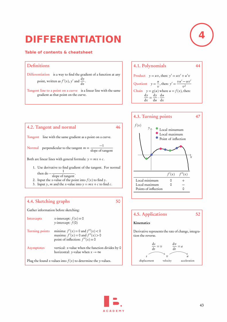
Definitions
Differentiation is a way to find the gradient of a function at any
point, written as f ′(x), y ′ anddydx
.
Tangent line to a point on a curve is a linear line with the samegradient as that point on the curve.
4.1. Polynomials 44
Product y = uv, then: y ′ = uv ′+ u ′v
Quotient y =uv
, then: y ′ =v u ′− uv ′
v2
Chain y = g (u) where u = f (x), then:dydx=
dydu· du
dx
4.2. Tangent and normal 46
Tangent line with the same gradient as a point on a curve.
Normal perpendicular to the tangent m =−1
slope of tangent
Both are linear lines with general formula: y = mx + c .
1. Use derivative to find gradient of the tangent. For normal
then do − 1slope of tangent
.
2. Input the x-value of the point into f (x) to find y.3. Input y, m and the x-value into y = mx + c to find c .
4.3. Turning points 47
x
yf (x)
Local minumumLocal maximumPoint of inflection
f ′(x) f ′′(x)
Local minimum 0 +Local maximum 0 −Points of inflection 0
4.4. Sketching graphs 50
Gather information before sketching:
Intercepts x-intercept: f (x) = 0y-intercept: f (0)
Turning points minima: f ′(x) = 0 and f ′′(x)< 0maxima: f ′(x) = 0 and f ′′(x)> 0point of inflection: f ′′(x) = 0
Asymptotes vertical: x-value when the function divides by 0horizontal: y-value when x→∞
Plug the found x-values into f (x) to determine the y-values.
4.5. Applications 52
Kinematics
Derivative represents the rate of change, integra-tion the reverse.
s v adisplacement velocity acceleration
d sdt= v
dvdt= a
43
DIFFERENTIATION Polynomials
4.1 Polynomials
As you have learnt in the section on functions, a straight line graph has a gradient. Thisgradient describes the rate at which the graph is changing and thanks to it we can tellhow steep the line will be. In fact gradients can be found for any function - the specialthing about linear functions is that their gradient is always the same (given by min y = mx + c ). For polynomial functions the gradient is always changing. This is wherecalculus comes in handy; we can use differentiation to derive a function using which wecan find the gradient for any value of x.
Using the following steps, you can find the derivative function ( f ′(x)) for anypolynomial function ( f (x)).
Polynomial a mathematical expression or function that contains severalterms often raised to different powers
e.g. y = 3x2, y = 121x5+ 7x3+ x or y = 4x23 + 2x
13
Principles y = f (x) = axn ⇒dydx= f ′(x) = naxn−1.
The (original) function is described by y or f (x), the derivative
(gradient) function is described bydydx
or f ′(x).
Derivative of a constant (number) 0
e.g. For f (x) = 5, f ′(x) = 0
Derivative of a sum sum of derivatives.
If a function you are looking to differentiate is made up of severalsummed parts, find the derivatives for each part separately and thenadd them together again.
e.g. f (x) = axn and g (x) = b x m
f ′(x)+ g ′(x) = naxn−1+mb x m−1
44
DIFFERENTIATION Polynomials 4
4.1.1 Rules
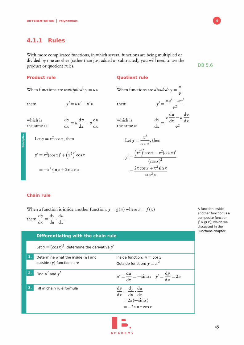
With more complicated functions, in which several functions are being multiplied ordivided by one another (rather than just added or subtracted), you will need to use theproduct or quotient rules. DB 5.6
Product rule Quotient rule
When functions are multiplied: y = uv When functions are divided: y =uv
then: y ′= uv ′+ u ′v then: y ′=v u ′− uv ′
v2
which isthe same as
dydx= u
dvdx+ v
dudx
which isthe same as
dydx=
vdudx− u
dvdx
v2
Let y = x2 cos x, then Let y =x2
cos x, then
y ′ = x2(cos x)′+�
x2�′
cos x y ′ =
�
x2�′
cos x − x2(cos x)′
(cos x)2
=−x2 sin x + 2x cos x =2x cos x + x2 sin x
cos2 x
Exam
ple.
Chain rule
When a function is inside another function: y = g (u) where u = f (x) A function insideanother function is acomposite function,f ◦ g (x), which wediscussed in theFunctions chapter
then:dydx=
dydu· du
dx.
Differentiating with the chain rule
Let y = (cos x)2, determine the derivative y ′
1. Determine what the inside (u) and
outside (y) functions are
Inside function: u = cos xOutside function: y = u2
2. Find u ′ and y ′ u ′ =dudx=− sin x; y ′ =
dydu= 2u
3. Fill in chain rule formula dydx=
dydu· du
dx= 2u(− sin x)=−2sin x cos x
45
DIFFERENTIATION Tangent and normal equation
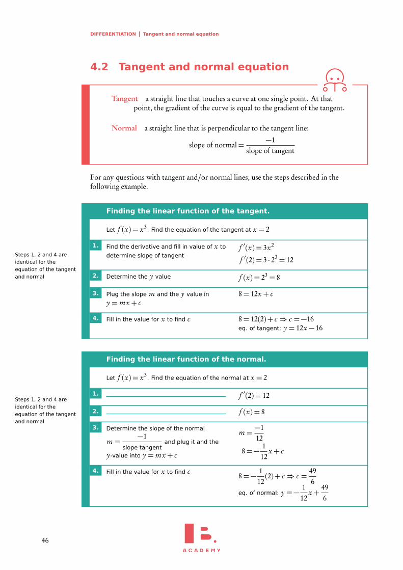
4.2 Tangent and normal equation
Tangent a straight line that touches a curve at one single point. At thatpoint, the gradient of the curve is equal to the gradient of the tangent.
Normal a straight line that is perpendicular to the tangent line:
slope of normal=−1
slope of tangent
For any questions with tangent and/or normal lines, use the steps described in thefollowing example.
Finding the linear function of the tangent.
Let f (x) = x3. Find the equation of the tangent at x = 2
1. Find the derivative and fill in value of x to
determine slope of tangentSteps 1, 2 and 4 areidentical for theequation of the tangentand normal
f ′(x) = 3x2
f ′(2) = 3 · 22 = 12
2. Determine the y value f (x) = 23 = 8
3. Plug the slope m and the y value in
y = mx + c8= 12x + c
4. Fill in the value for x to find c 8= 12(2)+ c ⇒ c =−16eq. of tangent: y = 12x − 16
Finding the linear function of the normal.
Let f (x) = x3. Find the equation of the normal at x = 2
1. f ′(2) = 12Steps 1, 2 and 4 areidentical for theequation of the tangentand normal
2. f (x) = 8
3. Determine the slope of the normal
m =−1
slope tangentand plug it and the
y-value into y = mx + c
m =−112
8=− 112
x + c
4. Fill in the value for x to find c 8=− 112(2)+ c ⇒ c =
496
eq. of normal: y =− 112
x +496
46
DIFFERENTIATION Turning points 4
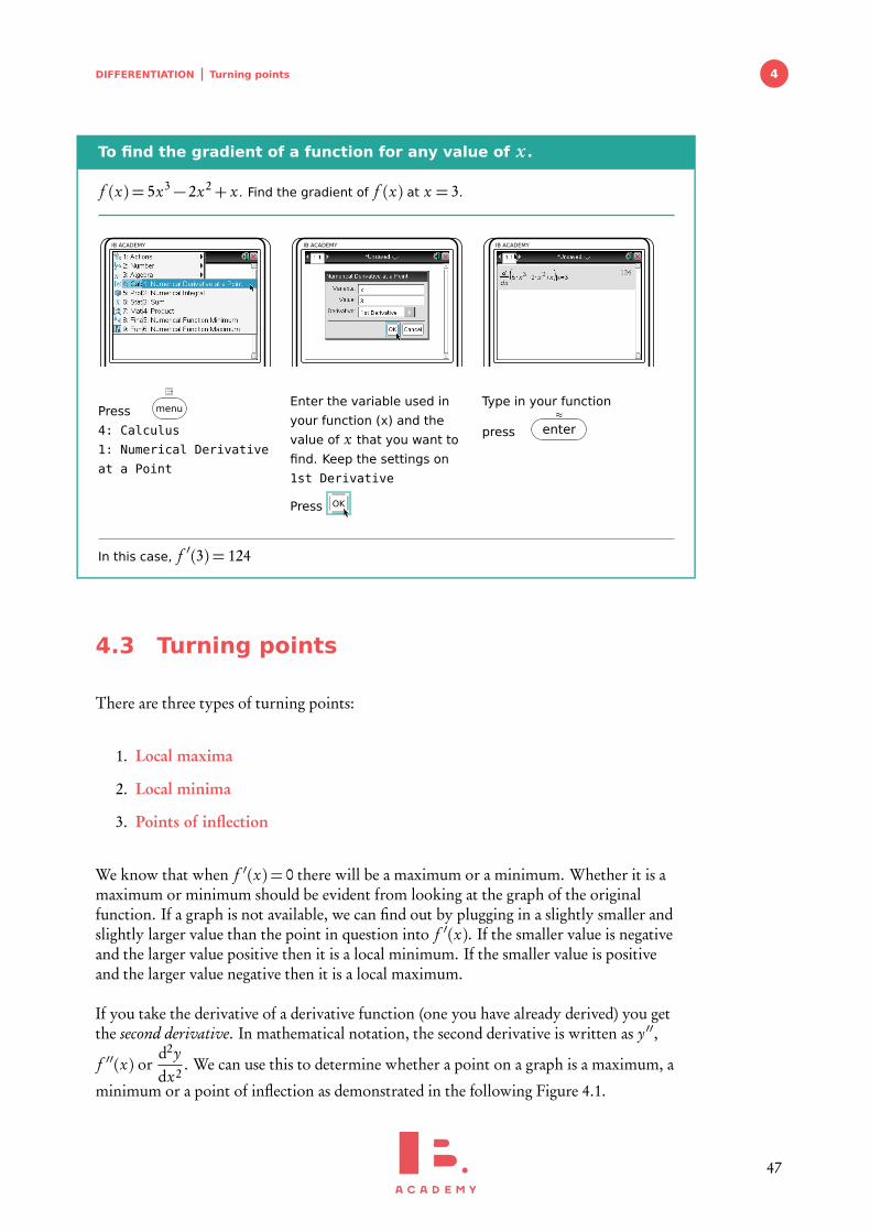
To find the gradient of a function for any value of x .
f (x) = 5x3− 2x2+ x . Find the gradient of f (x) at x = 3.
IB ACADEMY
Press menu
4: Calculus
1: Numerical Derivative
at a Point
IB ACADEMY
Enter the variable used in
your function (x) and the
value of x that you want to
find. Keep the settings on
1st Derivative
Press OK
IB ACADEMY
Type in your function
press
≈
enter
In this case, f ′(3) = 124
4.3 Turning points
There are three types of turning points:
1. Local maxima
2. Local minima
3. Points of inflection
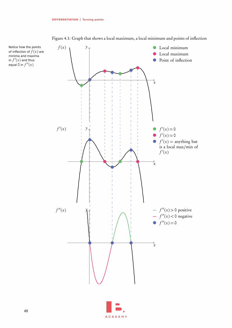
We know that when f ′(x) = 0 there will be a maximum or a minimum. Whether it is amaximum or minimum should be evident from looking at the graph of the originalfunction. If a graph is not available, we can find out by plugging in a slightly smaller andslightly larger value than the point in question into f ′(x). If the smaller value is negativeand the larger value positive then it is a local minimum. If the smaller value is positiveand the larger value negative then it is a local maximum.
If you take the derivative of a derivative function (one you have already derived) you getthe second derivative. In mathematical notation, the second derivative is written as y ′′,
f ′′(x) ord2ydx2
. We can use this to determine whether a point on a graph is a maximum, a
minimum or a point of inflection as demonstrated in the following Figure 4.1.
47
DIFFERENTIATION Turning points
Figure 4.1: Graph that shows a local maximum, a local minimum and points of inflection
Notice how the points
of inflection of f (x) areminima and maximain f ′(x) and thus
equal 0 in f ′′(x)
x
y
x
y
x
y
f (x)
f ′(x)
f ′′(x)
Local minimumLocal maximumPoint of inflection
f ′(x) = 0f ′(x) = 0f ′(x) = anything butis a local max/min off ′(x)
f ′′(x) = 0
f ′′(x)> 0 positivef ′′(x)< 0 negative
48
DIFFERENTIATION Turning points 4
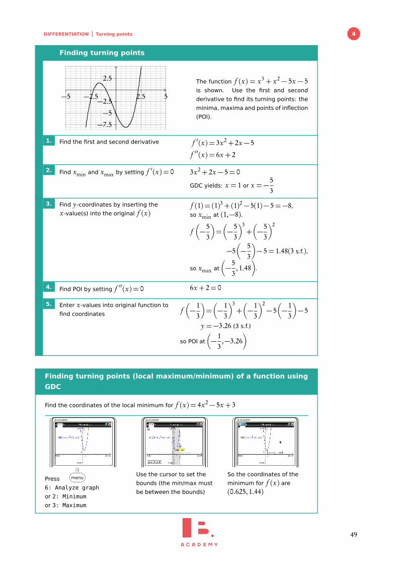
Finding turning points
−5 −2.5 2.5 5
−7.5
−5
−2.5
2.5 The function f (x) = x3 + x2 − 5x − 5is shown. Use the first and second
derivative to find its turning points: the
minima, maxima and points of inflection
(POI).
1. Find the first and second derivative f ′(x) = 3x2+ 2x − 5
f ′′(x) = 6x + 2
2. Find xmin and xmax by setting f ′(x) = 0 3x2+ 2x − 5= 0
GDC yields: x = 1 or x =−53
3. Find y-coordinates by inserting the
x-value(s) into the original f (x)f (1) = (1)3+(1)2− 5(1)− 5=−8,
so xmin at (1,−8).
f�
−53
�
=�
−53
�3+�
−53
�2
−5�
−53
�
− 5= 1.48(3 s.f.),
so xmax at
�
−53
,1.48�
.
4. Find POI by setting f ′′(x) = 0 6x + 2= 0
5. Enter x-values into original function to
find coordinates f�
−13
�
=�
−13
�3+�
−13
�2− 5
�
−13
�
− 5
y =−3.26 (3 s.f.)
so POI at
�
−13
,−3.26�
Finding turning points (local maximum/minimum) of a function using
GDC
Find the coordinates of the local minimum for f (x) = 4x2− 5x + 3
IB ACADEMY
Press menu
6: Analyze graph
or 2: Minimum
or 3: Maximum
IB ACADEMY
Use the cursor to set the
bounds (the min/max must
be between the bounds)
IB ACADEMY
So the coordinates of the
minimum for f (x) are
(0.625,1.44)
49
DIFFERENTIATION Sketching graphs
4.4 Sketching graphs
When sketching a graph, you will need the following information:
1. Intercepts,
2. Turning points (maximums, minimums and inflection points) and
3. Asymptotes
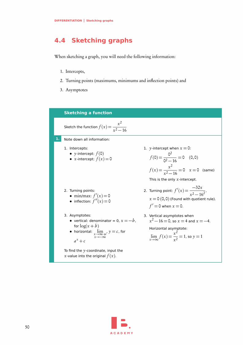
Sketching a function
Sketch the function f (x) =x2
x2− 16
1. Note down all information:
1. Intercepts:
• y-intercept: f (0)• x-intercept: f (x) = 0
2. Turning points:
• min/max: f ′(x) = 0• inflection: f ′′(x) = 0
3. Asymptotes:
• vertical: denominator = 0, x =−b ,
for log(x + b )• horizontal: lim
x→∞ orx→−∞
, y = c , for
ax + c
To find the y-coordinate, input the
x-value into the original f (x).
1. y-intercept when x = 0:
f (0) =02
02− 16= 0 (0,0)
f (x) =x2
x2− 16= 0 x = 0 (same)
This is the only x-intercept.
2. Turning point: f ′(x) =−32x
x2− 162 ,
x = 0 (0,0) (Found with quotient rule).
f ′ = 0 when x = 0.
3. Vertical asymptotes when
x2− 16= 0, so x = 4 and x =−4.
Horizontal asymptote:
limx→∞
f (x) =x2
x2= 1, so y = 1
50
DIFFERENTIATION Sketching graphs 4
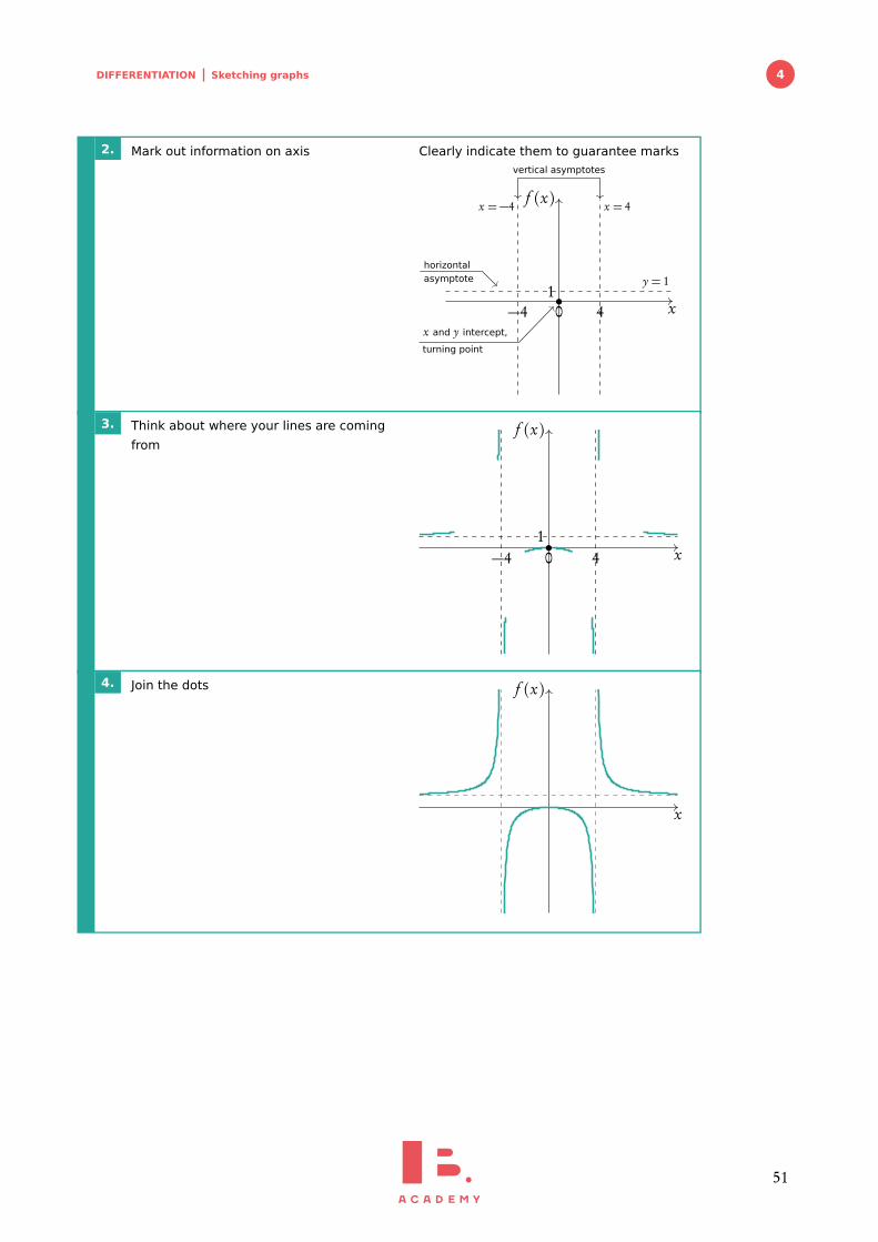
2. Mark out information on axis Clearly indicate them to guarantee marks
x
f (x)
x and y intercept,
turning point
x =−4 x = 4
y = 1
vertical asymptotes
horizontalasymptote
−4 0 41
3. Think about where your lines are coming
from
x
f (x)
−4 0 41
4. Join the dots
x
f (x)
51
DIFFERENTIATION Applications
4.5 Applications
4.5.1 Kinematics
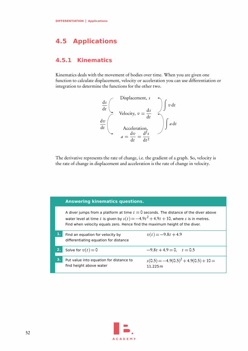
Kinematics deals with the movement of bodies over time. When you are given onefunction to calculate displacement, velocity or acceleration you can use differentiation orintegration to determine the functions for the other two.
Displacement, s
Velocity, v =d sdt
Acceleration,
a =dvdt=
d2 sdt 2
d sdt
dvdt
∫
a dt
∫
v dt
The derivative represents the rate of change, i.e. the gradient of a graph. So, velocity isthe rate of change in displacement and acceleration is the rate of change in velocity.
Answering kinematics questions.
A diver jumps from a platform at time t = 0 seconds. The distance of the diver above
water level at time t is given by s(t ) =−4.9t 2+ 4.9t + 10, where s is in metres.
Find when velocity equals zero. Hence find the maximum height of the diver.
1. Find an equation for velocity by
differentiating equation for distance
v(t ) =−9.8t + 4.9
2. Solve for v(t ) = 0 −9.8t + 4.9= 0, t = 0.5
3. Put value into equation for distance to
find height above waters(0.5) =−4.9(0.5)2+ 4.9(0.5)+ 10=11.225m
52
DIFFERENTIATION Applications 4
4.5.2 Optimization
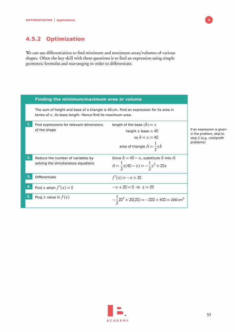
We can use differentiation to find minimum and maximum areas/volumes of variousshapes. Often the key skill with these questions is to find an expression using simplegeometric formulas and rearranging in order to differentiate.
Finding the minimum/maximum area or volume
The sum of height and base of a triangle is 40 cm. Find an expression for its area in
terms of x , its base length. Hence find its maximum area.
1. Find expressions for relevant dimensions
of the shape If an expression is givenin the problem, skip tostep 2 (e.g. cost/profitproblems)
length of the base (b )= xheight+ base= 40
so h + x = 40
area of triangle A=12
x h
2. Reduce the number of variables by
solving the simultaneous equations
Since h = 40− x , substitute h into A:
A=12
x(40− x) =−12
x2+ 20x
3. Differentiate f ′(x) =−x + 20
4. Find x when f ′(x) = 0 −x + 20= 0 ⇒ x = 20
5. Plug x value in f (x) −12
202+ 20(20) =−200+ 400= 200cm2
53

5INTEGRATIONTable of contents & cheatsheet
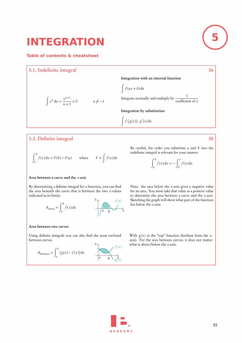
5.1. Indefinite integral 56
∫
xn dx =xn+1
n+ 1+C n 6=−1
Integration with an internal function∫
f (ax + b )dx
Integrate normally and multiply by1
coefficient of x
Integration by substitution∫
f�
g (x)�
· g ′(x)dx
5.2. Definite integral 58
∫ b
af (x)dx = F (b )− F (a) where F =
∫
f (x)dx
Be careful, the order you substitute a and b into theindefinite integral is relevant for your answer:
∫ b
af (x)dx =−
∫ a
bf (x)dx
Area between a curve and the x-axis
By determining a definite integral for a function, you can findthe area beneath the curve that is between the two x-valuesindicated as its limits.
Acurve =∫ b
af (x)dx
x
y
a b
f (x)
Note: the area below the x-axis gives a negative valuefor its area. You must take that value as a positive valueto determine the area between a curve and the x-axis.Sketching the graph will show what part of the functionlies below the x-axis.
Area between two curves
Using definite integrals you can also find the areas enclosedbetween curves.
Abetween =∫ b
a
�
g (x)− f (x)�
dxx
y
a b
f (x)
g (x)
With g (x) as the “top” function (furthest from the x-axis). For the area between curves, it does not matterwhat is above/below the x-axis.
55
INTEGRATION Indefinite integral and boundary condition
5.1 Indefinite integral and boundary
condition
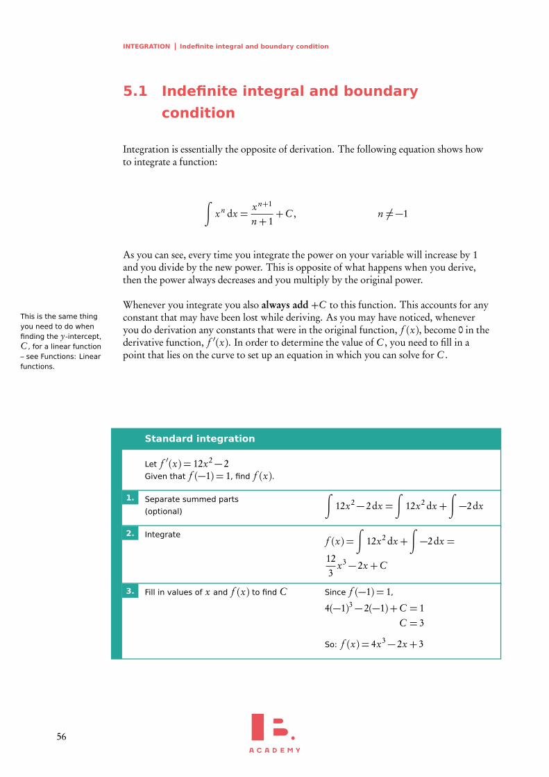
Integration is essentially the opposite of derivation. The following equation shows howto integrate a function:
∫
xn dx =xn+1
n+ 1+C , n 6=−1
As you can see, every time you integrate the power on your variable will increase by 1and you divide by the new power. This is opposite of what happens when you derive,then the power always decreases and you multiply by the original power.
Whenever you integrate you also always add +C to this function. This accounts for anyconstant that may have been lost while deriving.This is the same thing
you need to do whenfinding the y-intercept,C , for a linear function– see Functions: Linearfunctions.
As you may have noticed, wheneveryou do derivation any constants that were in the original function, f (x), become 0 in thederivative function, f ′(x). In order to determine the value of C , you need to fill in apoint that lies on the curve to set up an equation in which you can solve for C .
Standard integration
Let f ′(x) = 12x2− 2Given that f (−1) = 1, find f (x).
1. Separate summed parts
(optional)
∫
12x2− 2dx =∫
12x2 dx +∫
−2dx
2. Integratef (x) =
∫
12x2 dx +∫
−2dx =
123
x3− 2x +C
3. Fill in values of x and f (x) to find C Since f (−1) = 1,
4(−1)3− 2(−1)+C = 1C = 3
So: f (x) = 4x3− 2x + 3
56
INTEGRATION Indefinite integral and boundary condition 5
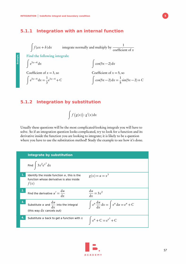
5.1.1 Integration with an internal function
∫
f (ax + b )dx integrate normally and multiply by1
coefficient of x
Find the following integrals:∫
e3x−4 dx
Coefficient of x = 3, so∫
e3x−4 dx =13
e3x−4+C
∫
cos(5x − 2)dx
Coefficient of x = 5, so∫
cos(5x − 2)dx =15
sin(5x − 2)+C
Exam
ple.
5.1.2 Integration by substitution
∫
f�
g (x)�
· g ′(x)dx
Usually these questions will be the most complicated-looking integrals you will have tosolve. So if an integration question looks complicated, try to look for a function and itsderivative inside the function you are looking to integrate; it is likely to be a questionwhere you have to use the substitution method! Study the example to see how it’s done.
Integrate by substitution
Find
∫
3x2ex3dx
1. Identify the inside function u , this is the
function whose derivative is also inside
f (x)
g (x) = u = x3
2.Find the derivative u ′ =
dudx
dudx= 3x2
3.Substitute u and
dudx
into the integral
(this way dx cancels out)
∫
eu dudx
dx =∫
eu du = eu +C
4. Substitute u back to get a function with x∫
eu +C = ex3+C
57
INTEGRATION Definite integral
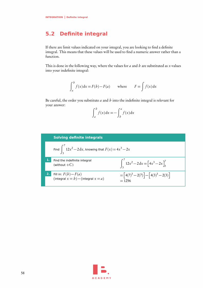
5.2 Definite integral
If there are limit values indicated on your integral, you are looking to find a definiteintegral. This means that these values will be used to find a numeric answer rather than afunction.
This is done in the following way, where the values for a and b are substituted as x-valuesinto your indefinite integral:
∫ b
af (x)dx = F (b )− F (a) where F =
∫
f (x)dx
Be careful, the order you substitute a and b into the indefinite integral is relevant foryour answer:
∫ b
af (x)dx =−
∫ a
bf (x)dx
Solving definite integrals
Find
∫ 7
312x2− 2dx , knowing that F (x) = 4x3− 2x
1. Find the indefinite integral
(without +C )
∫ 7
312x2− 2dx =
�
4x3− 2x�7
3
2. Fill in: F (b )− F (a)(integral x = b )− (integral x = a)
=�
4(7)3− 2(7)�
−�
4(3)3− 2(3)�
= 1256
58
INTEGRATION Definite integral 5
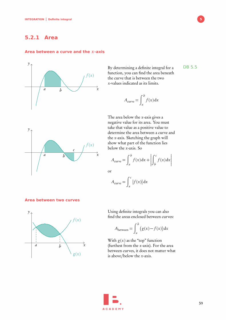
5.2.1 Area
Area between a curve and the x-axis
x
y
a b
f (x)
DB 5.5By determining a definite integral for afunction, you can find the area beneaththe curve that is between the twox-values indicated as its limits.
Acurve =∫ b
af (x)dx
x
y
a bc
f (x)
The area below the x-axis gives anegative value for its area. You musttake that value as a positive value todetermine the area between a curve andthe x-axis. Sketching the graph willshow what part of the function liesbelow the x-axis. So
Acurve =∫ b
af (x)dx +
�
�
�
�
�
∫ c
bf (x)dx
�
�
�
�
�
or
Acurve =∫ c
a
�
� f (x)�
�dx
Area between two curves
x
y
a b
f (x)
g (x)
Using definite integrals you can alsofind the areas enclosed between curves:
Abetween =∫ b
a
�
g (x)− f (x)�
dx
With g (x) as the “top” function(furthest from the x-axis). For the areabetween curves, it does not matter whatis above/below the x-axis.
59
INTEGRATION Definite integral
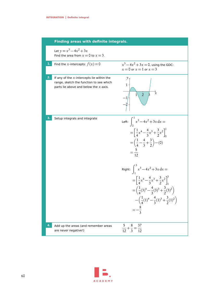
Finding areas with definite integrals.
Let y = x3− 4x2+ 3xFind the area from x = 0 to x = 3.
1. Find the x-intercepts: f (x) = 0 x3− 4x2+ 3x = 0, using the GDC:
x = 0 or x = 1 or x = 3
2. If any of the x-intercepts lie within the
range, sketch the function to see which
parts lie above and below the x-axis.
x
y
1 2 3
−2
−1
1
3. Setup integrals and integrateLeft:
∫ 1
0x3− 4x2+ 3x dx =
=�
14
x4− 43
x3+32
x2�1
0
=�
14− 4
3+
32
�
− (0)
=512
Right:
∫ 3
1x3− 4x2+ 3x dx =
=�
14
x4− 43
x3+32
x2�3
1
=�
14(3)4− 4
3(3)3+
32(3)2
�
−�
14(1)4− 4
3(1)3+
32(1)2
�
=−83
4. Add up the areas (and remember areas
are never negative!)
512+
83=
3712
60
INTEGRATION Definite integral 5
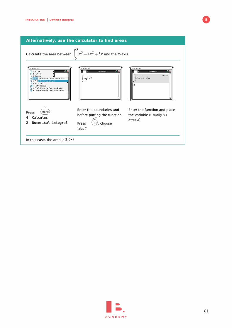
Alternatively, use the calculator to find areas
Calculate the area between
∫ 3
0x3− 4x2+ 3x and the x-axis
IB ACADEMY
Press menu
4: Calculus
2: Numerical integral
IB ACADEMY
Enter the boundaries and
before putting the function.
Press
∞β◦
, choose
‘abs(’
IB ACADEMY
Enter the function and place
the variable (usually x)
after d
In this case, the area is 3.083
61

6PROBABILITYTable of contents & cheatsheet
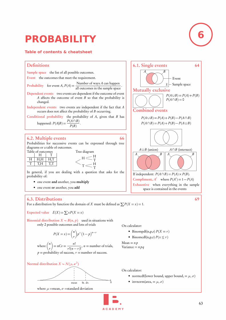
DefinitionsSample space the list of all possible outcomes.
Event the outcomes that meet the requirement.
Probability for event A, P (A) =Number of ways A can happen
all outcomes in the sample space.
Dependent events two events are dependent if the outcome of eventA affects the outcome of event B so that the probability ischanged.
Independent events two events are independent if the fact that Aoccurs does not affect the probability of B occurring.
Conditional probability the probability of A, given that B has
happened: P (A|B) =P (A∩B)
P (B).
6.2. Multiple events 66Probabilities for successive events can be expressed through treediagrams or a table of outcomes.Table of outcomes
H TH H,H H,TT T,H T,T
Tree diagram
H
T
HTHT
In general, if you are dealing with a question that asks for theprobability of:
• one event and another, you multiply
• one event or another, you add
6.1. Single events 64A B
S Sample space
Event
Mutually exclusiveP (A∪B) = P (A)+P (B)P (A∩B) = 0
Combined events
P (A∪B) = P (A)+ P (B)− P (A∩B)P (A∩B) = P (A)+ P (B)− P (A∪B)
A∪B (union) A∩B (intersect)A B A B
If independent: P (A∩B) = P (A)× P (B).Compliment, A′ where P (A′) = 1− P (A)Exhaustive when everything in the sample
space is contained in the events
6.3. Distributions 69For a distribution by function the domain of X must be defined as
∑
P (X = x) = 1.
Expected value E(X ) =∑
xP (X = x)
Binomial distribution X ∼ B(n, p) used in situations withonly 2 possible outcomes and lots of trials
P (X = x) =�
nr
�
p r �1− p�n−r
where�
nr
�
= nCr=n!
r !(n− r )!, n = number of trials,
p = probability of success, r = number of success.
On calculator:
• Binompdf(n,p,r) P (X = r )
• Binomcdf(n,p,r) P (x ≤ r )
Mean = n pVariance = n pq
Normal distribution X ∼ N (µ,σ2)
xmean St. dv.
where µ=mean, σ =standard deviation
On calculator:
• normcdf(lower bound, upper bound, =µ, σ )
• invnorm(area, =µ, σ )
63
PROBABILITY Single events (Venn diagrams)
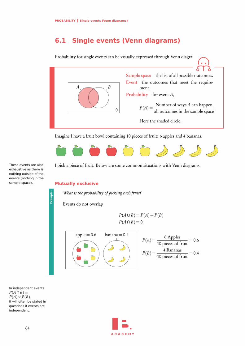
6.1 Single events (Venn diagrams)
Probability for single events can be visually expressed through Venn diagrams.
A B
0
Sample space the list of all possible outcomes.Event the outcomes that meet the require-
ment.Probability for event A,
P (A) =Number of ways A can happen
all outcomes in the sample space
Here the shaded circle.
Imagine I have a fruit bowl containing 10 pieces of fruit: 6 apples and 4 bananas.
I pick a piece of fruit. Below are some common situations with Venn diagrams.These events are alsoexhaustive as there isnothing outside of theevents (nothing in thesample space). Mutually exclusive
What is the probability of picking each fruit?
Events do not overlap
P (A∪B) = P (A)+ P (B)P (A∩B) = 0
apple= 0.6 banana= 0.4P (A) =
6 Apples10 pieces of fruit
= 0.6
P (B) =4 Bananas
10 pieces of fruit= 0.4
Exam
ple.
In independent eventsP (A∩B) =P (A)× P (B).It will often be stated inquestions if events areindependent.
64
PROBABILITY Single events (Venn diagrams) 6
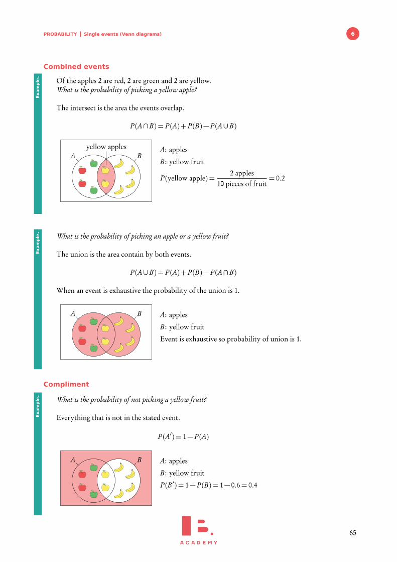
Combined events
Of the apples 2 are red, 2 are green and 2 are yellow.What is the probability of picking a yellow apple?
The intersect is the area the events overlap.
P (A∩B) = P (A)+ P (B)− P (A∪B)
A Byellow apples A: apples
B : yellow fruit
P (yellow apple) =2 apples
10 pieces of fruit= 0.2
Exam
ple.
What is the probability of picking an apple or a yellow fruit?
The union is the area contain by both events.
P (A∪B) = P (A)+ P (B)− P (A∩B)
When an event is exhaustive the probability of the union is 1.
A B A: apples
B : yellow fruit
Event is exhaustive so probability of union is 1.
Exam
ple.
Compliment
What is the probability of not picking a yellow fruit?
Everything that is not in the stated event.
P (A′) = 1− P (A)
A B A: apples
B : yellow fruit
P (B ′) = 1− P (B) = 1− 0.6= 0.4
Exam
ple.
65
PROBABILITY Multiple events (tree Diagrams)
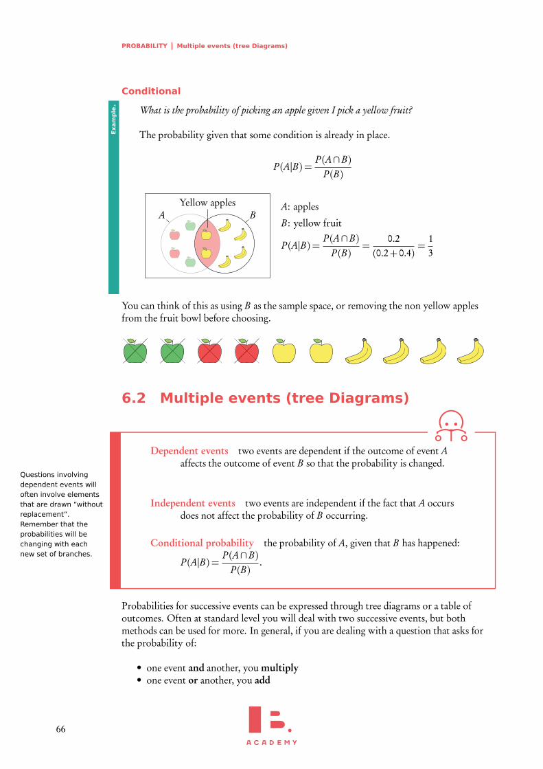
Conditional
What is the probability of picking an apple given I pick a yellow fruit?
The probability given that some condition is already in place.
P (A|B) =P (A∩B)
P (B)
A BYellow apples A: apples
B : yellow fruit
P (A|B) =P (A∩B)
P (B)=
0.2(0.2+ 0.4)
=13
Exam
ple.
You can think of this as using B as the sample space, or removing the non yellow applesfrom the fruit bowl before choosing.
6.2 Multiple events (tree Diagrams)
Dependent events two events are dependent if the outcome of event Aaffects the outcome of event B so that the probability is changed.
Questions involvingdependent events willoften involve elementsthat are drawn “withoutreplacement”.Remember that theprobabilities will bechanging with eachnew set of branches.
Independent events two events are independent if the fact that A occursdoes not affect the probability of B occurring.
Conditional probability the probability of A, given that B has happened:
P (A|B) =P (A∩B)
P (B).
Probabilities for successive events can be expressed through tree diagrams or a table ofoutcomes. Often at standard level you will deal with two successive events, but bothmethods can be used for more. In general, if you are dealing with a question that asks forthe probability of:
• one event and another, you multiply• one event or another, you add
66
PROBABILITY Multiple events (tree Diagrams) 6
Tree diagrams
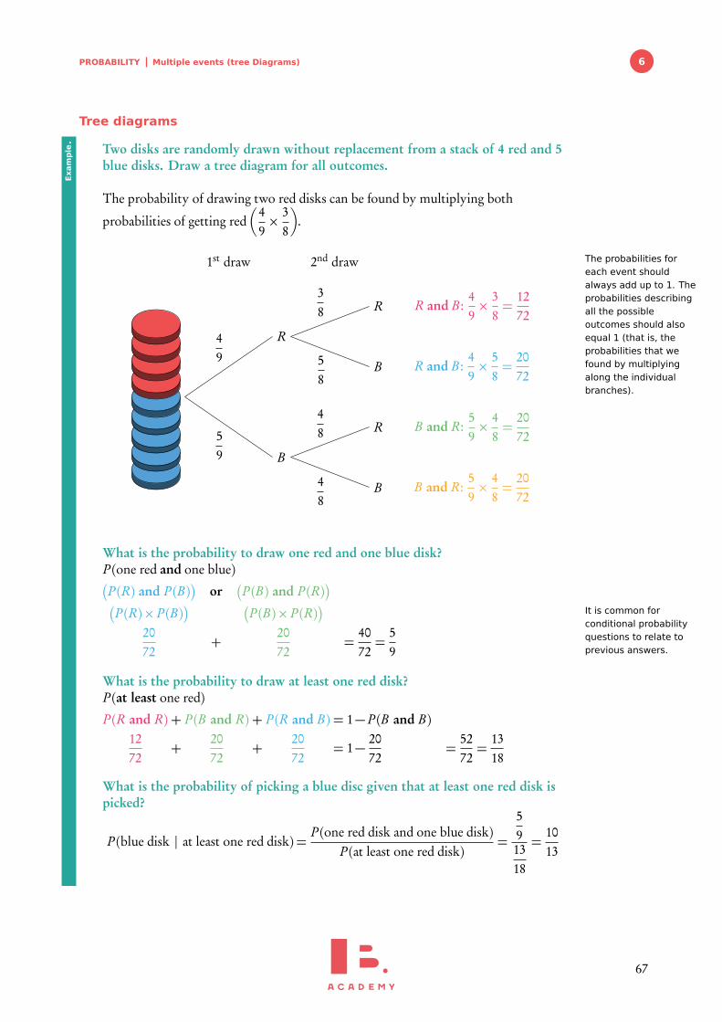
Two disks are randomly drawn without replacement from a stack of 4 red and 5blue disks. Draw a tree diagram for all outcomes.
The probability of drawing two red disks can be found by multiplying both
probabilities of getting red�
49× 3
8
�
.
The probabilities foreach event shouldalways add up to 1. Theprobabilities describingall the possibleoutcomes should alsoequal 1 (that is, theprobabilities that wefound by multiplyingalong the individualbranches).
R
B
R
B
R
B
1st draw 2nd draw
49
59
38
58
48
48
R and B :49× 3
8=
1272
R and B :49× 5
8=
2072
B and R:59× 4
8=
2072
B and R:59× 4
8=
2072
What is the probability to draw one red and one blue disk?P (one red and one blue)�
P (R) and P (B)�
or�
P (B) and P (R)�
�
P (R)× P (B)� �
P (B)× P (R)�
2072
+2072
=4072=
59
It is common forconditional probabilityquestions to relate toprevious answers.
What is the probability to draw at least one red disk?P (at least one red)
P (R and R) + P (B and R) + P (R and B) = 1− P (B and B)1272
+2072
+2072
= 1− 2072
=5272=
1318
What is the probability of picking a blue disc given that at least one red disk ispicked?
P (blue disk | at least one red disk) =P (one red disk and one blue disk)
P (at least one red disk)=
591318
=1013
Exam
ple.
67
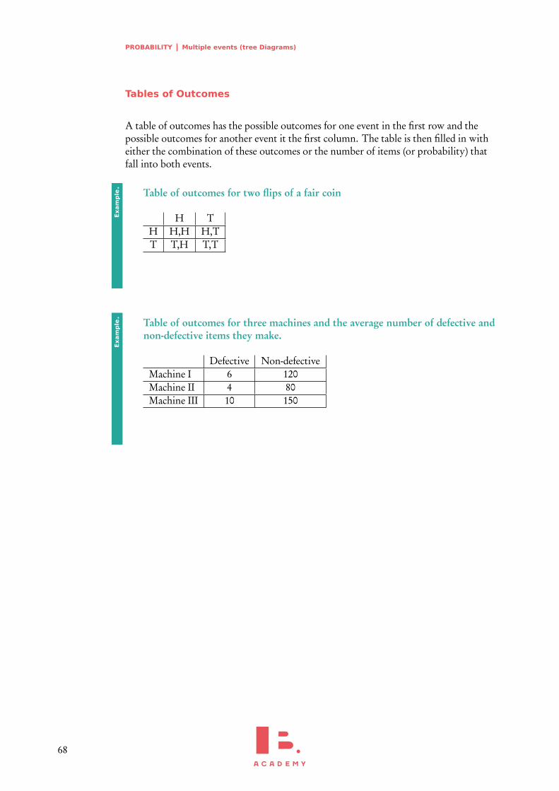
PROBABILITY Multiple events (tree Diagrams)
Tables of Outcomes
A table of outcomes has the possible outcomes for one event in the first row and thepossible outcomes for another event it the first column. The table is then filled in witheither the combination of these outcomes or the number of items (or probability) thatfall into both events.
Table of outcomes for two flips of a fair coin
H TH H,H H,TT T,H T,T
Exam
ple.
Table of outcomes for three machines and the average number of defective andnon-defective items they make.
Defective Non-defectiveMachine I 6 120Machine II 4 80Machine III 10 150
Exam
ple.
68
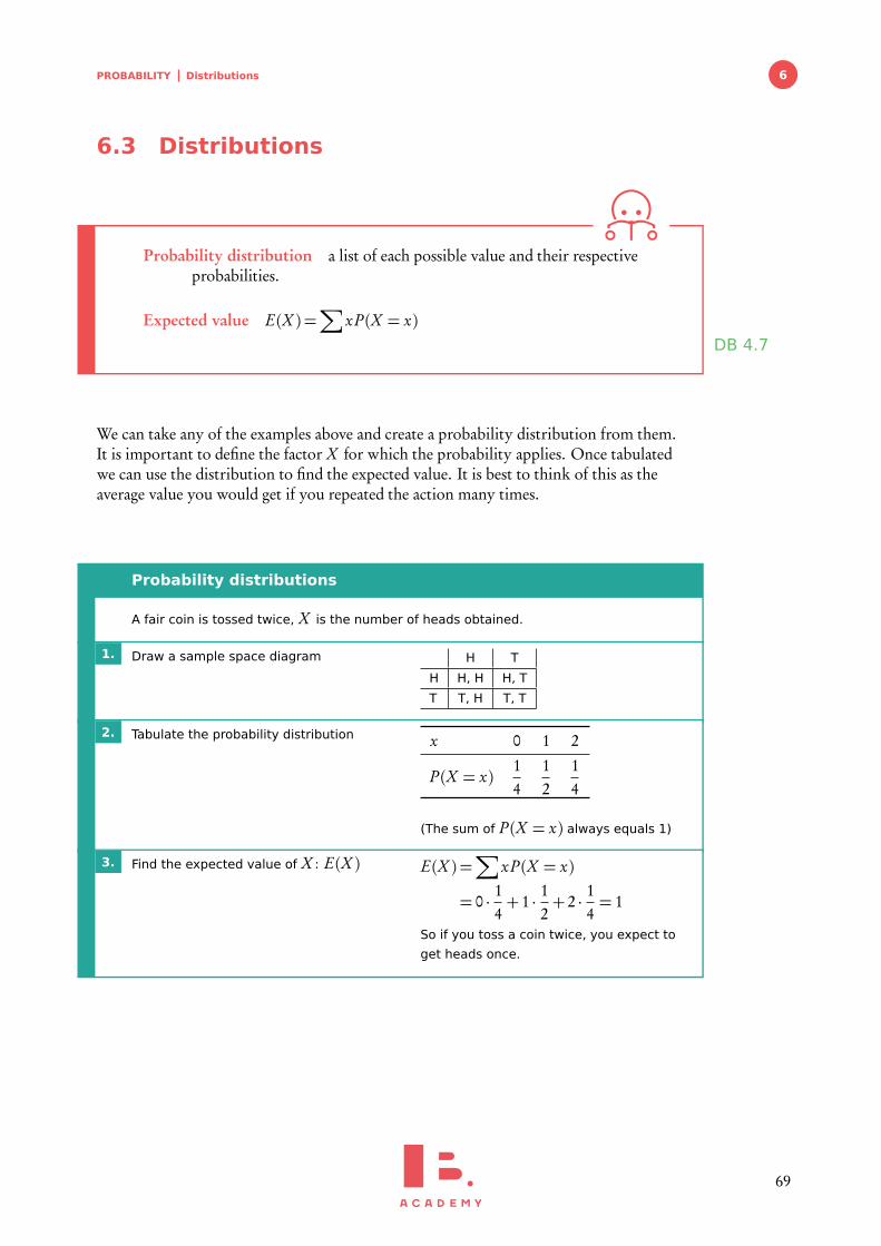
PROBABILITY Distributions 6
6.3 Distributions
Probability distribution a list of each possible value and their respectiveprobabilities.
Expected value E(X ) =∑
xP (X = x)DB 4.7
We can take any of the examples above and create a probability distribution from them.It is important to define the factor X for which the probability applies. Once tabulatedwe can use the distribution to find the expected value. It is best to think of this as theaverage value you would get if you repeated the action many times.
Probability distributions
A fair coin is tossed twice, X is the number of heads obtained.
1. Draw a sample space diagram H T
H H, H H, T
T T, H T, T
2. Tabulate the probability distribution x 0 1 2
P (X = x)14
12
14
(The sum of P (X = x) always equals 1)
3. Find the expected value of X : E(X ) E(X ) =∑
xP (X = x)
= 0 · 14+ 1 · 1
2+ 2 · 1
4= 1
So if you toss a coin twice, you expect to
get heads once.
69
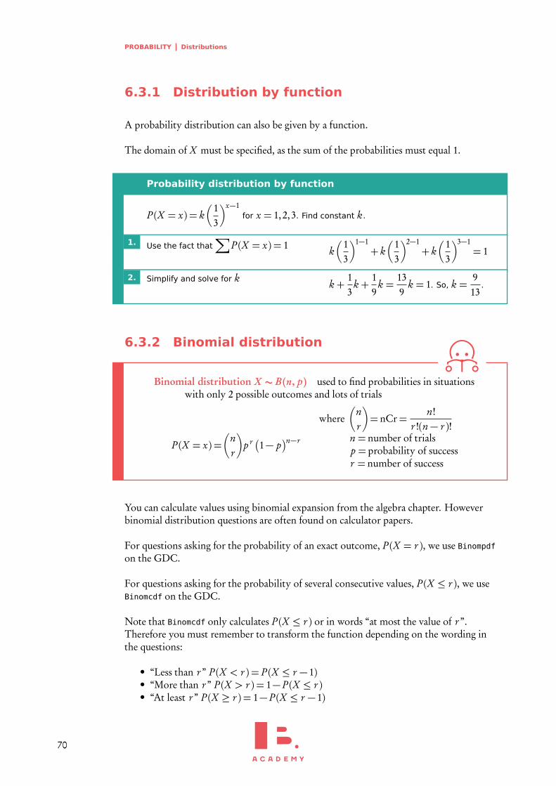
PROBABILITY Distributions
6.3.1 Distribution by function
A probability distribution can also be given by a function.
The domain of X must be specified, as the sum of the probabilities must equal 1.
Probability distribution by function
P (X = x) = k�
13
�x−1for x = 1,2,3. Find constant k .
1. Use the fact that∑
P (X = x) = 1 k�
13
�1−1+ k
�
13
�2−1+ k
�
13
�3−1= 1
2. Simplify and solve for k k +13
k +19
k =139
k = 1. So, k =913
.
6.3.2 Binomial distribution
Binomial distribution X ∼ B(n, p) used to find probabilities in situationswith only 2 possible outcomes and lots of trials
P (X = x) =�
nr
�
p r �1− p�n−r
where�
nr
�
= nCr=n!
r !(n− r )!n = number of trialsp = probability of successr = number of success
You can calculate values using binomial expansion from the algebra chapter. Howeverbinomial distribution questions are often found on calculator papers.
For questions asking for the probability of an exact outcome, P (X = r ), we use Binompdf
on the GDC.
For questions asking for the probability of several consecutive values, P (X ≤ r ), we useBinomcdf on the GDC.
Note that Binomcdf only calculates P (X ≤ r ) or in words “at most the value of r ”.Therefore you must remember to transform the function depending on the wording inthe questions:
• “Less than r ” P (X < r ) = P (X ≤ r − 1)• “More than r ” P (X > r ) = 1− P (X ≤ r )• “At least r ” P (X ≥ r ) = 1− P (X ≤ r − 1)
70
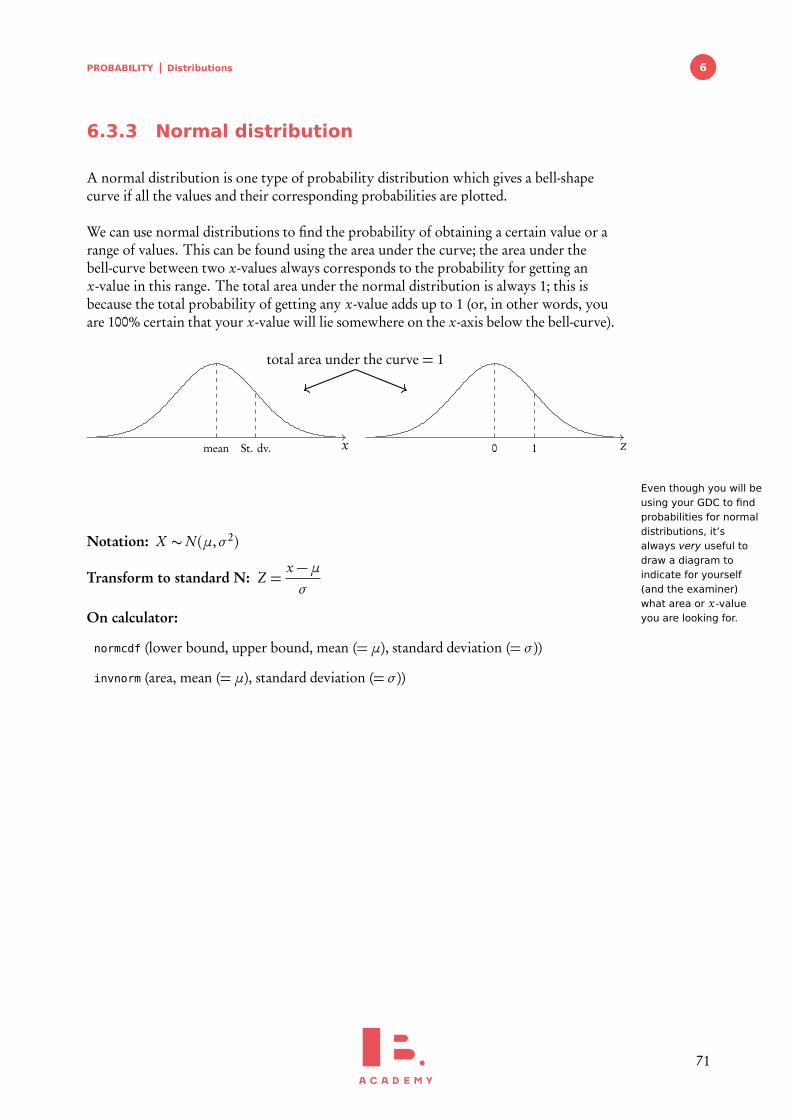
PROBABILITY Distributions 6
6.3.3 Normal distribution
A normal distribution is one type of probability distribution which gives a bell-shapecurve if all the values and their corresponding probabilities are plotted.
We can use normal distributions to find the probability of obtaining a certain value or arange of values. This can be found using the area under the curve; the area under thebell-curve between two x-values always corresponds to the probability for getting anx-value in this range. The total area under the normal distribution is always 1; this isbecause the total probability of getting any x-value adds up to 1 (or, in other words, youare 100% certain that your x-value will lie somewhere on the x-axis below the bell-curve).
xmean St. dv. z0 1
total area under the curve = 1
Even though you will beusing your GDC to findprobabilities for normaldistributions, it’salways very useful todraw a diagram toindicate for yourself(and the examiner)what area or x-valueyou are looking for.
Notation: X ∼N (µ,σ2)
Transform to standard N: Z =x −µσ
On calculator:
normcdf (lower bound, upper bound, mean (=µ), standard deviation (= σ ))
invnorm (area, mean (=µ), standard deviation (= σ ))
71
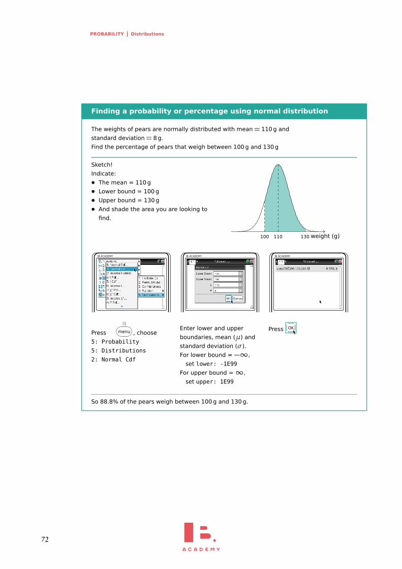
PROBABILITY Distributions
Finding a probability or percentage using normal distribution
The weights of pears are normally distributed with mean= 110g and
standard deviation= 8g.
Find the percentage of pears that weigh between 100 g and 130 g
Sketch!
Indicate:
• The mean = 110 g
• Lower bound = 100 g
• Upper bound = 130 g
• And shade the area you are looking to
find.
weight (g)100 110 130
IB ACADEMY
Press menu , choose
5: Probability
5: Distributions
2: Normal Cdf
IB ACADEMY
Enter lower and upper
boundaries, mean (µ) and
standard deviation (σ).
For lower bound = −∞,
set lower: -1E99
For upper bound =∞,
set upper: 1E99
IB ACADEMY
Press OK
So 88.8% of the pears weigh between 100 g and 130 g.
72
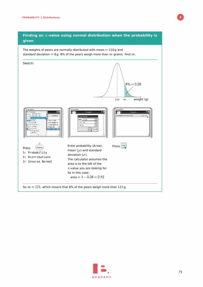
PROBABILITY Distributions 6
Finding an x-value using normal distribution when the probability is
given
The weights of pears are normally distributed with mean= 110g and
standard deviation= 8g. 8% of the pears weigh more than m grams. Find m.
Sketch!
weight (g)110 m
8%= 0.08
IB ACADEMY
Press menu
5: Probability
5: Distributions
3: Inverse Normal
IB ACADEMY
Enter probability (Area),
mean (µ) and standard
deviation (σ).
The calculator assumes the
area is to the left of the
x-value you are looking for.
So in this case:
area= 1− 0.08= 0.92
IB ACADEMY
Press OK
So m = 121, which means that 8% of the pears weigh more than 121 g.
73
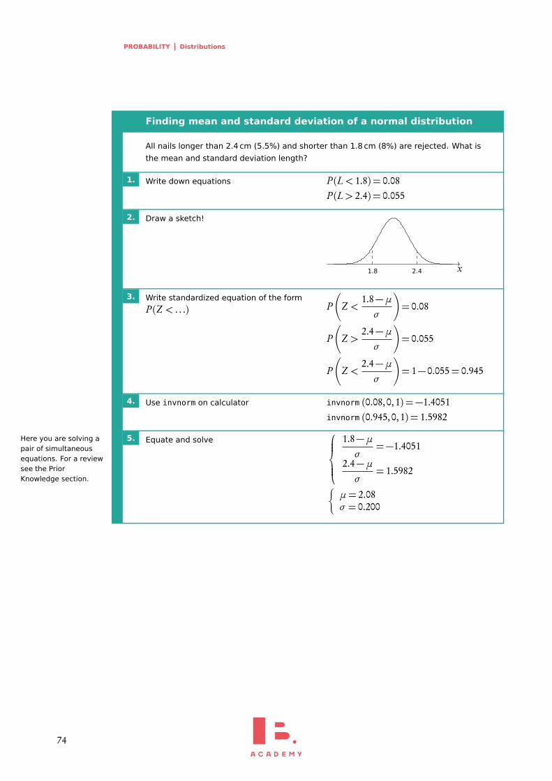
PROBABILITY Distributions
Finding mean and standard deviation of a normal distribution
All nails longer than 2.4 cm (5.5%) and shorter than 1.8 cm (8%) are rejected. What is
the mean and standard deviation length?
1. Write down equations P (L< 1.8) = 0.08P (L> 2.4) = 0.055
2. Draw a sketch!
x1.8 2.4
3. Write standardized equation of the form
P (Z < . . .) P
�
Z <1.8−µσ
�
= 0.08
P
�
Z >2.4−µσ
�
= 0.055
P
�
Z <2.4−µσ
�
= 1− 0.055= 0.945
4. Use invnorm on calculator invnorm (0.08,0,1) =−1.4051invnorm (0.945,0,1) = 1.5982
5. Equate and solveHere you are solving apair of simultaneousequations. For a reviewsee the PriorKnowledge section.
1.8−µσ
=−1.4051
2.4−µσ
= 1.5982�
µ= 2.08σ = 0.200
74
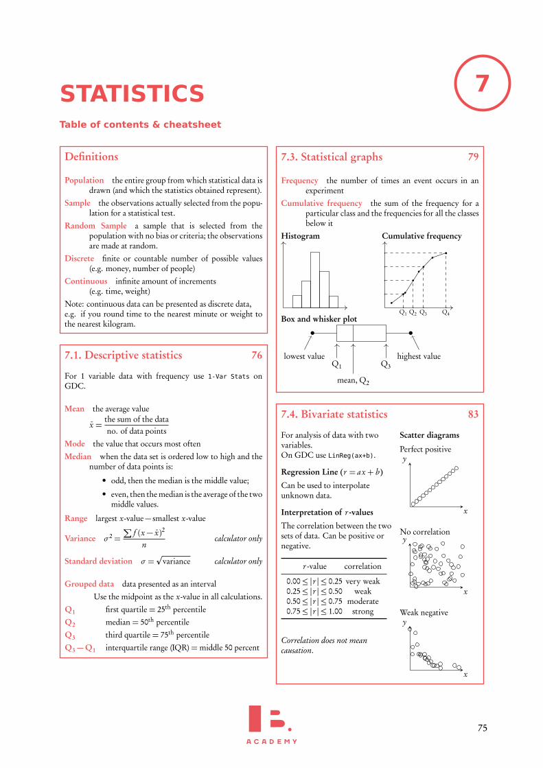
7STATISTICSTable of contents & cheatsheet
Definitions
Population the entire group from which statistical data isdrawn (and which the statistics obtained represent).
Sample the observations actually selected from the popu-lation for a statistical test.
Random Sample a sample that is selected from thepopulation with no bias or criteria; the observationsare made at random.
Discrete finite or countable number of possible values(e.g. money, number of people)
Continuous infinite amount of increments(e.g. time, weight)
Note: continuous data can be presented as discrete data,e.g. if you round time to the nearest minute or weight tothe nearest kilogram.
7.1. Descriptive statistics 76
For 1 variable data with frequency use 1-Var Stats onGDC.
Mean the average value
x =the sum of the datano. of data points
Mode the value that occurs most often
Median when the data set is ordered low to high and thenumber of data points is:
• odd, then the median is the middle value;
• even, then the median is the average of the twomiddle values.
Range largest x-value− smallest x-value
Variance σ2 =∑
f (x − x)2
ncalculator only
Standard deviation σ =p
variance calculator only
Grouped data data presented as an interval
Use the midpoint as the x-value in all calculations.
Q1 first quartile = 25th percentile
Q2 median = 50th percentile
Q3 third quartile = 75th percentile
Q3 −Q1 interquartile range (IQR) =middle 50 percent
7.3. Statistical graphs 79
Frequency the number of times an event occurs in anexperiment
Cumulative frequency the sum of the frequency for aparticular class and the frequencies for all the classesbelow it
Histogram Cumulative frequency
Q1 Q2 Q3 Q4Box and whisker plot
lowest valueQ1
mean, Q2
Q3
highest value
7.4. Bivariate statistics 83
For analysis of data with twovariables.On GDC use LinReg(ax+b).
Regression Line (r = ax + b )
Can be used to interpolateunknown data.
Interpretation of r -values
The correlation between the twosets of data. Can be positive ornegative.
r -value correlation
0.00≤ |r | ≤ 0.25 very weak0.25≤ |r | ≤ 0.50 weak0.50≤ |r | ≤ 0.75 moderate0.75≤ |r | ≤ 1.00 strong
Correlation does not meancausation.
Scatter diagrams
Perfect positive
x
y
No correlation
x
y
Weak negative
x
y
75
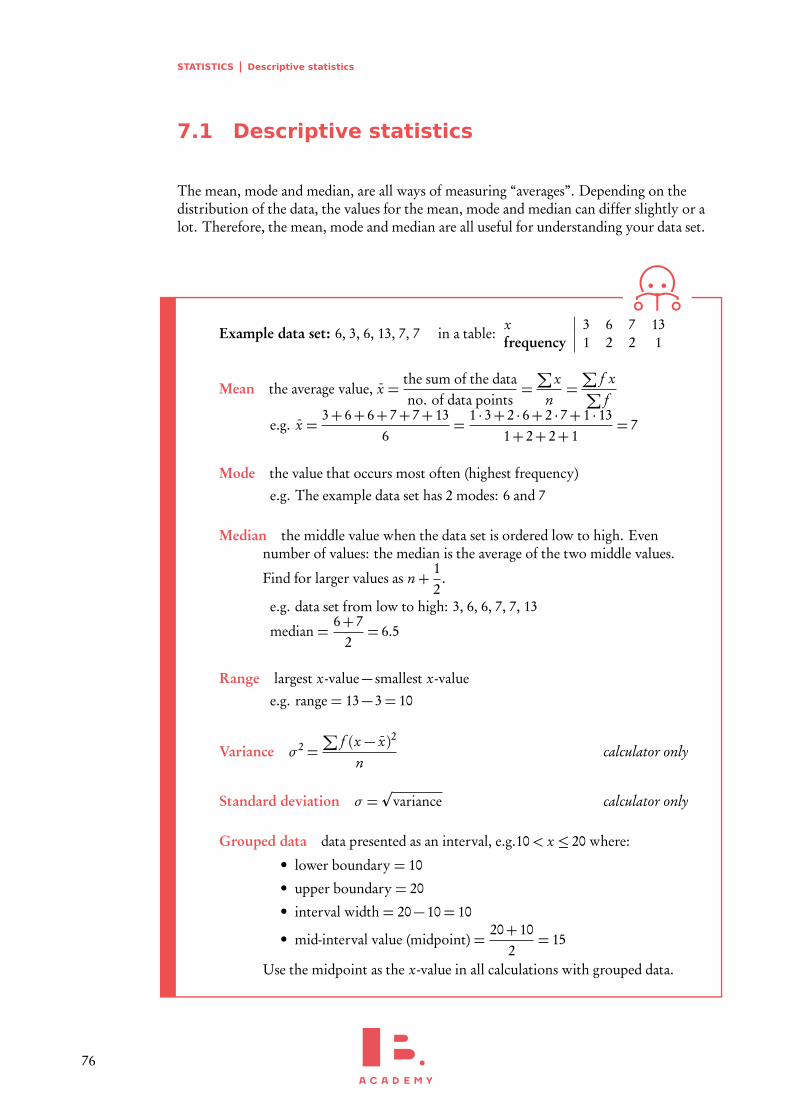
STATISTICS Descriptive statistics
7.1 Descriptive statistics
The mean, mode and median, are all ways of measuring “averages”. Depending on thedistribution of the data, the values for the mean, mode and median can differ slightly or alot. Therefore, the mean, mode and median are all useful for understanding your data set.
Example data set: 6, 3, 6, 13, 7, 7 in a table:x 3 6 7 13frequency 1 2 2 1
Mean the average value, x =the sum of the datano. of data points
=∑
xn=∑
f x∑
f
e.g. x =3+ 6+ 6+ 7+ 7+ 13
6=
1 · 3+ 2 · 6+ 2 · 7+ 1 · 131+ 2+ 2+ 1
= 7
Mode the value that occurs most often (highest frequency)
e.g. The example data set has 2 modes: 6 and 7
Median the middle value when the data set is ordered low to high. Evennumber of values: the median is the average of the two middle values.
Find for larger values as n+12
.
e.g. data set from low to high: 3, 6, 6, 7, 7, 13
median =6+ 7
2= 6.5
Range largest x-value− smallest x-value
e.g. range = 13− 3= 10
Variance σ2 =∑
f (x − x)2
ncalculator only
Standard deviation σ =p
variance calculator only
Grouped data data presented as an interval, e.g.10< x ≤ 20 where:
• lower boundary = 10
• upper boundary = 20
• interval width = 20− 10= 10
• mid-interval value (midpoint) =20+ 10
2= 15
Use the midpoint as the x-value in all calculations with grouped data.
76
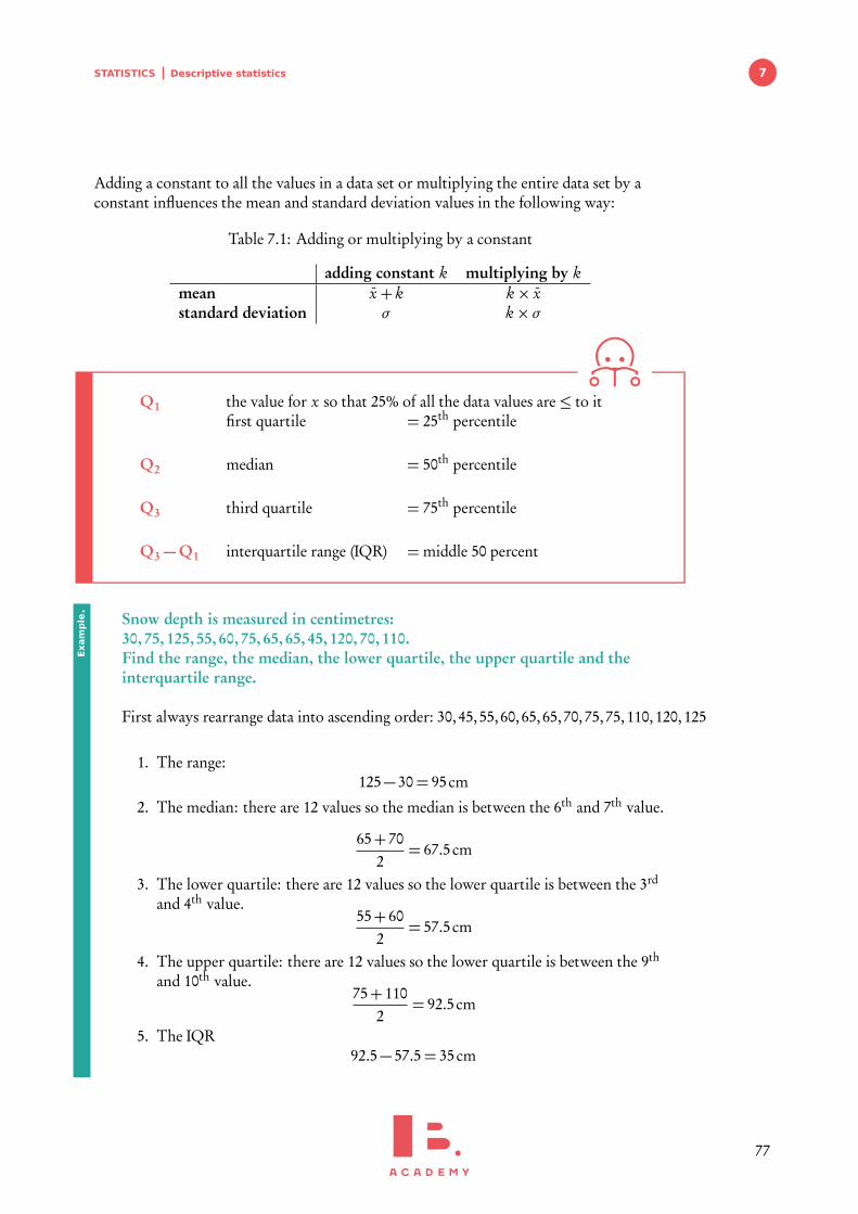
STATISTICS Descriptive statistics 7
Adding a constant to all the values in a data set or multiplying the entire data set by aconstant influences the mean and standard deviation values in the following way:
Table 7.1: Adding or multiplying by a constant
adding constant k multiplying by kmean x + k k × xstandard deviation σ k ×σ
Q1 the value for x so that 25% of all the data values are ≤ to itfirst quartile = 25th percentile
Q2 median = 50th percentile
Q3 third quartile = 75th percentile
Q3 −Q1 interquartile range (IQR) =middle 50 percent
Snow depth is measured in centimetres:30, 75, 125, 55, 60, 75, 65, 65, 45, 120, 70, 110.Find the range, the median, the lower quartile, the upper quartile and theinterquartile range.
First always rearrange data into ascending order: 30,45,55,60,65,65,70,75,75,110,120,125
1. The range:125− 30= 95cm
2. The median: there are 12 values so the median is between the 6th and 7th value.
65+ 702
= 67.5cm
3. The lower quartile: there are 12 values so the lower quartile is between the 3rd
and 4th value.55+ 60
2= 57.5cm
4. The upper quartile: there are 12 values so the lower quartile is between the 9th
and 10th value.75+ 110
2= 92.5cm
5. The IQR92.5− 57.5= 35cm
Exam
ple.
77
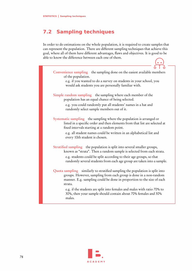
STATISTICS Sampling techniques
7.2 Sampling techniques
In order to do estimations on the whole population, it is required to create samples thatcan represent the population. There are different sampling techniques that achieve thisgoal, where all of them have different advantages, flaws and objectives. It is good to beable to know the difference between each one of them.
Convenience sampling the sampling done on the easiest available membersof the population.e.g. if you wanted to do a survey on students in your school, youwould ask students you are personally familiar with.
Simple random sampling the sampling where each member of thepopulation has an equal chance of being selected.
e.g. you could randomly put all students’ names in a hat andrandomly select sample members out of it.
Systematic sampling the sampling where the population is arranged orlisted in a specific order and then elements from that list are selected atfixed intervals starting at a random point.
e.g. all student names could be written in an alphabetical list andevery 10th student is chosen.
Stratified sampling the population is split into several smaller groups,known as “strata”. Then a random sample is selected from each strata.
e.g. students could be split according to their age groups, so thatrandomly several students from each age group are taken into a sample.
Quota sampling similarly to stratified sampling the population is split intogroups. However, sampling from each group is done in a non-randommanner. E.g. sampling could be done in proportion to the size of eachstrata.
e.g. if the students are split into females and males with ratio 70% to30%, then your sample should contain about 70% females and 30%males.
78
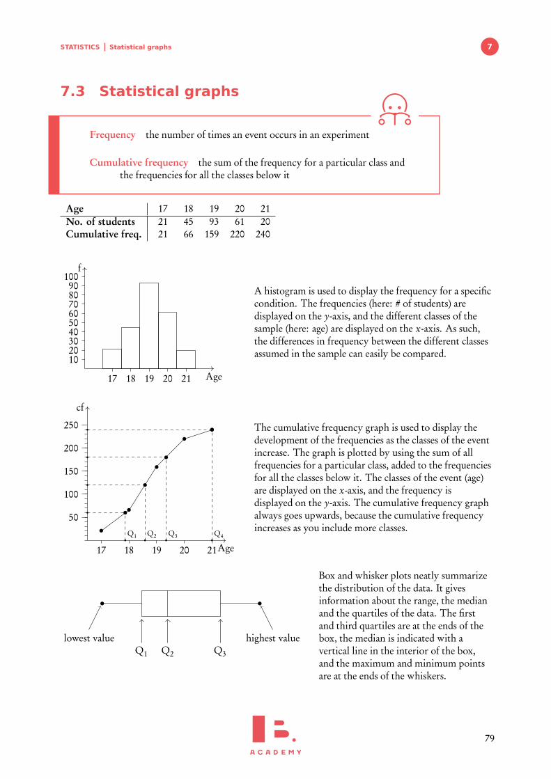
STATISTICS Statistical graphs 7
7.3 Statistical graphs
Frequency the number of times an event occurs in an experiment
Cumulative frequency the sum of the frequency for a particular class andthe frequencies for all the classes below it
Age 17 18 19 20 21No. of students 21 45 93 61 20Cumulative freq. 21 66 159 220 240
Age
f
17 18 19 20 21
102030405060708090
100A histogram is used to display the frequency for a specificcondition. The frequencies (here: # of students) aredisplayed on the y-axis, and the different classes of thesample (here: age) are displayed on the x-axis. As such,the differences in frequency between the different classesassumed in the sample can easily be compared.
Age
cf
17 18 19 20 21
50
100
150
200
250
Q1 Q2 Q3 Q4
The cumulative frequency graph is used to display thedevelopment of the frequencies as the classes of the eventincrease. The graph is plotted by using the sum of allfrequencies for a particular class, added to the frequenciesfor all the classes below it. The classes of the event (age)are displayed on the x-axis, and the frequency isdisplayed on the y-axis. The cumulative frequency graphalways goes upwards, because the cumulative frequencyincreases as you include more classes.
lowest valueQ1 Q2 Q3
highest value
Box and whisker plots neatly summarizethe distribution of the data. It givesinformation about the range, the medianand the quartiles of the data. The firstand third quartiles are at the ends of thebox, the median is indicated with avertical line in the interior of the box,and the maximum and minimum pointsare at the ends of the whiskers.
79
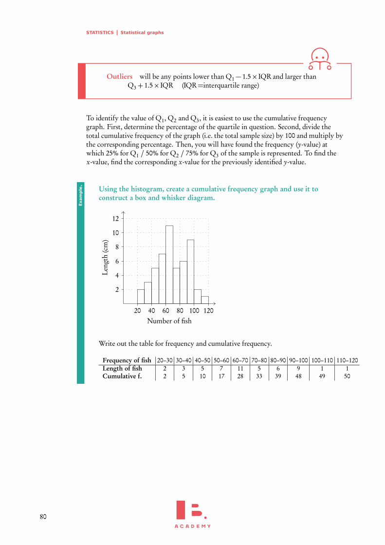
STATISTICS Statistical graphs
Outliers will be any points lower than Q1− 1.5× IQR and larger thanQ3+ 1.5× IQR (IQR=interquartile range)
To identify the value of Q1, Q2 and Q3, it is easiest to use the cumulative frequencygraph. First, determine the percentage of the quartile in question. Second, divide thetotal cumulative frequency of the graph (i.e. the total sample size) by 100 and multiply bythe corresponding percentage. Then, you will have found the frequency (y-value) atwhich 25% for Q1 / 50% for Q2 / 75% for Q3 of the sample is represented. To find thex-value, find the corresponding x-value for the previously identified y-value.
Using the histogram, create a cumulative frequency graph and use it toconstruct a box and whisker diagram.
Number of fish
Leng
th(c
m)
20 40 60 80 100 120
2
4
6
8
10
12
Write out the table for frequency and cumulative frequency.
Frequency of fish 20–30 30–40 40–50 50–60 60–70 70–80 80–90 90–100 100–110 110–120Length of fish 2 3 5 7 11 5 6 9 1 1Cumulative f. 2 5 10 17 28 33 39 48 49 50
Exam
ple.
80
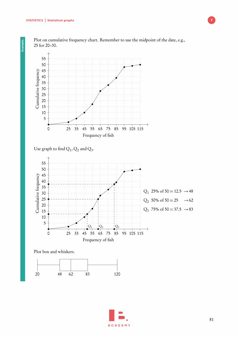
STATISTICS Statistical graphs 7
Plot on cumulative frequency chart. Remember to use the midpoint of the date, e.g.,25 for 20–30.
Frequency of fish
Cum
ulat
ive
freq
uenc
y
0 25 35 45 55 65 75 85 95 105 115
510152025303540455055
Use graph to find Q1, Q2 and Q3.
Frequency of fish
Cum
ulat
ive
freq
uenc
y
0 25 35 45 55 65 75 85 95 105 115
510152025303540455055
Q1 Q2 Q3
Q1 25% of 50= 12.5 → 48
Q2 50% of 50= 25 → 62
Q3 75% of 50= 37.5 → 83
Plot box and whiskers.
20 1206248 83
Exam
ple.
81
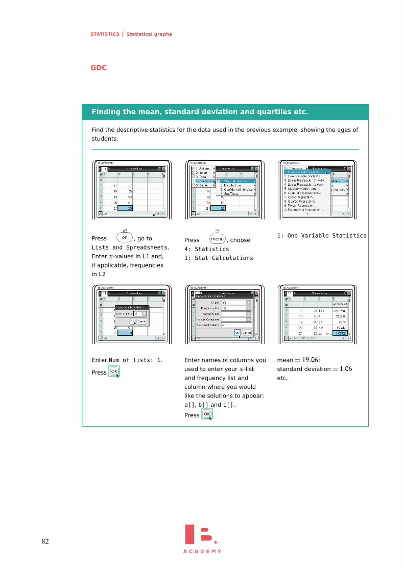
STATISTICS Statistical graphs
GDC
Finding the mean, standard deviation and quartiles etc.
Find the descriptive statistics for the data used in the previous example, showing the ages of
students.
IB ACADEMY
Press
off
on , go to
Lists and Spreadsheets.
Enter x-values in L1 and,
if applicable, frequencies
in L2
IB ACADEMY
Press menu , choose
4: Statistics
1: Stat Calculations
IB ACADEMY
1: One-Variable Statistics
IB ACADEMY
Enter Num of lists: 1.
Press OK
IB ACADEMY
Enter names of columns you
used to enter your x-list
and frequency list and
column where you would
like the solutions to appear:
a[], b[] and c[].
Press OK
IB ACADEMY
mean= 19.06;
standard deviation= 1.06etc.
82
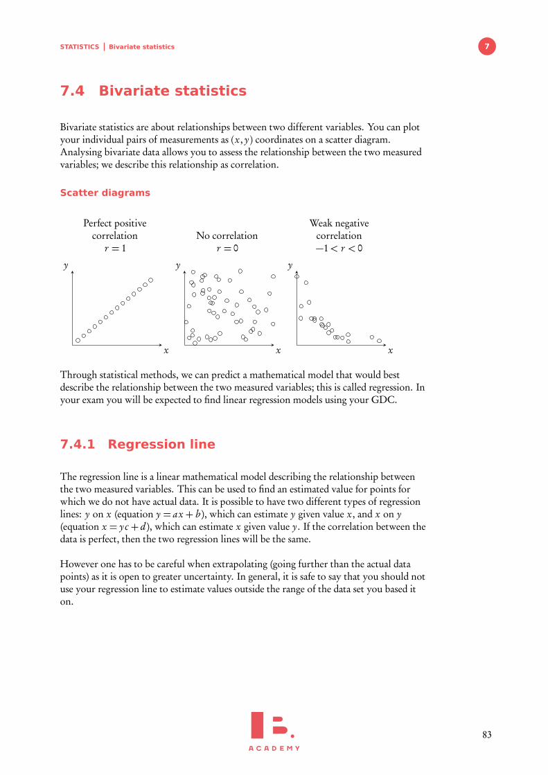
STATISTICS Bivariate statistics 7
7.4 Bivariate statistics
Bivariate statistics are about relationships between two different variables. You can plotyour individual pairs of measurements as (x, y) coordinates on a scatter diagram.Analysing bivariate data allows you to assess the relationship between the two measuredvariables; we describe this relationship as correlation.
Scatter diagrams
Perfect positivecorrelation
r = 1
x
y
No correlationr = 0
x
y
Weak negativecorrelation−1< r < 0
x
y
Through statistical methods, we can predict a mathematical model that would bestdescribe the relationship between the two measured variables; this is called regression. Inyour exam you will be expected to find linear regression models using your GDC.
7.4.1 Regression line
The regression line is a linear mathematical model describing the relationship betweenthe two measured variables. This can be used to find an estimated value for points forwhich we do not have actual data. It is possible to have two different types of regressionlines: y on x (equation y = ax + b ), which can estimate y given value x, and x on y(equation x = yc + d ), which can estimate x given value y. If the correlation between thedata is perfect, then the two regression lines will be the same.
However one has to be careful when extrapolating (going further than the actual datapoints) as it is open to greater uncertainty. In general, it is safe to say that you should notuse your regression line to estimate values outside the range of the data set you based iton.
83
STATISTICS Bivariate statistics
7.4.2 Pearson’s correlation coefficient
(−1 ≤ r ≤ 1)
Besides simply estimating the correlation between two variables from a scatter diagram,you can calculate a value that will describe it in a standardised way. This value is referredto as Pearson’s correlation coefficient (r ).
r = 0 means no correlation.r ± 1 means a perfect positive/negative correlation.
Interpretation of r -values:
r−value 0< |r | ≤ 0.25 0.25< |r | ≤ 0.50 0.50< |r | ≤ 0.75 0.75< |r |< 1
correlation very weak weak moderate strong
Remember thatcorrelation 6=causation.
Calculate r while finding the regression equation on your GDC. Make sure that STATDIAGNOSTICS is turned ON (can be found in the MODE settings), otherwise the r -value willnot appear.
When asked to “comment on” an r -value make sure to include both, whether thecorrelation is:
1. positive / negativeand
2. strong /moderate / weak / very weak
84
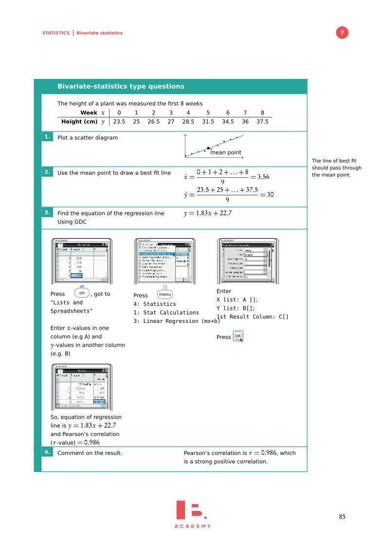
STATISTICS Bivariate statistics 7
Bivariate-statistics type questions
The height of a plant was measured the first 8 weeks
Week x 0 1 2 3 4 5 6 7 8
Height (cm) y 23.5 25 26.5 27 28.5 31.5 34.5 36 37.5
1. Plot a scatter diagram
mean pointThe line of best fitshould pass throughthe mean point.2. Use the mean point to draw a best fit line x =
0+ 1+ 2+ . . .+ 89
= 3.56
y =23.5+ 25+ . . .+ 37.5
9= 30
3. Find the equation of the regression line
Using GDC
y = 1.83x + 22.7
IB ACADEMY
Press
off
on , got to
“Lists and
Spreadsheets”
Enter x-values in one
column (e.g A) and
y-values in another column
(e.g. B)
IB ACADEMY
Press menu
4: Statistics
1: Stat Calculations
3: Linear Regression (mx+b)
IB ACADEMY
Enter
X list: A [];
Y list: B[];
1st Result Column: C[]
Press OK
IB ACADEMY
So, equation of regression
line is y = 1.83x + 22.7and Pearson’s correlation
(r -value) = 0.9864. Comment on the result. Pearson’s correlation is r = 0.986, which
is a strong positive correlation.
85

Related Documents