IAC-star: a code for synthetic color-magnitude diagram ... · branch (RGB) stars is associated to an intermediate-age to old star formation activity; a well developed red-tail of

arX

iv:a

stro

-ph/

0407

589v

1 2

8 Ju

l 200

4

IAC-star: a code for synthetic color-magnitude diagram

computation

Antonio Aparicio

Departamento de Astrofısica, Universidad de La Laguna/Instituto de Astrofısica de

Canarias. Vıa Lactea s/n. E38200 - La Laguna, Tenerife, Canary Islands, Spain

Carme Gallart

Instituto de Astrofısica de Canarias. Vıa Lactea s/n. E38200 - La Laguna, Tenerife,

Canary Islands, Spain

ABSTRACT

The code IAC-star is presented. It generates synthetic HR and color-

magnitude diagrams (CMDs) and is mainly aimed to star formation history

studies in nearby galaxies. Composite stellar populations are calculated on

a star by star basis, by computing the luminosity, effective temperature and

gravity of each star by direct bi-logarithmic interpolation in the metallicity

and age grid of a library of stellar evolution tracks. Visual (broad band and

HST) and infrared magnitudes are also provided for each star after applying

bolometric corrections. The Padua (Bertelli et al. 1994, Girardi et al. 2000)

and Teramo (Pietrinferni et al. 2004) stellar evolution libraries and various

bolometric corrections libraries are used in the current version. A variety of star

formation rate functions, initial mass functions and chemical enrichment laws

are allowed and binary stars can be computed. Although the main motivation

of the code is the computation of synthetic CMDs, it also provides integrated

masses, luminosities and magnitudes as well as surface brightness fluctuation

luminosities and magnitudes for the total synthetic stellar population, and

therefore it can also be used for population synthesis research.

The code is offered for free use and can be executed at the site

http://iac-star.iac.es, with the only requirement of referencing this paper

and crediting as indicated in the site.

Subject headings: HR-diagram, color-magnitude digram, population synthesis,

star formation history

– 2 –

1. Introduction

Galaxies evolve on two main paths: dynamically, including interactions and merging

with external systems and through the process of formation, evolution and death of stars

within them. The latter has the following relevant effects on the galaxy: (i) the evolution of

gas content, (ii) the chemical enrichment and (iii) the formation of the stellar populations

with different properties as the gas from which they form evolves. The star formation

history is therefore fundamental to understand the galaxy evolution process.

The color-magnitude diagram (CMD) is the best tool to study and derive the star

formation history (SFH) of a galaxy. Deep CMDs display stars born all over the life-time

of the galaxy and are indeed fossil records of the SFH. A qualitative sketch of the stellar

populations present in a galaxy can be done from a quick look to a good CMD. The presence

of stars in characteristic evolutionary phases indicates that star formation took place in

the system in different epochs of its history. For example, the presence of RR-Lyre stars is

indicative of an old, low metallicity stellar population; a substantial amount of red-giant

branch (RGB) stars is associated to an intermediate-age to old star formation activity; a

well developed red-tail of asymptotic giant branch (AGB) stars shows that intermediate-age

and young stars with relatively high metallicity are present in the system, and even a

few blue, bright stars as well as HII regions are evidences of a very recent star formation

activity.

A higher degree of sophistication is provided by isochrone fitting to significant features

of the CMD. Indeed, this method is simple and powerful enough to determine age and

metallicity of single stellar populations as the ones present in star clusters.

However, actually deciphering the information contained in a complex CMD and

deriving a quantitative, accurate SFH is complicated and requires more sophisticated

techniques. The standard procedure involves three main ingredients: (i) good data, from

which a deep, ideally reaching the oldest main-sequence turn-offs, observational CMD can

be plotted; (ii) a stellar evolution library complemented by a bolometric correction library

providing colors and magnitudes of stars as a function of age, mass and metallicity, and

(iii) a method to relate the number of stars populating different regions of the observational

CMD with the density distribution of stars in the CMD as a function of age, mass and

metallicity as predicted by the stellar evolution theory. The result of this comparison

provides the SFH of the system.

Usually, item (iii) involves computation of one or several synthetic CMDs from which

the star density distribution predicted from theory is deduced. Indeed, the synthetic CMD

technique is the most powerful one available for this kind of analysis and, in general, for the

– 3 –

study of the SFH of resolved stellar populations. The first to compute and use a synthetic

CMD using a monte-carlo technique was Maeder (1974). Chiosi, Bertelli, & Bressan (1988)

presented the first application of the Padua synthetic CMD code. Tosi et al. (1991) used,

for the first time, luminosity functions derived from synthetic CMDs to sketch recent SFHs

of nearby galaxies. Bertelli et al. (1992) were the first to use the global detailed morphology

together with number counts and ratios of star counts in different areas of the synthetic

and observed CMDs to derive the SFH of a galaxy (the LMC).

A more recent version of the Padua code is ZVAR, which distinctive feature is the age

and metallicity interpolation that is performed for each single star in the Padua grid of

stellar evolution tracks. This has been a heavily used code in the recent past (e.g., Gallart

et al. 1996; Vallenari et al. 1996a,b; Aparicio, Gallart, & Bertelli 1997a,b; Hurley-Keller,

Mateo, & Nemec 1998; Gallart et al. 1999; Aparicio, Tikhonov, & Karachentsev 2000;

Vallenari, Bertelli & Schmidtobreick 2000; Bertelli & Nasi 2001; Ng et al. 2002; Bertelli et

al. 2003; see Aparicio et al. 1996 for several examples of synthetic CMDs using ZVAR and

Aparicio 2003, for a review). Other codes have been developed by different groups for the

computation of synthetic CMDs (see Tolstoy & Saha 1996; Dolphin 1997; Holtzman et al.

1999; Ardeberg et al. 1997; Stappers et al. 1997; Dohm-Palmer et al. 1997; Hernandez,

Valls-Gabaud, & Gilmore 1999; Harris & Zaritsky 2001).

In this paper we present a new algorithm for the computation of synthetic CMDs.

It is intended to be as general as possible. For this purpose, a variety of inputs for the

initial mass function (IMF), SFH, metallicity law and binariety are allowed. Stars with

age and metallicity following a continuous distribution are computed through interpolation

in a stellar evolution library, providing synthetic CMDs with smooth, realistic stellar

distributions. This significantly improves the accuracy of the comparison with observed

CMDs as compared to with methods without such interpolation. The Padua stellar

evolution libraries by Bertelli et al. (1994; Bertelli94 from here on) and Girardi et al. (2000;

Girardi00; from here on) and Teramo (Pietrinferni et al. 2004) stellar evolution library are

used in the current version of the program, completed by the Cassisi et al. (2000) models

for very low mass stars. Together with the luminosity and temperature of each star, the

code provides the absolute magnitudes in Johnson-Cousins UBV RI, HST F218W , F336W ,

F439Wm F450W , F555W and F814 and infrared JHKLL′M filters. To this purpose the

bolometric correction libraries by Lejeune, Cuisinier, & Buser (1997), Castelli & Kurukz

(2002), Girardi et al. (2002) and Origlia & Leitherer (2000) are used, the later for the HST

filter system. In summary, in the current version of the code, the user can select among

three stellar evolution libraries and four bolometric correction libraries. The code includes

the thermally pulsating AGB (TP-AGB) following the prescription of Marigo, Bressan, &

Chiosi (1996).

– 4 –

The code is made available for free use. It can be executed at the internet site

http://iac-star.iac.es with the only requirement of crediting as mentioned in that

page. The present paper should be considered as the reference for the code. This paper will

be complemented by several others presenting, in particular, a method based on a genetic

algorithm to compute the SFH from comparison of an observed and a generic synthetic

CMD (Aparicio & Hidalgo 2004) and a library of population synthesis based in surface

brightness fluctuations (Marın-Franch & Aparicio 2004).

This paper is organized as follows. In §2, the fundamentals of synthetic CMD

computation are given, including short descriptions of the stellar evolution and bolometric

correction libraries used. In §3, §4 and §5, the basic stellar evolution, the main features

arising in a real CMD and the main aspects of chemical enrichment laws are summarized.

These topics are relevant for a better understanding of the computation process and the

synthetic results. Section 6 is devoted to explain how the code works as well as some

particularities including the computation of mass loss in advanced evolutionary phases.

Section 7 is a short outline of the code input and output. A full commented list of input

choices and a description of the output file content are available in the internet site from

which the program is run (http://iac-star.iac.es). This will be permanently updated,

including any future change in the input and output. Finally, a summary of the paper is

given in §8.

2. Fundamentals of synthetic CMD

The distribution of stars in a CMD depends on several aspects on the physics of stars

and galaxies. Broadly speaking, the density of stars in a given region of the CMD is

directly proportional to the time that stars of any mass and metallicity spend in that region

during their evolution. This information is provided primarily by stellar evolution theory,

on which the computation of synthetic CMDs strongly relies, complemented by bolometric

corrections. But, since the fraction of stars formed with different masses vary with mass, the

distribution of the stellar masses at birth, the so called IMF, provides a second, important

input characterizing the star density distribution on the CMD. Stars, on the other hand,

are not formed at the same rate during the life-time of a galaxy. The function accounting

for the star formation rate (SFR) as a function of time is a further important input. Besides

this, stars are born with the metallicity of the interstellar medium from which they form.

So, the chemical enrichment law (CEL) of the system holding them is another fundamental

information. The last important contribution to the morphology of the CMD comes from

the fraction and mass ratio distribution of binary stars. Other physical properties do affect

– 5 –

that morphology, like the internal, differential reddening or the mass distribution (stellar

population gradients, depth effects, etc) within the system. However, these are properties

that can be considered as external to the CMD itself. In most (or all) cases in which we are

interested, they can be added later on to the computed synthetic CMD.

In summary, the inputs necessary to compute a synthetic CMD are the following:

• A stellar evolution library, covering a wide range of stellar evolutionary phases and

stellar masses and metallicities. It should provide stellar luminosities, temperatures

and surface gravities as a function of mass, metallicity and age.

• A bolometric correction library to transform from stellar luminosities, temperatures

and surface gravities to magnitudes in a given photometric system.

• An IMF, φ(m).

• A SFR function, ψ(t).

• A CEL, Z(t).

• A function accounting for the fraction, and secondary to primary mass ratio

distribution, of binary stars, β(f, q).

In the following we will shortly comment on the stellar evolution and bolometric

correction libraries used here and on the computation algorithm.

2.1. The stellar evolution libraries

Computation of a synthetic CMD relies on a stellar evolutionary library, which should

be computed using the most up-to-date physics, well tested against observations, and

complete in terms of ages, metallicities and evolutionary phases. These three characteristics

are hard to be accomplished and, indeed, many of the accuracy and precision limitations

of synthetic CMD based techniques originate in this. In its current version, IAC-star uses

the Bertelli94, Girardi00 and Teramo (Pietrinferni et al. 2004) stellar evolution libraries,

completed by the Cassisi et al. (2000) models for very low mass stars. Even though the

Bertelli94 library has been basically superseded by the Girardi00 one, we have chosen to

include both libraries since many SFH studies in the past have been performed using the

Bertelli94 one which may be chosen for comparative studies. It is our intention to include

additional libraries in the future. In Table 1 the characteristics and main input physics of

– 6 –

the three libraries are listed. Figure 1 shows several tracks from the Bertelli94 library as

well as two very low mass star models computed from Cassisi et al. (2000).

2.2. The bolometric correction libraries

Comparison of synthetic and observed CMDs require transforming the first from the

theoretical plane (the Teff − L plane) to the observational one (the color-magnitude plane).

This is done by adopting a bolometric correction scale and a color - effective temperature

relation. It is important to note that, while the stellar evolution library is fundamental

for the computation of the synthetic CMD itself, an equally reliable bolometric correction

library is required if synthetic CMDs are to be compared with observed ones. This also

implies that the derivation of accurate SFHs relies on the accuracy of both stellar evolution

library and the model atmospheres set adopted for computing the bolometric correction

scale and color - Teff relation.

In its current version, IAC-star implements four choices for the bolometric correction

and color - Teff relation libraries:

• The Girardi et al. (2002) library providing bolometric corrections for visual, broad

band UBV RI and infrared JHK filters.

• The Castelli & Kurucz (2002) library for visual, broad band UBV RI and infrared

JHKL filters, completed with the Flucks et al. (1994) semi-empirical transformations

for M giants. Care has been taken that the two sets properly match.

• The Lejeune, Cuisinier, & Buser (1997) library for visual, broad band UBV RI filters

and infrared JHKLL′M filters.

• The Origlia & Leitherer (2000) library for F218W , F336W , F439W , F450W , F555W

and F814W filters of the HST WFPC2 and ACS.

These libraries fulfill the requirements of completeness and wide metallicity ([Fe/H ]),

temperature (Teff) and gravity (g) coverage and sampling, as well as having been empirically

calibrated. It is our intention to include other libraries, as well as transformations for

additional photometric bands such as the Stromgren ones, in the future as they become

available.

The bolometric correction and the color - Teff are functions of the following three

parameters: BC([Fe/H ], Teff , g). The used libraries allow obtaining bolometric corrections

– 7 –

for almost all cases, although they fail to fully cover a few, very low temperature cases.

Linear extrapolation is used in such cases. Since it is necessary in very few cases, the

deviation effects that could arise in the CMD from that extrapolation should be negligible.

However, detailed analysis of color distribution of stars in phases as the extended AGB

should be made with caution.

2.3. Computing a synthetic CMD

IAC-star uses a monte-carlo method to compute synthetic CMDs on a star by star

basis. A random number generator (RNG) is used to compute, first the mass, and then the

time of birth of the star, according to the distribution functions φ(m) and ψ(t), respectively.

The value of time is introduced in the function Z(t) to obtain the metallicity. If metallicity

dispersion is allowed, its exact value is obtained using such a dispersion and a new random

number. The binariety of the star is determined in a similar way, using a RNG and the

function β(f, q), in which f is the fraction of binaries and q the internal mass rate. If the

star turns out to be a binary, it is assumed to be the primary (most massive) star of the

system. The age and metallicity of the secondary are assumed to be the same as for the

primary. The mass of the secondary is computed using again the RNG and according to

the secondary to primary mass ratio distribution provided by q and an assumed IMF for

the secondaries. The lifetime of each star, according to the stellar evolution models, is

used at this point to decide whether the star is alive (and to calculate then its remaining

parameters), or dead (and to calculate the properties of the remnant). The case in which

only the secondary star is alive is allowed.

Once the mass, age and metallicity are known, luminosity, temperature and

surface gravity of the star are computed through interpolation within the chosen stellar

evolutionary library. If the star is a binary, the process is repeated for each component.

Finally, luminosity, temperature and gravity are interpolated in the chosen bolometric

correction library to obtain magnitudes and colors in the standard photometric system.

These are the computation fundamentals. In §7, we provide details about the procedure

itself. But before, it is clarifying to outline the aspects of the stellar evolution relevant to

the morphology of the CMD (§3); to review such morphology (§4), and to discuss the CEL,

its parameterization and its relation to basic physical properties of the system (§5).

– 8 –

3. Basic stellar evolution

Luminosity, L, and temperature Teff , as a function of stellar age and metallicity,

as well as lifetime, are, for our purposes, the main information provided by the stellar

evolutionary library. If s is a star of mass ms, metallicity Zs and age as, a first estimate

of its location in the CMD might be obtained just by time interpolation within a single

evolutionary track of age and metallicity closest to the stellar values. However, if a realistic

synthetic CMD is to be computed, interpolation must be done between tracks both in age

and metallicity. The fact that stars experience different particular physical processes along

their evolution that, like the He-flash, abruptly interrupt their smooth evolutionary paths,

makes this interpolation rather cumbersome. In the following, we will sketch the basic

stellar evolution directly affecting the synthetic CMD computation problem. In this sense,

it is useful to divide stars in three groups according to their masses: low, intermediate and

high mass stars (see Chiosi et al. 1992 and Chiosi 1998 for a short but clear summary of

the basic stellar evolution). The critical masses separating these groups depend on the

chemical composition and the input physics. But, roughly, the mass separating the low and

intermediate dominions, mlw, is in the range 1.7 − 2.0 M⊙ and the mass separating the

intermediate and high dominions, mup, is in the range 5 − 7 M⊙. In Fig. 2 the loci of the

different features that will be introduced in the following are displayed.

Stars of any mass spend a major fraction of their lives in the core H-burning, main

sequence (MS) phase. As H is exhausted in the core, the star leaves the MS while the

H-burning proceeds in a shell. At this point, a star may follow two types of paths in the

CMD, depending on its mass. In low mass stars, the H-exhausted, He core is not massive,

hot and dense enough to immediately start the He-burning. The core gravitationally

contracts and, as a consequence, degeneracy appears in the electronic gas. This degeneracy

stops the core collapse. As H-burning proceeds in a shell, the star climbs the RGB and

more He is incorporated into the degenerated core. When the mass of this core reaches

about 0.45 to 0.50 M⊙ (the precise mass depends on chemical composition, stellar mass

and input physics), He-burning starts violently, removing the electron degeneracy. This

is the so called He-flash. The star abruptly terminates the RGB phase and start the

horizontal-branch, in which He-burning and H-burning proceed in the core and a shell,

respectively. Since the He-flash is produced at essentially identical core mass, the maximum

RGB luminosity is almost constant, independently of the stellar metallicity and initial

mass. The same happens to the luminosity of the horizontal branch (HB). However, the

stellar surface effective temperature, which determines the position of the star in the HB,

strongly depends on several factors, among which the most important are the chemical

composition and total stellar mass. It must be noted that the latter depends not only on

the initial stellar mass, but also on the mass loss during the RGB and the He-flash.

– 9 –

In intermediate and high mass stars, the He-core ignites in non-degenerate conditions

as soon as the central temperature and density reach some threshold values, approximately

108 K and 104 g cm−3, respectively. This requires a minimum core mass of 0.33 M⊙.

Since this mass depends on the initial stellar mass, the luminosity of the star during this

phase increases with stellar mass. In intermediate mass stars (including the lower end of

high mass stars), the core He-burning phase takes place in two regions of the CMD. The

first one is close to the Hayashi line. Subsequently, when the energy produced in the He

core, which is increasing, equals the energy produced in the H shell, which is decreasing,

the outer envelope rapidly contracts passing from convective to radiative. Temperature

increases and the star migrates to a bluer region. This produces the blue-loop (BL) phase.

It appears rather red in Fig. 2 as corresponds to the high metallicity of the computed young

population.

Both in low and intermediate mass stars, a C-O core is formed as a result of core

He-burning. Upon the exhaustion of He in the core, the mass of the C-O core is constant

for low mass stars, but increases with stellar mass for all the others. The structure of stars

is hence formed by a C-O core, a He-burning shell, a H-burning shell and a H-rich envelope.

In low and intermediate mass stars, the mass of the C-O core is not high enough to ignite

and an electron degenerated core again develops. The star expands, produces a convective

envelope and evolves upward running almost parallel to the RGB. This is the asymptotic

giant branch (AGB) phase. Cooling in the regions external to the C-O core extinguishes

the H-burning shell but, eventually, the expansion of the envelope is stopped by its own

cooling, the envelope contracts and the H-shell re-ignites. This terminates the early-AGB

(E-AGB). After that, the He-shell becomes thermally unstable. Both, the H and He

shells alternate as the main sources of energy producing the TP-AGB phase. This process

results in efficient mass loss and terminates with the complete ejection of the envelope and

temporally producing a planetary nebula. The remnant is a C-O white dwarf of mass lower

than the Chandrasekar limit (1.4 M⊙). Intermediate (and low) mass stars fail to ignite the

C-O core.

In high mass stars, the C-O core ignites in non-degenerate conditions. The fraction of

high mass stars formed in a galaxy is small and their life-times short. For these reasons

they do not affect significantly the structure of the CMD and we do not go further in the

discussion of their evolution. It is enough to mention that mass loss plays a fundamental

role in determining the position in the CMD of core He-burning stars more massive than

about 15 M⊙, and that, after core C-O ignition, they proceed through a series of nuclear

burnings and finish theirs lives with a supernova explosion.

– 10 –

4. Main features of the CMD

The main features and the distribution of stars produced by stellar evolution in a CMD

can be seen in Fig. 2, where a synthetic CMD, computed for constant SFR from 13 Gyr

ago to date, is shown. The CMD is based in the Bertelli94 stellar evolution library and the

Lejeune et al. (1997) bolometric correction library. The IMF obtained by Kroupa, Tout &

Gilmore (1993) and a simple CEL with metallicity Z(t) increasing linearly with time, initial

value Z0 = 0.0001 and final value Zf = 0.02 have been used. Colors are associated to age

intervals to illustrate the distribution of stars in the CMD according to their age. Labels

are included to identify the MS, BL, RGB, AGB, HB and red-clump (RC) phases. The RC

is formed by a mix of the reddest HB stars and the bottom part of the core He-burning

phase of intermediate mass stars. The remaining features have been introduced in §3.

The MS provides the most important and unambiguous age information. But it is

interesting to note that, besides it, the BL and the AGB, if well populated, provide useful

and complementary age information, which is poor, however, on the RGB. But the latter

gives information on the integrated star formation rate for intermediate and old stellar

populations and provides clues to constrain the CEL.

The morphology of the CMD is altered by the presence of binary stars. Figure 3

illustrates the effect, which is most obvious in the lowest MS but affects also the overall

distribution of stars in the CMD.

To simplify the discussion of stellar populations based on CMD analysis, it is useful

to introduce some terminology. We will use the terms old, intermediate-age and young to

specify three stellar age ranges which are associated to features clearly recognizable in the

CMD. By old we will refer to populations that are not able to produce bright, extended

AGBs. This corresponds to ages larger than about 10 Gyr. Good examples of old objects

are globular clusters. Old populations will always produce a well populated RGB and

additionally, they may show a blue extended HB. However, the latter is not a unambiguous

age indicator, since it depends on metallicity and mass loss on the RGB. Intermediate-age

populations are those producing an RGB as well as extended, bright AGBs. They are

older than 1 − 2 Gyr. Finally, young populations are those igniting He in the nucleus in

non-degenerate conditions, and therefore failing to produce an RGB. The age separating the

young from the intermediate-age ranges is the MS life time of stars of mass equal to mlw,

the mass separating the low and intermediate-mass dominions. A pure young population

would not have had time for low-mass stars to evolve from the MS.

– 11 –

5. The chemical enrichment law of a stellar system

In its current version, IAC-star offers two main procedures to compute the CEL, Z(t):

(i) by linear interpolation in several, arbitrary Z(t) nodes given by the user, and (ii) from

the parameters (yield, infall and outflow rates, etc.) used in physical CEL scenarios. For a

better understanding of the second procedure, the CEL fundamentals are outlined in this

section. However, it must be noted and kept in mind that IAC-star is not a code to solve for

chemical enrichment law scenarios. It allows a wide range of choices for them and computes

stars with the necessary coupling between age, metallicity, SFR and gas fraction provided

by the input parameters. But it is the user responsibility to decide what kind of chemical

law is to be used. On the other hand, the linear interpolation in Z(t) nodes, which includes

a linear law and a constant one, is a simplistic, perhaps physically unrealistic choice, but it

may work well for many users, in particular when details about the actual metallicity law

are not known. It must be also noted that a simple, linear CEL is not far from the law of a

moderate infall model.

Metallicity laws for a closed box and for infall, outflow of well mixed material and

outflow of rich material can be found in Peimbert, Colın, & Sarmiento (1994). In IAC-star

the infall and outflow (of well mixed material) scenarios can be used as well as the close

box one, which is but a limit case of any of the former. The unmixed, rich material outflow

can be simulated by the well mixed material outflow if the yield is allowed to vary and we

are not interested on the Helium to Oxygen ratio, which, in any case, is beyond the scope

of this software.

Assuming instantaneous recycling, infall and outflow laws are given by (Peimbert et al.

1994)

Z(t) = Z0 +y

α{1− [α− (α− 1)µ(t)−1]−α/(1−α)} (Infall) (1)

Z(t) = Z0 +y

λ+ 1ln[(λ+ 1)µ(t)−1 − λ] (Outflow) (2)

The chemical enrichment theory has been developed elsewhere (see Tinsley 1980;

Peimbert et al. 1994 and references therein) and it is not our aim to discuss it here in any

detail. However, the former equations deserve some comments in order to understand the

CEL computation in IAC-star. The initial metallicity, Z0 should be 0 for physically realistic

models, but it will be useful to have the possibility of assuming some initial enrichment in

some cases. The yield, y is defined as the mass of newly formed metals that a generation

of stars ejects to the interstellar medium, relative to the mass locked in stars and stellar

remnants by the same stellar generation. µ is the gas mass fraction relative to the total

– 12 –

mass intervening in the chemical evolution; i.e. including stars, stellar remnants, low mass

objects, dust and gas itself but excluding dark matter, which does not intervene in such

process.

Parameters α and λ control infall and outflow respectively. They are defined as

fI = α(1 − R)ψ and fO = α(1 − R)ψ, where fI and fO are the infall and outflow rates,

respectively and R is the mass fraction returned to the interstellar medium by a generation

of stars. In this way, (1−R)ψ is the mass locked into stars and stellar remnants and fI and

fO are given as fractions (α and λ) of this mass. A few things must be pointed out. First,

since ψ is a function of time, also fI and fO are so. Second, both α and λ can take values

> 1. Finally, the simple closed box model is obtained from any of the former relations if,

respectively, α = 0 or λ = 0.

The mass fraction, µ, appearing in equations 1 and 2 is coupled to the SFR or, rather,

to its integral, by

µ(t) = 1−(1− R)Ψ(t)

M0 + (1−R)Ψ(t)(α− λ)(3)

where M0 is the initial mass of the system and Ψ(t) =∫ t0 ψ(t

′)dt′. This relation for µ is

valid for equation 1 and 2 just using λ = 0 in the first case and α = 0 in the second one.

Lets assume for simplicity, and only in the context of the chemical law computation, that

the time unit is the present age of the system, with t = 0 for the initial instant and t = 1

for the present day time, and that the integral of the SFR is normalized also for the system

age (∫ 10 ψ(t

′)dt′ = 1). With this, the initial mass of the system can be written as

M0 = (1− R)(λ− α−1

µf − 1) (4)

where µf is the final gas fraction. The yield, which is assumed here to be constant, can also

be expressed as a function of Z0 and Zf (the final metallicity):

y =(Zf − Z0)α

1− [α− (α− 1)µ−1f ]−α/(1−α)

(Infall) (5)

y =(Zf − Z0)(λ+ 1)

ln[(λ+ 1)µ−1f − λ]

(Outflow) (6)

In practice, the most frequent situation is one in which the researcher has observational

information about µf and Zf and can assume that µ0 = 1 and Z0 = 0 or small. R can be

derived from the stellar evolution models (it is R ≃ 0.2 for the Padua stellar evolution

– 13 –

models, although it depends slightly on the metallicity) and ψ(t) is the key function of the

stellar population model (usually what is sought in the analyzed galaxy). The remaining

parameters are α and λ, for which reasonable guesses need to be made. Of course, in this

way y is no longer the physical stellar yield, but an effective yield defined just by equations

5 and 6. If the physical relevance of the chemical evolution model is seeked, the consistency

of all the parameters must be analyzed. However, for the purposes of computing a synthetic

CMD, the chemical law is only an ingredient of the code, which can be imposed from

outside. Users of IAC-star are encouraged to check and decide the required chemical law.

We insist that IAC-star only provides the coupling between ψ(t), µ(t) and Z(t) for the set

of input Z0, Zf , µf and α or λ.

In Fig. 4 several examples of CELs for different choices of µf , α, λ and ψ(t) are given

for fixed Z0 and Zf . For ψ(t), an exponential law of the form ψ(t) = A exp(−t/βψ) is used.

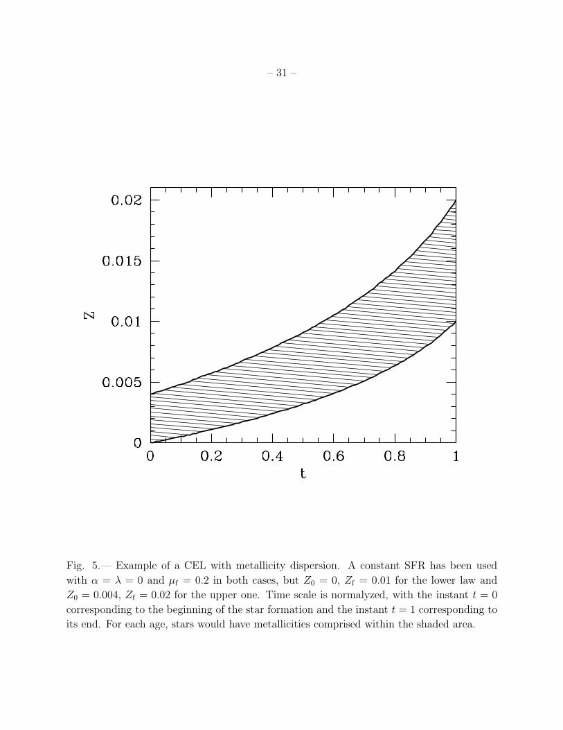
In Fig. 5 a law with metallicity dispersion is shown.

6. IAC-star computation outline

In this section we will outline how the IAC-star algorithm works paying attention to the

general interpolation procedure and to how different stellar mass ranges and evolutionary

phases are handled. Computation of mass loss in advanced evolutionary phases is explained

in the last paragraph. In Fig. 1 several tracks of different masses from the Bertelli94 library

are plotted as reference for the following discussion.

6.1. The general case

As discussed in §2, a monte-carlo algorithm and the corresponding probability

distribution functions are used to provide the age, as, mass, ms, and metallicity, Zs, of each

synthetic star. In the general, simplest case, mass and metallicity are used to compute the

evolutionary track of the star by bi-logarithmic interpolation within the evolutionary track

library. It is important to make this simple but important and cumbersome process clear.

Note that one of the difficulties is that tracks are not functions, but arbitrary curves, time

being the driving parameter. For this, interpolation must be done between homologous

sections of different tracks.

Let first introduce some notation. Tracks are identified by mass and metallicity. We

will name tracks by Ki,j, the first index denoting the metallicity and the second one, the

mass. Zs represents a value of metallicity between two values present in the stellar evolution

– 14 –

library. The algorithm input does not allow extrapolation outside the library limits in Z.

Lets call Z libi and Z lib

i+1 these two values, respectively. So Z libi ≤ Zs ≤ Z lib

i+1. A search is then

made within Z libi and Z lib

i+1 track subsets to look for the mass values embracing ms. Lets

call mlibi,j and mlib

i,j+1 the track mass values embracing ms for the Zlibi subset and mlib

i+1,k and

mlibi+1,k+1 the same for the Z lib

i+1 subset. So mlibi,j ≤ ms ≤ mlib

i,j+1 and mlibi+1,k ≤ ms ≤ mlib

i+1,k+1.

The track corresponding to star s can now be obtained by logarithmic interpolation between

tracks Ki,j, Ki,j+1, Ki+1,k, Ki+1,k+1. Lets call this interpolated track Ks. Additionally, lets

call τi,j the life time of track Ki,j, i.e., the time at which evolution within that track finish,

and τs the corresponding life time for the interpolated track.

Once Ks has been obtained, the photometric parameters of the star are obtained

straightforwardly by logarithmic interpolation of as within this track. However, before this,

whether the star is death or alive must be established. This is done just comparing as with

τs. If as ≤ τs, logarithmic interpolation is performed and the computation is finished for

this star. If not, a new dichotomy arises. If the star is of intermediate or high mass, as > τsmeans that it is death. The mass of the remnant is then computed as explained below and

added to the total mass of the system. If the star is of low mass, as > τs means that it is

beyond the He-flash. Computation in the HB track subset must be performed in this case.

For this, the mass loss of the star during the RGB is subtracted from ms (see below) and

τs is subtracted from as. The resulting mass and age, ms,HB and as,HB, are used in the HB

track subset. Computation is similar to that in the general library. If as,HB is larger than

the life time of the new interpolated HB track, the star is considered death and the remnant

mass is computed and stored as before.

We have outlined the general computation. However, a few special cases can occur

that need more comments. We will treat them in the following.

6.2. Interpolation and extrapolation between different mass ranges

It may occur that the tracks embracing the mass and metallicity of the synthetic star

belong to two different mass ranges (see Fig. 1). If some tracks are in the high mass range

and some in the intermediate mass range, interpolation can be performed as in the general

case up to the end of the tracks. After that, high mass stars are considered death while

intermediate mass stars continue through the TP-AGB, computed as outlined below.

The case is somewhat more complicated if some tracks are in the intermediate-mass

range and some in the low-mass range. The stellar physical processes are qualitatively

similar for both ranges up to the basis of the RGB: core H-burning (MS) or He-core

– 15 –

gravitationally contracting plus shell H-burning (sub-giant phase). Interpolation can hence

be performed up to that point but not afterward, when intermediate mass stars are about

to start the core He-burning while low mass stars evolve climbing the RGB. In this case, the

mass separating the intermediate and low mass ranges is firstly determined by logarithmic

interpolation between the four tracks embracing the mass and metallicity of the synthetic

star. This separating mass is used to determine the range to which the star belongs. After

this, interpolation is performed up to the RGB basis. Beyond that point, extrapolation is

made from tracks of the mass range to which the star belongs. The CMD related features

can be seen in Fig. 1

6.3. Very high and very low mass stars

The stellar mass interval is controled by the input IMF. Stars of masses beyond the

interval covered by the chosen stellar evolution library are handled in different ways,

depending on the mass being larger than the maximum mass of the library or smaller than

the minimum one. In the first case the star is simply considered death. The case of very

low mass stars is more complex.

The smallest mass computed in the used libraries are given in Table 1. Stars less

massive than that have MS life times larger than the age of globular clusters and are

certainly in the MS for any realistic case. They are normally below the limiting magnitude

in most CMDs of galaxies. However, they have a quite significant contribution to the total

mass of the system and, also to the integrated luminosity, magnitudes and colors. Although

this contribution can be estimated by integration of the IMF, it may be useful to have

the possibility of explicitly computing their colors and magnitudes. To this purpose, the

libraries mentioned above have been completed downward in mass using the models by

Cassisi et al. (2000). They present MS L and Teff of stars with masses between ∼ 0.09 M⊙

and 0.8 M⊙ for metallicity values in the range: 0.0002 ≤ 0.002. For present purpose these

models have been completed with a very low mass sequence for solar chemical composition

(Cassisi 2003, private communication). Since these stars have long evolution times and

the analysis of the CMD does not usually rely on their exact distribution in it, the effect

of age on their L and Teff can be neglected. A polynomic fit has been performed, for each

metallicity, to the m − L and the m − Teff plots of the model stars. This can be used to

estimate L and Teff of the synthetic star. The coefficients of the fit for the general equation

y = a0 + a1x+ a2x2 + a3x

3 + a4x4 + a5x

5 (7)

– 16 –

are given in Table 2. Here, x stands for logm and y for logL or log Teff , respectively.

Figure 1 shows two models computed with these relations for masses 0.4 and 0.6

M⊙ and Z = 0.004. A good agreement exists with the Bertelli94 tracks. Consistence is

also quite good comparing with the Girardi00 and the Teramo libraries (not shown here).

However the fact that the very low mass stars are computed from a different model set

(namely the Cassisi et al. 2000 one) and that no age computation is made for them must be

taken into account if accurate analysis of CMD is intended in the region around 0.6 M⊙ for

the Bertelli94 and the Teramo libraries and 0.15 M⊙ for the Girardi00 library; i.e., around

the lower mass limits of these libraries.

6.4. Mass loss

Mass loss by stellar winds plays an important role in the evolution of massive stars.

It is included in the Bertelli94 computation for stars with initial mass larger than 12 M⊙.

The reader is referred to Bertelli94 for details. Besides massive stars, mass loss during the

RGB and the AGB has dramatic consequences on the evolution of low and intermediate

mass stars. In these cases the effects of mass loss are included at the moment of computing

synthetic stars in IAC-star. Unfortunately, mass loss during these phases and, in particular,

during the AGB depends on poorly known physical parameters that should be fine-tuned.

In the modeling of mass loss during these phases we follow the criteria given by Bertelli94

and Marigo et al. (1996).

Mass loss during the RGB does not affect the internal structure of the star and can be

neglected in the computation of L and Teff . However, the integrated mass loss during this

phase determines the mass envelope of the subsequent HB stars and hence its Teff . For this

reason, mass loss can be integrated during the RGB and introduced in a single step at the

tip of the RGB (TRGB). To this purpose, the empirical relation by Reimers (1975) is used:

m = 1.27× 10−5ηm−1L1.5T−2eff M⊙/yr (8)

where L and m are in solar units and η is a scaling parameter. The lowest stellar initial

mass which evolution time up to the TRGB is smaller than or equal to the globular cluster

age (about 13 Gyr) is about 0.80 − 0.95 M⊙, depending on the metallicity, lower masses

corresponding to lower metallicities. From this, the mass loss during the RGB must be

subtracted. Since the core mass at the moment of the He-Flash is about 0.55 M⊙, the

envelope mass of these stars can be very small. As a consequence, the exact value adopted

for η strongly affects Teff at the zero-age HB. In the current version of IAC-star, η has a

– 17 –

default value of 0.35, but it can be modified by the user.

Computing the mass loss during the AGB is more complicated. It can be neglected

during the E-AGB, but it is the key parameter controlling the final evolution of the

star during the TP-AGB. Stellar evolution models of low and intermediate-mass stars

are in general computed up to the beginning of the TP-AGB only. From that point on,

computation is performed within IAC-star following the prescriptions by Marigo et al.

(1996). First, the starting point of the TP-AGB is assumed to be the point in the track

just before the first significant He-shell flash. Hence, the evolution through the TP-AGB

is followed using several basic relations: (i) the mass loss rate; (ii) a relation connecting

the core mass with the total luminosity of the star; (iii) the rate at which the core mass

increases as a result of shell H-burning, and (iv) an L − Teff relation for the TP-AGB.

Details on these relations can be found in Marigo et al. (1996) and references therein. We

shortly summarize them here for self-consistency.

The mass loss rate is taken as the minimum of the two following values:

log m = −11.4 + 0.0123P (9)

m = 6.07023× 10−3Lc−1v−1exp (10)

where m and L are the stellar mass and luminosity (in solar units), P is the pulsation

period (in days) c is the light speed (in km s−1) and vexp is the terminal velocity of the

stellar wind (in km s−1). Equations 9 and 10 stand for periods shorter and larger than

about 500 days, respectively. The wind expansion velocity is calculated in terms of the

period as (Vassiliadis & Wood 1993):

vexp = −13.5 + 0.056P (11)

and the period is derived from the period-mass-radius relation by Vassiliadis & Wood

(1993):

logP = −2.07 + 1.94 logR⋆ − 0.9 logm (12)

where R⋆ is the stellar radius in solar units.

To connect the core mass with the total luminosity of the star, the following two

equations are used:

– 18 –

L = 238000µ3wZ

0.04CNO(m

2c − 0.0305mc − 0.1802) (13)

for stars with core mass in the range 0.5 ≤ mc ≤ 0.66 (Boothroyd & Sackmann 1988), and

L = 122585µ2w(mc − 0.46)m0.19 (14)

for stars with 0.95 ≤ mc (Iben & Truran 1978; Groenewegen & de Jong 1993). For stars in

the interval 0.66 < mc < 0.95, linear interpolation is performed. In the former equations,

ZCNO is the total abundance (in mass fraction) of carbon, nitrogen and oxygen in the

envelope and µw = 4/(5X + 3− Z) is the average molecular weight for a fully ionized gas,

where X and Z are the hydrogen and metal abundances, respectively.

The rate at which the core mass increases as a result of shell H-burning is computed

using

∂mc

∂t= 9.555× 10−12LH

X(15)

where X is the hydrogen abundance (in mass fraction) in the envelope and LH is the

luminosity produced by the H-burning shell (in solar units). In fact, the latter is computed

by the relation (Iben 1977):

L = LH + 2000(M/7)0.4 exp[3.45(mc − 0.96)] (16)

Finally, the L − Teff relation of the TP-AGB is obtained by extrapolating the slope of

the E-AGB. In fact, to minimize random effects and possible inconsistencies, the slope is

computed using the following relation, obtained by bi-logarithmic fit of the slopes of all the

models at the end of the E-AGB:

log(−∂L

∂Teff) = −2.870 + 0.994 logL− 0.110 logZ (17)

where Z is the metallicity.

Using the former relations, the TP-AGB is computed for each HB and intermediate

age evolutionary track with mass m ≤ 5M⊙, according to the intermediate mass limit found

by Marigo et al. (1996). The TP-AGB computation is terminate either when the envelope

mass is zero or the core mass reaches the Chandrasekhar limit (1.4 M⊙).

– 19 –

7. Running IAC-star

IAC-star is made available for free use. It can be executed from the internet site

http://iac-star.iac.es. A number of interactive software facilities are intended to be

made available from this site, together with IAC-star itself. In fact, the content and format

of the page is expected to be up-dated, including new software and taking into account user

feed-backs. In the present form, a template is provided in which several input parameters

can be entered. For all them, default values as well as a brief option list for quick reference

are available. Once all the inputs are provided, the user can request the program to be

executed. This is performed by a dedicated computer at the Instituto de Astrofısica de

Canarias (IAC). The resulting data file is stored upon completion in a public access ftp

directory at the IAC. The address of this directory is given to the user by e-mail, to the

address provided by him or herself, together with the output file name and information on

the used inputs and the output file content. In the following we will describe the input

parameters and the output file content. Since the specific content of both may change in

future versions of the software, only a general description of them is provided. Detailed,

updated information can be found in the IAC-star internet site http://iac-star.iac.es.

7.1. Input parameters

The input parameters are introduced as follows (see the IAC-star internet site,

http://iac-star.iac.es, for updated details).

• The chosen stellar evolution and bolometric correction libraries.

• A seed for the random number generator. The routine used for random number

generation is “ran2”, obtained from Numerical Recipes in Fortran (Press et al. 1997).

• Total number of stars computed or saved into the output file. To prevent too long

runs, the maximum allowed total computed and saved stars are limited to some big

numbers.

• The minimum stellar luminosity or maximum magnitude in a given filter. Although

fainter stars are computed, only those brighter than this value are saved into the

output file.

• The SFR, ψ(t). It is computed by interpolation between several ψ(t) nodes, defined

by the user arbitrarily.

– 20 –

• The chemical enrichment law. Two alternative approaches are allowed to produce

the chemical enrichment law: (i) just an interpolation between several age-metallicity

nodes, defined by the user and permitting a completely arbitrary metallicity law;

(ii) computation from usual parameters involved in physical scenarios of chemical

evolution, even though a self-consistent physical formulation is not intended in this

case. Metallicity dispersion is allowed in both cases.

• The IMF. It is assumed to be a power law of the mass, but several mass intervals can

be defined.

• Binary star control. Both the fraction of binary stars and the secondary to primary

minimum mass ratio can be supplied.

• Mass loss parameter. Although the default η = 0.35 seems a reasonable choice, the

user can modify it here. It must be noted that η significantly affects the extension of

the HB for low metallicity stars.

7.2. The output file content

In the current version, the content of the output file is organized as follows (see the

IAC-star internet site, http://iac-star.iac.es, for updated details):

• A head containing information about the input parameters. In particular: the libraries

used, the total number of computed and stored stars; the minimum luminosity or

maximum magnitude stored; the current SFR, CEL and IMF laws; the fraction of

binaries and minimum secondary to primary mass ratio, and a heading line for the

column content, including a list of the photometric bands for which magnitudes have

been computed.

• Several lines each containing the information for a single or binary star. This

information includes physical parameters (luminosity, temperature, gravity, mass and

metallicity), photometric parameters and age.

• Closing: Integrated quantities are provided in the file closing lines, including the

total number of ever formed, currently alive and stored stars; the total mass ever

incorporated into stars (in other words, this is just the time integral of the SFR,∫ T0 ψ(t)dt); the mass currently locked into alive stars and into stellar remnants, and the

total luminosity and the integrated magnitudes. Besides these integrated quantities,

the logarithm of the sum of squared luminosities (log∑

i L2i , where Li is the luminosity

– 21 –

of the i-th star if it is single or the total luminosity of the system, if it is binary) and

the magnitudes derived from this are also given. These are the magnitudes associated

to surface brightness fluctuations (SBF). In this sense, IAC-star can be used as a SBF

population synthesis code (see Marın-Franch & Aparicio 2004).

8. Final remarks and conclusions

The program IAC-star, designed to generate synthetic CMDs is presented in this paper.

It calculates full synthetic stellar populations on a star by star basis, by computing the

luminosity, effective temperature and magnitudes of each star. A variety of stellar evolution

and bolometric correction libraries, SFR, IMF and CEL are allowed and binary stars can

be computed. The program provides also integrated masses, luminosities and magnitudes

as well as SBF luminosity and magnitudes for the total synthetic stellar population. In this

way, although it is mainly intended for synthetic CMD computation, it can be also used for

traditional and SBF population synthesis research.

Among the main characteristics of the program, the following are the most relevant:

• Luminosity and effective temperatures of each star are computed by direct bi-

logarithmic interpolation in the age-metallicity grid of a stellar evolution library. Two

Padua libraries (Bertelli94 and Girardi00) and the new Teramo library (Pietrinferni

et al. 2004) are used in the current version completed by the Cassisi et al. (2000)

models for very low mass stars. This produces a smooth distribution of stars in the

output synthetic CMD which is necessary if accurate studies of SFH are intended.

• Mass loss is computed during the RGB and the AGB phases.

• The AGB phase is extended to the TP-AGB, covering in this way all the significant

stellar evolution phases accurately.

• Color and luminosities in a variety of visual broad band, infrared and HST filters are

provided. Bolometric correction transformations by Girardi et al. (2002); Castelli &

Kurucz (2002); Flucks et al. (1994); Lejeune, Cuisinier, & Buser (1997); and Origlia

& Leitherer (2000) are used for this purpose.

The program is offered for free use and can be executed at the site

http://iac-star.iac.es, with the only requirement of referencing this paper and

acknowledging the IAC in any derived publication. It is intended to produce further

improved versions of the program after feed-back by the user community.

– 22 –

We are deeply indebted to Cesare Chiosi, Gianpaolo Bertelli and other colleagues

of the Padua stellar evolution group for a fruitful, long-term collaboration. Building up

IAC-star would not have been possible without this collaboration. We are also indebted

to Santi Cassisi for his help in the implementation of the Teramo stellar evolution library

and corresponding bolometric corrections, and for many useful discussions and advice. The

Computer Division of the IAC is acknowledged for implementing the hardware and the web

page interface of the program. Financial support has be provided by the IAC Research

Division. The authors are funded by the IAC (grant P3/94) and by the Science and

Technology Ministry of the Kingdom of Spain (grant AYA2001-1661 and AYA2002-01939).

REFERENCES

Alexander, D.R. & Ferguson, J.W. 1994, ApJ, 437, 879

Angulo, C., Arnould, M., Rayet, M., et al. (NACRE Collaboration), 1999, Nucl. Phys. A.,

656, 3

Aparicio, A. 2003, in Observed HR diagrams and stellar evolution models: the interplay

between observational constraints and theoretical limitations, eds. T. Lejeune & J.

Fernandes, ASP Conference Series, in press

Aparicio, A., Gallart, C., Chiosi, C. & Bertelli, G. 1996, ApJ, 469, L97

Aparicio, A., Gallart, C., & Bertelli, G. 1997a, AJ, 114, 669

Aparicio, A., Gallart, C., & Bertelli, G. 1997b, AJ, 114, 680

Aparicio, A. & Hidalgo, S. 2004, in preparation

Aparicio, A., Tikhonov, N., & Karachentsev, I. 2000, AJ, 119, 177

Ardeberg, A., Gustafsson, B., Linde, P., & Nissen, P. E. 1997, A&A, 322, L13

Bertelli, G., Bressan, A., Chiosi, C., Fagotto, F., & Nasi, E. 1994, A&AS, 106, 275

Bertelli, G., Mateo, M., Chiosi, C., & Bressan, A. 1992, ApJ, 388, 400

Bertelli, G. & Nasi, E. 2001, AJ, 121, 1013

Bertelli, G., Nasi, E., Girardi, L., Chiosi, C., Zoccali, M., Gallart, C. 2003, AJ, 125, 770

Boothroyd, A. I., & Sackmann, I.-J. 1988, ApJ, 328, 641

Cassisi, S., Castellani, V., Ciarcelluti, P., Piotto, G. & Zoccali, M. 2000, MNRAS, 315, 679

Castelli, F., Gratton, R.G. & Kurucz, R.L. 1997, A&A, 318, 841

Castelli, F. & Kurucz, R.L. 2002, in Modeling of Stellar Atmospheres, IAU Symp. 210

(N.E. Piskunov et al. Eds), in press

– 23 –

Caughlan, G.R. & Fowler, W.A. 1988, Atomic Data and Nuclear Data Tab. 40, 283

Chiosi, C. 1998, in Stellar Astrophysics for the Local Group, VIII Canary Islands Winter

School of Astrophysics, eds. Aparicio, A., Herrero, A., & Sanchez, F., Cambridge

University Press.

Chiosi, C., Bertelli, G., & Bressan, A. 1988, A&A, 196, 84

Chiosi, C., Bertelli, G., & Bressan, A. 1992, ARA&A, 30, 235

Cox, A.N., & Stewart, J.N. 1970a, ApJS, 19, 243

Cox, A.N., & Stewart, J.N. 1970b, ApJS, 19, 261

Dohm-Plamer, R.C., Skillman, E.D., Saha, A., et al. 1997, AJ, 114, 2527

Dolphin, A. E. 1997, New Astronomy, 2, 397

Fluks, M.A., Plez, B., The, P.S. et al. 1994, A&AS, 105, 311

Gallart, C., Aparicio, A., Bertelli, G. & Chiosi, C. 1996, AJ, 112, 1950

Gallart, C., Freedman, W. L., Aparicio, A., Bertelli, G., & Chiosi, C. 1999, AJ, 118, 2245

Girardi, L.,Bertelli, G., Bressan, A., Chiosi, C., Groenewegen, M.A.T., Marigo, P.,

Salasnich, B. & Weiss, A. 2002, A&A, 391, 195

Girardi L., Bressan A., Bertelli G., & Chiosi C. 2000, A&AS, 141, 371

Girardi L., Bressan A., Chiosi C., Bertelli G., Nasi E., 1996 A&AS, 117, 113

Groenewegen, M. A. T. & de Jong, T. 1993, A&A, 267, 410

Harris, J. & Zaritsky, D. 2001, ApJS, 136, 25

Hernandez, X., Valls-Gabaud, D., & Gilmore, G., 1999, MNRAS, 304, 705

Holtzman, J. A., Gallagher, J. S., Cole, A. A. et al. 1999, AJ, 118, 2262

Huebner W.F., Merts, A.L., Magee, N.H. & Argo, M.F. 1997, Los Alamos Scientific

Laboratory Report LA-6760-M

Hurley-Keller, D., Mateo, M., & Nemec, J. 1998, AJ, 115, 1840

Iben, I. 1977, ApJ, 217, 788

Iben, I., & Truran, J. W. 1978, ApJ, 220, 980

Iglesias, C.A. & Rogers, F.J. 1996, ApJ, 464, 943

Irwin, A.W. et al. 2004, in preparation

Kippenhahn, R., Thomas, H.-C. & Weigert, A. 1965, Z. Astrophys. 61, 241

Kroupa, P., Tout, C. A., & Gilmore, G. 1993, MNRAS, 262, 545

– 24 –

Kunz, R., Fey, M., Jaeger, M., Mayer, A., Hammer, J.W., Staudt, G., Harissopulos, S., &

Paradellis, T. 2002, ApJ, 567, 643

Kurucz, R.L. 1992, in Stellar Populations of Galaxies, eds. B. Barbuy and A. Renzini

(Dordrecht: Kluwer) p. 225

Landre, V., Prantzos, N., Aguer, P., Bogaert, G., Lefebre, A., & Thibaud, J.P. 1990, A&A,

240, 85

Lejeune, Th., Cuisinier, F., & Buser, R. 1997, A&AS, 125, 229

Maeder, A. 1974, A&A, 32, 177

Marigo, P., Bressan, A., & Chiosi, C. 1996, A&A, 313, 545

Marın-Franch, A., & Aparicio, A. 2004, in preparation

Mihalas, D., Hummer, D.G., Mihalas, B.W. & Dappen, W. 1990, ApJ, 350, 300

Ng, Y.K., Brogt, E., Chiosi, C., & Bertelli, G. 2002, A&A, 392, 1129

Origlia, L, & Leitherer, C. 2000, AJ, 119, 2018

Peimbert, M., Colın, P., & Sarmiento, A. 1994, in Violent Star Formation: from 30 Doradus

to QSOs, ed. Tenorio-Tagle, G., Cambridge University Press

Pietrinferni, A., Cassisi, S., Salaris, M. & Castelli, F. 2004, ApJ, submitted.

Press, W. H., Teukolsky, S. A., Vetterling, W. T., & Flannery, B. P. 1997. Numerical

Recipes in Fortran 77. The art of scientific computation, Cambridge University Press

Reimers, D. 1975, Mem. Soc. R. Sci. Liege 6 (8), 369

Rogers, F. J., & Iglesias, C. A. 1992, ApJS, 79, 507

Stappers, B. W., Mould, J. R., Sebo, K. R. et al. 1997, PASP, 109, 292

Tinsley, B. 1980, Fund. Cosmic Phys., 5, 287

Tolstoy, E., & Saha, A. 1996, ApJ, 462, 672

Tosi, M., Greggio, L., Marconi, G., & Focardi, P. 1991, AJ, 102, 951

Vallenari, A., Bertelli, G., & Schmidtobreick, L. 2000, A&A, 361, 73

Vallenari, A., Chiosi, C., Bertelli, G., & Ortolani, S. 1996a, A&A, 309, 358

Vallenari, A., Chiosi, C., Bertelli, G., Aparicio, A. & Ortolani, S. 1996b, A&A, 309, 367

Vassiliadis, E., & Wood, P. R. 1993, ApJ, 413, 641

Weaver, T.A. & Woosley, S.E. 1993 Phys. Rep. 227, 65

This preprint was prepared with the AAS LATEX macros v4.0.

– 25 –

Table 1. Model grids used in the current version of IAC-star

Models Teramo Girardi00 Bertelli94

Mass range [M⊙] 0.5-10 0.15-7 0.6-120

Z range (Z,nstep) 0.0001-0.04 (10) 0.0-0.03 (8) 0.0004-0.05 (5)

α = l/Hp 1.913 1.68 1.63

Y⊙, Z⊙ 0.2734, 0.0198 0.273, 0.019 0.282,0.02

Overshooting canonical & 0.2Hpa 0.5Hp

a,b 0.5Hpa,b

EOS Irwin04 Kipp65+Gir96+MHD90 Kipp65

Rad. Opacity OPAL96+Alex94 OPAL92+Alex94 OPAL92+Hueb77+Cox70

Nucl. Reactions NACRE+Kunz02 Caughlan88+Landre90+WW93 Caughlan88

Model Atm. Castelli02 Castelli97 Kurucz92+emp

Note. — Key to references: Teramo: Pietrinferni et al. (2004); Girardi00: Girardi et al. (2000);

Bertelli94: Bertelli et al. (1994); Irwin04: Irwin, A.W. et al. (2004); OPAL96: Iglesias & Rogers (1996);

Alex94: Alexander & Ferguson (1994); NACRE: Angulo et al. (1999); Kunz02: Kunz et al. (2002);

Castelli02: Castelli & Kurucz (2002); Kipp65: Kippenhahn, Thomas & Weigert (1965); Gir96: Girardi

et al. (1996); MHD90: Mihalas et al. (1990); OPAL92: Rogers & Iglesias (1992); Caughlan88: Caughlan

& Fowler (1988); Landre90: Landre et al. (1990); WW93: Weaver & Woosley (1993); Castelli97:Castelli,

Gratton & Kurucz (1997); Huebb77: Huebner et al. (1997); Cox70: Cox & Stewart (1970a,b); Kurucz92:

Kurucz (1992)

aThe prescription on how overshooting is turned off as a function of mass heavily determines the

morphology of the MS-TO at intermediate ages. Teramo: λ=(M/M⊙-0.9)/4 for 1.1M⊙ ≤ M≤ 1.7M⊙,

λ=0.2Hp for M≥ 1.7M⊙ and λ=0 for M≤ 1.1M⊙; Girardi00: λ = M/M⊙-1.0 for 1.0M⊙ ≤ M≤ 1.5M⊙,

with λ=0.5Hp for M≥ 1.5M⊙ and λ=0 for M≤ 1.0M⊙; Bertelli94: λ=0.5Hp for M≥ 1.6M⊙, λ=0.25Hp

for 1.0M⊙ ≤ M ≤ 1.5M⊙.

bThe parameter describing overshooting is its extent λ across the border of the convective zone, in units

of pressure scale height (Hp). This parameter, defined in Bressan et al. (1981) is not equivalent to others

present in the literature. E.g. λ = 0.5 in the Padova formalism approx corresponds to 0.25Hp above the

convective border adopted by the Teramo group.

– 26 –

Table 2. Coeficients of the logL− logm and log Teff − logm fits for very low mass stars

Relation a0 a1 a2 a3 a4 a5

Z=0.0002, Y=0.23:

logL vs. logm: 1.1387 11.3958 15.8615 8.7825 0.1773

log Teff vs. logm: 4.2038 4.3333 13.5738 22.1148 18.2446 6.0709

Z=0.0006, Y=0.23:

logL vs. logm: 1.1457 11.7429 16.6033 9.4539 0.3695

log Teff vs. logm: 4.1851 4.1282 12.2825 19.1799 15.4070 5.0853

Z=0.001, Y=0.23:

logL vs. logm: 1.0342 10.9539 14.2405 6.5840 –0.8234

log Teff vs. logm: 4.2229 4.7253 14.9449 24.4181 20.0889 6.6370

Z=0.002, Y=0.23:

logL vs. logm: 0.8190 9.6332 10.7591 2.8464 –2.2331

log Teff vs. logm: 4.2593 5.4559 18.3152 31.0882 26.0219 8.5882

Z=0.02, Y=0.27:

logL vs. logm: 0.3668 9.8685 16.8057 14.4196 3.9769

log Teff vs. logm: 3.8133 1.5630 3.2232 2.8249 0.7851

– 27 –

Fig. 1.— Set of evolutionary tracks for metallicity Z = 0.004 from the library of Bertelli94

(full and dashed lines) extended by two very low mass models interpolated from Cassisi et

al. (2000) of age 10 Gyr (starred dots). Colors indicate different mass ranges, as follows.

Red: high mass tracks; blue: intermediate mass tracks; magenta: low mass stars up to the

He-flash; black: low mass stars HB. In all the cases, dashed lines represent the TP-AGB

extensions of the Padua tracks computed by IAC-star. Labels correspond to the track initial

masses, in M⊙.

– 28 –

Fig. 2.— Synthetic CMD computed using constant SFR from 13 Gyr ago to date and

metallicity linearly increasing from Z0 = 0.0001 to Zf = 0.02 and a Kroupa et al. (1993) IMF.

The Bertelli94 stellar evolution library and the Lejeune et al. (1997) bolometric correction

library have been used. Stars in different age intervals are plotted in different colors. The

color code is given in the figure, in Gyr. Labels indicate the evolutionary phase (see text for

an explanation).

– 29 –

Fig. 3.— Synthetic CMD computed using constant SFR from 13 Gyr ago to date and

metallicity linearly increasing from Z0 = 0.0001 to Zf = 0.001, Salpeter IMF, and a 0.3

fraction of binary stars with minimum mass ratio 0.7. The Bertelli94 stellar evolution library

and the Lejeune et al. (1997) bolometric correction library have been used. Colors and

magnitudes of binary stars are represented in green. Green points in the single star locus of

the MS correspond to binary stars in which the primary is dead.

– 30 –

Fig. 4.— Examples of CELs for different choices of µf , α, λ and ψ(t) are given for fixed

Z0 = 0 and Zf = 0.02. For ψ(t), an exponential law of the form ψ(t) = A exp(−t/βψ) has

been used, where A is set to normalyze the integral of ψ(t) for the entyre life of the systen.

Time scale is normalyzed, with the instant t = 0 corresponding to the beginning of the

star formation and the instant t = 1 corresponding to its end. In the upper window the

parameter choices are displayed. Bracketed figures correspond to [βψ, µf , α, λ]. Closed-box

models are drawn in blue, infall models are drawn in red and outflow models in magenta.

– 31 –

Fig. 5.— Example of a CEL with metallicity dispersion. A constant SFR has been used

with α = λ = 0 and µf = 0.2 in both cases, but Z0 = 0, Zf = 0.01 for the lower law and

Z0 = 0.004, Zf = 0.02 for the upper one. Time scale is normalyzed, with the instant t = 0

corresponding to the beginning of the star formation and the instant t = 1 corresponding to

its end. For each age, stars would have metallicities comprised within the shaded area.