I T&I -3iF - Chinese University of Hong Kong

I T&I n -3iF COMPUllK

ELSEVIER Image and Vision Computing 16 (1998) 353-362

An efficient iterative pose estimation algorithm

S.H. Ora,*, W.S. Lukb, K.H. Wang”, I. King”

“Computer Science and Engineering Department, The Chinese University of Hong Kong, Shatin, NT, Hong Kong

‘K&h&eke Universiteit Leuven, Department Computerwetenschappen, Celrstijnenlaan ZOOA, B-3001 Heverlee, Belgium

Received 23 June 1997; received in revised form 29 October 1997; accepted 30 October 1997

Abstract

A novel model-based pose estimation algorithm is presented which estimates the motion of a three-dimensional object from a image sequence. The nonlinear estimation process within iteration is divided into two linear estimation stages, namely the depth approximation and the pose calculation. In the depth approximation stage, the depths of the feature points in three-dimensional space are estimated. In the pose calculation stage, the rotation and translation parameters between the estimated feature points and the model point set arer calculated by a fast singular value decomposition method. The whole process is executed recursively until the result is stable. Since both stages can be solved efficiently, the computational cost is low. As a result, the algorithm is well-suited for real computer vision applications. We demonstrate the capability of this algorithm by applying it to a real time head tracking problem. The results are satisfactory. 0 1998 Elsevier Science B.V. All rights reserved.

Keywords: Pose estimation; Real time vision; Human-computer Interface; Singular value decomposition

1. Introdution

Tracking the pose (position and orientation) of a moving object from an image sequence is useful in applications such as photogrammetry, passive navigation, industry inspection and human-computer interfaces [ 1,2]. However, this is a difficult problem because of the following reasons. Firstly, the depth information has been transformed by a nonlinear mapping to yield the foreshortening effect in the captured image. Moreover, the rotation of the object in three- dimensional space leads to a nonlinear formulation which increases dramatically the computational requirement for generating the solution.

In this paper, we are interested in the model-based pose estimation problem or the two-dimensional to three- dimensional problem as catagorized by Huang [3]. That is, when the three-dimensional structure of the object being investigated is known and its two-dimensional projected image is available, we want to compute the pose of the object. In practice, the model of the three-dimensional positions of the feature points of the object can be measured manually before tracking begins. A two-dimensional correlation method can be used to track the movements of the projected two-dimensional feature points. Using this

* Corresponding author. Tel: 00 852 2609 8402; fax: 00 852 2603 5024; e-mail: [email protected].

0262.8856/98/$19.00 0 1998 Elsevier Science B.V. All rights reserved.

PII SO262-8856(97)00073-S

information we would like to find the rotation (R) and translation (T) of the object in three-dimensional. A number of techniques have been developed by previous researches [4- 9, 2,101 to solve this problem. One way is to compute the motion information directly from the optical flow [I 1,8], which require massive computation power. In Ref. [4], a closed form solution for the pose from six points is derived. The method is extended to the estimation of more points by a consensus of sampling from the set. Robustness is achieved in this method at the expense of intensive computation of motion information from sampled subsets of the points.

Another method to increase the robustness is the use of the method of least-squares. Depending on the formulation (using Euler angles or quatemions to represent rotation), various methods can be used to recover the pose from exact data. However, the problem will become a nonlinear least squares one when noise exists. Iterative algorithms such as the Newton-Raphson method [7] are applied to find the solution, but with the drawback of being heavily dependant on the initial guess.

It is observed that a long image sequence can provide more information for the estimation process to suppress noise. Extended Kalman filter is used to model the problem as a recursive estimation process by Broida et al. [ 12,131 and Azarbayejani et al. [2]. The authors demonstrated that the pose of a moving object can be successfully recovered. However, the Kalman Filter method is found to be

354 S.H. Or et al./lmage and Vision Computing 16 (1998) 353-362

successful in those applications where the observed objects would not change their appearance rapidly, e.g. aerospace and vehicles applications [7]. In other applicatons such as human motion tracking, owing to the complexities of the motion involved, more work is needed to increase the robostness of the overall tracking system.

P

PP

Our interest is in devoping an efficient algorithm which is suitable for various applications on human motion analysis. This area is characterized by the rapid motion of the object concerned and high probability of occlusion/re-appearance of part of the object in the subsequent frames.

Specifically we are interested in solving the two- dimensional to three-dimensional problem as mentioned by Haung [3]. We notice that there is already a solution for the three-dimensional to three-dimensional problem as mentioned in Ref. [ 141. That is when the three-dimensional locations of the features in the new positions are available, we can use the method of singular value decomposition (SVD) to find out the motion parameters [14-161. A least- squares solution is found. However, the algorithm will sometimes give a wrong (reflection of the correct. answer) solution when the input data are severely corrupted by noise. This was fixed by Umeyama [ 151 and later shown to be valid even when both point sets are noisey [ 161. In this paper, we propose an algorithm which extends the above methods to handle the problem of recovery of motion information from two-dimensional projections of a given three-dimensional point set. Our solution consists of the following two mod- ules: (1) from the two-dimensional features on the image plane, we estimate the locations of the features in three dimensions; and (2) using the estimated three-dimensional information we use the method of SVD as in [14-161 to develop the motion parameters of the object. The above two processes are executed recursively until the solution is stable. Our contribution here is that our algorithm requires significantly reduced computation compared with other techniques [7,2] under the situation of large number of feature points, say over 20.

Fig. 1. Relationship between original point and projected point.

Qi = txQ, > 'Q, 9 fh

placed at (0, 0, fi, as shown in Fig. 1, where f is the focal length of the plane. Assume that a set of N model points (Pi, i E 1, 2,. . ., N} in three-dimensional space are given, which represents an object model. A rigid transformation (a rotation followed by a translation) is applied to this point set, yielding {Pi’], which is then projected on the image plane, giving { (Xpi, Ye,), i E 1,2,. . .,N) .l These two- dimensional feature points in our three-dimensional coordi- nate system are given by:

Let the three-dimensional coordinates of the transformed points Pi be (XPci, Y,c, Z,,,). The coordinates of P’i and Qi are related by:

XP,, YP,, XQ, =f q ‘Qi =vf q

The rest of this paper is organized as follows. In Section 2, the model-based pose estimation problem is formulated. Section 3 contains the first verson of our algorithm together with the convergence analysis of te algorithm. The weakness of our algorithm is identified and a more robust algorithm is then proposed. In Section 4, the performance of the improved algorithm is compared with two established approache, namely the Gauss-Newton method and the extended Kal- man filter method. In Section 5, we tested our algorithms on both synthetic and realistic image data. A head tracking application is implemented to test the validity of our approach on realistic images. Finally some possible enhancements of our algorithms are discussed in Section 6.

In this arrangement, any point Qi tracked in the image will give an inverse projection ray from the focal center with unit vector vi given by (Xi, + Y& +f*) - “*(XQ,, YQi, f). The actual coordinates of this point in three-dimensional space

are given by:

P’i = diVi, (1)

where di is the depth (a scalar) of the actual object from the perspectivity center.

The problem of pose estimation can be described as follows. Given { Qi, i E 1, 2,. . .,N} and a three-dimensional model (Pi, i E 1,2,. . .,N), where Pi = (Xp,, Ypc, Zp,) are the coordinates of the model points at a reference instant. We seek R, T and {di] such that the following measurement function:

e2(R, T, {di ]) = f IIdiVi - (R Pi + T)II* i=l

2. Problem formulation

Consider a camera with the origin of the focal plane ’ In this paper, we use a bold font to represent the two-dimensional vector

on the image plane.

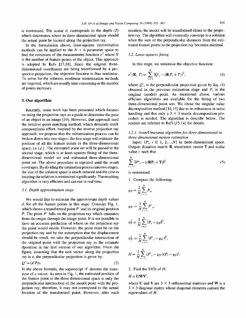
S.H. Or et al./Imqe and Vision Computing 16 (1998) 353-362 355

is minimized. The scalar di corresponds to the depth (2) which determines where in three-dimensional space should

the actual point be located along the projection ray. In the formulation above, least-squares minimization

methods can be applied to the N + 6 parameter space to find the minimum of the measurement function e2 where N is the number of feature points of the object. This approach is adopted In Refs [ 17,181. Since the original three- dimensional coordinates are being transformed by a per- specive projection, the objective function is thus nonlinear. To solve for the solution, nonlinear minimization methods are required, which are usually time consuming as the number of points increases.

3. Our algorithm

Recently, some work has been presented which focuses on using the projection rays as a guide to determine the pose of an object in an image [ 191. However, that approach used the iterative point matching method, which demands much computational effort. Inspired by the inverse projection ray approach, we propose that the minimization process can be broken down into two stages: the first stage will estimate the position of all the feature points in the three-dimensional space, i.e { di) . The estimated point set will be passed to the second stage, which is at least-squares fitting of the three- dimensional model set and estimated three-dimensional point set. The above procedure is repeated until the result coverages. By dividing the estimation process into two stages, the size of the solution space is much reduced and the cost in locating the solution is minimized significantly. The resulting algorithm is very efficient and can run in real time.

3.1. Depth approximation stage

We would like to estimate the approximate depth values di for all the feature points in this stage. Consider Fig. 1, which shows a transformed point P’ and its original position P. The point P’ falls on the projection ray which emanates from the origin through the image point. It is not possible to have an accurate prediction of where on the projection ray the point would reside. However, the point must be on the projection ray and by the assumption that the displacement should be small, we take the perpendicular intersection of the original point with the projection ray as the estimate dposition in the first version of our algorithm. From the figure, assuming that the unit vector along the projection ray is Y, the perpendicular projection is given by:

Q’ = (v’P)v. (3)

In the above formula, the superscript ‘t’ denotes the trans- pose of a vector. As seen in Fig. 1, the estimated position of the feature point in the three-dimensional space is only the perpendicular intersection of the model point with the projection ray; therefore, it may not correspond to the actual location of the transformed point. However, after each

iteration, the model will be transformed closer to the projection ray. The algorithm will eventually converge to a solution

when the sum of the perpendicular distances from the estimated feature points to the projection ray becomes minimal.

3.2. Least-squares jtting

In this stage, we minimize the objective function:

e2(R, T) = $ IIQ’, - (R Pi + T)I12, i= 1

(4)

where Qli is the perpendicular projection given by Eq. (4) obtained in the previous estimation stage and Pi is the original (model) point. As mentioned above, various efficient algorithms are available for the fitting of two three-dimensional point sets. We chose the singular value decomposition method [ 14,151 due to its robustness in noise handling and that only a 3 X 3 matrix decomposition procedure is needed. The algorithm is describe below. The readers are referred to Refs [ 15,141 for details.

3.2.1. ArunNrneyama algorithm for three-dimensional to

three-dimensional motion estimation Input: {Pi, i E 1, 2 , . . .,N} in three-dimensional space.

Output: Rotation matrix R, translation vector T and scalar value c such that

N

~ IIP’i - (CRPi + T)I12 i=l

(5)

is minimized.

1. Compute the following:

u; = f g lIPi - ppl12, r=l

up’ = ; 2 IIP’i - j,iP’l12, 2

1-l

H = ; ,$ (Prj - pp,)(Pi - P~)~. 1-l

2. Find the SVD of H:

H = UWV’,

where U and V are 3 X 3 orthonormal matrices and W is a 3 X 3 diagonal matrix whose diagonal elements contain the eigenvalues of H.

3.56 S.H. Or et al./lmage and Vision Computing 16 (1998) 353-362

3. If the rank of H > 2, the optimal transformation is given by:

s=

I

I if det(H) 2 0

diag(1, 1, -1) if det(H)<O

R = USV’,

c = -Lr(WS),

T = pp’ - CR/L,,

else, if the rank of H = 2,

1

I s=

if det( U) det( V) = 1

diag(1, 1, - 1) if det(U) det(V) = - 1

R= USV’,

c= $WS),

T = pp’ - cR/L~,

In the above, det(x) is the determinant of x and tr(x) is the trace of a matrix x.In Umeyama’s formulation, a scaling parameter c is also recovered. In our algorithm, we fix the value of c at one to reflect the fact that the object size does not change in subsequent images.

3.3. Algorithm I

The complete algorithm is as follows:

Input:

(Pi,i E 1, 2,. . . ,N] : transformed feature points (or the model) of the object, Q’i : (Xe,,, Y,,,), i E 1,2,. .., N: transformed feature point coordinates on the image plane.

Procedure:

While (change in R or T not iess than some threshold values):

estimate di by VIPi is the unit vector along the projection ray formed by image point Qi’ and the origin; perform at least-squares fitting to Eq. (5) to estimate R and T by the singular value decomposition method

114,151; update Pi by PieRPi + T.

end while.

3.4. Convergence analysis

We now perform a convergence analysis of our algorithm. The analysis of the convergence condition of a

particular algorithm is usually not treated in most pose estimation literature. However, it is an important criterion for the evaluation of algorithms. Many motion estimation algorithms are very sensitive to noise. Moreover, nonlinear algorithms usually lead to wrong results if the initial guess is not sufficiently close to the recovered values.

Assuming that a model point P is transformed to another location P’ by a rigid body transform, the perpendicular projection of P onto P’ is Q’ (see Fig. 1) and P’ is given by:

P’=RF’+T. (6)

From Fig. 1, Q’ can also be written as:

Q’ = p’ 1 - ‘p;p--;;y’).

The second term on the right hand side of the above equation, which is the fractional difference between the estimated position and the true one, can be treated as the error in prediction. By studying the dependencies of this term on figurations and motion characteristics, the performance of our algorithm can be readily characterized.

The second term inside the parenthesis on the right of Eq. (7) can be written as:

(P’ - P)‘P’ &=

llPrl12 ’ (8)

(RP)‘RP + (RP)‘T + T’(T - P) - P’RP =

(RP)‘RP + 2(RP)‘T + T’T (9)

The prediction error term E depends on the values of R, P and T. From the above equation, we would expect that for a large ratio of lITI/ to IIPII, the algorithm would converge to a wrong result as E approaches one.

From the above, we see that our algorithm would converge to wrong reuslts as the ratio IITII/IIPII increases. How- ever, imagine a scene in which an object moving at a fast speed, the feature points taken between successive frames would probably result in significant distances apart. Since our aligorithm will only try to bring the model as close to the projection ray as possible, this would result in te model being brought to a local minimum where the algorithm will be stuck. A more robust enhancement is therefore need to handle the translational movement.

Recall that our original algorithm can be viewed as follows:

Iterate until convergence

1. construct the initial estimate by projecting the model points individually onto the line formed by the camera origin and feature points;

2. fit a rotation matrix and a translation vector to account for the transformation between the estimated set and model set.

We can see that the initial guess plays an important role in the overal estimation process. Assuming there is no motion in the model points (i.e. the rotation and translation have

S.H. Or et al./hage and Vision Computing 16 (1998) 353-362 357

already been determined and the model points have been updated), the variables (di} now remain to be determined. They can be viewed as the parameters obtained from the minimization of 0, where:

0 = ~ lldivi - Pill* = ~ (d,? - diU:Pj - diP:~; + P:Pj). 1=I i=l

(10) In the above formula, Yi is the unit vector of the projection ray (with the property Y:Y~ = 1).

Differentiating the above equation with respect to di and setting the partial differential equals to zero and rearranging terms, we have:

di = v:P~, (11)

which is the same form as a dot product of Yi with Pi. We can see that our original algorithm is working in the

following way:

1. assume the object has no motion, determine ( di, i E 1, 2 ,...> NJ;

2. assume {di,i E 1, 2 , . . . ,N) are determined, estimate R and T;

3. update the state of the solution and iterate again.

3.5. Algorithm II

At this stage, we modify the minimization function in Eq. (10) so as to increase the robustness of our algorithm. The idea is to add the translation term into the minimization function in stage 1 so that the predicted position {di} for i E 1, 2,..., N will be more accurate.

The improved algorithm is as follows:

1. Minimize the function below to estimate { di,i E 1, 2, . . ..N].

~ IIdiVi - (P; + ~)ll*. (12) i=l

The resulting {d,, i E 1, 2,. .,N) and T is given by:

d, = v;(P; = T), (13)

T= - ($4) -’ (zAi’i)f (14)

where Ai is a 3 X 3 matrix given by

Ai = I - u~v:. (15)

For the derivation of the above formula, please refer to Appendix A. 2. Using the estimated (di, i E 1, 2,...,N) in the previous

stage, apply the SVD method to determine the rigid transformation R and T.

3. Update {P;, i E 1, 2,. . .,N} by Pt+RPt + T.

Note that the Ais are not needed to be stored explicitly. Firstly, each Ai depends only on Vi, which is fixed before the execution of our algorithm. Therefore, the value of (xr=, Ai) - ’ in Eq. (14) can be precomputed before the iterations, which avoids the expensive inverting operation of a matrix. Moreover, the matrix vector product A,Pi can be computed efficiently using the formula Pi - Vi(V:Pi). AS a rough estimate for the computational requirements at each iteration, for N data points, our algorithm needs only about 4 1 N arithmetic operations (additions, subtractions and multiplications) and one singular value decomposition operation for a 3 X 3 matrix that is about a hundred floating point operations. We also noticed the algorithm by DeMenthon and Davies [9] which requires only 24N arithmetic operations and two square root operations. However, our argument for the efficiency is still valid by the following reasons. Firstly, in the appraoch used by De Menthon and Davies, the algorithm requires an approximate pose estimate from the previous stage, which would inevitably contribute to the computational requirement. Moreover, their method does not guarentee the orthonormality of the resulting rotation matrix. Whereas our algorithm uses the singular value decomposition, which provides an orthonormal result, hence improves the accuracy and thus justifies the increase in computation. Hence, we conclude that the resulting algorithm is accurate and efficient.

4. Performance comparison

Various approaches have been applied successfully to the problem of motion analysis. In this section, we compare the performance of two established approaches with our algorithm. The main interest here is the computational efficincy since the main concern during the motion tracking application would probably be the timing requirement as well as accuracy and stability. We chose the Gauss-Newton method (by Lowe [7]) and the extended Kalman filter method (by Broida et al. [13] and Azarbayejani et al. [2]) due to their robustness and computational efficiency.

4.1. Gauss-Newton method

Lowe [7,20] used the Gauss-Newton method augmented with stabilization with prior variance to solve the pose tracking method and the following matrix equation is solved:

[“WI,= [ -oE]T where h is the unknown vector of corrections to be made to current estimate, E is the error between the current measurement and that of model prediction, J is the Jacobian matrix of the error with respect to the parameters; W is a diagonal weighting matrix which stabilizes the solution. It should be noted that Lowe’s approach minimizes the errors between

358 S.H. Or et al/Image and Vision Computing 16 (1998) 353-362

6wo .-

6ow --

l---/ m

. . ..~.~r.r.r.~p.~~.------4--- ___--9

o _L..;-;-_.;.8__yI_‘_- .‘.. ~.~.~.~~~.~.~..~.~.~.~.. ( :

7 10 15 20 25 30

No. of points

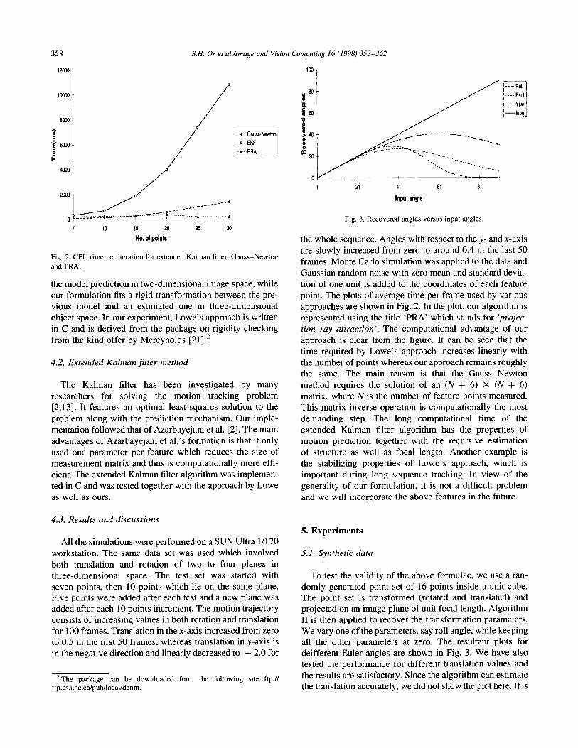
Fig. 2. CPU time per iteration for extended Kalman filter, Gauss-Newton

and PRA.

the model prediction in two-dimensional image space, while our formulation fits a rigid transformation between the previous model and an estimated one in three-dimensional object space. In our experiment, Lowe’s approach is written in C and is derived from the package on rigidity checking from the kind offer by Mcreynolds [213.*

4.2. Extended Kalman jilter method

The Kalman filter has been investigated by many researchers for solving the motion tracking problem [2,13]. It features an optimal least-squares solution to the problem along with the prediction mechanism. Our implementation followed that of Azarbayejani et al. [2]. The main advantages of Azarbayejani et al.‘s formation is that it only used one parameter per feature which reduces the size of measurement matrix and thus is computationally more efficient. The extended Kalman filter algorithm was implemented in C and was tested together with the approach by Lowe as well as ours.

I 21 41 61 61

Input angle

Fig. 3. Recovered angles versus input angles.

the whole sequence. Angles with respect to they- and x-axis are slowly increased from zero to around 0.4 in the last 50 frames. Monte Carlo simulation was applied to the data and Gaussian random noise with zero mean and standard devia- tion of one unit is added to the coordinates of each feature point. The plots of average time per frame used by various approaches are shown in Fig. 2. In the plot, our algorithm is represented using the title ‘PRA’ which stands for ‘projection ray attraction’. The computational advantage of our approach is clear from the figure. It can be seen that the time required by Lowe’s approach increases linearly with the number of points whereas our approach remains roughly the same. The main reason is that the Gauss-Newton method requires the solution of an (N + 6) X (N + 6) matrix, where N is the number of feature points measured. This matrix inverse operation is computationally the most demanding step. The long computational time of the extended Kalman filter algorithm has the properties of motion prediction together with the recursive estimation of structure as well as focal length. Another example is the stabilizing properties of Lowe’s approach, which is important during long sequence tracking. In view of the generality of our formulation, it is not a difficult problem and we will incorporate the above features in the future.

All the simulations were performed on a SUN Ultra l/170 workstation. The same data set was used which involved both translation and rotation of two to four planes in three-dimensional space. The test set was started with seven points, then 10 points which lie on the same plane. Five points were added after each test and a new plane was added after each 10 points increment. The motion trajectory consists of increasing values in both rotation and translation for 100 frames. Translation in the x-axis increased from zero to 0.5 in the first 50 frames, whereas translation in y-axis is in the negative direction and linearly decreased to - 2.0 for

4.3. Results and discussions

5. Experiments

‘The package can be downloaded form the following site ftp:/l ftp.cs.ubc.ca/pub/local/danm.

5.1. Synthetic data

To test the validity of the above formulae, we use a randomly generated point set of 16 points inside a unit cube. The point set is transformed (rotated and translated) and projected on an image plane of unit focal length. Algorithm II is then applied to recover the transformation parameters. We vary one of the parameters, say roll angle, while keeping all the other parameters at zero. The resultant plots for deifferent Euler angles are shown in Fig. 3. We have also tested the performance for different translation values and the results are satisfactory. Since the algorithm can estimate the translation accurately, we did not show the plot here. It is

S.H. Or et al./Image and Vision Computing 16 (1998) 353-362 359

12 T

1 11 21 31 41 51

Translation

Fig. 4. Recovered values for increasing translation.

observed that the rcovered Euler angle becomes unreliable after one or more of the input angles exceed 20”. Also note that the translation terms can be unambiguously recovered even for a large value compared with the magnitude of original model vectors. We have also performed the same set of experiments on Algorithm I. The same performance on recovered rotation is observed, while the estimated translation quickly drops to zero when the translation increases

4.0

3.5

2.5

as shown in Fig. 4. This is to be expected according to the analysis in Section 3.4.

The performance of our algorithm under a noisy environ- ment was also invetigated. Two sets of experiments were performed. We first descibe the set-up since they are uncom- mon for both experiments. A number of points are randomly generated in the three-dimensional space such that they will project on an image plane of size 2 X 2. These model points are then transformed by a rotation about the axis (1, 1, 1) by 6” followed by a translation of (5.0, 3.0, 6.0). The transformed points are then projected on the image plane. The image coordinates are then digitized to a screen resolution of 512 X 512. The process of digitization introduces noise in this case. 100 random scences are generated according to this set-up and the digitized coordinates are used together with the original generated three-dimensional model to determine the pose.

The errors shown in the following are all relative errors. We used quaternions to represent the rotation such that all the estimated results are in vector form. The relative error of a vector is defined by the Euclidean norm of the difference between the true vector divided by the Euclidean norm of the true vector. The first set of experiments tests the performance of the algorithm under different number of points in the scene. The results are shown in Fig. 5. From the plot, it is observed that the estimated rotation is relatively stable with respect to the variation of the number of points whereas the

6 6 10 12 14 16 16 20 22 24 26 28 30

No. of points

Fig. 5. Plot of error dependency on the number of points.

360 S.H. Or et al./Image and Vision Computing 16 (1998) 353-362

30

T P

Fig. 6. Plot of error in estimation versus measurment noise

translation has the greatest improvement from eight to 12 points. In addition, the digitization only introduces a small effect on the estimated results, as can be seen in the range of errors it is only within 3%.

Another set of experiments simulates the measurement noise by introducing an offset value to both digitized x and y coordinates. These offset values are normally distrib- uted with a variance of k pixels where k is the parameter to be varied in the experiments. 16 points are used in this set of experiments. Fig. 6 shows the results and our algorithm again is quite stable under the situation of increasing noise.

5.2. Real image testing

Pose tracking involves continuous monitoring of the pose of an object from the imput image sequence. Our algorithm can easily be adapted for continuous tracking by performing estimation between successive image frames. We tested our algorithm by applying it to track to track the head of a person in an image sequence. Our implementation is performed on an SGI Indy workstation. To verify the correct- ness of the recovered pose information, we produce the same motion on the workstation at the same time. Though it is difficult in this case to estimate the perfomance figure of the algorithm, an overall estimate of the usefulness of the algorithm can be obtained.

X2.1. Calibration A calibrated data point set for the face to be tracked is

needed in our experiment. Two methods can be used. In the first approach, one can measure dirctly the three- dimensional coordinates of the feature points on the face with respect to a reference point, say the nose tip, The drawback of this approach is that careful measurements are needed and that the process is intrusive. The second approach uses the structure from mtion algorithm. We

Fig. 7. Sample run ot the nead tracking application: (a) initialization;

(b) rotation of the head and reconstructed pose.

used the second approach, following the algorithm by Szeliski [ 171. An image sequence of the object is obtained and the feature points of the model are selected and tracked throughout the sequence to generate a batch of two- dimensional image coordinates of these feature points. The resulting data is input to the batch processing algorithm which performs a nonlinear minimization (Levenberg- Marquardt method). The algorithm will estimate the focal length f, the model set {P,, i, 2,. . .,N} as well as the motion parameters. This process usually requires much more time. For the case of a total of 250 data points for a synthetic head model, the total time needed is over 10 h on a SUN-Spare 10 workstation. In our real image experiment, only 12 points are used. All points are selected on the criteria that they can be tracked unambiguously throughout the sequence so as to increase the accuracy of the recovered pose. We use four points for the head boundary including ears, four points the mouth and four points for each of the eyebrows.

5.2.2. Initialization The user first clicks on the captured image with a mouse

to select the feature points. The selected feature points must be the same as those taken in the calibration stage. These selected feature points are then tracked by the normalized correlation method to give coordinates in successive frames. The correlation window is of size 5 X 5, whereas the search window is of size 7 X 7. The point inside the search window

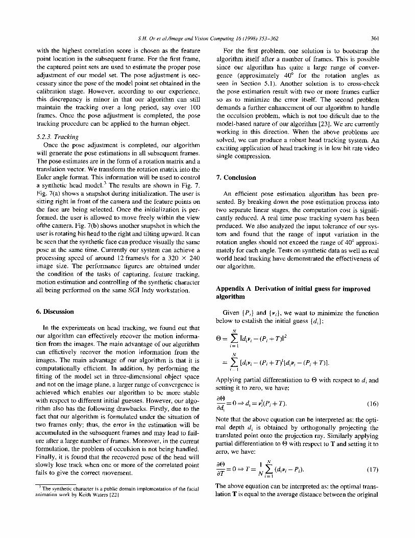
S.H. Or et al./lmage and Vision Computing 16 (1998) 353-362 361

with the highest correlation score is chosen as the feature point location in the subsequent frame. For the first frame,

the captured point sets are used to estimate the proper pose adjustment of our model set. The pose adjustment is nec- cessary since the pose of the model point set obtained in the calibration stage. However, according to our experience, this discrepancy is minor in that our algorithm can still maintain the tracking over a long period, say over 100 frames. Once the pose adjustment is completed, the pose

tracking procedure can be applied to the human object.

5.2.3. Tracking

Once the pose adjustment is completed, our algorithm will generate the pose estimations in all subsequent frames. The pose estimates are in the form of a rotation matrix and a translation vector. We transform the rotation matrix into the Euler angle format. This information will be used to control a synthetic head model.3 The results are shown in Fig. 7. Fig. 7(a) shows a snapshot during initialization. The user is sitting right in front of the camera and the feature points on the face are being selected. Once the initialization is performed, the user is allowed to move freely within the view ofthe camera. Fig. 7(b) shows another snapshot in which the user is rotating his head to the right and tilting upward. It can be seen that the synthetic face can produce visually the same pose at the same time. Currently our system can achieve a processing speed of around 12 frames/s for a 320 X 240 image size. The performance figures are obtained under the condition of the tasks of capturing, feature tracking, motion estimation and controlling of the synthetic character all being performed on the same SGI Indy workstation.

For the first problem, one solution is to bootstrap the

algorithm itself after a number of frames. This is possible since our algorithm has quite a large range of convergence (approximately 40” for the rotation angles as seen in Section 5.1). Another solution is to cross-check the pose estimation result with two or more frames earlier so as to minimize the error itself. The second problem demands a further enhancement of our algorithm to handle the occulsion problem, which is not too dificult due to the model-based nature of our algorithm [23]. We are currently working in this direction. When the above problems are solved, we can produce a robust head tracking system. An exciting application of head tracking is in low bit rate video single compression.

7. Conclusion

An efficient pose estimation algorithm has been presented. By breaking down the pose estimation process into two separate linear stages, the computation cost is significantly reduced. A real time pose tracking system has been produced. We also analyzed the input tolerance of our system and found that the range of input variation in the rotation angles should not exceed the range of 40” approximately for each angle. Tests on synthetic data as well as real world head tracking have demonstrated the effectiveness of our algorithm.

Appendix A Derivation of initial guess for improved algorithm

6. Discussion

In the experiments on head tracking, we found out that our algorithm can effectively recover the motion information from the images. The main advantage of our algorithm can effictively recover the motion information from the images. The main advantage of our algorithm is that it is computationally efficient. In addition, by performing the fitting of the model set in three-dimensional object space and not on the image plane, a larger range of convergence is achieved which enables our algorithm to be more stable with respect to different initial guesses. However, our algorithm also has the following drawbacks. Firstly, due to the fact that our algorithm is formulated under the situation of two frames only; thus, the error in the estimation will be accumulated in the subsequent frames and may lead to fail- ure after a large number of frames. Moreover, in the current formulation, the problem of occulsion is not being handled. Finally, it is found that the recovered pose of the head will slowly lose track when one or more of the correlated point fails to give the correct movement.

Given (Pi} and (vi), we want to minimize the function below to estalish the initial guess { di) :

O = ~ IIdivi - (Pi + T)II* i=l

= f_ [divi - (Pi + T)‘[div; - (Pi + T)].

i= I

Applying partial differentiation to 0 with respect to di and setting it to zero, we have:

a@ ~ = 0 j di = V:(Pi + T).

I

(16)

Note that the above equation can be interpreted as: the optimal depth di is obtained by orthogonally projecting the translated point onto the projection ray. Similarly applying partial differentiation to 0 with respect to T and setting it to zero, we have:

ao dT="*T=-

b,f_ (diVj_P') I . r=l

(17)

3 The synthetic character is a public domain implementation of the facial The above equation can be interpreted as: the optimal trans-

animation work by Keith Waters [22] lation T is equal to the average distance between the original

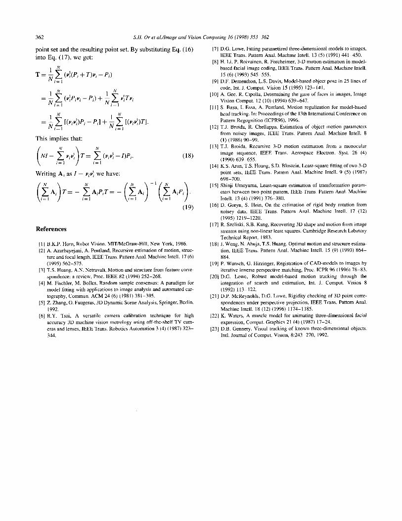
362 S.H. Or et al./lmage and Vision Computing 16 (1998) 353-362

point set and the resulting point set. By substituting Eq. (16) into Eq. (17), we get:

T = ~ ,~ (v:(P~ + T)vi - Pi) r-l

= ~ ~ (v:P~v~ - Pi) + ~ ~ VITVi r-l 1-l

= ~ ,~ [(viu:)Pi - Pi] + ~ ,~ [(ViV:)T]. 1-l r-1

This implies that:

Writing Ai as I - ViV: we have:

(18)

References

[1] B.K.P. Horn, Robot Vision. MIT/McGraw-Hill, New York, 1986.

[2] A. Azarbayejani, A. Pentland, Recursive estimation of motion, struc-

ture and focal length, IEEE Trans. Pattern Anal. Machine Intell. 17 (6)

(1995) 562-575.

[3] T.S. Huang, A.N. Netravali, Motion and structure from feature corre-

spondence: a review, Proc. IEEE 82 (1994) 252-268.

[4] M. Fischler, M. Belles, Random sample consensus: A paradigm for

model fitting with applications to image analysis and automated car-

tography, Commun. ACM 24 (6) (1981) 381-395.

[5] Z. Zhang, 0. Faugeras, 3D Dynamic Scene Analysis, Springer, Berlin,

1992.

[6] R.Y. Tsai, A versatile camera calibration technique for high

accuracy 3D machine vision metrology using off-the-shelf TV cam-

eras and lenses, IEEE Trans. Robotics Automation 3 (4) (1987) 323-

344.

[7] D.G. Lowe, Fitting parametized three-dimensional models to images,

IEEE Trans. Pattern Anal. Machine Intell. 13 (5) (1991) 441-450.

[8] H. Li, P. Roivainen, R. Forcheimer, 3-D motion estimation in model-

based facial image coding, IEEE Trans. Pattern Anal. Machine Intell.

15 (6) (1993) 545-555.

[9] D.F. Dementhon, L.S. Davis, Model-based object pose in 25 lines of

code, Int. J. Comput. Vision 15 (1995) 123-141. [IO] A. Gee, R. Cipolla, Determining the gaze of faces in images, Image

Vision Comput. 12 (10) (1994) 639-647. [l l] S. Basu, I. Essa, A. Pentland, Motion regulization for model-based

head tracking. In: Proceedings of the 13th International Conference on

Pattern Regognition (ICPR96), 1996.

[12] T.J. Broida, R. Chellappa, Estimation of object motion parameters

from noisey images, IEEE Trans. Pattern Anal. Machine Intell. 8

(1) (1986) 90-99. [13] T.J. Broida, Recursive 3-D motion estimation from a monocular

image sequence, IEEE Trans. Aerospace Electron. Syst. 26 (4)

(1990) 639-655. [ 141 KS. Arun, T.S. Huang, SD. Blostein, Least-square fitting of two 3-D

point sets, IEEE Trans. Pattern Anal. Machine Intell. 9 (5) (1987)

698-700. [ 151 Shinji Umeyama, Least-square estimation of transformation param-

eters between two point pattern, IEEE Trans. Pattern Anal. Machine

Intell. 13 (4) (1991) 376-380. [16] D. Goryn, S. Hein, On the estimation of rigid body rotation from

noisey data, IEEE Trans. Pattern Anal. Machine Intell. 17 (12)

(1995) 1219-1220. [17] R. Szeliski, S.B. Kang, Recovering 3D shape and motion from image

streams using non-linear least squares. Cambridge Research Labatory

Technical Report, 1983. [18] J. Weng, N. Ahuja, T.S. Huang, Optimal motion and structure estima-

tion, IEEE Trans. Pattern Anal. Machine Intell. 15 (9) (1993) 864-

884. [ 191 P. Wunsch, G. Hirzinger, Registration of CAD-models to images by

iterative inverse perspective matching, Proc. ICPR 96 (1996) 78-83. [20] D.G. Lowe, Robust model-based motion tracking through the

integration of search and estimation, Int. J. Comput. Vision 8

(1992) 113-122. [21] D.P. McReynolds, D.G. Lowe, Rigidity checking of 3D point corre-

spondences under perspective projection, IEEE Trans. Pattern Anal.

Machine Intell. 18 (12) (1996) 1174-1185.

[22] K. Waters, A muscle model for animating three-dimensional facial

expression, Comput. Graphics 21 (4) (1987) 17-24.

[23] D.B. Gennery. Visual tracking of known three-dimensional objects.

Intl. Journal of Comput. Vision, 8:243-270, 1992.

I T&I -3iF - Chinese University of Hong Kong

Documents