1 / 66 I. Quantum Waveform Detection Theory II. Quantum Waveform Estimation Theory III. Quantum Microwave Photonics * Mankei Tsang Department of Electrical and Computer Engineering Department of Physics National University of Singapore [email protected] http://mankei.tsang.googlepages.com/ February 28, 2013 ∗ This material is based on work supported by the Singapore National Research Foundation Fellowship (NRF-NRFF2011-07).

Welcome message from author
This document is posted to help you gain knowledge. Please leave a comment to let me know what you think about it! Share it to your friends and learn new things together.
Transcript
1 / 66
I. Quantum Waveform Detection TheoryII. Quantum Waveform Estimation Theory
III. Quantum Microwave Photonics ∗
Mankei TsangDepartment of Electrical and Computer Engineering
Department of PhysicsNational University of Singapore
http://mankei.tsang.googlepages.com/
February 28, 2013
∗This material is based on work supported by the Singapore National Research Foundation Fellowship (NRF-NRFF2011-07).
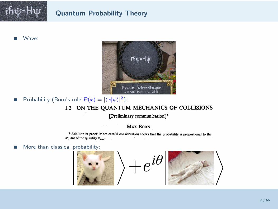
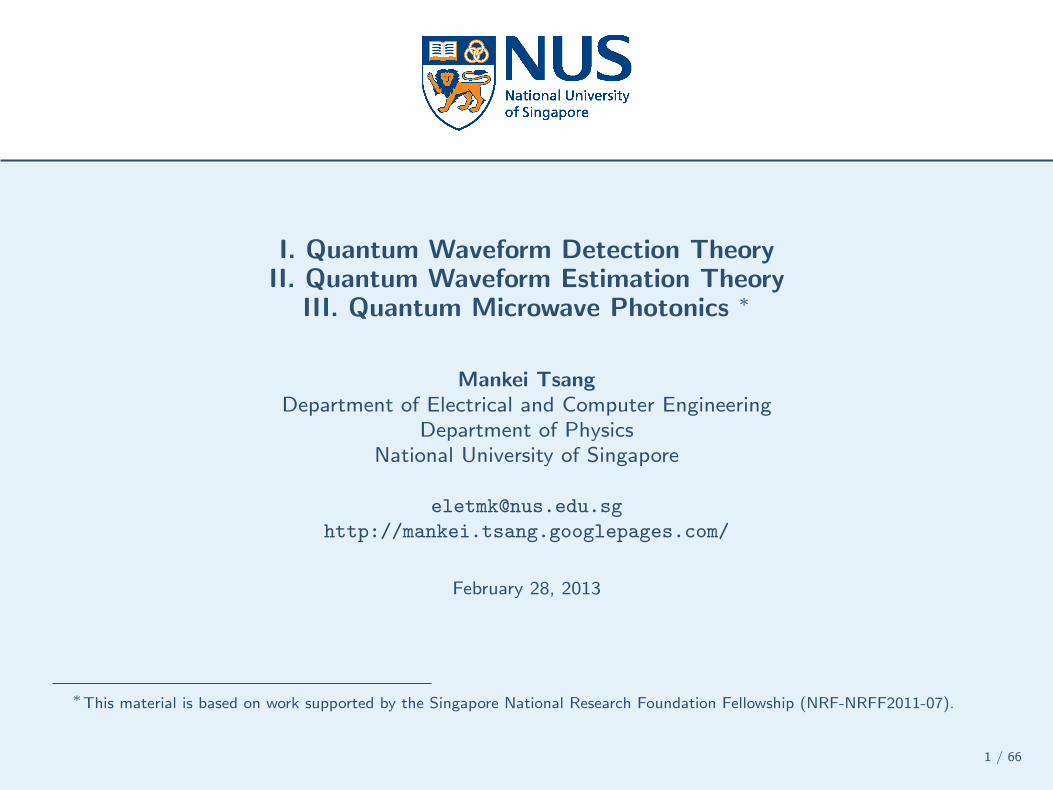
Quantum Probability Theory
2 / 66
Wave:
Probability (Born’s rule P (x) = |〈x|ψ〉|2):
More than classical probability:
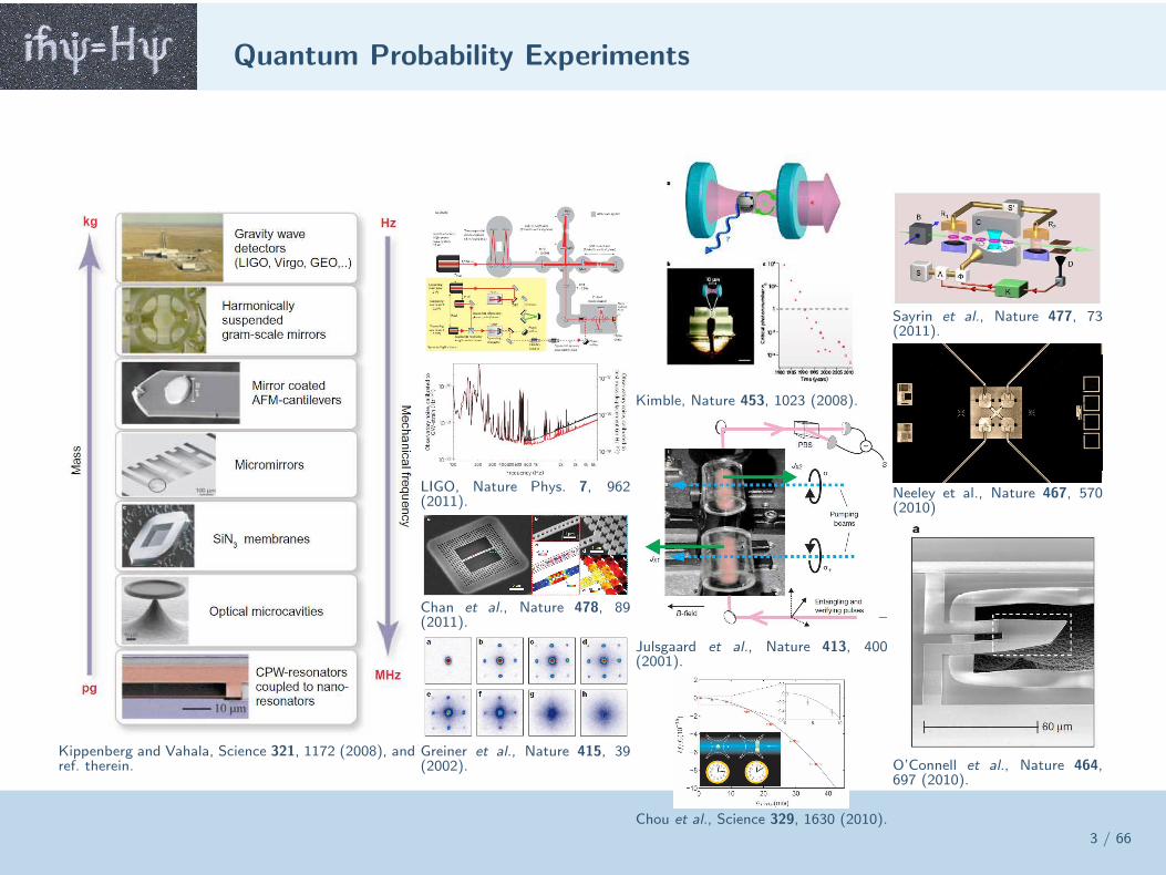
Quantum Probability Experiments
3 / 66
Kippenberg and Vahala, Science 321, 1172 (2008), andref. therein.
LIGO, Nature Phys. 7, 962(2011).
Chan et al., Nature 478, 89(2011).
Greiner et al., Nature 415, 39(2002).
Kimble, Nature 453, 1023 (2008).
Julsgaard et al., Nature 413, 400(2001).
Chou et al., Science 329, 1630 (2010).
Sayrin et al., Nature 477, 73(2011).
Neeley et al., Nature 467, 570(2010)
O’Connell et al., Nature 464,697 (2010).
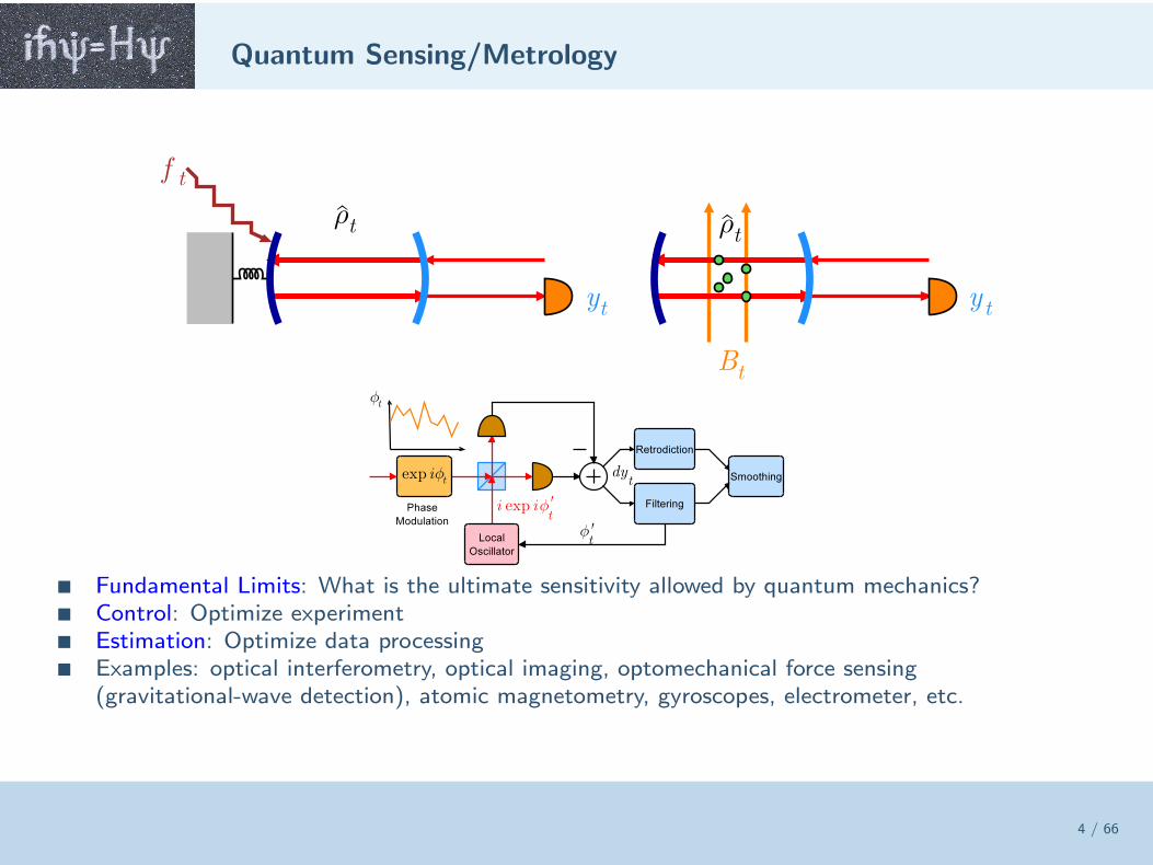
Quantum Sensing/Metrology
4 / 66
Fundamental Limits: What is the ultimate sensitivity allowed by quantum mechanics? Control: Optimize experiment Estimation: Optimize data processing Examples: optical interferometry, optical imaging, optomechanical force sensing
(gravitational-wave detection), atomic magnetometry, gyroscopes, electrometer, etc.
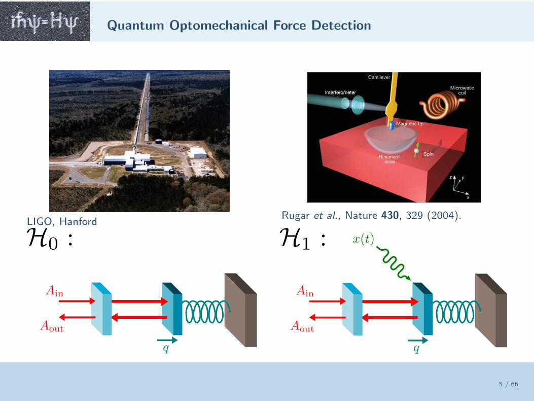
Quantum Optomechanical Force Detection
5 / 66
LIGO, HanfordRugar et al., Nature 430, 329 (2004).
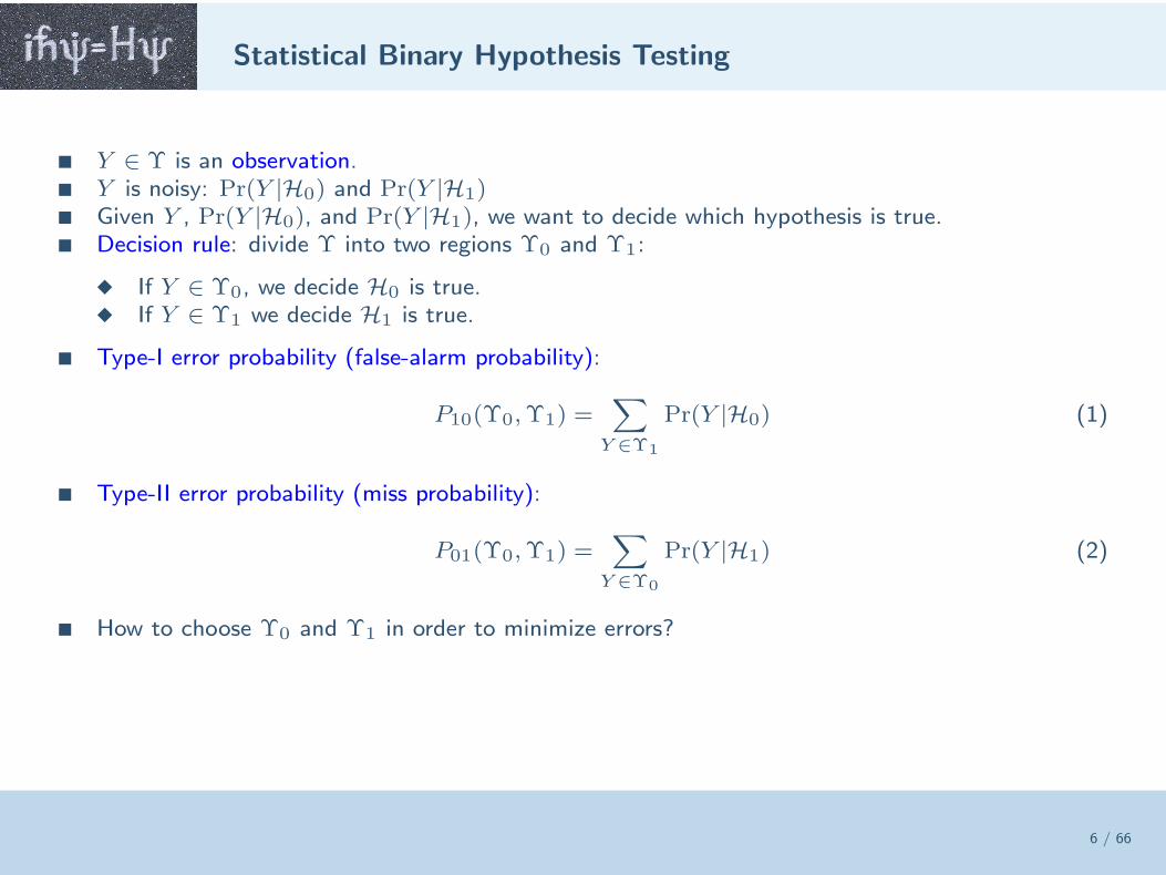
Statistical Binary Hypothesis Testing
6 / 66
Y ∈ Υ is an observation. Y is noisy: Pr(Y |H0) and Pr(Y |H1) Given Y , Pr(Y |H0), and Pr(Y |H1), we want to decide which hypothesis is true. Decision rule: divide Υ into two regions Υ0 and Υ1:
If Y ∈ Υ0, we decide H0 is true. If Y ∈ Υ1 we decide H1 is true.
Type-I error probability (false-alarm probability):
P10(Υ0,Υ1) =∑
Y ∈Υ1
Pr(Y |H0) (1)
Type-II error probability (miss probability):
P01(Υ0,Υ1) =∑
Y ∈Υ0
Pr(Y |H1) (2)
How to choose Υ0 and Υ1 in order to minimize errors?
Likelihood-Ratio Test
7 / 66
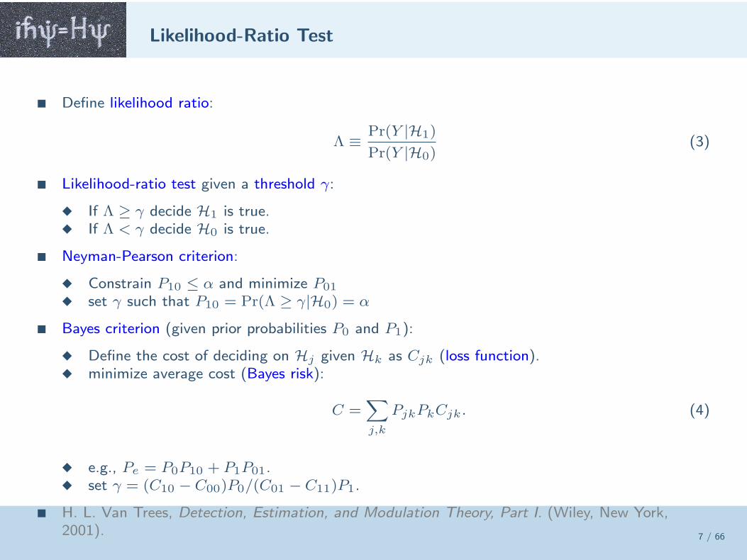
Define likelihood ratio:
Λ ≡ Pr(Y |H1)
Pr(Y |H0)(3)
Likelihood-ratio test given a threshold γ:
If Λ ≥ γ decide H1 is true. If Λ < γ decide H0 is true.
Neyman-Pearson criterion:
Constrain P10 ≤ α and minimize P01
set γ such that P10 = Pr(Λ ≥ γ|H0) = α
Bayes criterion (given prior probabilities P0 and P1):
Define the cost of deciding on Hj given Hk as Cjk (loss function). minimize average cost (Bayes risk):
C =∑
j,k
PjkPkCjk. (4)
e.g., Pe = P0P10 + P1P01. set γ = (C10 − C00)P0/(C01 − C11)P1.
H. L. Van Trees, Detection, Estimation, and Modulation Theory, Part I. (Wiley, New York,2001).
Error Probabilities
8 / 66
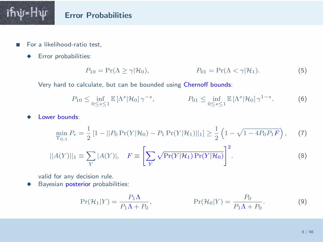
For a likelihood-ratio test,
Error probabilities:
P10 = Pr(Λ ≥ γ|H0), P01 = Pr(Λ < γ|H1). (5)
Very hard to calculate, but can be bounded using Chernoff bounds:
P10 ≤ inf0≤s≤1
E [Λs|H0] γ−s, P01 ≤ inf
0≤s≤1E [Λs|H0] γ
1−s. (6)
Lower bounds:
minΥ0,1
Pe =1
2[1− ||P0 Pr(Y |H0)− P1 Pr(Y |H1)||1] ≥
1
2
(
1−√
1− 4P0P1F)
, (7)
||A(Y )||1 ≡∑
Y
|A(Y )|, F ≡[
∑
Y
√
Pr(Y |H1) Pr(Y |H0)
]2
. (8)
valid for any decision rule. Bayesian posterior probabilities:
Pr(H1|Y ) =P1Λ
P1Λ + P0, Pr(H0|Y ) =
P0
P1Λ + P0. (9)
Quantum Hypothesis Testing
9 / 66
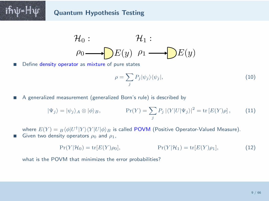
Define density operator as mixture of pure states
ρ =∑
j
Pj |ψj〉〈ψj |, (10)
A generalized measurement (generalized Born’s rule) is described by
|Ψj〉 = |ψj〉A ⊗ |φ〉B , Pr(Y ) =∑
j
Pj |〈Y |U |Ψj〉|2 = tr [E(Y )ρ] , (11)
where E(Y ) = B〈φ|U†|Y 〉〈Y |U |φ〉B is called POVM (Positive Operator-Valued Measure). Given two density operators ρ0 and ρ1,
Pr(Y |H0) = tr[E(Y )ρ0], Pr(Y |H1) = tr[E(Y )ρ1], (12)
what is the POVM that minimizes the error probabilities?
Quantum Error Bounds
10 / 66
C. W. Helstrom, Quantum Detection and Estimation Theory, (Academic Press, New York, 1976). Given constraint P10 ≤ α,
P01 ≥
1−[√αF +
√
(1− α)(1− F )]2, α < F,
0, α ≥ F.(13)
Average error probability:
minE(Y )
Pe =1
2(1− ||P1ρ1 − P0ρ0||1) ≥
1
2
(
1−√
1− 4P0P1F)
, (14)
||A||1 ≡ tr√
AA†, F ≡(
tr√√
ρ0ρ1√ρ0
)2
. (15)
For pure states,
F = |〈ψ0|ψ1〉|2 , (16)
and there exist POVMs such that the fidelity bounds are saturated.
Quantum Optics
11 / 66
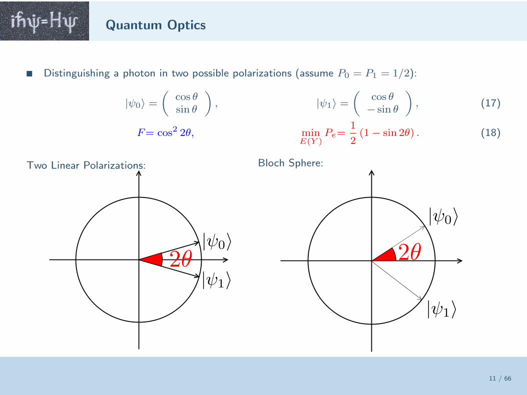
Distinguishing a photon in two possible polarizations (assume P0 = P1 = 1/2):
|ψ0〉 =(
cos θsin θ
)
, |ψ1〉 =(
cos θ− sin θ
)
, (17)
F= cos2 2θ, minE(Y )
Pe=1
2(1− sin 2θ) . (18)
Two Linear Polarizations: Bloch Sphere:
Optimal measurement
12 / 66
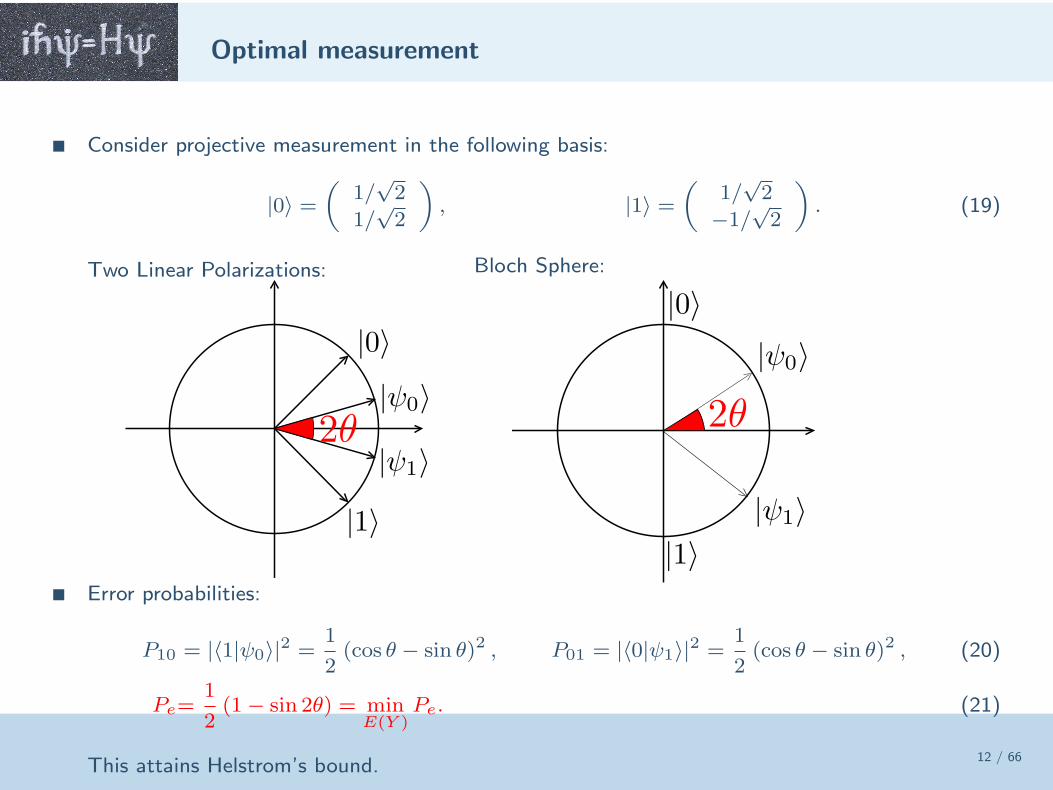
Consider projective measurement in the following basis:
|0〉 =(
1/√2
1/√2
)
, |1〉 =(
1/√2
−1/√2
)
. (19)
Two Linear Polarizations: Bloch Sphere:
Error probabilities:
P10 = |〈1|ψ0〉|2 =1
2(cos θ − sin θ)2 , P01 = |〈0|ψ1〉|2 =
1
2(cos θ − sin θ)2 , (20)
Pe=1
2(1− sin 2θ) = min
E(Y )Pe. (21)
This attains Helstrom’s bound.
Experiment
13 / 66
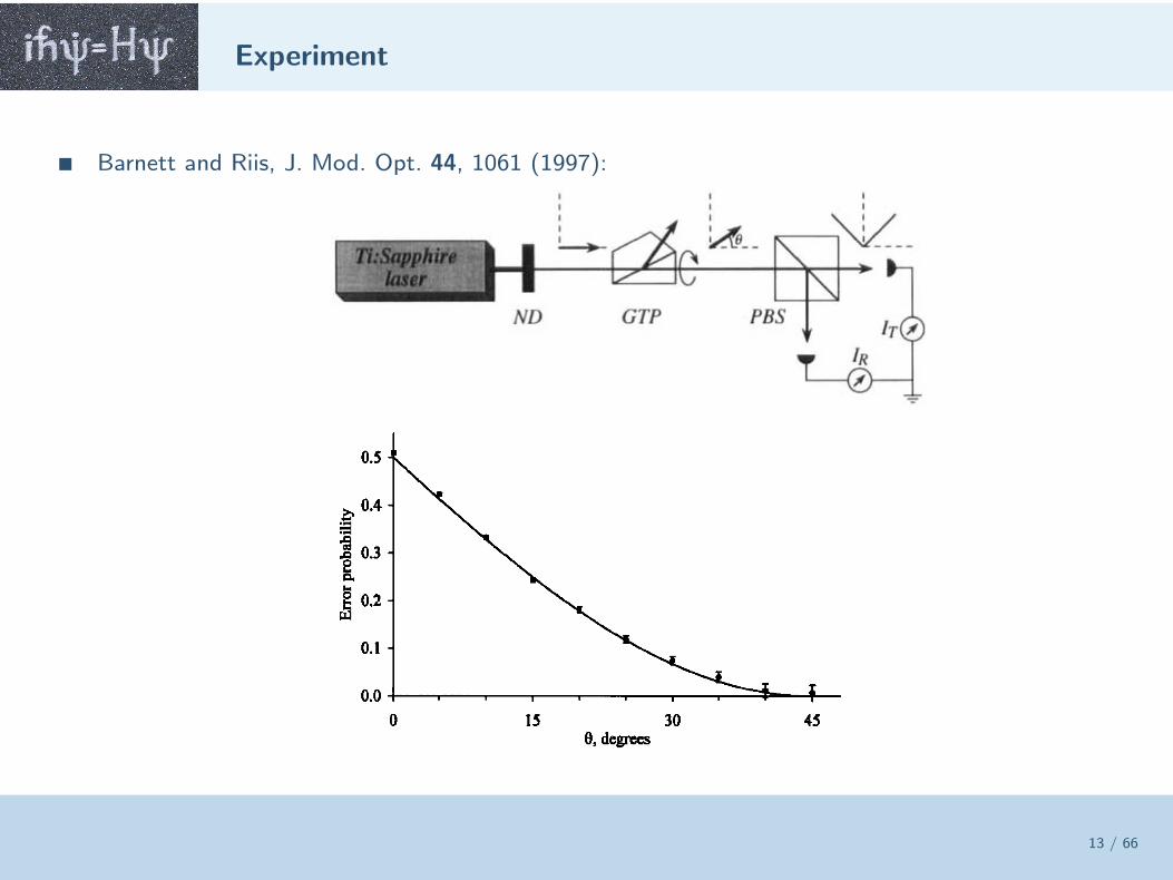
Barnett and Riis, J. Mod. Opt. 44, 1061 (1997):
Coherent-State Discrimination
14 / 66
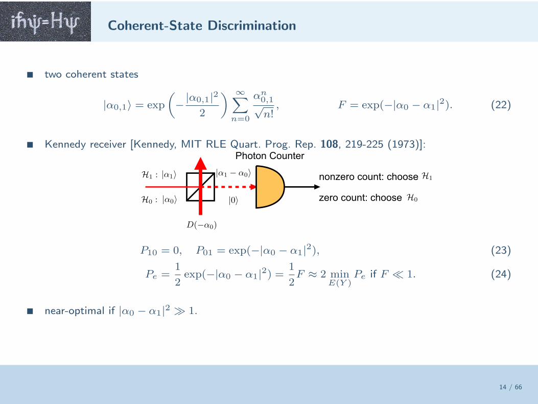
two coherent states
|α0,1〉 = exp
(
−|α0,1|22
) ∞∑
n=0
αn0,1√n!, F = exp(−|α0 − α1|2). (22)
Kennedy receiver [Kennedy, MIT RLE Quart. Prog. Rep. 108, 219-225 (1973)]:Photon Counter
zero count: choose
nonzero count: choose
P10 = 0, P01 = exp(−|α0 − α1|2), (23)
Pe =1
2exp(−|α0 − α1|2) =
1
2F ≈ 2 min
E(Y )Pe if F ≪ 1. (24)
near-optimal if |α0 − α1|2 ≫ 1.
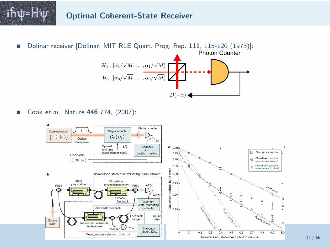
Optimal Coherent-State Receiver
15 / 66
Dolinar receiver [Dolinar, MIT RLE Quart. Prog. Rep. 111, 115-120 (1973)]:Photon Counter
Cook et al., Nature 446 774, (2007):
Helstrom bound for Waveform Estimation
16 / 66
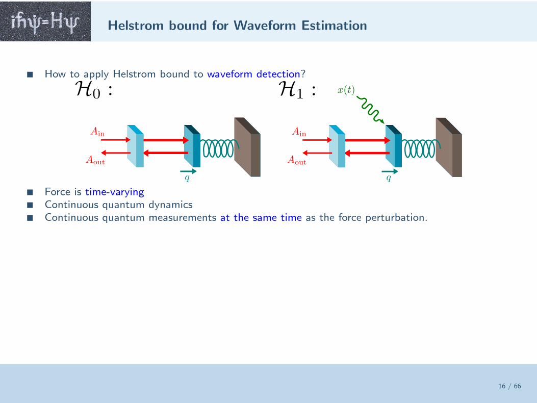
How to apply Helstrom bound to waveform detection?
Force is time-varying Continuous quantum dynamics Continuous quantum measurements at the same time as the force perturbation.
Quantum Information Theory to the Rescue
17 / 66
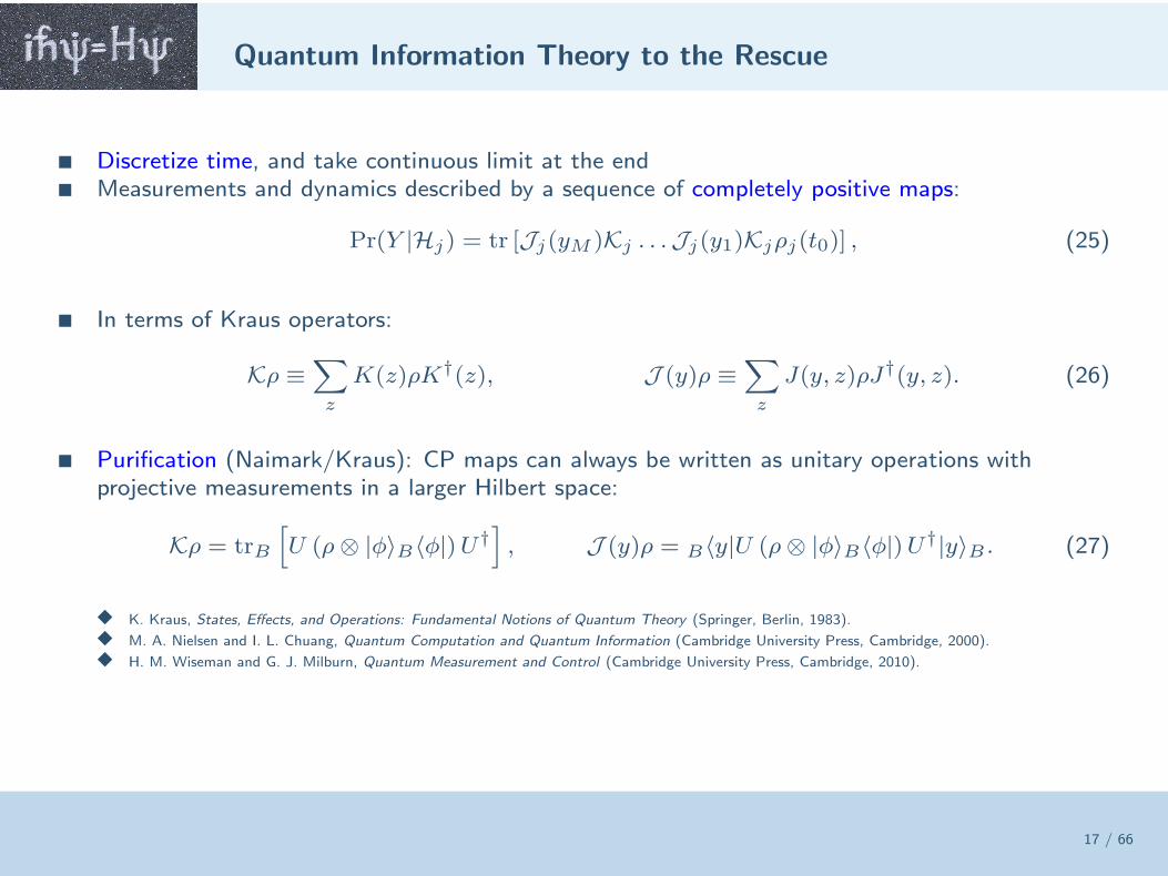
Discretize time, and take continuous limit at the end Measurements and dynamics described by a sequence of completely positive maps:
Pr(Y |Hj) = tr [Jj(yM )Kj . . .Jj(y1)Kjρj(t0)] , (25)
In terms of Kraus operators:
Kρ ≡∑
z
K(z)ρK†(z), J (y)ρ ≡∑
z
J(y, z)ρJ†(y, z). (26)
Purification (Naimark/Kraus): CP maps can always be written as unitary operations withprojective measurements in a larger Hilbert space:
Kρ = trB
[
U (ρ⊗ |φ〉B〈φ|)U†]
, J (y)ρ = B〈y|U (ρ⊗ |φ〉B〈φ|)U†|y〉B . (27)
K. Kraus, States, Effects, and Operations: Fundamental Notions of Quantum Theory (Springer, Berlin, 1983).
M. A. Nielsen and I. L. Chuang, Quantum Computation and Quantum Information (Cambridge University Press, Cambridge, 2000).
H. M. Wiseman and G. J. Milburn, Quantum Measurement and Control (Cambridge University Press, Cambridge, 2010).
Church of Larger Hilbert Space
18 / 66
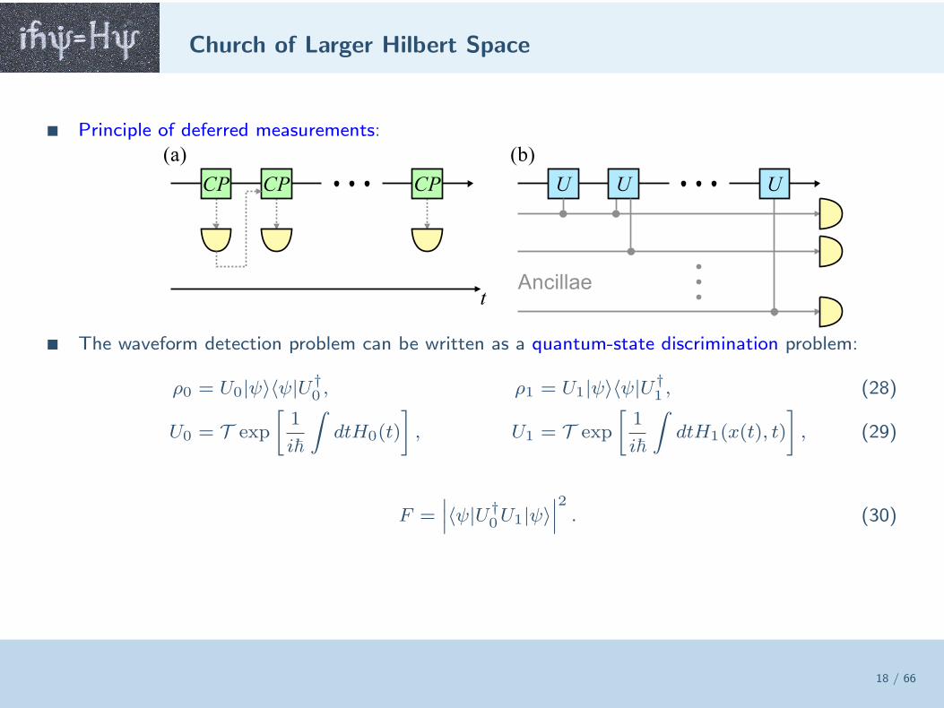
Principle of deferred measurements:
The waveform detection problem can be written as a quantum-state discrimination problem:
ρ0 = U0|ψ〉〈ψ|U†0 , ρ1 = U1|ψ〉〈ψ|U†
1 , (28)
U0 = T exp
[
1
i~
∫
dtH0(t)
]
, U1 = T exp
[
1
i~
∫
dtH1(x(t), t)
]
, (29)
F =∣
∣
∣〈ψ|U†
0U1|ψ〉∣
∣
∣
2. (30)
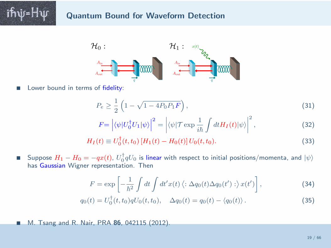
Quantum Bound for Waveform Detection
19 / 66
Lower bound in terms of fidelity:
Pe ≥ 1
2
(
1−√
1− 4P0P1F)
, (31)
F=∣
∣
∣〈ψ|U†
0U1|ψ〉∣
∣
∣
2=
∣
∣
∣
∣
〈ψ|T exp1
i~
∫
dtHI(t)|ψ〉∣
∣
∣
∣
2
, (32)
HI(t) ≡ U†0 (t, t0) [H1(t)−H0(t)]U0(t, t0). (33)
Suppose H1 −H0 = −qx(t), U†0qU0 is linear with respect to initial positions/momenta, and |ψ〉
has Gaussian Wigner representation. Then
F = exp
[
− 1
~2
∫
dt
∫
dt′x(t)⟨
: ∆q0(t)∆q0(t′) :⟩
x(t′)
]
, (34)
q0(t) = U†0 (t, t0)qU0(t, t0), ∆q0(t) = q0(t)− 〈q0(t)〉 . (35)
M. Tsang and R. Nair, PRA 86, 042115 (2012).
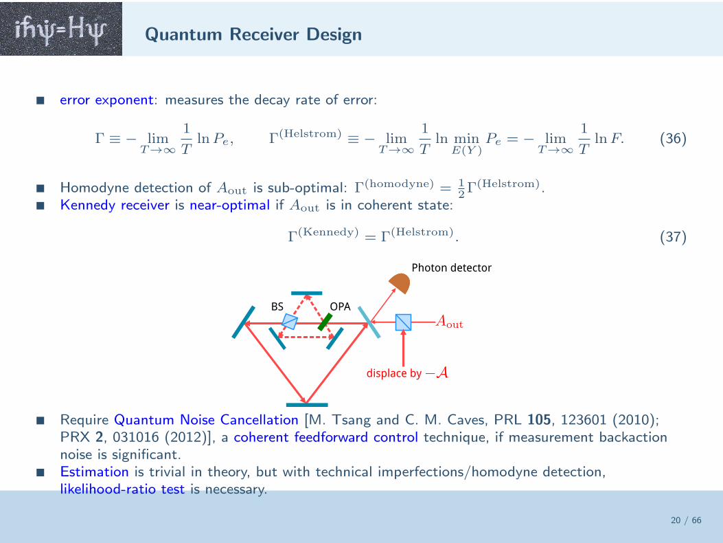
Quantum Receiver Design
20 / 66
error exponent: measures the decay rate of error:
Γ ≡ − limT→∞
1
TlnPe, Γ(Helstrom) ≡ − lim
T→∞
1
Tln min
E(Y )Pe = − lim
T→∞
1
TlnF. (36)
Homodyne detection of Aout is sub-optimal: Γ(homodyne) = 12Γ(Helstrom).
Kennedy receiver is near-optimal if Aout is in coherent state:
Γ(Kennedy) = Γ(Helstrom). (37)
OPABS
displace by
Photon detector
Require Quantum Noise Cancellation [M. Tsang and C. M. Caves, PRL 105, 123601 (2010);PRX 2, 031016 (2012)], a coherent feedforward control technique, if measurement backactionnoise is significant.
Estimation is trivial in theory, but with technical imperfections/homodyne detection,likelihood-ratio test is necessary.
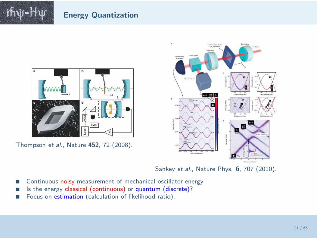
Energy Quantization
21 / 66
Thompson et al., Nature 452, 72 (2008).
Sankey et al., Nature Phys. 6, 707 (2010).
Continuous noisy measurement of mechanical oscillator energy Is the energy classical (continuous) or quantum (discrete)? Focus on estimation (calculation of likelihood ratio).
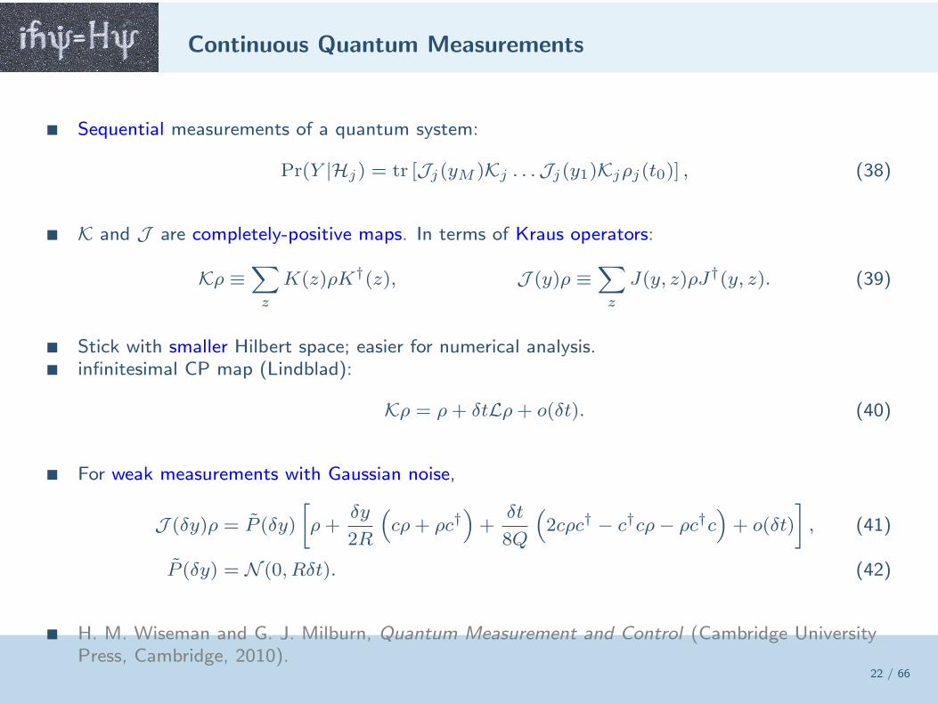
Continuous Quantum Measurements
22 / 66
Sequential measurements of a quantum system:
Pr(Y |Hj) = tr [Jj(yM )Kj . . .Jj(y1)Kjρj(t0)] , (38)
K and J are completely-positive maps. In terms of Kraus operators:
Kρ ≡∑
z
K(z)ρK†(z), J (y)ρ ≡∑
z
J(y, z)ρJ†(y, z). (39)
Stick with smaller Hilbert space; easier for numerical analysis. infinitesimal CP map (Lindblad):
Kρ = ρ+ δtLρ+ o(δt). (40)
For weak measurements with Gaussian noise,
J (δy)ρ = P (δy)
[
ρ+δy
2R
(
cρ+ ρc†)
+δt
8Q
(
2cρc† − c†cρ− ρc†c)
+ o(δt)
]
, (41)
P (δy) = N (0, Rδt). (42)
H. M. Wiseman and G. J. Milburn, Quantum Measurement and Control (Cambridge UniversityPress, Cambridge, 2010).
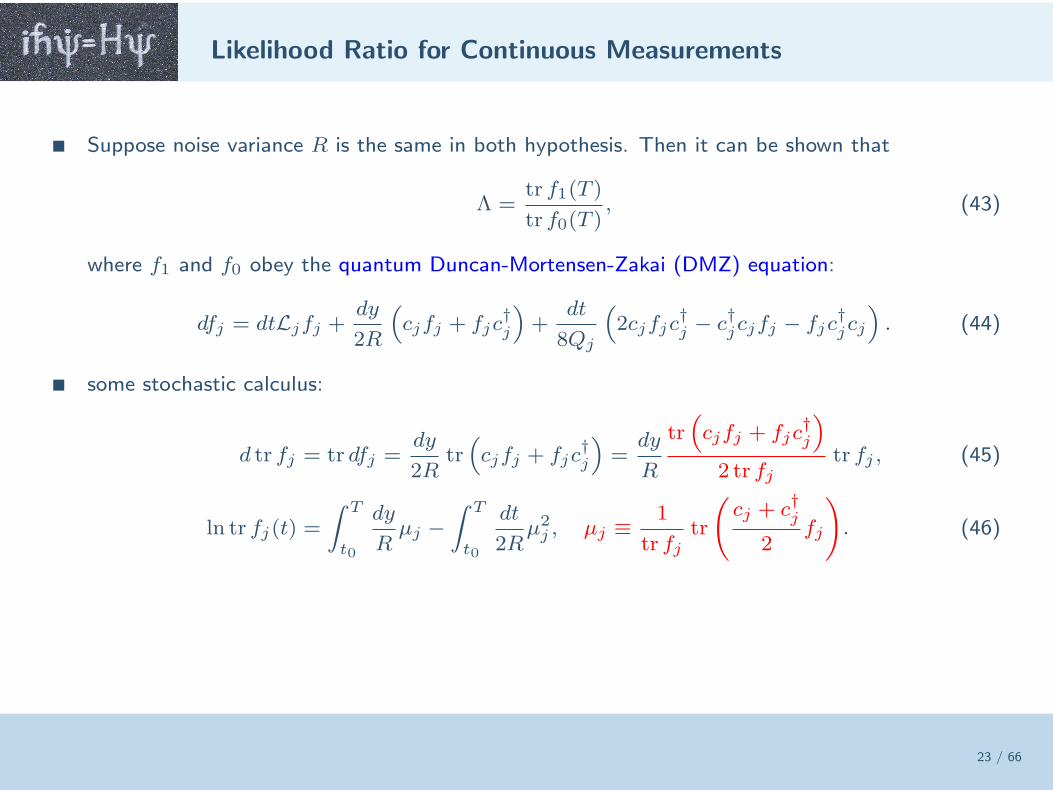
Likelihood Ratio for Continuous Measurements
23 / 66
Suppose noise variance R is the same in both hypothesis. Then it can be shown that
Λ =tr f1(T )
tr f0(T ), (43)
where f1 and f0 obey the quantum Duncan-Mortensen-Zakai (DMZ) equation:
dfj = dtLjfj +dy
2R
(
cjfj + fjc†j
)
+dt
8Qj
(
2cjfjc†j − c†jcjfj − fjc
†jcj
)
. (44)
some stochastic calculus:
d tr fj = tr dfj =dy
2Rtr(
cjfj + fjc†j
)
=dy
R
tr(
cjfj + fjc†j
)
2 tr fjtr fj , (45)
ln tr fj(t) =
∫ T
t0
dy
Rµj −
∫ T
t0
dt
2Rµ2j , µj ≡ 1
tr fjtr
(
cj + c†j
2fj
)
. (46)

Likelihood Ratio via Quantum Filtering
24 / 66
Final result:
Λ(T ) = exp
[∫ T
t0
dy
R(µ1 − µ0)−
∫ T
t0
dt
2R
(
µ21 − µ20)
]
. (47)
µj is the expected value of (cj + c†j)/2 given the observation record, assuming Hj is true, can becalculated by quantum filters.
Similar formula exists for continuous measurements with Poisson noise. M. Tsang, PRL 108, 170502 (2012) Quantum generalizations of the Duncan-Kailath estimator-correlator formula [Duncan, Inf.
Control 13, 62 (1968); Kailath, IEEE TIT 15, 350 (1969)] and Snyder’s formula [Snyder, IEEETIT 18, 91 (1972)].
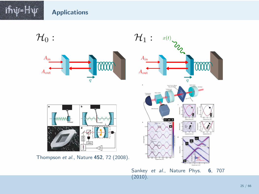
Applications
25 / 66
Thompson et al., Nature 452, 72 (2008).
Sankey et al., Nature Phys. 6, 707(2010).
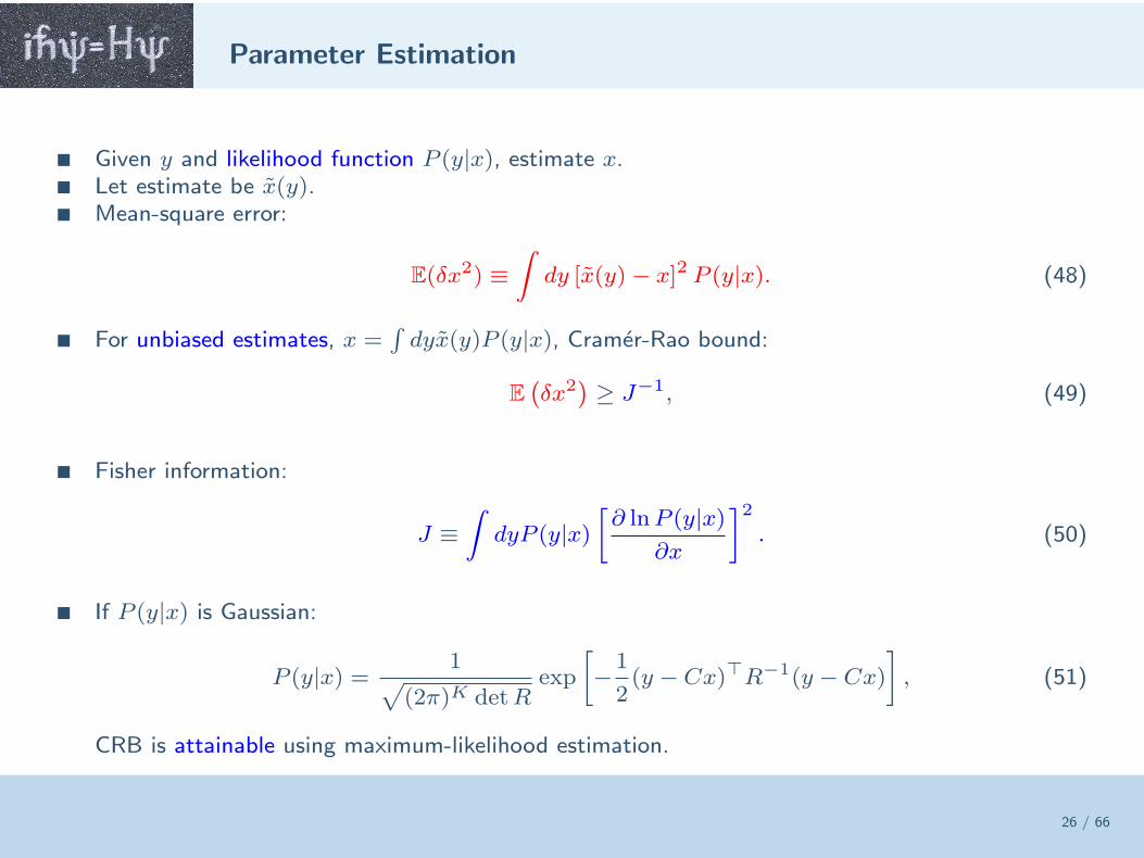
Parameter Estimation
26 / 66
Given y and likelihood function P (y|x), estimate x. Let estimate be x(y). Mean-square error:
E(δx2) ≡∫
dy [x(y)− x]2 P (y|x). (48)
For unbiased estimates, x =∫
dyx(y)P (y|x), Cramer-Rao bound:
E(
δx2)
≥ J−1, (49)
Fisher information:
J ≡∫
dyP (y|x)[
∂ lnP (y|x)∂x
]2
. (50)
If P (y|x) is Gaussian:
P (y|x) = 1√
(2π)K detRexp
[
−1
2(y − Cx)⊤R−1(y − Cx)
]
, (51)
CRB is attainable using maximum-likelihood estimation.
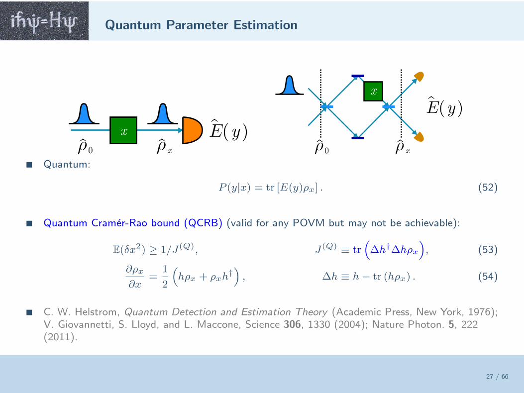
Quantum Parameter Estimation
27 / 66
Quantum:
P (y|x) = tr [E(y)ρx] . (52)
Quantum Cramer-Rao bound (QCRB) (valid for any POVM but may not be achievable):
E(δx2) ≥ 1/J(Q), J(Q) ≡ tr(
∆h†∆hρx)
, (53)
∂ρx
∂x=
1
2
(
hρx + ρxh†)
, ∆h ≡ h− tr (hρx) . (54)
C. W. Helstrom, Quantum Detection and Estimation Theory (Academic Press, New York, 1976);V. Giovannetti, S. Lloyd, and L. Maccone, Science 306, 1330 (2004); Nature Photon. 5, 222(2011).
Example: Optical Phase Estimation
28 / 66
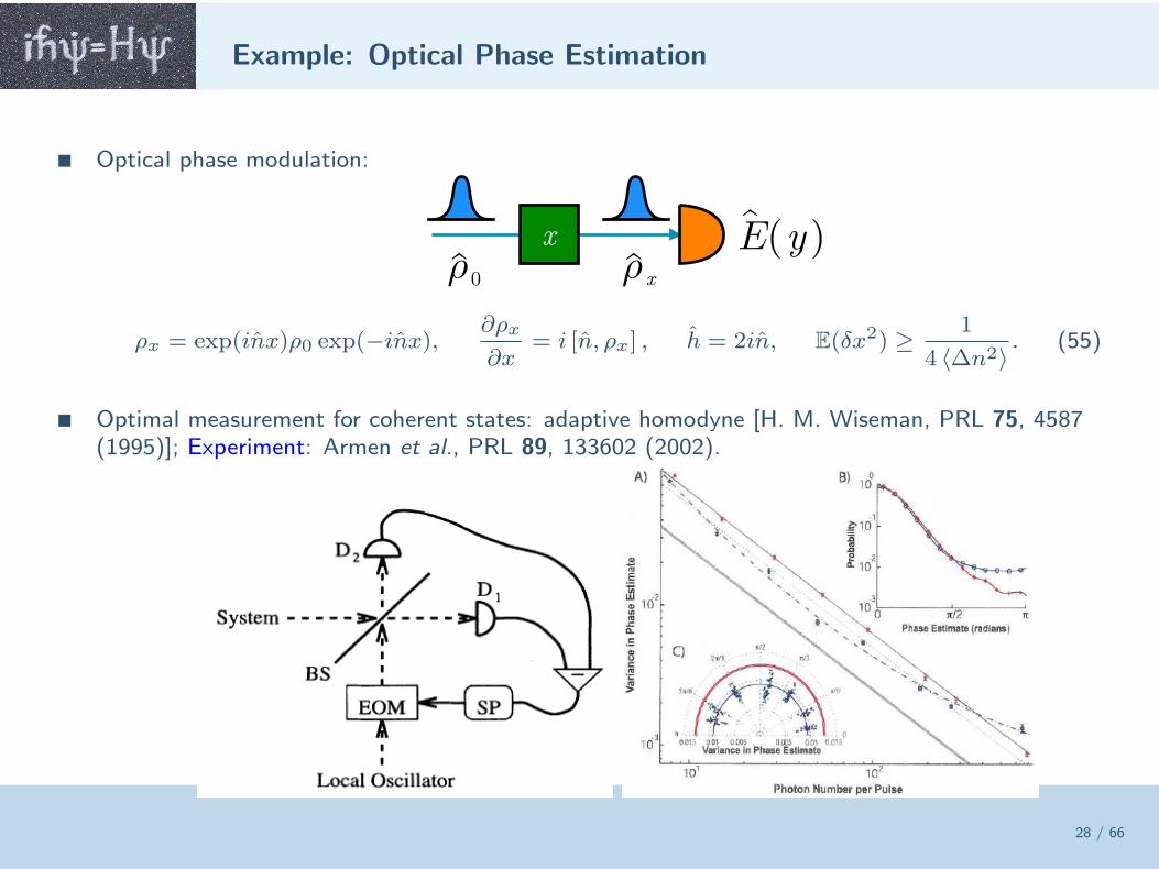
Optical phase modulation:
ρx = exp(inx)ρ0 exp(−inx),∂ρx
∂x= i [n, ρx] , h = 2in, E(δx2) ≥ 1
4 〈∆n2〉 . (55)
Optimal measurement for coherent states: adaptive homodyne [H. M. Wiseman, PRL 75, 4587(1995)]; Experiment: Armen et al., PRL 89, 133602 (2002).
Generalizations of Classical Cramer-Rao Bound
29 / 66
Error covariance matrix for multiple parameters with prior distribution P (x):
Σ ≡ E
[
(x− x) (x− x)⊤]
≡∫
dydxP (y|x)P (x) (x− x) (x− x)⊤ . (56)
Define loss function in terms of positive-semidefinite matrix Λ as
C(x, x) = (x− x)⊤ Λ (x− x) . (57)
Average cost/Bayes risk
C ≡ E [C(x, x)] = tr (ΛΣ) ≥ 0. (58)
Bayesian Cramer-Rao bound (Van Trees) for any Λ:
C ≥ tr(
ΛJ−1)
, J = J(Y ) + J(X), (59)
J(Y )jk
= E
[
∂ lnP (y|x)∂xj
∂ lnP (y|x)∂xk
]
, J(X)jk
= E
[
∂ lnP (x)
∂xj
∂ lnP (x)
∂xk
]
. (60)
More compact way: Σ ≥ J−1; i.e., Σ− J−1 is positive-semidefinite.
Revisiting Church of Larger Hilbert Space
30 / 66
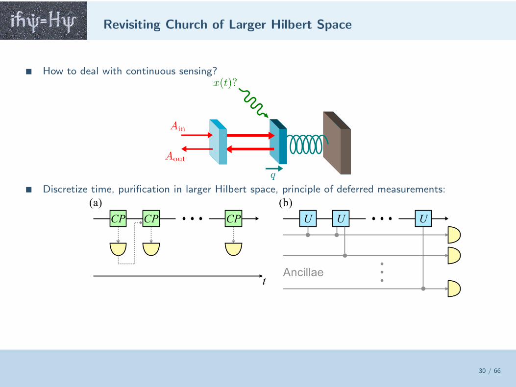
How to deal with continuous sensing?
Discretize time, purification in larger Hilbert space, principle of deferred measurements:
Dynamical Quantum Cramer-Rao Bound
31 / 66
Fisher information matrix J(t, t′)
∫
dtdt′Λ(t, t′)
E[
δx(t)δx(t′)]
− J−1(t, t′)
≥ 0, (61)
J−1(t, t′) is defined by∫
dt′J(t, t′)J−1(t′, τ) = δ(t− τ). Two components:
J(t, t′) = J(Q)(t, t′) + J(X)(t, t′). (62)
J(Q) is a two-time quantum covariance function:
J(Q)(t, t′) =4
~2E
tr[
: ∆h(t)∆h(t′) : ρ0]
, h(t) ≡ U†(t, t0)∂H(t)
∂x(t)U(t, t0).
J(X) incorporates a priori waveform information
J(X)(t, t′) = E
δ lnP [x]
δx(t)
δ lnP [x]
δx(t′)
. (63)
M. Tsang, H. M. Wiseman, and C. M. Caves, PRL 106, 090401 (2011).
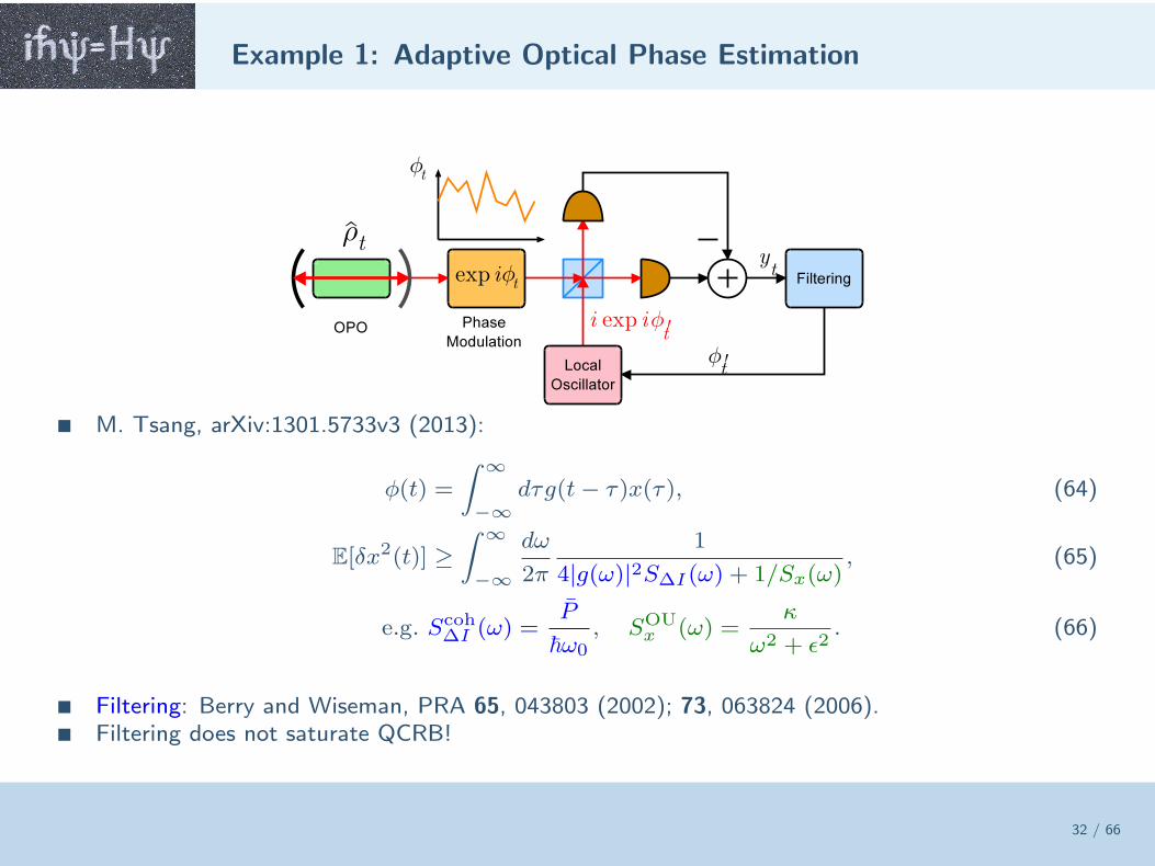
Example 1: Adaptive Optical Phase Estimation
32 / 66
M. Tsang, arXiv:1301.5733v3 (2013):
φ(t) =
∫ ∞
−∞
dτg(t− τ)x(τ), (64)
E[δx2(t)] ≥∫ ∞
−∞
dω
2π
1
4|g(ω)|2S∆I(ω) + 1/Sx(ω), (65)
e.g. Scoh∆I (ω) =
P
~ω0, SOU
x (ω) =κ
ω2 + ǫ2. (66)
Filtering: Berry and Wiseman, PRA 65, 043803 (2002); 73, 063824 (2006). Filtering does not saturate QCRB!
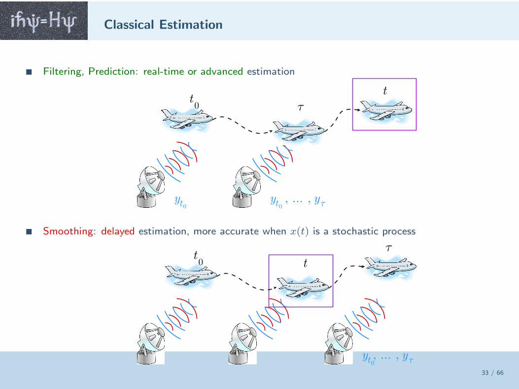
Classical Estimation
33 / 66
Filtering, Prediction: real-time or advanced estimation
Smoothing: delayed estimation, more accurate when x(t) is a stochastic process
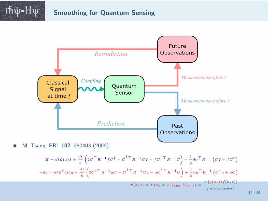
Smoothing for Quantum Sensing
34 / 66
M. Tsang, PRL 102, 250403 (2009).
df = dtL(x)f +dt
8
(
2C⊤
R−1
fC†
− C†⊤
R−1
Cf − fC†⊤
R−1
C
)
+1
2dy
⊤R
−1(
Cf + fC†)
−dg = dtL∗(x)g +
dt
8
(
2C†⊤
R−1
gC − C†⊤
R−1
Cg − gC†⊤
R−1
C
)
+1
2dy
⊤R
−1(
C†g + gC
)
h(x, t) = P (xt = x|Ypast, Yfuture) =tr [g(x, t)f(x, t)]∫
dx(numerator)
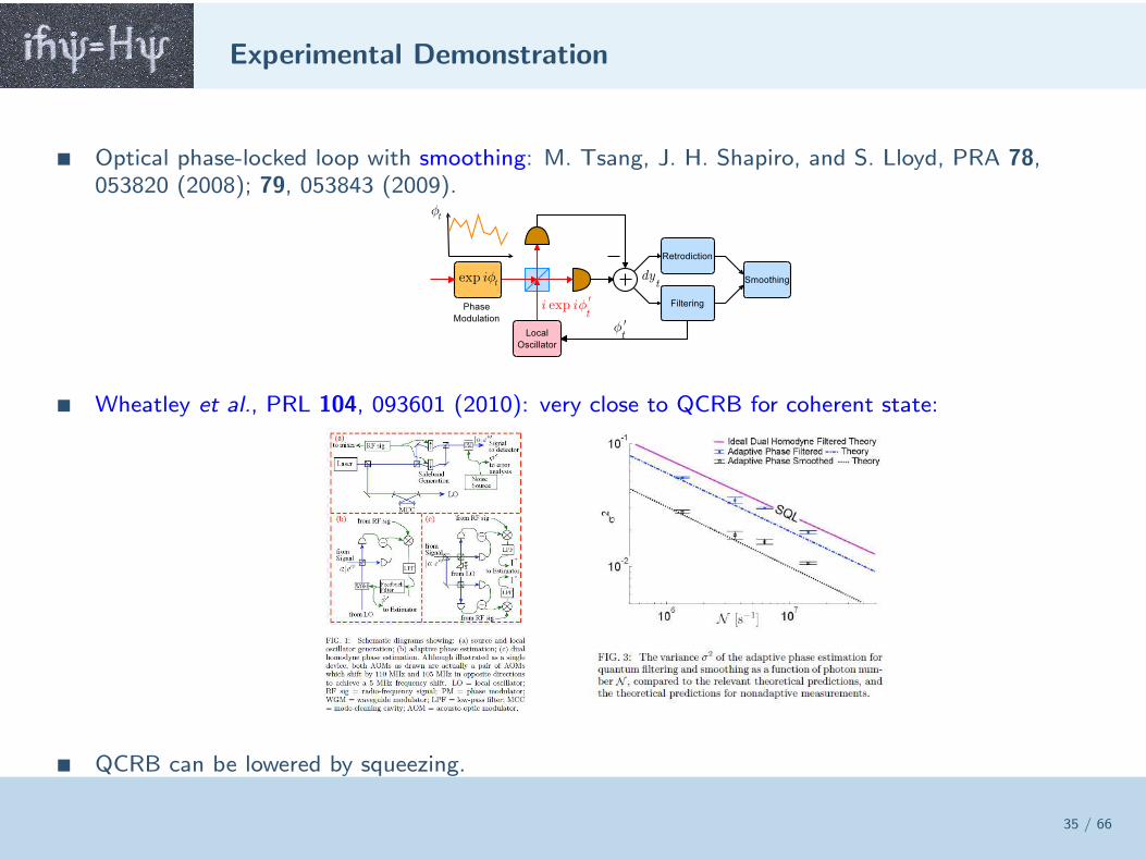
Experimental Demonstration
35 / 66
Optical phase-locked loop with smoothing: M. Tsang, J. H. Shapiro, and S. Lloyd, PRA 78,053820 (2008); 79, 053843 (2009).
Wheatley et al., PRL 104, 093601 (2010): very close to QCRB for coherent state:
QCRB can be lowered by squeezing.
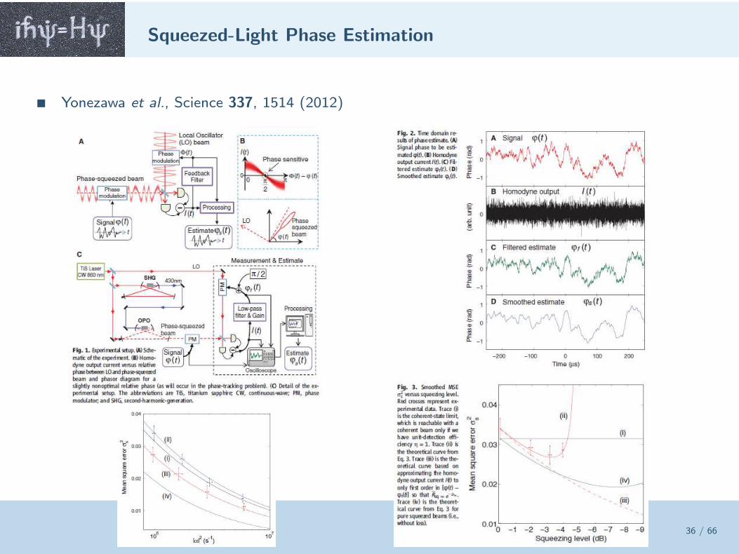
Squeezed-Light Phase Estimation
36 / 66
Yonezawa et al., Science 337, 1514 (2012)
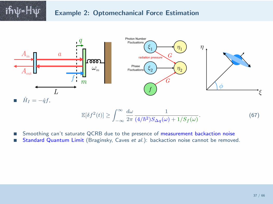
Example 2: Optomechanical Force Estimation
37 / 66
HI = −qf ,
E[δf2(t)] ≥∫ ∞
−∞
dω
2π
1
(4/~2)S∆q(ω) + 1/Sf (ω). (67)
Smoothing can’t saturate QCRB due to the presence of measurement backaction noise Standard Quantum Limit (Braginsky, Caves et al.): backaction noise cannot be removed.
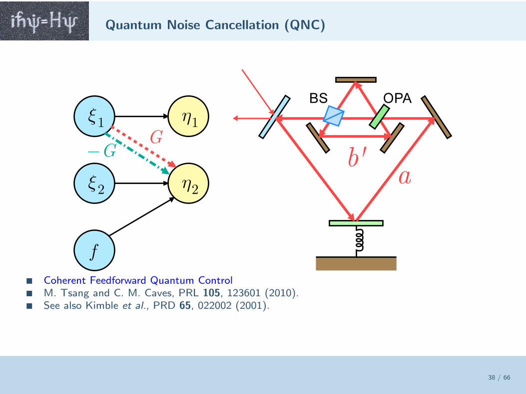
Quantum Noise Cancellation (QNC)
38 / 66
Coherent Feedforward Quantum Control M. Tsang and C. M. Caves, PRL 105, 123601 (2010). See also Kimble et al., PRD 65, 022002 (2001).
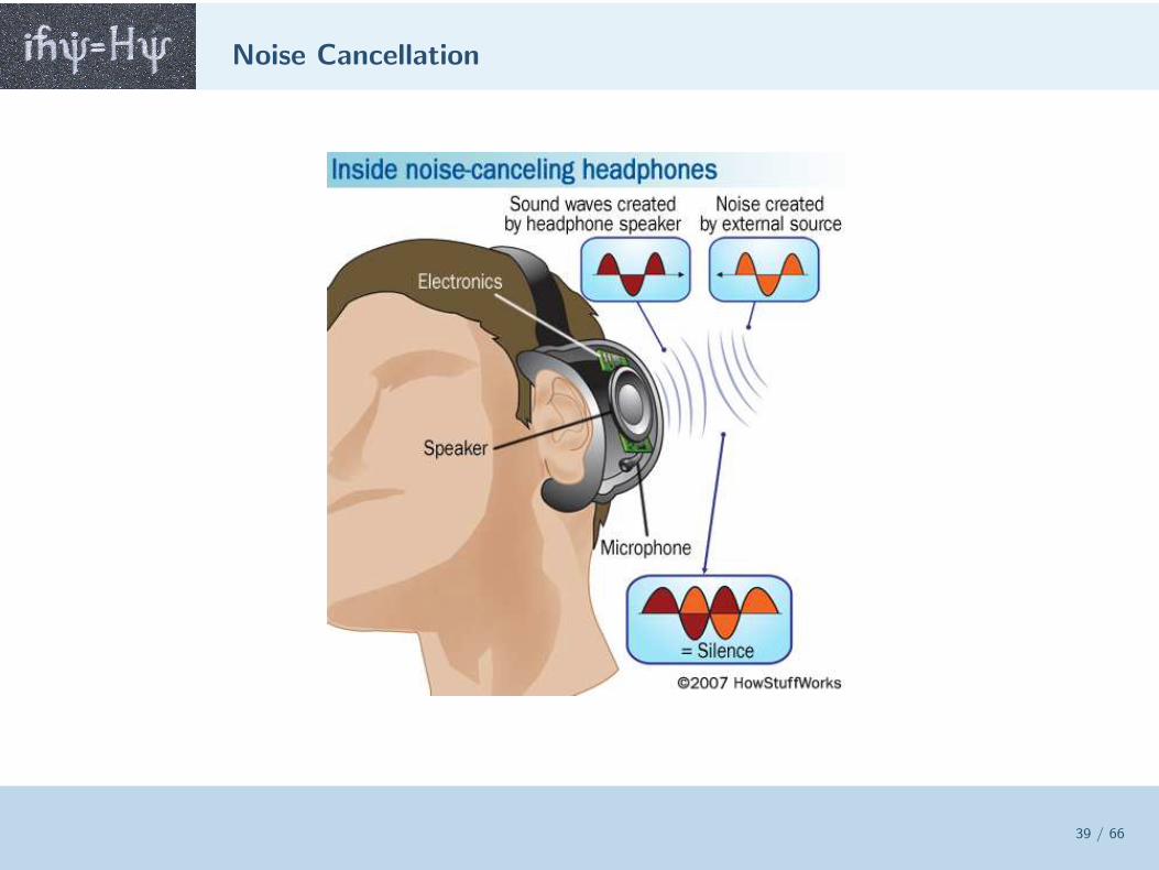
Noise Cancellation
39 / 66
Quantum Non-Demolition (QND) Observables
40 / 66
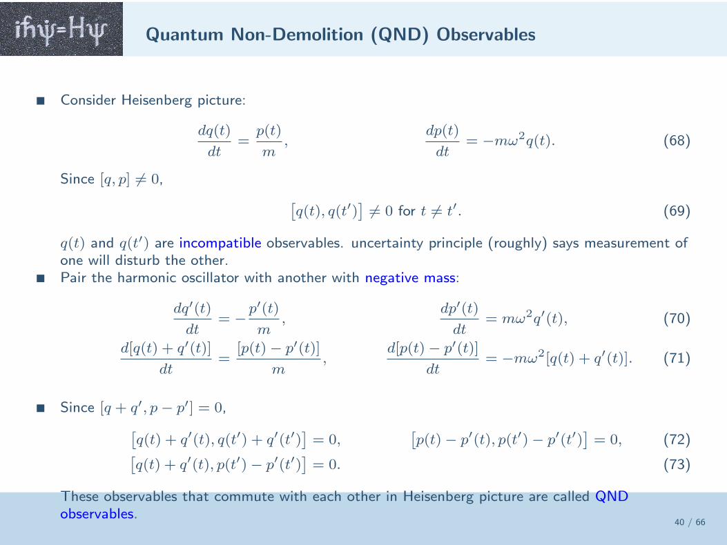
Consider Heisenberg picture:
dq(t)
dt=p(t)
m,
dp(t)
dt= −mω2q(t). (68)
Since [q, p] 6= 0,
[
q(t), q(t′)]
6= 0 for t 6= t′. (69)
q(t) and q(t′) are incompatible observables. uncertainty principle (roughly) says measurement ofone will disturb the other.
Pair the harmonic oscillator with another with negative mass:
dq′(t)
dt= −p
′(t)
m,
dp′(t)
dt= mω2q′(t), (70)
d[q(t) + q′(t)]
dt=
[p(t)− p′(t)]
m,
d[p(t)− p′(t)]
dt= −mω2[q(t) + q′(t)]. (71)
Since [q + q′, p− p′] = 0,
[
q(t) + q′(t), q(t′) + q′(t′)]
= 0,[
p(t)− p′(t), p(t′)− p′(t′)]
= 0, (72)[
q(t) + q′(t), p(t′)− p′(t′)]
= 0. (73)
These observables that commute with each other in Heisenberg picture are called QNDobservables.
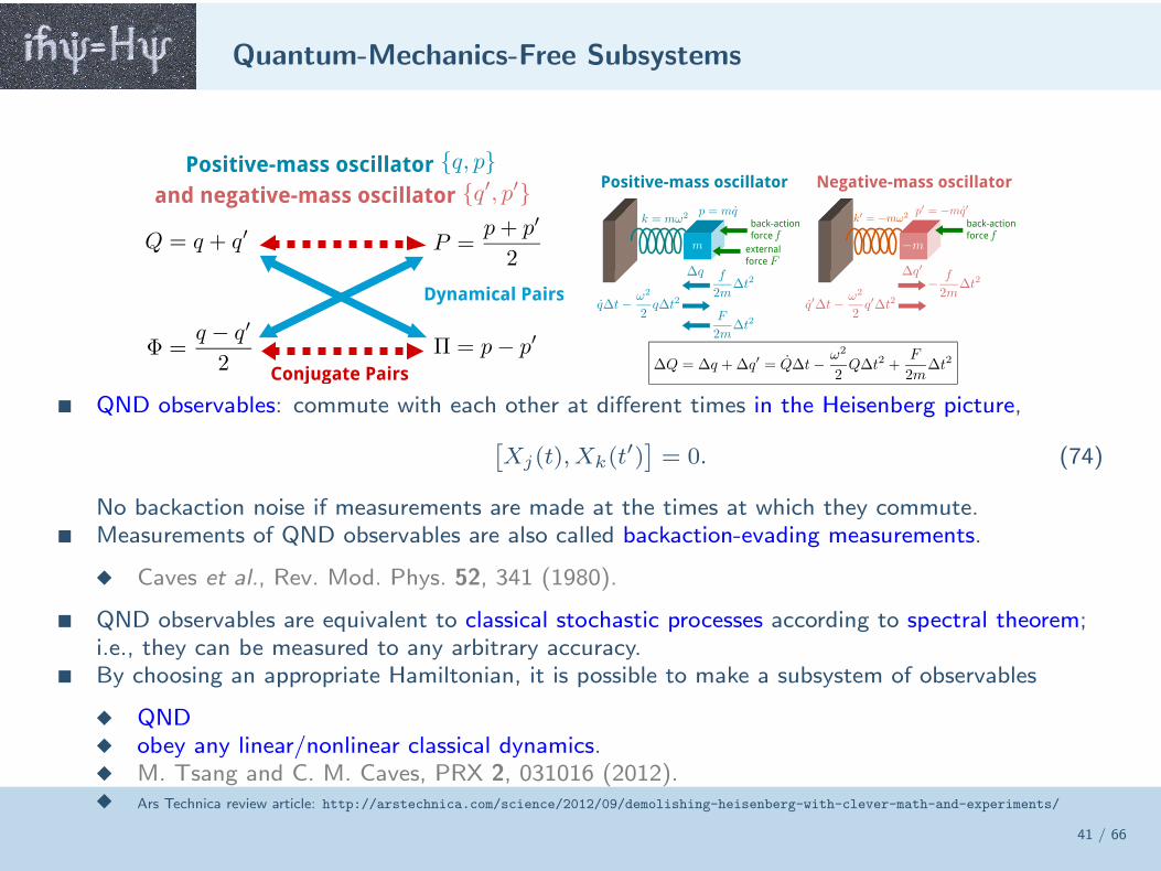
Quantum-Mechanics-Free Subsystems
41 / 66
Dynamical Pairs
Conjugate Pairs
Positive-mass oscillator
and negative-mass oscillatorPositive-mass oscillator
back-action
force
external
force
Negative-mass oscillator
back-action
force
QND observables: commute with each other at different times in the Heisenberg picture,
[
Xj(t), Xk(t′)]
= 0. (74)
No backaction noise if measurements are made at the times at which they commute. Measurements of QND observables are also called backaction-evading measurements.
Caves et al., Rev. Mod. Phys. 52, 341 (1980).
QND observables are equivalent to classical stochastic processes according to spectral theorem;i.e., they can be measured to any arbitrary accuracy.
By choosing an appropriate Hamiltonian, it is possible to make a subsystem of observables
QND obey any linear/nonlinear classical dynamics. M. Tsang and C. M. Caves, PRX 2, 031016 (2012). Ars Technica review article: http://arstechnica.com/science/2012/09/demolishing-heisenberg-with-clever-math-and-experiments/
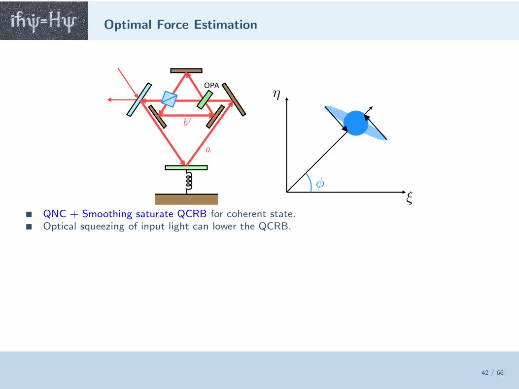
Optimal Force Estimation
42 / 66
QNC + Smoothing saturate QCRB for coherent state. Optical squeezing of input light can lower the QCRB.
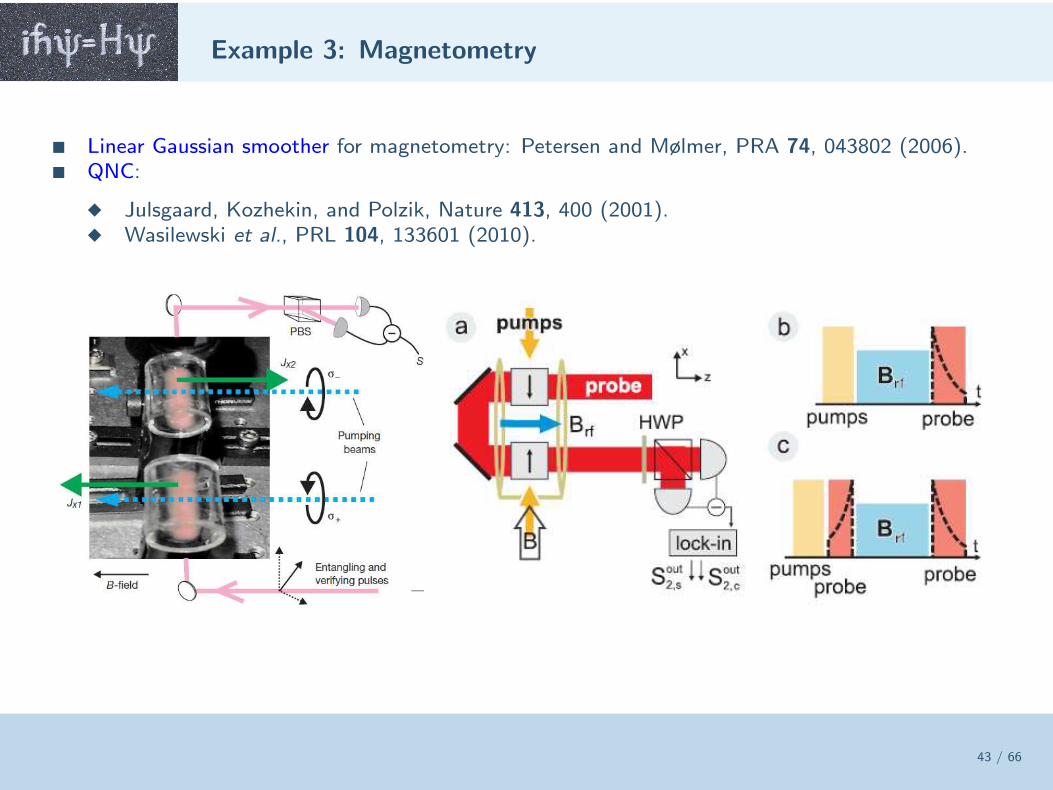
Example 3: Magnetometry
43 / 66
Linear Gaussian smoother for magnetometry: Petersen and Mølmer, PRA 74, 043802 (2006). QNC:
Julsgaard, Kozhekin, and Polzik, Nature 413, 400 (2001). Wasilewski et al., PRL 104, 133601 (2010).
Beyond Cramer-Rao Bounds
44 / 66
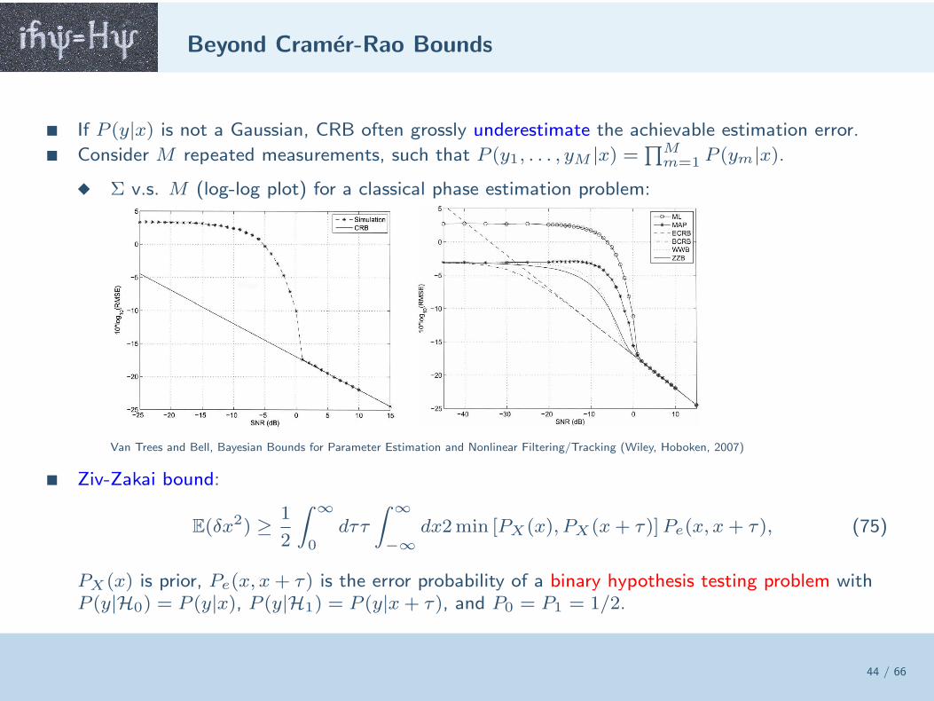
If P (y|x) is not a Gaussian, CRB often grossly underestimate the achievable estimation error.
Consider M repeated measurements, such that P (y1, . . . , yM |x) =∏Mm=1 P (ym|x).
Σ v.s. M (log-log plot) for a classical phase estimation problem:
Van Trees and Bell, Bayesian Bounds for Parameter Estimation and Nonlinear Filtering/Tracking (Wiley, Hoboken, 2007)
Ziv-Zakai bound:
E(δx2) ≥ 1
2
∫ ∞
0dττ
∫ ∞
−∞
dx2min [PX(x), PX(x+ τ)]Pe(x, x+ τ), (75)
PX(x) is prior, Pe(x, x+ τ) is the error probability of a binary hypothesis testing problem withP (y|H0) = P (y|x), P (y|H1) = P (y|x+ τ), and P0 = P1 = 1/2.
Quantum Ziv-Zakai Bounds
45 / 66
If P (y|x) = tr [E(y)ρx], for any POVM E(y),
Pe(x, x+ τ) ≥ 1
2
[
1− 1
2||ρx − ρx+τ ||1
]
≥ 1
2
[
1−√
1− F (ρx, ρx+τ )]
. (76)
We immediately obtain quantum Ziv-Zakai bounds on E(δx2). Can be used to prove Heisenberg limit:
E(δx2) ≥ C
〈n〉2 . (77)
see also Giovannetti et al., PRL 108, 260405 (2012); Hall et al., PRA 85, 041802(R) (2012). Compared with QCRB E(δx2) ≥ 1/4
⟨
∆n2⟩
, Heisenberg limit is much higher than QCRB when〈∆n2〉 ≫ 〈n〉2
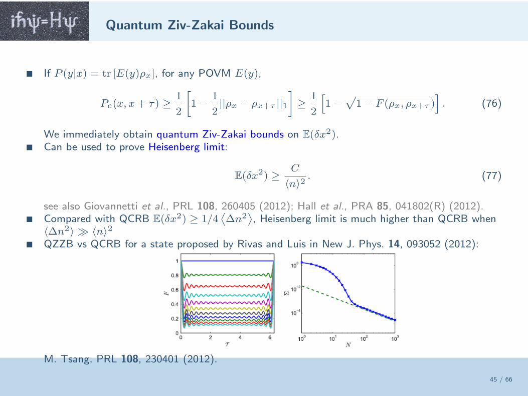
QZZB vs QCRB for a state proposed by Rivas and Luis in New J. Phys. 14, 093052 (2012):
M. Tsang, PRL 108, 230401 (2012).
Hybrid Quantum Systems
46 / 66
Electro-Optic Modulation
47 / 66
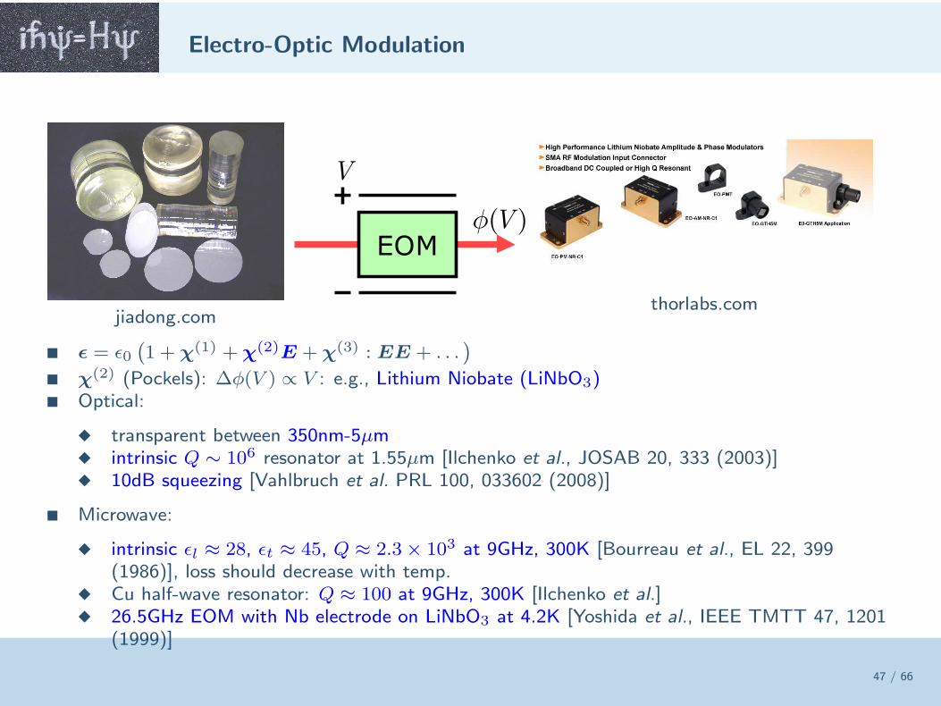
jiadong.comthorlabs.com
ǫ = ǫ0(
1 + χ(1) + χ(2)E + χ(3) : EE + . . .)
χ(2) (Pockels): ∆φ(V ) ∝ V : e.g., Lithium Niobate (LiNbO3) Optical:
transparent between 350nm-5µm intrinsic Q ∼ 106 resonator at 1.55µm [Ilchenko et al., JOSAB 20, 333 (2003)] 10dB squeezing [Vahlbruch et al. PRL 100, 033602 (2008)]
Microwave:
intrinsic ǫl ≈ 28, ǫt ≈ 45, Q ≈ 2.3× 10³ at 9GHz, 300K [Bourreau et al., EL 22, 399(1986)], loss should decrease with temp.
Cu half-wave resonator: Q ≈ 100 at 9GHz, 300K [Ilchenko et al.] 26.5GHz EOM with Nb electrode on LiNbO3 at 4.2K [Yoshida et al., IEEE TMTT 47, 1201
(1999)]
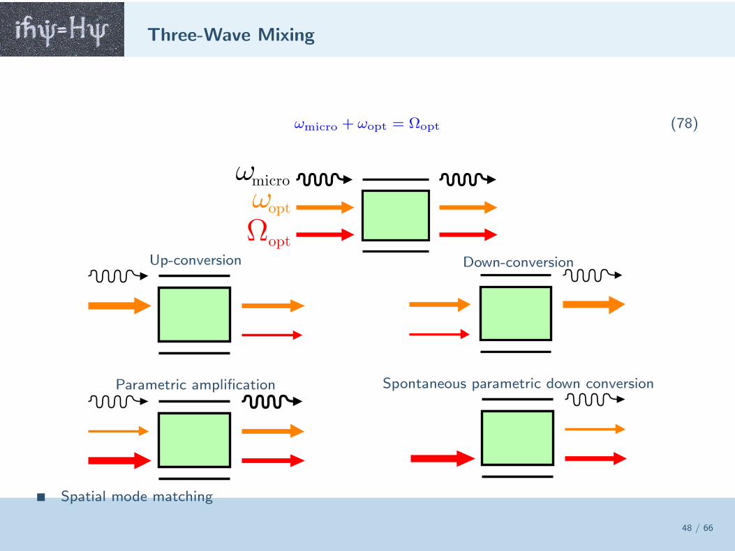
Three-Wave Mixing
48 / 66
ωmicro + ωopt = Ωopt (78)
Up-conversion
Parametric amplification
Down-conversion
Spontaneous parametric down conversion
Spatial mode matching
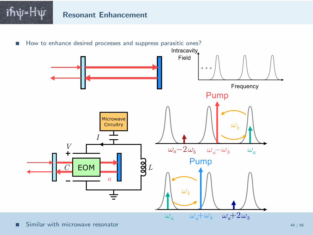
Resonant Enhancement
49 / 66
How to enhance desired processes and suppress parasitic ones?
Similar with microwave resonator
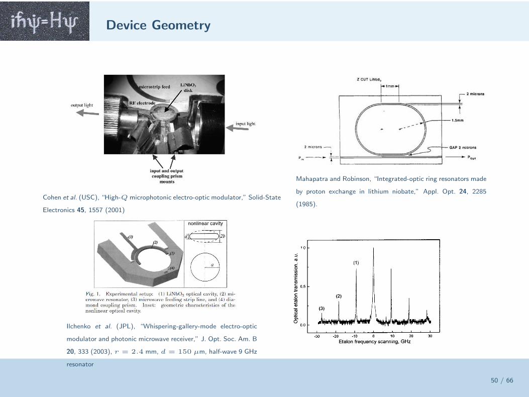
Device Geometry
50 / 66
Cohen et al. (USC), “High-Qmicrophotonic electro-optic modulator,” Solid-State
Electronics 45, 1557 (2001)
Mahapatra and Robinson, “Integrated-optic ring resonators made
by proton exchange in lithium niobate,” Appl. Opt. 24, 2285
(1985).
Ilchenko et al. (JPL), “Whispering-gallery-mode electro-optic
modulator and photonic microwave receiver,” J. Opt. Soc. Am. B
20, 333 (2003), r = 2.4 mm, d = 150 µm, half-wave 9 GHz
resonator
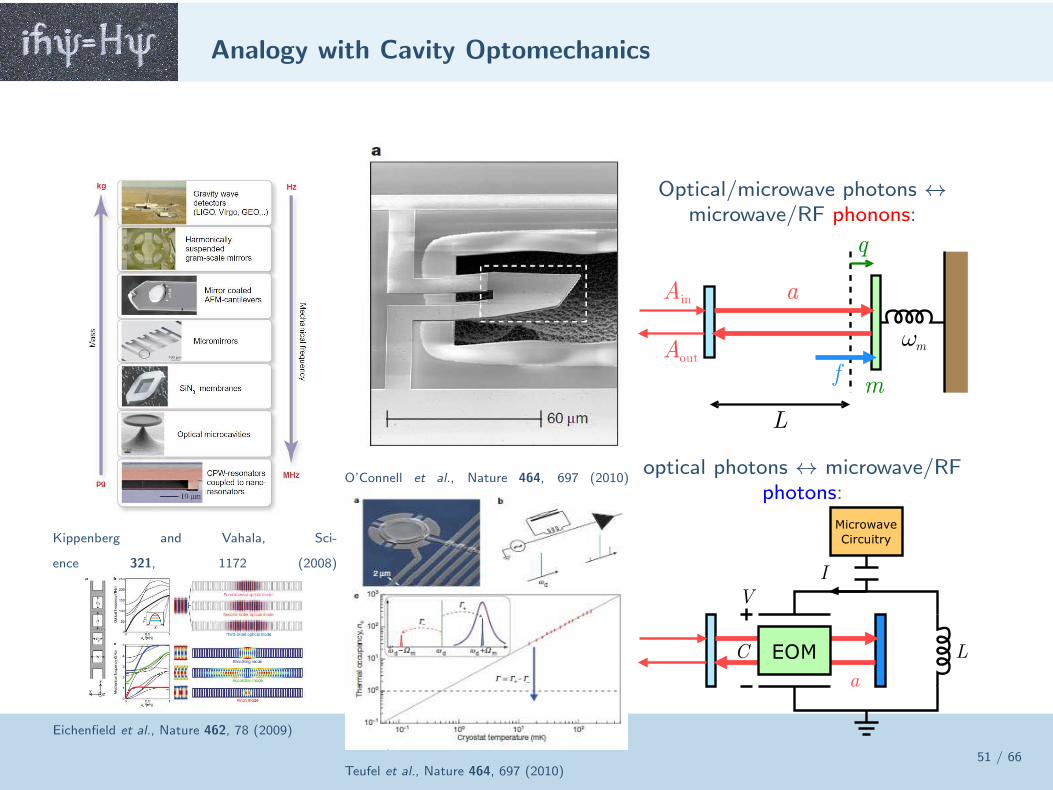
Analogy with Cavity Optomechanics
51 / 66
Kippenberg and Vahala, Sci-
ence 321, 1172 (2008)
Eichenfield et al., Nature 462, 78 (2009)
O’Connell et al., Nature 464, 697 (2010)
Teufel et al., Nature 464, 697 (2010)
Optical/microwave photons ↔microwave/RF phonons:
optical photons ↔ microwave/RFphotons:
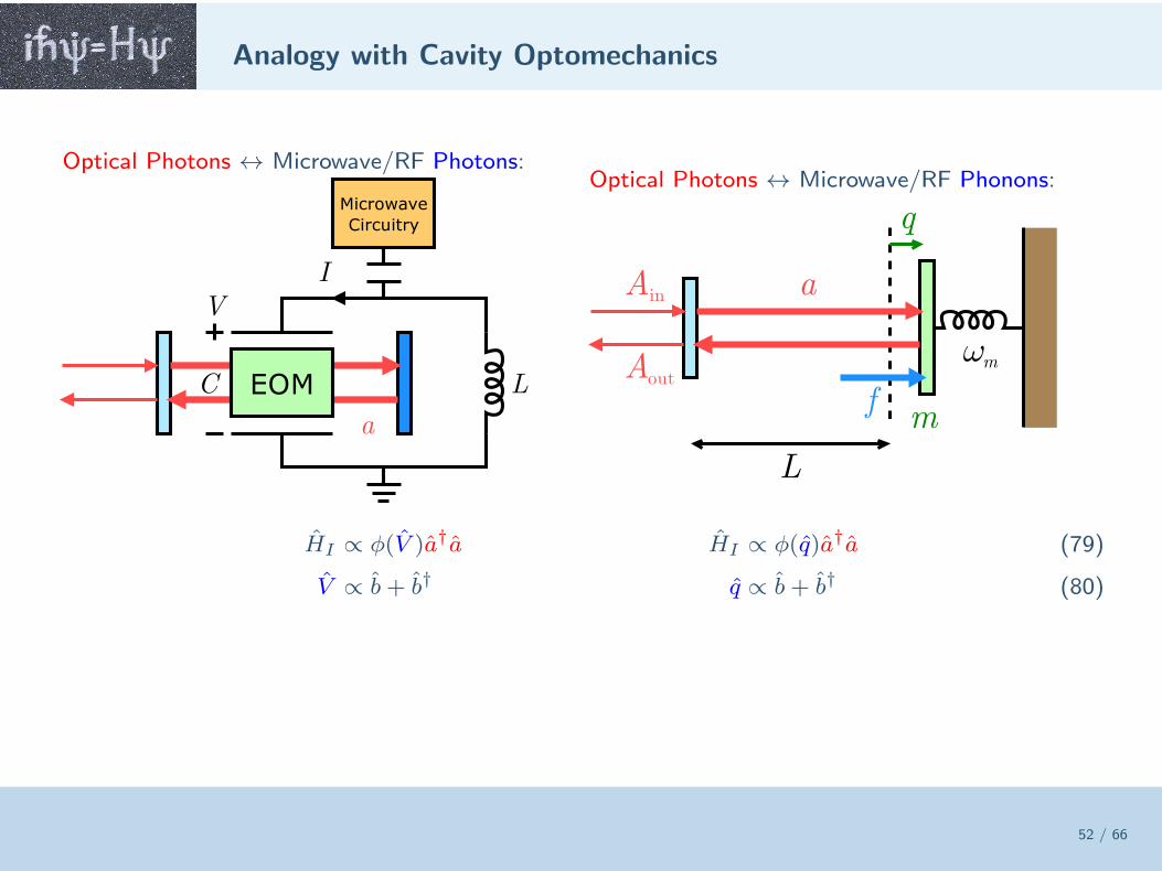
Analogy with Cavity Optomechanics
52 / 66
Optical Photons ↔ Microwave/RF Photons:Optical Photons ↔ Microwave/RF Phonons:
HI ∝ φ(V )a†a HI ∝ φ(q)a†a (79)
V ∝ b+ b† q ∝ b+ b† (80)
Laser Cooling of Mechanical Oscillator
53 / 66
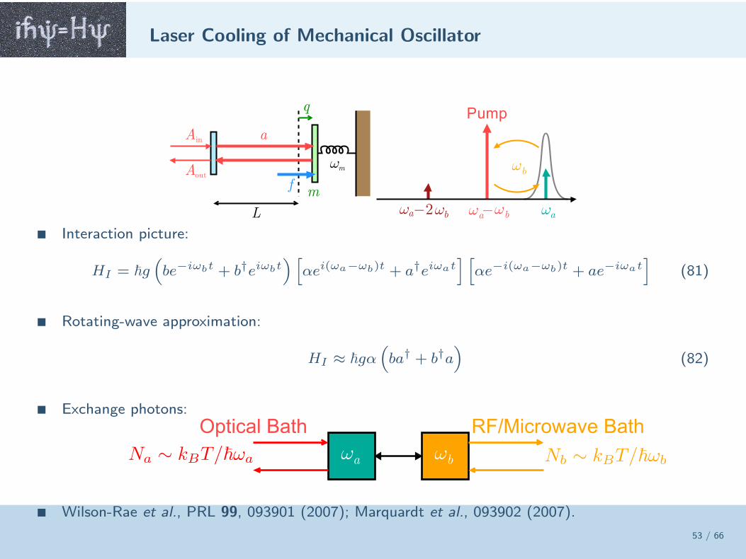
Interaction picture:
HI = ~g(
be−iωbt + b†eiωbt) [
αei(ωa−ωb)t + a†eiωat] [
αe−i(ωa−ωb)t + ae−iωat]
(81)
Rotating-wave approximation:
HI ≈ ~gα(
ba† + b†a)
(82)
Exchange photons:
b
a
Optical Bath RF/Microwave Bath
Wilson-Rae et al., PRL 99, 093901 (2007); Marquardt et al., 093902 (2007).
Recent Experiments of Optomechanical Cooling
54 / 66
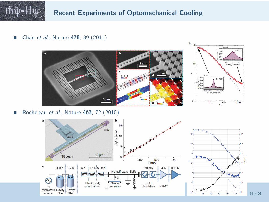
Chan et al., Nature 478, 89 (2011)
Rocheleau et al., Nature 463, 72 (2010)
Electro-Optic Cooling and Noiseless Frequency Conversion
55 / 66
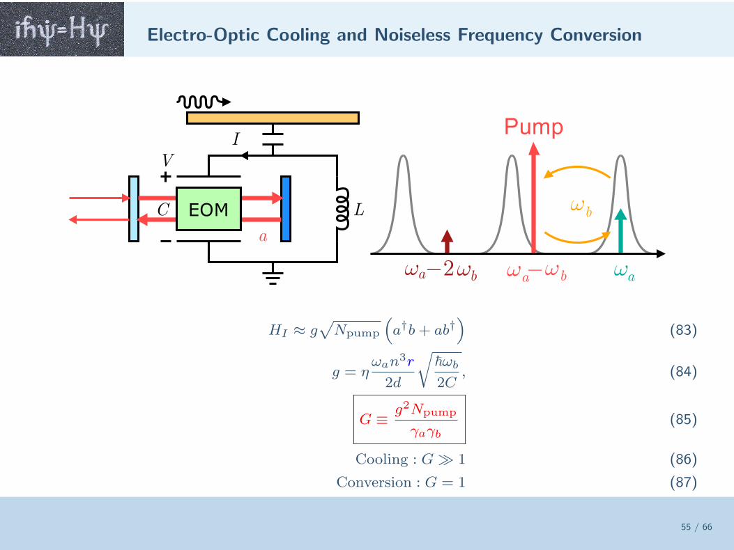
HI ≈ g√
Npump
(
a†b+ ab†)
(83)
g = ηωan3r
2d
√
~ωb
2C, (84)
G ≡ g2Npump
γaγb(85)
Cooling : G≫ 1 (86)
Conversion : G = 1 (87)
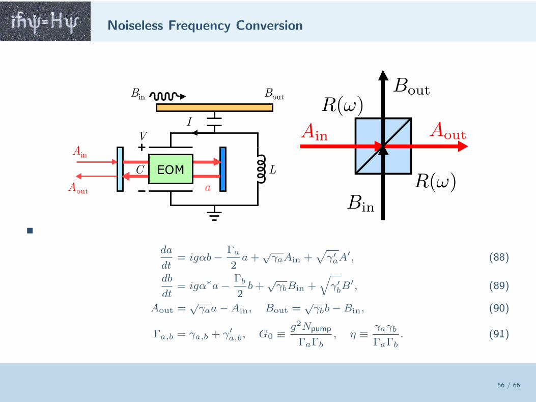
Noiseless Frequency Conversion
56 / 66
da
dt= igαb− Γa
2a+
√γaAin +
√
γ′aA′, (88)
db
dt= igα∗a− Γb
2b+
√γbBin +
√
γ′bB′, (89)
Aout =√γaa−Ain, Bout =
√γbb−Bin, (90)
Γa,b = γa,b + γ′a,b, G0 ≡ g2Npump
ΓaΓb
, η ≡ γaγb
ΓaΓb
. (91)
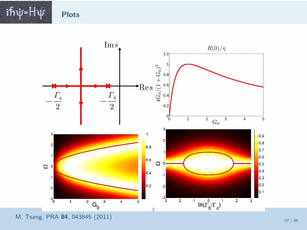
Plots
57 / 66
0 1 2 3 4 50
0.2
0.4
0.6
0.8
1
1.2
G0
4G
0/(1
+G
0)2
R(0)/η
M. Tsang, PRA 84, 043845 (2011)
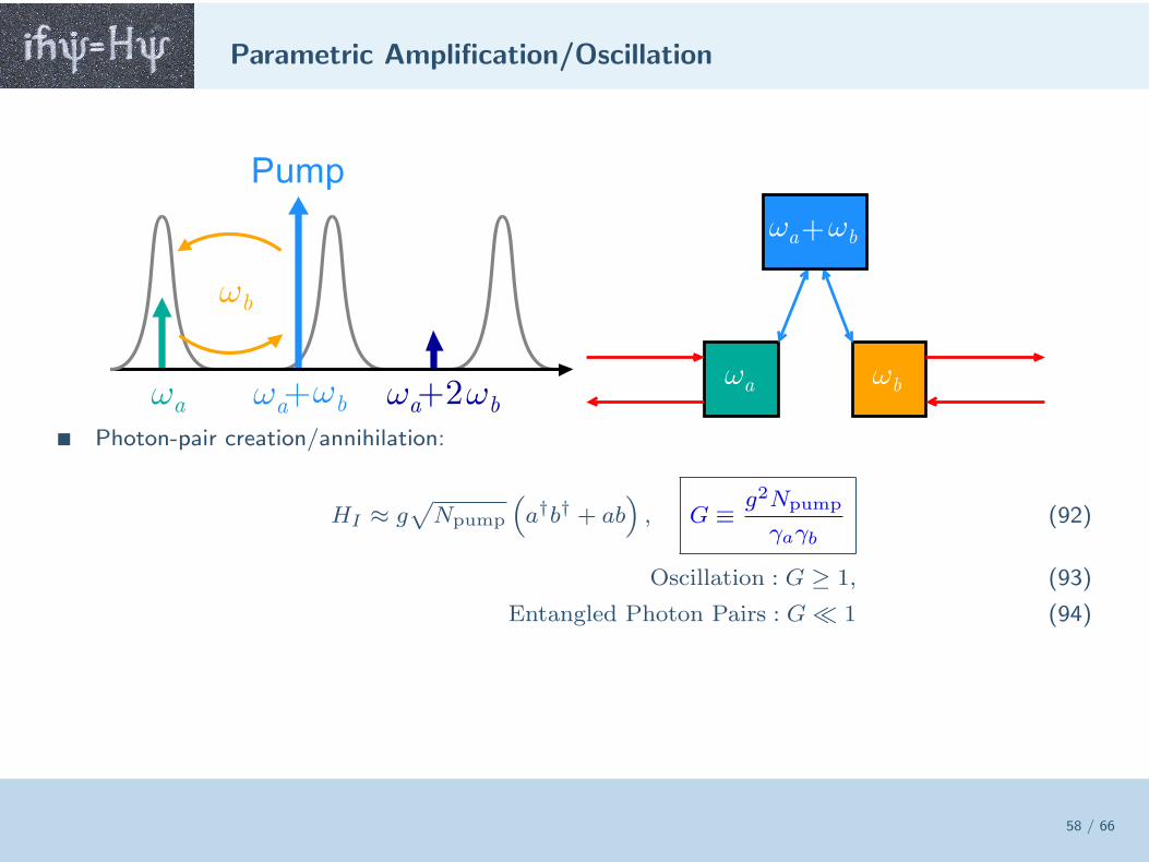
Parametric Amplification/Oscillation
58 / 66
Photon-pair creation/annihilation:
HI ≈ g√
Npump
(
a†b† + ab)
, G ≡ g2Npump
γaγb(92)
Oscillation : G ≥ 1, (93)
Entangled Photon Pairs : G≪ 1 (94)
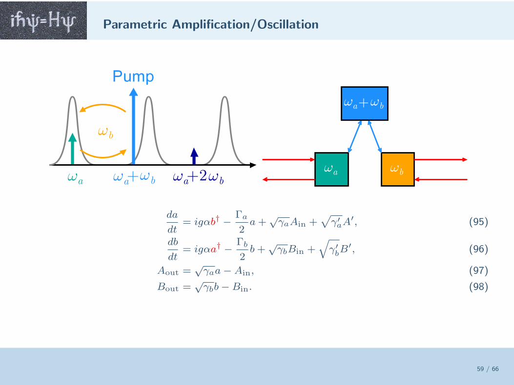
Parametric Amplification/Oscillation
59 / 66
da
dt= igαb† − Γa
2a+
√γaAin +
√
γ′aA′, (95)
db
dt= igαa† − Γb
2b+
√γbBin +
√
γ′bB′, (96)
Aout =√γaa−Ain, (97)
Bout =√γbb−Bin. (98)
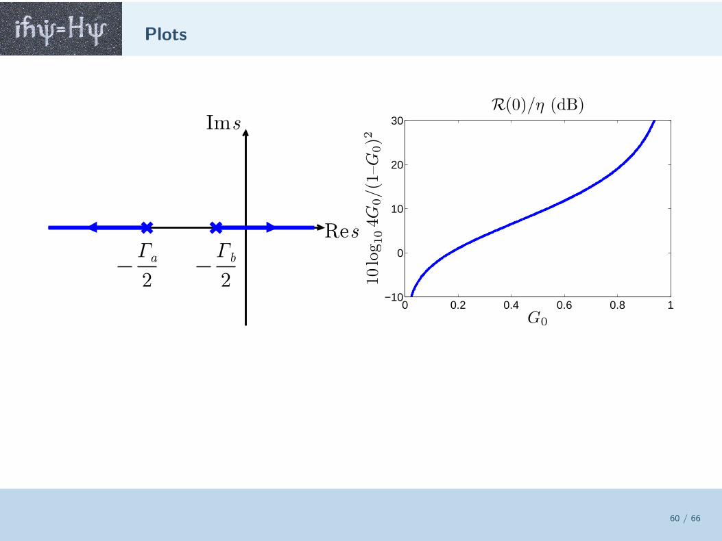
Plots
60 / 66
0 0.2 0.4 0.6 0.8 1−10
0
10
20
30
G0
10
log 1
04G
0/(1
–G
0)2
R(0)/η (dB)
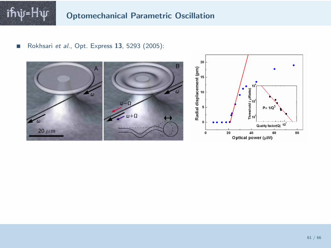
Optomechanical Parametric Oscillation
61 / 66
Rokhsari et al., Opt. Express 13, 5293 (2005):
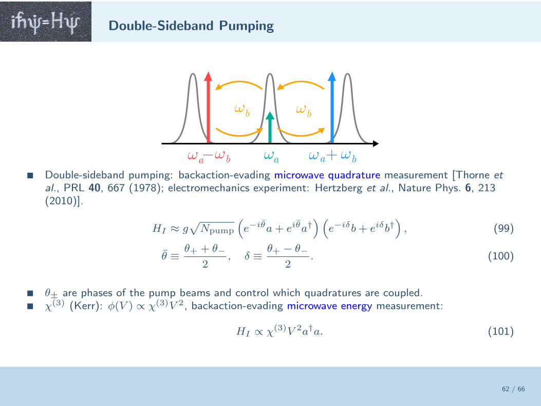
Double-Sideband Pumping
62 / 66
Double-sideband pumping: backaction-evading microwave quadrature measurement [Thorne et
al., PRL 40, 667 (1978); electromechanics experiment: Hertzberg et al., Nature Phys. 6, 213(2010)].
HI ≈ g√
Npump
(
e−iθa+ eiθa†)(
e−iδb+ eiδb†)
, (99)
θ ≡ θ+ + θ−
2, δ ≡ θ+ − θ−
2. (100)
θ± are phases of the pump beams and control which quadratures are coupled. χ(3) (Kerr): φ(V ) ∝ χ(3)V 2, backaction-evading microwave energy measurement:
HI ∝ χ(3)V 2a†a. (101)
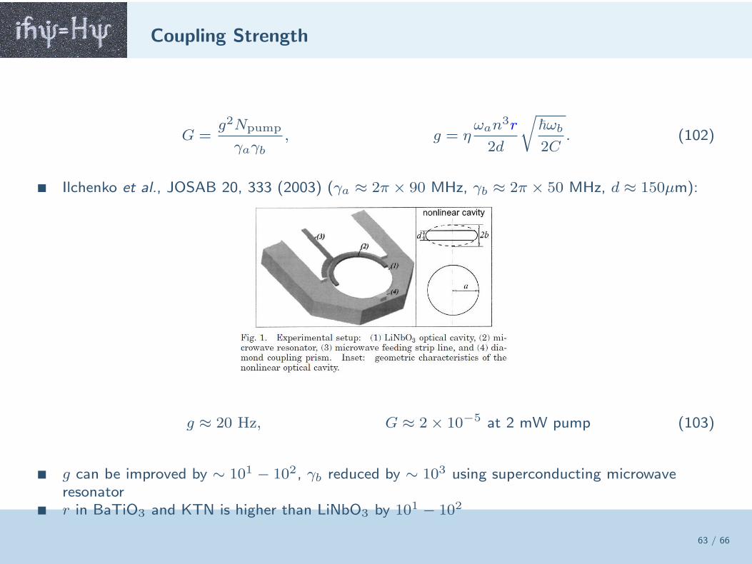
Coupling Strength
63 / 66
G =g2Npump
γaγb, g = η
ωan3r
2d
√
~ωb
2C. (102)
Ilchenko et al., JOSAB 20, 333 (2003) (γa ≈ 2π × 90 MHz, γb ≈ 2π × 50 MHz, d ≈ 150µm):
g ≈ 20 Hz, G ≈ 2× 10⁻⁵ at 2 mW pump (103)
g can be improved by ∼ 101 − 102, γb reduced by ∼ 103 using superconducting microwaveresonator
r in BaTiO3 and KTN is higher than LiNbO3 by 101 − 102
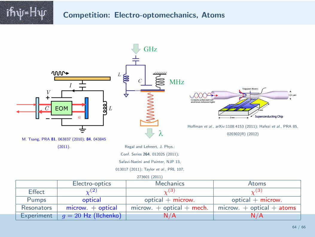
Competition: Electro-optomechanics, Atoms
64 / 66
M. Tsang, PRA 81, 063837 (2010); 84, 043845
(2011). Regal and Lehnert, J. Phys.:
Conf. Series 264, 012025 (2011);
Safavi-Naeini and Painter, NJP 13,
013017 (2011); Taylor et al., PRL 107,
273601 (2011)
Hoffman et al., arXiv:1108.4153 (2011); Hafezi et al., PRA 85,
020302(R) (2012)
Electro-optics Mechanics Atoms
Effect χ(2) χ(3) χ(3)
Pumps optical optical + microw. optical + microw.Resonators microw. + optical microw. + optical + mech. microw. + optical + atomsExperiment g = 20 Hz (Ilchenko) N/A N/A
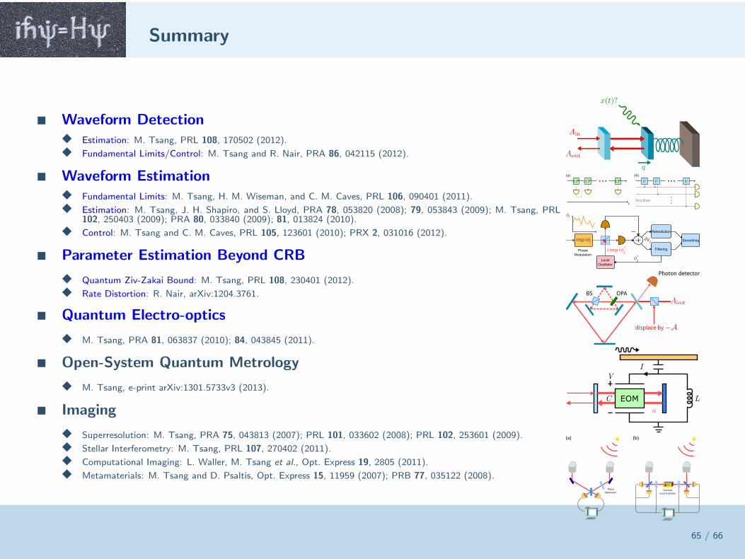
Summary
65 / 66
Waveform Detection
Estimation: M. Tsang, PRL 108, 170502 (2012).
Fundamental Limits/Control: M. Tsang and R. Nair, PRA 86, 042115 (2012).
Waveform Estimation Fundamental Limits: M. Tsang, H. M. Wiseman, and C. M. Caves, PRL 106, 090401 (2011).
Estimation: M. Tsang, J. H. Shapiro, and S. Lloyd, PRA 78, 053820 (2008); 79, 053843 (2009); M. Tsang, PRL102, 250403 (2009); PRA 80, 033840 (2009); 81, 013824 (2010).
Control: M. Tsang and C. M. Caves, PRL 105, 123601 (2010); PRX 2, 031016 (2012).
Parameter Estimation Beyond CRB
Quantum Ziv-Zakai Bound: M. Tsang, PRL 108, 230401 (2012).
Rate Distortion: R. Nair, arXiv:1204.3761.
Quantum Electro-optics
M. Tsang, PRA 81, 063837 (2010); 84, 043845 (2011).
Open-System Quantum Metrology
M. Tsang, e-print arXiv:1301.5733v3 (2013).
Imaging
Superresolution: M. Tsang, PRA 75, 043813 (2007); PRL 101, 033602 (2008); PRL 102, 253601 (2009).
Stellar Interferometry: M. Tsang, PRL 107, 270402 (2011).
Computational Imaging: L. Waller, M. Tsang et al., Opt. Express 19, 2805 (2011).
Metamaterials: M. Tsang and D. Psaltis, Opt. Express 15, 11959 (2007); PRB 77, 035122 (2008).
OPABS
displace by
Photon detector

Collaborations
66 / 66
Cavity electro-optics: with Aaron Danner at National U. Singapore Parameter estimation for optomechanical force sensing: with Warwick Bowen at U.
Queensland Time-varying optical phase estimation: with Hidehiro Yonezawa at U. Tokyo, Elanor
Huntington et al. at U. New South Wales
http://mankei.tsang.googlepages.com/
Supported by Singapore National Research Foundation Fellowship (NRF-NRFF2011-07).
Related Documents