M.Sc. (Mathematics), SEM- I Paper - IV ORDINARY DIFFRENTIAL EQUATION PSMT104 Note- There will be some addition to this study material. You should download it again after few weeks.

Welcome message from author
This document is posted to help you gain knowledge. Please leave a comment to let me know what you think about it! Share it to your friends and learn new things together.
Transcript
M.Sc. (Mathematics), SEM- I
Paper - IV
ORDINARY DIFFRENTIAL
EQUATION PSMT104 Note- There will be some addition to this study material. You should download it again after few weeks.
CONTENT
Unit No. Title
1. Basic Theory
2. Systems of First Order ODE
3. Linear Systems of ODE (I)
4. Linear Systems of ODE (II)
5. Method of Power Series
6. Sturm- Liouville Theory
***
SYLLABUS
Unit I. Existence and Uniqueness of Solutions (15 Lectures)
Existence and Uniqueness of solutions to initial value problem of 1st order ODE-
both autonomous, non autonomous, -approximate solutions, Ascoli lemma,
Cauchy-Peano existence theorem, Lipschitz condition, Picard’s method of
successive approximations, Picard-Lindelof theorem, System of Differential
equations. Reduction of n-th order differential equations.
[Reference Unit-I of Theory of Ordinary Differential Equations; Earl A. Coddington
and Norman Levinson, Tata McGraw Hill, India.]
Unit II. Linear Equations with constant coefficients (15 Lectures)
The second order homogeneous equations, Initial value problem for second
order equations, Uniqueness theorem, linear dependance and independence of
solutions, Wronskian,a formula for the Wronskian, The second order non-
homogeneous equations, The homogeneous equations of order n, Initial value
problem for order equations, The nonhomogeneous equations of order n,
Algebra of constant coefficient operators.
[Reference Unit-II of Earl A. Coddington, An Introduction to Ordinary Differential
Equations, Prentice-Hall of India.]
Unit III. Linear Equations with variable coefficients (15 Lectures)
Initial value problem for the homogeneous equation of order n, Existence and
Uniqueness theorem, solution of the homogeneous equations, Wronskian and
linear independance, reduction of the order of a homogeneous equation, the
non-homogeneous equations of order n.
[Reference III of Earl A. Coddington, An Introduction to Ordinary Differential
Equations, Prentice-Hall of India.]
Unit IV. Sturm-Liouville Problem & Qualitative Properties of Solutions (15
Lectures)
Eigen value problem, Eigen values and Eigen functions, the vibrating string
problem, Sturm Liouville problems, homogeneous and non-homogeneous
boundary conditions, orthogonality property of eigen functions, Existence of
Eigen values and Eigenfunctions, Sturm Separation theorem, Sturm comparison
theorem. Power series solution of second order linear equations, ordinary points,
singular points, regular singular points, existence of solution of homogeneous
second order linear equation, solution of Legendre’s equation, Legendre’s
polynomials, Rodrigues’ formula, orthogonality conditions, Bessel differential
equation, Bessel functions, Properties of Bessel function, orthogonality of Bessel
functions.
[Reference Unit IV (24, 25), Unit V (Review), Unit-VII (40, 43, Appendix A) and Unit
VIII (44, 45, 46, 47) : G. F. Simmons, Di_erential Equations with Applications and
Historical Notes, Second Edition, Tata McGraw Hill, India]
192
1BASIC THEORY
Unit Structure :
1.1 Introduction.
1.2 Ordinary Differential Equations.
1.3 First Order ODE.
1.4 Existence and Uniqueness of Solutions (Scalar Case).
1.5 Illustrative Examples.
1.6 Exercises.
1.1 INTRODUCTION
As we already know, a differential equation - DE - is anequation relating the following three items :
A function of one or more variables (the function being realvalued or vector values).
The independent variables of the function. A finite number of derivatives of the function.
The highest order of derivatives of the function appearing inthe equation is the order of the differential equation.
Usually, the function in a differential equation is an unknownfunction; it is an are observable quantity of a real process andtherefore we are interested in knowing the function. We use resultsand techniques of mathematical analysis along with our geometricintuition and tease the function out of the differential equation. Wethen speak of having solved the differential equation.
Depending on the nature of the function (in which adifferential equation is set) we classify the differential equations inthe following two types :
I) A function nX : I of a single real variable (say) t rangingin an open interval I gives rise to the succession of derivatives :
193
0 2 k
2 k
d dX d X d XX X, , , ... .....
dt dt dt dt
Now a differential equation in the function X t is therefore
an equation of the type :2
2, , , .... 0
k
k
dX d X d XF t X
dt dt dt
………………. (1)
Such an equation is said to be an ordinary differentialequation. Thus an ordinary differential equation is a differentialequation in which the constituent function : ( )X t X t is a function
of a single real variable.
We often use the acronym ODE in place of the full term :ordinary differential equation.
II) On the other hand, there are differential equations in a
function :u x u x of a real multivariable 1 2..... nx x x x which
ranges in an open subset of n . Such a function u u x gives
rise to mixed partial derivatives :
1 2
2
1 2
,1 ,
;1 ,
: ....n
i
i j
n
ui n
x
ui j n
x x
D u ux x x
for various multi-indices 1 2 .... n with
0,1, 2, ... ,i i the mixed partial derivative D u having the
order 1 2: ... n .
Now a differential equation in such a function u u x of a
multi - variable 1..... nx x x ranging in an open subset of n is
an equation of the type :
194
2
, , , .... : 0 i i j
u uF x u D u m
x x x------------------- (2)
its order being m. Equation (2) is said to be a partial differentialequation in ( )u x because it involves the mixed partial derivatives of
u. We use the acronym PDE for this type of differential equations.
There is more about the setting of a differential equation : In amathematical problem, a differential equation is accompanied byauxiliary data. A solution of a differential equation is required tosatisfy this auxiliary data. To be more specific we are given a subsetof the domain of a prospective solution and some of its derivativesof the solution at the points of this subset.
In case of the ODE, the auxiliary data is said to consist ofinitial conditions. An initial value problem consists of finding thesolution of the ODE which satisfies the accompanying initialconditions. Often, the pair consisting of (a) an ordinary differentialequation and (b) the initial conditions is referred as the initial valueproblem -IVP-.
Often the initial conditions are given at the end points of aninterval which are then called the boundary conditions. Also, theresulting initial value problem is called a boundary value problem.
In the case of a partial differential equation, theaccompanying auxiliary data is called the Cauchy data for PDE.The Cauchy problem for a given PDE consists of finding thesolution of the PDE which satisfies the requirements of the givenCauchy data.
We will explain more about these terms initial conditions,Cauchy data etc. - at later stages.
Partial differential equations, being more intricatemathematical objects are studied by using the concepts and results ofthe ordinary differential equations. Therefore, a basic course ondifferential equations begins with a treatment of ordinary differentialequations. In our treatment of the subject also, we will developenough theory of ODE and then apply it to the partial differentialequations.
Therefore, back to the theory of ODE.
195
1.2 ORDINARY DIFFERENTIAL EQUATIONS
To begin with, we reorganize the form (1) of the ODE in thefollowing manner. Unraveling it, we separate the top orderderivative and express it as a function of the remain variable
quantities, namely,1
1, ( ), , ..... ,
k
k
dX d Xt X t
dt dt
that is we form the
equation1
1, , ,
k k
k k
d X dX d xf t X
dt dt dt
…………………… (3)
We regard the equation (3) as the standard form of an ODE(of course, the ODE has order = k.) Note that the function
: ( )X t X t is a vector valued function of the real variable t and as
such it is a curve in n . Each ( )X t has n components :
1 2( ) ( ), ( ), .... , ( ) nX t X t X t X t and therefore all the derivative of it
has n components :
1 2
( )( ), ( ), ..... ( )
n
d X t d d dX t X t X t
dt dt dt dtfor
1 k . Consequently, the function f appearing on the right hand
side of (3) has n components : 1 2, , ... , nf f f f each if being a
real valued function. Consequently the DE (3) is actually thefollowing system of ODE in the functions :
1 2, , .... , t X t t X t nt X t
11
1 1
12
2 1
1
1
, , , ...,
, , , ...,
, , , ...,
k k
k k
k k
k k
k kn
nk k
d X dX d Xf t X
dt dt dt
d X dX d Xf t X
dt dt dt
d X dX d Xf t X
dt dt dt
……………… (4)
At this stage, we become more specific about the features ofthe ODE (3) (or equivalently about the system (4).)
Let I be an open internal and let denote an open subset of
n . We consider the open sets
......n nI
196
(there being 1k copies of n in the above Cartesian product).This set is being designated to accommodate the variable quantities :
1
1, ( ), ,
k
k
dx d xt X t t
dt dt
.
Clearly, the function f appearing on the right hand side of (3)must have this set as its domain of definition.
Choosing 0 0, t I x and 1 2 1, ... kw w w in n , we form the
initial condition 0 0 1 2 1, , , ... kt x w w w . Now, the initial value problem
for the ODE (3) is the following pair :
1
1
0 0 1 1
, , , ....
, , ,......
k k
k k
k
d X dX d Xf t X
dt dt dt
t x w w
……………. (5)
By a solution of the initial value problem (5) we mean an (atleast) k times continuously differentiable function (= curve in )
: X J , J being an open interval with 0 t J I , which
satisfies the following two items :
The differential equation :1
1
( ) ( ) ( )...,
k k
k k
d X t dX t d X tf t
dt dt dt
,for all t J
The initial conditions :
1
00 0 0 1 11
, , ....,k
kk
d X tdXx t x t w w
dt dt
Remarks :
(I) Though the independent variable t of the function X(t) in theODE (1) is stipulated to range in the interval I, we expect thesolution ( )t X t of the initial value problems (4) to be defined only
on a sub-internal J of I (with 0t J ). Indeed, we come across
concrete cases of the IVP in which a solution exists only on a sub-inter J of I and therefore, we grant this concession : a solution needbe defined only on a sub-interval J of I.
197
II) Often, the initial conditions are expressed more explicitly in
terms of the equations : 1
00 0 0 1 11
, , ....,k
kk
d X tdXx t x t w w
dt dt
.
An important special case of the ODE (3) is2 1
2 1, ,
k k
k k
d X dX d X d Xf X
dt dt dt dt
………………… (6)
in which the function f is independent of the variable
: : .... n n nt f . In this case we say that the ODE (6) is
autonomous.
Returning to the initial value problem (5), there are twoquestions :
Does the initial value problem (5) admit a solution at all? If it does is the solution unique?
Clearly, because f is the main ingredient of the ODE, theanswer to both of there questions naturally depends on the propertiesof f, especially on its behaviour around the initial condition
0 0 1 1, , ,....... kt x w w (i.e. how if varies continuously, differentially etc.
around 0 0 1 1, , ,...., kt x w w Following two examples illustrate that
answers to both the questions are (in general) in the negative :
Let : f be the function :
1 0
1 0
f x x
x
For this function we consider the (first order autonomous case
of) the initial value problem : ( ), ( ) 0dX
f X x odt
.
We contend that this initial value problem has no solution.
For, if there was a solution : X J with 0J , then
(0) (0) 1dX
fdt
implies that the solution ( )t X t is strictly
monotonic increasing in a neighborhood , of O.
198
On the other hand, 1( 0) ( )dX
f tdt
for all , 0 t
implies that ( )t X t t is strictly monotonic decreasing in
, 0 . Thus, if the solution of the above IVP exists then it is
strictly monotonic increasing as well as strictly monotonicdecreasing. This prevents a solution!
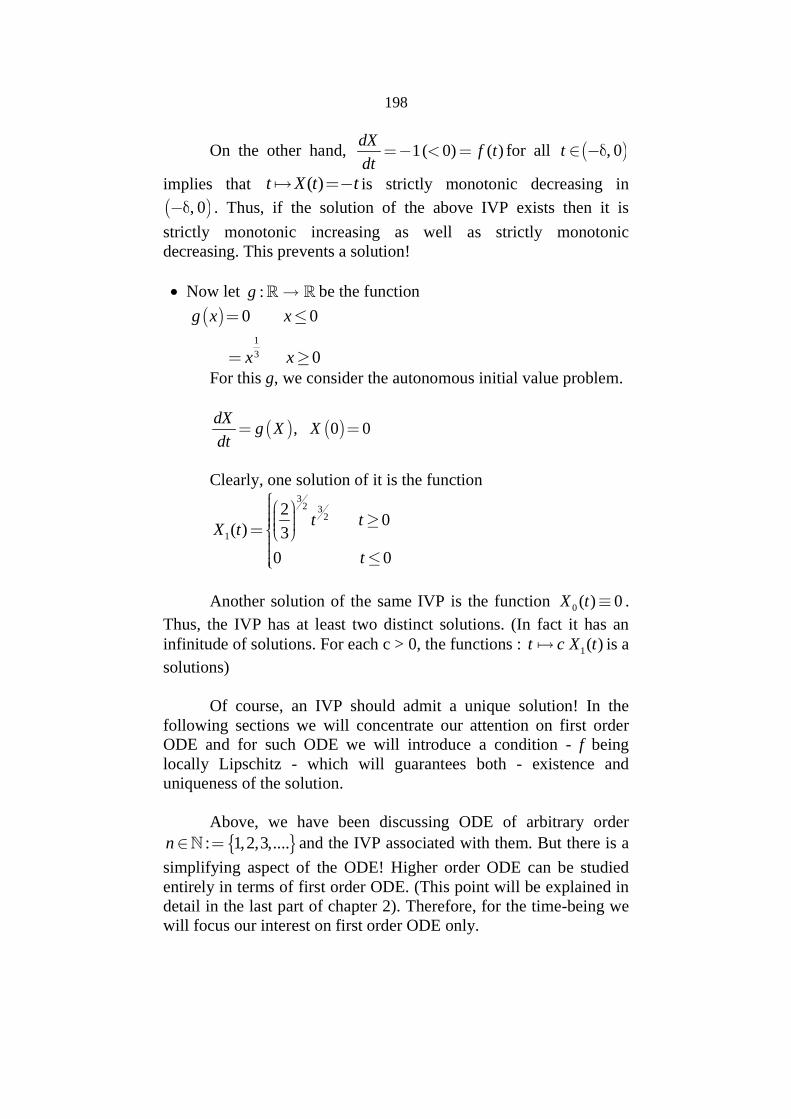
Now let : g be the function
1
3
0 0
0
g x x
x xFor this g, we consider the autonomous initial value problem.
, 0 0dX
g X Xdt
Clearly, one solution of it is the function3
2 32
1
20
( ) 3
0 0
t tX t
t
Another solution of the same IVP is the function 0 ( ) 0X t .
Thus, the IVP has at least two distinct solutions. (In fact it has aninfinitude of solutions. For each c > 0, the functions : 1( )t c X t is a
solutions)
Of course, an IVP should admit a unique solution! In thefollowing sections we will concentrate our attention on first orderODE and for such ODE we will introduce a condition - f beinglocally Lipschitz - which will guarantees both - existence anduniqueness of the solution.
Above, we have been discussing ODE of arbitrary order
: 1,2,3,....n and the IVP associated with them. But there is a
simplifying aspect of the ODE! Higher order ODE can be studiedentirely in terms of first order ODE. (This point will be explained indetail in the last part of chapter 2). Therefore, for the time-being wewill focus our interest on first order ODE only.
199
1.3 FIRST ORDER ODE
We begin some more generalities related to first order ODE.As in the preceding part, I denoted an open interval and , an open
subset of n .
We consider a function :
: nf I ……………….. (7)
giving rise to the first order ODE :
( , )dX
f t Xdt
……………………(8)
Note that for each t I held fixed the map :
, : ; ,nf t x f t x is a vector field on .
Interpreting “t” as the time variable we call the function (7) a timedependant vector field on . And, often, we call a solution
:X J of the ODE (8), an integral curve of the vector field f.An initial condition for the ODE (8) consists of a pair 0 0,t x
with 0t I , 0x and the associated initial value problem is :
0 0( , ),dX
f t X x t xdt
……………….. (9).
Finally, recall that a solution of (9) is an (at least) oncecontinuously differentiable curve
:X J
(J being an open interval with 0t J CI ) satisfying :
( )( , ( ))
dX tf t X t
dt for all t I and the initial condition
0 0X t x .
In the context of the IVP (9) we consider yet another equationthe following integral equation in an unknown function :X J :
0
0( ) ( , ( ))t
t
X t x f s x s ds t J …………………. (10).
200
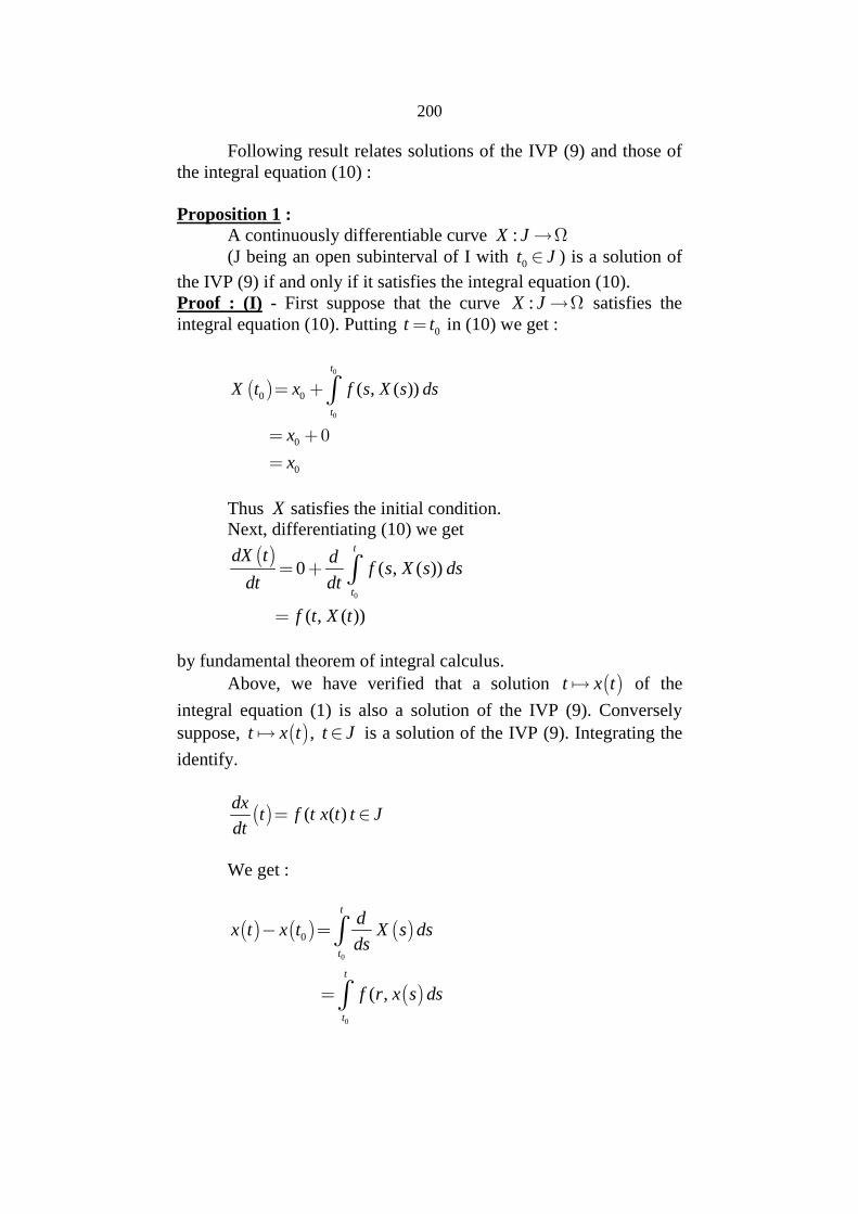
Following result relates solutions of the IVP (9) and those ofthe integral equation (10) :
Proposition 1 :A continuously differentiable curve :X J (J being an open subinterval of I with 0t J ) is a solution of
the IVP (9) if and only if it satisfies the integral equation (10).Proof : (I) - First suppose that the curve :X J satisfies theintegral equation (10). Putting 0t t in (10) we get :
0
0
0 0
0
0
( , ( ))
t
t
X t x f s X s ds
x
x
Thus X satisfies the initial condition.Next, differentiating (10) we get
0
0 ( , ( ))
( , ( ))
t
t
dX t df s X s ds
dt dt
f t X t
by fundamental theorem of integral calculus.Above, we have verified that a solution t x t of the
integral equation (1) is also a solution of the IVP (9). Converselysuppose, t x t , t J is a solution of the IVP (9). Integrating the
identify.
( ( )dx
t f t x t t Jdt
We get :
0
0
0
( ,
t
t
t
t
dx t x t X s ds
ds
f r x s ds
201
And therefore :
0
0 ( , )t
t
x t x f s X s ds
Thus we have :
0
0 ( ,t
t
x t x f s X s ds
For all t J proving that a solution of the IVP (9) is also a solutionof the integral equation (10).
1.4 EXISTENCE AND UNIQUENESS OF SOLUTIONS(SCALAR CASE)
In this section, we consider the scalar case, (i.e. a singledifferential equation) of the initial value problem. Now will be anopen subset of which, without loss of generality will be taken tobe an open internal, we write J for . Thus we have on function
:f I J
Along with 0t I , 0x J giving rise to the scalar case of the initial
value problem :
0 0( , ) ( )dX
f t x x t xdt
…………………… (11)
Following property of f ensures both, existence anduniqueness of the solution of (11).
Definition 1 : f is locally lipschitz on J, uniformly in t I if thefollowing two conditions are satisfied.
a) f is continuous on I J .b) For each 0t I , 0x J there exist finite numbers
0, 0K satisfying the following :
i) 0 0 0 0, , ,t t I x x J and
ii) , ( , )f t x f t y K x y holds for all 0 0,t t t and
for all pairs x, y in 0 0,x x .
Remark : An autonomous ODE arises from a function :f J
which is independent of the time variable t I . For such a function,
202
the condition (b) in the definition takes the following simpler from :for each 0x J , there exist 0, 0K satisfying :
i) 0 0,x x J and
ii) ( )f x f y K x y for all x, y in J.
Also note that this condition implies continuity of f at every
0x J and therefore there is no separate mention of condition (a) in
the definition of local Lipschitz property of such a :f J .
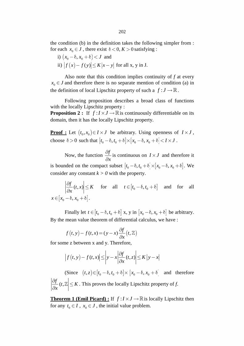
Following proposition describes a broad class of functionswith the locally Lipschitz property :Proposition 2 : If :f I J is continuously differentiable on its
domain, then it has the locally Lipschitz property.
Proof : Let 0 0,t x I J be arbitrary. Using openness of I J ,
choose 0 such that 0 0 0 0, ,t t x x I J .
Now, the functionf
x
is continuous on I J and therefore it
is bounded on the compact subset 0 0 0 0, ,t t x x . We
consider any constant k > 0 with the property.
( , )f
t x Kx
for all 0 0,t t t and for all
0 0,x x x .
Finally let 0 0,t t t x, y in 0 0,x x be arbitrary.
By the mean value theorem of differential calculus, we have :
, ( , ) ( ) ,f
f t y f t x y x tx
for some z between x and y. Therefore,
, ( , ) ( , )f
f t y f t x y x t z K y xx
(Since 0 0 0 0, , ,t z t t x x and therefore
( ,f
t Kx
. This proves the locally Lipschitz property of f.
Theorem 1 (Emil Picard) : If :f I J is locally Lipschitz then
for any 0t I , 0x J , the initial value problem.
203
0 0( , ), ( )df
f t x x t xdx
has a solution 0 0: ,x t t J for some 0 .
Proof : Choose 0 such that 0 0 0 0, , ,t t I x x J
and there exists 0K for which , ( , )f t x f t y K x y holds
for all 0 0 0 0, ,t t x x . We choose M > 0 such that
,f t x M for all 0 0,t t t , 0 0,x x x .
Using the constants 0 , K > 0, M > 0, chosen above, we
choose one more constant satisfying1
0 min ,K M
.
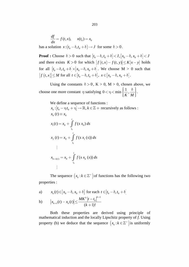
We define a sequence of functions :
0 0: ,kx t t k recursively as follows :
0
0
0
0 0
1 0 0
2 0 1
1( ) 0
( )
( ) ( )
( ) ( ( ))
( ( ))
t
t
t
t
t
k t k
t
x t x
x t x f s x ds
x t x f s x s ds
x x f s x s ds
The sequence :kx k of functions has the following two
properties :
a) 0 0( ) ,kx t x x for each 0 0,t t t
b)
1
01( ) ( )
( 1)!
kk
k k
MK t tx t x t
k
Both these properties are derived using principle ofmathematical induction and the locally Lipschitz property of f. Using
property (b) we deduce that the sequence :kx k is uniformly
204
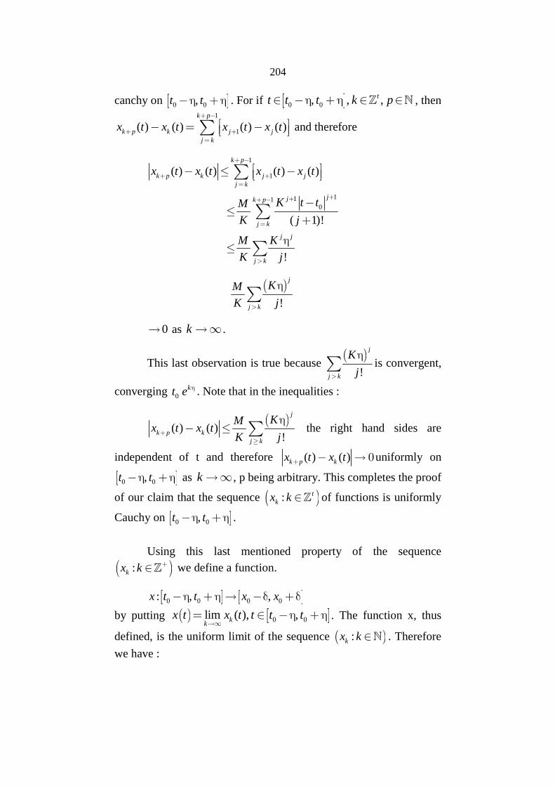
canchy on 0 0,t t . For if 0 0, , ,tt t t k p , then1
1( ) ( ) ( ) ( )k p
k p k j jj k
x t x t x t x t
and therefore
1
1
1110
( ) ( ) ( ) ( )
( 1)!
!
k p
k p k j jj k
jjk p
j k
j j
j k
x t x t x t x t
K t tM
K j
M K
K j
!
j
j k
KM
K j
0 as k .
This last observation is true because
!
j
j k
K
j
is convergent,
converging 0kt e . Note that in the inequalities :
( ) ( )
!
j
k p kj k
KMx t x t
K j
the right hand sides are
independent of t and therefore ( ) ( )k p kx t x t uniformly on
0 0,t t as k , p being arbitrary. This completes the proof
of our claim that the sequence : tkx k of functions is uniformly
Cauchy on 0 0,t t .
Using this last mentioned property of the sequence
:kx k we define a function.
0 0 0 0: , ,x t t x x
by putting 0 0lim ( ), ,kk
x t x t t t t
. The function x, thus
defined, is the uniform limit of the sequence :kx k . Therefore
we have :
205
0
0
0 1
0 1
lim ( )
lim ( , ( )
lim ( , ( )
kk
t
kk
t
t
kk
t
x t x t
x f s x s ds
x f s x s ds
0
0
0 1
0 1
lim ( , ( )
( , lim ( )
t
kk
t
t
kk
t
x f s x s ds
x f s x s ds
0
0 ( , ( )t
t
x f s x s ds
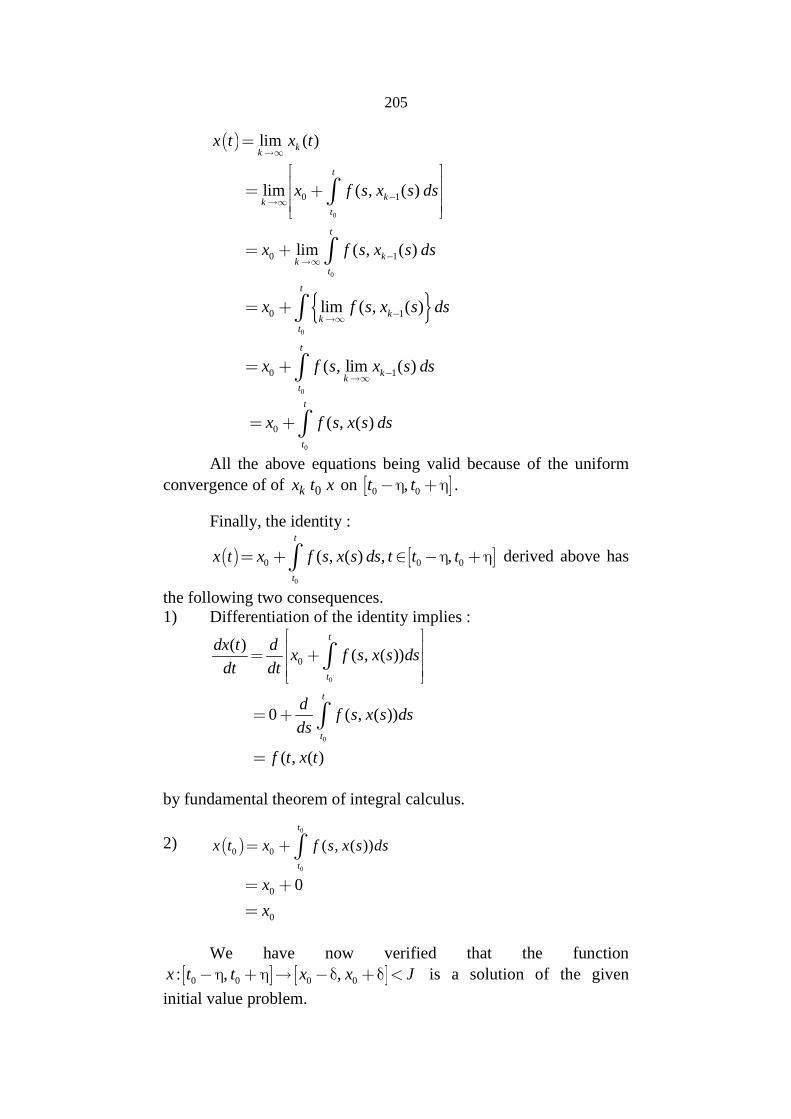
All the above equations being valid because of the uniform
convergence of of 0kx t x on 0 0,t t .
Finally, the identity :
0
0 0 0( , ( ) , ,t
t
x t x f s x s ds t t t derived above has
the following two consequences.1) Differentiation of the identity implies :
0
0
0
( )( , ( ))
0 ( , ( ))
( , ( )
t
t
t
t
dx t dx f s x s ds
dt dt
df s x s ds
ds
f t x t
by fundamental theorem of integral calculus.
2) 0
0
0 0 ( , ( ))
t
t
x t x f s x s ds
0
0
0x
x
We have now verified that the function
0 0 0 0: , ,x t t x x J is a solution of the given
initial value problem.
206
Remark : The above theorem there proves that the functions
kx constructed above are approximate solutions of the initial value
problem (11).
The sequence : tkx k is called Picard’s scheme of
approximate solutions of the initial value problem.
In the next chapter, we will generalize this result (the scalarcase) so as to become applicable to a system of first order ODE. Wewill also prove that any two solutions of the initial value problem(11) agree on the overlap of their domains.
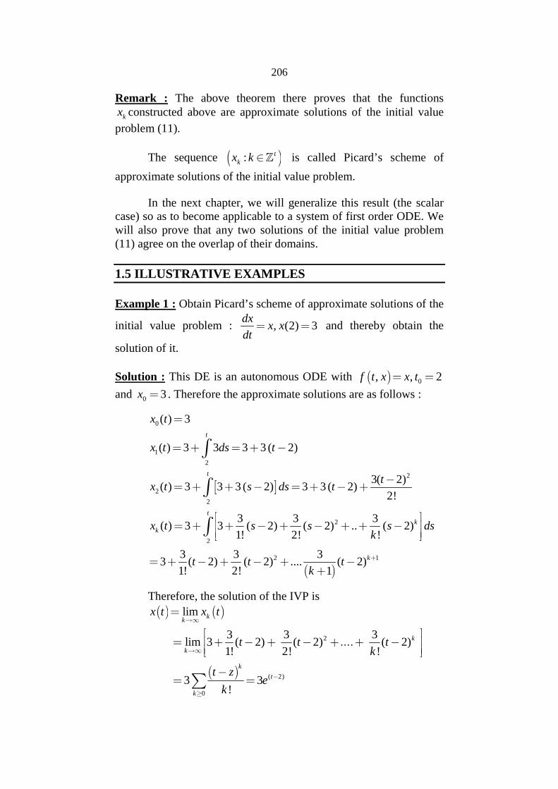
1.5 ILLUSTRATIVE EXAMPLES
Example 1 : Obtain Picard’s scheme of approximate solutions of the
initial value problem : , (2) 3dx
x xdt
and thereby obtain the
solution of it.
Solution : This DE is an autonomous ODE with 0, , 2f t x x t
and 0 3x . Therefore the approximate solutions are as follows :
0
1
2
2
2
2
2
2
2
( ) 3
( ) 3 3 3 3 ( 2)
3( 2)( ) 3 3 3 ( 2) 3 3 ( 2)
2!
3 3 3( ) 3 3 ( 2) ( 2) .. ( 2)
1! 2! !
3 33 ( 2) ( 2) ....
1! 2!
t
t
t
kk
x t
x t ds t
tx t s ds t
x t s s s dsk
t t
13
( 2)1
ktk
Therefore, the solution of the IVP is
2
( 2)
0
lim
3 3 3lim 3 ( 2) ( 2) ( 2)
1! 2! !
3 3!
kk
k
k
k
t
k
x t x t
t t tk
t ze
k
207
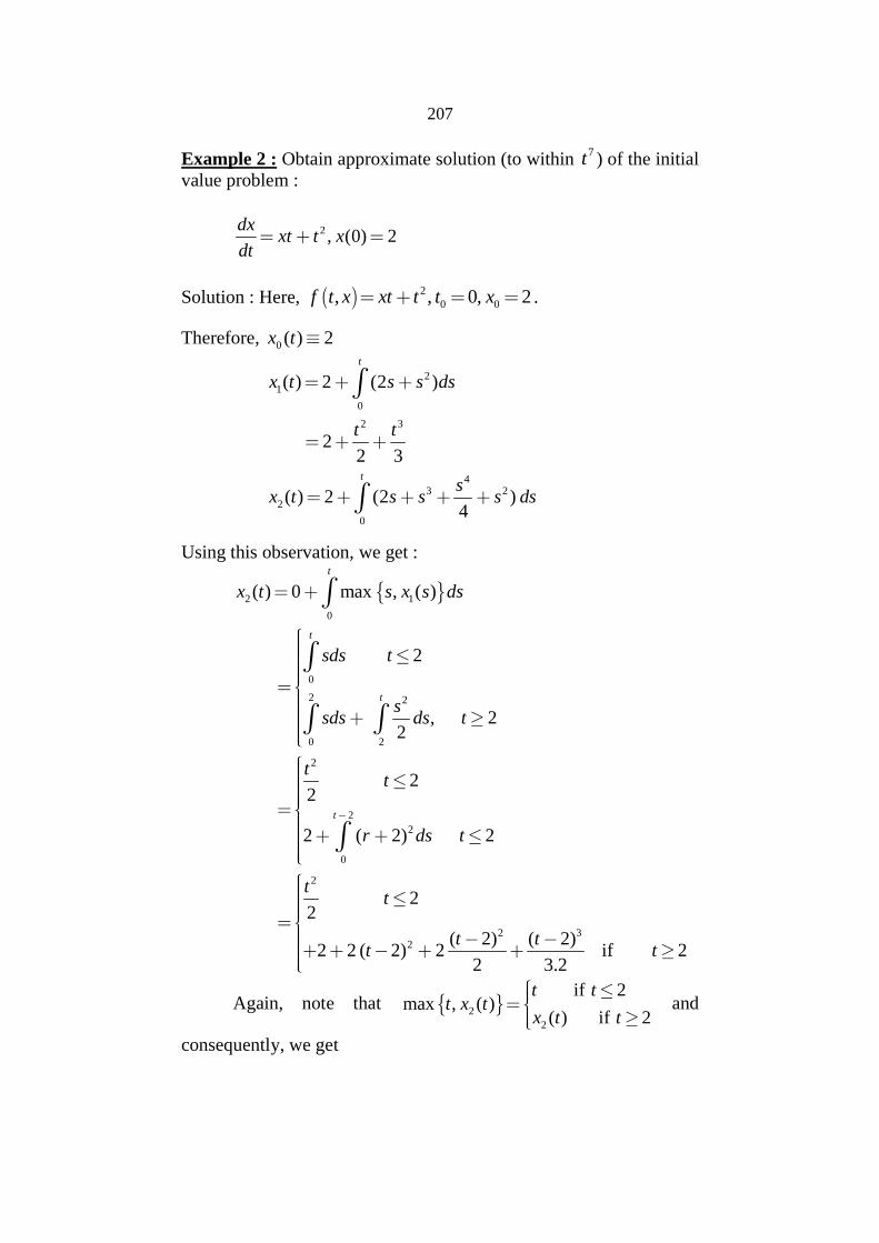
Example 2 : Obtain approximate solution (to within 7t ) of the initialvalue problem :
2 , (0) 2dx
xt t xdt
Solution : Here, 20 0, , 0, 2f t x xt t t x .
Therefore, 0 ( ) 2x t
21
0
2 3
43 2
2
0
( ) 2 (2 )
22 3
( ) 2 (2 )4
t
t
x t s s ds
t t
sx t s s s ds
Using this observation, we get :
2 1
0
0
2 2
0 2
2
2
2
0
( ) 0 max , ( )
2
, 22
22
2 ( 2) 2
t
t
t
t
x t s x s ds
sds t
ssds ds t
tt
r ds t
2
2 32
22
( 2) ( 2)2 2 ( 2) 2 if 2
2 3.2
tt
t tt t
Again, note that 2
2
if 2max , ( )
( ) if 2
t tt x t
x t t
and
consequently, we get
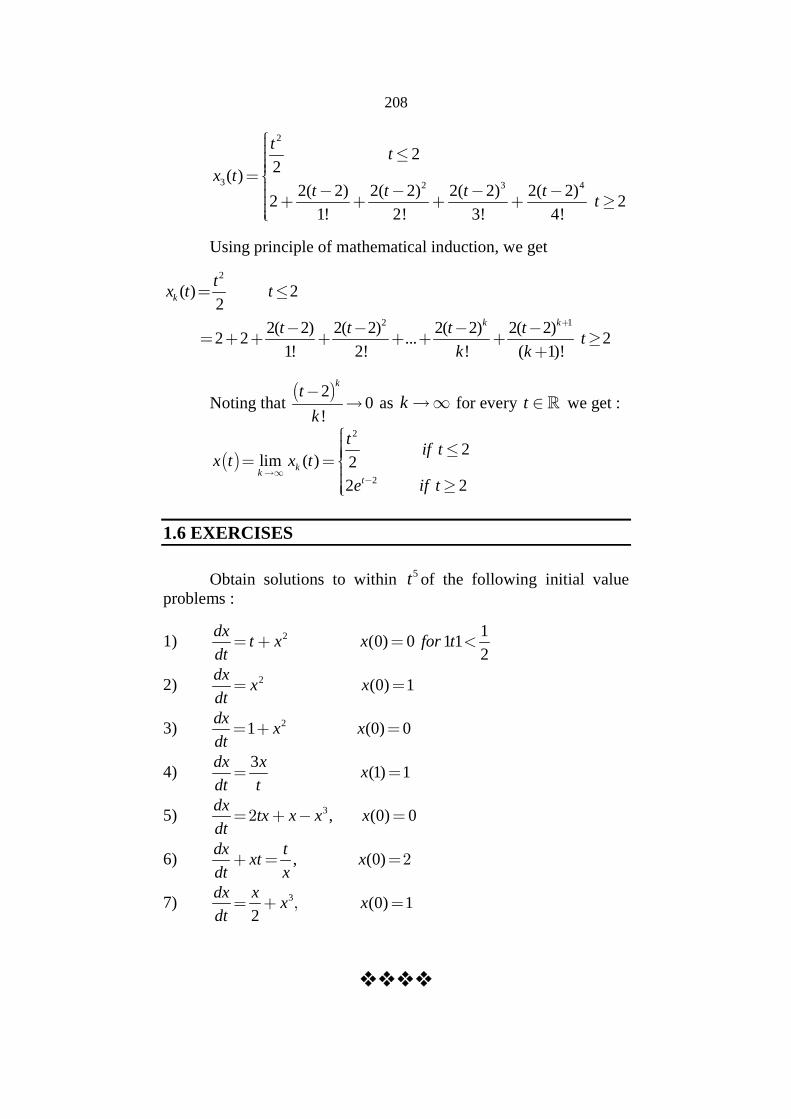
208
2
3 2 3 4
22
( )2( 2) 2( 2) 2( 2) 2( 2)
2 21! 2! 3! 4!
tt
x tt t t t
t
Using principle of mathematical induction, we get
2
2 1
( ) 22
2( 2) 2( 2) 2( 2) 2( 2)2 2 ... 2
1! 2! ! ( 1)!
k
k k
tx t t
t t t tt
k k
Noting that 2
0!
kt
k
as k for every t we get :
2
2
2lim ( ) 2
2 2k
kt
tif t
x t x t
e if t
1.6 EXERCISES
Obtain solutions to within 5t of the following initial valueproblems :
1) 2 1(0) 0 1 1
2
dxt x x for t
dt
2) 2 (0) 1dx
x xdt
3) 21 (0) 0dx
x xdt
4)3
(1) 1dx x
xdt t
5) 3, (0) 0dx
tx x x xdt
6) , (0)dx t
xt xdt x
7) 3 (0) 12
dx xx x
dt
209
2SYSTEMS OF FIRST ORDER ODE
Unit Structure :
2.1 Introduction.
2.2 Existence and Uniqueness of Solutions.
2.3 Uniqueness of a Solution.
2.4 The Autonomous ODE.
2.5 Solved Examples.
2.6 Higher Order ODE.
2.7 Exercises.
2.1 INTRODUCTION
Basic concepts related to differential equations such assystems of first order ordinary differential equations, the initial valueproblem associated with such a system, a local solutions of the initialvalue problem etc. were introduced in the first unit. At the end of theunit, we proved a result regarding the solution of a single first orderODE.
We will extend the results of a single ODE to a system of firstorder ODE and prove both, existence and uniqueness of solutions ofan initial value problem associated with a system of first order ODE.We will then derive some simple results giving information aboutthe nature of solution of such an initial value problem.
We will conclude the chapter by explaining how a system ofhigher order ODE can be reduced to a system of first order ODE.We can then invoke the existence / uniqueness theorems and applythem to the first order ODE and get some information about thesolutions of the higher order ODE.
2.2 EXISTENCE AND UNIQUENESS OF SOLUTIONS
We will use the same notations which were introduced inUnit 1.
Let be an open subset of n , I an open interval and let
: nf I be a time dependent vector field having components:
210
1 2, ,...., :nf f f I
The vector field gives rise to the first order ODE :
,dx
f t Xdt
… (1)which when written in terms of its components becomes thefollowing system of first order ODE :
11 1
22 1
1
( , , ...... , )
( , , ...... , )
( , , ...... , )
n
n
nn n
dxf t X X
dt
dxf t X X
dt
dxf t X X
dt
... (2)
Between the expressions (1) and (2) the compact form (1) ismore convenient and therefore we will use it throughout this chapter,bearing in mind that it is the same as the system (2).
Recall, given 0 0,t I x we have the initial value problem :
0 0( , ), ( )dx
f t X X t xdt
… (3)
a solution of which is a continuously differentiable curve :X J
satisfying( )
( , ( )dX t
f t X tdt
for all 0 0, ( )t I X t x . (J being an
open interval with 0t J I ).
Now, towards the existence / uniqueness of solution of (3) weintroduce the locally Lipschitz property of f:
Definition :The vector field f has the locally Lipschitz property if it
satisfies the following two conditions :
a) f is continuous on its domain andb) For 0 0,t I x , there exist two constants 0, 0K such
thati) 0 0 0, , ,t t I B x and
211
ii) ( )f t x f t y K x y for all 0 0,t t t and
for all x, y in 0 ,B x .
Remark :
We will also consider vector fields : nf as a special
case of : nf I in which ,f t x is independent of
: ( , ) ( )t f t x f x . Recall such vector field give rise to the
autonomous ODE : ( )dx
f xdt . Now, the definition of locally
Lipschitz property for such : nf takes the following simpler
form : For any 0x , there exist 0, 0K such that
0 ,B x and ( )f x f y K x y for all x, y, 0 ,B x .
Note that the above condition implies continuity of f at every
0x and as such there is no separate mention of continuity on f.
Now we have the following result :
Proposition 1: If : nf I is continuously differentiable on its
domain, then it has the locally Lipschitz property.
The proof of this proposition is on lines similar to that ofProposition 2 of Unit 1.
Theorem 1: (Local Existence of solutions) : If : nf I has
the locally Lipschitz property then the initial value problem :
0 0( , ), ( )dx
f t x x t xdt has a solution 0 0: ,X t t .
Proof : We give here a sketchy proof. (To fill up all the details thatare left here, consult the proof of Theorem 1 in unit 1)
For 0 0,t I x choose b > 0 such that
0 0 0, , ,t b t b I B x b and choose 0K such that
( )f t x f t y K x y holding for all 0 0,t t b t b and for
all x, y in 0 ,B x b .
Using the fact that continuous functions are bounded oncompact subsets of their domains, we choose a constant M > 0 such
that f t x M holds for all 0 0,t t b t b and for all
0 ,x B x b .
212
We choose one more constant which satisfying
10 min ,
b
k M
.
Now, we define the sequence of maps 0 0: , nkx t b t b
recursively by putting :
0 0( )x t x
0
1 0 0( ) ( )t
t
x t x f s x ds
0
2 0 1( ) ( ( ))t
t
x t x f s X s ds
0
01( ) ( ( ))t
k
t
kx t x f s X s ds
for each
0 0,t t b t b .
About the sequence :kx k we have the following :
a) 0( ) ,kx t B x b for each 0 0,t t b t b .
b) 1( ) ( )( 1)!
k
k k
MKx t x t
k
0 0, 0t t b t b k
c) :kx k is uniformly Cauchy on 0 0,t b t b
(verification of these properties is left for the reader). We consider
the uniform limit of the sequence 0 0 0: , ,x t t B x b
which is given by
0 0lim ( ) ,kk
x t x t t t b t b
Thus,
0
0 1( ) lim ( , ( )t
kk
t
x t x f s x s ds
0
0 lim ( , ( )t
kk
t
x f s x s ds
0
0 lim ( , ( )t
kk
t
x f s x s ds
0 0
0 0( , lim ( ) ( , ( )t t
kk
t t
x f s x s ds x f s x s ds
213
Thus the function ( )t x t satisfying the integral equation :
0
0( ) ( , ( )t
t
x t x f s x s ds for all 0 0,t t b t b .
Finally the validity of this integral equation has the following twoimplications :
1)0
0
00( ) ( , ( )
t
t
X t x f s x s ds 0 00x x
2)
0
0 ( , ( ))t
t
dx df s x s ds
dt dt ( , ( ))f t X t
This now proves that the curve 0 0: , ,X t t thus
obtained is a solution of the initial value problem.
2.3 UNIQUENESS OF A SOLUTION
We prove an inequality which will lead us to the uniquenessof the solutions :
Proposition 2 : (Gronwall’s Inequality) : Let
: , 0f a b : , 0g a b be continuous functions
and 0A , a constant satisfying
t
a
f t A f s g s ds for all ,t a b . Then
.
t
a
g s ds
f t A e
for all ,t a b .
Proof : First we assume A > 0 and put t
a
h t A f s g s ds
for all ,t a b . Then 0h t for all ,t a b and
( ) ( )
( ) ( )
h t f t g t
h t g t
that is,
( )( )
h tg t
h t
for all ,t a b . Integrating this inequality over
,a t for ,t a b we get ( )
log( )
a
th t
g s dsh a
.
214
Nothing that h a A , we get the desired inequality in this
case. Now suppose A = 0. Then for each n we have :
1
t
a
f t f s g s dsn
, for all t [ , )a b
Applying the above argument to1
An
, we get
1
a
g s ds
t
f t en
for every ,t a b and for every n . Holding t fixed and taking
limit of the last inequality as n we get
1g s ds
g s ds
t
a
t
a
f t en
A e
Now we prove the following essential uniqueness result of thesolution :
Proposition 3 : Let : , :x J y J be two solutions of the
initial value problem :
0 0( , ) ( )dx
f t x x t xdt .
then ( ) ( )x t y t for all t J J .
Proof : Recall that both x and y, being solutions of the initial valueproblem, satisfy the integral equations on their domain intervals :
0
0
0
0
( ) ( , ( ))
( ) ( , ( ))
t
t
t
t
x t x f s x s ds
y t x f s y s ds
Therefore 0
( ) ( ) , ( ) , ( )t
t
x t y t f s x s f s y s ds which
implies :
0
( ) ( ) 0 , ( ) , ( )t
t
x t y t f s x s f s y s
215
0
0 ( ) ( )t
t
K x s y s for all 0t t .
Applying Gronwalls result with A = 0, we get
0 ( ) ( ) 0x t y t for all 0t t .
This gives the desired equality ( ) ( )x t y t for all t J J .
Towards the uniqueness of the solution of the initial valueproblem (3), we consider all the solutions of the initial valueproblem (3). Let the totality of them be denoted by :
: :x J the solutions x being thus indexed by a
suitable indexing set .
Above we have verified that any two solutions, say1
x and
2x are equal on the overlap
1 2J J of their domains. Therefore,
we patch together all the solutions to get a maximal solution is thesolution defined on the largest open interval. It is obtained asfollows.
Let :J U J clearly J is an open sub internal of I
with 0x J and all the solutions x patch up to get a solution
:x J of the initial value problem (3).
Because, we consider all the solutions of (3) we get that J isthe largest open internal on which the solution of (3) is defined. Wesummarize all this discussion in the following theorem.
Theorem 2 : (Uniqueness of the solution) :The initial value problem (3) has a unique (maximal) solutiondefined on the largest open sub-interval J.
Clearly the solution is unique because it is defined on thelargest and hence unique internal J.
From now onwards we will consider this unique solutiondefined on the maximal interval.
216
2.4 THE AUTONOMOUS ODE
We note a few simple properties of the autonomous ODE :
( )dx
f xdt
determined by a locally Lipschitz and hence continuous vector field
: nf .
Now if :x J is a solution of this autonomous ODE then( )
( ( ))dx t
f x tdt
t I and continuity of f and differentiability of x(t)
and hence its continuity together implies that ( )dx
tdt
is continuous and
thus the curve :x J is continuously differential on I. This
argument also gives the following result. If : nf is k times
continuously differentiable then the solution :x J is k + 1 timescontinuously differentiable on its domain interval.
Note that a solution of an autonomous ODE may not bedefined for all t : We consider the initial value problem.
2 , (0) 1dx
x xdt
.
Clearly its solution is1
( )1
x tt
which is defined on
,1 only and not on the whole of .
It is a result that if the vector field f is compactly supported,then the solution of the initial value problem (3) is defined for allt . (We do not prove this result here).
2.5 SOLVED EXAMPLES
[Note : Recall, if :[ , ] ng a b is an integrable (vector valued)
functions with components 1 2, ,..., ng g g then b
a
g x dx
1 2( ) , ( ) ,...., ( ) ,b b b
n
a a a
g x dx g x dx g x dx . Equivalently written in the
columnal form, we have :
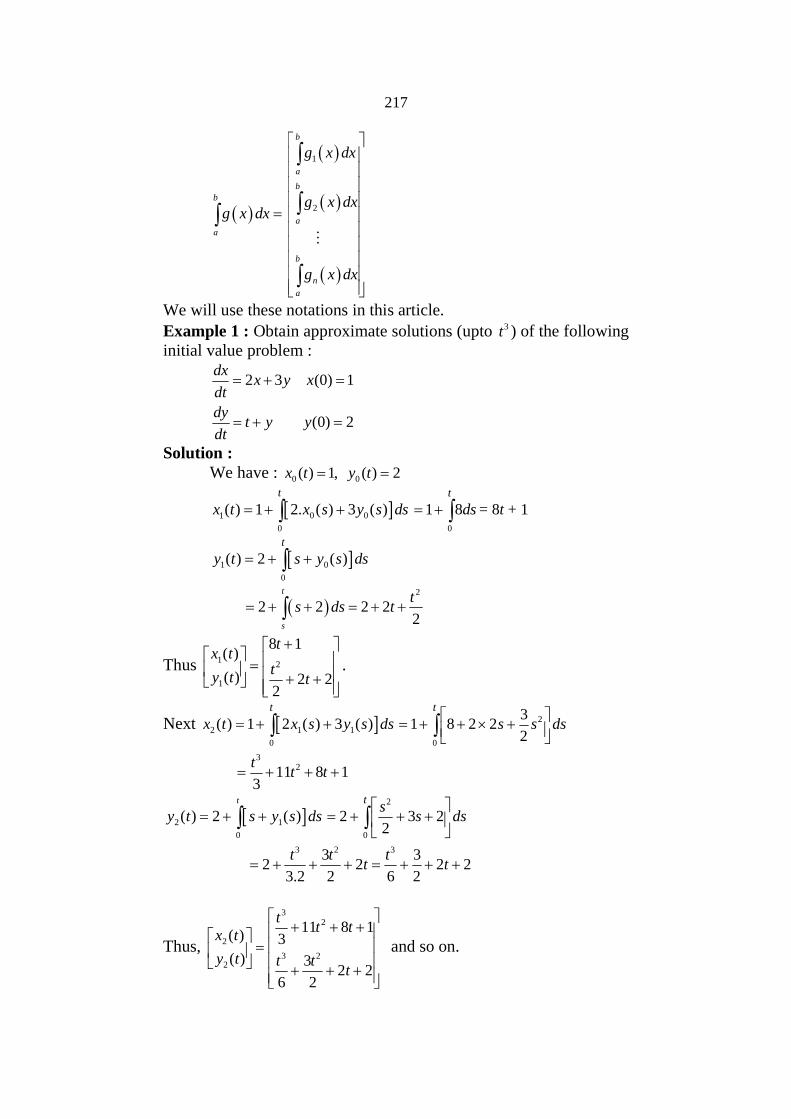
217
b
a
g x dx
1
2
b
a
b
a
b
n
a
g x dx
g x dx
g x dx
We will use these notations in this article.
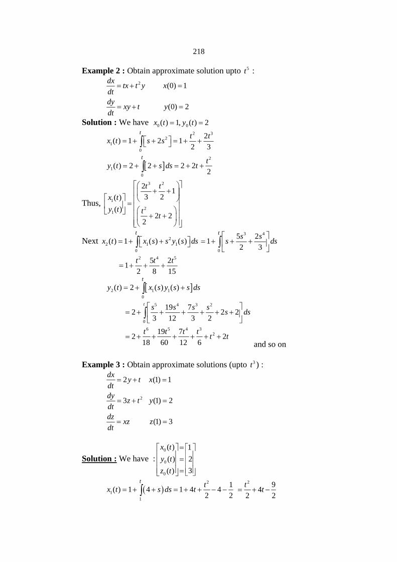
Example 1 : Obtain approximate solutions (upto 3t ) of the followinginitial value problem :
2 3 (0) 1
(0) 2
dxx y x
dt
dyt y y
dt
Solution :We have : 0 ( ) 1,x t 0 ( ) 2y t
1 0 0
0
( ) 1 2. ( ) 3 ( )t
x t x s y s ds 0
1 8t
ds = 8t + 1
0
1 0( ) 2 ( )t
y t s y s ds
2
2 2 2 22
t
s
ts ds t
Thus 12
1
8 1( )
( ) 2 22
tx t
ty t t
.
Next 2 1 1
0
( ) 1 2 ( ) 3 ( )t
x t x s y s ds 2
0
31 8 2 2
2
t
s s ds
3211 8 1
3
tt t
2 1
0
( ) 2 ( )t
y t s y s ds 2
0
2 3 22
ts
s ds
3 2 33 32 2 2 2
3.2 2 6 2
t t tt t
Thus,
32
2
3 22
11 8 1( ) 3
( ) 32 2
6 2
tt t
x t
y t t tt
and so on.
218
Example 2 : Obtain approximate solution upto 5t :
2 (0) 1
(0) 2
dxtx t y x
dt
dyxy t y
dt
Solution : We have 0 0( ) 1, ( ) 2x t y t
2 32
1
0
2
1
0
2( ) 1 2 1
2 3
( ) 2 2 2 22
t
t
t tx t s s
ty t s ds t
Thus,
3 2
1
21
21
3 2( )
( )2 2
2
t t
x t
y t tt
Next 22 1 1
0
( ) 1 ( ) ( )t
x t x s s y s ds 3 4
0
5 21
2 3
ts s
s ds
2 4 55 21
2 8 15
t t t
2 1 1
0
( ) 2 ( ) ( )t
y t x s y s s ds 5 4 3 2
0
6 5 4 32
19 72 2 2
3 12 3 2
19 72 2
18 60 12 6
ts s s s
s ds
t t t tt t
and so on
Example 3 : Obtain approximate solutions (upto 3t ) :
2
2 (1) 1
3 (1) 2
(1) 3
dxy t x
dt
dyz t y
dt
dzxz z
dt
Solution : We have :0
0
0
( ) 1
( ) 2
3( )
x t
y t
z t
2
1
1
1( ) 1 4 1 4 4
2 2
tt
x t s ds t 2 9
42 2
tt
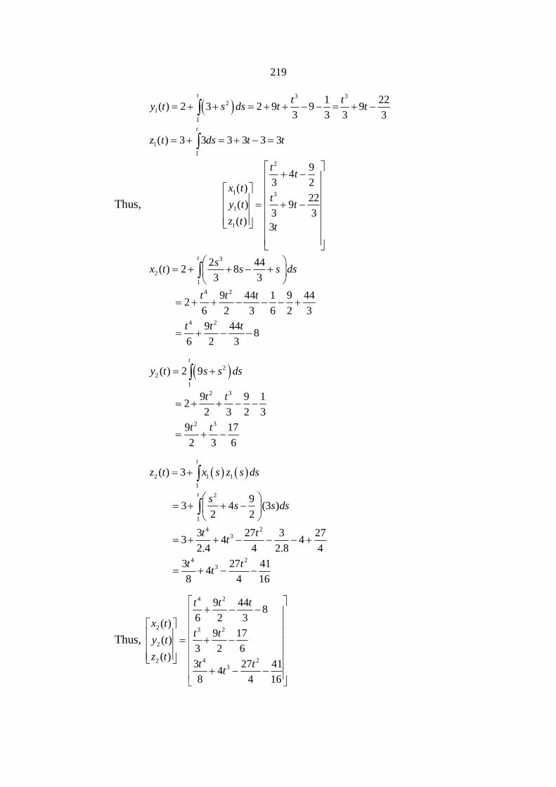
219
3 3
21
1
1 22( ) 2 3 2 9 9 9
3 3 3 3
tt t
y t s ds t t
1
1
( ) 3 3 3 3 3 3t
z t ds t t
Thus,
2
1 3
1
1
94
3 2( )
22( ) 9
3 3( )
3
tt
x tt
y t t
z tt
3
2
1
2 44( ) 2 8
3 3
ts
x t s s ds
4 2
4 2
9 44 1 9 442
6 2 3 6 2 3
9 448
6 2 3
t t t
t t t
22
1
( ) 2 9t
y t s s ds 2 3
2 3
9 9 12
2 3 2 3
9 17
2 3 6
t t
t t
2 1 1
1
( ) 3t
z t x s z s ds 2
1
4 23
4 23
93 4 (3 )
2 2
3 27 3 273 4 4
2.4 4 2.8 4
3 27 414
8 4 16
ts
s s ds
t tt
t tt
Thus,
4 2
2 3 2
2
4 223
9 448
6 2 3( )
9 17( )
3 2 6( )
3 27 414
8 4 16
t t t
x tt t
y t
z tt t
t
220
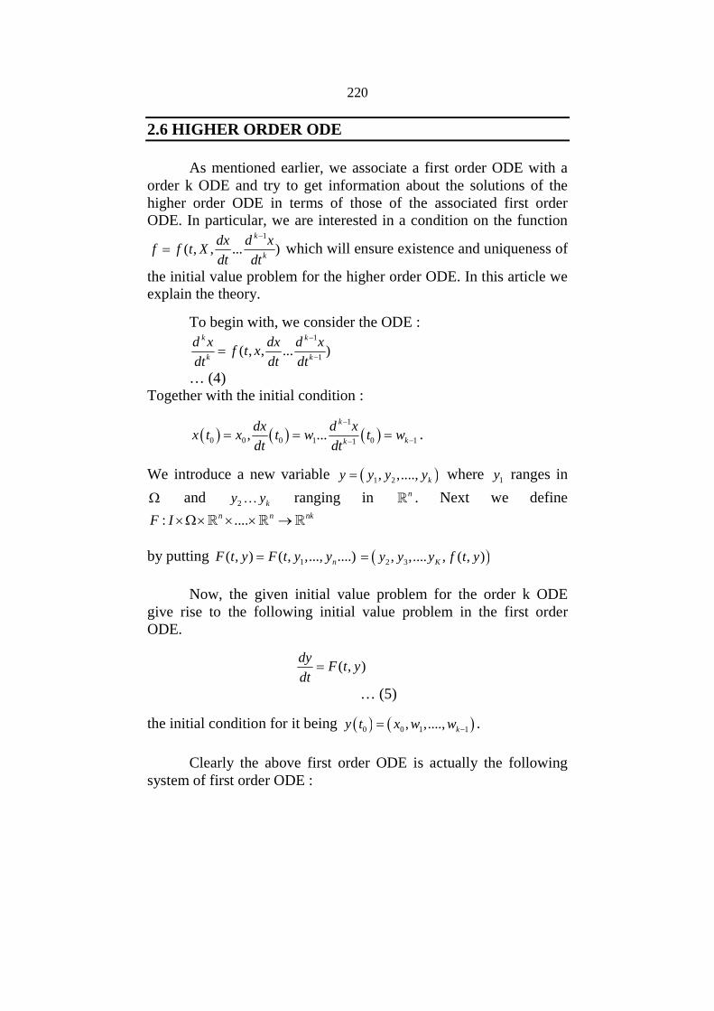
2.6 HIGHER ORDER ODE
As mentioned earlier, we associate a first order ODE with aorder k ODE and try to get information about the solutions of thehigher order ODE in terms of those of the associated first orderODE. In particular, we are interested in a condition on the function
1
( , , ... )k
k
dx d xf f t X
dt dt
which will ensure existence and uniqueness of
the initial value problem for the higher order ODE. In this article weexplain the theory.
To begin with, we consider the ODE :1
1( , , ... )
k k
k k
d x dx d xf t x
dt dt dt
… (4)Together with the initial condition :
1
0 0 0 1 0 11, ...
k
kk
dx d xx t x t w t w
dt dt
.
We introduce a new variable 1 2, ,...., ky y y y where 1y ranges in
and 2 ky y ranging in n . Next we define
: ....n n nkF I
by putting 1( , ) ( , ,..., ....)nF t y F t y y 2 3, ,.... , ( , )Ky y y f t y
Now, the given initial value problem for the order k ODEgive rise to the following initial value problem in the first orderODE.
( , )dy
F t ydt
… (5)
the initial condition for it being 0 0 1 1, ,...., ky t x w w .
Clearly the above first order ODE is actually the followingsystem of first order ODE :
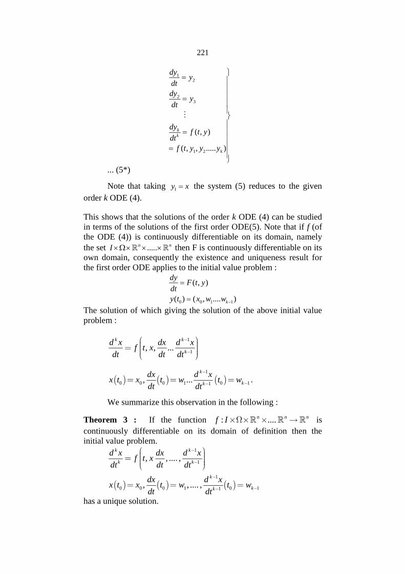
221
12
23
1 2
( , )
( , , ..... )
kk
k
dyy
dt
dyy
dt
dyf t y
dt
f t y y y
... (5*)
Note that taking 1y x the system (5) reduces to the given
order k ODE (4).
This shows that the solutions of the order k ODE (4) can be studiedin terms of the solutions of the first order ODE(5). Note that if f (ofthe ODE (4)) is continuously differentiable on its domain, namelythe set .....n nI then F is continuously differentiable on itsown domain, consequently the existence and uniqueness result forthe first order ODE applies to the initial value problem :
0 0 1 1
( , )
( ) ( , .... )k
dyF t y
dt
y t x w w
The solution of which giving the solution of the above initial valueproblem :
1
1, , ...
k k
k
d x dx d xf t x
dt dt dt
1
0 0 0 1 0 11, ...
k
kk
dx d xx t x t w t w
dt dt
.
We summarize this observation in the following :
Theorem 3 : If the function : ....n n nf I is
continuously differentiable on its domain of definition then theinitial value problem.
1
1
1
0 0 0 1 0 11
, , .... ,
, , .... ,
k k
k k
k
kk
d x dx d xf t x
dt dt dt
dx d xx t x t w t w
dt dt
has a unique solution.
222
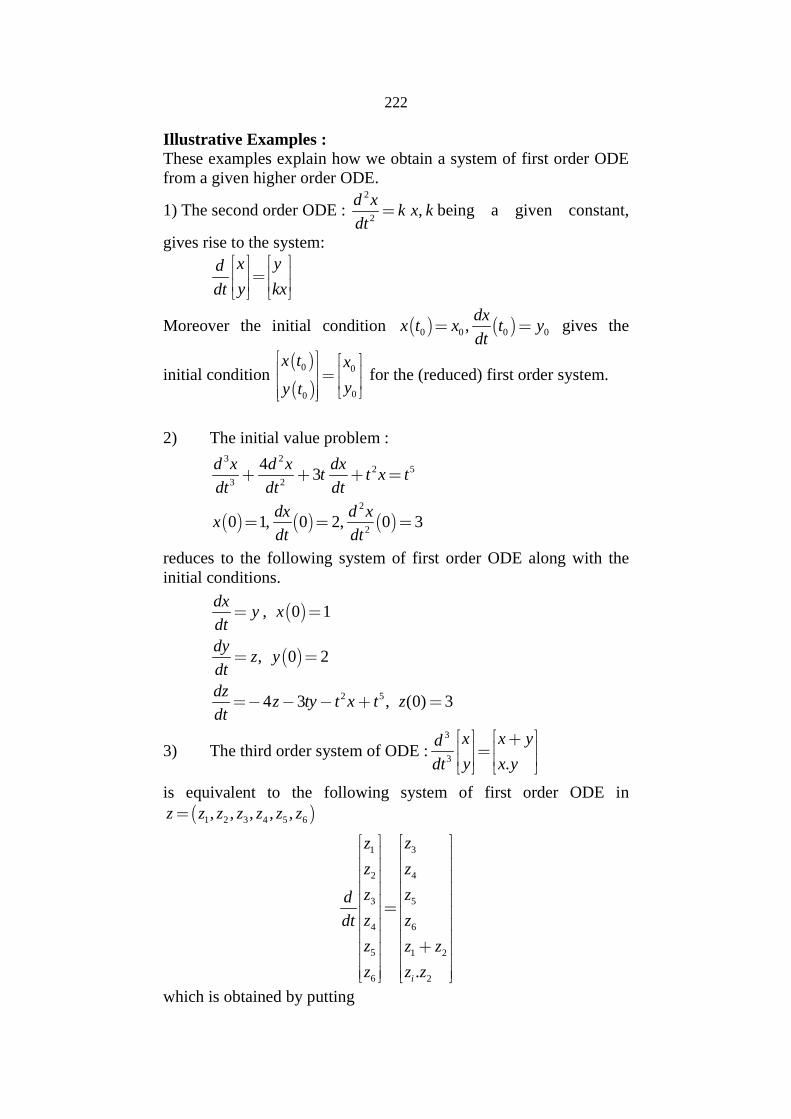
Illustrative Examples :These examples explain how we obtain a system of first order ODEfrom a given higher order ODE.
1) The second order ODE :2
2,
d xk x k
dt being a given constant,
gives rise to the system:
x yd
y kxdt
Moreover the initial condition 0 0 0 0,dx
x t x t ydt
gives the
initial condition
0 0
00
x t x
yy t
for the (reduced) first order system.
2) The initial value problem :
3 22 5
3 2
2
2
43
0 1, 0 2, 0 3
d x d x dxt t x t
dt dt dt
dx d xx
dt dt
reduces to the following system of first order ODE along with theinitial conditions.
2 5
, 0 1
, 0 2
4 3 , (0) 3
dxy x
dt
dyz y
dt
dzz ty t x t z
dt
3) The third order system of ODE :3
3 .
x x yd
y x ydt
is equivalent to the following system of first order ODE in
1 2 3 4 5 6, , , , ,z z z z z z z
31
2 4
3 5
4 6
5 1 2
6 2.i
zz
z z
z zd
z zdt
z z z
z z z
which is obtained by putting
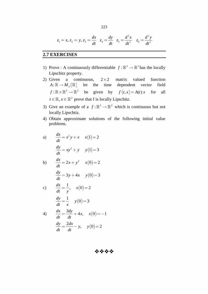
223
2 2
1 2 3 4 5 62 2, ,
dx dy d x d yz x z y z z z z
dt dt dt dt
2.7 EXERCISES
1) Prove : A continuously differentiable 2 2:f has the locally
Lipschitz property.
2) Given a continuous, 2 2 matrix valued function
2:A M let the time dependent vector field2 2:f be given by , ( )f t x A t x for all
2,t x prove that f is locally Lipschitz.
3) Give an example of a 2 2:f which is continuous but not
locally Lipschtiz.
4) Obtain approximate solutions of the following initial valueproblems.
a) 2 1 2dx
x y x xdt
2 1 3dy
xy y ydt
b) 22 0 2dx
x y xdt
3 4 0 3dy
y x ydt
c) 1
, 0 2dx
xdt y
1
0 3dy
ydt x
4) 3
4 , 0 1dx dy
x xdt dt
2
, 0 2dy dx
y ydt dt
224
3
LINEAR SYSTEMS OF ODE (I)
Unit Structure :
3.1 Introduction3.2 The Exponential of a Linear Endomorphism3.3 Properties of the Exponential3.4 Exercise
3.1 INTRODUCTION
We now consider following system of first order ordinarydifferential equations in the function
: ( )x t x t 1 2, ( ), ( ), ..., ( ) :nx t x t x t
111 1 12 2 1
221 1 22 2 2
1 1 2 2
....
....
....
n n
n n
nn n nn n
dxa x a x a x
dt
dxa x a x a x
dt
dxa x a x a x
dt
… (1)
where the coefficients ija appearing on the right hand sides of the
system (1) are all constant real numbers. (The case in which( ),ij ija a t t will be discussed in the next chapter). Writing X t
in the columnal form :
1
2
( )
( )
( )n
x t
x tX t
x t
and collecting the coefficients ija in a matrix A, that is
1 ,ijA a i j n , we rewrite the system (1) in the matrix form :
.dX
A Xdt
225
For a given vector nw with
1
2
n
w
ww
w
we form the initial
condition 0X w . Thus, we now have the initial value problem :
. , (0)dX
A X X wdt
… (2)
Later on, we will consider an arbitrary 0t and the initial value
problem :
0. , ( )dX
A X X t wdt
… ( 2 )
obtained by bringing 0t in place of t = 0. The solution of this more
general 2IVP is easily obtained from the solution of (2).
Therefore, we treat the particular case (2) in detail first.
Here we are taking .f X A X in our model differential
equation dX
f Xdt
(the first order, autonomous case) treating the
matrix ijA a as a linear transformation (= linear endomorphism)
of n , its action on a vector nx being given by
11 12 1 1
21 22 2 2
1 2
, , ....
, , .....
...................
, , ....
n
n
nn n nn
a a a x
a a a xA x
xa a a
11 1 12 2 1
21 1 22 2 2
1 1 2 2
....
....
.................................
....
n n
n n n
n n nn n
a x a x a x
a x a x a x
a x a x a x
.
where
1
2 n
n
x
xX
x
.
Thus in our treatment, the symbol A is made to play a double rule :(i) A as the n n matrix and (ii) A as a linear transformation (=
linear transformation) of n .
Note that when n = 1, the system (1) reduces to the single
differential equationdx
a xdt .
226
The solution of the initial value problem ,dx
a xdt
(0)X w w in this one-dimensional case (i.e. n = 1) is the
familiar function : ,tat we t . Recall :2 2 3 3
11! 2! 3!
ta ta t a t ae
The comparison between the on - dimensional initial valueproblem and its n-dimensional case suggests that we expect thesolution of the IVP(2) to be a curve of the form
: , ( ) . ...... (**)n tAX t X t e w where tAe is an n n
matrix which has the power series expansion :
2 2 3 3
........1! 2! 3!
tA t A t AI
suggested by (*) above. To carry forward the analogy, we call Ae ,
the exponential of A. We will define the new quantity Ae first.
(Replacing A by tA for t , will then yield tAe ). Once this is
accomplished, we will verify that the curve : ( ) tAX t X t e w is
indeed the solution of the initial value problem (2).
3.2 THE EXPONENTIAL OF A LINEAR ENDOMORPHISM
Let : n nA be a linear endomorphism having its matrix
ija
, we choose a finite constant C satisfying the inequality :
( )A x C x
for all nx (e.g. 3
2 max :1 ,ijC n a i j n will do the job).
Note that the above inequality implies :
k kA x C x and kk k kt A x t C x for every nx ,
every t and every k . In particular for the vector field
: n nf given by . , nf x A x x , we have :
( ) ( )f x f y A x A y
A x y
C x y
227
for any x, y, in n . In other words the vector field f(x)=Ax has theLipschitz property. Consequently the initial value problem (2) has aunique solution.
Next, we define a map : n nB as follows : Let nxbe arbitrary. Then we have :
2 3( ) ( )( ).......
1! 2! 3!
A x A xA xx
2
.......1! 2!
C
C x C xx
e x
This shows that the infinite sum :2 3( ) ( ) ( )
1! 2! 3!
A x A x A xx
converges absolutely. We put :
2( ) ( )( )
1! 2!
A x A xB x x
Thus the map B; expressed in terms of A, is given by2 3
1! 2! 3!
A A AB I
Note that each power kA is a linear transformation of n andthis implies the linearlity of B. in fact, for any a, b in , any x, y in
n , we have
2
2 2
( ) ( ) ( ) ( ) .....1! 2!
( ) ( ) ( ) ( ) ....1! 2! 2! 2!
A AB ax by ax by ax by ax by
a b a bax by A x A y A x A y
2 2( ) ( ) ( ) ( )........ ........
1! 2! 1! 2!
A x A x A y A ya x b y
( ) ( )a B x b B y
We adapt the notation Ae for B. occasionally we use the notation
exp(A) for Ae . Thus2( ) ( )
exp( ) ( ) ( ) .....1! 2!
A A x A xA x e x x
for every nx . Thus, each linear endomorphism A of n gives
228
rise to the linear endomorphism Ae . Moreover, if t is any realnumber then tA is also a linear endomorphism and it gives rise to the
exponential tAe given by :2 2 3 3
.....1! 2! 3!
tA tA t A t Ae I
it being a linear endomorphism of n where
2 2 3 3( ) ( ) ( )
.....1! 2! 3!
tA tA x t A x t A xe x x
for every nx .
Having defined the exponential Ae , we obtain the solution of theIVP(2) in terms of the exponentiation. Consider the map
: n nX
given by ( )tAx t e w2 2( ) ( )
....1! 2!
tA w t A ww t
Because the infinite series defining each X(t) convergesabsolutely we get that ( )t X t is differentiable and the derivative
( )dX
tdt
is obtained by termwise differentiation of the infinite series
defining X(t). Thus we have
2 2 3
2 2 3 3
( ) ( ) ( ) ( )0 .......
1! 1! 2!
( ) ( ) ( ).....
1! 2! 3!
( )
dX t A w tA w t A w
dt
tA w t A w t A wA w
A x t
Thus, we have : ( )
( )dX t
A x tdt
for every t . Moreover we
have : (0) 0 0 .....X w w .
This completes the proof that the map : nX given by
( )tax t e w is a solution of the IVP(2). We summarize this
observation in the following.
Theorem 1 : The map : nX given by ( )tax t e w is the
solution of the initial value problem . , (0)dX
A X X wdt
. The
proof of the following is self evident :
229
Corollary : The curve : nX given by 0 ( )t t A
x t e w
for all
t is the solution of the initial value problem :
0. , ( )dx
A X x t wdt .
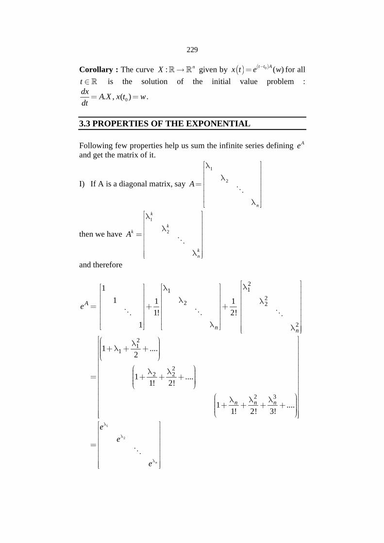
3.3 PROPERTIES OF THE EXPONENTIAL
Following few properties help us sum the infinite series defining Aeand get the matrix of it.
I) If A is a diagonal matrix, say
1
2
n
A
then we have
1
2
k
kk
kn
A
and therefore
211
22 2
2
1
1 1 1
1! 2!
1
A
nn
e
21
1
22 2
2 3
1 ....2
1 ....1! 2!
1 ....1! 2! 3!
n n n
1
2
n
e
e
e
230
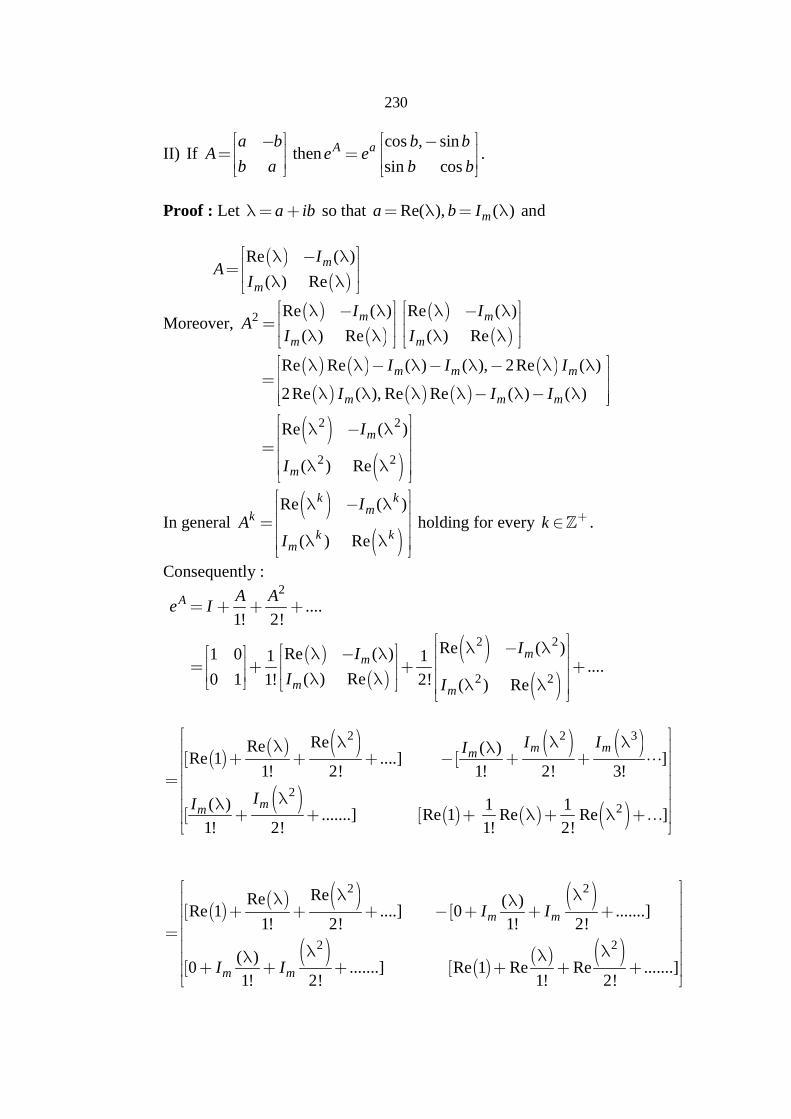
II) Ifa b
Ab a
thencos , sin
sin cosA a b b
e eb b
.
Proof : Let a ib so that Re( ), ( )ma b I and
Re ( )
( ) Rem
m
IA
I
Moreover,
2 Re ( ) Re ( )
( ) Re ( ) Rem m
m m
I IA
I I
2 2
2 2
Re Re ( ) ( ), 2Re ( )
2Re ( ), Re Re ( ) ( )
Re ( )
( ) Re
m m m
m m m
m
m
I I I
I I I
I
I
In general
Re ( )
( ) Re
k km
k
k km
IA
I
holding for every k .
Consequently :
2
2 2
2 2
....1! 2!
Re ( )Re ( )1 0 1 1....
( ) Re0 1 1! 2! ( ) Re
A
mm
m m
A Ae I
II
I I
2 2 3
2
2
ReRe ( )Re 1 ....] ]
1! 2! 1! 2! 3!
( ) 1 1.......] Re 1 Re Re ]
1! 2! 1! 2!
m mm
mm
I II
II
2 2
2 2
ReRe ( )Re 1 ....] 0 .......]
1! 2! 1! 2!
( )0 .......] Re 1 Re Re .......]
1! 2! 1! 2!
m m
m m
I I
I I
231
2 2
2 2
ReReRe 1 ....] 1 ...]
1 2! 1! 2!
( ) ( )(1) ...] Re 1 Re 1 Re 1 ...]
1! 2! 1! 2!
m m m
m m m
I I I
I I I
2 2
2 2
Re(1 ...) 1 ...)1! 2! 1! 2!
1 ...) Re 1 ...)1! 2! 1! 2!
m
m
I
I
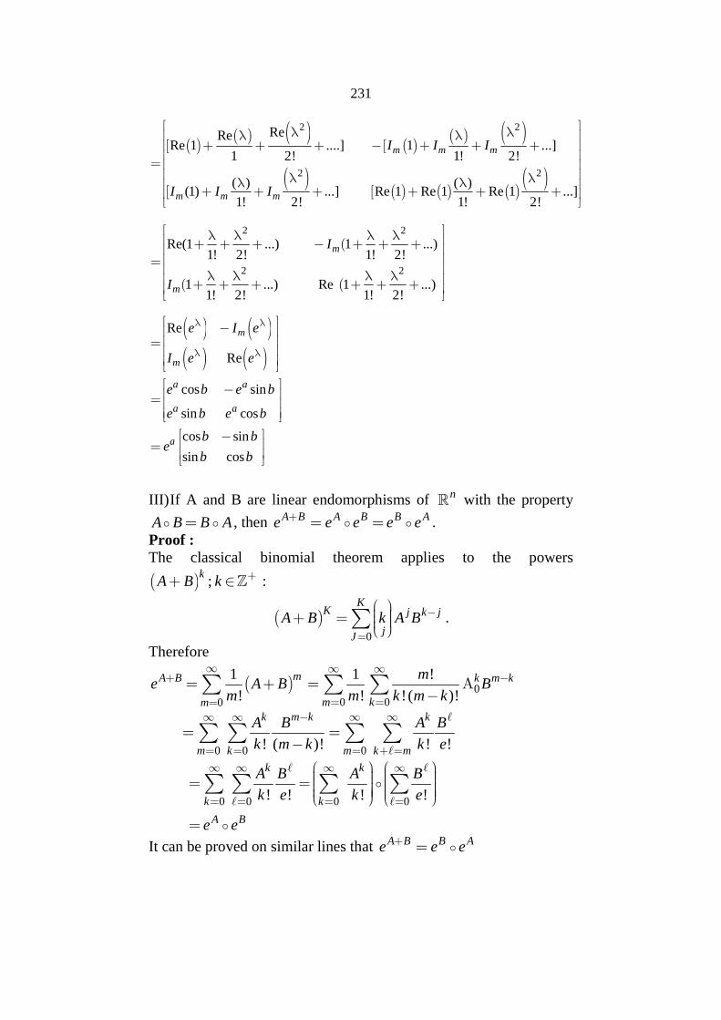
Re
Re
cos sin
sin cos
cos sin
sin cos
m
m
a a
a a
a
e I e
I e e
e b e b
e b e b
b be
b b
III)If A and B are linear endomorphisms of n with the property
A B B A , then A B A B B Ae e e e e .Proof :The classical binomial theorem applies to the powers
;k
A B k :
0
KK j k j
jJ
A B k A B
.
Therefore
0
1
!
mA B
m
e A Bm
00 0
1 !
! !( )!k m k
m k
mB
m k m k
0 0 ! ( )!
k m k
m k
A B
k m k
0 ! !
k
m k m
A B
k e
0 0 0 0! ! ! !
k k
k k
A B
A B A B
k e k e
e e
It can be proved on similar lines that A B B Ae e e
232
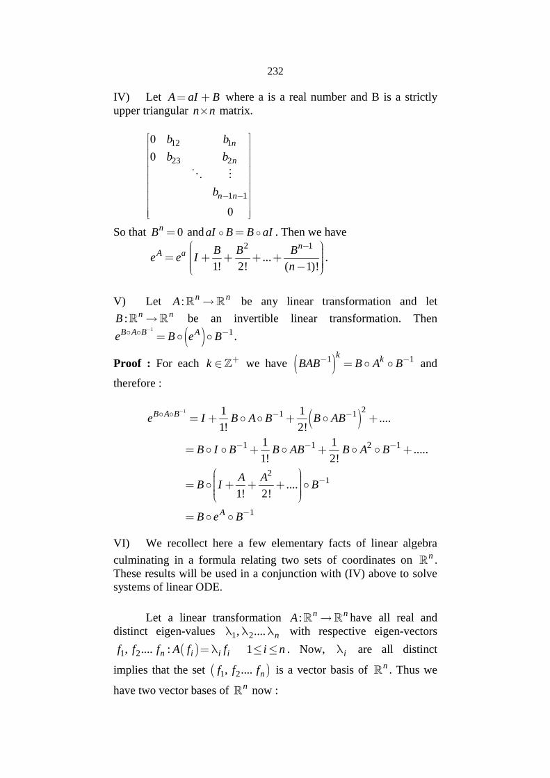
IV) Let A aI B where a is a real number and B is a strictlyupper triangular n n matrix.
12 1
23 2
1 1
0
0
0
n
n
n n
b b
b b
b
So that 0nB and aI B B aI . Then we have2 1
...1! 2! ( 1)!
A anB B B
e e In
.
V) Let : n nA be any linear transformation and let
: n nB be an invertible linear transformation. Then
1 1B A B Ae B e B
.
Proof : For each k we have 1 1k kBAB B A B and
therefore :
1 21 1
1 1 2 1
21
1
1 1....
1! 2!
1 1.....
1! 2!
....1! 2!
B A B
A
e I B A B B AB
B I B B AB B A B
A AB I B
B e B
VI) We recollect here a few elementary facts of linear algebra
culminating in a formula relating two sets of coordinates on n .These results will be used in a conjunction with (IV) above to solvesystems of linear ODE.
Let a linear transformation : n nA have all real anddistinct eigen-values 1 2, .... n with respective eigen-vectors
1 2, .... : 1n i i if f f A f f i n . Now, i are all distinct
implies that the set 1 2, .... nf f f is a vector basis of n . Thus we
have two vector bases of n now :
233
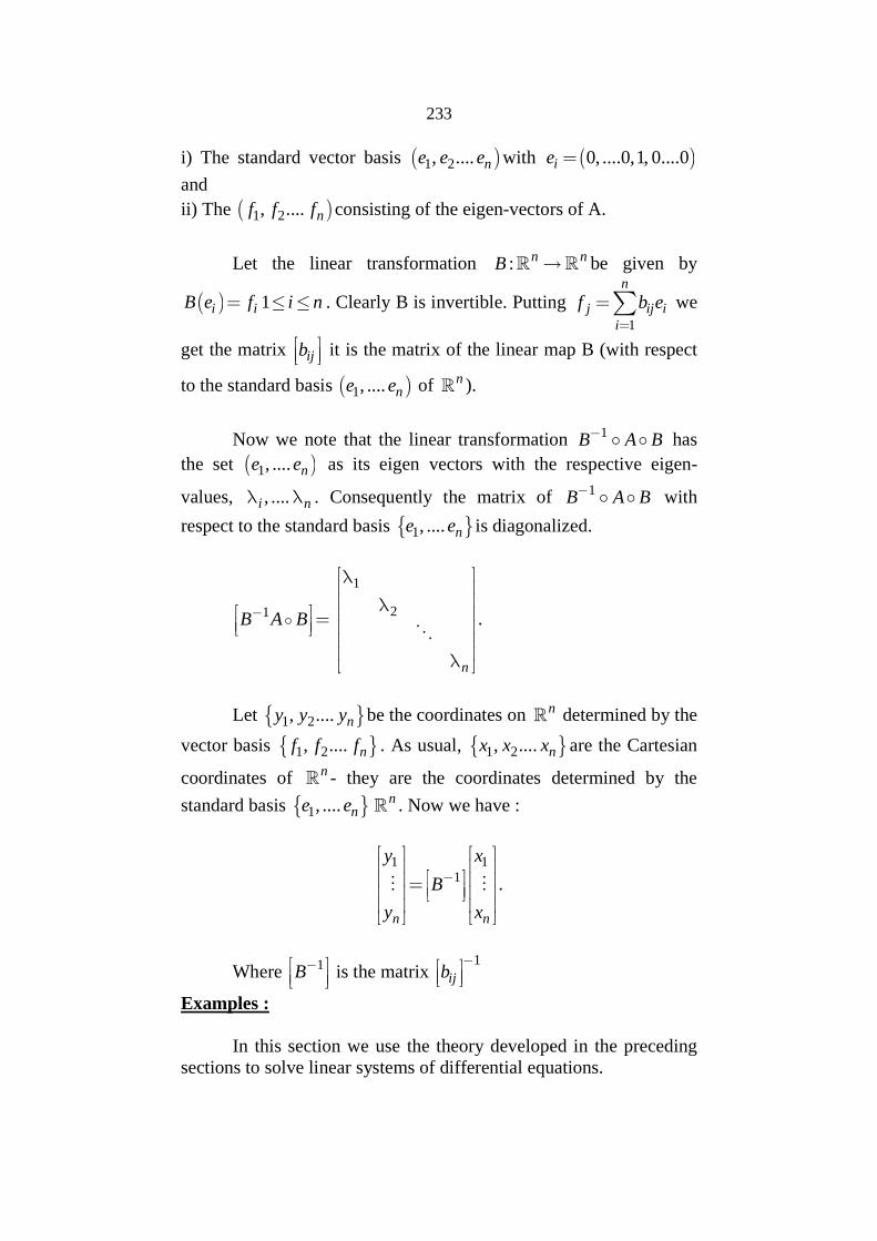
i) The standard vector basis 1 2, .... ne e e with 0, ....0,1, 0....0ie
and
ii) The 1 2, .... nf f f consisting of the eigen-vectors of A.
Let the linear transformation : n nB be given by
1i iB e f i n . Clearly B is invertible. Putting1
n
j ij ii
f b e
we
get the matrix ijb
it is the matrix of the linear map B (with respect
to the standard basis 1, .... ne e of n ).
Now we note that the linear transformation 1B A B has
the set 1, .... ne e as its eigen vectors with the respective eigen-
values, , ....i n . Consequently the matrix of 1B A B with
respect to the standard basis 1, .... ne e is diagonalized.
1
21
n
B A B
.
Let 1 2, .... ny y y be the coordinates on n determined by the
vector basis 1 2, .... nf f f . As usual, 1 2, .... nx x x are the Cartesian
coordinates of n - they are the coordinates determined by the
standard basis 1, .... ne e n . Now we have :
1 11
n n
y x
B
y x
.
Where 1B
is the matrix1
ijb
Examples :
In this section we use the theory developed in the precedingsections to solve linear systems of differential equations.
234
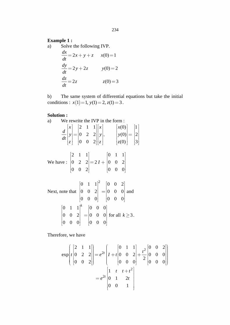
Example 1 :a) Solve the following IVP.
2 (0) 1
2 2 (0) 2
2 (0) 3
dxx y z x
dt
dyy z y
dt
dzz z
dt
b) The same system of differential equations but take the initialconditions : 1 1, (1) 2, (1) 3x y z .
Solution :a) We rewrite the IVP in the form :
2 1 1 (0) 1
0 2 2 (0) 2
0 0 2 (0) 3
x x xd
y y ydt
z z z
We have :
2 1 1 0 1 1
0 2 2 2 0 0 2
0 0 2 0 0 0
I
Next, note that
20 1 1 0 0 2
0 0 2 0 0 0
0 0 0 0 0 0
and
0 1 1 0 0 0
0 0 2 0 0 0
0 0 0 0 0 0
k
for all 3k .
Therefore, we have
22
2 1 1 0 1 1 0 0 2
exp 0 2 2 0 0 2 0 0 02
0 0 2 0 0 0 0 0 0
t tt e I t
2
2
1
0 1 2
0 0 1
t
t t t
e t
235
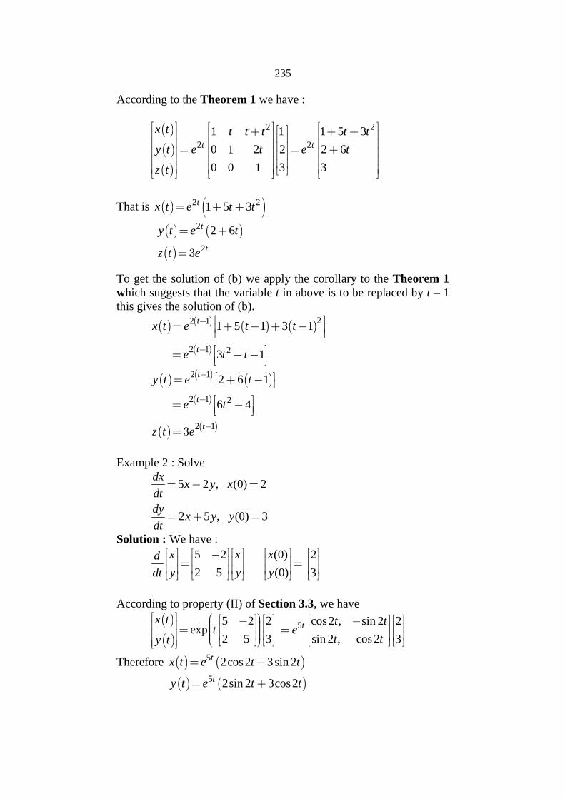
According to the Theorem 1 we have :
22
2 2
1 1 5 31
0 1 2 2 2 6
0 0 1 3 3
t t
x t t tt t t
y t e t e t
z t
That is 2 21 5 3tx t e t t
2
2
2 6t
t
y t e t
z t e
To get the solution of (b) we apply the corollary to the Theorem 1which suggests that the variable t in above is to be replaced by t – 1this gives the solution of (b).
22 1
2 1 2
1 5 1 3 1
3 1
t
t
x t e t t
e t t
2 1
2 1 2
2 1
2 6 1
6 4
t
t
t
y t e t
e t
z t e
Example 2 : Solve
5 2 , (0) 2
2 5 , (0) 3
dxx y x
dt
dyx y y
dt
Solution : We have :
5 2 (0) 2
2 5 (0) 3
x x xd
y y ydt
According to property (II) of Section 3.3, we have
5 2 2exp
2 5 3
x tt
y t
5 cos 2 , sin 2 2
sin 2 , cos 2 3t t t
et t
Therefore 5 2cos 2 3sin 2tx t e t t
5 2sin 2 3cos2ty t e t t
236
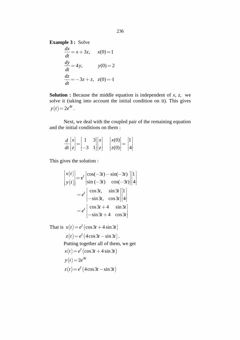
Example 3 : Solve
3 , (0) 1
4 , (0) 2
3 , (0)
dxx z x
dt
dyy y
dt
dzz z z
dt
Solution : Because the middle equation is independent of x, z, wesolve it (taking into account the initial condition on it). This gives
42 ty t e .
Next, we deal with the coupled pair of the remaining equationand the initial conditions on them :
1 3 (0) 1
3 1 (0) 4
x x xd
z z zdt
This gives the solution :
cos( 3 ) sin( 3 ) 1e
sin ( 3 ) cos( 3 ) 4t
x t t t
t ty t
cos3 , sin 3 1
sin 3 , cos3 4
cos3 4 sin 3
sin 3 4 cos3
t
t
t te
t t
t te
t t
That is cos3 4 sin 3tx t e t t
4cos3 sin3tz t e t t .
Putting together all of them, we get
cos3 4 sin 3tx t e t t
4ty t e
4cos3 sin3tz t e t t
237
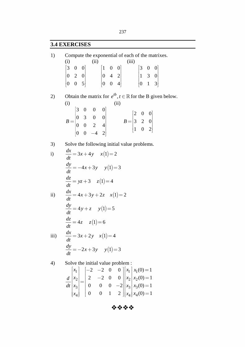
3.4 EXERCISES
1) Compute the exponential of each of the matrixes.(i) (ii) (iii)
3 0 0
0 2 0
0 0 5
1 0 0
0 4 2
0 0 4
3 0 0
1 3 0
0 1 3
2) Obtain the matrix for ,tbe t for the B given below.
(i) (ii)
3 0 0 0
0 3 0 0
0 0 2 4
0 0 4 2
B
2 0 0
3 2 0
1 0 2
B
3) Solve the following initial value problems.
i) 3 4 1 2dx
x y xdt
4 3 1 3dy
x y ydt
3 1 4dz
yz zdt
ii) 4 3 2 1 2dx
x y z xdt
4 1 5dy
y z ydt
4 1 6dz
z zdt
iii) 3 2 1 4dx
x y xdt
2 3 1 3dy
x y ydt
4) Solve the initial value problem :
1 1 1
2 2 2
33 3
44 4
(0) 12 2 0 0
(0) 12 2 0 0
(0) 10 0 0 2
(0) 10 0 1 2
x x x
x x xd
xx xdt
xx x
238
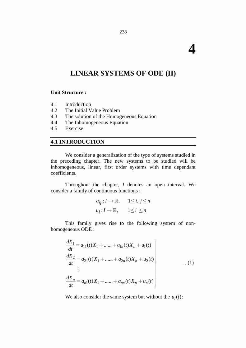
4
LINEAR SYSTEMS OF ODE (II)
Unit Structure :
4.1 Introduction4.2 The Initial Value Problem4.3 The solution of the Homogeneous Equation4.4 The Inhomogeneous Equation4.5 Exercise
4.1 INTRODUCTION
We consider a generalization of the type of systems studied inthe preceding chapter. The new systems to be studied will beinhomogeneous, linear, first order systems with time dependantcoefficients.
Throughout the chapter, I denotes an open interval. Weconsider a family of continuous functions :
: , 1 ,
: , 1
a I i j nij
u I i ni
This family gives rise to the following system of non-homogeneous ODE :
111 1 1 1
221 1 2 2
1 1
( ) ...... ( ) ( )
( ) ...... ( ) ( )
( ) ...... ( ) ( )
n n
n n
nn nn n n
dXa t X a t X u t
dt
dXa t X a t X u t
dt
dXa t X a t X u t
dt
… (1)
We also consider the same system but without the ( ) :iu t
239
111 1 1
221 1 2
1 1
( ) ...... ( )
( ) ...... ( )
( ) ...... ( )
n n
n n
nn nn n
dXa t X a t X
dt
dXa t X a t X
dt
dXa t X a t X
dt
…(2)
We call (2) the homogeneous part of the system (1).
Our method of obtaining solutions of (1) consists of obtaining(i) a particular solution of the inhomogeneous system (1), then (ii)obtain the space of all solutions of the homogeneous system (2) andthen combine (i) and (ii) to get all the solutions of the system (1).
We use the following abridged notations to which theoperations of linear algebra will be applicable.
For each , ( )t I A t is the n n matrix ( ) , ( )ija t u t denotes
the column
1( )
( )n
u t
u t
and as usual ( )X t is the column
1( )
( )n
x t
x t
.
In terms of these notations the systems (1) and (2) take thefollowing compact forms :
( ) ( )dx
A t X u tdt … (1)
( )dx
A t Xdt , the homogenous part of the above … (2)
4.2 THE INITIAL VALUE PROBLEM
Given 0 0, nt I x , we consider the IVP :
0 0( ) ( ) ... ( )dx
A t X u t X t xdt … (3)
Note that the vector field : n nf I given by
( , ) ( ) ( )f t x A t x y t is locally Lipschitz :
240
Justification : Let 0 0, nt I x be arbitrary. Choose 0 such
that 0 0,t t I . Now the map : nA I being
continuous on its domain I, is bounded one the compact interval
0 0,t t t and for any x, y in 0 ,B x we get.
, ( , ) ( ) ( ) ( ) ( )
( ) ( )
f t x f t y A t x u t A t y u t
A t x y
and therefore
, ,
( ) .
f t x f t y A t x y
A t x y
K x y
For all 0 0,t t t and for all x, y in 0 ,B x .
Therefore, the basic existence and uniqueness results areapplicable. The IVP (3) has a unique solution defined on the largestopen sub-interval , of I. We prove that , = I.
Proposition 1 :The solution of the IVP (3) is defined on the whole of I.
Proof :
(Sketchy, by contradiction method). Assume thecontradictory : , C I
, say, right hand end point of I, so that
0 ,t I .
Now, being the solution of the IVP (3) the curve
: , nX satisfies the integral equation :
0 0
0( ) ( ) ( ) ( )
t t
t t
X t x A s X s ds u s ds
Using continuity of the maps : , : nnA I M u I we
get a finite constant M such that ( ) , ( )A s M u s M for all
0 ,s t and therefore, we have :
0 0
0( ) ( ) ( )
t t
t t
X t x A s X s ds u s ds
241
0
0 ( )
t
t
x M X s ds M .
By Gronwall’s lemma, we get :
0( ) Mx t x M e for all 0 ,t t . Thus, the set
0( ) : ,X t t t is a bounded subset of n and therefore, the limit
lim ( )t
X t
exists. We call it ny .
Having arrived at the point y in n , we consider the initialvalue problem :
( ) ( )dx
A t X u t X ydt .
Let : , 0nX be a solution of this IVP.
Clearly the two solutions :
: , , : ,n nX X agree on the overlap
and therefore, they patch up to give a solution : : , nX
which contradicts the assumed maximality of the interval , .
Therefore, we must have : right hand end point of I. Similar
reasoning leades us to left hand end point of I and therefore
,I .
Thus, every solution of (2) whatever be the initial condition isdefined on the whole of .
4.3 THE SOLUTION OF THE HOMOGENEOUSEQUATION
We consider the set of all the solutions of the homogeneousequation (2). Let the set be denoted by V.
Proposition 2 : The set V has the structure of a n dimensional vectorspace.Proof : Let a, b in , X, Y, in V be arbitrary. We prove thataX bY also is in V :
242
( )
d dX dYaX bY a b
dt dt dt
a A t X b A t Y
( )A t aX bY because ( )A t is linear.
Thus, ( )d
aX bY A t aX bYdt i.e. aX bY V .
This shows that V is a real vector space. Actually V is
isomorphic with n , the brief explanation of which is as follows.
Choose 0t I arbitrarily and hold it fix. For each nx we
consider the unique solution of the initial value problem :
0( ) , ( )dx
A t X X t xdt .
We denote the unique solution of it by xX where we have
attached the suffix x to the solution xX to indicate the dependence
of the solution on the initial condition.
Now, we have an association rule xx X associating the
unique xX X with each nx . In other words, we have the map :
;nxV x X … (4)
(Which associates each nx , the element xX of V). It is easy to
show that this map is an isomorphism. First the linearity of the map :
Let a, b in , x, y in n be arbitrary. We consider the two curves :
: nx yaX bX I and : n
ax byX I .
It is clear that both are solutions of the IVP with the sameinitial condition ax + by and therefore by the uniqueness of thesolution, we get the desired equality.
Clearly 0xX implies 0x . The implies that the linear
map (4) is injective. Finally, let X be any element of V. Let
0 0X t x . Then0xX X showing that the map (4) is a surjective
map.
243
We have explained now that the map (3) is linear, it isinjective and surjective as well. Therefore (4) is a linear
isomorphism between V and n , i.e. V is indeed n-dimensional realvector space.
We consider a vector basis 1 2 ..... nX X X of the solution
space V. We call it a fundamental system of solutions of thehomogeneous ODE (2). Clearly for each t I , the vectors
1 2( ), ( ), ...., ( ),nX t X t X t are linearly independent vectors of n .
Putting them along the columns of a n n maxtrix, we denote theresulting n n matrix by ( )W t thus :
1 2( ) ( ) ( ) ( )nW t X t X t X t
or if the vector ( )jX t
has the coordinates : 1 2( ) ( ), ( ),......, ( )j j j njX t x t x t x t then
( ) ( ) ;1 ,ijW t x t i j n .
We call the resulting map : nW I M a fundamental
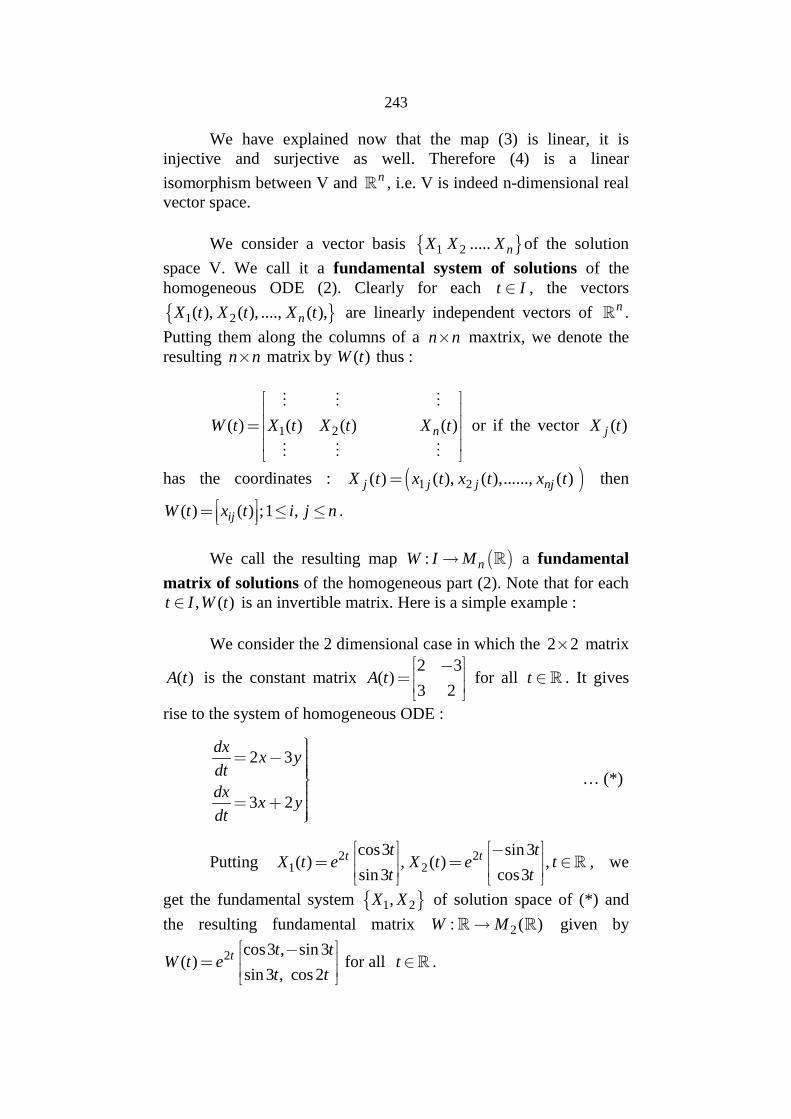
matrix of solutions of the homogeneous part (2). Note that for each, ( )t I W t is an invertible matrix. Here is a simple example :
We consider the 2 dimensional case in which the 2 2 matrix
( )A t is the constant matrix2 3
( )3 2
A t
for all t . It gives
rise to the system of homogeneous ODE :
2 3
3 2
dxx y
dt
dxx y
dt
… (*)
Putting 2 21 2
cos3 sin 3( ) , ( ) ,
sin 3 cos3t tt t
X t e X t e tt t
, we
get the fundamental system 1 2,X X of solution space of (*) and
the resulting fundamental matrix 2: ( )W M given by
2 cos3 , sin 3( )
sin 3 , cos 2t t t
W t et t
for all t .
244
4.4 THE INHOMOGENEOUS EQUATION
We now consider the inhomogeneous ODE (1) and itssolution space. To begin with, we have the following result relatingthe solutions of the two equations (1) and (2).
Proposition 3 : Let : nY I be a solution of the inhomogeneoussystem (1).
a) If : nX I is a solution of the homogeneous system (2) thenX Y is a solution of the inhomogeneous system (2).
b) Then the solution of the (inhomogeneous) initial value problem :
0 0( ) ( ), ( )dx
A t X u t X t xdt
is given by
0
1( ) ( ) ( ) ( ) ( )
t
t
X t Y t W t W s u s ds for all t I .
The proof of the theorem is a straight forward application ofthe fundamental theorem of integral calculus (applied to integrationof vector valued functions).
Proof :(a) We have 0
10 0 0 ( )
t
t
X t Y t W t W s u s ds
0
0 0
0
0 since * 0
t
t
x W t ds
x
(b) First note that
1 2
1 2
( ) ( ) ( )
( )( ) ( )
n
n
d dW t X t X t X t
dt dt
dX tdX t dX t
dt dt dt
245
1 2
1 2
( ) ( ) ( ) ( ) ( ) ( )
( ) ( ) ( ) ( )
( ) ( )
n
n
A t X t A t X t A t X t
A t X t X t X t
A t W t
Now, we have :
1
0
( ) ( ) ( ) ( ) ( )
t
t
d dX t Y t W t W s u s ds
dt dt
1 1
0 0
( ) ( ) ( ) ( ) ( ) ( ) ( )
t t
t t
d d dY t W t W s u s ds W t W s u s
dt dt dt
1 1
1
0
( ) ( ) ( ) ( ). ( ) ( ) ( ) ( ) ( )
( ) ( ) ( ) ( ) ( ) ( )
t
t
t
A t Y t A t W t W s u s ds W t W t u t
A t Y t W t W s u s ds u t
( ) ( ) ( ).A t x t u t
Thus( )
( ) ( ) ( )d X t
a t x t u tdt
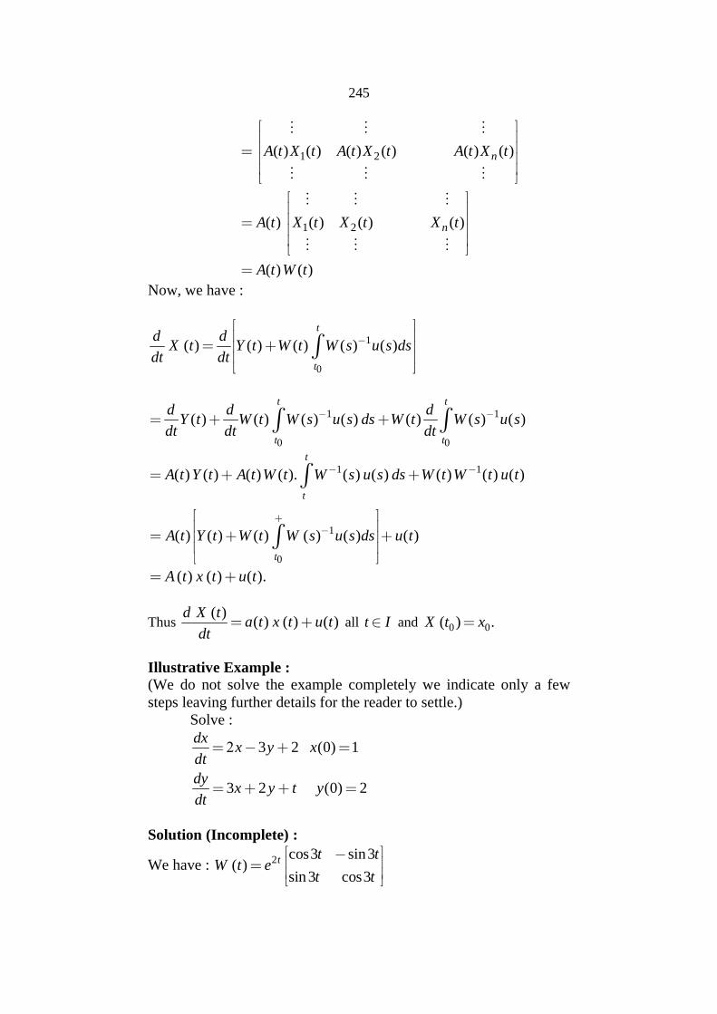
all t I and 0 0( ) .X t x
Illustrative Example :(We do not solve the example completely we indicate only a fewsteps leaving further details for the reader to settle.)
Solve :
3 2 (0) 1
3 2 (0) 2
dxx y x
dt
dyx y t y
dt
Solution (Incomplete) :
We have : 2 cos3 sin3( )
sin 3 cos3t t t
W t et t
246
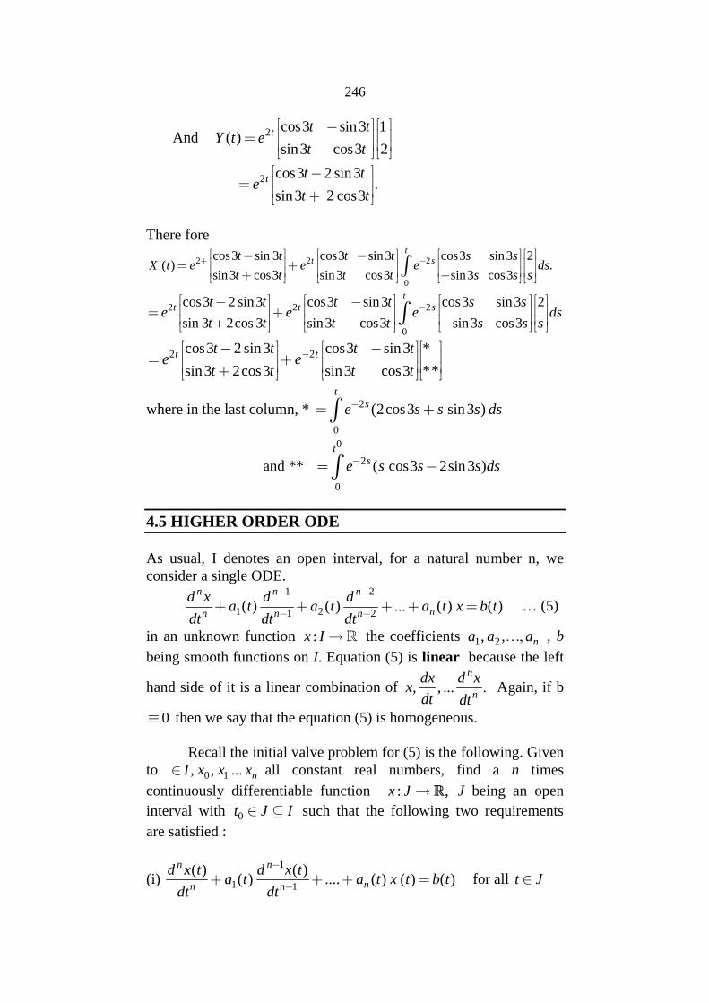
And 2 cos3 sin3 1( )
sin3 cos3 2t t t
Y t et t
2 cos3 2 sin3.
sin3 2 cos3t t t
et t
There fore
2 2 2
0
cos3 sin 3 cos3 sin 3 cos3 sin 3 2( ) .
sin 3 cos3 sin3 cos3 sin3 cos3
tt st t t t s s
X t e e e dst t t t s s s
2 2 2
0
cos3 2 sin3 cos3 sin3 cos3 sin3 2
sin 3 2cos 3 sin3 cos3 sin3 cos3
tt t st t t t s s
e e e dst t t t s s s
2 2cos3 2 sin3 cos3 sin3 *
sin3 2cos3 sin3 cos3 **tt t t t t
e et t t t
where in the last column, * 2
0
(2cos3 sin3 )
tse s s s ds
and **
0
2
0
( cos3 2sin 3 )
tse s s s ds
4.5 HIGHER ORDER ODE
As usual, I denotes an open interval, for a natural number n, weconsider a single ODE.
1 2
1 21 2( ) ( ) ... ( ) ( )
n n n
nn n n
d x d da t a t a t x b t
dt dt dt
… (5)
in an unknown function :x I the coefficients 1 2, , na a a , b
being smooth functions on I. Equation (5) is linear because the left
hand side of it is a linear combination of , , ... .n
n
dx d xx
dt dt Again, if b
0 then we say that the equation (5) is homogeneous.
Recall the initial valve problem for (5) is the following. Givento 0 1, , ... nI x x x all constant real numbers, find a n times
continuously differentiable function : ,x J J being an open
interval with 0t J I such that the following two requirements
are satisfied :
(i)1
1 1
( ) ( )( ) .... ( ) ( ) ( )
n n
nn n
d x t d x ta t a t x t b t
dt dt
for all t J
247
and (ii) 01
0 1 1.10 0
( )( ) , ( ) ...
n
nn
d x tdxx t x t x x
dt dt
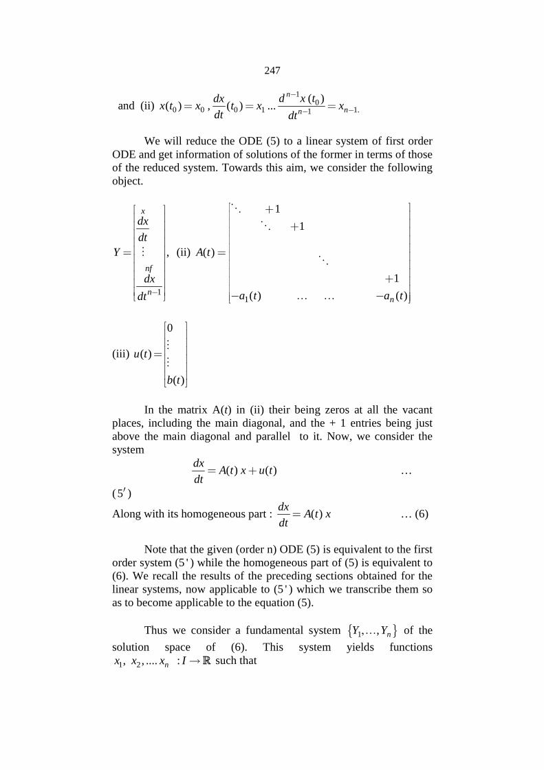
We will reduce the ODE (5) to a linear system of first orderODE and get information of solutions of the former in terms of thoseof the reduced system. Towards this aim, we consider the followingobject.
1
,
x
nf
n
dx
dt
Y
dx
dt
(ii)
1
1
1
( )
1
( ) ( )n
A t
a at t
(iii)
0
( )
( )
u t
b t
In the matrix A(t) in (ii) their being zeros at all the vacantplaces, including the main diagonal, and the + 1 entries being justabove the main diagonal and parallel to it. Now, we consider thesystem
( ) ( )dx
A t x u tdt
…
(5 )
Along with its homogeneous part : ( )dx
A t xdt
… (6)
Note that the given (order n) ODE (5) is equivalent to the firstorder system (5 ' ) while the homogeneous part of (5) is equivalent to(6). We recall the results of the preceding sections obtained for thelinear systems, now applicable to (5 ' ) which we transcribe them soas to become applicable to the equation (5).
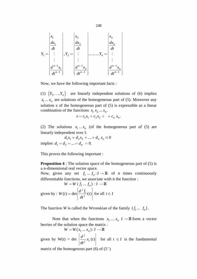
Thus we consider a fundamental system 1 , nY Y of the
solution space of (6). This system yields functions
1 2, , .... :nx x x I such that
248
1 2
1 2
1 2
1 1 11 2
1 1 1
, ... ... ...
n
n
n
n n nn
n n n
xx x
dxdx dx
dt dt dt
Y Y Y
d x d x d x
dt dt dt
Now, we have the following important facts :
(1) 1 , nY Y are linearly independent solutions of (6) implies
1 ... nx x are solutions of the homogeneous part of (5). Moreover any
solution x of the homogeneous part of (5) is expressible as a linearcombination of the functions 1 2 ... .nx x x
1 1 2 2 .n nx c x c x c x
(2) The solutions 1 ... nx x (of the homogeneous part of (5) are
linearly independent over I.
1 1 2 2 ... 0n nd x d x d x
implies 1 2 ... 0.nd d d
This proves the following important :
Proposition 4 : The solution space of the homogeneous part of (5) isa n-dimensional real vector space.Now, given any set 1 ... :nf f I of n times continuously
differentiable functions, we associate with it the function :
1 ... ) :nW W f f I
given by : ( ) det ( )j
jid f
W t tdt
for all t I
The function W is called the Wronskian of the family 1{ ... }.nf f
Note that when the functions 1 .... nx x I form a vector
berries of the solution space the matrix :
1( ... ) :nW W x x I
given by W(t) = det ( )j
ij
dx t
dt
for all t I is the fundamental
matrix of the homogenous part (6) of (5 ' )
249
4.6 A SOLUTION OF THE NON-HOMOGENEOUSEQUATION
Suppose, a fundamental system 1{ ...... }nx x of solutions of
the homogeneous equation (6) is found. We discuss a method –attributed to Lagrange-which yields a solution of the non-homogeneous ODE (5).
Recall, W(t) stands for the fundamental matrix with its (ij)th entry
( )j
ij
dx t
dt .
For each i, 1 i n , we consider the n n matrix denoted by Wj(t)obtained from W(t) by replacing its jth column by the column
( )
0
0
tb
We adopt the notations : D(t) for det(W(t)) and Di(t) for det(W i (t)).
Now, to obtain the desired solution we consider a function:x I which is in the form
1 1 2 2( ) ( ) ( ) ( ) ( ) . ( ) ( )n nx t v t x t v t x t t v t x t =1
( ) ( )n
jj jv t x t
,
where : (1 )jv I j n are unknown functions which are
required to satisfy a number of identities.
These identities will determine the functions jv which in turn
specify the x which will be the desired solution. Now differentiatingx(t). We get
1 1
jj j
n nj
j j
dx dvdxv x
dt dt dt
The first requirement on the jv is :
1
0j
jn
j
dvx
dt
… (i)
So that we are left with
1
nj
ji
dxdxv
dt dt
… (*)
250
Now differentiating (*) above, we get2
21 1
2
2
jn n
jj
jj
j
d x dv dxd xv
dt dtdt dt
The second requirement on the jv is
1
0j
nj
j
dv dx
dt dt
… (ii)
Leaving us with2
12
2
2
n
jj
jd xd xv
dt dt
…
(**)
Continuing this procedure we get analogous identities, therequirement on jv at the last stage being :
1
11
.nn
j
nj
jdv d xb
dt dt
Thus, we have the following two strings of identities :
1
1
1
1
( )
n
j jj
nj
jj
nn njx
jn nj
nnj
n
j
j
x v x
dxdxv
dt dt
I
d xdv
dt dt
dv d x
dt dt
1
1
1
0( )
( )
nj
jj
nj j
j
nnj j
nj
dvx
dt
dv dx
dt dt II
dv d xb t
dt dt
Multiplying the equations in (I) by an, an – 1,…., 1a , 1 and adding we
get1
1 11( ) ( ) ( ) ( )
n n
nn n n
d x d xa t a t x a t b t
dt dt
thus showing that the function x(t) is a solution of theinhomogeneous equation.On the other hand, using the simultaneous equations in (ii), we get :
( )
( )
j jdv D t
dt D t
251
and therefore
0
( )( )
( )
tj
j
t
D sv t ds j n
D s
This leads us to the desired solution
1
( ) ( ) ( ) .n
j jj
x t v t x t t I
4.5 EXERCISES
(1) Prove that each solution of the inhomogeneous equation (5) isdefined on I.(2) Prove : If a solution :x I of the homogeneous equation (6)vanishes at same t0 I , then x
(3) Solve : 5 3 (0) 1dx
x xdt
3 2 (0) 2dy
x y t ydt
(4) Solve : 3 4 (0) 1dx
x y t xdt
3 4 (0) 1dy
x y ydt
(5) Same D. E as above but x(1) = 1 , y(1) = 1.
252
5METHOD OF POWER SERIES
Unit Structure :
5.1 Introduction.
5.2 Power Series. (A Quick Review).
5.3 Method Of Power Series.
5.4 Illustrative Examples.
5.5 Legendre Equation, Legendre Polynomials.
5.6 Frobaneous Method.
5.7 Bessel Functions
5.8 Exercises.
5.1 INTRODUCTION
In this chapter, we study a type of second order ODE (scalarcase) which gives solutions in the form of absolutely convergentpower series. These ODE contain in their form, functions (e.g. thecoefficient functions) which are analytic in sense that they admitabsolutely convergent power series expansions. Naturally themethod of solving such DE makes use of techniques and propertiesof absolutely convergent power series. Therefore we call this methodthe method of power series.
The reader will realize that this method applies not only tosecond order linear ODE, it actually is applicable to a wider class ofODE of any order.
Recall, at the elementary level we could solve simple DE interms of elementary function such as the polynomials, the logarithmfunction, the exponential functions, the trigonometric functions andso on. But soon we find that things start going the opposite way :Differential equations generate new functions as their solutions.Such functions are called special functions. Most of these functionsare in the form of power series and as such are obtained by the
253
methods of power series. There is a more powerful method which iscalled Frobaneous method. We discuss briefly this method also.Using this method we introduce two special functions : (i) theLegendre polynomials and (ii) the Bessel functions. We derive someof their properties.
We begin our treatment of special functions by recalling basicfacts of power series.
5.2 POWER SERIES (A QUICK REVIEW)
A power series is an infinite sum of the type:
a0 + a1(t – t0) + a2(t – t0)2 + ….. …..+ ak(t – t0)
k + ……….
= ……………….. (1)
where a0, a1, a2, ………., ak, ……… are real constants. It isabsolutely convergent if there exists a r > 0 such that
The lub of all r > 0 satisfying the above inequality is theradius of convergence of the power series (1), we denote it by R. If(1) is absolutely convergent with R as its radius of convergence, itfollows that for each t (t0 – R, t0 + R) the infinite sum
converges, giving rise the function :
f :(t0 – R, t0 + R) —ℝ……………….. (2)
where
0
k
k
k Z
f t a t t
for each t (t0 – R, t0 + R).
The function (2) is the sum function of the (absolutelyconvergent) power series (1). It is a basic result that the sum function(2) is infinitely differentiable on its domain and the kth derivative
254
(kℤ+) is obtained by differentiating the infinite series termwise. Inparticular we have :
Consequently the power series (1) becomes
f(t) = ………. (3)
An important implication of (3) is the following result :
If the functions
f :(t0 – R, t0 + R) —ℝ
g :(t0 – R, t0 + R) —ℝ
admit the power series expansions :
then we have the following basic fact :
f(t) g(t)
if and only if ak = bk for all k ℤ+ that is, if and only if
=
holds for all k ℤ+
We make use of this basic result in what is to follow in thischapter.
5.3 METHOD OF POWER SERIES.
We consider a second order ODE of the type :
………. (4)
where the coefficient functions P(t) and Q(t) admit absolutelyconvergent power series expansions on an interval (-R, R) :
255
Recall, according to the theory of linear second orderhomogeneous ODE discussed in Unit4, the solution space of theODE (4) is a two dimensional vector space.
Now, because the functions P(t), Q(t) admit absolutelyconvergent power series expansions - we call such functionsanalytic - we expect a solution of (4) also to be analytic :
nnx t c t ……………………………………………… (6)
We prove below the following two results :a) Indeed, a solution t ı— x (t) of (4) has a power seriesexpansion (6) and obtain the constants ck, k ≥ 2 in terms of the
constants ak, bk, k, l in ℤ+ (The constants c0, c1, will play the role ofthe arbitrary constants in the solution of the second order ODE (4).)
b) The infinite series (6) is absolutely convergent in the interval(-R, R).
C) We proceed to prove these two claims.
Differentiating the power series (6) for the solution x(t), weget
for all t in (-R, R). Substituting these power series expansions alongwith those for P(t), Q(t) in the given DE we get :
In above the coefficient of the power tn-2 for n ≥ 2 is :
n(n-1)cn + a0(n-1)cn-1 + a1(n-2)cn-2 + ………. + an-2c1 + b0cn-2+ b1cn-3
+ ………. + bn-2c0
Equating it with zero we get the following succession of equations :
n(n-1)cn = -[a0(n-1)cn-1 + a1(n-2)cn-2 + ….. + an-2c1]
-[b0cn-2 + b1cn-3 + ………. + bn-2c0] ………. (*)
256
for n ≥ 2. These equations show that the constants (cn : n ≥ 2) can beobtained recursively in terms of arbitrary constants c0, c1 and thegiven constants a0, a1, a2, ………., b0, b1, b2, ………. Thus thesolution (6) is formally obtained. It remains only to prove that theformal series (6) is absolutely convergent for |t| < R and hence
determines a function x: (-R, R) —ℝ which then becomes the
solution of (2). Towards the justification of this claim, we have :
n(n-1)|cn| ≤ |a0|(n-1)|cn-1| + |a1|(n-2)|cn-2| + ………. + |an-2||c1|
+ |b0||cn-2| + |b1||cn-3| + ………. + |bn-2||c1|
≤ (n-1) [|a0||cn-1| + |a1||cn-2| + ………. + |an-2||c1| + …]
+ [|b0||cn-2| + |b1||cn-3| + ………. + |bn-2||c0|] ………. (6)
Now, let a number r satisfying 0 < r < R be arbitrary chosen.Also, choose one more constant say S with 0 < r < S < R. By theabsolute convergence of the two series in (5) in (-R, R) and by thechoice S < r, we have
We choose a D > 0 such that
Consequently, we have |an| ≤ , |bn| ≤ for all n ℤ+.
Next, we consider an arbitrary m ℕ (to be fixed later) andfor this m, another constant M, (again, larger enough but finite) sothat the following inequalities hold for 0 ≤ k ≤ m-1 :
|ck| ≤ ………. (8)
Substituting the estimates (7), (8) in the inequality (6) we get :
m(m-1)|cm| ≤ (m-1)
+
= (m – 1)
+
≤ (m-1)
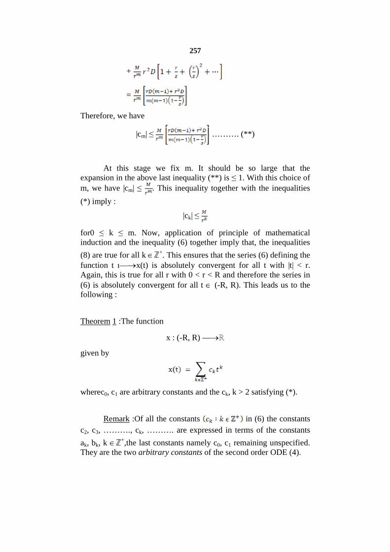
257
+
=
Therefore, we have
|cm| ≤ ………. (**)
At this stage we fix m. It should be so large that theexpansion in the above last inequality (**) is ≤ 1. With this choice of
m, we have |cm| ≤ . This inequality together with the inequalities
(*) imply :
|ck| ≤
for0 ≤ k ≤ m. Now, application of principle of mathematicalinduction and the inequality (6) together imply that, the inequalities
(8) are true for all k ℤ+. This ensures that the series (6) defining thefunction t ı—x(t) is absolutely convergent for all t with |t| < r.Again, this is true for all r with 0 < r < R and therefore the series in(6) is absolutely convergent for all t (-R, R). This leads us to thefollowing :
Theorem 1 :The function
x : (-R, R) —ℝ
given by
wherec0, c1 are arbitrary constants and the ck, k > 2 satisfying (*).
Remark :Of all the constants in (6) the constants
c2, c3, ………., ck, ………. are expressed in terms of the constants
ak, bk, k ℤ+,the last constants namely c0, c1 remaining unspecified.They are the two arbitrary constants of the second order ODE (4).
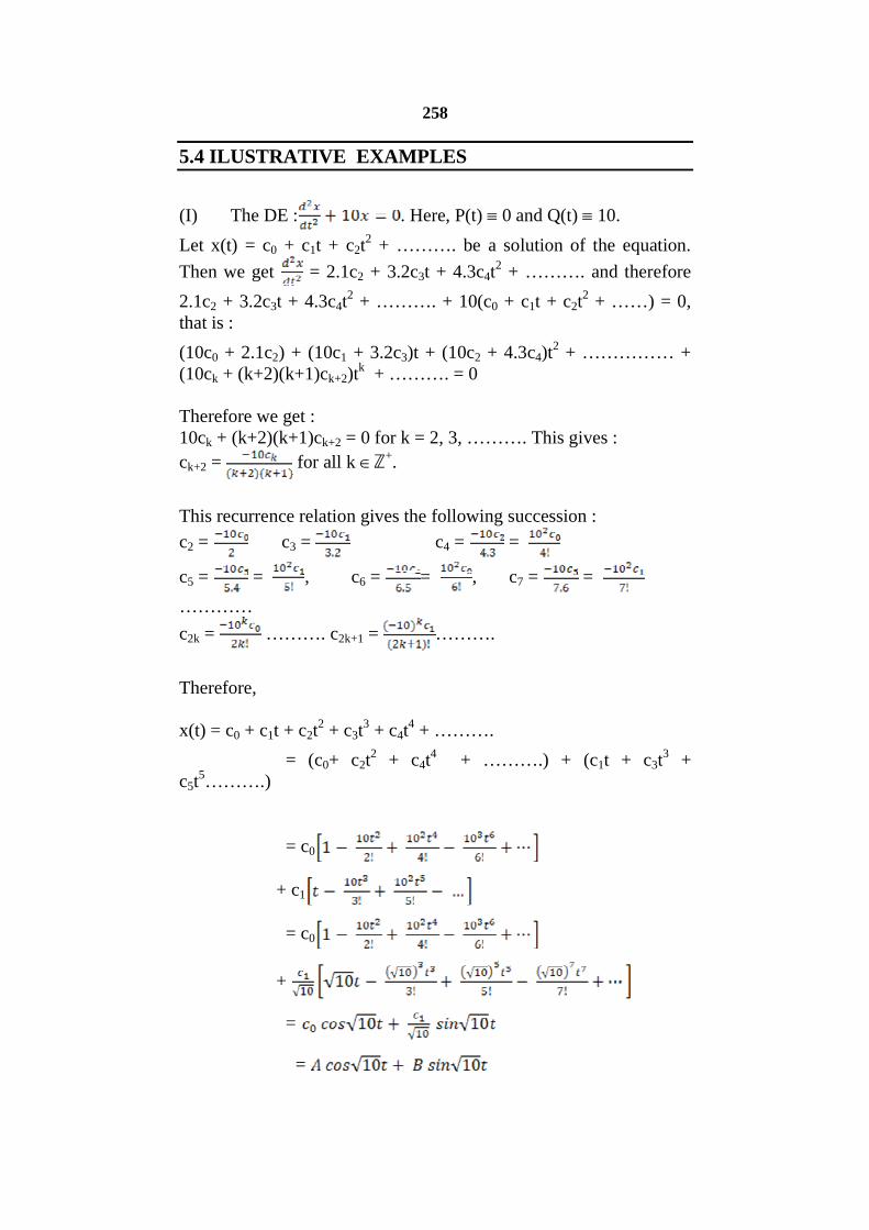
258
5.4 ILUSTRATIVE EXAMPLES
(I) The DE : . Here, P(t) 0 and Q(t) 10.
Let x(t) = c0 + c1t + c2t2 + ………. be a solution of the equation.
Then we get = 2.1c2 + 3.2c3t + 4.3c4t2 + ………. and therefore
2.1c2 + 3.2c3t + 4.3c4t2 + ………. + 10(c0 + c1t + c2t
2 + ……) = 0,that is :
(10c0 + 2.1c2) + (10c1 + 3.2c3)t + (10c2 + 4.3c4)t2 + …………… +
(10ck + (k+2)(k+1)ck+2)tk + ………. = 0
Therefore we get :10ck + (k+2)(k+1)ck+2 = 0 for k = 2, 3, ………. This gives :
ck+2 = for all k ℤ+.
This recurrence relation gives the following succession :
c2 = c3 = c4 = =
c5 = = , c6 = = , c7 = =
…………
c2k = ………. c2k+1 = ……….
Therefore,
x(t) = c0 + c1t + c2t2 + c3t
3 + c4t4 + ……….
= (c0+ c2t2 + c4t
4 + ……….) + (c1t + c3t3 +
c5t5……….)
= c0
+ c1
= c0
+
=
=
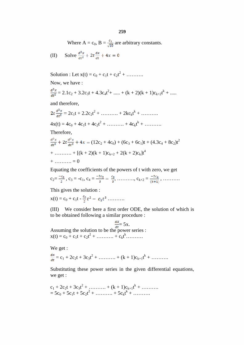
259
Where A = c0, B = are arbitrary constants.
(II) Solve
Solution : Let x(t) = c0 + c1t + c2t2 + ……….
Now, we have :
= 2.1c2 + 3.2c3t + 4.3c4t2+ ..... + (k + 2)(k + 1)ck+2t
k + .....
and therefore,
2c1t + 2.2c2t2 + ………. + 2kckt
k + ……….
4x(t) = 4c0 + 4c1t + 4c2t2 + ………. + 4ckt
k + ……….
Therefore,
(12c2 + 4c0) + (6c3 + 6c1)t + (4.3c4 + 8c2)t2
+ ………. + [(k + 2)(k + 1)ck+2 + 2(k + 2)ck]t4
+ ………. = 0
Equating the coefficients of the powers of t with zero, we get
c2= , c3 = -c1, c4 = , ………., ck+2 = , ……….
This gives the solution :
x(t) = c0 + c1t - ……….
(III) We consider here a first order ODE, the solution of which isto be obtained following a similar procedure :
= 5x.Assuming the solution to be the power series :x(t) = c0 + c1t + c2t
2 + ………. + cktk……….
We get :
= c1 + 2c2t + 3c3t2 + ………. + (k + 1)ck+1t
k + ……….
Substituting these power series in the given differential equations,we get :
c1 + 2c2t + 3c3t2 + ………. + (k + 1)ck+1t
k + ……….= 5c0 + 5c1t + 5c2t
2 + ………. + 5cktk + ……….
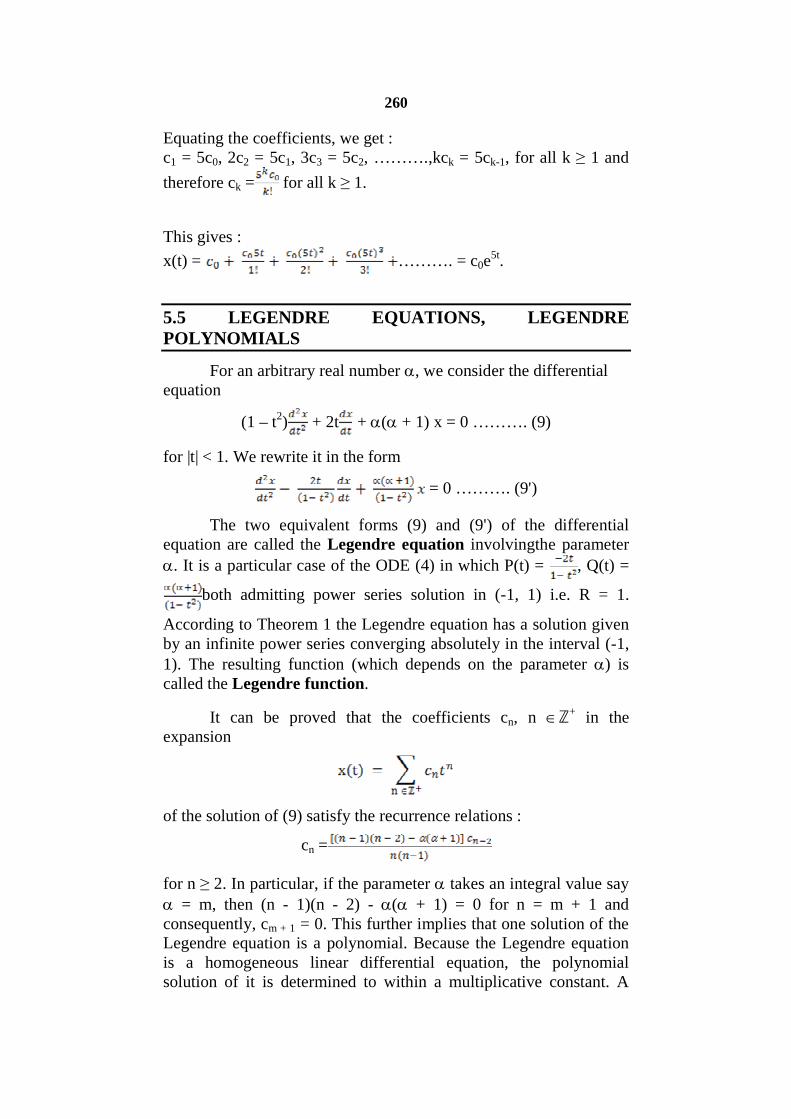
260
Equating the coefficients, we get :c1 = 5c0, 2c2 = 5c1, 3c3 = 5c2, ……….,kck = 5ck-1, for all k ≥ 1 and
therefore ck = for all k ≥ 1.
This gives :
x(t) = ………. = c0e5t.
5.5 LEGENDRE EQUATIONS, LEGENDREPOLYNOMIALS
For an arbitrary real number , we consider the differentialequation
(1 – t2) + 2t + ( + 1) x = 0 ………. (9)
for |t| < 1. We rewrite it in the form
= 0 ………. (9')
The two equivalent forms (9) and (9') of the differentialequation are called the Legendre equation involvingthe parameter
. It is a particular case of the ODE (4) in which P(t) = , Q(t) =
both admitting power series solution in (-1, 1) i.e. R = 1.
According to Theorem 1 the Legendre equation has a solution givenby an infinite power series converging absolutely in the interval (-1,1). The resulting function (which depends on the parameter ) iscalled the Legendre function.
It can be proved that the coefficients cn, n ℤ+ in theexpansion
of the solution of (9) satisfy the recurrence relations :
cn =
for n ≥ 2. In particular, if the parameter takes an integral value say = m, then (n - 1)(n - 2) - ( + 1) = 0 for n = m + 1 andconsequently, cm + 1 = 0. This further implies that one solution of theLegendre equation is a polynomial. Because the Legendre equationis a homogeneous linear differential equation, the polynomialsolution of it is determined to within a multiplicative constant. A
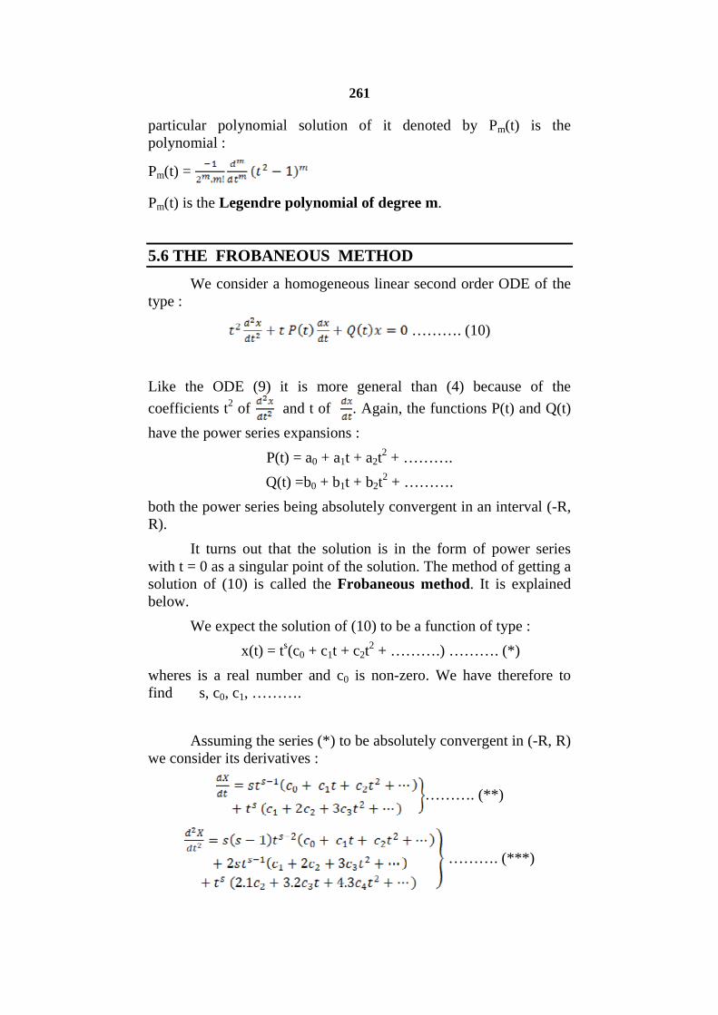
261
particular polynomial solution of it denoted by Pm(t) is thepolynomial :
Pm(t) =
Pm(t) is the Legendre polynomial of degree m.
5.6 THE FROBANEOUS METHOD
We consider a homogeneous linear second order ODE of thetype :
………. (10)
Like the ODE (9) it is more general than (4) because of the
coefficients t2 of and t of . Again, the functions P(t) and Q(t)
have the power series expansions :
P(t) = a0 + a1t + a2t2 + ……….
Q(t) =b0 + b1t + b2t2 + ……….
both the power series being absolutely convergent in an interval (-R,R).
It turns out that the solution is in the form of power serieswith t = 0 as a singular point of the solution. The method of getting asolution of (10) is called the Frobaneous method. It is explainedbelow.
We expect the solution of (10) to be a function of type :
x(t) = ts(c0 + c1t + c2t2 + ……….) ………. (*)
wheres is a real number and c0 is non-zero. We have therefore tofind s, c0, c1, ……….
Assuming the series (*) to be absolutely convergent in (-R, R)we consider its derivatives :
………. (**)
………. (***)
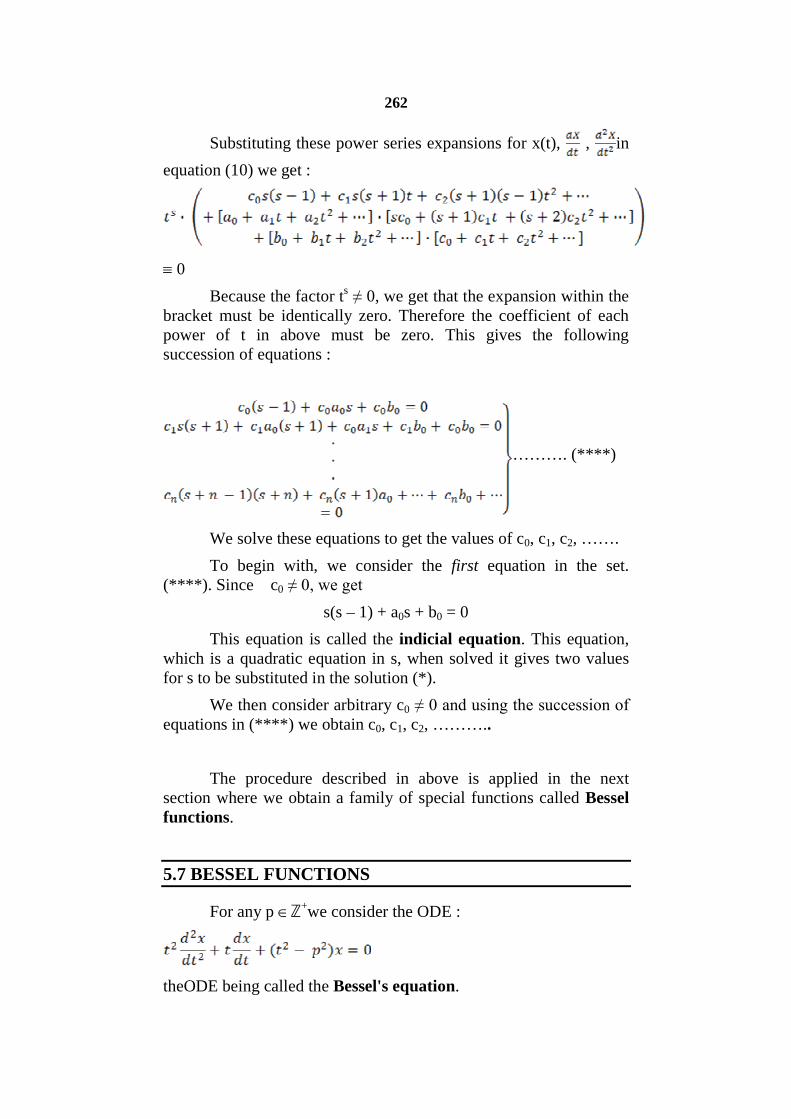
262
Substituting these power series expansions for x(t), , in
equation (10) we get :
0
Because the factor ts ≠ 0, we get that the expansion within thebracket must be identically zero. Therefore the coefficient of eachpower of t in above must be zero. This gives the followingsuccession of equations :
………. (****)
We solve these equations to get the values of c0, c1, c2, …….
To begin with, we consider the first equation in the set.(****). Since c0 ≠ 0, we get
s(s – 1) + a0s + b0 = 0
This equation is called the indicial equation. This equation,which is a quadratic equation in s, when solved it gives two valuesfor s to be substituted in the solution (*).
We then consider arbitrary c0 ≠ 0 and using the succession of equations in (****) we obtain c0, c1, c2, ………..
The procedure described in above is applied in the nextsection where we obtain a family of special functions called Besselfunctions.
5.7 BESSEL FUNCTIONS
For any p ℤ+we consider the ODE :
theODE being called the Bessel's equation.
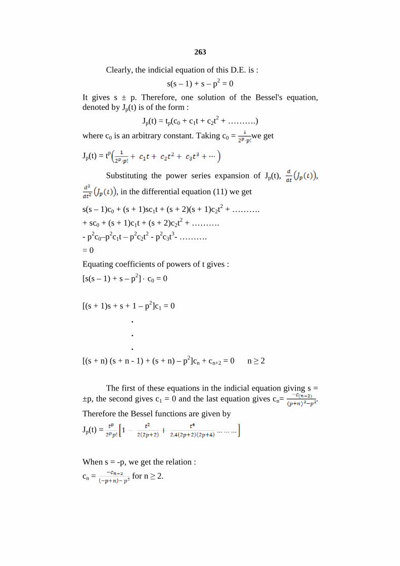
263
Clearly, the indicial equation of this D.E. is :
s(s – 1) + s – p2 = 0
It gives s ± p. Therefore, one solution of the Bessel's equation,denoted by Jp(t) is of the form :
Jp(t) = tp(c0 + c1t + c2t2 + ……….)
where c0 is an arbitrary constant. Taking c0 = we get
Jp(t) = tp
Substituting the power series expansion of Jp(t), ,
, in the differential equation (11) we get
s(s – 1)c0 + (s + 1)sc1t + (s + 2)(s + 1)c2t2 + ……….
+ sc0 + (s + 1)c1t + (s + 2)c2t2 + ……….
- p2c0–p2c1t – p2c2t2 - p2c3t
3- ……….
= 0
Equating coefficients of powers of t gives :
[s(s – 1) + s – p2] c0 = 0
[(s + 1)s + s + 1 – p2]c1 = 0
.
.
.
[(s + n) (s + n - 1) + (s + n) – p2]cn + cn+2 = 0 n ≥ 2
The first of these equations in the indicial equation giving s =±p, the second gives c1 = 0 and the last equation gives cn= .
Therefore the Bessel functions are given by
Jp(t) =
When s = -p, we get the relation :
cn = for n ≥ 2.
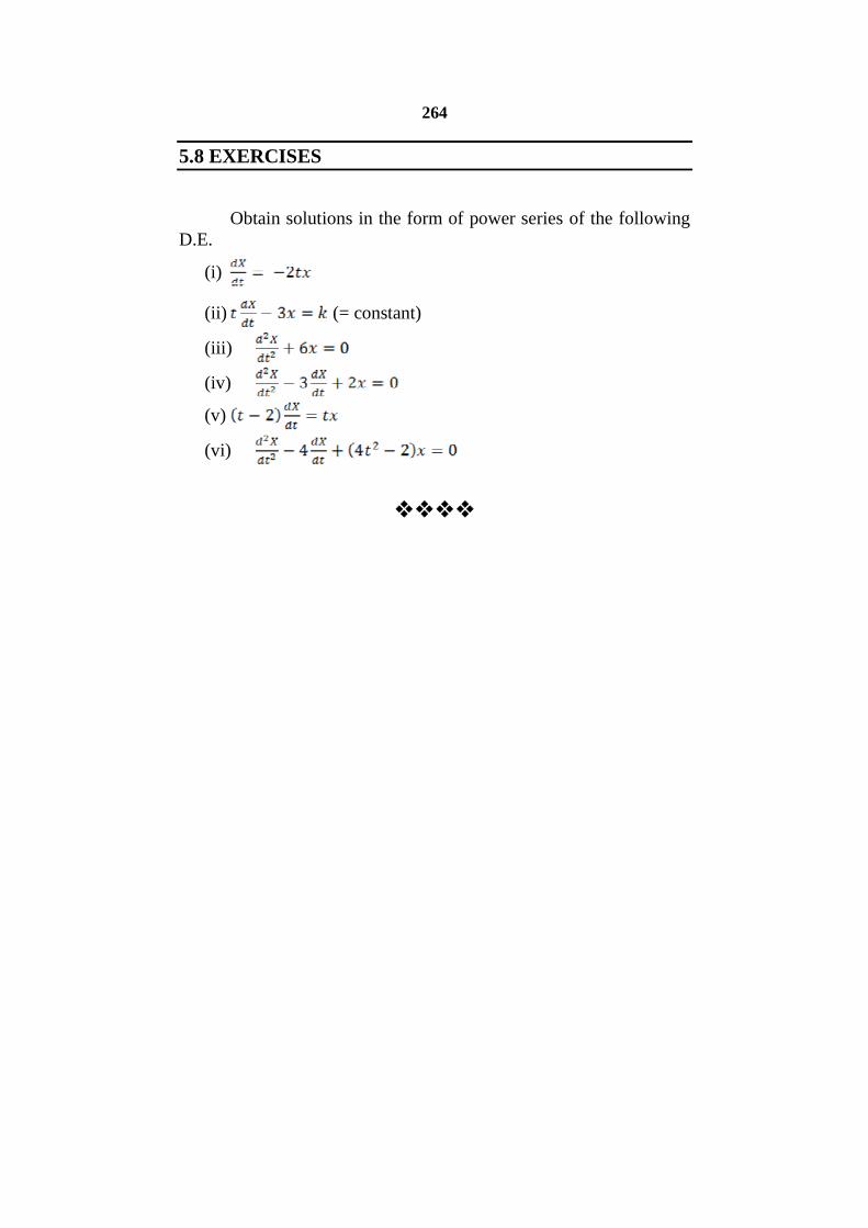
264
5.8 EXERCISES
Obtain solutions in the form of power series of the followingD.E.
(i)
(ii) (= constant)
(iii)
(iv)
(v)
(vi)
265
6
STURM – LIOUVILLE THEORY
Unit Structure :
6.1 Introduction :
6.2 The Sturmian Boundary Value Problem :
6.3 Vibrations of an Elastic String
6.4 Unit End Exercises
6.1 INTRODUCTION
Recall, the initial value problem for an ordinary differentialequation:
1
1( , , , ... )
k k
k k
d X dX d Xf t X
dtdt dt
is to obtain a solution :X I of it when the values :
10( ) , ( )o o
dXX t X t v
dt ,….,
1
0 11
k
kk
dt v
dt
of the solution
and its derivatives are prescribed at a single point to of its domaininternal. A Boundary Value Problem (BVP), is anotherfundamental problem in the theory of ODE in which the solution ofan ODE is required to satisfy a number of conditions at two points ofits domain (the two points actually being the boundary points of thedomain interval.)
In this chapter, we will study an important type of boundaryvalue problems associated with a certain type of linear second orderODE; we call the BVP the “Sturm Liouille eigenvalue problem.”The resulting theory is very vast and makes use of results fromfunctional analysis. Therefore, we only outline the theoryintroducing the concepts and stating the results without proof. Wewill illustrate the scope of the theory by using it to solve thevibrating string problem.
266
6.2 THE STURMAIN BOUNDARY VALUE PROBLEM
In the following, I stands for the interval [a,b]. All thefunctions ( )t X t , ( )t Y t , ( )t Z t etc appearing in the
discussion are assumed to be defined on internals containing I.
We use the following notations :C(I) is the vector space of all continuous functions
1: , ( )X I R C I is the subspace of C(I) which are continuously
differentiable on I while 2 ( )C I consist of those :X I in C(I)
which are twice continuously differentiable on I.
To introduce the type of boundary value problems we want todiscuss, we consider the following data:
(I) The functions p, q, r : I with the following properties :
(i) p is continuously differentiable on I i.e. 1( )p C I
(ii) q, r are continuous on I.
(iii) p(t) > 0 for all .t I
(II) Constants 1 2 1 2, , , with 2 21 2 O and 2 2
21O
(Note that 2 21 2 O is equivalent to the property that of the pair
1 2 , at least one is non-zero. The other inequality also has
similar interpretation).
(III) Arbitrary constants 1 2, .
Using the functions in (I) we construct the linear, second orderordinary differential equation :
( )pX q X r … (1)
i.e. , .d dX
p t t q t X t r t t Idt dt
in the unknown function t X t
The equation : PX q X … (2)
is the homogeneous part of it.
267
We require the solution function ( )t X t of (1) to satisfy the
boundary conditions :
1 2 1
1 2 2
( )X a X a
X b X b
… (3)
Taking together the DE(1) and the boundary conditions (3) we getthe pair
pX qX r
1 2 1 1 2 2( ) ,X a X a X b X b … (4)
The pair (4) is said to constitute the Sturmian boundary valueproblem.
In above, taking 1 20, 0r we get the homogeneous
Sturmian boundary value problem:
P X q X
1 2 1 20X a X a X b X b … (5)
In above for every 2( ),X C I we put
( ) ( )
.
L X pX q X
pX p X qX
Note that 2 ( )X C I implies that L(X) is continuous. Thus we get
the map2: ( ) ( )L C I C I
of the indicated vector spaces. Clearly L is linear.
Now for any 2, in ( )X Y C I we have
. .L X t Y t X t L Y t
. .d X td dY
p t Y t X t tdt dt dt
for all .t I We refer to this equality as the .Lagrange Identity
Integrating this identity over the interval , ,a b we get
. ( ).b
aL X t Y t X t L Y t dt
. .p b X b Y b X b Y b
p a X a Y a X a Y a … (*)
268
Moreover, if both the functions X, Y satisfy the boundary conditionsin (5) then it follows that the R.H. S. of (*) is zero and consequentlywe have :
.b b
a aL x y Y t dt X t L x t dt …(**)
We will explain more about this equality (**) at a later stage.
Here is a short list of properties of the spaces of solutions ofthe boundary value problem (4) and its homogeneous part (5).
(1) A finite linear combination :
1 1 2 2 ... n nC X C X C X
of solutions 1 2, , , nX X X of the B.V.P. (5) is also a solution of the
BVP (5).
(2) If X and Y are solutions of the in homogeneous BVP (5) thenthe difference X – Y is a solution of the homogeneous boundaryvalue problem (5).
(3) If :X I R is a solution solution of the BVP (5) and:Y I a solution of the non-homogeneous B.V.P. (4) then X + Y
is a solution of the BVP (4).
(4) Finally, let :Y I be a fixed solution of the
inhomogeneous BVP (4). Then every other solution :Y I of (4)
can be expressed in the form Y X Y for a unique solution X ofthe homogeneous BVP (5).
At this stage we describe a condition which ensures a uniquesolution of the boundary value problem (4). Towards this aim, recallthat the solution space of the second order, linear homogeneousODE (2) is a 2 dimensional vector space and we call a basis of thisvector space a fundamental system of the ODE.
We choose a fundamental system 1 2,X X of the ODE (2).
Next, using it and the constants 1 2 1 2, , of the boundary
conditions of (5) we form the quantity.
11 1 1 2 1
12 1 1 2 1
21 1 2 2 2
22 1 2 2 2
R X a X a
R X b X b
R X a X b
R X b X b
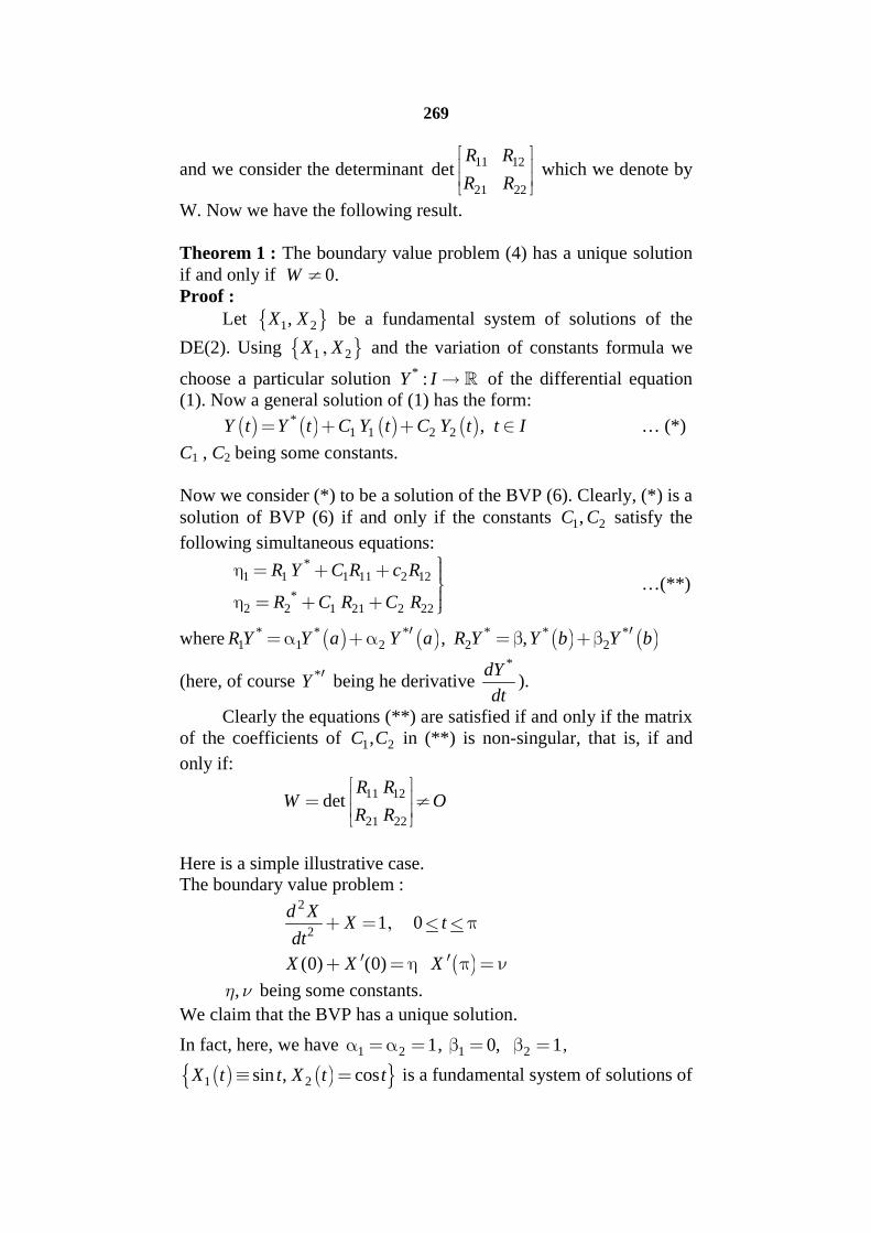
269
and we consider the determinant 11 12
21 22
detR R
R R
which we denote by
W. Now we have the following result.
Theorem 1 : The boundary value problem (4) has a unique solutionif and only if 0.W Proof :
Let 1 2,X X be a fundamental system of solutions of the
DE(2). Using 1 2X X and the variation of constants formula we
choose a particular solution * :Y I of the differential equation(1). Now a general solution of (1) has the form:
*1 1 2 2 ,Y t Y t C Y t C Y t t I … (*)
C1 , C2 being some constants.
Now we consider (*) to be a solution of the BVP (6). Clearly, (*) is asolution of BVP (6) if and only if the constants 1 2,C C satisfy the
following simultaneous equations:*
1 1 1 11 2 12
*2 2 1 21 2 22
R Y C R c R
R C R C R
…(**)
where * * * * * *1 1 2 2 2, ,R Y Y a Y a R Y Y b Y b
(here, of course *Y being he derivative*dY
dt).
Clearly the equations (**) are satisfied if and only if the matrixof the coefficients of 1 2,C C in (**) is non-singular, that is, if and
only if:
11 12
21 22
detR R
W OR R
Here is a simple illustrative case.The boundary value problem :
2
21 0
(0) (0)
d XX t
dt
X X X
, being some constants.
We claim that the BVP has a unique solution.
In fact, here, we have 1 2 1 , 1 0, 2 1 ,
1 2sin , cosX t t X t t is a fundamental system of solutions of
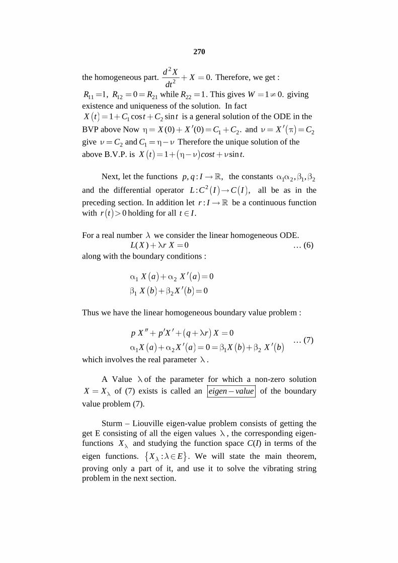
270
the homogeneous part.2
20.
d XX
dt Therefore, we get :
11 12 21 22, 0 while 1R R R R . This gives 1 0.W giving
existence and uniqueness of the solution. In fact
1 21 cos sinX t C t C t is a general solution of the ODE in the
BVP above Now 1 2(0) (0) .X X C C and 2X C
give 2 1andC C Therefore the unique solution of the
above B.V.P. is 1 sin .X t cost t
Next, let the functions , : ,p q I the constants 1 2 1 2, ,
and the differential operator 2: ,L C I C I all be as in the
preceding section. In addition let :r I be a continuous functionwith 0r t holding for all .t I
For a real number we consider the linear homogeneous ODE.( )L X r X … (6)
along with the boundary conditions :
1 2
1 2
0
0
X a X a
X b X b
Thus we have the linear homogeneous boundary value problem :
1 2 1 2
0
0
p X p X q r X
X a X a X b X b
… (7)
which involves the real parameter .
A Value of the parameter for which a non-zero solution
X X of (7) exists is called an eigen value of the boundary
value problem (7).
Sturm – Liouville eigen-value problem consists of getting theget E consisting of all the eigen values , the corresponding eigen-functions X and studying the function space C(I) in terms of the
eigen functions. :X E . We will state the main theorem,
proving only a part of it, and use it to solve the vibrating stringproblem in the next section.
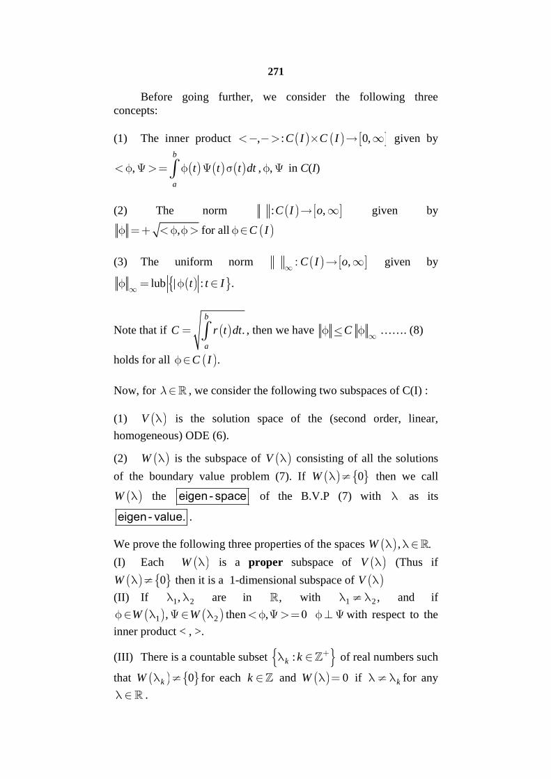
271
Before going further, we consider the following threeconcepts:
(1) The inner product , : 0,C I C I given by
, , ,
b
a
t t t dt in C(I)
(2) The norm : ,C I o given by
, for all C I
(3) The uniform norm ,C I o
given by
lub | : .t t I
Note that if .
b
a
C r t dt , then we have C
……. (8)
holds for all .C I
Now, for , we consider the following two subspaces of C(I) :
(1) V is the solution space of the (second order, linear,
homogeneous) ODE (6).
(2) W is the subspace of V consisting of all the solutions
of the boundary value problem (7). If 0W then we call
W the eigen - space of the B.V.P (7) with as its
eigen - value. .
We prove the following three properties of the spaces W ,
(I) Each W is a proper subspace of V (Thus if
0W then it is a 1-dimensional subspace of V
(II) If 1 2, are in , with 1 2 , and if
1 2, then ,W W with respect to the
inner product < , >.
(III) There is a countable subset :k k of real numbers such
that 0kW for each k and 0W if k for any
.
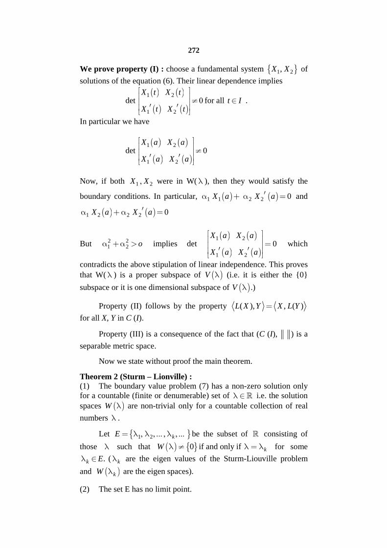
272
We prove property (I) : choose a fundamental system 1 2,X X of
solutions of the equation (6). Their linear dependence implies
det
1 2
1 2
X t X t
X t X t
for all t I .
In particular we have
det
1 2
1 2
0X a X a
X a X a
Now, if both 1 2X X were in W( ), then they would satisfy the
boundary conditions. In particular, 1 1 2 2 0X a X a and
1 2 2 2 0X a X a
But 2 21 2 o implies det
1 2
1 2
0X a X a
X a X a
which
contradicts the above stipulation of linear independence. This proves
that W( ) is a proper subspace of V (i.e. it is either the {0}
subspace or it is one dimensional subspace of V .)
Property (II) follows by the property ( ), , ( )L X Y X L Y
for all X, Y in C (I).
Property (III) is a consequence of the fact that (C (I), ) is a
separable metric space.
Now we state without proof the main theorem.
Theorem 2 (Sturm – Lionville) :(1) The boundary value problem (7) has a non-zero solution onlyfor a countable (finite or denumerable) set of i.e. the solutionspaces W are non-trivial only for a countable collection of real
numbers .
Let 1 2 kE be the subset of consisting of
those such that 0 if and only if kW for some
.k E ( k are the eigen values of the Sturm-Liouville problem
and kW are the eigen spaces).
(2) The set E has no limit point.
273
(3) Each kW is a 1 dimensional subspace of 2C I . For each
k E we choose k kX W with 1.kX Now we have
..k kW X X
(4) If , then , 0.k e k ek e X X ie X X
(5) If 2X C I then , kk
kX t X t X t X t
for all t I where the convergence of to infinite series to X(t) isuniform in t I .
(6) If ( ) is such that , 0kX C I X X holds for all kX then
X ≡ 0.
The proof of this theorem makes use of the properties of acompact operator on a separable Hilbert Space and as such it is to bestudied from a suitable advanced text-book on ODE (which usuallyrefer to text-books of functional analysis).
We state here two more results without proof :
Theorem 3 (Sturm-Liouville Separation Theorem.)The zeros of two linearly independent solutions of L(X) = 0 separateeach other.
Thus if 1 2X and X are two independent solutions of L(X) = 0,
their between two consecutive zeros of 1X is a zero of 2X and
between two consecutive zeros of 2X is a zero of 1X .
Theorem 4 (The Comparison Theorem)Consider two eigen-value problems of Sturm Liouville with the
respective date , , , ,p q r and * * * * *, , , ,p q r over the same
interval I = [a, b].
If *,p p * ,q q *r r in I and *0 , *0 hold with strict inequality in at least one place, then
the corresponding eigenvalues satisfy *n n for all n.
In the next section, we study the dynamics of an elasticvibrating string in which we will use the results of the Sturm-Liouville Theorem.
274
7.3 VIBRATIONS OF AN ELASTIC STRING
The vibrating motion of a stretched elastic string is governedby a partial differential equation called the (one-dimensional)
wave equation . Wave equation is solved by a method called
method of separation of variables. The resulting analysis makes useof the Sturm Liouville theory. We will therefore study the problemof the vibrating elastic string as an application of the Sturm-Liouville Theory.
We first explain the PDE, the wave equation of the vibrating string.
A string of natural length L is held horizontally along the X-axis of avertical XOY-plane. Its ends, A, B remain tied to the points (0, 0)and (L, 0) respectively. The string is plucked slightly and then is setin motion in such a way that each point C of the string vibratesvertically. We study the vibrating motion of the string as thecollective vertically oscillating motion of each point C of the string.
Therefore we consider an arbitrary point C of the string Let
,l A C x (The real number x and the point C determine each
other and therefore we may take of “the point x” instead of “thepoint C”.)
Let at an instant ( , )t Y t x be the instantaneous y-
coordinate of the point C (Since the oscillatory motion of C is onlyin the vertical direction, x-coordinate of C remains constant.)Therefore the (oscillatory) motion of the point C is described by thefunction ( , )t Y t x and the motion of the whole string is given by
the function , , 1t x Y t x t x … (9)
Now, the basic equations of motion enable us to derive theequation
2 22
2 20 ,
Y Yc t x L
t x
…(10)
satisfied by the function Y(t, x). Equation (10) is the waveequation which is satisfied by the vibrating string. In (10) c is aconstant determined by the mass of the string its elastic propertiesand the gravitational constant.)
Suppose the string was plucked slighlty and released withinitial velocity (= initial velocity of each point C). so that the string
275
executes the vibration motion as described above. We consider twocontinuous functions :
: 0, , : 0,f L g L describing initial position and
initial velocity of the string, that is :
0, , 0, , 0 .Y
Y x f x x g x x Lt
Now, we have the initial / boundary value problem for thefunction , , ;t x Y t x
2 22
2 20, 0
Y Yc t x L
t x
…(10)
,0 0 , 0,Y t Y t L t
0, 0, , 0 .Y
Y x f x x g x x Lt
We want to find out the function ,t x Y t
To begin with, we consider all the solutions of the wave equationwhich are of the type X(x). T(t):
, .Y t x X x T t
Now, 2 2.. ..
2 2, , ,
Y Yt x X x T t X x T t
t x
(the dots
indicating differentiation (twice) with respect to the appropriatevariable)
Now the equation takes the form
.. ..
2X x T t c X x T t
Assuming 0, 0 0, 0 ,X x T t for t x L we get
.. ..
2
1 T t X x
T t X xc …(11)
This shows that the common value in (11) is independent of t, x i.e.it must be a constant say d.
....
2
1 T t X xd
T t X xc …(12)
Now if 0d we would get ..
2 2with 0.T t c d T t c d If
0d , we would get T(t) = At + B for some constants a , B (A isnot zero because, otherwise T t B which gives Y(t, x) = B. X(x)
276
implying that the motion of the string is independent of t ie the stringis station any!). On the other hand, if d > o, we would get
. .d ct d ctT t Ae Be t
In either case (i.e d > 0, or d = 0) the factor T(t) becomes unboundedas t ranges in 0, . This renders Y(t, x) also unbounded (ie the
string stretching limitless, another physical impossibility!).Therefore we are left with the possibility d < 0. We put
2 ford . Then the above ODE (12) take the form :
.. ..
2 2 2,T t c T t X x X x .. (13)
We consider the second equation :
..
2 , 0 .X x X x x L
Its general solution is :
cos sinX x x x x , being constants. This gives:
, cos sinY t x T t x x with the condition 0T t . Now
0 , 0 .Y t x T t implies 0 and therefore
, . sin with 0,Y t x T t x T t 0.
But we have Y(t, L) = 0 and therefore sin 0L which implies thatL k for k . Therefore the parameter can take the values
, ,k
k kL
.
This shows that :
. cos sink k k
cL cLT t T t t t
k k
and ,k
LX x X x Sin x k
k
.
Thus, we get a sequence of solutions :
. cos . sin sink k k
cL cL LY t x t t x
k k K
for k , X ,k k being arbitrang constants. Now the general
solution Y(t, x) will be a linear combination of all of them.
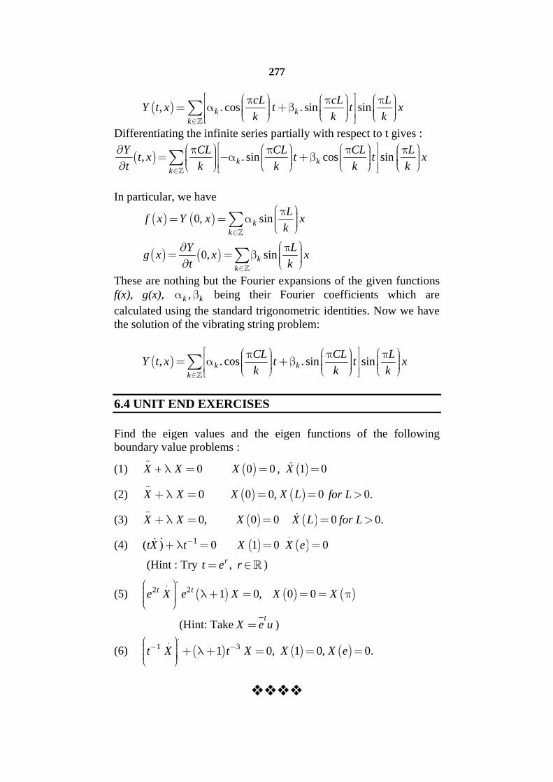
277
, . cos . sin sink kk
cL cL LY t x t t x
k k k
Differentiating the infinite series partially with respect to t gives :
, . sin cos sink kk
Y CL CL CL Lt x t t x
t k k k k
In particular, we have
0, sin
0, sin
kk
kk
Lf x Y x x
k
Y Lg x x x
t k
These are nothing but the Fourier expansions of the given functionsf(x), g(x), ,k k being their Fourier coefficients which are
calculated using the standard trigonometric identities. Now we havethe solution of the vibrating string problem:
, . cos . sin sink kk
CL CL LY t x t t x
k k k
6.4 UNIT END EXERCISES
Find the eigen values and the eigen functions of the followingboundary value problems :
(1) ..
0 0 0 , 1X X X X
(2) ..
0 0 0, 0 0.X X X X L for L
(3) ..
0, 0 0 0 0.X X X X L for L
(4) .
1( ) 0 1 0 0tX t X X e
(Hint : Try ,rt e r )
(5) ..
2 2 1 0, 0 0t te X e X X X
(Hint: Taket
X e u )
(6) ..
1 31 0, 1 0, 0.t X t X X X e
Related Documents