I once learned about magnetism, but please, remind me. - Gorupec's ...

1

I once learned about magnetism,

but please, remind me.

Prologue ......................................................... 1

1. Magnetic field ............................................ 1

2. The Lorentz force ....................................... 9

3. Magnetic flux ........................................... 13

4. Permanent magnet .................................... 17

5. Current-carrying wires ............................. 20

6. Computing the field.................................. 25

7. Electromagnetic induction........................ 29

8. Self-induction and inductance .................. 37

9. Energy contained in magnetic field .......... 42

10. Magnetic field and frames of reference.. 44

11. Force on a current-carrying wire ............ 50

12. Energies and work .................................. 54

13. Magnetic field and materials .................. 61

14. Hysteresis and eddy currents .................. 71

15. Forces and magnetic materials ............... 75

Appendix: Glossary ...................................... 84

Prologue

A hundred thousand years ago… Despite yesterday’s thunderstorm, Kiko, the leader of the group, insisted that they go to the Dark-sand beach. Younger children worried, but their

worries quickly evaporated playing games and catching fish in shallow water.

At one moment a flock of birds landed on the beach and Mink noticed it. She sneaked closer

and grabbed few stones from the ground… birds spotted her early, again, and flew away. Yet,

something was not quite right – these stones in her hand. In some unexplainable way, these

rock pieces liked to stick together. Mink yelled, “Guys, come look at this!” Kids soon found

several other pieces that behaved the same. Kiko seized best samples.

Later that day the whole tribe was trying Kiko’s magical rocks. The distance-acting rocks

quickly changed hands stretching smiles over people faces. Kiko was ‘the man’ of the

evening. Mink less so, but in her heart she did feel a silent pride.

1. Magnetic field

Our prologue story fictionalizes how it could have been when humans encountered

magnets for the very first time.1 Only, it must be that those ‘first-time’ encounters

happened many times over – people forget and rediscover. It also must be that every such

rediscovery made a solid impression on our early ancestors. Magnets impress people.

1 Look for 'lodestone'. These are dark stones made of mineral called magnetite. Most magnetite rock is

not magnetized, but some possibly got magnetized by a lighting bolt – becoming lodestones.

2

The rest of our story, however, is more recent. Few centuries ago scholars started thinking

more coherently about magnetism and about the intriguing action-over-a-distance.

Gravity also acts in a similar over-a-distance way, but somehow it doesn’t make ordinary

people intrigued. I guess, gravity is just too commonplace, too omnipresent. And we

experience it always in the boring downward direction… Moreover, gravity cannot act

repulsively, while magnetic rock can, depending on their orientation. Action-over-a-distance versus magnetic field

Some scholars frowned upon the pure action-over-a-distance. How can it be, they

complained, that two objects can act over a distance without anything happening in

between? There must be some mediator between objects to mediate forces or transfers any

kind of information. And if there is such a mediator, it should be included into our

theories and we should be able to say something about it.

Scholars proposed the concept of magnetic field. There is some invisible thing, they said,

that surrounds the body of a magnet. This invisible thing, the magnetic field, is in direct

contact with nearby objects and it is the magnetic field that is actually pushing or pulling

on the nearby ferric items.

So, by accepting the idea of magnetic field, we can think about magnetism in a local way.

Let me illustrate, in childish words, what this ‘local way’ means… Suppose you place a

magnet close to a needle. The magnet is strong enough that the needle will jump onto it.

How can the needle ‘know’ it must jump? Without the magnetic field, figuratively

speaking, the needle would have to look around, spot the magnet, estimate its size and

strength, and then decide whether to jump or not… But if we have the magnetic field, then

the needle does not need looking around. Instead, the needle only needs to feel (touch,

palpate) the magnetic field just there, at the location of the needle. The needle does not

need to know what kind of object is creating this field. Just by ‘feeling’ the local field, by

feeling its local strength and direction, the needle can ‘decide’ if it will jump and in what

direction it should jump. All that the needle needs to ‘know’ is available locally.

We might say: the magnetic field contains locally all the information needed to explain

observable magnetic effects at that location.2 It is only this way that the magnetic field can

relieve us from the action-over-a-distance trouble.

It is my impression that the idea of magnetic field also makes the mathematics easier. I

would suspect that even people who continued to hold the action-over-a-distance point of

view and who didn’t believe magnetic field is a real object, still appreciated the simpler

mathematics provided by the field approach.

Today, it is accepted that the magnetic field is not just a mathematical construction or only

a viewpoint. It is a real object, as real as the magnet body itself. There really exists this

thing around a magnet that spreads toward infinity.3 While the magnetic field is not made

2 Look for the 'principle of locality' to explore why the idea of locality has such an appeal.

3 The magnetic field quickly weakens with the distance from the magnet, but it does not have an end.

3

of regular mater (atoms), it is still a real resident of our Universe. Experiments indicate

that this invisible thing contains its own energy and can store its own linear and angular

momentum – and possessing these things makes it quite real.

The compass needle as a measuring instrument

People started shaping magnetic rocks into useful tools. If you carve a small bar out of a

magnetic rock, taking care that the bar shows the strongest magnetism at its tips, and if

you suspend this magnetic bar so that it freely and easily rotates around its center, then

you obtained a most useful little instrument – a compass needle. The compass needle is

nothing else but a small bar-shaped magnet that we can use to test magnetic fields of other

magnets.

The picture below shows how a compass needle might take different orientations at

several places near a magnetic rock.

As it happens to be, much to our good luck, the planet Earth also makes a large, although relatively

weak magnetic field. If there are no stronger magnets in vicinity, a compass needle will orient itself

into the north-south direction. Therefore, we can use the compass needle as an important navigational

aid… The tip of the compass needle that seeks the Earth’s geographic North Pole we unimaginatively

call the ‘north pole’ of the needle. The opposite tip we call the ‘south pole’.

Measuring the magnetic field

We can exploit the fact that a compass needle reacts to a magnetic field and use it as a

measuring probe. Here is how you can measure the field of a particular magnet.

• Take a small compass needle and place it at some position (point) near the magnet.

• Observe that the needle orients itself into certain direction. Record that

direction4… However, we also need to know how ‘eagerly’ the needle directs that

way. Therefore, forcefully turn the needle perpendicularly to its preferred direction

and record the torque magnitude needed to hold it that way.

• Use the recorded direction and the recorded torque magnitude to compose a vector;

this vector describes the magnetic field at that point in the space.

• Make such measurements for many points around the magnet.

4 Which direction should you record, the one pointed by the north-pole tip or the one pointed by the

south-pole tip of the needle? Record the direction pointed by the north-pole tip; this is a convention.

4

Once you draw a vector arrow for all the points where you made the measurements, you

might see a picture like this:

This swarm of vector arrows is describing the field of the magnet. We cannot see the

magnetic field, so we describe it by measurable effects it makes – in our case, by how it

rotates our compass needle. Each vector arrow tells how strongly and in what direction the

compass needle will be rotated if placed there.

We only sketched a finite number of arrows, but you can imagine how there exists one

vector arrow for every point in space. You can imagine a dense field of arrows, an infinite

number of them. Such continuous array of vectors is called a vector field. So, a magnetic

field is described (represented) by a vector field.

From your measurements you can conclude that the magnetic field weakens with the

distance from the magnet body. The field seems strongest at the magnet surface, but not

over the whole surface. A magnet might have few regions at its surface where its field is

particularly strong. These regions are often called north poles and south poles. (If you

have a compass needle, you can easily test if a region is a north or a south pole: the needle

will turn its north pole tip toward south pole regions and vice versa. Opposites attract.)

More importantly, you can conclude that in the space around the magnet the magnetic

field is continuous (it nowhere changes abruptly; it changes gradually). Thanks to that

fact, we don’t need to measure the field at infinite number of points and we don’t need to

use an infinitely small compass needle (a probe). Or better said, there exist a small-enough

probe, but still finitely-sized, that will produce measurements to a satisfying level of

detail. [In practice, you might be measuring the field with increasingly smaller probes and at

increasing number of points – at one moment you will notice that further refinement does not reveal

any new data of much interest to you. Then you can stop and rightfully believe that it is unlikely the

field contains more surprises.]

Characterizing and defining the magnetic field

We described the magnetic field in terms of torque it exerts on our compass needle.

Should we add anything else to describe the field completely? No, for static magnetic

fields we do not.5 If we know how a static field affects our compass needle at all the

5 If the magnetic field is not static then we might need to keep an eye on electric field too. In fact, then we are

dealing with a more general thing called the electromagnetic field (our static magnetic field is just a special case

of this one). Luckily, we can often approximate the magnetic field as static even if it cycles at 50-60Hz rate.

5

points in space, then we have the complete data, the complete description of the field, and

we can compute everything else this field can do. You may, if you wish, even define a

magnetic field as: the thing that rotates a compass needle.

There is, however, a small practical problem. The torque exerted on a compass needle

does not depend only on the strength of the field. It also depends, proportionally, on the

‘strength’6 of the compass needle itself. For this reason we should divide the measured

torque magnitudes with the strength of our compass needle to obtain a vector field that

does not depend on the particular compass needle. It is this vector field that I will simply

call the ‘magnetic field’ or the ‘B-field’.

The magnitudes of vectors of magnetic field are given in units called tesla (T). One tesla

represents a fairly strong (intense, dense) magnetic field. The intensity of the Earth’s

magnetic field, for example, is only in the 30-60 microtesla range. A strong rare-earth

magnet may provide field intensity of about 1 tesla (or a bit more) near its poles.

I feel the terminology is messy. In the nature there is the real object that we call the ‘magnetic field’

(or the ‘B-filed’). We can best describe this real object using a mathematical idea called a vector field.

This vector fields we again call ‘magnetic field’ or ‘B-field’ or even ‘magnetic flux density field’.

People tend to be sloppy about the difference. In sentences like ‘magnetic field rotates the needle’ the

real natural object is referred. In a sentence like ‘let sum two magnetic fields’ mathematical

representations (vector fields) are referred.

Furthermore, as said, the vector field that describes the magnetic field is imagined as an infinite array

of spatially distributed vectors. Each one of these vectors can be called many names, including:

‘magnetic field vector’, ‘B-field vector’, ‘B-vector’, ‘magnetic field strength/intensity/density

(vector)’ or even ‘flux density vector’… In most magnetism-related formulas, it is this vector that is

represented using the ‘B’ letter.

Vector fields are used to describe many things in physics, not just magnetic fields. For example, air

movements in the Earth’s atmosphere can be described by a vector field whose components are

velocity vectors… The term ‘field’ means a continuous set of quantities, one for each point in space.

In the case of vector fields those quantities are vectors (there are also scalar fields, tensor fields, etc)…

Physical fields, those that describe nature, are continuous. Our magnetic field does not suddenly stop

at the surface of the magnet body. It stretches inside the magnet too.

We said already that we may define the magnetic field as ‘the thing that rotates a compass

needle’. Later we will see that magnetism is related to electric currents, and electric

currents are streams of moving charges. So we can also define the magnetic field in term

of torque it exerts on current-carrying wire loops or in term of force it exerts on moving

charges. To put it in other words… Our magnetic field can do several things – it exerts

torques on compass needles (other magnets), it exerts forces on current-carrying wires and

it deflects moving charged particles from their paths. All these effects can be used to

measure or even define the same vector field, the magnetic field B. If made carefully, all

these measurement methods will give the same result for the B-field.

But we can define different fields around a magnet. For example you can start from our B field and

then transform it mathematically. One such example is the vector field A, called the ‘vector potential’

of the magnetic field. It is defined such that the curl of A filed makes our B filed (B = ∇ x A).

6 By ''strength' I mean the 'magnetic dipole moment' - we will talk more about it in chapter 4.

6

Interestingly, there are indications that the A field could actually be more fundamental than the B

field… It might be possible to define many other, less useful fields around a magnet. For example you

could measure the force (not the torque) a freely-rotating compass needle feels in a vicinity of a

magnet – this field would almost everywhere converge toward the magnet…Or: you could shake the

magnet body and record how strong electric field this creates around… You could define many fields

around a magnet, but the one that we defined, the B field, is the useful one.

To underline: The vector field B describes all the effects of a magnetic field completely

and in a local manner. To compute magnetic effects at some spot in space, all you need to

know is the magnitude and direction of magnetic field at that spot.

Depicting magnetic fields using field lines

You might enjoy the picture of the magnetic field that we sketched above, or you might be

thinking that it looks too fuzzy with all those arrows poking around. For some reason,

magnetic fields are rarely depicted using vector arrows. Instead, we depict them using

‘magnetic field lines’. Both ways are correct, but field lines are way more common.

When depicting a magnetic field using magnetic filed lines, remember that lines should be

drawn as closed loops and should not cross (nor even touch) each other. Of course, field

lines might exit your limited drawing area, in which case you cannot draw a complete

line, but only a segment of it. In this paper I often depict field line segments when it is

either obvious or unimportant how the lines actually close. But in any case, the field lines

are to be regarded as closed lines.

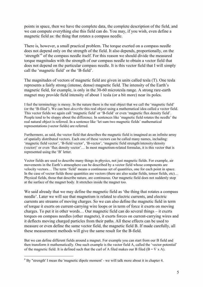
The magnetic field lines have directions. Outside the magnet body, their direction is from

magnet’s north pole to magnet’s south pole (but inside the magnet body it is from south

pole to north pole). Such direction was historically determined by convention… To make

it clear what their direction is, we usually draw small arrows on magnetic field lines.

Magnetic field lines are just a visual aid to depict the otherwise invisible magnetic field.

The field is certainly not ‘stringy’ in its nature – it is smooth. You have a freedom to

decide how many lines you will draw, but you need to be consistent about their relative

density within a single picture. In this paper, for example, I will sometimes only use a few

lines to coarsely mark a field… Note also that magnetic fields are three-dimensional

7

objects, so on the 2D paper plane we can only depict one intersection of the actual field

(well, we often have troubles depicting 3D objects on a 2D plane).

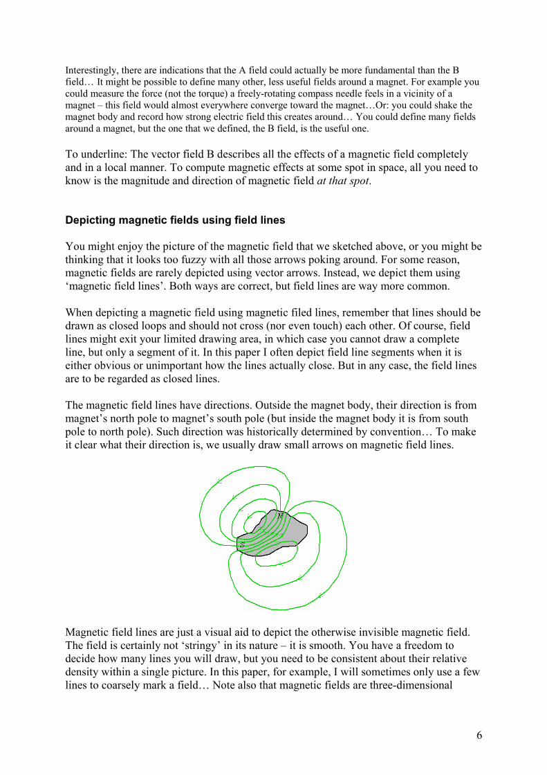
Even when a magnetic field is depicted by magnetic field lines, you can still easily tell the

direction of magnetic field vectors. At every point in space the direction of field vectors is

identical (better said, tangential) to the direction of field lines. I tried to depict this by

showing both, field vectors and field lines, on the same picture.

Not only their directions, but also the magnitude of magnetic field vectors can be deduced

from correctly drawn field lines. The magnitude is represented by the density of magnetic

field lines. Wherever magnetic field lines are drawn closer to each other, the field is

stronger. As you can see from the picture above, the field lines are quite dense near

magnet poles and inside the magnet (there the magnetic field vectors are also long).

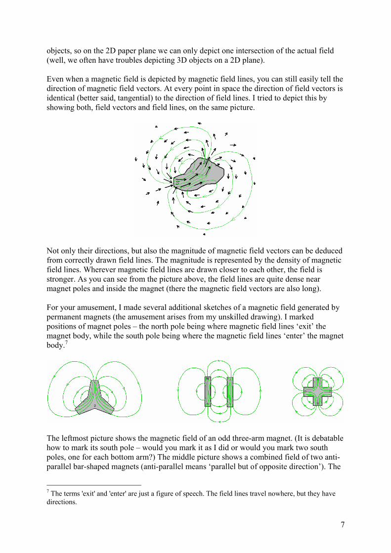
For your amusement, I made several additional sketches of a magnetic field generated by

permanent magnets (the amusement arises from my unskilled drawing). I marked

positions of magnet poles – the north pole being where magnetic field lines ‘exit’ the

magnet body, while the south pole being where the magnetic field lines ‘enter’ the magnet

body.7

The leftmost picture shows the magnetic field of an odd three-arm magnet. (It is debatable

how to mark its south pole – would you mark it as I did or would you mark two south

poles, one for each bottom arm?) The middle picture shows a combined field of two anti-

parallel bar-shaped magnets (anti-parallel means ‘parallel but of opposite direction’). The

7 The terms 'exit' and 'enter' are just a figure of speech. The field lines travel nowhere, but they have

directions.

8

rightmost picture shows the magnetic field of a magnet that has four poles (you might

often encounter similar multi-pole magnets inside electric motors).

Due to historical and practical reasons, you might find pictures of magnetic field where lines are only

drawn outside the magnet body. I urge you that you always imagine lines as loops that close

themselves through the magnet body. The historical reasons have something to do with the concept of

magnetic charges that I am avoiding (as magnetic charges do not exist physically).

Addition of magnetic fields

Magnetic fields add up neatly. When magnetic fields of two or more magnets overlap, you

can compute the resulting field by simple vector addition: for every point in space sum

corresponding field vectors of all overlapping fields to obtain the vector of the resulting

field. This resulting field will produce all the observable magnetic effects.

Indeed, it is not even possible to distinguish components that make the resulting field. For

example, if you only know a magnetic field at certain location but you have no idea how it

is produced, then you cannot make any local experiment or observation that might tell you

if this field is from one single magnet or if it is from a combination of several magnets.

Only the resultant field has a physical meaning; components of it are no more than a

mathematical abstraction.

After all, even a field of a single permanent magnet is the resultant field made by

summation of zillions of tiny fields generated by elementary particles (mostly electrons)

inside the magnet body. [Even a zero magnetic field inside, say, a wooden chunk is the

result of a vanishing summation of fields of elementary particles that make wood.]

As you can see, because only the resultant field is detectable, we can afford to describe the

magnetic field using a simple vector field. This is very fortunate. Imagine how many

parameters we would need to give for every point in space if we would need to track

every component of a magnetic field.

That said, let me take a more philosophical note at the end of the chapter…You will often hear

expressions like ‘this object makes its own magnetic field’. It is fine enough to think that each

magnetic object makes its own magnetic field... But the truth can easily be different... In physics we

recognize a more complete entity than our magnetic field – we call it the electromagnetic field.

Consider the following idea: there is only one Electromagnetic Field, one single never-ending

Electromagnetic Field that permeates all the space and the entire Universe. Magnetic objects do not

make own magnetic fields, but only ‘excite’ the one Electromagnetic Field locally. It is then this local

excitation that produces observable magnetic effects nearby (unexcited, the Field is totally

unobservable)… Why would such view be any truer?

Well, in addition to its electric and magnetic sides, the Electromagnetic Field also has its third aspect:

a quantum of energy and momentum that we call the photon. Some people say that the photon is again

a specific type of excitation in the Electromagnetic Field – an excitation that travels as a wave packet

through the Field. In this view, it is natural to imagine the Field as one single never-ending object

through which wave packets (photons) can propagate… But, of course, there are other people that say

that the photon is the fundamental one, not the field, and that the field is just a swarm of (virtual)

photons. In this picture, each magnetic object generates its own swarm of virtual photons and therefore

makes its own field… Luckily, we won’t have to choose sides in this paper.

9

Q: Can I shield myself from a magnetic field?

A: Yes and no. You cannot really shield yourself in a usual sense of the word ‘shield’. But

you can create an opposite field that can largely cancel the intruding field. Some materials

(iron) can do that for you and you may say that those materials can shield you from the

magnetic field… By the way, why would you want to shield yourself from the magnetic

field? It is not harmful by itself.

Q: What are some magnetic field records?

A: In a lab, continued-duration fields approaching 40 tesla were made (in destructive

experiments employing explosives, over 1000 tesla can be achieved briefly). In nature, we

believe, magnetar stars (a type of neutron star) might produce monstrous fields up to 100

gigatesla… On the other hand, we have detectors that can measure miniscule fields,

significantly below one femtotesla.

2. The Lorentz force

In our first chapter we described the magnetic field by its influence on a compass needle

(a probe magnet). We did however mention that the same field can also be measured or

defined by other means – most notably, by a force it exerts on a charged particle that is

moving through the field. This is usually understood as a more ‘formal’ way to define the

magnetic field.

The Lorentz force and its peculiar direction

When an electron moves through a magnetic field, the field exerts a force on the electron.

We call this force the ‘Lorentz force’. The force is larger if the electron moves faster. It is

also larger if the magnetic field is stronger. What complicates things is that the force

depends on the angle between the electron direction and the direction of the local field (by

the phrase ‘direction of the local field’ I mean the direction of magnetic field vectors at

the electron’s location).

Nevertheless, if we somehow manage to measure the velocity of an electron and the force

acting on it, then we can calculate the magnetic field in the vicinity of the electron…

Hmm, but taking those measurements does not seem like an easy job to do. Why then is

this the preferred way to define the magnetic field? Possibly because other magnetism-

involved things, like current-carrying wires or even permanent magnets, can be thought in

terms of moving charges… So basically, when looking under the hood, all the static

magnetic field does is exerting forces on moving charged particles.

The first thing to point out is that a charged particle will only feel a force if it actually

moves through a magnetic field. If the particle is standing still, it won’t feel any magnetic

force, not even inside extremely strong magnetic fields.

10

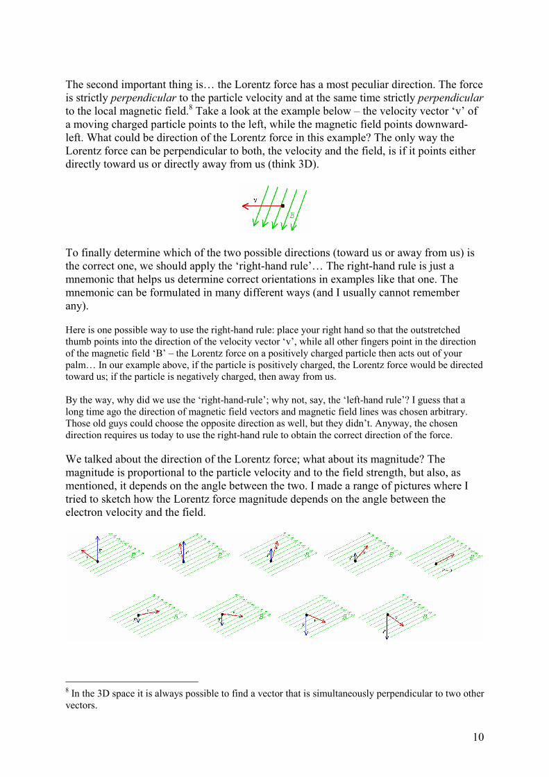
The second important thing is… the Lorentz force has a most peculiar direction. The force

is strictly perpendicular to the particle velocity and at the same time strictly perpendicular

to the local magnetic field.8 Take a look at the example below – the velocity vector ‘v’ of

a moving charged particle points to the left, while the magnetic field points downward-

left. What could be direction of the Lorentz force in this example? The only way the

Lorentz force can be perpendicular to both, the velocity and the field, is if it points either

directly toward us or directly away from us (think 3D).

To finally determine which of the two possible directions (toward us or away from us) is

the correct one, we should apply the ‘right-hand rule’… The right-hand rule is just a

mnemonic that helps us determine correct orientations in examples like that one. The

mnemonic can be formulated in many different ways (and I usually cannot remember

any).

Here is one possible way to use the right-hand rule: place your right hand so that the outstretched

thumb points into the direction of the velocity vector ‘v’, while all other fingers point in the direction

of the magnetic field ‘B’ – the Lorentz force on a positively charged particle then acts out of your

palm… In our example above, if the particle is positively charged, the Lorentz force would be directed

toward us; if the particle is negatively charged, then away from us.

By the way, why did we use the ‘right-hand-rule’; why not, say, the ‘left-hand rule’? I guess that a

long time ago the direction of magnetic field vectors and magnetic field lines was chosen arbitrary.

Those old guys could choose the opposite direction as well, but they didn’t. Anyway, the chosen

direction requires us today to use the right-hand rule to obtain the correct direction of the force.

We talked about the direction of the Lorentz force; what about its magnitude? The

magnitude is proportional to the particle velocity and to the field strength, but also, as

mentioned, it depends on the angle between the two. I made a range of pictures where I

tried to sketch how the Lorentz force magnitude depends on the angle between the

electron velocity and the field.

8 In the 3D space it is always possible to find a vector that is simultaneously perpendicular to two other

vectors.

11

On all these sketches, the red velocity vector is laying in the same plane as the field lines.

The blue force vector is perpendicular to that plane (think 3D). You can see, on the first

and on the last sketch, that the force magnitude is largest when the electron travels

perpendicularly to the magnetic field (illustratively said, when the electron cuts greatest

number of field lines per unit of time). If the velocity is parallel to the field, as on the

upper-row-rightmost picture, then no force will be acting on the electron. [If you plan to test

your right-hand-rule skills on the above sketches, just recall that an electron has a negative charge.]

Magnetic field bends trajectories of charged particles

The fact that the particle feels a force strictly perpendicular to its travel direction means

that the Lorentz force is pushing the particle aside, deflecting it from its traveling path.

Below we can see how a homogeneous magnetic field ‘B’ bends a trajectory of an

electron that enters into it with a velocity ‘v’. The depicted magnetic field is perpendicular

to the paper plane. That is, magnetic field lines extend along the depth axis. We usually

depict such perpendicular field by those x-es. Each green ‘x’ marks a place where a

magnetic field line pierces through the paper plane. The direction of the field lines is away

from us (hence x-es; if field lines were directed toward us we would typically draw them

as dots or tiny circles).

The electron comes from the right side, enters the field, makes a U-turn and exits back

toward the right side. As the electron moves through the field, the Lorentz force acts

perpendicularly to its traveling direction and continuously bends electron’s trajectory into

the U-turn. However, the speed of the electron does not change.9 [In fact, if an electron does

not manage to somehow exit the homogenous field, contrary to our example, it will continue circling.

If the electron also has a velocity component along the field lines, then it will assume a helical (like a

corkscrew) trajectory through the field.]

The Lorentz formula and the cross product

Can we quantitatively determine the Lorentz force felt by a charged particle that travels

with velocity ‘v’ through magnetic field ‘B’? Yes, we can use the famous Lorentz

formula. Here is the magnetic part of the Lorentz formula:

where ‘q’ is the charge of the particle. The ‘x’ symbol in the above formula represents the

cross-product. The cross-product is a specific type of mathematical operation on two

9 This is an approximation for low velocities. In reality a charged particle will lose some energy as its

path bends because it will radiate electromagnetic radiation (this is used in microwave ovens).

12

vectors (the ‘v’ and ‘B’ are both vectors, as well as the force ‘F’; the ‘q’ is the only scalar

in the above formula).

The cross-product is one of the two dissimilar mathematical operations to ‘multiply’ vectors (the other

one is the dot-product; the two methods produce very different results; do not interchange them).

• The result of the cross-product operation is again a vector (or a pseudovector).

• The resulting vector is perpendicular to both multiplied vectors, and its actual direction should

be chosen by the right-hand rule.

• The magnitude of the resulting vector depends on the magnitude of the multiplied vectors and

also on the angle between multiplied vectors.

Interestingly, all the properties of the cross-product fit perfectly to our needs and the cross-product

perfectly describes the force a moving charged particle feels in a magnetic field! You might be

thinking that the cross-product was invented just for this purpose, but it is not so. There are many other

examples where the cross-product also fits perfectly. The Nature seems to like it… More about the

cross-product can be found in the Appendix.

At the end of this chapter I need to be honest and say that the Lorentz force also includes

another part – the electric part. The complete Lorentz force, then, consists of its magnetic

part and its electric part. The magnetic part, as we said, is because a charged particle

might be moving through a magnetic field, while the electric part is because the particle

might be immersed in an electric field. Fortunately, the complete Lorentz formula retains

its simplicity:

This formula gives us a neat way to find out an unknown ‘B’ field. What we need to do is to balance

electric and magnetic forces so that the total force ‘F’ on electron is zero. We will know that the total

force is zero because electron trajectories won’t bend any more. Once we determine the electric field

‘E’ that balances an unknown magnetic field ‘B’, we can compute the ‘B’ using the above formula.

This method is nice because electrons do not accelerate during the measurement which avoids

radiation errors. Therefore the method is not entirely impractical to determine the field strength ‘B’,

although not something you can do in your living room.

It might interest you that the Lorentz formula is regarded as one of fundamental formulas in classical

physics. I guess, fundamental because it does not derive from other formulas – it follows directly from

observation of charged particles in electric and magnetic fields. It is also the one fundamental formula

that connects the world of material bodies with the more ethereal world of electric and magnetic fields.

Q: So, how big a circle does an electron make as it moves inside a homogeneous magnetic

field?

A: An electron speeding at about 90000 km/s (not much for an electron – this is a speed

an electron in an old CRT monitor might have) through a field of about 1T (a field of a

strong neodymium magnet) would make circles about 1 millimeter wide. Inside a much

weaker field of a refrigerator magnet it might go about 1 meter wide. A slower electron

would make tighter circles than a faster electron (interestingly, the frequency of circling

does not depend on the speed of the electron, but only on the strength of the magnetic

field).

13

3. Magnetic flux

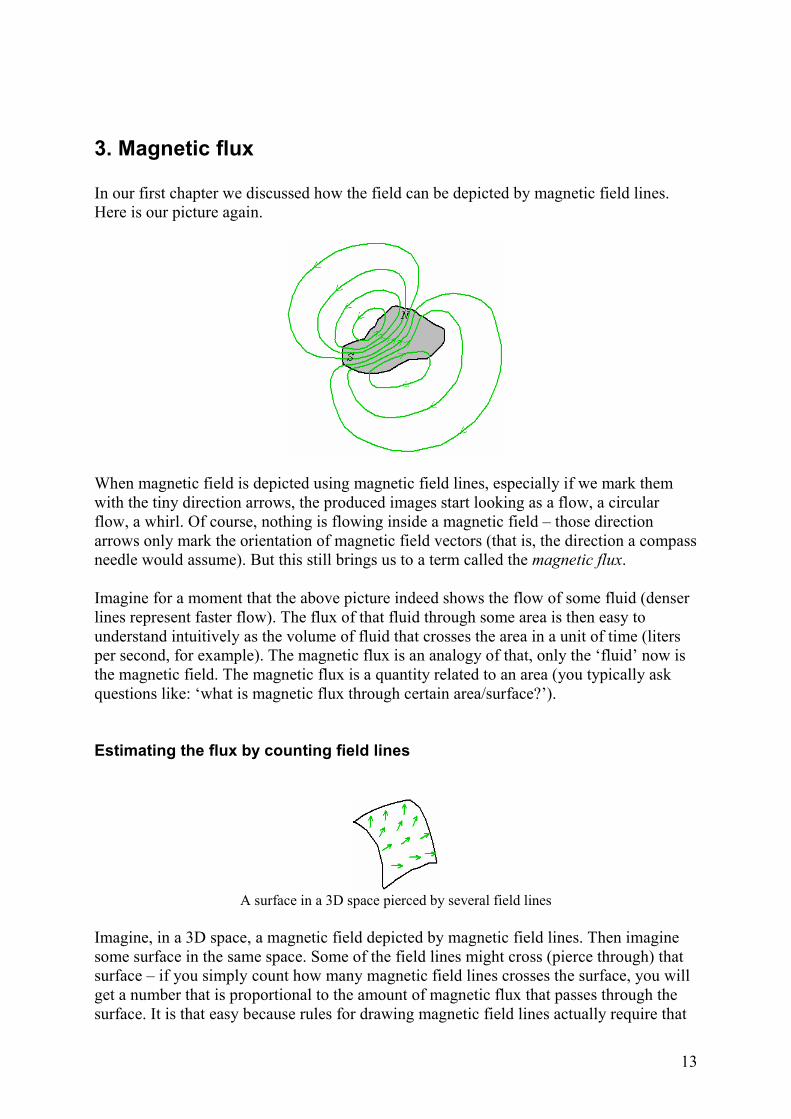
In our first chapter we discussed how the field can be depicted by magnetic field lines.

Here is our picture again.

When magnetic field is depicted using magnetic field lines, especially if we mark them

with the tiny direction arrows, the produced images start looking as a flow, a circular

flow, a whirl. Of course, nothing is flowing inside a magnetic field – those direction

arrows only mark the orientation of magnetic field vectors (that is, the direction a compass

needle would assume). But this still brings us to a term called the magnetic flux.

Imagine for a moment that the above picture indeed shows the flow of some fluid (denser

lines represent faster flow). The flux of that fluid through some area is then easy to

understand intuitively as the volume of fluid that crosses the area in a unit of time (liters

per second, for example). The magnetic flux is an analogy of that, only the ‘fluid’ now is

the magnetic field. The magnetic flux is a quantity related to an area (you typically ask

questions like: ‘what is magnetic flux through certain area/surface?’).

Estimating the flux by counting field lines

A surface in a 3D space pierced by several field lines

Imagine, in a 3D space, a magnetic field depicted by magnetic field lines. Then imagine

some surface in the same space. Some of the field lines might cross (pierce through) that

surface – if you simply count how many magnetic field lines crosses the surface, you will

get a number that is proportional to the amount of magnetic flux that passes through the

surface. It is that easy because rules for drawing magnetic field lines actually require that

14

each field line represents an equal amount of magnetic flux. We can guess that the original

idea behind field lines was not to depict the magnetic field, but to depict the magnetic

flux.

Important note: when counting magnetic field lines, count lines that pierce a surface from

one side as positive, and those that pierce it from the opposite side as negative – it is the

net count that actually represents the total magnetic flux through the surface.

In magnetism, a common example of a surface in a 3D space would be the smallest-area surface

bounded by a wire loop. (Another 3D surface example, but completely unrelated to magnetism, would

be a sail on a sailing boat.) A surface encircled by a wire loop would be an example of an ‘open

surface’. An open surface has an ‘edge’ that you can cross and reach the other side of the surface. A

‘closed surface’, on the other hand, has no such edge and an ant traveling over the closed surface

won’t be able to reach the other side – an example would be the surface of a ball. A closed surface

encloses a volume, completely separating it from the rest of the space.

On the example below we see a rectangular wire loop partially immersed into a magnetic

field. You can count that four of the magnetic field lines ‘travel’ inside the loop and

therefore these four field lines represent the magnetic flux that passes (‘flows’) through

the wire loop surface.

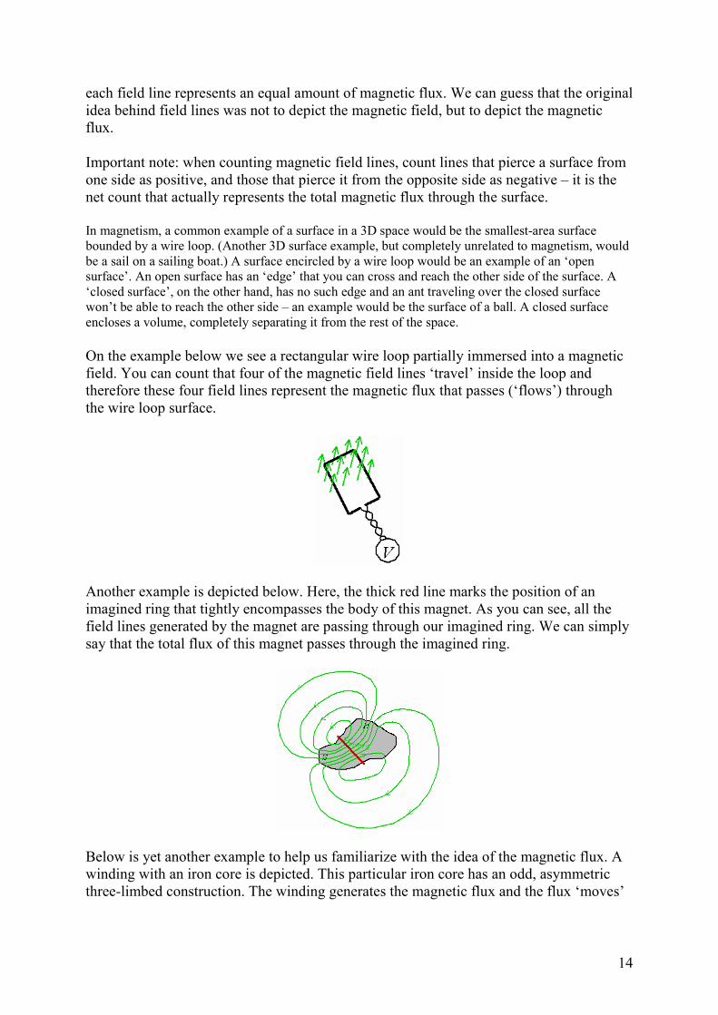
Another example is depicted below. Here, the thick red line marks the position of an

imagined ring that tightly encompasses the body of this magnet. As you can see, all the

field lines generated by the magnet are passing through our imagined ring. We can simply

say that the total flux of this magnet passes through the imagined ring.

Below is yet another example to help us familiarize with the idea of the magnetic flux. A

winding with an iron core is depicted. This particular iron core has an odd, asymmetric

three-limbed construction. The winding generates the magnetic flux and the flux ‘moves’

15

through the iron (magnetic flux likes to ‘move’ through iron; we will talk more about it in

chapter 13).

Regarding the above picture, I could speak like this: the total flux generated by the

winding goes up through the middle (B) limb and then splits into two fluxes. The smaller

of the two fluxes passes down through the leftmost (A) limb, while the larger one passes

down through the rightmost (C) limb… Such way of speaking is simplified and probably

incorrect, but gives an intuitive feeling what a flux is… If I ask you how big is the flux

that passes through the leftmost (A) limb, you should count the magnetic field lines and

provide an answer: only about one third of the total flux passes through the A limb.

Mathematical definition of the magnetic flux

Here is a more mathematical definition of a magnetic flux ‘Φ’ through a surface ‘S’: the

magnetic flux through a surface equals to the surface integral10 of the magnetic field.

I am only showing this scary-looking formula to illustrate how representing a magnetic

field using magnetic field lines (instead of magnetic field vectors) makes it easier to

intuitively understand the concept of the magnetic flux. [By the way, the dot symbol in the

above formula represents the ‘dot product’ – you can read more about it in the appendix. The ‘B’ as

well as the ‘dS’ are vectors in this formula. The magnetic flux ‘Φ’ is a scalar.]

The magnetic flux is usually denoted by the Greek letter Φ and its unit is weber [Wb –

note: one tesla is one weber per one square meter]. One weber is a large unit and you will

rarely encounter a magnet so large and/or so powerful to generate one weber of magnetic

flux through its body. (Well, the total flux of the planet Earth might reach giga-weber

range. Size matters.)

It appears that the concept of magnetic flux was important to old scientists – so much so

that they even called vectors of the B-field the ‘magnetic flux density’. This name is also

in use today, but I find it confusing – I prefer to call the B-field simply the ‘magnetic

field’ and to call vectors of the B-field the ‘magnetic field vectors’.

10 More about surface integrals can be found in the Appendix.

16

The magnetic flux continues to be an important concept in magnetism, almost as

important as the concept of the magnetic field itself. We will use it often, especially when

dealing with electromagnetic induction… If you still don’t have an intuitive feeling what

is the difference between the magnetic flux and the magnetic field strength, you should

memorize that on a correctly drawn picture, the magnetic flux is represented by the

number of magnetic field lines, while the strength of magnetic field is represented by the

density (concentration) of field lines.

The Gauss law for magnetic field

There is a law regarding magnetic fields: the total magnetic flux through any closed 3D

surface is always zero... An example of a closed surface is the surface of a magnet body.

Therefore the number of magnetic field lines that exit the magnet body is equal to the

number of magnetic field lines that enter the magnet body. This is a no-brainer because

we insist that magnetic field lines are always closed loops (every line that exits the magnet

body, must also return – so it cancels itself). The law, sometimes called the Gauss law for

magnetic field, is an important property of magnetic fields; it separates magnetic fields

into a specific sub-class of vector fields.

Not all vector fields obey the stated law. The electric field, for example, does not. The flux of the

electric field over a closed surface does not have to be zero. This is because the electric field originates

from charges (it diverges from positive charges and converges into negative charges)… The magnetic

field however obeys the Gauss law. We say: the magnetic field is such a vector field that has zero

divergence everywhere; it is a divergenceless field. (This is just another way to say that magnetic field

lines are closed lines that have no origin point and do not sink into any destination point. Yet another

way to say the same: there are no magnetic charges.)

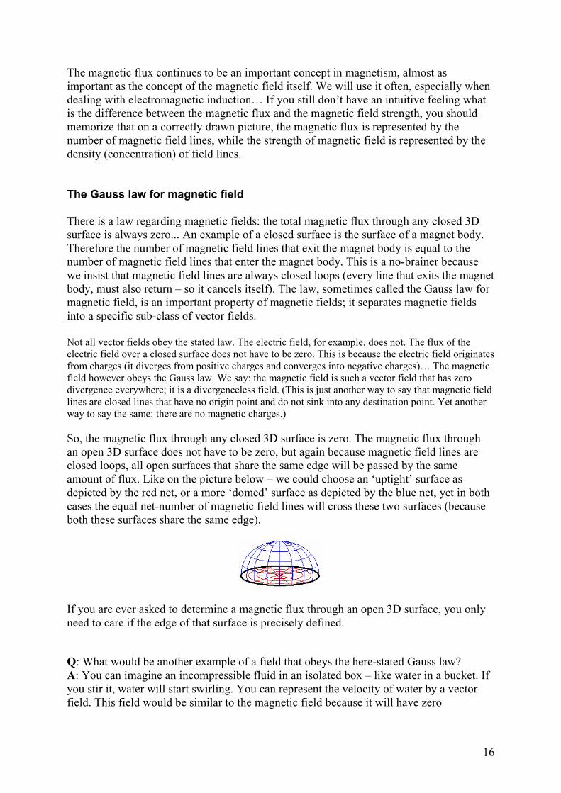
So, the magnetic flux through any closed 3D surface is zero. The magnetic flux through

an open 3D surface does not have to be zero, but again because magnetic field lines are

closed loops, all open surfaces that share the same edge will be passed by the same

amount of flux. Like on the picture below – we could choose an ‘uptight’ surface as

depicted by the red net, or a more ‘domed’ surface as depicted by the blue net, yet in both

cases the equal net-number of magnetic field lines will cross these two surfaces (because

both these surfaces share the same edge).

If you are ever asked to determine a magnetic flux through an open 3D surface, you only

need to care if the edge of that surface is precisely defined.

Q: What would be another example of a field that obeys the here-stated Gauss law?

A: You can imagine an incompressible fluid in an isolated box – like water in a bucket. If

you stir it, water will start swirling. You can represent the velocity of water by a vector

field. This field would be similar to the magnetic field because it will have zero

17

divergence everywhere (because water is incompressible and we have no sinks and no

springs in the bucket).

You may use the mental image of water in a bucket if it helps you to better understand the

magnetic flux and the magnetic field. The magnetic flux would be analogue to the flow of

water, while strength of magnetic field would be analogue to the velocity of water… You

might even imagine how a needle placed in the bucket aligns itself with the water flow.

You might imagine magnets as little pumps that stir the water in the bucket… But don’t

go too far in that direction. The magnetic field is not water in a bucket.

4. Permanent magnet

Previous chapters often referred to permanent magnets and I feel responsible to say more

about them.

Today, practically all permanent magnets are made artificially in factories and are cast in

various useful shapes and sizes. Many of them have two magnetic poles, but some have

hundreds11. Magnets can be made from various alloys that differ in properties – some

magnets are weak (but cheap), while some are strong (but expensive). Other interesting

properties describe how much is a magnet able to retain its magnetism under certain stress

(like high temperature, hammering or opposing fields of other magnets), how

mechanically strong it is or how much flux it produces per kilogram of weight.

Two permanent magnet examples are shown above. The left-side depicts a bar magnet

while the right-side depicts a C-shaped magnet. You can see that the bar magnet spreads

its magnetic field all over the place and keeps it concentrated (strong) only near its poles

and within its body. The C-shaped magnet has an air-gap where it generates relatively

concentrated and homogeneous magnetic field – narrower the gap, more homogenous the

field. Yes, even the C-shaped magnet has few magnetic field lines that run all over the

place but these are relatively rare and I didn’t even bother drawing them. And no, the field

lines will not take those 90-degree sharp turns (this is me being lazy at drawing) – field

lines have smooth, round corners.

11 The concept of magnetic pole is not very insightful. Poles are just places at the magnet surface near

local maxima of field strength… I mentioned a magnet with hundred poles – find it inside a stepper

motor. Want more? There are billions of poles at the surface of a computer hard disk.

18

The magnetic dipole moment

In our first chapter we used one small bar magnet (a compass needle) to probe a magnetic

field. Therefore we already know that if we place a bar magnet into a magnetic field (of

another magnet, for example) our bar magnet will try to align itself with the direction of

the field. If not aligned, the bar magnet will feel a torque that will try to rotate it into the

aligned direction. How much torque?

For a magnet we can define a property called the ‘magnetic dipole moment’.12 It tells how

much torque the magnet will feel if placed into a magnetic field of certain strength. The

magnetic dipole moment is a vector value. Its direction tells how the magnet will orient in

the field. For example, a compass needle has its magnetic dipole moment vector directed

from its south tip toward its north tip and so it will try to align this axis with the field.

The magnetic dipole moment is sometimes denoted with the letter ‘m’ (more often with

the letter ‘µµµµ’, but I am saving this letter for other purpose). If we know the magnetic

dipole moment ‘m’ of some magnet, we can compute the torque ‘τ’ it feels in a

homogeneous magnetic field ‘B’ using the following cross-product formula:

The largest torque is developed if the magnet is oriented perpendicularly across the field.

The torque is zero if the magnet and the field are aligned (also if anti-aligned, but this

orientation is unstable – even a tiny disturbance causes the magnet to flip over).

[You possibly noticed that we already used the above formula… In the first chapter we probed the

field by measuring torques it exerts on a compass needle. We had to divide the measured torques by

the magnetic moment ‘m’ of the compass needle to obtain the field ‘B’. We used the above relation,

but in the way to find out the ‘B’ from ‘m’ and ‘τ’.]

If we tear a magnet into pieces, then for each piece we can again find its magnetic dipole

moment. As expected, the total moment of the whole magnet equals to vector sum of

magnetic moments of its pieces (supposing that we retain orientation of each piece as it

was when the magnet was intact).

Magnetization

Another property related to magnets is called ‘magnetization’. It is actually a property of

material that makes the magnet. A material, iron for example, can have various levels of

magnetization. You can have a non-magnetized iron or an iron magnetized to saturation

level or anything in between. Even a single chunk of iron can have varying levels of

magnetization over its volume – and not only the magnitude, also the direction of the

12 Or just 'magnetic moment'... but I find both names clumsy. I guess the naming came from the

concept of ‘magnetic dipole’. A magnetic dipole can be though as an infinitely small, yet infinitely

intense bar magnet that generates a finite flux (I guess this is how in old days people imagined an

elementary magnetic particle or maybe an ‘essence of a magnet’).

19

magnetization might vary over the chunk’s volume… Magnetization is a vector value; it

has a direction.

If you integrate the magnetization of the material over the whole volume of a magnet, you

will obtain the magnetic dipole moment ‘m’ of that magnet. This comes from the

definition: magnetization is magnetic moment of a volume of magnetic material divided

by the volume when the volume tends toward zero.

A magnet that is strongly magnetized over its whole body does not have to have a large total magnetic

dipole moment. If the magnetization is not unidirectional then it might partially or totally cancel out.

Take for example the C-shaped magnet from the beginning of this chapter. It has a more voluminous

body than the similarly-magnetized bar-shaped magnet depicted next to it. Yet, being bent into an

almost closed shape, it certainly has a smaller magnetic dipole moment than the bar-shaped magnet.

Linear (translational) forces felt by permanent magnets

When immersed into an external magnetic field, a permanent magnet can, in addition to

torque (that tries to rotate it), feel a net force (that tries to translate it). All kids know

this… Yet, a magnet will not feel any translational force if we place it into a perfectly

homogenous (uniform) magnetic field. If we want our magnet attracted or repelled, we

must place it into a field that has some spatial change of intensity.

To quench your curiosity, I can give a formula that tells the force a small magnet feels when immersed

into a non-homogenous field:

The ‘m’ is the magnetic dipole moment of the magnet, while ‘B’ is the strength of the magnetic field.

The ∇ symbol represents the gradient (see the Appendix) of the ‘m·B’ field… This formula

disappoints you because it is not very practical. I however mention it so that you see how the field

must have a spatial intensity change (to be non-homogenous) to produce a translational force.

[By the way, you might know already that the force can be expressed as the gradient of the potential

energy. The ‘m·B’ factor is a value that could represent the potential energy of a small magnet in a

static field… although the idea of potential energy has its limitations in the magnetic field case.]

[While a homogeneous magnetic field cannot produce a translational force, it can produce torque…

This is why in our first chapter we were measuring torques (instead of forces) to describe and define

the magnetic field – torques are proportional to the field strength, while forces are not.]

Calculating the net force, attractive or repulsive, that a permanent magnet might feel when

immersed into a non-homogenous magnetic field is a difficult quest… This leads us to the

real purpose of this entire chapter. It is to tell you that permanent magnets are painfully

complex and that we should read easier chapters first. Even then, our insight into

permanent magnets will remain limited.

Q: So what is it inside a permanent magnet that makes it magnetic?

A: Primarily, spin magnetic moments of unpaired electrons. In permanent magnets, some

electrons have their magnetic moments aligned (or better said, not completely

20

randomized) and this generates the macroscopically observable magnetic field. I will talk

a bit more about it in the chapter 13.

Q: What is actually meant by the ‘strength’ of a magnet?

A: The strength of a magnet is not a value that is well defined; you should avoid that term.

It might mean (but is not limited to) any one of the following three things: the magnetic

moment that a magnet has, the total flux the magnet produces, or the strongest field the

magnet produces.

5. Current-carrying wires

People played with naturally-occurring permanent magnets for centuries. Eventually

someone invented electric current and then all hell breaks loose. It became even more

interesting when scholars found an intimate relationship between electric current and

magnetic field.

Scholars placed a compass needle near a current-carrying wire and the needle reacted.

They concluded that current-carrying wires generate magnetic field whose strength is

proportional to the current intensity. Then they probed and measured the shape of the

magnetic field around a current-carrying wire. Much to their surprise they found that the

field encircles the wire. That seemed, at first, quite dissimilar to permanent magnets. With

permanent magnets, field lines exit and enter the magnet body, but in the case of current-

carrying wires the field lines are neither exiting nor entering the wire body – just encircle

the wire.

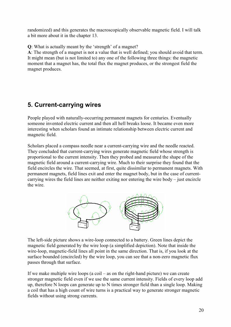
The left-side picture shows a wire-loop connected to a battery. Green lines depict the

magnetic field generated by the wire loop (a simplified depiction). Note that inside the

wire-loop, magnetic-field lines all point in the same direction. That is, if you look at the

surface bounded (encircled) by the wire loop, you can see that a non-zero magnetic flux

passes through that surface.

If we make multiple wire loops (a coil – as on the right-hand picture) we can create

stronger magnetic field even if we use the same current intensity. Fields of every loop add

up, therefore N loops can generate up to N times stronger field than a single loop. Making

a coil that has a high count of wire turns is a practical way to generate stronger magnetic

fields without using strong currents.

21

[Once people realized that current-carrying wire loops create magnetic fields, they started speculating

that electric currents also cause fields of permanent magnets. People imagined eternal circular currents

swirling within magnet body… indeed, this has some merit.]

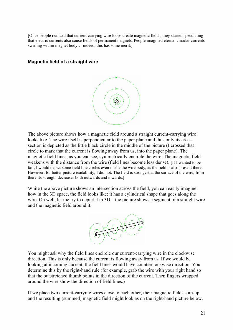
Magnetic field of a straight wire

The above picture shows how a magnetic field around a straight current-carrying wire

looks like. The wire itself is perpendicular to the paper plane and thus only its cross-

section is depicted as the little black circle in the middle of the picture (I crossed that

circle to mark that the current is flowing away from us, into the paper plane). The

magnetic field lines, as you can see, symmetrically encircle the wire. The magnetic field

weakens with the distance from the wire (field lines become less dense). [If I wanted to be

fair, I would depict some field line circles even inside the wire body, as the field is also present there.

However, for better picture readability, I did not. The field is strongest at the surface of the wire; from

there its strength decreases both outwards and inwards.]

While the above picture shows an intersection across the field, you can easily imagine

how in the 3D space, the field looks like: it has a cylindrical shape that goes along the

wire. Oh well, let me try to depict it in 3D – the picture shows a segment of a straight wire

and the magnetic field around it.

You might ask why the field lines encircle our current-carrying wire in the clockwise

direction. This is only because the current is flowing away from us. If we would be

looking at incoming current, the field lines would have counterclockwise direction. You

determine this by the right-hand rule (for example, grab the wire with your right hand so

that the outstretched thumb points in the direction of the current. Then fingers wrapped

around the wire show the direction of field lines.)

If we place two current-carrying wires close to each other, their magnetic fields sum-up

and the resulting (summed) magnetic field might look as on the right-hand picture below.

22

The picture depicts the situation when currents in both wires flow in the same direction

(away from us, in this case).

Please note that the left-side picture above shows a wrong way to depict a magnetic field (recall, field

lines should not cross each other). When you put two magnetic objects close together, only their

summed field actually exists, as it is correctly depicted on the right-side picture… Despite this and

stubbornly enough, I will still often depict fields of separate objects in the incorrect ‘intermeshed’ way

whenever I feel this adds to clarity (for example, when I want to explain how the objects interact with

physical forces).

It is good to note that at a far distance from the above two wires (far in comparison to the

distance between wires), the magnetic field will look quite circular – as if we are dealing

with magnetic field generated by one single wire that is carrying the double current

intensity.

The opposite case, when two parallel wires carry currents in opposite direction, is

depicted below. (The cross-section of a wire that carries current from the paper plane

toward the observer is usually depicted as a dot in the circle.)

In the above case, if we suppose that both wires carry equal currents, the magnetic field

will quickly drop to virtually zero at some appreciable distance from the wires.

(Interestingly, the field between the two wires grows stronger if the wires are getting

closer to each other.)

Magnetic field of a wire loops and coils

We can also depict the magnetic field of a current-carrying wire loop (below left) and of a

small coil (also called a solenoid or a winding - below right). I depicted cross-sections of

the loop, the coil and their magnetic fields, but you can imagine how in the 3D space both

fields are rotationally symmetric.

23

As you can see it on the right-side picture, the magnetic field of a coil (solenoid) looks

much like the magnetic field of a bar-shaped permanent magnet. We could even say that

the solenoid has its north and south poles (here, north being to the left). The field is the

strongest inside the solenoid (densest field lines) – which again is like with a bar magnet,

but with the benefit that the solenoid’s interior field is actually accessible. The total flux

of the solenoid, all its field lines, passes through its interior. Also, inside the solenoid the

field is relatively homogenous13.

Magnetic field of a wire loops in a plane

What if we place many current-carrying loops side-by-side in one single plane? The left-

side picture below shows several identical hexagonal loops that make a honeycomb

figure. All the loops carry the current of same intensity in the same clockwise direction.

The current direction is marked by arrows.

Recall what we said: if two nearby wires carry the same current in the opposite direction,

then with distance their combined field will quickly drop to practically zero. As a result,

all those currents that flow in the interior of the depicted honeycomb figure can be

disregarded. At some appreciable distance the combined magnetic field of all these

hexagonal loops will look as if there is only one large current-carrying loop that encircles

the whole figure (the right-side picture).

13 Homogenous fields are often sought (for example, to make accurate measurements) and people

invent various coil constructions to generate as homogenous magnetic fields as possible

24

Why am I mentioning this? A permanent magnet can be considered as a combination of

zillions of tiny current loops14 that all carry the current in the same direction. Therefore,

we can sometimes model a permanent magnet as a body that generates its magnetic field

as if macroscopic currents are circulating over its surface. Such model generates a field of

equal shape as the real permanent magnet. Yet, real magnets have no macroscopic

currents on their surfaces, but zillions of ultra-small current loops embedded within their

bodies.

Magnetic field of ‘current walls’ and toroidal coils

At the end I want to mention several special configurations of current-carrying wires. For

example, a ‘current wall’ (a.k.a. ‘current sheet’) – this is an infinite wall made of infinitely

long wires, all of them carrying identical current into the same direction. On the picture

below, it can be seen that the wall produces infinite homogenous magnetic field on both

its sides. The direction of the field is parallel to the wall, but opposite on each side of the

wall. Notably, the strength of the magnetic field is not diminishing with the distance from

the infinite current wall15.

Next, we have two infinite ‘current walls’ in parallel (the picture below). In the depicted

setup the magnetic field exists only between the two walls. As the two walls have the

same current intensities, but opposite current directions, the outside fields get canceled,

while the inside field is doubled (you obtain this by simple vector addition of fields

generated by the two current walls).

Imagine now an infinitely long coil/solenoid. A longitudinal cross-section of such infinite

solenoid is depicted below. In this case we have magnetic field that is entirely confined

within the coil tube. There are no field lines outside the tube.

14 When I say 'current-loop' I mean a closed-path current of any kind (like an electron 'orbiting' the

nucleus). When I say 'wire-loop' I mean a more specific macroscopic thing made of a conductive wire. 15 Why it is not diminishing with the distance? A point farther from the wall 'sees' more wires at

favorable angles (near-perpendicular) than a closer point. So, for a farther point more wires sum their

fields more constructively.

25

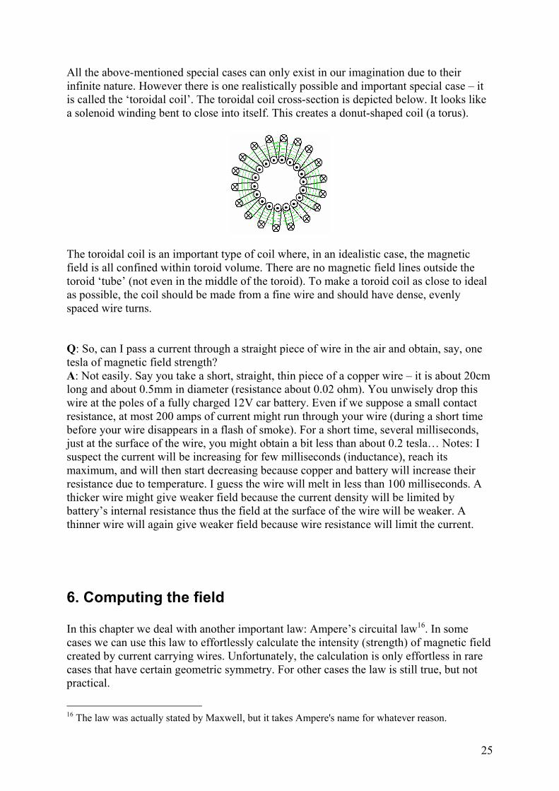
All the above-mentioned special cases can only exist in our imagination due to their

infinite nature. However there is one realistically possible and important special case – it

is called the ‘toroidal coil’. The toroidal coil cross-section is depicted below. It looks like

a solenoid winding bent to close into itself. This creates a donut-shaped coil (a torus).

The toroidal coil is an important type of coil where, in an idealistic case, the magnetic

field is all confined within toroid volume. There are no magnetic field lines outside the

toroid ‘tube’ (not even in the middle of the toroid). To make a toroid coil as close to ideal

as possible, the coil should be made from a fine wire and should have dense, evenly

spaced wire turns.

Q: So, can I pass a current through a straight piece of wire in the air and obtain, say, one

tesla of magnetic field strength?

A: Not easily. Say you take a short, straight, thin piece of a copper wire – it is about 20cm

long and about 0.5mm in diameter (resistance about 0.02 ohm). You unwisely drop this

wire at the poles of a fully charged 12V car battery. Even if we suppose a small contact

resistance, at most 200 amps of current might run through your wire (during a short time

before your wire disappears in a flash of smoke). For a short time, several milliseconds,

just at the surface of the wire, you might obtain a bit less than about 0.2 tesla… Notes: I

suspect the current will be increasing for few milliseconds (inductance), reach its

maximum, and will then start decreasing because copper and battery will increase their

resistance due to temperature. I guess the wire will melt in less than 100 milliseconds. A

thicker wire might give weaker field because the current density will be limited by

battery’s internal resistance thus the field at the surface of the wire will be weaker. A

thinner wire will again give weaker field because wire resistance will limit the current.

6. Computing the field

In this chapter we deal with another important law: Ampere’s circuital law16. In some

cases we can use this law to effortlessly calculate the intensity (strength) of magnetic field

created by current carrying wires. Unfortunately, the calculation is only effortless in rare

cases that have certain geometric symmetry. For other cases the law is still true, but not

practical.

16 The law was actually stated by Maxwell, but it takes Ampere's name for whatever reason.

26

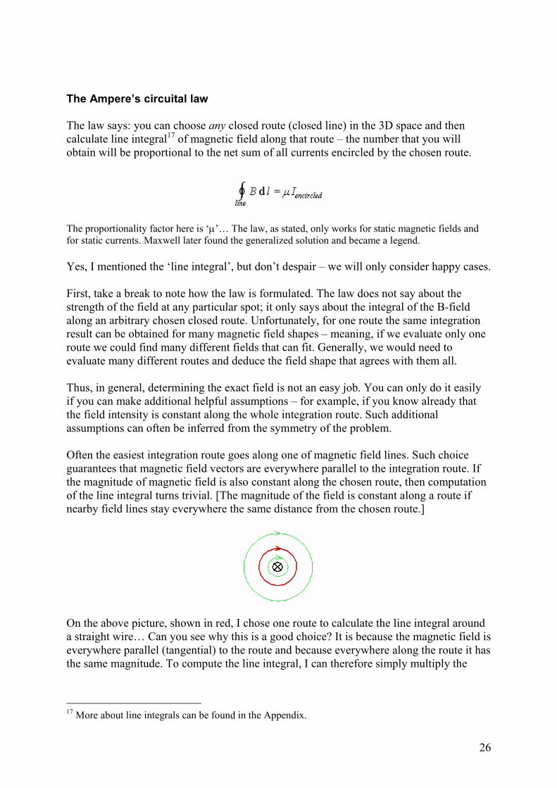
The Ampere’s circuital law

The law says: you can choose any closed route (closed line) in the 3D space and then

calculate line integral17 of magnetic field along that route – the number that you will

obtain will be proportional to the net sum of all currents encircled by the chosen route.

The proportionality factor here is ‘µ’… The law, as stated, only works for static magnetic fields and

for static currents. Maxwell later found the generalized solution and became a legend.

Yes, I mentioned the ‘line integral’, but don’t despair – we will only consider happy cases.

First, take a break to note how the law is formulated. The law does not say about the

strength of the field at any particular spot; it only says about the integral of the B-field

along an arbitrary chosen closed route. Unfortunately, for one route the same integration

result can be obtained for many magnetic field shapes – meaning, if we evaluate only one

route we could find many different fields that can fit. Generally, we would need to

evaluate many different routes and deduce the field shape that agrees with them all.

Thus, in general, determining the exact field is not an easy job. You can only do it easily

if you can make additional helpful assumptions – for example, if you know already that

the field intensity is constant along the whole integration route. Such additional

assumptions can often be inferred from the symmetry of the problem.

Often the easiest integration route goes along one of magnetic field lines. Such choice

guarantees that magnetic field vectors are everywhere parallel to the integration route. If

the magnitude of magnetic field is also constant along the chosen route, then computation

of the line integral turns trivial. [The magnitude of the field is constant along a route if

nearby field lines stay everywhere the same distance from the chosen route.]

On the above picture, shown in red, I chose one route to calculate the line integral around

a straight wire… Can you see why this is a good choice? It is because the magnetic field is

everywhere parallel (tangential) to the route and because everywhere along the route it has

the same magnitude. To compute the line integral, I can therefore simply multiply the

17 More about line integrals can be found in the Appendix.

27

length of the route (2rπ) with the magnitude of the magnetic field along it (B). So, the

Ampere’s law equation simplifies to:

The left side of the above formula is the computed line integral of the field ‘B’ at the

distance ‘r’ from the wire centre. The right-side of the formula is the encircled current ‘I’

multiplied by the proportionality factor ‘µ’.

Similarly, an easy integration route is chosen for the toroidal coil below. Computing the

line integral is again trivial for the same reason. The computed line integral is proportional

to currents carried by 18 encircled ‘inner’ wires of the toroid.

Why 18 wires? If you imagine a surface bounded by our chosen route, you will count that

this imagined surface is pierced 18 times by the current carrying wire – and each time it is

pierced from the same direction (toward us, in the depicted case).

What if we choose an integration route totally outside the toroid, as depicted below? We

did learn already that there is no magnetic field outside the toroid. We therefore know that

the line integral is zero… Okay, if the line integral is zero then, according to the Ampere’s

law, also the encircled current must be zero. Is it?

Yes, it is. To check it, we will again examine the surface bounded by our route. If we

assume an uptight surface that intersects the toroidal coil, then we will count as many

currents piercing the surface from one side as from the other side, making the net Iencircled

equal to zero. On the other hand, if we assume a ‘domed’ surface that bends around the

toroidal coil, then no current pierces this surface making the Iencircled again zero.

28

The Biot-Savart law

How do we calculate the magnetic field produced by current-carrying wires when we

don’t have such a neat symmetric problem? The Ampere’s law becomes impractical.

People my then resort to the Biot-Savart law. It gives the field at some particular spot:

The Biot-Savart law is quite mathematical and I am only mentioning it here. It introduces

an interesting concept of an infinitely small current segment ‘I·dl’. You can imagine the

current segment as a very short piece of a wire that has the length ‘dl’ and carries the

current ‘I’. Each such current segment contributes a small part of the magnetic field at the

spot we are interested in. The Biot-Savart formula simply sums (integrates) all these

contributions of all the current segments along a wire to obtain the total magnetic field at

the evaluated spot.

[In the Biot-Savart formula, the |r| is the distance between a current segment and the evaluated spot,

while the r-with-hat is the unit vector directed from the current segment toward the evaluated spot.]

The magnetic permeability

What is the proportionality factor ‘µ’ in the above formulas? The factor ‘µ’ is called the

‘magnetic permeability’ and is a scalar value. It has different values in different materials

and therefore we can talk about magnetic permeabilities of various materials.

The ‘µ’ factor says how strong magnetic field will a current-carrying wire generate if

immersed in certain material. For example, a current carrying wire placed in water will

create a slightly different filed strength than if placed in air (at the same distance from the

wire). Therefore, if you care to obtain a very accurate result, you will need to use slightly

different magnetic permeability constant ‘µ’ for air and for water.

For vacuum, the constant is called ‘magnetic permeability of vacuum’, it is marked as

‘µ0’, and it equals to: µ0=4·π·10-7 H/m.18 You will see this constant often and in various

equation settings.

The magnetic permeability of most materials is only a little bit larger or smaller than that

of vacuum. For air, we can take the same value as for vacuum because the difference is

negligible. But there are exceptions: ferromagnetic materials, in particular, may have

magnetic permeabilities many thousand times greater than that of vacuum.

18 The unit is: henry per meter. This one is the most common, but you can express the permeability

unit in different ways, like N/A2 or T·m/A or kg·m/A

2/s

2... It is all the same.

29

One example: The magnetic field around an extremely long and straight thin wire, placed

alone in the vacuum of the Universe, must be symmetric. That is, magnetic field lines

must form perfect circles around the wire (what else could they look like, after all19).

According to the Ampere’s law, all line integrals along any of these circular field lines

must give the same result, and this result equals to the wire current multiplied by µ0. From

this we can conclude that the strength of magnetic field must be decreasing inversely

proportionally with the distance from the wire. Why? Because lengths of field lines that

are circumferencing the wire increase proportionally with their distance from the wire

center (as 2·r·π) and therefore magnetic field strength must decrease inversely in order to

yield the same integration result. If the wire carries 1A of current, then at 1m radius from

the wire center, the magnetic field will be exactly B=2·10-7 T.

You might be suspicious about the value of the magnetic permeability of vacuum – why

exactly 4·π·10-7 H/m? It is because how we defined the unit of ampere – the ampere is

defined by the attractive force between two long, straight current-carrying wires placed

one meter apart in a vacuum. If the force between wires is exactly 2·10-7 N per every

meter of length, then the current intensity in the wires is 1 ampere, by definition.

Personally, I only acknowledge one fundamental constant, the ‘magnetic permeability of vacuum’- µ0.

This constant is one of the basic properties of our Universe. The presence of matter introduces

additional magnetic effects (diamagnetism, parmagnetism, ferromagnetism… we will talk about them

later) that are difficult to analyze from first principles and so we often tend to sum them up into a

magnetic permeability value µ that characterizes a material. However, all those permeabilities of

various materials do not have the same level of fundamentality as the magnetic permeability of

vacuum, µ0.

Q: But in what direction should I compute the line integral of the Ampere’s law?

A: Any direction is good, but mind that the integration direction and the positive direction

of the Iencircled correlate... For example, grab the integration route with your right hand so

that your fingers curl in the integration direction, the outstretched thumb then shows the

direction of Iencircled current that is to be taken as positive.

7. Electromagnetic induction

Not only current-carrying wires create magnetic fields, but changing magnetic fields also

induce voltages and currents in wires! This is called the ‘electromagnetic induction’.

First described by Michael Faraday, some 200 years ago, the electromagnetic induction is

one of the mankind’s finest discoveries. Most notably, we employ it inside power plant

generators to convert mechanical energy into electric energy.

19 This comes from the symmetry of the space. We could hardly justify a magnetic field of any other

shape but perfectly rotationally symmetric along the straight, thin, long, circular-intersection wire.

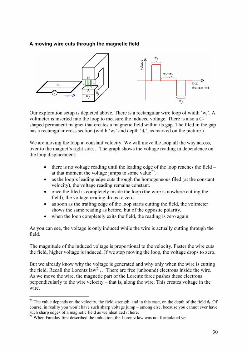
30

A moving wire cuts through the magnetic field

Our exploration setup is depicted above. There is a rectangular wire loop of width ‘wl’. A

voltmeter is inserted into the loop to measure the induced voltage. There is also a C-

shaped permanent magnet that creates a magnetic field within its gap. The filed in the gap

has a rectangular cross section (width ‘wf’ and depth ‘df’, as marked on the picture.)

We are moving the loop at constant velocity. We will move the loop all the way across,

over to the magnet’s right side… The graph shows the voltage reading in dependence on

the loop displacement:

• there is no voltage reading until the leading edge of the loop reaches the field –

at that moment the voltage jumps to some value20.

• as the loop’s leading edge cuts through the homogeneous filed (at the constant

velocity), the voltage reading remains constant.

• once the filed is completely inside the loop (the wire is nowhere cutting the

field), the voltage reading drops to zero.

• as soon as the trailing edge of the loop starts cutting the field, the voltmeter

shows the same reading as before, but of the opposite polarity.

• when the loop completely exits the field, the reading is zero again.

As you can see, the voltage is only induced while the wire is actually cutting through the

field.

The magnitude of the induced voltage is proportional to the velocity. Faster the wire cuts

the field, higher voltage is induced. If we stop moving the loop, the voltage drops to zero.

But we already know why the voltage is generated and why only when the wire is cutting

the field. Recall the Lorentz law21… There are free (unbound) electrons inside the wire.

As we move the wire, the magnetic part of the Lorentz force pushes these electrons

perpendicularly to the wire velocity – that is, along the wire. This creates voltage in the

wire.

20 The value depends on the velocity, the field strength, and in this case, on the depth of the field df. Of

course, in reality you won’t have such sharp voltage jump – among else, because you cannot ever have

such sharp edges of a magnetic field as we idealized it here. 21 When Faraday first described the induction, the Lorentz law was not formulated yet.

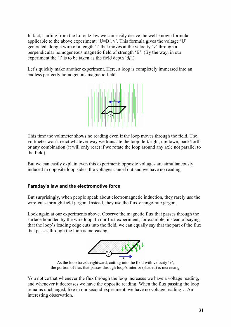
31

In fact, starting from the Lorentz law we can easily derive the well-known formula

applicable to the above experiment: ‘U=B·l·v’. This formula gives the voltage ‘U’

generated along a wire of a length ‘l’ that moves at the velocity ‘v’ through a

perpendicular homogeneous magnetic field of strength ‘B’. (By the way, in our

experiment the ‘l’ is to be taken as the field depth ‘df’.)

Let’s quickly make another experiment. Here, a loop is completely immersed into an

endless perfectly homogenous magnetic field.

This time the voltmeter shows no reading even if the loop moves through the field. The

voltmeter won’t react whatever way we translate the loop: left/right, up/down, back/forth

or any combination (it will only react if we rotate the loop around any axle not parallel to

the field).

But we can easily explain even this experiment: opposite voltages are simultaneously

induced in opposite loop sides; the voltages cancel out and we have no reading.

Faraday’s law and the electromotive force

But surprisingly, when people speak about electromagnetic induction, they rarely use the

wire-cuts-through-field jargon. Instead, they use the flux-change-rate jargon.

Look again at our experiments above. Observe the magnetic flux that passes through the

surface bounded by the wire loop. In our first experiment, for example, instead of saying

that the loop’s leading edge cuts into the field, we can equally say that the part of the flux

that passes through the loop is increasing.

As the loop travels rightward, cutting into the field with velocity ‘v’,

the portion of flux that passes through loop’s interior (shaded) is increasing.

You notice that whenever the flux through the loop increases we have a voltage reading,

and whenever it decreases we have the opposite reading. When the flux passing the loop

remains unchanged, like in our second experiment, we have no voltage reading… An

interesting observation.

32

We can say one clever thing about electromagnetic induction: the voltage induced in a

wire loop equals to the rate of change of magnetic flux that passes through the surface

bounded by the wire loop. This is known as the ‘Faraday’s law of induction’ and is

mathematically given by the suspiciously simple formula:

The left side of the formula is the voltage induced in the loop. This induced voltage is

often called the electromotive force (EMF). The right side of the formula is the rate-of-

change of the flux (that is, the time differentiation of the flux). Once again I must stress

that no voltage will be induced in a completely static system – the flux that passes the

wire loop must change in time.

You might be surprised that there is no scaling factor between the EMF and the flux change rate

(except for the minus one). The magnitudes of units chosen for the magnetic field (tesla) and for the

electric field (volts per meter) are chosen just right.22

The above formula tells the voltage generated in a single loop of wire. If we have a coil of N turns, the

induced EMF will be N times larger. Therefore, the formula will be: EMF = - N · (dΦ/dt).

The duality of the electromagnetic induction

By now you must be upset because I keep explaining the EMF using the flux-change-rate

jargon. What is wrong with the wire-cuts-through-field idea? After all, the later is based

on the fundamental Lorentz law… Nothing is wrong, but the wire-cuts-thorough-field

explanation cannot cover the whole story.

In our next experiment we have two wire loops, one inside the other. The outer loop is

connected to an AC current generator, while the inner loop is connected to a voltmeter.

The voltmeter shows readings (an AC voltage) because the outer loop, driven by the AC

current, generates a time-changing (alternating) magnetic flux. A part of this alternating

flux passes through the inner loop and generates the EMF there.

[In the picture, the longer flux line (green) represents the flux that induces the EMF in the inner loop.

The shorter flux line represents the flux that does not induce the EMF in the inner loop.]

22 This adjustment is also seen in the Lorentz law, F = q (E + v x B). The units for electric field (volts

per meter) and for magnetic field (tesla) are just right that we avoid ugly constants in the law.

33

The point is: in this experiment we cannot explain the induced EMF using the wire-cuts-

through-field explanation. Wires are stationary… On the other hand, the flux-change-rate

explanation and the Faraday’s law formula still fit perfectly.

So I guess that people prefer the flux-change-rate explanation because it seems to fit more

often. Sometimes, only the flux-change-rate can explain the induced EMF (example:

transformers). Other times, both, the flux-change-rate and the wire-cuts-through field can

explain the EMF (example: electric generators)… So, at least in everyday practice, the

flux-change-rate seems like a broader explanation – but is it truer? No.

The truth is that that the EMF can be produced in two different ways! In certain cases the

EMF is correctly explained by the wire-cuts-through-field explanation, while in other

cases the EMF is correctly explained by the flux-change-rate explanation.

The correct explanation for the EMF in the first two experiments is the wire-cuts-through-field. In

such experiments a wire cuts the field and the magnetic part of the Lorentz force pushes free electrons

along the wire. The EMF produced by this underlying cause is often called the ‘motional EMF’…

Although we could correctly compute the EMF using the flux-change rate and the Faraday’s law, by

doing so we would not address the actual underlying physics.

The third experiment is opposite. Here the EMF is produced by the changing flux, and we must use the

flux-change-rate and the Faraday’s law to compute the EMF. The EMF produced by this underlying

cause is occasionally called the ‘transformer EMF’… In this third experiment wires remain stationary

and thus the magnetic part of the Lorentz force is obviously zero. What else then pushes these

electrons along the wire? As we will see in a minute, it is the electric part of the Lorentz force.

[By the way, notice how in the first two experiments the total flux is actually stationary, while in the

third experiment the flux actually changes (being cyclically constructed and deconstructed).]

Purified experiments

To illustrate that we are dealing with two different phenomena, I am going to derive two

purified experiments. Let’s first deal with a straight piece of wire (not a loop) that moves

through a magnetic field. Is voltage generated across the wire?

The depicted magnetic field is perpendicular to the paper plane (hence the green ‘x’-es).

The wire moves toward the left. There might be methods to detect if voltage is generated

in the wire even without using a voltmeter.23 In principle, we could put ultra-sensitive

electrometers at wire tips to check a net charge there.

23 If you connect a voltmeter, each probe to each wire tip, then you created a wire loop… but in this

experiment we want to avoid loops of any kind.

34

Yes, the voltage is generated. It is correctly explained by the wire-cuts-through-filed

explanation. The magnetic part of the Lorentz force pushes negative electrons upward and

positive ions (nuclei) downward – causing a slight charge separation. The charge

separation causes an electric field and the voltage along the wire… That said, the flux-

change-rate explanation cannot even be proposed (no loops and no flux changes).

The second purified example… We deal with a completely confined magnetic field that

passes through a wire loop. The confined filed can be made, say, by a toroidal coil. Let the

current in the toroidal coil change in time causing flux change inside the toroid. The key

point is that the wire loop nowhere touches the magnetic field. Still, because the changing

flux passes through the surface bounded by the loop, the voltmeter shows readings.

This time, the flux-change-rate explanation fits beautifully. The voltage in the loop is

generated by the changing flux according to the Faraday’s law… That said, the wire-cuts-

through-field explanation fails – the wire is stationary and is not even touching the field.

I wonder if you worry about the action-over-a-distance again.

A changing magnetic field induces electric field

Let’s look again at the Faraday’s law formula, but this time in its full glory:24

This formula does not actually need wires. The voltage (EMF) will be generated even

without wires – just in the thin air. Moreover, the voltage is, by definition, a line integral

of some electric field. Therefore the Faraday’s formula actually claims the following:

whenever there is a changing magnetic flux, the nature produces a swirl of electric field

around it. If we happen to place a wire loop into this circular electric field, we could

24 For mathematically inclined, the Faraday's law written in its full glory takes the form of the

Maxwell-Faraday equation.

The left side is the voltage expressed as the closed-line integral of the induced electric field, while the

right-side is the time-derivation of flux expressed as the surface integral of magnetic field.

35

measure a voltage along the wire (or even have a current in the wire). But the circular

electric field and the voltage exist there in any case, even without our wires.

I tried to depict the swirl of electric field around a changing flux. The picture shows a

cross-section of a homogenous ‘beam’ of magnetic flux (green ‘x’-es). The flux increases

in time. The swirling electric field (gray circular lines) forms both inside and outside the

magnetic flux ‘beam’. The electric field is strongest along the edge of the flux ‘beam’ and

decreases both, outward and inward.

We can now explain our last purified experiment: the magnetic flux changes inside the

toroid tube and generates a swirl of electric field around itself. This electric field is not

confined within the tube (only the magnetic field is), but it can reach the wire loop. It

causes voltage reading (and relives us from the action-over-a-distance plague).

Few remarks:

• This swirling electric field is different than, say, the electric field inside a capacitor. A static

electric field, like inside a capacitor, is created by charge separation and cannot be circular.

However the electric field created by the changing magnetic flux can exist there in the space

in its divergenceless circular form.

• The existence of the circular electric field ruins the definitions of electric potential and voltage

(this circular field is not conservative). In this chapter I thus used the term ‘voltage’ loosely.

This clumsiness is avoided in the Maxwell-Faraday equation by not even mentioning the

voltage – only the line-integral of the electric field.

• The Maxwell-Faraday equation is one of the Maxwell’s equations. Another Maxwell equation,

the generalized version of the Ampere’s circuital law, says that a changing electric field

creates a swirl of magnetic field around itself. So we have a partial symmetry.

Our experiments reveal kind of duality of the electromagnetic induction. The EMF can be

generated in two ways: by moving the wire through magnetic field or by changing the flux

that is passing through the loop. It is not obvious how the two phenomena are connected,

but they match perfectly! [Imagine a case where a loop cuts into a field, as in our first experiment.

However, at one moment we also start reducing the strength of the field. The reduction rate is such

that the total flux through the loop is kept at a constant level. In this experiment both phenomena act at

the same time – and the voltage reading is the perfect zero.] It is hard to believe that this is just a

coincidence. Instead, the two phenomena must be connected somehow. We can safely

assume that the connection is made through Einstein’s relativity – the magnetic and

electric fields seem to be connected by relativistic effects (in the chapter 10 we will talk a

bit more about this).

36

Induced currents and the Lentz rule

When doing our induction experiments we had voltmeters inserted into wire loops.

Because voltmeters have a large (infinite) resistance, we did not yet encounter a case

where a current would have any chance to flow. But if we do not insert the voltmeter into

the loop, the induced EMF will be able to propel electric currents inside the wire loop.

The intensity of the induced current depends on both, on the magnitude of the induced

EMF and on the wire resistance. But things are more complicated because the current that

is now flowing through the wire generates a magnetic field (and flux) on its own. For this

reason, the computation of the current intensity is not totally straightforward. Instead, we

should make an equation (a differential equation, but of the simplest kind) and solve for

the current. [We may start from the Faraday’s law formula, but in the place of the flux ‘Φ’ we insert

the sum of the external flux and wire-loop’s own flux. As you are expecting, it is the change of this

summed (total) flux that generates the EMF along the loop and affects the induced current.]

Now hear this: A change in magnetic flux induces EMF of such direction that induces a

current in the wire of such direction that the wire starts generating its own magnetic flux

of such direction that opposes to the initial change in magnetic flux. Huh! A simpler way

to say it: conductive wire loops prefer to keep magnetic flux that passes through them

unchanged. Lower the resistance of a wire loop, more strongly it will oppose to any net

change of flux that passes through it. A conductive wire loop opposes the flux change by

creating its own flux of opposite direction. This opposing stance of a conductive wire loop

is marked by the minus sign in the Faraday’s law formula and is often called the ‘Lentz

rule’.

The picture shows an experiment with a conductive wire loop and a C-shaped permanent

magnet. We are about to push the magnet rightwards so that its flux crosses the wire and

enters the loop. Because the flux through the loop will be increasing, the EMF will be

induced along the loop. Because the loop has a small resistance, the current will start

flowing in the wire. This current will generate its own magnetic flux of the direction

opposite to the magnet’s flux.25

Because a current is flowing through the wire in this experiment, a force will emerge. I will talk more

about this in chapter 11. The consequence is that we must provide a mechanical work when pushing

the magnet. The loop will heat somewhat due to currents it experiences.

25 It is the part of the flux that passes through the wire loop that will have the opposing direction. If

you draw the summed magnetic field, it would look like if the loop tries to expel the magnet’s flux

from its interior.

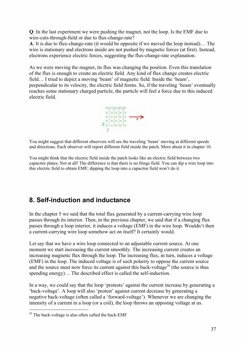
37

Q: In the last experiment we were pushing the magnet, not the loop. Is the EMF due to

wire-cuts-through-field or due to flux-change-rate?

A: It is due to flux-change-rate (it would be opposite if we moved the loop instead)… The

wire is stationary and electrons inside are not pushed by magnetic forces (at first). Instead,

electrons experience electric forces, suggesting the flux-change-rate explanation.

As we were moving the magnet, its flux was changing the position. Even this translation

of the flux is enough to create an electric field. Any kind of flux change creates electric

field… I tried to depict a moving ‘beam’ of magnetic field. Inside the ‘beam’,

perpendicular to its velocity, the electric field forms. So, if the traveling ‘beam’ eventually

reaches some stationary charged particle, the particle will feel a force due to this induced

electric field.

You might suggest that different observers will see the traveling ‘beam’ moving at different speeds

and directions. Each observer will report different field inside the patch. More about it in chapter 10.

You might think that the electric field inside the patch looks like an electric field between two

capacitor plates. Not at all! The difference is that there is no fringe field. You can dip a wire loop into

this electric field to obtain EMF; dipping the loop into a capacitor field won’t do it.

8. Self-induction and inductance

In the chapter 5 we said that the total flux generated by a current-carrying wire loop

passes through its interior. Then, in the previous chapter, we said that if a changing flux

passes through a loop interior, it induces a voltage (EMF) in the wire loop. Wouldn’t then

a current-carrying wire loop somehow act on itself? It certainly would.

Let say that we have a wire loop connected to an adjustable current source. At one

moment we start increasing the current smoothly. The increasing current creates an

increasing magnetic flux through the loop. The increasing flux, in turn, induces a voltage

(EMF) in the loop. The induced voltage is of such polarity to oppose the current source

and the source must now force its current against this back-voltage26 (the source is thus

spending energy)… The described effect is called the self-induction.

In a way, we could say that the loop ‘protests’ against the current increase by generating a

‘back-voltage’. A loop will also ‘protest’ against current decrease by generating a

negative back-voltage (often called a ‘forward-voltage’). Whenever we are changing the

intensity of a current in a loop (or a coil), the loop throws an opposing voltage at us.

26 The back-voltage is also often called the back-EMF

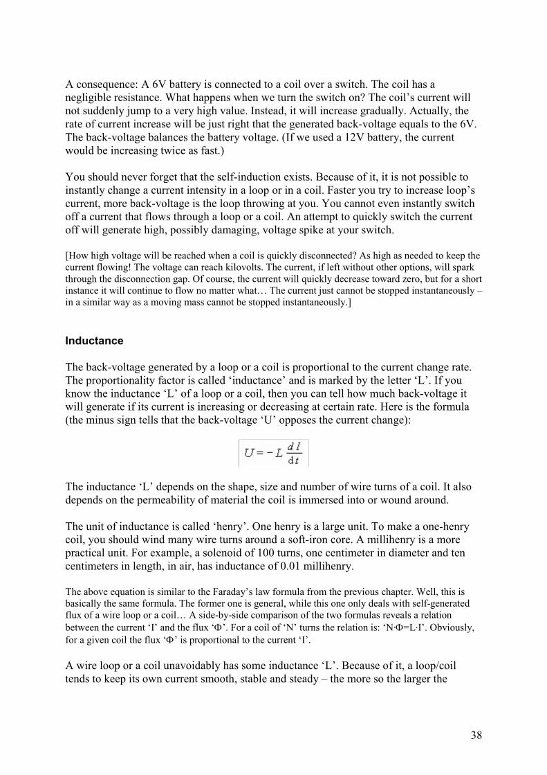
38

A consequence: A 6V battery is connected to a coil over a switch. The coil has a

negligible resistance. What happens when we turn the switch on? The coil’s current will

not suddenly jump to a very high value. Instead, it will increase gradually. Actually, the

rate of current increase will be just right that the generated back-voltage equals to the 6V.

The back-voltage balances the battery voltage. (If we used a 12V battery, the current

would be increasing twice as fast.)

You should never forget that the self-induction exists. Because of it, it is not possible to

instantly change a current intensity in a loop or in a coil. Faster you try to increase loop’s

current, more back-voltage is the loop throwing at you. You cannot even instantly switch

off a current that flows through a loop or a coil. An attempt to quickly switch the current

off will generate high, possibly damaging, voltage spike at your switch.

[How high voltage will be reached when a coil is quickly disconnected? As high as needed to keep the

current flowing! The voltage can reach kilovolts. The current, if left without other options, will spark

through the disconnection gap. Of course, the current will quickly decrease toward zero, but for a short

instance it will continue to flow no matter what… The current just cannot be stopped instantaneously –

in a similar way as a moving mass cannot be stopped instantaneously.]

Inductance

The back-voltage generated by a loop or a coil is proportional to the current change rate.

The proportionality factor is called ‘inductance’ and is marked by the letter ‘L’. If you

know the inductance ‘L’ of a loop or a coil, then you can tell how much back-voltage it

will generate if its current is increasing or decreasing at certain rate. Here is the formula

(the minus sign tells that the back-voltage ‘U’ opposes the current change):

The inductance ‘L’ depends on the shape, size and number of wire turns of a coil. It also

depends on the permeability of material the coil is immersed into or wound around.

The unit of inductance is called ‘henry’. One henry is a large unit. To make a one-henry

coil, you should wind many wire turns around a soft-iron core. A millihenry is a more

practical unit. For example, a solenoid of 100 turns, one centimeter in diameter and ten

centimeters in length, in air, has inductance of 0.01 millihenry.

The above equation is similar to the Faraday’s law formula from the previous chapter. Well, this is

basically the same formula. The former one is general, while this one only deals with self-generated

flux of a wire loop or a coil… A side-by-side comparison of the two formulas reveals a relation

between the current ‘I’ and the flux ‘Φ’. For a coil of ‘N’ turns the relation is: ‘N·Φ=L·I’. Obviously,

for a given coil the flux ‘Φ’ is proportional to the current ‘I’.

A wire loop or a coil unavoidably has some inductance ‘L’. Because of it, a loop/coil

tends to keep its own current smooth, stable and steady – the more so the larger the

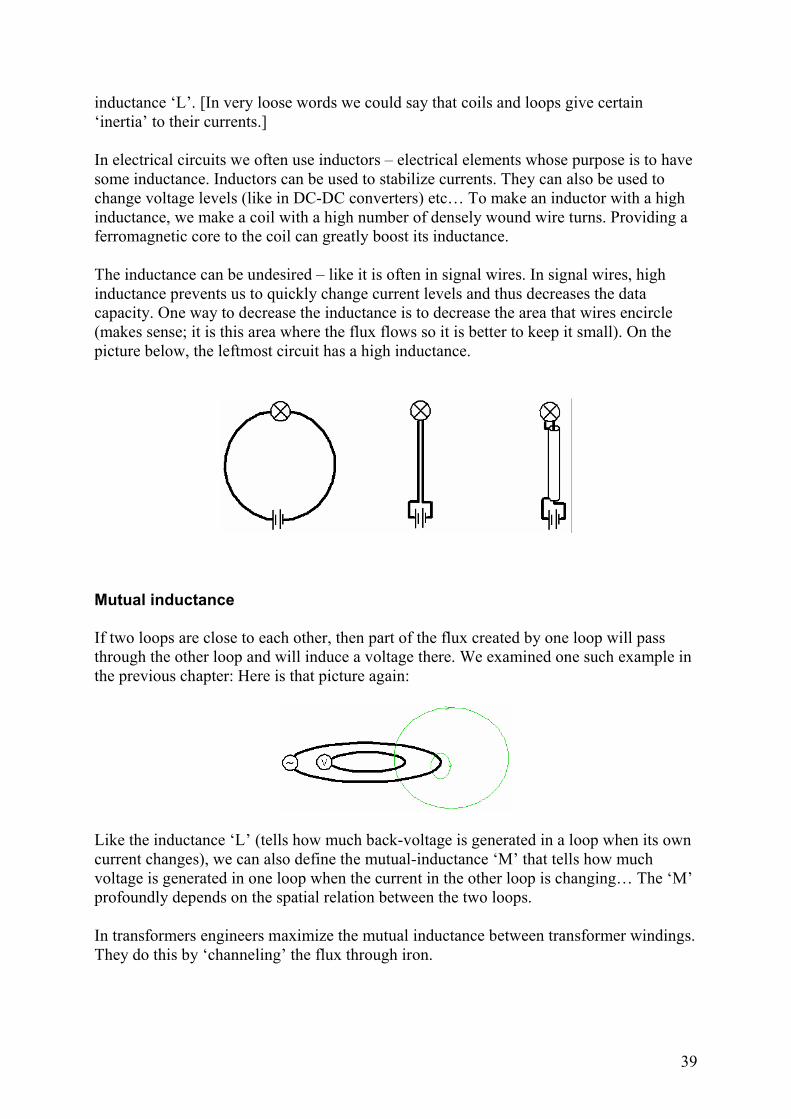
39

inductance ‘L’. [In very loose words we could say that coils and loops give certain

‘inertia’ to their currents.]

In electrical circuits we often use inductors – electrical elements whose purpose is to have

some inductance. Inductors can be used to stabilize currents. They can also be used to

change voltage levels (like in DC-DC converters) etc… To make an inductor with a high

inductance, we make a coil with a high number of densely wound wire turns. Providing a

ferromagnetic core to the coil can greatly boost its inductance.

The inductance can be undesired – like it is often in signal wires. In signal wires, high

inductance prevents us to quickly change current levels and thus decreases the data

capacity. One way to decrease the inductance is to decrease the area that wires encircle

(makes sense; it is this area where the flux flows so it is better to keep it small). On the

picture below, the leftmost circuit has a high inductance.

Mutual inductance

If two loops are close to each other, then part of the flux created by one loop will pass

through the other loop and will induce a voltage there. We examined one such example in

the previous chapter: Here is that picture again:

Like the inductance ‘L’ (tells how much back-voltage is generated in a loop when its own

current changes), we can also define the mutual-inductance ‘M’ that tells how much

voltage is generated in one loop when the current in the other loop is changing… The ‘M’

profoundly depends on the spatial relation between the two loops.

In transformers engineers maximize the mutual inductance between transformer windings.

They do this by ‘channeling’ the flux through iron.

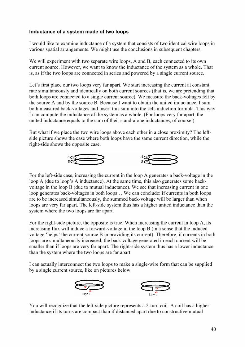
40

Inductance of a system made of two loops

I would like to examine inductance of a system that consists of two identical wire loops in

various spatial arrangements. We might use the conclusions in subsequent chapters.

We will experiment with two separate wire loops, A and B, each connected to its own

current source. However, we want to know the inductance of the system as a whole. That

is, as if the two loops are connected in series and powered by a single current source.

Let’s first place our two loops very far apart. We start increasing the current at constant

rate simultaneously and identically on both current sources (that is, we are pretending that

both loops are connected to a single current source). We measure the back-voltages felt by

the source A and by the source B. Because I want to obtain the united inductance, I sum

both measured back-voltages and insert this sum into the self-induction formula. This way

I can compute the inductance of the system as a whole. (For loops very far apart, the

united inductance equals to the sum of their stand-alone inductances, of course.)

But what if we place the two wire loops above each other in a close proximity? The left-

side picture shows the case where both loops have the same current direction, while the

right-side shows the opposite case.

For the left-side case, increasing the current in the loop A generates a back-voltage in the

loop A (due to loop’s A inductance). At the same time, this also generates some back-

voltage in the loop B (due to mutual inductance). We see that increasing current in one

loop generates back-voltages in both loops… We can conclude: if currents in both loops

are to be increased simultaneously, the summed back-voltage will be larger than when

loops are very far apart. The left-side system thus has a higher united inductance than the

system where the two loops are far apart.

For the right-side picture, the opposite is true. When increasing the current in loop A, its

increasing flux will induce a forward-voltage in the loop B (in a sense that the induced

voltage ‘helps’ the current source B in providing its current). Therefore, if currents in both

loops are simultaneously increased, the back voltage generated in each current will be

smaller than if loops are very far apart. The right-side system thus has a lower inductance

than the system where the two loops are far apart.

I can actually interconnect the two loops to make a single-wire form that can be supplied

by a single current source, like on pictures below:

You will recognize that the left-side picture represents a 2-turn coil. A coil has a higher

inductance if its turns are compact than if distanced apart due to constructive mutual

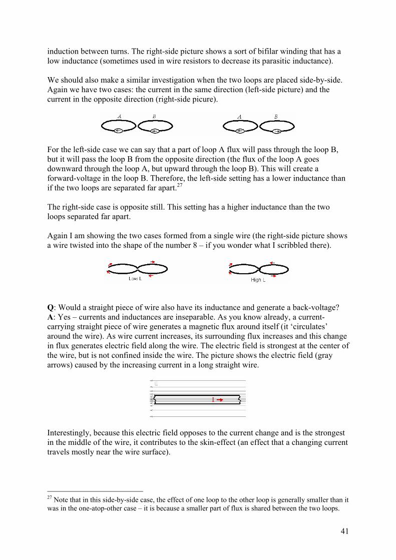
41

induction between turns. The right-side picture shows a sort of bifilar winding that has a

low inductance (sometimes used in wire resistors to decrease its parasitic inductance).

We should also make a similar investigation when the two loops are placed side-by-side.

Again we have two cases: the current in the same direction (left-side picture) and the

current in the opposite direction (right-side picure).

For the left-side case we can say that a part of loop A flux will pass through the loop B,

but it will pass the loop B from the opposite direction (the flux of the loop A goes

downward through the loop A, but upward through the loop B). This will create a

forward-voltage in the loop B. Therefore, the left-side setting has a lower inductance than

if the two loops are separated far apart.27

The right-side case is opposite still. This setting has a higher inductance than the two

loops separated far apart.

Again I am showing the two cases formed from a single wire (the right-side picture shows

a wire twisted into the shape of the number 8 – if you wonder what I scribbled there).

Q: Would a straight piece of wire also have its inductance and generate a back-voltage?

A: Yes – currents and inductances are inseparable. As you know already, a current-

carrying straight piece of wire generates a magnetic flux around itself (it ‘circulates’

around the wire). As wire current increases, its surrounding flux increases and this change

in flux generates electric field along the wire. The electric field is strongest at the center of

the wire, but is not confined inside the wire. The picture shows the electric field (gray

arrows) caused by the increasing current in a long straight wire.

Interestingly, because this electric field opposes to the current change and is the strongest

in the middle of the wire, it contributes to the skin-effect (an effect that a changing current

travels mostly near the wire surface).

27 Note that in this side-by-side case, the effect of one loop to the other loop is generally smaller than it

was in the one-atop-other case – it is because a smaller part of flux is shared between the two loops.

42

9. Energy contained in magnetic field

The magnetic field contains some amount of energy. Using today’s technology, we can

only store a small amount of energy into the field and so we don’t use it for large-scale

storage. Still, in electronic circuits we often use inductors or solenoids to temporarily and

repetitively store small amounts of energy (typically, a fraction of a joule might be stored

and extracted thousands times per second).

It is possible to measure how much energy is contained in the magnetic field of a coil.

You can, for example, put a coil into a calorimeter and then increase coil current from

zero to some value. You can measure how much electric energy was given by your battery

and how much energy was released as a heat. There will be a difference, and this energy

difference is stored in the coil’s magnetic field.

When doing these measurements, you will notice that the energy stored in the magnetic

field depends only on the intensity of coil’s current. As you increase the current, the

measured energy difference rises; as you decrease the current, the energy difference falls.

No matter in what way you change the coil current, the measured energy difference will

always be proportional to the square of the current intensity.

There is a simple formula that tells the amount of energy stored in magnetic field of a

standalone coil:

The funny thing about this formula is the ‘L’ factor – the inductance. This is the same ‘L’

that we encountered in the previous chapter (where it was connecting the current change

rate with the back-voltage).

It is not so difficult to relate the two formulas using some simple math. Imagine you have a current

source connected to a zero-resistance coil. The source does not need to provide any power to keep the

current at a constant level (the instantaneous power is ‘U·I’, but the voltage ‘U’ is zero for a zero-

resistance coil). However, when you start increasing the current, the coil ‘protests’ by generating a

back-voltage. The current source must now fight this back-voltage by providing equal voltage ‘U’ in

the forward direction. Therefore the current source now provides some instantaneous power.

Integrating this power over time gives the above energy formula.

If we now recall, from the previous chapter, results for inductivity ‘L’ of two spatially

related loops, and if we apply our new energy formula, then we can directly conclude:

• Two current-carrying wire loops placed on the same axis (one-above-the-other)

and having equal current direction will store more energy in their field if they are

closer to each other than if farther apart (supposing unchanged current intensities).

• Two current-carrying wire loops placed side-by-side will store less energy in their

fields if they carry current in the same direction than if they carry current in the

opposite direction (again, supposing unchanged current intensities).

We will use these conclusions in subsequent chapters.

43

The spooky energy density formula

It is nice to have the formula that relates the inductance ‘L’, the current intensity ‘I’ and

the energy ‘E’ stored in the magnetic field of a coil... However, we hope to generalize; we

want to relate the stored energy only to the magnetic field strength ‘B’. Can we do this?

We can note that the current in a coil is proportional to its flux (from N·Φ=L·I), and that

the flux is proportional to the field intensity ‘B’. Thus, we can expect that the stored

energy is proportional to the square of the field intensity (since it is proportional to the

square of the current intensity).

To make a more detailed computation, we could, for example, consider a toroidal coil. Its

field is all confined within the toroid tube. If we wisely choose an almost ideal toroidal

coil with a big diameter and a thin tube, our computation should turn easy because the

field inside such toroidal coil is homogeneous. So, after some math gymnastics28 we can

bring up a formula for energy density of magnetic field (the ‘u’ here is for energy density,

not voltage; the ‘µ’ is the magnetic permeability):

The above formula is fully general; it works for all magnetic fields not just those of

toroidal coils. It tells how the magnetic field energy is distributed in space. Integrating the

energy density ‘u’ over the whole space gives the total amount of energy contained in the

magnetic field.

And I find the above formula spooky. Why do we think that the energy is somehow dispersed in

volume? We can certainly say that a magnetic field is a result of certain configuration of currents in

space. And we can say that it certainly takes energy to build or alter these current configurations. But

to say that the energy is dispersed in the magnetic field exactly according the above formula is one

brave step further that cannot be justified as obvious… It would be nice to have an observational

confirmation that this energy density formula is true, but as far as I know, we have none (in principle

such experiment can be done, but practically it is out of our reach)… In the meantime we believe the

formula is true – it fits all observations and it fits our theories. It also has some elegance and

simplicity…In addition, we know that electromagnetic waves (the light) carry energy through vacuum.

In vacuum there are no current configurations and no moving electric charges; there are just magnetic

and electric fields all by themselves. So I guess this gives merit to the position that energy really is

contained/dispersed in magnetic field – possibly exactly according to the above energy density

formula.

28 For example: start from our energy formula E=LI

2/2, where L is the inductivity of the toroidal coil

and I is its current. Express the inductivity L from the relation N·Φ=L·I, and plug the flux as Φ=A·B

(where A is the toroid tube cross section area, and B is the field strength). The current intensity can be

taken from Ampere's law: 2·r·π·B=µ·N·I (where r is the middle radius of the toroid). By combining

those formulas and dividing the obtained energy with the toroid volume, V=2·r·π·A, you obtain the

energy density formula.

44

Q: So, what about permanent magnets – do permanent magnets have ‘energy contained in

magnetic field’?

A: Yes, according to the spooky energy density formula. But how to obtain the exact

number is not immediately clear. Obviously one should integrate the energy density also

inside the magnet body where the microscopic circular currents run. What are current

densities of those currents? Are those currents made by point-like particles (take for

example the intrinsic magnetic field produced by an electron spin – are electrons

dimensionless points)? If yes, our integral could become infinite which is obviously

wrong. In reality, the energy contained in magnetic field of a permanent magnet is rather

small. A walnut-sized neodymium magnet might hold 10 joules (tens of thousands times

less than an equal mass of gasoline).

10. Magnetic field and frames of reference

We were talking a lot about the magnetic field, less so about the electric field. Yet, the

two come together like the two faces of Janus. In this chapter we will relate the two fields.

Suppose there are two observers, each in its own frame of reference29. One observer might

be sitting inside a moving train, while the other one may be biking steadily on the nearby

road. The two observers use sensitive instruments to measure the field as they are passing

under a long overhead power line. Both observers will agree that they measured electric

and magnetic fields, but they will disagree about fine details. One observer might claim

just a bit more of magnetic field, while the other observer might claim just a bit more of

electric field.

The difference is not due to measurement errors! How an observer sees (measures) an

electric or magnetic field, depends on how the observer moves, that is, it depends on the

observer’s reference frame.

Electric and magnetic fields of a moving charged particle

As a simple example, we take the field of a charged particle. A stationary charged particle

generates a symmetric electric field that spreads radially from the particle. There is no

magnetic field. This is depicted below-left.

29 A frame of reference is a viewpoint from which we describe object movements. For example, a man

sitting at his porch says that his house is standing still, the train moves east at 100km/h and the bird is

flying south at 20km/h. At the same time, a man riding the train says that the train is standing still, the

house is moving west at 100km/h and the bird is flying sidewise, nearly west, at about 102km/h. Both

descriptions are correct and consistent, but are given in different reference frames.

45

.

However, as depicted on the right side, when the particle moves, its field is different. Its

electric field takes an ‘oblate’ shape (the field is stronger perpendicularly, but weaker in

direction parallel to the velocity). More interestingly, a magnetic field forms around the

particle (those green x-es and o-es). The oblateness of the electric field and the strength of

the magnetic field depend on how fast the particle moves relative to the observer.

I will repeat: the way the field looks depends on the relative velocity between particle and

its observer. If it is you who is moving, not the particle, again you will see the oblate

electric field and the wrapping magnetic field.

We are dealing with relativistic effects here. Einstein’s special theory of relativity

explains how different observers might describe things differently. A passing train looks

shorter for an observer at the station than for an observer inside the train (the effect of

length contraction). In a similar way, fields also look differently to different observers.

Several observers, each in its own reference frame, might be simultaneously looking at the same field,

and they will see it differently. Well, those observers would see all the things differently, not just the

fields, so fields are nothing special in that regard. That said, all those different observations are equally

real; equally true. The world described from any frame of reference is equally true.

The important thing is that electric and magnetic fields are not independent of each other.

You need to know both in one reference frame to be able to predict how any of them will

look in another reference frame. This is why we consider electric and magnetic fields as

two aspects of a more general field called the ‘electromagnetic field’.

The electromagnetic field is more complex than either electric or magnetic field. To

describe the electromagnetic field, we assign six numbers for each point of the space. So it

is not a mere vector field – it is a tensor field. In some cases the electromagnetic field may

show mostly electric-like properties, and then we call it the electric field; similarly, when

it shows mostly magnetic-like properties, we call it the magnetic field.

[The magnetic field that is found around the moving charged particle does not come out of nothing. It

comes from the electromagnetic field that exists around the particle. When observed from a relatively-

moving reference frame, this electromagnetic field shows us its magnetic side too.]

Current-carrying wire in different frames of reference

Knowing how the magnetic field of a single moving charge looks like, we can see how a

current-carrying wire makes its magnetic field. Inside the wire, moving electrons generate

both, electric field and a tiny amount of magnetic field around themselves. Their electric

46

field is canceled by the oppositely-charged stationary ions, but the magnetic field remains.

The current-carrying wire is electrically neutral (non-charged), and yet generates

macroscopic magnetic field.

Do you recall the Lorentz force? It acts on a charged particle and has two components: electric and

magnetic. The magnetic component is velocity-dependant, while the electric is not.

What velocity ‘v’ should we put into the Lorentz formula? We must put the velocity the particle has in

the frame of reference from which we are describing the magnetic field ‘B’ (and the electric field ‘E’).

The picture below shows a long current-carrying wire and its magnetic field. A negatively

charged particle moves alongside the wire in the direction opposite to the current. Because

the particle moves through magnetic field, it feels the magnetic part of the Lorentz force

(blue arrow). The particle does not feel any electric force because the wire is not charged.

How this situation looks from the frame of reference of the particle itself? Because the

particle has zero velocity in its own reference frame, the magnetic force it feels must be

zero (despite the presence the magnetic field). However, in the particle’s frame, the wire

is not electrically neutral any more! Instead, in this frame the wire has a slight positive

charge and generates some electric filed. The particle is driven toward the wire by the

electric part of the Lorentz force, ‘F = q·E’. Remarkably, the particle feels the same force

magnitude as in the lab frame.

The reason why a current-carrying wire seems charged to a moving observer is often explained as

follows: A stationary observer sees the wire as electrically neutral, meaning that he/she sees equal

average densities of negative electrons and positive ions in the wire. However for the moving

observer, electrons and ions in the wire both have an additional velocity component. This means that

the moving observer sees distances between electrons and ions in the wire to be contracted (in

comparison to the stationary observer). However, the amount o this contraction differs for electrons

and for ions.30 As a result, the moving observer does not see equal average densities of electrons and

ions in the wire, and thus he/she sees the wire electrically charged.

I find this explanation colorful, but not given in a very ‘field way’ of thinking. The particle, of course,

only experiences the local field – it is not looking around checking for average densities of electrons

and ions in the nearby wire. A better explanation might be what we already said earlier: the special

relativity predicts transformation of electromagnetic field when frames of reference change (in a way

similar to the length contraction). The electromagnetic field has different amount of electric-like and

30 Because the length-contraction formula is non-linear… Note that we are talking about low-speed

movements and still relativistic effects are easily visible (people say that this is because of enormous

strength of the electric force).

47

magnetic-like properties when observed from different reference frames. In our example, the field of

the wire simply has the electric component when observed from particle’s frame of reference.

Discussion: We said that the moving particle in our example sees the wire as electrically

charged. It feels the electric force and accelerates toward the wire. From our lab frame, we

can see this acceleration and we conclude that the particle is under some force. However,

in our lab frame the wire is electrically neutral and we cannot attribute this force to an

electric field. Instead, we must attribute it to some ‘new’ field that we call the magnetic

field… You notice that from the point of view of some charged particle, only the electric

field matters (particle’s speed is zero in its own frame of reference, so magnetic field

cannot act). The idea of magnetic force may thus only be needed when an ‘egoistic’

observer explains trajectories of moving charged particles from his frame. In our theories

we adopted this ‘egoistic’ viewpoint and so our theories contain magnetic forces. But

maybe a different approach is possible – we could explain particle trajectories exclusively

from particle’s point of view. Then our theories would not include magnetic forces.

Instead, we would be computing the painstaking field transformations all the time… Does

it mean that with such ‘non-egoistic’ approach we won’t need the magnetic field at all? I

don’t think so. We would still need the tensor containing six independent values to

describe the field – all six are necessary to compute field transformations. Whatever we

might call them, all components of the electromagnetic field would still remain. Obtaining fields in different frames of reference by Maxwell equations

The four famous Maxwell equations are completely describing the behavior of electric

and magnetic fields (or better said, the behavior of the classical electromagnetic field).

The equations are difficult to use analytically, so here we have to believe what more

hardworking people are telling us.

If we strictly treat our previous examples by Maxwell equations, we will obtain just the

described results. If, for example, we treat a moving charged particle by Maxwell

equations, we will find an ‘oblate’ electric field and some amount of magnetic field

around the particle.

Therefore, Maxwell equations already account for effects of reference frame change. They

work correctly from any frame of reference (we say, Maxwell equations are reference-

frame invariant). According to Maxwell equations, a changing electric field, even if it

only translates in space, creates a magnetic field. Similarly, a changing magnetic field

creates electric field.

Correction… Maxwell equations do not really tell what creates what (although we use this

figure of speech). Maxwell equations only associate the changing electric field with the

magnetic field and the changing magnetic field with the electric field. They tell that you

cannot have a changing electric field without magnetic field around it.

While Maxwell equations describe precisely how fields behave (including how they look

for observers in various frames of reference), they don’t tell why fields do that.

48

According to Maxwell equations, the magnetic field can arise either from currents (moving charges) or

from time-varying electric fields. However, the quantum theory explains that the magnetic field can

arise in one more way: it can arise from intrinsic magnetic dipole moments of charged elementary

particles (like electrons) called the ‘spin magnetic moment’. The spin magnetic moment is largely

responsible for magnetic fields of permanent magnets and materials… Maxwell equations do not

consider spin magnetic moments. You might try to model an elementary particle as a spinning ball of

charge (Maxwell equations can deal with spinning balls of charge), but I doubt this is a right approach.

Viewing field transformations from special relativity point of view

Some years following the Maxwell’s electrodynamics theory, another theory emerged –

the special theory of relativity. It deals meticulously with frames of reference in a more

general way. Everything, including the electromagnetic field, looks differently when

observed from different frames of reference. For example, a fast-moving train is just a bit

shorter than the same train when standing still (this effect is called the ‘length

contraction’).

For electromagnetic field, the effects that the special theory of relativity predicts are just

what Maxwell equations describe. The special theory of relativity can thus explain the

‘oblateness’ of electric field and the emergence of magnetic field around a moving

charged particle in a similar manner as it explains length contraction of material objects

and the space itself (using so called ‘Lorentz transformations’). This still might not answer

why the electromagnetic field does its transformations, but at least it shifts the problem to

a more general level: why there are the relativistic effects, and why there is the speed of

light… Personally, I find the fact that fields experience the Lorentz transformations in a

way similar to all other things, as an argument that fields are real objects, not just a

mathematical construction.

How does the electromagnetic field reshape in different frames of reference? I will just

write down the formulas that tell how B and E are morphing when you are switching

reference frames (formulas given here assume frames in relative motion only along the x-

axis).

The ‘γ’ is the Lorentz factor and ‘c’ is the speed of light. [You can see from these equations

that it is possible to have a charged particle that only generates electric field and no magnetic field

(Bx=By=Bz=0), yet when you are in motion relative to that particle, its field also possess a non-zero

magnetic field (that is, B’y and B’z might become nonzero). This describes how the electric field of a

charged particle gains the magnetic component when the particle is in motion.]

***

49

A more involved example: we should be able to analyze two long parallel wires that carry equal

currents, but in opposite direction. We will look at electrons and positive ions inside each wire and

examine forces acting on them. Note that for each particle (not only on each wire) the net force that it

feels must be identical in each frame of reference… The left-side picture below shows the case in the

lab-frame, while the right-side picture shows the same case in the frame of electrons in the wire ‘b’.

.

The description of the system from the lab-frame (left side) is simple – each wire generates its own

magnetic field, and the moving charges (electrons) in the other wire are moving through that field and

feel the magnetic part of the Lorentz force that pushes them away. Both wires are electrically neutral

so the electrical part of the Lorentz force is zero. Ions feel neither force as they do not even move.

It is more complex to describe the system from the reference frame of electrons in wire ‘b’ (the right

side). Ions inside both wires are now moving to the left and due to relativistic length contraction they

seem a bit denser now. Electrons in wire ‘a’ seem even more dense as they move about twice as fast,

but electrons in wire ‘b’ seem less as they are stationary in this reference frame. The result is that the

wire ‘a’ is slightly negatively charged, while the wire ‘b’ is slightly positively charged.

For the forces in the right-side-picture frame we can say:

• F’_mag_e_b - magnetic force on electrons in wire b – must be zero because electrons in wire

‘b’ have zero velocity

• F’_elec_e_b – electric force on electrons in wire b – is non-zero because the wire ‘a’ has

negative net charge and is thus pointed away from the wire ‘a’. It equals to the F_mag_e_b

from the lab-frame because electrons must feel the same overall force in both frames.

• F’_mag_i_b – magnetic force on ions in wire b – is non-zero because ions in wire ‘b’ have

their speed and because the wire ‘a’ generates some magnetic field that they can feel. The

direction is away from the wire ‘a’

• F’_elec_i_b – electric force on ions in wire b – is non-zero because positive ions are attracted

to negatively charged wire ‘a’. This force must be equal, but opposite, to F’_mag_i_b because

net force on ions must be zero (as it is the case in the lab-frame).

• F’_mag_e_a – magnetic force on electrons in wire a – is non-zero and is relatively large

because in this frame electrons are moving about twice as fast.

• F’_elec_e_a – electric force on electrons in wire a – non-zero because the wire ‘b’ is

positively charged and attracts electrons in wire ‘a’.

50

• F’_mag_i_a – magnetic force on ions in wire a – non-zero as they are moving through

magnetic field created by moving ions in wire ‘b’. It is equal, but opposite to F’_elec_i_a

because the net force on ions must be zero (as it is the case in the lab frame).

• F’_elec_i_a – electric force on ions in wire a – non-zero because the wire ‘b’ is positively

charged.

11. Force on a current-carrying wire

If a current-carrying wire is immersed into a magnetic field, the wire will feel a force

(supposing that the wire is not exactly parallel to the field). It is because the moving

electrons within the wire feel the magnetic part of the Lorentz force and then transfer that

force to the wire itself.

In the above example a wire is immersed in a homogeneous magnetic field. The wire

carries its current away from us. The force is perpendicular to both, the current direction

and the magnetic field direction (there are two such perpendicular directions, and the

correct one is determined by the right-hand-rule).

For a homogenous field and a straight wire perpendicular to that field, the force can be

calculated by multiplying the current intensity ‘I’ with the wire length ‘l’ and with the

field intensity ‘B’ (F=I·l·B). If the wire is not perpendicular to the field, the formula

should include a cross product (‘B’ and ‘l’ are vectors): 31

Don’t forget that whatever gadget is generating the magnetic field here, it will experience

the same force but in the opposite direction (Newton’s third law).32

A careful reader will notice that the representation of the magnetic field in the above

picture is not all correct. This is because the current-carrying wire creates its own

magnetic field and therefore both fields, the one produced by the wire and the

31 For non-homogenous field or curved wires, you should integrate. Regard each small segment of the

wire as a vector and compute the cross-product with the field at that point… Maybe using the

following formula:

32 Because, as you can guess, the current-carrying wire generates its own magnetic field that will exert

the force on the source of the surrounding field (whatever nature the field-source could be).

51

homogeneous external field, need to be summed up. This makes the overall magnetic field

somewhat distorted and no longer homogeneous.

The left-side drawing above shows both fields separately: the external field is depicted by

green field lines, while the wire-generated field is depicted by blue lines. The sum of the

two fields is depicted on the right-side picture… The resulting picture looks unlike the

picture that I sketched at the top of this chapter. Which one, then, should be considered

when calculating the force on the wire? It doesn’t matter; both provide the same result. Of

the two components that make the resultant field, only one, the external field, generates a

net force on the wire. The wire’s own field won’t generate any net force on the wire itself.

We can even generalize… whenever you have a magnetic object that is solid (a wire, a

coil, a magnet…) you can calculate the overall force or torque on it by only considering

the external magnetic field the object is immersed into. Object’s own magnetic field does

not have to be taken into account. The object’s own magnetic field can create tensions

within the object, but all those internal tensions cancel out and create no net force on the

object as a whole. This is all clear: you cannot lift yourself by pulling your own

bootstraps… In examples that will follow I might show only the external magnetic field

when I am explaining forces that act on an object. The object’s own magnetic field I

might ignore or just draw in a different color.

But when magnetic objects are not solid or when we are actually interested in tensions

within a solid object, then we must consider object’s own magnetic field… On the left-

side picture below, we have a rectangle-shaped wire loop. It is constructed from four

sides: a, b, c and d. The current is flowing through the wire loop. The intersection (across

the doted line) is depicted on the right-side picture. How do forces act on the wires in

points A and C? (In this example there are no external fields, just the field generated by

the loop itself.)

Let say that the rectangle-loop is very elongated so we can forget about sides b and d

when examining the magnetic field in points A and C. In fact, it is so elongated that we

approximate the magnetic field in points A and C as if we have two very long parallel

wires. The intersection shows magnetic field components of both wires, a and c. You can

see that each wire is immersed in the magnetic field of the other wire and this is why

52

forces are generated. In general, current-carrying wire loops tend to stretch themselves

out.

Torque and force on a current carrying wire loop

Three examples below show a current-carrying wire loop immersed into an external

magnetic field. Depending on the loop orientation, the loop can feel a torque (left picture)

or just a stretch/shrink force (middle picture) or a combination of both (right picture). (In

all these cases an additional amount of stretching force exists due to loop’s own field, as

explained just above… but this self-stretching force, as well as the loop’s own field, are

not depicted.)

A short digression… you can see from these pictures that the generated torque tries to orient the loop

into the orientation as on the middle picture. The wire loop tries to align itself with the external field,

just like a compass needle. We can define a magnetic dipole moment vector ‘m’ even for a current-

carrying loop (as we did for magnets). The magnetic dipole moment of a wire loop is a vector directed

perpendicularly to the loop plane. It can be calculated as ‘m=I·A’, where ‘I’ is the current intensity of

the wire loop, and ‘A’ is the surface area of the wire loop… Once you know the magnetic dipole

moment of a loop, you can use the torque formula mentioned in the chapter 4. It is easier to compute

torques using this formula than integrating forces along the wire.

Let’s also check an important example of a current-carrying wire loop in a non-

homogeneous magnetic field. In the example below, the field intensity decreases toward

the right. The left side of the loop is immersed into a stronger field than the right side of

the loop. Therefore the left side of the loop generates the larger force than the right side of

the loop. Our loop feels a net force that pulls it toward the left (if the loop current had the

opposite direction, then the net force would be pushing the loop toward the right).

When a current-carrying loop is immersed into a non-homogenous field, it can feel the net

force (inside a homogenous field it can only feel torque, but not a net force). [In the chapter

4 we made the same claim about permanent magnets too. Current-carrying loops and permanent

magnets have similarities. In my final chapter I will use this fact to make a simple model of iron and

permanent magnet.]

53

Our next example shows forces between two current-carrying wire loops facing each

other. On the left-side picture, the current runs in the same direction in both wire loops –

the force between loops is attractive. On the right-side picture the current runs in the

opposite direction – the force is repulsive.

How did I determine force arrow directions on these pictures? It is easy if I have field

lines depicted. The magnetic field acts locally so I only need to examine the direction of

the field lines as they pass through the wire segment for which I am determining the force.

I apply the right-hand rule: my right-hand fingers point in the direction of the local field,

the outstretched thumb in the direction of the current – and the force goes out of my palm.

We just learned that two facing loops that carry the current in the same direction will

attract each other. We can conclude that individual loops of a single coil will also

mutually attract. The coil tries to compress itself axially and stretch itself radially. The

picture below shows internal tensions in a current carrying coil due to its own field.

When two coils attract, the situation is similar as when two loops attract. To get the

attractive forces between coils we don’t need to examine fields of each loop separately,

but we can work with total fields of each coil, as depicted on the picture below-left.

54

The forces between depicted coils are attractive (if coils had the opposite current

directions, forces would be repulsive). Of course, supposing the same current, two coils

attract more strongly than two individual loops because contributions of all loops sum up.

Just for an illustration, I sketched the summed (resultant) magnetic field of the two coils

on the right-side picture. From this picture it is much more difficult to deduce that the two

coils attract. That is why, when examining forces between two object, I usually draw their

fields separately (that is, I separately draw components of the actual field).

Q: What is the force between two loops, distanced one centimeter apart, each carrying 1A

of current and each being 10 centimeters in diameter?

A: We might have a hard time to make an exact computation, but we can easily make an

approximation. Because the two loops are much closer to each other than is loop diameter,

we can compute it as if we have two parallel straight wires 10π centimeters long. The

result, for loops in the air, is about 6 micronewtons. Almost nothing… If we had 10A

currents in the loops (or if instead we had 10-turn windings), the result would be 600

micronewtons (0.6 millinewtons) – still quite nothing… To develop more serious forces

we need something different (hint: we need iron).

12. Energies and work

This optional chapter is divided into two parts. The shorter first part discusses if magnetic

field can do work. The longer second part relates potential energy and field energy.

It is often said that magnetic field does no work. Indeed, because the field applies strictly

perpendicular force to particle trajectory, it cannot change the speed and the kinetic

energy of the particle. Not directly… But indirectly, assisted by electric field, it might.

From chapter 7 we know that a changing magnetic field makes electric field. This electric

field can do work on charged particles. So, this is one indirect way.

But even steady magnetic field can be engaged into doing work. We will check a case

where a conductive wire is moved through a static magnetic field.

Work on a current-carrying wire

A straight current-carrying wire is immersed into a magnetic field. The wire is made of

positively-charged ions. Free electrons are running (drifting actually) between the ions.

55

As the electrons run, the magnetic filed bends their trajectories and pushes them toward

one sidewall of the wire33 - exaggeratedly depicted below.

The result is a slight charge separation that generates a weak electric field inside the wire,

perpendicular to wire length. So, electrons feel magnetic force ‘Fm’ that pushes them aside

and electric force ‘Fe’ in the opposite (restoring) direction. The two forces self-adjust and

balance perfectly. Electrons continue to move straight – as illustrated on the detail below.

What about the positively-charged ions (not depicted) that make the wire? The ions, being

stationary, feel only the downward electric force (or simply said, they are being attracted

toward electrons). Therefore, the wire experiences a downward force.

Because the wire feels some downward force, by moving the wire downward we should

be obtaining a mechanical work. This work will be made by electric forces (as the ions

feel electric forces). Still, to keep the language simple we often just say that a current-

carrying wire in a magnetic field feels a magnetic force.

So, let’s now move our wire downward (we are moving the wire without angling it).

The electron’s along-the-wire velocity now sums with the wire downward velocity – the

electron’s overall velocity ‘v’ is therefore angled downward. The magnetic force ‘Fm’

reorients to remain perpendicular to ‘v’… However, the electric force ‘Fe’ still points

straight up (the wire is not angled) and it now has a component (the thick blue arrow) that

does work on the electron: it decelerates the electron (it would accelerate it if we were

moving the wire upward instead).

Conclusion: The magnetic field separates charges in the wire and provokes an electric

field perpendicularly across the wire. This electric field does all the involved work.

33 That's a Hall effect.

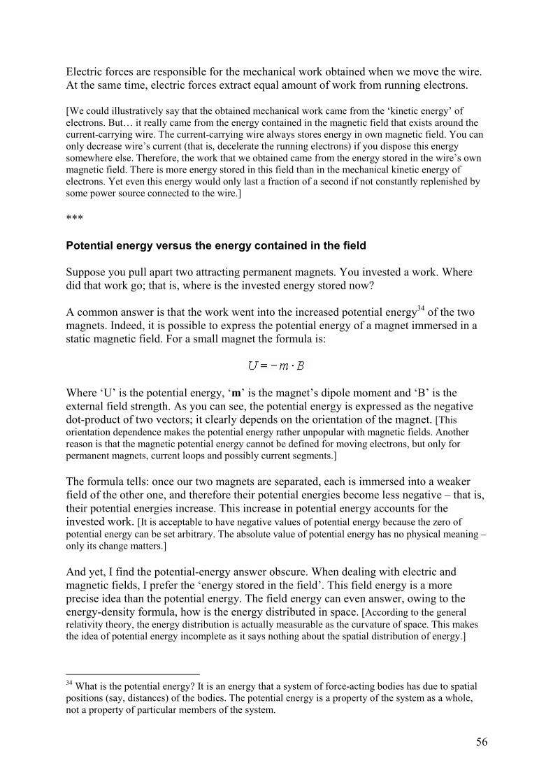
56

Electric forces are responsible for the mechanical work obtained when we move the wire.

At the same time, electric forces extract equal amount of work from running electrons.

[We could illustratively say that the obtained mechanical work came from the ‘kinetic energy’ of

electrons. But… it really came from the energy contained in the magnetic field that exists around the

current-carrying wire. The current-carrying wire always stores energy in own magnetic field. You can

only decrease wire’s current (that is, decelerate the running electrons) if you dispose this energy

somewhere else. Therefore, the work that we obtained came from the energy stored in the wire’s own

magnetic field. There is more energy stored in this field than in the mechanical kinetic energy of

electrons. Yet even this energy would only last a fraction of a second if not constantly replenished by

some power source connected to the wire.]

***

Potential energy versus the energy contained in the field

Suppose you pull apart two attracting permanent magnets. You invested a work. Where

did that work go; that is, where is the invested energy stored now?

A common answer is that the work went into the increased potential energy34 of the two

magnets. Indeed, it is possible to express the potential energy of a magnet immersed in a

static magnetic field. For a small magnet the formula is:

Where ‘U’ is the potential energy, ‘m’ is the magnet’s dipole moment and ‘B’ is the

external field strength. As you can see, the potential energy is expressed as the negative

dot-product of two vectors; it clearly depends on the orientation of the magnet. [This

orientation dependence makes the potential energy rather unpopular with magnetic fields. Another

reason is that the magnetic potential energy cannot be defined for moving electrons, but only for

permanent magnets, current loops and possibly current segments.]

The formula tells: once our two magnets are separated, each is immersed into a weaker

field of the other one, and therefore their potential energies become less negative – that is,

their potential energies increase. This increase in potential energy accounts for the

invested work. [It is acceptable to have negative values of potential energy because the zero of

potential energy can be set arbitrary. The absolute value of potential energy has no physical meaning –

only its change matters.]

And yet, I find the potential-energy answer obscure. When dealing with electric and

magnetic fields, I prefer the ‘energy stored in the field’. This field energy is a more

precise idea than the potential energy. The field energy can even answer, owing to the

energy-density formula, how is the energy distributed in space. [According to the general

relativity theory, the energy distribution is actually measurable as the curvature of space. This makes

the idea of potential energy incomplete as it says nothing about the spatial distribution of energy.]

34 What is the potential energy? It is an energy that a system of force-acting bodies has due to spatial

positions (say, distances) of the bodies. The potential energy is a property of the system as a whole,

not a property of particular members of the system.

57

How do the ‘potential energy’ and the ‘energy stored in the field’ relate? Let’s show this on an electric

field example… Suppose there are several charged objects arranged in the space. First, compute the

energy stored in the electric field of that system by integrating the energy density formula over all the

space35. Next, invest some work to slowly rearrange the objects. By definition, the potential energy of

the system changed for the invested work. Finally, for the new arrangement compute again the energy

stored in the field. You will see that the energy stored in the field also changed exactly for the amount

of the invested work.

The conclusion is that you should not count a change in the field energy and a change in the potential

energy both together! Only count one of them or you will make a double-counting error. The two

energy changes represent the same thing.

Is then a better answer: ‘the work invested when separating the two magnets is stored into

the magnetic field’? No. This is wrong. The magnetic field energy even decreases as we

separate our magnets… I will try to give a better answer, but let’s first examine two easy

thought experiments.

Energy considerations when separating zero-resistance loops

Our first experiment… Two zero-resistance wire loops are facing each other short

distance apart. We have two idealistic, adjustable voltage sources, each connected to one

wire loop. Voltage sources are set to zero volts and there is no current in the loops. Some

available energy, say 10J, resides inside our voltage sources. [Our sources could perhaps

be fly-wheel based, so we can always easily tell how much energy is inside.]

1. To build the magnetic field we adjust both sources to some voltage, wait a short

time and then decrease voltages back to zero. Eternal currents now flow in the

loops. Loops are now generating magnetic field and are attracting each other… We

‘spent’ some energy during this short-time excitation, say 4J, that is now stored in

the magnetic field. (6J remains inside sources; the total energy is still 10J.)

2. We move the two loops some distance farther apart. To do this, because the loops

attract, we must invest some work, say 2J. That is, we introduced 2J of additional

energy into the system. The total energy of the system should now be 12J.

35 Integrating this might not be straightforward if your world involves point charges – infinites will

arise. You would need to use some math tricks to hide them (like, subtracting energies of lone point-

charges, or stopping the integration early).

58

While we were moving the loops apart, currents inside them were increasing due to

induction (each loop kept the flux through it unchanged by increasing its current).

Therefore, we can suspect that the energy stored in the magnetic field also increased… I

even claim that the total energy contained in the magnetic field increased for invested

work, that is, for 2J. There is now 6J of energy stored in the magnetic field.

3. We will check this by adjusting a negative voltage, just long enough that loop

currents drop to zero. We should measure that 6J of energy is returned to voltage

sources (it came from the deconstruction of the magnetic field) and there is now

12J of energy stored in our voltage sources.

Indeed, all the energy of the system, 12J, is now back inside our voltage sources. There is

no energy in the field, or anywhere else, any more.

The diagram shows how energy contained inside power sources (red) and energy

contained in the magnetic field (green) changed during our first experiment.

Energy considerations when separating loops connected to a current source

Our second experiment is similar. Only, instead of voltage sources we now use idealistic

current sources. At the beginning, the current is set to zero and all the energy (10J) resides

within the current sources.

1. We gradually increase the current to some level. We ‘spent’ some energy from our

sources, say 4J, and this energy is now stored in the magnetic field. The 6J of

energy still remains inside sources. The total energy did not change.

2. We separate the loops investing some work, say 2J. This time the loop current

remained fixed by current sources.36 But to keep it fixed, the sources absorbed

some energy. This is because the sources had to counteract the induced voltage that

was trying to increase the current… The thing is: if we really make such an

experiment, we will see that even more energy is absorbed by sources than is the

work invested into the separation. Let say that 3J was absorbed by current sources.

How do we stand? The total energy of the system must be 12J. The sources contain 9J.

This must mean that the energy stored in the field fell form 4J down to 3J… We are not

36 We invested the same work, 2J, as in our previous experiment, but this does not mean that the

separation distance came out the same. The separation distance is greater in the second experiment.

59

surprised because we concluded the same in the chapter 9. We said: supposing unchanged

currents, if two attracting loops are farther apart there is less energy in their fields.

3. We gradually decrease currents back to zero and we measure how much energy is

returned to current sources – it should be 3J. This indeed was the energy stored in

magnetic field after the step 2. All the energy, 12J, is now inside current sources.

In this experiment, following things were simultaneously happening while we were

separating the loops: a) the field energy was decreasing, and b) the invested mechanical

energy plus the part of field energy was ‘pumped’ into the current sources.

Maybe you observed that our first experiment can be easily explained using potential energy. The

second experiment is harder. Let’s try it anyway… we shall only track the potential energy and the

energy stored in current sources (we will ignore the energy stored in the field):

• Initial condition: all the energy, 10J, is inside current sources

• After excitation: 6J remains inside current sources so 4J must be in the potential energy

• After separation (first variant): the potential energy is increased for the amount of added work, 2J,

so the potential energy is now 6J. But we also find 9J in sources… making 15J total –> fail!

• After separation (second variant): 9J is inside current sources; 2J is added, but the potential energy

decreased to 3J. The energy balance now fits, but we had to swallow a non-intuitive claim that the

potential energy decreases even if we are investing a work into the system.

So, the potential-energy approach can be made to work, although awkwardly. [A similar experiment

would be separating capacitor plates when connected to a fixed voltage source – again you will

encounter the awkwardness if you start counting the energy contained in the voltage source.]

Energy considerations when separating permanent magnets

We are back to the original question… we have two idealistic, non-conductive, thin, disc-

shaped permanent magnets. The magnetic field of such disc-magnet looks much like the

magnetic fields of a loop.

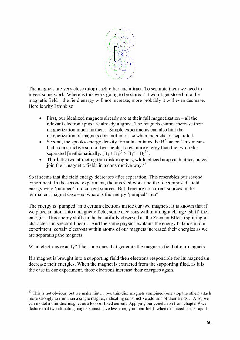
60

The magnets are very close (atop) each other and attract. To separate them we need to

invest some work. Where is this work going to be stored? It won’t get stored into the

magnetic field – the field energy will not increase; more probably it will even decrease.

Here is why I think so:

• First, our idealized magnets already are at their full magnetization – all the

relevant electron spins are already aligned. The magnets cannot increase their

magnetization much further… Simple experiments can also hint that

magnetization of magnets does not increase when magnets are separated.

• Second, the spooky energy density formula contains the B2 factor. This means

that a constructive sum of two fields stores more energy than the two fields

separated [mathematically: (B1 + B2)2 > B1

2 + B22 ].

• Third, the two attracting thin disk magnets, while placed atop each other, indeed

join their magnetic fields in a constructive way.37

So it seems that the field energy decreases after separation. This resembles our second

experiment. In the second experiment, the invested work and the ‘decomposed’ field

energy were ‘pumped’ into current sources. But there are no current sources in the

permanent magnet case – so where is the energy ‘pumped’ into?

The energy is ‘pumped’ into certain electrons inside our two magnets. It is known that if

we place an atom into a magnetic field, some electrons within it might change (shift) their

energies. This energy shift can be beautifully observed as the Zeeman Effect (splitting of

characteristic spectral lines)… And the same physics explains the energy balance in our

experiment: certain electrons within atoms of our magnets increased their energies as we

are separating the magnets.

What electrons exactly? The same ones that generate the magnetic field of our magnets.

If a magnet is brought into a supporting field then electrons responsible for its magnetism

decrease their energies. When the magnet is extracted from the supporting filed, as it is

the case in our experiment, those electrons increase their energies again.

37 This is not obvious, but we make hints... two thin-disc magnets combined (one atop the other) attach

more strongly to iron than a single magnet, indicating constructive addition of their fields… Also, we

can model a thin-disc magnet as a loop of fixed current. Applying our conclusion from chapter 9 we

deduce that two attracting magnets must have less energy in their fields when distanced farther apart.

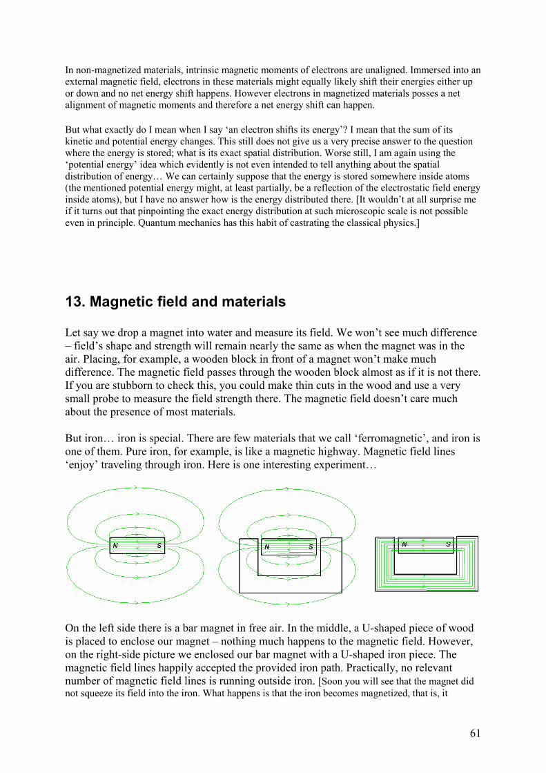
61

In non-magnetized materials, intrinsic magnetic moments of electrons are unaligned. Immersed into an

external magnetic field, electrons in these materials might equally likely shift their energies either up

or down and no net energy shift happens. However electrons in magnetized materials posses a net

alignment of magnetic moments and therefore a net energy shift can happen.

But what exactly do I mean when I say ‘an electron shifts its energy’? I mean that the sum of its

kinetic and potential energy changes. This still does not give us a very precise answer to the question

where the energy is stored; what is its exact spatial distribution. Worse still, I am again using the

‘potential energy’ idea which evidently is not even intended to tell anything about the spatial

distribution of energy… We can certainly suppose that the energy is stored somewhere inside atoms

(the mentioned potential energy might, at least partially, be a reflection of the electrostatic field energy

inside atoms), but I have no answer how is the energy distributed there. [It wouldn’t at all surprise me

if it turns out that pinpointing the exact energy distribution at such microscopic scale is not possible

even in principle. Quantum mechanics has this habit of castrating the classical physics.]

13. Magnetic field and materials

Let say we drop a magnet into water and measure its field. We won’t see much difference

– field’s shape and strength will remain nearly the same as when the magnet was in the

air. Placing, for example, a wooden block in front of a magnet won’t make much

difference. The magnetic field passes through the wooden block almost as if it is not there.

If you are stubborn to check this, you could make thin cuts in the wood and use a very

small probe to measure the field strength there. The magnetic field doesn’t care much

about the presence of most materials.

But iron… iron is special. There are few materials that we call ‘ferromagnetic’, and iron is

one of them. Pure iron, for example, is like a magnetic highway. Magnetic field lines

‘enjoy’ traveling through iron. Here is one interesting experiment…

On the left side there is a bar magnet in free air. In the middle, a U-shaped piece of wood

is placed to enclose our magnet – nothing much happens to the magnetic field. However,

on the right-side picture we enclosed our bar magnet with a U-shaped iron piece. The

magnetic field lines happily accepted the provided iron path. Practically, no relevant

number of magnetic field lines is running outside iron. [Soon you will see that the magnet did

not squeeze its field into the iron. What happens is that the iron becomes magnetized, that is, it

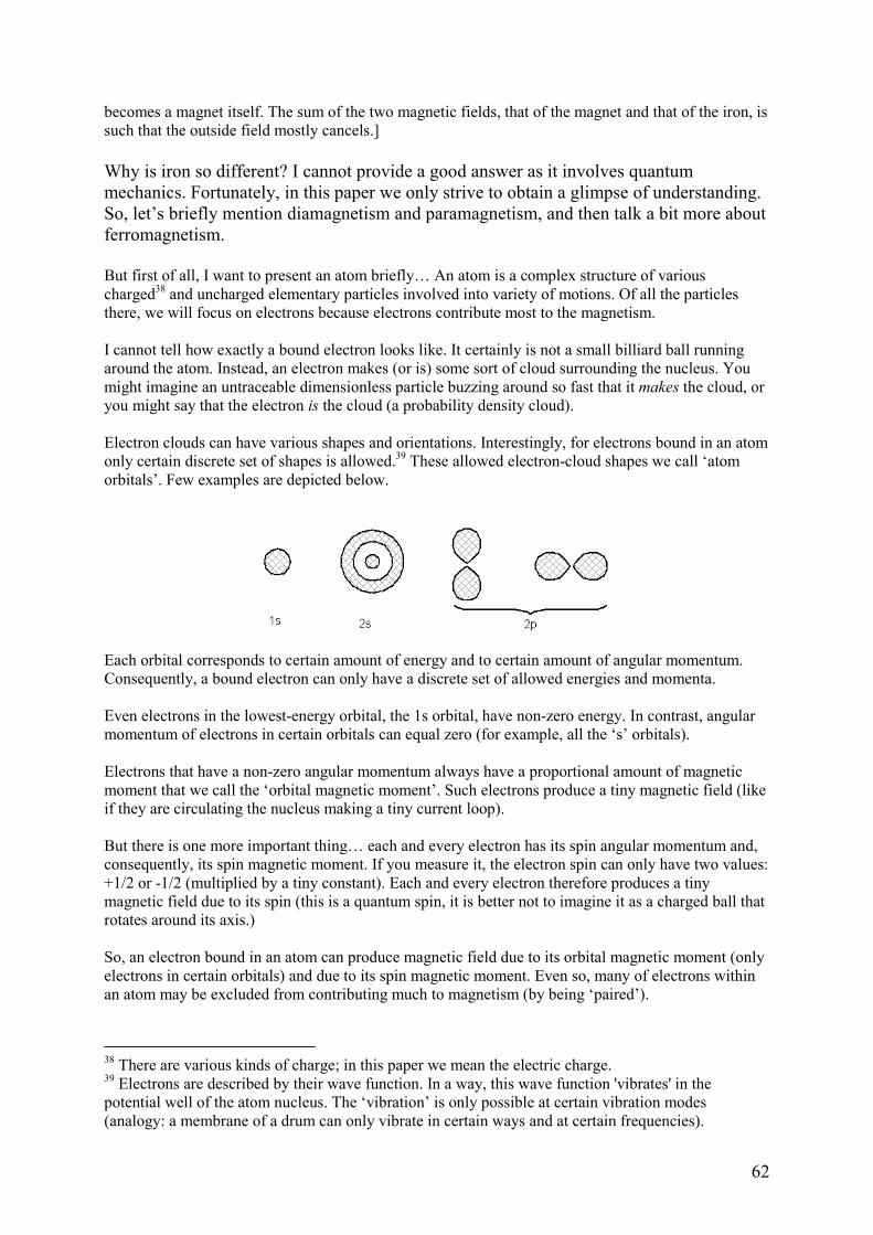
62

becomes a magnet itself. The sum of the two magnetic fields, that of the magnet and that of the iron, is

such that the outside field mostly cancels.]

Why is iron so different? I cannot provide a good answer as it involves quantum

mechanics. Fortunately, in this paper we only strive to obtain a glimpse of understanding.

So, let’s briefly mention diamagnetism and paramagnetism, and then talk a bit more about

ferromagnetism.

But first of all, I want to present an atom briefly… An atom is a complex structure of various

charged38 and uncharged elementary particles involved into variety of motions. Of all the particles

there, we will focus on electrons because electrons contribute most to the magnetism.

I cannot tell how exactly a bound electron looks like. It certainly is not a small billiard ball running

around the atom. Instead, an electron makes (or is) some sort of cloud surrounding the nucleus. You

might imagine an untraceable dimensionless particle buzzing around so fast that it makes the cloud, or

you might say that the electron is the cloud (a probability density cloud).

Electron clouds can have various shapes and orientations. Interestingly, for electrons bound in an atom

only certain discrete set of shapes is allowed.39 These allowed electron-cloud shapes we call ‘atom

orbitals’. Few examples are depicted below.

Each orbital corresponds to certain amount of energy and to certain amount of angular momentum.

Consequently, a bound electron can only have a discrete set of allowed energies and momenta.

Even electrons in the lowest-energy orbital, the 1s orbital, have non-zero energy. In contrast, angular

momentum of electrons in certain orbitals can equal zero (for example, all the ‘s’ orbitals).

Electrons that have a non-zero angular momentum always have a proportional amount of magnetic

moment that we call the ‘orbital magnetic moment’. Such electrons produce a tiny magnetic field (like

if they are circulating the nucleus making a tiny current loop).

But there is one more important thing… each and every electron has its spin angular momentum and,

consequently, its spin magnetic moment. If you measure it, the electron spin can only have two values:

+1/2 or -1/2 (multiplied by a tiny constant). Each and every electron therefore produces a tiny

magnetic field due to its spin (this is a quantum spin, it is better not to imagine it as a charged ball that

rotates around its axis.)

So, an electron bound in an atom can produce magnetic field due to its orbital magnetic moment (only

electrons in certain orbitals) and due to its spin magnetic moment. Even so, many of electrons within

an atom may be excluded from contributing much to magnetism (by being ‘paired’).

38 There are various kinds of charge; in this paper we mean the electric charge.

39 Electrons are described by their wave function. In a way, this wave function 'vibrates' in the

potential well of the atom nucleus. The ‘vibration’ is only possible at certain vibration modes

(analogy: a membrane of a drum can only vibrate in certain ways and at certain frequencies).

63

The Pauli Exclusion Principle forbids two electrons in one atom to have the same orbital and the same

spin. As the spin can only have two values, at most two electrons (of opposite spin) can share one

orbital. We call two such electrons ‘paired electrons’. Almost all magnetic properties of paired

electrons cancel out. As a result, only unpaired electrons can produce magnetic field.

If we place an atom into an external magnetic field, the energy level of its electrons changes (shifts).

Unpaired electrons can be strongly affected – depending on directions of their magnetic moments

relative to the external field, some might shift their energies up, some down. The amount of the energy

shift depends on the external field strength. [We did mention this energy shift already near the end of

the previous chapter. It is observable as the Zeeman Effect.]

Diamagnetism

Diamagnetism is an effect where some materials are slightly repelled by magnets. Water

or wood are examples of diamagnetic materials. The effect is very weak and cannot be

noticed without laboratory equipment.

Diamagnetism is, in fact, present in all materials but because it is so tiny it is often hidden

behind the stronger paramagnetism. Diamagnetism is only detectable if paramagnetism is

absent (like in materials that have all their electrons paired).

In books, diamagnetism is sometimes explained classically: electrons orbiting the nucleus

make tiny current loops and react to the external field by the Lentz rule (an increasing

external filed induces currents in these tiny loops that create opposing fields and a

repulsive force). A more worked-out classical explanation can involve the Larmor

precession: a spinning electron precesses about the direction of the external magnetic field

– this precession creates opposing fields and a repulsive force.

These classical explanations are resilient because they give good quantitative results. The

problem is that there is a theorem, Bohr-van Leeuwen theorem, that disproves any

classical explanation: if all the particles in a sample are classical particles then any

magnetization would be quickly eroded away by thermal randomization. In reality,

electrons are not classical (but are quantum) particles and the diamagnetic magnetization

can last as long as the external field is present.

Quantum computations show that each electron in an atom, even paired ones, will be

affected by the presence of an external magnetic field and will gain a slight opposing

magnetic moment. The cause is indeed similar to what classical theories say, but there is

no ‘dissipation’ of induced magnetic moments. The electrons seem to be insensitive to

thermal agitation because their energies are quantized – it takes a stronger kick than is

available to change their states. We could say that degrees of freedom of bound electrons

are frozen.

I know no practical use of diamagnetism, although people had fun levitating a small frog

in a 16 tesla field. Physicist mostly used diamagnetism to sharpen their theories.

[Some other effects used for levitation are also sometimes called diamagnetism. These involve

macroscopic currents – like levitating a fast-moving magnet above a copper plate or a copper ladder.

64

Furthermore, diamagnetism of superconductors can levitate trains. We are not talking about these

things here.]

Paramagnetism

Paramagnetism is an effect where some materials are slightly attracted to magnets.

As said earlier, unpaired electrons have magnetic moments and generate magnetic field on

their own. Normally we can’t detect this field around a paramagnetic material because all

its atoms are randomly oriented and generate no net magnetic field. But when such

material is placed into an external magnetic field, just a bit more of its atoms orient in the

direction aligned with the field than opposite it.40 The result is that a net magnetic field,

although a weak one, is generated by the paramagnetic material. The generated field is of

such orientation to support the external magnetic field.

At room temperatures the paramagnetic effect is fairly small (but still an order of

magnitude larger than the diamagnetic effect). The effect is temperature dependant and is

stronger at lower temperatures where the thermal agitation does not misalign orientations

of atom magnetic moments so readily. Once the external field is removed, the thermal

agitation will again randomize orientations of atoms and the net magnetization will

vanish. Aluminum and liquid oxygen are examples of paramagnetic materials.

Did you notice the difference between diamagnetism and paramagnetism? Diamagnetism is induced –

diamagnetic magnetic moments did not exist before the external field is applied. Paramagnetism,

however, is an alignment of already existing magnetic moments.

I cannot tell any practical use of paramagnetism. I mention it because atoms inside

paramagnetic materials make magnetic field on their own – just like atoms inside

ferromagnetic materials. In fact, there is just one, but important, step that leads from

paramagnetic to ferromagnetic material.

Ferromagnetism – magnetic domains

Ferromagnetism is economically important. Among else, it makes electric motors

possible. Ferromagnetic materials are few: iron, nickel, cobalt… But we won the jackpot

here because the iron, the foremost example with the strongest effect, is the cheap one.

In ferromagnetic materials, paramagnetic atoms spontaneously self-align. This self-

alignment does not happen due to magnetic forces – these are far too weak. It happens

because the quantum-mechanical effect, called the ‘exchange interaction’, causes it.

Ferromagnetism is, in a way, a side effect of a peculiar behavior of the exchange

interaction in ferromagnetic materials.

40 The two orientations differ in energy. Thus, according to Boltzman distribution, at any moment

more atoms will be in the lower-energy state (aligned) than in the higher-energy state (anti-aligned).

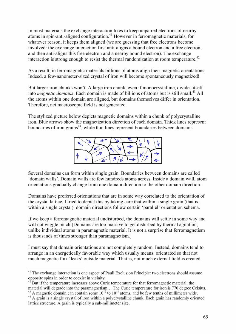
65

In most materials the exchange interaction likes to keep unpaired electrons of nearby

atoms in spin-anti-aligned configuration.41 However in ferromagnetic materials, for

whatever reason, it keeps them aligned (we are guessing that free electrons become

involved: the exchange interaction first anti-aligns a bound electron and a free electron,

and then anti-aligns this free electron and a nearby bound electron). The exchange

interaction is strong enough to resist the thermal randomization at room temperature.42

As a result, in ferromagnetic materials billions of atoms align their magnetic orientations.

Indeed, a few-nanometer-sized crystal of iron will become spontaneously magnetized!

But larger iron chunks won’t. A large iron chunk, even if monocrystalline, divides itself

into magnetic domains. Each domain is made of billions of atoms but is still small.43 All

the atoms within one domain are aligned, but domains themselves differ in orientation.

Therefore, net macroscopic field is not generated.

The stylized picture below depicts magnetic domains within a chunk of polycrystalline

iron. Blue arrows show the magnetization direction of each domain. Thick lines represent

boundaries of iron grains44, while thin lines represent boundaries between domains.

Several domains can form within single grain. Boundaries between domains are called

‘domain walls’. Domain walls are few hundreds atoms across. Inside a domain wall, atom

orientations gradually change from one domain direction to the other domain direction.

Domains have preferred orientations that are in some way correlated to the orientation of

the crystal lattice. I tried to depict this by taking care that within a single grain (that is,

within a single crystal), domain directions follow certain ‘parallel’ orientation schema.

If we keep a ferromagnetic material undisturbed, the domains will settle in some way and

will not wiggle much [Domains are too massive to get disturbed by thermal agitation,

unlike individual atoms in paramagnetic material. It is not a surprise that ferromagnetism

is thousands of times stronger than paramagnetism.]

I must say that domain orientations are not completely random. Instead, domains tend to

arrange in an energetically favorable way which usually means: orientated so that not

much magnetic flux ‘leaks’ outside material. That is, not much external field is created.

41 The exchange interaction is one aspect of Pauli Exclusion Principle: two electrons should assume

opposite spins in order to coexist in vicinity. 42 But if the temperature increases above Curie temperature for that ferromagnetic material, the

material will degrade into the paramagnetism… The Curie temperature for iron is 770 degree Celsius. 43 A magnetic domain can contain some 10

12 to 10

18 atoms, and be few tenths of millimeter wide.

44 A grain is a single crystal of iron within a polycrystalline chunk. Each grain has randomly oriented

lattice structure. A grain is typically a sub-millimeter size.

66

But why domains form at all? Why don’t all iron atoms align in the same direction? One reason is that

ordinary iron is polycrystalline. It consists of randomly oriented crystal grains, and domains tend to

follow these random orientations... But even a single, perfect crystal of iron, larger than several

nanometers, divides itself into magnetic domains. Moreover, these domains prefer to arrange in a way

that generates almost no field outside the iron. Why?

Many books show an illustration as the one below. It depicts an iron crystal as one domain (left side),

divided into two anti-parallel domains (middle) and divided further into four domains (right side). You

can see that the field size shrinks if the crystal divides itself into multiple domains. The right-side case

generates no external field. In the books it is often claimed that the external magnetic field costs

energy and it is therefore energetically favorable for the iron crystal to form domains.

I find this claim weird, if not even wrong. While the right-side case surely has the lowest total non-

thermal energy45, the energy contained in its magnetic field is not lower than in the left-side case.

Although less voluminous, the right-side magnetic field is stronger (denser) and its energy might be

even somewhat larger.

The reason why the right-side case still has the lowest total non-thermal energy is because its stronger

field causes larger energy down-shift of magnetically-active electrons within the iron. As mentioned

earlier, electrons down-shift their energies when immersed into a supporting field. [This explanation

also hints why domains arrange to minimize the outside field: because concentrating the entire field

inside, making it stronger inside, down-shifts electron energies for a greater amount.]

To make it less abstract, note that the left-side case on the above picture represents a small permanent

magnet. So, let’s cut that magnet vertically in half. The configuration of two side-by-side magnets is

unstable; forces are trying to flip the magnets into anti-parallel orientation. If one of the magnets flips,

the configuration becomes stable (and resembles the middle case from the picture above).

A home experiment: two parallel magnets are

unstable, while two anti-parallel magnets are stable.

Because the system of two magnets is obviously driven toward the anti-parallel configuration, we can

conclude that the anti-parallel configuration must have a lower total non-thermal energy (or, we might

say, it is energetically favorable). In a similar way, a single magnetic domain, if too large, splits into

two anti-parallel domains and achieves a more energetically favorable state.

45 I am using the term 'total non-thermal energy' to describe that part of energy of a system that is

capable of doing some macroscopically meaningful work. In a way, it is the usable part of the energy

of the system; a part that is not randomized (see also: Gibbs free energy and Helmholtz free energy).

67

[Let me also convince you that the anti-parallel configuration still has more energy stored in its

magnetic field… We can model our magnets using current loops of constant current, like it is depicted

below. In the chapter 9 we concluded: if loops carry equal currents, the anti-parallel side-by-side

configuration of loops contains more field energy than the parallel configuration.]

To round out the story of domain formtion: In a very tiny iron crystal, the exchange interaction orders

all the atoms into the same direction (a direction correlated with the crystal lattice direction). As the

crystal grows in size, the magnetic forces within it also grow and are trying to flip parallel columns of

atoms into anti-parallel directions. Once the magnetic forces grow sufficiently large, a whole bunch of

atoms flips over (the exchange interaction keeps atoms ‘tied’ into these bunches) and the crystal

divides into two domains.

[I am not saying that all those atoms flip at the same instant; the flipping will start from some point

and will then quickly spread, like a wave, and form the new domain. Atoms at the edge of the crystal,

or atoms near faults in crystal, or atoms at existing domain boundaries (domain walls) are the ones that

will be first to start flipping. Also, when domains are to resize, they can often do it by translation

(sliding) of walls between them – soon I will talk more about domain-wall translations.]

Anyway, it is the balance between strengths of exchange interaction and magnetic forces that

determines the sizes of resulting domains in different ferromagnetic materials.

Here is one interesting thought… We have two iron rings. The first one has domains

arranged in a typical unordered way, while the second one has circularly directed

domains. The second ring is interesting because it manages to develop a macroscopic

field, although completely confined within its body.

Which picture represents the real situation? It is the left-side one (the unordered one)…

However, even the right-side ring conforms to the energy-minimum requirement: it makes

no field outside its body. What I am saying is that we should be able to rearrange domains

from the unordered case into the ordered case without investing much energy.

Ok, it certainly can’t be easy to direct each and every domain into the circular pattern

(most domains would have to go against crystal lattice orientation). But I am not even

thinking about such extremes… Instead, let’s enlarge domains that already follow the

68

circular pattern on the expense of domains that oppose the pattern. This way we can still

obtain a net circular macroscopic field.

We are lucky with this idea because neighboring domains within single iron grain often

have opposite directions – we can therefore just slide the domain wall between them to

enlarge one and shrink the other one. Moving the domain wall is an energetically cheap

action if, by doing this, we don’t expand the magnetic field out of the iron.

By sliding a domain wall, one domain grows one the expense on the other one. The three pictures

above show how the magnetic orientations of atoms change when the domain wall slides.

Feromagnetic material in an external magnetic field

When we place a chunk of iron into an external magnetic field, an interesting thing

happens: its domain walls slide so that domains approximately aligned with the external

field grow in size while opposing domains shrink. The result is that the iron chunk,

previously non-magnetic, starts generating external field on its own. We say, the iron

chunk got magnetized (it became a magnet). The direction of its net magnetization is the

same as the direction of the external magnetic field… Look the pictures below.

The left side shows an iron bar immersed into an external magnetic field (green lines).

Domains inside iron resize and the iron starts generating its own field (blue lines). Inside

the bar, iron’s field reinforces the external field, while outside the bar, iron’s field opposes

69

the external field. The resulting field is shown on the right-side picture. It looks like if iron

bar sucked in the external field. [We can make magnetic shielding: we enclose the shielded object

with iron plates so that the iron ‘steals away’ magnetic field lines of any external field.]

If iron reacts to an external field by creating significant amount of supporting field inside

itself, can we arrange it in some sort of ring so that its own field is again constructively

acting on it? Well, something can be done. The picture below shows an iron ring and a

current-carrying wire passing through its center.

The current-carrying wire generates a low-strength circular magnetic field in the air. Yet,

inside the iron the field is much, much stronger. What happens is that the iron, being

directed by the weak external field, creates its own magnetic field that can be 100000

times stronger, or more.

This is a striking example of what can happen to iron when immersed into an external

magnetic field. This ‘magic’ happens when iron’s own magnetic field lines are not

required to travel long distances outside of iron body. In this case even a weak guiding

external field can cause significant resizing of iron’s magnetic domains and induce a

strong field inside the iron.

The above picture only shows the net magnetization of domains – not all domains will

take the circular pattern. Still, a surprisingly large net circular magnetization can be

obtained just by sliding domain walls and resizing magnetic domains. However if the

guiding field is really strong, it can even reorient domains away from the preferred

orientation of the crystal lattice.

For small guiding fields, the field generated within the iron will be very roughly

proportional to the guiding field. Very roughly indeed – nonlinearities are considerable.

Inductance consideration: In the above setup, the inductance of the central wire is larger than it would

be without the iron ring. Why? The central wire makes a loop (it starts at some current source, passes

through the iron ring and returns back to the current source). The total flux that passes through this

wire loop includes the large flux of the iron ring… So, changing the current in the wire causes large

flux change. This causes large back-EMF and, by definition, this means large inductance.

Energy consideration: We needed to invest less energy to establish the large flux within the iron ring

than we would need to establish an equally large flux in the air… Proof: imagine one toroidal coil with

an iron core, and another identical toroidal coil, but with the air core. Connect each to a separate

voltage source of the same voltage level. Then wait until field inside cores reaches, say, 0.1T (for both

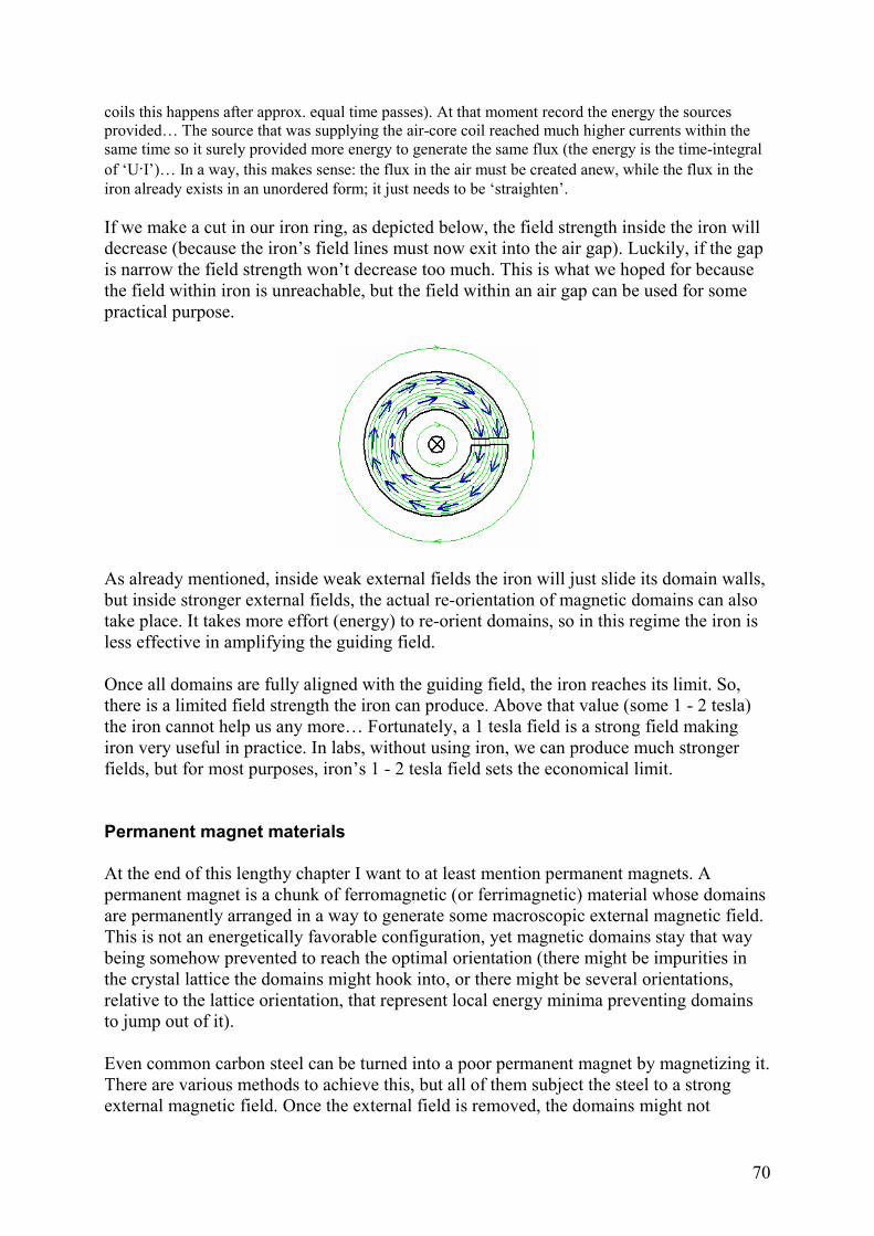
70

coils this happens after approx. equal time passes). At that moment record the energy the sources

provided… The source that was supplying the air-core coil reached much higher currents within the

same time so it surely provided more energy to generate the same flux (the energy is the time-integral

of ‘U·I’)… In a way, this makes sense: the flux in the air must be created anew, while the flux in the

iron already exists in an unordered form; it just needs to be ‘straighten’.

If we make a cut in our iron ring, as depicted below, the field strength inside the iron will

decrease (because the iron’s field lines must now exit into the air gap). Luckily, if the gap

is narrow the field strength won’t decrease too much. This is what we hoped for because

the field within iron is unreachable, but the field within an air gap can be used for some

practical purpose.

As already mentioned, inside weak external fields the iron will just slide its domain walls,

but inside stronger external fields, the actual re-orientation of magnetic domains can also

take place. It takes more effort (energy) to re-orient domains, so in this regime the iron is

less effective in amplifying the guiding field.

Once all domains are fully aligned with the guiding field, the iron reaches its limit. So,

there is a limited field strength the iron can produce. Above that value (some 1 - 2 tesla)

the iron cannot help us any more… Fortunately, a 1 tesla field is a strong field making

iron very useful in practice. In labs, without using iron, we can produce much stronger

fields, but for most purposes, iron’s 1 - 2 tesla field sets the economical limit.

Permanent magnet materials

At the end of this lengthy chapter I want to at least mention permanent magnets. A

permanent magnet is a chunk of ferromagnetic (or ferrimagnetic) material whose domains

are permanently arranged in a way to generate some macroscopic external magnetic field.

This is not an energetically favorable configuration, yet magnetic domains stay that way

being somehow prevented to reach the optimal orientation (there might be impurities in

the crystal lattice the domains might hook into, or there might be several orientations,

relative to the lattice orientation, that represent local energy minima preventing domains

to jump out of it).

Even common carbon steel can be turned into a poor permanent magnet by magnetizing it.

There are various methods to achieve this, but all of them subject the steel to a strong

external magnetic field. Once the external field is removed, the domains might not

71

completely return into the no-external-field state and the steel will retain some net

magnetization.

Some iron alloys are specifically engineered to retain strong magnetization and are used to

make fine permanent magnets. Some rare-earth alloys are even better… Yet in any case,

you can destroy the permanent magnetization of a magnet by various means – for example

by hammering it, by heating it to a high-enough temperature or even by immersing it into

a strong opposite or oscillating magnetic field. All this can unhook magnetic domains,

destroying the permanent magnetism of the magnet.

14. Hysteresis and eddy currents

Iron and other ferromagnetic materials are not perfect. These materials are non-linear,

have hysteresis, will saturate and are conductive… some more some less.

Hystersis

Let’s imagine an experiment as on the picture above. Here we have a winding that has an

iron almost-O-shaped core. The winding is supplied by current that we can adjust. I made

a very small gap in the O-core so that we can measure the field strength in the gap.

Because the gap is small, it does not affect our measurements very much – the

measurements will be very similar as if the core is gap-less. We are going to draw how the

magnetic field strength ‘B’ in the core depends on the winding current ‘I’.

In the above graph, we were increasing the current from zero to some rather high value.

As we can see, the generated magnetic field is not linear due to iron nonlinearities. We of

72

course expected the saturation once all domains get fully directed. The curve that we

obtained will differ for different ferromagnetic materials (for example, for different alloys

of iron), but all of them display non-linearity and saturation.

Now we are going to decrease the current all the way into the negative territory, and then

back again into the positive territory (making a full circle). We plot the field strength

during that full cycle.

We reveal a hysterisis loop. The width of the hysterisis loop very much depends on the

type of ferromagnetic material. Materials with wide hysterisis may be good for making

permanent magnets as they retain quite strong magnetic field even after the guiding field

is removed. We call these materials ‘magnetically hard materials’. On the other hand,

magnetically soft materials have narrow hysteresis loops and are used whenever a

changing magnetic flux needs to travel through them without generating much energy

loses (transformers, motors, relays, electromagnets…).

When we are using air-cored coils (or windings wound around any non-hysteresis

material) then all the energy that we invest when increasing their current, returns to us

when we decrease the current back to zero. However for windings wound around an iron

core, due to hysteresis loop of the iron, not all energy will be returned – some gets ‘lost’

(and iron gets warmer).

How does energy get lost due to hysteresis? We can make a thought experiment using the same

apparatus as at the beginning of this chapter, only this time we are using an idealized zero-resistance

winding wound around a core that has the linearized hysteresis loop as shown below.

At the beginning we are in the point ‘a’. In the point ‘a’ there is some current in the winding that

generates saturation-level magnetic field inside the core.

• We are decreasing the current toward zero. On our graph this means that we are advancing

from point ‘a’ toward point ‘b’. The magnetic field does not change during that time. Because

73

there is no flux change, no back-voltage is generated in the winding, and the energy that our

power source provides is thus zero.

• We continue decreasing the current further into the negative territory. On the above graph we

are advancing from point ‘b’ to point ‘c’. During this step the current is always negative. The

flux change rate is also negative (magnetic field is decreasing) which generates positive

(opposing) back-voltage. The result is that our power source needs to provide some energy.

• To make transition from point ‘c’ to point ‘d’ we increase the current back toward zero. The

flux does not change. No back-voltage is generated and no energy is ‘spent’ in this step.

• Finally, we increase the current back to the level we started with. In our graph, we move from

‘d’ back to ‘a’. During this step, the current is always positive. The flux change rate is also

positive (magnetic field is increasing) which generates negative (opposing) back-voltage.

Again our power source must provide some energy.

The wider the hysteresis loop is, the more energy will be lost in every cycle. More

precisely, the energy lost per cycle is proportional to the area bound by the hysteresis

loop. The power loses due to hysteresis is, as we can then conclude, proportional to cycle

frequency.

Imagine what happens in a transformer. The primary coil of transformer is connected to

an AC power supply. The primary coil therefore reverses magnetization of the transformer

core 50 times in one second (60 times in USA). Transformers would lose lots of energy if

their cores wouldn’t be made from materials that have narrow hysteresis loops.

I will now make a different hysteresis example. Let there is an iron disc that slowly rotates

in a magnetic field (the read arrow shows the rotation direction).

While in the static case the direction of iron magnetization would be aligned with external

(guiding) magnetic field, because the iron disk rotates and because the iron has the

magnetization hysteresis, there will be a misalignment of the iron magnetization and the

external field. The thing to note is that the misalignment will happen even if the rotation is

very slow. This misalignment, of course, introduces a torque, and because of this torque it

is more difficult to rotate the disc – it takes work to rotate the disc (and the disc is heated).

Eddy currents

Another source of losses in iron are eddy currents. At high cycling frequencies these

become nastier than hysteresis. This is because eddy current losses increase with the

square of the frequency.

Let’s imagine a square wire-loop. A perpendicular magnetic flux passes through the loop.

The flux changes in time.

74

The wire loop has its resistance ‘R’. As the flux changes, it induces the voltage ‘U’ along

the loop which in turn generates a current in the loop. Some power ‘P’ is dissipated in the

wire loop and this power can be calculated as ‘P = U2 / R’ [Note: the dissipated power

depends on the square of the induced voltage; that is, it depends on square of the flux

change rate; that is, it depends on the square of the frequency if we suppose that the flux

changes periodically.]

We made an example with a conductive wire loop. Obviously, because iron is also

conductive, we can expect that a changing flux that passes through iron will inevitably

generate currents in iron and those currents will dissipate energy. We call these currents

‘eddy currents’.

There are two way to fight eddy currents and both are used. The first one is to find a

material (an alloy of iron, perhaps) that has relatively high specific resistance. Because the

dissipated power is inversely proportional to the material resistance, high specific

resistance reduces power loses. For very high frequencies (kilohertz and above) we can

even use ferrite materials Ferrites are insulators so we won’t have any problem with eddy

currents. The disadvantage of ferrites is that they don’t have such high magnetic

permeabilities as iron alloys do.

The second way to fight eddy currents is to divide a solid magnetic core into electrically

insulated pieces – usually into planes or strips made of ferromagnetic metal. These are

called lamination. Dividing a solid chunk of iron into many thin, electrically insulated

pieces can significantly reduce eddy currents… Let’s imagine that we divided our original

square wire-loop into four small, mutually insulated, square wire-loops as in the image

below.

Each loop now has resistance of ‘R/2’ (because loop perimeter is half the length of the

original loop), but each is crossed by only quarter of the flux. As a result, the induced

voltage in each loop is only ‘U/4’. The power dissipated in each loop is therefore ‘P = (U2

/ R) / 8’. For all four loops the combined dissipated power is ‘P = (U2 / R) / 2’. That is, the

total power dissipation due to eddy currents halved.

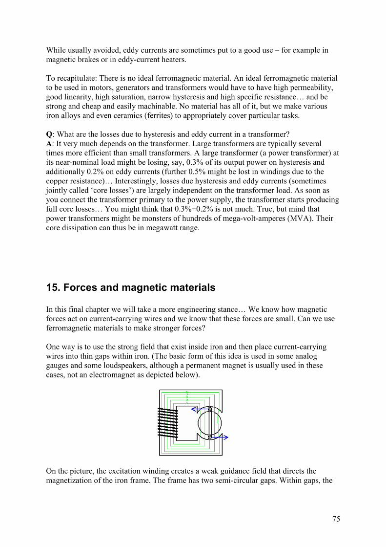
75

While usually avoided, eddy currents are sometimes put to a good use – for example in

magnetic brakes or in eddy-current heaters.

To recapitulate: There is no ideal ferromagnetic material. An ideal ferromagnetic material

to be used in motors, generators and transformers would have to have high permeability,

good linearity, high saturation, narrow hysteresis and high specific resistance… and be

strong and cheap and easily machinable. No material has all of it, but we make various

iron alloys and even ceramics (ferrites) to appropriately cover particular tasks.

Q: What are the losses due to hysteresis and eddy current in a transformer?

A: It very much depends on the transformer. Large transformers are typically several

times more efficient than small transformers. A large transformer (a power transformer) at

its near-nominal load might be losing, say, 0.3% of its output power on hysteresis and

additionally 0.2% on eddy currents (further 0.5% might be lost in windings due to the

copper resistance)… Interestingly, losses due hysteresis and eddy currents (sometimes

jointly called ‘core losses’) are largely independent on the transformer load. As soon as

you connect the transformer primary to the power supply, the transformer starts producing

full core losses… You might think that 0.3%+0.2% is not much. True, but mind that

power transformers might be monsters of hundreds of mega-volt-amperes (MVA). Their

core dissipation can thus be in megawatt range.

15. Forces and magnetic materials

In this final chapter we will take a more engineering stance… We know how magnetic

forces act on current-carrying wires and we know that these forces are small. Can we use

ferromagnetic materials to make stronger forces?

One way is to use the strong field that exist inside iron and then place current-carrying

wires into thin gaps within iron. (The basic form of this idea is used in some analog

gauges and some loudspeakers, although a permanent magnet is usually used in these

cases, not an electromagnet as depicted below).

On the picture, the excitation winding creates a weak guidance field that directs the

magnetization of the iron frame. The frame has two semi-circular gaps. Within gaps, the

76

field strength can reach about 1 tesla or so… It is iron that actually creates most of this

field (an engineer might say: iron provides most ampere-turns).

A wire loop is placed within gaps; it can move for an angle. The idea is to make gaps as

narrow as possible, not to weaken the field much. Narrower gaps also provide more

homogeneous field inside them. The central round iron piece does not rotate with the loop

(this lowers the inertia and reduces the hysteresis drag). By changing the current intensity

in the wire loop, we change the torque developed on the loop.

A simple model of iron

As we know from experience, iron is attracted by magnetic field and it might not be

obvious why it is so. I will try to explain it by making a model of iron. The model does

not necessarily depict the physical reality behind the scene, but it shows how the forces

act.

Let’s recall about iron… Regions of uniform magnetization, called magnetic domains, spontaneously

form in iron. Normally, their arrangement does not make a macroscopic field. However, when a chunk

of iron is placed into an external field, aligned domains grow in size, while opposing domains shrink –

as a result, iron gains some net magnetization and starts producing its own magnetic field… I am

repeating the picture of an iron block immersed into an external field.

To make a simplified model of iron, we could represent each magnetic domain by a tiny

current loop – inside each loop an eternal current flows. To simplify things further, we

will only consider those domains (current loops) that represent the net macroscopic

magnetization of the iron (other domains cancel out).

The picture below-left shows an iron block immersed in an external magnetic field. The

external field magnetizes the iron, and its net magnetization is represented by those

imagined current loops. Each loop generates a small amount of its own field directed to

support the external field.

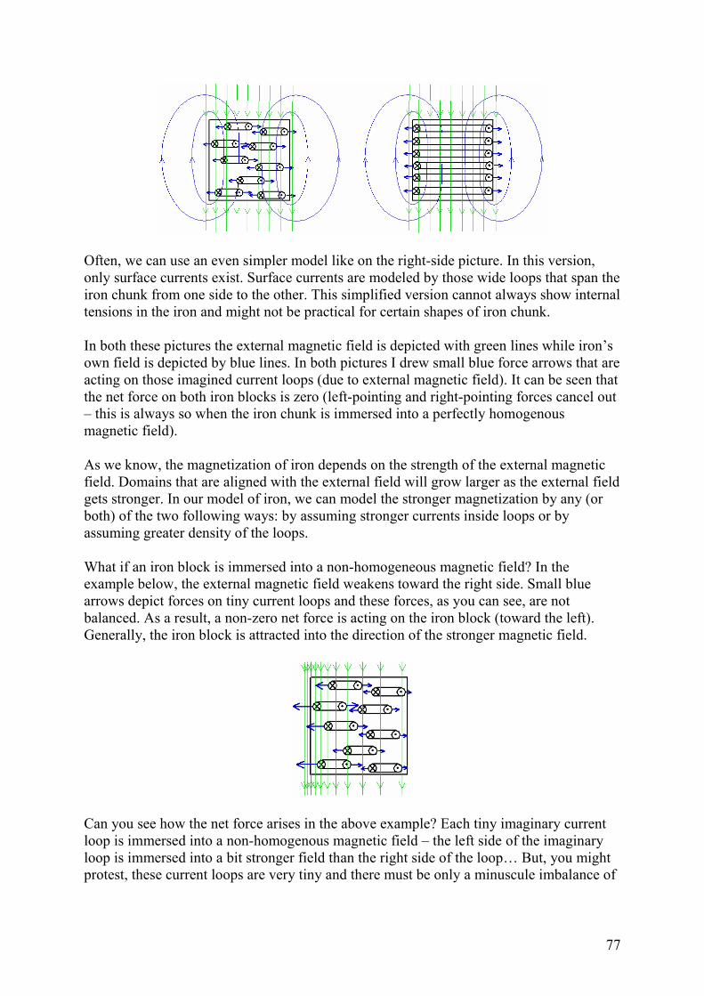
77

Often, we can use an even simpler model like on the right-side picture. In this version,

only surface currents exist. Surface currents are modeled by those wide loops that span the

iron chunk from one side to the other. This simplified version cannot always show internal

tensions in the iron and might not be practical for certain shapes of iron chunk.

In both these pictures the external magnetic field is depicted with green lines while iron’s

own field is depicted by blue lines. In both pictures I drew small blue force arrows that are

acting on those imagined current loops (due to external magnetic field). It can be seen that

the net force on both iron blocks is zero (left-pointing and right-pointing forces cancel out

– this is always so when the iron chunk is immersed into a perfectly homogenous

magnetic field).

As we know, the magnetization of iron depends on the strength of the external magnetic

field. Domains that are aligned with the external field will grow larger as the external field

gets stronger. In our model of iron, we can model the stronger magnetization by any (or

both) of the two following ways: by assuming stronger currents inside loops or by

assuming greater density of the loops.

What if an iron block is immersed into a non-homogeneous magnetic field? In the

example below, the external magnetic field weakens toward the right side. Small blue

arrows depict forces on tiny current loops and these forces, as you can see, are not

balanced. As a result, a non-zero net force is acting on the iron block (toward the left).

Generally, the iron block is attracted into the direction of the stronger magnetic field.

Can you see how the net force arises in the above example? Each tiny imaginary current

loop is immersed into a non-homogenous magnetic field – the left side of the imaginary

loop is immersed into a bit stronger field than the right side of the loop… But, you might

protest, these current loops are very tiny and there must be only a minuscule imbalance of

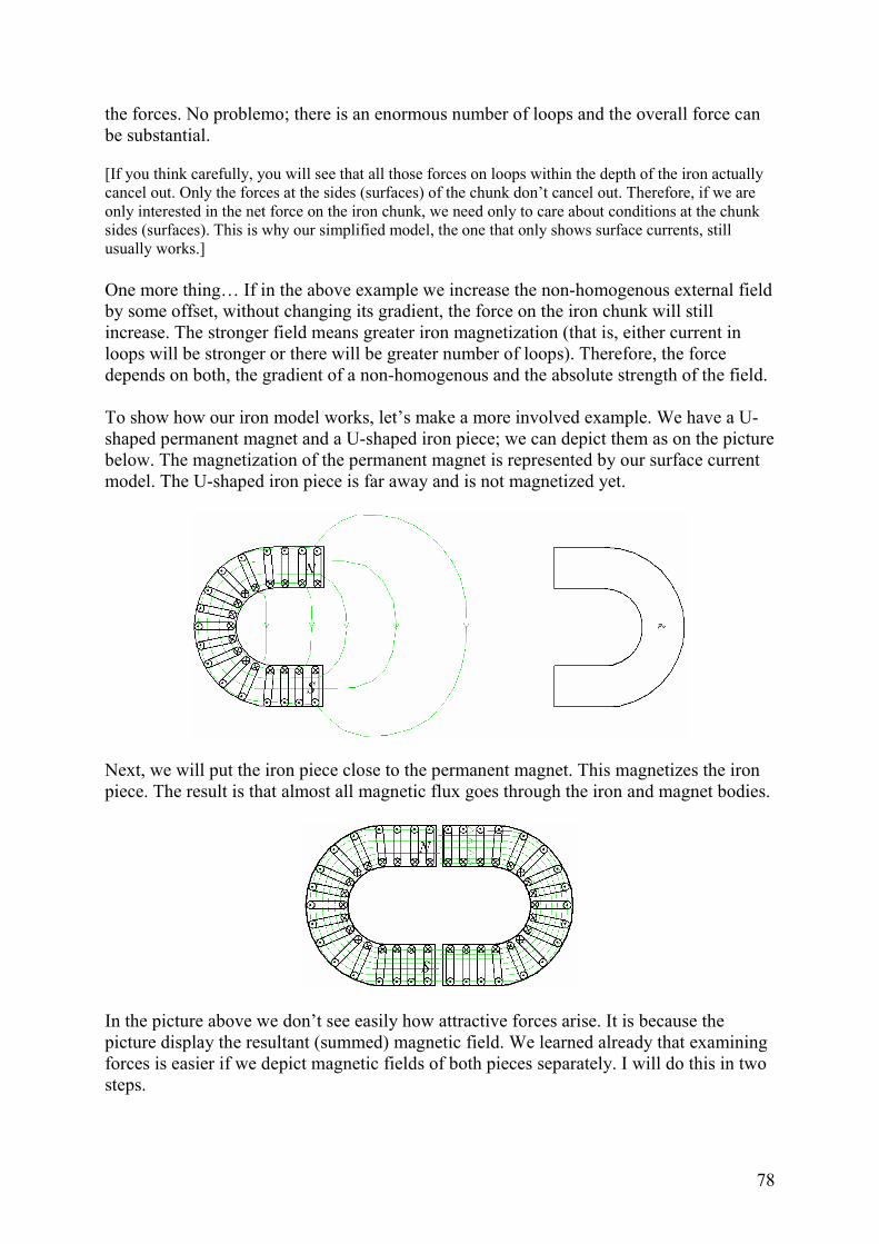
78

the forces. No problemo; there is an enormous number of loops and the overall force can

be substantial.

[If you think carefully, you will see that all those forces on loops within the depth of the iron actually

cancel out. Only the forces at the sides (surfaces) of the chunk don’t cancel out. Therefore, if we are

only interested in the net force on the iron chunk, we need only to care about conditions at the chunk

sides (surfaces). This is why our simplified model, the one that only shows surface currents, still

usually works.]

One more thing… If in the above example we increase the non-homogenous external field

by some offset, without changing its gradient, the force on the iron chunk will still

increase. The stronger field means greater iron magnetization (that is, either current in

loops will be stronger or there will be greater number of loops). Therefore, the force

depends on both, the gradient of a non-homogenous and the absolute strength of the field.

To show how our iron model works, let’s make a more involved example. We have a U-

shaped permanent magnet and a U-shaped iron piece; we can depict them as on the picture

below. The magnetization of the permanent magnet is represented by our surface current

model. The U-shaped iron piece is far away and is not magnetized yet.

Next, we will put the iron piece close to the permanent magnet. This magnetizes the iron

piece. The result is that almost all magnetic flux goes through the iron and magnet bodies.

In the picture above we don’t see easily how attractive forces arise. It is because the

picture display the resultant (summed) magnetic field. We learned already that examining

forces is easier if we depict magnetic fields of both pieces separately. I will do this in two

steps.

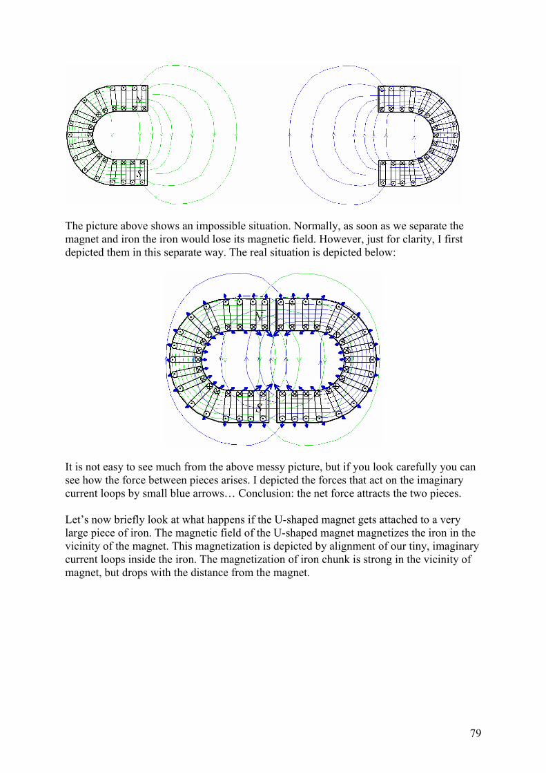
79

The picture above shows an impossible situation. Normally, as soon as we separate the

magnet and iron the iron would lose its magnetic field. However, just for clarity, I first

depicted them in this separate way. The real situation is depicted below:

It is not easy to see much from the above messy picture, but if you look carefully you can

see how the force between pieces arises. I depicted the forces that act on the imaginary

current loops by small blue arrows… Conclusion: the net force attracts the two pieces.

Let’s now briefly look at what happens if the U-shaped magnet gets attached to a very

large piece of iron. The magnetic field of the U-shaped magnet magnetizes the iron in the

vicinity of the magnet. This magnetization is depicted by alignment of our tiny, imaginary

current loops inside the iron. The magnetization of iron chunk is strong in the vicinity of

magnet, but drops with the distance from the magnet.

80

Once the iron is magnetized, it starts creating its own magnetic field locally as shown on

the right-side picture. This field is then acting on the magnet (onto these imaginary current

loops within the magnet body) and keeps the magnet attached to the iron block.

Using iron to increase developed forces

In our next example, the guiding magnetic field is created by a long current-carrying wire.

The wire is perpendicular to the paper plane. In the vicinity of the wire we placed one

semi-circular iron piece.

The current-carrying wire creates a weak, circular, non-homogenous magnetic field,

depicted by green lines. This weak field slightly magnetizes the iron and the iron starts

creating its own weak field (blue lines). Recall that the magnetic field of the wire is

decreasing away from the wire. This gradient therefore creates a net force on the iron

piece – the iron piece is weakly attracted toward the wire. At the same time, the blue field

(generated by the iron) acts on the wire and attracts it toward the iron with the equal force.

More interesting things happen on the picture below. We added another identical iron

piece, almost closing the iron ring. Now the field strength inside iron increases a lot.

Three components of the magnetic field exist in this system, but for clarity, I depicted

only one of them. The three components are:

81

• the weak circular field generated by the current-carrying wire (it looks the same as

on the previous picture)

• the field generated by the original iron piece – this one is depicted (similar in

shape, but much stronger than on the previous picture)

• the field generated by the newly added iron piece (identical, but mirrored to that of

the original iron piece).

The magnetization of the iron is now a lot stronger. This means, according to our model,

that circular currents inside imagined current loops are now much stronger. The original

iron piece now feels a much stronger force caused by the wire’s non-homogeneous field.

But even this force is insignificant when compared to the attractive force the piece feels

toward the other iron piece. Therefore, the original iron piece now feels a considerable

force toward the left. (The newly added iron piece feels equally strong force toward the

right.)

Interestingly, while our original iron piece now generates much stronger magnetic field

that could potentially produce strong attractive force on the current-carrying wire, the

current-carrying wire won’t actually feel any force. It is because the other iron piece also

generates its own magnetic field and the two fields basically cancel out – the wire is thus

immersed in the null field.

We managed to significantly increase the force that is acting on the original iron piece

without increasing current strength in the wire. All we did is that we added some more

iron to allow field lines to travel mostly through iron.

How is a torque in a slotted-rotor electric motor produced

In our last ‘experiment’ we have a setup as displayed below (forgive me the coarse

drawing). The picture shows a region around an air gap of a large electromagnet. The

major part of the electromagnet core and its winding are not depicted. The electromagnet

is able to create a magnetic field in its air gap. We are able to turn the electromagnet on or

off as we wish... In the air gap we place a current-carrying wire.

82

The homogeneous field of the electromagnet is depicted with green lines, and the circular

field of the wire is depicted with blue lines. Obviously, there is a force on the wire (blue

arrow).

Let suppose that we place two additional iron blocks into the gap, as it is displayed on the

picture below. We want to analyze this situation.

First, let’s look at the situation when the electromagnet is switched off, and only the wire

generates the magnetic field. As it can be seen on the picture below, the magnetic flux is

able to run mostly through iron and so the wire is able to generate relatively strong field

within the iron.

Recall that the field generated by the current-carrying wire is not homogenous – it

decreases with the distance from the wire. The magnetization of iron blocks therefore

83

won’t be homogeneous and, as we concluded earlier, there will be attractive force that

attracts iron blocks toward the wire. The wire, however, does not feel much force as it is

not immersed into any appreciable magnetic field (the fields generated by magnetized

blocks cancel out at the wire position due to symmetry of the setup).

Now we will turn the electromagnet on. The electromagnet will generate its flux, but most

of its flux (green lines) will be guided (‘sucked in’) by iron blocks – hardly any flux will

reach the wire so, basically, the wire will feel no much force from the electromagnet field

either.

The left-side picture above shows the two components of the magnetic field separately.

The right-side picture shows the resultant (summed) field. Again we can see that the field

that passes through iron blocks has a gradient that creates a force on the iron blocks. This

time, however, both blocks feel the force in the same direction (toward the left; toward the

stronger field)… The wire still does not feel much force. Although the setup is not

symmetric any more, majority of the flux is running through iron blocks, far away from

the wire. The wire only feels a modest force to the left.

Funny, it is like if these iron blocks took over the force from the wire.

In this last experiment I wanted to show how forces are generated inside a modern electric

motor with a slotted rotor. Our electromagnet represented the stator of the motor, our iron

blocks represented rotor teeth, and our wire represented conductors that are placed into

rotor slots. Forces are mostly generated in iron (rotor teeth).

Danijel Gorupec, 2020

[email protected]

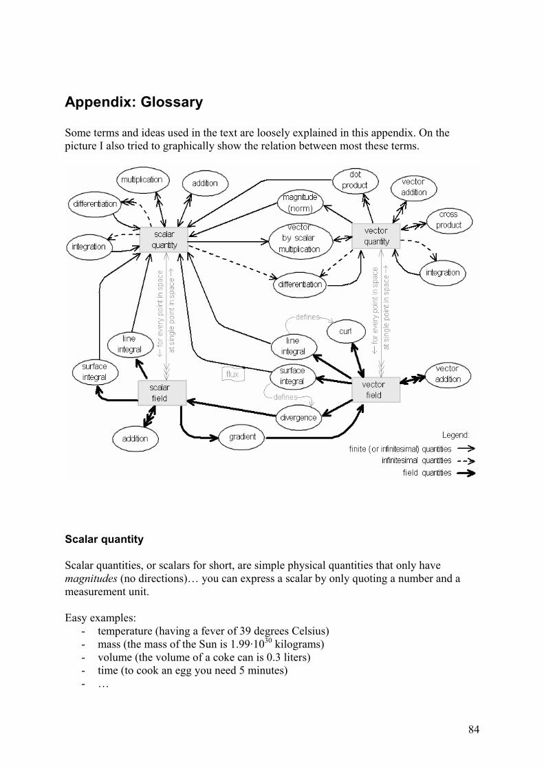
84

Appendix: Glossary

Some terms and ideas used in the text are loosely explained in this appendix. On the

picture I also tried to graphically show the relation between most these terms.

Scalar quantity

Scalar quantities, or scalars for short, are simple physical quantities that only have

magnitudes (no directions)… you can express a scalar by only quoting a number and a

measurement unit.

Easy examples:

- temperature (having a fever of 39 degrees Celsius)

- mass (the mass of the Sun is 1.99·1030 kilograms)

- volume (the volume of a coke can is 0.3 liters)

- time (to cook an egg you need 5 minutes)

- …

85

Less easy examples:

- distance (in sense of what your car’s odometer is showing)

- speed (in sense what you car’s instrument is showing; it differs from velocity)

- length, width, height

- electric current intensity

- …

Mathematically, scalar quantities are represented and handled as (the familiar) real numbers. You still

need to care about the measurement units – for example, when summing minutes to hours, convert the

units first (dissimilar units, like amperes and kilograms, cannot be summed at all). But even if units

might allow a math operation, it does not mean the result will make a sense – you need to understand

what and why you are doing (in other words, you need to know physics).

When you multiply or divide scalar quantities, you obtain a quantity of a different kind. For example,

if you multiply watts with seconds you obtain joules (or, multiplying meters with meters produces unit

of square-meters.)

Vector quantity

A vector quantity has magnitude and direction. Often you can feel if something is a vector

quantity (or ‘vector’, for short) because you can sense that this quantity possesses certain

directionality.

Easy examples:

- force (a force is pushing an object in certain direction)

- displacement (an object displaces in certain direction)

- velocity (an object travels in certain direction)

- linear momentum (an object has its momentum in certain direction)

- …

Less easy examples:

- position (tells the distance and direction from the origin)

- electric current density (charges flow in certain direction)

- angular velocity (a vector directed along the axis of rotation)

- torque (along the (would-be) axis of rotation)

- magnetic field intensity (its direction causes the compass needle to align)

- …

A velocity, for example, could be expressed as ‘nine meters per second straight ahead’,

where ‘nine meters per second’ is the magnitude, and ‘straight ahead’ is the direction.

We say that two vector quantities are equal if they have equal magnitude and equal

direction. If only the direction is the equal, we call them parallel.

We often sketch vector quantities as arrows (their lengths represent the magnitude). The

depicted example shows three force vectors (blue arrows), one velocity vector (red arrow)

and one quantity ‘m’ that is a simple scalar.

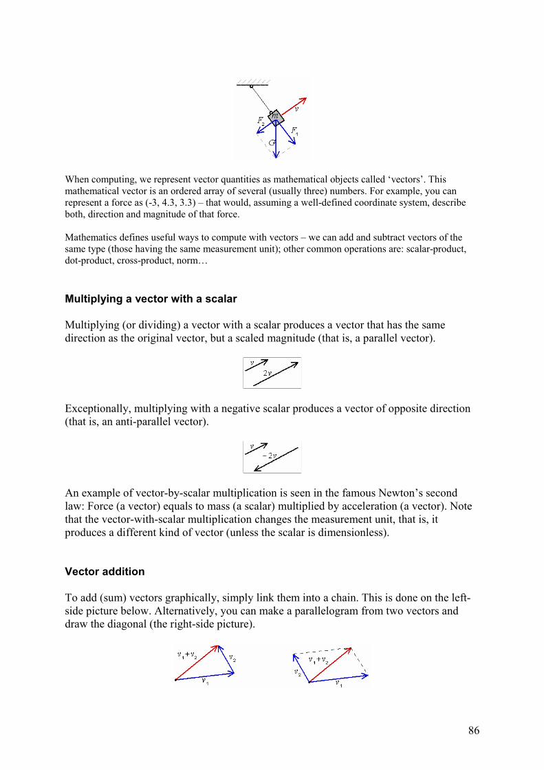
86

When computing, we represent vector quantities as mathematical objects called ‘vectors’. This

mathematical vector is an ordered array of several (usually three) numbers. For example, you can

represent a force as (-3, 4.3, 3.3) – that would, assuming a well-defined coordinate system, describe

both, direction and magnitude of that force.

Mathematics defines useful ways to compute with vectors – we can add and subtract vectors of the

same type (those having the same measurement unit); other common operations are: scalar-product,

dot-product, cross-product, norm…

Multiplying a vector with a scalar

Multiplying (or dividing) a vector with a scalar produces a vector that has the same

direction as the original vector, but a scaled magnitude (that is, a parallel vector).

Exceptionally, multiplying with a negative scalar produces a vector of opposite direction

(that is, an anti-parallel vector).

An example of vector-by-scalar multiplication is seen in the famous Newton’s second

law: Force (a vector) equals to mass (a scalar) multiplied by acceleration (a vector). Note

that the vector-with-scalar multiplication changes the measurement unit, that is, it

produces a different kind of vector (unless the scalar is dimensionless).

Vector addition

To add (sum) vectors graphically, simply link them into a chain. This is done on the left-

side picture below. Alternatively, you can make a parallelogram from two vectors and

draw the diagonal (the right-side picture).

87

Only sum vectors of the same type (velocities with velocities; forces with forces…).

Subtracting a vector equals to adding it, but multiplied with the -1 scalar first.

We can also split (resolve) one vector into two (or more) component vectors. On the

example below, the force ‘G’ is resolved into two perpendicular forces ‘F1’ and ‘F2’.

Dot product

The ‘dot product’ is one method to ‘multiply’ two vectors. The result is a scalar.

Computing the dot product of two parallel vectors is easy – just multiply their magnitudes

(and forget about their directions).

If the vectors are anti-parallel (opposite), it is still as easy, but the result is negative.

If vectors are not parallel, first find a projection of one vector on the other vector; then

you have two parallel vectors and you can multiply their magnitudes. Like this:

Clearly, if two vectors are perpendicular to each other, their dot-product is zero.

In physics, for example, the quantity of work is often expressed as a dot-product: the work

(a scalar) equals to force (a vector) dot-multiplied by displacement (a vector).

Cross product

Another method to ‘multiply’ two vectors is the ‘cross product’. The result is a vector (or

a pseudovector) that has a direction perpendicular to both multiplied vectors.

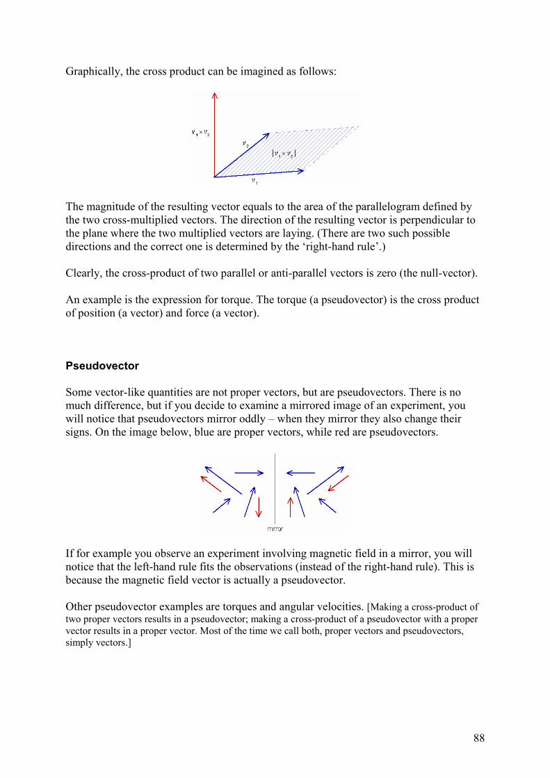
88

Graphically, the cross product can be imagined as follows:

The magnitude of the resulting vector equals to the area of the parallelogram defined by

the two cross-multiplied vectors. The direction of the resulting vector is perpendicular to

the plane where the two multiplied vectors are laying. (There are two such possible

directions and the correct one is determined by the ‘right-hand rule’.)

Clearly, the cross-product of two parallel or anti-parallel vectors is zero (the null-vector).

An example is the expression for torque. The torque (a pseudovector) is the cross product

of position (a vector) and force (a vector).

Pseudovector

Some vector-like quantities are not proper vectors, but are pseudovectors. There is no

much difference, but if you decide to examine a mirrored image of an experiment, you

will notice that pseudovectors mirror oddly – when they mirror they also change their

signs. On the image below, blue are proper vectors, while red are pseudovectors.

If for example you observe an experiment involving magnetic field in a mirror, you will

notice that the left-hand rule fits the observations (instead of the right-hand rule). This is

because the magnetic field vector is actually a pseudovector.

Other pseudovector examples are torques and angular velocities. [Making a cross-product of

two proper vectors results in a pseudovector; making a cross-product of a pseudovector with a proper

vector results in a proper vector. Most of the time we call both, proper vectors and pseudovectors,

simply vectors.]

89

Torque

The torque is a quantity that tells how ‘strongly’ is something being twisted or turned. For

example, a torque is developed when you are using a spanner to tightening a nut.

The torque is what a car engine is applying in order to turn wheels. The torque is what a

magnetic field is applying to rotate a compass needle.

Mathematically, the torque is represented as a vector (a pseudovector, actually). The

direction of the torque vector is along the turning axis.

Infinitesimal quantities

An infinitesimal quantity is an exceedingly small quantity, but not zero.

Sometimes we want to use quantities as small as practically possible, for example:

- To obtain an instantaneous velocity, we consider how far an object moves in a very

short time.

- A balanced stick can be tested for stability by tilting it for a very small degree.

- The area of a curved floor surface can be estimated by counting how many of very

small flat tiles (of known area) we need to cover it

While in practice we are limited on how small quantities we can handle, in our

imagination we can handle quantities so small that they near (but are not) the zero – we

call them infinitesimal quantities. If compared to finite quantities, infinitesimal ones are

completely insignificant. But infinitesimal quantities can be compared mutually (some are

larger, some smaller).

Generally, we can compute with infinitesimal quantities the usual way (as with finite

quantities). We can add, subtract, multiply… Notably, we can:

- divide two infinitesimal quantities and obtain a finite ratio

- sum a near-infinite number of infinitesimal quantities and obtain a finite sum

These two operations correspond to differentiation and integration, respectively. In

physics, you will therefore find infinitesimal quantities in many formulas.

An infinitesimal quantity is often denoted by adding the letter ‘d’ in front of the letter

usually used for quantity of such type – for example ‘dx’ my stand for an infinitesimal

displacement or ‘dt’ might stand for an infinitesimal time span.

You may think about infinitesimal quantity as a single step of a continuous change. While continuous

change is not stepped, you really couldn’t tell the difference if steps are infinitesimally small. So,

infinitesimals are like imagined ‘steps’ invented by mathematicians to analyze continuous changes.

90

Instantaneous rate of change; differentiation

The instantaneous rate of change relates two dependant quantities – it tells how much one

quantity changes when the other one changes for an infinitesimally small amount.

As an example, take the quantity of velocity:

- the ‘average velocity’ is obtained by dividing a finite distance covered in finite

time span

- but the ‘instantaneous velocity’ is obtained by dividing an infinitesimal distance

covered in infinitesimal time span. In math notation, this can be written as:

There are many more quantities that can be expressed as instantaneous change rate:

angular velocity (angle per time), current intensity (passed charge per time), electric field

intensity (electric potential per distance)…

Many physical laws are also expressed using instantaneous change rates. For example, the

Faraday’s law of induction says that the EMF generated in a wire loop is proportional to

the instantaneous change rate of magnetic flux (through the loop) in time:

In practice, we cannot measure infinitesimal quantities and therefore finding instantaneous

change rates by measurement is approximate. However, if we can express the dependence

between two quantities by a continuous function, then we can exactly compute the

instantaneous change rate – the procedure involves differentiation.

Example: the blue line in the graph shows the position of an object in time. Suppose that

we can express this position as: x(t)=sin t + 0.8t.

Differentiating the function x(t), we obtain a new function, x’(t)=cos x + 0.8. This new

function is called the derivative and is depicted green. For any point in time, our

derivative function has a value related to the slope of the original function. That is, the

value of the derivative at certain time ‘t’ is actually the instantaneous change rate of the

original function (a.k.a. primitive function) at that time.

91

Integral

The integral is a sum of infinitely many infinitesimal quantities.

How to find the area of a curved shape like shown below? We can divide the shape into

many narrow rectangles and sum their areas.

The result is inexact because rectangles do not fit the shape perfectly… However, if we

make the rectangles infinitesimally narrow, our computation can be exact!

A mathematical procedure, called integration, can sum infinite number of infinitesimal

quantities and obtain a finite result. The result is called the integral.

To compute the integral you should be able to express the involved range of infinitesimal

quantities by some continuous function. In the above example, we would need to know a

function that for the horizontal position (x) gives the area (dA) of the infinitesimally

narrow rectangle found at that position.

Say that the above shape can be represented as the area under curve ‘sin x + 2’ in the range 0 to 3. At

the postion ‘x’ we find an infinitesimal rectangle whose height equals to ‘sin x + 2’. The width of the

rectangle is fixed to ‘dx’. Therefore, the area of the rectangle at the position ‘x’ is ‘(sin x + 2) dx’.

Knowing this, we can exactly compute the total area of the shape by computing the following integral:

Many physical quantities can be expressed as an integral. Velocity, for example, can be

expressed as a time-integral of acceleration. Moreover, many physical laws are also

expressed in form of an integral.

Field

The field is a spatially extended quantity; it is a quantity that specifies a simpler quantity

(perhaps a scalar or a vector) for every point in space.

Fields that specify a scalar quantity for every point in space are called scalar fields. For

example, the temperature of the whole atmosphere can be described by a field that

specifies a temperature at each coordinate… The picture below shows one possible way to

draw a scalar field (this example draws isothermal lines).

92

Fields that specify a vector quantity for every point in space are called vector fields. For

example, air movements for the whole atmosphere can be described by a field that

specifies air velocity at each coordinate… Vector fields are often drawn with an array of

arrows, as shown below (some vector fields might also be drawn with field lines).

To express a field, you would need to quote infinitely many numbers (as well as the one

measurement unit). That is why we are forced to express a field mathematically by

quoting a continuous spatial function that describes field values at every point in space.

Physical fields are continuous. It means that within an infinitesimally small region, the

field does not change for any finite amount (it is constant). For example, if you want to

multiply the length of some infinitesimal line with the intensity of some field along line’s length, you

don’t need to worry which of the field values along the line to use – they are all the same. Note that I was talking about a field as way to describe some phenomena (e.g. the movement of the

atmosphere). However, a physicist might occasionally use the word ‘field’ when he/she talks about a

real physical object (for example the ‘electromagnetic field’).

Line integral

Imagine either a scalar or a vector field and some curve (path, trajectory) through that

field.

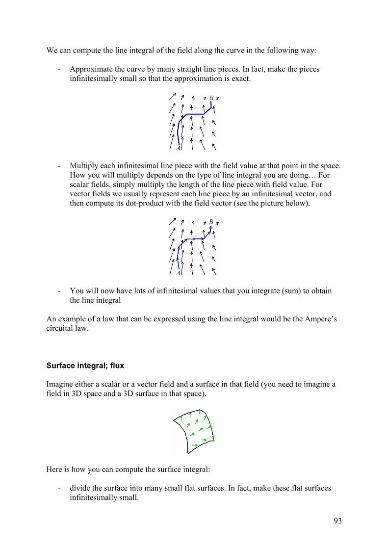
93

We can compute the line integral of the field along the curve in the following way:

- Approximate the curve by many straight line pieces. In fact, make the pieces

infinitesimally small so that the approximation is exact.

- Multiply each infinitesimal line piece with the field value at that point in the space.

How you will multiply depends on the type of line integral you are doing… For

scalar fields, simply multiply the length of the line piece with field value. For

vector fields we usually represent each line piece by an infinitesimal vector, and

then compute its dot-product with the field vector (see the picture below).

- You will now have lots of infinitesimal values that you integrate (sum) to obtain

the line integral

An example of a law that can be expressed using the line integral would be the Ampere’s

circuital law.

Surface integral; flux

Imagine either a scalar or a vector field and a surface in that field (you need to imagine a

field in 3D space and a 3D surface in that space).

Here is how you can compute the surface integral:

- divide the surface into many small flat surfaces. In fact, make these flat surfaces

infinitesimally small.

94

- multiply the area of each infinitesimal surface with the field value at this point in

space… For a scalar field, just multiply the field value and the infinitesimal surface

area. For a vector field, represent each infinitesimal surface by an infinitesimal

vector perpendicular to the surface and of magnitude equal to the surface area –

then make the dot-product of this surface vector and the local field.

- You will now have lots of infinitesimal values that you integrate (sum) to obtain

the surface integral.

An example of a law that is expressed as a surface integral would be the Gauss law.

The computed value of surface integral of a vector field is often called the flux. If, for

example, we represent velocities of water by a vector field, then the surface integral (flux)

of this field over some surface tells how much water flows through that surface per unit of

time.

Gradient

For a scalar field, we can talk about its gradient at some point. The gradient is a vector

that tells in what direction and at what rate the field changes the most (that is, it tells the

field’s steepest change). The example below shows a scalar field (contour lines) and its

gradient vectors (blue arrows) drawn for many points in the field.

If, for example, we suppose that the above picture shows a hill (its elevation represented

by contours, as on a topographic map), then the blue gradient arrows show the direction a

ball would roll downhill (and also the acceleration the ball would have).

Another example: imagine you have an unevenly heated solid body. We can represent its

temperature by a scalar field (the field tells the temperature of the body for every point).

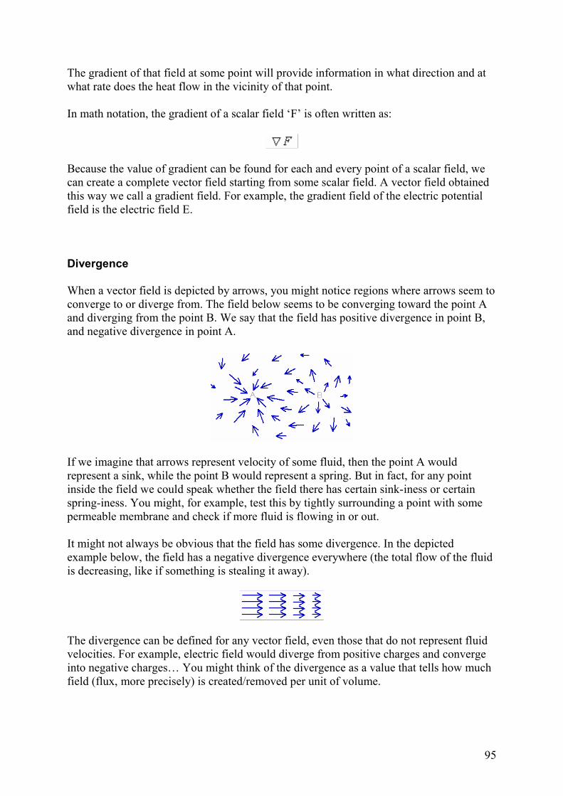
95

The gradient of that field at some point will provide information in what direction and at

what rate does the heat flow in the vicinity of that point.

In math notation, the gradient of a scalar field ‘F’ is often written as:

Because the value of gradient can be found for each and every point of a scalar field, we

can create a complete vector field starting from some scalar field. A vector field obtained

this way we call a gradient field. For example, the gradient field of the electric potential

field is the electric field E.

Divergence

When a vector field is depicted by arrows, you might notice regions where arrows seem to

converge to or diverge from. The field below seems to be converging toward the point A

and diverging from the point B. We say that the field has positive divergence in point B,

and negative divergence in point A.

If we imagine that arrows represent velocity of some fluid, then the point A would

represent a sink, while the point B would represent a spring. But in fact, for any point

inside the field we could speak whether the field there has certain sink-iness or certain

spring-iness. You might, for example, test this by tightly surrounding a point with some

permeable membrane and check if more fluid is flowing in or out.

It might not always be obvious that the field has some divergence. In the depicted

example below, the field has a negative divergence everywhere (the total flow of the fluid

is decreasing, like if something is stealing it away).

The divergence can be defined for any vector field, even those that do not represent fluid

velocities. For example, electric field would diverge from positive charges and converge

into negative charges… You might think of the divergence as a value that tells how much

field (flux, more precisely) is created/removed per unit of volume.

96

The divergence is a simple scalar value. In math notation, the divergence of a field ‘F’ is

usually written as:

Some vector fields have zero divergence everywhere (‘no springs, no sinks’). The

magnetic field is an example of such divergenceless field.

Because the value of divergence can be defined for each and every point of a vector field,

we can construct a new scalar field, called the divergence field, starting from the original

vector field. For example, the divergence of an electric field gives the charge density field

(multiplied by a scaling factor).

A more precise definition of divergence is here: imagine an infinitesimally small sphere around some

point inside a vector field. Compute the flux (that is, the surface integral of the field) that ‘passes’ the

surface of the sphere and then divide the obtained value with the volume of the sphere – the obtained

results is the divergence of the field at that point.

Curl

When a vector field is depicted by arrows, you might notice places where those arrows

make curls or whirls. The field below seems to be curling around points A and B.

If we imagine that arrows are representing velocity of some fluid, and if we place a tiny

turbine (a wheel) at spot A or B, the turbine will turn. But the thing is that we can place

the imaginary turbine (or better, a small ball with a rough surface) at any point within the

field – if the turbine turns, we say that the field has some curl at that point.

The field depicted below, for example, also has a curl (the turbine turns) despite field’s

straight appearance.

The quantity of curl at some point within the field is not a simple scalar, but is represented

with a vector. What is the direction of this vector? A small ball placed in the field will rotate around

some axis. The curl vector is directed along this axis. To further select one of the two possible

directions along the axis, one must use the Right Hand Rule.

97

But the rotating turbines/balls are only a thinking aid. The curl is defined for any vector

field, not only those that represent fluid velocities. For example, magnetic field can curl.

In mathematics, the curl of some field ‘F’ is usually written as:

Some vector fields, called conservative fields, do not have curl at any point. Examples are

gravitational field and a static electric field.

Because the value of curl is defined for each and every point of a vector field, we can

construct a new vector field, called the curl field, starting from the original vector field. A

famous example is the magnetic field B that can be written as the curl of the vector

potential field A.

A more precise definition of the curl is here: Imagine an infinitesimally small 3D surface at some

point inside a vector field. Compute the line integral of the field along the edges of that surface and

then divide the obtained value with the surface area – this gives the component of the curl vector

perpendicular to the surface. You might want to make this procedure three times for three orthogonal

orientations of infinitesimal surfaces at the same point – combining three components of curl vector

you will finally obtain the total curl vector of the field at the point.