I N T R O D U C T I O N T O C O M P U T E R G R A P H I C S Andries van Dam November 9, 2006 Radiosity 1/43 Introduction to Radiosity John F. Hughes, Andries van Dam Applets by Nick Diakopoulos

I N T R O D U C T I O N T O C O M P U T E R G R A P H I C S Andries van Dam November 9, 2006 Radiosity 1/43 Introduction to Radiosity John F. Hughes, Andries.
Dec 22, 2015
Welcome message from author
This document is posted to help you gain knowledge. Please leave a comment to let me know what you think about it! Share it to your friends and learn new things together.
Transcript
I N T R O D U C T I O N T O C O M P U T E R G R A P H I C S
Andries van Dam November 9, 2006 Radiosity 1/43
Introduction to Radiosity
John F. Hughes,Andries van Dam
Applets by Nick Diakopoulos

I N T R O D U C T I O N T O C O M P U T E R G R A P H I C S
Andries van Dam November 9, 2006 Radiosity 2/43
Color Bleeding Soft Shadows
No Ambient Term
View Independent
Used in other areas of Engineering
Radiosity for Inter-Object Diffuse Reflection
I N T R O D U C T I O N T O C O M P U T E R G R A P H I C S
Andries van Dam November 9, 2006 Radiosity 3/43
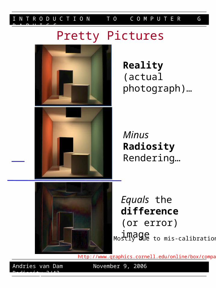
Pretty Pictures
Reality (actual photograph)…
Minus Radiosity Rendering…
Equals the difference (or error) image
http://www.graphics.cornell.edu/online/box/compare.html
Mostly due to mis-calibration

I N T R O D U C T I O N T O C O M P U T E R G R A P H I C S
Andries van Dam November 9, 2006 Radiosity 4/43
1. Model scene as “patches”2. Each patch has an initial
luminance value: all but luminaires (light sources) are probably zero
3. Iteratively determine how much luminance travels from each patch to each other patch until entire system converges to stable values
We can then render scene from any angle without recomputing these final patch luminances – they are viewer independent!
The Radiosity Technique:An Overview

I N T R O D U C T I O N T O C O M P U T E R G R A P H I C S
Andries van Dam November 9, 2006 Radiosity 5/43
Overview of Radiosity• The radiometric term radiosity means rate at which
energy leaves a surface• Sum of rates at which surface emits energy and
reflects (or transmits) energy received from all other surfaces.
• Radiosity simulations are based on thermal engineering model of emission and reflection of radiation using finite element approximations (FEM closely related to meshing).
• First determine all light interactions in a view-independent way, then render one or more views.
• Consider room with only floor and ceiling:
• Suppose ceiling is actually a fluorescent drop-panel ceiling which emits light…
• Floor gets some of this light and reflects it back• Ceiling gets some of this reflected light and sends it
back…• Simulation mimics these successive “bounces”
through progressive refinement – each iteration contributes less energy so process converges
floor
ceiling

I N T R O D U C T I O N T O C O M P U T E R G R A P H I C S
Andries van Dam November 9, 2006 Radiosity 6/43
Kajiya’s Rendering Equation• Generalized rendering equation formulated by Jim Kajiya,
19861:
• i.e.: Light energy traveling from point i to j is equal to light emitted from i to j, plus the integral over S (all points on all surfaces) of reflectance from point k to i to j, times the light from k to i, all attenuated by a geometry factor.
– is the amount of light traveling along the ray from point j to point k.
– is the amount of light emitted by the surface (luminance)
– is the Bidirectional Reflectance Distribution Function (BRDF) of the surface. Describes how much of the light incident on the surface at i from the direction of k leaves the surface in direction of j.
• λ is wavelength of light, use a different function for R, G, & B
– is a geometry term which involves occlusion, distance, and the angle between the surfaces
• More complete model of light transport than either raytracing or polygonal rendering, but omits, e.g., subsurface scattering
• How do we evaluate this function?– very difficult to solve complicated integral equations analytically
)( kjL
),( jikf
)( jiG
eL
dkikLjikfjiLjiGjiL
S
e )()()()()(
1J Kajiya. “The Rendering Equation.” SIGGRAPH 1984, pp. 143-150

I N T R O D U C T I O N T O C O M P U T E R G R A P H I C S
Andries van Dam November 9, 2006 Radiosity 7/43
• A scene has:– geometry– luminaires (light sources)– observation point
• Light transport to camera must be computed for every incoming angle to observation point, bouncing off all geometry (in all directions combined)
• This is far too hard• Both raytracing and radiosity are crude
approximations to rendering equation– Raytracing: consider only a very small, finite
number of rays and ignore diffuse inter-object reflections, perhaps using ambient hack to approximate that lost component. Can use either a BRDF or a simpler (e.g., Phong) model for luminaires
– Radiosity: approximate integral over differential source areas dA(i) with finite sum over finite areas; consider light transport not on basis of individual rays but on basis of energy transport between finite patches (e.g., quads or triangles that result from (adaptive) meshing)
Rendering a Scene
I N T R O D U C T I O N T O C O M P U T E R G R A P H I C S
Andries van Dam November 9, 2006 Radiosity 8/43
• Design an alternative simulation of real transfer of light energy
• With any luck, will be more accurate, but accuracy is relative
– hall of mirrors is specular raytracing
– museum with latex-painted walls is diffuse radiosity
• Raytracing and Radiosity both approximate BRDF function by leaving out contributions of incoming rays to a surface point
• Best solutions are hybrid techniques: use raytracing for specular components and radiosity for diffuse components
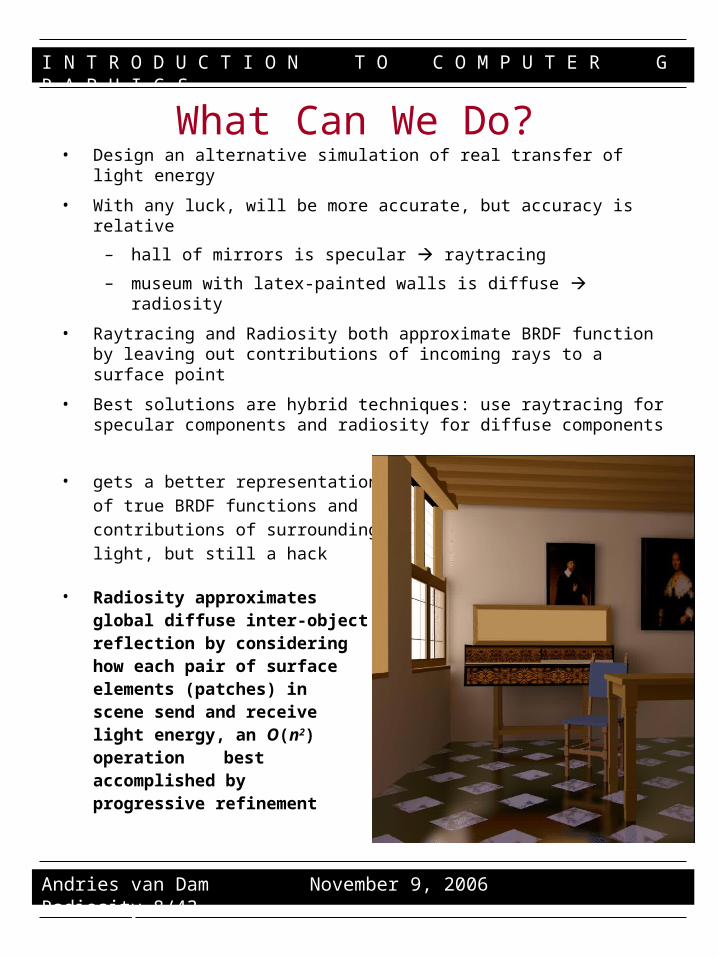
• gets a better representation of true BRDF functions and contributions of surrounding light, but still a hack
• Radiosity approximates global diffuse inter-object reflection by considering how each pair of surface elements (patches) inscene send and receive light energy, an O(n2) operation best accomplished byprogressive refinement
What Can We Do?
I N T R O D U C T I O N T O C O M P U T E R G R A P H I C S
Andries van Dam November 9, 2006 Radiosity 9/43
• Energy = light energy = radiosity for our purposes – it should really be rate, i.e., energy/unit time…
• Ei: initial amount of energy radiating from i’th patch• Bi: final amount of energy radiating from i’th patch• Bj: final amount of energy radiating from j’th patch• Fj-i: fraction of energy Bi emitted by j’th patch that is
gathered by i’th patch (relationship between i’th and j’th patches based on geometry: distance, relative angles)
• Fj-i Bj: total amount of patch j's energy sent to patch i• ρi: fraction of incoming energy to a patch that is then
exported in next iteration
Some Important Symbols

I N T R O D U C T I O N T O C O M P U T E R G R A P H I C S
Andries van Dam November 9, 2006 Radiosity 10/43
(1/2)
• Amount of light/radiosity/energy a patch finally emits is initial emission plus sum of emissions due to other n-1 patches in scene emitting to this patch: recursive definition. Note: F1-1 is zero only for planar patches!
n j i
jijiii BFEB
• Thus:• Rewrite as a vector product:
• And the whole system:
131321211111 ...)( EBFBFBFρB
13
2
1
131121111 ...)1( EB
B
B
FρFF
nj
jijiii BFBE1
or
Sender1
Sender2
Sendern
Receiver, patchi
…
Let’s Arrange Those Symbols

I N T R O D U C T I O N T O C O M P U T E R G R A P H I C S
Andries van Dam November 9, 2006 Radiosity 11/43
Decompose the first matrix as:
Can be rewritten:• (I – D()F)B = E
– where D() is diagonal matrix with i as its ith diagonal entry, and F is called Form Factor Matrix and is based on geometry between patches
• If we know E, D() , and F, we can determine B• If we let
A = I – D()F• Then we are solving (for B) the equation AB = E• This is a linear system, and methods for solving
these are well-known, e.g. Gaussian elimination or Gauss-Seidel iteration (although which method is best depends on nature of matrix A)
• Typically want B, knowing E and A
(2/2)Let’s Arrange Those Symbols
I N T R O D U C T I O N T O C O M P U T E R G R A P H I C S
Andries van Dam November 9, 2006 Radiosity 12/43
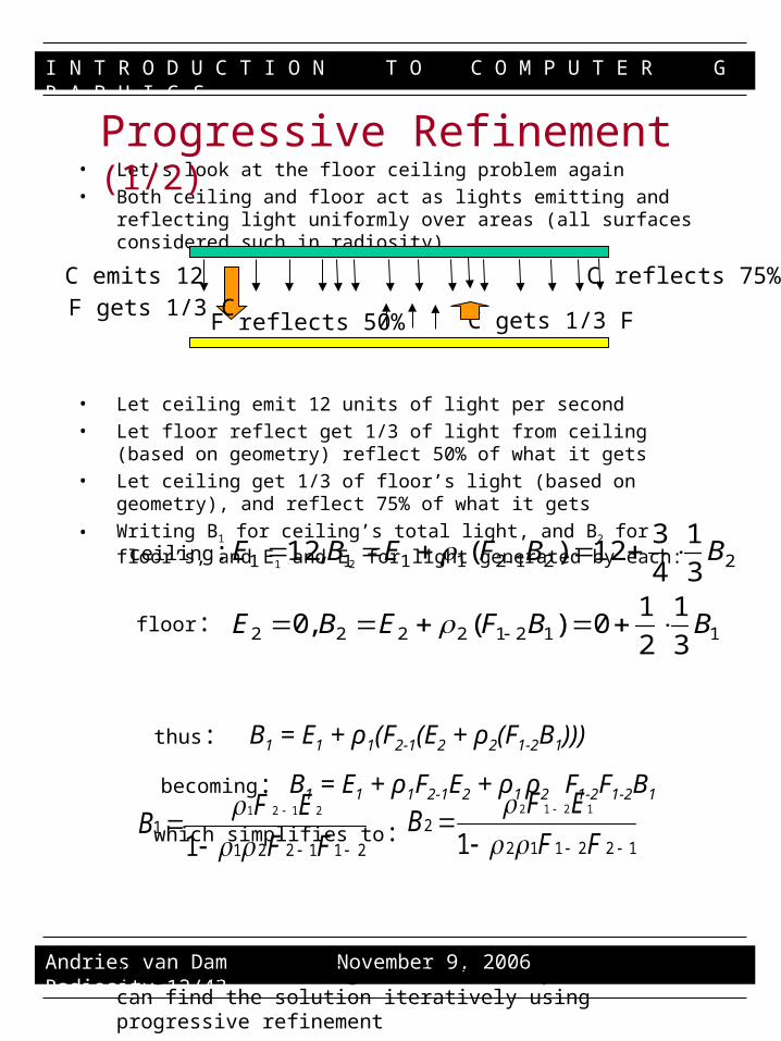
• Let’s look at the floor ceiling problem again• Both ceiling and floor act as lights emitting and reflecting light
uniformly over areas (all surfaces considered such in radiosity)
• Let ceiling emit 12 units of light per second• Let floor reflect get 1/3 of light from ceiling (based on
geometry) reflect 50% of what it gets• Let ceiling get 1/3 of floor’s light (based on geometry), and
reflect 75% of what it gets
• Writing B1 for ceiling’s total light, and B2 for floor’s, and E1 and E2 for light generated by each:
thus: B1 = E1 + ρ1(F2-1(E2 + ρ2(F1-2B1)))
becoming: B1 = E1 + ρ1F2-1E2 + ρ1 ρ2 F1-2F1-2B1
which simplifies to:
• In general, this algebra is too complex, but we can find the solution iteratively using progressive refinement
11212222
22121111
3
1
2
10)(,0
3
1
4
312)(,12
BBFEBE
BBFEBE
ceiling:
floor:
1221122
1
1212
FF
EFB
2112211
1
2121
FF
EFB
C emits 12F gets 1/3 C
F reflects 50% C gets 1/3 F
C reflects 75%
Progressive Refinement (1/2)

I N T R O D U C T I O N T O C O M P U T E R G R A P H I C S
Andries van Dam November 9, 2006 Radiosity 13/43
• Iterative method 1, gathering energy: send out light from emitters everywhere, accumulate it, resend from all patches… Each iteration uses radiosity values from previous iteration as estimates for recursive form. Iterate by rows.
Bk = E + D()FBk-1
B1 = E
B2 = E + D(FB1
B3 = E + D(FB2
Where Bk is your kth guess at radiosity values B1, B2…
Results for our example:
{12, 0} = {B1, B2}= {E1, E2}
{12, 2} =
{12.5, 2} =
{12.5, 2.08373} =
{12.5208, 2.08373}
{12.5208, 2.08681}
{12.5217, 2.08681}
{12.5217, 2.08695}
12
3
1
2
10 ,012 , 1212221211 BFEBFE
12
3
1
2
10 ,2
3
1
4
312
5.12
3
1
2
10,2
3
1
4
312
Progressive Refinement (2/2)

I N T R O D U C T I O N T O C O M P U T E R G R A P H I C S
Andries van Dam November 9, 2006 Radiosity 14/43
General Radiosity Equation (1/3)
• The radiosity equation for normalized unit areas of Lambertian diffuse patches is:
• Bi is total radiosity in watts/m2 (i.e. energy/unit-time / unit-area) radiating from patch i
– Note that we are now calculating Bi (and Ei) per unit area
• Ei is light emitted in watts/m2
• ρi is fraction of incident energy reflected by patch i (related to diffuse reflection coefficient kd in simple lighting model)
• Aj is area of j’th patch
• (Bj Aj) is total energy radiated by patch j with area Aj (i.e., unit radiosity x area)
nj i
ijjjiii A
FABEB
1
)(
Sender1
Sender2
Sendern
Receiver
…
I N T R O D U C T I O N T O C O M P U T E R G R A P H I C S
Andries van Dam November 9, 2006 Radiosity 15/43
General Radiosity Equation (2/3)
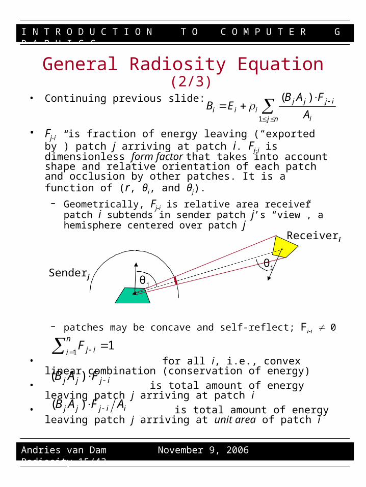
• Continuing previous slide:
• Fj-i is fraction of energy leaving (“exported by”) patch j arriving at patch i. Fj-i is dimensionless form factor that takes into account shape and relative orientation of each patch and occlusion by other patches. It is a function of (r, θi, and θj).
– Geometrically, Fj-i is relative area receiver patch i subtends in sender patch j’s “view”, a hemisphere centered over patch j
– patches may be concave and self-reflect; Fi-i 0
• for all i, i.e., convex linear combination (conservation of energy)
• is total amount of energy leaving patch j arriving at patch i
• is total amount of energy leaving patch j arriving at unit area of patch i
n
i ijF1
1
ijjj FAB )(
iijjj AFAB )(
nj i
ijjjiii A
FABEB
1
)(
θi
θj
Receiveri
Senderj

I N T R O D U C T I O N T O C O M P U T E R G R A P H I C S
Andries van Dam November 9, 2006 Radiosity 16/43
General Radiosity Equation (3/3)• Reciprocity relationship between Fi-j and Fj-i, proven later:
– which means form factors scaled for unit area of receiver patch are equal
• Therefore,
– which is easier to deal with, if less intuitive– Says that radiosity of receiver patch i is energy emitted by that patch +
attenuated sum of each sender j’s radiosity times form factor from i to j (not from j to i)
– for each receiver row i iterate across all sender columns j to gather energy those senders emit, attenuated by Fi-j.
• Note: we should calculate this for all wavelengths --- approximate with BiR, BiG, BiB`
nj
jijiii FBEB1

I N T R O D U C T I O N T O C O M P U T E R G R A P H I C S
Andries van Dam November 9, 2006 Radiosity 17/43
Computing Form Factors (1/7)
• Form factor from differential sending area dAi to differential receiving area dAj is:
for ray of length r between patches, at angles i, j to normals of the areas. Hij is 1 if dAj is visible from dAi and 0 otherwise.
• We will motivate this equation…
• Also see form factor applet:
jijji
djdi dAHr
dF2
coscos
Applet: http://www.cs.brown.edu/exploratories/freeSoftware/catalogs/lighting_and_shading.html
Receiverj
Senderi

I N T R O D U C T I O N T O C O M P U T E R G R A P H I C S
Andries van Dam November 9, 2006 Radiosity 18/43
Computing Form Factors (2/7)• When two patches directly face each other,
maximum energy is transmitted from Ai to Aj
- their normal vectors are parallel, cosj = 1, cosi =1 since i = j = 0
• Rotate Aj so that it is perpendicular to Ai. Now cosi is still 1, but cosj = 0 since j = 90
• In general, we calculate energy fraction by multiplying by cosj. Tilting Ai means multiplying by cosi
• Same as Lambertian diffuse reflection

I N T R O D U C T I O N T O C O M P U T E R G R A P H I C S
Andries van Dam November 9, 2006 Radiosity 19/43
Computing Form Factors (3/7)
• From where does the r2 term arise? The inverse-square law of light propagation:
• Consider a patch A1, at a distance R = 1 from light source L. If P photons hit area A1, their density is P/A1. These same P photons pass through A2. Since A2 is twice as far from L, by similar triangles, it has four times the area of A1. Therefore each similar patch on A2 receives 1/4 of the photons

I N T R O D U C T I O N T O C O M P U T E R G R A P H I C S
Andries van Dam November 9, 2006 Radiosity 20/43
Computing Form Factors (4/7)• The in the formula is a normalizing factor
• If we integrate form factor across surface of a unit hemisphere, we need to achieve unity (all light goes somewhere). By what constant k do we scale the integration to normalize this value? r = 1, qj = 0
1
][sincoscos
1
1cos2
0
2
0
k
dddA
k
dAk
iii
A i
A i

I N T R O D U C T I O N T O C O M P U T E R G R A P H I C S
Andries van Dam November 9, 2006 Radiosity 21/43
Computing Form Factors (5/7)
• Now consider a differential patch dAi radiating to finite patch Aj
• Fdi-j can be computed by projecting those parts of Aj visible from dAi onto the unit hemisphere centered about dAi.
• Form factor is effectively the ratio of curved patch area to the total surface area of the hemisphere.
• Total surface area encompasses all energy emitted by dAi
I N T R O D U C T I O N T O C O M P U T E R G R A P H I C S
Andries van Dam November 9, 2006 Radiosity 22/43
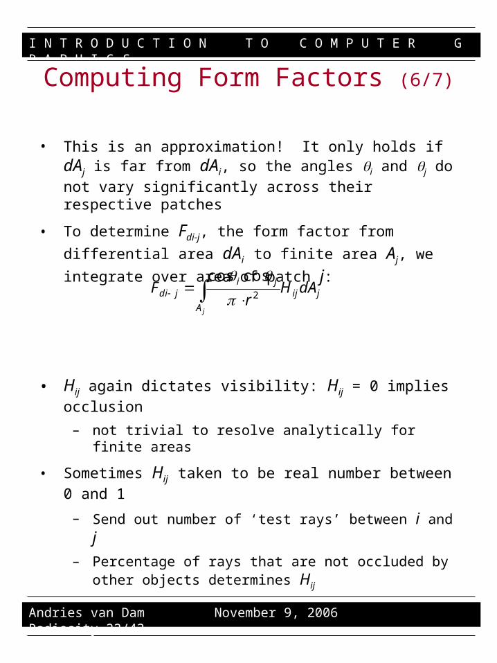
Computing Form Factors (6/7)
• This is an approximation! It only holds if dAj is far
from dAi, so the angles i and j do not vary significantly across their respective patches
• To determine Fdi-j, the form factor from differential
area dAi to finite area Aj, we integrate over area of
patch j:
• Hij again dictates visibility: Hij = 0 implies occlusion
– not trivial to resolve analytically for finite areas
• Sometimes Hij taken to be real number between 0 and 1
– Send out number of ‘test rays’ between i and j
– Percentage of rays that are not occluded by other objects determines Hij
jij
A
jijdi dAH
rF
j
2
coscos
I N T R O D U C T I O N T O C O M P U T E R G R A P H I C S
Andries van Dam November 9, 2006 Radiosity 23/43
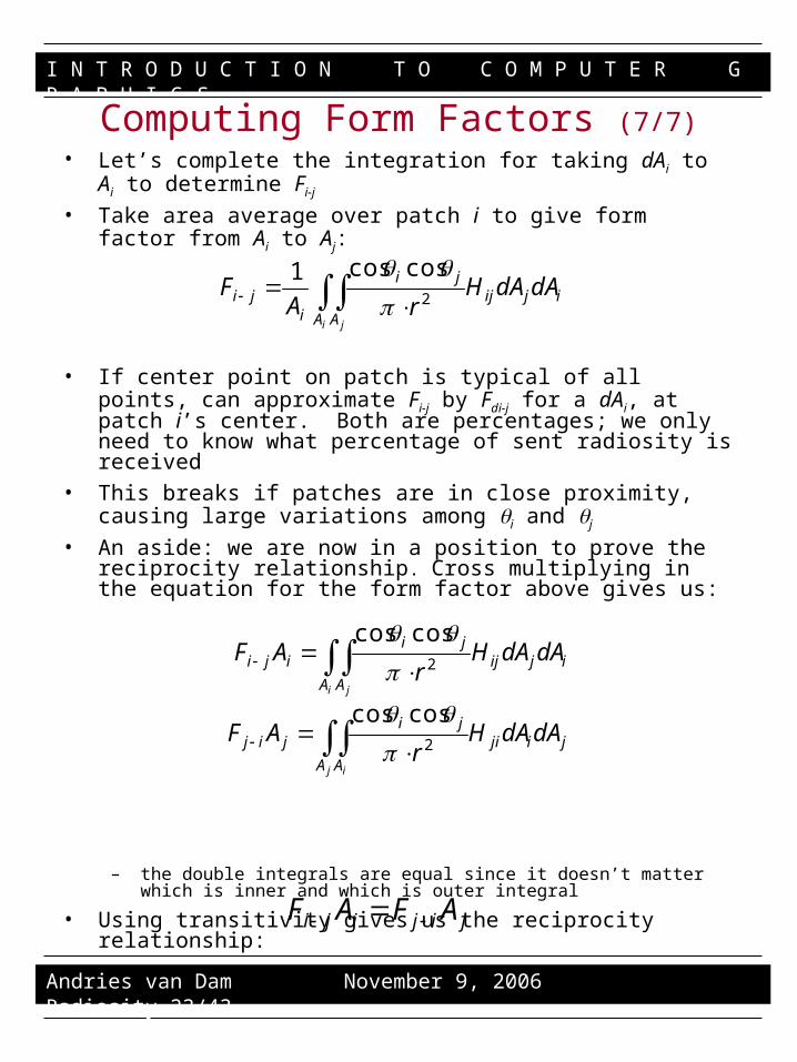
Computing Form Factors (7/7)• Let’s complete the integration for taking dAi to Ai to
determine Fi-j
• Take area average over patch i to give form factor from Ai to Aj:
• If center point on patch is typical of all points, can approximate Fi-j by Fdi-j for a dAi, at patch i’s center. Both are percentages; we only need to know what percentage of sent radiosity is received
• This breaks if patches are in close proximity, causing large variations among i and j
• An aside: we are now in a position to prove the reciprocity relationship. Cross multiplying in the equation for the form factor above gives us:
– the double integrals are equal since it doesn’t matter which is inner and which is outer integral
• Using transitivity gives us the reciprocity relationship:
i
A
jij
A
ji
iji dAdAH
rAF
i j
2
coscos1
i
A
jij
A
jiiji dAdAH
rAF
i j
2
coscos
j
A
iji
A
jijij dAdAH
rAF
j i
2
coscos
jijiji AFAF

I N T R O D U C T I O N T O C O M P U T E R G R A P H I C S
Andries van Dam November 9, 2006 Radiosity 24/43
Approximating Form Factors (1/2)
• Rather than projecting Aj onto a hemisphere, Cohen and Greenberg proposed projecting onto the upper half of a cube centered about dAi, with its top face parallel to the surface.
• Each face of the hemicube is divided into equal sized square cells.
• Think of each face of the cube as a film plane which records what a patch, dAi , “sees” in each of the five directions; center of dAi acts as COP.
• In other words, think of the cells on the faces as pixels and use the frustrum formed by the vertices of Aj onto each face.

I N T R O D U C T I O N T O C O M P U T E R G R A P H I C S
Andries van Dam November 9, 2006 Radiosity 25/43
Approximating Form Factors (2/2)
• Identity of closest intersecting patch is recorded at each cell (the survivor of the z buffer algorithm). Each hemicube cell p is associated with a precomputed delta form factor value,
where p is angle between p’s surface normal and vector of length r between dAi and p, and where A is area of cell
• Can approximate Fdi-j for any patch j by summing Fp associated with each cell p covered by patch j’s hemicube projection
• provides occlusion determination of patches through z buffer (albeit approximately, limited by the granularity/resolution of the cells on each plane)
• This eliminates the need to compute Hi-j
Ar
F pip
2
coscos

I N T R O D U C T I O N T O C O M P U T E R G R A P H I C S
Andries van Dam November 9, 2006 Radiosity 26/43
Faster Progressive Refinement: Shooting• Gathering: must process consecutive rows of receivers, for each
receiver looping through each column/sender; all rows must be processed for each iteration of the algorithm
– all form factors must be calculated before first iteration of Gauss-Seidel occurs
• Shooting: shoot energy in order from brightest to least bright patch (i.e., most significant light sources first)
– accumulate at receivers
– iteratively shoot from patch that has largest amount of “unshot” radiosity (e.g., for a single light source, the patch which has the largest form factor with that source will be next patch to shoot from)
• Computing form factor can be done by using a hemicube for each shooter that can be computed and discarded for each receiver (shown next)
– solves O(n2) processing / storage problem for each gathering iteration
– shooting converges faster than gathering
• In shooting, iterate by column not from left to right but in order of patch with most “unshot” radiosity
– can form an estimate of light on all destination patches with only first column shot, while gathering by row from all senders lights up only that row’s patch.
– iterating over column of brightest emitter lights up all patches reachable by emitter as a zeroth order approximation, improved by each successive emitter (and then brightest unshot patch)
– can add decreasing ambient term (goes to 0) as a hack
I N T R O D U C T I O N T O C O M P U T E R G R A P H I C S
Andries van Dam November 9, 2006 Radiosity 27/43
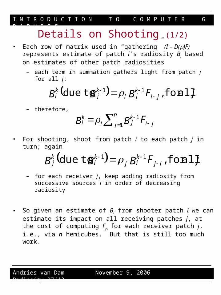
Details on Shooting (1/2)• Each row of matrix used in “gathering” (I – D()F)
represents estimate of patch i’s radiosity Bi based on estimates of other patch radiosities
– each term in summation gathers light from patch j for all j:
– therefore,
• For shooting, shoot from patch i to each patch j in turn; again
– for each receiver j, keep adding radiosity from successive sources i in order of decreasing radiosity
• So given an estimate of Bi from shooter patch i, we can estimate its impact on all receiving patches j, at the cost of computing Fj-i for each receiver patch j, i.e., via n hemicubes. But that is still too much work.
jFBBB jikji
kj
ki allfor , todue 11
n
j jikji
ki FBB 1
1
jFBBB ijkij
ki
kj allfor , todue 11

I N T R O D U C T I O N T O C O M P U T E R G R A P H I C S
Andries van Dam November 9, 2006 Radiosity 28/43
Details on Shooting (2/2)• Using reciprocity again, or just the original formulation,
which requires only the hemicube over patch i!
Thus only a single hemicube and its n form factors need be computed each pass!
• Note that for a given shooter i, we loop through all receiving patches j. Given our notation for the form factor matrix, holding i constant and looping through all j corresponds to traversing a column.
• See shooting vs.
gathering applet:
j
iji
kij
ki
kj A
AFBBB
11 todue
Applet: http://www.cs.brown.edu/exploratories/freeSoftware/catalogs/lighting_and_shading.html
I N T R O D U C T I O N T O C O M P U T E R G R A P H I C S
Andries van Dam November 9, 2006 Radiosity 29/43
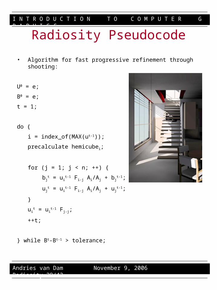
Radiosity Pseudocode
• Algorithm for fast progressive refinement through shooting:
U0 = e;
B0 = e;
t = 1;
do {
i = index_of(MAX(ut-1));
precalculate hemicubei;
for (j = 1; j < n; ++) {
bjt = ui
t-1 Fi-j Ai/Aj + bjt-1;
ujt = ui
t-1 Fi-j Ai/Aj + ujt-1;
}
uit = ui
t-1 Fj-j;
++t;
} while Bt-Bt-1 > tolerance;

I N T R O D U C T I O N T O C O M P U T E R G R A P H I C S
Andries van Dam November 9, 2006 Radiosity 30/43
Radiosity as an Approximation to the Rendering Eqn. (1/2)
• Why does this algorithm work as an approximation for the rendering equation?
• Remember Kajiya’s rendering equation:
• first need to turn integral into a summation since Radiosity is a discrete process:
• Note: we use fD instead of f. This is because we need a BRDF for patches, not for infinitely small points
• We thus need the integral of point BRDFs over entire area of patch to formulate a discrete BRDF
• But for radiosity BRDF function in continuous domain is just a constant f0 since all surfaces are perfectly diffuse
• Integrating f0 over patch is similar to integrating the differential form factor over hemisphere:
dkikLjikfjiLjiGjiL
S
e )()()()()(
ji
D
fkjif
coscos)( 0
k
e ikLjikfjiLjiGjiL DD )()()()()(

I N T R O D U C T I O N T O C O M P U T E R G R A P H I C S
Andries van Dam November 9, 2006 Radiosity 31/43
Radiosity as an Approximation to the Rendering Eqn. (2/2)
• The Geometry function in the discrete domain is now
due to inverse falloff and visibility terms• Now let’s combine the BRDF and geometry
terms
• The combined BRDF and Geometry term make the form factor equation Fi-j
• This makes new (approximated) rendering equation look like
• Radiosity is simply a discrete version of Kajiya’s rendering equation with a constant BRDF for all surfaces
ni
jie FjiLjLjLD
1
)()()(
2)(
r
HjiG ji
D
2
coscos
r
HGf jiji
DD

I N T R O D U C T I O N T O C O M P U T E R G R A P H I C S
Andries van Dam November 9, 2006 Radiosity 32/43
Limitations of Radiosity
• Assumption that radiation is uniform in all directions
• Assumption that radiosity is piecewise constant– usual renderings make this assumption, but then interpolate
cheaply to fake a nice-looking answer
– this introduces quantifiable errors
• Computation of form factors Fi-j can be tough
– especially with intervening surfaces, etc.
• Assumption that reflectivity is independent of directions to source and destination
• No volumetric objects (though there are equations and algorithms for calculating surface-to-volume form factors)
• no transparency or translucency
• Independence from wavelength – no fluorescence or phosphorescence
• Independence from phase – no diffraction
• Enormity of matrices! For large scenes, 10K x 10K matrices are not uncommon (shooting reduces need to have it all memory resident)

I N T R O D U C T I O N T O C O M P U T E R G R A P H I C S
Andries van Dam November 9, 2006 Radiosity 33/43
More Comments
• Even with these limitations, it produces lovely pictures
• For n surface patches, we have to build an n x n matrix and solve Ax = b, which takes O(n2), this gets rather expensive for large scenes
• Could we do it in O(n) instead?
• The answer, for lots of nice scenes, is “Yes”
Tangent: This is a lot like
• The Google search engine uses an system much like radiosity to rank its pages
– Site rankings are determined not only by the number of links from various sources, but by the number of links coming into those sources (and so on)
– After multiple iterations through the link network, site rankings stabilize
– Site importance is like luminance, and every site is initially considered an “emitter”
I N T R O D U C T I O N T O C O M P U T E R G R A P H I C S
Andries van Dam November 9, 2006 Radiosity 34/43
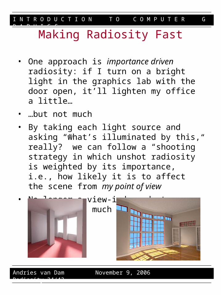
Making Radiosity Fast
• One approach is importance driven radiosity: if I turn on a bright light in the graphics lab with the door open, it’ll lighten my office a little…
• …but not much
• By taking each light source and asking “what’s illuminated by this, really?” we can follow a “shooting” strategy in which unshot radiosity is weighted by its importance, i.e., how likely it is to affect the scene from my point of view
• No longer a view-independent solution…but much faster

I N T R O D U C T I O N T O C O M P U T E R G R A P H I C S
Andries van Dam November 9, 2006 Radiosity 35/43
Combining Radiosity with Raytracing
• Radiosity is perfect for diffuse reflection; doesn’t handle specular
• Raytracing perfect for specular; doesn’t handle diffuse
Combining the two methods seems like an attractive compromise, however it proves to be more difficult than one would think
There is a good deal of material presented in the book:
Section 16.13.7 Combining Radiosity and Raytracing, pgs. 804-806
Photon Mapping: faster than Radiosity alone, more physically accurate model than simply combining specular and diffuse contributions
Photon MappingRaytracing + Radiosity
I N T R O D U C T I O N T O C O M P U T E R G R A P H I C S
Andries van Dam November 9, 2006 Radiosity 36/43
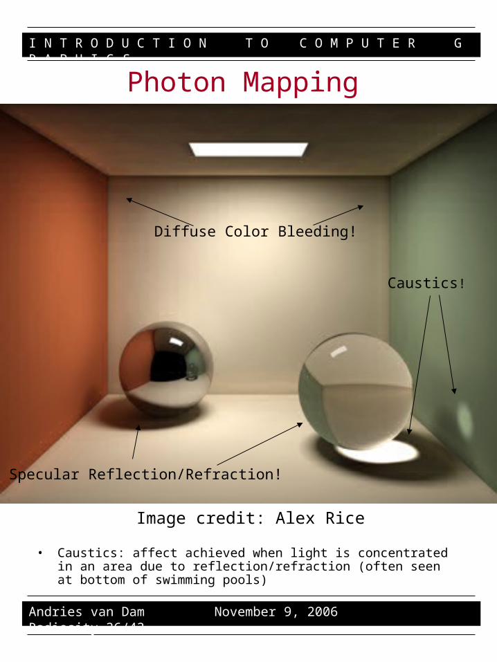
• Caustics: affect achieved when light is concentrated in an area due to reflection/refraction (often seen at bottom of swimming pools)
Photon Mapping
Diffuse Color Bleeding!
Specular Reflection/Refraction!
Caustics!
Image credit: Alex Rice
I N T R O D U C T I O N T O C O M P U T E R G R A P H I C S
Andries van Dam November 9, 2006 Radiosity 37/43
• SIGGRAPH paper by Henrik Wann Jensen
• Two-pass rendering technique combining forward- and back-mapping concepts
• Would really like to simulate all light, everywhere
– Settle for simulating some light as discrete photons
• Basic idea: Forward map, then back map
– Consider two ‘types’ of photons: diffuse-bouncing and specular-bouncing
– Shoot a large (finite) number of photons from light sources in random directions (forward-mapping light)
– Wherever the photons hit, store energy, position in diffuse or specular ‘map’ (usually a BSP tree), and resend photons
• Photons are attenuated by object’s reflectance; low-energy photons are not resent
• Diffuse photons bounce randomly, specular photons reflect/refract
– Once all photons collected, raytrace scene and add nearby photons to the contribution (back-mapping light)
Photon Mapping
I N T R O D U C T I O N T O C O M P U T E R G R A P H I C S
Andries van Dam November 9, 2006 Radiosity 38/43
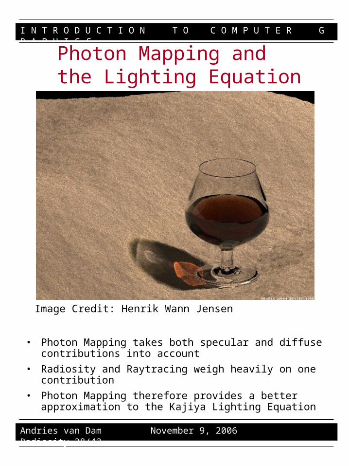
• Photon Mapping takes both specular and diffuse contributions into account
• Radiosity and Raytracing weigh heavily on one contribution
• Photon Mapping therefore provides a better approximation to the Kajiya Lighting Equation
Photon Mapping and the Lighting Equation
Image Credit: Henrik Wann Jensen

I N T R O D U C T I O N T O C O M P U T E R G R A P H I C S
Andries van Dam November 9, 2006 Radiosity 39/43
What is MLT? (1/3)
• Metropolis Light Transport: type of Monte Carlo algorithm
• Monte Carlo describes a group of rendering algorithms which randomly sample every path which a light ray can take in the world
– based on ray casting
– classical ray tracing is very simple, specialized type of Monte Carlo algorithm
– point sampling of complete rendering equation
– in general, capable of much more complicated effects than radiosity and classical ray tracing combined

I N T R O D U C T I O N T O C O M P U T E R G R A P H I C S
Andries van Dam November 9, 2006 Radiosity 40/43
Pretty Enough to Look At Again…
I N T R O D U C T I O N T O C O M P U T E R G R A P H I C S
Andries van Dam November 9, 2006 Radiosity 41/43
What is MLT? (2/3)
• Integrates Kajiya’s Lighting Equation
• There are many ways to integrate a function
• Simplest method is to take samples of function uniformly spaced across its domain
– basic high school calculus integration
– this is what ray tracing does
– might have to take many samples if function is very complicated in some area
• A smarter method: importance sampling
– if we already know something about a function, we can utilize this knowledge
– sample more in areas which contribute more to final value of the integral
• Metropolis sampling is a variety of importance sampling (Metropolis, Rosenbluth, Rosenbluth, Teller, and Teller, 1953)
– chooses samples in such a way that they are eventually distributed proportionally to the value of the function being integrated
I N T R O D U C T I O N T O C O M P U T E R G R A P H I C S
Andries van Dam November 9, 2006 Radiosity 42/43
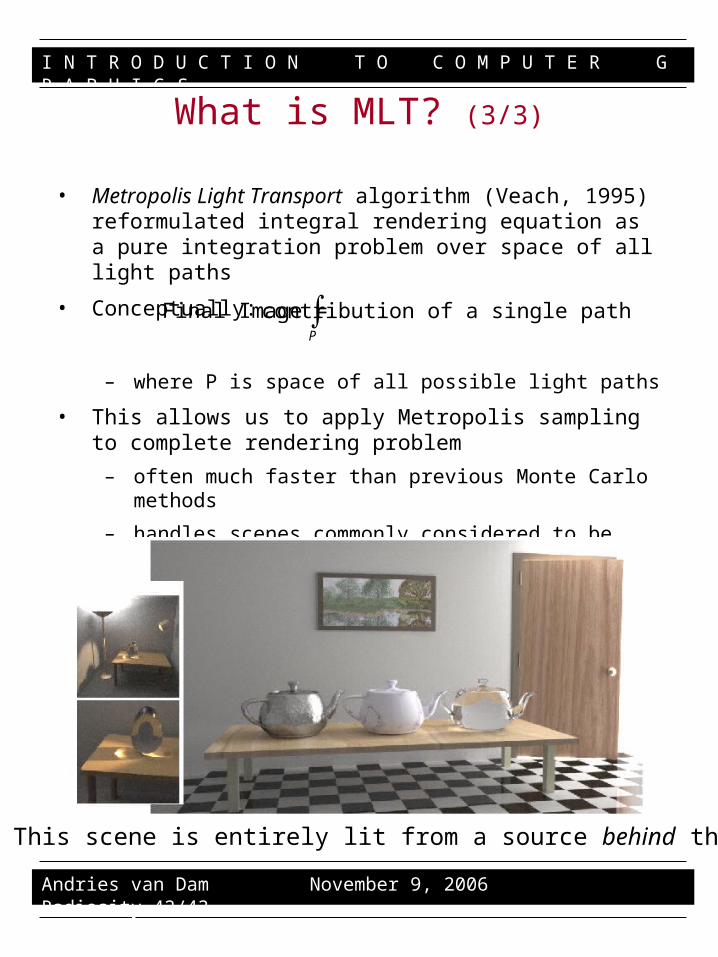
What is MLT? (3/3)
• Metropolis Light Transport algorithm (Veach, 1995) reformulated integral rendering equation as a pure integration problem over space of all light paths
• Conceptually:
– where P is space of all possible light paths
• This allows us to apply Metropolis sampling to complete rendering problem
– often much faster than previous Monte Carlo methods
– handles scenes commonly considered to be difficult
P
Final Image = contribution of a single path
This scene is entirely lit from a source behind the door
I N T R O D U C T I O N T O C O M P U T E R G R A P H I C S
Andries van Dam November 9, 2006 Radiosity 43/43
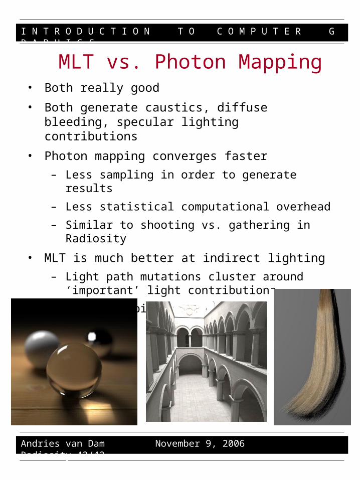
• Both really good
• Both generate caustics, diffuse bleeding, specular lighting contributions
• Photon mapping converges faster
– Less sampling in order to generate results
– Less statistical computational overhead
– Similar to shooting vs. gathering in Radiosity
• MLT is much better at indirect lighting
– Light path mutations cluster around ‘important’ light contributions
– Photon mapping blindly sprays photons randomly
MLT vs. Photon Mapping
Related Documents


![Introduction to Radiosity · EECS 487: Interactive Computer Graphics An[other] Intro to Radiosity(1/3) • The radiometric term radiosity means the rate at which energy leaves a surface,](https://static.cupdf.com/doc/110x72/5fc3a89f74fa74617b240ea3/introduction-to-eecs-487-interactive-computer-graphics-another-intro-to-radiosity13.jpg)


