i Monitoring Viruses in Wastewater to Support Public Health

i

Monitoring Viruses in Wastewater to Support Public Health:

Development and Demonstration of Improved Approaches for Two Applications

By

HANNAH RACHEL SAFFORD

DISSERTATION

Submitted in partial satisfaction of the requirements for the degree of

DOCTOR OF PHILOSOPHY

in

Civil and Environmental Engineering

in the

OFFICE OF GRADUATE STUDIES

of the

UNIVERSITY OF CALIFORNIA

DAVIS

Approved:

Heather N. Bischel, Chair

Jeannie L. Darby

Karen Shapiro

Committee in Charge

2022

ii

ABSTRACT

Viruses in wastewater present public-health challenges as well as public-health

opportunities. I consider both herein. I begin with a systematic literature review of nearly 300

studies, published from 2000 to 2018, that document applications of flow cytometry (FCM) to

ensure microbial water quality and hence facilitate safe and effective water treatment, distribution,

and reuse. I find that while there is a large body of evidence supporting widespread adoption of

FCM as a routine method for microbial water-quality assessment, key knowledge gaps impede the

technique from realizing its full potential. One of these gaps is robust protocols for FCM-based

analysis of waterborne viruses. In this dissertation, I hypothesize that a fractional factorial

experimental design is a better alternative to the “pipeline” strategy commonly followed for FCM

protocol optimization. I then demonstrate my approach, using a fractional factorial experimental

design to optimize staining of the bacteriophage T4 prior to FCM analysis. My results yield a

specific protocol for reliably identifying and quantifying T4 bacteriophage through FCM.

I also explain why manual gating of FCM data using a series of two-dimensional plots—

the typical approach to FCM data analysis—is problematic, especially with respect to applications

of FCM to facilitate advanced water treatment and reuse. I suggest that algorithmic clustering

approaches could expedite and improve FCM data analysis, and could even help position FCM as

a technique for real-time microbial water-quality monitoring. I test this theory by generating FCM

data from two solutions: (i) a mixed-target solution containing a variety of environmentally

relevant viral surrogates, and (ii) an environmental-spike solution comprising T4 bacteriophage in

a wastewater matrix. I first analyze these data through manual gating, and then compare results to

results obtained through algorithmic clustering: specifically, by coupling the OPTICS ordering

algorithm with either manual or automated identification of clusters from the OPTICS-ordered

iii

data. I demonstrate that OPTICS-assisted clustering can in some cases work as well or better than

manual gating of FCM data—and is certainly far faster and less labor-intensive. OPTICS-assisted

clustering can also point to features in FCM data that are difficult to detect through manual gating

alone. However, I also find that more needs to be done to position OPTICS as a reliable tool for

automated, objective analysis of FCM data from environmental samples, especially data generated

from challenging biological targets like viruses in challenging matrices like wastewater.

I explore wastewater-borne viruses as a public-health opportunity through the lens of the

COVID-19 pandemic. Wastewater-based epidemiology (WBE) quickly became recognized as a

useful complement to clinical testing following the pandemic’s onset. However, little is known

about sub-community relationships between wastewater and clinical data. I present a novel

framework for probabilistically aligning wastewater and clinical data with high spatial granularity.

I use this framework to uncover clear sub-regional (i.e., sub-city) and building/neighborhood-scale

correlations between wastewater and clinical data collected through the Healthy Davis Together

(HDT) pandemic-response initiative in Davis, CA. In addition, I hypothesize that multiple

imputation (using an expectation maximization-Markov chain Monte Carlo (MCMC) approach)

of non-detects in wastewater qPCR data is less likely to bias results than more commonly used

non-detect handling methods (e.g., censoring or single imputation). I use the HDT data to test this

hypothesis. I find that while results obtained using different non-detect handling methods are

similar, they are not the same—indicating the importance of specifying non-detect handling

method in WBE studies. I also find that the EM-MCMC method yields somewhat better agreement

between clinical and wastewater data than do the other non-detect handling methods examined.

Refinements to the algorithm, tuning parameters, and variable groupings used in this dissertation

could further recommend the EM-MCMC method for wastewater-data analysis in the future.

iv

I conclude the dissertation with a discussion of lessons learned from my experience helping

launch, grow, and manage the HDT WBE program. Conducting WBE requires significant

investments of time, money, labor, and expertise. Given that much information gleaned from

wastewater is not directly actionable, and/or duplicates information from other sources, it is

prudent to consider whether these investments are worth it. I present seven recommendations for

end users seeking to incorporate WBE into COVID-19 response: (1) avoid redundancy between

clinical testing and WBE; (2) emphasize statistical thinking, data analysis, and data management;

(3) define action thresholds; (4) monitor fewer sites more frequently; (5) build on existing

infrastructure and programs for wastewater collection and analysis; (6) be prepared to adapt as the

pandemic evolves; and (7) keep an eye on the future, including by proactively searching for

emerging variants of concern.

v

DEDICATION

To Dr. Sidney Adler (z’’l): a mensch, a scholar, and an inspiration.

vi

ACKNOWLEDGEMENTS

Earning a Ph.D. involves a lot of time working alone in the lab and on the laptop. I count

myself lucky that the solitary components of my doctoral experience have been far outweighed by

the components shared by my remarkable network of colleagues, friends, and family.

Professor Heather Bischel is the platonic ideal of a doctoral advisor. From the moment we

first connected (via Skype! Little did we know how many more video calls together were in our

future.), it was clear that we clicked personally and professionally. Heather, I am so grateful to you

for guiding me through the scientific components of my Ph.D., giving me the freedom and

flexibility to guiltlessly pursue opportunities outside of hard research, and simply being my buddy.

Hours never pass faster than when I’m chatting with you.

Another great thing about Heather is that she attracts great people to work with. The list of

those people is long but merits recording. Dani Peguero and Yilong Liu helped me find my

bearings in the lab early on, setting me up for success down the road. Though we never directly

collaborated on anything, my time with Heather’s group was richer for the years that the selfless

and hilarious Jeanne Sabin was part of it. Erica Koopman-Glass and Mel Johnson both helped me

(barely) avoid throwing Flo and Florina out the window when the fluidics lines got contaminated

for the millionth time. Dr. Minji Kim generously offered advice and training on all things PCR,

and is one of the most knowledgeable, patient, and kind scientists it is my privilege to know.

Professor Jeannie Darby was my first (wonderful) point of contact with the environmental

engineering graduate program at UC Davis and has been a mentor to me since then, graciously

serving on both my QE and dissertation committees. Professor Jonathan Herman got me started

on cluster analysis for flow cytometry (FCM) data and assisted in securing the U.S. Bureau of

Reclamation grant that funded much of my FCM work. Professor Sam Díaz-Muñoz provided (1)

vii

useful insight on enveloped viruses and (2) the protocols and materials I needed to start working

with enveloped bacteriophage in Heather’s lab.

My COVID-19 surveillance team kicks ass. Winston Bess, Michelle Clauzel, Roque

Guerrero, Noah Krasner, Randi Pechacek, Lezlie Rueda, Lifeng Wei, and Xiaoliu Wu did much

of the hands-on work with samples and data that enabled the COVID-related aspects of my

dissertation. Rachel Olson arrived as a deus ex machina to take over COVID-19 lab management

at just the time that I needed to step back to focus on writing. Courtney Doss and Sandra Macomb

did the dirty work (often literally) of facilitating and expanding regular sample collection.

Numerous others at Healthy Davis/Yolo Together (HDT/HYT) supported the surveillance project

in other ways, including financially. Professor James Sharpnack helped me do fancy things with

COVID-19 data, and if Heather is the platonic ideal of a doctoral advisor then Professor Karen

Shapiro is the platonic ideal of a project co-lead. Dr. Rogelio Zuniga Montanez was my partner in

crime and emotional support colleague through the first ~14 months of the COVID-19 project.

Rogelio, I will always give you grief for finding a job and leaving the project before me, and I will

always take any opportunity to work with you again.

Madison Hattaway, Wenting Li, Olivia Wrightwood, and (most recently) Camille Wolf—

where would I have been these past five years without you weirdly wonderful and wonderfully

weird ladies? Here’s to forearm tattoos, charismatic pets, athletic endeavors, and being reel hawt.

Finally, obviously, and indispensably, my family. Mom, Dad, Adam, and Leah, thank you

for tolerating my perpetual studenthood. I couldn’t have done any of it without you rooting for me,

and I promise this graduation will be the last one you have to endure. And Anna, my rock and

inspiration. Once I met you I could have dropped out of grad school and the move to Davis would

still have been worth it. I love you to the moon and back.

viii

TABLE OF CONTENTS

ABSTRACT ................................................................................................................................... ii DEDICATION .............................................................................................................................. v ACKNOWLEDGEMENTS ........................................................................................................ vi TABLE OF CONTENTS .......................................................................................................... viii ABBREVIATIONS ...................................................................................................................... xi LIST OF TABLES ..................................................................................................................... xiii LIST OF FIGURES ................................................................................................................... xiv CHAPTER 1: INTRODUCTION ................................................................................................ 1 CHAPTER 2: FLOW CYTOMETRY APPLICATIONS IN WATER TREATMENT, DISTRIBUTION, AND REUSE .................................................................................................. 4

2.1 Background ..................................................................................................................... 5 2.1.1 Principles of FCM ........................................................................................................ 5 2.1.2 Status of FCM in water-quality assessment ................................................................. 7

2.2 Review scope and methods ............................................................................................ 9 2.3 Applications of FCM in water treatment, distribution, and reuse .......................... 10

2.3.1 Source waters and receiving waters ............................................................................ 11 2.3.2 Wastewater treatment ................................................................................................. 13 2.3.3 Drinking-water treatment ........................................................................................... 19 2.3.4 Drinking-water distribution ........................................................................................ 27

2.4 Combination and comparison with other indicators ................................................ 29 2.4.1 Heterotrophic plate count (HPC) ................................................................................ 29 2.4.2 Epifluorescence microscopy (EFM) ........................................................................... 31 2.4.3 Molecular techniques .................................................................................................. 32 2.4.4 Adenosine tri-phosphate (ATP) .................................................................................. 34 2.4.5 Assimilable organic carbon (AOC) ............................................................................ 35

2.5 Cross-cutting methodological considerations ............................................................ 37 2.5.1 Sample preparation ..................................................................................................... 37 2.5.2 Sample staining ........................................................................................................... 40 2.5.3 Interpretation of viability data .................................................................................... 41

2.6 Research needs .............................................................................................................. 42 2.6.1 Flow virometry ........................................................................................................... 42 2.6.2 Specific pathogen detection ........................................................................................ 44 2.6.3 Automation ................................................................................................................. 45 2.6.4 Computational tools for FCM data analysis ............................................................... 47 2.6.5 Standardization ........................................................................................................... 48

2.7 Conclusion ..................................................................................................................... 50

ix

2.8 References ..................................................................................................................... 52 CHAPTER 3: OPTIMIZING DETECTION OF WATERBORNE VIRUSES THROUGH FLOW CYTOMETRY ............................................................................................................... 72

3.1 Motivation ..................................................................................................................... 74 3.1.1 Optimizing detection of waterborne viruses through FCM analysis .......................... 74 3.1.2 Analyzing FCM data collected from environmental samples .................................... 76

3.2 Materials and methods ...................................................................................................... 77 3.2.1 Phage stock preparation .............................................................................................. 77 3.2.2 Phage stock quantification .......................................................................................... 79 3.2.3 Flow cytometric analysis ............................................................................................ 80 3.2.4 Optimization design and protocols ............................................................................. 81 3.2.5 Optimization data analysis .......................................................................................... 82 3.2.6 Mixed-target and environmental-spike data generation ............................................. 82 3.2.7 Mixed-target and environmental-spike data analysis ................................................. 83

3.3 Results and discussion .................................................................................................. 85 3.3.1 Optimizing staining through fractional factorial experimental design ....................... 85 3.3.2 Automating data analysis through density-based clustering ...................................... 88

3.4 Conclusion ................................................................................................................... 100 3.5 References ................................................................................................................... 102

CHAPTER 4: WASTEWATER-BASED EPIDEMIOLOGY TO INFORM COVID-19 RESPONSE IN DAVIS, CALIFORNIA ................................................................................. 105

4.1 Background ................................................................................................................. 107 4.2 Materials and methods ............................................................................................... 108

4.2.1 Sample collection and processing ............................................................................. 108 4.2.2 RT-qPCR .................................................................................................................. 112 4.2.3 Multiple imputation of non-detects .......................................................................... 113 4.2.4 Data analysis ............................................................................................................. 115 4.2.5 Probabilistic assignment of clinical data to sampling zones .................................... 116

4.3 Results and discussion ................................................................................................ 117 4.3.1 Sample collection and processing ............................................................................. 117 4.3.2 EM-MCMC method performance ............................................................................ 118 4.3.3 Comparison of non-detect handling methods ........................................................... 118 4.3.4 Sub-community comparison of clinical and wastewater data .................................. 119

4.4 Conclusion ................................................................................................................... 123 4.5 References ................................................................................................................... 125

CHAPTER 5: PUBLIC-HEALTH VALUE OF WASTEWATER-BASED EPIDEMIOLOGY—PERSPECTIVES AND RECOMMENDATIONS ............................ 128

5.1 History of wastewater-based epidemiology .............................................................. 129 5.1.1 Early-warning system ............................................................................................... 130 5.1.2 Unbiased testing ....................................................................................................... 130

x

5.1.3 Cost-effective surveillance ....................................................................................... 132 5.2 Implications and recommendations for end users .................................................. 133 5.3 References ................................................................................................................... 137

APPENDIX A: SUPPLEMENTARY INFORMATION FOR CHAPTER 2 ...................... 141 A.1 Figures ......................................................................................................................... 141 A.2 Tables .......................................................................................................................... 144

APPENDIX B: SUPPLEMENTARY INFORMATION FOR CHAPTER 3 ...................... 148 B.1 Figures ......................................................................................................................... 148 B.2 Tables ............................................................................................................................... 164

APPENDIX C: SUPPLEMENTARY INFORMATION FOR CHAPTER 4 ...................... 172 C.1 Figures ......................................................................................................................... 172 C.2 Tables .......................................................................................................................... 178 C.3 MIQE ........................................................................................................................... 182

APPENDIX D: PERFORMANCE COMPARISON OF FOUR COMMERCIALLY AVAILABLE FLOW CYTOMETERS USING POLYSTYRENE BEADS ....................... 187

D.1 Abstract ....................................................................................................................... 187 D.2 Value of the data ......................................................................................................... 187 D.3 Data .............................................................................................................................. 188 D.4 Experimental design, materials, and methods ......................................................... 188 D.5 References ................................................................................................................... 189

xi

ABBREVIATIONS

ACS American Community Survey AOC Assimilable organic carbon ARG Antibiotic resistance gene ATP Adenosine tri-phosphate BCECF-AM 2’,7’-bis-(2-carboxyethyl)-5-(and-6)-carboxyfluorescein acetoxy methyl ester BN Building/neighborhood BRP Bacterial regrowth potential BSA Bovine serum albumin CFDA Carboxyfluorescein diacetate COD City of Davis Ct Threshold cycle CTC 5-cyano-2,3-ditolyl tetrazolium chloride DAPI 4’,6-diamidino-2-phenylindole DiBAC4(3) Bis-(1,3-dibutylbarbituric acid)trimethine oxonol DLS Dynamic light scattering DPR Direct potable reuse DWDS Drinking water distribution system DWT Drinking water treatment DWTP Drinking water treatment plant EBPR Enhanced biological phosphorus removal EFM Epifluorescence microscopy EM-MCMC Expectation maximization-Markov chain Monte Carlo EtBr Ethidium bromide FACS Fluorescence-activated cell sorting FCS Flow cytometry standard FDA Fluorescein diacetate FISH Fluorescent in situ hybridization FITC Fluorescein isothiocyanate FOPH Federal Office of Public Health [Switzerland] FSC Forward scatter GAC Granular activated carbon GAO Glycogen-accumulating organism gc Gene copies HDT Healthy Davis Together HNA High nucleic acid HPC Heterotrophic plate count ICC Intact cell count/counting LNA Low nucleic acid NPDWR National Primary Drinking Water Regulations LOD Limit of Detection MIQE Minimum information for publication of quantitative real-time PCR Experiments PAO Polyphosphate-accumulating organism PCR Polymerase chain reaction PFU Plaque-forming units

xii

PI Propidium iodide PMMoV Pepper mild mottle virus RO Reverse osmosis RT-ddPCR Reverse transcription-digital droplet PCR RT-FCM Real-time flow cytometry RT-qPCR Reverse transcription-quantitative PCR SARS-CoV-2 Severe acute respiratory coronavirus 2 SR Sub-regional SSC Side scatter SLMB Schweizerisches Lebensmittelbuch (Swiss Food Book) SWRCB State Water Resources Control Board TCC Total cell count/counting TE Tris-ethylenediaminetetraacetic acid (EDTA) TOC Total organic carbon USCB United States Census Bureau UV Ultraviolet VBNC Viable but non-cultivable WBE Wastewater-based epidemiology WWT Wastewater treatment WWTP Wastewater treatment plant

xiii

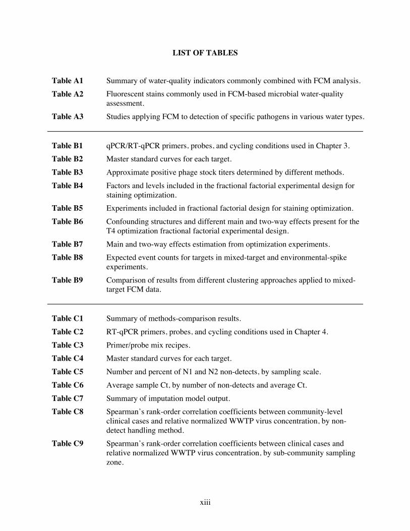
LIST OF TABLES

Table A1 Summary of water-quality indicators commonly combined with FCM analysis. Table A2 Fluorescent stains commonly used in FCM-based microbial water-quality

assessment. Table A3 Studies applying FCM to detection of specific pathogens in various water types.

Table B1 qPCR/RT-qPCR primers, probes, and cycling conditions used in Chapter 3. Table B2 Master standard curves for each target. Table B3 Approximate positive phage stock titers determined by different methods. Table B4 Factors and levels included in the fractional factorial experimental design for

staining optimization. Table B5 Experiments included in fractional factorial design for staining optimization. Table B6 Confounding structures and different main and two-way effects present for the

T4 optimization fractional factorial experimental design. Table B7 Main and two-way effects estimation from optimization experiments. Table B8 Expected event counts for targets in mixed-target and environmental-spike

experiments. Table B9 Comparison of results from different clustering approaches applied to mixed-

target FCM data. Table C1 Summary of methods-comparison results. Table C2 RT-qPCR primers, probes, and cycling conditions used in Chapter 4. Table C3 Primer/probe mix recipes. Table C4 Master standard curves for each target. Table C5 Number and percent of N1 and N2 non-detects, by sampling scale. Table C6 Average sample Ct, by number of non-detects and average Ct. Table C7 Summary of imputation model output. Table C8 Spearman’s rank-order correlation coefficients between community-level

clinical cases and relative normalized WWTP virus concentration, by non-detect handling method.

Table C9 Spearman’s rank-order correlation coefficients between clinical cases and relative normalized WWTP virus concentration, by sub-community sampling zone.

xiv

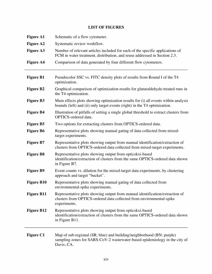
LIST OF FIGURES Figure A1 Schematic of a flow cytometer. Figure A2 Systematic review workflow. Figure A3 Number of relevant articles included for each of the specific applications of

FCM in water treatment, distribution, and reuse addressed in Section 2.3. Figure A4 Comparison of data generated by four different flow cytometers.

Figure B1 Pseudocolor SSC vs. FITC density plots of results from Round I of the T4

optimization. Figure B2 Graphical comparison of optimization results for glutaraldehyde-treated runs in

the T4 optimization. Figure B3 Main effects plots showing optimization results for (i) all events within analysis

bounds (left) and (ii) only target events (right) in the T4 optimization. Figure B4 Illustration of pitfalls of setting a single global threshold to extract clusters from

OPTICS-ordered data. Figure B5 Two options for extracting clusters from OPTICS-ordered data. Figure B6 Representative plots showing manual gating of data collected from mixed-

target experiments. Figure B7 Representative plots showing output from manual identification/extraction of

clusters from OPTICS-ordered data collected from mixed-target experiments. Figure B8 Representative plots showing output from opticskxi-based

identification/extraction of clusters from the same OPTICS-ordered data shown in Figure B7.

Figure B9 Event counts vs. dilution for the mixed-target data experiments, by clustering approach and target “bucket”.

Figure B10 Representative plots showing manual gating of data collected from environmental-spike experiments.

Figure B11 Representative plots showing output from manual identification/extraction of clusters from OPTICS-ordered data collected from environmental-spike experiments.

Figure B12 Representative plots showing output from opticskxi-based identification/extraction of clusters from the same OPTICS-ordered data shown in Figure B11.

Figure C1 Map of sub-regional (SR; blue) and building/neighborhood (BN; purple)

sampling zones for SARS-CoV-2 wastewater-based epidemiology in the city of Davis, CA.

xv

Figure C2 Timeline illustrating how zones sampled and sampling frequency evolved over the course of the sampling campaign.

Figure C3 Methods comparison results. Figure C4 (A) Visualization of the connection graph showing all maintenance holes

(MHs) in the City of Davis sewershed. (B) Illustration of how the connection graph is used to probabilistically assign positive clinical-test results from census blocks to sewershed monitoring zones for the purpose of comparing trends in wastewater data to trends in clinical data.

Figure C5 Representative quality-check trace plots generated by running the EM-MCMC model on raw qPCR data for Zone SR-L.

Figure C6 Community-level wastewater vs. clinical data in Davis, showing effects of different methods of handling non-detects.

Figure C7 Wastewater vs. clinical data in Davis.

1

CHAPTER 1: INTRODUCTION

Viruses are ubiquitous and persistent in wastewater. The presence of certain pathogenic

viruses can significantly impede wastewater reclamation and reuse since (i) even very low

concentrations of pathogenic viruses in wastewater can cause disease but (ii) it is difficult to

achieve and verify very high levels of pathogen removal. Conventional methods for detecting and

monitoring microbes in wastewater are labor-intensive and time-consuming. The California State

Water Resources Control Board has accordingly highlighted development of automated, near-real-

time methods for microbial water-quality assessment as key to enabling direct potable reuse of

wastewater.

Flow cytometry (FCM) has the potential to meet this need. FCM rapidly characterizes

particles (including microorganisms) in a sample based on how they scatter light and/or fluoresce

when passing through one or more laser beams. The technique is powerful, flexible, and delivers

results in a matter of minutes. Chapter 2 of this dissertation, published as a 2019 review article in

Water Research, comprises a systematic review of nearly 300 studies published from 2000 to 2018

that illustrate the benefits and challenges of using FCM for assessing source-water quality and

impacts of treatment-plant discharge on receiving waters, wastewater treatment, drinking water

treatment, and drinking water distribution. In this chapter, I discuss options for combining FCM

with other indicators of water quality and address several topics that cut across nearly all

applications reviewed. I also identify priority areas in which more work is needed to realize the

full potential of this approach. These include optimizing protocols for FCM-based analysis of

waterborne viruses, optimizing protocols for specifically detecting target pathogens, automating

sample handling and preparation to enable real-time FCM, developing computational tools to assist

data analysis, and improving standards for instrumentation, methods, and reporting requirements.

2

I find that while more work is needed to realize the full potential of FCM in water treatment,

distribution, and reuse, substantial progress has been made over the past two decades. There is

now a sufficiently large body of research documenting successful applications of FCM that the

approach could reasonably and realistically see widespread adoption as a routine method for water

quality assessment.

A key knowledge gap identified in Chapter 2 is protocols for applying FCM to waterborne

viruses. To date, efforts to develop FCM protocols for monitoring viruses in wastewater have

suffered from poor experimental design and overreliance on manual, highly subjective data-

analysis methods. In Chapter 3 of this dissertation, in preparation for submission as a research

article, I show how a fractional factorial experimental design can be used to rigorously optimize

FCM-based detection of viral surrogates relevant to water-reuse applications. I then explore the

potential of density-based clustering algorithms to expedite and aid interpretation of results.

Included as an appendix to Chapter 3 is a performance comparison of four commercially available

flow cytometers using polystyrene beads. A writeup of this comparison was published as a 2019

data article in Data in Brief.

While monitoring viruses in wastewater often presents a public-health challenge, it can

sometimes also be a public-health asset. Following the onset of the COVID-19 pandemic,

monitoring levels of fecally excreted SARS-CoV-2 (the virus that causes COVID-19) in

wastewater quickly became recognized as an efficient, unbiased way to track disease emergence

and spread. Many studies conducted in the past two years have found good agreement between

trends in SARS-CoV-2 levels measured at a community’s wastewater treatment plant (WWTP)

and trends in clinical-test results from that community. But it is unknown whether this agreement

holds at more granular spatial scales. In Chapter 3, under review for publication as a research

3

article, I present a novel framework for comparing wastewater and clinical data at the

building/neighborhood and sub-regional levels, and show results from applying this framework to

extensive data collected through the Healthy Davis Together (HDT) pandemic-response initiative.

I also demonstrate how different approaches to handling non-detects in wastewater data can affect

apparent trends, and explore whether multiple imputation of non-detects can improve on more

commonly used but less sophisticated methods. I build on lessons learned from my experience

conducting wastewater-based epidemiology (WBE) through HDT in Chapter 4, published as a

2022 opinion piece in Proceedings of the National Academies of Sciences (PNAS), I provide

perspectives and recommendations on how to carry out wastewater-based epidemiology in ways

that deliver maximum value to public-health officials, policymakers, and other information end-

users while minimizing unnecessary time and cost burdens.

4

CHAPTER 2: FLOW CYTOMETRY APPLICATIONS IN WATER TREATMENT, DISTRIBUTION, AND REUSE

Current methods used widely to characterize and monitor microbial water quality are

imperfect. Physiochemical parameters such as turbidity are sometimes correlated with microbial

contamination, but the relationships are scenario-specific and hence of limited value (Allen et al.

2008). Culture-based methods are relatively simple and low-cost but limited by low sensitivity and

high labor and time requirements (Ramírez-Castillo et al. 2015). In addition, waterborne pathogens

frequently exist in a viable but non-cultivable (VBNC) state, meaning that culture-based methods

may yield false negatives (Ramírez-Castillo et al. 2015). Molecular methods (e.g., polymerase

chain reaction (PCR), oligonucleotide DNA microarrays, and pyrosequencing) are generally faster

and more sensitive than culture-based methods, can be highly target-specific, and can provide

additional phylogenetic information about pathogens of interest. However, molecular methods are

susceptible to interference from inhibitory compounds found in environmental samples, such as

humic acids and metals (Olivieri et al. 2016, Ramírez-Castillo et al. 2015). Molecular methods

may also have limited ability to distinguish between viable and non-viable organisms.

Flow cytometry (FCM) offers an alternative approach to microbial water-quality

monitoring. FCM was first developed in the mid-1900s, but initial uses were limited due to

relatively high size thresholds for particle detection, non-specific binding of fluorescent stains, and

poor sensitivity and computational capacity (Wang et al. 2010b). Recent development of cheaper

and more powerful instrumentation, coupled with novel analysis techniques, has enabled numerous

additional uses of FCM, including in water-quality assessment.

Scholars have surveyed applications of FCM for aquatic and environmental microbiology

(Bergquist et al. 2009, Wang et al. 2010b), discussed types of information obtainable from FCM

that may be relevant for analysis of aquatic systems (Hammes and Egli 2010), and reviewed the

5

value of FCM for studying microbial populations and communities (Müller and Nebe-von-Caron

2010). More recently, FCM has been identified as a potentially valuable tool for virus enumeration

in water reuse (Rockey et al. 2018). This chapter builds on previous work by examining how FCM

can support—and indeed, has already been used to support—safe, effective water treatment,

distribution, and reuse. The chapter is structured as follows:

• Section 2.1 briefly explains how FCM works and how it is already being used to

characterize and monitor waterborne microbes.

• Sections 2.2 and 2.3 systematically review recent literature on FCM research and

applications related to source and receiving water quality, wastewater treatment, drinking

water treatment, and drinking water distribution.

• Sections 2.4–2.6 provide critical analysis based on insights from the review. Section 2.4

identifies options for combining FCM with other water quality indicators to enhance

analysis. Section 2.5 addresses three topics—sample preparation, sample staining, and

interpretation of viability data—that cut across nearly all applications of FCM reviewed.

Section 2.6 articulates research needs that must be met to realize the full potential of FCM

in water treatment, distribution, and reuse.

2.1 Background

2.1.1 Principles of FCM

Flow cytometry (FCM) refers to analysis of suspended particles—including bacteria,

protozoa, viruses, cell fragments, and inorganic debris—based on how they scatter light and/or

fluoresce when passing through a laser beam. Figure A1 illustrates the basic components of a flow

cytometer. In brief, the instrument draws sample into a focusing chamber that forces suspended

particles to align in single file. The focused stream is passed through one or more interrogation

6

points where a laser or other monochromatic light beam individually strikes each particle.

Detectors measure the extent to which each particle scatters light in the forward and side directions

and send these measurements to a computer for display and processing.

FCM data are typically presented in histograms or two-dimensional dot plots that visualize

the intensity and frequency of signals received on different parameters. In general, forward scatter

(FSC) signals are related to particle size, while side scatter (SSC) signals are related to particle

complexity and granularity. Fluorescence is also integral to FCM. Though many cells have some

natural autofluorescence that can be beneficially exploited for analysis, autofluorescence alone is

rarely sufficient to conclusively distinguish target populations and/or examine parameters of

interest. It is therefore standard practice for researchers to apply one or more fluorescent stains

prior to FCM (Section 2.6.2).

Correctly interpreting FCM data requires researchers to keep many factors in mind,

including the following. First, scatter indicates relative, not absolute, particle size and complexity.

Since the intensity of scatter signals depends on factors such as laser wavelength, collection angle,

surface roughness, and refractive index of the particle and sheath fluid, a particle that generates an

FSC signal double that of another particle is not necessarily twice as big. Second, most particles

are irregularly shaped, meaning that signal intensity depends on the orientation of a particle when

it reaches the interrogation point (Shapiro, 2003). Third, particles may clump together and register

as a single (larger) scatter or fluorescent signal. Fourth, particle diameter can affect analysis

strategies. Large-diameter particles preferentially scatter light in the forward direction while small-

diameter particles do not. Small-diameter particles scatter light weakly and inconsistently,

generating small amounts of scatter that can be hard to distinguish from noise. Finally, all particles

7

in a sample—including intact cells, fragmented cells, and inorganic debris—scatter light, making

it difficult to uniquely identify targets from scatter alone.

2.1.2 Status of FCM in water-quality assessment

FCM data can yield a wealth of information about the microbial characteristics of water

samples (Hammes and Egli 2010). Absolute cell counting (also known as total cell counting, or

TCC) is one of the most straightforward and common uses of FCM, although it can be hard to

obtain reliable counts for environmental samples containing many non-cell particles. Scatter and

fluorescence data indicate cell characteristics such as relative size, complexity, and nucleic-acid

content, and thus can serve as unique cytometric “fingerprints” of microbial communities present

in water samples (Koch et al. 2014). Fluorescent stains can capture cellular parameters such as

membrane integrity and enzymatic activity, which in turn can provide deeper insight into the

kinetics and efficacy of water-treatment processes. Finally, FCM can be used to specifically

identify target cells when present at high enough concentration and when the target can be stained

by a fluorescent marker. This final function can detect microorganisms of concern directly and/or

detect indicator populations known to be correlated with a target population or that serve for

tracking process performance (Hammes and Egli 2010).

FCM is now generally accepted as a valuable tool for detection, enumeration, and

characterization of waterborne microbial populations. However, it is not yet widely used in applied

settings (e.g., for ensuring compliance with water-quality regulations). A notable exception is

Switzerland. In 2012, Switzerland’s Federal Office of Public Health (FOPH) published official

methods in the Swiss Food Book (Schweizerisches Lebensmittelbuch, or SLMB)—a collection of

standards to ensure the safety of food and beverages for human consumption—for using FCM to

8

obtain total microbial cell counts and determine the ratios of high- and low-nucleic acid cells in

fresh water (Federal Office of Public Health 2012). The method was recommended for analyzing

water in drinking water treatment plants (DWTPs), drinking water distribution systems (DWDSs),

and household plumbing (among other areas). Although the SLMB was recently discontinued, a

similar resource is forthcoming from the Swiss Gas and Water Association. A revised version of

the FOPH’s FCM method are currently being developed for inclusion in this resource. In the

interim, the method is still recommended by the Swiss government for analysis of drinking water

(Kötzsch et al. 2010).

While no other federal or state government has yet formally endorsed FCM for water-

quality assessment, a growing number of utilities and regulatory bodies are exploring the benefits

of the approach. In California, a 2016 report commissioned by the State Water Resources Control

Board identified FCM as a rapid, potentially automatable method for characterizing water samples

(Olivieri et al. 2016). Scottish Water, the statutory corporation that provides water and sewage

services to the bulk of Scotland’s population, is actively collaborating with Cranfield University

to develop FCM techniques for full-scale DWTPs and DWDSs (Scottish Water 2014).

Northumbrian Water Group, a major water supplier in England, is working to validate FCM with

the ultimate objective of having FCM approved by the United Kingdom Drinking Water

Inspectorate as an alternative to culture-based methods for obtaining total and intact cell counts

(Marsh 2017). As instrumentation improves and protocols become standardized, it is likely that

FCM for water-quality assessment will continue to catch on with practitioners as well as

researchers.

9

2.2 Review scope and methods

The process for the literature review contained herein was informed by the Preferred

Reporting Items for Systematic Review and Meta-Analysis (PRISMA) guidelines (Moher et al.

2009). Primary research on the use of FCM related to any aspect of drinking-water sourcing,

treatment, and distribution and/or on any aspect of wastewater treatment and discharge was eligible

for inclusion in this review. Also eligible were studies on optimizing FCM sample preparation and

data analysis, as long as such studies explicitly defined applications related to water treatment,

distribution, and/or reuse. Studies focusing solely on marine samples were excluded. The review

was limited to research published in English-language peer-reviewed journal articles and books

from academic publishers. Only articles and books published between January 2000 and March

2018 were considered, both to keep the number of candidate references to a feasible level and

because it is only relatively recently that FCM has been considered a practically viable method for

water quality assessment (in part due to technological advances that have rendered FCM

instrumentation better and cheaper).

The literature search relied on three bibliographic databases: Web of Science, PubMed, and

the University of California library catalog. The latter, representing the largest university research

library in the world, was particularly valuable in ensuring as comprehensive a search as possible.

The search proceeded as follows. First, each of the databases was queried with the Boolean subject

search: ((“flow cytomet*”) AND (“bacteria” OR “virus*” OR “protozoa*”) AND (“drinking

water” OR “wastewater” OR “recycled water” OR “groundwater” OR “surface water” OR

“activated sludge” OR “biological reactor” OR “potable reuse” OR “nonpotable reuse” OR

“source water”) AND (“monitor*” OR “analyz*” OR “evaluat*”)). This search was intended to

capture references focused on using FCM for water-quality assessment—in particular, for studying

10

waterborne microbes. I selected the specific query after running preliminary searches to identify

terms that returned the greatest number of relevant results. The search resulted in a total of 1,375

references (651 from Web of Science, 504 from PubMed, and 220 from the University of

California library catalog). Duplicate references were eliminated, leaving 827 references that were

manually screened for relevance. The citations of each relevant reference were examined to

identify additional candidate references for the review. Full texts of candidates were obtained and

screened for relevance as well. A total of 281 references were ultimately included in the systematic

review. 145 references describe specific applications of FCM in water treatment, distribution, and

reuse (Section 2.5); 41 references address complementary topics (Sections 2.6–2.8), and 95

references cover both specific applications and complementary topics. Figure A2 summarizes the

systematic review process.

2.3 Applications of FCM in water treatment, distribution, and reuse

This section reviews applications of FCM for studying (1) source-water quality and

impacts of treatment-plant discharge on receiving waters, (2) wastewater treatment, (3) drinking-

water treatment, and (4) drinking-water distribution. Figure A3 breaks down these references by

application category.1 For convenience, the term “microbial water-quality assessment” is used to

refer generally to characterization and monitoring of waterborne microbes. It is important to note,

though, that no single parameter can provide a complete picture of microbial water quality. For

instance, two samples exhibiting the same TCC could contain different levels of pathogenic

bacteria. On the other hand, two samples devoid of pathogenic bacteria could exhibit different

TCCs, potentially indicating different levels of biological stability.

1 Some references were included in more than one category.

11

2.3.1 Source waters and receiving waters

Assessing microbial quality of natural waters (e.g., lakes, rivers, streams, and aquifers) is

important at the beginning and end of water-treatment processes. Upstream of treatment processes,

source water quality has considerable influence on the performance of water treatment,

distribution, and reuse processes: high-quality inputs make it easier to realize high-quality

products. Downstream, it is necessary to monitor water bodies receiving effluent from wastewater

treatment plants (WWTPs) to ensure successful removal of microbial hazards.

FCM has been used to analyze microbial quality of various source waters. Some studies

explore the potential of FCM for detecting specific pathogens in source waters and/or separating

out such pathogens for further analysis. These studies include Tanaka et al. (2000), Weir et al.

(2000), Riffard et al. (2001), Lindquist et al. (2001a,b), Chung et al. (2004), Shapiro et al. (2010),

and Keserue et al. (2011, 2012b). In addition, Vital et al. (2007a, 2008, 2012b) used FCM to

investigate growth of V. cholerae and E. coli O157 under different freshwater conditions. Tanaka

et al. (2000) found FCM to be valuable for studying organisms likely to be present in VBNC states

in the environment, as such organisms are impossible to quantify accurately using plate-based

methods. They further noted that FCM is particularly useful for environmental samples containing

a low ratio of target to total cells, since it is time- and labor-intensive to analyze these samples via

manual-count methods such as epifluorescence microscopy (EFM). Riffard et al. (2001) caution

that the presence of debris and autochthonous (i.e., native) microflora may interfere with direct

application of FCM to natural samples. They suggest integrating immunomagnetic separation or

similar sample processing to isolate target cells prior to FCM analysis. Time and labor

requirements associated with such processing would present a challenge for certain FCM

applications, such as “online” (i.e., real-time) water quality assessment to facilitate DPR.

12

FCM has also been used to characterize microbes in source waters more generally.

Mailloux and Fuller (2003), Wang et al. (2009), Anneser et al. (2010), Leys et al. (2010), Roudnew

et al. (2012, 2013, 2014), Smith et al. (2012, 2015), Wilhartitz et al. (2013), Besmer et al. (2016,

2017a), and Page et al. (2017) used FCM to examine microbial water quality in groundwater

systems. Stopa and Mastromanolis (2001), Yang et al. (2015a), Baumgartner et al. (2016), and

Elhadidy et al. (2016) used FCM to examine microbial water quality in surface water. Objectives

of these groundwater and surface-water studies included characterizing how microbial water

quality varies in space, time, and in response to perturbations like borehole purging, aquifer

recharge, and precipitation events. Most such studies assess microbial water quality through

quantification of bacterial TCC and ICC. Leys et al. (2010), Roudnew et al. (2012, 2013, 2014),

Smith et al. (2012, 2015), and Wilhartitz et al. (2013) additionally enumerate populations of “virus-

like particles (VLPs)” characterized by relatively small size and lower nucleic-acid content

compared to bacteria.

Some studies go beyond simple enumeration to achieve deeper insight into microbial

quality of source waters. Besmer et al. (2016, 2017a) applied automated FCM to better characterize

real-time fluctuations in microbial dynamics of source waters. Wang et al. (2009), Besmer et al.

(2016), and Elhadidy et al. (2016) each distinguished subpopulations representing low nucleic acid

(LNA) and high nucleic acid (HNA) bacteria. In particular, Wang et al. (2009) used fluorescence-

activated cell sorting (FACS)—a type of FCM in which the cytometer sorts and saves any cells

exhibiting scatter and fluorescence properties prespecified by the instrument operator—to enrich

LNA bacteria from source freshwater for further cultivation and examination. Others have

combined FCM with other techniques (e.g., phylogenetic analysis, determination of assimilable

organic content, etc.) that can provide complementary or confirmatory information (Section 2.6).

13

Finally, FCM has been used to assess how discharge from water-treatment plants impacts

environmental waters. Bricheux et al. (2013), Yang et al. (2015b), Harry et al. (2016), and Vivas

et al. (2017) used FCM to assess environmental toxicity of effluent from WWTPs (e.g., by tracking

changes in the number and viability of microbes in the receiving waterbody). Yuan et al. (2016)

did the same for drinking-water treatment residue. Keserue et al. (2012b) stained with fluorescent

antibodies before using FCM to specifically detect C. parvum and Giardia lamblia in a canal

receiving WWTP discharge. These researchers generally concluded that FCM is a useful,

cultivation-free approach for such applications. The biggest challenge noted was that it may be

difficult to apply FCM directly to environmental waters containing and/or receiving high particle

loads, since large particles and particle clumps can clog fluidics and/or result in multiple particles

passing through an interrogation point simultaneously. Adequate sample preparation (Section

2.6.1) can help reduce the likelihood of clogging or particle coincidence when applying FCM to

turbid samples.

2.3.2 Wastewater treatment

Wastewater treatment (WWT) is the first stage of water reuse. WWT processes include

preliminary treatment (screening to remove large pieces of trash), primary treatment (settling and

skimming to remove suspended solids and floatable contaminants), secondary treatment (passage

through activated-sludge reactors and clarifiers to remove organic matter and other contaminants),

and, in some cases, tertiary treatment (e.g., disinfection and nutrient removal). This section

discusses studies involving applications of FCM specific to WWT. Most such studies focus on

characterizing the microbial communities involved in activated-sludge processes and/or on

14

assessing the viability of activated-sludge bacteria, as discussed in Sections 2.3.2.1 and 2.3.2.2.

Other applications of FCM in WWT are reviewed in Section 2.3.2.3.

2.3.2.1 Microbial community characterization

Many studies have used FCM to help characterize microbial communities in WWT by

employing various staining and sorting techniques. Some rely on FACS to sort target cells for

further analysis. As Forster et al. (2003) explains, isolating certain microbial species and

subpopulations assists researchers in identifying keystone microbial species essential to particular

WWT processes. Specific studies using FACS to examine specific microbial species and

subpopulations involved in WWT include those conducted by Hung et al. (2002), Kawaharasaki

et al. (2002), Zilles et al. (2002a,b), Miyauchi et al. (2007), Günther et al. (2009, 2012), Schroeder

et al. (2009), Kim et al. (2010), and Mehlig et al. (2013). Each of these studies focused on

polyphosphate-accumulating organisms (PAOs) used for enhanced biological phosphorus removal

(EBPR). Kim et al. (2010) initially had trouble with PAOs forming aggregates that impeded FACS

but were ultimately able to achieve accurate sorting by using FSC and SSC to exclude events that

did not fit a single-cell profile. McIlroy et al. (2008) combined FACS with fluorescent in situ

hybridization (FISH)—a set of techniques involving the use of fluorescent probes that bind

specifically to target specific nucleic acid sequences on chromosomes—to isolate glycogen-

accumulating organisms (GAO) from an EBPR system. Mota et al. (2012) did the same to isolate

nitrite-reducing bacteria from activated sludge. Irie et al. (2016) was able to isolate target

Accumulibacter and Nitrospira microcolonies from activated sludge by FACS using only scatter

data.

15

Other studies targeted specific microbial strains or classes using non-FACS FCM. Forster

et al. (2002) used the nucleic-acid stain hexidium iodide (HI) to differentiate Gram-positive and

Gram-negative bacterial populations in samples taken from multiple stages of a WWTP. They

found that FCM-based measurements of HI fluorescence were able to distinguish Gram-positive

and Gram-negative bacteria as successfully as traditional microscopy. Tay et al. (2002) used FCM

and FISH to enumerate cells of Bacteroides spp. in microbial granules taken from an activated

sludge blanket. Similarly, Xia et al. (2010) used FCM and FISH to enumerate potential nitrifiers

and denitrifiers in a lab-scale suspended carrier biofilm reactor. Zheng et al. (2010, 2011) followed

a similar process to identify microbial species responsible for filamentous fungal bulking in

activated sludge (a complication that leads to poor sludge settling during clarification) and to

investigate how different conditions affect such species. Brown et al. (2014) tested different

approaches for using FCM to quantify viruses in activated sludge.

As is also true for environmental waters, researchers agreed on the importance of careful

sample preparation (Section 6.1) for successful FCM analysis of wastewater samples characterized

by high particle loads and/or high levels of particle aggregation. If preparation is adequate, the

advantages of FCM over conventional methods can be considerable. Forster et al. (2003) observed

that FCM “allowed analysis of several thousand bacterial events in seconds, while traditional Gram

staining requires growth and subsequent testing which can take days or weeks.” Brown et al.

(2014) highlighted the “high counting efficiency, ease of preparation and rapidity of [FCM]

analysis” relative to other approaches for studying viruses in activated sludge.

16

2.3.2.2 Viability assessment

Viability assessment is one of the most common procedures in microbiology. It is

particularly important when it comes to determining the infectivity risk of pathogenic

microorganisms in DPR and other water-treatment and -reuse scenarios. Membrane integrity—a

proxy for bacterial viability—can be assessed through FCM by combining a cell-permeant nucleic-

acid stain with a cell-impermeant nucleic-acid stain, as discussed further in Section 6.3. The SYTO

and SYBR stain families are the most common cell-permeant stains,2 while propidium iodide (PI)

is the most common cell-impermeant stain. Falcioni et al. (2005) described a step-by-step protocol

for this staining approach and subsequent FCM analysis in WWT. Studies applying the approach

to activated sludge include Andreottola et al. (2002a,b), Ziglio et al. (2002), Foladori et al. (2010a),

Abzazou et al. (2015), Lin et al. (2016), and Collado et al. (2017). Ziglio et al. (2002), Foladori et

al. (2010a), and Collado et al. (2017) also performed additional staining (with fluorescein esters

and fluorescein derivatives) coupled with FCM analysis to identify enzymatically active bacteria.

Moreover, Ziglio et al. (2002), Foladori et al. (2010a), and Abzazou (2015) explicitly concluded

that FCM is a promising method for rapid examination of microbial viability in wastewater

samples. Collado et al. (2017) found FCM to be valuable for enumerating VBNC bacteria.

However, they cautioned that FCM may not be sensitive enough for analysis of microbial species

important to WWT processes but present at low proportion in activated sludge, such as nitrifiers

(which often account for less than 10% of total bacterial cells in activated-sludge reactors).

Viability assays have also been used to assess the response of activated-sludge bacteria to

specific conditions, compounds, and processes. In the first category (specific conditions), Foladori

et al. (2015c) used FCM to examine viability of bacterial cells exposed to aerobic and anaerobic

2 This dissertation uses the shorthand SYTO/SYBR to refer to application of one or more stains in these families.

17

conditions, and Wu et al. (2015) stained activated-sludge samples with PI as well as with the

protein annexin V conjugated to the fluorescent protein allophycocyanin to assess viability of

anaerobic ammonium oxidation (anammox) bacteria present under starvation conditions. Wu et al.

(2015) further stained with pyronin Y to quantify the presence of synthesizing RNA as an indicator

of metabolic activity.

In the second category (specific compounds), Liu et al. (2013d) used the same staining

approach (annexin V + allophycocyanin) as Wu et al. (2015) with FCM to demonstrate that adding

Ca2+ had a significant positive effect on restoring a damaged anammox consortium. Foladori et al.

(2014) compared FCM to other approaches for investigating the physiological status of bacteria

after toxicant addition. They found that FCM-based information on physiological effects of

toxicants complements toxicity indicators obtained from tests that act on different cellular targets,

such as respirometry. Combarros et al. (2016a,b) used FCM to evaluate the toxicity of titanium

dioxide (TiO2) and graphene oxide—both increasingly prevalent in advanced manufacturing—on

Pseudomonas putida, a bacterial strain often predominant in activated-sludge processes. Foladori

et al. (2014) and Combarros et al. (2016a,b) also applied additional stains (with fluorescein esters

and fluorescein derivatives) for FCM-based assessment of toxicant effects on bacterial activity.

In the third category (specific processes), Foladori et al. (2007, 2010b), Prorot et al. (2008,

2011), and Meng et al. (2015) used FCM to investigate the impact of sludge-reduction processes

on bacterial viability. Prorot et al. (2008, 2011) focused on thermal treatment, Meng et al. (2015)

focused on ozonation, Foladori et al. (2007) focused on sonication, and Foladori et al. (2010b)

compared the effects of four techniques to reduce excess sludge volume: ultrasonication, high-

pressure homogenization, thermal treatment and ozonation. Rossi et al. (2007), Cunningham and

Lin (2010), Czekalski et al. (2016), Di Cesare et al. (2016), and Lee et al. (2016) used FCM to

18

study wastewater disinfection. Pang et al. (2014) used FCM to examine changes in bacterial

viability during alkaline anaerobic fermentation of waste activated sludge They found that by

coupling FCM with three-dimensional excitation-emission matrix (3D-EEM) fluorescence

spectroscopy, it was possible to completely characterize cell integrity and soluble organics in waste

activated sludge in 10% of the time required for conventional methods. Pang et al. (2014) further

concluded that FCM-based viability and FSC data provided a useful basis for inferring how

bacterial flocs disaggregate during degradation of waste activated sludge. Yankey et al. (2012)

stained with SYTO 9 and PI combined with FCM to evaluate the success of thermal treatment on

inactivating E. coli isolated from sewage sludge.

2.3.2.3 Other applications

Other documented uses of FCM in wastewater analysis are highly diverse, underscoring

the flexibility of FCM as a tool for studying, validating, and monitoring WWT processes.

Mezzanotte et al. (2004), Li et al. (2007), Manti et al. (2008), Muela et al. (2011), Ma et al. (2013),

and Huang et al. (2016b) used FCM to investigate changes in wastewater quality at multiple stages

and over time in full-scale WWTPs. All quantified changes in bacterial TCC and ICC, with Ma et

al. (2013) and Huang et al. (2016b) also using FCM to examine virus removal. Muela et al. (2011)

compared FCM results to numerous other microbiological parameters. They concluded that

microbiological parameters are essential to monitoring WWTP performance, that quantification of

active bacteria is an important microbiological indicator to track, and that FCM is a useful tool for

tracking it. Malaeb et al. (2013), Arends et al. (2014), Foladori et al. (2015a), Di et al. (2016), and

Bai et al. (2017) each used FCM to assess the performance of relatively novel approaches to WWT

(respectively: a microbial fuel cell-membrane bioreactor, constructed wetlands in combination

19

with bioelectrochemical production of hydrogen peroxide, constructed wetlands alone,

vermifiltration (for sludge reduction), and the introduction of plants into activated-sludge reactors).

Additional applications include assessment of wastewater toxicity (Shrivastava et al. 2017);

plasmid conjugation and horizontal genetic transfer in activated sludge (Pei and Gunsch 2009);

small-particle removal in WWT (Eisenmann et al. 2001 and Ivanov et al. 2004); and the extent to

which extraction of extracellular polymeric substances from an activated-sludge reactor for further

study affects bacterial viability in the reactor (Guo et al. 2014).

2.3.3 Drinking-water treatment

For some water-reuse applications, standard WWT may be sufficient to achieve water

quality targets. For others, such as DPR, it is necessary to incorporate additional DWT processes,

including filtration and disinfection for pathogen removal. This section discusses the use of FCM

in both such applications, as well as in assessing the broader effectiveness of DWT trains over

multiple stages.

2.3.3.1 Filtration

One group of studies on FCM applications in DWT focused on evaluating performance of

filtration units. This group can be subdivided into two categories: studies concerning packed-bed

filtration and studies concerning membrane filtration. The first category includes studies

conducted by Persson et al. (2005), Velten et al. (2007), Magic-Knezev et al. (2014), Casentini et

al. (2016), Frossard et al. (2016), and Vignola et al. (2018). Persson et al. (2005) examined the

performance of granular activated carbon (GAC) and expanded clay beds. They used FCM scatter

and fluorescence data to quantify percent reduction of autofluorescent microalgae and total

20

particles from untreated surface water, as well as percent reduction of fluorescent microspheres

and Salmonella typhimurium bacteriophages added in challenge tests. Velten et al. (2007)

combined FCM with adenosine tri-phosphate (ATP) analysis to investigate biofilm formation

during GAC start-up. Magic-Knezev et al. (2014) obtained FCM-based TCCs upstream and

downstream of three sand filtration systems in order to determine the efficacy of filtration on

improving microbial water quality. Vignola et al. (2018) did the same to study the effect of biofilms

in quartz-sand and GAC packed beds. Frossard et al. (2016) used FCM to enumerate bacteria in

sludge removed from a sand filter at a DWT plant, and Casentini et al. (2016) applied FCM to

examine microbial transport dynamics in a field-scale filter that used zero-valent iron for arsenic

removal. These studies demonstrate the value of FCM in confirming filter performance in water

treatment and reuse applications.

The second category includes studies on microfiltration, ultrafiltration, nanofiltration, and

reverse osmosis (RO). Wang et al. (2007) used FCM to quantify the fractions of various bacterial

populations in natural freshwater able to pass through 0.1, 0.2, and 0.45 µm pore size microfilters.

They found a significant fraction of natural freshwater bacterial communities is able to pass

through such microfilters, with bacterial shape being a major determinant of likelihood of passage.

This suggests that DWTPs relying heavily on microfilters to achieve treatment goals may need to

more carefully monitor filtrate to ensure that target bacteria are being excluded and adequate

microbial water quality is being achieved. Wang et al. (2008) later applied FCM to quantify total

particle removal and changes in the LNA/HNA ratio in groundwater passed through industrial-

scale microfiltration cartridges. Yu et al. (2014) used FCM to study microbes that cause fouling of

ultrafiltration membranes in DWT. In particular, they employed dual staining to assess the extent

to which addition of NaClO compromised bacterial membrane integrity, since damaged cells are

21

less able to form flocs that cause fouling. Mimoso et al. (2015) performed online FCM (Section

2.6.3) to monitor changes in TCC and the LNA/HNA ratio in water passed through a gravity-

driven ultrafiltration membrane. Liu et al. (2017a) applied FCM to examine cell breakage and

membrane fouling in ultrafiltration treatment of cyanobacteria-laden surface water. Habimana et

al. (2014) performed similar experiments to study biofilm formation on nanofiltration membranes

used in the polishing stage of DWT.

Finally, Dixon et al. (2012) and Huang et al. (2015) used FCM to study RO. Dixon et al.

(2012) applied FCM to rapidly detect biofouling of RO membranes used in desalination, while

Huang et al. (2015) relied on FCM to quantify virus removal by RO in an advanced water-reuse

facility. Both concluded that FCM alone was insufficient for these applications. Dixon et al. (2012)

observed that it is difficult to separate changes in TCC caused by membrane biofouling from

changes caused by membrane failure and/or fluctuations in influent quality. Huang et al. (2015)

found that FCM “can reliably quantify virus concentration changes in water reclamation

processes.” However, both Dixon et al. (2012) and Huang et al. (2015) suggested combining FCM

with other tests—including measurement of bacterial regrowth potential (BRP), measurement of

total organic carbon (TOC), and dynamic light scattering (DLS)—to provide a more complete

picture of RO performance.

2.3.3.2 Disinfection

Most studies using FCM to examine individual DWT processes focus on disinfection.

Disinfection is especially important in DPR, where the lack of an environmental buffer (a lake,

aquifer, or other water body where water is detained prior to entering a DWTP) renders effective

tertiary treatment critical. Disinfection studies can be grouped into several sub-categories.

22

The first category comprises studies that examine the effect of disinfection for inactivating

one or more specific waterborne pathogens, usually—though not exclusively—in pure culture.

Most studies combined PI with a SYTO or SYBR stain to assess disinfection impacts on cellular

membrane integrity. This method was employed by Widmer et al. (2002) to study the effect of

ozonation on Giardia lamblia cysts; by Howard and Inglis (2003) to study the effect of free

chlorine on Burkholderia pseudomallei; by Hwang et al. (2006a, b) to study the effect of copper

and silver on L. pneumophila and Pseudomonas aeruginosa (P. aeruginosa); by Giao et al. (2009)

to study the effect of chlorine on L. pneumophila; by Bosshard et al. (2009) to study the effect of

solar disinfection on Salmonella typhimurium and Shigella flexneri; by Joyce et al. (2011) to study

the effect of sonication on E. coli and Klebsiella pneumonia; by Ssemakalu et al. (2012) to study

the effect of solar radiation on multiple strains of Vibrio cholerae; by Carré et al. (2013) to study

the effect of TiO2 on Staphylococcus aureus (S. aureus) and P. aeruginosa; by Helmi et al. (2015)

to study the effect of chlorine on Enterococcus faecalis; by Andreozzi et al. (2016) to study the

potential of two specialized classes of molecules (polyamidoamine dendrimers and polyamino-

phenolic ligands) to remove L. pneumophila; and by Nie et al. (2016) to study the effect of chlorine,

chloramine, and ultraviolet (UV) radiation on S. aureus. Nie et al. observed that UV disinfection

inactivates cells without affecting membrane integrity, making UV-induced viability losses more

difficult to detect through FCM. Some studies use alternative FCM-based methods to examine the

effect of disinfection on specific pathogens. For instance, Tang et al. (2005) used fluorescent

microspheres to model the inactivation of C. parvum oocysts by ozonation, noting that loss in

microsphere fluorescence intensity has been previously demonstrated to serve as a good surrogate

for loss of C. parvum viability. Heaselgrave and Kilvington (2011) used scatter data,

23

autofluorescence data, and PI staining to assess the impact of solar disinfection on viability of

Giardia, Entamoeba invadens, and C. parvum.

The second category comprises studies that examine the effect of disinfection on cellular

integrity of Microcystis aeruginosa (Microcystis), since Microcystis and other cyanobacteria

commonly found in drinking water release toxic metabolites when lysed. The combination of

SYTO/SYBR and PI staining does not work as well for assessing viability of microalgae as it does

for assessing viability of other cell types because PI red fluorescence interferes with

autofluorescence of photosynthetic pigments that can be used to detect microalgae (Hyka et al.

2013). Instead, nearly all studies examining Microcystis viability stain with SYTOX Green,

another cell-impermeant nucleic-acid stain. This method was used by Daly et al. (2007) and Fan

et al. (2016) to study the effect of chlorine on Microcystis; by Ho et al. (2010) to study the effect

of chloramine; by Fan et al. (2013a,b) to compare the effects of copper sulphate, chlorine,

potassium permanganate, hydrogen peroxide, and ozone; by Zhou et al. (2014) to study the effects

of potassium ferrate (VI); and by Qi et al. (2016) to study the effect of KMnO4–Fe(II) pretreatment.

The only major challenge identified in applying FCM for Microcystis viability analysis came from

Fan et al. (2016). Fan et al. (2016) observed that because FCM is not well-suited to analysis of

particles larger than about 50 µm, applying FCM to environmental samples requires some sort of

dispersion method (e.g., syringe aspiration/dispersion) to break up Microcystis colonies commonly

found in non-lab settings. The SYTOX Green staining method was also used by Liu et al. (2017a),

who used FCM to examine Microcystis cell breakage caused by ultrafiltration, and by Liu et al.

(2015a), who compared FCM to other indicators (potassium release and dissolved organic carbon

release) of Microcystis cell breakage. The latter study found that, relative to the other indicators

24

considered, FCM has the “broadest application scope and the fewest influencing factors”, making

it a superior choice.

The third category comprises studies that use FCM to characterize the effects of

disinfection on microbial communities—rather than specific microbial species—in drinking water.

Most of these studies examine how disinfection reduces TCC and ICC for natural microbial

consortia and/or for pure cultures of indicator non-pathogenic bacteria, using the combination of

SYTO/SYBR and PI staining. This approach was used by Cunningham et al. (2008) to study the

effects of chlorine, iodine, and silver; by Wang et al. (2010a) to compare the effects of chemically

and electrochemically dosed chlorine; by Ramseier et al. (2011) to compare the effects of ozone,

chlorine, chlorine dioxide, monochloramine, ferrate (VI), and permanganate; by Kaur et al. (2013)

to study the effects of ultraviolet radiation and multiple concentrations of TiO2; by Rezaeinejad

and Ivanov (2013), Liu et al. (2015b), and Nescerecka et al. (2016b) to study the effects of chlorine;

by Berney et al. (2006) and Bigoni et al. (2014) to study the effects of solar disinfection; by Mikula

et al. (2014) to study the effects of phthalocyanines (photosensitive molecules that produce strong

oxidizing agents with cytotoxic effects); by Lohwacharin et al. (2015) to study the effects of

residual ozone and chlorine on bacterial growth in biological activated carbon filters; by Kong et

al. (2016) to study the effect of UV radiation and chlorine on Bacillus subtilis; and by Deng et al.

(2017) to study the effect of a graphene sponge decorated with copper nanoparticles.

Some disinfection studies do not fit into any of the aforementioned categories. Hammes et

al. (2007) relied on scatter and autofluorescence data to study how ozonation disrupts algae. They

specifically examined Scenedesmus vacuolatus as a representative for other types of algae

commonly found in drinking water. Two studies (Laingam et al. 2012 and Yang et al. 2014) used

FCM to evaluate the toxicity of disinfection byproducts produced from chlorination or

25

chloramination of drinking water. They both found that some of these byproducts were toxic to

mammalian cells. This suggests that chemical disinfection should be carried out with caution,

particularly when treating waters destined for direct human consumption. In two other studies,

Bazri et al. (2012) and Bazri and Mohseni (2013) tested and described an approach for using FCM

to assess the assimilable organic carbon (AOC) content of water following UV/hydrogen peroxide

(H2O2) disinfection. Finally, Yoon et al. (2017) used FCM to help assess the efficiency of chlorine,

UV, and UV/H2O2 disinfection in inactivating plasmid-encoded antibiotic resistance genes (ARGs)

by damaging ARG amplicons. Yoon et al. noted that while chlorine disinfection causes significant

membrane damage detectable through FCM, UV and UV/H2O2 disinfection does not.

One challenge associated with FCM-based assessment of disinfection efficacy is that

membrane-integrity stains do not always clearly distinguish between live and dead populations

(see Section 2.6.3). A second is that disinfection processes that damage DNA, such as chlorination,

have also been shown to affect binding of membrane-integrity stains to nucleic acids (Phe et al.

2004, 2007). These challenges can be addressed by using other stains to provide a more complete

picture of whether and how disinfection is succeeding. For example, Berney et al. (2006) evaluated

the effects of solar disinfection by applying FCM after staining with ethidium bromide (EB) to

evaluate efflux pump activity, DiBAC4(3) (bis(1,3-dibutylbarbituric acid) trimethine oxonol) to

evaluate membrane potential, and 2-NBDG (2-[N-(7-nitrobenz-2-oxa-1,3-diazol-4-yl) amino]-2-

deoxy-D-glucose) to evaluate glucose uptake. They found that loss of efflux pump activity,

membrane potential, and cultivability decreased significantly at a UVA fluence (i.e., time-

integrated flux) of ~1500 kJ/m2, while cell membranes only became permeable at a fluence of 2500

kJ/m2. FCM can also be combined with other indicators of cellular activity and viability to study

disinfection, as discussed further in Section 2.4. The overall takeaway is that there is no “one size

26

fits all” approach for using FCM to assess microbial water quality following different types of

disinfection processes.

2.3.3.3 Multistage studies

Numerous researchers applied FCM combined with SYTO or SYBR staining to quantify

TCC removal by multiple stages in one or more DWTPs in Australia, Switzerland, the Netherlands,

Italy, South Korea, and China. These researchers include Hoefel et al. (2005b), Hammes et al.

(2008), Ho et al. (2012), Vital et al. (2012b), Helmi et al. (2014), Foladori et al. (2015b), Besmer

and Hammes (2016), Park et al. (2016), Li et al. (2017), and Wang et al. (2017) Some of these

studies applied FCM to examine other indicators of treatment effectiveness as well, such as

changes in viability, activity, and number of total coliforms. There was consensus that FCM is a

valuable tool for assessing microbial water quality in DWTPs and for facilitating design and

optimization of treatment strategies. Helmi et al. (2014) and Foladori et al. (2015b) both noted that

FCM analyses are less labor-intensive than alternative methods and that—since FCM consumables

costs are low—FCM can be more cost-effective if enough analyses are performed to justify initial

investments in instrumentation. Hammes et al. (2008) commented that while FCM-based

quantification of TCC changes is a good baseline descriptive parameter of DWT processes, it is

important to remember that TCC includes inactive and dead cells. It is therefore often necessary

to supplement TCC with viability assessments, particularly for disinfection processes.

27

2.3.4 Drinking-water distribution

Changes in water quality throughout drinking-water distribution systems (DWDS) have

long been overlooked.3 As Fabris et al. (2016) writes: “[T]he aim should be to provide high quality

water at the customer tap, while in reality the goal is commonly rationalized to a more achievable

target of providing high quality water leaving the water treatment plant…The availability of more

sophisticated instrumentation has allowed greater insight into DWDS, with a greater focus on the

distribution systems as a dynamic rather than static infrastructure component.” This recent focus

on applying advanced analytical methods to DWDS is evident in the FCM literature. Of the 35

studies reviewed that use FCM to study water in DWDS, all but four were published in 2010 or

later. Nearly all of these used a SYTO or SYBR stain (more commonly SYBR) to stain samples

from DWDS to obtain bacterial TCC. Many also stained with PI to obtain bacterial ICC. The

exception is Lin et al. (2017), who used crystal violet to study the effect of sodium hypochlorite

on biofilms in DWDS.

Many researchers have used FCM to study how different factors affect microbial growth

in DWDS. Hoefel et al. (2005a), Rosenfeldt et al. (2009), Gillespie et al. (2014), Nescerecka et al.

(2014), Zhu et al. (2014), Huang et al. (2016), Lin et al. (2017), and Liu et al. (2017b) used FCM

to compare the efficacy of different types of disinfectant residual in limiting microbial growth in

DWDS, and/or to examine changes in microbial water quality associated with residual loss. Others

have used FCM to examine how microbial communities grow and change in DWDS absent a

disinfectant residual. These include Hammes et al. (2010a), Vital et al. (2012a), Lautenschlager et

al. (2013), Liu et al. (2013a,b,c), Prest et al. (2014), Wen et al. (2014), El-Chakhtoura et al. (2015),

Fabris et al. (2016), Liu et al. (2016), Prest et al. (2016c), Sawade et al. (2016), Van Nevel et al.

3 This dissertation uses the term drinking-water distribution system to refer to all infrastructure used to transport water from treatment plant to end user, including water mains, smaller pipes, and household plumbing.

28

(2016, 2017a), and Waller et al. (2018). Appenzeller et al. (2002) did not study bacterial growth

per se but did use FCM to investigate the effect of phosphate addition on limiting bacterial

adhesion to corroded pipes in a DWDS. The above studies generally found FCM useful for tracking

changes in microbial communities that are otherwise difficult to detect.

A final category of studies applied FCM to characterize microbial characteristics of water

directly available for human consumption. Most studies in this category—including Berney et al.

(2008), Lautenschlager et al. (2010), Kahlisch et al. (2010, 2012), Lipphaus et al. (2014), and

Zhang et al. (2015)—used FCM to analyze tap water (water exiting DWDS). Each of these

employed SYTO/SYBR combined with PI staining to obtain TCC and ICC. Kahlisch et al. (2010,

2012) also used FACS to separate bacteria for subsequent phylogenetic analysis. One repeated

takeaway from these studies is that the microbial characteristics of water exiting a tap differ

considerably from the characteristics of water exiting a DWTP. This is attributable to microbial

growth in DWDS, particularly when water remains stagnant in DWDS for a long time. Yu et al.

(2015) used PicoGreen staining in conjunction with FCM to enumerate bacteria in spiked samples

of bottled waters and teas. They reported that FCM-based TCCs were highly correlated with but

much faster to obtain than TCCs from traditional plate-counting. They further found that

stagnation in a barrel-style dispenser can increase microbial concentration in bottled water just as

stagnation in a DWDS can increase microbial concentration in tap water. Regulators should factor

in the likelihood of such changes when setting quality criteria.

Many studies emphasized the value of FCM for identifying concerning microbial activity

in a DWDS. Prest et al. (2014) wrote that FCM data can be rapidly collected on samples from a

large number of points in a distribution network to “provide a first set of information on the

bacterial community characteristics…[thereby revealing] areas in the network with excessive

29

bacterial growth or external contamination.” Van Nevel et al. (2017a) similarly observed that FCM

“is ideally suited for the fast detection of bacterial point contaminations…Based on this fast first

screening of samples, the target area to be examined in the drinking water network can be reduced

rapidly, enabling the exact localization of the source of contamination in a fast and efficient way.”

Besmer et al. (2017b) demonstrated the value of automated FCM for tracking microbial

contamination and subsequent shock chlorination of a DWDS in real time, concluding that there

is “clear potential for this continuous FCM approach to be further explored as a direct microbial

monitor in early warning systems.” Prest et al. (2016a,b) provides additional commentary on the

potential of FCM to enhance microbial monitoring in DWDS and outlines a systematic approach

for integrating the technique with other methods.

2.4 Combination and comparison with other indicators

Because FCM is still a relatively new approach for assessing microbial water quality, many

studies considered in this review report FCM results alongside other water-quality indicators.

These indicators can validate FCM results, provide complementary information, or argue for or

against the use of FCM in particular applications. This section describes the value added and

caveats associated with five indicators commonly combined with FCM for water quality analysis.

Information presented is summarized in Table A1.

2.4.1 Heterotrophic plate count (HPC)

HPCs are routinely incorporated in drinking-water regulations and used for monitoring

drinking water. In the United States, the National Primary Drinking Water Regulations (NPDWR)

require drinking water to have an HPC of no more than 500 colonies per mL. Because HPC is so

30

widely employed, HPC results provide a common basis of comparison across different labs,

settings, and times. Plate counting is also sometimes considered the “gold standard” of viability,

given that microbes detected through culturing are indisputably viable (Davey 2011). However,

HPC has several shortcomings relative to FCM. These include:

• High time requirements. HPC takes 3–7 days to deliver results, making it less able to detect

temporal changes in microbial water quality (Hammes et al. 2010a, Prest et al. 2014, 2016c,

El-Chakhtoura et al. 2015, Besmer et al. 2017a).

• Variable results. Hammes et al. (2008) reported that HPC-based TCCs of DWTP samples

had a standard error of >30%, compared with <5% for FCM. Prest et al. (2014) reported a

<5% standard error for FCM-based TCCs collected on drinking-water samples as well.

Variability in HPC results can be attributed in part to protocol variability across labs.

• Limited detection capacity. Only about 1% of bacteria in drinking water are cultivable

through HPC (Berney et al. 2007, Gillespie et al. 2014, Hammes et al. 2010b, Van Nevel

et al. 2017b). All reviewed studies comparing HPC to FCM confirmed that TCCs obtained

through HPC were a small fraction of TCCs obtained through FCM. Reported

discrepancies ranged from one to two log orders of magnitude (Andreottola et al. 2002a,

Zhu et al. 2014) up to four to five log orders of magnitude (Hoefel et al. 2003, Kahlisch et

al. 2010, 2012), depending on various factors that can affect the composition and

cultivability of the microbial community in a given water sample (e.g., the presence of

VBNC cells, or high nutrient concentrations that favor growth of select microbial strains).

Van Nevel et al. (2017b) adds that FCM is more amenable to automation than HPC, can be lower

cost, and can provide information on sample parameters beyond TCC that HPC cannot.

Transitioning to FCM will be complicated by the fact that—as noted above—multiple factors can

31

affect composition and cultivability of waterborne microbes, meaning that there is no consistent

statistical relationship between HPC and FCM. Yet given the advantages FCM can offer for

characterizing microbial water quality, the effort may well be worthwhile.

2.4.2 Epifluorescence microscopy (EFM)

EFM is a relatively well-established microbiological technique that, like FCM, relies on

single-cell/-particle fluorescence measurements to examine microorganisms. Studies generally

achieved similar TCCs and ICCs using EFM and FCM (Abzazou et al. 2015, Di Cesare et al. 2016,

Huang et al. 2015, Ma et al. 2013, Vivas et al. 2017, Ziglio et al. 2002). Good agreement has been

reported for EFM-based and FCM-based quantification of viral abundance in water samples as

well (Brown et al. 2014, Carreira et al. 2015). EFM is also a valuable tool for evaluating the success

of sample-preparation protocols for FCM. Foladori et al. (2010a) used EFM to enumerate the

bacterial aggregates remaining on a 20 µm filter used to remove clogging hazards prior to FCM

analysis. Vital et al. (2007a) and Vivas et al. (2017) used EFM to assess staining efficiency.

Finally, EFM can be applied to confirm and/or provide more information about phenomena

observed through FCM. Di Cesare et al. (2016) used EFM to check the accuracy of FCM-based

differentiation of single cells and aggregates. Wang et al. (2007) used FCM to enumerate bacteria

passing through filters of different pore sizes and then used EFM to investigate the morphologies

of filterable bacteria. Fernandes et al. (2014) used EFM for closer examination of membrane

damage detected by FCM in bleach-treated Salmonella cells. They found that many of the cells

had only partially compromised membranes, resulting in an intermediate fluorescence signal that

was difficult to classify using FCM alone but could be interpreted with EFM imaging.

32

The main drawback of EFM is that because the method relies on visual inspection and

manual counting, data analysis is time-consuming, labor-intensive, and subject to human error.

Wang et al. (2010b) reported the standard deviation of results collected on data from replicate

samples to be >10% for EFM but <5% for FCM. Variability in EFM measurements has also been

discussed elsewhere (Seo et al. 2010, Muthukrishnan et al. 2017). Because FCM is rapid, amenable

to automation, and “can be better standardized through fixed gating” (Frossard et al. 2016), it is

viewed by many as an improvement over EFM for cell counting. Nevertheless, EFM remains

valuable as a tool for validating FCM-based counts of bacteria, viruses, and other microorganisms.

EFM can also provide information that could facilitate protocol development for new applications

of FCM, such as for microbial water-quality assessment in DPR scenarios.

2.4.3 Molecular techniques

PCR, DNA sequencing, gel electrophoresis, and other molecular techniques are often used

to develop and validate FCM gating strategies and provide deeper insight into the nature of the

microbial community in a sample. These techniques are sometimes performed following FACS to

assess sorted fractions. Kahlisch et al. (2010, 2012) applied FACS to drinking water samples

stained with SYTO9 and PI. They then performed RNA and DNA extraction followed by

phylogenetic analysis on both the membrane-intact (“live”) and membrane-compromised (“dead”)

bacterial fractions. They found that the bacterial community structures identified in each fraction

differed depending on whether RNA-based or DNA-based phylogenetic analysis was used. This

suggests that RNA and DNA analysis should be conducted alongside FCM to obtain a

comprehensive view of the effects that different treatment steps have on microbial consortia.

Kahlisch et al. (2012) also commented that their protocol for using FCM to distinguish between

33

“live” and “dead” cells could be modified and extended (i.e., by replacing the general bacterial

primers they used with group-specific primers) to specifically monitor pathogens or other bacteria

relevant to human health.

Other studies combining FACS with molecular techniques illustrate effects of DWT on

specific microbial classes. Zilles et al. (2002a,b), McIlroy et al. (2008), Günther et al. (2012), Mota

et al. (2012), Mehlig et al. (2013), and Irie et al. (2016) applied FACS to enrich target microbial

communities in WWT prior to genetic analysis. Zilles et al. (2002a,b) and Mehlig et al. (2013)

used FACS to separate PAOs from activated-sludge samples. They then applied 16S rRNA gene

sequencing on the separated PAOs to identify dominant microbial species. McIlroy et al. (2008)

and Mota et al. (2012) used a similar approach to study, respectively, GAOs and nitrite-reducing

bacteria in the same. Günther et al. (2012) and Irie et al. (2016) combined FACS and molecular

techniques to determine the phylogenetic identities of cytometrically distinct cell clusters in

WWTP samples. Irie et al. (2016) also used FISH to quantify and examine the morphological

distribution of Accumulibacter (a PAO) and Nitrospira (a nitrifier) cells in each cluster. Wang et

al. (2009) applied FACS to isolate and enrich LNA bacteria in source water, using multiple

molecular techniques to characterize the enriched samples.

Molecular techniques have also been used in parallel with standard (i.e., non-FACS) FCM

to provide additional information on both specific microbial sub-groups and entire microbial

communities in water samples. Applications focusing on specific microbial sub-groups include

identifying bacteria capable of passing through filters with pore sizes in the 0.1–0.45 µm range

(Wang et al. 2007), determining phylogeny of ammonia-oxidizing bacteria in a suspended carrier

biofilm reactor for simultaneous nitrification and denitrification (Xia et al. 2010), studying L.

pneumophila disinfection (Andreozzi et al. 2016), testing for 16S rRNA markers indicating fecal

34

contamination (Baumgartner et al. 2016), and studying ozone-induced disruption of a particular

antibiotic-resistance gene (Czekalski et al. 2016). Studies combing molecular techniques with

FCM examine entire microbial communities in water samples and/or to track changes in microbial

community composition include Tay et al. (2002), Anneser et al. (2010), Hammes et al. (2011b),

Zheng et al. (2011), De Roy et al. (2012), Prest et al. (2014), Zhu et al. (2014), El-Chakhtoura et

al. (2015), Smith et al. (2015), Yang et al. (2015a), Liu et al. (2016), Park et al. (2016), Bai et al.

(2017), Wang et al. (2017), and Vignola et al. (2018).

2.4.4 Adenosine tri-phosphate (ATP)

Measuring ATP—a molecule commonly referred to as the “energy currency” of a cell—

provides an indicator of microbial viability. The assay is typically performed by extracting ATP

from target cells and then measuring light emission when the extracted ATP reacts with a

bioluminescent complex. Protocols can distinguish between intracellular and extracellular (free)

ATP. As Nescerecka et al. (2016b) notes, “the presence of intracellular ATP most likely indicates

the presence of viable microorganisms in a sample.” ATP measurement is fast, inexpensive, and

relatively straightforward. It has also been shown to signal changes in microbial water quality not

detected by HPC (Prest et al. 2014).

But ATP measurement alone is of limited value. As a bulk parameter, ATP levels cannot

provide viability information at the single-cell level. Variability in ATP production (caused by cell

type and cultivation conditions) complicates derivation of ATP/cell conversion factors that can be

used to obtain cell counts from ATP levels (Berney et al. 2008, Hammes et al. 2010b, Müller and

Bley 2011). Accurate assessment of intracellular ATP in environmental samples can be further

confounded by the presence of free ATP, substances that affect ATP production and degradation,

35

and/or interfering compounds (Berney et al. 2006, Hammes et al. 2010b, Müller and Bley 2011,

Nescerecka et al. 2014, 2016b, Lee et al. 2016, Van Nevel et al. 2017b). ATP is therefore best used

alongside more sophisticated techniques like FCM. For instance, ATP levels can help determine

the extent to which membrane damage detected through FCM actually compromises cell viability

(Nescerecka et al. 2014, Prest et al. 2016c). ATP can also be used as a quality-control measure for

FCM analysis, given that ATP levels correlate well with FCM-based TCC and ICC (Berney et al.

2008, Vital et al. 2012a, Ma et al. 2013, Nescerecka et al. 2014, El-Chakhtoura et al. 2015, Frossard

et al. 2016, Lee et al. 2016, Van Nevel et al. 2017b),

2.4.5 Assimilable organic carbon (AOC)

AOC refers to the small fraction of dissolved organic carbon that is readily taken up by

microorganisms, facilitating growth. Unlike the other four indicators described in this section,

AOC measurement does not directly assess the microbial community in a water sample. However,

AOC is a strong indicator of biological stability—that is, the inability of water to support microbial

growth—and hence relevant to drinking water treatment and distribution. AOC is measured by

comparing growth of test organisms (typically either Pseudomonas fluorescens (P. fluorescens) P-

17 or Spirillum sp. strain NOX) in the water sample of interest to growth on pure solutions of

acetate or oxalate. In the conventional AOC measurement assay, microbial growth quantification

involves multiple plate-based culturing steps and a 9-day incubation period (Van der Kooij et al.

1992). FCM may decrease time and labor required for the assay by expediting microbial-growth

quantification. This approach was first described by Hammes and Egli (2005), who found that

integrating FCM reduced time needed to obtain AOC results from several days to 30–40 hours.

The researchers used a natural microbial consortium in lieu of traditional pure cultures of test

36

organisms, arguing that this substitution yields more realistic results—though also acknowledging

that use of a mixed culture complicates standardization.

FCM-based AOC measurement has since been used in a variety of water treatment,

distribution, and reuse scenarios, including to:

• quantify formation of AOC during disinfection (Hammes et al. 2007, Rosenfeldt et al.

2009, Bazri et al. 2012),

• explore the combined effects of AOC and a disinfectant residual on bacterial growth in

drinking water (Liu et al. 2015b),

• assess the influence of AOC on growth of waterborne pathogens (Vital et al. 2007a, 2008,

2012b),

• study growth properties of different aquatic bacteria (Wang et al. 2007, 2009), and

• examine biological stability in full-scale drinking-water treatment and distribution systems

(Hammes et al. 2010a, 2011b, Lautenschlager et al. 2013, Park et al. 2016, Prest et al.

2016a).

Several groups have adapted the FCM-based AOC protocol for specific applications. Bazri and

Mohseni (2013) developed a modified protocol for use with waters containing a disinfectant

residual, while Elhadidy et al. (2016) developed a modified protocol for use with waters

characterized by high organic and particle content. Aggarwal et al. (2015) demonstrated that FCM-

based AOC measurement also works with the pure P. fluorescens and Spirillum NOX pure cultures

used in the conventional assay.

37

2.5 Cross-cutting methodological considerations

This section describes three cross-cutting topics relevant to nearly all applications of FCM

for microbial water-quality assessment: sample preparation, sample staining, and interpretation of

viability data.

2.5.1 Sample preparation

Preparation of water or wastewater samples for FCM analysis may involve one or more of the

following: fixation to preserve cell properties during subsequent preparation and analysis, dilution

or enrichment to achieve an appropriate particle concentration, disaggregation of particle clumps,

and filtration to remove clogging hazards and/or non-target particles. Samples may also be stained

with one or more fluorescent stains or antibodies to distinguish different populations (Section

2.5.2). Though the optimal preparation protocol for any experiment depends on sample type, target

particle(s), and instrumentation used, the literature still reveals some best practices regarding each

of the aforementioned steps.

• Fixation. Fixation may not be necessary for online FCM or for FCM analyses performed

shortly after sample collection, but becomes important when samples are held for extended

periods of time. However, fixation can have side effects that impede FCM, including

increased autofluorescence, alteration of fluorescent staining efficiency, greater particle

aggregation, distortion of light scatter via altered refractive indices, and loss of double-

stranded DNA (Günther et al. 2008, Hyka et al. 2013). Certain fixatives and fixation

procedures can also affect membrane integrity, morphology, and other cell characteristics

that may be the target of FCM analysis (Chao et al. 2011; Hu et al. 2017). FCM protocols

38

involving fixation should be optimized to avoid or minimize such effects (see, e.g., Günther

et al. 2008, Hyka et al. 2013, and Huang et al. 2015).

• Dilution and enrichment. Both overly high and overly low particle concentrations can cause

problems for FCM-based water quality assessment. At overly high concentrations, particle

coincidence (two or more particles passing through an interrogation point simultaneously)

can affect accuracy and increase risk of clogging caused by particle clumps. Overly high

concentrations can be addressed through dilution. Phosphate-buffered saline and bottled

Evian water are commonly used as diluents due to their demonstrated history of yielding

consistent results. There is general consensus that dilution to between 105 and 106

particles/mL is sufficient for FCM, as long as analysis speed is less than 1,000 particles/sec.

At overly low concentrations, large sample volumes must be processed to generate

sufficient data, increasing time and material costs required for FCM analysis. There is less

agreement on minimum particle concentration, although experiments conducted by

Hammes et al. (2008) suggest that a lower limit of ~102 particles/mL may be appropriate.

Overly low concentrations can be addressed through enrichment strategies such as FACS,

centrifugation, and immunomagnetic separation. Overly high concentrations are most

likely to be a problem for FCM-based analysis of raw or partially treated wastewater

(Besmer et al. 2014). Overly low concentrations are not a problem for general microbial

assessment of most waters involved in water treatment and reuse scenarios, as even

finished drinking water normally contains bacterial TCCs of 104–105 cells/mL (Hammes et

al. 2008).4 However, pathogenic bacteria and viruses are often present, and can pose health

risks at, concentrations well below 102 pathogens/mL. FCM-based assessment of

4 An exception is water treated through membrane filtration.

39

waterborne pathogens is hence difficult (Ramírez-Castillo et al. 2015). Development of

automated dilution and concentration systems is a necessary prerequisite to using FCM for

online monitoring of samples containing overly high or low particle concentrations.

• Disaggregation. FCM analysis requires samples consisting mostly of a single-particle

suspension. Particle aggregation can result in inaccurate enumeration and identification. In

microbial water-quality assessment, treatment is often needed to disrupt activated-sludge

flocs, biofilms, and similar aggregates in wastewater and natural-water samples.

Disaggregation is widely achieved via sonication, though this method requires care to avoid

inadvertent cell death or damage (Bricheux et al. 2013). Foladori et al. (2007) found that a

specific energy (Es) of 80 kJ/L is sufficient to achieve disaggregation of activated-sludge

flocs without adversely impacting individual cells. Abzazou et al. (2015) disaggregated

particles in activated-sludge samples by first passing samples ten times through a syringe

needle and then repeatedly sonicating. They found this two-step disaggregation procedure

to be more reliable in terms of maintaining bacterial viability.

• Filtration. The maximum particle size that can pass through a flow cytometer without

presenting a clogging hazard varies by instrument and manufacturer but tends to be around

40 µm. Filters with smaller pore sizes are used to sort out non-target particles prior to FCM

analysis; for instance, filters with 0.1–0.45 µm pore sizes are commonly applied to exclude

or retain bacteria while 30 kDa centrifugal filters have been applied to retain viruses

(Huang et al. 2015, 2016). However, filtration size thresholds are imperfect. Wang et al.

(2007) found that a significant fraction of freshwater bacteria can pass through 0.45, 0.22,

and 0.1 µm filters. They reported that bacterial shape influences filterability, with slender,

spiral-shaped species more likely to assume an orientation during filtration that enables

40

passage. This result means that the performance of filtration protocols needs to be carefully

tested rather than merely assumed.

2.5.2 Sample staining

Although FSC and SSC provide some information about the number and type of particles

in a sample, FCM nearly always also involves one or more fluorescent stains that can distinguish

cells from debris, specifically identify target cell populations, and provide additional information

about cell properties. Table A2 summarizes fluorescent stains commonly used in FCM-based

microbial water-quality assessment.5 Factors that may influence the selection of a stain (or stains)

and staining protocol include stain brightness, stability, binding specificity and efficiency

(including effect of additives and incubation temperature and time), excitation/emission spectra,

and potential spectral overlap. The reader is referred to general texts on FCM for more detailed

discussion of these factors (e.g., Shapiro 2003). However, articles reviewed do contain several

insights relevant to staining for FCM-based microbial water quality assessment. It has been

observed that natural waters and other challenging samples may contain aggregates and exhibit

nonuniform background fluorescence that can inhibit staining (Zhou et al. 2007, Müller and Nebe-

von-Caron 2010, Günther et al. 2012). Modified staining methods may be useful in distinguishing

signal from noise in such samples. Lenaerts et al. (2007) found that using DNA-based molecular

beacons—hairpin-shaped fluorescent probes that bind specifically to target nucleic-acid

sequences—for FISH yielded improved FCM-based discrimination of P. putida in river water and

activated sludge relative to the use of standard linear fluorescent probes. Yu et al. (2015) reported

that addition of EDTA can counteract adverse effects of cations on staining efficiency of nucleic-

5 This table is not exhaustive; the literature contains numerous examples of other stains that have been applied—albeit less widely—to FCM analysis of water samples.

41

acid stains like PicoGreen. Certain water-treatment processes may also affect staining. As

mentioned in Section 2.3.3.2, Phe et al. (2004, 2007) observed that chlorination damages nucleic

acids, making it more difficult for stains like SYBR Green II and PI to bind. Phe et al. (2004, 2007)

cautioned that potential changes in staining success must be taken into consideration to when

analyzing FCM data. Systematic development and testing of staining protocols, as discussed in

Nescerecka et al. (2016a), can help avoid these and similar pitfalls.

2.5.3 Interpretation of viability data

Characterizing cellular viability is one of the most common applications of FCM for

microbial water-quality assessment. However, there is not a universally accepted definition of

viability nor a universally accepted method for assessing it. FCM-based viability assessment is

often achieved by combining a cell-permeant nucleic-acid stain (e.g., the SYTO and SYBR stain

families) with the cell-impermeant nucleic-acid stain PI. A problem with this approach is that, as

discussed in Section 2.6.1, it cannot be used to assess viral viability. Yet the assay is imperfect

even for analysis of microbes with cell membranes. SYTO/SYBR and PI staining does not always

clearly distinguish between membrane-intact and membrane-compromised populations;

intermediate states are often observed (Berney et al. 2007, Kaur et al. 2013). Moreover, membrane

damage does not correlate perfectly with viability. Hammes et al. (2011a) observed that while cells

with severely compromised cytoplasmic membranes can be reasonably categorized as dead or

dying, cells with intact membranes are not always viable. For instance, UVC disinfection

inactivates cells by severely damaging nucleic acids but does not affect membrane integrity (Kong

et al. 2016; Nie et al. 2016; Yoon et al. 2017). The most convincing viability assessments combine

42

information on membrane integrity with other stains and microbial water quality indicators, as

discussed in previous sections.

2.6 Research needs

2.6.1 Flow virometry

Waterborne viruses are a leading cause of illness in the United States (Varughese et al.

2018). According to the National Research Council, viruses “are of special interest in potable reuse

applications because of their small size, resistance to disinfection, and their low infectious dose”

(National Research Council 2012). Viruses have historically presented a challenge for FCM-based

assessment (Vital et al. 2007b). Small particles tend to generate weak scatter and fluorescence

signals that are hard to detect, particularly in particle-dense environmental samples. Development

of better instrumentation and new fluorescent stains has begun to overcome these technical

limitations and enable progress in “flow virometry” for water-quality assessment. Roudnew et al.

(2012, 2013, 2014) and Wilhartitz et al. (2013) used FCM to characterize viruses (or virus-like

particles) in groundwater, while Ma et al. (2013) and Huang et al. (2016) used FCM to assess viral

removal at various stages of WWT. Brown et al. (2014) applied FCM to quantify viruses in

activated sludge. Li et al. (2010) developed an FCM-based assay to detect infectious adenoviruses

in natural waters. The assay involved staining with fluorescently labeled antibodies specific to

proteins expressed by infectious adenoviruses, followed by FACS for rapid quantitation. Rockey

et al. provides additional discussion on advances in flow virometry for microbial water-quality

assessment.

These few promising examples notwithstanding, literature on applications of FCM for

studying viruses in water treatment, distribution, and reuse is sparse compared to literature on

43

applications of FCM for studying other microbes in the same. Of the 145 studies reviewed on

specific applications of FCM, viruses were a primary focus in only the eight studies cited above.

Additional effort is needed to optimize sample pretreatment and staining protocols for FCM

analysis of waterborne viruses. There is a particular need for development of FCM-based assays

for viral infectivity, since the combination of SYTO/SYBR and PI stains for characterizing

bacterial viability does not work on viruses. Gaudin and Barteneva (2015) showed that FCM can

be used to rapidly assess infectivity of Junin virus based on a combination of virus size and levels

of glycoprotein present in the viral envelope (as detected using a fluorescently labeled antibody).

However, their approach relied on a flow cytometer customized with an especially powerful laser

as well as a digital focusing system to concentrate the interrogation beam and hence increase

scatter signal. Such sophisticated instrumentation is impractical for widespread use. Further study

could yield more accessible viral infectivity assays for waterborne pathogens of interest. Such

assays could be useful in microbial risk assessments. They could also provide additional insight

into the efficacy of disinfection processes for inactivating viruses, since different disinfection

processes have been shown to have unique virus-inactivation mechanisms (Wigginton et al. 2012).

There is an additional need for robust mechanisms to validate that potential virus populations

identified through FCM are indeed viruses rather than bacterial debris or other small particles.

Finally, Pype et al. (2016) note that while “online” FCM has been demonstrated for automated,

real-time detection of waterborne bacteria (Section 2.6.3), no studies have yet applied online FCM

to viruses.

44

2.6.2 Specific pathogen detection

Only a fraction of the microorganisms found in environmental waters, drinking water, and

wastewater are potential human health hazards (National Research Council 2012). Strategies for

rapidly, accurately, and specifically characterizing these target pathogens are hence valuable for

ensuring safe water treatment and water reuse. Yet most studies applying FCM for water quality

assessment consider broader microbial dynamics (e.g., quantification of bacterial TCC and ICC,

comparison of HNA and LNA bacterial populations, analysis of changes in overall cytometric

fingerprints). Moreover, work on specific pathogens often examine pathogenic behavior in pure

culture (see for instance, Widmer et al. 2002, Howard and Inglis 2003, Pianetti et al. 2005, Allegra

et al. 2008, Bosshard et al. 2009, Khan et al. 2010, Wang et al. 2010a, Vital et al. 2010, Heaselgrave

and Kilvington 2011, Ssemakalu et al. 2012, Fernandes et al. 2014, Andreozzi et al. 2016, Nie et

al. 2016).

While this work can inform development of effective treatment processes, it is not as

helpful for monitoring. Table A3 lists studies that have used FCM to detect—and/or isolate for

further analysis—particular pathogens in samples of various water types, including both spiked

and natural samples. It is evident that while FCM-based protocols for protozoa are reasonably well

developed, more needs to be done to develop similar protocols for bacterial and viral pathogens in

order to realize the full potential of FCM as a versatile tool for water quality assessment. Emphasis

should be placed on FCM-based protocols for studying and monitoring bacteria and viruses

identified by the National Research Council as known waterborne hazards. These are E. coli O157,

Campylobacter jejuni, Salmonella, Shigella, Vibrio, Legionella, noroviruses, adenoviruses,

coxsackieviruses, echoviruses, Hepatitis A virus, and astroviruses (National Reseach Council

2012). A critical step will be identifying appropriate preenrichment strategies (e.g., large-volume

45

sampling and concentration), as waterborne pathogens are often present at concentrations too low

for FCM detection. Expeditious development of such protocols and strategies calls for increased

reliance on interdisciplinary collaboration, as FCM-based methods developed in other settings

may, with some modification, prove useful for microbial water-quality assessment. For instance,

protocols documented for using FCM to detect Salmonella, E. coli O157, and Shigella in food-

safety contexts (McClelland and Pinder 1994, Xue et al. 2016) could be adapted for applications

in water treatment, distribution, and reuse.

2.6.3 Automation

Microbial water-quality assessment today relies heavily on application of standard culture-

based methods to samples collected at predetermined intervals. This approach is problematic for

two reasons. First, periodic sampling offers only limited insight into the temporal dynamics of

microbial communities. Second, culture-based methods generally take one to three days to deliver

results for most bacteria, and even longer for viruses and some bacteria (e.g., up to 10 days for

Legionella). This means that by the time contamination has been detected, it is often too late to

prevent public exposure (Hojris et al. 2016). FCM is far faster, yielding useful information in

minutes or hours. Unfortunately, the potential of FCM is limited by the lack of systems that

integrate FCM instrumentation with automated sample handling.

Researchers have experimented with coupling flow cytometers to automated sample-

handling modules since the 1980s (Broger et al. 2011, Arnoldini et al. 2013). But applications of

real-time FCM (RT-FCM) to microbial water-quality assessment have been explored almost

exclusively by the Hammes research group. This group first described development and

laboratory-scale testing of a RT-FCM system for microbial water-quality assessment in 2012

46

(Hammes et al. 2012). Hammes et al. (2012) used this system to collect stable online measurements

of bacterial TCC and ICC from pure and mixed cultures at concentrations ranging from 103–106

cells/mL. The group has since demonstrated RT-FCM for a variety of applications, including

examining temporal variability of microbial dynamics in multiple water matrices (Besmer et al.

2014, 2016, 2017a); assessing effectiveness of membrane filtration at mitigating microbial

contamination in river water and wastewater (Mimoso et al. 2015); characterizing microbial

variation at a drinking water treatment plant (Besmer and Hammes 2016); and tracking microbial

contamination and subsequent chlorination in drinking water (Besmer et al. 2017b).

This research has facilitated recent progress towards commercialization of automated FCM

for microbial water-quality assessment. The company SIGRIST sells the BactoSense, a fully

automated instrument that uses FCM to enable continuous real-time monitoring of TCC in drinking

water. The company OnCyt Microbiology sells a module that equips conventional flow cytometers

with the capacity for automated sample handling and continuous measurements. Additional

progress on this front could enable near-immediate detection of treatment process failure, and

helping grow the market for flow cytometers in microbial water-quality assessment

More research is also needed to support partial automation of FCM analysis in cases for

which complete automation is difficult or infeasible (e.g., when specific detection of a particular

microbial strain requires a complex staining protocol or when field conditions prevent a cytometer

from being installed in situ). Van Nevel et al. (2013) explored whether multi-well autoloaders can

be used in FCM analysis without compromising results. They found that autoloaders can

accurately measure TCC in up to 96 samples, “as long as a reproducible staining protocol and a

total measurement time of below 80 min is used.” Further automating stand-alone components of

47

FCM sample handling and data analysis will (1) make FCM even less time-intensive and

technically demanding for operators and (2) limit opportunities for human error.

2.6.4 Computational tools for FCM data analysis

As discussed in Section 2.1.1, FCM data are typically presented as histograms or two-

dimensional dot plots showing the intensity and frequency of electronic signals recorded by the

instrument’s detectors. Researchers analyze the data by setting “gates” around data clusters

believed to represent populations that share certain characteristics. Gated populations can then be

related to experimental treatments and/or outcomes of interest. The success of this workflow relies

heavily on researcher expertise, often to a problematic extent. One study found that when 15

laboratories analyzed the same samples by FCM, the mean inter-laboratory coefficient of variation

ranged from 17–44%. Gating was found to be a significant source of variability (Maecker et al.

2005). Manual analysis of FCM data is also time-consuming, with analysis time increasing

dramatically for experiments involving complex gating strategies, multiple stains, and/or large

numbers of samples (Verschoor et al. 2015).

Multiple software packages and algorithms have been developed to assist in FCM data

analysis (Aghaeepour et al. 2013, Verschoor et al. 2015). But such computational tools have been

used for FCM analysis of environmental samples only infrequently. Koch et al. (2014) identified

and compared four computational tools for objectively comparing FCM dot plots generated by

microbial biofilms grown from wastewater inocula. They found that all four tools were suitable to

monitor changes in the microbial communities evidenced by changes in the dot plots. De Roy et

al. (2012) and Van Nevel et al. (2017a) used computational tools to characterize aquatic microbial

communities and to understand how communities respond to various perturbations. These few

48

studies illustrate the considerable benefits that such tools could have in water treatment,

distribution, and reuse. These benefits include:

• Reducing the time and expertise requirements associated with FCM data analysis, making

it much easier for water treatment plant operators to use FCM for process assessment and

control.

• Improving reproducibility of results, giving regulators and other officials greater

confidence in the reliability of water quality reports based on FCM data.

• Supporting RT-FCM by enabling rapid, automated data analysis.

• Advancing discovery of biological phenomena and patterns that are difficult to detect

through visual inspection alone (Verschoor et al. 2015).

There is a particular need for tools to facilitate higher-order analysis of FCM data. Research to

date has been largely restricted to examination of patterns in two-dimensional data (i.e., dot plots),

even though FCM trials generate data in three or more dimensions (forward scatter, side scatter,

and multiple fluorescence signals). Rich insight into environmental samples could be obtained by

using computational tools to analyze all dimensions of an FCM dataset simultaneously.

Researchers have also tended to use algorithmic approaches to characterize entire microbial

communities. There is unexplored potential to develop algorithms that can rapidly and reliably

identify specific microbial species in environmental samples, even when the target is obscured by

the presence of other microorganisms and particles.

2.6.5 Standardization

Lack of standardization impedes use of FCM as a routine method for microbial water-

quality assessment. There can be considerable variability among flow cytometers manufactured

49

by different companies, and even among different models manufactured by the same company.

Key sources of variability include the number, wavelengths, and power of excitation lasers; the

number and types of detectors; sample-handling systems and options; and whether fixed or

dynamic detector voltages are used. An additional complication is that FCM data is measured in

arbitrary units of internal relative intensity. This means that a large or highly fluorescent particle

will always generate a stronger signal than a small or dim particle, but the difference in signal

intensity will vary from instrument to instrument. As a result, the appearance of the cytometric

fingerprint generated can be highly instrument-dependent (Figure A4).

Some progress has been made addressing the standardization challenge. Prest et al. (2013)

found that applying a strict, reproducible staining protocol and using fixed gating positions for

LNA and HNA bacterial communities enables consistent, reliable detection of changes in water

quality, regardless of instrument used. Czeh et al. (2013) described an instrument-independent

fluorescence emission calibration protocol to support side-by-side evaluation of seven flow-

cytometer models, while Castillo-Hair et al. (2016) developed software for converting FCM data

from arbitrary to calibrated units. Such methods and tools merit further exploration and testing on

environmental samples. In addition, researchers should publish experimental data as Flow

Cytometry Standard (FCS) files alongside final scientific papers. The FCS format is developed

and maintained by the International Society for Advancement of Cytometry and is available as a

data-export option on nearly all commercially available cytometers. FCS files contain key

metadata that facilitate comparison among data collected in different experiments and on different

instruments.

Compounding challenges associated with instrument variability is variability in

documentation of FCM experimental information and protocols. Most of the articles reviewed

50

include some specifics about the instrument model, instrument settings, lasers and detectors,

fluorescent stains, and controls used, but few provide details on all of the above. General guidelines

have been suggested (e.g., by Alvarez et al. 2010) for consistent FCM reporting. Such guidelines

could inform development of a standard FCM reporting template for water-quality analyses, which

would in turn support replicability and rigorous comparison of results. Another valuable resource

would be an a searchable, open-source database to facilitate protocol exchange and standardization

(including protocols published in the scientific literature as well as those published by regulatory

bodies) for FCM-based microbial water-quality assessment.

2.7 Conclusion

FCM is a relatively new but promising approach for microbial water-quality assessment.

FCM’s value has already been demonstrated in a variety of applications related to water treatment,

distribution, and reuse, and FCM accuracy has been widely validated. FCM could be particularly

useful in facilitating DPR, since the high microbial and pathogenic loads and limited time between

treatment and distribution associated with DPR require assays that are fast, sensitive, and amenable

to automation. FCM-based analysis of water samples generally requires sample pretreatment and

staining. Analysis is strengthened when coupled with complementary methods such as HPC, EFM,

molecular techniques, ATP determination, and AOC measurement.

Although substantial progress has recently been made in FCM-based examination of water

samples, there are several areas in which more work is needed to realize the full potential of FCM

for microbial water quality assessment. These include:

• Improving detection and characterization of waterborne viruses.

• Establishing protocols for specific detection of waterborne pathogens.

51

• Automating sample preparation, processing, and analysis.

• New computational tools and methods to enable rapid, objective analysis of FCM data.

• Standard methods and resources to support replicability and comparison of results obtained

using different instruments and settings.

52

2.8 References

Abzazou, T., Salvadó, H., Bruguera-Casamada, C., Simón, P., Lardin, C. and Araujo, R.M. (2015). Assessment of total bacterial cells in extended aeration activated sludge plants using flow cytometry as a microbial monitoring tool. Environ. Sci. Pollut. Res. 22(15), 11446–11455.

Aggarwal, S., Jeon, Y. and Hozalski, R.M. (2015). Feasibility of using a particle counter or flow-cytometer for bacterial enumeration in the assimilable organic carbon (AOC) analysis method. Biodegradation 26(5), 387–397.

Aghaeepour, N., Finak, G., The FlowCAP Consortium, The DREAM Consortium, Hoos, H., Mosmann, T.R., Brinkman, R., Gottardo, R. and Scheuermann, R.H. (2013). Critical assessment of automated flow cytometry data analysis techniques. Nat. Methods 10(3), 228–238.

Al-Sabi, M.N.S., Gad, J.A., Riber, U., Kurtzhals, J.A. and Enemark, H.L. (2015). New filtration system for efficient recovery of waterborne Cryptosporidium oocysts and Giardia cysts. J. Appl. Microbiol. 119(3), 894–903.

Allegra, S., Berger, F., Berthelot, P., Grattard, F., Pozzetto, B. and Riffard, S. (2008). Use of flow cytometry to monitor Legionella viability. Appl. Environ. Microbiol. 74(24), 7813–7816.

Allen, M.J., Brecher, R.W., Copes, R., Hrudey, S.E., Payment, P. (2008). Turbidity and microbial risk in drinking water. Prepared for the Minister of Health, Province of British Columbia.

Alvarez, D.F., Helm, K., Degregori, J., Roederer, M. and Majka, S. (2010). Publishing flow cytometry data. Am. J. Physiol. Lung Cell Mol. Physiol. 298(2), L127–L130.

Andreottola, G., Baldassarre, L., Collivignarelli, C., Pedrazzani, R., Principi, P., Sorlini, C. and Ziglio, G. (2002a). A comparison among different methods for evaluating the biomass activity in activated sludge systems: preliminary results. Wat. Sci. Technol. 46(1–2), 413–417.

Andreottola, G., Foladori, P., Gelmini, A. and Ziglio, G. (2002b). Biomass active fraction evaluated by a direct method and respirometric techniques. Wat. Sci. Technol. 46(1–2), 371–379.

Andreozzi, E., Barbieri, F., Ottaviani, M.F., Giorgi, L., Bruscolini, F., Manti, A., Battistelli, M., Sabatini, L. and Pianetti, A. (2016). Dendrimers and Polyamino-Phenolic Ligands: Activity of New Molecules Against Legionella pneumophila Biofilms. Front. Microbiol. 7, 1–16.

Anneser, B., Pilloni, G., Bayer, A., Lueders, T., Griebler, C., Einsiedl, F. and Richters, L. (2010). High Resolution Analysis of Contaminated Aquifer Sediments and Groundwater—What Can be Learned in Terms of Natural Attenuation? Geomicrobiol. J. 27(2), 130–142.

Appenzeller, B.M.R., Duval, Y.B., Thomas, F. and Block, J.-C. (2002). Influence of Phosphate on Bacterial Adhesion onto Iron Oxyhydroxide in Drinking Water. Environ. Sci. Technol. 36, 646–652.

53

Arends, J.B.A., Van Denhouwe, S., Verstraete, W., Boon, N. and Rabaey, K. (2014). Enhanced disinfection of wastewater by combining wetland treatment with bioelectrochemical H2O2 production. Bioresour. Technol. 155, 352–358.

Arnoldini, M., Heck, T., Blanco-Fernández, A. and Hammes, F. (2013). Monitoring of dynamic microbiological processes using real-time flow cytometry. PLoS One 8(11), 1–11.

Bai, Y., Huo, Y., Liao, K. and Qu, J. (2017). Influence of microbial community diversity and function on pollutant removal in ecological wastewater treatment. Appl. Microbiol. Biotechnol. 101(19), 7293–7302.

Baumgartner, A., Diston, D., Niederhauser, I. and Felleisen, R. (2016). Using flow cytometry and Bacteroidales 16S rRNA markers to study the hygienic quality of source water. J. Verbrauch Lebensm. 11(1), 83–88.

Bazri, M.M., Barbeau, B. and Mohseni, M. (2012). Impact of UV/H2O2 advanced oxidation treatment on molecular weight distribution of NOM and biostability of water. Water Res. 46(16), 5297–5304.

Bazri, M.M. and Mohseni, M. (2013). A rapid technique for assessing assimilable organic carbon of UV/H2O2-treated water. J. Environ. Sci. Health A 48(9), 1086–1093.

Bergquist, P.L., Hardiman, E.M., Ferrari, B.C. and Winsley, T. (2009). Applications of flow cytometry in environmental microbiology and biotechnology. Extremophiles 13(3), 389–401.

Berney, M., Hammes, F., Bosshard, F., Weilenmann, H.-U. and Egli, T. (2007). Assessment and interpretation of bacterial viability by using the LIVE/DEAD BacLight Kit in combination with flow cytometry. Appl. Environ. Microbiol. 73(10), 3283–3290.

Berney, M., Vital, M., Hülshoff, I., Weilenmann, H.-U., Egli, T. and Hammes, F. (2008). Rapid, cultivation-independent assessment of microbial viability in drinking water. Water Res. 42(14), 4010–4018.

Berney, M., Weilenmann, H.-U. and Egli, T. (2006). Flow-cytometric study of vital cellular functions in Escherichia coli during solar disinfection (SODIS). Microbiology 152, 1719–1729.

Besmer, M.D., Epting, J., Page, R.M., Sigrist, J.A., Huggenberger, P. and Hammes, F. (2016). Online flow cytometry reveals microbial dynamics influenced by concurrent natural and operational events in groundwater used for drinking water treatment. Sci. Rep. 6, 1–10.

Besmer, M.D. and Hammes, F. (2016). Short-term microbial dynamics in a drinking water plant treating groundwater with occasional high microbial loads. Water Res. 107, 11–18.

Besmer, M.D., Hammes, F., Sigrist, J.A. and Ort, C. (2017a). Evaluating Monitoring Strategies to Detect Precipitation-Induced Microbial Contamination Events in Karstic Springs Used for Drinking Water. Front. Microbiol. 8, 1–12.

Besmer, M.D., Sigrist, J.A., Props, R., Buysschaert, B., Mao, G., Boon, N. and Hammes, F. (2017b). Laboratory-Scale Simulation and Real-Time Tracking of a Microbial Contamination Event and Subsequent Shock-Chlorination in Drinking Water. Front. Microbiol. 8, 1–11.

54

Besmer, M.D., Weissbrodt, D.G., Kratochvil, B.E., Sigrist, J.A., Weyland, M.S. and Hammes, F. (2014). The feasibility of automated online flow cytometry for in-situ monitoring of microbial dynamics in aquatic ecosystems. Front. Microbiol. 5, 1–12.

Bigoni, R., Kötzsch, S., Sorlini, S. and Egli, T. (2014). Solar water disinfection by a Parabolic Trough Concentrator (PTC): flow-cytometric analysis of bacterial inactivation. J. Clean. Prod. 67, 62–71.

Bosshard, F., Berney, M., Scheifele, M., Weilenmann, H.-U. and Egli, T. (2009). Solar disinfection (SODIS) and subsequent dark storage of Salmonella typhimurium and Shigella flexneri monitored by flow cytometry. Microbiology 155(Pt 4), 1310–1317.

Bricheux, G., Le Moal, G., Hennequin, C., Coffe, G., Donnadieu, F., Portelli, C., Bohatier, J. and Forestier, C. (2013). Characterization and evolution of natural aquatic biofilm communities exposed in vitro to herbicides. Ecotoxicol. Environ. Saf. 88, 126–134.

Broger, T., Odermatt, R.P., Huber, P. and Sonnleitner, B. (2011). Real-time on-line flow cytometry for bioprocess monitoring. J. Biotechnol. 154(4), 240–247.

Brown, M.R., Camézuli, S., Davenport, R.J., Petelenz-Kurdziel, E., Øvreas, L. and Curtis, T.P. (2014). Flow cytometric quantification of viruses in activated sludge. Water Res. 68, 414–422.

Byappanahalli, M.N., Whitman, R.L., Shively, D.A., Ting, W.T.E., Tseng, C.C. and Nevers, M.B. (2006). Seasonal persistence and population characteristics of Escherichia coli and enterococci in deep backshore sand of two freshwater beaches. J. Wat. Health 4(3), 313–320.

Carré, G., Benhamida, D., Peluso, J., Muller, C.D., Lett, M.C., Gies, J.P., Keller, V., Keller, N. and André, P. (2013). On the use of capillary cytometry for assessing the bactericidal effect of TiO2. Identification and involvement of reactive oxygen species. Photochem. Photobiol. Sci. 12(4), 610–620.

Carreira, C., Staal, M., Middelboe, M. and Brussaard, C.P. (2015). Counting viruses and bacteria in photosynthetic microbial mats. Appl. Environ. Microbiol. 81(6), 2149–2155.

Casentini, B., Falcione, F.T., Amalfitano, S., Fazi, S. and Rossetti, S. (2016). Arsenic removal by discontinuous ZVI two steps system for drinking water production at household scale. Water Res. 106, 135–145.

Castillo-Hair, S.M., Sexton, J.T., Landry, B.P., Olson, E.J., Igoshin, O.A. and Tabor, J.J. (2016). FlowCal: A User-Friendly, Open Source Software Tool for Automatically Converting Flow Cytometry Data from Arbitrary to Calibrated Units. ACS Synth. Biol. 5(7), 774–780.

Chao, Y. and Zhang, T. (2011). Optimization of fixation methods for observation of bacterial cell morphology and surface ultrastructures by atomic force microscopy. Appl. Microbiol. Biotechnol. 92(2), 381–392.

Chung, J., Vesey, G., Gauci, M. and Ashbolt, N.J. (2004). Fluorescence resonance energy transfer (FRET)-based specific labeling of Cryptosporidium oocysts for detection in environmental samples. Cytometry A 60(1), 97–106.

Collado, S., Oulego, P., Alonso, S. and Díaz, M. (2017). Flow cytometric characterization of bacterial abundance and physiological status in a nitrifying-denitrifying activated sludge system treating landfill leachate. Environ. Sci. Pollut. Res. 24(26), 21262–21271.

55

Collier, S.A., Stockman, L.J., Hicks, L.A., Garrison, L.E., Zhou, F.J. and Beach, M.J. (2012). Direct healthcare costs of selected diseases primarily or partially transmitted by water. Epidemiol. Infect. 140(11), 2003–2013.

Combarros, R.G., Collado, S. and Díaz, M. (2016a). Toxicity of graphene oxide on growth and metabolism of Pseudomonas putida. J Hazard Mater 310, 246–252.

Combarros, R.G., Collado, S. and Díaz, M. (2016b). Toxicity of titanium dioxide nanoparticles on Pseudomonas putida. Water Res. 90, 378–386.

Cunningham, J.H., Cunningham, C., Van Aken, B. and Lin, L.-S. (2008). Feasibility of disinfection kinetics and minimum inhibitory concentration determination on bacterial cultures using flow cytometry. Wat. Sci. Technol. 58(4), 937–944.

Cunningham, J.H. and Lin, L.-S. (2010). Fate of Amoxicillin in Mixed-Culture Bioreactors and Its Effects on Microbial Growth and Resistance to Silver Ions. Environ. Sci. Tech. 44(5), 1827–1832.

Czeh, A., Schwartz, A., Mandy, F., Szoke, Z., Koszegi, B., Feher-Toth, S., Nagyeri, G., Jakso, P., Katona, R.L., Kemeny, A., Woth, G. and Lustyik, G. (2013). Comparison and Evaluation of Seven Different Bench-Top Flow Cytometers with a Modified Six-Plexed Mycotoxin Kit. Cytometry A 83A(83A), 1073–1084.

Czekalski, N., Imminger, S., Salhi, E., Veljkovic, M., Kleffel, K., Drissner, D., Hammes, F., Bürgmann, H. and von Gunten, U. (2016). Inactivation of Antibiotic Resistant Bacteria and Resistance Genes by Ozone: From Laboratory Experiments to Full-Scale Wastewater Treatment. Environ. Sci. Tech. 50(21), 11862–11871.

Daly, R.I., Ho, L. and Brookes, J.D. (2007). Effect of Chlorination on Microcystis aeruginosa Cell Integrity and Subsequent Microcysting Release and Degradation. Environ. Sci. Tech. 41, 4447–4453.

Davey, H.M. (2011). Life, Death, and In-Between: Meanings and Methods in Microbiology. Appl. Env. Microbiol. 77(16), 5571–5576.

De Roy, K., Clement, L., Thas, O., Wang, Y. and Boon, N. (2012). Flow cytometry for fast microbial community fingerprinting. Water Res. 46(3), 907–919.

Deng, C.H., Gong, J.L., Zeng, G.M., Zhang, P., Song, B., Zhang, X.G., Liu, H.Y. and Huan, S.Y. (2017). Graphene sponge decorated with copper nanoparticles as a novel bactericidal filter for inactivation of Escherichia coli. Chemosphere 184, 347–357.

Di Cesare, A., Fontaneto, D., Doppelbauer, J. and Corno, G. (2016). Fitness and Recovery of Bacterial Communities and Antibiotic Resistance Genes in Urban Wastewaters Exposed to Classical Disinfection Treatments. Environ. Sci. Technol. 50(18), 10153–10161.

Di, W., Xing, M. and Yang, J. (2016). Investigation on the difference between biofilm morphologies of the vermifilter and conventional biofilter with the flow cytometer. Bioresour. Technol. 216, 308–316.

Dixon, M.B., Qiu, T., Blaikie, M. and Pelekani, C. (2012). The application of the Bacterial Regrowth Potential method and Flow Cytometry for biofouling detection at the Penneshaw Desalination Plant in South Australia. Desalination 284, 245–252.

56

Eisenmann, H., Letsiou, I., Feuchtinger, A., Beisker, W., Mannweiler, E., Hutzler, P. and Arnz, P. (2001). Interception of Small Particles by Flocculent Structures, Sessile Ciliates, and the Basic Layer of a Wastewater Biofilm. Appl. Environ. Microbiol. 67(9), 4286–4292.

El-Chakhtoura, J., Prest, E., Saikaly, P., van Loosdrecht, M., Hammes, F. and Vrouwenvelder, H. (2015). Dynamics of bacterial communities before and after distribution in a full-scale drinking water network. Water Res. 74, 180–190.

Elhadidy, A.M., Van Dyke, M.I., Peldszus, S. and Huck, P.M. (2016). Application of flow cytometry to monitor assimilable organic carbon (AOC) and microbial community changes in water. J. Microbiol. Methods 130, 154–163.

Fabris, R., Braun, K., Ho, L., Verberk, J.Q.J.C. and Drikas, M. (2016). Bacteriological water quality changes in parallel pilot distribution systems. Water Sci. Tech. Water Supply 16(6), 1710–1720.

Falcioni, T., Manti, A., Boi, P., Canonico, B., Balsamo, M. and Papa, S. (2005). Enumeration of acticvated sludge bacteria in a wastewater treatment plant. J. Biol. Regul. Homeost. Agents 19, 176–179.

Fan, J., Daly, R., Hobson, P., Ho, L. and Brookes, J. (2013a). Impact of potassium permanganate on cyanobacterial cell integrity and toxin release and degradation. Chemosphere 92(5), 529–534.

Fan, J., Ho, L., Hobson, P. and Brookes, J. (2013b). Evaluating the effectiveness of copper sulphate, chlorine, potassium permanganate, hydrogen peroxide and ozone on cyanobacterial cell integrity. Water Res. 47(14), 5153–5164.

Fan, J., Rao, L., Chiu, Y.-T. and Lin, T.-F. (2016). Impact of chlorine on the cell integrity and toxin release and degradation of colonial Microcystis. Water Res. 102, 394–404.

Federal Office of Public Health (2012). Analysis method 333.1: Determining the total cell count and ratios of high and low nucleic acid cells in fresh water using flow cytometry.

Fernandes, E., Martins, V.C., Nóbrega, C., Carvalho, C.M., Cardoso, F.A., Cardoso, S., Dias, J., Deng, D., Kluskens, L.D., Freitas, P.P. and Azeredo, J. (2014). A bacteriophage detection tool for viability assessment of Salmonella cells. Biosens. Bioelectron. 52, 239–246.

Ferrari, B.C., Stoner, K. and Bergquist, P.L. (2006). Applying fluorescence based technology to the recovery and isolation of Cryptosporidium and Giardia from industrial wastewater streams. Water Res. 40(3), 541–548.

Foladori, P., Bruni, L. and Tamburini, S. (2014). Toxicant inhibition in activated sludge: fractionation of the physiological status of bacteria. J. Hazard. Mater. 280, 758–766.

Foladori, P., Bruni, L. and Tamburini, S. (2015a). Bacteria viability and decay in water and soil of vertical subsurface flow constructed wetlands. Ecol. Eng. 82, 49–56.

Foladori, P., Bruni, L., Tamburini, S., Menapace, V. and Ziglio, G. (2015b). Surrogate parameters for the rapid microbial monitoring in a civil protection module used for drinking water production. Chem. Eng. J. 265, 67–74.

57

Foladori, P., Bruni, L., Tamburini, S. and Ziglio, G. (2010a). Direct quantification of bacterial biomass in influent, effluent and activated sludge of wastewater treatment plants by using flow cytometry. Water Res. 44(13), 3807–3818.

Foladori, P., Laura, B., Gianni, A. and Giuliano, Z. (2007). Effects of sonication on bacteria viability in wastewater treatment plants evaluated by flow cytometry—Fecal indicators, wastewater and activated sludge. Water Res. 41(1), 235–243.

Foladori, P., Tamburini, S. and Bruni, L. (2010b). Bacteria permeabilization and disruption caused by sludge reduction technologies evaluated by flow cytometry. Water Res. 44(17), 4888–4899.

Foladori, P., Velho, V.F., Costa, R.H., Bruni, L., Quaranta, A. and Andreottola, G. (2015c). Concerning the role of cell lysis-cryptic growth in anaerobic side-stream reactors: the single-cell analysis of viable, dead and lysed bacteria. Water Res. 74, 132–142.

Fong, T.T. and Lipp, E.K. (2005). Enteric viruses of humans and animals in aquatic environments: health risks, detection, and potential water quality assessment tools. Microbiol. Mol. Biol. Rev. 69(2), 357–371.

Forster, S., Lappin-Scott, H.M., Snape, J.R. and Porter, J. (2003). Rains, drains and active strains: towards online assessment of wastewater bacterial communities. J. Microbiol. Methods 55(3), 859–864.

Forster, S., Snape, J.R., Lappin-Scott, H.M. and Porter, J. (2002). Simultaneous Fluorescent Gram Staining and Activity Assessment of Activated Sludge Bacteria. Appl. Environ. Microbiol. 68(10), 4772–4779.

Frossard, A., Hammes, F. and Gessner, M.O. (2016). Flow Cytometric Assessment of Bacterial Abundance in Soils, Sediments and Sludge. Front. Microbiol. 7, 1–8.

Füchslin, H.P., Kötzsch, S., Keserue, H.-A. and Egli, T. (2010). Rapid and quantitative detection of Legionella pneumophila applying immunomagnetic separation and flow cytometry. Cytometry A 77(3), 264–274.

Giao, M.S., Wilks, S.A., Azevedo, N.F., Vieira, M.J. and Keevil, C.W. (2009). Validation of SYTO 9/propidium iodide uptake for rapid detection of viable but noncultivable Legionella pneumophila. Microb. Ecol. 58(1), 56–62.

Gillespie, S., Lipphaus, P., Green, J., Parsons, S., Weir, P., Juskowiak, K., Jefferson, B., Jarvis, P. and Nocker, A. (2014). Assessing microbiological water quality in drinking water distribution systems with disinfectant residual using flow cytometry. Water Res. 65, 224–234.

Günther, S., Hübschmann, T., Rudolf, M., Eschenhagen, M., Röske, I., Harms, H. and Müller, S. (2008). Fixation procedures for flow cytometric analysis of environmental bacteria. J. Microbiol. Methods 75(1), 127–134.

Günther, S., Koch, C., Hübschmann, T., Röske, I., Müller, R.A., Bley, T., Harms, H. and Müller, S. (2012). Correlation of community dynamics and process parameters as a tool for the prediction of the stability of wastewater treatment. Environ. Sci. Technol. 46(1), 84–92.

Günther, S., Trutnau, M., Kleinsteuber, S., Hause, G., Bley, T., Röske, I., Harms, H. and Müller, S. (2009). Dynamics of polyphosphate-accumulating bacteria in wastewater treatment plant

58

microbial communities detected via DAPI (4',6'-diamidino-2-phenylindole) and tetracycline labeling. Appl. Environ. Microbiol. 75(7), 2111–2121.

Guo, X., Liu, J. and Xiao, B. (2014). Evaluation of the damage of cell wall and cell membrane for various extracellular polymeric substance extractions of activated sludge. J. Biotechnol. 188, 130–135.

Habimana, O., Semiao, A.J. and Casey, E. (2014). Upon impact: the fate of adhering Pseudomonas fluorescens cells during nanofiltration. Environ. Sci. Technol. 48(16), 9641–9650.

Hammes, F., Berger, C., Köster, O. and Egli, T. (2010a). Assessing biological stability of drinking water without disinfectant residuals in a full-scale water supply system. J. Water Supply Res. T 59(1), 31–40.

Hammes, F., Berney, M. and Egli, T. (2011a). Cultivation-independent assessment of bacterial viability. Adv. Biochem. Eng. Biotechnol. 124, 123–150.

Hammes, F., Berney, M., Wang, Y., Vital, M., Köster, O. and Egli, T. (2008). Flow-cytometric total bacterial cell counts as a descriptive microbiological parameter for drinking water treatment processes. Water Res. 42(1–2), 269–277.

Hammes, F., Boon, N., Vital, M., Ross, P., Magic-Knezev, A. and Dignum, M. (2011b). Bacterial colonization of pellet softening reactors used during drinking water treatment. Appl. Environ. Microbiol. 77(3), 1041–1048.

Hammes, F., Broger, T., Weilenmann, H.-U., Vital, M., Helbing, J., Bosshart, U., Huber, P., Odermatt, R.P. and Sonnleitner, B. (2012). Development and laboratory-scale testing of a fully automated online flow cytometer for drinking water analysis. Cytometry A 81(6), 508–516.

Hammes, F. and Egli, T. (2010). Cytometric methods for measuring bacteria in water: advantages, pitfalls and applications. Anal. Bioanal. Chem. 397(3), 1083–1095.

Hammes, F., Goldschmidt, F., Vital, M., Wang, Y. and Egli, T. (2010b). Measurement and interpretation of microbial adenosine tri-phosphate (ATP) in aquatic environments. Water Res. 44(13), 3915–3923.

Hammes, F., Meylan, S., Salhi, E., Köster, O., Egli, T. and von Gunten, U. (2007). Formation of assimilable organic carbon (AOC) and specific natural organic matter (NOM) fractions during ozonation of phytoplankton. Water Res. 41(7), 1447–1454.

Hammes, F.A. and Egli, T. (2005). New Method for Assimilable Organic Carbon Determination Using Flow-Cytometric Enumeration and a Natural Microbial Consortium as Inoculum. Environ. Sci. Technol. 39, 3289–3294.

Harry, I.S., Ameh, E., Coulon, F. and Nocker, A. (2016). Impact of Treated Sewage Effluent on the Microbiology of a Small Brook Using Flow Cytometry as a Diagnostic Tool. Water Air Soil Pollut. 227(57), 1–11.

Heaselgrave, W. and Kilvington, S. (2011). The efficacy of simulated solar disinfection (SODIS) against Ascaris, Giardia, Acanthamoeba, Naegleria, Entamoeba and Cryptosporidium. Acta Trop. 119(2–3), 138–143.

59

Helmi, K., Barthod, F., Méheut, G., Henry, A., Poty, F., Laurent, F. and Charni-Ben-Tabassi, N. (2015). Methods for microbiological quality assessment in drinking water: a comparative study. J. Water Health 13(1), 34–41.

Helmi, K., Watt, A., Jacob, P., Ben-Hadj-Salah, I., Henry, A., Méheut, G. and Charni-Ben-Tabassi, N. (2014). Monitoring of three drinking water treatment plants using flow cytometry. Wat. Sci. Technol. 14(5), 850–856.

Ho, L., Braun, K., Fabris, R., Hoefel, D., Morran, J., Monis, P. and Drikas, M. (2012). Comparison of drinking water treatment process streams for optimal bacteriological water quality. Water Res. 46(12), 3934–3942.

Ho, L., Kayal, N., Trolio, R. and Newcombe, G. (2010). Determining the fate of Microcystis aeruginosa cells and microcystin toxins following chloramination. Water Sci. Technol. 62(2), 442–450.

Hoefel, D., Monis, P.T., Grooby, W.L., Andrews, S. and Saint, C.P. (2005a). Culture-independent techniques for rapid detection of bacteria associated with loss of chloramine residual in a drinking water system. Appl. Environ. Microbiol. 71(11), 6479–6488.

Hoefel, D., Monis, P.T., Grooby, W.L., Andrews, S. and Saint, C.P. (2005b). Profiling bacterial survival through a water treatment process and subsequent distribution system. J. Appl. Microbiol. 99(1), 175–186.

Hoefel, D., Warwick, L.G., Monis, P.T., Andrews, S. and Saint, C.P. (2003). Enumeration of water-borne bacteria using viability assays and flow cytometry: a comparison to culture-based techniques. J. Microbiol. Methods 55(3), 585–597.

Hojris, B., Christensen, S.C.B., Albrechtsen, H.-J., Smith, C. and Dahlqvist, M. (2016). A novel, optical, on-line bacteria sensor for monitoring drinking water quality. Sci. Rep. 6(23935), 1–10.

Howard, K. and Inglis, T.J. (2003). The effect of free chlorine on Burkholderia pseudomallei in potable water. Water Res. 37(18), 4425–4432.

Hu, W., Murata, K. and Zhang, D. (2017). Applicability of LIVE/DEAD BacLight stain with glutaraldehyde fixation for the measurement of bacterial abundance and viability in rainwater. J. Env. Sci. (China) 51(1987), 202–213.

Huang, H., Sawade, E., Cook, D., Chow, C.W.K., Drikas, M. and Jin, B. (2016). High-performance size exclusion chromatography with a multi-wavelength absorbance detector study on dissolved organic matter characterisation along a water distribution system. J. Environ. Sci. 44, 235–243.

Huang, X., Min, J.H., Lu, W., Jaktar, K., Yu, C. and Jiang, S.C. (2015). Evaluation of methods for reverse osmosis membrane integrity monitoring for wastewater reuse. J. Water Process Eng. 7, 161–168.

Huang, X., Zhao, Z., Hernandez, D. and Jiang, S.C. (2016b). Near Real-Time Flow Cytometry Monitoring of Bacterial and Viral Removal Efficiencies during Water Reclamation Processes. Water 8(464), 1–11.

60

Hung, C.-H., Peccia, J., Zilles, J.L. and Noguera, D.R. (2002). Physical Enrichment of Polyphosphate-Accumulating Organisms in Activated Sludge. Water Environ. Res. 74(4), 354–361.

Hwang, M.G., Katayama, H. and Ohgaki, S. (2006a). Accumulation of copper and silver onto cell body and its effect on the inactivation of Pseudomonas aeruginosa. Wat. Sci. Tech. 54(3), 29–34.

Hwang, M.G., Katayama, H. and Ohgaki, S. (2006b). Effect of Intracellular Resuscitation of Legionella pneumophila in Acanthamoeba polyphage Cells on the Antimicrobial Properties of Silver and Copper. Environ. Sci. Technol. 40(23), 7434–7439.

Hyka, P., Lickova, S., Přibyl, P., Melzoch, K. and Kovar, K. (2013). Flow cytometry for the development of biotechnological processes with microalgae. Biotechnol. Adv. 31(1), 2–16.

Irie, K., Fujitani, H. and Tsuneda, S. (2016). Physical enrichment of uncultured Accumulibacter and Nitrospira from activated sludge by unlabeled cell sorting technique. J. Biosci. Bioeng. 122(4), 475–481.

Ivanov, V., Tay, J.-H., Tay, S.T.-L. and Jiang, H.-L. (2004). Removal of micro-particles by microbial granules used for aerobic wastewater treatment. Wat. Sci. Tech. 50(12), 147–154.

Joyce, E., Al-Hashimi, A. and Mason, T.J. (2011). Assessing the effect of different ultrasonic frequencies on bacterial viability using flow cytometry. J. Appl. Microbiol. 110(4), 862–870.

Kahlisch, L., Henne, K., Gröbe, L., Brettar, I. and Höfle, M.G. (2012). Assessing the Viability of Bacterial Species in Drinking Water by Combined Cellular and Molecular Analyses. Microb. Ecol. 63, 383–397.

Kahlisch, L., Henne, K., Groebe, L., Draheim, J., Höfle, M.G. and Brettar, I. (2010). Molecular analysis of the bacterial drinking water community with respect to live/dead status. Water Sci. Technol. 61(1), 9–14.

Kaur, J., Karthikeyan, R. and Smith, R. (2013). Assessment of Escherichia coli reactivation after photocatalytic water disinfection using flow cytometry: comparison with a culture-based method. Water Sci. Tech. Water Supply 13(3), 816–825.

Kawaharasaki, M., Manome, A., Kanagawa, T. and Nakamura, K. (2002). Flow cytometric sorting and RFLP analysis of phosphate accumulating bacteria in an enhanced biological phosphorus removal system. Water Sci. Technol. 46(1–2), 139–144.

Keserue, H.A., Baumgartner, A., Felleisen, R. and Egli, T. (2012a). Rapid detection of total and viable Legionella pneumophila in tap water by immunomagnetic separation, double fluorescent staining and flow cytometry. Microb. Biotechnol. 5(6), 753–763.

Keserue, H.A., Füchslin, H.P. and Egli, T. (2011). Rapid detection and enumeration of Giardia lamblia cysts in water samples by immunomagnetic separation and flow cytometric analysis. Appl. Environ. Microbiol. 77(15), 5420–5427.

Keserue, H.A., Füchslin, H.P., Wittwer, M., Nguyen-Viet, H., Nguyen, T.T., Surinkul, N., Koottatep, T., Schürch, N. and Egli, T. (2012b). Comparison of rapid methods for detection of Giardia spp. and Cryptosporidium spp. (oo)cysts using transportable instrumentation in a field deployment. Environ. Sci. Technol. 46(16), 8952–8959.

61

Khan, M.M., Pyle, B.H. and Camper, A.K. (2010). Specific and rapid enumeration of viable but nonculturable and viable-culturable gram-negative bacteria by using flow cytometry. Appl. Environ. Microbiol. 76(15), 5088–5096.

Kim, J.M., Lee, H.J., Kim, S.Y., Song, J.J., Park, W. and Jeon, C.O. (2010). Analysis of the fine-scale population structure of “Candidatus accumulibacter phosphatis” in enhanced biological phosphorus removal sludge, using fluorescence in situ hybridization and flow cytometric sorting. Appl. Environ. Microbiol. 76(12), 3825–3835.

Koch, C., Harnisch, F., Schröder, U. and Müller, S. (2014). Cytometric fingerprints: evaluation of new tools for analyzing microbial community dynamics. Front. Microbiol. 5, 1–12.

Kong, X., Ma, J., Wen, G. and Wei, Y. (2016). Considerable discrepancies among HPC, ATP, and FCM detection methods in evaluating the disinfection efficiency of Gram-positive and -negative bacterium by ultraviolet radiation and chlorination. Desalin. Water Treat. 57(37), 17537–17546.

Kötzsch, S., Alisch, S. and Egli, T. (2012). Durchflusszytometrische: Analyse von Wasserproben. Swiss Federal Office of Public Health.

Laingam, S., Froscio, S.M., Bull, R.J. and Humpage, A.R. (2012). In vitro toxicity and genotoxicity assessment of disinfection by-products, organic N-chloramines. Environ. Mol. Mutagen. 53(2), 83–93.

Lautenschlager, K., Boon, N., Wang, Y., Egli, T. and Hammes, F. (2010). Overnight stagnation of drinking water in household taps induces microbial growth and changes in community composition. Water Res. 44(17), 4868–4877.

Lautenschlager, K., Hwang, C., Liu, W.T., Boon, N., Koster, O., Vrouwenvelder, H., Egli, T. and Hammes, F. (2013). A microbiology-based multi-parametric approach towards assessing biological stability in drinking water distribution networks. Water Res. 47(9), 3015–3025.

Lee, Y., Imminger, S., Czekalski, N., von Gunten, U. and Hammes, F. (2016). Inactivation efficiency of Escherichia coli and autochthonous bacteria during ozonation of municipal wastewater effluents quantified with flow cytometry and adenosine tri-phosphate analyses. Water Res. 101, 617–627.

Lenaerts, J., Lappin-Scott, H.M. and Porter, J. (2007). Improved fluorescent in situ hybridization method for detection of bacteria from activated sludge and river water by using DNA molecular beacons and flow cytometry. Appl. Environ. Microbiol. 73(6), 2020–2023.

Leys, R., Roudnew, B. and Watts, C.H.S. (2010). Paroster extraordinarius sp. nov., a new groundwater diving beetle from the Flinders Ranges, with notes on other diving beetles from gravels in South Australia (Coleoptera: Dytiscidae). Aust. Entomol. 49(1), 66–72.

Li, C., Ling, F., Zhang, M., Liu, W.-T., Li, Y. and Liu, W. (2017). Characterization of bacterial community dynamics in a full-scale drinking water treatment plant. J Environ Sci 51, 21–30.

Li, C.S., Chia, W.C. and Chen, P.S. (2007). Fluorochrome and flow cytometry to monitor microorganisms in treated hospital wastewater. J. Environ. Sci. Health A 42(2), 195–203.

Li, D., He, M. and Jiang, S.C. (2010). Detection of infectious adenoviruses in environmental waters by fluorescence-activated cell sorting assay. Appl. Environ. Microbiol. 76(5), 1442–1448.

62

Lin, H., Zhu, X., Wang, Y. and Yu, X. (2017). Effect of sodium hypochlorite on typical biofilms formed in drinking water distribution systems. J. Water Health 15(2), 218–227.

Lin, S., Wang, X., Chao, Y., He, Y. and Liu, M. (2016). Predicting biofilm thickness and biofilm viability based on the concentration of carbon-nitrogen-phosphorus by support vector regression. Environ. Sci. Pollut. Res. Int. 23(1), 418–425.

Lindquist, H.D.A., Bennett, J.W., Ware, M., Stetler, R.E., Gauci, M. and Schaefer III, F.W. (2001a). Testing Methods for Detection of Cryptosporidium Spp in Water Samples. Southeast Asian J. Trop. Med. Public Health 32(Suppl 2), 190–194.

Lindquist, H.D.A., Ware, M., Stetler, R.E., Wymer, L. and Schaefer III, F.W. (2001b). A Comparison of Four Fluorescent Antibody-Based Methods for Purifying, Detecting, and Confirming Cryptosporidium Parvum in Surface Waters. J. Parasitol. 87(5), 1124–1131.

Lipphaus, P., Hammes, F., Kötzsch, S., Green, J., Gillespie, S. and Nocker, A. (2014). Microbiological tap water profile of a medium-sized building and effect of water stagnation. Environ. Technol. 35(5–8), 620–628.

Liu, B., Liang, H., Qu, F., Chang, H., Shao, S., Ren, N. and Li, G. (2015a). Comparison of evaluation methods for Microcystis cell breakage based on dissolved organic carbon release, potassium release and flow cytometry. Chem. Eng. J. 281, 174–182.

Liu, B., Qu, F., Liang, H., Van der Bruggen, B., Cheng, X., Yu, H., Xu, G. and Li, G. (2017a). Microcystis aeruginosa-laden surface water treatment using ultrafiltration: Membrane fouling, cell integrity and extracellular organic matter rejection. Water Res. 112, 83–92.

Liu, G., Ling, F.Q., Magic-Knezev, A., Liu, W.T., Verberk, J.Q.J.C. and Van Dijk, J.C. (2013a). Quantification and identification of particle-associated bacteria in unchlorinated drinking water from three treatment plants by cultivation-independent methods. Water Res. 47(10), 3523–3533.

Liu, G., Lut, M.C., Verberk, J.Q.J.C. and Van Dijk, J.C. (2013b). A comparison of additional treatment processes to limit particle accumulation and microbial growth during drinking water distribution. Water Res. 47(8), 2719–2728.

Liu, G., Van der Mark, E.J., Verberk, J.Q.J.C. and Van Dijk, J.C. (2013c). Flow cytometry total cell counts: a field study assessing microbiological water quality and growth in unchlorinated drinking water distribution systems. Biomed. Res. Int. 2013, 1–10.

Liu, J., Zhao, Z., Chen, C., Cao, P. and Wang, Y. (2017b). In-situ features of LNA and HNA bacteria in branch ends of drinking water distribution systems. J. Water Supply Res. T. 66(5), 300–307.

Liu, S., Zhang, Z. and Ni, J. (2013d). Effects of Ca2+ on activity restoration of the damaged anammox consortium. Bioresour. Technol. 143, 315–321.

Liu, T., Kong, W., Chen, N., Zhu, J., Wang, J., He, X. and Jin, Y. (2016). Bacterial characterization of Beijing drinking water by flow cytometry and MiSeq sequencing of the 16S rRNA gene. Ecol. Evol. 6(4), 923–934.

Liu, X., Wang, J., Liu, T., Kong, W., He, X., Jin, Y. and Zhang, B. (2015b). Effects of assimilable organic carbon and free chlorine on bacterial growth in drinking water. PLoS One 10(6), 1–11.

63

Lohwacharin, J., Phetrak, A., Takizawa, S., Kanisawa, Y. and Okabe, S. (2015). Bacterial growth during the start-up period of pilot-scale biological activated carbon filters: Effects of residual ozone and chlorine and backwash intervals. Process Biochem. 50(10), 1640–1647.

Ma, L., Mao, G., Liu, J., Yu, H., Gao, G. and Wang, Y. (2013). Rapid quantification of bacteria and viruses in influent, settled water, activated sludge and effluent from a wastewater treatment plant using flow cytometry. Water Sci. Technol. 68(8), 1763–1769.

Maecker, H.T., Rinfret, A., D’Souza, P., Darden, J., Roig, E., Landry, C., Hayes, P., Birungi, J., Anzala, O., Garcia, M., Harari, A., Frank, I., Baydo, R., Baker, M., Holbrook, J., Ottinger, J., Lamoreaux, L., Epling, C.L., Sinclair, E., Suni, M.A., Punt, K., Calarota, S., El-Bahi, S., Alter, G., Maila, H., Kuta, E., Cox, J., Gray, C., Altfeld, M., Nougarede, N., Boyer, J., Tussey, L., Tobery, T., Bredt, B., Roederer, M., Koup, R., Maino, V.C., Weinhold, K., Pantaleo, G., Gilmour, J., Horton, H. and Sekaly, R.P. (2005). Standardization of cytokine flow cytometry assays. BMC Immunol. 6(13), 1–18.

Magic-Knezev, A., Zandvliet, L., Oorthuizen, W.A. and Van der Mark, E.J. (2014). Progress in Slow Sand and Alternative Biofiltration Processes. Nakamoto, N., Graham, N., Collins, M.R. and Gimbel, R. (eds), pp. 51–58.

Mailloux, B.J. and Fuller, M.E. (2003). Determination of In Situ Bacterial Growth Rates in Aquifers and Aquifer Sediments. Appl. Environ. Microbiol. 69(7), 3798–3808.

Malaeb, L., Katuri, K.P., Logan, B.E., Maab, H., Nunes, S.P. and Saikaly, P.E. (2013). A hybrid microbial fuel cell membrane bioreactor with a conductive ultrafiltration membrane biocathode for wastewater treatment. Environ Sci Technol 47(20), 11821–11828.

Manti, A., Boi, P., Falcioni, T., Canonico, B., Ventura, A., Sisti, D., Pianetti, A., Balsamo, M. and Papa, S. (2008). Bacterial Cell Monitoring in Wastewater Treatment Plants by Flow Cytometry. Wat. Environ. Res. 80(4), 346–354.

Marsh, A. (2017). Bugs in the Water: No Cause for Alarm. Martens-Habbena, W., Sass, H. (2006). Sensitive determination of microbial growth by nucleic

acid staining in aqueous suspension. Appl. Environ. Micobiol. 72(1), 87–95. McClelland, R.G. and Pinder, A.C. (1994). Detetion of Salmonella typhimurium in Dairy

Products with Flow Cytometry and Monoclonal Antibodies. Appl. Environ. Microbiol. 60(12), 4255–4262.

McIlroy, S., Hoefel, D., Schroeder, S., Ahn, J., Tillett, D., Saint, C. and Seviour, R.J. (2008). FACS enrichment and identification of floc-associated alphaproteobacterial tetrad-forming organisms in an activated sludge community. FEMS Microbiol. Lett. 285(1), 130–135.

Mehlig, L., Petzold, M., Heder, C., Günther, S., Müller, S., Eschenhagen, M., Röske, I. and Röske, K. (2013). Biodiversity of Polyphosphate Accumulating Bacteria in Eight WWTPs with Different Modes of Operation. J. Environ. Eng. 139(8), 1089–1098.

Meng, X., Liu, D. and Frigon, M. (2015). The process of activated sludge ozonation: effect of ozone on cells, flocs, macromolecules and nutrient release. Water Sci. Technol. 71(7), 1026–1032.

64

Messner, M., Shaw, S., Regil, S., Rotert, K., Blank, V. and Soller, J. (2006). An approach for developing a national estimate of waterborne disease due to drinking water and a national estimate model application. J. Water Health 4(Suppl 2), 201–240.

Mezzanotte, V., Prato, N., Sgorbati, S. and Citterio, S. (2004). Analysis of Microbiological Characteristics of Wastewater along the Polishing Sequence of a Treatment Plant. Water Environ. Res. 76(5), 463–467.

Mikula, P., Kalhotka, L., Jancula, D., Zezulka, S., Korinkova, R., Cerny, J., Marsalek, B. and Toman, P. (2014). Evaluation of antibacterial properties of novel phthalocyanines against Escherichia coli—comparison of analytical methods. J. Photochem. Photobiol. B 138, 230–239.

Mimoso, J., Pronk, W., Morgenroth, E. and Hammes, F. (2015). Bacterial growth in batch-operated membrane filtration systems for drinking water treatment. Sep. Purif. Technol. 156, 165–174.

Miyauchi, R., Oki, K., Aoi, Y. and Tsuneda, S. (2007). Diversity of nitrite reductase genes in “Candidatus Accumulibacter phosphatis”-dominated cultures enriched by flow-cytometric sorting. Appl. Environ. Microbiol. 73(16), 5331–5337.

Moher, D., Liberati, A., Tetzlaff, J., Altman, D.G. and Group, T.P. (2009). Preferred Reporting Items for Systematic Reviews and Meta-Analyses: The PRISMA Statement. PLoS Medicine 6(7), 1–6.

Mota, C.R., So, M.J. and de los Reyes III, F.L. (2012). Identification of Nitrite-Reducing Bacteria Using Sequential mRNA Fluorescence In Situ Hybridization and Fluorescence-Activated Cell Sorting. Microb. Ecol. 64, 256–267.

Muela, A., Orruño, M., Alonso, M.L., Pazos, M., Arana, I., Alonso, R.M., Jiménez, R.M., Garaizabal, I., Maguregui, M.I. and Barcina, I. (2011). Microbiological parameters as an additional tool to improve wastewater treatment plant monitoring. Ecol. Indic. 11(2), 431–437.

Müller, S. and Bley, T. (2011). High Resolution Microbial Single Cell Analytics, Springer-Verlag.

Müller, S. and Nebe-von-Caron, G. (2010). Functional single-cell analyses: flow cytometry and cell sorting of microbial populations and communities. FEMS Microbiol. Rev. 34(4), 554–587.

Muthukrishnan, T., Govender, A., Dobretsov, S. and Abed, R.M.M. (2017). Evaluating the Reliability of Counting Bacteria Using Epifluorescence Microscopy. J. Mar. Sci. Eng. 5(4), 1–18.

National Research Council (2012). Water Reuse: Potential for Expanding the Nation’s Water Supply Through Reuse of Municipal Wastewater, The National Academy of Sciences, Washington, D.C.

Nescerecka, A., Hammes, F. and Juhna, T. (2016a). A pipeline for developing and testing staining protocols for flow cytometry, demonstrated with SYBR Green I and propidium iodide viability staining. J. Microbiol. Methods 131, 172–180.

65

Nescerecka, A., Juhna, T. and Hammes, F. (2016b). Behavior and stability of adenosine triphosphate (ATP) during chlorine disinfection. Water Res. 101, 490–497.

Nescerecka, A., Rubulis, J., Vital, M., Juhna, T. and Hammes, F. (2014). Biological instability in a chlorinated drinking water distribution network. PLoS One 9(5), 1–11.

Nie, X., Liu, W., Chen, M., Liu, M. and Ao, L. (2016). Flow cytometric assessment of the effects of chlorine, chloramine, and UV on bacteria by using nucleic acid stains and 5-cyano-2,3-ditolyltetrazolium chloride. Front. Env. Sci. Eng. 10(6), 1–9.

Olivieri, A., Crook, J., Anderson, M., Bull, R., Drewes, J., Haas, C., Jakubowski, W., McCarty, P., Nelson, K., Rose, J., Sedlak, D. and Wade, T. (2016). Expert Panel Final Report: Evaluation of the Feasibility of Developing Uniform Water Recycling Criteria for Direct Potable Reuse, California State Water Resources Control Board.

Page, R.M., Besmer, M.D., Epting, J., Sigrist, J.A., Hammes, F. and Huggenberger, P. (2017). Online analysis: Deeper insights into water quality dynamics in spring water. Sci. Total Environ. 599–600, 227–236.

Pang, L., Ni, J. and Tang, X. (2014). Fast characterization of soluble organic intermediates and integrity of microbial cells in the process of alkaline anaerobic fermentation of waste activated sludge. Biochem. Eng. J. 86, 49–56.

Park, J.W., Kim, H.-C., Meyer, A.S., Kim, S. and Maeng, S.K. (2016). Influences of NOM composition and bacteriological characteristics on biological stability in a full-scale drinking water treatment plant. Chemosphere 160, 189–198.

Pei, R. and Gunsch, K. (2009). Plasmid Conjugation in an Activated Sludge Microbial Community. Environ. Eng. Sci. 26(4), 825–831.

Persson, F., Långmark, J., Heinicke, G., Hedberg, T., Tobiason, J., Stenström, T.A. and Hermansson, M. (2005). Characterisation of the behaviour of particles in biofilters for pre-treatment of drinking water. Water Res. 39(16), 3791–3800.

Phe, M.H., Dossot, M. and Block, J.C. (2004). Chlorination effect on the fluorescence of nucleic acid staining dyes. Water Res. 38(17), 3729–3737.

Phe, M.H., Dossot, M., Guilloteau, H. and Block, J.C. (2007). Highly chlorinated Escherichia coli cannot be stained by propidium iodide. Can. J. Microbiol. 53(5), 664–670.

Pianetti, A., Falcioni, T., Bruscolini, F., Sabatini, L., Sisti, E. and Papa, S. (2005). Determination of the viability of Aeromonas hydrophila in different types of water by flow cytometry, and comparison with classical methods. Appl. Environ. Microbiol. 71(12), 7948–7954.

Prest, E.I., El-Chakhtoura, J., Hammes, F., Saikaly, P.E., van Loosdrecht, M.C. and Vrouwenvelder, J.S. (2014). Combining flow cytometry and 16S rRNA gene pyrosequencing: a promising approach for drinking water monitoring and characterization. Water Res. 63, 179–189.

Prest, E.I., Hammes, F., Kötzsch, S., van Loosdrecht, M.C.M. and Vrouwenvelder, J.S. (2013). Monitoring microbiological changes in drinking water systems using a fast and reproducible flow cytometric method. Water Res. 47(19), 7131–7142.

66

Prest, E.I., Hammes, F., Kötzsch, S., van Loosdrecht, M.C.M. and Vrouwenvelder, J.S. (2016a). A systematic approach for the assessment of bacterial growth-controlling factors linked to biological stability of drinking water in distribution systems. Water Sci. Tech. Water Supply 16(4), 865–880.

Prest, E.I., Hammes, F., van Loosdrecht, M.C. and Vrouwenvelder, J.S. (2016b). Biological Stability of Drinking Water: Controlling Factors, Methods, and Challenges. Front. Microbiol. 7, 1–24.

Prest, E.I., Weissbrodt, D.G., Hammes, F., van Loosdrecht, M.C. and Vrouwenvelder, J.S. (2016c). Long-Term Bacterial Dynamics in a Full-Scale Drinking Water Distribution System. PLoS One 11(10), 1–20.

Prorot, A., Eskicioglu, C., Droste, R., Dagot, C. and Leprat, P. (2008). Assessment of physiological state of microorganisms in activated sludge with flow cytometry: application for monitoring sludge production minimization. J. Ind. Microbiol. Biotechnol. 35(11), 1261–1268.

Prorot, A., Laurent, J., Dagot, C. and Leprat, P. (2011). Sludge disintegration during heat treatment at low temperature: A better understanding of involved mechanisms with a multiparametric approach. Biochem. Eng. J. 54(3), 178–184.

Pype, M.-L., Lawrence, M.G., Keller, J. and Gernjak, W. (2016). Reverse osmosis integrity monitoring in water reuse: The challenge to verify virus removal—A review. Water Res. 98, 384–395.

Qi, J., Lan, H., Miao, S., Xu, Q., Liu, R., Liu, H. and Qu, J. (2016). KMnO4-Fe(II) pretreatment to enhance Microcystis aeruginosa removal by aluminum coagulation: Does it work after long distance transportation? Water Res. 88, 127–134.

Ramírez-Castillo, F.Y., Loera-Muro, A., Jacques, M., Garneau, P., Avelar-González, F.J., Harel, J. and Guerrero-Barrera, A.L. (2015). Waterborne pathogens: detection methods and challenges. Pathogens 4(2), 307–334.

Ramseier, M.K., von Gunten, U., Freihofer, P. and Hammes, F. (2011). Kinetics of membrane damage to high (HNA) and low (LNA) nucleic acid bacterial clusters in drinking water by ozone, chlorine, chlorine dioxide, monochloramine, ferrate(VI), and permanganate. Water Res. 45(3), 1490–1500.

Rezaeinejad, S. and Ivanov, V. (2013). Assessment of correlation between physiological states of Escherichia coli cells and their susceptibility to chlorine using flow cytometry. Water Sci. Tech. Water Supply 13(4), 1056–1062.

Riffard, S., Douglass, S., Brooks, T., Springthorpe, S., Filion, L.G. and Sattar, S.A. (2001). Occurrence of Legionella in groundwater: an ecological study. Water Sci. Technol. 43(12), 99–102.

Rockey, N., Bischel, H., Kohn, T., Pecson, B. and Wigginton, K. (2018). The Utility of Flow Cytometry for Potable Reuse. Curr. Opin. Biotechnol. 57: 42–49.

Rosenfeldt, E.J., Baeza, C. and Knappe, D.R.U. (2009). Effect of free chlorine application on microbial quality of drinking water in chloraminated distribution systems. Journal AWWA 101(10), 60–70.

67

Rossi, S., Antonelli, M., Mezzanotte, V. and Nurizzo, C. (2007). Peracetic Acid Disinfection: A Feasible Alternative to Wastewater Chlorination. Water Environ. Res. 79(4), 341–350.

Roudnew, B., Lavery, T.J., Seymour, J.R., Jeffries, T.C. and Mitchell, J.G. (2014). Variability in bacteria and virus-like particle abundances during purging of unconfined aquifers. Groundwater 52(1), 118–124.

Roudnew, B., Lavery, T.J., Seymour, J.R., Smith, R.J. and Mitchell, J.G. (2013). Spatially varying complexity of bacterial and virus-like particle communities within an aquifer system. Aquat. Microb. Ecol. 68(3), 259–266.

Roudnew, B., Seymour, J.R., Jeffries, T.C., Lavery, T.J., Smith, R.J. and Mitchell, J.G. (2012). Bacterial and Virus-Like Particle Abundances in Purged and Unpurged Groundwater Depth Profiles. Groundwater Monit. Remediat. 32(4), 72–77.

Sawade, E., Monis, P., Cook, D. and Drikas, M. (2016). Is nitrification the only cause of microbiologically induced chloramine decay? Water Res. 88, 904–911.

Schroeder, S., Petrovski, S., Campbell, B., McIlroy, S. and Seviour, R. (2009). Phylogeny and in situ identification of a novel gammaproteobacterium in activated sludge. FEMS Microbiol. Lett. 297(2), 157–163.

Scottish Water. (2014). Business Plan 2015 to 2021 Appendices. Seo, E.-Y., Ahn, T.-S. and Zo, Y.-G. (2010). Agreement, Precision, and Accuracy of

Epifluorescence Microscopy Methods for Enumeration of Total Bacterial Numbers. Appl. Environ. Microbiol. 76(6), 1981–1991.

Shapiro, H.M. (2003). Practical Flow Cytometry, John Wiley & Sons, Inc., Hoboken, New Jersey.

Shapiro, K., Mazet, J.A., Schriewer, A., Wuertz, S., Fritz, H., Miller, W.A., Largier, J. and Conrad, P.A. (2010). Detection of Toxoplasma gondii oocysts and surrogate microspheres in water using ultrafiltration and capsule filtration. Water Res. 44(3), 893–903.

Shrivastava, P., Naoghare, P.K., Gandhi, D., Devi, S.S., Krishnamurthi, K., Bafana, A., Kashyap, S.M. and Chakrabarti, T. (2017). Application of cell-based assays for toxicity characterization of complex wastewater matrices: Possible applications in wastewater recycle and reuse. Ecotoxicol. Environ. Saf. 142, 555–566.

Smith, R.J., Jeffries, T.C., Roudnew, B., Fitch, A.J., Seymour, J.R., Delpin, M.W., Newton, K., Brown, M.H. and Mitchell, J.G. (2012). Metagenomic comparison of microbial communities inhabiting confined and unconfined aquifer ecosystems. Environ. Microbiol. 14(1), 240–253.

Smith, R.J., Paterson, J.S., Sibley, C.A., Hutson, J.L. and Mitchell, J.G. (2015).Putative Effect of Aquifer Recharge on the Abundance and Taxonomic Composition of Endemic Microbial Communities. PLoS One 10(6), 1–17.

Ssemakalu, C.C., Pillay, M. and Barros, E. (2012). The effect of solar ultraviolet radiation and ambient temperature on the culturability of toxigenic and non-toxigenic Vibrio cholerae in Pretoria, South Africa. Afr. J. Microbiol. Res. 6(30), 5957–5964.

68

Stopa, P.J. and Mastromanolis, S.A. (2001). The use of blue-excitable nucleic-acid dyes for the detection of bacteria in well water using a simple field fluorometer and a flow cytometer. J. Microbiol. Methods 45, 143–153.

Tanaka, Y., Yamaguchi, N. and Nasu, M. (2000). Viability of Escherichia coli O157:H7 in natural river water determined by the use of flow cytometry. J. Appl. Microbiol. 88, 228–236.

Tang, G., Adu-Sarkodie, K., Kim, D., Kim, J.-H., Teefy, S., Shukairy, H.M. and Mariñas, B.J. (2005). Modeling Cryptosporidium parvum Oocyst Inactivation and Bromate Formation in a Full-Scale Ozone Contactor. Environ. Sci. Technol. 39, 9343–9350.

Tay, S.T.-L., Ivanov, V., Yi, S., Zhuang, W.-Q. and Tay, J.-H. (2002). Presence of Anaerobic Bacteroides in Aerobically grown Microbial Granules. Microb. Ecol. 44(3), 278–285.

Van der Kooij, D., Visser, A. and Hijnen, W.A.M. (1992). Assimilable Organic Carbon as Indicator of Bacterial Regrowth. J. Am. Water Works Assoc. 84(2), 57–65.

Van Nevel, S., Buysschaert, B., De Gusseme, B. and Boon, N. (2016). Flow cytometric examination of bacterial growth in a local drinking water network. Water Environ. J. 30(1–2), 167–176.

Van Nevel, S., Buysschaert, B., De Roy, K., De Gusseme, B., Clement, L. and Boon, N. (2017a). Flow cytometry for immediate follow-up of drinking water networks after maintenance. Water Res. 111, 66–73.

Van Nevel, S., Koetzsch, S., Proctor, C.R., Besmer, M.D., Prest, E.I., Vrouwenvelder, J.S., Knezev, A., Boon, N. and Hammes, F. (2017b). Flow cytometric bacterial cell counts challenge conventional heterotrophic plate counts for routine microbiological drinking water monitoring. Water Res. 113, 191–206.

Van Nevel, S., Koetzsch, S., Weilenmann, H.-U., Boon, N., Hammes, F. (2012). Routine bacterial analysis with automated flow cytometry. J. Microbiol. Methods 94, 73–76.

Varughese, E.A., Brinkman, N.E., Anneken, E.M., Cashdollar, J.L., Fout, G.S., Furlong, E.T., Kolpin, D.W., Glassmeyer, S.T. and Keely, S.P. (2018). Estimating virus occurrence using Bayesian modeling in multiple drinking water systems of the United States. Sci. Total Environ. 619–620, 1330–1339.

Velten, S., Hammes, F., Boller, M. and Egli, T. (2007). Rapid and direct estimation of active biomass on granular activated carbon through adenosine tri-phosphate (ATP) determination. Water Res. 41(9), 1973–1983.

Verhille, S. (2013). Understanding microbial indicators for drinking water assessment: interpretation of test results and public health significance. National Collaborating Centre for Environmental Health.

Verschoor, C.P., Lelic, A., Bramson, J.L. and Bowdish, D.M. (2015). An Introduction to Automated Flow Cytometry Gating Tools and Their Implementation. Front. Immunol. 6, 1–9.

Vignola, M., Werner, D., Wade, M.J., Meynet, P. and Davenport, R.J. (2018). Medium shapes the microbial community of water filters with implications for effluent quality. Water Res. 129, 499–508.

69

Vital, M., Dignum, M., Magic-Knezev, A., Ross, P., Rietveld, L. and Hammes, F. (2012a). Flow cytometry and adenosine tri-phosphate analysis: alternative possibilities to evaluate major bacteriological changes in drinking water treatment and distribution systems. Water Res. 46(15), 4665–4676.

Vital, M., Füchslin, H.P., Hammes, F. and Egli, T. (2007a). Growth of Vibrio cholerae O1 Ogawa Eltor in freshwater. Microbiology 153, 1993–2001.

Vital, M., Hammes, F., Berney, M. and Egli, T. (2007b). Assessing the feasibility of total virus detection with flow cytometry in drinking water: Deliverable 3.3.5, Techneau.

Vital, M., Hammes, F. and Egli, T. (2008). Escherichia coli O157 can grow in natural freshwater at low carbon concentrations. Environ. Microbiol. 10(9), 2387–2396.

Vital, M., Hammes, F. and Egli, T. (2012b). Competition of Escherichia coli O157 with a drinking water bacterial community at low nutrient concentrations. Water Res. 46(19), 6279–6290.

Vital, M., Stucki, D., Egli, T. and Hammes, F. (2010). Evaluating the growth potential of pathogenic bacteria in water. Appl. Environ. Microbiol. 76(19), 6477–6484.

Vivas, Z., Perujo, N., Feixa, A. and Romaní, A.M. (2017). Changes in bacterioplankton density and viability in the Tordera river due to the input of effluents from waste water treatment plants. Limnetica 36(2), 461–475.

Waller, S.A., Packman, A.I. and Hausner, M. (2018). Comparison of biofilm cell quantification methods for drinking water distribution systems. J. Microbiol. Methods 144, 8–21.

Wang, F., Li, W., Zhang, J., Qi, W., Zhou, Y., Xiang, Y. and Shi, N. (2017). Characterization of suspended bacteria from processing units in an advanced drinking water treatment plant of China. Environ. Sci. Pollut. Res. Int. 24(13), 12176–12184.

Wang, Y., Claeys, L., van der Ha, D., Verstraete, W. and Boon, N. (2010a). Effects of chemically and electrochemically dosed chlorine on Escherichia coli and Legionella beliardensis assessed by flow cytometry. Appl. Microbiol. Biotechnol. 87(1), 331–341.

Wang, Y., Hammes, F., Boon, N., Chami, M. and Egli, T. (2009). Isolation and characterization of low nucleic acid (LNA)-content bacteria. ISME J. 3(8), 889–902.

Wang, Y., Hammes, F., Boon, N. and Egli, T. (2007). Quantification of the Filterability of Freshwater Bacteria through 0.45, 0.22, and 0.1 μm Pore Size Filters and Shape-Dependent Enrichment of Filterable Bacterial Communities. Environ. Sci. Tech. 41, 7080–7086.

Wang, Y., Hammes, F., De Roy, K., Verstraete, W. and Boon, N. (2010b). Past, present and future applications of flow cytometry in aquatic microbiology. Trends Biotechnol. 28(8), 416–424.

Wang, Y., Hammes, F. and Egli, T. (2008). The impact of industrial-scale cartridge filtration on the native microbial communities from groundwater. Water Res. 42(16), 4319–4326.

Weir, C., Vesey, G., Slade, M., Ferrari, B., Veal, D.A. and Williams, K. (2000). An Immunoglobulin G1 Monoclonal Antibody Highly Specific to the Wall of Cryptosporidium Oocysts. Clin. Diagn. Lab. Immunol. 7(5), 745–750.

70

Wen, G., Ma, J., Huang, T.-L. and Egli, T. (2014). Using coagulation to restrict microbial re-growth in tap water by phosphate limitation in water treatment. J. Hazard. Mater. 280, 348–355.

Widmer, G., Clancy, T., Ward, H.D., Miller, D., Batzer, G.M., Pearson, C.B. and Bukhari, Z. (2002). Structural and Biochemical Alterations in Giardia Lamblia Cysts Exposed to Ozone. J. Parasitol. 88(6), 1100–1106.

Wigginton, K.R., Pecson, B.M., Sigstam, T., Bosshard, F., Kohn, T. (2012). Virus Inactivation Mechanisms: Impacts of Disinfectants on Virus Function and Structural Integrity. Environ. Sci. Technol. 46, 12069–12078.

Wilhartitz, I.C., Kirschner, A.K., Brussaard, C.P., Fischer, U.R., Wieltschnig, C., Stadler, H. and Farnleitner, A.H. (2013). Dynamics of natural prokaryotes, viruses, and heterotrophic nanoflagellates in alpine karstic groundwater. MicrobiologyOpen 2(4), 633–643.

Wu, X., Liu, S., Dong, G. and Hou, X. (2015). The starvation tolerance of anammox bacteria culture at 35ºC. J. Biosci. Bioeng. 120(4), 450–455.

Xia, S., Li, J., Wang, R., Li, J. and Zhang, Z. (2010). Tracking composition and dynamics of nitrification and denitrification microbial community in a biofilm reactor by PCR-DGGE and combining FISH with flow cytometry. Biochem. Eng. J. 49(3), 370–378.

Xue, Y., Wilkes, J.G., Moskal, T.J., Williams, A.J., Cooper, W.M., Nayak, R., Rafii, F. and Buzatu, D.A. (2016). Development of a Flow Cytometry-Based Method for Rapid Detection of Escherichia coli and Shigella Spp. Using an Oligonucleotide Probe. PLoS One 11(2), 1–13.

Yang, F., Zhang, J., Chu, W., Yin, D. and Templeton, M.R. (2014). Haloactamides versus halomethanes formation and toxicity in chloraminated drinking water. J. Hazard. Mater. 274, 156–163.

Yang, X., Huang, T. and Zhang, H. (2015a). Effects of Seasonal Thermal Stratification on the Functional Diversity and Composition of the Microbial Community in a Drinking Water Reservoir. Water 7(10), 5525–5546.

Yang, Y., Lu, Y., Wu, Q.-Y., Hu, H.-Y., Chen, Y.-H. and Liu, W.-L. (2015b). Evidence of ATP assay as an appropriate alternative of MTT assay for cytotoxicity of secondary effluents from WWTPs. Ecotoxicol. Environ. Saf. 122, 490–496.

Yankey, W.B., Chen, Y.-C. and Chen, H. (2012). Evaluation of USEPA Time-Temperature Requirement for Escherichia coli Destruction by Standard Culture Method and Flow Cytometry. J. Residuals Sci. Tech. 9(1), 9–19.

Yoon, Y., Chung, H.J., Di, D.Y.W., Dodd, M.C., Hur, H.-G. and Lee, Y. (2017). Inactivation efficiency of plasmid-encoded antibiotic resistance genes during water treatment with chlorine, UV, and UV/H2O2. Water Res. 123, 783–793.

Yu, M., Wu, L., Huang, T., Wang, S. and Yan, X. (2015). Rapid detection and enumeration of total bacteria in drinking water and tea beverages using a laboratory-built high-sensitivity flow cytometer. Analytical Methods 7(7), 3072–3079.

Yu, W., Xu, L., Graham, N. and Qu, J. (2014). Pre-treatment for ultrafiltration: effect of pre-chlorination on membrane fouling. Sci. Rep. 4(6513), 1–8.

71

Yuan, N., Wang, C. and Pei, Y. (2016). Bacterial toxicity assessment of drinking water treatment residue (DWTR) and lake sediment amended with DWTR. J. Environ. Manage. 182, 21–28.

Zhang, H.-H., Chen, S.-N., Huang, T.-L., Shang, P.-L., Yang, X. and Ma, W.-X. (2015). Indoor Heating Drives Water Bacterial Growth and Community Metabolic Profile Changes in Building Tap Pipes during the Winter Season. Int. J. Environ. Res. Public Health 12(10), 13649–13661.

Zheng, S., Sun, J. and Han, H. (2011). Effect of dissolved oxygen changes on activated sludge fungal bulking during lab-scale treatment of acidic industrial wastewater. Environ. Sci. Technol. 45(20), 8928–8934.

Zheng, S., Zhang, Y., Tong, T., Cui, C. and Sun, J. (2010). Dominance of yeast in activated sludge under acidic pH and high organic loading. Biochem Eng J 52(2–3), 282–288.

Zhou, S., Shao, Y., Gao, N., Zhu, S., Li, L., Deng, J. and Zhu, M. (2014). Removal of Microcystis aeruginosa by potassium ferrate (VI): Impacts on cells integrity, intracellular organic matter release and disinfection by-products formation. Chem. Eng. J. 251, 304–309.

Zhou, Z., Pons, M.N., Raskin, L. and Zilles, J.L. (2007). Automated image analysis for quantitative fluorescence in situ hybridization with environmental samples. Appl. Environ. Microbiol. 73(9), 2956–2962.

Zhu, Z., Wu, C., Zhong, D., Yuan, Y., Shan, L. and Zhang, J. (2014). Effects of pipe materials on chlorine-resistant biofilm formation under long-term high chlorine level. Appl. Biochem. Biotechnol. 173(6), 1564–1578.

Ziglio, G., Andreottola, G., Barbesti, S., Boschetti, G., Bruni, L., Foladori, P. and Villa, R. (2002). Assessment of activated sludge viability with flow cytometry. Water Res. 36, 460–468.

Zilles, J.L., Hung, C.-H. and Noguera, D.R. (2002a). Presence of Rhodocyclus in a full-scale wastewater treatment plant and their participation in enhanced biological phosphorus removal. Wat. Sci. Tech. 46(1–2), 123–128.

Zilles, J.L., Peccia, J. and Noguera, D.R. (2002b). Microbiology of Enhanced Biological Phosphorus Removal in Aerated-Anoxic Orbal Processes. Wat. Environ. Res. 74(5), 428–436.

72

CHAPTER 3: OPTIMIZING DETECTION OF WATERBORNE VIRUSES THROUGH FLOW CYTOMETRY

Water reuse is becoming essential to meeting water demand. Strategies for nonpotable and

indirect potable reuse are well established (National Research Council, 2012; Olivieri et al. 2016).

Direct potable reuse (DPR)—i.e., reuse of water for potable purposes without an environmental

buffer—represents the final frontier. While DPR offers multiple advantages (Arnold et al. 2012),

it also engenders concerns about technical feasibility, cost, safety, and societal acceptance. A 2016

California State Water Resources Control Board (SWRCB) report concluded that improved

methods of monitoring waterborne microorganisms “would enhance the understanding and

acceptability of DPR” by reducing threats to human health (California State Water Resources

Control Board 2016). For instance, pathogens in drinking water may cause more than 30 million

cases of gastrointestinal illness in the United States alone every year (Byappanhalli et al. 2006;

Messner et al. 2006), at an annual cost of at least $1 billion (Collier et al. 2012).

Current methods of microbial water-quality assessment are indeed imperfect. Culture-

based methods are relatively simple and low-cost but also are imprecise, cannot detect viable but

non-cultivable pathogens, and take a long time to yield results (Ramírez-Castillo et al. 2015).

Molecular methods are generally faster and more sensitive, can be highly target-specific, are better

suited for detection of protozoa and viruses, and can provide useful additional phylogenetic

information. But such methods are also susceptible to environmental interference and may be

unable to distinguish between viable and non-viable organisms (Ramírez-Castillo et al. 2015;

Olivieri et al. 2016).

Flow cytometry (FCM) offers a promising alternative. FCM characterizes particles

(including microorganisms) based on how they scatter light in the forward and side directions

and/or fluoresce when passing through one or more laser beams. Improvements in instrumentation

73

and techniques have recently enabled a proliferation of new, successful applications of FCM for

water-quality assessment. However, knowledge gaps make it impossible to realize the full

potential of FCM in water reuse. As discussed in Chapter 2, one major need is improved protocols

for FCM-based detection and enumeration of viruses (“flow virometry”) in environmental water

samples. This need was recently echoed by Dlusskaya et al. (2021), who demonstrated that current

use of flow virometry is “neither sensitive nor accurate enough to quantify most natural viral

populations.” Advances in FCM hardware, as well as in fluorescent dyes used for FCM staining,

will certainly be needed to position flow virometry as a viable technique for detecting many viral

classes present in wastewater, such as the enteric viruses that can be as small as 20 µm in diameter.

But advances in protocols for flow virometry could still deliver interim improvements in detection

capabilities, helping extend the suite of viruses that could feasibly be monitored through FCM.

Researchers seeking to develop such protocols have generally adopted a sequential,

“pipeline”-type strategy (Nescerecka et al. 2016) for optimizing sample preparation (Brusaard

2004; Huang et al. 2015). A problem with this approach is that it overlooks potential interaction

effects between factors of interest. In this chapter, I use the bacteriophage T4—an environmentally

relevant viral surrogate—to explore whether a fractional factorial experimental design delivers

better results. In addition, most studies applying FCM for virus detection in water-reuse contexts

employ manual gating to categorize data. As Bashashati and Brinkman (2009) observe, manual

gating is a “tedious, time-consuming, and often inaccurate task” that can yield high variation in

results. Also in this chapter, I test the value of density-based clustering to aid and improve analysis

of viral surrogates in complex matrices.

74

The chapter is structured as follows:

• Section 3.1 provides additional detail on the motivation for work discussed in this

chapter.

• Sections 3.2 presents materials and methods used.

• Section 3.3 summarizes and discusses results.

• Section 3.4 concludes.

3.1 Motivation

3.1.1 Optimizing detection of waterborne viruses through FCM analysis

T4 is a large (~90 nm width and ~200 nm length) nonenveloped somatic coliphage

containing a linear double-stranded DNA (dsDNA) genome of 168,903 base pairs (bp) in length

(Miller et al. 2003; Rao and Black, 2010; Kuznetsov et al. 2011). Brusaard and colleagues

demonstrated and refined a staining protocol for FCM-based detection of T4 and other viruses

through general nucleic-acid staining (Brusaard et al. 2000; Brusaard 2004). Briefly, this protocol

includes fixing with glutaraldehyde at a final concentration of 0.5%, flash-freezing in liquid

nitrogen, dilution in Tris-EDTA (TE) buffer, staining with SYBR Green I at a final dilution of 5 ×

10-5 the commercial stock, and incubating the sample with the stain for 10 min in the dark at 80°C.

This protocol has been used and adapted by many others for FCM-based virus detection.

However, Huang et al. (2015) reported that the Brusaard protocol did not enable clear

separation of virus signal from noise in samples from a water-reclamation plant—a setting of

interest with respect to water-quality assessment through FCM. Huang et al. concluded that better

results for reclaimed-water samples could be obtained by using an 0.2% glutaraldehyde

75

concentration, omitting the flash-freezing step, staining at room temperature for 15 minutes, using

SYBR Gold instead of SYBR Green I, and staining at a final dilution of 1 × 10-4.

Both Brusaard et al. and Huang et al. developed their protocols using a “pipeline”

optimization approach. As stated above, a problem with this approach is that it does not test for

possible interaction effects between sample treatments. Indeed, we might well expect that

interaction effects exist between factors commonly varied in FCM staining protocols. Increasing

either the sample-staining time or temperature may improve stain saturation on the target, and

therefore improve results. But coupling a prolonged staining time with a high staining temperature

could actually worsen results by causing oversaturation, i.e., non-specific binding of stain to non-

target sites. Similarly, Ruijgrok et al. (1994) demonstrated that glutaraldehyde fixation is equally

effective using either 0.01% glutaraldehyde concentration for 5 minutes or 0.1% glutaraldehyde

concentration for 1 minute. Hence the optimal time and reagent concentration for glutaraldehyde

fixation identified when the two factors are varied in combination may not be the same as the

concentration identified when the factors are examined separately.

Interaction effects may be exhaustively investigated using a full factorial experimental

design, wherein all possible factor combinations are tested independently. But full factorial

experimental designs become prohibitively time-consuming and resource-intensive when more

than a very small number of factors is studied. Researchers can usually obtain near-equivalent

information on the relative contributions of different factors and factor combinations by

conducting only a strategic subset of the experiments included in a full factorial design. A

fractional factorial design “confounds high-order interactions with the main effects or two-factor

effects to reduce the number of experimental runs” (Case et al. 2000). Fractional factorial designs

can hence enable efficient identification of “the most important factors or process/design

76

parameters that influence critical quality characteristics” (Antony 2016). A goal of the work

presented in this chapter was to use the bacteriophage T4 to test the value of a fractional factorial

experimental design for optimizing sample-preparation protocols for FCM-based analysis of

waterborne viruses.

3.1.2 Analyzing FCM data collected from environmental samples

FCM data are typically presented by plotting the intensity and frequency of electronic

signals recorded by a cytometer’s detectors. Most researchers then analyze the data by manually

drawing “gates” around clusters of points that share certain characteristics and then relating the

gated populations to experimental treatments and/or outcomes of interest. The success of this

workflow is heavily reliant on researcher expertise, often to a problematic extent. Bashashati and

Brinkman (2009) found that when identical and identically prepared samples were analyzed via

FCM by 15 laboratories experienced in FCM, the mean interlaboratory coefficient of variation

ranged from 17–44%. Most of the variation was attributed to differences in gating.

Applying cluster-analysis techniques instead of manual gating to FCM data could yield three

clear benefits with respect to microbial water-quality analysis. First, cluster analysis could improve

consistency across labs using different instruments. As I showed in a peer-reviewed data brief

(included as Appendix D), “data from identical samples can produce electronic signals of

considerably different intensities depending on the instrument used for analysis” (Safford and

Bischel 2019). Hence analytical gates set on one instrument cannot be readily adopted on other

instruments. But a well-defined cluster-analysis algorithm can. Second, cluster analysis could

improve accuracy of results relative to manual gating. Accurate results are essential for public

health if FCM is used as a quality-check mechanism in water-reuse applications. Third, cluster

77

analysis could improve the speed at which results are delivered. By minimizing human

involvement in FCM data processing, cluster analysis could support real-time validation of

microorganism removal in advanced water-treatment—a priority need identified by the California

SWRCB (CASWRCB 2016).

Despite these advantages, no studies have tested the efficacy of automated, objective

cluster-analysis techniques to analyze FCM data for microbial water-quality assessment. A second

goal of the work presented in this chapter was to test the value of a density-based clustering

strategy for this purpose. Density-based clustering may be better suited to FCM data analysis than

other widely used clustering strategies (such as k-means and hierarchical clustering) because

density-based clustering can identify (i) clusters of varying and complex shapes, (ii) clusters of

varying densities in the same dataset, and (iii) noise points that should not be assigned to any

cluster (Rhys 2020).

3.2 Materials and methods

3.2.1 Phage stock preparation

The bacteriophage T4 (ATCC 11303-B4) and its host Escherichia coli (Migula) Castellani

and Chalmers (E. coli; ATCC 11303) was ordered from the American Type Culture Collection

(ATCC) and propagated from freeze-dried specimens per ATCC recommendations. φ6

bacteriophage (strain HB104) and its host Pseudomonas syringae (P. syringae) were generously

provided as stock solutions by Samuel Díaz-Muñoz (UC Davis). Host aliquots containing 25%

glycerol by volume were stored at -80°C until use. Phage aliquots were stored untreated at -80°C

until use.

78

Purified, high-titer phage stocks were prepared using protocols based on Bonilla and Barr

(2018), as follows. The bacterial host was incubated overnight in ~25 mL of nutrient broth (ATCC

Medium 129) at 37°C for E. coli, 25°C for P. syringae, and shaking at 80 RPM for both. A ~20-

mL aliquot of the overnight culture was spiked into 250 mL of nutrient broth and incubated at the

same conditions for 1 hour, after which 200 µL of phage stock (~108 phage/mL) was added. The

mixture was left for 5 hours at the same incubation conditions, then stored overnight at 4°C. The

next day, the mixture was aliquoted into sterile 50-mL Falcon tubes. Tubes were centrifuged at

3,200 rcf for 20 minutes, after which the supernatant was removed and passed through an 0.2 µm

syringe filter. For φ6, which has an envelope that can be disrupted by chloroform treatment, the

supernatants were immediately combined. For T4, an additional bacterial-lysis step was

performed: chloroform was added to each tube at 10% v/v, tubes were incubated for 10 minutes at

room temperature, tubes were centrifuged at 3,200 rcf for 5 minutes, and the resulting supernatants

were then combined. The combined supernatants were concentrated by transferring 15 mL of

solution at a time to the upper reservoir of a 100 kDa Amicon® Ultra-15 Centrifugal Filter Unit

and centrifuging at 3,200 rcf for 5 minutes. A wash step was performed by adding an additional

15 mL of Tris-EDTA (TE) buffer to the upper reservoir. The washed retentate was then reserved.

Negative control stocks were prepared using the same protocol as above, but without the phage

spike. One group of positive and negative stock aliquots was prepared by 100x dilution in Milli-Q

(MQ) water; a second group was prepared by 100x dilution in Tris-EDTA (TE) buffer. Subsets of

each group were fixed with glutaraldehyde (0.5% final concentration, 15 min at 4°C). All final

phage-stock aliquots were stored at -80°C until use.

79

3.2.2 Phage stock quantification

I assessed the titers of the purified stock via both plate-based culturing and quantitative

polymerase chain reaction (qPCR)/real-time qPCR (RT-qPCR). For culturing, 100 mm x 15 mm

plates were prepared with 15 mL of nutrient agar (ATCC Medium 129) each, and glass tubes were

prepared with 7 mL of soft agar “stabs”; plates and stabs were stored at 4°C. 10x dilutions of the

phage stocks were prepared in TE buffer, and overnight host cultures were prepared as described

above. During plating, plates were allowed to come to room temperature, and stabs were melted

in a 100°C water bath for at least 2 hours. Stabs were immersed in room-temperature water until

cool to touch, after which 200 µL of host and 100 µL of stock dilution were immediately added.

Stabs were vortexed gently, poured onto plates, allowed to set at room temperature, and incubated

at temperature overnight without shaking. Stock titers were determined as plaque-forming units

(PFU) /mL by counting visually distinct plaques and performing appropriate calculations.

For qPCR/RT-qPCR, I diluted the initial stocks to an appropriate concentration in TE

buffer, then extracted the diluted stock using the PureLinkTM Viral RNA/DNA Mini Kit

(InvitrogenTM), per the manufacturer’s instructions but without the use of carrier RNA. Extracts

were then analyzed using qPCR for the DNA phage T4 and one-step RT-qPCR for the RNA phage

φ6. qPCR/RT-qPCR amplifications were performed on StepOnePlus qPCR thermocyclers

(Applied Biosystems). For the T4 qPCR assay, each 12-µL reaction contained the following

components: 0.5 µM forward and reverse primers, 0.2 µM probe, 0.48 µL RNAse-free water, 6

µL TaqMan Universal PCR Master Mix (Applied Biosystems), and 5 µL sample extract. For the

φ6 RT-qPCR assay, each 25-µL reaction contained the following components: 1 µM forward and

reverse primers, 0.15 µM probe, 0.625 µL bovine serum albumin (BSA; 25 mg/mL), 12.5 µL

RNAse-free water, 2.5 µL 10x Multiplex Enzyme Mix from the Path-IDTM Multiplex One-Step

80

Kit (Applied Biosystems), 12.5 µL of 2x Multiplex RT-PCR Buffer from the Path-IDTM kit, and 5

µL sample extract. Mastermix preparation and plating were carried out in a separate location from

sample loading to avoid contamination. Each stock was assayed in triplicate, and titers were

determined as gene copies (gc)/mL using six-point standard curves constructed from serially

diluted plasmids. Table B1 summarizes primers, probes, and cycling conditions for the two qPCR

assays performed as part of this work and Table B2 details the master standard curves used for

each target. Approximate positive phage stock titers determined by these methods are reported in

Table B3.

3.2.3 Flow cytometric analysis

Working stocks of all fluorescent stains used in for FCM analysis were prepared in advance

and stored in aliquots at -20°C. SYBR Green I and SYBR Gold stains (both obtained from

ThermoFisher Scientific as 10,000X concentrates in dimethyl sulfoxide (DMSO)) were prepared

in advance by dilution in TE buffer. Stain aliquots were thawed at room temperature in the dark

immediately prior to use.

FCM analysis was carried out using the 60 mW, 488 nm (blue) solid-state laser on a

NovoCyte 2070V Flow Cytometer coupled with a NovoSampler Pro autosampler (Agilent). Green

fluorescence (alias FITC) intensity was collected at 530 ± 30 nm; forward and side scatter (aliases

FSC and SSC) intensities were collected as well. For both the optimization experiments and for

the generation data for the cluster-analysis experiments, a 10-µL volume of each sample

considered was measured using the lowest possible instrument flowrate (5 µL/min) and a FITC =

800 threshold. The FITC threshold was established based on preliminary experiments with

different thresholds for T4 analysis (data not shown). For the optimization experiments, 10 µL of

81

an unstained control was run after each sample. Unstained samples were identical to stained

samples in all treatment aspects except for stain addition. The instrument was flushed in between

each sample and control by running 150 µL of 1x NovoClean solution (Agilent) followed

immediately by 150 µL of MQ water through the SIP at the highest possible instrument flowrate

(120 µL/min). Adequate instrument performance was ensured by performing the instrument’s

built-in quality control (QC) test at least monthly.

3.2.4 Optimization design and protocols

I created a 2IV6-2 fractional factorial design to assess main and interaction effects of six two-

level factors on nucleic-acid staining of T4 for FCM analysis. Table B4 summarizes the factors

and factor levels tested in the optimization experiment, as well as corresponding rationales. For

these experiments, previously prepared T4 stock aliquots (see above) were thawed immediately

before each round of testing and diluted an additional 10x in the appropriate medium prior to

staining. Samples were incubated in the dark for the appropriate length of time following stain

addition; incubation at higher temperatures was performed by immersion in a water bath.

Table B5 presents the matrix of experiments included in the design. Factors were

strategically assigned in the matrix to avoid confounding main effects with interaction effects

thought to have the highest likelihood of proving significant. The corresponding estimation

structures are provided in Table B6, with main effects and low-order (two-way) interaction effects

emphasized in bold. Four complete rounds of the experimental design were performed. Run order

was randomized within each round.

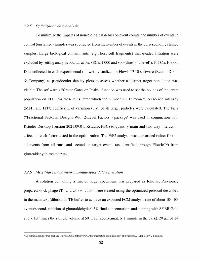
82

3.2.5 Optimization data analysis

To minimize the impacts of non-biological debris on event counts, the number of events in

control (unstained) samples was subtracted from the number of events in the corresponding stained

samples. Large biological contaminants (e.g., host cell fragments) that evaded filtration were

excluded by setting analysis bounds at 0 ≤ SSC ≤ 1,000 and 800 (threshold level) ≤ FITC ≤ 10,000.

Data collected in each experimental run were visualized in FlowJoTM 10 software (Becton Dixon

& Company) as pseudocolor density plots to assess whether a distinct target population was

visible. The software’s “Create Gates on Peaks” function was used to set the bounds of the target

population on FITC for these runs, after which the number, FITC mean fluorescence intensity

(MFI), and FITC coefficient of variation (CV) of all target particles were calculated. The FrF2

(“Fractional Factorial Designs With 2-Level Factors”) package6 was used in conjunction with

Rstudio Desktop (version 2021.09.01, Rstudio, PBC) to quantify main and two-way interaction

effects of each factor tested in the optimization. The FrF2 analysis was performed twice: first on

all events from all runs, and second on target events (as identified through FlowJoTM) from

glutaraldehyde-treated runs.

3.2.6 Mixed-target and environmental-spike data generation

A solution containing a mix of target specimens was prepared as follows. Previously

prepared stock phage (T4 and φ6) solutions were treated using the optimized protocol described

in the main text (dilution in TE buffer to achieve an expected FCM analysis rate of about 102–103

events/second, addition of glutaraldehyde 0.5% final concentration, and staining with SYBR Gold

at 5 x 10-5 times the sample volume at 50°C for approximately 1 minute in the dark). 20 µL of T4

6 Documentation for this package is available at https://www.rdocumentation.org/packages/FrF2/versions/2.1/topics/FrF2-package.

83

stock (10-3 dilution) and 20 µL of φ6 stock (10-3 dilution) were added to 1 µL of an 0.2-µm diameter

fluorescent polystyrene spherical bead suspension, 2 µL of an 0.5-µm diameter bead suspension,

and 15 µL of PBS. This mixed-target solution was then serially diluted to achieve 2x, 4x, 8x, and

16x dilutions of the starting solution. 4 µL of an 0.8-µm diameter bead suspension were added to

each dilution as a constant-concentration reference.

Separately, tertiary treated effluent from the UC Davis Wastewater Treatment Plant was

syringe-filtered at 0.2 µm to exclude bacteria and large debris while retaining the natural virus and

VLP community in the environmental matrix. The filtered effluent was diluted 10x in Milli-Q

water to reduce the background particle count to a level suitable for FCM analysis while still

providing a challenging matrix. The filtered effluent was then spiked with the same mixed-target

solution described above, but without the φ6 and 0.5 µm beads. Table B7 provides expected

concentrations of each target in the mixed-target and environmental-spike solutions per effective

volume (10 µL) analyzed via FCM. 10 replicates of each solution dilution were run on the

NovoCyte using settings and protocols described above. Data were exported as .fsc and .csv files

for manual and automated analysis, respectively.

3.2.7 Mixed-target and environmental-spike data analysis

The mixed-target and data were analyzed manually by plotting data from the undiluted

mixed solution as SSC vs. FITC log-log scale pseudocolor density plots, then drawing gates around

apparent clusters of interest. These gates were applied to data from all dilutions of the mixed

solution. Relevant gates were also applied to the environmental-spike data. Mixed-target and

environmental-spike data were also analyzed computationally as follows. I applied a log

transformation to the FSC, SSC, and FITC data collected from each replicate, then standardized

84

the features by centering each and rescaling to have standard deviation 1 (so that no single feature

would have outside influence over the clusters). I then used the open-source software Rstudio

(version 2021.9.1.372) to apply the implementation of the OPTICS ordering algorithm developed

by Ankerst et al. (1999) available in the dbscan package for R (Hahsler et al. 2019). Distance

between points was measured using Euclidean distance. Based on Sander et al. (1998), I set k equal

to 2*[dimensionality of the dataset], or 6 in this case (with the three dimensions of the dataset

being FSC, SSC, and FITC). Based on preliminary experimentation with different ε values (results

not shown), I set ε equal to 0.1 to bound the algorithm and reduce computational time. I used

MATLAB® software (version R2021a; MathWorks) to inspect reachability plots of the OPTICS-

ordered data for manual extraction/identification of clusters. I used the opticskxi package available

in R (Charlton 2019) for automated extraction of clusters from the OPTICS-ordered data with a

maximum iteration number of 1,000 and a maximum cluster number (k) of six for the mixed-target

data and four for the environmental-spike data. For the mixed-target data, the minimum-points-

per-cluster (MinPts) parameter started at 8,000 for the 1x dilution and was cut in half for each

subsequent dilution (ending at 500 for the 16x dilution). For the environmental-spike data, the

MinPts parameter was set at 8,000 for both the spiked environmental sample replicates and the

negative control replicates. The k value for the mixed-target data was selected based on the number

of clusters identified through manual gating; the k value for the environmental-spike data was

selected based on the three clusters identified through manual gating plus a fourth to provide the

algorithm room to identify a cluster corresponding to background in the wastewater matrix. The

MinPts parameters were selected based on the lowest expected target event count. The R and

MATLAB® scripts used for mixed-target data analysis are available at

https://github.com/hsafford/FCMClustering2022.

85

3.3 Results and discussion

3.3.1 Optimizing staining through fractional factorial experimental design

A representative suite of results plots is displayed in Figure B1. Results from the T4

optimization are also summarized numerically in Table B8, and graphically in Figure B2. I found

that a distinct target population was only visible for the eight glutaraldehyde-treated runs. Indeed,

glutaraldehyde addition had a highly significant (p < 0.001) effect on total event count, FITC mean

fluorescence intensity (MFI; a measure of brightness achieved through nucleic-acid staining), and

the FITC coefficient of variation (CV; a measure of the spread of the target fluorescence). Adding

glutaraldehyde increased the total sample event count by 65,402 events, increased FITC MFI by

360 units, and decreased FITC CV by 9 percentage points.

There are three possible explanations for the observed increase in total sample event count for

glutaraldehyde-treated samples:

(1) Glutaraldehyde addition increases the presence of fluorescent phantom events such as

autofluorescent colloidal particles (Dlusskaya et al. 2019).

(2) Glutaraldehyde addition enhances the fluorescence of non-target events (e.g., bacterial

debris) above the FITC threshold, such that the signal is not masked by electronic noise.

(3) Glutaraldehyde addition enhances the fluorescence of target events (here, T4) above the

FITC threshold, such that the signal is not masked by electronic noise.

To test (1) and (2), I used FCM to compare untreated and glutaraldehyde-treated 0.2-µm filtered

phosphate buffered saline (PBS) after staining with SYBR Gold. I also compared FCM data

collected on untreated and glutaraldehyde-treated samples of the negative stock stained with

SYBR Gold. In neither case did FCM reveal a distinct target population, nor a substantial increase

in event count, after glutaraldehyde addition. These results suggest that glutaraldehyde addition

86

not only helps visibly separate the target signal from non-target events, but also increases the

absolute number of target events detected through FCM. The average target event count for the

eight runs that incorporated glutaraldehyde was approximately 1.4 * 1010 events/mL: about an

order of magnitude greater than the qPCR-based titer (108–109 gc/mL) and about two orders of

magnitude greater than the culture-based titer (107–108 PFU/mL). These discrepancies may be

attributed to factors such as non-specific staining of particles (e.g., cellular debris) in FCM, losses

during DNA extraction in PCR, and aforementioned challenges with plate-based culturing.

The fractional factorial design enabled me to quantify main and two-way interaction effects

of each factor tested in the optimization. I performed this quantification first on all events within

analysis bounds (described in “Materials and methods”). Results are shown in Figure B3 and Table

B8. Though this analysis suggested the presence of numerous significant main effects as well as

several significant two-way interaction effects between glutaraldehyde and other experimental

factors, results were compromised by the fact that the analysis did not distinguish between target

and non-target events. Because a distinct target population was only visible for glutaraldehyde-

treated runs, and because the goal of the optimization was to develop a staining protocol that most

successfully separates the target population from background, I also performed the quantification

using only data from target events identified in glutaraldehyde-treated runs.

No statistically significant two-way interaction effects were observed in the target-only

analysis. However, the fact that glutaraldehyde was included as a variable in the fractional factorial

experimental design meant that only a small subset of two-way interaction effects between non-

glutaraldehyde factors were analyzed. Further experimental work could explore other possible

two-way interaction effects. The target-only analysis also did not identify any statistically

significant main effects on FITC MFI. Diluent was the only variable that had a significant main

87

effect on event count: the main effect of using TE buffer instead of MQ water was -7,807 events

with a p-value of 0.023. I have no obvious explanation for why this was the case. My a priori

expectation was that diluting T4 in buffer would increase apparent event count by inhibiting

particle aggregation relative to dilution in MQ water of low ionic strength (Szermer-Olearnik et

al. 2017). The increased tendency of free stain to form colloids (and hence generate FCM events)

in low-ionic-strength water (Zhang et al. 2015) is one possible explanation for why the opposite

effect was observed.

Stain temperature and diluent had very strongly significant (p < 0.001) main effects on FITC

CV. Staining at 50°C rather than 25°C had a main effect of decreasing FITC CV by 2.7 percentage

points, while using TE buffer rather than MQ water had a main effect of decreasing FITC CV by

4.4 percentage points. Stain concentration had a strongly significant (0.001 < p < 0.01) effect on

FITC CV: staining at 1 x 10-4 times the sample volume had a main effect of increasing FITC CV

by 1.8 percentage points relative to staining at 5 x 10-5 times the sample volume. Stain time and

stain type both had significant (0.01 < p < 0.05) effects on FITC CV. Staining for 15 minutes

instead of 1 minute had a main effect of decreasing FITC CV by 1.2 percentage points, while

staining with SYBR Gold rather than SYBR Green I had a main effect of increasing FITC CV by

1.5 percentage points. Based on the relative magnitude of these effects—and their relative

statistical significances—I conclude that stain temperature and diluent are the most important

sample-preparation factors besides glutaraldehyde addition. In other words, dilution in TE buffer

and staining at 50°C can increase the “tightness” of the T4 FITC signal, thereby aiding

discrimination of T4 from background.

I further conclude that using SYBR Green I (instead of SYBR Gold) and staining for 15

minutes (instead of 1 minute) could improve target discrimination of T4 slightly further. However,

88

it is important to weigh these small potential advantages against their drawbacks. A sample-

preparation protocol that specifies 15 minutes for staining may be less useful for online, near-real-

time FCM than a protocol that specifies only one. SYBR Green I exhibits a large fluorescence

enhancement upon binding to DNA but not RNA. Hence a protocol using this stain may be less

effective at detecting a wide variety of viruses than SYBR Gold, which exhibits a large

fluorescence enhancement upon binding to DNA and RNA.

Overall, my results suggest that a protocol for reliably identifying and quantifying T4

bacteriophage through FCM should involve diluting the sample in TE buffer to achieve an FCM

analysis rate of about 102–103 events/second, adding glutaraldehyde at a final concentration of

0.5%, and staining with either SYBR Green I or SYBR Gold (depending on whether the species

of interest in a given sample include DNA and RNA viruses) at 5 x 10-5 times the sample volume

at 50°C for at least 1 minute prior to analysis.

3.3.2 Automating data analysis through density-based clustering

3.3.2.1 Mixed-target experiments—approach

In a real-world setting such as an advanced water-treatment plant, a suite of

microbiological targets (e.g., different classes of protozoa, bacteria, and viruses) may be present

and of possible interest. To test the capacity of an automated clustering algorithm to accurately

detect and quantify waterborne viruses alongside other specimens, I prepared a solution containing

known concentrations of biological and non-biological targets in the submicron size range. These

targets were φ6 and T4 bacteriophage stocks as well as fluorescent polystyrene spherical beads of

0.2, 0.5, and 0.8 µm in diameter. T4 was included in the target mix because, as discussed above,

it is an environmentally relevant viral surrogate that generates a clear FCM signal. φ6 was included

89

in the specimen mix to represent viral classes that are neither physically large enough nor contain

a large enough genome to be detectable through FCM as distinct populations (Dlusskaya et al.

2021),7 but may still generate an indeterminate “virus-like particle (VLP)” signal at or near the

limit of detection of most flow cytometers. 0.2, 0.5, and 0.8 µm beads were included because these

engineered particles are (i) similar in size to many bacterial classes, and (ii) highly uniform. The

latter characteristic is important because while biological targets tend to generate more dispersed

(i.e., higher-CV) FCM data of variable density, engineered particles generate tightly grouped data

of relatively uniform density. Combining biological and engineered targets in a single solution

hence enabled me to test the performance of an algorithmic approach to FCM data analysis on a

mixed-density dataset.

As detailed in “Materials and methods”, I collected FCM data on 10 replicates of each of

five serial dilutions (1x, 2x, 4x, 8x, and 16x) of the mixed-target solution. The 0.8 µm bead

component of the solution was kept undiluted (i.e., the concentration of 0.8 µm beads remained

constant across the five serial dilutions) as a control/reference. I first analyzed the data by manual

gating of apparent populations of interest on SSC vs. FITC pseudocolor density plots. I then

analyzed the data with the aid of the OPTICS ordering algorithm developed by Ankerst et al.

(1999). OPTICS outputs all points in a dataset ordered by a calculated and characteristic

“reachability distance”. Plotting reachability distance against order yields a reachability plot that

can be used to identify clusters by looking for “valleys” of low reachability distance separated by

“peaks” of noise, with deeper valleys representing denser clusters. There are three ways to extract

clusters from the reachability plot. The most straightforward option is to set a single global

reachability threshold, such that points with below-threshold reachability distances are grouped

7 Indeed, no protocol for reliably detecting/discriminating φ6 through FCM has yet been developed.

90

into clusters. Unfortunately, this approach fails when—as is often the case in real-world

environmental samples—the number of targets and the spatial density of FCM data generated by

those targets are variable. Figure B4 illustrates the problem: a global threshold set low enough to

accurately capture high-density clusters misses low-density clusters, while a global threshold set

high enough to capture low-density clusters incorrectly categorizes noise points as belonging to

high-density clusters.

The alternative options are (i) manually extracting clusters from the OPTICS ordering of a

dataset via visual inspection of peaks and valleys on the reachability plot (Figure B5A), or (ii)

identifying an algorithm that can perform the inspection automatically. Ankerst et al. suggested an

automated method for extracting clusters by identifying all “steep up” and “steep down” areas on

the reachability plot, as characterized by the ξ steepness parameter. A drawback of this approach

is that ξ must be tuned to the data based on trial and error; it is difficult if not impossible to estimate

ξ a priori. The opticskxi package available in R provides a variant cluster-extraction algorithm

that “iteratively investigates the largest differences” in steepness until either a given number of

clusters are defined or the maximum number of iterations is reached (Charlton n.d.; Figure B5B).

3.3.2.2 Mixed-target experiments—results

I compared results from manual extraction and opticskxi-based extraction of clusters from

the OPTICS-ordered mixed-target data to results obtained through manual gating.8 Figures B6,

B7, and B8 contain representative plots respectively illustrating results from manual gating,

manual cluster extraction from the OPTICS ordering, and opticskxi-based cluster extraction from

8 It is important to note that the nature of FCM analysis makes validating results at the single-particle level difficult if not impossible. Results are therefore typically evaluated by comparing bulk target counts/concentrations obtained through FCM to the same obtained through other methods (e.g. electron microscopy, culturing, qPCR).

91

the OPTICS ordering for the mixed-target experiments. A first observation is that manual

extraction resulted in labeling far more points as noise than did opticskxi-based extraction. For

manual extraction, I separated valleys from peaks (and hence clusters from noise) by setting

cutpoints at the apparent “knees” of the reachability plot curves. The opticskxi algorithm, by

contrast, set cutpoints at or near the peaks of the reachability plot curves. Charlon (n.d.) notes the

tendency of the opticskxi algorithm to assign noise points to clusters, and provides a framework

for systematically varying (i) the dimension-reduction methods used in the OPTICS ordering prior

to clustering, and/or (ii) parameters employed in the opticskxi extraction in order to identify the

optimal approach. However, applying this framework proved too computationally intensive for

this study (requiring >24 hours of computer runtime for individual datasets).

A second observation is that somewhat different clusters were obtained using the different

strategies. In manual gating we set six gates: one each for each of the three bead sizes, T4, φ6 and

other virus-like particles (VLPs), and an additional apparent cluster thought to correspond to 0.5

µm bead doublets.9 Neither manual extraction nor opticskxi-based extraction identified a cluster

matching the manual gates drawn for φ6/VLPs and for the 0.5 µm doublet. Manual extraction

tended to identify events falling within these gates as noise, while opticskxi-based extraction

tended to assign events falling into the φ6/VLP gate as part of the T4 cluster and events falling

into the 0.5 µm doublet gate as part of the 0.5 µm bead cluster. On the other hand, both OPTICS-

assisted approaches frequently detected two separate clusters within the SSC vs. FITC region

designated by manual gating as corresponding to 0.2 µm beads. Inspecting a 3D plot of the data

revealed why this was the case: some of the events exhibiting the same SSC and FITC signal

intensity ranges exhibited meaningfully different FSC signal intensities.

9 A doublet occurs when two particles pass through the interrogation laser beam of a flow cytometer simultaneously.

92

To enable numerical comparison of results across the different clustering approaches

despite these discrepancies, I established four consistent “buckets” corresponding to viruses

(including T4, φ6, and other VLPs), 0.2 µm beads, 0.5 µm beads (including 0.5 µm doublets), and

0.8 µm beads. Table B9 shows average event counts obtained using each of the three approaches

across all replicates for each dilution analyzed. Figure B9 plots these data. There were clear

differences between the theoretical and detected event counts for each target. Event counts were

higher than expected for the 0.2 and 0.5 µm bead buckets, slightly lower than expected for the 0.8

bead bucket, and much lower than expected for the virus bucket. Discrepancies between theoretical

and detected event counts for the bead buckets are most likely explained by the fact that the

manufacturer-provided concentrations of the various bead solutions used in this study are only

approximate within an order of magnitude. Discrepancies between theoretical and detected event

counts for the virus bucket can be explained by the fact that φ6, as a small and difficult-to-stain

enveloped virus, emits only a faint FITC signal. From other experiments with φ6 conducted as

part of a project not included in this dissertation, it is likely that a majority of the φ6 particles

spiked into the mixed-target solution were not stained brightly enough to rise above the FITC limit

of detection. As Dlusskaya et al. (2021) concluded, conventional FCM instrumentation is not yet

capable of reliably detecting small enveloped viruses like φ6.

Restricting analysis to the detected event counts shows that results were generally

consistent across all three clustering approaches for the bead buckets: a promising indication that

algorithmically assisted clustering is a viable approach to FCM data analysis. For the virus bucket,

event counts from manual gating and opticskxi-based extraction were similar to each other but

generally higher than event counts from manual extraction. This can be explained by recalling that

while engineered particles generate tightly grouped data of fairly uniform density, biological

93

targets tend to generate more dispersed (i.e., higher-CV) FCM data of variable density. Consider

in turn how each of the three clustering approaches considered in this study handle the variable-

density clusters associated with T4 and φ6 in this study. For manual gating, I established relatively

large gates for T4 and φ6. Any point falling within these gates was categorized as part of a virus

cluster, regardless of how close that point was to the dense cluster core. Because T4 and φ6 were

considered together as part of the virus bucket, manual gating defined all points in the general

T4/φ6/VLP region as viruses.

For the OPTICS-assisted methods, it is important to recognize that the OPTICS ordering

of the mixed-target data did not reveal a shift in reachability distance marking the transition from

the T4 cluster to the φ6/VLP region. In other words, reachability distance increased gradually

towards the border of the T4 cluster, then continued to increase at roughly the same rate as the T4

cluster border bled into the φ6/VLP region. As the 1x and 2x plots in Figures B7 and B8 illustrate,

this resulted in manual and opticskxi-based extraction delivering quite different results. For

opticskxi extraction, as discussed above, the algorithm tended to assign high-reachability-distance

points included in a given reachability-plot curve (points located towards the peak) to the same

cluster as low-reachability-distance points (points located towards the valley). The upshot is that

the OPTICS ordering placed many points corresponding to the T4 and φ6/VLP regions on the

same curve of the reachability plot, and so the opticskxi extraction assigned all of those points to

the T4 cluster. These points were then in turn grouped into the virus bucket. By contrast, setting a

cutpoint at the knee of the curve in manual extraction resulted in points near the valley of the

T4/φ6/VLP curve being assigned to the T4 cluster (and then to the virus bucket), and points near

the peak being assigned to noise.

94

To sum, key takeaways from the mixed-target test are as follows. First, good agreement

between results obtained through manual gating and results obtained through algorithmically

assisted methods for the bead targets is promising evidence in favor of automated FCM data

analysis. Agreement (within an order of magnitude) between expected and detected event counts

for the three bead targets at different dilutions provides additional support. Second, there are pros

and cons to the different clustering methods with respect to virus targets. Manual gating reliably

identified a suite of events thought to correspond to T4 and a second suite thought to correspond

to φ6/VLPs. But fixed gates are a blunt instrument for handling data from biological targets, which

may be subject to influence from variability in target morphology, staining efficacy, and other

factors. OPTICS-assisted clustering is faster and more objective than manual gating. And while

manual gates impose sharp, regularly shaped bounds on apparent clusters, algorithmically

identified clusters have shaggy boundaries that would be nearly impossible to capture by hand.

Unfortunately, neither manual extraction nor opticskxi-based extraction of clusters from the

OPTICS ordering reliably identified and separated the two viruses spiked into the mixed-target

solution. Manual extraction identified the T4 cluster but categorized particles in the φ6/VLP region

as noise, while opticskxi-based extraction tended to identify a single cluster corresponding to T4

and φ6/VLPs together. Third and finally, it is worth considering how the multidimensional nature

of FCM data intersects with results from the mixed-target study. As stated above, a challenge with

manual gating is that analyzing multidimensional FCM data on a series of two-dimensional dot

plots is time-consuming and not conducive to identification of patterns in multidimensional space.

OPTICS eliminates the tedious human element of the manual-gating workflow and also considers

all dimensions of an FCM dataset at once. The latter characteristic of OPTICS may help uncover

patterns that would be missed through the manual-gating workflow. It is notable that in the mixed-

95

target study, manual gating identified a single region thought to correspond to 0.2 µm beads, while

both of the OPTICS-assisted approaches revealed that some points within this region actually

emitted meaningfully different FSC signals. On the other hand, the dimensionality-reduction

employed in OPTICS may also result in different dimensions carrying equal weight when they

really should not. For instance, T4 and φ6 stained with SYBR Gold both exhibit FCM signals that

rise above background noise on the FITC dimension (T4 more than φ6), but not the FSC or SSC

dimensions. Weighting FITC more strongly may therefore yield more accurate results for

clustering virus-generated FCM data. Indeed, it is possible that equal weighting of all dimensions

contributed to challenges identifying T4 and φ6 through OPTICS-assisted clustering.

3.3.2.3 Environmental-spike experiments—approach

I conducted the mixed-target experiments described above to assess the capacity of

automated clustering to accurately detect and quantify waterborne viruses alongside other

specimens. I performed a modified version of this experiment to assess the capacity of automated

clustering to accurately detect and quantify waterborne viruses in a challenging environmental

matrix, where the presence of an increased background signal could confound FCM analysis

and/or alter the target signal.10 Specifically, I spiked a mixed T4/bead solution described above

into tertiary-treated wastewater effluent that had been syringe-filtered at 0.2 µm and diluted 10x.

The T4/bead solution used in the environmental-spike experiments was the same as the mixed-

target solution used in the experiments described in Sections 3.3.2.1 and 3.3.2.2, but with φ6 and

0.5 µm beads omitted. φ6 was omitted from the mixed-target solution for the environmental spike

10 For instance, adherence of viral particles to suspended solids in wastewater (Chahal et al. 2016) could decrease event count; or uptake of stain by the natural virus community inn wastewater could reduce T4 fluorescence intensity by reducing dye available for target staining.

96

because results from the mixed-target experiments and from experiments conducted from a

separate project made it clear that φ6 was unlikely to generate a characteristic signal that could be

differentiated from background VLPs in the wastewater matrix, even with the aid of algorithmic

clustering tools. T4 provided a better and sufficient viral target for the environmental-spike test.

0.5 µm beads were omitted because they did not serve a clear purpose for the environmental-spike

test. By contrast, I expected that 0.2 µm beads, because of their relatively small size and weak

fluorescent signal, might also be obscured by VLPs in the wastewater and hence provide a second

useful test of the capacity of automated clustering to distinguish target from background signal. I

included 0.8 µm beads as a control/reference that, because of its relatively large size and strong

fluorescent signal, was unlikely to be obscured by the wastewater background. I also prepared a

negative control environmental spike by substituting the T4-negative control for the T4 stock and

keeping all other spike-preparation steps the same.

I again collected FCM data on 10 replicates of each of the two solutions tested (positive

environmental spike and negative control). I first analyzed the data by manual gating, applying the

same gates for T4, 0.2 µm beads, and 0.8 µm beads used in the mixed-target experiments. I then

applied OPTICS ordering with manual cluster extraction, and OPTICS ordering with opticskxi-

based extraction.

3.3.2.4 Environmental-spike experiments—results

Figures B10, B11A, and B12A contain representative plots respectively illustrating results

from manual gating, manual cluster extraction from the OPTICS ordering, and opticskxi-based

cluster extraction from the OPTICS ordering for the environmental-spike experiments. There was

less agreement between these three clustering methods for the environmental-spike data than there

97

was for the mixed-target data. Through manual clustering, I identified the three targets: an 0.8 µm

bead cluster, an 0.2 µm bead cluster, and—for the T4-positive sample but not the T4-negative—a

T4 cluster that, while partially obscured by background from the wastewater matrix, still clearly

fell within the T4 gate established for the mixed-target experiments. As Table 10 shows, expected

event counts were roughly in line with detected event counts obtained through manual gating,

exhibiting the same discrepancy patterns observed for the mixed-target experiments. I also

observed a low-SSC, high-FITC cluster in most of the replicate runs for both the T4-positive and

T4-negative samples. This cluster does not obviously correspond to any target used in the

environmental-spike experiments and hence is likely attributable to contamination in a reagent or

in the instrument fluidics.

The two OPTICS-based clustering approaches yielded quite different results. As was also

true for the mixed-target experiments, manual identification/extraction of clusters from the

OPTICS-ordered data successfully detected the 0.8 µm bead cluster, the 0.2 µm bead cluster, and

often a sub-cluster in the 0.2 µm bead zone corresponding to particles exhibiting signals of similar

intensity on the FITC and SSC channels but different on the FSC channel. This clustering approach

also detected one or more clusters in the low-FITC, low-SSC region corresponding to φ6/VLPs in

the mixed-target experiments (and hence to background—including natural virus particles—in the

wastewater matrix for the environmental-spike experiments). For the T4-positive samples, one of

the clusters containing points in this region also extended higher in the FITC direction to include

points located in the T4 region. Finally, this clustering approach tended to detect one or more

clusters comprising points with very low SSC signal intensities. Manual identification/extraction

did not tend to clearly distinguish the T4 cluster, nor did it detect the visually apparent low-SSC,

high-FITC foreign cluster.

98

Results were similarly poor for opticskxi-based clustering. The constraining k parameter

meant that the opticskxi algorithm did not yield as many clusters as manual extraction. Rather, this

approach consistently detected a cluster corresponding to the 0.8 µm beads, a cluster that included

the 0.2 µm beads as well as many other points dispersed as apparent noise, and a cluster that

included the VLP/background region for the negative-control replicates and also extended to the

T4 region for the spiked-sample replicates. This cluster also sometimes spilled over to include

much of the 0.2 µm bead region. The opticskxi approach occasionally detected the higher-FSC

sub-cluster in the 0.2 µm bead region, occasionally detected the low-SSC, high-FITC foreign

cluster, and never detected a clearly distinct T4 cluster.

Because (i) the reachability plots from the environmental-spike data were so complex, (ii)

I set manual gates exclusively based on the SSC vs. FITC pseudocolor density plot, and (iii) of

possible issues (discussed in Section 3.3.2.2) with OPTICS over-weighting FSC signal intensities

for virus data, I also generated OPTICS orderings of the environmental-spike data using only the

SSC vs. FITC dimensions. Figures B11B and B12B contain representative plots respectively

illustrating results from manual and opticskxi-based clustering using these reduced-dimension

orderings. The reachability plots of these orderings were indeed simpler but did not yield

significantly better results, especially with respect to T4 detection.

Results from the mixed-target and environmental-spike experiments show overall that

OPTICS is a promising approach for automating FCM analysis. The mixed-target experiments

showed that OPTICS ordering coupled with either manual or opticskxi-based cluster

identification/extraction works as well or better than manual gating for analysis of dense and well-

defined clusters such as those generated by fluorescent polystyrene beads. The fact that OPTICS

identified points identified as 0.2 µm beads through manual gating that were meaningfully

99

different when evaluated on the FSC dimension is a promising sign that algorithmic clustering can

draw attention to features in FCM data that are difficult to detect through conventional analysis.

Though the most automated clustering approach tested in this chapter—OPTICS ordering coupled

with opticskxi-based extraction—falsely grouped many likely noise points in with target events, it

is reasonable to expect that further parameter refinement could correct this deficiency.

The mixed-target and environmental-spike experiments also showed that OPTICS-based

clustering works less well on relatively dispersed FCM data such as those generated by viruses or

other biological targets, especially when points in the dispersed target cluster overlap with points

resulting from background in an environmental matrix like wastewater. In the mixed-target

experiments, neither of the OPTICS-based clustering approaches identified separate T4 and

φ6/VLP clusters. Manual cluster identification/extraction reliably identified the T4 cluster while

labeling points in the φ6/VLP region as noise. This is an arguably acceptable result given that the

apparent φ6/VLP events constitute more of a vague cloud of points than they do a clearly defined

cluster. In the environmental-spike experiments, though, coupling OPTICS ordering with manual

cluster identification/extraction failed to distinguish spiked T4. OPTICS coupled with opticskxi-

based cluster extraction, by comparison, grouped apparent T4 points with points in the

φ6/VLP/background region in both the mixed-target and the environmental-spike experiments.

Again, this is an arguably acceptable result if a goal of advancing FCM for microbial water-quality

monitoring is to obtain information on total virus counts. However, OPTICS coupled with

opticskxi-based cluster extraction in the environmental-spike experiments sometimes grouped T4

with distinctly non-viral 0.2 µm beads.

100

3.4 Conclusion

In this chapter, I presented methods for increasing the rigor, efficiency, and accuracy of

FCM protocol optimization and of FCM data analysis. Specifically, I proposed using fractional

factorial experimental designs for optimizing FCM sample-preparation protocols, and OPTICS-

assisted clustering for analyzing complex FCM data. Both approaches can be considered for any

application of FCM, but were here demonstrated using the bacteriophage T4, an environmentally

relevant viral surrogate, in the context of water-treatment and -reuse scenarios.

Through the fractional factorial experimental design, I identified multiple factors with

statistically significant main effects on the count, coefficient of variation (CV), and mean

fluorescence intensity (MFI) of T4, and based on these was able to suggest an optimized protocol

for FCM-based T4 detection that represents a blend of—and perhaps an improvement on—

protocols from the literature developed using a traditional “pipeline” optimization approach. I did

not observe any statistically significant interaction effects among the factors tested in the T4

optimization, but still expect that the fractional factorial experimental design framework could

uncover such effects in other FCM protocol-optimization studies.

Through the mixed-target and environmental-spike experiments discussed in this chapter,

I demonstrated that OPTICS-based clustering can in some cases work as well or better than manual

gating of FCM data—and is certainly far faster and less labor-intensive. As an objective data-

analysis technique, OPTICS-based clustering could be useful for facilitating comparison of data

collected on the same targets by different labs using different instruments. OPTICS-assisted

clustering can also help uncover features in FCM data that are difficult to detect through manual

gating alone.

101

My results also showed that more needs to be done to position OPTICS-based clustering

as a reliable tool for automated, objective analysis of FCM data from environmental samples,

especially data generated from challenging biological targets like viruses in challenging matrices

like wastewater. Future work could focus, for instance, on helping researchers efficiently select

the best parameters for the OPTICS ordering based on information available about the dataset in

question, on determining whether and how to weight different dimensions of FCM data in the

OPTICS ordering, or on developing methods for automatically extracting clusters from OPTICS-

based reachability plots that are more flexible and better at discriminating noise than opticskxi.

OPTICS could also be useful as a tool to assist manual gating in complex samples. For instance,

a researcher could apply OPTICS-based clustering on a target (e.g., T4) in a clean sample, and

then use the cluster boundary identified using OPTICS to establish a T4 gate to be used in complex

samples where OPTICS-based clustering fails.

102

3.5 References

Ankerst, M., Breunig, M.M., Kriegel, H.-P. and Sander, J. (1999). OPTICS: ordering points to identify the clustering structure. ACM SIGMOD Record 28(2): 49–60.

Antony, J. (2016). 7 – Fractional Factorial Designs. Design of Experiment for Engineers and Scientists. Elsevier.

Arnold, R.G., Saez, A.E., Snyder, S. Maeng, S.K., Lee, C., Woods, G.J., Li, X. and Choi, H. (2012). Direct potable reuse of reclaimed wastewater: It is time for a rational discussion. Rev. Environ. Health 27(4): 197–206.

Bashashati, A. and Brinkman, R.R. (2009). A Survey of Flow Cytometry Data Analysis Methods. Adv. Bioinform.

Bonilla, N. and Barr, J.J. (2018). Chapter 4—Phage on Tap: A Quick and Efficient Protocol for the Preparation of Bacteriophage Laboratory Stocks. The Human Virome: Methods and Protocols. Springer Science+Business Media, Berlin, Germany.

Brusaard, C.P.D. (2004). Optimization of Procedures for Counting Viruses by Flow Cytometry. Appl. Environ. Microbiol. 70 (3): 1506–1513.

Brusaard, C.P.D., Marie, D. and Bratbak, G. (2000). Flow cytometric detection of viruses. J. Virol. Methods 85(1–2): 175–182.

Byappanahalli, M.N., Whitman, R.L., Shively, D.A., Evert Ting, W.T., Tseng, C.C. and Nevers, M.B. (2006). Seasonal persistence and population characteristics of Escherichia coli and enterococci in deep backshore sand of two freshwater beaches. J. Water Health, 4(3): 313–320.

California State Water Resources Control Board [CASWRCB] (2016). Investigation on the Feasibility of Developing Uniform Water Recycling Criteria for Direct Potable Reuse.

Case, J., Rice, A., Wood, J., Gaudry, L., Vowels, M. and Nordon, R.E. (2001). Characterization of Cytokine Interactions by Flow Cytometry and Factorial Analysis. Cytometry 43(1): 69–81.

Chahal, C., van den Akker, B., Young, F., Franco, C., Blackbeard, J and Monis, P. (2016). Pathogen and Particle Associations in Wastewater: Significance and Implications for Treatment and Disinfection Processes. Adv. Appl. Microbiol. 97, 63–119.

Chalron, T. (n.d.). opticskxi: OPTICS K-Xi Density-Based Clustering. (n.d.). Available at https://cran.r-project.org/web/packages/opticskxi/vignettes/opticskxi.pdf.

Charlon, T. (2019). opticskxi: OPTICS K-Xi Density-Based Clustering. R package version 0.1 (2019).

Collier, S.A., Stockman, L.J., Hicks, L.A., Garrison, L.E., Zhou, F.J. and Beach, M.J. (2012). Direct healthcare costs of selected diseases primarily or partially transmitted by water. Epidemiol. Infect. 140(11): 2003–2013.

Dlusskaya, E., Dey, R., Pollard, P.C. and Ashbolt, N. J. (2021). Outer Limits of Flow Cytometry to Quantify Viruses in Water. Environ. Sci. Tech. Water 1(5): 1127–1135.

103

Gendron, L., Verreault, D., Veillette, M., Moineau, S. and Duchaine, C. (2010). Evaluation of Filters for the Sampling and Quantification of RNA Phage Aerosols. Aerosol Sci. Technol. 44: 893–901.

Gerriets, J.E., Greiner, T.C. and Gebhart, C.L. (2008). Implementation of a T4 extraction control for molecular assays of cerebrospinal fluid and stool specimens. J. Mol. Diagn. 10(1): 28–32.

Hahsler, M., Piekenbrock, M., and Doran, D. (2019). dbscan: Fast Density-Based Clustering with R. J. Stat. Softw. 91: 1–30.

Huang, X., Min, J.H., Lu, W., Jaktar, K., Yu, C. and Huang, S. (2015). Evaluation of methods for reverse osmosis membrane integrity monitoring for wastewater reuse. J. Water Process Eng. 7: 161–168.

Kuznetsov, Y.G., Chang, S.-C. and McPherson, A. (2011). Investigation of bacteriophage T4 by atomic force microscopy. Bacteriophage 1(3): 165–173.

Messner, M., Shaw, S., Regli, S., Rotert, K., Blank, V. and Soller, J. (2006). An approach for developing a national estimate of waterborne disease due to drinking water and a national estimate model application. J. Water Health, 4(Suppl. 2): 201–240.

Miller, E.S., Kutter, E., Mosig, G., Arisaka, F., Kunisawa, T. and Rüger, W. (2003). Bacteriophage T4 genome. Microbiol. Mol. Bio. Rev. 67(1): 86–156.

National Research Council. (2012). Water Reuse: Potential for Expanding the Nation’s Water Supply through Reuse of Municipal Wastewater. National Academies Press, Washington, DC.

Nescerecka, A., Hammes, F. and Juhna, T. (2016). A pipeline for developing and testing staining protocols for flow cytometry, demonstrated with SYBR Green I and propidium iodide viability staining. J. Microbiol. Methods 131, 172–180.

Olivieri, A., Crook, J., Anderson, M., Bull, R., Drewes, J., Haas, C, Jakubowski, W., McCarty, P., Nelson, K., Rose, J., Sedlak, D. and Wade, T. (2016). Evaluation of the Feasibility of Developing Uniform Water Recycling Criteria for Direct Potable Reuse. National Water Research Institute, Fountain Valley, CA.

Ramírez-Castillo, F.Y., Loera-Muro, A., Jacques, M., Garneau, P., Avelar-González, F.J., Harel, J. and Guerrero-Barrera, A.L. (2015). Waterborne Pathogens: Detection Methods and Challenges. Pathogens 4(2): 307–334.

Rao, V.B. and Black, L.W. (2010). Structure and assembly of bacteriophage T4 head. Virol. J. 7. Rhys, H.I. (2020). Machine Learning with R, the Tidyverse, and Mlr. Manning Publications Co.,

Shelter Island, NY. Ruijgrok, J.M., de Wijn, J.R. and Boon, M.E. (1994). Glutaraldehyde crosslinking of collagen:

Effects of time, temperature, concentration and presoaking as measured by shrinkage temperature. Clin. Mater. 17(1): 23–27.

Safford, H.R. and Bischel, H.N. (2019). Performance comparison of four commercially available cytometers using fluorescent, polystyrene, submicron-scale beads. Data in Brief 24.

104

Sander, J., Ester, M. Kriegel, H.-P. and Xu, X. (1998). Density-Based Clustering in Spatial Databases: The Algorithm GDBSCAN and Its Applications. Data Min. Knowl. Discov. 2: 169–194.

Szermer-Olearnik, B., Drab, M., Mąkosa, M., Zembala, M., Barbasz, J., Dąbrowska, K. and Boratyński, J. (2017). Aggregation/dispersion transitions of T4 phage triggered by environmental ion availability. J. Nanobiotech. 15.

Zhang, Y., Yildirim, E., Antila, H.S., Valenzuela, L.D., Sammalkorpi, M. and Lutkenhaus, J.L. (2015). The influence of ionic strength and mixing ratio on the colloidal stability of PDAC/PSS polyelectrolyte complexes. Soft Matter 11(37).

105

CHAPTER 4: WASTEWATER-BASED EPIDEMIOLOGY TO INFORM COVID-19 RESPONSE IN DAVIS, CALIFORNIA

Following the onset of the COVID-19 pandemic in the spring of 2020, wastewater

surveillance (also known as wastewater-based epidemiology, or WBE) quickly became recognized

as a useful complement to clinical testing for monitoring disease emergence and spread. WBE is

less resource-intensive than large-scale diagnostic testing. WBE is also unbiased, capturing data

on entire populations rather than just the subset of individuals who come in for clinical testing (Wu

et al. 2021).

Most studies comparing wastewater and clinical data during the pandemic focused on the

community scale; i.e., comparing trends in data collected from the influent to a given WWTP to

trends in data collected from clinical tests of a subpopulation served by that WWTP. These studies

frequently found good agreement between the two data sources. Far less is known about

relationships between wastewater and clinical data at sub-community levels. A first objective of

this chapter is to advance and inform uses of WBE at multiple scales for pandemic response. For

instance, comparing data trends for wastewater collected from different neighborhoods could help

public-health officials strategically allocate resources such as testing, contact tracing and

vaccination outreach.

Separately, SARS-CoV-2 RNA in wastewater samples is typically quantified using either

reverse transcription-quantitative polymerase chain reaction (RT-qPCR) or RT-droplet digital

PCR (RT-ddPCR) (CDC 2021b). While RT-ddPCR is becoming more popular for WBE (Kan

2021) due to its greater specificity and sensitivity (Ciesielski et al. 2021; Falzone et al. 2021),

many laboratories continue to use RT-qPCR due to the higher cost and time requirements of RT-

ddPCR and the large upfront capital investment of ddPCR instrumentation.

106

Bivins et al. (2021) recently drew attention to how variability in RT-qPCR methods and

reporting affects results and interpretation. An additional and important source of variability not

considered by these authors is how non-detects are handled. qPCR non-detects occur routinely for

reasons including low or zero starting target abundance, poor assay design/performance, or human

error (McCall et al. 2014; Zanardi et al. 2019). There is no current consensus on how to best

manage qPCR non-detects. Researchers, whether through scientific software or manual analysis,

typically handle non-detects either using single imputation (setting all non-detects equal to a

constant value such as the mean of detected replicates, half the detection limit, or zero) or by

censoring (excluding non-detects from analysis altogether).

Unfortunately, both single imputation and censoring can substantially bias qPCR results

(McCall et al. 2014). The biasing effect is amplified when, as is often the case for wastewater data,

the target is present in low concentrations to begin with. A second objective of this chapter is to

explore whether multiple imputation of non-detects in wastewater qPCR data can improve on more

commonly used but less sophisticated non-detect-handling approaches. The chapter is structured

as follows:

• Section 4.1 provides background on the study setting and design.

• Section 4.2 presents materials and methods used.

• Section 4.3 summarizes and discusses results.

• Section 4.4 concludes.

107

4.1 Background

I used wastewater data collected through the Healthy Davis Together (HDT) program to

(1) explore the value of multiple imputation for handling qPCR non-detects, (2) examine

relationships between wastewater and clinical data at multiple spatial scales.

HDT is a joint, multi-pronged initiative between the city of Davis and the University of

California, Davis (UC Davis) for local management and mitigation of COVID-19. Beginning in

November 2020, HDT made free, saliva-based PCR tests for COVID-19 available to anyone living

or working in Davis. Uptake of the clinical-testing program was considerable. The fraction of

Davis residents who reported receiving at least one COVID-19 test rose from 30% to 73% from

September 2020 to March 2021. As of April 2021, Yolo County had performed the most tests per

capita of California’s 58 counties, at a rate quadruple the state median.

HDT also conducts WBE at the community, sub-regional, and building/neighborhood

scales (Figure C1). At the community scale, samples are collected from the influent to the City of

Davis Wastewater Treatment Plant (COD WWTP). The COD WWTP captures all of Davis’s

municipal wastewater, with no contributions from UC Davis or from neighboring jurisdictions. At

the sub-regional scale, samples are collected from sewershed nodes isolating the wastewater

contributions of different geographic areas in the city. At the building/neighborhood scale, samples

are collected from sewershed nodes isolating high-priority building complexes or neighborhoods

identified through discussion with local officials. The HDT WBE program began in September

2020 with weekly samples collected from the COD WWTP. Zones were added and sampling

frequency increased over the course of the sampling campaign (Figure C2). At full scale-up, the

surveillance program sampled daily from the COD WWTP and 3x/week from each of 16 sub-

regional and seven building/neighborhood zones.

108

4.2 Materials and methods

4.2.1 Sample collection and processing

24-h composite samples were collected from each zone using insulated HachTM AS950

Portable Compact Samplers (Thermo Fisher Scientific, USA) programmed to collect 30 mL of

sample every 15 minutes. The bulk of samples were processed immediately, with a small number

stored at 4°C for up to one week before processing.

Samples were pasteurized for 30 minutes at 60°C to reduce biohazard risk while preserving

RNA quality. Samples were then spiked with a known concentration of φ6 bacteriophage (strain

HB104; generously provided by Samuel Díaz-Muñoz, UC Davis) as an internal recovery control

(Aquino de Carvalho 2017; Bivins et al. 2020). The φ6 spike solution was prepared using

previously described methods (Kantor et al 2021), modified slightly by using ATCC® Medium 129

in place of LB media. The final steps in the processing pipeline were sample concentration and

extraction. From September 2020 through the end of February 2021, these steps were performed

via ultrafiltration and column-based manual extraction (Section 4.2.1.1). From February 2021

through June 2021, these steps were performed via automated particle-based capture (Section

4.2.1.2). The particle-based method enabled far higher throughput than the ultrafiltration-based

method, and the switch was necessary to accommodate greater numbers of samples as the sampling

campaign scaled up. An internal four-sample comparison of the two methods (Section 4.2.1.3)

found that while the ultrafiltration method yielded higher concentrations of the fecal-strength

indicator PMMoV, the magnetic-bead method appeared to be more sensitive for SARS-CoV-2, as

indicated by detection of the N1 and N2 regions of the SARS-CoV-2 nucleocapsid gene (Figure

C3; Table C1).

109

4.2.1.1 Ultrafiltration + column-based extraction

50-mL aliquots of pasteurized wastewater sample were spiked with φ6 bacteriophage

solution containing 3.51 × 108 gene copies (gc) per uL of solution. Early in the sampling campaign

the spike volume was 18 µL; this volume was later decreased to 5 µL. Recovery calculations

accounted for differences in spike volume. Spiked aliquots were vigorously shaken by hand and

then incubated for 30 minutes at room temperature. Following incubation, the ultrafiltration

method followed a protocol based on Ahmed et al. (2020). Sample aliquots were centrifuged for

10 minutes at 4°C and 4,000 rcf to settle out large solids. 100 kDa Amicon® Ultra-15 centrifugal

filter devices (Fisher Scientific) were pre-wet with 10 mL of autoclaved 1x Tris-EDTA (TE)

buffer. 15 mL of sample supernatant was loaded into each device, and devices were centrifuged at

4°C and 4,000 rpm for as long as it took to pass the entire volume of sample through the device.

Flow-through was discarded, and devices were reloaded with additional sample twice more to

concentrate the entire 45 mL of supernatant volume. In the event of filter clogging for a challenging

sample, the entire contents of the upper reservoir of the Amicon® device were transferred into a

new pre-wetted device and concentration was resumed. The retentate was then augmented with

autoclaved 1x TE buffer to achieve a known final volume of 1 mL. A small subset of samples was

augmented to only 0.5 mL, and an additional subset was augmented to a volume ranging from 1–

2 mL. Disparate volumes were accounted for during data analysis.

Samples concentrated through ultrafiltration were extracted using the NucleoSpin® RNA

Stool Kit (Macherey-Nagel). Due to supply-chain limitations, the AllPrep® PowerViral®

DNA/RNA Kit (Qiagen) was substituted for a small number of extractions. The NucleoSpin® and

AllPrep® PowerViral® kits involve similar approaches and internal tests yielded comparable

results. A 200 µL subsample from the ultrafiltration concentrate was always used as the starting

110

sample volume. Macherey-Nagel kit was used following the manufacturer’s instructions for

isolating total RNA with the following modifications: (1) bead beating was only carried out for 2

minutes, and (2) the DNA digestion step was omitted. The Qiagen kit was used following the

manufacturer’s instructions but omitting the bead-beating step. With both kits, samples were eluted

into 105 µL of RNAse-free water. Extracts were typically stored on ice and subjected to RT-qPCR

analysis the same day to avoid losses from RNA degradation. When same-day analysis was not

possible, extracts were immediately stored at -80°C until analysis.

4.2.1.2 Particle-based capture

In the particle-based capture method, 5 mL of each wastewater sample was deposited into

a separate well of a KingFisher 24 deep-well plate (Thermo Fisher). Each well was spiked with 5

µL of φ6 bacteriophage solution containing 9.02 × 107 to 3.51 × 108 gc per uL of solution. Each

spiked sample was manually agitated by pipetting up and down using a 5-mL pipette at least three

times; samples were then incubated for 30 minutes at room temperature. Following incubation,

concentration was carried out using Nanotrap® Magnetic Virus Particles (Ceres Nanosciences) on

a KingFisher Flex robot (Thermo Fisher). Concentration followed the protocol by Karthikeyan et

al. (2021), but with only 5 mL instead of 10 mL starting sample volume. Concentrated viruses

were eluted from the Nanotrap® beads using 400 mL of lysis buffer per sample from the MagMAX

Microbiome Ultra Nucleic Acid Isolation Kit (Thermo Fisher). Concentrated samples were

extracted using the MagMAX kit in conjunction with 96 deep-well plates on the KingFisher Flex,

per the manufacturer’s recommendations. Samples were eluted in 100 µL of elution solution from

the MagMAX kit. Again, extracts were typically stored on ice and immediately subjected to same-

111

day analysis. When same-day analysis was not possible, extracts were immediately stored at -80°C

until analysis.

4.2.1.3 Methods comparison

An internal comparison of the two concentration and extraction methods was performed

on four raw samples: three from different sewershed sampling sites, and one from the City of Davis

WWTP. Samples were pasteurized on arrival, stored at -80°C for several weeks, and then thawed

at room temperature prior to processing. Each of the four samples was processed using one of two

methods: ultrafiltration or magnetic beads. The ultrafiltration method was performed as described

above, using the NucleoSpin® kit for column-based extraction. Because the methods comparison

was performed prior to my lab’s acquisition of a KingFisher Flex, the magnetic-bead method was

carried out manually, according to a protocol adopted from Rasile and Maas (2021). In brief, 600

µL of Nanotrap® particles were added to 40 mL of each sample in 50-mL conical tubes. Samples

were inverted several times and incubated for 20 minutes at room temperature. Sample tubes were

placed on magnetic racks for 20 minutes to collect the particles, and the supernatant was discarded.

Particles were resuspended in 1 mL of lysis buffer from the PureLinkTM Viral RNA/DNA Mini Kit

(Invitrogen), and the entirety of the suspension was then extracted using the PureLinkTM kit

according to the manufacturer’s instructions, but without the addition of carrier RNA. RT-qPCR

was then performed as described above. The method comparison employed three process replicates

per method per sample, and three RT-qPCR technical replicates per process replicate. Results of

the methods comparison are summarized in Figure C3 and Table C1. Two-way ANOVA showed

that the ultrafiltration method yielded higher concentrations of the fecal-strength indicator

PMMoV while the magnetic-particle method yielded higher concentrations of both the N1 and N2

regions of the SARS-CoV-2 nucleocapsid gene; however, average concentrations of positive

112

replicates for all targets across all samples (Table C1) were generally of the same order of

magnitude (with the exception of N1 for the WWTP sample and PMMoV for one of the sewershed

samples, where slightly more than an order of magnitude separated average concentrations of

positive replicates for the two methods).

4.2.2 RT-qPCR

Sample extracts were analyzed by one-step RT-qPCR for four targets: N1 and N2 targeting

regions of the nucleocapsid (N) gene of SARS-CoV-2, φ6 bacteriophage, and PMMoV (used for

normalization of SARS-CoV-2 results). RT-qPCR amplifications were performed in 25 µL

reactions on StepOnePlus qPCR thermocyclers (Applied Biosystems). Each reaction contained the

following components: 0.625 µL bovine serum albumin (BSA; 25 mg/mL), 1.875 µL primer/probe

mix, 2.5 µL RNAse-free water, 2.5 µL 10x Multiplex Enzyme Mix from the Path-IDTM Multiplex

One-Step Kit (Applied Biosystems), 12.5 µL of 2x Multiplex RT-PCR Buffer from the Path-IDTM

kit, and 5 µL of sample extract or control. Preparation and plating of RT-qPCR mastermix was

carried out in a separate location from sample loading to avoid contamination. Triplicate wells

were run for each target of each sample. Each run included a positive plasmid control and a no-

template control, both run in duplicate.

Table C2 summarizes primers, probes, and cycling conditions for RT-qPCR assays

performed as part of this work and Table C3 provides the primer/probe mix recipes. Six-point

master standard curves for each target (Table C4) were constructed using serial dilutions of

plasmid containing the targets at known concentrations, with each dilution assayed in triplicate or

quadruplicate. Per Bivins et al. (2021), the Minimum Information for Publication of Quantitative

Real-Time PCR Experiments (MIQE) checklist for this chapter is included as Appendix D.

113

4.2.3 Multiple imputation of non-detects

With the help of colleagues in the UC Davis Department of Statistics, and inspired by

McCall et al. (2014), I developed and applied an expectation maximization-Markov chain Monte

Carlo (EM-MCMC) model for multiple imputation multiple imputation of non-detect N1 and N2

Ct values in wastewater qPCR data. The multiple-imputation method for handling non-detects was

inspired by the EM algorithm presented in McCall et al. (2014). We began by grouping results by

sampling zone11 separately for each target (i.e., N1 and N2). Within each zone we modeled the Ct

values (!!,#) for each technical replicate (index ") and sampling date (index #) as independent and

identically distributed. The values were modeled with a normal distribution characterized by a

common variance $$% and common prior on the mean parameters %!,#. The normal distribution was

truncated to be positive.

We then used an empirical Bayesian approach to learn the prior for the model parameters,

enabling discovery of hyperparameters shared by all samples from the same zone via the EM

algorithm. The approach reduces variability in estimated mean Ct values by specifying a common

prior for all samples from a given location. Specifically, we modeled the priors for all %!,# and

common $ as two Gamma distributions with shape and rate parameters &!&, '!& and&!', '!',

respectively. We estimated these hyperparameters12 with the EM algorithm, which alternates

between calculating the posterior distribution for the latent (i.e., model-inferred) parameters given

the current hyperparameters (E step) and updating the hyperparameters using maximum likelihood

based on the posterior expectation. Because closed forms for the posterior distribution do not exist

11 The method can accommodate other types of groupings—e.g., by sampling scale. 12 A hyperparameter is a parameter used only to influence the learning behavior of a model. Hyperparameter values are not derived from training or experimental data. By contrast, parameters are values determined by the model from analyzing input data.

114

for this application, we sampled from the posterior using MCMC via Python’s Stan package

(pystan). The EM-MCMC algorithm can be summarized as:

(1) Initialize the hyperparameters &!&, '!&, &!', '!'.

(2) Generate ) (a user-defined choice) Monte Carlo samples of the latent parameters %!,#

and $ within the group using MCMC with the current hyperparameters.

(3) Compute the maximum likelihood estimates of the hyperparameters given the )

sampled latent parameters (solved numerically via the scipy.stats.gamma.fit method).

(4) Repeat steps 2 and 3 until convergence of hyperparameters.

We carried out this process independently for each target and group using the hyperparameter

priors &!& = 1, '!& = 1/35, &!' = 3, '!' = 1. The model was run for 20 iterations, generating 104

MCMC samples per iteration of which the first 500 were dropped. The model was then run again

for one iteration (again with 104 MCMC samples and 500 drop samples) using the hyperparameter

estimates. The Python script used for implementation is available at https://tinyurl.com/Safford-

et-al-EM-MCMC. The model output contained estimated posterior mean N1 and N2 Cts (%̅!() and

%̅!(%) for each sample. Ct values were converted to concentration values (in gc/reaction) using the

master standard curves presented in Table C4 and effective volumes analyzed.

I compared output from the EM-MCMC method with ouput from the following three (more

conventional) methods for handling qPCR non-detects in wastewater data:

(1) [LOD0.5], single imputation with half the detection limit.

(2) [Ctmax], single imputation with the maximum qPCR cycle number.

(3) [Ctavg], censoring non-detects entirely.

For the LOD0.5 method, I substituted 0.05 gene copies (gc)/reaction for N1 and 0.1 gc/reaction for

N2 (i.e., half the N1 and N2 LODs presented in Table C4) as the target concentrations for any

115

technical replicate yielding a non-detect. For the Ctmax method, we similarly substituted 0.010

gc/reaction and 0.047 gc/reaction (values calculated from the master standard curves using the

assay’s maximum Ct of 45) as the target concentrations. For the Ctavg method, non-detect values

were simply dropped from N1 and N2 concentration calculations (and average concentrations of

samples with no positive replicates were set to zero).

4.2.4 Data analysis

N1, N2, and PMMoV reaction concentrations calculated using each non-detect handling method

were converted to gc/L of initial sample based on effective volumes analyzed. MATLAB®

software (version R2021a; MathWorks) was used for subsequent analysis. N1 and N2

concentrations were averaged into a single concentration (+()(%) per sample to facilitate data

visualization and trend analysis. +()(% values were normalized using PMMoV according to the

formula +*+,- = - .!"!#.$%%&'

. ∗ 10/, where 105 is a scaling factor. Normalized outliers were

winsorized at the [1,95] percentile levels. Finally, relative normalized values were calculated

separately for each non-detect handling method using the formula +*+,-,,01 = .(&)*.(&)*,*,-

, where

+*+,-,-23 is the maximum normalized value of all sewershed samples. Relative normalized values

were used to visualize and compare trends in wastewater data processed using different non-detect

handling methods. Because virus concentrations detected in WWTP influent differed substantially

from virus concentrations detected in sewershed samples, these calculations were performed

separately on sewershed and WWTP data. Values in between sampling dates were linearly

interpolated to facilitate comparison of wastewater and clinical data, and the MATLAB

“smoothdata” function was applied using a centered 7-day moving average.

116

4.2.5 Probabilistic assignment of clinical data to sampling zones

All clinical data collected by HDT’s asymptomatic community-testing program13 since

program inception were provided as an anonymized dataset indicating the date that each test was

administered, the ZIP code and census block corresponding to the testee’s address, and whether

the test was positive. Use of these data was deemed exempt from IRB review by the University of

California, Davis IRB Administration. To compare clinical and wastewater data at the city/WWTP

scale, I selected a subset of these data comprising all clinical-testing results for Davis ZIP codes

(95616, 95617, and 95618). Again with the help of colleagues in the UC Davis Department of

Statistics, I designed a Python tool (available at https://tinyurl.com/Safford-et-al-Predictive) that

combines information on municipal wastewater flows with U.S. Census Bureau data to

probabilistically assign HDT asymptomatic testing results to sewershed sampling zones via three

steps. First, we used the geospatial coordinates of all maintenance holes (MHs) in the Davis sewer

system, along with information indicating the relative positions (upstream/downstream) of each

MH, to build a graph capturing directional connections among all MHs (Figure C4A). Second, we

used 2019 American Community Survey (ACS) data from the U.S. Census Bureau (UCSB) to

estimate the number of people living in each census block included in the HDT clinical-testing

dataset. We assumed that each person in each census block produces the same amount of

wastewater (a “unit”) each day, and that each person has an equal probability of discharging the

wastewater unit to each MH located within the block (Figure C4B).

Finally, we used the connection graph to probabilistically assign positive clinical-testing

results from census blocks to sewershed monitoring zones.

13 During the time covered by the sampling campaign, HDT also conducted a testing program open only to UC Davis students and employees. Data from this program were not included in the dataset used for this chapter.

117

4.3 Results and discussion

4.3.1 Sample collection and processing

I analyzed 964 wastewater samples collected during the sampling campaign, comprising

77 samples from the COD WWTP, 695 from the sub-regional zones, and 191 from the

building/neighborhood zones. Mean φ6 recovery was 1.30±0.28% across all samples, in line with

values reported elsewhere (Pecson et al. 2021). Per Kantor et al. (2021), we captured the recovery

efficiency for each sample but did not attempt to use this value to correct the concentration data.

At least one sample from each monitoring site and a total of 377 samples across all sites

tested positive for SARS-CoV-2 (i.e., N1 or N2 above LOD in at least one technical replicate).

Non-detect replicates were common even among positive samples; only 32 samples were positive

for all N1 and N2 technical replicates. N1 and N2 non-detect percentages were similar and

inversely proportional to sampling scale (Table C5). This suggests that reliable detection of SARS-

CoV-2 may become more challenging the further upstream in a sewershed that sampling is

conducted. Pepper mild mottle virus (PMMoV) non-detects were never observed, indicating that

the high percentages of N1/N2 non-detects can be attributed to frequently low abundance of

SARS-CoV-2 in the wastewater samples rather than a systematic problem with the qPCR protocols

used. This is further supported by (1) inclusion of N1 and N2 positive controls for every qPCR

run, and (2) the fact that samples yielding higher numbers of positive technical replicates also

exhibited lower Cts on average for those replicates (Table C6)—i.e., non-detects were more

common when the target was present at lower concentrations.

118

4.3.2 EM-MCMC method performance

Trace plots of posterior means generated by the EM-MCMC method over time generally

showed good convergence. Trace plots of the MCMC samples exhibited no obvious patterns,

indicating strong mixing of the Markov chains (Figure C5). Table C7 summarizes model output.

The table shows that the number of positive replicates for a given sample exhibits a weak negative

correlation with average standard deviations of imputed N1 and N2 mean Cts. This indicates that

as the number of positive replicates increases, so too does the model’s confidence in its estimate

of the “true” Ct. The table also shows that, as we would expect, the more positive replicates of a

sample there are, the closer the average of those replicates is likely to be to the imputed mean Ct.

The very large values for samples with zero positive replicates indicate that the model, having no

information about those samples, simply defaults to the prior specifications placed on it.

4.3.3 Comparison of non-detect handling methods

I used COD WWTP data to compare the EM-MCMC method with three other, commonly

used methods for handling non-detects in wastewater qPCR data: LOD0.5 (single imputation with

half the detection limit); Ctmax (single imputation with the maximum qPCR cycle number), and

Ctavg (censoring non-detects entirely). Figure C6 co-plots the community-level clinical data with

the relative normalized SARS-CoV-2 concentrations calculated using each method. We see from

this plot that while apparent relative normalized virus concentrations are similar when calculated

using different non-detect handling methods, they are not the same. From mid-April through mid-

May, for instance, relative normalized virus concentrations calculated using the Ctavg method are

higher than the other methods tested. Conversely, the apparent relative normalized virus

concentration from the sample collected on December 9 was highest when calculated using the

119

EM-MCMC method. I applied Spearman’s rank-order correlation to quantitatively assess how well

the clinical-data trends match the wastewater-data trends for results obtained using each of the

non-detect handling methods tested. The results (Table C8) show a slightly stronger correlation

when using the EM-MCMC method, indicating the potential value of this approach.

4.3.4 Sub-community comparison of clinical and wastewater data

Figure C7 co-plots the clinical data and relative normalized virus concentrations

(calculated using the EM-MCMC non-detect handling method) for each sampling zone. Table C9

presents the accompanying Spearman’s rank-order correlation coefficients. For these data,

coupling visual and quantitative inspection yields a holistic assessment of how well sub-

community trends in the clinical and wastewater do (or do not) match. Visual inspection enables

rapid though subjective identification of interesting features in the data. The Spearman correlation

analysis, on the other hand, provides a useful objective framework for interpreting the data but

suffers from limitations. For instance, trends in clinical data collected from symptomatic

individuals have been observed to lag trends in wastewater data (Wu et al. 2020; Larsen and

Wigginton 2021). But a systematic lag is less likely when clinical data derives from large-scale

asymptomatic testing (Olesen et al. 2021). Moreover, because Davis is a small community that

experienced a relatively low COVID-19 burden during this study, daily numbers of HDT-reported

cases were generally low. Double-digit numbers of confirmed cases were reported on only 11 of

the 234 days included in this study, and days on which the number of confirmed cases was zero or

one were common. Probabilistically assigned case levels at the sub-regional and

building/neighborhood scales were frequently fractional and near zero as a result. For these

120

sampling zones characterized by sparse positive data, the results of the Spearman analysis can be

significantly affected by only one or several data points.

Despite these caveats, I found reasonably good agreement between sub-community clinical

and wastewater data in most instances. Visual inspection shows that zones and time periods

exhibiting greater activity (i.e., more frequent detections) in clinical data tended to also exhibit

greater activity in wastewater data. I observed more data activity in the sub-regional zones than in

the even more granular building/neighborhood zones. I also observed more activity in bigger zones

at both scales. These findings are logical—it makes sense for average COVID-19 case counts to

be higher in zones covering more people—but important because it indicates that the predictive

probability model is reasonably successful at assigning positive cases to the appropriate sampling

zones.

These takeaways are supported by the results of the Spearman analysis. I generally

observed much higher correlation coefficients for the 10 zones where WBE began prior to the

winter COVID-19 surge. This may be explained by greater activity (in the wastewater and clinical

data alike) during the winter surge, as well as by the fact that sampling zones added later in the

campaign were generally smaller—and hence less active—than zones added earlier. The larger

datasets available for zones where sampling began early also strengthen the robustness of data

comparisons (as indicated by the universally low p-values of correlation coefficients for these

zones). A notable exception to this trend is zone SR-G. I note that this zone largely comprises

apartment complexes targeted at low-income renters—a hard-to-count population that may have

been underestimated in the UCSB data used in this study (Hsieh and Thorman, 2018).

In multiple zones (e.g., BN-D, BN-E, SR-C, SR-E, and SR-I), even relatively small and

isolated spikes in clinical data were matched by spikes in wastewater data. As Zulli et al. (2021)

121

observe, parallel spikes in wastewater virus concentrations and clinical case rates recorded at the

community and regional levels during the winter 2020/2021 COVID-19 surge indicate that

wastewater monitoring can provide accurate information on changes in disease burden. My results

indicate that wastewater monitoring may also be valuable at the sub-regional and

building/neighborhood levels.

Wastewater data from most zones were characterized by major peaks and valleys—with a

high positive result frequently occurring right after a low positive result and vice versa—rather

than smooth trends. This phenomenon can be mostly attributed to low-frequency sampling during

the period of highest disease burden. Based on daily sampling of wastewater from multiple

WWTPs in Wisconsin, Feng et al. (2021) concluded that “a minimum of two samples collected

per week [is] needed to maintain accuracy in trend analysis.” Due to staffing and lab-capacity

constraints, however, wastewater samples for this study were only collected on a weekly basis

from November through late January. Trend smoothness generally improved when sampling

frequency was increased in late winter / early spring. Data from zone SR-L provide a particularly

good example of how increased sampling frequency made it easier to trace trends.

Even after sampling frequency increased, I occasionally observed isolated high-positive

results that did not appear part of broader trends (e.g., for zone SR-H in late March and zone SR-

F in late April). These isolated positives could be due to aberrations (such as an infected group of

individuals temporarily visiting a zone or coincidental passage of a large amount of virus-rich fecal

matter near an autosampler actively drawing up volume) rather than sustained community spread.

This possibility cautions against basing public-health interventions on individual data points.

There are multiple explanations for mismatches between wastewater and clinical data

trends (e.g., the spike observed for clinical—but not wastewater—data in early April for Zone SR-

122

B). One explanation is that while the predictive probability model performs reasonably well, it is

still at best an approximation of the number of clinically confirmed cases in each wastewater

sampling zone. Furthermore, generally low COVID-19 levels in Davis yielded sparse and/or weak

positive signals in the clinical data, which in turn made it difficult to perceive trends at more

granular spatial levels. A more precise comparison of wastewater and clinical data would require

disclosing the addresses of individuals testing positive—an unacceptable privacy violation.

A second explanation is that the HDT dataset used in this study is incomplete. The dataset

does not include results from other COVID-19 testing opportunities available to Davis residents

(e.g., tests conducted in medical settings or through county-run testing programs). The HDT

dataset also does not include results from the parallel on-campus testing program for UC Davis

students and employees even though these individuals frequently reside off campus. This

explanation could account for the February spike in wastewater—but not clinical—data observed

for Zone BN-D, since Zone BN-D includes an apartment complex targeted at students.

A final explanation is that neither WBE nor clinical testing reliably capture the “true” level

of COVID-19 infections in a sampling zone. WBE results can be affected by many factors,

including variability in SARS-CoV-2 excretion rates (Chen et al. 2020), wastewater composition

and temperature, average in-sewer travel time, per-capita water use (Hart and Halden 2020),

autosampler settings (Ort et al. 2010), and movement of people in and out of sampling zones.

Clinical-testing results can be further biased by various types of self-selection (Griffith et al. 2020;

Georganas et al. 2021). Though it is impossible to precisely determine the relative contributions

of these factors and biases, context can suggest which are likely to have the greatest influence in a

given instance. For example, an unexplained spike in wastewater—but not clinical—data for a

zone housing disproportionate numbers of individuals with characteristics that could cause lower

123

propensity to test (e.g., limited access to transportation; low English proficiency) could be a sign

of the presence of infected individuals detected through WBE but not clinical testing.

4.4 Conclusion

In this chapter, I hypothesized that (i) conventional methods of handling qPCR non-detects

could substantially bias apparent trends in wastewater data, and that (ii) such bias could be

minimized by instead using a combined expectation maximization-Markov Chain Monte Carlo

(EM-MCMC) strategy to estimate non-detect values. I tested this hypothesis with data collected

from November 2020–June 2021 at the City of Davis Wastewater Treatment Plant. Specifically, I

compared trends in city/community-level clinical data to trends in WWTP data obtained using four

different non-detect handling methods: single imputation with half the detection limit, single

imputation with the maximum qPCR cycle number, censoring, and the EM-MCMC method. While

results obtained using different non-detect handling methods were more similar than expected,

they were not the same. This indicates the importance of specifying non-detect handling method

in WBE studies. Moreover, Spearman’s rank-order correlation showed stronger agreement

between clinical and wastewater data using the EM-MCMC method. Refinements to the algorithm,

tuning parameters, and variable groupings presented herein could further recommend this method

for wastewater-data analysis in the future.

I also found that WBE can provide useful information about disease prevalence and trends

at granular spatial scales. Visual and quantitative comparison of sub-community-level data from a

large, asymptomatic clinical-testing initiative in Davis, CA with data from a parallel WBE

campaign revealed significant correlations, especially in sampling zones for which greater

numbers of data points were available and where COVID-19 burden was relatively high. My

124

results suggest that strategically geotargeted WBE could support pandemic response by, for

instance, informing allocation of resources such as testing, personal protective equipment, and

vaccination outreach. In addition, the predictive probability model I developed with colleagues for

spatially aligning clinical and wastewater data by wastewater-sampling zone provides a framework

that can be easily extended to support similar analyses in other regions and communities.

I acknowledge two limitations of this work. First, some comparisons presented herein are

incomplete because sampling zones were added over time. Only two of the seven sampling zones

at the building/neighborhood scale, for instance, were active during the winter pandemic surge.

Though this means that my results do not provide deep insight into the value of spatially granular

WBE during periods of peak disease spread, it is important to note that WBE tends to be more

valuable outside of such periods—e.g., as an early-warning system when background case levels

are low. Second, I did not rigorously test the effect of different data groupings when running the

EM-MCMC model. Though grouping data by sampling zone is a logical choice, it is possible that

alternate groupings (e.g., grouping by sampling scale, grouping temporally, pooling results from

adjacent sites, etc.), coupled with appropriate tuning of model parameters, could further improve

model performance.

125

4.5 References

Ahmed, W., Bertsch, P.M., Bivins, A., Bibby, K., Farkas, K., Gathercole, A., Haramoto, E., Gyawali, P., Korajkic, A., McMinn, B.R., Mueller, J.F., Simpson, S.L., Smith, W.J.M., Symonds, E.M., Thomas, K.V., Verhagen, R. and Kitajima, M. (2020). Comparison of virus concentration methods for the RT-qPCR-based recovery of murine hepatitis virus, a surrogate for SARS-CoV-2 from untreated wastewater. Sci. Tot. Environ. 739.

Aquino de Carvalho, N.; Stachler, E.N., Cimabue, N. and Bibby, K. (2017). Evaluation of Phi6 Persistence and Suitability as an Enveloped Virus Surrogate. Environ. Sci. Technol. 51(15), 8692–8700.

Bivins, A., Greaves, J., Fischer, R., Yinda, K.C., Ahmed, W., Kitajima, M., Munster, V.J. and Bibby, K. (2020). Persistence of SARS-CoV-2 in Water and Wastewater. Environ. Sci. Technol. Lett. 7, 937–942.

Bivins, A., Kaya, D., Bibby, K., Simpson, S.L., Bustin, S.A., Shanks, O.C. and Ahmed, W. (2021). Variability in RT-qPCR assay parameters indicates unreliable SARS-CoV-2 RNA quantification for wastewater surveillance. Water Res. 203, 117516.

U.S. Centers for Disease Control and Prevention [CDC]. (2021a). CDC 2019-Novel Coronavirus (2019-nCoV) Real-Time RT-PCR Diagnostic Panel. Catalog # 2019-nCoVEUA-01. Available at https://www.fda.gov/media/134922/download?fbclid=IwAR1DdEweazD3ixmrpZMc07VXM0_n1qx455rGV7E0fAEcA1QZf3Peh0Qxypo. Accessed November 24, 2021.

U.S. Centers for Disease Control and Prevention [CDC]. (2021b). Waterborne Disease & Outbreak Surveillance Reporting: Testing Methods. Available at https://www.cdc.gov/healthywater/surveillance/wastewater-surveillance/testing-methods.html. Accessed October 4, 2021.

Chen, Y., Chen, L., Deng, Q., Zhang, G., Wu, J., Ni, L., Yang, Y., Liu, B., Wang, W., Wei, C., Yang, J., Ye, G. and Cheng, Z. (2020). The presence of SARS-CoV-2 RNA in the feces of COVID-19 patients. J. Med. Virol. 92, 7: 833–840.

Ciesielski, M., Blackwood, D., Clerkin, T., Gonzalez, R., Thompson, H., Larson, A. and Noble, R. (2021). Assessing sensitivity and reproducibility of RT-ddPCR and RT-qPCR for the quantification of SARS-CoV-2 in wastewater. J. Virol. Methods 297, 114230.

Falzone, L., Musso, N., Gattuso, G., Bongiorno, D., Palermo, C.I., Scalia, G., Libra, M. and Stefani, S. (2020). Sensitivity assessment of droplet digital PCR for SARS-CoV-2 detection. Int. J. Mol. Med. 46(3), 957–964.

Feng, S., Roguet, A., McClary-Gutierrez, J.S., Newton, R.J., Kloczko, N., Meiman, J.G. and McLellan, S.L. (2021). Evaluation of Sampling, Analysis, and Normalization Methods for SARS-CoV-2 Concentrations in Wastewater to Assess COVID-19 Burdens in Wisconsin Communities. Environ. Sci. Technol. Water 1(8), 1955–1965.

Gendron, L., Verreault, D., Veillette, M., Moineau and S. Duchaine, C. (2010). Evaluation of Filters for the Sampling and Quantification of RNA Phage Aerosols. Aerosol Sci. Tech. 44: 893–901.

126

Georganas, S., Velias, A. and Vandoros, S. (2021). Debiasing Covid-19 prevalence estimates. medRxiv preprint.

Griffith, G.J., Morris, T.T., Tudball, M.J., Herbert, A., Mancano, G., Pike, L., Sharp, G.C., Sterne, J., Palmer, T.M., Smith, G.D., Tilling, K., Zuccolo, L., Davies, N.M. and Hemani, G. (2020). Collider bias undermines our understanding of COVID-190 disease risk and severity. Nat. Commun. 11: 5749.

Hart, O.E. and Halden, R.U. (2020). Computational analysis of SARS-CoV-2/COVID-19 surveillance by wastewater-based epidemiology locally and globally: Feasibility, economy, opportunities and challenges. Sci. Tot. Environ. 730: 138875.

Hsieh, V. and Thorman, T. (2018). 2020 Census: Where Are California’s Hard-to-Count Communities? Public Policy Institute of California. Available at https://www.ppic.org/blog/2020-census-where-are-californias-hard-to-count-communities/. Accessed November 19, 2021.

Karthikeyan, S., Ronguillo, N., Belda-Ferre, P., Alvarado, Javidi, T., Longhurst, C.A. and Knight, R. (2021). High-Throughput Wastewater SARS-CoV-2 Detection Enables Forecasting of Community Infection Dynamics in San Diego County. mSystems, 6(2).

Kan, A. (2021). COVID-19 Testing at the Community Level – Digital PCR is a Key Tool. BioInformatics. Available at https://bioinfoinc.com/covid-19-testing-at-the-community-level-digital-pcr-is-a-key-tool/. Accessed November 19, 2021.

Kantor, R.S., Nelson, K.L., Greenwald, H.D. and Kennedy, L.C. (2021). Challenges in Measuring the Recovery of SARS-CoV-2 from Wastewater. Environ. Sci. Technol. 55(6), 3514–3519.

Larsen, D.A. and Wigginton, K.R. (2021). Tracking COVID-19 with wastewater. Nat. Biotechnol. 38: 1151–1153.

McCall, M.N., McMurray, H.R., Land, H. and Almudevar, A. (2014). On non-detects in qPCR data. Bioinformatics 30(16), 2310–2316.

Olesen, S.W., Imakaev, M. and Duvallet, C. (2021). Making waves: Defining the lead time of wastewater-based epidemiology for COVID-19. Water Res. 202, 117433.

Ort, C., Lawrence, M.G., Rieckerman, J. and Joss, A. (2010). Sampling for Pharmaceuticals and Personal Care Products (PPCPs) and Illicit Drugs in Wastewater Systems: Are Your Conclusions Valid? A Critical Review. Environ. Sci. Technol. 44: 6024–6035.

Pecson, B.M., Darby, E., Haas, C.N., Amha, Y.M., Bartolo, M., Danielson, R., Dearborn, Y., Di Giovanni, G., Ferguson, C., Fevig, S., Gaddis, E., Gray, D., Lukasik, G., Mull, B., Olivas, L., Olivieri, A. and Qu, Y. (2021). SARS-CoV-2 Interlaboratory Consortium, Reproducibility and sensitivity of 36 methods to quantify the SARS-CoV-2 genetic signal in raw wastewater: findings from an interlaboratory methods evaluation in the U.S. Environ. Sci. Water Res. Technol. 7, 504–520.

Rasile, B. and Maas, K. (2021). SARS-CoV-2 Wastewater RNA Concentration and Extraction (Nanotrap and NucleoMag® RNA Water). Available at dx.doi.org/10.17504/protocols.io.bn58mg9w. Deposited January 19.

127

Wu, F., Xiao, A., Zhang, J., Moniz, K., Endo, N., Armas, F., Bushman, M., Chai, P.R., Duvallet, C., Erickson, T.B., Foppe, K., Ghaeli, N., Gu, X., Hanage, W.P., Huang, K.H., Lee, W.L., McElroy, K.A., Rhode, S.F., Matus, M., Wuertz, S., Thompson, J. and Alm, E.J. (2021). Wastewater surveillance of SARS-CoV-2 across 40 U.S. states from February to June 2020. Wat. Res. 202, 117400.

Wu, F., Zhang, J., Xiao, A., Gu, X., Lee, W.L., Armas, F., Kauffman, K., Hanage, W., Matus, M., Ghaeli, N., Endo, N., Duvallet, C., Poyet, M., Moniz, K., Washburne, A.D., Erickson, T.B., Chai, P.R., Thompson, J. and Alm, E.J. (2020). SARS-CoV-2 Titers in Wastewater Are Higher than Expected from Clinically Confirmed Cases. mSystems, 5(4): e00614-20.

Zanardi, N., Morini, M., Tangaro, M.A., Zambelli, F., Bosco, M.C., Varesio, L., Eva, A. and Cangelosi, D. (2019). PIPE-T: a new Galaxy tool for the analysis of RT-qPCR expression data. Sci. Rep. 9, 17550.

Zhang, T., Breitbart, M., Lee, W.H., Run, J.-Q., Wei, C.L., Soh, S.W.L., Hibberd, M.L., Liu, E.T., Rohwer, F. and Ruan, Y. (2005). RNA Viral Community in Human Feces: Prevalence of Plant Pathogenic Viruses. PLoS Biol. 4(1).

Zulli, A., Pan, A., Bart, S.M., Crawford, F.W., Kaplan, E.H., Cartter, M., Jo, A.I., Cozens, D., Sanchez, M., Brackney, D.E. and Peccia, J. (2021). Predicting daily COVID-19 case rates from SARS-CoV-2 RNA concentrations across a diversity of wastewater catchments. medRxiv preprint.

128

CHAPTER 5: PUBLIC-HEALTH VALUE OF WASTEWATER-BASED EPIDEMIOLOGY—PERSPECTIVES AND RECOMMENDATIONS

As discussed in Chapters 1 and 4, the COVID-19 pandemic sparked an explosion of interest

in wastewater-based epidemiology (WBE). Much has been said, in the scientific literature (e.g.,

Polo et al. 2020; Larsen and Wigginton 2021) and popular press (e.g., Anthes 2021; Park 2021)

alike, about the public-health value of tracking SARS-CoV-2 in wastewater. Emergence of the

omicron variant in late 2021 pushed WBE for COVID-19 management back into headlines (Allday

2021). Unfortunately, WBE coverage is rarely balanced by a discussion of limitations and tradeoffs

relevant to end users—i.e., issues beyond technical challenges encountered in the lab.

Such issues came up frequently as part of the Healthy Davis Together (HDT) WBE

program, details of which are presented in Chapter 4. Data from the program proved valuable for

informing local COVID-19 mitigation efforts. Results from wastewater collected from UC Davis

dorm outflows, for instance, supported the safe return of students to campus for in-person learning

(Fell 2021). At the time of this writing, results from wastewater collected from neighborhoods and

broader city areas continue to help public officials understand spatial changes in COVID-19 trends

and react accordingly (Healthy Davis Together n.d.).

At the same time, launching and running a WBE campaign requires significant investments

of time, money, labor, and expertise. Given that much information gleaned from wastewater is not

directly actionable, and/or duplicates information from other sources, it is prudent to consider

whether these investments are worth it. I briefly address that topic in this chapter. The chapter is

structured as follows:

• Section 5.1 gives a summary history of WBE.

129

• Section 5.2 offers insights based on my experience co-managing the HDT WBE program

about when WBE makes sense, and when constraints argue for spending scarce resources

elsewhere.

5.1 History of wastewater-based epidemiology

The history of WBE has become a well-told story among practitioners (Polo et al. 2020).

Though proposed as far back as the mid-1940s (Paul et al. 1940; Trask and Paul 1942), WBE only

began to gain traction as an epidemiological tool in the early 21st century. Applications of WBE in

the 2000s and the 2010s were diverse—including monitoring use of pharmaceuticals (Bischel et

al. 2015) and illicit drugs (Zuccato et al. 2008), tracking flu prevalence (Heijnen and Medema

2011), and perhaps most notably, containing polio outbreaks (Berchenko et al. 2017; Brouwer et

al. 2018)—but remained known to only a relatively small group of specialists.

In 2020, the COVID-19 pandemic catapulted WBE into the mainstream. Rapid disease

spread coupled with global shortages of clinical tests drove attention to early reports (e.g., Medema

2020) demonstrating the utility of WBE for tracking COVID-19. The following months saw

colleges, cities, and states alike incorporate WBE into pandemic response. There are now hundreds

of WBE programs, comprising thousands of sites, tracking COVID-19 worldwide (Naughton et

al. 2021). Such programs can provide—and are providing—meaningful public-health benefits. But

in recognizing those benefits, it is equally important to acknowledge their limitations.

130

5.1.1 Early-warning system

Individuals infected with SARS-CoV-2 typically begin excreting the virus several days

before becoming symptomatic, and hence several days before they are likely to seek COVID-19

testing. WBE can therefore help public-health officials proactively identify “hotspots” of disease

emergence and spread (Ahmed et al. 2020). WBE’s value as a leading indicator of infection was

heralded early in the pandemic, especially amid prolonged delays in access to and delivery of

diagnostic-testing results (Mervosh and Fernandez 2020).

But as Oleson et al. (2021) persuasively argue, WBE serves as a true early-warning system

only when background levels of COVID-19 are very low and clinical testing of the surveilled

population is scarce or deficient. Otherwise, WBE can serve as an independent indicator of disease

prevalence but not a leading indicator of outbreak potential. The extent to which sewage

prevalence of SARS-CoV-2 leads community infection also depends on physical characteristics

(e.g., hydraulic lag) of the sewershed. Indeed, my comparisons of wastewater results with clinical

results from HDT’s (widely accessible and widely utilized) asymptomatic-testing program show

good agreement between the two datasets but no consistent lead of one indicator over the other

(Chapter 4).

5.1.2 Unbiased testing

Clinical-testing programs only provide information on the subset of individuals who

consent to testing. Estimations of COVID-19 prevalence from clinical data may therefore be biased

due to factors such as health-seeking behavior (Thompson et al. 2021), under-testing of

asymptomatic cases (Angelopoulos et al. 2020), inequitable access to testing (Wu et al. 2020), and

131

testing mandates that apply only to certain groups (e.g., educators). Conversely, WBE captures the

pooled contributions of all individuals in a catchment area.

The problem is that acting on pooled wastewater results is hard. In a clinical setting,

individual contributions to a positive pooled sample can be retested to identify the source(s) of the

positive (Harvard University 2021). Not so for wastewater samples. While researchers have

proposed in-sewer sensor networks that would isolate positive building outflows (Nourinejad et

al. 2021), such networks would require much cheaper and faster instrumentation and methods for

detecting SARS-CoV-2 in wastewater. Moreover, the prospect of tracing genetic signals in

wastewater back to individual sources amplifies privacy and ethical concerns surrounding WBE

(Canadian Coalition 2020; Jacobs et al. 2021).

The actionability challenge leaves those seeking to incorporate WBE into active COVID-

19 response with two options. Option one is to restrict WBE to settings where performing swift,

directed interventions that include the entire population of interest is feasible. The efficacy of this

approach has already been demonstrated at multiple college campuses, where detection of SARS-

CoV-2 in the outflow of residential dormitories may trigger testing of all dorm residents and

isolation of residents testing positive (Betancourt et al. 2021; Karthikeyan et al. 2021). Other

settings where WBE may be reasonably coupled with direct interventions include cruise ships,

airplanes, nursing homes, and prisons.

Option 2 is to apply indirect interventions. In Davis, HDT geotargets text and email alerts

to residents of a neighborhood where a sustained increase in wastewater SARS-CoV-2 levels is

observed. The alerts note that local virus levels are rising, emphasize good hygiene and social-

distancing behaviors, and provide a link to sign up for clinical testing. HDT also occasionally

distributes door hangers to residences in areas where wastewater SARS-CoV-2 levels are

132

especially concerning and where testing uptake is low. The hangers can be redeemed at HDT-run

testing sites for small incentives (typically $5 gift cards to local businesses).

5.1.3 Cost-effective surveillance

WBE can be a cost-effective way to track disease trends. The median list price of a PCR-

based clinical test for COVID-19 at a U.S. hospital is $148 (Kurani et al. 2021). Multiply this by

the hundreds or thousands of tests that must be conducted every week to obtain reliable data on

COVID-19 trends in a community of any significant size and the tab quickly grows. By contrast,

it costs our lab only about $300 to analyze a wastewater sample representing an entire population

or sub-population.1 Strategically replacing some clinical testing with WBE at a national scale could

save millions or billions of dollars without compromising surveillance accuracy (Hart and Halden

2020).

But cost-effective is not the same as cost-free. The group I worked with on the HDT WBE

program spent hundreds of thousands of dollars on equipment to establish a high-throughput

sample-processing pipeline in our lab employs. Purchasing portable wastewater autosamplers cost

tens of thousands more. HDT hired more than a dozen new staff to collect, process, and analyze

samples, while I and my colleagues (along with colleagues at the City of Davis and UC Davis)

scaled down or abandoned other projects to focus on the WBE program. For my group, the

tradeoffs made sense. HDT funded program costs, and the program is scientifically important for

the group as well as important for the public-health of our community. The calculus may be less

favorable for others…at least for now. Creative integration of Moore swabs (Sikorski and Levine

1 This estimate factors in costs of operating instrumentation, overhead, and labor (though not costs of sample collection or initial equipment investments). When considering marginal materials costs alone, the per-sample outlay in our lab was closer to the $13 cited by a university lab using a similar workflow. See Karthikeyan et al. (2021).

133

2020), loop-mediated isothermal amplification (Amoah et al. 2021; Bivins et al 2021), and other

inexpensive techniques may soon shift the WBE cost-benefit ratio in a favorable direction.

5.2 Implications and recommendations for end users

With the above discussion in mind, I offer the following recommendations for end users

seeking to incorporate WBE into COVID-19 response.

(1) Avoid redundancy between clinical testing and WBE. Methods validation and/or quality

control may require some parallel deployment of clinical testing and WBE. It is generally

inefficient, though, to use both methods for the same scale of surveillance. WBE will add

little at a hospital that mandates clinical testing of all patients, visitors, and staff. But WBE

is far cheaper and less labor-intensive than mass diagnostic testing for tracking broad

disease trends. Well-designed COVID-19 response strategies will integrate the two

surveillance approaches in ways that are complementary, not duplicative.

(2) Emphasize statistical thinking, data analysis, and data management. Existing literature

on WBE for SARS-CoV-2 focuses heavily on optimizing sample collection and

processing. Comparatively little attention has been paid to proactive design of wastewater

sampling schemes that statistically maximize informational returns on investment

(Keshaviah et al. 2021). Similarly, little attention has been paid to optimizing methods for

pulling, organizing, analyzing, and presenting data, even though wastewater data can only

support positive health outcomes when interpreted clearly and correctly. My research

demonstrates, for instance, that common methods of handling non-detects in quantitative

PCR data can bias identification of trends in wastewater data (Chapter 4). Better methods

for imputing these “missing” data could enable more effective pandemic response. A strong

134

WBE team will also include one or more data scientists tasked with synthesizing results

(e.g., via an online “dashboard”) for decision makers and the public.

(3) Define action thresholds. WBE is only worthwhile if it is clear how results will be used.

In collaboration with HDT, my colleagues and I defined wastewater action thresholds that

consider (for a given site) the number of positive replicates, the virus concentration in a

sample, and the number of consecutive positive samples. Action thresholds are tailored to

different settings. For UC Davis, a single positive sample from a previously negative dorm

outflow may spur testing of all dorm residents. For the city, action thresholds are set higher

due to population mixing across sampling zones and greater resources needed for

meaningful response. Geotargeted alerts are typically only issued following a sustained

increase in wastewater virus levels over three consecutive dates for a given sampling zone.

(4) Monitor fewer sites more frequently. A study conducted by Feng et al. (2021) in

Wisconsin concluded that “a minimum of two samples collected per week [is] needed to

maintain accuracy in trend analysis.” My colleagues and I similarly observed that high-

frequency sampling (3x/week for most of our sites) is needed to obtain reliable, actionable

information on COVID-19 trends. Resource-constrained WBE practitioners should

consider monitoring fewer sites more frequently, sacrificing some spatial granularity to

achieve greater sampling frequency. An exception is in a university (or similar residential)

setting, where the purpose of WBE is less to track trends and more to flag individual

buildings that could house infected individuals. Achieving universal coverage of all

buildings included in such settings may be worth sacrificing sampling frequency.

(5) Build on existing infrastructure and programs. WBE programs do not always need to

start from scratch. Wastewater treatment plant operators routinely collect influent

135

samples—and sometimes also samples from further up in the sewershed—to measure a

suite of physical, chemical, and biological water-quality indicators. Structuring WBE

around sample collection that already occurs is an easy way to reduce startup costs and

time. Jurisdictions can also pursue partnerships with local academic and/or private-sector

labs possessing instrumentation, personnel, and expertise that could be leveraged for in-

house analysis of SARS-CoV-2 in wastewater. Investing to augment local capacity may be

cheaper and logistically simpler than outsourcing sample analysis. Finally, personnel

involved in WBE program need not all be full-time staff. Temporary part-time (TPT)

employees and undergraduate student assistants hired through HDT help us immensely in

collecting samples, performing routine lab tasks, and organizing data.

(6) Be prepared to adapt. Successful WBE programs will be as dynamic as the COVID-19

pandemic itself. In helping manage the HDT WBE program, I had to respond creatively

when construction rendered certain sampling sites inaccessible, instrument malfunctions

caused losses of samples and data, and supply shortages prevented us from carrying out

laboratory protocols exactly as written. My experience speaks to the importance of

designing workflows that can easily accommodate changes. Practitioners should similarly

be prepared to adapt PCR protocols as new variants emerge.

(7) Keep an eye on the future. In addition to providing information about the state of the

pandemic today, wastewater data can also suggest how the pandemic may evolve down the

line. Crits-Cristoph et al. (2021) demonstrated that genomic sequencing of wastewater

samples “can provide evidence for recent introductions” of new viral strains in a region

before those strains are detected by clinical sequencing. Wastewater sequencing in multiple

countries has also revealed novel SARS-CoV-2 lineages not detected in human circulation

136

but potentially relevant to human health (Smyth et al 2021; UK Health Security Agency

2021). Regular communication among WBE practitioners, epidemiologists, and public-

health officials is needed to ensure (i) that important wastewater results like these inform

broader policy responses, and (ii) that practitioners adjust scope and approach to align with

immediate needs. We have been pleased to see such multilateral communication occurring

with respect to the omicron variant. Recent spikes in wastewater viral load in South Africa

(National Institute for Communicable Diseases 2021) have triggered experts to sound the

alarm about omicron’s transmissibility, while researchers around the world are rapidly

modifying WBE programs to focus on omicron detection (Allday 2021; Kupfer 2021).

Continued proactive deployment of WBE will do much to help permanently end the current

pandemic—and forestall emergence of others.

137

5.3 References

Ahmed, W., Tscharke, B., Bertsch, P.M., Bibby, J., Bivins, A., Choi, P., Clarke, L., Dwyer, J., Edson, J., Nguyen, T.M.H., O’Brien, J.W., Simpson, S.L., Sherman, P., Thomas, K.V., Verhagen, R., Zaugg, J. and Mueller, J.F. (2021). SARS-CoV-2 RNA monitoring in wastewater as a potential early warning system for COVID-19 transmission in the community: A temporal case study. Sci. Tot. Environ. 761, 144216.

Allday, E, (2021). Bay Area scientists are waiting for omicron to show up. The first place they find it might be SFO sewage. San Francisco Chronicle. Available at https://www.sfchronicle.com/health/article/Will-omicron-turn-up-in-SFO-s-wastewater-How-16664197.php. Accessed December 1, 2021.

Amoah, I.D., Mthethwa, N.P., Pillay, L., Deepnarain, N., Pillay, K., Awolusi, O.O., Kumari, S. and Bux, F. (2021). RT-Lamp: A Cheaper, Simpler and Faster Alternative for the Detection of SARS-CoV-2 in Wastewater. Food Environ. Virol. 13(4), 447–456.

Angelopoulos, A.N., Pathak, R., Varma, R. and Jordan, M.I. (2020). On Identifying and Mitigating Bias in Estimation of the COVID-19 Case Fatality Rate. Harvard Data Science Review. Available at https://doi.org/10.1162/99608f92.f01ee285. Accessed February 20, 2022.

Anthes, E. (2021). From the Wastewater Drain, Solid Pandemic Data. The New York Times. Available at https://www.nytimes.com/2021/05/07/health/coronavirus-sewage.html. Accessed November 23, 2021.

Berchenko, Y., Manor, Y. Freedman, L.S., Kaliner, E., Grotto, I., Mendelson, E. and Huppert, A. (2017). Estimation of polio infection prevalence from environmental surveillance data. Sci. Transl. Med. 9(383).

Betancourt, W.Q., Schmitz, B.W., Innes, G.K., Prasek, S.M., Pogreba Brown, K.M., Stark, E.R., Foster, A.R., Sprissler, R.S., Harris, D.T., Scherchan, S.P., Gerba, C.P. and Pepper, I.L. (2021). COVID-19 containment on a college campus via wastewater-based epidemiology, targeted clinical testing, and an intervention. Sci. Tot. Environ. 779, 146408.

Bischel, H.N., Özel Duygan, B.D., Strande, L., McArdell, C.S., Udert, K.M. and Kohn, T. (2015). Pathogens and pharmaceuticals in source-separated urine in eThekwini, South Africa. Water Res. 85, 57–65.

Bivins, A., Lott, M., Shaffer, M., Wu, Z., North, D., Lipp, E.K. and Bibby, K. (2022). Building-level wastewater surveillance using tampon swabs and RT-LAMP for rapid SARS-CoV-2 RNA detection. Environ. Sci.: Water Res. Tech., 1.

Canadian Coalition on Wastewater-related COVID-19 Research [Canadian Coalition]. (2020). Ethics and communications guidance for wastewater surveillance to inform public health decision-making about COVID-19. Available at https://cwn-rce.ca/wp-content/uploads/COVID19-Wastewater-Coalition-Ethics-and-Communications-Guidance-v4-Sept-2020.pdf. Accessed November 23, 2021.

Crits-Cristoph, A., Kantor, R.S., Olm, M.R., Whitney, O.N., Al-Shayeb, B., Lou, Y.C., Flamholz, A., Kennedy, L.C., Greenwald, H., Hinkle, A., Hetzel, J., Spitzer, S., Koble, J., Tan, A., Hyde, F., Schroth, G., Kuerstenn, S., Banfield, J. and Nelson, K.L. (2021). Genome

138

Sequencing of Sewage Detects Regionally Prevalent SARS-CoV-2 Variants. Clin. Sci. Epidemiol. 12(1).

Fell, A. (2021). Digging Deeper: Wastewater Testing and Air Monitoring. University of California, Davis (2021). https://www.ucdavis.edu/covid-19/testing-tracking/wastewater-testing-and-air-monitoring. Accessed November 23, 2021.

Feng, S. (2021). Evaluation of Sampling, Analysis, and Normalization Methods for SARS-CoV-2 Concentrations in Wastewater to Assess COVID-19 Burdens in Wisconsin Communities. Environ. Sci. Technol. Water 1(8), 1955–1965.

Hart, O.E. and Halden, R.U. (2020). Computational analysis of SARS-CoV-2/COVID-19 surveillance by wastewater-based epidemiology locally and globally: Feasibility, economy, opportunities and challenges. Sci. Tot. Environ. 730, 138875.

Harvard University. (2021). Novel pooled testing strategies can significantly increase ability to identify COVID-19 infections, track disease. T.H. Chan School of Public Health. Available at https://www.hsph.harvard.edu/news/press-releases/novel-covid19-pooled-testing-strategies/. Accessed November 23, 2021.

Healthy Davis Together. Neighborhood Wastewater Data. (n.d.). Available at https://healthydavistogether.org/wastewater-testing/#/central-davis/recent. Accessed November 23, 2021.

Heijnen, L. and Medema. G. (2011). Surveillance of influenza A and the pandemic influenza A (H1N1) 2009 in sewage and surface water in the Netherlands. J. Water Health 9(3), 434–442.

Jacobs, D., McDaniel, T., Varsani, A., Halden, R.U., Forrest, S., Lee, H. (2021). Wastewater Monitoring Raises Privacy and Ethical Considerations. IEEE-TTS 2, 116–121.

Karthikeyan, S., Nguyen, A., McDonald, D. Zong, Y., Ronquillo, N., Ren, J., Zou, J., Farmer, S., Humphrey, g., Henderson, D., Javidi, T., Messer, J., Anderson, C., Schooley, R., Martin, N.K. and Knight, R. (2021). Rapid, Large-Scale Wastewater Surveillance and Automated Reporting System Enable Early Detection of Nearly 85% of COVID-19 Cases on a University Campus. mSystems 6, e00793-21.

Keshaviah, A., Hu, X.C. and Henry, M. (2021). Developing a Flexible National Wastewater Surveillance System for COVID-19 and Beyond. Environ. Health. Perspect. 129(4).

Kupfer, M. (2021). Ottawa wastewater researchers monitoring omicron variant. CBC News. Available at https://www.cbc.ca/news/canada/ottawa/ottawa-wastewater-covid-19-omicron-variant-tracking-1.6266962. Accessed December 1, 2021.

Kurani, N., Pollitz, K., Cotliar, D., Ramirez, G., and Cox, C. (2021). COVID-19 test prices and payment policies. Peterson Center on Healthcare, Kaiser Family Foundation. Available at https://www.healthsystemtracker.org/brief/covid-19-test-prices-and-payment-policy/. Accessed November 23, 2021).

Larsen, D.A. and Wigginton, K.R. (2020). Tracking COVID-19 with wastewater. Nat. Biotech. 38, 1151–1153.

Medema, G. (2020). Presence of SARS-Coronavirus-2 RNA in Sewage and Correlation with Reported COVID-19 Prevalence in the Early Stage of the Epidemic in The Netherlands. Environ. Sci. Tech. Lett. 7(7), 511–516.

139

Mervosh, S. and Fernandez, M. (2020). ‘It’s Like Having No Testing’: Coronavirus Test Results Are Still Delayed. The New York Times. Available at https://www.nytimes.com/2020/08/04/us/virus-testing-delays.html#:~:text=People%20who%20had%20been%20tested,waiting%2010%20days%20or%20more. Accessed November 23, 2021.

National Institute for Communicable Diseases. (2021). Wastewater-Based Epidemiology for SARS-CoV-2 in South Africa. National Health Laboratory Service. Available at https://www.nicd.ac.za/diseases-a-z-index/disease-index-covid-19/surveillance-reports/weekly-reports/wastewater-based-epidemiology-for-sars-cov-2-in-south-africa/. Accessed December 1, 2021.

Naughton, C.C., Roman Jr., F.A., Alvarado, A.G.F., Tariqi, A.Q., Deeming, M.A., Bibby, K., Bivins, A., Rose, J.B., Medema, G., Ahmed, W., Katsivelis, P., Allan, V., Sinclair, R., Zhang, Y. and Kinyua, M. (2021). Show us the Data: Global COVID-19 Wastewater Monitoring Efforts, Equity, and Gaps. medRxiv [Preprint]. Available at https://doi.org/10.1101/2021.03.14.21253564.

Nourinejad, M., Berman, O. and Larson, R.C. (2021). Placing sensors in sewer networks: A system to pinpoint new cases of coronavirus. PLoS One 16, ee0248893.

Olesen, S.W., Imakaev, M. and Duvallet, C. (2021). Making waves: Defining the lead time of wastewater-based epidemiology for COVID-19. Water Res. 202, 117433.

Park, A. (2021). Human Waste Could Be The Next Big Weapon in Controlling COVID-19. TIME. Available at https://time.com/6071484/human-waste-covid-19-mitigation/. Accessed November 23, 2021.

Paul, J.R., Trask, J.D. and Gard, S. (1940). II. Poliomyelitic Virus in Urban Sewage. J. Exp. Med. 71(6), 765–777.

Polo, D., Quintela-Baluja, M., Corbishley, A., Jones, D.L., Singer, A.C. Graham, D.W. and Romalde, J.L. (2020). Making waves: Wastewater-based epidemiology for COVID-19 – approaches and challenges for surveillance and prediction. Water Res. 186, 116404.

Sikorski, M.J. and Levine, M.M. (2020). Reviving the “Moore Swab”: a Classic Environmental Surveillance Tool Involving Filtration of Flowing Surface Water and Sewage Water To Recover Typhoidal Salmonella Bacteria. Appl. Environ. Microb. 86, e00060-20.

Smyth, D.S., Trujillo, M., Gregory, D.A., Cheung, K., Gao, A., Graham, M., Guan, Y., Guldenpfennig, C., Hoxie, I., Kannoly, S., Kubota, ., Lyddon, T.D., Markman, M., Rushford, C., San, K.M., Sompanya, G., Spagnolo, F., Suarez, R., Teixeiro, E., Daniels, M., Johnson, M.C. and Dennehy, J.J. (2022). Tracking Cryptic SARS-CoV-2 Lineages Detected in NYC Wastewater. Nat. Commun. 13(635).

Thompson, L.A., Gurka, M.J., Filipp, S.L., Schatz, D.A., Mercado, R.E., Ostrov, D.A., Atkinson, M.A. and Rasmussen, S.A. (2021). The influence of selection bias on identifying an association between allergy medication use and SARS-CoV-2 infection. EClinicalMedicine 37, 100936.

Trask, J.D. and Paul, J.R. (1942). Periodic Examination of Sewage for the Virus of Poliomyelitis. J. Exp. Med. 75(1), 1–6.

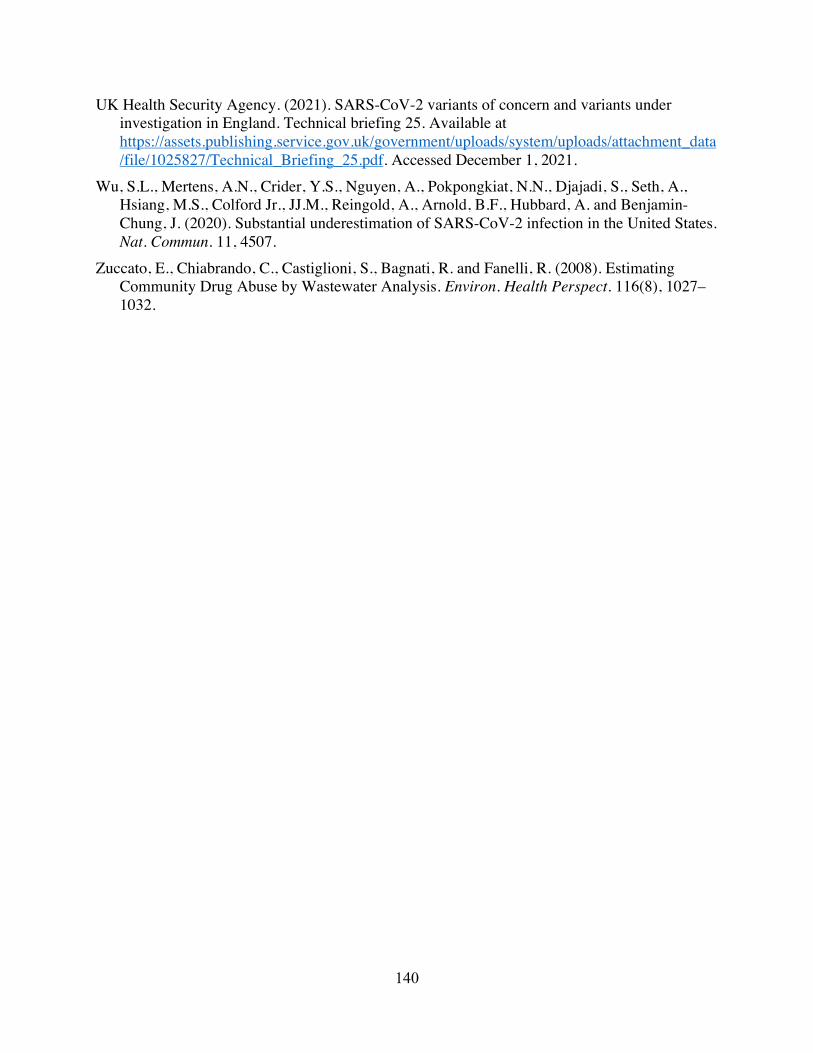
140

UK Health Security Agency. (2021). SARS-CoV-2 variants of concern and variants under investigation in England. Technical briefing 25. Available at https://assets.publishing.service.gov.uk/government/uploads/system/uploads/attachment_data/file/1025827/Technical_Briefing_25.pdf. Accessed December 1, 2021.

Wu, S.L., Mertens, A.N., Crider, Y.S., Nguyen, A., Pokpongkiat, N.N., Djajadi, S., Seth, A., Hsiang, M.S., Colford Jr., JJ.M., Reingold, A., Arnold, B.F., Hubbard, A. and Benjamin-Chung, J. (2020). Substantial underestimation of SARS-CoV-2 infection in the United States. Nat. Commun. 11, 4507.

Zuccato, E., Chiabrando, C., Castiglioni, S., Bagnati, R. and Fanelli, R. (2008). Estimating Community Drug Abuse by Wastewater Analysis. Environ. Health Perspect. 116(8), 1027–1032.

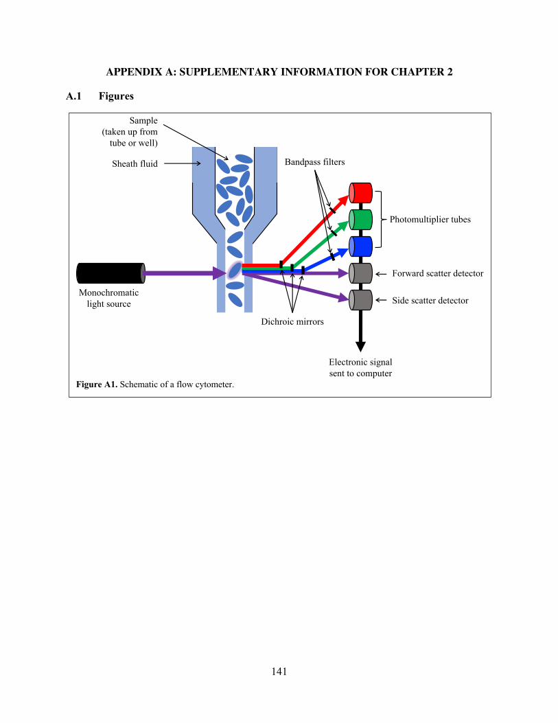
141

APPENDIX A: SUPPLEMENTARY INFORMATION FOR CHAPTER 2

A.1 Figures

Figure A1. Schematic of a flow cytometer.

Photomultiplier tubes

Forward scatter detector

Side scatter detectorMonochromatic

light source

Sheath fluid

Sample(taken up from

tube or well)

Dichroic mirrors

Bandpass filters

Electronic signal sent to computer

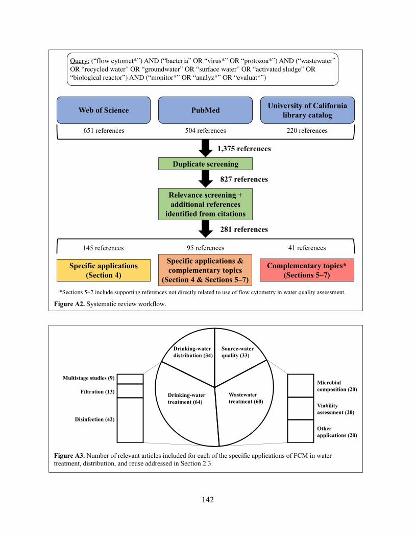
142

Figure A2. Systematic review workflow.

Web of Science PubMed University of California library catalog

Query: (“flow cytomet*”) AND (“bacteria” OR “virus*” OR “protozoa*”) AND (“wastewater” OR “recycled water” OR “groundwater” OR “surface water” OR “activated sludge” OR “biological reactor”) AND (“monitor*” OR “analyz*” OR “evaluat*”)

651 references 504 references 220 references

Duplicate screening

1,375 references

827 references

Relevance screening + additional references

identified from citations

281 references

Specific applications & complementary topics

(Section 4 & Sections 5–7)

Complementary topics*(Sections 5–7)

Specific applications(Section 4)

145 references 95 references 41 references

*Sections 5–7 include supporting references not directly related to use of flow cytometry in water quality assessment.

Figure A3. Number of relevant articles included for each of the specific applications of FCM in water treatment, distribution, and reuse addressed in Section 2.3.

Source-water quality (33)

Wastewatertreatment (60)

Drinking-water treatment (64)

Drinking-water distribution (34)

Disinfection (42)

Filtration (13)

Multistage studies (9)

Other applications (20)

Viability assessment (20)

Microbial composition (20)

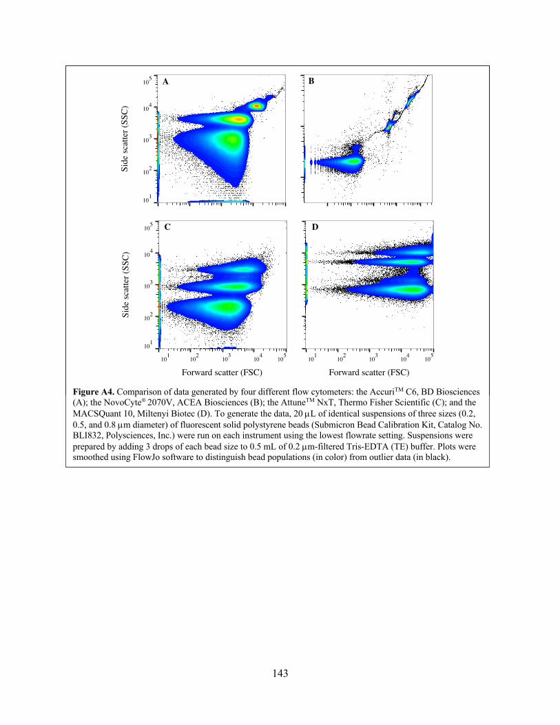
143

Figure 2.4. Illustration of the high dimensionality of data generated by flow cytometry. For an instrument equipped with two lasers, a forward scatter detector, a side scatter detector, and three fluorescence detectors, data is captured in a total of ten dimensions.

Fluorescence detectors

Forward scatter detector

Side scatter detectorLaser 1

Fluorescence detectors

Forward scatter detector

Side scatter detectorLaser 2

Particle trajectory

Figure A4. Comparison of data generated by four different flow cytometers: the AccuriTM C6, BD Biosciences (A); the NovoCyte® 2070V, ACEA Biosciences (B); the AttuneTM NxT, Thermo Fisher Scientific (C); and the MACSQuant 10, Miltenyi Biotec (D). To generate the data, 20 µL of identical suspensions of three sizes (0.2, 0.5, and 0.8 µm diameter) of fluorescent solid polystyrene beads (Submicron Bead Calibration Kit, Catalog No. BLI832, Polysciences, Inc.) were run on each instrument using the lowest flowrate setting. Suspensions were prepared by adding 3 drops of each bead size to 0.5 mL of 0.2 µm-filtered Tris-EDTA (TE) buffer. Plots were smoothed using FlowJo software to distinguish bead populations (in color) from outlier data (in black).

101

102

103

104

105

Forward scatter (FSC)10

110

210

310

410

5

Forward scatter (FSC)

101

102

103

104

105

Side

scat

ter (

SSC

)

101

102

103

104

105

Side

scat

ter (

SSC

)

A

C D

B

A.2 Tables

Table A1. Summary of water-quality indicators commonly combined with FCM analysis. Method/indicator Description Advantages Disadvantages

Heterotrophic plate count (HPC)

Culture-based measurement of the heterotrophic microorganism population in a water sample.

• Widely employed, so provides a common basis of comparison to many studies.

• Confirms the presence of viable bacteria.

• Takes multiple days to deliver results. • High variability. • Limited detection capacity—only about

1% of bacteria in drinking water are detectable through HPC.

Epifluorescence microscopy (EFM)

Illumination of a sample from above with fluorescent light, enabling visual inspection of particle characteristics that cannot be detected through traditional optical microscopy.

• Useful validation tool, since good agreement has been reported between EFM- and FCM-based TCC and ICC results.

• Provides additional information about factors such as cellular morphology, cellular damage, and staining efficacy that can aid interpretation of FCM data.

• Time-consuming and labor-intensive. • Highly subject to human error.

Molecular techniques

Techniques such as PCR, DNA sequencing, and gel electrophoresis.

• Can identify specific microbial strains present in a sample. Particularly valuable when a strain cannot be specifically stained by a fluorescent antibody or other marker.

• Provides deeper insight into the differential impacts of water-treatment processes on various microbial classes (e.g., PAOs and GAOs).

• Does not distinguish between viable and non-viable microorganisms.

• Limited potential for online analysis.

Adenosine tri-phosphate (ATP)

Measurement of ATP—the “energy currency” of a cell—through extraction and reaction with a bioluminescent complex.

• Offers a fast, simple, and cost-effective indication of the overall level of viable microbes in a sample.

• Does not provide viability information at the single-cell level.

• Measurements can be confounded by the presence of free ATP and other interfering compounds.

Assimilable organic carbon (AOC)

Assay that provides an indication of biological stability (i.e., the inability of water to support microbial growth).

• Highly relevant to drinking water treatment. • Conventional assay is time-consuming. • Using pure cultures of test organisms in

may be an imperfect proxy for real-world conditions. Using mixed cultures may yield more realistic but less consistent results.

144

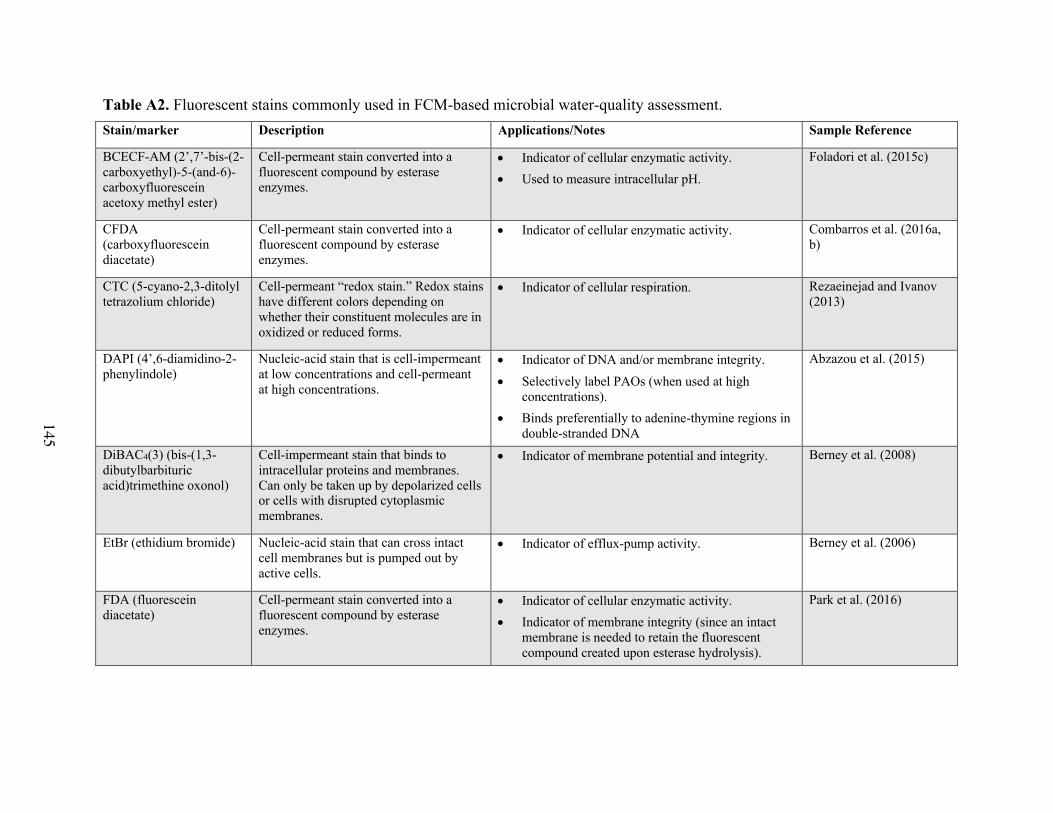
Table A2. Fluorescent stains commonly used in FCM-based microbial water-quality assessment. Stain/marker Description Applications/Notes Sample Reference

BCECF-AM (2’,7’-bis-(2-carboxyethyl)-5-(and-6)-carboxyfluorescein acetoxy methyl ester)

Cell-permeant stain converted into a fluorescent compound by esterase enzymes.

• Indicator of cellular enzymatic activity. • Used to measure intracellular pH.

Foladori et al. (2015c)

CFDA (carboxyfluorescein diacetate)

Cell-permeant stain converted into a fluorescent compound by esterase enzymes.

• Indicator of cellular enzymatic activity. Combarros et al. (2016a, b)

CTC (5-cyano-2,3-ditolyl tetrazolium chloride)

Cell-permeant “redox stain.” Redox stains have different colors depending on whether their constituent molecules are in oxidized or reduced forms.

• Indicator of cellular respiration. Rezaeinejad and Ivanov (2013)

DAPI (4’,6-diamidino-2-phenylindole)

Nucleic-acid stain that is cell-impermeant at low concentrations and cell-permeant at high concentrations.

• Indicator of DNA and/or membrane integrity. • Selectively label PAOs (when used at high

concentrations). • Binds preferentially to adenine-thymine regions in

double-stranded DNA

Abzazou et al. (2015)

DiBAC4(3) (bis-(1,3-dibutylbarbituric acid)trimethine oxonol)

Cell-impermeant stain that binds to intracellular proteins and membranes. Can only be taken up by depolarized cells or cells with disrupted cytoplasmic membranes.

• Indicator of membrane potential and integrity. Berney et al. (2008)

EtBr (ethidium bromide) Nucleic-acid stain that can cross intact cell membranes but is pumped out by active cells.

• Indicator of efflux-pump activity. Berney et al. (2006)

FDA (fluorescein diacetate)

Cell-permeant stain converted into a fluorescent compound by esterase enzymes.

• Indicator of cellular enzymatic activity. • Indicator of membrane integrity (since an intact

membrane is needed to retain the fluorescent compound created upon esterase hydrolysis).

Park et al. (2016)

145

Fluorescent probes Antibodies and other biomolecules that can be conjugated to fluorochromes for specific detection of targets.

• In some cases, the biomolecule is not directly fluorochrome-labeled but is instead detected by a secondary fluorochrome-labeled biomolecule.

• FITC (fluorescein isothiocyanate) is one of the most commonly conjugated fluorochromes.

Keserue et al. (2012a,b)

PI (propidium iodide) Cell-impermeant nucleic-acid stain. • Indicator of membrane integrity. • Commonly coupled with a SYBR or SYTO stain.

Kahlisch et al. (2012)

PicoGreen Cell-impermeant nucleic-acid stain. • Binds preferentially to double-stranded DNA. • Similar to SYBR Green I, but relatively more

sensitive to interference from organic compounds and relatively less sensitive to interference from cations (Martens-Habbena and Sass 2006).

Yu et al. (2015)

SYBR stain family Ultrasensitive, cell-permeant nucleic-acid stains. Includes SYBR Gold, Green I, and Green II.

• SYBR Gold is the most sensitive stain in this family. Binds to all nucleic acids and exhibits a >1000-fold fluorescence enhancement upon doing so.

• SYBR Green I binds preferentially to double-stranded DNA and exhibits a large fluorescence enhancement upon doing so.

• SYBR Green II binds preferentially to RNA and single-stranded DNA and exhibits a large fluorescence enhancement upon doing so.

Huang et al. (2016)

SYTO stain family Cell-permeant nucleic-acid stains available as blue-, green-, orange, or red-fluorescent stains.

• Different SYTO stains exhibit different cell permeability, fluorescence enhancement upon binding, excitation and emission spectra, DNA/RNA selectivity, binding affinity, and other characteristics.

• SYTO 9 is used in FCM analysis of water samples as part of the widely used LIVE/DEAD® BacLightTM Bacterial Viability Kit (ThermoFisher).

Khan et al. (2010)

SYTOX Green Cell-impermeant nucleic-acid stain. • Alternative to PI for viability assays applied to Microcystis, since PI red fluorescence interferes with autofluorescence of photosynthetic pigments that can be used to detect microalgae.

Fan et al. (2016)

146

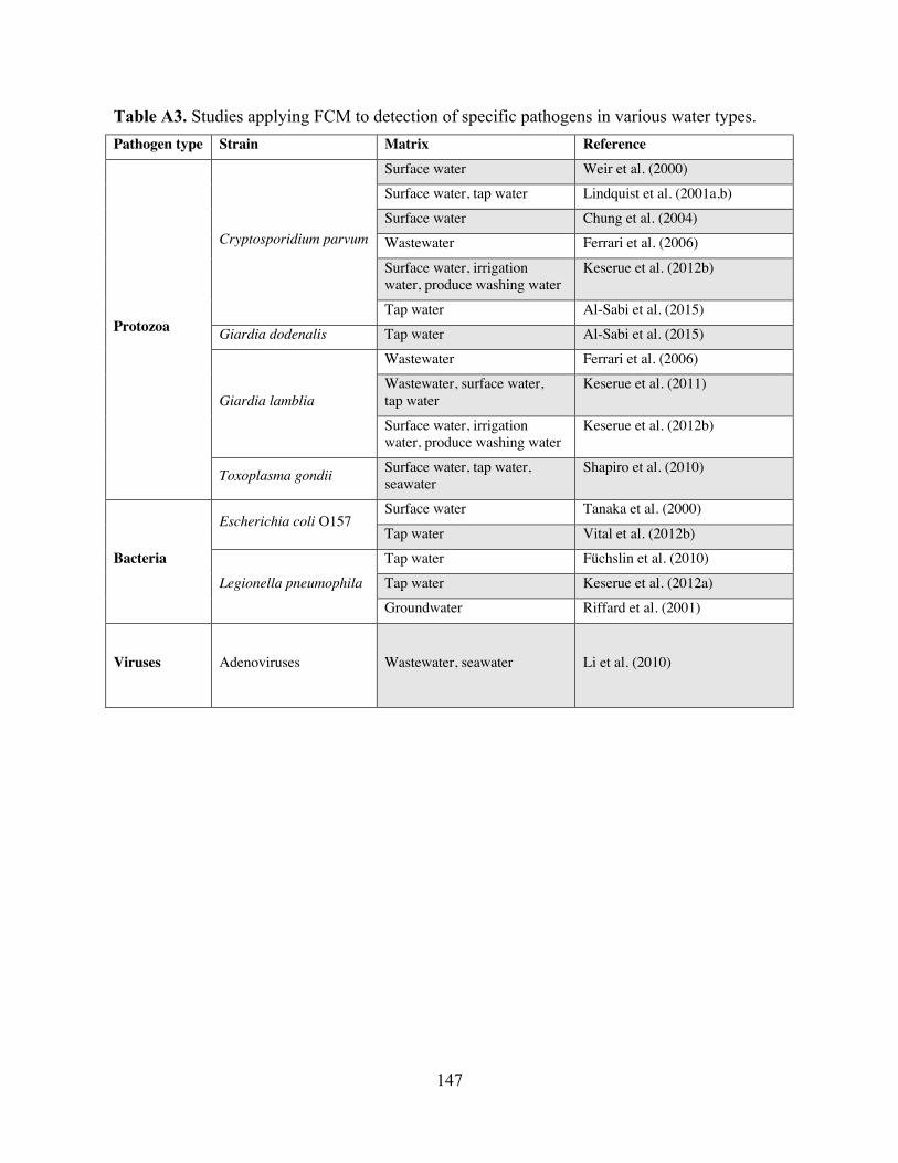
147

Table A3. Studies applying FCM to detection of specific pathogens in various water types. Pathogen type Strain Matrix Reference

Protozoa

Cryptosporidium parvum

Surface water Weir et al. (2000) Surface water, tap water Lindquist et al. (2001a,b) Surface water Chung et al. (2004) Wastewater Ferrari et al. (2006)

Surface water, irrigation water, produce washing water

Keserue et al. (2012b)

Tap water Al-Sabi et al. (2015) Giardia dodenalis Tap water Al-Sabi et al. (2015)

Giardia lamblia

Wastewater Ferrari et al. (2006) Wastewater, surface water, tap water

Keserue et al. (2011)

Surface water, irrigation water, produce washing water

Keserue et al. (2012b)

Toxoplasma gondii Surface water, tap water, seawater

Shapiro et al. (2010)

Bacteria

Escherichia coli O157 Surface water Tanaka et al. (2000)

Tap water Vital et al. (2012b)

Legionella pneumophila

Tap water Füchslin et al. (2010) Tap water Keserue et al. (2012a) Groundwater Riffard et al. (2001)

Viruses Adenoviruses Wastewater, seawater Li et al. (2010)

148

APPENDIX B: SUPPLEMENTARY INFORMATION FOR CHAPTER 3

B.1 Figures

Figure B1. Pseudocolor SSC vs. FITC density plots of results from Round I of the T4 optimization. Red box indicates gates used to obtain target event counts. As described in the “Materials and methods” section, gates were set based on the FITC peak.

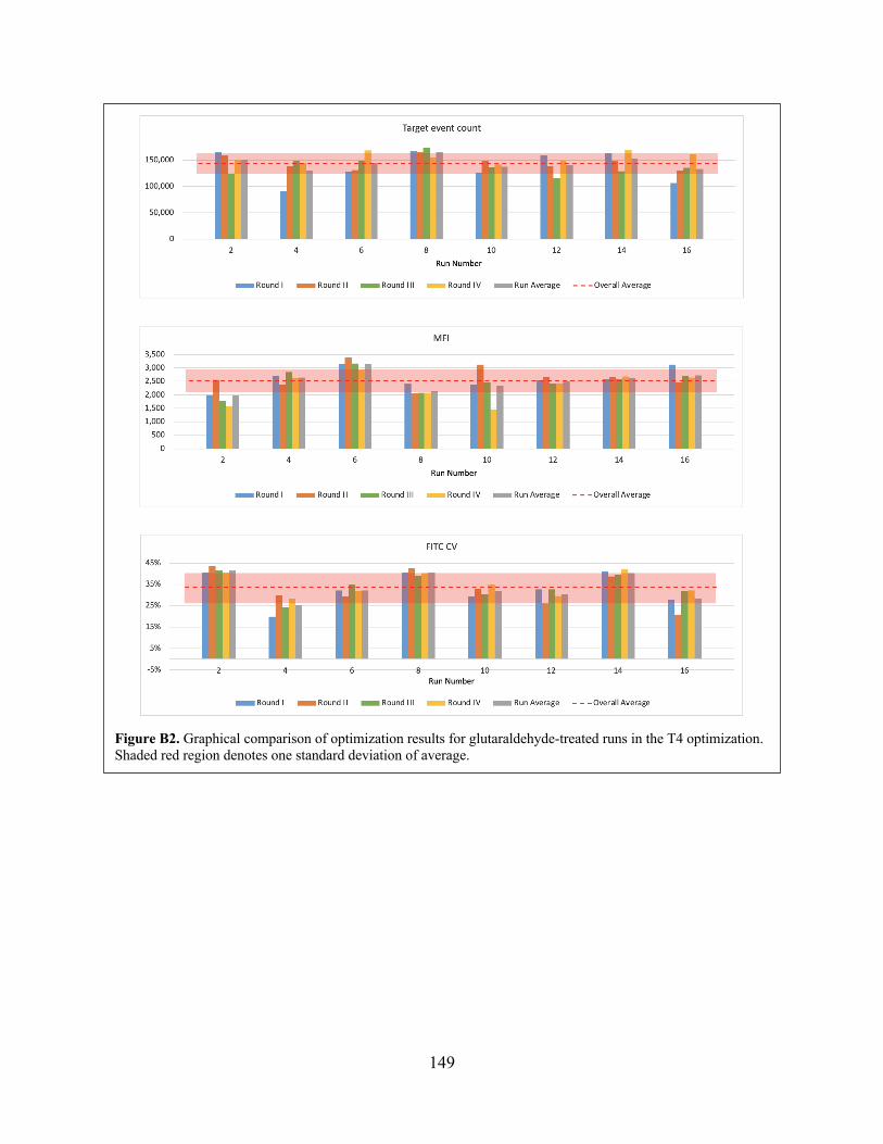
149

Figure B2. Graphical comparison of optimization results for glutaraldehyde-treated runs in the T4 optimization. Shaded red region denotes one standard deviation of average.

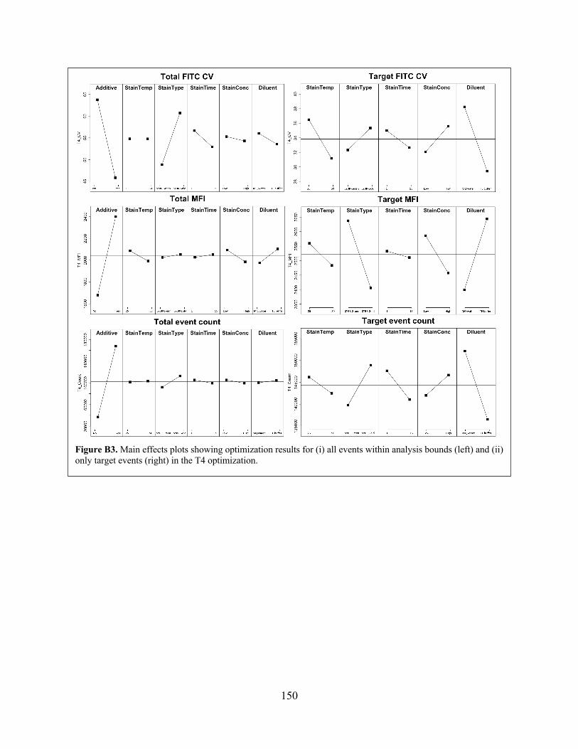
150

Figure B3. Main effects plots showing optimization results for (i) all events within analysis bounds (left) and (ii) only target events (right) in the T4 optimization.

151

Figure B4. Illustration of pitfalls of setting a single global threshold to extract clusters from OPTICS-ordered data. For samples containing clusters of varying densities, setting a single global threshold results in either missed clusters (top plot) and/or noise points incorrectly categorized as clusters (bottom plot).

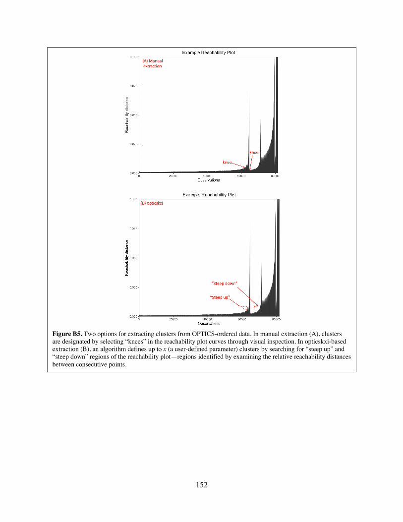
152

Figure B5. Two options for extracting clusters from OPTICS-ordered data. In manual extraction (A), clusters are designated by selecting “knees” in the reachability plot curves through visual inspection. In opticskxi-based extraction (B), an algorithm defines up to x (a user-defined parameter) clusters by searching for “steep up” and “steep down” regions of the reachability plot—regions identified by examining the relative reachability distances between consecutive points.

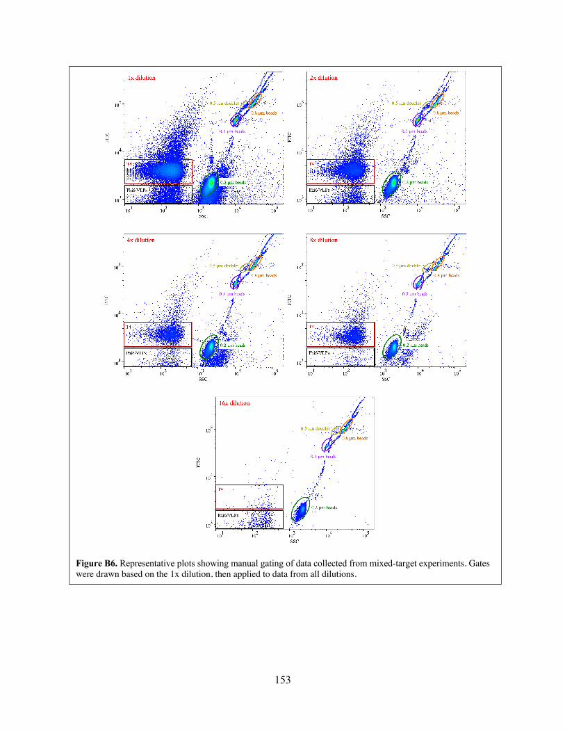
153

Figure B6. Representative plots showing manual gating of data collected from mixed-target experiments. Gates were drawn based on the 1x dilution, then applied to data from all dilutions.

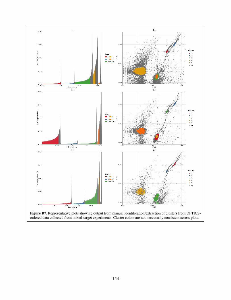
154

Figure B7. Representative plots showing output from manual identification/extraction of clusters from OPTICS-ordered data collected from mixed-target experiments. Cluster colors are not necessarily consistent across plots.

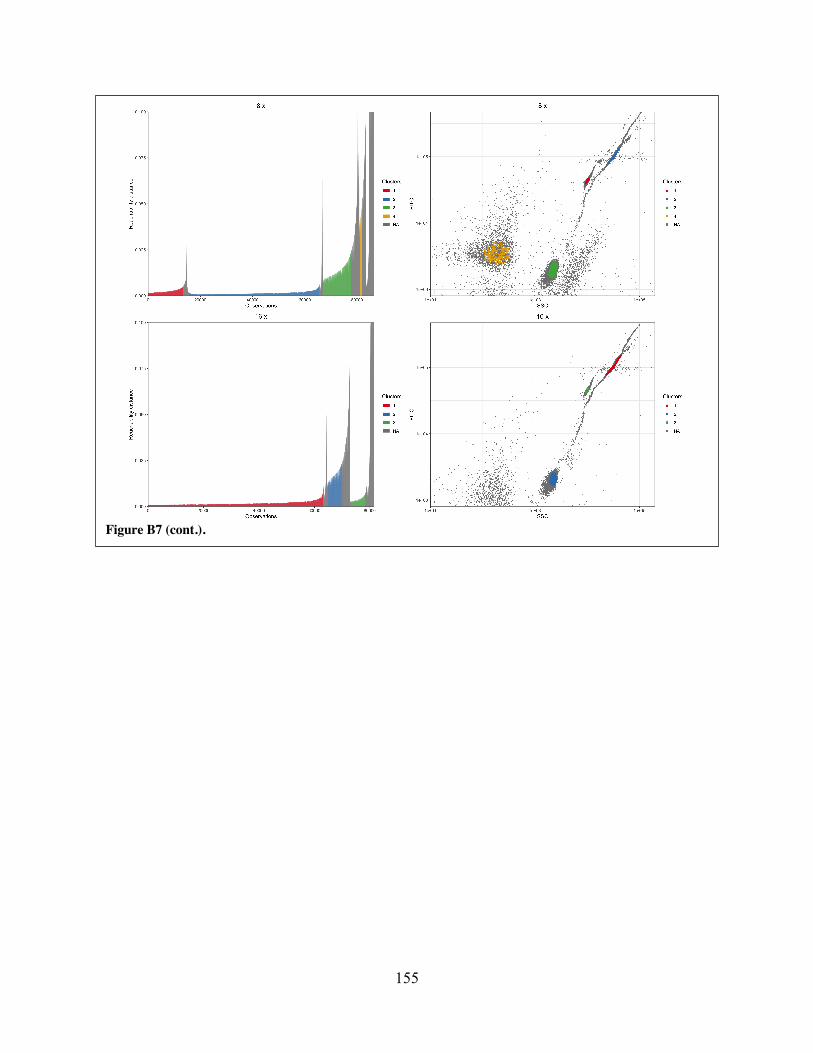
155

Figure B7 (cont.).

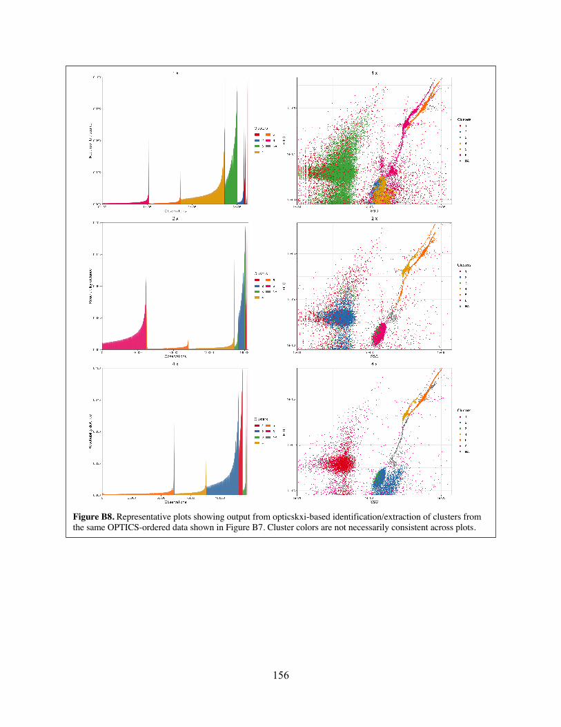
156

Figure B8. Representative plots showing output from opticskxi-based identification/extraction of clusters from the same OPTICS-ordered data shown in Figure B7. Cluster colors are not necessarily consistent across plots.

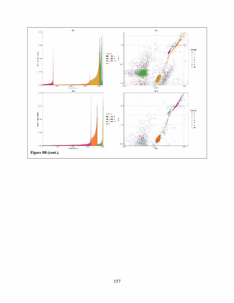
157

Figure B8 (cont.).

158

Figure B9. Event counts vs. dilution for the mixed-target data experiments, by clustering approach and target “bucket”. MG = manual gating; O:ME = OPTICS: Manual extraction; O:kxi = OPTICS: kxi extraction.

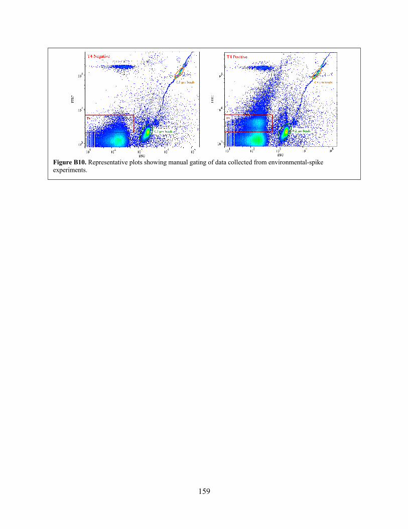
159

Figure B10. Representative plots showing manual gating of data collected from environmental-spike experiments.

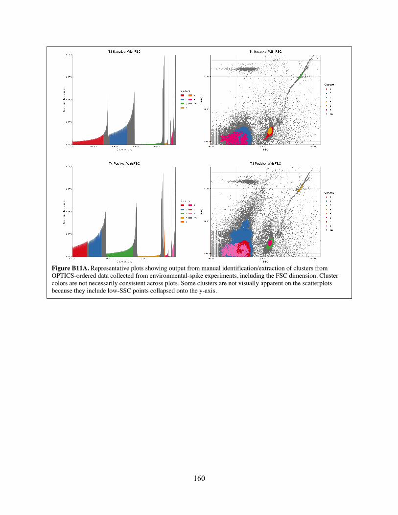
160

Figure B11A. Representative plots showing output from manual identification/extraction of clusters from OPTICS-ordered data collected from environmental-spike experiments, including the FSC dimension. Cluster colors are not necessarily consistent across plots. Some clusters are not visually apparent on the scatterplots because they include low-SSC points collapsed onto the y-axis.

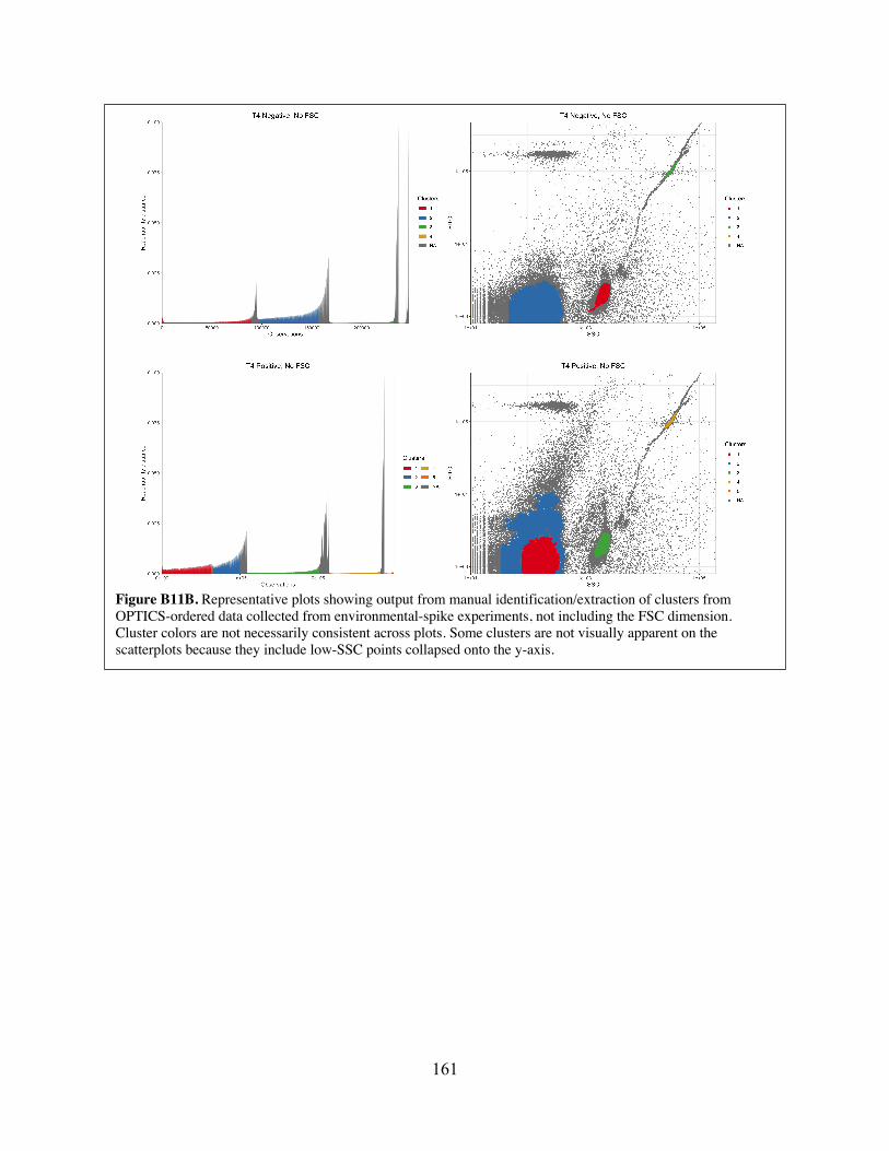
161

Figure B11B. Representative plots showing output from manual identification/extraction of clusters from OPTICS-ordered data collected from environmental-spike experiments, not including the FSC dimension. Cluster colors are not necessarily consistent across plots. Some clusters are not visually apparent on the scatterplots because they include low-SSC points collapsed onto the y-axis.

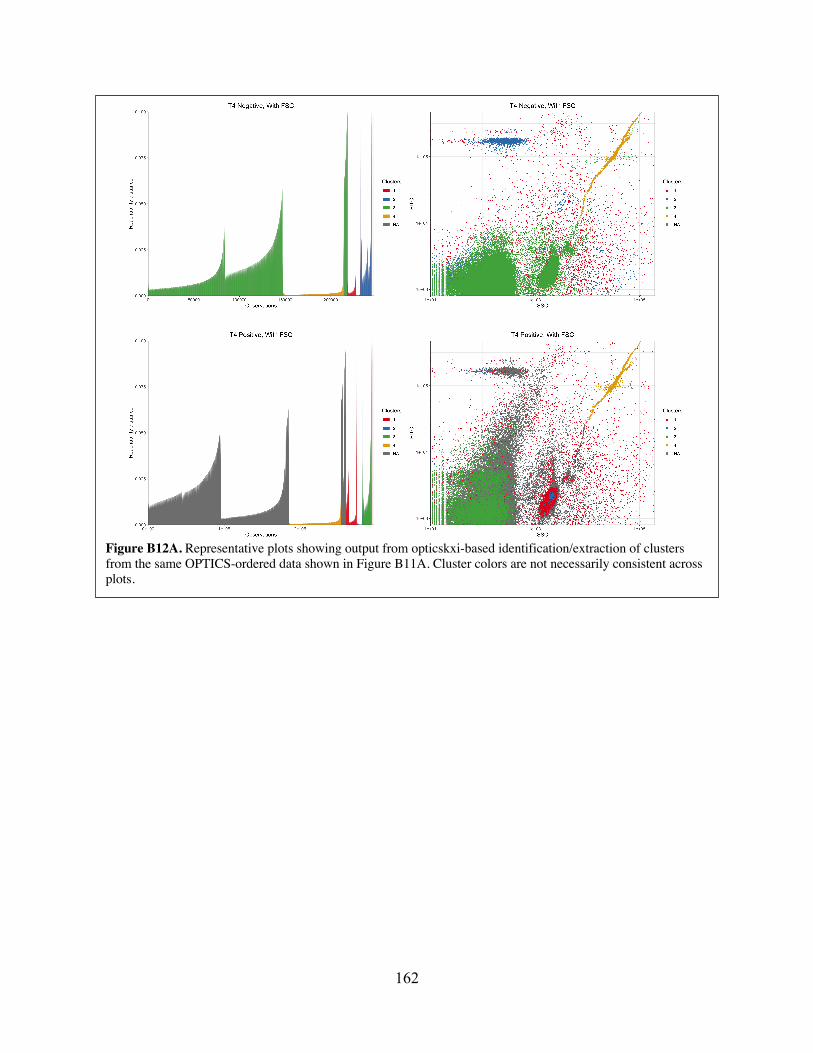
162

Figure B12A. Representative plots showing output from opticskxi-based identification/extraction of clusters from the same OPTICS-ordered data shown in Figure B11A. Cluster colors are not necessarily consistent across plots.

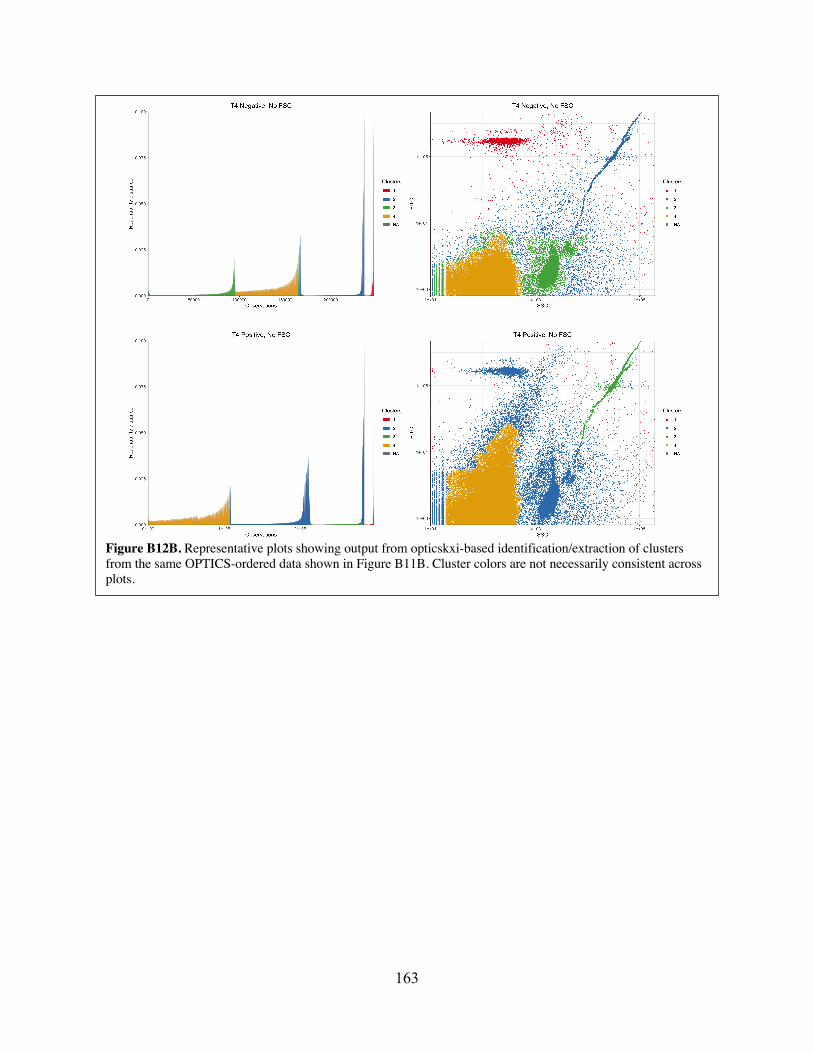
163

Figure B12B. Representative plots showing output from opticskxi-based identification/extraction of clusters from the same OPTICS-ordered data shown in Figure B11B. Cluster colors are not necessarily consistent across plots.

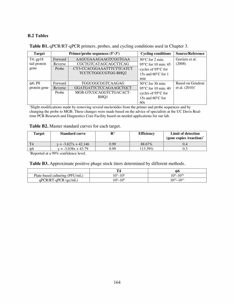
164

B.2 Tables

Table B1. qPCR/RT-qPCR primers, probes, and cycling conditions used in Chapter 3. Target Primer/probe sequences (5’-3’) Cycling conditions Source/Reference

T4; gp18 tail protein gene

Forward AAGCGAAAGAAGTCGGTGAA 50°C for 2 min; 95°C for 10 min; 45 cycles of 95°C for 15s and 60°C for 1 min

Gerriets et al. (2008) Reverse CGCTGTCATAGCAGCTTCAG

Probe CY5-CCACGGAAATTTCTTCATCT TCCTCTGGCCGTGG-BHQ2

φ6; P8 protein gene

Forward TGGCGGCGGTCAAGAG 50°C for 30 min; 95°C for 10 min; 40 cycles of 95°C for 15s and 60°C for 60s

Based on Gendron et al. (2010)* Reverse GGATGATTCTCCAGAAGCTGCT

Probe MGB-GTCGCAGGTCTGACACT-BHQ1

*Slight modifications made by removing several nucleotides from the primer and probe sequences and by changing the probe to MGB. These changes were made based on the advice of specialists at the UC Davis Real-time PCR Research and Diagnostics Core Facility based on needed applications for our lab.

Table B2. Master standard curves for each target.

Target Standard curve R2 Efficiency Limit of detection (gene copies /reaction)*

T4 y = -3.627x + 42.146 0.99 88.67% 0.4 φ6 y = -3.038x + 43.79 0.99 113.39% 0.3 *Reported at a 99% confidence level.

Table B3. Approximate positive phage stock titers determined by different methods.

T4 φ6 Plate-based culturing (PFU/mL) 107–108 109–1010

qPCR/RT-qPCR (gc/mL) 108–109 1010–1011

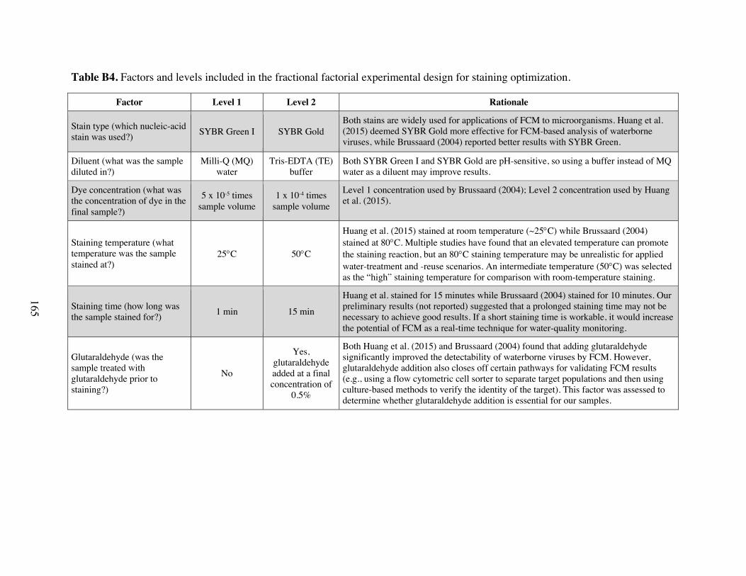
Table B4. Factors and levels included in the fractional factorial experimental design for staining optimization.

Factor Level 1 Level 2 Rationale

Stain type (which nucleic-acid stain was used?) SYBR Green I SYBR Gold

Both stains are widely used for applications of FCM to microorganisms. Huang et al. (2015) deemed SYBR Gold more effective for FCM-based analysis of waterborne viruses, while Brussaard (2004) reported better results with SYBR Green.

Diluent (what was the sample diluted in?)

Milli-Q (MQ) water

Tris-EDTA (TE) buffer

Both SYBR Green I and SYBR Gold are pH-sensitive, so using a buffer instead of MQ water as a diluent may improve results.

Dye concentration (what was the concentration of dye in the final sample?)

5 x 10-5 times sample volume

1 x 10-4 times sample volume

Level 1 concentration used by Brussaard (2004); Level 2 concentration used by Huang et al. (2015).

Staining temperature (what temperature was the sample stained at?)

25°C 50°C

Huang et al. (2015) stained at room temperature (~25°C) while Brussaard (2004) stained at 80°C. Multiple studies have found that an elevated temperature can promote the staining reaction, but an 80°C staining temperature may be unrealistic for applied water-treatment and -reuse scenarios. An intermediate temperature (50°C) was selected as the “high” staining temperature for comparison with room-temperature staining.

Staining time (how long was the sample stained for?) 1 min 15 min

Huang et al. stained for 15 minutes while Brussaard (2004) stained for 10 minutes. Our preliminary results (not reported) suggested that a prolonged staining time may not be necessary to achieve good results. If a short staining time is workable, it would increase the potential of FCM as a real-time technique for water-quality monitoring.

Glutaraldehyde (was the sample treated with glutaraldehyde prior to staining?)

No

Yes, glutaraldehyde added at a final concentration of

0.5%

Both Huang et al. (2015) and Brussaard (2004) found that adding glutaraldehyde significantly improved the detectability of waterborne viruses by FCM. However, glutaraldehyde addition also closes off certain pathways for validating FCM results (e.g., using a flow cytometric cell sorter to separate target populations and then using culture-based methods to verify the identity of the target). This factor was assessed to determine whether glutaraldehyde addition is essential for our samples.

165

Table B5. Experiments included in fractional factorial design for staining optimization. Factor levels are detailed in Tables B4.

Aliases A B C D E F Factors Glutaraldehyde Staining temperature Stain type Staining time Stain concentration Diluent

Run order Factor levels 1 1 1 1 1 1 1 2 2 1 1 1 2 1 3 1 2 1 1 2 2 4 2 2 1 1 1 2 5 1 1 2 1 2 2 6 2 1 2 1 1 2 7 1 2 2 1 1 1 8 2 2 2 1 2 1 9 1 1 1 2 1 2 10 2 1 1 2 2 2 11 1 2 1 2 2 1 12 2 2 1 2 1 1 13 1 1 2 2 2 1 14 2 1 2 2 1 1 15 1 2 2 2 1 2 16 2 2 2 2 2 2

166

167

Table B6. Confounding structures and different main and two-way effects present for the T4 optimization fractional factorial experimental design. Estimation

factor Confounding structure Main and two-way effects present

I1 A + ABCE + ABCDF + DEF Glutaraldehyde I2 B + ACE + CDF + ABDEF Staining temperature I3 C + ABE + BDF + ACDEF Stain type I4 D + ABCDE + BCF + AEF Staining time I5 E + ABC + BCDEF + ADF Stain concentration I6 F + ABCEF + BCD + ADE Diluent I7 AB + CE + ACDF + BDEF Glutaraldehyde/Staining temperature

Stain type/Stain concentration I8 AC + BE + ABDF + CDEF Glutaraldehyde/Stain type

Staining temperature/Stain concentration I9 AD + BCDE + ABCF + EF Glutaraldehyde/Stain time

Stain concentration/Diluent I10 AE + BC + ABCDEF + DF Glutaraldehyde/Stain concentration

Staining temperature/Stain type Staining time/Diluent

I11 AF + BCEF + ABCD + DE Glutaraldehyde/Diluent Staining time/Stain concentration

I12 BD + ACDE + CF + ABEF Staining temperature/Staining time Stain type/Diluent

I13 BF + ACEF + CD + ABDE Staining temperature/Diluent Stain type/Staining time

I14 ABD + CDE + ACF + BEF N/A I15 ACD + BDE + ABF + CEF N/A I16 I + ABCE + BCDF + ADEF N/A

168

Table B7. Main and two-way effects estimation from optimization experiments. Factor All runs Glutaraldehyde-treated runs

Effect on total event count (p-value)

Effect on MFI

(p-value)

Effect on FITC CV (p-value)

Effect on target event count (p-value)

Effect on MFI

(p-value)

Effect on FITC CV (p-value)

Glutaraldehyde 65,402 (0.000)***

360 (0.000)***

-9.0 (0.000)***

— — —

Staining temperature

868 (0.696)

-47 (0.058)†

0.0 (0.988)

-1,860 (0.570)

-38 (0.635)

-2.7 (0.000)***

Stain type 10,330 (0.000)***

14 (0.568)

5.9 (0.000)***

4,576 (0.169)

-116 (0.156)

1.5 (0.011)*

Staining time -3,040 (0.175)

13 (0.597)

-1.9 (0.005)**

-3,286 (0.319)

-11 (0.890)

-1.2 (0.044)*

Stain concentration

-3,052 (0.173)

-54 (0.029)*

-0.5 (0.441)

2,325 (0.478)

-64 (0.424)

1.8 (0.004)**

Diluent 1,999 (0.370)

64 (0.010)*

-1.2 (0.059)**

-7,807 (0.023)*

122 (0.135)

-4.4 (0.000)***

Glutaraldehyde/ Staining

temperature

-5,290 (0.020)*

62 (0.013)*

-2.3 (0.001)***

— — —

Glutaraldehyde/ Stain type

-1,924 (0.388)

28 (0.258)*

-2.6 (0.000)***

— — —

Glutaraldehyde/ Stain time

-320 (0.885)

51 (0.039)*

0.3 (0.632)

— — —

Glutaraldehyde/ Stain

concentration

624 (0.778)

-84 (0.001)***

0.5 (0.447)

— — —

Glutaraldehyde/ Diluent

-3,895 (0.084)

113 (0.000)***

-0.8 (0.205)

— — —

Staining temperature/ Staining time

-428 (0.847)

2 (0.938)

-0.3 (0.639)

-2,309 (0.481)

-56 (0.485)

-0.8 (0.173)

Staining temperature/

Diluent

-181 (0.935)

3 (0.886)

-0.4 (0.555)

-2,734 (0.405)

85 (0.293)

0.1 (0.888)

Significance levels: † = 0.05–0.1; * = 0.01–0.05; ** = 0.001–0.01; *** = 0–0.001

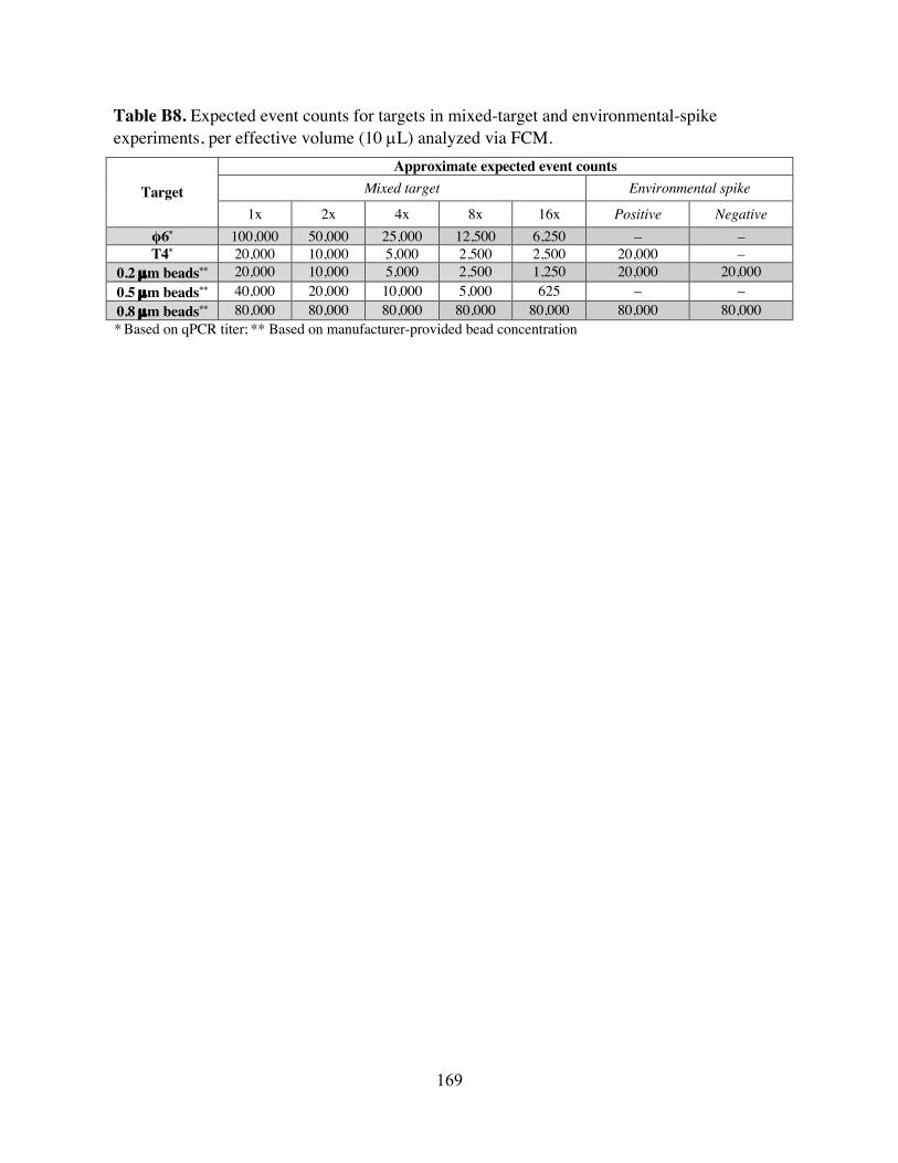
169

Table B8. Expected event counts for targets in mixed-target and environmental-spike experiments, per effective volume (10 µL) analyzed via FCM.

Target

Approximate expected event counts Mixed target Environmental spike

1x 2x 4x 8x 16x Positive Negative φ6* 100,000 50,000 25,000 12,500 6,250 – – T4* 20,000 10,000 5,000 2,500 2,500 20,000 –

0.2 µm beads** 20,000 10,000 5,000 2,500 1,250 20,000 20,000 0.5 µm beads** 40,000 20,000 10,000 5,000 625 – – 0.8 µm beads** 80,000 80,000 80,000 80,000 80,000 80,000 80,000 * Based on qPCR titer; ** Based on manufacturer-provided bead concentration

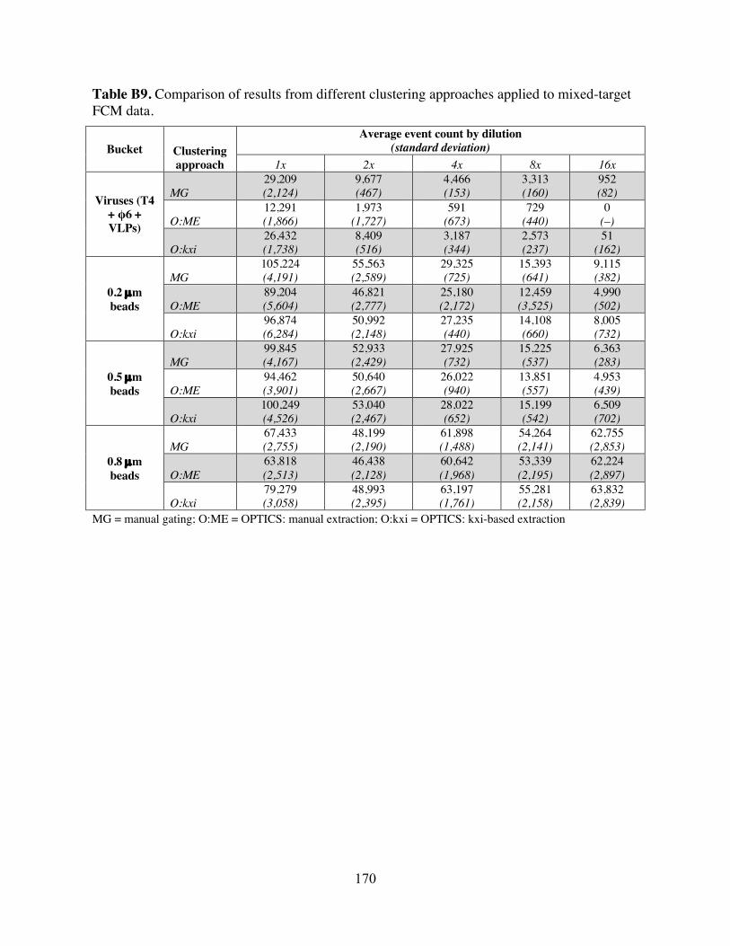
170

Table B9. Comparison of results from different clustering approaches applied to mixed-target FCM data.

Bucket Clustering approach

Average event count by dilution (standard deviation)

1x 2x 4x 8x 16x

Viruses (T4 + φ6 + VLPs)

MG 29,209 (2,124)

9,677 (467)

4,466 (153)

3,313 (160)

952 (82)

O:ME 12,291 (1,866)

1,973 (1,727)

591 (673)

729 (440)

0 (–)

O:kxi 26,432 (1,738)

8,409 (516)

3,187 (344)

2,573 (237)

51 (162)

0.2 µm beads

MG 105,224 (4,191)

55,563 (2,589)

29,325 (725)

15,393 (641)

9,115 (382)

O:ME 89,204 (5,604)

46,821 (2,777)

25,180 (2,172)

12,459 (3,525)

4,990 (502)

O:kxi 96,874 (6,284)

50,992 (2,148)

27,235 (440)

14,108 (660)

8,005 (732)

0.5 µm beads

MG 99,845 (4,167)

52,933 (2,429)

27,925 (732)

15,225 (537)

6,363 (283)

O:ME 94,462 (3,901)

50,640 (2,667)

26,022 (940)

13,851 (557)

4,953 (439)

O:kxi 100,249 (4,526)

53,040 (2,467)

28,022 (652)

15,199 (542)

6,509 (702)

0.8 µm beads

MG 67,433 (2,755)

48,199 (2,190)

61,898 (1,488)

54,264 (2,141)

62,755 (2,853)

O:ME 63,818 (2,513)

46,438 (2,128)

60,642 (1,968)

53,339 (2,195)

62,224 (2,897)

O:kxi 79,279 (3,058)

48,993 (2,395)

63,197 (1,761)

55,281 (2,158)

63,832 (2,839)

MG = manual gating; O:ME = OPTICS: manual extraction; O:kxi = OPTICS: kxi-based extraction

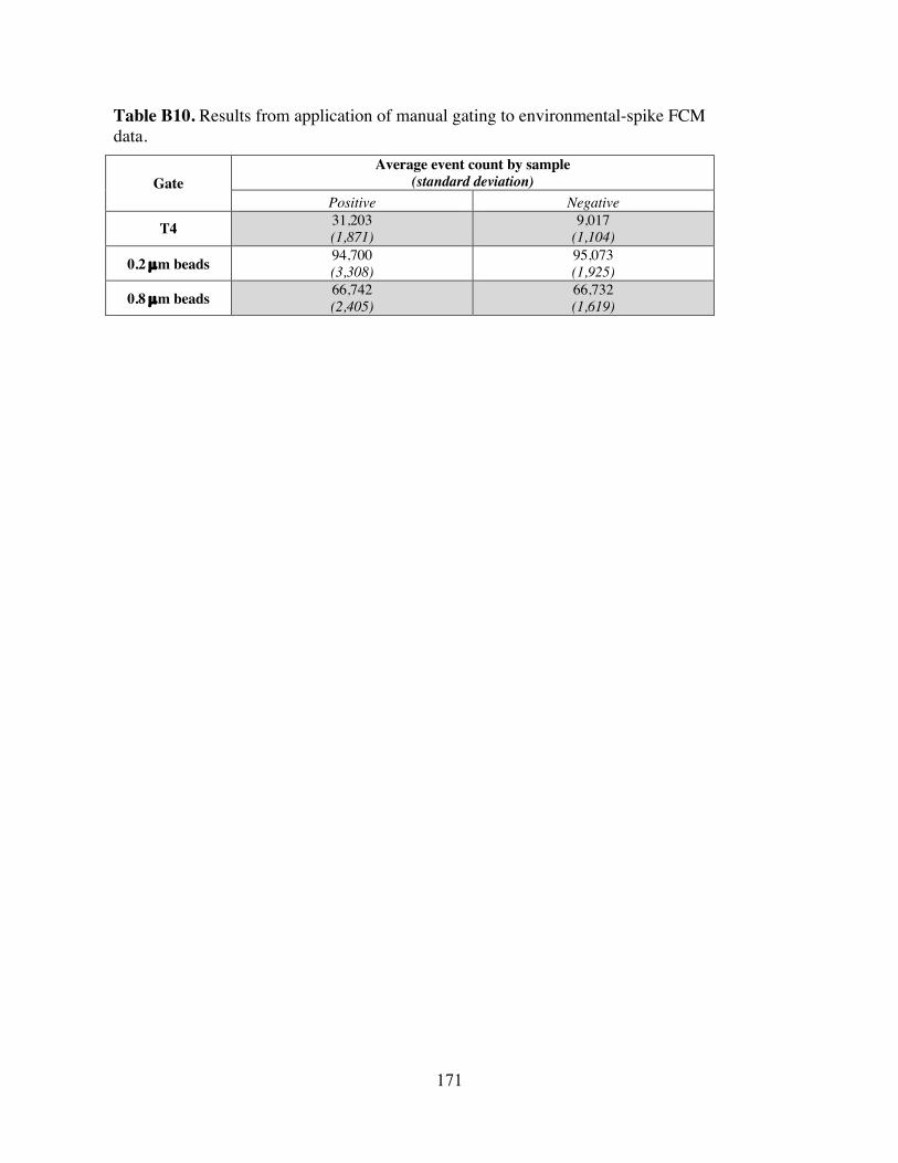
171

Table B10. Results from application of manual gating to environmental-spike FCM data.

Gate Average event count by sample

(standard deviation) Positive Negative

T4 31,203 (1,871)

9,017 (1,104)

0.2 µm beads 94,700 (3,308)

95,073 (1,925)

0.8 µm beads 66,742 (2,405)

66,732 (1,619)

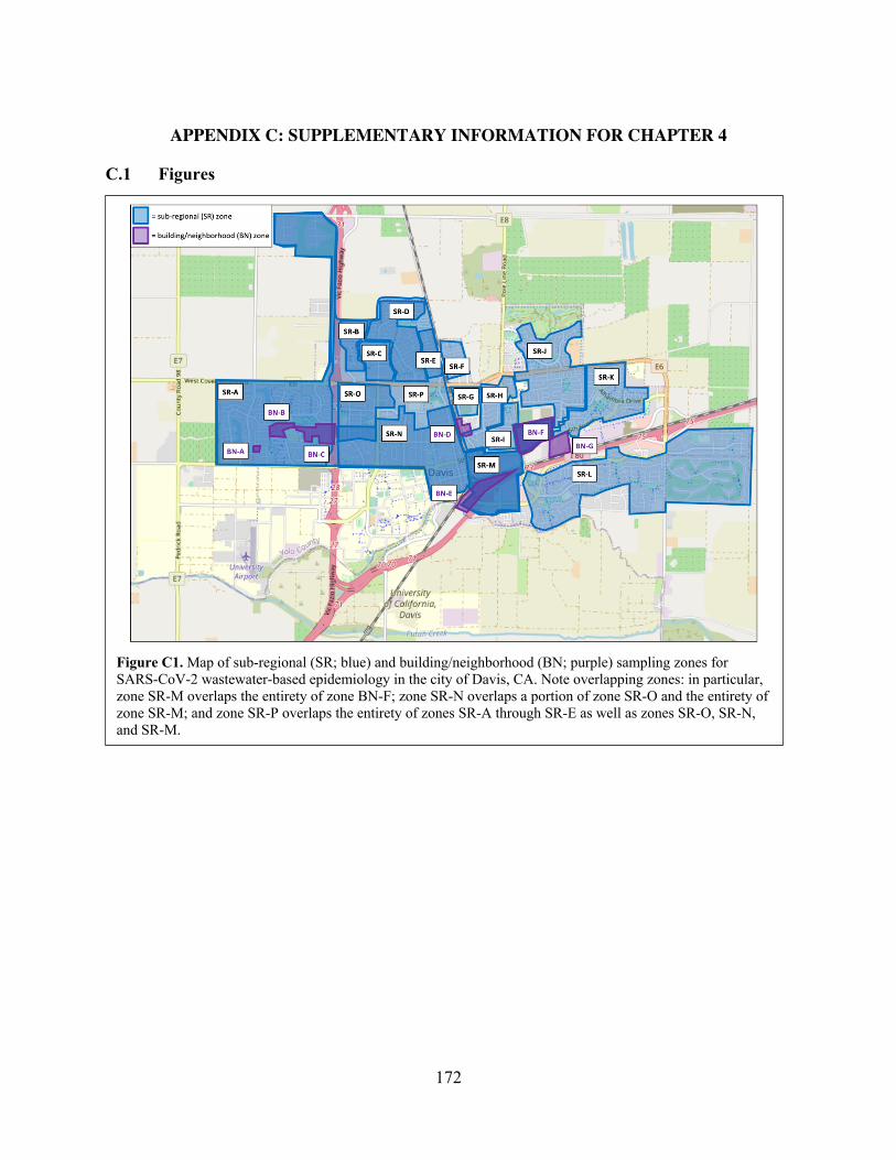
172

APPENDIX C: SUPPLEMENTARY INFORMATION FOR CHAPTER 4

C.1 Figures

Figure C1. Map of sub-regional (SR; blue) and building/neighborhood (BN; purple) sampling zones for

SARS-CoV-2 wastewater-based epidemiology in the city of Davis, CA. Note overlapping zones: in particular,

zone SR-M overlaps the entirety of zone BN-F; zone SR-N overlaps a portion of zone SR-O and the entirety of

zone SR-M; and zone SR-P overlaps the entirety of zones SR-A through SR-E as well as zones SR-O, SR-N,

and SR-M.

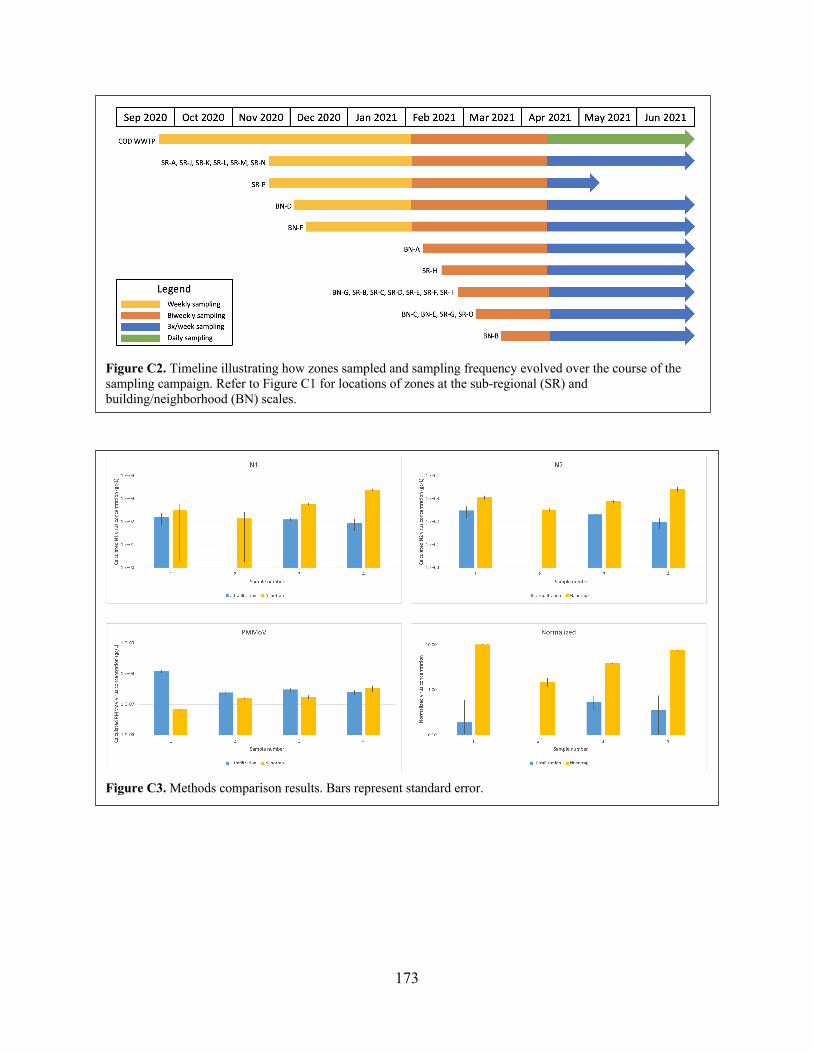
173

Figure C2. Timeline illustrating how zones sampled and sampling frequency evolved over the course of the

sampling campaign. Refer to Figure C1 for locations of zones at the sub-regional (SR) and

building/neighborhood (BN) scales.

Figure C3. Methods comparison results. Bars represent standard error.

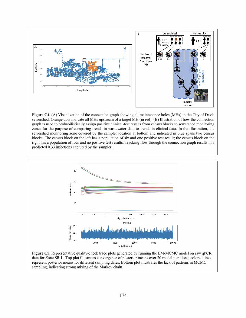
174

Figure C5. Representative quality-check trace plots generated by running the EM-MCMC model on raw qPCR

data for Zone SR-L. Top plot illustrates convergence of posterior means over 20 model iterations; colored lines

represent posterior means for different sampling dates. Bottom plot illustrates the lack of patterns in MCMC

sampling, indicating strong mixing of the Markov chain.

Figure C4. (A) Visualization of the connection graph showing all maintenance holes (MHs) in the City of Davis

sewershed. Orange dots indicate all MHs upstream of a target MH (in red). (B) Illustration of how the connection

graph is used to probabilistically assign positive clinical-test results from census blocks to sewershed monitoring

zones for the purpose of comparing trends in wastewater data to trends in clinical data. In the illustration, the

sewershed monitoring zone covered by the sampler location at bottom and indicated in blue spans two census

blocks. The census block on the left has a population of six and one positive test result; the census block on the

right has a population of four and no positive test results. Tracking flow through the connection graph results in a

predicted 0.33 infections captured by the sampler.

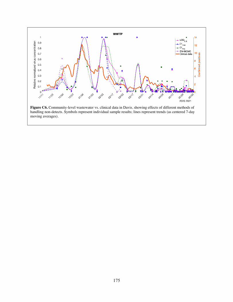
175

Figure C6. Community-level wastewater vs. clinical data in Davis, showing effects of different methods of handling non-detects. Symbols represent individual sample results; lines represent trends (as centered 7-day moving averages).

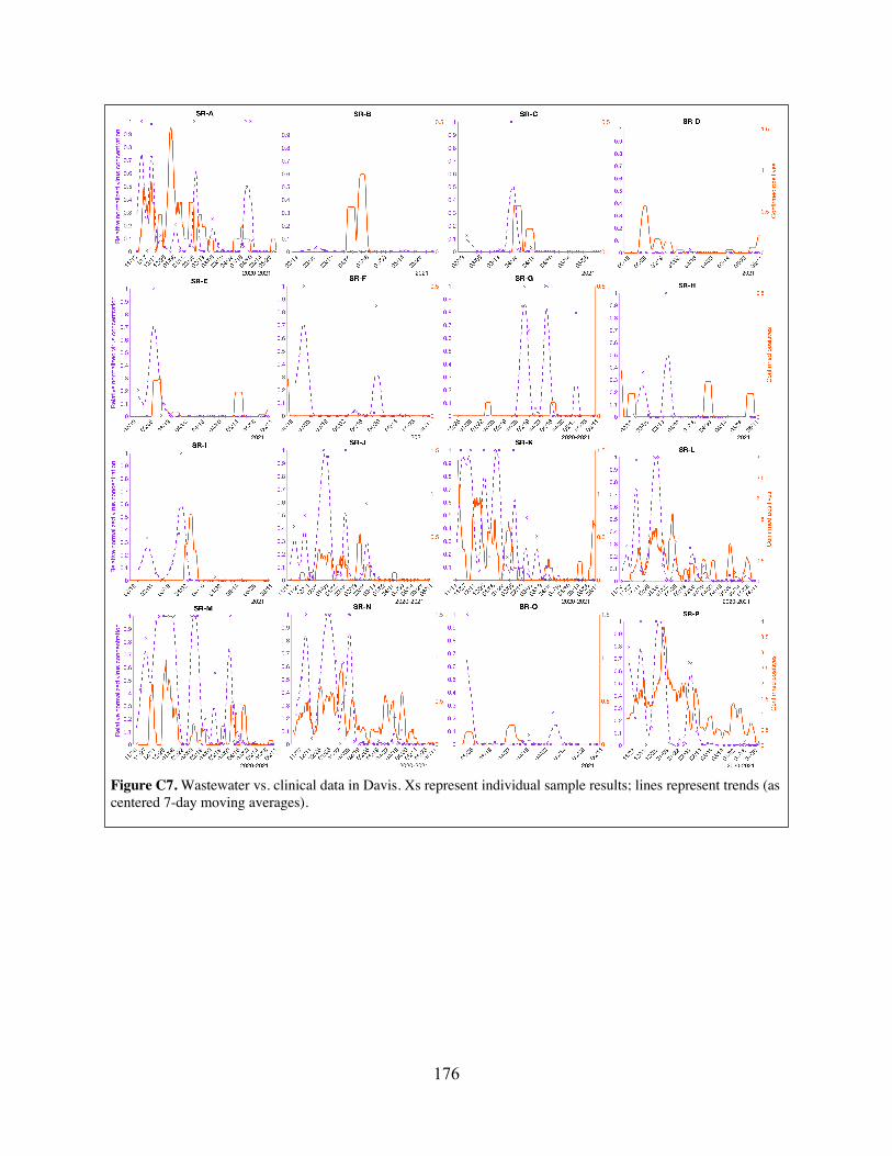
176

Figure C7. Wastewater vs. clinical data in Davis. Xs represent individual sample results; lines represent trends (as centered 7-day moving averages).

177

Figure C7 (continued).

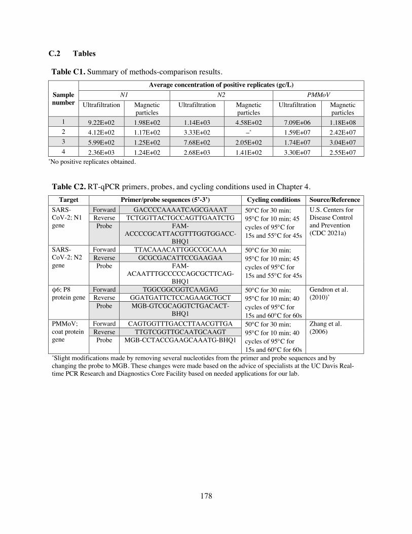
178

C.2 Tables

Table C1. Summary of methods-comparison results.

Sample number

Average concentration of positive replicates (gc/L) N1 N2 PMMoV

Ultrafiltration Magnetic particles

Ultrafiltration Magnetic particles

Ultrafiltration Magnetic particles

1 9.22E+02 1.98E+02 1.14E+03 4.58E+02 7.09E+06 1.18E+08 2 4.12E+02 1.17E+02 3.33E+02 –* 1.59E+07 2.42E+07 3 5.99E+02 1.25E+02 7.68E+02 2.05E+02 1.74E+07 3.04E+07 4 2.36E+03 1.24E+02 2.68E+03 1.41E+02 3.30E+07 2.55E+07

*No positive replicates obtained.

Table C2. RT-qPCR primers, probes, and cycling conditions used in Chapter 4. Target Primer/probe sequences (5’-3’) Cycling conditions Source/Reference

SARS-CoV-2; N1 gene

Forward GACCCCAAAATCAGCGAAAT 50°C for 30 min; 95°C for 10 min; 45 cycles of 95°C for 15s and 55°C for 45s

U.S. Centers for Disease Control and Prevention (CDC 2021a)

Reverse TCTGGTTACTGCCAGTTGAATCTG Probe FAM-

ACCCCGCATTACGTTTGGTGGACC-BHQ1

SARS-CoV-2; N2 gene

Forward TTACAAACATTGGCCGCAAA 50°C for 30 min; 95°C for 10 min; 45 cycles of 95°C for 15s and 55°C for 45s

Reverse GCGCGACATTCCGAAGAA Probe FAM-

ACAATTTGCCCCCAGCGCTTCAG-BHQ1

φ6; P8 protein gene

Forward TGGCGGCGGTCAAGAG 50°C for 30 min; 95°C for 10 min; 40 cycles of 95°C for 15s and 60°C for 60s

Gendron et al. (2010)* Reverse GGATGATTCTCCAGAAGCTGCT

Probe MGB-GTCGCAGGTCTGACACT-BHQ1

PMMoV; coat protein gene

Forward CAGTGGTTTGACCTTAACGTTGA 50°C for 30 min; 95°C for 10 min; 40 cycles of 95°C for 15s and 60°C for 60s

Zhang et al. (2006) Reverse TTGTCGGTTGCAATGCAAGT

Probe MGB-CCTACCGAAGCAAATG-BHQ1

*Slight modifications made by removing several nucleotides from the primer and probe sequences and by changing the probe to MGB. These changes were made based on the advice of specialists at the UC Davis Real-time PCR Research and Diagnostics Core Facility based on needed applications for our lab.

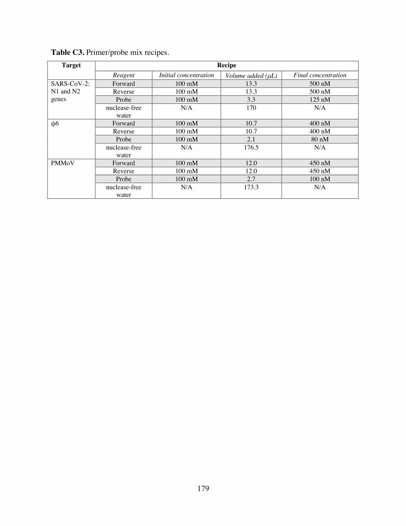
179

Table C3. Primer/probe mix recipes. Target Recipe

Reagent Initial concentration Volume added (µL) Final concentration SARS-CoV-2; N1 and N2 genes

Forward 100 mM 13.3 500 nM Reverse 100 mM 13.3 500 nM Probe 100 mM 3.3 125 nM

nuclease-free water

N/A 170 N/A

φ6 Forward 100 mM 10.7 400 nM Reverse 100 mM 10.7 400 nM Probe 100 mM 2.1 80 nM

nuclease-free water

N/A 176.5 N/A

PMMoV Forward 100 mM 12.0 450 nM Reverse 100 mM 12.0 450 nM Probe 100 mM 2.7 100 nM

nuclease-free water

N/A 173.3 N/A

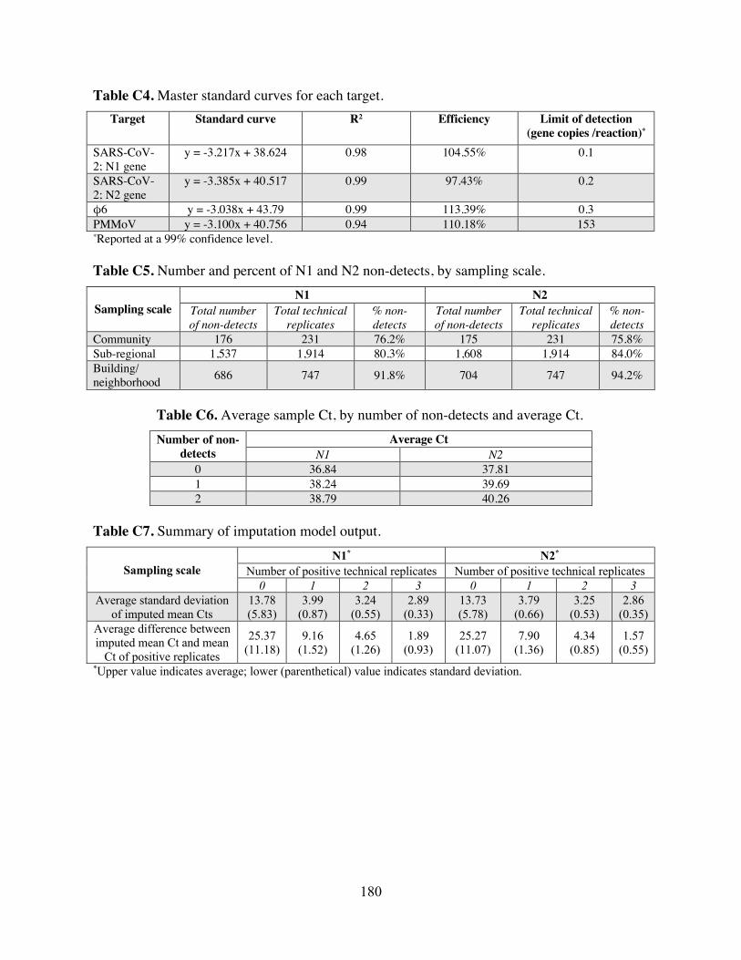
180

Table C4. Master standard curves for each target. Target Standard curve R2 Efficiency Limit of detection

(gene copies /reaction)*

SARS-CoV-2; N1 gene

y = -3.217x + 38.624 0.98 104.55% 0.1

SARS-CoV-2; N2 gene

y = -3.385x + 40.517 0.99 97.43% 0.2

φ6 y = -3.038x + 43.79 0.99 113.39% 0.3 PMMoV y = -3.100x + 40.756 0.94 110.18% 153 *Reported at a 99% confidence level.

Table C5. Number and percent of N1 and N2 non-detects, by sampling scale.

Sampling scale N1 N2

Total number of non-detects

Total technical replicates

% non-detects

Total number of non-detects

Total technical replicates

% non-detects

Community 176 231 76.2% 175 231 75.8% Sub-regional 1,537 1,914 80.3% 1,608 1,914 84.0% Building/ neighborhood 686 747 91.8% 704 747 94.2%

Table C6. Average sample Ct, by number of non-detects and average Ct. Number of non-

detects Average Ct

N1 N2 0 36.84 37.81 1 38.24 39.69 2 38.79 40.26

Table C7. Summary of imputation model output.

Sampling scale N1* N2*

Number of positive technical replicates Number of positive technical replicates

0 1 2 3 0 1 2 3 Average standard deviation

of imputed mean Cts

13.78

(5.83)

3.99

(0.87) 3.24

(0.55)

2.89

(0.33)

13.73

(5.78)

3.79

(0.66)

3.25

(0.53)

2.86

(0.35)

Average difference between

imputed mean Ct and mean

Ct of positive replicates

25.37

(11.18)

9.16

(1.52)

4.65

(1.26)

1.89

(0.93)

25.27

(11.07)

7.90

(1.36)

4.34

(0.85)

1.57

(0.55)

*Upper value indicates average; lower (parenthetical) value indicates standard deviation.

181

Table C8. Spearman’s rank-order correlation coefficients between community-level clinical cases and relative normalized WWTP virus concentration, by non-detect handling method. All correlations were highly significant (p < 0.01).

Non-detect handling method

LOD0.5 Ctmax Ctavg EM-MCMC 0.4740 0.5049 0.4337 0.5457

Table C9. Spearman’s rank-order correlation coefficients between clinical cases and relative normalized WWTP virus concentration, by sub-community sampling zone.

Sub-regional Building/neighborhood Zone ID Correlation

coefficient Zone ID Correlation

coefficient SR-A 0.0199 BN-A -0.0871

(0.810) (0.487) SR-B -0.5986

*** BN-B -0.6087***

(0.000) (0.000)

SR-C 0.4793***

BN-C 0.8216***

(0.000) (0.000)

SR-D -0.0937 BN-D 0.5270***

(0.509) (0.000) SR-E -0.6165

*** BN-E 0.3883

***

(0.000) (0.000)

SR-F 0.4503*** BN-F 0.3753***

(0.000) (0.000) SR-G -0.8113***

BN-G -0.7583

(0.000) (0.000)

SR-H -0.3691***

(0.004)

SR-I 0.0280

(0.844)

SR-J 0.4067***

(0.000) SR-K 0.3694***

(0.000)

SR-L 0.3782*** (0.000)

SR-M 0.5927*** (0.000)

SR-N 0.7220*** (0.000)

SR-O -0.3343**

(0.025)

SR-P 0.3970***

(0.000) p-values are in parentheses: *** p<0.01, ** p<0.05, * p<0.1

182

C.3 MIQE

ITEM TO CHECK IMPORTANCE CHECKLIST Experimental design

Definition of experimental and control groups E

Experimental groups: wastewater samples collected from 24 locations in the City of Davis. Control groups: N/A.

Number within each group E 964 wastewater samples were analyzed over the

duration of the experimental period.

Assay carried out by core lab or investigator's lab? D

Sample collection was performed by staff at the City of Davis and UC Davis. All sample processing and analysis was conducted in the Bischel Lab at UC Davis.

Acknowledgement of authors’ contributions D

Sample

Description E

Samples were 24-hour composites collected by insulated, ice-packed autosamplers deployed at the sampling zones.

Volume/mass of sample processed D

45 or 5 mL of wastewater, depending on the concentration method used.

Microdissection or macrodissection E N/A

Processing procedure E

Samples were either processed immediately or were stored at 4C for up to one week before processing. Prior to concentration, samples were pasteurized for 30 minutes at 60C and then spiked with a known quantity of φ6 bacteriophage. Concentration was carried out using either ultrafiltration (via 100 kDa Amicon devices) or magnetic-particle capture (via Nanotrap Magnetic Virus Particles on a KingFisher Flex robot).

If frozen - how and how quickly? E Samples were not frozen. If fixed - with what, how quickly? E Samples were not fixed. Sample storage conditions and duration (especially for FFPE samples) E See above. NUCLEIC ACID EXTRACTION

Procedure and/or instrumentation E

Samples concentrated by ultrafiltration were extracted using either the Macherey-Nagel NucleoSpin RNA Stool Kit or the Qiagen AllPrep PowerViral DNA/RNA Kit. Samples concentrated using magnetic particles were concentrated using the MagMAX Microbiome Ultra Nucleic Acid Isolation Kit on a KingFisher Flex robot.

Name of kit and details of any modifications E

Kits listed above. The Macherey Nagel kit was used following the manufacturer's instructions for isolating total RNA with the following modifications: (1) bead beating was only carried out for 2 minutes, and (2) the DNA digestion step was omitted. The Qiagen kit was used following the manufacturer's instructions but

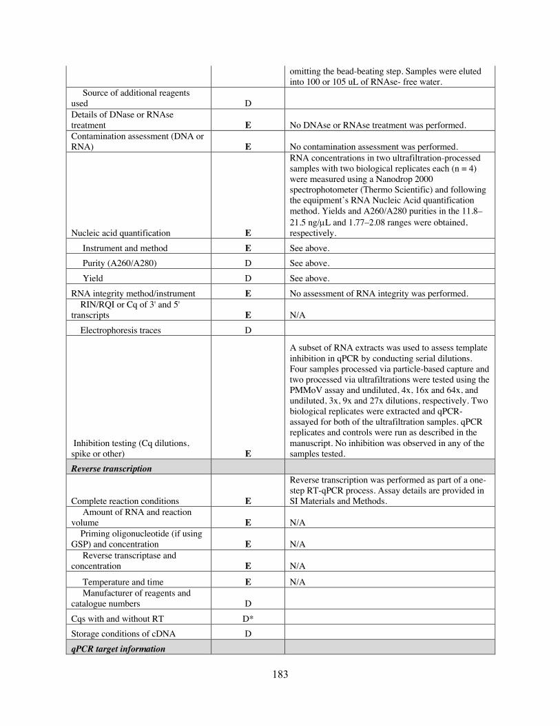
183

omitting the bead-beating step. Samples were eluted into 100 or 105 uL of RNAse- free water.

Source of additional reagents used D Details of DNase or RNAse treatment E No DNAse or RNAse treatment was performed. Contamination assessment (DNA or RNA) E No contamination assessment was performed.

Nucleic acid quantification E

RNA concentrations in two ultrafiltration-processed samples with two biological replicates each (n = 4) were measured using a Nanodrop 2000 spectrophotometer (Thermo Scientific) and following the equipment’s RNA Nucleic Acid quantification method. Yields and A260/A280 purities in the 11.8–21.5 ng/µL and 1.77–2.08 ranges were obtained, respectively.

Instrument and method E See above. Purity (A260/A280) D See above. Yield D See above. RNA integrity method/instrument E No assessment of RNA integrity was performed. RIN/RQI or Cq of 3' and 5' transcripts E N/A Electrophoresis traces D

Inhibition testing (Cq dilutions, spike or other) E

A subset of RNA extracts was used to assess template inhibition in qPCR by conducting serial dilutions. Four samples processed via particle-based capture and two processed via ultrafiltrations were tested using the PMMoV assay and undiluted, 4x, 16x and 64x, and undiluted, 3x, 9x and 27x dilutions, respectively. Two biological replicates were extracted and qPCR-assayed for both of the ultrafiltration samples. qPCR replicates and controls were run as described in the manuscript. No inhibition was observed in any of the samples tested.

Reverse transcription

Complete reaction conditions E

Reverse transcription was performed as part of a one-step RT-qPCR process. Assay details are provided in SI Materials and Methods.

Amount of RNA and reaction volume E N/A Priming oligonucleotide (if using GSP) and concentration E N/A Reverse transcriptase and concentration E N/A

Temperature and time E N/A Manufacturer of reagents and catalogue numbers D Cqs with and without RT D* Storage conditions of cDNA D qPCR target information

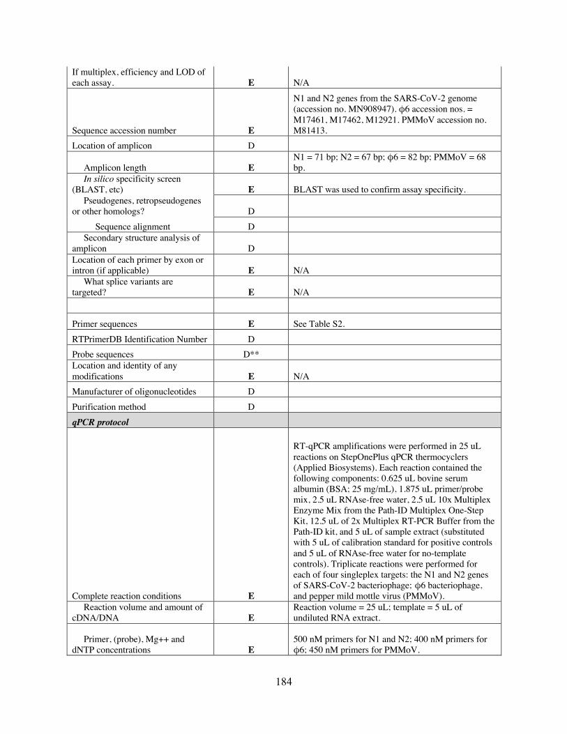
184

If multiplex, efficiency and LOD of each assay. E N/A

Sequence accession number E

N1 and N2 genes from the SARS-CoV-2 genome (accession no. MN908947). φ6 accession nos. = M17461, M17462, M12921. PMMoV accession no. M81413.

Location of amplicon D

Amplicon length E N1 = 71 bp; N2 = 67 bp; φ6 = 82 bp; PMMoV = 68 bp.

In silico specificity screen (BLAST, etc) E BLAST was used to confirm assay specificity. Pseudogenes, retropseudogenes or other homologs? D Sequence alignment D Secondary structure analysis of amplicon D Location of each primer by exon or intron (if applicable) E N/A What splice variants are targeted? E N/A qPCR OLIGONUCLEOTIDES

Primer sequences E See Table S2. RTPrimerDB Identification Number D Probe sequences D** Location and identity of any modifications E N/A Manufacturer of oligonucleotides D Purification method D qPCR protocol

Complete reaction conditions E

RT-qPCR amplifications were performed in 25 uL reactions on StepOnePlus qPCR thermocyclers (Applied Biosystems). Each reaction contained the following components: 0.625 uL bovine serum albumin (BSA; 25 mg/mL), 1.875 uL primer/probe mix, 2.5 uL RNAse-free water, 2.5 uL 10x Multiplex Enzyme Mix from the Path-ID Multiplex One-Step Kit, 12.5 uL of 2x Multiplex RT-PCR Buffer from the Path-ID kit, and 5 uL of sample extract (substituted with 5 uL of calibration standard for positive controls and 5 uL of RNAse-free water for no-template controls). Triplicate reactions were performed for each of four singleplex targets: the N1 and N2 genes of SARS-CoV-2 bacteriophage; φ6 bacteriophage, and pepper mild mottle virus (PMMoV).

Reaction volume and amount of cDNA/DNA E

Reaction volume = 25 uL; template = 5 uL of undiluted RNA extract.

Primer, (probe), Mg++ and dNTP concentrations E

500 nM primers for N1 and N2; 400 nM primers for φ6; 450 nM primers for PMMoV.

185

Polymerase identity and concentration E

2x Multiplex RT-PCR Buffer (ThermoFisher) containing AmpliTaq Gold ultrapure thermostable DNA polymerase; added to achieve 12.5 uL of multiplex buffer in each 25 uL reaction.

Buffer/kit identity and manufacturer E See above. Exact chemical constitution of the buffer D Additives (SYBR Green I, DMSO, etc.) E See "Complete reaction conditions", above. Manufacturer of plates/tubes and catalog number D

Complete thermocycling parameters E See Table C2.

Reaction setup (manual/robotic) D Manual.

Manufacturer of qPCR instrument E Applied Biosystems. qPCR VALIDATION Evidence of optimisation (from gradients) D

Specificity (gel, sequence, melt, or digest) E

NGS sequence-verified SARS-CoV-2 (2019-nCoV) RUO plasmid controls were purchased from IDT for the N1 and N2 assays. Restriction enzyme digestion folowed by gel electrophoresis was peformed for the synthesized PMMoV and φ6 plasmids.

For SYBR Green I, Cq of the NTC E N/A Standard curves with slope and y-intercept E See Table C4. PCR efficiency calculated from slope E See Table C4. Confidence interval for PCR efficiency or standard error D See Table C4.

r2 of standard curve E See Table C4.

Linear dynamic range E

1,000,000 - 2.5 gene copies/reaction (N1) 1,000,000 - 5 gene copies/reaction (N2) 1,000,000 - 1,000 gene copies/reaction (PMMoV) 5.78E+09 - 5.78E+04 gene copies/reaction (φ6)

Cq variation at lower limit E 0.09 (N1); 0.63 (N2); 0.96 (PMMoV); 0.10 (φ6) Confidence intervals throughout range D 95%

Evidence for limit of detection E N/A If multiplex, efficiency and LOD of each assay. E N/A DATA ANALYSIS qPCR analysis program (source, version) E StepOne Plus v2.3

Cq method determination E Standard curve

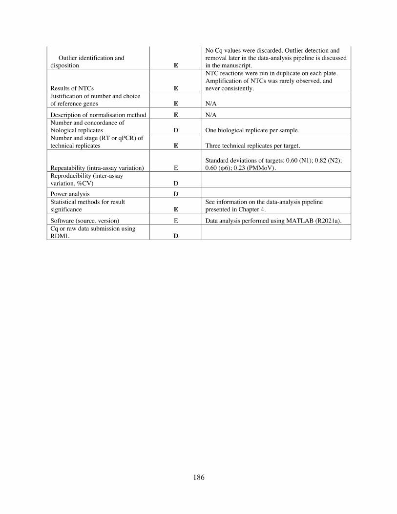
186

Outlier identification and disposition E

No Cq values were discarded. Outlier detection and removal later in the data-analysis pipeline is discussed in the manuscript.

Results of NTCs E

NTC reactions were run in duplicate on each plate. Amplification of NTCs was rarely observed, and never consistently.

Justification of number and choice of reference genes E N/A

Description of normalisation method E N/A Number and concordance of biological replicates D One biological replicate per sample. Number and stage (RT or qPCR) of technical replicates E Three technical replicates per target.

Repeatability (intra-assay variation) E Standard deviations of targets: 0.60 (N1); 0.82 (N2); 0.60 (φ6); 0.23 (PMMoV).

Reproducibility (inter-assay variation, %CV) D Power analysis D Statistical methods for result significance E

See information on the data-analysis pipeline presented in Chapter 4.

Software (source, version) E Data analysis performed using MATLAB (R2021a). Cq or raw data submission using RDML D

187

APPENDIX D: PERFORMANCE COMPARISON OF FOUR COMMERCIALLY AVAILABLE FLOW CYTOMETERS USING POLYSTYRENE BEADS

D.1 Abstract

Accurate comparison of flow cytometric data requires an understanding of how the

cytometric fingerprint of a sample may vary from instrument to instrument. Key sources of

variability include the number, wavelengths, and power of excitation lasers; the number and types

of emission detectors; sample-handling systems and options; and whether fixed or dynamic

detector voltages are used. To explore this variability, suspensions of three sizes (0.2, 0.5, and 0.8

µm-diameter) of solid, fluorescent, polystyrene beads were prepared. The suspensions were then

run at on four commercially available flow cytometers, keeping instrument settings as consistent

as possible. The results are displayed graphically in Figure 3 of the article “Flow cytometry

applications in water treatment, distribution, and reuse: A review” (Safford and Bischel, 2019).

This dataset contains the complete .FCS files generated from the experimental comparison. In the

development and application of flow cytometry to water quality assessment, we recommend data

sharing in this manner to enable comprehensive reporting, meaningful comparison of results

obtained using different cytometer models, enhanced exploration of data along multiple

parameters, and use of acquired data for computational advancements in the field.

D.2 Value of the data

• These data support comparison of results from flow cytometry experiments by illustrating

how the appearance of identical suspensions of polystyrene beads varies depending on the

instrument used for analysis.

• The .FCS (Flow Cytometry Standard) files that comprise this dataset contain metadata

useful for researchers seeking to replicate the results.

188

• Access to underlying .FCS files allows deeper exploration of flow cytometry data by

providing information on all scatter and fluorescent parameters collected during flow

cytometry experiments.

D.3 Data

The data comprise four .FCS (Flow Cytometry Standard) files generated by running

identical samples of a suspension of three sizes of submicron-diameter, fluorescent, solid,

polystyrene beads on four commercially available flow cytometers: the AccuriTM C6 (BD

Biosciences), the NovoCyte® 2070V (ACEA Biosciences), the AttuneTM NxT (Thermo Fisher

Scientific), and the MACSQuant 10 (Miltenyi Biotec). The data are available for download at:

http://dx.doi.org/10.17632/c7nh26z8p3.1.

D.4 Experimental design, materials, and methods

Suspensions of polystyrene beads were prepared by adding 3 drops each of 0.2, 0.5, and

0.8 µm-diameter fluorescent, solid, polystyrene bead solutions (Submicron Bead Calibration Kit,

Catalog No. BLI832, Polysciences, Inc.) to 0.5 mL of 0.2 µm-filtered Tris-EDTA (TE) buffer.

Immediately prior to analysis, the suspensions were vortexed to ensure an even distribution of

beads in solution. A 20 µL volume of the suspension was analyzed on each of four commercially

available flow cytometers: the AccuriTM C6 (BD Biosciences), the NovoCyte® 2070V (ACEA

Biosciences), the AttuneTM NxT (Thermo Fisher Scientific), and the MACSQuant 10 (Miltenyi

Biotec).

The lowest available flowrate setting was used for analysis. Since the beads used in this

experimental comparison excite under interrogation with 488-nm (blue) laser light, data were

189

collected using a 488-nm (blue) laser and all available detectors for that laser. Data were also

sometimes collected off of lasers of other wavelengths where available. Since the beads used in

this experimental comparison emit green photons under blue excitation, a threshold was set for

each instrument using green fluorescence (~530 nm) as a trigger to exclude instrument noise.

D.5 References

Safford, H.R. and Bischel, H.N. (2019). Flow cytometry applications for in water treatment, distribution, and reuse: A review. Water Res. 151, 110–133.