I. INTRODUCTION AND OUTLINE - WordPress.com ·  · 2013-04-18I. INTRODUCTION AND OUTLINE ... Fortunately, the marriage between particle physics and cosmology has provided a way ...

I. INTRODUCTION AND OUTLINE

Most aspects of high energy physics beyond the standard model can only be testedby going to energies far greater than those which present accelerators can provide.Fortunately, the marriage between particle physics and cosmology has provided a wayto “experimentally” test the new theories of fundamental forces.

The key realization, discovered both in the context of the inflationary Universescenario [1] and of topological defects models [2] is that physics of the very early Uni-verse may explain the origin of structure in the Universe. It now appears that arich set of data concerning the nonrandom distribution of matter on a wide rangeof cosmological scales, and on the anisotropies in the cosmic microwave background(CMB), may potentially be explained by high energy physics. In addition, studyingthe consequences of particle physics models in the context of cosmology may leadto severe constraints on new microscopic theories. Finally, particle physics and fieldtheory may provide explanations of some deep cosmological puzzles, e.g. why theUniverse at the present time appears so homogeneous, so close to being spatially flat,and why it contains the observed small net baryon to entropy ratio.

In these lectures, I focus on three important aspects of modern cosmology. Thefirst concerns some fundamental problems of inflationary cosmology. In particular,some recent progress in the understanding of “reheating” in inflation will be reviewed.

The second topic is the classical and quantum theory of cosmological perturba-tions, the main tool of modern cosmology. A general relativistic and quantum me-chanical analysis of the generation and evolution of linearized fluctuations is essentialin order to be able to accurately calculate the amplitude of density perturbations andCMB anisotropies.

As a third topic, I discuss the role of topological defects in baryogenesis and aspossible sees for cosmological structure formation.

The specific outline is as follows:

1. Introduction and Outline

2. Lecture 1: Inflationary Universe: Progress and Problems

2.A Problems of Standard Cosmology2.B Inflationary Universe Scenario2.C Problems of Inflation2.D Inflation and Nonsingular Cosmology2.E Reheating in Inflationary Cosmology2.F Summary

3. Lecture 2: Classical and Quantum Theory of Cosmological Perturba-

tions

3.A Basic Issues3.B Newtonian Theory

2

3.C Relativistic Theory: Classical Analysis3.D Relativistic Theory: Quantum Analysis3.E Summary

4. Lecture 3: Topological Defects, Structure Formation and Baryogen-

esis

4.A Quantifying Data on Large-Scale Structure4.B Topological Defects4.C Formation of Defects in Cosmological Phase Transitions4.D Evolution of Strings and Scaling4.E Cosmic Strings and Structure Formation4.F Specific Predictions4.G Principles of Baryogenesis4.H GUT Baryogenesis and Topological Defects4.I Electroweak Baryogenesis and Topological Defects4.J Summary

Unless otherwise specified, units in which h = c = kB = 1 will be used. Distancesare expressed in Mpc (1pc ≃ 3.06 light years). Following the usual convention, hindicates the expansion rate of the Universe in units of 100 km s−1 Mpc−1, Ω = ρ/ρc

is the ratio of the energy density ρ to the critical density ρc (the density which yieldsa spatially flat Universe), G is Newton’s constant and mpl is the Planck mass.

II. INFLATIONARY UNIVERSE: PROGRESS AND PROBLEMS

The hypothesis that the Universe underwent a period of exponential expansion atvery early times has become the most popular theory of the early Universe. Not onlydoes it solve some of the problems of standard big bang cosmology, but it also providesa causal theory for the origin of inhomogeneities in the Universe which is predictiveand in reasonable agreement with current observational results. Nevertheless, thereare several problems of principle which merit further study.

A. Problems of Standard Cosmology

The standard big bang cosmology rests on three theoretical pillars: the cosmolog-ical principle, Einstein’s general theory of relativity and a perfect fluid description ofmatter.

The cosmological principle states that on large distance scales the Universe ishomogeneous. This implies that the metric of space-time can be written in Friedmann-Robertson-Walker (FRW) form:

ds2 = a(t)2

[

dr2

1 − kr2+ r2(dϑ2 + sin2 ϑdϕ2)

]

, (1)

3

where the constant k determines the topology of the spatial sections. In the following,we shall usually set k = 0, i.e. consider a spatially closed Universe. In this case, wecan without loss of generality take the scale factor a(t) to be equal to 1 at the presenttime t0, i.e. a(t0) = 1. The coordinates r, ϑ and ϕ are comoving spherical coordinates.World lines with constant comoving coordinates are geodesics corresponding to par-ticles at rest. If the Universe is expanding, i.e. a(t) is increasing, then the physicaldistance ∆xp(t) between two points at rest with fixed comoving distance ∆xc grows:

∆xp = a(t)∆xc . (2)

The dynamics of an expanding Universe is determined by the Einstein equations,which relate the expansion rate to the matter content, specifically to the energydensity ρ and pressure p. For a homogeneous and isotropic Universe, they reduce tothe Friedmann-Robertston-Walker (FRW) equations

(

a

a

)2

− k

a2=

8πG

3ρ (3)

a

a= −4πG

3(ρ+ 3p) . (4)

These equations can be combined to yield the continuity equation (with Hubble con-stant H = a/a)

ρ = −3H(ρ+ p) . (5)

The third key assumption of standard cosmology is that matter is described byan ideal gas with an equation of state

p = wρ . (6)

For cold matter, pressure is negligible and hence w = 0. From (5) it follows that

ρm(t) ∼ a−3(t) , (7)

where ρm is the energy density in cold matter. For radiation we have w = 1/3 andhence it follows from (5) that

ρr(t) ∼ a−4(t) , (8)

ρr(t) being the energy density in radiation.The three classic observational pillars of standard cosmology are Hubble’s law, the

existence and black body nature of the nearly isotropic CMB, and the abundancesof light elements (nucleosynthesis). These successes are discussed in detail in manytextbooks on cosmology, and will therefore not be reviewed here.

4

It is, however, important to recall two important aspects concerning the thermalhistory of the early Universe. Since the energy density in radiation redshifts fasterthan the matter energy density, it follows by working backwards in time from thepresent data that although the energy density of the Universe is now mostly in coldmatter, it was initially dominated by radiation. The transition occurred at a timedenoted by teq, the “time of equal matter and radiation”. As will be discussed inSection 3, teq is the time when perturbations can start to grow by gravitationalclustering. The second important time is trec, the “time of recombination” whenphotons fell out of equilibrium (since ions and electrons had by then combined toform electrically neutral atoms). The photons of the CMB have travelled withoutscattering from trec. Their spatial distribution is predicted to be a black body since thecosmological redshift preserves the black body nature of the initial spectrum (simplyredshifting the temperature) which was in turn determined by thermal equilibrium.CMB anisotropies probe the density fluctuations at trec. Note that for the usualvalues of the cosmological parameters, teq < trec.

Standard Big Bang cosmology is faced with several important problems. Only oneof these, the age problem, is a potential conflict with observations. The others whichI will focus on here – the homogeneity, flatness and formation of structure problems(see e.g. [1]) – are questions which have no answer within the theory and are thereforethe main motivation for the new cosmological models which will be discussed in latersections of these lecture notes.

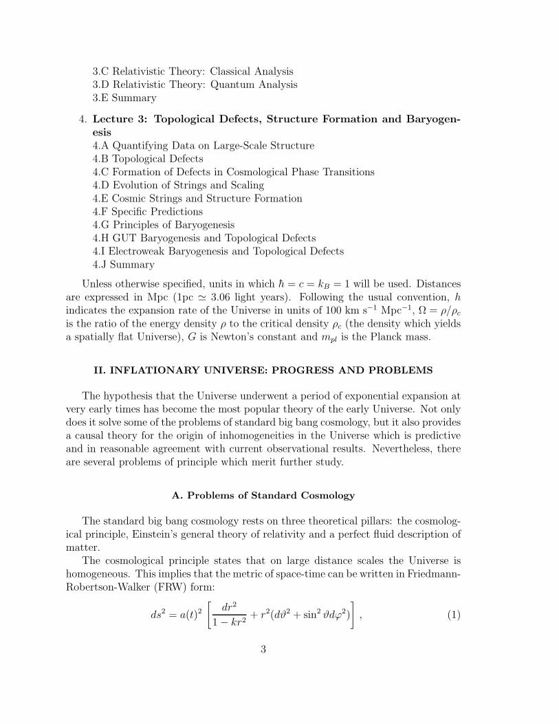
The horizon problem is illustrated in Fig. 1. As is sketched, the comoving regionℓp(trec) over which the CMB is observed to be homogeneous to better than one part in104 is much larger than the comoving forward light cone ℓf(trec) at trec, which is themaximal distance over which microphysical forces could have caused the homogeneity:

ℓp(trec) =

t0∫

trec

dt a−1(t) ≃ 3 t0

(

1 −(

trec

t0

)1/3)

(9)

ℓf (trec) =

trec∫

0

dt a−1(t) ≃ 3 t2/30 t1/3

rec . (10)

From the above equations it is obvious that ℓp(trec) ≫ ℓf(trec). Hence, standardcosmology cannot explain the observed isotropy of the CMB.

5

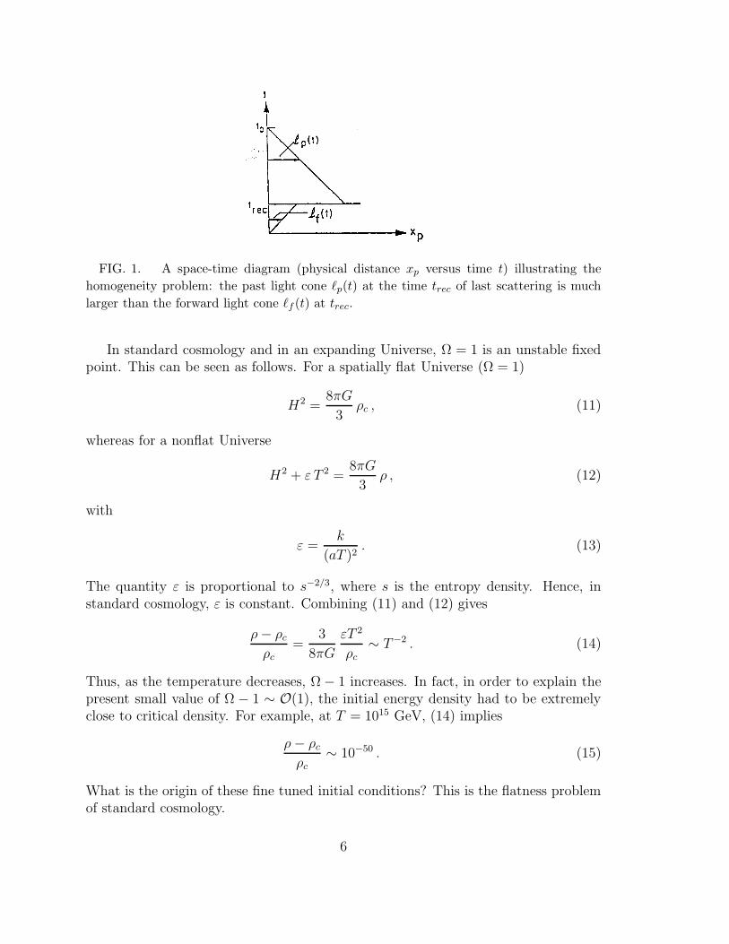
FIG. 1. A space-time diagram (physical distance xp versus time t) illustrating the

homogeneity problem: the past light cone ℓp(t) at the time trec of last scattering is much

larger than the forward light cone ℓf (t) at trec.

In standard cosmology and in an expanding Universe, Ω = 1 is an unstable fixedpoint. This can be seen as follows. For a spatially flat Universe (Ω = 1)

H2 =8πG

3ρc , (11)

whereas for a nonflat Universe

H2 + ε T 2 =8πG

3ρ , (12)

with

ε =k

(aT )2. (13)

The quantity ε is proportional to s−2/3, where s is the entropy density. Hence, instandard cosmology, ε is constant. Combining (11) and (12) gives

ρ− ρc

ρc=

3

8πG

εT 2

ρc∼ T−2 . (14)

Thus, as the temperature decreases, Ω − 1 increases. In fact, in order to explain thepresent small value of Ω − 1 ∼ O(1), the initial energy density had to be extremelyclose to critical density. For example, at T = 1015 GeV, (14) implies

ρ− ρc

ρc∼ 10−50 . (15)

What is the origin of these fine tuned initial conditions? This is the flatness problemof standard cosmology.

6

The third of the classic problems of standard cosmological model is the “forma-tion of structure problem.” Observations indicate that galaxies and even clusters ofgalaxies have nonrandom correlations on scales larger than 50 Mpc (see e.g. [3,4]).This scale is comparable to the comoving horizon at teq. Thus, if the initial densityperturbations were produced much before teq, the correlations cannot be explained bya causal mechanism. Gravity alone is, in general, too weak to build up correlationson the scale of clusters after teq (see, however, the explosion scenario of [5]). Hence,the two questions of what generates the primordial density perturbations and whatcauses the observed correlations, do not have an answer in the context of standardcosmology. This problem is illustrated by Fig. 2.

FIG. 2. A sketch (conformal separation vs. time) of the formation of structure problem:

the comoving separation dc between two clusters is larger than the forward light cone at

time teq.

There are other serious problems of standard cosmology, e.g. the age and thecosmological constant problems. However, to date modern cosmology does not shedany light on these problems, and I will therefore not address them here.

B. Inflationary Universe Scenario

The idea of inflation [1] is very simple (for some early reviews of inflation see e.g.[6–9]). We assume there is a time interval beginning at ti and ending at tR (the“reheating time”) during which the Universe is exponentially expanding, i.e.,

a(t) ∼ eHt, tǫ [ti, tR] (16)

with constant Hubble expansion parameter H . Such a period is called “de Sitter”or “inflationary.” The success of Big Bang nucleosynthesis sets an upper limit to thetime of reheating:

tR ≪ tNS , (17)

tNS being the time of nucleosynthesis.

7

FIG. 3. The phases of an inflationary Universe. The times ti and tR denote the beginning

and end of inflation, respectively. In some models of inflation, there is no initial radiation

dominated FRW period. Rather, the classical space-time emerges directly in an inflationary

state from some initial quantum gravity state.

The phases of an inflationary Universe are sketched in Fig. 3. Before the onsetof inflation there are no constraints on the state of the Universe. In some models aclassical space-time emerges immediately in an inflationary state, in others there isan initial radiation dominated FRW period. Our sketch applies to the second case.After tR, the Universe is very hot and dense, and the subsequent evolution is asin standard cosmology. During the inflationary phase, the number density of anyparticles initially in thermal equilibrium at t = ti decays exponentially. Hence, thematter temperature Tm(t) also decays exponentially. At t = tR, all of the energywhich is responsible for inflation (see later) is released as thermal energy. This is anonadiabatic process during which the entropy increases by a large factor.

Fig. 4 is a sketch of how a period of inflation can solve the homogeneity problem.∆t = tR−ti is the period of inflation. During inflation, the forward light cone increasesexponentially compared to a model without inflation, whereas the past light cone isnot affected for t ≥ tR. Hence, provided ∆t is sufficiently large, ℓf (tR) will be greaterthan ℓp(tR).

8

FIG. 4. Sketch (physical coordinates vs. time) of the solution of the homogeneity

problem. During inflation, the forward light cone lf (t) is expanded exponentially when

measured in physical coordinates. Hence, it does not require many e-foldings of inflation in

order that lf (t) becomes larger than the past light cone at the time of last scattering. The

dashed line is the forward light cone without inflation.

Inflation also can solve the flatness problem [10,1] The key point is that the entropydensity s is no longer constant. As will be explained later, the temperatures at tiand tR are essentially equal. Hence, the entropy increases during inflation by a factorexp(3H∆t). Thus, ǫ decreases by a factor of exp(−2H∆t). Hence, (ρ − ρc)/ρ canbe of order 1 both at ti and at the present time. In fact, if inflation occurs at all,then rather generically, the theory predicts that at the present time Ω = 1 to a highaccuracy (now Ω < 1 requires special initial conditions or rather special models [11]).

Most importantly, inflation provides a mechanism which in a causal way generatesthe primordial perturbations required for galaxies, clusters and even larger objects.In inflationary Universe models, the Hubble radius (“apparent” horizon), 3t, and the“actual” horizon (the forward light cone) do not coincide at late times. Provided thatthe duration of inflation is sufficiently long, then (as sketched in Fig. 5) all scaleswithin our apparent horizon were inside the actual horizon since ti. Thus, it is inprinciple possible to have a casual generation mechanism for perturbations [12–15].

The generation of perturbations is supposed to be due to a causal microphysicalprocess. Such processes can only act coherently on length scales smaller than theHubble radius ℓH(t) where

ℓH(t) = H−1(t) . (18)

A heuristic way to understand the meaning of ℓH(t) is to realize that it is the distance

9

which light (and hence the maximal distance any causal effects) can propagate in oneexpansion time.

FIG. 5. A sketch (physical coordinates vs. time) of the solution of the formation of

structure problem. Provided that the period of inflation is sufficiently long, the separation

dc between two galaxy clusters is at all times smaller than the forward light cone. The

dashed line indicates the Hubble radius. Note that dc starts out smaller than the Hubble

radius, crosses it during the de Sitter period, and then reenters it at late times.

As will be discussed in Chapter 4, the density perturbations produced duringinflation are due to quantum fluctuations in the matter and gravitational fields [13,14].The amplitude of these inhomogeneities corresponds to a temperature TH

TH ∼ H , (19)

the Hawking temperature of the de Sitter phase. This implies that at all times t duringinflation, perturbations with a fixed physical wavelength ∼ H−1 will be produced.Subsequently, the length of the waves is stretched with the expansion of space, andsoon becomes larger than the Hubble radius. The phases of the inhomogeneitiesare random. Thus, the inflationary Universe scenario predicts perturbations on allscales ranging from the comoving Hubble radius at the beginning of inflation tothe corresponding quantity at the time of reheating. In particular, provided thatinflation lasts sufficiently long, perturbations on scales of galaxies and beyond will begenerated. Note, however, that it is very dangerous to interpret de Sitter Hawking

10

radiation as thermal radiation. In fact, the equation of state of this “radiation” isnot thermal [16].

Obviously, the key question is how to obtain inflation. From the FRW equations,it follows that in order to get exponential increase of the scale factor, the equation ofstate of matter must be

p = −ρ (20)

This is where the connection with particle physics comes in. The energy density andpressure of a scalar quantum field ϕ are given by

ρ(ϕ) =1

2ϕ2 +

1

2(∇ϕ)2 + V (ϕ) (21)

p(ϕ) =1

2ϕ2 − 1

6(∇ϕ)2 − V (ϕ) . (22)

Thus, provided that at some initial time ti

ϕ(x, ti) = ∇ϕ(xi ti) = 0 (23)

and

V (ϕ(xi, ti)) > 0 , (24)

the equation of state of matter will be (20).The next question is how to realize the required initial conditions (23) and to

maintain the key constraints

ϕ2 ≪ V (ϕ) , (∇ϕ)2 ≪ V (ϕ) (25)

for sufficiently long. Various ways of realizing these conditions were put forward, andthey gave rise to different models of inflation. I will focus on “old inflation,” “newinflation”” and “chaotic inflation.” There are many other attempts at producing aninflationary scenario, but there is as of now no convincing realization.

Old Inflation

The old inflationary Universe model [1,17] is based on a scalar field theory whichundergoes a first order phase transition. As a toy model, consider a scalar fieldtheory with the potential V (ϕ) of Figure 6. This potential has a metastable “false”vacuum at ϕ = 0, whereas the lowest energy state (the “true” vacuum) is ϕ = a.Finite temperature effects [18] lead to extra terms in the finite temperature effectivepotential which are proportional to ϕ2T 2 (the resulting finite temperature effectivepotential is also depicted in Figure 6). Thus, at high temperatures, the energeticallypreferred state is the false vacuum state. Note that this is only true if ϕ is in thermalequilibrium with the other fields in the system.

11

FIG. 6. The finite temperature effective potential in a theory with a first order phase

transition.

For fairly general initial conditions, ϕ(x) is trapped in the metastable state ϕ = 0as the Universe cools below the critical temperature Tc. As the Universe expandsfurther, all contributions to the energy-momentum tensor Tµν except for the contri-bution

Tµν ∼ V (ϕ)gµν (26)

redshift. Hence, provided that the potential V (ϕ) is shifted upwards such that V (a) =0, then the equation of state in the false vacuum approaches p = −ρ, and inflationsets in. After a period Γ−1, where Γ is the tunnelling rate, bubbles of ϕ = a beginto nucleate [19] in a sea of false vacuum ϕ = 0. Inflation lasts until the false vacuumdecays. During inflation, the Hubble constant is given by

H2 =8πG

3V (0) . (27)

Note that the condition V (a) = 0, which looks rather unnatural, is required to avoida large cosmological constant today (none of the present inflationary Universe modelsmanages to circumvent or solve the cosmological constant problem).

It was immediately realized that old inflation has a serious “graceful exit”problem [1,20]. The bubbles nucleate after inflation with radius r ≪ 2tR and wouldtoday be much smaller than our apparent horizon. Thus, unless bubbles percolate,the model predicts extremely large inhomogeneities inside the Hubble radius, in con-tradiction with the observed isotropy of the microwave background radiation.

For bubbles to percolate, a sufficiently large number must be produced so thatthey collide and homogenize over a scale larger than the present Hubble radius. How-ever, with exponential expansion, the volume between bubbles expands exponentiallywhereas the volume inside bubbles expands only with a low power. This preventspercolation.

New Inflation

12

Because of the graceful exit problem, old inflation never was considered to be aviable cosmological model. However, soon after the seminal paper by Guth, Linde [21]

and independently Albrecht and Steinhardt [22] put forwards a modified scenario, theNew Inflationary Universe.

The starting point is a scalar field theory with a double well potential whichundergoes a second order phase transition (Fig. 7). V (ϕ) is symmetric and ϕ = 0 isa local maximum of the zero temperature potential. Once again, it was argued thatfinite temperature effects confine ϕ(x) to values near ϕ = 0 at temperatures T ≥ Tc.For T < Tc, thermal fluctuations trigger the instability of ϕ(x) = 0 and ϕ(x) evolvestowards either of the global minima at ϕ = ±σ by the classical equation of motion

ϕ+ 3Hϕ− a−2 2 ϕ = −V ′(ϕ) . (28)

Within a fluctuation region, ϕ(x) will be homogeneous. In such a region, we canneglect the spatial gradient terms in Eq. (28). Then, from (21) and (22) we can readoff the induced equation of state. The condition for inflation is

ϕ2 ≪ V (ϕ) , (29)

i.e. slow rolling. Often, the “slow rolling” approximation is made to find solutionsof (28). This consists of dropping the ϕ term.

FIG. 7. The finite temperature effective potential in a theory with a second order phase

transition.

There is no graceful exit problem in the new inflationary Universe. Since thefluctuation domains are established before the onset of inflation, any boundary wallswill be inflated outside the present Hubble radius.

Let us, for the moment, return to the general features of the new inflationaryUniverse scenario. At the time tc of the phase transition, ϕ(t) will start to movefrom near ϕ = 0 towards either ±σ as described by the classical equation of motion,i.e. (28). At or soon after tc, the energy-momentum tensor of the Universe will startto be dominated by V (ϕ), and inflation will commence. ti shall denote the time of the

13

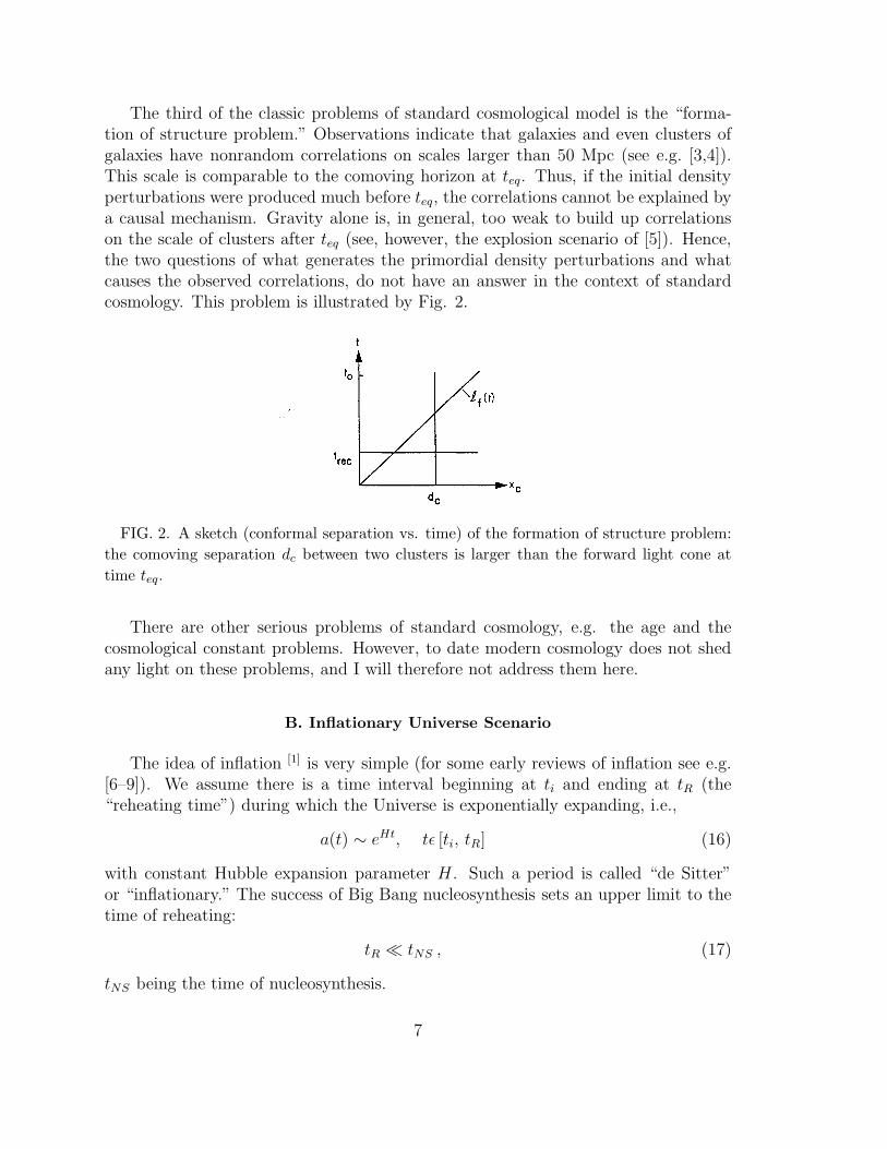
onset of inflation. Eventually, φ(t) will reach large values for which nonlinear effectsbecome important. The time at which this occurs is tB. For t > tB , ϕ(t) rapidlyaccelerates, reaches ±σ, overshoots and starts oscillating about the global minimumof V (ϕ). The amplitude of this oscillation is damped by the expansion of the Universeand (predominantly) by the coupling of ϕ to other fields. At time tR, the energy in ϕdrops below the energy of the thermal bath of particles produced during the periodof oscillation.

The evolution of ϕ(t) is sketched in Fig. 8. The time period between tB and tRis called the reheating period and is usually short compared to the Hubble expansiontime. For t > tR, the Universe is again radiation dominated.

FIG. 8. Evolution of ϕ(t) and T (t) in the new inflationary Universe.

In order to obtain inflation, the potential V (ϕ) must be very flat near the falsevacuum at ϕ = 0. This can only be the case if all of the coupling constants appearingin the potential are small. However, this implies that the ϕ cannot be in thermalequilibrium at early times, which would be required to localize ϕ in the false vacuum.In the absence of thermal equilibrium, the initial conditions for ϕ are only constrainedby requiring that the total energy density in ϕ not exceed the total energy densityof the Universe. Most of the phase space of these initial conditions lies at values of|ϕ| >> σ. This leads to the “chaotic” inflation scenario [23].

Chaotic Inflation

Consider a region in space where at the initial time ϕ(x) is very large, homo-geneous and static. In this case, the energy-momentum tensor will be immediatelydominated by the large potential energy term and induce an equation of state p ≃ −ρwhich leads to inflation. Due to the large Hubble damping term in the scalar fieldequation of motion, ϕ(x) will only roll very slowly towards ϕ = 0. The kinetic energycontribution to Tµν will remain small, the spatial gradient contribution will be expo-nentially suppressed due to the expansion of the Universe, and thus inflation persists.

14

Note that in contrast to old and new inflation, no initial thermal bath is required.Note also that the precise form of V (ϕ) is irrelevant to the mechanism. In particular,V (ϕ) need not be a double well potential. This is a significant advantage, since forscalar fields other than Higgs fields used for spontaneous symmetry breaking, thereis no particle physics motivation for assuming a double well potential, and since theinflaton (the field which gives rise to inflation) cannot be a conventional Higgs fielddue to the severe fine tuning constraints.

The field and temperature evolution in a chaotic inflation model is similar to whatis depicted in Figure 8, except that ϕ is rolling towards the true vacuum at ϕ = σfrom the direction of large field values.

Chaotic inflation is a much more radical departure from standard cosmology thanold and new inflation. In the latter, the inflationary phase can be viewed as a shortphase of exponential expansion bounded at both ends by phases of radiation dom-ination. In chaotic inflation, a piece of the Universe emerges with an inflationaryequation of state immediately after the quantum gravity (or string) epoch.

The chaotic inflationary Universe scenario has been developed in great detail (seee.g. [24] for a recent review). One important addition is the inclusion of stochasticnoise [25] in the equation of motion for ϕ in order to take into account the effects ofquantum fluctuations. It can in fact be shown that for sufficiently large values of|ϕ|, the stochastic force terms are more important than the classical relaxation forceV ′(ϕ). There is equal probability for the quantum fluctuations to lead to an increaseor decrease of |ϕ|. Hence, in a substantial fraction of comoving volume, the fieldϕ will climb up the potential. This leads to the conclusion that chaotic inflation iseternal. At all times, a large fraction of the physical space will be inflating. Anotherconsequence of including stochastic terms is that on large scales (much larger thanthe present Hubble radius), the Universe will look extremely inhomogeneous.

C. Problems of Inflationary Cosmology

In spite of its great success at resolving some of the problems of standard cos-mology and of providing a causal, predictive theory of structure formation, there areseveral important unresolved conceptual problems in inflationary cosmology. I willfocus on three of these problems, the cosmological constant mystery, the fluctuationproblem, and the dynamics of reheating.

Cosmological Constant Problem

Since the cosmological constant acts as an effective energy density, its value isbounded from above by the present energy density of the Universe. In Planck units,the constraint on the effective cosmological constant Λeff is (see e.g. [26])

Λeff

m4pl

≤ 10−122 . (30)

15

This constraint applies both to the bare cosmological constant and to any mattercontribution which acts as an effective cosmological constant.

The true vacuum value of the potential V (ϕ) acts as an effective cosmologicalconstant. Its value is not constrained by any particle physics requirements (in theabsence of special symmetries). The cosmological constant problem is thus even moreaccute in inflationary cosmology than it usually is. The same unknown mechanismwhich must act to shift the potential (see Figure 6) such that inflation occurs in thefalse vacuum must also adjust the potential to vanish in the true vacuum.

Supersymmetric theories may provide a resolution of this problem, since unbro-ken supersymmetry forces V (ϕ) = 0 in the supersymmetric vacuum. However, su-persymmetry breaking will induce a nonvanishing V (ϕ) in the true vacuum aftersupersymmetry breaking.

We may therefore be forced to look for realizations of inflation which do not makeuse of scalar fields. There are several possibilities. It is possible to obtain inflation inhigher derivative gravity theories. In fact, the first model with exponential expansionof the Universe was obtained [27] in an R2 gravity theory. The extra degrees of freedomassociated with the higher derivative terms act as scalar fields with a potential whichautomatically vanishes in the true vacuum. For some recent work on higher derivativegravity inflation see also [28].

Another way to obtain inflation is by making use of condensates (see [29] and[30] for different approaches to this problem). An additional motivation for followingthis route to inflation is that the symmetry breaking mechanisms observed in nature(in condensed matter systems) are induced by the formation of condensates such asCooper pairs. Again, in a model of condensates there is no freedom to add a constantto the effective potential.

The main problem of studying the possibility of obtaining inflation using conden-sates is that the quantum effects which determine the theory are highly nonpertur-bative. In particular, the effective potential written in terms of a condensate 〈ϕ〉does not correspond to a renormalizable theory and will in general [31] contain termsof arbitrary power in 〈ϕ〉. However (see [32]), one may make progress by assumingcertain general properties of the effective potential.

Let us [32] consider a theory in which at some time ti a condensate 〈ϕ〉 forms, i.e.〈ϕ〉 = 0 for t < ti and 〈ϕ〉 6= 0 for t > ti. The expectation value of the HamiltonianH written in terms of the condensate 〈ϕ〉 contains terms of arbitrary powers of 〈ϕ〉:

〈H〉 =∑

n

(−1)nn!an〈ϕ〉n . (31)

We summarize our ignorance of the nonperturbative physics in the assumption thatthe resulting series is asymptotic, and in particular Borel summable, with coefficientsan ∝ 1. In this case, we can resum the series to obtain [32]

〈H〉 =∫

∞

0

f(t)dt

t(tmpl + 〈ϕ〉)e−1/t , (32)

16

where the function f(t) is related to the coefficients an via

an =1

n!

∫

∞

0dtf(t)t−n−2e−1/t . (33)

The expectation value of the Hamiltonian 〈H〉 can be interpreted as the effectivepotential Veff of this theory. The question is under which conditions this potentialgives rise to inflation. If we regard 〈ϕ〉 as a classical field (i.e. neglect the ultravioletand infrared divergences of the theory), then the dynamics of the model can be readoff directly from (32), with initial conditions for 〈ϕ〉 at the time ti close to 〈ϕ〉 = 0.It is easy to check that rather generically, the conditions required to have slow rollingof ϕ, namely

V ′mpl <<√

48πV (34)

V ′′m2pl << 24πV , (35)

are satisfied. However, since the potential decays only slowly at large values of 〈ϕ〉and since there is no true vacuum state at finite values of 〈ϕ〉, the slow rolling con-ditions are satisfied for all times. In this case, inflation would never end - an obviouscosmological disaster.

However, 〈ϕ〉 is not a classical scalar field but the expectation value of a condensateoperator. Thus, we have to worry about diverging contributions to this expectationvalue. In particular, in a theory with symmetry breaking there will often be masslessexcitations which will give rise to infrared divergences. It is necessary to introducean infrared cutoff energy ε whose value is determined in the context of cosmologyby the Hubble expansion rate. Note in particular that this cutoff is time-dependent.Effectively, we thus have a theory of two scalar fields 〈ϕ〉 and ε. In this case, the firstof the slow rolling conditions becomes (if ε is expressed in Planck units)

ε2m2pl + ϕ2 << 2V . (36)

The infrared cutoff changes the form of the effective potential. We assume thatthis change can be modelled by replacing 〈ϕ〉 by 〈ϕ〉/ε. If we (following [33]) takethe infrared cutoff to be

ε(t) =H(0)

mpl[1 − a(Ht)p] , (37)

where 0 < a << 1 and p is an integer and the time at the beginning of the rolling hasbeen set to t = 0, then it can be shown [32] that an period of inflation with a gracefulexit is realized. After the condensate 〈ϕ〉 starts rolling at 〈ϕ〉 ∼ 0, inflation willcommence. As inflation proceeds, ε(t) will slowly grow and will eventually dominatethe energy functional, signaling an end of the inflationary period. From (37) it followsthat inflation lasts until a1/pHt = 1.

17

This analysis demonstrates that it is in principle possible to obtain inflation fromcondensates. However, the model must be studied in much more detail before we candetermine whether it gives a realization of inflation which is free of problems.

Fluctuation Problem

A generic problem for all realizations of inflation studied up to now concerns theamplitude of the density perturbations which are induced by quantum fluctuationsduring the period of exponential expansion. From the amplitude of CMB anisotropiesmeasured by COBE, and from the present amplitude of density inhomogeneities onscales of clusters of galaxies, it follows that the amplitude of the mass fluctuationsδM/M on a length scale given by the comoving wavenumber k at the time tH(k)when that scale crosses the Hubble radius in the FRW period is

δM

M(k, tH(k)) ∝ 10−5 . (38)

The generation and evolution of fluctuations will be discussed in detail in Section3. The perturbations arise during inflation as quantum excitations. Their amplitudeat the time ti(k) when the scale k leaves the Hubble radius during inflation is givenby

δM

M(k, ti(k)) ≃ V ′δϕ

ρ|ti(k) , (39)

where δϕ is given by the amplitude of the quantum fluctuation of δϕ(k) (note thatthis is a momentum space quantity). While the scale k is outside of the Hubbleradius, the fluctuation amplitude grows by general relativistic gravitational effects.The amplitudes at ti(k) and tH(k) are related by

δM

M(K, tH(k)) ≃ 1

1 + p/ρ|ti(k)

δM

M(k, ti(k)) (40)

(see e.g. [34]). Combining (39) and (40) and working out the result for the potential

V (ϕ) = λϕ4 (41)

we obtain the result [35–37]

δM

M(K, tH(k)) ≃ 102λ1/2 . (42)

Thus, in order to agree with the observed value (38), the coupling constant λ mustbe extremely small:

λ ≤ 10−12 . (43)

It has been shown in [38] that the above conclusion is generic, at least for models inwhich inflation is driven by a scalar field. In order that inflation does not produce a too

18

large amplitude of the spectrum of perturbations, a dimensionless number appearingin the potential must be set to a very small value. A possible resolution of thisproblem will be mentioned in the following subsection.

Reheating Problem

A question which has recently received a lot of attention and will be discussed ingreater detail in one of the following subsections is the issue of reheating in inflationarycosmology. The question concerns the energy transfer between the inflaton and matterfields which is supposed to take place at the end of inflation (see Fig. 8).

According to either new inflation or chaotic inflation, the dynamics of the inflatonleads first to a transfer of energy from potential energy of the inflaton to kineticenergy. After the period of slow rolling, the inflaton ϕ begins to oscillate about thetrue minimum of V (ϕ). Quantum mechanically, the state of homogeneous oscillationcorresponds to a coherent state. Any coupling of ϕ to other fields (and even selfcoupling terms of ϕ) will lead to a decay of this state. This corresponds to the particleproduction. The produced particles will be relativistic, and thus at the conclusion ofthe reheating period a radiation dominated Universe will emerge.

The key questions are by what mechanism and how fast the decay of the coherentstate takes place. It is important to determine the temperature of the produced par-ticles at the end of the reheating period. The answers are relevant to many importantquestions regarding the post-inflationary evolution. For example, it is important toknow whether the temperature after reheating is high enough to allow GUT baryogen-esis and the production of GUT-scale topological defects. In supersymmetric models,the answer determines the predicted abundance of gravitinos and other moduli fields.

Recently, there has been a complete change in our understanding of reheating.This topic will be discussed in detail below.

D. Inflation and Nonsingular Cosmology

The question we wish to address in this subsection is whether it is possible toconstruct a class of effective actions for gravity which have improved singularity prop-erties and which predict inflation, with the constraint that they give the correct lowcurvature limit. Since Planck scale physics will generate corrections to the Einsteinaction, it is quite reasonable to consider higher derivative gravity models.

What follows is a summary of recent work [28] in which we have constructed aneffective action for gravity in which all solutions with sufficient symmetry are non-singular. The theory is a higher derivative modification of the Einstein action, andis obtained by a constructive procedure well motivated in analogy with the analysisof point particle motion in special relativity. The resulting theory is asymptoticallyfree in a sense which will be specified below.

Our aim is to construct a theory with the property that the metric gµν approachesthe de Sitter metric gDS

µν , a metric with maximal symmetry which admits a geodesi-

19

cally complete and nonsingular extension, as the curvature R approaches the Planckvalue Rpl. Here, R stands for any curvature invariant. Naturally, from our classicalconsiderations, Rpl is a free parameter. However, if our theory is connected withPlanck scale physics, we expect Rpl to be set by the Planck scale.

If successful, the above construction will have some very appealing consequences.Consider, for example, a collapsing spatially homogeneous Universe. According toEinstein’s theory, this Universe will collapse in finite proper time to a final “bigcrunch” singularity (top left Penrose diagram of Figure 9). In our theory, however, theUniverse will approach a de Sitter model as the curvature increases. If the Universe isclosed, there will be a de Sitter bounce followed by re-expansion (bottom left Penrosediagram in Figure 9). Similarly, in our theory spherically symmetric vacuum solutionswould be nonsingular, i.e., black holes would have no singularities in their centers.The structure of a large black hole would be unchanged compared to what is predictedby Einstein’s theory (top right, Figure 9) outside and even slightly inside the horizon,since all curvature invariants are small in those regions. However, for r → 0 (wherer is the radial Schwarzschild coordinate), the solution changes and approaches a deSitter solution (bottom right, Figure 9). This would have interesting consequencesfor the black hole information loss problem.

FIG. 9. Penrose diagrams for collapsing Universe (left) and black hole (right) in Ein-

stein’s theory (top) and in the nonsingular Universe (bottom). C, E, DS and H stand for

contracting phase, expanding phase, de Sitter phase and horizon, respectively, and wavy

lines indicate singularities.

20

To motivate our effective action construction, we turn to a well known analogy,point particle motion in the theory of special relativity.

An Analogy

The transition from the Newtonian theory of point particle motion to the specialrelativistic theory transforms a theory with no bound on the velocity into one inwhich there is a limiting velocity, the speed of light c (in the following we use unitsin which h = c = 1). This transition can be obtained [28] by starting with the actionof a point particle with world line x(t):

Sold =∫

dt1

2x2 , (44)

introducing [39] a Lagrange multiplier field ϕwhich couples to x2, the quantity to bemade finite, and which has a potential V (ϕ). The new action is

Snew =∫

dt[

1

2x2 + ϕx2 − V (ϕ)

]

. (45)

From the constraint equation

x2 =∂V

∂ϕ, (46)

it follows that x2 is limited provided V (ϕ) increases no faster than linearly in ϕ forlarge |ϕ|. The small ϕ asymptotics of V (ϕ) is determined by demanding that at lowvelocities the correct Newtonian limit results:

V (ϕ) ∼ ϕ2 as |ϕ| → 0 , (47)

V (ϕ) ∼ ϕ as |ϕ| → ∞ . (48)

Choosing the simple interpolating potential

V (ϕ) =2ϕ2

1 + 2ϕ, (49)

the Lagrange multiplier can be integrated out, resulting in the well-known action

Snew =1

2

∫

dt√

1 − x2 (50)

for point particle motion in special relativity.

Construction

Our procedure for obtaining a nonsingular Universe theory [28] is based on gen-eralizing the above Lagrange multiplier construction to gravity. Starting from the

21

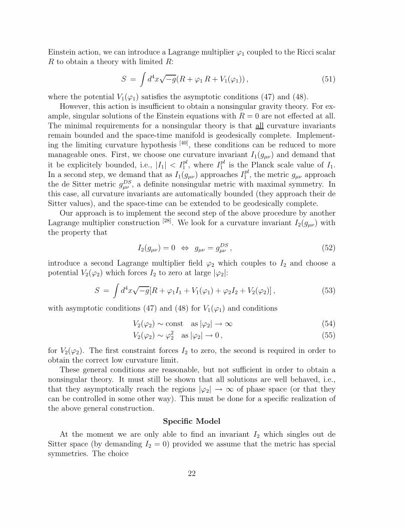
Einstein action, we can introduce a Lagrange multiplier ϕ1 coupled to the Ricci scalarR to obtain a theory with limited R:

S =∫

d4x√−g(R + ϕ1R + V1(ϕ1)) , (51)

where the potential V1(ϕ1) satisfies the asymptotic conditions (47) and (48).However, this action is insufficient to obtain a nonsingular gravity theory. For ex-

ample, singular solutions of the Einstein equations with R = 0 are not effected at all.The minimal requirements for a nonsingular theory is that all curvature invariantsremain bounded and the space-time manifold is geodesically complete. Implement-ing the limiting curvature hypothesis [40], these conditions can be reduced to moremanageable ones. First, we choose one curvature invariant I1(gµν) and demand that

it be explicitely bounded, i.e., |I1| < Ipl1 , where Ipl

1 is the Planck scale value of I1.In a second step, we demand that as I1(gµν) approaches Ipl

1 , the metric gµν approachthe de Sitter metric gDS

µν , a definite nonsingular metric with maximal symmetry. Inthis case, all curvature invariants are automatically bounded (they approach their deSitter values), and the space-time can be extended to be geodesically complete.

Our approach is to implement the second step of the above procedure by anotherLagrange multiplier construction [28]. We look for a curvature invariant I2(gµν) withthe property that

I2(gµν) = 0 ⇔ gµν = gDSµν , (52)

introduce a second Lagrange multiplier field ϕ2 which couples to I2 and choose apotential V2(ϕ2) which forces I2 to zero at large |ϕ2|:

S =∫

d4x√−g[R + ϕ1I1 + V1(ϕ1) + ϕ2I2 + V2(ϕ2)] , (53)

with asymptotic conditions (47) and (48) for V1(ϕ1) and conditions

V2(ϕ2) ∼ const as |ϕ2| → ∞ (54)

V2(ϕ2) ∼ ϕ22 as |ϕ2| → 0 , (55)

for V2(ϕ2). The first constraint forces I2 to zero, the second is required in order toobtain the correct low curvature limit.

These general conditions are reasonable, but not sufficient in order to obtain anonsingular theory. It must still be shown that all solutions are well behaved, i.e.,that they asymptotically reach the regions |ϕ2| → ∞ of phase space (or that theycan be controlled in some other way). This must be done for a specific realization ofthe above general construction.

Specific Model

At the moment we are only able to find an invariant I2 which singles out deSitter space (by demanding I2 = 0) provided we assume that the metric has specialsymmetries. The choice

22

I2 = (4RµνRµν −R2 + C2)1/2 , (56)

singles out the de Sitter metric among all homogeneous and isotropic metrics (inwhich case adding C2, the Weyl tensor square, is superfluous), all homogeneous andanisotropic metrics, and all radially symmetric metrics.

We choose the action [28,41]

S =∫

d4x√−g

[

R + ϕ1R− (ϕ2 +3√2ϕ1)I

1/22 + V1(ϕ1) + V2(ϕ2)

]

(57)

with

V1(ϕ1) = 12H20

ϕ21

1 + ϕ1

(

1 − ln(1 + ϕ1)

1 + ϕ1

)

(58)

V2(ϕ2) = −2√

3H20

ϕ22

1 + ϕ22

. (59)

The general equations of motion resulting from this action are quite messy. How-ever, when restricted to homogeneous and isotropic metrics of the form

ds2 = dt2 − a(t)2(dx2 + dy2 + dz2) , (60)

the equations are fairly simple. WithH = a/a, the two ϕ1 and ϕ2 constraint equationsare

H2 =1

12V ′

1 (61)

H = − 1

2√

3V ′

2 , (62)

and the dynamical g00 equation becomes

3(1 − 2ϕ1)H2 +

1

2(V1 + V2) =

√3H(ϕ2 + 3Hϕ2) . (63)

The phase space of all vacuum configurations is the half plane (ϕ1 ≥ 0, ϕ2). Equa-tions (61) and (62) can be used to express H and H in terms of ϕ1 and ϕ2. Theremaining dynamical equation (63) can then be recast as

dϕ2

dϕ1= − V ′′

1

4V ′2

[

−√

3ϕ2 + (1 − 2ϕ1) −2

V ′1

(V1 + V2)

]

. (64)

The solutions can be studied analytically in the asymptotic regions and numericallythroughout the entire phase space.

23

FIG. 10. Phase diagram of the homogeneous and isotropic solutions of the nonsingular

Universe. The asymptotic regions are labelled by A, B, C and D, flow lines are indicated

by arrows.

The resulting phase diagram of vacuum solutions is sketched in Fig. 10 (fornumerical results, see [41]). The point (ϕ1, ϕ2) = (0, 0) corresponds to Minkowskispace-time M4, the regions |ϕ2| → ∞ to de Sitter space. As shown, all solutionseither are periodic about M4 or else they asymptotically approach de Sitter space.Hence, all solutions are nonsingular. This conclusion remains unchanged if we addspatial curvature to the model.

One of the most interesting properties of our theory is asymptotic freedom [41],i.e., the coupling between matter and gravity goes to zero at high curvatures. It iseasy to add matter (e.g., dust or radiation) to our model by taking the combinedaction

S = Sg + Sm , (65)

where Sg is the gravity action previously discussed, and Sm is the usual matter actionin an external background space-time metric.

We find [41] that in the asymptotic de Sitter regions, the trajectories of the solu-tions in the (ϕ1, ϕ2) plane are unchanged by adding matter. This applies, for example,in a phase of de Sitter contraction when the matter energy density is increasing expo-nentially but does not affect the metric. The physical reason for asymptotic freedomis obvious: in the asymptotic regions of phase space, the space-time curvature ap-proaches its maximal value and thus cannot be changed even by adding an arbitraryhigh matter energy density.

Naturally, the phase space trajectories near (ϕ1, ϕ2) = (0, 0) are strongly effectedby adding matter. In particular, M4 ceases to be a stable fixed point of the evolutionequations.

24

Discussion

We have shown that a class of higher derivative extensions of the Einstein theoryexist for which many interesting solutions are nonsingular. Our class of models is veryspecial. Most higher derivative theories of gravity have, in fact, much worse singularityproperties than the Einstein theory. What is special about our class of theories isthat they are obtained using a well motivated Lagrange multiplier construction whichimplements the limiting curvature hypothesis. We have shown thati) all homogeneous and isotropic solutions are nonsingular [28,41]

ii) the two-dimensional black holes are nonsingular [42]

iii) nonsingular two-dimensional cosmologies exist [43].By construction, all solutions are de Sitter at high curvature. Thus, the theories

automatically have a period of inflation (driven by the gravity sector in analogy toStarobinsky inflation [27]) in the early Universe.

A very important property of our theories is asymptotic freedom. This means thatthe coupling between matter and gravity goes to zero at high curvature, and mightlead to an automatic suppression mechanism for scalar fluctuations.

E. Reheating in Inflationary Cosmology

Reheating is an important stage in inflationary cosmology. It determines thestate of the Universe after inflation and has consequences for baryogenesis, defectformation, and, as will be shown below, maybe even for the composition of the darkmatter of the Universe.

After slow rolling, the inflaton field begins to oscillate uniformly in space aboutthe true vacuum state. Quantum mechanically, this corresponds to a coherent stateof k = 0 inflaton particles. Due to interactions of the inflaton with itself and withother fields, the coherent state will decay into quanta of elementary particles. Thiscorresponds to post-inflationary particle production.

Reheating is usually studied using simple scalar field toy models. The one we willadopt here consists of two real scalar fields, the inflaton ϕ with Lagrangian

Lo =1

2∂µϕ∂

µϕ− 1

4λ(ϕ2 − σ2)2 (66)

interacting with a massless scalar field χ representing ordinary matter. The interac-tion Lagrangian is taken to be

LI =1

2g2ϕ2χ2 . (67)

Self interactions of χ are neglected.By a change of variables

ϕ = ϕ+ σ , (68)

25

the interaction Lagrangian can be written as

LI = g2σϕχ2 +1

2g2ϕ2χ2 . (69)

During the phase of coherent oscillations, the field ϕ oscillates with a frequency

ω = mϕ = λ1/2σ (70)

(neglecting the expansion of the Universe which can be taken into account as in[44,45]).

Elementary Theory of Reheating

According to the elementary theory of reheating (see e.g. [46] and [47]), the decayof the inflaton is calculated using first order perturbations theory. According to theFeynman rules, the decay rate ΓB of ϕ (calculated assuming that the cubic couplingterm dominates) is given by

ΓB =g2σ2

8πmφ. (71)

The decay leads to a decrease in the amplitude of ϕ (from now on we will dropthe tilde sign) which can be approximated by adding an extra damping term to theequation of motion for ϕ:

ϕ+ 3Hϕ+ ΓBϕ = −V ′(ϕ) . (72)

From the above equation it follows that as long as H > ΓB, particle production isnegligible. During the phase of coherent oscillation of ϕ, the energy density and henceH are decreasing. Thus, eventually H = ΓB, and at that point reheating occurs (theremaining energy density in ϕ is very quickly transferred to χ particles.

The temperature TR at the completion of reheating can be estimated by computingthe temperature of radiation corresponding to the value of H at which H = ΓB. Fromthe FRW equations it follows that

TR ∼ (ΓBmpl)1/2 . (73)

If we now use the “naturalness” constraint1

g2 ∼ λ (74)

1At one loop order, the cubic interaction term will contribute to λ by an amout ∆λ ∼ g2. A

renormalized value of λ smaller than g2 needs to be finely tuned at each order in perturbation

theory, which is “unnatural”.

26

in conjunction with the constraint on the value of λ from (43), it follows that forσ < mpl,

TR < 1010GeV . (75)

This would imply no GUT baryogenesis, no GUT-scale defect production, and nogravitino problems in supersymmetric models with m3/2 > TR, where m3/2 is thegravitino mass. As we shall see, these conclusions change radically if we adopt animproved analysis of reheating.

Modern Theory of Reheating

However, as was first realized in [48], the above analysis misses an essential point.To see this, we focus on the equation of motion for the matter field χ coupled tothe inflaton ϕ via the interaction Lagrangian LI of (69). Taking into account for themoment only the cubic interaction term, the equation of motion becomes

χ + 3Hχ− ((∇a

)2 −m2χ − 2g2σϕ)χ = 0 . (76)

Since the equation is linear in χ, the equations for the Fourier modes χk decouple:

χk + 3Hχk + (k2p +m2

χ + 2g2σϕ)χk = 0, (77)

where kp is the time-dependent physical wavenumber.Let us for the moment neglect the expansion of the Universe. In this case, the

friction term in (77) drops out and kp is time-independent, and Equation (77) be-comes a harmonic oscillator equation with a time-dependent mass determined by thedynamics of ϕ. In the reheating phase, ϕ is undergoing oscillations. Thus, the mass in(77) is varying periodically. In the mathematics literature, this equation is called theMathieu equation. It is well known that there is an instability. In physics, the effectis known as parametric resonance (see e.g. [49]). At frequencies ωn correspondingto half integer multiples of the frequency ω of the variation of the mass, i.e.

ω2k = k2

p +m2χ = (

n

2ω)2 n = 1, 2, ..., (78)

there are instability bands with widths ∆ωn. For values of ωk within the instabilityband, the value of χk increases exponentially:

χk ∼ eµt with µ ∼ g2σϕ0

ω, (79)

with ϕ0 being the amplitude of the oscillation of ϕ. Since the widths of the instabilitybands decrease as a power of the (small) coupling constant g2 with increasing n, forpractical purposes only the lowest instability band is important. Its width is

∆ωk ∼ gσ1/2ϕ1/20 . (80)

27

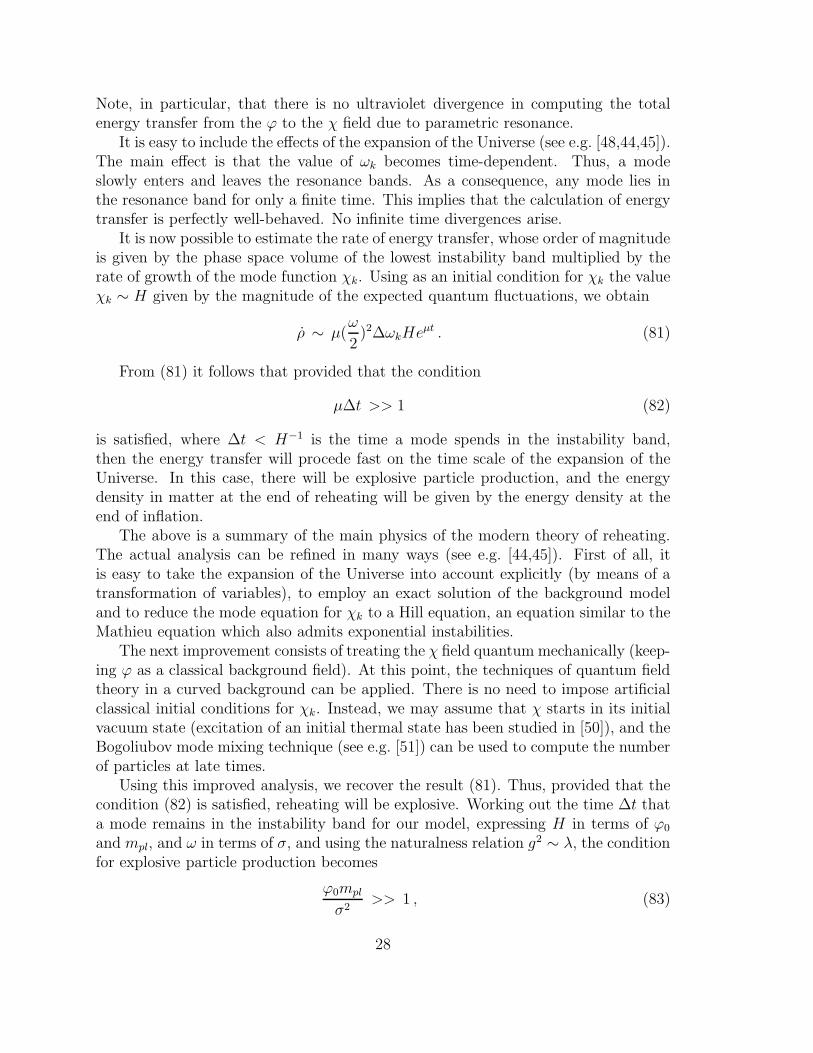
Note, in particular, that there is no ultraviolet divergence in computing the totalenergy transfer from the ϕ to the χ field due to parametric resonance.

It is easy to include the effects of the expansion of the Universe (see e.g. [48,44,45]).The main effect is that the value of ωk becomes time-dependent. Thus, a modeslowly enters and leaves the resonance bands. As a consequence, any mode lies inthe resonance band for only a finite time. This implies that the calculation of energytransfer is perfectly well-behaved. No infinite time divergences arise.

It is now possible to estimate the rate of energy transfer, whose order of magnitudeis given by the phase space volume of the lowest instability band multiplied by therate of growth of the mode function χk. Using as an initial condition for χk the valueχk ∼ H given by the magnitude of the expected quantum fluctuations, we obtain

ρ ∼ µ(ω

2)2∆ωkHe

µt . (81)

From (81) it follows that provided that the condition

µ∆t >> 1 (82)

is satisfied, where ∆t < H−1 is the time a mode spends in the instability band,then the energy transfer will procede fast on the time scale of the expansion of theUniverse. In this case, there will be explosive particle production, and the energydensity in matter at the end of reheating will be given by the energy density at theend of inflation.

The above is a summary of the main physics of the modern theory of reheating.The actual analysis can be refined in many ways (see e.g. [44,45]). First of all, itis easy to take the expansion of the Universe into account explicitly (by means of atransformation of variables), to employ an exact solution of the background modeland to reduce the mode equation for χk to a Hill equation, an equation similar to theMathieu equation which also admits exponential instabilities.

The next improvement consists of treating the χ field quantum mechanically (keep-ing ϕ as a classical background field). At this point, the techniques of quantum fieldtheory in a curved background can be applied. There is no need to impose artificialclassical initial conditions for χk. Instead, we may assume that χ starts in its initialvacuum state (excitation of an initial thermal state has been studied in [50]), and theBogoliubov mode mixing technique (see e.g. [51]) can be used to compute the numberof particles at late times.

Using this improved analysis, we recover the result (81). Thus, provided that thecondition (82) is satisfied, reheating will be explosive. Working out the time ∆t thata mode remains in the instability band for our model, expressing H in terms of ϕ0

and mpl, and ω in terms of σ, and using the naturalness relation g2 ∼ λ, the conditionfor explosive particle production becomes

ϕ0mpl

σ2>> 1 , (83)

28

which is satisfied for all chaotic inflation models with σ < mpl (recall that slow rollingends when ϕ ∼ mpl and that therefore the initial amplitude ϕ0 of oscillation is of theorder mpl).

We conclude that rather generically, reheating in chaotic inflation models will beexplosive. This implies that the energy density after reheating will be approximatelyequal to the energy density at the end of the slow rolling period. Therefore, assuggested in [52,53] and [54], respectively, GUT scale defects may be produced afterreheating and GUT-scale baryogenesis scenarios may be realized, provided that theGUT energy scale is lower than the energy scale at the end of slow rolling.

Note, however, that the state of χ after parametric resonance is not a thermalstate. The spectrum consists of high peaks in distinct wave bands. An importantquestion which remains to be studied is how this state thermalizes. For some inter-esting work on this issue see [55]. As emphasized in [52] and [53], the large peaksin the spectrum may lead to symmetry restoration and to the efficient production oftopological defects (for a differing view on this issue see [56,57]). Since the state afterexplosive particle production is not a thermal state, it is useful to follow [44] and callthis process “preheating” instead of reheating.

A futher interesting conjecture which emerges from the parametric resonance anal-ysis of preheating [44,45] is that the dark matter in the Universe may consist of remnantcoherent oscillations of the inflaton field. In fact, it can easily be checked from (83)that the condition for efficient transfer of energy eventually breaks down when ϕ0

has decreased to a sufficiently small value. For the model considered here, an orderof magnitude calculation shows that the remnant oscillations may well contributesignificantly to the present value of Ω.

Note that the details of the analysis of preheating are quite model-dependent.In fact [44], in many models one does not get the kind of “narrow-band” resonancediscussed here, but “wide-band” resonance. In this case, the energy transfer is evenmore efficient.

There has recently been a lot of work on various aspects of reheating (see e.g.[58–61] for different approaches). Many important questions, e.g. concerning ther-malization and back-reaction effects during and after preheating (or parametric res-onance) remain to be fully analyzed.

F. Summary

The inflationary Universe is an attractive scenario for early Universe cosmology.It can resolve some of the problems of standard cosmology, and in addition gives riseto a predictive theory of structure formation (see e.g. [62] for a recent review).

However, important unsolved problems of principle remain. Rather generically,the predicted amplitude of perturbations is too large (the spectral shape, however, isin quite good agreement with the observations). The present realizations of inflationbased on scalar field also make the cosmological constant problem more accute. In

29

addition, there are no convincing particle-physics based realizations of inflation. Manymodels of inflation resort to introducing a new matter sector. It is important to searchfor a better connection between modern particle physics / field theory and inflation.String cosmology and dilaton gravity (see e.g. the recent reviews in [63]) may providean interesting new approach to the unification of inflation and fundamental physics.

Recently, there has been much progress in the understanding of the energy transferat the end of inflation between the inflaton field and matter. It appears that resonancephenomena such as parametric resonance play a crucial role. These new reheatingscenarios lead to a high reheating temperature, although much more work remains tobe done before one can reach a final conclusion on this issue.

III. CLASSICAL AND QUANTUM THEORY OF COSMOLOGICAL

PERTURBATIONS

In inflationary Universe and topological defect models of structure formation,small amplitude seed perturbations are predicted to arise due to particle physicseffects in the very early Universe. They then grow by gravitational instability toproduce the cosmological structures we observe today. In order to be able to makethe connection between particle physics and observations, it is important to under-stand the gravitational evolution of fluctuations. This section will introduce the basicconcepts of this topic.

As is evident from Figure 5 and from the discussion of inflation in the previoussection, general relativity and quantum mechanics both play a fundamental role inthe theory of perturbations. In inflationary Universe models, quantum effects seedthe fluctuations, and thus a quantum analysis of the generation of fluctuations isessential. However, since the fluctuations are small, a linearized analysis is sufficient.Since the scales on which we are interested in following the fluctuations are larger thanthe Hubble radius for a long time interval, Newtonian gravity is obviously inadequateto treat these perturbations, and general relativistic effects become essential.

In this section, we will first introduce some basic notation, then discuss the New-tonian theory of linear fluctuations before turning to the full relativistic analysis.

A. Basic Issues

In this article we only discuss theories in which structures grow by gravitationalaccretion. The basic mechanism is easy to understand. Consider first a flat space-time background. A density perturbation with δρ > 0 leads to an excess gravitationalattractive force F acting on the surrounding matter. This force is proportional to δρ,and will hence lead to exponential growth of the perturbation since

δρ ∼ F ∼ δρ⇒ δρ ∼ exp(αt) (84)

30

with a constant α which is proportional to Newton’s constant G.In an expanding background space-time, the acceleration is damped by the ex-

pansion. If r(t) is the physical distance of a test particle from the perturbation, thenon a scale r

δρ ∼ F ∼ δρ

r2(t), (85)

which results in power-law increase of δρ. The goal of this subsection is to discuss thegrowth rates of inhomogeneities in more detail (see e.g. [64,65] for modern reviews).

Because of our assumption that all perturbations start out with a small amplitude,we can linearize the equations for gravitational fluctuations. The analysis is thengreatly simplified by going to momentum space in which all modes δ(k) decouple.We expand the fractional density contrast δ(x) as follows:

δ(x) =δρ(x)

ρ= (2π)−3/2V 1/2

∫

d3k eik·xδ(k) , (86)

where V is a cutoff volume which disappears from all physical observables.The “power spectrum” P (k) is defined by

P (k) =< |δ(k)|2 > , (87)

where the braces denote an ensemble average (in most structure formation models,the generation of perturbations is a stochastic process, and hence observables canonly be calculated by averaging over the ensemble. For observations, the braces canbe viewed as an angular average).

The physical measure of mass fluctuations on a length scale λ is the r.m.s. massfluctuation δM/M(λ) on this scale. It is determined by the power spectrum in thefollowing way. We pick a center x0 of a sphere Bλ(x0) of radius λ and calculate

|δMM

|2 (x0, λ) = |∫

Bλ(x0)

d3xδ(x)1

V (Bλ)|2 , (88)

where V (Bλ) is the volume of the sphere. Inserting the Fourier decomposition (86)and taking the average value of this quantity over all x0 yields

<

(

δM

M

)2

(λ) >=∫

d3kWk(λ)|δ(k)|2 (89)

with a window function Wk(λ) with the following properties

Wk(λ)≃ 1 k < kλ = 2π/λ≃ 0 k > kλ .

(90)

Therefore the r.m.s. mass perturbation on a scale λ becomes

31

< |δMM

(λ)|2 >∼ k3λP (kλ) . (91)

If P (k) ∼ kn then n is called the index of the power spectrum. For n = 1 we getthe so-called Harrison-Zel’dovich scale invariant spectrum [66].

Both inflationary Universe and topological defect models of structure formationpredict a roughly scale invariant spectrum. The distinguishing feature of this spec-trum is that the r.m.s. mass perturbations are independent of the scale k whenmeasured at the time tH(k) when the associated wavelength is equal to the Hubbleradius, i.e., when the scale “enters” the Hubble radius. Let us derive this fact for thescales entering during the matter dominated epoch. The time tH(k) is determined by

k−1a(tH(k)) = tH(k) (92)

which leads to tH(k) ∼ k−3. According to the linear theory of cosmological perturba-tions discussed in the following subsection, the mass fluctuations increase as a(t) fort > teq. Hence

δM

M(k, tH(k)) =

(

tH(k)

t

)2/3δM

M(k, t) ∼ const , (93)

since the first factor scales (from (92) as k−2 and – using (91) and inserting n = 1 –the second as k2.

B. Newtonian Theory

The Newtonian theory of cosmological perturbations is an approximate analysiswhich is valid on wavelengths λ much smaller than the Hubble radius t and fornegligible pressure p, i.e., p ≪ ρ. It is based on expanding the hydrodynamicalequations about a homogeneous background solution.

The starting points are the continuity, Euler and Poisson equations

ρ+ ∇(ρv) = 0 (94)

v + (v · ∇)v = −∇φ− 1

ρ∇p (95)

∇2φ = 4πGρ (96)

for a fluid with energy density ρ, pressure p, velocity v and Newtonian gravitationalpotential φ, written in terms of physical coordinates (t, r).

The transition to an expanding space is made by introducing comoving coordinatesx and peculiar velocity u = x:

32

r = a(t)x (97)

v = a(t)x+ a(t)u . (98)

The first term on the right hand side of (98) is the expansion velocity.The perturbation equations are obtained by linearizing Equations (94 - 96) about

a homogeneous background solution ρ = ρ(t), p = 0 and u = 0. The linearizationansatz can be written

ρ(x, t) = ρ(t)(1 + δ(x, t)) |δ| << 1. (99)

If we consider adiabatic perturbations (no entropy density variations), then after somealgebra the linearized equations become

δ + ∇ · u = 0 , (100)

u+ 2a

au = −a2(∇δφ+ c2s∇δ) (101)

and

∇2δφ = 4πGρa2δ , (102)

with the speed of sound cs given by

c2s =∂p

∂ρ. (103)

The two first order equations (100) and (101) can be combined to yield a single secondorder differential equation for δ. With the help of (102) this equation reads

δ + 2Hδ − 4πGρδ − c2sa2

∇2δ = 0 (104)

which in momentum space becomes

δk + 2Hδk +

(

c2sk2

a2− 4πGρ

)

δk = 0 . (105)

Here, H(t) as usual denotes the expansion rate, and δk stands for δ(k).Already a quick look at Equation (105) reveals the presence of a distinguished

scale for cosmological perturbations, the Jeans length

λJ =2π

kJ(106)

33

with

k2J =

(

k

a

)2

=4πGρ

c2s. (107)

On length scales larger than λJ , the spatial gradient term is negligible, and the termlinear in δ in (105) acts like a negative mass square quadratic potential with dampingdue to the expansion of the Universe, in agreement with the intuitive analysis leadingto (refintu1) and (85). On length scales smaller than λJ , however, (105) becomes adamped harmonic oscillator equation and perturbations on these scales decay.

For t > teq and for λ≫ λJ , Equation (105) becomes

δk +4

3tδk −

2

3t2δk = 0 (108)

and has the general solution

δk(t) = c1t2/3 + c2t

−1 . (109)

This demonstrates that for t > teq and λ≫ λJ , the dominant mode of perturbationsincreases as a(t), a result we already used in the previous subsection (see (93)).

For λ≪ λJ and t > teq, Equation (105) becomes

δk + 2Hδk + c2s

(

k

a

)2

δk = 0 , (110)

and has solutions corresponding to damped oscillations:

δk(t) ∼ a−1/2(t) exp±icsk∫

dt′a(t′)−1 . (111)

As an important application of the Newtonian theory of cosmological perturba-tions, let us compare sub-horizon scale fluctuations in a baryon-dominated Universe(Ω = ΩB = 1) and in a CDM-dominated Universe with ΩCDM = 0.9 and Ω = 1. Weconsider scales which enter the Hubble radius at about teq.

In the initial time interval teq < t < trec, the baryons are coupled to the photons.Hence, the baryonic fluid has a large pressure pB

pB ≃ pr =1

3ρr , (112)

and therefore the speed of sound is relativistic

cs ≃(

pr

ρm

)1/2

=1√3

(

ρr

ρm

)1/2

. (113)

34

The value of cs slowly decreases in this time interval, attaining a value of about 1/10at trec. From (107) it follows that the Jeans mass MJ , the mass inside a sphere ofradius λJ , increases until trec when it reaches its maximal value Mmax

J

MmaxJ = MJ(trec) =

4π

3λJ(trec)

3ρ(trec) ∼ 1017(Ωh2)−1/2M⊙ . (114)

At the time of recombination, the baryons decouple from the radiation fluid.Hence, the baryon pressure pB drops abruptly, as does the Jeans length (see (107)).The remaining pressure pB is determined by the temperature and thus continues todecrease as t increases. It can be shown that the Jeans mass continues to decreaseafter trec, starting from a value

M−

J (trec) ∼ 106(Ωh2)−1/2 M⊙ (115)

(where the superscript “−” indicates the mass immediately after teq.In contrast, CDM has negligible pressure throughout the period t > teq and hence

experiences no Jeans damping. A CDM perturbation which enters the Hubble radiusat teq with amplitude δi has an amplitude at trec given by

δCDMk (trec) ≃

a(trec)

a(teq)δi , (116)

whereas a perturbation with the same scale and initial amplitude in a baryon-dominated Universe is damped

δBDMk (trec) ≃

(

a(trec)

a(teq)

)−1/2

δi . (117)

In order for the perturbations to have the same amplitude today, the initial size ofthe inhomogeneity must be much larger in a BDM-dominated Universe than in aCDM-dominated one:

δBDMk (teq) ≃

(

z(teq)

z(trec)

)3/2

δCDMk (teq) . (118)

For Ω = 1 and h = 1/2 the enhancement factor is about 30.In a CDM-dominated Universe the baryons experience Jeans damping, but after

trec the baryons quickly fall into the potential wells created by the CDM perturbations,and hence the baryon perturbations are proportional to the CDM inhomogeneities.

The above considerations, coupled with information about CMB anisotropies, canbe used to rule out a model with Ω = ΩB = 1. The argument goes as follows. Foradiabatic fluctuations, the amplitude of CMB anisotropies on an angular scale ϑ isdetermined by the value of δρ/ρ (strictly speaking, the relativistic potential Φ to bediscussed in the following subsection) on the corresponding length scale λ(ϑ) at teq:

35

δT

T(ϑ) =

1

3

δρ

ρ(λ(ϑ), teq) . (119)

On scales of clusters we know that (for Ω = 1 and h = 1/2)

(

δρ

ρ

)

CDM

(λ(ϑ), teq) ≃ z(teq)−1 ≃ 10−4 , (120)

using the fact that today on cluster scales δρ/ρ ≃ 1. The bounds on δT/T on smallangular scales are

δT

T(ϑ) << 10−4 , (121)

consistent with the predictions for a CDM model, but inconsistent with those of aΩ = ΩB = 1 model, according to which we would expect anisotropies of the order of10−3. This is yet another argument in support of the existence of nonbaryonic darkmatter.

To conclude this subsection, let us briefly discuss two further aspects relatedto Newtonian perturbations. The first concerns matter inhomogeneities during theradiation-dominated epoch. We consider matter fluctuations with cs = 0 in a smoothrelativistic background. In this case, Equation (105) becomes

δk + 2Hδk − 4πGρmδk = 0 , (122)

where ρm denotes the average matter energy density. The Hubble expansion param-eter obeys

H2 =8πG

3(ρm + ρr) , (123)

with ρr the background radiation energy density. For t < teq, ρm is negligible in both(122) and (123), and (122) has the general solution

δk(t) = c1 log t+ c2 . (124)

In particular, this result implies that CDM perturbations which enter the Hubbleradius before teq have an amplitude which grows only logarithmically in time untilteq.

Finally, we consider hot dark matter (HDM) fluctuations. Whereas CDM particlesare cold, i.e. their peculiar velocity is negligible for all times relevant for structureformation, HDM particles have relativistic velocities at teq, i.e. v(teq) ∼ 1. The primecandidate for HDM is a 25h2

50eV tau neutrino.The new aspect of HDM is related to neutrino free streaming [67]. Because of

the large velocity of the dark matter particles, pure dark matter inhomogeneities arewashed out on all scales below the neutrino free streaming length λc

j(t),

36

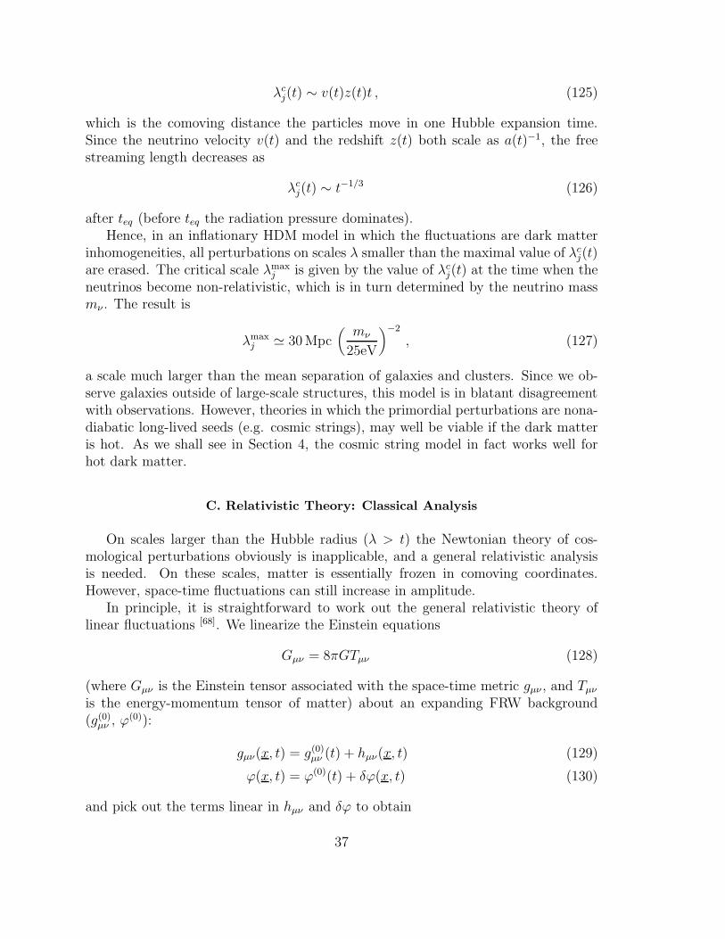
λcj(t) ∼ v(t)z(t)t , (125)

which is the comoving distance the particles move in one Hubble expansion time.Since the neutrino velocity v(t) and the redshift z(t) both scale as a(t)−1, the freestreaming length decreases as

λcj(t) ∼ t−1/3 (126)

after teq (before teq the radiation pressure dominates).Hence, in an inflationary HDM model in which the fluctuations are dark matter

inhomogeneities, all perturbations on scales λ smaller than the maximal value of λcj(t)

are erased. The critical scale λmaxj is given by the value of λc

j(t) at the time when theneutrinos become non-relativistic, which is in turn determined by the neutrino massmν . The result is

λmaxj ≃ 30 Mpc

(

mν

25eV

)−2

, (127)

a scale much larger than the mean separation of galaxies and clusters. Since we ob-serve galaxies outside of large-scale structures, this model is in blatant disagreementwith observations. However, theories in which the primordial perturbations are nona-diabatic long-lived seeds (e.g. cosmic strings), may well be viable if the dark matteris hot. As we shall see in Section 4, the cosmic string model in fact works well forhot dark matter.

C. Relativistic Theory: Classical Analysis

On scales larger than the Hubble radius (λ > t) the Newtonian theory of cos-mological perturbations obviously is inapplicable, and a general relativistic analysisis needed. On these scales, matter is essentially frozen in comoving coordinates.However, space-time fluctuations can still increase in amplitude.

In principle, it is straightforward to work out the general relativistic theory oflinear fluctuations [68]. We linearize the Einstein equations

Gµν = 8πGTµν (128)

(where Gµν is the Einstein tensor associated with the space-time metric gµν , and Tµν

is the energy-momentum tensor of matter) about an expanding FRW background(g(0)

µν , ϕ(0)):

gµν(x, t) = g(0)µν (t) + hµν(x, t) (129)

ϕ(x, t) = ϕ(0)(t) + δϕ(x, t) (130)

and pick out the terms linear in hµν and δϕ to obtain

37

δGµν = 8πGδTµν . (131)

In the above, hµν is the perturbation in the metric and δϕ is the fluctuation of thematter field ϕ. We have denoted all matter fields collectively by ϕ.

In practice, there are many complications which make this analysis highly nontriv-ial. The first problem is “gauge invariance” [69] Imagine starting with a homogeneousFRW cosmology and introducing new coordinates which mix x and t. In terms of thenew coordinates, the metric now looks inhomogeneous. The inhomogeneous piece ofthe metric, however, must be a pure coordinate (or ”gauge”) artefact. Thus, whenanalyzing relativistic perturbations, care must be taken to factor out effects due tocoordinate transformations.

FIG. 11. Sketch of how two choices of the mapping from the background space-time

manifold M0 to the physical manifold M induce two different coordinate systems on M.

The issue of gauge dependence is illustrated in Fig. 11. A coordinate system onthe physical inhomogeneous space-time manifold M can be viewed as a mapping Dof an unperturbed space-time M0 into M. A physical quantity Q is a geometricalfunction defined on M. There is a corresponding physical quantity (0)Q defined onM0. In the coordinate system given by D, the perturbation δQ of Q at the space-timepoint p ǫM is

δQ(p) = Q(p) − (0)Q (D−1(p)) . (132)

However, in a second coordinate system D the perturbation is given by

δQ(p) = Q(p) − (0)Q(D−1(p)) . (133)

The difference

38

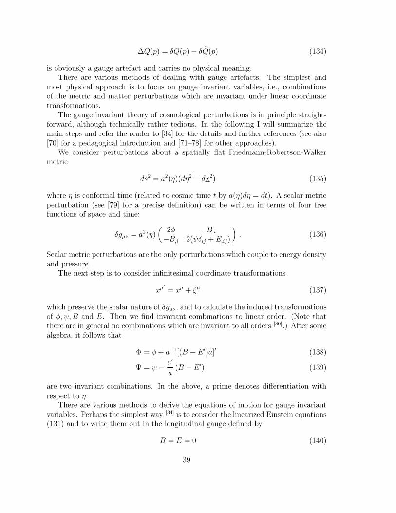
∆Q(p) = δQ(p) − δQ(p) (134)

is obviously a gauge artefact and carries no physical meaning.There are various methods of dealing with gauge artefacts. The simplest and

most physical approach is to focus on gauge invariant variables, i.e., combinationsof the metric and matter perturbations which are invariant under linear coordinatetransformations.

The gauge invariant theory of cosmological perturbations is in principle straight-forward, although technically rather tedious. In the following I will summarize themain steps and refer the reader to [34] for the details and further references (see also[70] for a pedagogical introduction and [71–78] for other approaches).

We consider perturbations about a spatially flat Friedmann-Robertson-Walkermetric

ds2 = a2(η)(dη2 − dx2) (135)

where η is conformal time (related to cosmic time t by a(η)dη = dt). A scalar metricperturbation (see [79] for a precise definition) can be written in terms of four freefunctions of space and time:

δgµν = a2(η)(

2φ −B,i

−B,i 2(ψδij + E,ij)

)

. (136)

Scalar metric perturbations are the only perturbations which couple to energy densityand pressure.

The next step is to consider infinitesimal coordinate transformations

xµ′

= xµ + ξµ (137)

which preserve the scalar nature of δgµν , and to calculate the induced transformationsof φ, ψ,B and E. Then we find invariant combinations to linear order. (Note thatthere are in general no combinations which are invariant to all orders [80].) After somealgebra, it follows that

Φ = φ+ a−1[(B − E ′)a]′ (138)

Ψ = ψ − a′

a(B − E ′) (139)

are two invariant combinations. In the above, a prime denotes differentiation withrespect to η.

There are various methods to derive the equations of motion for gauge invariantvariables. Perhaps the simplest way [34] is to consider the linearized Einstein equations(131) and to write them out in the longitudinal gauge defined by

B = E = 0 (140)

39

and in which Φ = φ and Ψ = ψ, to directly obtain gauge invariant equations.For several types of matter, in particular for scalar field matter, the perturbation

of Tµν has the special property

δT ij ∼ δi

j (141)

which imples Φ = Ψ. Hence, the scalar-type cosmological perturbations can in thiscase be described by a single gauge invariant variable. The equation of motion takesthe form [37,81,75,82]

ξ = O

(

k

aH

)2

Hξ (142)

where

ξ =2

3

H−1Φ + Φ

1 + w+ Φ . (143)

The variable w = p/ρ (with p and ρ background pressure and energy densityrespectively) is a measure of the background equation of state. In particular, onscales larger than the Hubble radius, the right hand side of (142) is negligible, andhence ξ is constant.

The result that ξ = 0 is a very powerful one. Let us first imagine that the equationof state of matter is constant, i.e., w = const. In this case, ξ = 0 implies

Φ(t) = const , (144)

i.e., this gauge invariant measure of perturbations remains constant outside the Hub-ble radius.

Next, consider the evolution of Φ during a phase transition from an initial phasewith w = wi to a phase with w = wf . Long before and after the transition, Φ isconstant because of (144), and hence ξ = 0 becomes

Φ

1 + w+ Φ = const , (145)

In order to make contact with matter perturbations and Newtonian intuition, itis important to remark that, as a consequence of the Einstein constraint equations,at Hubble radius crossing Φ is a measure of the fractional density fluctuations:

Φ(k, tH(k)) ∼ δρ

ρ(k, tH(k)) . (146)

(Note that the latter quantity is approximately gauge invariant on scales smaller thanthe Hubble radius).

40

D. Relativistic Theory: Quantum Analysis

The question of the origin of classical density perturbations from quantum fluc-tuations in the de Sitter phase of an inflationary Universe is a rather subtle issue.Starting from a homogeneous quantum state (e.g., the vacuum state in the FRWcoordinate frame at time ti, the beginning of inflation), a naive semiclassical anaylsiswould predict the absence of fluctuations since < ψ|Tµν(x)|ψ > is independent ofspace.

However, as a simple thought experiment shows, such a naive analysis is inap-propriate. Imagine a local gravitational mass detector D positioned close to a largemass M which is suspended from a pole. The decay of an alpha particle will severthe cord by which the mass is held to the pole and the mass will drop. According tothe semiclassical prescription

Gµν = 8πG < ψ|Tµν |ψ > , (147)

the metric (i.e., the mass measured) will slowly decrease. This is obviously not whathappens. The mass detector shows a signal which corresponds to one of the classicaltrajectories which make up the state |ψ >, a trajectory corresponding to a suddendrop in the gravitational force measured.

The origin of classical density perturbations as a consequence of quantum fluctua-tions in a homogeneous state |ψ > can be analyzed along similar lines. The quantumto classical transition is picking out [83–85] one of the typical classical trajectorieswhich make up the wave function of |ψ >. We can implement [86,87] the procedure asfollows: Define a classical scalar field

ϕcl(x, t) = ϕ0(t) + δϕ(x, t) (148)

with vanishing spatial average of δϕ. The induced classical energy momentum tensorT cl

µν(x, t) which is the source for the metric is given by

T clµν(x, t) = Tµν(ϕcl(x, t)) , (149)

where Tµν (ϕcl(x, t)) is defined as the canonical energy-momentum tensor of the clas-sical scalar field ϕcl(x, t). Unless δϕ vanishes, T cl

µν is inhomogeneous.For applications to chaotic inflation, we take |ψ > to be a Gaussian state with

mean value ϕ0(t)

< ψ|ϕ2(x, t)|ψ >= ϕ20(t) . (150)

Its width is taken to be the width of the vacuum state of the free scalar field theorywith mass determined by the curvature of V (ϕ) at ϕ0. This state is used to definethe Fourier transform δϕ(k, t) by

|δϕ(k)|2 =< ψ| |ϕ(k)|2 |ψ > . (151)

41

The amplitude of δϕ(k) is identified with the width of the ground state wave functionof the harmonic osciallator ϕ(k). (Recall that each Fourier mode of a free scalar fieldis a harmonic oscillator). Note that no divergences arise in the above construction.

By linearizing (149) about ϕ0(t) we obtain the perturbation of the energy-momentum tensor. In particular, the energy density fluctuation δρ(k) is given by

δρ(k) = ϕ0δ ˙ϕ(k) + V ′(ϕ0)δϕ(k) . (152)

To obtain the initial amplitude (39) of δM/M , the above is to be evaluated at thetime ti(k).

The computation of the spectrum of density perturbations produced in the deSitter phase has been reduced to the evaluation of the expectation value (151). First,we must specify the state |ψ >. (Recall that in non-Minkowski space-times there isno uniquely defined vacuum state of a quantum field theory [51]). We pick the FRWframe of the pre-inflationary period. In this frame, the number density of particlesdecreases exponentially. Hence we choose |ψ > to be the vacuum state in this frame(see [88] for a discussion of other choices). ψ[ϕ(k), t], the wave functional of |ψ >,can be calculated explicitly. It is basically the superposition of the ground state wavefunctions for all oscillators

ψ[ϕ(k), t] = N exp

−1

2(2π)−3a3(t)

∫

d3kω(k, t)|ϕ(k)|2

. (153)

N is a normalization constant and ω(k, t) ∼ H at t = ti(k). Hence

δϕ(k, t) = (2π)3/2a−3/2ω(k, t)−1/2 ∼ (2π)3/2k−3/2H , t = ti(k) . (154)

Given the above determination of the intitial amplitude of density perturbationsat the time when they leave the Hubble radius during the de Sitter phase, and thegeneral relativistic analysis of the evolution of fluctuations discussed in the previoussubsection, it is easy to evaluate the r.m.s. inhomogeneities when they reenter theHubble radius at time tf (k).

First, we combine (152), (154), (39), (87) and (91) to obtain

(

δM

M

)2

(k, ti(k)) ∼ k3

(

V ′(ϕ0)δϕ(k, ti(k))

ρ0

)2

∼(

V ′(ϕ0)H

ρ0

)2

. (155)

If the background scalar field is rolling slowly, then

V ′(ϕ0(ti(k))) = 3H|ϕ0(ti(k))| . (156)

and

(1 + p/ρ)(ti(k)) ≃ ρ−10 ϕ2

0(ti(k)) . (157)

Combining (155), (156), (157) and (40) we get

42

δM

M(k, tf (k)) ∼

3H2|ϕ0(ti(k))|ϕ2

0(ti(k))=

3H2

|ϕ0(ti(k))|(158)

This result can now be evaluated for specific models of inflation to find the conditionson the particle physics parameters which give a value

δM

M(k, tf (k)) ∼ 10−5 (159)

which is required if quantum fluctuations from inflation are to provide the seeds forgalaxy formation and agree with the CMB anisotropy limits.

For chaotic inflation with a potential

V (ϕ) =1

2m2ϕ2 , (160)

we can solve the slow rolling equations for the inflaton to obtain

δM

M(k, tf(k)) ∼ 10

m

mpl(161)

which implies that m ∼ 1013 GeV to agree with (159).Similarly, for a quartic potential

V (ϕ) =1

4λϕ4 (162)

we obtain

δM

M(k, tf (k)) ∼ 10 · λ1/2 (163)

which requires λ ≤ 10−12 in order not to conflict with observations.The conditions (161) and (163) require the presence of small parameters in the

particle physics model. It has been shown quite generally [38] that small parametersare required if inflation is to solve the fluctuation problem.

I have chosen to present the analysis of fluctuations in inflationary cosmology intwo separate steps in order to highlight the crucial physics issues. Having done this,it is possible to step back and construct a unified analysis of the quantum generationand classical evolution of perturbations in an inflationary Universe (for a detailedreview see [34]).

The basic point is that at the linearized level, the equations describing both grav-itational and matter perturbations can be quantized in a consistent way. The use ofgauge invariant variables makes the analysis both physically clear and computation-ally simple.

The first step of this analysis is to consider the action for the linear perturbationsin a background homogeneous and isotropic Universe, and to express the result in

43

terms of gauge invariant variables describing the fluctuations. Focusing on the scalarperturbations, it turns out that after a lot of algebra the action reduces to the actionof a single gauge invariant free scalar field with a time dependent mass [89,90] (the timedependence relects the expansion of the background space-time). This result is notsuprising. Based on the study of classical cosmological perturbations, we know thatthere is only one field degree of freedom for the scalar perturbations (for matter the-ories which obey (141)). Since at the linearized level there are no mode interactions,the action for this field must be that of a free scalar field.

The action thus has the same form as the action for a scalar matter field in a timedependent gravitational or electromagnetic background, and we can use standardmethods to quantize this theory (see e.g. [51]). If we employ canonical quantization,then the mode functions of the field operator obey the same classical equations as wederived in the gauge-invariant analysis of relativistic perturbations.

The time dependence of the mass is relected in the nontrivial form of the solutionsof the mode equations. The mode equations have growing modes which correspondto particle production or equivalently to the generation and amplification of fluctua-tions. We can start the system off (e.g. at the beginning of inflation) in the vacuumstate (defined as a state with no particles with respect to a local comoving observer).The state defined this way will not be the vacuum state from the point of view ofan observer at a later time. The Bogoliubov mode mixing technique can be used tocalculate the number density of perticles at a later time. In particular, expectationvalues of field operators such as the power spectrum can be computed, and the re-sults agree with those obtained using the heuristic analysis at the beginning of thissubsection.

E. Summary

To summarize the main results of the analysis of density fluctuations in inflationarycosmology:

1. Quantum vacuum fluctuations in the de Sitter phase of an inflationary Universeare the source of perturbations.

2. The quantum perturbations decohere on scales outside the Hubble radius andcan hence be treated classically.

3. As a consequence of the change in the background equation of state, the clas-sical evolution outside the Hubble radius produces a large amplification of theperturbations. In fact, unless the particle physics model contains very smallcoupling constants, the predicted fluctuations are in excess of those allowed bythe bounds on cosmic microwave anisotropies.

44

4. The quantum generation and classical evolution of fluctuations can be treatedin a unified manner. The formalism is no more complicated that the study of afree scalar field in a time dependent background.

5. Inflationary Universe models generically produce an approximately scale invari-ant Harrison-Zel’dovich spectrum

δM

M(k, tf(k)) ≃ const. (164)

It is not hard to construct models which give a different spectrum. All that isrequired is a significant change in H during the period of inflation.

Once inside the Hubble radius, the evolution of the mass perturbations is influ-enced by the damping effects discussed in Section 3.B, which in turn depend on thecomposition of the dark matter.

On scales which enter the Hubble radius before teq, the perturbations can onlygrow logarithmically in time between tf (k) and teq. This implies that (up to loga-rithmic corrections), the mass perturbation spectrum is flat for wavelengths smallerthan λeq, the comoving Hubble radius at teq:

δM

M(λ, t) ≃ const, t ≤ teq, λ < λeq, (165)

whereas on larger scales

δM

M(λ, t) ∝ λ−2. (166)

Equations (165) and (166) give the power spectrum in an Ω = 1 inflationary CDMmodel. If the dark matter is hot, then neutrino free streaming cuts off the powerspectrum at λmax

J (see (127)).

IV. TOPOLOGICAL DEFECTS, STRUCTURE FORMATION AND

BARYOGENESIS

A. Quantifying Data on Large-Scale Structure

It is length scales corresponding to galaxies and larger which are of greatest inter-est in cosmology when attempting to find an imprint of the primordial fluctuationsproduced by particle physics. On these scales, gravitational effects are assumed tobe dominant, and the fluctuations are not too far from the linear regime. On smallerscales, nonlinear gravitational and hydrodynamical effects determine the final stateand mask the initial perturbations.

45

To set the scales, consider the mean separation of galaxies, which is about 5h−1

Mpc [91], and that of Abell clusters which is around 25h−1 Mpc [92]. The largestcoherent structures seen in current redshift surveys have a length of about 100h−1

Mpc [3,4], the recent detections of CMB anisotropies probe the density field on lengthscales of about 103h−1 Mpc, and the present horizon corresponds to a distance ofabout 3 · 103h−1 Mpc.

Galaxies are gravitationally bound systems containing billions of stars. They arenon-randomly distributed in space. A quantitative measure of this non-randomnessis the “two-point correlation function” ξ2(r) which gives the excess probability offinding a galaxy at a distance r from a given galaxy:

ξ2(r) =<n(r) − n0

n0> . (167)

Here, n0 is the average number density of galaxies, and n(r) is the density of galaxiesa distance r from a given one. The pointed braces stand for ensemble averaging.

Recent observational results from a various galaxy redshift surveys yield reason-able agreement [93] with a form

ξ2(r) ≃(

r0r

)γ

(168)

with scaling length r0 ≃ 5h−1 Mpc and power γ ≃ 1.8. A theory of structureformation must explain both the amplitude and the slope of this correlation function.

On scales larger than galaxies, a better way to quantify structure is by means oflarge-scale systematic redshift surveys. Such surveys have discovered coherent planarstructures and voids on scales of up to 100h−1 Mpc. Fig. 12 is a sketch of redshiftversus angle α in the sky for one 6o slice of the sky [3]. The second direction inthe sky has been projected onto the α − z plane. The most prominent feature isthe band of galaxies at a distance of about 100h−1 Mpc. This band also appears inneighboring slices and is therefore presumably part of a planar density enhancementof comoving planar size of at least (50 × 100) × h−2 Mpc2. This structure is oftencalled the “Great Wall.” The challenge for theories of structure formation is not onlyto explain the fact that galaxies are nonrandomly distributed, but also to predictboth the observed scale and topology of the galaxy distribution. Topological defectmodels of structure formation attempt to address these questions.

Until 1992 there was little evidence for any convergence of the galaxy distributiontowards homogeneity. Each new survey led to the discovery of new coherent structuresin the Universe on a scale comparable to that of the survey. In 1996, results of a muchdeeper redshift survey were published [4] which for the first time find no coherentstructures on the scale of the entire survey. In fact, so coherent structures on scaleslarger than 100h−1 Mpc are seen. This is the first direct evidence for the cosmologicalprinciple from optical surveys (the isotropy of the CMB has for a long time been astrong point in its support).

46

FIG. 12. Results from the CFA redshift survey. Radial distance gives the redshift of

galaxies, the angular distance corresponds to right ascension. The results from several slices

of the sky (at different declinations) have been projected into the same cone.

In summary, a lot of data from optical and infrared galaxies are currently available,and new data are being collected at a rapid rate. The observational constraints ontheories of structure formation are becoming tighter.

B. Toplogical Defects

According to particle physics theories, matter at high energies and temperaturesmust be described in terms of fields. Gauge symmetries have proved to be extremelyuseful in describing the standard model of particle physics, according to which athigh energies the laws of nature are invariant under a nonabelian group G of internalsymmetry transformations G = SU(3)c × SU(2)L × U(1)Y which at a temperature ofabout 200 MeV is spontaneously broken down to G′ = SU(3)c ×U(1). The subscripton the SU(3) subgroup indicates that it is the color symmetry group of the stronginteractions, SU(2)L× U(1)Y is the Glashow-Weinberg-Salam (WS) model of weakand electromagnetic interactions, the subscripts L and Y denoting left handednessand hypercharge respectively. At low energies, the WS model spontaneously breaksto the U(1) subgroup of electromagnetism.

Spontaneous symmetry breaking is induced by an order parameter ϕ taking on anontrivial expectation value < ϕ > below a certain temperture Tc. In some particlephysics models, ϕ is a fundamental scalar field in a nontrivial representation of thegauge group G which is broken. However, ϕ could also be a fermion condensate, asin the BCS theory of superconductivity.

47

Earlier we have seen that symmetry breaking phase transitions in gauge fieldtheories do not, in general, lead to inflation. In most models, the coupling constantswhich arise in the effective potential for the scalar field ϕ driving the phase transitionare too large to generate a period of slow rolling which lasts more than one Hubbletime H−1(t). Nevertheless, there are interesting remnants of the phase transition:topological defects.

Consider a single component real scalar field with a typical symmetry breakingpotential

V (ϕ) =1

4λ(ϕ2 − η2)2 (169)

Unless λ ≪ 1 there will be no inflation. The phase transition will take place on ashort time scale τ < H−1, and will lead to correlation regions of radius ξ < t inside ofwhich ϕ is approximately constant, but outside of which ϕ ranges randomly over thevacuum manifold M, the set of values of ϕ which minimizes V (ϕ) – in our exampleϕ = ±η. The correlation regions are separated by domain walls, regions in spacewhere ϕ leaves the vacuum manifold M and where, therefore, potential energy islocalized. Via the usual gravitational force, this energy density can act as a seed forstructure.

Topological defects are familiar from solid state and condensed matter systems.Crystal defects, for example, form when water freezes or when a metal crystallizes [94].Point defects, line defects and planar defects are possible. Defects are also commonin liquid crystals [95]. They arise in a temperature quench from the disordered to theordered phase. Vortices in 4He are analogs of global cosmic strings. Vortices and otherdefects are also produced [96] during a quench below the critical temperature in 3He.Finally, vortex lines may play an important role in the theory of superconductivity [97].

The analogies between defects in particle physics and condensed matter physicsare quite deep. Defects form for the same reason: the vacuum manifold is topologi-cally nontrivial. The arguments [98] which say that in a theory which admits defects,such defects will inevitably form, are applicable both in cosmology and in condensedmatter physics. Different, however, is the defect dynamics. The motion of defectsin condensed matter systems is friction-dominated, whereas the defects in cosmologyobey relativistic equations, second order in time derivatives, since they come from arelativistic field theory.

After these general comments we turn to a classification of topological defects [98].We consider theories with an n-component order parameter ϕ and with a potential

energy function (free energy density) of the form (6.1) with ϕ2 =n∑

i=1ϕ2

i .

There are various types of local and global topological defects (regions of trappedenergy density) depending on the number n of components of ϕ (see e.g. [99] for acomprehensive survey of topological defect models). The more rigorous mathematicaldefinition refers to the homotopy of M. The words “local” and “global” refer towhether the symmetry which is broken is a gauge or global symmetry. In the case of

48

local symmetries, the topological defects have a well defined core outside of which ϕcontains no energy density in spite of nonvanishing gradients ∇ϕ: the gauge fields Aµ

can absorb the gradient, i.e., Dµϕ = 0 when ∂µϕ 6= 0, where the covariant derivativeDµ is defined by Dµ = ∂µ + ieAµ, e being the gauge coupling constant. Globaltopological defects, however, have long range density fields and forces.

Table 1 contains a list of topological defects with their topological characteristics.A “v” marks acceptable theories, a “x” theories which are in conflict with observations(for η ∼ 1016 GeV).

Theories with domain walls are ruled out [100] since a single domain wall stretchingacross the Universe today would overclose the Universe. Local monopoles are alsoruled out [101] since they would overclose the Universe. Local textures are ineffectiveat producing structures because there is no traped potential energy.

From now on we will focus on one type of defects: cosmic strings (see e.g.[99,102,103] for recent reviews, and [104] for a classic review paper). These arisein theories with a complex order parameter (n = 2). In this case the vacuum mani-fold of the model is

M = S1 , (170)

which has nonvanishing first homotopy group:

Π1(M) = Z 6= 1 . (171)

A cosmic string is a line of trapped energy density which arises whenever the field ϕ(x)circles M along a closed path in space (e.g., along a circle). In this case, continuityof ϕ implies that there must be a point with ϕ = 0 on any disk whose boundary isthe closed path. The points on different sheets connect up to form a line overdensityof field energy.

To construct a field configuration with a string along the z axis [105], take ϕ(x) tocover M along a circle with radius r about the point (x, y) = (0, 0):

49

ϕ(r, ϑ) ≃ ηeiϑ , r ≫ η−1 . (172)

This configuration has winding number 1, i.e., it covers M exactly once. Maintainingcylindrical symmetry, we can extend (172) to arbitrary r

ϕ(r, ϑ) = f(r)eiϑ , (173)

where f(0) = 0 and f(r) tends to η for large r. The width w can be found bybalancing potential and tension energy. The result is

w ∼ λ−1/2η−1 . (174)

For local cosmic strings, i.e., strings arising due to the spontaneous breaking ofa gauge symmetry, the energy density decays exponentially for r ≫ w. In this case,the energy µ per unit length of a string is finite and depends only on the symmetrybreaking scale η

µ ∼ η2 (175)

(independent of the coupling λ). The value of µ is the only free parameter in a cosmicstring model.

C. Formation of Defects in Cosmological Phase Transitions

The symmetry breaking phase transition takes place at T = Tc (called the criticaltemperature). From condensed matter physics it is well known that in many casestopological defects form during phase transitions, particularly if the transition rateis fast on a scale compared to the system size. When cooling a metal, defects inthe crystal configuration will be frozen in; during a temperature quench of 4He, thinvortex tubes of the normal phase are trapped in the superfluid; and analogously in atemperature quench of a superconductor, flux lines are trapped in a surrounding seaof the superconducting Meissner phase.

In cosmology, the rate at which the phase transition proceeds is given by theexpansion rate of the Universe. Hence, topological defects will inevitably be producedin a cosmological phase transition [98], provided the underlying particle physics modelallows such defects.

The argument which ensures that in theories which admit topological or semitopo-logical defects, such defects will be produced during a phase transition in the veryearly Universe is called the Kibble mechanism [98]. To illustrate the physics, considera mechanical toy model, first introduced by Mazenko, Unruh and Wald [106]. Take(see Fig. 13) a lattice of points on a flat table. At each point, a pencil is pivoted.It is free to rotate and oscillate. The tips of nearest neighbor pencils are connectedwith springs (to mimic the spatial gradient terms in the scalar field Lagrangean).

50

Newtonian gravity creates a potential energy V (ϕ) for each pencil (ϕ is the anglerelative to the vertical direction). V (ϕ) is minimized for |ϕ| = η (in our toy modelη = π/2). Hence, the Lagrangean of this pencil model is analogous to that of a scalarfield with symmetry breaking potential (169).

FIG. 13. The pencil model: the potential energy of a simple pencil has the same form

as that of scalar fields used for spontaneous symmetry breaking. The springs connecting

nearest neighbor pencils give rise to contributions to the energy which mimic spatial gradient

terms in field theory.

At high temperatures T ≫ Tc, all pencils undergo large amplitude high frequencyoscillations. However, by causality, the phases of oscillation of pencils with largeseparation s are uncorrelated. For a system in thermal equilibrium, the length sbeyond which phases are random is the correlation length ξ(t). However, since thesystem is quenched rapidly, there is a causality bound on ξ:

ξ(t) < t , (176)

where t is the causal horizon.The critical temperature Tc is the temperature at which the thermal energy is

equal to the energy a pencil needs to jump from horizontal to vertical position. ForT < Tc, all pencils want to lie flat on the table. However, their orientations arerandom beyond a distance ξ(t) determined by equating the free energy gained bysymmetry breaking (a volume effect) with the gradient energy lost (a surface effect).As expected, ξ(T ) diverges at Tc. Very close to Tc, the thermal energy T is largerthan the volume energy gain Ecorr in a correlation volume. Hence, these domainsare unstable to thermal fluctuations. As T decreases, the thermal energy decreasesmore rapidly than Ecorr. Below the “Ginsburg temperature” TG, there is insufficientthermal energy to excite a correlation volume into the state ϕ = 0. Domains of size

ξ(tG) ∼ λ−1η−1 (177)

freeze out [98,107]. The boundaries between these domains become topological defects.An improved version of this argument has recently been given by Zurek [108] (see also[109]).

51

We conclude that in a theory in which a symmetry breaking phase transitionssatisfies the topological criteria for the existence of a fixed type of defect, a network ofsuch defects will form during the phase transition and will freeze out at the Ginsburgtemperature. The correlation length is initially given by (177), if the field ϕ is inthermal equilibrium before the transition. Independent of this last assumption, thecausality bound implies that ξ(tG) < tG.

For times t > tG the evolution of the network of defects may be complicated (asfor cosmic strings) or trivial (as for textures). In any case (see the caveats of [110]),the causality bound persists at late times and states that even at late times, the meanseparation and length scale of defects is bounded by ξ(t) ≤ t.

Applied to cosmic strings, the Kibble mechanism implies that at the time of thephase transition, a network of cosmic strings with typical step length ξ(tG) will form.According to numerical simulations [111], about 80% of the initial energy is in infinitestrings (strings with curvature radius larger than the Hubble radius) and 20% inclosed loops.

D. Evolution of Strings and Scaling

FIG. 14. Formation of a loop by a self intersection of an infinite string. According to the

original cosmic string scenario, loops form with a radius R determined by the instantaneous

coherence length of the infinite string network.

The evolution of the cosmic string network for t > tG is complicated. The keyprocesses are loop production by intersections of infinite strings (see Fig. 14) andloop shrinking by gravitational radiation. These two processes combine to create amechanism by which the infinite string network loses energy (and length as measuredin comoving coordinates). It can be shown (see e.g. [104]) that, as a consequence, thecorrelation length of the string network is always proportional to its causality limit

ξ(t) ∼ t . (178)

Hence, the energy density ρ∞(t) in long strings is a fixed fraction of the backgroundenergy density ρc(t)

52

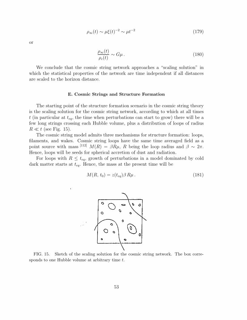
ρ∞(t) ∼ µξ(t)−2 ∼ µt−2 (179)

or

ρ∞(t)

ρc(t)∼ Gµ . (180)

We conclude that the cosmic string network approaches a “scaling solution” inwhich the statistical properties of the network are time independent if all distancesare scaled to the horizon distance.

E. Cosmic Strings and Structure Formation

The starting point of the structure formation scenario in the cosmic string theoryis the scaling solution for the cosmic string network, according to which at all timest (in particular at teq, the time when perturbations can start to grow) there will be afew long strings crossing each Hubble volume, plus a distribution of loops of radiusR ≪ t (see Fig. 15).

The cosmic string model admits three mechanisms for structure formation: loops,filaments, and wakes. Cosmic string loops have the same time averaged field as apoint source with mass [112] M(R) = βRµ, R being the loop radius and β ∼ 2π.Hence, loops will be seeds for spherical accretion of dust and radiation.

For loops with R ≤ teq, growth of perturbations in a model dominated by colddark matter starts at teq. Hence, the mass at the present time will be

M(R, t0) = z(teq)β Rµ . (181)

FIG. 15. Sketch of the scaling solution for the cosmic string network. The box corre-

sponds to one Hubble volume at arbitrary time t.

53

In the original cosmic string model [2,113] it was assumed that loops dominate overwakes. However, according to the newer cosmic string evolution simulations [114], mostof the energy in strings is in the long strings, and hence the loop accretion mechanismis subdominant.

The second mechanism involves long strings moving with relativistic speed intheir normal plane which give rise to velocity perturbations in their wake [115]. Themechanism is illustrated in Fig. 16: space normal to the string is a cone with deficitangle [116]

α = 8πGµ . (182)

If the string is moving with normal velocity v through a bath of dark matter, avelocity perturbation

δv = 4πGµvγ (183)

[with γ = (1 − v2)−1/2] towards the plane behind the string results. At times af-ter teq, this induces planar overdensities, the most prominent (i.e., thickest at thepresent time) and numerous of which were created at teq, the time of equal mat-ter and radiation [117–119]. The corresponding planar dimensions are (in comovingcoordinates)

teqz(teq) × teqz(teq)v ∼ (40 × 40v) Mpc2 . (184)

FIG. 16. Sketch of the mechanism by which a long straight cosmic string S moving

with velocity v in transverse direction through a plasma induces a velocity perturbation ∆v

towards the wake. Shown on the left is the deficit angle, in the center is a sketch of the

string moving in the plasma, and on the right is the sketch of how the plasma moves in the

frame in which the string is at rest.

The thickness d of these wakes can be calculated using the Zel’dovichapproximation [120]. The result is (for Gµ = 10−6)

d ≃ Gµvγ(v)z(teq)2 teq ≃ 4vMpc . (185)

Wakes arise if there is little small scale structure on the string. In this case, thestring tension equals the mass density, the string moves at relativistic speeds, andthere is no local gravitational attraction towards the string.

54

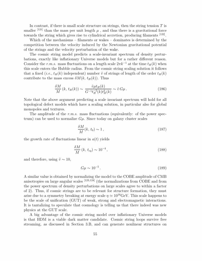
In contrast, if there is small scale structure on strings, then the string tension T issmaller [121] than the mass per unit length µ , and thus there is a gravitational forcetowards the string which gives rise to cylindrical accretion, producing filaments [122].

Which of the mechanisms – filaments or wakes – dominates is determined by thecompetition between the velocity induced by the Newtonian gravitational potentialof the strings and the velocity perturbation of the wake.

The cosmic string model predicts a scale-invariant spectrum of density pertur-bations, exactly like inflationary Universe models but for a rather different reason.Consider the r.m.s. mass fluctuations on a length scale 2πk−1 at the time tH(k) whenthis scale enters the Hubble radius. From the cosmic string scaling solution it followsthat a fixed (i.e., tH(k) independent) number v of strings of length of the order tH(k)contribute to the mass excess δM(k, tH(k)). Thus

δM

M(k, tH(k)) ∼ vµtH(k)

G−1t−2H (k)t3H(k)

∼ v Gµ . (186)

Note that the above argument predicting a scale invariant spectrum will hold for alltopological defect models which have a scaling solution, in particular also for globalmonopoles and textures.

The amplitude of the r.m.s. mass fluctuations (equivalently: of the power spec-trum) can be used to normalize Gµ. Since today on galaxy cluster scales

δM

M(k, t0) ∼ 1 , (187)

the growth rate of fluctuations linear in a(t) yields

δM

M(k, teq) ∼ 10−4 , (188)

and therefore, using v ∼ 10,

Gµ ∼ 10−5 . (189)

A similar value is obtained by normalizing the model to the COBE amplitude of CMBanisotropies on large angular scales [123,124] (the normalizations from COBE and fromthe power spectrum of density perturbations on large scales agree to within a factorof 2). Thus, if cosmic strings are to be relevant for structure formation, they mustarise due to a symmetry breaking at energy scale η ≃ 1016GeV. This scale happens tobe the scale of unification (GUT) of weak, strong and electromagnetic interactions.It is tantalizing to speculate that cosmology is telling us that there indeed was newphysics at the GUT scale.

A big advantage of the cosmic string model over inflationary Universe modelsis that HDM is a viable dark matter candidate. Cosmic string loops survive freestreaming, as discussed in Section 3.B, and can generate nonlinear structures on

55

galactic scales, as discussed in detail in [125,126]. Accretion of hot dark matter by astring wake was studied in [119]. In this case, nonlinear perturbations develop onlylate. At some time tnl, all scales up to a distance qmax from the wake center gononlinear. Here

qmax ∼ Gµvγ(v)z(teq)2teq ∼ 4vMpc , (190)

and it is the comoving thickness of the wake at tnl. Demanding that tnl correspondsto a redshift greater than 1 leads to the constraint

Gµ > 5 · 10−7 . (191)

Note that in a cosmic string and hot dark matter model, wakes form nonlinear struc-tures only very recently. Accretion onto loops and small scale structure on the longstrings provide two mechanisms which may lead to high redshift objects such asquasars and high redshift galaxies. The first mechanism has recently been studied in[127], the second in [128,129].

The power spectrum of density fluctuations in a cosmic string model with HDMhas recently been studied numerically by Mahonen [130], based on previous work of[131] (see also [132] for an earlier semi-analytical study). The spectral shape agreesquite well with observations, and a bias factor of less than 2 is required to give thebest-fit amplitude for a COBE normalized model. Note, however, that the resultsdepend quite sensitively on the details of the string scaling solution which are atpresent not well understood.

Due to lack of space, I will not discuss the global monopole [133] and globaltexture [134] models of structure formation. There has been a lot of work on thetexture model, and the reader is referred to [136,135] for recent review articles.

F. Signatures for Strings

The cosmic string theory of structure formation makes several distinctive predic-tions, both in terms of the galaxy distribution and in terms of CMB anisotropies. Onlarge scales (corresponding to the comoving Hubble radius at teq and larger, struc-ture is predicted to be dominated either by planar [117–119] or filamentary [122] galaxyconcentrations. For models in which the strings have no local gravity, the resultingnonlinear structures will look very different from the nonlinear structures in modelsin which local gravity is the dominant force. As discovered and discussed recently in[137], a baryon number excess is predicted in the nonlinear wakes. This may explainthe “cluster baryon crisis” [138], the fact that the ratio of baryons to dark matter inrich clusters is larger than what is compatible with the nucleosynthesis constraints ina spatially flat Universe.

56

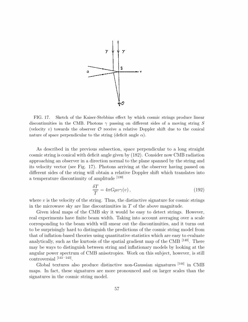
FIG. 17. Sketch of the Kaiser-Stebbins effect by which cosmic strings produce linear

discontinuities in the CMB. Photons γ passing on different sides of a moving string S

(velocity v) towards the observer O receive a relative Doppler shift due to the conical

nature of space perpendicular to the string (deficit angle α).

As described in the previous subsection, space perpendicular to a long straightcosmic string is conical with deficit angle given by (182). Consider now CMB radiationapproaching an observer in a direction normal to the plane spanned by the string andits velocity vector (see Fig. 17). Photons arriving at the observer having passed ondifferent sides of the string will obtain a relative Doppler shift which translates intoa temperature discontinuity of amplitude [139]

δT

T= 4πGµvγ(v) , (192)

where v is the velocity of the string. Thus, the distinctive signature for cosmic stringsin the microwave sky are line discontinuities in T of the above magnitude.

Given ideal maps of the CMB sky it would be easy to detect strings. However,real experiments have finite beam width. Taking into account averaging over a scalecorresponding to the beam width will smear out the discontinuities, and it turns outto be surprisingly hard to distinguish the predictions of the cosmic string model fromthat of inflation-based theories using quantitative statistics which are easy to evaluateanalytically, such as the kurtosis of the spatial gradient map of the CMB [140]. Theremay be ways to distinguish between string and inflationary models by looking at theangular power spectrum of CMB anisotropies. Work on this subject, however, is stillcontroversial [141–143].

Global textures also produce distinctive non-Gaussian signatures [144] in CMBmaps. In fact, these signatures are more pronounced and on larger scales than thesignatures in the cosmic string model.

57

G. Principles of Baryogenesis

Baryogenesis is another area where particle physics and cosmology connect in avery deep way. The goal is to explain the observed asymmetry between matter andantimatter in the Universe. In particular, the objective is to be able to explain theobserved value of the net baryon to entropy ratio at the present time

∆nB

s(t0) ∼ 10−10 (193)

starting from initial conditions in the very early Universe when this ratio vanishes.Here, ∆nB is the net baryon number density and s the entropy density.

As pointed out by Sakharov [145], three basic criteria must be satisfied in order tohave a chance at explaining the data:

1. The theory describing the microphysics must contain baryon number violatingprocesses.

2. These processes must be C and CP violating.

3. The baryon number violating processes must occur out of thermal equilibrium.

As was discovered in the 1970’s [146], all three criteria can be satisfied in GUTtheories. In these models, baryon number violating processes are mediated by su-perheavy Higgs and gauge particles. The baryon number violation is visible in theLagrangian, and occurs in perturbation theory (and is therefore in principle easy tocalculate). In addition to standard model CP violation, there are typically manynew sources of CP violation in the GUT sector. The third Sakharov condition canalso be realized: After the GUT symmetry-breaking phase transition, the superheavyparticles may fall out of thermal equilibrium. The out-of-equilibrium decay of theseparticles can thus generate a nonvanishing baryon to entropy ratio.

The magnitude of the predicted nB/s depends on the asymmetry ε per decay, onthe coupling constant λ of the nB violating processes, and on the ratio nX/s of thenumber density nX of superheavy Higgs and gauge particles to the number densityof photons, evaluated at the time td when the baryon number violating processesfall out of thermal equilibrium, and assuming that this time occurs after the phasetransition. The quantity ε is proportional to the CP-violation parameter in the model.In a GUT theory, this CP violation parameter can be large (order 1), whereas in thestandard electroweak theory it is given by the CP violating phases in the CKM massmatrix and is very small. As shown in [146] it is easily possible to construct modelswhich give the right nB/s ratio after the GUT phase transition (for recent reviews ofbaryogenesis see [147] and [148]).

58

H. GUT Baryogenesis and Topological Defects

The ratio nB/s, however, does not only depend on ε, but also on nX/s(td). If thetemperature Td at the time td is greater than the mass mX of the superheavy particles,then it follows from the thermal history in standard cosmology that nX ∼ s. However,if Td < mX , then the number density of X particles is diluted exponentially in thetime interval between when T = mX and when T = Td. Thus, the predicted baryonto entropy ratio is exponentially suppressed:

nB

s∼ 1

g∗λ2εe−mX/Td , (194)

where g∗ is the number of spin degrees of freedom in thermal equilibrium at the timeof the phase transition. In this case, the standard GUT baryogenesis mechanism isineffective.

However, topological defects may come to the rescue [149]. As we have seen ear-lier in this section, topological defects will inevitably be produced in the symmetrybreaking GUT transition provided they are topologically allowed in that symmetrybreaking scheme. The topological defects provide an alternative mechanism of GUTbaryogenesis.

Inside of topological defects, the GUT symmetry is restored. In fact, the defectscan be viewed as solitonic configurations of X particles. The continuous decay ofdefects at times after td provides an alternative way to generate a nonvanishing baryonto entropy ratio. The defects constitute out of equilibrium configurations, and hencetheir decay can produce a nonvanishing nB/s in the same way as the decay of free Xquanta.

The way to compute the resulting nB/s ratio is as follows: The defect scalingsolution gives the energy density in defects at all times. Taking the time derivativeof this density, and taking into account the expansion of the Universe, we obtain theloss of energy attributed to defect decay. By energetics, we can estimate the numberof decays of individual quanta which the defect decay corresponds to. We can thenuse the usual perturbative results to compute the resulting net baryon number.

Provided that mX < Td, then at the time when the baryon number violatingprocesses fall out of equilibrium (when we start generating a nonvanishing nB) theenergy density in free X quanta is much larger than the defect density, and hencethe defect-driven baryogenesis mechanism is subdominant. However, if mX > Td,then as indicated in (194), the energy density in free quanta decays exponentially. Inconstrast, the density in defects only decreases as a power of time, and hence soondominates baryogenesis.

One of the most important ingredients in the calculation is the time dependenceof ξ(t), the separation between defects. Immediately after the phase transition at thetime tf of the formation of the defect network, the separation is ξ(tf) ∼ λ−1η−1. Inthe time period immediately following, the time period of relevance for baryogenesis,ξ(t) approaches the Hubble radius according to the equation [107]

59

ξ(t) ≃ ξ(tf)(t

tf)5/4 . (195)

Using this result to calculate the defect density, we obtain after some algebra

nB

s|defect ∼ λ2Td

η

nB

s|0 , (196)

where nB/s|0 is the unsuppressed value of nB/s which can be obtained using thestandard GUT baryogenesis mechanism. We see from (196) that even for low valuesof Td, the magnitude of nB/s which is obtained via the defect mechanism is onlysuppressed by a power of Td. However, the maximum strength of the defect channelis smaller than the maximum strength of the usual mechanism by a geometrical sup-pression factor λ2 which expresses the fact that even at the time of defect formation,the defect network only occupies a small volume.

I. Electroweak Baryogenesis and Topological Defects

It has been known for some time that there are baryon number violating processeseven in the standard electroweak theory. These processes are, however, nonpertur-bative. They are connected with the t’Hooft anomaly [150], which in turn is due tothe fact that the gauge theory vacuum is degenerate, and that the different degen-erate vacuum states have different quantum numbers (Chern-Simons numbers). Intheories with fermions, this implies different baryon number. Configurations such assphalerons [151] which interpolate between two such vacuum states thus correspond tobaryon number violating processes.

As pointed out in [152], the anomalous baryon number violating processes are inthermal equilibrium above the electroweak symmetry breaking scale. Therefore, anynet baryon to entropy ratio generated at a higher scale will be erased, unless thisratio is protected by an additional quantum number such as a nonvanishing B − Lwhich is conserved by electroweak processes.

However, as first suggested in [153] and discussed in detail in many recent papers(see [154] for reviews of the literature), it is possible to regenerate a nonvanishingnB/s below the electroweak symmetry breaking scale. Since there are nB violatingprocesses and both C and CP violation in the standard model, Sakharov’s conditionsare satisfied provided that one can realize an out-of-equilibrium state after the phasetransition. Standard model CP violation is extremely weak. Thus, it appears neces-sary to add some sector with extra CP violation to the standard model in order toobtain an appreciable nB/s ratio. A simple possibility which has been invoked oftenis to add a second Higgs doublet to the theory, with CP violating relative phases.

The standard way to obtain out-of-equilibrium baryon number violating processesimmediately after the electroweak phase transition is [154] to assume that the transi-tion is strongly first order and proceeds by the nucleation of bubbles (note that theseare two assumptions, the second being stronger than the first!).

60

Bubbles are out-of-equilibrium configurations. Outside of the bubble (in the falsevacuum), the baryon number violating processes are unsuppressed, inside they areexponentially suppressed. In the bubble wall, the Higgs fields have a nontrivial pro-file, and hence (in models with additional CP violation in the Higgs sector) there isenhanced CP violation in the bubble wall. In order to obtain net baryon production,one may either use fermion scattering off bubble walls [155] (because of the CP viola-tion in the scattering, this generates a lepton asymmetry outside the bubble whichconverts via sphalerons to a baryon asymmetry) or sphaleron processes in the bubblewall itself [156,157]. It has been shown that, using optimistic parameters (in particulara large CP violating phase ∆θCP in the Higgs sector) it is possible to generate theobserved nB/s ratio. The resulting baryon to entropy ratio is of the order

nB

s∼ α2

W (g∗)−1(mt

T)2∆θCP , (197)

where αW refers to the electroweak interaction strength, g∗ is the number of spindegrees of freedom in thermal quilibrium at the time of the phase transition, and mt

is the top quark mass. The dependence on the top quark mass enters because netbaryogenesis only appears at the one-loop level.

However, analytical and numerical studies show that, for the large Higgs masseswhich are indicated by the current experimental bounds, the electroweak phase tran-sition will unlikely be sufficiently strongly first order to proceed by bubble nucleation.In addition, there are some concerns as to whether it will proceed by bubble nucleationat all (see e.g. [158]).

Once again, topological defects come to the rescue. In models which admit de-fects, such defects will inevitably be produced in a phase transition independent ofits order. Moving topological defects can play the same role in baryogenesis as nucle-ating bubbles. In the defect core, the electroweak symmetry is unbroken and hencesphaleron processes are unsuppressed [159]. In the defect walls there is enhanced CPviolation for the same reason as in bubble walls. Hence, at a fixed point in space, anonvanishing baryon number will be produced when a topological defect passes by.

Defect-mediated electroweak baryogenesis has been worked out in detail in [160](see [161] for previous work) in the case of cosmic strings. The scenario is as follows:at a particular point x in space, antibaryons are produced when the front side of thedefect passes by. While x is in the defect core, partial equilibration of nB takes placevia sphaleron processes. As the back side of the defect passes by, the same number ofbaryons are produced as the number of antibaryons when the front side of the defectpasses by. Thus, at the end a positive number of baryons are left behind.

As in the case of defect-mediated GUT baryogenesis, the strength of defect-mediated electroweak baryogenesis is suppressed by the ratio SF of the volume whichis passed by defects divided by the total volume, i.e.

nB

s∼ SF

nB

s|0 , (198)

61

where (nB/s)|0 is the result of (197) obtained in the bubble nucleation mechanism.A big caveat for defect-mediated electroweak baryogenesis is that the standard

electroweak theory does not admit topological defects. However, in a theory withadditional physics just above the electroweak scale it is possible to obtain defects(see e.g. [162] for some specific models). The closer the scale η of the new physics isto the electroweak scale ηEW , the larger the volume in defects and the more efficientdefect-mediated electroweak baryogenesis. Using the result of (195) for the separationof defects, we obtain

SF ∼ λ(ηEW

η)3/2 . (199)

Obviously, the advantage of the defect-mediated baryongenesis scenario is that itdoes not depend on the order and on the detailed dynamics of the electroweak phasetransition.

J. Summary

As we have seen, topological defects may play an important role in cosmology.Defects are inevitably produced during symmetry breaking phase transitions in theearly Universe in all theories in which defects are topologically stable. Theories givingrise to domain walls or local monopoles are ruled out by cosmological constraints.Those producing cosmic strings, global monopoles and textures are quite attractive.

If the scale of symmetry breaking at which the defects are produced is about1016 GeV, then defects can act as the seeds for galaxy formation. Defect theories ofstructure formation predict a roughly scale-invariant spectrum of density perturba-tions, similar to inflation-based models. However, the phases in the density field aredistributed in a non-Gaussian manner. Thus, the predictions of defect models canbe distinguished from those of inflationary models. In addition, the predictions ofdifferent defect models can be distinguished from eachother.

Focusing on the cosmic string theory of structure formation, we have seen thatthe model gives rise to several distinctive signatures. The large-scale structure in theUniverse is predicted to be dominated by either planar or filamentary structures (de-pending on whether there is small-scale structure on the strings), with a distinctivescale given by the comoving Hubble radius at teq. There are many ways topolog-ical measures with which one can quantify this prediction (see e.g. [163]). In theCMB, the distinctive signature for strings is predicted to be line discontinuities in thetemperature maps.

Topological defects may also play a crucial role in baryogenesis. This applies bothto GUT and electroweak baryogenesis. The crucial point is that defects constitute out-of-equilibrium configurations, and may therefore be the sites of net baryon production.

Acknowledgments

62