I Geostru DownHoleI © 2013 Geostru Software Geostru DownHole Parte I DownHole 1

I

Geostru DownHoleI

© 2013 Geostru Software

Geostru DownHole

Parte I DownHole 1

................................................................................................................................... 11 Work theory

.......................................................................................................................................................... 1Introduction

.......................................................................................................................................................... 2Experimental procedure

.......................................................................................................................................................... 3Direct method

.......................................................................................................................................................... 5Interval method

................................................................................................................................... 72 Menu

.......................................................................................................................................................... 7File

.......................................................................................................................................................... 8Edit

.......................................................................................................................................................... 8View

.......................................................................................................................................................... 8Export

.......................................................................................................................................................... 9Options

.......................................................................................................................................................... 9Utility

................................................................................................................................... 93 Input

................................................................................................................................... 104 Output

Parte II SEG2 file import 11

Parte III Contact 18

Geostru DownHole1


1 DownHole

1.1 Work theory

1.1.1 Introduction

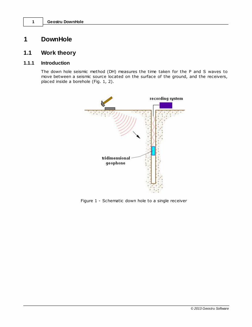
The down hole seismic method (DH) measures the time taken for the P and S waves tomove between a seismic source located on the surface of the ground, and the receivers,placed inside a borehole (Fig. 1, 2).

Figure 1 - Schematic down hole to a single receiver

DownHole 2


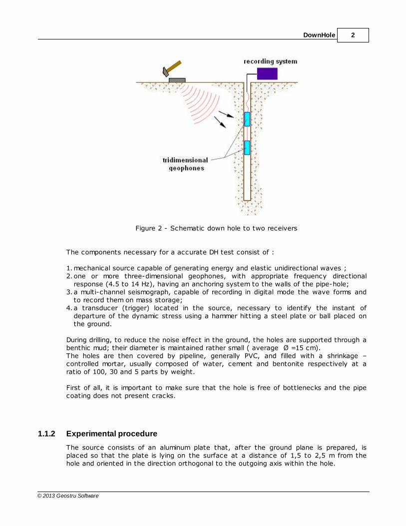
Figure 2 - Schematic down hole to two receivers

The components necessary for a accurate DH test consist of :

1.mechanical source capable of generating energy and elastic unidirectional waves ;2. one or more three-dimensional geophones, with appropriate frequency directional

response (4.5 to 14 Hz), having an anchoring system to the walls of the pipe-hole;3. a multi-channel seismograph, capable of recording in digital mode the wave forms and

to record them on mass storage; 4. a transducer (trigger) located in the source, necessary to identify the instant of

departure of the dynamic stress using a hammer hitting a steel plate or ball placed onthe ground.

During drilling, to reduce the noise effect in the ground, the holes are supported through abenthic mud; their diameter is maintained rather small ( average Ø =15 cm).The holes are then covered by pipeline, generally PVC, and filled with a shrinkage –controlled mortar, usually composed of water, cement and bentonite respectively at aratio of 100, 30 and 5 parts by weight.

First of all, it is important to make sure that the hole is free of bottlenecks and the pipecoating does not present cracks.

1.1.2 Experimental procedure

The source consists of an aluminum plate that, after the ground plane is prepared, isplaced so that the plate is lying on the surface at a distance of 1,5 to 2,5 m from thehole and oriented in the direction orthogonal to the outgoing axis within the hole.

Geostru DownHole3


At the source is hooked the speed sensor used as a trigger. If you have two receivers,these are connected so as to prevent relative rotation and to set the distance. The firstof the two receivers is connected to a rod (ground) battery that allows the orientationfrom the surface and the moving. Once at the test depth, the geophones are oriented sothat each sensor is a transducer, parallel to the axis of source (absolute orientation). Atthis point, the receivers are secured to the walls of pipe coating, the source will beaffected in the vertical direction (to generate waves compression P) or laterally (togenerate shear waves SH) and, simultaneously start the registration of trigger signal andreceivers.

Once the registrations are recorded, the depth of the receivers is changed and the testprocedure repeated.

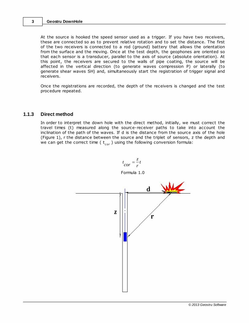
1.1.3 Direct method

In order to interpret the down hole with the direct method, initially, we must correct thetravel times (t) measured along the source-receiver paths to take into account theinclination of the path of the waves. If d is the distance from the source axis of the hole(Figure 1), r the distance between the source and the triplet of sensors, z the depth andwe can get the correct time ( t

cor ) using the following conversion formula:

tr

zcor

t

Formula 1.0

DownHole 4


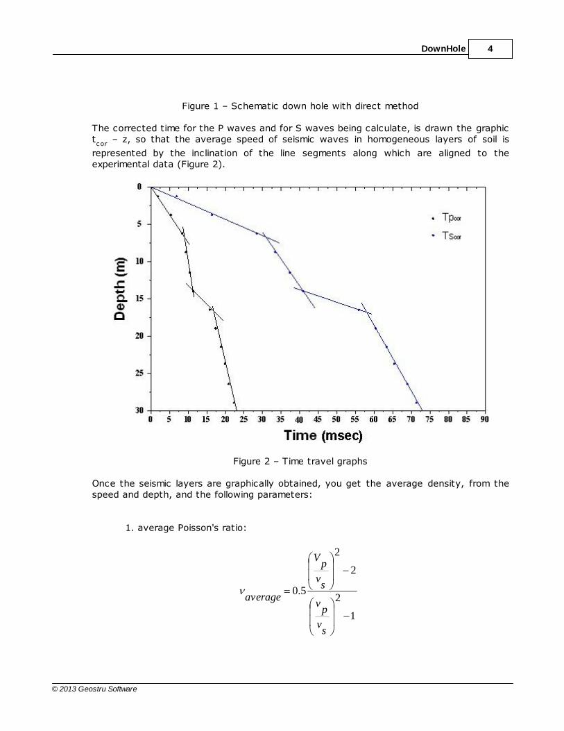
Figure 1 – Schematic down hole with direct method

The corrected time for the P waves and for S waves being calculate, is drawn the graphictcor

– z, so that the average speed of seismic waves in homogeneous layers of soil is

represented by the inclination of the line segments along which are aligned to theexperimental data (Figure 2).

Figure 2 – Time travel graphs

Once the seismic layers are graphically obtained, you get the average density, from thespeed and depth, and the following parameters:

1. average Poisson's ratio:

1

2

2

2

5.0

sv

pv

sv

pV

average

Geostru DownHole5


2. average shear deformation modulus:

2s

vaverage

G

3. average oedometric modulus:

2p

Vaverage

dE

4. average Young's modulus:

122s

vaverage

E

5. average bulk modulus:

23

42s

vp

vaverage

vE

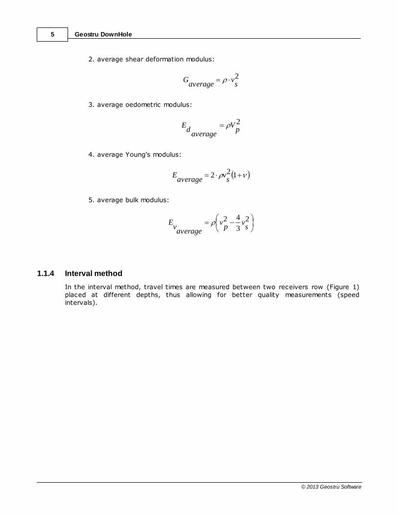
1.1.4 Interval method

In the interval method, travel times are measured between two receivers row (Figure 1)placed at different depths, thus allowing for better quality measurements (speedintervals).

DownHole 6


Figure 1 - Diagram of down hole using interval method

When you have only one receiver, that is assuming that the pairs do not match a singleimpulse, the rate determined values are defined in the pseudo-range, allowing only anapparent better definition of the velocity profile. The obtained measurements makepossible to calculate the correct time using 1.0 formula and the speed range of P and Swaves, with the graph (Figure 6), with the following formula:

cort

cort

zz

spv

12

12,

Geostru DownHole7


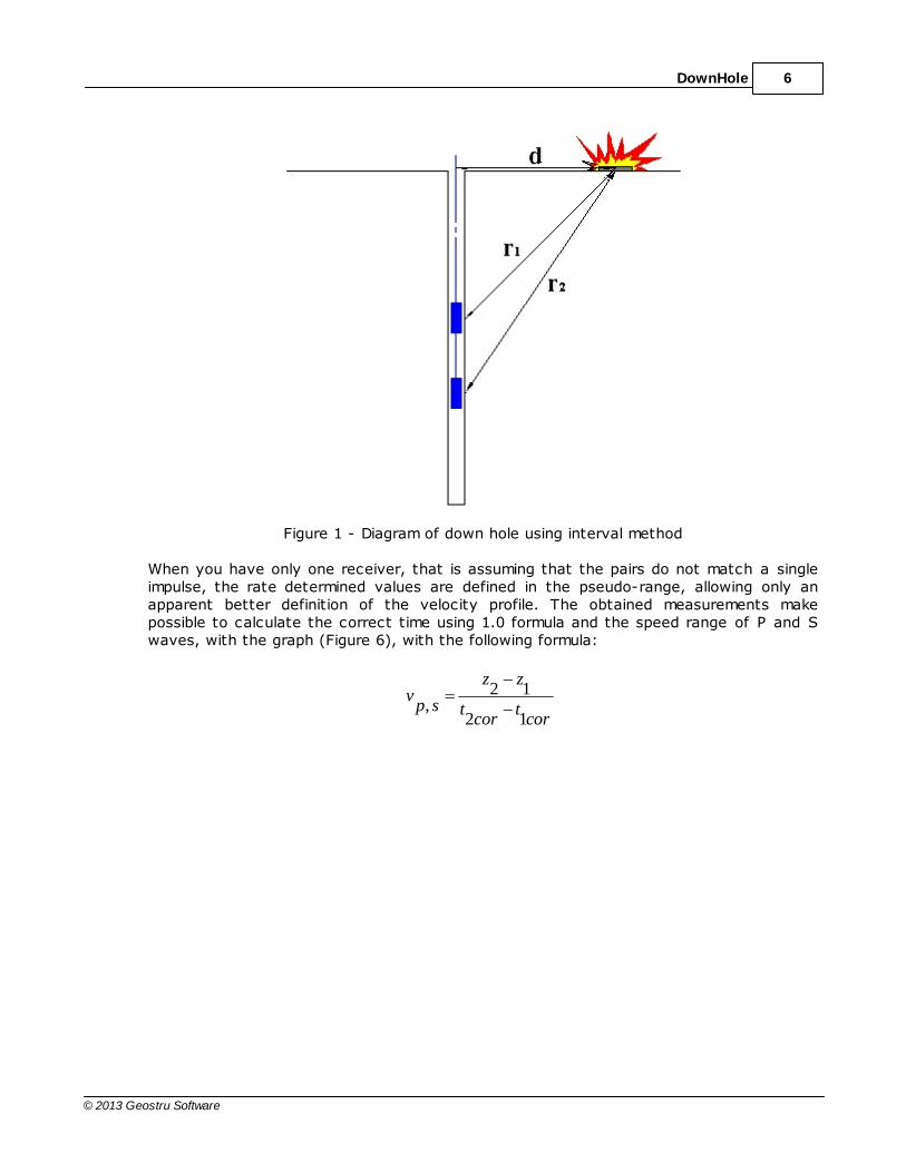
Figure 2 - Profile of seismic velocity with range method

With the calculated speed range is possible to calculate the density, the Poisson's ratio,the shear deformation modulus, the oedometric modulus, Young's modulus, the bulkmodulus for each interval, with the formulas above. But the method has its limitations:

a) does not take into consideration the speed of the overlying strata; b) is not applicable if t2

cor < t1

cor

1.2 Menu

1.2.1 File

NewCreates file(s) for a new project..

OpenOpens file(s) from a previously created project.

SaveSave file(s) for the currently open project, replacing any previous version.

Save asSave file(s) for the currently open project under the name and in the folder entered in asubsequent dialogue window.

DownHole 8


SEG2 file importImport data from SEG2 files

ExitExit from program.

1.2.2 Edit

Copy imageCopies to the clipboard the selected area of the active window.

1.2.3 View

Display soil texturesDisplay or hide the window with textures.

Zoom windowLets you draw a selection rectangle or "window" to zoom part of your display in thedrawing window. Use the left button to select one corner of the view you want. Now thecursor becomes a stretching rectangle. Select a second corner for the view. The screenis redrawn to show the part of your drawing that fits within the rectangle.

Zoom allA zoom factor is applied, such that the whole content of the worksheet is displayed.

MoveEnables frame around the drawing to be moved by dragging the drawing. Note that actualcoordinates of the drawing do not change but the frame’s scales do.

TextChange the font size.

1.2.4 Export

Export in RTF formatDisplay the computation report in an internal editor window which allows to Save in a RTF(Rich Text Format) format file that can be read by most text processing programs andalso can be printed from its own File menu. The report includes a theoretical introduction,the results of the analysis and also the graphs and diagrams.

Export in DXF formatExport in DXF format the contents of the worksheet window for the purpose of furtherelaboration by a CAD program.

Export in Bitmap format

Geostru DownHole9


Export in BMP format the contents of the worksheet window.

1.2.5 Options

OptionsAllows customization of the working parameters such as graphics colors, printing marginsand so on.

1.2.6 Utility

StratigraphyIn this section you can assign and customize the stratigraphy for the study area. This canbe assigned directly by using the input from the left side of the workspace or be derivedfrom seismic data stratigraphy defined during the analysis phase. To this end, is simply toimport the data interest from the Run menu. Each layer can be customized by inserting acolor or textures and a customized description. Textures cab be activated by selectingthe dedicated button on the toolbar.

1.3 Input

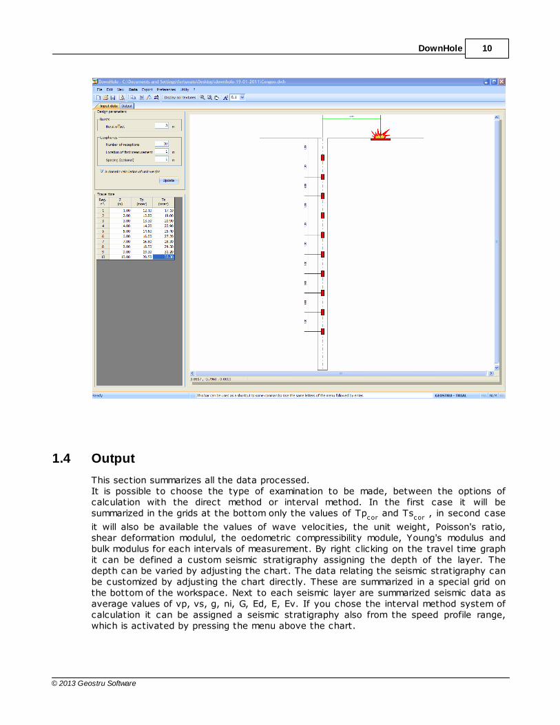
The input section shall define the data to be used for the survey. It is necessary toestablish design parameters as the distance between the source of the outbreak (shot,explosion) and the axis of the hole, the number of records received (parameters) and theposition of the first measurement. If it is specified a fixed spacing between themeasurements, the program automatically calculates the depth of each recording. Thedepth and the travel time between the source and receiver for the P and also for the Swaves must be entered for each test. This data can be entered manually or extractedfrom SEG2 files.It is possible to use copy and paste commands to make more versatile the operation ofdata entry. Finally, by right clicking on the drawing, you can insert a custom descriptionfor the project

DownHole 10


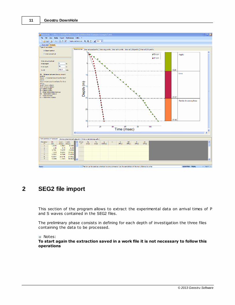
1.4 Output

This section summarizes all the data processed. It is possible to choose the type of examination to be made, between the options ofcalculation with the direct method or interval method. In the first case it will besummarized in the grids at the bottom only the values of Tp

cor and Ts

cor , in second case

it will also be available the values of wave velocities, the unit weight, Poisson's ratio,shear deformation modulul, the oedometric compressibility module, Young's modulus andbulk modulus for each intervals of measurement. By right clicking on the travel time graphit can be defined a custom seismic stratigraphy assigning the depth of the layer. Thedepth can be varied by adjusting the chart. The data relating the seismic stratigraphy canbe customized by adjusting the chart directly. These are summarized in a special grid onthe bottom of the workspace. Next to each seismic layer are summarized seismic data asaverage values of vp, vs, g, ni, G, Ed, E, Ev. If you chose the interval method system ofcalculation it can be assigned a seismic stratigraphy also from the speed profile range,which is activated by pressing the menu above the chart.

Geostru DownHole11


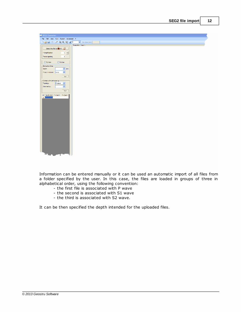
2 SEG2 file import

This section of the program allows to extract the experimental data on arrival times of Pand S waves contained in the SEG2 files.

The preliminary phase consists in defining for each depth of investigation the three filescontaining the data to be processed.

Notes:To start again the extraction saved in a work file it is not necessary to follow thisoperations

SEG2 file import 12


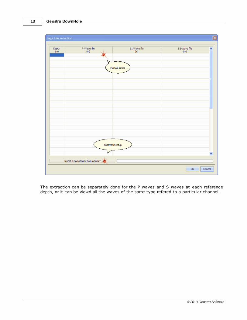
Information can be entered manually or it can be used an automatic import of all files froma folder specified by the user. In this case, the files are loaded in groups of three inalphabetical order, using the following convention:

- the first file is associated with P wave - the second is associated with S1 wave- the third is associated with S2 wave.

It can be then specified the depth intended for the uploaded files.

Geostru DownHole13


The extraction can be separately done for the P waves and S waves at each referencedepth, or it can be viewd all the waves of the same type refered to a particular channel.

SEG2 file import 14


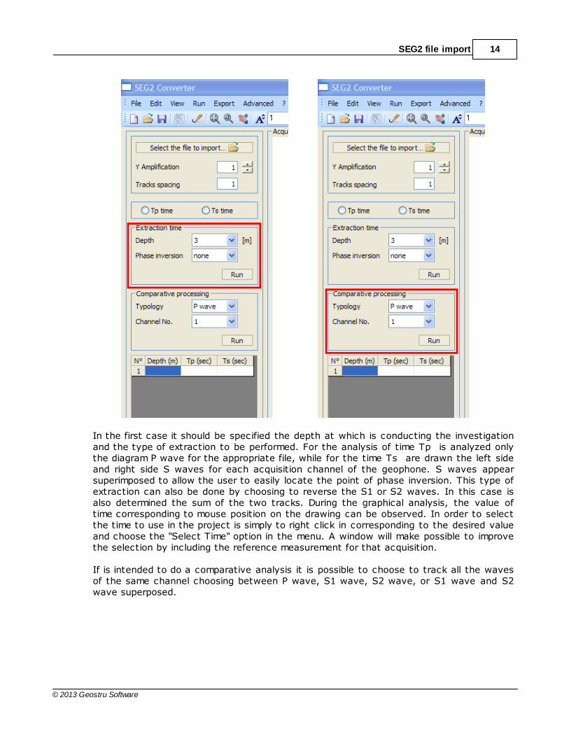
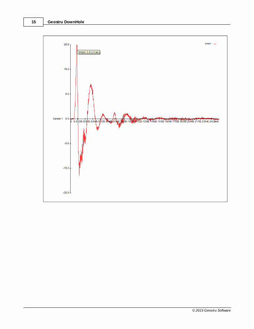
In the first case it should be specified the depth at which is conducting the investigationand the type of extraction to be performed. For the analysis of time Tp is analyzed onlythe diagram P wave for the appropriate file, while for the time Ts are drawn the left sideand right side S waves for each acquisition channel of the geophone. S waves appearsuperimposed to allow the user to easily locate the point of phase inversion. This type ofextraction can also be done by choosing to reverse the S1 or S2 waves. In this case isalso determined the sum of the two tracks. During the graphical analysis, the value oftime corresponding to mouse position on the drawing can be observed. In order to selectthe time to use in the project is simply to right click in corresponding to the desired valueand choose the "Select Time" option in the menu. A window will make possible to improvethe selection by including the reference measurement for that acquisition.

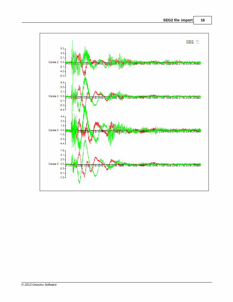
If is intended to do a comparative analysis it is possible to choose to track all the wavesof the same channel choosing between P wave, S1 wave, S2 wave, or S1 wave and S2wave superposed.

Geostru DownHole15


SEG2 file import 16


Geostru DownHole17


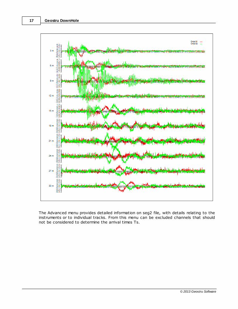
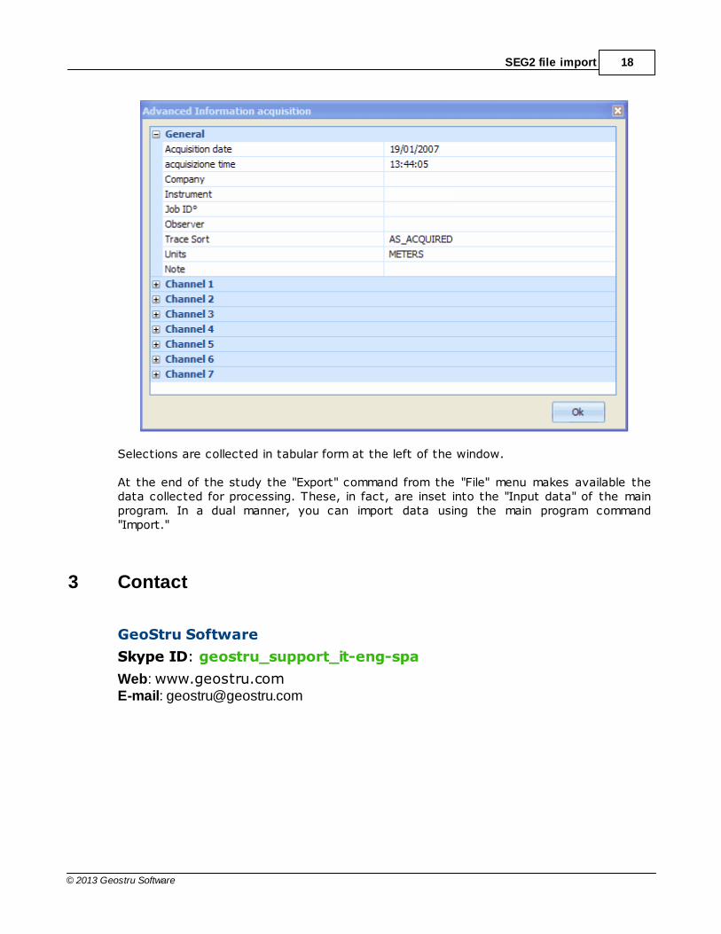
The Advanced menu provides detailed information on seg2 file, with details relating to theinstruments or to individual tracks. From this menu can be excluded channels that shouldnot be considered to determine the arrival times Ts.

SEG2 file import 18


Selections are collected in tabular form at the left of the window.

At the end of the study the "Export" command from the "File" menu makes available thedata collected for processing. These, in fact, are inset into the "Input data" of the mainprogram. In a dual manner, you can import data using the main program command"Import."

3 Contact

GeoStru Software

Skype ID: geostru_support_it-eng-spa

Web: www.geostru.comE-mail: [email protected]

I Geostru DownHoleI © 2013 Geostru Software Geostru DownHole Parte I DownHole 1

Documents