Hysteretic models that incorporate strength and stiffness deterioration

EARTHQUAKE ENGINEERING AND STRUCTURAL DYNAMICSEarthquake Engng Struct. Dyn. 2005; 34:1489–1511Published online 13 June 2005 in Wiley InterScience (www.interscience.wiley.com). DOI: 10.1002/eqe.495

Hysteretic models that incorporate strengthand sti�ness deterioration

Luis F. Ibarra1;∗;†;‡, Ricardo A. Medina2 and Helmut Krawinkler3

1Southwest Research Institute; CNWRA; San Antonio; TX 78238; U.S.A.2Department of Civil and Environmental Engineering; University of Maryland; College Park;

MD 20742; U.S.A.3Department of Civil and Environmental Engineering; Stanford University; Palo Alto; CA 94305; U.S.A.

SUMMARY

This paper presents the description, calibration and application of relatively simple hysteretic modelsthat include strength and sti�ness deterioration properties, features that are critical for demand predic-tions as a structural system approaches collapse. Three of the basic hysteretic models used in seismicdemand evaluation are modi�ed to include deterioration properties: bilinear, peak-oriented, and pinch-ing. The modi�ed models include most of the sources of deterioration: i.e. various modes of cyclicdeterioration and softening of the post-yielding sti�ness, and also account for a residual strength afterdeterioration. The models incorporate an energy-based deterioration parameter that controls four cyclicdeterioration modes: basic strength, post-capping strength, unloading sti�ness, and accelerated reloadingsti�ness deterioration. Calibration of the hysteretic models on steel, plywood, and reinforced-concretecomponents demonstrates that the proposed models are capable of simulating the main characteris-tics that in�uence deterioration. An application of a peak-oriented deterioration model in the seismicevaluation of single-degree-of-freedom (SDOF) systems is illustrated. The advantages of using deterio-rating hysteretic models for obtaining the response of highly inelastic systems are discussed. Copyright? 2005 John Wiley & Sons, Ltd.

KEY WORDS: hysteretic behaviour; strength deterioration; cyclic deterioration; collapse

1. INTRODUCTION

The main objective of performance-based earthquake engineering is to evaluate the per-formance of a system at di�erent seismic hazard levels. Considering the need for a com-prehensive performance assessment, it becomes a necessity to develop hysteretic modelsthat incorporate all-important phenomena contributing to demand prediction as the structure

∗Correspondence to: Luis F. Ibarra, Southwest Research Institute, CNWRA, U.S.A.†E-mail: [email protected]‡Senior Research Engineer.

Contract=grant sponsor: Paci�c Earthquake Engineering Research (PEER) CenterReceived 19 June 2004

Revised 12 January 2005Copyright ? 2005 John Wiley & Sons, Ltd. Accepted 1 March 2005

1490 L. F. IBARRA, R. A. MEDINA AND H. KRAWINKLER

approaches collapse. In earthquake engineering, collapse implies that the structural system isno longer capable to maintain its gravity load-carrying capacity in the presence of seismice�ects, which can be caused by main shocks and/or aftershocks. Local collapse may occur,for instance, if a vertical load-carrying component fails in compression or if shear transfer islost between horizontal and vertical components (e.g. shear failure between a �at slab and acolumn). Global collapse occurs if a local failure propagates (progressive collapse) or if anindividual storey displaces su�ciently so that the second order P−� e�ects fully o�set the�rst order storey shear resistance. Collapse assessment requires hysteretic models capable ofrepresenting all the important modes of deterioration that are observed in experimental studies.In most seismic demand studies, hysteresis models are being employed that have a non-

deteriorating backbone curve and hysteresis rules that either ignore sti�ness deterioration (bi-linear model) or account for sti�ness deterioration by modifying the path with which thereloading branch approaches the backbone curve, e.g. the peak-oriented model [1] or various‘pinching’ models. In 1970, Takeda [2] developed a model with a trilinear backbone curvethat degrades the unloading sti�ness based on the maximum displacement of the system. Thismodel was created speci�cally for reinforced-concrete components, and the backbone curveis trilinear because it includes a segment for uncracked concrete. In addition to models withpiecewise linear behaviour, smooth hysteretic models have been developed that include acontinuous change of sti�ness due to yielding, and sharp changes due to unloading, e.g. theWen–Bouc model [3].The need to simulate structural response far into the inelastic range, in which components

deteriorate in strength and sti�ness, led to the development of more versatile models such asthe smooth hysteretic degrading model developed by Sivaselvan and Reinhorn [4], which in-cludes rules for sti�ness and strength deterioration as well as pinching. This model, however,does not include a negative backbone tangent sti�ness. The model developed by Song andPincheira [5] is capable of representing cyclic strength and sti�ness deterioration based ondissipated hysteretic energy, and it is essentially a peak-oriented model that considers pinch-ing based on deterioration parameters. The backbone curve includes a post-capping negativetangent sti�ness and a residual strength branch. Because the backbone curve does not deteri-orate, unloading and accelerated cyclic deterioration are the only modes included, and priorto reaching the peak strength the model is incapable of reproducing strength deterioration.This paper has a threefold objective: (a) to describe the properties of proposed hysteretic

models that incorporate both monotonic and cyclic deterioration; (b) to illustrate the calibrationof these hysteretic models on component tests of steel, plywood, and reinforced-concretespecimens; and (c) to exemplify the utilization of the hysteretic models in the seismic responseevaluation of single-degree-of-freedom (SDOF) systems.

2. PROPOSED HYSTERETIC MODELS INCLUDING STRENGTHAND STIFFNESS DETERIORATION

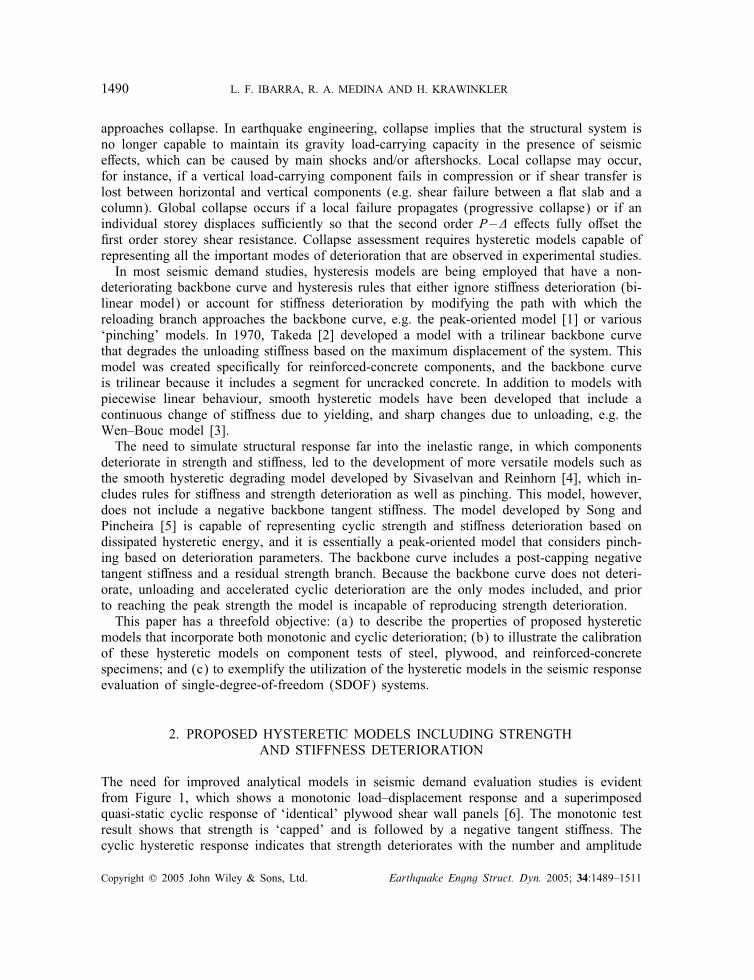
The need for improved analytical models in seismic demand evaluation studies is evidentfrom Figure 1, which shows a monotonic load–displacement response and a superimposedquasi-static cyclic response of ‘identical’ plywood shear wall panels [6]. The monotonic testresult shows that strength is ‘capped’ and is followed by a negative tangent sti�ness. Thecyclic hysteretic response indicates that strength deteriorates with the number and amplitude

Copyright ? 2005 John Wiley & Sons, Ltd. Earthquake Engng Struct. Dyn. 2005; 34:1489–1511

HYSTERETIC MODELS 1491

UCSD Test PWD East Wall

-10

-5

0

5

10

-6 -4 -2 0 2 4 6 8Displacement (in)

Loa

d (k

ips)

MonotonicISO

3

12

4

Figure 1. Monotonic and cyclic experimental response of a plywood panel [6].

of cycles, even if the displacement associated with the strength cap has not been reached (1).It also indicates that strength deterioration occurs in the post-capping range (2), and that theunloading sti�ness may also deteriorate (3). Furthermore, it is observed that the reloadingsti�ness may deteriorate at an accelerated rate (4).Several hysteretic models have been developed to represent hysteretic behaviour similar

to that of Figure 1 [4, 5]. However, few models integrate all the important deteriorationsources such as strength deterioration in the backbone curve (post-capping sti�ness branch)and cyclic deterioration of strength and sti�ness. For this reason, deteriorating models aredeveloped in this study for bilinear, peak-oriented and pinched hysteretic systems. The modelsare implemented in an in-house computer program called SNAP, which is based on theprogram NLDYNA [7]. SNAP is used to carry out dynamic and quasi-static inelastic analysisof SDOF systems. The component deterioration models are also implemented in the computerprogram DRAIN-2DX [8], which is used to carry out dynamic non-linear analyses of multi-degree-of-freedom (MDOF) systems.This section presents a description of the salient properties of the proposed deteriorating

hysteretic models. In the discussion the term deteriorating hysteretic models refers to modelsthat include strength deterioration of the backbone curve and/or cyclic deterioration. Con-versely, non-deteriorating hysteretic models do not incorporate any of the above types ofdeterioration.

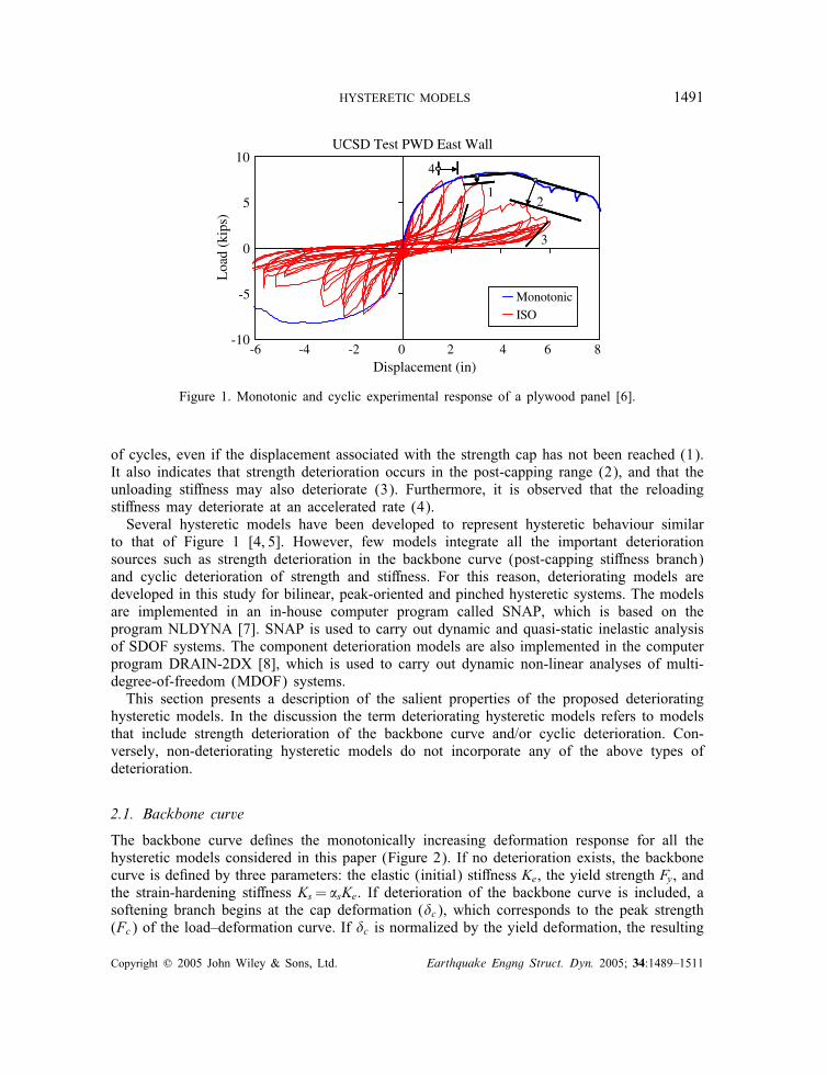
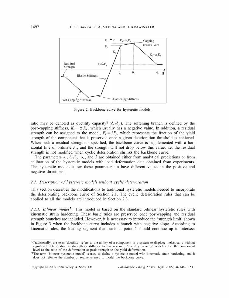
2.1. Backbone curve

The backbone curve de�nes the monotonically increasing deformation response for all thehysteretic models considered in this paper (Figure 2). If no deterioration exists, the backbonecurve is de�ned by three parameters: the elastic (initial) sti�ness Ke, the yield strength Fy, andthe strain-hardening sti�ness Ks= �sKe. If deterioration of the backbone curve is included, asoftening branch begins at the cap deformation (�c), which corresponds to the peak strength(Fc) of the load–deformation curve. If �c is normalized by the yield deformation, the resulting



δy δc δr

Residual Strength

Capping

(Peak) Point

Ke

Hardening Stiffness Post-Capping Stiffness

Elastic Stiffness

Fy

Fc F Ks=αsKe

Kc=αcKe

Fr=λFy

Figure 2. Backbone curve for hysteretic models.

ratio may be denoted as ductility capacity§ (�c=�y). The softening branch is de�ned by thepost-capping sti�ness, Kc= �cKe, which usually has a negative value. In addition, a residualstrength can be assigned to the model, Fr = �Fy, which represents the fraction of the yieldstrength of the component that is preserved once a given deterioration threshold is achieved.When such a residual strength is speci�ed, the backbone curve is supplemented with a hor-izontal line of ordinate Fr , and the strength will not drop below this value, i.e. the residualstrength is not modi�ed when cyclic deterioration shrinks the backbone curve.The parameters �s, �c=�y, �c, and � are obtained either from analytical predictions or from

calibration of the hysteretic models with load–deformation data obtained from experiments.The hysteretic models allow these parameters to have di�erent values in the positive andnegative directions.

2.2. Description of hysteretic models without cyclic deterioration

This section describes the modi�cations to traditional hysteretic models needed to incorporatethe deteriorating backbone curve of Section 2.1. The cyclic deterioration rules that can beapplied to all the models are introduced in Section 2.3.

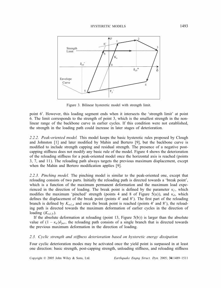
2.2.1. Bilinear model¶. This model is based on the standard bilinear hysteretic rules withkinematic strain hardening. These basic rules are preserved once post-capping and residualstrength branches are included. However, it is necessary to introduce the ‘strength limit’ shownin Figure 3 when the backbone curve includes a branch with negative slope. According tokinematic rules, the loading segment that starts at point 5 should continue up to intersect

§Traditionally, the term ‘ductility’ refers to the ability of a component or a system to displace inelastically withoutsigni�cant deterioration in strength or sti�ness. In this research, ‘ductility capacity’ is de�ned at the componentlevel as the ratio of the deformation at peak strength to the yield deformation.

¶The term ‘bilinear hysteretic model’ is used to de�ne a hysteretic model with kinematic strain hardening, and itdoes not refer to the number of segments used to model the backbone curve.



2

5

Ke

3

Fy-

6

0

1

δc0-

δc0+ δ

EnvelopeCurve

4

Strength Limit

6’

F

Figure 3. Bilinear hysteretic model with strength limit.

point 6′. However, this loading segment ends when it intersects the ‘strength limit’ at point6. The limit corresponds to the strength of point 3, which is the smallest strength in the non-linear range of the backbone curve in earlier cycles. If this condition were not established,the strength in the loading path could increase in later stages of deterioration.

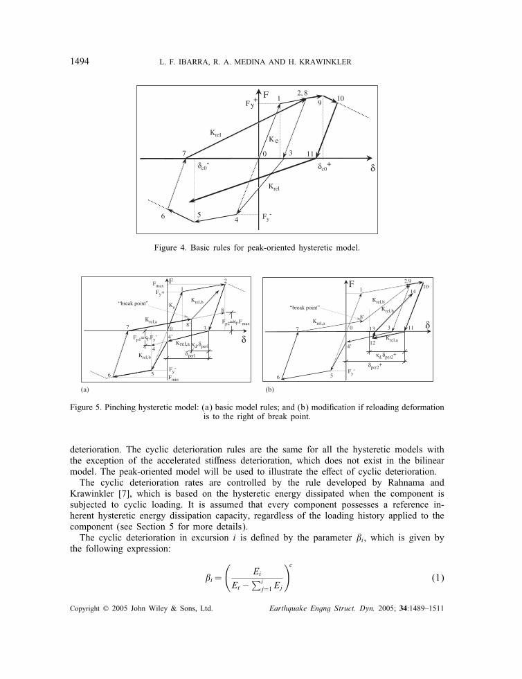
2.2.2. Peak-oriented model. This model keeps the basic hysteretic rules proposed by Cloughand Johnston [1] and later modi�ed by Mahin and Bertero [9], but the backbone curve ismodi�ed to include strength capping and residual strength. The presence of a negative post-capping sti�ness does not modify any basic rule of the model. Figure 4 shows the deteriorationof the reloading sti�ness for a peak-oriented model once the horizontal axis is reached (points3, 7, and 11). The reloading path always targets the previous maximum displacement, exceptwhen the Mahin and Bertero modi�cation applies [9].

2.2.3. Pinching model. The pinching model is similar to the peak-oriented one, except thatreloading consists of two parts. Initially the reloading path is directed towards a ‘break point’,which is a function of the maximum permanent deformation and the maximum load expe-rienced in the direction of loading. The break point is de�ned by the parameter �f, whichmodi�es the maximum ‘pinched’ strength (points 4 and 8 of Figure 5(a)), and �d, whichde�nes the displacement of the break point (points 4′ and 8′). The �rst part of the reloadingbranch is de�ned by Krel; a and once the break point is reached (points 4′ and 8′), the reload-ing path is directed towards the maximum deformation of earlier cycles in the direction ofloading (Krel; b).If the absolute deformation at reloading (point 13, Figure 5(b)) is larger than the absolute

value of (1 − �d)�per , the reloading path consists of a single branch that is directed towardsthe previous maximum deformation in the direction of loading.

2.3. Cyclic strength and sti�ness deterioration based on hysteretic energy dissipation

Four cyclic deterioration modes may be activated once the yield point is surpassed in at leastone direction: basic strength, post-capping strength, unloading sti�ness, and reloading sti�ness



6

2, 8

K e

Fy+

3

F

0

1

54

Krel

Krel

7

910

11

Fy-

δc0- δc0

+ δ

Figure 4. Basic rules for peak-oriented hysteretic model.

Fp2=κf.Fmax

κd.δperl

κd.δper2+

δper2+

δperl

Fp1=κf.Fy-

Krel,a

Ke

Fy+

3

F

0

1

2

6 5

7

4’

4

8’

Fy-

Fy-

Fmax

8

Fmin

Krel,a

Krel,b

Krel,b Krel,b

Krel,a

“break point”

30

1

6 5

7

4’

8’

11

10

12

13 δδ

2,9

14F

“break point” Krel,b

Krel,a

(a) (b)

Figure 5. Pinching hysteretic model: (a) basic model rules; and (b) modi�cation if reloading deformationis to the right of break point.

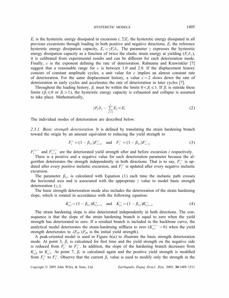
deterioration. The cyclic deterioration rules are the same for all the hysteretic models withthe exception of the accelerated sti�ness deterioration, which does not exist in the bilinearmodel. The peak-oriented model will be used to illustrate the e�ect of cyclic deterioration.The cyclic deterioration rates are controlled by the rule developed by Rahnama and

Krawinkler [7], which is based on the hysteretic energy dissipated when the component issubjected to cyclic loading. It is assumed that every component possesses a reference in-herent hysteretic energy dissipation capacity, regardless of the loading history applied to thecomponent (see Section 5 for more details).The cyclic deterioration in excursion i is de�ned by the parameter �i, which is given by

the following expression:

�i=

(Ei

Et −∑i

j=1 Ej

)c(1)



Ei is the hysteretic energy dissipated in excursion i, �Ej the hysteretic energy dissipated in allprevious excursions through loading in both positive and negative directions, Et the referencehysteretic energy dissipation capacity, Et = �Fy�y. The parameter � expresses the hystereticenergy dissipation capacity as a function of twice the elastic strain energy at yielding (Fy�y),it is calibrated from experimental results and can be di�erent for each deterioration mode.Finally, c is the exponent de�ning the rate of deterioration. Rahnama and Krawinkler [7]suggest that a reasonable range for c is between 1.0 and 2.0. If the displacement historyconsists of constant amplitude cycles, a unit value for c implies an almost constant rateof deterioration. For the same displacement history, a value c=2 slows down the rate ofdeterioration in early cycles and accelerates the rate of deterioration in later cycles [7].Throughout the loading history, �i must be within the limits 0¡�i61. If �i is outside these

limits (�i60 or �i¿1), the hysteretic energy capacity is exhausted and collapse is assumedto take place. Mathematically,

�Fy�y −i∑j=1Ej¡Ei (2)

The individual modes of deterioration are described below.

2.3.1. Basic strength deterioration. It is de�ned by translating the strain hardening branchtoward the origin by an amount equivalent to reducing the yield strength to

F+i =(1− �s; i)F+i−1 and F−i =(1− �s; i)F−

i−1 (3)

F+=−i and F+=−i−1 are the deteriorated yield strength after and before excursion i respectively.There is a positive and a negative value for each deterioration parameter because the al-

gorithm deteriorates the strength independently in both directions. That is to say, F−i is up-

dated after every positive inelastic excursion, and F+i is updated after every negative inelasticexcursion.The parameter �s; i is calculated with Equation (1) each time the inelastic path crosses

the horizontal axis and is associated with the appropriate � value to model basic strengthdeterioration (�s).The basic strength deterioration mode also includes the deterioration of the strain hardening

slope, which is rotated in accordance with the following equation:

K+s; i=(1− �s; i)K+s; i−1 and K−s; i=(1− �s; i)K−

s; i−1 (4)

The strain hardening slope is also deteriorated independently in both directions. The con-sequence is that the slope of the strain hardening branch is equal to zero when the yieldstrength has deteriorated to zero. If a residual branch is included in the backbone curve, theanalytical model deteriorates the strain-hardening sti�ness to zero (K+=−s; i =0) when the yieldstrength deteriorates to �Fy0 (Fy0 is the initial yield strength).A peak-oriented model is used in Figure 6(a) to illustrate the basic strength deterioration

mode. At point 3, �s is calculated for �rst time and the yield strength on the negative sideis reduced from F−

y to F−1 . In addition, the slope of the hardening branch decreases from

K−s;0 to K

−s;1. At point 7, �s is calculated again and the positive yield strength is modi�ed

from F+y to F+1 . Observe that the current �s value is used to modify only the strength in the



(a) (b)

(c) (d)

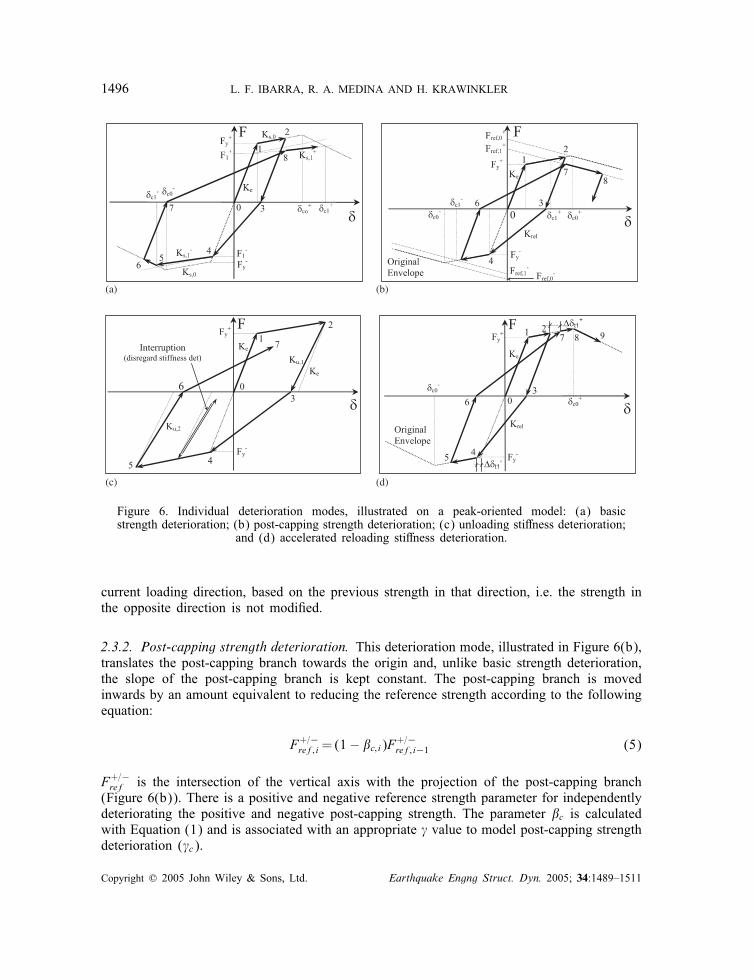
Figure 6. Individual deterioration modes, illustrated on a peak-oriented model: (a) basicstrength deterioration; (b) post-capping strength deterioration; (c) unloading sti�ness deterioration;

and (d) accelerated reloading sti�ness deterioration.

current loading direction, based on the previous strength in that direction, i.e. the strength inthe opposite direction is not modi�ed.

2.3.2. Post-capping strength deterioration. This deterioration mode, illustrated in Figure 6(b),translates the post-capping branch towards the origin and, unlike basic strength deterioration,the slope of the post-capping branch is kept constant. The post-capping branch is movedinwards by an amount equivalent to reducing the reference strength according to the followingequation:

F+=−ref; i=(1− �c; i)F+=−ref; i−1 (5)

F+=−ref is the intersection of the vertical axis with the projection of the post-capping branch(Figure 6(b)). There is a positive and negative reference strength parameter for independentlydeteriorating the positive and negative post-capping strength. The parameter �c is calculatedwith Equation (1) and is associated with an appropriate � value to model post-capping strengthdeterioration (�c).



The deterioration of post-capping strength is computed each time the horizontal axis iscrossed, but it may not a�ect the loading path in early stages of non-linearity. In Figure 6(b)the �rst post-capping strength deterioration is calculated at point 3 and the negative referencepoint moves to F−

ref;1. This backbone modi�cation does not a�ect the loading path because thenegative displacement does not reach the post-capping branch. At point 6, the post-cappingstrength deterioration is computed again, and this time the loading path is modi�ed becausethe updated cap displacement (�+c;1) is exceeded in this excursion.

2.3.3. Unloading sti�ness deterioration. The unloading sti�ness (Ku) is deteriorated inaccordance with the following equation:

Ku; i=(1− �k; i)Ku; i−1 (6)

Ku; i and Ku; i−1 are the deteriorated unloading sti�nesses after and before excursion i, respec-tively. The parameter �k; i is computed from Equation (1) and is associated with an appropriatecyclic deterioration parameter �k . It is the only �-parameter that is computed when a load re-versal takes place in the inelastic range, unlike the other three �-parameters that are computedwhen the loading path crosses the horizontal axis. Furthermore, this is the only deteriorationmode in which the deteriorating quantity, i.e. the unloading sti�ness, is updated simultane-ously in both directions (i.e. for positive and negative unloading). Consequently, the unloadingsti�ness deteriorates up to twice as much as the other deteriorating quantities, and if the samerate of deterioration is expected in the four deterioration modes, �k should be about twice aslarge as the other � values, i.e. �k =2�s; c; a.Figure 6(c) shows a peak-oriented model that includes unloading sti�ness deterioration. At

point 2 the �rst reversal in the inelastic range occurs and the unloading sti�ness deterioratesfrom Ke to Ku;1. At point 5 the �rst reversal on the negative side takes place and Ku;2 iscalculated based on the updated �k and Ku;1. Unlike other deterioration modes, Ku;2 is updatedbased on the value of the unloading sti�ness on the other side of the loop.Unloading sti�ness deterioration is disregarded if the reversal is considered an interruption

in the direction of loading. In peak-oriented and pinching models, an interruption occurs whenthe path is on the unloading sti�ness and a reversal takes place before the path targets themaximum displacement on the opposite side (see Figure 6(c)). In the bilinear model, aninterruption occurs when the path is on the unloading sti�ness and has a reversal beforereaching the backbone curve on the opposite side.

2.3.4. Accelerated reloading sti�ness deterioration. This deterioration mode increases the ab-solute value of the target displacement, de�ned as the maximum positive or negative dis-placement of past cycles, according to the direction of loading. Accelerated reloading sti�nessdeterioration is de�ned only for peak-oriented and pinching models, and it is governed by thefollowing equation:

�+=−t; i =(1 + �a; i)�+=−t; i−1 (7)

There is a target displacement (�t) for each loading direction, and the reloading sti�nessdeterioration is calculated each time the horizontal axis is crossed (Figure 6(d)). Equation (1)is employed to compute �a based on an appropriate parameter �a.



3. CALIBRATION OF HYSTERETIC MODELS ON COMPONENT TESTS

The deteriorating hysteretic models have been calibrated with load–deformation data obtainedfrom experiments on steel, plywood, and reinforced-concrete components. Simulations areobtained by tuning the deterioration parameters to experimental data.

3.1. Steel specimens

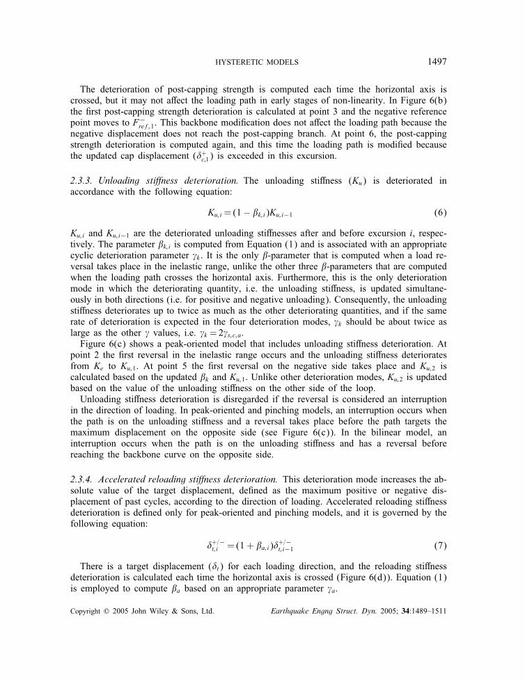
Figures 7(a) and (b) illustrate the calibration of the bilinear model on beam load–displacementrelationships for steel beam-column subassemblies [10]. Because monotonic tests were notavailable to obtain the backbone curve for the simulations, the parameters of the backbonecurve (Fy, �y, �c, �s and �c) were estimated from the load–displacement relationship of the

(a)

(b)

Figure 7. Calibration of bilinear model on steel component tests [10]: (a) test LS-1, SAC standardloading protocol; and (b) test LS-2, SAC near-fault protocol.



second excursion of the near-fault test (Figure 7(b)). This second excursion is considered tobe close to a monotonic load–displacement relationship because only small structural damageoccurred during the �rst excursion in the opposite direction. Based on this approach, thefollowing properties are utilized for the simulations: Fy=103 kips, �y=1:03 in, �s=0:03,�c= −0:03, �c=�y=2:75 and no residual strength (�=0). The cyclic deterioration parametersare: c=1:0 and �s= �c= �k =130. The use of di�erent � values for each deterioration modecould have resulted in a somewhat better calibration. However, all �’s are set at the same valueto illustrate that adequate simulations can be obtained through the use of a single hystereticenergy dissipation parameter. It turns out that the response is not very sensitive to smallvariations in �’s. An appropriate value was obtained by a trial and error method that providedan empirical best �t to the experimental data.The two specimens, LS-1 and LS-2, are identical but are subjected to very di�erent loading

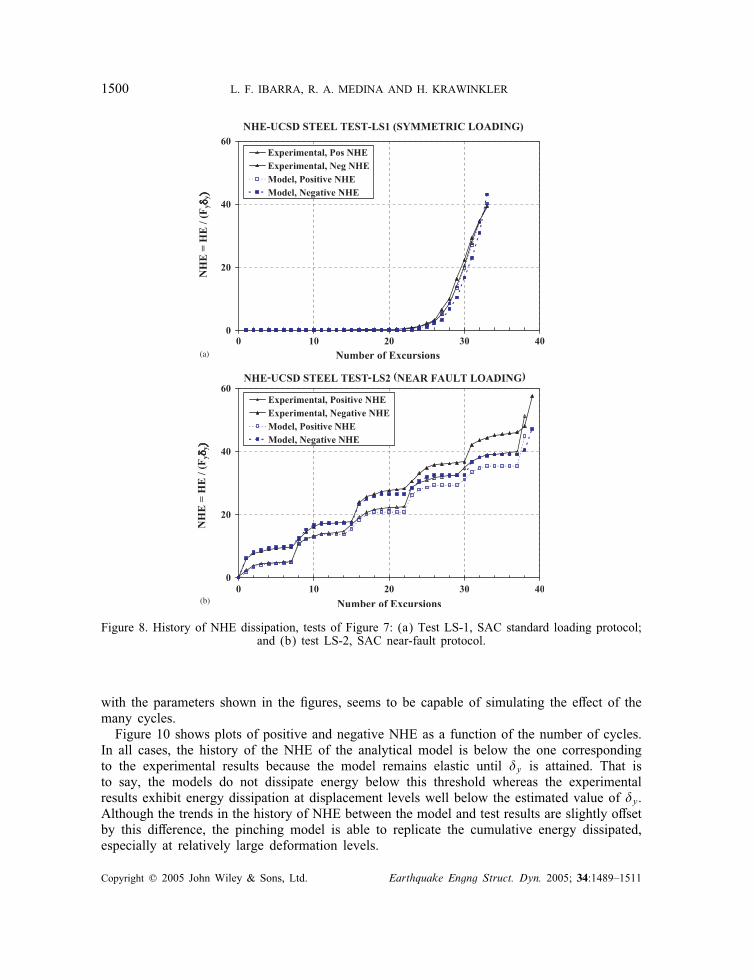
histories, which provides an opportunity to assess the generality of a deterioration model thatincludes cyclic deterioration. The analytical model provides a reasonable correlation with theexperimental loops for both loading histories, within the constraints of a simple bilinear modelthat does not account for cyclic hardening, a phenomenon that may lead to a considerableincrease in strength during early cycles in which little cyclic deterioration is noticeable. Theimportant observation is that the large inelastic cycles, in which signi�cant cyclic deteriorationtakes place, are well simulated by the analytical model.Figure 8 shows plots of negative and positive normalized hysteretic energy (NHE=hysteretic

energy dissipated=Fy�y) as a function of the number of cycles for the two specimens. In allcases the history of NHE is similar for both the analytical model and the experimental results.Thus, the bilinear hysteretic model is able to replicate the cumulative energy dissipated underthe action of various loading protocols.Note that the sum of positive and negative NHE is smaller than the input parameter

�s; c; k =130. The reasons are that (a) complete loss of restoring force is not reached in eithercase, and (b) deterioration in these examples comes to a large part from cyclic loading butin part also from the presence of a post-capping sti�ness which does not depend on NHE. Areasonable calibration of the hysteretic model refers to the selection of model parameters thatproduce NHE histories that are close to those exhibited in the component tests throughoutthe entire range of loading. The fact that the NHE at the end of loading does not correspondwith the �s; c; k; a value does not imply that the selected cyclic deterioration parameters areerroneous.

3.2. Plywood specimens

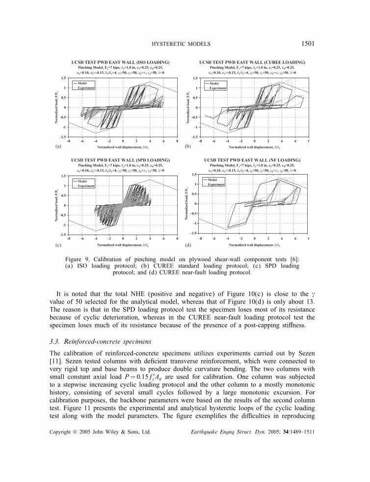
Figure 9 shows the calibration of the pinching model based on plywood shear wall test re-sults [6]. Four ‘identical’ specimens were subjected to di�erent loading protocols. The problemwith plywood panels is that ‘identical’ specimens cannot be created because of di�erences inworkmanship, and response di�erences have to be expected even if identical loading historiesare applied. This is evident from the backbone curve, which is obtained from a monotonictest but is clearly exceeded in two of the four cyclic test results illustrated in Figure 9.Nevertheless, the responses to the very di�erent loading histories permit a general assess-ment of the adequacy of the proposed deterioration models. In particular, the SPD loadingprotocol, see Figure 9(c), has a very large number of cycles that causes a very di�erentresponse from those of the other three loading histories. The proposed deterioration model,



(a)

(b)

Figure 8. History of NHE dissipation, tests of Figure 7: (a) Test LS-1, SAC standard loading protocol;and (b) test LS-2, SAC near-fault protocol.

with the parameters shown in the �gures, seems to be capable of simulating the e�ect of themany cycles.Figure 10 shows plots of positive and negative NHE as a function of the number of cycles.

In all cases, the history of the NHE of the analytical model is below the one correspondingto the experimental results because the model remains elastic until �y is attained. That isto say, the models do not dissipate energy below this threshold whereas the experimentalresults exhibit energy dissipation at displacement levels well below the estimated value of �y.Although the trends in the history of NHE between the model and test results are slightly o�setby this di�erence, the pinching model is able to replicate the cumulative energy dissipated,especially at relatively large deformation levels.



(a)

(c) (d)

(b)

Figure 9. Calibration of pinching model on plywood shear-wall component tests [6]:(a) ISO loading protocol; (b) CUREE standard loading protocol; (c) SPD loading

protocol; and (d) CUREE near-fault loading protocol.

It is noted that the total NHE (positive and negative) of Figure 10(c) is close to the �value of 50 selected for the analytical model, whereas that of Figure 10(d) is only about 13.The reason is that in the SPD loading protocol test the specimen loses most of its resistancebecause of cyclic deterioration, whereas in the CUREE near-fault loading protocol test thespecimen loses much of its resistance because of the presence of a post-capping sti�ness.

3.3. Reinforced-concrete specimens

The calibration of reinforced-concrete specimens utilizes experiments carried out by Sezen[11]. Sezen tested columns with de�cient transverse reinforcement, which were connected tovery rigid top and base beams to produce double curvature bending. The two columns withsmall constant axial load P=0:15f′

cAg are used for calibration. One column was subjectedto a stepwise increasing cyclic loading protocol and the other column to a mostly monotonichistory, consisting of several small cycles followed by a large monotonic excursion. Forcalibration purposes, the backbone parameters were based on the results of the second columntest. Figure 11 presents the experimental and analytical hysteretic loops of the cyclic loadingtest along with the model parameters. The �gure exempli�es the di�culties in reproducing



(a) (b)

(d)(c)

Figure 10. History of NHE dissipation, tests of Figure 9: (a) ISO loading protocol; (b) CUREE standardloading protocol; (c) SPD loading protocol; and (d) CUREE near-fault loading protocol.

Figure 11. Calibration of pinching model on a reinforced-concrete column [11].



Figure 12. History of NHE dissipation, test of Figure 11.

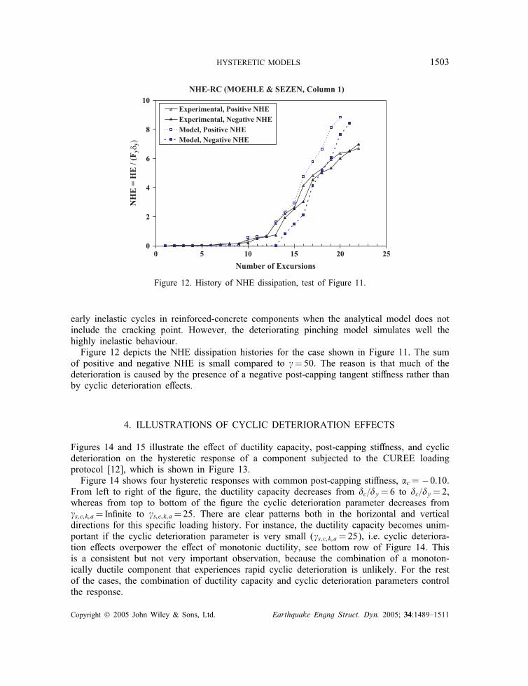
early inelastic cycles in reinforced-concrete components when the analytical model does notinclude the cracking point. However, the deteriorating pinching model simulates well thehighly inelastic behaviour.Figure 12 depicts the NHE dissipation histories for the case shown in Figure 11. The sum

of positive and negative NHE is small compared to �=50. The reason is that much of thedeterioration is caused by the presence of a negative post-capping tangent sti�ness rather thanby cyclic deterioration e�ects.

4. ILLUSTRATIONS OF CYCLIC DETERIORATION EFFECTS

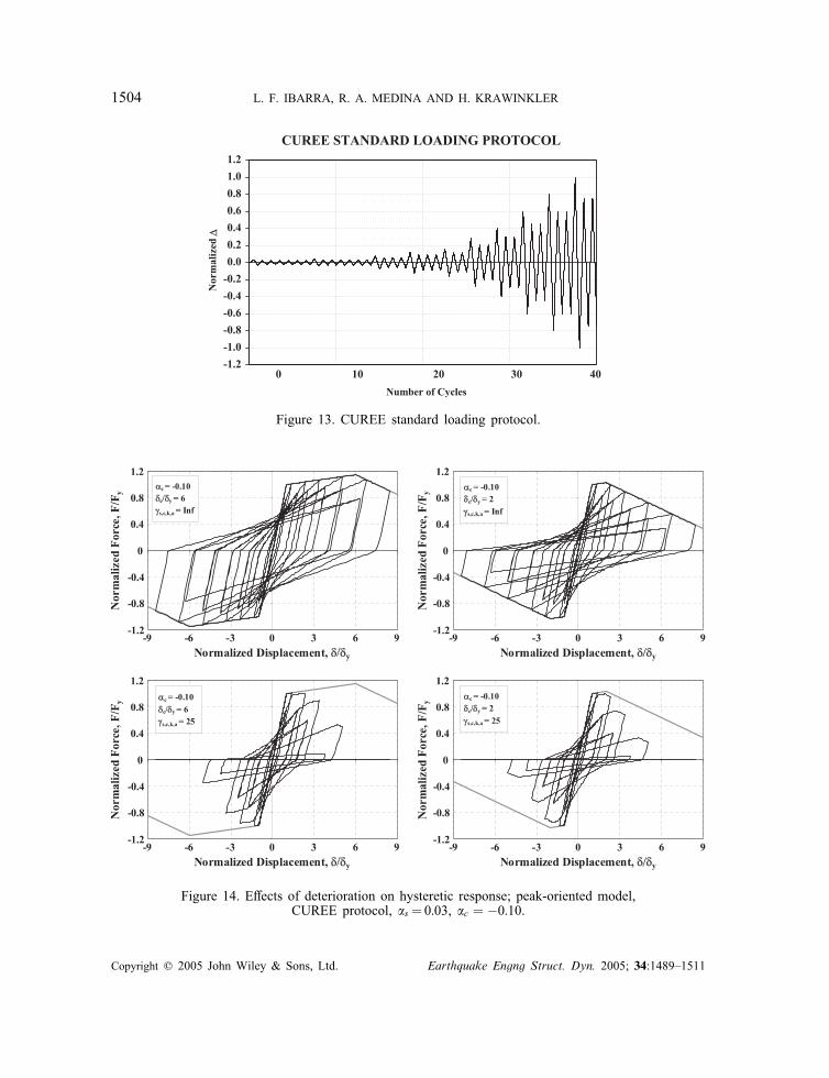
Figures 14 and 15 illustrate the e�ect of ductility capacity, post-capping sti�ness, and cyclicdeterioration on the hysteretic response of a component subjected to the CUREE loadingprotocol [12], which is shown in Figure 13.Figure 14 shows four hysteretic responses with common post-capping sti�ness, �c= −0:10.

From left to right of the �gure, the ductility capacity decreases from �c=�y=6 to �c=�y=2,whereas from top to bottom of the �gure the cyclic deterioration parameter decreases from�s; c; k; a=In�nite to �s; c; k; a=25. There are clear patterns both in the horizontal and verticaldirections for this speci�c loading history. For instance, the ductility capacity becomes unim-portant if the cyclic deterioration parameter is very small (�s; c; k; a=25), i.e. cyclic deteriora-tion e�ects overpower the e�ect of monotonic ductility, see bottom row of Figure 14. Thisis a consistent but not very important observation, because the combination of a monoton-ically ductile component that experiences rapid cyclic deterioration is unlikely. For the restof the cases, the combination of ductility capacity and cyclic deterioration parameters controlthe response.



Figure 13. CUREE standard loading protocol.

Figure 14. E�ects of deterioration on hysteretic response; peak-oriented model,CUREE protocol, �s=0:03, �c = −0:10.



(a) (b)

(d)(c)

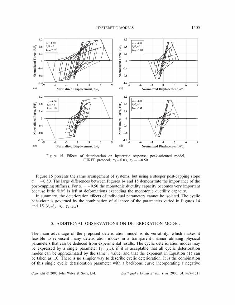
Figure 15. E�ects of deterioration on hysteretic response; peak-oriented model,CUREE protocol, �s=0:03, �c = −0:50.

Figure 15 presents the same arrangement of systems, but using a steeper post-capping slope�c=−0:50. The large di�erences between Figures 14 and 15 demonstrate the importance of thepost-capping sti�ness. For �c=−0:50 the monotonic ductility capacity becomes very importantbecause little ‘life’ is left at deformations exceeding the monotonic ductility capacity.In summary, the deterioration e�ects of individual parameters cannot be isolated. The cyclic

behaviour is governed by the combination of all three of the parameters varied in Figures 14and 15 (�c=�y, �c, �s; c; k; a).

5. ADDITIONAL OBSERVATIONS ON DETERIORATION MODEL

The main advantage of the proposed deterioration model is its versatility, which makes itfeasible to represent many deterioration modes in a transparent manner utilizing physicalparameters that can be deduced from experimental results. The cyclic deterioration modes maybe expressed by a single parameter (�s; c; k; a), if it is acceptable that all cyclic deteriorationmodes can be approximated by the same � value, and that the exponent in Equation (1) canbe taken as 1.0. There is no simpler way to describe cyclic deterioration. It is the combinationof this single cyclic deterioration parameter with a backbone curve incorporating a negative



post-capping tangent sti�ness that makes this deterioration model simple but versatile. Thefollowing observations are made in the context of damage and deterioration modelling.

• There are fundamental di�erences between the proposed deterioration model and cumu-lative damage models. The latter count cumulative damage and use a counter (oftenreferred to as a damage index) to indicate the degree of damage or complete ‘failure’(for the latter the counter usually takes a value of 1.0). Most cumulative damage models(e.g. the Park–Ang model [13]) do not consider the fact that cumulative damage causesa decrease in strength and sti�ness of components and therefore lead to an increase indeformations in a structure, which ultimately may cause collapse. The component cu-mulative damage models known to the authors do not permit tracking of the responseof a structure till collapse, whereas the component deterioration models proposed here,when implemented in a computer analysis program, do permit prediction of collapse ofa structure.

• The proposed deterioration models incorporate cyclic deterioration controlled by hys-teretic energy dissipation as well as deterioration of the backbone curve (strength cappingat �c=�y and a post-capping decrease in strength de�ned by �c). This dual deteriorationbehaviour is equivalent to the two-part damage concept contained in some cumulativedamage models such as the Park–Ang model [13]. This model, which was developedspeci�cally for reinforced-concrete components, consists of a linear combination of dis-placement and energy demands, expressed as follows:

DM=�max�ult

+�

Fy�ult

∫dHE (8)

where DM is a damage index, �max is the maximum displacement of the system, �ult isthe monotonic displacement capacity of the system, and � is a structural performanceparameter. In concept, the parameters �ult and � of this cumulative damage model areanalogous to �c and � of the proposed deterioration model.

• Figures 8, 10, and 12 show that the reference cyclic hysteretic energy dissipation ca-pacity, �Fy�y, is rarely achieved in component tests. Components usually reach zeroresistance long before this reference capacity is utilized. This happens because of thepresence of strength capping and a negative post-capping tangent sti�ness that leads tozero resistance (or a residual strength) even if no cyclic loading is performed. The post-capping strength deterioration and the cyclic strength deterioration are analogous to thephenomena expressed by the two terms of the Park–Ang damage model (Equation (8)).

6. APPLICATION OF HYSTERETIC MODELS TO SEISMIC EVALUATIONOF SDOF SYSTEMS

The deterioration models discussed in the previous sections have been employed in an exten-sive parameter study on the e�ects of deterioration on the inelastic dynamic response of SDOFsystems and MDOF frame structures [14]. Representative results are illustrated in Figures 16and 17 for a peak-oriented SDOF system subjected to a series of 40 ground motion records.A reference non-deteriorating system is used as well as three systems with various levelsof deterioration. The results are not comprehensive, but serve to illustrate the impact that



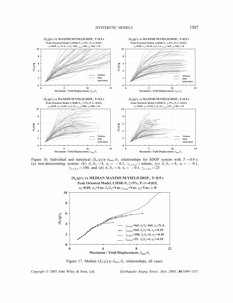
Figure 16. Individual and statistical (Sa=g)=�–�max=�y relationships for SDOF system with T =0:9 s:(a) non-deteriorating system; (b) �c=�y=4, �c= − 0:1, �s; c; k; a= in�nite; (c) �c=�y=4, �c= − 0:1,

�s; c; k; a=100; and (d) �c=�y=4, �c= − 0:1, �s; c; k; a=25.

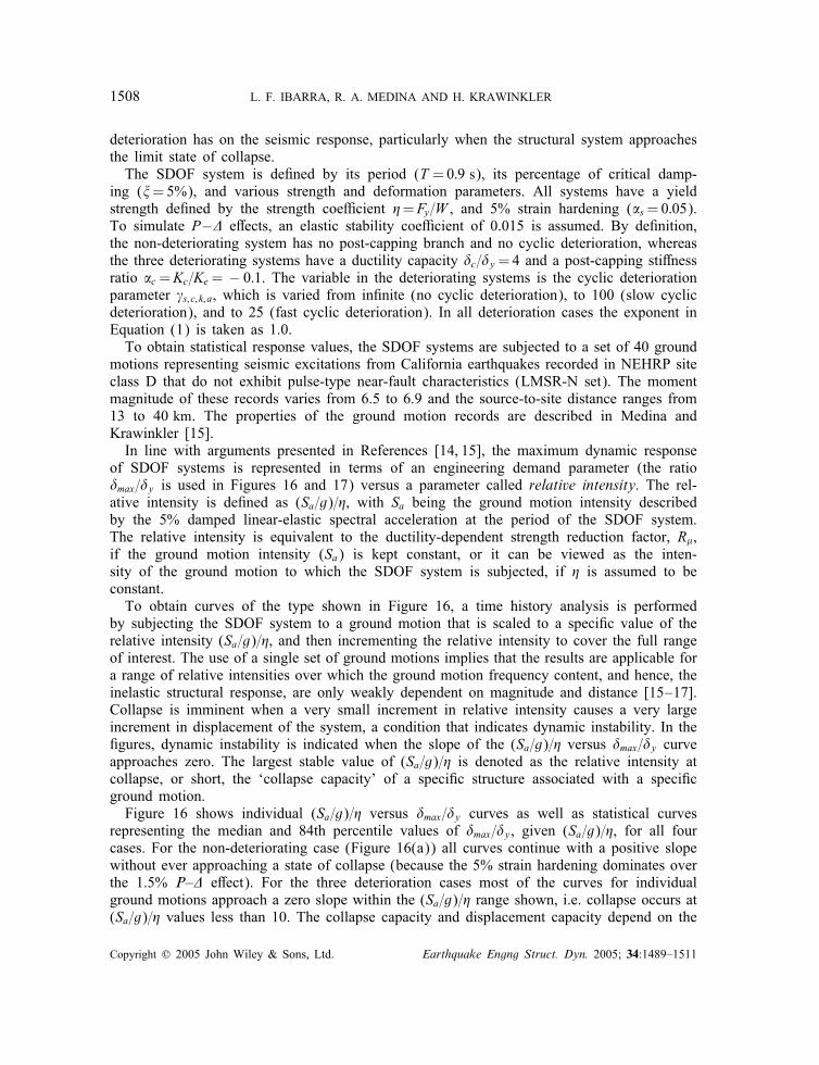
Figure 17. Median (Sa=g)=�–�max=�y relationships, all cases.



deterioration has on the seismic response, particularly when the structural system approachesthe limit state of collapse.The SDOF system is de�ned by its period (T =0:9 s), its percentage of critical damp-

ing (=5%), and various strength and deformation parameters. All systems have a yieldstrength de�ned by the strength coe�cient �=Fy=W , and 5% strain hardening (�s=0:05).To simulate P−� e�ects, an elastic stability coe�cient of 0.015 is assumed. By de�nition,the non-deteriorating system has no post-capping branch and no cyclic deterioration, whereasthe three deteriorating systems have a ductility capacity �c=�y=4 and a post-capping sti�nessratio �c=Kc=Ke= − 0:1. The variable in the deteriorating systems is the cyclic deteriorationparameter �s; c; k; a, which is varied from in�nite (no cyclic deterioration), to 100 (slow cyclicdeterioration), and to 25 (fast cyclic deterioration). In all deterioration cases the exponent inEquation (1) is taken as 1.0.To obtain statistical response values, the SDOF systems are subjected to a set of 40 ground

motions representing seismic excitations from California earthquakes recorded in NEHRP siteclass D that do not exhibit pulse-type near-fault characteristics (LMSR-N set). The momentmagnitude of these records varies from 6.5 to 6.9 and the source-to-site distance ranges from13 to 40 km. The properties of the ground motion records are described in Medina andKrawinkler [15].In line with arguments presented in References [14, 15], the maximum dynamic response

of SDOF systems is represented in terms of an engineering demand parameter (the ratio�max=�y is used in Figures 16 and 17) versus a parameter called relative intensity. The rel-ative intensity is de�ned as (Sa=g)=�, with Sa being the ground motion intensity describedby the 5% damped linear-elastic spectral acceleration at the period of the SDOF system.The relative intensity is equivalent to the ductility-dependent strength reduction factor, R,if the ground motion intensity (Sa) is kept constant, or it can be viewed as the inten-sity of the ground motion to which the SDOF system is subjected, if � is assumed to beconstant.To obtain curves of the type shown in Figure 16, a time history analysis is performed

by subjecting the SDOF system to a ground motion that is scaled to a speci�c value of therelative intensity (Sa=g)=�, and then incrementing the relative intensity to cover the full rangeof interest. The use of a single set of ground motions implies that the results are applicable fora range of relative intensities over which the ground motion frequency content, and hence, theinelastic structural response, are only weakly dependent on magnitude and distance [15–17].Collapse is imminent when a very small increment in relative intensity causes a very largeincrement in displacement of the system, a condition that indicates dynamic instability. In the�gures, dynamic instability is indicated when the slope of the (Sa=g)=� versus �max=�y curveapproaches zero. The largest stable value of (Sa=g)=� is denoted as the relative intensity atcollapse, or short, the ‘collapse capacity’ of a speci�c structure associated with a speci�cground motion.Figure 16 shows individual (Sa=g)=� versus �max=�y curves as well as statistical curves

representing the median and 84th percentile values of �max=�y, given (Sa=g)=�, for all fourcases. For the non-deteriorating case (Figure 16(a)) all curves continue with a positive slopewithout ever approaching a state of collapse (because the 5% strain hardening dominates overthe 1.5% P–� e�ect). For the three deterioration cases most of the curves for individualground motions approach a zero slope within the (Sa=g)=� range shown, i.e. collapse occurs at(Sa=g)=� values less than 10. The collapse capacity and displacement capacity depend on the



rate of deterioration, which is slowest when �s; c; k; a, is equal to in�nite (no cyclic deterioration)and fastest when �s; c; k; a, is equal to 25.The e�ect of deterioration is best evaluated from the median curves, which for all four

cases are presented in Figure 17. Without deterioration, the system never approaches col-lapse. If a strength cap is applied (at �c=�y=4), which is followed by a post-capping branch(with �c= − 0:1), the median curves deviate from those of the non-deteriorating case to anextent that depends on the rate of cyclic deterioration. For �s; c; k; a, equal to in�nite, the de-viation starts at �max=�y=4, which corresponds to the deformation assigned to the strengthcap, and strength capping alone leads to collapse at (Sa=g)=� of about 6. If the hystereticenergy dissipation capacity is relatively large (i.e. �s; c; k; a=100), which implies a low rate ofcyclic deterioration, the e�ect of cyclic deterioration is small. On the other hand, a value of�s; c; k; a=25, which implies a high rate of cyclic deterioration, leads to an early deviation fromthe non-deteriorating case and to a considerable decrease in the collapse capacity comparedto the case with strength capping but without cyclic deterioration.The above results demonstrate that modelling of deterioration is not very important at

relatively small levels of deformations. However, deterioration becomes an overriding consid-eration when the structure (in this case represented by a simple SDOF system) approachescollapse. When and to what extent the relationship between the relative intensity and an en-gineering demand parameter deviates from that of a non-deteriorating system depends on thecombination of important system parameters, such as ductility ratio (�c=�y), post-capping sti�-ness ratio (�c), and the energy dissipation capacity of the system, de�ned by �s; c; k; a, whichcontrols cyclic deterioration. The magnitude of the P−� e�ect also plays an important role.Comprehensive results on the e�ects of all these parameters for SDOF and MDOF systemsare presented in Ibarra [14].

7. CONCLUSIONS

This paper presents the description, calibration and application of relatively simple hystereticmodels that incorporate the most important sources of strength and sti�ness deterioration.Adequate modelling of deterioration is critical for demand prediction for highly inelasticsystems.The hysteretic models include a post-capping softening branch, residual strength, and cyclic

deterioration. Cyclic deterioration permits to trace deterioration as a function of pastloading history. The rate of deterioration is de�ned by the parameter �i, which depends onthe hysteretic energy dissipated in past cycles and on a reference energy dissipation capacityexpressed as �Fy�y. Four modes of cyclic deterioration can be simulated: basic strength, post-capping strength, unloading sti�ness, and accelerated reloading sti�ness deterioration. Basedon calibrations performed with experimental data from component tests of steel, wood, andreinforced-concrete specimens, it appears that, for a given component, the backbone character-istics and a single parameter (�s; c; k; a) that controls all four modes of cyclic deterioration areadequate to represent component behaviour regardless of the loading history. This conclusionis only preliminary because more work needs to be performed to establish consistent methodsfor assessing all important deterioration parameters (�c=�y, �c, �′s, c) for the full range ofrelevant structural components. Work on this task is in progress.



Results from the seismic evaluation of various SDOF systems demonstrate that strengthdeterioration becomes a dominant factor when the response of a structure approaches thelimit state of collapse. At early stages of inelastic behaviour, both deteriorating and non-deteriorating systems exhibit similar responses. The di�erences become important when thepost-capping sti�ness is attained in the response.In summary, the response of structural systems that undergo large inelastic excursions is

controlled by deterioration in assemblies of components. The implementation of a rigorousseismic performance assessment methodology is not complete without models capable of track-ing the history of damage until or at least close to collapse and incorporate, in an explicitmanner, the e�ects of deterioration in the seismic response. The deterioration models presentedin this paper are intended to assist in accomplishing this objective.

ACKNOWLEDGEMENTS

The authors are grateful to Dr Mohsen Rahnama who developed the early version of the SDOF programSNAP in which the deteriorating models were implemented. Thanks are due to Dr Ashraf Ayoub andManuel Miranda who contributed to the implementation of the models in SNAP. This research wassupported by the NSF sponsored Paci�c Earthquake Engineering Research (PEER) Center. The studiesof the �rst author were mainly supported by the Consejo Nacional de Ciencia y Tecnologia (CONACYT)and complemented by funds from PEER. These sources of support are much appreciated.

REFERENCES

1. Clough RW, Johnston SB. E�ect of sti�ness degradation on earthquake ductility requirements. Proceedings ofJapan Earthquake Engineering Symposium, Tokyo, Japan, 1966.

2. Takeda T, Sozen MA, Nielson NN. Reinforced concrete response to simulated earthquakes. ASCE Journal ofthe Structural Division 1970; 96:2557–2573.

3. Wen YK. Method for random vibration of hysteretic systems. ASCE Journal of the Engineering MechanicsDivision 1976; 112:249–263.

4. Sivaselvan MV, Reinhorn AM. Hysteretic models for deteriorating inelastic structures. Journal of EngineeringMechanics 2000; 126:633–640.

5. Song J, Pincheira J. Spectral displacement demands of sti�ness and strength degrading systems. EarthquakeSpectra 2000; 16:817–851.

6. Gatto KS, Uang CM. E�ects of loading protocol and rate of loading on woodframe shearwall response. SeventhU.S. National Conference on Earthquake Engineering, EERI, Oakland, CA, 2002.

7. Rahnama M, Krawinkler H. E�ects of soft soil and hysteresis model on seismic demands. John A. BlumeEarthquake Engineering Center Report No. 108. Department of CEE, Stanford University, 1993.

8. Prakash V, Powell GH, Campbell. DRAIN-2DX: basic program description and user guide. Report No.UCB/SEMM-1993/17, University of California, Berkeley, CA, 1993.

9. Mahin SA, Bertero VV. Nonlinear seismic response of a coupled wall system. ASCE Journal of the StructuralDivision 1976; 102:1759–1980.

10. Uang CM, Yu QS, Gilton CS. E�ects of loading history on cyclic performance of steel RBS moment connections.Proceedings of the 12th WCEE, Upper Hutt, New Zealand, 2000.

11. Sezen H. Evaluation and testing of existing reinforced concrete building columns. CE299 Report. Universityof California, Berkeley, 2000.

12. Krawinkler H, Parisi F, Ibarra L, Ayoub A, Medina R. Development of a testing protocol for woodframestructures. CUREE Publication No. W-02. 2000.

13. Park Y, Ang A. Mechanistic seismic damage model for reinforced concrete. Journal of Structural Engineering1985; 111:722–739.

14. Ibarra L. Global collapse of frame structures under seismic excitations. PhD Dissertation, Department of CEE,Stanford University, 2003.



15. Medina RA, Krawinkler H. Seismic demands for non-deteriorating frame structures and their dependence onground motions. John A. Blume Earthquake Engineering Center Report No. 144. Department of CEE, StanfordUniversity, 2003.

16. Shome N, Cornell A. Probabilistic seismic demand analysis of nonlinear structures. Report No. RMS-35.Department of Civil Engineering, Stanford University.

17. Jalayer F. Direct probabilistic seismic analysis: implementing nonlinear dynamic assessments. PhD Dissertation,Department of CEE, Stanford University, 2003.


Hysteretic models that incorporate strength and stiffness deterioration

Documents