Hyperplane Queries In a Feature-Space M-Tree for Speeding Up Active Learning

Hyperplane Queries in a Feature-Space M-tree for

Speeding up Active Learning

Michel Crucianu1,2, Daniel Estevez1, Vincent Oria3, and Jean-Philippe Tarel4

1 Vertigo-CEDRIC, CNAM, 292 rue St. Martin, 75141 Paris Cedex 03, France

Michel.Crucianu(a)cnam.fr,Esteve_D(a)auditeur.cnam.fr http://cedric.cnam.fr/vertigo/2 INRIA Rocquencourt, 78153 Le Chesnay Cedex, France

3 Department of Computer Science, New Jersey Institute of Technology, University Heights, Newark, NJ 07079, USA

Vincent.Oria(a)njit.edu http://web.njit.edu/∼oria/4 Laboratoire Central des Ponts et Chaussees, 58 Bd. Lefebvre, 75015 Paris, France

Tarel(a)lcpc.fr http://perso.lcpc.fr/tarel.jean-philippe/

Abstract—In content-based retrieval, relevance feedback

(RF) is a noticeable method for reducing the “semantic

gap” between the low-level features describing the content

and the usually higher-level meaning of user’s target.

While recent RF methods based on active learning are

able to identify complex target classes after relatively few

iterations, they can be quite slow on very large databases.

To address this scalability issue for active RF, we put

forward a method that consists in the construction of an

M-tree in the feature space associated to a kernel function

and in performing approximate kNN hyperplane querieswith this feature space M-tree. The experiments performed

on two image databases show that a significant speedup

can be achieved, at the expense of a limited increase in

the number of feedback rounds.

Keywords—scalability, content-based retrieval, relevance

feedback, M-tree, approximate search, hyperplane queries

I. INTRODUCTION

The query-by-example paradigm for content-based re-

trieval is known to suffer from the discrepancy—known

as “semantic gap”—between the low-level features that

can be readily extracted from documents and higher-

level descriptions that are meaningful for the users of

the search engine. By including the user in the retrieval

loop, relevance feedback (RF) is in many cases able to

bridge this semantic gap. First introduced for the retrieval

of text documents [1], RF rapidly developed for image

retrieval ([2], [3]), mainly because a user can be very

fast in evaluating the relevance of an image.

An RF session is divided into several consecutive

rounds (or iterations); at every round the user provides

feedback regarding the retrieval results, e.g. by qualify-

ing items5 returned as either “relevant” or “irrelevant”;

from this feedback, the engine learns the features de-

scribing the relevant items and returns improved results

to the user. An RF mechanism employs a learner and a

selector. At every feedback round, the user marks (part

of) the items returned by the search engine as “relevant”

or “irrelevant”. The learner exploits this information to

re-estimate the target of the user. Since the number of

examples is typically very low, this stage is very fast with

such learners as support vector machines (SVM, [4]).

With the current estimation of the target, the selector

chooses other items for which the user is asked to

provide feedback during the next round.

State of the art RF methods rely on active learning [5],

[6]: the user is asked to provide feedback on those items

that can maximize the transfer of information from the

user to the system. This typically implies the selection,

at every feedback round, of the most ambiguous items

(sometimes with a complementary condition of low

redundancy, as in [7]), i.e. those items that are closest

to the frontier of what the system considers (at the

current round) to be the target class. To be able to search

very large databases, we should avoid evaluating the

ambiguousness of all the items in the database. Existing

multidimensional data structures and associated search

methods [8] mostly concern similarity-based retrieval

with queries having the same nature as the items stored in

the database. But a decision frontier is different in nature

from the items in the database, so specific solutions are

needed for answering such frontier-based queries.

The decision frontier can be quite complex in the

5While our evaluations here only concern image databases, RF

in general and our method in particular are not specific to such

databases, so we prefer to speak about “items” rather than images.

space where the items are described, making the retrieval

problem difficult to formulate in this initial space. How-

ever, by the use of specific kernel functions [9] the initial

space is mapped to a corresponding feature space, where

a hyperplane can be an appropriate decision frontier [4].

Our main contribution here is to put forward a retrieval

method that consists in performing approximate kNNhyperplane queries with an M-tree built in this feature

space. This method is not limited to the RF context,

it can be employed for active learning in general. The

experiments performed on two image databases show

that a significant speedup can be achieved, at the expense

of a limited increase in the number of feedback rounds.

These results also point out that approximate search

methods can behave well in very challenging conditions:

high-dimensional spaces, with queries expected to have

a low selectivity.

The next section summarizes the background of this

work: use of SVM for active feedback, existing proposals

for the scalability of relevance feedback and approximate

kNN retrieval with an M-tree. Our hyperplane-basedretrieval method is described in Section III. The results of

an experimental evaluation are presented in Section IV,

and several issues regarding approximate retrieval and

the properties of various kernel functions are discussed

in Section V.

II. BACKGROUND

A. Active relevance feedback with support vector ma-

chines

Part of the recent work on RF (e.g. [6], [10], [7]) is

based on support vector machines (SVM) because they

avoid too restrictive assumptions regarding the data, are

very flexible and allow fast learning with a reasonably

low number of examples.

Support vector machines belong to the family of

kernel methods [4], who first map the data from the

original (input) space I to a higher-dimensional featurespace H and then perform linear algorithms in H. Thenonlinear mapping φ : I → H is implicitly definedby a kernel function K : I × I → R endowing Hwith a Hilbert space structure if the kernel is positive

definite [9]. The inner product 〈·, ·〉 : H × H → R

can be expressed as 〈φ(x), φ(y)〉 = K(x,y). This“kernel trick” allows to reduce inner products in H toordinary kernel computations in I and thus extend linearalgorithms relying on inner products in H to nonlinearalgorithms based on more ordinary computations in I.It is important to note that the input space I does notneed to be a vector space, as long as a positive definite

kernel can be defined (such kernels also exist for strings,

sets, trees, etc.). For all the experiments we present in

Section IV, I = Rd, but the method we put forward is

not restricted to this case.

O

O

O

O

O

O

O

O

O

O

φ

OO

O

OO

OOO OO O

OO

O

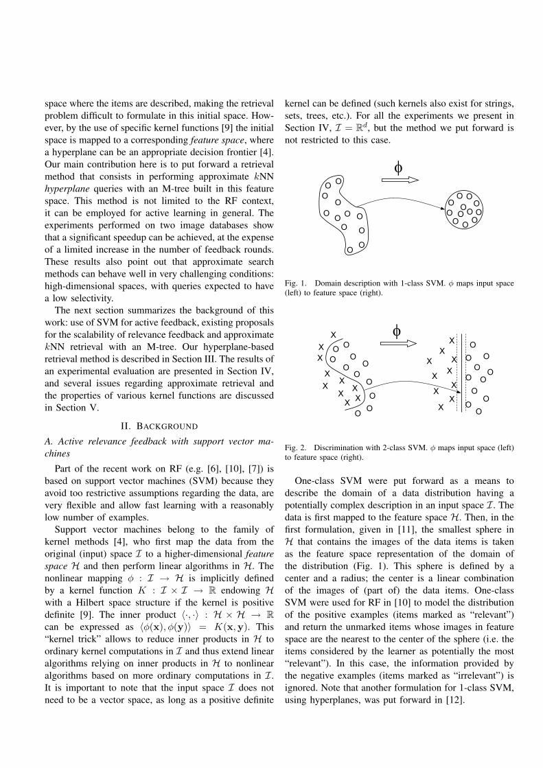
Fig. 1. Domain description with 1-class SVM. φ maps input space

(left) to feature space (right).

OXX

X

XX

X XX

X

O

OOO

O

O

O

O

OX

φO

OXX

X

XX

X

XX

X

O

OOO

OO

O

O

OX

O

Fig. 2. Discrimination with 2-class SVM. φ maps input space (left)

to feature space (right).

One-class SVM were put forward as a means to

describe the domain of a data distribution having a

potentially complex description in an input space I. Thedata is first mapped to the feature space H. Then, in thefirst formulation, given in [11], the smallest sphere in

H that contains the images of the data items is takenas the feature space representation of the domain of

the distribution (Fig. 1). This sphere is defined by a

center and a radius; the center is a linear combination

of the images of (part of) the data items. One-class

SVM were used for RF in [10] to model the distribution

of the positive examples (items marked as “relevant”)

and return the unmarked items whose images in feature

space are the nearest to the center of the sphere (i.e. the

items considered by the learner as potentially the most

“relevant”). In this case, the information provided by

the negative examples (items marked as “irrelevant”) is

ignored. Note that another formulation for 1-class SVM,

using hyperplanes, was put forward in [12].

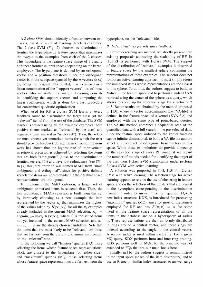
A 2-class SVM aims to identify a frontier between two

classes, based on a set of learning (labeled) examples.

The 2-class SVM (Fig. 2) chooses as discrimination

frontier the hyperplane in feature space that maximizes

the margin to the examples from each of the 2 classes.

This hyperplane is the feature space image of a usually

nonlinear frontier in input space (depending on the kernel

employed). The hyperplane is defined by an orthogonal

vector and a position threshold. Since the orthogonal

vector is in the subspace spanned by the n vectors φ(xi)(xi being the original data points), it is expressed as a

linear combination of the “support vectors”, i.e. of those

vectors who are within the margin. Learning consists

in identifying the support vectors and computing the

linear coefficients, which is done by a fast procedure

for constrained quadratic optimization.

When used for RF, a 2-class SVM learns at every

feedback round to discriminate the target class (of the

“relevant” items) from the rest of the database. The SVM

learner is trained using all the available examples, both

positive (items marked as “relevant” by the user) and

negative (items marked as “irrelevant”). Then, the selec-

tor must choose yet unmarked items for which the user

should provide feedback during the next round. Previous

work has shown that the highest rate of improvement

in retrieval precision is achieved by selecting the items

that are both “ambiguous” (close to the discrimination

frontier, see e.g. [6]) and have low redundancy (see [7]).

In [7] this joint criterion was named MAO, from “most

ambiguous and orthogonal”, since for positive definite

kernels the items are non-redundant if their feature space

representations are orthogonal.

To implement the MAO criterion, a larger set of

ambiguous unmarked items is selected first. Then, the

low redundancy (MAO) selection is built from this set

by iteratively choosing as a new example the item

represented by the vector xj that minimizes the highest

of the values taken by K(xi,xj) for all the xi examples

already included in the current MAO selection: xj =argminx∈S maxi K(x,xi), where S is the set of itemsnot yet included in the current MAO selection and xi,

i = 1, . . . , n are the already chosen candidates. Note thatthe items that are most likely to be “relevant” are those

that are farthest from the current discrimination frontier,

on the “relevant” side.

In the following we call “frontier” queries (FQ) those

selecting the items whose feature space representations,

φ(x), are closest to the hyperplane (on either side),and “maximum” queries (MQ) those selecting items

whose feature space representations are farthest from the

hyperplane, on the “relevant” side.

B. Index structures for relevance feedback

Before describing our method, we shortly present here

existing proposals addressing the scalability of RF. In

[10] RF is performed with 1-class SVM. The support

of the distribution of “relevant” examples is described

in feature space by the smallest sphere containing the

representations of these examples. The selector does not

follow an active learning approach: it must simply return

the unmarked items whose representations are the closest

to this sphere. To do this, the authors suggest to build an

M-tree in the feature space and to perform standard kNNretrieval using the center of the sphere as a query, which

allows to speed up the selection stage by a factor of 2

to 3. Better results are obtained by the method proposed

in [13], where a vector approximation file (VA-file) is

defined in the feature space of a kernel (KVA-file) and

employed with the same type of point-based queries.

The VA-file method combines a sequential scan of the

quantified data with a full search in the pre-selected data.

Since the feature space induced by the kernel function

can be infinite-dimensional, to build a VA-file the authors

select a reduced set of orthogonal basis vectors in this

space. While these two solutions do provide a speedup

of the selection stage of every RF round, if we regard

the number of rounds needed for identifying the target of

the user then 1-class SVM significantly under perform

2-class SVM with active learning.

A solution was proposed in [14], [15] for 2-class

SVM with active learning. The selection stage for active

learning appears to rely on the use of clustering in feature

space and on the selection of the clusters that are nearest

to the hyperplane corresponding to the discrimination

frontier in order to answer “frontier” queries (FQ). A

new index structure, KDX, is introduced for processing

“maximum” queries (MQ): since for most of the kernels

employed for RF one has K(x,x) = α for somefixed α, the feature space representations of all theitems in the database are on a hypersphere of radius

α. These representations are then uniformly distributedin rings around a central vector, and these rings are

indexed according to the angle to the central vector.

A second index is used within each ring. For a given

MQ query, KDX performs intra and inter-ring pruning.

KDX performs well for MQs, but the principle was not

extended to FQs that are our main focus here.

Finally, in [16] the authors suggest to remain instead

in the input space (space of the item descriptors) and to

use an R-tree or similar index structures to answer range

queries corresponding to the hyper-rectangles where ei-

ther positive or negative examples were already found.

However, the input space can also be high-dimensional

(e.g., the dimension of typical image descriptors is

between 20 and a few hundreds), so an R-tree can hardly

be expected to perform well.

C. M-tree for exact and approximate search

The M-tree index structure was introduced in [17],

[18] to address cases where the representation space

is not a vector space, but is only endowed with a

metric structure. The M-tree and the associated retrieval

methods rely on the properties of a metric, the triangular

inequality being especially important. We only provide

here a very brief description of kNN retrieval, the readershould refer to [17], [18] for further details.

Let Q be the query object, Op the parent object of

the current node N , Or a rooting object belonging to

node N , r(Or) the covering radius of Or and T (Or)the sub-tree having Or as root. Retrieval is based on the

following results:

1) If d(Or, Q) > r(Q)+r(Or), then it is safe to pruneT (Or) since d(Oj , Q) > r(Q) for each object Oj

in T (Or).2) If |d(Op, Q) − d(Or, Op)| > r(Q) + r(Or), thenit is not even necessary to compute d(Or, Q)since d(Or, Q) ≥ |d(Op, Q) − d(Or, Op)|, sod(Or, Q) > r(Q) + r(Or).

To answer kNN (or “top-k”) queries, the method in[18], [17] makes use of a priority queue, PR, of pointers

to active sub-trees (where objects satisfying the query

can potentially be found) and of a k-elements array, NN,for storing neighbors by increasing order of their distance

to the query. Below, dmin(T (Or)) = max{d(Or, Q) −r(Or), 0} is the lower bound for the distance betweenany object in T (Or) and Q, dmax(T (Or)) = d(Or, Q)+r(Or) is the upper bound for the distance between anyobject in T (Or) and Q, and dk is the largest distance

in NN. The value of dk can be seen here as a dynamic

search radius. Nodes in PR are sorted by increasing order

of their dmin values.

The algorithm for answering kNN queries begins withan empty NN array, with PR containing the root node and

with an infinite value for the dynamic search range dk.

When a node in the PR list is processed it is removed

from PR and all its children are added to PR (unless they

are leaves). Objects are progressively found and, if their

distance to the query is lower than dk, are introduced in

the NN array (an object already in the array may have to

be removed) and dk is updated. Search stops when the

dmin of the first entry in PR (the entry with the lowest

dmin) is higher than the distance to the query of the k-th entry in NN (the entry having highest distance to the

query): none of the remaining nodes can improve over

the kNN already in NN.Approximate retrieval with the M-tree was also stud-

ied. The Approximately Correct Nearest Neighbor (AC-

NN) algorithm introduced in [19] was applied to the M-

tree in [20]. By accepting as approximate NN for a query

an object that is within a distance lower than (1 + ǫ)dk

to the query, where dk is the distance to the true NN and

ǫ > 0, search can be stopped earlier, which produces arelative improvement in retrieval speed.

In [20] the authors notice that kNN retrieval usingthe dynamic radius algorithm described above can be

described as having two stages: during the first stage,

exact or approximate nearest neighbors are found; during

the second stage, further nodes are retrieved from the pri-

ority queue PR in order to check whether the neighbors

already found are the nearest indeed. They consider then

difficult cases, where the distribution of the distances

between the items in the database is concentrated (but

not to the point where NN queries become meaningless)

and produces significant overlap in the M-tree, with

the important consequence of reducing the selectivity in

processing queries. In such difficult cases, the second

stage can become very long (with respect to the first)

because, given the significant node overlap, the priority

queue still contains many candidate nodes when the

nearest neighbors are found; however, below a certain

search radius, the probability of finding better neighbors

in the remaining nodes becomes negligible. In brief,

many candidate nodes intersect the search range but the

intersections are empty.

The Probably Approximately Correct (PAC-NN) algo-

rithm put forward in [20] attempts to provide a solution

to this problem. Besides the use of the accuracy param-

eter ǫ defining the quality of approximation (as for AC-NN), a confidence parameter δ is introduced. The PAC-NN algorithm attempts to guarantee with probability at

least 1−δ that the “relative error” ǫ will not be exceededby the approximate nearest neighbor returned. For this,

search is stopped when the dynamic search radius be-

comes lower than the bound (1+ǫ)rq,δ, where rq,δ is such

that P (∃o, d(q, o) ≤ rq,δ) ≤ δ and has to be estimatedfrom the data (either before or after the construction of

the M-tree, but prior to query processing).

PAC-NN generalizes both the AC-NN retrieval, ob-

tained when δ = 0, and the Correct Nearest Neighbor(C-NN) retrieval (ǫ = 0 and δ = 0). PAC-NN avoids

searching “too close” to the query object and uses the

distance distribution to the query object to derive a

stopping criterion. We further explore here approximate

retrieval with the M-tree for a different type of queries.

III. HYPERPLANE QUERIES IN AN M-TREE

A. Principle of the method

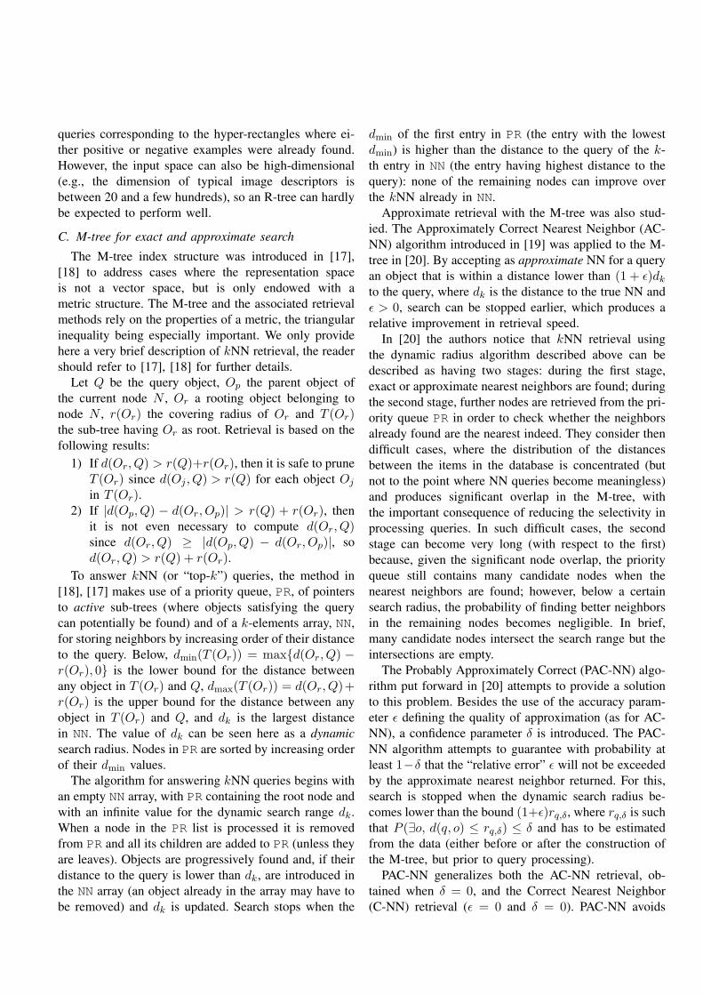
We perform RF using 2-class SVM and active learn-

ing. To speed up the selection stage of every feedback

round, we build an M-tree in the feature space (FSM-

tree in the following) associated to the kernel and we

retrieve with this FSM-tree the kNN of the hyperplanethat is the frontier given by the SVM (see Fig. 3). We

speak of kNN hyperplane queries or, more generally, of“frontier” queries (FQ).

Building the index structure in the feature space rather

than in the input space has two potential benefits. First,

the query has a simpler expression in the feature space:

a hyperplane in the feature space usually corresponds to

a complex nonlinear surface in input space. Second, the

input space does not need to be a vector space; as long

as a positive definite kernel can be defined (such kernels

also exist for sets, trees, etc.), a distance-based index

(like the M-tree) in feature space can be used. This can

actually be done with a more general class of kernels,

the conditionally positive definite ones [21].

++

+ ++

o

o

+ +

++

o o o

+

Fig. 3. The frontier in input space (left) of the class of “relevant”

images, as estimated by the SVM, is mapped to a hyperplane that is

used as a query in the FSM-tree (right).

However, feature spaces are usually of much higher

dimension than the input space. But since the dimension

of the input space is already very high, the impact of this

difference may not be very important. In fact, for several

of the kernels we employ, the distribution of distances

computed in the feature space is not very different from

the distribution of distances in the input space, so metric

indexing should be nearly as effective in feature space

as in input space. But given the high dimension of

both spaces, we do not expect component-based indexing

methods (SR-tree, VA-file, etc.) to perform well.

The use of hyperplanes as queries poses several dif-

ficulties. First, dimension reduction methods cannot be

used: hyperplanes are not necessarily orthogonal to the

reduced space, so items can be close to the query in

original space and far from it in the reduced space (fil-

tering in the reduced space can produce false negatives).

The same difficulties occur if we attempt to use index

structures that rely on various types of low-dimensional

projections.

Second, a hyperplane query can be expected to be

much less selective than a point. As we shall see later,

approximate kNN retrieval does provide a practical solu-tion to this problem. Third, for many index structures the

computations involved can be complex; the M-tree offers

simple computations of the distance to a hyperplane (or,

for a sub-tree, of the minimal and maximal distances).

The first step of our method is the construction

of an M-tree in the feature space (FSM-tree) associ-

ated to the kernel employed for the SVM. If x1 and

x2 represent two items in the input space, then the

distance between their images in feature space can

be easily computed as d(φ(x1), φ(x2)) = ||φ(x1) −φ(x2)|| =

√

< (φ(x1) − φ(x2)), (φ(x1) − φ(x2)) > =√

K(x1,x1) + K(x2,x2) − 2K(x1,x2).Now, consider the hyperplane H in feature space

associated to the discrimination frontier of an SVM. It

can be defined as∣

∣

∣

∣

∣

∑

i

αi yi K(p,xi) + b

∣

∣

∣

∣

∣

= 0 (1)

where xi are the support vectors, yi the associated labels

(+1 or −1), αi the corresponding coefficients and b theoffset. Then, for some point p in the original space, the

distance in feature space between its image φ(p) and thehyperplane H, d(p,H), can be written as

d(p,H) =|∑

i αi yi K(p,xi) + b |√

∑

i,j αi αj yi yj K(xi,xj)(2)

The denominator is the norm of the vector defining the

hyperplane in feature space and xi, xj are all support

vectors.

Consider now an FQ of range r(H), i.e. attemptingto retrieve the items whose image in feature space is

within a distance range of r(H) to H. If p corresponds

to a routing node in the M-tree, then the sub-tree under

the node of center p and radius r can be further ignored

(pruned) if d(p,H) > r(H)+r. With the same notationsas for the M-tree, it is easy to show that:

1) If d(Or, H) > r(H) + r(Or) then the sub-treeT (Or) can be safely pruned since, for each objectOj in T (Or), d(Oj , H) > r(H).

2) Unfortunately, d(Or, H) ≥ |d(Op, H)−d(Or, Op)|is false and only d(Or, H) ≥ d(Op, H) −d(Or, Op) holds, so it is actually necessary to com-pute d(Or, H) when d(Op, H) − d(Or, Op) ≤ 0(i.e. in more cases than for point queries).

B. Search algorithms with hyperplane queries

We can now write the algorithms performing kNNfrontier queries. Since we are using the FSM-tree to

select, at every feedback round, new (unmarked) images,

we need a mechanism for excluding the images that

were marked at previous rounds; below we consider that

the test predicate isUnmarked only returns true for

unmarked images. With the notations from the previous

section and following the presentation of the original

kNN search in [17], [18], the method for answering kNNfrontier queries is given by Algorithms 1, 2 and 3.

Algorithm 1 KNNFS (T : rootNode, H: query, k:nbNeighbors)

1: PR = [T, ]2: NN[i] = random set of k items3: while PR not empty and NN[k].d ≥ dmin(head(PR))

do

4: NextNode = KNNChooseNode (PR)

5: KNNFSNodeSearch (NextNode, H , k)6: end while

Algorithm 2 KNNSChooseNode (PR: priorityQueue):

node

1: dmin(T (O∗

r)) = min{dmin(T (Or))} over all entriesin PR

2: remove entry [T (O∗

r), dmin(T (O∗

r))] from PR3: return T (O∗

r)

Here, NN[k].d is the distance field of the last entry

in NN (i.e. the leaf entry having highest distance to

the query among the entries already examined) and

dmin(head(PR)) is the dmin field of the first entry

in the PR list (i.e. the non-leaf entry having lowest dmin

among the entries not yet examined).

To obtain the corresponding approximate kNN re-trieval versions (see Section II-C), the following changes

should be performed:

Algorithm 3 KNNFSNodeSearch (N : node, H: query,k: nbNeighbors)

1: if N is not a leaf then2: for all Or ∈ N do3: if d(Op, H) − d(Or, Op) ≤ dk + r(Or) then4: Compute d(Or, H)5: Compute dmin(T (Or))6: if dmin(T (Or)) ≤ dk then

7: Add [T (Or), dmin(T (Or))] to PR8: end if

9: end if

10: end for

11: else

12: for all Oj ∈ N do13: if isUnmarked(Oj) ∧ d(Op, H)− d(Oj , Op) ≤

dk then

14: Compute d(Oj , H)15: if d(Oj , H) ≤ dk then

16: dk = NNUpdate ([Oj , d(Oj , H)])17: end if

18: end if

19: end for

20: end if

• For AC-NN search, in Algorithm 1, line 3,

NN[k].d is replaced with NN[k].d/(1 + ǫ) andin Algorithm 3, lines 3 and 6, dk is replaced with

dk/(1 + ǫ).• For PAC-NN, besides the changes corresponding to

AC-NN, search is immediately stopped in Algo-

rithm 3 if the dk value returned at line 16 satisfies

dk ≤ (1 + ǫ)rq,δ.

We implemented these algorithms, as well as relatively

similar algorithms for “maximum” queries, using the M-

tree package [22].

IV. EXPERIMENTAL EVALUATION

To evaluate the method we put forward here we per-

formed experimental comparisons with (exact) sequential

search on two ground-truth image databases, one of

which contains 110,000 images. The use of a ground

truth is required because the user is emulated during

the relevance feedback (RF) sessions: the membership

of images to the classes of the ground truth must be

known by the emulated user if he is to provide reliable

feedback. The comparisons were performed against se-

quential search because the description of the clustering

method used in [15] for frontier queries is not detailed

enough and the index structures suggested in [16] for

indexing in the input space (R-tree, etc.) are known to

be ineffective for the high-dimensional input space we

employ.

A. Experimental setup

To ease future comparisons, we employed databases

that are publicly available and have a non-controversial

ground-truth. Since RF algorithms must help reduce

the semantic gap, it is necessary to avoid having too

many “trivial” classes, for which simple low-level visual

similarity is sufficient for correct classification. For an

evaluation of RF it should nevertheless be possible to

identify the target class relatively well with a limited

number of examples. With these criteria in mind, the

two databases we retained are:

• GT72 (3744 images), composed of the 52 most dif-

ficult classes—in terms of internal diversity within

classes and of separability between classes—from

the well-known Columbia color database, where

each class contains 72 images.

• Amsterdam Library of Object Images (ALOI,

110,250 images, [23]), a color image collection

of 1,000 small objects where the viewing angle,

illumination angle and illumination color for each

object were systematically varied in order to pro-

duce about 110 images for each object. Similarity-

based retrieval is more difficult for ALOI than

for GT72 because there is more diversity in the

illumination conditions and there are many more

classes.

We use the following generic descriptors for the visual

content of the images [24]: a Laplacian weighted color

histogram [25], a probability weighted color histogram

[25], a classic HSV color histogram, a shape histogram

based on the Hough transform and a texture histogram

relying on the Fourier transform. Previous evaluations

[7], [24] have shown that the joint use of these de-

scriptors helps avoiding the numerical gap for generalist

image databases like the ones we employ here, i.e.

sufficient information allowing to discriminate between

images is provided by these descriptors.

Linear PCA is applied to the descriptors in order to

reduce the dimension of the joint descriptor from more

than 600 to about 150.

The first kernel we consider is the Gaussian one (or

Radial Basis Function, RBF in the following figures),

K(xi,xj) = exp (−γ‖xi−xj‖2). This classical kernel,

often employed by default, is highly sensitive to the scale

parameter γ (the inverse of the variance of the Gaussian).

The angular kernel (ANG in the following figures),

K(xi,xj) = −‖xi−xj‖, was introduced in [9] as a con-ditionally positive definite kernel, but the convergence of

SVM remains guaranteed with this kernel and distance-

based methods in feature space can still be applied [21].

The use of the Laplace kernel (LAPL in the next

figures),K(xi,xj) = exp (−γ‖xi−xj‖), was advocatedfor histogram-based image descriptors [26]. The scale

parameter is γ again and was fixed, following [7], to0.001; with such a small value for γ the “angular” partof the Laplace kernel entirely covers the domain of the

input data, so this kernel behaves very similarly to the

angular kernel.

In [7], the angular and Laplace kernels were shown to

provide consistently better results than the RBF kernel

for image retrieval with relevance feedback. We nev-

ertheless decided to compare them again here in order

to study the relation between kernel properties and the

speedup obtained. The L1 norm was employed in all

cases.

For the evaluations, an FSM-tree is built for every

database and kernel employed, then all the experiments

are performed. Following [18], [20], the parameters we

employ are:

• number of candidates for sampling: 10% of the

number of items (images);

• minimum node utilization: 0.4;• promotion method: confirmed (CONFIRMED);

• root promotion method: minimal radius

(MIN RAD);

• confirmed promotion method: minimal maximal ra-

dius (mM RAD);

• mM RAD promotion method: average (AVG);

• split method: hyperplane (G HYPERPL).

On a standard PC running Linux, the construction of

an FSM-tree only takes about 10 seconds for the GT72

database and 2 minutes for the large ALOI database.

For all the four databases, at every feedback round the

emulated user must label images displayed in a window

of size ws = 9. Every search session is initialized byconsidering one “relevant” example and ws−1 randomlyselected “irrelevant” examples. We focus on ranking

most of the “relevant” images before the “irrelevant”

ones. To evaluate the speed of improvement of this rank-

ing, we use a precision measure computed as follows: let

n be the number of images in the target class; at everyRF round, we count the number of images from the target

class that are found in the n images considered as mostpositive by the current decision function of the SVM;

this number is then divided by n. The “mean precision”

reported is obtained by averaging the precision measure

defined above over all the RF sessions.

B. Evaluation results

For both databases, the exact retrieval for kNN frontierqueries produces an insignificant speedup with respect

to the evaluation of all the items in a database. This

was expected, given the rather low selectivity of the

hyperplane queries and of the FSM-tree. With AC-NN, a

significant speedup is only be obtained for high values of

ǫ, with a strong negative impact on the precision measuredefined above.

For PAC-NN retrieval, the gain in retrieval speed

during the selection stage of every feedback round

is evaluated using the ratio of distance computations

with the FSM-tree to distance computations with full

sequential scan: the lower the ratio, the higher the gain

in retrieval speed. These ratios are shown in Fig. 4 for

GT72 and Fig. 6 for ALOI. The corresponding loss in

precision is evaluated by depicting, for each kernel, both

the evolution of the mean precision with the exact (or

correct) NN retrieval and with the PAC-NN retrieval.

These losses in precision are shown in Fig. 5 for GT72

and Fig. 7 for ALOI.

PAC-NN retrieval with the FSM-tree produces a sig-

nificant speedup, providing answers in real-time even

on the ALOI database, with a relatively low loss in

precision. Since the databases we have hold in main

memory, the speedup we evaluated only concerns the

number of distance computations and directly translates

into gains in computation time. We expect the speedup to

be even more important for larger databases that require

access to secondary storage.

The Laplace and angular kernels behave similarly, as

expected for γ = 0.001. It is important to highlight thatfor the angular kernel d(φ(xi), φ(xj)) =

√

‖xi − xj‖,so the distribution of distances computed in the feature

space is actually more “spread” than the distribution of

distances in the input space.

V. DISCUSSION

As seen from Fig. 4 to Fig. 7, the speedup for the RBF

kernel is much higher than for the other two kernels,

but the precision remains low and hardly improves with

more feedback rounds. We believe that this is due to

the fact that the RBF kernel decreases quickly, so it is

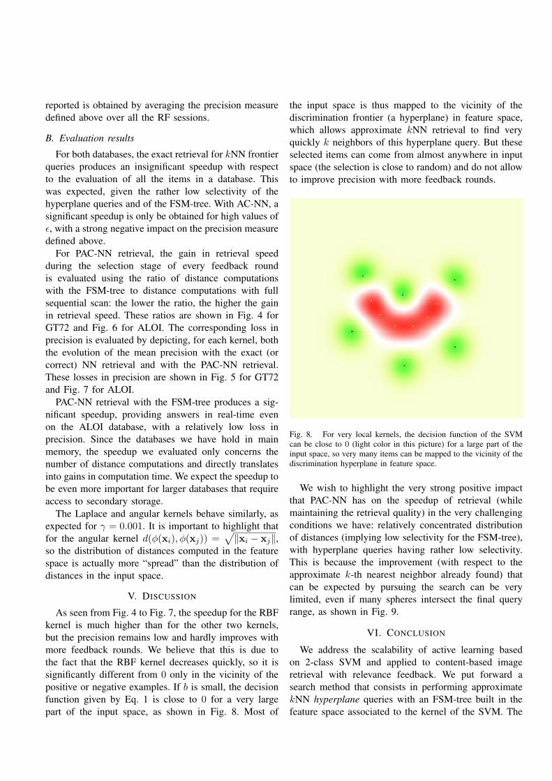
significantly different from 0 only in the vicinity of thepositive or negative examples. If b is small, the decisionfunction given by Eq. 1 is close to 0 for a very largepart of the input space, as shown in Fig. 8. Most of

the input space is thus mapped to the vicinity of the

discrimination frontier (a hyperplane) in feature space,

which allows approximate kNN retrieval to find veryquickly k neighbors of this hyperplane query. But theseselected items can come from almost anywhere in input

space (the selection is close to random) and do not allow

to improve precision with more feedback rounds.

Fig. 8. For very local kernels, the decision function of the SVM

can be close to 0 (light color in this picture) for a large part of the

input space, so very many items can be mapped to the vicinity of the

discrimination hyperplane in feature space.

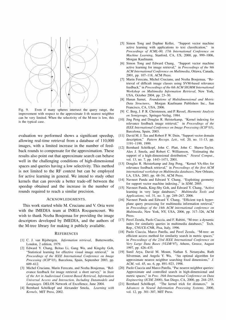
We wish to highlight the very strong positive impact

that PAC-NN has on the speedup of retrieval (while

maintaining the retrieval quality) in the very challenging

conditions we have: relatively concentrated distribution

of distances (implying low selectivity for the FSM-tree),

with hyperplane queries having rather low selectivity.

This is because the improvement (with respect to the

approximate k-th nearest neighbor already found) thatcan be expected by pursuing the search can be very

limited, even if many spheres intersect the final query

range, as shown in Fig. 9.

VI. CONCLUSION

We address the scalability of active learning based

on 2-class SVM and applied to content-based image

retrieval with relevance feedback. We put forward a

search method that consists in performing approximate

kNN hyperplane queries with an FSM-tree built in thefeature space associated to the kernel of the SVM. The

0

0.05

0.1

0.15

0.2

0.25

0.3

0 2 4 6 8 10 12 14

Usin

g F

SM

-tre

e /

se

qu

en

tia

l

Iteration

ANG-PAC LAPL-PAC RBF-PAC

Fig. 4. For the GT72 database and the 3 kernels (ANGular, LAPLace and RBF), the ratio of distance computations with the FSM-tree

(and PAC-NN) to distance computations with full evaluation (sequential scan) as a function of feedback rounds.

0.65

0.7

0.75

0.8

0.85

0.9

0.95

1

2 4 6 8 10 12 14

Me

an

pre

cis

ion

Iteration

ANGANG-PAC

LAPLLAPL-PAC

RBFRBF-PAC

Fig. 5. For the GT72 database and the 3 kernels, evolution of the mean precision obtained with exact search (empty marks) and approximate

search (PAC, filled marks).

0

0.05

0.1

0.15

0.2

0.25

0 2 4 6 8 10 12 14

Usin

g F

SM

-tre

e /

se

qu

en

tia

l

Iteration

ANG-PAC LAPL-PAC RBF-PAC

Fig. 6. For the ALOI database (ANGular, LAPLace and RBF), the ratio of distance computations with the FSM-tree (and PAC-NN) to

distance computations with full evaluation (sequential scan) as a function of feedback rounds.

0.55

0.6

0.65

0.7

0.75

0.8

0.85

0.9

2 4 6 8 10 12 14

Me

an

pre

cis

ion

Iteration

ANGANG-PAC

LAPLLAPL-PAC

RBFRBF-PAC

Fig. 7. For the ALOI database, evolution of the mean precision obtained with exact (empty marks) and approximate search (PAC, filled

marks).

+

+

++

++

Fig. 9. Even if many spheres intersect the query range, the

improvement with respect to the approximate k-th nearest neighbor

can be very limited. When the selectivity of the M-tree is low, this

is the typical case.

evaluation we performed shows a significant speedup,

allowing real-time retrieval from a database of 110,000

images, with a limited increase in the number of feed-

back rounds to compensate for the approximation. These

results also point out that approximate search can behave

well in the challenging conditions of high-dimensional

spaces and queries having a low selectivity. This method

is not limited to the RF context but can be employed

for active learning in general. We intend to study other

kernels that can provide a better trade-off between the

speedup obtained and the increase in the number of

rounds required to reach a similar precision.

ACKNOWLEDGMENTS.

This work started while M. Crucianu and V. Oria were

with the IMEDIA team at INRIA Rocquencourt. We

wish to thank Nozha Boujemaa for providing the image

descriptors developed by IMEDIA, and the authors of

the M-tree library for making it publicly available.

REFERENCES

[1] C. J. van Rijsbergen, Information retrieval, Butterworths,

London, 2 edition, 1979.

[2] Edward Y. Chang, Beitao Li, Gang Wu, and Kingshy Goh,

“Statistical learning for effective visual image retrieval,” in

Proceedings of the IEEE International Conference on Image

Processing (ICIP’03), Barcelona, Spain, September 2003, pp.

609–612.

[3] Michel Crucianu, Marin Ferecatu, and Nozha Boujemaa, “Rel-

evance feedback for image retrieval: a short survey,” in State

of the Art in Audiovisual Content-Based Retrieval, Information

Universal Access and Interaction, Including Datamodels and

Languages. DELOS Network of Excellence, June 2004.

[4] Bernhard Scholkopf and Alexander Smola, Learning with

Kernels, MIT Press, 2002.

[5] Simon Tong and Daphne Koller, “Support vector machine

active learning with applications to text classification,” in

Proceedings of ICML-00, 17th International Conference on

Machine Learning, Stanford, CA, US, 2000, pp. 999–1006,

Morgan Kaufmann.

[6] Simon Tong and Edward Chang, “Support vector machine

active learning for image retrieval,” in Proceedings of the 9th

ACM International Conference on Multimedia, Ottawa, Canada,

2001, pp. 107–118, ACM Press.

[7] Marin Ferecatu, Michel Crucianu, and Nozha Boujemaa, “Re-

trieval of difficult image classes using SVM-based relevance

feedback,” in Proceedings of the 6th ACM SIGMM International

Workshop on Multimedia Information Retrieval, New York,

USA, October 2004, pp. 23–30.

[8] Hanan Samet, Foundations of Multidimensional and Metric

Data Structures, Morgan Kaufmann Publishers Inc., San

Francisco, CA, USA, 2006.

[9] C. Berg, J. P. R. Christensen, and P. Ressel, Harmonic Analysis

on Semigroups, Springer-Verlag, 1984.

[10] Jing Peng and Douglas R. Heisterkamp, “Kernel indexing for

relevance feedback image retrieval,” in Proceedings of the

IEEE International Conference on Image Processing (ICIP’03),

Barcelona, Spain, 2003.

[11] David M. J. Tax and Robert P. W. Duin, “Support vector domain

description,” Pattern Recogn. Lett., vol. 20, no. 11-13, pp.

1191–1199, 1999.

[12] Bernhard Scholkopf, John C. Platt, John C. Shawe-Taylor,

Alex J. Smola, and Robert C. Williamson, “Estimating the

support of a high-dimensional distribution,” Neural Comput.,

vol. 13, no. 7, pp. 1443–1471, 2001.

[13] Douglas R. Heisterkamp and Jing Peng, “Kernel VA-files for

relevance feedback retrieval,” in Proceedings of the first ACM

international workshop on Multimedia databases, New Orleans,

LA, USA, 2003, pp. 48–54, ACM Press.

[14] Navneet Panda and Edward Y. Chang, “Exploiting geometry

for support vector machine indexing.,” in SDM, 2005.

[15] Navneet Panda, King-Shy Goh, and Edward Y. Chang, “Active

learning in very large databases,” Multimedia Tools and

Applications, vol. 31, no. 3, pp. 249–267, 2006.

[16] Navneet Panda and Edward Y. Chang, “Efficient top-k hyper-

plane query processing for multimedia information retrieval,”

in Proceedings of the 14th ACM international conference on

Multimedia, New York, NY, USA, 2006, pp. 317–326, ACM

Press.

[17] Pavel Zezula, Paolo Ciaccia, and F. Rabitti, “M-tree: a dynamic

index for similarity queries in multimedia databases,” Tech.

Rep., CNUCE-CNR, Pisa, Italy, 1996.

[18] Paolo Ciaccia, Marco Patella, and Pavel Zezula, “M-tree: an

efficient access method for similarity search in metric spaces,”

in Proceedings of the 23rd IEEE International Conference on

Very Large Data Bases (VLDB’97), Athens, Greece, August

1997, pp. 426–435.

[19] Sunil Arya, David M. Mount, Nathan S. Netanyahu, Ruth

Silverman, and Angela Y. Wu, “An optimal algorithm for

approximate nearest neighbor searching fixed dimensions,” J.

ACM, vol. 45, no. 6, pp. 891–923, 1998.

[20] Paolo Ciaccia and Marco Patella, “Pac nearest neighbor queries:

Approximate and controlled search in high-dimensional and

metric spaces,” in Proc. 16th International Conference on Data

Engineering (ICDE 2000), San Diego, CA, 2000, pp. 244–255.

[21] Bernhard Scholkopf, “The kernel trick for distances,” in

Advances in Neural Information Processing Systems. 2000,

vol. 12, pp. 301–307, MIT Press.

[22] Marco Patella, Paolo Ciaccia, and Pavel Zezula, “M-tree

library,” http://www-db.deis.unibo.it/Mtree/, 2000.

[23] J. M. Geusebroek, G. J. Burghouts, and A. W. M. Smeulders,

“The Amsterdam library of object images,” Int. J. Comput.

Vision, vol. 61, no. 1, pp. 103–112, 2005.

[24] Marin Ferecatu, Image retrieval with active relevance feedback

using both visual and keyword-based descriptors, Ph.D. thesis,

Universite de Versailles, France, 2005.

[25] Nozha Boujemaa, Julien Fauqueur, Marin Ferecatu, Francois

Fleuret, Valerie Gouet, Bertrand Le Saux, and Hichem Sahbi,

“IKONA: Interactive generic and specific image retrieval,”

in Proceedings of the International workshop on Multimedia

Content-Based Indexing and Retrieval (MMCBIR’2001), Roc-

quencourt, France, 2001, pp. 25–29.

[26] Olivier Chapelle, P. Haffner, and Vladimir N. Vapnik, “Support-

vector machines for histogram-based image classification,”

IEEE Transactions on Neural Networks, vol. 10, no. 5, pp.

1055–1064, 1999.