Hydrological Model Selection: a Bayesian Alternative

Hydrological model selection: A Bayesian alternative

Lucy Marshall

School of Civil and Environmental Engineering, University of New South Wales, Sydney, New South Wales, Australia

David Nott

School of Mathematics, University of New South Wales, Sydney, New South Wales, Australia

Ashish Sharma

School of Civil and Environmental Engineering, University of New South Wales, Sydney, New South Wales, Australia

Received 7 October 2004; revised 9 June 2005; accepted 25 July 2005; published 28 October 2005.

[1] The evaluation and comparison of hydrological models has long been a challenge tothe practicing hydrological community. No single model can be identified as ideal over therange of possible hydrological situations. With the variety of models available, hydrologicmodelers are faced with the problem of determining which model is best applied to acatchment for a particular modeling exercise. The model selection problem is welldocumented in hydrologic studies, but a broadly applicable as well as theoretically andpractically sound method for comparing model performance does not exist in theliterature. Bayesian statistical inference, with computations carried out via Markov chainMonte Carlo (MCMC) methods, offers an attractive alternative to conventional modelselection methods allowing for the combination of any preexisting knowledge aboutindividual models and their respective parameters with the available catchment data toassess both parameter and model uncertainty. The aim of this study is to present a methodby which hydrological models may be compared in a Bayesian framework. The studybuilds on previous work (Marshall et al., 2004) in which a Bayesian approachimplemented using MCMC algorithms was presented as a simple and efficient basis forassessing parameter uncertainty in hydrological models. In this study, a model selectionframework is developed in which an adaptive Metropolis algorithm is used to calculate themodel’s posterior odds. The model used to illustrate our approach is a version of theAustralian Water Balance Model (Boughton, 1993) reformulated such that it can have aflexible number of soil moisture storages. To assess the model selection method in acontrolled setting, artificial runoff data were created corresponding to a known modelconfiguration. These data were used to evaluate the accuracy of the model selectionmethod and its sensitivity to the size of the sample being used. An application of theBayesian model identification methodology to 11 years of daily streamflow data from theMurrumbidgee River at Mittagang Crossing in southeastern Australia concludes our study.

Citation: Marshall, L., D. Nott, and A. Sharma (2005), Hydrological model selection: A Bayesian alternative, Water Resour. Res., 41,

W10422, doi:10.1029/2004WR003719.

1. Introduction

[2] An issue in many hydrological studies is determiningwhich model is best applied to a catchment in any modelingexercise. No model can be identified as ideal for the rangeof hydrological conditions and catchments that exist. Whenselecting a model, we are not solely reliant on its predictiveperformance but will also take into account the modeler’spreference and familiarity in using particular models, theaim of the modeling task, the time available to develop andapply a model and the level of accuracy required. Inaddition to these issues, significant attention is also paidto the performance of the model when applied to a specificcatchment. Assessing the relative performance of competing

models can be difficult given the limited data that are oftenavailable. This is further complicated by difficulties inobtaining a unique set of values for the model parameters.Traditional comparison of models has proceeded by splittingavailable catchment data, and then performing calibration/validation of the model using the split data samples. Typicalcomparisons have focused on identifying the hydrologicalmodel (from a limited selection) that best reproducesthe measured flow for specific catchments according to anumber of numerical criteria [Franchini and Pacciani, 1991;Chiew et al., 1993; Refsgaard and Knudsen, 1996; Ye et al.,1997; Donnelly-Makowecki and Moore, 1999]. Others haveevaluated the tradeoff between model performance and easeof use for simple versus complex models [Loague andFreeze, 1985; Jakeman and Hornberger, 1993; Michaudand Sorooshian, 1994]. The current state of model selectionmethods can be summarized as follows.

Copyright 2005 by the American Geophysical Union.0043-1397/05/2004WR003719

W10422

WATER RESOURCES RESEARCH, VOL. 41, W10422, doi:10.1029/2004WR003719, 2005

1 of 11

[3] 1. Most model selection methods currently in use areaimed at assessing model choice based on a quantitativecriterion of model accuracy.[4] 2. These criteria cannot always allow assessment of

specific attributes of the hydrograph (for example, peakflows or storm volumes). While multiobjective formulations[e.g., Madsen, 2003; Vrugt et al., 2003b] are desirable forsuch criteria, specifying the weight for each objective can bedifficult.[5] 3. A common problem across all methods is spec-

ifying the form of the model errors. Simplistic errormodels (such as independent normal errors) are oftenunrealistic, particularly in regard to independence assump-tions [Kavetski et al., 2002].[6] 4. Measures based purely on ranking by a residual

sum of squares (such as the Nash-Sutcliffe coefficient [Nashand Sutcliffe, 1970]) are problematic. They will always favorthe most complex model among a class of nested models.The need to balance a tradeoff between model complexityand model performance is well recognized. Most simplecriteria for assessing model performance do not adequatelycharacterize the model’s predictive performance, and willchoose the model with the lowest calibration error.[7] 5. Some currently used model selection methods do

attempt to penalize model complexity (such as AIC [Akaike,1973] and BIC [Schwarz, 1978]). AIC is known not to beconsistent (that is, it will not necessarily choose the correctmodel as the sample size increases) while BIC is only anapproximation to the exact Bayesian techniques imple-mented later.[8] 6. The Bayesian approach is completely general. In

hydrological modeling, model and parameter uncertaintycan be significant considering the frequent lack of data andever-increasing complexity of new models. Whilst easilyapplied, most traditional methods of model comparison donot explicitly account for model and parameter uncertainty.Bayesian methods describe parameter and model uncertaintyprobabilistically. Many models may be compared without achange in the method, and there is no limit on the modelstructure (models are not required to be nested). Bayesianmethods also allow prior knowledge about the models to betaken into account. The results are not solely reliant oninformation from the available data, but enable specialistand preexisting knowledge to inform the results. In consid-ering the common modeling problems of overfitting andmodel complexity, Bayesian model selection methods arealso natural Ockham’s razors [Berger and Pericchi, 2000],favoring simpler models automatically. The traditionalapproach to Bayesian model selection requires calculationof the Bayes factor, which is the posterior probability ratioof the models (assuming equal prior probabilities).[9] A framework for comparison of models in a Bayesian

context is presented here. We evaluate an improved basis forcalculating the Bayes factor for a set of alternate hydrologicmodels. We also compare use of the Bayes factor for modelcomparison with two alternate model performance measuresthat have been used frequently in hydrology. The firstof these measures, the Nash–Sutcliffe coefficient of deter-mination, is used routinely for most model evaluationexercises, and suffers from the limitation of being structuredto prefer the most complex model under all circumstances.The second measure, the Bayesian information criterion

(BIC), is based on a large sample (asymptotic) approxima-tion to the Bayes factor, but may differ substantially from theuse of Bayes factors in small samples. We present selectedcase studies where the true model structure is known, andillustrate the limitations of using the Nash-Sutcliffe and theBIC for model comparison and selection. We then proceedon to a real case study, using daily rainfall runoff data fromthe Murrumbidgee River at Mittagang Crossing, a catchmentlocated in south eastern Australia, to illustrate the usefulnessof the proposed method for estimating the Bayes factor.While this study does not examine multiple objective for-mulations, extensions to include multiple objective functionscan be accommodated in the proposed framework.

2. Bayesian Theory and Model Comparison

[10] A range of methods exists for determining theoptimum values that parameters within a model shouldtake to reproduce the catchment behavior. The identifica-tion of an ideal parameter set is a complicated task. Often,a single optimum set does not exist. Bayesian inferenceprovides a framework within which the issues of parameteruncertainty and uncertainty of the observed data can beaddressed. The end product is a probability distribution(known as the posterior distribution) on the modelunknowns that describes model and parameter uncertaintyafter the data have been observed. The application ofBayesian methods to hydrological modeling has not beenextensive but recently more substantial interest has beenstimulated [Kuczera, 1983; Romanowicz et al., 1994;Freer et al., 1996; Kuczera and Parent, 1998; Kuczeraand Mroczkowski, 1998; Bates and Campbell, 2001;Thiemann et al., 2001; Marshall et al., 2004]. One ofthe reasons behind this emerging use is the advent ofMarkov chain Monte Carlo sampling methods, details onwhich are presented next.

2.1. Bayes Theorem and MCMC Methods

[11] Let q denote a vector of parameters of interest (suchas the parameters of a rainfall-runoff model). Let y denoteobserved data. In order to describe uncertainty about qprobabilistically after observing data y there must be amodel that provides a joint probability distribution for qand y. Then, Bayes’ theorem describes the relationshipbetween the conditional distribution for q given y and thejoint distribution of q and y. Bayes’ theorem states

p qjyð Þ ¼ p q; yð Þp yð Þ ¼ p qð Þf yjqð Þ

p yð Þ ð1Þ

where p(qjy) is the distribution of q given y (the posteriordistribution, describing uncertainty about q after observingy); p(q, y) is the joint probability distribution for q and y;p(q) is the distribution of q before collecting dataexpressing our prior knowledge of q (otherwise knownas the prior distribution); f(yjq) is the likelihood function(also known as the sampling distribution, specifying thedistribution of y given the unknowns q), and p(y) is anormalizing constant also known as the marginal like-lihood, a focal part of the model comparison problemaddressed in this study.[12] Bayesian statistical methods combine prior knowl-

edge about parameters and the observed data to produce the

2 of 11

W10422 MARSHALL ET AL.: HYDROLOGICAL MODEL SELECTION W10422

posterior distribution of the model parameters. If there arelimited data available, or the data do not influence theparameter, the resulting posterior distribution should beheavily influenced by the prior. Alternatively, when thedata provide a large amount of information about theparameter compared to the prior, the posterior distributionwill be dictated by the likelihood function.[13] While the conceptual elegance of the Bayesian

framework is undeniable, the computational effort requiredto implement Bayesian procedures has hindered their appli-cation. This effort is often due to the difficulty in evaluatingmoments and other statistics of interest from the posteriordistribution in (1), which is a multidimensional functionexpressed in terms of the unknown model parameters q, andcan assume a form that is not always easy to integrate.Markov chain Monte Carlo (MCMC) sampling is a rela-tively recent addition to the Bayesian computational toolkitand provides a simple and elegant way around the compu-tational difficulties noted above. The aim of MCMC sam-pling is to generate samples of the parameter values fromthe posterior distribution by simulating a random processthat has the posterior distribution as its stationary distribu-tion. Some recent studies concerned with developing effi-cient strategies for sampling the parameter space ofhydrologic models include those of Vrugt et al. [2003a,2003b] and Marshall et al. [2004].

2.2. Bayesian Model Comparison and Bayes Factors

[14] The Bayesian approach to model selection describesparameter and model uncertainty probabilistically. In com-paring two models, the traditional Bayesian approachrequires calculation of the Bayes factor, which representsthe odds of one model versus the other after observing thedata assuming equal prior model probabilities. Say we wishto choose a model from the set of models M = {M1,. . .Mn},given data y for implementing the model. Let p(Mi) be theprior probability of model Mi, and qi be the set of uncertainmodel parameters corresponding to model Mi. The tradi-tional approach to Bayesian model selection would comparetwo models through their posterior probability ratio:

P M1jyð ÞP M2jyð Þ ¼

P M1ð ÞP M2ð Þ �

m yjM1ð Þm yjM2ð Þ ð2Þ

where P(Mijy) is the posterior probability of model Mi,P(Mi) is the prior probability of model Mi, and m(yjMi) isthe model’s marginal likelihood. The second term on theright hand side of equation (2) is known as the Bayes factor.The marginal likelihood m(yjMi) is defined through theintegral

m yjMið Þ ¼Z

f yjqi;Mið Þp qijMið Þdq ð3Þ

over the parameter space, which must usually be estimatednumerically. Calculation of Bayes factors can be problem-atic due to the difficulties in estimating this often high-dimensional integral.[15] There are other Bayesian approaches which analyt-

ically approximate the marginal likelihood. The BIC crite-rion of Schwarz [1978] is an asymptotic approximation tothe Bayes factor. The criterion holds that the model log

marginal likelihood is approximately �0.5 BIC, where (if Nis the size of the sample):

BIC ¼ � 2 log maximized likelihoodð Þþ logNð Þ number of parametersð Þ ð4Þ

Note that for all results presented further in this paper,�0.5BIC has been included as an estimator of the marginallikelihood to allow comparison. The BIC and otherassociated approximations have the distinct advantage ofsimplicity over the Bayes factor, since they don’t requirenumerical methods for approximating the integral in themarginal likelihood. In cases where the prior information issmall relative to the information provided by the data, theBIC can yield results consistent with the Bayes factor [Kassand Raftery, 1995]. The BIC also accounts for overfitting bytending to favor simple models, as the criterion penalizesaccording to the number of parameters in a model.However, there are inherent risks in using the BIC alone.The method requires some regularity conditions on themodel and can differ from the use of Bayes factors if theavailable data are limited, as shown later.

2.3. Issues in Computing and Using Bayes Factors

[16] One concern in the use of Bayes factors lies in thecomputational difficulties of calculating the marginal like-lihood. Direct derivation of the marginal likelihood isimpossible in all but the simplest models: most modelsare too complex to allow analytic calculation of the integral(equation (3)). Other approaches are aimed at sampling(using Monte Carlo methods) the model and parameterspace simultaneously [Green, 1995] but it may be hard todesign good samplers for jumping between different mod-els. A good summary of some of the available methods forcomputing Bayes Factors and their associated benefits andlimitations is given by Han and Carlin [2001].[17] In model comparison studies, it can be argued that

most techniques without explicit penalization of modelcomplexity will pick the most complex model. However,Bayes factors act as natural Ockham’s razors [Berger andPericchi, 2000], favoring simpler models that give a com-parable level of fit to the data.[18] A difficult issue occurs in assigning meaningful

priors to the models and model parameters. This can be alengthy process, particularly as the number of models beingconsidered increases. The Bayes factor can be sensitive tothe choice of prior [Kass and Raftery, 1995]. There areproblems associated with assigning default or improperpriors. To illustrate, an example is presented (adapted fromLindley [1957]) whereby an attempt by a modeler toindicate that prior knowledge about a model is small, leadsto the alternative model being selected. Say we have data yi,i = 1,. . .,n assumed independent and two models (denotedM0 and M1) are introduced to fit the data. Model M0 is ofthe form

yi � N 0; 1ð Þ ð5Þ

Model M1 is of the form

yi � N m; 1ð Þ ð6Þ

W10422 MARSHALL ET AL.: HYDROLOGICAL MODEL SELECTION

3 of 11

W10422

Assuming little prior knowledge, a prior distribution is placedupon the parameter m in model M1 of the form: p(mjm 6¼ 0) �U[�c, c] where U[�c, c] denotes a uniform distributiondefined on the interval from �c to c, and where c is a largeconstant. To compare each model in fitting the data, themarginal likelihood of each model is determined:

p yjM0ð Þ ¼ 2pð Þ�n=2exp

�1

2

Xni¼1

y2i

!ð7Þ

p yjM1ð Þ ¼ 2pð Þ�n=2

2cexp

�1

2

Xni¼1

y2i

!

Z c

�c

exp�1

2nm2 � 2m

Xni¼1

yi

! !dm ð8Þ

In equation (8), for modelM1, the limit as c approaches infinity

of the integral approaches2pn

� �1/2

exp1

2n

Xni¼1

yi

!20@

1A,

but clearly1

capproaches zero so that p(yjM1) ! 0

regardless of the data. So with a vague enough prior on min model M1, model M0 will be accepted as the bettermodel regardless of the data.[19] This example illustrates that prior distributions on

parameters should generally be proper and have not toolarge a spread if the inference of interest involves modelcomparison. In the application of hydrological models, thismay create difficulties when the number of parameters islarge. However, very often parameters can be related tophysical catchment attributes or can be compared to param-eters in models with similar mechanism. This means that thespecification of meaningful priors is often feasible. Despitethe inherent difficulties in defining prior distributions forparameters in models, the process does have its advan-tages. It allows the use of extra specialist information thatmay exist about the model to be combined with availabledata.

3. Proposed Approach to Calculating BayesFactors

[20] A solution to the problem of calculating Bayesfactors is provided by Chib and Jeliazkov [2001], whouse an MCMC framework for estimating the marginallikelihood of a model by integrating over the parameterspace. The difficulty in using an MCMC approach is thatthese techniques obtain draws from the posterior distribu-tion, whereas the marginal likelihood is obtained by inte-grating the likelihood function with respect to the prior(equation (3)). Chib and Jeliazkov [2001] developed amethod for calculating Bayes factors in the context ofMCMC sampling by relating the marginal likelihood tothe posterior density calculated at a single point.

3.1. Estimation of Models’ Marginal Likelihood

[21] Consider again Bayes theorem (1) and note that theequation has been simplified to exclude an implicit condi-tioning of all variables on a common model M. If oneconsiders this explicitly, the normalizing constant p(y) in (1)

becomes the same as the marginal likelihood m(yjM) in (2)or (3). This can be used to express the marginal likelihood(using the notation defined previously) as

m yjMð Þ ¼ f yjM ; qð Þp qjMð Þp qjy;Mð Þ ð9Þ

where f(yjM, q) is the likelihood function for model M,p(qjM) is the prior density for the parameter q in model Mand p(qjy, M) is the posterior density of the parameters inmodel M. Chib and Jeliazkov [2001] provide an MCMCframework for estimating the marginal likelihood of amodel by integrating over the parameter space. By takinglogs, at some fixed value q* for q, the above identitybecomes

logm yjMð Þ ¼ log f yjM ; q*ð Þ þ logp q*jMð Þ � logp q*jy;Mð Þð10Þ

From this, the marginal likelihood can be found byestimating the log posterior ordinate, log p(q*jy, M) byusing the sampled parameter values from the MCMCprocess. Thus little further computation is required than thatto obtain samples from the model parameters’ posteriordistributions.[22] It is obvious that evaluation of the models’ marginal

likelihood using the above approximation first requireschoice of the value q*. For efficiency, q* is taken to bethe point where the posterior density of the model param-eters is maximized. Then, the aim of the exercise is toestimate the posterior density at q*. An estimate of thisposterior ordinate becomes:

p̂ q*jyð Þ ¼K�1

PKg¼1

a q gð Þ; q*jy�

q q gð Þ; q*jy�

J�1PJj¼1

a q*; q jð Þ� ð11Þ

where q(g) (for g = 1. . .K) are draws from the posteriordistribution generated via a suitable MCMC algorithm (ourstudy used a modified form of the Adaptive Metropolisalgorithm, details on which are outlined below); q( j) aredraws from q(q*, qjy), the proposal density for the transitionfrom the fixed parameter value q* to q; and a(q, q*jy) is theacceptance probability for a transition from q to q*. Explicitdefinitions of these quantities are given below.[23] The benefit of the method presented here lies in the

combined attraction of accuracy in estimating the marginallikelihood and the relative computational ease. MCMCtraces are only generated once, and thus calculation of themarginal likelihood is straightforward and computationallyundemanding when an efficient MCMC scheme is avail-able. A particular appeal of the approach is that a samplefrom the posterior distribution is obtained, which allowsfurther assessment of the model being considered. Itshould be noted that the resulting value of the marginallikelihood is an estimate that has a standard error of itsown. The standard error may be determined and itsderivation is given by Chib and Jeliazkov [2001]. Thenumerical value estimated would then produce an estimateof the possible variation in the estimate if the simulation

4 of 11

W10422 MARSHALL ET AL.: HYDROLOGICAL MODEL SELECTION W10422

were repeated, but only assuming the same value of q* isused.

3.2. Adaptive Metropolis Algorithm

[24] The issues of model complexity and complicatedparameter interaction have lead to difficulties in developingan efficient MCMC sampling regime that may be applied toa wide range of different models. The adaptive Metropolisalgorithm [Haario et al., 2001] is an approach that hascharacteristics well suited to hydrological models. Themethod is a variation on the conventional Metropolisalgorithm. The adaptive algorithm is characterized by amultivariate normal proposal distribution, with mean at thecurrent parameter value and varying covariance. The pro-posal covariance matrix is updated at each iteration basedon the covariance matrix of the sampled parameter values inthe parameter chain to that point. In this way, the proposaldistribution is updated using the knowledge learnt so farabout the posterior distribution. At iteration t, Haario et al.[2001] consider a multivariate normal proposal N(qt, Ct)where Ct is the proposal covariance.[25] For an initial period t0, Ct = C0 (where C0 is some

arbitrary initial covariance). For convenience, C0 is setat the covariance of the parameters under their priordistributions. After this initial period the proposal covari-ance is based on the estimated posterior covariance of theparameters:

Ct ¼C0 t � t0

sdCov q0 . . . ::qt�1ð Þ þ sdeId t > t0

8<: ð12Þ

where e is a small value simply to ensure Ct does notbecome singular; and sd is a scaling parameter to ensurereasonable acceptance rates of the proposed states.[26] The adaptive Metropolis algorithm is easily imple-

mented in models of high dimension. Also, the use of theparameters’ covariance matrix in the proposal ensuresreasonable acceptance rates even when there are highlycorrelated and interdependent parameters (frequently thecase in rainfall-runoff models). Marshall et al. [2004]compare the performance of the Adaptive Metropolis algo-rithm in the context of rainfall-runoff modeling, with other

sampling algorithms used routinely in hydrology, and findthat the adaptive Metropolis algorithm offers significantadvantages over the others in speed and in the ease withwhich it can be implemented. When the approach tocalculating the marginal likelihood is combined with theefficient adaptive Metropolis algorithm it offers a powerfultool for comparing models that may be implemented on alarge scale.

3.3. Algorithm for Calculating theMarginal Likelihood

[27] A full MCMC run is first performed to obtain a set ofparameter values q* with high posterior probability (thesampled value with highest posterior probability is chosen).[28] Estimation of the model’s marginal likelihood then

proceeds as follows.[29] 1. For g = 1,. . ., K,[30] 1a. Sample q(g) from the posterior distribution

(using the adaptive Metropolis algorithm).[31] 1b. Calculate a(q(g), q*jy), the probability of

accepting a move from q(g) to q*, which is defined as:

a q gð Þ; q*jy�

¼ min 1;p yjq*ð Þp q*ð Þ

p yjq gð Þ�

p q gð Þ�

8<:

9=; ð13Þ

using the same notation following (1).[32] 1c. Calculate q(q(g), q*jy), the proposal density at

q* if the current value is q(g).[33] 2. For j = 1,. . ., J[34] 2a. Sample q(j) from q(q*,qjy) (given the fixed q*).[35] 2b. Calculate a(q*, q(j)jy), the probability of

accepting the move from q* to q(j).[36] 3. Calculate the estimated posterior ordinate using

(11), and substitute into (10) to obtain the estimatedmarginal likelihood.[37] 4. To compare models, estimate the model’s posterior

odds ratio using (2).[38] Note that in practice, K and J (the simulation sample

sizes) may be different, but for the study they were chosento be equal. It should also be noted that the estimate of themarginal likelihood requires that the draws from the poste-rior chain have reached equilibrium. This means the fullMCMC run is not used in estimating the marginal likeli-hood, but that an initial ‘‘burn in’’ number of iterations isdiscarded once the sampled values have converged to theposterior. This requires that the chain be monitored todiagnose when convergence is achieved. Further detail onhow convergence may be determined is given in section 4.5.

4. Case Study

[39] The study builds on previous work in which theparameters of the Australian water balance model (AWBM)[Boughton, 1993] were estimated using computations car-ried out via Markov chain Monte Carlo methods [Bates andCampbell, 2001]. The traditional AWBM is characterizedby three surface storages that describe moisture variabilityover the catchment. To assess the appropriateness of thisstandard structure, the AWBM was reformulated to includetwo, three or four soil moisture stores. A model selectionframework was developed by calculating Bayes factorsusing the proposed method to estimate the models’ marginal

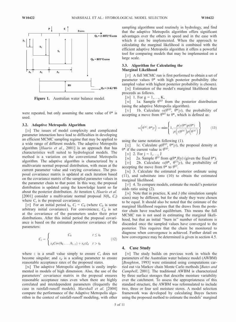
Figure 1. Australian water balance model.

W10422 MARSHALL ET AL.: HYDROLOGICAL MODEL SELECTION

5 of 11

W10422

likelihood. The framework used the adaptive Metropolisalgorithm to calculate the model’s posterior odds. Forcomparison, the BIC for each model was also estimated.

4.1. Australian Water Balance Model

[40] The AWBM (Figure 1) is an eight parameter satura-tion overland flow model that was developed by Boughton[1993] to compute daily runoff from daily rainfall andevapotranspiration records.[41] The model consists of three surface storages that are

associated with three fractional areas to represent thevariability of moisture capacity over the catchment. Thedepths of these storages correspond to the parameters S1,S2, and S3 and the fractional areas are represented by theparameters A1, A2, A3. The surface storage depths aresubject to the constraint S1 < S2 < S3. Two other param-eters are used to determine the proportion of base flowrecharge from surface runoff and discharge from the baseflow. The base flow index (BFI) determines the proportionof excess moisture at each time step that is returned to thebase flow. The daily recession constant (K) is used todescribe the daily discharge from the total base flow.[42] In a catchment, the surface storage capacity may

vary considerably over the catchment area. The use of threesurface storages to represent the catchment variability maynot be appropriate for a specific catchment. Boughton[1990] provides a systematic method by which the numberof partial areas of runoff may be approximated. In thisstudy, an alternative method is used to consider the vari-ability of soil moisture over a real catchment by formulatingthe model to vary the number of surface storages. Inaddition to the traditional model (Figure 1) in which threesurface stores represent the variability of soil moisturecapacity, the model was formulated to include a total oftwo, four or ten surface stores.

4.2. Study Catchment and Description of Data

[43] The selected study area was the Murrumbidgee Riverat Mittagang Crossing, an 1891 km2 catchment located inMurray Darling Basin in the state of New South Wales,Australia. Data were available in the form of daily rainfall,evapotranspiration and runoff data and a period of elevenyears was selected for simulations. The mean annual rainfallof the catchment is 882 mm and the mean annual runoff is134mm. Summary statistics for the runoff data are given inTable 1. The data shows an underlying base flow in thecatchment, which is well modeled by the base flow com-ponent of the AWBM. There is significant variability in theobserved runoff with a larger proportion of low-flow daysand few high peak events observed over the data set. Thecatchment also shows some seasonality, with a largervolume of runoff (>70%) occurring in the months fromJuly to December.

4.3. Prior Densities

[44] Our existing analysis of the traditional AWBM con-siders 8 parameters: K (the daily recession constant); BFI(the base flow index); A1, A2, A3 (the fractional areacoefficients); S1, S2, S3 (the surface storage parameters)and s2 (the error variance). In addition, priors must bespecified for parameters describing correlation in time ofmodel errors where needed. In this study (as in the work todate), the BFI will be kept fixed at a constant value.

[45] It was desirable to have prior densities that were asmeaningful as possible given little available knowledge. Assuch, priors were assigned considering previous implemen-tations of the model and previous studies that assessedsimilar parameters in models for a range of catchments.For the three-storage model, the prior densities implementedwere those used by Bates and Campbell [2001]. For thetwo- and four-storage models, in the absence of alternativeinformation, the prior distributions for the A parameterswere assumed to be diffuse beta distributions (defined overthe interval 0 to 1). The prior densities assumed for thestorage capacity parameters S1, S2 and S3 are based on theresults found by Nathan and McMahon [1990] for the SFBmodel (similar model structure as the AWBM) and anaverage surface capacity. For simplicity, the prior densitiesfor the S parameters for the two-, four- and ten-storagemodels were selected to have the same form as the three-storage model.

4.4. Likelihood Function

[46] The likelihood function is the way in which errorbetween the modeled and observed streamflow is described.Model comparison via the Bayes factor provides a formalcomparison of the performance of models which assumedifferent error structures, although other more informalchecks can also be helpful. When considering differenthydrological models, modelers often apply multiple criteriato assess the model performance, and this technique has alsobeen applied in a Bayesian setting [Vrugt et al., 2003b]. Theidea of multiple objectives could ultimately be applied tomodel comparison in a Bayesian framework by reducing thedata to multiple summary statistics that are focused ondifferent aspects of the model of interest. Each summarystatistic has a likelihood function implied by the likelihoodfor the full data, which could be used for model selection.Using implied likelihoods for summary statistics in this wayallows us to target different objectives when we do notbelieve the model to be correct. The main aim of this studywas to illustrate the rationale of estimating the Bayes factorusing the approach proposed earlier so we have avoidedconsidering this approach.[47] As such, two different forms of the likelihood

function were used to estimate the posterior distributions.The first assumed normally, independently and identicallydistributed errors:

p Qjqð Þ ¼ 2ps2� ��n=2Y

t

exp � Qt � f xt; qð Þ½ �2

2s2

( )ð14Þ

Table 1. Summary of Characteristics of Murrumbidgee River at

Mittagang Crossing Runoff Data

Value

Annual runoff, mm 134Annual rainfall, mm 882Proportion of zero rain days 0.41Proportion of zero flow days 0.0Average nonzero daily rainfall, mm 6.20Average daily flow, mm 0.24Standard deviation of nonzero daily rainfall 7.5Standard deviation of daily flow 0.65

6 of 11

W10422 MARSHALL ET AL.: HYDROLOGICAL MODEL SELECTION W10422

where p(Qjq) is the likelihood, Qt is the observed stream-flow at time step t, f(xt; q) is the calculated flow at time stept, xt is the set of inputs at time t (including precipitation andevapotranspiration estimates), and q is the set of modelparameters. The second assumed heteroscedastic, correlatederror terms by applying a Box Cox transformation andfitting an autoregressive (order 4) error model:

p Qjqð Þ ¼ 2ps2� �� n�pð Þ=2Y

t

exp �e2t =2s2

� �Qt þ lð Þ�1 ð15Þ

where

et ¼ log Qt þ lð Þ= f xt; qð Þ þ lð Þ½ �

�Xpj¼1

fj log Qt�j þ l� �

= f xt�j; q� �

þ l� �� �

and f is the set of autoregressive coefficients, p is the orderof the autoregressive error model, and l is the parameter forthe flow transformation. Following previous studies [Batesand Campbell, 2001; Marshall et al., 2004], l was set at0.5. For each AWBM structure, both likelihood functionswere considered, giving a total of 8 individual models forthe study. It would be expected for hydrological models ofthis type that the assumption of normally, independently andidentically distributed errors would not be appropriate,considering the dominance of low or zero flows and few‘‘peak’’ events (Table 1). In particular, the soil moistureaccounting method by which the daily flow is calculatedindicates that the assumption of correlated error termswould be more appropriate.

4.5. Convergence of the Parameter Sequenceto the Target Distribution

[48] An important issue in any method based on MCMCtechniques is determining when the simulated parametervalues have converged to the posterior distribution. Theapproach we adopted to monitor convergence was sug-gested by Gelman and Rubin [1992]. An underestimateand an overestimate of the target distribution variance for asuitable scalar function of the parameters are formed. Atconvergence, the estimates will be roughly equal. A numberof sequences are run. Convergence occurs when the meansof the individual sequence distributions is the same asthe mean obtained by mixing all the sequences together.The convergence is monitored by the factor (R) by whichthe conservative estimate of the variance must be reduced.[49] Alternative methods of determining convergence do

exist, such as monitoring the parameter’s estimated poste-rior mean and variance, which should stabilize when thechain has converged. However these methods are not asrigorous as the method proposed above, and as such wereonly used as a tool for confirming convergence results.

4.6. Application

[50] The model selection method was evaluated usingfour separate applications. These were as follows.[51] 1. First is an application using artificial runoff data of

same length as the historical record. For the first simulation,the hypothesis was that most model comparison criteriawould pick a more complicated model, even if it isn’t thecorrect model. To verify the approach in a controlled

setting, artificial runoff data of 11 years were createdcorresponding to the two-storage model. These data wereused to check if the method would select the two-storagemodel convincingly. This result was compared to a com-monly used fit criterion.[52] 2. Second is an application to real rainfall-runoff

data. Next, the method was applied to real catchment data todetermine which model configuration best represents thecatchment. A ten-storage configuration was included in thegroup of models. An 11 year long runoff record was used.[53] 3. The third and fourth applications use shorter

records of artificially generated and observed runoff. Theseapplications were designed to assess the advantages of theapproach over the simpler Bayesian information criterion(BIC). It has been argued that the BIC will give greaterweight to simpler models if there is insufficient data toidentify each model. Real runoff data of length 6 monthsand artificial runoff data of length 2 months were used, theartificial data corresponding to the three-storage AWBMconfiguration.[54] Initially, a full MCMC run of 100,000 iterations was

performed for each model to obtain the approximate pa-rameter values with maximum posterior density. As themethod provided by Chib and Jeliazkov [2001] is for anonadaptive Metropolis algorithm, the proposal covariancewas updated for the first 50,000 iterations, and then keptfixed, and the final 50,000 iterations used in calculating themarginal likelihood. Convergence was diagnosed after50,000 iterations for each model. The first 50,000 iterationsfrom each simulation were discarded and the remaining50,000 used in all calculations.

5. Discussion of Results

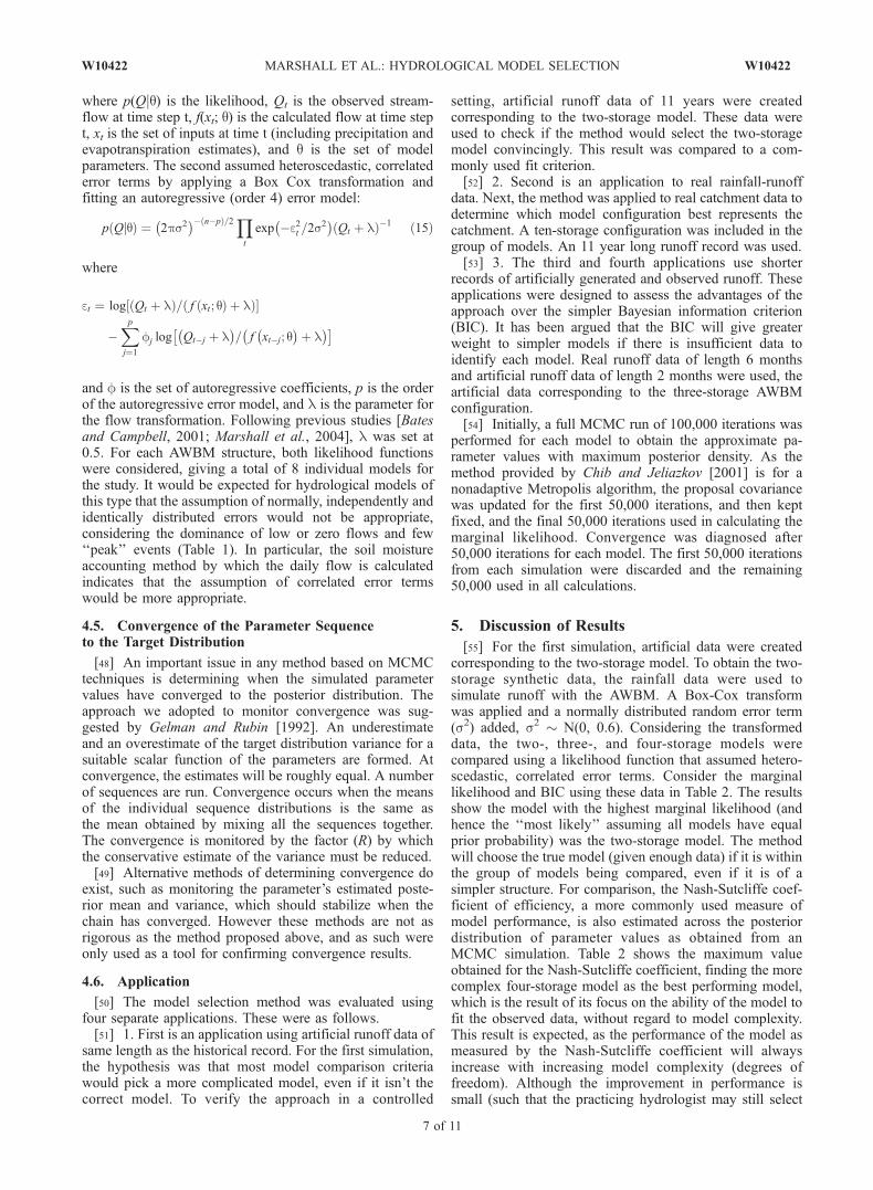
[55] For the first simulation, artificial data were createdcorresponding to the two-storage model. To obtain the two-storage synthetic data, the rainfall data were used tosimulate runoff with the AWBM. A Box-Cox transformwas applied and a normally distributed random error term(s2) added, s2 � N(0, 0.6). Considering the transformeddata, the two-, three-, and four-storage models werecompared using a likelihood function that assumed hetero-scedastic, correlated error terms. Consider the marginallikelihood and BIC using these data in Table 2. The resultsshow the model with the highest marginal likelihood (andhence the ‘‘most likely’’ assuming all models have equalprior probability) was the two-storage model. The methodwill choose the true model (given enough data) if it is withinthe group of models being compared, even if it is of asimpler structure. For comparison, the Nash-Sutcliffe coef-ficient of efficiency, a more commonly used measure ofmodel performance, is also estimated across the posteriordistribution of parameter values as obtained from anMCMC simulation. Table 2 shows the maximum valueobtained for the Nash-Sutcliffe coefficient, finding the morecomplex four-storage model as the best performing model,which is the result of its focus on the ability of the model tofit the observed data, without regard to model complexity.This result is expected, as the performance of the model asmeasured by the Nash-Sutcliffe coefficient will alwaysincrease with increasing model complexity (degrees offreedom). Although the improvement in performance issmall (such that the practicing hydrologist may still select

W10422 MARSHALL ET AL.: HYDROLOGICAL MODEL SELECTION

7 of 11

W10422

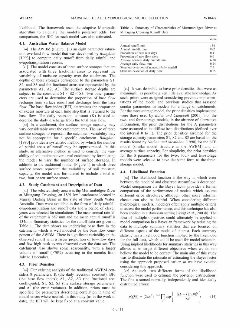
the simpler model over a more complex model) if the Nash-Sutcliffe coefficient were indicative of the ‘‘best’’ model touse, an incorrect conclusion may be reached. The resultslisted in Table 2 for the coefficient are also reliant on a pointestimate of the parameters in the model. If we consider theposterior distribution of the Nash-Sutcliffe coefficient fordifferent models (Figure 2), the concerns in relying onsuch point estimates for assessment of fit are highlighted.Figure 2 shows a scaled histogram for the criterion over thedistribution of parameter sets for each model. Figure 2illustrates that the two-storage and three-storage modelsshow little appreciable difference between model perform-ances as estimated by the criteria. The histogram for thefour-storage model shows an improvement across the rangeof values. The range of possible values means that ignoringparameter uncertainty can lead to an optimistic assessmentof model fit.[56] It must be noted here that the Nash-Sutcliffe criterion

can be more useful in model comparison studies using splitcalibration/validation data samples than one in which theentire length of data is used for calibration. However theseresults may be sensitive to how the data is split and theamount of data available. The very necessity of splitting theavailable data makes the approach less desirable as catch-ment data is often limited in availability (this is not requiredof Bayesian techniques). A criterion based approach willalso suffer from the problems of parameter uncertainty asdiscussed above.[57] Using the real runoff data from the catchment at

Mittagang crossing, the eight main models were nextcompared to determine the relative benefits of modelingthe data errors as heteroscedastic and correlated, and to

examine the effect of assuming a different number of partialareas for runoff. The resulting estimated marginal likelihoodand BIC of each model are given in Table 3. The marginallog likelihoods show that the models with correlated errorfunctions and transformed flow overwhelmingly outperformthe models that assume independent errors. This reflects theexpectation that the assumption of normally distributed,independent errors is not appropriate. The data indicates adominance of low, with fewer high runoff events (Table 1).The low underlying base flow means that normally distrib-uted errors are not likely, and the results show the benefit ofapplying a transformation to the data. Similarly, the soilmoisture accounting method within the model means thaterrors are likely to be correlated in time. In comparing thedifferent complexity models, the most complex model (theten-storage model) did not have the highest marginallikelihood. It has been suggested that Bayesian analysiswill choose the simplest model consistent with the data[Jefferys and Berger, 1992], and in our case study the mostcomplex model was rejected. Using a limited data set (withonly 6 months data, Table 4 and Figure 3), a simpler modelhad the highest marginal likelihood. This is most likely dueto the fact that there is insufficient data to identify the morecomplicated models outputs. It was interesting to note thatboth the BIC and the marginal likelihood suggested thesame simpler configuration with this limited data set. Thishas often not been the case, with the BIC often known tofavor an oversimplified model when the data are limited.

Figure 2. Distribution of Nash-Sutcliffe coefficient over parameters’ posterior distributions.

Table 2. Model Comparison for Artificially Generated Data From

a Two-Storage Model Configuration

AWBM VersionMarginal LogLikelihood �0.5 BIC

Nash-SutcliffeCoefficient

Two-storage model �2014 �1991 0.703Three-storage model �2027 �1995 0.703Four-storage model �2034 �1998 0.722

Table 3. Model Comparison for an 11-year Record From the

Murrumbidgee River at Mittagang Crossing

AWBM VersionError ModelAssumption

Marginal LogLikelihood �0.5 BIC

Two-storage model Independent Errors �3515 �3494Two-storage model Correlated Errors 5670 5702Three-storage model Independent Errors �3504 �3479Three-storage model Correlated Errors 5673 5713Four-storage model Independent Errors �3496 �3479Four-storage model Correlated Errors 5743 5760Ten-storage model Independent Errors �3568 �3493Ten-storage model Correlated Errors 5623 5745

8 of 11

W10422 MARSHALL ET AL.: HYDROLOGICAL MODEL SELECTION W10422

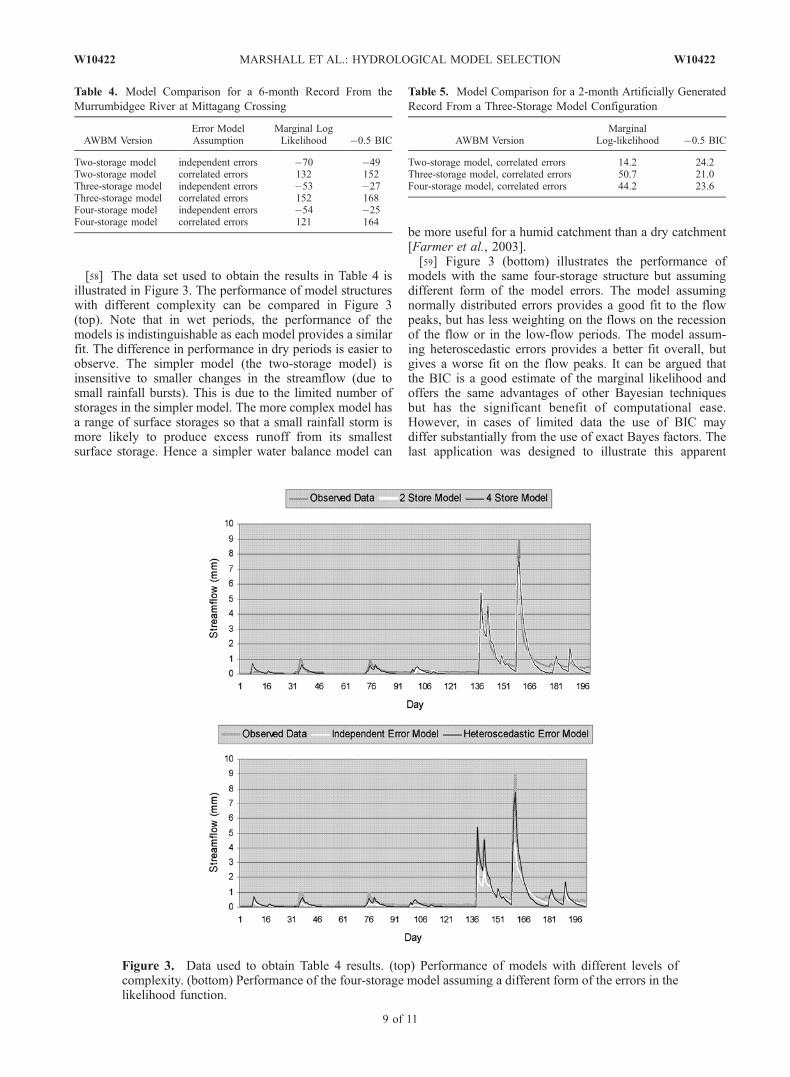
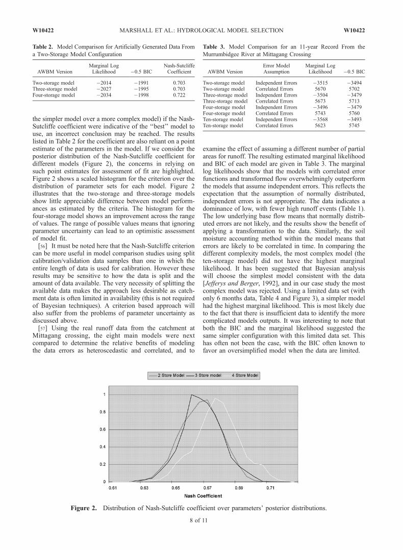
[58] The data set used to obtain the results in Table 4 isillustrated in Figure 3. The performance of model structureswith different complexity can be compared in Figure 3(top). Note that in wet periods, the performance of themodels is indistinguishable as each model provides a similarfit. The difference in performance in dry periods is easier toobserve. The simpler model (the two-storage model) isinsensitive to smaller changes in the streamflow (due tosmall rainfall bursts). This is due to the limited number ofstorages in the simpler model. The more complex model hasa range of surface storages so that a small rainfall storm ismore likely to produce excess runoff from its smallestsurface storage. Hence a simpler water balance model can

be more useful for a humid catchment than a dry catchment[Farmer et al., 2003].[59] Figure 3 (bottom) illustrates the performance of

models with the same four-storage structure but assumingdifferent form of the model errors. The model assumingnormally distributed errors provides a good fit to the flowpeaks, but has less weighting on the flows on the recessionof the flow or in the low-flow periods. The model assum-ing heteroscedastic errors provides a better fit overall, butgives a worse fit on the flow peaks. It can be argued thatthe BIC is a good estimate of the marginal likelihood andoffers the same advantages of other Bayesian techniquesbut has the significant benefit of computational ease.However, in cases of limited data the use of BIC maydiffer substantially from the use of exact Bayes factors. Thelast application was designed to illustrate this apparent

Figure 3. Data used to obtain Table 4 results. (top) Performance of models with different levels ofcomplexity. (bottom) Performance of the four-storage model assuming a different form of the errors in thelikelihood function.

Table 4. Model Comparison for a 6-month Record From the

Murrumbidgee River at Mittagang Crossing

AWBM VersionError ModelAssumption

Marginal LogLikelihood �0.5 BIC

Two-storage model independent errors �70 �49Two-storage model correlated errors 132 152Three-storage model independent errors �53 �27Three-storage model correlated errors 152 168Four-storage model independent errors �54 �25Four-storage model correlated errors 121 164

Table 5. Model Comparison for a 2-month Artificially Generated

Record From a Three-Storage Model Configuration

AWBM VersionMarginal

Log-likelihood �0.5 BIC

Two-storage model, correlated errors 14.2 24.2Three-storage model, correlated errors 50.7 21.0Four-storage model, correlated errors 44.2 23.6

W10422 MARSHALL ET AL.: HYDROLOGICAL MODEL SELECTION

9 of 11

W10422

shortcoming in the BIC when used with smaller data sets.Results from the use of a 2 month long artificiallygenerated runoff record where the true model is thethree-storage AWBM, are presented in Table 5. In all caseswhere a sufficiently long data set was available, the BICreproduced the results of the marginal likelihood. However,when artificial data were created corresponding to thethree-storage model (Table 5), the BIC differed from theexact Bayes factor, with BIC favoring a simplified modelcompared to the exact Bayes factor, which chose the truemodel. The results emphasized the risk in using the BIC asan approximation to the marginal likelihood in cases wherethere may not be enough data.

5.1. Evaluation of Chib and Jeliazkov Method

[60] The widespread use of Bayes Factors has beensomewhat hindered by the computational difficulties inaccurately calculating the marginal likelihood of a model.Only in rare cases is it possible to determine the marginallikelihood analytically. In lower-dimensional models, itmay be possible to use ordinary Monte Carlo simulation.However, methods can become complicated in higher-di-mensional models. The method of comparing models viatheir posterior probabilities is flexible and simple. It allowsmany models to be compared without a change in method.There are no limits on the types of models being selected,and it is not necessary to use standard distributions. Unlikestandard hypothesis testing, models are not required to benested. Calculation of the marginal likelihood is straightfor-ward and computationally undemanding when an MCMCscheme is available. When combined with the flexibleadaptive Metropolis algorithm the method described offersa powerful framework for Bayesian model comparison.However, the method provided here for calculating Bayesfactors can be difficult computationally depending on themodel complexity if a suitable MCMC algorithm cannot beapplied. It is more demanding than estimating the BIC,which can be shown to approximate the marginal likelihoodasymptotically. There are inherent risks in relying on suchapproximations, however. The BIC may not yield consistentmodel selection in all cases [Kass and Raftery, 1995] anddoesn’t apply to all models. If there is insufficient data, thereis evidence that the BIC will pick too simple a model. Thiswas evident in the case study shown where the use of BICdiffered from the use of the exact Bayes factor when 2months of data were used to calibrate the model.

5.2. Why Not Bayes Factors? Problems in SuccessfulImplementation of Bayes Factors

[61] The sensitivity of results to the choice of priordistributions for parameters is an important issue in calcu-lating Bayes factors. It can often be difficult to specifymeaningful priors for all model parameters. For estimationof parameters in a fixed model, vague priors are chosen sothat inference is driven by the likelihood. However, inBayesian model comparison, the Bayes factor may besensitive to the choice of prior distribution and use ofimproper noninformative priors is problematic. In addition,in Bayesian model comparison, specification of priors on allparameters in each model is required, and this can bedifficult when considering many high-dimensional models.There may also be difficulties in applying diffuse priorswhere prior information is small.

[62] In general, prior distributions should be selected withcare when comparing models. Bayesian methodology relieson the use of probability models, not only for the specifi-cation of prior distributions, but also in the specification of alikelihood function. Naturally, the assumptions made in thelikelihood specification should be checked.

6. Conclusion

[63] When using a hydrological model it can be difficultto choose from the variety of models that exist. The rangeavailable to the practicing hydrologist means that choosingthe best model, depending on the aim of the modelingexercise, is a complex task. A range of factors must beconsidered when comparing different models, including(but not limited to) the difficult task of quantifying amodel’s performance on a specific catchment. The problemsof assessing model performance can be amplified by theuncertainty surrounding the parameters of the model. Thelack of current, error-free and complete data means thatparameters in models can be poorly identified. A single,unique set of parameter values can be difficult, if notimpossible to obtain. Bayesian methods can provide anideal means to compare competing models whilst allowingfor model uncertainty. The methods employed here fullyaccount for both model and parameter uncertainty. Ratherthan requiring the estimation of an optimum set of param-eters to choose the best models, Bayes factors are aprobabilistic approach to the model selection problem. Thatis, they indicate the probability of one model relative toanother.[64] Bayesian methods will favor simpler models giving a

comparable level of fit to more complex models, bynaturally penalizing model complexity. By specifying theprior model probability, Bayes factors provide a way ofincluding any specialist knowledge. Prior distributions arealso specified for all model parameters. Criterion basedmethods do not allow existing knowledge to be taken intoaccount when comparing models. While the computationaladvantages of these methods are well known, their use canresult in an incorrect model choice particularly when thedata are limited.[65] Estimation of Bayes factors has been complicated

by the computational effort required, particularly for high-dimensional models. Chib and Jeliazkov [2001] haveprovided one solution to this problem that uses thesampled values from an MCMC chain to estimate themarginal likelihood. The main benefit of the methodologyproposed lies in its flexibility and wide applicability. It canbe used for high-dimensional models and for comparingmodels of different dimension or structure. Realistically, itcould be used to compare (say) conceptual rainfall runoffmodels and distributed models. Little extra computationaleffort and programming is necessary than that required fora full MCMC run sampling from the posterior. Anyconcerns with the method are due to the issues generallyassociated with applying any MCMC techniques. It can bedifficult to implement efficient MCMC methods for com-plex or high-dimensional models. Of particular importanceis the rate of mixing and efficiency of the method insampling the posterior. The convergence to the posteriordistribution should also be considered. How to determinewhen to stop sampling from the posterior is a critical issue

10 of 11

W10422 MARSHALL ET AL.: HYDROLOGICAL MODEL SELECTION W10422

to those implementing MCMC schemes, and should beconsidered in this method of calculation of the marginallikelihood.

[66] Acknowledgments. The authors are thankful to Eddy Campbellfor helpful suggestions and to Francis Chiew for sharing the catchment dataused in the study. Comments from three anonymous WRR reviewers aregratefully acknowledged. Partial support for this work came from aUniversity of New South Wales Goldstar Research Grant.

ReferencesAkaike, H. (1973), Information theory and an extension of the maximumlikelihood principle, in Second International Symposium on InformationTheory, edited by B. N. Petrox and F. Caski, p. 267, Akad. Kiad’o,Budapest.

Bates, B. C., and E. Campbell (2001), A Markov chain Monte Carloscheme for parameter estimation and inference in conceptual rainfall-runoff modeling, Water Resour. Res., 37(4), 937–947.

Berger, J. O., and L. R. Pericchi (2000), Objective Bayesian methodsfor model selection: Introduction and comparison, in Model Selection,pp. 135–207, edited by P. Lahirini, Inst. of Math. Stat., Beachwood,Ohio.

Boughton, W. C. (1990), Systematic procedure for evaluating partial areasof watershed runoff, J. Irrig. Drain. Eng., 116, 83–98.

Boughton, W. C. (1993), A hydrograph based model for estimating thewater yield of ungauged catchments, Natl. Conf. Publ. Inst. Eng.,93(14), 317–324.

Chib, S., and I. Jeliazkov (2001), Marginal likelihood from the Metropolis-Hastings output, J. Am. Stat. Assoc., 96(543), 270–281.

Chiew, F. H. S., M. J. Stewardson, and T. A. McMahon (1993), Comparisonof six rainfall-runoff modeling approaches, J. Hydrol., 147, 1–36.

Donnelly-Makowecki, L. M., and R. D. Moore (1999), Hierarchical testingof three rainfall-runoff models in small forested catchments, J. Hydrol.,219, 136–152.

Farmer, D., M. Sivapalan, and C. Jothityangkoon (2003), Climate, soil andvegetation controls upon the variability of water balance in temperate andsemiarid landscapes: Downward approach to water balance analysis,Water Resour. Res., 39(2), 1035, doi:10.1029/2001WR000328.

Franchini, M., and M. Pacciani (1991), Comparative analysis of severalconceptual rainfall-runoff models, J. Hydrol., 122, 161–219.

Freer, J., K. Beven, and B. Ambroise (1996), Bayesian estimation ofuncertainty in runoff prediction and the value of data: An applicationof the GLUE approach, Water Resour. Res., 32(7), 2161–2173.

Gelman, A., and D. B. Rubin (1992), Inference from iterative simulationusing multiple sequences, Stat. Sci., 7(4), 457–511.

Green, P. J. (1995), Reversible jump Markov chain Monte Carlo computa-tion and Bayesian model determination, Biometrika, 82, 711–732.

Haario, H., E. Saksman, and J. Tamminen (2001), An adaptive Metropolisalgorithm, Bernoulli, 7(2), 223–242.

Han, C., and B. P. Carlin (2001), Markov chain Monte Carlo methods forcomputing Bayes factors: A comparative review, J. Am. Stat. Assoc.,96(455), 1122–1132.

Jakeman, A. J., and G. M. Hornberger (1993), How much complexity iswarranted in a rainfall-runoff model?, Water Resour. Res., 29(8), 2637–2649.

Jefferys, W. H., and J. O. Berger (1992), Sharpening Ockham’s razor on aBayesian strop, Am. Sci., 89, 64–72.

Kass, R. E., and A. E. Raftery (1995), Bayes factors, J. Am. Stat. Assoc.,90(430), 773–795.

Kavetski, D., S. W. Franks, and G. Kuczera (2002), Confronting inputuncertainty in environmental modeling, in Calibration of Watershed Mod-

els, Water Sci. Appl. Ser., vol. 6, edited by Q. Duan, et al., pp. 49–68,AGU, Washington, D. C.

Kuczera, G. (1983), Improved parameter inference in catchment models: 1.Evaluating parameter uncertainty,Water Resour. Res., 19(5), 1151–1162.

Kuczera, G., and M. Mroczkowski (1998), Assessment of hydrologicparameter uncertainty and the worth of multiresponse data,Water Resour.Res., 34(6), 1481–1489.

Kuczera, G., and E. Parent (1998), Monte Carlo assessment of parameteruncertainty in conceptual catchment models: The Metropolis algorithm,J. Hydrol., 211, 69–85.

Lindley, D. V. (1957), A statistical paradox, Biometrika, 44, 187–192.Loague, K. M., and R. A. Freeze (1985), A comparison of rainfall-runoffmodeling techniques on small upland catchments, Water Resour. Res.,21(2), 229–248.

Madsen, H. (2003), Parameter estimation in distributed hydrological catch-ment modelling using automatic calibration with multiple objectives,Adv. Water Resour., 26, 205–216.

Marshall, L., D. J. Nott, and A. Sharma (2004), A comparative studyof Markov chain Monte Carlo methods for conceptual rainfall-runoffmodel ing, Water Resour. Res. , 40 , W02501, doi :10.1029/2003WR002378.

Michaud, J., and S. Sorooshian (1994), Comparison of simple versuscomplex distributed runoff models on a midsized semiarid watershed,Water Resour. Res., 30(3), 593–605.

Nash, J. E., and J. V. Sutcliffe (1970), River flow forecasting throughconceptual models, 1. A discussion of principles, J. Hydrol., 10, 282–290.

Nathan, R. J., and T. A. McMahon (1990), The SFB model part II—Opera-tional considerations, Civ. Eng. Trans. Inst. Eng. Aust., 32(3), 162–166.

Refsgaard, J. C., and J. Knudsen (1996), Operational validation and inter-comparison of different types of hydrological models, Water Resour.Res., 32(7), 2189–2202.

Romanowicz, R., K. Beven, and J. A. Tawn (1994), Evaluation of predic-tive uncertainty in nonlinear hydrological models using a Bayesian ap-proach, in Statistics for the Environment, vol. 2, Water Related Issues,edited by V. Barnett and K. F. Turkman, pp. 297–317, John Wiley,Hoboken, N. J.

Schwarz, G. (1978), Estimating the dimension of a model, Ann. Stat., 6,461–464.

Thiemann, M., M. Trosset, H. Gupta, and S. Sorooshian (2001), Bayesianrecursive parameter estimation for hydrologic models, Water Resour.Res., 37(10), 2521–2535.

Vrugt, J. A., H. V. Gupta, W. Bouten, and S. Sorooshian (2003a), Ashuffled complex evolution Metropolis algorithm for optimization anduncertainty assessment of hydrologic model parameters, Water Resour.Res., 39(8), 1201, doi:10.1029/2002WR001642.

Vrugt, J. A., H. V. Gupta, L. A. Bastidas, W. Bouten, and S. Sorooshian(2003b), Effective and efficient algorithm for multiobjective optimizationof hydrologic models, Water Resour. Res., 39(8), 1214, doi:10.1029/2002WR001746.

Ye, W., B. C. Bates, N. R. Viney, M. Sivapalan, and A. J. Jakeman (1997),Performance of conceptual rainfall-runoff models in low-yielding ephem-eral catchments, Water Resour. Res., 33(1), 153–166.

����������������������������L. Marshall and A. Sharma, School of Civil and Environmental

Engineering, University of New South Wales, Sydney, NSW 2052,Australia. ([email protected])

D. Nott, School of Mathematics, University of New South Wales,Sydney, NSW 2052, Australia.

W10422 MARSHALL ET AL.: HYDROLOGICAL MODEL SELECTION

11 of 11

W10422