Hydrol. Earth Syst. Sci. Discuss., ... · 2 1 Abstract 2 In a warming climate, the water budget of the land is subject to varying forces such as increasing 3 evaporative demand ,

1

Trends in evapotranspiration and its drivers in Great Britain: 1961 to 2015 1

Eleanor M. Blyth, Alberto Martinez-de la Torre, Emma L. Robinson 2

Centre for Ecology and Hydrology, Maclean Building, Benson Lane, Crowmarsh Gifford, Wallingford, 3

OX10 8BB, UK 4

Correspondence to: Eleanor M. Blyth ([email protected]) 5

6

Hydrol. Earth Syst. Sci. Discuss., https://doi.org/10.5194/hess-2018-153Manuscript under review for journal Hydrol. Earth Syst. Sci.Discussion started: 11 April 2018c© Author(s) 2018. CC BY 4.0 License.

2

Abstract 1

In a warming climate, the water budget of the land is subject to varying forces such as increasing 2

evaporative demand, mainly through the increased temperature, and changes to the precipitation, 3

which might go up or down. 4

Using a verified, physically based model with 55 years of observation-based meteorological forcing, 5

an analysis of the water budget demonstrates that Great Britain is getting warmer and wetter. 6

Increases in precipitation (3.0±2.0 mm yr-1 yr-1) and air temperature (0.20±0.13 K decade-1) are 7

driving increases in river flow (2.16 mm yr-1 yr-1) and evapotranspiration (0.87 mm yr-1 yr-1), with no 8

significant trend in the soil moisture. 9

The change in evapotranspiration is roughly constant across the regions whereas runoff varies 10

greatly between regions: the biggest change is seen in Scotland (4.56 mm yr-1 yr-1), where 11

precipitation increases were also the greatest (5.4±3.0 mm yr-1 yr-1) and smallest trend (0.29 mm yr-1 12

yr-1) is seen in the English Lowlands (East Anglia and Midlands), where the increase in rainfall is not 13

statistically significant (1.1±0.7 mm yr-1 yr-1). 14

Relative to their contribution to the evapotranspiration budget, the increase in interception is higher 15

than the other components. This is due to the fact that it correlates strongly with precipitation which 16

is seeing a greater increase than the potential evapotranspiration. This leads to a higher increase in 17

actual evapotranspiration that the potential evapotranspiration, and a negligible increase in soil 18

moisture or groundwater store. 19


3

1. Introduction 1

Evapotranspiration affects many important physical aspects of the land: the dryness of the soil, 2

vegetation growth, the temperature of the air and the amount of water in the rivers and 3

groundwater reserves. It is therefore important to understand how evapotranspiration responds to 4

changing climate. 5

For Great Britain (hereafter GB), studies based on the National River Water Archive have shown an 6

overall increase in riverflow of 1.6 mm yr-1 yr-1 over the last five decades (Hannaford, 2015). 7

Meanwhile, an analysis of the meteorological data for the years 1961-2012 has shown an overall 8

increase in potential evaporation for GB over that time of 0.77±0.77 mm yr-1 yr-1 (Robinson et al, 9

2017a). With an increase of rainfall at 2.86±0.65 mm yr-1 yr-1 (Robinson et al, 2017a) and assuming 10

the evapotranspiration increases roughly in line with potential evaporation (Kay et al, 2013), this 11

would imply an increase in soil moisture or groundwater recharge of about 0.5 mm yr-1 yr-1. 12

There is uncertainty in two of these estimates: firstly, the riverflow record is based on a sub-set of 13

rivers and the remainder – particularly in the Scottish Highlands which contribute a large portion of 14

the water – is gap-filled using a simple model. Secondly, the actual evapotranspiration may not 15

follow the potential evaporation. The estimate made by Kay et al (2013) was using a simple model 16

with little representation of vegetation processes. 17

To answer the question about how the actual evapotranspiration has changed over the last 55 years, 18

we would ideally have a direct observation of it both at the long term and over a representative 19

large scale. However, evapotranspiration is difficult to measure. Direct observations of evaporation 20

in GB from flux-tower data exist over short time periods or over small areas, but there are no large-21

scale, long term observations of this elusive flux. 22

Since there are few long term observations of evapotranspiration, the only way to study its evolution 23

and response to changes in climate is by using a model. 24

However, evapotranspiration is also difficult to model as it depends on the trio of soil, vegetation 25

and atmospheric conditions and the interactions between them. Key processes include the 26

availability of soil moisture to plants during dry spells, the response of plants to temperature, 27

sunshine and soil moisture, the intercepted of rainfall by plants. Assumptions about the processes 28

involved and their interactions (see Wang and Dickinson, 2012 for a review of methods) can have a 29

significant impact on the resulting modelled evaporation (see Schellekens et al, 2017 for overview of 30

model differences). 31


4

A previous study using a simple soil-moisture-stress-based model (Kay et al, 2013) indicated that 1

there has been an increase in evaporation over the last few decades. However, this modelled trend 2

is only due to changes in soil moisture stress and evaporative demand. The overall trend might be 3

altered by other aspects of the vegetation-atmospheric interactions such as rainfall interception and 4

transpiration responses to changes in meteorology and soil moisture stress. 5

In this paper, a comprehensive land surface model will be used to diagnose the changes in 6

evapotranspiration in GB over 55 years (1961 to 2015) including the analysis of the different 7

components of evapotranspiration (bare soil, transpiration, interception). 8

The questions that will be addressed are as follows: 9

1. Is the evaporation of GB and the regions increasing or decreasing? 10

2. Which components of the evaporation are contributing to the trend? 11

3. What meteorological changes are driving these changes? 12

In Sect. 2, the model, the ancillary and the driving data will be described before the model outputs 13

are presented which will be evaluated with available data. In Sect. 3, the resulting trends in the 14

model outputs will be analysed to address the three questions formulated above. Sect. 4 then 15

discusses the implications of these results while Sect. 5 presents the conclusions about the study. 16

17


5

2 Method 1

This study uses a physically-based model (JULES: Joint UK Land Environment Simulator, Best et al, 2

2011, Clark et al, 2011) driven by observation-based driving data for 55 years (see Sect. 2.1). The 3

accuracy of the model will be assessed by comparing to a range of independent datasets (see Sect. 4

2.2 for mean monthly evapotranspiration fluxes based on flux-tower data from 4 contrasting sites, 5

annual regional runoff-data from river-flow data, and Sect. 2.3 for estimates from other large-scale 6

models). 7

2.1 JULES model description and setup 8

The JULES model includes many of the processes that are likely to affect changes in water loss (see 9

Appendix A). It is used here in a new assessment of the GB water balance for the years 1961 to 2015. 10

Figure 1 show maps of the time-average quantities of evapotranspiration, sensible heat, soil 11

moisture and soil temperature and Figure 2 shows the spatial average annual values of runoff, 12

evapotranspiration, soil moisture and soil temperature. The rest of the paper describes the 13

provenance of this figure, and analyses the implications of the results. The model output, ancillary 14

files and meteorological forcing data are collectively referred to as CHESS (Climate, Hydrological and 15

Ecological research Support System). 16


6

1

2

Figure 1. Top and middle rows: Modelled estimates of mean evapotranspiration, sensible heat, soil 3

moisture and soil temperature averaged over 1961 to 2015 for GB. 4

5

6

Figure 2. Modelled estimates of runoff, evapotranspiration, soil moisture and soil temperature, 7

averaged over GB against year. 8


7

Using land cover maps (CEH Land Cover 2000: Fuller et al, 2002), soils maps (Harmonised World Soil 1

Database: FAO/IIASA/ISRIC/ISS-CAS/JRC, 2012) and a newly disaggregated meteorological driving 2

data (Robinson et al, 2017a), the model has been run at a landscape scale of 1 km. This spatial scale 3

is a compromise between being small enough to make reasonable comparisons with observational 4

datasets (such as flux towers), and large enough to be able to obtain reasonable meteorological 5

driving data and with a feasible computer cost. 6

The model used a fixed vegetation map based on observations in the year 2000 (CEH Land Cover 7

2000: Fuller et al., 2002) to prescribe the land cover fractions of the 8 different categories: broad 8

leaf trees, needle leaf trees, grass, crops, shrub, water, bare soil and urban. Parameters values for 9

these land covers are part of the model configuration (see Appendix B). 10

The phenology for each month was prescribed for the deciduous vegetation and the crops. The soil 11

hydrology component of JULES is based on the Darcy Richards equations (see Appendix A for a 12

summary) with the vertical discretization into four layers. The parameters used in the equations 13

depend on the soil type and maps of these were derived from the Harmonised World Soil Database 14

(see Appendix B for a description of their provenance). 15

The meteorological dataset used in the simulations is described in Robinson et al (2017a). This 16

dataset is a combination of daily precipitation based on observations (Gridded Estimates of daily and 17

monthly Areal Rainfall: GEAR: Keller et al, 2006) and other meteorological data from the 18

observation-based product MORECS (Thompson et al, 1981, Hough and Jones, 1997). The MORECS 19

data is presented at 40km and for CHESS, the data is downscaled using information about 20

topography. Robinson et al (2017a) analysed the CHESS data and showed a positive trend in the air 21

temperature as well as a positive trend in short wave radiation, which is due to increasing short 22

wave radiation in the spring months. The short wave radiation is based on sunshine hours and the 23

CHESS data includes a spatially varied impact of aerosol loading that affects the relationship 24

between sunshine hours and short wave radiation. However, it does not explicitly include any time-25

variation of the aerosols (dimming and brightening). To some extent the dimming and brightening is 26

included implicitly as the sunshine hours are above a certain threshold of intensity, and therefore 27

overall lower light levels will result in fewer hours. This is discussed in more detail in Sect. 4. The 28

data have since been extended to 2015 (Robinson et al, 2017b). 29

The model represents a significant upgrade to the current product available which employed a much 30

simpler water balance model: the Met Office Regional Evaporation Calculation Scheme (hereafter 31

MORECS: Thompson et al, 1981, Hough and Jones, 1997), that does not represent photosynthetic 32


8

processes, has a simple soil-physics routine and runs on a 40 km grid square on a daily time step. The 1

MORECS evapotranspiration is used widely and provides an interesting point of comparison for this 2

new evapotranspiration data product (see Sect. 2.3). 3

2.2 Evaluating the model results with observations 4

This paper makes no attempt to calibrate the model further than has already been done for global 5

simulations. But it is instructive for this analysis to quantify the performance of the model with a 6

standard configuration. Ideally we would be able to evaluate the model with observations at the 7

1km scale with daily or monthly data. However, it is only possible to make direct observations of 8

evapotranspiration using eddy-correlation systems which observe the hourly fluxes over an area of 9

about 100m. At the other extreme, river-flow data can be used in combination with the precipitation 10

to imply the evapotranspiration of a catchment (~100 km) over a year. In this section, the results of 11

the modelled actual evapotranspiration are compared to data from four eddy-correlation systems 12

and the river-flow records of the UK. 13

2.2.1 Evaporation from eddy-correlation systems. 14

There are several flux sites across GB. Out of these, four have been selected, based on the following 15

criteria: a good energy closure, running for several years when the CHESS data is available and 16

represents contrasting land cover types (trees and grass) and regional variation (Scotland and 17

England). Their locations are shown in Fig. 3, and Table 1 lists the data that are available, the dates 18

and location coordinates of each site. 19

20

Figure 3: Map showing the positions of the flux sites used for validation. AH=Alice Holt, 21

CA=Cardington, EB=Easter Bush, GF=Griffin Forest. The colours correspond to the vegetation type at 22

the site: green=broadleaf (BL), deciduous, blue=needleleaf (NL), evergreen, red=grass (GR). 23


9

Latitude Longitude Years Land

cover

at

site

% Land cover of CHESS square:

BroadLeaf,NeedleLeaf,GRass,Shrub,Crop,Urban

Alice Holt 51.1535 -0.8583 1999-

2013

BL 36*, 2, 24, 0, 38, 0

Cardington 52.1 -0.416 2005-

2011

GR 0, 0, 53.5, 7, 25.5, 14

Easter

Bush

55.8660 -3.2058 2003-

2005

GR 10, 0, 53.5*, 4, 25, 7.5

Griffin

Forest

56.6072 -3.7981 1997-

1999

NL 0.5, 91*, 0, 8.5, 0, 0

Table 1: Sites used to compare with the CHESS data and JULES runs with details of land cover. * 1

indicates the land cover used in the single dominant vegetation cover runs (Fig. 4). 2

As each CHESS grid square contains a range of vegetation types, two model results are shown: with 3

the grid square covered entirely by the vegetation at the site of each flux tower and the grid square 4

with the fractional vegetation cover as used in CHESS (see Sect. 2.1). The original flux data are 5

measured at 30 minute intervals; the data are checked for quality and gap-filled before daily 6

averages are calculated. From the daily averages, mean-monthly values are calculated and 7

presented here. 8

Fig. 4 shows the comparison of the model output with the mean monthly observed data. 9

10


10

Figure 4: Climatological monthly average latent and sensible heat fluxes for each of the sites (black 1

solid), compared to the CHESS square (green solid), as well as the same square re-run with the single 2

dominant vegetation cover (green dashed). 3

The first thing to note is that CHESS tends to simulate higher evaporation than the observations for 4

all of the sites. Following Blyth et al (2010) we compare the evaporative fraction (the ratio of 5

evapotranspiration to the sum of evapotranspiration and sensible heat flux) in Table 2 which allows 6

for equal underestimation of both sensible and latent heat fluxes. In this case, Griffin Forest and 7

Cardington overestimate the total evaporation while Alice Holt underestimates it and Easter Bush is 8

the same. On average however, there is a systematic overestimation of the evaporation in JULES 9

which has been noted previously (van den Hoof et al, 2013) and is discussed in Sect. 3. 10

2.2.2 The seasonality of evapotranspiration 11

Differences in seasonal evapotranspiration between the data and the model are shown in Fig. 4, 12

which highlight some issues with the model, discussed below. 13

For the forest sites (Alice Holt and Griffin Forest) the main discrepancy is in the winter when the 14

model substantially overestimates the evapotranspiration compared to the data: while the 15

observations indicate values of latent heat around zero to 10 W m-2, the model has values of about 16

20 W m-2. In the case of Griffin Forest, the energy for the modelled winter evapotranspiration is 17

coming from the negative sensible heat flux (around -40 W m-2 compared to an observed value of 18

around -10 W m-2). In the case of Alice Holt, the negative winter time sensible heat flux is reasonably 19

matched by the observations for the run with single dominant vegetation cover (BL; broad leaf 20

trees). The energy required by the model for the winter evapotranspiration must therefore be due 21

to an overestimate of the net radiation balance. 22

In the case of the grass sites (Cardington and Easter Bush), the winter time fluxes are reasonably well 23

modelled, but the summer modelled evapotranspiration is too high. In Cardington, this 24

overestimation in latent heat is matched by an underestimation of sensible heat. In Easter Bush, 25

there is no simultaneous reduction in sensible heat and therefore energy required for the high latent 26

heat must be due to an overestimate of the net radiation. 27

The conclusions are the same for both types of model runs (single dominant vegetation cover and 28

mixed vegetation cover), apart from Alice Holt, where the high winter latent heat fluxes are for the 29

BL run. This can be explained by the fact that the CHESS square contains substantial fraction of crops 30

and grasses (62% - see Table 1). 31


11

2.2.3 Analysis of modelled components of evapotranspiration at the flux sites 1

Figure 5 shows the different components of the modelled evapotranspiration (soil surface 2

evaporation, transpiration and interception). A summary of the results is shown in Table 2. 3

4

5

Figure 5: Seasonal variation in evapotranspiration observed (black solid) and modelled (green solid), 6

and components – interception (cyan dashed), soil surface evaporation (orange dashed) and 7

transpiration (green solid). 8

Evaporative

Fraction as %

P

(mm yr-1)

Transpiration,

Tr

Soil surface

evaporation, BS

Interception, I

Obs Model % Etot

total

% P % Etot

total

% P % Etot

total

% P

Alice Holt 88 81 832 54 29 24 13 22 11

Cardington 77 85 562 60 45 22 17 18 13

Easter Bush 77 77 876 50 21 24 9 27 12

Griffin Forest 61 95 1215 35 11 13 4 52 17

Table 2: Summary of model results at the four flux sites: Annual average evaporative fraction 9

(modelled and observed) and precipitation (P). Annual average fluxes of modelled transpiration (Tr), 10

soil surface evaporation (BS) and interception (I) as % of total evapotranspiration (Etot) and 11

precipitation (P). 12

There are no observations of these components at the four flux sites, so it is not possible to evaluate 13

them directly. However there are estimates of the three components for different vegetation types 14

in the literature which can be used to assess the model results. In order to translate between the 15

quoted figures and the model, it is important to note that some authors present the results as the 16

fraction of the total evaporation and others as the fraction of the total precipitation. For instance, 17

Van den Hoof et al (2013) summarises work from a range of studies in Europe (Wilson et al, 2001, 18


12

Verstraeten et al, 2005, and Choudhury and DiGirolamo, 1998), focusses on the former and quotes 1

values of forest interception to range from 13% to 25% of the total evaporation while for grasses it is 2

closer to 10%. 3

Meanwhile, Nisbet (2005) summarises a large body of work by scientists studying interception and 4

transpiration in the UK (Calder, 1990, Calder et al, 2003, Roberts, 1983), focusses on the latter and 5

quotes a percentage of rainfall that is intercepted: about 20% of rainfall for broadleaf trees and 35% 6

for needleleaf. The evidence suggests that the annual fraction of rainfall intercepted by trees is fairly 7

constant across a wide range of annual rainfall regimes, although increases slightly at low annual 8

rainfalls (<500 mm yr-1). The data are sparser for grass and no values are given in this report, 9

although interception rates of heather and bracken are quoted at about 20% of rainfall. 10

The model results in Table 2 confirm the analysis of Nisbet (2005). The fraction of rainfall that is lost 11

through interception is fairly constant over the four sites, ranging from 11% to 17%. This translates 12

into a large fraction of total evaporation that is due to interception: 18% to 52%. At Griffin Forest, 13

the model evaporative fraction is much higher than the observation (95% compared to 61%). 52% of 14

the model evaporation is due to interception. Compared to the Van den Hoof et al (2013) figures of 15

interception, this might be considered to be too high. However, this only represents 17% of the 16

precipitation in this high-rainfall area. Many of the studies from Van den Hoof are in regions with 17

much lower annual precipitation. The value of 17% is low compared to other estimates of 18

interception loss in needle-leaf trees as reported in Nisbet (2005). 19

In the much lower rainfall regime where Alice Holt is sited, the modelled interception is only 22% of 20

the evaporation budget, which is dominated by the transpiration (54%). 21

This analysis suggests that the model has a reasonable representation of interception, capturing its 22

conservative relationship to the precipitation. 23

The transpiration, on the other hand, is more controlled by the available energy and has a more 24

uniform relationship with total evaporation (see Roberts, 1983) ranging from 35% to 60%, and a 25

wider range of fractions of precipitation, from 11% to 45%. The values of transpiration are lower 26

than the values given by Van den Hoof et al (2013) and Nisbet (2005) who quote values for trees 27

from 53% to 70% of total evaporation being due to transpiration. It is possible that the total value of 28

transpiration is reasonable, but the fraction is low due to the overestimation of the total 29

evaporation. 30


13

The bare soil evaporation compares reasonably well with data quoted in the literature although 1

figures are rather low. The values range from 13% to 24% of the total evaporation and correspond 2

to values quoted in van den Hoof et al (2013) of 20% and 30%. The low bias might be due to the fact 3

that the UK sites are in relatively high rainfall areas with high interception so that even if the total 4

evaporation is correct, the percentage is low. 5

2.2.4 River flow 6

At the annual timescale, changes in water storage in a UK catchment are negligible and the area-7

average evapotranspiration can be estimated as precipitation minus river-flow. Daily river flow 8

records for the UK are available in the National River Water Archive (NRFA) which is hosted at CEH, 9

Wallingford. A subset of these records have been chosen for their length of record, accuracy, little or 10

quantifiably affected by abstractions. The annual runoff from these catchments is then combined 11

with a model to scale up to the regional and GB scale to present net annual and monthly runoff. The 12

method for this is described in Marsh et al (2015). Hannaford (2015) has summarised the results, 13

which are reproduced here in Figs. 6, 8 and Table 3. The challenge addressed here is to identify 14

whether using a model to fill in the gaps introduces a bias to the results. 15

Fig. 6 plots the total GB annual river flows from these processed observations. The GB runoff, and 16

precipitation minus the evapotranspiration (the difference being the soil-moisture) from the model 17

is also shown. It is apparent from this figure that the modelled runoff is slightly lower than that 18

observed, which is commensurate with the analysis in the previous sub-section that the modelled 19

evapotranspiration is too high. However, the percentage difference is very small (0.15%) which is not 20

consistent with the previous estimates of the bias (roughly 10%). An analysis of the regions shows 21

where this discrepancy occurs. 22

23


14

Figure 6. Comparison of CHESS annual runoff and precipitation-evaporation (P-E) to the observed GB 1

annual river flow (NRFA; data available up to 2011). 2

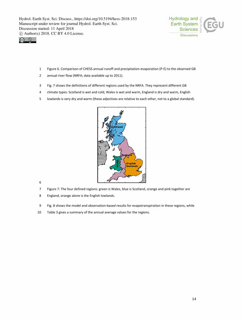
Fig. 7 shows the definitions of different regions used by the NRFA. They represent different GB 3

climate types: Scotland is wet and cold, Wales is wet and warm, England is dry and warm, English 4

lowlands is very dry and warm (these adjectives are relative to each other, not to a global standard). 5

6

Figure 7: The four defined regions: green is Wales, blue is Scotland, orange and pink together are 7

England, orange alone is the English lowlands. 8

Fig. 8 shows the model and observation-based results for evapotranspiration in these regions, while 9

Table 3 gives a summary of the annual average values for the regions. 10


15

1

Figure 8: Annual averages for evapotranspiration in the four regions for CHESS and precipitation-2

runoff (P-Q) observed. Here, the observation-based products used are GEAR for precipitation and 3

NRFA for runoff. 4

Annual

average

(mm yr-1)

Precipitation Model

Runoff

Observed

Runoff

Model

Evap.

Observed

Evap. (P-Q)

Bias in

Evap (%

Observed)

Scotland 1485 1032 972 458 513 -10.5%

Wales 1377 863 945 516 432 +19.5%

England 825 342 369 485 456 +4.5%

English

Lowlands

681 206 273 479 408 +17.5%

5

Table 3: Annual average water balance for the four regions. 6

Table 3 shows that in Wales, England and the English lowlands, the model overestimates 7

evapotranspiration by 5 to 20%. This corroborates the results of the analysis with the flux data which 8


16

show an overestimation of about 10%. However, in Scotland the comparison indicates the opposite: 1

the model has a lower evapotranspiration than the precipitation-runoff product. This anomalous 2

outcome is probably a result of the way the riverflow observations were sampled and then 3

extrapolated to the regional scale. As explained above, the estimate is made with ‘Index 4

Catchments’ chosen for the length of record (see Marsh et al, 2015), which in the Scottish region are 5

mainly in the low-lying East of the region. Due to the short record length, the Highland and West of 6

Scotland runoff data is not used and instead the area contribution was estimated by a model. The 7

evapotranspiration in this wet region will be near to the potential evapotranspiration (PET), so the 8

value of PET used in the model will dominate the result. 9

The PET product used for the gap-filling was from MORECS, which is based on observations and 10

calculated at the 40 km grid-scale. In flat terrain, it is a valid assumption that PET will not vary over a 11

40 km grid and that it can be used at the 1 km grid-scale. However, in hilly terrain such as western 12

Scotland, that is no longer the case. As indicated in Blyth (1999), since is it always windier on the 13

tops of the hills where PET is lower (due to the cold temperatures), the area-averaged PET is lower in 14

a hilly region than would be implied using topographic-mean data. This may explain the 15

overestimation of PET and underestimation of the river flows in Scotland in the observation-based 16

product of Hannaford (2015). 17

If the results for Scotland are ignored, the comparison suggests an overestimate of the model of the 18

order of 10 to 15%. 19

2.3 Evaluating the model by comparison with other modelled estimates 20

There are several available large-scale evapotranspiration estimates to compare to the model. All of 21

these estimates are model-derived. It is not expected that they will be more accurate than CHESS 22

and this is not an evaluation exercise. However, it is interesting to make the comparison. Table 4 23

describes the datasets: their derivation and the annual mean evapotranspiration for GB and the four 24

regions in Fig. 7. They are derived from models of differing complexity, either driven by satellite-25

derived data, or ground-based weather data. Fig. 8 shows the maps of the annual mean 26

evapotranspiration from the four products (CHESS scaled up to 40 km, eartH2Observe, GLEAM and 27

MORECS) while Fig. 10 shows how the GB average varies over time. 28

Product

(version)

References Methods Annual Evapotranspiration (mm yr-1)

GB S W E El


17

eartH2Obseve

(WRR1)

Schellekens et al

(2017)

Ensemble mean of 10

global models (4 land

surface models and 6

hydrological models)

(see Table 1 in given

reference for details)

502 477 546 485 474

GLEAM (v3.0a) Martens et al

(2017)

Miralles et al

(2011)

Data-driven model

(Priestley-Taylor),

using meteorological

data from reanalysis,

satellite and gauged-

based global datasets

(0.25 resolution )

463 471 568 439 410

MORECS (v4) Thompson et al,

(1981)

Hough and

Jones (1997)

Data-driven model

(Penman-Monteith),

using observed GB

meteorological data

(40 km resolution)

524 482 543 528 522

Table 4: Description of the three large-scale evapotranspiration estimates for GB, and annual 1

averages over GB and the four regions: Scotland (S), Wales (W), England (E) and English lowlands 2

(El). 3

4

5


18

1

2

Figure 9: Maps of mean evapotranspiration for eartH2Observe, GLEAM, MORECS and CHESS 3

(averaged up to 40 km). 4

5

Figure 10: Annual average evapotranspiration for eartH2Observe, GLEAM and MORECS and CHESS. 6

It can be seen from the Figs. 9 and 10 and from the Table 4 that the main differences between the 7

various products is the total evapotranspiration. CHESS evapotranspiration is higher than GLEAM 8

and lower than MORECS, and close to the ensemble product from eartH2Oobserve. 9

To understand the evapotranspiration in all of these estimates, it is important to know the assumed 10

role and values of PET (or equivalent) in the model. Fig. 11 shows the value of PET for GLEAM, 11


19

MORECS and CHESS (not available for E2O). It is clear from this figure that the MORECS PET is higher 1

than the CHESS PET, commensurate with the difference in actual evapotranspiration. This suggests 2

that the difference between CHESS evapotranspiration and MORECS evapotranspiration is due to 3

the PET. A comparison of CHESS PET with GLEAM PET shows that they have a similar magnitude. 4

This indicates that the reason the GLEAM evapotranspiration is lower is due to model differences, 5

not the PET. 6

This result corroborates the results of the analysis in Schellekens et al (2017) which showed that 7

GLEAM had much lower evapotranspiration than a wide spread of models in the temperate regions. 8

9

10

Figure 11: Annual average potential evapotranspiration for GLEAM, MORECS and CHESS. 11

2.4 Summary and discussions of model evaluation 12

The evaluation of the model show that the overall evaporation is overestimated by of the order of 13

10%. In winter, this overestimate is greater for trees than for grass, whereas for grass the 14

overestimate is in the summer. According to analysis of observations, the model underestimates the 15

interception from trees, especially conifer trees. 16

The winter evaporation for deciduous trees tends to be overestimated. This is probably due to the 17

known issue in the model of using a single aerodynamic resistance for the trees and underlying soil 18

surface evaporation. 19


20

Analysis of river flows suggests that the use of a fine grid (1km compared to 40km) for evaluating 1

evaporation results in more accurate estimates of the water budget over areas of high terrain. 2

Although comparison with observations is not perfect, the model displays reasonable allocation of 3

evaporation across the different components compared to observational evidence, and we 4

therefore deem it good enough to proceed with the subsequent analysesPETI. 5


21

3 Results 1

In this section, the results of the model will be used to address the four questions formulated in the 2

introduction. 3

1. Is the evaporation of GB and the regions increasing or decreasing? 4

2. Which components of the evaporation are contributing to the trend? 5

3. What meteorological changes are driving these changes? 6

The analysis starts with a study of annual and seasonal evapotranspiration in GB. Then we move on 7

to a study of evapotranspiration in the regions of GB (Scotland, Wales, England and English lowlands, 8

as defined in Fig. 7). These two sections answer the first question. The trends in the different 9

components of evapotranspiration for whole of GB are quantified to answer the second question. 10

The third question is addressed by studying the correlation between the evapotranspiration in the 11

regions and the different drivers of change (precipitation and solar radiation). 12

3.1 Trends in GB water balance: annual average and seasons. 13

Annual (Seasons:

Winter, Spring,

Summer, Autumn)

Average Rate Of Change (units yr-1)

Precipitation (mm

yr-1)

1106

(1284,896,929,1313)

2.96±2.03

(6.95±6.25, 0.28±2.61, 2.25±4.01, 2.13±4.20)

Evapotranspiration

(mm yr-1)

481

(190,585,794,345)

0.87±0.55

(0.52±1.03, 1.12±0.64, 0.92±0.67, 0.46±0.51)

Runoff (mm yr-1) 630

(901,604,365,636)

2.18±1.84

(3.45±5.05, 0.75±2.18, 0.86±1.67, 1.17±2.71)

Soil Moisture (m3

m-3)

1267

(1345,1293,1162,1246)

-0.02±0.77

(-2.50±3.07, -0.33±0.55, 0.05±1.22, -0.02±0.98)

PET (mm yr-1) 479 (134, 592, 885,

296)

0.74±0.66 (0.20±0.53, 1.37±0.65, 0.96±1.68,

0.38±0.49)

Observed Runoff

(mm yr-1)

629 1.57±2.04

Table 5: Annual average and seasonal average fluxes and trends in the fluxes of: Precipitation, 14

Evapotranspiration, Runoff, Soil Moisture and Potential Evapotranspiration. 15


22

1

Figure 12: Bar chart showing annual and seasonal water budgets and trends (evapotranspiration and 2

runoff). Trends are represented on the right y-axis. 3

The annual average of total evapotranspiration has been presented and compared to observations in 4

Sect. 2 (Table 3). Here the seasonal variation in evapotranspiration is explored. The seasons are 5

defined as Winter (December to February), Spring (March to May), Summer (June to August) and 6

Autumn (September to November). 7

Table 5 and Fig. 12 show that here is a strong seasonality to the evapotranspiration, with summer-8

time values over four times the winter-time values. This seasonality is strongly driven by the 9

seasonal variation in PET which has a 6-fold increase from the winter values to the summer values. 10

Soil moisture control reduces the summer evapotranspiration to about 75% of the PET, while the 11

winter and autumn evapotranspiration exceed the PET by on average 25%. The reverse is true of the 12

river flow which responds to a low seasonal variation in precipitation (only 1.35 variation between 13

winter and summer) but exhibit some soil moisture control with summer runoff 2.5 times smaller 14

than winter runoff. 15

The largest trend in evapotranspiration is seen in the spring months (1.12 mm yr-1 yr-1). This result 16

corroborates the results of an analysis of PET by Robinson et al (2017a), who demonstrated that the 17


23

largest increase in the PET for GB was in spring due to an increase of spring sunshine hours and a 1

decrease in relative humidity. In Sect. 4 we discuss the impact of this on the riverflow. 2

Unlike the PET results however, the smallest trend of evapotranspiration is seen in the autumn. This 3

may be due to soil moisture control of evapotranspiration. 4

The trends in runoff are overall two times larger than the evapotranspiration trends. This is due to 5

the very large increase in winter runoff due to the large positive trend in precipitation in Scotland. 6

The other seasons have a similar upward trend of about 1 mm yr-1 yr-1. 7

3.2 Regional trends. 8

Annual Average (rate

of change in units yr-1)

Scotland Wales England English

lowlands

Precipitation (mm yr-1) 1495 (5.41±3.00) 1386 (2.93±2.86) 832

(1.51±1.87)

686

(1.07±1.76)

Evapotranspiration

(mm yr-1)

460 (0.87±0.47) 518 (0.93±0.72) 487

(0.86±0.66)

481

(0.91±0.71)

Runoff (mm yr-1) 1042 (4.56±2.82) 869 (2.12±2.80) 347

(0.79±1.75)

209

(0.33±1.50)

PET (mm yr-1) 423 (0.53±0.46) 496 (0.69±0.68) 509

(0.87±0.77)

519

(1.03±0.86)

Soil Moisture (m3 m-3) 1534 (0.29±0.56) 1139 (-

0.03±0.66)

1128 (-

0.20±1.00)

1177 (-

0.29±1.12)

Observed total runoff

(mm yr-1)

972

(3.60±2.63)

945 (2.67±3.72) 369

(0.38±1.83)

273

(0.13±1.68)

Table 6: Annual average GB and regional fluxes and trends in the fluxes of: Precipitation, 9

Evapotranspiration, Runoff, Potential Evapotranspiration and Soil Moisture. Bottom row shows 10

annual observed averages from NRFA runoff product. 11

12


24

1

Figure 13: Bar chart showing annual GB and regional water budgets and trends (evapotranspiration 2

and runoff). Trends are represented on the right y-axis. 3

The water balance of the different regions can be summarised as follows: the water balance is runoff 4

dominated in Scotland (runoff is 70% of rainfall) and evaporation dominated in the English lowlands 5

(runoff is 30% of rainfall). 6

Table 6 and Fig. 13 show that the trend in evapotranspiration is roughly constant between regions, 7

in the same way that the total evapotranspiration is fairly constant. However, the runoff trends are 8

more varied between regions. Scotland dominates the trend with an increase in runoff of 4.56 mm 9

yr-1 yr-1 and the English lowlands have the smallest trend of 0.33 mm yr-1 yr-1. 10

3.3 Totals and trends in the components of evapotranspiration for GB. 11

There are three components of the evapotranspiration. The JULES model calculates each explicitly 12

and their totals and trends for GB are given in Table 7. 13

Average

(mm yr-1)

Rate Of Change

(mm yr-1 yr-1)

Evapotranspiration 481 0.87±0.55


25

Soil surface evaporation 100 (21%) 0.14±0.47 (16%)

Transpiration 229 (48%) 0.47±0.23 (51%)

Interception 137 (28%) 0.31±0.22 (33%)

Table 7: Annual average and trends in GB evapotranspiration and components. 1

The percentage of evapotranspiration that is due to interception is about 30%, due to soil surface 2

evaporation is about 20% and due to transpiration is due to about 50%. Despite the possible errors 3

in the modelled allocation of evapotranspiration between the components reported in Sect. 2, it is 4

likely that the trends of the components are well represented. A key factor is the contribution of the 5

component to the trend in total evapotranspiration. These vary between components and they are 6

slightly different to the contributions they make to the annual average. This means they are not all 7

increasing at the same rate: the interception in increasing more rapidly than the other two 8

components. This is discussed in more detail in Sect. 4. 9

Figure 14 displays how the components vary across the regions. Although transpiration generally 10

dominates, they are nearly equal in Scotland which experiences very high rainfall rates. 11

12

Figure 14: Bar chart of annual average evapotranspiration components in GB and regions. 13

14


26

3.4 What meteorological variable is driving the trend? 1

To understand the reason for the trend in evapotranspiration, we study the correlation between the 2

annual evapotranspiration and its two main drivers: precipitation and radiation. The analysis is 3

carried out for the regions and for the separate components. A discussion of the trends in radiation 4

due to changes in aerosols and cloud cover and how it is represented in the CHESS dataset is given in 5

Sect. 4. 6

Table 8 and Fig. 14 show the results of the correlations. 7

R P v Etot SW v Etot P v I SW v I P v Tr SW v Tr P v BS SW v BS

GB 0.66 0.42 0.86 -0.09 0.11 0.74 0.49 0.44

Scotland 0.65 0.50 0.80 -0.01 0.09 0.81 0.51 0.44

Wales 0.47 0.45 0.83 -0.15 -0.20 0.84 0.27 0.37

England 0.58 0.28 0.84 -0.24 0.12 0.56 0.31 0.42

English

lowlands

0.64 0.19 0.82 -0.28 0.35 0.36 0.25 0.46

Table 8: Correlation of annual Precipitation (P) and Shortwave radiation (Sw) with Total 8

evapotranspiration (Etot), Interception (I), Transpiration (Tr) and Soil surface evaporation (Bs), for GB 9

and for the four regions. 10

11


27

Figure 15: Bar chart showing correlation of annual Precipitation (P) and Shortwave radiation (SW) 1

with Total evapotranspiration (Etot), Interception (I), Transpiration (Tr) and Soil surface evaporation 2

(BS) for GB and the regions. 3

The important take-away result from this Fig. 15 and Table 8 is that there is always a strong 4

correlation between rainfall and interception (3rd column in Fig 15 and Table 8) and always a strong 5

correlation of transpiration with radiation (6th column in Fig. 15 and Table 8). 6

From the analysis, soil surface evaporation seems to have similar correlations with both precipitation 7

and radiation. 8

The implications for these results is discussed in the following section. 9


28

4. Discussion 1

4.1 Trends in the annual GB water budget 2

Hannaford (2015) suggest that the overall runoff of GB is increasing by 1.6 mm yr-1 yr-1 while 3

Robinson et al (2017a) show an increase in precipitation of 2.86 mm yr-1 yr-1 (updated analysis of 4

data including later years shows 2.96 mm yr-1 yr-1 – Table 5) If this was taken as the only evidence for 5

a change in actual evapotranspiration, we could calculate an increase of 1.36 mm yr-1 yr-1. However, 6

Robinson et al (2017a) indicate an increase in PET, which represents an upper limit of transpiration, 7

of only 0.77 mm yr-1 yr-1 and Kay et al (2013) have suggested that the overall trend in 8

evapotranspiration of GB is close to the trend in PET, which they estimate as 0.7 mm yr-1 yr-1. 9

If all this were true, then there would be an increase in soil moisture or groundwater store of the 10

order of 0.5 mm yr-1 yr-1. 11

The results of this study give slightly different results. The overall trend in evapotranspiration is 0.87 12

mm yr-1 yr-1 and the runoff is larger than that given by Hannaford (2015) at 2.16 mm yr-1 yr-1. This 13

then almost balances the water budget leaving negligible increase in soil moisture or groundwater. 14

We have already demonstrated (Sect 2.2.4) that the Hannaford (2015) estimates of riverflow are too 15

low in Scotland. This was probably due to the use of large-scale area-average Potential Evaporation 16

over hilly terrain to gap-fill the data which will tend to overestimate the evaporative loss leading to 17

runoff-estimates that are too low. It is possible that the trend in runoff, rather than the total, is 18

affected by the lack of interception trend (discussed below) in the estimated runoff. A deeper 19

analysis of the flows in Scotland should be carried out to understand these trends. 20

The reason why the evaporative loss might be greater than the potential could be due to the large 21

fractional component of interception (30%): in the wet and windy areas (West Scotland), there is a 22

higher fraction of evergreen needle leaf trees which have a high interception capacity (see Calder, 23

1990). The evaporation from a wet forest often exceeds the PET, drawing down energy in the form 24

of negative sensible heat (i.e. cooling the air) to drive it (Stewart et al, 1977). 25

If the drivers of interception are increasing faster than the PET, then with such a high interception 26

fraction, there might be a larger trend in the evapotranspiration than the potential evaporation. This 27

is discussed in Sect. 4.4. 28

4.2 Impact of seasonal variation of trend in evapotranspiration on river flows. 29


29

The results of this study indicate a clear increasing trend in spring evapotranspiration, driven by an 1

increase in PET reported in Robinson et al (2017a). 2

It is interesting to note the impact of this on the river flows. In their review, Watts et al (2015) 3

suggest that there is no clear evidence of how actual evaporation has changed over the last few 4

decades. Hannaford (2015) notes that, while there is an observed increase in winter, summer and 5

autumn river flows from 1961 to 2010, there is a decrease in the spring (see table 1). This is 6

reiterated in Harrigan et al., (2017) who note that we need an ‘improved understanding of the 7

drivers of these seasonal changes in river flow’. 8

This study clearly indicates that some of the spring-time drop in runoff will be due increased 9

evapotranspiration in addition to a reduction of rainfall. 10

4.3 Temporal changes in shortwave radiation over the study time period in Great Britain. 11

There is an overall increase in downward short wave radiation apparent in the observations used in 12

this study of 1.1±0.7 Wm-2 decade-1 over GB. 13

There are two possible reasons for an increase in short wave radiation: one is that there is less cloud 14

and the other that the air is more transparent due to a reduction in aerosols (pollution). 15

The aerosol effect has been widely studied and is referred to as ‘dimming and brightening’ since, the 16

aerosol amount increased throughout the 20th century until about the 1970’s, when due to 17

legislation, it began to fall. Observations reported by Wild (2009) illustrate this at the global scale. 18

Across Europe, the dimming resulted in a decrease in the total Short Wave Radiation of 1.4 Wm-2 19

decade-1 from the beginning of the century to the mid-1970s and the brightening to an increase of 20

2.2 Wm-2 decade-1 up to the mid-1990s. This change in radiation has been shown to have a 21

significant impact on river flows in the region (Gedney et al 2014). 22

GB has a somewhat different temporal pattern of dimming and brightening to mainland Europe. 23

Using an ensemble of computer model runs, Folini and Wild (2011) simulated the aerosols in Europe. 24

Their results agree with the overall result of Wild (2009) for Europe, but also note some interesting 25

regional variations: in the case of GB from 1960 onward, there is no dimming, only brightening. For 26

the All-Sky conditions (i.e. including clouds. See Fig 9 of the Folini and Wild (2011) paper) the 27

increase in radiation is about 0.8 Wm-2 decade-1. This tallies with an observational study by Stjern et 28

al. (2009) which included a long term record at Aberdeen (the only GB station in the study) where 29

there was no dimming from 1960’s only a brightening of 1 Wm-2 decade-1. This is also consistent with 30

the increase of short wave (0.9 ±1.1 Wm-2 decade-1 for the years 1979-2012) given in the 31


30

observation-based meteorological forcing dataset WFDEI (Weedon et al, 2014) which included 1

explicit aerosol effects. 2

The short-wave radiation data used in CHESS is based on sun-shine hours. There is a spatially varying 3

aerosol effect included, but it is based on data from 1978 and does not change in time. As reported 4

in Robinson et al (2017), it may be that the aerosol effect is implicit in the sunshine hours record as 5

there is a threshold of 120 Wm-2 and the number of hours above that threshold will be affected by 6

the pollution levels, although the changes in cloud cover are likely to be dominant in this signal. 7

The biggest increase in short wave is in the spring. This is consistent with data from across Europe 8

(Sanchez-Lorenzo et al., 2008) and may be due to changes in the Atlantic Multidecadal Oscillation 9

(AMO) which has resulted in decreased spring precipitation in Northern Europe (Sutton and Dong, 10

2012). 11

It is concluded therefore that the CHESS data gives a reasonable representation of the shortwave 12

radiation over GB for the study period. 13

4.4 Analysis of correlations. 14

It is generally accepted (e.g. Teuling et al., 2009, Wang and Dickenson, 2012), that in moisture 15

limited regions, there will be a strong correlation of evapotranspiration with precipitation, while in 16

wet, cloudy regions, there will be a stronger correlation with radiation. However, in the analysis 17

presented by Teuling et al (2009), most of GB is deemed to be radiation limited (confirming its wet 18

and cloudy climate) apart from west Scotland and central England. The result for west Scotland is a 19

counter-intuitive result since it is the wettest region of GB. 20

A correlation analysis of annual evapotranspiration with precipitation and short-wave radiation was 21

carried out with the CHESS model results and reported in Sect. 3.4. In this analysis, the same 22

patterns emerged: the correlation of evapotranspiration and precipitation was high in Scotland. To 23

understand why the evapotranspiration correlates more strongly with precipitation than radiation in 24

Scotland, the correlations for the four regions for each of the components of evapotranspiration 25

against precipitation (P) and shortwave (SW) radiation were made. 26

The important take-away result from this analysis (see Fig. 14 and Table 8) is that there is always a 27

strong correlation between rainfall and interception (3rd column in Fig 14 and Table 8). This tallies 28

with the results of the analysis in Sect. 4 and the evidence from Nisbet (2005) that interception is 29

near to a fixed fraction of rainfall. Interception is not ‘limited’ by rainfall, but it strongly correlates 30

with it because it is unlimited. 31


31

Transpiration however is generally limited by energy in GB since there is usually enough water and 1

often not enough sunshine. This results in a strong correlation of transpiration with radiation (6th 2

column in Fig. 14 and Table 8). 3

Soil surface evaporation has similar correlations with both precipitation and radiation. 4

These results show why the evapotranspiration-precipitation correlation dominates in Scotland: it is 5

because the rainfall is high and so interception is nearly as large as the Transpiration component of 6

the evapotranspiration (see Fig. 15). English lowlands provide the opposite case. The 7

evapotranspiration is dominated by transpiration (see Fig. 15) and it is equally water limited and 8

radiation limited. 9

4.5 Importance of interception to the GB hydrology. 10

As discussed above, this study highlights the importance of interception to the overall hydrological 11

balance and trends in GB. It may also have implications for floods. 12

Floods represent a major hazard for the UK and recently there has been effort to identify natural 13

ways to alleviate the floods. Dadson et al (2018) and Stratford et al (2017) both review the evidence 14

of whether the presence of trees have an impact to reduce flood peaks. They both conclude that 15

there can be an impact of mature trees to reduce smaller floods, probably do the interception. 16

Using a physically based model (JULES) with detailed representations of all the evaporation 17

components, including interception, enables us to quantify the effect of land-cover on hydrology at 18

the GB scale. The interception in the model has some uncertainties, and possibly underestimates the 19

effect (see Sect. 2.2.3). However, the results are consistent with the observations and can be used as 20

evidence for this increasingly important issue. 21

4.6 Possible impact of rising CO2 levels on water balance of GB. 22

Over the 55 years of the study period, there has not only been a change in the physical climate, but a 23

50% increase in the atmospheric concentration of CO2, from 300 ppm to 450 ppm. It is possible that 24

this has affected the water balance of GB due to the response of vegetation to CO2. There is 25

evidence (Leakey et al, 2009) at the canopy scale that plants will transpire less in increased 26

atmospheric CO2 levels. However, models differ substantially in their prediction of the large-scale, 27

long term response to elevated CO2 which includes changes to ecosystems and vegetation structure 28

(de Kauwe et al, 2013). 29


32

The JULES model includes the effect of an increase in CO2 on evapotranspiration, although it might 1

reduce the transpiration too much (Prudhomme et al, 2014). As a result of this uncertainty, in the 2

version of CHESS reported here, we used the CO2 level half way through the period (in 1986) and 3

kept it constant. 4

However, it is instructive to analyse to what extent the water balance would be predicted to change 5

in the presence of a 50% increase in CO2 according to the model. The model showed that overall 6

evapotranspiration and runoff were unchanged. There was a change in the trend however: 7

evapotranspiration trend was reduced: to 0.60 mm yr-1 yr-1 (from 0.87 mm yr-1 yr-1) while the positive 8

trend in runoff increases: to 2.33 mm yr-1 yr-1 (from 2.16 mm yr-1 yr-1 with no CO2 increase). Most of 9

the difference in trend comes from a lower positive trend in transpiration of 0.11 mm yr-1 yr-1 10

(compared to 0.47 mm yr-1 yr-1 in the constant CO2 run). In the earlier part of the run, when transient 11

CO2 levels were lower than the constant CO2 run, the stomata were more open, so stomatal 12

conductance was higher, while the reverse was true in the later part of the run, with higher CO2 13

levels. This leads to the same mean transpiration over the run, but a weaker trend. 14

15


33

5. Conclusions 1

This study set out to explore the long term evolution of the water budget of Great Britain (GB), 2

including how and why it is changing. 3

A study of the river flows (summarised in Hannaford, 2015) suggest that the runoff from GB is 4

increasing with time (1.6 mm yr-1 yr-1 over the last 50 years) with a decrease in spring time (Harrigan 5

et al, 2017). It is possible that the increase is an underestimate due to the methods of gap-filing 6

used. 7

The Potential Evapotranspiration (PET), which expresses the likely increase of a well-watered grass 8

due to changes in wind, radiation and temperature, has been estimated by Robinson et al (2017a) to 9

be 0.77 mm yr-1 yr-1 and by Kay et al (2013) to be 0.7 mm yr-1 yr-1. 10

In order to examine the actual evapotranspiraiotn, we used a validated model of the land surface 11

(JULES: Joint UK Land Environment Simulator) which was driven by observation-based 12

meteorological data (Robinson et al, 2017a) over 5 decades. The modelled evapotranspiration 13

increased at a rate of 0.87 mm yr-1 yr-1 which is greater than the increase in Potential 14

Evapotranspiration. 15

The analysis showed that the interception was a large component of the overall evapotranspiration 16

(30%) and increasing at a slightly higher rate (proportionally) than the other components. 17

In this paper, it was demonstrated that annual interception correlates strongly with annual 18

precipitation rather than solar radiation. Over the last 5 decades, precipitation has increased faster 19

(2.96±2.03 mm yr-1 yr-1) than the PET (0.74±0.66 mm yr-1 yr-1). This increase in precipitation, 20

combined with the high interception rates in GB (due to the wet conditions) explains why the trend 21

in evapotranspiration is higher than the trend in PET. 22

Thus the paper clearly demonstrated that a representation all three components of 23

evapotranspiration (interception, transpiration and bare-soil evaporation) are needed to understand 24

the trends in the GB water-budgets. 25

In addition, the study demonstrated the importance of evapotranspiration to the annual and 26

seasonal water budget of Great Britain and its regions. For instance, the observed decreasing spring-27

time runoff reported in Harrigan et al (2017) is a combination of decreased in the precipitation and 28

increased evaporation in this season. 29


34

Future directions for this research should include a focus on the evaporation processes that have 1

been demonstrated to be so important: interception, the winter-time soil surface evaporation under 2

deciduous trees and the summer-time transpiration of grass. Narrowing our uncertainty in these key 3

processes will help identify the role of land cover on the UK water budgets. 4


35

6. Data and model availability 1

This paper presents the results of the model in a particular code version and configuration. The 2

version of a model refers to the code which are used to solve the equations of the processes (this 3

can be summarised by its Version Number). The configuration includes the selection of the options 4

used (such as whether to use dynamic vegetation or not), the look-up tables of parameters used in 5

the equations, the meteorological data used to drive the model and the ancillary data used to set up 6

the maps of soils and land cover classification. This will also have a Version Number and a reference 7

name. This information is given in Appendix B. 8

Code availability: The JULES code is available freely and can be applied for through the JULES 9

repository: https://code.metoffice.gov.uk/trac/jules. The version used for the CHESS runs based 10

on JULES vn4.5, branch: r3488_albmar_spdm. More detailed information about the JULES code, 11

use and availability: http://jules.jchmr.org. 12

Data availability: The data (drivers and initial inputs) of the Configuration for running the model for 13

CHESS is described in the rose suite number u-au394 (see Appendix B). All the model outputs 14

analysed here and more (evaporation components, runoff, latent and sensible fluxes, soil 15

moisture and temperature, surface temperature, carbon gross and net productivities) are 16

publicly available as the CEH CHESS-land dataset (Martinez-de la Torre et al, 2018b). 17

The flux data used for evaluation is available upon request from the author. 18

19


36

Appendix A 1

A1 Overview of hydrology in JULES 2

This summary follows water as it arrives as precipitation at the land surface, and describes the 3

journey it takes through the land surface through interception, the snow pack, surface runoff 4

generation, vertical adjustment of soil moisture, drainage and evapotranspiration (Best et al, Clark et 5

al). 6

Each of the above-ground processes (interception, snow and evapotranspiration) are calculated for 7

each of the different land-surfaces represented within each grid-box. While the equations are 8

universal, the parameters change for each land cover type. The derivation of the maps of fractional 9

cover of each land cover and the parameters used are described in Appendix B. 10

The below ground processes (surface runoff generation, vertical adjustment of soil moisture and 11

drainage) are calculated based on the grid-average soil moisture. Parameters for these equations 12

depend on the soil type and topographical information. The derivation of these for CHESS are given 13

in Appendix B. 14

Since this application is in the UK which has a temperate climate, we have not covered the cold 15

processes included in JULES, such as snow and soil freezing. Snow sublimation only accounts for 1% 16

of the modelled total evapotranspiration for the GB area (2% in Scotland, 0.5% in the rest of GB) and 17

so, for the sake of brevity, we have omitted to describe the snow model here. Readers are referred 18

to Best et al (2011) for more details. 19

A2. Rainfall intensity and interception 20

One of the most important aspects of any distributed hydrology model is how to deal with 21

precipitation that is supplied as a time- and space- average. If the precipitation is assumed to fall 22

evenly over a wide area or over a long time period, then infiltration through the vegetation canopy 23

or top soil layers is too low, resulting in a surface that is too wet and deeper soils that are too dry. 24

In JULES, the spatial distribution of intensity of rainfall is assumed to follow an exponential statistical 25

distribution. 26

𝑓(𝑃) = (𝜇

𝑃) exp(

−𝜇𝑃𝑖

𝑃) (A1) 27


37

where P (kg m-2 s-1) is the area-average rainfall rate, Pi (kg m-2 s-1) is the rainfall rate over a small area 1

and μ is the fraction of the grid box area over which the rain is assumed to fall. In CHESS, since the 2

grid box is small, this is set as 1. 3

This rainfall-intensity distribution is used in two ways. Firstly to calculate how much of the rainfall 4

falls through the vegetation canopy to the understorey, called ‘throughfall’ (Tf). Secondly, how much 5

of the throughfall infiltrates the soil (see Sect. A3). The throughfall is dependent not just on the 6

rainfall intensity but how much water is already on the leaves and also has a dripping element to it. 7

𝑇𝑓 = 𝑃 (1 −𝐶

𝐶𝑚) 𝑒𝑥𝑝 (−

𝜀𝐶𝑚

𝑃𝛥𝑡) + 𝑃

𝐶

𝐶𝑚 (A2) 8

where C (mm) is the amount of rainfall stored on the leaves, Cm (mm) is the maximum capacity 9

which depends on the leaf area index of the vegetation and ε is a tuning factor. 10

Vegetation is assumed to have a certain capacity that gets filled up by rain and reduced by 11

evaporation, called ‘interception’. The interception rate is calculated as a fraction of the open-water 12

evaporation rate, where the fraction (F) is the proportion of water stored to the maximum capacity 13

of that vegetation type. 14

𝐹 =𝐶

𝐶𝑚 (A3) 15

The value of F (dimensionless) is converted to an effective surface resistance which is merged with 16

resistances from the other evaporation components for the calculation of the tile-17

evapotranspiration based on the surface energy balance (see Sect. A6). 18

A3. Surface water partitioning 19

Surface runoff is generated either through infiltration excess (also known as Hortonian flow), or 20

saturation excess (also known as Dunn flow). These are both represented in the JULES model. 21

Infiltration excess runoff will be generated by JULES if the water-flux over the time step (either 22

rainfall, throughfall or snow melt) exceeds the maximum infiltration rate of the soil. The water-flux 23

rate is assumed to vary in intensity across the grid and to have been altered by the interception (see 24

Eq. (48) in Best et al, 2011). The maximum infiltration rate is the saturated hydraulic conductivity 25

multiplied by a vegetation dependent parameter (4 for trees and 2 for grasses). However, this 26

maximum infiltration rate is so high that it is never invoked. 27

Saturation excess runoff is based on the concept of the fact that the soil moisture across an area will 28

not be uniform but that a fraction of the model grid cell (fsat) will be at saturation. This fraction is 29


38

used as a multiplier on the remaining water arriving at the soil surface to convert to surface runoff. 1

There are two options for representing this in JULES. In this study we use the PDM, based on a 2

Pareto distribution to describe the spatial variation of soil moisture: 3

𝑓𝑠𝑎𝑡 = 1 − (1 −𝜃−𝜃0

𝜃𝑠−𝜃0)𝑏𝑏−1⁄

(A4) 4

where θ (m3 m-3) is the mean volumetric soil moisture, θ0 (m3 m-3) is the minimum soil moisture for 5

the PDM scheme to start producing surface runoff, and θs (m3 m-3) the saturated soil moisture. b 6

(dimensionless) is a tunable parameter. Martinez-de la Torre et al (2018a) introduced a method for 7

identifying values of b and θ0 from topographical data in the UK and these values are used here. 8

A4. Vertical soil water distribution 9

After the interception and the surface runoff, the remaining water enters the soil at the surface and 10

is redistributed through the 3 m of soil moisture using the Darcy-Richard Equations. The resulting 11

soil moisture profile allows the model to distinguish between the soil moisture near the surface 12

which controls the soil surface evaporation and deeper layers which can be accessed by plants with 13

different root depths (see Sect. A6). This distinction affects the sub-diurnal timing of energy fluxes 14

which is important for weather prediction. The essential equations are as follows: 15

𝑊 = 𝑘 (𝑑𝜓

𝑑𝑧+ 1) (A5) 16

where W (kg m-2 s-1) is the vertical flux of water through the soil, z (m) is the vertical distance, k (kg 17

m-2 s-1) is the conductivity of the soil, and ψ is the suction (m). There are two options for calculating 18

the conductivity and suction in JULES. In this study we use the van Genuchten (1980) formulations: 19

(𝜃

𝜃𝑠) =

1

[1+(𝛼𝜓)(

11−𝑚

)]

𝑚 (A6) 20

𝑘 = 𝑘𝑠 (𝜃

𝜃𝑠)0.5

[1 − (1 − (𝜃 𝜃𝑠⁄ )

1/𝑚)𝑚

]

2

(A7) 21

Where 𝜓𝑠 (m) is the suction at saturation and 𝑘𝑠 (kg m-2 s-1) is the conductivity at saturation while α 22

and m are model parameters. All four of these parameters are dependent on the soil type and the 23

values used in CHESS are described in Appendix B. 24

Not shown here are the heat-diffusion equations which act on the same layers. The transfer of heat 25

is important to the soil hydrology when the soil freezes which alters the hydraulic conductivity. 26


39

A5. Drainage 1

The bottom boundary condition of the soil column can affect the performance of the model. At 3 m 2

deep in the standard version, the model is assumed to drain at the rate of the gravity drainage using 3

the soil moisture of the bottom layer – thus assuming there is an infinitely thick layer below with the 4

same soil moisture. Different options are available such as a zero flux layer or a deeper groundwater 5

store that can bring water upwelling and are presented in Best et al (2011). 6

A6. Evapotranspiration 7

Apart from the interception (see Sect. A1), the evaporation is assumed to consist of two 8

components: bare soil evaporation and transpiration. 9

The soil surface evaporation control is the simplest and depends on the soil moisture in the top 10

layer: 11

𝑟𝑠𝑜𝑖𝑙 = 100 (𝜃𝑐

𝜃1)2

(A8) 12

Where rsoil (s m-1)is the surface resistance used for bare soil, θ1 (m3 m-3) is the soil moisture in the top 13

soil layer and θc (m3 m-3) is the soil moisture at critical point (defined in Appendix B). 14

The transpiration is more complex as it depends on the response of the photosynthesis of the plant 15

to environmental controls: light levels, temperature, ambient carbon dioxide, soil moisture and 16

humidity. The surface resistance of the plant to the optimum photosynthesis (no limits) is inferred 17

and assumed to apply to the transpiration. 18

The effective surface resistance is made from a combination of the three components: interception, 19

bare soil and transpiration. The actual evapotranspiration depends on the amount of energy 20

available, which depends on the radiation balance and the soil heat fluxes. Details are given in Best 21

et al (2011). 22

23


40

Appendix B 1

The configuration (ancillary files, science options and parameters, and driving data) used for the 2

CHESS simulation presented here are all documented in the rose suite u-au394 3

(https://code.metoffice.gov.uk/trac/roses-u/browser/a/u/3/9/4/). Instructions for how to access 4

this are given in the website: http://jules.jchmr.org. A summary of the options and driver datasets is 5

given here. 6

The model is run with 8 surface tiles (5 plant functional types: broadleaf trees, needleleaf trees, 7

grasses, shrubs and crops; and 3 non-vegetated types: open water, bare soil and urban) derived 8

from the CEH Land Cover 2000 (Fuller et al, 2002) map at a resolution of 25 m. Table B1 shows how 9

the Land Cover 2000 classes were mapped onto JULES land cover types. These were then aggregated 10

to 1 km resolution, as fractions of the total gridbox. 11

The soil hydrology component of JULES is based on the Darcy Richards equations (see Appendix A for 12

a summary) and, in this configuration, the van Genuchten (1980) approach, with the vertical 13

discretization into four layers of varying depth: 0.0-0.1 m, 0.1-0.35 m, 0.35-1.0 m and 1.0-3.0 m. The 14

soil hydraulic characteristics are assumed to be spatially uniform for each grid cell, and have been 15

calculated for the model domain from the Harmonised World Soil Database (HWSD; 16

FAO/IIASA/ISRIC/ISS-CAS/JRC, 2012), by classifying soils by their texture, then using the values from 17

Wösten et al (1999). We used a newly developed terrain slope dependency for the PDM scheme in 18

the production of saturation excess runoff (Martinez-de la Torre et al, 2018a), and the slope was 19

derived from the Great Britain 50 m resolution CEH-IHDTM database (Morris and Flavin, 1990; 20

1994). 21

The phenology for each month was prescribed for the deciduous vegetation and the crops. The 22

dynamical vegetation scheme was switched off. A 10-layer approach is used for canopy radiation 23

interception, including an exponential decline of leaf nitrogen with canopy height. For the run with 24

increasing atmospheric CO2 concentration, we used annual values from the US NOAA (National 25

Oceanic and Atmospheric Administration) Global Monitoring Division 26

(https://www.esrl.noaa.gov/gmd/ccgg/trends/global.html). 27

A 10-year spin up run was conducted to initialize the model. The meteorological data used to drive 28

the model is publicly available (CHESS-met: Robinson et al, 2017b). It is a daily dataset based on 29

observations from 1961 to 2015. The model is integrated at a half-hourly time step, using a daily 30

disaggregation scheme (Williams and Clark, 2014) to disaggregate the driving data. In terms of 31

precipitation, precipitation events start at a random time during the day and last for 2 hours in the 32


41

case of convective precipitation, or 5 hours in the case of large-scale precipitation. The input rainfall 1

is assumed to be convective for temperatures above 15 °C, and covers the complete 1 km grid 2

cell.The rest of options and parameters (radiation, snow, vegetation, non-vegetated tiles) are 3

available on the rose suite u-au394. 4

5

6

7

Land Cover 2000 class JULES surface type

Water (inland) Water

Saltmarsh Water

Supra-littoral rock Bare soil

Supra-littoral sediment Bare soil

Bog (deep peat) Shrub

Dense dwarf shrub heath Shrub

Open dwarf shrub heath Shrub

Montane habitats Shrub

Broad-leaved / mixed woodland Broadleaf tree

Coniferous woodland Needleleaf tree

Improved grassland Grass

Neutral grass Grass

Setaside grass Grass

Bracken Shrub

Calcareous grass Grass

Acid grassland Grass

Fen, marsh, swamp Grass

Arable cereals Crop


42

Arable horticulture Crop

Arable non-rotational Shrub

Suburban / rural development Urban

Continuous urban Urban

Inland bare ground Bare soil

Table B1 Allocation of Land Cover 2000 map classes to JULES surface types 1

Author Contribution: EMB designed the study, carried out the analysis and wrote the manuscript, 2

AM performed the model runs, summarised the results and created the figures, ELR set up the 3

system for running the model (ancillary data and driving data) and for evaluating the model with the 4

flux data and runoff data. 5

References 6

Best, M. J., Pryor, M., Clark, D. B., Rooney, G. G., Essery, R. L. H., Menard, C. B., Edwards, J. M., 7

Hendry, M. A., Porson, A., Gedney, N., Mercado, L. M., Sitch, S., Blyth, E.M., Boucher, O., 8

Cox, P. M., Grimmond, C. S. B., and Harding R.J.: The Joint UK Land Environment Simulator 9

(JULES), model description – Part 1: energy and water fluxes. Geosci Model Dev. 4, 677-699. 10

Doi: 10.5194/gmd-4-677-2011, 2011. 11

Blyth, E.M.: Estimating potential evaporation over a hill. Boundary Layer Meteorology 92, 185-193, 12

1999. 13

Blyth, E. M., Gash, J. H. C., Lloyd, A., Pryor, M., Weedon, G.P., and Shuttleworth, W. J.: Evaluating the 14

JULES land surface model energy fluxes using FLUXNET data. J. Hydrometeorol. 11, 509-519, 15

2011. 16

Calder, I. R.: Evaporation in the Uplands. John Wiley and Sons, Chichester, 1990. 17

Calder, I. R., Reid, I., Nisbet, T., and Green, J. C.: Impact of lowland forests in England on water 18

resources – application of the HYLUC model. Water Resources Research 39, 1319-1328, 19

2003. 20

Choudhury, B. and DiGirolamo, N.: A biophysical process-based estimate of global land surface 21

evaporation using satellite and ancillary data – 1. Model description and comparison with 22

observations. J. Hydrol. 205, 164-185, 1998. 23


43

Clark, D.B., Mercado, L.M., Sitch, S., Jones, C. D., Gedney, N., Best, M.J., Pryor, M., Rooney, 1

G.G., Essery, R.L.H., Blyth, E., Boucher, O., Harding, R.J., Huntingford, C., Cox, P.M.: The Joint 2

UK Land Environment Simulator (JULES), model description. Part 2: Carbon fluxes and 3

vegetation dynamics. Geoscientific Model Development, 4 (3). 701-722. 10.5194/gmd-4-4

701-2011, 2011 5

Dadson, S.J., Hall, J.W., Murgatroyd, A., Acreman, M., Bates, P., Beven, K., Heathwaite, L., Holden, J., 6

Holman, I.P., Lane, S.N., O’Connell, E., Penning-Rowsell, E., Reynard, N., Sear, D., Thorne, C. 7

and Wilby, R., 2018, A restatement of the natural science evidence concerning catchment-8

based natural flood management in the UK. Proc. R. Soc. A 473: 10160706 9

De Kauwe, M. G., Medlyn, B. E., Zaehle, Z., Walker, A. P., Dietze, M. C., Hickler, T., Jain, A. K., Luo, Y., 10

Parton, W. J., Prentice, I. C., Smith, B., Thornton, P. E., Wang, S., Wang, Y. P., Warlind, D., 11

Weng, E., Crous, K., Y., Ellsworth, D. S., Hanson, P. J., Kim, H. S., Warren, J. M., Oren, R., and 12

Norby, R. J.: Forest water use and water use efficiency at elevated CO2: a model-data 13

intercomparison at two contrasting temperate forest FACE sites. Global Change Biology 19, 14

1759-1779, doi: 10.1111/gcb.12164, 2013 15

FAO/IIASA/ISRIC/ISS-CAS/JRC: Harmonized World Soil Database (version 1.2), FAO, R., Italy and 16

IIASA, Laxenburg, Austria, 2012 17

Folini, D. and Wild, M., 2011. Aerosol emissions and dimming/brightening in Europe: sensitivity 18

studies with ECHAM5-HAM. J. Of Geophysical Research. 116 D21204. doi 19

10.1029/2011JD016227 20

Fuller, R. M., Smith, G. M., Sanderson, J. M., Hill, R. A., and Thomson, A. G.: The UK Land Cover Map 21

2000: Construction of a parcel-based vector map from satellite images. Cartographic Journal 22

39, 15-25, 2002. 23

Gedney, N., Huntingford, C., Weedon, G.P., Bellouin, N., Boucher, O. and Cox, P.M., 2014. Detection 24

of solar dimming and brightening on Borthern Hemisphere river flow. Nature Geoscience, 25

doi: 10.1038/NGEO2263 26

Hannaford, J.: Climate-driven changes in UK river flows: A review of the evidence. Progress in 27

Physical Geography 39, 29-48, 2015. 28


44

Harrigan, S., Hannaford, J., Muchan, K. and Marsh, T., 2017. Designation and trend analysis of the 1

updated UK Benchmark Network of river flow stations: the UKBN2 dataset. Hydrology 2

Research, in press. doi: 10.2166/nh.2017.058 3

Hough, M. N. and Jones, R, J, A.: The United Kingdom Meteorological Office rainfall and evaporation 4

calculation system: MORECS version 2.0 - an overview. Hydrology and Earth System Sciences 5

1, 227-239, 1997. 6

Kay, A. L., Bell, V. A., Blyth, E. M., Crooks, S. M., Davies, H. N., and Reynard, N.S.: A hydrological 7

perspective on evaporation: historical trends and future projections in Britain. Journal of 8

water and climate. 04.3 193-208, 2013. 9

Keller, V., Young, A. R., Morris, D. G., and Davies, H.: Task 1.1: Estimation of precipitation inputs. 10

Environment Agency R&D Project w6-101. Centre for Ecology & Hydrology: Wallingford, UK; 11

35, 2006 12

Leakey, A. D. B., Ainsworth, E. A., Bernacchi, C. J., Rogers, A., Long, S. P., and Ort, D. R.: Elevated CO2 13

effects on plant carbon, nitrogen, and water relations: six important lessons from FACE. J. 14

Exp. Biol. 60, 2859-2876, doi: 10.1093/jxb/erp096, 2009. 15

Marsh, T., Sanderson, F., and Swain, O.: Derivation of the UK National and Regional runoff series, 16

National Hydrological Monitoring Programme, CEH, Wallingford, OX10 8BB, UK, 2015. 17

Martínez-de la Torre, A., Blyth, E.M., and Weedon, G.P., Improving river flow generation over Great 18

Britain in a land surface model required for coupled land-atmosphere interactions. 19

Manuscript submitted to Hydrol. Earth Syst. Sci., 2018a. 20

Martínez-de la Torre, A., Blyth, E.M., and Robinson, E.L.: Water, carbon and energy fluxes simulation 21

for Great Britain using the JULES Land Surface Model and the Climate Hydrology and Ecology 22

research Support System meteorology dataset (1961-2015) [CHESS-land], NERC 23

Environmental Information Data Centre, 2018b. 24

Morris, D.G. and Flavin, R.W., A digital terrain model for hydrology, Proc 4th International 25

Symposium on Spatial Data Handling. Vol 1 Jul 23-27, Z., pp 250-262, 1990. 26

Morris, D.G. and Flavin, R.W., Sub-set of UK 50m by 50m hydrological digital terrain model grids, 27

NERC, I.o.H., Wallingford, 1994.Nisbet, T.: Forest use by trees. Forestry commission 28

information note. April 2005, 2005. 29


45

Prudhomme, C., Giuntoli, I., Robinson, E. L., Clark, D. B., Arnell, N. W., Dankers, R., Fekete, B. M., 1

Franssen, W., Gerten, D., Gosling, S. N., Hagemann, S., Hannah, D. M., Kim, H., Masaki, Y., 2

Satoh, Y., Stacke, T., Wada, Y., and Wisser D.: Hydrological droughts in the 21st century, 3

hotspots and uncertainties from a global multimodel ensemble experiment. PNAS 111, 3262-4

3267, 2014. 5

Roberts, J. M.: Forest transpiration: a conservative hydrological process? Journal of hydrology 66, 6

133-141, 1983. 7

Robinson, E. L., Blyth, E. M., Clark, D. B., Finch, J., and Rudd, A. C.: Trends in atmospheric evaporative 8

demand in Great Britain using high-resolution meteorological data. Hydrol. Earth Syst. Sci. 9

21, 1189-1224, doi: 10.5194/hess-21-1189-2017, 2017a. 10

Robinson, E.L., Blyth, E. M., Clark, D.B., Comyn-Platt, E., Finch, J. and Rudd, A.C.: Climate hydrology 11

and ecology research support system meteorology dataset for Great Britain (1961-2015) 12

[CHESS-met] v1.2, NERC Environmental Information Data Centre., doi:10.5285/b745e7b1-13

626c-4ccc-ac27-56582e77b900, 2017b. 14

Sanchez-Lorenzo, A. and Wild, M.: Decadal variations in estimated surface solar radiation over 15

Switzerland since the late 19th century, Atmos. Chem. Phys., 12, 8635-8644, 16

doi:10.5194/acp-12-8635-2012, 2012 17

Schellekens, J., Dutra, E., Martínez-de la Torre, A., Balsamo, G., van Dijk, A., Weiland, F. S., Minvielle, 18

M., Calvet, J. C., Decharme, B., Eisner, S., Fink, G., Florke, M., Pessenteiner, S., van Beek, R., 19

Polcher, J., Beck, H., Orth, R., Calton, B., Burke, S., Dorigo, W., and Weedon, G.: A global 20

water resources ensemble of hydrological models: the eartH2Observe Tier-1 dataset. Earth 21

System Science Data 9, 389-413, 2017. 22

Stewart, J.B.: Evaporation from the wet canopy of a pine forest. Water Resources Research 13, 915-23

921, doi: 10.1029/WR013i006p00915, 1977. 24

Stjern, C.W., Kristjansson, J.E. and Hansen, A.W., 2009. Global dimming and brightenin - an analysis 25

of surface radiation and cloud cover data in northern Europe. Int. J. Climatol. 29, 643-653. 26

Stratford, C.; Miller, J.; House, A.; Old, G.; Acreman, M.; Duenas-Lopez, M.A.; Nisbet, T.; Burgess-27

Gamble, L.; Chappell, N.; Clarke, S.; Leeson, L.; Monbiot, G.; Paterson, J.; Robinson, M.; Rogers, 28

M.; Tickner, D.. 2017 Do trees in UK-relevant river catchments influence fluvial flood peaks?: a 29


46

systematic review. Wallingford, UK, NERC/Centre for Ecology & Hydrology, 46pp. (CEH Project no. 1

C06063) 2

Sutton, R.T. and Dong, B.: Atlantic Ocean influence on a shift in European cliamte int eh 1990s, Nat 3

Geosci., 5, 788-792, doi:10.1038/bgeo1595, 2012 4

Teuling, A. J., Hirschi, M., Ohmura, A., Wild, M., Reichstein, M., Ciais, P., Buchmann, N., Ammann, C., 5

Montagnani, L., Richardson, A. D., Wohlfahrt, G., and Seneviratne, S. I.: A regional 6

perspective on trends in continental evaporation. Geophysical Research Letters 13, doi: 7

10.1029/2008GL036584, 2009. 8

Thompson, N., Barrie, I.A., and Ayles, M.: The Meteorological Office rainfall and evaporation 9

calculation system: MORECS. Memorandum 45. UK; 69, 1981. 10

van den Hoof, C., Vidale, P.-L., Verhoef, A., and Vincke, C.: Improved evaporative flux partitioning 11

and carbon flux in the land surface model JULES: Impact on the simulation of land surface 12

processes in temperate Europe. Ag and Forest Met. 181, 108-124, doi: 13

19.1016/j.agrformet.2013.07.011, 2013. 14

van Genuchten, M. T.: A closed-form equation for predicting the hydraulic conductivity of 15

unsaturated soils. Soil Sci.Soc.Am.J. 44: 892-898, 1980 16

Verstraeten, W., Muys, B., Freyen, J., Veroustraete, F., Minnaert, M., Meiresonne, L., and De Shrijve, 17

A.: Comparative analysis of the actual evapotranspiration of Flemish forest and cropland 18

using the soil water balance model WAVE, HESS 9 (3), 2005. 19

Wang, K. and Dickinson, R. E.: A review of global terrestrial evapotranspiration: Observation, 20

modeling, climatology and climate variability. Reviews of Geophysics 50, RG2005, 21

doi:10.1029/2011RG000373, 2012 22

Watts, G., Batterbee, R.W., Bloomfield, J.P., Crossman, J., Daccache, A., Durance, I., Elliott, J.A., 23

Garner, G., Hannaford, J., Hannah, D.M., Hess, T., Jackson, C.R., Kay, A.L., Kernan, M., Knox, 24

J., Mackay, J., Monteith, D.T., Ormerod, S.J., rance, J., Suart, M.E., Wade, R.L., Wade, S.D., 25

Weatherhead, K., Whitehead, P.G., and Wilby, R.L.: Climate change and water in the UK - 26

past changes and future prospects. Prog. Phys. Geogr., 39, 6-28, doi: 27

10.1177/0309133314542957, 2015 28


47

Weedon, G.P., Balsamo, G., Bellouin, N., Gomes, S., Bet, M.J., and Viterbo, P.: The WFDEI 1

meteorological forcing data set: WATCH Forcing Data methodology applied to ERA-Interim 2

reanalysis data, Water Reour. Res., 50, 7505-7514, doi: 10.1002/2014WR015638, 2014. 3

Wild, M.: Global dimming and brightening: A review, J. Geophys. Res., 114 D00D16, doi: 4

10.1029/2008jd011470, 2009 5

Williams, K. and Clark, D.B.: Disaggregation of daily data in JULES, Exeter, Met Office, 26pp. (Hadley 6

Centre Technical Note 96). 2014. 7

Wilson, K., Hanson, P., Mulholland, P., Baldocchi, D., and Wullschleger, S., A comparison of methods 8

for determining forest evapotranspiration and its components: sap-flow, soil water budget, 9

eddy covariance and catchment water balance. Agric. For. Meteorol. 106, 153-168, 2001. 10

Wösten, J.H.M., Lilly, A., Nemes, A. and Le Bas, C., Development and use of a database of hydraulic 11

properties of European soils. Geoderma 90(3), 169-185. doi:10.1016/S0016-7061(98)00132-12

3, 1999. 13

14


Hydrol. Earth Syst. Sci. Discuss., ... · 2 1 Abstract 2 In a warming climate, the water budget of the land is subject to varying forces such as increasing 3 evaporative demand ,

Documents