HYDROGRAPH STUDY AND PEAK DISCHARGE DETERMINATION OF HAWAIIAN SMALL WATERSHEDS: ISLAND OF OAHU by I-Pai Wu Technical Report No. 30 HAES Journal Series No. 1107 March 1969 This is a report of cooperative research published with the approval of the Director of the Water Resources Research Center and the Director of the Hawaii Agricultural Experiment Station. Project Completion Report for PILOT STUDY OF SMALL WATERSHED FLOOD HYDROLOGY, PHASE II OWRR No. B-003-HI, Grant Agreement No. 14-01-0001-1493 Principal Investigator: I-pai Wu Project Period: September 1, 1967 to December 31, 1968 The programs activities described herein were supported in part by funds provided by the United States Department of the Interior as author- ized under the Water Resources Act of 1964, Public Law 88-379. It was also supported by funds provided by the Hawaii Agricultural Experiment Station, College of Tropical Agriculture, University of Hawaii, City and County of Honolulu.

Welcome message from author
This document is posted to help you gain knowledge. Please leave a comment to let me know what you think about it! Share it to your friends and learn new things together.
Transcript

HYDROGRAPH STUDY AND PEAK DISCHARGE DETERMINATION
OF HAWAIIAN SMALL WATERSHEDS: ISLAND OF OAHU
by
I-Pai Wu
Technical Report No. 30
HAES Journal Series No. 1107
March 1969
This is a report of cooperative research published with theapproval of the Director of the Water Resources Research Centerand the Director of the Hawaii Agricultural Experiment Station.
Project Completion Reportfor
PILOT STUDY OF SMALL WATERSHED FLOOD HYDROLOGY, PHASE IIOWRR Pro~ect No. B-003-HI, Grant Agreement No. 14-01-0001-1493
Principal Investigator: I-pai WuProject Period: September 1, 1967 to December 31, 1968
The programs an~ activities described herein were supported in part byfunds provided by the United States Department of the Interior as authorized under the Water Resources Act of 1964, Public Law 88-379. It wasalso supported by funds provided by the Hawaii Agricultural ExperimentStation, College of Tropical Agriculture, University of Hawaii, City andCounty of Honolulu.


ABSTRACT
Hawaiian small watersheds are unique in watershed hydrology
because of the high infiltration rate3 small size3 and mountainous
topography. The flood hydrograph which has a short time to peak and
small recession constant can be expressed as a steep triangular shape.
A peak discharge equation is derived from the concept of a triangular
hydrograph and a linear storage of recession flow. The peak discharge
equation can be shown as a very simple form 3 Q = CAR3 where C is apcoefficient and can be determined by the hydrograph time parameters;
time to peak and recession constant3 A is the watershed area3 and R
is surface runoff in inches. A Zineari ty test between peak discharge
and runoff has been made for Hawaiian small watersheds and a good
linear relationship was found between peak discharge and surface run
off which is less than six inches not only for an individual small
watershed but for watersheds of similar size.


CONTENTS
LIST OF TABLES v
LIST OF FIGURES vi
INTRODUCTI ON .
CHARACTERISTICS OF FLOOD HYDROGRAPHS : 2
DEVELOPMENT OF PEAK DISCHARGE EQUATIONS FROM A TRIANGULAR HYDROGRAPHSTUDY. . . . . . . . . . . . . . . . . . . . . • . . . . . . . • . . . . . . . . . . . . . . . . . . . . . . . . . . . . . . . .. 5
LINEARITY TEST OF THE HYDROGRAPHS 9
DETERMINATION OF PEAK DISCHARGE 10
DISCUSSION OF THE RESULTS 19
CONCLUSIONS 23
ACKNOWLEDGEMENTS 23
BIBLIOGRAPHy 24
APPENDICES 25
APPENDIX A: FLOOD HYDROGRAPHS OF HAWAIIAN SMALL WATERSHEDS 27
APPENDIX B: COMPOSITE DIMENSIONLESS RECESSION LINE OF HAWAIIANSMALL WATERSHEDS 65
APPENDIX C: TABULATED BASIC INFORMATION OF FLOOD HYDROGRAPHS:INCLUDES WATERSHED AREA, DATE, PEAK DISCHARGE, VOLUME OF RUNOFF,AND RECESSION CONSTANT OF HAWAIIAN SMALL WATERSHEDS 75
LIST OF TABLES
Table
1 Watershed Characteristics and Average Time Parameters ofSmall Hawaiian Watersheds (Oahu) 6
2 Linearity Test of Hawaiian Small Watersheds (Oahu) 15
v

LIST OF FIGURES
Figure
1 Map of Oahu Showing Locations of Gaging Stations during Fiscal
Year 1967 ················· 3
2 Hydrograph Showing Discharge in Waihee Stream at Station 2838,and in Waiahole Stream, at Station 2910, on Oahu during Febru-
ary 3-5, 1965 ·············· 4
3 A Typical Triangular Hydrograph ········· 7
4a Linearity Test of Hawaiian Small Watersheds: Group 1 11
4b Linearity Test of Hawaiian Small Watersheds: Group 2 12
4c Linearity Test of Hawaiian Small Watersheds: Group 3 13
4d Linearity Test of Hawaiian Small Watersheds: Group 4 14
5 Relationship Between Time to Peak and Recession Constant ofHawaiian Small Watersheds ············· 17
6 Relationship Between Recession Constant and Area ofHawaiian Small Watersheds 18
7 Comparison of Measured Peaks of Flood Discharge with ThoseCalculated by Using Equation (9) 20
8 Calculated Peaks of 6 Inches and 4 Inches of Runoff UsingEquation (9) Are Superposed on the Recorded Peak Flood Dis-charged Plotted against the Drainage Area · 21
9 Comparison of the Depth-Duration Relation of 100-Year Frequency Rainfall, Probable Maximum Rainfall, and Standard ProjectStorm of Oahu, Hawaii with the World's Greatest Rainfalls(11) 22
vi

INTRODUCTION
Increased utilization of land in potential flood areas has
created flood problems in Hawaii. Inadequate bases for planning and
design of flood protection stem largely from lack of basic rainfall
and stream runoff data. Watersheds in Hawaii differ from watersheds in
continental areas in she, topography, precipitation received, infil
tration capacity, vegetation cover, interflow, and channel storage,
Peak discharge equations and drainage design criteria which are avail
able are empirically derived under temperate and continental conditions,
and hence result in unsatisfactory fit to tropical oceanic-island
conditions.
Hawaiian watersheds are small in size, mostly less than five
square miles. This is the only region in the United States with fairly
long rainfall and stream flow records for watersheds of this size. The
variations of precipitation in Hawaii in both space and time are so
extreme that in spite of the extraordinary density of rain gages, a
clear understanding of the distribution of precipitation during a storm
is lacking for any watershed of consequence. Since the true rainfall
pattern or the average amount of rainfall falling in any watershed is
practically unknown, the steep rainfall gradients, which sometimes
exceed twenty-five inches per mile, present a great difficulty in the
study of rainfall-runoff relations.
Therefore, the study of peak flow of Hawaiian small watersheds
deals primarily with the channel phase of runoff, which, as defined by
Larson (1), to a large extent determines the time distribution of run
off. This study i? based on the evaluation of about 200 hydrographs
from twenty-nine small watersheds on the island of Oahu.
The existing drainage design criteria for the Hawaiian Islands
are arbitrarily set into two groups: the rational formula is used
for areas less than 100 acres with the coefficient "e" revised from
mainland standards and frequency analysis or envelope curves based on
maximum experience are used for watersheds larger than 100 acres (2).
A frequency analysis for annual peak discharge was made for twenty
three watersheds (island of Oahu) The peak discharge of 100-year return
periods was correlated with watershed characteristics and 100-year
twenty-four-hour precipitation for the determination of peak discharge

2
for ungaged areas (3).
CHARACTERISTICS OF FLOOD HYDROGRAPHS
The typical characteristics of Hawaiian small watersheds are:
small size, steep slope, and high infiltration. Due to the small size
and steep slope, the time of concentration is short and in turn the
time to peak of the hydrograph is also short. The highly permeable
soil absorbsa large amount of rainfall. A less intense and small rain
fall which will not produce a large amount of runoff or significantly
increase stream flow will produce a flat small hydrograph. For a
heavy intense storm whose intensity is much greater than infiltration
capacity, a sharp rise will be produced in the hydrograph. The flood
hydrograph for a single storm which has a sharp rise and a steep slope
of recession can be expressed as a steep triangular shape.
Flood hydrographs were collected from twenty-nine small watersheds
on the island of Oahu. The base flow was small when compared with peak
discharge, hence, an arbitrary line was drawn to separate base flow
from the hydrograph. Peak discharge and amount of runoff for each
hydrograph were measured and determined. A map showing the location
of gaging stations on Oahu is shown in Figure I and a typical shape of
a flood hydrograph is presented in Figure 2.
Since the shape of the flood hydrograph is a steep triangle, two
hydrograph parameters, the time to peak and the recession constant,
which express the slope of the rising and recession part of the hydro
graph, respectively, can be used to determine the size of the hydrograph.
Time to peak, L , which is affected by a combination of storm and water-p
shed characteristics, varies both within a single watershed and in
comparison to others. The time to peak is determined arbitrarily by
following the general slope of the rising part of the hydrograph. Be
cause the variation within a single watershed is small compared with
variations among watersheds, an average time to peak can be determined
for each watershed. The recession constant, K, theoretically influenced
by watershed characteristics, only varies among watersheds and may be
considered a constant within a watershed since the variation within any
single watershed is small.

~:'A: I 120
-'\::>
,,' 0 " 1'!l'·OC' " 00' .,' 1!l1".0'
"I L I I I~
t0 , . ,
"'LES
OAHU
1--1",EXPLANATION
0Ga9in9 Station
•-_.- .. Creat .taq. Station<
-,-;'
'".,-- , .. '-/-........... . .•••-.f~- ---=--,- I I I I..>0"
"<0
I D, I I I I I I I I-
,,' 0" IH'OO' IS' ocr .S' ISf"4O'
FIGURE 1. MAP OF OAHU SHOWING LOCATIONS OF GAGING STATIONS DURING FISCAL YEAR 1967.[FROM USGS PROGRESS REPORT NO. 10 (4)]
IoN
4
WA. \,A.. HOLE.100
500
2.50
~o.(
(/)
zo..J..J«~
zo..J..J_ oL__..J::=--- ~_i__.:.__=~_========3
~ IOOOr----~---:-=---------...----------...,Z 1'-1100W..U>a=.( 750Iu(()
o
DAYS
FIGURE 2. HYDROGRAPH SHOWING DISCHARGE IN WAIHEE STREAM AT STATION 2838, AND INWAIAHOLE STREAM, AT STATION 2910, ON OAHU DURING FEBRUARY 3-5, 1965.[FROM USGS REPORT R26 (5)]

The recession constant, K, is a constant or coefficient of an
assumed linear storage model of recession flow, S = KQ, where S is
the surface-water storage and Q is the outflow. Theoretically, the
K-value can be determined by plotting the recession curve on semi-log
paper or plotting in its dimensionless form Q/Qp against time on semi
log paper. However, there is not only one straight line for the reces
sion curve but two or three where the last two are caused by interflow
and ground water. The recession flow of Hawaiian small watersheds is
largely surface runoff, therefore the first part of the recession is
used to determine the recession constant which is designated as Kl .
Plotting the recession in the dimensionless form, Qp/Q, has the advan
tage of eliminating the effect of the size of the hydrograph and a
single line can be drawn to represent the recession characteristics
for each watershed.
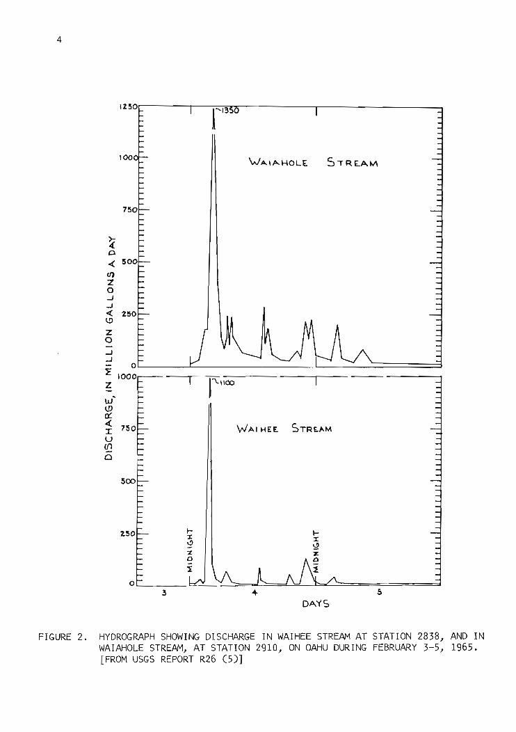
The flood hydrographs for each watershed (up to 1966) were plotted
and are shown in Appendix A. The dimensionless plotting of recession
curves and the Kl-values of each watershed are shown in Appendix B. A
list of flood hydrographs including watershed area~ dates of the flood
hydrograph, time to peak, recession constants, inches of runof~
average figures of time to peak, and recession constant are given in
Appendix C.
The two hydrograph time parameters for Hawaiian small watersheds
are short and range from about fifteen minutes to two hours. The aver
age figure of time to peak and recession constant and several commonly
used watershed characteristics are listed in Table 1.
DEVELOPMENT OF PEAK DISCHARGE EQUATIONSFROM A TRIANGULAR HYDROGRAPH STUDY
The typical shape of flood hydrographs of small watersheds, as
shown in Figure 2, and in Appendix A, indicates the possibility of
using a triangular hydrograph to design the size of Hawaiian hydro
graphs and determine the peak rate of flow of a small watershed.
The general form for the peak discharge is shown in Figure 3.
. The triangular hydrograph has been applied by Mockus (7), and Holtan
and Overton (8) as an approach for the determination of peak discharge
and may be expressed as,
5

6
Table 1. Watershed Characteristics and Average Time Parametersof Small Hawaiian Watersheds (Oahu).
Average Estimated....Time ParametersLength Slope Time of
Watershed Watershed Area of of Height* Concen- Time to RecessionMain Main of tration peak ConstantNo.
sq. mi. 1 acresStream Stream Watershed t c t p Kl***
ft % ft hr hr hr
2000 1.38 883 16,840 3.63 1.510 0.59 1.11 0.76
2080 4.04 2,586 49,100 0.73 1,600 1.90 1.92 1.61
2116 2.13 1,363 15,720 12.40 3,121 0.41 0.38 0.72
2118 3.27 2,093 12,000 13.30 3,566 0.29 1.34 1.44
2128 4.29 2,7 46 47,640 2.64 2,096 1.70 0.95 0.74
2130 45.70 29,248 2.58 2.40
2160 26.40 16,896 0.90 1.61
2230 6.07 3,885 50,940 1. 58 2,568 2.29 1.30 1.03
2245 2.59 1,658 38,840 3.75 2,792 1.21 0.25 0.75
2270 8.78 5,619 1.25 2.80
2280 2.73 1,747 22,840 3.50 2,480 0.68 1.27 1.01
2290 2.61 1,670 14,660 4.63 2,276 0.42 0.71 0.66
2390 1.06 678 7 ,283 12.60 1,920 0.20 0.76 0.72
2400 1.14 730 9,100 14.90 2,814 0.23 0.66 0.83
2440 1.18 755 11,700 8.65 2,141 0.34 0.75 0.70
2460 1.04 666 12,240 9.40 2,165 0.35 0.83 0.73
2470 3.63 2,323 22,480 4.92 2,435 0.68 0.58 1.27
2540 2.04 1,306 14,360 4.43 2,540 0.40 0.94 0.54
2739 4.38 2,803 25,480 1.15 2,782 0.75 0.80 1. 32
2750 0.97 621 5,594 11.80 2,128 0.14 0.70 0.48
2830 0.28 179 1,438 23.00 2,222 0.03 0.58 0.43
2838 0.31 198 2,250 19.70 2,069 0.05 0.55 0.59
2840 0.93 595 4,875 11.40 2,377 0.19 0.80 0.42
2910 0.99 634 3,750 6.92 2,500 0.09 0.79 0.45
2960 3.74 2,394 0.75 0.94
2965 3.'74 2,394 21,700 2.73 2,630 0.63 0.66 1. 34
3030 2.78 1,779 0.74 0.75
3300 9.79 6,266 69,040 2.60 2,260 2.53 0.90 2.43
3450 2.98 1,907 68,300 1.81 1,740 2.75 0.57 1.64
*Difference in the elevation between the gaging station and the highest point of the watershed[see WRRC, Technical Report No. 15, p. 25 (3»).
**Estimated from Kirpich formula (6).***Estimated from the composite dimensionless recession line (see Appendix B).

•..u.....
o....(!)II:C%o!!!o
;',,
_______ ACTUAL HYDRI)GRAPH
_____ TRIANGULAR tllYDROGRAPH
l.trI
1I
I,t,I
\\
" ' ......... _----- ----
I:--+;--i TI ME. (t)t p r
FIGURE 3. A TYPICAL TRIANGULAR HYDROGRAPH.
"'-.J

8
2+ t )
r(1)
where Qp is peak discharge, A is the area of the drainage basin, R is
runoff or effective rainfall expressed as depth of water over the basin,
t p is time to peak, and t r is the time from the peak rate to the end of
the triangle. Since the typical hydrograph shape is a steep triangle,
t r can be expressed by the recession constant, Kl' The section of
the recession curve, from the peak to approximately 50 percent of
the curve, can be plotted as nearly a straight line on semi-log paper.
Hence, the recession constant, Kl , can be calculated as,
(2)
2.3 log 0.5 Qp
Since !It can be replaced as 0.5 t r accordin2; to the triangular shape
then,
2.3 log 2
or,
Kl = 0.724 t r ,
t r = 1. 38 Kl'
The peak discharge equation can be expressed as a function of
the two hydrograph parameters, time to peak and recession constant,
2Q = A~ (Kl )P t p 1 + 1.38
t p
(3)
This relation can also be derived by using Holtan and Overton's
(8) result that the recession constant, K, can be considered as the
time lapse between a given flow rate and the occurrence of 1/3 times
that rate. If the hydrograph shape is close to a triangle, the fol
lowing relations may exist:
K = 0.67 t r ,
t r = 1. 5 K.

Therefore,
~= AR ( 2 )
t Kp 1 + 1.5 t
P
(4)
9
As Kl is the measured figure from the first part of the recession and
covers a great par~ of the recession flow and K cannot be determined
directly, equation (3) is easier to apply for the peak discharge esti
mation.
'LINEARITY TEST Of THE HYDROGRAPHS
The modified peak discharge equation, equation (3), expresses
a linear function for peak discharge and runoff if the two hydrograph
time parameters of a watershed are constant. The assumption of line
arity has been used since 1932 when Sherman (9) introduced the unit
hydrograph concept that peak discharge is directly proportional to the
volume of runoff for a given duration of unit hydrograph. The most
important property of such a linear re~ationship is that of superposi
tion which allows a flood hydrograph to be constructed if the duration
of effective rainfall and its corresponding unit hydrograph are known.
In fact, the peak discharge-runoff relation produced by a water
shed system is so complex that it is rarely linear. If a linear system
does not exist, the use of a linear model to determine the hydrograph
and its peak will 'yield a poor estimate. A test of linearity must
therefore be made before the linear model, equation (3) can be used.
Such a linearity test was made by using about 200 hydrographs
for twenty-nine small watersheds on the island of Oahu. The test was
made by plotting the peak discharge per unit area of all the storms
that were recorde~ for every watershed in this study, ~fA, against
runoff, R, expressed in inches. If a linear relation can be obtained,
the peak discharge, ~, should be directly proportional to the amount
of runoff since the area of a given watershed is constant. Results
have shown that a good linear relation exists between Q fA and Randp
further that this relation is unique and uninfluenced by time to peak.
The time to peak of Hawaiian hydrographs, affected mainly by a short
intense storm, is short enough that its variation would not signifi-

10
cantly affect the general shape of a storm hydrograph. Furthermore,
small Hawaiian watersheds of Oahu can be presented as four groups and
each group can be expressed by a single linear relationship between
Qp/A and R as shown in Figures 4a, 4b, 4c, and 4d. By studying the
watersheds in each group, it seems that the linear relation holds true
for small watersheds of similar size, and the watershed area is sig
nificantly correlated with the recession constant, Kl , as shown in
Table 2.
Four empirical relations have been found and may be used for
determining peak discharge and for verifying the derived equations.
They are:
a.
b.
c.
d.
For a watershed area of less than 1 square mile:
~ = 1.4 AR ~)
For a watershed area from 1 to 3 square miles:
Qp= 0.9 AR (6)
For a watershed area from 3 to 6 square miles:
Qp = 0.6 AR (7)
For a watershed area larger than 6 square miles:
Qp = 0.32 AR. (8)
The linearity test proves that Hawaiian small watersheds can be
treated as a linear system and the linear equation, equation (3), can
be used. However, there are a few points where eight or nine inches
of runoff do not follow the linear pattern and may fall away from the
linear line (see Figures 4a and 4b). Six inches can be considered as
the limit of this linear relation of the small watersheds studied when
the duration of the storms is short and insignificant. The linear rela
tion may still be applied to flood hydrographs when the amount of runoff,
R, is larger than six inches. In this case, the hydrograph is a result
of linear superposition which is possibly superposed with certain time
lqgs according to the storm duration.
DETERMINATION OF PEAK DISCHARGE
The peak discharge equation, equation (3), can be further simpli
fied if the time parameters, time to peak, t , and recession constant,p
Kl
, are known. There is no good correlation between time to peak and
recession constant. If they can be expressed by the linear line,

ben
fa 6,6.1)
O(8.e ,9.9 )
/
•/
VJ
I Waterah -d Hum
tI I/' 2390
oj 2MO27502~0
I 2838
If:o IAR2830
a Qp. 1.4
0007 a
IIo a
a 0
3
2
c(
~
6
7
5
•...ua...........:! 4u
o 2 3 4
R (In.)5 6 7 8
FIGURE 4a. LINEARITY TEST OF HAWAIIAN SMALL WATERSHEDS: GROUP 1.
I-'I-'

2I-'N
7 i I I I I iii iii
61 I I I I I I I I I I
y o
Water1hed Numbers
20002 1162245246022902440247029103030
o
o
A
o
Qp • 0.9 I AR
%o
2
n
--ell.. 5u0
"co-u4
<l"'-
Q.
a 3
I I0
60
o
2 3 4R (In.)
5 6 7 8
FIGURE 4b. LINEARITY TEST OF HAWAIIAN SMALL WATERSHEDS: GROUP 2.

3
27392960296534502128211822302280
Numbers
8764 ~
R (In.)
32
I
)
,V Watershec
/)
V,.".
/'Qp =0.6 AR
! /'0
V6'0 ./ o 0I
~oo
~o
7
~
"Q.
a
;-I~-UUo--
FIGURE 4c. LINEARITY TEST OF HAWAIIAN SMALL WATERSHEDS: GROUP 3.
....~

4I-'~
Numbers
21303300216020802270
shed
87654R (In.)
32
j
,Qp.0.32 AR
~
Waterl
0 .------
~~
------0
00 ~-~~
00 0
0~
-o
3
<"00.
4
7
2
6
......If..g ~
"14U......
FIGURE 4d. LINEARITY TEST OF HAWAIIAN SMALL WATERSHEDS: GROUP 4.

Table 2. Linearity Test of Hawaiian Small Watersheds (Oahu).
15
Watershed Watershed RecessionGroup No. Area Constant
(sq. mi.)
I 2390 1.06 0.72
2540 2.04 0.54
2750 0.97 0.48
2830 0.28 0.43
2838 0.31 0.59
2840 0.93 0.42
Area Range(approx. )
Less than
1 sq. mi.
LinearRelation
~=1.4 AR
(Fig. 4a)
II 2000 1.38 0.76
2116 2.13 0.72
2245 2.59 0.75
2290 2.61 0.66
2400 1.14 0.83 From 1 to ~=0.9 AR2440 1.18 0.70 3 sq. mi. (Fig. 4b)
2460 1.04 0.73
2470 3.63 1.27
2910 0.99 0.45
3030 2.78 0.75
III 2118 3.27 1.44
2128 4.29 0.74
2230 6.07 1.03
2280 2.73 1.01 From 3 to Q =0.6 AR
2739 4.38 1.32 6 sq. mi. (Fig. 4c)
2960 3.74 0.94
2965 3.74 1.34
3450 2.98 1.35
IV 2080 4.04 1.61
2130 45.70 2.40Larger than Q =0.32 AR
2160 26.40 1.61 6 sq. mi. (Fig. 4d)2270 8.78 2.80
3300 9.79 2.43

16
t p = Kl , as shown in Figure 5, a simple relation can be derived, from
equation (3),
or,
ARQp = O. 84 Ki""
Qp = CAR
(9)
(10)
where C is a coefficient and a function of the hydrograph time para
meters, time to peak and recession constant.
The simple form, shown as equation (10), can be applied to the
four groups of basins of varying areas. The results are shown in Table 2.
The derived equation, equation (9), is simple enough to use.
The peak discharge can be estimated for a given design runoff, R, from
any watershed (including ungaged watersheds) if the area, A, and reces
sion constant, Kl , are given. Since the recession constant, Kl , is
mainly affected by watershed characteristics, multiple correlation are
made between Kl-values and watershed characteristics. Results indicate
that watershed area alone is the most significant factor for its corre
lation to the recession constant. A regression equation is obtained
and may be expressed as,
Kl = 0.43 + 0.0003A (11)
where the recession constant, Kl , is in hours and watershed area, A,
is in acres. The linear regression between Kl and A is shown in
Figure 6.
So far, the only factor which remains unsolved is the amount of
runoff, R. To determine the amount of runoff from a given storm is
in itself a complicated research problem. A reasonable solution is
yet to be found.
If the amount of runoff, R, can be reasonably estimated, the
peak discharge can be calculated by using equation (9).

3
~2s:
Q.--.xC.,
Q.
.2•EF
0 //
7V 0
0
~0
0
0 0c
0 oC6
V 0
0
o I
Recession2
Constant K. (hr.)3
FIGURE 5. RELATIONSHIP BETWEEN TIME TO PEAK AND RECESSIONCONSTANT OF HAWAIIAN SMALL WATERSHEDS. 1-1
'-J

K, • 0.43 + 0.0003A I-'00
A VV
//
)
/./'
4/6v/
~A
6
67 6
6
4
vt: f
:w:
3
IIIcr:l 2o:I:
zo-f1)
f1)
lUUlUII:
...z~f1)
zou
1000 2000 3000 4000 5000 6000 7000 8000
WATERSHED AREA A. (ACRES)
FIGURE 6. RELATIONSHIP BETWEEN RECESSION CONSTANT AND AREA OF HAWAIIANSMALL WATERSHEDS.

19
DISCUSSION OF THE RESULTS
The reliability of the derived simple peak discharge equation,
equation (9), has been tested and found to be good when the measured
peaks of discharge are compared with those calculated from equation (9).
A good agreement of measured discharge and calculated discharge is shown
in Figure 7. All the data points were distributed close to the 45° line.
Equation (9) has shown that the peak discharge, ~, is a function
of the watershed area, A, recession constant, Kl , and inches of runoff,
R. Since Kl can be expressed as a function of A, the peak discharge
will be a single function of watershed area, A, for a given amount of R.
~ = f(A) (12)
for R = 1,
where f(A) may be read as a function of A. Peak discharges from runoff
other than one inch can be simply expressed as,
~ = R f(A) (13)
because of the linearity characteristic of the peak discharge and
runoff of Hawaiian small watersheds. However, the limitation of
R within six inches should be emphasized. Since the duration of ef
fective rainfall is small, 0.5 to one hour may be a good estimate of
the duration of rainfall. More than six inches of rainfall in an hour
will not occur frequently and, as a matter of fact, it is larger than
the lOa-year maxi~um rainfall for the island of Oahu (10). Using
equation (9), the peak discharge, Qp, was plotted against the water
shed area for six inches and four inches of runoff. Results are super
posed on a graph where all the extreme peak floods from each station
are plotted against the drainage area and shown in Figure 8. It is
very interesting to find that the curve of six inches of runoff is about
an envelope curve for all the extremes and the four-inch runoff curve
passes through the upper part of all the extremes. A comparison of
the depth-duration relation of lOa-year frequency rainfall, probable
maximum rainfall, and standard project storm of Oahu, Hawaii with the
world's greatest rainfall is shown in Figure 9. In addition to the
lOa-year maximum rainfall on Oahu, a four-inch rainfall with a duration

Q.o
~....::J•CCIIE......o
IIIC)a::ct:ro(/)
o
:w::4l&.IQ.
/0
IAI 0./0 IeILn" n'
jy7;00
o 0 BOOo 0 0
~oo ~"o°oo 0
f(0 00h. '1B 0<0' 0 0' 0f" 0 cP 00
I""" I~ 0 oo~ cfl: 0 0
Cl:>
01/o 1/
10 I~ I~I 0 0 0 1:9...., alT _ 0
o 0, I .;...; 00 0
1/ '0 0
o I V~0° 0 Va
Vc[,'O~o 0
o 0
100 0
V1/
VV
VV
No
10 100 1000
PEAK DISCHARGE? Qp? (Calculated)
FIGURE 7. COMPARISON OF MEASURED PEAKS OF FLOOD DISCHARGE WITH THOSE CALCULATEDBY USING EQUATION (9).

21
4001005010
R- S- I-I--~---I....- I...- 10- C
A ....- R-.-~ --- -- ..~ V L-,.-
.".... ~
./----_0 ~
..... \; 4p... :/ ./ cP
V I( 1,;100'" A 0 --u
1/ "'"/ .., 1....-
4 4 I...
V 0 l/ Q
./ 0 D ..
~V D j/
A lC lC
P 0 lr
It,
"1.1""0
P3
I
10
300
100
ofu
050o
Drainage Area in 100 Acres
Legend
o Windward Side
4 Honolulu District
o Between Mountain Ranges
x Leeward Side in Waianae District
FIGURE 8. CALCULATED PEAKS OF 6 INCHES AND 4 INCHES OF RUNOFF USING EQUATION (9)ARE SUPERPOSED ON THE RECORDED PEAK FLOOD DISCHARGE PLOTTED AGAINST THEDRAINAGE AREA.

NN
II I 1'1 I I II I r 11 T II III I I I I III I I I I II/~• Wot'.LD'S q"'.""Te~T R"I"'lI'AL.L. .....
••'>~ -- .,,.~ -~ -'\'~
~ -..~""'. -
Q •
1-' ./-
I- lc'~~ pll.oeA&L.E MAXIMU.... POINT ~
I- ........~ r ~ l,.)i RAIN~ALL. j O"WU HAWAII. -~ bY'
-to-
~ ~t; -
e,..->'" • ..........: ~ STANDARD PROJac.T SToAM,
~ • ~~ l,..-:I,.oo'HO"O~U'-U ....~o W'''DWAR.l) -
~ l0 V l>- $\Dl! of O!",HU.
• .A ~
I- ./ ..,........-./ / @--e--e 100 - Y.AR. MAll. R,A.... PA...... -='I-- /
-.-/. ::::;..--- - 0 ............
==V • l-#"/ VI- ~ • -V b~~
........ 100- "(EAR. Q.A'Nf'A"L., --:::- Ho .....ol.-uL-lo.> ""NO W1NO~ACl.O -
........-:: .M'"0 ........ f-1 roalof'1 OA;U'I, ,I 11-,,-~ I I I I 1 I II I.. I I I I " I I I
4·
2
1086
2.0
2.00
1000eooE>OO
4-00
2000
..J....<LL%
«a:
~
l':r 100~ 80
..:. ~O
+0
2 ..,." 8 10 1.0 "f<) 101O -' "9 12. /8 2.+ 5 10 .2.0 ~ :3 ,,(} 12 24-\. A JL A ~
V V V V--MI,..UTES HOUR5 OAY~ MON"nfS
DURATlOW, D
FIGURE 9. COMPARISON OF THE DEPTH-DURATION RELATJON OF lOO-YEAR FREQUENCYRAINFALL, PROBABLE MAXIMUM RAINFALL, AND STANDARD PROJECT STORMOF OAHU, HAWAII WITH THE WORLD'S GREATEST RAINFALLS (11).

23
of about one hour is shown as the lOa-year rainfall in the Honolulu
and windward areas of Oahu.
CONCLUSIONS
In summary, the following conclusions may be made:
1. The relationship between peak discharge and surface runoff expressed
in inches appears to be linear for a given small watershed re
gardless of intensity, duration, and size of the storm. The time
to peak which varies slightly in different hydrographs will not
change the general shape of the hydrograph or the linearity of the
peak discharge and runoff relation. However, this linear relation
cannot be extended beyond six inches of runoff.
2. Two hydrograph time parameters, time to peak and recession constant,
are both small and of nearly the same magnitude owing to the typi
cal shape of the steep triangular hydrograph of Hawaiian small
watersheds.
3. Watershed area is the most significant factor in estimating the
recession constant and is the dominant factor in determining flood
peak discharge.
4. The derivation of the simple peak flow equation, equation (9), was
based on stream flow records of twenty-nine watersheds on Oahu with
areas ranging from 0.2 to ten square miles. The applicability of
equation (9) to watersheds smaller than 100 acres is not known.
ACKNOWLEDGEMENTS
The author wishes to express his appreciation to the Hawaii Agri
cultural Experiment Station, College of Tropical Agriculture, University
of Hawaii, City and County of Honolulu, and the Office of Water Resources
Research, U. S. Dept. of the Interior, for their support of this project.
He is also grateful to the Water Resources Division, USGS, Honolulu,
Hawaii, for giving him access to the flow records used in this study
and to Dr. L. S. Lau, Associate Director, Water Resources Research Cen
ter, University of Hawaii, who provided helpful discussion and review
of the manuscript.

24
BIBLIOGRAPHY
1. Larson, C. L. and R. E. Machmeier. 1968. "Peak Flow and CriticalDuration for Small Watersheds." Trans. of ASAE, Vol. 11, No.2,pp. 208-213.
2. Chow, V. T. 1966. An' Investigation of the Drainage Problem ofthe City and County of Honolulu. Unpublished report, City andCounty of Honolulu, Hawaii.
3. Wu, I-pai. 1967. Hydrological Data and Peak Discharge Determination of Small Hawaiian Watersheds: Island of Oahu. TechnicalReport No. 15, WRRC and Technical Paper No. 939, HAES, Universityof Hawaii.
4. Hoffard, S. H. and K. H. Fowler. 1968.Floods in Hawaii through June 303 1967.Division, Honolulu, Hawaii.
An Investigation ofUSGS, Water Resources
5. Hoffard, S. H. 1965. Floods of December 1964 - February 1965 inHawaii. Report R26, USGS, Water Resources Division, Honolulu,Hawaii .
6. Kirpich, Z. P. 1940. "Time of' C.oncentration of Small AgriculturalWatersheds." Civil Engineering3 Vol. 10, No.6, p. 362.
7. Mockus, V. 1957. Use of Storm and Watershed Characteristics inSyntheUc Hydrograph Analysis and Application. Paper presentedat the annual meeting of the AGU, Pacific Southwest Region, Sacramento, California.
8. Holtan, H. N. and D. E. Overton. 1963. "Analyses and Applicationof Simple Hydrographs." Journal of HydrologY3 Vol. 1, No.3,pp. 250-264.
9. Sherman, L. K. 1932. "Streamflow from Rainfall by the Unit-GraphMethod." Engineering News Record3 Vol. 108, pp. 501-505.
10. U.S. Weather Bureau. 1962. Rainfall-Frequency Atlas of theHawaiian Islands -- for Areas to 200 Square Miles 3 Duration to24 Hours3 and Return Periods from 1 to 100 Years. TechnicalPaper No. 43.
11. Paulnus, J. L. H. 1965. Indian Ocean and Taiwan Rainfalls SetNew Records. Monthly Weather Review, Vol. 93, No.5, pp. 331-335.

APPENDICES


APPENDIX A: FLOOD HYDROGRAPHS
OF HAWAIIAN SMALL WATERSHEDS


29
Ill±thh+rtchj"P3 5 79/1
Jon. 14, 19237
WATER$HED NO.2 000
o24 1 3 5
OCt. 28, 1936
2000
1000
3000
QCcfs)
4000
5000
Time
2400
024Mar. 2) /939
Chrs.)
II
_J
/3o
800
QCcfst
1600

30
2000
22 24 I 14 16 18 20
Mar. 12, 19~1 Mar. 3, 1939Ti me (hn.)
10 12 14 16
Dec. 20, 1924
400
0 10 12 14 16
Mar. I, 19~2
NO. 2000
800
1200
1600
Q
(cf.)
2400
1600
Q(cf.)
800
o2~0~22~~24~Oct 6, 1961
( hn.)

31
1600
NO.2 0 80
,,I,,,,,,,, -,-'
I ! 'ri°t-l-+t"tt1"'o, ! I ! I1 3 5 7 9
Mar. 13, 1962( hra.)
800
1200
Q(cfs)
1200
I-I/,
, ! I ! I ! I ! I ! I ! ,! I ! ! ! I ! I
16 18 20 22 24
Feb. 21, 1959Oct. 23, 1958
Tim. (hra.)
II,I/, ,, ,/'
I ,/I ,/J' I ! 8/-(! IQ" ! Ik! I 'R! Io
800
400
Q( cfs)

32
, , ! I! ! ! ! I , ! ! I, ! , !
6 15 ~ 17 ~ 19Jan. 31, 1963
234 5JCI1. 10, 1965
( hre.)
14 15 16Sept. 9, 1965
Tim e (hn.)
NO. 2116
50
120
360
100
240
480
150
Q(cfa)
200
Q
(efe)

33
,/
II,,
. ,'. ,,
'/'.
/ './ -._._._._._.-.-,
I "I ! I ! I ! I , I ! I ! I ! I ! ! ! !24 I 2 3 4 5
Nov. /3, /~
NO. 2118
400
o
200
600
800
1000
Q
(ets)
Time (hrs.)

1600
1200
Q(ds)
800
400
o6000
4800
Q(cfs)
3600
24°0
1200
o
34
NO. 2128
24
14 16 16Dec.. 6, 1~57
357OV. 21. 195'1'
Time (hrs.)
I ._-.-.-.--------I I I 'J·'"C, I , ! , ,! ,! I, , ! ! I! !
21 23 1 3 5 'TApr. 16, 1960
Time. ( hrs·)

35
'1000
No. 2130
'I' i me (i'll's.)
_.-,I, _.-f' - __._._0
5000
1000
3000
13 1'\ 23
Novo 2 8. 1 9 54
3 5
Time (hl"s.)

36
NO. 2160
_~_._. _ _ 0-
16 18j 963
I , ! , I I I
IIII _._.-.-.
-t-._'I
! "' , I ! I ! I I ! ! I ,8 10 \2 14
Ap .... 14,4 (, 8Ma)' 12, j 9~0
Time (hrs.)
800
j 600
24°0
3200
0:3
180 0
1600
Q(~ts)
j 200
Q
(cfs)
800
400
o13
Tim e (h r.s. )

37
] 2 000
NO. 2160
10000
Q(cfs )
800 0
6000
4000
2000
o f Jm L"±'c1"t'Q', ! ! I ! I ! I3 23 24 I 3 5 'T 9
Apr. 16, 1.960
Time (hrs.)

38
5000
NO. 2230
4000
3000
'2000
\000
Ti me (hr5')

39
500
400
Q
( cfs)
300
200
NO. 2245
--' --'..-'
05 6 7 8
feb. 28, 195"8
Time ( hrs. )
100
3 00
Q( cfs)
200
\00
_.-.--_.-o
18 19 20 2\
.Dec. G, 19 5 '"('
TilTle (hrs.)
22.

402400
NO. 22'70
\ "3 5 7Oct. 23, j 9 5 e
, ! ! I, I , I , I , I ! I
, _.-'J................._._._.-.-.-.-.
II
! ,,! ! I21 22
( hrs.)'Time
400
800
j200
1600
2000
1200
Q(cts )
800
4°0
o7 e \0 12 '4 ,6
Jan. S2 I, i 9l;S
Time ( hr5·)

2000NO. 2280
41
3 5Dec. 7. 1942
Time (hr •. )
3 5Mar. 2.1939
T;me (hrs.)
Q
( cfs)
Q
( cfs)
1600
1200
800
400
0 '5 17 20Mar. 26, 1952
1600
1200
800
400
o
20 22 24 1 3Dec. 14. 1965
8 10 12Jon. 1,1937
I !

42
2400
2000
1600
Q(eft) 1200
800
400
1200
800
Q(cft)
400
o10
NO.2280
12 14 16
F.b. 28, 1932
12 14 16
Oct. 4, 1963
1200
800
400
o8
Tim. (h r •.)
18
10 12 I
Mar. 3, 1933
22241 3
Nov. 13, 1964
Time (hr •. )

43
1600NO. 2290
\200
4 20 22 2"'4Oc:t-. 6. 1961
1 '3 5 7 20 22 z+ 2S~pr. 2.8, 1937 Ap... :3, 1939
Time (hrs.)
II-'-'-'-'-'~--
III
1'3 ~1 2'3ApI"". 1, 192"3
o
600
400
Q( c.f5)
3200
2400
,600
Boo
o5 'T 9 11
:P~c.. 23, 193+lEt 16 20
Mar. 2Et, 195'2
T i lT1 e (hrs· )
e 10 \2/'Iov. 5, 1925

44
2000
1600
\200
800
NO. 2390
400
of~ 15 17 19
Apr: 11, 19303 5 'T '3
:PC!'c. 30, 1960
Time. (hrs.)
21 24' '3 5"Nov. 28, 19S4
600
Q( cfs)
400
200
o20 22 .2-4- I
:Dec.. 6, 195622 2+ I "3
Mar-. 1, 1939
'Ti me (hrs.)
22 .24 I "3J>~c.. 13, j92'(

45
2000
NO. 2400
\600
Q(cfs )
(200
800
400
III
o ..._~I.....""""-,l",,i,,""''''\8 20 22
Fet>. 2'7,1935
3000 'Time ( hI's.)
6l(cfS )
2000
o7 17
19E>0 "'ov. \ 7,
'Time (hrs.)
\000

46
\600
NO. 2440
\ 200
Q(cfs)
800
400
0 ..._ ......101;5;;__.......................
4- 6 8:Dec.. '30, 1960
_._.": , I ! ! , ! I ! I ! " , ! , ,
15 17 19 2\ 23
MQY 16, 192 7
Time (hrs.)
14 16 18 20Nov. \ 7,1948

47
1600NO. 2460
\ 200
_.- .._.-"12 1"5
Fe b. 2 a, 193211
1'7 18 19Nov. \ 7, 1949
16
_.-8
.Mar.
'Time (hrs.)
16
16 1'7 18Oc"t-. t 5, 193 B
Time (hrs.)
14 15Mar. 23. 1927
13o
800
o
400
100
200
300
400

48
2000
1600
1200
800
400
NO. 2-+ 'TO
IIIIIIIII
IIIk._._._.-·-·I
IIIII _
IIT'tO' I I I, II I , I'T 9 11 n
Mar. 11, 1951
Time (hrs.)

2000
\000
1200
800
No. 2540
49
15' 17 19 21Apr. 1-4, 196'3
Time (hrs.)

50
2000
e 10 12 14MAr. 12, 1962
61~ .21 2'3
M~7 13, 196010 12 14 16 1'7
1'1(1)' 1'3, 196Q
NO. 2'739
\600
800
\200
Q(cfs )
T irne (hr-s·)

51
2000
NO. 2750
.2+123+Nov. 20, 19S7
Time (hrs.)
o\0 12
t\rr-. '0, 19~1
o '-..._--"..;;~19 2021 222~ I'T IS 192021:Dt'c.. ~. 19~6 :Pee. G, '9S7
400
80Q
800
1200
\600
1200
Q( cfs)
Q( cfS)
Ti me (hrs.)

52
500
400
Q( C.f5)
300
200
100
o
~oo
Q
(cfs )
20
NO. 2830
21 22
Sep"t.26, 19"37
,I ...............
I L-· T -·/(· ! ! I r-j-·-.-I·-·-·-,·-·-·T-·-+ 5 Eo 9 \0 \ 1
A pc-. 8, 1939 Sept". 27. 1937
Time (hc-s.)
,12
200
100
o12 13
June 11, 1937
2
2, 19"398
Apr. 7,14 15feb. 28, 1938
Time (hrs.)

53
NO. 2830
22
Apr. 16, 196023 12110
Dec. 26, 19569
o~-""""....__.......- ....._.....
\00
300
200
QCCf5)
TimQ (hr~.)

S4
200
23 2+Mar. 23, 1964-
Q(C.ts )
100
No. 2838
,I -'-',-'-'T" I1014 15 16
Ma)' 1 (, 196"3
Time (hrs.)
1
1800
1.+ ISMay 14, 1963
Time ( hrs·)
'3 4-feb. 4, 1965
2.o
600
300
\500
Q
(c.fs)
1200 400
Q(cfsl
~oo '300

55
1000
NO. 2840
800
Q
(Cfs )
600
I ;-1--+-',-'1'-',- I16 '7 18 19
/'1cH. \4, 1943
II
: ...-' .---,--+--, I I1'3 20 2 I 14 I 5 16
May 9, 1940 Mo.)' 8, 1943
Time (hrs.)
I18
o ..............L_...__....L~~...19 .20 2 I 22
Nov. \4, 19+'1
200
400
6000
-i 0oo
2000
o23 2+ 1
Fe b. :3, 1'3"'5
Time (hr5.)

56
i 600
\200
Q( cfs)
800
400
o
NO. 2910
.-.-
2 '3 -4-Feb. 3, \965
400
300
200
100
o
2.0 21 22. 23
Arr. 16. t960'T i me (hrs.)
10 ItJan. 26, 1956
Time (h.-s.)

57
1600NO. 2~60
1200
Q(CiS )'
eoo
! , E';j·,-r'""',-j' ! ! ! !
i7 1~ 21 :2'3 1 2.
1"1"1 18, 1917
Time (hr:!>.)
400

58
2000
1600NO· 2965
_.-"I _.-
'
I ~._._
- I ... -f 15.1-:"! ! ! ! I ! ! , ! ! I w.~.u..L..l..I..I."u........I..I..r;IO.I."""""'I;,;l;,;,,(;,,l,,..I..I."""",j,,,j,""
f 0 12 14 1& 10 (2 14 t & t 5 17 19 21
Mar. 6. 196'3 Har. 26, 19~'3 :Dec. 4, 1960
-'-'-'-" ---+--
2-+ i
400
°
aDO
1200
'Time (hrs.)
4000
"3000
Q(cfs )
2000
1000
1~ 15 1'7NOV. 1, 1961
Time (hr.s.)

1600
~200
Q: cfs )
600
400
8
NO. 2.965
10 12 14 16 t aAllj' 26, 19 G5
18
fe b. 18, 19 G0
59
Time (hr~.)

60
1600
1200
Q(cfs)
600
400
o
1600
t 200
aoo
400
o
NO. 3030
Time
1-._._'-'-'-'-'I ! ! ! I ! I ! ! ! I ! I
'7 19 21 2~
May 4, 1~&5
Time (nrs.)
I _I , 1[+,1 iTiTjT, I ! !6 10 {2 14 16
Jan. 26, {95-6

o( c.fs )
5000
4000
'3000
2000
100 0
o
NO.303o
12 14 16Nov. 1, 1961
Time ( hrs.)
61
62
i 2.00
400
2000
1600
QCCfs)
12.00
600
400
o
NO. 3300
Time (hrs.)
Time (hl"s.)
(0 12 14 16 18
Sept-. 5, 1962.

63
1600
400
NO. 3450
800
I _.-.
o ..........__......~.......I..I."""-...........~IIIIo;;;I~~..............~ ..~~;..I",l~u.~...u~~~! ,'-iTt; t,ri"r; I ! I ! !1~ 11 13 is 9 11 13 15 17 1910 12 t..... 16 18
Nov. i, 1959 MQr. 30, 1960 Mat". 2&, 19"'3
lZ00
Q
(<:fs)
Time ( hr-s.)
2000
1600
Q(cfS )
1200
600
400
o I ! !
9
I _.-.-.-.I 1.11"'1·1'"' I ! I! I!11 t~ 15 17
Jan. 6, 19!>+
'T i me (hr5· )
............


APPENDIX B: COMPOSITE DIMENSIONLESS RECESSION LINE
OF HAWAIIAN SMALL WATERSHEDS


10 120 110TIM! ("'I.)
oI "'-.....~~_..I......o 120
(.Ia.)
I 0 10 120TIME (.'a. )
NO. 2111 NO. 2111 0
7 70
6 • 0
00
a I
00
40 4
0
8> 000
0
Qp Q, 00- I 0
1C1=0.711 - I K1
8 1.44Q Q
00
& 0
0
2 2 0
0
0
a
0
67
WATERSHED NO. 2000 NO. 2010
I
7 0
10
0
e00
0 0
4 4
00 •
50
0 5Q, Qp- 0 -Q
8K,· 0.71 Q o K1= "II
0
2 0 2 0
0
80
0

o 80 120 180TINI (min.)
• 0 1O 120 110 0 10 110 110 140TIME (1II1n.) TINE ( IIIln.)
NO. 1180 ho. 22107
0
8o 0
0 a0
00
40
0
0
00 5
0 0
Op Op- 0 0-0 0 0
0
2 0 'k: 1.11 2 Itl Loa0
1 1
0
68
WATIRIHID NO. 2111 MO. 211O0
O'
T ~ q,
10
o 00
o 0,00
0
4 0 4
00
I I0
Qp Op o 0
- K1: 0.77 - 0
K;: 2.400 0
0
2 2

69
oo
,0 120 180TIME (min.)
o
I0 .0 110 lao 0 .0 110 .ao 140
TIMe: (mil. ) TIIiI ( .In.)
NO. 2210 NO. 22.01
••
0
4 4co 0
o 0• 0 I0
Qp 0 Qp- - 00
Q Q000 0
0 "18 1.01 K: 0."0 1
o 0

70
o 80 120TIME ( •• ft.)
2
IQp-Q
K: 1.271
o
WATERSHED NO. 2470 NO• 2540
•7 :E•
0
5 0
4 4
1 I0 .0 110 110 0
TIMa «•••.) •7 NO. 2700
810.
0
271e 0
0 0
5 50 0
0
40
00
I0
Q, Qp 0'
1(1: ••120 K: 0.4.- -Q Q 1
2 I
Q
Qp-

71
I O~""~'~O""'~'IOTI. (.'a.)(.aa.)
T'M.
t
• NO. 1100
15 15
0
4 4
Q, Q, 0
- I - IQ Q 0
0
0
a .112 K1• I ••'
0
0
WATERIHED NO. a••o NO. a•••
• •I
o 0
I 0
0
• ,4 4
0
00
o 0
Qp Gp 8 0- I - •Q Q 0
K= .•4 • KI I .••1 1
I a •

72
TIME (.,•• )
"
I '-'..L-~......llo....""'-~o 80 120
TIME (.'a.)
WATERSHED HO. 2400 NO.' 21eO7 7
• •0
5 5
4 0 4
~0
Qp QpI 0- I -Q Q
K: .8. 0.721·1
2 20
···.0 120
TIME (.,••)
NO. 2480
5
o
60 120 110
TIME (.'nJ
o
NO. 2440
5
4
3 •Qp 0
Qp
- -Q Q
2 2 Ie.-O.7.
K:O.701

73
I~""'''''''''''''''-~...Jo 80 120 110TIME (.1 •. )
•
I 0 0 0 10 ,!O( ••1.) TI"I (. a.)
NO. 2140 NO. .t,O
• •I ,
0
4 40
0 0
Qp I Qp I- -G G
2K
1:O.42 K
18 O. 4,8
WATERSHED NO. 2110 .... .1'1
•7 7
0
8 80
I 0 I0
0
0 0 0
Gp'4- 4
0 Gp- -Q Q
I K: 0.4'I K- 0.'.
I 1

74
WATIRIHID NO. '.10
•
•I
K: ... 41
I
o .0 110 110TIMI «.In.)

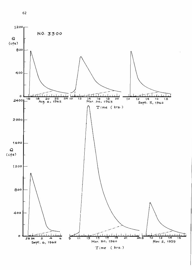
APPENDIX C: TABULATED BASIC INFORMATION OF FLOOD HYDROGRAPHS:
INCLUDES WATERSHED AREA, DATE, PEAK DISCHARGE,
VOLUME OF RUNOFF, AND RECESSION CONSTANT OF
HAWAIIAN SMALL WATERSHEDS

Watershed No. 2000 Area: 883.2 acres
77
Date t k1 Q R Qp/A(h~) (hr) (c¥s) (in)
1-19-17 0.75 0.77 2320 3.335 2.6263-25-20 2.00 0.75 4-060 8.226 4-.5961-14--23 1. 33 1.01 4-460 8.760 5.049
10-16-24 2.00 0.97 3620 7.604 4.09812-20-24 1.50 1.04 1935 2.556 2.19010-28-36 1.06 0.48 3430 3.557 3.8831-28-38 0.75 0.72 2480 2.667 2.8073- 2-39 1.67 0.29 3250 4.402 3.6793- 3-39 0.25 0.36 1740 1.111 1.9703-12-51 0.84 0.72 1620 2.178 1. 8343- 1-52 1. 33 1. 04 1339 2.245 1. 516
10- 6-61 0.75 0.72 2110 2.867 2.38911- 1-61 1.00 0.97 3100 4.184 3.509
5-14-63 1. 00 1.20 2920 5.069 3.3063-23-64 0.50 0.36 2630 2.779 2.977
Average t p = 1.11 hoursAverage kl = 0.76 hours
Watershed No. 2080 Area: 2585.6 acres
t kl Q RDate (h~) (hr) (c¥s) (in) Qp/A
7- 3-53 1.25 1. 95 1940 2.050 0.75010-23-58 2.75 1.68 1780 2.119 0.688
2-21-59 1. 84 1. 32 1960 1. 564 0.7588- 6-59 1. 92 1.77 1120 1.048 0.433
11- 1-61 1.50 1.68 1420 1.344 0.5493-13-62 2.33 1.20 1330 1. 519 0.5146-11-63 1. 82 1. 70 1320 1.412 0.510
Average t p = 1.92 hoursAverage kl = 1.61 hours
Watershed No. 2116 Area: 1363 acres
Date t kl Qp R Qp/A(h~) (hr) (cfs) (in)
12-29-60 0.41 0.77 219 0.139 0.1601-31-63 0.50 0.77 563 0.397 0.4103-22-64 0.25 0.87 219 0.105 0.1603-24-64 0.50 0.48 356 0.200 O. :26J7-25-64 0.25 0.70 194 0.107 0.1421-10-65 0.50 0.70 414 0.306 0.3412-22-65 0.17 0.77 186 0.108 0.1369- 9-65 0.41 0.72 186 0.107 0.136
Average t pAverage k
l
= 0.37 hours= 0.721 hours

78
Watershed No. 2118 Area: 2092.8 acres
Datet p k1 Q R
Qp/A(hr) (hr) (c¥s) (in)
3-14-61 1. 25 1.60 644 0.550 0.30711-13-65 1.42 1.28 1060 0.826 0.506
Average t p = 1.34 hoursAverage k1 = 1.44 hours
Watershed No. 2128 Area: 2745.6 acres
Date t k1 Qp R(h~ ) (hr) (cfs) (in) Qp/A
11-21-57 0.41 0.87 1280 0.579 0.46612- 6-57 0.67 0.48 2350 0.872 0.855
4-16-60 0.75 0.80 1750 0.801 0.6373-13-62 1.41 0.87 1135 0.675 0.4135-14-63 1.50 0.82 5680 3.504 2.068
Average t p = 0.95 hoursAverage kl = 0.78 hours
Watershed No. 2130 Area: 29248 acres
Date t .k1 Q RQp/A(h~) (hr) (c¥s) (in)
11-28-54 4.0 2.31 13600 2.279 0.4654-15-63 1. 83 2.48 6140 0.623 0.210
12-14-65 2.60 1.66 5610 0.724 0.19112-14-65 1. 91 3.09 11860 1.156 0.400
Average t p = 2.58 hoursAverage kl = 2.39 hours
Watershed No. 2160 Area: 16~896 acres
Date t kl Qp RQp/A(h~) (hr) (cfs) (in)
11-19-52 0.50 1. 33 1795 0.160 0.1068- 6-59 0.50 1. 81 1805 0.181 0.1064-16-60 1.08 0.65 7967 0.757 0.4715-12-60 0.75 1. 21 3210 0.251 0.1895-14-60 1. 25 1. 40 11519 2.423 0.6812-13-61 1.67 2.22 3226 0.406 0.1904-14-63 0.58 2.17 3233 0.363 0.192
Average t p = 0.90 hoursAverage kl = 1.54 hours
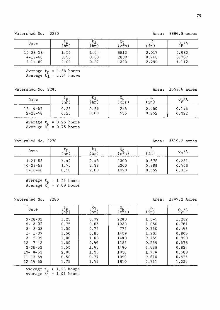
Watershed No. 2230
79
Area: 3884.8 acres
Date t kl Qp RQp/A(h~) (hr) (cfs) ( in)
10-23-58 1. 50 1.64 3810 2.017 0.9804-17-60 0.50 0.63 2880 0.768 0.7675-14-60 2.00 0.87 4320 2.299 1.112
Average t p = 1.33 hoursAverage kl = 1.04 hours
Watershed No. 2245 Area: 1657.6 acres
Datet p k1 Qp R
Qp/A(hr) (hr) (cfs) (in)
12- 6-57 0.25 0.89 255 0.090 0.1532-28-58 0.25 0.60 535 0.252 0.322
Average t p = 0.25 hoursAverage kl = 0.75 hours
Watershed No. 2270 Area: 5619.2 acres
Date t p kl Q RQp/A(hr) (hr) (c¥s) ( in)
1-21-55 1.42 2.48 1300 0.678 0.23110-23-58 1. 75 2.98 2300 0.968 0.409
5-13-60 0.58 2.60 1990 0.552 0.354
Average t p = 1.25 hoursAverage k1 = 2.69 hours
Watershed No. 2280 Area: 1747.2 Acres
Date t p k1 Q RQp/A(hr) (hr) (c¥s) ( in)
2-28-32 1.25 0.72 2240 1.845 1.2826- 3-32 0.75 0.65 1330 1.050 0.7613- 3-33 1.50 0.72 775 0.730 0.4431- 1-37 1.50 0.85 1409 1.231 0.8063- 2-39 1.00 1.08 1448 0.769 0.828
12- 7-42 1.00 0.46 1185 0.539 0.6783-26-52 1.50 1.45 1440 1.688 0.824
10- 4-63 2.00 1. 93 1030 1. 774 0.58911-13-64 0.50 0.77 1090 0.610 0.62312-14-65 1. 75 1.45 1810 2.711 1.035
Average t p = 1.28 hoursAverage k 1 = 1.01 hours

80
Watershed No. 2290 Area: 1670.4 acres
t p kl Qp RQp/ADate (hr) (hr) (cfs) ( in)
4- 1-23 0.75 0.85 1748 0.799 1.04511- 5-25 0.25 0.60 1500 0.646 0.89712-23-34 1. 00 0.87 2320 1. 873 1.400
9-28-37 0.50 0.36 1432 0.423 0.8574- 3-39 0.50 0.82 1064 0.658 0.6363-26-52 1.50 0.60 1965 1.622 1.176
10- 6-61 0.50 0.53 1100 0.458 0.658
Average t p = 0.71 hoursAverage k 1 = 0.66 hours
Watershed No. 2390 Area: 678.4 acres
Datet p kl Qp R
Qp/A(hr) (hr) (cfs) (in)
12-13-27 0.50 0.72 314 0.521 0.4624-11-30 1. 50 0.67 2080 7.352 3.0663- 1-39 0.50 0.79 555 0.663 0.818
11-28-54 0.67 0.91 676 1.071 0.99612- 6-56 0.75 0.43 376 0.521 0.55412-30-60 0.67 0.53 1400 1.360 2.063
Average t p = 0.77 hoursAverage k1 = 0.68 hours
Watershed No. 2400 Area: 729.6 acres
Date t p k1 Q RQp/A(hr) (hr) (c¥s) (in)
4-11-30 0.91 0.89 1500 2.826 2.1382-27-35 0.67 1.02 2180 3.956 2.9873- 2-39 0.67 0.53 1700 2.234 2.3304- 8-39 0.75 0.60 1140 1.156 1.562
11-17-48 0.75 1.08 1428 3.595 1. 95712-30-60 0.25 0.83 2867 3.741 8.929
Average t p = 0.66 hoursAverage k1 = 0.83 hours

Watershed No. 2440
81
Area: 755.2 acres
1 t p kl Q RDate
(hr) ·(hr) (c¥s) (in) Qp/A
5-16-27 1.00 0.96 1160 2.029 1.53511-17-48 1.00 0.72 950 1.430 1.25712-30-60 0.50 0.41 1100 1.117 1.456
Average t p = 0.83 hoursAverage k 1 = 0.70 hours
Watershed No. 2460 Area: 665.6 acres
Datet p kl Qp R
Qp/A(hr) (hr) (cfs) (in)
3-23-27 0.75 0.56 325 0.318 0.4874-11-30 0.75 0.86 1547 1.424 2.3242-28-32 0.67 .0.58 426 0.425 0.640
10-15-38 0.91 0.86 931 1.353 1.39811-17-49 0.75 1.02 781 1.060 1.173
3- 6-63 0.67 0.53 406 0.369 0.609
Average t p = 0.75 hoursAverage k 1 = 0.73 hours
Watershed No. 2470 Area: 2323.2 acres
Datet p k1 Qp R
Qp/A(hr) (hr) (cfs) (in)
12- 3-50 0.92 1. 20 2090 1. 225 0.8993-11-51 0.50 1.39 1180 0.766 0.507
12-29-60 0.33 0.34 1460 0.448 0.628
Average t p = 0.58 hoursAverage k 1 = 0.98 hours
Watershed No. 2540 Area: 1306.0 acres
t kl Qp RDate (h~) (hr) (cfs) (in) Qp/A
3- 6-63 0.67 0.37 2105 1.182 1. 6044-14-63 0.91 0.48 755 0.478 0.575
12-12-63 1. 25 0.77 665 0.568 0.506
Average t p = 0.94 hoursAverage kl = 0.54 hours

82
Watershed No. 2739 Area: 2803.0 acres
Datet p kl Qp R
Qp/A(hr) (hr) (cfs) (in)
3- 5-60 1. 33 1. 57 1400 0.982 0.5005-13-60 0.33 0.65 1900 0.<+80 0.6765-13-60 0.75 1.25 865 0.459 0.3083-12-62 0.75 1.54 1470 0.636 0.523
Average t p = 0.80 hoursAverage kl = 1.25 hours
Watershed No. 2750 Area: 620.8 acresji
Date t p kl Qp R(hr) (hr) (cfs) ( in) Qp/A
4-12-17 1.00 0.80 588 0.948 0.9474-19-17 0.67 0.48 542 0.600 0.8735- 8-43 0.50 0.48 1080 1. 328 1. 7392-29-48 0.75 0.55 712 1.106 1.1463-12-51 0.50 0.35 1030 1.138 1.6594-10-51 0.41 0.34 944 0.758 1.520
12- 6-56 1.00 0.35 1950 2.688 3.14111-20-57 1. 25 0.35 1010 1. 581 1.62612- 6-57 0.67 0.24 1720 1. 992 2.770
7- 3-58 0.75 0.48 970 1. 359 1.56212-30-60 0.25 0.72 1280 1. 201 2.061
Average t p = 0.70 hoursAverage kl = 0.47 hours
Watershed No. 2830 Area: 179.2 acres
Date t p k 1 Q RQp/A(hr) (hr) (c¥s) (in)
12-28-36 0.67 0.48 136 0.496 0.7586-11-37 0.33 0.55 169 0.412 0.9439-26-37 0.67 0.41 224 0.807 1. 2479-27-37 1.00 0.19 449 1.685 2.5052-28-38 0.41 0.19 223 0.407 1.2443- 2-39 0.50 0.31 177 0.407 0.9874- 7-39 0.50 0.42 180 0.535 1.0044- 8-39 0.50 0.48 203 0.636 1.132
11-15-42 0.50 0.36 169 0.412 0.9434-16-60 0.67 0.48 129 0.412 0.719
Average t p = 0.58 hoursAverage kl = 0.39 hours

Watershed No. 2838 Area: 198.4 acres
83
t p k 1 Q RQp/ADate
(hr) (hr) (c¥s) ( in)
4-15-63 0.25 0.81 148 0.378 0.7055-14-63 0.41 0.79 346 1.134 1. 7435-17-63 1.00 0.87 97 0.493 0.4883-23-64 0.33 0.62 146 0.463 0.7351-24-65 0.75 0.31 131 0.619 0.6602- 4-65 0.58 0.42 1700 6.134 8.568
Average t p = 0.55 hoursAverage k 1 = 0.64 hours
Watershed No. 2840 Area: 595.2 acres
t k 1 Qf) RDate (h~) (hr) (cfs) (in) Qp/A
5- 9-40 0.42 0.23 720 0.593 1. 2095- 8-43 0.59 0.36 506 0.510 0.850
11-14-47 1.00 0.65 937 1.386 1. 5743-14-63 0.75 0.38 512 0.522 0.8602- 3-65 1. 25 0.48 5100 9.897 8.568
Average t p = 0.80 hoursAverage kl = 0.42 hours
Watershed No. 2910 Area: 633.6 acres
t k 1 Qp RDate (h~) (hr) (cfs) (in) Qp/A
1-26-56 0.57 0.57 466 0.481 0.7354-16-60 1.00 0.34 813 1. 013 1.2832- 3-65 0.80 0.45 1800 2.821 2.840
Average t p = 0.79 hoursAverage kl = 0.45 hours

84
Watershed No. 2960 Area: 2393.6 acres
Datet p k 1 Qp R
Qp/A(hr) (hr) (cfs) (in)
4-27-16 1.00 1. 26 680 0.333 0.2843-10-17 0.75 0.77 465 0.182 0.1945-18-17 0.50 1. 56 960 0.459 0.4012- 1-61 0.75 0.96 1240 0.713 0.518
Average tp = 0.75 hoursAverage k1 = 1.14 hours ,
I~
Watershed No. 2965 Area: 2393.6 acres
Datet p k 1 Qp R
Qp/A(hr) (hr) (cfs) ( in)
2-18-60 0.50 1. 97 1125 0.828 0.47012- 4-60 0.25 1.32 900 0.541 0.37611- 1-61 0.75 1.22 3510 2.174 1.466
3-13-62 1. 25 1.01 1885 1. 066 0.7873- 6-63 0.50 1. 51 1470 0.968 0.6143-26-63 0.50 1.59 1260 0.771 0.5267-25-64 0.33 1. 01 3070 1.870 1.2822- 4-65 1.17 1.27 4120 3.691 1. 7218-26-65 0.67 0.84 1585 0.877 0.622
Average t p = 0.66 hoursAverage k 1 = 1.30 hours
Watershed No. 3030 Area: 1779.2 acres
t p k1 Qp RQp/ADate (hr) (hr) (cfs) (in)
1-26-56 0.75 0.84 1070 0.772 0.5141-21-57 0.91 0.84 1420 0.772 0.798
11-21-57 1.00 0.63 991 0.607 0.55612- 6-57 0.25 0.75 990 0.408 0.55610-31-61 1.00 0.63 1325 1.015 0.74411- 1-61 1.00 0.77 4130 2.343 2.321
3-26-63 0.50 0.72 1135 0.916 0.6377-25-64 0.67 0.65 1570 0.607 0.8825- 4-65 0.58 0.48 1635 0.853 0.918
Average t p = 0.74 hoursAverage k 1 = 0.70 hours

Watershed No. 3300
85
Area: 6265.6 acres
Datet p k l Qp R
Qp/A(hr) (hr) (cfs) (in)
11- 2-59 1.0 2.53 580 0.244 0.0923-30-60 2.0 2.84 2242 1. 350 0.3578- 6-62 0.25 2.12 794 0.250 0.1269- 5-62 0.25 1. 93 744 0.178 0.1189- 6-62 0.50 2.05 1092 0.372 0.1663-26-63 1. 50 2.66 700 0.369 0.112
Average t p = 0.92 hoursAverage kl = 2.35 hours
Watershed No. 3450 Area: 1907.2 acres
Date t p kl Q R(hr) (hr) (c¥s) ( in) Qp/A
11- 1-59 0.50 1. 63 635 0.517 0.3323-30-60 0.75 1. 89 1445 1.503 0.757
10-31-61 0.25 1.71 1580 1.493 0.82811- 1-61 0.25 1. 88 1185 1.132 0.621
3-26-63 1. 08 1. 60 1120 1.112 0.5875-14-63 0.91 1. 35 1840 1. 678 0.9431- 6-64 0.25 1. 45 1830 1. 297 0.959
Average t p = 0.57 hoursAverage k l = 1.64 hours
Related Documents