Hydrograph Recession Analysis for Finnish Watersheds

FACULTY OF TECHNOLOGY

Hydrograph Recession Analysis for Finnish Watersheds

Rajib Maharjan

Master’s Thesis

Master’s Degree Programme (BCBU) Environmental Engineering

August 2014

UNIVERSITY OF OULU Abstract Thesis

Faculty of Technology

Department

Department of Process and Environmental

Engineering

Degree Programme

Master’s Degree Programme (BCBU) in

Environmental Engineering

Author

Maharjan, Rajib

Supervisor

Klöve, B., Professor

Title of the thesis

Hydrograph Recession Analysis for Finnish Watersheds

Study option

Water Resources and

Environmental

Engineering

Type of the thesis

Master’s Thesis

Submission date

22 August 2014

Number of Pages

80

Abstract

Groundwater plays an important role in feeding springs and streams, supporting wetlands and land

surface stability. In Finland, most water is held in the soil than the surface systems. Hence, Finland’s

water resources depend on groundwater and biogeochemical processes. The study of groundwater in

peatland is important for maintaining ecological balance and conservation of water resources. The

groundwater level is one of the key indicators of aquifer conditions and groundwater basins. It helps

to interpret hydrogeology, groundwater flow, groundwater sustainability and land usability. The

study tries to analyze ground water recharge on peatland catchments using hydrograph recession

analysis.

The equation for the hydrograph recession curve can be utilized to predict groundwater recharge

during each recession period. The steps involved during recession curve analysis include selection of

analytical expression, derivation of recession characteristic and optimization of the parameters.

While computing groundwater recharge with recession curve, the high variability of each recession

segments creates major problem. Each segment shows the outflow process which creates short-term

or seasonal influence. The variation in rate of recession which causes problems for derivation of

recession characteristics. The computer software such as hydro-office, VBA macro excel and Matlab

are used for recession analysis. The results obtained do not consider climatic influences. The results

were then confirmed by using water balance model and statistical tests. The e-water toolkit is used

for water balance model and statistical tests are performed using R-software.

The rainfall-runoff data are used as input to the software used in each method. From the analysis,

required output recession parameters are obtained for further calculation. These estimated recession

parameters can be used to predict low flows (groundwater contribution to runoff) to understand

catchment groundwater resources and as inputs for the rainfall-runoff model analysis. Hence, the

objective of this thesis is to analyze groundwater recharge by studying the recession limb of the

runoff hydrograph. The thesis work compares various recession analysis methods. It also tries to

identify the better method by comparing groundwater recharge from different methods with

groundwater recharge from unsaturated water balance model. Furthermore, the recession parameters

obtained from different methods are compared with the theoretical values. Statistical tests are used

to identify the best method among recession analysis methods used in this study

Additional information

Acknowledgement This thesis is written as completion to Master’s Degree in Programme (BCBU) in

Environmental Engineering, at university of Oulu, Finland. The intent of this thesis is to

study surface and underground hydrology of Peatland catchment. This thesis work is

funded by university of Oulu (Water Resource and Environmental Laboratory) and

MVTT (Maa-ja Vesitekniikan Tuki). I want to express my gratitude to university of

Oulu and MVTT for generous financial support.

I will be forever grateful to Professor Björn Klöve (Director, Water Resource and

Environmental Engineering Laboratory, University of Oulu), Anna-Kaisa Ronkanen,

and Meseret Menberu for their continues help and support. I would to like express my

huge thank you to all of them for never letting me down with precious help and support.

I would also like to thank Metsähallitus, Jouni Penttinen and my advisor Meseret

Menberu for providing required data and catchment information.

Besides, I would like to thank all my friends and family who have supported me all the

time.

Rajib Maharjan

August 2014

Abbreviations

A area of the catchment (m2)

BFI base flow index

as(z) Proportion of the soil evaporation at depth z relative

to the total soil evaporation (dimensionless)

cj,k Wavelet coefficients where j describes levels of wavelets and

k is an integer

D (θ) hydraulic diffusivity (m2/s)

E cumulative evaporation in m per day

Ep pan evaporation (mm)

Ecum (t) total evapotranspiration

Es,a(t) actual soil evaporation (m/s) at time t

Eto under storey transpiration

Etg soil evaporation

Etu over storey transpiration

Fc centered frequency from wavelet analysis

F(x) function of independent variable

fs signal frequency

Gr groundwater recharges (m/d)

H height (cm)

Hs (t) depth through which soil evaporation occur (m)

IRS individual recession segment

Icap infiltration capacity at soil surface (m/s)

J number of time steps in vertical mass balance for single

horizontal redistribution time

k recession constant parameter

ks recession constant during surface flow

ki recession constant during interflow flow

kg recession constant during groundwater flow

Kv (θ) hydraulic conductivity

K_light light extinction co-efficient

Kv (θ1(t)) unsaturated hydraulic conductivity of bottom layer along

vertical axes (m/s)

Ksub saturated hydraulic conductivity of sub-surface underneath

the soil profile (m/s)

LAI leaf area index

MRC master recession curve

Md elevation of upslope soil material m

M number of soil material at down slope

N length of discrete data and (n+1) is wavelet levels

P (t) precipitation through fall at the soil surface after accounting

canopy interception at time t

P cumulative change in storage in m per day

PET potential evapotranspiration

Q runoff at time t (m3/s)

Qb base flow (m3/s)

Qt runoff at the end of recession period (m3s-1) per unit area

Qo initial recession flow (m3/s)

Q1 runoff at t1

Q2 runoff at t2

Qgi total rate of groundwater inflow (m3/d)

Qgo total rate of groundwater outflow (m3/d)

Qt rate of runoff produced by stored water in time

Qv Darcy’s vertical flux (m/s)

qvtop total upper boundary flux (m/s)

qo,in (t) total incoming overland flow at time t (m/s)

qo,out (t) total outgoing overland flow at time t (m/s)

qvbot flux from lower boundary

qiecum (t) infiltration excess runoff (inflow)

qrcum (t) saturated excess runoff (outflow)

qrcum (t) cumulative recharge

Qhorm (t) volume of water as subsurface flow from soil material m

qvtop (t + jδt’) moisture from soil infiltration (m/s)

Qtopmp (t + δt) flux across top of soil material m

Qbotm (t + δt) flux across bottom soil material m

Qbot cumulative infiltration recharge in m per day

Qtop cumulative soil infiltration runoff with contribution from

upslope in m per day

R base flow recharges (m3/s)

Rs solar radiation (MJ/m2/day)

Rcum (t) cumulative rainfall

S sum of water source and sinks

∆S change in storage

SEs (z,t) actual soil evaporation per unit control volume at depth z at

time t

Sy specific yield

Ta daily averages mean air temperature (0C)

t recession period (d)

t1 time for 1 complete log cycle (d)

Vtp total potential runoff at beginning (m3)

Vr total potential runoff volume at end (m3)

VR volume recharge between recessions (m3)

Vd volume recharge between recession (m per day)

Vt volume of water stored at time t

Winm volume of water received as horizontal subsurface flow from

soil material m.

Wavail soil moisture after drainage

WET total evaporation demand

wto total plant transpiration

wtu total soil evapotranspiration

ws total soil moisture available

Wdelta cumulative soil runoff in m per day

WT wavelet transformation

W (2jx-k) wavelet function

y1 groundwater stage at t1

y2 groundwater stage at t2

ZFP zero flux plane

θi volumetric water content

θir residual soil moisture content

µ specific yield

TABLE OF CONTENTS

Table of contents .................................................................................................................... 8

1 INTRODUCTION ............................................................................................................ 10

2 LITERATURE .................................................................................................................. 12

2.1 Peatlands hydrology ................................................................................................... 12

2.1.1 Hydrological measures ..................................................................................... 12

2.1.2 Hydrological cycle in catchment ...................................................................... 13

2.1.3 Surface water and ground water interactions .................................................... 13

2.1.4 Runoff in Peatland and groundwater ................................................................ 14

2.1.5 Water retention and subsurface flow ................................................................ 14

2.1.6 Surface and subsurface flow paths ................................................................... 15

2.2 Runoff components .................................................................................................... 16

2.3 Hydrograph recession analysis ................................................................................... 18

2.3.1 Individual Recession Segment (IRS) ................................................................ 19

2.3.2 Master Recession Curve (MRC) ....................................................................... 20

2.3.3 Wavelet Transformation (WT) ......................................................................... 21

2.3.4 Recession constant and recharge from baseflow separation ............................. 23

2.3.5 Recession constant and storage from specific yield ......................................... 23

2.4 Groundwater movement in soil .................................................................................. 24

2.5 Water balance model .................................................................................................. 25

2.5.1 Soil moisture balance ........................................................................................ 26

3 Materials ............................................................................................................................ 30

3.1 Site Description .......................................................................................................... 30

3.2 Data preparation ......................................................................................................... 31

4 Methods ............................................................................................................................. 34

4.1 Hydrograph recession analysis ................................................................................... 34

4.1.1 Individual recession segment ............................................................................ 34

4.1.2 Master recession ............................................................................................... 37

4.1.3 Wavelet transformation .................................................................................... 38

4.1.4 Recession constant and recharge from baseflow separation ............................. 39

4.1.5 Recession constant and storage from specific yield ......................................... 40

4.2 Unsaturated moisture balance components ................................................................ 41

4.2.1 Soil-water mass balance ................................................................................... 43

4.2.2 Class U3M-1D output ....................................................................................... 46

5 Calculations ....................................................................................................................... 49

5.1 Recession constant and recharge from hydrograph analysis ...................................... 49

5.1.1 Individual recession segments (IRS) ................................................................ 49

5.1.2 Master recession curve (MRC) ......................................................................... 52

5.1.3 Wavelet transformation .................................................................................... 53

5.1.4 Base flow separation ......................................................................................... 56

5.2 Recession constant and storage from specific yield ................................................... 57

5.3 Recharge volume from unsaturated water balance .................................................... 58

6 Results and discussions ..................................................................................................... 60

7 Conclusion ........................................................................................................................ 66

8 References ......................................................................................................................... 68

9 Appendices ........................................................................................................................ 81

10

1 INTRODUCTION

Peatlands are major important part of global ecosystem. It shows significant interaction

with natural hydrological system, biogeochemical cycling and terrestrial as well as

aquatic biodiversity. In Finland, peatlands have high influence in ecological as well as

socio-economic aspects. It covers one-third of Finnish land area which is 2.0 million ha

of 9.3 million ha (Virtanen and Valpola, 2011). The hydrological study is used to

develop the functions and process related peatlands system. Hydrological study is an

important part of environmental and ecological study in Finland. The study of

hydrological behavior in surface and subsurface of two peatlands catchment is the major

objective of this thesis.

In peatlands as in other soil formation there is interactive connection between the

surface and subsurface hydrological water system. This study intends to calculate yearly

groundwater recharge of two catchments using recession hydrograph. It includes study

of various hydrograph recession analysis methods. It also includes various climatic

factors that influence runoff hydrograph. The amount of water received by catchment is

disintegrated in different time period. The hydrological features of catchment influences

runoff and water storage in the catchment. The runoff generated is highly influenced by

upslope contributions from surface flow as well as interflow. In peatlands water storage

is high due to different in hydraulic conductivity and pore density (Labadz et al., 2010).

The upper layer acrotelm consists of newly formed peat which has high hydraulic

conductivity and limited storage capacity. The lower layer catotelm consists of

compressed decompositions which remains permanently saturated resulting in low

hydraulic conductivity. Due to unique hydrological surface condition, it is also highly

affected by climatic factors (Labadz et al., 2010).The hydrology of catchment depends

on its location and climatic features.

The runoff data obtained is used to draw hydrograph. It consists of various flow

components. The recession limb of the hydrograph can be analyzed to study changes in

catchment characteristics. Recession analysis method has been used successfully in

many catchments for various purposes such as flow predictions, low flow probabilities

and groundwater storage calculations (Price, 2011). In this study, the hydrograph

recession analysis is carried out using several methods: individual recession analysis,

11

master recession analysis, wavelet transformation, baseflow separation and also by

using specific yield. Wavelet transformation is only used for calculation of recession

constant. From other methods, numerical quantities can be obtained whereas wavelet

analysis is effective in visual quantification. The software programs used in this study

are Hydro-office software (Hydro Office, 2011), VBA macro excel spread sheet

(Posavec et al., 2006), Matlab and Baseflow program (Morawietz, 2007). The

groundwater recharge volumes calculated from recession analysis and specific yield

were verified by applying unsaturated water balance model. The unsaturated moisture

balance is carried out with Class-1D unsaturated moisture movement model (E-water

toolkit, 2000). It is a physical based eco-hydrological modeling tool. The objective of

the thesis is to thoroughly study groundwater recharge using hydrograph recession

methods. Furthermore, the groundwater recharges obtained from different methods are

compared with groundwater recharge from unsaturated water balance model using

statistical approach.

12

2 LITERATURE

2.1 Peatlands hydrology

Peatlands are the area consisting peat layers. They are formed by partially decomposed

dead plants in the waterlogged conditions with reduced amount of oxygen in the soil.

Peatlands store large amount of water which help in stream flow during dry seasons. It

also contributes in the attenuation of flood peaks by preventing flood damages in

downstream areas (Querner et al., 2009). Peatlands requires persistent long term water

sources. The major sources of water are precipitation, surface runoff during rainfall or

snowmelt, water bodies nearby, groundwater or combination of these sources. The

sources of water loss from the peatlands are evapotranspiration, transpiration of plants

and surface water or groundwater flow (Anderson and Samargo, 2007).

2.1.1 Hydrological measures

The peatlands behavior can be defined by three hydrological behaviors such as water

level, hydro pattern and residence time (EPA, 2008). The water level in peatlands is

related to soil surface. It contains large areas of exposed, saturated soil covered with

macrophytic vegetation. So, water level can be used as indicator for the existence of

different vegetation in various types of soil zones. The hydrological pattern is

dependent on the net difference between inflows and outflows from various water

systems. It determines temporal variability of water levels. The hydrological pattern in

peatlands involves timing, duration and distribution of water levels (Chaubey and Ward,

2006). The hydrological system in peatlands is more static which may not show short-

term or long-term variations. But some hydrological systems such as tidal marshes

show fluctuation in short time period whereas some may fluctuate more slowly over

time.

Another measure for peatlands hydrology is residence time or travel time of water

through peatlands (Belyea and Nilsmalmer, 2004). The residence time is the ratio of

volume of water to the duration of water flow through peatlands. The exchanges of

water in some peatlands are very fast resulting in short residence period whereas in

some peatlands the flow is slow thereby creating long residence period. The short

13

residence time occurs when the flow through the peatland is large compared to the

volume of flow. The long residence time occurs when the flow through the peatland is

small as compared to the volume of flow. The residence time explains the water loss

from the hydrological system in peatlands (EPA, 2008).

2.1.2 Hydrological cycle in catchment

A catchment can also be studied as an individual hydrological system. The major water

source for any catchment is rainfall and some external sources such as irrigation

(Wagener et al., 2007). The incoming water is converted to infiltration, overland flow

and some as interception storage. The water from overland flow is the combination of

surface runoff and interflow. It travels to runoff points through some flow channels. The

infiltrated water is stored by soil as unsaturated moisture (Wang et al., 2009). The

infiltrated water contributes to interflow and groundwater storage. The accumulated

storage contributes to the surface runoff. The evaporation losses at various stages and

runoff are the out flow sources for the catchment. So, a catchment can be considered an

individual hydrological system where incoming and outgoing water fluxes are balanced

(Kuchment et al., 2011).

2.1.3 Surface water and ground water interactions

Surface water and groundwater interaction depends on various geological features and

viability of water pressure (National Water Commission, 2012). In peatland, the

interconnection of surface water and groundwater occurs in three different ways: Inflow

from bed, outflow from bed and both inflow and outflow from other places (Water,

2011). The water runoff from Peatland can be the rapid drainage of water from land

surface or in similar way by which lakes and rivers receive water. Generally, the

peatland formed in depressed land surface interacts as streams and lakes. Peatlands

formed in slopes and drainage divides received water from groundwater flow from up

slopes and precipitation (Malak, 2011). In peatland there is also surface water and upper

zone soil interaction. The soil contains layers in which top layer is fibrous root mat

which high hydraulic conductivity. Upper soil zone contains sufficient interaction

between surface water and upper soil. The lower layer is fine-grained soil. It contains

highly decomposed sediments which makes the process of water and solute transfer

between surface water and ground water much slower (Brown et al., 2011)

14

2.1.4 Runoff in Peatland and groundwater

Runoff is flow of water from the catchment. It can be described as overland flow and

subsurface flow. Infiltration excess, saturation excess and return flows occur as

overland flows. Subsurface flow occurs as preferential flow, subsurface flow, and

groundwater (Linard, 2009). The runoff generation process describes various water

entering mechanisms such as rainfall, snowmelt, soil and ground water movements

(Koivusalo, 2002). Runoff shows all the processes influencing hydrologic cycle. It helps

to understand the hydrological phenomena in catchments. Runoff can also be

considered as good indicators of groundwater storage, water level fluctuation and

groundwater contribution to peatlands (Bay, 1968).The interaction between

groundwater and peatlands is determined by the hydrological setting of the area. Most

peatlands depend on groundwater and is effected by drainage, climate, groundwater use

or land uses. Also peatlands are often aquitards which control groundwater runoff

(Klöve, 2008). In most peatlands groundwater table not only depends on precipitation-

evaporation relations but also on water table in channels and streams.

The groundwater recharge occurs when head gradients produces flow from the surface

to deeper peat. The head gradients also indicate flow from the deeper peat towards

surface (Fraser et al., 2001). Groundwater supports for the stability of peatlands by

ingesting water. There is excess water in surface supporting runoff during dry periods.

In peatlands groundwater also provides ecologically important services such as thermal,

temporal and chemical buffering, aquatic ecosystem and plant diversity etc. (Klöve et

al., 2013). In peatlands, the surface features are dependent on ground water. The

groundwater dependence can be classified according to the response of surface

ecosystem. The changes in groundwater can be entirely dependent, highly dependent,

proportionally dependent, facultative dependence and no dependence on catchment

ecosystem (Barrow, 2010).

2.1.5 Water retention and subsurface flow

The moisture content in peat soil is usually very high ranging from 600-1800%

compared to dry mass of dry material in the same volume (Labadz et al., 2010).

According to Darcy’s law, water flow through a unit area of wet peat is determined by

the hydraulic conductivity of material and its hydraulic gradient. Generally, it has low

15

hydraulic conductivity and high water retention capacity even in high hydraulic gradient

(Miyazaki, 2006). The velocity of water flow through peat is also widely dependent on

its physical properties. The properties influencing flow are vegetation composition,

compaction, decomposition and presence of micro pores and entrapped gas bubbles

(Smith et al., 2004). Peat bog can be defined as diplotelmic substance. It contains an

upper layer consisting roots and recent decomposing plants known as acrotelm. The

lower layer consist denser and more decomposed humified peat known as catotelm

(Water, 2010). In general condition, acrotelm has less thickness, higher hydraulic

conductivity and limited storage capacity. Catotelm is denser due to continuous deposits

from acrotelm and less hydraulic conductivity. This ensures storage of large amount of

water in peat bogs and poor water supply to streams by means of base flow. It also helps

to maintain favorable conditions for continuing surface vegetation (Labadz et al., 2010).

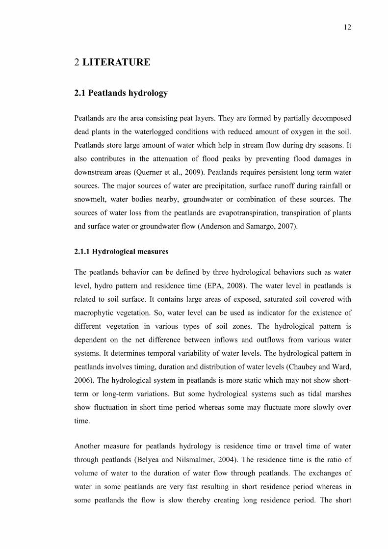
2.1.6 Surface and subsurface flow paths

The water flow regime in peatland shows two different flow paths during wet and dry

period (Andradottir, 2010). The flow is mainly defined by water head and pore water

chemistry between interacting surfaces (see Figure 1). Two distinct recharge and runoff

zones can be obtained as it is influenced by local groundwater. During base flow, a

small amount of water is contributed by hill slopes. It results in small runoff but in wet

condition, additional overland flow path is obtained (Fitzgerald et al., 2003). In dry

conditions only small runoff are obtained. Also the response times and runoff recession

are shorter. In wet condition there is more hydrological coupling between upslope and

down slope. It causes complete saturation of hill slope and peat slope (Ballantyne,

2004). The interference zone receives sufficient runoff through open fen and littoral

zones. The response time for groundwater flow in deeper peat with low hydraulic

conductivity in dry period is longer. During wet period it can be seen with few days of

major rainfall (Branfireun and Roulet, 1998).

16

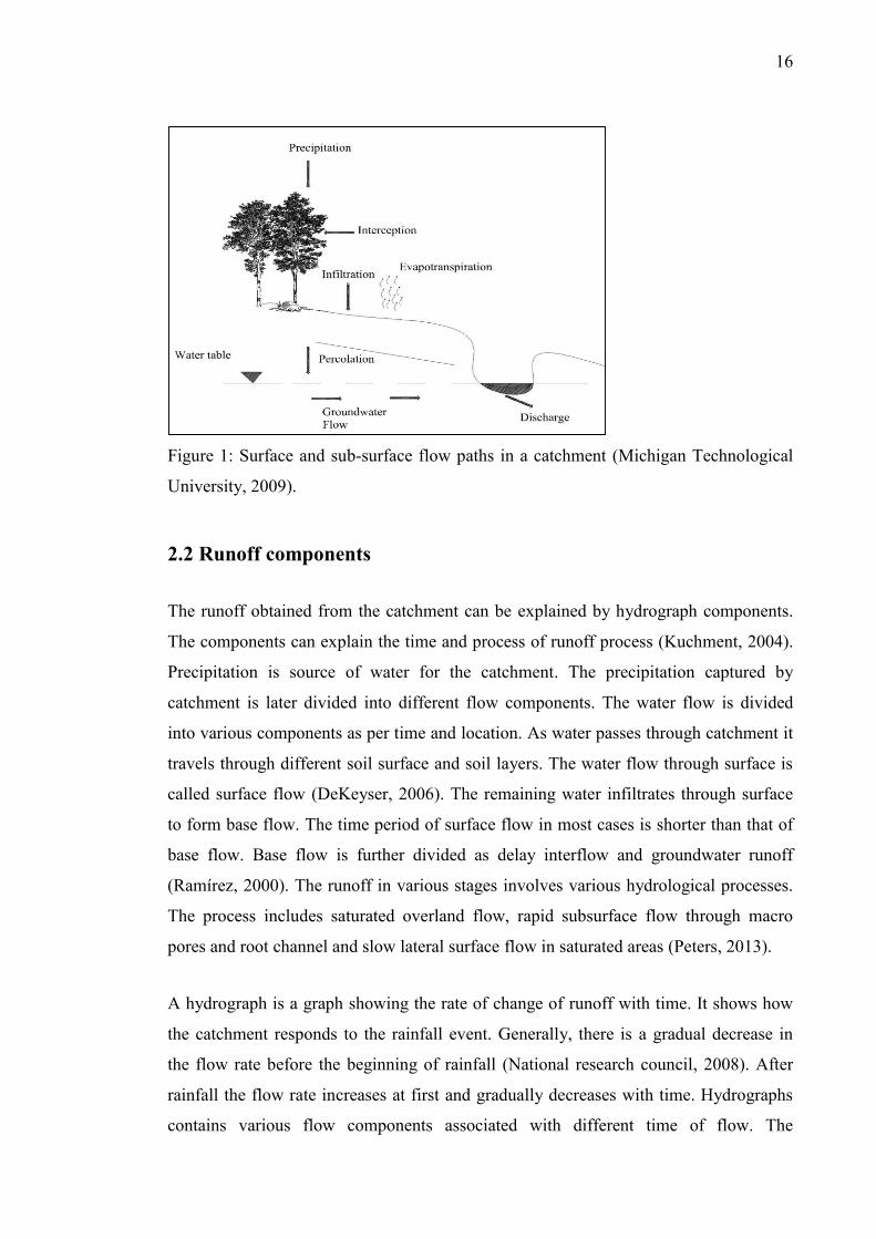
Figure 1: Surface and sub-surface flow paths in a catchment (Michigan Technological

University, 2009).

2.2 Runoff components

The runoff obtained from the catchment can be explained by hydrograph components.

The components can explain the time and process of runoff process (Kuchment, 2004).

Precipitation is source of water for the catchment. The precipitation captured by

catchment is later divided into different flow components. The water flow is divided

into various components as per time and location. As water passes through catchment it

travels through different soil surface and soil layers. The water flow through surface is

called surface flow (DeKeyser, 2006). The remaining water infiltrates through surface

to form base flow. The time period of surface flow in most cases is shorter than that of

base flow. Base flow is further divided as delay interflow and groundwater runoff

(Ramírez, 2000). The runoff in various stages involves various hydrological processes.

The process includes saturated overland flow, rapid subsurface flow through macro

pores and root channel and slow lateral surface flow in saturated areas (Peters, 2013).

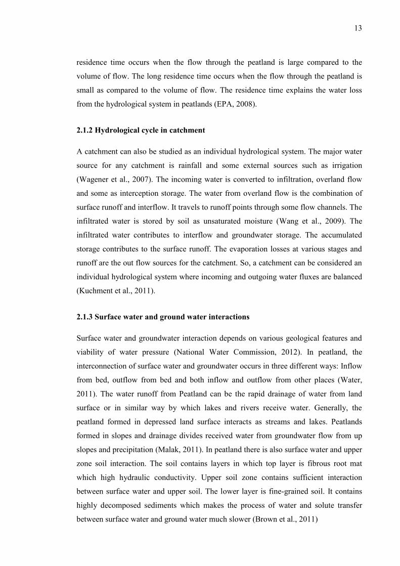
A hydrograph is a graph showing the rate of change of runoff with time. It shows how

the catchment responds to the rainfall event. Generally, there is a gradual decrease in

the flow rate before the beginning of rainfall (National research council, 2008). After

rainfall the flow rate increases at first and gradually decreases with time. Hydrographs

contains various flow components associated with different time of flow. The

17

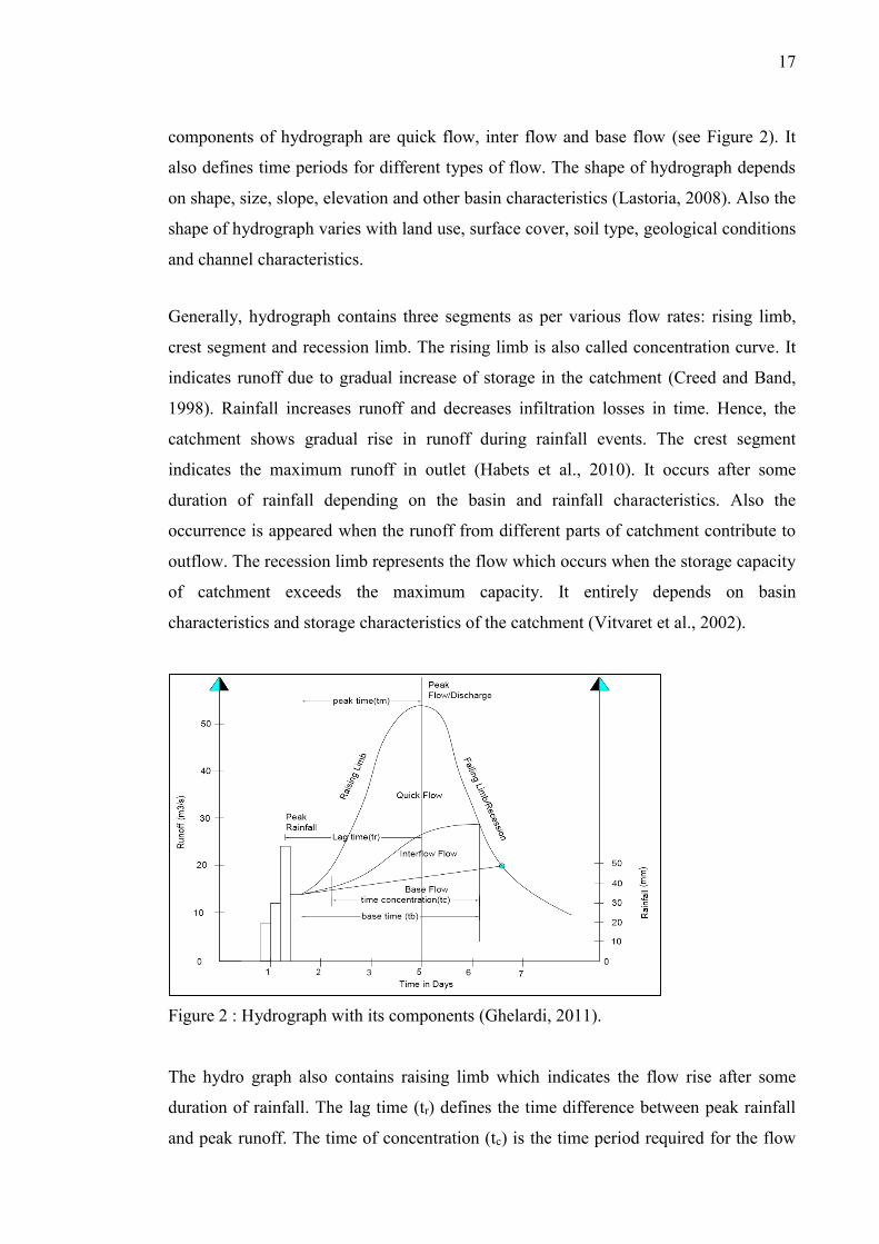
components of hydrograph are quick flow, inter flow and base flow (see Figure 2). It

also defines time periods for different types of flow. The shape of hydrograph depends

on shape, size, slope, elevation and other basin characteristics (Lastoria, 2008). Also the

shape of hydrograph varies with land use, surface cover, soil type, geological conditions

and channel characteristics.

Generally, hydrograph contains three segments as per various flow rates: rising limb,

crest segment and recession limb. The rising limb is also called concentration curve. It

indicates runoff due to gradual increase of storage in the catchment (Creed and Band,

1998). Rainfall increases runoff and decreases infiltration losses in time. Hence, the

catchment shows gradual rise in runoff during rainfall events. The crest segment

indicates the maximum runoff in outlet (Habets et al., 2010). It occurs after some

duration of rainfall depending on the basin and rainfall characteristics. Also the

occurrence is appeared when the runoff from different parts of catchment contribute to

outflow. The recession limb represents the flow which occurs when the storage capacity

of catchment exceeds the maximum capacity. It entirely depends on basin

characteristics and storage characteristics of the catchment (Vitvaret et al., 2002).

Figure 2 : Hydrograph with its components (Ghelardi, 2011).

The hydro graph also contains raising limb which indicates the flow rise after some

duration of rainfall. The lag time (tr) defines the time difference between peak rainfall

and peak runoff. The time of concentration (tc) is the time period required for the flow

18

due to rainfall to reach runoff charge point due. The falling limb defines the recession

flow. It contains information about different flow such as interflow and base flow. The

base flow after inflection point is mostly dominated by groundwater flow (Han, 2010).

2.3 Hydrograph recession analysis

A recession hydrograph is a part of hydrograph showing decrease of runoff rate after

rainfall or snow melt. The recession part in hydrograph is independent of rainfall

characteristics. It indicates the water flow to the outlet event after hours of rainfall event

(Knapp, 1979). It depends on the basin characteristics and entirely represents the basin

storage capability. The starting point of recession limb of hydrograph is called

inflection point. The starting point or point of inflection represents the maximum

storage which includes surface storage, interflow storage and groundwater storage

(Granato, 2012).

There is change in slope of recession hydrograph as the flow changes. Initially, there is

steep slope. The flow is dominated by flood flow component which gradually decreases

when flow component is dominated by subsurface flow. The curve shows similar

behavior till the end of recession period. In the condition of subsequent rainfall, the

curve rises indicating the increase of flow. So, the runoff in outlet during recession

period is dominated by flow from natural groundwater storages (Natural Heritage

Institute, 2003). To understand runoff process and groundwater flow components such

as interflow, shallow groundwater flow and deep groundwater flow, the analysis of

recession curve can be carried out. For analysis, the recession segments can be selected

from hydrograph. The selected segments can be analyzed individually or collectively

(Eylon et al., 2006). The recession curve indicates water from surface storage,

subsurface flow and groundwater flow. The recession curves can be analyzed as an

exponential segment representing the depletion of a reservoir. The rate of depletion of

reservoir is represented by recession co-efficient (α) (Martins, 2007). The equation (1)

is the recession equation showing relation of runoff with time.

Qt = Qoe-αt or Qok

t (1)

Where Qt is runoff at time t after flow Qo

19

Qo is intial runoff at time to

k = e-α= recession constant

The recession hydrograph represents surface flow, inter flow and groundwater flow.

The recession constant can be defined as the product of three components as per

equation (2) (Subramanya, 2008).

k = ks × ki × kg (2)

Where ks is recession constant during surface flow

ki is recession constant during interflow flow

kg is recession constant during groundwater flow

The recession parameters can be used for quantifying various hydrological processes.

The most common application in which the recession parameters is used are low flow

forecasting, estimation of groundwater resource of the catchment, rainfall-runoff

models and hydrograph analysis (Matonse and Kroll, 2009). Hydrograph recession

analysis can be carried out in using the semi-logarithmic plot of a single hydrograph

segments, master recession, relative new approach based on wavelet transformation and

baseflow separation (Sujono et al., 2004). The methods for recession analysis can be

described as below:

2.3.1 Individual Recession Segment (IRS)

The hydrograph recession analysis can be carried out with cumulative analysis of

individual recession segments in a hydrograph (Yarnell et al., 2013). The flow during

recession period consists of runoff from different sources in a catchment. These sources

are considered to be in exponential term. It is based on the concept that the change in

slope indicates decreasing contribution of surface and interflow to the runoff. The

hydrograph recession consists of three flow components in which the time

concentration for base flow is much higher than surface flow and inters flow (Focus,

2001).

The recession constant is calculated using the recession slope obtained from flow

hydrograph. Recession constant is calculated as an exponential function of the recession

20

slope (i.e. e-α = k). In this method, each individual recession segment or the ratio of

runoff value (Qo/Qt) of individual recession segment is plotted in semi logarithmic scale

(Commonwealth of Australia, 2006). In time series hydrograph the increase in

magnitude of slope represents the increase in surface flow and inter flow. Similarly,

when the flow is plotted in semi logarithmic scale the slope obtained represents base

flow (Anderson and Burt, 1980). Various experiments by researchers proved that

change in slope in recession flow is directly related with base flow. Usually, while

plotting recession segments, a straight line cannot be obtained. This is due to the fact

that recession flow is composed of different flow components (Szilagyi, 1999).

2.3.2 Master Recession Curve (MRC)

The calculation of recession constant from single recession segments shows high

variability. To overcome this problem a single master recession curve from each

recession curve can be drawn. A master recession curve can be defined as envelope of

various recession curves (Sujono et al., 2004). The Master Recession Curve (MRC)

represents the mean flow recession rate. The MRC curve is derived from simple

exponential decay of flow. The flow hydrograph may also contain information of

sudden decline which cannot be considered by MRC (Ramírez et al., 2002). Analysis of

recession curve using MRC involved various methods: (a) co-relation method, (b)

matching strip method and (c) tabulation method.

a) Correlation method

In this method a fixed time period for is computed from current flow and previous flow

measured at certain time t. The procedure is applied for all recession periods. An

envelope line is drawn from origin and recession constant (Ritzema, 1994). The

equation (3) is used for calculating recession constant in correlation method.

K = (Q/Qo)1/t (3)

Where k is function of slope of correlation line

t is lag time

21

b) Matching strip method

Matching strip method is similar to semi logarithmic plot for individual recession

segments. In this method all the recession segments are plotted in semi logarithmic

scale (Hisz, 2010). The recession segments are super imposed and horizontally adjusted

until the entire recession curve overlap to form a single curve. The master recession

curve is drawn with visual estimate and slope of the mean line gives recession

parameter k (Strang, 1964).

c) Tabulation method

In this method master recession curve is derived from multiple recession curves. The

starting value of each recession curve is chosen and the highest starting value of

becomes starting value for the master recession curve (Stewart, 2014). The other

recession curves are combined with master recession curve in the descending order of

the starting value of each segment. The resulting curve gives a master recession curve.

The process of constructing master recession curve is either analytical or computational

(Strang, 1964).

2.3.3 Wavelet Transformation (WT)

Wavelet transformation is an accurate way of the separation of signal characteristics in

both time and frequencies simultaneously. It is the recent method which is used for

analyzing temporal and spatial climate variability. It is implemented in the geophysical

signal identifying transient features and quantifying the temporal variability of stream

flow and flood hydrograph (Careyn et al., 2013). The main purpose of wavelet analysis

for frequency-time domain signal is to identify any change in signal in time. As in

signal, wavelet transformation method can be used for identifying any change in

hydrological characteristics (Sujono et al., 2004).

In this method the time series data is processed as frequency signal. The runoff data are

transformed to frequency signals using Fourier Transformation. In Fourier analysis the

signal as imposed by its corresponding frequencies extended over time -∞ to +∞. But

22

the time series data are defined by certain time frame which is lost in Fourier

transformation. The wavelet transformation overcomes this defect. It breaks down

signal into constituent parts and produces location in both time and frequency. The

process of wavelet transformation of time-frequency domain signal includes wavelet

decomposition and presentation in mean square maps (Gurley and Kareem, 1999). The

decomposition of an arbitrary signal is decomposed to infinite summation of wavelets

according to wavelet expansion. During the analysis of discrete time series, wavelet

function is wrapped around time interval independent variable t over signal duration T.

The equation (4) shows wavelet decomposition function (Yuan, 1997).

f(x) = ∑ ∑ cj,k∞

k=-∞

∞

j=-∞W(2jx-k) (4)

Where f(x) is function of independent variable

cj,k is wavelet coefficients where j describes levels of wavelets and k isan

integer

W(2jx-k) is wavelet function

The signal behavior is analyzed by mean square values of the signal. The mean square

values are computed by squaring discrete time series function and integrating over the

interval of 0≤x<1. As in signal, the change in hydrograph can be analyzed by wavelet

transformation. The recession hydrograph consists of different flow components such as

surface flow and base flow. There is certain change in frequency and location when the

flow component changed. In hydrograph, base flow component has longest time so it

has lowest frequency which is known as cut-off frequency (fc) (Palmroth et al., 2010).

The location and frequency value can be computed by observing wavelet maps or by

calculating centered frequency. The centered frequency of frequency signals is

computed using equation (5) (Williams, 2004).

fc = 2jfs/N (5)

Where fc is centered frequency

fs is 1/∆t where ∆t is time interval

N is length of discrete data

23

The equation (6) is used for calculation of recession parameter k using the centered

frequency (Sujono et al., 2001).

k = e-fc (6)

Where k is recession parameter

2.3.4 Recession constant and recharge from baseflow separation

Baseflow represents the part of flow draining from groundwater. It is an important part

of basin hydrology. It inflects groundwater system dependence in climate and

geography of basin (Qian et al., 2012). Baseflow is part of flow obtained from

groundwater. The amount of base flow depends on the area of drainage, catchment soil

properties and baseflow index. Base flow index defines the amount of water as surface

flow and groundwater flow. It suggests the percentage of groundwater and delayed

subsurface runoff in the catchment (Ahiablame et al., 2012). The baseflow recession

constant denotes the rate by which flow decreases. It is applicable for short term

variations in flow. The short term recession rates depend on precipitation and

evapotranspiration. The potential baseflow supply by infiltrated precipitation depends

on baseflow index and its recession rate (Bako and owoade, 1988).

2.3.5 Recession constant and storage from specific yield

Specific yield is the total amount of water drained to the groundwater storage in the

influence of gravity. The specific yield is determined by groundwater storage change in

catchment and change in groundwater level (Hilberts et al., 2005). The average

groundwater depletion and average storage calculated from the recession method is

compared to verify the correctness of the recession analysis method. The Equation (7)

specific yield for this study is calculated using equation (7) (Gehamn et al., 2009).

Sy = ∆S/∆h (7)

Where Sy is Specific Yield

∆S is change in groundwater volume per unit area

24

∆h is change in ground water table elevation

The well hydrograph from ground water table also represents slope off recession curve.

In similar catchment there is similar behavior in groundwater hydrograph and flow

hydrograph. So, the equation of recession curve in flow hydrograph can also be used for

groundwater level. The equation can only be applied to dry season. During dry season

the water stored in catchment is removed by groundwater drainage and also due to

evapotranspiration (Raghavendran, 2013).

2.4 Groundwater movement in soil

The movement of water takes place from higher elevation to lower elevation or high

pressure zones to low pressure zones. The high elevation or high pressure zones can be

termed as recharge areas. In recharge areas water accumulates from various sources

resulting high hydraulic pressure head (Biggs, 2012). The low elevation or low pressure

zones can be termed as runoff areas. In runoff areas water flow to the low hydraulic

pressure heads through an outlet or any other medium. The water movement is mostly

downward and sideways. The vertical movement is due to gravity and capillary forces

(Eagleson, 1978). The capillary force results in rise of water in soil. In absence of

capillary action gravity pulls water downward.

The rate of movement depends on adhesion and cohesion. The water molecules are

attracted to the solid surface which is known as adhesion. The attraction of water

molecules with each other is known as cohesion. In multilayered soil, when the 1st layer

is fully saturated, water moves from 1st layer to 2nd layer (Meixler, 1999). The rate and

direction of water movement is affected when it travels from one layer to another due to

change in pore size and shape of soil material. The pore size and shape of soil material

depends on the factors such as texture and structure, organic matter and bulk density

(Athavale et al., 1992).

The porosity of soil material defines the maximum volume of water below water table.

Porosity can be defined as the sum of specific yield and specific retention. The specific

yield is the ratio of water volume that drains out due to gravity to the volume of soil.

The specific retention is the ratio of volume water remained in soil to the volume of

soil. Specific yield estimates are based on the water available in unsaturated zone

25

(Taboada, 2003). The change in amount of water in unsaturated zone denotes the

change in groundwater level. In unsaturated zone all water due to gravitational fall

contributes groundwater storage (Williams, 2009).

2.5 Water balance model

Water balance model is a tool for analysis hydrologic data and gives valuable

information about the hydrological cycle. From water balance model, required

management option can be identified (Gathenya, 2007). The model is based on the

conservation of mass. The analysis involves water content change in soil volume. The

water content at certain period is equal to difference between amount of water added to

the soil volume and amount of water withdrawn from it. The main purpose of water

balance is to identify the division of water supply into various components (Xu and

Singh, 1998). Water balance can be conducted to any specific area with emphasis to soil

moisture and vegetation. It includes all inflows, outflows and water storage and is based

on land surface, groundwater, soil moisture with certain area. The general conceptual

water balance model is that, inflow = outflow + change in storage (Lindborg et al.,

2006).

Water balance has many applications: some of the applications are synthesis of long

term record of the catchment and generation of runoff records from un-gauged

catchments. It can also be used to compare circulation models, forecasting yield and

possible hydrological effects with time control, deriving climatic and hydrological

classification. Water balance models can explain hydrological phenomena with fewer

parameters (Xu, 2002).Water balance extend the information on each parameter which

allows more accurate determination of parameters. It also provides reliable correlation

between the parameter values and catchment behavior. It can also be used for checking

whether all flow components are considered quantitatively. Water balance can be

regarded as the model which includes all the hydrological process of the catchment. It

helps in the evaluation of the effect of change in its components (Xu and Singh, 1998).

26

2.5.1 Soil moisture balance

The soil moisture balance accounts the amount of water added, removed or stored in

soil in certain duration of time. Generally soil moisture balance is used to identify

whether soil water deficits or exceeds (IAEA, 2008). In soil, water moves through soil

pores due to gravity or capillary forces. The rate and direction of water highly depends

on the soil layers due to variation in pore size of the soil. In soil water content can be

described as gravitational water, bound water and capillary water (Manzoni et al.,

2013). Gravitational and bound water is not available for plants. The gravitational flow

in macrospores is rapidly drained out through drainage. The bound water is tightly

adhered to soil particles and cannot be taken up by roots. Capillary water is the water

filled in small spaces of soil particle and easily gets to surface by capillarity force

(Hudson and Berman, 1994). The soil moisture held in soil is due to surface tension.

The study of soil water balance requires knowledge of various saturation zones beneath

the earth surface. Unsaturated zone is also known as vadose zone that between land

surface and water table. The saturated zone is also known as phreatic zone. It contains

water at greater pressure than atmospheric pressure and the soil pores are completely

filled with water (Sumangala, 2011). Water table is the surface dividing saturated and

unsaturated zone where pore pressure is equal to atmospheric pressure. Capillary fringe

is zone just above water table which is a saturated by capillary forces (Vandewiele et

al., 1992). The two types of water balance model are explained below.

a) Saturated moisture balance

The water balance in the saturated zone is also known as groundwater balance. The

water balance in saturated zone helps to determine the significant components effective

ground water regime (Zhang et al., 2002). In this method, all the components relating to

inflow and outflow in groundwater system are quantified. Also the equation of

groundwater balance can be used for quantifying unknown components which are

difficult to quantify from physical methods. The general equation for groundwater

balance is shown as equation (8) (Noraly, 2011):

R - G + 1000 (Qgi - Qgo )/A = μ∆h/∆t (8)

27

Where Qgi is groundwater inflow (m3/d)

Qgo is groundwater outflow (m3/d)

µ is specific yield

∆h is change in water table during time interval ∆t

The amount of water available in saturated zone depends on porosity and permeability

of soil material. It is also affected by climatic factor and soil type. The

evapotranspiration from shallow stores and leakage are difficult to quantify. They are

determined by various modeling methods (Shunjun et al., 2006).

b) Unsaturated moisture balance

Unsaturated zone is also known as vadose zone. This zone acts as interactive medium

for the transfer of land surface to groundwater and vice versa. It defines

interrelationship between various catchment low parameters (Reilly and Lech, 2007).

The study of unsaturated zone helps to examine the process of groundwater flow

generation and routing along with groundwater runoff to outlet. It is based on the

assumption that at some point beneath soil surface, there is change in hydraulic

conductivity of soil from higher to lower soil layer. This fact indicates that all water

below that point percolates to groundwater storage. The point that lies just below zone

of root water uptake is known as zero flux plane (Wood, 2011). Above this plane there

is upward movement of soil moisture due to evaporation. Soil moisture below the zero

flux planes contribute to groundwater by process of percolation (Moubarak, 2013). The

unsaturated soil layer can hold maximum water capacity of soil. The amount of water

stored in unsaturated zone depends on actual evapotranspiration, percolated

groundwater and rate of capillary raise from groundwater. The properties of soil are

used to compute water balance parameters (Khire et al., 1997)

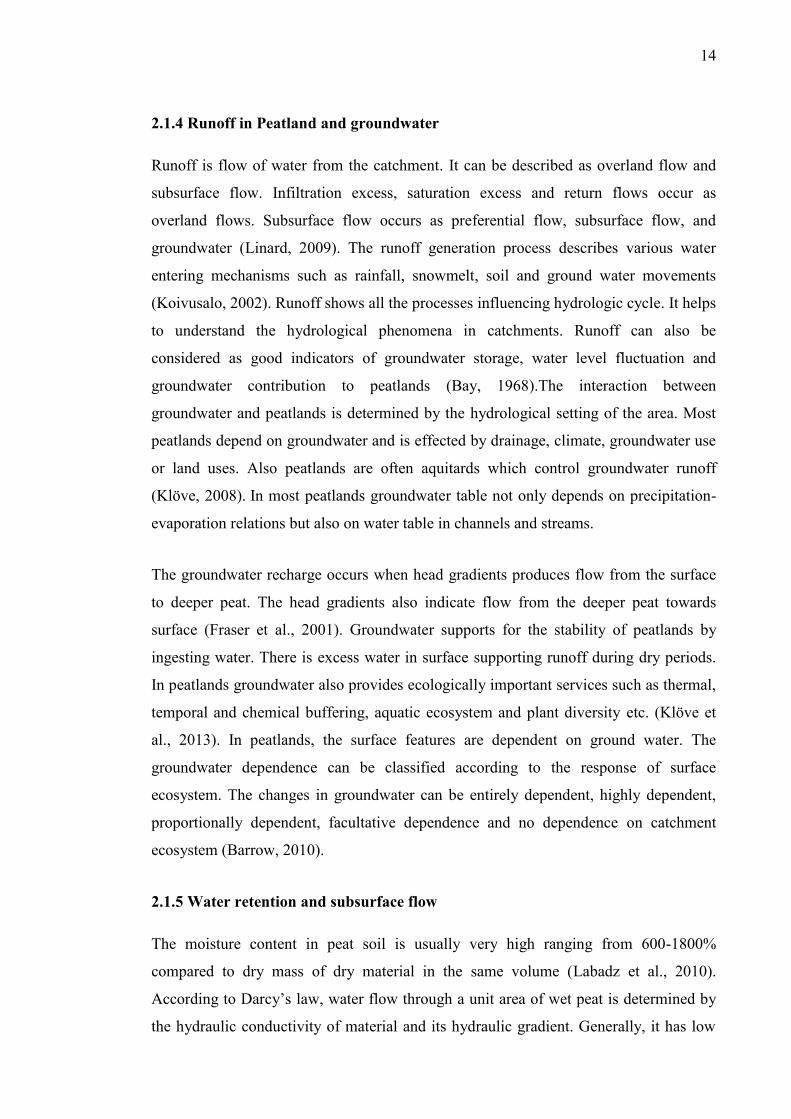
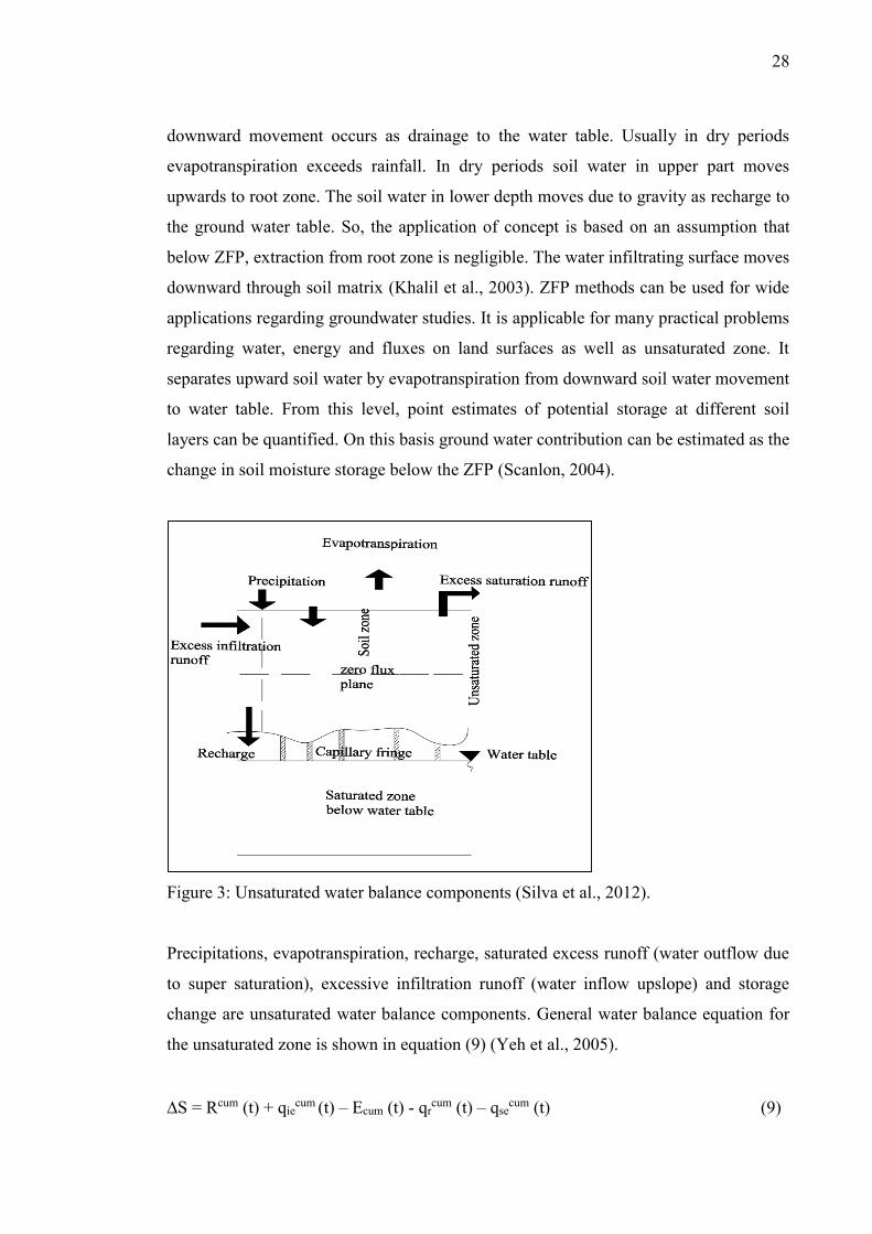
Figure 3 depicts water balance in unsaturated zone with Zero Flux Planes (ZFP)

concept. ZFP method is one of the methods for determining soil moisture balance in

unsaturated soil. Zero flux planes are an arbitrary layer in unsaturated zone which

separates upward and downward movement of water in wetted soil (ISMAR, 2005).

Above this plane evaporation occurs, resulting upward movements of water. Below it,

28

downward movement occurs as drainage to the water table. Usually in dry periods

evapotranspiration exceeds rainfall. In dry periods soil water in upper part moves

upwards to root zone. The soil water in lower depth moves due to gravity as recharge to

the ground water table. So, the application of concept is based on an assumption that

below ZFP, extraction from root zone is negligible. The water infiltrating surface moves

downward through soil matrix (Khalil et al., 2003). ZFP methods can be used for wide

applications regarding groundwater studies. It is applicable for many practical problems

regarding water, energy and fluxes on land surfaces as well as unsaturated zone. It

separates upward soil water by evapotranspiration from downward soil water movement

to water table. From this level, point estimates of potential storage at different soil

layers can be quantified. On this basis ground water contribution can be estimated as the

change in soil moisture storage below the ZFP (Scanlon, 2004).

Figure 3: Unsaturated water balance components (Silva et al., 2012).

Precipitations, evapotranspiration, recharge, saturated excess runoff (water outflow due

to super saturation), excessive infiltration runoff (water inflow upslope) and storage

change are unsaturated water balance components. General water balance equation for

the unsaturated zone is shown in equation (9) (Yeh et al., 2005).

∆S = Rcum (t) + qiecum (t) – Ecum (t) - qr

cum (t) – qsecum (t) (9)

29

Where ∆S is change in storage

Rcum (t) is cumulative rainfall

qiecum (t) is infiltration excess runoff (inflow)

qrcum (t) is saturated excess runoff (outflow)

Ecum (t) is total evapotranspiration

qrcum (t) is cumulative recharge

30

3 MATERIALS

3.1 Site Description

The two catchments studied in this thesis are Marjasuo and Röyvänsuo. Marjasuo

peatland has been drained since 1968 for forestry and was restored in 2011.Röyvänsuo

is a pristine peatland located in Isosyöte National park. Both of the study catchments are

the part of larger Iijoki catchment (Ronkanen et al., 2010). The catchments lie in

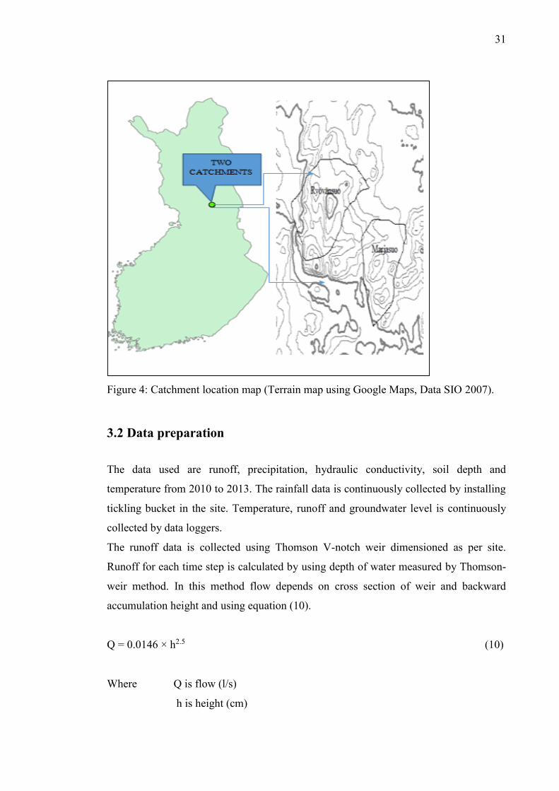
northern Finland at Taivalkoski municipality and both are state owned (Figure 4). The

geographical locations of the catchments Marjasuo and Röyvänsuo are at 65o48’19.79’’

latitude and 27o48’42.246’’longitude and 65o49’12.213’’ latitude and 27o48’13.978’’

longitude respectively. Marjasuo covers land area of 65ha (0.65km²) and Röyvänsuo

75ha (0.75km²). The two catchments contain almost similar terrestrial and soil

formations. Marjasuo has 2.27 ha (3.5%) open water or pond, 30.55 ha (47%) mineral

soil, 16.5 ha (25.5%) fen or open mire and 15.6 ha (24%) forested peatland and

paludified forest. Similarly, Röyvänsuo contains 0.5 ha (<1%) open water, 44.25 ha

(59%) mineral soil, 18.75 ha (25%) fen (open mire) and 11.25 ha (15%) forested

peatland and paludified forest.

For the study of the catchment, tree cover is taken as surface vegetation. The soil layers

are homogenous mixture of sand, loam and peat. The study used field measured

averaged hydraulic conductivity. Also initial soil moisture content is taken as per site

measurement. The average hydraulic conductivity for Marjasuo and Röyvänsuo is 9.56

x 10-5m/s (808.74 cm/d) and 1.814 x 10-5 m/s (148.95 cm/d). The initial soil moisture

for both of the catchments ranges from 0.4-0.6 (Kellomäki et al., 2010). The other

inputs for modeling unsaturated movement are land use, climate data and hydraulic

parameters. The landuse data are taken from standard values for tree vegetation from

user manual (E-water toolkit, 2000). The climate data is calculated from temperature

data measured.

31

Figure 4: Catchment location map (Terrain map using Google Maps, Data SIO 2007).

3.2 Data preparation

The data used are runoff, precipitation, hydraulic conductivity, soil depth and

temperature from 2010 to 2013. The rainfall data is continuously collected by installing

tickling bucket in the site. Temperature, runoff and groundwater level is continuously

collected by data loggers.

The runoff data is collected using Thomson V-notch weir dimensioned as per site.

Runoff for each time step is calculated by using depth of water measured by Thomson-

weir method. In this method flow depends on cross section of weir and backward

accumulation height and using equation (10).

Q = 0.0146 × h2.5 (10)

Where Q is flow (l/s)

h is height (cm)

32

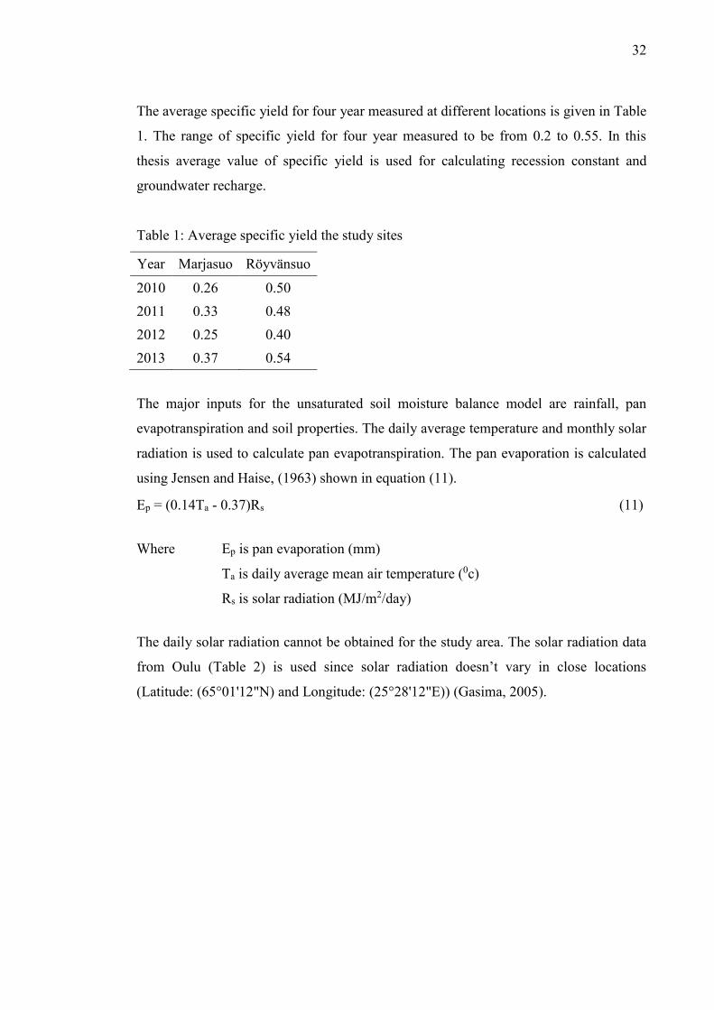
The average specific yield for four year measured at different locations is given in Table

1. The range of specific yield for four year measured to be from 0.2 to 0.55. In this

thesis average value of specific yield is used for calculating recession constant and

groundwater recharge.

Table 1: Average specific yield the study sites

Year Marjasuo Röyvänsuo

2010 0.26 0.50

2011 0.33 0.48

2012 0.25 0.40

2013 0.37 0.54

The major inputs for the unsaturated soil moisture balance model are rainfall, pan

evapotranspiration and soil properties. The daily average temperature and monthly solar

radiation is used to calculate pan evapotranspiration. The pan evaporation is calculated

using Jensen and Haise, (1963) shown in equation (11).

Ep = (0.14Ta - 0.37)Rs (11)

Where Ep is pan evaporation (mm)

Ta is daily average mean air temperature (0c)

Rs is solar radiation (MJ/m2/day)

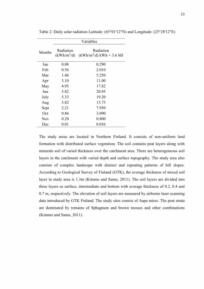
The daily solar radiation cannot be obtained for the study area. The solar radiation data

from Oulu (Table 2) is used since solar radiation doesn’t vary in close locations

(Latitude: (65°01'12"N) and Longitude: (25°28'12"E)) (Gasima, 2005).

33

Table 2: Daily solar radiation Latitude: (65°01'12"N) and Longitude: (25°28'12"E)

Months

Variables

Radiation

(kWh/m2/d)

Radiation

(kWh/m2/d) kWh = 3.6 MJ

Jan 0.08 0.290

Feb 0.56 2.010

Mar 1.46 5.250

Apr 3.10 11.00

May 4.95 17.82

Jun 5.82 20.95

July 5.33 19.20

Aug 3.82 13.75

Sept 2.21 7.950

Oct 0.86 3.090

Nov 0.20 0.800

Dec 0.01 0.036

The study areas are located in Northern Finland. It consists of non-uniform land

formation with distributed surface vegetation. The soil contains peat layers along with

minerals soil of varied thickness over the catchment area. There are heterogeneous soil

layers in the catchment with varied depth and surface topography. The study area also

consists of complex landscape with distinct and repeating patterns of hill slopes.

According to Geological Survey of Finland (GTK), the average thickness of mixed soil

layer in study area is 1.3m (Kimmo and Samu, 2011). The soil layers are divided into

three layers as surface, intermediate and bottom with average thickness of 0.2, 0.4 and

0.7 m, respectively. The elevation of soil layers are measured by airborne laser scanning

data introduced by GTK Finland. The study sites consist of Aapa mires. The peat strata

are dominated by remains of Sphagnum and brown mosses and other combinations

(Kimmo and Samu, 2011).

34

4 METHODS

The hydrograph recession parameters and groundwater recharge of Marjasuo and

Röyvänsuo are computed using the hydrograph recession analysis methods and specific

yield approach. Hydrograph graphs are drawn from the time series flow data. Recession

analysis involves separation of recession curves from hydrograph. The recession curves

are analyzed for calculating recession parameters and groundwater change. The

methods used in this study are individual recession segment, master recession curve,

wavelength transformation, baseflow separation and an approach using specific yield.

From all methods recession constant and groundwater recharge volume are calculated.

The wavelet transformation is only used for calculating recession constant. These

methods are carried out using four year hydrologic data collected from both catchments.

The parameters obtained from water balance model are assumed to be reliable with

some uncertainties. In this study the groundwater recharge obtained from unsaturated

water balance model is considered to be logical. Hence, the groundwater recharge

obtained using recession analysis methods and specific yield are compared to

groundwater recharge from unsaturated water balance model to suggest a more reliable

method. Finally, statistical tests are carried out to observe the significance of the results

obtained. The basic approaches used for this study are discussed in the following

sections.

4.1 Hydrograph recession analysis

4.1.1 Individual recession segment

The analysis of Individual recession segment is carried out using RC 4.0 tool from

hydroOffice software (HydroOffice, 2010). By using RC tool, an individual recession

segments are separated from runoff hydrograph. The runoff data is the main input and

rainfall is optional. An individual recession curve is selected for short time period with

small numbers of declining runoff values. In an individual analysis there is different

flow constant for the slow and fast runoff. It consists of two linear models. One

represents fast flow and the other represents slow flow. For each model, the recession

segment is divided into two portions (upper and lower).The initial flow and constant (k)

35

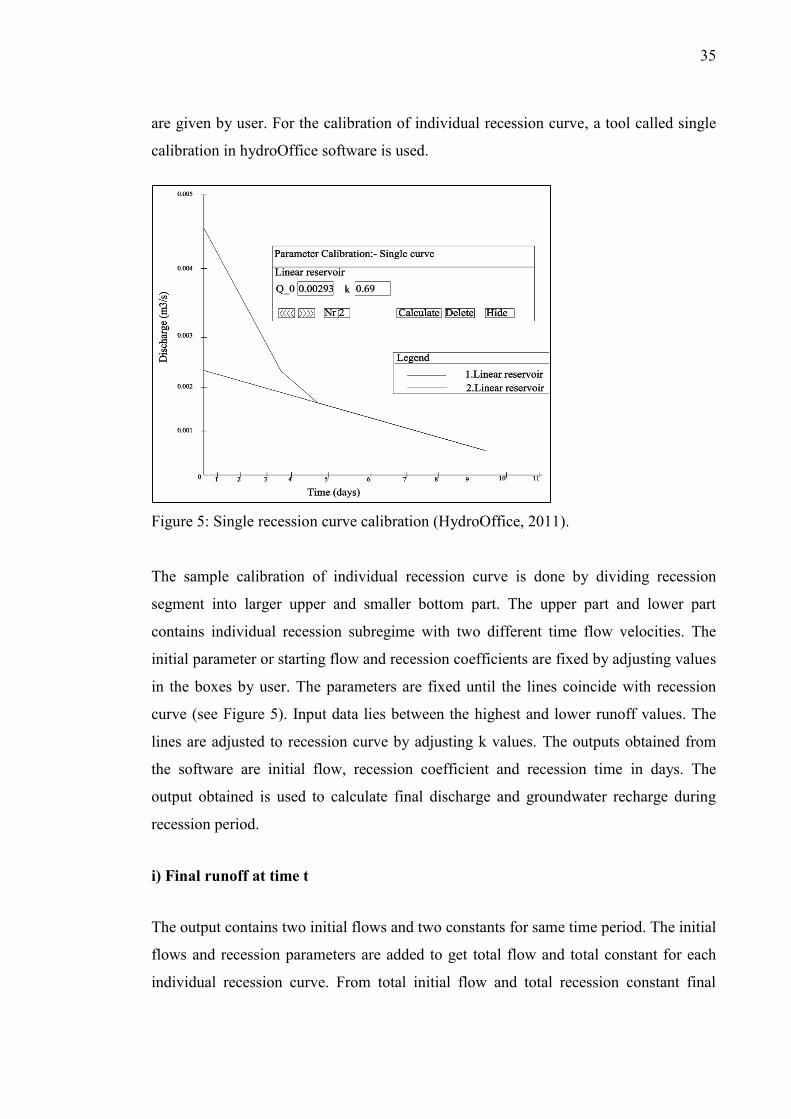
are given by user. For the calibration of individual recession curve, a tool called single

calibration in hydroOffice software is used.

Figure 5: Single recession curve calibration (HydroOffice, 2011).

The sample calibration of individual recession curve is done by dividing recession

segment into larger upper and smaller bottom part. The upper part and lower part

contains individual recession subregime with two different time flow velocities. The

initial parameter or starting flow and recession coefficients are fixed by adjusting values

in the boxes by user. The parameters are fixed until the lines coincide with recession

curve (see Figure 5). Input data lies between the highest and lower runoff values. The

lines are adjusted to recession curve by adjusting k values. The outputs obtained from

the software are initial flow, recession coefficient and recession time in days. The

output obtained is used to calculate final discharge and groundwater recharge during

recession period.

i) Final runoff at time t

The output contains two initial flows and two constants for same time period. The initial

flows and recession parameters are added to get total flow and total constant for each

individual recession curve. From total initial flow and total recession constant final

36

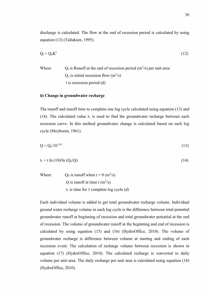
discharge is calculated. The flow at the end of recession period is calculated by using

equation (12) (Tallaksen, 1995).

Qt = QoKt (12)

Where Qt is Runoff at the end of recession period (m3/s) per unit area

Qo is initial recession flow (m3/s)

t is recession period (d)

ii) Change in groundwater recharge

The runoff and runoff time to complete one log cycle calculated using equation (13) and

(14). The calculated value t1 is used to find the groundwater recharge between each

recession curve. In this method groundwater change is calculated based on each log

cycle (Meyboom, 1961).

Q = Qo/10 t/t1 (13)

t1 = t ln (10)/ln (Qo/Q) (14)

Where Q0 is runoff when t = 0 (m3/s)

Q is runoff at time t (m3/s)

t1 is time for 1 complete log cycle (d)

Each individual volume is added to get total groundwater recharge volume. Individual

ground water recharge volume in each log cycle is the difference between total potential

groundwater runoff at beginning of recession and total groundwater potential at the end

of recession. The volume of groundwater runoff at the beginning and end of recession is

calculated by using equation (15) and (16) (HydroOffice, 2010). The volume of

groundwater recharge is difference between volume at starting and ending of each

recession event. The calculation of recharge volume between recession is shown in

equation (17) (HydroOffice, 2010). The calculated recharge is converted to daily

volume per unit area. The daily recharge per unit area is calculated using equation (18)

(HydroOffice, 2010).

37

Vtp = (Qo × t1)/2.3 (15)

Vr = (Qo × t1)/(2.3 × 10 t/t1) (16)

VR = Vtp – Vr (17)

Vd = VR/A (18)

Where Q0 is runoff when t = 0 (m3/s)

Vtp is total potential runoff at beginning (m3)

Vr is total potential runoff volume at end (m3)

t is total time of recession (d)

t1 is time for 1 complete log cycle (d)

VR is volume between recessions (m3)

A is Area of the catchment (m2)

Vd is storage volume between recession (m/day)

4.1.2 Master recession

In master recession curve analysis a single curve is obtained representing all Individual

recession curves. The analysis of master recession curve is carried out by separating

each recession segment from yearly hydrograph. The adapted matching strip method is

used for construction of master recession curve. In this method each recession segments

are adjusted horizontally until they overlap to form a group of shared lines. A visual

basic spreadsheet macro is used for master recession analysis. It consists of different

regression models. In this thesis exponential regression models are used to obtain final

master recession curve from all Individual recession segment (Posavec et al., 2006).

In the VBA excel sheet, each individual recession curve is fitted to an exponential

regression model to draw master recession curve. The time series runoff data is an

initial to the automated VBA macro. The automated VBA macro is used to separate

individual recession and time of recession from hydrograph. The separation of

individual recession is carried out using separation criteria set by flow duration curve.

38

The flow duration curve shows the percentage of time that a given flow rate is equaled

or exceeded. The separation criterion of (10 % - 70 %) is selected for each year. The

high runoff data values are selected as initial runoff exceeding the corresponding runoff

values from (10 % - 70 %) in an individual recession curve (Posavec et al., 2006).

The process includes the selection of variable length of recession period from runoff

data. The separated time is then ranked in descending order from which initial value of

recession is obtained. Then the highest flow values are selected along with declining

values. It is then plotted in semi-logarithmic scale in decreasing order which gives the

equation with two variables x and y. In the semi-logarithmic plot, x represents time of

flow and y represents flow rates. The second highest number gives the second

recession. The curve obtained with second highest value is adjusted to the last point

value of first recession curve. The adjustment is carried out with segment translation. In

segment translation, the time of second recession is shifted to required place along axes

till it fit to the end of first recession. The process continues till the last recession curve is

combined (Posavec et al., 2006).

Finally, a regression line is drawn with the best fitted model criteria. The regression line

obtained is called master recession curve. The criteria are based on trend line R2

describing the data which varies from 0-1. The values approaching to 1 are the best

fitted models. The data obtained from VBA macro excel sheet are runoff values for

each individual recession, time of recession and equation for regression line. From the

exponential regression equation recession constant is calculated (Posavec et al., 2006).

From the recession constant, runoff during each recession and time of recession

groundwater recharge is calculated. The calculated processes are similar to individual

recession analysis.

4.1.3 Wavelet transformation

Wavelet analysis is carried out to find centered frequency from time series runoff data.

Hydrograph interflow is relatively faster than baseflow. The runoff is changed to

frequency signal. The time of baseflow is longer. As a consequence, signal frequency is

reduced. The central frequency is frequency at which there is change in signal behavior.

The wavelength transformation of catchments is done using Matlab. The time series

runoff data is converted to frequency signals. To obtain frequency signals from time

39

series data Fast Fourier Transformation (FFT) is used. By using FFT the time domain

data is decomposed to frequency signals. From the frequency signals center frequency

is obtained. To find center frequency a band pass filter criteria called Nyquist rate is

used. The Nyquist frequency and Nyquist rate are two different terms. Nyquist

frequency is twice the highest frequency in the signal whereas Nyquist rate is used to

obtain symmetric signal. The Nyquist rate is obtained from amplitude modulation which

converts signals to symmetric signal within maximum amplitude. In this maximum

amplitude is taken as 1. From the symmetric frequency signal center frequency is

obtained. The centered frequency obtained from wavelet analysis is used to find the

recession parameters for the catchment. The equation (19) is used to calculate recession

parameter k using the centered frequency (Sujono et al., 2004).

k = e-fc (19)

Where k is recession parameter

fc is centered frequency from wavelet analysis

The wavelet transformation in this study is only used to compute recession parameter.

The process is relatively new and requires further study to relate with groundwater

processes. The calculation further requires initial flow and recession period. The

calculation of these flow characteristics requires further studies on reconstruction of

original signal. The original signals can be obtained from Short Time Fourier Frequency

(STFT) transformation but phase angle cannot be regenerated. Due to change in phase

angle random data is obtained and data obtained is not equal to original data. The Fast

Fourier Transformation (FFT) of signal results in randomization of phase. By doing

Inverse Fast Fourier Transformation (IFFT) original signal can be regenerated but at

random phase. By using this method the frequency at which baseflow occurs is only

obtained. It is unable to determine the original runoff and time at which baseflow starts.

4.1.4 Recession constant and recharge from baseflow separation

Baseflow is separated from total flow using smoothed minima technique. Baseflow

program is used for baseflow separation. Baseflow program is VBA excel which is used

to separate surface and base flow (Morawietz, 2007). For separation of base flow mean

daily flow is divided into non-overlapping blocks of 5 days. The minima value is

40

calculated for each block. The minima value is called central value. The separation

criteria for each bock is as 0.9 × central value <original value. The central value gives

ordinate for baseflow line. The process is continued to obtain baseflow ordinates from

all values. Base flow index is obtained as the ratio of volume of water lying under base

flow line to the volume of water below mean daily flow line (Institute of Hydrology,

1980).

The baseflow index obtained is used to calculate groundwater recharge volume and

recession constant. The equation (20) is used for calculate groundwater recharge

volume from baseflow index. Similarly, equation (21) is used to calculate recession

constant (Szilagyi et al., 2003).

BFI = Qb/Q = R (20)

BFI = (6k (1-k))/3k (21)

Where BFI is Base Flow Index

R is baseflow volume (m3)

Qb is baseflow (m3/s)

Q is total flow (m3/s)

k is recession constant

4.1.5 Recession constant and storage from specific yield

The specific yield is related to groundwater table. The specific yield and change in

groundwater level is used to calculate recession constant and groundwater recharge. The

time series graph of groundwater level data is similar to runoff hydrograph. From the

groundwater level data, the depletion curves are selected. The change in groundwater

level during each depletion curve is used to calculate recession constants. The recession

slope is calculated as the ratio of product of specific yield and time to the change in

groundwater level as shown in equation (22). From recession slope recession constant is

calculated using equation (23) (Raghavendran, 2013).

Sy = (α × t)/∆h (22)

41

k = e-α (23)

Where k is recession parameter

Sy is Specific yield

t is time (days)

Δh is change in groundwater level

α is recession slope

For yearly groundwater recharge, the average groundwater level change in each

depletion curve and average specific yield is used. The recharge calculation is based on

the assumption that percolated water immediately goes to storage. This method is

applicable for short recession periods (Crosbie et al., 2005). Equation (24) is used to

calculate the change groundwater volume (Raghavendran, 2013).

Gr = havg × Sy (24)

Where Gr is groundwater recharge (m/d)

havg is average water level (m)

4.2 Unsaturated moisture balance components

The water balance model is used for each year. The calculations are carried out with

daily data. The water balance model gives yearly groundwater recharge. The outputs

obtained from unsaturated moisture balance are rainfall, infiltration, contribution from

upslope, total evaporation, recharge and saturated runoff. The groundwater recharge

volume obtained as moisture balance output is used to compare the groundwater

recharge obtained from different methods used.

The outputs from unsaturated balance moisture model are computed using a software

toolkit called class U3M-1D. This program uses Richard’s equation for water balance

calculation. The equation is applicable for any soil, weather conditions or vegetation

type. The software toolkit contains three alternatives for soil hydraulic modeling: Van

Genuchten soil hydraulic model, Vogel and Cislerova soil hydraulic model and Brooks

and Corey soil hydraulic model. Brooks and Corey soil hydraulic model is chosen in

42

this study. Brooks and Corey soil hydraulic model is chosen due to easier mathematical

manipulation and flexibility of program allowing user input hydraulic parameters. In

input, the hydraulic parameters are adjusted to mixed soil and available data are used

such as hydraulic conductivity and porosity.

The software calculates transfer of soil moisture in various layers of the soil in all

directions. The unsaturated moisture movement model separates the upward soil

moisture and downward soil moisture. The soil moisture in upward direction is

evaporation and surface runoff. The soil moisture in downward direction is divided in

moisture from top and moisture from bottom of each soil layers. The moisture from top

is infiltrated runoff. The soil moisture from bottom is recharge to groundwater storage.

The recharge volume obtained from unsaturated moisture balance is compared to

recharge volume obtained recession analysis methods and specific yield approach.

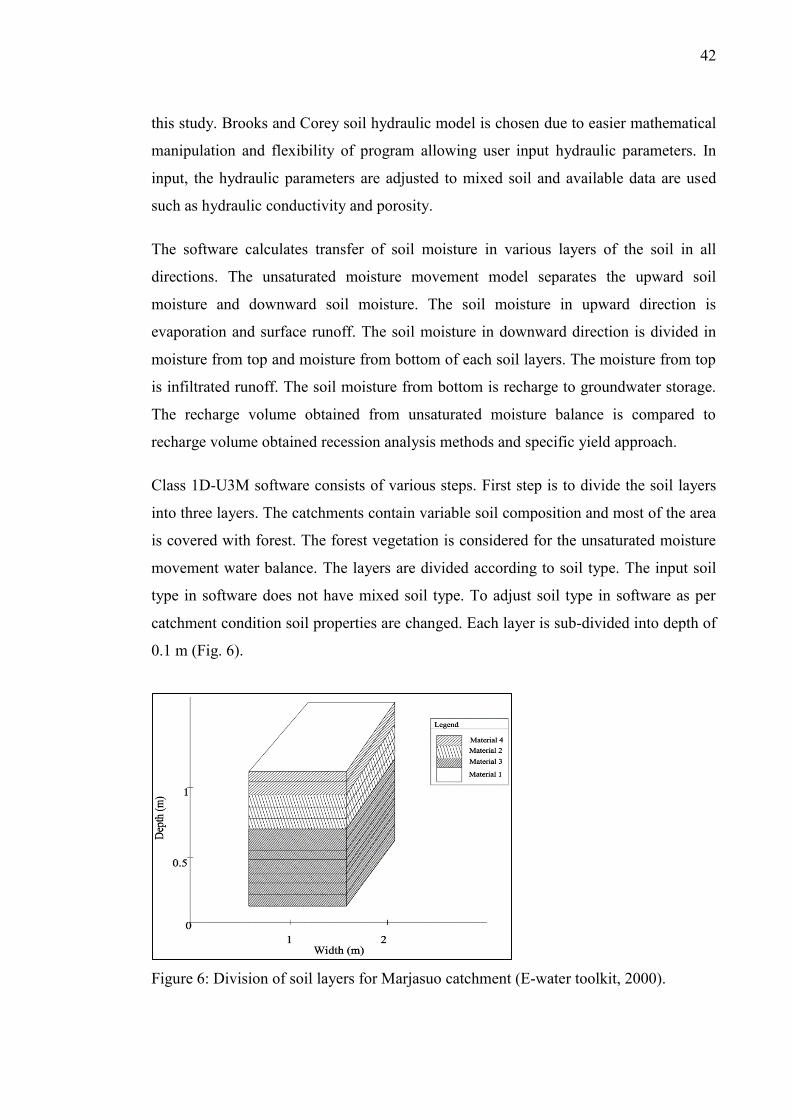
Class 1D-U3M software consists of various steps. First step is to divide the soil layers

into three layers. The catchments contain variable soil composition and most of the area

is covered with forest. The forest vegetation is considered for the unsaturated moisture

movement water balance. The layers are divided according to soil type. The input soil

type in software does not have mixed soil type. To adjust soil type in software as per

catchment condition soil properties are changed. Each layer is sub-divided into depth of

0.1 m (Fig. 6).

Figure 6: Division of soil layers for Marjasuo catchment (E-water toolkit, 2000).

43

The program calculates various components of evaporation by using input pan

evaporation. The evapotranspiration depends on surface vegetation. The constant

default values for tree vegetation 0.8, 0.85 and 1 is used for light extinction coefficient

(k_light), pan evapotranspiration constant (Kpan) and leaf area index (LAI), respectively.

By using different constants and pan evaporation, different evaporation components are

calculated. The equations (25), (26) and (27) are used to calculate different components

of evapotranspiration (Vaze et al., 2004). The steps and calculation involved are

discussed in the following sections.

Eto = PET × (1- exp(k_light × LAI)) (25)

Etg = PET × exp(- k_light × LAI) (26)

Etu = 0 (27)

Where PET is potential evapotranspiration

LAI is leaf area index

k_light is light extinction co-efficient

Eto is under storey transpiration

Etg is soil evaporation

Etu is over storey transpiration

4.2.1 Soil-water mass balance

The local water balance is performed for each layer of soil. For water balance three

boundaries conditions are considered. The upper, lower and upslope boundary are three

boundary conditions. The water balance is based on Richard’s equation. The equation is

derived from equation for vertical Darcy’s flux. Equation (28) shows the vertical flow

and water content in each soil layer (Tuteja et al., 2004).

∂θ(z,t)/∂t = - ∂qv(z,t)/∂z + S(z,t) (28)

Where θ is volumetric water content

qv is Darcy’s vertical flux (m/s)

44

S is sum of water source and sinks

The vertical flux can be expressed in terms of hydraulic diffusivity and vertical

hydraulic conductivity. The equation (29) is used to calculate the vertical flux (Tuteja et

al., 2004). The unsaturated soil moisture flow in unsaturated zone contains various

sources and sinks. The equation for flow in unsaturated zone depends on moisture loss

by transpiration, evaporation and moisture gain from horizontal slopes. The equation

(30) shows flow in unsaturated zone (Tuteja et al., 2004). For water balance model three

boundary conditions are considered. The boundary conditions are explained as follows.

qv = - (D(θ)∂θ/∂z) - Kv(θ) (29)

Es,a(t) = ∫ Sz

z-Hs(t) Es(z,t)dz = Es,a(t) ∫

as(z)

∫ as(z)z

z-Hs(t)

z

z-Hs(t)dz (30)

Where D(ϴ) is hydraulic diffusivity (m2/s)

Kv(ϴ) is hydraulic conductivity

Es,a(t) is actual soil evaporation (m/s) at time t

SEs(z,t) is actual soil evaporation per unit control volume at depth z at

time t

Hs(t) is depth through which soil evaporation occur (m)

as(z) is proportion of the soil evaporation at depth z relative to the total

soil evaporation (dimensionless)

i) Upper boundary

The upper boundary condition is time dependent specific flux boundary used at the soil

surface. The upper boundary flux contains flux infiltrated to soil and flux which cannot

infiltrate from upper soil. The flux which do not infiltrate is surface runoff. Total flux

infiltrated in upper boundary is given by equation (31) and the overland flow is given

equation (32) (Tuteja et al., 2004).

qtop

v = - min(Icap(t),p(t) + qo,in(t)) (31)

qo,out (t) = - max(0,p(t) + qo,in(t) - Icap(t) ) (32)

45

Where qtop

v is total upper boundary flux (m/s)

qo,in(t) is total incoming overland flow at time t (m/s)

qo,in(t) is total outgoing overland flow at time t (m/s)

Icap is infiltration capacity at soil surface (m/s)

P(t) is precipitation through fall at the soil surface after accounting

canopy interception at time

ii) Lower boundary

The lower boundary is used to separate the infiltrated runoff and recharge area of the

catchment. It includes total infiltrated soil moisture from upper boundary. The

infiltrated soil moisture is divided into soil moisture from top of soil layer and bottom

of soil layer. The soil moisture from top results in infiltrated runoff. The soil moisture

from bottom results in groundwater recharge. The amount of recharge depends on the

minimum flux under unit gradient from bottom layer of soil and hydraulic conductivity

of soil layer. The equation for the lower boundary with infiltrated runoff is given by

equation (33) and free drainage condition is given by equation (34) (Tuteja et al., 2004).

qbot

v(t) = - min(Kv(θ1(t), Ksub) + Q

bot

v(t) (33)

qbot

v(t) = - min(Kv(θ1(t), Ksub) (34)

where qbot

v(t) is flux from lower boundary

Kv(θ1(t)) is unsaturated hydraulic conductivity of bottom layer along

vertical axes (m/s)

Ksub is saturated hydraulic conductivity of sub-surface underneath the

soil profile (m/s)

Winm is volume of water received as horizontal subsurface flow from soil

material m

(-ve signs on equations indicate flux is opposite to z-axis whereas

flux runoff is along the z-axis.)

46

iii) Upslope boundary

The upslope boundary defines horizontal transfer of moisture from upslope soil layer to

downslope soil layer. The volume of moisture remained at the end of each time step i.e.

receiving water from upslope and contribution to lower layer is calculated using

equation (35) (Tuteja et al., 2004).

Win m (t) = Q

hor

m(t)/Md (m) - Md (m-1) (35)

Where Md is elevation of upslope soil material m

m is number of soil material at downslope

Win m is volume of water received as horizontal subsurface flow from soil

material m.

Qhor

m(t) is volume of water as subsurface flow from soil material m.

4.2.2 Class U3M-1D output

The soil moisture flow is based on various soil layers and soil material in each soil

layer. The unsaturated moisture movement is computed in each time step. The vertical

moisture movement and horizontal moisture movement is calculated by numerical

simulation in each time step as (t’+Ϩt). The vertical simulation is carried for short time

step t’. After vertical simulation horizontal simulation is carried out for Ϩt. Soil

moisture, hydraulic conductivity and diffusivity is expressed as geometric mean of all

corresponding layers. In each time, step soil from uppermost soil layer to deepest soil

layer is calculated. The total moisture is received as a rainfall which represents the total

volume as inflow. The total inflow to unit soil area is calculated using equation (36).

The total moisture received by unit area contributes to overland flow and infiltration of

soil moisture. The flux across top resulting overland flow is calculated using equation

(37). The total soil moisture infiltrated is calculated using equation (38) (Tuteja et al.,

2004).

Wmp

in(t + j∂t') = W mp

in/J (36)

47

Qmp

top(t + ∂t) = ∑ q

top

v(t + j∂t')

j

j=1 ∂t' (37)

qtop

v(t + j∂t') = q

top

v(t + ∂t) = - min (Icap(t), p(t) + qo,in(t)) (38)

Where Win mp(t + j∂t') is total water volume received as inflow

qtop

v(t + j∂t') is moisture from soil infiltration (m/s)

Qtop

v(t + j∂t') is flux across top of soil material m

J is number of time steps in vertical mass balance for single horizontal

redistribution time

The infiltrated soil moisture further contributes in infiltrated runoff and groundwater

recharge. The flux at bottom of soil layers contributing infiltrated runoff is calculated

using equation (39). The total soil moisture contributing recharge to groundwater

storage is calculated using equation (40) (Tuteja et al., 2004).

Qmp

bot(t + ∂t) = ∑ q

top

v(t + j∂t')

j

j=1 ∂t' (39)

qbot

v(t + j∂t') = q

bot

v(t + ∂t') = - min (Kv(θ1(t), Ksub) (40)

Where Q mpbot

(t + ∂t) is flux across bottom soil material m

q mpbot

(t + ∂t') is moisture from soil infiltration (m/s)

The remaining vertical soil moisture is considered for total evapotranspiration. Moisture

accumulated in soil surface and saturated soil is remaining vertical soil moisture. The

remaining soil moisture for each time step can be calculated using equation (41) (Tuteja

et al., 2004).

Wavail i (t + jδt') = max(0, θi(t + jδt') − θi

r) (41)

Where Wavail i is soil moisture after drainage

θi is volumetric water content

θir is residual soil moisture content

48

Penman Monteith equation is used to calculate total evapotranspiration from each soil

layers. The actual evapotranspiration is calculated as minimum of total

evapotranspiration and total moisture available. Equation (42) show formula for

calculating total evapotranspiration demand (Tuteja et al., 2004).

WET i (t + j∂t') = wto

i (t + j∂t') + wtui (t + j∂t') + ws

i (t + j∂t') (42)

Where WET

i is total evaporation demand

wto

i is total plant transpiration

wtu

i is total soil evapotranspiration

WET

i (t + j∂t') is total soil moisture available

The outputs obtained from the software are total evaporation (E), saturated runoff

(Wdelta), infiltration runoff (Qtop) and infiltration recharge (Qbot). The soil moisture

fluxes are separated in upward and downward direction. Total evaporation (E) and

saturated runoff (Wdelta) represents upward flow. The total evaporation and saturated

runoff lies above arbitrary plane called zero flux plane. The infiltration runoff (Qtop) and

infiltration recharge (Qbot) represents downward flow. The infiltration runoff and

infiltration recharge lies below zero flux plane.

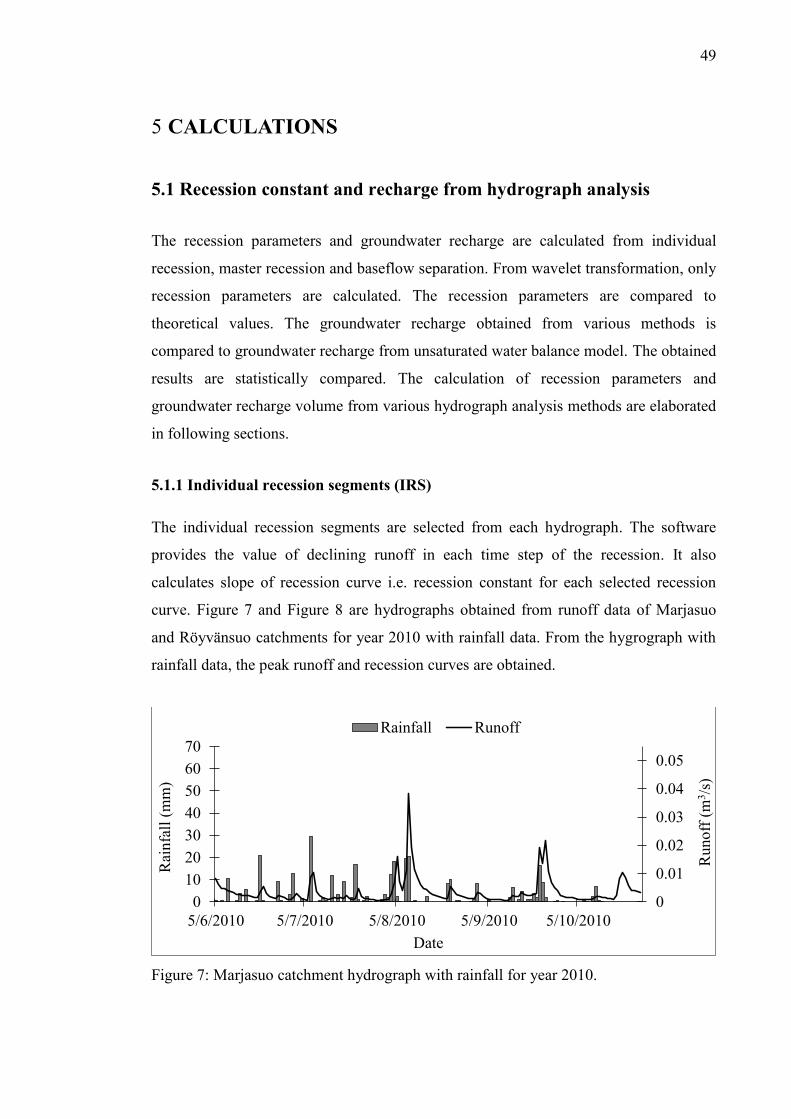
49

5 CALCULATIONS

5.1 Recession constant and recharge from hydrograph analysis

The recession parameters and groundwater recharge are calculated from individual

recession, master recession and baseflow separation. From wavelet transformation, only

recession parameters are calculated. The recession parameters are compared to

theoretical values. The groundwater recharge obtained from various methods is

compared to groundwater recharge from unsaturated water balance model. The obtained

results are statistically compared. The calculation of recession parameters and

groundwater recharge volume from various hydrograph analysis methods are elaborated

in following sections.

5.1.1 Individual recession segments (IRS)

The individual recession segments are selected from each hydrograph. The software

provides the value of declining runoff in each time step of the recession. It also

calculates slope of recession curve i.e. recession constant for each selected recession

curve. Figure 7 and Figure 8 are hydrographs obtained from runoff data of Marjasuo

and Röyvänsuo catchments for year 2010 with rainfall data. From the hygrograph with

rainfall data, the peak runoff and recession curves are obtained.

Figure 7: Marjasuo catchment hydrograph with rainfall for year 2010.

0

0.01

0.02

0.03

0.04

0.05

0

10

20

30

40

50

60

70

5/6/2010 5/7/2010 5/8/2010 5/9/2010 5/10/2010

Runoff

(m

3/s

)

Rai

nfa

ll (

mm

)

Date

Rainfall Runoff

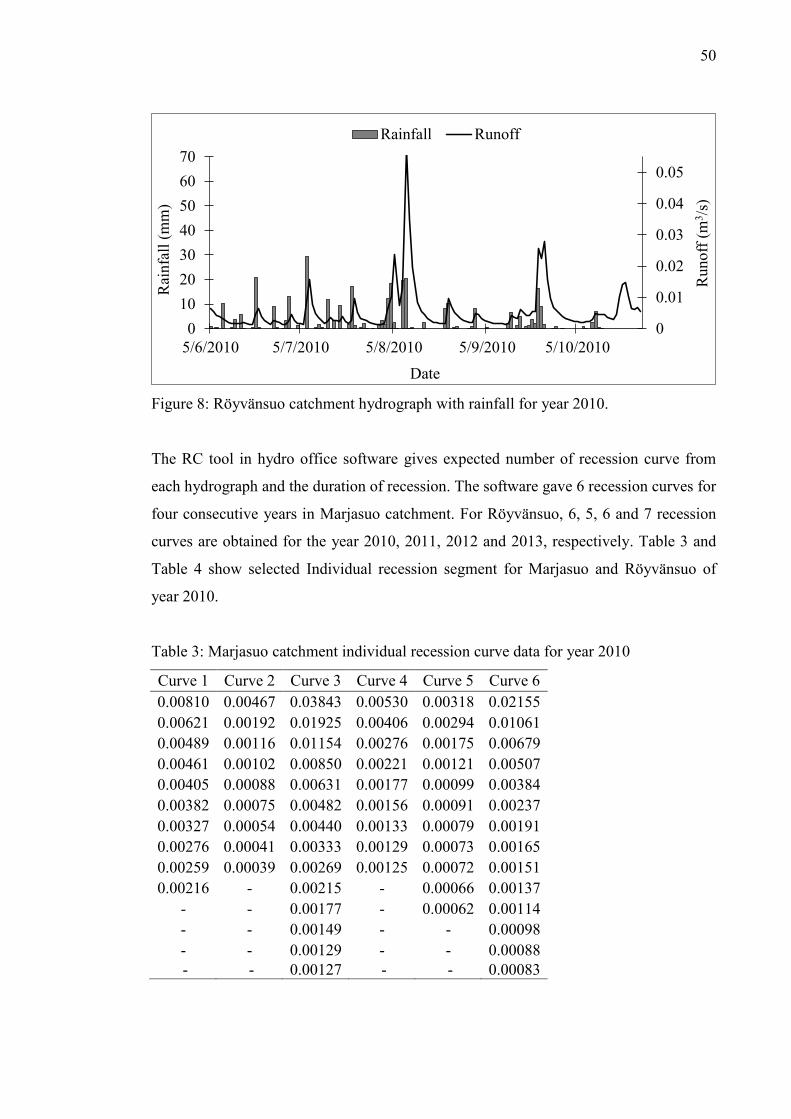
50

Figure 8: Röyvänsuo catchment hydrograph with rainfall for year 2010.

The RC tool in hydro office software gives expected number of recession curve from

each hydrograph and the duration of recession. The software gave 6 recession curves for

four consecutive years in Marjasuo catchment. For Röyvänsuo, 6, 5, 6 and 7 recession

curves are obtained for the year 2010, 2011, 2012 and 2013, respectively. Table 3 and

Table 4 show selected Individual recession segment for Marjasuo and Röyvänsuo of

year 2010.

Table 3: Marjasuo catchment individual recession curve data for year 2010

Curve 1 Curve 2 Curve 3 Curve 4 Curve 5 Curve 6

0.00810 0.00467 0.03843 0.00530 0.00318 0.02155

0.00621 0.00192 0.01925 0.00406 0.00294 0.01061

0.00489 0.00116 0.01154 0.00276 0.00175 0.00679

0.00461 0.00102 0.00850 0.00221 0.00121 0.00507

0.00405 0.00088 0.00631 0.00177 0.00099 0.00384

0.00382 0.00075 0.00482 0.00156 0.00091 0.00237

0.00327 0.00054 0.00440 0.00133 0.00079 0.00191

0.00276 0.00041 0.00333 0.00129 0.00073 0.00165

0.00259 0.00039 0.00269 0.00125 0.00072 0.00151

0.00216 - 0.00215 - 0.00066 0.00137

- - 0.00177 - 0.00062 0.00114

- - 0.00149 - - 0.00098

- - 0.00129 - - 0.00088

- - 0.00127 - - 0.00083

0

0.01

0.02

0.03

0.04

0.05

0

10

20

30

40

50

60

70

5/6/2010 5/7/2010 5/8/2010 5/9/2010 5/10/2010

Runoff

(m

3/s

)

Rai

nfa

ll (

mm

)

Date

Rainfall Runoff

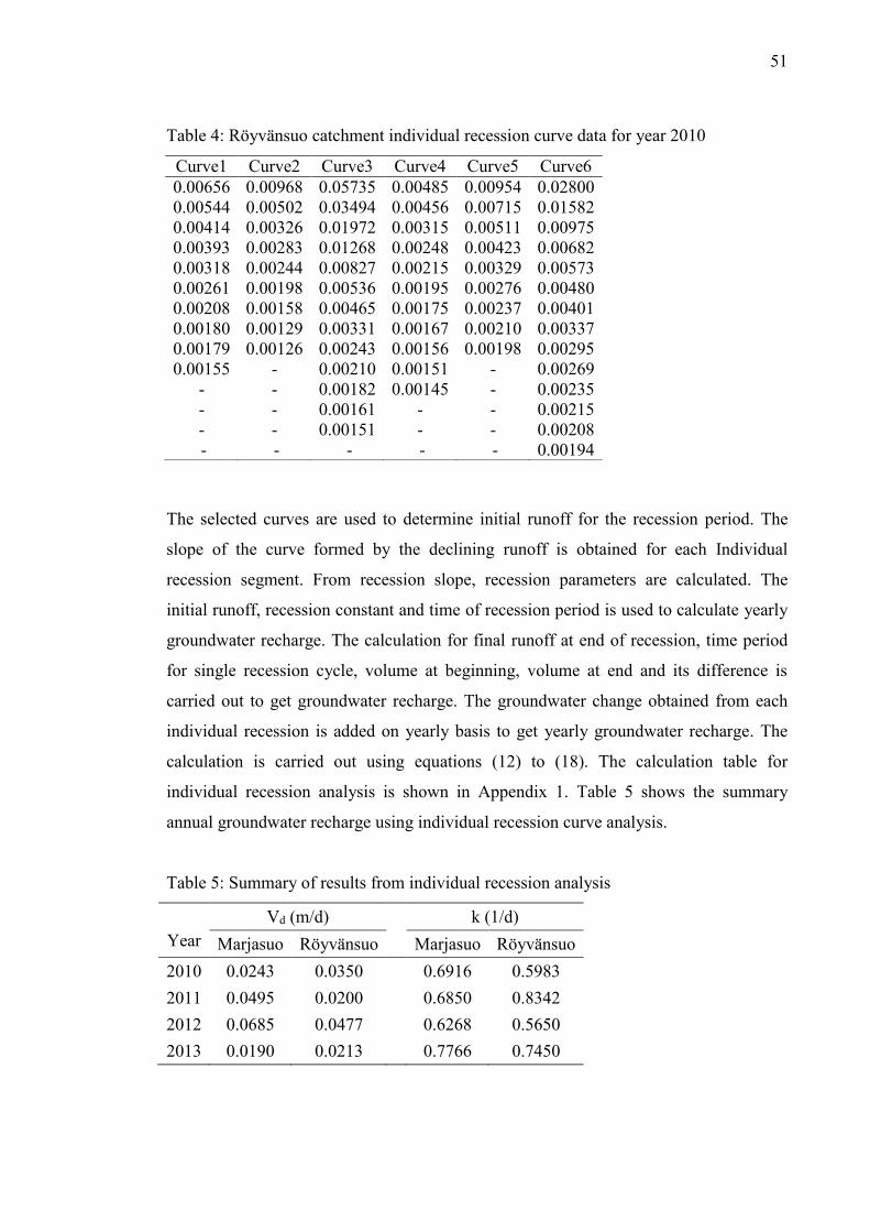
51

Table 4: Röyvänsuo catchment individual recession curve data for year 2010

Curve1 Curve2 Curve3 Curve4 Curve5 Curve6

0.00656 0.00968 0.05735 0.00485 0.00954 0.02800

0.00544 0.00502 0.03494 0.00456 0.00715 0.01582

0.00414 0.00326 0.01972 0.00315 0.00511 0.00975

0.00393 0.00283 0.01268 0.00248 0.00423 0.00682

0.00318 0.00244 0.00827 0.00215 0.00329 0.00573

0.00261 0.00198 0.00536 0.00195 0.00276 0.00480

0.00208 0.00158 0.00465 0.00175 0.00237 0.00401

0.00180 0.00129 0.00331 0.00167 0.00210 0.00337

0.00179 0.00126 0.00243 0.00156 0.00198 0.00295

0.00155 - 0.00210 0.00151 - 0.00269

- - 0.00182 0.00145 - 0.00235

- - 0.00161 - - 0.00215

- - 0.00151 - - 0.00208

- - - - - 0.00194

The selected curves are used to determine initial runoff for the recession period. The

slope of the curve formed by the declining runoff is obtained for each Individual

recession segment. From recession slope, recession parameters are calculated. The

initial runoff, recession constant and time of recession period is used to calculate yearly

groundwater recharge. The calculation for final runoff at end of recession, time period

for single recession cycle, volume at beginning, volume at end and its difference is

carried out to get groundwater recharge. The groundwater change obtained from each

individual recession is added on yearly basis to get yearly groundwater recharge. The

calculation is carried out using equations (12) to (18). The calculation table for

individual recession analysis is shown in Appendix 1. Table 5 shows the summary

annual groundwater recharge using individual recession curve analysis.

Table 5: Summary of results from individual recession analysis

Year

Vd (m/d) k (1/d)

Marjasuo Röyvänsuo Marjasuo Röyvänsuo

2010 0.0243 0.0350 0.6916 0.5983

2011 0.0495 0.0200

0.6850 0.8342

2012 0.0685 0.0477

0.6268 0.5650

2013 0.0190 0.0213 0.7766 0.7450

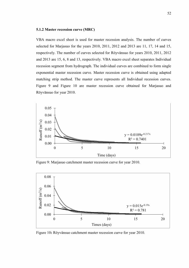
52

5.1.2 Master recession curve (MRC)

VBA macro excel sheet is used for master recession analysis. The number of curves

selected for Marjasuo for the years 2010, 2011, 2012 and 2013 are 11, 17, 14 and 15,

respectively. The number of curves selected for Röyvänsuo for years 2010, 2011, 2012

and 2013 are 15, 6, 8 and 13, respectively. VBA macro excel sheet separates Individual

recession segment from hydrograph. The individual curves are combined to form single

exponential master recession curve. Master recession curve is obtained using adapted

matching strip method. The master curve represents all Individual recession curves.

Figure 9 and Figure 10 are master recession curve obtained for Marjasuo and

Röyvänsuo for year 2010.

Figure 9: Marjasuo catchment master recession curve for year 2010.

Figure 10: Röyvänsuo catchment master recession curve for year 2010.

y = 0.0109e-0.217x

R² = 0.74010.00

0.01

0.02

0.03

0.04

0.05

0 5 10 15 20

Runoff

(m

3/s

)

Time (days)

y = 0.015e-0.19x

R² = 0.7810.00

0.02

0.04

0.06

0.08

0 5 10 15 20

Runoff

(m

3/s

)

Times (days)

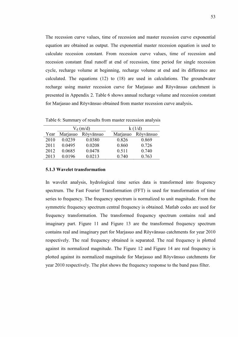
53

The recession curve values, time of recession and master recession curve exponential

equation are obtained as output. The exponential master recession equation is used to

calculate recession constant. From recession curve values, time of recession and

recession constant final runoff at end of recession, time period for single recession

cycle, recharge volume at beginning, recharge volume at end and its difference are

calculated. The equations (12) to (18) are used in calculations. The groundwater

recharge using master recession curve for Marjasuo and Röyvänsuo catchment is

presented in Appendix 2. Table 6 shows annual recharge volume and recession constant

for Marjasuo and Röyvänsuo obtained from master recession curve analysis.

Table 6: Summary of results from master recession analysis

Year

Vd (m/d) k (1/d)

Marjasuo Röyvänsuo Marjasuo Röyvänsuo

2010 0.0239 0.0380 0.826 0.869

2011 0.0495 0.0208

0.860 0.726

2012 0.0685 0.0478

0.511 0.740

2013 0.0196 0.0213 0.740 0.763

5.1.3 Wavelet transformation

In wavelet analysis, hydrological time series data is transformed into frequency

spectrum. The Fast Fourier Transformation (FFT) is used for transformation of time

series to frequency. The frequency spectrum is normalized to unit magnitude. From the

symmetric frequency spectrum central frequency is obtained. Matlab codes are used for

frequency transformation. The transformed frequency spectrum contains real and

imaginary part. Figure 11 and Figure 13 are the transformed frequency spectrum

contains real and imaginary part for Marjasuo and Röyvänsuo catchments for year 2010

respectively. The real frequency obtained is separated. The real frequency is plotted

against its normalized magnitude. The Figure 12 and Figure 14 are real frequency is

plotted against its normalized magnitude for Marjasuo and Röyvänsuo catchments for

year 2010 respectively. The plot shows the frequency response to the band pass filter.

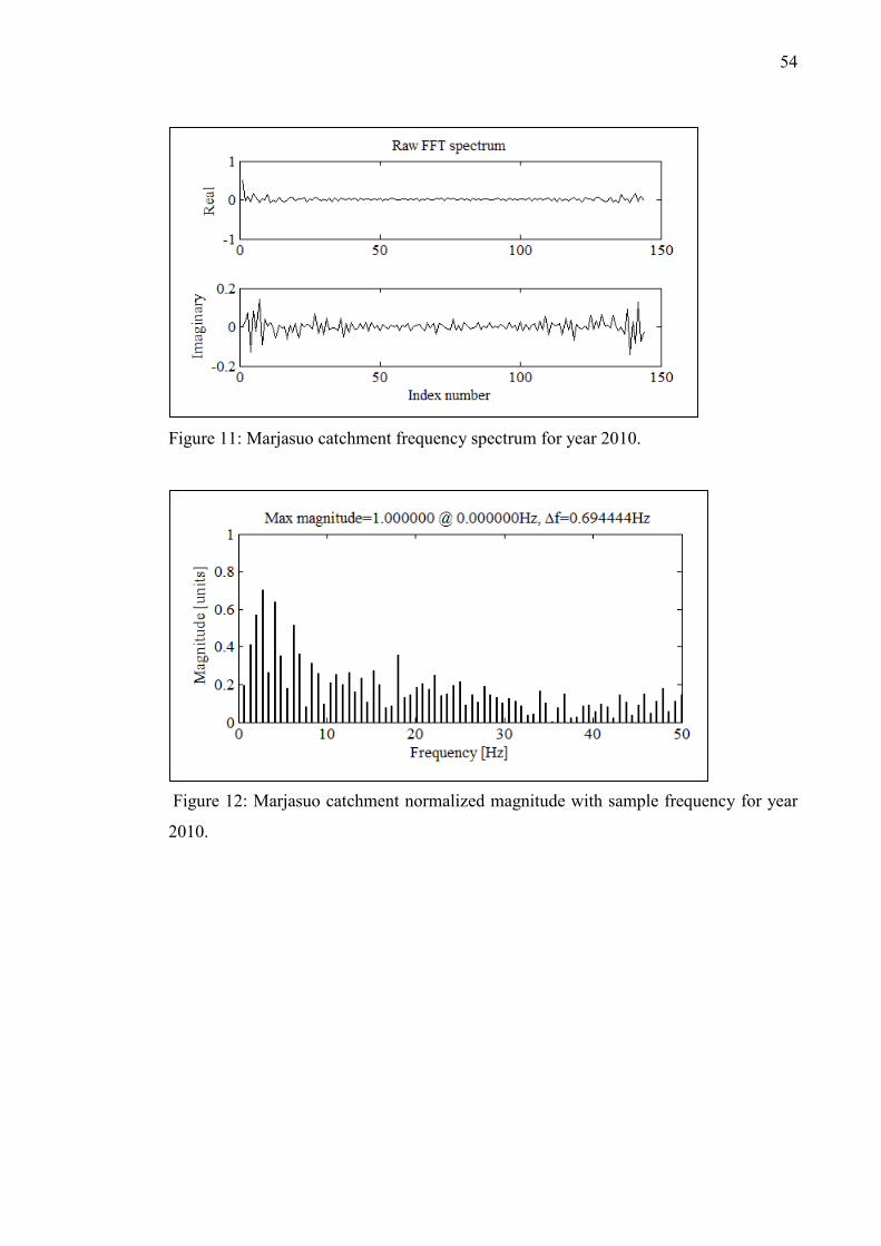
54

Figure 11: Marjasuo catchment frequency spectrum for year 2010.

Figure 12: Marjasuo catchment normalized magnitude with sample frequency for year

2010.

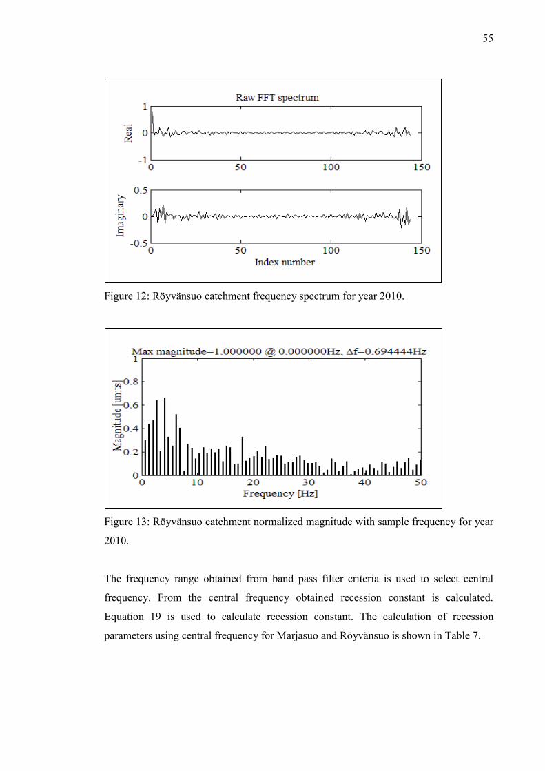
55

Figure 12: Röyvänsuo catchment frequency spectrum for year 2010.

Figure 13: Röyvänsuo catchment normalized magnitude with sample frequency for year

2010.

The frequency range obtained from band pass filter criteria is used to select central

frequency. From the central frequency obtained recession constant is calculated.

Equation 19 is used to calculate recession constant. The calculation of recession

parameters using central frequency for Marjasuo and Röyvänsuo is shown in Table 7.

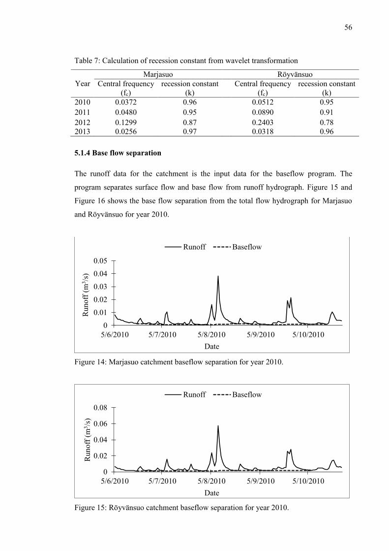
56

Table 7: Calculation of recession constant from wavelet transformation

Year

Marjasuo Röyvänsuo

Central frequency

(fc)

recession constant

(k)

Central frequency

(fc)

recession constant

(k)

2010 0.0372 0.96

0.0512 0.95

2011 0.0480 0.95

0.0890 0.91

2012 0.1299 0.87

0.2403 0.78

2013 0.0256 0.97 0.0318 0.96

5.1.4 Base flow separation

The runoff data for the catchment is the input data for the baseflow program. The

program separates surface flow and base flow from runoff hydrograph. Figure 15 and

Figure 16 shows the base flow separation from the total flow hydrograph for Marjasuo

and Röyvänsuo for year 2010.

Figure 14: Marjasuo catchment baseflow separation for year 2010.

Figure 15: Röyvänsuo catchment baseflow separation for year 2010.

0

0.01

0.02

0.03

0.04

0.05

5/6/2010 5/7/2010 5/8/2010 5/9/2010 5/10/2010

Runoff

(m

3/s

)

Date

Runoff Baseflow

0

0.02

0.04

0.06

0.08

5/6/2010 5/7/2010 5/8/2010 5/9/2010 5/10/2010

Run

off

(m

3/s

)

Date

Runoff Baseflow

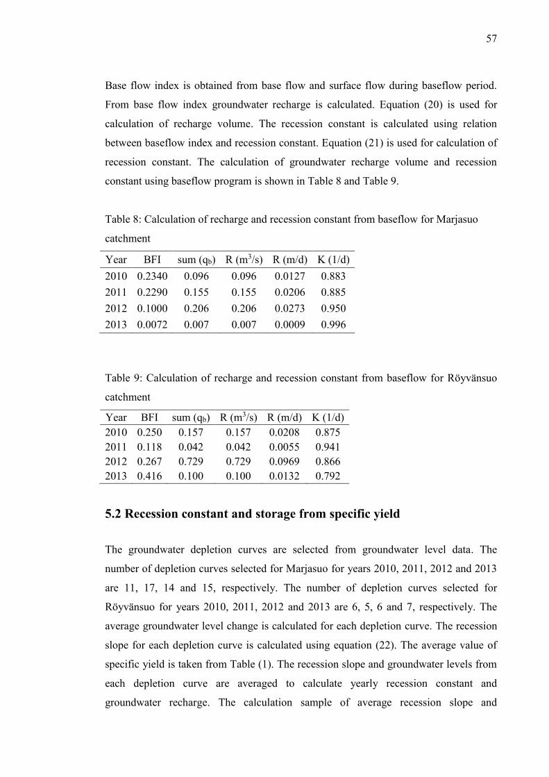
57

Base flow index is obtained from base flow and surface flow during baseflow period.

From base flow index groundwater recharge is calculated. Equation (20) is used for

calculation of recharge volume. The recession constant is calculated using relation

between baseflow index and recession constant. Equation (21) is used for calculation of

recession constant. The calculation of groundwater recharge volume and recession

constant using baseflow program is shown in Table 8 and Table 9.

Table 8: Calculation of recharge and recession constant from baseflow for Marjasuo

catchment

Year BFI sum (qb) R (m3/s) R (m/d) K (1/d)

2010 0.2340 0.096 0.096 0.0127 0.883

2011 0.2290 0.155 0.155 0.0206 0.885

2012 0.1000 0.206 0.206 0.0273 0.950

2013 0.0072 0.007 0.007 0.0009 0.996

Table 9: Calculation of recharge and recession constant from baseflow for Röyvänsuo

catchment

Year BFI sum (qb) R (m3/s) R (m/d) K (1/d)

2010 0.250 0.157 0.157 0.0208 0.875

2011 0.118 0.042 0.042 0.0055 0.941

2012 0.267 0.729 0.729 0.0969 0.866

2013 0.416 0.100 0.100 0.0132 0.792

5.2 Recession constant and storage from specific yield

The groundwater depletion curves are selected from groundwater level data. The

number of depletion curves selected for Marjasuo for years 2010, 2011, 2012 and 2013

are 11, 17, 14 and 15, respectively. The number of depletion curves selected for

Röyvänsuo for years 2010, 2011, 2012 and 2013 are 6, 5, 6 and 7, respectively. The

average groundwater level change is calculated for each depletion curve. The recession

slope for each depletion curve is calculated using equation (22). The average value of

specific yield is taken from Table (1). The recession slope and groundwater levels from

each depletion curve are averaged to calculate yearly recession constant and

groundwater recharge. The calculation sample of average recession slope and

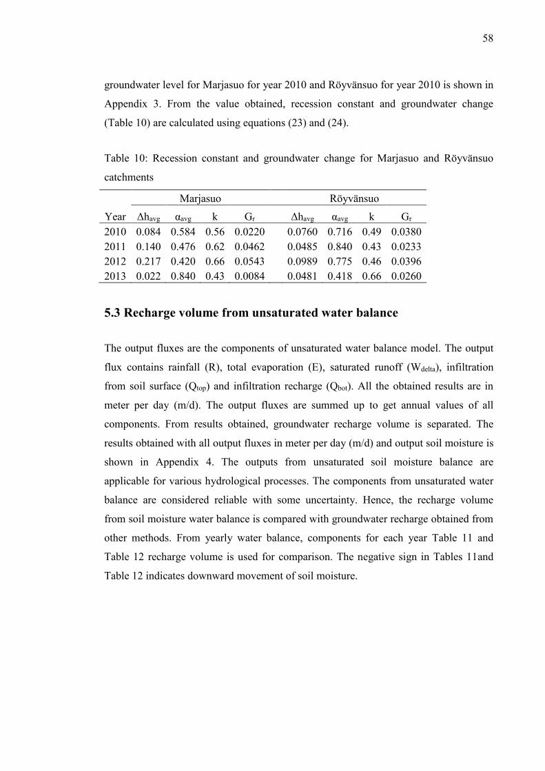
58

groundwater level for Marjasuo for year 2010 and Röyvänsuo for year 2010 is shown in

Appendix 3. From the value obtained, recession constant and groundwater change

(Table 10) are calculated using equations (23) and (24).

Table 10: Recession constant and groundwater change for Marjasuo and Röyvänsuo

catchments

Year

Marjasuo Röyvänsuo

Δhavg αavg k Gr Δhavg αavg k Gr

2010 0.084 0.584 0.56 0.0220

0.0760 0.716 0.49 0.0380

2011 0.140 0.476 0.62 0.0462

0.0485 0.840 0.43 0.0233

2012 0.217 0.420 0.66 0.0543

0.0989 0.775 0.46 0.0396

2013 0.022 0.840 0.43 0.0084 0.0481 0.418 0.66 0.0260

5.3 Recharge volume from unsaturated water balance

The output fluxes are the components of unsaturated water balance model. The output

flux contains rainfall (R), total evaporation (E), saturated runoff (Wdelta), infiltration

from soil surface (Qtop) and infiltration recharge (Qbot). All the obtained results are in

meter per day (m/d). The output fluxes are summed up to get annual values of all

components. From results obtained, groundwater recharge volume is separated. The

results obtained with all output fluxes in meter per day (m/d) and output soil moisture is

shown in Appendix 4. The outputs from unsaturated soil moisture balance are

applicable for various hydrological processes. The components from unsaturated water

balance are considered reliable with some uncertainty. Hence, the recharge volume

from soil moisture water balance is compared with groundwater recharge obtained from

other methods. From yearly water balance, components for each year Table 11 and

Table 12 recharge volume is used for comparison. The negative sign in Tables 11and

Table 12 indicates downward movement of soil moisture.

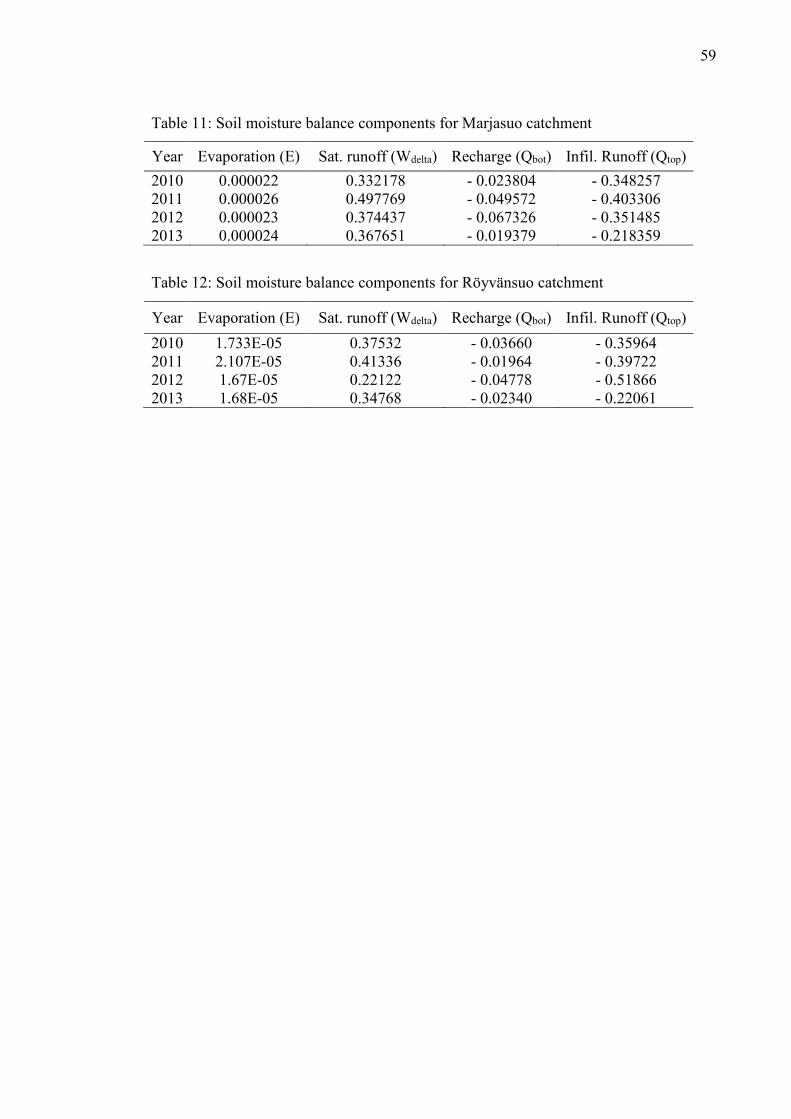
59

Table 11: Soil moisture balance components for Marjasuo catchment

Year Evaporation (E) Sat. runoff (Wdelta) Recharge (Qbot) Infil. Runoff (Qtop)

2010 0.000022 0.332178 - 0.023804 - 0.348257

2011 0.000026 0.497769 - 0.049572 - 0.403306

2012 0.000023 0.374437 - 0.067326 - 0.351485

2013 0.000024 0.367651 - 0.019379 - 0.218359

Table 12: Soil moisture balance components for Röyvänsuo catchment

Year Evaporation (E) Sat. runoff (Wdelta) Recharge (Qbot) Infil. Runoff (Qtop)

2010 1.733E-05 0.37532 - 0.03660 - 0.35964

2011 2.107E-05 0.41336 - 0.01964 - 0.39722

2012 1.67E-05 0.22122 - 0.04778 - 0.51866

2013 1.68E-05 0.34768 - 0.02340 - 0.22061

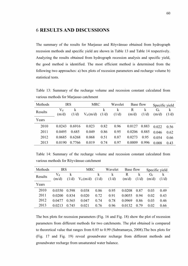
60

6 RESULTS AND DISCUSSIONS

The summary of the results for Marjasuo and Röyvänsuo obtained from hydrograph

recession methods and specific yield are shown in Table 13 and Table 14 respectively.

Analyzing the results obtained from hydrograph recession analysis and specific yield,

the good method is identified. The most efficient method is determined from the

following two approaches: a) box plots of recession parameters and recharge volume b)

statistical tests.

Table 13: Summary of the recharge volume and recession constant calculated from

various methods for Marjasuo catchment

Methods IRS MRC Wavelet Base flow Specific yield

Results Vd

(m/d)

k

(1/d) Vd (m/d)

k

(1/d)

k

(1/d)

R

(m/d)

k

(1/d)

Gr

(m/d)

k

(1/d)

Years

2010 0.0243 0.6916 0.023 0.82 0.96 0.0127 0.883 0.022 0.56

2011 0.0495 0.685 0.049 0.86 0.95 0.0206 0.885 0.046 0.62

2012 0.0685 0.6268 0.068 0.51 0.87 0.0273 0.95 0.054 0.66

2013 0.0190 0.7766 0.019 0.74 0.97 0.0009 0.996 0.008 0.43

Table 14: Summary of the recharge volume and recession constant calculated from

various methods for Röyvänsuo catchment

The box plots for recession parameters (Fig. 16 and Fig. 18) show the plot of recession

parameters from different methods for two catchments. The plot obtained is compared

to theoretical value that ranges from 0.85 to 0.99 (Subramanya, 2008).The box plots for

(Fig. 17 and Fig. 19) reveal groundwater recharge from different methods and

groundwater recharge from unsaturated water balance.

Methods IRS MRC Wavelet Base flow Specific yield

Results Vd

(m/d)

k

(1/d) Vd (m/d)

k

(1/d)

k

(1/d)

R

(m/d)

k

(1/d)

Gr

(m/d)

k

(1/d)

Years

2010 0.0350 0.598 0.038 0.86 0.95 0.0208 0.87 0.03 0.49

2011 0.0200 0.834 0.020 0.72 0.91 0.0055 0.94 0.02 0.43

2012 0.0477 0.565 0.047 0.74 0.78 0.0969 0.86 0.03 0.46

2013 0.0213 0.745 0.021 0.76 0.96 0.0132 0.79 0.02 0.66

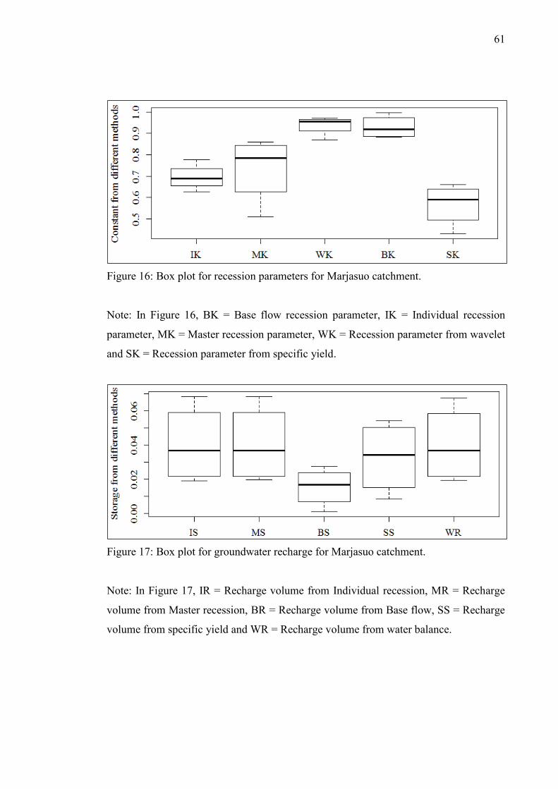
61

Figure 16: Box plot for recession parameters for Marjasuo catchment.

Note: In Figure 16, BK = Base flow recession parameter, IK = Individual recession

parameter, MK = Master recession parameter, WK = Recession parameter from wavelet

and SK = Recession parameter from specific yield.

Figure 17: Box plot for groundwater recharge for Marjasuo catchment.

Note: In Figure 17, IR = Recharge volume from Individual recession, MR = Recharge

volume from Master recession, BR = Recharge volume from Base flow, SS = Recharge

volume from specific yield and WR = Recharge volume from water balance.

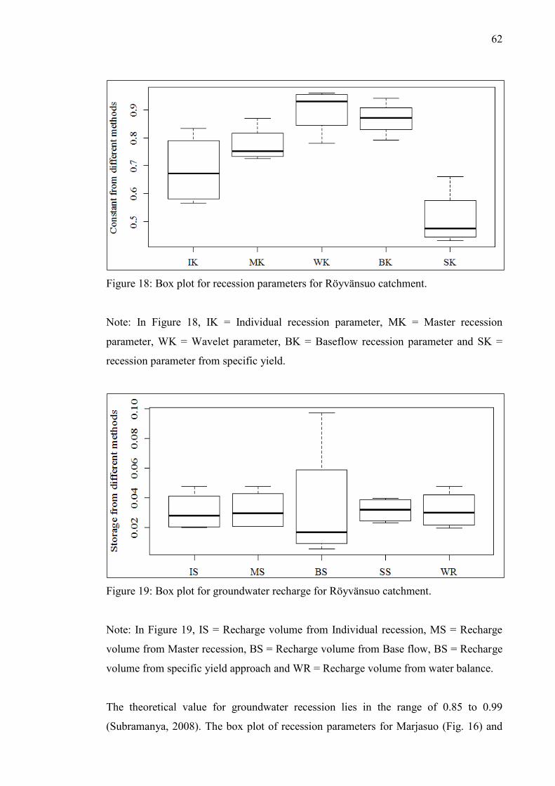
62

Figure 18: Box plot for recession parameters for Röyvänsuo catchment.

Note: In Figure 18, IK = Individual recession parameter, MK = Master recession

parameter, WK = Wavelet parameter, BK = Baseflow recession parameter and SK =

recession parameter from specific yield.

Figure 19: Box plot for groundwater recharge for Röyvänsuo catchment.

Note: In Figure 19, IS = Recharge volume from Individual recession, MS = Recharge

volume from Master recession, BS = Recharge volume from Base flow, BS = Recharge

volume from specific yield approach and WR = Recharge volume from water balance.

The theoretical value for groundwater recession lies in the range of 0.85 to 0.99

(Subramanya, 2008). The box plot of recession parameters for Marjasuo (Fig. 16) and

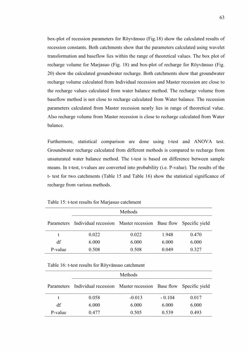
63

box-plot of recession parameters for Röyvänsuo (Fig.18) show the calculated results of

recession constants. Both catchments show that the parameters calculated using wavelet

transformation and baseflow lies within the range of theoretical values. The box plot of

recharge volume for Marjasuo (Fig. 18) and box-plot of recharge for Röyvänsuo (Fig.

20) show the calculated groundwater recharge. Both catchments show that groundwater

recharge volume calculated from Individual recession and Master recession are close to

the recharge values calculated from water balance method. The recharge volume from

baseflow method is not close to recharge calculated from Water balance. The recession

parameters calculated from Master recession nearly lies in range of theoretical value.

Also recharge volume from Master recession is close to recharge calculated from Water

balance.

Furthermore, statistical comparison are done using t-test and ANOVA test.

Groundwater recharge calculated from different methods is compared to recharge from

unsaturated water balance method. The t-test is based on difference between sample

means. In t-test, t-values are converted into probability (i.e. P-value). The results of the

t- test for two catchments (Table 15 and Table 16) show the statistical significance of

recharge from various methods.

Table 15: t-test results for Marjasuo catchment

Methods

Parameters Individual recession Master recession Base flow Specific yield

t 0.022 0.022 1.948 0.470

df 6.000 6.000 6.000 6.000

P-value 0.508 0.508 0.049 0.327

Table 16: t-test results for Röyvänsuo catchment

Methods

Parameters Individual recession Master recession Base flow Specific yield

t 0.058 -0.013 - 0.104 0.017

df 6.000 6.000 6.000 6.000

P-value 0.477 0.505 0.539 0.493

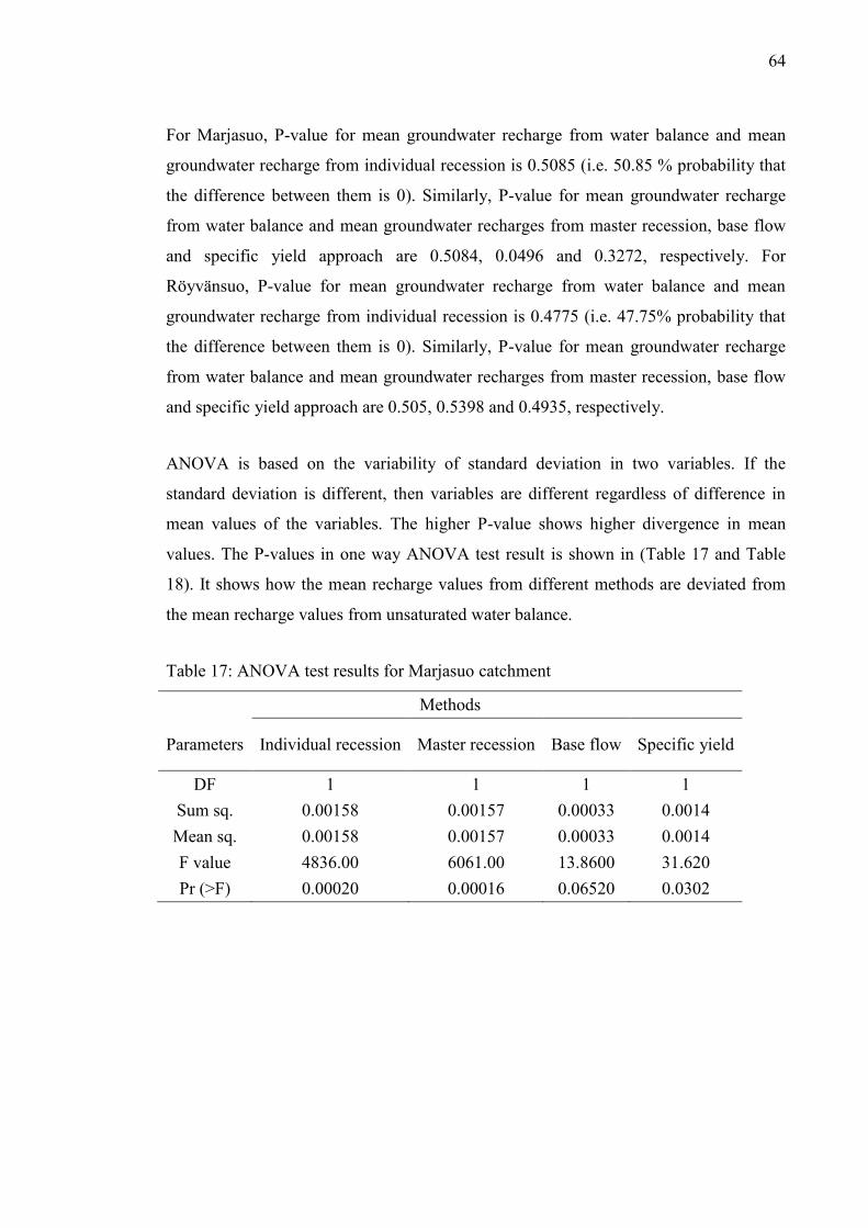
64

For Marjasuo, P-value for mean groundwater recharge from water balance and mean

groundwater recharge from individual recession is 0.5085 (i.e. 50.85 % probability that

the difference between them is 0). Similarly, P-value for mean groundwater recharge

from water balance and mean groundwater recharges from master recession, base flow

and specific yield approach are 0.5084, 0.0496 and 0.3272, respectively. For

Röyvänsuo, P-value for mean groundwater recharge from water balance and mean

groundwater recharge from individual recession is 0.4775 (i.e. 47.75% probability that

the difference between them is 0). Similarly, P-value for mean groundwater recharge

from water balance and mean groundwater recharges from master recession, base flow

and specific yield approach are 0.505, 0.5398 and 0.4935, respectively.

ANOVA is based on the variability of standard deviation in two variables. If the

standard deviation is different, then variables are different regardless of difference in

mean values of the variables. The higher P-value shows higher divergence in mean

values. The P-values in one way ANOVA test result is shown in (Table 17 and Table

18). It shows how the mean recharge values from different methods are deviated from

the mean recharge values from unsaturated water balance.

Table 17: ANOVA test results for Marjasuo catchment

Methods

Parameters Individual recession Master recession Base flow Specific yield

DF 1 1 1 1

Sum sq. 0.00158 0.00157 0.00033 0.0014

Mean sq. 0.00158 0.00157 0.00033 0.0014

F value 4836.00 6061.00 13.8600 31.620

Pr (>F) 0.00020 0.00016 0.06520 0.0302

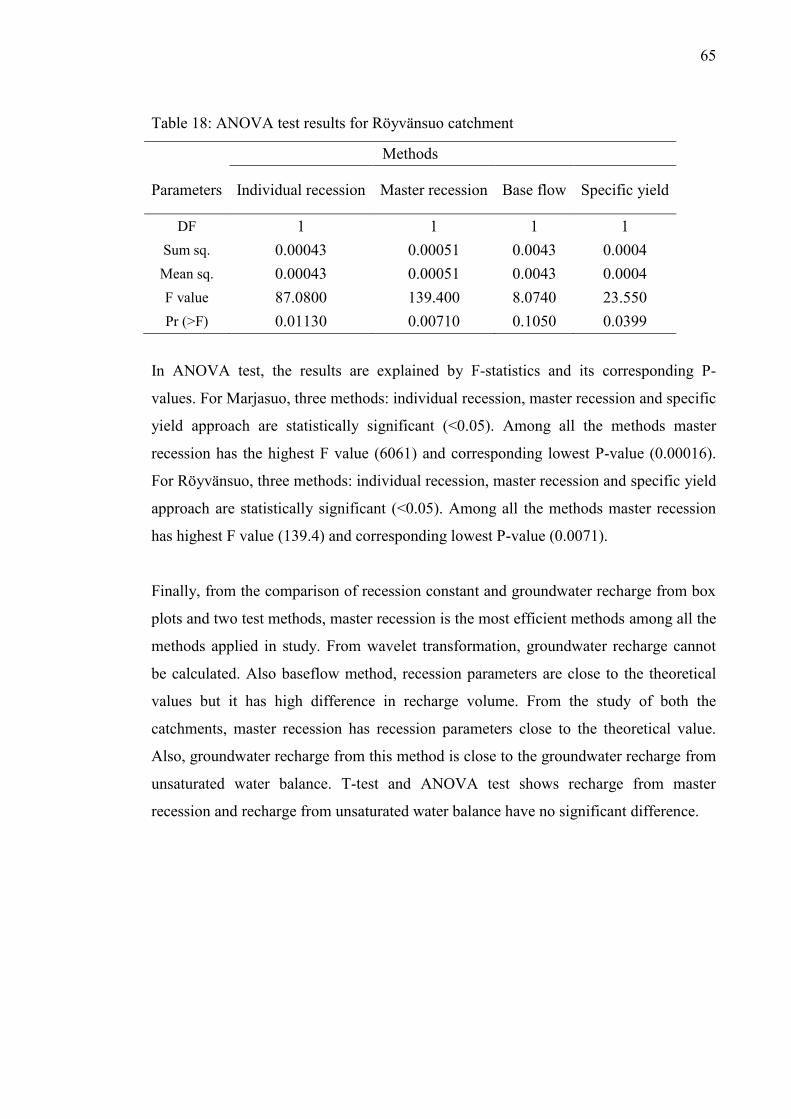
65

Table 18: ANOVA test results for Röyvänsuo catchment

Methods

Parameters Individual recession Master recession Base flow Specific yield

DF 1 1 1 1

Sum sq. 0.00043 0.00051 0.0043 0.0004

Mean sq. 0.00043 0.00051 0.0043 0.0004

F value 87.0800 139.400 8.0740 23.550

Pr (>F) 0.01130 0.00710 0.1050 0.0399

In ANOVA test, the results are explained by F-statistics and its corresponding P-

values. For Marjasuo, three methods: individual recession, master recession and specific

yield approach are statistically significant (<0.05). Among all the methods master

recession has the highest F value (6061) and corresponding lowest P-value (0.00016).

For Röyvänsuo, three methods: individual recession, master recession and specific yield

approach are statistically significant (<0.05). Among all the methods master recession

has highest F value (139.4) and corresponding lowest P-value (0.0071).

Finally, from the comparison of recession constant and groundwater recharge from box

plots and two test methods, master recession is the most efficient methods among all the

methods applied in study. From wavelet transformation, groundwater recharge cannot

be calculated. Also baseflow method, recession parameters are close to the theoretical

values but it has high difference in recharge volume. From the study of both the

catchments, master recession has recession parameters close to the theoretical value.

Also, groundwater recharge from this method is close to the groundwater recharge from

unsaturated water balance. T-test and ANOVA test shows recharge from master

recession and recharge from unsaturated water balance have no significant difference.

66

7 CONCLUSION

The study is based on comparison of different methods for calculation of recession

constant and groundwater recharge using hydrograph recession analysis. Hydrograph

recession analysis of catchments Marjasuo and Röyvänsuo is carried out with runoff

data. Different recession analysis methods: individual recession, master recession,

wavelet transformation and baseflow separation are used to compute recession constant

and groundwater recharge. Wavelet transformation is only used for calculating

recession constant. For further implication of wavelet analysis further work is required.

The groundwater level change during recession is related to groundwater recharge. The

recession constant and groundwater recharge can also be calculated with specific yield

and groundwater level. So, the results from specific yield are used for comparison.

The water balance parameters are computed by unsaturated moisture movement model.

The unsaturated moisture model includes catchments parameters related to the runoff

process. The water balance components obtained from water balance models are almost

accurate and are used in various land use practices and effective soil-water

conservation. The water balance model provides parameters for the purpose of rainfall

designs, storage yield, and prediction of meteorological, study of hydrological and

ecological processes. The statistical comparison of groundwater recharge method and

groundwater recharge from unsaturated water balance model shows master recession

analysis method is the most efficient hydrograph recession analysis techniques among

the methods used in this study.

Hydrograph recession also correlates climatic and geomorphologic features of the

catchment. Hydrograph recession parameters contain embedded information about the

flow regime and hydro geological characteristic of the catchment. Hydrograph recession

analysis should be carried in fast and objective manner. The different recession analysis

method used in this study gives recession parameters and groundwater recharge for the

catchments. The recession parameters denote the slope of depletion curve. It also

represents the rate by which water flow from the catchment to the runoff point. The

flow in the catchment is also influenced by catchment slope and climate. The climatic

information in hydrograph is further clarified by unsaturated moisture movement

model. In unsaturated moisture model, soil moisture content in various soil layers are

67

calculated at certain time period. It also contains the direction of flow at certain time.

The amount and direction of flow is influenced by climatic condition and hydraulic

conductivity of the catchment. The recharge component obtained from unsaturated

moisture model is used to compare recharge calculated from different methods.

The recession parameters calculated from various methods differs from each other. The

recession parameter depends on the selection of recession curve and procedure of its

analysis. The calculation in this study also shows different recession parameters and

groundwater recharge values. To identify the best method, statistical tests are carried

out. The wavelet transformation is a recent method applied for qualitative analysis of

data which gives recession constant close to theoretical values. The study provides

adequate information about various methods of hydrograph recession analysis and

specific yield by which recession constant and groundwater recharge are calculated.

68

8 REFERENCES

Ahiablame, L., Chaubey, I., Engel, B., Cherkauer, K. and Merwade, V. (2012).

Estimation of annual baseflow at ungauged sites in Indiana USA. Journal of Hydrology.

doi: http://dx.doi.org/10.1016/j.jhydrol.2012.10.002.

Anderson, J. and Samargo, E. (2007). Wetland Hydrology. Available:

http://forestandrange.org/new_wetlands/pdfs/deq-water-wetlands-idmanualchap2.pdf.

Last accessed 15th dec 2013.

Anderson, M. G. and Burt, T. P. (1980). Interpretation of recession flow. Journal of

Hydrology. 46 (1), 89-101.

Andradottir, H. O. (2010). Proceedings of the 14th International Workshop on Physical

Processes in Natural Waters. June 28 - July 1, Reykjavík, Iceland, pp. 166.

Athavale, R.N., Rangarajan, R. and Muralidharan, D. (1992). Measurement of Natural

Recharge in India. Journal of Geological Society of India. 39(3), 235-244.

Australian Water Resources. (2006). Appendix C Theme Report: Groundwater, Robert

Garran Offices: Commonwealth of Australia.

Ballantyne, C.K. (2004). Geomorphological changes and trends in Scotland: debris-

flows. Scottish Natural Heritage Commissioned Report No. 052 (ROAME No.

F00AC107A).

Bako, M. D. and owoade, A. (1988). Field Application of a Numerical Method for the

Derivation of Baseflow Recession Constant. Hydrological Processes. 2 (1), 331-336.

Barrow, D. (2010). Ground water Dependence of Ecological Sites Located in the Table

Mountain Group. Available: http://etd.uovs.ac.za/ETD-db//theses/available/etd-

08142012-125601/unrestricted/BarrowD.pdf. Last accessed 26th Dec 2013.

Bay-Delta Authority. (2003) San Joaquin Basin Ecological Flow Analysis, Berkeley,

California: Natural Heritage Institute.

69

Bay, R.R. (1968). The Hydrology of Several Peat Deposits in Northern Minnesota,

U.S.A. Available: http://www.nrs.fs.fed.us/pubs/jrnl/1968/nc_1968_Bay_002.pdf. Last

accessed 27th Dec 2013.

Belyea, L.R. and Nilsmalmer. (2004). Carbon sequestration in peatland: patterns and

mechanisms of response to climate change. Global Change Biology. 10 (6), 1043–1052.

Biggs, A.J.W., Witheyman, S.L., Williams, K.M., Cupples, N., de Voil, C.A., Power,

R.E. and Stone, B.J., (2012). Assessing the salinity impacts of coal seam gas water on

landscapes and surface streams. August 2012. Final report of Activity 3 of the Healthy

Head Waters Coal Seam Gas Water Feasibility Study. Department of Natural Resources

and Mines, Toowoomba.

Branfireun B.A., and Roulet, N.T. (1998). The baseflow and stormflow hydrology of a

precambrian shield headwater peatland. Hydrological Processes. 12 (1),

Brownbill, R.J, Lamontagne, S., Williams, R.M., Cook, P.G., Simmons, C.T. and

Merrick, N. (2011). Interconnection of surface and groundwater systems– river losses

from losing-disconnected streams. Technical final report, June 2011, NSW Office of

Water, Sydney.

Careyn S. K.D., Tetzlaff, J., Buttle, H., Laudon, J., McDonnell, K., McGuire, J.,

Seibert, C., Soulsby and J., Shanley, (2013). Use of color maps and wavelet coherence

to discern seasonal and inter annual climate influences on streamflow variability in

northern catchments, Water Resources. Res., 49, doi:10.1002/wrcr.20469.

Chaubey, I. and Ward, G. M. (2006). Hydrologic Budget Analysis of a Small Natural

Wetland in Southeast USA. Journal of Environmental Informatics. 8 (1), 10-21.

Committee on Reducing Stormwater Runoff Contributions to Water Pollution. (2008).

Urban Stormwater Management in the United States, The National Academies Press

Washington, D.C.: National research council.

70

Creed, I. F. and Band, L. E. (1998). Export of nitrogen from catchments within a

temperate forest: Evidence for a unifying mechanism regulated by variable source area

dynamics. Water resource research. 34 (11), 3105–3120.

Crosbie, R. S., Binning, P.and Kalma, J. D. (2005). A time series approach to inferring

groundwater recharge using the water table fluctuation method. Water Resources. Res.,

41, W01008, doi: 10.1029/2004WR003077.

Data SIO, NOAA, U.S. Navy, NGA, GEBCO. (2007). Google Maps [online].

[Accessed 18 April 2014]. Available at: <http://maps.google.fi >.

DeKeyser, S. (2006). Water Quality and Wetland Function in the Northern Prairie

Pothole Region, Cooperative States Research, Education and Extension Service

(CSREES): Regional water program.

E-water toolkit. 2000. class-U3M-1D. [ONLINE]

Available at: http://toolkit.ewater.com.au/Tools/CLASS-U3M-1D. [Accessed 01 March

14].

Eagleson, P.S. (1978). Climate, Soil, and Vegetation. A Simplified Model of Soil

Moisture Movement in the Liquid Phase. Water resource research. 14 (15), 722-730.

EPA, U.S. (2008). Methods for Evaluating Wetland Condition: Wetland Hydrology.

Office of Water, U.S. Environmental Protection Agency, Washington, DC.EPA-822-R-

08-024.

Eylon, S., Carpenter, Theresa M., Fickenscher, Peter, and Georgakakos and Konstantine

P. (2006). Evaluation of the National Weather Service Operational Hydrologic Model

and Forecasts for the American River Basin. Publications, Agencies and Staff of the

U.S. Department of Commerce. Paper 51.

Fitzgerald, D. F., Price J. S. and Gibson, J. J., (2003). Hill slope-swamp interactions and

flow pathways in a hypermaritime rainforest, British Columbia. Hydrological

Processes. 17 (1), 3005–3022.

71

FOCUS, (2001). FOCUS Surface Water Scenarios in the EU Process under

19/414/EEC. Report of the FOCUS Working Group on Surface Water Scenarios, EC

Document Reference SANCO/4802/2001-rev.2.245pp.

Fraser, C.J.D., Roulet, N.T. and Lafleur, M. (2001). Groundwater flow pattern in a large

peatland. Journal of Hydrology. 246, 142-154.

Gasima. (2005). Sunrise, sunset, dawn and dusk times around the World. [ONLINE]

Available at: http://www.gaisma.com/en/location/oulu.html. [Accessed 06 July 14].

Gathenya, J. M., Thiong G. T. and Mwangi, J.K. (2007). Hydrologic modelling and

water quality assessment of Sasumua Watershed. Nairobi, Kenya: Jomo Kenyatta

University of Agriculture and Technology.

Gehman C. L., Harry, D. L., Sanford, W. E., Stednick, J. D. and Beckman, N. A.

(2009). Estimating specific yield and storage change in an unconfined aquifer using

temporal gravity surveys. Water Resour. Res., 45, W00D21, doi:

10.1029/2007WR006096.

Ghelardi, V. (2011). United States Department of Transportation - Federal Highway

Administration. [ONLINE]

Available at: http://www.fhwa.dot.gov/engineering/hydraulics/pubs/08090/02.cfm.

[Accessed 11 June 14].

Granato, G.E. (2012). Estimating basin lag time and hydrograph-timing indexes used to

characterize storm flows for runoff-quality analysis: U.S. Geological Survey Scientific

Investigations Report 2012–5110, 47 p., Available: http://pubs.usgs.gov/sir/2012/5110.

Last accessed: 24th June 2014.

Gurley, K. and Kareem, A. (1999). Applications of wavelet transforms in earthquake,

wind and ocean engineering. Engineering Structures. 21 (9), 149–167.

Han, D. (2010). Concise Hydrology. Bookboon.com: Bookboon.com. 62-69.

72

Habets, F., Gascoin, S., Korkmaz, S., Thiery D., Zribi, M., Amraoui, N., Carli, M.,

Ducharne, A., Leblois, E., Ledoux E., Martin, E., Noilhan, J., Ottle, C., and Viennot, P.

(2010). Multi-model comparison of a major flood in the groundwater-fed basin of the

Somme River (France). Hydrology and Earth System Sciences. 14 (2), 99–117.

Hilberts A. G. J., Troch, P. A., and Paniconi, C. (2005). Storage-dependent drainable

porosity for complex hillslopes. Water Resour. Res., 41, W06001, doi:

10.1029/2004WR003725.

Hisz D., (2010). Predicting Long-Term Well Performance from Short-Term Well Tests

in the Piedmont. All Theses. Paper 963.

Hudson and Berman D. (1994). Soil organic matter and available water capacity. J. Soil

and Water Cons. 49(2) 189-194.

HydroOffice, (2010). Software for Water Science. [ONLINE] Available at:

http://hydrooffice.org/Downloads/List.aspx?section=Manuals. [Accessed 07 May 14].

HydroOffice, (2011). HydroOffice software - software for water science. Software.

Modules. RC. (Online) Available from: http://www.hydrooffice.org

Idowu, O. A. and Martins, O. (2007). Hydrograph Analysis for Groundwater Recharge

in the Phreatic Basement Aquifer of the Opeki River Basin, Southwestern Nigeria.

ASSET An International Journal. 6 (2), 132-141.

Institute of Hydrology. (1980). Low flow studies. Wallingford, UK, Institute of

Hydrology, Research Report 1

International Atomic Energy Agency. (2008). Field Estimation of Soil Water Content.

Vienna, Austria: IAEA.

International Symposium on Management of Aquifer Recharge. (2005). Recharge

systems for protecting and enhancing groundwater resources. Berlin, Germany: ISMAR.

73

Kellomäki S., Maajärvi M., Strandman H., Kipeläinen A., Peltola H., (2010). Model

Computations on Climate Change Effects on Snow Cover, Soil Moisture and Soil Frost

in Boreal Conditions over Finland. Silva Fennia. 44(2): 213-233.

Khalil, M., Sakai, M., Mizoguchi, M.and Miyazaki, T. (2003). Current and Prospective

Applications of Zero Flux Plane (ZFP) Method. J. Jpn. Soc. Soil Phys. 1 (95), 75-90.

Khire, M.V., Benson G.H., and Bosscher, P.J. (1997). Water Balance Modelling of

Earthen Final Covers. Journal of Geotechnical and Geoenvironmental Engineering. 123

(8), 744-754.

Klöve, B. (2008). Hydrology of headwater peatlands: how are these ecosystems

connected to and dependent on groundwater?

Available:

http://www.fao.org/forestry/1743601b590797dfe824d4d5fce2ec5e277a77.pdf. Last

accessed 12th Dec 2013

Klöve, B., Ala-Aho, P., Bertrand, G., Gurdak, J.J., Kupfersberger, H., Kvaerner, J.,

Muotka, T., Mykrä, H., Preda, E., Rossi, P., Bertacchi, C., Velasco, E. and Pulido-

Velazquez, M. (2013). Climate change impacts on groundwater and dependent

ecosystems. J. Hydrol. Available: http://dx.doi.org/10.1016/j.jhydrol.2013.06.037

Knapp, B. (1979). Elements of geographical hydrology. Broadwick Street, London

W1V 1FP, UK: Unwin Hyman Ltd. 12-56.57-72.

Koivusalo, H. (2002). Process-oriented investigation of snow accumulation, snowmelt

and runoff generation in forested sites in Finland. Espoo: Helsinki University of

Technology Water Resources Publications

Kuchment, L.S. (2004). The Hydrological Cycle and Human Impact on it, in Water

Resources Management. Encyclopedia of Life Support Systems (EOLSS), Developed

under the Auspices of the UNESCO, Eolss Publishers, Oxford UK,

[http://www.eolss.net].

74

Kuchment, L.S., Gelfan A.N. and Demidov, V.N. (2011). Modeling of the Hydrological

Cycle of a Forest River Basin and Hydrological Consequences of Forest Cutting. The

Open Hydrology Journal. 5 (18), 9-18.

Labadz, J., Allott, T., Evans, E., Butcher, D., Billett, M., Stainer, S., Yallop, A., Jones,

P., Innerdale, M., Harmon, N., Maher, K. and Bradbury, R. (2010). Peatland

Hydrology. Available:http://www.iucn-uk-peatlandprogramme.org/sites/all/files/Review

%206%20Peatland%20Hydrology_0.pdf. Last accessed 9th jan 2014.

Lastoria, B. (2008). Hydrological processes on the land surface: A survey of modelling

approaches. FORALPS Technical Report, 9.Università degli Studi di Trento,

Dipartimento di Ingegneria Civile e Ambientale, Trento, Italy, 56 pp.

Linard, J.I., Wolock, D.M., Webb, R.M.T. and Wieczorek, M.E. (2009). Identifying

hydrologic processes in agricultural watersheds using precipitation-runoff models: U.S.

Geological Survey Scientific Investigations Report 2009–5126, 22 p.

Lindborg, T., Lindborg, R., Löfgren, A., Soderback, B., Bradshaw C. and Kautsky U.

(2006). A Strategy for Describing the Biosphere at Candidate Sites for Repositories of

Nuclear Waste: Linking Ecosystem and Landscape Modeling. Royal Swedish Academy

of Sciences. 35 (8), 418-424.

Lough, H. and Williams, H. (2009).Vertical flow in Canterbury groundwater systems

and its significance for groundwater management. Environment Canterbury Technical

Report U09/45, 69 p.

Manzoni, S., Vico, G., Porporato, A.and Katu, G. (2013). Biological constraints on

water transport in the soil–plant–atmosphere system. Advances in Water Resources. 51

(1), 292–304.

Matonse, A. H., and Kroll. C. (2009), Simulating low streamflows with hillslope

storage models, Water Resour. Res., 45, W01407, doi: 10.1029/2007WR006529.

75

Meixler, M.S. (1999). Regional settings, Pages 11-24 in M.B. Bain and N.J. Stevenson,

editors. Aquatic habitat assessment: common methods. American Fisheries Society,

Bethesda, Maryland.

Meyboom, P. (1961), Estimating Ground-Water Recharge from Stream Hydrographs. J.

Geophys. Res. 66(4), 1203–1214.

Michigan Technological University. (2009). Center for Science and Environmental

Outreach. [ONLINE]

Available at: http://cseo.mtu.edu/community/groundwater/GWmyths.htm. [Accessed 02

June 14].

Miyazaki, T. (2006). Water Flow in Soils. 2nd ed. 6000 Broken Sound Parkway NW:

CRC Press. 19-35.Water 2010, 2, 1-x manuscripts; doi: 10.3390/w20x000x.

Moore G.K. (1992). Hydrograph analysis in fractured rock terrane. Gound water 30(3),

390-395.

Morawietz, M. (2007). Baseflow. [ONLINE]

Available at: http://www.fi.muni.cz/~xforejt/baseflow/. [Accessed 28 July 14].

Moubarak, J. (2013). Quantifying Groundwater Recharge Beneath Furrow Irrigated

Corn Using Lysimetry, an Unsaturated Zone Water Balance and Numerical Modeling.

Colorado State University: Fort Collins, Colorado.

National Water Commission. (2012), Groundwater Essentials, NWC, Canberra Water

2011, 3, 323-355; doi: 10.3390/w3010323

Noraly, V.B. (2011). Conjunctive water management: How to use the full

potential .B.Sc. The Netherlands: Wageningen University.

Palmroth S., Katul, G. G., Hui, D., McCarthy, H. R., Jackson, R. B. and Oren R. (2010).

Estimation of long term basin scale evapotranspiration from streamflow time series,

Water Resour. Res., 46, W10512, doi: 10.1029/2009WR008838.

76

Peters, D.L. (2013). Runoff Processes.

Available: http://geog.uvic.ca/geog370/370_9_runoff_Spring_13_Part%201.pdf. Last

accessed 20th may 2014.

Posavec, K., Parlov, J. and Bacani, A. (2006). A Visual Basic spreadsheet macro for

estimating groundwater recharge. Groundwater—September–October. 44 (5), 764–767.

Price, K. (2011). Effects of watershed topography, soils, land use, and climate on

baseflow hydrology in humid regions: A review. Progress in Physical Geography. 35

(4), 465–492.

Qian, K.Z., Wan, L., Wang, X.S., Lv, J.J, Liang, S.H. (2012). Periodical characteristics

of baseflow in the source region of the Yangtze River. Journal of Arid Land. 4 (2),

113−122.

Querner, E.P., Mioduszewski, W., Povilaitis, A., Ślesicka, A. (2009) 'Modelling

Peatland Hydrology: Three Cases from Northern Europe', Polish Journal of

Environmental Studies, 19(1), pp. 149-159.

Raghavendran, S. (2013). Estimation of Changes in Groundwater Storage using

Recession Curve Method. Karnataka, Surathkal: National Institute of Technology.

Ramírez H.D.R., Warner, G.S., and Scatena, F.N., (2002). Prediction of Master

Recession Curves and Baseflow Recession in the Luquillo Mountains of Puerto

Rico. Journal of American water resource association. 38 (3), 693-704.

Ramírez, J. A. (2000). Prediction and Modeling of Flood Hydrology and Hydraulics.

Chapter 11 of Inland Flood Hazards: Human, Riparian and Aquatic Communities Eds.

Ellen Wohl, Cambridge University Press.

Reilly, N. and Lech, M. (2007). A bibliographic index for natural resource management

in the Upper Burdekin and Fitzroy Catchments. CRC LEME Open File Report 182.

444pp

77

Ritzema, H.P. (1994). Drainage Principles and Applications. 2nd ed. Wageningen,

Netherland: ILRI publication 16. 65-74.

Ronkanen, A.K., Marttila, H., Siekkinen, J. and Kløve, B. (2010). Stable isotopes

studies to increase knowledge from the role of peatlands in catchment hydrology, paper

presented to Abstracts and Programme of the Cost Action FP0601 Forman Workshop at

the Finnish Environment Institute, Helsinki and Hyytiälä Forestry Field Station, Finland

6.9.2010−8.9.2010, viewed: 18th April 2014. Available:

http:// www.metla.fi/julkaisut/workingpapers/2010/mwp168.pdf.

Scanlon, B.R. (2004). Evaluation of Methods of Estimating Recharge in Semiarid and

Arid Regions in the Southwestern U.S. Groundwater Recharge in a Desert

Environment: The Southwestern United States. 9 (1), 235-254.

Shunjun, H., Changyan, T., Yudong, S., Xiaobing, C. and Yuetan, L. (2006). Models

for calculating phreatic water evaporation on bare and Tamarix-vegetated

lands. Chinese Science Bulletin. 51 (1), 43-50.

Silva, L.A., Silva, A.M., Coelho, G., Mello, C.R. and Pereira, D.R. (2012).

Groundwater recharge estimate at Alto Rio Grande – MG watershed. Soil and water

engineering. 32 (6), 237-277.

Stewart, M.K. (2014). New baseflow separation and recession analysis approaches for

streamflow. Hydrology and Earth System Sciences. 11 (1), 7089–7131.

Subramanya, K. (2008). Engineering hydrology. West patel nagar, New Dehli: Tata

McGraw-Hill publishing. 199-201.

Sujono, J., Sliikashe S., and Hiiramatsu, K. (2001). Hydrograph Recession Analysis

using Wavelet transforms. J．Fac．Agr．，Kyushu Univ. 45 (2), 557－564.

Sujono, J., Sliikashe S., and Hiiramatsu, K. (2004). A comparison of techniques for

hydrograph recession analysis. Hydrological processes. 18 (3), 403–413.

78

Sumangala, K.N. (2011). Hydro Geochemical Quality Assesment of Groundwater – A

General Perspective. Doctor of Philosophy. Kerala, India: Cochin University of Science

and Technology.

szilagyi, J. (1999). On the use of semi-logarithmic plots for baseflow

separation. Ground water. 37 (5), 660-662.

Szilagyi, J., Harvey E.F., and Ayers, J.F. (2003). Regional Estimation of Base Recharge

to Ground Water Using Water Balance and a Base-Flow Index. Groundwater. 4 (4),

504-513.

Taboada, M.A. (2003). Soil Shrinkage Characteristics in Swelling Soils. Trieste. 3 (21),

471-486.

Tallaksen, L.M., (1995). A review of baseflow recession analysis. J. Hydrol. 165, 349-

370.

Tfaily, M. (2011). Molecular Characterization of Dissolved Organic Matter In Northern

Peatlands: Identifying The Chemical Signatures Of Climate Change. Electronic Theses,

Treatises and Dissertations. Paper 6020.

Thompson, G. S., Lunn, R., Hutt, A., Burlton, D. and Charman. D. (2004). Bogged

Down with Conservation Work: Restoration of Internationally Important Mire Sites in

Northern England. Biologist, 51, 45-48.

Thorsten, W., Sivapalan, M., Troch, P. and Woods, R. (2007). Catchment Classification

and Hydrologic Similarity. Geography Compass. 1 (4), 901-931.

Toebes, C., and Strang, D. D. (1964). On recession curves: 1. Recession equations. J.

Hydrol. 3: 2-5.

Tuteja, N.K., Vaze, J., Murphy, B. and Beale, G. (2004). Class: Catchment Scale

Multiple-Landuse Atmosphere Soil Water and Solute Transport Model. Co-operative

Research Centre for Catchment Hydrology. Technical Report No. 04/12.

79

Vandewiele, G.L., Xu, C.Y. and Ni-Lar-Win. (1992). Methodology and comparative

study of monthly water balance models in Belgium, China and Burma. Journal of

Hydrology, 134; 315-347.

Vaze, J., Tuteja, N.K. and Teng, T., (2004). Unsaturated Moisture Movement

Model. Available: http://www.toolkit.net.au/Tools/CLASS-U3M-1D/documentation.

Last accessed 15th may 2014.

Virtanen, K. and Valpola, S. (2011). Energy Potential of Finnish Peatlands. Geological

Survey of Finland. Special Paper (49), 153–161.

Vitvar, T., Burns, D.A., Lawrence, G.B, McDonnell J.J. and Wolock, D.M. (2002).

Estimation of baseflow residence times in watersheds from the runoff hydrograph

recession: method and application in the Never sink watershed, Catskill Mountains,

New York. Hydrological Processes. 16 (1), 1871–1877.

Wang, Q.J., Horton, R. and Fan J. (2009). An Analytical Solution for One-Dimensional

Water Infiltration and Redistribution in Unsaturated Soil. Pedosphere. 19 (1), 104-110.

Williams, R.E., Rathbone, D.A., Scrutton, N.S. and Bruce, N.C. (2004).

Biotransformation of explosives by the old yellow enzyme family of flavor

proteins. Appl. Environ. Microbiol.70:3566-3574.

Wood, C. (2011). Improved estimates of groundwater recharge in South East South

Australia. DFW Technical Report 2011/15.Government of South Australia, through

Department for Water, Adelaide.

Xu, C.Y (2002). Hydrologic Models. 2nd ed. Villavägen 16, Sweden :Earth Sciences

Centre. 3-17.

XU, C.Y. and Singh, V. P. (1998). A Review on Monthly Water Balance Models for

Water Resources Investigations. Water Resources Management. 12 (1), 31–50.

80

Yarnell, Sarah M., Peek, R.A., Rheinheimer, D., Lind, A., Viers, A.H. (2013).

Management of the Spring Snowmelt Recession: An Integrated Analysis of Empirical,

Hydrodynamic, and Hydropower Modeling Applications. California Energy

Commission. Publication number: CEC-500-2014-030.

Yeh, H.F., Lee, C.H., Chen, J.F. and Chen, W.P. (2005). Estimation of Groundwater

Recharge Using Water Balance Model. Water Resources and the Regime of Water

Bodies. 34(2), 171-180.

Yuan, X.Z. (1997). An Introduction to Wavelet Theory and its Applications in

Statistics. Master of Science. K. Alifax, Nova Scotta: Dalhousie University.

Zhang, L., Walker, G.R. and Dawes, W.R. (2002). Water balance modeling: concepts

and applications. In: McVicar, T.R, Li Rui, Walker .J., Fitz-patrick R.W. and Liu

Changming (eds), Regional water and Soil Assesment for Managing Sustainable

Agriculture in China and Australia, ACIAR Monograph No.84,31-47.

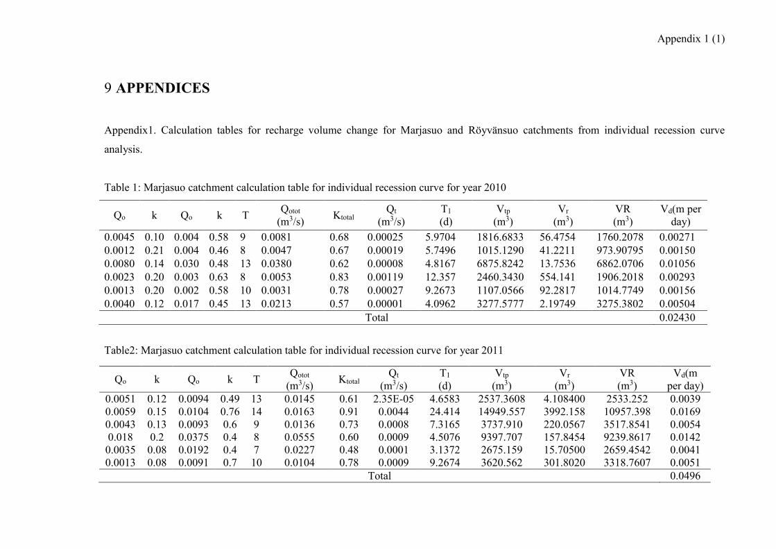
Appendix 1 (1)

9 APPENDICES

Appendix1. Calculation tables for recharge volume change for Marjasuo and Röyvänsuo catchments from individual recession curve

analysis.

Table 1: Marjasuo catchment calculation table for individual recession curve for year 2010

Table2: Marjasuo catchment calculation table for individual recession curve for year 2011

Qo k Qo k T Qotot

(m3/s) Ktotal

Qt

(m3/s)

T1

(d)

Vtp

(m3)

Vr

(m3)

VR

(m3)

Vd(m per

day)

0.0045 0.10 0.004 0.58 9 0.0081 0.68 0.00025 5.9704 1816.6833 56.4754 1760.2078 0.00271

0.0012 0.21 0.004 0.46 8 0.0047 0.67 0.00019 5.7496 1015.1290 41.2211 973.90795 0.00150

0.0080 0.14 0.030 0.48 13 0.0380 0.62 0.00008 4.8167 6875.8242 13.7536 6862.0706 0.01056

0.0023 0.20 0.003 0.63 8 0.0053 0.83 0.00119 12.357 2460.3430 554.141 1906.2018 0.00293

0.0013 0.20 0.002 0.58 10 0.0031 0.78 0.00027 9.2673 1107.0566 92.2817 1014.7749 0.00156

0.0040 0.12 0.017 0.45 13 0.0213 0.57 0.00001 4.0962 3277.5777 2.19749 3275.3802 0.00504

Total 0.02430

Qo k Qo k T Qotot

(m3/s) Ktotal

Qt

(m3/s)

T1

(d)

Vtp

(m3)

Vr

(m3)

VR

(m3)

Vd(m

per day)

0.0051 0.12 0.0094 0.49 13 0.0145 0.61 2.35E-05 4.6583 2537.3608 4.108400 2533.252 0.0039

0.0059 0.15 0.0104 0.76 14 0.0163 0.91 0.0044 24.414 14949.557 3992.158 10957.398 0.0169

0.0043 0.13 0.0093 0.6 9 0.0136 0.73 0.0008 7.3165 3737.910 220.0567 3517.8541 0.0054

0.018 0.2 0.0375 0.4 8 0.0555 0.60 0.0009 4.5076 9397.707 157.8454 9239.8617 0.0142

0.0035 0.08 0.0192 0.4 7 0.0227 0.48 0.0001 3.1372 2675.159 15.70500 2659.4542 0.0041

0.0013 0.08 0.0091 0.7 10 0.0104 0.78 0.0009 9.2674 3620.562 301.8020 3318.7607 0.0051

Total 0.0496

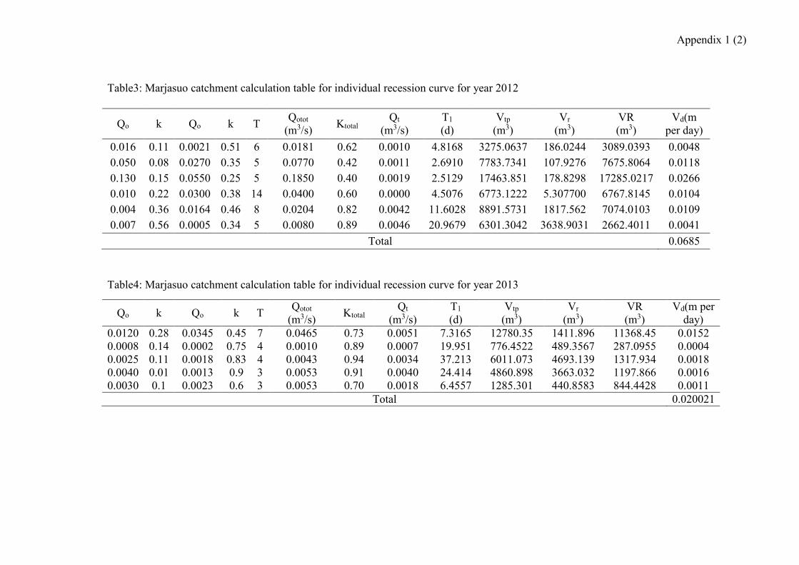
Appendix 1 (2)

Table3: Marjasuo catchment calculation table for individual recession curve for year 2012

Table4: Marjasuo catchment calculation table for individual recession curve for year 2013

Qo k Qo k T Qotot

(m3/s) Ktotal

Qt

(m3/s)

T1

(d)

Vtp

(m3)

Vr

(m3)

VR

(m3)

Vd(m

per day)

0.016 0.11 0.0021 0.51 6 0.0181 0.62 0.0010 4.8168 3275.0637 186.0244 3089.0393 0.0048

0.050 0.08 0.0270 0.35 5 0.0770 0.42 0.0011 2.6910 7783.7341 107.9276 7675.8064 0.0118

0.130 0.15 0.0550 0.25 5 0.1850 0.40 0.0019 2.5129 17463.851 178.8298 17285.0217 0.0266

0.010 0.22 0.0300 0.38 14 0.0400 0.60 0.0000 4.5076 6773.1222 5.307700 6767.8145 0.0104

0.004 0.36 0.0164 0.46 8 0.0204 0.82 0.0042 11.6028 8891.5731 1817.562 7074.0103 0.0109

0.007 0.56 0.0005 0.34 5 0.0080 0.89 0.0046 20.9679 6301.3042 3638.9031 2662.4011 0.0041

Total 0.0685

Qo k Qo k T Qotot

(m3/s) Ktotal

Qt

(m3/s)

T1

(d)

Vtp

(m3)

Vr

(m3)

VR

(m3)

Vd(m per

day)

0.0120 0.28 0.0345 0.45 7 0.0465 0.73 0.0051 7.3165 12780.35 1411.896 11368.45 0.0152

0.0008 0.14 0.0002 0.75 4 0.0010 0.89 0.0007 19.951 776.4522 489.3567 287.0955 0.0004

0.0025 0.11 0.0018 0.83 4 0.0043 0.94 0.0034 37.213 6011.073 4693.139 1317.934 0.0018

0.0040 0.01 0.0013 0.9 3 0.0053 0.91 0.0040 24.414 4860.898 3663.032 1197.866 0.0016

0.0030 0.1 0.0023 0.6 3 0.0053 0.70 0.0018 6.4557 1285.301 440.8583 844.4428 0.0011

Total 0.020021

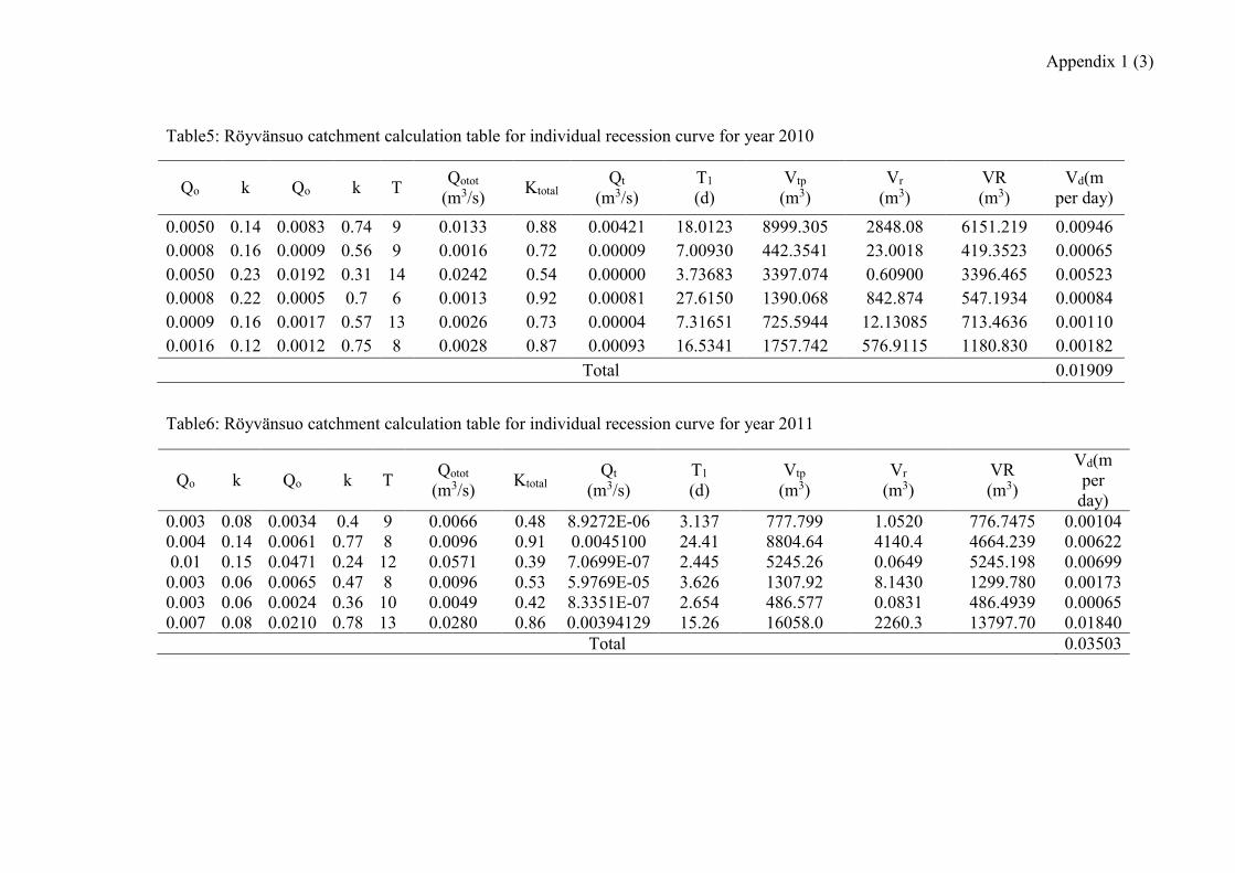
Appendix 1 (3)

Table5: Röyvänsuo catchment calculation table for individual recession curve for year 2010

Table6: Röyvänsuo catchment calculation table for individual recession curve for year 2011

Qo k Qo k T Qotot

(m3/s) Ktotal

Qt

(m3/s)

T1

(d)

Vtp

(m3)

Vr

(m3)

VR

(m3)

Vd(m

per day)

0.0050 0.14 0.0083 0.74 9 0.0133 0.88 0.00421 18.0123 8999.305 2848.08 6151.219 0.00946

0.0008 0.16 0.0009 0.56 9 0.0016 0.72 0.00009 7.00930 442.3541 23.0018 419.3523 0.00065

0.0050 0.23 0.0192 0.31 14 0.0242 0.54 0.00000 3.73683 3397.074 0.60900 3396.465 0.00523

0.0008 0.22 0.0005 0.7 6 0.0013 0.92 0.00081 27.6150 1390.068 842.874 547.1934 0.00084

0.0009 0.16 0.0017 0.57 13 0.0026 0.73 0.00004 7.31651 725.5944 12.13085 713.4636 0.00110

0.0016 0.12 0.0012 0.75 8 0.0028 0.87 0.00093 16.5341 1757.742 576.9115 1180.830 0.00182

Total 0.01909

Qo k Qo k T Qotot

(m3/s) Ktotal

Qt

(m3/s)

T1

(d)

Vtp

(m3)

Vr

(m3)

VR

(m3)

Vd(m

per

day)

0.003 0.08 0.0034 0.4 9 0.0066 0.48 8.9272E-06 3.137 777.799 1.0520 776.7475 0.00104

0.004 0.14 0.0061 0.77 8 0.0096 0.91 0.0045100 24.41 8804.64 4140.4 4664.239 0.00622

0.01 0.15 0.0471 0.24 12 0.0571 0.39 7.0699E-07 2.445 5245.26 0.0649 5245.198 0.00699

0.003 0.06 0.0065 0.47 8 0.0096 0.53 5.9769E-05 3.626 1307.92 8.1430 1299.780 0.00173

0.003 0.06 0.0024 0.36 10 0.0049 0.42 8.3351E-07 2.654 486.577 0.0831 486.4939 0.00065

0.007 0.08 0.0210 0.78 13 0.0280 0.86 0.00394129 15.26 16058.0 2260.3 13797.70 0.01840

Total 0.03503

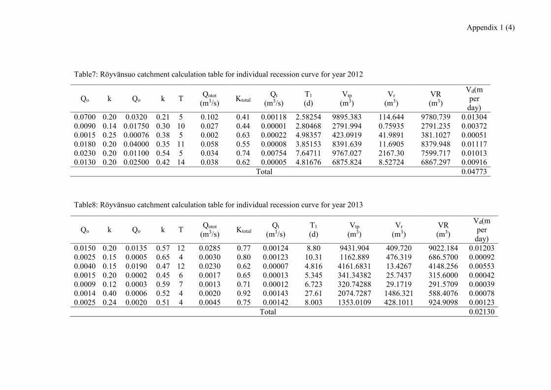
Appendix 1 (4)

Table7: Röyvänsuo catchment calculation table for individual recession curve for year 2012

Table8: Röyvänsuo catchment calculation table for individual recession curve for year 2013

Qo k Qo k T Qotot

(m3/s) Ktotal

Qt

(m3/s)

T1

(d)

Vtp

(m3)

Vr

(m3)

VR

(m3)

Vd(m

per

day)

0.0700 0.20 0.0320 0.21 5 0.102 0.41 0.00118 2.58254 9895.383 114.644 9780.739 0.01304

0.0090 0.14 0.01750 0.30 10 0.027 0.44 0.00001 2.80468 2791.994 0.75935 2791.235 0.00372

0.0015 0.25 0.00076 0.38 5 0.002 0.63 0.00022 4.98357 423.0919 41.9891 381.1027 0.00051

0.0180 0.20 0.04000 0.35 11 0.058 0.55 0.00008 3.85153 8391.639 11.6905 8379.948 0.01117

0.0230 0.20 0.01100 0.54 5 0.034 0.74 0.00754 7.64711 9767.027 2167.30 7599.717 0.01013

0.0130 0.20 0.02500 0.42 14 0.038 0.62 0.00005 4.81676 6875.824 8.52724 6867.297 0.00916

Total 0.04773

Qo k Qo k T Qotot

(m3/s) Ktotal

Qt

(m3/s)

T1

(d)

Vtp

(m3)

Vr

(m3)

VR

(m3)

Vd(m

per

day)

0.0150 0.20 0.0135 0.57 12 0.0285 0.77 0.00124 8.80 9431.904 409.720 9022.184 0.01203

0.0025 0.15 0.0005 0.65 4 0.0030 0.80 0.00123 10.31 1162.889 476.319 686.5700 0.00092

0.0040 0.15 0.0190 0.47 12 0.0230 0.62 0.00007 4.816 4161.6831 13.4267 4148.256 0.00553

0.0015 0.20 0.0002 0.45 6 0.0017 0.65 0.00013 5.345 341.34382 25.7437 315.6000 0.00042

0.0009 0.12 0.0003 0.59 7 0.0013 0.71 0.00012 6.723 320.74288 29.1719 291.5709 0.00039

0.0014 0.40 0.0006 0.52 4 0.0020 0.92 0.00143 27.61 2074.7287 1486.321 588.4076 0.00078

0.0025 0.24 0.0020 0.51 4 0.0045 0.75 0.00142 8.003 1353.0109 428.1011 924.9098 0.00123

Total 0.02130

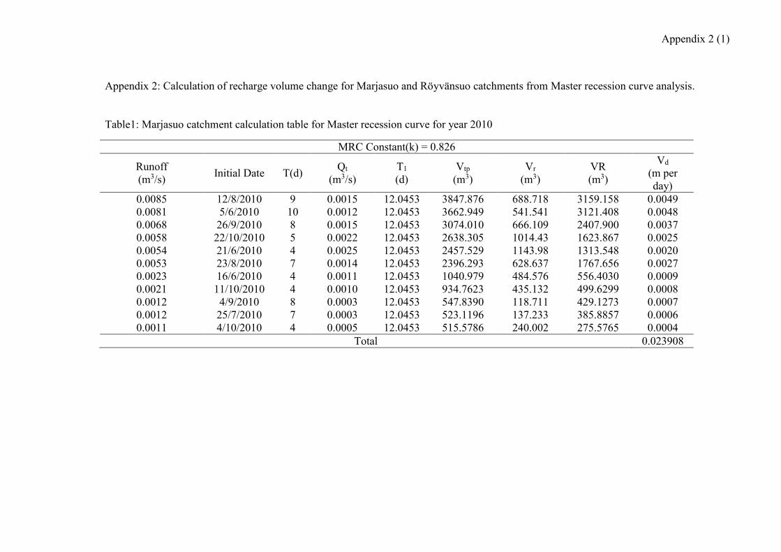
Appendix 2 (1)

Appendix 2: Calculation of recharge volume change for Marjasuo and Röyvänsuo catchments from Master recession curve analysis.

Table1: Marjasuo catchment calculation table for Master recession curve for year 2010

MRC Constant(k) = 0.826

Runoff

(m3/s) Initial Date T(d)

Qt

(m3/s)

T1

(d)

Vtp

(m3)

Vr

(m3)

VR

(m3)

Vd

(m per

day)

0.0085 12/8/2010 9 0.0015 12.0453 3847.876 688.718 3159.158 0.0049

0.0081 5/6/2010 10 0.0012 12.0453 3662.949 541.541 3121.408 0.0048

0.0068 26/9/2010 8 0.0015 12.0453 3074.010 666.109 2407.900 0.0037

0.0058 22/10/2010 5 0.0022 12.0453 2638.305 1014.43 1623.867 0.0025

0.0054 21/6/2010 4 0.0025 12.0453 2457.529 1143.98 1313.548 0.0020

0.0053 23/8/2010 7 0.0014 12.0453 2396.293 628.637 1767.656 0.0027

0.0023 16/6/2010 4 0.0011 12.0453 1040.979 484.576 556.4030 0.0009

0.0021 11/10/2010 4 0.0010 12.0453 934.7623 435.132 499.6299 0.0008

0.0012 4/9/2010 8 0.0003 12.0453 547.8390 118.711 429.1273 0.0007

0.0012 25/7/2010 7 0.0003 12.0453 523.1196 137.233 385.8857 0.0006

0.0011 4/10/2010 4 0.0005 12.0453 515.5786 240.002 275.5765 0.0004

Total 0.023908

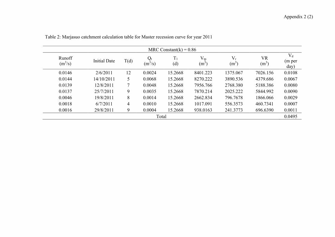
Appendix 2 (2)

Table 2: Marjasuo catchment calculation table for Master recession curve for year 2011

MRC Constant(k) = 0.86

Runoff

(m3/s) Initial Date T(d)

Qt

(m3/s)

T1

(d)

Vtp

(m3)

Vr

(m3)

VR

(m3)

Vd

(m per

day)

0.0146 2/6/2011 12 0.0024 15.2668 8401.223 1375.067 7026.156 0.0108

0.0144 14/10/2011 5 0.0068 15.2668 8270.222 3890.536 4379.686 0.0067

0.0139 12/8/2011 7 0.0048 15.2668 7956.766 2768.380 5188.386 0.0080

0.0137 25/7/2011 9 0.0035 15.2668 7870.214 2025.222 5844.992 0.0090

0.0046 19/8/2011 8 0.0014 15.2668 2662.834 796.7678 1866.066 0.0029

0.0018 6/7/2011 4 0.0010 15.2668 1017.091 556.3573 460.7341 0.0007

0.0016 29/8/2011 9 0.0004 15.2668 938.0163 241.3773 696.6390 0.0011

Total 0.0495

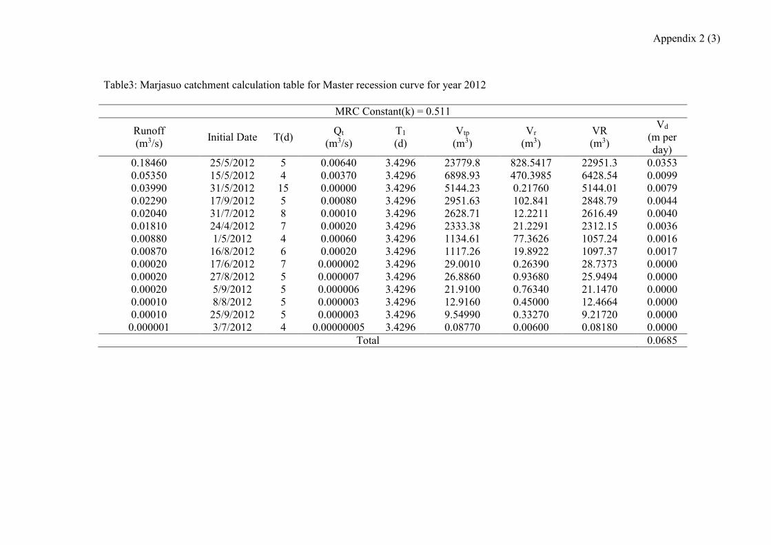
Appendix 2 (3)

Table3: Marjasuo catchment calculation table for Master recession curve for year 2012

MRC Constant(k) = 0.511

Runoff

(m3/s) Initial Date T(d)

Qt

(m3/s)

T1

(d)

Vtp

(m3)

Vr

(m3)

VR

(m3)

Vd

(m per

day)

0.18460 25/5/2012 5 0.00640 3.4296 23779.8 828.5417 22951.3 0.0353

0.05350 15/5/2012 4 0.00370 3.4296 6898.93 470.3985 6428.54 0.0099

0.03990 31/5/2012 15 0.00000 3.4296 5144.23 0.21760 5144.01 0.0079

0.02290 17/9/2012 5 0.00080 3.4296 2951.63 102.841 2848.79 0.0044

0.02040 31/7/2012 8 0.00010 3.4296 2628.71 12.2211 2616.49 0.0040

0.01810 24/4/2012 7 0.00020 3.4296 2333.38 21.2291 2312.15 0.0036

0.00880 1/5/2012 4 0.00060 3.4296 1134.61 77.3626 1057.24 0.0016

0.00870 16/8/2012 6 0.00020 3.4296 1117.26 19.8922 1097.37 0.0017

0.00020 17/6/2012 7 0.000002 3.4296 29.0010 0.26390 28.7373 0.0000

0.00020 27/8/2012 5 0.000007 3.4296 26.8860 0.93680 25.9494 0.0000

0.00020 5/9/2012 5 0.000006 3.4296 21.9100 0.76340 21.1470 0.0000

0.00010 8/8/2012 5 0.000003 3.4296 12.9160 0.45000 12.4664 0.0000

0.00010 25/9/2012 5 0.000003 3.4296 9.54990 0.33270 9.21720 0.0000

0.000001 3/7/2012 4 0.00000005 3.4296 0.08770 0.00600 0.08180 0.0000

Total 0.0685

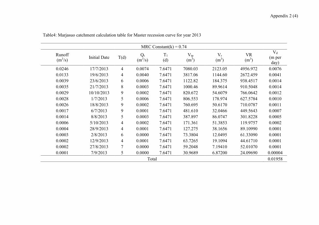
Appendix 2 (4)

Table4: Marjasuo catchment calculation table for Master recession curve for year 2013

MRC Constant(k) = 0.74

Runoff

(m3/s) Initial Date T(d)

Qt

(m3/s)

T1

(d)

Vtp

(m3)

Vr

(m3)

VR

(m3)

Vd

(m per

day)

0.0246 17/7/2013 4 0.0074 7.6471 7080.03 2123.05 4956.972 0.0076

0.0133 19/6/2013 4 0.0040 7.6471 3817.06 1144.60 2672.459 0.0041

0.0039 23/6/2013 6 0.0006 7.6471 1122.82 184.375 938.4517 0.0014

0.0035 21/7/2013 8 0.0003 7.6471 1000.46 89.9614 910.5048 0.0014

0.0029 10/10/2013 9 0.0002 7.6471 820.672 54.6079 766.0642 0.0012

0.0028 1/7/2013 5 0.0006 7.6471 806.553 178.974 627.5784 0.0010

0.0026 18/8/2013 9 0.0002 7.6471 760.695 50.6170 710.0787 0.0011

0.0017 6/7/2013 9 0.0001 7.6471 481.610 32.0466 449.5643 0.0007

0.0014 8/8/2013 5 0.0003 7.6471 387.897 86.0747 301.8228 0.0005

0.0006 5/10/2013 4 0.0002 7.6471 171.361 51.3853 119.9757 0.0002

0.0004 28/9/2013 4 0.0001 7.6471 127.275 38.1656 89.10990 0.0001

0.0003 2/8/2013 6 0.0000 7.6471 73.3804 12.0495 61.33090 0.0001

0.0002 12/9/2013 4 0.0001 7.6471 63.7265 19.1094 44.61710 0.0001

0.0002 27/8/2013 7 0.0000 7.6471 59.2048 7.19410 52.01070 0.0001

0.0001 7/9/2013 5 0.0000 7.6471 30.9689 6.87200 24.09690 0.00004

Total 0.01958

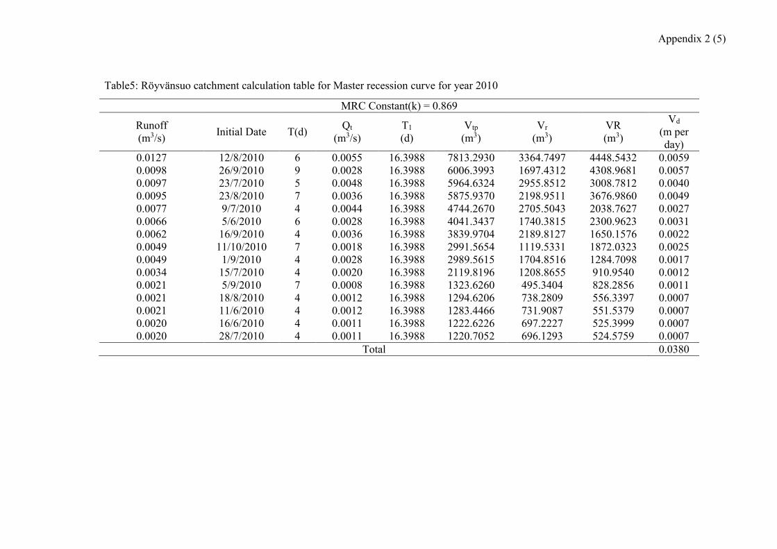
Appendix 2 (5)

Table5: Röyvänsuo catchment calculation table for Master recession curve for year 2010

MRC Constant(k) = 0.869

Runoff

(m3/s) Initial Date T(d)

Qt

(m3/s)

T1

(d)

Vtp

(m3)

Vr

(m3)

VR

(m3)

Vd

(m per

day)

0.0127 12/8/2010 6 0.0055 16.3988 7813.2930 3364.7497 4448.5432 0.0059

0.0098 26/9/2010 9 0.0028 16.3988 6006.3993 1697.4312 4308.9681 0.0057

0.0097 23/7/2010 5 0.0048 16.3988 5964.6324 2955.8512 3008.7812 0.0040

0.0095 23/8/2010 7 0.0036 16.3988 5875.9370 2198.9511 3676.9860 0.0049

0.0077 9/7/2010 4 0.0044 16.3988 4744.2670 2705.5043 2038.7627 0.0027

0.0066 5/6/2010 6 0.0028 16.3988 4041.3437 1740.3815 2300.9623 0.0031

0.0062 16/9/2010 4 0.0036 16.3988 3839.9704 2189.8127 1650.1576 0.0022

0.0049 11/10/2010 7 0.0018 16.3988 2991.5654 1119.5331 1872.0323 0.0025

0.0049 1/9/2010 4 0.0028 16.3988 2989.5615 1704.8516 1284.7098 0.0017

0.0034 15/7/2010 4 0.0020 16.3988 2119.8196 1208.8655 910.9540 0.0012

0.0021 5/9/2010 7 0.0008 16.3988 1323.6260 495.3404 828.2856 0.0011

0.0021 18/8/2010 4 0.0012 16.3988 1294.6206 738.2809 556.3397 0.0007

0.0021 11/6/2010 4 0.0012 16.3988 1283.4466 731.9087 551.5379 0.0007

0.0020 16/6/2010 4 0.0011 16.3988 1222.6226 697.2227 525.3999 0.0007

0.0020 28/7/2010 4 0.0011 16.3988 1220.7052 696.1293 524.5759 0.0007

Total 0.0380

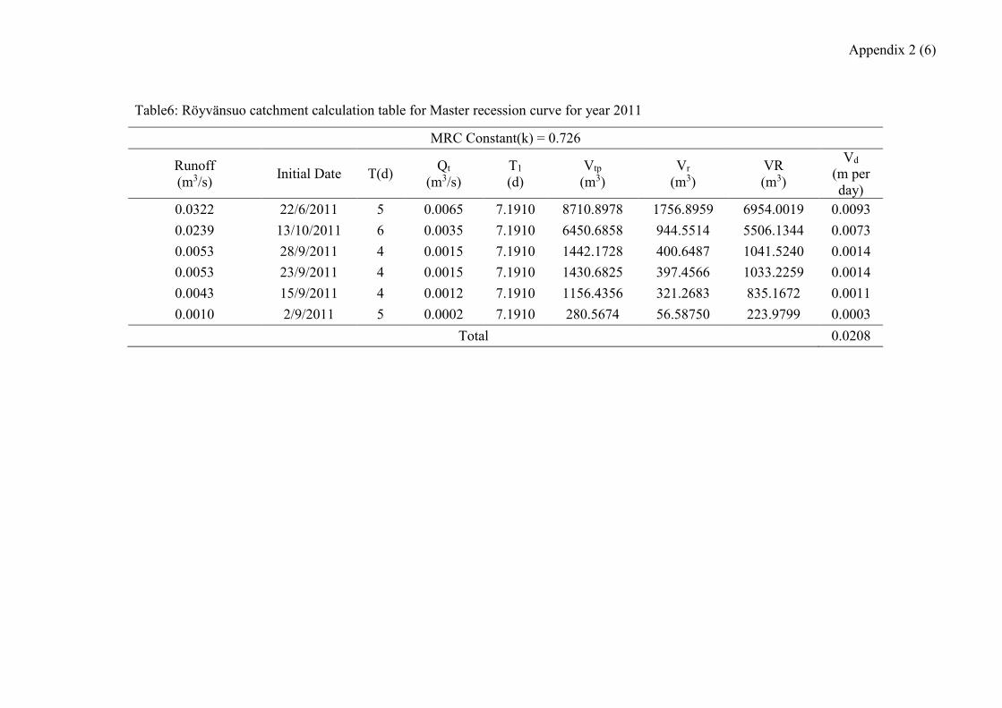
Appendix 2 (6)

Table6: Röyvänsuo catchment calculation table for Master recession curve for year 2011

MRC Constant(k) = 0.726

Runoff

(m3/s) Initial Date T(d)

Qt

(m3/s)

T1

(d)

Vtp

(m3)

Vr

(m3)

VR

(m3)

Vd

(m per

day)

0.0322 22/6/2011 5 0.0065 7.1910 8710.8978 1756.8959 6954.0019 0.0093

0.0239 13/10/2011 6 0.0035 7.1910 6450.6858 944.5514 5506.1344 0.0073

0.0053 28/9/2011 4 0.0015 7.1910 1442.1728 400.6487 1041.5240 0.0014

0.0053 23/9/2011 4 0.0015 7.1910 1430.6825 397.4566 1033.2259 0.0014

0.0043 15/9/2011 4 0.0012 7.1910 1156.4356 321.2683 835.1672 0.0011

0.0010 2/9/2011 5 0.0002 7.1910 280.5674 56.58750 223.9799 0.0003

Total 0.0208

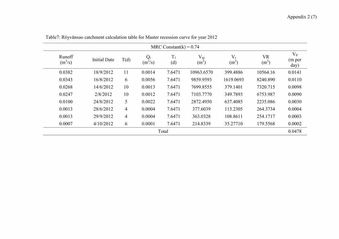
Appendix 2 (7)

Table7: Röyvänsuo catchment calculation table for Master recession curve for year 2012

MRC Constant(k) = 0.74

Runoff

(m3/s) Initial Date T(d)

Qt

(m3/s)

T1

(d)

Vtp

(m3)

Vr

(m3)

VR

(m3)

Vd

(m per

day)

0.0382 18/9/2012 11 0.0014 7.6471 10963.6570 399.4886 10564.16 0.0141

0.0343 16/8/2012 6 0.0056 7.6471 9859.9593 1619.0693 8240.890 0.0110

0.0268 14/6/2012 10 0.0013 7.6471 7699.8555 379.1401 7320.715 0.0098

0.0247 2/8/2012 10 0.0012 7.6471 7103.7770 349.7893 6753.987 0.0090

0.0100 24/8/2012 5 0.0022 7.6471 2872.4950 637.4085 2235.086 0.0030

0.0013 28/6/2012 4 0.0004 7.6471 377.6039 113.2305 264.3734 0.0004

0.0013 29/9/2012 4 0.0004 7.6471 363.0328 108.8611 254.1717 0.0003

0.0007 4/10/2012 6 0.0001 7.6471 214.8339 35.27710 179.5568 0.0002

Total 0.0478

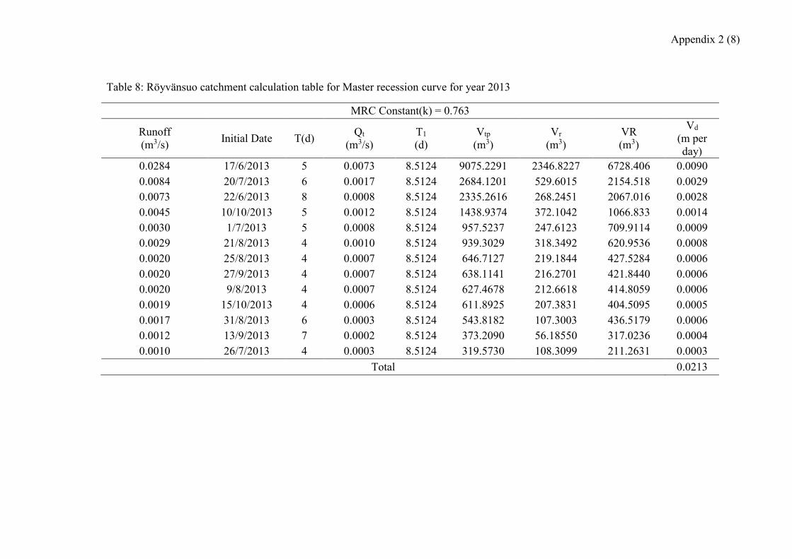
Appendix 2 (8)

Table 8: Röyvänsuo catchment calculation table for Master recession curve for year 2013

MRC Constant(k) = 0.763

Runoff

(m3/s) Initial Date T(d)

Qt

(m3/s)

T1

(d)

Vtp

(m3)

Vr

(m3)

VR

(m3)

Vd

(m per

day)

0.0284 17/6/2013 5 0.0073 8.5124 9075.2291 2346.8227 6728.406 0.0090

0.0084 20/7/2013 6 0.0017 8.5124 2684.1201 529.6015 2154.518 0.0029

0.0073 22/6/2013 8 0.0008 8.5124 2335.2616 268.2451 2067.016 0.0028

0.0045 10/10/2013 5 0.0012 8.5124 1438.9374 372.1042 1066.833 0.0014

0.0030 1/7/2013 5 0.0008 8.5124 957.5237 247.6123 709.9114 0.0009

0.0029 21/8/2013 4 0.0010 8.5124 939.3029 318.3492 620.9536 0.0008

0.0020 25/8/2013 4 0.0007 8.5124 646.7127 219.1844 427.5284 0.0006

0.0020 27/9/2013 4 0.0007 8.5124 638.1141 216.2701 421.8440 0.0006

0.0020 9/8/2013 4 0.0007 8.5124 627.4678 212.6618 414.8059 0.0006

0.0019 15/10/2013 4 0.0006 8.5124 611.8925 207.3831 404.5095 0.0005

0.0017 31/8/2013 6 0.0003 8.5124 543.8182 107.3003 436.5179 0.0006

0.0012 13/9/2013 7 0.0002 8.5124 373.2090 56.18550 317.0236 0.0004

0.0010 26/7/2013 4 0.0003 8.5124 319.5730 108.3099 211.2631 0.0003

Total 0.0213

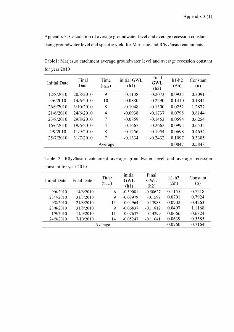
Appendix 3 (1)

Appendix 3: Calculation of average groundwater level and average recession constant

using groundwater level and specific yield for Marjasuo and Röyvänsuo catchments.

Table1: Marjasuo catchment average groundwater level and average recession constant

for year 2010

Initial Date Final

Date

Time

(tdays)

initial GWL

(h1)

Final

GWL

(h2)

h1-h2

(Δh)

Constant

(α)

12/8/2010 20/8/2010 9 -0.1138 -0.2073 0.0935 0.3091

5/6/2010 14/6/2010 10 -0.0880 -0.2290 0.1410 0.1844

26/9/2010 3/10/2010 8 -0.1048 -0.1300 0.0252 1.2877

21/6/2010 24/6/2010 4 -0.0938 -0.1737 0.0798 0.8144

23/8/2010 29/8/2010 7 -0.0859 -0.1453 0.0594 0.6254

16/6/2010 19/6/2010 4 -0.1667 -0.2662 0.0995 0.6535

4/9/2010 11/9/2010 8 -0.1256 -0.1954 0.0698 0.4654

25/7/2010 31/7/2010 7 -0.1334 -0.2432 0.1097 0.3385

Average 0.0847 0.5848

Table 2: Röyvänsuo catchment average groundwater level and average recession

constant for year 2010

Initial Date Final Date Time

(tdays)

initial

GWL

(h1)

Final

GWL

(h2)

h1-h2

(Δh)

Constant

(α)

9/6/2010 14/6/2010 6 -0.39081 -0.50627 0.1155 0.7218

23/7/2010 31/7/2010 9 -0.08979 -0.1599 0.0701 0.7924

9/8/2010 21/8/2010 13 -0.04964 -0.13988 0.0902 0.4263

23/8/2010 31/8/2010 9 -0.06837 -0.11812 0.0497 1.1168

1/9/2010 11/9/2010 11 -0.07637 -0.14299 0.0666 0.6824

24/9/2010 7/10/2010 14 -0.05247 -0.11641 0.0639 0.5585

Average 0.0760 0.7164

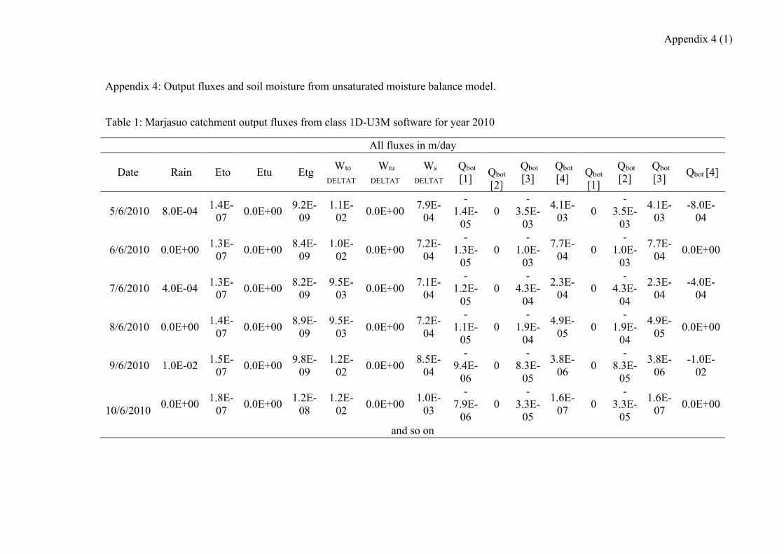
Appendix 4 (1)

Appendix 4: Output fluxes and soil moisture from unsaturated moisture balance model.

Table 1: Marjasuo catchment output fluxes from class 1D-U3M software for year 2010

All fluxes in m/day

Date Rain Eto Etu Etg Wto

DELTAT

Wtu

DELTAT

Ws

DELTAT

Qbot

[1]

Qbot

[2]

Qbot

[3]

Qbot

[4]

Qbot

[1]

Qbot

[2]

Qbot

[3] Qbot [4]

5/6/2010 8.0E-04 1.4E-

07 0.0E+00

9.2E-

09

1.1E-

02 0.0E+00

7.9E-

04

-

1.4E-

05

0

-

3.5E-

03

4.1E-

03 0

-

3.5E-

03

4.1E-

03

-8.0E-

04

6/6/2010 0.0E+00 1.3E-

07 0.0E+00

8.4E-

09

1.0E-

02 0.0E+00

7.2E-

04

-

1.3E-

05

0

-

1.0E-

03

7.7E-

04 0

-

1.0E-

03

7.7E-

04 0.0E+00

7/6/2010 4.0E-04 1.3E-

07 0.0E+00

8.2E-

09

9.5E-

03 0.0E+00

7.1E-

04

-

1.2E-

05

0

-

4.3E-

04

2.3E-

04 0

-

4.3E-

04

2.3E-

04

-4.0E-

04

8/6/2010 0.0E+00 1.4E-

07 0.0E+00

8.9E-

09

9.5E-

03 0.0E+00

7.2E-

04

-

1.1E-

05

0

-

1.9E-

04

4.9E-

05 0

-

1.9E-

04

4.9E-

05 0.0E+00

9/6/2010 1.0E-02 1.5E-

07 0.0E+00

9.8E-

09

1.2E-

02 0.0E+00

8.5E-

04

-

9.4E-

06

0

-

8.3E-

05

3.8E-

06 0

-

8.3E-

05

3.8E-

06

-1.0E-

02

10/6/2010 0.0E+00

1.8E-

07 0.0E+00

1.2E-

08

1.2E-

02 0.0E+00

1.0E-

03

-

7.9E-

06

0

-

3.3E-

05

1.6E-

07 0

-

3.3E-

05

1.6E-

07 0.0E+00

and so on

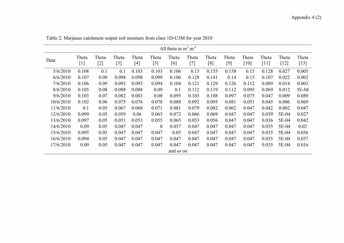
Appendix 4 (2)

Table 2: Marjasuo catchment output soil moisture from class 1D-U3M for year 2010

All theta in m3.m-3

Date Theta

[1]

Theta

[2]

Theta

[3]

Theta

[4]

Theta

[5]

Theta

[6]

Theta

[7]

Theta

[8]

Theta

[9]

Theta

[10]

Theta

[11]

Theta

[12]

Theta

[13]

5/6/2010 0.108 0.1 0.1 0.103 0.103 0.106 0.13 0.155 0.158 0.15 0.128 0.027 0.005

6/6/2010 0.107 0.09 0.098 0.098 0.099 0.106 0.128 0.141 0.14 0.13 0.107 0.022 0.002

7/6/2010 0.106 0.09 0.093 0.093 0.094 0.104 0.121 0.129 0.126 0.112 0.089 0.014 0.003

8/6/2010 0.105 0.08 0.088 0.088 0.09 0.1 0.112 0.119 0.112 0.095 0.069 0.012 5E-04

9/6/2010 0.103 0.07 0.082 0.083 0.08 0.095 0.103 0.108 0.097 0.075 0.047 0.009 0.089

10/6/2010 0.102 0.06 0.075 0.076 0.078 0.088 0.092 0.095 0.081 0.051 0.045 0.006 0.069

11/6/2010 0.1 0.05 0.067 0.068 0.071 0.081 0.079 0.082 0.062 0.047 0.042 0.002 0.047

12/6/2010 0.099 0.05 0.059 0.06 0.063 0.072 0.066 0.069 0.047 0.047 0.039 5E-04 0.027

13/6/2010 0.097 0.05 0.051 0.053 0.055 0.065 0.053 0.056 0.047 0.047 0.036 5E-04 0.042

14/6/2010 0.09 0.05 0.047 0.047 0 0.057 0.047 0.047 0.047 0.047 0.035 5E-04 0.02

15/6/2010 0.095 0.05 0.047 0.047 0.047 0.05 0.047 0.047 0.047 0.047 0.035 5E-04 0.056

16/6/2010 0.094 0.05 0.047 0.047 0.047 0.047 0.047 0.047 0.047 0.047 0.035 5E-04 0.037

17/6/2010 0.09 0.05 0.047 0.047 0.047 0.047 0.047 0.047 0.047 0.047 0.035 5E-04 0.016

and so on

Appendix 2 (5)