HYDROGEOLOGY OF A SANITARY LANDFILL, MANDAN, NORTH DAKOTA by Raymond D,. :Butler Bachelor of Science, University of North Dakota, 1970 A Thesis Submitted to the Graduate Faculty of the University of North Dakota in partial fulfillment of the requirements for the degree of Master of Science Grand Forks, North Dalwta December 1973

Welcome message from author
This document is posted to help you gain knowledge. Please leave a comment to let me know what you think about it! Share it to your friends and learn new things together.
Transcript

HYDROGEOLOGY OF A SANITARY LANDFILL,
MANDAN, NORTH DAKOTA
by
Raymond D,. :Butler
Bachelor of Science, University of North Dakota, 1970
A Thesis
Submitted to the Graduate Faculty
of the
University of North Dakota
in partial fulfillment of the requirements
for the degree of
Master of Science
Grand Forks, North Dalwta
December 1973

··r·1 I •·
This thesis submitted by Raymond D. Butler in partial fulfillment of the requirements for the Degree of Master of Science from the University of North Dakota is hereby approved by the Faculty Advisory Committee under whom the work has been done.
Dean of the Graduate School
ii

Permission
Title __ HYD=-R....;.;..OG.;..;E;...O;.;;;L:;:;.;;O;..;;G;.;;;Yc....._O.;;;.F_Ac.:;;._S;;;..;;AN=I;;..:;T;;;;.'.A.R=Y;.....=:LAND=;;;;;iF:..:I:::.:LL=,:.....;;.;:r,.,r..AN=ID.;;;.AN=.:..,_, -:N:.c..O:.,;;;R.;;.:TH;;:;.::....;;;.DAK;;..:. =.::.OT;;;;;'A;.:;_.. __
In presenting this thesis in partial fulfillment of the requirements for a graduate degree from the University of North Dakota, I agree that the Library of this University shall make it freely available for inspection. I further agree that permission for extensive copying for scholarly purposes may be granted by the professor who supervised my thesis work or, in his absence, by the Chairman of the Department or the Dean of the Graduate School. It is understood that any copying or publication or other use of this thesis or part thereof for financial gain shall not be allowed without my written permission. It is also understood that due recognition shall be given to me and to the University of North Dakota in any scholarly use which may be made of any material in my thesis.
Signature (l<c~d., LJ, Q ~ Date ~~~~'-'-;{5J~t.t~' 1~l2~~~;:=.c..;...;v&::..=....·-t_~,~L,"'--~~4..--•c....'t,~Y~1~~J::;,_,.
iii

ACKNOWLEDGEMENTS
I am grateful to individuals and organizations who offered
assistance and support during this study. All the members of my
committee, Lee Clayton, S·tephen R. Moran, and Frank R. Karner are
gratefully acknowledged £or their useful criticisms and suggestions
during the course of this project.
Mr. Phil Ra.ndich of the U.S. Geological Survey, :Bismarck,
North Dakota and Frank Schulte, formerly of the University of North
Dakota, are acknowledged for their useful advice and information
regarding this study.
I would like to thank the City of Mandan and private landowners
for allowing drilling in the Mandan landfill area.
I would like to thank my wife, Susan, for her assistance and
encouragement throughout the project.
I am grateful ·1:;o the North Dako·l:;a Geological Survey for field
support during the summer of 1972.
I am also g:t"ateful to Zachmaier Well Drilling, Mandan, North
Dakota for allowing drilling time during their busy season.
iv
TABLE OF CONTENTS
ACKNOWLEDG.EMENTS. • • • • • • . . • • • • • • • • • • • • • •
LIST OF TABLES. • • • • • • • • • • • • • • • • • • • • • • •
LIST OF ILLUSTRATIONS • • • • • • • • • • • • • • • • • • • •
.ABSTP .. A.CT • • • • • • • • • • • • • . . • • • • • • • • • • • •
Cri..a.pter I.
II.
III.
IV.
INTRODUCTION • • • • • • • • • • • • • • • • • • • • •
Purpose. Location Topography Climate .. Soil •• Vegetation
• •
• • •
• •
• • • • • •
• • •
• • • • • • • •
•
• • • •
• • • • • •
• • • •
• • • • • •
• •
GEOLOGY. • • • • • • • •
Pre-Pleistocene Geology. Pleistocene Geology ••• History •••••••••
• • •
• • •
• • • • • •
•
• • •
• • • • •
• • • • • •
• • • •
•
• • • • • •
• • • •
• • • • . . • • • •
GEUE.1:lAL INFORMATION ON THE ¥..ANDAN LANDFILL
Terminology. History ....
• • .. . • •
• • • • •
• • • • . . •
• • •
•
• • • • • •
• • • • • •
• • • • • •
• • •
• • • • • • • . ..
• • • • • •
•
• •
• • • • •
• • • • •
•
• • •
• • • • • • • • •
• • • • • •
• • • • • • • • • • . . .
GROUNDWATER THEORY • • • • • • • • • • • • • • • • • •
Introduction ••••••••• Terminol'ogy • • • • • • • • • •
Flow-System Terminology ••• Water-Chemistry Terminology.
Groundwater Flow ••••••• Eerrioulli Theorem ••••••
• • • •
Darcy's Law •••••••••• Continuity and Laplace Equations
Groundwater Flow Models ••••• Groundwater Chemistry ••••••
V
• • • •
• •
•
• • • •
• • • • •
• • • • • • • • .. •
• • •
• • •
..
• • • • • • • • • •
• • • • • • • • • • • • • • •· . • • • •
• • • •
• • • • •
• • • • • • • • • •
•
• • • • • • • •
Page
iv
vii
viii
X
1
1 2 5 5 8 8
13
13 18 21
23
23 24
28
28 29 29 32 32 33 34 34 35 37
\ \
v.
VI.
GROUNDWATER OF THE MANDAN LANDFILL . ARE...\ . . . . . . . . . 41
Introduction • • .• • • • • • • • • • • • • • • • • • • 41 Field Studies. • • • • • • • • • • • • • • • • • • • 41 Laboratory Methods • • • • • • • • • • • • • • • • • 45
Groundwater Flow. • • • • • • • • • • • • • • • • ! . . 45 Local and Intermedi.a.te Flow Systems. • • • • • • • • 48 Regional Flow System • • • • • • • • • • • • • • • • 54 Deeper Regional Flow System. • • • • • • • • • • • • 55
Groundwater Chemistry. • • • • • • • • • • • • • • • • 56 Water Chemistry of Uncontaminated Groundwater. • • • 56 Water Chemistry of Canta.mi.Dated Groundwater. • • • • 58 Factors of Leachate Generation • • • • • • • • • • • 63
CONCLUSIONS • • • • • • • • • • • • • • • • • • • . . . . APPENDIX A: Methods of Data Collection and Analysis • • • . .. . .
72
75
APPENDIX B: Lithologic Logs of .Test Holes in tha Mandan Landfill Area. • • • • • • • • • • • • • • • • • • 92
APPENDIX C: Physical Well Data ••••••••••••••••• 106
APPENDIX D: Chemical Data (in ppm)
RE!FERENCES • . . . . . . . . . . -· .
vi
. . . . . . . . . . . . . . . • • • . . . . • • . . . . . .
112
119
LIST OF TAELES
Table
1. Clim.a.tic data. for Y.iandan, North Dakota, 1915 to 1972 . . . .
2. Na.mes and characteristics of soils in the Mandan landfill study area •••••••••••••••••
. .
Page
7
10
3. Stratigraphic column of the :Bismarck-Mandan area • • • • • 14
Chemical analyses of shallow groundwater from the Coteau Formation in the Mandan landfill area. (in ppm)
vii
. . 60
t.
LIST OF ILLUSTRATIONS
Fig,..ire
1 • Map Showing the Location of the f1andan Landfill Study Area • • • • • • • • • • • • • • • • • • • • • • • •
2. Aerial Photograph of the Mand.an Landfill Area Looking Southwest ••••••••••••• . . .
3. Photograph of the Mandan Landfill Looking Southeast
Soil Map of the Mand.an Landfill Study Area, Modified From the 1936 Soil Map of Morton County-Ea.stern Sheet, Compiled by the United States Department of Agriculture and North Dakota Agricultural
• • • •
. . . .
Station • • • • • • • • • • • • • • • • • • • • • • • • •
Page
3
4
,6
9
5. Map of the Surficia.l Geology of the Mand.an Landfill Area • • 19
6. Photograph of the Method of Filling of the Mandan Landfill ••••••• • • • • • • • • • • • • • • • • • • 26
7. Diagram Showing the History of Filling of the Mandan Landfill, 1950 to 1973 ••••••••• • • • • • • • • • 27
8. Theoretical Flow Pattern and :Boundaries Between Different Flow Systems •••••••••••••••••• 36
9. The Prairie Profile • • • • • • • • • • • • • • • • • • • • 38
10. Hydrochemical Model for Regional Groundwater-Flow Systems • • • • • • • • • • • • • • .. • • • • • .. • • • • 40
11.
12.
Map Showing the Location of Recharge and Discharge Areas and Wells in the Study Area •••••••• • • • •
Photograph of a Multiple Piezometer Installation . . . • • •
Map Showing the Pattern of Local Groundwater-Flow Syst3ms in the Mandan Landfill Area •••••••
Map Showing the Pattern of Intermediate GroundwaterFlow System in the Manda.11. Landfill Ar~a • • • • •
• • • •
. . •- . Geology and Pattern of Groundwater Flow in the Mandan
Landfill.Area Along Cross-Section A-A' (Fig. 11) •• • • •
viii
43
44
46
47
49
Figure
16. Map Showing Values of Chloride and Total Dissolved Solids for Shallow Wells in the Mandan Landfill Area
17. Temperature Profiles for Air and Refuse Cells in the Mandan Landfill (modified from van Derwerker,
. . .
1952 ••••••••••••••• • • • • • • • • • • • •
Page
59
70
18. Diag.r:am Showing the Location Format • • • • • • • • • • • • 77
ix
ABSTRACT
The data from this study can be applied to much of southwestern
North Dakota because the geologic and climatic conditions are similar.
The I'1andan landfill is on the Heart River floodplain and next
to the river on the north and steep valley wall on the south. The
sanitary landfill bas been used for over 20 years.
The only pre-Pleistocene unit exposed is the Cannonball For.::nation,
which is interbedded sand, silt, and clay. Quaternary units consist of
till, fluvial sand, silt, clay, and gravel, and eolian sand and silt.
A local flow system recharges on the upland next to the valley and
discharges in the valley. Flow is mostly lateral and toward the river.
An intermediate flow system discharges in the Missouri River valley and
ma.y receive seepage from local flow systems.
Shallow groundwater near the landfill is generally a calcium
bicarbonate type. Deeper groundwater is generally a sodium bicarbonate
sulfate type.
Shallow g:r."Oundwater bas been contaminated by landfill leachate.
Greatest changes in groundwater occur near the center of the landfill,
where there are increases in calcimn, magnesium, total hard.ri.ess,
bicarbonate, total alkalinity, total dissolved solids, and chloride
and decreases in sulfate and pH.
Leachate production is low because of lack of moisture, low
temperature, and large amounts cf cellulose-based refuse. Recharge
rarely occurs, but some parts of the landfill receive enough moisture
X
.from groundwater and infiltration to produce leachate. The greatest
amount o.f decomposition (mostly anaerobic) occurs soon after burial.
xi
CHAPTER I
INTRODUCTION
North Dakota is a state with limited groundwater and surface
water resources. These resources should be protected from pollution
including pollution from sanitary landfills.
Purpose
This is a report on the hydrogeology of a. sanitary landfill at
Mandan, North Dakota. The purpose of the report is to provide data
on the generation and movement of landfill leachates in this geologic
and climatic setting. This information can be applied to landfills in
much of the rest of southwestern North Dakota.
Detailed information on leachates from landfills in most of North
Dakota is not available. The contamination of the small amou.".lt of
available water may create social and economic problems. New
industrial developments resulting from increased lignite production
may create waste-disposal problems for several communities in south
western North Dakota.
The Mandal.1 landfill was selected for study because of its long
use and because it is in a geologic and climatic setting simi.la.r to
that of most of southwestern North Dakota. The landfill has been in
operation for 20 years. This should be enough time for any ground
water to have migrated far enough away from the landfill to evaluate
the environmental impact.

2
'·'-Part of the problem was to describe the geology and hydrogeology
of the study area. The surficial geology was mapped on aerial photo
graphs (scale: 1 to 4000). Info:r:mation was obtained by walking the
area, shoveling, hand augering, continuous-flight augering, and
hydraulic rotary drilling. County soil maps and U.S. Geological
Survey topographic maps were used. Well elevations were dete:rmined
by the transit-stadia. method.
Drilling was used to determine the subsurface geology and
to install piezometers. The groundwater flow rate, direction, and
quality were dete:rm.ined. Single and multiple piezometer installations
were used to determine permeabilities, to monitor water levels, and
to collect water samples.
The problem also involved determining the environmental impact
of the landfill. Changes in the dynamic groundwater flow system were
monitored by piezometers. Changes in water quality were dete:rmined
by chemical analyses.
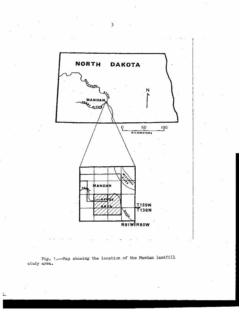
Locati.on
The study area is south of the city limits of Mandan (Figures 1
and 2) in sections ,4 and 35 of T.139 N., R.81 W., and in the northern
half of sections 2 and 3 of To138 N., R.81 W. The site is on the lower
end of ·the Heart River basin where the Heart River valley joins the
Missouri River valley.
l>'T.and.an has a population of about 11,100 (North Dakota Highway.
Department, 1972). The area is largely rural, and farming and gm.zing
are the major industries. The landfill serves the city of Mandan and
nearby area.
3
NORTH DAKOTA
N
f 50 100
KllOMITIUl$
R81W RBOW
Fig. 1.--P,a.p showing the location of the Mandan landfill study area.
4
\
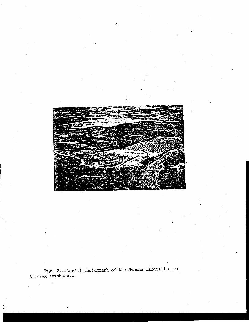
Fig .. 2.-Aerial photograph of the Mandan land£ill area looking southwest..
5
Topography
The landfill is on the floodplain of the Heart River (Figure 3).
The south bank of the river bord.ers the north flank of the landfill.
On the south and west, a steep valley wall rises 35 m to a rolling
upland.
Climate ·~.
Mandan lies on the boundary of a dry subhumid, continental
climate to the east and a semiarid climate to the west. The winters
are long and cold; the summers are short, hot, and dry. Climatic
data for the 57 year period 1915 to 1972 and for 1972 are summarized
in Table 1.
The temperature at Mandan varies considerably throughout the
year. A record high of 45.5°c (114°F) and a low of -42.8°C (-45°F)
has been recorded. The mean annual temperature for the 57 year period
is 5°c (41°F). January has a mean daily temperature of -13.3°c (8°F)
and in July it is 21.7°C (71°F). Short, hot spells occur in July and
August. Normally the ground is frozen to a depth of 1 m :from
November to April.
The precipitation is irregular and seasonally distributed. Mean
annual precipitation is 400 mm (15.9 inches) of which 70 percent
occurs between April and August. During 1972 the seasonal precipitation
(April to September) was about 25 mm (1 inch) less than normal.
Thunderstorms are common during the warmer months.
Normally the maximum precipitation of 70 mm (3.5 inches) occurs
in June. December, January, and February each receive only about
10 mm (o.4 inches) of precipitation.

6
Fig. 3.-Photogra.ph of the Mandan land.fill looking southeast.

""
TABLE 1
CLIMA.TIC DA.TA FOR MA.NDAN, NORTH DAKOTA, 1915-197Z}
Daily Month Precipitation,mm Temperature,°C Pan Evaporation,mm Wind Velocity,m/s
1915-1971 1972 1915-1971 1972 1915-1971 1972 1915-1971 1972 (Mean) (Total) (Min.) (Max.) (Mean) (Mean) (Mean) (Total) (Mean) (Mean)
Jan 9,9 .13.2 -18,9 - 7.s -13,3 -15,6 • • • • 2.2 1.8
Feb 10,2 6.6 -16.1 ;_ 4.4 -10,6 -13,9 • • • • 2.3 1.6
Mar 17.e 26,4 - 8.9 2,2 - 3,3 - 3.9 • • • • 2.6 1,8
Apr 37,6 57.9 - o.6 12.2 6.1 4.4 97.3 78,0 3,0 1,7 -.J
May 54.4 ·63,3 5,6 19,4 12,8 13,9 175.8 159.5 2,8 1,5
Jun 88.9 47.5 11.1 23.9 17,8 17.8 181,9 186,4 2,2 1,4
Jul 60.7 55,6 14~4 2s.9 21,7 18,3 235,5 184,9 1.8 1.0
Aug l1.J. 2 31.2 12.8 28,3 20.6 18,9 217.2 216.7 1,9 1.2 _,,., ... _
Sep 35.3 19.9 6,7 21.7 14.4 12.s 132,3 145,8 2,1 1.3
Oct 22.1 51,3 o.6 14.4 13.3 3.9 • • • • 2.2 1.4
Nov 13.7 -.7,8 3.9 - 2,2. • • • • 2.2
Dec 9.7 -15,0 - 3.9 - 9.4 • • • • 2.1
Total · 403.5 1040.0 971, 3
* Recorded a.t Northern Great Plains Research . .C~nter, Mandan, North Dakota,

8
Evaporation is hig.l;. from April to September. Potential evaporation
is about 750 mm (30 inches). The potential evaporation minus the mean
annual precipitation is about 350 mm (14 inches), leaving a soil moisture
deficiency most of the year. The mean seasonal evaporation of 670 mm
(27 inches) for 1972 was close to the 57 year mean •
. The prevailing wind is from the northwest. It averages about
2.4 m/s (5 miles an hour) from April to Augu.st. Winds are strongest
during the spring and gentlest during the summer.
The growing season is about 124 days long. It starts about Ma.y
19 and ends about September 20.
Chestnut soils, regosols, and lithosols occur on the uplands.
A humic gley and several types of alluvial soils occur on the bottom
lands (Figure 4 and Table 2).
Most of the upland soils have good to excessive surface drainage.
The permeabilities are generally fair to high. Bottom.land soils range
from well drained to poorly drained. The permeabilities are low to fair.
In general most of the soils are loose and friable. This makes
them highly susceptible to wind and water erosion.
The upland soils are less fertile than the bottom.land soils. In
general the uplands are used for grazing and the bottom.lands are
planted with alfalfa and are grazed.
Vegetation
The Heart River bottomland has a thick natural forest of cotton
wood, ash, boxelder, and a field of alfalfa (Figure 2). Willows
9
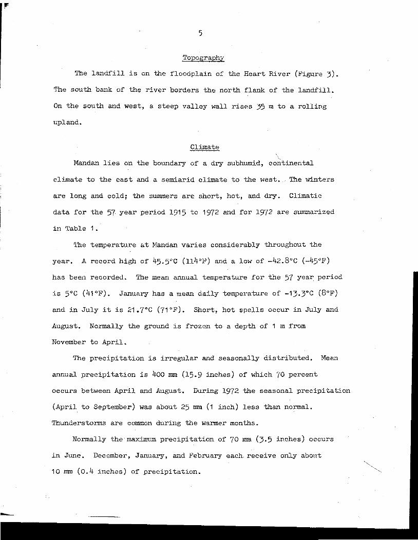
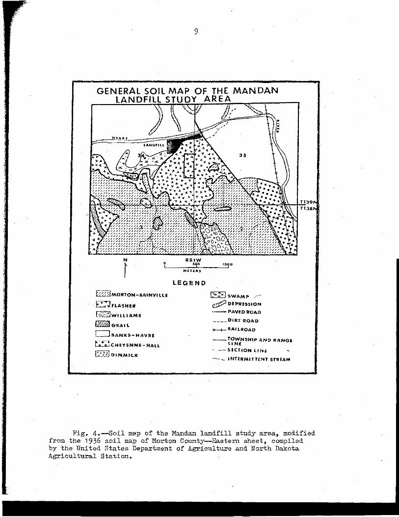
GENERAL SOIL MAP OF THE MANDAN LANDFILL STUDY AREA
HtAlli
N
f 0 I
~~Vi~IMORTON-BAINVtllE
~FLASHER
~WILLIAMS
fDGUII.
c=J BANKS-HAVRE
E •• pjCHEYENNE-HALL
K<:JI OIMMIC.K
R81W sqo
METER$
LEGEND
IE_3 SWAMP /
~ DEP!U!SSIOH
-PAVl!DROAD
----DIRT ROAD
+-+-RAILROAD
__ TOWNSHIP AN!> RANGE LINE
-- SECTION llNE
-~- INTERMITTENT STREAM
Fig. 4.~Soil map of the ~..andan landfill study area, modified from the 1936 soil map of Morton County~Eastern sheet, compiled by the United States Department of Agriculture and North Dakota Agricultural Station.

TABLE 2
NAMES AND CHARA.GTERISTICS OF SOILS IN THE MANDAN IANDFILL STUDY AREA.
Property Williams Morton Bainville Flasher Hall
Parent Material till, sandy silt, clay silty, clay sand, silt alluv:i.um, malium clayey to fine
Texture silt loam loam loam to clay fine sandy loam, silt loam loam loam to loamy
fine sand
Position ridge tops undulating rolling hilly.to steep terrace upland upland broken upland _,,
0 Slope 6-9% 3-8% 10...:30% 15-00% 3-6%
Surface moderately well drained excessively well to excess- well drained Drainage · well drained drained ively drained
' Other Charac- calcareous, calcareous\ calcareous, fair to good fair to good teristics fair permea- fair permea- fair permea- permeability permeability
bility bility bility
Group Name Chestnut Chestnut Regosol Lithosol Chestnut (Edwards and others, 1951)
7th Approxi- Typic Typic Typic Entic Typic mation Group Argiustoll Haploboroll Ustorthent Haplustoll Haplustoll Name (Patterson and others, 1968)
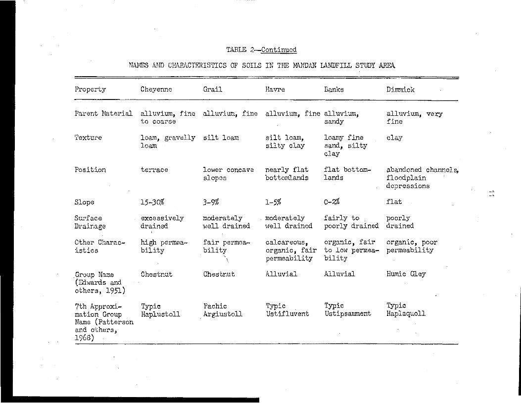
TABLE 2--Continued
NAMES AND CHARACTERISTICS OF SOILS IN THE MANDAN LANDFILL STUDY A.REA.
Property Cheyenne Grail Havre Banks Dimmick
Parent Material alluvium, fine alluvium, fine alluvium, fine alluvium, alluvium, very to coarse sandy fine
Texture loam, gravelly silt loam silt loam, loamy- fine clay loam silty clay sand, silty
clay
Position terrace lower concave nearly flat flat bottom- abandoned channel~ slopes bottomlands lands floodplain
depressions -' -'
Slope 15-30% 3-9% 1-5% o-~ flat
Surface excessively moderately moderately fairly to poorly Drainage drained well drained well drained poorly drained drained
Other Charac- high permea- fair permea- calcareous, organic, fair organic, poor istics bility bility organic, fair to low permea- permeability
permeability bility
.Group Name Chestnut Chestnut Alluvial Alluvial Humic ffi.ey (Edwards and others, 1951)
7th Approxi- Typic Pachic Typic Typic Typic ma tion Group Haplustoll Argiustoll Ustifluvent Ustipsarument Haplaquoll Name (Patterson and others, 1968)

12
grow along the river baxlks. Depressions in the floodplain contain
willows and marsh grasses.
The steep valley walls and gullied slopes are covered with oak,
ash, elm, chokecherry, and poison ivy. Upper reaches of the gullies
contain bu.ffaloberry, buckbrush, and wild rose.
Native short and tall grasses grow on the uplands. Western
wheatgrass, blue gamma, and needlegrass are common. A young forest
of cottonwood grows on the northern part of the uplands.
The landi'ill has no vegetation on its upper surface. Sparse weeds
and bushes grow on its flanks.

CHAPTER II
GEOLOGY
':t(· > • -~-
About 2700 m of Paleozoic,1and Cenozoic sediment occurs in the
Bismarck-Mandan area. The Cannonball Formation is the only pre
Pleistocene unit exposed. Several Quaternary formations as defined
and described by Bickley (1972) and mapped by Groenewold (1972) are
present. They are the Braddock, Four Bears, Coteau, Denbigh, and
Oahe Formations.
Pre-Pleistocene Geolog:.y:
Stratigraphic information on the Paleocene and Quaternary \Ulits
was obtained by te~t drilling and from lithologic logs (Groenewold,
1972). Information on the Cretaceous units was obtained from the
geology report of Burleigh County (Ku.me and Hansen, 1965) and basic
data report (Randich, 1965). The stratigraphic column of the
Bismarck-Mandan area is given in Table 3.
The Dakota Group (early Cretaceous) is the oldest stratigraphic
unit considered in this report. It occurs at a depth of 933 m to
1066 min Burleigh County. It is a massive marine sandstone ranging
in thickness from 37 to 100 m.
The Pierre Formation (late Cretaceous) consists of dark-gray
marine shale about 335 m thick in Burleigh County. The upper part of the
Pierre is often fractured and contains some sandy lenses (Randich, 1965).
The top of the Pierre in the study area is at a depth of 373 m.
13
14
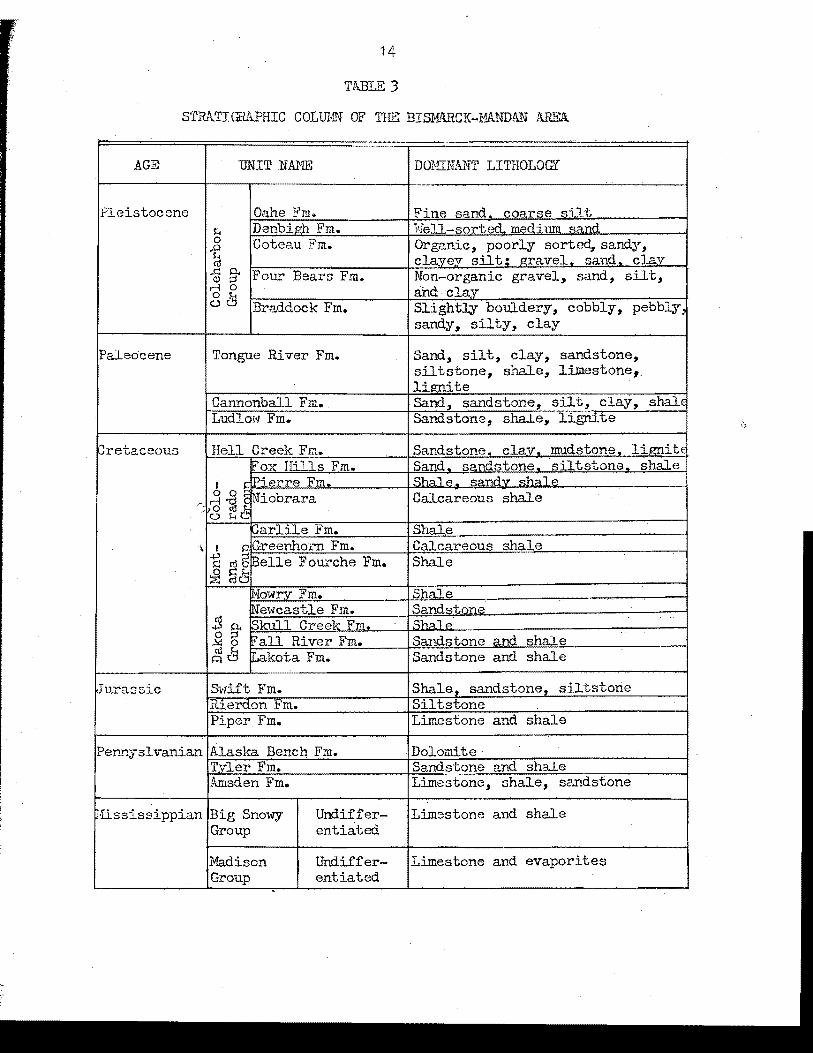
TABLE 3
STRA.TIGRAPHIC COLUMN OF THE BISMARCK-MANDAN AREA.
AGE DNIT NAME D01-ITNANT LITHOLOGY
Pleistocene Oahe Fm. Fine sand. coarse "lilt H Denbigh Fm. Well sorter! m~diu.m l'l.::rnd 0 Coteau Fm. Organic, poorly sorte~ sandy, -e ct! clayev silt! goravel. sand .. clav
rG p., Four Bears Fm. Non-organic gravel, sand, silt, C) ::::s rl 0 and clay g~ Braddock Fm. Slightly bouldery, cobbly, pebbly1
sandy, silty, clay
!Paleocene Tongue River Fm. Sand, silt, clay, sandstone, siltstone, shale, limestone, lir:mite
Cannonball Fm. Sand, sandstone, silt, clay, shaJ.E Ludlow Fm. Sandstone, shaJ.e, lignite
K:retaceous Hell Creek Fm .. Sandstone. clav. mudstone~ liP"nitE ;;,OY Hi1 ls Fm. Sand- sandstone. siltstone. shale
I f: Pierre Fm. c:n,"11..,. "'"'"'"hr "',..,"' 1"' 0 0:;: :Jiobrara Calcareous shale .-rl1a} ',O
. 0 Ht.:
1..iarlile Fm. Shale \ I Q Greenhorn Fm. Calcareous shale
-P ~ Belle Fourche Fm. Shale i:-.1 ['j 0 0 §rS ~
ilfowrv Fm. Sh<>l"" Newcastle Fm. Sand.~tn.,..,,:,
ro Skull Creek Fm. _qh;:\1,::, -i-) 0.. 0:::, ri'all River Fm. Sandstone and shale ,.!4 0
~lg Lakota Fm .. Sandstone and shale
~u.rassic Swift .Fm. Shale. sandstone .. siltstone Riera.on Fm. Siltstone Piper Fm. Limestone and shale
D - 1 • i er..n;y s-vanian Alaska Bench Fm. Dolomite
Tyler Fm. Sandstone and shale Amsden Fm. Limestone, shale, sandstone
~tis sis si ppian Big Snowy Undiffer- Limestone and shale Group entiated
Madison Undiffer- Limestone and evaporites Group entiated
.

15
TABLE 3--Continued
STRATIGRAPHIC COLUNN OF THE BISM.l'ffiGK...,MANDAN AREA.
AGE UNIT NAME DOMINANT LITHOLOGY
Devonian Birdbear Fm. Limestone Duperow Fm. Limestone Souris Bay Fm. Dolom.i te and .L.i.mestone Dawson Bay Fm. Dolomite and limestone
Silurian Interlake Fm. Dolomite Stonewall Fm. Limestone and dolomite
Ordovician Stonv Mountain Fm. Limestone Red River Fm. Limestone and do.Lomite Winnepeg Undiffer- Sandstone, shaie siltstone Group entiated
Ca.l!lbro- Deadwood Fm. Sandstone, shale, limestone Ordovician
Precambrian Granite
16
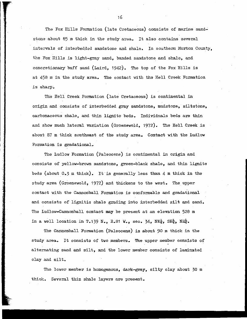
The Fox Hills Formation (late Cretaceous) consists of marine sand~
stone·about 85 m thick in the study area. It also contains several
intervals of interbedded sandstone and shale. In southern Morton County,
the Fox Hills is light-gray sand, banded sandstone and shale, and
concretionary buff sand (Laird, 1942). The top of the Fox Hills is
at 458 m in the study area. The contact with the Hell Creek Formation.
is sharp.
The Hell Creek Formation (late Cretaceous) is continental in
origin and consists of interbedded gray sandstone, mudstone, siltstone,
carbonaceous shale)' and thin lignite beds. Individuals beds are thin
and show much lateral variation (Groenewold, 1972). The Hell Creek is
about 8.7 m thick southeast of the study area. Contact with the Ludlow
Formation is g:ra.da.tional.
The Ludlow Formation (Paleocene) is continental in origin and
consists of yellow-brown sandstone, green-black shale, and thin lignite
beds (about 0.3 m thick). It·is generally less than 4 m thick in the
study area (Groenewold, 1972) and thickens to the west. The. upper
contact with the Cannonball Formation is conformable and gradational
and consists of lignitic shale grading into interbedded silt and sand.
The Ludlow-Cannonball contact may be present at an elevation 528 m
in a well location in T.139 N., R.81 W., sec. 34, NEi, SE!,. Nfili.
The Cannonball Formation (Paleocene) is about 90 m thick in the
study area. It consists of two members. The upper member consists of
alternating sand and silt, and the lower member consists of laminated
clay and silt.
Th~ lower member is homogenous, dark-gray, silty clay about 30 m
tl:iick. Several thin shale layers are present.
17
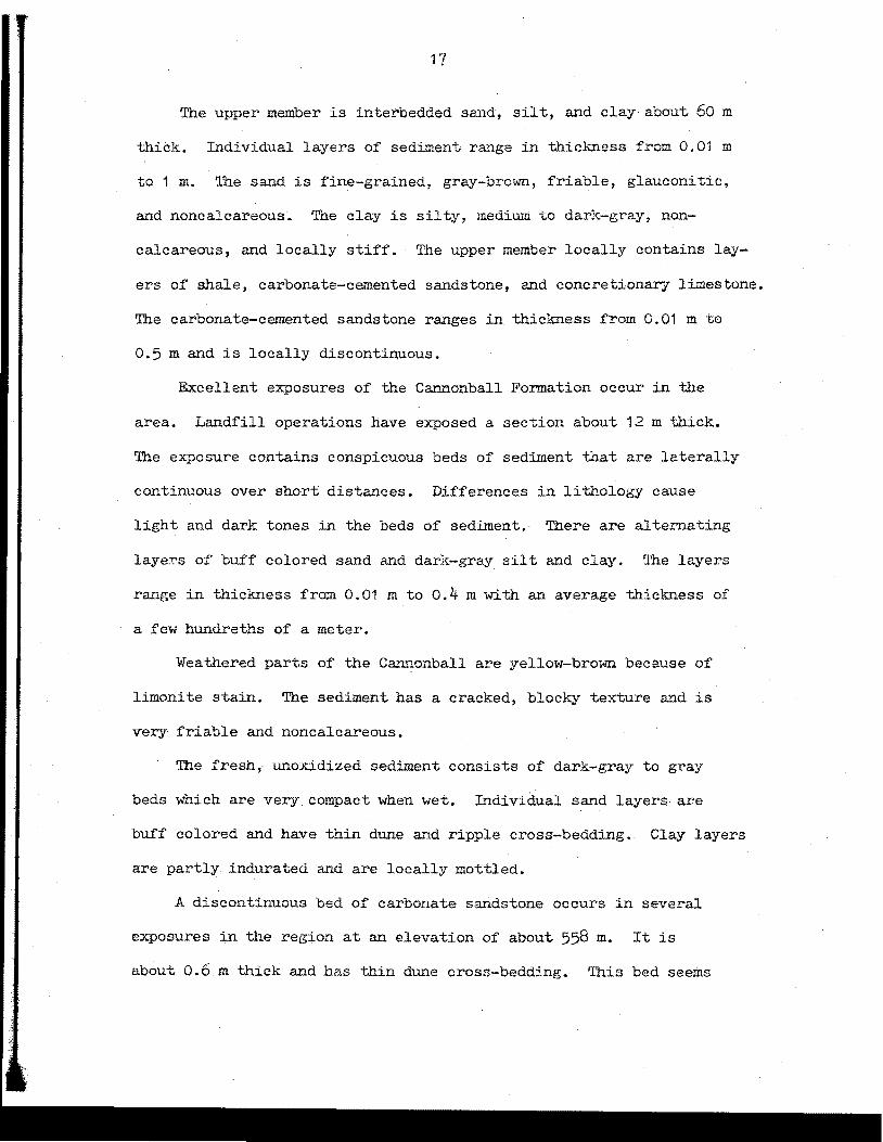
The upper member is interbedded sand, silt, and clay about 60 m
thick. Individual layers of sediment range in thickness from 0.01 m
to 1 m. The sand is fine-grained, gray-brown, friable, glauconitic,
and noncalcareous. T'.ae clay is silty, medium to dark-gray, non-:
calcareous, and locally stiff. The upper member locally contains lay
ers of shale, carbonate-cemented sandstone, and concretionary limestone.
The carbonate-cemented sandstone ranges in thickness from 0.01 m t0
0.5 m and is locally discontinuous.
Excellent exposures of the Cannonball Formation occur in the
area. Landfill operations have exposed a section about 12 m thick.
The exposure contains conspicuous beds of sediment that are laterally
continuous over short distances. Differences in lithology cause
light and dark tones in the beds of sediment. There are alternating
layers of buf'f colored sand and dark-gray silt and clay. The layers
range in thickness from 0.01 m to o.4 m with an average thickness of
a few hundreths of a meter.
Weathered parts of the Ca.11nonball are yellow-brown because of
limonite stain. The sediment has a cracked, blocky texture and is
very friable and noncalcareous.
The fresh, unoxidized sediment consists of dark-gray to gray
beds which are very compact when wet. Individual sand layers are
buff colored and have thin dune and ripple cross-bedding •. Clay layers
are partly indurated and are locally mottled.
A discontinuous bed of carbonate sandstone occurs in several
exposures in the region at an elevation of about 558 m. It is
about 0.6 m thick and has thin dune cross-bedding. This bed seems
18
to be regionally persistent. Laird (1942) reported a concretionary
sandstone bed forming a topographic her.ch in southern Morton County.
Hall (1958) also noted a concretionary layer about the same elevation
in the area.
The Cannonball Formation is mostly offshore and nearshore
sediment in the study area.
Pleistocene Geology
Quaternary stratigrapbj.c units present i."l the study area are the
Braddock, Four Bears, Coteau, Oenbigh, and Oahe Formations (Bickley,
1972). They consist of alluvial, colluvial, and eolian sediment.
Figure 5 is a map of the surficial geology of the area.
The Braddock Formation is olive-drab glacial till. It consists
of boulde:ry, cobbly, pebbly, sandy, silty, clay and reaches a
maximum thickness of 1 m on the upland area. Much of this unit has
been removed by erosion leaving scattered granitic boulders over
parts of the upland. The Braddock may be Wisconsinan in age.
The Four Bears Formation occurs as an elevated terrace deposit
15 m above the floodplain on the south side of the Heart River valley.
J.n excellent exposure occurs near the landfill. It consists of a
northwest-southeast trending channel deposit buried by sand and silt
of the Oahe Formation. The cha.n...-,.el is incised 16 m' into the Can.>1.onball
Formation to the. top of a carbonate-cemented sandstone bed. The deposit
is m thick and consists of two facies. The lower facies is buff-
colored sand with :flat-bedding, tabular-bedding, and cross-bedding.
Organic :fragments occur on bedding sur~aces in parts of the deposit.
Coal pebbles, clay pebbles, and gastropod fragments are also abundant

19
MAP OF THE SURFACE GEOLOGY OF THE MANDAN LANDFILL STU DY AREA
N
i y R81W
sq11 MtTIRS
LEGEND
mcANNONBALL FM •• 51U'l'CLA'I' AND CLAY
r:::;}CANNONBAl.t. fM.,HLTY,CUY!T SAND
ITTI:E1 FOUR lliARS FM., till AND UND
~FOUR BEARS FM., ~AND AND GOAVH
~OAHE FM •• uu AND SAND (CAPPING!
lliIITloENBIGH FM,,UND
LJCOTEAU FM., SAND, .. Lf,A .. D cu,r
~ BRADDOCI( FM., Y!L~
I:::-;-;! COTEAU l'M. • ORGANIC $1Ll AND CUT
>oqo
ti-,:'.af SWAMP
i::::;P llEPRl5SION
-- PAVl!D ROAD
____ DIRT ROAD
-t-+- RAI LROAi)
__ TOWNSHIP AN!) RANGI LINE
-- SECTION LINI!
--- INTERMITTENT STREAM
Fig. 5.~Map of the surficial geology of the Mandan landfill area.
20
in the lower part of this sand. The upper facies is gray, laminated
silt.
The contact of the F'our Bears with the Cannonball Formation is
sharp. The elevation of this contact varies considerably.
The Four Bears Formation was deposited during a drainage diversion
of the Heart River. It is Wisconsinan in age .•
The Coteau Formation is mostly a thick alluvial deposit filling
the Heart River valley. Minor a.mounts of colluvial and marsh deposits
also occur.
The Coteau Formation has a maximw:n thickness of 30 min the study
area. It consists of blue-gray silt as much as 3 m thick at the base
of t..l-ie valley alluvium. The clay grades upward to sand and silt.
Lenses of gravel as much as 3 m thick occur in this sandy unit. The
lenses are laterally continuous for 300 m and consist of fine to med
ium gravel with lignite and gastropod fragments. About 10 m of gray
silt overlie the sandy unit.
Colluvial deposits of the Coteau Formation occur at the base
of slopes. They consist of gray, dirty, organic, silty clay ranging
in thickness from 0.0 m to 0.3 m.
Poorly drained depressions on the floodplain contain marshy dep-
osits of the Coteau Formation consisting of black, organic clay. The
deposits range in thickness from o.c m to 0.2 m.
Most of the Coteau Formation was deposited as the Heart River
meandered across its valley and deposited coarse sediment in point
bars and sediment on natural levees and floodbasins. The Coteau
Formation is Holocene in age.

21
The Denbigh Formation is light-tan, loose, well-sorted, medium
grained sand. It is 3 m thick over the Four Bears Formation in the
northern part of the study area. The Denbigh Formation is wind-blown
sand that is Holocene in age.
The Oahe.Formation is the uppermost Quaternary unit in the study
area. It forms a thin capping of buff to gray, loose silt and sand
as much as 1 m thick. The Oahe thins away from the river. It is wind
blown silt and sand and is Holocene in age.
History
Before the Pleistocene the area consisted of an undulating to
rolling upland. The pre-glacial path of the Heart River may have
been to the east across Burleigh County. Evidence for a pre-glacial
Heart River is inconclusive (Randich, 1973).
A glacial advance caused deposition of ground moraine and outwa.sh~
Drainage through part of the valley now occupied by the Heart River
was forced to flow west. A fluvial terrace was formed by the west
flowing river on the south side of the valley. This terrace is about
15 m above the present floodplain.
A diversion of the Missouri River caused the Missouri to flow
south. The Heart River drainage was captured and flowed south.
The Missouri River cut a deep trench into Tertiary and Cretaceous
sediment as it formed a wide valley.
Since then the Heart River has, at sometime, downcut into the
Cannonball Formation. As much as 30 m of clay, silt, sand, and gravel
fills the valley.· The meandering river has fonned a valley about
1500 m wide. Several cutoff meanders occur to the north and east of
22
the land.fill. They contain colluvium and marshy deposits.
Eolian sand and silt has been deposited on the uplands. As much
as 1 m of silt caps the uplands. The sand may be as much as 2 m thick.
Erosion has ra~oved much of the glacial till and created an
integrated drainage. Many minor streams dissect the uplands and valley
wall.
The channel of the Heart River has been modified for flood control.
Several mea.~ders were cutoff by a dike.
The river is actively downcutting and has steep banks. The river
is attempting to regain its former course in a cutoff meander. It
has eroded sediment very near the dike. The present channel is about
5 m below the floodplain and is about 10 to 12 m wide from bank to
bank.
Flow in the Heart River varies during the year. Spring runoff
usually causes flooding. Thunderstorms also cause high flows. Normal
summer flow is about 3.6 m3/s (120 cubic feet a second). Discharge is
controlled in part by Heart Butte Dam at Lake Tschida in western
Morton County.

CHAPTER III
GENERAL INFORMATION ON THE MANDAJ.\f LANDFILL
1'he purpose of this chapter is to give general information
on landfills and landfill terminology and to give data on the Manda..~
landfill.
Terminology
The terminology relating to landfills as used in this report
needs to be defined.
Sanitary Landfill.--According to the .American Society of
Civil Engineers (1959, p.1) a sanitary landfill is
••• a method of disposing of refuse on land without creating nuisances or hazards to public health or safety by utilizing the principles of engineering to confine the refuse to the smallest practical area, to reduce it to the smallest practical volume, and to cover it with a layer of earth at the conclusion of each day's operation or at such mars frequent intervals as may be necessar-J.
Refuse.--Refuse refers to all solid wastes such as putrescible
and nonputrescible material including garbage, rubbish, ashes, street
cleanings, dead animals, abandoned vehicles and machinery, construct
ion and demolition waste (North Dakota State Department of Health,
1970).
Garbage.--Garbage consists of putrescible an:i.rna.L and vegetable
wastes from handling, preparation, and consumption of food, including
wastes from markets, storage facilities, handling and sale of
23
24
produce and other food products (North Dakota State Department of
Heal th, 1970).
Rubbish.--Rubbish consists of nonputrescible solid waste that
is combustible or noncombustible. It includes paper, rags, cartons,
furniture, rubber, plastics, yard trimmings, leaves, glass, cans,
dust, metal furniture, and crockery (North Dakota State Department
of Health, 1970).
Cell.--A cell is a layer of refuse surrounded by earth.
The fill is of some convenient width and it is lengthened as needed.
Refuse is placed at ?ne end, covered with earth, and compacted.
Leachate.--Leachate is a liquid leached from decomposing
refuse and containing organic or inorganic contaminants.
History
The presen~ land.fill site became a sanitary land.fill about
1950 after a study was made to determine the feasibility of operating
a sa..'li tary land.fill in a cold northern climate (Van Derwerker,
1952) • The site of the 1950 study was ·on the uplands south of the
present site.
Refuse in the present site was initially placed in a trench
excavated down to the water table in alluvial sediment. When
the trench was filled, a combined ramp and area method of filling
was used. Refuse was placed at the foot of a slope (length:height =
3:1), pushed up the slope, compacted ~bout 20 to 30 percent of
original volume, and covered with a layer of earth about 0.3 m
thick. Earth used for fill was taken from an outcrop of the
Cannonball Formation and stockpiled along the sides of the cell.

25
Additional refuse cells are constructed by the progressive
slope (ramp) method until a complete layer of refuse about 4 m thick
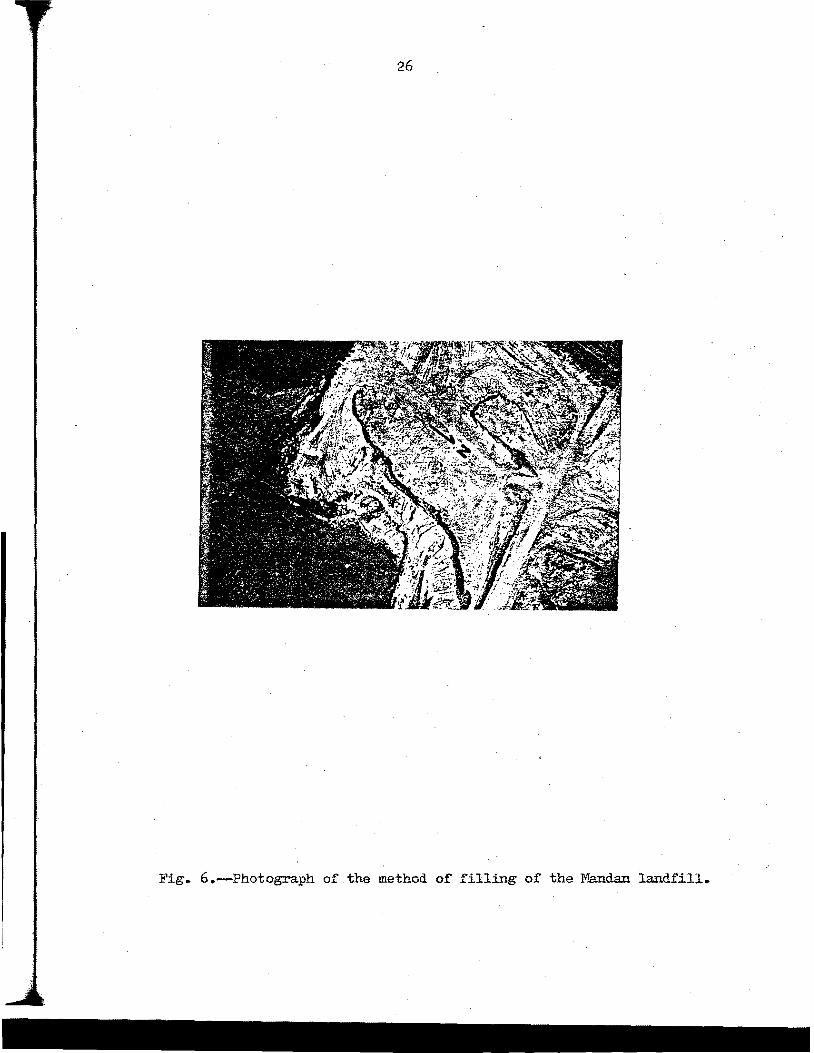
has formed (Figure 6). A final cover of 0.6 m of earth is added.
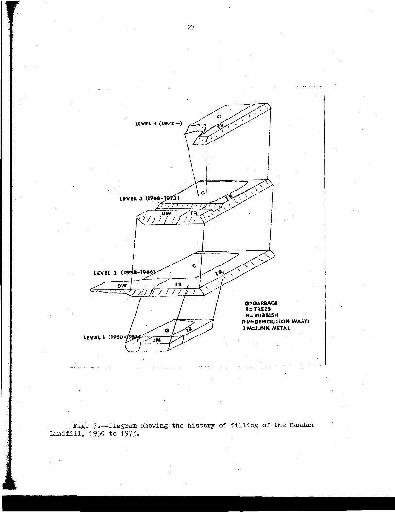
A map of the history of filling of t.~e Mandan landfill is given
in Figure 7. A core of garbage consisting of about everything except
trees, branches, auto bodies, and demolition concrete was formed.
A perimeter of rubbish consisting mostly trees, auto bodies, and
large appliances was built to provide a windbreak. around the core.
In general it takes about 6 years to complete a 12 m layer
of refuse. In 1952 the daily production of refuse in Mandan was
about 1.4 kg (3 pounds) for each person. Today the daily output
for each person is about 1.8 kg (4 pounds).
The present dimensions of the landfill are as :follows:
Length= 800 m
Width= 500 m
Thickness= 15 m
Surface area= 4 X 10⁵ m2
Volume= 6 X 10⁶ ;J.
The landfill is about 15 m above the floodplain on the south,
west, and north sides. The east side borders the sloping valley wall.
The flan.ks are nearly vertical and surface runoff is rapid.
The flan.ks are exposed to flooding of the Heart River.
The upper surface of the landfill has about 1 percent slope
toward t..~e Heart River. Differential settlement has caused several
large oval-shaped depressions to :form. These depressions fill with
rain and runoff which may remain as much as a·week after a storm.
26
Fig. 6.~Photograph of the method of filling of the Mandan landfill.
27
LEVEL 4 (1973-)
G=GARBAGi T: TR.HS R: RUABISH
DW:DEMOLITION WASTE J M:JUNK METAL
Fig. ?.~Diagram showing the history of filling of the Mandan landfill, 1950 to 1973.
CHAPTER IV
GROillIDWATER THEORY
Introduction
Groundwater theory developed from several important early
papers (Meinzer, 1923a, 1923b; Hubbert, 1940). Hubbert (1940)
presented the physical laws of steady-state gro-qndwater flow
mathematically.
In the early 1960s a theoretical background of groundwater
flow was presented to complement field studies (Toth, 1962, 1963).
Groundwater flow patterns were derived mathematically by solving
standard boundary value problems.
Several studies have expanded groundwater theory into usable
mathematical models of various flow systems. The flow models had
areas ranging from thousands of square kilometers to a few square
kilometers or less (Meyboom, 1963, 1966, 1967a, 1967b; Williams,
1968; Freeze, 1969; Hitchen, 1969a, 1969b).
Early work in groundwater chemistry by Chebotarev (1955)
established a sequence of chemical facies for groundwater flow systems.
The results of several thousand water sample analyses were used to
show the changes. Brown (1963) used groundwater chemistry in a
groundwater study. :Back (1960) and Charron (1965) used groundwater
chemistry to determine flow directions. Meyboom (1966) and Toth
(1968) used water chemistry as a secondary indicator of various
flow systems.
28'
29
There have been several flow models developed for parts of the
Great Plains that used groundwater chemistry. Hamilton (1970)
developed a groundwater flow model for the Little ~lissou~i River Basin
in western North Dakota. Hagmaier (1971) developed a model for uran
ium. deposition in the Powder River Basin in Wyoming. Schulte (1972)
used water chemistry as a flow system indicator in a flow model of
Spiritwood La.~e area in central North Dakota.
Terminology
The terms as they are used in this report are defined below.
These terms are in common usage in groundwater studies.
Flow-System Terminology
Flow System.--The flow system as defined by Toth (1963, p.4806) is
••• a set of flow lines in which any two flow lines adjacent at one point of the flow region remain adjacent through the whole region; they can be intersected any-where by an uninterrupted surface across which flow takes place in one direction.
Topography and length of flow path can be used to define
three types of flow systems; local, intermediate, and regional.
Local Flow System.--Flow in a local flow system is from a small
topograhic high to an adjacent low. The length of flow path in a
local flow system ranges from a few hundred meters or less up to a
thousand meters.
Intermediate Flow System.--Flow in an intermediate flow system
is from a regional topographic high to a regional low. The length of
flow path in an intermediate flow system ranges from a thousand
meters up to several thousand meters.
30
Regional Flow System.~Flow in a regional flow system is from
a large regional topographic high to a regional low. The length of
flow path in a regional flow system ranges from a few thousand meters
to several tens of thousands of meters.
Groundwater flow is three dimensional and can be resolved into
flow components and resultants. The flow vectors are mu.tu.ally
:perpendicular.
Longitudinal Component.~The longitudinal component parallels a
river or divide. It is called underflow.
Vertical Component .-The vertical component is along a line.
extended to the center of the earth. It may be up or down.
Lateral Compo~ent.--The lateral component is normal to the plane
of the longitudinal and vertical components. It may be called lateral
flow.
The three components can be resolved into a total flow vector,
a horizontal component, and a flow resultant.
Total Flow Vector.--The total flow vector is the direction of
flow in three dimensional space. It is the vector sum of the horiz
ontal flow component and the flow resultant.
Horizontal Flow Comnonent.--The horizontal flow component is the
direction of flow in a plane normal to the vertical~
Flow Resultant.-The flow resultant is the direction of flow in
a plane parallel to the vertical. An approximation is obtained by
constructing a cross-section across the flow field. The cross-section
31
may be constructed by contouring values of potential in a plane of the
section. Flow resultants are drawn at right angles to lines of equal
potential. It is assumed that the sediment is homogeno~s and iso
tropic.
Corrections must be made for anisotropic conditions. Isa
potential lines and flow resultants are refracted at permeability
interfaces according to the ta.~gent law (Hubbert, 1940, p. 943). The
flow resultant must also be corrected for distortion in a vertically
exaggerated section (van Everdinger, 1963).
Static Head,--The static head is the height above a standard
datum of the surface of a column of water (or other liquid) that
ca.~ be supported by the static pressure at a given point. It is the
sum of elevation head and pressure head. Head, when used alone, is
understood to mean static head (Lohman and others, 1972).
Total Head.--The total head of a liquid at a given point is
the sum of elevation head, pressure head, and velocity head. It is
equal to the static head plus velocity head of the fluid (Lohman and
others, 1972).
Water Table.--The water table is an imaginary plane in an
unconfined aquifer at which pore pressure equals at~ospheric pressure.
The configuration of the water table is a subdued replica of the
topography.
Rechar~.--Recharge is the addition of water to the groundwater
flow system through the unsaturated zone to the water table. A recharge
area occurs where there is downward movement of groundwater away from
the water table.

32
Discharge.--Discharge is the loss of water from the groundwater
flow system by evapotranspiration, stream baseflow, springs, and
seepage areas. A discharge~ occurs where there is upward movement
of groundwater toward the water table.
Water-Chemistry Terminology
Parts Per Million.--Parts per million is the concentration of
dissolved matter, by weight, in a million parts of solution by weight.
E;guivalents Per Million.~Equivalents per million is the
normality of a solution multiplied by 1000.
Hydrochemical Facies.--A hydrochemical facies is a body of water
in a groundwater flow system differing from other bodies of water by
its chemical characteristics. The hydrocha~ical facies classification
of Back (1960) is used in this report. Equivalents per million of
cations and anions in solution are used to compute percentage values.
As used by Hamilton (1970, p.9) a facies term alone
••• indicates that the ion content of the water is composed of at least 90 percent of that member (for example, bicarbonate water indicates that the anions are composed of at least 90 percent bicarbonate). Double anion terms (for example bicarbonate-sulfate) describe water that is composed of at least 50 percent but less than 90 percent of the first named member (bicarbonate); the second member is greater than 10 but less than 50 percent of the total anions. A calciummagnesium facies indicates that the cations are composed of at least 90 percent calcium and magnesium. But, a calciumsodium facies represents water in which the calcium and magnesium comprise at least 50 percent of the total cations.
GrotL~dwater Flow
The following is a brief description of groundwater concepts.
Groundwater flow theory fundamentals are based on. the Bernoulli 'I'.heorem,
Darcy's Law, the Continuity Equation, and the Laplace Equation.
..
33
Bernoulli Theorem
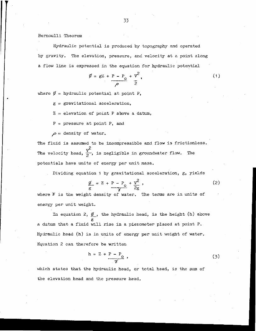
Hydraulic potential is produced by topography and operated
by gravity. The elevation, pressure, and velocity ate.. point along
a flow line is expressed in the equation for hydraulic potential
¢=gZ+P-P +v2 0 ' ---
,.0 2
where¢= hydraulic potential at point P,
g gravitational acceleration,
Z = elevation of point P above a datum,
P = pressure at point P, and
;:> = density of water.
The fluid is assumed to be incompressible and flow is frictionless.
The velocity head,~, is negligible in groundwater flow. The
potentials have units of energy per unit mass.
Dividing equation 1 by gravitational acceleration, g, yields
d = z + p - p + v2 ' .I!- 0 -g ~-o~ 2g
where o is the weight density of water. The terms are in units of
energy per unit weight.
In equation 2, ¢, the hydraulic head, is the height (h) above g
a datum that a fluid will rise .in a piezometer placed at point P.
Hydraulic head (h) is in units of energy per unit weight of water.
Equation 2 can therefore be written
h=Z+P-P 0
which states that the hydraulic head, or total head, is the sum of
the elevation head and the pressure head.
{1)
(2)
(3)
34
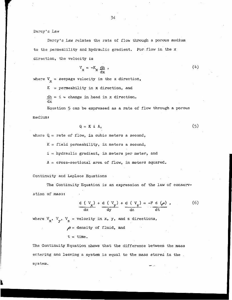
Darcy's Law
Darcy's Law relates the rate of flow through a porous medium
to the permeability and hydraulic gradient. For.flow in the x
direction, the velocity is
V = -K dh , X X dx
where V = seepage velocity in the x direction, X
K = permeability in x direction, and
dh = i = change in head in x direction. dx
Equation 5 can be expressed as a rate of flow through a porous
medium:
Q, = Ki A,
where Q. = rate of' flow, in cubic meters a second,
K == field permeability, in meters a second,
i = hydraulic gradient, in meters per meter, and
A= cross-sectional area of flow, in meters squared.
Continuity and Laplace Equations
The Continuity Equation is an expression of' the law of conserv
ation of mass:
d ( V) + d ( V) + d ( V) = -F d (;:,) --~-x~ y z
dx dy dz dt
where V, V, V = velocity in x, y, and z directions, X y Z
fJ = density of fluid, and
t = time.
T'ne Continuity Equation shows that the difference between the mass
entering and leaving a system is equal to the mass stored in the
system.
(4)
(5)
(6)

35
Assuming a constant density, equation 6 becomes
d V + d V + d V = - F d..n • X ___:L ~~z ,-
d:x: dy dz dt
For steady state conditions the right hand side of equation 7
becomes zero, and the Continuity Equation becomes
dV X
dx
+ dV + dV = 0. _;[_ ~ dy dz
(7)
(8)
The Continuity Equation in this form is combined with equation 4,
Darcy's Law, to obtain the Laplace Equation;
LJ + LJ + d2 ~ = 0 •
dx2 dy2 dz2
This equation can be used to express the distribution of hydraulic
potential in three-dimensional space.
Groundwater Flow Models
Present-day groundwater flow models are based on flow models
developed by Toth (1962, 1963) and Meyboom (1963). Toth developed a
mathematical framework for isotropic, homogenous material and ideal
boundary conditions. Meyboom utilized field observations to develop
a flow model for the semiarid western Canadian prairie.
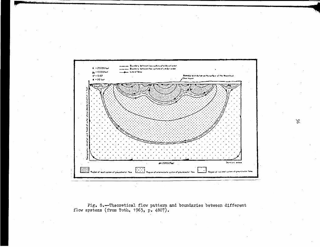
A t..heoretical model of groundwater flow by Toth (1962, 1963)
described three types of flow systems: local, intermediate, and
regional. Superimposition of smaller flow systems on larger ones was
a characteristic of the model (Figures). Complicated problems such
as heterogeneity, anisotropy, water-table irregularity, and strat
igraphic pinchouts were treated with detailed mathematical a.~d
digital computer techniques. Three-dimensional modeling was also
attempted.
(9)
• tr'iltltft' ··.· .2 :·,
• • lQOl)O ,,.,
~, ,ccooi.., ( 1 • 0.01.' • • ~o , ... ,
-- e,. ... ~ ... , ._ ...... '"'• ., • .,._, •' c,at.•, .. '•"~•' ---- Uo..,"44-f• twt .. ,, ... ft.,,.,,,,•,•• of •·••le• orw __.,._ l_....efbu
P.kt41 ,,,h .i,....,,.. .- .... ...,,4oc,, •' ........... t ..... 1
- /'-• ,., .. ~----------= ~<~-.~';j~'llflli.,_,~;.•,_:_t'•.'.(.•.•.•-·lf"r.:T:-:-:11•.•.~•.•2•.•.f•l'VS:'._,_.\IF""Jl
t ,. .. ! .. ~
! . : " 1 ~ -i ;. £• ~ t J s ... ,, o,J •• ,. .. f• ZOOCO,._t
R'«m ~ 11•9• •f ~ftf lf't .... •f 9f'OVIUfMlPt«t flo,. D ·o . . .
R•91.- ,f-..,t~,..•d.of• tr,•• .. ofgttNNf-a._, flow R•1,oa •* ,,1,0....,1 ,,,, ... 0:f',;,,..•~'-,••• 41a.,..
Fig. 8.~Theoretical flow pattern and boundaries between different flow systems (from Toth, 1963, :p. 4807).
\.>,I
°'
.... -,~

37
Groundwater flow in Saskatchewan, Canada. was modeled into the
Prairie Profile (Figure 9) by Meyboom (1963). By definition the
Prairie Profile
••• consists of a central topographic high bounded at either side by an area of' lower elevation. Geologically the profile is made up of two layers of different permeability, the upper layer having the lower permeability. Through the profile is a s·ceady flow of groundwater from the area of recharge to the area of discharge. The ratio of permeabilities is such that groundwater flow is essentially downward through the material of low permeability and lateral and upward through the more permeable layer. The potential distribution is governed by the differential equation of La.place.
Groundwater flow in the Mandan landfill has some of these
characteristics. One half.of an asymmetric Prairie Profile is
developed at the landfill site.
The models of: 'Poth and Meyboom conflict on whether or not
unconfined groundwater flow systems can cross major topographic divides
and large river valleys. Toth (1963) indicates that they cannot
cross these features while Meyboom (1963) indicates large-scale
flow systems can cross these features.
Application of computer teclw..iques to groundwater flow
description and modeling was researched by Freeze and Witherspoon
(1966, 1967, 1968) and Freeze (1969). A three-dimensional ground
water flow model for nonsteady, heterogenous, anisotropic conditions
was developed with the aid of a computer.
Groundwater Chemistry
Groundwater c..}iemistry may be used to indicate the type of ground
water flow. Chebotarev (1955) developed a hydrochemical model for
groundwater flow. Meyboom (1966), Toth (1968), Char:ron·(1965), and

38
! -"S
g -f 1 "S
~~
i1 Ji
! ;:! u" - .. Ji{
I ~,
i " I} ~ .!; t ii ~
.i !: ~
f.
: ,; ,it 'li fl :: .,, .,
I I . : :
l l -:. ~
I
~
l I
I
I I
• -r-C\I
,...
39
Back (1960) have used groundwater chemistry to indicate groundwater flow
directions.
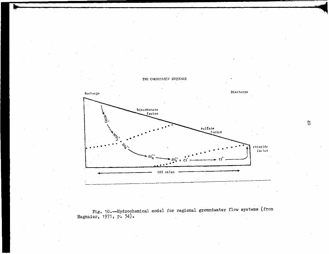
Chebotarev's (1955) hydrochemical model was developed using the
analyses of several thousand groundwater samples. The sequence
(Figure 1 0 ) that develops is
Hco; ~ HC03- + S04--~ 304---?' 304- + Cl-~ Cl- • ( 10)
The solubilities of common salts and the length of contact time
between water and sediment results in a hydrochemical sequence that
proceeds toward a saline composition. Theoretically the longest flow
path should be the most saline.
The time of contact between groundwater and sediment should
result in a characteristic type of water. Water along a short flow
path (or in a local flow system) should be rich in carbonate.
Bicarbonate and sulfate water should develop in an intermediate flow
system. Regional flow systems should be rich in bicarbonate, sulfate,
and chloride. Deviations from these hydrochemical patterns may be
due too short a flow path for the particular type of water to develop.
The presence of very soluble minerals may cause anomalous water types.
..
Rt!chargc
\~ .. r>o'
..., )(
•••••• . .
THE CH.EDOTA~V S'EQ\.,'ENCE:
• • .Po'
• • • . . - .
•
? '
'---so4--sri;; • •• • • •
100 miles
••• •••• . . . .
c( :------ cC
Dlsch,:u:·r.c
~
•"'" ch lode,• r ;u: {..:!'
. Fig. 10.~Hydrochemical model for regional groundwater flow systems (from Hagma.ier, 1971, p. 34).
~
t

CHAPTER V
GROUNDWATER OF THE MA.!-H)AN LANDFILL A..'l=lEA
Introduction
The purpose of this chapter is to describe the groundwater flow
systems in the study area and to evaluate the contamination of
groundwater in the landfill area..
The groundwater flow system was determined using (1) selected
values of hydraulic potential, (2) the location of recharge and dis
charge areas, (3) composition, physical properties, and stratigraphy
of the sediment, (4) topography, (5) chemical and physical properties
of the groundwater. A cross-section was made through part of the
landfill area to show the groundwater flow patterns.
Several assumptions were made for this study. Flow is assumed
to be in a steady state. Water levels are assumed to have changed
very little over a season and over a 30 year period. The sediment
is assumed to be homogenous on a large scale. An impermeable bounda.rJ
is assumed to exist at depth. The Pierre Formation forms the base
of the regional flow system in the study area and separates it from
deeper flow systems.
Hydraulic potential data obtained by piezometers and water
chemistry were used to evaluate the groundwater flow systems. A
piezometer is a cased well, screened at the bottom, and sealed in the
borehole with cement for a short distance above the screen. It is
41
42
used to measure the hydraulic potential at a point in the groundwater
flow system. A discussion of the type of piezometer used. in this study
and installation procedures are given in Appendix A. The theory and
characteristics of various piezometers used in a North Dakota groundwater
study are summarized by Schulte (1972).
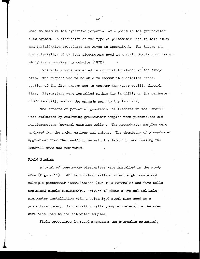
Piezometers were installed in critical locations in the study
area. The purpose was to be able to construct a detailed cross
section of the flow system and to monitor the water quality through
time. Piezometers were installed within the landfill; on the perimeter
of the landfill, and on the uplands next to the landfill.
The effects of potential generation of leachate in the landfill
were evaluated by ·analyzing grout1dwater samples from piezometers and
nonpiezometers (several existing wells). The groundwater ~amples were
analyzed for the major cations and anions. The chemistry of groundwater
upgradient from the landfill, beneath the landfill, and leaving the
landfill area was monitored.
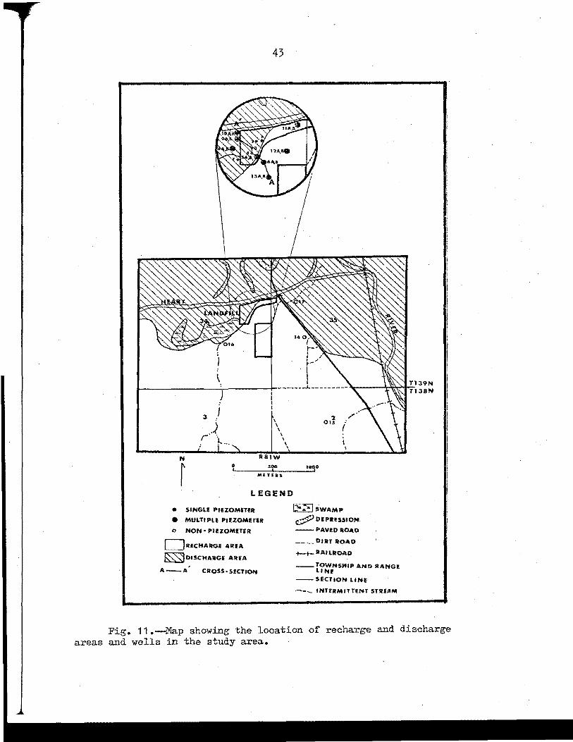
Field Studies
A total of twenty-one piezometers were installed in the study
area (Pigure 11). Of the thirteen wells drilled, eight contained
multiple-piezometer installations (two in a borehole) and five wells
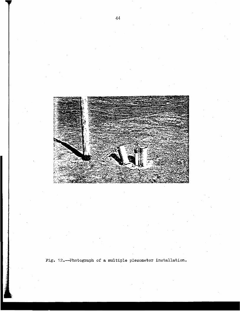
conte.ined single piezometers. Figure 12 shows a typical multiple
piezometer installation with a galvanized-steel pipe used as a
protective cover. Four existing wells (nonpiezometers) in the area
were also used to collect water samples.
Field procedures included measuring the hydraulic potential,
43
14 or }--
' I /
~ .... -'
\ I ..--...--------------'~-------'---_ ---- --~---+..i;~.,-;T;..139N J T138N
N 0
\ \ \
R81W
\ \ \
'
f M!TEl:S
LEGEND
• SINGLE P!EZOMET£11:
• MULTIPU PIEZOMIETER
o NON• PIEZOMIETER
DRICHARGE AREA
~DISCHARGE ARfA
A-A' CROSS•SECTION
2 ou
t-:-1 swAMP
c:;f? DEPRl!SSION .
-- PAV!D ROAD
____ DIRT ROAD
+-t-- AAI lROAP
__ TOWNSHIP AND RANGE LINE
-- SECTION LINE
·-~- INTERMITTENT STIUAM
Fig. 11.~Ma.p showing the location of recharge and discharge areas and wells in the study area.
44
Fig. 12.~Photograph of a multiple piezometer installation.
45
temperature of groundwater, pH, and specific conductance. Water samples
were collected for later analyses. The physical properties of ground
water samples such as color, odor, and turbidity were noted. Proced
ures used in this part of the study are described in Appendix A.
Laborator<J Methods
Groundwater samples were collected monthly and stored for later
a..~alyses. The samples were analyzed for calcium, magnesium, total
hardness, carbonate, bicarbonate, total alkalinity, sulfate, chloride,
nitrate, total iron, sodium, and potassium. Analytical methods and
results of chemical analyses are given in Appendix A and D, respectively.
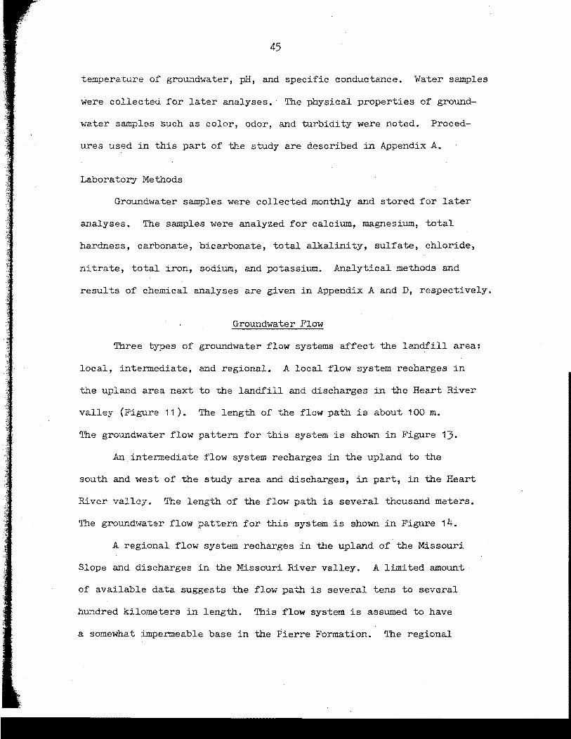
Groundwater Flow
Three types of groundwater flow systems affect the landfill area:
local, intermediate, and regional. A local flow system recharges in
the upland area next to the landfill and discharges in the Heart River
valley (Figure 11). The length of the flow path is about 100 m.
The groundwater flow pattern for this system is shown in Figure 13.
An intermediate flow system recharges in the upland to the
south and west of the study area and discharges, in part, in the Heart
River valley. The length of the flow path is several thousand meters.
The groundwater flow pattern for this system is shown in Figure 14.
A regional flow system recharges in the upland of the Missouri
Slope and discharges in the Missouri River valley. A limited amount
of available data suggests the flow path is several tens to several
hundred kilometers in length. This flow system is assumed to have
a somewhat impermeable base in the Pierre Formation. The regional
46
I I 1\1\.
_,,,. , I
1--~ . : I ..r-, ' / - t-~ I I _. I I _,,,...
11-~~~~~~~-+---~~~~+-- .---L---------:1,,-~~-++....____;_J.;~ )'
3 /
) r ·.
~ ' '·
N 0
i • WELL SITE
-,.. f LOW DIRECTION
c:::=J RECHARGE AREA
c:::::J DISCHARGE AREA
I I I I
l\ ' \
R81W 500
\ \
'
METERS
LEGEND
IOOO
(
\
r
SWAMP
~ DEPRESSION
-- PAVED ROAD
---- DIRT ROAD
+-+-RAILROAD
__ TOWNSHIP AND RANGE LINE .
SECTION LINE
-··~ INTERM.ITTENT STREAM
Fig. 13.~I1ap showing the pattern of local groundwater-flow systems in the Mandan landfill area. - (General recharge and discharge areas for the study area are also given.)

47
.i • .,.. r~ I
I - - I / 1--,.,,,. ,.,,,. -+-I
\ I - I
_____ .l ---- --- .----H~!-!T~139N T138N ) I -I
J .. I
3
r·-<, \ \-.. \
.. ~-·, \
N R81W
0 500 r I I
METERS
LEGEND • WELL SITE
-+- f LOW DlllJ!CTION
LJ RECHARGE AREA
D DISCHARGE ARIA
.......
...... ,,..-
• i .......
V
1opo
lj-;.-1 SWAMP
~DEPRESSION
-PAVH)ROAD
---- DIRT ROAD
+-+- RA! LROAD
__ TOWNSHIP AND RANGI LINE
-· - SECTION LIN!
.-.._ INTERMITTENT STREAM
Fig. 14.~~.ap showing the pattern of intermediate groundwaterflow system in the Mandan landfill area.. (General recharge and discharge areas in the study area are also given.)
48
flow system affects the potential distribution of the intermediate
flow system in the area.
A deeper groundwater flow system occurs below the Pierre Formation
at a depth of 670 m. The Dakota Group is a part of this flow system.
Recharge occurs over a wide area in the northern Great Plains. Dis-- '
charge occurs partly in eastern North Dakota. This flow system is
believed to have little effect on the important flow systems in the
study area.
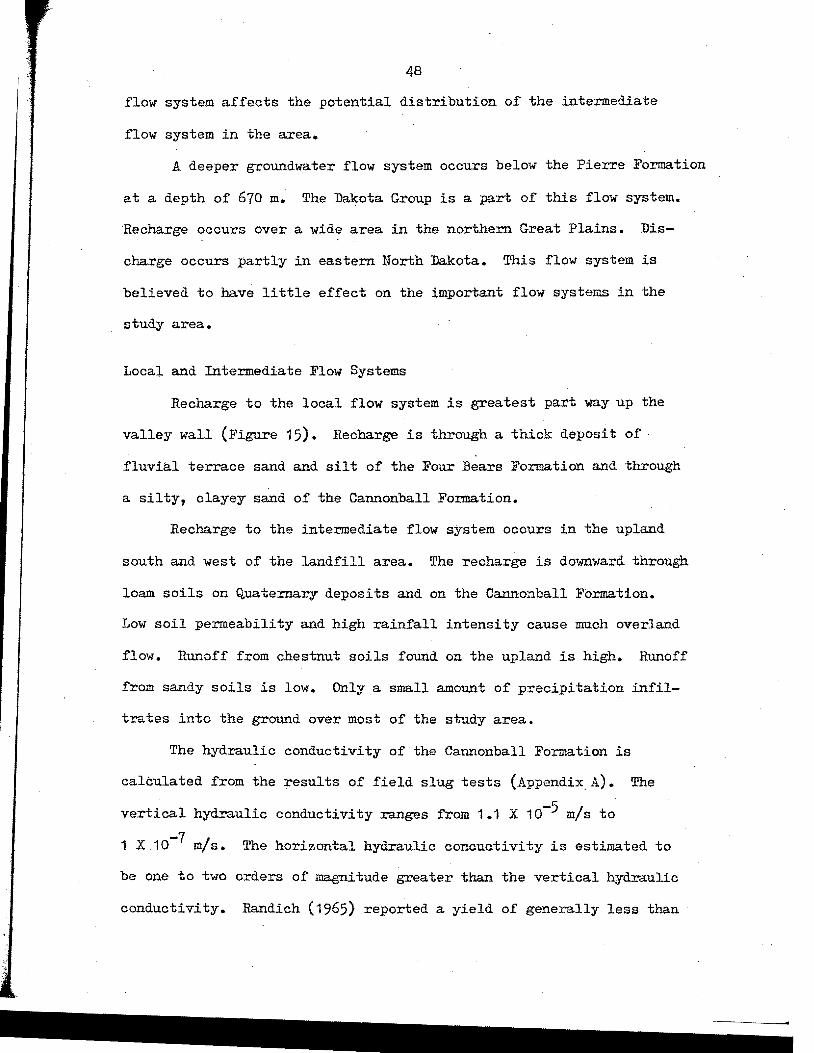
Local and Intermediate Flow Systems
Recharge to the local flow system is greatest part way up the
valley wall (Figure 15). Recharge is through a thick deposit of
fluvia.l terrace sand and silt of the Four Bears Formation and through
a silty, clayey sand of the Cannonball Fo:rma.tion.
Recharge to the intermediate flow system occurs in the upland
south and west of the landfill area. The recharge is downward through
loam soils on Quaternary deposits and on the Cannonball Formation.
Low soil permeability and high rainfall intensity cause much overland
flow. Runoff from chestnut soils found on the upland is high. Runoff
from sandy soils is low. Only a small a.mount of precipitation infil
trates into the ground over most of the study area.
The hydraulic conductivity of the Cannonball Formation is
calculated from the results of field slug tests (Appendix_A). The
vertical hydraulic conductivity ranges from 1.1 X 10⁻⁵ m/s to
1 X 10⁻⁷ m/s. The horizontal hydraulic concuctivity is estimated to
be one to two orders of magnitude greater than the vertical hydraulic
conductivity. Randich (1965) reported a yield of generally less than

lifililt1"""
1':?.,.~ .. 1'.~~.·.:·1··F<:· <r;' 'f~~ ·,. .. " "ll ·
I MlfUt5, A A 1111
17SO
,Jo
,,o
510
500
490
480
470
00
·area
slit
( ___ •• A9.5,9m ••••••• ---,"lfD-iand·-------·-····----· 49
;-.-·~~ .. ··~·:•.1;9.8Wt}Mff?};.fWJ1L~~;~-:~~~-=------::!~-~-----~::::::::~i;:;·: ·.: •f'-;---~3.f-. .~ •• oe • .. •o t~1.,...f• • •, •:~ •1o:.:o :o'>V •, D t.o::•o• .. o•o•:o.•' .••,: • • ~~.f •o • o:, •., : • • • • •" o • •" • • "'{I-~'• -0 ......... ,f1ti.\Jt1 • ..c:L1y,~q.n,,.fJ:e •• •,•lo •f • (l!f6f.'I• •••• IP. 10···· t ~i~ .••o•flo• •••• *'vi>•.O ftql
.• :: • "'.,• • "•:.,. •.• •• : ,,,f:"' .~• •,• :111: • oi.• Cl =O•o•oo ~•:Po: .... ••• .•:o~ • •.•: •: .• ,..• • .!:.~••• o o •o•: .. :: "•::o" • • •.••'> :.:i •"' .; •. • "'4:,0•• # • •,,"' Q •o /~ o: • •,.',• • 0 :,•; <l•o 'o•• •'°• 111 0 :::••.,::o:• :•• • •. •.• • '•o ,..• oo•.,-...~.• ,o•: o'° .• .• •: • o•: ~?"• ,.•,• ,,,..•.t;
'!,.: .. : "~.° .: : • : : : ; •"' •• 0: : ... · :: : •. · .. •• : •• '. 0 • : : :.: •: f.·11·:.:: 0 =·: 0 •::;.·. • •• ; :: • : •: :•. :.·11111~. : ••• ..... ; • 0: )·:. ·.:: I>: '•'..
0 0" •.:.•:: 'l...a·: .• 0:.:•:·.•·0 ~•4 '.._:~:. •:~o~: 0•,/o o ,::::•:.••._.,:::;.•,,•:••:•.•:••".• -.: •".•o•:0 • :'I:•.:;.°•:••.•: 0•:: •,.;
••••• .. • _ •• t.i .,
0:· .... ,tl't: •• ·~·:.·.·,..·. 11
... : 11 ' 0 °.'o"''>~• .. • .. 11co•.· .. ··.••.0•0 0·.·1:.··:··.·: •• ·.·:o·:.·e·· ·o·.·.·. •,0
.. : •••• .·,·.··: ... -~
~OAIU fM,
~ !OUR HARi PM,
fil§l CANNONBALL FM,
Qcoruu fM, rn lUOlOW-IIIU CIIIK fMS,
(:SSj LANOflU
O MO I I t
---- OSOLOGIC CONTACT --SI:.- WATU TAUi
••49$ - - lQUIPOTINTIAL LINI
+- ·now DIUCTION
'1700
16,0
1600
IUO
uoo
Fig. alo~g
15 • ...-Geology and pattern of groundwater flow in the Mandan landfill cross-section A-A' (Fig. 11).
.· 'iifi\ll\:l'i@h iilltmirn. n11111111111
.i:,..
'°
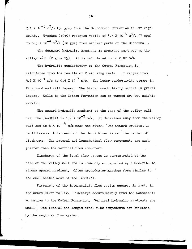
50
3.1 X 1 o-3 m3 /s (50 gpm) from the Cannonball Formation in Burleigh
County. Tyschen (1949) reported yields of 4.3 X 10⁻⁴
m3/s (7 gpm)
-4 . to 6.3 X 10 rr?/s (10 gpm) from sandier parts of the Cannonball.
The downward hydraulic gradient is greatest part way up the
valley wall (Figure 15). It is calculated to be 0.02 m/m.
The hydraulic conductivity of the Coteau Formation is
calculated from the results of field slug tests. It ranges from
3.2 X 10⁻⁴ m/s to 6.4 X 10-? m/s. The lower conductivity occurs in
fine sand and silt layers. The higher conductivity occurs in gravel
layers. Wells in the Coteau Formation can be pumped dry but quickly
refill.
The upward hydraulic gradient at the base of the valley wall
near the landfill is 1.2 X 10⁻³ m/m. It decreases away from the valley
-4 wall and is 6 X 10 m/m near the river. · The upward gradient is
small because this reach of the Heart River is not the center of
discharge. The lateral and longitudinal flow components are much
greater than the vertical flow component.
Discharge of the local flow system is concentrated at the
base of the valley wall and is commonly accompanied by a moderate to
strong upward gradient. Often grou..~dwater marshes form similar to
the one located west of the landfill.
Discharge of the intermediate flow system occurs, in part, in
the Heart River valley. Discharge occurs mainly from the Cannonball
Formation to the Coteau Formation. Vertical hydraulic gradients are
small. The lateral and longitudinal flow components are affected
by the regional flow system.
' r !
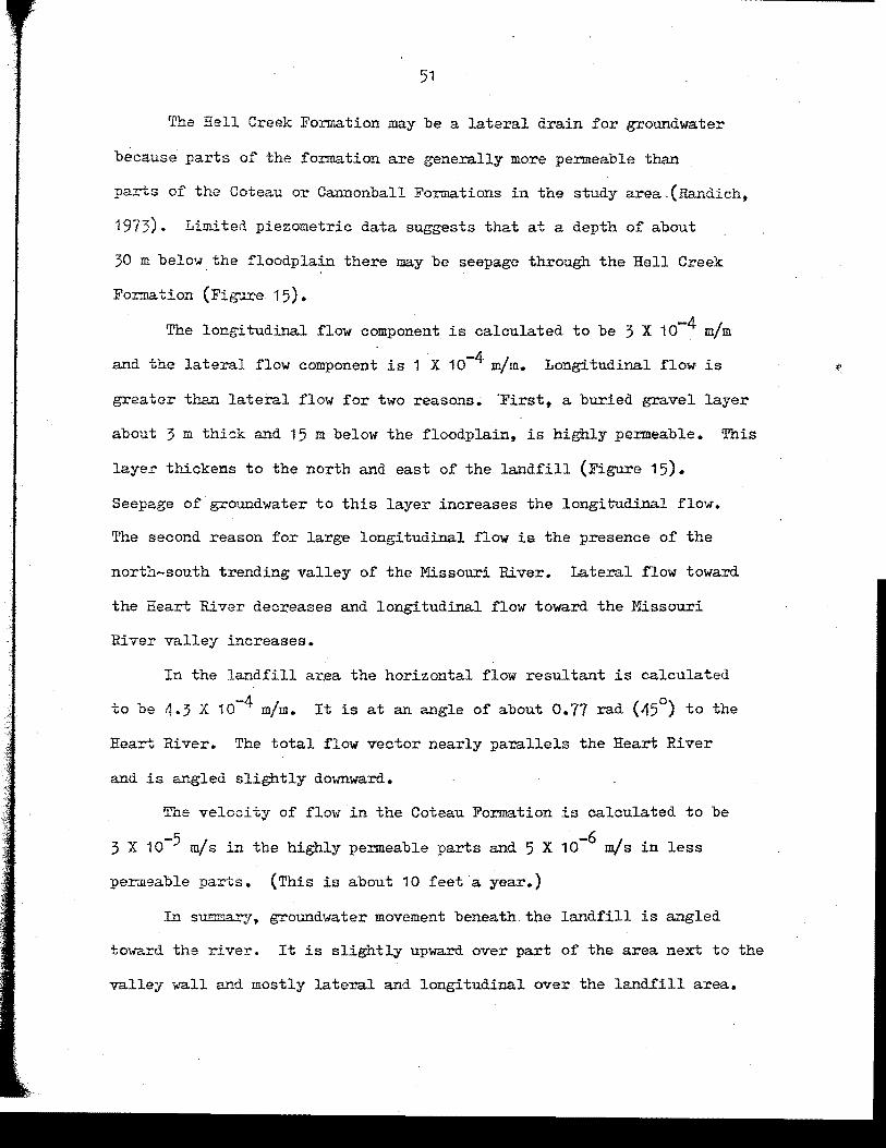
51
The Hell Creek Formation may be a lateral drain for groundwater
because parts of the formation are generally more permeable than
parts of the Coteau or Cannonball Formations in the study area,(Randich,
1973). Limited piezometric data suggests that at a depth of about
30 m below the floodplain there may be seepage through the Hell Creek
Formation (Figr..u:-e 15).
The longitudinal flow component is calculated to be 3 X 10⁻⁴ m/m
and the lateral flow component is 1 X 10⁻⁴ m/m. Longitudinal flow is
greater than lateral flow for two reasons. 'First, a buried gravel layer
about 3 m thick and 15 m below the floodplain, is highly permeable. This
layer thickens to the north and east of the landfill (Figure 15).
Seepage of groundwater to this layer increases the longitudinal flow.
The second reason for large longitudinal flow is the presence of the
north-south trending valley of the Missouri River. Lateral flow toward
the Heart River decreases and longitudinal flow toward the Missouri
River valley increases.
In the landfill ar~a the horizontal flow resultant is calculated
to be 4.3 X 10⁻⁴ m/m. It is at an angle of about 0.77 rad (45°) to the
Heart River. The total flow vector nearly parallels the Heart River
and is angled slightly downward.
The velocity of flow in the Coteau Formation is calculated to be
3 X 10⁻⁵ m/s in the highly permeable parts and 5 X 10⁻⁶ m/s in less
permeable parts. (This is about 10 feet a year.)
In summary, groundwater movement beneath.the landfill is angled
toward the river. It is slightly upward over part of the area next to the
valley wall and mostly lateral and longitudinal over the land.fill area.

52
In.filtration through the layers of refuse is downward. Recharge
rarely occurs b.ecause, even during a heavy thunderstorm, the wetting
front seldom moves below 1 to 2 m. The greatest in.filtration occurs at
the start of rainfall and decreases with time.
Infiltration through the upper layers of refuse is reduced for
several reasons. Compaction by landfill equipment and traffic reduces
the permeability of the fill. Montmorillonite clays in the cover
material tend to absorb moisture and swell, thus reducing the
infiltration, Ponds of water may form on the upper surface of the
landfill after a storm.
Infiltration may be increased in areas containing demolition
rubble and large trees. Cavities within this refuse were detected
by drilling. Other cavities exist where large objects such as large
appliances and car bodies are buried.
In general, drilling indicates that most of the landfill is
well compacted. Areas of garbage are generally more compacted than
areas of rubbish.
To have recharge in the refuse layers, it is necessary for the
field capacity of the material to be exceeded. Reduced infiltration
through the surface, low water content of refuse before burial, and
a generally shallow wetting front inh.ibit recharge. Local pockets
of saturated refuse may occur where water is channeled from above, where
the refuse has been exposed by erosion, or where the water table has
risen and saturated part of the lower layer of refuse (the first refuse
layer was placed near the water table). Drilling indicated the material
at the bottom of the fill was partly wet and decomposed.
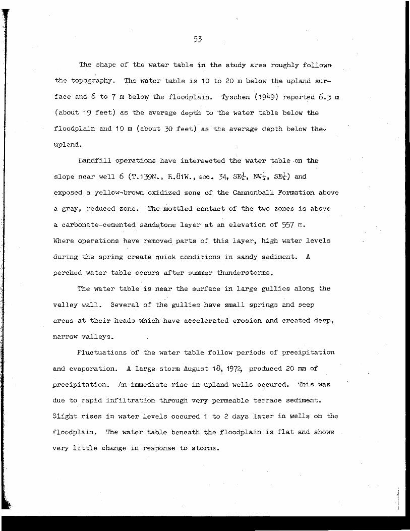
53
The shape of the water table in the study area roughly follows·
the topography. The water table is 10 to 20 m below the upland sur
face a.~d 6 to 7 m belo~ the floodplain. Tyschen (1949) reported 6.3 m
(about 19 feet) as the average depth to the water table below the
floodplain and 10 m (about 30 feet) as the average dept.~ below theo
upland.
Landfill operations have intersected the water table on the
slope near well 6 (T.139N., R.81W. 1 sec,. 34, SE!, NW!, SE!) and
exposed a yellow-brown oxidized zone of the Cannonball Formation above
a gray, reduced zone. The mottled contact of the two zones is above
a carbonate-cemented sands.tone layer at an elevation of 557 m.
Where operations have removed parts of this layer, high water levels
during the spring create quick conditions in sandy sediment •. A
perched water table occurs after summer thunderstonns.
The water table is near the surface in large gullies along the
valley wall. Several of the gullies have small springs and seep
areas at their heads which have accelerated erosion and created deep,
narrow valleys.
Fluctuations of the water table follow periods of precipitation
and evaporation. A large storm August 18, 1972, produced 20 mm of
precipitation . .An irrnnediate rise in upland wells occured. This was
due to rapid infiltration through very permeable terrace sediment.
Slight rises in water levels occured 1 to 2 days later in wells on the
floodplain. The water table beneath the floodplain is flat and shows
very little change in response to storms.
I

54
Water levels in wells in the landfill area had a normal seasonal
decline. During the monitored period, August to November, 1972, the
decline was 0.3 m.
In general recharge areas showed the greatest changes in water
levels. Discharge areas had only slight changes. The seasonal decline
decreased after the third week in September when frost stopped most
evapotranspiration.
Regional Flow System
The regional groundwater flow system recharges, on its western
fla.'l'lk, on the upland of the Missouri Slope and discharges in the
Missouri River valley. Lateral flow toward the Missouri River near
Ma.ndan is rapid. The Pierre Formation is assumed to form an impermeable
base to this syste ~
The regional flow pattern has smaller flow systems super
imposed on it. The small amount of data on hydraulic potential
makes it difficult to define the groundwater flow system. Strati
graphy, groundwater chemistry, topography, and the location of
recharge and discharge areas were used to define the regional ground
water flow system.
The effect of the regional flow system is to increase longi
tudinal flow in the intermediate flow system. It is believed that
the Hell Creek Formation may be lowering the potential in.the landfill
area and increasing the underflow. Seepage from smaller flow systems
may be considerable below a depth of 30 min the study area.

55
Deeper Regional Flow System
A deeper flow system, of which the Dakota Group is a part, occurs
below the Pierre Formation at a depth of about 670 m. Recharge to this
flow system is believed to take place over the northern Great Plains.
Seepage from superimposed flow systems may add considerable recharge.
Discharge of the deep flow system occurs in the Red River valley of the
eastern Da.~otas.
This deep regional flow system has very little effect on the
local and intermediate flow systems in the study area, but may
receive recharge from the regional flow system of the Missouri River.
It is not known how much recharge takes place.

56
Groundwater Chemistry
The purpose of this section is to describe the physical and
chemical properties of groundwater in the landfill area, and to
describe leachate generation in the Mandan landfill.
The quality of shallow groundwater upgradient from the landfill,
groundwater beneath the land.fill, and groundwater downgradient from
the landfill is compared to determine the degree of contamination
of groundwater by leachate. Changes in water quality over a period
of time were determined by collecting samples at monthly intervals
from August to October 1972.
Chemical analyses were made on fifty-four groundwater samples
collected from shallow and deep wells ra.,.~ging in depth from 10 m to
100 m. The major cations and anions determined were calcium,
magnesium, sodium, potassium, iron, carbonate, bicarbonate, sulfate,
nitrate, and chloride. Also determined were the pH, temperature,
specific conductance, total alkalinity, total hardness, and total
dissolved solids. Appendices C and D give the results of chemical
analyses and summarize the important properties of groundwater samples.
Water Chemistry of Uncontaminated Groundwater
Groundwater chemistry of the Hell Creek, Cannonball, and
Coteau Formations in the stud~ area is discussed in detail. Chemical
analyses were made on groundwater samples collected from a rela
tively small area and small number of wells in these formations.
The results of these analyses are cba:ra.cteristic of groundwater in
parts of the formations in the study area.

57
Water samples were collected from three wells in the Rell Creek
Formation in the study area. The Hell Creek has predominately sodium
bicarbonate-chloride to sodium-calcium bicarbonate-chloride type water.
The water is generally soft and the total dissolved solid range from
1501 to 1935 ppm. The pH is about 8.0.
Water samples were collected from eight wells in the Cannonball
Formation in the study area. The water type in the Cannonball ranges
from predominately calcium-sodium sulfate-bicarbonate to sodium-calcium
bicarbonate-sulfate and calcium bicarbonate-sulfate. The water is
moderately soft and has a range of total dissolved solids from about
830 to 1180 ppm. The pH :ranges from 7.25 to a.15. Chloride is generally
low and iron is absent. High amounts of calcium and magnesium reflect
a short flow (local flow system). Deep wells in the Cannonball
Fo:rmation contain sodium and sulfate.
Water samples were collected from nine uncontaminated wells in
the Coteau Formation in the study area. The water type in the Coteau
ranges from calcium-sodium sulfate-bicarbonate to calcium-sodium
bicarbonate-sulfate and calcium-magnesium bicarbonate. The water is mod
erately hard and the total dissolved solids range from 669 to 1667 ppm.
The pH ranges from 7.22 to 7.66. Water from the Coteau is free of iron
and carbonate and low in nitrate and chloride. Generally shallow wells
yield calcium, magnesium, and bicarbonate water. They reflect short flow
paths. Deep wells yield water with sodium and sulfate, possibly from
water of the Cannonball Formation discharging into the Coteau in the

~I
58
Heart River valley. The chemical analyses for groundwater from the
Coteau are given in Table 4.
Water Chemistry of Contaminated Groundwater
Water samples from wells in the Coteau Formation beneath the
Mandan landfill showed varying amounts of contamination. In general,
total hardness, total aL~alinity, total dissolved solids, iron,
and chloride have increased. Decreases occurrei in sulfate and pH.
The greatest changes in water chemistry occurred in wells near the
center of the landfill. The groundwater is contaminated to a depth
of about 2 m. The contaminated water follows the lateral flow
direction for about 150 m toward the Heart River. Most contamination
occurs near wells 2 and 3 (Figure 16). Table 4 gives the results of
chemical analyses of shallow groundwater from wells beneath the
landfillo
The total hardness ranges from 240 to 760 ppm and the total
alkalinity from 250 to 600 ppm, which is as much as a 100 percent
increase. The toxal dissolved solids range from 625 to 1774, which
is as much as a 100 percent increase. Iron has increased from zero
to about Oo39 ppm and chloride has increased from an average of 18
ppm to 333 ppm maximum. Sulfate has decreased to as little as zero
ppm. The pH has decreased to a about 6.9 to 7.4.
In general the greatest changes in water chemistry of shallow
wells in the landfill area were the increased hardness, total dissolved
solids, total alkalinity, chloride, and decrease in sulfate and pH.

8A ~j, as> .!SL 7S7
N
59
13A a \ Riff
13B&,
12A~ f 1262
1213fo;i
" ,, /,
~ I / /
/ / / .,
I ;
1/ //
I I I I
I' r.==:::=:...·'-'
f 0 so 100
MlTERS
LEGEND ..tl:... CHlORIDI COOICINTRAl'ION, ppm ~6ij' TOTAL DISSOLVED SOLIDS, ppm
• WrLL SITE
:::.::::::: DIRT ROAD
=PAVIOROAD
.:JCS. HIGHWAT
Fig. 16.-Na.p showing values of chloride and total dissolved solids for shallow wells in the Mandan landfill area.
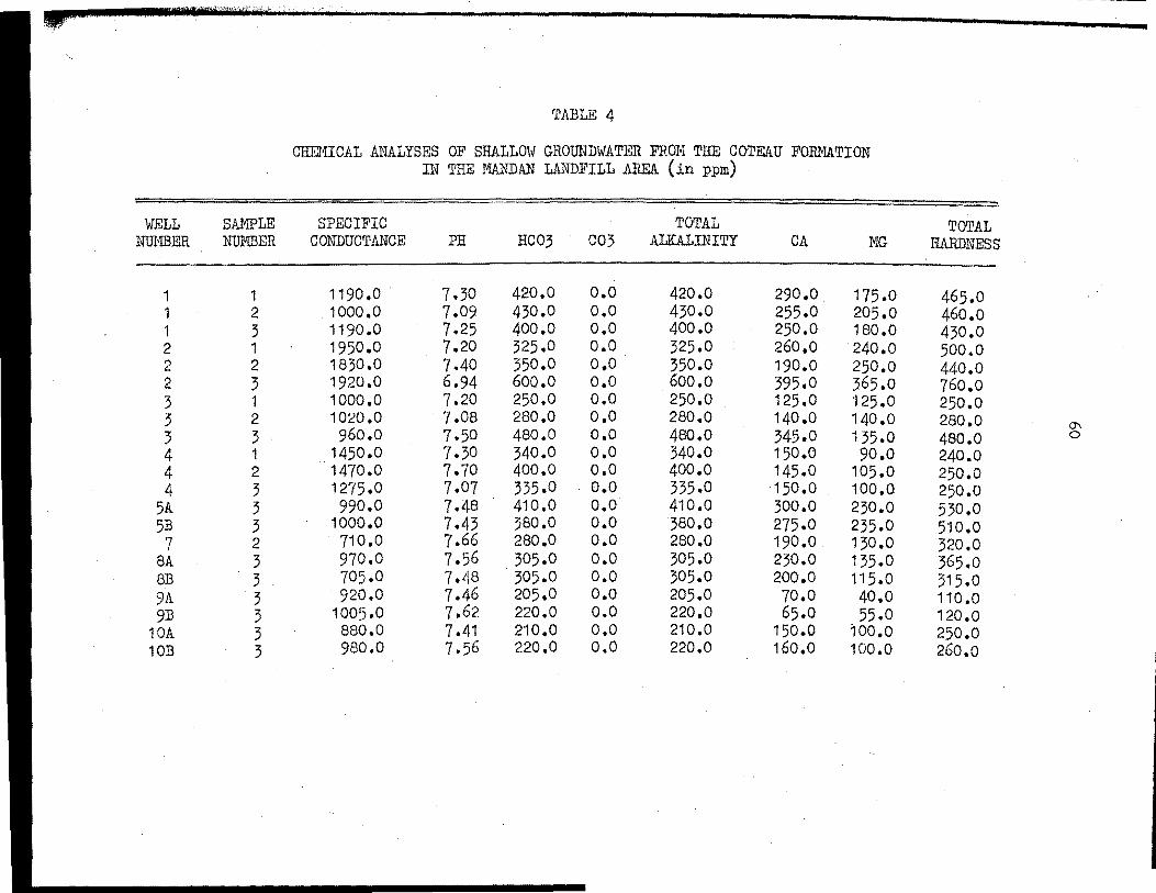
TABLE 4
CHEMICAL ANALYSES OF SHALLOW GROUNDWATER FROM THE COTEAU FORMATION IN THE MANDAN LANDFILL AREA (in ppm)
WELL SAMPLE SPECIFIC TOTAL TOTAL NUMBER NUMBER CONDUCTANCE PH HC03 C03 ALKALINITY CA MG- HARDNESS
1 1 1190 .o 7.30 420.0 o.o 420.0 290.0 175.0 465.0 1 2 . 1000.0 7.09 430.0 o.o 430.0 255.0 205.0 460.0 1 3 1190.0 7.25 400.0 o.o 400.0 250.0 180.0 430.0 2 1 1950.0 7.20 325.0 o.o 325.0 260.0 240.0 500.0 2 2 1 a30.o 7.40 350.0 o.o 350.0 190.0 250.0 440.0 2 3 1920.0 6.94 600.0 o.o 600.0 395.0 365.0 760.0 3 1 1000.0 7.20 250.0 o.o 250.0 125.0 125.0 250.0 3 2 1020 .o · 7 .08 280.0 o.o 280.0 140.0 140.0 280.0
°' 3 3 960.0 1.50 480.0 o.o 400.0 345.0 135.0 480.0 0
4 1 1450.0 7 .30 340.0 .. o.o 340.0 150.0 90.0 240.0 4 2 1470.0 1.10 400.0 o.o 400.0 145.0 105.0 250.0 4 3 1275.0 7.07 335.0 o.o 335.0 150.0 100.0 250.0
5A 3 990.0 7.48 410.0 o.o 410.0 300.0 230.0 530.0 513 3 1000.0 7.43 380.0 o.o 380.0 275.0 235.0 510.0 7 2 710.0 7.66 280.0 o.o 280.0 190.0 130.0 320.0
8A 3 970.0 7.56 305.0 o.o 305.0 230.0 135.0 365.0 8)3 3 705.0 7.48 305.0 o.o 305.0 200.0 115.0 315.0 9A 3 920.0 7.46 205.0 o.o 205.0 70.0 40.0 110.0 9B 3 1005.0 7.62 220.0 o.o 220.0 65.0 55.0 120.0
10A 3 880.0 7.41 210.0 o.o 210.0 150.0 100.0 250.0 1013 3 980.0 7.56 220.0 o.o 220.0 160.0 100.0 260.0
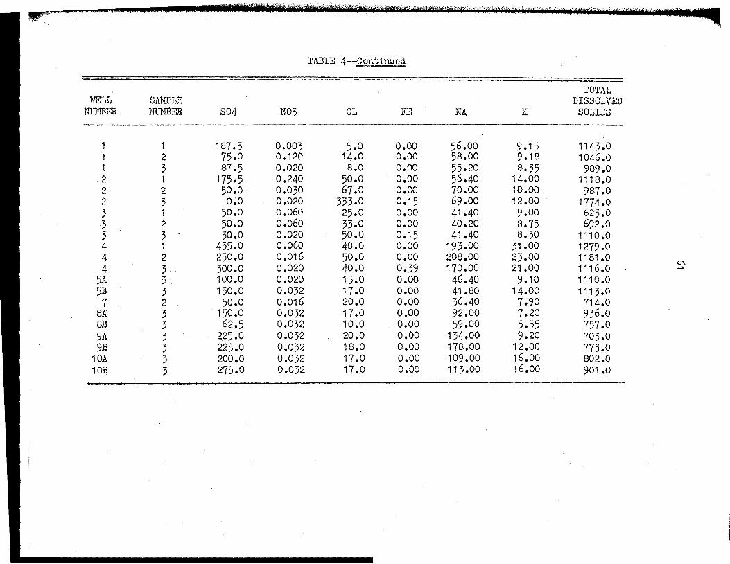
~""""'""' , "*·" "''"*•' .zz , :u u uu : s;:;a st! I JIIBNlillliillliillilllilll'iilliill'tiil(iiilataiif~:kiiff'iliilliitifh'!ii·,.,.,, n.;v.·.· "@*·'". •··.··•·····••.· •....... ~; " . . . . . . . . I rl 11.. I ilt l ftnM 1/1 i ih hi ·"u t' [" t T'tSifT''t11f't'4Wli(rfl@Wnta1nr•r1rr Ill •
TABLE 4~Continucd
IJ.'OTAL WELL SAMPLE DISSOLVED
NUMBER NUMBER S04 N03 CL FE NA K SOLIDS
1 1 187. 5 0.003 5.0 o.oo 56.00 9.15 1143.0 1 2 75,0 0.120 14.0 o.oo 58,00 9 .18 1046.0 1 3 87,5 0.020 8.o o.oo 55.20 8.35 989.0 2 1 175.5 · 0.240 50.0 o.oo 56,40 14.00 1118.0 2 2 50.0 0.030 67.0 o.oo 70.00 10.00 987,0 2 3 o;o 0.020 333.0 0.15 69.00 12.00 · 1774.0 3 1 50.0 0.060 25.0 o.oo 41.40 9.00 625.0 3 2 50.0 0.060 33.0 o.oo 40.20 8,75 692.0 3 3 50.0 0.020 50.0 0.15 41.40 8,30 111 o.o 4 1 435.0 0.060 40.0 o.oo 193.00 31.00 1279.0 4 2 250.0 0.016 50.0 o.oo 208.00 23.00 1181 .o 4 300.0 0.020 40.0 0.39 170.00 21.00 1116.0 °' 3 ...
5A 3. 100.0 0.020 15.0 o.oo 46.40 9.10 1110.0 513 3 150.0 0.032 17 .o o.oo 41.80 14.00 1113.0 7 2 50.0 0.016 20.0 o.oo 36.40 7.90 714.0
8A 3 150.0 0.032 17 .o o.oo 92.00 7.20 936.0 813 3 62,5 0.032 10.0 o.oo 59.00 5.55 757.0 9A 3 2.25.0 0.032 20.0 o.oo 134.00 9.20 703.0 9B 3 225.0 0.032 18.0 o.oo 178.00 12.00 773.0
10A 3 200.0 0.032 n .o o.oo 109.00 16.00 802.0 1013 3 275.0 0.032 17,0 o.oo 113.00 16.00 901.0
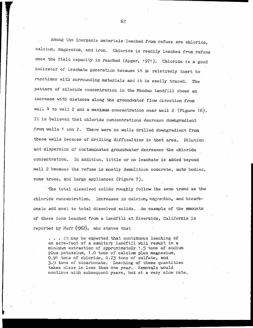
I
62
.A.~ong the inorganic materials leached from refuse are chloride,
calcium, magnesium, and iron. Chloride is readily leached from refuse
once the field capacity is reached (Apgar, 1971). Chloride is a good
indicator of leachate generation because it :is relatively inert to
ree.ctions w"i. th surrounding materials and it is easily traced.. The
pattern of chloride concentration in the Mandan land:fill shows an
increase with distance along the groundwater flow direction from
well 4 to well 2 and a maximum concentration near well 2 (Figure 16}.
It is believed that chloride concentrations decrease do:wngradient
from wells 1 and 2. There were no wells drilled downgradient.from
these wells because of drilling difficulties in that area. Dilution
and dispersion o:f contaminated groundwater decreases the chloride
concentration. In addition, little or no leachate is added beyond
well 2 because the refuse is mostly demolition concrete, auto bodies,
some trees, a..~d large appliances (Figure 7).
The total dissolved solids roughly follow the same trend as the
chloride concentration. Increases in calciu.m,, UJa{,wesiu!:l, and bicarb-
onate add most to total dissolved solids. An example of the amounts
of these ions leached from a landfill at Riverside, California is
reported by Merz (1962), who states that
.•. it may be expected that continuous leaching of an acre-foot of a sanitary landfill will result in a minimum extraction of approximately 1.5 tons of sodium plus potassium, 1.0 tons of calcium plus magnesium, 0.91 tons of chloride, 0.23 tons of sulfate, and 3.9 tons of bicarbonate. Leaching of these quantities takes olace in less than one year. Removals would contin;e w"i.th subsequent years, but at a very slow rate.

The Heart River near the Jlfandan landfill is contaminated very
little by groundwater from beneath the landfill. The amount of
contamination depends on the amount of contamination of groundwater
beneath the landfill by leachate and on the amount of flow in the
river. For river flows ranging from 0.3 m3/s (10 cfs) to 3 m3/s
(100 cfs), the dilution of contaminated groundwater discharging into
the river ranges from 1000 to 10.000 times 9 respectively. For example,
if the chloride concentration is 100 ppm, the concentration would
decrease to 0.001 :ppm for a flow of 3 m3/s and 0.1 ppm for a flow
3; of 0.3 m s. These small values indicate almost undetectable changes,
for a wide range of flows, in water quality of the Heart River due
to contaminated groundwater discharging from the landfill area.
For the monitored period (August to October, 1972), groundwater
quality beneath the landfill decreased with time. However, the
monitored period was short and evidence for changes in water quality
with time may be inconclusive.
Factors of Leachate Generation
The generation and movement of refuse leachate controls the
amounts of contamination of shallow groundwater in the Mandan landfill
area. Some of the factors controlling the generation and composition
of leachate are (1) spatial and time distribution of moisture, (2)
composition of refuse, (3) temperature of refuse cell, (4} available
oxygen, (5) depth of burial and degree of compaction, and (6) length
of time since burial. The effects of each generally overlap one
another.
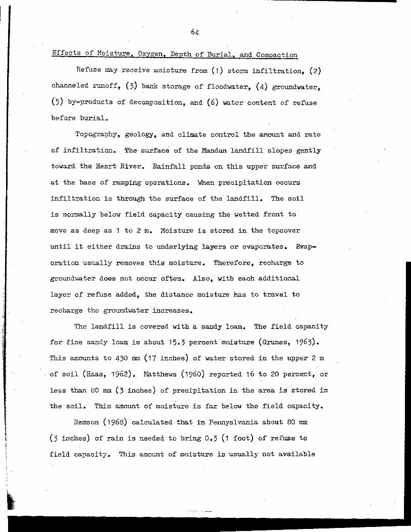
Effects of Moisture. O:x;vgen, Depth of Burial, and Compaction
Refuse ma.y receive moisture from (1) storm i..~filtration, (2)
channeled runoff, (3) bank storage of floodwater, (4) groundwater,
(5) by-products of decomposition, and (6) water content of refuse
before burial.
Topography, geology, and climate control the a.mount and rate
of infiltration. The surface of the Mandan landfill slopes gently
toward the Heart River. Rainfall ponds on this upper surface and
at the base of ramping operations. 'When precipitation occurs
infiltration is through the surface of the landfill. The soil
is normally below field capacity causing the wetted front to
move as deep as 1 to 2 m. Moisture is stored in the topcover
until it either drains to underlying layers or evaporates. Evap
oration usually removes this moisture. Therefore, recharge to
groundwater does not occur often. Also, with each additional
layer of refuse added, the distance moisture has to travel to
recharge the groundwater increases.
The landfill is covered with a sandy loam. The field capacity
for fine sandy loam is about 15.3 percent moisture (Grunes, 1963).
This amounts to 430 nnn (17 inches) of water stored in the upper 2 m
of soil (Haas, 1962). Matthews (1960) reported 16 to 20 percent, or
less than 80 mm (3 inches) of precipitation in the area is stored in
the soil. This amount of moisture is far below the field capacity.
Remson (1968) calculated that in Pennyslvania about 80 mm
(3 inches) of rain is needed to bring 0.3 (1 foot) of refuse to
field capacity. This amount of moisture is usually not available
in the study area because the field capacity of refuse is rarely
exceeded. The intensity of rainfall is normally greater than the
rate of infiltration causing mostly runoff.
The moisture content of refuse ready for burial in 1952 in
the Mandan landfill was about 23 percent (Weaver, 1964). A similar
value of 18 percent was reported for landfills in northeastern
Illinois (Funga.roli, 1971). Comparing these values to the amount of
moisture at field capacity of soils in the area, it appears that as
much moisture is needed to bring a layer of refuse to field capacity
as is needed for a layer of soil. After the upper meter of topcover of
the landfill reaches field capacity, excess moisture generally satu.ra:tes
only a thin layer of underlying refuse. Evaporation removes much of
the stored moisture in the soil within a few days.
The amount of water available from decomposing refuse is gen
erally too small to aid in further decomposition. Decomposition in
the Handan landfill is very slow and aerobic decomposition produces
very little water.
Several gullies occur on the flanks of the landfill. The
gullies cut into bulky wastes such as trees, tires, large metal
objects, and demolition waste. Runoff from the gullies to the refuse
is generally insignificant.
Some water from Heart River flooding may seep into the flanks
of the landfill. This water generally seeps into refuse composed
of trees, auto bodies, large appliances, and demolition waste.
It is believed that the addition of water :from seepage has little
effect on promoting decomposition in this part of the landfill.
66
Much of the moisture available for leachate generatfon in the
landfill comes from groundwater. During the spring a high water table
intersects the lower meter or two of refuse and saturates the material.
This is a seasonal event at best, but enough water may recharge the
refuse to accelerate decomposition and produce leachate. Contaminants
that have migrated to the lower layer of refuse, or contaminants
generated in this layer, enter the groundwater by direct contact in the
layer or by downward movement to the water table at some later time.
Data obtained by drilling indicated a low moisture content of
refuse and soil to a depth of 11 to 12 m. Below this the material was
partly saturated or saturated by moisture from groundwater.
In general the upper 10 m of refuse is an aerobic environment.
With depth, partic~larly near the lower few meters of refuse, ox:ygen
decreases and moisture increases. Water chemistry of wells in the
landfill area reflect} these conditions. Anaerobic decomposition is , \
greater than aerobic decomposition. Localized pockets of aerobic
or anaerobic environments may exist but were not investigated.
Anaerobic conditions beneath the landfill are indicated by a
decrease in sulfate in shallow groundwater. Drilling indicated
blue-gray (reduced)' sediment near the lower layer of refuse and below
the water table. An odor of hydrogen sulfide was detected in the
piezometers and in water samples collected over a period of several
months .•
The decrease in sulfate is because it is red~ced by bacteria.
Krauskopf (1967, p. 276) gives a symbolic reaction for sulfate reduction
using the simplest organic compound, methane (cn4
)
11111
67
2H \ so;;+ CH4 ~ H2S + CO2 + 2H20 • ( 11 )
The reduction is slow when only organic matter is present. Anaerobic
bacteria may act as a catalyst and accelerate the reaction • .Anaer-
obic bacteria are generally present in landfills in semiarid areas
(Stone, 1970).
The products of sulfate reduction are hydrogen sulfide, carbon
dioxide, and water. These products are present in the Mandan landfill.
Dissolved hydrogen sulfide gas, (H2S), was detected by its odor in
wells 2, 3, and 4. The pH of the water is.decreased according to
the reaction
.+ H
2S ~ H + HS •
Carbon dioxide (equation 11) combines with water to form
carbonic acid (H2
co3
). Carbonic acid may dissociate to form
h . (H+) ydrogen ions and bicarbonate
+ H
2co
3-} H + Hco
3 .
Bicarbonate has increased two to three times in wells beneath the
landfill. From a normal range of pH of 7 .3 to 7 .8 in uncontaminated
groundwater, the pH of contaminated groundwater decreased to about
6.9 to 7 .4.
The increase in hydrogen ions (H+) may cause calcium carb
onate (caco3
) to go into solution and release calcium or magnesium
. (H +-t) ions Ca , Mg
CaC03 + H+ ~·ca+++ HC03-.
The calcium and magnesium in contaminated groundwater has increased
as much as two times.
Carbon dioxide is an important product of aerobic and anaerobic
(12)
(13)
( 14)
68
decomposition. Its density is greater than air, causing it to diffuse
downward. The total alkalinity a.'1d total hardness are increased.
Total iron increases slightly in contaminated groundwater.
Anaerobically-produced iron is mostly ferrous iron, Fe-H+(Langmuir,
1969). It combines with water to form ferric hydroxides such as
Fe(OH)3
• Ferric iron, Fe++, is stable under low Eh and low pH
conditions. It may oxidize to ferrous iron. In this report iron
is reported as total iron and the relative proportions of each
are not known.
Ammonia(~) may be produced by anaerobic decomposition of
refuse • .Ammonia is stable under low Eh and low pH conditions.
Nitrate (N02-No3
) is an oxidized form of nitrogen a.'1d exists in
high Eh-pH environments. Nitrogen compounds have not contaminated
the groundwater in the Mandan landfill area. Nitrogen compounds are
not produced in sufficient amounts to comtaminate the groundwater
(Table 4).
Effects of Composition
Refuse in the Iv!andan landfill contains a large amount of paper
and paper products (cellulose base). Typically, the refuse consists
of 65 percent paper (by volume), 25 percent grass and garden trimmings,
5 percent organic garbage, and 5 percent inorganic matter (North
Dakota Health Service, 1970). At Mandan the refuse is about half
from homes and half from business (van Derwerker, 1952).
Cellulose compounds are biochemically oxidized by bacteria in
aerobic or anaerobic environments. Water-soluble compounds such as
carbon dioxide are produced. Stone (1970) reported that aerobic
69
thermophilic organisms biochemically oxidize carbonaceous compounds and
.slowly consume more complex nutrients like cellulose. This is
assumed to be a slow process in the Mandan lan~fill.
Bacteria consume oxygen in respiration. 1'he biological oxygen
demand is a measure of the amount of oxygen bacteria need and,
therefore, a measure of the rate of decomposition. Comsumption of
the readily decomposed organic matter produces a high biological oxygen
demand and a high oxygen (02
) demand. Mter about 6 weeks of burial
in the Mandan landfill, a maximum o2
has been used and decomposition
slows (van Derwerker, 1952J. Weaver (1964) reparted a 5-day biolog
ical demand of 77,050 ppm for refuse ready for burial in Mandan
landfills. Mter 1 year of burial the biological oxygen demand was
reduced by over 50 percent to 30,000 ppm, and after two years it
was reduced to 23,500 ppm. For the same periods, the oxygen consumed
was 271,000, 208,000, and 230,000 ppm, respectively. 1'1:lese figures
indicate maximum decomposition within 1 year of burial in the Mandan
landfill.
Effects of Temperature
Temperature is an important factor affecting decomposition of
refuse in the Mandan landfill. Almost no decomposition occurs in
Mandan landfills until the summer months (van Derwerker, 1952)~
Temperatures in three refuse cells were recorded during 1950 to 1951.
Figure 17 shows the temperature profiles for air and refuse cells for a
Mandan landfill. Cell 1 was completed in November, cell 2 in November,
and cell 3 in the summer. Cell temperatures are stable for cells 1
and 2, indicating very little biological activity. Cell 3 had a
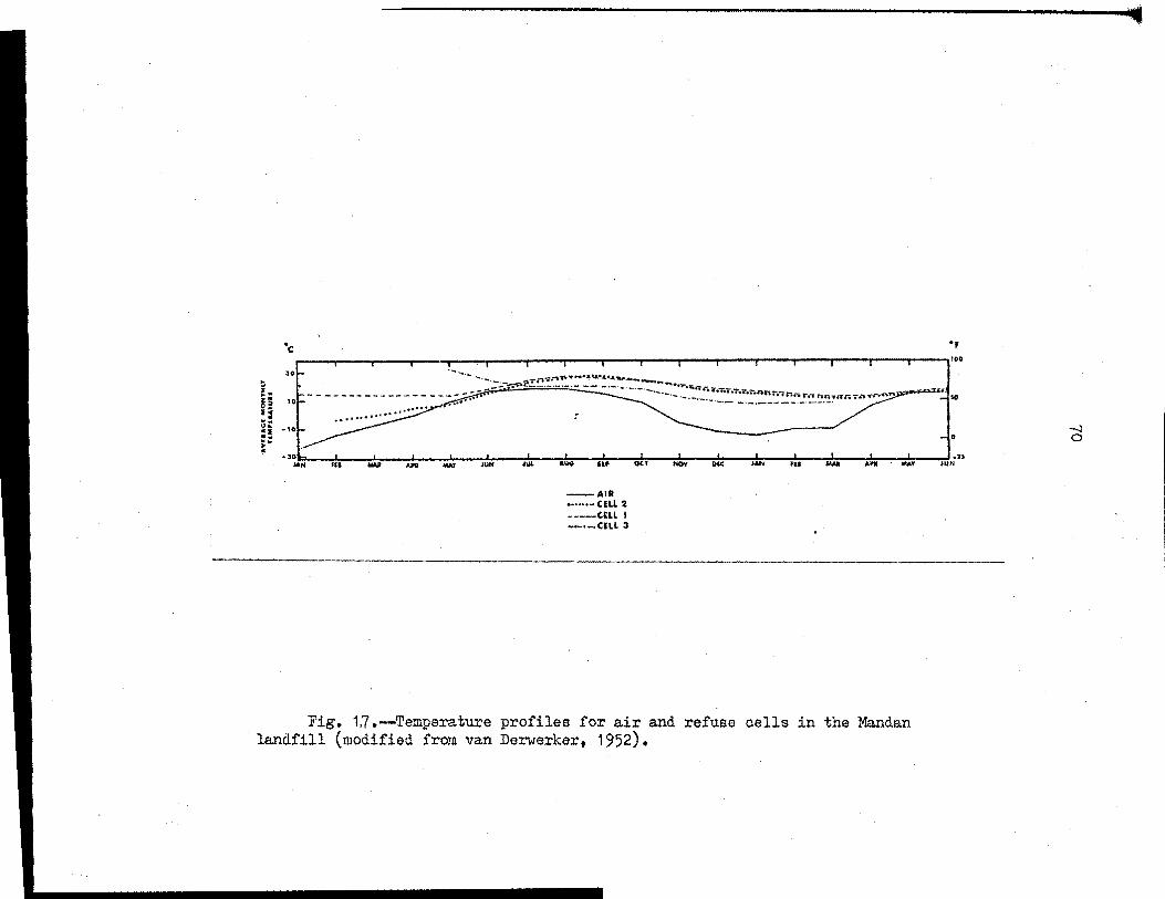
·, ..
!: z ~
i I :; .. . ; ..
., ,--'"""l--.,..--.,----,r---r--.,---,---,r---r---,---r---,r---r--,---,--,--1 100 ·-- .... -~ ............... ___ --~~
·- ··-·;-.:.--..-,l'!:'2.:.~.---·-·-· -·-···-·---. .:::::-••.-... ,.,.. u, • .-.......... ~,..,,.,.,.,,. ,...., ""~"" .,..-. .,..~ ...{50
- - ---- ... -- --- - ------ ~--- ·-· ... ·-·-·-·--·-·-------·-·-·-·-·
0
i=,--,,.. .. ,..._...,,_..,_ ___ .._ ___ ,.... __ ..,,,u,i,N,,__....,,u,.~---,,.,..u"o--"'u"•,--"0<+.,,r--KOV,+,---,o,.io,;;--....,.,.,.!,,,,,--,,.i.,,----'*'--"",.,1,,.,,..--,....,,,J,,--,.,.,1,,.. ... ,s
--AIR •• .. ••••CELL 2 -·---CELL I --•-,CELL 3
Fig. 1J.~Temperature profiles for air and refuse cells in the Mandan landfill (modified from van Derwerker, 1952).
......:i 0
71
maximum temperature of 34°0 (93°F) which declined to 28°C (83°F) within
2 weeks, indicating maximum bacterial action and digestion of organic
material soon after burial. In general the highest number of micro
organisms occur at 15°c to 20°0 (Camp, 1963). With a 5°c drop the
microorganisms decrease 10 to 20 percent. The temperature of the cells
0 in the Mandan landfills are low compared to temperatures of 60 0
(140°F) to 80°0 (180°F) reported in other landfills (van Derwerker,
1952). Decomposition of refuse in the Mandan landfill is slowed
considerably by the low mean annual air temperature of 5°0 (41°F).
Effects of Time
Stabilization of the Mandan landfill is proceeding slowly.
Drilling indicates fresh refuse to about 5 m (upper layer), fairly
fresh refuse from 5 m to 7 m, partly decomposed refuse from 7 m to
10 m, and badly decomposed refuse and crude fiber from 10 m to
12 or 13 m below the upper surface. For example, newspaper print
buried for about 8 years was readable. Rags, paper products, and
paper buried for 8 years or less were decomposed very little or
not at all.
CHAPTER VI
CONCLUSIONS
The following is a summary of cona,J.usions reached in this study.
(1) The Heart River valley near the Mandan landfill is the
discharge area for a local flow system and part of a.n intermediate
now system.
(2) The potential distribution is affected to a depth of 30 m
by the valley.
(3) Recharge to the local flow system is concentrated in an
area along the valley wall. Discharge of the local :flow system is
greatest at the base of the valley wall.
(4) The recharge area of the intermediate flow system occurs
in the upland area to the south and west of the landfill. The discharge
area occurs mostly in the Missouri River valley. There is some
seepage of the intermediate flow system to the Heart River valley.
(5) Groundwater flow. near the landfill is mostly lateral and
longitudinal. Beneath the landfill, flow is about at an angle of
0.7 rad to the Heart River.
(6) Much of the groundwater leaves this part of the valley
as underflow •.
(7) The velocity of groundwater flow near the landfill is
about 3 ma year.
72

73
(8) Shallow groundwater of the Heart River valley near the
landfill is generally a calcium-magnesium bicarbonate or calcium
sodium bicarbonate-sulfate type. The groundwater chemistry reflects
the short flow path of a local flow system.
(9) Deep groundwater of the study area is a sodium-calcium
sulfate-bicarbonate to a calcium-sodium bicarbonate-sulfate type.
This reflects the long flow path of an intermediate flow system.
(10) Very deep groundwater in this study is a sodium-calcium
bicarbonate-chloride to sodium bicarbonate-chloride type. This
reflects a long flow path of a regional flow system.
· (11) Shallow groundwater beneath the landfill has been
contaminated by refuse leachate. Total hardness, total dissolved
solids, alkalinity, and chloride have increased as much as several
times. Sulfate and pH have decreased.
(12) Beneath the landfill the groundwater shows an increase
of contamination along the direction of groundwater flow. The amount
of contamination is greatest near the center of the landfill and is
believed to decrease toward the north and east.
(13) The Heart River near the Mandan landfill is contaminated
very little by groundwater from beneath the landfill. The. amount of
dilution of contaminated groundwater by the Heart River ranges from
1000 to 10,000 times, depending on the amount of flow in the river
and the amount of contamination of groundwater by leachate.
(14) Refuse contaminants have entered the .flow system by contact
with a high water table, by infiltration through a relatively.thin
layer of refuse (during the early years of the landfill), and
-
74
possibly by infrequent recharge through parts of the landfill. Recharge
rarely occurs because small amounts of precipitation and high evapor
ation leave the material below field capacity much of the time.
(15) The low temperatures occurring much of the year slow
bacterial action and cause a very slow :rate of decomposition of refuse.
(16) The large amount of cellulose-based refuse takes much time
to dec.ompose.
(17) The main processes operating in the Mandan landfill are
reduction of sulfate, production of carbon dioxide (and related
reactions), and leaching o.f chloride, calcium, magnesium, and
possibly other minor metals.
(18) The data on leachate generation and movement in the 1/Jandan
landfill can be used to evaluate potential contamination of ground
water by leachate from landfills in much of southwestern North Dakota.
APPENDIX A
METHODS OF DATA COLLECTION .AND WATER .Ai"\IALYSIS
76
METHODS OF DAT.A COLl.,ECTION .AND WATE..t{ At'WILYSIS
Location Format
The location format used in this study for the location of test
wells follows the scheme shown in Figure 18. The first numeral of this
system is the township north of its base, the second is the range west
of t.~e principal meridian, and the third is the section in which the
well is located. The lower case letters following the section number
are the position of the well within the section. The first letter is
the quarter section (160 acre tract), the second letter is the quarter
quarter section (40 acre tract), and the third letter is the 10 acre
subdivision within the quarter-quarter section. The subdivisions of
the sections, _quarter sections. and quarter-quarter sections are lettered
a, b, c, and din a counterclockwise direction beginning in the
northeast quarter. A well located in Nl!.1t of the Swt of the NEi of
sec. 35, T.139N., R.8fW. is designated 139-81-35aca.
Drilling and Piezometer Installation
The purpose of the test-drilling was to collect stratigraphic
information and to install piezometers. The piezometers were used
to determine the groundwater flow pattern and to collect water samples.
The test wells in the Mandan landfill area were made with two
different drilling rigs. A truck-mounted hydraulic rotary rig was
contracted from a private well driller who drilled about 75 percent
of the test holes for the study. Several shallow holes in the landfill
were made with the North Dakota Geological Survey truck-mounted auger
(0.15 m diameter).

d> ....
d'cr
Fig. 18
o>..,... d',.
d'..;,
77
d"c'" d',...
d'o
showing the location format.

78
The sediment was inspected at about 0.3 m intervals and lithologic
logs of the stratigraphic units were compiled. The field descriptions
of the stratigraphic units are given in Appendix B.
The advantages and disadvantages of drilling with the truck
mounted auger and truck-mounted hydraulic rotary rig in most types
of sediment are discussed by Schulte (1972) in a study of the ground
water geology of the Spiritwood Lake area in central North Dakota.
Drilling in refuse with each of the two types of drilling rigs
caused advantages and disadvantages for each.
The truck-mounted auger is less expensive than the hydraulic
rotary rig. Go~d stratigraphic samples with original moisture
content are obtained. The auger cannot be used to drill in refuse
that offers resistance to drilling (concrete, metal, trees, and rags),
or in unconsolidated sediment such as that found below the water
table. Test holes cannot be flushed prior to installing
piezometers.
The hydraulic rotary rig is about five times as expensive as
the auger (Schulte, 1972). However, the hydraulic rotary rig can
be used to drill through most types of refuse in landfills (rocks,
light metal, small trees, rags, and some demolition concrete). The
stratigraphic samples are of·cen very distrubed and are lacking
original moisture contents. Loss of circulation water to large
cavities in the refuse and clogging of the circulation system with
refuse also occurs. The resulting odor of refuse and its unsanitary
nature make drilling very u..."1.pleasa.nt. An advc:mtage is that test holes
can be flushed before piezometers are installed.
79
Open standpipe piezometers were installed in the Mandan landfill
area (Casagrande, 1949). The piezometers were installed in 0.1 m
(4 inch) diameter holes and 0.15 m (6 inch) diameter holes. All
standpipes were 0.025 m (1 inch) diameter. Single and multiple
piezometers (two in a borehole) were installed.
The procedures followed for installing the piezometers were
generally the same. A length of plastic pipe about o.6 m to 1 m
longer than the test hole was prepared. The lower end of the pipe was
plugged with a 0.025 m (1 inch) plastic cap. The lower 0.75 m of
pipe was slotted with a hacksaw. The slots were about 0.025 m
apart and cut a third of the way into the pipe in a spiralling-up
manner.
The plastic pipe was then inserted into the test hole. Fi~ to
medium gravel (buckshot) was packed around the screened inter',al and
packed for a short distance above that. A 1 m thickness of neat cement
was used to seal the screened interval from the open hole. A single
installation was completed by backfilling the hole to the top with
silty, clayey material. After the backfill settled, cement was used
to seal the open hole at ground level. The plastic pipe was cut about
0.18 m (7 inches) above ground level. Protective pipe of galvanized
0.08 m (3 inches) diameter steel was installed around the plastic
pipe and cemented in the ground. The standpipe was closed.with a vented
0.025 m plastic cap. Wood fence posts were installed to mark locations
of the wells.
Multiple piezometer installations were ma.de in a similar manner.
Two sections of pipe, complete with screens and end caps, were

80
installed in the borehole. One pipe was staggered 3 to 5 m above the
lower end of the other pipe. The lower pipe was gravel packed,
cemented, and backfilled to the lower end of the upper pipe. The
u pp er pipe was then completed in a similar manner. The two pipes
were cut 0.18 m above ground, cemented, enclosed with steel pipe,
and capped.
Boreholes made with hydraulic rotary equip~ent were flushed
before piezometers were installed. Once installed, the piezometers
were cleaned by adding water (from the Heart River) and then bailing
water out of tb.e pipe. Auger holes were not cleaned before piezometers
were installed. Water was later poured into the standpipe a.~d bailed
out. Much of the sediment was removed in this ma,."lller because samples
collected later from the bottom of the piezometer were free of sediment.
The piezometers were not used for 1 to 2 weeks after installation.
Water levels were allowed to come to equilibrium and groundwater was
allowed to clear.
Methods used for piezometer installation follow general techniques
used by Schulte (1972). Slotted pipes were very efficient in the
sediment found in the study area. Sediment permeabilities were great
enough to allow water to enter the standpipe faster than it could be
removed. The piezometers responded to changes in water levels with
very little lag ti.me (as much as 2 days).
· The method of sealing the bottom of the piezometers from the open
borehole was effective. With the exception of possibly two installations,
most piezometers were properly sealed with cement above the screened
interval. Some difficulty occurs in sealing each piezometer properly
81
in a multiple installation. Care must be taken to pack a sealing
material, such as clay, in the part of the borehole between the
cemented section of the lower piezometer and the bottom of the
upper piezometer. If this is done correctly, a good seal should
result for both piezometers.
Collection of Water Samoles
Water samples that are representative of the source at the
time of sampling were collected. Procedures used by the United States
Geological Survey (Rainwater and Thatcher, 1960) were generally
followed in this study. Alternate procedures are also described.
Water samples were obtained from standpipe piezometers and from
pumped wells in the study area. The water samples were collected in
high-density polyethylene bottles with polyethylene-lined bakelite
screw caps. The sample bottles were rinsed with distilled water and
labeled with masking tape and permanent ink before collection.
After the samples were collected, the caps were tightly screwed down
and sealed with tape to create a seal for transportation and storage.
Grou...11.dwater samples were collected from two kinds of wells,
standpipe piezometers and pumped domestic and stock wells. The pumped
wells ranged in depth from 30 m to 100 m and were operated by either
surface pu.rnps (electric) or submersible pumps. Stagnant water was
cleared from the casing of the pumped wells by pumping for several
minutes. TJ:te standpipe piezometers were flushed at the time of
installation and were bailed periodically during the field season.
Most of the water s2.mples are representative of the water at the point
of collection because (1) the piezometer standpipes are plastic and
82
do not react w.i th water or ions in the water, and (2) most of the
samples were collected near the slats at t.."l.e bottom of the standpipe.
·water samples from standpipe piezometers were collected using a
sampler consisting of a 0.45 m (18-inch) piece of 0.018 m (3/4-inch)
diameter plastic pipe. One end of the pipe is open and has a nylon
li,."'1.e attached through two holes drilled below the upper rim. The
nylon line is used to raise or lower the sampler through the stand
pipe. The lower end of the sampler is closed with a plastic-coated
metal cap. Plastic-coated lead weights are used ta increase the
weight of the sampler. The sampler is lowered to the water 1e~re1 in
the standpipe and then allowed to free fall to the bottom. Water
will begin to fill the sampler once it stops free falling. The water
sampler is retriev_ed using the attached nylon line.
Water Level Measurements
The elevation of the static water level in a piezometer is
considered to be hydraulic potential at the bottom of the well. It is
assumed that the piezometer standpipe does not leak and that the water
in the standpipe is sealed off from all pressure except the pore
pressure at the bottom of the well. The static water level is assumed
to have recovered from any addition or subtraction of water.
The first two assumptions are valid for most of the piezometers
in the study area because care was taken ta properly complete and
seal the piezometers, The piezometers stabilized within a few days
aster adding or subtracting water. The piezometers were monitored
almost daily for a month after installation and at longer periods
therea:fter.
83
1he water level in standpipe piezometers was measured with a
battery operated electric wateri-level indicator (Soiltest, model
DR-760A). The total head at the bottom of the piezometer was determined
by subtracting the measured depth to water from the elevation of ground
level.
Elevation Determinations
The study area is covered in the Mandan Quadrangle and
Bismarck Quadrangle of the United States Geological Survey 7.5 minute
(scale 1:24,ooo) series of topographic maps. The topographic coverage
was considered inadequate for determining well elevations. A base
station was set up on the floodplain west of the landfill. The elevation
of this station (496.9 m or 1640 feet) was determined with an .American
Paulin Altimeter (Model M-1) using a nearby benchmark for vertical
control. Elevations of all the piezometers (at ground level) and
selected points in the study area were then determined to hundreths of
a meter by the transit-stadia method. Several traverses were established
to provide topographic coverage of most of the study area. Topographic
maps were used to determine elevations of selected points in the southern
part of the study area.
Analysis of Water Samples
The temperature, specific conductance, pH, ·and concentration of
major cations and anions were determined for 54 groundwater samples
collected in the study area. Other chemical analyses published by the
United States Geological Survey and Tyschen (1949) were used in
84
evaluating the water chemistry of the area but are not included in
the discussion of a...~alytical methods.
The temperature, specific conductance, and pH of water samples
were determined in the field. The water samples were refrigerated
after collection until they were transported to the laboratory.
The changes in water chemistry ocan:nng during transport are assumed
to be insignificant. Before analysis in the laboratory, the samples
were prepared for storage following procedures of Rainwater and
Thatcher (1960) ..
Three sets of groundwater samples were collected over a period
of several months. All the samples of a particular set were collected
within a few hours on the same day and physical measurements were
ma.de at that .... i..ime.
The following procedures are described in the order in which the
samples were analyzed. The reproducibility of some of the methods
(temperature, specific conductance, and pH) was determined by
repeating the sample analysis. Accuracy of methods used is based on
manual specifications of the instrument.
Water Temperature
Groundwater temperatures were determined in the field at the
bottom of standpipe piezometers. Measurements were made with a Whitney
portable thermister (Model TC-5A) equipped with about 61 m (200 feet)
of insulated cable and 0 .. 019 m (3/4-inch) diameter temperature probe.
For each reading, the probe was lowered to the bottom of the standpipe
and allowed to come to an equilibrium temperature •. The temperature
was recorded when it remained constant for a few minutes.
85
Tne accuracy of the thermister is about 0.1°c for the range 0°C
to 40°c, Temperatures measured in the field were reproducible to 0.02°C.
pH
The pH of water samples was measured in the field and later in
the laboratory. The Coleman Precision Portable pH Meter (Model 37A)
was used with a Coleman 3-472 Tri-Purpose Shielded Glass Electrode
and a 3-711 reference electrode. A 7.0 pH buffered solution was used
to standarize the instrument before each use. The instrument was
checked against buffered solutions of pH 6.o to pH 8.0. All solutions
were temperature corrected ,vith the manual temperature compensator.
The Precision Portable pH Meter is accurate to± 0.005 pH units and,
ideally, readings are reproducible to.± 0.001 pH units.
The pH values were remeasured in the laboratory ,vi th the same
instrument. The pH of samples with an original pH of 6.9 to 7 .2
showed the most change. The changes were as large as± 0.6 pH units,
but more com.~only were about± 0.3 units. The pH values measured in
the field are used in this report.
Specific Conductance
T'ne specific conductance was measured in the field with a Solu
Bridge Conductivity Meter (Soil test Model A-105). The meter measures
conductance in the range of 50 to 8000 micromhos and has a manual
temperature compensator. Measurements are made by immersing the electrode
in the groundwater sample. The results are generally reproducible to
within± 10 percent.
86
Alkalinity (Hco3
- + co3--)
In groundwater chemistry, alkalinity is the capacity of a water
to neutralize a strong acid and mostly depends on:the carbonate a.,.~d
bicarbonate in solution (Rainwater and Thatcher, 1960, p.93).
Alkalinity of water samples in this study was determined by the
potentiometric method. This method consists of titrating a 50 ml
sample of water with a 0.02 normal solution of sulfuric acid against
a pH meter to the end points of pH 8.0 for carbonate and pH 4.o for
bicarbonate. The total alkalinity, carbonate, and bicarbonate were
calculated following the procedures given by APHA (1965, p.52).
The normality of the sulfuric acid was checked periodically
against a sodium carbonate standard to check its stability. The values
determined for alkalinity were reproducible to within.± 2 percent.
Calcium and Magnesium (Hardness)
Hardness in natural water is caused by calcium and magnesium
ions. The concentrations of calcium and magnesium were determined by
titration ,vith a 0.01 normal solution of CDTA (disodium dihydrogen 1,
2-cychlhexanediaminetetraacetate). Calcium was determined by adding
1 ml of 9 normal sodium hydroxide to a 10 ml sample diluted to 100 ml
a...Dd titrating with CDTA in the presence of Cal-red indicator to an
end point (color change from red to pure blue) •. The total hardness
was determined by diluting a 10 ml sample to 100 ml, adding 1 ml
non-ammonia buffer, and titrating with CDTA in the presence EBT indicator
to an end point (color change red to pure blue). The concentration of
magnesium was calculated as the difference between total hardness and
87
calcium concentration. The reagent was checked for stability by
titrating a standard solution of calcium chloride.
Calcium determinations were reproducible to ,ri. thin + 1 ppm and
magnesium to within+ 2 ppm.
Sulfate
The turbidimetric method was used to determine the sulfate
concentration (APHA, 1965). The value of light absorbance through a
suspension of barium sulfate in the water sample was determined
using a Hellige Turbidimeter. The absorbance values were determined
by passing light through a blue filter. A 10 ml water sample was
diluted to 50 ml, 10 ml of Sulfaver salt-acid solution added, and
barium. chloride crystals added to form a suspension of barium sulfate.
Absorbance values were compared with a calibration curve that was
constructed using absorbance values from several standard solutions.
The concentration of sulfate in the water sample was read directly
from the curve.
There is about± 5 percent error in the determination. The
accuracy of the instrument was about+ 0.5 percent,
Chloride
The chloride concentration was determined with a Coleman Chloride
Ion-Selective Electrode (3-802). The selective-ion electrodes are
similar to glass electrodes used to measure pH. The selective-ion
electrode, the Calomel reference-electrode, and Coleman Precision
Portable pH Meter (Model 37A) were used in combination to measure
the activity of the chloride ion.
The procedure was to prepare a standard 1 molar solution of
88
of chloride a.nd make several solutions ranging in concentration from
-6 1 molar to 1 X 10 molar by dilution of the 1 molar solution with
distilled water. The solutions are maintained at 25°c and each is
measured with the chloride probe to ob-tain .a reading in millivolts
on the pH meter. A calibration curve of chloride concentration and
millivolts is constructed and used as a reference for detenning the
chloride co~centration in a water sample.
Ideally, the reproducibility of chloride concentration was
wit..lti.n + 1 ppm of the initial value.
Nitrate
Nitrate concentration was determined by the cadmium-reduction
wet chemical method (Hach Chemical Company Catalog number 10, 1968,
p. 42). A:I.1 80 ml water sample is treated with 2 ml concentrated ammon
ium chloride. Th0 sample is passed through the cadmium-reduction
column. 'E<'len a 25 ml aliquot is treated with 1/2 ml sulfanilic
acid and 1/2 ml alpha-naphthylamine and allowed to stand 20 minutes.
A Hellige Colorimete,r 'tvas used to read the nitrate concentration.
The reproducibility of nitrate determinations is about± 10
percent.
Iron, Potassiu.m, Sodium
The concentrations of iron, sodium, and potassium in water
samples were deter.mined with a Perkin-Elmer model 403 Atomic Absorption/
Flame Emission Spectre-Photometer using an air-acetylene mixture.
Specified currents and flow rates for each element were used. Wave
lengths were set using the rating specifications. The instrument

89
was calibrated for each use with prepared standards whose concentrations
were in the optimum operating range for the particular element
determined. The instrument has single readouts, averages of ten
readouts, and averages of one hundred readouts. The averages of one
hundred readouts were used in most cases. The instrument was
recalibrated periodically or when readouts were unstable. Samples having
concentrations greater than the optimum operating range were diluted
100 to 400 times with double-distilled water (1 part sample, 99 parts
distilled water for dilution of 100 times).
The concentrations of the elements determined with the atomic
absorption unit were reproducible to within± 1 percent under ideal
conditions.
Total Dissolved Solids
The total dissolved solids were determined by calculation
following Rainwater and Thatcher (1960, p.271). The constituents
were converted to forms in the anhydrous state and summed. The method
assumes that all constituents were analyzed. In this study manganese,
silica, and trace elements were not determined. Several samples were
analyzed for manganese but the amount present was generally much less
than 1 ppm. It is assumed no large error was made by ignoring
minor constituents.

90
Hydraulic Conductivitv and Rate of Flow .Determinations
Slug tests (falling-head) were used to determine in situ permea
bilities of sediment in the Cannonball and Coteau Formations in the
Mandan landfill area. The sediment surrounding the screened interval
of several piezometers was slug-tGsted. The sediment ranged from
silty, sandy clay to medium gravel.
In the slug test, water is added to a stabilized piezometer and
the hydraulic head is measured at different times. From the equation for
the basic time lag :ratio (Hvorslev, 1951)
,i = 1n ...E.g_ = 1n Ho , T Ho-y H
( 15)
the equation
t 2-t1 = T( 1n J!2. - 1n g.2) = ....!_ 1n H1 H2 H1 FK H2
( 16)
can be derived. Equation 16 relates time (t1 , t 2 , •• ) to head
measurements (Ho, H1, H2, •• ), cross-sectional area of piezometer (A),
sr.ape factor of piezometer (F), and hydraulic conductivity (K).
Rea:r:ranging equation 16 for the hydraulic conductivity, K (in cm/s),
( 17)
gives the equation used to calculate the hydraulic conductivity based
on field data where t 1,t2, •• = measured time, s,
H1, H2, •• = measured head, m,
A= cross-sectio~ area of piezometer, cm, and
F = shape factor of piezometer, cm, ( about 1 34 cm for O .025 m .Jiameter water intake, 0.031 ·m diameter standpipe, and about 1m screened interval).
·r
,.1JD I

91
Water from the Heart River near the landfill was used in the
slug tests. The specific conductivity of this water ranged from 1300
to 1500 micromhos per.centimeter.
The hydraulic conductivity of sandy, silty, clay and fine sand
of the Cannonball Formation ranged from 1 X 10⁻⁵ m/s to 1 X 10⁻⁷ m/s.
The hydraulic conductivity of fine sand and medium gravel in the
Coteau Formation in the landfill area was 6.4 X 10⁻⁷ m/s and 3.2 X 10⁻⁴
m/s, respectively.
The rate (velocity) of flow of shallow groundwater in the landfill
was calculated from the equation for the rate of flow,
v = K i n ,
where v = rate {velocity) of flow, m/s,
K = hydraulic conductivity, m/s,
i = hydraulic gradient; m/m,and
n =porosity,% X 100.
The rate of flow of groundwater in the Coteau Formation in
the landfill area ranged from 3 X 10⁻⁵ m/s in permeable sediment
(18)
(gravel) to 5 X 10-G m/s in less permeable sediment (fine sand and silt).

APPENDIX B
LITHOLOGIC LOGS OF TEST HOIES
n"\f THE MANDAN LANDFILL AREA

93
139_:_.81-34adc 1 Well Number 1 Elevation: 503.43 m (1661.50 feet)
Material
La.YJ.dfill 'f'opcover; fine sands, silts of
Cannonball Formation Refuse: fresh, undecomposed paper,
food, rags Refuse; mixed with clay Refuse; fairly fresh Refuse; fairly fresh, mixed with rock
Coteau F'ormation Clay; dark gray, dense, reduced Clay; silty, dark gray Clay; sandy Sand; fine to medium, blue Sand; silty, clayey, blue Clay; dark blue, dense
Thickness, m Depth, m
o.6 0-0.6
3.3 0.6-3.9
1.5 3.9-5.4 0.9 5.4-6.3 0.3 6.3-6.6
2 .1 6.6-8. 7 2.4 8.7-11.1 1 .2 11 .1-12 .. 3 2.4 12.3-14.7 0.9 14.7-15.6 o.6 15.6-16. 2
One piezometer was installed at a depth of 15.5 min the sand.
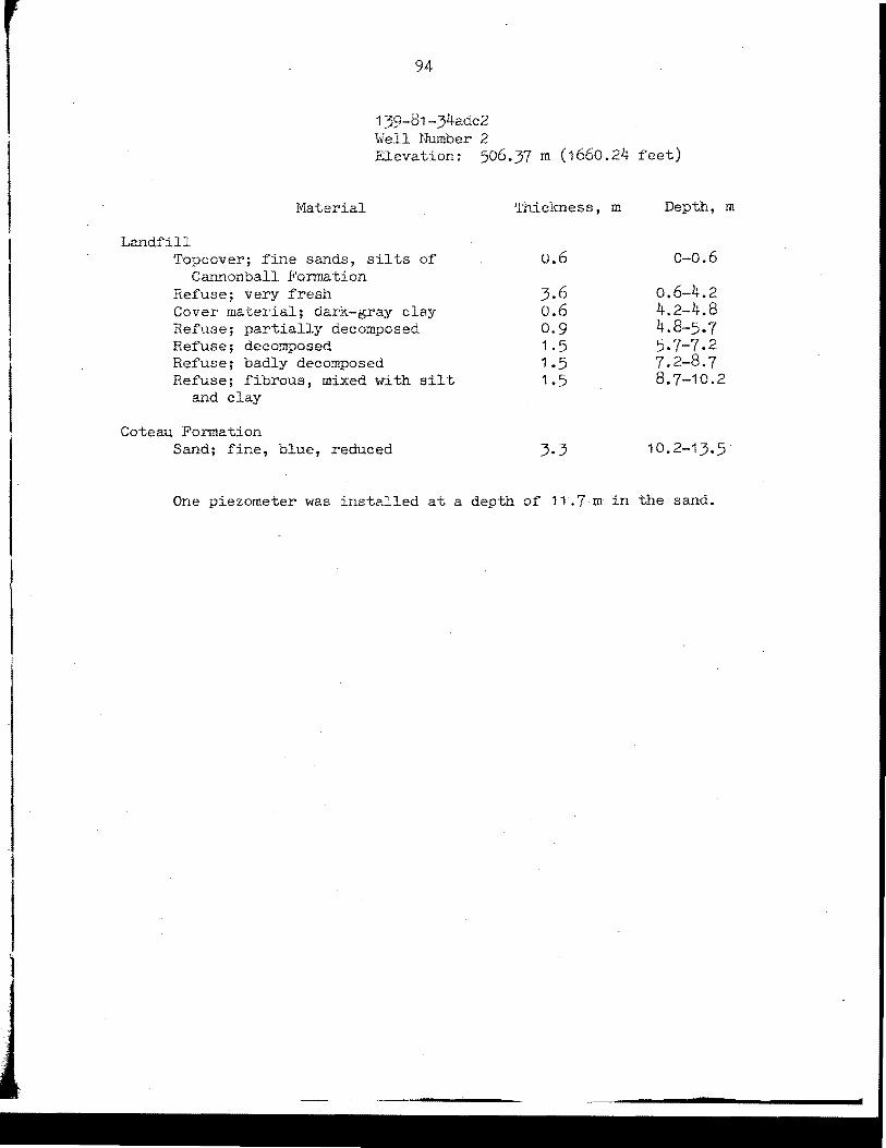
l
94
139-81-34adc2 Well Number 2 Elevation: 506.37 m (1660.24 feet)
Material
Land.fill Topcover; fine sands, silts of
Cannonball Fonnation Refuse; very fresh Cover material; dark-gray clay Refuse; partially decomposed Refuse; decomposed Refuse; badly decomposed Refuse; fibrous, mixed with silt
and clay
Coteau Formation Sand; fine, blue, reduced
Thickness, m
o.6
3.6 o.6 0.9 1.5 1.5 1.5
3.3
Depth, m
0-0.6
o.6-4.2 4.2-4.8 4.8-5.7 5.7-7.2 7.2-8.7 8.7-10.2
10.2-13.5
One piezometer was installed at a depth of '.11 .. 7 m in the sand.
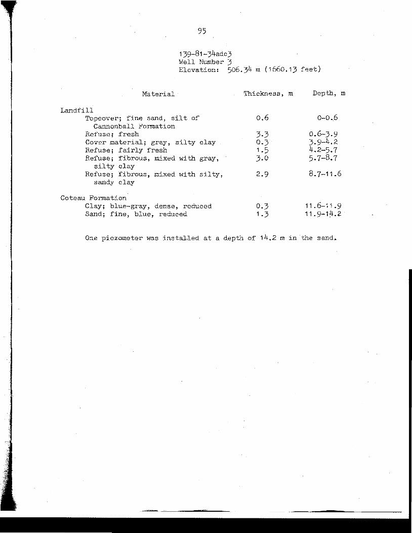
95
139-81-34adc3 Well Number 3 Elevation: 506.34 m (1660.13 feet)
Material
Landfill Topcover; fine sand, silt of
Cannonball Formation Refuse; fresh Cover material; gray, silty clay Refuse; fairly fresh Refuse; fibrous, mixed with gray,
silty clay Refuse; :fibrous, mixed with silty,
sandy clay
Coteau Formation Clay; blue-gray, dense, reduced Sand; fine, blue, reduced
Thickness, m
o.6
3.3 0 1.5 3.0
2.9
0.3 1.3
Depth, m
0-0.6
0.6-3.9 3.9-4.2 4.2-5.7 5.7-8.7
8.7-11.6
11 . 6-11 .9 11.9-1~.2
One piezometer was instal-J.ed at a depth of 14.2 min the sand.
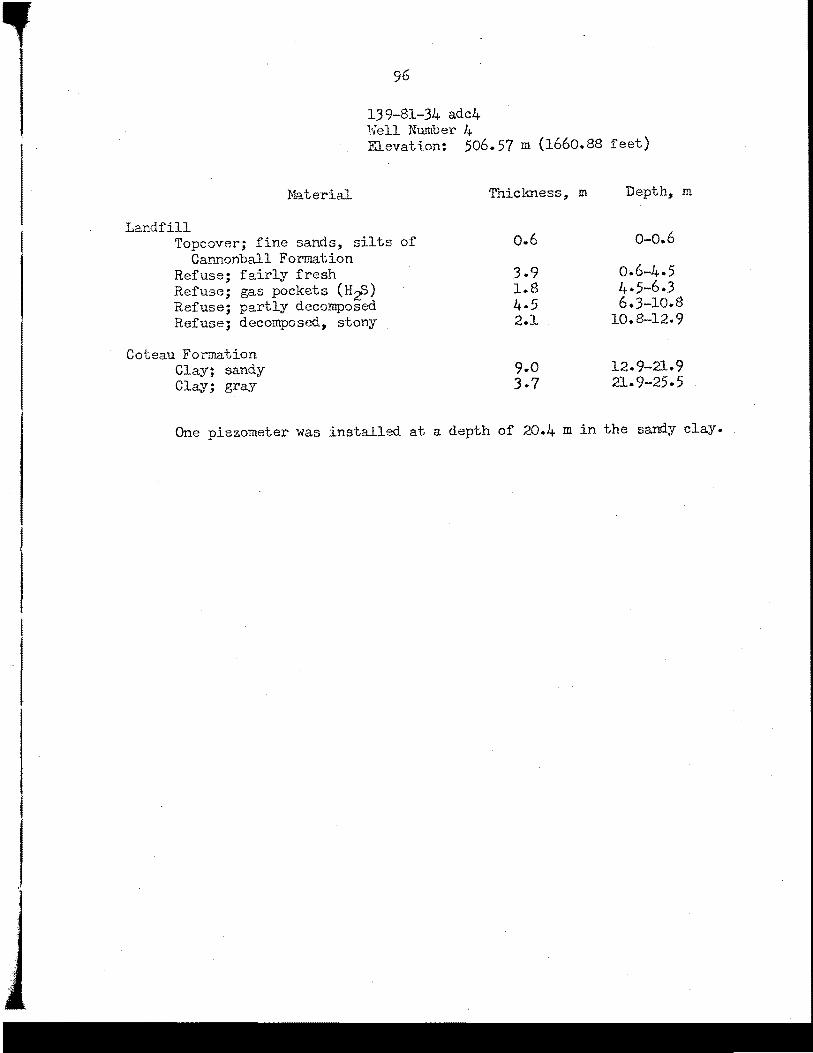
96
139-81-34 adc4 Well Number 4 Elevation: 506.57 m (1660.88 feet)
Material T'niclmess, m Depth, m
Landfill Topcover; fine sands, silts of o.6 o-o.6
Cannonball Formation Refuse; fairly fresh 3.9 o.6-4.5 Refuse; gas pockets (HzS) 1.8 4.5-6.J Refuse; partly decomposed 4.5 6.3-10 .. S Refuse; decomposed, stony 2.1 10.8-12.9
Coteau Formation Clay; sandy 9 .. 0 12.9-21.9 Clay; gray 3.7 21.9-25.5
One piezometer was installed at a depth of 20.4 min the sandy clay.
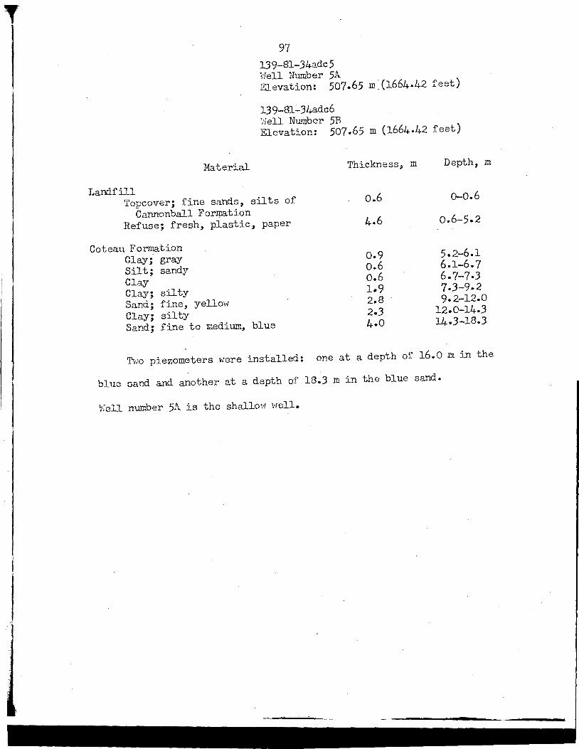
T 97
13 9-81-34adc 5 i"Jell Number 5A. Elevation: 507 .. 65 m.(1664.42 feet)
139-81-34adc6 ;'Jell Number 5B Elevation: 507.65 m (1664-42 feet)
Material
Landfill Topcover; fine sands, silts of
Cannonball Formation Refuse; fresh, plastic, paper
Coteau Formation Clay; gray Silt; sandy Clay Clay; silty Sand; fine, yellow Clay; silty Sand; fine to medium, blue
Thickness,
o.6
4.6
o.9 o.6 o.6 1 .. 9 2.8 .2.3 4.0
m Depth, m
o-o.6
0.6-s • .2
5.2-6.l 6.1-6.7 6.7-7.3 7.3-9.2 9.2-12.0
12.0-14.3 J.4..J-18.3
'I\10 piezometers were installed: one at a depth of 16.0 m in the
blue sand and another at a depth of 18.3 min the blue sand.
Well number 5A. is the shallow well.

j
j
98
l39-81-34addl Nwnber 6A
Elevation: 513.93 m (1685.(X) feet)
139-81-34add2 Well Number 6B Elevation: 513.93 m (1685.00 feet)
Material
Cannonball Formation Sand; fine, yellow Clay; silty Clay; sandy Clay Clay; silty Shale; calcareous Clay Clay; sandy, blue Clay; gray Clay; silty, sandy Shale; dense, light blue-gray Sand; silt; clay; alternating Sand; fine Sand; silt; ~lay; alternating Sand; fine to medium
Thickness, m Depth, m
2.1 0-2.l 0.9 2.1-3.0 o.6 3.0-J.6 0.3 J.6-3.9 0.4 3-9-4.3 0.3 4-3-4.6 2.4 4.6-7.0 o.6 7.0-7.6 4.6 7.6-12.2. 2.9 12.2-15;1 0.5 15.1-15.6 2.8 15.6-18.4 3.5 18.4-22 .. 9 3.0 22 .. 9-25.9 1.6 25-9-27.5
Two piezometers were installed: one at a depth of 27.5 min a
sand and another at a depth of lJ.8 m in a silty, sandy clay. 1/lell
number 6B is the shallow well.
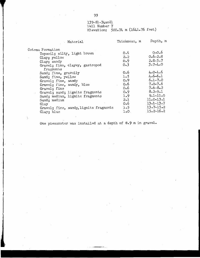
I
99
13 9-Sl-34acdl Uell Wumber 7 Elevation: 5CIJ.74 m (1641.76 feet)
Material
Coteau Formation Topsoil; silty, light brown Clay; yellow Clay; sandy Gravel; fine, clayey, gastropod
fragments Sand; fine, gravelly Sand; fine, yellow Gravel; fine, sandy Gravel; fine, sandy, blue Gravel; fine Gravel; sand; lignite fragments Sand; mediur,1, lignite fragments Sand; medium Clay Gravel; fine, sandy, lignite fragments Clay; blue
Thickness, m
o.6 2.2 0.9 0.3
o.6 1.5 0.9 o.6 o.6 0.9 1.9 2.1 o.6 :i.. 5 1.0
Depth, m
0-0.6 0.6-2.8 2.8-3-7 3.7-4.0
4.0-4.6 4.6-6 .. l 6.l-7.0 7.0-7.6 7.6-8.2 8.2-9.1 9.1-11.0
11.0-13.1 13.1-i3.7 13.7-15~2 15.2-16.2
One piezometer was installed at a depth of 8.9 min gravel.

J 100
139-81-34acd2 :·Jell Number 8A Eaevation: 500.20 m (1640.00 feet)
13 9-81-34acd3 Well Number 8B Elevation: 500.20 m (1640.00 feet)
Material
Coteau Formation Topsoil; sandy, light bro1m Clay; yellm-; Clay; silty, yellow Clay; blue Clay; blue, gastropod and lignite
fragments
Thickness,
o.6 2.5 0.9 o.6 2.1
0.9 1.6
m Depth,
0-0.6 0.6-J.1 J.1-4.0 4.0-4.6 4.6-6.7
6. 7-7.6 7.6-9.2
m
Gravel; fine, sandy Gravel; coarse, sandy Clay; blue, lignite fragments Gravel; fine to medium
0.9 9.2-io.1
Gravel; medium to coarse, lignite fragments
o.6 3.0
10.1-10.7 10.7-13.7
Two piezometers were installed: one was installed at a depth
of 7.2 min a fine gravel and another was installed at a depth of
10. 9 m in a coarse gravel. \foll number 8A is the shallow well.
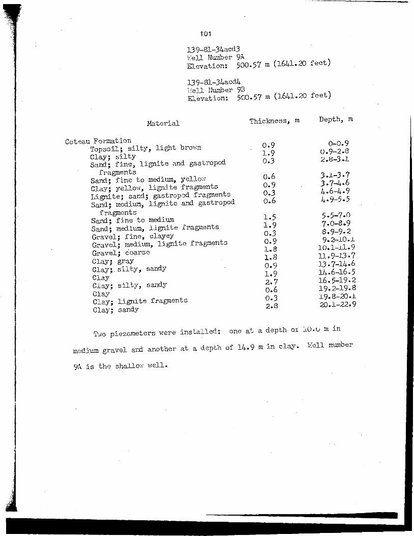
101
13 9-81-34acd3 Well Number 9A Elevation: 500.57 m (1641.20 feet)
13 9-81-34acd.4 Hell Number 9B Elevation: 500.57 m (1641.20 feet)
Material
Coteau Formation Topsoil; silty, light brown Clay; silty Sand; fine, lignite and gastropod
fragments Sand; fine to medium, yellow Clay; yellow, lignite fragments Lignite; sand; gastropod fragments Sand; medium, lignite and gastropod
fragments Sand; fine to medium Sand; medium, lignite fragments Gravel; fine, clayey Gravel; medium, lignite fragments Gravel; coarse Clay; gray Clay;. silty, sandy Clay Clay; silty, sandy Clay Clay; lignite fragments Clay; sandy
Thickness, m Depth, m
o.9 0-0.9 1.9 0.9-2.8 0.3 2.8-3.1
o.6 3.1-3.7 0.9 3.7-4.6 0.3 4.6-4-9 o.6 4.9-5.5
1.5 5.5-7.0 1.9 7.0-8 .. 9 o.3 8.9-9-2 o.9 9.2-lO .. J.
1.8 10.1-J.l-9 1.8 11.9-13-7 0.9 13 .7-14.6 1.9 14.6-16.5 2.7 16.5-19.2 o.6 19.2-19.8 0.3 1.9.s-20.1. 2.8 20.1-22.9
Two piezometers were installed: one at a depth o:r :i.O.u min
medium gravel .and another at a depth of 14 .. 9 m in clay. Well number
9A. is the shallow well.
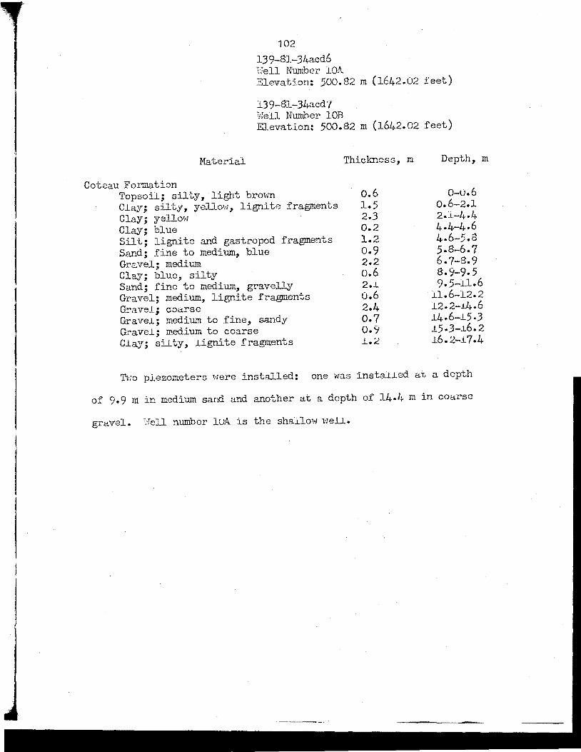
102
13 9-81-34acd6 Number 1.0A
Elevation: 500.82 m (1642.02 feet)
139-81-:-34acd'/ Well Number lOB Elevation: 500.82 m (1642.02 feet)
Material Thickness, m
Coteau Formation Topsoil; silty, light brown o.6 Cl.ay; silty, yellow, lignite fragments 1.5 Clay; yellow 2.3 Clay; blue 0.2 Silt; lignite and gastropod fragments 1.2 Sand; fine to medium, blue 0.9 Grsvel; medium 2.2 Clay; blue, silty o.6 Sand; fine to medium, gravelly 2.1 Gravel; medium~ lignite fragments o.6 Grave1-; co~rse 2.4 Grave.L; medium to fine, sandy O. 7 Gravel.; medium to coarse 0.9 Cl.ay; silty, l.ignite fragments 1..2
Depth, m
0-0.6 0.6-2.1 2.l-l~.4 4.4-4.6 4.6-5.8 5.8-6.7 6.7-8-9 8.9-9.5 9. 5-11.6
11.6-12.2 12.2-J.4.6 1.4.6-1.5.3 l.5 • J-.L6 • 2 1.6. 2-.L 7 .4
Two plezometers were installed: one was insta:U.ed at a depth
of 9.9 min medium sand and another at a depth of 14.4 min co~rse
grc.vel. number luA is the sha.i.low ,-rnl.L.

103
139-81-34adal l\'eJ..L Number IL!\. Elevation: 504.05 m (1652.63 feet)
139-81-34ada2 !Jell Number 11B Elevation:. 504.05 m (1652.63 feet)
Material
Landfill Topcoyer; sand, siit, rubble
Cannonball Formation Sandstone; fine, calcareous, dense Clay; silty, sandy, yellow Sand; fine, yellow Clay; yellow, silty Clay; blue, sandy Clay; silty, dense, blue-gray Sandstone; fine, calcareous, dense Clay; blue-gray
Ludlow-Hell Creek Formations (?) Clay; lignitic Clay; gray, sandy Sand; fine Clay; gray, dense ·
Thickness,
o.6
o.6 5.$ 1.2 1.0 3.6 9.6 0.3 2.0
0
0.3 o.6 L2 0.7
m Depth, m
0-0.6
0.6-1.2 1.2-7-0 7.0-8.2 8.2-9.2 9.2-12.a
12.S-22.4 22.4-22-7 22,-7-24-7
"' ~ . .
24.7-25.0 25.0-25.6 25.6-26.8 26.S-27.5
Two piezometers were installed: one at a depth of 15.4 min silty
clay and another at a depth of 26.6 m in fine sand. Well number llA
is the shallow well.

104
139-81-34addl Well Number 12A. Elevation: 522-49 m (1713.07 feet)
139-81-34add2 ';foll Number lZB Elevation: 522-49 m (l?J.3.07 feet)
Material
Oahe Formation Topsoil.; silty, sandy, light bro\'ffi
Cannonball Formation Clay; yellow Clay; dark gray, yellow, mottled Clay; sandy Clay; sandy, silt~ yellow Clay;·dark gray, yellow, mottled Sandstone; fine, calcareous, light
blue-gray Clay; silty, dark gray, yellow Clay; light gray, bentonitic Clay; silt; sand; dark green, inter-
bedded Clay; greenish-brown, sandy Sandstone; fine, calcareous, dense Sand; fine, clayey Sand; blue-green
Thickness,
o.6
2.8 1.2 o.6 0.9 1.5 o.5
1.1 o.6 o.6
12.5 0.9 2.5
m Depth, m
0-0.6
0.6-J .. 4 3.4-4.6 4.6-5.2 5.2-6.1 6.1-7-6 7.6-8.l
8.1-9.2 9.2-9.8 9.8-10.4
10.4-22.9 22.9-23 .. 8 23 .8-26.3 26.3-27-5
'I\"10 piezometers were installed: one at a depth of 22.3 m in
sandy clay and another at a depth of 27 .3 m in sand. Well number
12A is the shallo':! well.
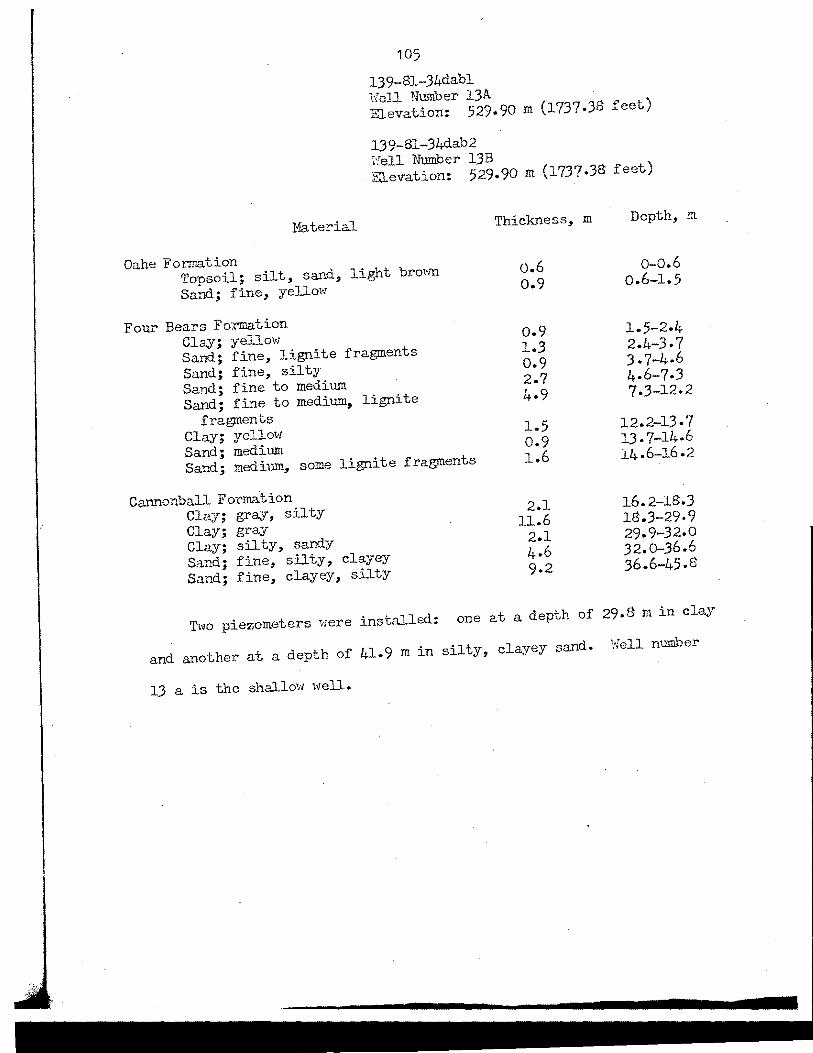
105
l39-8l-34dabl 1.foll Number 13A. Elevation: 529.90 m (l737-38 feet)
l39-81-34dab2 :-:ell Number 13B Elevation: 529.90 m (1737.38 feet)
M"a.terial
Oahe Formation Topsoil; silt., sand., light brown Sand; fine, yellow
Four Bears Formation Clay; yellow Sand; fine, lignite fragments Sand; fine, silty Sand; fine to medium Sand; fine to medium, lignite
fragments Clay; yellow Sand; medium Sand; medium, some lignite fragments
Cannonball Formation Clay; gray, silty Clay; gray Clay; silty, sandy Sand; fine, silty, clayey Sand; fine, clayey, silty
Thickness, m
o.6 o.9
o.9 l.3 0.9 2.7 4.9
1.5 0.9 1.6
2.1 11.6
2.1 4.6 9.2
Depth, m
0-0.6 0.6-1.5
1.5-2.4 2.4-3-7 3. 7-4.6 4.6-7-3 7.J-l2.2
12.2-13. 7 13. 7-14.6 l4.6-16.2
16.2-18.J 18.3-29·9 29.9-32.0 32.0-36.6 36.6-45.8
Tlvo piezometers were installed: one at a depth of 29.S m in clay
and another at a depth of 41.9 min silty, clayey sand. Well number
13 a is the shallow well.

,
APPENDIX C
PHYSICAL WELL DATA
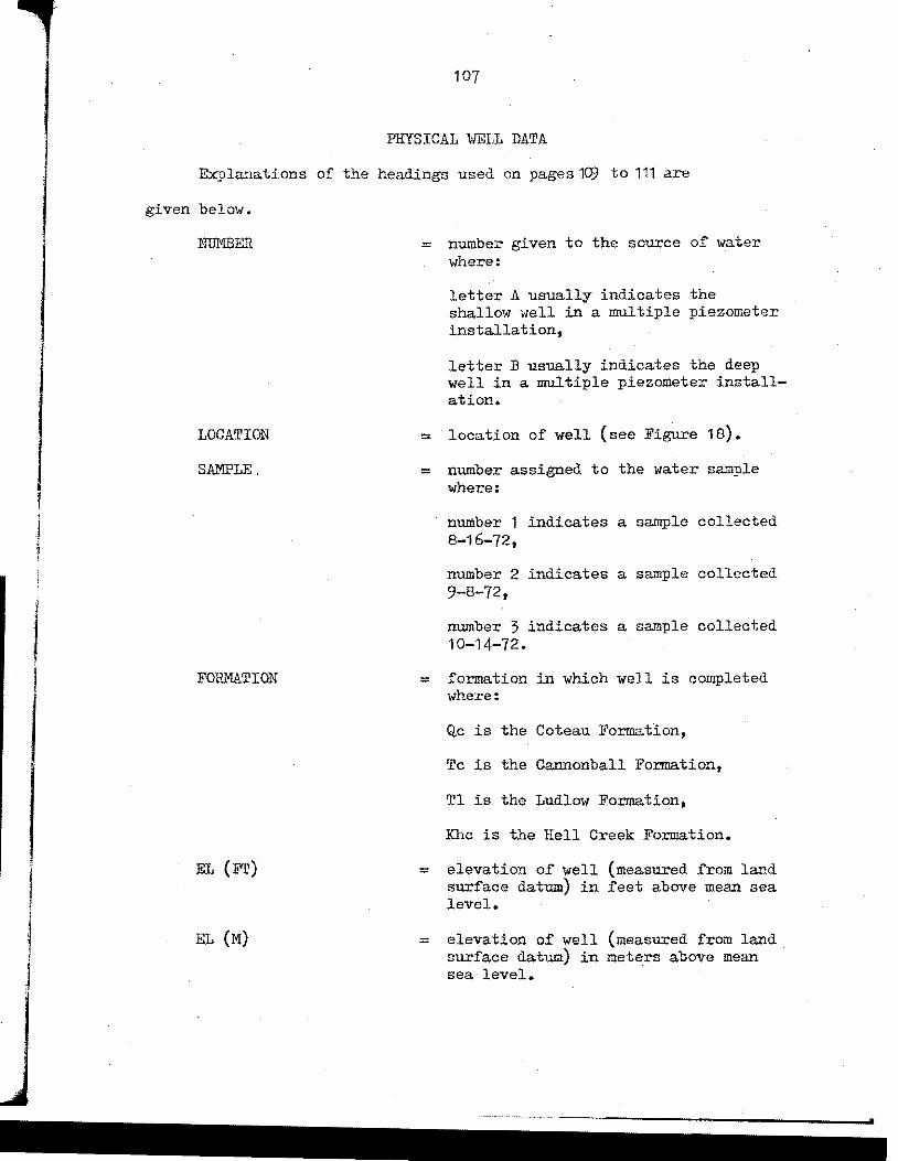
, I
l
~
l l
I
J
107
PHYSICAL WELL DATA
Explanations of the headings used on pages 1(},1 to 111 are
given below.
NUMBER
LOCATION
SA...~LE.
FORMATION
EL (FT}
EL (M)
= number given to the souxce of water where:
letter A usually indicates the shallow well in a multiple piezometer installation,
letter B usually indicates the deep well in a multiple piezometer installation.
=·location of well (see Figure 18).
= number assigned to the water sample where:
number 1 indicates a sample collected 8-16-72,
number 2 indicates a sample collected 9-8-72,
nwnber 3 indicates a sample collected 10-14-72.
= formation in which well is completed where:
Qc is the Coteau Formation,
Tc is the Cannonball Formationt
Tl is the Ludlow Formation,
Khc is the Hell Creek Formation.
= elevation of well (measured from land surface datum) in feet above mean sea level.
= elevation of well (measured from land surface datum} in meters above mean · sea level.
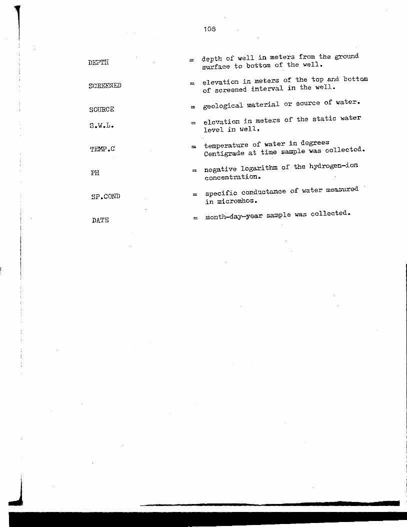
l DEPTH
SCREENED
SOURCE
s.w.L.
TE!YIP.C
PH
SP.COND
DATE
108
= depth of well in meters from the ground surface to bottom of the well.
= elevation in meters of the top and bottom of screened interval in the well.
= geological material or source of water.
= elevation in meters of the static water level in well.
= temperature of water in degrees Centigrade at time sample was collected.
= negative logarithm of the hydrogen-ion concentration.
= specific conductance of water measured in micromhos.
= month-day-year sample was collected.
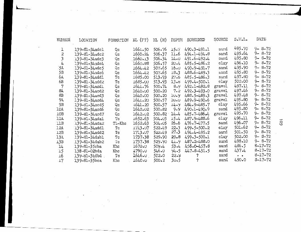
t.. --~
NUNBER LOCATION FOH.Mt'l..TION EL (FT) E1 (M) DEPTH SCREENED SOUl1CE s.w.L. DA.TE
1 139-81-34adcl Qc 1661.50 506.76 15.'{ 490.3-491.1 sand 495.70 9- 8-72 2 13 9-81-34a.dc2 Qc 1660.24 506.37 11.6 494-1-494.8 sand 495.64 9- 8-72 3 13 9-81-34adc3 Qc 1660.1.3 506.34 14.0 491.6-492-4 sand 495.80 9- 8-72 4 13 9-8l-34adc4 Qc 1660.88 506.57 2u.4 485.5-486.2 clay 496.10 9- 8-72
:5A 13 9-81-34adc 5 Qc 1664.42 50?.65 16.u 490.9-491.7 sand 495.90 9- 8-72 5B 13 9-81-34adc6 Qc 1661~.42 50'/.65 1.8.3 488.6-489-3 sand 4-95 .80 9- 8-72 6A 13 9-81-34addl Tc 1685.00 513 .·93 2?:6 485.5-486.3 sand 497.80 9- 8-72 6B 139-81-34add2 Tc 16s5.w 513.93 13 .ts 4 99 .4-500. l clay 502.00 9- 8-72 7 13 9-81-34acdl Qc 1641.76 500.74 8.9 492.1-492.8 gravel 497.11 9- 8-72
8A 13 9-Bl-34acd2 Qc 1640.uo 500.20 7.2 492.J-49J.o gravel 497.46 9- 8-72 8B 139-81-34acd3 Qc 1640.00 500.20 lU.1/ 4S8.5-489.J gravel 497.48 9- 8-72 9A 13 9-81-34acd4 Qc 164.1.20 500.57 1u.u 489.9-490.6 gravel 495 .80 9- 8-72 9B 13 9-81-34acd5 Qc 1.641. 20 500.57 .14.~ 484.9-485.7 clay 495.66 9- 8-72
lOA 139-81-34acd6 Qc 1642.02 500.82 9.9 490.1-490.9 sand 495.80 9- 8-72 lOB 13 9-81-34acd? Qc 1642.u2 500.82 14.4 485.7-486~4 gravel 495.70 9- 8-72 lli 13 9-81-34adal Tc 1.652.63 504.05 1.5.4 487.9-488.6 clay 496.11 9- 8-72 _..
llB l39-81-34ada2 Tl-Khc 1652.63 504.05 26.6 476.7-477•5 sand 496.07 9- 8-72 0 \D
12A 13 9-81-34addl Tc l'/13.07 522.49 22.3 499.5-500.2 clay 501.62 9- 8-72 12B 13 9-81-34add2 Tc 1713.u7 5:a.49 27.3 494.4_495.2 sand 501.50 9- 8-72 13A 139-81-34dabl Tc 1737.38 529.90 29.8 499-3-500.1 clay 502.00 9- 8-72 13B 139-81-34dab2 Tc 1737.38 529.90 41..9 487.2-488.0 sand 498.10 9- 8-72 14 139-8l-35cba Khc 1670.u 509.4 53.4 456.0-457.8 sand 486.5 8-17-72 15 138-81-02bda Khc J.790.U 546.0 94.5 44 7. 8-/+51. 5 sand 437.4 8-17-72 16 13~-81-34dbd . Tc 1646.u . 502.0 22.;l ? sand • • 8-17-72 17 139-81-35bca Khc 1640.u 500.2 3u.5 ? sand 490.0 8-17-72

L
NUMBER LOCATION SAMPLE
1 13 9-81-34adcl 1 1 1J9-81-34adcl 2 1 13 9-81-.34adcl 3 2 139-81-34adc2 1 2 139-81-34adc2 2 2 139-81-34adc2 3 3 13 9-81-34adc3 1 3 13 9-81-34adc3 2 3 13 9-81-34adc3 3 4 13 9-81-34adc4 1 4 139-81-34adc4 2 4 139..:s1-34adc4 3
5A 139-81-34adc5 1 5A 13 9-81-Jl~adc 5 2 5A 139-81-34adc5 3 5B 13.9-81-34adc6 1 5B 13 9-81-34adc6 2 5B 13 9-81-34adc6 3 6A. 139-81-3l}addl 1 6A 13 9-81.,. 3l}n.ddl 2 6A. 139-81-34addl 3 6B 13 9-81-34add2 1 6B 13 9-81-34add2 2 6B 139-81-34add2 3
7 13 9-81;.. 34acdl 2 7 13 9-81-34acdl 3
SA 13 9-81-3l.i.acd2 2 SA 139-81-34acd2 3 8B 13 9-81-34acd3 2 8B 139-81-34acd3 3 9A 13 9-81-34acd4 1 9A 139-81-34acd4 3 9B 13 9-81-34acd5 2 9B 139-81-3l~a.cd5 3
'I'EMP.C PH
9.26 7.30 -· , .. ' 7.09 . . 7.25
11.65 7.20 . . 7.40 . . . 6.94 10.18 7.20 . . 7.08 . . 7.35 10.31 7.30 . . 7.70 . . 7.07 9.40 7.45 . . 7.27 . . 7.48 8.68 7.75 . . 7.22 . . 7.43 9.28 7.58 . . 7.76 . . 7.33 9.48 7.98 . . 7.95 . . 7.40 7.68 7.66 . . 7.50 7•h5 7.41 . . 7.56 7.00 7.39 • • 7.48 8.10 7.43 • • 7.46 8.75 7.60 . . 7.62
----- -=~,-#-~--~~----------··~-·
SP.COND DATE
1190 8-16-72 1000 9- 8-72
900 10-14-72 1950 8-16-72 1830 9- 8-72 1920 10-14-72 1000 8-16-72 1020 9- 8-72
960 10-14-72 1450 8-16-72 1470 9- 8-72 1275 10-14-72 1400 8-16-72 1060 9- 8-72
990 10-14-72 1490 8-16-72 1260 9- 8-72 1000 10-14-72 1040 8-16-72 1080 9- 8-72 1010 10-14-72 ·1090 8-16-72 1070 9- 8-72 1160 10-14-72
710 9- 8-72 665 10-14-72 750 9- 8-72 970 10-14-72 970 9- 8-72 . 705 10-14-72
1190 8-16-72 920 10-14-72
1140 9- 8-72 1005 10-14-72
_ ... ..... 0
J ...
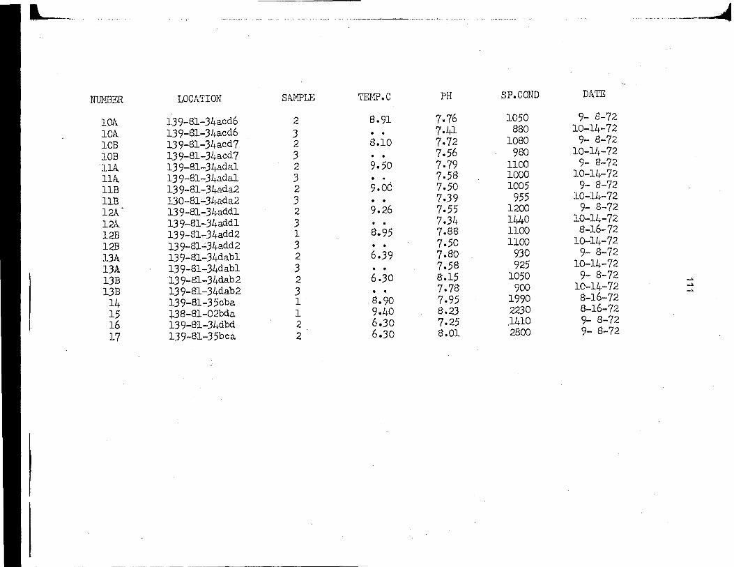
I ~
NtnlfilER LOCATION SAMPLE TEMP.C PH SP.COND DATE
lOA 13 9-81-34acd6 2 8.91 7.76 1050 9- 8-72
lOA. 139-81-34acd6 3 . . 7.41 880 10-14-72
lOB 139-81-34acd7 2 8.10 7.72 1080 9- 8-72
lOB 13 9-81-34acd 7 3 . . 7.56 980 10-14-72
llA 13 9-81-34adal 2 9.50 7.79 1100 9- 8-72
11/i. 139-81-34adal 3 . . 7.58 1000 10-14-72
llB 13 9-81-34ada2 2 9.06 7.50 1005 9- 8-72
130-81..;34ada2 3 • • 7.39 955 10-14-72
12A 13 9-81-34addl 2 9.26 7.55 1200 8-72
12A. 13 9-81-34addl 3 • • 7.34 1440 10-14-72
12B 139-81.:.J4add2 l 8.95 7.88 1100 8..;16-72
12B 13 9-81~ 34add2 3 . . 7.50 1100 10-14-72
13A 139-81-34dabl 2 6.39 7.80 930 9- 8-72
13A 139-81-34dabl 3 . . 7.58 925 10-14-72
13B 139-81-34dab2 2 6.JO 8.15 1050 9- 8-72 .... 13B 139-81-34dab2 3 7.78 900 10-14-72 ......
• • .... 14 139-81-35cba l . 8.90 7.95 1990 8-16-72
15 +38-81-02bda 1 9.40 8.23 2230 8-16-72
16 13 9-81-34dbd 2 6.30 7.25 .1410 9- 8-72
17 139-81-35bca 2 6.30 8.01 2800 9- 8-72
, l l
[
'
L
APPENDIX D
CHEMICAL DATA
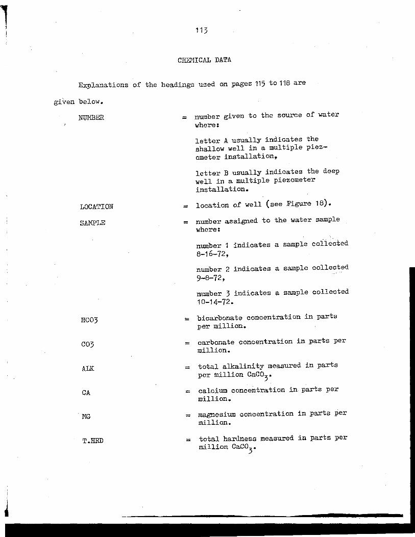
1 J
J
113
CHEMICAL DATA
Explanations of the headings used on pages 115 to118 are
given below.
NUMBER
LOCATION
SAMPLE
HC03
C03
ALIC
CA
. MG
T.HIID
= number given to the source of water where:
letter A usually indicates the shallow well in a multiple piezometer installation~
letter B usually indicates the deep well in a multiple piezometer installation.
= location of well (see Figure 18).
= number assigned to the water sample where:
number 1 indicates a sample coiiected 8-16-72,
number 2 indicates a sample collected 9-8-72,
number 3 indicates a sample collected 10-14-72.
= bicarbonate concentration in parts per million.
= carbonate concentration in parts per million.
= total alkalinity measured in parts per million Caco3•
= calcium concentration in parts per million •
= magnesium concentration in parts per million.
= total hardness measured in parts per million Caco
3•
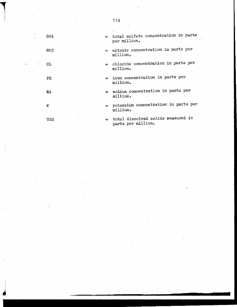
, ;
S04
N03
CL
FE
NA
K
TDS
i
"
114
= total sulfate concentration in parts per million.
= nitrate concentration in parts per million.
= chloride concentration in parts per million.
= iron concentration in parts per million.
= sodium concentration in parts per million.
= potassium concentration in parts per million.
= total dissolved solids measured in parts per million.

L ___ ........
NUMBER LOCATION SAMPLE HC03 C03 ALK CA MG T.HRD
1 139-81-34adcl 1 420.0 o.o 420.0 290.0 175.0 465.0 1 13 9-81-34adcl 2 430.0 o.o 430.0 255.0 205.0 460.0 1 13 9-81-34adcl 3 400.0 o.o 400.0 250.0 180.0 1+30.0 2 139-81-34adc2 1 375.0 o.o 325.0 260.0. 240.0 500?0 2 13 9-81-34adc2 2 350.0 o.o 350.0 190.0 250.0 1+40.0 2 139-81-34adc2 3 600.0 o.o 600.0 395.0 365.0 760.0 3 139-81-34adc3 1 250.0 o.o 250.0 125.0 125.0 250.0 3 139-81-34adc3 2 280.0 o.o 280.0 140.0 140.0 280.0 3 13 9-81-.34adc3 3 480.0 o.o 480.0 345.0 135.0 480.0 4 13 9-81-34adc4 1 340.0 o.o 31.0.0 150.0 90.0 240.0 4 13 9-81-34adc4 2 400.0 o.o 400.0 145.0 105.0 250.0 4 139-81-34adc4 3 335.0 o.o 335.0 150.0 100.0 250.0
5A 139-81-34adc5 1 450.0 o.o 450.0 250.0 235.0 485.0 5A 13 9-81-34adc 5 2 250.0 o.o 25Q.O 165.0 220.0 385.0 5A 13 9-81-34adc 5 3 410.0 o.o 410.0 300.0 230.0 530.0 5B. 139-81-34adc6 1 430.0 430.0 · 280.0 220.0 500.0
..... o.o ..... 5B 13 9-81-34adc6 ·2 420.0 o.o 420.0 320.0 200.0 520.0 V1
5B 139-81-34adc6 3 380.0 o.o 380.0 275.0 235.0 510.0 6A 13 9-81-3/+addl 1 240.0 o.o 240.0 190.0 90.0 280.0 6A 139-81-34addl 2 250.0 o.o 250.0 140.0 140.0 280.0 6A 13 9-81-34addl 3 240.0 o.o 240.0 145.0 140.0 285.0 6B 13 9-81-34udd2 1 210.0 o.o 210.0 115.0 85.0 200.0 6B 13 9-81-34add2 2 210.0 o.o 210.0 115.0 95.0 210.0 6B 139-81-34add2 3 210.0 o.o 270.0 125.0 125.0 250.0
7 13 9-81-34acdl 2 280.0 o.o 280.0 190.0 130.0 320.0 7 13 9-81-34acdl 3 290.0 o.o 290.0 210.0 105.0 315.0
BA 13 9-81-34acd2 2 300.0 o.o 300.0 200.0 90.0 290.0 8A 13 9-81-34acd2 3· 305.0 o.o 305.0 230.0 135.0 365.0 8B 13 9-81-34acd3 2 250.0 o.o 250.0 170.0 100.0 270.0 8B 13 9-81-34acd3 3 305.0 o.o 305.0 200.0 115.0 315.0 9A 13 9-81-34acd4 1 250.0 o.o 250.0 130.0 60.0 190.0 9A 13 9-81-34acd4 3 205.0 o.o 205.0 70.0 1.0.0 110.0 9B 139-81-34acd5 2 240.0 o.o 240.0 70.0 30.0 100.0 9B 139-81-34acd5 3 2;20.0 o.o 220.0 65.0 55.0 120.0
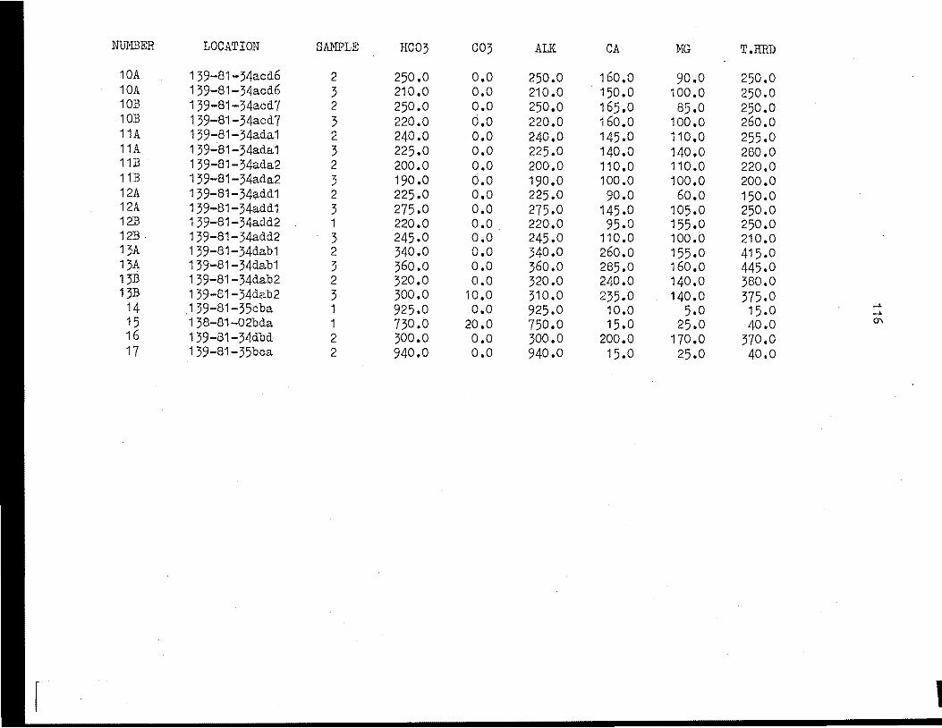
NUMBER LOCATION SAMPLE HC03 003 ALK CA MG T.HRD
10A 139-81-34acd6 2 250.0 o.o 250.0 160.0 90.0 250.0 10A 139-81-34acd6 3 210.0 o.o 210.0 150.0 100.0 250.0 10:B 139-81-34acd7 2 250.0 o.o 250.0 165.0 85.0 250.0 10B 139-81-34acd7 3 220.0 d.o 220.0 160.0 100.0 260.0 11A 139-81-34ada1 2 240.0 o.o 240.0 145.0 110.0 255.0 11A 139...:a1-34ada1 3 225.0 o.o 225.0 140.0 140.0 280.0 11B 139-81-34ada2 2 200.0 o.o 200.0 110.0 110.0 220.0 11:B 139-81-34ada2 3 190.0 o.o 190.0 100.0 100.0 200.0 12A 139-81-34add1 2 225.0 o.o 225.0 90.0 60.0 150.0 12A 139-81-34add1 3 275.0 o.o 275.0 145.0 105.0 250.0 12B 139-B1-34add2 1 220.0 o.o 220.0 95.0 155 .o 250.0 12B 139-81-34add2 3 245.0 o.o 245.0 110.0 100.0 210.0 13A 139-81-34dab1 2 340.0 o.o 340.0 260.0 155.0 415.0 13A 139-81-34dab1 3 360.0 o.o 360.0 285.0 160.0 445.0 13B 139-81-34dab2 2 320.0 o.o 320.0 240.0 140.0 380.0 13B 139-81-34dab2 3 300.0 10.0 310.0 235.0 140.0 375.0
14 .139-81-35cba o.o 925.0 10.0 5.0 15.0 ..... 1 .o .....
15 1 38-81-02bda 1 730.0 20.0 750.0 15.0 25.0 40.0 °' 16 139-81-34dbd 2 300.0 o.o 300.0 200.0 170.0 370.0 17 139-81-35boa 2 940,0 o.o 940.0 15.0 25.0 40.0
1
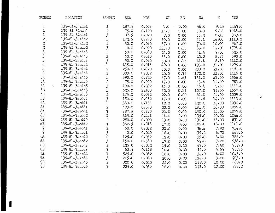
NUMBER LOCATION SAMPLE S0h N03 CL FE NA K TDS
1 13 9-81-34adci 1 187.5 0.003 5·~0 o.oo 56.0 9.15 11/+3 .o 1 139-81-34adcl 2 75.0 0.120 14.c o.oo 58.0 9.18 1046.0 1 139-81-34adcl 3 87.5 0.020 s.o o.oo 55.2 8.35 989.0 2 139-81-34adc2 1 172.5 0.240 50.0 o.oo 56.4 14.00 1118.0 2 13 9-81-34adc 2 2 50.0 0.030 67.0 o.oo 70.0 10.00 987.0 2 139-81-34adc2 3 o.o 0.020 333.0 0.15 69.0 12.00 1774.0 3 139-81-34adc3 l 50.0 0.060 25.0 o.oo 41.4 9.00 625.0 3 139-81-34a.dc3 2 50.0 0.020 33.0 o.oo l.0.2 8.75 692.0 3 139-81-34adc3 3 50.0 0.060 50.0 0.15 41.4 8.30 1110.0 4 139-81-34adc4 l 435.0 0.016 4o.o o.oo 193.0 31.00 1279.0 4 13 9-81-34adc4 2 250.0 0.020 50.0 o.oo 208.0 23.00 1181.0 4 13 9-81-3l,adc4 3 300.0 0.032 40.0 0.39 170.0 21.00 1116.0
5A 13 9-81-34adc 5 l 390.0 0.720 67.0 1.63 131.0 41.00 1566.0 5A 139-81-34adc5 2 75.0 0.020 17.0 o.oo 43.6 12.00 783.0 5A 139-81-34adc5 3 100.0 0.032 15.0 o.oo 46.4 9.10 1111.0 5B 139-81-34adc6 l 525.0 2.100 50.0 0.15 127.0 35.00 1667.0 5B 139-81-34adc6 61.0 1229.0
... 2 175.0 0.032 22.0 o.oo 29.00 .....
5B 13 9-81-.34adc6 3 150.0 0.032 17.0 o.oo 41.8 14.00 1113.0 -.J
6A 13 9-81-34addl 1 360.0 0.154 18.0 o.oo 120.0 14.00 1032.0 6A 13 9-81-34addl 2 400.0 0.040 22.0 o.oo 131.0 16.00 1099.0 6A 13 9-81-34addl 3 387,5 0.370 20.0 o.oo 130.0 14.00 1077.0 6B 13 9-81-34add2 1 465.0 o.448 14.0 o.oo 135.0 20.00 1044.0 6B 139-81-34add2 2 250.0 0.020 13.0 o.oo 132.0 16.00 831.0 6B 139-81-34add2 3 362.5 0.016 17.0 o.oo 185.0 16.00 1101.0 7 139-81-34acdl 2 50.0 0.032 20.0 o.oo 36.4 7.90 714.0 7 13 9-81-.34acdl 3 o.o 0.040 1s.o o.oo 39.2 6.70 669.0
8A. 13 9-81-3hacd2 2 125.0 0.032 12.0 o.oo 55 .o 6.oo 788.o BA 139-81-34acd2 3 150.0 0.560 17.0 o.oo 92.0 7.20 936.0 8B 13 9-81-34acd3 2 125.0 0.032 15.0 o.oo 89.0 7.40 757.0 8B 13 9-81-34acd3 3 62.5 0.16s 10.0 o.oo 59.0 5.55 757.0 9A 13 9-81-3 4acd4 1 525.0 0.032 18.o o.oo 54.0 6.oo 1043 .o 9A 139-81-34acd4 3 225.0 0.040 20.0 o.oo 134.0 9.20 703.0 9B 139-81-34acd5 2 300.0 0.040 22.0 o.oo 188.0 10.00 860.0 9B 13 9-81-34acd5 3 225.0 0.032 18.0 o.oo 178.0 12.00 773.0
I

NUMBER LOCA'rION SAMPLE S04 N03 CL FE NA K TDS
10A 139-81-34acd6 2 250.0 0, 112 17 .o o.oo 123.0 16.00 906.0 10A 139-81-34acd6 3 200.0 0.032 17.0 o.oo 109.0 16.00 802.0 10B 139-81-34acd7 2 275.0 0.020 18.0 o.oo 125.0 12.00 930.0 10B 139~81-34acd7 3 275.0 0.032 17.0 o.oo 113.0 16.00 901.0 11A 139-81-34ada1 2 300.0 0.060 15.0 o.oo 135 .o 12.00 957.0 11A 139-81-34ada1 3 300.0 0~032 18.0 o.oo 121.0 20.00 964.0 11B 139-81-34ada2 2 300.0 0.240 22.0 o.oo 143.0 24.00 909.0 11B 139-81-34ada2 3 250.0 0.032 17.0 o.oo 117.0 23.00 797.0
l
12A 139-81-34add1 2 300.0 0.024 18.0 0,00 191.0 16.00 900.0 12A 1 39-81-34add 1 3 487,5 0.032 20.0 o.oo 214.0 16.00 1263.0 12B 139-81-34add2 1 525.0 0.470 14.0 o.oo 176.0 21.00 1206.0 12B 139-81-34add2 3 307.5 0.020 18.0 o.oo 195.0 16.00 1072.0 13A 139-81-34dab1 ·2 125.0 0.112 12.0 o.oo 51.2 8,55 952()0 13A 139-81-34dab1 3 150.0 0.015 a.o o.oo 54.0 8.10 1025 .o 13B 139-81-34dab2 2 150.0 o.b6o 11.0 o.oo 82.0 a.90 952.0 13B 139-81-34dab2 3 150.0 0.032 12.0 o.oo 104.0 a.75 950.0 _.
14 139-81-35cba 1 7.5 0.450 67.0 o.oo 472.0 14.00 1501.0 _., CD
15 138-81-02bda 1 330.0 0.112 100.0 0.13 468.0 10.00 1698.0 16 139-81-34dbd 2 325.0 o.~40 25.0 o.oo 151.0 8.25 1179 .o 17 139-81-35bca 2 o.o 0.024. 400.0 0.32 548,0 6.20 1935.0
II''

REFERENCES

120
REFERENCES
ASCE, 1959, .Manual of engineering practice: American Society of Civil Engineers, no. 39, 61 p.
Apgar, M.A., and Langmuir, D., 1971, Groundwater pollution potential of a landfill above the water table: Groundwater, v. 9, no. 6, p. 76-94-
APHA, 1965, Methods for the analysis of water and waste water: New York, American Public Health Association, Twelfth edition, 769 p.
Back, W., 1960, Origin of hydrochemical facies of groundwater in the Atlantic coastal plain: Proceedings 0£ 22nd International Geological Congress, Copenhagen, 1960, v. 1, p. 87-95 •
.Bickley, w. B., 1972, Stratigraphy and history of the Sa.kakawea Sequence, south-central North Dakota: University of North Dakota, Grand Forks, North Dakota, unpublished Ph.D. thesis 329 p.
Brown, I. c., 1963, Chemical methods as an aid to hydrogeology: Proceedings of Hydrologic Symposium 3, Canada National Research Council, p. 181-203.
Camp, T. R., 1963, Water and its impurities: Reinhold Publishing Corporation, New York, p. 245-247.
Casagrande, A., 1949, Soil mechanics in the design and construction of the Logan International Airport: Boston Society of Civil Engineers Journal, v. 36, p. 192-221.
Charron, J.E., 1965, Groundwater resources of Emerson area, Manitoba: Canada Geological Su...-vey Paper 64-7, 37 p.
Chebotarev, I. I., 1955, Metamorphism of natural waters in the crust of weathering: Geochimica et Cosmochimica Acta, v. 8, p. 22-49, 131-171, 198-213.
Edwards, M. J., and Albeiter, J. K., 1951, Soil survey of Morton County, North Dakota: United States Department of Agriculture Series 1936, no. 28, 145 p.
Freeze, R. A., 1969, Theoretical analysis 0£ regional groundwater flow: Canada Department of Energy, Mines, and Resources, Inland Waters Branch, Scientific Series 3, 147 p.
Freeze, R. A., and Witherspoon, P.A., 1966, Theoretical analysis 0£ regional groundwater flow: 1. Analytical and numerical solutions to the mathematical model: Water Resources Research, v. 2, p. 641-656.

121
Freeze, R. A., and Witherspoon, P.A., 1967, Theoretical analysis of regional groundwater flow: 2. The effect of water table configuration and subsurface permeability variation: Water Resources Research, v. 3, p. 623-643.
Freeze, R. A., and Witherspoon, P.A., 1968, Theoretical analysis of groundwater flow: 3. Quantitative interpretations: Water Resources Research, v. 4, p. 581-590.
Fungaroli, A. A., and Steiner, R. L., 1971, Laboratory study of the behavior of a sanitary landfill: Journal Water Pollution Control Federation, v. 43, p. 252-267.
Groenewold, G. H., 1972, Applied geology of the Bismarck-Mandan area, North Dakota.: University of North Dakota, Grand Forks, :North :Da.kota, unpublished Ph.D. thesis, 99 p.
Grunes, D. L., and others, 1963, Relationship between yield responses to applied fertilizers and laboratory measures of nitrogen and phosphorus availability: Soil Science Society of America Proceedings, v. 27, no. 6, p. 676-679.
Haas, E. J., and Willis, W. o., 1962, Moisture storage and use by dryla.nd spring wheat cropping systems: Soil Science Society of America Proceedings, v. 26, no. 5, p. 506-509.
Hagmaier, J. L., 1971, Groundwater flow, hydrochemistry, and uranium deposition in the Powder River Basin, Wyoming: University of North Dakota, Grand Forks, North Dakota, unpublished Ph.D. thesis, 166 p.
Hall, G., 1958, Stratigraphy of the Cannonball Formation, southwestern :North Da..lcota: University of North Dakota, Grand Forks, North Dakota, unpublished Masters thesis, 115 p.
Hamilton, T. M., 1970, Groundwater flow in part of the Little Missouri River basin, North Dakota: University of North Dakota, Grand Forks, North Dakota, unpublished Ph.D. thesis, 179 p.
Hitchen, B., 1969a, Fluid flow in the western Canada sedimentary basin: 1. Effect of topography: Water Resources Research, v. 5, p. 186-195.
Hitchen, B., 1969b, Fluid flow in the western Canada sedimentary basin: 2. Effect of geology: Water Resources Research, v. 5, p. 460-469.
Hubbert, M. K., 1940, The theory of groundwater motion: Journal of Geology, v. 48, p. 785-944.
Hvorslev, M. J., 1951, Time lag and soil permeability in groundwater observations: United States Corps of Engineers, Waterways Experimental Station Bulletin 36, 86 p.
-
122
Krauskopf, K. F., 1967, Introduction to geochemistry: McGraw-Hill Book Company, New York,. 721 p.
Kume, J., and Hansen, D. E., 1965, Geology and groundwater resources of Burleigh County, North Dakota: Part I, Geology: North Dakota Geological Survey Bulletin 42, 111 p.
Laird, W. M., and Mitchell, R.H., 1942, Geology of the southern part of ,Morton County, North Dakota: North Dakota Geological Survey !3nlletin 1 4, 42 p·.
Langmuir, D .. , 1969, Geochemistry of iron in a coastal-plain groundwater of the Camden, New Jersey, area: United States Geological Survey Professional Paper 650-e, p. 224-235.
Lohma.~, s. W., and others, 1972, Definitions of selected groundwater terms--revisions and conceptual refinements: United States Geological Survey Water-Supply Paper 1988, 21 p.
~.atthews, O. R., and Army, T. J., 1960, Moisture storage on fallowed wheatland in the Great Plains: Soil Science Society of America Proceedings, v. 24, p. 414-418.
Meinzer, O. E., 1923a, Outline of groundwater hydrology with definitions: United States Geological Survey Water-Supply Paper 494, 71 p.
Meinzer, O. E., 1923b, The occurrence of groundwater in the United States, with a discussion of principles: United States Geological Survey Water-Supply Paper 489, 321 p.
Merz, R. c., 1962, Landfill settlement rates: Public Works, v. 93, p. 224-235.
Meyboom, P., 1963, Patterns of groundwater flow in the prairie profile: Canada National Research Council Proceedings Hydrology Symposium 3, p. 5-33.
Meyboom, P., 1966, Groundwater studies in the Assiniboine River drainage basin: Part I, The evaluation of a flow system in south-central Saskatchewan: Canada Geological Survey Bulletin 139, 65 p.
Meyboom, P., 1967a, Mass transfer studies to determine the groundwater regime of permanent lakes in hummocky moraine of western Canada: Journal of Hydrology, v. 5, p. 117-142.
Meyboom, P., 1967b, Groundwater studies in the Assiniboine River drainage basin: Part II, Hydrologic characteristics of phreatophytic vegetation in south-central Saskatchewan: Canada Geological Survey :Bulletin 139, 64 p.

123
North Dakota State Department of Health, 1970, Solid waste management regulations no. 86: Bismarck, North Dakota, 5 p.
North Dakota State Department of Health, 1970, Solid waste in North Dakota: Official Bulletin: Bismarck, North Dakota, p. 19-24.
North Dakota State Highway Department, 1972, Official highway map: Bismarck, North Dakota.
Patterson, D. D., Johnsgard, G. A., Sweeney, M. D., and Omadt, H. W., 1968, Soil su:rvey report for county general soils maps, North Dakota: North Dakota State University Agricultural Experiment Station J3ulletin 473, 60 p.
Rainwater, F. H., and Thatcher, L. L., 1960, Methods for collection and analysis of water samples: United States Geological Survey Water-Supply Paper 1454, 301 p.
Randich, P. G~, 1965, Geology and groundwater resources, Burleigh County, North Dakota: Part III, Groundwater Resources: North Dakota Geological Survey Bulletin 42, 92 P•
Randich, P. G., 1973, Personal Communication: United States Geological Survey, Bismarck, North Dakota.
Remson, I., Funga.roli, A. A., and Lawrence, A. W., 1968, Water movement in an unsaturated sanitary landfill: Proceedings of American Society Civil Engineers, Sanitary Engineering Division, v. 94, no. SA 2, p. 307-317.
Schulte, F. J., 1972, Groundwater of the Spiritwood Lake area, Stutsman County, North Dakota: University of North Dakota, Grand Forks, North Dakota, unpublished Ph.D. thesis, 329 p.
Stone, R., and Gupta, R. K., 1970, Aerobic and anaerobic landfill stabilization process: Proceedings of American Society Civil Engineers, Sanitary Engineering Division, v. 96, no. SA 6, p. 1399-1414.
Toth, J., 1962, A theory of groundwater motion 1n small drainage basins in cent:ral Alberta, Canada: Journal Geophysical Research, v. 67, p. 4375-4387.
Toth, J., 1963, A theoretical analysis of groundwater flow in small drainage basins: Journal Geophysical Research, v. 68, p. 4795-4812.
Toth, J., 1968, A hydrogeological study of the Three Hills area, Alberta: Alberta Research Council Bulletin 24, 117 p.
Tyschen, P. C., 1949, Ground.water hydrology of the Lower Heart River Basin and Dickinson irrigation project: University of Nebraska, Lincoln, Nebraska, unpublished Masters thesis, 149 p.

124
United States Department of Agriculture, 1972, Summary of climatic data, 1915-1972, ~Tandan, North Dakota; Northern Great Plains Research Center, Mandan, North Dakota, unpublished, 8 p.
van Derwerker, R. J., 1952, Sanitary landfills in northern states~ A report on the I1andan, North Dakota, project: Public Health Report, v. 67, no. 3, p. 242-248.
van Everdinger, R. o., 1963, Groundwater flow diagrams in sections with exaggerated vertical scale: Canada Geological Survey Paper 63-27, 21 p.
Weaver, L., 1964, Refuse disposal, Its significance: Groundwater, v. 2, no. 1, p. 26-30.
Williams, R. E., 1968, Flow of groundwater adjacent to small, closed basins in glacial till: Water Resources Research, v. 4, p. 777-883.
Related Documents