Chapter 3 Hydroelectric System Models Starting from general equations this chapter presents complete nonlinear models of a hydroelectric power plant, along with the simplifications that allow the obtaining of new models. On one hand, nonlinear models of hydroelectric power plants with or without surge tank effects are proposed -these models are useful in the design of new types of nonlinear controllers when large power variations are necessary. On the other hand, linearized models of hydroelectric power plants with surge tank effects are presented. In this case the models can be used when, for stability studies, a frequency response study is necessary. Comprehensive tables are included where the new and the old models are classified. Besides, a practical method of calculating the mechanical power in steady state is shown. A time domain analysis of all models is presented along with a frequency response study of linearized models. The last part gives suggestions for modelling hydroelectric plants. The Appendix summarises the different models described in this chapter. 3.1 Preliminary Concepts Authors in the bibliography use many kinds of notations to describe the variables and parameters. In order to study and compare the models, it is necessary to make use of uniform

Welcome message from author
This document is posted to help you gain knowledge. Please leave a comment to let me know what you think about it! Share it to your friends and learn new things together.
Transcript

Chapter 3
Hydroelectric System Models
Starting from general equations this chapter presents complete nonlinear models of a
hydroelectric power plant, along with the simplifications that allow the obtaining of new
models. On one hand, nonlinear models of hydroelectric power plants with or without surge
tank effects are proposed -these models are useful in the design of new types of nonlinear
controllers when large power variations are necessary. On the other hand, linearized models
of hydroelectric power plants with surge tank effects are presented. In this case the models
can be used when, for stability studies, a frequency response study is necessary.
Comprehensive tables are included where the new and the old models are classified.
Besides, a practical method of calculating the mechanical power in steady state is shown. A
time domain analysis of all models is presented along with a frequency response study of
linearized models. The last part gives suggestions for modelling hydroelectric plants. The
Appendix summarises the different models described in this chapter.
3.1 Preliminary Concepts
Authors in the bibliography use many kinds of notations to describe the variables and
parameters. In order to study and compare the models, it is necessary to make use of uniform

HYDROELECTRIC SYSTEM MODELS22
the notation of the variables and parameters. This fact, subsequently, allows the description
of different models of hydroelectric power plants. Table 3.1 lists and describes the
parameters used in this Chapter, after making them uniform, and Table 3.2 presents the
variables utilised after the same procedure is carried out.
PARAMETER MEANING
A(p,c,s)Cross section area of a conduit in [m2] (p: penstock, c: tunnel, s: surgetank).
L(p,c) Length of the conduit in [m] (p: penstock, c: tunnel).
a Wave velocity in [m/s].
g Acceleration due to gravity [m2/s].
α ( )Ef//1g ⋅φ+κ⋅ρ=α
ρ Density of water [kg/m3].
κ Bulk modulus of compression of water [ 2skg/(m⋅ ].
φ Internal conduit diameter [m].
f Thickness of pipe wall [m].
E Young’s modulus of elasticity of pipe material.
wT Water starting time at any load in [s].
TWP,WCWater starting time at rated or base load in [s] (WP: penstock, WC:tunnel).
Cs Storage constant of surge tank in [s].
ec,ep,eT Elastic time in [s] (e: conduit, ep: penstock, ec: tunnel).
Tp Pilot valve and servomotor time constant in [s].
Tg Main servo time constant in [s].
T Surge tank natural period in [s].
0,2p,1pf Head loss coefficients in [pu] (p1: penstock, p2: tunnel, 0: surge chamberorifice).
Φp,c Friction coefficient in [pu] (p: penstock, c: tunnel).
kf Head loss constant due to friction in [pu].
At Turbine gain in [pu].
z(p,c,n)Hydraulic surge impedance of the conduit (p: penstock, c: tunnel, n:normalized).
D1 Turbine damping in [pu/pu].
Table 3.1: List of parameters.
In Table 3.2 the superbar “ - ” indicates normalised values (expressed in [pu]).

PRELIMINARY CONCEPTS 23
VARIABLE MEANING
)w,0,2l,l,r,t(H Head in [pu] (t: turbine, r: riser of the surge tank, l: loss in penstock, l2: lossin tunnel, 0: reservoir, w: reservoir).
)NL,0,s,c,p,t(U Velocity of the water in the conduit or flow in [pu] (t: turbine, p: penstock,c: tunnel, s: surge tank, 0: initial value, NL: no load).
)css,tss(H Head in steady state [pu] (tss: turbine, css: tunnel).
)css,tss(U Velocity or flow of the water in the conduit in steady state in [pu] (tss:turbine, css: tunnel).
U U )rated( Velocity of the water in the conduit in [m/s] (rated: normalised)
) rated ,base(Q Flow in the conduit in [m3] (base, rated: turbine flow rate with gates fullyopen and head at the turbine equal to H(base)).
)base(H H Head in [m] (base: base value of head, i.e. the total available static head).
G G ∆ Gate opening in [pu]. / Deviation of the gate opening in [pu].
mmechanical PP ∆ Turbine mechanical power [pu]/Deviation of the mechanical power in [pu]
ω∆ Deviation of the rotor speed in [pu].
Table 3.2: List of variables.
In Figure 3.1 a complete layout of a hydraulic power plant is depicted. The main elements
of this plant and some parameters are shown. On the other hand, Figure 3.2 shows the main
variables of a hydroelectric power plant.
Figure 3.1: Plot of the distribution ofparameters in a hydraulic power plant.
Figure 3.2: Plot of the distribution of headsand flows in a hydraulic power plant.
3.1.1 Definitions
The most significant parameters that govern a hydroelectric power plant are:
• Elastic time:
α== /g/La/LT )c,p()c,p()c,p(e

HYDROELECTRIC SYSTEM MODELS24
• Hydraulic surge impedance of the conduit:
( )α⋅⋅= gA/1z )c,p()c,p(
The water starting time TW is defined as the time required to accelerate the flow from
zero to the rated (or base) flow ( ) base(Q ) under the base head ( )base(H ���������et al, 1987).
• Water starting time in penstock:
TzH
Q
gA
LT epp
base
base
p
pWP ⋅=⋅
⋅=
• Water starting time in tunnel:
TzHQ
gAL
T eccbase
base
c
cWC ⋅=⋅
⋅=
• Storage constant of surge tank:
Q
HAC
base
basess
⋅=
• Surge tank natural period:
CT2T sWC ⋅⋅π⋅=
• Relationship between flow and velocity of water in the conduit (tunnel or penstock):
UAQ ⋅=
• Relationship between the normalised flow and the normalised water velocity in the
conduit (tunnel or penstock):
UQUA
UAQ
Q
ratedrated
=⇒⋅
⋅=
3.1.2 System Dynamic Equations
The basic and general equations of the hydroelectric system dynamics (Kundur, 1994) are
given by:
• Flow Equation (water velocity) in the penstock:
tt HGU ⋅= (3. 1)
PRELIMINARY CONCEPTS 25
• Mechanical Power Equations:
HUPmechanical ⋅= (3. 2)
( ) tNLtmechanical HUUP ⋅−= (3. 3)
The difference between equations (3. 2) and (3. 3) is the term NLU that considers the no
load flow or the minimal flow needed to make the turbine deliver useful power.
• Newton’s second law:
x
Hg
t
U
∂∂⋅−=
∂∂
(3. 4)
• Continuity equation:
t
H
x
U
∂∂⋅α−=
∂∂
(3. 5)
where x indicates the distance between two points and t is the time. The solutions of
these equations (in per units) in the Laplace domain are given by:
)sT(sinhHz/1)sTcosh(UU e2ne21 ⋅⋅⋅+⋅⋅= (3. 6)
22fe2ne12 UUk)sT(tanhUz)sT(hsecHH ⋅⋅−⋅⋅⋅−⋅⋅= (3. 7)
The subscripts 1 and 2 refer to the conditions at the upstream and downstream ends of the
conduit, respectively, e.g. when the surge tank-penstock-turbine hydraulic circuit is
considered, the subscript 2 indicates downstream water (turbine) and the subscript 1
indicates upstream water (surge tank).
3.1.3 Linearized Equations
By linearizing the nonlinear relationships at an operating point, the flow in the penstock
(3. 1) and the mechanical power (3. 2), become:
• Equation of the flow in the penstock (velocity of water)
GaHaGG
UH
H
UU 1311 ∆⋅+∆⋅=∆⋅
∂∂+∆⋅
∂∂=∆ (3. 8)
• Equation of the mechanical power
UaHaUU
PH
H
PP 2321
mmm ∆⋅+∆⋅=∆⋅
∂∂+∆⋅
∂∂=∆ (3. 9)

HYDROELECTRIC SYSTEM MODELS26
The partial derivatives a11, a13, a21 and a23 depend on the kind of turbine and on the
operating point. In Oldenburger and Donelson (1962) ideal values for the Francis turbine are
a11= 0.5, a13= 1, a21= 1.5 and a23= 1.
3.1.4 Classification of the Models
The models can be classified in two basic groups:
• Nonlinear Models.
• Linearized Models.
3.2 Nonlinear Models
Nonlinear models of turbine hydraulic control systems are needed in those cases where large
turbine velocity and power changes exist, for instance in isolated power stations, and, in
cases when a load rejection happens and the electric system restoration follows a break-up.
In Figure 3.3 a block diagram of a hydroelectric system model is depicted, where the
nonlinear dynamics (turbine and mechanical power) are included.
Figure 3.3: Block Diagram of the hydroelectric system used in the models of Kundur (1994).
NONLINEAR MODELS 27
Before describing different kinds of nonlinear models of hydroelectric systems, Table 3.3
presents a classification of these models: models with surge tank effects and models with no
surge tank effects. Each one of these types has two more possibilities: the first considers
elastic or non-elastic water columns, and the second takes into account the continuity
equation as modified or non modified.
The associated number to each element of the table corresponds to the number of the
Section of this Chapter where the model is described.
Table 3. 3: Table of nonlinear models.
With Surge Tank Effects(3.2.1)
With No Surge Tank Effects(3.2.2)
Nonlinear Models
Elastic Water Columnin the Penstock and
Non-elastic Water Columnin the Tunnel
Kundur (1994)Model:
K4 (3.2.1.3)
Non-elasticWater Columns
Kundur (1994)
Models:K3 K32, K31
(3.2.2.1)
IEEE W. Group (1992)Quiroga and Riera (1999)
Models:WG3 QR33, QR32,
QR31 (3.2.2.2)
Kundur (1994)Model:
K2 (3.2.2.3)
IEEE W. Group (1992)Model:
WG2 (3.2.2.4)
IEEE W. Group (1992)Quiroga and Riera (1999)
Models:WG5, QR52, QR51
(3.2.1.2)
Kundur (1994)
Models:K5, K52, K51
(3.2.1.1)
IEEE W. Group (1992)Model:
WG4 (3.2.1.4)
Elastic Water Columnin the Penstock
Non-elastic WaterColumn in the Penstock
HYDROELECTRIC SYSTEM MODELS28
3.2.1 Models with Surge Tank Effects
The main function of the surge tank is to hydraulically isolate the turbine from deviations
generated in the head by transients in the conduits. By including the surge tank there appears
an undulatory phenomenon whose time period is T. This Subsection presents those models
that consider the surge tank effects.
3.2.1.1 Model with an elastic water column in the penstock and a non-elastic water column
in the tunnel (Kundur, 1994) - Model K5, K51, K52
The model K5 is the most complete since it incorporates all relevant characteristics in a
hydroelectric plant: it is a nonlinear model that includes surge tank effects, and considers an
elastic water column in the penstock, a non-elastic water column in the tunnel, and the
complete continuity equation.
Firstly, the relationship between the head and the flow in the turbine must be calculated.
In this case equations (3. 6) and (3. 7) should be used in the following hydraulic circuits:
• Circuit 1: Reservoir-Tunnel-Surge Tank.
• Circuit 2: Surge Tank-Penstock-Turbine.
By combining conveniently both relationships, a transfer function is obtained, which
connects the turbine flow and its head:
)sT(tanhz)s(G
)sT(tanhz
)s(G1
HH
UU)s(F
eppp
ep
p
0t
0t
⋅⋅++Φ
⋅⋅+−=
−−= (3. 10)
According to Oldenburger and Donelson (1962), G(s) is
( )( ) secccs
eccc
0p
s0
CssTtanhzCs1
sTtanhz
UU
HH)s(G
⋅⋅⋅⋅+Φ⋅⋅+⋅⋅+Φ=
−−= (3. 11)
The hyperbolic tangent function is given by
( )( )∏
∏∞=
=
∞=
=
⋅⋅−
⋅⋅−
π⋅−⋅
⋅⋅+
π⋅
⋅+⋅⋅
=+−=⋅
n
1n
2
ep
n
1n
2
epep
sT2
sT2
ep
1n2
Ts21
n
Ts1Ts
e1
e1sTtanh
ep
ep
(3. 12)

NONLINEAR MODELS 29
Kundur (1994) considers for the hydraulic circuit reservoir-tunnel-surge tank the
expansion with n=0, so sT)sT(tanh ecec ⋅≅⋅ . The physical meaning is that the reservoir
water level is considered constant. By replacing this result in (3. 11), G(s) becomes
sWC2
cs
WCc
0p
0s
CTsCs1
Ts
UU
HH)s(G
⋅⋅+Φ⋅⋅+⋅+Φ=
−−= (3. 13)
The models K52 and K51 are obtained by considering in (3. 10) the approximations n=2
and n=1 of equation (3. 12). Finally, the models K5, K52 and K51 are completed by
combining equations (3. 1), (3. 3), (3. 10) and (3. 13), as is it shown in Figure 3.3.
3.2.1.2 Model with an elastic water column in the penstock and a non-elastic water
column in the tunnel (IEEE Working Group, 1992; Quiroga and Riera, 1999) -
Models WG5, QR52, QR51
The solution of the continuity equation (3. 6) for these models is modified and is given by
sct UUU −= (3. 14)
By applying this last equation in (3. 7), the dynamic equations of the hydraulic circuit 1
and circuit 2, can be expressed as follows.
• Dynamics of the Tunnel:
2Q2lr HH0.1H −−= (3. 15)
cc2p2l UUfH ⋅⋅= (3. 16)
dt
UdTH c
WC2Q ⋅= (3. 17)
• Dynamics of the Surge Tank:
ss0ss
r UUfdtUC
1H ⋅⋅−⋅⋅= ∫ (3. 18)
• Dynamics of the Penstock:
2t1pl UfH ⋅= (3. 19)
( ) teppQ UsTtanhzH ⋅⋅⋅= (3. 20)
( ) Qlrtepplrt HHHUsTtanhzHHH −−=⋅⋅⋅−−= (3. 21)
HYDROELECTRIC SYSTEM MODELS30
• Mechanical Power:
( ) dampingNLtttmechanical PUUHAP −−⋅⋅= (3. 22)
ω∆⋅⋅= GDP 1damping (3. 23)
The term dampingP represents the damping effect due to friction and it is proportional to the
rotor speed deviation and to the gate opening. It is indispensable to include equation (3. 1)
that represents the relation among the turbine flow, the turbine head and the gate opening.
Figure 3.4 shows in detail a functional diagram with all the associated dynamics.
For the models QR52 and QR51 equations (3. 1), (3. 14) to (3. 20), (3. 22) and (3. 23) are
valid; on the other hand if the approximations n=2,1 of (3. 12) in (3. 21) are considered, then
( ) t2,1nepplrt UsTtanhzHHH ⋅⋅⋅−−==
(3. 24)
Figure 3.4: Functional diagram of model WG5 from the IEEE Working Group (1992)including associated dynamics.
NONLINEAR MODELS 31
3.2.1.3 Model with non-elastic water columns (Kundur, 1994) – Model K4
This model also considers the approximation sT)sT(tanh ecec ⋅≅⋅ - invariable water level of
the reservoir - (Kundur, 1994). Since this model considers non-elastic water columns, these
columns can be seen as rigid conduits, and the following result is deduced for the penstock:
sT)sT(tanh epep ⋅≅⋅ (IEEE Working Group, 1992). Hence, equation (3. 10) becomes
sTz)s(G
sTz
)s(G1
HH
UU)s(F
eppp
epp
0t
0t
⋅⋅++Φ
⋅⋅+−=
−−= (3. 25)
where G(s) for this equation comes from (3. 13).
Therefore, to obtain the complete model, as Figure 3.3 shows, equation (3. 25) must be
combined with equations (3. 1) and (3. 3).
3.2.1.4 Model with non-elastic water columns (IEEE Working Group, 1992)–Model WG4
This model is based on equations (3. 14) to (3. 19), (3. 22) and (3. 23). Moreover, this model
is obtained by considering the approximations: sT)sT(tanh ecec ⋅≅⋅ and
sT)sT(tanh epep ⋅≅⋅ . The remaining equation of the dynamics of the penstock for this case
is given by
WP
ltrt
T
HHH
dt
Ud −−= (3. 26)
3.2.1.5 Comparisons between the models with an elastic water column in the penstock and
a non-elastic water column in the tunnel (3.2.1.1 and 3.2.1.2)
The comparison between models with an elastic water column in the penstock and a non-
elastic water column in the tunnel requires on one hand the analysis of the flow and head in
the hydraulic circuit reservoir-tunnel-surge tank, and on the other hand the analysis of the
equation of the dynamics of the surge tank.
HYDROELECTRIC SYSTEM MODELS32
Analysis of the Heads
The point of departure for model K5 is equation (3. 7), which is applied to the reservoir-
tunnel-surge tank hydraulic circuit. The result is an equation that relates heads in this
hydraulic circuit given by
( ) ccceccrw UUsTtanhzH'H ⋅Φ+⋅⋅⋅+=
( ) 2l2Qr2lcWCrw HHHHdt/UdTH'H ++=+⋅+= (3. 27)
where
( )sThsecH'H ecww ⋅⋅= (3. 28)
This means that the reservoir head 'Hw ����� �������� �������������ω) and Tec.
If the reservoir level is considered constant, as Subsection 3.2.1.3 shows, this means that
the reservoir has considerably large dimensions and implies that sT)sT(tanh ecec ⋅≅⋅ and
1)sT(hsec ec ≅⋅ . Therefore, ww H'H = , and then
2l2Qrw HHHH ++= (3. 29)
In model WG5 the relationship of the heads in the reservoir-tunnel-surge tank hydraulic
circuit is deduced from equation (3. 15), which is depicted in Figure 3.2, and can be
reformulated as
( ) 2l2Qr2lcWCr0 HHHHdt/UdTHH ++=+⋅+= (3. 30)
where 0.1HH w0 == . Hence, this last equation is similar to the equation of the heads of
the model K5 (3. 29).
Analysis of the Flows
The comparison between the models K5 and WG5 requires, moreover, the analysis of the
flows of the reservoir-tunnel-surge tank hydraulic circuit. By applying equation (3. 6) in
model K5, then
( ) )sT(sinhHz/1)sTcosh(UUU ecrcectsc ⋅⋅⋅+⋅⋅+= (3. 31)

NONLINEAR MODELS 33
According to the approximation sT)sT(tanh ecec ⋅≅⋅ , whose significance is equivalent to
1)sTcosh( ec ≅⋅ and sT)sTsenh( ecec ⋅≅⋅ , the continuity equation takes the following form
( ) )sT(Hz/1UUU ecrctsc ⋅⋅⋅++= (3. 32)
In accordance with equation (3. 14), the model WG5 uses the following modified
continuity equation (Figure 3.2)
tsc UUU +=
This equation implies that the impedance of the tunnel (zc) is considered to be quite large,
and in this dissertation is it called the modified continuity equation in order to differentiate it
from the continuity equation, which is represented by equation (3. 31).
Analysis of the dynamic equation of the surge tank
In model K5 the equation of the surge tank without considering the riser (an element present
in some surge tanks) has the following expression
∫ ⋅⋅= dtUC
1H s
sr (3. 33)
In model WG5 this dynamics is given by (3. 18). Therefore, the difference between both
models is that K5 does not consider the surge chamber orifice head loss coefficient. Thus,
the models consider different surge tanks.
3.2.1.6 Comparison between models with non-elastic water columns (3.2.1.3 and 3.2.1.4)
Analysis of the Heads
The analysis of the reservoir-tunnel-surge tank hydraulic circuit is coincident to the one
presented in Subsection 3.2.1.5. The surge tank-penstock-turbine hydraulic circuit takes the
approximation n=0 for the hyperbolic tangent function, or sT)sT(tanh epep ⋅≅⋅ (non-elastic
water column in the penstock). This also means that 1)sT(hsec ep ≅⋅ .
By applying equation (3. 7) to the surge tank-penstock-turbine hydraulic circuit,
( ) tptepprt UUsTtanhz'HH ⋅Φ−⋅⋅⋅−=
lQrt HH'HH −−=
where ( )sThsecH'H ecrr ⋅⋅= , so rr H'H = , and
lQrt HHHH −−= (3. 34)

HYDROELECTRIC SYSTEM MODELS34
In model WG4 the relationship of the heads is deduced from equation (3. 21), which is
similar to equation (3. 34), as can be seen in Figure 3.2. This means that there are not
differences in heads between the models K4 and WG4.
3.2.2 Models with no Surge Tank Effects
In this part a second group of nonlinear models is presented. These are the models that do
not consider surge tank effects.
3.2.2.1 Models with an elastic water column in the penstock (Kundur, 1994) – Models K3,
K32, K31
To obtain the model K3, equations (3. 6) and (3. 7) are applied to the reservoir-penstock-
turbine hydraulic circuit. By combining both equations, then
( )sTtanhz
1
HH
UU)s(F
eppp0t
0t
⋅⋅+Φ−=
−−= (3. 35)
The models K32 and K31 are obtained by considering in (3. 35) the approximations n=2
and n=1 of (3. 12). Finally, the models K3, K32 and K31 are completed by combining
equations (3. 1) and (3. 3), as can be seen in Figure 3.3.
3.2.2.2 Model with an elastic water column in the penstock (IEEE Working Group, 1992;
Quiroga and Riera, 1999) – Model WG3, QR33, QR32, QR31
The model WG3 is obtained by combining equations: (3. 1), (3. 19), (3. 22), (3. 23) and the
equation of the dynamic of the penstock, which for the present case is
( ) ( ) Qlteppl00t HH0.1UsTtanhzHH/HH −−=⋅⋅⋅−−= (3. 36)
where( ) teppQ UsTtanhzH ⋅⋅⋅=
For the models QR33, QR32 and QR31 equations (3. 1), (3. 19), (3. 22), (3. 23) are valid;
on the other hand by considering the approximations n=2 and n=1 of the hyperbolic tangent
(3. 12) in equation (3. 36), the dynamic of the penstock is given by
( ) t2,1nepplt UsTtanhzH0.1H ⋅⋅⋅−−==
(3. 37)

NONLINEAR MODELS 35
3.2.2.3 Model with a non-elastic water column in the penstock (Kundur, 1994) – Model K2
This model is obtained by considering equation (3. 35) and the approximation of a non-
elastic water column in penstock: sT)sT(tanh epep ⋅≅⋅ . Apart from this, the friction
coefficient in the penstock is taken as 0p =Φ . The transfer function F(s) is, hence, given by
sT1
HH
UU)s(F
WP0t
0t
⋅−=
−−= (3. 38)
To obtain the complete set of equations of this model it is necessary to combine this last
equation with (3. 1) and (3. 3), as Figure 3.3 shows.
3.2.2.4 Model with a non-elastic water column in the penstock (IEEE Working Group,
1992) – Model WG2
This model is based on equations (3. 1), (3. 19), (3. 22), (3. 23) and an equation of the
dynamics of the penstock, given by
WP
ltt
T
HH0.1
dt
Ud −−= (3. 39)
3.2.2.5 Comparison between the models 3.2.2.1 and 3.2.2.2
Analysis of the Heads
Equation (3. 36) is taken as a point of departure, thus
( ) ( ) 0.1UfUsTtanhz0.1HUsTtanhzH t1ptepplteppt +⋅−⋅⋅⋅−=+−⋅⋅⋅−=
( ) t1pteppt UfUsTtanhz0.1H ⋅−⋅⋅⋅−=−
( ) 1peppt
t
fsTtanhz1
)s(F0.1H
U
+⋅⋅−==
−
Therefore, a transfer function F(s) is found similar to the one obtained with equation
(3. 35) in Kundur (1994). The distribution of the heads for a hydraulic plant without surge
tank effects are shown in Figure 3. 5.

HYDROELECTRIC SYSTEM MODELS36
Figure 3. 5: Diagram of heads and flows distribution in models WG3, QR33, QR32, QR31and WG2.
3.3 Linearized Models
These models are obtained by combining the linearized equation of the mechanical power
(3. 2) and the linearized equation of the flow (3. 1). These models are useful in cases of
small signal stability as well as frequency response studies (IEEE Working Group, 1992;
Kundur, 1994). The linearized models are classified in Table 3.4.
Table 3. 4: Table of the linearized models.
Quiroga (1998a)Model: Qlin
(3.3.1.1)
Non-elastic water columns
With Surge Tank Effects(3.3.1)
With No Surge Tank Effects(3.3.2)
Kundur (1994)Model: Klin
(3.3.2.1)
Gaden (1945)Model: Glin0
(3.3.2.2)
Linearized Models
Elastic water column inthe penstock and non-elasticwater column in the tunnel
Elastic water columnin the penstock
Quiroga (1998a)Model: Qlin0
(3.3.1.2)
Non-elastic watercolumn in the penstock

LINEARIZED MODELS 37
3.3.1 Models with Surge Tank Effects
3.3.1.1 Model with an elastic water column in the penstock and a non-elastic water column
in the tunnel (Quiroga, 1998a) –Model Qlin
This model is based on the combination of the flow in the penstock (3. 8), the mechanical
power (3. 9) (both linearized at an operating point) and the transfer functions F(s) (3. 10)
and G(s) (3. 13).
( ) ( )
( )sTtanhz
)s(G)s(G5.0sTz5.05.01
)s(GsTtanhz
)s(GsTtanhz1
G
P
epp
eppp
epp
eppp
m
⋅⋅+⋅+⋅⋅⋅+Φ⋅+
−⋅⋅+⋅⋅−Φ−=
∆∆
(3. 40)
This model may be interesting when a frequency response study is necessary, in
particular, when stability studies are required.
3.3.1.2 Model with non-elastic water columns (Quiroga, 1998a) – Model Qlin0
The model Qlin0 is obtained from the model Qlin by considering the approximation n=0 for
the hyperbolic tangent, which means to consider a non-elastic water column in the penstock.
By using equations: (3. 8), (3. 9), (3. 13) and (3. 25), where non-elastic water columns are
considered, the resulting transfer function is
sTz
)s(G)s(G5.0sTz5.05.01
)s(GsTz
)s(GsTz1
G
P
epp
eppp
epp
eppp
m
⋅⋅+⋅+⋅⋅⋅+Φ⋅+
−⋅⋅+⋅⋅−Φ−=
∆∆
(3. 41)
3.3.2 Models with no Surge Tank Effects
3.3.2.1 Model with an elastic water column in the penstock (Kundur, 1994) – Model Klin
This model is obtained by combining equations (3. 8), (3. 9) and (3. 35) where an elastic
water in penstock column is considered:
( )( )sTtanhz5.05.01
sTtanhz1
GP
eppp
epppm
⋅⋅⋅+Φ⋅+⋅⋅−Φ−
=∆∆
(3. 42)

HYDROELECTRIC SYSTEM MODELS38
3.3.2.2 Models with a non-elastic water column in the penstock (Gaden, 1945) – Model
Glin0
These models are based on equations (3. 8), (3. 9) and (3. 38). Here the transfer function
F(s) considers a non-elastic water column in the penstock and the penstock head loss
coefficient equal to zero. The transfer function that relates the mechanical power with the
gate opening for the ideal turbine case has the following expression
sT5.01
sT1
sTz5.01
sTz1
GP
WP
WP
epp
eppm
⋅⋅+⋅−=
⋅⋅⋅+⋅⋅−
=∆∆
(3. 43)
This transfer function has been used for fifty years since the simplicity of representing a
hydroelectric plant with no surge tank effects by a transfer function with one pole and one
zero.
In general, for the non ideal turbine case, the transfer function conserves its shape of one
pole and one zero, the difference are the coefficients that here represent partial
differentiation at an operating point, and coincide with the coefficients in equations (3. 8)
and (3. 9) (Ramey and Skooglund, 1970).
( )sTa1
sTa/aaa1a
GP
11
2321131123
m
⋅⋅+⋅⋅⋅−+⋅=
∆∆
ϖ
ϖ (3. 44)
3.4 Conclusions of the Presented Models
Two ways of classifying the hydroelectric models into groups have been presented. The first
considers the nonlinear models, since two of their equations are nonlinear: the mechanical
power; and the relationship among the turbine flow, the turbine head and the gate opening.
The second takes into account the linearized models, where the above mentioned equations
are linearized at an operating point. Both groups can also be divided into models with and
without surge tank effects. Apart from that, both sub-groups consider the following
possibilities: 1) an elastic water column in the penstock and a non-elastic water column in
the tunnel, and 2) non-elastic water columns.

CONCLUSIONS OF THE PRESENTED MODELS 39
To simplify some models, two approximations are considered. The first supposes the
reservoir level as invariable, or a very large reservoir, which mathematically can be written
as sT)sT(tanh ecec ⋅≅⋅ . The second considers non-elastic water column in the penstock
(rigid conduit), which mathematically is equivalent to sT)sT(tanh epep ⋅≅⋅ .
The nonlinear models allow the representation of the behaviour of hydroelectric power
plants, in an accurate manner, and can be used at every operating point without modifying
the parameters: TWP, TWC or Cs.
On the other hand, when linearized models are considered, these parameters must be
adjusted at the operating point. Furthermore, linearized models allow the studying of models
from the frequency response viewpoint, and thus facilitating the control system stability
study or small-signal stability study.
3.5 Static Analysis
Analysis of the steady state behaviour of some representative models is proposed in this
section. The main objective is to determine the value in steady state of the main process
variables (flow, head and gate opening) and, also, to calculate the mechanical power that the
hydroelectric plant generates in the steady state.
Kundur (1994) uses in his developments the variable 0U , which allows the formulation
of the models as a transfer function represented by means of F(s) (equations (3. 10) or
(3. 25)). Therefore, it is useful to determine 0U when the models of Kundur (1994) are
considered. First, the flow of the turbine in steady state tssU is computed and then the
variable 0U is calculated. There are two ways of calculating this last variable: the first
corresponds to the equation of the dynamics of the penstock (according to Kundur (1994)),
which is taken as an initial step. The second is derived from the comparison between the
models of Kundur (1994) and the IEEE Working Group (1992).
Furthermore, it is included in this Section a manner of presenting the calculation of the
minimal flow needed by the turbine to overcome the problem of friction, or the no load flow
( NLU ).

HYDROELECTRIC SYSTEM MODELS40
3.5.1 Determination of the Flow of the Turbine in Steady State
3.5.1.1 Calculation of tssU for a nonlinear model with surge tank effects
For simplicity in the following explanation the nonlinear model WG4 (Section 3.2.1.4) with
surge tank effects and non-elastic water columns is considered. However, the same results
are obtained if the nonlinear models WG5, QR52 or QR51, with surge tank effects and an
elastic water column in the penstock and a non-elastic column in the tunnel (Section 3.2.1.2)
are used instead.
Equations that describe this model come from equations: (3. 14) to (3. 19), (3. 22), (3. 23)
and (3. 26). If these equations are written in a convenient manner, then the following system
is obtained:
⋅−−=
−=
⋅
+
⋅−⋅=
2c
WC
2p
WC
r
WC
c
s
t
s
cr
2t
WP
1p
2WP
rWP
t
UT
f
T
H
T
1
dt
Ud
C
U
C
U
dt
Hd
UT
f
GT1
HT1
dt
Ud
(3. 45)
Since in steady state the variations of the state variables crt U and H ,U with respect to
time are zero, then
⋅−−=
−=
⋅
+
⋅−⋅=
2css
WC
2p
WC
rss
WC
s
tss
s
css
2tss
WP
1p
2WP
rssWP
UT
f
T
H
T
10
C
U
C
U0
UT
f
GT1
HT1
0
Operating conveniently, the following equations are obtained
=
−=
⋅
+=
csstss
2p
rss
2p
2tss
2tss1p2rss
UU
f
H
f
1U
UfG1
H

STATIC ANALYSIS 41
The solutions of this system are:
21p2p
21p
rss
G
1ff
G
1f
H++
+= (3. 46)
( )2p1p2
2
21p2p
21p
2pcsstss ffG1
G
G
1ff
G
1f
1f
1UU
+⋅+=
++
+−⋅== (3. 47)
Hence, the values of the state variables in steady state are a function of the friction
coefficients of the tunnel and the penstock, i.e. the tunnel and the penstock head loss
coefficients, and the gate opening.
3.5.1.2 Deduction of tssU for a nonlinear model with no surge tank effects
The deduction can be made in a similar way by using the model WG2 with no surge tank
effects and a non-elastic water column in the penstock (Section 3.2.2.4). From the equations
(3. 1), (3. 19) and (3. 39) the following expression is obtained
⋅−−⋅= 2
t1p2
2t
WP
t UfG
U1
T
1
dt
Ud
In steady state the turbine flow variation is zero. Hence, the expression of the flow in
steady state can be written as
1p2
tss
fG
11
U+
= (3. 48)
3.5.1.3 Determination of 0U used in the models of Kundur (1994)
The reasoning starts from equation (3. 7) for the surge tank-penstock-turbine hydraulic
circuit, and the following expression is obtained
( ) ( ) ( )0tpeppep0r0t UU)sT(tanhz)sT(hsecHHHH −⋅Φ+⋅⋅−⋅⋅−=−

HYDROELECTRIC SYSTEM MODELS42
This equation in steady state becomes
( )0tssprsstss UUHH −⋅Φ−= (3. 49)
Equation (3. 7) written for the reservoir-tunnel-surge tank hydraulic circuit is
( ) ( ) ( )0cceccec0w0r UU)sT(tanhz)sT(hsecHHHH −⋅Φ+⋅⋅−⋅⋅−=−
By considering 0.1HH w0 == , then
( ) ( )0ccecc0r UU)sT(tanhzHH −⋅Φ+⋅⋅−=−
For steady state this last expression is
( )0tssc0rss UUHH −⋅Φ−= (3. 50)
Replacing (3. 50) in (3. 49) and recalling that 22tsstss G/UH = , then
cp
02
2tss
tss0
HG
U
UUΦ+Φ
−+= (3. 51)
Therefore, when the models from Kundur (1994) are utilised, the variable 0U must be
adjusted for each value of the gate opening (G ).
In Figure 3.6 the variable 0U in steady state for two hydroelectric power stations, whose
values are shown in Table 3.5, is plotted. This figure shows a parabolic shape since it is a
function of the square of the gate opening.
0 0.1 0.2 0.3 0.4 0.5 0.6 0.7 0.8 0.9 1
0
0.05
0.1
0.15
0.2
0.25
G [pu]
U0
[pu]
a: Parameters 1b: Parameters 2
a
b
Figure 3.6: Plot of 0U in function of the variable G for two hydroelectric power stations.

STATIC ANALYSIS 43
3.5.1.4 Determination of 0U by using the comparison between equations
In this section the initial flow 0U is obtained from the dynamics of the tunnel, which is
described by IEEE Working Group (1992), although Kundur (1994) presents a similar
dynamics of the tunnel, as it is explained bellow:
• The dynamics of the tunnel for the case of Kundur is obtained by writing equation
(3. 7) for the reservoir-tunnel-surge tank hydraulic circuit. Thus,
( ) ( ) ( )0cceccec0w0r UU)sT(tanhz)sT(hsecHHHH −⋅Φ+⋅⋅−⋅⋅−=−
Once again, 0.1HH w0 == is considered. By taking the approximation:
sT)sT(tanh ecec ⋅≅⋅ , and recalling that cecWC zTT ⋅= , then
( ) ( )0ccWC0r UU)sT(HH −⋅Φ+⋅−= (3. 52)
• Combining the equations (3. 15) and (3. 16), the following expression is obtained
cc2pcWCr UUfUsT0.1H ⋅⋅−⋅⋅−= (3. 53)
At this point, it is supposed that the friction coefficient of the tunnel (Φc) is equal to the
tunnel head loss coefficient (fp2). This supposition is replaced in equation (3. 53).
Valuing (3. 52) and (3. 53) for steady state and equalling them, hence
( ) 20css css
UUU =−
In addition, as tsscss UU = , the following expression for the flow can be inferred:
2tsstss0 UUU −= (3. 54)
3.5.1.5 Verification of supposition made in 3.5.1.4.
In the preceding Section a first consideration has been proposed where the friction
coefficient of the tunnel (Φc) was supposed equal to the tunnel head loss coefficient (fp2). At

HYDROELECTRIC SYSTEM MODELS44
this point a second consideration is needed to make the comparison between the models of
IEEE Working Group (1992) and Kundur (1994). This second consideration supposes that
the friction coefficient of the penstock (Φp) is equal to the penstock head loss coefficient
(fp1).
The next demonstration has the objective to show that these suppositions are completely
valid. The first step is to equal equations (3. 54) and (3. 51):
2tsstss
cp
02
2tss
tss UUH
G
U
U −=Φ+Φ
−+
operating mathematically the last expression, gives
cp2
0tss
G
1H
UΦ+Φ+
=
equalling (3. 47) and the previous expression, hence
( )2p1p2
2
cp2
0
ffG1
G
G
1H
+⋅+=
Φ+Φ+
operating conveniently, then
c2p1pp ff Φ−=−Φ
From this expression a possible and reasonable solution is to consider p1pf Φ= and
c2pf Φ= .
❏3.5.2 Determination of the Mechanical Power
3.5.2.1 Calculations for nonlinear models with and with no surge tank effects
• When the surge tank effects are considered, the expression of the mechanical power is
given by equation (3. 22). Then the following expression for steady state is obtained

STATIC ANALYSIS 45
( ) ( )2
2tss
NLtssttssNLtsstmecss G
UUUAHUUAP ⋅−⋅=⋅−⋅= (3. 55)
Note that for steady state the term ω∆⋅⋅ GD1 is equal to zero.
If equation (3. 47) is replaced in (3. 55), then
( )( ) ( )pc2
NLt2/3
pc2
tmecss G1
UA
G1
GAP
Φ+Φ⋅+⋅−
Φ+Φ⋅+⋅= (3. 56)
For a specific power station the values of Φc, Φp, At and NLU are constants; therefore,
the mechanical power varies as a function of the gate opening G .
• Following the same procedure for a model with no surge tank effects the equation
(3. 48) is replaced in equation (3. 55), then
( ) p2
NLt2/3
p2
tmecss G1
UA
G1
GAP
Φ⋅+⋅−
Φ⋅+⋅= (3. 57)
Considering a power station with no surge tank effects, clearly means that the plant has
no tunnel and the tunnel friction coefficient of the tunnel (Φc) disappears from the
expression of the mechanical power in steady state.
3.5.2.2 Calculations for a linearized model with and with no surge effects
For the case of a model with surge tank effects, equation (3. 41) may be taken as an initial
step, and by applying the final value theorem, the following expression can be obtained for
the steady state
⋅⋅⋅+⋅+⋅⋅⋅+Φ⋅+
−⋅⋅+⋅⋅−Φ−⋅=
→ s
G
sTz
)s(F)s(F5.0sTz5.05.01
)s(FsTz
)s(FsTz1
slimP
epp
11eppp
1epp
1eppp
0smecss
G5.05.01
1P
cp
cpmecss ⋅
Φ⋅+Φ⋅+Φ−Φ−
= (3. 58 )

HYDROELECTRIC SYSTEM MODELS46
In the case of model with no surge tank effects it is necessary to take, as a starting point,
the equation (3. 42). Applying the final value theorem, then
( )( ) G
5.01
1
s
G
sTtanhz5.05.01
sTtanhz1slimP
p
p
eppp
eppp
0smecss ⋅
Φ⋅+Φ−
=
⋅
⋅⋅⋅+Φ⋅+⋅⋅−Φ−
⋅=→
(3. 59)
which evidently is a particular case of the previous one. In Figure 3.7 is plotted the
mechanical power value in steady sate for two hydroelectric plants whose parameters are in
Table 3.5.
0 0.1 0.2 0.3 0.4 0.5 0.6 0.7 0.8 0.9 1
−0.1
0
0.1
0.2
0.3
0.4
0.5
0.6
0.7
0.8
0.9
Pm
ech
[pu]
G [pu]
a: Parameters 1b: Parameters 2
Figure 3.7: Mechanical power generated by the turbine in hydroelectric plants with surgetank effects as function of G .
3.5.2.3 Calculation of the gate opening (G ) for 0Pmecss=
It is important to determine the minimum value of the gate opening that the turbine needs to
generate net power. Two possible cases are analysed:
• Case 1: Plant with surge tank effects.
If 0Pmecss= is considered in equation (3. 56), then
( ) ( )( ) 2/1
pc2NL
NLt0P
U1
UAG
mecss Φ+Φ⋅−⋅==
The expression ( )pc2NLU Φ+Φ⋅ takes a very small value for real parameters of
hydroelectric plants, hence, the minimum value of the gate opening may be approximated by

STATIC ANALYSIS 47
( ) NLt0P UAGmecss
⋅≅= (3. 60)
• Case 2: Plant with no surge tank effects.
In the same way in equation (3. 57) is considered 0Pmecss= , then
( ) ( ) 2/1
p2NL
NLt0P
U1
UAG
mecss Φ⋅−⋅== (3. 61)
In this case the expression p2NLU Φ⋅ takes a small value for real power plants, and it can
be affirmed that ( ) NLt0P UAGmecss
⋅≅= .
Parameters
IEEE W.Group
(1)With STE
IEEE WorkingGroup (1992)
Appalachia
(2)With STE
Oldenburger andDonelson (1962)
Susqueda
(3)With STE
Quiroga (1999)
Blenheim-Gilboa 3
(4)With no STE
Hannet et al.(1994)
St Lawrence32(5)
With no STEHannet et al.
(1994)
Niagara 1
(6)With no STE
Hannet et al.(1994)
TWP [s] 1.77 1 0.82 1.72 0.39 0.9
TWC [s] 5.79 52 9.15 - - -
Cs [s] 138.22 900 170.7 - - -
Tep [s] 0.42 0.25 0.208 0.06246* 0.0205 0.0328*
fp1 [pu] 0.0138 0.03 0.01 0.01* 0.01* 0.01*
fp2 [pu] 0.046 0.12 0.05 - - -
f0 [pu] 0.1854 0 0 - - -
At [pu] 1.004 1 1.67 1.4 1.65 1.17
NLU [pu] 0.0538 0.0538 0.13 0.185 0.184 0.094
Tg [s] 0.5 0.5 0.5 0.67 0.5 0.1
zp 4.187 4 3.95 27.5376 19.024 27.439
T [s] 178 1370 248 - - -
Table 3.5: Parameters for different power plants. (* Means estimated parameters)

HYDROELECTRIC SYSTEM MODELS48
3.6 Time Domain Analysis of Models
In this section a time domain analysis for all models presented in Sections 3.2 and 3.3 is
proposed. The simulation toolbox SIMULINK of the MATLAB software is utilised to
obtain the time response of nonlinear and linearized models. For a good comprehension of
the dynamic study, the analysis is divided into four subsections.
3.6.1 Nonlinear Models with Surge Tank Effects
This set of models may also be divided into two groups. On one hand the models of the
IEEE Working Group (1992) and the derived models of Quiroga and Riera (1999); on the
other hand the models of Kundur (1994) and their derived models.
3.6.1.1 Models WG4, QR51, QR52, WG5
In Figure 3.4 the functional diagram of model WG5 is depicted and Figure 3.8 presents the
block used for the calculation of the hyperbolic tangent, which is a part of the penstock
dynamic used in this nonlinear model with surge tank effects and elastic water column in the
penstock and non-elastic water column in the tunnel.
Figure 3.9 represents the block used in the calculation of the hyperbolic tangent. Here the
hyperbolic tangent is approximated by equation (3. 12) (models WG4, QR51, QR52).
Figure 3.8: Representation of the block used for the calculation of the hyperbolic tangent(model WG5).
sT2 epe ⋅⋅−
zp
2+
-
+
-
OutIn ∑
∑

TIME DOMAIN ANALYSIS OF MODELS 49
Figure 3.9: Representation of the block that can be used for the calculation of the hyperbolictangent function in the models WG4 (n=0), QR51 (n=1) and QR52 (n=2).
Several lumped-parameters approximations of the hyperbolic tangent are considered:
• For n=0, hyperbolic tangent has the following expression
( ) epep TssTtanh ⋅≅⋅
zp OutIn
( )
π⋅
⋅+⋅
π⋅⋅
+
π⋅
⋅+⋅
π
⋅+⋅⋅
≅⋅= 2
ep
2
ep
2
ep
2
ep
ep
2nep
4
Ts1
Ts21
4
Ts1
Ts1Ts
sTtanh
( )
π⋅⋅
+
π
⋅+⋅⋅
≅⋅= 2
ep
2
ep
ep
1nep
Ts21
Ts1Ts
sTtanh
( ) ep0nep TssTtanh ⋅≅⋅=
zp
zpIn
In Out
Out
Model WG4 (n=0)
Model QR51 (n=1)
Model QR2 (n=2)

HYDROELECTRIC SYSTEM MODELS50
• For n=1:
( )
π⋅⋅
+
π⋅
+⋅⋅
≅⋅2
ep
2
ep
ep
ep
Ts21
Ts1Ts
sTtanh
• For n=2:
( )
π⋅⋅⋅
+⋅
π⋅⋅
+
π⋅
⋅+⋅
π⋅
+⋅⋅
≅⋅2
ep
2
ep
2
ep
2
ep
ep
ep
3
Ts21
Ts21
2
Ts1
Ts1Ts
sTtanh
• For n=3:
( )
π⋅⋅⋅
+⋅
π⋅⋅⋅
+⋅
π⋅⋅
+
π⋅⋅⋅
+⋅
π⋅
⋅+⋅
π⋅
+⋅⋅
≅⋅2
ep
2
ep
2
ep
2
ep
2
ep
2
ep
ep
ep
5
Ts21
3
Ts21
Ts21
3
Ts51
2
Ts1
Ts1Ts
sTtanh
Figures 3.10 and 3.11 show the responses after applying a step function of a ten per cent
on the gate opening for different nonlinear models with surge tank effects. The models from
(IEEE Working Group, 1992) these are: WG5 and WG4 and the derived models from the
lumped-parameters approximations of the hyperbolic tangent (Quiroga and Riera, 1999)
equation (3. 24). In both figures the response of the turbine mechanical power is depicted.

TIME DOMAIN ANALYSIS OF MODELS 51
10 11 12 13 14 15 16 17
0.56
0.58
0.6
0.62
0.64
0.66
0.68
0.7
0.72
time (sec)
Pm
ech Models with Surge Tank Effects: Parameters 1
a: Non−linear Model: Non−elastic water column (n=0)b: Non−linear Model: Elastic water column (n=1)c: Non−linear Model: Elastic water column (n=2)d: Non−linear Model: Elastic water column (tanh(Te.s)
ab
cd
Figure 3.10: Comparison among the models WG4, QR51, QR52 and WG5, detail.
0 50 100 150 200 250 300 350 400
0.58
0.6
0.62
0.64
0.66
0.68
0.7
0.72
time (sec)
Pm
ech
Models with Surge Tank Effects: Parameters 1
Figure 3.11: Comparison among the models WG4, QR51, QR52 and WG5.

HYDROELECTRIC SYSTEM MODELS52
Figure 3.10 shows the non-minimal phase behaviour of the models of hydroelectric
systems. The model WG4 (non-elastic water columns, graphic a) presents a phase lag
compared to the group formed by the models QR51 (graphic b), QR52 (graphic c), and the
model that considers the exact value of the hyperbolic tangent WG5 (graphic d).
It is important to note the oscillation period caused by the surge tank, which is presented
in Figure 3.11. The period (T) of this oscillation depends on the physical characteristics of
the hydroelectric system such as the cross sections of the tunnel and the surge tank, and the
length of the tunnel, and is given by
sWCT
Ts CT2Ag
LA2T ⋅⋅π⋅=
⋅⋅⋅π⋅= (3. 62)
3.6.1.2 Models K4, K51, K52
To simulate the models of Kundur 1994 and models derived from them, the hyperbolic
tangent must be approximated; therefore, equation (3. 10) is turned into
2,1,0neppp
2,1,0nepp
0t
0t
)sT(tanhz)s(G
)sT(tanhz
)s(G1
HH
UU)s(F
=
=
⋅⋅++Φ
⋅⋅+−=
−−=
Figure 3.12 shows a block diagram that is used for the temporal dynamic study of the
models of Kundur (1994) and his derived models.
Figure 3.12: Block diagram for the models of Kundur (1994) and his derived models.
TIME DOMAIN ANALYSIS OF MODELS 53
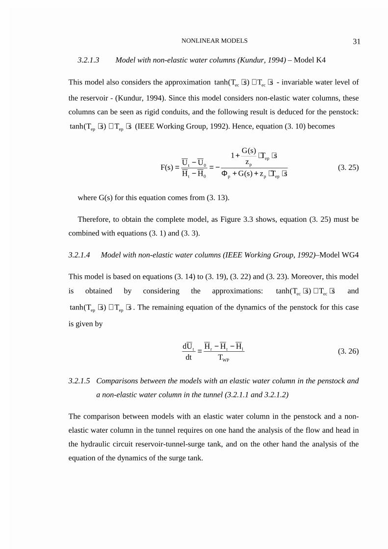
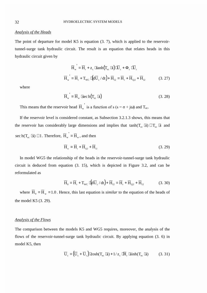
In Figures 3.13 and 3.14 the simulation results for the models K4, K51 and K52 (Kundur,
1994) by using the approximations of the hyperbolic tangent are presented. The variable 0U
is adjusted according to the value of the gate opening (equation (3. 51)).
10 11 12 13 14 15 16 170.56
0.58
0.6
0.62
0.64
0.66
0.68
0.7
time (sec)
Pm
ech
a: Non−linear Model: Non−elastic water column (n=0)b: Non−linear Model: Elastic water column (n=1)c: Non−linear Model: Elastic water column (n=2)
Models with Surge Tank Effects: Parameters 1
ab c
Figure 3.13: Comparison among the models K4, K51 and K52, detail.
0 50 100 150 200 250 300 350 400
0.58
0.6
0.62
0.64
0.66
0.68
0.7
0.72
time (sec)
Pm
ech
Models with Surge Tank Effects: Parameters 1
Figure 3.14: Comparison among the models K4, K51 and K52.

HYDROELECTRIC SYSTEM MODELS54
Graphics a, b and c of Figure 3.13 correspond to graphics a, b and c of Figure 3.10. Both
figures are obtained, according to the parameters of Table 3.5, by simulating nonlinear
models with surge tank effects. The steady state is reached when the oscillation of period T
is completely damped, as Figure 3.14 shows.
3.6.2 Linearized Models with Surge Tank Effects
The time starting constants of the tunnel and penstock (TWC and TWP) for the linearized
models must be adjusted according to the variation of the gate opening (G ). In these cases,
according to Kundur (1994), the constant wT is used, and is calculated by
0
0w H
Q
Ag
LT ⋅
⋅=
It is known that in a nominal operating point (subscript 0)
base
00
base
0000 H
HG
Q
Q HGQ ⋅=⇒⋅=
replacing Q0 into the first expression
0
base
0base
0w H
H
HQ
GAg
LT
⋅⋅
⋅=
as base0 HH ≅
0Wbase
base0w GT
H
QG
Ag
LT ⋅≅⋅⋅
⋅= (3. 63)
The surge constant Cs must also be adjusted according to the following expression
0
s
0base
basesS G
C
GQ
HAC =
⋅⋅= (3. 64)

TIME DOMAIN ANALYSIS OF MODELS 55
Equation (3. 40) is used to simulate these models, where the hyperbolic tangent is
approximated for n=0,1,2:
( ) ( )
( )2,1,0nep
peppp
2,1,0nepp
2,1,0neppp
m
sTtanhz
)s(G)s(G5.0sTz5.05.01
)s(GsTtanhz
)s(GsTtanhz1
G
P
=
==
⋅⋅+⋅+⋅⋅⋅+Φ⋅+
−⋅⋅+⋅⋅−Φ−=
∆∆
3.6.2.1 Model Qlin0
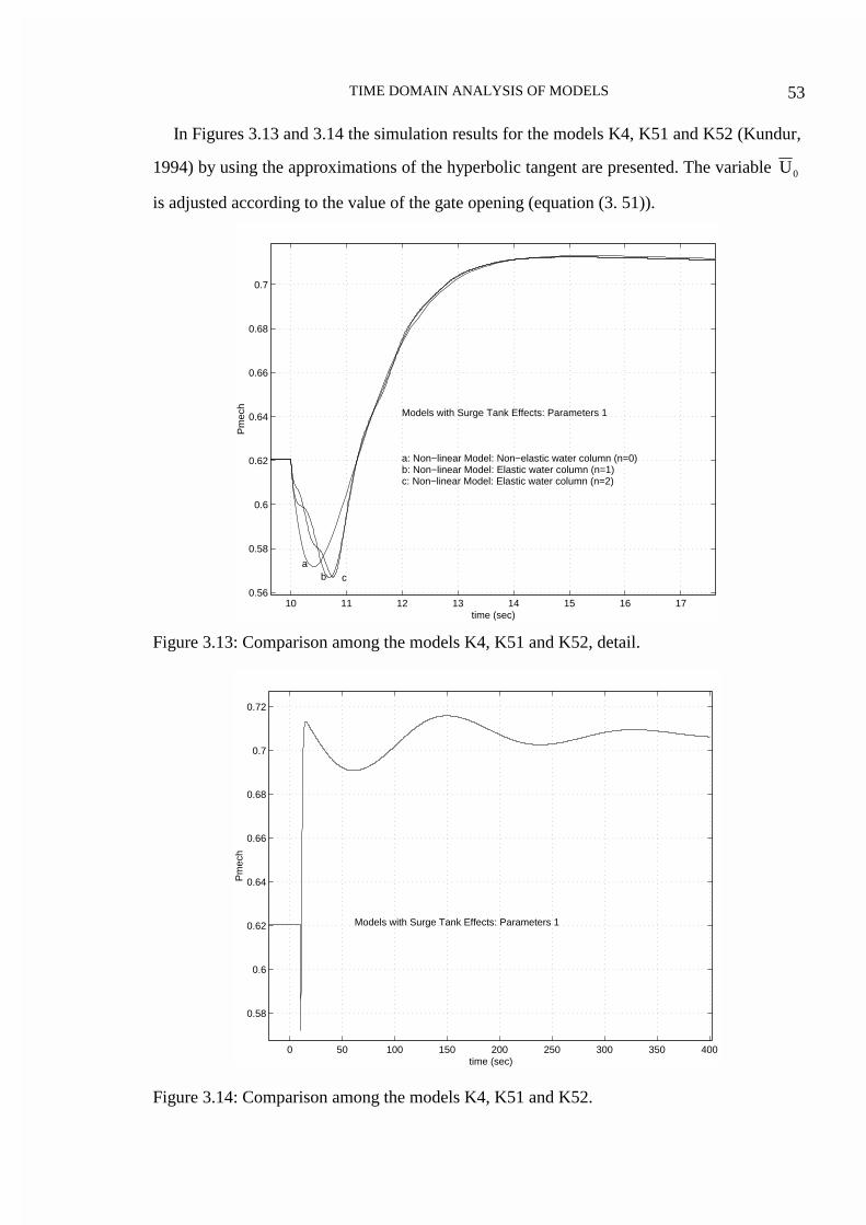
Figure 3.15 shows the response obtained when the gate opening varies a one per cent. The
behaviour is similar to that produced by a nonlinear model with surge tank effects and non-
elastic water columns WG4 and K4, see graphic a from Figures 3.10 and 3.13
Figure 3.16 shows the way the steady state is reached after a damping oscillation whose
period is T.
10 11 12 13 14 15 16 17
0.614
0.616
0.618
0.62
0.622
0.624
0.626
0.628
0.63
Pm
ech
time (sec)
Linearized Model: Non−elastic water columns
Model with Surge Tank Effects: Parameters 1
Figure 3.15: Simulation of the linearized model Qlin0, for a variation of 0.01 [pu] in the gateopening, detail.
HYDROELECTRIC SYSTEM MODELS56
0 50 100 150 200 250 300 350 4000.612
0.614
0.616
0.618
0.62
0.622
0.624
0.626
0.628
0.63
Pm
ech
time (sec)
Linearized Model: Non−elastic water columns
Model with Surge Tank Effects: Parameters 1
Figure 3.16: Simulation of the linearized model Qlin0, for a variation of 0.01 [pu] in the gateopening.
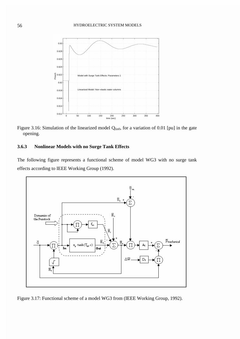
3.6.3 Nonlinear Models with no Surge Tank Effects
The following figure represents a functional scheme of model WG3 with no surge tank
effects according to IEEE Working Group (1992).
Figure 3.17: Functional scheme of a model WG3 from (IEEE Working Group, 1992).

TIME DOMAIN ANALYSIS OF MODELS 57
On one hand, the “In-Out” block of Figure 3.8 is used to simulate the model WG3. On
the other hand, the blocks of Figure 3.9 are utilised to simulate the models: WG2, QR31,
and QR32.
3.6.3.1 Models WG2, QR31, QR32, QR33
Using the approximation of the hyperbolic tangent function, the equation of the turbine head
is expressed as
( ) t3,2,1,0nepplt UsTtanhzH1H ⋅⋅⋅−−==
(3. 65)
10 10.5 11 11.5
0.4
0.42
0.44
0.46
0.48
0.5
0.52
0.54
0.56
0.58
time [sec]
Pm
ech
Models with no Surge Tank Effects: Parameters 5
a: Non−linear Model − Non−elastic water columnb: Non−linear Model − Elastic water column (n=1)c: Non−linear Model − Elastic water column (n=2)d: Non−linear Model − Elastic water column (n=3)e: Non−linear Model − Elastic water column (tanh(Te.s)
e
a−d
a−de
Figure 3.18: Comparison among the models WG2, QR31, QR32, QR33 and WG3.
Figure 3.18 depicts the simulation results for models with no surge tank effects, which
correspond to the hydroelectric plant of St. Lawrence 32 and whose parameters are shown in
Table 3.5. A slightly different behaviour during the transient can be seen, which does not
appear in hydroelectric plants with surge tank effects. This difference can also be observed
in the model that considers a non-elastic water column in the penstock (WG2, graphic a).

HYDROELECTRIC SYSTEM MODELS58
When surge tank effects are not considered; there is no phase lag between the responses
of the models with an elastic or a non-elastic water column in the penstock.
It can be seen, moreover, that simulations for n=0,1,2,3 approximations have a similar
behaviour. There appears a slight difference for the response of the model WG3 (graphic e).
3.6.3.2 Models K2, K31, K32
These models are based on equation (3. 35), where the hyperbolic tangent function is
approximated for n=0,1,2. Therefore, the transfer function becomes
2,1,0neppp0t
0t
)sT(tanhz
1
HH
UU)s(F
=⋅⋅+Φ
−=−−=
10 10.5 11 11.50.4
0.42
0.44
0.46
0.48
0.5
0.52
0.54
0.56
0.58
time [sec]
Pm
ech
Models with no Surge Tank Effects: Parameters 5
a: Non−linear Model − Non−elastic water column b: Non−linear Model − Elastic water column (n=1)c: Non−linear Model − Elastic water column (n=2)
a
a
b−c
b−c
Figure 3.19: Comparison among the models K2, K31 and K32.
Once again, in these models one can observe the phase lag behaviour described in section
(3.6.3.1).
TIME DOMAIN ANALYSIS OF MODELS 59
3.6.4 Linearized Models with no Surge Tank Effects
These models are based on schemes given by equation (3. 42). Since these models are
linearized at an operating point, it is necessary to use wT , which is calculated using equation
(3. 63).
3.6.4.1 Model Klin
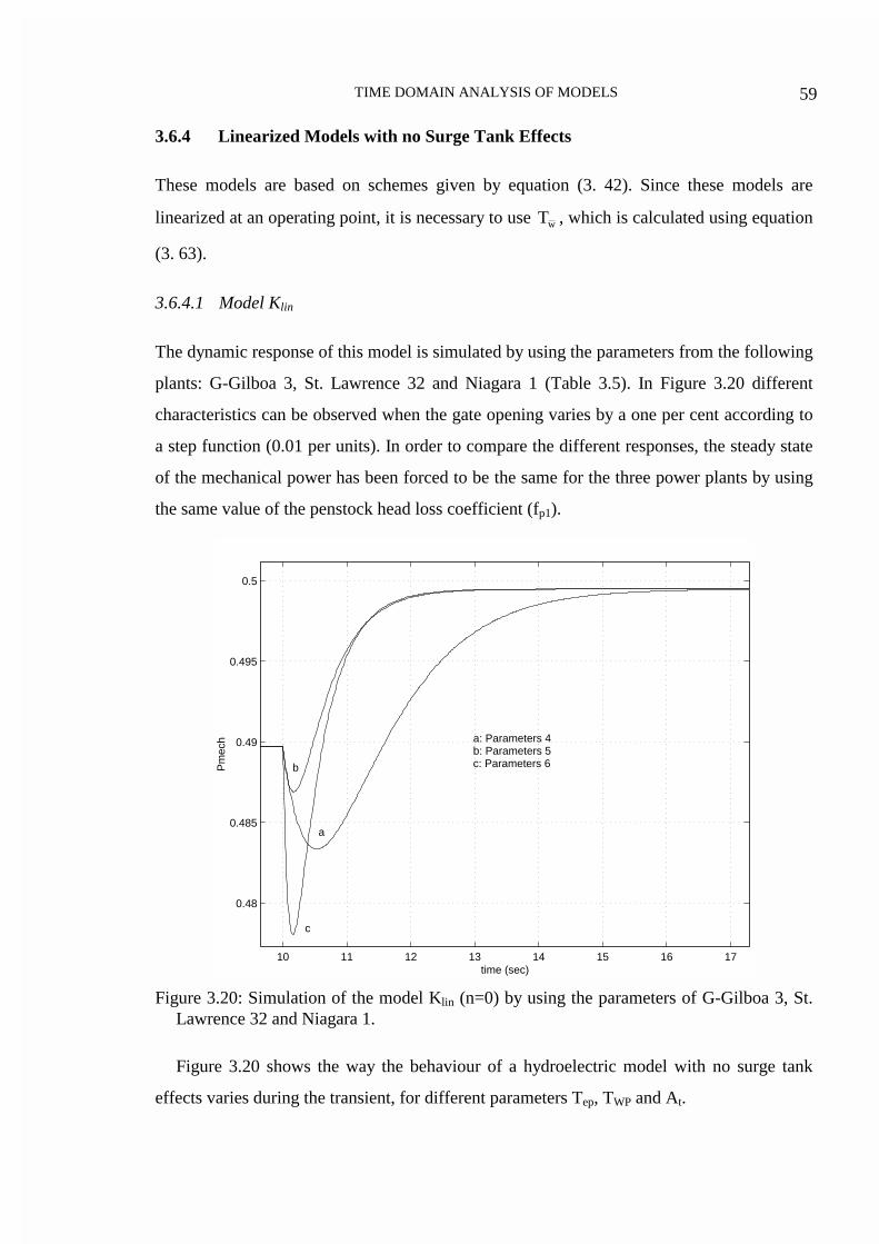
The dynamic response of this model is simulated by using the parameters from the following
plants: G-Gilboa 3, St. Lawrence 32 and Niagara 1 (Table 3.5). In Figure 3.20 different
characteristics can be observed when the gate opening varies by a one per cent according to
a step function (0.01 per units). In order to compare the different responses, the steady state
of the mechanical power has been forced to be the same for the three power plants by using
the same value of the penstock head loss coefficient (fp1).
10 11 12 13 14 15 16 17
0.48
0.485
0.49
0.495
0.5
time (sec)
Pm
ech a: Parameters 4
b: Parameters 5c: Parameters 6
a
b
c
Figure 3.20: Simulation of the model Klin (n=0) by using the parameters of G-Gilboa 3, St.Lawrence 32 and Niagara 1.
Figure 3.20 shows the way the behaviour of a hydroelectric model with no surge tank
effects varies during the transient, for different parameters Tep, TWP and At.
HYDROELECTRIC SYSTEM MODELS60
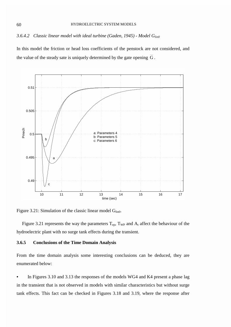
3.6.4.2 Classic linear model with ideal turbine (Gaden, 1945) - Model Glin0
In this model the friction or head loss coefficients of the penstock are not considered, and
the value of the steady sate is uniquely determined by the gate opening G .
10 11 12 13 14 15 16 17
0.49
0.495
0.5
0.505
0.51
time (sec)
Pm
ech
a: Parameters 4b: Parameters 5c: Parameters 6
a
b
c
Figure 3.21: Simulation of the classic linear model Glin0.
Figure 3.21 represents the way the parameters Tep, TWP and At affect the behaviour of the
hydroelectric plant with no surge tank effects during the transient.
3.6.5 Conclusions of the Time Domain Analysis
From the time domain analysis some interesting conclusions can be deduced, they are
enumerated below:
• In Figures 3.10 and 3.13 the responses of the models WG4 and K4 present a phase lag
in the transient that is not observed in models with similar characteristics but without surge
tank effects. This fact can be checked in Figures 3.18 and 3.19, where the response after
TIME DOMAIN ANALYSIS OF MODELS 61
applying a step function of a ten per cent on the gate opening of the models (WG2, QR31,
QR32, QR33, WG3; and K2, K31, K32) are depicted. This phenomenon is due to the
parameter Tep, whose value for the model without a surge tank is up to a magnitude order
less than the case of a model with a surge tank, as Table 3.5 shows, i.e. Tep = 0.208 s
(Susqueda, with a surge tank) and Tep = 0.0205 s (St. Lawrence 32, without a surge tank).
• In Figure 3.10, moreover, it can be seen that the models QR51 and QR52, where the
approximations of the hyperbolic tangent are n=1 and n=2 respectively, have a great
similarity respect to the model WG5. This similarity is improved by taking larger values of n
in the approximation.
• After the transient, the models WG5, QR52, QR51, WG4, K52, K51 and K4 have the
same response. This means that there appears a damped oscillation whose period is given by
T. This behaviour is shown in Figures 3.11 and 3.14.
• Another way to verify that the supposition made in Subsection 3.5.1.4, (fp1 = Φp and
fp2 = Φc) is correct, it is by means of the similarities among the responses of the models of
WG4, QR51 and QR52 (graphics a, b and c, respectively, in Figure 3.10), with respect to the
models K4, K51 and K52 presented in Figure 3.13.
• The models WG3, QR33, QR32, QR31, WG2, K32, K31 and K2, as Figures 3.18 and
3.19 show, have similar behaviours since there is not phase lag during the transient.
• In the case of linearized models with surge tank effects, only Qlin0 is considered since
the models Qlin1 and Qlin2, with approximations of the hyperbolic tangent greater than n=0,
are unstable, as is it shown in Section 3.7.
• Linearized models without surge tank effects (Klin and Glin0) have a particular interest
since they allow to observe the variations that appear during non-minimal phase behaviour,
which, in essence, are due to differences among parameters TWP and Tep.

HYDROELECTRIC SYSTEM MODELS62
3.7 Frequency Response Analysis of Models
In this Section is presented an analysis of the linearized models described in Section 3.3.
The parameters of Table 3.5 are also utilised for this study. For an easier understanding of
this study, the different analyses are separated into two sections. Each section presents the
frequency responses, Bode plots and the Nyquist diagrams, where the stability is verified.
The sections are:
• Section 3.7.1, where the behaviours of the models Klin and Glin0 without surge tank
effects are presented.
• Section 3.7.2, where the behaviours of the models Qlin and Qlin0 with surge tank effects
are presented.
Moreover, it is important to mention that Oldenburger and Donelson (1962) present a
complete frequency response study of linearized models for different working points. In this
Section the analysis for the linearized models working at an operating point is presented in
order to illustrate the behaviour of them in a certain situation.
3.7.1 Models with no Surge Tank Effects
3.7.1.1 Models Klin and Glin0
The point of departure is equation (3. 42) that represents the relationship between the
mechanical power and the gate opening. In Figure 3.22 is depicted a Bode plot for the
linearized model without surge tank for the approximations n=0,1 of the hyperbolic tangent.
Frequency (rad/sec)
Pha
se (
deg)
; Mag
nitu
de (
dB)
Bode Diagrams
0
2
4
6
8
n=0
n=1
10−2
10−1
100
101
102
103
−600
−500
−400
−300
−200
−100
0
n=1
n=0
Figure 3.22: Bode plot for models of Klin, approximations n = 0, 1. Parameters B. Gilboa 3.

FREQUENCY RESPONSE ANALYSIS OF MODELS 63
In Figures 3.22, 3.23 and 3.24 the parameters from B. Gilboa 3 (a hydroelectric plant
without a surge tank Table 3.5) are used.
3.7.1.2 Stability Study
In Figures 3.23 and 3.24 Nyquist diagrams for models Klin with n = 0, 1 are presented. In
both cases the point (-1,0) of the complex plane is rounded in the clockwise sense, which,
for a non-minimal phase transfer function, means that this is a stable system.
Real Axis
Imag
inar
y A
xis
Nyquist Diagrams
−2 −1.5 −1 −0.5 0 0.5 1−2
−1.5
−1
−0.5
0
0.5
1
1.5
2
Figure 3.23: Nyquist diagram for the model of Glin0, approximation n = 0. Parameters fromB. Gilboa 3.
Real Axis
Imag
inar
y A
xis
Nyquist Diagrams
−2 −1.5 −1 −0.5 0 0.5 1−2
−1.5
−1
−0.5
0
0.5
1
1.5
2
Figure 3.24: Nyquist diagram for the model of Klin, approximation n = 1. Parameters from B.Gilboa 3.
HYDROELECTRIC SYSTEM MODELS64
3.7.2 Models with Surge Tank Effects
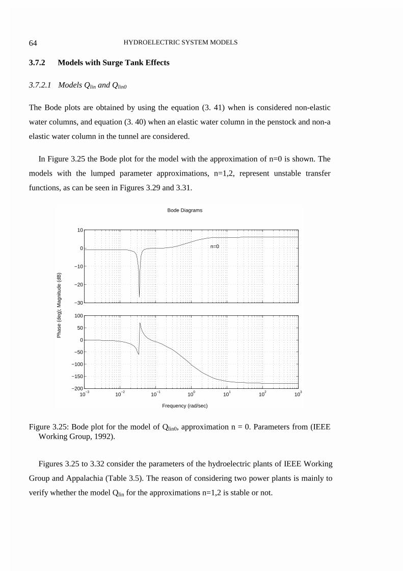
3.7.2.1 Models Qlin and Qlin0
The Bode plots are obtained by using the equation (3. 41) when is considered non-elastic
water columns, and equation (3. 40) when an elastic water column in the penstock and non-a
elastic water column in the tunnel are considered.
In Figure 3.25 the Bode plot for the model with the approximation of n=0 is shown. The
models with the lumped parameter approximations, n=1,2, represent unstable transfer
functions, as can be seen in Figures 3.29 and 3.31.
Frequency (rad/sec)
Pha
se (
deg)
; Mag
nitu
de (
dB)
Bode Diagrams
−30
−20
−10
0
10
n=0
10−3
10−2
10−1
100
101
102
103
−200
−150
−100
−50
0
50
100
Figure 3.25: Bode plot for the model of Qlin0, approximation n = 0. Parameters from (IEEEWorking Group, 1992).
Figures 3.25 to 3.32 consider the parameters of the hydroelectric plants of IEEE Working
Group and Appalachia (Table 3.5). The reason of considering two power plants is mainly to
verify whether the model Qlin for the approximations n=1,2 is stable or not.

FREQUENCY RESPONSE ANALYSIS OF MODELS 65
Frequency (rad/sec)
Pha
se (
deg)
; Mag
nitu
de (
dB)
Bode Diagrams
−50
0
50
100
n=1
n=2
n=2
10−3
10−2
10−1
100
101
102
103
−200
−150
−100
−50
0
50
100
n=2
n=1
Figure 3.26: Bode plot for the model of Qlin, approximations n = 1, 2. Parameters from(IEEE Working Group, 1992).
Frequency (rad/sec)
Pha
se (
deg)
; Mag
nitu
de (
dB)
Bode Diagrams
−50
0
50
100
n=1
n=1
n=0
n=0
10−3
10−2
10−1
100
101
102
103
−200
−150
−100
−50
0
50
100
n=0
n=0
n=1n=1
Figure 3.27: Bode plot for the model of Qlin0 and Qlin, approximations n = 0, 1. Parametersfrom Appalachia power plant.
HYDROELECTRIC SYSTEM MODELS66
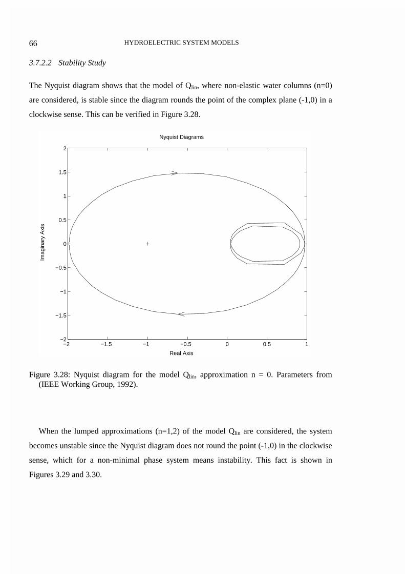
3.7.2.2 Stability Study
The Nyquist diagram shows that the model of Qlin, where non-elastic water columns (n=0)
are considered, is stable since the diagram rounds the point of the complex plane (-1,0) in a
clockwise sense. This can be verified in Figure 3.28.
Real Axis
Imag
inar
y A
xis
Nyquist Diagrams
−2 −1.5 −1 −0.5 0 0.5 1−2
−1.5
−1
−0.5
0
0.5
1
1.5
2
Figure 3.28: Nyquist diagram for the model Qlin, approximation n = 0. Parameters from(IEEE Working Group, 1992).
When the lumped approximations (n=1,2) of the model Qlin are considered, the system
becomes unstable since the Nyquist diagram does not round the point (-1,0) in the clockwise
sense, which for a non-minimal phase system means instability. This fact is shown in
Figures 3.29 and 3.30.
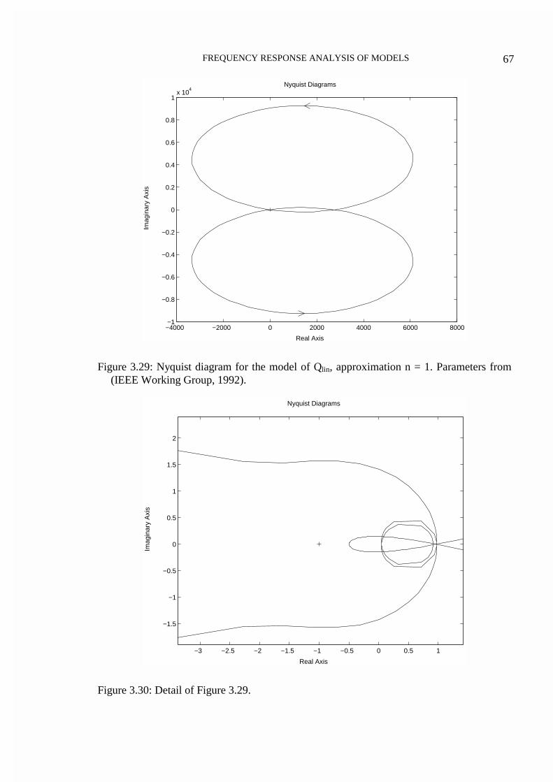
FREQUENCY RESPONSE ANALYSIS OF MODELS 67
Real Axis
Imag
inar
y A
xis
Nyquist Diagrams
−4000 −2000 0 2000 4000 6000 8000−1
−0.8
−0.6
−0.4
−0.2
0
0.2
0.4
0.6
0.8
1x 10
4
Figure 3.29: Nyquist diagram for the model of Qlin, approximation n = 1. Parameters from(IEEE Working Group, 1992).
Real Axis
Imag
inar
y A
xis
Nyquist Diagrams
−3 −2.5 −2 −1.5 −1 −0.5 0 0.5 1
−1.5
−1
−0.5
0
0.5
1
1.5
2
Figure 3.30: Detail of Figure 3.29.
HYDROELECTRIC SYSTEM MODELS68
Real Axis
Imag
inar
y A
xis
Nyquist Diagrams
−1.5 −1 −0.5 0 0.5 1 1.5 2
x 104
−3
−2
−1
0
1
2
3x 10
4
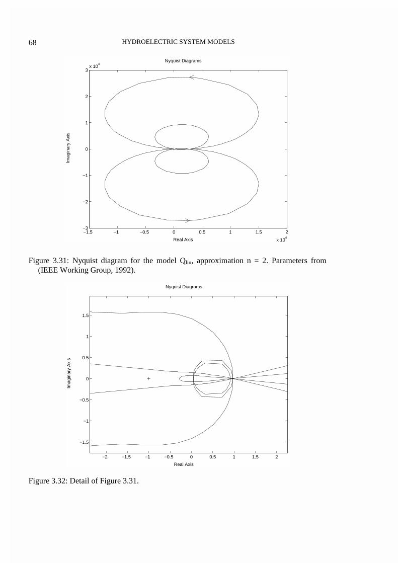
Figure 3.31: Nyquist diagram for the model Qlin, approximation n = 2. Parameters from(IEEE Working Group, 1992).
Real Axis
Imag
inar
y A
xis
Nyquist Diagrams
−2 −1.5 −1 −0.5 0 0.5 1 1.5 2
−1.5
−1
−0.5
0
0.5
1
1.5
Figure 3.32: Detail of Figure 3.31.

SUGGESTIONS FOR MODELLING HYDROELECTRIC POWER PLANTS 69
3.8 Suggestions for Modelling Hydroelectric Power Plants
After presenting the time domain and frequency response analyses of different models for
hydroelectric power plants, some suggestions are given below that add more information to
the Guidelines for Modelling Hydraulic Turbines presented in Section 9.1.5 of Kundur
(1994). These complementary suggestions are divided into two parts, on one hand the
hydroelectric models that consider surge tank effects, and, on the other hand, the
hydroelectric models without surge tank effects.
3.8.1 Models with Surge Tank Effects
3.8.1.1 Nonlinear Models
For this case some models deduced according to two different ways are presented:
1) The model WG5 allows the best approximation since it represents all the phenomena
in detail. On one hand, the model WG5 shows the non-minimal-phase behaviour for a step
input. On the other hand, the model WG5 has the inconvenient of incorporating the
hyperbolic tangent function of complex variable in an equation system of state variables.
Therefore, when a control must be designed, instead of WG5, it is necessary to take the
lumped approximations of this function and the model WG5 is turned into QR52, QR51 or
WG4.
The greater the value of the lumped approximation, the greater the number of state
variables. In the case of working with an interconnected system, it is probable that the
models WG4 and QR51 are sufficient to represent, in a very accurate manner, the behaviour
of a hydroelectric plant with surge tank effects.
2) The models of Kundur (1994) K5, K52 and K51 have the disadvantage that the
variable 0U must be updated for each value of the gate opening (G ). Apart from this, the
models of Kundur (1994) have similar behaviours with respect to the models WG5, QR52
and QR51. For these reasons the models of Kundur are interesting in the analysis of the
hydroelectric plant in a general sense but not for the design of a speed system control.
HYDROELECTRIC SYSTEM MODELS70
3.8.1.2 Linearized Models
These models are interesting when a frequency response study is necessary for stability
studies. However, only the simplest model can be used since these models are unstable for
lumped approximations greater than n=0.
3.8.2 Models with no Surge Tank Effects
3.8.2.1 Nonlinear Models
In this case there appears a similar situation to the case of nonlinear models with surge tank
effects: the model that considers the hyperbolic tangent function, calculated according to
Figure 3.18, gives the best approximation to the real system, and there is only a slight
difference among the four lumped approximations n=0,1,2,3 and the model that takes the
complete hyperbolic tangent (WG3).
For the K3, K32 and K32 models the conclusions exposed for hydroelectric plants with
surge tank effects are still valid. Therefore, these models are interesting for performing
behaviour analysis and not for designing controllers.
3.8.2.2 Linearized Models
The models Klin and Glin are useful in those cases when small-signal stability studies are
required (Kundur, 1994).
3.9 Summary
A study of hydroelectric models has been presented in this Chapter. This study classifies the
models into two groups: nonlinear models and linearized models, Sections 3.2 and 3.3,
respectively. Each group has been subdivided into models with and without surge tank
effects. Moreover, each of these has two particularities: the first considers elastic water
column in the penstock and non-elastic water column in the tunnel, and the second
contemplates non-elastic water columns. In the group of nonlinear models, with or without
surge tank effects, a comparison has been performed where differences and similarities
among the models are shown.

SUMMARY 71
Subsequently, Section 3.5, presented a way to calculate the turbine and tunnel flows in
steady state, which allows to calculate the mechanical power in steady state as function of
the gate opening.
Section 3.6 presented a time domain analysis where all models have been simulated for
different real hydroelectric plants (parameters are shown in Table 3.5). The behaviours have
been compared.
All linearized models have been used in the frequency response analysis, which is
exposed in Section 3.7. Bode plots and Nyquist diagrams have been presented for the
determination of the stability of these models.
In Section 3.8 suggestions for modelling hydroelectric plants are proposed.
Related Documents