Hydroelastic waves and their interaction with fixed structures Paul Brocklehurst Thesis submitted for the degree of Doctor of Philosophy School of Mathematics University of East Anglia Norwich, NR4 7TJ England September 2012 This copy of the thesis has been supplied on condition that anyone who consults it is understood to recognise that its copyright rests with the author and that use of any information derived there from must be in accordance with current UK Copyright Law. In addition, any quotation or extract must include full attribution.

Welcome message from author
This document is posted to help you gain knowledge. Please leave a comment to let me know what you think about it! Share it to your friends and learn new things together.
Transcript

Hydroelastic waves and theirinteraction with fixed
structures
Paul Brocklehurst
Thesis submitted for the degree of Doctor of Philosophy
School of Mathematics
University of East Anglia
Norwich, NR4 7TJ
England
September 2012
This copy of the thesis has been supplied on condition that anyone who consults it is understood
to recognise that its copyright rests with the author and that use of any information derived there
from must be in accordance with current UK Copyright Law. In addition, any quotation or extract
must include full attribution.

Abstract
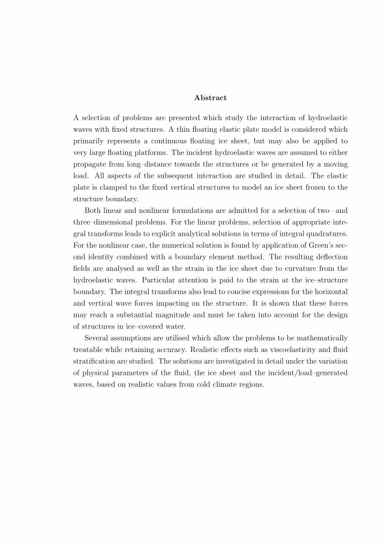
A selection of problems are presented which study the interaction of hydroelastic
waves with fixed structures. A thin floating elastic plate model is considered which
primarily represents a continuous floating ice sheet, but may also be applied to
very large floating platforms. The incident hydroelastic waves are assumed to either
propagate from long–distance towards the structures or be generated by a moving
load. All aspects of the subsequent interaction are studied in detail. The elastic
plate is clamped to the fixed vertical structures to model an ice sheet frozen to the
structure boundary.
Both linear and nonlinear formulations are admitted for a selection of two– and
three–dimensional problems. For the linear problems, selection of appropriate inte-
gral transforms leads to explicit analytical solutions in terms of integral quadratures.
For the nonlinear case, the numerical solution is found by application of Green’s sec-
ond identity combined with a boundary element method. The resulting deflection
fields are analysed as well as the strain in the ice sheet due to curvature from the
hydroelastic waves. Particular attention is paid to the strain at the ice–structure
boundary. The integral transforms also lead to concise expressions for the horizontal
and vertical wave forces impacting on the structure. It is shown that these forces
may reach a substantial magnitude and must be taken into account for the design
of structures in ice–covered water.
Several assumptions are utilised which allow the problems to be mathematically
treatable while retaining accuracy. Realistic effects such as viscoelasticity and fluid
stratification are studied. The solutions are investigated in detail under the variation
of physical parameters of the fluid, the ice sheet and the incident/load–generated
waves, based on realistic values from cold climate regions.


Acknowledgements
There are several people I would like to thank for their contribution to the thesis.
My primary supervisor, Alexander Korobkin, never failed to instantly provide the
perfect solution to any problems I encountered. This has led to my belief in his
mathematical omniscience. In addition, his enthusiasm for the subject and affable
manner made him a privilege to work with. My secondary supervisor, Emilian
Parau, was invaluable: he is a talented and dedicated mathematician whose door
was always open for guidance. I could not have asked for a better supervisory team
and I’ve learned a great deal from them both. I would also like to acknowledge Luke
Bennetts and Michael Meylan for their comments and advice at various conferences.
Mark Cooker’s revision of the thesis was extremely thorough and helpful.
I will always have fond memories of my PhD experience in Norwich, largely due
to the excellent company of Matt, Ben M., Ben H., Nina & Vicky. I enjoyed every
minute of house–sharing with Rob. I am extremely thankful for Hannah’s support
and companionship. My parents are wonderful people to whom I owe tremendous
gratitude.


Contents
1 Introduction 1
1.1 Preliminaries . . . . . . . . . . . . . . . . . . . . . . . . . . . . . . . 1
1.2 Literature review . . . . . . . . . . . . . . . . . . . . . . . . . . . . . 1
1.3 Methods of solution . . . . . . . . . . . . . . . . . . . . . . . . . . . . 9
1.4 Theoretical assumptions . . . . . . . . . . . . . . . . . . . . . . . . . 11
1.5 Thesis outline . . . . . . . . . . . . . . . . . . . . . . . . . . . . . . . 15
1.6 Applications . . . . . . . . . . . . . . . . . . . . . . . . . . . . . . . . 17
2 Two-dimensional hydroelastic wave interaction with a vertical wall 20
2.1 Introduction . . . . . . . . . . . . . . . . . . . . . . . . . . . . . . . . 20
2.2 Formulation . . . . . . . . . . . . . . . . . . . . . . . . . . . . . . . . 21
2.2.1 Schematic and parameters . . . . . . . . . . . . . . . . . . . . 21
2.2.2 Governing Equations and boundary conditions . . . . . . . . . 22
2.2.3 Incident Waves . . . . . . . . . . . . . . . . . . . . . . . . . . 24
2.2.4 Dispersion relation . . . . . . . . . . . . . . . . . . . . . . . . 25
2.2.5 Nondimensionalisation . . . . . . . . . . . . . . . . . . . . . . 26
2.2.6 Typical values of wavelength and wave period . . . . . . . . . 27
2.2.7 Linear superposition . . . . . . . . . . . . . . . . . . . . . . . 28
2.3 Solution . . . . . . . . . . . . . . . . . . . . . . . . . . . . . . . . . . 29
2.3.1 Fourier transform . . . . . . . . . . . . . . . . . . . . . . . . . 29
2.3.2 Velocity potential . . . . . . . . . . . . . . . . . . . . . . . . . 30
2.3.3 Plate deflection . . . . . . . . . . . . . . . . . . . . . . . . . . 31
2.3.4 Q(k) and L(k, z) . . . . . . . . . . . . . . . . . . . . . . . . . 35
2.3.5 Inverse transforms . . . . . . . . . . . . . . . . . . . . . . . . 37
2.4 Numerical results . . . . . . . . . . . . . . . . . . . . . . . . . . . . . 39
2.4.1 Deflection of the ice sheet . . . . . . . . . . . . . . . . . . . . 39
2.4.2 Strain in the ice sheet . . . . . . . . . . . . . . . . . . . . . . 41
2.4.3 Shear force on the wall . . . . . . . . . . . . . . . . . . . . . . 45
2.4.4 Horizontal force . . . . . . . . . . . . . . . . . . . . . . . . . . 47
2.5 Summary . . . . . . . . . . . . . . . . . . . . . . . . . . . . . . . . . 51
2.5.1 Comparison with other authors . . . . . . . . . . . . . . . . . 52
2.5.2 Comparison with other methods of solution . . . . . . . . . . 52
i

3 Hydroelastic wave diffraction by a vertical cylinder 54
3.1 Introduction . . . . . . . . . . . . . . . . . . . . . . . . . . . . . . . . 54
3.2 Mathematical formulation . . . . . . . . . . . . . . . . . . . . . . . . 55
3.2.1 Schematic and parameters . . . . . . . . . . . . . . . . . . . . 55
3.2.2 Governing equations and boundary conditions . . . . . . . . . 56
3.2.3 Incident waves and nondimensionalisation . . . . . . . . . . . 57
3.2.4 Decomposition of azimuthal coordinate . . . . . . . . . . . . . 58
3.3 Method of solution . . . . . . . . . . . . . . . . . . . . . . . . . . . . 60
3.3.1 Weber transform . . . . . . . . . . . . . . . . . . . . . . . . . 60
3.3.2 Velocity potential . . . . . . . . . . . . . . . . . . . . . . . . . 62
3.3.3 Plate equation . . . . . . . . . . . . . . . . . . . . . . . . . . . 62
3.3.4 Numerical techniques for inverse Weber transforms . . . . . . 64
3.4 Numerical results . . . . . . . . . . . . . . . . . . . . . . . . . . . . . 67
3.4.1 Deflection in the ice sheet . . . . . . . . . . . . . . . . . . . . 67
3.4.2 Strain in the ice sheet . . . . . . . . . . . . . . . . . . . . . . 69
3.4.3 Shear force . . . . . . . . . . . . . . . . . . . . . . . . . . . . 72
3.4.4 Horizontal force . . . . . . . . . . . . . . . . . . . . . . . . . . 75
3.5 Summary . . . . . . . . . . . . . . . . . . . . . . . . . . . . . . . . . 76
4 Hydroelastic wave reflection by a vertical wall in a two-layer fluid 79
4.1 Introduction . . . . . . . . . . . . . . . . . . . . . . . . . . . . . . . . 79
4.2 Mathematical formulation . . . . . . . . . . . . . . . . . . . . . . . . 80
4.2.1 Schematic and parameters . . . . . . . . . . . . . . . . . . . . 80
4.2.2 Governing equations and boundary conditions . . . . . . . . . 80
4.2.3 Incident waves . . . . . . . . . . . . . . . . . . . . . . . . . . . 82
4.2.4 Dispersion relation . . . . . . . . . . . . . . . . . . . . . . . . 84
4.2.5 Nondimensionalisation . . . . . . . . . . . . . . . . . . . . . . 87
4.2.6 Notes regarding the roots k1 and k2 . . . . . . . . . . . . . . . 87
4.2.7 Nondimensional BVP . . . . . . . . . . . . . . . . . . . . . . . 91
4.2.8 Total forms for the potentials & deflections . . . . . . . . . . . 91
4.3 Solution . . . . . . . . . . . . . . . . . . . . . . . . . . . . . . . . . . 93
4.3.1 Fourier transform . . . . . . . . . . . . . . . . . . . . . . . . . 93
4.3.2 Velocity potentials . . . . . . . . . . . . . . . . . . . . . . . . 94
4.3.3 Plate deflection . . . . . . . . . . . . . . . . . . . . . . . . . . 98
4.3.4 Interfacial deflection . . . . . . . . . . . . . . . . . . . . . . . 102
4.4 Numerical results . . . . . . . . . . . . . . . . . . . . . . . . . . . . . 104
4.4.1 Plate & interfacial deflection . . . . . . . . . . . . . . . . . . . 105
4.4.2 Strain in the ice sheet . . . . . . . . . . . . . . . . . . . . . . 114
4.4.3 Shear force . . . . . . . . . . . . . . . . . . . . . . . . . . . . 119
4.5 Summary . . . . . . . . . . . . . . . . . . . . . . . . . . . . . . . . . 122
ii
5 Hydroelastic waves generated by a moving load in the vicinity of a
vertical wall: linear formulation 124
5.1 Introduction . . . . . . . . . . . . . . . . . . . . . . . . . . . . . . . . 124
5.2 Open ice case . . . . . . . . . . . . . . . . . . . . . . . . . . . . . . . 125
5.2.1 Mathematical formulation . . . . . . . . . . . . . . . . . . . . 125
5.2.1.1 Schematic, parameters and governing equations . . . 125
5.2.1.2 Critical speeds . . . . . . . . . . . . . . . . . . . . . 127
5.2.1.3 Nondimensionalisation & expression for the moving
load . . . . . . . . . . . . . . . . . . . . . . . . . . . 128
5.2.2 Solution by double Fourier transform . . . . . . . . . . . . . . 130
5.2.2.1 Velocity potential . . . . . . . . . . . . . . . . . . . . 131
5.2.2.2 Plate deflection . . . . . . . . . . . . . . . . . . . . . 131
5.2.2.3 Method of residues . . . . . . . . . . . . . . . . . . . 132
5.2.3 Numerical results for the ice deflection . . . . . . . . . . . . . 135
5.3 Vertical wall case . . . . . . . . . . . . . . . . . . . . . . . . . . . . . 138
5.3.1 Mathematical formulation: schematic and governing equations 138
5.3.2 Solution by double Fourier transform . . . . . . . . . . . . . . 139
5.3.2.1 Velocity potential . . . . . . . . . . . . . . . . . . . . 140
5.3.2.2 Plate deflection . . . . . . . . . . . . . . . . . . . . . 141
5.3.2.3 Difficulties using the method of residues . . . . . . . 142
5.3.2.4 Inverse transforms . . . . . . . . . . . . . . . . . . . 143
5.3.3 Numerical results . . . . . . . . . . . . . . . . . . . . . . . . . 146
5.3.3.1 Deflection . . . . . . . . . . . . . . . . . . . . . . . . 146
5.3.3.2 Strain in the ice sheet . . . . . . . . . . . . . . . . . 155
5.3.4 Comparison between vertical wall and open ice case . . . . . . 160
5.4 Summary . . . . . . . . . . . . . . . . . . . . . . . . . . . . . . . . . 162
6 Hydroelastic waves generated by a moving load in the vicinity of a
vertical wall: nonlinear formulation 164
6.1 Introduction . . . . . . . . . . . . . . . . . . . . . . . . . . . . . . . . 164
6.2 Mathematical formulation . . . . . . . . . . . . . . . . . . . . . . . . 165
6.2.1 Schematic and parameters . . . . . . . . . . . . . . . . . . . . 165
6.2.2 Governing equations and boundary conditions . . . . . . . . . 166
6.2.3 Dispersion relation and critical speed . . . . . . . . . . . . . . 167
6.2.4 Nondimensionalisation & expression for the moving load . . . 168
6.3 Solution . . . . . . . . . . . . . . . . . . . . . . . . . . . . . . . . . . 169
6.3.1 Green’s second identity . . . . . . . . . . . . . . . . . . . . . . 169
6.3.2 Each surface integral evaluated . . . . . . . . . . . . . . . . . 172
6.3.2.1 The surface SW . . . . . . . . . . . . . . . . . . . . . 172
6.3.2.2 The surface SR . . . . . . . . . . . . . . . . . . . . . 172
6.3.2.3 The surface Sε . . . . . . . . . . . . . . . . . . . . . 173
6.3.2.4 The surface SF . . . . . . . . . . . . . . . . . . . . . 177
iii
6.3.3 Formulating the numerical procedure . . . . . . . . . . . . . . 178
6.3.4 The numerical scheme . . . . . . . . . . . . . . . . . . . . . . 181
6.4 Numerical results . . . . . . . . . . . . . . . . . . . . . . . . . . . . . 183
6.4.1 Deflection . . . . . . . . . . . . . . . . . . . . . . . . . . . . . 183
6.4.2 Comparison with linear model . . . . . . . . . . . . . . . . . . 187
6.5 Summary . . . . . . . . . . . . . . . . . . . . . . . . . . . . . . . . . 191
7 Final discussion 192
7.1 Summary and conclusions . . . . . . . . . . . . . . . . . . . . . . . . 192
7.2 Future work . . . . . . . . . . . . . . . . . . . . . . . . . . . . . . . . 195
iv
Chapter 1
Introduction
1.1 Preliminaries
That waves exist in ice sheets is a surprising revelation for some, owing to the
misconception that ice is rigid. In fact, the ice cover of the Arctic Ocean has been
shown to be in almost perpetual motion. The constant swell, ebb, and flow of the
ocean upon which the ice rests causes small–amplitude waves to propagate through
the ice sheet. The study of the behaviour of ice has a long and fascinating history,
but the naturally emerging trend is the consideration of ice as an elastic material.
Development of this elastic theory allowed the fluid-ice interaction to become well
understood, and the literature available is now rich and diverse. However, fewer
studies are available on the interaction of these “hydroelastic” waves with rigid
structures. This thesis is concerned with such interactions, driven by the expected
need for offshore wind farms, drilling rigs and oil/gas platforms to be built in ice–
covered waters, among other applications.
The introduction is arranged as follows. Section 1.2 summarises the progress thus
far in the field with a literature review. It is arranged in a roughly chronological
order, with some effort to group similar topics. Focus here is more on the subject
matter rather than the solution methodology, which is discussed further in Section
1.3. Section 1.4 explains some theoretical assumptions utilised within the thesis with
justification for their usage. Section 1.5 presents an outline of each chapter within
the thesis, accompanied by more specific literature discussion. Section 1.6 discusses
the intended applications of each chapter, as well as expanding on the more general
applications of hydroelasticity.
1.2 Literature review
The first foray into the field is widely accredited to Greenhill (1887) as far back as
the 19th century. He considered an elastic beam resting on fluid of finite depth,
even describing the dispersion of ice–coupled waves. The idea was later extended
by Ewing & Crary (1934), beginning a series of papers that experimentally studied
1
flexural waves in expansive ice sheets. Some earlier models of wave-ice interaction
were simplified “mass–loading” models that did not account for the elastic or inelas-
tic behaviour of the ice. Weitz & Keller (1950) and Peters (1950) were among such
studies, treating the ice sheet as a disconnected set of mass points on the surface.
Such models were considered to be fundamentally flawed and were thus superseded
by the elastic counterpart. Stoker (1957) studied surface gravity wave interaction
with a thin floating elastic sheet, though the equations assumed a shallow water
model. Kouzov (1963a) studied acoustic waves propagating through compressible
fluid bounded by two thin elastic plates. In an innovative study Kouzov (1963b) also
solved the problem of hydroelastic wave diffraction at a crack in an elastic plate.
One of the early attempts to model ocean wave penetration into sea ice is given by
Hendrickson & Webb (1963).
Meanwhile, various experiments were undertaken, verifying the presence of waves
in ice sheets. Press & Ewing (1951); Press et al. (1951); Oliver et al. (1954), in a series
of experiments, created ice–coupled waves artificially. Hunkins (1962) conducted
experiments at four drifting research stations, detecting waves of long period 15–
60 seconds. The waves had small–amplitude and long wavelengths, and it was
concluded that such waves propagate with little attenuation throughout the Arctic.
Robin (1963) conducted shipborne wave recorder experiments in the Weddell sea,
and similar conclusions were drawn as to the period and amplitude of waves and their
penetration into large sheets of ice. Wadhams (1972) also conducted experiments
on ice wave attenuation; in this case measurements were obtained by upwards sonar
from a submarine.
Considered by many as a pioneering study in usage of the thin-elastic plate
model, Evans & Davies (1968) fully solved problem of wave reflection and trans-
mission by a semi–infinite elastic plate in finite water. This work is a somewhat
obscure technical report, originally intended to have military applications, but is
often accredited for kick–starting the subsequent fervour in the field. They treated
the problem as time–harmonic, but the explicit solution was too complex to be
computed. The authors were forced to resort to a shallow–water approximation.
Much of the theory regarding waves in ice sheets has spawned from studies in
the Marginal Ice Zone (MIZ). This is an area at the intersection of ice fields and
open ocean where the ice is not continuous, but rather made up of smaller ice floes.
The interaction of these smaller floes with incoming ocean waves, and indeed the
interaction of the floes with each other, has been studied extensively. While not
directly related to this thesis, which considers continuous ice, studies regarding this
topic were instrumental in establishing hydroelastic theory. Early measurements in
the MIZ were conducted by Wadhams (1975), who used airborne laser profiling to
measure swell. The response of a single ice floe to swell were measured by Squire &
Martin (1980) and Goodman et al. (1980).
The accompanying hydroelastic theory was being developed in tandem, led by
such authors as Squire; the works of Squire (1984c,d,b,a) being excellent examples.
2
The dispersion relations considered here were more detailed than in previous work
in the field. Bates & Shapiro (1980) studied long–period waves in an ice cover, using
the elastic plate model. Several studies were also under way in Russia, Timokov &
Kheisin (1987) being one example. Studies concerned with the complicated interac-
tions in the MIZ became more common: works concerning the breakup of ice floes
are found by Squire & Martin (1980) and Goodman et al. (1980). Work concerning
floe collision is given by Martin & Becker (1987, 1988), Crocker (1992) and Rottier
(1992).
In an important series of papers, Fox & Squire (1990, 1991b, 1994) studied waves
at the sea–ice boundary. They were the first authors to correctly match the poten-
tials across the boundary, superseding earlier work which was incompletely matched.
The thin plate equation was utilised, now thoroughly established as the optimal
model for the ice cover. The model assumes that the velocity potential is periodic
and can be expressed in terms of time–independent part, which many future papers
adopted. The reflection and transmission coefficients, describing the wave energy
reflected and transmitted by the ice relative to the incident free–surface wave, were
studied for various parameters. In a related model, Meylan & Squire (1993a,b) solve
the finite–length floe version of this problem, using a different solution methodology.
The model predicted perfect transmission for certain values of the ice wavelength
and floe diameter. The problem was later solved for finite depth (Meylan & Squire,
1994).
No hydroelastic literature review is complete without reference to the study of
moving loads on an ice sheet. Such studies have a plethora of applications, discussed
in Section 1.6. Wilson (1958) pioneered the theoretical treatment of moving loads
on ice sheets, and Kerr (1976) gives an early review of the research on this topic.
Experiments were conducted by Takizawa (1985) and Squire et al. (1988). The
theory was further developed by Davys et al. (1985) and later Schulkes et al. (1987).
Schulkes & Sneyd (1988) considered the time–dependent version of the problem,
with most earlier work assuming periodic motion. Hosking et al. (1988) introduces
viscoelasticity in an attempt to better match the theory with experiments. The
problem was later revisited in three–dimensions by Milinazzo et al. (1995), and by
Parau & Vanden-Broeck (2011) to incorporate nonlinear effects. In addition, Duffy
(1996) studied the generation of internal ocean waves at the interface of a two–layer
fluid by a moving load on an ice sheet. The comprehensive book by Squire et al.
(1996) studies the subject in greater detail.
Primarily the above papers utilised the standard thin elastic plate model, out-
lined later in Section 1.4. Others attempted to incorporate the more inhomogeneous
aspects of ice. Fox & Squire (1991a) attempted to model thick elastic plates, with
comparison to the thin elastic plate model. Wadhams & Holt (1991) studied waves
in frazil and pancake ice, alternate forms of ice consisting of small crystals. Some
authors attempted to model the slight attenuation of ice waves over long distances:
Wadhams (1973) using the explanation of hysteresis due to Norton creep; Bates &
3

Shapiro (1980) and Squire & Fox (1992) using linear viscoelasticity. A sophisticated
model incorporating inhomogeneous, non–idealised features of ice was attempted by
Marchenko (1996, 1997); Marchenko & Voliak (1997).
The work on ocean wave penetration into ice sheets by Fox & Squire (1994) was
reworked by Sturova (1999), including a study of oblique angles of wave incidence.
Barrett & Squire (1996) further extend the work by considering an abrupt change in
ice rigidity, density or thickness. Sahoo et al. (2001) considered the same problem
with different edge conditions, and Kim & Ertekin (1998) used a different set of
orthogonal eigenfunctions which resulted in an improvement in numerical efficiency.
The field of hydroelasticity continued to expand, aided in part by the interest
in Very Large Floating Structures (VLFS), which can be modelled using the same
thin elastic plate model. These VLFS are explained further in Section 1.6, and for
now we only recognise their contribution to the literature. Wu et al. (1995) is an
early example of solution by eigenfunction expansion. Kashiwagi (1998) solved the
propagation of waves through a VLFS using an alternate method. The application of
plate theory to VLFS led to new challenges for authors: reducing the elastic response
of the platforms to incoming waves (Khabakhpasheva & Korobkin, 2002); fixing the
platform to the bottom of the ocean using a spring (Korobkin, 2000); the response
of the platforms to tsunamis or larger amplitude waves (Masuda & Miyazaki, 1999).
Andrianov & Hermans (2003) studied the influence of water depth on the platform
response. Utsunomiya et al. (1998) analysed the response to waves of a VLFS near
a breakwater. The review papers by Kashiwagi (2000) and Watanabe et al. (2004)
further summarise the progress in this field.
Entering the 21st century, the field showed no signs of stagnation. Further
experimental findings exemplified the continuing demand for ice–related studies.
Exploiting modernising technology, Schulz-Stellenfleth & Lehner (2002) took mea-
surements of waves damped by sea ice using space–borne synthetic aperture radar
images of the MIZ. Further observations were made in the Okhotsk Sea using an
ultrasonic sounder. Downer & Haskell (2001) studied ice floe kinematics in the Ross
Sea. Marko (2003) studied ice draft, ice velocity, ice concentration and current pro-
file data inside the Sea of Okhotsk ice pack. This study was motivated by intense
wave occurrences in 1998 which produced high–amplitude waves. A survey of re-
cent changes in the thickness of Arctic sea ice was presented by Wadhams (2004).
Emerging warming trends exhibited in the Arctic, and the international concern
regarding global climate change, has led to further interest into ice–wave behaviour.
Serreze et al. (2007) investigates the shrinking Arctic ice cover due to this warming;
Kwok et al. (2009b) documents the reducing ice thickness. As a consequence of such
trends, we can expect higher amplitude waves, and waves that are able to penetrate
further into the pack ice (Squire, 2007).
Returning to the problem of wave reflection/transmission at the ice–water bound-
ary, three–dimensional scattering by ice sheets was studied by Balmforth & Craster
(1999) in a frequently referenced paper. Explicitly building the edge–conditions
4
into the analysis, they were able to solve fully the problem by revisiting the method
of Evans & Davies (1968). Tkacheva (2004) provide another study, also revisiting
the Weiner–Hopf method. There was further study by Teng et al. (2001), using an
eigenfunction approach, who stated the energy conservation relation for free, simply–
supported and built–in edge conditions. Utilising residue calculus techniques, the
problem was also studied by Linton & Chung (2003), who included the case of waves
incident from the ice into the ocean, as well as the reverse. Chung & Linton (2005)
extended the problem further by considering wave transmission across a gap between
two plates.
One problem subject to recent attention is that of wave propagation across a
crack in an ice sheet. The problem was touched on in an earlier referenced paper
by Barrett & Squire (1996), but it was studied first in more detail by Squire &
Dixon (2000) for infinite depth. Simple formulae were derived for the reflection and
transmission coefficients across the crack. The authors report a strong dependence
on wave period in their results, with perfect transmission across the crack occurring
for certain values of the period. Squire & Dixon (2001) extend the problem to
consider multiple cracks. Evans & Porter (2003) revisited the crack problem in two–
dimensions, for finite depth, obtaining an explicit solution. The same authors also
consider the multiple crack problem, finding that large resonant motion can occur
in the strip between two cracks. Porter & Evans (2007) generalise the problem to
consider a finite number of straight cracks, and are forced to approximate a solution
using Galerkin’s method. The fascinating resultant wave fields are evidence of the
power of the model.
Several authors endeavour to expound the dynamics of finite ice floe interaction
with ocean waves (as opposed to a continuous or semi–infinite ice sheet). Meylan
(2002) studied the wave response of a single ice floe of arbitrary geometry. The fully
three–dimensional problem was solved explicitly for fluid of infinite depth. The
author concludes that ice floe stiffness is the most important factor in determining
ice floe motion, scattering, and force. Peter et al. (2004) studied a circular ice floe
in fluid of finite depth. Peter & Meylan (2004) consider multiple floe interaction for
floes of arbitrary shapes. Their infinite depth formulation changes the sum of the
discrete roots of the dispersion relation into an integral.
As the theory continued to evolve, the models became more complex, taking
into account various subtleties in the physical formulation that were simplified in
the past. An example is given by Williams & Squire (2004), who allow the ice to vary
spatially; variable ice thickness, pressure ridges, changes of material property, and
open/refrozen holes in the ice are all considered. Williams & Squire (2006) study
scattering at the boundary between three floating sheets of arbitrary thicknesses.
Bennetts (2007) investigated the scattering of waves in ice of variable thickness.
Several authors have studied the effect of variable bottom topography, as opposed
to a flat bed; Wang & Meylan (2002) and Belibassakis & Athanassoulis (2005) being
two examples. Porter & Porter (2004) combined both varying ice thickness and
5
varying bottom topography in an accomplished manner. Brevdo & Il’ichev (2006)
investigates the effect of wind stress on a viscoelastic ice plate, and in addition the
water is assumed to be weakly compressible.
Implicit in the vast majority of the above references is the assumption of zero
draught. This assumption asserts that the ice is constantly in contact with the
underlying fluid, and that the bottom of the ice sheet is flat. These assumptions
in turn also imply that no submergence of the ice is possible. Examples of studies
that incorporate non–zero draught include Andrianov (2005), Williams & Squire
(2008) and Bennetts (2007). The effect of submergence of an ice sheet was studied
by Williams & Porter (2009).
Further research into the MIZ is ongoing, and more recent example are cited
here. Kohout & Meylan (2008) study arrangements of ice floes in two dimensions,
working towards a wave attenuation model. They also derive a floe breaking model.
Meylan & Masson (2006) investigated wave scattering in the MIZ by presenting a
linear Boltzmann equation. In a more numerically–based study, Ogasawara & Sakai
(2006) utilise a boundary element method and finite element method approach to
analyse the characteristics of waves in the MIZ. Bennetts et al. (2010) present a
three-dimensional model of wave attenuation in the marginal ice zone. Dumont
et al. (2011) introduced a model for the MIZ, combining wave scattering theory with
a floe–breaking parametrisation. Vaughan & Squire (2011) study wave propagation
through a field of ice floes with particular interest on the ice–fracturing capability
of the waves. Williams et al. (2012) attempt to include ice–sheets in a larger scale
model for wave interaction in the MIZ, contriving a probability–based method for
the possibility of ice fracture.
With the earlier referenced impact of global warming in mind, there has been
further progression from modelling continuous ice sheets towards more detailed in-
teractions with smaller floes. Bennetts & Squire (2009) investigated wave scattering
by multiple arrays of circular ice floes, which are allowed to have realistic draught.
Two–dimensional and three–dimensional models are compared. Bennetts & Squire
(2010) further investigated this problem, this time allowing the ice to vary in thick-
ness through the upper and lower surfaces. In a related study, Peter & Meylan
(2009) studied wave scattering by vast fields of elastic bodies. Vaughan et al. (2009)
investigated the decay of flexural gravity waves along the boundary between ice and
sea, with the aim of replicating the attenuation that occurs while also accounting
for heterogeneity in the ice sheet.
The inverse of the problem of a solitary finite ice floe is that of an ice polynya.
A polynya is an opening or lake within an otherwise continuous ice sheet. Such
problems have also received some attention, owing to the prevalence of polynyas
throughout ice covered regions. Bennetts et al. (2009) studied wave scattering by
an ice polynya. Bennetts & Williams (2010) extended the problem to consider
polynyas of arbitrary shape. Results are compared for differently shaped polynyas
over a range of relevant wavenumbers. The wave elevation within the polynya is
6
also studied.
Studies that incorporate nonlinear effects are far less common than linear stud-
ies, owing to the difficulty of treatment of the equations involved. The complicated,
high–order equations and boundary conditions involved in hydroelasticity already
provide a challenge for authors; introduction of nonlinearity further complicates the
problem. Here we provide several examples of nonlinear studies. Early examples are
found in Forbes (1986, 1988), the latter using a Galerkin method to find a solution.
Peake (2001) studies the nonlinear stability of a fluid–loaded elastic plate. Hegarty &
Squire (2004) addressed large–amplitude waves in a solitary ice floe; nonlinear terms
are present in the fluid and elastic plate equations, the small–amplitude linearisation
of previous work being no longer valid. A solution is found via perturbation expan-
sion and matching methods. Parau & Dias (2002) provide another early example,
investigating weakly nonlinear effects in the study of a moving load on an ice sheet.
The solution is based on dynamical systems theory. Hegarty & Squire (2008) extend
their previous work by using a boundary element method to solve large–amplitude
wave propagation through an ice floe. Parau & Vanden-Broeck (2011) further in-
vestigate ice response to a moving load by applying Green’s theorem and using a
boundary element method, based on the work of Forbes (1989). In this study the ice
is linear, but the fluid equations are fully nonlinear. Bonnefoy et al. (2009) utilise a
nonlinear higher order spectral method in an application to the same problem.
In the previous few years, research is ongoing into a multitude of topics within
hydroelasticity, manifesting itself in a burgeoning understanding of the dynamics of
ice sheets. For example, Meylan & Sturova (2009) investigated the motion of an
elastic plate that is released from rest and the solution allowed to evolve. Three dif-
ferent solution methods were presented and compared. The authors of Hassan et al.
(2009) incorporate plate submergence, studying the plate deflection at oblique and
normal incidence. The submergence problem was subsequently studied by Williams
& Meylan (2011) for a semi–infinite plate, who also discussed the problem of wave
scattering by a rigid submerged dock. Continuing the trend for increasing realism
in ice modelling, Sturova (2009) studied the time dependent response of a heteroge-
neous ice plate, resting on fluid of finite depth. Ehrenmark & Porter (2012) assessed
hydroelastic wave scattering over a plane incline. Xu & Lu (2009) report an opti-
misation of the eigenfunction matching method for the wave scattering by a semi–
infinite plate problem. Athanassoulis & Belibassakis (2009) introduce a new system
of equations for the analysis of a thick floating non–uniform ice sheets, incorporating
variable bottom topography on the sea bed.
Further progress has been made on the application of nonlinear equations to
model the fluid–ice interactions. A finite element model approach was used by
Weir et al. (2011) to solve the equations within the fluid and a floating beam.
Particular attention was paid to nonlinearity in the beam, exploring different beam
theories. The time–dependence of the solution methodology allowed the evolution
of the solution to be studied. Nonlinear hydroelastic waves were also modelled by
7

Plotnikov & Toland (2011) using the Cosserat theory of hyperelastic shells. In a
related study Mollazadeh et al. (2011) apply the method of fundamental solutions
to the semi–infinite floating elastic plate problem, using fully non–linear equations
for the fluid. Nonlinear travelling waves bound between two thin elastic plates were
studied by Blyth et al. (2011).
In an attempt to rectify the exiguity of controlled experiments on floating elas-
tic plates, a study was conducted by Montiel et al. (2011). These were the first
experiments conducted to record the wave response of a three–dimensional floating
disc. The disc was made of expanded PVC, which is claimed to have comparable
properties to sea ice when scaled. The goal was to validate the linear elastic plate
theory by comparison with a floating elastic disc. The authors report generally good
agreement between theory and experiment for the deflection of the disc, with some
differences occurring at low frequencies. Related experiments were conducted by
Wang & Shen (2010), in this case studying wave propagation through a mixture of
grease and pancake ice. Carried out in two wave tanks, the experiments aimed to
understand amplitude attenuation in waves through such a medium. The authors
compare the results with the viscous ice model of Keller (1998), concluding that
such a model is not sufficient to adequately describe the dispersion relation and
attenuation.
Some literature is available on the interaction of ice with ocean structures. How-
ever, most studies differ in focus from the present study: forces on the cylinder
are due to crushing or pushing from ice drifting into the structure. The present
study focuses more on wave forces on structures in a continuous ice field, and the
horizontal drift of the ice is not considered. In addition, the literature referenced
here primarily approach the problem from an engineering standpoint, using certain
idealisations for the interactions, instead of solving the full sets of fluid and elas-
tic equations and boundary conditions. Nevertheless it is prudent to provide some
examples here.
An early study of the crushing of ice into a vertical structure is given by Mat-
lock et al. (1969, 1971). In this simplified model the structure is represented as a
spring–mass system. The moving ice sheet is modelled as a rigid base on rollers,
carrying a series of cantilevered teeth. The ice impinges on the structure at a pre-
scribed velocity. Sundararajan & Reddy (1973) provides a stochastic analysis of
the problem, this time modelling the structure as elastic. An experimental study
is given by Tsuchiya et al. (1985) who conducted ice–loading tests on a structure
in Hokkaido, Japan. The theory is advanced by Karr et al. (1993) who considered
nonlinear effects, incorporating intermittent ice breakage and intermittent contact
of the structure with the ice. A more technically involved study is found in Jor-
daan (2001), incorporating damage mechanics and ice fracture in a finite element
model. In the work of Venturella et al. (2011), the earlier Matlock model is ex-
panded via modal analysis. Further reading may be found in the theses by Croteau
(1983) and Gurtner (2009), and the books by Sanderson (1988) and Cammaert &
8
Muggeridge (1988). Contained within are further technical studies and literature
reviews, in addition to recommendations on the design of structures to best resist
the ice encroachment.
Finally, we present several sources where further reading regarding hydroelastic
waves can be found. The early history of the study of ocean waves in ice–covered
seas was summarised in the excellent review article by Squire et al. (1995). The
review was subsequently updated in Squire (2007) to account for the flurry of activity
around the turn of the century. A theme issue entitled “The mathematical challenges
and modelling of hydroelasticity” was published following an ICMS workshop of the
same name (see Korobkin et al., 2011); many of the papers contained within are
relevant to the present study. Squire (2011) addresses up–to–date emerging trends,
and speculates on the future challenges of hydroelasticity. It is certain that this
fascinating field will continue to flourish.
1.3 Methods of solution
A numerous assortment of techniques have been utilised to find a solution for prob-
lems within the field of hydroelasticity. In this section we briefly describe the most
frequently used of these methods. To begin, we discuss the method of eigenfunction
expansion. The generalised method may be traced back to the work of Povzner
(1953) and Ikebe (1960). A description of its application to water–wave problems
may be found in Linton & McIver (2001). With application to hydroelastic prob-
lems, the basic idea is that each root of the dispersion relation (the real roots and
the infinite set of imaginary roots) constitutes a vertical “mode”. The eigenfunction
expansion is the summation of all of the modes to obtain a general solution. The
unknown coefficients in the sum must be found by application of various bound-
ary conditions; once the sum is truncated, the resulting system of equations can be
solved readily. In problems where regions of fluid are both without and with an
ice cover, the eigenfunctions must be matched across the boundaries. The method
proves effective and efficient for solving a variety of problems. Fox & Squire (1990)
were the first to include all of the evanescent modes and solve the scattering of
waves at the ice–ocean boundary. Similar application was made to a finite floating
plate by Wu et al. (1995). Evans & Porter (2003) applied the method to model
wave scattering by a finite crack in an ice sheet, fully exploiting the symmetry of
the problem to provide a concise solution.
Commonly, authors use techniques based on the application of Green’s theorem.
Authors select an appropriate Green’s function G, which can have an integral repre-
sentation or be expressed as the reciprocal of the distance between so–called “field”
and “source” points. G must satisfy Laplace’s equation as well as any other equa-
tions and boundary conditions in a problem. Employment of Green’s second identity
allows a solution for the velocity potential to be expressed in terms of integral equa-
tions. However, the evaluation of these integrals can present some difficulties, often
9

being singular due to the nature of the Green’s function. Once these are overcome,
the method presents a concise and powerful tool, and is widely used throughout
applied mathematics. Its application to hydroelastic problems was initially made
by Meylan & Squire (1993b), who solved the problem of wave interaction with a
finite ice floe. It has subsequently been used by many authors, and is particularly
useful when the problem considered involves arbitrary geometry.
Another method that may be applied to hydroelastic problems is the Weiner-
Hopf technique. Typically a Fourier transform is applied to the dependent variables.
Exploiting the analytic properties of the transform, the functions are then split into
two parts, usually denoted by a “+” and a “–”. Further manipulations on the
functional equations leads to the solution being expressed in terms of integrals.
Initially this method was applied by Evans & Davies (1968) for the problem of wave
scattering at the ice–ocean boundary, though the resulting solution was found to be
cumbersome and complicated. It was later shown by Balmforth & Craster (1999)
that the solution may be written in a more straightforward manner. Tkacheva (2001)
revisited the method and was able to derive extremely concise expressions for the
reflection and transmission coefficients. The method has also notably been used by
Chung & Fox (2002) for the same problem, who showed that the solutions of Evans
& Davies (1968) can be calculated without numerical computation of the integral
transforms by finding the roots of the dispersion equations (Squire, 2007).
In the hydroelastic literature, the use of integral transforms is ubiquitous. They
are frequently used in conjunction with one of the other referenced methods, and
they provide a valuable tool for a variety of situations. Transforms can sometimes
even be used exclusively to derive an explicit solution to problems in hydroelasticity.
Integral transforms are especially useful given the high order of the elastic governing
differential equations, which reduce to algebraic equations in transformed space.
Judicious choice of a particular transform may also assist in dealing with various
boundary conditions. After inverse transforms have been performed, the solution is
given in terms of integral quadratures. Milinazzo et al. (1995) provide one example,
solving the problem of a moving load on an ice sheet in three dimensions by double
application of Fourier transforms. Meylan et al. (2004) used Laplace transforms
to find an explicit solution to the time–dependent floating elastic plate problem.
Fourier transforms are used by Porter & Evans (2007) to solve the diffraction of
flexural waves by finite straight cracks in an elastic plate.
As the hydroelastic formulations incorporate more inhomogeneous effects and
become more realistic, the associated geometries become asymmetric, and the gov-
erning equations more complicated. Consequently authors are forced away from
analytic solutions to numerically–driven approaches. One such approach is the so–
called spectral method, applied by such authors as Bonnefoy et al. (2009), which
writes the solution as a sum of “basis functions”, often used in conjunction with a
fast Fourier transform. Another approach is the Galerkin technique, utilised for ex-
ample by Bennetts & Williams (2010) to solve a set of integro–differential equations
10
by expanding the solution in terms of a set of trial functions. Other methods are
more computationally based, such as the boundary element method, used by such
authors as Wang & Meylan (2004). The alternative finite element method is concep-
tually similar, in which a mesh is constructed for computation of the behaviour of
the required surface. Korobkin et al. (2011) discusses the advantages of such meth-
ods compared with analytical or semi–analytical methods, calling for a combination
of both approaches to facilitate further progress in the field.
The above provides a mere sample of the techniques used by hydroelastic mod-
ellers. For further reading, one might consult the excellent book by Linton & McIver
(2001) which elucidates many of the above methods in reference to water wave
scattering theory. The thesis of Bennetts (2007) contains detailed notes on solu-
tion methods with application to hydroelastic problems, as does the work of Squire
(2007).
1.4 Theoretical assumptions
Ice formation, though a complex process, can be reduced to several distinct stages.
The first stage, as turbulent open water begins to freeze, is defined as frazil ice; “a
suspension of fine spicules or platelets of ice in water” (Wadhams & Holt, 1991). As
the frazil crystals begin to clump together, they form a soupy layer of slurry with
ice concentration (by volume) approximately 20− 40% (Martin & Kauffman, 1981).
From here, further freezing causes the ice to form into a disjoint cover called pancake
ice: the action of wind and waves causes the gradual formulation into almost–circular
discs some centimeters to tens of centimeters in diameter and several centimeters in
thickness (Lange, 1989). The process continues until the ice reaches a continuous
state. Through partial melting and refreezing, multiyear ice can solidify further and
attain more thickness; the ice thickness distribution in the Arctic ocean is studied in
detail by Wadhams (1990). The ice is often interspersed with regions of open water
called leads or polynyas, and sometimes the ice buckles forming pressure ridges
(Squire et al., 1996).
The structure of this continuous ice is complicated and governed by many con-
tributing factors. In greatest detail it can be described at the atomic level (see
Fletcher, 1970; Glen, 1987). The structure of oxygen and hydrogen atoms within
the ice is well known due to X-ray crystallography. Throughout the thickness of
the ice sheet there exists variation in its properties; Frankenstein & Garner (1967)
explain how the ice depends on brine volume, which can be computed from the tem-
perature and salinity. Squire et al. (1996) further describe this brine dependence,
with reference to brine pockets and grooves. A temperature gradient may be present
throughout the ice, with differences throughout the vertical structure (Fox & Squire,
1994). An up to date synopsis regarding the various properties of ice may also be
found in Timco & Weeks (2010).
We now outline the assumptions that we apply to the physically complex ice
11

sheet described above, and to the fluid foundation, in order to allow the problem to
be mathematically treatable. As reviewed in Section 1.2, the general consensus is to
represent the ice sheet by an elastic plate, and this is adopted throughout this thesis.
Justification for this assumption is common throughout the literature (see Squire
et al., 1995) and the elastic behaviour of ice was experimentally confirmed long
ago (Press & Ewing, 1951; Oliver et al., 1954). Further, experiments conducted by
Squire & Fox (1992); Squire (1984a); Squire et al. (1994) compare favourably with
the theory. In particular, Squire (1993b) discusses the usage of the elastic plate
model versus the mass–loading model, concluding that the elastic model is superior
and especially effective at modelling large ice sheets.
The linear, thin plate equation has been studied by many authors in the past
(Timoshenko et al., 1959; Ugural, 1981; Ventsel & Krauthammer, 2001; Squire et al.,
1996); therefore we choose to only briefly explain its derivation here. The basic
assumptions are based on the idea that the waves passing through the plate have
small amplitude in comparison with their wavelength, and hence the curvature in
the plate is small. In full, the assumptions are (see Ugural, 1981):
• The deflection of the midsurface is small compared with the thickness of the
plate, and the square of the slope is therefore negligible
• The midplane remains unstrained subsequent to bending
• Plane segments initially normal to the midsurface remain plane and normal
to that surface after the bending, implying that the vertical shear strains are
negligible
• The stress normal to the midplane is small compared with the other stress
components and may be neglected.
The above are known as Kirchoff’s hypothesis (or Kirchoff–Love theory), a sim-
plification of the Euler-Bernoulli plate theory to consider thin plates. Under such
assumptions, we may introduce an equation for the equilibrium of the bending and
twisting moments for an elastic plate under some external load q. We assume the
plate has thickness h and density ρi, and occupies the x-y plane. The vertical dis-
placement or deflection of the plate is defined by w(x, y, t). From Squire et al. (1996)
we then have
∂2M1
∂x2+ 2
∂2M12
∂x∂y+∂2M2
∂y2+ρih
3
12
∂2
∂t2
(
∂2w
∂x2+∂2w
∂y2
)
= ρih∂2w
∂t2− q. (1.1)
In the above equation, M1 and M2 are the bending moments of the plate and M12
12

is the twisting moment. These may be expressed in terms of the deflection as:
M1 = −EJ(
∂2w
∂x2+ ν
∂2w
∂y2
)
, (1.2)
M2 = −EJ(
∂2w
∂y2+ ν
∂2w
∂x2
)
, (1.3)
M12 = −EJ(1− ν)∂2w
∂x∂y. (1.4)
Here the quantity EJ is known as the flexural rigidity of the elastic plate and ν
is Poisson’s ratio. E is Young’s modulus, a measure of the stiffness of an elastic
material, and J = h3/12(1− ν2). We substitute equations (1.2)-(1.4) into equation
(1.1) to obtain the linear Euler–Bernoulli thin plate equation:
EJ∇4w + ρih∂2w
∂t2= q, (1.5)
where the biharmonic operator is the double application of the Laplacian, given by
∇2 =∂2
∂x2+
∂2
∂y2,
∇4 = ∇2∇2 =∂4
∂x4+ 2
∂4
∂x2y2+
∂4
∂y4.
In equation (1.5) we have neglected the effect of rotatory inertia, which must only
be included if the loading q is applied suddenly or is of high frequency (Squire et al.,
1996), neither of which are true in this thesis. Though it is generally small, we retain
the second term in equation (1.5), representing the acceleration of the plate. The
equivalent equation governing the deflection for thick plates, retaining the effects of
rotatory inertia and transverse shears, is given in Fox & Squire (1991a), equation
(4). However, the authors note that in application to ice sheet deflections, the
thick and thin plate formulations provide essentially identical results. The authors
of Balmforth & Craster (1999) concur, stating that it would take a very unusual
selection of parameter values for the thick-plate inclusion to have any effect, and
conclude that the thin plate model may be used instead with negligible consequence.
Hence, we may use equation (1.5) without loss of accuracy.
In application to ice sheets, there is evidence that Young’s modulus E varies with
depth. This is discussed in full in Kerr & Palmer (1972), who re–express Young’s
modulus as E(z) (z being the vertical co–ordinate) using Hamilton’s variational
principle. However, the authors prove that for a variable Young’s modulus and
a constant Poisson’s ratio the resulting formulations for plates and beams are the
same as those for the corresponding homogeneous problems, if a modified “relaxed”
flexural rigidity EJ is used. This conclusion is shared by Squire et al. (1996).
However, little data is available on the distribution E(z) and it is difficult to establish
for each case (Kerr & Haynes, 1988). Hence in this thesis we use a constant E, but
with reference to the close ties between the inhomogeneous and homogeneous cases
13
discussed in Kerr & Palmer (1972), this usage is justified. Any variety in the vertical
structure of the ice is ignored, and the ice sheet is assumed isotropic, uniform and
homogeneous. The ice sheet is also considered to be of infinite extent, covering the
entire free surface of the domain.
We proceed to state assumptions applied to the fluid foundation upon which the
ice plate rests. Firstly, the fluid is assumed to be in contact with the lower surface
ice sheet at all times and for all space. Known as the zero draught assumption, this
is adopted by the vast majority of authors in the field (Squire et al., 1995; Watanabe
et al., 2004). Given the assumed–small deflections of the ice, the long periods of
the waves we will consider, and the infinite extent of the ice sheet, this assumption
seems reasonable. The usual assumptions on the fluid apply, in accordance with
linear water wave theory (Stoker, 1957; Newman, 1997; Linton & McIver, 2001).
The incompressibility of water is assumed. We neglect the viscous effects of the
fluid, given that they are negligible for oceanic flow of the amplitude and scale we
consider (Phillips, 1977). Hence by Kelvin’s theorem the flow is irrotational (Fox &
Squire, 1994). This allows the fluid velocity to be expressed as the gradient of the
velocity potential. We model the fluid as having finite depth. However, the linear
fluid assumptions are not valid in Chapter 6, where the fluid equations are fully
nonlinear and we adopt an infinite depth approximation.
Underneath an ice sheet, the vertical structure of the fluid density may vary;
the fluid may stratify into layers due to the seasonal melting and freezing of the ice
(Squire et al., 1996; Lewis & Walker, 1970). Within these stratified layers, waves
may propagate internally under the ice sheet, even forcing ice flexure; this was
studied by Czipott et al. (1991). An internal wave was tracked under the ice cover
in the Arctic Ocean, reaching pycnocline displacement of up to 36 m. Though the
density gradient may be gradual, we assume two distinct layers of different densities
under the ice in the manner introduced by Schulkes et al. (1987). Without the
presence of an ice cover the problem is well studied, and was originally proposed as
early as Lamb (1932). The theory was developed by Linton & McIver (1995) for
wave scattering by horizontal cylinders in a two layer fluid. In Chapter 4 we adopt
the two–layer formulation and assess its impact with regards to hydroelastic wave
interaction with structures.
Another assumption used within the thesis is that the ice has constant thickness.
Given the kind of continuous ice we are modelling, and that we assume the plate
is thin compared to its wavelengths, this is fair. Throughout the thesis, we use the
data set of Squire et al. (1988) for the ice parameters, where the ice was reported as
consistently 1.6m thick over a large area, providing further justification. In addition,
we assume that the fluid bed is perfectly flat. Given the deep water of the data set
of Squire et al. (1988) (a depth of 350 m), it is unlikely that small undulations in
the bottom topography will have more than a negligible effect on the deflection of
the ice sheet. In general the classical theory of hydroelasticity also adopts these
assumptions (Squire et al., 1995), with some examples to the contrary available
14

more recently (Porter & Porter, 2004; Bennetts, 2007).
A small rate of decay has been cited in the ocean over very long distances (Hunk-
ins, 1962; Robin, 1963; Squire et al., 1995). Initially, we will neglect any wave at-
tenuation in the ice sheet. We consider the motion of the ice sheet relatively close
to fixed structures, and hence this assumption seems fair. However, in Chapter 5 we
adopt a simple viscoelastic model for improved realism. Viscoelasticity in ice has
also been studied by Bates & Shapiro (1980), Hosking et al. (1988) and Squire &
Fox (1992) and found to be a good approach to modelling the attenuation.
Finally, throughout the thesis, we are interested in the strain throughout the ice
sheet caused by the hydroelastic waves. Strain is defined as a dimensionless, nor-
malized measure of deformation, describing the ratio of deformation to the initial
dimension of the ice. The strain in this thesis is calculated within the linear plate
theory (Ugural, 1981). If the calculated strain exceeds the so–called “yield strain”,
the ice is likely to fracture. Ice fracture is reviewed in Squire et al. (1995), and many
authors have investigated the conditions under which it occurs. In particular Squire
(1993a) investigates breakup in continuous sheets of ice. However, few experimen-
tal studies are available, and the exact yield strain of ice is difficult to calculate.
Recently Prinsenberg & Peterson (2011) recorded flexural failure induced by swell
at the ice edge in the Beaufort Sea. Timco & Weeks (2010) provide a database on
the flexural strength of ice, which Williams et al. (2012) attempt to convert into a
strain threshold, including a probability based model for the ice fracture. The exact
theory of ice breakup is beyond the scope of this thesis and we will adopt a constant
yield strain based on the available literature.
1.5 Thesis outline
Here we provide an outline of the thesis. The inclusion of vertical structures com-
plicates the modelling of ice sheets, as we must incorporate wave reflection and
diffraction by the structure, as well as satisfy conditions at its boundary. However,
due to the framework of assumptions outlined in the above Section 1.4, we will show
that solutions may be explicitly derived for a variety of problems.
Chapter 2 presents the most simplified model of hydroelastic interaction with a
structure. We consider wave reflection by a vertical wall in two dimensions, where
the fluid has an ice cover. The ice is considered to be frozen to the vertical structure.
An incident hydroelastic wave approaches the wall, and the subsequent interaction
is studied in detail. An analytic solution is found using integral transform methods.
Results are presented for the ice deflection and strain in the ice sheet, as well as
forces on the structure caused by the hydroelastic waves. This simplified formulation
helps provide a firm basis for extension of the model.
Chakrabarti et al. (2003) also studied hydroelastic waves both incident on a
vertical wall and due to an oscillating wave-maker. In Chakrabarti et al. (2003),
the ice was not fixed to the wall, whereas in the present study, the ice clamping
15

leads to a specific effect on the ice deflection; moreover, the case of infinite depth
was studied as opposed to the finite depth case considered in Chapter 2. One of the
methods of solution in Chakrabarti et al. (2003) made effective use of a Fourier cosine
transform, which we also utilise in this study. Williams & Squire (2002) studied
oblique wave reflection by a vertical wall to which the ice is frozen. The fluid was
again assumed to be of infinite depth, and the authors used tools based on Green’s
second identity to obtain a solution. Unlike the work by Chakrabarti et al. (2003)
and Williams & Squire (2002), we study the hydroelastic wave forces on the cylinder,
providing explicit formulae for their calculation, which are of practical importance
for the design of offshore structures. The work of Chapter 2 was published in the
paper by Brocklehurst et al. (2010). Subsequently a similar paper was published by
Bhattacharjee & Guedes-Soares (2012), who provide a comparison with the solution
of Chapter 2 which is also presented here.
In Chapter 3, we extend the model into three dimensions by considering hydroe-
lastic wave diffraction by a vertical cylinder. The ice is assumed to be frozen to the
structure. Utilising a Fourier decomposition and applying a Weber transform, ex-
plicit solutions are provided for the ice deflection and velocity potential of the fluid.
The strain in the ice at the cylinder-ice boundary is analysed, to assess whether the
ice–clamping condition is viable. Expressions for the vertical shear force and the
horizontal wave force are also presented.
Water wave scattering by a vertical cylinder was first examined by Omer Jr &
Hall (1949), and later McCamy (1954). Mei (1983) obtained a solution by decom-
posing the potentials of the incident and reflected waves into Fourier series with
respect to the azimuthal coordinate. Consideration of arrays of vertical cylinders is
now commonplace, pioneered by such authors as Spring & Monkmeyer (1974) and
Linton & Evans (1990). The inclusion of an ice cover to diffraction problems in-
volving a vertical cylinder has been studied considerably less. Malenica & Korobkin
(2003) considered the problem of water wave interaction with a vertical cylinder
frozen into a circular finite ice floe, as opposed to the continuous ice considered in
Chapter 3. The efficient technique of eigenfunction expansions in the region covered
by the ice flow and in the open water region was used. The work of Malenica &
Korobkin (2003) was part of a conference proceedings, and expressions for the strain
and forces on the cylinder were not published. The advantages and disadvantages
of each method of solution are discussed in Chapter 3. The work of Chapter 3 was
published in the paper Brocklehurst et al. (2011).
In Chapter 4, the two–dimensional vertical wall problem of Chapter 2 is repeated,
with the inclusion of fluid stratification. The fluid has two distinct layers of different
density, as discussed in Section 1.4. We investigate the effect of this stratification on
the interaction with the hydroelastic wall. In particular, we assess whether incident
waves in the interface between the two fluids can generate reflected waves in the ice
cover and vice versa. The effect of two fluid layers on the forces on the wall and the
strain in the ice sheet is also studied in detail. Hydroelastic wave studies including
16
fluid stratification are sparse. The most closely related work to the formulation of
Chapter 4 is given by Bhattacharjee & Sahoo (2008), who investigated scattering
by a crack in an ice sheet resting on a two–layer fluid.
Chapter 5 studies waves in an ice sheet due to a moving load, in three dimen-
sions. We use a simple model for the viscoelasticity of the ice sheet. The problem
is solved by integral transform techniques combined with application of residue cal-
culus theory. We then proceed to model load–induced waves in the vicinity of a
vertical wall. The ice is assumed to be frozen to the vertical wall. In both cases
the pattern and magnitude of the deflection are studied in detail under a variety
of parameters, including the speed of the moving load and the newly introduced
viscoelastic parameter. In the vertical wall case, we investigate the effect of variance
in the distance of the load from the wall. The strain at the ice–wall boundary is
investigated to ascertain under which parameter values the connection is likely to
be broken.
The problem of a moving load on a viscoelastic ice–cover was studied by Hosking
et al. (1988). The authors use a slightly different viscoelastic formulation to the one
considered in Chapter 5, and a solution is found by integral transforms. While the
study is thorough and well executed, no three–dimensional plots of the ice deflection
are presented, so we present several here for the no–wall case. The problem was
revisited by Milinazzo et al. (1995), though the ice was considered purely elastic.
However, the primary focus of Chapter 5 is the vertical wall case, which is hitherto
unstudied.
In Chapter 6 the moving load model is repeated, but we consider fully nonlinear
equations for the fluid motion. The solution is found by application of Green’s
theorem using a free–surface Green’s function, and the solution is then computed
numerically using a boundary element method. The solution is based on the method
of Parau & Vanden-Broeck (2011), who solved the problem where no vertical wall
is present. Comparison is made with the linear model of Chapter 5.
1.6 Applications
Understanding large masses of ice and their dynamics is of crucial importance to
humanity. Together, the Antarctic and Greenland ice sheets contain more than 99%
of the freshwater ice on Earth. The Antarctic land–ice extends almost 14 million
square kilometres, and the Greenland land–ice about 1.7 million square kilometres.
If both melted, the global sea level would rise by approximately 70 metres (National
Snow and Ice Data Center). Surrounding these is yet more ice in the form of ice
shelves, which reach hundreds of metres in thickness (Griggs & Bamber, 2011).
We are concerned with polar sea ice, which is thinner (usually approximately 1–3
metres in thickness) and much more seasonally dependent. Sea ice typically covers
about 14 to 16 million square kilometers in late winter in the Arctic and 17 to 20
million square kilometers in the Antarctic Southern Ocean (National Snow and Ice
17

Data Center), though in summer they may reduce significantly through melting.
Understanding the dynamics of sea–ice waves forms part of the motivation for this
and many other studies referenced in Section 1.2.
The principle application of the first several chapter of this thesis is specifically
the interaction of waves in sea ice with offshore structures. Offshore structures
come in a variety of types, from rigid to compliant structures (see for example a
recent review by El-Reedy, 2012). The design and installation of such structures
has been a challenge for generations of engineers. Such structures may be required
to resist wave forces due to impinging ice sheets. Recent warming trends in global
temperature has led to increased interest in the seasonal variation of sea ice extent
(see for example Kwok et al., 2009a). As a consequence of this variation, large bodies
of ice may break off and drift from the poles (Arrigo et al., 2002), interacting with
existing structures, calling for a need to study further the impact of such interaction.
Also of vital importance is the design of new structures, with the ice interaction in
mind. It is common knowledge that the earth’s fossil fuels are declining rapidly, and
demand will soon outstrip supply. It is also well known that the Arctic contains oil
and gas reserves; recently, a review on the subject was conducted by Lloyds Insurance
(see Emmerson & Lahn, 2012), discussing current and future projects in the Arctic.
Extracting these resources is thus the next logical step. Quoting from Emmerson
& Lahn (2012), “the combined effects of global resource depletion, climate change
and technological progress mean that the natural resource base of the Arctic is
now increasingly significant and commercially viable”. Further, the authors state
that the Arctic is likely to attract substantial investment over the coming decade,
potentially reaching hundreds of billions of dollars or more. An earlier review was
conducted in ISO19906 (2010), pertaining to the design and construction of offshore
structures in the Arctic and other cold regions. Understanding the hydroelastic
wave forces on new structures is therefore of paramount importance.
There is a certain irony that oil and gas industries may now proliferate into the
Arctic because of the receding ice cover, when they are purportedly contributors
to the increased greenhouse gases that led to such recession. Indeed, Stroeve et al.
(2007) claim that “climate models are in near universal agreement that Arctic sea ice
extent will decline through the 21st century in response to atmospheric greenhouse
gas loading”. In view of the theory of global warming, many call for an increase in
cleaner, renewable energy. Hence, one application of this thesis is the development of
offshore wind farms in ice–covered seas. Ice loads on such structures were the subject
of a study by Gravesen et al. (2003), in application to development of offshore wind
farms in Denmark and Canada. The study was advanced and published in Gravesen
et al. (2005). Offshore wind farms in ice–covered seas were also discussed by Battisti
et al. (2006).
As mentioned in Section 1.2, the same equations used to model an ice sheet may
be applied to a Very Large Floating Structure (VLFS). These VLFS may have a vari-
ety of purposes, from floating airports (see mega–float in Tokyo Bay) to breakwaters,
18
oil and natural gas platforms, wind and solar power plants or even for habitation
(see DeltaSync, floating city). Such structures may become commonplace sooner
than many expect, owing to the growing population and increasing need for space
(Andrianov, 2005). The present work may be applied to these VLFS, in particular
so–called pontoon–type VLFS which are very flexible. The boundary conditions
considered in this thesis are suitable for VLFS that are fixed at one boundary. A
review of the synergies between VLFS and ice research may be found in Squire
(2008).
The thesis is not wholly restricted to ice–covered ocean waves. Many applications
for this thesis can be found within the context of lake or river ice. This type of ice
has different properties to sea ice, owing to the lack of salinity (see Squire et al.,
1996). There are studies within the literature of wave interaction with this kind of
ice; see for example Xia & Shen (2002). River and lake ice is studied in greater detail
in Ashton (1986), who discussed several applications. The interaction of ice with
multi–span bridges, piers, or tidal jetties may be modelled by the present study. We
may also apply the work to waves in a frozen lake behind a dam. Waves interacting
with the side of a river channel, or harbour, are of interest in cold–climate shipping
lanes and are examples of further potential application of the thesis.
Chapters (5) and (6) are concerned with moving loads on ice sheets. Such prob-
lems have numerous practical applications. The book by Squire et al. (1996) dis-
cusses the historical applications, chronicling some early attempts to cross ice pas-
sages and, in the late 19th century in Canada, to construct a railway line on the
ice. Nowadays, with many research teams based in polar regions, there is need for
vehicles to safely drive on the ice, or for aircraft to land on it. Such applications
are relevant to the present study. The problem is curious in that there exists a crit-
ical speed which, if matched by the speed of the load, exaggerated and potentially
dangerous ice response can occur.
We consider moving load problems that occur in the vicinity of a vertical wall.
This particular problem has multiple applications throughout cold climate regions.
For example, there exists a class of vehicles termed icebreakers which are designed
specifically to fracture the ice (see for example Ashton, 1986). For example, an air–
cushioned vehicle similar to a hovercraft may be driven on the ice to intentionally
incite fracture. Applications for this type of vehicle may be found in harbours, rivers
and canals where ships need to transport cargo but are restricted by ice growth
in winter. Further, there are several accounts of flooding due to ice blockage in
rivers in parts of Canada, Alaska and Russia. She et al. (2007) studied such events
in reference to ice jam events on the Athabasca River. Nzokou et al. (2009) has
studied wave interaction with an ice cover on a river, in order to model ice breakup.
Better understanding of this phenomenon combined with application of ice–breaking
vehicles may help avoid future disasters. In the present study we investigate the
strain in the ice and the dependence of the solution on the load speed and distance
from the wall. The wall may represent a river bank or the wall of a canal or harbour.
19
Chapter 2
Two-dimensional hydroelastic
wave interaction with a vertical
wall
2.1 Introduction
We begin our investigation by studying the problem of linear hydroelastic wave re-
flection by a vertical wall in two dimensions. We will use this model to demonstrate
the formulation of hydroelastic problems and illustrate some of the techniques used
throughout this thesis. This will provide a firm basis for expanding to more com-
plicated formulations. We will consider an incident wave propagating through a
hydroelastic plate towards a vertical wall. The plate extends semi–infinitely and
floats on water of finite depth. In general we shall refer to the hydroelastic plate as
an ice sheet, although it could also represent a VLFS. The plate is clamped to the
wall, to imitate an ice sheet frozen to an ocean structure or a VLFS fixed in place.
Various assumptions used in this chapter are stated here (see Section 1.4 for
justification). Firstly the fluid is assumed to be ideal, incompressible and inviscid,
with irrotational motion. We assume that the plate is in contact with the fluid at
all time (there is no gap between the lower edge of the plate and the fluid below).
The ice sheet has constant thickness. The fluid bed is considered perfectly flat and
perpendicular to the vertical wall. The vertical wall is rigid and impermeable. The
incident hydroelastic wave is assumed to be regular and periodic.
We investigate how the hydroelastic wave interacts with the vertical wall and
derive an exact solution for the velocity potential in the fluid and the deflection of
the hydroelastic plate. The behaviour of the solution under variation of the physical
parameters will be analysed in detail. We will pay particular attention to the de-
flection in the vicinity of the vertical wall, and the specific effect of the ice–clamping
condition. The elastic strain caused by the deflection of the plate will be studied,
along with the horizontal and vertical forces acting on the vertical wall. Section
2.2 contains the mathematical formulation of the problem and defines the relevant
20

parameters. We then outline the boundary value problem to be solved. Section 2.3
demonstrates the method of solution. Numerical results are then presented and dis-
cussed in Section 2.4. A summary and conclusion of the chapter is given in Section
2.5.
2.2 Formulation
2.2.1 Schematic and parameters
The geometry of the problem and co-ordinate system are shown in Figure 2.1. We
z
xIce sheet Incident
wave
Fluid
Bed
0
-H
wall
w(x,t)
ϕ(x,z,t)
Figure 2.1: Schematic of a semi–infinite ice sheet meeting a vertical wall.
introduce Cartesian coordinates with the x-axis being along the ice sheet at rest and
the z-axis directed vertically upwards along the wall. Time is denoted by t. The
fluid bed is flat and the fluid has depth H. The pressure in the fluid is represented by
p(x, z, t), and the density of the fluid by ρ. The irrotational fluid velocity V(x, z, t)
is equal to the gradient of the velocity potential φ(x, z, t), hence ∇φ = V. The
vertical deflection of the ice sheet (the distance the ice sheet is displaced relative
to its position at rest) is denoted by w(x, t). The ice has mass per unit length M ,
where M = ρih, ρi is the ice density and h is the ice thickness. The ice sheet has
flexural rigidity EJ , where E is Young’s modulus and J = h3/[12(1− ν2)], where ν
is Poisson’s ratio. The incident wave parameters are: a, wave amplitude; ω, wave
frequency; k, wavenumber and c, phase velocity. The acceleration due to gravity is
denoted g, and the imaginary number is given by i2 = −1.
Though the amount of physical parameters involved in the problem may seem
numerous, they are necessary to fully describe the details of the elastic plate and
fluid, and they will be re–used in every chapter of this thesis. In Section 2.2.5 we
reduce the amount of parameters via nondimensionalisation. Typical values for each
physical parameter can be found in Table 2.1. The primary focus of this chapter is for
21

Parameter (a) McMurdo Sound (b) Lake Saroma
g 9.8 ms−2 9.8 ms−2
H 350 m 6.8 mh 1.6 m 0.17 mν 0.3 0.33E 4.2 x 10⁹ Nm−2 5.1 x 10⁸ Nm−2
J 0.375 m3 4.6 x 10⁻⁴ m3
ρi 917 kgm−3
ρ 1024 kgm−3 1026 kgm−3
M 1467.2 kgm−2 155.89 kgm−2
Table 2.1: Values of typical parameters taken from measurements at (a) McMurdoSound, Antarctica (Squire et al., 1988) and (b) Lake Saroma, Japan (Takizawa,1985). For the data set (b), the ice density is absent from Takizawa (1985) and wehence assume the value ρi = 917 kgm−3. The fluid for (a) is ocean water, and for(b) is a brackish mixture of salt–water and fresh–water.
hydroelastic waves in oceans and the data from McMurdo sound is most pertinent,
but the data from Lake Saroma is presented for comparison. Typical values of the
incident wave parameters will be discussed later.
2.2.2 Governing Equations and boundary conditions
We now state the governing differential equations for the velocity potential and plate
deflection, and give boundary conditions based on the physical situation. Due to our
assumptions for the fluid stated in Section 2.1, the conservation of mass equation
∇.V = 0 means that the potential φ(x, z, t) is a solution of Laplace’s equation in
the fluid (see for example Linton & McIver, 2001),
∇2φ = 0, (x > 0, −H ≤ z ≤ 0). (2.1)
Here the Laplacian ∇2 is given by
∇2 =∂2
∂x2+
∂2
∂z2.
Two boundary conditions on φ are due to the rigid wall:
φx = 0, (x = 0, −H ≤ z ≤ 0), (2.2)
and due to the impermeability of the bed:
φz = 0, (x > 0, z = −H). (2.3)
Conditions (2.2) and (2.3) ensure no flow through the wall and the bed respectively.
Here and in the rest of the thesis, subscripts of variables represent derivatives. The
22
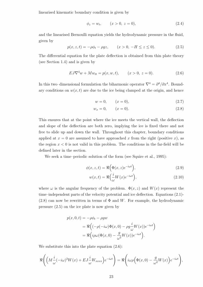
linearised kinematic boundary condition is given by
φz = wt, (x > 0, z = 0), (2.4)
and the linearised Bernoulli equation yields the hydrodynamic pressure in the fluid,
given by
p(x, z, t) = −ρφt − ρgz, (x > 0, −H ≤ z ≤ 0). (2.5)
The differential equation for the plate deflection is obtained from thin plate theory
(see Section 1.4) and is given by
EJ∇4w +Mwtt = p(x, w, t), (x > 0, z = 0). (2.6)
In this two–dimensional formulation the biharmonic operator ∇4 = ∂4/∂x4. Bound-
ary conditions on w(x, t) are due to the ice being clamped at the origin, and hence
w = 0, (x = 0), (2.7)
wx = 0, (x = 0). (2.8)
This ensures that at the point where the ice meets the vertical wall, the deflection
and slope of the deflection are both zero, implying the ice is fixed there and not
free to slide up and down the wall. Throughout this chapter, boundary conditions
applied at x = 0 are assumed to have approached x from the right (positive x), as
the region x < 0 is not valid in this problem. The conditions in the far-field will be
defined later in the section.
We seek a time–periodic solution of the form (see Squire et al., 1995):
φ(x, z, t) = ℜ(
Φ(x, z)e−iωt)
, (2.9)
w(x, t) = ℜ( i
ωW (x)e−iωt
)
, (2.10)
where ω is the angular frequency of the problem. Φ(x, z) and W (x) represent the
time–independent parts of the velocity potential and ice deflection. Equations (2.1)-
(2.8) can now be rewritten in terms of Φ and W . For example, the hydrodynamic
pressure (2.5) on the ice plate is now given by
p(x, 0, t) = −ρφt − ρgw
= ℜ(
(−ρ(−iω)Φ(x, 0)− ρgi
ωW (x))e−iωt
)
= ℜ(
iρω(Φ(x, 0)− g
ω2W (x))e−iωt
)
.
We substitute this into the plate equation (2.6):
ℜ(
(
Mi
ω(−iω)2W (x) + EJ
i
ωWxxxx
)
e−iωt
)
= ℜ(
iωρ(
Φ(x, 0)− g
ω2W (x)
)
e−iωt
)
,
23

which leads to
EJWxxxx + (ρg −Mω2)W = ω2ρΦ(x, 0).
Proceeding in this manner, substituting equations (2.9) and (2.10) into the remain-
ing boundary conditions and governing equations (2.1)–(2.8) leads to the following
boundary value problem (BVP) for Φ and W :
∇2Φ = 0, (x > 0, −H < z < 0), (2.11)
Φz = 0, (x > 0, z = −H), (2.12)
Φx = 0, (x = 0, −H < z < 0), (2.13)
EJWxxxx +(
ρg −Mω2)
W = ω2ρΦ(x, 0), (x > 0, z = 0), (2.14)
W = 0, (x = 0), (2.15)
Wx = 0, (x = 0), (2.16)
W = Φz, (x > 0, z = 0). (2.17)
We now proceed to find expressions for the incident hydroelastic waves.
2.2.3 Incident Waves
The velocity potential of the incident wave that propagates from x = +∞ takes the
general form
Φinc(x, z) = A(z)e−ikx, (2.18)
where A(z) unknown. The incident wave must satisfy Laplace’s equation (2.11),
giving:
Azz − Ak2 = 0,
and invoking the bed condition (2.12) means that this has general solution
A(z) = A0 cosh(k(z +H)),
where A0 is an unknown constant. The coupled incident wave for the plate deflection
is given by
Winc =∂Φinc
∂z(x, 0) = Az(0)e
−ikx.
Returning briefly to the original form of the deflection w(x, t) by using (2.10), the
physical, real part of the incident wave is given by:
winc(x, t) = ℜ( i
ωAz(0)e
−i(kx+ωt))
=Az(0)
ωsin(kx+ ωt).
We see that the amplitude of the wave is given by a = Az(0)/ω. Hence
ωa = A0k sinh(kH), (2.19)
24

and using equations (2.18) and (2.19) the expressions for the incident waves are:
Φinc(x, z) =aω
k
cosh(k[z +H])
sinh(kH)e−ikx, (2.20)
Winc(x) = aωe−ikx. (2.21)
Together with the plate equation (2.14), the incident waves may be used to de-
rive the dispersion relation which links the incident wave frequency to the incident
wavenumber.
2.2.4 Dispersion relation
Substituting Φinc(x, 0) and Winc(x) into the plate equation (2.14) gives
EJ(−ik)4aωe−ikx + (ρg −Mω2)aωe−ikx = ω2ρaω
k tanh(kH)e−ikx,
which rearranges to
EJk4 + ρg −Mω2 =ρω2
k tanh(kH).
Hence, the dispersion relation for hydroelastic waves is given by (see for example
Squire et al., 1995)
ω2 =ρg + EJk4
M +ρ
k tanh(kH)
. (2.22)
For a given frequency ω of the problem, the dispersion relation provides the corre-
sponding value for k as prescribed by hydroelastic wave theory. First solved in full
by Fox & Squire (1994), it can be shown that equation (2.22) has one real root, two
complex roots and an infinite set of imaginary roots. In this formulation, we are
concerned only with the single real root k. The corresponding dispersion relation
for free surface gravity waves follows from (2.22) if we allow the ice sheet thickness
to tend to zero (h → 0 leading to M = 0 and EJ = 0). A plot of the phase speed
c = ω/k against k is found in Figure 2.2, for both of the data sets in Table 2.1. We
note that there exists a minimum for c regardless of what data is chosen, which we
denote cmin, corresponding to a value k = kcr. In some problems, for example Parau
& Dias (2002), the linear theory breaks down close to cmin. However, this difficulty
seems to be constrained to problems involving waves generated by moving loads.
Chapters 5 and 6 of this thesis involve such waves, and cmin is further addressed
there. In the present problem there are no difficulties when the wavenumber is close
to kcr. From Figure 2.2 we see that the data set taken from McMurdo sound gives
faster phase speed than that of Lake Saroma. Also, the critical wavenumber kcr is
much smaller.
25

0 0.05 0.1 0.1510
20
30
40
50
60
70(a)
k (m−1)
c (m
s−1 )
0 0.2 0.4 0.65.5
6
6.5
7
7.5
8
8.5(b)
k (m−1)
c (m
s−1 )
Figure 2.2: The phase speed c plotted against the wavenumber k for the followingdata sets: (a) McMurdo Sound, (b) Lake Saroma.
Parameter/variable Dimension
x Lt Tk L−1
E ML−1T−2
J L3
H Lρ ML−3
M ML−2
g LT−2
ω T−1
a Lh L
Table 2.2: The dimensions of the parameters in the problem.
2.2.5 Nondimensionalisation
With the dispersion relation derived, we now nondimensionalise the problem to
reduce the number of parameters. Table 2.2 shows the dimensions for the parameters
of the problem.
Inspired by the frequent appearance of the term kH in the problem thus far,
we will use the depth H as a length scale. In the data from McMurdo sound in
Table 2.1(a) the fluid depth is 350m. Due to the linear formulation of the problem,
we will be looking for waves that have a large wavelength in comparison with the
wave amplitude, so the choice of H proves suitable as a length scale. We denote
dimensionless variables/parameters by an asterisk, and we substitute k∗ = kH into
the dispersion relation (2.22) to give
g
ω2H− ρih
ρH=
1
k∗ tanh(k∗)− EJ
H5ρω2k∗4. (2.23)
26

This gives rise to the dimensionless parameter
γ =EJ
H5ρω2,
which will appear frequently throughout the problem. The parameter γ depends
on the characteristics of the fluid, the plate and the incident wave. It is small
and depending on the value of k, γ typically varies from O(10−5) to O(10−8). To
summarise, we nondimensionalise thus:
z∗ =z
H, x∗ =
x
H, t∗ = tω, k∗ = kH, γ =
EJ
H5ρω2,
W ∗(x∗, t∗) =W (x, t)
aω, Φ∗(x∗, z∗, t∗) =
Φ(x, z, t)
Haω.
The asterisks are now dropped and all variables are assumed to be dimensionless
in the below analysis. The BVP (2.11)-(2.17) is rewritten in terms of dimensionless
quantities as
∇2Φ = 0, (x > 0, −1 < z < 0), (2.24)
Φz = 0, (x > 0, z = −1), (2.25)
Φx = 0, (x = 0, −1 < z < 0), (2.26)
γWxxxx +
(
1
k tanh(k)− γk4
)
W = Φ(x, 0), (x > 0), (2.27)
W = 0, (x = 0), (2.28)
Wx = 0, (x = 0), (2.29)
W = Φz, (x > 0, z = 0). (2.30)
Note that we have substituted equation (2.23) into equation (2.27), which reduces
the problem to dependence on only two dimensionless parameters, k and γ.
2.2.6 Typical values of wavelength and wave period
At this stage, it is prudent to define typical values of the parameter k, which will be
varied frequently throughout the analysis. The period of waves in the Arctic ocean
can range from T = 0.1 − 60 s for deep water, and most commonly T = 15 − 60 s
(Hunkins, 1962). This is in agreement with Menemenlis et al. (1995), who measured
ocean ice waves of period T = 20− 50 s.
Figure 2.3 shows the wave period and wavelengths plotted against the dimension-
less wavenumber k. A range of period 0− 60 s corresponds to a range of k = 1− 50.
This range of k is equivalent to wavelengths of 0− 2000 m. Waves in ice sheets are
known to have very long wavelengths; Squire et al. (1995) notes the principal range
to be 0 − 500 m. With these facts in mind, in this chapter we will analyse waves
of range k = 1 − 20, corresponding to wave period T = 5 − 50 s and wavelength
λ = 100 − 2000 m, which is a large enough range to represent typical waves in ice
27

0 10 20 30 40 500
10
20
30
40
50
60(a)
k
wav
e pe
riod
T (
s)
0 10 20 30 40 500
200
400
600
800
1000(b)
k
wav
elen
gth
λ (m
)
Figure 2.3: (a) The wave period T plotted against the dimensionless wavenumberk. (b) The wavelength λ plotted against the dimensionless wavenumber k. Otherparameters are taken from Table 2.1(a).
sheets.
2.2.7 Linear superposition
In dimensionless form, the incident waves (2.20)-(2.21) are
Φinc(x, z) =cosh(k[z + 1])
k sinh(k)e−ikx,
Winc(x) = e−ikx.
The incident waves approach the wall from x = +∞, and upon contact with the
wall reflected waves are generated which must be accounted for in the solution. The
reflected waves take the form
Φref (x, z) = aDcosh(k[z + 1])
k sinh(k)eikx,
Wref (x) = aD eikx,
where aD is the amplitude of the reflected wave, which must be found as part of the
solution. By linear superposition, we may express the total potential and deflection
as the sum of the incident waves and the reflected waves. However, this would not
alone be enough to satisfy all the conditions arising from the presence of a vertical
wall. Hence the total form of the potential and deflection are:
Φ(x, z) = Φinc(x, z) + Φref (x, z) + ϕ(x, z), (2.31)
W (x) = Winc(x) +Wref (x) + w(x). (2.32)
28
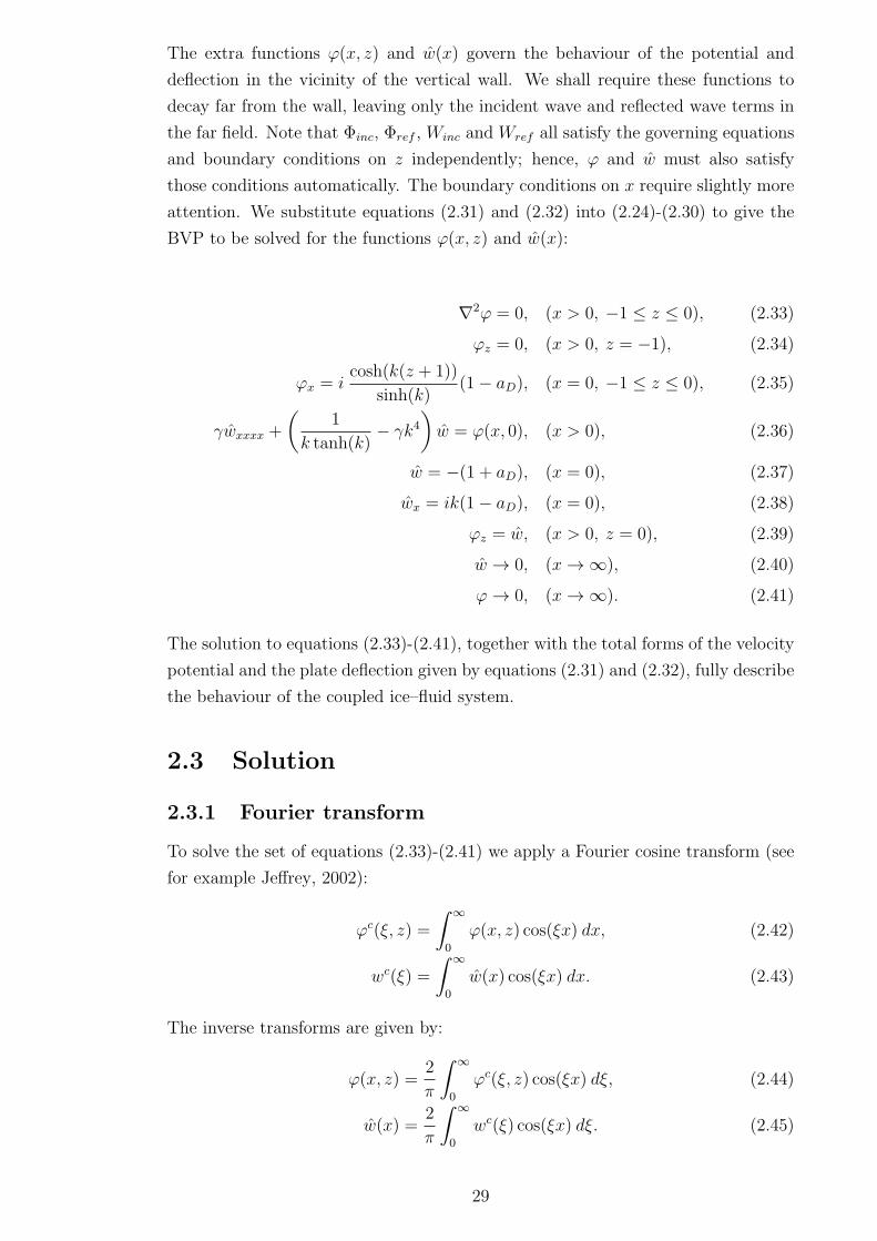
The extra functions ϕ(x, z) and w(x) govern the behaviour of the potential and
deflection in the vicinity of the vertical wall. We shall require these functions to
decay far from the wall, leaving only the incident wave and reflected wave terms in
the far field. Note that Φinc, Φref , Winc and Wref all satisfy the governing equations
and boundary conditions on z independently; hence, ϕ and w must also satisfy
those conditions automatically. The boundary conditions on x require slightly more
attention. We substitute equations (2.31) and (2.32) into (2.24)-(2.30) to give the
BVP to be solved for the functions ϕ(x, z) and w(x):
∇2ϕ = 0, (x > 0, −1 ≤ z ≤ 0), (2.33)
ϕz = 0, (x > 0, z = −1), (2.34)
ϕx = icosh(k(z + 1))
sinh(k)(1− aD), (x = 0, −1 ≤ z ≤ 0), (2.35)
γwxxxx +
(
1
k tanh(k)− γk4
)
w = ϕ(x, 0), (x > 0), (2.36)
w = −(1 + aD), (x = 0), (2.37)
wx = ik(1− aD), (x = 0), (2.38)
ϕz = w, (x > 0, z = 0), (2.39)
w → 0, (x→ ∞), (2.40)
ϕ→ 0, (x→ ∞). (2.41)
The solution to equations (2.33)-(2.41), together with the total forms of the velocity
potential and the plate deflection given by equations (2.31) and (2.32), fully describe
the behaviour of the coupled ice–fluid system.
2.3 Solution
2.3.1 Fourier transform
To solve the set of equations (2.33)-(2.41) we apply a Fourier cosine transform (see
for example Jeffrey, 2002):
ϕc(ξ, z) =
∫ ∞
0
ϕ(x, z) cos(ξx) dx, (2.42)
wc(ξ) =
∫ ∞
0
w(x) cos(ξx) dx. (2.43)
The inverse transforms are given by:
ϕ(x, z) =2
π
∫ ∞
0
ϕc(ξ, z) cos(ξx) dξ, (2.44)
w(x) =2
π
∫ ∞
0
wc(ξ) cos(ξx) dξ. (2.45)
29
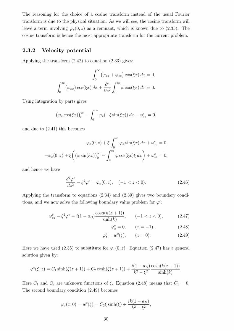
The reasoning for the choice of a cosine transform instead of the usual Fourier
transform is due to the physical situation. As we will see, the cosine transform will
leave a term involving ϕx(0, z) as a remnant, which is known due to (2.35). The
cosine transform is hence the most appropriate transform for the current problem.
2.3.2 Velocity potential
Applying the transform (2.42) to equation (2.33) gives:
∫ ∞
0
(
ϕxx + ϕzz
)
cos(ξx) dx = 0,
∫ ∞
0
(
ϕxx
)
cos(ξx) dx+∂2
∂z2
∫ ∞
0
ϕ cos(ξx) dx = 0.
Using integration by parts gives
(
ϕx cos(ξx))∞0−∫ ∞
0
ϕx(−ξ sin(ξx)) dx+ ϕczz = 0,
and due to (2.41) this becomes
−ϕx(0, z) + ξ
∫ ∞
0
ϕx sin(ξx) dx+ ϕczz = 0,
−ϕx(0, z) + ξ
(
(
ϕ sin(ξx))∞0−∫ ∞
0
ϕ cos(ξx)ξ dx
)
+ ϕczz = 0,
and hence we have
d2ϕc
dz2− ξ2ϕc = ϕx(0, z), (−1 < z < 0). (2.46)
Applying the transform to equations (2.34) and (2.39) gives two boundary condi-
tions, and we now solve the following boundary value problem for ϕc:
ϕczz − ξ2ϕc = i(1− aD)
cosh(k(z + 1))
sinh(k), (−1 < z < 0), (2.47)
ϕcz = 0, (z = −1), (2.48)
ϕcz = wc(ξ), (z = 0). (2.49)
Here we have used (2.35) to substitute for ϕx(0, z). Equation (2.47) has a general
solution given by:
ϕc(ξ, z) = C1 sinh(ξ(z + 1)) + C2 cosh(ξ(z + 1)) +i(1− aD)
k2 − ξ2cosh(k(z + 1))
sinh(k).
Here C1 and C2 are unknown functions of ξ. Equation (2.48) means that C1 = 0.
The second boundary condition (2.49) becomes
ϕz(x, 0) = wc(ξ) = C2ξ sinh(ξ) +ik(1− aD)
k2 − ξ2,
30

which rearranges to
C2 =1
ξ sinh(ξ)
(
wc(ξ)− ik(1− aD)
k2 − ξ2
)
.
Hence ϕc is given by
ϕc(ξ, z) =cosh(ξ(z + 1))
ξ sinh(ξ)
(
wc(ξ)− ik(1− aD)
k2 − ξ2
)
+i(1− aD)
k2 − ξ2cosh(k(z + 1))
sinh(k).
(2.50)
We will show later that ϕc is finite at ξ = k. Note that this is not the final equation
for the potential ϕc because it includes wc which is unknown at this point. In
addition the reflected wave amplitude aD is yet to be determined.
2.3.3 Plate deflection
Applying the transform (2.43) to the ice plate equation (2.36) gives
γ
∫ ∞
0
wxxxx cos(ξx) dx+
(
1
k tanh(k)− γk4
)
wc = ϕc(ξ, 0). (2.51)
We can evaluate the far left integral by repetitive integration by parts, and by using
equations (2.38) and (2.40) we have:
∫ ∞
0
wxxxx cos(ξx) dx
=(
wxxx cos(ξx))∞0+ ξ
∫ ∞
0
wxxx sin(ξx) dx
= −wxxx(0) + ξ(
(
wxx sin(ξx))∞0−∫ ∞
0
wxxξ cos(ξx) dx)
= −wxxx(0)− ξ2∫ ∞
0
wxx cos(ξx) dx
= −wxxx(0)− ξ2(
(
wx cos(ξx))∞0+
∫ ∞
0
wxξ sin(ξx) dx)
= −wxxx(0) + ξ2wx(0)− ξ3∫ ∞
0
wx sin(ξx) dx
= −wxxx(0) + ξ2wx(0)− ξ3(
(
w sin(ξx))∞0−∫ ∞
0
wξ cos(ξx) dx)
= −wxxx(0) + ξ2ik(1− aD) + ξ4wc(ξ).
Hence equation (2.51) becomes
(
1
k tanh(k)− γk4 + γξ4
)
wc(ξ) = ϕc(ξ, 0) + γ(
wxxx(0)− ξ2ik(1− aD))
. (2.52)
Owing to the cosine Fourier transform, we now have an algebraic equation for the
deflection wc instead of a complicated fourth–order differential equation. Using
31

(2.50) we can now substitute ϕc(ξ, 0) into equation (2.52) to give:
(
γ(ξ4 − k4) +1
k tanh(k)− 1
ξ tanh(ξ)
)
wc(ξ) =
i(1− aD)
k2 − ξ2
(
1
tanh(k)− k
ξ tanh(ξ)
)
+ γ(
wxxx(0)− ξ2ik(1− aD))
. (2.53)
We notice that the left hand side of equation (2.53) is equal to zero at ξ = k due
to the dispersion relation (2.22). Hence, to avoid a singularity we require that the
limit of the right hand side as ξ → k is also equal to zero. We therefore require
0 = γ(
wxxx(0)− k3i(1− aD))
+ i(1− aD) limξ→k
(
1
k2 − ξ2
(
1
tanh(k)− k
ξ tanh(ξ)
)
)
.
(2.54)
We assess the limit on the right hand side using L’Hopital’s rule:
limξ→k
(
1
k2 − ξ2
(
1
tanh(k)− k
ξ tanh(ξ)
)
)
= limξ→k
(
−1
2ξ
(
k
ξ2 tanh(ξ)+
k
ξ cosh2(ξ) tanh2(ξ)
)
)
= limξ→k
(
−1
2ξ
(
k
ξ2 tanh(ξ)+
k
ξ sinh2(ξ)
)
)
= limξ→k
(
−1
2ξ
(
k
ξ2 tanh(ξ)+k
ξ
{
1
tanh2(ξ)− 1
})
)
=1
2k− 1
2k2 tanh(k)− 1
2k tanh2(k).
Substituting this into equation (2.54) gives
γwxxx(0) = ik3(1− aD)γ + i(1− aD)( 1
2k2 tanh(k)+
1
2k tanh2(k)− 1
2k
)
. (2.55)
We define the function
V (k) =1
2k2 tanh(k)+
1
2k tanh2(k)− 1
2k, (2.56)
and then the right hand side of equation (2.53) now reads
i(1− aD)
(
V (k) +1
k2 − ξ2
(
1
tanh(k)− k
ξ tanh(ξ)
)
+ γk3 − γξ2k
)
.
By dividing across the left hand side of (2.53) we can explicitly write the equation
for plate deflection as
wc(ξ) = i(1− aD)Q(ξ), (2.57)
32

where the function Q(ξ) is defined as
Q(ξ) =
ξ tanh(ξ)(
V (k) + γk(k2 − ξ2))
+1
k2 − ξ2
(
ξ tanh(ξ)
tanh(k)− k
)
ξ tanh(ξ)
(
γ(ξ4 − k4) +1
k tanh(k)
)
− 1
. (2.58)
The coefficient aD which defines the reflected wave amplitude is still undefined.
We note that we have two equations for the deflection w(0). One is found by applying
the inverse transform (2.45) at x = 0, giving
w(0) =2
π
∫ ∞
0
wc(ξ) dξ.
The other is given by equation (2.37), due to the ice–clamping condition. Equating
these, we have
w(0) = −(1 + aD) = i(1− aD)2
π
∫ ∞
0
Q(ξ) dξ.
Denoting
χ =2
π
∫ ∞
0
Q(ξ) dξ,
we have
1 + aD = −iχ(1− aD),
aD
(
1− iχ)
= −(
1 + iχ)
,
aD = −1 + iχ
1− iχ. (2.59)
Equation (2.59) directly implies that
|aD| = 1, (2.60)
which in turn means we can write
aD = eiθ, (2.61)
where θ is the phase shift between the incident and reflected waves. Equation (2.60)
corresponds to the energy conservation relation for hydroelastic wave reflection by
a vertical wall. To calculate θ, we introduce the parameter α such that
eiα =
{
1+iχ(1+χ2)1/2
if χ > 0,1−iχ
(1+χ2)1/2if χ < 0.
For χ > 0, by equations (2.61) and (2.59) we have
eiθ = −e2iα = e2iα+iπ.
33

If χ < 0, we have
aeiθ = −ae−2iα = ae−2iα+iπ.
We calculate α via the equation
cos(α) =1
(1 + χ2)1
2
,
and finally
θ =
{
π + 2α if χ > 0,
π − 2α if χ < 0.
The phase shift θ is plotted against k in Figure 2.4. The phase shift tends to 2π in
0 5 10 15 200.4
0.5
0.6
0.7
0.8
0.9
1
k
θ / 2
π
Figure 2.4: The phase shift θ/2π is plotted against k. The values of other parametersare taken from Table 2.1(a).
the limit k → 0. This is expected as the limit k → 0 represents a flat ice surface,
and θ = 2π indicates no phase shift.
Equation (2.57) becomes
wc(ξ) = i(1− eiθ)Q(ξ), (2.62)
with Q(ξ) given by equation (2.58). The final solution for the plate deflection is
then given by (2.62).
With wc(ξ) and aD obtained, the final solution for the velocity potential ϕc is
written:
ϕc(ξ, z) = i(1− eiθ)L(ξ, z), (2.63)
34
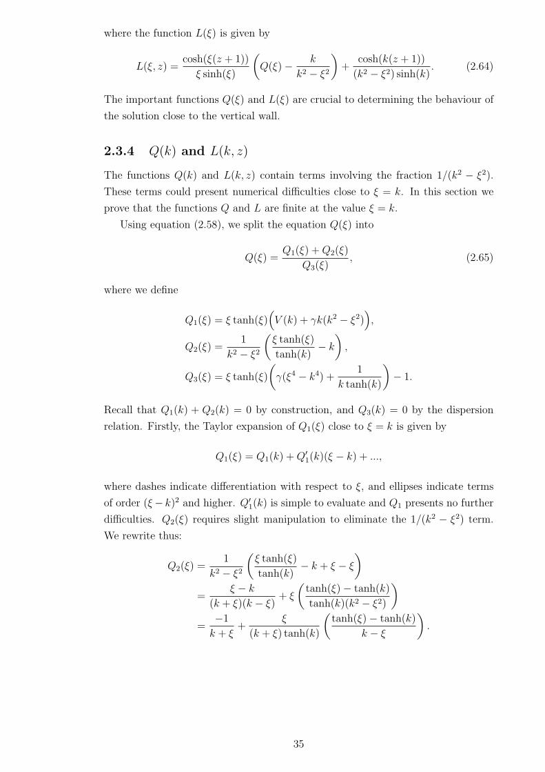
where the function L(ξ) is given by
L(ξ, z) =cosh(ξ(z + 1))
ξ sinh(ξ)
(
Q(ξ)− k
k2 − ξ2
)
+cosh(k(z + 1))
(k2 − ξ2) sinh(k). (2.64)
The important functions Q(ξ) and L(ξ) are crucial to determining the behaviour of
the solution close to the vertical wall.
2.3.4 Q(k) and L(k, z)
The functions Q(k) and L(k, z) contain terms involving the fraction 1/(k2 − ξ2).
These terms could present numerical difficulties close to ξ = k. In this section we
prove that the functions Q and L are finite at the value ξ = k.
Using equation (2.58), we split the equation Q(ξ) into
Q(ξ) =Q1(ξ) +Q2(ξ)
Q3(ξ), (2.65)
where we define
Q1(ξ) = ξ tanh(ξ)(
V (k) + γk(k2 − ξ2))
,
Q2(ξ) =1
k2 − ξ2
(
ξ tanh(ξ)
tanh(k)− k
)
,
Q3(ξ) = ξ tanh(ξ)
(
γ(ξ4 − k4) +1
k tanh(k)
)
− 1.
Recall that Q1(k) + Q2(k) = 0 by construction, and Q3(k) = 0 by the dispersion
relation. Firstly, the Taylor expansion of Q1(ξ) close to ξ = k is given by
Q1(ξ) = Q1(k) +Q′1(k)(ξ − k) + ...,
where dashes indicate differentiation with respect to ξ, and ellipses indicate terms
of order (ξ− k)2 and higher. Q′1(k) is simple to evaluate and Q1 presents no further
difficulties. Q2(ξ) requires slight manipulation to eliminate the 1/(k2 − ξ2) term.
We rewrite thus:
Q2(ξ) =1
k2 − ξ2
(
ξ tanh(ξ)
tanh(k)− k + ξ − ξ
)
=ξ − k
(k + ξ)(k − ξ)+ ξ
(
tanh(ξ)− tanh(k)
tanh(k)(k2 − ξ2)
)
=−1
k + ξ+
ξ
(k + ξ) tanh(k)
(
tanh(ξ)− tanh(k)
k − ξ
)
.
35

It is simpler to expand each part separately about ξ = k using Taylor series:
−1
k + ξ= − 1
2k+
1
4k2(ξ − k) + ...,
ξ
k + ξ=
1
2+
1
4k(ξ − k) + ...,
tanh(ξ) = tanh(k) +1
cosh2(k)(ξ − k)− sinh(k)
cosh3(k)(ξ − k)2 +O(ξ − k)3,
which means we can write
tanh(ξ)− tanh(k)
k − ξ= − 1
cosh2(k)+
sinh(k)
cosh3(k)(ξ − k) + ...,
having cancelled the (k− ξ) factor on the right hand side. Hence, after multiplying
the terms together, Q2(ξ) close to ξ = k becomes
Q2(ξ) = Q(k) + A(k)(ξ − k) + ...,
where
A(k) =1
4k2+
1
2 cosh2(k)− 1
4k sinh(k) cosh(k).
The function Q3(ξ) can also be expanded close to ξ = k using Taylor series as
Q1(ξ) = Q3(k) +Q′3(k)(ξ − k) + ...,
and the differentiation is again trivial. Hence, with Q1, Q2 and Q3 all expanded, we
use (2.65) to write
Q(ξ) =Q1(k) +Q′
1(k)(ξ − k) +Q2(k) + A(k)(ξ − k)
Q3(k) +Q′3(k)(ξ − k)
+ ... .
Evaluating the above equation at ξ = k means Q1(k) + Q2(k) = 0 and Q3(k) = 0.
The remaining terms all have a (ξ − k) factor, which cancels leaving
Q(k) =Q′
1(k) + A(k)
Q′3(k)
.
Performing the differentiation yields the long-winded but exact value of Q(k), given
by
Q(k) =
(
tanh(k) + kcosh2(k)
)
V (k)− 2k3γ tanh(k) + 14k2
+ 12 cosh2(k)
− 14k sinh(k) cosh(k)
(
tanh(k) + kcosh2(k)
)
1k tanh(k)
+ 4k4γ tanh(k).
(2.66)
36

Using (2.64), the function L(k, z) can now be written
L(k, z) = Q(k)cosh(k(z + 1))
k sinh(k)+ lim
ξ→k
1
k2 − ξ2
(
cosh(k(z + 1))
sinh(k)− k cosh(ξ(z + 1))
ξ sinh(ξ)
)
.
(2.67)
The second term in this equation requires application of l’Hopital’s rule, which is
straightforward and we obtain
limξ→k
L(ξ, z) =(z + 1) sinh(k(z + 1)) + 2Q(k) cosh(k(z + 1)
2k sinh(k)
− cosh(k(z + 1))(
sinh(k) + k cosh(k))
2k2 sinh2(k). (2.68)
The function Q(ξ) given by equation (2.58) is therefore smooth everywhere. The
function Q is plotted against ξ in Figure 2.5.
0 10 20 30 40 50
0
0.1
0.2
0.3
0.4
0.5
ξ
Q(ξ
)
Figure 2.5: The function Q is plotted against ξ for k = 2 (blue), k = 10 (red),k = 20 (green).
We note that Q(0) = k−1, and that Q(ξ) decays with order ξ−2 as ξ → ∞.
2.3.5 Inverse transforms
Recall that the inverse transforms to return to x− z co-ordinates are given by
ϕ(x, z) =2
π
∫ ∞
0
ϕc(ξ, z) cos(ξx) dξ, (2.69)
w(x) =2
π
∫ ∞
0
wc(ξ) cos(ξx) dξ. (2.70)
37
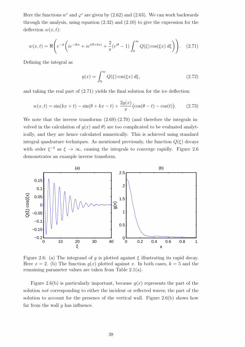
Here the functions wc and ϕc are given by (2.62) and (2.63). We can work backwards
through the analysis, using equation (2.32) and (2.10) to give the expression for the
deflection w(x, t):
w(x, t) = ℜ(
e−it
(
ie−ikx + iei(θ+kx) +2
π(eiθ − 1)
∫ ∞
0
Q(ξ) cos(ξx) dξ
)
)
. (2.71)
Defining the integral as
g(x) =
∫ ∞
0
Q(ξ) cos(ξx) dξ, (2.72)
and taking the real part of (2.71) yields the final solution for the ice deflection:
w(x, t) = sin(kx+ t)− sin(θ + kx− t) +2g(x)
π
(
cos(θ − t)− cos(t))
. (2.73)
We note that the inverse transforms (2.69)-(2.70) (and therefore the integrals in-
volved in the calculation of g(x) and θ) are too complicated to be evaluated analyt-
ically, and they are hence calculated numerically. This is achieved using standard
integral quadrature techniques. As mentioned previously, the function Q(ξ) decays
with order ξ−2 as ξ → ∞, causing the integrals to converge rapidly. Figure 2.6
demonstrates an example inverse transform.
0 10 20 30 40−0.2
−0.15
−0.1
−0.05
0
0.05
0.1
0.15
(a)
ξ
Q(ξ
) co
s(ξx
)
0 0.2 0.4 0.6 0.8 10
0.5
1
1.5
2
2.5(b)
x
g(x)
Figure 2.6: (a) The integrand of g is plotted against ξ illustrating its rapid decay.Here x = 2. (b) The function g(x) plotted against x. In both cases, k = 5 and theremaining parameter values are taken from Table 2.1(a).
Figure 2.6(b) is particularly important, because g(x) represents the part of the
solution not corresponding to either the incident or reflected waves; the part of the
solution to account for the presence of the vertical wall. Figure 2.6(b) shows how
far from the wall g has influence.
38

2.4 Numerical results
In this section, we present numerical results for the ice deflection and the strain in
the ice sheet. We also study the vertical shear force on the wall, and the horizontal
force. There are many physical parameters in the present problem, defining the
properties of the fluid and the ice sheet, that can vary in certain ranges. When
presenting results, the data from Table 2.1(a) is used unless stated otherwise. We
are particularly interested in varying the wavenumber k, as well as the thickness
of the ice sheet, to give a fair representation of waves in ice sheets. We should be
careful when varying the fluid depth H, since it was used as a length scale. Therefore
when investigating the effect of varying H we must revert to dimensional variables.
We note that the dimensionless solution depends only on two parameters, γ and
k. Note that γ contains ω, which depends on k. When varying parameters, we will
state the parameters in their dimensional quantity for clarity, then substitute those
values to calculate the dimensionless solution. The results are mostly presented
in dimensionless variables; however, some results (such as forces on the wall) are
best presented dimensionally, to facilitate a physical understanding. We continue to
assume that all variables/parameters are dimensionless; for clarity we add the suffix
‘dim’ to dimensional quantities, which are also accompanied by units.
Since the variables which are periodic in time, the notation “| |” is used to
indicate the magnitude of a variable with respect to time (the maximum value of
the variable for any time). For example, the deflection w(x, t) given by equation
(2.73) can be rewritten as
w(x, t) = c(x) sin(t) + d(x) cos(t), (2.74)
for functions c(x) and d(x). Introducing A(x) and δ(x) such that c = A cos(δ) and
d = −A sin(δ) this can be rewritten more conveniently as
w(x, t) = A(x) cos(t+ δ). (2.75)
This allows us to plot the magnitude of the deflection |w(x)|, given by A =√c2 + d2.
This procedure removes time as a factor from figures for clarity.
2.4.1 Deflection of the ice sheet
We begin by plotting the ice sheet deflection, given by equation (2.73). Figure
2.7 shows the deflection for three values of the wavenumber k. We see that the
ice deflection and slope of the deflection are zero at x = 0 as required by the
ice–clamping condition. We also note the effect of the ice clamping on the first
wave peak. It is smaller in magnitude and wavelength than subsequent waves. For
k = 20, there is also some disturbance in the subsequent wave peaks, until the
deflection settles to a regular wave. This phenomenon is less visible for smaller k
values because the wavelength is long enough such that there is only one or two
39
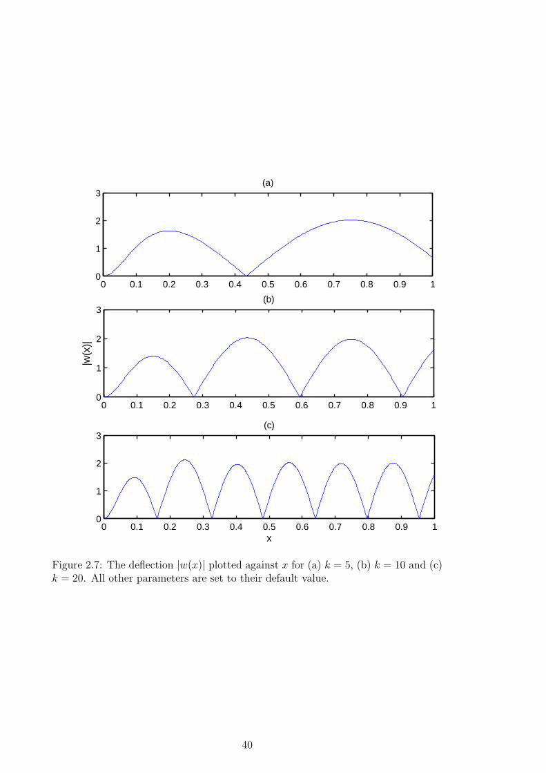
0 0.1 0.2 0.3 0.4 0.5 0.6 0.7 0.8 0.9 10
1
2
3(a)
0 0.1 0.2 0.3 0.4 0.5 0.6 0.7 0.8 0.9 10
1
2
3
|w(x
)|
(b)
0 0.1 0.2 0.3 0.4 0.5 0.6 0.7 0.8 0.9 10
1
2
3
x
(c)
Figure 2.7: The deflection |w(x)| plotted against x for (a) k = 5, (b) k = 10 and (c)k = 20. All other parameters are set to their default value.
40
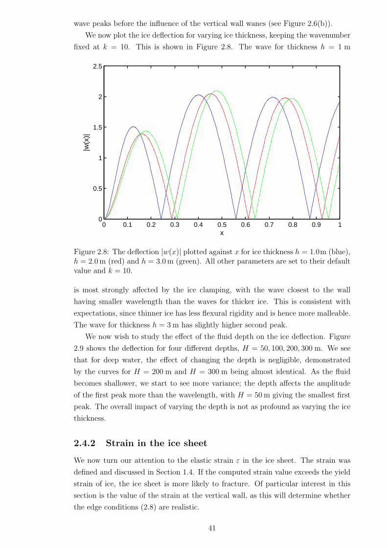
wave peaks before the influence of the vertical wall wanes (see Figure 2.6(b)).
We now plot the ice deflection for varying ice thickness, keeping the wavenumber
fixed at k = 10. This is shown in Figure 2.8. The wave for thickness h = 1 m
0 0.1 0.2 0.3 0.4 0.5 0.6 0.7 0.8 0.9 10
0.5
1
1.5
2
2.5
x
|w(x
)|
Figure 2.8: The deflection |w(x)| plotted against x for ice thickness h = 1.0m (blue),h = 2.0m (red) and h = 3.0m (green). All other parameters are set to their defaultvalue and k = 10.
is most strongly affected by the ice clamping, with the wave closest to the wall
having smaller wavelength than the waves for thicker ice. This is consistent with
expectations, since thinner ice has less flexural rigidity and is hence more malleable.
The wave for thickness h = 3 m has slightly higher second peak.
We now wish to study the effect of the fluid depth on the ice deflection. Figure
2.9 shows the deflection for four different depths, H = 50, 100, 200, 300 m. We see
that for deep water, the effect of changing the depth is negligible, demonstrated
by the curves for H = 200 m and H = 300 m being almost identical. As the fluid
becomes shallower, we start to see more variance; the depth affects the amplitude
of the first peak more than the wavelength, with H = 50m giving the smallest first
peak. The overall impact of varying the depth is not as profound as varying the ice
thickness.
2.4.2 Strain in the ice sheet
We now turn our attention to the elastic strain ε in the ice sheet. The strain was
defined and discussed in Section 1.4. If the computed strain value exceeds the yield
strain of ice, the ice sheet is more likely to fracture. Of particular interest in this
section is the value of the strain at the vertical wall, as this will determine whether
the edge conditions (2.8) are realistic.
41

0 20 40 60 80 100 120 140 1600
0.5
1
1.5
2
2.5
xdim
(m)
|w|
Figure 2.9: The deflection |w(x)| plotted against x for fluid depth H = 300m (blue),H = 200 m (red), H = 100 m (green) and H = 50 m (black). All other parametersare set to their default value and kdim = 0.05 m−1.
Squire (1993a) dealt with ice–breakup, and the theory was found to be in ac-
cordance with Goodman et al. (1980), who used a wire strainmeter to measure the
strains in sea ice. An observed fracture strain is reported at 3x10⁻⁵, and the theory
suggests a crack will propagate if the strain reaches 4.3 x 10⁻⁵. Squire & Martin
(1980) determine the fracture strain for Bering Sea ice to be 4.4− 8.5x10⁻⁵. In this
chapter we take an estimate of yield strain εcr = 8 x 10⁻⁵.
In dimensionless variables, the strain is calculated by the equation (Ugural,
1981):
ε =ah
2H2
∂2w
∂x2. (2.76)
It should be noted that calculation of the second derivative in (2.76) is not straight-
forward. According to (2.73), we need to evaluate the second derivative of the
function g(x) given by (2.72), where Q(ξ) = O(1/ξ2) as ξ → ∞. We define a new
function q(ξ) as
q(ξ) = Q(ξ) +k
ξ2 + 1, (2.77)
42

where q(ξ) = O(1/ξ3) as ξ → ∞. Then
∂2g(x)
∂x2=
∂2
∂x2
∫ ∞
0
(q − k
ξ2 + 1) cos(ξx) dξ
=∂2
∂x2
(
∫ ∞
0
q(ξ) cos(ξx) dξ −∫ ∞
0
k cos(ξx)
ξ2 + 1dξ)
= −∫ ∞
0
ξ2q(ξ) cos(ξx) dξ − k∂2
∂x2
(π
2e−x)
= −∫ ∞
0
ξ2q(ξ) cos(ξx) dξ − kπ
2e−x,
where the last integral can be numerically evaluated. Here we have used the standard
result from Gradshteyn & Ryzhik (2007):
∫ ∞
0
cos(yx)
y2 + 1dy =
π
2e−x. (2.78)
The strain can then be calculated by differentiating equation (2.73) and using (2.76)
to give
ε =ah
2H2
(
−k2 sin(kx+ t) + k2 sin(θ + kx− t)
− 2
π
(
cos(θ − t)− cos(t))
(∫ ∞
0
ξ2q(ξ) cos(ξx) dξ − kπ
2e−x
)
)
.
To begin, we plot the maximum strain with respect to time |ε| against x, fork = 5 and k = 10. This is shown in Figure 2.10. The most striking feature of this
figure is that the strain is far higher at the point where the ice meets the vertical
wall than for the rest of the strain profile. This is due to the ice–clamping condition.
If fracture occurs, it is likely to do so at x = 0. We note that the strain has a linear
dependence on the wave amplitude; it is arbitrarily chosen as a = 1 cm for this
graph. The strain is below its yield value εcr for both values of k for the current
parameters. We also see that away from the wall, the strain is higher for larger k;
this is of course expected, since shorter wavelength causes more curvature in the ice
and hence more strain.
With the knowledge that the strain is highest at the ice-wall connection, we may
now plot the maximum strain (the strain at x = 0) for each k. This is shown in
Figure 2.11 for varying values of the ice thickness. The strain is finite in the k → 0
limit. In general the maximum strain increases as the waves become shorter, though
there exists a non-zero k for each curve that gives minimum strain for each thickness.
For long waves, the highest maximum strain is given by thinner ice. However, this
is reversed as the waves become shorter, and for short waves, thicker ice gives more
strain at the ice-wall boundary.
The maximum strain is plotted against k for varying fluid depth H in Figure
2.12. Depth variation is not as important as ice thickness in determining the strain
43

0 0.5 1 1.50
0.5
1
1.5
2
2.5
3
3.5
4x 10
−5
x
|ε|
Figure 2.10: The strain |ε| is plotted against x for k = 5 (blue) and k = 10 (red).All other parameters are set to their default value and the amplitude is chosen asa = 1 cm.
0 5 10 15 20 250
1
2x 10
−4
k
|ε(x
=0)
|
Figure 2.11: The maximum strain |ε(x=0)| is plotted against k for ice thicknessh = 1.0 m (blue), h = 2.0 m (red) and h = 3.0 m (green). The dashed line indicatesthe critical strain |εcr|. All other parameters are set to their default value and theamplitude is chosen as a = 1 cm.
44

0 0.01 0.02 0.03 0.04 0.053
3.5
4
4.5
5
5.5
6x 10
−5
kdim
(m−1)
|ε(x
=0)
|
Figure 2.12: The maximum strain |ε(x=0)| is plotted against k for fluid depth H =50m (blue), H = 100m (red) and H = 200 m (green). All other parameters are setto their default value and the amplitude is chosen as a = 1 cm.
along the wall, which is expected due to the results for the ice deflection. The depth
only influences longer waves from approximately kdim = 0−0.04m−1 (corresponding
to λ ≈ 0−150m). We see that shallower water causes more strain within this range,
but all three curves coalesce in the limit kdim → 0 and when kdim > 0.04 m−1.
Because the amplitude was chosen rather arbitrarily in the preceding analysis of
the strain, we now investigate the wave amplitude in more detail to allow a broader
understanding. Due to the linear dependence of the strain on wave amplitude, we
can plot the maximum allowable amplitude while retaining a strain of |εcr|. This isshown in Figure 2.13. The maximum allowable strain at x = 0 is compared with
the maximum allowable strain far from the wall for comparison. As k grows, only
waves of a few centimetres are permitted.
2.4.3 Shear force on the wall
One of the physical forces on the wall caused by the motion of the ice sheet is the
vertical shear force. Due to the ice–clamping condition, the ice exerts a lifting force
on the wall, something that must be considered in the design of ocean structures in
ice–covered water. The shear force is defined in dimensionless variables as (Ugural,
1981)
V SH = −wxxx(0, t) (2.79)
The dimensional shear force is given by V SHdim = (aEJ/H3)V SH . Fortunately, we do
not have to perform the differentiation of w: the third derivative can be calculated
45
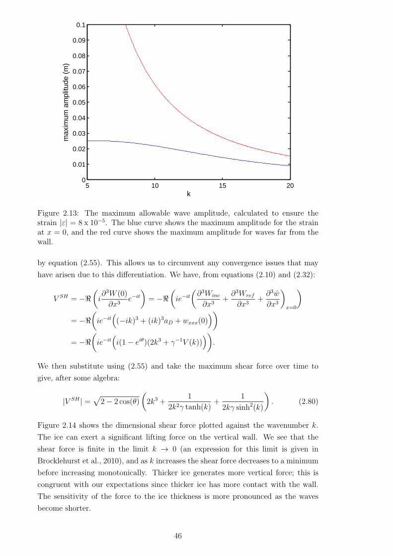
5 10 15 200
0.01
0.02
0.03
0.04
0.05
0.06
0.07
0.08
0.09
0.1
k
max
imum
am
plitu
de (
m)
Figure 2.13: The maximum allowable wave amplitude, calculated to ensure thestrain |ε| = 8 x 10⁻⁵. The blue curve shows the maximum amplitude for the strainat x = 0, and the red curve shows the maximum amplitude for waves far from thewall.
by equation (2.55). This allows us to circumvent any convergence issues that may
have arisen due to this differentiation. We have, from equations (2.10) and (2.32):
V SH = −ℜ(
i∂3W (0)
∂x3e−it
)
= −ℜ(
ie−it
(
∂3Winc
∂x3+∂3Wref
∂x3+∂3w
∂x3
)
x=0
)
= −ℜ(
ie−it(
(−ik)3 + (ik)3aD + wxxx(0))
)
= −ℜ(
ie−it(
i(1− eiθ)(2k3 + γ−1V (k)))
)
.
We then substitute using (2.55) and take the maximum shear force over time to
give, after some algebra:
|V SH | =√
2− 2 cos(θ)
(
2k3 +1
2k2γ tanh(k)+
1
2kγ sinh2(k)
)
. (2.80)
Figure 2.14 shows the dimensional shear force plotted against the wavenumber k.
The ice can exert a significant lifting force on the vertical wall. We see that the
shear force is finite in the limit k → 0 (an expression for this limit is given in
Brocklehurst et al., 2010), and as k increases the shear force decreases to a minimum
before increasing monotonically. Thicker ice generates more vertical force; this is
congruent with our expectations since thicker ice has more contact with the wall.
The sensitivity of the force to the ice thickness is more pronounced as the waves
become shorter.
46
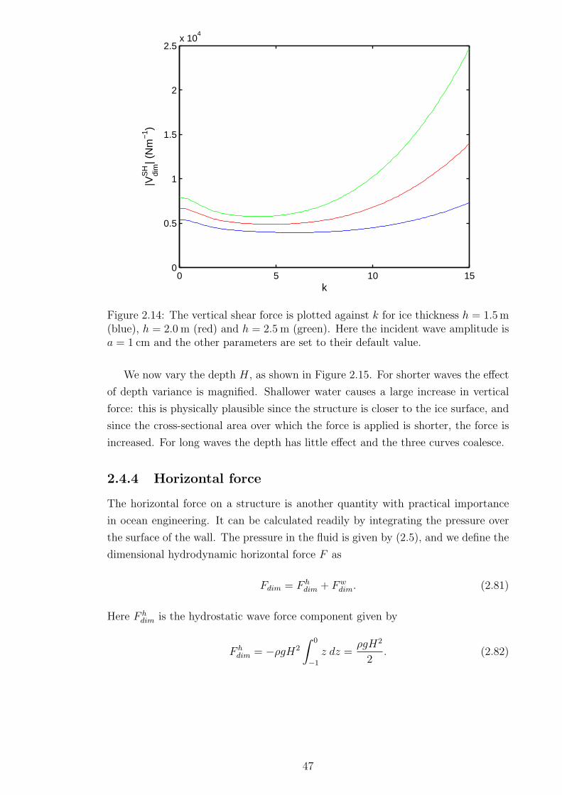
0 5 10 150
0.5
1
1.5
2
2.5x 10
4
k
|VS
Hdi
m| (
Nm
−1 )
Figure 2.14: The vertical shear force is plotted against k for ice thickness h = 1.5m(blue), h = 2.0 m (red) and h = 2.5 m (green). Here the incident wave amplitude isa = 1 cm and the other parameters are set to their default value.
We now vary the depth H, as shown in Figure 2.15. For shorter waves the effect
of depth variance is magnified. Shallower water causes a large increase in vertical
force: this is physically plausible since the structure is closer to the ice surface, and
since the cross-sectional area over which the force is applied is shorter, the force is
increased. For long waves the depth has little effect and the three curves coalesce.
2.4.4 Horizontal force
The horizontal force on a structure is another quantity with practical importance
in ocean engineering. It can be calculated readily by integrating the pressure over
the surface of the wall. The pressure in the fluid is given by (2.5), and we define the
dimensional hydrodynamic horizontal force F as
Fdim = F hdim + Fw
dim. (2.81)
Here F hdim is the hydrostatic wave force component given by
F hdim = −ρgH2
∫ 0
−1
z dz =ρgH2
2. (2.82)
47
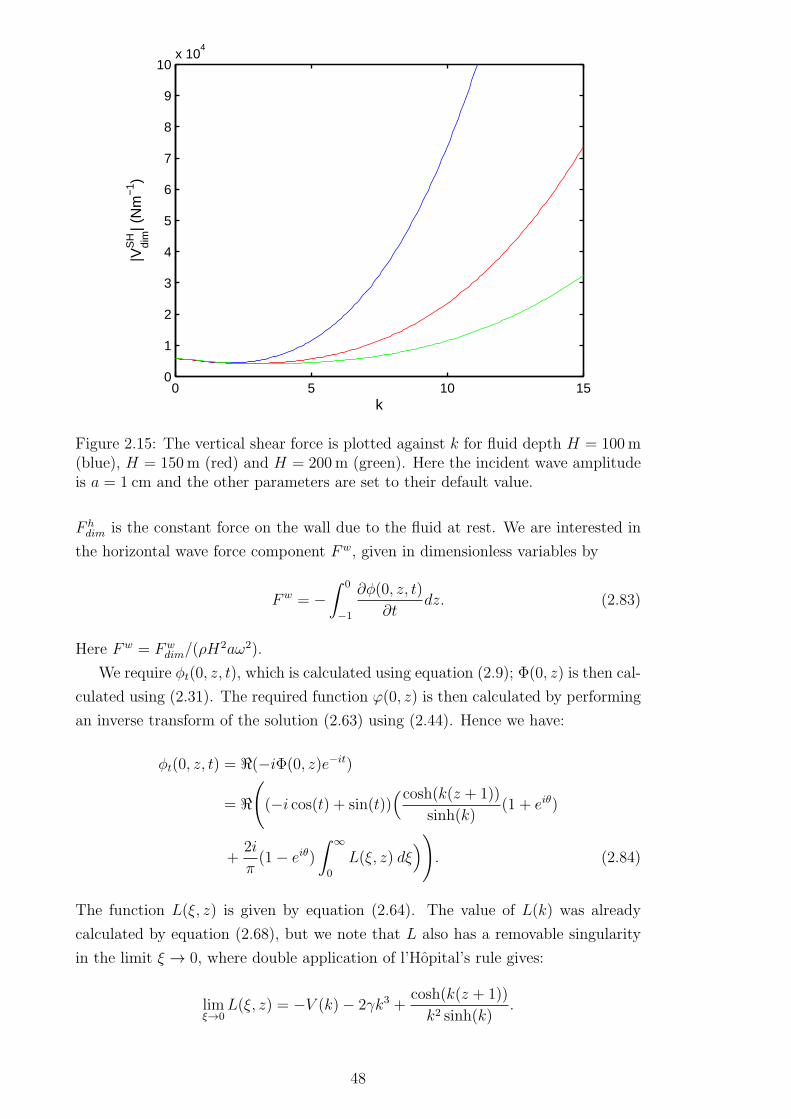
0 5 10 150
1
2
3
4
5
6
7
8
9
10x 10
4
k
|VS
Hdi
m| (
Nm
−1 )
Figure 2.15: The vertical shear force is plotted against k for fluid depth H = 100m(blue), H = 150m (red) and H = 200m (green). Here the incident wave amplitudeis a = 1 cm and the other parameters are set to their default value.
F hdim is the constant force on the wall due to the fluid at rest. We are interested in
the horizontal wave force component Fw, given in dimensionless variables by
Fw = −∫ 0
−1
∂φ(0, z, t)
∂tdz. (2.83)
Here Fw = Fwdim/(ρH
2aω2).
We require φt(0, z, t), which is calculated using equation (2.9); Φ(0, z) is then cal-
culated using (2.31). The required function ϕ(0, z) is then calculated by performing
an inverse transform of the solution (2.63) using (2.44). Hence we have:
φt(0, z, t) = ℜ(−iΦ(0, z)e−it)
= ℜ(
(−i cos(t) + sin(t))(cosh(k(z + 1))
sinh(k)(1 + eiθ)
+2i
π(1− eiθ)
∫ ∞
0
L(ξ, z) dξ)
)
. (2.84)
The function L(ξ, z) is given by equation (2.64). The value of L(k) was already
calculated by equation (2.68), but we note that L also has a removable singularity
in the limit ξ → 0, where double application of l’Hopital’s rule gives:
limξ→0
L(ξ, z) = −V (k)− 2γk3 +cosh(k(z + 1))
k2 sinh(k).
48
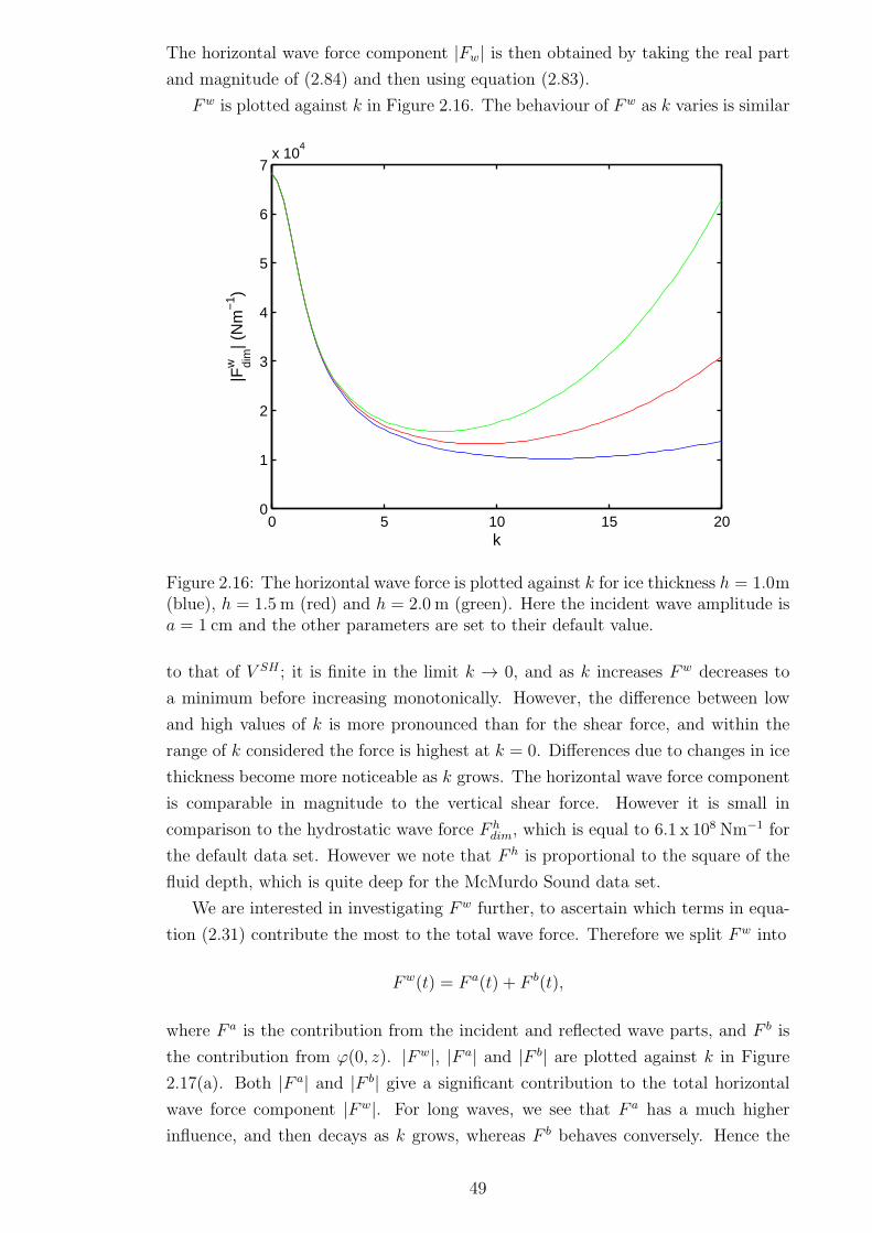
The horizontal wave force component |Fw| is then obtained by taking the real part
and magnitude of (2.84) and then using equation (2.83).
Fw is plotted against k in Figure 2.16. The behaviour of Fw as k varies is similar
0 5 10 15 200
1
2
3
4
5
6
7x 10
4
k
|Fw di
m| (
Nm
−1 )
Figure 2.16: The horizontal wave force is plotted against k for ice thickness h = 1.0m(blue), h = 1.5 m (red) and h = 2.0 m (green). Here the incident wave amplitude isa = 1 cm and the other parameters are set to their default value.
to that of V SH ; it is finite in the limit k → 0, and as k increases Fw decreases to
a minimum before increasing monotonically. However, the difference between low
and high values of k is more pronounced than for the shear force, and within the
range of k considered the force is highest at k = 0. Differences due to changes in ice
thickness become more noticeable as k grows. The horizontal wave force component
is comparable in magnitude to the vertical shear force. However it is small in
comparison to the hydrostatic wave force F hdim, which is equal to 6.1 x 10⁸ Nm−1 for
the default data set. However we note that F h is proportional to the square of the
fluid depth, which is quite deep for the McMurdo Sound data set.
We are interested in investigating Fw further, to ascertain which terms in equa-
tion (2.31) contribute the most to the total wave force. Therefore we split Fw into
Fw(t) = F a(t) + F b(t),
where F a is the contribution from the incident and reflected wave parts, and F b is
the contribution from ϕ(0, z). |Fw|, |F a| and |F b| are plotted against k in Figure
2.17(a). Both |F a| and |F b| give a significant contribution to the total horizontal
wave force component |Fw|. For long waves, we see that F a has a much higher
influence, and then decays as k grows, whereas F b behaves conversely. Hence the
49
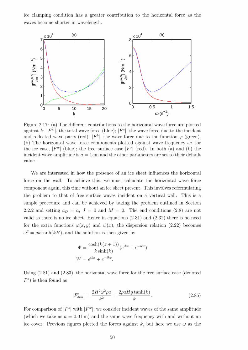
ice–clamping condition has a greater contribution to the horizontal force as the
waves become shorter in wavelength.
0 5 10 15 200
1
2
3
4
5
6
7x 10
4
k
|Fw
,a,b
dim
| (N
m−
1 )(a)
0 0.5 1 1.50
2
4
6
8x 10
4 (b)
ω (s−1)
|Fw
,sdi
m| (
Nm
−1 )
Figure 2.17: (a) The different contributions to the horizontal wave force are plottedagainst k: |Fw|, the total wave force (blue); |F a|, the wave force due to the incidentand reflected wave parts (red); |F b|, the wave force due to the function ϕ (green).(b) The horizontal wave force components plotted against wave frequency ω: forthe ice case, |Fw| (blue); the free–surface case |F s| (red). In both (a) and (b) theincident wave amplitude is a = 1cm and the other parameters are set to their defaultvalue.
We are interested in how the presence of an ice sheet influences the horizontal
force on the wall. To achieve this, we must calculate the horizontal wave force
component again, this time without an ice sheet present. This involves reformulating
the problem to that of free surface waves incident on a vertical wall. This is a
simple procedure and can be achieved by taking the problem outlined in Section
2.2.2 and setting aD = a, J = 0 and M = 0. The end conditions (2.8) are not
valid as there is no ice sheet. Hence in equations (2.31) and (2.32) there is no need
for the extra functions ϕ(x, y) and w(x), the dispersion relation (2.22) becomes
ω2 = gk tanh(kH), and the solution is then given by
Φ =cosh(k(z + 1))
k sinh(k)(eikx + e−ikx),
W = eikx + e−ikx.
Using (2.81) and (2.83), the horizontal wave force for the free surface case (denoted
F s) is then found as
|F sdim| =
2H2ω2ρa
k2=
2ρaHg tanh(k)
k. (2.85)
For comparison of |F s| with |Fw|, we consider incident waves of the same amplitude
(which we take as a = 0.01 m) and the same wave frequency with and without an
ice cover. Previous figures plotted the forces against k, but here we use ω as the
50
horizontal axis. The wave frequency ω is consistent for such comparison, whereas
the wavenumber k is not, due to the different dispersion relations. Figure 2.17(b)
compares |F s| and |Fw| on the same graph. For low wave frequency the horizontal
force on the wall is almost the same between the ice and free surface cases. As wave
frequency increases the difference becomes more pronounced, and the presence of
the ice causes significantly higher force.
2.5 Summary
The problem of hydroelastic wave interaction with a vertical wall in two dimensions
was solved within linear theory. The fluid was of finite depth and the ice was clamped
to the vertical wall. The Euler-Bernoulli thin plate equation was used to model the
ice sheet, and the fluid was modelled by linear water wave theory. The velocity
potential and ice deflection were separated into time-independent functions, which
were then decomposed into parts representing the incident wave, reflected wave
and extra functions to account for the conditions caused by the presence of an ice
cover. The extra functions w and ϕ describe the behaviour of the solution in the
vicinity of the vertical wall. The hydroelastic dispersion relation was derived. The
BVP was rewritten in terms of w and ϕ. Physical parameters such as the flexural
rigidity, thickness of the ice, the fluid depth and others were combined into two
dimensionless parameters k∗ and γ = EJ/(ρω2H5), which define the behaviour of
the fluid-structure interaction.
The problem was solved analytically by Fourier cosine transforms. The solution
was presented in terms of infinite integral quadratures, which converge quickly. The
phase shift between the incident and reflected waves was found as part of the solu-
tion. Numerical results were then presented for the ice deflection and strain in the
ice sheet, as well as the vertical and horizontal forces on the vertical wall.
The ice sheet deflection was plotted for various parameters. The deflection is
zero and its slope is zero where the ice is clamped to the vertical wall. The first
wave peak in the deflection is the smallest due to this clamping. For larger values
of k, the highest deflection is the second wave peak from the wall. Changing the
ice thickness, or other parameters contained within γ, has a significant effect on the
shape and magnitude of ice deflection.
The strain in the ice sheet was calculated and analysed for different wavenum-
bers and fluid depths. The ice clamping introduces a limit on the incident wave
amplitude, in order for the strain in the ice sheet to remain below critical yield.
This limit means the amplitude must be considerably lower than it would be in the
absence of ice clamping, but allows waves of smaller wavelength to be analysed. The
strain is highest at the vertical wall where the clamping takes place. The strain in
the ice sheet begins finite for very long waves, decreases slightly as k increases, and
then increases monotonically for shorter waves.
Forces on the vertical wall caused by the incident hydroelastic waves were calcu-
51
lated. The consideration of such forces is crucial in the design of off-shore structures.
The vertical shear force on the wall that the ice causes was calculated, and changes
in γ and k were investigated. As k increases from zero, the shear force begins finite
and then decreases to a minimum before rising with k. The horizontal force acting
on the wall was also calculated. The wave force component was found to be of the
same order as the shear force. Comparison was made to the horizontal wave force
with no ice sheet present, to demonstrate the increased force the ice sheet causes.
If this formulation were to be applied to the ocean, where constant ice flexure
is caused by tides, a crack could possibly appear at the ice-wall boundary due to
the induced strain. As shown in Section 2.4.2 this is highly dependent on the wave
amplitude and wavenumber k. The problem could then be easily reformulated with
different boundary conditions to reflect this change. The analysis of the free-edge
problem is very similar to that in the present paper but the function Q(ξ) is slightly
different. However, considering applications in frozen lakes where the incident wave
amplitude would be smaller, the strain at the ice-structure connection may not be
above the yield strain and the model holds.
The model and solution outline in this chapter provides a firm basis for exten-
sion. While the model is linearised and many assumptions are made to simplify the
problem, we have gained familiarity and experience with all aspects of the formula-
tion and solution of hydroelastic problems. We may now proceed to complicate the
model by incorporating more realistic effects.
2.5.1 Comparison with other authors
The work presented in Chapter 2 was published in the article Brocklehurst et al.
(2010). Shortly afterwards, a similar paper was published by Bhattacharjee &
Guedes-Soares (2012) entitled “Flexural gravity waves over a floating ice sheet near
a vertical wall”. The problem studied was linear two-dimensional wave reflection
by a vertical wall in fluid of finite depth. Bhattacharjee & Guedes-Soares (2012)
considered the wall as both rigid and harmonically oscillating. They also considered
three different edge conditions at the ice-wall boundary: free edge, simply supported
and clamped conditions. The problem was solved by eigenfunction expansion. For
the clamped condition case, the authors presented a comparison with the solution of
the present solution of Chapter 2. The authors presented graphs of the ice deflection
and the strain in the ice with both solutions compared and found the solutions to
be in excellent agreement. This comparison is shown in Figure 2.18.
Given that the solution methods were different, this provides verification to both.
2.5.2 Comparison with other methods of solution
When comparing the present method to the method based on Green’s functions
developed by Williams & Squire (2002), both methods provide analytical solutions.
Eigenfunction expansions such as those used by Evans & Porter (2003) or Bhat-
52

(a) (b)
Figure 2.18: (a) The strain in the ice against x for k = 10. (b) The deflectionagainst x for k = 5. Comparison of the solution of Bhattacharjee & Guedes-Soares(2012) (solid line) with that of the present solution (dashed line). This figure wasreproduced from Bhattacharjee & Guedes-Soares (2012), in which η = w.
tacharjee & Guedes-Soares (2012) could also be used as an alternative approach.
The solution in the present method is provided in terms of integral quadratures,
whereas an eigenfunction expansion defines the solution in terms of infinite series.
Methods based on Green’s functions inevitably require numerical computation of
the solution as opposed to the explicit solution provided here. The present method
can be also used for free-edge ice cover as can the methods by Williams & Squire
(2002) and Evans & Porter (2003). The present method allows an explicit definition
of the phase shift between the incident and reflected waves in terms of quadratures.
Both alternative methods would require numerical calculation of the phase shift.
The use of a Fourier cosine transform also presents a very simple expression for
the shear force, avoiding potential issues with the convergence of a third derivative
other methods could present. The linear superposition involved in the present so-
lution also allows us to easily compare the contribution from each wave part. In
addition, as we will see throughout this thesis, the function Q(ξ) appears in other
problems also, and that we are now familiar with its behaviour is beneficial.
53

Chapter 3
Hydroelastic wave diffraction by a
vertical cylinder
3.1 Introduction
We now extend the problem solved in Chapter 2 into three dimensions. We consider a
vertical cylinder in fluid of finite depth, in the presence of an infinite ice sheet. This
study is motivated by the expected need to build ocean structures in ice-covered
water, discussed fully in Chapter 1. The vertical cylinder represents one of the
supporting stands of such a structure. The hydroelastic behaviour of the ice sheet is
described by linear elastic plate theory, and the fluid flow by the potential flow model,
as in Chapter 2. The ice sheet is frozen to the vertical cylinder. Incident hydroelastic
waves approach the cylinder and are diffracted and reflected. The two-dimensional
hydroelastic incident wave is regular. We are interested in the deflection field, as
well as the various forces on the cylinder. The distribution of these forces around the
circumference of the cylinder is also studied. The strain at the ice-cylinder interface
is of particular interest, and we will estimate whether the ice–clamping condition
will be maintained. Key parameters under investigation include the cylinder radius
and the wavenumber of the incident wave.
The assumptions discussed in Section 2.1 are applicable here also; the fluid is
assumed inviscid and incompressible with irrotational flow. We assume the problem
is time–harmonic, allowing us to remove time as a factor from the results. We
retain the linear thin plate model, which is extended to three dimensions. The
added dimension greatly complicates the problem: we exploit the axisymmetry of
the vertical cylinder and introduce polar co-ordinates. As in Chapter 2 it is possible
to express the ice deflection and velocity potential as the linear sum of the incident
wave, reflected wave and an extra function to account for the boundary conditions
due to the presence of a cylinder.
The structure of the chapter is as follows. Section 3.2 describes the mathematical
formulation of the problem, and relevant physical parameters are defined. Section
3.3 demonstrates the method of solution. The solutions for the ice deflection and
velocity potential of the flow are derived. Section 3.4 presents numerical results,
54
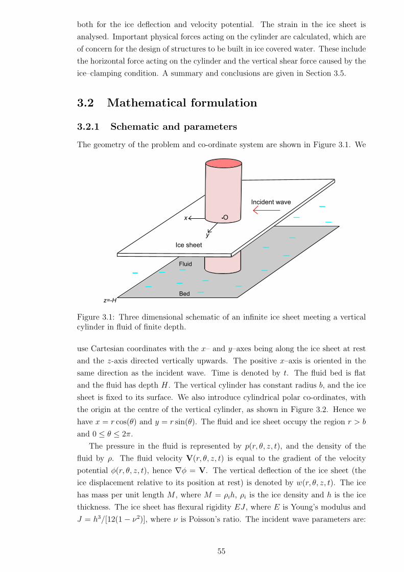
both for the ice deflection and velocity potential. The strain in the ice sheet is
analysed. Important physical forces acting on the cylinder are calculated, which are
of concern for the design of structures to be built in ice covered water. These include
the horizontal force acting on the cylinder and the vertical shear force caused by the
ice–clamping condition. A summary and conclusions are given in Section 3.5.
3.2 Mathematical formulation
3.2.1 Schematic and parameters
The geometry of the problem and co-ordinate system are shown in Figure 3.1. We
Fluid
Bed
z=-H
Ice sheet
O
Incident wave
x
y
Figure 3.1: Three dimensional schematic of an infinite ice sheet meeting a verticalcylinder in fluid of finite depth.
use Cartesian coordinates with the x– and y–axes being along the ice sheet at rest
and the z-axis directed vertically upwards. The positive x–axis is oriented in the
same direction as the incident wave. Time is denoted by t. The fluid bed is flat
and the fluid has depth H. The vertical cylinder has constant radius b, and the ice
sheet is fixed to its surface. We also introduce cylindrical polar co-ordinates, with
the origin at the centre of the vertical cylinder, as shown in Figure 3.2. Hence we
have x = r cos(θ) and y = r sin(θ). The fluid and ice sheet occupy the region r > b
and 0 ≤ θ ≤ 2π.
The pressure in the fluid is represented by p(r, θ, z, t), and the density of the
fluid by ρ. The fluid velocity V(r, θ, z, t) is equal to the gradient of the velocity
potential φ(r, θ, z, t), hence ∇φ = V. The vertical deflection of the ice sheet (the
ice displacement relative to its position at rest) is denoted by w(r, θ, z, t). The ice
has mass per unit length M , where M = ρih, ρi is the ice density and h is the ice
thickness. The ice sheet has flexural rigidity EJ , where E is Young’s modulus and
J = h3/[12(1 − ν2)], where ν is Poisson’s ratio. The incident wave parameters are:
55

a, wave amplitude; ω, wave frequency; k, wavenumber and c, phase velocity. The
acceleration due to gravity is denoted g.
b
b
y
x
r
θ
Incident
waves
Figure 3.2: Cylindrical polar co-ordinate system.
3.2.2 Governing equations and boundary conditions
The governing equations and boundary conditions are now expressed in polar co-
ordinates. The velocity potential satisfies Laplace’s equation in the flow region:
∇2φ = 0, (−H < z < 0, r > b, 0 ≤ θ ≤ 2π), (3.1)
where the Laplacian in polar co-ordinates is given by
∇2 =1
r
∂
∂r
(
r∂
∂r
)
+1
r2∂2
∂θ2+
∂2
∂z2. (3.2)
The linearised Bernoulli equation gives the pressure in the fluid as
p(r, θ, z, t) = −ρφt − ρgz, (−H < z < 0, r > b, 0 ≤ θ ≤ 2π), (3.3)
where subscripts indicate partial derivatives. Boundary conditions for Laplace’s
equation (3.1) are due to the rigid vertical wall of the cylinder, the fluid bed, and
the linearised kinematic condition on the ice cover respectively:
φr = 0, (r = b), (3.4)
φz = 0, (z = −H), (3.5)
φz = wt, (z = 0). (3.6)
The deflection of the ice cover is governed by the Bernoulli-Euler thin elastic plate
equation:
EJ∇4w +Mwtt = p, (z = 0, r > b, 0 ≤ θ ≤ 2π), (3.7)
56

where the biharmonic operator is defined as ∇4 = ∇2∇2. Boundary conditions due
to the ice–clamping condition are given by
w = 0, (r = b), (3.8)
wr = 0, (r = b). (3.9)
The conditions in the far field are defined later.
As in Chapter 2, both the ice deflection and the fluid flow are assumed periodic
in time with the frequency ω of the incident wave. The solution of the coupled
problem (3.1)-(3.9) is sought in the form (see for example Squire et al., 1995):
φ(r, θ, z, t) = ℜ(
Φ(r, θ, z)e−iωt)
, (3.10)
w(r, θ, t) = ℜ( i
ωW (r, θ)e−iωt
)
. (3.11)
The problem now depends on the time–independent variables Φ and W .
3.2.3 Incident waves and nondimensionalisation
The velocity potential Φinc(r, θ, z) and the deflectionWinc(r, θ) of the incident waves
have the form:
Φinc(r, θ, z) =aω
k
cosh(k(z +H))
sinh(kH)eikr cos(θ), (3.12)
Winc(r, θ) = aω eikr cos(θ). (3.13)
These expressions are obtained simply by substituting x = r cos(θ) into the ex-
pressions for the incident waves derived in Chapter 2, given by equations (2.20)
and (2.21). The wave frequency ω and wavenumber k are related by the dispersion
relation for hydroelastic waves which is unchanged from equation (2.22):
ω2(
M +ρ
k tanh(kH)
)
= ρg + EJk4. (3.14)
We proceed to nondimensionalise the problem (3.1)-(3.9), using the depth H
as a length scale. The following non–dimensional variables and parameters are
introduced, denoted by asterisks:
r∗ =r
H, z∗ =
z
H, b∗ =
b
H, t∗ = tω, k∗ = kH,
W ∗(r∗, θ, t∗) =W (r, θ)
aω, Φ∗(r∗, θ, z∗) =
Φ(r, θ, z)
Haω,
where k∗ is the dimensionless incident wavenumber and b∗ is the dimensionless radius
of the vertical cylinder. We also retain the dimensionless parameter γ = EJ/ρω2H5
from Chapter 2. In the following analysis the asterisks are dropped and only dimen-
sionless quantities are used if not stated otherwise.
57
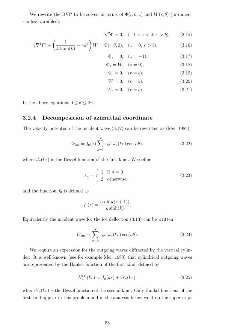
We rewrite the BVP to be solved in terms of Φ(r, θ, z) and W (r, θ) (in dimen-
sionless variables):
∇2Φ = 0, (−1 < z < 0, r > b), (3.15)
γ∇4W +
(
1
k tanh(k)− γk4
)
W = Φ(r, θ, 0), (z = 0, r > b), (3.16)
Φz = 0, (z = −1), (3.17)
Φz = W, (z = 0), (3.18)
Φr = 0, (r = b), (3.19)
W = 0, (r = b), (3.20)
Wr = 0, (r = b). (3.21)
In the above equations 0 ≤ θ ≤ 2π.
3.2.4 Decomposition of azimuthal coordinate
The velocity potential of the incident wave (3.12) can be rewritten as (Mei, 1983):
Φinc = f0(z)∞∑
n=0
εninJn(kr) cos(nθ), (3.22)
where Jn(kr) is the Bessel function of the first kind. We define
εn =
{
1 if n = 0,
2 otherwise,(3.23)
and the function f0 is defined as
f0(z) =cosh(k(z + 1))
k sinh(k).
Equivalently the incident wave for the ice deflection (3.13) can be written
Winc =∞∑
n=0
εninJn(kr) cos(nθ). (3.24)
We require an expression for the outgoing waves diffracted by the vertical cylin-
der. It is well known (see for example Mei, 1983) that cylindrical outgoing waves
are represented by the Hankel function of the first kind, defined by
H(1)n (kr) = Jn(kr) + iYn(kr), (3.25)
where Yn(kr) is the Bessel function of the second kind. Only Hankel functions of the
first kind appear in this problem and in the analysis below we drop the superscript
58
in (3.25). Therefore, the diffracted waves are given by
Φdif = f0(z)∞∑
n=0
εninaDnHn(kr) cos(nθ), (3.26)
Wdif =∞∑
n=0
εninaDnHn(kr) cos(nθ), (3.27)
where the complex coefficients aDn must be determined as part of the solution. Note
that the incident and reflected waves satisfy equations satisfy equations (3.15)-(3.18)
and correctly describe the far-field behaviour of the hydroelastic waves.
Using linear superposition (as in Section 2.2.7) we may express the total velocity
potential and ice deflection as:
Φ(r, θ, z) =∞∑
n=0
εn in cos(nθ)
(
f0(z)Jn(kr) + aDn f0(z)Hn(kr) + ϕn(r, z)
)
,
(3.28)
W (r, θ) =∞∑
n=0
εn in cos(nθ)
(
Jn(kr) + aDn Hn(kr) + wn(r)
)
, (3.29)
Here we have introduced the unknown functions ϕn(r, z) and wn(r) to describe
the flow and ice deflection in the vicinity of the cylinder, owing to the boundary
conditions (3.19)-(3.21). The functions ϕn(r, z) and wn(r) are such that they do not
give contributions to the wave pattern in the far field (Brocklehurst et al., 2011):
√rϕn(r, z) → 0,
√rwn(r) → 0, r → ∞. (3.30)
In order to derive the boundary–value problems for the unknown functions
ϕn(r, z) and wn(r), where n ≥ 0, we substitute equations (3.28)-(3.29) into equa-
tions (3.15)–(3.21). As noted previously, Jn(kr) and Hn(kr) satisfy the governing
equations (3.15)–(3.16) independently, and hence the new functions ϕn(r, z) and
wn(r) must also satisfy them. It is convenient to introduce the differential operator
Sn < ϕn(r, z) >=
(
∂2
∂r2+
1
r
∂
∂r− n2
r2
)
ϕn(r, z). (3.31)
59

The resulting n boundary-value problems are formulated as
Sn < ϕn > +ϕnzz = 0, (−1 < z < 0, r > b), (3.32)
γS2n < wn > +
( 1
k tanh(k)− γk4
)
wn = ϕn, (z = 0, r > b), (3.33)
ϕnz = 0, (z = −1, r > b), (3.34)
ϕnr = −f0(z)k(
J ′n(kb) + aDnH
′n(kb)
)
, (−1 < z < 0, r = b), (3.35)
ϕnz = wn, (z = 0, r > b), (3.36)
wn = −Jn(kb)− aDnHn(kb), (r = b), (3.37)
wnr = −kJ ′n(kb)− aDn kH
′n(kb), (r = b). (3.38)
In this chapter, primes indicate differentiation with respect to argument. We note
that the above BVP has no dependence on θ.
3.3 Method of solution
3.3.1 Weber transform
In order to handle the fourth order derivative in equation (3.33) we employ a modi-
fied Weber transform (Emmerhoff & Sclavounos, 1992). We may then use the helpful
properties of this transform to greatly simplify the differential equations in (3.32)-
(3.38) and facilitate a solution. Usually in problems with cylindrical symmetry, a
standard Hankel transform proves useful; however, in the present problem the fluid
occupies the region r > b, and this requires the choice of a Weber transform.
The Weber transform is defined as
F (s) =
∫ ∞
b
r f(r) Zn(r, s) dr, (3.39)
where a function f(r) is defined in r > b and such that√rf(r) → 0 as r → ∞.
Here Zn is given by
Zn(r, s) = Jn(sr)Y′n(sb)− J ′
n(sb)Yn(sr),
and Zn has the following useful (easily proved) properties:
Zn(b, s) =2
πsb,
∂Zn
∂r(b, s) = 0, Zn → 0 as r → ∞. (3.40)
The corresponding inverse transform reads
f(r) =
∫ ∞
0
F (s) s Zn(r, s)
(J ′n(sb))
2 + (Y ′n(sb))
2ds. (3.41)
Defining the integral operator in (3.39) as F (s) = Web[f(r)], using integration by
60
parts and the properties above, we now find an expression for Web[Sn < f(r) >]:
Web[Sn < f(r) >] =
∫ ∞
b
rfrrZn dr +
∫ ∞
b
frZn dr − n2
∫ ∞
b
Znf
rdr
=(
rZnfr)∞b−∫ ∞
b
frZn dr −∫ ∞
b
frr∂Zn
∂rdr
+
∫ ∞
b
frZn dr − n2
∫ ∞
b
Znf
rdr
= −2fr(b)
πs−(
(
rZnf)∞b−∫ ∞
b
f∂Zn
∂rdr
−∫ ∞
b
r∂2Zn
∂r2f dr
)
− n2
∫ ∞
b
Znf
rdr
= −2fr(b)
πs+
∫ ∞
b
1
r
(
r2∂2Zn
∂r2+ r
∂Zn
∂r− n2Zn
)
f dr
Web[Sn < f(r) >] = −2fr(b)
πs− s2
∫ ∞
b
rfZn dr,
and hence we have
Web[Sn < f(r) >] = −s2Web[f(r)]− 2fr(b)
πs. (3.42)
Note that in the above, we have substituted
−r2Zn = r2∂2Zn
∂r2+ r
∂Zn
∂r− n2Zn,
due to the fact that Zn is a solution to Bessel’s equation, since Zn is a linear com-
bination of Jn and Yn.
We also require an expression for Web[S2n < f(r) >]. This is achieved by defining
g(r) = Sn < f(r) >. Using equation (3.42), we then have:
Web[S2n < f(r) >] = Web[Sn < g(r) >] = −s2Web[Sn < f(r) >]− 2
πsgr(b)
= −s2(
−s2Web[f(r)]− 2
πsfr(b)
)
− 2
πs
∂
∂r(Sn < f(r) >)r=b,
and hence we have
Web[S2n < f(r) >] = s4Web[f(r)] +
2s
πf ′(b)− 2
πs
∂
∂r(Sn < f(r) >)r=b. (3.43)
With expressions (3.42) and (3.43) derived, we may now proceed to apply the Weber
transform to the governing equations and boundary conditions (3.32)-(3.38).
61

3.3.2 Velocity potential
Applying the Weber transform to (3.32), where Web[ϕn(r, z)] = ψn(s, z), and using
equations (3.42) and (3.35), we arrive at the differential equation
∂2ψn
∂z2− s2ψn =
2
πsϕnr(b, z)
=Pn
scosh(k(z + 1)), (3.44)
where the coefficients Pn are defined as
Pn =−2
π sinh(k)(J ′
n(kb) + aDnH′n(kb)). (3.45)
The general solution to equation (3.44) is
ψn(s, z) = νn sinh(s(z + 1)) + µn cosh(s(z + 1)) +Pn cosh(k(z + 1))
s(k2 − s2). (3.46)
Applying the Weber transform to (3.34) and (3.36), we obtain the boundary condi-
tions
∂ψn
∂z= 0, (z = −1), (3.47)
∂ψn
∂z= Wn, (z = 0), (3.48)
where Wn(s) = Web[wn(r)]. Applying the boundary condition (3.47) to the general
solution (3.46) we obtain νn = 0, and the boundary condition (3.48) implies
µn =1
s sinh(s)
(
Wn −kPn sinh(k)
s(k2 − s2)
)
.
Hence the solution of the boundary-value problem (3.44)-(3.48) is
ψn(s, z) =cosh(s(z + 1))
s sinh(s)
(
Wn(s)−Pnk sinh(kH)
s(k2 − s2)
)
+Pn cosh(k(z + 1))
s(k2 − s2), (3.49)
where Wn and the coefficients aDn are to be determined in the next section.
3.3.3 Plate equation
We now apply the Weber transform to the plate equation (3.33) and make use of
(3.43) to obtain the following equation for Wn:
γ(
s4Wn +2s
πwnr(b)−
2
πsVn
)
+( 1
k tanh(k)− γk4
)
Wn = ψn(s, 0), (3.50)
where we define the function
Vn(k, b) =∂
∂r(Sn < wn(r) >)r=b, (3.51)
62
which will be used below in calculations of the shear force acting on the cylinder
due to the clamped condition at r = b. Equation (3.50) can be simplified by noting
that
wnr(b) = −kJ ′n(kb)− kaDnH
′n(kb) =
1
2πk sinh(k)Pn, (3.52)
which follows from (3.38) and (3.45). Inserting (3.52) and (3.49) into the transformed
plate equation (3.50) and rearranging the result to factorise Wn(s) on the left-hand
side, we find
Wn
(
γ(s4 − k4) +1
k tanh(k)− 1
s tanh(s)
)
=
2γ
πsVn − γskPn sinh(k) + Pn sinh(k)
(
1
s(k2 − s2)
( 1
tanh(k)− k
s tanh(s)
)
)
. (3.53)
Clearly the left-hand side of (3.53) is zero at s = k. Hence, to avoid a singularity of
the function Wn(s) at this point we require that the limit of the right-hand side is
also zero as s → k. This limit can be calculated by applying l’Hopital’s rule to the
final term of the right-hand side of (3.53):
lims→k
(
coth(k)− k(s tanh(s))−1
s(k2 − s2)
)
= lims→k
−k(
−(s tanh(s))−2(tanh(s) + s sech2(s)))
k2 − 3s2
=(k tanh(k))−1 + (sinh2(k))−1
−2k2
= −−V (k)
k,
where the function V (k) was introduced in equation (2.56).
Equating the right-hand side of (3.53) with zero at s = k, we obtain an expression
for Vn(k, b):
Vn =π
2Pn sinh(k)
(
k3 +V (k)
γ
)
. (3.54)
Inserting (3.54) into (3.53) and noting that the right–hand side is now also equal to
zero at s = k, we find that
Wn(s) =Pn sinh(k)
sQ(s). (3.55)
Here Q(s) is the same function that appeared in the solution of the equivalent two-
dimensional problem of Chapter 2:
Q(s) =s tanh(s)
(
V (k) + γk(k2 − s2))
+ 1k2−s2
(
s tanh(s)tanh(k)
− k)
s tanh(s)(
γ(s4 − k4) + 1k tanh(k)
)
− 1. (3.56)
The function Q was plotted previously in Figure 2.5. Recall that Q(k) is finite and
is given by equation (2.66).
63

The coefficients aDn are still uncalculated. We note that we have two equations
for wn(b); the first comes from boundary condition (3.37):
wn(b) = −Jn(kb)− aDnHn(kb), (3.57)
and the second arises from performing an inverse transform (3.41) on the solution
(3.55):
wn(b) = Pn sinh(k)2
πb
∫ ∞
0
Q(s)
s(
(J ′n(sb))
2 + (Y ′n(sb))
2) ds. (3.58)
Here we have used the condition Zn(b, s) = 2/(πsb) (see equation (3.40)). Equating
(3.57) and (3.58) and substituting for Pn using (3.45), we have
−Jn(kb)− aDnHn(kb) = − 2
π(J ′
n(kb) + aDnHn(kb))2
πbτn, (3.59)
where
τn =
∫ ∞
0
Q(s)
s(
(J ′n(sb))
2 + (Y ′n(sb))
2)ds.
By resolving (3.59) into real and imaginary parts and defining
χn =4τnπ2b
J ′n(kb)− Jn(kb),
ηn =4τnπ2b
Y ′n(kb)− Yn(kb), (3.60)
we can write
aDn =iχn
ηn − iχn
. (3.61)
The final solution for the problem is then given by performing inverse Weber
transforms on the functions ψn(r, z) in (3.49) and Wn(r) in (3.55), and by working
backwards through the analysis using equations (3.28)-(3.29) and (3.10)-(3.11). The
inverse transforms are too complicated to be evaluated analytically, and must be
calculated numerically. In the following section, we outline techniques for doing so.
3.3.4 Numerical techniques for inverse Weber transforms
The inverse transform for the plate deflection is given by
wn(r) =
∫ ∞
0
Wn(s) s Zn(r, s)
(J ′n(sb))
2 + (Y ′n(sb))
2ds
= Pn sinh(k) I(r),
where the integral I is defined as
I(r) =
∫ ∞
0
Q(s) Zn(r, s)
ζds, (3.62)
64

and we have defined ζ = (J ′n(sb))
2 + (Y ′n(sb))
2. Due to the presence of Bessel func-
tions in its the numerator and denominator, the integrand is extremely oscillatory,
and becomes increasingly more so as r grows. Despite the fact that Q decays with
order s−2 as s→ ∞, the convergence of the integrand can be quite slow. Examples
of the integrand are plotted in Figure 3.3.
0 20 40 60 80 100
−5
0
5
10
x 10−4
s
Q(s
) Z
n(r,s
) ζ−
1
Figure 3.3: The integrand of (3.62) plotted against s for r = 0.1 (blue), r = 0.5(red) and r = 1.0 (green). The cylinder radius is given by b = 0.01, k = 5 andn = 1. All other parameters are taken from Table 2.1(a).
We are able to improve the convergence of the integral by investigating the
behaviour of the integrand as s→ ∞. Firstly, the asymptotic expressions for Bessel
functions of order n for large argument are given by (Bowman, 1958):
Jn(sr) ≈√
2
πsrcos(
sr − nπ
2− π
4
)
, (3.63)
Yn(sr) ≈√
2
πsrsin(
sr − nπ
2− π
4
)
, (3.64)
to leading order. Using the differentiation rules for Bessel functions combined with
equations (3.63)-(3.64), for large arguments we have
J ′n(sb) = −Jn+1(sb) +
n
sbJn(sb) ≈
√
2
πsbcos
(
sb− π
4− (n+ 1)π
2
)
≈√
2
πsbsin(
sb− π
4− nπ
2
)
, (3.65)
and similarly
Y ′n(sb) ≈
√
2
πsbcos(
sb− π
4− nπ
2
)
. (3.66)
65

Hence, using (3.65)-(3.66)an asymptotic expression for Zn as s→ ∞ is given by
Zn = Jn(sr)Y′n(sb)− J ′
n(sb)Yn(sr)
≈√
2
πsrcos(
sr − nπ
2− π
4
)
√
2
πsbcos(
sb− π
4− nπ
2
)
−√
2
πsbsin(
sb− π
4− nπ
2
)
√
2
πsrsin(
sr − nπ
2− π
4
)
=2
πs√br
cos
(
(
sr − nπ
2− π
4
)
−(
sb− nπ
2− π
4
)
)
=2
πs√br
cos(s(r − b)). (3.67)
Similarly we may find an expression for ζ as s→ ∞, given by
ζ ≈ 2
πsbcos2
(
sb− (n+ 1)π
2− π
4
)
+2
πsbsin2
(
sb− (n+ 1)π
2− π
4
)
=2
πsb. (3.68)
We note that Q(s) ∼ −ks−2 as s→ ∞. Combining this fact with (3.67) and (3.68),
we obtain an expression for the integrand of I as s→ ∞:
Q(s)Zn
ζ≈ −k
√
b
r
cos(s(r − b))
s2. (3.69)
To improve the convergence of I, we now define the function g(s) as
g(s) =Q(s)Zn
ζ+ k
√
b
r
cos(s(r − b))
s2 + 1, (3.70)
and then I can be rewritten
I(r) =
∫ ∞
0
g(s) ds− k
√
b
r
∫ ∞
0
cos(s(r − b))
s2 + 1ds
=
∫ ∞
0
g(s) ds− kπ
2
√
b
reb−r. (3.71)
Here we have used the result in equation (2.78). We note that the integrand in
equation (3.71) decays faster than the integrand of equation (3.62) and its behaviour
is now less oscillatory as s → ∞, greatly improving the computational efficiency of
the problem.
We note that there is some literature on the subject of integrals involving prod-
ucts of Bessel functions. Lucas (1995) considered such integrals for Bessel functions
of arbitrary order, using asymptotic expressions and extrapolation on a sequence of
partial sums. The author notes that standard infinite integration routines perform
extremely poorly when calculating such integrals. However, the integral I in equa-
tion (3.62) is more complicated than the integrals considered by Lucas (1995) as
it includes the term (J ′n(sb))
2 + (Y ′n(sb))
2 in the denominator. Using the technique
66
outlined above (resulting in equation (3.71)) and using a very fine integration grid,
combined with ensuring the integral is truncated to high order, leads to satisfactory
accuracy. The efficiency could possibly be improved by using techniques similar to
those in Lucas (1995), but such numerical investigation is beyond the scope of this
thesis.
When the integrals are calculated and wn(r) are known, they are substituted
into the expression for the total deflection W (r, θ) given by equation (3.29). This
expression is in terms of an infinite sum from n = 0 to n = ∞. We note that the
convergence of this sum is fast: in the calculations we continue to increase n until
the magnitude of the contribution from each term is less than 10−20. Usually this
occurs between n = 5 and n = 15.
3.4 Numerical results
In this section we present results for the solution derived in Section 3.3. Results
are presented for the ice deflection and strain in the ice sheet, as well as for the
magnitude of the shear and horizontal forces acting on the cylinder. Recall that
the default data set is given by Table 2.1(a). The wavenumber k and the cylinder
radius b are varied frequently, and hence are not assigned a default value but are
quoted for each plot. We continue to assume that all variables and parameters are
dimensionless unless accompanied by their units. Throughout this section we use
the same notation as Section 2.3 to indicate magnitude, to be interpreted as the
maximum value with respect to time.
3.4.1 Deflection in the ice sheet
In Section 2.4.1, the deflection results were presented in terms of the magnitude
with respect to time. In this three-dimensional formulation, is it clearer to present
a snapshot of the deflection for some fixed time. We begin by plotting the deflection
for k = 5, corresponding to an incident wave of long wavelength λ = 440m. We also
take b = 0.01, corresponding to a structure with support cylinder radius bdim = 3.5m.
The ice deflection is shown in Figure 3.4.
Recall that the incident wave approaches from x = −∞ and travels in the positive
x direction. Because the cylinder radius is small in comparison with the incident
wavelength, the effect of the cylinder on the waves is small. However, we see a
disturbance in the vicinity of the cylinder among the regular incident waves. The
deflection is smallest directly in the wake of the cylinder, as expected. Although it
is invisible from this viewpoint, the deflection and slope of the deflection are zero
at the contact point between the cylinder and the ice sheet, as prescribed by the
ice–clamping condition.
We repeat the calculations, increasing the wavenumber to k = 10. Other param-
eters are the same as for Figure 3.4. The deflection for this case is plotted in Figure
67
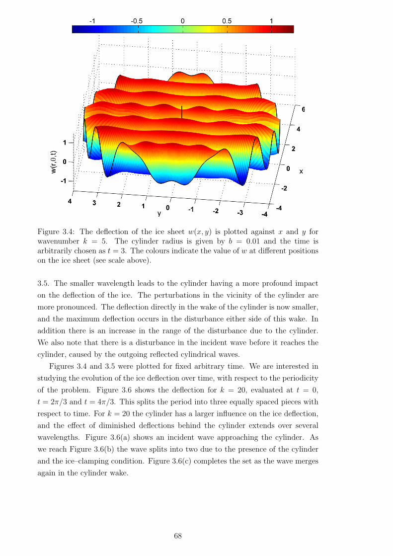
Figure 3.4: The deflection of the ice sheet w(x, y) is plotted against x and y forwavenumber k = 5. The cylinder radius is given by b = 0.01 and the time isarbitrarily chosen as t = 3. The colours indicate the value of w at different positionson the ice sheet (see scale above).
3.5. The smaller wavelength leads to the cylinder having a more profound impact
on the deflection of the ice. The perturbations in the vicinity of the cylinder are
more pronounced. The deflection directly in the wake of the cylinder is now smaller,
and the maximum deflection occurs in the disturbance either side of this wake. In
addition there is an increase in the range of the disturbance due to the cylinder.
We also note that there is a disturbance in the incident wave before it reaches the
cylinder, caused by the outgoing reflected cylindrical waves.
Figures 3.4 and 3.5 were plotted for fixed arbitrary time. We are interested in
studying the evolution of the ice deflection over time, with respect to the periodicity
of the problem. Figure 3.6 shows the deflection for k = 20, evaluated at t = 0,
t = 2π/3 and t = 4π/3. This splits the period into three equally spaced pieces with
respect to time. For k = 20 the cylinder has a larger influence on the ice deflection,
and the effect of diminished deflections behind the cylinder extends over several
wavelengths. Figure 3.6(a) shows an incident wave approaching the cylinder. As
we reach Figure 3.6(b) the wave splits into two due to the presence of the cylinder
and the ice–clamping condition. Figure 3.6(c) completes the set as the wave merges
again in the cylinder wake.
68

Figure 3.5: The deflection of the ice sheet w(x, y) is plotted against x and y forwavenumber k = 10. The cylinder radius is given by b = 0.01 and the time isarbitrarily chosen as t = 3.
3.4.2 Strain in the ice sheet
We now calculate the strain in the ice sheet. As in Chapter 2, the strain is of partic-
ular interest in the present problem as we are interested in whether the clamped–ice
condition at r = b can be maintained. In this study we are interested in the radial
strain component εr, defined as
εr =ah
2H2
∂2w
∂r2. (3.72)
The calculation of the strain is not straightforward. As seen in Section 3.3.4, the
inverse Weber transform for the deflection of the ice sheet involves an integrand
that behaves with order s−2 as s → ∞. Direct calculation of the second derivative
with respect to r required for the strain in (3.72) would lead to this integrand being
multiplied by s2, leaving the integral undefined. However, after performing the
derivative in equation (3.72), we use the technique to improve the convergence of
the integrals outlined in Section 3.3.4. This results in an integrand which behaves
with order s−1 as s→ ∞. The strain can then be calculated without any problems.
Based on the results of Section 2.4.2, the strain is expected to be highest at
r = b. To begin, we plot the polar distribution of the strain in the ice sheet around
the cylinder. Figure 3.7(a) shows the strain εr against θ for varying values of the
wavenumber k. Firstly we see that the strain is highest at θ = π, which is the
angle from which the incident wave approaches the cylinder. The minimum value of
69
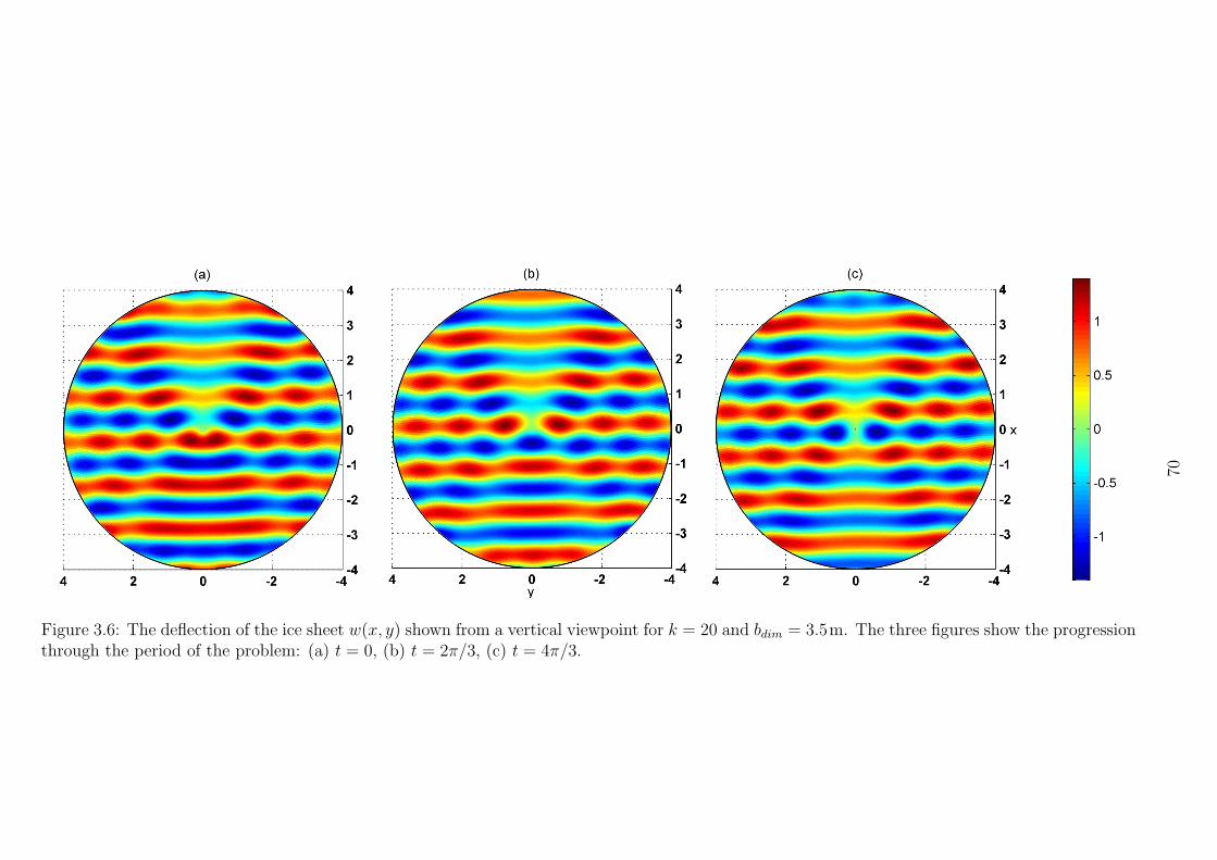
Figure 3.6: The deflection of the ice sheet w(x, y) shown from a vertical viewpoint for k = 20 and bdim = 3.5m. The three figures show the progressionthrough the period of the problem: (a) t = 0, (b) t = 2π/3, (c) t = 4π/3.
70
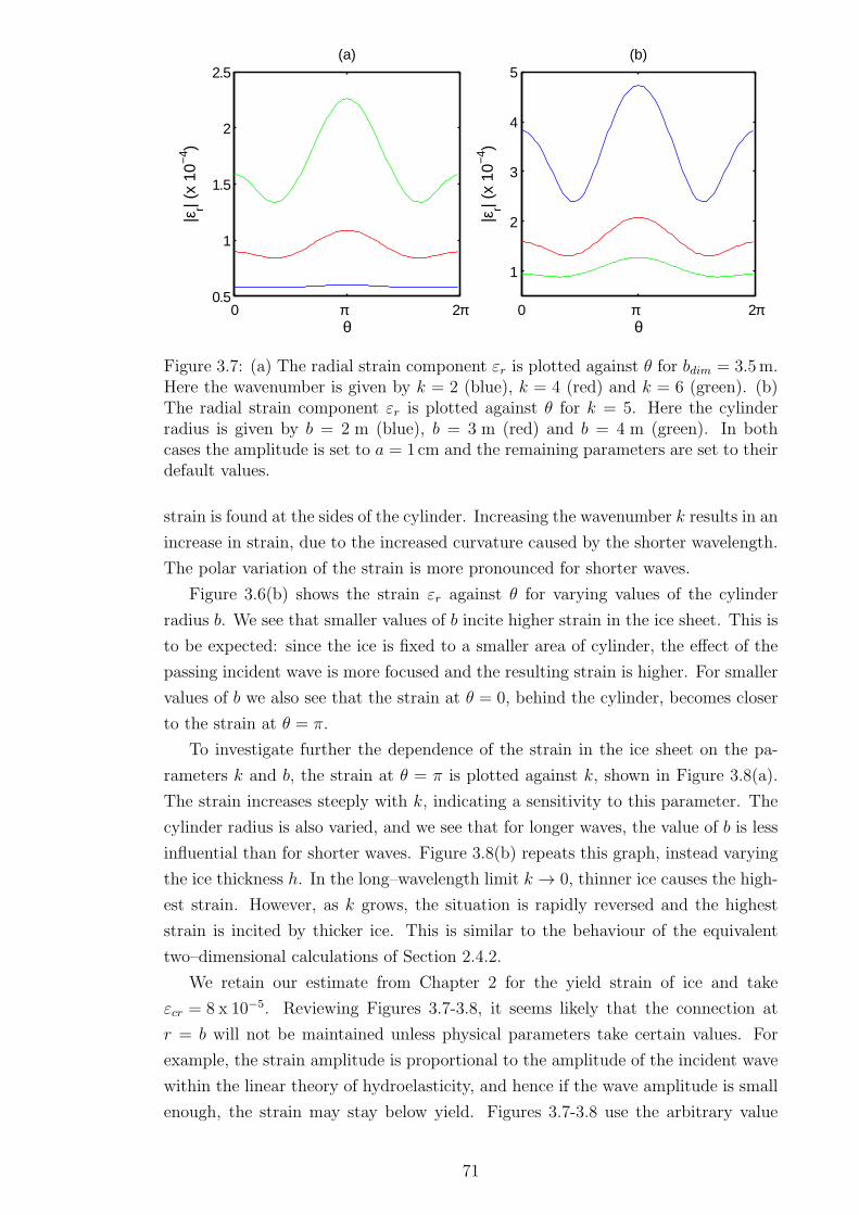
0 π 2π0.5
1
1.5
2
2.5(a)
θ
|εr| (
x 10
−4 )
0 π 2π
1
2
3
4
5(b)
θ
|εr| (
x 10
−4 )
Figure 3.7: (a) The radial strain component εr is plotted against θ for bdim = 3.5m.Here the wavenumber is given by k = 2 (blue), k = 4 (red) and k = 6 (green). (b)The radial strain component εr is plotted against θ for k = 5. Here the cylinderradius is given by b = 2 m (blue), b = 3 m (red) and b = 4 m (green). In bothcases the amplitude is set to a = 1cm and the remaining parameters are set to theirdefault values.
strain is found at the sides of the cylinder. Increasing the wavenumber k results in an
increase in strain, due to the increased curvature caused by the shorter wavelength.
The polar variation of the strain is more pronounced for shorter waves.
Figure 3.6(b) shows the strain εr against θ for varying values of the cylinder
radius b. We see that smaller values of b incite higher strain in the ice sheet. This is
to be expected: since the ice is fixed to a smaller area of cylinder, the effect of the
passing incident wave is more focused and the resulting strain is higher. For smaller
values of b we also see that the strain at θ = 0, behind the cylinder, becomes closer
to the strain at θ = π.
To investigate further the dependence of the strain in the ice sheet on the pa-
rameters k and b, the strain at θ = π is plotted against k, shown in Figure 3.8(a).
The strain increases steeply with k, indicating a sensitivity to this parameter. The
cylinder radius is also varied, and we see that for longer waves, the value of b is less
influential than for shorter waves. Figure 3.8(b) repeats this graph, instead varying
the ice thickness h. In the long–wavelength limit k → 0, thinner ice causes the high-
est strain. However, as k grows, the situation is rapidly reversed and the highest
strain is incited by thicker ice. This is similar to the behaviour of the equivalent
two–dimensional calculations of Section 2.4.2.
We retain our estimate from Chapter 2 for the yield strain of ice and take
εcr = 8 x 10⁻⁵. Reviewing Figures 3.7-3.8, it seems likely that the connection at
r = b will not be maintained unless physical parameters take certain values. For
example, the strain amplitude is proportional to the amplitude of the incident wave
within the linear theory of hydroelasticity, and hence if the wave amplitude is small
enough, the strain may stay below yield. Figures 3.7-3.8 use the arbitrary value
71
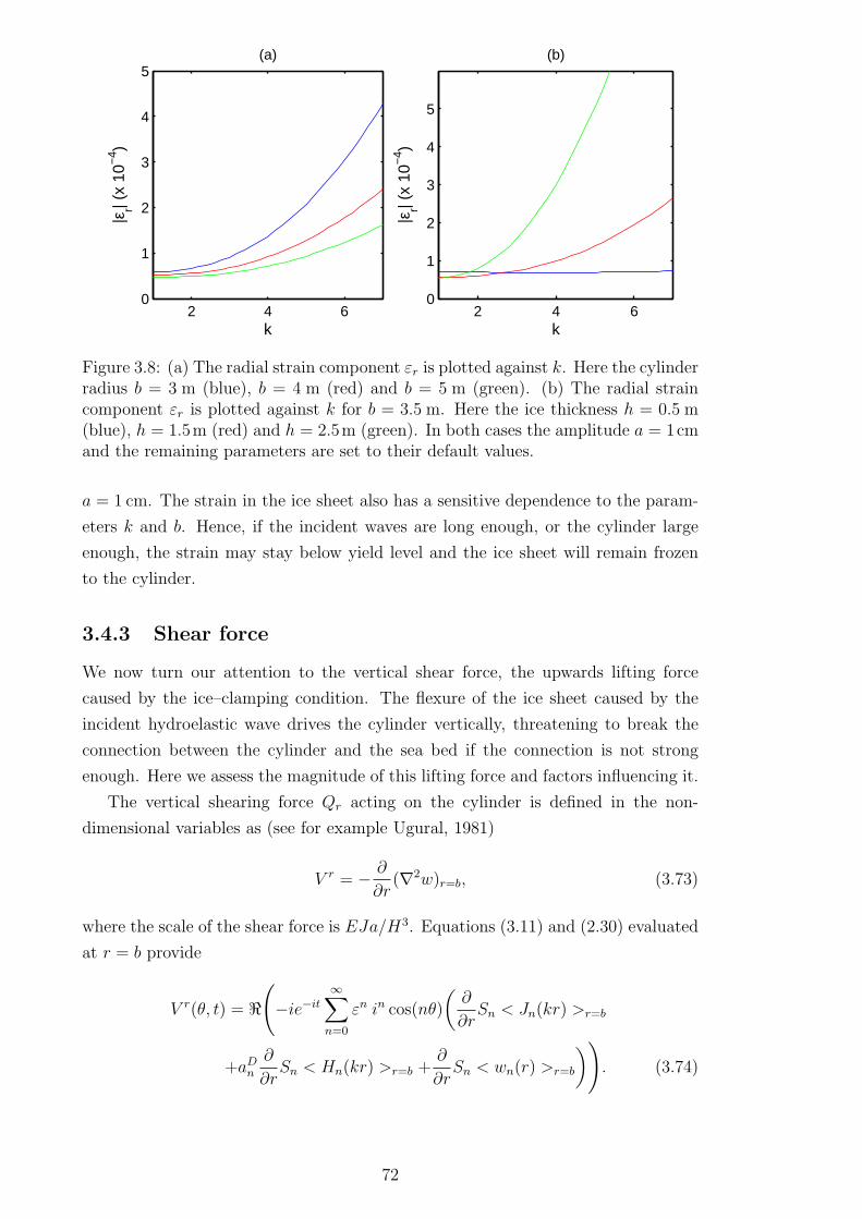
2 4 60
1
2
3
4
5(a)
k
|εr| (
x 10
−4 )
2 4 60
1
2
3
4
5
(b)
k
|εr| (
x 10
−4 )
Figure 3.8: (a) The radial strain component εr is plotted against k. Here the cylinderradius b = 3 m (blue), b = 4 m (red) and b = 5 m (green). (b) The radial straincomponent εr is plotted against k for b = 3.5 m. Here the ice thickness h = 0.5 m(blue), h = 1.5m (red) and h = 2.5m (green). In both cases the amplitude a = 1cmand the remaining parameters are set to their default values.
a = 1 cm. The strain in the ice sheet also has a sensitive dependence to the param-
eters k and b. Hence, if the incident waves are long enough, or the cylinder large
enough, the strain may stay below yield level and the ice sheet will remain frozen
to the cylinder.
3.4.3 Shear force
We now turn our attention to the vertical shear force, the upwards lifting force
caused by the ice–clamping condition. The flexure of the ice sheet caused by the
incident hydroelastic wave drives the cylinder vertically, threatening to break the
connection between the cylinder and the sea bed if the connection is not strong
enough. Here we assess the magnitude of this lifting force and factors influencing it.
The vertical shearing force Qr acting on the cylinder is defined in the non-
dimensional variables as (see for example Ugural, 1981)
V r = − ∂
∂r(∇2w)r=b, (3.73)
where the scale of the shear force is EJa/H3. Equations (3.11) and (2.30) evaluated
at r = b provide
V r(θ, t) = ℜ(
−ie−it
∞∑
n=0
εn in cos(nθ)
(
∂
∂rSn < Jn(kr) >r=b
+aDn∂
∂rSn < Hn(kr) >r=b +
∂
∂rSn < wn(r) >r=b
)
)
. (3.74)
72
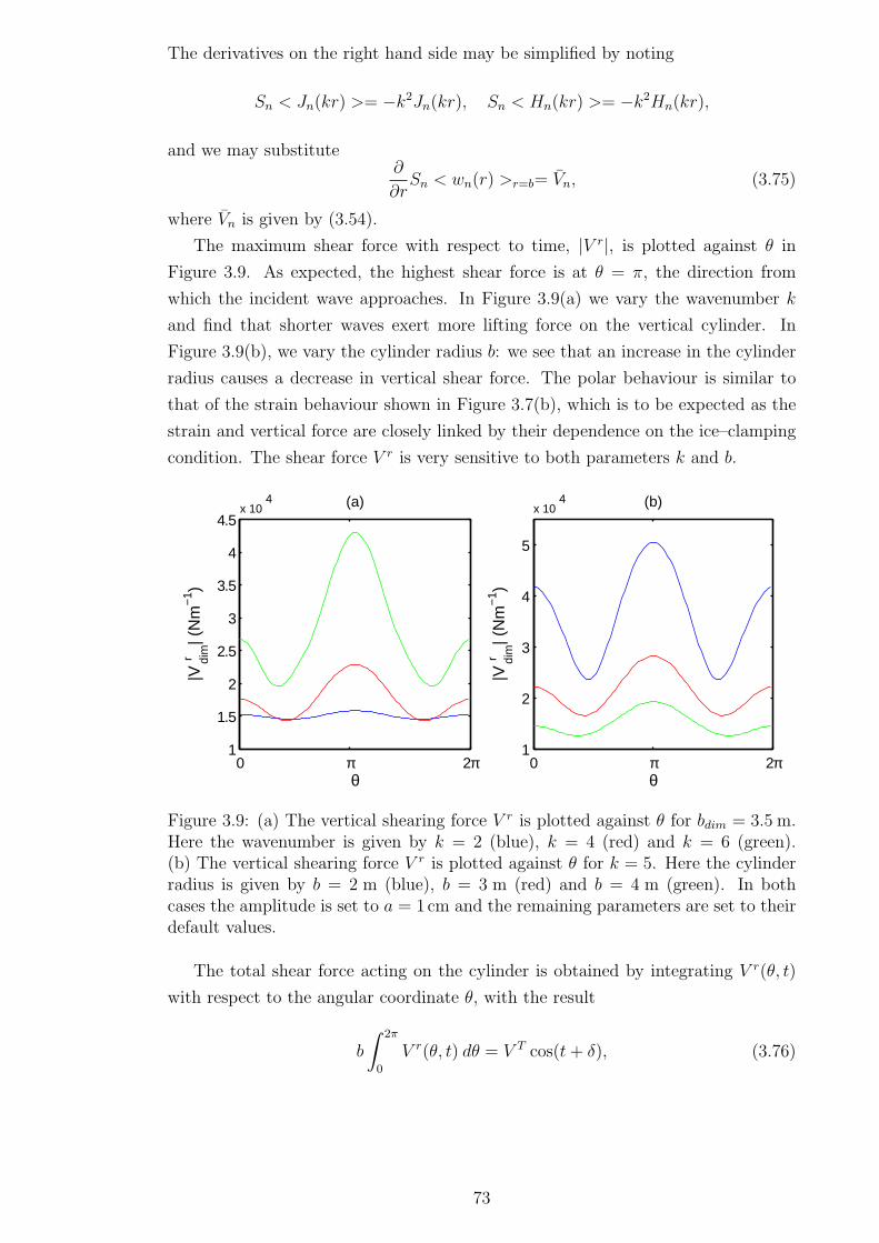
The derivatives on the right hand side may be simplified by noting
Sn < Jn(kr) >= −k2Jn(kr), Sn < Hn(kr) >= −k2Hn(kr),
and we may substitute∂
∂rSn < wn(r) >r=b= Vn, (3.75)
where Vn is given by (3.54).
The maximum shear force with respect to time, |V r|, is plotted against θ in
Figure 3.9. As expected, the highest shear force is at θ = π, the direction from
which the incident wave approaches. In Figure 3.9(a) we vary the wavenumber k
and find that shorter waves exert more lifting force on the vertical cylinder. In
Figure 3.9(b), we vary the cylinder radius b: we see that an increase in the cylinder
radius causes a decrease in vertical shear force. The polar behaviour is similar to
that of the strain behaviour shown in Figure 3.7(b), which is to be expected as the
strain and vertical force are closely linked by their dependence on the ice–clamping
condition. The shear force V r is very sensitive to both parameters k and b.
0 π 2π1
1.5
2
2.5
3
3.5
4
4.5x 10
4 (a)
θ
|V r di
m| (
Nm
−1 )
0 π 2π1
2
3
4
5
x 104 (b)
θ
|V r di
m| (
Nm
−1 )
Figure 3.9: (a) The vertical shearing force V r is plotted against θ for bdim = 3.5 m.Here the wavenumber is given by k = 2 (blue), k = 4 (red) and k = 6 (green).(b) The vertical shearing force V r is plotted against θ for k = 5. Here the cylinderradius is given by b = 2 m (blue), b = 3 m (red) and b = 4 m (green). In bothcases the amplitude is set to a = 1cm and the remaining parameters are set to theirdefault values.
The total shear force acting on the cylinder is obtained by integrating V r(θ, t)
with respect to the angular coordinate θ, with the result
b
∫ 2π
0
V r(θ, t) dθ = V T cos(t+ δ), (3.76)
73

where
V T = 2πb(u2 + v2)1
2 , (3.77)
u = J ′0(kb)
(
2k3(β0 − 1) +V (k)β0γ
)
+ Y ′0(kb)
(
2k3α0 +V (k)α0
γ
)
,
v = J ′0(kb)
(
−2k3α0 −V (k)α0
γ
)
+ Y ′0(kb)
(
2k3β0 +V (k)β0γ
)
,
aD0 = α0 + iβ0.
Note that V T is the maximum total shear force with respect to time, and the phase
shift δ is not studied here. Also note that in the integration of V r(θ, t) in (3.76)
the only contribution to the result comes from the terms with n = 0, due to the
periodicity of the cosine function. The scale of V T is equal to EJa/H2.
The total shear force V T is plotted against k in Figure 3.10, under variation of the
ice thickness. The results are very similar to those of the equivalent two–dimensional
problem, shown in Section 2.4.3. The shear force is finite in the long wave limit, and
declines to a minimum before rising again with k. There is a sensitive dependence
on the ice thickness h, with thicker ice causing higher total shear force.
2 4 6 8 100
2
4
6
8
10
12
14x 10
5 (a)
k
|VT di
m| (
N)
2 4 6 8 100
1
2
3
4
5
6
7x 10
5 (b)
bdim
(m)
|VT di
m| (
N)
Figure 3.10: (a) The total vertical shearing force V T is plotted against k for b = 3.5m.Here the ice thickness is given by h = 0.5 m (blue), h = 1.5 m (red) and h = 2.5 m(green). (b) The total vertical shearing force V T is plotted against b for k = 5. Herethe ice thickness is given by h = 0.5m (blue), h = 1.5m (red) and h = 2.5m (green).In both cases the amplitude is set to a = 1 cm and the remaining parameters areset to their default values.
Figure 3.10 shows the total shear force plotted against the cylinder radius b.
This relationship is shown to be linear, with a monotonic increase in shear force as
the cylinder radius increases. Three values of the ice thickness h are also presented,
with thicker ice again causing higher shear force. Figure 3.10 shows that the total
shear force can be substantial in magnitude, with upwards lifting forces of order
106 N possible.
74

3.4.4 Horizontal force
We now investigate the other important component of force acting on the cylinder:
the horizontal force caused by the incoming incident waves. The component of force
in the y direction is zero due to the symmetry of the problem. The component of
force in the x direction, F x, is obtained by integrating the hydrodynamic pressure
over the surface of the cylinder:
F x(t) = −b∫ 0
−1
∫ 2π
0
pD(b, θ, z, t) cos(θ)dθdz. (3.78)
The scale of the force F x is aρH3ω2. Here pD is the hydrodynamic pressure, which
can be calculated from equations (3.3), (3.10) and (3.29) as
pD(b, θ, z, t) = ℜ(
−ie−it
∞∑
n=0
εn in cos(nθ)
(
f0(z)Jn(kb)
+ aDn f0(z)Hn(kb) + ϕn(b, z)
)
)
. (3.79)
When integrating in (3.78) with respect to θ, we note that only the terms in (3.79)
with n = 1 contribute to the result, due to the orthogonality of the cosine and
sine functions. The contribution from ϕ1(b, z) in (3.79) is calculated by using (3.49)
and inverse Weber transform. After manipulations we find the non-dimensional
component of force in the positive x direction:
F x(t) = F cos(t+ δf ),
where
F =16
k3bπ2(χ21 + η21)
1
2
∫ ∞
0
(s2 − k2)Q(s) + k
s3(
(J ′1(sb))
2 + (Y ′1(sb))
2) ds (3.80)
is the maximum force with respect to time, over one period. The quantities χ1 and
η1 are given by (3.60).
The force F x is plotted against k in Figure 3.11(a), for several values of the
cylinder radius b. Starting at k = 2, as we increase k the horizontal force increases
slightly before decreasing to a minimum. As we reach k = 10, the force begins to
rise again in magnitude. The dependence on the parameter b is once again quite
sensitive, with a thicker cylinder causing considerably higher horizontal force, the
reasoning for which is apparent.
We wish to compare F x in the presence of an ice sheet, with the hydrodynamic
force acting on a vertical cylinder with no ice sheet present. From Mei (1983), the
horizontal force on a vertical cylinder due to incident free surface waves is given by
(in dimensionless variables and in the notation of this thesis):
F xfs =
4 tanh(k)
k2(
(J ′1(kb))
2 + (Y ′1(kb))
2) , (3.81)
75
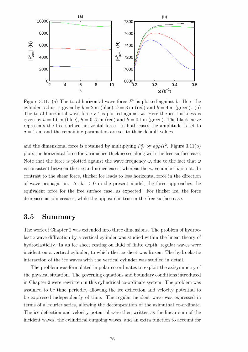
2 4 6 8 100
2000
4000
6000
8000
10000(a)
k
|Fx di
m|
(N)
0.2 0.3 0.4 0.56800
7000
7200
7400
7600
7800(b)
ω (s−1)
|Fx di
m|
(N)
Figure 3.11: (a) The total horizontal wave force F x is plotted against k. Here thecylinder radius is given by b = 2 m (blue), b = 3 m (red) and b = 4 m (green). (b)The total horizontal wave force F x is plotted against k. Here the ice thickness isgiven by h = 1.6m (blue), h = 0.75m (red) and h = 0.1m (green). The black curverepresents the free surface horizontal force. In both cases the amplitude is set toa = 1 cm and the remaining parameters are set to their default values.
and the dimensional force is obtained by multiplying F xfs by agρH
2. Figure 3.11(b)
plots the horizontal force for various ice thicknesses along with the free surface case.
Note that the force is plotted against the wave frequency ω, due to the fact that ω
is consistent between the ice and no-ice cases, whereas the wavenumber k is not. In
contrast to the shear force, thicker ice leads to less horizontal force in the direction
of wave propagation. As h → 0 in the present model, the force approaches the
equivalent force for the free surface case, as expected. For thicker ice, the force
decreases as ω increases, while the opposite is true in the free surface case.
3.5 Summary
The work of Chapter 2 was extended into three dimensions. The problem of hydroe-
lastic wave diffraction by a vertical cylinder was studied within the linear theory of
hydroelasticity. In an ice sheet resting on fluid of finite depth, regular waves were
incident on a vertical cylinder, to which the ice sheet was frozen. The hydroelastic
interaction of the ice waves with the vertical cylinder was studied in detail.
The problem was formulated in polar co-ordinates to exploit the axisymmetry of
the physical situation. The governing equations and boundary conditions introduced
in Chapter 2 were rewritten in this cylindrical co-ordinate system. The problem was
assumed to be time–periodic, allowing the ice deflection and velocity potential to
be expressed independently of time. The regular incident wave was expressed in
terms of a Fourier series, allowing the decomposition of the azimuthal co-ordinate.
The ice deflection and velocity potential were then written as the linear sum of the
incident waves, the cylindrical outgoing waves, and an extra function to account for
76

the boundary conditions on the cylinder.
The resulting boundary value problem was solved by Weber transform. This
method leads to the solution being explicitly written in terms of integral quadratures.
Numerical results were presented for the ice deflection for varying values of the
wavenumber k. The deflection and slope of the deflection were equal to zero at the
ice-cylinder boundary, as prescribed by the ice–clamping condition. The presence of
the cylinder causes disturbance in the wave profile close to the cylinder, with reduced
deflection nearby in the cylinder’s wake. The influence of the cylinder becomes more
pronounced as the incident wavelength becomes smaller, due to the cylinder radius
being small in comparison with this wavelength.
The strain in the ice at the ice-cylinder connection point was also analysed in
detail. These strains are generally high, but under certain conditions on the wave
amplitude and wavelength the connection may be maintained. It is unlikely that the
ice will remain frozen to the cylinder under the constant swell of large–amplitude
ocean waves, but in applications involving frozen lakes where one expects smaller
wave amplitude, the clamped boundary condition proves realistic. In the event of the
ice breaking off from the surface of the cylinder, the problem can be reformulated and
solved using the same method, with free edge conditions being considered instead
of the fixed edge conditions of the present problem.
Expressions for the vertical shear and horizontal force components were also
calculated. We conclude that these forces can reach large magnitudes, even for
small–amplitude, long waves. The forces must therefore be considered when design-
ing ocean structures in the presence of an ice cover. The behaviour of these forces
under variation of parameters such as the incident wavenumber, the cylinder radius
and the ice thickness was studied in detail.
An alternative method of solution that could have been used to tackle the present
problem is one utilised by Malenica & Korobkin (2003). The velocity potential in
both the free surface and ice–covered regions are expressed in terms of eigenfunction
expansions, the eigenvalues of which are the solutions of the corresponding dispersion
relation. Because the dispersion relations consist of an infinite number of imaginary
roots, the resulting series must be truncated, leading to a linear system of equations
for unknown coefficients. The Weber transform and its inherent propensity for
symmetry leads to several advantages for solving the present problem. Firstly, the
important function Q(s) appeared in the equivalent two–dimensional problem of
Chapter 2 and its properties and behaviour are therefore well known. Also Q(s)
and its behaviour govern every aspect of the problem, hence familiarity is useful.
Also, the Weber transform solution expresses the unknown coefficients aDn in terms
of exact integral quadrature. The velocity potential and ice deflection are expressed
in terms of an infinite sum, but the solution converges extremely quickly, in the
sense that few Fourier modes are required. The present method also leads to very
concise expressions for the forces on the structure. The total horizontal force given
by equation (3.80) is expressed in terms of integral quadrature, the integrand of
77

which decays rapidly. The total vertical shear force is given by (3.77), and (due to
auspicious cancellation during the Weber transform) we are not required to calculate
the third derivative, which could have led to convergence difficulties. The force is
instead expressed algebraically once the coefficient aD1 is obtained.
78
Chapter 4
Hydroelastic wave reflection by a
vertical wall in a two-layer fluid
4.1 Introduction
There are many ways to generalise the hydroelastic model in Chapter 2 and attain
more realism. One approach is to consider a fluid stratified into two layers of different
densities, as opposed to one layer of constant density. The reasoning and justification
for choosing this particular complication was discussed in Section 1.4. The physical
formulation is very similar to that of Chapter 2, and the assumptions discussed
in Section 2.1 apply here also. The incident hydroelastic wave propagates towards
the vertical wall, to which the elastic plate is clamped. The elastic plate extends
semi–infinitely and the fluid is of finite depth. Because the fluid is now stratified,
in addition to the waves propagating in the ice sheet at the surface there are also
waves at the boundary between the two layers. These are referred to as “interfacial”
or “internal” waves. We will see that there are two wavenumbers for each value of
the wave frequency, with one wavenumber representing the surface waves and the
second representing the interfacial waves.
We will derive the solution to the hydroelastic wave problem and investigate how
the stratification affects the behaviour of the solution. We will investigate whether
waves of the interfacial mode can penetrate to the surface, and vice versa. We will
consider different cases for the incident waves to investigate whether incident waves
of one mode can excite waves of another mode. Also, we compare the solution
of the present problem to that of Chapter 2, in order to assess the effect of fluid
stratification in problems of hydroelasticity. Section 4.2 recaps the mathematical
formulation of the problem and introduces new parameters. We then outline the
boundary value problem to be solved. Section 4.3 demonstrates the method of
solution. Numerical results are then presented and discussed in Section 4.4. A
summary and conclusion of the chapter are given in Section 4.5.
79

4.2 Mathematical formulation
4.2.1 Schematic and parameters
The geometry of the problem and co-ordinate system are shown in Figure 4.1. The
z
xIce sheet Incident
wave
Bed
0
-H2
wall
-H1
Fluid layer 1
Fluid layer 2 ϕ2(x,z,t)
w(x,t)
ϕ1(x,z,t)
ξ(x,t)
Figure 4.1: Schematic of a semi–infinite ice sheet meeting a vertical wall in a two-layer fluid.
formulation is similar to that outlined in Schulkes et al. (1987) with some notational
differences. We introduce Cartesian coordinates with the positive x-axis coinciding
with the ice sheet at rest and the z-axis directed vertically upwards along the wall.
Time is denoted by t. We denote the upper layer of fluid as layer 1, with density
ρ1 and velocity potential φ1(x, z, t). The lower layer of fluid, layer 2, has density
ρ2 and velocity potential φ2(x, z, t) where ρ1 < ρ2. The interface between fluids 1
and 2 at rest is at z = −H1, and the fluid bed is at z = −H2. The deflection of
the ice sheet (its vertical displacement relative to its position at rest) is denoted by
w(x, t). Similarly the vertical displacement of the interface is denoted by ξ(x, t). The
pressure in the fluid is represented by p(x, z, t). Recapping the remaining parameters
from Chapter 2: the ice has mass per unit length M , where M = ρih, ρi is the ice
density and h is the uniform ice thickness. The ice sheet has flexural rigidity EJ ,
where E is Young’s modulus and J = h3/[12(1 − ν2)], where ν is Poisson’s ratio.
The acceleration due to gravity is denoted g. The incident wave parameters are
introduced and specified after we establish the form of the incident waves.
4.2.2 Governing equations and boundary conditions
We now derive the governing differential equations for the velocity potentials, plate
deflection, and interfacial deflection. We also state the boundary conditions based
on the physical situation. The analysis is similar to that of Section 2.2.2, with some
additions to account for the two–layer fluid model. The velocity potentials in both
80

layers must satisfy Laplace’s equation in the (linearised) fluid domain:
∇2φ1 = 0, (x > 0, −H1 < z < 0), (4.1)
∇2φ2 = 0, (x > 0, −H2 < z < H1). (4.2)
Boundary conditions at the rigid wall are
φ1x = 0, (x = 0, −H1 < z < 0), (4.3)
φ2x = 0, (x = 0, −H2 < z < −H1). (4.4)
The condition at the fluid bed is
φ2z = 0, (x > 0, z = −H2). (4.5)
These conditions ensure no flow through the wall and the bed, respectively. The
linearised kinematic boundary condition at the ice-fluid boundary is given by
φ1z = wt, (x > 0, z = 0), (4.6)
and the kinematic conditions at the fluid interface are
φ1z = ξt, (x > 0, z = −H1), (4.7)
φ2z = ξt, (x > 0, z = −H1). (4.8)
The linearised Bernoulli equation for the pressure is combined with the plate equa-
tion (see Section 2.2.2) to give
EJ∇4w +Mwtt = −ρ1gw − ρ1 φ1t, (x > 0, z = 0). (4.9)
The dynamic condition at the interface is:
ρ1(φ1t + gξ) = ρ2(φ2t + gξ), (x > 0, z = −H1). (4.10)
Boundary conditions on w(x, t) are due to the ice being clamped at the wall, and
hence
w = 0, (x = 0), (4.11)
wx = 0, (x = 0). (4.12)
81

We assume that the flow is time–harmonic with period ω. Therefore we take:
φ1(x, z, t) = ℜ(
Φ1(x, z)e−iωt)
, (4.13)
φ2(x, z, t) = ℜ(
Φ2(x, z)e−iωt)
, (4.14)
w(x, t) = ℜ( i
ωW (x)e−iωt
)
, (4.15)
ξ(x, t) = ℜ( i
ωΞ(x)e−iωt
)
. (4.16)
For completeness we recast the problem in terms of the unknown variables Φ1, Φ2,
W and Ξ:
∇2Φ1 = 0, (x > 0, −H1 < z < 0), (4.17)
∇2Φ2 = 0, (x > 0, −H2 < z < −H1), (4.18)
Φ2z = 0, (x > 0, z = −H2), (4.19)
Φ1z = W, (x > 0, z = 0), (4.20)
Φ1z = Φ2z = Ξ, (x > 0, z = −H1), (4.21)
ρ1(gΞ− ω2Φ1) = ρ2(gΞ− ω2Φ2), (x > 0, z = −H1), (4.22)
EJ∇4W +W (ρ1g − ω2M) = ρ1ω2 Φ1, (x > 0, z = 0), (4.23)
Φ1x = 0, (x = 0, −H1 < z < 0), (4.24)
Φ2x = 0, (x = 0, −H2 < z < −H1), (4.25)
W = 0, (x = 0), (4.26)
Wx = 0, (x = 0). (4.27)
Conditions as x tends to infinity are not included yet in this formulation, and will
be derived in the following section.
4.2.3 Incident waves
We now derive the forms of the incident waves for Φ1, Φ2, Ξ and W . This is
equivalent to finding expressions for hydroelastic unidirectional waves propagating
in a two-layer fluid of finite depth. They must therefore satisfy equations (4.17)-
(4.22). We begin by assuming left–travelling waves of the form:
Φ1inc = B(z) e−ikx, (4.28)
Φ2inc = A(z) e−ikx, (4.29)
where A(z) and B(z) are to be found. We substitute equations (4.28)-(4.29) into
(4.17)-(4.18) to obtain
Azz − k2A = 0, (4.30)
Bzz − k2B = 0. (4.31)
82

In conjunction with the boundary condition (4.19), we find that the general solution
to equation (4.30) is
A(z) = A1(k) cosh(k(z +H2)), (4.32)
where A1 is a function of k be found. Similarly, the general solution for equation
(4.31) is
B(z) = B1(k) cosh(kz) + B2(k) sinh(kz), (4.33)
where B1 and B2 are both functions of k to be found. Using the interfacial fluid
condition (4.21), we find
B2(k) = A1(k)sinh(k(H2 −H1))
cosh(kH1)+B1(k)
sinh(kH1)
cosh(kH1).
Combining equations (4.21) and (4.22) gives
ρ1
(
g∂Φ2inc
∂z− ω2Φ1inc
)
= ρ2
(
g∂Φ2inc
∂z− ω2Φ2inc
)
, (z = −H1).
Substituting our current expressions (4.28)-(4.29) for Φ1inc and Φ2inc into this equa-
tion gives
ρ1
(
gA1(k)k sinh(k(H2 −H1))− ω2(
B1(k) cosh(kH1)− B2(k) sinh(kH1))
)
= ρ2
(
gA1(k)k sinh(k(H2 −H1))− ω2A1(k) cosh(k(H2 −H1)))
.
After considerable rearranging we obtain
B1(k) = A1(k)cosh(kH1) sinh(k(H2 −H1))
ρ1/ρ2θ(k, ω),
where we have defined
θ(k, ω) =ρ1ρ2
tanh(kH1) + coth(k(H2 −H1))−gk(ρ2 − ρ1)
ρ2ω2. (4.34)
We define
Winc(x) = a e−ikx, (4.35)
where a is the amplitude of the incident hydroelastic wave. We use the kinematic
condition (4.20) to give
a = kA1(k)(sinh(k(H2 −H1))
cosh(kH1)+
sinh(k(H2 −H1)) sinh(kH1)
ρ1/ρ2θ(k, ω)
)
,
which after more rearranging gives
A1(k) =a(ρ1/ρ2)
kχ(k, ω) sinh(kH1) sinh(k(H2 −H1)),
83
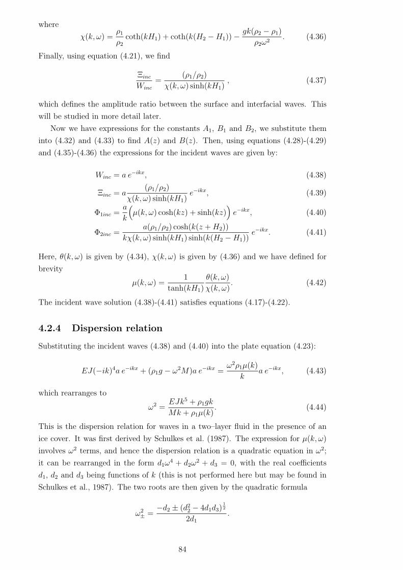
where
χ(k, ω) =ρ1ρ2
coth(kH1) + coth(k(H2 −H1))−gk(ρ2 − ρ1)
ρ2ω2. (4.36)
Finally, using equation (4.21), we find
Ξinc
Winc
=(ρ1/ρ2)
χ(k, ω) sinh(kH1), (4.37)
which defines the amplitude ratio between the surface and interfacial waves. This
will be studied in more detail later.
Now we have expressions for the constants A1, B1 and B2, we substitute them
into (4.32) and (4.33) to find A(z) and B(z). Then, using equations (4.28)-(4.29)
and (4.35)-(4.36) the expressions for the incident waves are given by:
Winc = a e−ikx, (4.38)
Ξinc = a(ρ1/ρ2)
χ(k, ω) sinh(kH1)e−ikx, (4.39)
Φ1inc =a
k
(
µ(k, ω) cosh(kz) + sinh(kz))
e−ikx, (4.40)
Φ2inc =a(ρ1/ρ2) cosh(k(z +H2))
kχ(k, ω) sinh(kH1) sinh(k(H2 −H1))e−ikx. (4.41)
Here, θ(k, ω) is given by (4.34), χ(k, ω) is given by (4.36) and we have defined for
brevity
µ(k, ω) =1
tanh(kH1)
θ(k, ω)
χ(k, ω). (4.42)
The incident wave solution (4.38)-(4.41) satisfies equations (4.17)-(4.22).
4.2.4 Dispersion relation
Substituting the incident waves (4.38) and (4.40) into the plate equation (4.23):
EJ(−ik)4a e−ikx + (ρ1g − ω2M)a e−ikx =ω2ρ1µ(k)
ka e−ikx, (4.43)
which rearranges to
ω2 =EJk5 + ρ1gk
Mk + ρ1µ(k). (4.44)
This is the dispersion relation for waves in a two–layer fluid in the presence of an
ice cover. It was first derived by Schulkes et al. (1987). The expression for µ(k, ω)
involves ω2 terms, and hence the dispersion relation is a quadratic equation in ω2;
it can be rearranged in the form d1ω4 + d2ω
2 + d3 = 0, with the real coefficients
d1, d2 and d3 being functions of k (this is not performed here but may be found in
Schulkes et al., 1987). The two roots are then given by the quadratic formula
ω2± =
−d2 ± (d22 − 4d1d3)1
2
2d1.
84
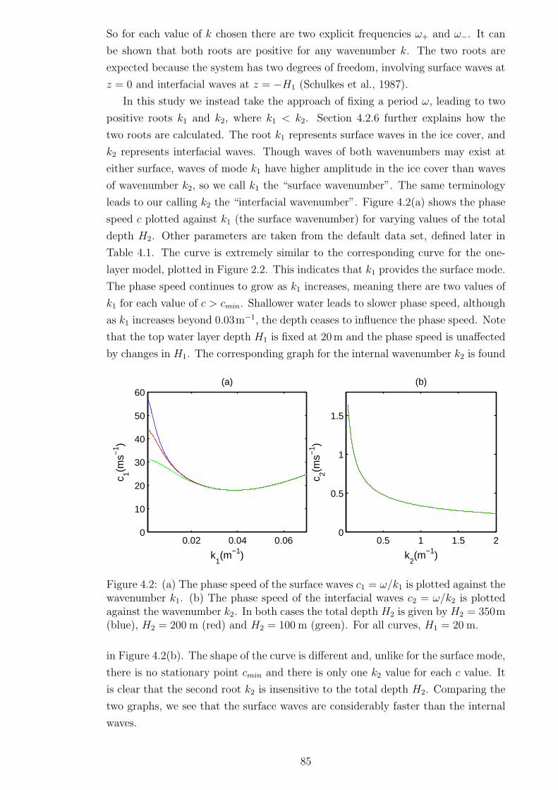
So for each value of k chosen there are two explicit frequencies ω+ and ω−. It can
be shown that both roots are positive for any wavenumber k. The two roots are
expected because the system has two degrees of freedom, involving surface waves at
z = 0 and interfacial waves at z = −H1 (Schulkes et al., 1987).
In this study we instead take the approach of fixing a period ω, leading to two
positive roots k1 and k2, where k1 < k2. Section 4.2.6 further explains how the
two roots are calculated. The root k1 represents surface waves in the ice cover, and
k2 represents interfacial waves. Though waves of both wavenumbers may exist at
either surface, waves of mode k1 have higher amplitude in the ice cover than waves
of wavenumber k2, so we call k1 the “surface wavenumber”. The same terminology
leads to our calling k2 the “interfacial wavenumber”. Figure 4.2(a) shows the phase
speed c plotted against k1 (the surface wavenumber) for varying values of the total
depth H2. Other parameters are taken from the default data set, defined later in
Table 4.1. The curve is extremely similar to the corresponding curve for the one-
layer model, plotted in Figure 2.2. This indicates that k1 provides the surface mode.
The phase speed continues to grow as k1 increases, meaning there are two values of
k1 for each value of c > cmin. Shallower water leads to slower phase speed, although
as k1 increases beyond 0.03m−1, the depth ceases to influence the phase speed. Note
that the top water layer depth H1 is fixed at 20m and the phase speed is unaffected
by changes in H1. The corresponding graph for the internal wavenumber k2 is found
0.02 0.04 0.060
10
20
30
40
50
60(a)
k1(m−1)
c 1(ms−
1 )
0.5 1 1.5 20
0.5
1
1.5
(b)
k2(m−1)
c 2(ms−
1 )
Figure 4.2: (a) The phase speed of the surface waves c1 = ω/k1 is plotted against thewavenumber k1. (b) The phase speed of the interfacial waves c2 = ω/k2 is plottedagainst the wavenumber k2. In both cases the total depth H2 is given by H2 = 350m(blue), H2 = 200 m (red) and H2 = 100 m (green). For all curves, H1 = 20 m.
in Figure 4.2(b). The shape of the curve is different and, unlike for the surface mode,
there is no stationary point cmin and there is only one k2 value for each c value. It
is clear that the second root k2 is insensitive to the total depth H2. Comparing the
two graphs, we see that the surface waves are considerably faster than the internal
waves.
85

Parameter Typical value
g 9.8 ms−2
h 1.6 mν 0.3E 4.2 x 10⁹ Nm−2
J 0.375 m3
ρi 917 kgm−3
M 1467.2 kgm−2
ρ1 1000 kgm−3
ρ2 1024 kgm−3
H1 20 mH2 350 m
Table 4.1: Values of typical parameters taken from measurements at McMurdoSound, Antarctica (Squire et al., 1988), with some additions for the two-layer fluidproblem.
Schulkes et al. (1987) noticed that some earlier results can be viewed as limiting
cases of the dispersion relation (4.44). For example, if we take ρ2 → ρ1 we have
µ(k) → coth(kH1) and we obtain the dispersion relation from Chapter 2, that is, the
dispersion relation for an elastic plate resting on a one-layer fluid of finite depth with
density ρ1. This is also the case when we consider the limit H1 → H2. Alternatively
if we take H1 → 0, we obtain the dispersion relation for an elastic plate resting on a
one-layer fluid of finite depth, but this time with density ρ2. Also, taking the limit
of very small ice thickness leads to EJ → 0 and we recover the dispersion relation
for a two-layer fluid of finite depth with no ice cover.
In this study, we will consider various depths H1 and H2, in the ranges
5 m ≤ H1 ≤ 20 m, and 100 m ≤ H2 ≤ 350 m. The density ratio ρ1/ρ2 is open to
debate, as there is little literature on the subject of varying fluid density under an ice
sheet. Schulkes et al. (1987) take an upper layer density of ρ1 = 1024 kgm−3 and a
lower layer density of ρ2 = 1025.3kgm−3. For our study, we will take ρ2 = 1024kgm−3
and vary ρ1 between 1000 kgm−3 ≤ ρ1 ≤ 1020 kgm−3, which is a wide enough range
to sufficiently demonstrate the effect of fluid stratification under an ice sheet. The
default values of each parameter, used to plot all figures, are given in Table 4.1.
Mohapatra & Bora (2009) for illustrative purposes took a density ratio of 0.5 for
the two fluid layers, and state “the values of the two roots of the dispersion equation
approach the same value ... if we take the ratio of the two densities nearer to 0.97”.
However, this is incorrect; in fact, the root k2 grows rapidly in the limit ρ1 → ρ2,
whereas k1 is insensitive to changes in ρ1. This is demonstrated in Figure 4.3.
86

0.2 0.4 0.6 0.8 1 1.2 1.4 1.6 1.8 20.93
0.94
0.95
0.96
0.97
0.98
0.99
1
k2 (m−1)
ρ 1/ρ2
Figure 4.3: The root k2 plotted against the density ratio ρ1/ρ2.
4.2.5 Nondimensionalisation
We define the dimensionless parameters/variables as
k∗ = kH2, ρ =ρ1ρ2, H =
H1
H2
, x∗ =x
H2
, z∗ =z
H2
, t∗ = ωt,
γ =EJ
H52ρ1ω
2, α =
ρ1g − ω2M
ρ1ω2H2
, β =ω2H2
g(1− ρ),
Φ∗1 =
Φ1
H2aω, Φ∗
2 =Φ2
H2aω, Ξ∗ =
ξ
aω, W ∗ =
W
aω.
The asterisks are dropped in the analysis below, and all variables are assumed di-
mensionless unless stated otherwise or accompanied by units. The parameters k1
and k2 are also assumed dimensionless.
4.2.6 Notes regarding the roots k1 and k2
Because we are fixing a constant ω and using it to calculate the values of k, the
functions θ, χ and µ are denoted as functions of k only, though we note that they
also contain ω. Now, we further discuss the calculation of the roots k1 and k2.
We can rewrite the dispersion relation (4.44) in dimensionless form as
f(k) = γk5 + αk − µ(k) = 0, (4.45)
where α and γ are coefficients defined above which depend on ω2. Because it is
impossible to rearrange the dispersion equation (4.44) to explicitly define k1 and
k2 algebraically, they are found via iterative root finding. However, we should note
87
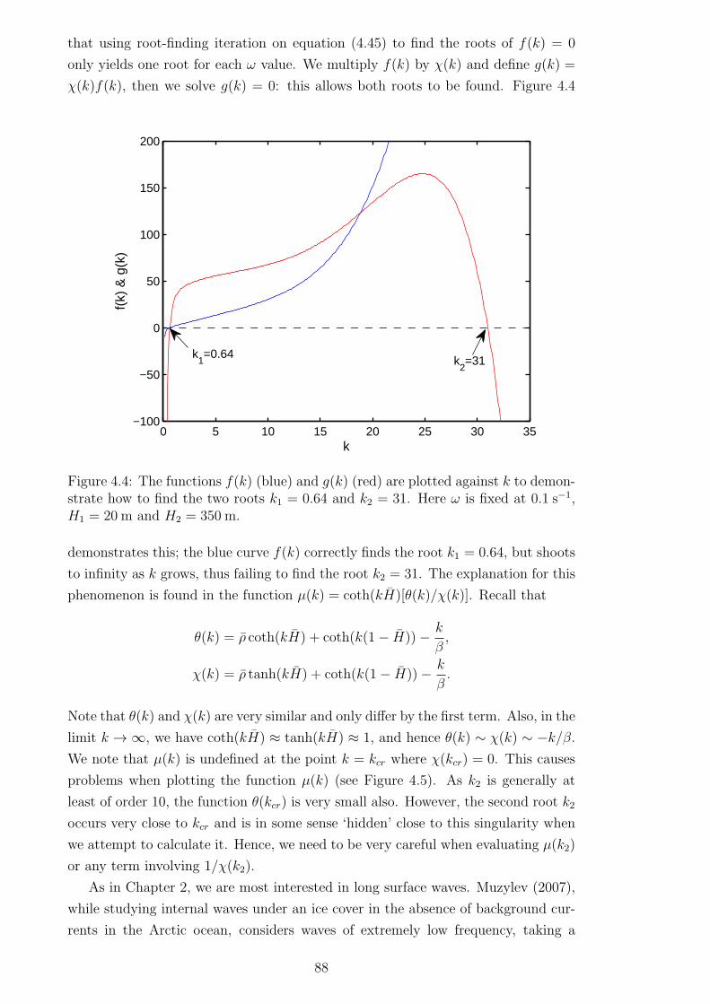
that using root-finding iteration on equation (4.45) to find the roots of f(k) = 0
only yields one root for each ω value. We multiply f(k) by χ(k) and define g(k) =
χ(k)f(k), then we solve g(k) = 0: this allows both roots to be found. Figure 4.4
0 5 10 15 20 25 30 35−100
−50
0
50
100
150
200
k
f(k)
& g
(k)
k1=0.64 k
2=31
Figure 4.4: The functions f(k) (blue) and g(k) (red) are plotted against k to demon-strate how to find the two roots k1 = 0.64 and k2 = 31. Here ω is fixed at 0.1 s−1,H1 = 20 m and H2 = 350 m.
demonstrates this; the blue curve f(k) correctly finds the root k1 = 0.64, but shoots
to infinity as k grows, thus failing to find the root k2 = 31. The explanation for this
phenomenon is found in the function µ(k) = coth(kH)[θ(k)/χ(k)]. Recall that
θ(k) = ρ coth(kH) + coth(k(1− H))− k
β,
χ(k) = ρ tanh(kH) + coth(k(1− H))− k
β.
Note that θ(k) and χ(k) are very similar and only differ by the first term. Also, in the
limit k → ∞, we have coth(kH) ≈ tanh(kH) ≈ 1, and hence θ(k) ∼ χ(k) ∼ −k/β.We note that µ(k) is undefined at the point k = kcr where χ(kcr) = 0. This causes
problems when plotting the function µ(k) (see Figure 4.5). As k2 is generally at
least of order 10, the function θ(kcr) is very small also. However, the second root k2
occurs very close to kcr and is in some sense ‘hidden’ close to this singularity when
we attempt to calculate it. Hence, we need to be very careful when evaluating µ(k2)
or any term involving 1/χ(k2).
As in Chapter 2, we are most interested in long surface waves. Muzylev (2007),
while studying internal waves under an ice cover in the absence of background cur-
rents in the Arctic ocean, considers waves of extremely low frequency, taking a
88
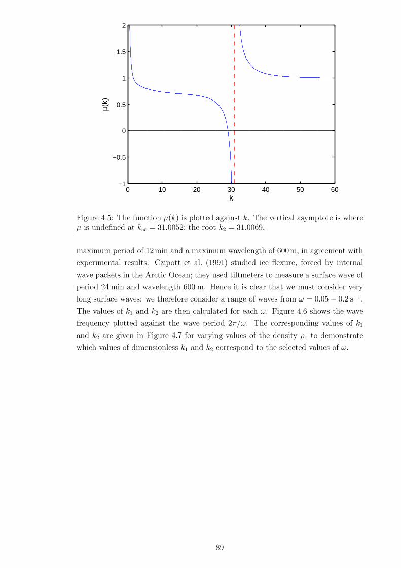
0 10 20 30 40 50 60−1
−0.5
0
0.5
1
1.5
2
k
µ(k)
Figure 4.5: The function µ(k) is plotted against k. The vertical asymptote is whereµ is undefined at kcr = 31.0052; the root k2 = 31.0069.
maximum period of 12min and a maximum wavelength of 600m, in agreement with
experimental results. Czipott et al. (1991) studied ice flexure, forced by internal
wave packets in the Arctic Ocean; they used tiltmeters to measure a surface wave of
period 24 min and wavelength 600 m. Hence it is clear that we must consider very
long surface waves: we therefore consider a range of waves from ω = 0.05− 0.2 s−1.
The values of k1 and k2 are then calculated for each ω. Figure 4.6 shows the wave
frequency plotted against the wave period 2π/ω. The corresponding values of k1
and k2 are given in Figure 4.7 for varying values of the density ρ1 to demonstrate
which values of dimensionless k1 and k2 correspond to the selected values of ω.
89
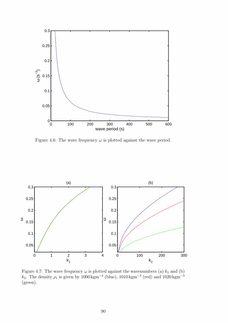
0 100 200 300 400 500 6000
0.05
0.1
0.15
0.2
0.25
0.3
wave period (s)
ω (
s−1 )
Figure 4.6: The wave frequency ω is plotted against the wave period.
0 1 2 3 4
0.05
0.1
0.15
0.2
0.25
0.3
k1
ω
(a)
0 100 200 300
0.05
0.1
0.15
0.2
0.25
0.3(b)
k2
ω
Figure 4.7: The wave frequency ω is plotted against the wavenumbers (a) k1 and (b)k2. The density ρ1 is given by 1000 kgm−3 (blue), 1010 kgm−3 (red) and 1020 kgm−3
(green).
90

4.2.7 Nondimensional BVP
We rewrite the boundary value problem (4.17)-(4.27) in terms of the dimensionless
parameters and variables defined in Section 4.2.5.
∇2Φ1 = 0, (x > 0, −H < z < 0), (4.46)
∇2Φ2 = 0, (x > 0, −1 < z < −H), (4.47)
Φ2z = 0, (x > 0, z = −1), (4.48)
Φ1z = W, (x > 0, z = 0), (4.49)
Φ1z = Φ2z = Ξ, (x > 0, z = −H), (4.50)
γ∇4W + αW = Φ1(x, 0), (x > 0, z = 0), (4.51)
Φ2z = β(Φ2 − ρΦ1), (x > 0, z = −H), (4.52)
Φ1x = 0, (x = 0, −H < z < 0), (4.53)
Φ2x = 0, (x = 0, −1 < z < −H), (4.54)
W = 0, (x = 0), (4.55)
Wx = 0, (x = 0). (4.56)
We note that the boundary value problem depends on the five dimensionless param-
eters H, ρ, α, β and γ which define the physical properties of the ice and the two
fluid layers.
4.2.8 Total forms for the potentials & deflections
In a similar manner to Chapter 2, we use linear superposition to express the total
forms of Φ1, Φ2, Ξ and W . They are expressed as the sum of an incident wave
term, a reflected wave term, and an extra function (which decreases to zero in the
far field), which describes the motion near the vertical wall. Hence we have
Φ1(x, z) = Φ1inc(x, z) + Φ1ref (x, z) + ϕ1(x, z), (4.57)
Φ2(x, z) = Φ2inc(x, z) + Φ2ref (x, z) + ϕ2(x, z), (4.58)
W (x) = Winc(x) +Wref (x) + w(x), (4.59)
Ξ(x) = Ξinc(x) + Ξref (x) + ξ(x). (4.60)
Given that there are two wavenumbers k1 and k2, we will later choose incident waves
of one mode or both. The simplest way to proceed is to define, using equations
(4.38)-(4.41);
f1(k, z) =µ(k)
kcosh(kz) +
sinh(kz)
k,
f2(k, z) =ρ cosh(k(z + 1))
k sinh(kH) sinh(k(1− H)) χ(k),
f3(k) =ρ
sinh(k1H) χ(k),
91

and then we take the forms of the incident waves as
Φ1inc = aI1 f1(k1, z) e−ik1x + aI2 f1(k2, z) e
−ik2x, (4.61)
Φ2inc = aI1 f2(k1, z) e−ik1x + aI2 f2(k2, z) e
−ik2x, (4.62)
Winc = aI1 e−ik1x + aI2 e
−ik2x, (4.63)
Ξinc = aI1 f3(k1) e−ik1x + aI2 f3(k2) e
−ik2x. (4.64)
These equations define the waves propagating towards the vertical wall from x =
+∞. Here, the coefficients aI1 and aI2 are known constants. We may choose which
values to take for aI1 and aI2 based on what kinds of incident waves we wish to
consider; waves of mode k1 or k2 or both. This is discussed more in Section 4.4. The
reflected waves are then given by
Φ1ref = aD1 f1(k1, z) e+ik1x + aD2 f1(k2, z) e
+ik2x, (4.65)
Φ2ref = aD1 f2(k1, z) e+ik1x + aD2 f2(k2, z) e
+ik2x, (4.66)
Wref = aD1 e+ik1x + aD2 e
+ik2x, (4.67)
Ξref = aD1 f3(k1) e+ik1x + aD2 f3(k2) e
+ik2x, (4.68)
where the unknown coefficients aD1 and aD2 are the reflected wave amplitudes that
must be found as part of the complete solution.
Note that even if we take incident waves of only one mode, the far–field must
account for reflected waves of both modes. This is due to the vertical wall reflection
generating waves of both modes k1 and k2. See wave–scattering in a two–layer fluid
(without an ice cover), addressed in Linton & McIver (1995).
Using equations (4.61)-(4.68) we may now rewrite the BVP (4.46)-(4.56) in terms
of the new variables ϕ1(x, z), ϕ2(x, z), w(x) and ξ(x). We include the far-field
condition that all these new variables decay as x → ∞, leaving only the reflected
92
and incident wave components in the far field.
∇2ϕ1 = 0, (x > 0, −H ≤ z ≤ 0), (4.69)
∇2ϕ2 = 0, (x > 0, −1 ≤ z ≤ −H), (4.70)
ϕ2z = 0, (x > 0, z = −1), (4.71)
ϕ1z = w, (x > 0, z = 0), (4.72)
ϕ1z = ϕ2z = ξ, (x > 0, z = −H), (4.73)
γ∇4w + αw = ϕ1(x, 0), (x > 0, z = 0), (4.74)
ϕ2z = β(ϕ2 − ρϕ1), (x > 0, z = −H), (4.75)
ϕ1x = i(aI1 − aD1 )k1f1(k1, z)
+i(aI2 − aD2 )k2f1(k2, z), (x = 0, −H ≤ z ≤ 0), (4.76)
ϕ2x = i(aI1 − aD1 )k1f2(k1, z)
+i(aI2 − aD2 )k2f2(k2, z), (x = 0, −1 ≤ z ≤ −H), (4.77)
w = −aI1 − aD1 − aI2 − aD2 , (x = 0), (4.78)
wx = ik1(aI1 − aD1 ) + ik2(a
I2 − aD2 ), (x = 0), (4.79)
ϕ1, ϕ2, w, ξ → 0, (x→ ∞). (4.80)
In the following section we outline the solution to the above boundary value problem.
4.3 Solution
4.3.1 Fourier transform
We apply Fourier cosine transforms defined by:
ϕc1(s, z) =
∫ ∞
0
ϕ1(x, z) cos(sx) dx, (4.81)
ϕc2(s, z) =
∫ ∞
0
ϕ2(x, z) cos(sx) dx, (4.82)
wc(s) =
∫ ∞
0
w(x) cos(sx) dx, (4.83)
ξc(s) =
∫ ∞
0
ξ(x) cos(sx) dx. (4.84)
As in the previous Chapters 2 and 3, we aim to use the Fourier cosine transforms
to reduce the fourth–order differential equation (4.74) to an algebraic equation. In
the following section, an algebraic expression is obtained for the velocity potentials
ϕc1 and ϕc
2.
93

4.3.2 Velocity potentials
Applying the transform to equation (4.69) gives
∫ ∞
0
[ϕ1xx + ϕ1zz] cos(sx) dx = 0,
∫ ∞
0
[ϕ1xx] cos(sx) dx+∂2
∂z2
∫ ∞
0
ϕ1 cos(sx) dx = 0.
Using integration by parts on the left hand integral gives
[ϕ1x cos(sx)]∞0 −
∫ ∞
0
ϕ1x(−s sin(sx)) dx+ ϕc1zz = 0,
and due to (4.80) this becomes
−ϕ1x(0, z) + s
∫ ∞
0
ϕ1x sin(sx) dx+ ϕc1zz = 0,
−ϕ1x(0, z) + s(
[ϕ1 sin(sx)]∞0 − s
∫ ∞
0
ϕ1 cos(sx)s dx)
+ ϕc1zz = 0,
and hence we have
ϕc1zz − s2ϕc
1 = ϕ1x(0, z), (−H ≤ z ≤ 0).
Substituting (4.76) on the right hand side gives
ϕc1zz − s2ϕc
1 = i(aI1 − aD1 )k1f1(k1, z) + i(aI2 − aD2 )k2f1(k2, z). (4.85)
Performing a similar procedure for ϕ2(x, z) leads to
ϕc2zz − s2ϕc
2 = i(aI1 − aD1 )k1f2(k1, z) + i(aI2 − aD2 )k2f2(k2, z). (4.86)
The general solutions to the ordinary differential equations with respect to z (4.85)
and (4.86) are:
ϕc1(s, z) = C1 cosh(sz) + C2 sinh(sz)
+ A1(s)k1f1(k1, z) + A2(s)k2f1(k2, z), (4.87)
ϕc2(s, z) = C3 cosh(s(z + 1)) + C4 sinh(s(z + 1))
+ A1(s)k1f2(k1, z) + A2(s)k2f2(k2, z), (4.88)
where Ci(s) are functions of s and are constant with respect to z, and for brevity
we have defined the functions
A1(s) = iaI1 − aD1k21 − s2
,
A2(s) = iaI2 − aD2k22 − s2
.
94
The four boundary conditions come from the Fourier cosine transform of (4.71),
(4.72), (4.73) and (4.75) respectively:
ϕc2z = 0, (z = −1), (4.89)
ϕc1z = W c, (z = 0), (4.90)
ϕc1z = ϕc
2z, (z = −H), (4.91)
ϕc2z = β(ϕc
2 − ρϕc1), (z = −H). (4.92)
Now we find Ci(s). We begin with C4 by substituting (4.89) into general solution
(4.88) to find
C4s+ A1f2z(k1,−1)− A2f2z(k2,−1) = 0,
which leads to
C4 = 0.
Next, for C2, we substitute (4.90) into (4.87) to give
C2s+ A1f1(k1, 0) + A2f1(k2, 0) = wc,
which rearranges to
C2 =wc
s− A1
k1s
− A2k2s.
For C3, we use condition (4.91) with (4.87) and (4.88):
−C1s sinh(sH) + C2s cosh(sH) + A1f1z(k1,−H) + A2f1z(k2,−H)
= C3s sinh(s(1− H)) + A1f2z(k1,−H) + A2f2z(k2,−H). (4.93)
This can be rearranged to give
C3 =1
s sinh(s(1− H))
(
−C1s sinh(sH) + C2s cosh(sH)
+ A1[f1z(k1,−H)− f2z(k1,−H)] + A2[f1z(k2,−H)− f2z(k2,−H)])
.
95

Now, the terms in the two square brackets are both of the form
f1z(k,−H)− f2z(k,−H) =
= −µ(k)k sinh(kH) + k cosh(kH)− ρk sinh(k(1− H))
sinh(kH) sinh(k(1− H)) χ(k)
= k cosh(kH)− k cosh(kH)θ(k)
χ(k)− ρk
sinh(kH)χ(k)
=k
χ(k)
(
cosh(kH)[χ(k)− θ(k)]− ρ
sinh(kH)
)
=k
χ(k)
(
cosh(kH)[ρ coth(kH)− ρ tanh(kH)]− ρ
sinh(kH)
)
=k
χ(k)
(
ρ
sinh(kH)[cosh2(kH)− sinh2(kH)]− ρ
sinh(kH)
)
=k
χ(k)
(
ρ
sinh(kH)− ρ
sinh(kH)
)
= 0.
Hence we have
C3 =1
s sinh(s(1− H))
(
−C1s sinh(sH) + C2s cosh(sH))
. (4.94)
Lastly, we use condition (4.92) with (4.87) and (4.88) to give
C3s sinh(s(1− H)) + A1f2z(k1,−H) + A2f2z(k2,−H)
= β(
C3 cosh(s(1− H)) + A1f2(k1,−H) + A2f2(k2, H)
−ρ{
C1 cosh(sH)− C2 sinh(sH) + A1f1(k1,−H) + A2f1(k2,−H)}
)
,
which rearranges to
C3
(
s sinh(s(1− H))− β cosh(s(1− H)))
= −βρC1 cosh(sH) + βρC2 sinh(sH)
+A1[βf2(k1,−H)− βρf1(k1,−H)− f2z(k1,−H)]
+A2[βf2(k2,−H)− βρf2(k1,−H)− f2z(k2,−H)].
96

Evaluating the terms in the square brackets gives
βf2(k,−H)− βρf1(k,−H)− f2z(k,−H) =
= βρ
(
cosh(k(1− H))
sinh(kH) sinh(k(1− H)) χ(k)− cosh2(kH)
sinh(kH)
θ(k)
χ(k)
+ sinh(kH)− k
β sinh(kH)χ(k)
)
=βρ
χ(k) sinh(kH)
(
coth(k(1− H))− θ(k) cosh2(kH) + χ(k) sinh2(kH)− k
β
)
=βρ
χ(k) sinh(kH)
(
coth(k(1− H)) +(
χ(k)− θ(k))
sinh2(kH)− θ(k)− k
β
)
=βρ
χ(k) sinh(kH)
(
coth(k(1− H)) +(
coth(kH)− tanh(kH))
ρ sinh2(kH)
− θ(k)− k
β
)
=βρ
χ(k) sinh(kH)
(
coth(k(1− H)) +(
cosh2(kH)− sinh2(kH))
ρsinh(kH)
cosh(kH)
− θ(k)− k
β
)
=βρ
χ(k) sinh(kH)
(
coth(k(1− H)) + ρ tanh(kH)− k
β− θ(k)
)
=βρ
χ(k) sinh(kH)
(
θ(k)− θ(k)
)
= 0.
Hence we have
C3 =−βρC1 cosh(sH) + βρC2 sinh(sH)
s sinh(s(1− H))− β cosh(s(1− H)). (4.95)
We now have two equations (4.94) and (4.95) for C3 in terms of C1 and C2:
C3
(
s sinh(s(1− H))− β cosh(s(1− H)))
= −βρC1 cosh(sH) + βρC2 sinh(sH),
C3
(
s sinh(s(1− H)))
= C2s cosh(sH)− C1s sinh(sH).
Dividing the first equation by the second gives:
1− β
scoth(s(1− H)) =
−βρC1 cosh(sH) + βρC2 sinh(sH)
C2s cosh(sH)− C1s sinh(sH),
97

Dividing both sides by β and factorising gives:
C2
(
ρ sinh(sH)− s cosh(sH)
{
1
β− 1
scoth(s(1− H))
}
)
= C1
(
ρ cosh(sH)− s sinh(sH)
{
1
β− 1
scoth(s(1− H))
}
)
,
Hence we have
C1 = C2cosh(sH)
sinh(sH)
(
ρ tanh(sH) + coth(s(1− H))− sβ
ρ coth(sH) + coth(s(1− H))− sβ
)
C1 = C2 µ(s).
To summarise, we have established that the functions Ci are given by:
C1 =wc µ(s)
s− A1
k1µ(s)
s− A2
k2µ(s)
s, (4.96)
C2 =wc
s− A1
k1s
− A2k2s, (4.97)
C3 =(
wc − A1k1 − A2k2
)cosh(sH)− µ(s) sinh(sH)
s sinh(s(1− H)), (4.98)
C4 = 0. (4.99)
The velocity potentials ϕc1 and ϕc
2 are then given by substituting (4.96)-(4.99) into
the general solutions (4.87) and (4.88). However, the solution is not yet complete
as C1-C4 are in terms of wc(s) which is still unknown at this point. In addition the
coefficients aD1 and aD2 (contained within A1 and A2) must be determined.
4.3.3 Plate deflection
Applying the Fourier cosine transform to the ice plate equation (4.74) gives
γ
∫ ∞
0
wxxxx cos(sx) dx+ αwc = ϕc1(s, 0). (4.100)
98
We can evaluate the integral by repetitive integration by parts. Combined with the
use of equation (4.80) this gives:
∫ ∞
0
wxxxx cos(sx) dx
=(
wxxx cos(sx))∞0+ s
∫ ∞
0
wxxx sin(sx) dx
= −wxxx(0) + s(
(
wxx sin(sx))∞0−∫ ∞
0
wxxs cos(sx) dx)
= −wxxx(0)− s2∫ ∞
0
wxx cos(sx) dx
= −wxxx(0)− s2(
(
wx cos(sx))∞0+
∫ ∞
0
wxs sin(sx) dx)
= −wxxx(0) + s2wx(0)− s3∫ ∞
0
wx sin(sx) dx
= −wxxx(0) + s2wx(0)− s3(
(
w sin(sx))∞0−∫ ∞
0
ws cos(sx) dx)
= −wxxx(0) + s2wx(0) + s4wc(s). (4.101)
Rearranging, we have
wc(s4γ + α) = ϕc1(s, 0) + γ(wxxx(0)− s2wx(0)),
and substituting for ϕ1(s, 0) using our results from Section 4.3.2 gives:
wc(s4γ + α) =wcµ(s)
s− A1
k1µ(s)
s− A2
k1µ(s)
s
+ A1f1(k1, 0) + A2f1(k2, 0) + γ(wxxx(0)− s2wx(0)).
(4.102)
Substituting for f1(k, 0) and using equation (4.79) to substitute for wx(0) we find:
wc(
s4γ + α− µ(s))
=i(aI1 − aD1 )
k21 − s2
(
µ(k1)−k1µ(s)
s− s2γk1(k
21 − s2)
)
+i(aI2 − aD2 )
k22 − s2
(
µ(k2)−k2µ(s)
s− s2γk2(k
22 − s2)
)
+ γwxxx(0).
We multiply each side of this equation by s χ(s) tanh(sH) and we arrive at
wc(s) =
i(aI1−aD
1)
k21−s2
M(k1, s) +i(aI
2−aD
2)
k22−s2
M(k2, s) + γwxxx(0)s χ(s) tanh(sH)
s χ(s) tanh(sH)(
γs4 + α)
− θ(s). (4.103)
Here the function M(k, s) is defined as
M(k, s) = s θ(k)χ(s) tanh(sH)
χ(k) tanh(kH)− kθ(s)− s3γk(k2 − s2)χ(s) tanh(sH). (4.104)
99

Note that at s = k, M = 0 algebraically. Hence, terms involving M(k, s)/(k2 − s2)
in the numerator of (4.103) are not undefined as s → k, but are finite and may be
calculated by using l’Hopital’s rule. The function M(k, s) is plotted in Figure 4.8
for both k = k1 and k = k2.
0 10 20 30−150
−100
−50
0
50
100(a)
s
M(k
1,s)
0 10 20 30−6000
−4000
−2000
0
2000
4000
6000
8000
10000
12000(b)
s
M(k
2,s)
Figure 4.8: The functions (a) M(k1, s) and (b) M(k2, s) are plotted against s. Thedefault data set is used for both graphs with ω = 0.1s−1 (giving k1 = 0.64, k2 = 31).
At this stage, there are 3 unknown quantities in equation (4.103), namely aD1 ,
aD2 and wxxx(0). We note that the denominator of equation (4.103) is the dispersion
relation as a function of s instead of k; therefore, the denominator is equal to zero
when s = k1 or s = k2. Hence, we require the numerator to also equal zero when
s = k1 and s = k2 to avoid a singularity. We may use this fact to find expressions
for two of the unknowns, wxxx and aD2 .
Firstly we assess the limit of the numerator of (4.103) as s→ k2. We require
0 =i(aI1 − aD1 )
k21 − k22M(k1, k2) + i(aI2 − aD2 ) lim
s→k2
M(k2, s)
k22 − s2+ γwxxx(0)k2 χ(k2) tanh(k2H),
and we may rearrange to give
wxxx(0) = −i(aI2 − aD2 )m2 +
i(aI1−aD
1)
k21−k2
2
M(k1, k2)
γχ(k2) tanh(k2H)k2. (4.105)
Here we have defined the constant m2 as
m2 = lims→k2
M(k2, s)
k22 − s2. (4.106)
This limit can be evaluated easily by applying l’Hopital’s rule. We now evaluate the
limit of the numerator in (4.103) as s→ k1, again requiring this limit to equal zero.
100

This gives
0 = i(aI1 − aD1 ) lims→k1
M(k1, s)
k21 − s2+ i(aI2 − aD2 )
M(k2, k1)
k22 − k21
− χ(k1) tanh(k1H)k1χ(k2) tanh(k2H)k2
(
i(aI2 − aD2 )m2 +i(aI1 − aD1 )
k21 − k22M(k1, k2)
)
. (4.107)
We now define
m1 = lims→k1
M(k1, s)
k21 − s2, (4.108)
and we can rearrange (4.107) to give
aI2 − aD2 = c(aI1 − aD1 ), (4.109)
where we have defined the constant c as
c =m1 − χ(k1) tanh(k1H)k1
χ(k2) tanh(k2H)k2
M(k1,k2)
k21−k2
2
χ(k1) tanh(k1H)k1χ(k2) tanh(k2H)k2
m2 − M(k2,k1)
k22−k2
1
. (4.110)
Hence, we now have an expression for the unknown aD2 in terms of aD1 , and we can
rewrite the solution for the deflection as
wc = i(aI1 − aD1 )Q(s), (4.111)
where
Q(s) =
M(k1,s)
k21−s2
+ cM(k2,s)
k22−s2
− χ(s) tanh(sH)s
χ(k2) tanh(k2H)k2
(
m2c+M(k1,k2)
k21−k2
2
)
s χ(s) tanh(sH)(
γs4 + α)
− θ(s). (4.112)
The function Q(s) is smooth and is finite at s = k1 and s = k2. This function defines
the behaviour of the ice deflection in the vicinity of the vertical wall, allowing all
conditions for the problem to be satisfied. Taking the limit of Q(s) as H1 → H2 or
H1 → 0 or ρ1 → ρ2 will lead to the same function Q(s) derived in the one-layer fluid
problem in Chapter 2. Figure 4.9 shows Q(s) plotted against s for various values of
the frequency ω.
The solution is still not yet complete as we have yet to find an expression for
aD1 . We note that we have two equations for w(0); one is given by equation (4.78),
and the other given by performing an inverse transform on equation (4.111) and
evaluating at x = 0. Hence we have
w(0) = −aI1 − aD1 − aI2 − aD2 ,
w(0) =2
πi(aI1 − aD1 )
∫ ∞
0
Q(s) ds.
Defining τ = 2π
∫∞0Q(s) ds, equating these and substituting for aD2 using (4.109)
101
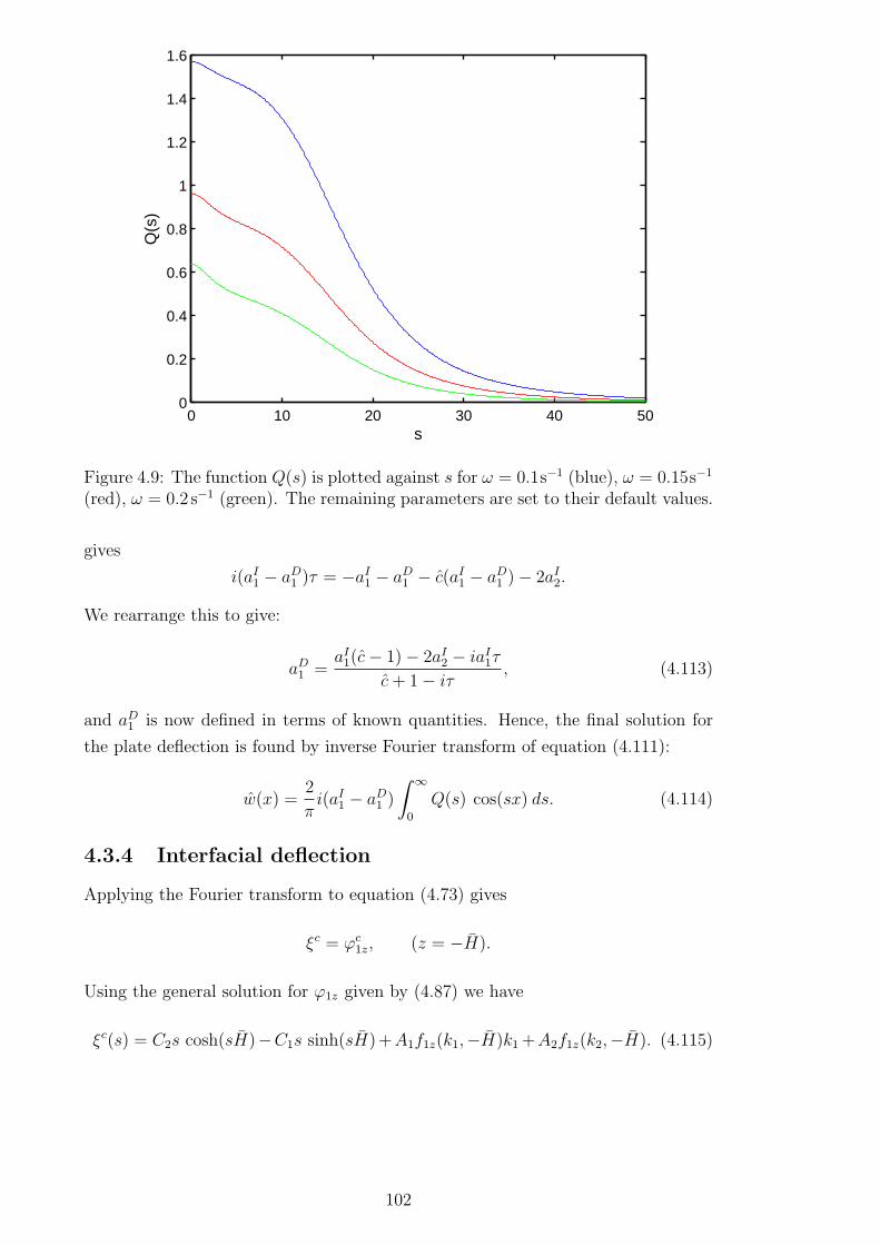
0 10 20 30 40 500
0.2
0.4
0.6
0.8
1
1.2
1.4
1.6
s
Q(s
)
Figure 4.9: The function Q(s) is plotted against s for ω = 0.1s−1 (blue), ω = 0.15s−1
(red), ω = 0.2 s−1 (green). The remaining parameters are set to their default values.
gives
i(aI1 − aD1 )τ = −aI1 − aD1 − c(aI1 − aD1 )− 2aI2.
We rearrange this to give:
aD1 =aI1(c− 1)− 2aI2 − iaI1τ
c+ 1− iτ, (4.113)
and aD1 is now defined in terms of known quantities. Hence, the final solution for
the plate deflection is found by inverse Fourier transform of equation (4.111):
w(x) =2
πi(aI1 − aD1 )
∫ ∞
0
Q(s) cos(sx) ds. (4.114)
4.3.4 Interfacial deflection
Applying the Fourier transform to equation (4.73) gives
ξc = ϕc1z, (z = −H).
Using the general solution for ϕ1z given by (4.87) we have
ξc(s) = C2s cosh(sH)−C1s sinh(sH)+A1f1z(k1,−H)k1+A2f1z(k2,−H). (4.115)
102

We substitute for C1 and C2 using (4.96) and (4.97), and evaluate f1z to give:
ξc(s) = s cosh(sH)
(
wC
s− A1
k1s
− A2k2s
)
− s sinh(sH)
(
wCµ(s)
s− A1
k1µ(s)
s− A2
k2µ(s)
s
)
+ A1
(
−µ(k1)k1 sinh(k1H) + k1 cosh(k1H)
)
+ A2
(
−µ(k2)k2 sinh(k2H) + k2 cosh(k2H)
)
,
ξc(s) = wc(
cosh(sH)− µ(s) sinh(sH))
+i(aI1 − aD1 )
k21 − s2k1
(
µ(s) sinh(sH)− cosh(sH)
+ cosh(k1H)− µ(k1) sinh(k1H)
)
+i(aI2 − aD2 )
k22 − s2k1
(
µ(s) sinh(sH)− cosh(sH)
+ cosh(k2H)− µ(k2) sinh(k2H)
)
.
We use the expression cosh(sH) − µ(s) sinh(sH) = ρ/(χ(s) sinh(sH)) to simplify
and substitute for aD2 using equation (4.109). This leads us to:
ξc(s) = i(aI1 − aD1 )ρ L(s), (4.116)
where the function L(s) is given by
L(s) =Q(s) + k1
k21−s2
(
χ(s) sinh(sH)
χ(k1) sinh(k1H)− 1)
+ k2k22−s2
(
χ(s) sinh(sH)
χ(k2) sinh(k2H)− 1)
χ(s) sinh(sH). (4.117)
Note that the bracketed terms in the numerator of (4.117) are zero as s → k1 and
s → k2 respectively. This means there are no singularities due to the 1/(k2 − s2)
terms in the limits s→ k . As noted previously, there is a zero in the denominator
where k = kcr, leading to χ(kcr) = 0. Hence, we need to verify that the numerator
is also zero at this point. Denoting the numerator of L(s) as Lnum, we have
Lnum(kcr) = Q(kcr)−k1
k21 − k2cr− k2c
k22 − k2cr. (4.118)
103

Returning to the equation for Q(s) given by (4.112), we have
Q(kcr) =
M(k1,kcr)
k21−k2cr
+ cM(k2,kcr)
k22−k2cr
−θ(kcr), (4.119)
and by our definition of the function M given by (4.104) we have M(k, kcr) =
−kθ(kcr). Hence,Q(kcr) =
k1k21 − k2cr
+ ck2
k22 − k2cr,
and substituting this into (4.119) confirms that Lnum(kcr) = 0 identically.
0 10 20 30 40 500
0.5
1
1.5
s
L(s)
Figure 4.10: The function L(s) is plotted against s for ω = 0.1s−1 (blue), ω = 0.15s−1
(red), ω = 0.2 s−1 (green). The remaining parameters are set to their default values.
Figure 4.10 shows the functions L(s) plotted against s for varying values of ω.
We note that L(s) shows similar characteristics to the function Q(s). Also, L(s)
decays rapidly as s → ∞. The final solution for the interfacial deflection is found
by inverse Fourier transform of equation (4.116):
ξ(x) =2
πiρ(aI1 − aD1 )
∫ ∞
0
L(s) cos(sx) ds. (4.120)
4.4 Numerical results
Results are now presented for the solution in Section 4.3. Note that the inverse
transforms are too complicated to calculate analytically and hence are calculated
numerically. Recall that the default values of the parameters are given by Table 4.1.
We consider 3 different cases for the results;
104

(i) Incident waves with mode k1 only, representing surface waves. In this case we
take the parameters aI1 = 1 and aI2 = 0. This scales the incident surface wave
amplitude to 1, allowing us to compare the interfacial response.
(ii) Incident waves with mode k2 only, representing interfacial waves. In this case
we take the parameter aI2 = f−13 (k2). This scales the incident interfacial am-
plitude to 1, allowing us to compare the surface response.
(iii) Incident waves with modes k1 and k2, representing both surface and interfa-
cial waves. In this case, the relationship between aI1 and aI2 must be estimated
based on realistic observations, of which little is available. We take aI2 =
f−13 (k2), scaling the incident k2 wave amplitude to 1, and choose aI1 = 0.01.
This estimates that the incident interfacial wave amplitude is 100 times larger
than the incident surface wave amplitude. It should be noted that this ra-
tio represents just one possible choice; results should be more qualitatively
interpreted than quantitatively.
We note that the three cases have different amplitude scales, which must be borne
in mind when directly comparing results between each case.
4.4.1 Plate & interfacial deflection
We return to the total, non-periodic forms of the deflections w(x, t) and ξ(x, t). We
define
winv(x) =
∫ ∞
0
Q(s) cos(sx) ds,
ξinv(x) =
∫ ∞
0
L(s) cos(sx) ds.
We also express aD1 in the form aD1 = aR + iaI by multiplying equation (4.113) by
the complex conjugate of the denominator. This gives
aR =aI1(c− 1)(c+ 1)− 2aI2(c+ 1) + aI1τ
2
(c+ 1)2 + τ 2, (4.121)
aI =−2aI1τ − 2aI2τ
(c+ 1)2 + τ 2. (4.122)
We substitute the solutions (4.114) and (4.120) into the total forms forW (x) and
Ξ(x) given by equations (4.59) and (4.60), and finally return to the time-dependent
105

solution using equations (4.15) and (4.16). This gives:
w(x, t) = sin(t)
(
aI1 cos(k1x) + aI2 cos(k2x) + aR cos(k1x)− aI sin(k1x)
+(
aI2 − c(aI1 − aR))
cos(k2x)− caI sin(k2x) +2
πaIwinv(x)
)
+ cos(t)
(
aI1 sin(k1x) + aI2 sin(k2x)− aI cos(k1x)− aR sin(k1x)
−(
aI2 − c(aI1 − aR))
sin(k2x)− caI cos(k2x) +2
π(aI1 − aR)winv(x)
)
,
ξ(x, t) = sin(t)
(
aI1f3(k1) cos(k1x) + aI2f3(k2) cos(k2x) + aRf3(k1) cos(k1x)
− aIf3(k1) sin(k1x) +(
aI2 − c(aI1 − aR))
f3(k2) cos(k2x)
− caIf3(k2) sin(k2x) +2
πaIξinv(x)
)
+ cos(t)
(
aI1f3(k1) sin(k1x)
+ aI2f3(k2) sin(k2x)− aIf3(k1) cos(k1x)− aRf3(k1) sin(k1x)
−(
aI2 − c(aI1 − aR))
f3(k2) sin(k2x)− caIf3(k2) cos(k2x)
+2
π(aI1 − aR)ξinv(x)
)
.
Note that the moduli of the deflections were calculated in the same way as Chapter
2 to remove time as a factor from the plots.
Case (i): aI1 = 1, aI2 = 0.
We first investigate the case where we consider only incident waves of mode k1, that
is, incident waves of the surface mode.
Figure 4.11 shows the plate and interfacial deflection for the frequency ω =
0.2 s−1. Firstly we notice that the deflection and the slope of the deflection are 0
at the point x = 0, as required by the ice–clamping conditions. The ice deflection
shows similar characteristics to the equivalent one-layer problem: the vertical wall
affects the shape of the first wave peak closest to the wall. We notice that the
interfacial deflection is similar in amplitude to the plate deflection. There is no
appearance of the mode k2 for this value of ω. This is because k2 is large enough
that the parameter c is very small, which dampens any term involving the interfacial
mode.
Figure 4.12 shows the deflections for the frequency ω = 0.1 s−1. For the plate
deflection, we notice the increased wavelength of k1 and there is also slightly more
disturbance in the first wave peak closest to the wall. For the interfacial deflection we
106
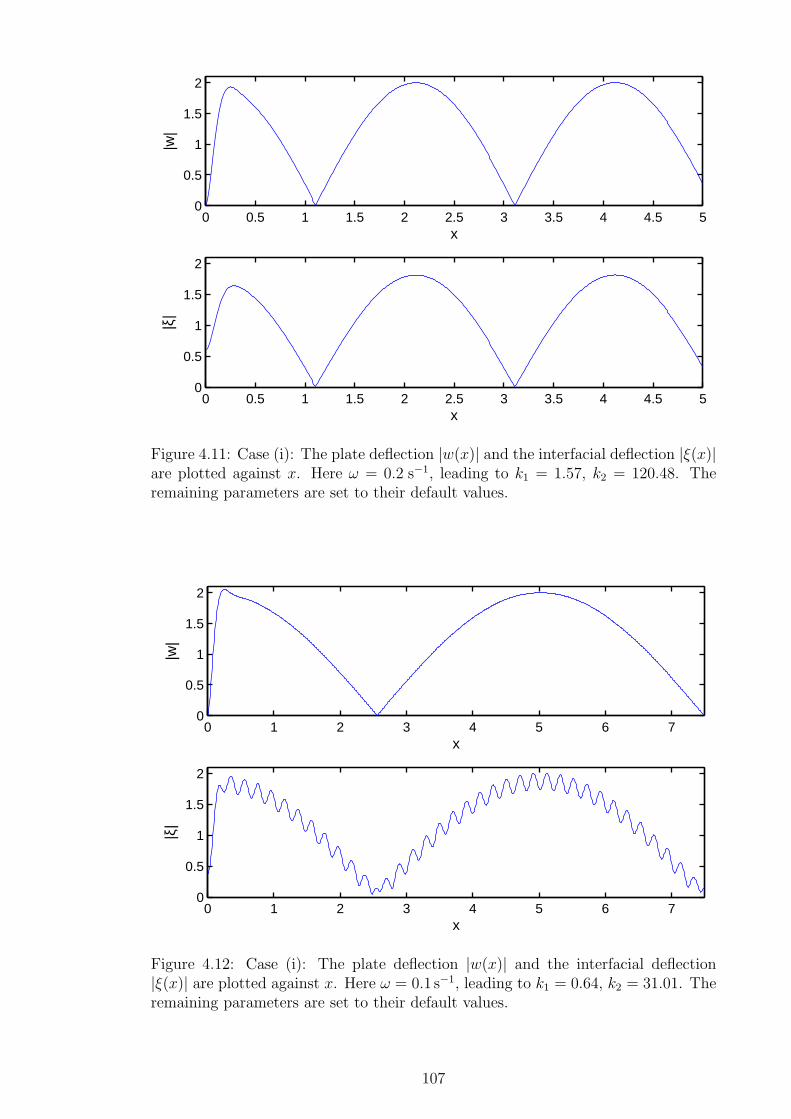
0 0.5 1 1.5 2 2.5 3 3.5 4 4.5 50
0.5
1
1.5
2
x
|w|
0 0.5 1 1.5 2 2.5 3 3.5 4 4.5 50
0.5
1
1.5
2
x
|ξ|
Figure 4.11: Case (i): The plate deflection |w(x)| and the interfacial deflection |ξ(x)|are plotted against x. Here ω = 0.2 s−1, leading to k1 = 1.57, k2 = 120.48. Theremaining parameters are set to their default values.
0 1 2 3 4 5 6 70
0.5
1
1.5
2
x
|w|
0 1 2 3 4 5 6 70
0.5
1
1.5
2
x
|ξ|
Figure 4.12: Case (i): The plate deflection |w(x)| and the interfacial deflection|ξ(x)| are plotted against x. Here ω = 0.1 s−1, leading to k1 = 0.64, k2 = 31.01. Theremaining parameters are set to their default values.
107
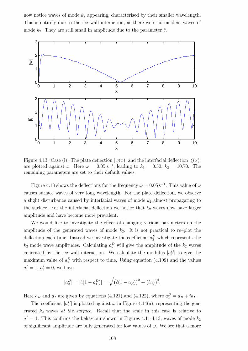
now notice waves of mode k2 appearing, characterised by their smaller wavelength.
This is entirely due to the ice–wall interaction, as there were no incident waves of
mode k2. They are still small in amplitude due to the parameter c.
0 1 2 3 4 5 6 7 8 9 100
1
2
3
x
|w|
0 1 2 3 4 5 6 7 8 9 100
1
2
3
x
|ξ|
Figure 4.13: Case (i): The plate deflection |w(x)| and the interfacial deflection |ξ(x)|are plotted against x. Here ω = 0.05 s−1, leading to k1 = 0.30, k2 = 10.70. Theremaining parameters are set to their default values.
Figure 4.13 shows the deflections for the frequency ω = 0.05 s−1. This value of ω
causes surface waves of very long wavelength. For the plate deflection, we observe
a slight disturbance caused by interfacial waves of mode k2 almost propagating to
the surface. For the interfacial deflection we notice that k2 waves now have larger
amplitude and have become more prevalent.
We would like to investigate the effect of changing various parameters on the
amplitude of the generated waves of mode k2. It is not practical to re–plot the
deflection each time. Instead we investigate the coefficient aD2 which represents the
k2 mode wave amplitudes. Calculating aD2 will give the amplitude of the k2 waves
generated by the ice–wall interaction. We calculate the modulus |aD2 | to give the
maximum value of aD2 with respect to time. Using equation (4.109) and the values
aI1 = 1, aI2 = 0, we have
|aD2 | = |c(1− aD1 )| =√
(
c(1− aR))2
+(
caI)2.
Here aR and aI are given by equations (4.121) and (4.122), where aD1 = aR + iaI .
The coefficient |aD2 | is plotted against ω in Figure 4.14(a), representing the gen-
erated k2 waves at the surface. Recall that the scale in this case is relative to
aI1 = 1. This confirms the behaviour shown in Figures 4.11-4.13; waves of mode k2
of significant amplitude are only generated for low values of ω. We see that a more
108

0.04 0.06 0.08 0.10
0.005
0.01
0.015(a)
ω(s−1)
|a2D|
0.04 0.06 0.08 0.1 0.12 0.140
0.2
0.4
0.6
0.8
1
1.2
1.4(b)
ω(s−1)
f 3(k2)
|a2D|
Figure 4.14: Case (i): The coefficients (a) |aD2 | and (b) f3(k2)|aD2 | are plottedagainst ω, where the density ρ1 is given by 1000kgm−3 (blue), 1010kgm−3 (red) and1020 kgm−3 (green).
pronounced density difference between the two layers permits generated k2 waves
of higher amplitude. This is because as ρ1 approaches ρ2, k2 grows and hence the
waves have much smaller wavelength which cannot propagate through the elastic
surface. Figure 4.15(a) shows the effect the parameter H1 has on this coefficient.
Interestingly the value H1 = 10m seems to generate the highest k2 wave amplitudes.
It is clear that depth H1 has a noticeable affect on |aD2 | for low values of ω. As ω
increases beyond 0.1 s−1 however, all of the curves tend to zero regardless of the
value of H1.
0.04 0.06 0.08 0.10
0.005
0.01
0.015
0.02
(a)
ω (s−1)
|a2D|
0.04 0.06 0.08 0.1 0.12 0.140
0.5
1
1.5(b)
ω (s−1)
f 3(k2)
* |a
2D|
Figure 4.15: Case (i): The coefficients (a) |aD2 | and (b) f3(k2)|aD2 | are plotted againstω, where the depth H1 is given by 20 m (blue), 10 m (red) and 5 m (green).
The coefficient f3(k2)|aD2 | is plotted against ω in Figure 4.14(b), representing the
generated k2 waves at the interface. As confirmed in Figure 4.13, for low values of ω
109
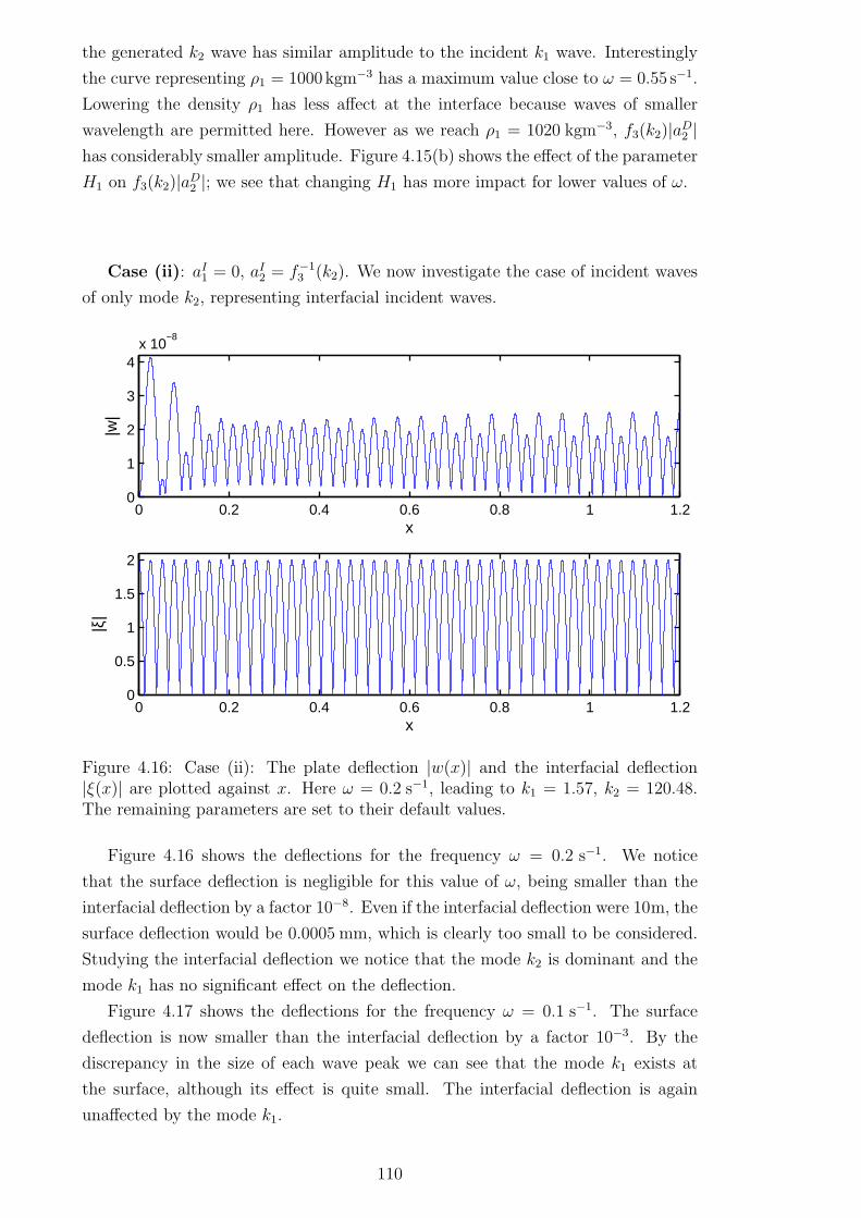
the generated k2 wave has similar amplitude to the incident k1 wave. Interestingly
the curve representing ρ1 = 1000kgm−3 has a maximum value close to ω = 0.55 s−1.
Lowering the density ρ1 has less affect at the interface because waves of smaller
wavelength are permitted here. However as we reach ρ1 = 1020 kgm−3, f3(k2)|aD2 |has considerably smaller amplitude. Figure 4.15(b) shows the effect of the parameter
H1 on f3(k2)|aD2 |; we see that changing H1 has more impact for lower values of ω.
Case (ii): aI1 = 0, aI2 = f−13 (k2). We now investigate the case of incident waves
of only mode k2, representing interfacial incident waves.
0 0.2 0.4 0.6 0.8 1 1.20
1
2
3
4x 10
−8
x
|w|
0 0.2 0.4 0.6 0.8 1 1.20
0.5
1
1.5
2
x
|ξ|
Figure 4.16: Case (ii): The plate deflection |w(x)| and the interfacial deflection|ξ(x)| are plotted against x. Here ω = 0.2 s−1, leading to k1 = 1.57, k2 = 120.48.The remaining parameters are set to their default values.
Figure 4.16 shows the deflections for the frequency ω = 0.2 s−1. We notice
that the surface deflection is negligible for this value of ω, being smaller than the
interfacial deflection by a factor 10−8. Even if the interfacial deflection were 10m, the
surface deflection would be 0.0005 mm, which is clearly too small to be considered.
Studying the interfacial deflection we notice that the mode k2 is dominant and the
mode k1 has no significant effect on the deflection.
Figure 4.17 shows the deflections for the frequency ω = 0.1 s−1. The surface
deflection is now smaller than the interfacial deflection by a factor 10−3. By the
discrepancy in the size of each wave peak we can see that the mode k1 exists at
the surface, although its effect is quite small. The interfacial deflection is again
unaffected by the mode k1.
110

0 0.5 1 1.5 2 2.50
0.5
1
x 10−3
x
|w|
0 0.5 1 1.5 2 2.50
0.5
1
1.5
2
x
|ξ|
Figure 4.17: Case (ii): The plate deflection |w(x)| and the interfacial deflection|ξ(x)| are plotted against x. Here ω = 0.1 s−1, leading to k1 = 0.64, k2 = 31.01. Theremaining parameters are set to their default values.
0 0.5 1 1.5 2 2.5 3 3.5 4 4.5 5 5.50
0.01
0.02
0.03
x
|w|
0 0.5 1 1.5 2 2.5 3 3.5 4 4.5 5 5.50
0.5
1
1.5
2
x
|ξ|
Figure 4.18: Case (ii): The plate deflection |w(x)| and the interfacial deflection|ξ(x)| are plotted against x. Here ω = 0.05 s−1, leading to k1 = 0.30, k2 = 10.70.The remaining parameters are set to their default values.
111

Figure 4.18 shows the deflections for the frequency ω = 0.05 s−1. We see that
the surface deflection now has significant amplitude compared to the interfacial
deflection. However, the wave mode k1 still has a negligible effect on the surface and
interfacial deflections. This implies that incident waves of mode k2 fail to generate
significant waves of mode k1. However, waves of mode k2 can exist with significant
amplitude on the surface, given that the wavelength is long enough.
We now investigate the coefficient |aD1 |, which shows more clearly the amplitude
of generated waves of mode k1. This is calculated by
|aD1 | =√aR2 + aI2,
where aR and aI are given by equations (4.121) and (4.122).
0.04 0.06 0.08 0.10
1
2
3
4
5
6x 10
−4 (a)
ω (s−1)
|a1D|
0.04 0.06 0.08 0.10
1
2
3
4
5
6x 10
−4 (b)
ω (s−1)
f 3(k1)
|a1D|
Figure 4.19: Case (ii): The coefficients (a) |aD1 | and (b) f3(k1)|aD1 | are plottedagainst ω, where the density ρ1 is given by 1000kgm−3 (blue), 1010kgm−3 (red) and1020kgm−3 (green).
Figure 4.19(a) shows the coefficient |aD1 |, representing the generated k1 waves at
the surface, plotted against ω. Figure 4.19(b) shows f3(k1)|aD1 | plotted against ω. In
both cases the density ρ1 is varied. Recall that the incident k2 wave at the interface
is scaled to 1 (so f3(k2)aI2 = 1). In general the k1 amplitudes are much smaller
than the incident k2 amplitudes, though this is expected as the surface response is
constrained by the elasticity of the ice sheet. As expected, the more pronounced the
density difference between the two layers, the higher the amplitude of the generated
k2 waves. Figure 4.20 shows the same plot, this time varying H1. Again it seems
that the middle depth H1 = 10 m causes the highest k1 amplitude.
Case (iii): aI1 = 0.01, aI2 = f−13 (k2). We now investigate the case where there is
an incident wave for both k1 and k2.
112
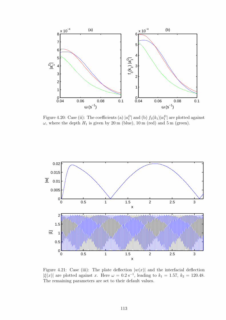
0.04 0.06 0.08 0.10
1
2
3
4
5
6
7
8x 10
−4 (a)
ω (s−1)
|a1D|
0.04 0.06 0.08 0.10
1
2
3
4
5
6x 10
−4 (b)
ω (s−1)
f 3(k1)
|a1D|
Figure 4.20: Case (ii): The coefficients (a) |aD1 | and (b) f3(k1)|aD1 | are plotted againstω, where the depth H1 is given by 20 m (blue), 10 m (red) and 5 m (green).
0 0.5 1 1.5 2 2.5 30
0.005
0.01
0.015
0.02
x
|w|
0 0.5 1 1.5 2 2.5 30
0.5
1
1.5
2
x
|ξ|
Figure 4.21: Case (iii): The plate deflection |w(x)| and the interfacial deflection|ξ(x)| are plotted against x. Here ω = 0.2 s−1, leading to k1 = 1.57, k2 = 120.48.The remaining parameters are set to their default values.
113
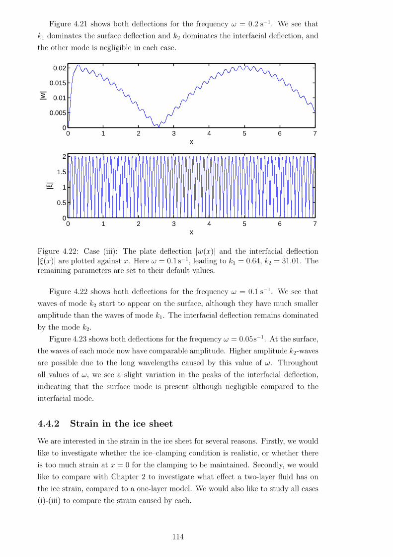
Figure 4.21 shows both deflections for the frequency ω = 0.2 s−1. We see that
k1 dominates the surface deflection and k2 dominates the interfacial deflection, and
the other mode is negligible in each case.
0 1 2 3 4 5 6 70
0.005
0.01
0.015
0.02
x
|w|
0 1 2 3 4 5 6 70
0.5
1
1.5
2
x
|ξ|
Figure 4.22: Case (iii): The plate deflection |w(x)| and the interfacial deflection|ξ(x)| are plotted against x. Here ω = 0.1 s−1, leading to k1 = 0.64, k2 = 31.01. Theremaining parameters are set to their default values.
Figure 4.22 shows both deflections for the frequency ω = 0.1 s−1. We see that
waves of mode k2 start to appear on the surface, although they have much smaller
amplitude than the waves of mode k1. The interfacial deflection remains dominated
by the mode k2.
Figure 4.23 shows both deflections for the frequency ω = 0.05s−1. At the surface,
the waves of each mode now have comparable amplitude. Higher amplitude k2-waves
are possible due to the long wavelengths caused by this value of ω. Throughout
all values of ω, we see a slight variation in the peaks of the interfacial deflection,
indicating that the surface mode is present although negligible compared to the
interfacial mode.
4.4.2 Strain in the ice sheet
We are interested in the strain in the ice sheet for several reasons. Firstly, we would
like to investigate whether the ice–clamping condition is realistic, or whether there
is too much strain at x = 0 for the clamping to be maintained. Secondly, we would
like to compare with Chapter 2 to investigate what effect a two-layer fluid has on
the ice strain, compared to a one-layer model. We would also like to study all cases
(i)-(iii) to compare the strain caused by each.
114

0 1 2 3 4 5 6 7 8 9 100
0.01
0.02
0.03
0.04
x
|w|
0 1 2 3 4 5 6 7 8 9 100
0.5
1
1.5
2
x
|ξ|
Figure 4.23: Case (iii): The plate deflection |w(x)| and the interfacial deflection|ξ(x)| are plotted against x. Here ω = 0.05 s−1, leading to k1 = 0.30, k2 = 10.70.The remaining parameters are set to their default values.
The strain is dimensionless, and considering our nondimensionalisation it is cal-
culated by (Ugural, 1981)
ε =ah
2H22
∂2w
∂x2. (4.123)
For simplicity we take a = 1m in our calculations. Using equation (4.15) to express
w(x, t) in terms of W (x) and using the total form of the plate deflection we have
∂2W
∂x2=∂2Winc
∂x2+∂2Wref
∂x2+∂2w
∂x2.
Substituting the correct expressions using Section 4.2.8 and equation (4.114), we
differentiate W twice and find that
∂2W
∂x2= −k21aI1e−ik1x − k22a
I2e
−ik2x − k21aD1 e
ik1x − k22aD2 e
ik2x
+2
πi(aI1 − aD1 )
∂2
∂x2
∫ ∞
0
Q(s) cos(sx) ds. (4.124)
The last term describes the interaction between the ice and the wall for small x.
The integral
I(x) =∂2
∂x2
∫ ∞
0
Q(s) cos(sx) ds (4.125)
in this expression requires some attention. We cannot differentiate directly, as this
would lead to a term s2Q(s) in the integrand. The function Q(s) decays with order
s−2 which would leave the integral undefined. Firstly, we investigate the function
115
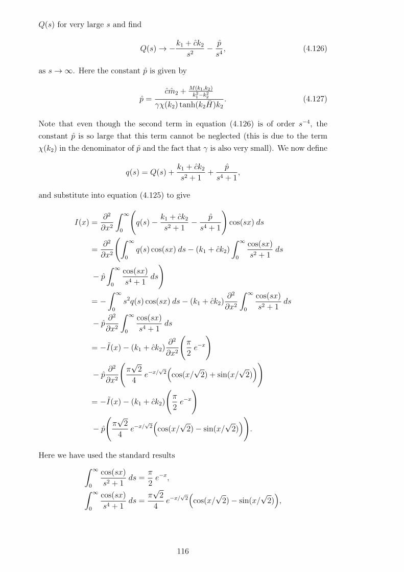
Q(s) for very large s and find
Q(s) → −k1 + ck2s2
− p
s4, (4.126)
as s→ ∞. Here the constant p is given by
p =cm2 +
M(k1,k2)
k21−k2
2
γχ(k2) tanh(k2H)k2. (4.127)
Note that even though the second term in equation (4.126) is of order s−4, the
constant p is so large that this term cannot be neglected (this is due to the term
χ(k2) in the denominator of p and the fact that γ is also very small). We now define
q(s) = Q(s) +k1 + ck2s2 + 1
+p
s4 + 1,
and substitute into equation (4.125) to give
I(x) =∂2
∂x2
∫ ∞
0
(
q(s)− k1 + ck2s2 + 1
− p
s4 + 1
)
cos(sx) ds
=∂2
∂x2
(
∫ ∞
0
q(s) cos(sx) ds− (k1 + ck2)
∫ ∞
0
cos(sx)
s2 + 1ds
− p
∫ ∞
0
cos(sx)
s4 + 1ds
)
= −∫ ∞
0
s2q(s) cos(sx) ds− (k1 + ck2)∂2
∂x2
∫ ∞
0
cos(sx)
s2 + 1ds
− p∂2
∂x2
∫ ∞
0
cos(sx)
s4 + 1ds
= −I(x)− (k1 + ck2)∂2
∂x2
(
π
2e−x
)
− p∂2
∂x2
(
π√2
4e−x/
√2(
cos(x/√2) + sin(x/
√2))
)
= −I(x)− (k1 + ck2)
(
π
2e−x
)
− p
(
π√2
4e−x/
√2(
cos(x/√2)− sin(x/
√2))
)
.
Here we have used the standard results
∫ ∞
0
cos(sx)
s2 + 1ds =
π
2e−x,
∫ ∞
0
cos(sx)
s4 + 1ds =
π√2
4e−x/
√2(
cos(x/√2)− sin(x/
√2))
,
116
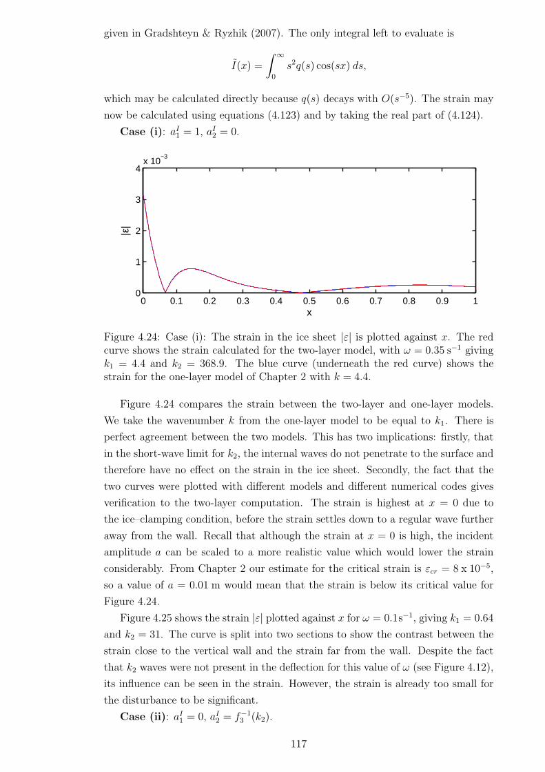
given in Gradshteyn & Ryzhik (2007). The only integral left to evaluate is
I(x) =
∫ ∞
0
s2q(s) cos(sx) ds,
which may be calculated directly because q(s) decays with O(s−5). The strain may
now be calculated using equations (4.123) and by taking the real part of (4.124).
Case (i): aI1 = 1, aI2 = 0.
0 0.1 0.2 0.3 0.4 0.5 0.6 0.7 0.8 0.9 10
1
2
3
4x 10
−3
x
|ε|
Figure 4.24: Case (i): The strain in the ice sheet |ε| is plotted against x. The redcurve shows the strain calculated for the two-layer model, with ω = 0.35 s−1 givingk1 = 4.4 and k2 = 368.9. The blue curve (underneath the red curve) shows thestrain for the one-layer model of Chapter 2 with k = 4.4.
Figure 4.24 compares the strain between the two-layer and one-layer models.
We take the wavenumber k from the one-layer model to be equal to k1. There is
perfect agreement between the two models. This has two implications: firstly, that
in the short-wave limit for k2, the internal waves do not penetrate to the surface and
therefore have no effect on the strain in the ice sheet. Secondly, the fact that the
two curves were plotted with different models and different numerical codes gives
verification to the two-layer computation. The strain is highest at x = 0 due to
the ice–clamping condition, before the strain settles down to a regular wave further
away from the wall. Recall that although the strain at x = 0 is high, the incident
amplitude a can be scaled to a more realistic value which would lower the strain
considerably. From Chapter 2 our estimate for the critical strain is εcr = 8 x 10⁻⁵,
so a value of a = 0.01 m would mean that the strain is below its critical value for
Figure 4.24.
Figure 4.25 shows the strain |ε| plotted against x for ω = 0.1s−1, giving k1 = 0.64
and k2 = 31. The curve is split into two sections to show the contrast between the
strain close to the vertical wall and the strain far from the wall. Despite the fact
that k2 waves were not present in the deflection for this value of ω (see Figure 4.12),
its influence can be seen in the strain. However, the strain is already too small for
the disturbance to be significant.
Case (ii): aI1 = 0, aI2 = f−13 (k2).
117
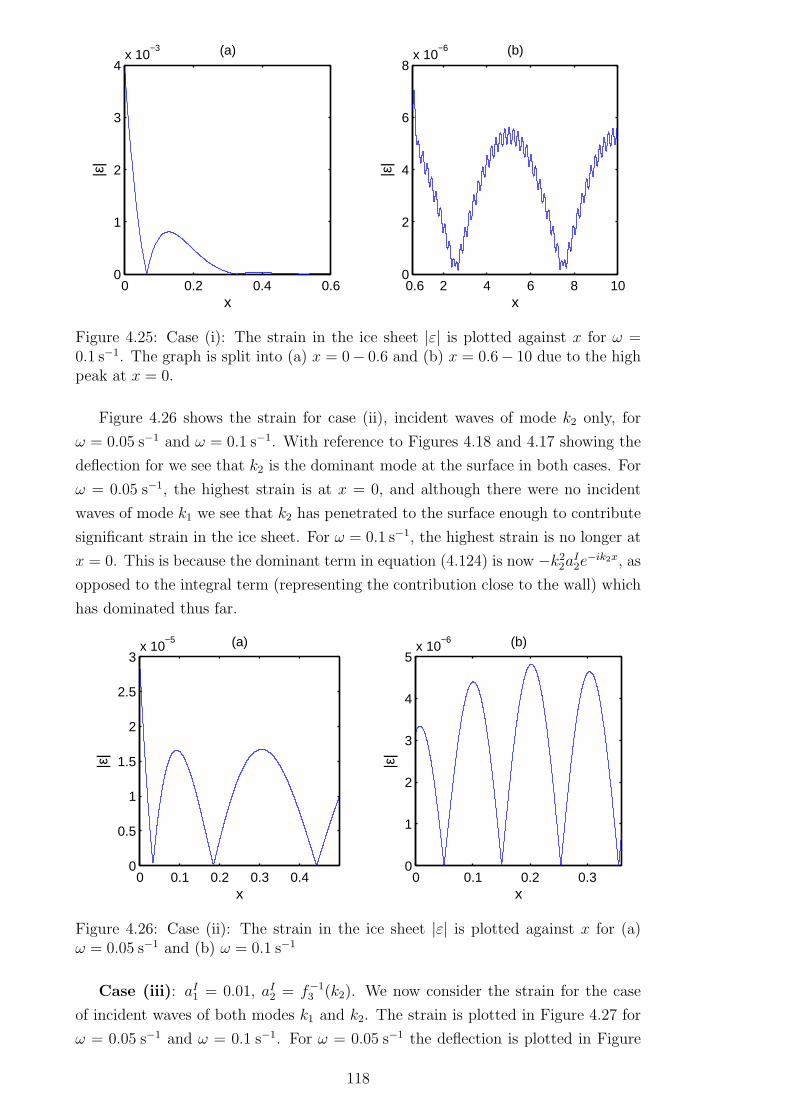
0 0.2 0.4 0.60
1
2
3
4x 10
−3 (a)
x
|ε|
0.6 2 4 6 8 100
2
4
6
8x 10
−6 (b)
x
|ε|
Figure 4.25: Case (i): The strain in the ice sheet |ε| is plotted against x for ω =0.1 s−1. The graph is split into (a) x = 0− 0.6 and (b) x = 0.6− 10 due to the highpeak at x = 0.
Figure 4.26 shows the strain for case (ii), incident waves of mode k2 only, for
ω = 0.05 s−1 and ω = 0.1 s−1. With reference to Figures 4.18 and 4.17 showing the
deflection for we see that k2 is the dominant mode at the surface in both cases. For
ω = 0.05 s−1, the highest strain is at x = 0, and although there were no incident
waves of mode k1 we see that k2 has penetrated to the surface enough to contribute
significant strain in the ice sheet. For ω = 0.1 s−1, the highest strain is no longer at
x = 0. This is because the dominant term in equation (4.124) is now −k22aI2e−ik2x, as
opposed to the integral term (representing the contribution close to the wall) which
has dominated thus far.
0 0.1 0.2 0.3 0.40
0.5
1
1.5
2
2.5
3x 10
−5 (a)
x
|ε|
0 0.1 0.2 0.30
1
2
3
4
5x 10
−6 (b)
x
|ε|
Figure 4.26: Case (ii): The strain in the ice sheet |ε| is plotted against x for (a)ω = 0.05 s−1 and (b) ω = 0.1 s−1
Case (iii): aI1 = 0.01, aI2 = f−13 (k2). We now consider the strain for the case
of incident waves of both modes k1 and k2. The strain is plotted in Figure 4.27 for
ω = 0.05 s−1 and ω = 0.1 s−1. For ω = 0.05 s−1 the deflection is plotted in Figure
118

4.23. For the equivalent strain curve we see that the strain caused by the mode k2
is dominant over the strain caused by the ice–clamping condition. For ω = 0.1 s−1,
the opposite is true; as we can see in Figure 4.22 the mode k2 is less prevalent in
the ice deflection and hence contributes less to the strain.
0 0.2 0.4 0.6 0.8 10
0.5
1
1.5
2x 10
−5 (a)
x
|ε|
0 0.2 0.4 0.60
1
2
3
4
5x 10
−5 (b)
x
|ε|
Figure 4.27: Case (iii): The strain in the ice sheet |ε| is plotted against x for (a)ω = 0.05 s−1 and (b) ω = 0.1 s−1
4.4.3 Shear force
The shear force is defined as the vertical lifting force acting on the vertical wall
generated by the ice–clamping condition. It is calculated in dimensionless form by
(Ugural, 1981):
V SH = −∂3w(0, t)
∂x3. (4.128)
Recalling that wxxx(0, t) = ℜ(iWxxx(0)e−it) and using the total form for the plate
deflection we have
Wxxx(0) =∂3Winc
∂x3+∂3Wref
∂x3+∂3w
∂x3.
Note that we do not have to use an inverse transform to calculate wxxx(0) as it
is already given by equation (4.105). This avoids any difficulty with convergence
that would have occurred in the resulting integrand. Recalling that we define the
constant p in equation (4.127), substituting the respective expressions for Winc and
Wref and differentiating gives
Wxxx(0) = i(aI1 − aD1 )(k31 + ck32 − p). (4.129)
The maximum shear force with respect to time is then given by
|V SH | = (k31 + ck32 − p)√
a2I + (aR − aI1)2. (4.130)
119

In the following figures we present the dimensionless shear force (unlike in previous
chapters), because the amplitude a appears in its dimensional form, which varies in
each case (i)–(iii).
Case (i): aI1 = 1, aI2 = 0. For case (i) the shear force is plotted against ω
in Figure 4.28. The values of the shear force show excellent agreement with the
equivalent one-layer model, indicating that the contribution from the waves of mode
k2 is small for this case. The shear force is higher for longer waves. We vary ρ1 and
H1, the interfacial parameters, and confirm that they have little effect on the shear
force for the incident wave under consideration.
0.05 0.1 0.151.35
1.4
1.45
1.5
1.55x 10
4 (a)
ω (s−1)
|VS
H|
0.05 0.1 0.15 0.2 0.251.2
1.25
1.3
1.35
1.4
1.45
1.5
1.55x 10
4 (b)
ω (s−1)
|VS
H|
Figure 4.28: Case (i): The shear force |V SH | is plotted against ω for varying pa-rameters. (a) ρ1 is given by 1000 kgm−3 (blue), 1010 kgm−3 (red) and 1020kg m−3
(green). (b) H1 is given by 20m (blue), 10m (red) and 5m (green).
Case (ii): aI1 = 0, aI2 = f−13 (k2). The shear force is plotted against ω for case
(ii) in Figure 4.29. Here there are only incident waves of mode k2. Smaller values of
ω permit waves of k2 to exist on the surface, which causes considerable shear force
on the wall. However as ω increases, the k2 waves no longer penetrate to the surface
and the shear force tends to zero. We also see that as ρ approaches 1, the interfacial
waves have less effect on the shear force as expected. When varying the depth H1
we note that a depth of 5m gives the lowest shear force of the depths considered.
Case (iii): aI1 = 0.01, aI2 = f−13 (k2). Figure 4.30 shows the shear force plotted
against ω for case (iii), incident waves of both modes. To compare directly with case
(i), recall that the surface waves were scaled to 1 for that case, whereas here the
surface waves are scaled to 0.01. We see some interesting behaviour in the long-wave
limit of ω. For ρ1 = 1000 kgm−3 the maximum shear force actually approaches zero
at ω = 0.06 s−1. This is because |aI1 − a1D| approaches zero at that point, implying
that the contributions from the incident and reflected k1 waves cancel each other
out. We see that as ω grows, the parameter ρ1 becomes less important due to the
interfacial waves dying on the surface. Figure 4.30(b) shows that the depth H1 has
little influence on the maximum shear force.
120
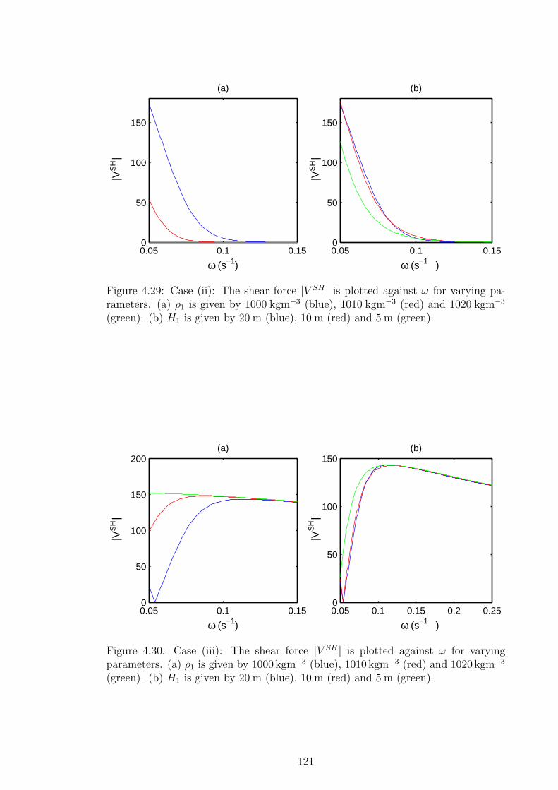
0.05 0.1 0.150
50
100
150
(a)
ω (s−1)
|VS
H|
0.05 0.1 0.150
50
100
150
(b)
ω (s−1 )
|VS
H|
Figure 4.29: Case (ii): The shear force |V SH | is plotted against ω for varying pa-rameters. (a) ρ1 is given by 1000 kgm−3 (blue), 1010 kgm−3 (red) and 1020 kgm−3
(green). (b) H1 is given by 20 m (blue), 10 m (red) and 5 m (green).
0.05 0.1 0.150
50
100
150
200(a)
ω (s−1)
|VS
H|
0.05 0.1 0.15 0.2 0.250
50
100
150(b)
ω (s−1 )
|VS
H|
Figure 4.30: Case (iii): The shear force |V SH | is plotted against ω for varyingparameters. (a) ρ1 is given by 1000kgm−3 (blue), 1010kgm−3 (red) and 1020kgm−3
(green). (b) H1 is given by 20 m (blue), 10 m (red) and 5 m (green).
121

4.5 Summary
The problem of hydroelastic wave interaction with a vertical wall was extended to
consider a two–layer fluid, which is expected to better describe the flow under the ice
cover. The fluid was of finite depth and the ice sheet was clamped to the vertical wall.
The problem was formulated and solved within linear hydroelastic wave theory. Due
to the two fluid layers, there are two solutions in the dispersion relation, giving one
wavenumber representing surface waves and another representing interfacial waves.
The problem was solved by Fourier transform after using linear superposition to
separate the incident and reflected waves. This method led to an explicit solution
in terms of integral quadratures. The integrals converge reasonably quickly, and
the computational time involved was therefore short. The method was algebraically
cumbersome but this is unavoidable due to the complicated physical formulation.
The method allowed the incident and reflected wave-amplitude coefficients of both
modes to be written explicitly. This is one advantage over methods such as an
eigenfunction expansion or a Green’s function formulation. In hydroelastic mod-
els, there can be difficulties with calculating the strain or the shear force, which
require calculation of the second and third derivative of the ice deflection. In the
present formulation, the explicit solution allows asymptotic expressions to assist in
the calculation of the strain. The Fourier transform method also leads to a concise
algebraic expression for the vertical shear force, sidestepping the usual problems
with convergence.
Three cases were considered for results: (i) incident waves of the surface mode
k1, (ii) incident waves of the interfacial mode k2 and (iii) incident waves of both
modes. For case (i), the results were consistent with those of Chapter 2, the equiv-
alent one-layer fluid problem. However, it was shown that the ice–wall interaction
can generate interfacial waves of mode k2, and the amplitude of these waves is con-
siderable and similar to the surface wave amplitude. This is especially pronounced
for low frequency ω and when the two layers have a more pronounced density dif-
ference. For this case the generated interfacial mode fails to have much influence on
the ice deflection because the waves are not strong enough to penetrate to the ice
cover.
For case (ii) we saw that reflection of incident waves of mode k2 do not generate
significant waves of mode k1. The k1 waves exist, but they are dwarfed by the
influence of the mode k2. For higher values of ω especially, the surface response from
both modes is negligible and the disturbance is localised at the interface between the
two fluid layers. However, it was shown that for small ω, waves of mode k2 can still
contribute significant strain in the ice sheet due to their short wavelength, but this
strain is not above the critical strain for ice. Case (iii) shows the most interaction
between the two wave modes. For small values of ω it was shown that waves of k1
and k2 have similar amplitude at the surface. The interfacial deflection however was
dominated by the mode k2, partly due to the scaling chosen for this case.
122

The results show that even if there are only incident waves of one mode, reflected
waves of both modes can be generated. This is especially true for lower frequencies
which usually characterise hydroelastic problems. We conclude that if the fluid under
an ice sheet has stratified into two layers, and if the density difference between the
two layers is pronounced, then the effect of this stratification cannot be neglected.
123

Chapter 5
Hydroelastic waves generated by a
moving load in the vicinity of a
vertical wall: linear formulation
5.1 Introduction
In this chapter the one-layer fluid formulation is reconsidered. Thus far throughout
this thesis we have considered problems with regular incident waves that are periodic.
Now we are concerned with waves generated by a moving load on an ice sheet in three
dimensions. This area of mathematics has many applications as discussed in Section
1. We first investigate a moving load on a semi–infinite expanse of open ice with no
obstacles. We then proceed to study a load moving in the vicinity of a vertical wall.
In both cases, the load has constant velocity and exerts a downwards force on the
ice sheet, acting as a wave source. In the vertical wall case the ice sheet is frozen
to the vertical wall. The fluid is of finite depth in both cases. We are interested
in the shape and magnitude of the ice deflection, and what factors influence them.
Also of interest is whether the motion of the moving load can generate large enough
surface response to break the ice connection to the vertical wall. Key parameters
under investigation include the distance of the load from the wall and the speed at
which the load is moving.
We introduce a simple viscoelastic formulation which takes into account ice re-
laxation time. This has two benefits: firstly, it ensures that the hydroelastic waves
decay at a distance from the source. Since the source of the waves is no longer
periodic as in previous chapters, this is a necessary constraint. In addition, incor-
porating viscoelasticity adds further realism to the model, as ice has been shown to
behave viscoelastically in practice, as discussed in Chapter 1. We will also intro-
duce a moving frame of reference to assist in the solution of the problem and provide
clarity to the results.
In this chapter, the problem is formulated within linear hydroelastic theory.
Chapter 6 addresses the nonlinear formulation of the same problem. The assump-
124
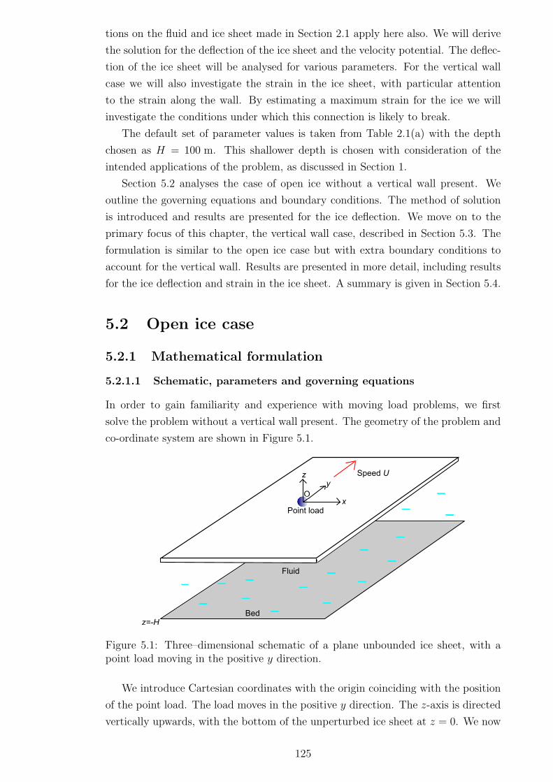
tions on the fluid and ice sheet made in Section 2.1 apply here also. We will derive
the solution for the deflection of the ice sheet and the velocity potential. The deflec-
tion of the ice sheet will be analysed for various parameters. For the vertical wall
case we will also investigate the strain in the ice sheet, with particular attention
to the strain along the wall. By estimating a maximum strain for the ice we will
investigate the conditions under which this connection is likely to break.
The default set of parameter values is taken from Table 2.1(a) with the depth
chosen as H = 100 m. This shallower depth is chosen with consideration of the
intended applications of the problem, as discussed in Section 1.
Section 5.2 analyses the case of open ice without a vertical wall present. We
outline the governing equations and boundary conditions. The method of solution
is introduced and results are presented for the ice deflection. We move on to the
primary focus of this chapter, the vertical wall case, described in Section 5.3. The
formulation is similar to the open ice case but with extra boundary conditions to
account for the vertical wall. Results are presented in more detail, including results
for the ice deflection and strain in the ice sheet. A summary is given in Section 5.4.
5.2 Open ice case
5.2.1 Mathematical formulation
5.2.1.1 Schematic, parameters and governing equations
In order to gain familiarity and experience with moving load problems, we first
solve the problem without a vertical wall present. The geometry of the problem and
co-ordinate system are shown in Figure 5.1.
Fluid
Bed
x
yz
Point load
Speed U
z=-H
O
Figure 5.1: Three–dimensional schematic of a plane unbounded ice sheet, with apoint load moving in the positive y direction.
We introduce Cartesian coordinates with the origin coinciding with the position
of the point load. The load moves in the positive y direction. The z-axis is directed
vertically upwards, with the bottom of the unperturbed ice sheet at z = 0. We now
125
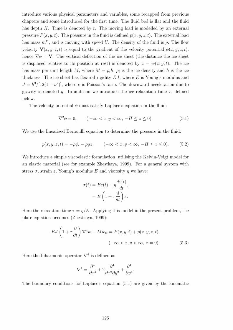
introduce various physical parameters and variables, some recapped from previous
chapters and some introduced for the first time. The fluid bed is flat and the fluid
has depth H. Time is denoted by t. The moving load is modelled by an external
pressure P (x, y, t). The pressure in the fluid is defined p(x, y, z, t). The external load
has mass mV , and is moving with speed U . The density of the fluid is ρ. The flow
velocity V(x, y, z, t) is equal to the gradient of the velocity potential φ(x, y, z, t),
hence ∇φ = V. The vertical deflection of the ice sheet (the distance the ice sheet
is displaced relative to its position at rest) is denoted by z = w(x, y, t). The ice
has mass per unit length M , where M = ρih, ρi is the ice density and h is the ice
thickness. The ice sheet has flexural rigidity EJ , where E is Young’s modulus and
J = h3/[12(1 − ν2)], where ν is Poisson’s ratio. The downward acceleration due to
gravity is denoted g. In addition we introduce the ice relaxation time τ , defined
below.
The velocity potential φ must satisfy Laplace’s equation in the fluid:
∇2φ = 0, (−∞ < x, y <∞, −H ≤ z ≤ 0). (5.1)
We use the linearised Bernoulli equation to determine the pressure in the fluid:
p(x, y, z, t) = −ρφt − ρgz, (−∞ < x, y <∞, −H ≤ z ≤ 0). (5.2)
We introduce a simple viscoelastic formulation, utilising the Kelvin-Voigt model for
an elastic material (see for example Zhestkaya, 1999). For a general system with
stress σ, strain ε, Young’s modulus E and viscosity η we have:
σ(t) = Eε(t) + ηdε(t)
dt,
= E
(
1 + τd
dt
)
ε.
Here the relaxation time τ = η/E. Applying this model in the present problem, the
plate equation becomes (Zhestkaya, 1999):
EJ
(
1 + τ∂
∂t
)
∇4w +Mwtt = P (x, y, t) + p(x, y, z, t),
(−∞ < x, y <∞, z = 0). (5.3)
Here the biharmonic operator ∇4 is defined as
∇4 =∂4
∂x4+ 2
∂4
∂x2∂y2+
∂4
∂y4.
The boundary conditions for Laplace’s equation (5.1) are given by the kinematic
126
condition at the ice-fluid interface and the fluid bed respectively:
φz = wt, (z = 0), (5.4)
φz = 0, (z = −H). (5.5)
Conditions in the far field are defined later.
5.2.1.2 Critical speeds
The dispersion relation for the viscoelastic ice plate governed by equation (5.3) can
by derived by setting P = 0 (no load) and considering waves propagating in the x
direction. Substituting w = ei(kx−ωt) into equations (5.1)-(5.5), we obtain
EJ(1− iωτ)k4 + ρg −Mω2 =ρω2
k tanh(kH). (5.6)
This is the viscoelastic dispersion relation which allows us to compute the wavenum-
ber k for a given frequency ω. Note that ω is real and positive. The term with the
relaxation time τ shows that k is a complex number. It is the same as the hydroelas-
tic dispersion relation for a one-layer fluid considered in previous chapters, with the
addition of a term representing viscoelastic decay. Experiments conducted in Japan
(Takizawa, 1985) observe a lag in the position of maximum ice depression directly
behind the moving load that was unexplained by the elastic formulation. Hosking
et al. (1988) suggest that viscoelastic theory can account for this lag. Takizawa
(1985) propose that the lag time should be comparable with the relaxation time,
which should hence range from roughly 0.2 s to 0.8 s.
As discussed in Chapter 1, one feature of problems involving moving loads of
ice sheets is the appearance of certain critical speeds, at which the linear theory
breaks down. The first critical speed occurs when the load moves with speed cmin,
where cmin is the minimum phase speed of hydroelastic waves. Setting τ = 0, the
phase speed c = ω/k and the group speed cg = dω/dk are plotted against k in
Figure 5.2. For the parameters under consideration, cmin = 18.05 ms−1. It is well
known that a source speed U = cmin results in increased ice deflections (Squire
et al., 1996). Davys et al. (1985) explain thus: “for a source travelling at the critical
speed energy is radiated directly forward at the same speed and will continuously
accumulate underneath the source”. At the value U = cmin, Davys et al. (1985) and
Milinazzo et al. (1995) report unbounded deflection. However, Hosking et al. (1988)
incorporated a viscoelastic formulation and found that this forces a finite response
at the critical speed.
Many authors such as Schulkes & Sneyd (1988), Parau & Vanden-Broeck (2011),
Milinazzo et al. (1995) have noted the differing shapes of deflection above and below
the critical speed. At load speeds above cmin, two different wave systems appear:
shorter, faster waves that are elastic dominated and propagate ahead of the source,
and longer, slower gravity-dominated waves behind the source. In addition, fast load
127

0 0.01 0.02 0.03 0.04 0.05 0.0610
15
20
25
30
35
40
k (m−1)
c, c
g (m
s−
1 )
Figure 5.2: The phase (red) and group (blue) speeds plotted against the wavenumberk. Parameter values are from Table 2.1(a) with H = 100 m.
speeds generate a wave profile that is curved around the moving load. Below cmin,
there is only one wave system and the wave pattern is regular, moving perpendicular
to the direction of load movement.
Schulkes & Sneyd (1988) noted another possible sub-critical speed given by√gH.
This is the speed at which gravity waves propagate on shallow water of uniform
depth. However, they state that it is possible√gH is not a critical speed for two–
dimensional point sources, but only for line sources. Also, time-dependence seems to
be a factor in qualifying this critical speed (Schulkes & Sneyd (1988) were studying
the time-dependent response of an ice sheet to a moving load). Milinazzo et al.
(1995) concluded that a steady solution does exist when the speed U approaches√gH, but such a solution is not realisable since the solution may grow with time.
5.2.1.3 Nondimensionalisation & expression for the moving load
As in previous chapters, we continue to use the total depth H as a length scale. We
introduce a frame of reference moving with speed U by defining:
x∗ =x
H, y∗ =
y − Ut
H, z∗ =
z
H.
In addition dimensionless time and dimensionless relaxation time are defined:
t∗ =U
Ht, τ ∗ =
U
Hτ.
128
The moving load is modelled using the Dirac delta function, and can be expressed
in dimensional variables as
P (x, y, t) = −mV g
H2δ(y − Ut
H
)
δ( x
H
)
, (−∞ < x <∞, −∞ < y <∞). (5.7)
Here mV is the mass of the moving load. The minus in the right hand side indicates
that the force is applied in a downwards direction. The Dirac delta function is
defined as
δ(x) =
{
∞, x=0
0, otherwise,(5.8)
with the integral∫ ∞
−∞δ(x) dx = 1. (5.9)
Hence we have
P ∗(x∗, y∗, t∗) =H2
mV gP (x, y, t) = −δ(y∗)δ(x∗). (5.10)
The dimensionless deflection and velocity potential are defined as
w∗(x∗, y∗) =ρU2H
mV gw(x, y, t), φ∗(x∗, y∗, z∗) =
ρUH
mV gφ(x, y, z, t).
We also define several dimensionless parameters, given by
α =M
ρH, β =
gH
U2, γ =
EJ
ρU2H3.
The asterisks are henceforth dropped in the following, and all variables/parameters
are assumed dimensionless. We now rewrite the boundary value problem (5.1)-(5.5)
in terms of the dimensionless variables and parameters:
γ
(
1− τ∂
∂y
)
∇4w + αwyy + βw − φy = −δ(y)δ(x),
(−∞ < x, y <∞, z = 0), (5.11)
∇2φ = 0, (−∞ < x, y <∞, −1 ≤ z ≤ 0), (5.12)
φz = −wy, (z = 0), (5.13)
φz = 0, (z = −1), (5.14)
w → 0, (x2 + y2) → ∞, (5.15)
φ→ 0, (x2 + y2) → ∞. (5.16)
Here we have introduced conditions (5.15)-(5.16) ensuring that all waves decay far
from the load. The above boundary value problem (5.11)-(5.16) describes the pat-
tern of hydroelastic waves in the moving co–ordinate system.
129

5.2.2 Solution by double Fourier transform
We apply Fourier transforms in both the x and y directions. Using ξ as the transform
variable in the x direction we define:
wX(ξ, y) =1√2π
∫ ∞
−∞w(x, y) e−iξx dx, (5.17)
with the corresponding inverse transform given by
w(x, y) =1√2π
∫ ∞
−∞wX(ξ, y) eiξy dξ. (5.18)
Using transform variable η, in the y direction we define:
wY (x, η) =1√2π
∫ ∞
−∞w(x, y) e−iηy dy, (5.19)
with inverse transform
w(x, y) =1√2π
∫ ∞
−∞wY (x, η) eiηy dη. (5.20)
We now seek to obtain an expression for a Fourier transform acting on a derivative
of x or y. For example, defining F (w) as Fourier transform (5.19) acting on the
function w(x, y) to give F (w) = wY , we have:
F
(
∂w
∂y
)
=1√2π
∫ ∞
−∞wy(x, y) e
−iηy dy
=1√2π
(
(we−iηy)∞−∞ + iη
∫ ∞
−∞w(x, y) e−iηy dy
)
= iη
∫ ∞
−∞w(x, y) e−iηy dy
= iηwY . (5.21)
Here we have used integration by parts and the fact that w decays in the far field
(5.16). We may use (5.21) to give an expression for F (wyy); defining g(y) = wy we
have:
F (wyy) = F (gy) = iηF (g) = (iη)2wY = −η2wY .
We use a similar process to obtain the expression
F (wyyyy) = η4wY .
We also note that the Fourier transform in the x direction has no effect on y deriva-
tives and vice versa; for example, F (wx) = wYx , etc.
130
5.2.2.1 Velocity potential
Using the facts derived in the above subsection, we apply the transforms to Laplace’s
equation (5.12), given by
φxx + φyy + φzz = 0.
Applying both integral transforms (5.17) and (5.19) to the variable φ(x, y, z), we
obtain:
−ξ2φXY − η2φXY + φXYzz = 0.
Applying the transforms to the boundary conditions (5.13) and (5.14), we have the
following BVP for the variable φXY (ξ, η, z):
φXYzz − (ξ2 + η2)φXY = 0, (−1 ≤ z ≤ 0), (5.22)
φXYz = −iηwXY , (z = 0), (5.23)
φXYz = 0, (z = −1). (5.24)
With consideration of boundary condition (5.24), the general solution to equation
(5.22) is given by
φXY = A cosh(√
ξ2 + η2(z + 1))
,
where A is an unknown function of ξ and η. Application of the boundary condition
(5.23) gives
A =−iηwXY
√
ξ2 + η2 sinh(√
ξ2 + η2) . (5.25)
Hence, φXY is given by
φXY = −iη ψ(z) wXY , (5.26)
where we have defined
ψ(z) =cosh
(√
ξ2 + η2(z + 1))
√
ξ2 + η2 sinh(√
ξ2 + η2) . (5.27)
Equation (5.26) defines the velocity potential φXY in terms of the plate deflection
wXY which is still to be determined.
5.2.2.2 Plate deflection
We now apply the transforms to the left hand side of the plate equation (5.11), given
by:
LHS = γ
(
1− τ∂
∂y
)
(wxxxx + 2wxxyy + wyyyy) + αwyy + βw − φy.
After applying both transforms (5.17) and (5.19) we obtain:
LHS = γ(1− iητ)(ξ4wXY +2ξ2η2wXY +η4wXY )−αη2wXY +βwXY − iηφXY . (5.28)
131
We now apply both transforms to the right hand side of equation (5.11), given by
RHS = −δ(x)δ(y).
Using the property of the Dirac delta function given by equation (5.9), after applying
the integral transforms we arrive at
RHS = − 1
2π. (5.29)
Combining the LHS and the RHS and substituting for φXY using equation (5.26),
we have
wXY(
γ(1− iητ)(ξ4 + 2η2ξ2 + η4) + β − αη2 − η2ψ(0))
= − 1
2π.
We substitute the expression for ψ using equation (5.27) and define the function
Q(ξ, η) as
Q(ξ, η) = γ(1− iητ)(ξ4 + 2η2ξ2 + η4) + β − αη2 − η2 coth(√
ξ2 + η2)√
ξ2 + η2. (5.30)
After performing inverse transforms defined in equations (5.18) and (5.20), we
arrive at the final solution for the ice deflection, which can be expressed as
w(x, y) = − 1
4π2
∫ ∞
−∞
{∫ ∞
−∞
eiηy
Q(ξ, η)dη
}
eiξx dξ. (5.31)
5.2.2.3 Method of residues
The integral with respect to η in equation (5.31) is suitable for the application of
complex integration by the method of residues. There are poles in the complex plane,
which can be calculated readily. The poles arise due to the zeros of the function Q
in the complex plane. The value of the integral can then be calculated by summing
the contribution to the integral from each pole and applying the Cauchy residue
theorem. Defining
Q = QR + i QI ,
η = a+ i b,
the poles occur when Q = 0, at the values of a and b for which
QR(ξ, a, b) = QI(ξ, a, b) = 0.
Figure 5.3 shows the location of the poles graphically. For all parameter values,
there are 6 poles that have both a real and imaginary part. As U increases, or as
τ decreases, the upper pair of poles in the lower half plane appraoch the real axis.
However, as long as τ is non-zero, there are no poles on the real axis. The poles are
132

−4 −3 −2 −1 0 1 2 3 4
−4
−3
−2
−1
0
1
2
3
4
a
b
Figure 5.3: The complex η plane a vs b, showing the location of the poles in theintegrand of (5.31). The blue lines represent the contour QI = 0, and the red linesrepresent the contour QR = 0. Poles occur at the intersections of these two lines.Here U = 20 ms−1, τ = 10 s, ξ = 1, and other parameters are taken from Table2.1(a) with H = 100 m.
symmetric about the imaginary axis.
In addition to these 6 poles, there is an infinite set of purely imaginary poles.
These can be located by setting η = ib in the expression for Q(ξ, η), and the poles
occur where:
Q(ξ, ib) = 0 = γ(1 + bτ)(ξ4 − 2ξ2b2 + b4) + β + αb2 +b2 coth(
√
ξ2 − b2)√
ξ2 − b2. (5.32)
Equation (5.32) has no roots for ξ > b, but when b > ξ, and using coth(iθ) =
−i cot(θ) it becomes
γ
b2(1 + bτ)(ξ4 − 2ξ2b2 + b4) +
β
b2+ α =
cot(√
b2 − ξ2)√
b2 − ξ2. (5.33)
Equation (5.33) has an infinite set of solutions, shown graphically in Figure 5.4.
This set of poles is not symmetric about the real axis, but differ slightly due to the
bτ term in equation (5.33).
The locations of the poles are straightforward to calculate using root–finding
algorithms. Each pole is denoted (ap, bp), where p = 1, 2...6 represents the poles
with real and imaginary parts, and p = 7, ...n represents the infinite set of imaginary
poles. Once the poles are calculated, we draw the integral contour shown in Figure
5.5; a large semi-circle of radius R. For positive y, the semicircle is as shown, and for
133
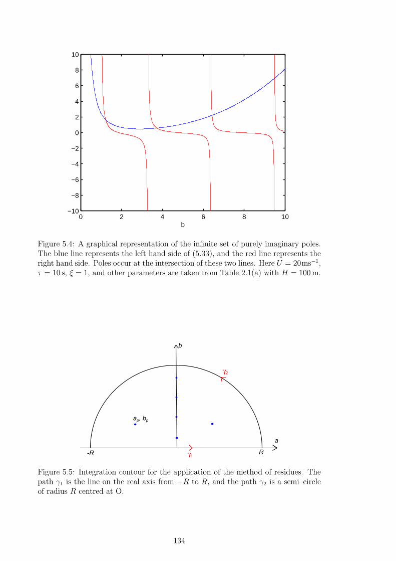
0 2 4 6 8 10−10
−8
−6
−4
−2
0
2
4
6
8
10
b
Figure 5.4: A graphical representation of the infinite set of purely imaginary poles.The blue line represents the left hand side of (5.33), and the red line represents theright hand side. Poles occur at the intersection of these two lines. Here U = 20ms−1,τ = 10 s, ξ = 1, and other parameters are taken from Table 2.1(a) with H = 100m.
a
b
ap, bp
g2
g1R-R
Figure 5.5: Integration contour for the application of the method of residues. Thepath γ1 is the line on the real axis from −R to R, and the path γ2 is a semi–circleof radius R centred at O.
134

negative y, the contour is closed below the real axis. The Cauchy residue theorem
(Jeffrey, 2002) states:
∫
γ1+γ2
eiηy
Q(ξ, η)dη = 2πi
n∑
p=1
Res(ap, bp), (5.34)
where the paths γ1 and γ2 are as defined in Figure 5.5. Here “Res” denotes the
residue at each pole. All of the poles are simple poles (poles of order 1), and the
residue is hence calculated (see Jeffrey, 2002) by
Res(ap, bp) = eiy(ap+ibp)∂Q
∂η
−1
(ap,bp)
. (5.35)
We now take the limit R → ∞. The contribution from the integral path γ2 vanishes
in this limit by Jordan’s lemma (Jeffrey, 2002), due to the fact that Q is of order η5
as η → ∞. Hence we are left with
∫ ∞
−∞
eiηy
Q(ξ, η)dη = 2πi
n∑
p=1
Res(ap, bp). (5.36)
The convergence of the series (5.36) is fast, and n is usually taken as 15, by
which time the contribution from the poles (an, bn) is negligible. The resultant ξ
integral in (5.31) is smooth and can be calculated by standard methods; note that
the integrand is even and hence its symmetry can be exploited. The imaginary part
of both integrands is odd and hence disappear due to the symmetric integration
limits, and w(x, y) is hence real.
5.2.3 Numerical results for the ice deflection
The primary focus of this chapter is the vertical wall model, presented in Section 5.3.
For open ice, the problem has been solved previously by Hosking et al. (1988), albeit
using a slightly different two–parameter viscoelastic model. However, the solution
for the point-source part of this work was only approximated asymptotically. In
addition, no three-dimensional graphs were presented. Hence several results are
presented here for the open ice case. This also helps indicate the effect of the load
speed U and serves as a build-up to the vertical wall case. We fix the viscoelastic
time τ at τ = 0.1 s. The effect of viscoelasticity will be studied in more detail for
the vertical wall case.
The deflection is plotted in Figure 5.6 for speed U = 15ms−1, which is less than
the critical speed cmin. We see that the waves in front and behind the source have
comparable magnitudes, but the wave behind the source is slightly larger. This is
due to the viscoelastic parameter τ in the formulation: with τ = 0 the waves are
symmetric. The waves decay a short distance from the source.
Figure 5.7 shows the deflection for the load speed U = 25 ms−1, with τ = 0.1 s.
Recall that cmin = 18.05 ms−1 for the default data set, so the speed U considered
135
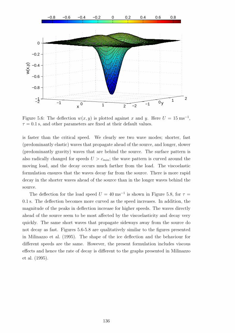
−2 −1 0 1 2 −2 −1 0 1 2−1
−0.8
−0.6
−0.4
−0.2
0
yx
w(x
,y)
−0.8 −0.6 −0.4 −0.2 0 0.2 0.4 0.6 0.8
Figure 5.6: The deflection w(x, y) is plotted against x and y. Here U = 15 ms−1,τ = 0.1 s, and other parameters are fixed at their default values.
is faster than the critical speed. We clearly see two wave modes; shorter, fast
(predominantly elastic) waves that propagate ahead of the source, and longer, slower
(predominantly gravity) waves that are behind the source. The surface pattern is
also radically changed for speeds U > cmin; the wave pattern is curved around the
moving load, and the decay occurs much farther from the load. The viscoelastic
formulation ensures that the waves decay far from the source. There is more rapid
decay in the shorter waves ahead of the source than in the longer waves behind the
source.
The deflection for the load speed U = 40 ms−1 is shown in Figure 5.8, for τ =
0.1 s. The deflection becomes more curved as the speed increases. In addition, the
magnitude of the peaks in deflection increase for higher speeds. The waves directly
ahead of the source seem to be most affected by the viscoelasticity and decay very
quickly. The same short waves that propagate sideways away from the source do
not decay as fast. Figures 5.6-5.8 are qualitatively similar to the figures presented
in Milinazzo et al. (1995). The shape of the ice deflection and the behaviour for
different speeds are the same. However, the present formulation includes viscous
effects and hence the rate of decay is different to the graphs presented in Milinazzo
et al. (1995).
136

−5
0
5
−6 −4 −2 0 2 4 6
−2−1
01
y
x
w(x
,y)
−2 −1.5 −1 −0.5 0 0.5 1 1.5 2
Figure 5.7: The deflection w(x, y) is plotted against x and y. Here U = 25 ms−1,τ = 0.1 s, and other parameters are fixed at their default values.
−6−4
−20
24
6−6
−4−2
02
46
−2
−1
0
1
y
x
w(x
,y)
−2.5 −2 −1.5 −1 −0.5 0 0.5 1 1.5 2 2.5
Figure 5.8: The deflection w(x, y) is plotted against x and y. Here U = 40 ms−1,τ = 0.1 s, and other parameters are fixed at their default values.
137

5.3 Vertical wall case
5.3.1 Mathematical formulation: schematic and governing
equations
With key ideas established for the formulation and solution methodology for hydroe-
lastic problems involving moving loads, we proceed to the vertical wall formulation.
The geometry of the problem and co-ordinate system are shown in Figure 5.9.
Fluid
Bed
ertica
l wall
x
yz
Point loadx=x0
Speed U
z=-H
O
Figure 5.9: Schematic of a semi–infinite ice sheet meeting a vertical wall in threedimensions, with a load on the ice sheet moving parallel to the vertical wall.
Parameters defined for the open ice case in Section 5.2.1.1 are the same here.
Note that it is convenient to move the origin so the vertical wall is at x = 0. The
ice is fixed to the vertical wall. The load moves in the positive y direction, in a
direction parallel to the vertical wall at a constant distance x0 from the wall. The
pressure due to the moving load hence becomes (in dimensional form):
P (x, y, t) = −mV g
H2δ(y − Ut
H
)
δ(x− x0
H
)
, (x > 0, −∞ < y <∞). (5.37)
The dimensionless parameters remain the same as defined in Section 5.2.1.3, with
the addition x∗0 = x0/H. Following equation (5.10) from the previous section, in
dimensionless form the pressure defined in equation (5.37) becomes
P ∗(x∗, y∗, t∗) = −δ(y∗)δ(x∗ − x∗0), (x > 0, −∞ < y <∞). (5.38)
We drop the asterisks and the variables are henceforth assumed dimensionless.
We recap in full the governing equations that remain unchanged from (5.11)-(5.16),
noting the change in the range of x:
138

γ
(
1− τ∂
∂y
)
∇4w + αwyy + βw − φy = −δ(y)δ(x− x0),
(x > 0, −∞ < y <∞, z = 0), (5.39)
∇2φ = 0, (x > 0, −∞ < y <∞, −1 ≤ z ≤ 0), (5.40)
φz = −wy, (z = 0), (5.41)
φz = 0, (z = −1), (5.42)
w,→ 0, |x|, |y| → ∞. (5.43)
φ→ 0, |x|, |y| → ∞. (5.44)
In addition, there is a boundary condition ensuring no flow through the vertical wall
at x = 0:
φx = 0, (x = 0). (5.45)
We also have two conditions along the wall owing to the ice clamping, given by
w = 0, (x = 0), (5.46)
wx = 0, (x = 0). (5.47)
Equations (5.39)-(5.47) provide the dimensionless BVP to be solved, which is an
extension of the BVP solved in Section 5.2 to include the effect of a vertical wall.
5.3.2 Solution by double Fourier transform
Unlike for the open ice case of Section 5.2, in the x direction we use a cosine Fourier
transform due to the boundary conditions available and the range of x. Using ξ as
the transform variable we define:
wc(ξ, y) =
√
2
π
∫ ∞
0
w(x, y) cos(ξx) dx, (5.48)
with inverse transform
w(x, y) =
√
2
π
∫ ∞
0
wc(ξ, y) cos(ξx) dξ. (5.49)
In the y direction we apply a standard Fourier transform, with transform variable
η:
wf (x, η) =1√2π
∫ ∞
−∞w(x, y) e−iηy dy. (5.50)
with inverse transform
w(x, y) =1√2π
∫ ∞
−∞wf (x, η) eiηy dη. (5.51)
139
We define the action of applying transform (5.48) to a general variable θ as C(θ).
Similarly the application of transform (5.50) is defined as F (θ). We apply the Fourier
transforms to the governing equations and boundary conditions (5.39)-(5.47). Firstly
we seek to find an expression for C(wxx) and C(wxxxx). We have
C(wxx) =
√
2
π
∫ ∞
0
wxx(x, y) cos(ξx) dx
=
√
2
π
(
(
wx cos(ξx))∞0+ ξ
∫ ∞
0
wx(x, y) sin(ξx) dx
)
=
√
2
π
(
−wx(0, y) + ξ(
(
w sin(ξx))∞0
− ξ
∫ ∞
0
w(x, y) cos(ξx))
)
dx
C(wxx) = −√
2
πwx(0, y)− ξ2wc, (5.52)
where we have used equation (5.44). Redefining g(x) = wxx we can utilise (5.52) to
write:
C(gxx) = −√
2
πgx(0, y)− ξ2C(g)
= −√
2
πwxxx(0, y)− ξ2
(
−√
2
πwx(0, y)− ξ2wc
)
,
C(wxxxx) = −√
2
πwxxx(0, y) + ξ4wc, (5.53)
where we have used boundary condition (5.47).
5.3.2.1 Velocity potential
Using the formulae derived in the above subsection, we apply the transforms to
Laplace’s equation (5.40), given by
φxx + φyy + φzz = 0.
Applying the cosine transform and using equation (5.52) we obtain
−√
2
πφx(0, y)− ξ2φ+ φc
yy + φczz = 0,
and using (5.45) we have φx(0, y) = 0. We now apply the Fourier transform to give:
−ξ2φcf − η2φcf + φcfzz = 0.
Hence, the expression for φcf is identical as for the open ice Section 5.2.2.1, though
the the velocity potentials would differ for each section after inverse transforms. The
140

velocity potential for the vertical wall case is therefore given by
φcf = −iη ψ(z) wcf , (5.54)
where ψ(z) is given by equation (5.27). As before, the transformed deflection wcf is
unknown at this point.
5.3.2.2 Plate deflection
We now apply the transforms to the left hand side of the plate equation (5.39), given
by
LHS = γ
(
1− τ∂
∂y
)
(wxxxx + 2wxxyy + wyyyy) + αwyy + βw − φy.
Starting by applying the Fourier cosine transform (5.48), we obtain
C(LHS) = γ
(
1− τ∂
∂y
)(
−√
2
πwxxx(0, y)+ξ
4wc−2ξ2wcyy+w
cyyyy
)
+αwcyyβw
c−φcy.
(5.55)
Applying the Fourier transform (5.50) to equation (5.55) gives
F (C(LHS)) = γ(1− τiη)
(
(ξ4 + 2η2ξ2 + η4)wcf −√
2
πwf
xxx(0, y)
)
− αη2wcf + βwcf − iηφcf .
We now apply both transforms to the right hand side of equation (5.39), starting
with the cosine Fourier transform:
RHS = −δ(y)δ(x− x0),
C(RHS) = −√
2
πδ(y)
∫ ∞
0
δ(x− x0) cos(ξx) dx
= −√
2
πδ(y) cos(ξx0), (5.56)
where we have used the sifting property of the Dirac delta function (Bracewell,
1999). Applying the Fourier transform to equation (5.56) gives
F (C(RHS)) = −√
2
π
1√2π
cos(ξx0)
∫ ∞
−∞δ(y)e−iηy dy
= − 1
πcos(ξx0). (5.57)
Combining the LHS and the RHS and substituting for φcf using equation (5.54), we
arrive at
wcf =
√
2π(1− iητ)γwf
xxx(0, η)− 1πcos(ξx0)
Q(ξ, η).
Here the function Q(ξ, η) is defined as before (see equation 5.30).
141

We still have one unknown quantity, namely wfxxx(0, y). Using boundary condi-
tion (5.46) and performing an inverse Fourier cosine transform using equation (5.49),
we have
w(0, y) =
√
2
π
∫ ∞
0
wc(ξ, y) dξ = 0. (5.58)
Equation (5.58) directly implies that
∫ ∞
0
wcf (ξ, η) dξ = 0,
and we rearrange to obtain
√
2
π(1− iητ)γwf
xxx(0, y) =
∫∞0
cos(ξx0)Q−1(ξ, η) dξ
π∫∞0Q−1(ξ, η) dξ
. (5.59)
Defining the right hand side of equation (5.59) as
L(η) =
∫∞0
cos(ξx0)Q−1(ξ, η) dξ
π∫∞0Q−1(ξ, η) dξ
, (5.60)
we reach the final solution for the plate deflection, given by
wcf (ξ, η) =L(η)− 1
πcos(ξx0)
Q(ξ, η). (5.61)
We arrive at w(x, y) by performing two inverse transforms given by equations (5.49)
and (5.51) on equation (5.61). We have
w(x, y) =1
π
∫ ∞
0
(
∫ ∞
−∞wcfeiηy dη
)
cos(ξx) dξ, (5.62)
which is the final solution for the deflection w(x, y) for the vertical wall case.
5.3.2.3 Difficulties using the method of residues
In the previous Section 5.2, the integrals similar to those in (5.62) were evaluated
using the method of residues. However, in the present problem, the integrand con-
tains the function L(η), which contains integrals with respect to ξ (see equation
5.60). These ξ integrals are difficult to calculate by the method of residues, due to
the fact that the poles are harder to locate. Applying the method of residues would
require calculation of L(ap + ibp). Defining ξ = c + id, Figure 5.10 demonstrates
the difficulties in this calculation. The infinite set of poles that were found on the
imaginary axis for integrals with respect to η now have both imaginary and real
parts, making them hard to calculate efficiently. In addition, there are now poles on
the real axis which complicate the calculations.
Hence, in the interest of efficiency we are forced to proceed using standard inte-
gration techniques for the present problem.
142

−8 −6 −4 −2 0 2 4 6 8
−8
−6
−4
−2
0
2
4
6
8
c
d
Figure 5.10: An example plot of the poles for integrals with respect to ξ = c + id.We again define Q(ξ, η) = QR + iQI . The red line (QR = 0) and blue line (QI = 0)intersect to show the location of the poles in the c-d plane. Here η = ap+ ibp, where(ap, bp) is a pole for the dη integral in equation (5.62).
5.3.2.4 Inverse transforms
Note that wcf contains both an imaginary part and a real part. These can be
resolved into
wcf = wcfR + i wcf
I ,
and by equation (5.62) we then have
w(x, y) =1
π
∫ ∞
0
(
∫ ∞
−∞
(
wcfR cos(ηy)− wcf
I sin(ηy))
dη
+ i
∫ ∞
−∞
(
wcfR sin(ηy)− wcf
I cos(ηy))
dη
)
cos(ξx) dξ. (5.63)
Note that wcfR and cosine are even functions, whereas wcf
I and sine are odd functions.
The product of an even and an odd function is an odd function itself; hence, the
imaginary integral in equation (5.63) has an odd integrand, and due to the symmetric
limits this integral is equal to zero. The deflection w(x, y) is therefore purely real.
For load speeds U > cmin, we have to be more careful in dealing with the integrals
(5.62). The function Q has imaginary and real parts and can therefore be expressed
as
Q(ξ, η) = QR(ξ, η) + i QI(ξ, η),
143

where
QR = γ(ξ4 + 2η2ξ2 + η4) + β − αη2 − η2 coth(√
ξ2 + η2)√
ξ2 + η2, (5.64)
QI = −ητγ(ξ4 + 2η2ξ2 + η4). (5.65)
For U < cmin there are no solutions to the equation QR = 0. However, when
U > cmin, there are values of ξ and η such that QR = 0. Figure 5.11 demonstrates
this fact.
0 1 2 3 4 5 6 7 8
−2
0
2
4
6
8
10
η
QR
Figure 5.11: The function QR is plotted for U = 13 ms−1 (blue) and U = 23 ms−1
(red). Here ξ is fixed at ξ = 1. Recall that the critical speed cmin for the defaultdata set is given by cmin = 18.05 ms−1.
Recall that the factor 1/Q(ξ, η) appears frequently in the solution (5.61). Re-
solving into real and imaginary parts, we have
1
Q=
QR
Q2R +Q2
I
− iQI
Q2R +Q2
I
. (5.66)
Due to the fact that QI is usually small owing to its factor γ, the denominators
in (5.66) are very small at the roots QR = 0. Hence, the functions ℜ(1/Q) and
ℑ(1/Q) experience very sharp peaks of high magnitude for load speeds U > cmin,
resulting from division by a very small number. This phenomenon is shown in Figure
5.12. Hence, the integrands involved in calculations of wcf and the function L(η)
become increasingly difficult to evaluate as U grows or as the viscoelastic parameter
τ → 0 (note that when the load speed is less than the critical speed, the integrands
are smooth and well behaved). Special treatment of the integrals is required to
accurately calculate their value. As ever, two concerns are numerical accuracy and
numerical efficiency, and we seek to optimise both.
144
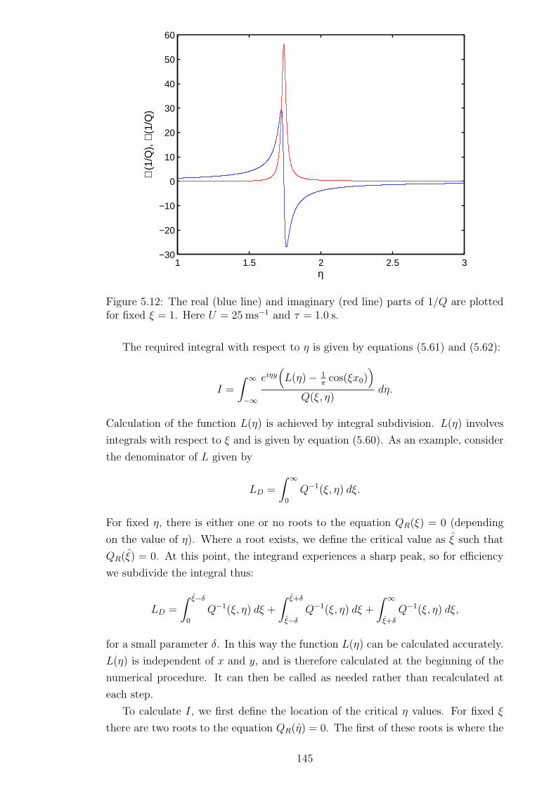
1 1.5 2 2.5 3−30
−20
−10
0
10
20
30
40
50
60
η
ℜ(1
/Q),
ℑ(1
/Q)
Figure 5.12: The real (blue line) and imaginary (red line) parts of 1/Q are plottedfor fixed ξ = 1. Here U = 25 ms−1 and τ = 1.0 s.
The required integral with respect to η is given by equations (5.61) and (5.62):
I =
∫ ∞
−∞
eiηy(
L(η)− 1πcos(ξx0)
)
Q(ξ, η)dη.
Calculation of the function L(η) is achieved by integral subdivision. L(η) involves
integrals with respect to ξ and is given by equation (5.60). As an example, consider
the denominator of L given by
LD =
∫ ∞
0
Q−1(ξ, η) dξ.
For fixed η, there is either one or no roots to the equation QR(ξ) = 0 (depending
on the value of η). Where a root exists, we define the critical value as ξ such that
QR(ξ) = 0. At this point, the integrand experiences a sharp peak, so for efficiency
we subdivide the integral thus:
LD =
∫ ξ−δ
0
Q−1(ξ, η) dξ +
∫ ξ+δ
ξ−δ
Q−1(ξ, η) dξ +
∫ ∞
ξ+δ
Q−1(ξ, η) dξ,
for a small parameter δ. In this way the function L(η) can be calculated accurately.
L(η) is independent of x and y, and is therefore calculated at the beginning of the
numerical procedure. It can then be called as needed rather than recalculated at
each step.
To calculate I, we first define the location of the critical η values. For fixed ξ
there are two roots to the equation QR(η) = 0. The first of these roots is where the
145

integrand is most troublesome, and hence the integral is subdivided at η using the
procedure outlined above. Combined with exploiting the symmetry of the integrand,
these techniques allow the integrals to be calculated accurately whilst minimising
the time of the computation.
5.3.3 Numerical results
Recall that the default parameters are given by Table 2.1(a) with H = 100 m.
Parameters U , τ and x0 will be varied frequently and are hence not given a default
value but stated explicitly. For each 3D plot, the aspect ratio of x and y are
kept equal for clarity. In each plot the colour bars are generated to have equal
magnitude for depression and elevation for easy comparison. However, the colours
are not consistent from plot to plot, and the scale should be consulted for each plot
independently. The characteristic length scale for the default parameter set is given
by ℓ = 20.01 m, which should be borne in mind when considering values of x0, the
distance from the wall.
We begin by analysing the deflection for U < cmin. Recall that for the default
data set, cmin = 18.05 ms−1. We then proceed to analyse the ice deflection for load
speeds greater than cmin. The deflections for both the open ice case and vertical wall
case are then directly compared. We then investigate the strains along the vertical
wall, to determine whether the ice connection will be maintained, and if not, what
factors most influence the ice fracture.
5.3.3.1 Deflection
(i): U < cmin
We begin by plotting the deflection for τ = 0.1 s, U = 10 ms−1, and x0 = 25 m,
shown in Figure 5.13.
Recall that H = 100 m and hence x0 = 25 m corresponds to a load at x = 0.25,
etc. This value of x0 places the moving load quite close to the wall, and the speed U
is less than the critical speed cmin. For the values of the parameters given, there is
little wave elevation ahead or behind the moving load. The pattern of the depression
caused by the moving load is distorted from being symmetric by the ice–clamping
condition. The deflection and slope of the deflection are zero along the wall due to
this condition.
We increase the load speed to U = 15 ms−1. The wave pattern for this speed is
shown in Figure 5.14.
We begin to see wave elevation ahead and behind the source. Due to the vis-
coelastic formulation, this elevation is not symmetric: the wave elevation is slightly
higher behind the load than ahead of it. The magnitude of the deflection is also
considerably higher for this increased speed. Also, the depression caused by the load
increases in area as the load speed increases.
We now move the load further away from the vertical wall, taking x0 = 75 m,
146

0 0.5 1 1.5 −10
1
−0.2
−0.15
−0.1
−0.05
0
yx
w(x
,y)
−0.15 −0.1 −0.05 0 0.05 0.1 0.15
Figure 5.13: The deflection w(x, y) is plotted against x and y. Here τ = 0.1 s,U = 10 ms−1, x0 = 25 m.
0 0.5 1 1.5 2−20
2−0.5
−0.4
−0.3
−0.2
−0.1
0
y
x
w(x
,y)
−0.4 −0.3 −0.2 −0.1 0 0.1 0.2 0.3 0.4
Figure 5.14: The deflection w(x, y) is plotted against x and y. Here τ = 0.1 s,U = 15 ms−1, x0 = 25 m.
147
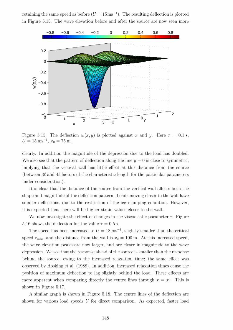
retaining the same speed as before (U = 15ms−1). The resulting deflection is plotted
in Figure 5.15. The wave elevation before and after the source are now seen more
0 1 2 3 −2 −1 0 1 2−1
−0.8
−0.6
−0.4
−0.2
0
0.2
yx
w(x
,y)
−0.8 −0.6 −0.4 −0.2 0 0.2 0.4 0.6 0.8
Figure 5.15: The deflection w(x, y) is plotted against x and y. Here τ = 0.1 s,U = 15 ms−1, x0 = 75 m.
clearly. In addition the magnitude of the depression due to the load has doubled.
We also see that the pattern of deflection along the line y = 0 is close to symmetric,
implying that the vertical wall has little effect at this distance from the source
(between 3ℓ and 4ℓ factors of the characteristic length for the particular parameters
under consideration).
It is clear that the distance of the source from the vertical wall affects both the
shape and magnitude of the deflection pattern. Loads moving closer to the wall have
smaller deflections, due to the restriction of the ice–clamping condition. However,
it is expected that there will be higher strain values closer to the wall.
We now investigate the effect of changes in the viscoelastic parameter τ . Figure
5.16 shows the deflection for the value τ = 0.5 s.
The speed has been increased to U = 18 ms−1, slightly smaller than the critical
speed cmin, and the distance from the wall is x0 = 100 m. At this increased speed,
the wave elevation peaks are now larger, and are closer in magnitude to the wave
depression. We see that the response ahead of the source is smaller than the response
behind the source, owing to the increased relaxation time; the same effect was
observed by Hosking et al. (1988). In addition, increased relaxation times cause the
position of maximum deflection to lag slightly behind the load. These effects are
more apparent when comparing directly the centre lines through x = x0. This is
shown in Figure 5.17.
A similar graph is shown in Figure 5.18. The centre lines of the deflection are
shown for various load speeds U for direct comparison. As expected, faster load
148

02
4 −2 −1 0 1 2
−2
−1.5
−1
−0.5
0
0.5
yx
w(x
,y)
−1.5 −1 −0.5 0 0.5 1 1.5
Figure 5.16: The deflection w(x, y) is plotted against x and y. Here τ = 0.5 s,U = 18 ms−1, x0 = 100 m.
−5 −4 −3 −2 −1 0 1 2 3
−1.5
−1
−0.5
0
0.5
y
w(x
0,y)
Figure 5.17: The deflection w(x, y) through x = x0 is plotted against y. Herex0 = 200 m, U = 17ms−1. Relaxation time τ is given by: τ = 2.0 s (blue), τ = 1.0 s(red), τ = 0.5 s (green), τ = 0.1 s (black).
149
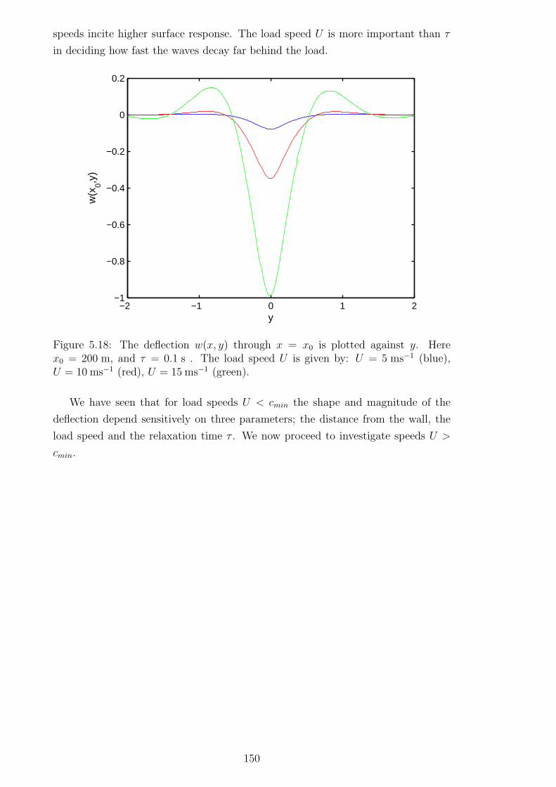
speeds incite higher surface response. The load speed U is more important than τ
in deciding how fast the waves decay far behind the load.
−2 −1 0 1 2−1
−0.8
−0.6
−0.4
−0.2
0
0.2
y
w(x
0,y)
Figure 5.18: The deflection w(x, y) through x = x0 is plotted against y. Herex0 = 200 m, and τ = 0.1 s . The load speed U is given by: U = 5 ms−1 (blue),U = 10 ms−1 (red), U = 15 ms−1 (green).
We have seen that for load speeds U < cmin the shape and magnitude of the
deflection depend sensitively on three parameters; the distance from the wall, the
load speed and the relaxation time τ . We now proceed to investigate speeds U >
cmin.
150

(ii): U > cmin
Figure 5.19 shows the ice deflection for a load moving with speed U = 20ms−1. Here
0
2
4
6
8−6 −4 −2 0 2 4 6
−2
−1
0
1
y
x
w(x
,y)
−1.5 −1 −0.5 0 0.5 1 1.5
Figure 5.19: The deflection w(x, y) plotted against x and y for the load speedU = 20 ms−1, with τ = 0.1 s and x0 = 200 m.
the relaxation time is τ = 0.1 s and the load is 200 m from the wall. We observe a
drastic change in the deflection pattern; the waves decay much slower and propagate
further from the source. In addition the waves are no longer straight but are curved,
both ahead and behind the source. There is strong interaction with the vertical wall
despite the increased distance x0. As we are quite close to the critical speed cmin,
the waves ahead and behind the source have comparable wavelength, but the waves
ahead of the source have slightly smaller wavelength.
Figure 5.20 shows the deflection for the load speed U = 26 ms−1, with τ = 0.1 s
and x0 = 600 m. Similar to the open ice case in Section 5.2, both wave modes are
visible and the wave pattern is curved. The waves decay faster ahead of the source
than behind the source as before. However, there is now a region between the
vertical wall and the moving load where considerable disturbance is present. Recall
that the graphs are for a moving frame of reference, moving with speed U . Hence
the disturbance can be explained as standing waves trapped between the vertical
wall and the wave source, the moving load.
Figure 5.21 shows the deflection for the load speed U = 30 ms−1, with τ = 0.1 s
and x0 = 600 m. The wave pattern becomes even more curved. The deflection is
high at the point where the longer wave behind the load is close to the vertical wall.
In a similar fashion as for the open ice case, we observe that the viscoelastic decay
affects the waves ahead of the source more as U increases.
We now investigate the effect of τ for high load speeds. Figure 5.22 compares the
deflection through the centre line x = x0 for various values of τ . Here x0 = 400 m
and U = 25 ms−1. The viscoelasticity strongly affects the shorter waves ahead of
the source; for τ = 1.0 s the waves decay almost immediately. Behind the source,
151
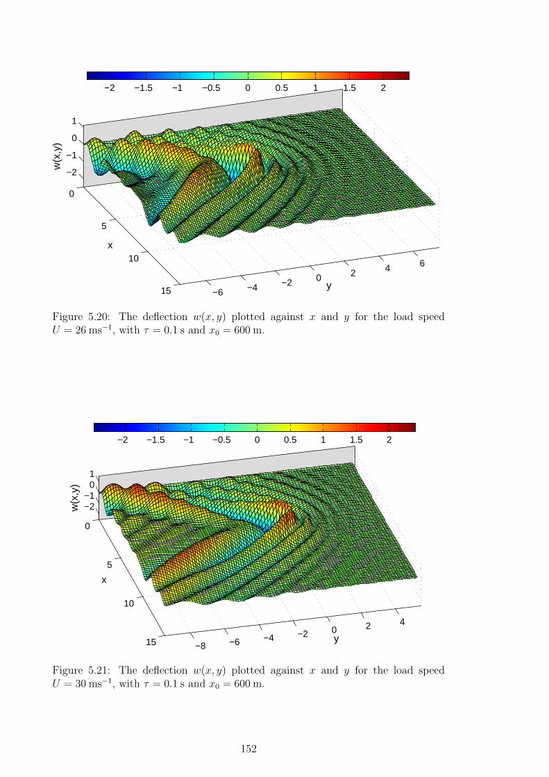
0
5
10
15 −6 −4 −2 0 2 4 6
−2
−1
0
1
y
x
w(x
,y)
−2 −1.5 −1 −0.5 0 0.5 1 1.5 2
Figure 5.20: The deflection w(x, y) plotted against x and y for the load speedU = 26 ms−1, with τ = 0.1 s and x0 = 600 m.
0
5
10
15 −8 −6 −4 −2 0 2 4
−2−1
01
y
x
w(x
,y)
−2 −1.5 −1 −0.5 0 0.5 1 1.5 2
Figure 5.21: The deflection w(x, y) plotted against x and y for the load speedU = 30 ms−1, with τ = 0.1 s and x0 = 600 m.
152
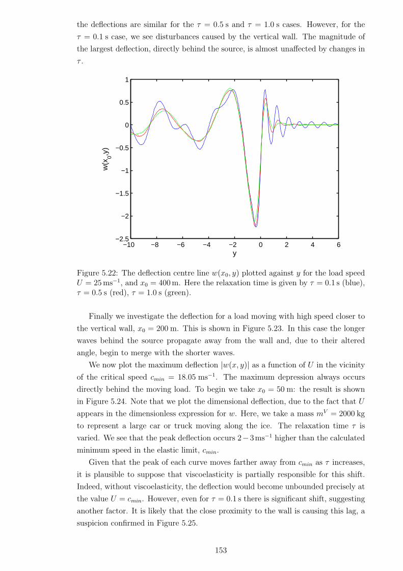
the deflections are similar for the τ = 0.5 s and τ = 1.0 s cases. However, for the
τ = 0.1 s case, we see disturbances caused by the vertical wall. The magnitude of
the largest deflection, directly behind the source, is almost unaffected by changes in
τ .
−10 −8 −6 −4 −2 0 2 4 6−2.5
−2
−1.5
−1
−0.5
0
0.5
1
y
w(x
0,y)
Figure 5.22: The deflection centre line w(x0, y) plotted against y for the load speedU = 25ms−1, and x0 = 400m. Here the relaxation time is given by τ = 0.1 s (blue),τ = 0.5 s (red), τ = 1.0 s (green).
Finally we investigate the deflection for a load moving with high speed closer to
the vertical wall, x0 = 200 m. This is shown in Figure 5.23. In this case the longer
waves behind the source propagate away from the wall and, due to their altered
angle, begin to merge with the shorter waves.
We now plot the maximum deflection |w(x, y)| as a function of U in the vicinity
of the critical speed cmin = 18.05 ms−1. The maximum depression always occurs
directly behind the moving load. To begin we take x0 = 50 m: the result is shown
in Figure 5.24. Note that we plot the dimensional deflection, due to the fact that U
appears in the dimensionless expression for w. Here, we take a mass mV = 2000 kg
to represent a large car or truck moving along the ice. The relaxation time τ is
varied. We see that the peak deflection occurs 2−3ms−1 higher than the calculated
minimum speed in the elastic limit, cmin.
Given that the peak of each curve moves farther away from cmin as τ increases,
it is plausible to suppose that viscoelasticity is partially responsible for this shift.
Indeed, without viscoelasticity, the deflection would become unbounded precisely at
the value U = cmin. However, even for τ = 0.1 s there is significant shift, suggesting
another factor. It is likely that the close proximity to the wall is causing this lag, a
suspicion confirmed in Figure 5.25.
153

0
5
10
15
−5
0
5
−2−1
01
y
x
w(x
,y)
−2.5 −2 −1.5 −1 −0.5 0 0.5 1 1.5 2 2.5
Figure 5.23: The deflection w(x, y) plotted against y for the load speed U = 30ms−1.Here τ = 0.1 s and x0 = 200 m.
14 15 16 17 18.05 19 20 21 22 235
6
7
8
9
10
11x 10
−4
U (ms−1)
|w(x
,y)|
(m
)
Figure 5.24: The maximum deflection |w(x, y)| is plotted against the load speed U ,for τ = 0.1 s (blue), τ = 0.5 s (red) and τ = 1.0 s (green). Here x0 = 50 m.
154
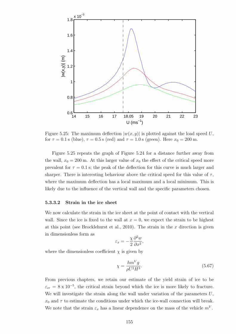
14 15 16 17 18.05 19 20 21 22 230.6
0.8
1
1.2
1.4
1.6
1.8x 10
−3
U (ms−1)
|w(x
,y)|
(m
)
Figure 5.25: The maximum deflection |w(x, y)| is plotted against the load speed U ,for τ = 0.1 s (blue), τ = 0.5 s (red) and τ = 1.0 s (green). Here x0 = 200 m.
Figure 5.25 repeats the graph of Figure 5.24 for a distance further away from
the wall, x0 = 200 m. At this larger value of x0 the effect of the critical speed more
prevalent for τ = 0.1 s; the peak of the deflection for this curve is much larger and
sharper. There is interesting behaviour above the critical speed for this value of τ ,
where the maximum deflection has a local maximum and a local minimum. This is
likely due to the influence of the vertical wall and the specific parameters chosen.
5.3.3.2 Strain in the ice sheet
We now calculate the strain in the ice sheet at the point of contact with the vertical
wall. Since the ice is fixed to the wall at x = 0, we expect the strain to be highest
at this point (see Brocklehurst et al., 2010). The strain in the x direction is given
in dimensionless form as
εx = −χ2
∂2w
∂x2,
where the dimensionless coefficient χ is given by
χ =hmV g
ρU2H3. (5.67)
From previous chapters, we retain our estimate of the yield strain of ice to be
εcr = 8 x 10⁻⁵, the critical strain beyond which the ice is more likely to fracture.
We will investigate the strain along the wall under variation of the parameters U ,
x0 and τ to estimate the conditions under which the ice-wall connection will break.
We note that the strain εx has a linear dependence on the mass of the vehicle mV .
155

We begin by investigating the strain for the default data set of Table 2.1(a) with
H = 100 m. We choose the parameters U = 17 ms−1, τ = 0.1 s and x0 = 50 m.
In addition we take mV = 2000 kg to represent a heavy car or truck. The strain is
plotted along the line x = 0 and is shown in Figure 5.26. We see that despite the
−1.5 −1 −0.5 0 0.5 1 1.5−2.5
−2
−1.5
−1
−0.5
0
0.5x 10
−6
y
ε x
Figure 5.26: The strain εx is plotted against y along the line x = 0. Here τ = 0.1 s,x0 = 50m, U = 17ms−1 and mV = 2000kg. Other parameters are taken from Table2.1(a) with H = 100 m.
heavy load moving quite close to the vertical wall, the strain is still well below its
critical value (the maximum strain here being 2.4 x 10⁻⁶), predicting that the ice is
likely to remain frozen to the wall under these conditions. This is due to the fact
that the ice thickness h = 1.6 m is large enough to support very heavy loads.
With the proposed applications discussed in Section 1.6 in mind, the data set of
Takizawa (1985) seems more appropriate. Taken from experiments on Lake Saroma,
Japan, this data set is characterised by shallower water (H = 6.8 m) and thinner
ice (h = 0.175m) than the McMurdo Sound set. The full set of parameters is found
in Table 2.1(b). The critical speed for this data set is calculated numerically as
cmin = 5.98 ms−1 and the characteristic length ℓ = 2.23 m. Takizawa (1985) was
driving a skidoo of weight mV = 235 kg and investigating the waves incited by this
moving load.
The strain along the wall for the new data set is found in Figure 5.27. Here
τ = 0.1 s, U = 5 ms−1 and the distance from the wall x0 is varied from 2.5− 7.5 m.
As expected, the strain is highest when the moving load is closest to the vertical
wall. For x0 = 2.5 m the strain is beyond the yield strain εcr = 8 x 10⁻⁵, suggesting
that the ice connection is likely to fracture. The dependence on the distance x0
proves quite sensitive, as seen by the strain for x0 = 7.5 m having strain below
the yield strain. There is a small lag from the position of the load to the position
of maximum strain. As shown in (5.27) the distance x0 does not affect this lag,
implying another cause for this phenomenon.
156

−2 −1.5 −1 −0.5 0 0.5 1 1.5 2−20
−10
0
x 10−5
y
ε x
Figure 5.27: The strain εx is plotted against y along the line x = 0. Here τ = 0.1 s,U = 5 ms−1 and mV = 235 kg. The distance from the wall x0 is given by 2.5 m(blue), 5 m (red) and 7.5 m (green). Other parameters are taken from Table 2.1(b).Here the dotted black line indicates the yield strain εcr.
Another important factor for deciding whether the ice will fracture is the amount
of time that the ice is above its yield strain. If this proves to be a short time, it
is conceivable that the ice connection may survive. Retaining starred variables for
clarity, the time taken for the load to pass between two points y∗1 and y∗2 is
t =H(y∗2 − y∗1)
U.
For Figure 5.27, we see that when x0 = 2.5 m, the strain will be over its yield
value for approximately 1 second. Although not large, given the peak magnitude of
this strain, it is likely to be substantial enough to fracture the ice, though this is
speculative.
Figure 5.28 varies the speed U to investigate its effect on the strain along the
wall. The parameters are τ = 0.1 s, x0 = 5 m and U is varied from 3 − 5 ms−1 (all
of which are below the critical speed cmin). We see that faster load speeds cause
more strain at the ice-wall connection, which is to be expected. However, the effect
of varying U is not quite as profound as varying x0 in terms of the magnitude of
the strain. In all cases there is a small area close to y = 0 where the ice is likely to
fracture for the parameter values considered.
We now investigate the effect of the relaxation time τ on the strain along the
wall, shown in Figure 5.30. Parameters are set to U = 5 ms−1, x0 = 5 m, and τ
is varied from 0.1 − 1.0 s. We see that τ also affects the strain magnitude, with
157

−2 −1.5 −1 −0.5 0 0.5 1 1.5 2−12
−10
−8
−6
−4
−2
0
2x 10
−5
y
ε cr
Figure 5.28: The strain εx is plotted against y along the line x = 0. Here τ = 0.1 s,x0 = 5 m and mV = 235 kg. The speed U of the moving load is given by 3 ms−1
(blue), 4 ms−1 (red) and 5 ms−1 (green). Other parameters are taken from Table2.1(b).
−3 −2 −1 0 1 2 3−12
−10
−8
−6
−4
−2
0
2x 10
−5
y
ε x
Figure 5.29: The strain εx is plotted against y along the line x = 0. Here U = 5ms−1,x0 = 5m and mV = 235 kg. The relaxation time τ of the ice is given by 0.1 s (blue),0.5 s (red) and 1.0 s (green). Other parameters are taken from Table 2.1(b).
158

lower values of τ causing higher peaks in the strain. In addition, we see that the
viscoelasticity is responsible for the lag between the load location y = 0 and the
location of maximum strain. This is expected since other authors have speculated
that the viscoelasticity was responsible for the lag effect in the deflection caused by
the moving load (Hosking et al., 1988; Takizawa, 1985).
−6 −4 −2 0 2 4−16
−14
−12
−10
−8
−6
−4
−2
0
2x 10
−5
y
ε x
Figure 5.30: The strain εx is plotted against y along the line x = 0. Here τ = 0.1 s,x0 = 5 m and mV = 235 kg. The load speed U of the moving load is given by6.5 ms−1 (blue), 7.5 ms−1 (red) and 8.5 ms−1 (green). Other parameters are takenfrom Table 2.1(b).
Figure 5.31 investigates the strain along the wall for speeds greater than the
minimum speed cmin = 5.98ms−1. Here, the other parameters are fixed as τ = 0.1 s,
x0 = 10 m and the load speed U varies between 6.5 − 8.5 ms−1. In the vicinity of
y = 0, the peaks in deflection are similar for each value of U . Even though x0 is
slightly higher than in the previous graphs, the strain has a higher magnitude and
is likely to fracture the ice for the parameter values considered. However, we see
that faster speeds cause slightly lower maximum strain. As the speed increases, we
move further from the critical speed, at which the deflection (and hence strain along
the wall) is highest. There is disturbance both ahead and behind the moving load.
Ahead of the load we see the shorter waves that propagate ahead of the source as
seen in Section 5.3.3.1. Shorter waves are also visible in the strain profile at the
wall for y < 0: this is due to the curved wave profile for higher speeds. The longer
wavelength is still visible but decays quickly.
We are also interested in the strain in the ice near the moving load. The strain
along the line y = 0 is plotted in Figure 5.31. We see that the strain is above
critical strain at the ice connection to the wall, but also above the critical strain
159

0 0.5 1 1.5 2
−1.5
−1
−0.5
0
0.5
1
1.5
x 10−4
x
ε x
Figure 5.31: The strain εx is plotted against x along the line y = 0. Here τ = 0.1 s,x0 = 5m and mV = 235 kg. The load speed is U = 6.5 ms−1. Other parameters aretaken from Table 2.1(b).
near the location of the load, x = 0.735. However, it is certain that the strain is
over-estimated at this point due to the point-load formulation. The entirety of the
mass is focused to one infinitesimally small point due to the nature of the Dirac
delta function used to model the point load. In reality the load would be spread
over an area which would dampen the strain at this point. Indeed, Takizawa (1985)
has ridden a skiddoo of mass mV = 235 kg without any reported fracture.
5.3.4 Comparison between vertical wall and open ice case
We now compare directly the results from Sections (5.2) and (5.3); the open ice case
and the vertical wall case. The deflection for each case is plotted in Figure 5.32 for
a speed U = 15 ms−1. As expected, the two cases are very similar, and are almost
identical to the right of the load. For Figure 5.32(a) the presence of a vertical wall
breaks the symmetry and also makes the deflection pattern slightly more circular
near the vertical load.
This comparison is repeated in Figure 5.33 for a higher load speed U = 25ms−1.
In this case, the differences are more profound. However, the region to the right of
the moving load is still very similar to each other, indicating that for the value of x0
considered, the influence of the vertical wall is confined mostly to the zone between
the wall and the moving load.
160
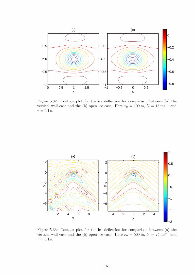
(a)
x
y
0 0.5 1 1.5−1
−0.5
0
0.5
(b)
x
y
−1 −0.5 0 0.5−1
−0.5
0
0.5
−0.8
−0.6
−0.4
−0.2
0
Figure 5.32: Contour plot for the ice deflection for comparison between (a) thevertical wall case and the (b) open ice case. Here x0 = 100 m, U = 15 ms−1 andτ = 0.1 s.
(a)
x
y
0 2 4 6 8
−6
−4
−2
0
2
(b)
x
y
−4 −2 0 2 4
−6
−4
−2
0
2
−2
−1.5
−1
−0.5
0
0.5
1
Figure 5.33: Contour plot for the ice deflection for comparison between (a) thevertical wall case and the (b) open ice case. Here x0 = 500 m, U = 25 ms−1 andτ = 0.1 s.
161

5.4 Summary
The problem of a moving load on an ice sheet was solved within the linear theory
of hydroelasticity, both in open ice and near a vertical wall. For the latter case,
the ice was frozen to the vertical wall. The moving load incites a response in the
ice sheet in the form of outgoing waves. In both cases a simple viscoelastic model
was introduced, adding further realism to the formulation. Both cases were solved
by applying Fourier transforms in the x and y directions along the plane of the ice
sheet. For the open ice case, the resulting integral transforms were calculated using
the method of residues and the application of the Cauchy residue theorem. For the
vertical wall case, the integrals were solved by standard integration techniques and
integrand subdivision. The deflection in the ice sheet was studied extensively under
variation of important parameters. The strain in the ice sheet was studied, with
particular attention to the strain along the vertical wall to assess whether the ice
connection would be maintained.
For problems involving moving loads on ice sheets, there exists a critical speed
cmin, corresponding to the minimum phase speed of hydroelastic waves. Ice has been
proven experimentally to produce abnormally high deflections close to this critical
speed. If the load moves at this speed, the viscoelastic formulation is necessary to
find a bounded solution. The effect of viscoelasticity on the deflection at speeds
U = cmin was studied. In addition, whether the load moves at speed above or below
this critical speed has a dramatic impact on the shape of the deflection pattern, and
the decay of the waves in the far field. For slow load speeds, the waves are mostly
localised. For speeds U > cmin, there are two visible sets of waves; faster waves ahead
of the source that have smaller wavelength and are elastic-dominated, and slower
waves behind the source that have a longer wavelength and are gravity-dominated.
The effect of a vertical wall on the ice deflection for slow load speeds is mostly
dampening; if the load is close to the vertical wall, the magnitude of the ice response
is smaller because of the restriction of the ice being frozen to the wall. For faster
speeds, there is considerable interaction between the vertical wall and the generated
waves, causing wave reflection and visible disturbance in the vicinity of the wall.
For slow load speeds, the viscoelasticity causes the response ahead of the moving
load to become smaller than the response behind, whereas these would usually be
symmetric in the elastic limit. In addition the viscoelasticity causes a lag between
the moving load and the position of maximum deflection. For fast load speeds, the
viscoelasticity affects the waves ahead of the source most profoundly, and the decay
there is quite fast. Lower values of viscoelastic parameter τ markedly increase the
disturbance in the wave pattern.
The strain along the wall was studied for both data sets in Table 2.1. For
the parameter set from McMurdo Sound, we conclude that only a very heavy load
moving very close to the vertical wall would produce enough strain to fracture the
ice, due to the thickness of the ice in this data set. For the data from Lake Saroma,
162
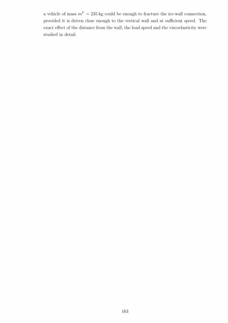
a vehicle of mass mV = 235 kg could be enough to fracture the ice-wall connection,
provided it is driven close enough to the vertical wall and at sufficient speed. The
exact effect of the distance from the wall, the load speed and the viscoelasticity were
studied in detail.
163
Chapter 6
Hydroelastic waves generated by a
moving load in the vicinity of a
vertical wall: nonlinear
formulation
6.1 Introduction
We extend the model of Section 5.3 to consider nonlinear effects. A semi–infinite
ice sheet meets a vertical wall, to which the ice is frozen. We investigate the effect
of a load moving close to the wall. In this chapter the fluid is considered to be of
infinite depth. This assumption is justified by the deep water of the default data
set, for which we will be taking the data from McMurdo Sound, Table 2.1(a). Other
features of the model are the same as the previous section; the fluid is incompressible,
inviscid and irrotational flow is assumed. The load moves parallel to the wall, a
constant distance from it, with constant velocity. The motion of the load generates
hydroelastic waves which are studied in detail.
The model for the ice sheet is the same linear thin elastic plate model used in all
previous chapters. However, we now consider fully nonlinear equations for the fluid
flow beneath the plate. The nonlinear Bernoulli and kinematic conditions replace
their linear counterparts. The introduction of this nonlinearity means that integral
transforms used in the previous chapters cannot be used as the method of solution.
Instead we utilise a boundary integral equation method, after application of Green’s
second identity using a suitable free-surface Green’s function. The solution is then
computed numerically using Newton’s method. The method is based on work by
Parau & Vanden-Broeck (2011) who solved the problem of hydroelastic waves due
to a moving load without a vertical wall present. Their solution was in turn based
on Forbes (1989) who developed a method to solve problems involving nonlinear
free-surface flows.
Another change from the linear formulation of Chapter 5 is the definition of
164
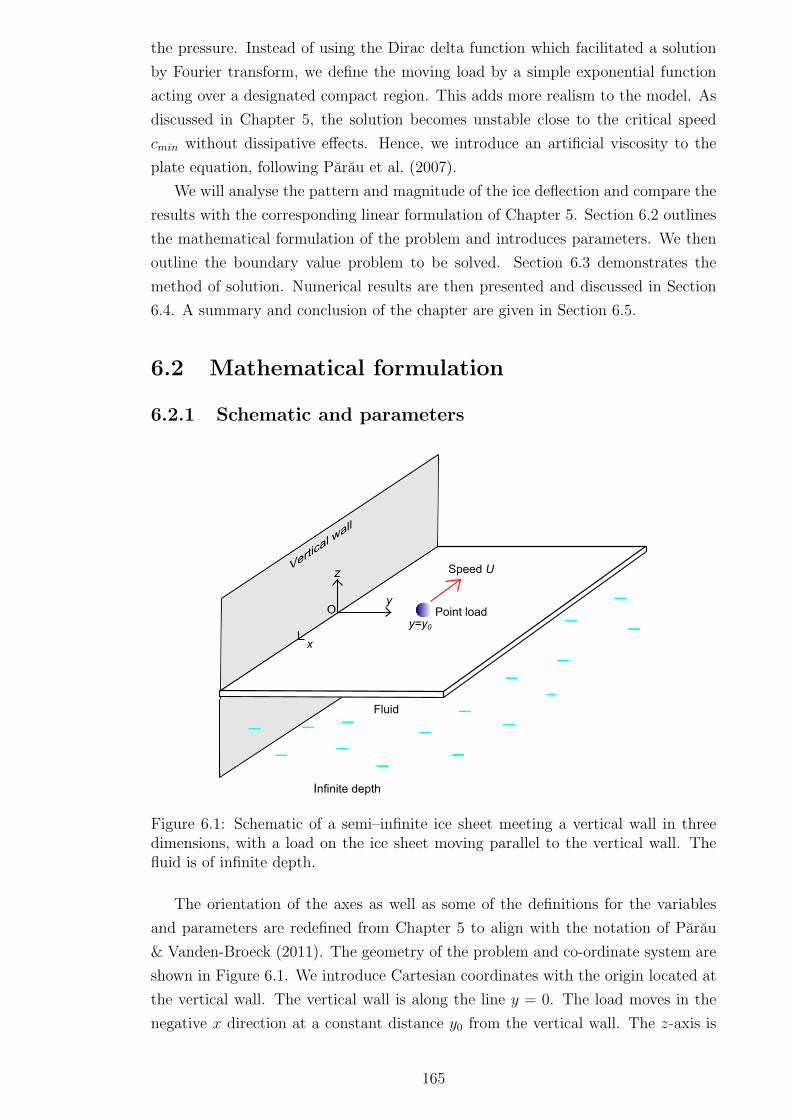
the pressure. Instead of using the Dirac delta function which facilitated a solution
by Fourier transform, we define the moving load by a simple exponential function
acting over a designated compact region. This adds more realism to the model. As
discussed in Chapter 5, the solution becomes unstable close to the critical speed
cmin without dissipative effects. Hence, we introduce an artificial viscosity to the
plate equation, following Parau et al. (2007).
We will analyse the pattern and magnitude of the ice deflection and compare the
results with the corresponding linear formulation of Chapter 5. Section 6.2 outlines
the mathematical formulation of the problem and introduces parameters. We then
outline the boundary value problem to be solved. Section 6.3 demonstrates the
method of solution. Numerical results are then presented and discussed in Section
6.4. A summary and conclusion of the chapter are given in Section 6.5.
6.2 Mathematical formulation
6.2.1 Schematic and parameters
Fluid
Vertica
l wall
x
y
z
Point load
Speed U
O
y=y0
Infinite depth
Figure 6.1: Schematic of a semi–infinite ice sheet meeting a vertical wall in threedimensions, with a load on the ice sheet moving parallel to the vertical wall. Thefluid is of infinite depth.
The orientation of the axes as well as some of the definitions for the variables
and parameters are redefined from Chapter 5 to align with the notation of Parau
& Vanden-Broeck (2011). The geometry of the problem and co-ordinate system are
shown in Figure 6.1. We introduce Cartesian coordinates with the origin located at
the vertical wall. The vertical wall is along the line y = 0. The load moves in the
negative x direction at a constant distance y0 from the vertical wall. The z-axis is
165

directed vertically upwards, with the bottom of the unperturbed ice sheet at z = 0.
The fluid has infinite depth. Time is denoted by t. The moving load is defined as
an external pressure P (x, y, t), and the pressure in the fluid is defined p(x, y, z, t).
The moving load has magnitude P0 and is moving with speed U . The size of the
support of the pressure is defined L. The density of the fluid is ρ. The fluid
velocity V(x, y, z, t) is equal to the gradient of the velocity potential Φ(x, y, z, t),
hence ∇Φ = V. The vertical deflection of the ice sheet (the distance the ice sheet
is displaced relative to its position at rest) is denoted by w(x, y, t). The ice has
mass per unit length M , where M = ρih, ρi is the ice density and h is the ice
thickness. The ice sheet has flexural rigidity EJ , where E is Young’s modulus and
J = h3/[12(1 − ν2)], where ν is Poisson’s ratio. The acceleration due to gravity is
denoted g. In addition we introduce the artificial viscosity µ, defined below.
6.2.2 Governing equations and boundary conditions
We now introduce nonlinear versions of the governing equations, as opposed to their
linearised counterparts which have been used in the previous chapters. Note that
we retain the linear elastic plate model, but the fluid is fully nonlinear. Due to
this nonlinear model, the boundary conditions applied at the surface are applied at
z = w(x, y, t) instead of z = 0 as for the linear models.
The velocity potential Φ(x, y, z, t) must satisfy Laplace’s equation in the fluid:
∇2Φ = 0, (−∞ < x <∞, 0 < y <∞, −∞ < z < 0). (6.1)
The plate equation is given by
EJ∇4w = p(x, y, z, t) + P (x, y, t), (−∞ < x <∞, 0 < y <∞, z = 0). (6.2)
Following Parau & Vanden-Broeck (2011) we neglect the inertia of the thin plate,
and hence the acceleration term Mwtt is not considered. According to Schulkes &
Sneyd (1988), this is justified “provided the wavelength of the surface displacement
is much larger than the ice thickness h. Since the water motion penetrates to a
depth comparable with one wavelength, the inertia of the thin ice plate will then be
small compared with that of the moving-water layer”.
The nonlinear Bernoulli equation gives the pressure in the fluid as
p(x, y, z, t) = −ρgz − ρΦt −ρ
2|∇Φ|2, (−∞ < x <∞, 0 < y <∞). (6.3)
The nonlinear kinematic condition is
wt + Φxwx + Φywy = Φz, (−∞ < x <∞, 0 < y <∞, z = w(x, y, t)). (6.4)
Equations (6.2) and (6.3) combine to give the dynamic condition at the plate-fluid
166

interface:
ρΦt +ρ
2
(
Φ2x + Φ2
y + Φ2z
)
+ ρgw + EJ∇4w = P (x, y, t),
(−∞ < x <∞, 0 < y <∞, z = w(x, y, t)). (6.5)
From Forbes (1989), when the free surface is described by z = w(x, y, t), it is
necessary to impose an upstream radiation condition:
w → 0, |∇Φ| → 0, (x→ −∞). (6.6)
We also have the condition of no flow through the vertical wall:
Φy = 0, (y = 0). (6.7)
There is zero flow in the water far below the ice, so
|∇Φ| → 0, (z → −∞). (6.8)
The ice clamping gives two boundary conditions, namely
w = 0, (y = 0), (6.9)
wy = 0, (y = 0). (6.10)
Equations (6.1)-(6.10) define the nonlinear boundary value problem to be solved.
6.2.3 Dispersion relation and critical speed
By linearising equations (6.1)-(6.10) and looking for waves of the form ei(lx+my−ωt),
we obtain the dispersion relation for infinite depth (Parau & Vanden-Broeck, 2011):
ω2 = gk +EJk5
ρ, (6.11)
where k2 = l2 +m2. Note that this dispersion relation could also be derived from
taking the limit H → ∞ in the equation for the hydroelastic dispersion relation for
finite depth (2.22), and neglecting the mass of the plate. The phase speed c = ω/k
is therefore given by
c2(k) =EJk3
ρ+g
k.
By differentiating with respect to k and after some algebra, we obtain a concise
expression for the minimum phase speed, given by
cmin =
√
4
3
(
3EJg3
ρ
)1
8
.
167

We note that for the data of Table 2.1(a) with infinite depth, the critical speed
cmin = 18.55 ms−1.
6.2.4 Nondimensionalisation & expression for the moving
load
Recall that L is defined as the size of the support for the moving pressure. We use
L as the length scale and the load speed U as the velocity scale. We also introduce
a moving frame of reference, moving with speed U , noting that the load moves in
the negative x direction. Hence we have
x∗ =x+ Ut
L, y∗ =
y
L, z∗ =
z
L, t∗ =
Ut
L.
The dimensionless velocity potential and plate deflection are given by
Φ∗(x∗, y∗, z∗) =Φ(x, y, z, t) + Ux
LU, w∗ =
w
L.
In terms of the new dimensionless moving frame, the derivatives are given by
∂
∂t=U
L
∂
∂x∗,
∂
∂x=
1
L
∂
∂x∗,
∂
∂y=
1
L
∂
∂y∗,
∂
∂z=
1
L
∂
∂z∗.
Applying these changes to the kinematic condition and substituting Φ = LUΦ∗ −LU(x∗ + t∗) and w = Lw∗ gives
U
L
∂
∂x∗
(
Lw∗)
+1
L2
∂
∂x∗
(
LUΦ∗ − LU(x∗ + t∗)) ∂
∂x∗
(
Lw∗)
+1
L2
∂
∂y∗
(
LUΦ∗ − LU(x∗ + t∗)) ∂
∂y∗
(
Lw∗)
=1
L
∂
∂z∗
(
LUΦ∗ − LU(x∗ + t∗))
.
Hence we have∂w∗
∂x∗+
(
∂Φ∗
∂x∗− 1
)
∂w∗
∂x∗+∂Φ∗
∂y∗∂w∗
∂y∗=∂Φ∗
∂z∗,
and after cancellation the kinematic condition in dimensionless form is given by
Φ∗x∗w∗
x∗ + Φ∗y∗w
∗y∗ = Φ∗
z∗ . (6.12)
We proceed to nondimensionalise the dynamic condition (6.5). Substituting for x∗,
y∗ and z∗ we have:
−UρL
Φx∗ +ρ
2L2
(
Φ2x∗ + Φ2
y∗ + Φ2z∗
)
+ ρgw + EJ∇∗4w = P.
We now substitute Φ = LUΦ∗ − LU(x∗ + t∗), w = Lw∗ and P = P0P∗ (where P0 is
the magnitude of the moving pressure) to give
U2ρ(Φ∗x∗ − 1) +
U2ρ
2
(
Φ∗2x∗ − 2Φ∗
x∗ + 1 + Φ∗2y∗ + Φ∗2
z∗
)
+ ρgLw∗ +EJ
L3∇∗4w∗ = P0P
∗.
168
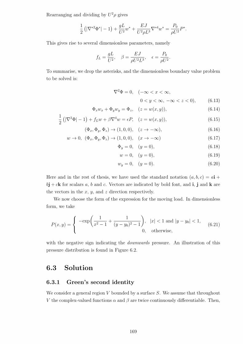
Rearranging and dividing by U2ρ gives
1
2
(
|∇∗2Φ∗| − 1)
+gL
U2w∗ +
EJ
U2ρL3∇∗4w∗ =
P0
ρU2P ∗.
This gives rise to several dimensionless parameters, namely
fL =gL
U2, β =
EJ
ρU2L3, ǫ =
P0
ρU2.
To summarise, we drop the asterisks, and the dimensionless boundary value problem
to be solved is:
∇2Φ = 0, (−∞ < x <∞,
0 < y <∞, −∞ < z < 0), (6.13)
Φxwx + Φywy = Φz, (z = w(x, y)), (6.14)
1
2
(
|∇2Φ| − 1)
+ fLw + β∇4w = ǫP, (z = w(x, y)), (6.15)
(Φx,Φy,Φz) → (1, 0, 0), (z → −∞), (6.16)
w → 0, (Φx,Φy,Φz) → (1, 0, 0), (x→ −∞) (6.17)
Φy = 0, (y = 0), (6.18)
w = 0, (y = 0), (6.19)
wy = 0, (y = 0). (6.20)
Here and in the rest of thesis, we have used the standard notation (a, b, c) = ai +
bj+ ck for scalars a, b and c. Vectors are indicated by bold font, and i, j and k are
the vectors in the x, y, and z direction respectively.
We now choose the form of the expression for the moving load. In dimensionless
form, we take
P (x, y) =
−exp
(
1
x2 − 1+
1
(y − y0)2 − 1
)
, |x| < 1 and |y − y0| < 1,
0, otherwise,(6.21)
with the negative sign indicating the downwards pressure. An illustration of this
pressure distribution is found in Figure 6.2.
6.3 Solution
6.3.1 Green’s second identity
We consider a general region V bounded by a surface S. We assume that throughout
V the complex-valued functions α and β are twice continuously differentiable. Then,
169

x
y
−2 −1 0 10
0.5
1
1.5
2
2.5
3
3.5
−0.14
−0.12
−0.1
−0.08
−0.06
−0.04
−0.02
0
Figure 6.2: An illustration of the pressure distribution for y0 = 2.
α and β must satisfy Green’s second identity (Linton & McIver, 2001):
∫∫∫
V
(
α∇2β − β∇2α)
dV =
∫∫
S
(
α∂β
∂n− β
∂α
∂n
)
dS, (6.22)
where n is the unit vector normal to the surface. The Green’s function for the
present problem is the linear combination of the three-dimensional free-space Green’s
function (Parau & Vanden-Broeck, 2011) plus its image in the y plane, to account
for the vertical wall:
G(Q, Q) =1
4π(
(x− x)2 + (y − y)2 + (z − z)2) 1
2
+1
4π(
(x− x)2 + (y + y)2 + (z − z)2) 1
2
. (6.23)
The Green’s function G is the linear sum of two fractions. In the first fraction,
the denominator represents 4π multiplied by the distance between two points, Q =
(x, y, z) and Q = (x, y, z). The second fraction represents 4π multiplied by the
image of the first fraction in the y = 0 plane. We substitute G = β and Φ− x = α
into Green’s second identity (6.22):
∫∫∫
V
(
(Φ− x)∇2G−G∇2(Φ− x))
dV =
∫∫
S
(
(Φ− x)∂G
∂n−G
∂(Φ− x)
∂n
)
dS.
(6.24)
G satisfies ∇2G = 0, and by equation (6.13) we have ∇2(Φ − x) = ∇2(Φ) = 0.
Hence, the left hand side of (6.24) is equal to zero.
For the application of Green’s second identity to the present problem, we choose
the region sketched in Figure 6.3. The region V consists of half of a large hemisphere
170

x
y
z
SF
SR
SW
Q ~
y=R
x=-R
x=R
Sϵ
ϵ
Figure 6.3: The region V for the application of Green’s second identity.
of radius R centred around the origin, with a smaller hemisphere of radius ε centred
at Q excluded from the region. The large hemisphere is divided in half by the
vertical wall along the line y = 0. The surface is bounded above by the ice sheet.
The surface S therefore comprises 4 surfaces:
• SW , the flat section which is the union of the vertical wall and the large
hemisphere
• SR, the circular surface of the large hemisphere
• Sε, the circular surface of the small hemisphere around the point Q
• SF , the ice-water interface.
Hence, we have
I =
∫∫
SW+SR+Sε+SF
(
(Φ− x)∂G
∂n−G
∂(Φ− x)
∂n
)
dS = 0. (6.25)
We choose the unit normal n for each surface to point into the fluid.
The Green’s function is designed such that it is singular at the point Q. For
the application of Green’s second identity, if Q lies on or within S then it must be
excluded from the domain V (Linton & McIver, 2001). As we will see, an expression
for the velocity potential Φ at the point Q can extracted by taking the limit ε→ 0
and R → ∞. The point Q can be moved arbitrarily to give Φ everywhere on the
free surface.
171

6.3.2 Each surface integral evaluated
6.3.2.1 The surface SW
We wish to calculate the calculation to the integral due to the surface SW :
∫∫
SW
(
(Φ− x)∂G
∂n−G
∂(Φ− x)
∂n
)
dS. (6.26)
For the surface SW , the unit normal pointing into the fluid is given by n = j. We
have
∂G
∂n= ∇(G).n =
(
∂G
∂x
∂G
∂y,∂G
∂z
)
.(0, 1, 0)
=∂G
∂y
= − 1
4π
(
(x− x)2 + (y − y)2 + (z − z)2)− 3
2
(y − y)
− 1
4π
(
(x− x)2 + (y + y)2 + (z − z)2)− 3
2
(y + y).
On the vertical wall, y = 0, and hence we are left with
∂G
∂n= (y − y)
(
(x− x)2 + y2 + (z − z)2)− 3
2
= 0. (6.27)
Also,
∂(Φ− x)
∂n= ∇(Φ− x).n =
(
∂(Φ− x)
∂x,∂(Φ− x)
∂y,∂(Φ− x)
∂z
)
.(0, 1, 0)
=∂(Φ− x)
∂y=∂Φ
∂y. (6.28)
By equation (6.7), Φy = 0 when y = 0. Hence, the contribution to the integral I
from the surface SW is equal to zero.
6.3.2.2 The surface SR
The required calculation is
∫∫
SR
(
(Φ− x)∂G
∂n−G
∂(Φ− x)
∂n
)
dS. (6.29)
The equation for the large spherical surface SR is given by
x2 + y2 + z2 = R2. (6.30)
172

When a surface can be expressed in the form of a function f = 0, the unit normal
vector n is (see for example Jeffrey, 2002):
n =∇f|∇f | . (6.31)
In this case, since we require the inwardly oriented normal, we have
n =∇(R2 − x2 − y2 − z2)
|∇(R2 − x2 − y2 − z2)| =(−2x,−2y,−2z)
(4x2 + 4y2 + 4z2)= − 1
R(x, y, z).
For the first term in the integral, we have
∂G
∂n= ∇(G).n =
(
∂G
∂x,∂G
∂y,∂G
∂z
)
.(x, y, z)
(
− 1
R
)
=1
4πR
(
(x− x)2 + (y − y)2 + (z − z)2)− 3
2
(
x(x− x) + y(y − y) + z(z − z))
+1
4πR
(
(x− x)2 + (y + y)2 + (z − z)2)− 3
2
(
x(x− x) + y(y + y) + z(z − z))
.
We take the limit R → ∞. In this limit, x, y and z are negligible in comparison
with x, y, and z. Hence in the limit R → ∞:
∂G
∂n∼ 1
4πR
(
(x)2 + (y)2 + (z)2)− 3
2
(
x(x) + y(y) + z(z))
+1
4πR
(
(x)2 + (y)2 + (z)2)− 3
2
(
x(x) + y(y) + z(z))
=1
4πR
(
R2)− 3
2
R2 +1
4πR
(
R2)− 3
2
R2
∂G
∂n=
1
2π
1
R2. (6.32)
Clearly equals zero in the limit R → ∞.
For the second term in the required integral over SR, we have
G∂(Φ− x)
∂n= G∇(Φ− x).n = G(Φx − 1,Φy,Φz).(x, y, z)
(
− 1
R
)
. (6.33)
In the limit R → ∞, using the same argument as before, G ∼ (2πR)−1 and so we
have
G∂(Φ− x)
∂n∼ − 1
2π
1
R2
(
x(Φx − 1) + yΦy + zΦz
)
,
which tends to zero in the limit R → ∞. Hence, the contribution to I from the
surface SR is zero.
6.3.2.3 The surface Sε
We evaluate the integral over the surface Sε:
∫∫
Sε
(
(Φ− x)∂G
∂n−G
∂(Φ− x)
∂n
)
dS. (6.34)
173

The equation for this spherical surface centred around the point Q is
ε2 = (x− x)2 + (y − y)2 + (z − z)2,
and the normal pointing into the fluid is given by
n =
(
2(x− x), 2(y − y), 2(z − z))
(
4(x− x)2 + 4(y − y)2 + 4(z − z)2) 1
2
=(x− x, y − y, z − z)
ε.
We split the Green’s function into G = G1 +G2, where
G1 =1
4π(
(x− x)2 + (y − y)2 + (z − z)2) 1
2
,
G2 =1
4π(
(x− x)2 + (y + y)2 + (z − z)2) 1
2
.
Equation (6.34) is then written as
0 =
∫∫
Sε
(Φ− x)∂G2
∂ndS −
∫∫
Sε
G2∂(Φ− x)
∂ndS
+
∫∫
Sε
(
(Φ− x)∂G1
∂n−G1
∂(Φ− x)
∂n
)
dS = I1 − I2 + I3, (6.35)
respectively.
To begin, we evaluate I1. We have
∂G2
∂n= ∇G2.n = − 1
4π
1
ε
(
(x− x)2 + (y + y)(y − y) + (z − z)2)
(
(x− x)2 + (y + y)2 + (z − z)2) 3
2
= − 1
4π
1
ε
(
(x− x)2 + (y − y)2 + (z − z)2 + (y + y)(y − y)− (y − y)2)
(
(x− x)2 + (y − y)2 + (z − z)2 + (y + y)2 − (y − y)2) 3
2
= − 1
4π
1
ε
(
ε2 + (y + y)(y − y)− (y − y)2)
(
ε2 + (y + y)2 − (y − y)2) 3
2
= − 1
4π
1
ε
(
ε2 + 2yy − 2y2)
(
ε2 + 4yy) 3
2
.
Hence we have
I1 = − 1
4π
∫∫
sε
Φ− x
ε
(
ε2 + 2yy − 2y2)
(
ε2 + 4yy) 3
2
dS. (6.36)
We need to project the surface onto the x-y plane. To achieve this, we use the
174
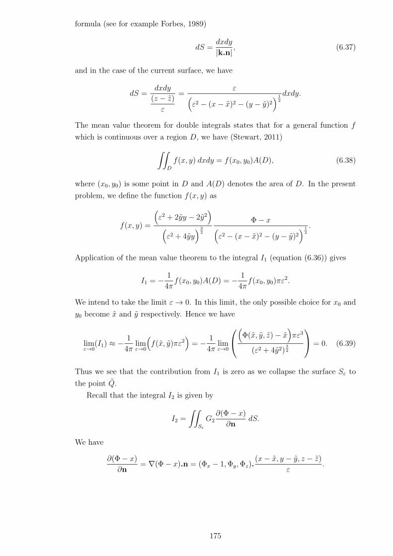
formula (see for example Forbes, 1989)
dS =dxdy
|k.n| , (6.37)
and in the case of the current surface, we have
dS =dxdy
(z − z)
ε
=ε
(
ε2 − (x− x)2 − (y − y)2) 1
2
dxdy.
The mean value theorem for double integrals states that for a general function f
which is continuous over a region D, we have (Stewart, 2011)
∫∫
D
f(x, y) dxdy = f(x0, y0)A(D), (6.38)
where (x0, y0) is some point in D and A(D) denotes the area of D. In the present
problem, we define the function f(x, y) as
f(x, y) =
(
ε2 + 2yy − 2y2)
(
ε2 + 4yy) 3
2
Φ− x(
ε2 − (x− x)2 − (y − y)2) 1
2
.
Application of the mean value theorem to the integral I1 (equation (6.36)) gives
I1 = − 1
4πf(x0, y0)A(D) = − 1
4πf(x0, y0)πε
2.
We intend to take the limit ε→ 0. In this limit, the only possible choice for x0 and
y0 become x and y respectively. Hence we have
limε→0
(I1) ≈ − 1
4πlimε→0
(
f(x, y)πε2)
= − 1
4πlimε→0
(
Φ(x, y, z)− x)
πε3
(ε2 + 4y2)3
2
= 0. (6.39)
Thus we see that the contribution from I1 is zero as we collapse the surface Sε to
the point Q.
Recall that the integral I2 is given by
I2 =
∫∫
Sε
G2∂(Φ− x)
∂ndS.
We have
∂(Φ− x)
∂n= ∇(Φ− x).n = (Φx − 1,Φy,Φz).
(x− x, y − y, z − z)
ε.
175

Hence
I2 =
∫∫
Sε
1
4π
1
ε
(Φ− x)(x− x) + Φy(y − y) + Φz(z − z)(
(x− x)2 + (y + y)2 + (z − z)2) 1
2
dS
=
∫∫
Sε
1
4π
1
ε
(Φ− x)(x− x) + Φy(y − y) + Φz(z − z)(
ε2 + (y + y)2 − (y − y)2) 1
2
dS
=
∫∫
Sε
1
4π
(Φ− x)(x− x) + Φy(y − y) + Φz(z − z)(
ε2 + 4yy) 1
2
(
ε2 − (x− x)2 − (y − y)2) 1
2
dxdy
I2 =1
4π
∫∫
D
g(x, y) dxdy, (6.40)
where we have projected the surface onto the x-y plane. Application of the mean
value theorem for double integrals as before leads to
I2 =1
4πg(x0, y0)πε
2,
where x0 and y0 are some point within the region D. We collapse the surface Sε and
hence (x0, y0) → (x, y) as before, leading to
limε→0
I2 ≈1
4limε→0
(
g(x, y)ε2)
= 0. (6.41)
We are left with the integral I3, the part of the integral over Sε containing G1
terms:∫∫
Sε
(
(Φ− x)∂G1
∂n−G1
∂(Φ− x)
∂n
)
dS. (6.42)
We have
∂G1
∂n= ∇G1.n = (
∂G1
∂x,∂G1
∂y,∂G1
∂z).(x− x, y − y, z − z)
ε
= − 1
4π
1
ε
(x− x)2 + (y − y)2 + (z − z)2
(
(x− x)2 + (y − y)2 + (z − z)2) 3
2
= − 1
4π
1
ε
ε2
(ε2)3
2
= − 1
4π
1
ε2.
Substituting this into equation (6.42) and projecting onto the x-y plane gives
I3 =1
4π
∫∫
Dε
(
−Φ− x
ε2− 1
ε
∂(Φ− x)
∂n
)
ε(
ε2 − (x− x)2 − (y − y)2) 1
2
dxdy.
We introduce cylindrical polar co-ordinates and substitute dxdy = r drdθ. Then I3
176
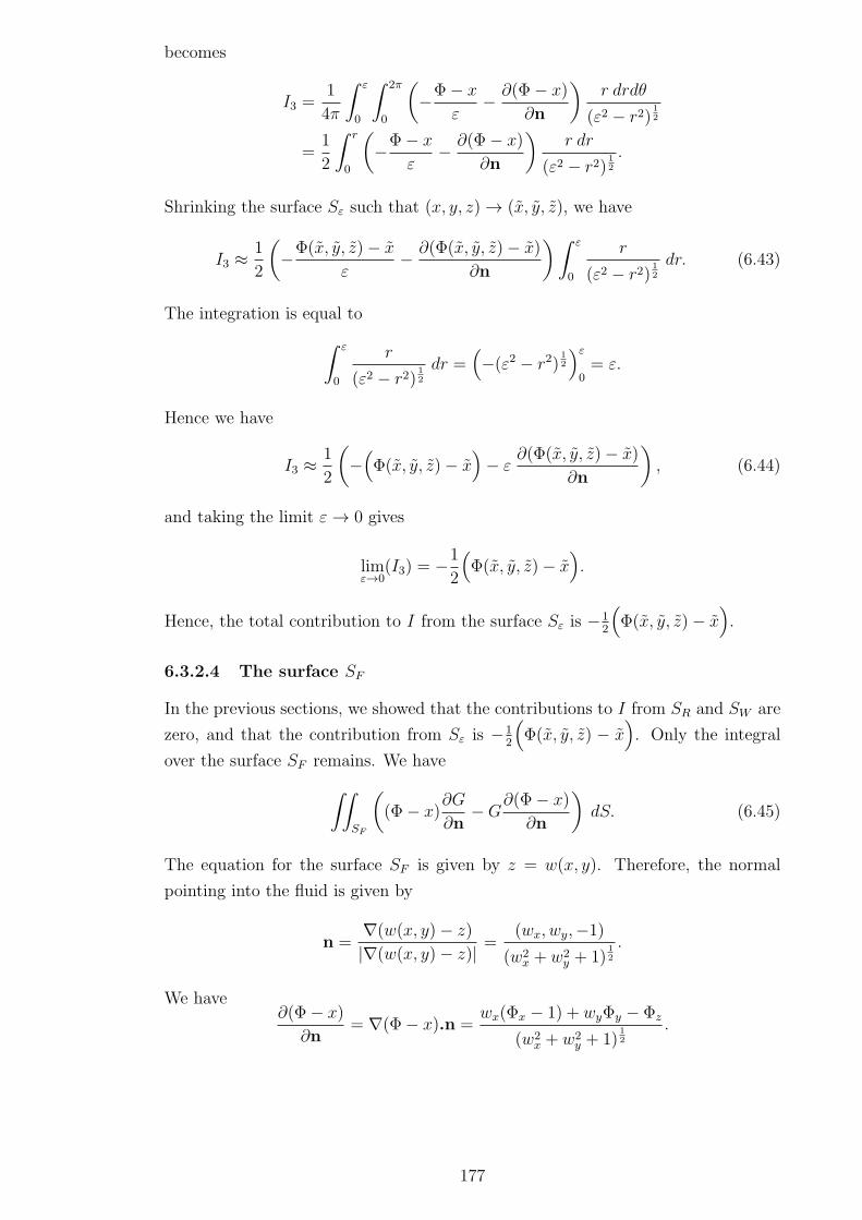
becomes
I3 =1
4π
∫ ε
0
∫ 2π
0
(
−Φ− x
ε− ∂(Φ− x)
∂n
)
r drdθ
(ε2 − r2)1
2
=1
2
∫ r
0
(
−Φ− x
ε− ∂(Φ− x)
∂n
)
r dr
(ε2 − r2)1
2
.
Shrinking the surface Sε such that (x, y, z) → (x, y, z), we have
I3 ≈1
2
(
−Φ(x, y, z)− x
ε− ∂(Φ(x, y, z)− x)
∂n
)∫ ε
0
r
(ε2 − r2)1
2
dr. (6.43)
The integration is equal to
∫ ε
0
r
(ε2 − r2)1
2
dr =(
−(ε2 − r2)1
2
)ε
0= ε.
Hence we have
I3 ≈1
2
(
−(
Φ(x, y, z)− x)
− ε∂(Φ(x, y, z)− x)
∂n
)
, (6.44)
and taking the limit ε→ 0 gives
limε→0
(I3) = −1
2
(
Φ(x, y, z)− x)
.
Hence, the total contribution to I from the surface Sε is −12
(
Φ(x, y, z)− x)
.
6.3.2.4 The surface SF
In the previous sections, we showed that the contributions to I from SR and SW are
zero, and that the contribution from Sε is −12
(
Φ(x, y, z) − x)
. Only the integral
over the surface SF remains. We have
∫∫
SF
(
(Φ− x)∂G
∂n−G
∂(Φ− x)
∂n
)
dS. (6.45)
The equation for the surface SF is given by z = w(x, y). Therefore, the normal
pointing into the fluid is given by
n =∇(w(x, y)− z)
|∇(w(x, y)− z)| =(wx, wy,−1)
(w2x + w2
y + 1)1
2
.
We have∂(Φ− x)
∂n= ∇(Φ− x).n =
wx(Φx − 1) + wyΦy − Φz
(w2x + w2
y + 1)1
2
.
177

Using the kinematic condition (6.14) to simplify the numerator leads to
∂(Φ− x)
∂n= − Gwx
(w2x + w2
y + 1)1
2
.
We also have
∂G
∂n= ∇G.n = − 1
4π
(x− x)wx + (y − y)wy − (z − z)(
(x− x)2 + (y − y)2 + (z − z)2) 3
2
(w2x + w2
y + 1)1
2
− 1
4π
(x− x)wx + (y + y)wy − (z − z)(
(x− x)2 + (y + y)2 + (z − z)2) 3
2
(w2x + w2
y + 1)1
2
.
We project the surface onto the x-y plane using the formulae:
dS =dxdy
|k.n| = (w2x + w2
y + 1)1
2dxdy.
Hence, the contribution to I from the surface SF is given by
1
4π
∫ ∞
0
∫ ∞
−∞
(
(Φ− x)z − z − (x− x)wx − (y − y)wy(
(x− x)2 + (y − y)2 + (z − z)2) 3
2
+ (Φ− x)z − z − (x− x)wx − (y + y)wy(
(x− x)2 + (y + y)2 + (z − z)2) 3
2
+wx
(
(x− x)2 + (y − y)2 + (z − z)2) 1
2
+wx
(
(x− x)2 + (y + y)2 + (z − z)2) 1
2
)
dxdy. (6.46)
6.3.3 Formulating the numerical procedure
To simplify the formulation and reduce the computation time, Forbes (1989) com-
bined the kinematic and dynamic boundary conditions into one formula. This was
achieved by introducing a new variable, the velocity potential at the ice surface:
φ(x, y) = Φ(x, y, w(x, y)). (6.47)
Recall that the dynamic boundary condition (6.15) is given by
1
2
(
Φ2x + Φ2
y + Φ2z − 1
)
+ fLw + β∇4w = ǫP, (z = w(x, y)), (6.48)
and the kinematic boundary condition (6.14) is
Φxwx + Φywy = Φz, (z = w(x, y)). (6.49)
178
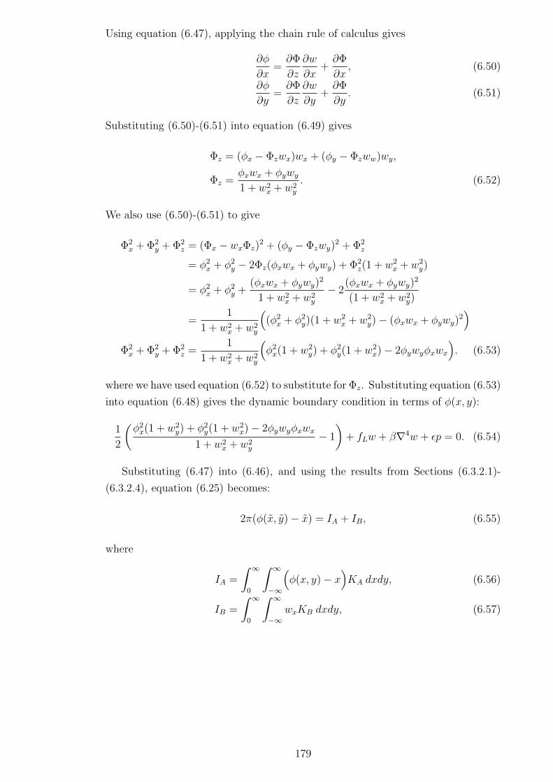
Using equation (6.47), applying the chain rule of calculus gives
∂φ
∂x=∂Φ
∂z
∂w
∂x+∂Φ
∂x, (6.50)
∂φ
∂y=∂Φ
∂z
∂w
∂y+∂Φ
∂y. (6.51)
Substituting (6.50)-(6.51) into equation (6.49) gives
Φz = (φx − Φzwx)wx + (φy − Φzww)wy,
Φz =φxwx + φywy
1 + w2x + w2
y
. (6.52)
We also use (6.50)-(6.51) to give
Φ2x + Φ2
y + Φ2z = (Φx − wxΦz)
2 + (φy − Φzwy)2 + Φ2
z
= φ2x + φ2
y − 2Φz(φxwx + φywy) + Φ2z(1 + w2
x + w2y)
= φ2x + φ2
y +(φxwx + φywy)
2
1 + w2x + w2
y
− 2(φxwx + φywy)
2
(1 + w2x + w2
y)
=1
1 + w2x + w2
y
(
(φ2x + φ2
y)(1 + w2x + w2
y)− (φxwx + φywy)2)
Φ2x + Φ2
y + Φ2z =
1
1 + w2x + w2
y
(
φ2x(1 + w2
y) + φ2y(1 + w2
x)− 2φywyφxwx
)
. (6.53)
where we have used equation (6.52) to substitute for Φz. Substituting equation (6.53)
into equation (6.48) gives the dynamic boundary condition in terms of φ(x, y):
1
2
(
φ2x(1 + w2
y) + φ2y(1 + w2
x)− 2φywyφxwx
1 + w2x + w2
y
− 1
)
+ fLw + β∇4w + ǫp = 0. (6.54)
Substituting (6.47) into (6.46), and using the results from Sections (6.3.2.1)-
(6.3.2.4), equation (6.25) becomes:
2π(φ(x, y)− x) = IA + IB, (6.55)
where
IA =
∫ ∞
0
∫ ∞
−∞
(
φ(x, y)− x)
KA dxdy, (6.56)
IB =
∫ ∞
0
∫ ∞
−∞wxKB dxdy, (6.57)
179
where the kernel functions are given by
KA =w(x, y)− w(x, y)− (x− x)wx − (y − y)wy(
(x− x)2 + (y − y)2 + (w(x, y)− w(x, y))2) 3
2
+w(x, y)− w(x, y)− (x− x)wx − (y + y)wy(
(x− x)2 + (y + y)2 + (w(x, y)− w(x, y))2) 3
2
,
KB =1
(
(x− x)2 + (y − y)2 + (w(x, y)− w(x, y))2) 1
2
+1
(
(x− x)2 + (y + y)2 + (w(x, y)− w(x, y))2) 1
2
. (6.58)
The integral IA can be rewritten as
IA =
∫ ∞
0
∫ ∞
−∞
(
φ(x, y)− φ(x, y)− x+ x)
KA dxdy+ (φ(x, y)− x)
∫ ∞
0
∫ ∞
−∞KA dxdy.
(6.59)
This technique, used by Forbes (1989), renders IA less singular. The second integral
in (6.59) can be evaluated:
∫ ∞
0
∫ ∞
−∞KA dxdy =
∫∫
SF
∂G
∂ndS = 0. (6.60)
Forbes (1989) showed this result by using the Gauss flux theorem and the fact that
G is harmonic within V . Hence, the final expression for IA is
IA =
∫ ∞
0
∫ ∞
−∞
(
φ(x, y)− φ(x, y)− x+ x)
KA dxdy. (6.61)
The integral IA is now non-singular, whereas IB is singular at x = x, y = y.
Following Forbes (1989), we rewrite the integral IB as
IB = I ′B + I ′′B, (6.62)
where
I ′B =
∫ ∞
0
∫ ∞
−∞
(
wx(x, y)KB − wx(x, y)S)
dxdy, (6.63)
I ′′B = wx(x, y)
∫ ∞
0
∫ ∞
−∞S dxdy. (6.64)
180
Here S is given by
S =1
(
A(x− x)2 + B(x− x)(y − y) + C(y − y)2) 1
2
+1
(
A(x− x)2 + B(x− x)(y + y) + C(y + y)2) 1
2
,
where
A = 1 + w2x(x, y),
B = 2wx(x, y)wy(x, y),
C = 1 + w2y(x, y).
The integral I ′′B can be integrated directly in closed form by using the standard
result (Forbes, 1989):
∫∫
dsdt√As2 + bst+ Ct2
=t√A
ln(
2As+ Bt+ 2√
A(As2 + Bst+ Ct2))
+s√C
ln(
2Ct+ Bs+ 2√
A(As2 + Bst+ Ct2))
,
which can be exploited after the integrals are truncated later.
6.3.4 The numerical scheme
We aim to set up a numerical scheme to computationally solve equation (6.55),
where the integrals are given by (6.61) and (6.62)-(6.64), combined with the dynamic
boundary condition (6.54). Following Parau & Vanden-Broeck (2011) we truncate
the intervals −∞ < x < ∞ and 0 < y < ∞ to x1 < x < xN and y1 < y < yM
respectively. We introduce the mesh points xi = x1 + (i− 1)∆x, i = 1, 2, ..., N and
yj = y1 + (j − 1)∆y, j = 1, 2, ...,M .
The 2NM unknowns are given by
u = (wx1,1 , wx1,2 , ..., wxN,M−1, wxN,M
, φx1,1 , ..., φxN,M)T .
We evaluate the (now truncated) integrals (6.61) and (6.62)-(6.64) as well as the
dynamic condition (6.54) at the midpoints (xi+1/2, yj), i = 1, ..., N − 1, j = 1, ...,M ,
so we have 2(N − 1)M equations. The values of w and φ at the midpoints were
obtained by interpolation. Following Parau & Vanden-Broeck (2011) we also impose
a radiation condition (from equation (6.6)) on the first row upstream: wx1j= 0,
φx1j= 1, j = 1, ...,M , giving another 2M equations. We integrate wx and φx with
respect to x by the trapezoidal rule to give the values of w and φ.
We now state the conditions imposed on the boundaries of the grid. With re-
spect to the stated upstream radiation condition (6.6) and the dynamic boundary
181
condition (6.54), the integration is started by taking the following values for the first
row (along i = 1 for j = 1, ...,M):
w1,j = 0, wx1,j= 0, wy1,j = 0, (6.65)
φ1,j = x1, φx1,j= 1, φy1,j = 0. (6.66)
Following Parau & Vanden-Broeck (2011), we also impose a radiation condition
downstream, and for the final row we take (along i = N for j = 1, ...,M):
wxN,j= 0, φxN,j
= 0. (6.67)
Finally the clamped–ice conditions (6.10) require that along the vertical wall we
have (along j = 1 for i = 1,M):
wi,1 = 0, wxi,1= 0. (6.68)
Inside the grid, the values of the other derivatives, wy, φy and ∇4w are calculated
using central finite differences, utilising formulae from Abramowitz & Stegun (1972).
For example, the bi-Laplacian is approximated by
∇4w =1
(∆x)4(wi+2,j − 4wi+1,j + 6wi,j − 4wi−1,j + wi−2,j)
+1
(∆y)4(wi,j+2 − 4wi,j+1 + 6wi,j − 4wi,j−1 + wi,j−2)
+1
(∆y)2(∆x)2(4wi,j − 2wi+1,j − 2wi−1,j − 2wi,j+1 − 2wi,j−1
+ wi+1,j+1 + wi+1,j−1 + wi−1,j+1 + wi−1,j−1).
Along the edges of the grid we use extrapolation, except for along the vertical wall
where we use forward finite differences.
We then solve the 2NM equations by using Newton’s method for a system of
nonlinear equations. After each step, a correction vector c is added to the vector u
of unknowns, where c is given by solving the matrix equation (Forbes, 1989)
J(u) c = −E(u).
Here E defines the error vector. We continue this procedure until the magnitude of
the error vector ||E|| < 10−20.
For load speeds U > cmin, the solution will not converge without dissipation
of some kind. This was also true in Chapter 5, where the viscoelastic relaxation
time τ 6= 0 was necessary to find a solution for fast speeds. Therefore for fast load
speeds, we follow Parau et al. (2007) and introduce an artificial viscosity µ, known
as the Rayleigh viscosity. This was first introduced by Rayleigh (1883) to obtain a
unique solution for linear problems involving gravity-capillary waves by taking the
182

limit µ→ 0. For speeds U > cmin, the dynamic boundary condition (6.54) becomes
1
2
(
φ2x(1 + w2
y) + φ2y(1 + w2
x)− 2φywyφxwx
1 + w2x + w2
y
− 1
)
+fLw+β∇4w+ ǫp+µ(φ−x) = 0.
(6.69)
This dissipative term allows the solution to converge for fast load speeds.
6.4 Numerical results
In this section we present numerical results for the regime outlined in Section 6.3.4.
The default parameters are taken from Table 2.1(a), with infinite fluid depth. We fix
the length scale in the present problem at L = 20 m. This choice allows us to keep
∆x and ∆y small, while also allowing the grid to fully capture the ice deflection.
The values of the load speed U and the distance from the wall y0 are quoted for
each graph. The parameters of the grid ∆x, ∆y, m and n are stated for each graph.
6.4.1 Deflection
For this section, the value of P0 is arbitrary, as varying P0 affects the magnitude of
the deflection much more than its pattern, which we are interested in here. We take
the mass of the moving load to be such that mV g = 50000 N, giving mV ≈ 5200 kg.
This represents a large vehicle or truck on the ice. Using the length scale L = 20m,
this corresponds to a value P0 = 641 Nm−2.
(i): U < cmin
We begin by plotting the deflection for low source speeds U < cmin. In the following,
it is assumed that the artificial viscosity µ = 0. Figure 6.4 shows the ice deflection
for the load speed U = 10ms−1 and distance from the wall y0 = 100m. We see that
the surface elevation response is small for such a low speed U . The deformation
is localised around the position of the load. The pattern in the depression caused
by the moving load is similar to those observed for low source speeds for the linear
formulation of Chapter 5. The position of maximum depression is at the position of
the load (at x = 0), in contrast to the slight lag exhibited by the linear model due
to the viscoelastic formulation.
We now shift the load to a distance y0 = 80 m from the wall, retaining the
load speed U = 10 ms−1. The resulting deflection is shown in Figure 6.5. The
wave pattern behind the moving load is altered due to this change in y0. A wave
has appeared in close proximity to the vertical wall. The maximum depression is
unchanged from the y = 100 m case. The surface response ahead of the load is still
negligible. To investigate this phenomenon further, the distance y0 is decreased to
y0 = 50 m. Figure 6.6 shows the resulting ice deflection. The waves behind the
source have further increased in amplitude. In the present nonlinear formulation, it
appears that the load, when moving in close proximity to the vertical wall, causes
increased deflections in the wake of the load. This is in contrast to the linear model
183
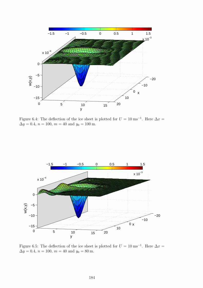
−20
−10
0
10
200 5 10 15
−15
−10
−5
0
x 10−4
x
y
w(x
,y)
−1.5 −1 −0.5 0 0.5 1 1.5
x 10−3
Figure 6.4: The deflection of the ice sheet is plotted for U = 10 ms−1. Here ∆x =∆y = 0.4, n = 100, m = 40 and y0 = 100 m.
−20−10
010
200 5 10 15
−15
−10
−5
0
x 10−4
x
y
w(x
,y)
−1.5 −1 −0.5 0 0.5 1 1.5
x 10−3
Figure 6.5: The deflection of the ice sheet is plotted for U = 10 ms−1. Here ∆x =∆y = 0.4, n = 100, m = 40 and y0 = 80 m.
184

−15−10
−50
510
15
05
10
−1.5
−1
−0.5
0
0.5
1
x 10−3
x
y
w(x
,y)
−1 −0.5 0 0.5 1
x 10−3
Figure 6.6: The deflection of the ice sheet is plotted for U = 10 ms−1. Here ∆x =∆y = 0.3, n = 100, m = 40 and y0 = 50 m.
of Chapter 5, where a small distance from the wall to the load led to a smaller
depression in the ice, and a differing shape of that depression. The explanation for
this discord could lie in the nonlinear wave interaction with the wall, or the more
sophisticated model for the moving pressure load adopted in the present problem.
We now investigate the effect of increasing the load speed to U = 15 ms−1, and
we set the distance y0 = 100 m. The computed solution is shown in Figure 6.7.
We observe an increase in the maximum depression caused by the moving load.
−20−15−10−505101520
010
−20
−15
−10
−5
0
x 10−4
xy
w(x
,y)
−1.5 −1 −0.5 0 0.5 1 1.5
x 10−3
Figure 6.7: The deflection of the ice sheet is plotted for U = 15 ms−1. Here ∆x =∆y = 0.4, n = 100, m = 40 and y0 = 100 m.
In addition we now see elevation both behind and ahead of the source due to the
185

motion of the load. Both of these trends were also present for the linear formulation.
However, in Figure 6.7, the waves take longer to decay than for the linear case, and
there is a disturbance reaching the edges of the grid ahead and behind the source,
close to the wall.
(ii): U > cmin
We now investigate load speeds faster than the critical speed cmin. The artificial
viscosity µ must now be present for the solution to converge. To begin, we plot
the deflection for the parameters U = 20 ms−1 and y0 = 200 m, shown in Figure
6.8. By now we are familiar with the change in deflection magnitude and varied
−20−15−10−505101520
0
10
20
30
40
−2
−1
0
1
x 10−3
x
w(x
,y)
y
−2.5 −2 −1.5 −1 −0.5 0 0.5 1 1.5 2
x 10−3
Figure 6.8: The deflection of the ice sheet is plotted for U = 20 ms−1. Here ∆x =∆y = 0.6, n = 80, m = 80 and y0 = 200 m. The artificial viscosity is given byµ = 0.1.
pattern caused by load speeds U > cmin. The maximum deflection has increased,
and the waves generated by the moving load propagate further than for the case
U < cmin. The wave profile is more curved owing to the increased speed. The
solution regime of shorter, elastic waves ahead of the source and slower, gravity
waves behind the source that was observed in the linear model is also present in
the nonlinear formulation. We note that the solution decays towards the edges of
the grid, owing to the artificial viscosity and radiation conditions. In general the
behaviour is very similar to that of the equivalent linear graph shown in Figure 5.19.
However, in Figure 6.8 there are fewer long waves behind the source than for the
linear case. This is due to the fact that the grid is smaller, because we are now
more constrained by computational restrictions: for a solution to be realistic and to
186

converge, the parameters ∆x and ∆y must be small. In addition, grid sizes larger
than 80x80 are not numerically feasible.
−100
1020
30
0
10
20
30
40
50
60
−15
−10
−5
0
5
x 10−4
x
y
w(x
,y)
−1 −0.5 0 0.5 1 1.5
x 10−3
Figure 6.9: The deflection of the ice sheet is plotted for U = 25 ms−1. Here ∆x =∆y = 0.7, n = 80, m = 80 and y0 = 400 m. The artificial viscosity is given byµ = 0.2.
Finally we plot the deflection for a fast load speed U = 25ms−1 and distance from
the wall y0 = 400 m, the solution for which is shown in Figure 6.9. The disparity
in wavelength between the shorter and longer waves is more apparent. We begin to
see significant disturbance between the vertical wall and the moving load, owing to
wave reflection by the wall. This is similar to the behaviour shown in Chapter 5
for fast load speeds, indicating that this phenomenon is not purely linear. Only one
long wave appears behind the source, and its amplitude is small compared to the
wave peak ahead of the load or the wave depression caused by the load.
6.4.2 Comparison with linear model
In this section we compare the results between the present nonlinear model and
the linear model of Chapter 5. Such a comparison is difficult to interpret because
there are many differences between the two models. For example, the expression for
the pressure is a point load in the linear formulation, whereas it is modelled as a
non-uniform distribution over a prescribed rectangle in the nonlinear formulation.
The linear model assumes finite depth, whereas the nonlinear model does not. The
linear model includes a term for the plate acceleration whereas the nonlinear model
187

neglects this term. Finally, in the linear model the dissipation is inherent in the
viscoelastic plate equation, whereas for the nonlinear model we add an artificial
viscosity. Hence, while assessing any disparity between the two models it is difficult
to determine whether nonlinear effects are responsible, or one of the other differences
mentioned above.
For this comparison we would like to set the relevant parameters such that the
two expressions for the moving loads are equivalent. Because one is a point load
and the other is a load distribution, we achieve this by requiring that
∫∫
R
PL dxdy =
∫∫
R
PN dxdy, (6.70)
where R is the region occupied by the ice sheet in each case. Here PL is the expres-
sion for the load in the linear formulation given by equation (5.38), and PN is the
expression for the load in the nonlinear formulation given by equation (6.21). The
left hand side of (6.70) is therefore given by (in dimensionless variables and in the
notation of Chapter 5):
mV g
H2
∫ ∞
−∞
∫ ∞
0
−δ(x− x0)δ(y)H2dxdy = −mV g. (6.71)
The right hand side of (6.70) becomes (in dimensionless variables)
−P0L2
∫ y0+1
y0−1
∫ 1
−1
exp
(
1
x2 − 1+
1
(y − y0)2 − 1
)
dxdy. (6.72)
The integral in equation (6.72) may be computed numerically as c = 0.1971305088,
and is independent of y0. Hence, equating (6.71) and (6.72), we arrive at
P0L2c = mV g. (6.73)
We may then select a mass mV for the load in the linear formulation and, using
equation (6.73), calculate the value of P0 such that the nonlinear load is equivalent.
For this comparison, as before we take the value mV g = 50000 N leading to P0 =
641 Nm−2.
We may now compare the results directly. Firstly we select a load speed U =
15ms−1 and a distance from the wall of 100m. In both models there is no dissipation
(ie. τ = 0 for the linear model and µ = 0 for the nonlinear model). The deflection
through the centre line x = 0 is given in Figure 6.10. There is excellent agreement
between the two data sets. The value of the deflection at y = y0 is slightly smaller for
the nonlinear model. The maximum ice excursion predicted for these parameters is
approximately 2mm for each model. We repeat this comparison, instead plotting the
deflection through the centre line y = y0, shown in Figure 6.11. Again we experience
near-perfect agreement between the two models, giving credence to both.
We repeat this comparison, increasing the speed of the load to U = 20ms−1 and
188
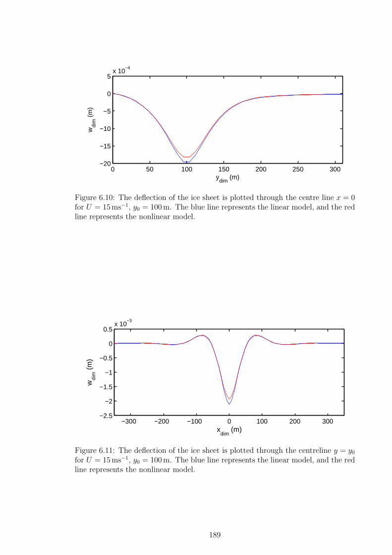
0 50 100 150 200 250 300−20
−15
−10
−5
0
5x 10
−4
ydim
(m)
wdi
m (
m)
Figure 6.10: The deflection of the ice sheet is plotted through the centre line x = 0for U = 15ms−1, y0 = 100m. The blue line represents the linear model, and the redline represents the nonlinear model.
−300 −200 −100 0 100 200 300−2.5
−2
−1.5
−1
−0.5
0
0.5x 10
−3
xdim
(m)
wdi
m (
m)
Figure 6.11: The deflection of the ice sheet is plotted through the centreline y = y0for U = 15ms−1, y0 = 100m. The blue line represents the linear model, and the redline represents the nonlinear model.
189

the distance from the wall to y0 = 200 m. This speed is slightly above the critical
speed, and hence we require the presence of viscosity in each model for bounded
solutions. We therefore select τ = 0.1 s and µ = 0.1. The deflection through the
centre line x = 0 is shown in Figure 6.12. For these parameters, the agreement
0 100 200 300 400 500 600 700−3
−2
−1
0
1
2x 10
−3
ydim
(m)
wdi
m (
m)
Figure 6.12: The deflection of the ice sheet is plotted through the centre line x = 0for U = 20ms−1, y0 = 200m. The blue line represents the linear model, and the redline represents the nonlinear model.
between the two models is still excellent, though slightly worse than for slower load
speeds. In this case the nonlinear model predicts a slightly higher surface depression
at the point of the load. There is also a steeper rise in deflection at the vertical wall
in the nonlinear model. Once again, the maximum ice excursion is approximately
2mm for each model. For further comparison, the centre line through y = y0 is shown
in Figure 6.13. The agreement in this case is fairly good, though some disagreement
−400 −300 −200 −100 0 100 200 300 400
−2
−1
0
1
x 10−3
xdim
(m)
wdi
m (
m)
Figure 6.13: The deflection of the ice sheet is plotted through the centreline y = y0for U = 20ms−1, y0 = 200m. The blue line represents the linear model, and the redline represents the nonlinear model.
starts to appear towards the edges of the grid. Behind the load, the nonlinear model
predicts smaller wave amplitudes. This is likely due to the truncation of the grid
in the nonlinear model, and the radiation condition imposed downstream. Ahead
190

of the load, the linear model predicts slightly longer wavelengths, though the wave
amplitudes are similar in each case. This discrepancy is likely due to the differing
expressions for the moving pressure. Towards the centre of the grid, there is excellent
agreement.
6.5 Summary
The problem of a moving load on an ice sheet was solved for fully nonlinear fluid
equations. The ice was frozen to the vertical wall. The fluid was of infinite depth.
This chapter represents an extension of the linear model in Chapter 5. Based on the
work of Forbes (1989) and Parau & Vanden-Broeck (2011), the problem was solved
by application of Green’s theorem using the free–surface Green’s function, and use
of a boundary integral method. The introduction of a vertical wall complicates
the problem, but choice of a suitable surface over which to apply Green’s theorem
leads to a solution. Some elegant simplifications introduced by Forbes (1989) led to
further efficiency in the method, and the numerical computations involved are not
overly cumbersome. The deflection of the ice sheet was studied in detail for various
load speeds, and a comparison with the linear theory was presented.
In general the response of the ice sheet to the moving load followed the trends
introduced in Chapter 5. Whether the load moves with speed above or below the
critical speed cmin is the most important factor governing the shape of the deflection
pattern. For slow load speeds, the surface response is mostly localized around the
support of the pressure. However, placing the load closer to the wall increases the
deflections in the wake of the moving load. This was not the case in the linear
formulation, indicating that nonlinearity is responsible for this behaviour. For fast
load speeds, the deflection becomes curved and the waves propagate at a further
distance from the load. For certain values of the load speed and the distance from
the wall, disturbance exists between the load and the wall, representing trapped
standing waves due to the interaction with the vertical wall.
Direct comparison with the linear theory yields good agreement, despite the
differences in the two models. This agreement is better for slower load speeds, where
the shape and magnitude of the deflection in both cases agrees almost perfectly. For
faster load speeds, we begin to see some disparity, though in the vicinity of the load
the predicted ice response is the same.
191
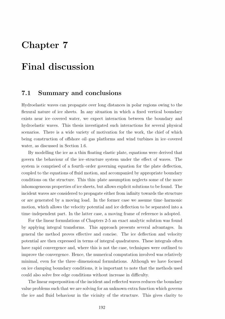
Chapter 7
Final discussion
7.1 Summary and conclusions
Hydroelastic waves can propagate over long distances in polar regions owing to the
flexural nature of ice sheets. In any situation in which a fixed vertical boundary
exists near ice–covered water, we expect interaction between the boundary and
hydroelastic waves. This thesis investigated such interactions for several physical
scenarios. There is a wide variety of motivation for the work, the chief of which
being construction of offshore oil–gas platforms and wind turbines in ice–covered
water, as discussed in Section 1.6.
By modelling the ice as a thin floating elastic plate, equations were derived that
govern the behaviour of the ice–structure system under the effect of waves. The
system is comprised of a fourth–order governing equation for the plate deflection,
coupled to the equations of fluid motion, and accompanied by appropriate boundary
conditions on the structure. This thin–plate assumption neglects some of the more
inhomogeneous properties of ice sheets, but allows explicit solutions to be found. The
incident waves are considered to propagate either from infinity towards the structure
or are generated by a moving load. In the former case we assume time–harmonic
motion, which allows the velocity potential and ice deflection to be separated into a
time–independent part. In the latter case, a moving frame of reference is adopted.
For the linear formulations of Chapters 2-5 an exact analytic solution was found
by applying integral transforms. This approach presents several advantages. In
general the method proves effective and concise. The ice deflection and velocity
potential are then expressed in terms of integral quadratures. These integrals often
have rapid convergence and, where this is not the case, techniques were outlined to
improve the convergence. Hence, the numerical computation involved was relatively
minimal, even for the three–dimensional formulations. Although we have focused
on ice clamping boundary conditions, it is important to note that the methods used
could also solve free edge conditions without increase in difficulty.
The linear superposition of the incident and reflected waves reduces the boundary
value problems such that we are solving for an unknown extra function which governs
the ice and fluid behaviour in the vicinity of the structure. This gives clarity to
192

the problem and later allows us to analyse the contribution from each part of the
solution. The integral transform solution method leads to simple expressions for
the forces on the structure. Through eliminating a singularity in Fourier space, we
were able to define algebraic expressions for the third derivative of the ice deflection,
giving the vertical shear force. This allows us to sidestep the convergence difficulties
that may have arisen from evaluating such a derivative. The method also allows
simple expressions for the horizontal force (as well as for the phase shift between
the incident and reflected waves) to be defined which may then be studied easily.
For the nonlinear study of Chapter 6, a solution is found by application of Green’s
second identity to a suitable Green’s function. The numerical procedure and solu-
tion are based on that of Parau & Vanden-Broeck (2011) and Forbes (1989), where
a boundary element method is utilised and finite difference techniques are applied.
While computationally intense, the Green’s theorem / boundary element approach
is a powerful method which adeptly deals with the complicated nonlinear fluid equa-
tions. The solution is not exact but may be computed to extreme accuracy.
Many results describing the features of the ice–structure problems were pre-
sented. Primarily the focus was on the following:
• The ice deflection field caused by the reflection or diffraction of hydroelastic
waves
• The strain in the ice sheet due to the curvature caused by these waves
• The vertical lifting force caused by the waves, which exists due to the ice being
frozen to the structure
• The horizontal force on the wall caused by the waves.
Detailed conclusions and summaries may be found at the end of each chapter, and
we therefore only discuss broad trends and the salient conclusions of each chapter
here.
For Chapter 2, we considered hydroelastic incident waves propagating towards
a vertical wall in two dimensions. The ice was frozen to the wall which introduces
a specific effect on the ice deflection. The deflection and slope of the ice are both
zero at the ice–wall boundary, restricting the motion of the ice sheet in the vicinity
of the structure. The first wave peak nearest the wall was diminished, and there is
disturbance in subsequent waves due to interaction with the wall. The deflection
pattern was shown to depend more on ice thickness than on the finite fluid depth.
The strain in the ice sheet was shown to be roughly 2–3 times higher in magnitude
at the ice–wall connection point than far from the wall. However, it was shown
that the ice–clamping condition can be maintained provided the amplitude of the
incident wave is small enough. The strain also sensitively depends on the incident
wavenumber k. The value of k also effects the vertical and horizontal forces. The
vertical force on the wall is in general higher for short waves than for long waves,
193
whereas the opposite is true for the horizontal force. In general the horizontal and
shear forces are similar in magnitude, and they may reach substantial quantity.
Chapter 3 extended the study to three dimensions, solving the problem of hy-
droelastic wave diffraction by a vertical cylinder. We conclude that for long incident
waves, the cylinder has a small effect on the wave pattern as it passes the cylinder.
This is due to the cylinder radius being generally small in comparison with the in-
cident wavelength. For shorter waves, there is much more pronounced disturbance
due to wave reflection and evanescent outgoing waves from the cylinder. In partic-
ular, the deflection is diminished in the wake of the cylinder. The strain in the ice
due to the ice–clamping condition can reach high levels, particularly at θ = π, the
direction from which the incident wave approaches. We conclude that the ice is un-
likely to remain frozen to the cylinder unless the wave amplitudes are only several
millimetres, or if the wavelength is long. The vertical and horizontal forces were
shown to depend on a number of parameters. They were both highest at θ = π, and
behind the cylinder the forces were smaller by up to half. Other dependences on the
cylinder radius b and the ice thickness were investigated. Once again we note that
the wave forces on the cylinder can reach surprisingly high magnitude.
In Chapter 4 we adopt a two–layer fluid model, motivated by density stratifica-
tion that often occurs underneath an ice sheet. This entails two free surfaces; one at
the ice–cover and the other at the interface between the two fluid layers. The disper-
sion relation has two modes corresponding to a surface wavenumber (characterised
by longer, smaller–amplitude waves) and an interfacial wavenumber (characterised
by larger–amplitude short waves). It is shown that after wave reflection by the
wall, incident interfacial waves can generate waves in the ice cover, and vice versa.
Further, waves of either mode may propagate at either free surface under various
conditions. The effect this two–layer formulation has on the strain in the ice and
forces on the wall was analysed. It is concluded that if stratification exists and the
two fluids have distinct densities then the effect of the stratification should not be
ignored.
We consider the linear formulation of waves generated by a moving load on an ice
sheet near a vertical wall in Chapter 5. A simple viscoelastic model was introduced
to account for wave attenuation in the ice sheet. It is well documented that the wave
profiles depend on the speed of the moving load, and whether this speed is above or
below the critical speed cmin. In the elastic limit the deflection is unbounded at cmin,
but the viscoelastic formulation renders a finite response there. Speculation from
other authors regarding a potential second critical speed is not shared by the present
study and we report only one critical speed cmin. The load speed that produces
maximum ice deflection is perturbed slightly above cmin due to the viscoelasticity.
For any given speed, the position of maximum deflection lags slightly behind the
load. Close proximity of the load to the wall causes damped wave deflection due to
the ice–clamping condition. The introduction of a vertical wall means that for faster
load speeds we observe disturbance due to wave reflection and trapping. Whether
194

the moving load will fracture the ice–wall connection depends on the mass and speed
of the load, together with its distance from the wall. Various parameter changes
were analysed using the data set of Takizawa (1985), taken from a frozen lake in
Japan.
The same problem was studied in Chapter 6 with fully nonlinear fluid equa-
tions. The model also uses a more sophisticated expression for the moving pressure.
The solution displayed the same traits as its linear counterpart. The two models
behave slightly differently as the load is moved close to the wall, with the nonlin-
ear theory predicting increased deflection in the wake of the load. The trapped
wave phenomenon observed in the linear formulation (for high load speeds) was also
observed in the nonlinear formulation. Direct comparison between models showed
excellent agreement in the shape and magnitude of the surface response. For faster
speeds the agreement is slightly worse towards the edges of the grid, though it is
hard to say which of the differences between the two models is responsible.
In conclusion, the present study helps elucidate the numerous factors that govern
hydroelastic wave interaction with structures. The rigorous formulation and solu-
tion of the pertinent boundary value problems means that all aspect of the wave
interaction can be described. Results for the ice deflection and incited forces are
expected to assist in the wave–consideration aspect of designing structures to be
built in ice–covered regions.
7.2 Future work
There are a multitude of options when considering enhancement of the models used
here. The introduction of vertical boundaries meant it was necessary to apply cer-
tain simplifications to facilitate concise solutions. We may for example replace the
assumption that the ice has constant thickness, and investigate the effect of an ice
sheet of varying thickness. Similarly the effect of variable bottom topography has
been included by several authors and could be applied to the present problem. The
assumption of non–zero draught could also be studied and its validity assessed. The
mathematical theory for these suggestions is already in place, though their inclusion
in wave–structure interaction problems would present a challenge.
Regarding ice–structure interaction in three dimensions, one problem that war-
rants study is a multiple–cylinder model, representing structures that have more
than one support. We expect that some wave trapping may occur between the
cylinders, in view of the work done in water wave scattering theory. A multipole ap-
proach may be necessary to solve the problem, or we may exploit the rapid decay of
the function Q in the solution of Chapter 3 to consider each cylinder independently.
Free edge conditions must be considered in addition to the clamped–ice condition,
bearing in mind the conclusions of Chapter 3.
Alternatively we may envisage a situation where an ice sheet is partially frozen
to a vertical cylinder; that is, free edge conditions for a prescribed interval of θ
195
and clamped edge conditions elsewhere. Matching across these mixed boundary
conditions would mean the problem would be challenging to solve. A related problem
is also relevant: considering a non-continuous ice sheet, so that the ice only partially
covers the free surface. Further research must certainly be made into the fracture
process of ice, to improve the naive assumption we use that the yield strain has a
constant value. Investigation must be made into the variety of factors that affect
ice fracture.
One problem plaguing hydroelasticity from a broad standpoint is the paucity
of realistic field experiments that have been conducted on waves in ice sheets or
ice floes, something which must be rectified in future to ensure that the theory is
credible. For the particular theory of ice–structure interaction, forces due to the
crushing of ice into a structure have been studied experimentally, but not forces due
to waves in ice.
Other inhomogeneous aspects of the ice must be taken into account for the
accuracy of the models to improve. Although the thin plate equation has been
proven to be accurate in certain circumstances, for others the assumptions of small–
deflection theory may prove inappropriate. A more sophisticated plate equation,
incorporating the effect of thick ice, shear stresses or nonlinear effects must be
adopted. Further, we could include a viscous layer on the underside of the ice
sheet, modelling the semi–frozen slush that accumulates there. It is certain that
such changes would require more advanced solution methods. The development of
numerical methods such as finite or boundary element methods is likely to play a
large role in the future of hydroelastic research. Nonlinear effects of either the ice
sheet or the fluid motion may be of crucial importance to the problems studied here
and elsewhere within hydroelasticity.
196

Bibliography
Abramowitz M. & Stegun I., 1972. Handbook of mathematical functions with formulas, graphs
and mathematical tables. Dover Publications.
Andrianov A., 2005. Hydroelastic Analysis of Very Large Floating Structures. Ph.D. thesis, Delft
University of Technology, The Netherlands.
Andrianov A. & Hermans A., 2003. The influence of water depth on the hydroelastic response
of a very large floating platform. Marine Structures, 16:355–371.
Arrigo K., van Dijken G., Ainley D., Fahnestock M. & Markus T., 2002. Ecological
impact of a large antarctic iceberg. Geophys. Res. Letters, 29(7):1104.
Ashton G., 1986. River and lake ice engineering. Water Resources Pubns.
Athanassoulis M. & Belibassakis K., 2009. A novel coupled-mode theory with application to
hydroelastic analysis of thick, non-uniform floating bodies over general bathymetry. Proceedings
of the Institution of Mechanical Engineers, Part M: Journal of Engineering for the Maritime
Environment, 223(3):419–438.
Balmforth N. & Craster R., 1999. Ocean waves and ice sheets. J. Fluid Mech., 395(1):89–124.
Barrett M. & Squire V., 1996. Ice-coupled wave propagation across an abrupt change in ice
rigidity, density, or thickness. Journal of Geophysical Research, 101(C9):20825–20832.
Bates H. & Shapiro L., 1980. Long–period gravity waves in ice–covered sea. J. Geophys. Res.,
85(C2):1095–1100.
Battisti L., Fedrizzi R., Brighenti A. & Laakso T., 2006. Sea ice and icing risk for offshore
wind turbines. In Proceedings of the OWEMES, pages 20–22.
Belibassakis K. & Athanassoulis G., 2005. A coupled-mode model for the hydroelastic anal-
ysis of large floating bodies over variable bathymetry regions. J. Fluid. Mech., 531:221–250.
Bennetts L., 2007. Wave scattering by ice sheets of varying thickness. Ph.D. thesis, University
of Bristol, England.
Bennetts L., Peter M., Squire V. & Meylan M., 2010. A three-dimensional model of wave
attenuation in the marginal ice zone. J. Geophys. Res, 115:C12043.
Bennetts L. & Squire V., 2009. Wave scattering by multiple rows of circular ice floes. J. Fluid
Mech., 639(1):213–238.
Bennetts L. & Squire V., 2010. Linear wave forcing of an array of axisymmetric ice floes. IMA
J. App. Math., 75(1):108–138.
Bennetts L. & Williams T., 2010. Wave scattering by ice floes and polynyas of arbitrary shape.
J. Fluid Mech., 662:5–35.
197

Bennetts L., Williams T. & Squire V., 2009. An approximation to wave scattering by an
ice polynya. In Proceedings 24th International Workshop on Water Waves and Floating Bodies.
University of East Anglia, Zelenogorsk, Russia, page 4.
Bhattacharjee J. & Guedes-Soares C., 2012. Flexural gravity waves over a floating ice sheet
near a vertical wall. J. Eng. Math., 75:29–48.
Bhattacharjee J. & Sahoo T., 2008. Flexural gravity wave problems in two-layer fluids. Wave
Motion, 45(3):133–153.
Blyth M., Parau E. & Vanden-Broeck J.M., 2011. Hydroelastic waves on fluid sheets.
Journal of Fluid Mechanics, 689:541–551.
Bonnefoy F., Meylan M. & Ferrant P., 2009. Nonlinear higher-order spectral solution for
a two-dimensional moving load on ice. J. Fluid Mech., 621(1):215–242.
Bowman F., 1958. Introduction to Bessel functions. Dover Publications.
Bracewell R., 1999. The Fourier Transform & Its Applications. McGraw-Hill, third edition.
Brevdo L. & Il’ichev A., 2006. Uni-modal destabilization of a visco-elastic floating ice layer by
wind stress. European Journal of Mechanics-A/Solids, 25(3):509–525.
Brocklehurst P., Korobkin A. & Parau E., 2010. Interaction of hydro-elastic waves with a
vertical wall. J. Eng. Math., 68:215–231.
Brocklehurst P., Korobkin A. & Parau E., 2011. Hydroelastic wave diffraction by a vertical
cylinder. Phil. Trans. Roy. Soc. Lond. A, 369:2832–2851.
Cammaert A. & Muggeridge D., 1988. Ice interaction with offshore structures. Van Nostrand
Reinhold Co. Inc., New York, NY.
Chakrabarti A., Ahluwalia D. & Manam S., 2003. Surface water waves involving a vertical
barrier in the presence of an ice cover. Int. Journal of Eng. Sci., 41:1145–1162.
Chung H. & Fox C., 2002. Calculation of wave-ice interaction using the wiener-hopf technique.
New Zealand J. Math, 31(1):1–18.
Chung H. & Linton C., 2005. Reflection and transmission of waves across a gap between two
semi-infinite elastic plates on water. Quart. J. Mech. Appl. Math., 58:1–15.
Crocker R.M.G., 1992. Ice floe collisions interpreted from accelerometer data during limex.
Atmos. -Ocean, 30(2):246–269.
Croteau P., 1983. Dynamic interactions between floating ice and offshore structures. Ph.D.
thesis, Univ. of California, Berkeley, CA, USA.
Czipott P., Levine M., Paulson C., Menemenlis D., Farmer D. & Williams R., 1991.
Ice flexure forced by internal wave packets in the arctic ocean. Science, 254:832–834.
Davys J., Hosking R. & Sneyd A., 1985. Waves due to a steadily moving source on a floating
ice plate. J. Fluid Mech., 158:269–287.
Downer J. & Haskell T., 2001. Ice-floe kinematics in the ross sea marginal ice zone using gps
and accelerometers. Annals of Glaciology, 33(1):345–349.
Duffy D., 1996. On the generation of internal waves beneath sea ice by a moving load. Cold Reg.
Sci. Tech., 24(1):29–39.
198

Dumont D., Kohout A. & Bertino L., 2011. A wave-based model for the marginal ice zone
including a floe breaking parameterization. J. Geophys. Res, 116:C04001.
Ehrenmark U. & Porter D., 2012. Water wave scattering by a floating elastic plate over a
plane incline. Quart. J. Mech. App. Math., 65(3):409–434.
El-Reedy M., 2012. Offshore Structures: Design, Construction and Maintenance. Gulf Profes-
sional Publishing.
Emmerhoff O. & Sclavounos P., 1992. The slow-drift motion of arrays of vertical cylinders.
J. Fluid Mech., 242:31–50.
Emmerson C. & Lahn G., 2012. Arctic Opening: Opportunity and Risk in the High North.
Lloyds, Chatham House.
Evans D. & Davies T., 1968. Wave-ice interaction. Technical Report 1313, New Jersey:Davidson
Lab, Stevens Inst. of Tech.
Evans D. & Porter R., 2003. Wave scattering by narrow cracks in ice sheets floating on water
of finite depth. J. Fluid Mech., 484:143–165.
Ewing M. & Crary A., 1934. Propagation of elastic waves in ice, ii. Physics, 5:181–184.
Fletcher N., 1970. The Chemical Physic of Ice. Cambridge University Press.
Forbes L., 1986. Surface waves of large amplitude beneath an elastic sheet. part 1. high-order
series solution. J. Fluid Mech, 169:409–428.
Forbes L., 1988. Surface waves of large amplitude beneath an elastic sheet. part 2. galerkin
solution. J. Fluid Mech., 188(1):491–508.
Forbes L., 1989. An algorithm for 3-dimensional free-surface problems in hydrodynamics.
J. Comp. Phys., 82:330–347.
Fox C. & Squire V., 1990. Reflection and transmission characteristics at the edge of shore fast
sea ice. J. Geophys. Res., 95:11629–11639.
Fox C. & Squire V., 1991a. Coupling between an ocean and an ice shelf. Ann. Glaciol., 15:101–
108.
Fox C. & Squire V., 1991b. Strain in shore fast ice due to incoming ocean waves and swell.
J. Geophys. Res., 96(C3):4531–4547.
Fox C. & Squire V., 1994. On the oblique reflexion and transmission of ocean wave at shore
fast sea ice. Phil. Trans. R. Soc. Lond. A, 347:185–218.
Frankenstein G. & Garner R., 1967. Equations for determining the brine volume of sea ice
from -0.5c to -22.9c. J. Glaciology, 6:934–944.
Glen J., 1987. Fifty years of progress in ice physics. Journal of Glaciology, Special Issue:52–59.
Goodman D., Wadhams P. & Squire V., 1980. The flexural response of a tabular ice island
to ocean swell. Annals of Glaciology, 1:23–27.
Gradshteyn I. & Ryzhik I., 2007. Table of Integrals, Series, and Products. Academic Press
(Elsevier), seventh edition.
199

Gravesen H., Petersen B., Søresen S. & Vølund P., 2003. Ice forces on wind turbine
foundations in denmark. In Proceedings of the International Conference on Port and Ocean
Engineering under Arctic Conditions, 17.
Gravesen H., Sørensen S., Vølund P., Barker A. & Timco G., 2005. Ice loading on
danish wind turbines: Part 2. analyses of dynamic model test results. Cold regions science and
technology, 41(1):25–47.
Greenhill A., 1887. Wave motion in hydrodynamics. Am. J. Math., 9:62–112.
Griggs J. & Bamber J., 2011. Antarctic ice–shelf thickness from satellite radar altimetry.
Journal of Glaciology, 57:485–498.
Gurtner A., 2009. Experimental and Numerical Investigations of Ice-Structure Interaction. Ph.D.
thesis, Norwegian University of Science and Technology, Norway.
Hassan M., Meylan M. & Peter M., 2009. Water-wave scattering by submerged elastic plates.
Quart. J. Mech. App. Math., 62(3):321–344.
Hegarty G. & Squire V., 2004. On modelling the interaction of large amplitude waves with a
solitary floe. In Proceedings of the 14th international offshore and polar engineering conference,
volume 1, pages 845–850.
Hegarty G. & Squire V., 2008. A boundary-integral method for the interaction of large-
amplitude ocean waves with a compliant floating raft such as a sea-ice floe. J. of Eng. Math.,
62(4):355–372.
Hendrickson J. & Webb L., 1963. Theoretical investigation of semi-infinite ice floes in water
of infinite depth. Rep. NBy–32225,Natl. Engng. Sci. Co., Pasadena, CA.
Hosking R., Sneyd A. & Waugh D., 1988. Viscoelastic response of a floating ice plate to a
steadily moving load. J. Fluid. Mech., 196:409–430.
Hunkins K., 1962. Waves on the arctic ocean. J. Geophys. Res., 67:2477–2489.
Ikebe T., 1960. Eigenfunction expansions associated with the schroedinger operators and their
applications to scattering theory. Archive for Rational Mechanics and Analysis, 5(1):1–34.
ISO19906, 2010. Petroleum and natural gas industries: Arctic offshore structures. BSI.
Jeffrey A., 2002. Advanced Engineering Methods. Harcourt / Academic Press.
Jordaan I., 2001. Mechanics of ice-structure interaction. Engineering Fracture Mechanics, 68(17-
18):1923–1960.
Karr D., Troesch A. & Wingate W., 1993. Nonlinear dynamic response of a simple ice-
structure interaction model. Journal of Offshore Mechanics and Arctic Engineering, 115(4):246–
252.
Kashiwagi M., 1998. A new solution method for hydroelastic problems of a very large floating
structure in waves. In OMAE 1998: 17th International Conference on Offshore Mechanics and
Arctic Engineering, page 1998.
Kashiwagi M., 2000. Research on hydroelastic responses of vlfs: recent progress and future work.
Int. J. Off. Pol. Eng., 10(2):81–90.
Keller J., 1998. Gravity waves on ice-covered water. J. Geophys. Res., 103:7663–7669.
200

Kerr A., 1976. The bearing capacity of floating ice plates subjected to static or quasi-static loads.
Journal of Glaciology, 17(76).
Kerr A. & Haynes F., 1988. On the determination of the average young’s modulus for a floating
ice cover. Cold Reg.Sci. Tech., 15(1):39–43.
Kerr A. & Palmer W., 1972. The deformations and stresses in floating ice plates. Acta Mech.,
15:57–72.
Khabakhpasheva T. & Korobkin A., 2002. Hydroelastic behaviour of compound floating plate
in waves. J. Eng. Math., 44(1):21–40.
Kim J. & Ertekin R., 1998. An eigenfunction-expansion method for predicting hydroelastic
behavior of a shallow-draft vlfs. In Proceedings of the 2nd International Conference on Hydroe-
lasticity in Marine Technology, pages 47–59.
Kohout A. & Meylan M., 2008. An elastic plate model for wave attenuation and ice floe
breaking in the marginal ice zone. J. Geophys. Res, 113:C09016.
Korobkin A., 2000. Unsteady hydroelasticity of floating plates. Journal of Fluids and Structures,
14(7):971–991.
Korobkin A., Parau E. & Vanden-Broeck J., 2011. The mathematical challenges and mod-
elling of hydroelasticity. Phil. Trans. Roy. Soc. Lond. A, 369(1947):2803–2812.
Kouzov D., 1963a. Diffraction of a plane hydro–acoustic wave on the boundary of two elastic
plates. Prikl. Mat. Mekh, 27:541–546.
Kouzov D., 1963b. Diffraction of a plane hydroelastic wave at a crack in an elastic plate. Prikl.
Mat. Mekh, 27:1037–1043.
Kwok R., Cunningham G., Wensnahan M., Rigor I., Zwally H., Yi D. et al., 2009a.
Thinning and volume loss of the arctic ocean sea ice cover: 2003–2008. J. Geophys. Res,
114(C7):C07.
Kwok R., Rothrock D. et al., 2009b. Decline in arctic sea ice thickness from submarine and
icesat records: 1958–2008. Geophys. Res. Lett., 36(15):L15501.
Lamb H., 1932. Hydrodynamics 6th ed.. Cambridge University Press.
Lange M., 1989. Development of sea ice in the weddell sea. Annals of Glaciology, 12:92–96.
Lewis E. & Walker E., 1970. The water structure under a growing sea ice sheet. J. Geophys.
Res., 75(33):6836–6845.
Linton C. & Chung H., 2003. Reflection and transmission at the ocean/sea-ice boundary. Wave
motion, 38(1):43–52.
Linton C. & Evans D., 1990. The interaction of waves with arrays of vertical circular cylinders.
J. Fluid Mech., 215(1):549–569.
Linton C. & McIver M., 1995. The interaction of waves with horizontal cylinders in two-layer
fluids. J. Fluid Mech., 304(1):213–229.
Linton C. & McIver P., 2001. Mathematical techniques for wave/structure interactions. Chap-
man and Hall/CRC.
201
Lucas S., 1995. Evaluating infinite integrals involving products of bessel functions. J. Comp.
Appl. Math., 64:269–282.
Malenica S. & Korobkin A., 2003. Water wave diffraction by vertical circular cylinder in
partially frozen sea. Proc. 18th International Workshop on Water Waves and Floating Bodies,
LeCroisic, France.
Marchenko A., 1996. Swell wave propagation in an inhomogeneous ice sheet. Fluid Dynamics,
31(5):761–767.
Marchenko A., 1997. Flexural-gravity wave diffraction at linear irregularities in sheet ice. Fluid
Dynamics, 32(4):548–560.
Marchenko A. & Voliak K., 1997. Surface wave propagation in shallow water beneath an
inhomogeneous ice cover. Journal of Physical Oceanography, 27(8):1602–1613.
Marko J., 2003. Observations and analyses of an intense waves-in-ice event in the sea of okhotsk.
J. Geophys. Res, 108:3296.
Martin S. & Becker P., 1987. High–frequency ice floe collisions in the greenland sea during
the 1984 marginal ice zone experiment. J. Geophys. Res., 92(C7):7071–7084.
Martin S. & Becker P., 1988. Ice floe collisions and relation to ice deformation in the bering
sea. J. Geophys. Res., 93(C2):1303–1315.
Martin S. & Kauffman P., 1981. A field and laboratory study of wave damping by grease ice.
J. Glaciol., 27(96):283–313.
Masuda K. & Miyazaki T., 1999. A study on estimation of wave exciting forces on floating
structure under tsunami. Proc 3rd Int Wksp Very Large Floating Structures, Honolulu, Hawaii,
USA, September, pages 22–24.
Matlock H., Dawkins W. & Panak J., 1969. A model for the prediction of ice-structure
interaction. In Offshore Technology Conference.
Matlock H., Dawkins W. & Panak J., 1971. Analytical model for ice-structure interaction.
J. Eng. Mech. Div., 97(4):1083–1092.
McCamy R., 1954. Wave forces on a pile: a diffraction theory. Technical Report 69, U.S. Army
Corp. of Engineers.
Mei C., 1983. The Applied Dynamics of Ocean Surface Waves. John Wiley and Sons.
Menemenlis D., Farmer D. & Czipott P., 1995. A note on infragravity waves in the arctic
ocean. J. Geophys. Res., 100:7089–7093.
Meylan M., 2002. Wave response of an ice floe of arbitrary geometry. J. Geophys. Res., 107(1).
Meylan M., Hazard C. & Loret F., 2004. Linear time-dependent motion of a two-dimensional
floating elastic plate in finite depth water using the laplace transform. In Proceedings 19th
International Workshop on Water Waves and Floating Bodies, Cortona, Italy.
Meylan M. & Masson D., 2006. A linear boltzmann equation to model wave scattering in the
marginal ice zone. Ocean Modelling, 11(3):417–427.
Meylan M. & Squire V., 1993a. A model for the motion and bending of an ice floe in ocean
waves. Proc. 3rd. Int. Offshore and Polar Eng. Conf., Golden, Colo., II:718–723.
202

Meylan M. & Squire V., 1993b. A model for the motion and bending of an ice floe in ocean
waves. Int. J. Offshore Polar Eng., 3(4):322–323.
Meylan M. & Squire V., 1994. The response of ice floes to ocean waves. J. Geophys. Res.,
99:891–900.
Meylan M. & Sturova I., 2009. Time-dependent motion of a two-dimensional floating elastic
plate. Journal of Fluids and Structures, 25(3):445–460.
Milinazzo F., Shinbrot M. & Evans N., 1995. A mathematical analysis of the steady response
of floating ice to the uniform motion of a rectangular load. Journal of Fluid Mechanics, 287:173–
197.
Mohapatra S. & Bora S., 2009. Propagation of oblique waves over small bottom undulation in
an ice-covered two-layer fluid. Geophysical and Astrophysical Fluid Dynamics, 103(5):347–374.
Mollazadeh M., Khanjani M. & Tavakoli A., 2011. Applicability of the method of funda-
mental solutions to interaction of fully nonlinear water waves with a semi-infinite floating ice
plate. Cold Reg. Sci. Tech.
Montiel F., Bonnefoy F., Bennetts L., Squire V., Ferrant P. & Marsault P., 2011.
Experimental validation of a linear numerical model for the water wave scattering by a compliant
floating disk. In Proc. 26th Int. Workshop on Water Waves and Floating Bodies, Athens, Greece,
pages 17–20.
Muzylev S., 2007. Internal waves under an ice cover. Oceanology, 418:145–148.
Newman J., 1997. Marine Hydrodynamics. The MIT Press, Cambridge, USA.
Nzokou F., Morse B. & Quach-Thanh T., 2009. River ice cover flexure by an incoming wave.
Cold Reg. Sci. Tech., 55(2):230–237.
Ogasawara T. & Sakai S., 2006. Numerical analysis of the characteristics of waves propagating
in arbitrary ice-covered sea. Annals of Glaciology, 44(1):95–100.
Oliver J., Crary A. & Cotell R., 1954. Elastic waves in arctic pack ice. Eos Trans. AGU,
35:282–292.
Omer Jr G. & Hall H., 1949. The scattering of a tsunami by a cylindrical island. Bulletin of
the Seismological Society of America, 39(4):257–260.
Parau E. & Dias F., 2002. Nonlinear effects in the response of a floating ice plate to a moving
load. J. Fluid Mech., 460:281–305.
Parau E. & Vanden-Broeck J.M., 2011. Three-dimensional waves beneath an ice sheet due
to a steadily moving pressure. Phil. Trans. R. Soc, 369:2973–2988.
Parau E., Vanden-Broeck J.M. & Cooker M., 2007. Three-dimensional capillary-gravity
waves generated by a moving disturbance. Phys. fluids, 19:082102.
Peake N., 2001. Nonlinear stability of a fluid-loaded elastic plate with mean flow. J. Fluid Mech.,
434:101–118.
Peter M. & Meylan M., 2004. Infinite-depth interaction theory for arbitrary floating bodies
applied to wave forcing of ice floes. J. Fluid Mech., 500:145–167.
203
Peter M. & Meylan M., 2009. Water-wave scattering by vast fields of bodies. SIAM J. App.
Math., 70(5):1567.
Peter M., Meylan M. & Chung H., 2004. Wave scattering by a circular elastic plate in water
of finite depth: a closed form solution. Int. J. Offshore Polar Eng., 14(2):81–85.
Peters A., 1950. The effect of a floating mat on water waves. Commun. Pure Appl. Maths,
3:319–354.
Phillips O., 1977. The dynamics of the upper ocean. Cambridge University Press, 2nd edition.
Plotnikov P. & Toland J., 2011. Modelling nonlinear hydroelastic waves. Phil. Trans. Roy.
Soc. Lond. A, 369(1947):2942–2956.
Porter D. & Porter R., 2004. Approximations to wave scattering by an ice sheet of variable
thickness over undulating bed topography. J. Fluid Mech., 509(1):145–179.
Porter R. & Evans D., 2007. Diffraction of flexural waves by finite straight cracks in an elastic
sheet over water. Journal of Fluids and Structures, 23(2):309–327.
Povzner A., 1953. On the expansion of arbitrary functions in characteristic functions of the
operator -δu+cu. Matematicheskii Sbornik, 74(1):109–156.
Press F., Crary A., Oliver J. & Katz S., 1951. Air–coupled flexural waves in floating ice.
Eos Trans. AGU, 32:166–172.
Press F. & Ewing M., 1951. Propagation of elastic waves in a floating ice sheet. Eos Trans.
AGU, 32:673–678.
Prinsenberg S. & Peterson I., 2011. Observing regional-scale pack-ice decay processes with
helicopter-borne sensors and moored upward-looking sonars. Annals of Glaciology, 52(57):35–42.
Rayleigh L., 1883. The form of standing waves on the surface of running water. Proc. Lond.
Math. Soc., 15:69–78.
Robin G., 1963. Wave propagation through fields of pack ice. Phil. Trans. R. Soc. Lond. A,
255:313–339.
Rottier P., 1992. Floe pair interaction event rates in the marginal ice zone. J. Geophys. Res.,
97(C6):9391–9400.
Sahoo T., Yip T. & Chwang A., 2001. Scattering of surface waves by a semi-infinite floating
elastic plate. Physics of Fluids, 13:3215.
Sanderson T., 1988. Ice mechanics and risks to offshore structures. Kluwer Academic Publishers,
Norwell, MA.
Schulkes R., Hosking R. & Sneyd A., 1987. Waves due to a steadily moving source on a
floating ice plate. part 2. J. Fluid. Mech., 180:297–318.
Schulkes R. & Sneyd A., 1988. Time-dependent response of floating ice to a steadily moving
load. Journal of Fluid Mechanics, 186:25–46.
Schulz-Stellenfleth J. & Lehner S., 2002. Spaceborne synthetic aperture radar observations
of ocean waves travelling into sea ice. J. Geophys. Res, 107(C8):10–1029.
Serreze M., Holland M. & Stroeve J., 2007. Perspectives on the arctic’s shrinking sea-ice
cover. Science, 315(5818):1533–1536.
204
She Y., Tanekou F., Hicks F., Morse B., Keller D., Abarca N., Krath C., Nolin
S., Stander E., Andrishak R. et al., 2007. Ice jam formation and release events on the
athabasca river, 2007. Proceedings of the 14th Workshop on River Ice. 20-22 June 2007, Quebec
City.
Spring B. & Monkmeyer P., 1974. Interaction of plane waves with vertical cylinders. In
Proceeding of the Fourteenth International Conference on Coastal Engineering, pages 1828–1847.
Squire V., 1984a. How waves break up inshore fast ice. Polar Rec., 22(138):281–285.
Squire V., 1984b. On the critical angle for waves entering shore fast ice. Cold Reg. Sci. Tech.,
10(1):59–68.
Squire V., 1984c. Sea ice. Sci. Prog. Oxford, 69:19–43.
Squire V., 1984d. A theoretical, laboratory and field study of ice–coupled waves. J. Geophys.
Res., 89(C5):8069–8079.
Squire V., 1993a. The breakup of shore fast sea ice. Cold Reg. Sci. and Tech., 21:211–218.
Squire V., 1993b. A comparison of the mass–loading and elatic–plate models of an ice field. Cold
Reg. Sci. and Tech., 21:219–229.
Squire V., 2007. Of ocean waves and sea ice revisited. Cold Reg. Sci. and Tech., 49(2):110–133.
Squire V., 2008. Synergies between vlfs hydroelasticity and sea ice research. Int. J. Offshore
Polar Eng., 18(4):241–253.
Squire V., 2011. Past, present and impendent hydroelastic challenges in the polar and subpolar
seas. Phil. Trans. Roy. Soc. Lond. A, 369(1947):2813–2831.
Squire V. & Dixon T., 2000. An analytical model for wave propagation across a crack in an ice
sheet. International Journal of Offshore and Polar Engineering, 10:173–176.
Squire V. & Dixon T., 2001. How a region of cracked sea ice affects ice-coupled wave propagation.
Annals of Glaciology, 33(1):327–332.
Squire V., Dugan J., Wadhams P., Rottier P. & Liu A., 1995. Of ocean waves and ice
sheets. Annu. Rev. Fluid Mech., 27:115–168.
Squire V. & Fox C., 1992. On ice–coupled waves: a comparison of data and theory. Advances
in Ice technology, Proc. 2nd Int. Conf. on Ice. Tech., Boston: Comp. Mech., pages 269–280.
Squire V., Hosking R., Kerr A. & Langhorne P., 1996. Moving Loads on Ice Plates. Kluwer
Academic Publishers.
Squire V. & Martin S., 1980. A field study of the physical properties, response to swell, and
subsequent fracture of a single ice floe in the winter bering sea. Technical Report 18, Univ.
Wash. Sci.
Squire V., Robinson W., Langhorne P. & Haskell T., 1988. Vehicles and aircraft on
floating ice. Nature, 333:159–161.
Squire V., Rottier P. & Fox C., 1994. A first look at some wave-ice interaction data from
mcmurdo sound, antarctica. In In Sea Ice Observations and Modelling - Proceedings of the 93’s
International Symposium on Sea Ice. Y. Zhouwen, C.L. Tang, R.H. Preller, W. Huiding eds
China Ocean Press, Beijing, pages 19–33.
205

Stewart J., 2011. Multivariable calculus. Thomas Brookes/Cole, seventh edition.
Stoker J., 1957. Water Waves. Interscience Publishers Inc.
Stroeve J., Holland M., Meier W., Scambos T. & Serreze M., 2007. Arctic sea ice
decline: Faster than forecast. Geophysical Research Letters, 34(9):9501.
Sturova I., 1999. Oblique incidence of surface waves on an elastic strip. Zh. Prikl. Mekh. Tekh.
Fiz, 40(4):62–68.
Sturova I., 2009. Time-dependent response of a heterogeneous elastic plate floating on shallow
water of variable depth. J. Fluid Mech., 637(1):305–325.
Sundararajan C. & Reddy D., 1973. Stochastic analysis of ice-structure interaction. In Pro-
ceedings of the Second International Conference on Port and Ocean Engineering Under Arctic
Conditions.
Takizawa T., 1985. Deflection of a floating sea ice sheet induced by a moving load. Cold Regions
Sci. Tech., 11:171–180.
Teng B., Cheng L., Liu S. & Li F., 2001. Modified eigenfunction expansion methods for
interaction of water waves with a semi-infinite elastic plate. Applied Ocean Research, 23(6):357–
368.
Timco G. & Weeks W., 2010. A review of the engineering properties of sea ice. Cold Reg. Sci.
Tech., 60(2):107–129.
Timokov L. & Kheisin D., 1987. Dynamics of sea ice. Leningrad: Gidrometeoizdat.
Timoshenko S., Woinowsky-Krieger S. & Woinowsky S., 1959. Theory of plates and shells,
volume 2. McGraw-hill New York.
Tkacheva L., 2001. Surface wave diffraction on a floating elastic plate. Fluid Dyn., 36:776–789.
Tkacheva L., 2004. The diffraction of surface waves by a floating elastic plate at oblique incidence.
J. App. Math. Mech., 68(3):425–436.
Tsuchiya M., Kanie S., Ikejiri K., Ikejiri A. & Saeki H., 1985. An experimental study on
ice-structure interaction. In Offshore Technology Conference.
Ugural A., 1981. Stresses in Plates and Shells. McGraw Hill Book Company.
Utsunomiya T., Watanabe E. & Taylor R., 1998. Wave response analysis of a box-like vlfs
close to a breakwater. In OMAE 1998: 17th International Conference on Offshore Mechanics
and Arctic Engineering, page 1998.
Vaughan G., Bennetts L. & Squire V., 2009. The decay of flexural-gravity waves in long sea
ice transects. Proc. Roy. Soc. Lond. A, 465(2109):2785–2812.
Vaughan G. & Squire V., 2011. Wave induced fracture probabilities for arctic sea-ice. Cold
Reg. Sci. Tech.
Ventsel E. & Krauthammer T., 2001. Thin plates and shells: theory, analysis, and applica-
tions. CRC.
Venturella M., Patil M. & McCue L., 2011. Modal analysis of the ice-structure interaction
problem. J. Offshore Mech. Arc. Eng., 133:041501.
206

Wadhams P., 1972. Measurement of wave attenuation in pack ice by inverted echo sounding.
In Sea Ice (Proceedings of an international conference), National Research Council, Rejkjavik,
Iceland, pages 255–260.
Wadhams P., 1973. Attentuation of swell by sea ice. J. Geophys. Res., 78(18):3552–3563.
Wadhams P., 1975. Airborne laser profiling of swell in an open ice field. J. Geophys. Res.,
80(33):4520–4528.
Wadhams P., 1990. Waves in frazil and pancake ice and their detection in seasat synthetic aperture
radar imagery. Ice Technology for Polar Operations, Computational Mechanics Publications.
Wadhams P., 2004. Recent observations on arctic ocean ice thickness. Gayana (Concepcion),
68(2):572–575.
Wadhams P. & Holt B., 1991. Waves in frazil and pancake ice and their detection in seasat
synthetic aperture radar imagery. J. Geophys. Res., 96:8835–8852.
Wang C. & Meylan M., 2002. The linear wave response of a floating thin plate on water of
variable depth. App. Ocean. Res., 24(3):163–174.
Wang C. & Meylan M., 2004. A higher-order-coupled boundary element and finite element
method for the wave forcing of a floating elastic plate. J. Fluids and Structures, 19(4):557–572.
Wang R. & Shen H., 2010. Experimental study on surface wave propagating through a grease-
pancake ice mixture. Cold Reg. Sci. Tech., 61(2-3):90–96.
Watanabe E., Utsunomiya T. & Wang C., 2004. Hydroelastic analysis of pontoon-type vlfs:
a literature survey. Eng. Structures, 26:245–256.
Weir P., Bennetts L. & Squire V., 2011. Nonlinear fem approach to the analysis of the
hydroelastic behaviour of floating beams. In The 10th International Conference on Mathematical
and Numerical Aspects of Waves, pages 189–192.
Weitz M. & Keller J., 1950. Reflection of water waves from floating ice in water of finite depth.
Commun. Pure Appl. Maths, 3:305–318.
Williams T., Bennetts L., Dumont D., Squire V. & Bertino L., 2012. Towards the inclu-
sion of wave-ice interactions in large-scale models for the marginal ice zone. arXiv:1203.2981.
Williams T. & Meylan M., 2011. The wiener–hopf and residue calculus solutions for a sub-
merged semi-infinite elastic plate. J. Eng. Math., pages 1–26.
Williams T. & Porter R., 2009. The effect of submergence on the scattering by the interface
between two semi-infinite sheets. Journal of Fluids and Structures, 25(5):777–793.
Williams T. & Squire V., 2002. Ice coupled waves near a deep water tide crack or ice jetty. In
Ice in the Environment: Proceedings of the 16th IAHR International Symposium on Ice, pages
318–326.
Williams T. & Squire V., 2004. Oblique scattering of plane flexural–gravity waves by hetero-
geneities in sea–ice. Proc. Roy. Soc. Lond. A, 460(2052):3469–3497.
Williams T. & Squire V., 2006. Scattering of flexural–gravity waves at the boundaries between
three floating sheets with applications. J. Fluid Mech., 569(1):113–140.
207

Williams T. & Squire V., 2008. The effect of submergence on wave scattering across a transition
between two floating flexible plates. Wave Motion, 45(3):361–379.
Wilson J., 1958. Moving loads on floating ice sheets. University of Michigan Research Institute
(UMRI Project 2432).
Wu C., Watanabe E. & Utsunomiya T., 1995. An eigenfunction expansion-matching method
for analyzing the wave-induced responses of an elastic floating plate. Applied Ocean Research,
17(5):301–310.
Xia X. & Shen H., 2002. Nonlinear interaction of ice cover with shallow water waves in channels.
J. Fluid Mech., 467:259–268.
Xu F. & Lu D., 2009. An optimization of eigenfunction expansion method for the interaction of
water waves with an elastic plate. Journal of Hydrodynamics, Ser. B, 21(4):526–530.
Zhestkaya V., 1999. Numerical solution of the problem of an ice sheet under a moving load. J.
App. Mech. and Tech. Phys., 40:770–775.
208
Related Documents