Aalto University School of Engineering Department of Applied Mechanics Aino Saari Hydrodynamic study on a ducted propeller in a large vessel by time-accurate self-propulsion simulation with Reynolds-Averaged Navier- Stokes -equations Master’s Thesis submitted in partial fulfillment of the requirements for the degree of Master of Science in Technology Helsinki, September 8, 2014 Supervisor: Professor Jerzy Matusiak Advisors: Juho Ilkko .Sc. (Tech.) Miklos Lakatos M.Sc. (Tech.)

Welcome message from author
This document is posted to help you gain knowledge. Please leave a comment to let me know what you think about it! Share it to your friends and learn new things together.
Transcript

Aalto University
School of Engineering
Department of Applied Mechanics
Aino Saari
Hydrodynamic study on a ducted propeller ina large vessel by time-accurate self-propulsionsimulation with Reynolds-Averaged Navier-Stokes -equations
Master’s Thesis submitted in partial fulfillment of the requirements for the degreeof Master of Science in Technology
Helsinki, September 8, 2014
Supervisor: Professor Jerzy MatusiakAdvisors: Juho Ilkko .Sc. (Tech.)
Miklos Lakatos M.Sc. (Tech.)

Aalto UniversitySchool of Engineering
ABSTRACT OFMASTER’S THESIS
Author: Aino Saari
Title: Hydrodynamic study on a ducted propeller in a large vesselby time-accurate self-propulsion simulation with Reynolds-Averaged Navier-Stokes -equations
Date: September 8, 2014 Pages: 74 + 19
Department: Department of Applied Mechanics
Professorship: Marine Engineering Code: Kul-24
Supervisor: Professor Jerzy Matusiak
Advisors: Juho Ilkko .Sc. (Tech.)Miklos Lakatos M.Sc. (Tech.)
In this master’s thesis the suitability of a ducted propeller on a large vessel isstudied. The study is done from the hydrodynamic point of view and aims atevaluating the effect of a ducted propulsion on the ship power demand whencompared to a conventional propulsion system. Based on the results obtained, itis decided whether the further investigations on the topic are advisable.
The study is done with a case vessel with the propeller Ka4-55 in duct 19A. Thehull form is modified from an existing hull form. There are both model test andRANS-simulation results for the original vessel and they are used as a referenceline. The ducted propeller performance behind the vessel is studied by a time-accurate self-propulsion simulation with RANS-solver FINFLO. The duct andpropeller are modeled with the Chimera grid method.
Approximative results are obtained at the self-propulsion point of the modifiedvessel. The rotation rate of the ducted propeller is significantly lower than that ofthe conventional propeller used in comparison and the power demand is higher.FINFLO has tendency to overestimate the propeller torque if the computationalgrid is not dense enough. When this is taken into account and a correction ismade to the obtained torque value, the power demand of the ducted propelleris decreased. Thus it is probable that with a duct and propeller optimized forthe vessel in the case, an improvement in the power demand would be achieved.However, the self-propulsion simulation with FINFLO has uncertainties and inorder to obtain more reliable results, the self-propulsion tests should be done byother RANS-solvers or in model tests.
Keywords: ducted propulsion, power demand, self-propulsion simulation,CFD, RANS, time-accurate simulation, Chimera grid
Language: English
ii

Aalto-yliopistoInsinooritieteiden korkeakoulu
DIPLOMITYONTIIVISTELMA
Tekija: Aino Saari
Tyon nimi: Tutkimus suulakepotkurista isossa aluksessa hydrodynamii-kan nakokulmasta kayttaen ajan suhteen tarkkaa itsepro-pulsiosimulointia Reynolds-keskiarvotetuilla Navier-Stokes -yhtaloilla
Paivays: 8. syyskuuta 2014 Sivumaara: 74 + 19
Laitos: Sovelletun mekaniikan laitos
Professuuri: Meritekniikka Koodi: Kul-24
Valvoja: Professori Jerzy Matusiak
Ohjaajat: Diplomi-insinoori Juho IlkkoDiplomi-insinoori Miklos Lakatos
Tassa diplomityossa tarkastellaan suulakepotkurin sopivuutta suuren aluksenpropulsiolaitteeksi. Tutkimus tehdaan hydrodynamiikan nakokulmasta ja sen tar-koituksena on selvittaa suulakepotkurin vaikutus laivan tehontarpeeseen verrat-tuna tavanomaiseen avopotkuriin. Saatujen tulosten perusteella paatetaan, kan-nattaako jatkossa panostaa suulakepotkurien kayttoon suurissa aluksissa.
Tarkastelussa kaytettiin potkuria Ka4-55 ja suulaketta 19A ja laivan runkomuotosaatiin muokkaamalla olemassa oleva runkomuoto suulakepotkurille sopivaksi. Al-kuperaisella runkomuodolla tehtyja RANS simulointeja ja mallikokeita pidettiinvertailukohtana. Suulakepotkurin toimivuutta aluksen perassa testattiin itsepro-pulsiosimuloinnilla. Simuloinnit tehtiin ajan suhteen tarkkana RANS-ratkaisijaFINFLOlla. Suulake ja potkuri mallinnettiin Chimera-hilalla.
Itsepropulsiosimuloinnista saatiin suuntaa-antavia tuloksia. Potkurinpyorimisnopeus laski huomattavasti avopotkurin pyorimisnopeudesta ja potku-rin tehontarve nousi. FINFLOlla on taipumusta yliarvioida potkurimomentti,kun laskentahilan tiheys ei ole riittaava. Kun tama otetaan huomioon ja pot-kurimomenttia korjataan, potkruin tehontarve on pienempi kuin avopotkurintehontarve. Siten on todennakoista, etta suulake-potkuri yhdistelmalla, joka onoptimoitu kyseiselle alukselle, tehontarve tulee laskemaan. On kuitenkin huo-mattava, etta laskentatuloksiin liittyy epavarmuustekijoita ja siten on tehtavaitsepropulsiosimulointeja muilla RANS-ratkaisijoilla tai itsepropulsiomallikoeennen kuin voidaan tehda varmoja johtopaatoksia.
Avainsanat: suulakepotkuri, tehontarve, itsepropulsiosimulointi, CFD,RANS, ajansuhteen tarkka laskenta, Chimera hila
Kieli: Englanti
iii

Acknowledgements
This thesis was written for Deltamarin Ltd. in cooperation with Finflo Ltd. duringthe first half of the year 2014. I wish to thank Deltamarin for the opportunity forwriting this thesis and Finflo for making the topic possible. I really enjoyed doingthis thesis and it is almost a pity that now it is finished.
I would like to thank my supervisor Professor Jerzy Matusiak for valuable guidanceand support during the process.
I wish to thank my instructors Juho Ilkko and Miklos Lakatos for sharing theirknowledge. I also appreciate the advice and comments of Timo Siikonen, TommiMikkola, Antonio Sanchez-Caja, Esa Salminen, Matias Niemelainen and Matti Tam-mero. It is wonderful that there are so many people whom you can ask for advicewhen you need it.
Special thanks to my family and friends who supported me during this process andat least pretended to be interested in my topic.
Helsinki, September 8, 2014
Aino Saari
iv

Contents
Contents v
List of Tables vii
Abbreviations and Acronyms x
1 Introduction 1
2 Ducted propulsion 32.1 Development of ducted propellers . . . . . . . . . . . . . . . . . . . . 42.2 Physical background . . . . . . . . . . . . . . . . . . . . . . . . . . . 7
2.2.1 Ducted propeller by momentum theory . . . . . . . . . . . . . 72.2.2 Forces created by the duct . . . . . . . . . . . . . . . . . . . . 112.2.3 Accelerating and decelerating ducts . . . . . . . . . . . . . . . 13
3 State of the art of ship flow simulation 153.1 Propeller simulation with conventional and ducted propellers . . . . . 15
3.1.1 Actuator disk model . . . . . . . . . . . . . . . . . . . . . . . 153.1.2 Lifting line and lifting surface models . . . . . . . . . . . . . . 163.1.3 Boundary element methods . . . . . . . . . . . . . . . . . . . 173.1.4 RANS simulation . . . . . . . . . . . . . . . . . . . . . . . . . 17
3.2 Self-propulsion simulation . . . . . . . . . . . . . . . . . . . . . . . . 193.2.1 Hybrid methods . . . . . . . . . . . . . . . . . . . . . . . . . . 203.2.2 Full RANS simulation . . . . . . . . . . . . . . . . . . . . . . 20
4 Test case 224.1 Hull form . . . . . . . . . . . . . . . . . . . . . . . . . . . . . . . . . 224.2 Duct . . . . . . . . . . . . . . . . . . . . . . . . . . . . . . . . . . . . 234.3 Propeller . . . . . . . . . . . . . . . . . . . . . . . . . . . . . . . . . . 24
4.3.1 Propeller rotation rate and pitch optimization . . . . . . . . . 244.3.2 Propeller excitations . . . . . . . . . . . . . . . . . . . . . . . 25
5 Methods 275.1 Governing equations for ship flows . . . . . . . . . . . . . . . . . . . . 27
5.1.1 Potential flow theory . . . . . . . . . . . . . . . . . . . . . . . 285.1.2 RANS equations . . . . . . . . . . . . . . . . . . . . . . . . . 29
5.2 Ship flow simulation tools . . . . . . . . . . . . . . . . . . . . . . . . 335.2.1 Potential flow solver ν-Shallo . . . . . . . . . . . . . . . . . 33
v

5.2.2 RANS solver FINFLO . . . . . . . . . . . . . . . . . . . . . . 345.2.3 Grid generation . . . . . . . . . . . . . . . . . . . . . . . . . . 36
5.3 Simulation schemes and parameters in FINFLO . . . . . . . . . . . . 405.3.1 Resistance simulation scheme . . . . . . . . . . . . . . . . . . 405.3.2 Self-propulsion simulation scheme . . . . . . . . . . . . . . . . 415.3.3 Simulation parameters . . . . . . . . . . . . . . . . . . . . . . 42
6 Results and discussion 446.1 Resistance simulation . . . . . . . . . . . . . . . . . . . . . . . . . . . 456.2 Propeller open water simulation . . . . . . . . . . . . . . . . . . . . . 52
6.2.1 Ducted propeller Ka4-55 in 19A . . . . . . . . . . . . . . . . . 526.2.2 Open propeller . . . . . . . . . . . . . . . . . . . . . . . . . . 54
6.3 Self-propulsion simulation . . . . . . . . . . . . . . . . . . . . . . . . 56
7 Conclusions 667.1 Resistance . . . . . . . . . . . . . . . . . . . . . . . . . . . . . . . . . 667.2 Simulation of the propeller in the open water condition . . . . . . . . 677.3 Self-propulsion . . . . . . . . . . . . . . . . . . . . . . . . . . . . . . 677.4 Recommendations for further work . . . . . . . . . . . . . . . . . . . 68
A Duct geometry i
B Propeller geometry ii
C Ka-series polynomials v
D FINFLO input and boundary conditions viiiD.1 Resistance simulation . . . . . . . . . . . . . . . . . . . . . . . . . . . viiiD.2 Self-propulsion simulation . . . . . . . . . . . . . . . . . . . . . . . . x
vi

List of Tables
4.1 Ship reference values . . . . . . . . . . . . . . . . . . . . . . . . . . . 23
5.1 Grid dimensions . . . . . . . . . . . . . . . . . . . . . . . . . . . . . . 395.2 FINFLOboundary conditions for the ship simulation . . . . . . . . . 405.3 Free stream values (model scale) . . . . . . . . . . . . . . . . . . . . . 425.4 Simulation parameters used in FINFLOsimulations . . . . . . . . . . 43
6.1 Dynamic position of the ship calculated with ν-Shalloas a percent-age of the dynamic position of the vessel A. . . . . . . . . . . . . . . 45
6.2 Resistance test results as percentage values (model scale) . . . . . . . 516.3 The propeller open water simulation results on grid level L2 as a
percentage of the model test results (Oosterveld, 1970) of the propellerKa4-55 in duct 19A . . . . . . . . . . . . . . . . . . . . . . . . . . . . 53
6.4 The propeller open water simulation results on L1 as a percentage ofthe model test results (Oosterveld, 1970) of the propeller Ka4-55 induct 19A . . . . . . . . . . . . . . . . . . . . . . . . . . . . . . . . . . 54
6.5 Propeller open water simulation results as a percentage of the modeltest results of the open propeller of vessel A . . . . . . . . . . . . . . 55
6.6 Self-propulsion results as a percentage of the self-propulsion modeltest data of the vessel A(model scale) . . . . . . . . . . . . . . . . . . 64
A.1 Propeller Ka4-55 geometry. Taken from (Kuiper, 1992). . . . . . . . . i
B.1 Ordinates of nozzle 19A. Taken from (Kuiper, 1992). . . . . . . . . . iiiB.2 Ordinates of propeller of Ka-series. Taken from (Kuiper, 1992). . . . iv
C.1 Coefficients for polynomials, Ka3-65 and Ka4-55. Taken from (Oost-erveld, 1970) . . . . . . . . . . . . . . . . . . . . . . . . . . . . . . . . vi
C.2 Coefficients for polynomials, Ka4-70 and Ka5-75. Taken from (Oost-erveld, 1970) . . . . . . . . . . . . . . . . . . . . . . . . . . . . . . . . vii
vii

List of Figures
2.1 Possible location of 1) a fixed duct with rudder, 2) a rotating ductwith a movable flap. Taken from (Becker Marine Systems, a) . . . . . 3
2.2 Supporting types of a rotating duct . . . . . . . . . . . . . . . . . . . 42.3 Supporting types of a fixed duct. . . . . . . . . . . . . . . . . . . . . 42.4 Nozzle shapes 19 and 19A. Taken from (Carlton, 1994) . . . . . . . . 52.5 Propeller Ka4-70. Taken from (Carlton, 1994) . . . . . . . . . . . . . 52.6 Simplified model of ducted propeller. . . . . . . . . . . . . . . . . . . 82.7 Pressure jump at the propeller plane . . . . . . . . . . . . . . . . . . 82.8 Forces on the foil . . . . . . . . . . . . . . . . . . . . . . . . . . . . . 112.9 Force components of a duct. Modified from (Matusiak, 2007a). . . . . 112.10 Duct forces according to 2D wing theory . . . . . . . . . . . . . . . . 122.11 Force components of a duct with small angle of attack. Modified from
(Matusiak, 2007a). . . . . . . . . . . . . . . . . . . . . . . . . . . . . 122.12 Accelerating and decelerating duct forms. Modified from (Carlton,
1994). . . . . . . . . . . . . . . . . . . . . . . . . . . . . . . . . . . . 13
3.1 Lifting and lifting surface presentations for foil sections . . . . . . . . 163.2 Sliding mesh. Taken from (Dhinesh et al., 2010). . . . . . . . . . . . . 183.3 Overlapping mesh. Taken from (Zheng and Liou, 2003). . . . . . . . . 18
4.1 Sketch of the aft ship modifications . . . . . . . . . . . . . . . . . . . 234.2 Profile of the Wageningen nozzle 19A . . . . . . . . . . . . . . . . . . 234.3 Scheme for finding the optimal propeller rotation rate and P/D, when
the propeller thrust and diameter are known . . . . . . . . . . . . . . 244.4 Propeller open water curves and KT(J) . . . . . . . . . . . . . . . . . 254.5 Modified stern with the chosen ducted propeller Ka4-55 . . . . . . . . 26
5.1 Components of turbulent velocity. Taken from (Mikkola, 2013) . . . . 315.2 Surface capturing methods. Taken from (Mikkola, 2013) . . . . . . . 335.3 Hull surface panels before and after several iterations. Taken from
(Marzi and Hafermann, 2008). . . . . . . . . . . . . . . . . . . . . . . 345.4 Cells used for right and left value interpolation with MUSCL ap-
proach. Cells used for left and right values are marked with L and Rrespectively. . . . . . . . . . . . . . . . . . . . . . . . . . . . . . . . . 35
5.5 Hull surface panelization in Catia . . . . . . . . . . . . . . . . . . . . 375.6 Volume mesh for resistance simulation . . . . . . . . . . . . . . . . . 38
viii

5.7 Overlapping meshes of propeller and duct used in self-propulsion sim-ulation. The duct surface and mesh outer edge are red and the pro-peller surface and mesh outer edge are blue . . . . . . . . . . . . . . . 39
5.8 Meshes of propeller and duct used in self-propulsion simulation . . . . 395.9 Self-propulsion scheme . . . . . . . . . . . . . . . . . . . . . . . . . . 41
6.1 Convergence of the total resistance coefficient of the vessel B . . . . . 466.2 Convergence of the turbulent kinetic energy of the vessel B . . . . . . 476.3 Convergence of the minimum and maximum wave heights of the vessel B 486.4 Wave patterns of modified (above) and original (below) hull forms . . 496.5 Wave pattern at the aft region of modified (above) and original (be-
low) hull forms . . . . . . . . . . . . . . . . . . . . . . . . . . . . . . 496.6 Nominal wake at the propeller plane of the original vessel (left) and
modified vessel (right) . . . . . . . . . . . . . . . . . . . . . . . . . . 506.7 Nominal wake at the propeller disk of original (left) and modified
(right) hull forms . . . . . . . . . . . . . . . . . . . . . . . . . . . . . 506.8 Propeller open water curves and simulation results for Ka4-55 in duct
19A with P/D = 1.2. The simulation results on grid level L2 aremarked with dots and the results on grid level L1 with crosses. Thedesign point of the propeller is marked with the dashed line. . . . . . 53
6.9 Propeller open water curves and simulation results for the open pro-peller used in the vessel A. The simulation results (grid level L2) aremarked with dots and the design point is marked with a dashed line. 55
6.10 Convergence of the total resistance coefficient in quasi-static (QS)and time-accurate (TA) simulations on the coarse and medium grids(L3 and L2) . . . . . . . . . . . . . . . . . . . . . . . . . . . . . . . . 56
6.11 Convergence of the turbulent kinetic energy . . . . . . . . . . . . . . 576.12 Convergence of the minimum and maximum wave heights . . . . . . . 576.13 Convergence of the total thrust of the propeller and the duct . . . . . 586.14 Convergence of the propeller thrust . . . . . . . . . . . . . . . . . . . 586.15 Convergence of the duct thrust . . . . . . . . . . . . . . . . . . . . . 596.16 Convergence of the propeller moment . . . . . . . . . . . . . . . . . . 596.17 Wave pattern of the self-propulsion simulation obtained on grid level
L3 . . . . . . . . . . . . . . . . . . . . . . . . . . . . . . . . . . . . . 606.18 Wake field at D/3 after the propeller plane . . . . . . . . . . . . . . . 616.19 Thrust forces of the propeller blades during one propeller revolution . 626.20 Moments around the propeller axis of the propeller blades during one
propeller revolution . . . . . . . . . . . . . . . . . . . . . . . . . . . . 62
B.1 Geometry of propeller Ka4-55 . . . . . . . . . . . . . . . . . . . . . . iii
ix

Abbreviations and Acronyms
Nomenlecture
Upper case
A cross-sectional areaA0 propeller disk areaAe effective propeller disk areaAe/A0 propeller area ratioAx,y, Bx,y, Cx,y polynomial coefficientsC constant valueCA correlation allowance coefficientCF friction resistance coefficientCf skin friction coefficientCFL Courant numberCT thrust loading coefficient, total resistance coefficientCT,p propeller thrust loading coefficientD propeller diameter, drag forceE total internal energyEAR propeller area ratioF inviscid flux vector in x -direction
F flux through a faceFD towing force in self-propulsion simulationFi body forceFk kinetic energy fluxFn Froude numberFtot total forceFtot, Gtot, Htot total flux in x, y, z direction respectivelyFv viscous flux term in x-directionI, J,K coordinate directionsJ propeller advance coefficientKT thrust loading coefficientKTN nozzle thrust loading coefficientKQ torque loading coefficientKQT torque loading coefficient by thrust identityL nozzle length, lift force, characteristic length
x

LPP length between perpendicularsLOS overall submerged length of a shipP/D propeller pitch-diameter ratioPE effective powerPD power delivered at propellerPT thrust powerQ source term, propeller torqueR propeller radiusRi relation of the change of the conservative quantities in the
sequential nodesRij Reynolds stressRn Reynolds numberRR residual resistanceRT total resistanceRV viscous resistanceS ship wetted surface, boundary of control volumeSij rate of strain tensorT thrustTp propeller thrustTtot total thrustT∞ free stream temperatureU vector of conservative termsU0 inflow velocity, free stream velocityUA propeller induced velocity at propeller planeUA,0 propeller induced velocity far down streamU l, U r left and right values of conservative quantitiesV control volume, velocityVs ship velocity~V velocity vectorVA advance velocityV∞ free stream velocityZ number of propeller blades
Lower case
c chord length, void fractiond cell heightf frequencyg acceleration due to gravitationh free surface heightk turbulent kinetic energym potential flow source strength, model scalem mass flown propeller rotation ratenx, ny, nz surface unit normals in x, y, z directionp pressure∆p change in pressure
xi

p average pressurep′ fluctuating pressurepa atmospheric pressurep∞ pressure far fieldp− pressure before propeller planep+ pressure after propeller planer distance between two points, radiust thrust deduction factoru velocityu average velocityu′ fluctuating velocityuτ friction velocityw velocity in z direction, wake fractionwn nominal wake fractionwT effective wake fraction (Taylor wake fraction)x, y, z coordinatesy+ non-dimensional distance
Greek letters
α angle of attackαp under relaxation coefficient of pressure correctionαu under relaxation coefficient of velocity correctionδij Kronecker deltaε dissipation of turbulent kinetic energyη0 open water efficiencyηD propulsive efficiencyηI ideal efficiency of a propellerηR relative rotative efficiency of a propellerκ parameter defining discretization schemeµ molecular viscosityµT eddy viscosityν kinematic viscosityρ densityσji viscous stressτ duct loading factorτwall wall shear stressφ velocity potential, scalar functionω specific rate of dissipation of turbulent kinetic energy∇ displacement, nabla operator
Subscripts
∞ free streami cell indexi, j componentm model scale
xii

p propellers ship scaletot totalx, y, z coordinate direction
Abbreviations
BEM Boundary Element MethodCFD Computational Fluid DynamicsCPU Central Processing UnitCRS Cooperative Research ShipsDES Detached Eddy SimulationDNS Direct Navies-StokesFMG Full Multi-GridFVM Finite Volume MethodHSVA Hamburgische Schiffbau VersuchsanstaltITTC International Towing Tank ConferenceLE Leading EdgeLES Large Eddy SimulationMUSCL Monotonic Upstream-Centered Scheme for Conservation
LawMRF Multi Reference FrameNS Navier-StokesNSMB Netherlands Ship Model BasinPOW Propeller Open Water curvesRANS Reynolds-averaged Navies-StokesRPM Revolutions Per MinuteRPS Revolutions Per SecondRSM Reynolds Stress ModelSST Shear Stress TransportTA Time AccurateTE Trailing EdgeVOF Volume of FluidQS Quasi Static
xiii

Chapter 1
Introduction
The energy efficiency of ships is becoming increasingly important and the shippropulsion systems are one field where improvements for the energy efficiency aresearched. The propulsion with a better efficiency means less required power froma main engine and hence it is more profitable for a ship owner. A more impor-tant advantage is, that the propulsion system with the better efficiency is moreenvironmentally friendly since the exhaust emissions are smaller.
At present the efficiency of the ships is mainly attempted to improve by opti-mizing the hull and propeller forms separately with the CFD (Computational FluidDynamics) tools and/or model tests. The hull flow simulation by RANS (Reynolds-averaged Navier-Stokes) and propeller simulation by the potential flow theory cangive quite well optimized shapes, but since the hull-propeller interaction is not usu-ally studied in these processes, surprises in the propulsion efficiency might occurwhen the self-propulsion model test is done. Thus it would be a great advantageto be able to include the self-propulsion testing for the optimization process donewith the CFD. The self-propulsion simulation tools are currently being developedand they are already able to give results with moderate accuracy but they are notyet used in the daily design. However, even at its current state, the self-propulsionsimulation can give more freedom for developing new propeller-hull combinations asit is not necessary to conduct expensive model tests to get an idea of the function-ality of the combination. At the first stages of a development of a new concept itcan be enough to get approximate results in order to decide whether the concept isworth of a deeper study.
By tradition, in large merchant vessels conventional open propellers either witha fixed or a controllable pitch are used and the maximum efficiency of the propelleris reached by using the largest possible diameter and optimizing the propeller shapewhen the nominal wake field of the ship is known. The efficiency of the open pro-peller behind the hull can be in some situations further improved by different flowstabilizing devices, such as pre-swirl stators and ducts positioned upstream of thepropeller. These devices are intended for creating a more uniform inflow to the pro-peller and in this way improving the propeller efficiency. In addition to conventionalopen propeller solutions, alternative propulsion systems are searched for decreasingthe required power even more. For example ducted propeller arrangements, whichare by tradition used in small vessels requiring a lot of thrust while moving slowly,have raised interest. The traditional vessels for the ducted propulsion are for exam-ple trawlers, tugboats and dredgers but it is, however, possible that implementing a
1

CHAPTER 1. INTRODUCTION 2
ducted propeller in a large vessel having a relatively highly loaded propeller, wouldresult in a decrease in power demand. In this thesis a such implementation is donein order to find out whether it is a profitable solution from the hydrodynamic pointof view. The profitability of the implementation is studied by the resistance andself-propulsion simulations with RANS by FINFLO-solver and obtained results arecompared to the model test and RANS simulation results of the same vessel withthe open propeller.
In this thesis, the introduction is given in Chapter 1. In Chapter 2 the ductedpropellers are introduced, the history and the state of the art of the ducted propellersare discussed and the description of the physical background is given. In Chapter 3the state of the art of the propeller and self-propulsion simulation is reviewed andin Chapter 4 the test case vessel and selection of the ducted propeller is presented.A description of the ship flow simulation both with the potential flow and RANSequations is introduced in Chapter 5 as well as the simulation programs ν-Shalloand FINFLO. In Chapter 6 the simulation results of the resistance, propeller openwater and self-propulsion tests are presented and discussed. Finally in Chapter 7conclusions are made and recommendations for further work are given.

Chapter 2
Ducted propulsion
A ducted propulsion unit consist of a propeller with a fixed or controllable pitch andduct which can be fixed or rotate around a vertical axis. With the fixed duct thepropeller is located at the approximately same location as the open propeller whilethe rotating propeller without the rudder can be placed more astern. Examples ofduct locations for fixed and rotating ducts are shown in Figure 2.1. In addition tothe propeller location, the duct type affects also the duct support type, since thesteerable duct must be free to rotate while there are no such requirements for fixedduct supports.
Figure 2.1: Possible location of 1) a fixed duct with rudder, 2) a rotating duct witha movable flap. Taken from (Becker Marine Systems, a)
A rotating duct is supported with one or two support points which are locatedabove and below the duct at its rotation axis. If the supporting is done with onepoint, the point above the duct is used and the support type is called hanged, whilefor the two point support an additional heel support is build below the duct and thesupport type is called heel supported. These support types are shown in Figure 2.2.(Becker Marine Systems, b) For fixed ducts the support types are called the strutsupport and head-box support. When the strut supports are used, two or threeaerofoil-shaped struts support the duct whereas in the head-box support the ductis fixed to the hull with a box shaped support. (Minchev et al., 2009) Examples of
3

CHAPTER 2. DUCTED PROPULSION 4
the fixed duct supports are shown in Figure 2.3.
(a) Hanged rotating duct (b) Heel supportedrotating duct
Figure 2.2: Supporting types of a rotating duct
(a) Strut supported fixed duct (b) Head-box supported rotat-ing duct
Figure 2.3: Supporting types of a fixed duct.
The above-mentioned matters affect the suitability of the ducted propulsion indifferent cases. For example, a steerable duct is not necessarily fitting for a vesselneeding a good maneuvering performance but can be a good choice for a vesselhaving a lot of straight course sailing, whereas a fixed duct with a rudder givesbetter maneuvering capability but also requires more room in the aft. Next thedevelopment of ducted propellers starting from 1930s is reviewed and the currentstate of the art of the ducted propulsion is described.
2.1 Development of ducted propellers
The first articles considering the ducted propulsion were published by Stipa in 1931and Kort in 1934. In these articles model tests of ducted propellers were reportedand since the results with accelerating nozzles were considered to be encouraging,the research on the ducted propulsion was continued. (Sacks and Burnell, 1959) One

CHAPTER 2. DUCTED PROPULSION 5
of the following studies was the extensive model test experiments by van Manen in1950s at NSMB (Netherlands Ship Model Basin). In these model tests the duct andpropeller shapes were optimized and the resulting shapes were published togetherwith the propeller open water curves. The most popular duct shapes developed werethe nozzles 19A and 37, where the nozzle 37 is designed to have a good bollard pullperformance also in the astern direction. The nozzle shapes are shown in Figure 2.4.Additionally a propeller series was developed for the accelerating ducts, since theconventional propellers had a bad cavitation behavior. The new Ka-propeller serieshad wide blade tips (so called Kaplan-type), which reduced the danger of cavita-tion. In Figure 2.5 is shown an example of the propeller blade design in Ka-series.(Oosterveld, 1970)
Figure 2.4: Nozzle shapes 19 and 19A. Taken from (Carlton, 1994)
Figure 2.5: Propeller Ka4-70. Taken from (Carlton, 1994)

CHAPTER 2. DUCTED PROPULSION 6
The work done on the ducted propulsion development at NSMB has created thebasis for the further development of the ducted propulsion. The NSMB duct series(known also as Wageningen duct series) together with the Ka-propeller series arestill used as a comparison and starting point for new designs because the model testsresults and geometry information of the series are freely available and can be foundfor example in (Oosterveld, 1970).
The traditional use of the ducted propulsion is in small vessels which operateclose to the bollard pull condition, i.e. close to the condition where the ship does notadvance but still needs a lot of thrust from the propeller. A great deal of the researchis considering this kind of traditional combinations but also different applicationshave been considered. Based on the model tests done at NSMB it was suggested thatthe ducted propulsion would be feasible, if the thrust loading coefficient of the vesselwas high enough, i.e. CT > 2− 3, which means that the ducted propulsion is analternative for example for towing vessels, trawlers, tankers, coasters and some of thesingle screw cargo ships (Oosterveld, 1970). The assumption was studied with modeltests of tankers having a ducted propulsion by Oosterveld (1970) and a 2 – 6 %decrease in the power demand was obtained when compared to the conventionalpropellers. However, even though power savings were obtained with the ducts ofNSMB series and they are still offered by manufacturers, it is known that theyare not optimal designs for all cases as it is possible to create duct shapes havingsmaller duct resistance and greater duct thrust, especially for higher speeds (Dangand Laheji, 2004).
Researches on the duct shape and propeller optimization have been done forexample by Pylkkanen (1991), Taketani et al. (2009), Tamura et al. (2010) andMinchev et al. (2009). Pylkkanen (1991) studied the effect of the propeller advancenumber on the ducted propeller efficiency with different duct shapes which weremodified from the nozzle 19A. Taketani et al. (2009) and Tamura et al. (2010) de-veloped a new duct and propeller for ‘Z-peller’ propulsion system of Niigata PowerSystems Co., Ltd by using the nozzle 19A as an initial nozzle shape for the newdesign, while Minchev et al. (2009) compared the nozzle 19A with the MAN DieselAHT nozzle. Both ‘Z-peller’ and AHT nozzle produced more thrust in the bollardpull condition when compared to the nozzle 19A, which reveals that with the mod-ern design and CFD tools the ducted propellers can be further optimized. Betterresults in the optimization can be achieved by instead of optimizing only the ductedpropeller, including also the hull modifications and the duct support optimization inthe process (Minchev et al., 2009). An example of a such optimization process canbe found in (Minchev et al., 2009). By tradition the ducted propellers are optimizedfor the bollard pull condition but it is also possible to optimize the ducts for the freesailing condition and for example HR-nozzle (Wartsila) and Rice Speed nozzle (RiceSpeed) are designed for higher velocities. In (Celik et al., 2011) the performanceof these nozzles in a high speed passenger ferry has been studied and compared tothe performance of the nozzle 19A. It was found out that the newer nozzle designsHR-nozzle and Rice Speed nozzle were more suitable for the high speed ship thanthe nozzle 19A having about 10 % smaller power demand.
Regardless of the evidence of the ducted propulsion feasibility in tankers and newduct shapes designed for free sailing, the ducts are still most commonly used in smallvessels, even though also large ducts with diameters up to eight meters have been
CHAPTER 2. DUCTED PROPULSION 7
manufactured. With larger ducts, however, the manufacture becomes complicatedsince it is difficult to reach the required tolerances in the duct circularity. Themanufacture has also been limiting the complexity of the duct shapes, which inpractice have been axisymmetric although also non-axisymmetric duct shapes withvarying duct foil shapes and radii have been designed in order to smooth the wakefield at the propeller plane. (Carlton, 1994) For example Oosterveld (1970) testednon-axisymmetric ducts behind a tanker and found out that non-axisymmetry of thenozzle decreased the required power by 3 % more than the axisymmetric duct. Withthis kind of non-conventional duct shape designs a better propeller efficiency wouldbe achieved, but the high cost and manufacture difficulties have prevented theiruse in practice (Carlton, 1994). Other ideas for improving the ducted propulsionefficiency are for instance the duct with suction and/or injection at the trailingedge, ring propeller which has the propeller blades fixed to the duct (Oosterveld,1970) and the duct with the movable flaps (Becker Marine Systems, b). The ductshave also been used before the propeller for stabilizing the flow field (Becker MarineSystems, b).
Above the topic of the ducted propulsion has been discussed in a general level.Next a deeper review of the physical background and characteristics of a ductedpropeller is given.
2.2 Physical background
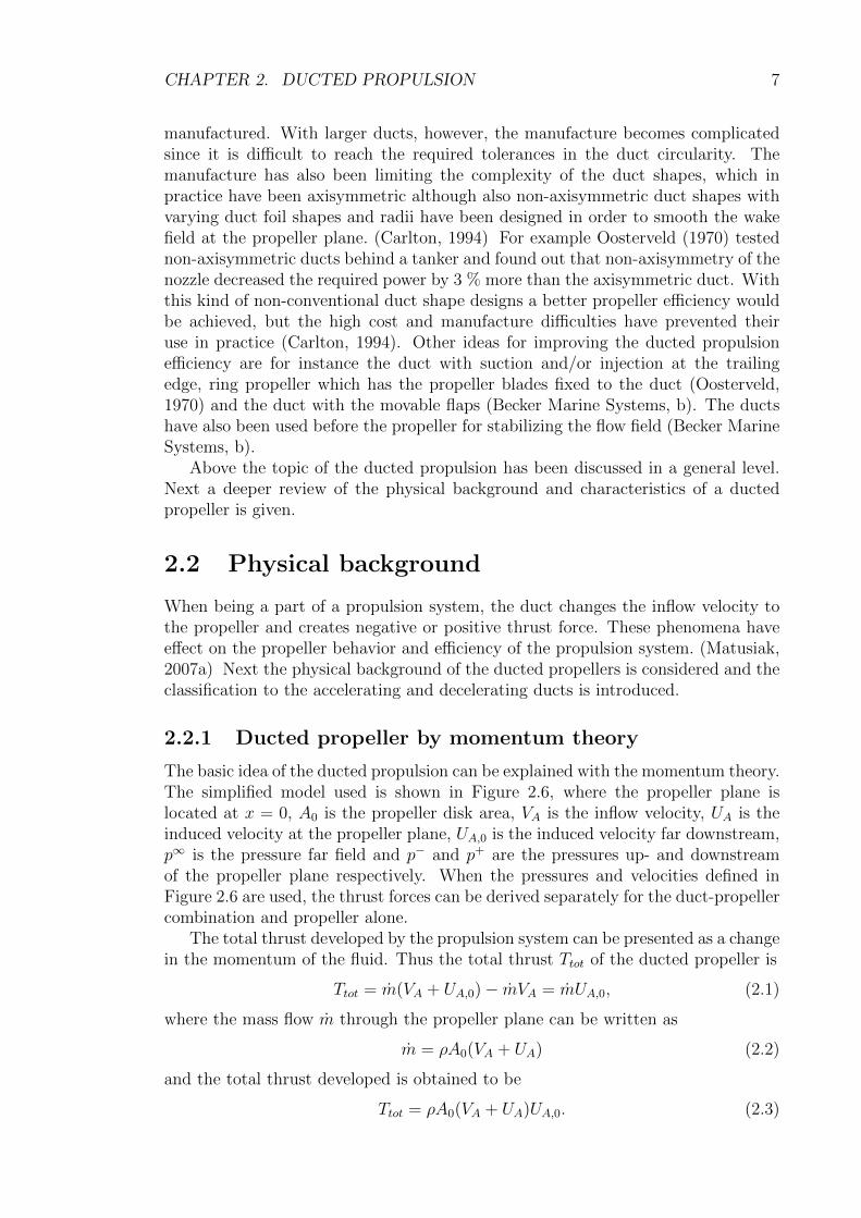
When being a part of a propulsion system, the duct changes the inflow velocity tothe propeller and creates negative or positive thrust force. These phenomena haveeffect on the propeller behavior and efficiency of the propulsion system. (Matusiak,2007a) Next the physical background of the ducted propellers is considered and theclassification to the accelerating and decelerating ducts is introduced.
2.2.1 Ducted propeller by momentum theory
The basic idea of the ducted propulsion can be explained with the momentum theory.The simplified model used is shown in Figure 2.6, where the propeller plane islocated at x = 0, A0 is the propeller disk area, VA is the inflow velocity, UA is theinduced velocity at the propeller plane, UA,0 is the induced velocity far downstream,p∞ is the pressure far field and p− and p+ are the pressures up- and downstreamof the propeller plane respectively. When the pressures and velocities defined inFigure 2.6 are used, the thrust forces can be derived separately for the duct-propellercombination and propeller alone.
The total thrust developed by the propulsion system can be presented as a changein the momentum of the fluid. Thus the total thrust Ttot of the ducted propeller is
Ttot = m(VA + UA,0)− mVA = mUA,0, (2.1)
where the mass flow m through the propeller plane can be written as
m = ρA0(VA + UA) (2.2)
and the total thrust developed is obtained to be
Ttot = ρA0(VA + UA)UA,0. (2.3)

CHAPTER 2. DUCTED PROPULSION 8
Figure 2.6: Simplified model of ducted propeller.
As the momentums in Equation (2.1) are defined far up- and downstream fromthe propeller plane, the thrust obtained includes both propeller and duct thrusts.(Kerwin, 2010; van Manen and Oosterveld, 1972)
The propeller thrust alone can be obtained with the pressure jump created bythe propeller at the propeller plane, shown in Figure 2.7. The propeller thrust Tp
Figure 2.7: Pressure jump at the propeller plane
expressed with the pressure jump ∆p is
Tp = ∆pA0, (2.4)
where the pressure jump can be calculated from the Bernoulli equation
p+ 12ρV 2 + ρgz = C, (2.5)
where C is constant. The pressure before the propeller plane p− is obtained bywriting the Bernoulli equation far upstream and right before the propeller planeand setting them equal
p∞ +1
2ρV 2
A = p− +1
2ρ(VA + UA)2 (2.6)
p− = p∞ +1
2ρV 2
A −1
2ρ(VA + UA)2. (2.7)

CHAPTER 2. DUCTED PROPULSION 9
Respectively the pressure right after the propeller plane p+ is obtained by theBernoulli equations just after the propeller plane and far downstream
p+ +1
2ρ(VA + UA)2 = p∞ +
1
2ρ(VA + UA,0)
2 (2.8)
p+ = p∞ +1
2ρ(VA + UA,0)
2 − 1
2ρ(VA + UA)2. (2.9)
Hence the pressure jump at the propeller plane can be calculated to be
∆p = p+ − p− =1
2ρ(2VA + UA,0)UA,0 (2.10)
and the thrust developed by the propeller is obtained by substituting the pressurejump from Equation (2.10) to Equation (2.4)
Tp =1
2ρA0(2VA + UA,0)UA,0. (2.11)
As the pressures jump is defined inside the duct and pressure values are defined veryclose to each other, the effect of the duct is not included in the thrust definition.(Matusiak, 2007a; Kerwin, 2010; van Manen and Oosterveld, 1972)
A general coefficient used for presenting the propeller loading rate is the non-dimensional thrust loading coefficient CT which is defined as
CT =T
12ρA0V 2
A
. (2.12)
For the ducted propeller the thrust loading coefficient is usually calculated with thetotal thrust of the system, which gives
CT =Ttot
12ρA0V 2
A
. (2.13)
The propeller loading coefficient is obtained from the total thrust loading coefficientwith the duct loading factor τ so that
CT,p = τCT (2.14)
where τ is defined as
τ =TpTtot
. (2.15)
The smaller τ is, the larger part of the total thrust is created by the duct. If τ = 1,no thrust is created by the duct and when τ > 1, the duct creates negative thrust andthe propeller loading increases since the propeller has to create the thrust also forcanceling the negative thrust created by the duct. Thus, the situation where τ > 1,is not desirable and the smaller τ is, the less power is demanded from the propellerand the more effective the propulsion system is. A measure used for estimating theefficiency of a propulsion system is the ideal efficiency ηI which is obtained with
ηI =PTPD
, (2.16)

CHAPTER 2. DUCTED PROPULSION 10
where PT is a thrust power and PD is a power delivered at the propeller. The thrustpower can be simply calculated from
PT = TtotVA = ρA0(VA + UA)UA,0VA (2.17)
and the power delivered at the propeller PD can be calculated as a kinetic energyflux through the propeller plane, which is
Fk = 12m2V
22 − 1
2m1V
21 , (2.18)
where subscripts 1 and 2 correspond to chosen cross sections in the flow field. Toobtain the power delivered at the propeller PD, these cross sections are set justbefore and after the propeller plane and thus the power delivered at the propeller isobtained to be
PD = 12m(VA + UA,0)
2 − 12mV 2
A (2.19)
= 12ρA0(VA + UA)[(VA + UA,0)
2 − V 2A ]. (2.20)
When Equations (2.17) and (2.20) are substituted to Equation (2.16), the idealefficiency ηI is after simplifying obtained to form
ηI =1
1 + 12
UA,0
VA
. (2.21)
Since it is more practical to express the ideal efficiency with a parameter linked withthe thrust instead of the rate of induced and incoming velocities UA,0/VA, the velocityrate is expressed in terms of the thrust loading coefficient. The relation betweenthe velocity rate and the thrust loading coefficient is obtained by first calculatingthe thrust loading coefficient in Equation (2.12) with the propeller thrust fromEquation (2.11)
CT,p = 2(1 +1
2
UA,0VA
)UA,0VA
(2.22)
and next solving the rate of velocitiesUA,0
VAfrom Equation (2.22). The rate of veloc-
ities is obtained to beUA,0VA
= −1 +√
1 + CT,p (2.23)
and when this is substituted to Equation (2.21), the ideal efficiency is obtained tobe
ηI =2
1 +√
1 + CT,p. (2.24)
The ideal efficiency can be further modified to a form where the duct effect canbe easily seen when the relationship from Equation (2.14) is substituted to idealefficiency expression in Equation (2.24)
ηI =2
1 +√
1 + τCT. (2.25)
From Equation (2.25) it can be seen that the duct creating thrust (τ < 1) increasesthe ideal efficiency and respectively a duct creating negative thrust (τ > 1) decreasesthe ideal efficiency. (Matusiak, 2007a; Kerwin, 2010; van Manen and Oosterveld,1972)
From the efficiency point of view, a ducted propeller is the better the larger partof the thrust is created by the duct. However, the actuator disk theory does notexplain, how a duct creates thrust and thus it is discussed in the next section.
CHAPTER 2. DUCTED PROPULSION 11
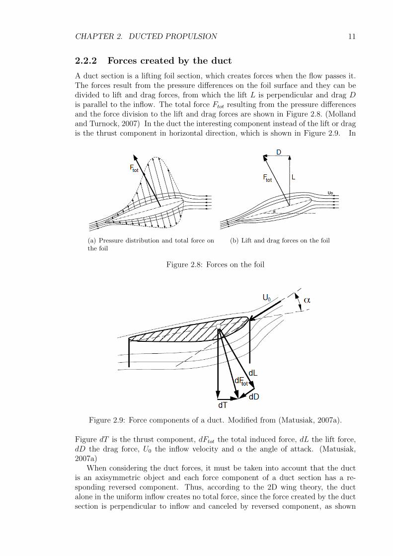
2.2.2 Forces created by the duct
A duct section is a lifting foil section, which creates forces when the flow passes it.The forces result from the pressure differences on the foil surface and they can bedivided to lift and drag forces, from which the lift L is perpendicular and drag Dis parallel to the inflow. The total force Ftot resulting from the pressure differencesand the force division to the lift and drag forces are shown in Figure 2.8. (Mollandand Turnock, 2007) In the duct the interesting component instead of the lift or dragis the thrust component in horizontal direction, which is shown in Figure 2.9. In
(a) Pressure distribution and total force onthe foil
(b) Lift and drag forces on the foil
Figure 2.8: Forces on the foil
Figure 2.9: Force components of a duct. Modified from (Matusiak, 2007a).
Figure dT is the thrust component, dFtot the total induced force, dL the lift force,dD the drag force, U0 the inflow velocity and α the angle of attack. (Matusiak,2007a)
When considering the duct forces, it must be taken into account that the ductis an axisymmetric object and each force component of a duct section has a re-sponding reversed component. Thus, according to the 2D wing theory, the ductalone in the uniform inflow creates no total force, since the force created by the ductsection is perpendicular to inflow and canceled by reversed component, as shown

CHAPTER 2. DUCTED PROPULSION 12
in Figure 2.10(a). Adding a rotating propeller inside the duct modifies the inflowangle and a thrust force is created, as shown in Figure 2.10(b). When the viscousforces and the induced drag by free vortices are taken into account, the propelleris still a requirement for the duct to create positive thrust, since the viscous effectsand vortices create drag. However, if the inflow angle to the duct is too small ornegative, the duct creates negative thrust force, as shown in Figure 2.11. (Matusiak,2007a)
(a) Duct without propeller (b) Duct with working pro-peller
Figure 2.10: Duct forces according to 2D wing theory
Figure 2.11: Force components of a duct with small angle of attack. Modified from(Matusiak, 2007a).
It was mentioned previously, that the duct creates negative thrust only if theinflow angle to the duct is too small but in reality, also the duct section shapeaffects the thrust generation. There are duct shapes which are not able to generatepositive thrust while others can produce a remarkable amount of it. By using theconventional classification of the duct profiles to accelerating and decelerating ducts,
CHAPTER 2. DUCTED PROPULSION 13
it can be said that decelerating ducts do not create thrust while accelerating ductsdo. Next the classification to accelerating and decelerating ducts is declared.
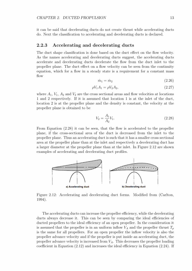
2.2.3 Accelerating and decelerating ducts
The duct shape classification is done based on the duct effect on the flow velocity.As the names accelerating and decelerating ducts suggest, the accelerating ductsaccelerate and decelerating ducts decelerate the flow from the duct inlet to thepropeller plane. The duct effect on a flow velocity can be seen from the continuityequation, which for a flow in a steady state is a requirement for a constant massflow
m1 = m2 (2.26)
ρV1A1 = ρV2A2, (2.27)
where A1, V1, A2 and V2 are the cross sectional areas and flow velocities at locations1 and 2 respectively. If it is assumed that location 1 is at the inlet of the duct,location 2 is at the propeller plane and the density is constant, the velocity at thepropeller plane is obtained to be
V2 =A1
A2
V1. (2.28)
From Equation (2.28) it can be seen, that the flow is accelerated to the propellerplane, if the cross-sectional area of the duct is decreased from the inlet to thepropeller plane. Thus an accelerating duct is such that it has a smaller cross sectionalarea at the propeller plane than at the inlet and respectively a decelerating duct hasa larger diameter at the propeller plane than at the inlet. In Figure 2.12 are shownexamples of accelerating and decelerating duct profiles.
Figure 2.12: Accelerating and decelerating duct forms. Modified from (Carlton,1994).
The accelerating ducts can increase the propeller efficiency, while the deceleratingducts always decrease it. This can be seen by comparing the ideal efficiencies ofducted propellers to the ideal efficiency of an open propeller. In the consideration itis assumed that the propeller is in an uniform inflow VA and the propeller thrust Tpis the same for all propellers. For an open propeller the inflow velocity is also thepropeller advance velocity and if the propeller is put inside an accelerating duct, thepropeller advance velocity is increased from VA. This decreases the propeller loadingcoefficient in Equation (2.12) and increases the ideal efficiency in Equation (2.24). If

CHAPTER 2. DUCTED PROPULSION 14
the propeller is instead put inside a decelerating duct, the propeller advance velocityis decreased from VA, the propeller loading coefficient is increased and the propellerideal efficiency is decreased.
Traditionally the accelerating ducts are used because they are able to create the-oretically up to 50 % more thrust in the bollard pull condition than the conventionalopen propellers (Carlton, 1994). The accelerating ducts can also have a better idealefficiency but on the other hand the increased inflow velocity can cause cavitationproblems on the propeller blades and the advantage of the duct can be canceled bythe viscous resistance of the duct. As the decelerating ducts have a negative effecton the efficiency, they are in practice used only in the naval ships for reducing thecavitation risk and noise level of the vessel. Because the accelerating ducts can havea positive effect on the propulsion power demand, they are a potential propulsionsystem when new, more efficient solutions for the ship propulsion are searched. De-velopment projects both for the duct and propeller geometries and ducted propellersimulation tools exist. For example at CRS (Cooperative Research Ships) a simu-lation tool for ducted propulsion is being developed, as it is expected that ductedpropellers will in future raise interest also among other kind of ship types than thosewhich traditionally use the ducted propulsion.
In this chapter the development of the ducted propellers was discussed, thephysical background was considered with the momentum theory and the thrustcreation mechanism of the duct was presented. Also the classification to acceleratingand decelerating ducts was clarified and the possibilities of the accelerating ductswere reviewed. In the next chapter the state of the art of the simulation methods forconventional propellers and their extensions for the ducted propulsion is presentedand the state of the art and basics of the self-propulsion simulation methods arediscussed.

Chapter 3
State of the art of ship flow simu-lation
The flow simulation is an useful tool in the hydrodynamic design of the ships sinceit can produce detailed information about the flow around the hull and propelleralready before model tests. Different simulation tools have been and are beingdeveloped for ship resistance, propeller and self-propulsion testing. The resistancesimulation tools using RANS-equations give already results with good accuracy andthey are being used as daily design tools and as well the potential flow methods arecommonly used in the propeller design and analysis. The self-propulsion simulationis such a new field that the methods are not yet commonly used in design purposesbut are being further developed. In this chapter short reviews of the propellersimulation and self-propulsion simulation methods are given.
3.1 Propeller simulation with conventional and
ducted propellers
The CFD tools for the propeller design are on a good level. The CFD simulationis used for the design and analysis of the propellers and tools used are mostlypotential flow based methods, such as lifting line and lifting surface methods andpanel methods. The most simplified propeller model is the actuator disk modelwhereas the RANS solvers have the most detailed description of the propeller andflow. The propeller simulation methods have first been developed for open propellersbut they can be applied also for the ducted propellers. The nozzle around thepropeller creates though additional challenges to the simulation, the main challengebeing the simulation of the tip vortex flow in a gap between the propeller blade tipand the duct (Yu et al., 2013). In next sections the different propeller simulationmethods are shortly described.
3.1.1 Actuator disk model
The easiest way for the propeller flow modeling is the actuator disk model, whichtheoretical background was explained in Section 2.2.1 by the momentum theory.The general actuator disk model for open propellers is based on the assumption
15

CHAPTER 3. STATE OF THE ART OF SHIP FLOW SIMULATION 16
that the propeller is a thin, permeable disk in the flow, which introduces a pressurejump to the flow. The flow at the propeller disk is accelerated and either only axialor both axial and tangential velocities are taken into account. This basic model canbe extended for the ducted propellers, in which case the propeller thrust is given bythe similar actuator disk which is used for the open propellers and the duct thrustis given by a zero thickness ring around the propeller disk. (Kerwin, 2010)
The thrust created by the actuator disk can be calculated either if the pressurejump at the propeller disk is known or if both the incoming and induced flow veloc-ities are known. In practice the actuator disk is used for introducing the propellereffect on the RANS equations by defining a force or pressure distribution for thedisk and scaling it to give the required thrust and torque. The force distributioncan be uniform, have radial force distribution or have a changing force distributionboth in radial and circumferential directions. Since the actuator disk only intro-duces a force distribution, its accuracy depends on the method used for the forcedistribution calculation and how detailed force distribution is given to the actuatordisk. (Sanchez-Caja and Pylkkanen, 2007)
The force distribution can be obtained for example by propeller simulationswith lifting line method (Sanchez-Caja and Pylkkanen, 2007) or boundary elementmethod (BEM) (Bosschers et al., 2008; Ripjkema et al., 2013), which are discussedin next sections. It is also possible to define the force distribution without anypropeller simulation, for example with the circulation distribution defined by Houghand Ordway (1964), and then only a basic information about propeller is needed(Zhang, 2010).
3.1.2 Lifting line and lifting surface models
The lifting surface and lifting line are potential flow methods which in the ship hy-drodynamics are used for the propeller design and analysis. In the lifting surfacemethod the propeller blades are presented by lifting surfaces having propeller spe-cific vortex sheet distributions while the lifting line model is a simplification of thelifting surface model and the propeller blades are presented with the lifting lineshaving line vortex distributions. In both methods the propeller induced velocitiesand propeller forces can be solved based on the vorticity distribution. The methodshave continuous vortex distributions, which are often discretized for computationalpurposes with panels. Then instead of continuous vortex distributions, approxi-mated constant vortex values are given on each panel. These discretized calculationmodels are called vortex lattice solutions. (Kerwin, 2010)
(a) Lifting line (b) Lifting surface
Figure 3.1: Lifting and lifting surface presentations for foil sections

CHAPTER 3. STATE OF THE ART OF SHIP FLOW SIMULATION 17
The duct can be implemented to the lifting line presentation with an imagevortex system, which creates such a boundary at the duct surface, that no flowpenetrates through it. The boundary is created by modeling the duct mean linewith a system of ring vortices and additionally the duct thickness can be taken intoaccount with a system of ring sources. (Stubblefield, 2008) With the lifting line andsurface models the tip gap can be modeled or the gap can be ignored. For exampleVan Houten (1986) developed a model for tip gap flow calculation but in an opensource propeller design and analysis code OpenProp v 2.4 no duct gap is takeninto account (Epps, 2010).
3.1.3 Boundary element methods
The boundary element methods, or panel methods, are potential flow methods whichcan be used in the propeller modeling and preliminary ship resistance simulations. Ina propeller simulation by BEM the propeller is discretized with panels and dependingon the method a distribution of either sources and vortices, sources and dipoles oronly vortices is defined on the panels. The propeller forces are calculated by solvingeither the velocities or velocity potentials and further solving the pressures and forcesfrom the velocities. (Kerwin, 2010) A duct can be included to a panel method bycreating panels for the duct geometry and the tip gap flow can be modeled withpanels generated for the tip vortex.
A panel method for the ducted propellers was developed by Kerwin et al. (1987)and has been further inspected for example by Baltazar and Falcao de Campos(2009) and Baltazar et al. (2012). Baltazar and Falcao de Campos (2009) concen-trated on the effect of the gap modeling when Baltazar et al. (2012) tested differentwake calculation methods.
3.1.4 RANS simulation
The most detailed and physically correct description of the propeller flow is obtainedwith the RANS simulation. The previously reviewed methods were potential flowbased, i.e. the flow was assumed to be irrotational and inviscid while in RANSsimulations no such simplifications are done. Additionally, while in lifting line andBEM methods the solution is calculated only on the propeller surface and in thepropeller wake, in the RANS methods also the fluid is modeled.
The propeller simulation with RANS can be done time accurately or as a quasi-static computation (Siikonen, 2013). The quasi-static simulation is used in thepropeller open water condition, where the inflow to a propeller is uniform, and it isenough to model a section with only one propeller blade with periodical boundaryconditions at the section sides because the situation is symmetric. (Watanabe et al.,2003) However, when a propeller is located in an non-uniform wake field, the wholepropeller must be modeled and a time accurate simulation is required.
In both cases, the computational domain consists of two domains, which are thedomain rotating with the propeller and the static outer domain. The domains canbe overlapping, as in the Chimera method, or alternatively the blocks have no overlaps or gaps between them, as in the sliding mesh method. In both sliding mesh andChimera grid methods the propeller rotation is implemented to the flow by rotating

CHAPTER 3. STATE OF THE ART OF SHIP FLOW SIMULATION 18
the propeller block in each time step so that the taken rotation angle correspondsto the actual propeller rotation rate. (Siikonen, 2013)
In the sliding mesh method the flow variables are interpolated at the interfacebetween the static and sliding meshes. (Siikonen, 2013) In the Chimera grid, ordynamic overset grid, the propeller is modeled as a separate sub-block which is thenset on the major grid and in the domain each grid point is marked either as active,interpolated or hole point. The hole points are the points where the calculationresults are discarded or the calculation is not done at all, i.e. the points inside ageometry or outside the computational domain. At the edge of the hole boundaryand at the outer edge of the sub-domain, the interpolation points are defined in themajor grid and in the sub-domain respectively and the information between grids iscommunicated via the interpolated boundary points. At the overlap region the gridpoints are active and the flow problem is solved as usual in both grids. (Zheng andLiou, 2003; Carrica et al., 2010) In Figure 3.2 is shown the principle of the slidingmesh and in Figure 3.3 are shown the different regions of the overlapping grids.
Figure 3.2: Sliding mesh. Taken from (Dhinesh et al., 2010).
Figure 3.3: Overlapping mesh. Taken from (Zheng and Liou, 2003).
In addition to the time-accurate simulation, the sliding mesh and Chimera gridmethods can be used for the quasi-static simulation. In the propeller simulation thequasi-static simulation is used either in the open water condition for final results or
CHAPTER 3. STATE OF THE ART OF SHIP FLOW SIMULATION 19
in a non-symmetric situation for computing the initial state for the time-accuratesimulation. In the quasi-static simulation the needed CPU (Central ProcessingUnit) time is reduced by using approximative boundary conditions at the boundarybetween the static and rotating blocks instead of actual physical boundary conditionsused in the time-accurate simulation. There are two alternatives for the boundarycondition approximations called multi reference frame (MRF) and mixing planeor steady-averaged method. In MRF it is assumed that only a weak interactionbetween the moving and fixed domains exist and the rotating block adopts theboundary conditions of one position and uses them for the whole simulation. In themixing plane model the flow quantities are averaged circumferentially at the meshblock interfaces and the averaged values are used as boundary values. (Siikonen,2013)
The propeller simulations with RANS have been done for example by Sanchez-Caja et al. (2008), Yu et al. (2013) and Watanabe et al. (2003), of whom Sanchez-Caja et al. (2008) and Yu et al. (2013) have used the MRF-method for the ductedpropeller simulation and Watanabe et al. (2003) used both the time-accurate simu-lation and the steady state simulation with the open propeller. Yu et al. (2013)obtained accurate simulation results when compared to model tests results andSanchez-Caja et al. (2008) obtained a quite accurate prediction of the total thrustwhereas the torque was underestimated. Watanabe et al. (2003) obtained resultswith a fairly good accuracy for the thrust with both methods while the torque wasoverestimated.
As described in previews sections, there are many different methods for thepropeller simulation and depending on the method, different amount of physicalproperties are taken into account in the simulation. At present the potential flowbased methods are most commonly used in propeller design and analysis becauseof their lighter computational load while in the hull resistance simulation it is self-evident to use RANS solvers, which can predict the hull resistance accurately in themost of cases. Thus the self-propulsion schemes are based on the RANS simulationof the hull flow and the propeller calculation is included to the calculation modeleither by coupling RANS with a potential flow solver or by time-accurate RANSsimulation. These different methods are discussed in the next section.
3.2 Self-propulsion simulation
The aim of the self-propulsion simulation is to give reliable results of the propulsionparameters and thus a reliable powering prediction. The self-propulsion modelsconsist basically of the hull resistance simulation and propeller simulation modelswhich are combined together.
In the simplest self-propulsion methods the propeller is modeled with an actuatordisk model, which introduces a constant body force distribution to RANS equations.The body force distribution is defined separately from the RANS solver and thusthe methods with the actuator disk are called coupled or hybrid methods. In fullRANS self-propulsion methods the actual propeller geometry is implemented to thesimulation by the sliding mesh method or Chimera grid model.

CHAPTER 3. STATE OF THE ART OF SHIP FLOW SIMULATION 20
3.2.1 Hybrid methods
The hybrid methods couple RANS equations with potential flow solvers and use theactuator disk model for introducing the propeller forces calculated by the poten-tial flow solver to the RANS equations. They are relatively simple and fast whencompared to the time-accurate RANS simulation and can thus be effective designtools.
In the simplest hybrid self-propulsion models the propeller force distribution isgiven to the actuator disk at the beginning of the simulation and is not updatedduring the computation. Thus the force distribution is defined based either on theopen water condition or nominal wake obtained from the resistance test. Hence theself-propulsion point is not reached as the hull-propeller interaction both changesthe wake field where the propeller operates and influences the hull resistance. Toobtain more realistic results, the correct force distribution of the propeller is searchedwith an iterative process where the general idea is to update the wake field usedin the propeller simulation program and calculate a new force distribution whichis then updated to the actuator disk in the RANS model. The iteration procedureis repeated until the wake field does not change anymore, i.e. until the wake fieldobtained is the effective wake field. In addition to updating the force distribution,also the required thrust and torque values are updated if the ship resistance haschanged. (Sanchez-Caja and Pylkkanen, 2007)
The self-propulsion simulations with hybrid methods have been done for exampleby Bosschers et al. (2008) and Ripjkema et al. (2013) by using BEM for the propellersimulation and Sanchez-Caja and Pylkkanen (2007) by using a lifting line method.Also Tahara et al. (2006), Kawamura et al. (1997) and Phillips et al. (2009) haveused a potential flow based solvers for propeller performance calculation and coupledit with a RANS solver.
3.2.2 Full RANS simulation
The self-propulsion simulation with a hybrid method is effective, since only a con-stant source term is added to a RANS hull flow solution. The propeller simulationwith a potential flow solver is fast and thus updating the actuator disk force distri-bution does not lengthen the computation time significantly. Even though the use ofthe potential flow solver makes the computation quick, it has also its disadvantages.For example the viscous effects on the propeller are taken into account only withapproximative viscous force coefficients and moreover the accuracy of the hybridmethod depends on the accuracy of the propeller calculation program and whetherthe actuator disk model can adopt both radially and circumferentially non-uniformthrust and torque distributions. In the full RANS simulation these aspects are notcritical since the propeller geometry and viscous effects are directly included in thesimulation. Instead the different time scales in the propeller and hull flows andheavy computation can cause difficulties.
In the full RANS self-propulsion simulation the propeller is added to the compu-tation either by sliding mesh model or Chimera grid model discussed in Chapter 3.1.4and the simulation is done as a time-accurate simulation. In the coupled methodsthe self-propulsion point is reached by updating the wake field for the propellersimulation tool while in the full RANS simulation the self-propulsion point is by

CHAPTER 3. STATE OF THE ART OF SHIP FLOW SIMULATION 21
tradition searched in the same way as in the model tests, i.e. several simulations arerun with different propeller rotation rates and the self-propulsion point is estimatedby interpolating from the points closest to the real self-propulsion point (Carricaet al., 2010). However, the time-accurate simulation requires a lot of CPU time andthus more effective methods for finding the self-propulsion point have been devel-oped. These methods, called speed controllers, basically monitor the total resistanceand propeller thrust and based on these update the propeller rotation rate.
The simulations with speed-controllers has been done by Carrica et al. (2010),Carrica et al. (2011) and Dhinesh et al. (2010), where Carrica et al. (2010) and Car-rica et al. (2011) used the Chimera grid method for the propeller implementationand Dhinesh et al. (2010) used the sliding mesh method. A simple way for checkingthe self-propulsion model is to do a self-propulsion simulation with a predefined pro-peller rotation rate for a vessel which self-propulsion point is already known from themodel tests. This kind of simulation has been done by Gao et al. (2012) and Zhang(2010) with the sliding mesh method. The accuracy of the self-propulsion resultswith the different full RANS computation models vary when compared to model testresults. The maximum difference to the model test results in the referenced articlesis in the propeller rotation rate not more than 4 % and in the propeller thrust notmore than 3 %.
In this chapter the different propeller simulation models have been described,including both the potential flow and RANS models. The self-propulsion schemescoupling the RANS solvers and potential flow solvers for the propeller have beenshortly introduced as well as the time-accurate self-propulsion models. In the nextchapter the test case used is presented and the procedure for the propeller pitch-diameter ratio and propeller rotation rate optimization used in the propeller choiceis described.

Chapter 4
Test case
The purpose of this master’s thesis is to test the full RANS self-propulsion simulationof FINFLO and to examine the ducted propeller performance in a large vessel. Thestudy is done with a case vessel which is modified from an existing hull form whichhas a conventional open propeller. The obtained simulation results are comparedto the results of the original hull and propeller arrangement. As the model testand simulation results of the original vessel are obtained in the model scale, thesimulations with the modified vessel are also conducted in the model scale. In thischapter the test case is introduced and the choice of the duct-propeller combinationis justified.
4.1 Hull form
A large vessel with an existing model test data and RANS simulation results ischosen as a comparison case. The comparison vessel A has a conventional openpropeller and a rudder and the test case vessel B is obtained by modifying the originalvessel A. The conventional propeller and rudder are replaced with the propeller andsteerable duct and the propeller diameter is kept the same. In order to fit theducted propeller to the ship, modifications are needed for the aft hull shape. First,the propeller shaft is lifted so that the duct bottom is located above the hull baseline. Second, the propeller is moved aft-wards so that there is a gap between theduct top and the hull. Once the location of the ducted propeller is determined, theskeg is reshaped to suit the new propeller position. In the modifications the shiplength between perpendiculars LPP is kept constant and the ship wetted surfacearea S and displacement ∇ are slightly increased, as shown in Table 4.1. A sketchof the modifications made is shown in Figure 4.1.
22

CHAPTER 4. TEST CASE 23
Table 4.1: Ship reference values
Vessel A Vessel B Difference
LPP [m] 176.65 176.65 0.0 %
S [m2] 3 870 3 945 1.94 %
∇ [m3] 42 890 42 970 0.18 %
D [m] 6.0 6.0 0.0 %
Vs [kn] 14.0 14.0 0.0 %
Fn [-] 0.1714 0.1714 0.0 %
Figure 4.1: Sketch of the aft ship modifications
4.2 Duct
The duct and propeller are chosen from the Wageningen Ka-series. The duct shapeis chosen to be 19A, which is the most common duct shape from Wageningen seriesdesigned for having a good forward performance. The duct profile 19A is shown inFigure 4.2 and the detailed description of the duct geometry is given in Appendix A.The propeller is located at the mid-plane of the duct and the tip gap between thepropeller blade tip and duct inner surface is approximately 0.4 % of the propeller di-ameter, which is similar to the tip gap used in the model tests at NSMB (Oosterveld,1970).
Figure 4.2: Profile of the Wageningen nozzle 19A
CHAPTER 4. TEST CASE 24
4.3 Propeller
The propeller is chosen from the propellers tested in the nozzle 19A, which meansthat there are four possible propellers, Ka3-65, Ka4-55, Ka4-70 and Ka5-75, whichhave the model test data and geometry specifications available. In order to choosethe most suitable propeller for the vessel B, the propeller efficiencies and the dangerof harmful propeller excitations at the optimal propeller rotation rates are studied.The study is done by first searching the optimal propeller rotation rates and pitch-diameter ratios for each propeller and next calculating the propeller pressure forcesbased on the optimal propeller rotation rates. Finally the propeller with the lowdanger of vibration problems with the best efficiency is chosen.
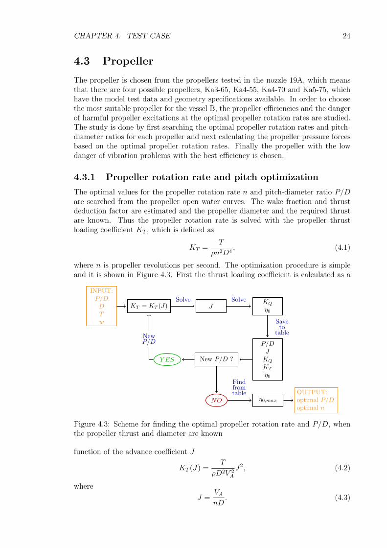
4.3.1 Propeller rotation rate and pitch optimization
The optimal values for the propeller rotation rate n and pitch-diameter ratio P/Dare searched from the propeller open water curves. The wake fraction and thrustdeduction factor are estimated and the propeller diameter and the required thrustare known. Thus the propeller rotation rate is solved with the propeller thrustloading coefficient KT , which is defined as
KT =T
ρn2D4, (4.1)
where n is propeller revolutions per second. The optimization procedure is simpleand it is shown in Figure 4.3. First the thrust loading coefficient is calculated as a
INPUT:P/DDTw
KT = KT (J) JKQ
η0
Saveto
table
P/DJKQ
KT
η0
New P/D ?
NO
Y ES
Findfromtable
η0,max
OUTPUT:optimal P/Doptimal n
NewP/D
Solve Solve
Figure 4.3: Scheme for finding the optimal propeller rotation rate and P/D, whenthe propeller thrust and diameter are known
function of the advance coefficient J
KT (J) =T
ρD2V 2A
J2, (4.2)
where
J =VAnD
. (4.3)

CHAPTER 4. TEST CASE 25
Next the cross section points of the KT (J) and the KT given by propeller openwater results are searched. The cross section points define the advance coefficientsfor each propeller pitch-diameter ratio and the corresponding torque loading coeffi-cients KQ and open water efficiencies η0 are searched from the propeller open watercurves, as shown in Figure 4.4. From the values obtained for each pitch-diameterratio, the optimal propeller rotation rate is found by searching for the best pro-peller efficiency and solving the optimal propeller rotation rate from Equation (4.3).(Matusiak, 2007a)
Figure 4.4: Propeller open water curves and KT(J)
In the propeller optimization the required power, the ship wake field and thepropeller open water curves must be known. As in this thesis the choice of thepropeller is done before any simulation is done with the new hull form, the requiredpower and the wake fraction are estimated based on the model test results of theoriginal hull. It is approximated that the rudder creates 3 % of the hull resistanceand thus the required power of the new hull is estimated to decrease by 3 % fromthe power demand of the original hull form and the Taylor wake fraction is kept thesame as in the original hull.
The best efficiency is achieved with the propeller Ka3-65 and the lowest efficiencywith the propeller Ka5-75. The differences are however small and the largest differ-ence is less than 1.5 %. The difference between the four bladed propellers Ka4-55and Ka4-70 is less than 0.5 %.
4.3.2 Propeller excitations
Other aspect to be considered when selecting the propeller is the pressure forceson the hull created by the blades of the rotating propeller passing the hull. Thefrequency of these pressure forces is calculated with
f = nZ, (4.4)

CHAPTER 4. TEST CASE 26
where Z is the number of the propeller blades. The frequency should not be close tothe hull girder natural frequencies since then the propeller might excite significanthull vibrations. According to American Bureau of Shipping (2006) the first naturalfrequencies of ships are 1 - 2 Hz and the highest significant natural frequencies areabout 6 Hz. Usually the propeller revolutions are such that these frequencies arenot close. However, with a three bladed propeller it is more probable than withpropeller with more blades.
The conclusion of the propeller study is, that the propeller Ka3-65 would be themost efficient choice, but with the three bladed propeller the propeller excitationfrequency can get quite close to the significant hull natural frequencies. In orderto avoid possible vibration problems, the propeller is chosen to be the four bladedpropeller Ka4-55 instead of Ka3-65 since the difference in the efficiencies is notlarge and the four bladed propeller is a more realistic choice. The chosen propellerKa4-55 has the area ratio of Ae/A0 = 0.55 and the best efficiency is obtained withthe pitch-diameter ratio P/D = 1.2. A detailed description of the geometry of thechosen propeller Ka4-55 is shown in Appendix B.
In this chapter the differences of the original vessel and the test case vessel havebeen presented and the duct and propeller have been chosen. In Figure 4.5 thefinal stern arrangement with the modified aft shape and chosen ducted propeller isshown. In order to keep the ship simulation as simple as possible, the duct supportis not modeled. In the next chapter the methods used in the simulation and thecomputational grids are described.
Figure 4.5: Modified stern with the chosen ducted propeller Ka4-55

Chapter 5
Methods
The ship hull and self-propulsion characteristics are tested with RANS simulationswhich are done with FINFLO-solver (Finflo Ltd.). The initial position of the shipis calculated with the potential flow solver ν-Shallo (HSVA). Next the basis of theship flow simulation is described and computational models used are introduced.
5.1 Governing equations for ship flows
The description of the viscous fluid flow is given with the Navier-Stokes -equations(NS-equations) and continuity equation, which are respectively written with thetensor notation as
∂ui∂t
+ uj∂ui∂xj
= −1
ρ
∂p
∂xi+
1
ρ
∂σij∂xj
+ Fi (5.1)
∂ui∂xi
= 0, (5.2)
where σij is the viscous stress term, ui is the velocity component, xi is the coordinatedirection and Fi is the body force component (source component). The viscous stressterm is defined as
σij = µSij = µ
(∂ui∂xj
+∂uj∂xi
), (5.3)
where µ is the dynamic viscosity and Sij is the rate of strain tensor. The NS-equations and continuity equation create the basis for the ship flow simulation,the NS-equations describing the momentum of the viscous flow and the continuityequation taking care of the mass balance. In Equations (5.1) and (5.2) the densityρ is assumed to be constant, which is a good approximation for the ship flows. Inaddition to the NS- and continuity equations there is an equation for the energyconservation, but it is usually not included in the ship flow simulation and is thusnot discussed here. (Larsson and Raven, 2010)
The flow simulations are done in different situations with varying requirementsfor the accuracy and CPU time and hence the NS-equations have been simplifiedand/or modified in different ways. For example, the simplified equations are used inthe potential flow theory whereas the RANS-equations are obtained by modifyingthe presentation of the flow velocities. However, though the momentum equationsmay change, the continuity equation remains the same. (Larsson and Raven, 2010)
27
CHAPTER 5. METHODS 28
The momentum equations and continuity equation are generic equations andhence boundary conditions are needed to specify the case in line. In the ship flowsimulation these specifying boundary conditions are defined at the free surface andon the solid surfaces, i.e. on the hull surface and on the possible appendages. Thehull surface boundary conditions define that there is no flow through the hull surface(no penetration condition) and the tangential velocity on the hull surface is equalto the surface velocity (no-slip condition). On the free surface the boundary condi-tions needed are the kinetic, or dynamic, and kinematic boundary conditions. Thedynamic boundary condition says that the pressure on the free surface is equal toatmospheric pressure while the kinematic boundary condition says that the particleson the free surface remain there. The dynamic and kinematic boundary conditionscan be respectively written as
p|z=h = pa (5.4)
and
w =Dh
Dt, (5.5)
where h is the free surface height, pa is the atmospheric pressure and w is the verticalvelocity component. (Matusiak, 2005; Larsson and Raven, 2010)
Above the generic equations for the ship flow simulation together with the bound-ary conditions have been presented. In this thesis the NS-equations as such are notused, but two different set of equations derived from NS-equations are applied. Thepotential flow model is obtained with simplifications made on the NS-equations andthe RANS-equations are obtained by re-formulating the velocity components of theNS-equations. Next these two flow descriptions are presented.
5.1.1 Potential flow theory
In the potential flow theory the flow is assumed to be incompressible, inviscid andirrotational, which means that the density of the fluid is constant (incompressibility),the kinematic viscosity is neglected (inviscid fluid) and the fluid particles do not haveangular velocities, i.e. spin (irrotational fluid). The assumptions can be respectivelywritten as
ρ = C (5.6)
ν = 0 (5.7)
∇× ~V = 0. (5.8)
In reality the flow described in the potential flow theory does not exist but nonethe-less the theory is widely used because it enables quite simple and fast computationalmodels. In practice the potential flow theory is considered to be suitable in situ-ations, where the viscous effects are limited to a very thin layer close to the solidsurfaces and the flow in the global scale is of interest. (Sanchez-Caja, 2013)
In the potential flow theory the momentum of the fluid is described with the Eulerequations, which are obtained by neglecting the viscosity from the NS-equations andare written as
∂ui∂t
+ uj∂ui∂xj
= −1
ρ
∂p
∂xi+ Fi. (5.9)

CHAPTER 5. METHODS 29
The Euler equations can be further modified to the Bernoulli equation, which forthe irrotational, steady state flow is
1
2ρV 2 + ρgz + p = C. (5.10)
The Bernoulli equation is constant along a streamline in the inviscid region and itis usually written at the point of interest and at a point far field, where the pressureand velocity are known. (Larsson and Raven, 2010)
In potential flow applications the Bernoulli equation and the continuity equationare written using velocity potentials φ instead of velocities. The velocity potentialsare used for describing the velocity field and they are defined as
~V =∂φ
∂x~i+
∂φ
∂y~j +
∂φ
∂z~k = ∇φ (5.11)
and the resulting continuity and Bernoulli equations are respectively
∂2φ
∂x2+∂2φ
∂y2+∂2φ
∂z2= ∇2φ = 0 (5.12)
and1
2∇φ · ∇φ+
ρ
p+ gz = C. (5.13)
The advantage of the use of velocity potentials can be seen from the newly obtainedcontinuity equation (5.12), which is the Laplace equation. There are already existingfundamental solutions for the Laplace equation and additionally the equation ishomogeneous and linear, which means that the superposition principle can be usedfor the velocity potentials. Thus also a complex flow field can be described by acomposition of simple velocity potentials. The common velocity potential types arenamed as sources, dipoles and vortices, of which the sources and dipoles are mainlyused in panel methods while the vortices are important in lifting line and liftingsurface methods. The velocities can be solved from the continuity equation andfurther the pressures from the Bernoulli equation. (Larsson and Raven, 2010)
In the ship hydrodynamics, the potential flow solvers are used for the propellersimulation, as described in Section 3.1, and for the hull flow simulation. In the hullflow simulation panel methods, where the hull surface and free-surface are discretizedwith panels, are used. The resistance of the ship cannot be estimated reliable withthe potential flow theory since the viscous effects and the turbulence are neglected.Instead the potential flow simulations are a useful tool for optimizing the wavepattern, even though the stern waves are usually overestimated. It is also possibleto evaluate the dynamic position of the hull, i.e. the dynamic sinkage and trim, witha panel method.
5.1.2 RANS equations
In the potential flow theory significant simplifications are made with the assumptionsof inviscid, incompressible and irrotational fluid. In reality the fluid is always viscous

CHAPTER 5. METHODS 30
and the flow characteristics change depending on the viscosity and flow velocity. Thedependence is expressed with the non-dimensional Reynold number Rn, which is
Rn =uL
ν, (5.14)
where L is the characteristic dimension. With low Reynold numbers the flow islaminar and when the Reynold number gets high enough, the flow transforms to aturbulent flow. In a laminar flow individual tracks of flow particles can be followedand streamlines follow smoothly surface curvatures whereas in turbulent flows theparticle tracks are random and the flow velocities and pressures fluctuate. The shiphull flow is always turbulent and hence the turbulence simulation has an importantrole in the ship simulation. (Matusiak, 2007b)
The turbulent flow problems can be solved either with the time accurate simula-tion of the turbulence or by treating the turbulence as a steady state phenomenonand calculating the effect of turbulence with a turbulence model. The method forthe time accurate simulation of the turbulence is called DNS (Direct Navier-Stokes)where the actual velocities are solved from the NS-equations. In order to get cor-rect results from DNS, all the turbulent time scales must be modeled, i.e. also thesmallest turbulent fluctuations must be caught. Thus a fine mesh and small timesteps are required and a lot of CPU time is needed for the solution. In practice DNSsimulation is possible only for flows with low global Reynolds numbers. Other tur-bulence simulation models which use the NS-equations are for instance LES (LargeEddy Simulation) and its lighter version DES (Detached Eddy Simulation). In LESand DES only a part of the turbulence is solved time accurately, in the same wayas in DNS, and the turbulence scales smaller than the grid resolution are modeledby place-averaged equations. (Siikonen, 2013)
A common practice is to use instead of DNS, LES or DES some turbulencemodel which is based on the time-averaging of the turbulent flow. The usage ofthese turbulence models requires a modification of the NS-equations to a such form,that the effect of the turbulence stands out from the equations. The modified formis the RANS-equations, where the turbulent flow velocities are divided to averageand fluctuating velocity components, u and u′ respectively
u = u+ u′. (5.15)
The velocity components are also shown in Figure 5.1. Similarly the pressure isdivided to average and fluctuating components, p and p′ respectively
p = p+ p′. (5.16)
The velocity and pressure components from Equations (5.15) and (5.16) are substi-tuted to NS-equations (5.1) and after substitution a time average is taken from theequations. As a result the RANS equations are obtained
∂ui∂t
+∂ujui∂xj
= −1
ρ
∂p
∂xi+
1
ρ
∂
∂xj(σij +Rij) + Fi, (5.17)
where Rij is the Reynolds stress and overline marks the time average. The Reynoldsstress is a correlation between fluctuating velocity components and is defined as
Rij = Rji = −ρu′ju′i. (5.18)
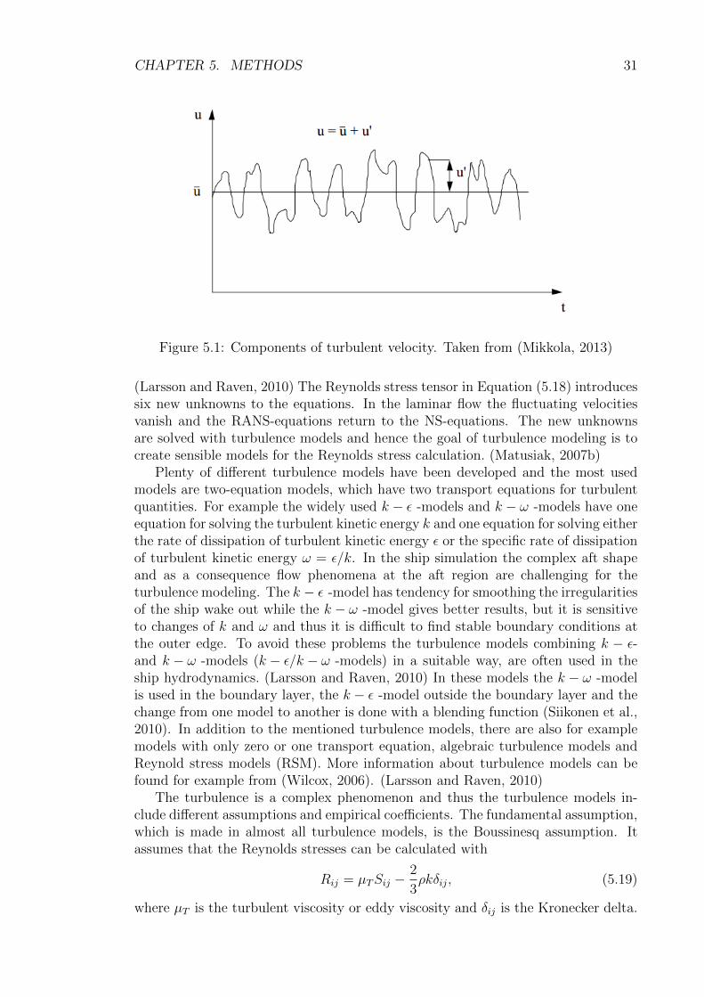
CHAPTER 5. METHODS 31
Figure 5.1: Components of turbulent velocity. Taken from (Mikkola, 2013)
(Larsson and Raven, 2010) The Reynolds stress tensor in Equation (5.18) introducessix new unknowns to the equations. In the laminar flow the fluctuating velocitiesvanish and the RANS-equations return to the NS-equations. The new unknownsare solved with turbulence models and hence the goal of turbulence modeling is tocreate sensible models for the Reynolds stress calculation. (Matusiak, 2007b)
Plenty of different turbulence models have been developed and the most usedmodels are two-equation models, which have two transport equations for turbulentquantities. For example the widely used k − ε -models and k − ω -models have oneequation for solving the turbulent kinetic energy k and one equation for solving eitherthe rate of dissipation of turbulent kinetic energy ε or the specific rate of dissipationof turbulent kinetic energy ω = ε/k. In the ship simulation the complex aft shapeand as a consequence flow phenomena at the aft region are challenging for theturbulence modeling. The k − ε -model has tendency for smoothing the irregularitiesof the ship wake out while the k − ω -model gives better results, but it is sensitiveto changes of k and ω and thus it is difficult to find stable boundary conditions atthe outer edge. To avoid these problems the turbulence models combining k − ε-and k − ω -models (k − ε/k − ω -models) in a suitable way, are often used in theship hydrodynamics. (Larsson and Raven, 2010) In these models the k − ω -modelis used in the boundary layer, the k − ε -model outside the boundary layer and thechange from one model to another is done with a blending function (Siikonen et al.,2010). In addition to the mentioned turbulence models, there are also for examplemodels with only zero or one transport equation, algebraic turbulence models andReynold stress models (RSM). More information about turbulence models can befound for example from (Wilcox, 2006). (Larsson and Raven, 2010)
The turbulence is a complex phenomenon and thus the turbulence models in-clude different assumptions and empirical coefficients. The fundamental assumption,which is made in almost all turbulence models, is the Boussinesq assumption. Itassumes that the Reynolds stresses can be calculated with
Rij = µTSij −2
3ρkδij, (5.19)
where µT is the turbulent viscosity or eddy viscosity and δij is the Kronecker delta.

CHAPTER 5. METHODS 32
The turbulent kinetic energy is defined as
k =1
2u′iu′i (5.20)
and the Kronekcer delta is
δij =
{1 if i = j0 if i 6= j
. (5.21)
The Boussinesq assumption in Equation (5.19) is obtained by first assuming thatthe Reynolds stresses can be calculated in the same way as viscous stresses σij, whenthe molecular viscosity µ is replaced with the eddy viscosity µT
Rij = µTSij, (5.22)
where the eddy viscosity µT is not constant but depends on the location and flowcharacteristics. With this assumption the sum of the diagonal Reynolds stress termsRii is zero according to the continuity equation while according to Equation (5.18)it is not. In order to include them to the Reynolds stress calculation, next the sumof the diagonal terms is expressed with the turbulent kinetic energy k as
Rii = −2ρk (5.23)
and added to Equation (5.22) with the Kronecker delta, so that they are non-zeroonly at the diagonal of the Rij tensor. Additionally Rii is divided by three since Rii
is the sum of three terms. The turbulence models aim at modeling the turbulentquantities, such as k, ε and ω, which are further needed in the modeling of the eddyviscosity. (Larsson and Raven, 2010)
Together with the turbulence simulation, the free surface computation is impor-tant in the ship flow simulation. At present there are two kind methods for the freesurface modeling, which are the interface tracking methods (surface tracking meth-ods) and the interface capturing methods. In the surface tracking methods a timestepping approach is used, in which the free surface is updated after each time step.During one time step, first the free surface is kept constant while the flow below thefree surface is computed and at the end of each iteration round the new free surfaceheight is solved and the volume mesh is updated to correspond the newly obtainedfree surface. When the flow below the fixed free surface is computed, the dynamicboundary condition (p|z=h = pa) is applied to the free surface whereas the kinematicboundary condition (w = Dh/Dt) is used for solving the new free surface. (Larssonand Raven, 2010)
The interface capturing methods differ from the interface tracking methods sig-nificantly. In the interface capturing methods also the air above the free surface ismodeled. The two most used interface capturing methods are the Volume of Fluid(VOF) method and the Level Set method. In VOF method a void fraction c isdefined to tell how much of the volume of a cell is water, so that if c = 1, the cellis full of water and if c = 0, the cell contains only air. During the simulation thevoid fraction is solved from a transport equation and the free surface location isdefined based on the value of c, usually at c = 0.5. In Level Set method a scalarfunction φ is defined for representing the distances of the fluid particles to the freesurface. Usually value φ = 0 is given on the free surface, negative values in the

CHAPTER 5. METHODS 33
air and positive in the water. The scalar function values are fixed to fluid particlesand transported with them. The transportation is solved from a transport equationdefined for φ and since the scalar values are fixed to particles, the free surface shouldalways be found at φ = 0. (Larsson and Raven, 2010) In Figure 5.2 are shown theprinciples of the VOF and Level Set methods.
(a) VOF (b) Level Set
Figure 5.2: Surface capturing methods. Taken from (Mikkola, 2013)
5.2 Ship flow simulation tools
In the previous section the equations used in the potential flow and RANS simu-lations were described. The solvers used in this study are the potential flow solverν-Shallo and the RANS solver FINFLO. Next the solvers are shortly introducedand the computation grids used are described together with the boundary conditionsapplied.
5.2.1 Potential flow solver ν-Shallo
ν-Shallo is a potential flow solver which can be used for the wave resistance simu-lation. It applies fully non-linear boundary conditions for the free surface elevationand can be used for calculating the dynamic sinkage and trim. The fully non-linearboundary conditions of the free surface mean that effect of curved flow along thehull surface is taken into account.
For the caluclation, the hull surface and free surface are discretized with panels.The initial mesh of the hull is imported to ν-Shallo and the free surface mesh iscreated automatically by ν-Shallo. The hull surface mesh is cut to wetted anddry parts based on the free-surface level as is shown in Figure 5.3(b) and only thewetted part of the mesh is used in calculation and it is updated during the simulation.(Marzi and Hafermann, 2008)
The flow field is described with velocity potentials using sources and parallel freestream velocity. Each panel has a source and the total velocity potential of eachpanel is a composition of the free stream velocity potential and all panel sources.

CHAPTER 5. METHODS 34
For example the velocity potential at the panel j is written as
φj = −Ux+∑i
mi−4π
ri, (5.24)
where mi is the point source strength, ri is the distance between the point sourceand point j where the potential is calculated.
The dynamic position of the ship is obtained by calculating vertical componentsof the body forces from the pressures and by updating the wetted part of the hull gridso that the equilibrium equation is satisfied. The wave elevation is calculated withthe Bernoulli equation and the free-surface mesh is updated to correspond the newfree-surface. In Figure 5.3 are shown examples of the mesh before simulation andthe updated wetted surface mesh after several iterations. (Marzi and Hafermann,2008)
(a) Initial panel mesh on hull
(b) Panel mesh after several iterations. Dry part (yellow) and wetted part (red)
Figure 5.3: Hull surface panels before and after several iterations. Taken from(Marzi and Hafermann, 2008).
5.2.2 RANS solver FINFLO
There is a large variety of different RANS solvers suitable for the ship flow sim-ulation, for example STAR-CCM+ (CD-adapco), FINEtm/Marine (NUMECA),CFDShip-Iowa (IIHR), FINFLO (Finflo Ltd.) and FLUENT (ANSYS, Inc.). Inthis thesis FINFLO solver is used for the resistance and self-propulsion simulations.FINFLO is capable of computing the ship which is free to trim and sink, i.e. whichhas two degrees of freedom. Often though the trim and sinkage are predefined andthe computation is done with the fixed ship. The propeller can be implemented tothe calculation by the actuator disk model, as done in (Lakatos, 2013), or by theChimera grid or sliding mesh method. The free surface calculation is done by asurface tracking method or kept constant. (Finflo Ltd., 2012)
In FINFLO the RANS equations together with the equations for the turbulentquantities and scalar transport equation are presented as
∂U
∂t+∂Ftot∂x
+∂Gtot
∂y+∂Htot
∂z= Q, (5.25)
where Ftot, Gtot and Htot are the flux vectors in x, y and z directions respectively,Q is the source term and U includes the consecrative quantities to be solved and isgiven as
U = (ρ, ρu, ρv, ρw,E, ρk, ρε, ρφ)T , (5.26)

CHAPTER 5. METHODS 35
where E is the total internal energy and φ is the scalar function. In FINFLOthe flux terms are further divided to inviscid and viscous parts, for example in x-direction the total flux is divided to Ftot = F + Fv, where F is the inviscid and Fvis the viscous flux term. (Finflo Ltd., 2012)
FINFLO uses the finite volume method (FVM) for spatial discretization, whichmeans that the flow equations are solved in the integral form, which is
d
dt
∫V
U dV +
∫S
~F (U) · d~S =
∫V
Q dV (5.27)
where V is an arbitrary control volume and S its boundary. When the integrals aresolved for a computational cell i, the equation for the cell is obtained to be
VidUidt
=∑Faces
(−SF + ViQi), (5.28)
where the flux for a face, F , is calculated with
F = nxFtot + nyGtot + nzHtot (5.29)
where nx, ny and nz are the surface unit normals. The inviscid and viscid fluxed aresolved separately. The inviscid fluxes are obtained by Roe’s flux difference splittingmethod, which is an approximative Riemann solver. In Roe’s method the rightand left values, U r and U l respectively, are needed at the cell faces. These valuesare interpolated with the MUSCL approach and the van Albada limiter is used foravoiding peaks in the solution. The MUSCL schemes for left and right values are
U li+1/2 = Ui +
φ(Ri)
4[(1− κ)(Ui − Ui−1) + (1 + κ)(Ui+1 − Ui)] (5.30)
U ri+1/2 = Ui+1 +
φ(Ri+1)
4[(1 + κ)(Ui+1 − Ui) + (1− κ)(Ui+2 − Ui+1)], (5.31)
where κ is the parameter used for controlling the discretization type, subscriptsmark the calculation points, φ(R) is the limiter and R is the relation of the changein the conservative quantity in the sequential nodes. (Finflo Ltd., 2012) For the
Figure 5.4: Cells used for right and left value interpolation with MUSCL approach.Cells used for left and right values are marked with L and R respectively.
propeller flow the convective terms are obtained with an upwind-biased method andthe pressures are computed as central differences with a Rhie-Chow -type dissipationterm. In Figure 5.4 are shown the nodes used for right and left values.

CHAPTER 5. METHODS 36
The viscous fluxes are calculated by using the thin-layer approximation, wherethe derivatives in a direction perpendicular to a solid surface are calculated by usingonly the perpendicular components. The thin layer approximation can be writtenas (
∂u
∂x
)i
≈(nxu)i+1/2 − (nxu)i−1/2
di, (5.32)
where di is the cell thickness and the velocities at the cell faces are calculated asaverage values form the cell values. (Finflo Ltd., 2012)
In FINFLO a turbulent flow is computed with a turbulence model. Thereare available for example Algebraic models, two equation models and RSM mod-els and the description of these can be found in (Finflo Ltd., 2012). In this the-sis the two equation model SST k − ω (Shear Stress Transport) is applied. TheSST k − ω -model is a k − ε/k − ω -model where an additional limitation is appliedto the eddy viscosity µT in order to avoid non-physical values close to the wall.(Siikonen et al., 2010)
The RANS simulation takes a lot of CPU time, and thus different computa-tion acceleration schemes are included in FINFLO. The methods used are thecoarse-grain parallelization and full multi-grid (FMG) method. In coarse-grain par-allelization the simulation problem is divided for multiple computer cores. Eachcore solves its own flow problem independently of other processes and after eachiteration round, the cores change information needed in boundary conditions andconvergence monitoring with each other. In FMG the calculation is done on severalgrid levels starting from the coarsest grid and proceeding to the finest. On each gridlevel a converged solution is calculated and then used as an initial guess for the finergrid level. (Siikonen, 2014)
5.2.3 Grid generation
The flow simulations in ν-Shallo and FINFLO require different computationalgrids. In ν-Shallo only the hull surface and free surface are discretized while inFINFLO also the fluid domain is modeled.
The hull panelization for ν-Shallo simulation is done with Catia V5-software.For the panelization the hull surface is divided into patches so that the panel qualitycan be easier controlled and the panel sizes adjusted to be suitable for calculation indifferent areas. The panelization is more dense at the bow and skeg areas, whereaslarger panels are used in the areas with simpler geometry. The created panel meshhas both rectangular and triangular panels so that there are no panels with a badaspect ratio. The total amount of the panels on the half hull is 4691. In Figure 5.5are shown the hull division to patches and the hull panelization.
In the panelization for the potential flow solver only the reasonable aspect ratioand panel sizes were required. The grid generation for the RANS simulation is amore complex process, since also the fluid is discretized. The volume grid must havea good quality, i.e. no negative volumes or negative skewness, and the boundarylayer close to the solid walls must be taken into account so that there are enoughcontrol volumes inside the boundary layer and the heights of the first volumes aresuitable. In practice about 30 computation volumes are used inside the boundarylayer and outside the boundary layer the grid is coarser. The requirement for the

CHAPTER 5. METHODS 37
(a) Hull division for meshing
(b) Panel mesh
Figure 5.5: Hull surface panelization in Catia
first cell height is given with the non-dimensional distance to the wall y+, which isin turbulent boundary layers given as
y+ =ρuτy
µ(5.33)
where uτ is the friction velocity, which is
uτ =
√τwρ, (5.34)
where τw is the wall shear stress. The non-dimensional distance y+ at the firstcalculation node should be y+ ≈ 1 in order to obtain results with the acceptableaccuracy. (Siikonen, 2013) As the wall friction velocity and consequently the y+
values are not known before the simulation, approximative equations are used inthe grid generation phase for estimating the first cell heights. There are plenty ofapproximative equations for the skin friction coefficient Cf , which can be found forexample in (White, 2006). Once the skin friction coefficient is known, the wall shearstress can be solved from the equation
Cf =τw
12ρU2∞. (5.35)
Further, when the wall shear stress is know, the height of the first cell can be solvedfrom Equation (5.33). (White, 2006) In this thesis the first cell height for the hullmesh is approximated according to the equation
y+ ≤ 0.01LOS√RnLOS
, (5.36)
where LOS is the overall submerged length of the ship and RnLOSis the Reynolds
number with the reference length LOS.The structured grid used in FINFLO simulations is created with Gridgen soft-
ware (Pointwise, Inc.). The volume meshes are separately generated for the hull,propeller and duct and each of them consist of blocks having six faces. In the hull

CHAPTER 5. METHODS 38
volume block the hull surface is surrounded by a quarter ball shaped volume meshwith the radius of about 15× LPP , as shown in Figure 5.6. The block has three facesat the symmetry plane and the rest three faces are the hull surface, the free surfaceand the outer edge of the quarter ball. The hull volume block has 304× 192× 160volumes, altogether 9 338 880 volumes, where I-direction is from ship bow to aft,J-direction is from ship surface to quarter ball surface and K-direction is from shipbottom to free surface. The height of the first cell on the hull surface is 2.0 · 10−5 m,which gives the approximation of non-dimensional distances to wall be y+ ≈ 1. Af-ter the hull volume block is generated, it is divided to 19 smaller blocks in orderto be able to use coarse grain parallelization. For the self-propulsion simulation thevolume mesh of the resistance simulation is mirrored.
In the same manner as the hull volume, the volume meshes are created forthe propeller and duct. The propeller mesh has 7 208 960 volumes and duct mesh6 815 744 volumes and these volume meshes are overlapping, as shown in Figure 5.7.In Figure 5.8 are shown the surface meshes of the duct and propeller behind thehull. In Table 5.1 is given number of volumes of each grid part and total amount ofvolumes in both simulation cases.
Figure 5.6: Volume mesh for resistance simulation

CHAPTER 5. METHODS 39
Figure 5.7: Overlapping meshes of propeller and duct used in self-propulsion simu-lation. The duct surface and mesh outer edge are red and the propeller surface andmesh outer edge are blue
Figure 5.8: Meshes of propeller and duct used in self-propulsion simulation
Table 5.1: Grid dimensions
Blocks Volumes
Resistance simulation Half hull 76 9 338 880
Total 76 9 338 880
Self-propulsion simulation Whole hull 152 18 677 760
Propeller 12 7 208 960
Duct 6 6 815 744
Total 170 32 702 464

CHAPTER 5. METHODS 40
When the computational grids for FINFLO are generated, the boundary con-ditions for boundary faces are defined. The boundary conditions used in the shipsimulation in FINFLO are listed in Table 5.2. Each block face must have a bound-ary condition and these are defined in the boundary condition file, which shown inAppendix D.
Table 5.2: FINFLO boundary conditions for the ship simulation
Name Explanation Where applied Simulation cases
CON Connectivity Internal connections Both
EXT External Outer boundaries ofhull volume mesh
Both
MIR Mirror Symmetry plane ofhull volume mesh
Resistance
ROT Rotating solid Propeller surfaces Self-propulsion
MOV Moving solid Ship surface andduct surface
Both
CHI Chimera Outer boundaries ofpropeller and duct blocks
Self-propulsion
FRE Free surface Free surface plane Both
5.3 Simulation schemes and parameters in
FINFLO
In this section the simulation schemes used in resistance and self-propulsion simu-lation by FINFLO are presented and the most important simulation parametersare shown. Both the resistance and self-propulsion RANS simulations are done inmodel scale and the dynamic position of the ship is calculated with the potentialflow solver ν-Shallo before FINFLO simulations. With the method developed in(Ajanko, 2008) it would be possible to use also the wave pattern from ν-Shalloin FINFLO simulation, but in this thesis only the dynamic position of the shipcalculated by ν-Shallo is used and the free surface is solved in FINFLO startingfrom the flat free surface.
5.3.1 Resistance simulation scheme
The ship resistance simulation is done in model scale with FMG by using three gridlevels L3, L2 and L1, where level L1 is the finest grid and level L3 is the coarsestgrid. The grid on level L1 is the actual grid created while on levels L2 and L3 themesh is made coarser by joining neighboring shells together. On level L2 each secondconnector is kept and respectively on level L3 each second connector of the meshon L2 is kept. The resistance simulations are started on grid level L3 and when thecalculation is converged, i.e. residuals do not change significantly, the simulation iscontinued on grid level L2 and further on level L1.

CHAPTER 5. METHODS 41
5.3.2 Self-propulsion simulation scheme
The self-propulsion simulation is done in model scale by the time accurate simulationon grid levels L3 and L2. The simulation is started as a quasi-static simulation withMRF method on grid level L3 and the free surface calculation is included. Whenthe solution is converged, the free surface is frozen and the actual time accuratesimulations on grid level L3 and further on level L2 are done. The propeller andduct are implemented to the hull volume grid as separate grid blocks with theChimera grid method introduced in Section 3.1.4.
The initial guess for the propeller rotation rate is got from the propeller openwater curves and the approximation is done based on the nominal wake at thepropeller plane and hull resistance obtained in the resistance simulation. The quasi-static simulation on grid level L3 is done with the initial guess for the propellerrotation rate, which is after the quasi-static simulation updated to corresponding tothe new ship resistance. Next the time accurate simulation is done on grid level L3and the propeller rotation rate is updated few times during the simulation, until itdoes not essentially change anymore. When the self-propulsion point is reached ongrid level L3, the simulation is continued on level L2. In Figure 5.9 is shown theidea of the self-propulsion scheme used.
RESISTANCESIMULATION
CalculateRPS
QUASI-STATICSIMULATION
MRFL3
Free-surface calculation
UpdateRPS
TIME ACCURATESIMULATION
L3Frozen free-surface
SELF-PROPULSIONPOINT?
UpdateRPS
NO YES
TIME ACCURATESIMULATION
L2
FINAL RESULT
Frozen free-surface
SELF-PROPULSIONSIMULATION
Figure 5.9: Self-propulsion scheme

CHAPTER 5. METHODS 42
Since the self-propulsion simulation is done in model scale, the viscous effectsin the simulation are over predicted. This is because the scaling from full scale tomodel scale is done with the Froude scaling law, i.e. the Froude numbers (Fn = V√
gL)
are kept equal in the model and full scale and thus the Reynolds number in modelscale is too small. Hence the propeller has to create relatively more thrust in themodel scale than in full scale at the self-propulsion point. To take this difference intoaccount, the model is towed in the model test with a correction force FD. However,in the self-propulsion simulation no towing force is added to the simulation, but asuch propeller rotation rate is searched that the resulting thrust force together withthe towing force cancels the ship resistance
T + FD = RT . (5.37)
The towing force corresponds to the difference in friction coefficients between thefull and the model scale and according to ITTC-57 method it is calculated as
FD = 12ρmV
2mSm [CFm − (CFs + CA)] , (5.38)
where CFm and CFs are the friction coefficients in model and full scale respectivelyand CA is the correlation allowance coefficient. The friction coefficient accordingITTC-57 friction line is
CF =0.075
(log(Rn)− 2)2. (5.39)
The correlation allowance CA is defined empirically and in this thesis the valuedefined by HSVA for the original vessel A is used also for the modified vessel B.(Matusiak, 2007a)
5.3.3 Simulation parameters
The simulation is controlled by an input-file in which the simulation parameters aredefined. The input files for the resistance and self-propulsion simulations are shownin Appenfix D. The most important free stream values and simulation parametersare shown in Tables 5.3 and 5.4 respectively.
Table 5.3: Free stream values (model scale)
Parameter Value
V∞ [m/s] 1.499
T∞ [°C] 15.0
ρ∞ [kg/m3] 1000
ν [m2/s] 1.139
Fn [-] 0.1714
RnLPP[-] 1.0073 · 107

CHAPTER 5. METHODS 43
Table 5.4: Simulation parameters used in FINFLO simulations
Parameter Value
Turbulence model SST k − ωCFL 2.0
CFLFRE 2.0
INTERK -3 -3 1 / -3 -3 -3
αu (ALFAUB) 0.5
αp (ALFAP) 0.02
In Table 5.4 CFL is the flow Courant number, which is defined as
CFL =u∆t
∆x, (5.40)
and CFLFRE is the Courant number for the free surface calculation. INTERKdefines the discretization parameters used in the I, J and K directions given re-spectively in the table, where the left hand side values are used in the resistancesimulation and the right hand side values in the self-propulsion simulation. Value -3is the third-order upwind scheme without flux limitation and value 1 is the second-order upwind biased scheme with the van Albada limiter. Parameters αu and αp arethe under-relaxation factors for the velocity and pressure correction respectively.
The FINFLO simulations are run on a server with 48 Intel Xeon X5560 pro-cessors (2.80 GHz) and 108 GB of main memory. The resistance simulations weredone by using 19 cores while 22 cores were used for the self-propulsion simulation.In the resistance simulation on the finest grid level L1 the computation time of oneiteration was approximately 8.2 sec./iteration and 20 000 iterations were done. Inthe time-accurate self-propulsion simulation one propeller revolution was divided to250 time steps. On the medium grid level L2 the computation time of one time stepwas approximately 20 minutes.
In this chapter the ship flow simulation equations, potential flow model andRANS equation together with the boundary conditions for the ship and free sur-faces have been presented. The simulation tools ν-Shallo and FINFLO have beenintroduced and the computational grids to be used have been described. The sim-ulation schemes for the resistance and self-propulsion simulation in FINFLO havebeen presented and the most important simulation parameters have been shown. Inthe next chapter the simulation results are presented and discussed.

Chapter 6
Results and discussion
The resistance and self-propulsion simulations were done with the large vessel andducted propeller by FINFLO in model scale. Before the self-propulsion simulationwas run, the propeller open water simulations were done for the ducted propeller.For a comparison, the propeller open water simulations were done also for the openpropeller used in the original vessel A.
In the resistance simulation the hull resistance and the nominal wake field werestudied and compared to corresponding results of the original vessel. There are nomodel test results for the modified hull B. The propeller open water simulationswere done in order to obtain knowledge of how accurately FINFLO can simulatethe propeller flow. The obtained KT , KTN , KQ, η0 and τ were considered andcompared to the propeller open water model test results. In the self-propulsionsimulation the results were obtained for the propeller rotation rate n, thrust T andtorque Q. Additionally the thrust and torque coefficients KT and KQ, the effectivewake fraction wT , the thrust deduction factor t, the effective power PE and thepower delivered at propeller PD, the hull efficiency ηH , the propulsive efficiency ηD,the relative rotative efficiency ηR and the open water efficiency η0 were computedand compared to corresponding values of the original vessel. The thrust deductionfactor is in model scale calculated from
t = 1− RTm − FDTtot,m
(6.1)
and the wake fraction is
w = 1− VAV. (6.2)
The nominal wake field is obtained from the resistance simulation and in this thesisthe averaged nominal wake field in the axial direction at the propeller disk is markedwith wn and called the nominal wake fraction. The effective wake fraction wTis computed from the self-propulsion test results by using the thrust identity. Inboth cases the average advance velocity of the propeller VA can be calculated fromEquation (6.2). The effective power is calculated from
PE = RTV (6.3)
and the power delivered at propeller is obtained from
PD = 2πQn. (6.4)
44

CHAPTER 6. RESULTS AND DISCUSSION 45
The hull efficiency is defined as
ηH =1− t1− w
, (6.5)
the propulsive efficiency is obtained from
ηD =PEPD
(6.6)
and the relative rotative efficiency from
ηR =KQT
KQ
, (6.7)
where KQT is the torque coefficient which corresponds to the computed thrust. Allthe results are given and compared in the model scale as the simulations were donein the model scale. In order to obtain a full scale prediction from the model scaleresults, an extrapolation method, for example ITTC-57 or ITTC-78, should be used.However, since only the percentage differences have been considered and the shipscales and velocities of the vessels A and B are equal, the scaling has no effect onthe presented results. In the next sections the results for the resistance, propelleropen water and self-propulsion simulations are shown and discussed.
6.1 Resistance simulation
The dynamic position of the ship was calculated before FINFLO simulations byν-Shallo. In Table 6.1 the trim angle and dynamic sinkage are shown as a percent-age of the values of the original hull. It can be seen, that the sinkage of the vessel Bhas increased form the sinkage of the vessel A and the trim angle is smaller.
Table 6.1: Dynamic position of the ship calculated with ν-Shallo as a percentageof the dynamic position of the vessel A.
Vessel B Vessel A
Trim angle [%] 96.7 100.0
Sinkage [%] 101.0 100.0
The resistance simulation by FINFLO was done on three grid levels L3, L2and L1. In Figures 6.1, 6.2 and 6.3 the convergence curves of the total resistancecoefficient, turbulent kinetic energy and minimum and maximum wave heights areshown. It can be seen, that the simulation has converged, even though there aresmall fluctuations on values on the finest grid level.

CHAPTER 6. RESULTS AND DISCUSSION 46
(a) Convergence of the total resistance coefficient on the coarsest grid level (L3)
(b) Convergence of the total resistance coefficient on the medium (L2) and fine(L1) grids
Figure 6.1: Convergence of the total resistance coefficient of the vessel B

CHAPTER 6. RESULTS AND DISCUSSION 47
(a) Convergence of the turbulent kinetic energy
(b) Convergence of the turbulent kinetic energy on the finest grid level (L1)
Figure 6.2: Convergence of the turbulent kinetic energy of the vessel B

CHAPTER 6. RESULTS AND DISCUSSION 48
Figure 6.3: Convergence of the minimum and maximum wave heights of the vesselB
The wave patterns of the both vessels A and B are shown in Figure 6.4 and thewave patterns at the aft region are shown closer in Figure 6.5. In Figures 6.6 and6.7 the wake fields of the both vessels are shown at the propeller plane and at thepropeller disk, respectively.
In Figure 6.4 it can be seen that the wave pattern has changed not only at theaft region but also at the bow and midship areas. The bow wave has become a bitdeeper and the waves at the midship region are lower. Also the aft waves of themodified vessel are a bit lower than in the original vessel. In Figures 6.6 and 6.7 itcan be seen that the flow is slower at the wake field with the modified hull, i.e. thenominal wake fraction is increased. It must be though noticed, that the location ofthe propeller disk is more astern in the vessel B.

CHAPTER 6. RESULTS AND DISCUSSION 49
Figure 6.4: Wave patterns of modified (above) and original (below) hull forms
Figure 6.5: Wave pattern at the aft region of modified (above) and original (below)hull forms

CHAPTER 6. RESULTS AND DISCUSSION 50
Figure 6.6: Nominal wake at the propeller plane of the original vessel (left) andmodified vessel (right)
Figure 6.7: Nominal wake at the propeller disk of original (left) and modified (right)hull forms

CHAPTER 6. RESULTS AND DISCUSSION 51
The changes in the hull resistance and averaged nominal wake wn are given inTable 6.2 as a percentage of the models test results of the original vessel A. Addi-tionally, the changes in viscous and residual resistances, RV and RT respectively, aregiven as percentages of the simulation results of the original vessel. Both simulationshave been done without appendages. However, in the model tests the nominal wakefield is measured from the model having the pre-swirl stators and in the resistancetest both the rudder and pre-swirl stators are included. Thus, in the comparison ofthe simulation results and the model test data it must be taken into account, thatthe appendages create additional resistance and the pre-swirl stators slow the flowand thus increase the nominal wake fraction.
Table 6.2: Resistance test results as percentage values (model scale)
Vessel B Vessel A
FINFLO FINFLO HSVA
RT [%] 95.9 96.4 100.0
RR [%] 99.2 100.0 -
RV [%] 99.6 100.0 -
wn [%] 85.0 82.8 100.0
From the results it can be seen that even though the hull form modificationsmade were small, they had a little effect on the ship resistance and wake field.The comparison of the FINFLO simulation results of the vessels A and B shows,that the resistance of the new hull form is 0.5 % smaller than the resistance of theoriginal hull. When the viscous and residual resistance components are compared, itis noticed that the viscous resistance has decreased less than 0.5 % and the residualresistance has decreased almost by 1.0 %. In addition, the consideration of thecomposition of the total resistance reveals that with the modified hull form theshare of the viscous resistance has increased and the share of the residual resistancedecreased when compared to the total resistance composition of the original hull. InFigures 6.4 and 6.5 it can be seen that the changed position of the ship, which resultsfrom the modification made on the skeg, gives lower waves both at the midshipsection and at the aft region. The bow wave is a bit deeper in the modified vessel,but the changes in the mid-ship and stern regions are more remarkable, as can beseen from the decreased residual resistance. The nominal wake fraction wn wasincreased by 2.7 % with the new hull form, which means that the averaged flowvelocity in the x-direction is decreased, as can be seen in Figure 6.7.
When the resistance simulation results of the original hull shape are comparedto the model test results, it can be noticed that FINFLO underestimates both theresistance value and the averaged nominal wake value so that the total resistance isunderestimated by 3.6 % and the nominal wake fraction by 17.2 %. In the resistancesimulation no appendages are included while in the model tests the rudder andpre-swirl stators are used. These appendages create additional resistance and forexample the rudder was estimated to create 3 % of the total resistance in Chapter 4.Thus the accuracy of the FINFLO resistance prediction can be regarded goodwhile a relative large difference is though obtained in the nominal wake prediction.Probable reasons for the inaccuracy of the wake field prediction are the turbulence

CHAPTER 6. RESULTS AND DISCUSSION 52
modeling, which is challenging at the ship stern region because of the complex hullshape and flow vorticity, and the insufficient grid resolution at the wake field.
6.2 Propeller open water simulation
The propeller open water simulations were done both for the propeller Ka4-55 induct 19A, which was the propeller chosen to the vessel B, and for the open propellerof the vessel A. The propulsion points in both cases were calculated on the mediumgrid level L2 with nine advance numbers, which were controlled with the inflowvelocity while the propeller rotation rate was kept constant. Additionally, the effectof the grid resolution was studied with the ducted propeller by recalculating twopoints on the finest grid level L1.
6.2.1 Ducted propeller Ka4-55 in 19A
In Figure 6.8 the calculated points for both grid levels L2 and L1 and the propelleropen water curves obtained from the propeller model tests are shown. In Table 6.3the values computed on the grid level L2 are shown as a percentage of the modeltest results and in Table 6.4 the results on the grid level L1 are shown. From theresults it can be seen, that on the grid level L2 the largest difference in the totalthrust is 8.7 %. The thrust created by the duct is greatly underestimated and themaximum difference of 50.5 % is obtained at J = 0.1, when the advance numbershaving a positive duct thrust are considered. The difference decreases when theadvance number increases, the minimum difference being 11.9 %. As the duct thrustis underestimated and the total thrust approximately right, the propeller thrust isoverestimated, which can also be from the too high duct loading factor τ . The errorin τ increases when the propeller advance number decreases and similar behaviorcan be seen in the propeller torque calculation. The torque is overestimated, thedifference being largest (40 %) with small advance numbers and getting smallerwhen the advance number is increased.
The simulation on the finest grid level L1 gives more accurate results. At theadvance number J = 0.7, which is close to the design point of the propeller ofthe vessel B, the differences in the propeller thrust and torque are less than 1 %.However, the duct thrust is still underestimated by the same amount as on the gridlevel L2 and thus also the total thrust is underestimated. With the smaller advancenumber J = 0.5 the differences are a bit larger, but still the simulation accuracyof the propeller thrust and torque has improved remarkably form the medium gridsimulation. Also at J = 0.5 the duct thrust is almost equal to the thrust obtainedon the medium grid level.
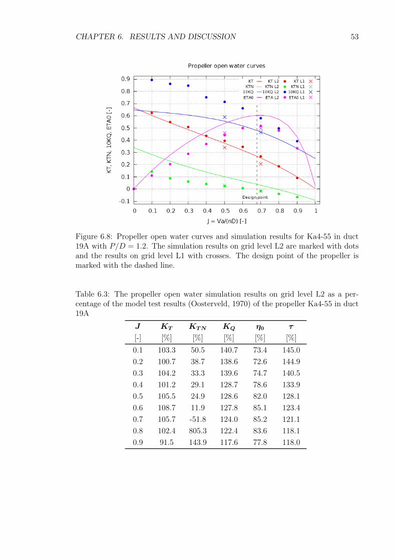
CHAPTER 6. RESULTS AND DISCUSSION 53
Figure 6.8: Propeller open water curves and simulation results for Ka4-55 in duct19A with P/D = 1.2. The simulation results on grid level L2 are marked with dotsand the results on grid level L1 with crosses. The design point of the propeller ismarked with the dashed line.
Table 6.3: The propeller open water simulation results on grid level L2 as a per-centage of the model test results (Oosterveld, 1970) of the propeller Ka4-55 in duct19A
J KT KTN KQ η0 τ
[-] [%] [%] [%] [%] [%]
0.1 103.3 50.5 140.7 73.4 145.0
0.2 100.7 38.7 138.6 72.6 144.9
0.3 104.2 33.3 139.6 74.7 140.5
0.4 101.2 29.1 128.7 78.6 133.9
0.5 105.5 24.9 128.6 82.0 128.1
0.6 108.7 11.9 127.8 85.1 123.4
0.7 105.7 -51.8 124.0 85.2 121.1
0.8 102.4 805.3 122.4 83.6 118.1
0.9 91.5 143.9 117.6 77.8 118.0

CHAPTER 6. RESULTS AND DISCUSSION 54
Table 6.4: The propeller open water simulation results on L1 as a percentage of themodel test results (Oosterveld, 1970) of the propeller Ka4-55 in duct 19A
J KT KTN KQ η0 τ
[-] [%] [%] [%] [%] [%]
0.5 90.3 28.4 106.2 85.1 125.3
0.7 81.5 -48.3 99.2 82.2 122.5
The comparison of the results on the medium and fine grids (L2 and L1) showthat the accuracy of the propeller performance prediction increases remarkably whenthe fine grid is used. Reason for this is the Chimera interpolation, which works betterwith the finer grid. The Chimera interpolation on the boundary of the over-lappinggrid is not in a so-called conservation form. Consequently, the continuity equationcan be locally untrue, which means that the mass is either created or disappeared(the mesh is leaking). With coarse grids more leakage occurs, while with fine gridsthe continuity equation is better satisfied.
A fundamentally same duct thrust value is obtainend with the both grid levels l2and L1, and thus the reason for this inaccuracy is probably not the grid resolution.As described in Chapter 2, the duct thrust is affected by the inflow velocity and theinflow angle and thus the possible reasons for the duct thrust underestimation are atoo small inflow angle, a too high inflow velocity, an overestimated viscous resistanceor a combination of these. Additionally the free vortices and viscous resistance affectthe duct thrust.
The inflow angle and velocity are bounded to the propeller performance while theviscous resistance calculation has more to do with the simulation of the boundarylayer. Since the propeller performance changed when changing the grid level butthe duct thrust remained the same, the propeller behavior is not the reason for theerror in the duct thrust calculation. Hence either the boundary layer calculationhas a large effect or the nozzle geometry used in the simulation is not correct. Inthe simulation the duct boundary layer is modeled as a turbulent boundary layerwhile it based on the Reynolds number along the duct chord is laminar. As the flowbehavior is different in laminar and turbulent flows, applying the turbulence modelin a laminar boundary layer can give unrealistic results. However, the same situationis in the propeller simulation, but still quite accurate results for the propeller forcesare obtained. Thus the most probable reason for the difference in the duct thrustprediction is the nozzle profile shape, where the roundings of the leading and trailingedges are not exactly the same as in the nozzle used in the model test. The edgeshapes affect the flow field around the nozzle and as a consequence the forces areaffected. For example, a blunter trailing edge creates larger free vortices and thusthe induced drag is increased and the total force in the x-direction decreased.
6.2.2 Open propeller
In Figure 6.9 the calculated points and the propeller open water curves of the pro-peller of the vessel A are shown. In Table 6.5 the values computed on the gridlevel L2 as a percentage of the model test values are given. From the results it canbe seen, that the thrust is overestimated when the advance coefficient is J < 0.8,

CHAPTER 6. RESULTS AND DISCUSSION 55
the difference being largest (42.7 %) at the smallest advance coefficients. For thehigher advance coefficients the propeller thrust is a bit underestimated. The torquevalues are similarly overestimated, the difference being largest (47.6 %) at the smalladvance coefficients.
Figure 6.9: Propeller open water curves and simulation results for the open propellerused in the vessel A. The simulation results (grid level L2) are marked with dotsand the design point is marked with a dashed line.
Table 6.5: Propeller open water simulation results as a percentage of the model testresults of the open propeller of vessel A
J KT KQ η0
[-] [%] [%] [%]
0.1 135.4 134.7 100.5
0.2 142.7 145.4 98.1
0.3 141.7 147.6 96.0
0.4 138.2 147.0 94.0
0.5 132.5 145.7 90.9
0.6 126.4 142.9 88.5
0.7 114.7 136.9 83.8
0.8 89.8 127.1 70.7
0.9 19.4 104.2 18.6
The open water simulation of the open propeller on grid level L2 gives the samekind of results as the ducted propeller simulation on L2, i.e. because of the coarsegrid the Chimera interpolation does not work well and thus the propeller thrust

CHAPTER 6. RESULTS AND DISCUSSION 56
and torque are overestimated. It is supposed that the accuracy of the simulationincreases also in this case when the simulation is done with the denser grid.
6.3 Self-propulsion simulation
The self-propulsion simulation was done on two grid levels L3 and L2. In Fig-ures 6.10, 6.11 and 6.12 the convergence curves of the total resistance coefficient,turbulent kinetic energy and minimum and maximum wave heights are shown, re-spectively. In Figures 6.13, 6.14, 6.15 and 6.16 the convergences of the total thrustof ducted propeller, propeller thrust, duct thrust and propeller moment are shown,respectively. It can be seen, that the rotating propeller causes oscillation to thetotal resistance. In the convergence curves of the propeller and duct forces, the up-dates in the propeller rotation rate can be seen as jumps in the force level. On thegrid level L2 the force calculation has reached a sufficient convergence during theninth propeller revolution (the third propeller revolution on the level L2) whereasthe turbulent kinetic energy has not yet converged.
Figure 6.10: Convergence of the total resistance coefficient in quasi-static (QS) andtime-accurate (TA) simulations on the coarse and medium grids (L3 and L2)

CHAPTER 6. RESULTS AND DISCUSSION 57
Figure 6.11: Convergence of the turbulent kinetic energy
Figure 6.12: Convergence of the minimum and maximum wave heights

CHAPTER 6. RESULTS AND DISCUSSION 58
Figure 6.13: Convergence of the total thrust of the propeller and the duct
Figure 6.14: Convergence of the propeller thrust
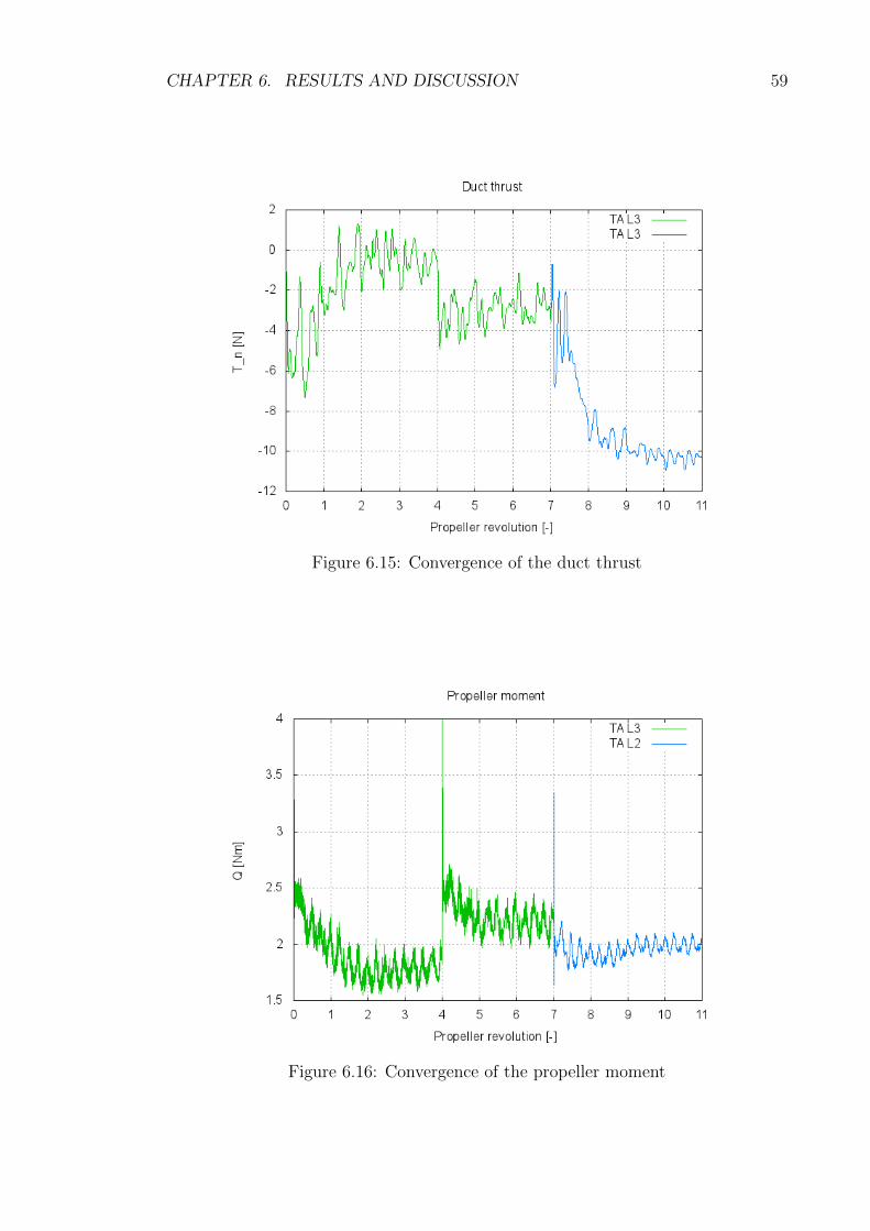
CHAPTER 6. RESULTS AND DISCUSSION 59
Figure 6.15: Convergence of the duct thrust
Figure 6.16: Convergence of the propeller moment

CHAPTER 6. RESULTS AND DISCUSSION 60
The wave pattern obtained on the grid level L3 and further used in the time-accurate simulations is shown in Figure 6.17. When the wave pattern in Figure 6.17is compared to the wave formation obtained in the resistance simulation, shown inFigure 6.4, it can be seen that the wave form used in the self-propulsion simulationis not fully developed. Additionally the effect of the propeller can be seen in the aftwave, where the wave pattern is not symmetric.
Figure 6.17: Wave pattern of the self-propulsion simulation obtained on grid levelL3
The wake fields of the original vessel A and modified vessel B at the locationsD/3 aft-wards from the propeller planes are shown in Figure 6.18. The effect of theduct can be seen in Figure 6.18(b) as a ring shaped region with a lower flow speedand varying yz-velocity directions. When the velocity distribution is compared tothe wake of the original vessel in Figure 6.18(a), it can be seen the flow inside theduct is more uniformly accelerated than the flow with the open propeller.

CHAPTER 6. RESULTS AND DISCUSSION 61
(a) Original vessel A
(b) Modified vessel B
Figure 6.18: Wake field at D/3 after the propeller plane
The thrust and moment of each propeller blade during one propeller revolutionare shown in Figures 6.19 and 6.20. The thrust force of a blade is the total force ofthe blade in x-direction and the torque of a blade is defined around the propelleraxis.
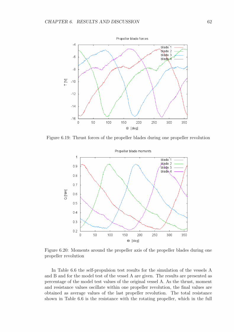
CHAPTER 6. RESULTS AND DISCUSSION 62
Figure 6.19: Thrust forces of the propeller blades during one propeller revolution
Figure 6.20: Moments around the propeller axis of the propeller blades during onepropeller revolution
In Table 6.6 the self-propulsion test results for the simulation of the vessels Aand B and for the model test of the vessel A are given. The results are presented aspercentage of the model test values of the original vessel A. As the thrust, momentand resistance values oscillate within one propeller revolution, the final values areobtained as average values of the last propeller revolution. The total resistanceshown in Table 6.6 is the resistance with the rotating propeller, which in the full

CHAPTER 6. RESULTS AND DISCUSSION 63
scale self-propulsion point is equal to the thrust and in model scale equal to thedifference of the obtained resistance and towing force. The wake fraction wT is theeffective wake fraction obtained from the propeller open water curves based on thepropeller thrust and rotation rate. In the simulation of the vessel B there is thenozzle and propeller included and in the simulation and model test of the vessel A,the propeller, rudder and pre-swirl stators are included.
From the results it can be seen that the with the vessel B the self-propulsionpoint is reached, the total thrust being only 0.3 % smaller than the resistance. Theself-propulsion simulation of the vessel A is done with a fixed propeller rotationrate defined in the model test and the self-propulsion point is not reached, thethrust being only 86.5 % of the thrust achieved in the model test measurement.However, the general guidelines of the simulation of the vessel A reveal, that thetorque is overestimated with relation to thrust and the effective wake fraction isunderestimated.
Since the self-propulsion point is not reached in the simulation of the vessel A,the results of the vessel B are compared to model test data of the vessel A. In thecomparison it can be seen that the required thrust has increased by 6.0 %. However,with the ducted propeller the amount of the thrust created by the propeller is only81.5 % of the propeller thrust of the original vessel. The duct loading factor isobtained to be τ = 0.77, which is 10.2 % smaller than what was expected based onthe propeller open water curves. The propeller rotation rate has decreased by 12.4 %from the original vessel but the required torque is 35.2 % larger. The increasedpropeller torque results with 18.8 % increase in the power delivered at propeller and23.2 % decrease in the propulsive efficiency ηD. Additionally the hull efficiency hasdecreased remarkably by 25.7 %, when the wake fraction has decreased and thrustdeduction factor increased.
Based on the resistance simulation, the wake fraction was expected to be underpredicted. Since the wake fraction is underestimated, the inflow velocity to thepropeller is higher than in reality and hence the propeller rotation rate is supposedto be over predicted, as can be seen from the simulation of the vessel A. Similarly thepropeller torque value is supposed to be over predicted based on the results of theducted propeller open water simulations and self-propulsion simulation of the vesselA and thus also the power delivered at propeller is overestimated. The amount of theover prediction can be approximated from the open water simulation results. Sincethe self-propulsion simulation is done on the grid level L2, the difference betweenthe real and calculated torque values is estimated based on the propeller open watersimulation on the level L2. The difference is at the design point obtained with thelinear interpolation to be 27.8 %. When the new torque value is calculated with thisdifference, the power delivered at the propeller is only 85.4 % of the power deliveredat propeller of the vessel A. However, the background grid is in the self-propulsionsimulation a bit denser than in the open water simulation and thus the differencemight be smaller. Since the actual needed correction is not known because of thedifferent grids, an estimation is done also for the minimum correction needed in orderto obtain at least equal PD in both vessels A and B. The study reveals, that theequal PD is obtained when the propeller torque is in the simulation overestimatedby 15.4 % and with the overestimation of 11.2 % the PD of the vessel B is 5 % largerthan the PD of the vessel A.

CHAPTER 6. RESULTS AND DISCUSSION 64
Table 6.6: Self-propulsion results as a percentage of the self-propulsion model testdata of the vessel A(model scale)
Vessel B Vessel A
FINFLO HSVA FINFLO
RT [%] 105.7 100.0 109.9
n [%] 87.6 100.0 100.0
Ttot [%] 106.0 100.0 86.5
Tp [%] 81.5 100.0 86.5
Q [%] 135.2 100.0 92.5
KT [%] 138.2 100.0 86.5
KQ [%] 176.3 100.0 92.5
wT [%] 76.9 100.0 76.9
t [%] 167.7 100.0 73.1
PE [%] 90.7 100.0 93.2
PD [%] 118.2 100.0 92.4
η0 [%] 101.8 100.0 106.3
ηR [%] 102.6 100.0 98.3
ηH [%] 74.3 100.0 93.4
ηD [%] 76.8 100.0 100.9
In the new estimation of the power delivered at the propeller, the possible cor-rections needed for the thrust forces are not considered. Based on the propelleropen water simulations, the propeller thrust would be over predicted and the ductthrust underestimated. However, in the self-propulsion simulation the duct loadingfactor is smaller (the duct creates larger amount of the total thrust) than whatwas expected based on the open water curves from the model tests and hence thepropeller open water simulation results cannot be used as a guideline for the thrustcorrections. If the thrust is assumed to be approximately correct, the duct worksvery well behind the vessel B and decreases the propeller loading remarkably. In thecase where the corrections would be needed, the obtained propulsion point is notthe self-propulsion point.
In addition to uncertainties in the propeller simulation, the self-propulsion simu-lation results are affected also by the simplifications made in the simulation problemstatement. In the self-propulsion simulation the ship position is kept the same as inthe resistance simulation even though in reality the working propeller may changethe trim angle and sinkage of the ship. The free-surface shape is calculated on thecoarsest grid level L3 and then kept static during the time accurate simulations andthus the free-surface shape used is not quite accurate at the beginning and furtherit does not adopt the changes which the rotating propeller would cause. This meansthat the kinematic boundary condition of the free surface is not satisfied and theflow below the free surface is not exactly right. Additionally, the final self-propulsionsimulation results are calculated on the grid level L2 which is too coarse for obtain-ing accurate results. Especially the Chimera grid interpolation suffers from the too

CHAPTER 6. RESULTS AND DISCUSSION 65
coarse grid. To obtain the grid convergence, i.e. the more dense grid does not affectthe results, and sufficient accuracy in Chimera interpolation, the simulation shouldbe done on the finest grid level and possibly especially the propeller, duct and wakeregion grids would need even more computational cells.
In this chapter the results obtained in the resistance, propeller open water andself-propulsion simulations of the modified vessel B have been presented and dis-cussed. The results have been given as percentages of the corresponding results ofthe original vessel model tests and the results of the RANS simulations of the origi-nal vessel A used for comparison have been shown. In the next chapter the obtainedresults are further discussed and concluding remarks of the study are made.

Chapter 7
Conclusions
In the previous chapter the results obtained were presented and discussed. In thischapter the conclusions of the results are made and the recommendations for thefurther work are given.
7.1 Resistance
The resistance simulations were conducted for the vessels A and B with the barehulls. The results of the simulation with the vessel A were compared to the corre-sponding model test data, the only difference in the models used being that in themodel test the model included also the rudder and pre-swirl stators. The compari-son revealed, that the bare hull resistance obtained with FINFLO is 3.6 % smallerthan the resistance obtained in the model test basin. Partly this difference resultsfrom the effect of the appendages and for example in Chapter 4 it is approximatedthat the rudder resistance is 3 % of the total resistance. Hence the accuracy ofthe FINFLO resistance prediction is regarded good. While the resistance was wellestimated, a relatively large difference was obtained in the nominal wake field pre-diction. The nominal wake fraction wn by FINFLO is 17.2 % smaller than in themodel test measurement, which is probable a result of the inaccuracies in the tur-bulence modeling and grid resolution. Additionally the pre-swirl stators used in themodel test measurement affect the wake by increasing the wake factor by few per-cents. This effect is though small when compared to the total difference of 17.2 %between the simulation and model test results.
The comparison of the simulation results of the vessels A and B showed, that thehull form modifications had positive effect on the hull resistance. The modificationsmade on the aft skeg changed the dynamic position of the ship, which resultedwith the better wave pattern and thus decreased the total resistance. The averagednominal wake wn was increased with the new hull form at the propeller plane.
66

CHAPTER 7. CONCLUSIONS 67
7.2 Simulation of the propeller in the open water
condition
The propeller open water simulations were done in order to evaluate the accuracyof FINFLO-solver in the ducted propeller simulation. The ducted propeller simu-lations were done on the grid level L2 and additionally two points were calculatedon the finest grid level L1. The results were compared to the model test resultsof the open water test. For a comparison point, the open water simulations wereconducted also for the open propeller of the vessel A on the grid level L2.
The propeller open water simulations with the both propellers showed that atoo coarse grid does not give accurate results but the propeller thrust and torqueare overestimated, especially at the lower advance numbers. The simulation withthe finest grid level improved the simulation results of the ducted propeller thrustand torque remarkably while the duct force prediction was not improved. The mostprobable reason for the difference in the duct force prediction are the small inaccu-racies in the duct geometry at the leading and trailing edges. These inaccuraciesaffect the pressure field at the leading edge and the free vortices at the trailing edge.
7.3 Self-propulsion
The self-propulsion simulations were conducted for the vessels A and B on the gridlevel L2. The simulation of the vessel A was done with a fixed propeller rotationrate defined in the model test and the self-propulsion point was not reached. In theself-propulsion simulation of the vessel B, the self-propulsion point was searched byupdating the propeller rotation rate and was obtained with 0.3 % difference in theobtained and required thrust. The propeller open water simulations revealed thatthe propeller simulation accuracy on the grid level L2 is not good. Additionally,the fixed free surface used in the simulation and the wake field calculation arenot accurate. Hence the self-propulsion results obtained in the simulation are onlyapproximate.
The comparison of the self-propulsion simulation results of the vessel B to themodel test data of the vessel A showed, that the total thrust required was in-creased by 6.0 %, the power delivered at the propeller increased by 18.2 % and thepropeller rotation rate decreased by 12.4 %. The hull efficiency was decreased re-markably. Based on these results the ducted propeller is not an effective solution forthe propulsion of the vessel B. However, if the guidelines from the propeller openwater simulation are considered and a correction is done to the estimated propellertorque, more promising results are obtained. If the propeller torque is over pre-dicted as much as in the propeller open water simulation on the grid level L2 at thedesign point, the power delivered at the propeller is decreased by 14.6 % from thePD of the vessel A. If the torque of the propeller is overestimated at least by 15.4 %,the required power delivered at the propeller is equal or decreased from that of theoriginal vessel A and with the overestimation of 11.2 %, the power demand wouldincrease 5 %.
The results reveal that the most remarkable effect of the ducted propeller is thedecreased propeller rotation rate, which can enable a usage of more efficient slow

CHAPTER 7. CONCLUSIONS 68
speed engines. It is also possible, that the power demand of the vessel is decreasedwith the ducted propeller, if there is a quite large difference in the simulation andreal torque values like the propeller open water simulation results suggest. As theducted propeller used in the simulation was not optimized for the case vessel, it ispossible that even if the power demand with the used ducted propeller is increasedby 5 %, the PD would be decreased with the duct and propeller shapes optimizedfor the vessel. Additionally, in this thesis the changes in the aft shape were keptas small as possible. With larger changes also the hull shape could be optimizedto be more suitable for the ducted propeller. However, no reliable conclusions canbe made because of the uncertainties in the duct simulation and force corrections.It seems though, that the ducted propulsion could be an effective solution for thiskind of vessel.
7.4 Recommendations for further work
The resistance simulation by FINFLO gives already fairly accurate results for theresistance but the wake field is not correct. Improvements could be possibly obtainedwith a denser grid at the wake field. Other widely known reason for the inaccuratewake field prediction is the problematic turbulence modeling at the wake field. Asthe SST k − ω turbulence model used in the FINFLO ship simulation is the onecommonly used in ship hydrodynamics, it is suggested that the field of the turbulencemodeling at ship applications is followed in order to find out if a turbulence modelmore suitable for ship flow simulations is released.
In the propeller simulation with the fine grid fairly accurate results are obtainedfor the propeller thrust and torque, while the duct performance simulation is incor-rect. To get more reliable results of the ducted propulsion simulation, the reasonfor the inaccuracies in the duct simulation should be clarified and corrected. As themost probable reason for the inaccuracies is the slightly incorrect duct geometry,the first step would be to find a more detailed description of the leading and trail-ing edge roundings than that used in this thesis. After the possible corrections aremade on the duct geometry, the open water simulations should be repeated. If thepossible corrections on the geometry do not affect the results remarkable, furtherinvestigations for the reason of the inaccuracies should be done. For example adenser background grid might improve results, as it is possible that with the cur-rent grid the duct wake field and free vortices are not correctly modeled and thusthe duct forces are inaccurate. Additionally, as the open water simulations per-formed in this thesis were done as quasi-static simulations with MRF method, alsothe time-accurate simulation might give more information about the problem. Itis possible that the approximated boundary conditions used in MRF method affectthe simulation results.
The accuracy of the self-propulsion simulation depends strongly on the wakefield simulation and on the propeller simulation. A step towards a more accurateself-propulsion simulation would be the usage of a denser grid at the aft regionwhere the propeller is located since even though the wake field might still be incor-rect, the propeller simulation would be more accurate. Other improvements for theself-propulsion scheme used in FINFLO would be an automatized procedure forupdating the propeller rotation rate based on the changes in ship resistance since

CHAPTER 7. CONCLUSIONS 69
currently these changes are done manually.When considering the ducted propeller in the large vessel, more testing is required
in order to validate the efficiency of the solution. Either the self-propulsion testshould be done in a model test or the self-propulsion simulation should be repeatedby at least one other RANS solver to see if the trends in the propeller rotation rateand power demand estimations are true. Further investigations should also be doneon different ducted propellers in order to find an optimum design for a large vessel.

Bibliography
R. Ajanko. Laivarungon virtauslaskentaprosessin kehittaminen. Master’s thesis,Teknillinen Korkeakoulu, 2008.
American Bureau of Shipping. Guidance notes on ship vibration, April 2006.Available: https://www.eagle.org/eagleExternalPortalWEB/ShowProperty/BEA%20Repository/Rules&Guides/Current/147_ShipVibration/Pub147_ShipVib.
J. Baltazar and J. A. C. Falcao de Campos. On the Modelling of the Flow in DuctedPropellers With a Panel Method. In K. Koushan and S. Steen, editors, Proceedingsof the First International Symposium on Marine Propulsors - smp’09. 22-24 June2009. Trondheim, Norway. MARINTEK, 2009. [Referenced:10.02.2014]. ISBN(electronic): 978-82-7174-264-5. ISBN (printed): 978-82-7174-263-8. Available:http://www.marinepropulsors.com/proceedings-2009.php.
J. Baltazar, J. A. C. Falcao de Campos, and J. Bosschers. Open-Water Thrustand Torque Prediction of a Ducted Propeller System with a Panel Method. In-ternational Journal of Rotating Machinery, 2012:11 pages, 2012. [Referenced:10.02.2014]. DOI: 10.1155/2012/474785. Available: http://www.hindawi.com/
journals/ijrm/2012/474785/.
Becker Marine Systems. Becker nozzle: High-performance and efficient heavy-duty manoeuvring solution. Product brochure, a. [Online] [Referenced:25.03.2014] Available: http://www.becker-marine-systems.com/05_downloads/
zzpdf/product_pdf/Becker_Nozzle.pdf.
Becker Marine Systems. Product brochure, b. [Online] [Referenced:17.02.2014] . Available: http://www.becker-marine-systems.com/05_downloads/zzpdf/product_pdf/Becker_Product_Brochure.pdf.
J. Bosschers, G. Vaz, A. Starke, and E. van Wijngaarden. Computationalanalysis of propeller sheet caviattion and propeller-ship interaction. In RINAconference “MARINE CFD2008”. 26-27 March 2008. Southampton, UK., 2008.[Referenced:05.02.2014]. Available: http://www.marin.nl/upload_mm/1/e/a/
1807585792_1999999096_Computational_analysis_of_sheet_cavitation_and_
propeller-ship_interaction_-_RINA_CFD2008.pdf.
J. S. Carlton. Marine Propellers and Propulsion. Butterworth-Heinemann, 1st edi-tion, 1994. ISBN 075061143X.
70

BIBLIOGRAPHY 71
P. M. Carrica, A. M. Castro, and F. Stern. Self-propulsion computations using aspeed controller and a discretized propeller with dynamic overset grids. Jour-nal of Marine Science and Technology, 15(4):316–330, Dec 2010. [Referenced:06.02.2014]. DOI:10.1007/s00773-010-0098-6.
P. M. Carrica, H. Fu, and F. Stern. Computations of self-propulsion free to sink andtrim and of motions in head waves of the KRISO Container Ship (KCS) model.Applied Ocean Research, 33(4):309–320, Oct 2011. [Referenced: 06.02.2014].DOI:10.1016/j.apor.2011.07.003.
F. Celik, A. Dogrul, and Y. Arikan. Investigation of the Optimum Duct Ge-ometry for A Passenger Ferry. In C. Pensa and P. Cioffi, editors, Confer-ence proceedings. 9th Symposium on High Speed MMarine Vessels. May 2011.Naples, Italy., 2011. [Referenced:10.02.2014]. ISBN: 978-88-906112-0-9. Available:http://www.din.unina.it/HSMV%202011%20Proceedings/html/Papers/17.pdf.
J. Dang and H. Laheji. Hydrodynamic Aspects of Steerable Thrusters. InPresentation. Dynamic Positioning Conference. 22-30 September, 2004. Hous-ton, USA. Wartsila Propulsion Netherlands BV (WPNL), 2004. [Referenced:06.03.2014]. Available:http://www.dynamic-positioning.com/dp2004/thrusters_dang_pp.pdf.
G. Dhinesh, K. Murali, and V. A. Subramanian. Estimation of hull-propeller in-teraction of a self-propelling model hull using a ranse solver. Ships and OffshoreStructures, 5(2):125–139, Aug 2010. DOI: 10.1080/17445300903231109.
B. Epps. Openprop v2.4 theory document, December 2010. Available: http://engineering.dartmouth.edu/epps/openprop/index.html.
Finflo Ltd. Finflo user guide version 8.1, 2012.
Q. Gao, W. Jin, and D. Vassalos. The calculations of propeller induced velocity byRANS and momentum theory. Journal of Marine Science and Application, 11(2):164–168, Jun 2012. DOI: 10.1007/s11804-012-1118-1.
G. R. Hough and D. E. Ordway. The generalized actuator disk. TAR-TR 6401, Therm Advanced Research, Inc., January 1964. [Refer-enced: 07.02.2014] Available: http://oai.dtic.mil/oai/oai?verb=getRecord&metadataPrefix=html&identifier=AD0433976.
T. Kawamura, H. Miyata, and K. Mashimo. Numerical simulation of the flow aboutself-propelling tanker models. Journal of Marine Science and Technology, 2(4):245–256, Dec 1997. DOI: 10.1007/BF02491531.
J. E. Kerwin. Principles of Naval Architecture Series: Propulsion. The Society ofNaval Architect, 2010. ISBN 093977383X. ISBN: 978-0-939773-83-1.
J. E. Kerwin, S. A. A. Kinnas, J.-T. Lee, and W.-Z. Shih. A SurfacePanel Method for the Hydrodynamic Analysis of Ducted Propellers. Mas-sachusetts Inst of Tech Cambridge Dept of Ocean Engineering, 1987. [Refer-enced: 11.02.2014]. Available: http://oai.dtic.mil/oai/oai?verb=getRecord&metadataPrefix=html&identifier=ADA192569.

BIBLIOGRAPHY 72
G. Kuiper. The Wageningen Propeller Series. MARIN, May 1992. ISBN-10: 90-9007247-0.
M. Lakatos. Evaluation of a propulsion calculation procedure using an actuatordisk model featured in a RANS model. Master’s thesis, Aalto University Schoolof Engineering, 2013.
L. Larsson and H. C. Raven. The Principles of Naval Architecture Series: ShipResistance and Flow. The Society of Naval Architects and Marine Engineers,2010. ISBN: 978-0-939773-76-3.
J. Marzi and D. Hafermann. The ν-Shallo User Guide, Release 1.8.5. Hamburgis-che Schiffbau Versuchanstalt GmbH, October 2008.
J. Matusiak. Johdatus laivan aallonmuodostukseen, 2005. Helsinki University ofTechonology, M - 227.
J. Matusiak. Laivan propulsio. Picaset Oy, 7 edition, 2007a. Helsinki University ofTechnology, Ship Laboratory, M-176.
J. Matusiak. Laskennallinen laivahydrodynamiikka, September 2007b. HelsinkiUniversity of Technology.
T. Mikkola. Computational ship hydrodynamics. Lecture notes, 2013. Aalto Uni-versity.
A. Minchev, J. R. Nielsen, and E. Lundgren. Ducted Propeller Design and Verifi-cation for Contemporary Offshore Support Vessels. In K. Koushan and S. Steen,editors, Proceedings of the First International Symposium on Marine Propulsors -smp’09. 22-24 June 2009. Trondheim, Norway. MARINTEK, 2009. [Referenced:10.02.2014]. ISBN (electronic): 978-82-7174-264-5. ISBN (printed): 978-82-7174-263-8. Available: http://www.marinepropulsors.com/proceedings-2009.php.
A. F. Molland and S. R. Turnock. Marine Rudders and Control Surfaces.Butterworth-Heinemann, 1 TH edition, 2007.
M. W. C. Oosterveld. Wake adapted ducted propellers. Publication No. 345, NSMB.,1970.
A. B. Phillips, S. R. Turnock, and M. Furlong. Evaluation of manoeuvring coeffi-cients of a self-propelled ship using a blade element momentum propeller modelcoupled to a Reynolds-averaged Navier-Stokes flow solver. Ocean Engineering, 36(15-16):1217–1225, Nov 2009. DOI: 10.1016/j.oceaneng.2009.07.019.
J. V. Pylkkanen. Influence of Advance Number on the Performance of DuctedPropellers in Three Duct Configurations. Helsinki University of Techonology,Ship Laboratory, M-156., 1991.
D. Ripjkema, B. Starke, and J. Bosschers. Numerical simulation of propeller-hullinteraction and determination of the effective wakr field using hybrid RANS-BEM approach. In R. B. J. Binns and N. Bose, editors, Proceedings of theThird International Symposium on Marine Propulsors - smp13. 5-8 May 2013.

BIBLIOGRAPHY 73
Launceston, Tasmania, Australia. Australian Maritime College, University of Tas-mania, 2013. [Referenced:05.02.2014]. ISBN: 978-646-90334-7. Available: http://www.marinepropulsors.com/proceedings-2013.php.
A. H. Sacks and J. A. Burnell. Ducted propellers - critical review of the state of theart. Report No. ARD-232, June 1959.
A. Sanchez-Caja. Proepller theory. Lecture Notes of Potential Flow Theory forLifting Surfaces, extended course. Aalto Univesity School of Engineering, 2013.
A. Sanchez-Caja and J. Pylkkanen. Prediction of effective wake at model andfull scale using a rans code with actuator disk model. In Second InternationalConference on Maritime Research and Transportation. 28-30 June, 2007. Ischia,Naples, Italy., 2007. [Referenced: 05.02.2014]. http://www.icmrt07.unina.it/Proceedings/.
A. Sanchez-Caja, J. Pylkkanen, and T. P. Sipila. Simulation of the IncompressibleViscous Flow around Ducted Propellers with Rudders using a RANSE Solver.In 27th Symposium on Naval Hydrodynamics. 5-10 October, 2008. Seoul, Korea.,2008. [Referenced: 10.02.2014]. ISBN: 978-1-61738-774-6. Available: http://202.114.89.60/resource/pdf/4318.pdf.
T. Siikonen. Virtaussimulointi. Course material. Aalto University School of Engi-neering., 2013.
T. Siikonen. Laskennallisen virtausmekaniikan jatkokurssi. Course material. AaltoUniversity School of Engineering., 2014.
T. Siikonen, E. Salminen, and J. Ilkko. Comparison between hull flow simulation ofa model-scale and a full-scale tanker. Technical Report F-66, Finflo Ltd., 2010.
J. M. Stubblefield. Numerically-Based Ducted Propeller Design Using Vortex LatticeLifting Line Theory. Master’s thesis, Massachusetts Institute of Technology, June2008.
Y. Tahara, R. V. Wilson, P. M. Carrica, and F. Stern. RANS simulation of acontainer ship using a single-phase level-set method with overset grids and theprognosis for extension to a self-propulsion simulator. Journal of Marine Sci-ence and Technology, 11(4):209–228, Dec 2006. doi: 10.1007/s00773-006-0231-8.DOI:10.1007/s00773-006-0231-8.
T. Taketani, K. Kimura, N. Ishii, M. Matsuura, and Y. Tamura. Advanced de-sign of a ducted propeller with high bollard pull performance. In K. Koushanand S. Steen, editors, Proceedings of the First International Symposium on Ma-rine Propulsors - smp’09. 22-24 June 2009. Trondheim, Norway. MARINTEK,June 2009. [Referenced: 10.02.2014]. ISBN (electronic): 978-82-7174-264-5.ISBN (printed): 978-82-7174-263-8. Available: http://www.marinepropulsors.com/proceedings-2009.php.

BIBLIOGRAPHY 74
Y. Tamura, Y. Nanke, M. Matsuura, T. Taketani, K. Kimura, and N. Ishii. Develop-ment of a high performance ducted propeller. In The 21dt International Tug, Sal-vage & OSV Convention and Exhibition. 2010. Vancouver, Canada., 2010. [Ref-erenced: 10.02.2014] Available: http://towmasters.files.wordpress.com/2010/09/its6_high_performance_ducted_propeller.pdf.
R. Van Houten. Analysis of ducted propellers in steady flow. Technical ReportARMC Report No. 4.76-1, Airflow Research and Manufacturing Corporation,1986.
J. D. van Manen and M. W. C. Oosterveld. Series of model tests onducted propellers. Netherland Ship Model Basin Wageningen, 1972. [Refer-enced: 10.02.2014]. Available: http://oai.dtic.mil/oai/oai?verb=getRecord&metadataPrefix=html&identifier=AD0746868.
T. Watanabe, T. Kawamura, Y. Takekoshi, M. Maeda, and S. Rhee. Simulationof Steady and Unsteady Cavitation on a Marine Propeller Using a RANS CFDCode. In Fifth International Symposium on Cavitation. 1-4 November, 2003.Osaka, Japan., 2003. [Referenced: 13.02.2014]. Available: http://202.114.89.60/resource/pdf/4428.pdf.
F. White. Viscous Fluid Flow. Mc Graw Hill, 3rd edition, 2006. ISBN: 007-124493-X.
D. C. Wilcox. Turbulence Modeling for CFD (Third Edition). DCW Industries,2006. ISBN: 1-928729-08-8.
L. Yu, M. Druckenbrod, M. Greve, and M. Abdel-Maksoud. An Automatic Op-timization Process for Optimal Ducted Propeller Design and Its ApplicationBased on CFD Techniques. In R. B. J. Binns and N. Bose, editors, Proceedingsof the Third International Symposium on Marine Propulsors - smp13. 5-8 May2013. Launceston, Tasmania, Australia. Australian Maritime College, Universityof Tasmania, 2013. [Referenced:10.02.2014]. ISBN: 978-646-90334-7. Available:http://www.marinepropulsors.com/proceedings-2013.php.
Z.-r. Zhang. Verification and Validation for RANS Simulation of KCS ContainerShip Without/With Propeller. Journal of Hydrodynamics, Ser. B, 22(5):932–939,Oct 2010. DOI: 10.1016/S1001-6058(10)60055-8.
Y. Zheng and M.-S. Liou. A Novel Approach of Three-Dimensional Hybrid GridMethodology: Part 1. Grid Generation. Computer Methods in Applied Me-chanics and Engineering, 192(37-38):4147–4171, Sep 2003. DOI: 10.1016/S0045-7825(03)00385-2.

Appendix A
Duct geometry
Geometry data of the duct is shown in Table A.1. For nozzle the 19A the length-diameter ratio is L/D = 0.5.
Table A.1: Propeller Ka4-55 geometry. Taken from (Kuiper, 1992).
x/L yinner/L youter/L
0 18.25
1.25 14.66 20.72
2.5 12.8 21.07
5 10.07 20.8
7.5 8 –
10 6.34 –
15 3.87 –
20 2.17 –
25 1.1 –
30 0.48 –
40 0 –
50 0 –
60 0 –
70 0.29 –
80 0.82 –
90 1.45 –
95 1.86 –
100 2.36 6.36
i

Appendix B
Propeller geometry
The geometry of the propeller 4-55 is shown in Figure B.1. In Table B.1 are shownthe propeller parameters and in Table B.2 are shown shown the coordinates forpropeller geometry for suction and pressure side. The zero location is at 0 % , thetrailing edge is at -100 % and the leading edge is at 100 %. The profiles are givenas a percentage of the maximum thickness of the blade section. The chord lengthof a propeller is calculated with
cr =Kr ·D · EAR
Z, (B.1)
where Kr is given in Table B.1, D is the propeller diameter, EAR is the propellerare ratio (Ae/A0) and Z is the number of blades (Kuiper, 1992).
ii

APPENDIX B. PROPELLER GEOMETRY iii
Figure B.1: Geometry of propeller Ka4-55
Table B.1: Ordinates of nozzle 19A. Taken from (Kuiper, 1992).
r/R P/D Rake Skew/cr cr/D fmax/cr tmax/cr xtmax/cr Kr
0.2 1.20 0.0 0.050 0.1818 0.0469 0.0400 0.3498 1.322
0.3 1.20 0.0 0.028 0.2074 0.0538 0.0352 0.3976 1.508
0.4 1.20 0.0 0.013 0.2306 0.0501 0.0300 0.4602 1.677
0.5 1.20 0.0 0.006 0.2518 0.0417 0.0245 0.4913 1.831
0.6 1.20 0.0 0.000 0.2709 0.0351 0.0190 0.4998 1.970
0.7 1.20 0.0 0.000 0.2866 0.0241 0.0138 0.5000 2.084
0.8 1.20 0.0 0.000 0.2980 0.0154 0.0092 0.5000 2.167
0.9 1.20 0.0 0.000 0.3050 0.0100 0.0061 0.5000 2.218
1.0 1.20 0.0 0.000 0.3076 0.0081 0.0050 0.5000 2.237

APPENDIX B. PROPELLER GEOMETRY iv
Tab
leB
.2:
Ord
inat
esof
pro
pel
ler
ofK
a-se
ries
.T
aken
from
(Kuip
er,
1992
).
r/R
-100%
=TE
-80%
-60%
-40%
-20
0%
=xtm
ax
20%
40%
60%
80%
90%
95%
100%
=LE
Fac
e=
suct
ion
sid
e
0.2
-45.5
265.4
282
.50
95.
0010
0.00
98.1
392
.29
81.5
665.
52
54.
79
48.
02
-
0.3
-43.6
767.7
084
.14
95.
8610
0.00
97.7
590
.89
78.3
459.
17
46.
15
37.
87
-
0.4
-42.9
267.5
085
.69
96.
2510
0.00
97.2
289
.31
75.0
052.
92
38.
61
30.
27
-
0.5
-42.4
568.7
686
.42
96.
6010
0.00
96.7
787
.27
70.9
746.
86
31.
58
23.
77
-
0.6
-43.5
868.2
685
.89
96.
4710
0.00
96.4
785
.89
68.2
643.
58
28.
59
20.
44
-
0.7
-45.3
169.2
486
.33
96.
5810
0.00
96.5
886
.33
69.2
445.
31
30.
79
22.
88
-
0.8
-48.1
670.8
487
.04
96.
7610
0.00
96.7
687
.04
70.8
448.
16
34.
39
26.
90
-
0.9
-51.7
572.9
488
.09
97.
1710
0.00
97.1
788
.09
72.9
451.
75
38.
87
31.
87
-
1.0
-52.0
073.0
088
.00
97.
0010
0.00
97.0
088
.00
73.0
052.
00
39.
25
32.
31
-
Bac
k=
pre
ssu
resi
de
0.2
20.2
17.
291.7
70.
10
--
0.21
1.46
4.37
10.5
216
.04
20.
62
33.
33
0.3
13.8
54.
621.0
7-
--
0.12
0.83
2.72
6.1
58.2
810
.30
21.
18
0.4
9.17
2.36
0.5
6-
--
-0.
421.
39
2.92
3.8
94.4
413
.47
0.5
6.62
0.68
0.1
7-
--
-0.
170.
51
1.02
1.3
61.5
37.
81

Appendix C
Ka-series polynomials
The propeller open water curves for Ka-series are presented as polynomials of ad-vance coefficient and P/D. In Equations C.1, C.2 and C.3 are given the polynomialfor total thrust coefficient KT , nozzle thrust coefficient KTN and torque coefficientKQ. In Tables C.1 and C.2 are given the coefficients for the polynomials. (Ooster-veld, 1970)
KT = A0,0 + A0,1J + . . .+ A0,6J6
+ A1,0P
D+ A1,1
P
DJ + . . .+ A1,6
P
DJ6
+ A2,0P
D
2
+ A2,1P
D
2
J+ . . .+ A2,6P
D
2
J6
. . . . . . . . . . . . . . . . . . . . . . . . . . . . . . . . . . . .
+ A6,0P
D
6
+ A6,1P
D
6
J+ . . .+ A6,6P
D
6
J6 (C.1)
KTN =B0,0 +B0,1J + . . . . . . . . . . . . . . . . . .
. . . . . . . . . . . . . . . . . . . . . +B6,6P
D
6
J6 (C.2)
KQ =C0,0 + C0,1J + . . . . . . . . . . . . . . . . . .
. . . . . . . . . . . . . . . . . . . . . +C6,6P
D
6
J6 (C.3)
v

APPENDIX C. KA-SERIES POLYNOMIALS vi
Table C.1: Coefficients for polynomials, Ka3-65 and Ka4-55. Taken from (Ooster-veld, 1970)
Ka3-65 Ka4-55
x y Axy Bxy Cxy Axy Bxy Cxy
0 0 0.028100 0.154000 0.006260 -0.375000 -0.045100 -0.034700
0 1 -0.143910 0.115560 -0.203050 0.018568
0 2 -0.123761 -0.017942 0.830306
0 3 -0.38373 -2.746930 -0.663741
0 4 -0.008089 -0.244626 -0.195582
0 5 -0.741240 0.317452
0 6 0.646894 0.067548 -0.093739
1 0 -0.542674 2.030070 0.244461 0.158951
1 1 -0.429709 -0.749643 -0.392301 -0.578464 -0.048433
1 2 -0.016644 -0.611743 1.116820
1 3 4.319840 0.751953 0.024157
1 4 -0.341290
1 5 -0.123376
1 6 -0.162202 -0.08916
2 0 0.671268 0.972388 -3.031670 -0.212253
2 1 -0.146178
2 2 0.286926 1.468570 -0.917516
2 3 -2.007860
2 4
2 5
2 6
3 0 -0.182294 -0.317644 0.040041 2.836970 0.068186 0.156133
3 1 0.174041
3 2 -1.084980 0.102334
3 3 0.391304
3 4
3 5
3 6 -0.032298
4 0 -0.994962
4 1 0.030740
4 2 0.073587
4 3 0.199637
4 4
4 5
4 6
5 0 -0.031826
5 1 0.060168 0.015742 -0.014568
5 2 -0.109363
5 3
5 4 0.043862
5 5
5 6
6 0 -0.003460 0.043782 -0.008581 0.007947
6 1 -0.17378 -0.000674
6 2 0.001721 0.038275
6 3
6 4 -0.021971
6 5
6 6 0.000700
0 7 0.088319 0.022850

APPENDIX C. KA-SERIES POLYNOMIALS vii
Table C.2: Coefficients for polynomials, Ka4-70 and Ka5-75. Taken from (Ooster-veld, 1970)
Ka4-70 Ka5-75
x y Axy Bxy Cxy Axy Bxy Cxy
0 0 0.030550 0.076594 0.006735 0.033000 0.007210 -0.000813
0 1 -0.148687 0.075223 -0.153463 0.034885
0 2 -0.061881 -0.016306 -0.014670
0 3 -0.391137 -0.138094 -0.398491 -0.276187
0 4 -0.007244 -0.006398
0 5 -0.370620
0 6 0.323447
1 0 -0.271337
1 1 -0.432612 -0.687921 -0.435515 -0.626198
1 2 0.225189 -0.024012 -0.031380 0.450379
1 3
1 4
1 5
1 6 -0.081101
2 0 0.667657 0.666028 0.664045 0.359718
2 1
2 2 0.734285 0.005193 0.283225 0.010386
2 3
2 4
2 5
2 6
3 0 -0.172529 -0.202467 0.046605 -0.162764 0.053169 -0.087289
3 1
3 2 -0.542490
3 3
3 4
3 5
3 6 -0.016149
4 0 -0.007366 -0.014731
4 1
4 2
4 3 0.099819
4 4
4 5
4 6
5 0
5 1
5 2 0.030084
5 3
5 4
5 5
5 6
6 0 -0.001730
6 1 -0.017293 -0.000337 -0.017208
6 2 -0.001876 0.00861 -0.003751
6 3
6 4
6 5
6 6
0 7

Appendix D
FINFLO input and boundary con-ditions
The simulation in FINFLO is controlled with input- and boundary condition-files.Below are shown these files for resistance and self-propulsion simulations.
D.1 Resistance simulation
Input-file for the resistance simulation.
&INPUTS
NAME = ’Resistance, 14kts’
FLUXTY = ’INCO’
FULLNC = ’no’
CFL = 2.0
CFLL = 2.0
ICMAX = 20000
IPRESC = 1
LEVEL = 1
FRSTEM = 288.15
TEMINI = 288.15
FRSPRE = 101325.0
AREF = 7.406
CHLREF = 7.654
FRSVEL = 1.4990
ITURB = 6
KP = 15000
MPRINT = 10000
KRRINT = 4000
ALPHA = 0.0
ARTSSP = 10.
ALFAP = 0.02
FRSDEN = 1000.
ISTATE = 6
IDRXX = 6
XMOM = -3.827
YMOM = 0.0
viii

APPENDIX D. FINFLO INPUT AND BOUNDARY CONDITIONS ix
ZMOM = 0.0
XXTRAC = ’no’
TURCOC = ’yes’
IFSBC = 4
JFIRST = 32
NFSD = 4
ICFST = 350
GK = -1.
GML = -0.1
CFLFRE = 4.
DTWMIN = 1.E-4
DTWMAX = 0.01
DWMV = 0.001
FREDIF = 200
FRESUC = ’yes’
DT = 1e-3
DISTANC = ’NO’
NEGVC = ’YES’
NEGV = -1E-5
&END
&BLOCKS
FRSMUTB(:) = 76*0.01 FRSTURB(:) = 76*0.0002 TURLIMB(:) = 76*15000.
ALFAUB(:) = 76*0.5
IK(:) = 76*1 IL(:) = 76*2 IT(:) = 76*-2
MGRID(:)= 76*1
IGRID(:,1)= 76*21
IGRID(:,2)= 76*5
IGRID(:,3)= 76*1
MOV(:) = 76*0
INTERK(:) = 76*1
&END
&FLIGHT
XCG(1) = -3.827
ZCG(1) = 0.0
TRIMA(1) = 0.1278
DRAUGHTI(1) = 0
DRAUGHT(1) = 0.4200
&END
&WORKS
IOLD1 = 1
GRIDFI = ’VOLUME_out.grd’
BCFILE = ’VOLUME_out.bc’
&END
&FORCE_GROUP_DATA
&END
Boundary condition-file for resistance simulation (before splitting).

APPENDIX D. FINFLO INPUT AND BOUNDARY CONDITIONS x
Resistance simulation - 14 kn
1
-------- Block No. 1 --------
304 192 160
1 1
MIR 1 192 1 160
2 1
MOV 1 304 1 160 4 H
0 0.0 0.0 0.0 0.0 0.0 0.0 0.0 0.0 0.0 0.0 0.0 0.0 0.0
3 1
MIR 1 304 1 192
4 1
MIR 1 192 1 160
5 1
EXT 1 304 1 160
6 1
FRE 1 304 1 192
D.2 Self-propulsion simulation
Below is given the input file for the self-propulsion simulation on the medium gridlevel.
&INPUTS
NAME = ’ducted self-propulsion, TA L2’
FLUXTY = ’INCO’
FULLNC = ’no’
LUSGS = 1
CFL = 2.0
CFLL = 2.0
ICMAX = 60
IPRESC = 1
LEVEL = 2
FRSTEM = 288.15
TEMINI = 288.15
FRSPRE = 101325.0
AREF = 14.812
CHLREF = 7.799
FRSVEL = 1.499
ITURB = 6
KP = 10000
KRRINT = 60
MPRINT = 12
ALPHA = 0.0
ARTSSP = 20.0
ALFAP = 0.02
FRSDEN = 1000.
ISTATE = 6
IDRXX = 6
XMOM = -0.12267

APPENDIX D. FINFLO INPUT AND BOUNDARY CONDITIONS xi
YMOM = 0.0
ZMOM = -0.26871
XXTRAC = ’no’
TURCOC = ’yes’
IFSBC = 4
JFIRST = 32
NFSD = 4
ICFST = 350
GK = -1.
GML = -0.1
CFLFRE = 1.0
DTWMIN = 1.E-4
DTWMAX = 0.01
DWMV = 0.0001
FREDIF = 200
FRESUC = ’yes’
DT = 6.60E-4
TMAX = 0.6601
TIMEC = ’yes’
DISTANC = ’yes’
NEGVC = ’NO’
NEGV = -1E-5
INCHIMC = ’yes’
REFLECC = ’yes’
ENTROPY_FIXC = ’yes’
&END
&BLOCKS
FRSMUTB(:) = 170*0.01 FRSTURB(:) = 170*0.0002 TURLIMB(:) = 170*15000.
ALFAUB(:) = 170*0.5
MGRID(:)= 170*1
IGRID(1:158,1)= 158*21
IGRID(1:158,2)= 158*6
IGRID(1:158,3)= 158*1
IGRID(159:170,1)= 12*10
IGRID(159:170,3)= 12*2
IGRID(159:170,4)= 12*1
MOV(:) = 170*3
INTERK(:) = 170*-3
INTERI(:) = 170*-3
INTERJ(:) = 170*-3
NCHIMT(153:158) = 6*1
NCHIMT(159:170) = 12*2
ZEROVB(:) = 170*’no’
&END
&FLIGHT
XCG(1) = -3.827
ZCG(1) = 0.0
TRIMA(1) = 0.1278

APPENDIX D. FINFLO INPUT AND BOUNDARY CONDITIONS xii
DRAUGHTI(1) = 0
DRAUGHT(1) = 0.4200
XCGI(2) = 0.04332756
YCGI(2) = 0.0
ZCGI(2) = 0.1611785
XCG(2) = 0.04332756
YCG(2) = 0.0
ZCG(2) = 0.1611785
VX(2) = -1.0
VY(2) = 0.0
VZ(2) = 0.0
SHAFT(2) = 38.0761
THETARI(2) = 180
THETAR(2) = 180
&END
&FORCE_GROUP_DATA
FORCE_GROUP_INFO=
’p’ ’Propeller’ 0.01516464 0.0 0.1611785 -1.0 0.0 0.1611785
’d’ ’Nozzle ’ 0.01516464 0.0 0.1611785 -1.0 0.0 0.1611785
’e’ ’blade1’ 0.01516464 0.0 0.1611785 -1.0 0.0 0.1611785
’f’ ’blade2’ 0.01516464 0.0 0.1611785 -1.0 0.0 0.1611785
’g’ ’blade3’ 0.01516464 0.0 0.1611785 -1.0 0.0 0.1611785
’h’ ’blade4’ 0.01516464 0.0 0.1611785 -1.0 0.0 0.1611785
’i’ ’duct inside’ 0.01516464 0.0 0.1611785 -1.0 0.0 0.1611785
’u’ ’duct outside’ 0.01516464 0.0 0.1611785 -1.0 0.0 0.1611785
&END
&WORKS
IOLD1 = 1
GRIDFI = ’../self-propulsion/VOLUME_hull_out.grd’
BCFILE = ’../self-propulsion/VOLUME_hull_out.bc’
&END
Below is shown the boundary condition file for the self-propulsion simulation.
Self-propulsion simulation - 14 kn
20
-------- Block No. 1 --------
304 192 160
1 1
CON 1 192 1 160 2 4 1
2 1
MOV 1 304 1 160 4 Ho
0 0.0 0.0 0.0 0.0 0.0 0.0 0.0 0.0 0.0 0.0 0.0 0.0 0.0
3 1
CON 1 304 1 192 2 3 1
4 1
CON 1 192 1 160 2 1 1
5 1
EXT 1 304 1 160

APPENDIX D. FINFLO INPUT AND BOUNDARY CONDITIONS xiii
6 1
FRE 1 304 1 192
-------- Block No. 2 --------
304 192 160
1 1
CON 1 192 1 160 1 4 1
2 1
MOV 1 304 1 160 4 Hv
0 0.0 0.0 0.0 0.0 0.0 0.0 0.0 0.0 0.0 0.0 0.0 0.0 0.0
3 1
CON 1 304 1 192 1 3 1
4 1
CON 1 192 1 160 1 1 1
5 1
EXT 1 304 1 160
6 1
FRE 1 304 1 192
-------- Block No. 3 --------
128 32 256
1 2
CON 1 32 1 128 4 1 2
CON 1 32 129 256 6 1 2
2 1
MOV 1 128 1 256 4 dtu
0 0.0 0.0 0.0 0.0 0.0 0.0 0.0 0.0 0.0 0.0 0.0 0.0 0.0
3 1
CON 1 128 1 32 1 6 1
4 2
CON 1 32 1 128 4 4 2
CON 1 32 129 256 6 4 2
5 1
CON 1 128 1 256 2 2 1
6 1
CON 1 128 1 32 1 3 1
-------- Block No. 4 --------
128 32 256
1 4
CON 1 16 1 128 4 1 1
CON 17 32 1 128 3 1 2
CON 1 16 129 256 6 1 1
CON 17 32 129 256 5 1 2
2 1
CON 1 128 1 256 1 5 1
3 1
CON 1 128 1 32 2 6 1
4 4
CON 1 16 1 128 4 4 1
CON 17 32 1 128 3 4 2
CON 1 16 129 256 6 4 1
CON 17 32 129 256 5 4 2

APPENDIX D. FINFLO INPUT AND BOUNDARY CONDITIONS xiv
5 1
CHI 1 128 1 256
6 1
CON 1 128 1 32 2 3 1
-------- Block No. 5 --------
192 48 128
1 2
CHI 1 32 1 128
CON 33 48 1 128 2 1 2
2 1
CON 1 192 1 128 5 2 1
3 1
CON 1 192 1 48 5 6 1
4 2
CHI 1 32 1 128
CON 33 48 1 128 2 4 2
5 1
CON 1 192 1 128 4 2 1
6 1
CON 1 192 1 48 5 3 1
-------- Block No. 6 --------
192 48 128
1 2
CON 1 16 1 128 2 1 1
CON 17 48 1 128 1 1 1
2 1
CON 1 192 1 128 3 5 1
3 1
CON 1 192 1 48 6 6 1
4 2
CON 1 16 1 128 2 4 1
CON 17 48 1 128 1 4 1
5 1
MOV 1 192 1 128 4 dti
0 0.0 0.0 0.0 0.0 0.0 0.0 0.0 0.0 0.0 0.0 0.0 0.0 0.0
6 1
CON 1 192 1 48 6 3 1
-------- Block No. 7 --------
192 48 128
1 2
CHI 1 32 1 128
CON 33 48 1 128 2 1 4
2 1
CON 1 192 1 128 3 2 1
3 1
CON 1 192 1 48 3 6 1
4 2
CHI 1 32 1 128
CON 33 48 1 128 2 4 4
5 1

APPENDIX D. FINFLO INPUT AND BOUNDARY CONDITIONS xv
CON 1 192 1 128 6 2 1
6 1
CON 1 192 1 48 3 3 1
-------- Block No. 8 --------
192 48 128
1 2
CON 1 16 1 128 2 1 3
CON 17 48 1 128 1 1 2
2 1
CON 1 192 1 128 5 5 1
3 1
CON 1 192 1 48 4 6 1
4 2
CON 1 16 1 128 2 4 3
CON 17 48 1 128 1 4 2
5 1
MOV 1 192 1 128 4 dti
0 0.0 0.0 0.0 0.0 0.0 0.0 0.0 0.0 0.0 0.0 0.0 0.0 0.0
6 1
CON 1 192 1 48 4 3 1
-------- Block No. 9 --------
16 80 32
1 2
CON 1 80 1 16 7 1 2
CON 1 80 17 32 7 1 1
2 1
ROT 1 16 1 32 pt
0 0.0 0.0 0.0 0.0 0.0 0.0 0.0 0.0 0.0 0.0 0.0 0.0 0.0
3 1
CON 1 16 1 80 16 6 1
4 2
CON 1 80 1 16 8 1 1
CON 1 80 17 32 8 1 4
5 1
CHI 1 16 1 32
6 1
CON 1 16 1 80 10 3 1
-------- Block No. 10 --------
96 80 224
1 4
CON 1 80 1 16 7 4 1
CON 1 80 17 112 8 1 3
CON 1 80 113 208 8 1 2
CON 1 80 209 224 7 4 2
2 1
ROT 1 96 1 224 pte
0 0.0 0.0 0.0 0.0 0.0 0.0 0.0 0.0 0.0 0.0 0.0 0.0 0.0
3 1
CON 1 96 1 80 17 6 1
4 4

APPENDIX D. FINFLO INPUT AND BOUNDARY CONDITIONS xvi
CON 1 80 1 16 9 1 1
CON 1 80 17 112 8 4 3
CON 1 80 113 208 8 4 2
CON 1 80 209 224 9 1 2
5 1
CHI 1 96 1 224
6 1
CON 1 96 1 80 11 3 1
-------- Block No. 11 --------
16 80 32
1 2
CON 1 80 1 16 8 4 1
CON 1 80 17 32 8 4 4
2 1
ROT 1 16 1 32 pt
0 0.0 0.0 0.0 0.0 0.0 0.0 0.0 0.0 0.0 0.0 0.0 0.0 0.0
3 1
CON 1 16 1 80 18 6 1
4 2
CON 1 80 1 16 9 4 2
CON 1 80 17 32 9 4 1
5 1
CHI 1 16 1 32
6 1
CON 1 16 1 80 12 3 1
-------- Block No. 12 --------
16 80 32
1 2
CON 1 80 1 16 10 1 2
CON 1 80 17 32 10 1 1
2 1
ROT 1 16 1 32 pt
0 0.0 0.0 0.0 0.0 0.0 0.0 0.0 0.0 0.0 0.0 0.0 0.0 0.0
3 1
CON 1 16 1 80 7 6 1
4 2
CON 1 80 1 16 11 1 1
CON 1 80 17 32 11 1 4
5 1
CHI 1 16 1 32
6 1
CON 1 16 1 80 13 3 1
-------- Block No. 13 --------
96 80 224
1 4
CON 1 80 1 16 10 4 1
CON 1 80 17 112 11 1 3
CON 1 80 113 208 11 1 2
CON 1 80 209 224 10 4 2
2 1

APPENDIX D. FINFLO INPUT AND BOUNDARY CONDITIONS xvii
ROT 1 96 1 224 ptf
0 0.0 0.0 0.0 0.0 0.0 0.0 0.0 0.0 0.0 0.0 0.0 0.0 0.0
3 1
CON 1 96 1 80 8 6 1
4 4
CON 1 80 1 16 12 1 1
CON 1 80 17 112 11 4 3
CON 1 80 113 208 11 4 2
CON 1 80 209 224 12 1 2
5 1
CHI 1 96 1 224
6 1
CON 1 96 1 80 14 3 1
-------- Block No. 14 --------
16 80 32
1 2
CON 1 80 1 16 11 4 1
CON 1 80 17 32 11 4 4
2 1
ROT 1 16 1 32 pt
0 0.0 0.0 0.0 0.0 0.0 0.0 0.0 0.0 0.0 0.0 0.0 0.0 0.0
3 1
CON 1 16 1 80 9 6 1
4 2
CON 1 80 1 16 12 4 2
CON 1 80 17 32 12 4 1
5 1
CHI 1 16 1 32
6 1
CON 1 16 1 80 15 3 1
-------- Block No. 15 --------
16 80 32
1 2
CON 1 80 1 16 13 1 2
CON 1 80 17 32 13 1 1
2 1
ROT 1 16 1 32 pt
0 0.0 0.0 0.0 0.0 0.0 0.0 0.0 0.0 0.0 0.0 0.0 0.0 0.0
3 1
CON 1 16 1 80 10 6 1
4 2
CON 1 80 1 16 14 1 1
CON 1 80 17 32 14 1 4
5 1
CHI 1 16 1 32
6 1
CON 1 16 1 80 16 3 1
-------- Block No. 16 --------
96 80 224
1 4

APPENDIX D. FINFLO INPUT AND BOUNDARY CONDITIONS xviii
CON 1 80 1 16 13 4 1
CON 1 80 17 112 14 1 3
CON 1 80 113 208 14 1 2
CON 1 80 209 224 13 4 2
2 1
ROT 1 96 1 224 ptg
0 0.0 0.0 0.0 0.0 0.0 0.0 0.0 0.0 0.0 0.0 0.0 0.0 0.0
3 1
CON 1 96 1 80 11 6 1
4 4
CON 1 80 1 16 15 1 1
CON 1 80 17 112 14 4 3
CON 1 80 113 208 14 4 2
CON 1 80 209 224 15 1 2
5 1
CHI 1 96 1 224
6 1
CON 1 96 1 80 17 3 1
-------- Block No. 17 --------
16 80 32
1 2
CON 1 80 1 16 14 4 1
CON 1 80 17 32 14 4 4
2 1
ROT 1 16 1 32 pt
0 0.0 0.0 0.0 0.0 0.0 0.0 0.0 0.0 0.0 0.0 0.0 0.0 0.0
3 1
CON 1 16 1 80 12 6 1
4 2
CON 1 80 1 16 15 4 2
CON 1 80 17 32 15 4 1
5 1
CHI 1 16 1 32
6 1
CON 1 16 1 80 18 3 1
-------- Block No. 18 --------
16 80 32
1 2
CON 1 80 1 16 16 1 2
CON 1 80 17 32 16 1 1
2 1
ROT 1 16 1 32 pt
0 0.0 0.0 0.0 0.0 0.0 0.0 0.0 0.0 0.0 0.0 0.0 0.0 0.0
3 1
CON 1 16 1 80 13 6 1
4 2
CON 1 80 1 16 17 1 1
CON 1 80 17 32 17 1 4
5 1
CHI 1 16 1 32

APPENDIX D. FINFLO INPUT AND BOUNDARY CONDITIONS xix
6 1
CON 1 16 1 80 7 3 1
-------- Block No. 19 --------
96 80 224
1 4
CON 1 80 1 16 16 4 1
CON 1 80 17 112 17 1 3
CON 1 80 113 208 17 1 2
CON 1 80 209 224 16 4 2
2 1
ROT 1 96 1 224 pth
0 0.0 0.0 0.0 0.0 0.0 0.0 0.0 0.0 0.0 0.0 0.0 0.0 0.0
3 1
CON 1 96 1 80 14 6 1
4 4
CON 1 80 1 16 18 1 1
CON 1 80 17 112 17 4 3
CON 1 80 113 208 17 4 2
CON 1 80 209 224 18 1 2
5 1
CHI 1 96 1 224
6 1
CON 1 96 1 80 8 3 1
-------- Block No. 20 --------
16 80 32
1 2
CON 1 80 1 16 17 4 1
CON 1 80 17 32 17 4 4
2 1
ROT 1 16 1 32 pt
0 0.0 0.0 0.0 0.0 0.0 0.0 0.0 0.0 0.0 0.0 0.0 0.0 0.0
3 1
CON 1 16 1 80 15 6 1
4 2
CON 1 80 1 16 18 4 2
CON 1 80 17 32 18 4 1
5 1
CHI 1 16 1 32
6 1
CON 1 16 1 80 9 3 1
Related Documents