HYDRODYNAMIC STUDY OF THREE PHASE FLUIDIZED BED WITH MODERATELY VISCOUS SOLUTIONS-CFD ANALYSIS A Project Report submitted by RAHUL NAIR (Roll No: 107CH033) In partial fulfillment of the requirements of the degree of Bachelor of Technology in Chemical Engineering Under the guidance of Prof H. M. Jena DEPARTMENT OF CHEMICAL ENGINEERING NATIONAL INSTITUTE OF TECHNOLOGY, ROURKELA ORISSA -769 008 INDIA

Welcome message from author
This document is posted to help you gain knowledge. Please leave a comment to let me know what you think about it! Share it to your friends and learn new things together.
Transcript

HYDRODYNAMIC STUDY OF THREE PHASE FLUIDIZED BED WITH
MODERATELY VISCOUS SOLUTIONS-CFD ANALYSIS
A Project Report submitted by
RAHUL NAIR
(Roll No: 107CH033)
In partial fulfillment of the requirements
of the degree of
Bachelor of Technology in Chemical Engineering
Under the guidance of
Prof H. M. Jena
DEPARTMENT OF CHEMICAL ENGINEERING
NATIONAL INSTITUTE OF TECHNOLOGY, ROURKELA
ORISSA -769 008
INDIA
[i]
DEPARTMENT OF CHEMICAL ENGINEERING
NATIONAL INSTITUTE OF TECHNOLOGY, ROURKELA
ORISSA -769 008, INDIA
CERTIFICATE
This is to certify that the report entitled “Hydrodynamic Study of Three Phase Fluidized Bed
with Moderately Viscous Solutions-CFD Analysis”, submitted by RAHUL NAIR, ROLL NO-
107CH033 to National Institute of Technology, Rourkela is a record of bonafide project work
under my supervision and is worthy for the partial fulfillment of the degree of Bachelor of
Technology (Chemical Engineering) of the Institute. It is based on candidate’s own work and has
not been submitted elsewhere.
Supervisor:
Prof H. M. Jena
Department of Chemical Engineering
National Institute of Technology
Rourkela - 769008

[ii]
ACKNOWLEDGEMENT
I feel immense pleasure and privilege to express my deep sense of gratitude, indebtedness and
thankfulness to Prof H. M. Jena who have helped, inspired and encouraged me and also for his
valued criticism during the preparation of this report.
I am thankful to Prof R. K. Singh for acting as a project coordinator.
I am also grateful to Prof K.C.Biswal, Head of the Department, Chemical Engineering for
providing the necessary facilities for the completion of this project.
I am also thankful to my friends for their valuable suggestions.
RAHUL NAIR (107CH033)
B.TECH
NATIONAL INSTITUTE OF TECHNOLOGY
ROURKELA

[iii]
ABSTRACT
Fluidization basically refers to the process of passing a fluid upwards through a packed bed of
solid particles resulting in a pressure drop due to the drag force of fluid. If the fluid velocity is
gradually increased then the pressure drop increases as well as the drag force on the particles and
after some time the particles will no longer be in a state of rest but will start to move and will
remain suspended in the fluid. This condition represents fluidization. Three-phase fluidized beds
or slurry bubble columns have gained considerable importance because of the good heat and
mass transfer characteristics in their applications in physical, chemical, petrochemical, and
biochemical processing. They are operated by a number of industries around the world for
carrying out various reactions and for them to be successful their hydrodynamics (phase holdups,
bed expansion, pressure drop etc) have to be studied.
To understand better the bed complexities while designing and carrying out reactions CFD-
Computational Fluid Dynamics is promoted as a useful tool. The potential of CFD for describing
the hydrodynamics and heat and mass transfer of multiphase fluidized beds has been established
by several publications. CFD predicts the flow characteristics, bed hydrodynamics, phase
holdups and heat and mass transfer happening inside the bed qualitatively.
In the current work an attempt has been made to study the hydrodynamics of three phase
fluidized bed with moderately viscous solutions. The simulation is done for a column of 1.88m
height and 0.1m diameter filled with 4mm glass beads till a certain height. GAMBIT 2.2.30 is
used to develop the computational grid of 0.01m and FLUENT 6.3.26 is used to carry out the
simulation. It is observed that the bed expands considerably with increase in glycerol
concentration for a constant inlet gas and liquid velocity. The gas holdups as well as liquid
holdups are found to increase with glycerol concentrations for constant inlet velocities whereas
solid holdup decreases.
Keywords: fluidization, phase holdup, computational fluid dynamics
[iv]
TABLE OF CONTENTS
CERTIFICATE i
ACKNOWLEDGEMENT ii
ABSTRACT iii
CONTENTS iv
LIST OF FIGURES vii
LIST OF TABLES ix
NOMENCLATURE x Chapter 1 Introduction 1-4
1.1 Fluidization 1
1.2 Applications of gas-liquid-solid fluidized bed 3
1.3 Modes of operation and flow regimes 3
Chapter 2 Literature Review 5-10
2.1 Recent Research on Gas-Liquid-Solid Fluidization 5
2.2 Hydrodynamics of A Three Phase Fluidized Bed 6
2.3 Previous studies on CFD modeling of solid-liquid-gas fluidized bed 7
2.4 Current work 10
Chapter 3 Numerical Methodology in Multiphase Flow 11-20
3.1 Computational Fluid Dynamics 11
3.2 Advantages of CFD 11
3.3 Governing Equations in Computational Fluid Dynamics 13
[v]
3.3.1 The Mass Conservation Equation 13
3.3.2 Momentum Equations 13
3.3.3 Boundary Conditions 14
3.4 How CFD Code Works 14
3.4.1 Pre-processing 14
3.4.2 Solver 15
3.4.3 Post processing 17
3.5 CFD Approaches in Multiphase Flows 17
3.5.1 The Euler-Lagrange Approach 17
3.5.2 The Euler-Euler Approach 18
3.6 Some Multiphase Systems 20
3.7 Choosing a Multiphase Model 20
Chapter 4 Modelling and Simulation of Three Phase Fluidized Bed
With Moderately Viscous Solutions 21-26
4.1 Problem Description 21
4.2 Experimental Setup 22
4.3 Geometry and mesh 22
4.4 Simulation and Models Used 23
4.4.1 Turbulence Modeling 23
4.4.2 Discretization 24
4.4.2 Solution Controls 26

[vi]
Chapter 5 Results and Discussion 27-42
5.1 Phase Dynamics 28
5.2 Bed Expansion 30
5.3 Phase Holdup 37
5.4 Pressure Drop Variations 41
Chapter 6 Conclusions 44
REFERENCES 46

[vii]
LIST OF FIGURES
Figure no Caption Page no
Figure 1 2D Mesh 22
Figure 2 Contours of volume fraction of glass beads for air velocity of 0.02123m/s and liquid velocity of 0.15 m/s for 24% glycerol solution 27
Figure 3 Contours of volume fractions of solid, liquid and gas at liquid velocity of 0.125m/s and gas velocity of 0.02123m/s for 30% glycerol solution 28
Figure 4 Velocity vectors of glass beads (actual) 29
Figure 5 Velocity vectors (magnified) 30
Figure 6 X-Y plot for velocity magnitude of glycerol solution 31
Figure 7 Contours of volume fraction of glass beads at liquid velocity 32 0.125m/s and gas velocity 0.02123m/s.
Figure 8 Variation in volume fraction of glass beads at constant 33 inlet air velocity of 0.02123m/s and varying glycerol solution velocity for 6% glycerol solution.
Figure 9 X-Y plot 30% glycerol solution 34
Figure 10 Bed expansion for different glycerol solutions for different gas 35 velocities and constant liquid velocity of 0.15m/s.
Figure 11 Bed expansion for different glycerol solutions for different gas 35 velocities and constant liquid velocity of 0.125m/s.
Figure 12 Bed expansion vs liquid velocity for a constant air velocity of 36 0.04246 m/s for different glycerol solutions.
Figure 13 Gas holdup vs velocity of glycerol solution at constant air velocity 37 of 0.02123 m/s for different glycerol solutions.
Figure 14 Gas holdup vs air velocity at constant liquid velocity of 0.15m/s for 38 different glycerol solutions.
[viii]
Figure 15 Gas holdup vs glycerol concentration for constant liquid velocity of 38
0.15m/s
Figure 16 Comparison of experimental vs simulated gas holdup 39
Figure 17 Variation of liquid holdup with glycerol concentration for a particular 40 inlet air velocity and constant liquid velocity of 0.15 m/s.
Figure 18 Variation of solid holdup for different glycerol solutions for inlet 40 liquid velocity of 0.15 m/s and a particular gas velocity
Figure 19 Contours of static gauge pressure (mixture phase) in the column 41 for 30% glycerol solution at inlet gas velocity of 0.04246 m/s and liquid velocity of 0.075 m/s.
Figure 20 Variation of pressure drop with respect to glycerol concentration 42 for uniform liquid velocity of 0.15 m/s and uniform inlet gas velocities.
Figure 21 Variation of pressure drop with gas velocity for constant liquid 43 velocity of 0.15 m/s for particular glycerol solutions.

[ix]
LIST OF TABLES
Table no Caption Page no
Table 1 Properties of air and glass beads 21
Table 2 Properties of glycerol solutions 21
Table 3 Model constants used for simulation 23
Table 4 Models used for considering interactions among phases 25

[x]
NOMENCLATURE
g= Acceleration due to gravity, m/s2
ρk = Density of phase k= g (gas), l (liquid), s (solid), kg/m3
ε= Dissipation rate of turbulent kinetic energy, J
µeff= Effective viscosity, kg/m-s
Mi,g= Interphase force term for gas phase
Mi,l= Interphase force term for liquid phase
Mi,s= Interphase force term for solid phase
P= Pressure, Pa
t= Time, s
K= Turbulent kinetic energy, J
uk= Velocity of phase k= g (gas), l (liquid), s (solid), m/s
εk= Volume fraction of phase k= g (gas), l (liquid), s (solid)
1
CHAPTER 1
INTRODUCTION
1.1 Fluidization
Fluidization basically refers to the process of passing a fluid upwards through a packed bed of
solid particles resulting in a pressure drop due to the drag force of fluid. If the fluid velocity is
gradually increased then the pressure drop increases as well as the drag force on the particles and
ultimately after some time a stage comes when the solid particles will no longer be in a state of
rest but will start to move and will remain suspended in the fluid medium. The pressure drop
now becomes constant but the bed height continues to increase. This condition when solid
particles behave as a fluid represents fluidization.
Fluidization has gained wide acceptance in many industrial applications particularly in the fields
of catalytic cracking and coal gasification. In a typical gas-liquid-solid fluidized bed solid
particles fill the bed to a particular height and gas as well as liquid are sent co-currently to
fluidize the solid particles. Here liquid is the continuous phase and gas as dispersed bubbles if
the superficial gas velocity is low. Three-phase fluidized beds or slurry bubble columns (ut <
0.05 m/s) have gained considerable importance in their application in physical, chemical,
petrochemical, electrochemical and biochemical processing because of the good heat and mass
transfer characteristics (Fan, 1989).
Gas–liquid–solid fluidized beds are used extensively in the refining, petrochemical,
pharmaceutical, biotechnology, food and environmental industries. Some of these processes use
solids whose densities are only slightly higher than the density of water (Bigot et al., 1990; Fan,
1989; Merchant; Nore, 1992). Gas-liquid-solid fluidized beds can be made to operate differently

2
by changing the velocities of solid and liquid phases and also by changing the properties of any
or all phases. Minimum liquid fluidization velocity, ULmf, and the transition velocity from the
coalesced to dispersed bubble regime, Ucd are important in determining the operatibility of the
fluidized beds. The minimum liquid fluidization velocity is the superficial liquid velocity at
which the bed becomes fluidized for a given superficial gas velocity. In the coalesced bubble
regime, bubble size varies as the bubbles continuously coalesce and split, while in the dispersed
bubble regime, there is no coalescence and thus the bubble size is more uniform and generally
smaller (Luo et al., 1997). Any three phase fluidization systems can be operated in different
forms namely:-
Any of the phases acting like reactants or products.
Gas-liquid reactions where solid acts as a catalyst.
Two of them as reacting phases and the third being inert.
All three as inerts like in unit operations.
Three phase reactors can be operated as slurry bubble column or fluidized bed reactors. In the
initial one the particle density is slightly higher than the liquid, size varies from 5-150µm and
volume fraction is less than 0.15 (Krishna et al., 1997). Hence, liquid phase along with solid is
treated as homogeneous with mixture density. In the latter one the particle density is much higher
than the liquid and size exceeds 150 µm, volume fraction ranges from 0.6(packed stage) to 0.2 as
close to dilute transport stage (Panneerselvam et al., 2009).
3
1.2 Applications of Gas-Liquid-Solid Fluidized Bed
Fluidization has always lived up to the expectations, turning into a well established technology
used in chemical, petrochemical and biochemical processing (Muroyama et al., 1985); three
phase reactors are nowadays employed in many areas such as coal liquefaction, biomass
gasification and fermentation, bio-oxidation process for waste water treatment.
In the biotechnological processes three gas-liquid-solid reactors are used in the production of cell
mass and primary and secondary metabolites with microorganisms, and cultivation of animal cell
lines (K. Schügerl). Three-phase fluidized beds enjoy widespread use in a number of applications
including methanol production, conversion of glucose to ethanol various hydrogenation and
oxidation reactions, hydro treating and conversion of heavy petroleum and synthetic crude, coal
liquefaction.
Three phase fluidized beds are also used in hydrogenation and hydro de-sulferization of residual
oil and Fischer-Tropsch process (Jena et al., 2009). Fluidized beds are also used in facilitating
catalytic and non-catalytic reactions, drying and other forms of mass transfer. One of the
widespread use is in Fluidized Catalytic Cracking units in the oil refineries for the manufacture
of gasoline where fine catalyst particles are used to increase the reactor performance by
increasing the available surface area for reaction.
1.3 Modes of Operation and Flow Regimes Gas-liquid-solid fluidization can be classified mainly into four modes of operation. Two of them
in co-current modes and the other two in counter-current modes. Co-current three-phase
fluidization is classified as liquid as the continuous phase and co-current three-phase fluidization
with gas as the continuous phase. The counter-current modes are divided as inverse three-phase
4
fluidization and fluidization represented by a turbulent contact absorber (TCA). In inverse three-
phase fluidization liquid constitutes the continuous phase whereas gas forms the discreet phase.
In this operation the bed of particles with density lower than that of the liquid is fluidized by a
downward liquid flow, opposite to the net buoyant force on the particles, while the gas is sent
counter currently to that liquid, forming discrete bubbles in the bed. Counter current three phase
fluidization with gas as the continuous phase is called turbulent contact absorber, mobile bed or
turbulent bed contactor (Epstein., 1981). The gas-liquid contacting is more and the flow rates are
much higher as compared to the conventional counter current packed beds.

5
CHAPTER 2
LITERATURE REVIEW
2.1 Recent Research on Gas-Liquid-Solid Fluidization Numerous researches have been done in understanding the gas-liquid-solid fluidization
characteristics. Most of the previous studies related to three-phase fluidized bed reactors have
been directed towards the understanding the complex hydrodynamics, and its influence on the
phase holdup and transport properties.
Recent research on fluidized bed reactors focuses on the following topics:
Flow structure quantification: It mainly focuses on local and globally averaged phase
holdups and phase velocities for different operating conditions and parameters. Rigby et
al.(1970), Muroyama and Fan(1985), Lee and DeLasa(1987), Yu and Kim(1988) used
electro-resistivity probe and optical fiber probe for investigating bubble phase holdup and
velocity in three-phase fluidized beds for various operating conditions. Recently Warsito
and Fan (2001, 2003) quantified the solid and gas holdup in three-phase fluidized bed
using the electron capacitance tomography ( ECT) (Panneerselvam et al., 2009).
Flow regime identification: Muroyama and Fan (1985) developed the flow regime
diagram for air–water–particle fluidized bed for a range of gas and liquid superficial
velocities. Chen et al. (1995) investigated the identification of flow regimes by using
pressure fluctuations measurements. Briens and Ellis(2005) used spectral analysis of the
pressure fluctuation for identifying the flow regime transition from dispersed to coalesced
bubbling flow regime based on various data mining methods like fractal and chaos
analysis, discrete wake decomposition method etc. Fraguío et al.(2006) used solid phase

6
tracer experiments for flow regime identification in three phase fluidized beds
(Panneerselvam et al., 2009).
Advanced modeling approaches: A large number of experimental studies have been
directed towards the quantification of flow structure and flow regime identification for
different process parameters and physical properties but still the complex hydrodynamics
of these reactors are not well understood due to complicated phenomena such as particle–
particle interactions or because of interactions between all the three phases
simultaneously. For this reason, computational fluid dynamics (CFD) has been promoted
as a useful tool for understanding multiphase reactors (Dudukovic et al., 1999) for precise
design and scale up. The two approaches used for this purpose are the Euler–Euler
formulation based on the interpenetrating multi-fluid model, and the Euler–Lagrangian
approach based on solving Newton's equation of motion for the dispersed phase.
2.2 Hydrodynamics of a Three Phase Fluidized Bed Hydrodynamic properties of a three phase fluidized bed are important for analyzing their
performance. These include mainly bed expansion behaviour, phase holdups and pressure drop.
All the three phase holdups should add to give unity as a three phase fluidized bed constitutes of
three phases. Bed expansion is important in determining the size of the system while the phase
holdups are essential in mixing and studying about the overall performance of the system. For
chemical processes where mass transfer is the rate-limiting step, it is important to estimate the
gas holdup since this relates directly to the mass transfer (Fan et al., 1987) and (Schweitzer et al.,
2001). The gas holdup is found to be influenced by the formation of bubbles by many
researchers. Also it is found to be influenced by superficial gas velocities, particle size, liquid
velocity etc.

7
Various investigators have made attempts to simulate the small bubble behaviour of the ebullated
bed reactor under atmospheric conditions by the use of a liquid or a liquid solution having
special properties in the laboratory experimental systems (Fan et al., 1987), (Safoniuk et al.,
2002) and (Song et al., 1989). A high viscous and low surface tension liquid enhances the gas
holdup due to the following reasons:
Higher liquid viscosity exerts higher drag on the gas bubble which in turn lowers bubble
rise velocities and hence increases the gas holdup.
The same is done by lower surface tension of liquid due to formation of surface tension
gradient on the bubble surface.
Presence of surfactants also increases the gas holdup as they increase drag on the gas
bubble by decreasing bubble rise velocities due to the formation of a surface tension
gradient on the bubble surface (Shah et al., 1985).
2.3 Previous Studies on CFD Modeling of Solid-Liquid-Gas fluidized bed (Panneerselvam et
al., 2009): Bahary et al. (1994) used Multi fluid Eulerian approach for three phase fluidized bed
where Gas phase was treated as a particulate phase having 4mm diameter and a kinetic
theory granular flow model applied for solid phase. They verified the different flow
regimes in the fluidized bed.
Grevskott et al. (1996) used two fluid Eulerian–Eulerian model for three phase bubble
column. The liquid phase along with the particles is considered pseudo homogeneous by
modifying the viscosity and density. They included the bubble size distribution based on
the bubble induced turbulent length scale and the local turbulent kinetic energy level.

8
They studied the variation of bubble size distribution, liquid circulation and solid
movement.
Mitra-Majumdar et al. (1997) used 2-D axis-symmetric, multi-fluid Eulerian approach for
three- phase bubble column. They used modified drag correlation between the liquid and
the gas phase to account for the effect of solid particles and between the solid of gas
bubbles. Axial variation of gas holdup and solid hold up profiles for various range of
liquid and gas superficial velocities and solid circulation velocity were the parameters
studied.
Jianping and Shonglin(1998) used 2-D, Eulerian–Eulerian method for three-phase bubble
column. Pseudo-two-phase fluid dynamic model. ksus− εsus–kb− εb turbulence model used
for turbulence. They validated local axial liquid velocity and local gas holdup with
experimental data.
Li et al. (1999) used 2-D, Eulerian–Lagrangian model for three-phase fluidization. The
Eulerian fluid dynamic method, the dispersed particle method (DPM) and the volume-of-
fluid (VOF) method are used to account for the flow of liquid, solid, and gas phases,
respectively. A continuum surface force (CSF) model, a surface tension force model and
Newton's third law are applied to account for the interphase couplings of gas–liquid,
particle–bubble and particle–liquid interactions, respectively. A close distance interaction
(CDI) model is included in the particle–particle collision analysis, which considers the
liquid interstitial effects between colliding particles. They investigated single bubble
rising velocity in a liquid–solid fluidized bed and the bubble wake structure and bubble
rise velocity in liquid and liquid–solid medium are simulated.
9
Padial et al. (2000) used 3-D, multi-fluid Eulerian approach for three-phase draft- tube
bubble column. The drag force between solid particles and gas bubbles was modeled in
the same way as that of drag force between liquid and gas bubbles. They simulated gas
volume fraction and liquid circulation in draft tube bubble column.
Matonis et al. (2002) used 3-D, multi-fluid Eulerian approach for slurry bubble column.
Kinetic theory granular flow (KTGF) model for describing the particulate phase and a k–
ε based turbulence model for liquid phase turbulence was used. Time averaged solid
velocity and volume fraction profiles, normal and shear Reynolds stress were studied and
compared with experimental data.
Schallenberg et al. (2005) used 3-D, multi-fluid Eulerian approach for three-phase bubble
column. Extended k– ε turbulence model to account for bubble-induced turbulence was
used. The interphase momentum between two dispersed phases is included. They
validated local gas and solid holdup as well as liquid velocities with experimental data.
Zhang and Ahmadi (2005) used 2-D, Eulerian–Lagrangian model for three-phase slurry
reactor. They included the interactions between bubble–liquid and particle–liquid. The
drag, lift, buoyancy, and virtual mass forces are also included. Particle–particle and
bubble–bubble interactions are accounted for by the hard sphere model approach. Bubble
coalescence is also included in the model. Transient characteristics of gas, liquid, and
particle phase flows in terms of flow structure and instantaneous velocities were studied.
10
2.4 Current Work
There are many literatures available for three phase fluidization with moderately viscous
solutions which are mainly based on experimental data and due to complex hydrodynamics
involved in them it is difficult to analyze those systems exactly but CFD being a flow modeling
software helps us in understanding the behaviour with much accuracy. Also not much work has
been done till now using computational methods, the current work is carried out using CFD to
analyze hydrodynamics of three phase fluidization with moderately viscous solutions. The
simulation is done for a bed of height 1.88m and 0.1m diameter. Glass beads of size 4mm
constitute the solid phase. The static bed height is 25.6cm. The gas (air) and liquid (glycerol
solution) are sent co currently from the bottom of the bed. Different concentrations of glycerol
solutions are used ranging from 6% to 30%. The CFD software package of Fluent 6.3 has been
used in running the simulations for the cases while the computational grid has been made using
GAMBIT 2.2 and the results obtained are validated from the literature.
11
CHAPTER 3
NUMERICL METHODOLOGY IN
MULTIPHASE FLOW 3.1 Computational Fluid Dynamics CFD is a branch of fluid mechanics that deals with the study of fluid flow problems by analyzing
the problem using well set algorithms. Computers are used to perform numerous calculations
involved using softwares such as Fluent, CFX. Navier–Stokes equations form the fundamental
basis of almost all CFD problems which define any single-phase fluid flow. These equations can
be simplified by removing terms describing viscosity to yield the Euler equations. Further
simplification, by removing terms describing vorticity yields the full potential equations. They
can be linearized to yield the linearized potential equations. Even with simplified equations and
high speed supercomputers, in many cases only approximate solutions can be achieved. More
accurate codes are written that can accurately and quickly simulate even complex scenarios such
as supersonic or turbulent flows.
3.2 Advantages of CFD CFD has seen dramatic growth over the last several decades. This technology has widely been
applied to various engineering applications such as automobile and aircraft design, weather
science, civil engineering process engineering, and oceanography. The most fundamental
consideration in CFD is how one treats a continuous fluid in a discretized fashion on a computer.
It allows us to design and simulate any real systems without having to design it practically. CFD
predicts performance before modifying or installing systems. The ability to simulate the flow
behaviour of any new product or process improves the understanding of fluid behaviour and
12
hence it reduces the time of prototype production and testing, leading to a successful glitch free
design. Using CFD, we can build a computational model that represents a system or device that
we want to study. A key advantage of CFD is that it is a very compelling, non-intrusive, virtual
modeling technique with powerful visualization capabilities, and researchers can evaluate the
performance of any practical system on the computer without the time, expense, and disruption
required to make actual changes onsite. After our required design is built, we apply the fluid flow
physics and chemistry to this virtual model and correspondingly the software will output a
prediction of fluid dynamics and related physical phenomena (Kumar., 2009). Once the
simulation is done then various parameters like temperature, pressure, mass fraction etc can be
analyzed. Some of the main advantages of CFD can be summarized as:
1. CFD is particularly useful in simulating conditions where it is not possible to take
measurements manually.
2. It can predict performance at any scale, thereby minimizing the risk in designing full
fledged plants and reducing the number of pilot stages required to scale-up.
3. It provides the much needed flexibility in changing design parameters without the
expense of onsite changes. It therefore costs less than laboratory or field experiments,
thereby allowing engineers to try and develop something alternate which will be feasible.
4. It produces the results in a relatively short time as compared to the onsite experience.
5. It is also cost effective as it allows testing of a large number of variables without
modifying existing processes or plants.
13
3.3 Governing Equations in Computational Fluid Dynamics For all flows, conservation equations for mass and momentum are to be solved. For flows
involving heat transfer or compressibility, an additional equation for energy conservation is
solved.
3.3.1 The Mass Conservation Equation The equation for conservation of mass, or continuity equation, can be written as follows:
(εk ρk) + ∇( εk ρkuk) = 0
Where ρk is the density and εk is the volume fraction of phase k=g, s, l and the volume fraction of
the three phases satisfy the following condition:
εg + εl + εs =1
3.3.2 Momentum Equations For liquid phase
(ρl εlul) + ∇(ρl εlulul)=- εl∆P + ∇(εl µeff,l (∇ul+ ulT))+ ρl εlg +Mi,l
For gas phase
(ρg εgug) +∇(ρg εgugug)=- εg∆P + ∇(εg µeff,g (∇ug+ ugT)) + ρg εgg +Mi,g
For solid phase
(ρs εsus) + ∇(ρs εsusus)=- εs∆P+∇(εs µeff,s (∇us+ usT))+ ρs εsg +Mi,s
P is the pressure and µeff is the effective viscosity. The terms Mi,l Mi,g and Mi,s of the above
momentum equations represent the interphase force term for liquid, gas and solid phase,
respectively.
14
3.3.3 Boundary Conditions
For any fluid flow problems the governing equations remain same, the difference in solving lies
on the boundary conditions. They are quite different for each of the problems. The boundary
conditions as well as the initial conditions set by the user decided the fate of the solution
obtained from the governing equations. One such example can be when there is no relative
motion between the surface and the fluid immediately adjacent to it the slip velocity is taken as
zero. This is called the no-slip condition. If the surface is stationary, with the flow moving past
it, then u = v = w = 0 at the surface for a viscous flow. This is one particular case of a physical
boundary condition imposed for the problem.
3.4 How CFD Code Works There are three steps for solving a CFD problem:
1. Pre-processing
2. Solver
3. Post-processing
3.4.1 Pre-processing This is the first step in solving any CFD problem. It basically involves designing and building
the domain. It involves the following steps (Bakker., 2002):
Definition of the geometry of the region: The computational domain.
Grid generation the subdivision of the domain into a number of smaller, non-overlapping sub
domains (or control volumes or elements Selection of physical or chemical phenomena that
need to be modeled).
Definition of fluid properties.

15
Specification of appropriate boundary conditions at cells, which coincide with or touch the
boundary.
The solution to a flow problem (velocity, pressure, temperature etc.) is defined at nodes inside
each cell. The accuracy of a CFD solution is governed by the number of cells in the grid.
Optimal meshes are often non-uniform: finer in areas where large variations occur from point to
point and coarser in regions with relatively little change. Over 50% of the time spent in industry
on a CFD project is devoted to the definition of the domain geometry and grid generation.
GAMBIT, T-GRID are some of the softwares used in pre-processing.
3.4.2 Solver After the geometry has been made then the next step is to do the flow calculations. CFD solver
does the flow calculations and displays the results obtained. FLUENT, FloWizard, FIDAP, CFX
and POLYFLOW are some of the types of solvers. Numerous iterations are performed till the
solution converges and the results obtained. The first step is the setting of the under relaxation
factors which are essential for the solution convergence as wrong or improper under relaxation
factors can hamper the convergence. Initialization of the solution is also as important as setting
under relaxation factors because it helps the solver to assume some initial values required to
solve the governing equations involved.
ANSYS has developed two solvers namely FLUENT and CFX. They are high precision solvers
and rely heavily on a pressure-based solution technique for broad applicability. The CFX solver
uses finite elements (cell vertex numerics), similar to those used in mechanical analysis, to
discretize the domain. In contrast, the FLUENT solver uses finite volumes (cell centered
numerics). CFX software focuses on one approach to solve the governing equations of motion
16
(coupled algebraic multigrid), while the FLUENT product offers several solution approaches
(density-, segregated- and coupled-pressure-based methods) (Kumar., 2009).
Navier–Stokes equations form the backbone in CFD codes and its solution usually relies on a
discretization method: it means that derivatives in partial differential equations are approximated
by algebraic expressions which can be alternatively obtained by means of the finite-difference or
the finite-element method. Fluent mainly uses finite volume method for discretization. The
governing equations predicted at discrete points in the domain and several iterations are carried
till convergence as follows (Ravelli et al., 2008) :
(1) Fluid properties are updated in relation to the current solution; if the calculation is at the first
iteration, the fluid properties are updated consistent with the initialized solution.
(2) The three momentum equations are solved consecutively using the current value for pressure
so as to update the velocity field.
(3) Since the velocities obtained in the previous step may not satisfy the continuity equation, one
more equation for the pressure correction is derived from the continuity equation and the
linearized momentum equations: once solved, it gives the correct pressure so that continuity is
satisfied. The pressure–velocity coupling is made by the SIMPLE algorithm, as in FLUENT
default options.
(4) Other equations for scalar quantities such as turbulence, chemical species and radiation are
solved using the previously updated value of the other variables; when inter-phase coupling is to
be considered, the source terms in the appropriate continuous phase equations have to be updated
with a discrete phase trajectory calculation.
(5) Finally, the convergence of the equations set is checked and all the procedure is repeated
until convergence criteria are met.

17
3.4.3 Post- processing This is the last step and it consists of analyzing the data obtained. FLUENT provides all sorts of
post processing tools and the simulation results can be interpreted and analyzed using various
plots and tools. It includes:
Domain geometry and grid display
Vector plots
Line and shaded contour plots
2D and 3D surface plots
Particle tracking
Animation for dynamic result
Residual plots
3.5 CFD Approaches in Multiphase Flows Currently there are two approaches for the numerical calculation of multiphase flows: the Euler-
Lagrange approach and the Euler-Euler approach.
1. The Euler-Lagrange Approach
2. The Euler-Euler approach
3.5.1 The Euler-Lagrange Approach The Lagrangian discrete phase model in FLUENT follows the Euler-Lagrange approach. The
fluid phase is treated as a continuum by solving the time-averaged Navier-Stokes equations,
while the dispersed phase is solved by tracking a large number of particles, bubbles, or droplets
through the calculated flow field. The dispersed phase can exchange momentum, mass, and
energy with the fluid phase. A fundamental assumption made in this model is that the dispersed
second phase occupies a low volume fraction, even though high mass loading (m particles ≥ m fluid)

18
is acceptable. The particle or droplet trajectories are computed individually at specified intervals
during the fluid phase calculation. This makes the model appropriate for the modeling of spray
dryers, coal and liquid fuel combustion, and some particle-laden flows, but inappropriate for the
modeling of liquid-liquid mixtures, fluidized beds, or any application where the volume fraction
of the second phase is not negligible (Fluent., 2006).
3.5.2 The Euler-Euler Approach
In the Euler-Euler approach, the different phases are treated mathematically as interpenetrating
continua. Since the volume of a phase cannot be occupied by the other phases, the concept of
phase volume fraction is introduced. These volume fractions are assumed to be continuous
functions of space and time and their sum is equal to one. Conservation equations for each phase
are derived to obtain a set of equations, which have similar structure for all phases. These
equations are closed by providing constitutive relations that are obtained from empirical
information, or, in the case of granular flows, by application of kinetic theory. In FLUENT, three
different Euler-Euler multiphase models are available: the volume of fluid (VOF) model, the
mixture model, and the Eulerian model (Fluent., 2006).
1. The VOF Model
The VOF model is a surface-tracking technique applied to a fixed Eulerian mesh. It is designed
for two or more immiscible fluids where the position of the interface between the fluids is of
interest. In the VOF model, a single set of momentum equations is shared by the fluids, and the
volume fraction of each of the fluids in each computational cell is tracked throughout the
domain. Applications of the VOF model include stratified flows, free-surface flows, filling,
sloshing, the motion of large bubbles in a liquid, the motion of liquid after a dam break, the

19
prediction of jet breakup (surface tension), and the steady or transient tracking of any liquid-gas
interface.
2. The Mixture Model
The mixture model is designed for two or more phases (fluid or particulate). As in the Eulerian
model, the phases are treated as interpenetrating continua. The mixture model solves for the
mixture momentum equation and prescribes relative velocities to describe the dispersed phases.
Applications of the mixture model include particle-laden flows with low loading, bubbly flows,
sedimentation, and cyclone separators. The mixture model can also be used without relative
velocities for the dispersed phases to model homogeneous multiphase flow.
3. The Eulerian Model
It is the most complex of the multiphase models in FLUENT. It solves a set of n momentum and
continuity equations for each phase. Coupling is achieved through the pressure and interphase
exchange coefficients. The manner in which this coupling is handled depends upon the type of
phases involved; granular (fluid-solid) flows are handled differently than non-granular (fluid-
fluid) flows. For granular flows, the properties are obtained from application of kinetic theory.
Momentum exchange between the phases is also dependent upon the type of mixture being
modeled. FLUENT's user-defined functions allow you to customize the calculation of the
momentum exchange. Applications of the Eulerian multiphase model include bubble columns,
risers, particle suspension, and fluidized beds.
20
3.6 Some Multiphase Systems Some examples of multiphase flow systems are as follows:
Fluidized bed examples: fluidized bed reactors, circulating fluidized beds.
Slurry flow examples: slurry transport, mineral processing.
Particle-laden flow examples: cyclone separators, air classifiers, dust collectors, and dust-
laden environmental flows.
Stratified/free-surface flow examples: sloshing in offshore separator devices, boiling and
condensation in nuclear reactors.
Pneumatic transport examples: transport of cement, grains, and metal powders.
3.7 Choosing a Multiphase Model
The multiphase models vary for variety of the problems. Some guidelines for deciding the
multiphase models are (Fluent., 2006):
Discrete phase model is used for bubbly, droplet, and particle-laden flows in which the
dispersed-phase volume fractions are less than or equal to 10%.
Mixture model or the Eulerian model is used for bubbly, droplet, and particle-laden flows
in which the phases mix and/or dispersed-phase volume fractions exceed 10%.
For slug flows VOF model is used.
For stratified/free-surface flows VOF model is used.
For pneumatic transport, use the mixture model for homogeneous flow or the Eulerian
model for granular flow.
21
CHAPTER 4
MODELLING AND SIMULATION OF
THREE PHASE FLUIDIZED BED
WITH MODERATELY VISCOUS SOLUTIONS
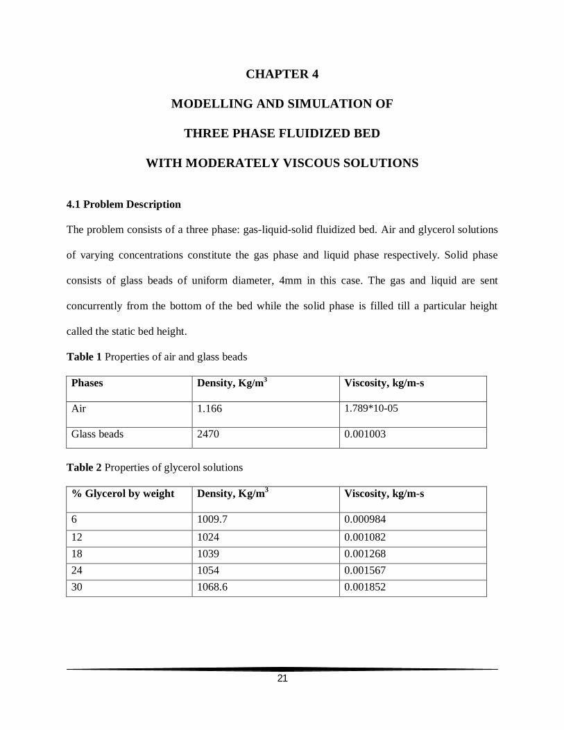
4.1 Problem Description
The problem consists of a three phase: gas-liquid-solid fluidized bed. Air and glycerol solutions
of varying concentrations constitute the gas phase and liquid phase respectively. Solid phase
consists of glass beads of uniform diameter, 4mm in this case. The gas and liquid are sent
concurrently from the bottom of the bed while the solid phase is filled till a particular height
called the static bed height.
Table 1 Properties of air and glass beads
Phases Density, Kg/m3
Viscosity, kg/m-s
Air 1.166 1.789*10-05
Glass beads 2470 0.001003
Table 2 Properties of glycerol solutions
% Glycerol by weight Density, Kg/m3
Viscosity, kg/m-s
6 1009.7 0.000984 12 1024 0.001082 18 1039 0.001268 24 1054 0.001567 30 1068.6 0.001852

22
4.2 Experimental Setup
Column specifications: 0.1m diameter
1.88m height
Static bed height= 25.6cm
4.3 Geometry and mesh
GAMBIT 2.2.30 was used for making 2D
rectangular geometry of width of 0.1m and height
1.88m. Coarse mesh size of 0.01m is used for the
whole geometry. It consists of 1880 quadrilateral
cells, 376 -2D wall faces, 3562 -2D interior faces.
A typical 2D rectangular mesh is shown in the
Figure1.
Figure 1: 2D Mesh
23
4.4 Simulation and Models Used
Fluent 6.3.26 is used for running the simulations. 2D segregated 1st order implicit unsteady
solver is used (the segregated solver must be used for multiphase calculations). Standard k-ε
dispersed eulerian multiphase model with standard wall functions were used.
The model constants used during simulation are given in the table below.
Table 3: Model constants used for simulation
Cmu
0.09
C1- ε
1.44
C2- ε 1.92
C3- ε 1.3
TKE Prandtl Number
1
TDR Prandtl Number
1.3
Dispersion Prandtl Number
0.75
4.4.1 Turbulence Modeling
Standard k-ε model is used which is a de facto standard version of the two-equation model that
involves transport equations for the turbulent kinetic energy, k and its dissipation rate, ε. At high
Reynolds numbers the rate of dissipation of kinetic energy is equal to the viscosity multiplied
by the fluctuating vorticity. An exact transport equation for the fluctuating vorticity, and thus the
dissipation rate, can be derived from the Navier Stokes equation. The k - epsilon model consists
of the turbulent kinetic energy equation. Its popularity in industrial flow and heat transfer
simulations is because of robustness, economy, and reasonable accuracy for a wide range of
24
turbulent flows. It is a semi-empirical model, and the derivation of the model equations relies on
phenomenological considerations and empiricism (Fluent., 2006).
4.4.2 Discretization
FLUENT uses a control-volume-based technique to convert the governing equations to algebraic
equations that can be solved numerically. This control volume technique consists of integrating
the governing equations about each control volume, yielding discrete equations that conserve
each quantity on a control-volume basis (Fluent., 2006). In the current work First Order Upwind
discretization scheme is used to dicretize momentum, volume fraction, turbulent kinetic energy
and turbulent dissipation rate. In this scheme quantities at cell faces are determined by assuming
that the cell-center values of any field variable represent a cell-average value and hold
throughout the entire cell; the face quantities are identical to the cell quantities. The main
advantage is that it is easy to implement and gives stable results with reasonable accuracy and
takes less computational time (Fluent., 2006). For pressure-velocity coupling Semi-Implicit
Method for Pressure-Linked Equations (SIMPLE) is used. It is one of the most commonly used
methods. It is based on the premise that fluid flows from regions with high pressure to low
pressure.

25
Table 4: Models used for considering interactions among phases. Interactions
Model
Solid-Air
Gidaspow
Solid-Glycerol solution
Gidaspow
Air- Glycerol solution
Schiller-Naumann
Water is taken as continuous phase while glass and air as dispersed phase.
Interphase interaction models considered are tabulated below:
Velocity Inlet Boundary Conditions: Air velocity was varied as 0.02123 m/s, 0.04246
m/s, 0.06369 m/s and 0.08492 m/s while liquid velocity was varied from 0.05 to 0.15 m/s
in multiples of 0.0125 and inlet air volume fractions obtained as fraction of air entering in
a mixture of gas and liquid.
Pressure outlet boundary conditions:
Mixture Gauge Pressure- 0 Pascal
Backflow volume fraction for air = 0
Specified shear was set as X=0 and Y=0 for gas and solid whereas no slip condition for
water was used.

26
4.4.2 Solution Controls
Segregated solver is used which solves the equations individually unlike coupled solver. 1st order
implicit unsteady formulation used. Velocity formulation is taken as absolute. Multiphase model
is taken as Eulerian. Standard k-epsilon dispersed multiphase model with standard wall functions
is used. Under relaxation factor for pressure, momentum and volume fraction were taken as 0.3,
0.2, and 0.5 respectively. The discretization scheme for momentum, volume fraction, turbulence
kinetic energy and turbulence dissipation rate were all first order upwind. Pressure-velocity
coupling scheme was Phase Coupled SIMPLE. Convergence criteria of 0.001 was used and
iterations were carried with time step size of 0.001.
27
CHAPTER 5
RESULTS AND DISCUSSION
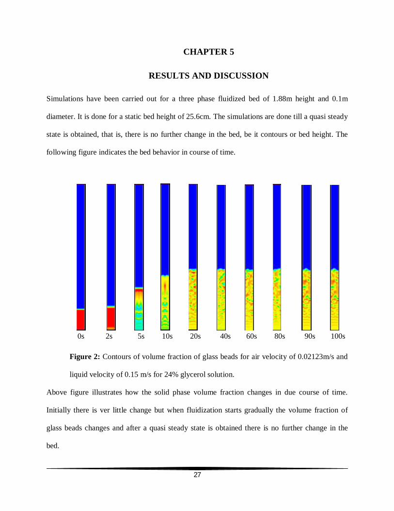
Simulations have been carried out for a three phase fluidized bed of 1.88m height and 0.1m
diameter. It is done for a static bed height of 25.6cm. The simulations are done till a quasi steady
state is obtained, that is, there is no further change in the bed, be it contours or bed height. The
following figure indicates the bed behavior in course of time.
0s 2s 5s 10s 20s 40s 60s 80s 90s 100s Figure 2: Contours of volume fraction of glass beads for air velocity of 0.02123m/s and
liquid velocity of 0.15 m/s for 24% glycerol solution.
Above figure illustrates how the solid phase volume fraction changes in due course of time.
Initially there is ver little change but when fluidization starts gradually the volume fraction of
glass beads changes and after a quasi steady state is obtained there is no further change in the
bed.

28
5.1 Phase Dynamics
All the three phases can be represented by contour plots. The following figure shows the
contours of glass beads, air and glycerol solution after achieving a quasi steady state. The color
scale given to the left of each contours gives the value of volume fraction corresponding to the
color. The contour of water indicates that the volume fraction of water or liquid holdup is less in
the fluidized part of the column as compared to the remaining part. The contour of air indicates
that the gas holdup is significantly more in fluidized part of the bed as compared to the
remaining part.
Solid Liquid Gas
Figure 3: Contours of volume fractions of solid, liquid and gas at liquid velocity of 0.125m/s
and gas velocity of 0.02123m/s for 30% glycerol solution.

29
The following figure shows the velocity vector of glass beads for 30% glycerol solution and for
inlet gas velocity of 0.06369 m/s and liquid velocity of 0.15 m/s.
Figure 4: Velocity vector of glass beads (actual)
30
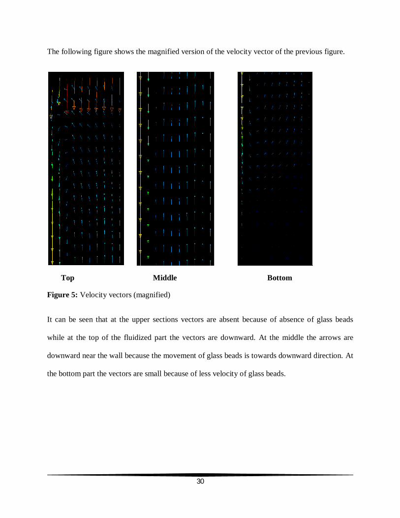
The following figure shows the magnified version of the velocity vector of the previous figure.
Top Middle Bottom
Figure 5: Velocity vectors (magnified)
It can be seen that at the upper sections vectors are absent because of absence of glass beads
while at the top of the fluidized part the vectors are downward. At the middle the arrows are
downward near the wall because the movement of glass beads is towards downward direction. At
the bottom part the vectors are small because of less velocity of glass beads.

31
Figure 6: X-Y plot for velocity magnitude of glycerol solution
The above plot indicates the velocity profile of glycerol solution inside the bed. It can be seen
that the average velocity is near 0.15 m/s. The inlet air velocity is 0.02123 m/s and the
concentration of the glycerol solution is 30%. A parabolic profile is desired after fully developed
flow.
32
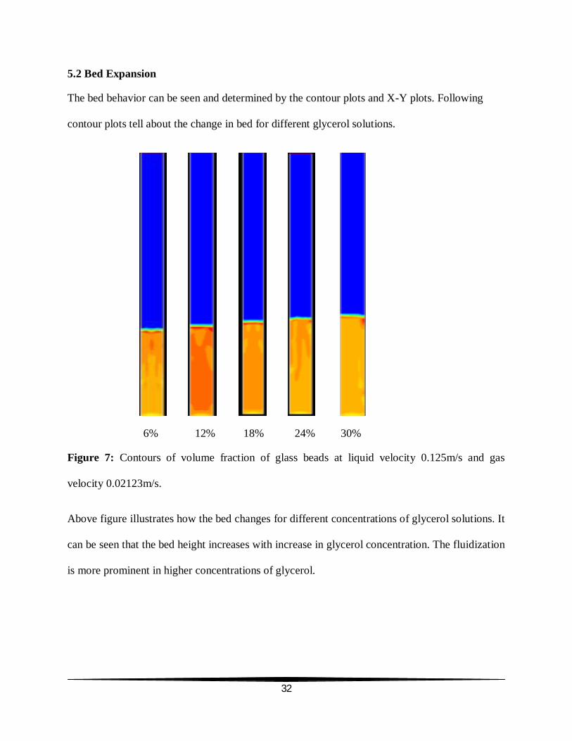
5.2 Bed Expansion
The bed behavior can be seen and determined by the contour plots and X-Y plots. Following
contour plots tell about the change in bed for different glycerol solutions.
6% 12% 18% 24% 30%
Figure 7: Contours of volume fraction of glass beads at liquid velocity 0.125m/s and gas
velocity 0.02123m/s.
Above figure illustrates how the bed changes for different concentrations of glycerol solutions. It
can be seen that the bed height increases with increase in glycerol concentration. The fluidization
is more prominent in higher concentrations of glycerol.

33
The following figure shows the expansion of bed with varying liquid velocity for a constant gas
velocity for 6% glycerol solution. It shows that the bed height increases with increase in liquid
velocity.
Liquid velocity 0.05m/s 0.0625m/s 0.075 m/s 0.1 m/s 0.125m/s 0.15m/s
Figure 8: Variation in volume fraction of glass beads at constant inlet air velocity of 0.02123m/s
and varying glycerol solution velocity for 6% glycerol solution.
The above contours are obtained after a quasi steady state is reached and there is no further
change in the bed. It can be seen that initially there is almost no change in the bed but when the
velocity of glycerol solution is increased the bed starts to expand at higher velocities the bed has
risen by a considerable amount.
34
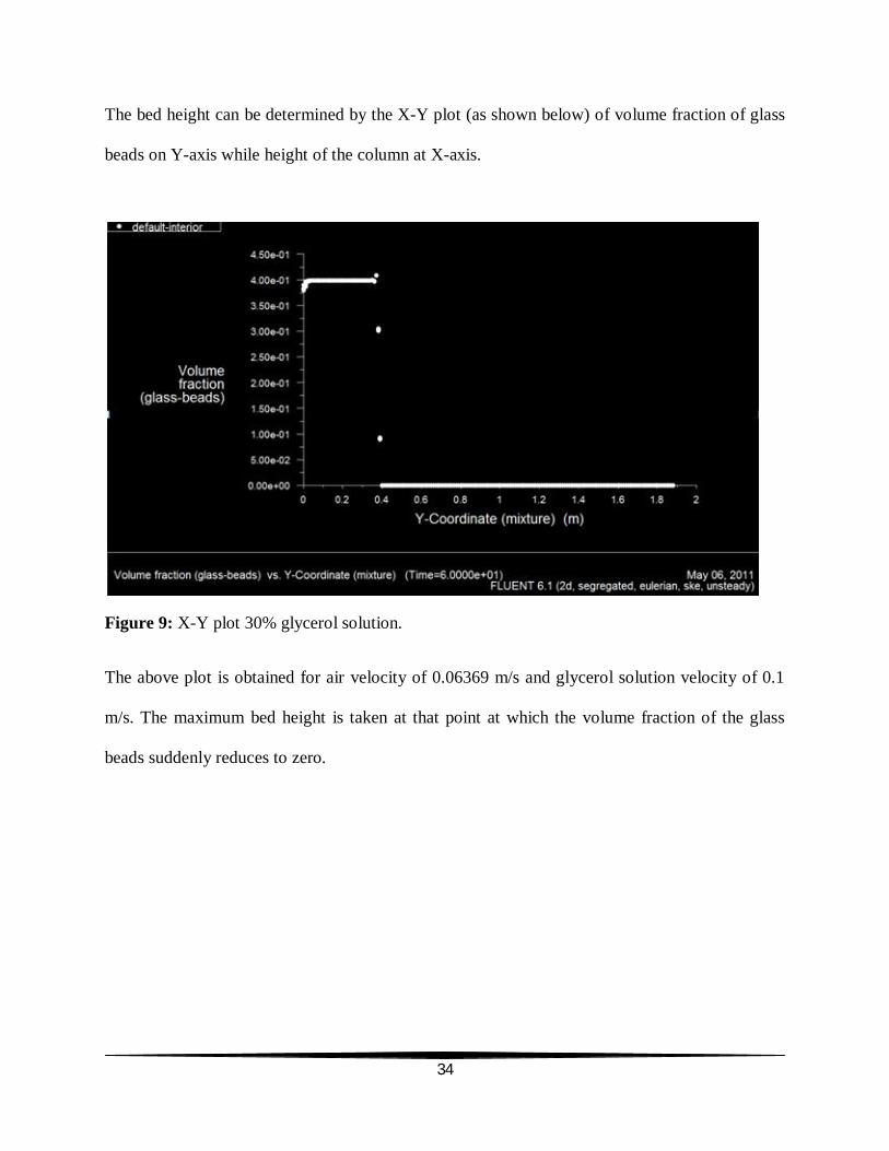
The bed height can be determined by the X-Y plot (as shown below) of volume fraction of glass
beads on Y-axis while height of the column at X-axis.
Figure 9: X-Y plot 30% glycerol solution.
The above plot is obtained for air velocity of 0.06369 m/s and glycerol solution velocity of 0.1
m/s. The maximum bed height is taken at that point at which the volume fraction of the glass
beads suddenly reduces to zero.
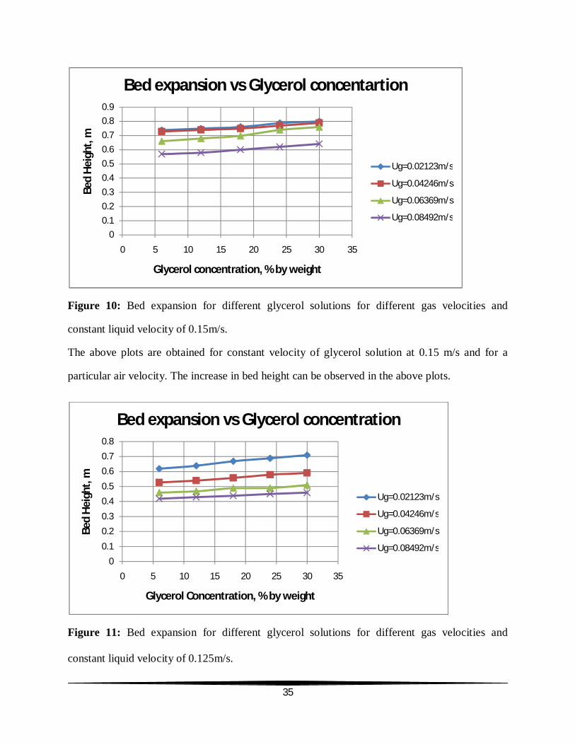
35
Figure 10: Bed expansion for different glycerol solutions for different gas velocities and
constant liquid velocity of 0.15m/s.
The above plots are obtained for constant velocity of glycerol solution at 0.15 m/s and for a
particular air velocity. The increase in bed height can be observed in the above plots.
Figure 11: Bed expansion for different glycerol solutions for different gas velocities and
constant liquid velocity of 0.125m/s.
00.10.20.30.40.50.60.70.80.9
0 5 10 15 20 25 30 35
Bed
Hei
ght,
m
Glycerol concentration, % by weight
Bed expansion vs Glycerol concentartion
Ug=0.02123m/s
Ug=0.04246m/s
Ug=0.06369m/s
Ug=0.08492m/s
00.1
0.20.3
0.40.5
0.60.70.8
0 5 10 15 20 25 30 35
Bed
Hei
ght,
m
Glycerol Concentration, % by weight
Bed expansion vs Glycerol concentration
Ug=0.02123m/s
Ug=0.04246m/s
Ug=0.06369m/s
Ug=0.08492m/s
36
It is clear from the previous figures that the bed expands considerably as the concentration of
glycerol solution is increased from 6% by weight to 30% by weight for a constant inlet air
velocity and glycerol solution velocity.
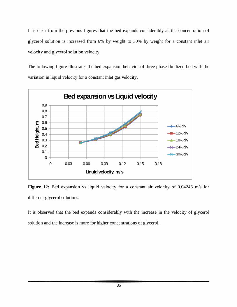
The following figure illustrates the bed expansion behavior of three phase fluidized bed with the
variation in liquid velocity for a constant inlet gas velocity.
Figure 12: Bed expansion vs liquid velocity for a constant air velocity of 0.04246 m/s for
different glycerol solutions.
It is observed that the bed expands considerably with the increase in the velocity of glycerol
solution and the increase is more for higher concentrations of glycerol.
00.10.20.30.40.50.60.70.80.9
0 0.03 0.06 0.09 0.12 0.15 0.18
Bed
Hei
ght,
m
Liquid velocity, m/s
Bed expansion vs Liquid velocity
6% gly
12% gly
18% gly
24% gly
30% gly

37
5.3 Phase Holdup
Phase holdup is obtained as mean area-weighted average of volume fraction of any phase at
different points in fluidized part of the bed. It is done so because the volume fraction of phases
are different at different points in the fluidized bed and hence area weighted average of volume
fraction is determined at heights 10cm, 20 cm 30 cm etc till fluidized part is over and the average
of these values provides us with the phase hold up.
Following figures illustrates the variations in gas holdup at different inlet velocities.
Figure 13: Gas holdup vs velocity of glycerol solution at constant air velocity of 0.02123 m/s for
different glycerol solutions.
Above figure illustrates that as the liquid velocity is increased for a particular glycerol solution
the gas holdup decreases for a constant air velocity.
0
0.005
0.01
0.015
0.02
0.025
0.03
0.035
0 0.03 0.06 0.09 0.12 0.15 0.18
Gas
hol
dup
Liquid velocity, m/s
Gas holdup vs Liquid velocity
6% gly
12% gly
18% gly
24% gly
30% gly

38
Figure 14: Gas holdup vs air velocity at constant liquid velocity of 0.15m/s for different glycerol
solutions.
The above figure illustrates that the gas holdup increases with increase in air velocity for a
particular glycerol solution.
Following figure illustrates the variation of gas holdup with increase in glycerol concentration.
Figure 15: Gas holdup vs glycerol concentration for constant liquid velocity of 0.15m/s.
0.015
0.025
0.035
0.045
0.055
0.065
0 0.02 0.04 0.06 0.08 0.1
Gas
hol
dup
Air velocity, m/s
Gas holdup vs Air velocity
6% gly
12% gly
18% gly
24% gly
30% gly
0.0150.02
0.0250.03
0.0350.04
0.0450.05
0.0550.06
0.065
0 5 10 15 20 25 30 35
Gas
hol
dup
Glycerol concentration, % by weight
Gas holdup vs Glycerol concentration
Ug=0.02123 m/s
Ug=0.04246 m/s
Ug=0.06369 m/s
Ug=0.08492 m/s

39
The figure tells about the variation in gas holdup with glycerol concentration and it is seen that
the gas holdup increases with the increase in glycerol concentration. The increase is fairly more
for higher gas velocity as compared to the lower velocities. It is seen that initially the increase is
less or almost same but as the concentration increases the gas holdup starts to increase more. It is
so because as the glycerol concentration increases the viscosity of the solution increases and
hence the bubble rise velocities decrease there by increasing the gas holdup.
Figure 16: Comparison of experimental vs simulated gas holdup
The above plots are done for comparing the simulated and experimentally obtained values for
constant inlet liquid velocity of 0.06369 m/s and air velocity 0f 0.02123 m/s for different
concentrations of glycerol solutions and are found to be in good agreement with one another. The
reason for small deviation may be that the glass beads used in experiment have a range of
diameters while in the simulation all glass beads are taken to be of the uniform diameter.
0
0.01
0.02
0.03
0.04
0.05
0.06
0 5 10 15 20 25 30 35
Gas
hol
dup
Glycerol concentration, % by weight
Comparison of experimental vs simulated gas holdup values
experimental
simulated

40
The following plots show the variations of liquid holdup and solid holdup with glycerol
concentration.
Figure 17: Variation of liquid holdup with glycerol concentration for a particular inlet air
velocity and constant liquid velocity of 0.15 m/s.
Figure 18: Variation of solid holdup for different glycerol solutions for inlet liquid velocity of
0.15 m/s and a particular gas velocity.
0.3
0.4
0.5
0.6
0.7
0.8
0.9
0 5 10 15 20 25 30 35
Liqu
id h
oldu
p
Glycerol concentration, % by weight
Liquid holdup vs Glycerol concentration
Ug=0.02123 m/s
Ug=0.04246 m/s
Ug=0.06369 m/s
Ug=0.08492 m/s
0.10.120.140.160.18
0.20.220.240.260.28
0 5 10 15 20 25 30 35
Solid
hol
dup
Glycerol concentration, % by weight
Solid holdup vs Glycerol concentration
Ug=0.02123 m/s
Ug=0.04246 m/s
Ug=0.06369 m/s
Ug=0.08492 m/s
41
It is seen from the Figure 17 that the liquid holdup rises slightly with the increase in
concentration of glycerol solution for a particular inlet velocity of gas and liquid. Since liquid as
well as gas holdup is increasing with the increase in concentration of the glycerol solution so
arithmetically the solid holdup has to decrease as all the three phases sum up to unity in terms of
volume fraction which is observed in the previous figure.
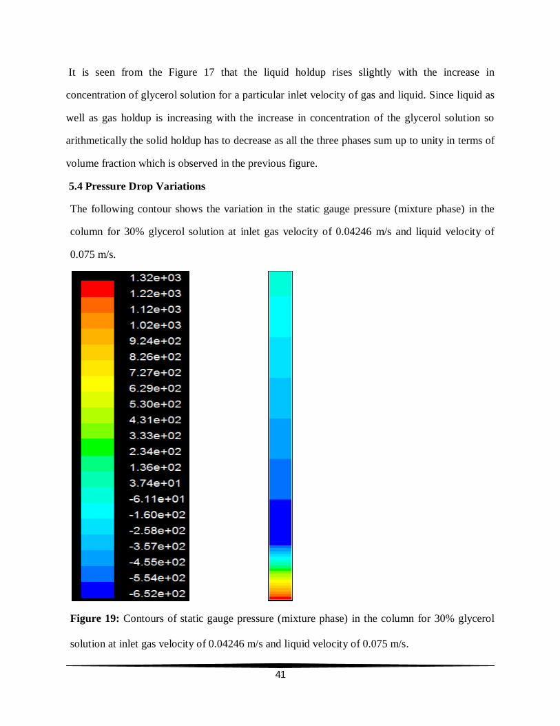
5.4 Pressure Drop Variations
The following contour shows the variation in the static gauge pressure (mixture phase) in the
column for 30% glycerol solution at inlet gas velocity of 0.04246 m/s and liquid velocity of
0.075 m/s.
Figure 19: Contours of static gauge pressure (mixture phase) in the column for 30% glycerol
solution at inlet gas velocity of 0.04246 m/s and liquid velocity of 0.075 m/s.
42
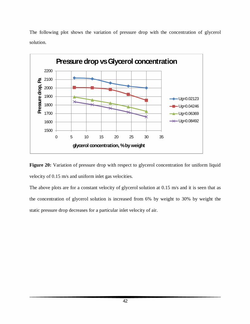
The following plot shows the variation of pressure drop with the concentration of glycerol
solution.
Figure 20: Variation of pressure drop with respect to glycerol concentration for uniform liquid
velocity of 0.15 m/s and uniform inlet gas velocities.
The above plots are for a constant velocity of glycerol solution at 0.15 m/s and it is seen that as
the concentration of glycerol solution is increased from 6% by weight to 30% by weight the
static pressure drop decreases for a particular inlet velocity of air.
1500
1600
1700
1800
1900
2000
2100
2200
0 5 10 15 20 25 30 35
Pres
sure
dro
p, P
a
glycerol concentration, % by weight
Pressure drop vs Glycerol concentration
Ug=0.02123
Ug=0.04246
Ug=0.06369
Ug=0.08492
43
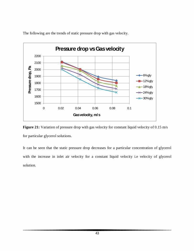
The following are the trends of static pressure drop with gas velocity.
Figure 21: Variation of pressure drop with gas velocity for constant liquid velocity of 0.15 m/s
for particular glycerol solutions.
It can be seen that the static pressure drop decreases for a particular concentration of glycerol
with the increase in inlet air velocity for a constant liquid velocity i.e velocity of glycerol
solution.
1500
1600
1700
1800
1900
2000
2100
2200
0 0.02 0.04 0.06 0.08 0.1
Pres
sure
dro
p, P
a
Gas velocity, m/s
Pressure drop vs Gas velocity
6% gly
12% gly
18% gly
24% gly
30% gly

44
CHAPTER 6
CONCLUSIONS
Simulations have been carried out successfully for a three phase co current fluidized bed of
1.88m height and 0.1m diameter in which glass beads of 4mm diameter filled to a height of
25.6cm constitute the solid phase. Air and different concentrations of glycerol solutions are
passed from the bottom of the domain to fluidize the bed. The aim was to observe the bed
expansion for different glycerol solutions along with the phase holdup and pressure drop. Some
of the conclusions obtained from the simulations are as follows:
I. The fluidization is found to be more prominent in higher concentrations of glycerol
solutions.
II. The bed height is found to increase with the increase in concentrations of glycerol
solutions for a particular inlet air and liquid velocity.
III. The bed height is also found to increase with the increase in liquid velocity for a
particular glycerol concentration for a constant air velocity.
IV. Gas holdup is showing an increasing trend with increase in concentrations of glycerol
for a particular inlet air and liquid velocity.
V. Gas holdup is also increasing with increase in gas velocity for any concentrations of the
glycerol solutions taken for a constant liquid velocity.
VI. It is found that the gas holdup decreases with the increase in liquid velocity for any
concentrations of the glycerol solutions taken for a constant air velocity.
VII. It is found that the liquid holdup increases with increase in glycerol concentration for
constant inlet gas and liquid velocity.
45
VIII. It is also observed that the solid holdup decreases with increase in glycerol concentration
for constant inlet gas and liquid velocity.
IX. The pressure drop is decreasing with increase in glycerol concentration for constant inlet
gas and liquid velocity.
X. The pressure drop is also decreasing with increase in air velocity for any glycerol
concentration for a particular liquid velocity.
The results obtained from the simulations have been compared from the literature Jena et al.,
2009 and they are found to be in good agreement with each other.
46
REFERENCES
Bakker A, - Fluent introductory notes, Fluent Inc, Lebanon (2002)
Bahary M, - Experimental and computational studies of hydrodynamics in three phase and two
phase fluidized beds. PhD thesis, Illinois Institute of Technology (1994).
Bigot, V., Guyot I. Bataille D., Roustan M., -Possibilities of use of two sensors depression
metrological techniques and fiber optics, to characterize the hydrodynamics of a fluidized bed
triphasic, In: Stork, A., Wild, G. (Eds.), Recent Advances in Process Engineering, vol. 4 (1990).
pp. 143-156.
Dudukovic M.P., Devanathan N., Holub R. -Multiphase reactors Models and experimental
verification, Revuedel' Institute Francais du Petrole; 46 (1991), pp.439–465.
Epstein N, three-phase fluidization-some knowledge gaps- Can J Chem Engg, 59 (1981),
pp.649-657.
L.S. Fan, Gas–liquid–solid fluidization engineering, Butterworth series in chemical engineering,
Butterworth Publishers, Boston, MA (1989).
L.S. Fan, F. Bavarian, R.L. Gorowara and B.E. Kreischer, Hydrodynamics of gas–liquid–solid
fluidization under high gas hold-up conditions, Powder Technology 53 (1987), pp. 285–293.
Fluent 6.3 Documentation, 2006. Fluent Inc., Lebanon.

47
Fraguío, M.S., Cassanello M.C., Larachi F., Chaouki,J. -Flow regime transition pointers in three-
phase fluidized beds inferred from a solid tracer trajectory, Chemical
EngineeringandProcessing,45 (2006), pp.350–358.
Grevskott S, Sannaes B H, Dudukovic M.P, Hjarbo K W, Svendsen H F, Liquid circulation
bubble size distributions and solid movements in two and three phase bubble columns, Chemical
Engineering Science, 51 (1996), pp.1703-1713.
Jena H M, Roy G K and Mahapatra S S, Determination of optimum gas holdup conditions in a
three-phase fluidized bed by genetic algorithm, Computers & Chemical Engineering, 34(2009)-,
pp.476-484.
Jianping W, Shonglin X, 1998-Local Hydrodynamics in a gas-liquid –solid three phase bubble
column reactors, Chemical Engineering Science,56 (1998)-, pp.5893-5933.
Kumar A, CFD Modeling of Gas-Liquid-Solid Fluidized Bed, B. Tech Thesis (2009) NIT
Rourkela. India.
Lee S.L.P., DeLasa, H.I. -Phase holdups in three-phase fluidized beds. A.I.Ch.E. Journal 33
(1987), pp.1359–1370.
Li Y, Zhang J, Fan L S - Numerical simulation of gas-liquid-solid fluidization system using a
combined CFD-VOF-DPM method bubble wake behaviour , 54 (1999), pp.5101-5107.
Luo X., Jiang P., Fan L.S. -High-pressure three-phase fluidization: hydrodynamics and heat
transfer, A.I.Ch.E. Journal, 43 (1997), pp.2432–2445.

48
Matonis D., Gidaspow D., Bahary M., -CFD simulation of flow and turbulence in a slurry bubble
column, A.I.Ch.E. Journal 48 (2002), pp. 1413–1429.
Merchant F.J.A., Margaritis A., Wallace J.B., -A novel technique for measuring solute
diffusivities in entrapment matrices used in immobilization", Biotechnology and Bioengineering
30 (1992), pp.936–945.
Mitra-Majumdar D, Farouk B, Shah Y T, 1997-Hydrodynamic modeling of three phase flow
through a vertical column, Chemical Engineering Science, 52(1997), pp.4485-4497.
Muroyama, K. and L.S. Fan, ―Fundamentals of Gas-Liquid-Solid Fluidization‖, AIChE.J. Vol.3,
No.1, (1985), pp. 1-34.
Padial N T, Van der Heyden W B, Rauenzahn R M, Yarbo S L, Three dimensional simulation of
a three phase draft tube bubble column, Chemical Engineering Science,55 (2000), pp.3261-3273.
Panneerselvam R., Savithri S., Surender G.D., CFD simulation of hydrodynamics of gas-solid –
liquid fluidized bed reactor, Chemical Engineering science, 64 (2009), pp.1119-1135.
S. Ravelli_, A. Perdichizzi, G. Barigozzi. "Description, applications and numerical modeling of
bubbling fluidized bed combustion in waste-to-energy plants", Progress in Energy and
Combustion Science 34 (2008),pp.224–253.
Rigby G.R., VanBrokland G.P., Park W.H., Capes C.E. "Properties of bubbles in three-phase
fluidized bed as measured by an electro resistivity probe", Chemical Engineering Science 25
(1970), pp.1729–1741.

49
M. Safoniuk, J.R. Grace, L. Hackman and C.A. Mcknight, Gas hold-up in a three-phase fluidized
bed, AIChE Journal 48 (2002), pp. 1581–1587.
Biofluidization: Application of the fluidization technique in biotechnology, The Canadian
Journal of Chemical Engineering Volume 67(1989), Issue 2, pages 178–184.
J.M. Schweitzer, J. Bayle and T. Gauthier, Local gas hold-up measurements in fluidized bed and
slurry bubble column, Chemical Engineering Science 56 (2001), pp. 1103–1110.
Y. T. Shah, S. Joseph, D. N. Smith and J. A. Ruether, Ind. Eng. Chem. Proc. Des. Dev., 24
(1985), pp.1140.
G.H. Song, F. Bavarian and L.S. Fan, Hydrodynamics of three-phase fluidized bed containing
cylindrical hydro treating catalysts, Canadian Journal of Chemical Engineering 67 (1989),
pp.265–275.
Related Documents