Hydrodynamic stability and breakdown of the viscous regime over riblets

J. Fluid Mech. (2011), vol. 678, pp. 317–347. c© Cambridge University Press 2011

doi:10.1017/jfm.2011.114

317

Hydrodynamic stability and breakdownof the viscous regime over riblets

RICARDO GARCIA-MAYORAL† AND JAVIER JIMENEZSchool of Aeronautics, Universidad Politecnica de Madrid, 28040 Madrid, Spain

(Received 12 July 2010; revised 1 February 2011; accepted 3 March 2011;

first published online 19 April 2011)

The interaction of the overlying turbulent flow with a riblet surface and its impact ondrag reduction are analysed. The ‘viscous regime’ of vanishing riblet spacing, in whichthe drag reduction produced by the riblets is proportional to their size, is reasonablywell understood, but this paper focuses on the behaviour for spacings s+ � 10–20,expressed in wall units, where the viscous regime breaks down and the reductioneventually becomes an increase. Experimental evidence suggests that the two regimesare largely independent, and, based on a re-evaluation of existing data, it is shown thatthe optimal rib size is collapsed best by the square root of the groove cross-section,

�+g = A+

g

1/2. The mechanism of the breakdown is investigated by systematic DNSs

with increasing riblet sizes. It is found that the breakdown is caused by the appearanceof long spanwise rollers below y+ ≈ 20, with typical streamwise wavelengths λ+

x ≈ 150,that develop from a two-dimensional Kelvin–Helmholtz-like instability of the meanstreamwise flow, similar to those over plant canopies and porous surfaces. Theyaccount for the drag breakdown, both qualitatively and quantitatively. It is shownthat a simplified linear instability model explains the scaling of the breakdown spacingwith �+

g .

Key words: drag reduction, turbulent boundary layers, turbulence control

1. IntroductionThe reduction of skin friction in turbulent flows has been an active area of research

for several decades, and surface riblets have been one of the few drag-reductiontechniques successfully demonstrated not only in theory, but in practice as well. Theyare small protrusions aligned with the direction of the flow that confer an anisotropicroughness to the surface. The most comprehensive compilations of riblet experimentsare those of Walsh & Lindemann (1984), Walsh (1990b), Bruse et al. (1993) andBechert et al. (1997), in which the maximum drag reductions are of the order of 10 %,and are achieved for riblets with peak-to-peak spacings of approximately 15 wall units.

The dependence of the performance of riblets with a particular geometry in termsof the rib spacing is sketched in figure 1. In the limit of very small riblets, which wewill call the ‘viscous’ regime, the reduction in drag is proportional to the riblet size,and its mechanism is fairly well understood and quantified (Bechert & Bartenwerfer1989; Luchini, Manzo & Pozzi 1991). However, as the riblets get larger and their effectsaturates, a minimum drag is reached when the viscous regime ‘breaks down’. We willsee below that the two regimes are only weakly related, and that the breakdown is

† Email address for correspondence: [email protected]

318 R. Garcıa-Mayoral and J. Jimenez

0 20 40

0

0.1

ms

Viscous regime

Optimumperformance

k–roughness

�τ/

τ 0

s+

Figure 1. Effect of the peak-to-peak distance, s+, on the skin friction of a triangular ribletwith 60◦ peak sharpness, from Bechert et al. (1997).

worse understood than the viscous limit, in spite of having been the subject of severalstudies (Choi, Moin & Kim 1993; Goldstein & Tuan 1998). The main focus of ourpaper is to determine the parameters that best describe the extent of the linear regimeand the mechanism that controls the breakdown. Apart from the theoretical interest,a practical reason is that the breakdown spacing limits the optimum performance ofa given riblet geometry, which can roughly be estimated as the product of the viscousslope and the breakdown size. In particular, if it could be clarified how the latter isrelated to the geometry of the riblets, it might be possible to design surfaces withlarger critical sizes than the ones available at present, and consequently with betterpeak performances.

The paper is organized in two parts. The first one summarizes the availableexperiments and theoretical understanding. Within this part, § 2 reviews the differentdrag-reduction regimes and discusses the physical mechanisms proposed in theliterature both for the viscous regime and for its breakdown, and § 3 discusses thesuitability of the parameters traditionally used to characterize the latter and proposesan empirical alternative. The second part of the paper addresses the mechanism ofthe breakdown, using direct numerical simulations (DNSs). Section 4 outlines thenumerical method and the parameters of the simulations. The results are presented in§ 5, which also discusses the relationship between the breakdown, the riblet size andthe overlying turbulent flow, and § 6 proposes a linear stability model that captures theessential attributes of the breakdown, including an approximate justification of thescaling parameter proposed in § 3. The conclusions are summarized in the final section.

2. Drag-reduction regimes for riblets2.1. The viscous regime

Early in the investigation of riblets, Walsh & Lindemann (1984) showed that theReynolds number dependence of the effect of a given riblet geometry on the skinfriction could be approximately expressed in terms of the riblet spacing measured inwall units, s+ = suτ/ν, where ν is the kinematic viscosity, and uτ =

√τw is the friction

velocity defined in terms of the kinematic skin friction τw . Throughout this paper thefluid density will be taken as constant and equal to unity. Figure 1 shows a typicalcurve of drag reduction as a function of the riblet spacing. In the viscous regime, forsmall s+, the contribution of the nonlinear terms to the interaction of the flow withthe riblets is negligible and, if τw0 is the skin friction for a smooth wall, the drag

Breakdown of the viscous regime for riblet surfaces 319

0 10 20 30

–0.05

0

0.05

0 10 20 30

–0.10

–0.05

0

0.05

(a) (b)

�τ/τ

0

s+ s+

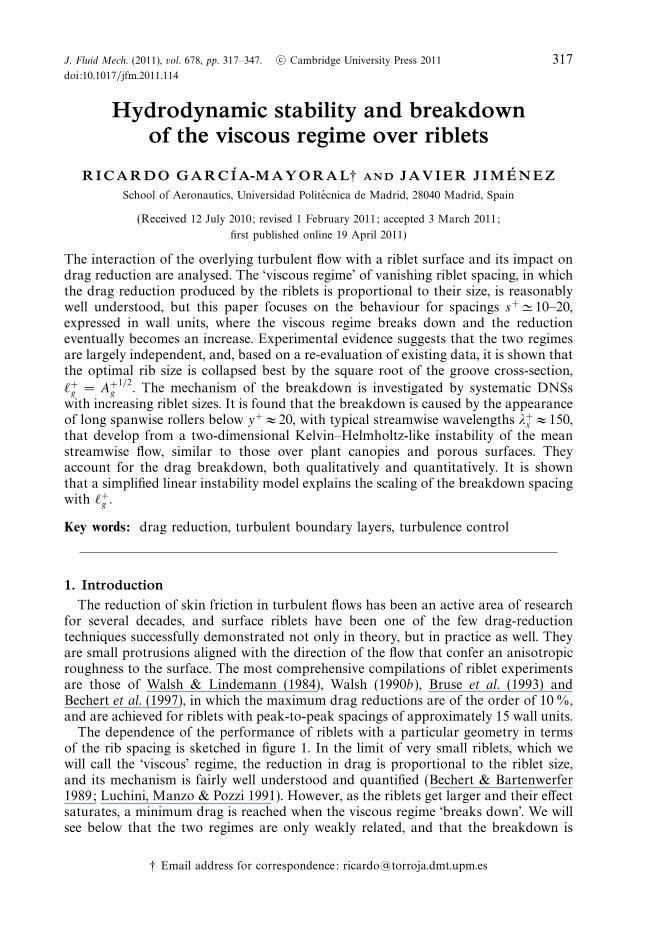
Figure 2. Drag reduction curves of various riblets, adapted from Bechert et al. (1997).(a) Blades with fixed height-to-spacing ratio, h/s = 0.5, and different tip width, t/s. Solidsymbols, t/s = 0.04; open symbols, t/s = 0.01; grey, t/s = 0.02 with improved bladealignment and groove impermeability. (b) Riblets with approximately equal viscous slope ms .�, blades with h/s = 0.4 and t/s = 0.01; �, blades with h/s = 0.5 and t/s = 0.04; �, scallopedgroves with h/s = 0.7 and t/s = 0.015; �, scalloped groves with h/s = 1.0 and t/s = 0.018;�, trapezoidal riblets with tip angle 30◦; �, trapezoidal riblets, 45◦.

reduction DR = −�τw/τw0 depends linearly on s+. That regime eventually breaksdown, and the drag reduction is typically maximum for spacings s+

opt ≈ 10−20. Foreven larger riblets, the reduction ultimately becomes a drag increase and follows atypical k -roughness behaviour (Jimenez 2004). The parameters that determine theoptimum performance of a given riblet are s+

opt and the slope of the drag curve in theviscous regime:

ms = − ∂(�τw/τw0)

∂s+

∣∣∣∣s=0

= − �τw/τw0

s+

∣∣∣∣s+�1

. (2.1)

Both depend on the geometry, but the qualitative behaviour is always as just described.The analysis of the available experimental evidence suggests that the viscous and

breakdown regimes are essentially unrelated phenomena. For example, blade thicknesshas a strong effect on the viscous performance of thin-blade riblets without appreciablychanging their groove geometry, and figure 2(a) shows an example of progressivelythicker blades (1–4 %), with fairly different viscous slopes and very similar breakdownspacings. Conversely, figure 2(b) is a compilation of drag curves for riblets with similarms but different geometries, whose optimum spacings vary widely. To separate thetwo effects as much as possible, and to focus on the breakdown mechanism, mostof our discussion from now on will use drag curves normalized so that their initialviscous slopes are unity.

It is widely believed that the drag-reduction properties of riblets in the viscousregime are well described by the concept of ‘protrusion height’, which was initiallyintroduced by Bechert & Bartenwerfer (1989) as an offset between the virtual originseen by the mean streamwise flow and some notional mean surface location. Thecorrect form was given by Luchini et al. (1991), who defined it as the offset betweenthe virtual origins of the streamwise and spanwise flows. From here on, we willdenote the streamwise, wall-normal and spanwise coordinates by x, y and z,respectively, and the corresponding velocity components by u, v and w. The originfor y will be taken at the top of the riblet tips.

There is a thin near-wall region in turbulent flows over smooth walls where viscouseffects are dominant, nonlinear inertial effects can be neglected and the mean velocity

320 R. Garcıa-Mayoral and J. Jimenez

profile is linear. Its thickness is 5–10 wall units (Tennekes & Lumley 1972). From thepoint of view of a small protrusion in this layer, the outer flow can be represented asa time-dependent but otherwise uniform shear. Riblets destroy that uniformity nearthe wall but, if s+ � 1, the flow still behaves as a uniform shear for y � s. A furthersimplification is that the problem decouples into two two-dimensional sub-problemsin the z–y cross-plane, because the equations of motion are locally linear, the ribletsare uniform in the streamwise direction and the shear varies only slowly with x whencompared to its variations in the cross-plane. The first sub-problem is the longitudinalflow of u, driven by a streamwise shear that takes the form

u ≈ Sx(x, t) (y − ∆u) (2.2)

at y+ � 1, and the other is the transverse flow of v and w, driven by

w ≈ Sz(x, t) (y − ∆w) and v ≈ 0. (2.3)

Far from the wall, the effect of the riblets reduces to the virtual origins ∆u and∆w (Luchini 1995), which are different for the two flow directions. What Luchiniet al. (1991) suggested was that the ‘protrusion height’ between the two virtualorigins, �h = ∆w − ∆u, was the controlling parameter for the viscous drag reduction.Intuitively, if the virtual origin for the crossflow is farther into the flow than theone for the longitudinal one (�h > 0), the spanwise flow induced by the overlyingstreamwise vortices is impeded more severely than over a smooth wall. The vorticesare displaced away from the wall, and the turbulent mixing of streamwise momentumis reduced. Since this mixing is responsible for the high local wall shear (Orlandi &Jimenez 1994), the result is a lower skin friction. This was verified by Jimenez (1994)by DNSs in which �h was introduced independently of the presence of riblets.

The numerical calculation of �h only requires the solution of the two stationarytwo-dimensional Stokes problems for ∆u and ∆w , which are computationally muchless intensive than the three-dimensional, time-dependent, turbulent flow over ribbedwalls. Note that the linearity of the Stokes problems implies that ∆u, ∆w and �h areall proportional to the riblet size in the viscous regime, as observed in experiments.

2.2. The breakdown of the viscous regime

As s+ increases, the predictions of the viscous theory break down, particularly thelinear dependence on s of the drag. The theories proposed in the literature for thisdeterioration of performance fall in two broad groups, both of which focus on thebehaviour of the crossflow.

The first one is that the riblets lose effectiveness once s+, which is used as a measureof the Reynolds number of the crossflow, increases beyond the Stokes regime. Forexample, Goldstein & Tuan (1998) suggested that the deterioration is due to thegeneration of secondary streamwise vorticity over the riblets, as the unsteady crossflowseparates and sheds small-scale vortices that create extra dissipation. However, itis known that spanwise oscillations of the wall, which also presumably introduceunsteady streamwise vorticity, can decrease drag (Jung, Mangiavacchi & Akhavan1992), and that modifying the spanwise boundary condition to inhibit the creation ofsecondary wall vorticity increases drag (Jimenez 1992; Jimenez & Pinelli 1999). Bothobservations suggest that introducing small-scale streamwise vorticity near the walldecreases drag by damping the larger streamwise vortices of the buffer layer, and thatinertial crossflow effects need not be detrimental to drag reduction.

A related possibility that was considered during the course of the present study wasthat the concept of protrusion height could be extended beyond the strictly viscous

Breakdown of the viscous regime for riblet surfaces 321

regime, and that the observed deviations from linearity would be due to the increasedimportance of advection in the vicinity of the riblets. In that model, the flow far fromthe riblets would still be a uniform shear but within the riblets, it would begin to feelthe effects of the finite Reynolds number. If that were the case, the breakdown couldstill be estimated from simple two-dimensional calculations analogous to the viscousones. Unfortunately, simulations based on that model (Garcıa-Mayoral & Jimenez2007) resulted only in small departures from the viscous values, of variable signdepending on the riblet geometry and size. Changes of the order required to explainthe experiments were not reached until s+ ≈ 20–40, which is too large compared tos+ ≈ 10–20 found experimentally.

The second group of theories assumes that the observed optimum spacing is relatedto the scale of the turbulent structures in the unperturbed turbulent wall region. Inthat group we could mention the observations by Choi et al. (1993), Suzuki & Kasagi(1994) and Lee & Lee (2001), that the streamwise turbulent vortices lodge within theriblet grooves for riblets in the early drag-degradation regime.

All those models result in optimum spacings of roughly the right order of magnitude,but they can be characterized as ‘circumstantial’ in the sense that they are based onobservations at spacings for which the viscous regime has already broken down,rather than at those preceding the deterioration. Moreover, although they suggestplausible reasons for why the Stokes regime fails beyond a certain riblet size, noneof them provides convincing physical arguments for why that failure should lead toa drag increase. As a consequence, it is difficult to establish with certainty whetherthe observed phenomena are consequences or causes of the breakdown, and theultimate reason for the observed degradation of the effectiveness of riblets can stillbe considered as open.

3. Scaling of the riblet dimension at breakdownAs already mentioned, one of the earliest observations concerning riblets was that

the drag-reduction curves for a given riblet geometry could be described in terms ofthe riblet size expressed in wall units. Size has often been taken to mean the spacings+, although occasionally the depth h+ has also been used. For a particular geometry,both quantities are proportional to each other, and the choice is immaterial, but thesame is not true when comparing riblets of different shapes, and we saw in figure 2that s+ is not, in that sense, a particularly good characterization of the position ofthe viscous breakdown.

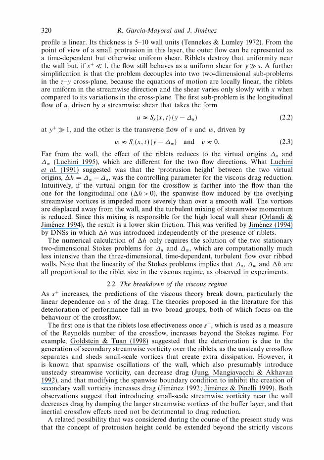
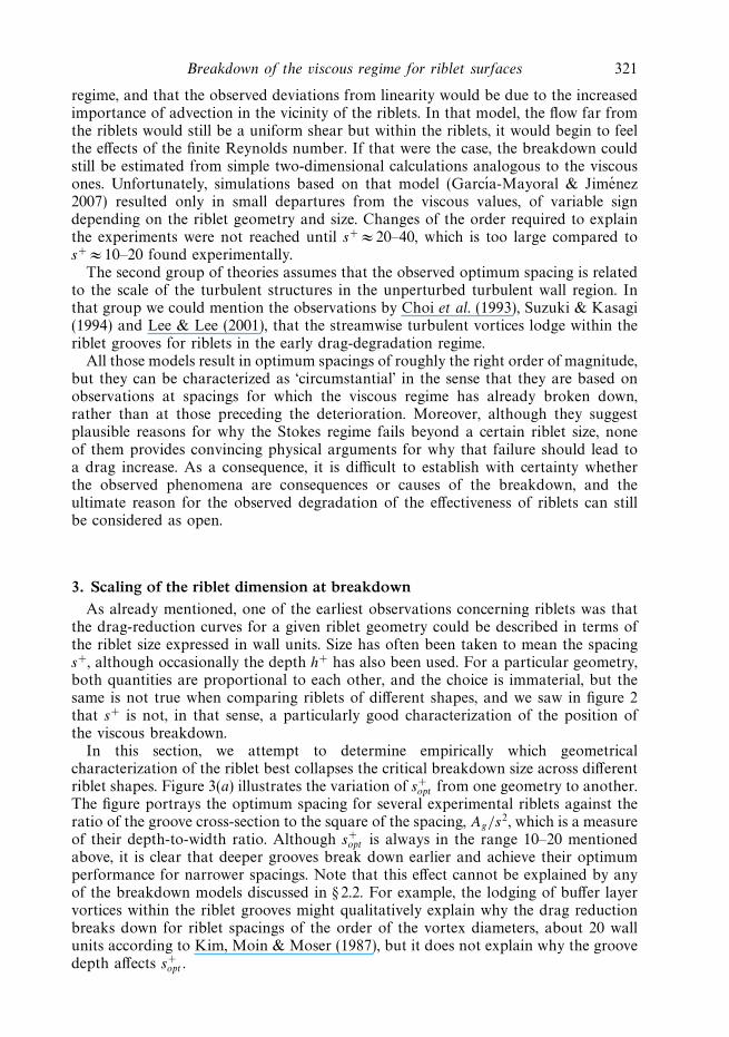
In this section, we attempt to determine empirically which geometricalcharacterization of the riblet best collapses the critical breakdown size across differentriblet shapes. Figure 3(a) illustrates the variation of s+

opt from one geometry to another.The figure portrays the optimum spacing for several experimental riblets against theratio of the groove cross-section to the square of the spacing, Ag/s

2, which is a measureof their depth-to-width ratio. Although s+

opt is always in the range 10–20 mentionedabove, it is clear that deeper grooves break down earlier and achieve their optimumperformance for narrower spacings. Note that this effect cannot be explained by anyof the breakdown models discussed in § 2.2. For example, the lodging of buffer layervortices within the riblet grooves might qualitatively explain why the drag reductionbreaks down for riblet spacings of the order of the vortex diameters, about 20 wallunits according to Kim, Moin & Moser (1987), but it does not explain why the groovedepth affects s+

opt .

322 R. Garcıa-Mayoral and J. Jimenez

0 10 20 30s+opt

s+ opt

h+opt

�+g,opt

0 5 10 15

0 10 20

(b)

(c)

(d )

0.5 1.00

10

20

Ag/s2

(a)s

hAg

Figure 3. (a) Riblet spacing for maximum drag reduction, as a function of the relative groovecross-section Ag/s

2. �, triangular riblets; �, notched-top and flat-valley riblets; �, scallopedsemicircular grooves; �, blades. The solid symbols are from Walsh & Lindemann (1984)and Walsh (1990b), and the open symbols are from Bechert et al. (1997). Error bars havebeen estimated from the drag measurement errors given in the references. (b–d) Histogramsof the optimum performance point, expressed in terms of the peak-to-peak spacing s, thegroove depth h and the square root of the groove cross-section, �g =

√Ag , for several riblet

geometries.

A non-exhaustive search among possible definitions of riblet size gave as a resultthat the best collapse of breakdown dimensions was achieved in terms of the groovecross-section, �+

g = (A+g )1/2. We portray in figures 3(b)–3(d ) the histograms of the

breakdown dimensions of several riblets, expressed as s+, h+ and �+g . We have omitted

experiments for which the optimum performance could not be clearly defined, such asthe measurements for fibres of Bruse et al. (1993), or those for seal fur of Itoh et al.(2006). Disregarding them, the histograms show that the optimum values of s+ andh+ have scatters of the order of 40 %, while the scatter for �+

g is only about 10 %.The implied optimum is �+

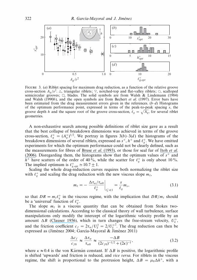
g,opt � 10.7 ± 1.Scaling the whole drag-reduction curves requires both normalizing the riblet size

with �+g and scaling the drag reduction with the new viscous slope m�,

m� = − �τw/τw0

�+g

∣∣∣∣�+g �1

=s

�g

ms, (3.1)

so that DR = m��+g in the viscous regime, with the implication that DR/m� should

be a ‘universal’ function of �+g .

The slope m� is a viscous quantity that can be obtained from Stokes two-dimensional calculations. According to the classical theory of wall turbulence, surfacemanipulations only modify the intercept of the logarithmic velocity profile by anamount �B (Clauser 1956), which in turn changes the free-stream velocity, U+

δ ,

and the friction coefficient cf = 2τw/U 2δ = 2/U+

δ

2. The drag reduction can then be

expressed as (Jimenez 2004; Garcıa-Mayoral & Jimenez 2011)

�cf

cf 0

≈ �τw

τw0

≈ −�B

(2cf 0)−1/2 + (2κ)−1, (3.2)

where κ ≈ 0.4 is the von Karman constant. If �B is positive, the logarithmic profileis shifted ‘upwards’ and friction is reduced, and vice versa. For riblets in the viscousregime, the shift is proportional to the protrusion height, �B = µ0�h+, with a

Breakdown of the viscous regime for riblet surfaces 323

0 20 40–20

0

20

–DR

/ms

–DR

/m�

0 10 20–15

0

15

–DR

/mh

0 10 20

–10

0

10

�+g

0.05 0.100

0.05

0.10

m�L+opt

DR

max

(a)

(c) (d)

(b)

s+ h+

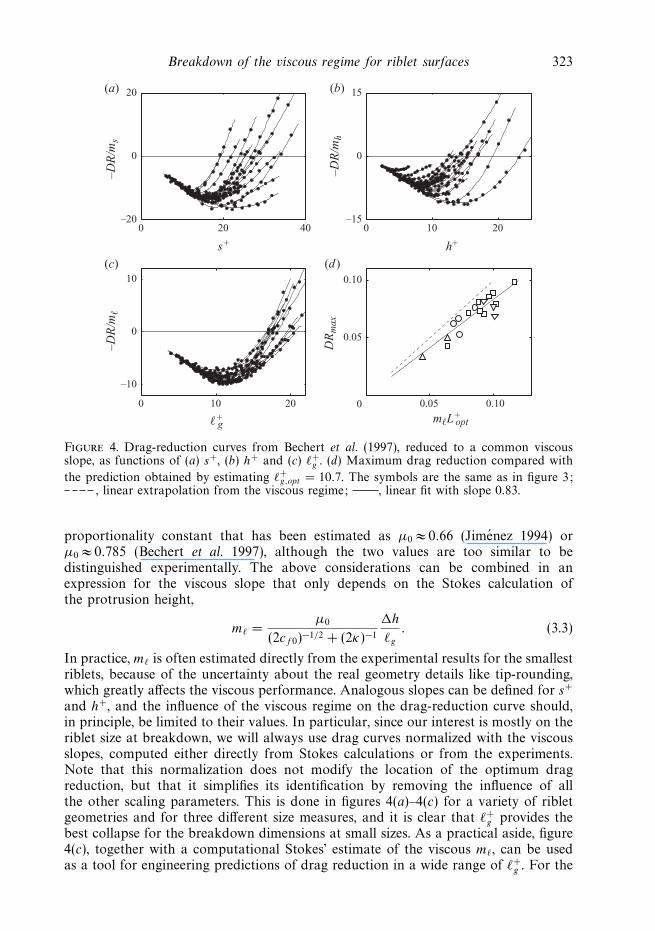
Figure 4. Drag-reduction curves from Bechert et al. (1997), reduced to a common viscousslope, as functions of (a) s+, (b) h+ and (c) �+

g . (d) Maximum drag reduction compared with

the prediction obtained by estimating �+g,opt = 10.7. The symbols are the same as in figure 3;

, linear extrapolation from the viscous regime; , linear fit with slope 0.83.

proportionality constant that has been estimated as µ0 ≈ 0.66 (Jimenez 1994) orµ0 ≈ 0.785 (Bechert et al. 1997), although the two values are too similar to bedistinguished experimentally. The above considerations can be combined in anexpression for the viscous slope that only depends on the Stokes calculation ofthe protrusion height,

m� =µ0

(2cf 0)−1/2 + (2κ)−1

�h

�g

. (3.3)

In practice, m� is often estimated directly from the experimental results for the smallestriblets, because of the uncertainty about the real geometry details like tip-rounding,which greatly affects the viscous performance. Analogous slopes can be defined for s+

and h+, and the influence of the viscous regime on the drag-reduction curve should,in principle, be limited to their values. In particular, since our interest is mostly on theriblet size at breakdown, we will always use drag curves normalized with the viscousslopes, computed either directly from Stokes calculations or from the experiments.Note that this normalization does not modify the location of the optimum dragreduction, but that it simplifies its identification by removing the influence of allthe other scaling parameters. This is done in figures 4(a)–4(c) for a variety of ribletgeometries and for three different size measures, and it is clear that �+

g provides thebest collapse for the breakdown dimensions at small sizes. As a practical aside, figure4(c), together with a computational Stokes’ estimate of the viscous m�, can be usedas a tool for engineering predictions of drag reduction in a wide range of �+

g . For the

324 R. Garcıa-Mayoral and J. Jimenez

geometries included in the figure,

DRmax ≈ 0.83 m� �+g,opt , (3.4)

where the optimum riblet spacing can be approximated by its mean value �+g,opt = 10.7,

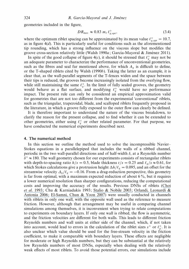
as in figure 4(d). This is particularly useful for conditions such as the aforementionedtip rounding, which has a strong influence on the viscous slope but modifies thegroove cross-section relatively little (Walsh 1990a; Garcıa-Mayoral & Jimenez 2011).

In spite of the good collapse of figure 4(c), it should be stressed that �+g may not be

an adequate parameter to characterize the performance of unconventional geometries,such as the fibres and seal fur mentioned above, for which Ag is difficult to define,or the T-shaped riblets cited by Walsh (1990b). Taking the latter as an example, it isclear that, as the wall-parallel segments of the T-fences widen and the space betweentheir tips is reduced, the grooves become increasingly isolated from the overlying flow,while still maintaining the same �+

g . In the limit of fully sealed grooves, the geometrywould behave as a flat surface, and modifying �+

g would have no performanceimpact. The present rule can only be considered an empirical approximation validfor geometries that are not too different from the experimental ‘conventional’ riblets,such as the triangular, trapezoidal, blade, and scalloped riblets frequently proposed inthe literature, in which a groove fully exposed to the outer flow can clearly be defined.

It is therefore important to understand the nature of the viscous breakdown, toclarify the reason for the present collapse, and to find whether it can be extended toother geometries, either using �+

g or other related parameter. For that purpose, wehave conducted the numerical experiments described next.

4. The numerical methodIn this section we outline the method used to solve the incompressible Navier–

Stokes equations in a parallelepiped that includes the walls of a ribbed channel,periodic in the two wall-parallel directions and of half-width δ, at a Reynolds numberδ+ ≈ 180. The wall geometry chosen for our experiments consists of rectangular ribletswith depth-to-spacing ratio h/s = 0.5, blade thickness t/s = 0.25 and �g/s ≈ 0.61, forwhich Stokes calculations give a protrusion height �h/�g = 0.095, and an offset for thestreamwise velocity ∆u/�g = −0.16. From a drag-reduction perspective, this geometryis far from optimal, with a maximum expected reduction of about 6 %, but it requiresa lower numerical resolution than sharper configurations, reducing the computationalcosts and improving the accuracy of the results. Previous DNSs of riblets (Choiet al. 1993; Chu & Karniadakis 1993; Stalio & Nobile 2003; Orlandi, Leonardi &Antonia 2006; El-Samni, Chun & Yoon 2007) were usually conducted in channelswith riblets in only one wall, with the opposite wall used as the reference to measurefriction. However, although that arrangement may be useful in comparing channelsimulations among themselves, it is inconvenient when trying to relate computationsto experiments on boundary layers. If only one wall is ribbed, the flow is asymmetric,and the friction velocities are different for both walls. This leads to different frictionReynolds numbers and wall units at either side of the channel, which, if not takeninto account, would lead to errors in the calculation of the riblet sizes s+ or �+

g . It isalso unclear which value should be used for the free-stream velocity in the frictioncoefficient, to make it comparable with boundary layers. These effects are negligiblefor moderate or high Reynolds numbers, but they can be substantial at the relativelylow Reynolds numbers of most DNSs, especially when dealing with the relativelyweak effects of most riblets. To avoid those potential errors, our simulations include

Breakdown of the viscous regime for riblet surfaces 325

riblets in both walls and use as reference a smooth-wall channel with the same massflux between the two planes defined by the riblet tips. We also take as referencevelocity the one at the centreline.

When the spacing between riblets is in the drag-reducing range, the accuraterepresentation of the flow near the ribbed walls requires a finer grid than the onerequired for the body of the channel. To alleviate the computational cost, our grid isdivided into three blocks, one near each wall in which the resolution is fine enough torepresent the riblets, and a coarser central one in which the resolution is only enoughto simulate the turbulence. The walls are modelled with the immersed-boundarytechnique detailed below.

The velocities and pressure are collocated and expanded in Fourier series alongthe two wall-parallel directions x and z. The differential operators are approximatedspectrally along those directions, and the nonlinear terms are de-aliased using the 2/3rule. The spatial differential operators in y are discretized using second-order, centredfinite-differences on a non-uniform grid. The grid spacing in y is coarsest at the centreof the channel, �y+

max ≈ 3, and finest near the walls, �y+min ≈ 0.3, remaining nearly

constant within the riblet grooves. The number of x modes is set so that �x+ ≈ 6 inthe three blocks, expressed in terms of collocation points. In the central block of thegrid, the resolution along z is just enough to capture the smallest turbulent scales,�z+ ≈ 2, while the number of z modes in the blocks containing the riblets is alwaysset to 24 physical collocation points per riblet. This resolution is similar to those ofGoldstein, Handler & Sirovich (1995) and Goldstein & Tuan (1998), who also useda combination of spectral methods and immersed boundaries for their riblet DNSs.In our simulations, the riblet surfaces are chosen to coincide with collocation points.Depending on the case, the spanwise grid is between 1.5 and 6 times finer in the wallblocks than in the central one. The additional Fourier modes of the wall blocks requireboundary conditions at the interface with the central block, where they disappear. Weimpose at those points that the three velocities and ∂p/∂y vanish, and require thatthe wall blocks extend far enough into the channel for those four quantities to havedecayed to negligible levels at the interface. This condition is checked a posteriori andfound to be satisfied beyond one or two riblet heights above the plane of the riblet tips.

Incompressibility is enforced weakly (Nordstrom, Mattsson & Swanson 2007). Ifwe denote the velocity divergence by D = ∇ · u, the equations of motion are

∂u∂t

+ u · ∇u = −∇p +1

Re∇2u, (4.1)

∂D

∂t= −λDD +

1

ReD

∇2D, (4.2)

where λD and ReD are positive coefficients, so that D is driven continuously andexponentially towards zero, instead of being required to vanish strictly. This weakform of the incompressibility condition allows us to use a collocated grid, whileeliminating the usual ‘chequerboard’ problem (Ferziger & Peric 1996).

The temporal integrator is a fractional-step, pressure-correction, three-substepRunge–Kutta, which only corrects the pressure in the final step (Le & Moin 1991):[

1 − �tβk

ReL

]un

k = unk−1 + �t

[αk

ReL

(un

k−1

)− γkN

(un

k−1

)−ζkN

(un

k−2

)− (αk + βk)G(pn)

], k = 1, 2, 3 (4.3)

326 R. Garcıa-Mayoral and J. Jimenez

Dn+1 = D(un

3

), (4.4)

Dn+1 = Dn + �t F

(Dn +

�t

2F (Dn)

), (4.5)

L(φn+1) = − 1

�t

(Dn+1 − Dn+1

), (4.6)

pn+1 = pn + φn+1, (4.7)

un+1 = un3 − �tGφn+1, (4.8)

where k is the Runge–Kutta substep, un0 = un, N is the de-aliased convective term

operator, D, G and L are the discretized divergence, gradient and Laplacian operators,and F (D) = −λDD + L(D)/ReD . The coefficients αk , βk , γk and ζk are those in Le &Moin (1991).

To model the no-slip condition at the riblet walls, we use the direct-forcingimmersed-boundary technique of Iaccarino & Verzicco (2003). Numerically, theimmersed-boundary condition

un+1 − un

�t=

V − un

�t, (4.9)

where V is the desired velocity at the forcing points, is approximated by[1 − �t

βk

ReL

]un

k =(V n

k−1 − unk−1

)+

[1 − �t

βk

ReL

]un

k−1, (4.10)

which, in practice, is a modification of (4.3) at the forcing points. In principle, theterm V n

k−1 could be explicitly calculated from unk−1 by linear interpolation (Garcıa-

Mayoral & Jimenez 2007), but in our rectangular riblets, whose surface is formedby grid points, it is always zero. In addition, (4.10) is used to force the velocities tovanish at all the points within the solid part of the riblets, and there is a notional flatboundary at the level of the groove floors, where the velocities and ∂p/∂y are alsorequired to vanish. The resulting velocities at the riblet surface are not exactly zero,but they are at worst of order 0.1uτ for u, and 0.01uτ for v and w, which is in bothcases roughly one order of magnitude smaller than the corresponding values in thefirst grid point away from the surface. They are mostly due to the imposition of theimmersed-boundary method before the pressure correction step, a feature commonto other fractional-step implementations (Fadlun et al. 2000).

The variable time step is adjusted to maintain fixed convective and viscous Courant–Friedrichs–Lewy numbers, CFLC = 0.5 and CFLV = 2.5 respectively, so that

�t = min

{CFLC

[�x

π|u| ,�z

π|w| ,�y

|v|

], Re CFLV

[�x2

π2,�z2

c

π2,�z2

r

π2,�y2

min

4

]}, (4.11)

where the subscripts ‘c’ and ‘r ’ refer to the central and riblet blocks. The parametersλD and ReD are chosen at each time step so that (4.5) is stable for �t given by(4.11). The resulting divergence in the flow is never higher than D+ ≈ 2 × 10−4, whichshould be compared with the magnitude of other velocity gradients. For example, themagnitude of the vorticity is |ω+| ≈ 0.05–0.2.

The channel half-height is δ = 1 in all cases, including in the smooth reference one,and is defined as the distance from the centre of the channel to the riblet tips, whilethe domain half-height is slightly larger, extending to the groove floors. The viscosityis always ν = 1/3250, chosen so that δ+ ≈ 180 in the smooth case. The time-dependent

Breakdown of the viscous regime for riblet surfaces 327

mean streamwise pressure gradient Px is adjusted to ensure a constant flow rate Q

in y ∈ (0, 2δ). This is done at each substep by a correction �Unk to the instantaneous

plane-averaged streamwise-velocity profile Unk ,

[1 − �t

βk

Re

∂2

∂y2

]U n

k = −�t (αk + βk), (4.12)

�Px =Q − Qn

k

Qnk

, (4.13)

�Unk = �PxU

nk , (4.14)

where Qnk is the flow rate associated with the auxiliary U n

k , and Qnk is the flow rate

of the uncorrected Unk . For simplicity, U n

k is only defined for y ∈ (0, 2δ), and its

boundary conditions are U nk = 0 at the riblet tip planes, so there is no correction

within the grooves owing to the constant Q constrain. This entails a very small errorbecause the corrections on Px and Un

k are several orders of magnitude smaller thantheir uncorrected values. Except for that small error, the procedure is equivalent toimposing on the discretized Navier–Stokes problem (4.3)–(4.8) the time-dependentpressure gradient required to obtain a constant flow rate, which is the procedure usedin most channel DNSs, both smooth and rough.

Besides the turbulent smooth channel computed as a reference, in which the wallswere also implemented using immersed boundaries, the code was validated on atwo-dimensional Taylor–Green vortex and on the transition of the wake of a laminarcylinder. The Taylor–Green vortex was used to test the time accuracy of the integrator,which was found to be second order for the velocity and first order for the pressure,with the second-order velocity errors mostly associated with viscous terms, as inmost incompressible fractional-step Runge–Kutta schemes (Simens et al. 2009). Thecylinder flow is a stringent test for immersed-boundary methods, since the detachmentand transition to an unsteady wake are very sensitive to the geometry of the obstacle(Linnick & Fasel 2005). In our tests, the flow transitioned at Re ≈ 42, defined with thecylinder diameter, which is in good agreement with the experimental range Re = 40–49 (Roshko 1953; Williamson 1989). The code was further tested by reproducing oneof the simulations with triangular riblets in Choi et al. (1993).

The parameters of our main set of simulations are given in table 1. The number ofriblets in the box is varied to span the full drag-reducing range. To our knowledge,this is the first time that such a systematic parameter sweep has been undertaken fornumerical riblets, except perhaps that by El-Samni et al. (2007), who included fivedifferent riblet sizes. Notice that Lz is increased slightly in case 17S, to obtain thedesired �+

g while keeping the fixed geometric resolution of the riblets. In addition, cases10S and 17S were repeated while independently doubling Nx , Nzr

, and the length andwidth of the channel, to check whether the simulations could be considered convergedwith respect to the grid and box sizes. The results agreed well with the ones used inthe paper. One of those cases, 17D, has been included in table 1 because it will beused in figure 14. The simulations in our main set were run for roughly 150 eddyturn-over times, δ/uτ , of which the first few were discarded to avoid the effects of theinitial transients on the statistics. They had to be run for such long times to reducethe effect of the wall-friction oscillations, which, for our relatively small simulationboxes, are of the order of 10 %.

328 R. Garcıa-Mayoral and J. Jimenez

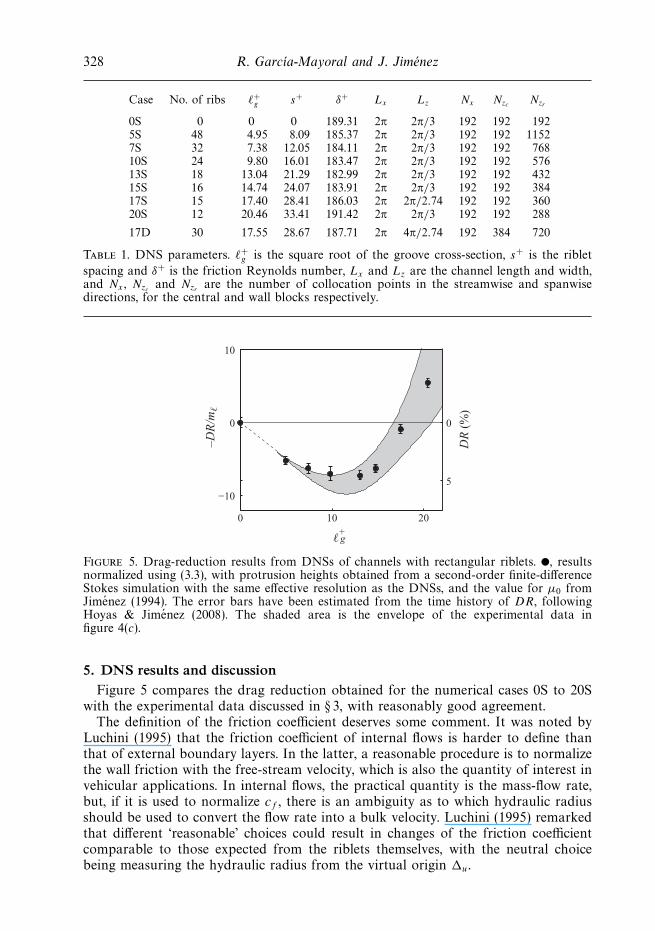
Case No. of ribs �+g s+ δ+ Lx Lz Nx Nzc

Nzr

0S 0 0 0 189.31 2π 2π/3 192 192 1925S 48 4.95 8.09 185.37 2π 2π/3 192 192 11527S 32 7.38 12.05 184.11 2π 2π/3 192 192 76810S 24 9.80 16.01 183.47 2π 2π/3 192 192 57613S 18 13.04 21.29 182.99 2π 2π/3 192 192 43215S 16 14.74 24.07 183.91 2π 2π/3 192 192 38417S 15 17.40 28.41 186.03 2π 2π/2.74 192 192 36020S 12 20.46 33.41 191.42 2π 2π/3 192 192 288

17D 30 17.55 28.67 187.71 2π 4π/2.74 192 384 720

Table 1. DNS parameters. �+g is the square root of the groove cross-section, s+ is the riblet

spacing and δ+ is the friction Reynolds number, Lx and Lz are the channel length and width,and Nx , Nzc

and Nzrare the number of collocation points in the streamwise and spanwise

directions, for the central and wall blocks respectively.

0 10 20

−10

0

10

5

0

DR

(%

)

�+g

–DR

/m�

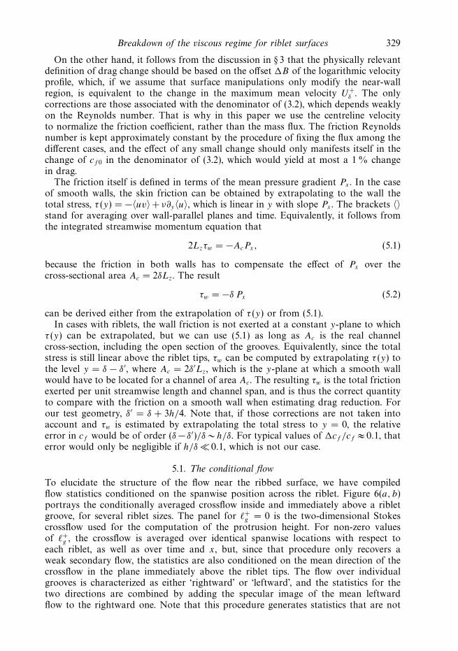
Figure 5. Drag-reduction results from DNSs of channels with rectangular riblets. �, resultsnormalized using (3.3), with protrusion heights obtained from a second-order finite-differenceStokes simulation with the same effective resolution as the DNSs, and the value for µ0 fromJimenez (1994). The error bars have been estimated from the time history of DR, followingHoyas & Jimenez (2008). The shaded area is the envelope of the experimental data infigure 4(c).

5. DNS results and discussionFigure 5 compares the drag reduction obtained for the numerical cases 0S to 20S

with the experimental data discussed in § 3, with reasonably good agreement.The definition of the friction coefficient deserves some comment. It was noted by

Luchini (1995) that the friction coefficient of internal flows is harder to define thanthat of external boundary layers. In the latter, a reasonable procedure is to normalizethe wall friction with the free-stream velocity, which is also the quantity of interest invehicular applications. In internal flows, the practical quantity is the mass-flow rate,but, if it is used to normalize cf , there is an ambiguity as to which hydraulic radiusshould be used to convert the flow rate into a bulk velocity. Luchini (1995) remarkedthat different ‘reasonable’ choices could result in changes of the friction coefficientcomparable to those expected from the riblets themselves, with the neutral choicebeing measuring the hydraulic radius from the virtual origin �u.

Breakdown of the viscous regime for riblet surfaces 329

On the other hand, it follows from the discussion in § 3 that the physically relevantdefinition of drag change should be based on the offset �B of the logarithmic velocityprofile, which, if we assume that surface manipulations only modify the near-wallregion, is equivalent to the change in the maximum mean velocity U+

δ . The onlycorrections are those associated with the denominator of (3.2), which depends weaklyon the Reynolds number. That is why in this paper we use the centreline velocityto normalize the friction coefficient, rather than the mass flux. The friction Reynoldsnumber is kept approximately constant by the procedure of fixing the flux among thedifferent cases, and the effect of any small change should only manifests itself in thechange of cf 0 in the denominator of (3.2), which would yield at most a 1% changein drag.

The friction itself is defined in terms of the mean pressure gradient Px . In the caseof smooth walls, the skin friction can be obtained by extrapolating to the wall thetotal stress, τ (y) = −〈uv〉 + ν∂y〈u〉, which is linear in y with slope Px . The brackets 〈〉stand for averaging over wall-parallel planes and time. Equivalently, it follows fromthe integrated streamwise momentum equation that

2Lzτw = −AcPx, (5.1)

because the friction in both walls has to compensate the effect of Px over thecross-sectional area Ac = 2δLz. The result

τw = −δ Px (5.2)

can be derived either from the extrapolation of τ (y) or from (5.1).In cases with riblets, the wall friction is not exerted at a constant y-plane to which

τ (y) can be extrapolated, but we can use (5.1) as long as Ac is the real channelcross-section, including the open section of the grooves. Equivalently, since the totalstress is still linear above the riblet tips, τw can be computed by extrapolating τ (y) tothe level y = δ − δ′, where Ac = 2δ′Lz, which is the y-plane at which a smooth wallwould have to be located for a channel of area Ac. The resulting τw is the total frictionexerted per unit streamwise length and channel span, and is thus the correct quantityto compare with the friction on a smooth wall when estimating drag reduction. Forour test geometry, δ′ = δ + 3h/4. Note that, if those corrections are not taken intoaccount and τw is estimated by extrapolating the total stress to y = 0, the relativeerror in cf would be of order (δ − δ′)/δ ∼ h/δ. For typical values of �cf /cf ≈ 0.1, thaterror would only be negligible if h/δ � 0.1, which is not our case.

5.1. The conditional flow

To elucidate the structure of the flow near the ribbed surface, we have compiledflow statistics conditioned on the spanwise position across the riblet. Figure 6(a, b)portrays the conditionally averaged crossflow inside and immediately above a ribletgroove, for several riblet sizes. The panel for �+

g = 0 is the two-dimensional Stokescrossflow used for the computation of the protrusion height. For non-zero valuesof �+

g , the crossflow is averaged over identical spanwise locations with respect toeach riblet, as well as over time and x, but, since that procedure only recovers aweak secondary flow, the statistics are also conditioned on the mean direction of thecrossflow in the plane immediately above the riblet tips. The flow over individualgrooves is characterized as either ‘rightward’ or ‘leftward’, and the statistics for thetwo directions are combined by adding the specular image of the mean leftwardflow to the rightward one. Note that this procedure generates statistics that are not

330 R. Garcıa-Mayoral and J. Jimenez

–0.5

0

0.5

y/s

y/s

0 1–0.5

0

0.5

z/s0 1

z/s0 1

z/s0 1

z/s

(a)

(b)

20 400

0.1

0.2

0.3

y+

ωx′+ ω+

x,c

(c)

0 10.02

0.04

0.06

0.08

z/s

(d)

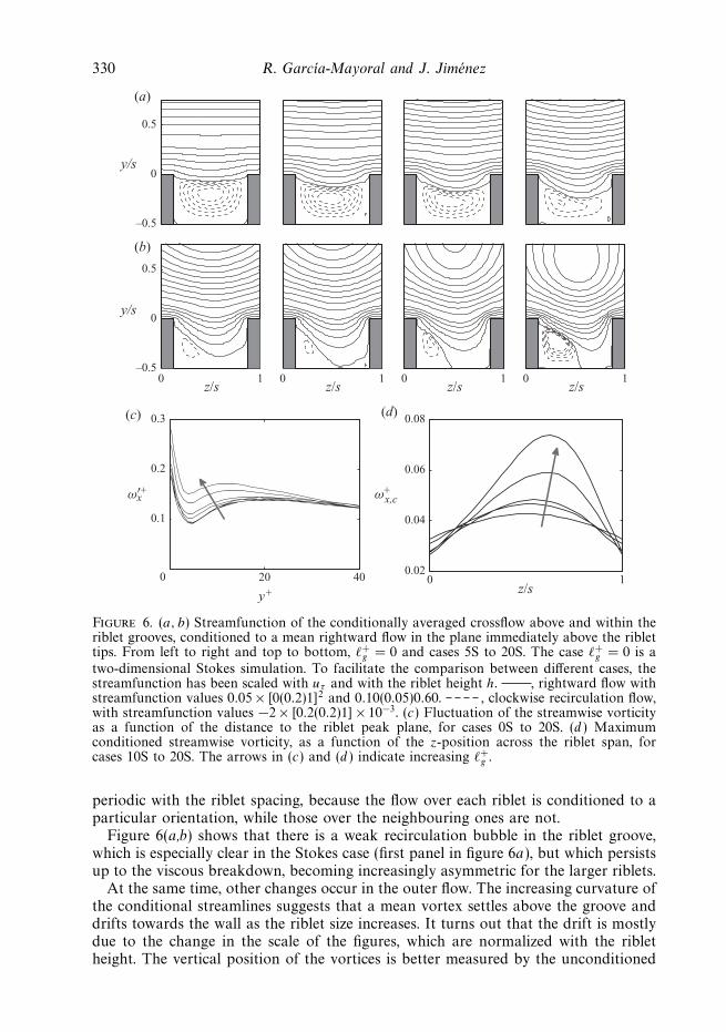
Figure 6. (a, b) Streamfunction of the conditionally averaged crossflow above and within theriblet grooves, conditioned to a mean rightward flow in the plane immediately above the riblettips. From left to right and top to bottom, �+

g = 0 and cases 5S to 20S. The case �+g = 0 is a

two-dimensional Stokes simulation. To facilitate the comparison between different cases, thestreamfunction has been scaled with uτ and with the riblet height h. , rightward flow withstreamfunction values 0.05 × [0(0.2)1]2 and 0.10(0.05)0.60. , clockwise recirculation flow,with streamfunction values −2 × [0.2(0.2)1] × 10−3. (c) Fluctuation of the streamwise vorticityas a function of the distance to the riblet peak plane, for cases 0S to 20S. (d ) Maximumconditioned streamwise vorticity, as a function of the z-position across the riblet span, forcases 10S to 20S. The arrows in (c) and (d ) indicate increasing �+

g .

periodic with the riblet spacing, because the flow over each riblet is conditioned to aparticular orientation, while those over the neighbouring ones are not.

Figure 6(a,b) shows that there is a weak recirculation bubble in the riblet groove,which is especially clear in the Stokes case (first panel in figure 6a), but which persistsup to the viscous breakdown, becoming increasingly asymmetric for the larger riblets.

At the same time, other changes occur in the outer flow. The increasing curvature ofthe conditional streamlines suggests that a mean vortex settles above the groove anddrifts towards the wall as the riblet size increases. It turns out that the drift is mostlydue to the change in the scale of the figures, which are normalized with the ribletheight. The vertical position of the vortices is better measured by the unconditioned

Breakdown of the viscous regime for riblet surfaces 331

root-mean-squared intensity of the vorticity ωx , which is shown in figure 6(c). Thequasi-streamwise vortices correspond to the maximum away from the wall and slowlyapproach the wall as the riblets get larger, but they never get closer than y+ ≈ 10–15.The simplest interpretation of the velocity fields in figure 6(a,b) is that the vorticestend to linger on top of the grooves. This tendency can be measured by the modulationin z of the conditionally averaged maximum streamwise vorticity, maxy〈ωx〉c, wherethe brackets now refer to the conditional mean. This quantity is shown in figure 6(d ).It is maximum above the grooves and minimum above the riblet tips. Its modulationis negligible for the smallest riblets and increases with the riblet size, showing thatthe vortices get increasingly localized above the grooves for the larger riblets.

Goldstein et al. (1995) and Goldstein & Tuan (1998) suggested that one of the effectsof the riblets was to order the turbulent flow near the wall by preventing the spanwisemotion of the streamwise vortices, inhibiting the instability of the streamwise-velocitystreaks, and eventually the bursting. They conjectured that this effect would be partof the drag-reduction mechanism. The vortex localization observed in figure 6(d )supports the flow-ordering idea, but it is interesting that the localization is weak forthe riblets that actually reduce drag and strongest for those that increase it, suggestingthat other phenomena may be more important for the drag evolution.

The actual lodging of the vortices inside the grooves, which was documented byChoi et al. (1993) and Lee & Lee (2001) for grooves with �+

g � 25, and proposed asa mechanism for the drag deterioration, is not observed in the present simulations.Figures 5 and 6(a,b) suggest that, if it happens at all, it probably only does for verylarge riblets in the drag-increasing regime, rather than in those in the neighbourhoodof the performance optimum. In that sense, it should probably be considered aconsequence, rather than the cause, of the penetration of the outer flow into verylarge grooves.

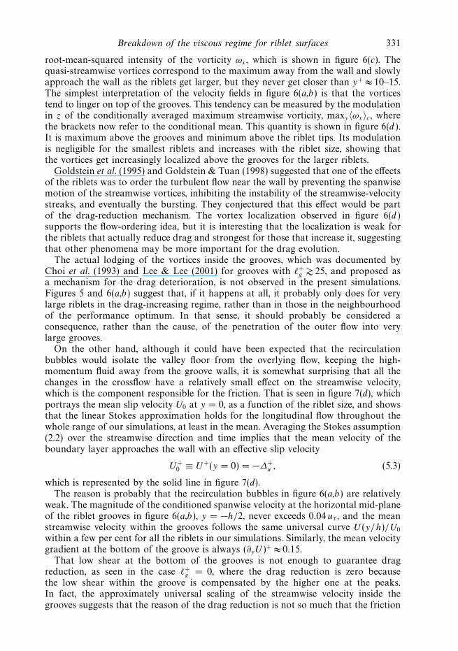
On the other hand, although it could have been expected that the recirculationbubbles would isolate the valley floor from the overlying flow, keeping the high-momentum fluid away from the groove walls, it is somewhat surprising that all thechanges in the crossflow have a relatively small effect on the streamwise velocity,which is the component responsible for the friction. That is seen in figure 7(d), whichportrays the mean slip velocity U0 at y = 0, as a function of the riblet size, and showsthat the linear Stokes approximation holds for the longitudinal flow throughout thewhole range of our simulations, at least in the mean. Averaging the Stokes assumption(2.2) over the streamwise direction and time implies that the mean velocity of theboundary layer approaches the wall with an effective slip velocity

U+0 ≡ U+(y = 0) = −∆+

u , (5.3)

which is represented by the solid line in figure 7(d).The reason is probably that the recirculation bubbles in figure 6(a,b) are relatively

weak. The magnitude of the conditioned spanwise velocity at the horizontal mid-planeof the riblet grooves in figure 6(a,b), y = −h/2, never exceeds 0.04 uτ , and the meanstreamwise velocity within the grooves follows the same universal curve U (y/h)/U0

within a few per cent for all the riblets in our simulations. Similarly, the mean velocitygradient at the bottom of the groove is always (∂yU )+ ≈ 0.15.

That low shear at the bottom of the grooves is not enough to guarantee dragreduction, as seen in the case �+

g = 0, where the drag reduction is zero becausethe low shear within the groove is compensated by the higher one at the peaks.In fact, the approximately universal scaling of the streamwise velocity inside thegrooves suggests that the reason of the drag reduction is not so much that the friction

332 R. Garcıa-Mayoral and J. Jimenez

10

1

2(a)

(d) (e)

(b) (c)

z/s z/s z/s

τ+vi

sc

0 1

0

0.5

τ+uv

10

1

2

τ+to

t

10 200

2

4

�+g �+

g

U+ 0

0 10 20

–0.1

0

0.1

∆τ+

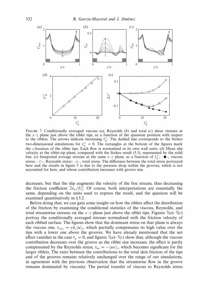
Figure 7. Conditionally averaged viscous (a), Reynolds (b) and total (c) shear stresses atthe x–z plane just above the riblet tips, as a function of the spanwise position with respectto the riblets. The arrows indicate increasing �+

g . The dashed line corresponds to the Stokes

two-dimensional simulations for �+g = 0. The rectangles at the bottom of the figures mark

the z-location of the riblet tips. Each flow is normalized in its own wall units. (d) Mean slipvelocity at the riblet-tip plane, compared with the Stokes result (5.3), represented by the solidline. (e) Integrated average stresses at the same x–z plane, as a function of �+

g ; –�–, viscousstress; –�–, Reynolds stress; –�–, total stress. The difference between the total stress portrayedhere and the results in figure 5 is due to the pressure drop within the grooves, which is notaccounted for here, and whose contribution increases with groove size.

decreases, but that the slip augments the velocity of the free stream, thus decreasingthe friction coefficient 2τw/U 2

δ . Of course, both interpretations are essentially thesame, depending on the units used to express the result, and the question will beexamined quantitatively in § 5.2.

Before doing that, we can gain some insight on how the riblets affect the distributionof the friction by examining the conditional statistics of the viscous, Reynolds, andtotal streamwise stresses on the x–z plane just above the riblet tips. Figures 7(a)–7(c)portray the conditionally averaged stresses normalized with the friction velocity ofeach ribbed surface. The figures show that the dominant stress on that plane is alwaysthe viscous one, τvisc = ν∂y〈u〉c, which partially compensates its high value over thetips with a lower one above the grooves. We have already mentioned that the neteffect vanishes in the case �g = 0, and figures 7(a)–7(c) show that, although the viscouscontribution decreases over the groove as the riblet size increases, the effect is partlycompensated by the Reynolds stress, τuv = −〈uv〉c, which becomes significant for thelarger riblets. The ratio between the contributions to the total skin friction of the tipsand of the grooves remains relatively unchanged over the range of our simulations,in agreement with the previous observation that the streamwise flow in the grooveremains dominated by viscosity. The partial transfer of viscous to Reynolds stress

Breakdown of the viscous regime for riblet surfaces 333

λz+

λx+

101

102

102 103

λx+

102 103

λx+

102 103

λx+

102 103

(a) (b) (c) (d)

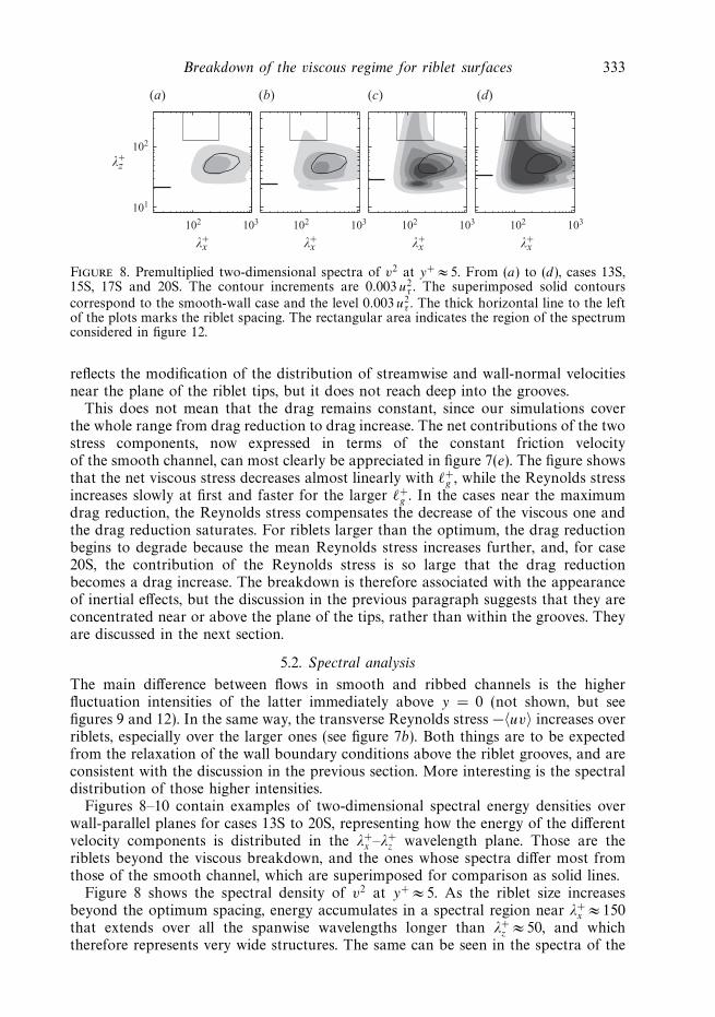
Figure 8. Premultiplied two-dimensional spectra of v2 at y+ ≈ 5. From (a) to (d), cases 13S,15S, 17S and 20S. The contour increments are 0.003 u2

τ . The superimposed solid contourscorrespond to the smooth-wall case and the level 0.003 u2

τ . The thick horizontal line to the leftof the plots marks the riblet spacing. The rectangular area indicates the region of the spectrumconsidered in figure 12.

reflects the modification of the distribution of streamwise and wall-normal velocitiesnear the plane of the riblet tips, but it does not reach deep into the grooves.

This does not mean that the drag remains constant, since our simulations coverthe whole range from drag reduction to drag increase. The net contributions of the twostress components, now expressed in terms of the constant friction velocityof the smooth channel, can most clearly be appreciated in figure 7(e). The figure showsthat the net viscous stress decreases almost linearly with �+

g , while the Reynolds stressincreases slowly at first and faster for the larger �+

g . In the cases near the maximumdrag reduction, the Reynolds stress compensates the decrease of the viscous one andthe drag reduction saturates. For riblets larger than the optimum, the drag reductionbegins to degrade because the mean Reynolds stress increases further, and, for case20S, the contribution of the Reynolds stress is so large that the drag reductionbecomes a drag increase. The breakdown is therefore associated with the appearanceof inertial effects, but the discussion in the previous paragraph suggests that they areconcentrated near or above the plane of the tips, rather than within the grooves. Theyare discussed in the next section.

5.2. Spectral analysis

The main difference between flows in smooth and ribbed channels is the higherfluctuation intensities of the latter immediately above y = 0 (not shown, but seefigures 9 and 12). In the same way, the transverse Reynolds stress −〈uv〉 increases overriblets, especially over the larger ones (see figure 7b). Both things are to be expectedfrom the relaxation of the wall boundary conditions above the riblet grooves, and areconsistent with the discussion in the previous section. More interesting is the spectraldistribution of those higher intensities.

Figures 8–10 contain examples of two-dimensional spectral energy densities overwall-parallel planes for cases 13S to 20S, representing how the energy of the differentvelocity components is distributed in the λ+

x –λ+z wavelength plane. Those are the

riblets beyond the viscous breakdown, and the ones whose spectra differ most fromthose of the smooth channel, which are superimposed for comparison as solid lines.

Figure 8 shows the spectral density of v2 at y+ ≈ 5. As the riblet size increasesbeyond the optimum spacing, energy accumulates in a spectral region near λ+

x ≈ 150that extends over all the spanwise wavelengths longer than λ+

z ≈ 50, and whichtherefore represents very wide structures. The same can be seen in the spectra of the

334 R. Garcıa-Mayoral and J. Jimenez

λz+

101

102

λx+

102 103

λx+

102 103

λx+

102 103

λx+

102 103

(a) (b) (c) (d)

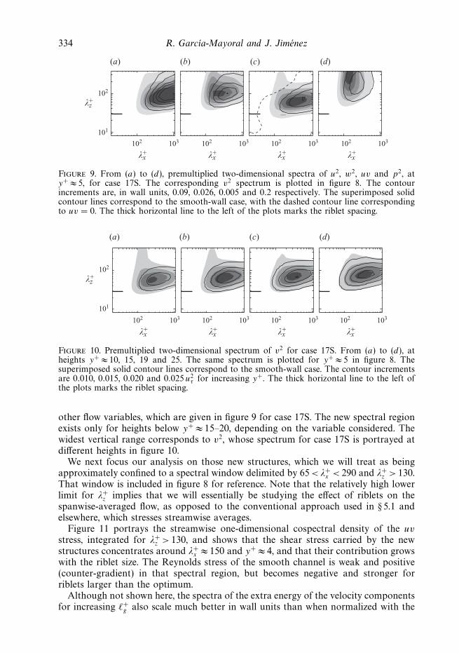
Figure 9. From (a) to (d), premultiplied two-dimensional spectra of u2, w2, uv and p2, aty+ ≈ 5, for case 17S. The corresponding v2 spectrum is plotted in figure 8. The contourincrements are, in wall units, 0.09, 0.026, 0.005 and 0.2 respectively. The superimposed solidcontour lines correspond to the smooth-wall case, with the dashed contour line correspondingto uv = 0. The thick horizontal line to the left of the plots marks the riblet spacing.

λz+

101

102

λx+

102 103

λx+

102 103

λx+

102 103

λx+

102 103

(a) (b) (c) (d)

Figure 10. Premultiplied two-dimensional spectrum of v2 for case 17S. From (a) to (d), atheights y+ ≈ 10, 15, 19 and 25. The same spectrum is plotted for y+ ≈ 5 in figure 8. Thesuperimposed solid contour lines correspond to the smooth-wall case. The contour incrementsare 0.010, 0.015, 0.020 and 0.025 u2

τ for increasing y+. The thick horizontal line to the left ofthe plots marks the riblet spacing.

other flow variables, which are given in figure 9 for case 17S. The new spectral regionexists only for heights below y+ ≈ 15–20, depending on the variable considered. Thewidest vertical range corresponds to v2, whose spectrum for case 17S is portrayed atdifferent heights in figure 10.

We next focus our analysis on those new structures, which we will treat as beingapproximately confined to a spectral window delimited by 65< λ+

x < 290 and λ+z > 130.

That window is included in figure 8 for reference. Note that the relatively high lowerlimit for λ+

z implies that we will essentially be studying the effect of riblets on thespanwise-averaged flow, as opposed to the conventional approach used in § 5.1 andelsewhere, which stresses streamwise averages.

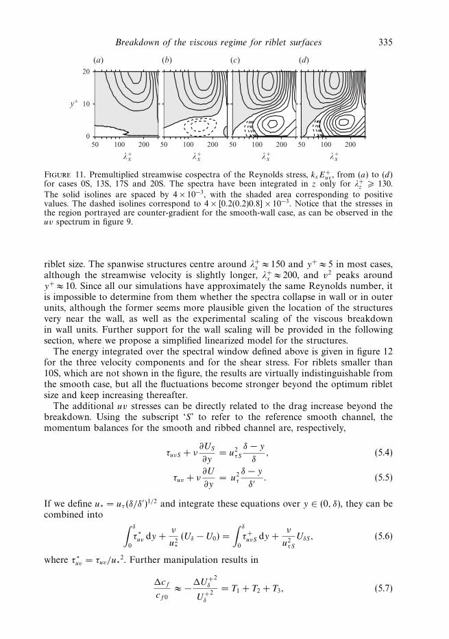
Figure 11 portrays the streamwise one-dimensional cospectral density of the uv

stress, integrated for λ+z > 130, and shows that the shear stress carried by the new

structures concentrates around λ+x ≈ 150 and y+ ≈ 4, and that their contribution grows

with the riblet size. The Reynolds stress of the smooth channel is weak and positive(counter-gradient) in that spectral region, but becomes negative and stronger forriblets larger than the optimum.

Although not shown here, the spectra of the extra energy of the velocity componentsfor increasing �+

g also scale much better in wall units than when normalized with the

Breakdown of the viscous regime for riblet surfaces 335

50 100 2000

10

20

λx+ λx

+ λx+ λx

+

y+

50 100 200 50 100 200 50 100 200

(a) (b) (c) (d)

Figure 11. Premultiplied streamwise cospectra of the Reynolds stress, kxE+uv , from (a) to (d)

for cases 0S, 13S, 17S and 20S. The spectra have been integrated in z only for λ+z � 130.

The solid isolines are spaced by 4 × 10−3, with the shaded area corresponding to positivevalues. The dashed isolines correspond to 4 × [0.2(0.2)0.8] × 10−3. Notice that the stresses inthe region portrayed are counter-gradient for the smooth-wall case, as can be observed in theuv spectrum in figure 9.

riblet size. The spanwise structures centre around λ+x ≈ 150 and y+ ≈ 5 in most cases,

although the streamwise velocity is slightly longer, λ+x ≈ 200, and v2 peaks around

y+ ≈ 10. Since all our simulations have approximately the same Reynolds number, itis impossible to determine from them whether the spectra collapse in wall or in outerunits, although the former seems more plausible given the location of the structuresvery near the wall, as well as the experimental scaling of the viscous breakdownin wall units. Further support for the wall scaling will be provided in the followingsection, where we propose a simplified linearized model for the structures.

The energy integrated over the spectral window defined above is given in figure 12for the three velocity components and for the shear stress. For riblets smaller than10S, which are not shown in the figure, the results are virtually indistinguishable fromthe smooth case, but all the fluctuations become stronger beyond the optimum ribletsize and keep increasing thereafter.

The additional uv stresses can be directly related to the drag increase beyond thebreakdown. Using the subscript ‘S’ to refer to the reference smooth channel, themomentum balances for the smooth and ribbed channel are, respectively,

τuvS + ν∂US

∂y= u2

τS

δ − y

δ, (5.4)

τuv + ν∂U

∂y= u2

τ

δ − y

δ′ . (5.5)

If we define u∗ = uτ (δ/δ′)1/2 and integrate these equations over y ∈ (0, δ), they can be

combined into ∫ δ

0

τ ∗uv dy +

ν

u2∗(Uδ − U0) =

∫ δ

0

τ+uvS dy +

ν

u2τS

UδS, (5.6)

where τ ∗uv = τuv/u∗

2. Further manipulation results in

�cf

cf 0

≈ −�U+δ

2

U+δ

2= T1 + T2 + T3, (5.7)

336 R. Garcıa-Mayoral and J. Jimenez

0

0.4(a)

(c)

(b)

(d)

u+2

w+2

0

0.1

v+2

250

0.4

y+ y+0 25

0

0.03

−(uv)+

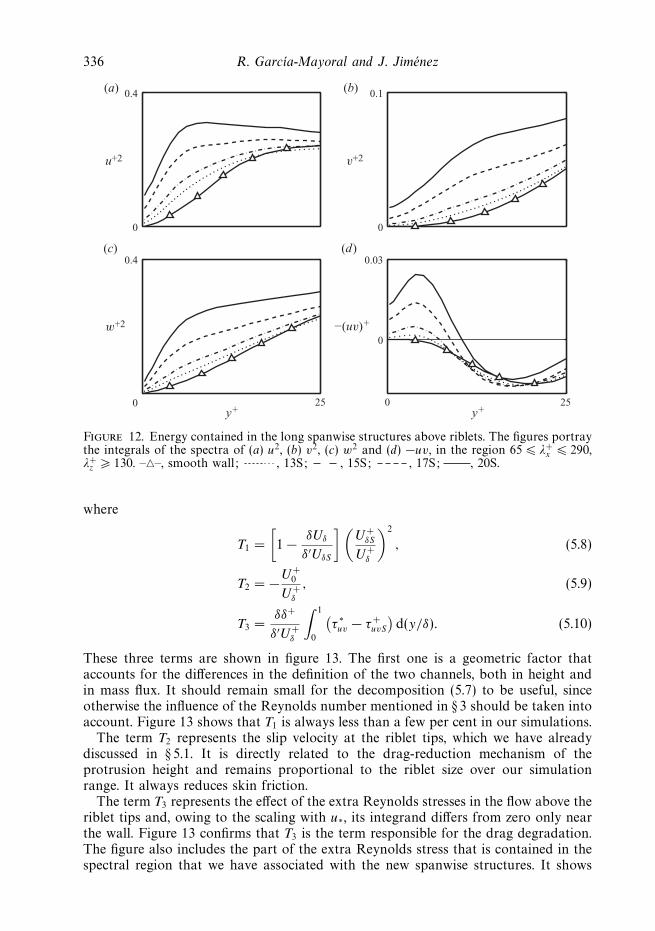
Figure 12. Energy contained in the long spanwise structures above riblets. The figures portraythe integrals of the spectra of (a) u2, (b) v2, (c) w2 and (d) −uv, in the region 65 � λ+

x � 290,λ+

z � 130. –�–, smooth wall; , 13S; , 15S; , 17S; , 20S.

where

T1 =

[1 − δUδ

δ′UδS

](U+

δS

U+δ

)2

, (5.8)

T2 = −U+0

U+δ

, (5.9)

T3 =δδ+

δ′U+δ

∫ 1

0

(τ ∗uv − τ+

uvS

)d(y/δ). (5.10)

These three terms are shown in figure 13. The first one is a geometric factor thataccounts for the differences in the definition of the two channels, both in height andin mass flux. It should remain small for the decomposition (5.7) to be useful, sinceotherwise the influence of the Reynolds number mentioned in § 3 should be taken intoaccount. Figure 13 shows that T1 is always less than a few per cent in our simulations.

The term T2 represents the slip velocity at the riblet tips, which we have alreadydiscussed in § 5.1. It is directly related to the drag-reduction mechanism of theprotrusion height and remains proportional to the riblet size over our simulationrange. It always reduces skin friction.

The term T3 represents the effect of the extra Reynolds stresses in the flow above theriblet tips and, owing to the scaling with u∗, its integrand differs from zero only nearthe wall. Figure 13 confirms that T3 is the term responsible for the drag degradation.The figure also includes the part of the extra Reynolds stress that is contained in thespectral region that we have associated with the new spanwise structures. It shows

Breakdown of the viscous regime for riblet surfaces 337

0 10 20

−0.15

0

0.15

�+g

�c f

/cf0

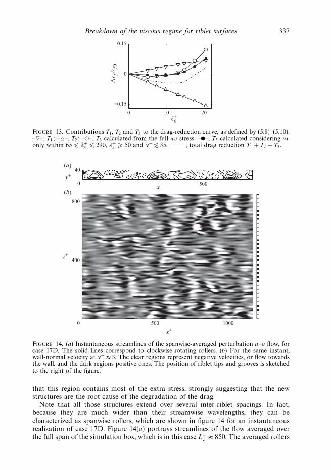
Figure 13. Contributions T1, T2 and T3 to the drag-reduction curve, as defined by (5.8)–(5.10).–�–, T1; –�–, T2; –�–, T3 calculated from the full uv stress. –�–, T3 calculated considering uvonly within 65 � λ+

x � 290, λ+z � 50 and y+ � 35. , total drag reduction T1 + T2 + T3.

5000

40(a)

(b)x+

y+

z+

x+

500 10000

400

800

Figure 14. (a) Instantaneous streamlines of the spanwise-averaged perturbation u–v flow, forcase 17D. The solid lines correspond to clockwise-rotating rollers. (b) For the same instant,wall-normal velocity at y+ ≈ 3. The clear regions represent negative velocities, or flow towardsthe wall, and the dark regions positive ones. The position of riblet tips and grooves is sketchedto the right of the figure.

that this region contains most of the extra stress, strongly suggesting that the newstructures are the root cause of the degradation of the drag.

Note that all those structures extend over several inter-riblet spacings. In fact,because they are much wider than their streamwise wavelengths, they can becharacterized as spanwise rollers, which are shown in figure 14 for an instantaneousrealization of case 17D. Figure 14(a) portrays streamlines of the flow averaged overthe full span of the simulation box, which is in this case L+

z ≈ 850. The averaged rollers

338 R. Garcıa-Mayoral and J. Jimenez

6

8

10

12

λz+

101

102

λx+

102 103

λx+

102 103

λx+

102 103

λx+

102 103

(a) (b) (c) (d)

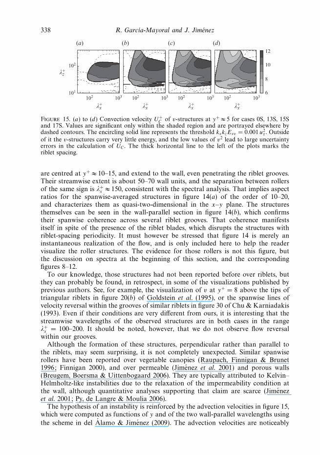
Figure 15. (a) to (d) Convection velocity U+C of v-structures at y+ ≈ 5 for cases 0S, 13S, 15S

and 17S. Values are significant only within the shaded region and are portrayed elsewhere bydashed contours. The encircling solid line represents the threshold kxkzEvv = 0.001 u2

τ . Outsideof it the v-structures carry very little energy, and the low values of v2 lead to large uncertaintyerrors in the calculation of UC . The thick horizontal line to the left of the plots marks theriblet spacing.

are centred at y+ ≈ 10–15, and extend to the wall, even penetrating the riblet grooves.Their streamwise extent is about 50–70 wall units, and the separation between rollersof the same sign is λ+

x ≈ 150, consistent with the spectral analysis. That implies aspectratios for the spanwise-averaged structures in figure 14(a) of the order of 10–20,and characterizes them as quasi-two-dimensional in the x–y plane. The structuresthemselves can be seen in the wall-parallel section in figure 14(b), which confirmstheir spanwise coherence across several riblet grooves. That coherence manifestsitself in spite of the presence of the riblet blades, which disrupts the structures withriblet-spacing periodicity. It must however be stressed that figure 14 is merely aninstantaneous realization of the flow, and is only included here to help the readervisualize the roller structures. The evidence for those rollers is not this figure, butthe discussion on spectra at the beginning of this section, and the correspondingfigures 8–12.

To our knowledge, those structures had not been reported before over riblets, butthey can probably be found, in retrospect, in some of the visualizations published byprevious authors. See, for example, the visualization of v at y+ = 8 above the tips oftriangular riblets in figure 20(b) of Goldstein et al. (1995), or the spanwise lines ofvelocity reversal within the grooves of similar riblets in figure 30 of Chu & Karniadakis(1993). Even if their conditions are very different from ours, it is interesting that thestreamwise wavelengths of the observed structures are in both cases in the rangeλ+

x = 100–200. It should be noted, however, that we do not observe flow reversalwithin our grooves.

Although the formation of these structures, perpendicular rather than parallel tothe riblets, may seem surprising, it is not completely unexpected. Similar spanwiserollers have been reported over vegetable canopies (Raupach, Finnigan & Brunet1996; Finnigan 2000), and over permeable (Jimenez et al. 2001) and porous walls(Breugem, Boersma & Uittenbogaard 2006). They are typically attributed to Kelvin–Helmholtz-like instabilities due to the relaxation of the impermeability condition atthe wall, although quantitative analyses supporting that claim are scarce (Jimenezet al. 2001; Py, de Langre & Moulia 2006).

The hypothesis of an instability is reinforced by the advection velocities in figure 15,which were computed as functions of y and of the two wall-parallel wavelengths using

the scheme in del Alamo & Jimenez (2009). The advection velocities are noticeably

Breakdown of the viscous regime for riblet surfaces 339

lower for the spanwise structures than for the spectral region of the regular flow. Nearthe wall, for y+ � 15, the latter are of order 10 uτ , while the former are 6–8 uτ . Theeffect becomes more noticeable for the larger riblets and suggests that the structuresare not advected by the local flow but correspond to unstable eigenstructures with anextended y-support. The linearized stability of this part of the flow is analysed in thenext section.

6. A linear stability modelIn this section we propose a model for the aforementioned Kelvin–Helmholtz-like

instability, which captures the essential physics involved, including its relation withthe riblet geometry.

Since the spanwise rollers are quasi-two-dimensional in x–y, we restrict ourselvesto two-dimensional solutions of the linearized Navier–Stokes equations. Denoting byprime superscripts the derivatives with respect to y of the base flow U , we have

∂u

∂t+ U

∂u

∂x+ v U ′ = −∂p

∂x, (6.1)

∂v

∂t+ U

∂v

∂x= −∂p

∂y, (6.2)

where the lowercase symbols are perturbations. The viscous terms are omittedfor simplicity, since we are looking for essentially inviscid Kelvin–Helmholtz-like instabilities, on which viscosity would only have a damping effect. Imposingincompressibility, the Rayleigh equation for v is(

∂

∂t+ U

∂

∂x

)∇2v = U ′′ ∂v

∂x, (6.3)

for which we seek solutions of the form v = v(y) exp[iα(x − ct)].The problem is solved in a notional domain between the two planes at the riblet

tips, y ∈ (0, 2δ), and the two dimensionality is preserved by using z-independentboundary conditions that account for the presence of riblets in a spanwise-averagedsense.

Consider the lower wall. The first step is to describe the flow along the grooves,where variables will be denoted by the subscript ‘g’. This part of the problem takesplace in the real groove geometry in y ∈ (−h, 0). Since we are interested in theonset of the instability, we will assume that the effective Reynolds number is lowand that the longitudinal flow along the grooves satisfies approximately the viscousStokes equations. Note that this approximation is consistent with the behaviour ofthe conditioned average streamwise velocity in the direct simulations. We also assumethat the longitudinal velocity gradients within the grooves are small with respectto the transverse ones and that the dynamical effect of the transverse velocitiescan be neglected. In particular, we neglect the variation across the groove of thestreamwise pressure gradient and the streamwise contributions of the viscous term.The streamwise momentum equation within the groove is then

∂2ug

∂y2+

∂2ug

∂z2≡ ∇2

yzug =1

ν

dpg

dx. (6.4)

The velocity satisfies ug = 0 at the groove walls, and we will assume that ∂ug/∂y = 0at the plane of the riblet tips. Note that the last boundary condition refers to theperturbations and is not equivalent to assuming that the mean velocity gradient

340 R. Garcıa-Mayoral and J. Jimenez

vanishes at y = 0. The assumption is that the streamwise pressure gradient ispredominantly balanced by the viscous stresses at the groove walls, rather than bythose at the interface with the outer flow. That assumption is especially adequate forsmall riblets but has to be justified a posteriori. For example, consider the solutionsin figure 19, which are obtained by coupling the outer flow perturbations to grooveswith the no-slip condition at their top interface.The length scales of the perturbationsat y = 0 scale in wall units, essentially because the true outer boundary conditionfor the flow within the grooves, ∂ug/∂y = 0, should have been applied at y → ∞and involves the overlying velocity profile. In the particular case of the figure,(∂u/∂y)+ ≈ 0.10u+|y=0. On the other hand, the gradients over the walls of the grooves,not shown in the figure, are inversely proportional to the groove diameter. For atypical groove, (∂ug/∂n)+ ≈ 4u+|y=0/�

+g . The assumption that the shear at the groove

top can be neglected with respect to that at the walls is valid as long as �+g � 40,

which is enough to explore the onset of the instability. The same assumption alsoallows us to use an inviscid approximation for the outside flow, even while using aStokes model for the flow in the groove.

The coupling of the grooves and the body of the channel is made by assumingthat the outside pressure drives the flow along the grooves and that the transpirationvelocity at y = 0 is due to the longitudinal variations of the volumetric flux of ug .

Since the right-hand side of (6.4) is only a function of x and t , we can write

ug = −(

1

ν

dpg

dx

)f (y, z), (6.5)

where f (y, z) verifies

∇2yzf = −1, (6.6)

with boundary conditions identical to those for ug , so that f depends only onthe groove geometry. The streamwise variation of ug is related to the z-averagedtranspiration velocity v at y = 0 by integrating the continuity equation over thegroove cross-section:

∂

∂x

∫ ∫Ag

ug dy dz +

∫s

vg|y=0 dz = 0, (6.7)

v|y=0 = −s−1 ∂

∂x

∫ ∫Ag

ug dy dz. (6.8)

Note that s in (6.8) is the distance between neighbouring riblets, not the width ofthe groove, because v needs to be averaged over the whole y = 0 plane to be usedas a boundary condition for (6.3). Introducing (6.5) into (6.8), and assuming thatp|y=0 =pg , we obtain

∂2p

∂x2

∣∣∣∣y=0

=ν

L3w

v|y=0 , (6.9)

where

L3w = s−1

∫ ∫Ag

f dy dz. (6.10)

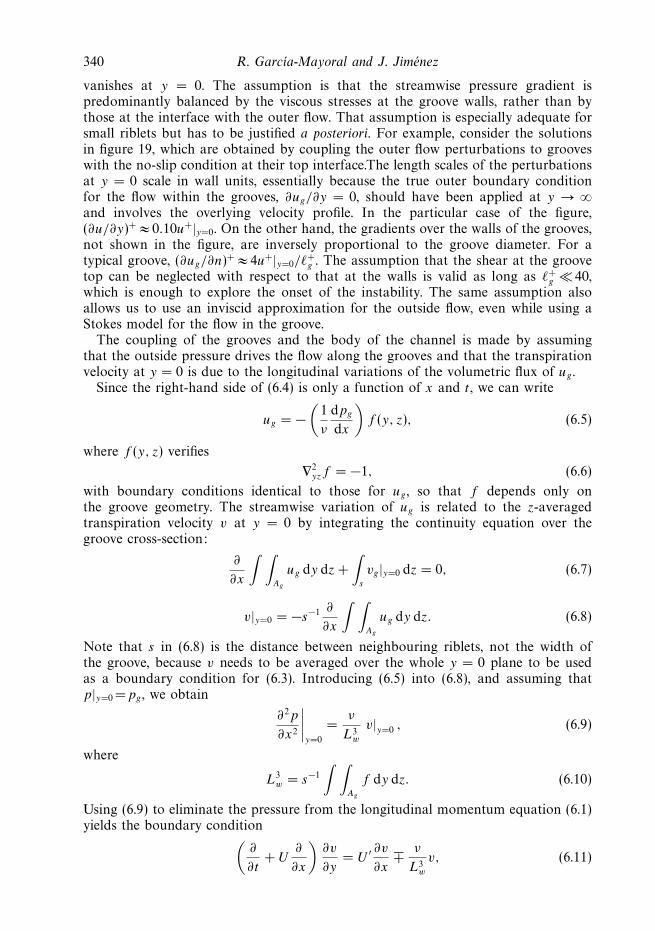
Using (6.9) to eliminate the pressure from the longitudinal momentum equation (6.1)yields the boundary condition(

∂

∂t+ U

∂

∂x

)∂v

∂y= U ′ ∂v

∂x∓ ν

L3w

v, (6.11)

Breakdown of the viscous regime for riblet surfaces 341

0.2 0.6 1.0

0.3

0.4

�g /s

Lw

/�g

Figure 16. Value of the parameter Lw in (6.10), compared with �g , for: �, triangular; �,scalloped; �, blade riblets. The solid lines connect riblets of the same type with equal tip widthand variable depth-to-width ratio, ranging from h/s = 0.2 to 1.0, while the arrow indicatesdecreasing tip width, from t/s = 0.5 to 0.02.

where the two signs of the last term apply respectively to the upper and lower walls.If we denote the values of the mean profile at y = 0 by U0 and U ′

0, (6.11) can berewritten as

(U0 − c)∂v

∂y=

(U ′

0 ± iν

αL3w

)v, (6.12)

which shows that U0 changes only the real part of the advection velocity by a fixedamount. From the point of view of the stability characteristics of the flow, it can beassumed to be zero. The solutions of the system (6.3)–(6.12) depend only on the baseflow profile U (y) and on the characteristic penetration length Lw , which is linked tothe groove cross-section through the integral in (6.10). The viscosity can be eliminatedby expressing everything in wall units. It turns out that, for conventional geometries,Lw is closely linked to our empirical parameter �g =

√Ag . For example, figure 16

compiles values of Lw computed for triangular, rectangular and scalloped riblets, withdepth-to-width ratios between 0.2 and 1.0, and tip widths between 2 % and 50 % oftheir spacing. It shows that, at least within that range of geometries, �g and Lw areessentially proportional to each other. The approximation

�g ≈ 2.8 Lw (6.13)

has less than 10 % error for conventional sharp riblets with h/s � 0.4, providingsome theoretical justification for the empirical scaling of the breakdown size discussedin § 3.

6.1. The piecewise-linear profile

Before turning our attention to the quantitative analysis of the instability induced bythe riblets on a turbulent velocity profile, it is useful to apply the previous formulationto a piecewise-linear base flow

U (y) = U∞ y/H, y < H,

= U∞, y � H,

}(6.14)

where the basic mechanisms are more easily understood. The solutions of (6.3) canthen be expressed as combinations of exponentials, exp(±αy), which are continuous

342 R. Garcıa-Mayoral and J. Jimenez

100 101 102 103 100 101 102 1030

0.1

0.2

(a) (b)

λx/H λx/H

σI

0

0.5

1.0

c R/U

∞

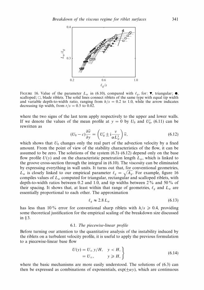
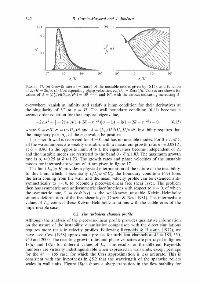
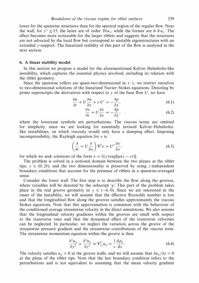
Figure 17. (a) Growth rate σI = Im(σ ) of the unstable modes given by (6.15), as a functionof λx/H = 2π/α. (b) Corresponding phase velocities, cR/U∞ = Re(σ )/α. Curves are shown forvalues of Λ = (L3

w/ν)(U∞α/H 2) = 10[−2(.2)3] and 106, with the arrows indicating increasing Λ.

everywhere, vanish at infinity and satisfy a jump condition for their derivatives atthe singularity of U ′′ at y = H . The wall boundary condition (6.11) becomes asecond-order equation for the temporal eigenvalue,

−2Λσ 2 +[

− 2i + Λ(1 + 2α − e−2α)]σ + (Λ − i)(1 − 2α − e−2α) = 0, (6.15)

where α = αH , σ = (c/U∞) α and Λ = (Lw/H )3(U∞H/ν) α. Instability requires thatthe imaginary part, σI , of the eigenvalue be positive.

The smooth wall is recovered for Λ = 0 and has no unstable modes. For 0 <Λ � 1,all the wavenumbers are weakly unstable, with a maximum growth rate, σI ≈ 0.081Λ,at α = 0.80. In the opposite limit, Λ � 1, the eigenvalues become independent of Λ,and the unstable modes are restricted to the band 0< α � 1.83. The maximum growthrate is σI ≈ 0.25 at α ≈ 1.23. The growth rates and phase velocities of the unstablemodes for intermediate values of Λ are given in figure 17.

The limit Lw � H provides a physical interpretation of the nature of the instability.In this limit, which is essentially ν/L3

wα � U ′0, the boundary condition (6.9) loses

the term coming from the wall, and the mean velocity profile can be extended anti-symmetrically to y < 0, to become a piecewise-linear free shear layer. The problemthen has symmetric and antisymmetric eigenfunctions with respect to y = 0, of whichthe symmetric one, v = cosh(αy), is the well-known unstable Kelvin–Helmholtzsinuous deformation of the free shear layer (Drazin & Reid 1981). The intermediatevalues of Lw connect these Kelvin–Helmholtz solutions with the stable ones of theimpermeable case.

6.2. The turbulent channel profile

Although the analysis of the piecewise-linear profile provides qualitative informationon the nature of the instability, quantitative comparison with the direct simulationsrequires more realistic velocity profiles. Following Reynolds & Hussain (1972), wehave used Cess (1958) approximate profiles for turbulent channels at δ+ = 185, 550,950 and 2000. The resulting growth rates and phase velocities are portrayed in figures18(a) and 18(b) for different values of Lw . The results for the different Reynoldsnumbers are virtually indistinguishable when expressed in wall units, except perhapsfor the δ+ = 185 case, for which the Cess approximation is less accurate. This isconsistent with the hypothesis in § 5.2 that the wavelength of the spanwise rollersscales in wall units. Figure 18(c) shows a sharp transition in the flow stability for

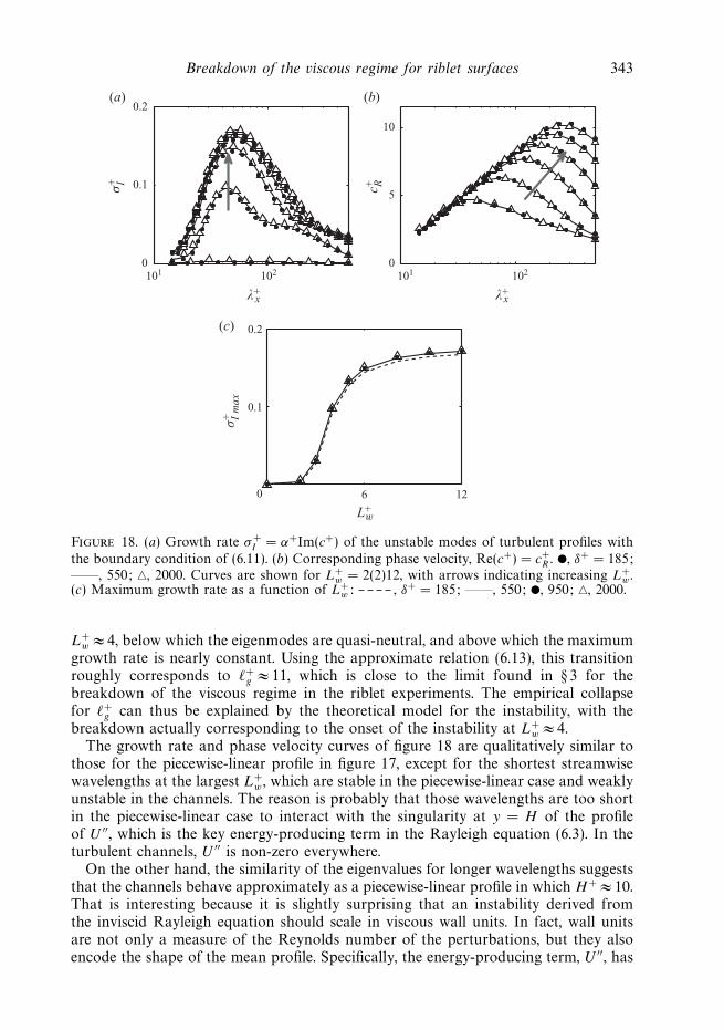
Breakdown of the viscous regime for riblet surfaces 343

101 1020

0.1

0.2(a) (b)

(c)

λ+x

101 102

λ+x

σ+ I

0

5

10

c+ R

6 120

0.1

0.2

L+w

σ+ I

max

Figure 18. (a) Growth rate σ+I = α+Im(c+) of the unstable modes of turbulent profiles with

the boundary condition of (6.11). (b) Corresponding phase velocity, Re(c+) = c+R . �, δ+ = 185;

——, 550; �, 2000. Curves are shown for L+w = 2(2)12, with arrows indicating increasing L+

w .(c) Maximum growth rate as a function of L+

w: , δ+ = 185; ——, 550; �, 950; �, 2000.

L+w ≈ 4, below which the eigenmodes are quasi-neutral, and above which the maximum

growth rate is nearly constant. Using the approximate relation (6.13), this transitionroughly corresponds to �+

g ≈ 11, which is close to the limit found in § 3 for thebreakdown of the viscous regime in the riblet experiments. The empirical collapsefor �+

g can thus be explained by the theoretical model for the instability, with thebreakdown actually corresponding to the onset of the instability at L+

w ≈ 4.The growth rate and phase velocity curves of figure 18 are qualitatively similar to

those for the piecewise-linear profile in figure 17, except for the shortest streamwisewavelengths at the largest L+

w , which are stable in the piecewise-linear case and weaklyunstable in the channels. The reason is probably that those wavelengths are too shortin the piecewise-linear case to interact with the singularity at y = H of the profileof U ′′, which is the key energy-producing term in the Rayleigh equation (6.3). In theturbulent channels, U ′′ is non-zero everywhere.

On the other hand, the similarity of the eigenvalues for longer wavelengths suggeststhat the channels behave approximately as a piecewise-linear profile in which H+ ≈ 10.That is interesting because it is slightly surprising that an instability derived fromthe inviscid Rayleigh equation should scale in viscous wall units. In fact, wall unitsare not only a measure of the Reynolds number of the perturbations, but they alsoencode the shape of the mean profile. Specifically, the energy-producing term, U ′′, has

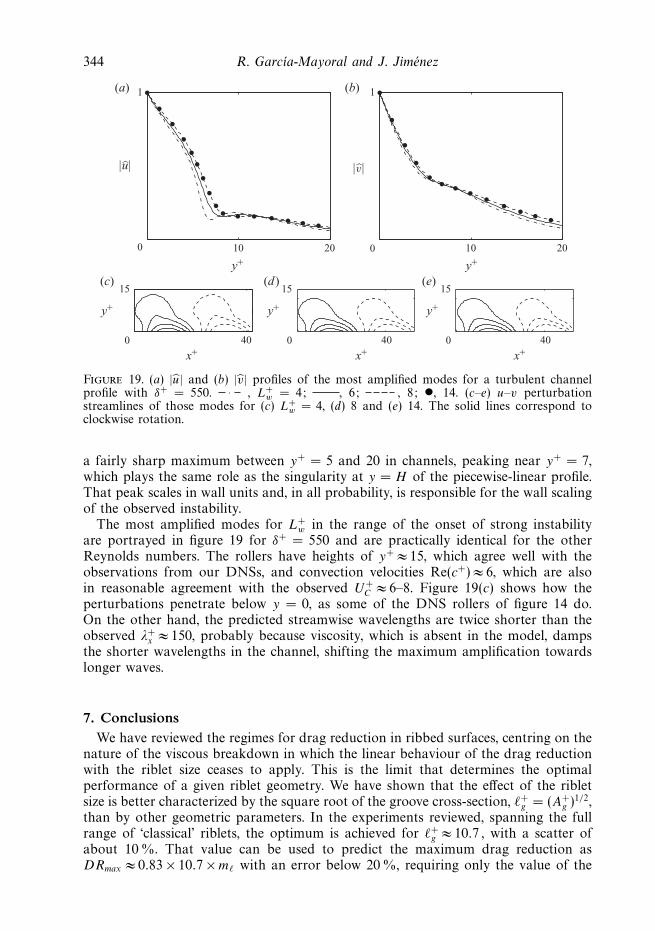
344 R. Garcıa-Mayoral and J. Jimenez

10 200

1(a)

(c) (d) (e)

(b)

|u|

10 200

1

|v|

400

15

y+

0

15

y+

0

15

y+

y+

x+40

x+40

x+

y+

Figure 19. (a) |u| and (b) |v| profiles of the most amplified modes for a turbulent channelprofile with δ+ = 550. , L+

w = 4; , 6; , 8; •, 14. (c–e) u–v perturbationstreamlines of those modes for (c) L+

w = 4, (d) 8 and (e) 14. The solid lines correspond toclockwise rotation.

a fairly sharp maximum between y+ = 5 and 20 in channels, peaking near y+ = 7,which plays the same role as the singularity at y = H of the piecewise-linear profile.That peak scales in wall units and, in all probability, is responsible for the wall scalingof the observed instability.

The most amplified modes for L+w in the range of the onset of strong instability

are portrayed in figure 19 for δ+ = 550 and are practically identical for the otherReynolds numbers. The rollers have heights of y+ ≈ 15, which agree well with theobservations from our DNSs, and convection velocities Re(c+) ≈ 6, which are alsoin reasonable agreement with the observed U+

C ≈ 6–8. Figure 19(c) shows how theperturbations penetrate below y = 0, as some of the DNS rollers of figure 14 do.On the other hand, the predicted streamwise wavelengths are twice shorter than theobserved λ+

x ≈ 150, probably because viscosity, which is absent in the model, dampsthe shorter wavelengths in the channel, shifting the maximum amplification towardslonger waves.

7. ConclusionsWe have reviewed the regimes for drag reduction in ribbed surfaces, centring on the

nature of the viscous breakdown in which the linear behaviour of the drag reductionwith the riblet size ceases to apply. This is the limit that determines the optimalperformance of a given riblet geometry. We have shown that the effect of the ribletsize is better characterized by the square root of the groove cross-section, �+

g = (A+g )1/2,

than by other geometric parameters. In the experiments reviewed, spanning the fullrange of ‘classical’ riblets, the optimum is achieved for �+

g ≈ 10.7 , with a scatter ofabout 10 %. That value can be used to predict the maximum drag reduction asDRmax ≈ 0.83 × 10.7 × m� with an error below 20 %, requiring only the value of the

Breakdown of the viscous regime for riblet surfaces 345

slope of the drag curve in the viscous regime, obtainable from two-dimensional Stokescomputations.

We have analysed the relationship between performance and riblet size from directnumerical simulations spanning the whole range of riblet behaviours, from dragreduction to drag increase. We have shown that the overlying quasi-streamwisevortices of the turbulent buffer layer tend to get localized above the riblet grooves,but that the vortices do not appear to lodge within the groove over the whole range ofour simulations. Contrary to some previous conjectures, this vortex localization doesnot appear to be involved in the drag-reduction mechanism because it is relativelyweak for the riblets that reduce drag and only becomes strong beyond the viscousbreakdown. We have found that the breakdown coincides with the disappearance ofa transverse recirculating region in the riblet grooves, which weakens and becomesincreasingly asymmetric beyond the observed breakdown of the viscous regime. Thatcoincides with the increase of the Reynolds stresses measured at the plane of theriblet tips, that eventually leads to the degradation of the drag.

On the other hand, the changes of the crossflow do not modify the streamwise flowwithin the grooves substantially, and the slip velocity measured at the riblet tips followsthe prediction of the viscous Stokes regime for the whole range of our simulations.The main change at the time of the breakdown is the appearance of essentiallytwo-dimensional spanwise rollers just above the wall, y+ � 20, with characteristicstreamwise wavelengths λ+

x ≈ 150. They are similar to those found over permeableand porous surfaces and canopies, and can be traced to a Kelvin–Helmholtz-likeinstability associated with the relaxation of the impermeability condition for the wall-normal velocity. The extra Reynolds stresses associated with those rollers account formost of the drag degradation observed past the breakdown of the viscous regime.

We have presented a simplified inviscid model for that instability which confirmsits Kelvin–Helmholtz nature, and which agrees reasonably well with the observedwavelengths and shapes of the perturbation. The parameter that determines the onsetof the instability is a penetration length L+

w that, for conventional riblet geometries, isessentially proportional to the empirical parameter �+

g found above to characterize thebreakdown. The instability turns on for L+

w � 4, which corresponds to the empiricalviscous breakdown point �+

g ≈ 11. Although it might be surprising that an inviscidinstability scales in viscous wall units, this is due to the scaling in wall units of themean velocity profile near the wall.

This work was supported in part by the CICYT grant TRA2009-11498 and bythe sixth framework AVERT program of the European Commission, AST5-CT-2006-030914. R.G.-M. was supported by an FPI fellowship from the Spanish Ministry ofEducation and Science.

REFERENCES

del Alamo, J. C. & Jimenez, J. 2009 Estimation of turbulent convection velocities and correctionsto Taylor’s approximation. J. Fluid Mech. 640, 5–26.

Bechert, D. W. & Bartenwerfer, M. 1989 The viscous flow on surfaces with longitudinal ribs.J. Fluid Mech. 206, 105–129.

Bechert, D. W., Bruse, M., Hage, W., van der Hoeven, J. G. T. & Hoppe, G. 1997 Experimentson drag-reducing surfaces and their optimization with adjustable geometry. J. Fluid Mech.338, 59–87.

Breugem, W. P., Boersma, B. J. & Uittenbogaard, R. E. 2006 The influence of wall permeabilityon turbulent channel flow. J. Fluid Mech. 562, 35–72.

346 R. Garcıa-Mayoral and J. Jimenez

Bruse, M., Bechert, D. W., van der Hoeven, J. G. T., Hage, W. & Hoppe, G. 1993 Experimentswith conventional and with novel adjustable drag-reducing surfaces. In Near-Wall TurbulentFlows (ed. R. M. C. So, C. G. Speziale & B. E. Launder), pp. 719–738. Elsevier.

Cess, R. D. 1958 A survey of the literature on heat transfer in turbulent tube flow. Report 8-0529-R24. Westinghouse Research.

Choi, H., Moin, P. & Kim, J. 1993 Direct numerical simulation of turbulent flow over riblets. J. FluidMech. 255, 503–539.

Chu, D. C. & Karniadakis, G. E. M. 1993 A direct numerical simulation of laminar and turbulentflow over riblet-mounted surfaces. J. Fluid Mech. 250, 1–42.

Clauser, F. H. 1956 The turbulent boundary layer. Adv. Appl. Mech. 4, 1–51.

Drazin, P. G. & Reid, W. H. 1981 Hydrodynamic Stability . Cambridge University Press.

El-Samni, O. A., Chun, H. H. & Yoon, H. S. 2007 Drag reduction of turbulent flow over thinrectangular riblets. Intl J. Engng Sci. 45, 436–454.

Fadlun, E. A., Verzicco, R., Orlandi, P. & Mohd-Yusof, J. 2000 Combined immersed-boundaryfinite-difference methods for three-dimensional complex flow simulations. J. Comput. Phys.161, 35–60.

Ferziger, J. H. & Peric, M. 1996 Computational Methods for Fluid Dynamics . Springer.

Finnigan, J. 2000 Turbulence in plant canopies. Annu. Rev. Fluid Mech. 32, 519–571.

Garcıa-Mayoral, R. & Jimenez, J. 2007 On the effect of riblet geometry on drag reduction. Tech.Rep. ETSIA/MF-072. School of Aeronautics, Universidad Politecnica de Madrid.

Garcıa-Mayoral, R. & Jimenez, J. 2011 Drag reduction by riblets. Phil. Trans. R. Soc. A 369,1412–1427.

Goldstein, D. B., Handler, R. & Sirovich, L. 1995 Direct numerical simulation of turbulent flowover a modeled riblet covered surface. J. Fluid Mech. 302, 333–376.

Goldstein, D. B. & Tuan, T. C. 1998 Secondary flow induced by riblets. J. Fluid Mech. 363, 115–151.

Hoyas, S. & Jimenez, J. 2008 Reynolds number effects on the Reynolds-stress budgets in turbulentchannels. Phys. Fluids 20, 101511.

Iaccarino, G. & Verzicco, R. 2003 Immersed boundary technique for turbulent flow simulations.Appl. Mech. Rev. 56 (3), 331–347.

Itoh, M., Tamano, S., Iguchi, R., Yokota, K., Akino, N., Hino, R. & Kubo, S. 2006 Turbulentdrag reduction by the seal fur surface. Phys. Fluids 18 (6), 065102.

Jimenez, J. 1992 Wall friction and the structure of near-wall turbulence. In 11th Australasian FluidMech. Conf. (ed. M. R. Davis & G. J. Walker), pp. 813–816. Hobart, Australia.

Jimenez, J. 1994 On the structure and control of near wall turbulence. Phys. Fluids 6 (2), 944–953.

Jimenez, J. 2004 Turbulent flows over rough walls. Annu. Rev. Fluid Mech. 36, 173–196.

Jimenez, J. & Pinelli, A. 1999 The autonomous cycle of near wall turbulence. J. Fluid Mech. 389,335–359.

Jimenez, J., Uhlman, M., Pinelli, A. & Kawahara, G. 2001 Turbulent shear flow over active andpassive porous surfaces. J. Fluid Mech. 442, 89–117.

Jung, W. J., Mangiavacchi, N. & Akhavan, R. 1992 Suppression of turbulence in wall-boundedflows by high-frequency spanwise oscillations. Phys. Fluids A 4, 1605–1607.

Kim, J., Moin, P. & Moser, R. D. 1987 Turbulence statistics in fully developed channel flow at lowReynolds number. J. Fluid Mech. 177, 133–166.

Le, H. & Moin, P. 1991 An improvement of fractional step methods for the incompressible Navier–Stokes equations. J. Comput. Phys. 92 (2), 369–379.

Lee, S.-J. & Lee, S.-H. 2001 Flow field analysis of a turbulent boundary layer over a riblet surface.Exp. Fluids 30, 153–166.

Linnick, M. N. & Fasel, H. F. 2005 A high-order immersed interface method for simulatingunsteady incompressible flows on irregular domains. J. Comput. Phys. 204 (1), 157–192.

Luchini, P. 1995 Asymptotic analysis of laminar boundary-layer flow over finely grooved surfaces.Eur. J. Mech. B/Fluids 14, 169–195.

Luchini, P., Manzo, F. & Pozzi, A. 1991 Resistance of a grooved surface to parallel flow andcross-flow. J. Fluid Mech. 228, 87–109.

Nordstrom, J., Mattsson, K. & Swanson, C. 2007 Boundary conditions for a divergence freevelocity-pressure formulation of the Navier–Stokes equations. J. Comput. Phys. 225, 874–890.

Orlandi, P. & Jimenez, J. 1994 On the generation of turbulent wall friction. Phys. Fluids 6, 634–641.

Breakdown of the viscous regime for riblet surfaces 347

Orlandi, P., Leonardi, S. & Antonia, R. A. 2006 Turbulent channel flow with either transverse orlongitudinal roughness elements on one wall. J. Fluid Mech. 561, 279–305.

Py, C., de Langre, E. & Moulia, B. 2006 A frequency lock-in mechanism in the interaction betweenwind and crop canopies. J. Fluid Mech. 568, 425–449.

Raupach, M. R., Finnigan, J. & Brunet, Y. 1996 Coherent eddies and turbulence in vegetationcanopies: the mixing-layer analogy. Boundary-Layer Meteorol. 78, 351–382.

Reynolds, W. C. & Hussain, A. K. M. F. 1972 The mechanics of an organized wave in turbulentshear flow. Part 3. Theoretical models and comparisons with experiments. J. Fluid Mech. 54,263–288.

Roshko, A. 1953 On the development of turbulent wakes from vortex streets. NACA Tech. Note2913.

Simens, M. P., Jimenez, J., Hoyas, S. & Mizuno, Y. 2009 A high-resolution code for turbulentboundary layers. J. Comput. Phys. 228, 4218–4231.

Stalio, E. & Nobile, E. 2003 Direct numerical simulation of heat transfer over riblets. Intl J. HeatFluid Flow 24, 356–371.

Suzuki, Y. & Kasagi, N. 1994 Turbulent drag reduction mechanism above a riblet surface. AIAAJ. 32 (9), 1781–1790.

Tennekes, H. & Lumley, J. L. 1972 A First Course in Turbulence. MIT Press.

Walsh, M. J. 1990a Effect of detailed surface geometry on riblet drag reduction performance.J. Aircraft 27 (6), 572–573.

Walsh, M. J. 1990b Riblets. In Viscous Drag Reduction in Boundary Layers (ed. D. M. Bushnell &J. N. Hefner), pp. 203–261. AIAA.

Walsh, M. J. & Lindemann, A. M. 1984 Optimization and application of riblets for turbulent dragreduction. AIAA Paper 84-0347.

Williamson, C. H. K. 1989 Oblique and parallel modes of vortex shedding in the wake of a circularcylinder at low Reynolds numbers. J. Fluid Mech. 206, 579–627.