HYDRODYNAMIC ANALYSIS OF INTERCEPTORS WITH CFD METHODS

7th Int. Conference on Fast Sea Transportation - FAST 2003 – Ischia, Italy

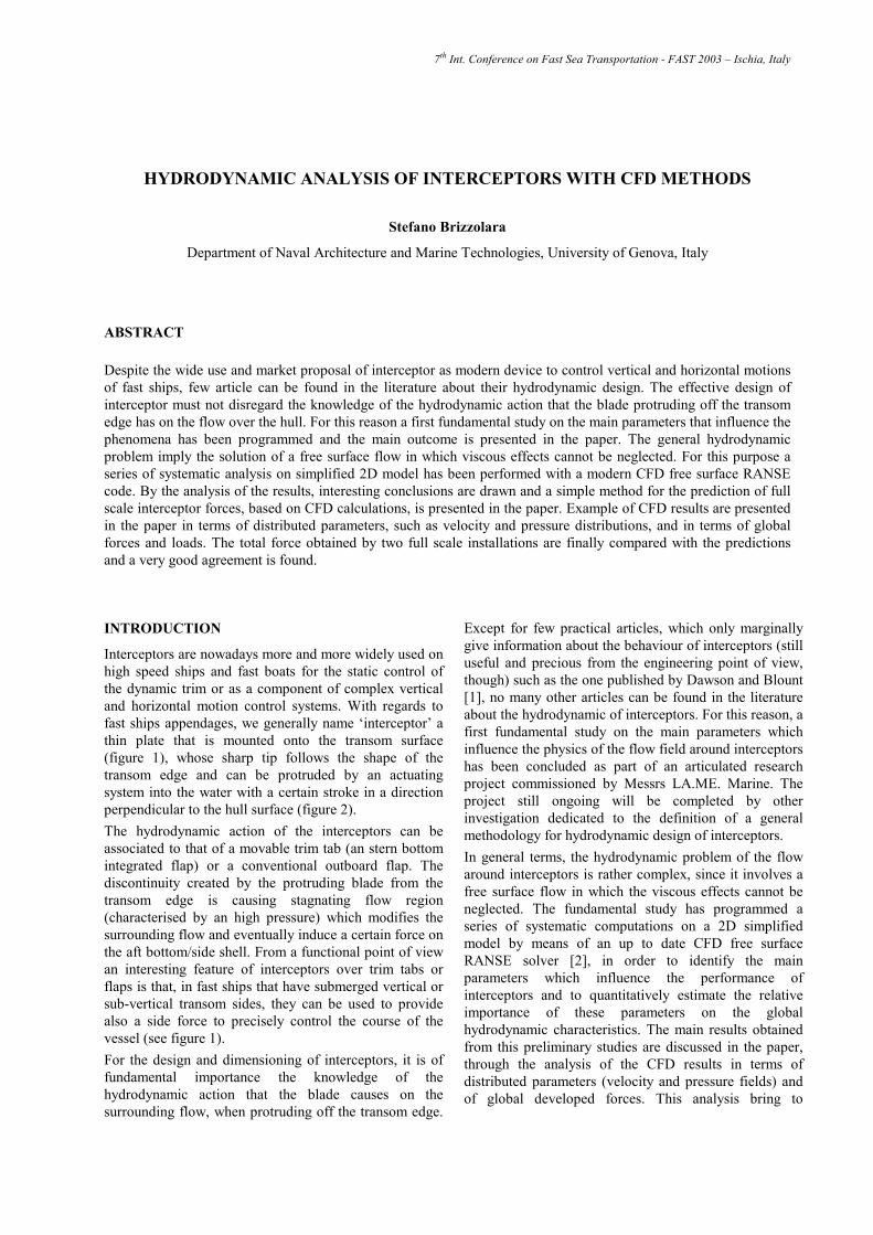
HYDRODYNAMIC ANALYSIS OF INTERCEPTORS WITH CFD METHODS

Stefano Brizzolara

Department of Naval Architecture and Marine Technologies, University of Genova, Italy

ABSTRACT Despite the wide use and market proposal of interceptor as modern device to control vertical and horizontal motions of fast ships, few article can be found in the literature about their hydrodynamic design. The effective design of interceptor must not disregard the knowledge of the hydrodynamic action that the blade protruding off the transom edge has on the flow over the hull. For this reason a first fundamental study on the main parameters that influence the phenomena has been programmed and the main outcome is presented in the paper. The general hydrodynamic problem imply the solution of a free surface flow in which viscous effects cannot be neglected. For this purpose a series of systematic analysis on simplified 2D model has been performed with a modern CFD free surface RANSE code. By the analysis of the results, interesting conclusions are drawn and a simple method for the prediction of full scale interceptor forces, based on CFD calculations, is presented in the paper. Example of CFD results are presented in the paper in terms of distributed parameters, such as velocity and pressure distributions, and in terms of global forces and loads. The total force obtained by two full scale installations are finally compared with the predictions and a very good agreement is found.

INTRODUCTION

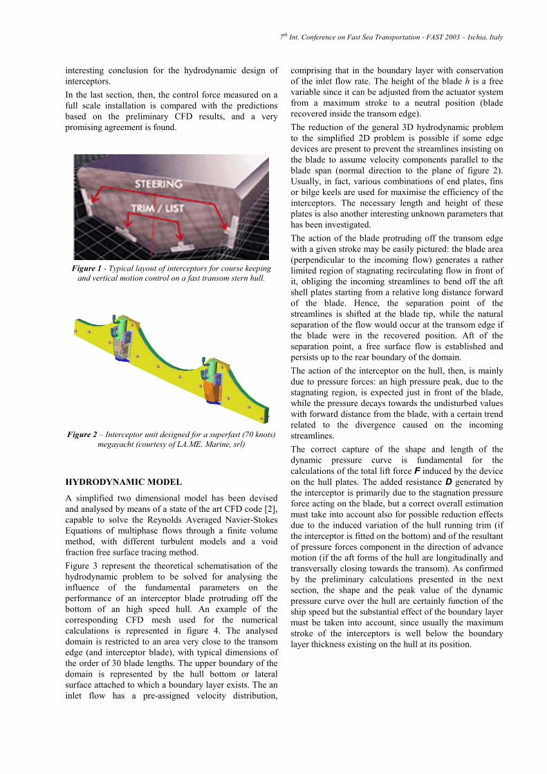
Interceptors are nowadays more and more widely used on high speed ships and fast boats for the static control of the dynamic trim or as a component of complex vertical and horizontal motion control systems. With regards to fast ships appendages, we generally name ‘interceptor’ a thin plate that is mounted onto the transom surface (figure 1), whose sharp tip follows the shape of the transom edge and can be protruded by an actuating system into the water with a certain stroke in a direction perpendicular to the hull surface (figure 2). The hydrodynamic action of the interceptors can be associated to that of a movable trim tab (an stern bottom integrated flap) or a conventional outboard flap. The discontinuity created by the protruding blade from the transom edge is causing stagnating flow region (characterised by an high pressure) which modifies the surrounding flow and eventually induce a certain force on the aft bottom/side shell. From a functional point of view an interesting feature of interceptors over trim tabs or flaps is that, in fast ships that have submerged vertical or sub-vertical transom sides, they can be used to provide also a side force to precisely control the course of the vessel (see figure 1). For the design and dimensioning of interceptors, it is of fundamental importance the knowledge of the hydrodynamic action that the blade causes on the surrounding flow, when protruding off the transom edge.

Except for few practical articles, which only marginally give information about the behaviour of interceptors (still useful and precious from the engineering point of view, though) such as the one published by Dawson and Blount [1], no many other articles can be found in the literature about the hydrodynamic of interceptors. For this reason, a first fundamental study on the main parameters which influence the physics of the flow field around interceptors has been concluded as part of an articulated research project commissioned by Messrs LA.ME. Marine. The project still ongoing will be completed by other investigation dedicated to the definition of a general methodology for hydrodynamic design of interceptors. In general terms, the hydrodynamic problem of the flow around interceptors is rather complex, since it involves a free surface flow in which the viscous effects cannot be neglected. The fundamental study has programmed a series of systematic computations on a 2D simplified model by means of an up to date CFD free surface RANSE solver [2], in order to identify the main parameters which influence the performance of interceptors and to quantitatively estimate the relative importance of these parameters on the global hydrodynamic characteristics. The main results obtained from this preliminary studies are discussed in the paper, through the analysis of the CFD results in terms of distributed parameters (velocity and pressure fields) and of global developed forces. This analysis bring to


interesting conclusion for the hydrodynamic design of interceptors. In the last section, then, the control force measured on a full scale installation is compared with the predictions based on the preliminary CFD results, and a very promising agreement is found.

Figure 1 - Typical layout of interceptors for course keeping and vertical motion control on a fast transom stern hull.

Figure 2 – Interceptor unit designed for a superfast (70 knots) megayacht (courtesy of LA.ME. Marine, srl)

HYDRODYNAMIC MODEL

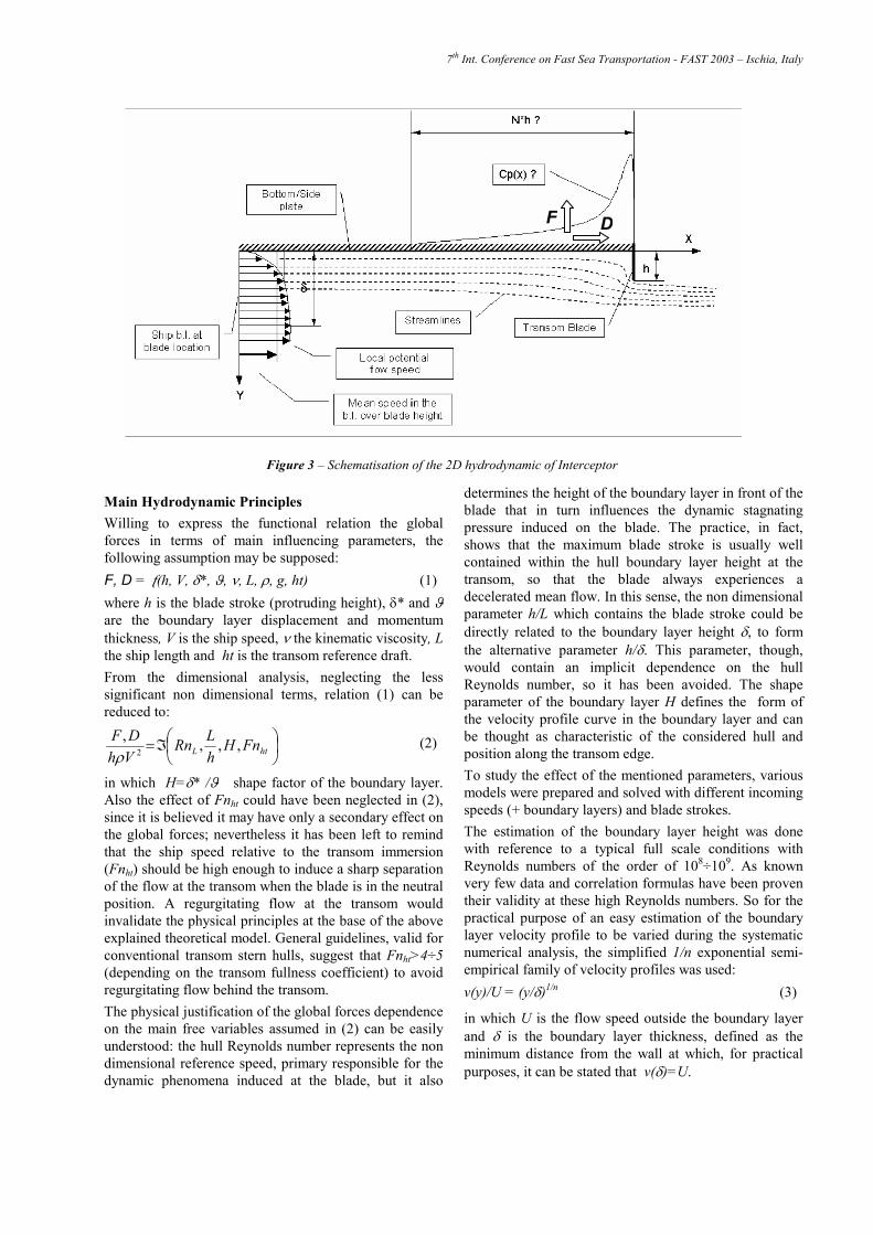
A simplified two dimensional model has been devised and analysed by means of a state of the art CFD code [2], capable to solve the Reynolds Averaged Navier-Stokes Equations of multiphase flows through a finite volume method, with different turbulent models and a void fraction free surface tracing method. Figure 3 represent the theoretical schematisation of the hydrodynamic problem to be solved for analysing the influence of the fundamental parameters on the performance of an interceptor blade protruding off the bottom of an high speed hull. An example of the corresponding CFD mesh used for the numerical calculations is represented in figure 4. The analysed domain is restricted to an area very close to the transom edge (and interceptor blade), with typical dimensions of the order of 30 blade lengths. The upper boundary of the domain is represented by the hull bottom or lateral surface attached to which a boundary layer exists. The an inlet flow has a pre-assigned velocity distribution,

comprising that in the boundary layer with conservation of the inlet flow rate. The height of the blade h is a free variable since it can be adjusted from the actuator system from a maximum stroke to a neutral position (blade recovered inside the transom edge). The reduction of the general 3D hydrodynamic problem to the simplified 2D problem is possible if some edge devices are present to prevent the streamlines insisting on the blade to assume velocity components parallel to the blade span (normal direction to the plane of figure 2). Usually, in fact, various combinations of end plates, fins or bilge keels are used for maximise the efficiency of the interceptors. The necessary length and height of these plates is also another interesting unknown parameters that has been investigated. The action of the blade protruding off the transom edge with a given stroke may be easily pictured: the blade area (perpendicular to the incoming flow) generates a rather limited region of stagnating recirculating flow in front of it, obliging the incoming streamlines to bend off the aft shell plates starting from a relative long distance forward of the blade. Hence, the separation point of the streamlines is shifted at the blade tip, while the natural separation of the flow would occur at the transom edge if the blade were in the recovered position. Aft of the separation point, a free surface flow is established and persists up to the rear boundary of the domain. The action of the interceptor on the hull, then, is mainly due to pressure forces: an high pressure peak, due to the stagnating region, is expected just in front of the blade, while the pressure decays towards the undisturbed values with forward distance from the blade, with a certain trend related to the divergence caused on the incoming streamlines. The correct capture of the shape and length of the dynamic pressure curve is fundamental for the calculations of the total lift force F induced by the device on the hull plates. The added resistance D generated by the interceptor is primarily due to the stagnation pressure force acting on the blade, but a correct overall estimation must take into account also for possible reduction effects due to the induced variation of the hull running trim (if the interceptor is fitted on the bottom) and of the resultant of pressure forces component in the direction of advance motion (if the aft forms of the hull are longitudinally and transversally closing towards the transom). As confirmed by the preliminary calculations presented in the next section, the shape and the peak value of the dynamic pressure curve over the hull are certainly function of the ship speed but the substantial effect of the boundary layer must be taken into account, since usually the maximum stroke of the interceptors is well below the boundary layer thickness existing on the hull at its position.


Main Hydrodynamic Principles Willing to express the functional relation the global forces in terms of main influencing parameters, the following assumption may be supposed: F, D = ƒ(h, V, δ*, ϑ, ν, L, ρ, g, ht) (1) where h is the blade stroke (protruding height), δ* and ϑare the boundary layer displacement and momentum thickness, V is the ship speed, ν the kinematic viscosity, Lthe ship length and ht is the transom reference draft. From the dimensional analysis, neglecting the less significant non dimensional terms, relation (1) can be reduced to:

ℑ= htL FnH

hLRn

VhDF ,,,,

2ρ(2)

in which H=δ* /ϑ shape factor of the boundary layer. Also the effect of Fnht could have been neglected in (2), since it is believed it may have only a secondary effect on the global forces; nevertheless it has been left to remind that the ship speed relative to the transom immersion (Fnht) should be high enough to induce a sharp separation of the flow at the transom when the blade is in the neutral position. A regurgitating flow at the transom would invalidate the physical principles at the base of the above explained theoretical model. General guidelines, valid for conventional transom stern hulls, suggest that Fnht>4÷5 (depending on the transom fullness coefficient) to avoid regurgitating flow behind the transom. The physical justification of the global forces dependence on the main free variables assumed in (2) can be easily understood: the hull Reynolds number represents the non dimensional reference speed, primary responsible for the dynamic phenomena induced at the blade, but it also

determines the height of the boundary layer in front of the blade that in turn influences the dynamic stagnating pressure induced on the blade. The practice, in fact, shows that the maximum blade stroke is usually well contained within the hull boundary layer height at the transom, so that the blade always experiences a decelerated mean flow. In this sense, the non dimensional parameter h/L which contains the blade stroke could be directly related to the boundary layer height δ, to form the alternative parameter h/δ. This parameter, though, would contain an implicit dependence on the hull Reynolds number, so it has been avoided. The shape parameter of the boundary layer H defines the form of the velocity profile curve in the boundary layer and can be thought as characteristic of the considered hull and position along the transom edge. To study the effect of the mentioned parameters, various models were prepared and solved with different incoming speeds (+ boundary layers) and blade strokes. The estimation of the boundary layer height was done with reference to a typical full scale conditions with Reynolds numbers of the order of 108÷109. As known very few data and correlation formulas have been proven their validity at these high Reynolds numbers. So for the practical purpose of an easy estimation of the boundary layer velocity profile to be varied during the systematic numerical analysis, the simplified 1/n exponential semi-empirical family of velocity profiles was used: v(y)/U = (y/δ)1/n (3)

in which U is the flow speed outside the boundary layer and δ is the boundary layer thickness, defined as the minimum distance from the wall at which, for practical purposes, it can be stated that v(δ)=U.

Figure 3 – Schematisation of the 2D hydrodynamic of Interceptor

F D


As well known [3], for these family of profiles the following relations are valid: H = (n+2)/n δ*/δ = (1+n)/n2 (4) ϑ/δ = (n+1)(n+2)/n3

The reference boundary layer height may be estimated with the semi-empirical formula of Prandtl (5a) or the method of Wieghardt (5b) below reported:

5/1373.0 −⋅⋅= xRnxδ (5a)

( ) 61274.0 −′⋅⋅= xnRxδ (5b)

in which x is the longitudinal position along the hull and Rnx the Reynolds number at the length x, and Rnx

' is the Reynolds number corrected for ∆Cf addendum. Rigorously Prandtl boundary layer height (5a) is valid for the profile family of (4) with n=7. In fact, these family of profiles have been used at the boundary for the CFD calculations. Recent measurements on full scale boundary layers of fast catamaran and monohull ships [4], though, has evidenced that the velocity profiles in the boundary layer on the stern bottom find good correlations with practical formulations of the type (3) with values of the exponent n close to 9 and boundary layer heights estimated through Prandtl (5a) or Wieghardt (5b) formulae, depending on the Reynolds number and hull typology. For the velocity profiles just introduced, it can be interesting to express the effective momentum of the flow contained into the boundary layer from the wall up to a general height y, relative to that of the undisturbed flow. This quantity results:

nyeffeff y

nndt

Utv

yUq

qyq 2

0

2

22

1 2)(1)(

+=

== ∫ δρ

(6)

The trend of the relative effective momentum (6) can be linked to the trend of the stagnation pressure at the blade that will be predicted with the CFD methods, if one assumes that the maximum dynamic pressure at the blade is due to the pure stagnation of the flow contained in the

boundary layer within an height equal to the blade height. Under this hypothesis, at a given speed, the pressure coefficient at the blade should change with respect to the blade height in the following way:

12)( −=∝ HnbladeP hhhC (7)

and for a given blade height assuming a variation of the external speed U:

)(2)( mnbladeP RnhC ⋅∝ (8)

with m=5 for Prandtl or m=6 for Wieghardt formulae. The drag force D induced by the blade could be thought as due to the dynamic pressure, assumed to be constant over the blade height, i.e.:

2

0

2

21

21 UhCdyCUD blade

P

hbladeP ρρ ≅= ∫ (9)

but, as already mentioned, the total added drag must take into account also the other effects induced by the interceptor on the ship, such as dynamic trim variation (usually in the sense of reducing the total resistance) and pressure recovery at the stern in case sterns with aft buttocks which rise up toward the transom. The vertical (lift) force F is related to the form of the dynamic pressure curve induced by the blade on the hull and hence no simple direct relations are possible and in general it must be evaluated by the following integral:

∫=Nh

hullP dxxCF

0

)( (10)

in which the integrand function Cp(x) and upper limit constant N are unknowns. Experiment or CFD calculations, as those presented in the next chapter, are in general needed to solve this problem. Final aim of the next research studies is, in fact, the definition of simple formulas which can express the magnitude of these two forces with respect to the main introduced parameters in a simple general 2D case. It is obvious that the prediction of these forces in case of complex 3D hull geometries will require in any case ad hoc CFD studies, involving the accurate prediction of the three dimensional boundary

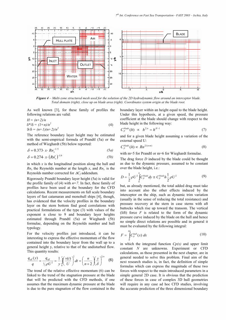
Figure 4 – Multi-zone structured mesh used for the solution of the 2D hydrodynamic flow around an interceptor blade. Total domain (right), close up on blade area (right). Coordinates system origin at the blade root.

INLETOUTLET

WATER

AIRHULL PLATE

BLADE


layer height and local speed direction (in the b.l.) at the interceptor position.

CFD MODEL

The theoretical hydrodynamic bidimensional model of the interceptors described in the previous section, has been simulated with a state of the art CFD code [2], in order to analyse the influence of the main identified free variables on the local flow characteristics and on the global forces. With reference to figure 4, a relative limited focused on the proximity of the blade has been analysed and it extends about 35 blade heights forward and 20 aft of the blade position and spans about 35÷50 blade heights in depth. The finite volume cells of the domain are initially assigned with water or air densities in relation to the guessed separating boundary of the free surface. A symmetry condition at the bottom of the domain and a non-slippery condition at the hull bottom have been imposed. The inlet boundary condition assumes a velocity distribution which comprehends the initially undisturbed boundary layer profile. The outlet has a static pressure and a mass conservation boundary condition. Blade obstruction is represented in the CFD model by means of a series of special cells called “baffle” that create a solid infinitely thin obstruction to the flow on one the cells face. The steady state solution has been obtained by solving a virtual non stationary problem and stopping the solution at convergence. Convergence criteria involved both velocities and tracking of the contour of the free surface of the flow behind the blade with inner additional sub-cycles. On the whole model, the effect of the gravity force was imposed to reproduce the flow on the of an interceptor protruding off the transom bottom edge. The turbulence model employed is a standard k-ε model for high Reynolds numbers. An example of the free surface shape obtained at convergence is pictured in figure 5. Obviously the free surface behind the transom is in general influenced from

the slope of the bottom in front of it and the transom draft at rest. Nevertheless, since the scope of this simulations is not to study the wave behind transom and since a variation of the free surface flow behind the transom is believed to only marginally influence the flow in front of the blade as far as the flow separates naturally, a flat bottom was used to investigate the general problem. The model required about 700 principal iterations to reach the steady state solution.

Figure 5 – Example of the free surface at convergence, Rn=1.2⋅109 , L/h=590

CFD RESULTS

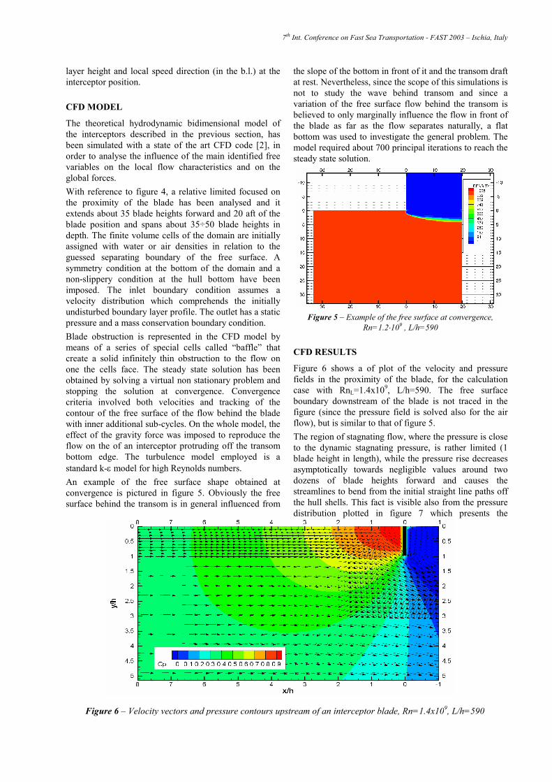
Figure 6 shows a of plot of the velocity and pressure fields in the proximity of the blade, for the calculation case with RnL=1.4x109, L/h=590. The free surface boundary downstream of the blade is not traced in the figure (since the pressure field is solved also for the air flow), but is similar to that of figure 5. The region of stagnating flow, where the pressure is close to the dynamic stagnating pressure, is rather limited (1 blade height in length), while the pressure rise decreases asymptotically towards negligible values around two dozens of blade heights forward and causes the streamlines to bend from the initial straight line paths off the hull shells. This fact is visible also from the pressure distribution plotted in figure 7 which presents the

Figure 6 – Velocity vectors and pressure contours upstream of an interceptor blade, Rn=1.4x109, L/h=590


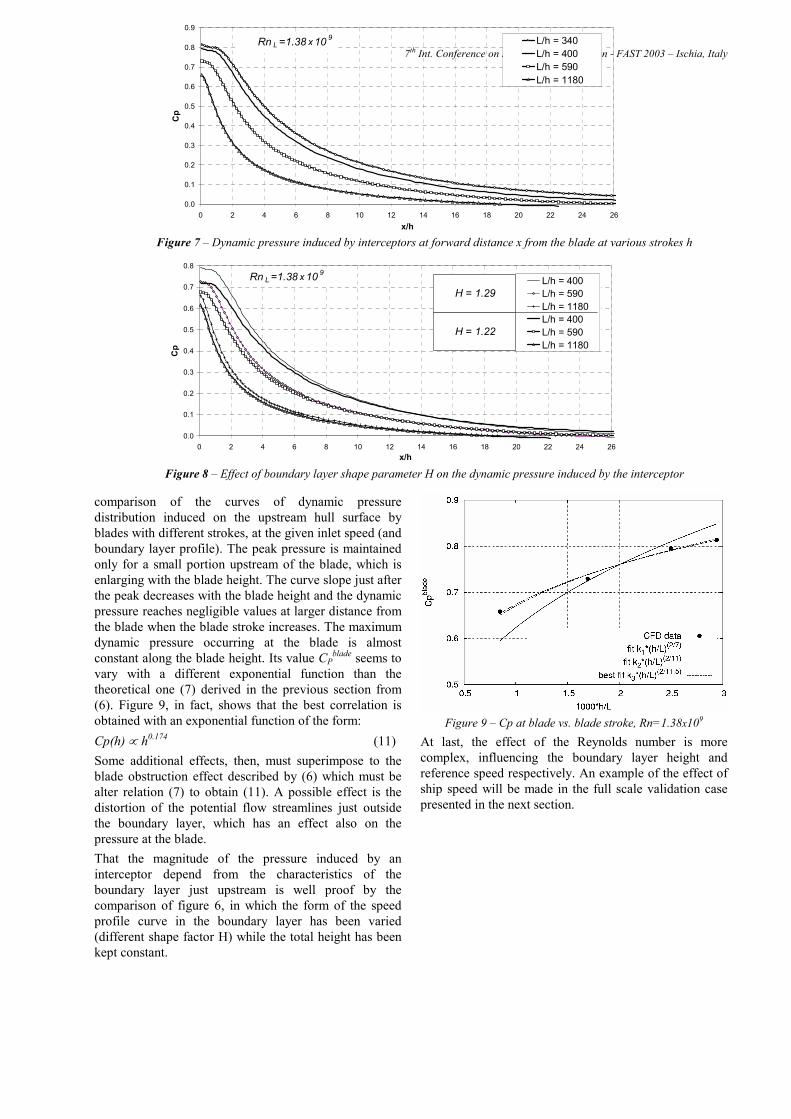
comparison of the curves of dynamic pressure distribution induced on the upstream hull surface by blades with different strokes, at the given inlet speed (and boundary layer profile). The peak pressure is maintained only for a small portion upstream of the blade, which is enlarging with the blade height. The curve slope just after the peak decreases with the blade height and the dynamic pressure reaches negligible values at larger distance from the blade when the blade stroke increases. The maximum dynamic pressure occurring at the blade is almost constant along the blade height. Its value CP

blade seems to vary with a different exponential function than the theoretical one (7) derived in the previous section from (6). Figure 9, in fact, shows that the best correlation is obtained with an exponential function of the form: Cp(h) ∝ h0.174 (11) Some additional effects, then, must superimpose to the blade obstruction effect described by (6) which must be alter relation (7) to obtain (11). A possible effect is the distortion of the potential flow streamlines just outside the boundary layer, which has an effect also on the pressure at the blade. That the magnitude of the pressure induced by an interceptor depend from the characteristics of the boundary layer just upstream is well proof by the comparison of figure 6, in which the form of the speed profile curve in the boundary layer has been varied (different shape factor H) while the total height has been kept constant.

Figure 9 – Cp at blade vs. blade stroke, Rn=1.38x109

At last, the effect of the Reynolds number is more complex, influencing the boundary layer height and reference speed respectively. An example of the effect of ship speed will be made in the full scale validation case presented in the next section.

Figure 7 – Dynamic pressure induced by interceptors at forward distance x from the blade at various strokes h

0.0

0.1

0.2

0.3

0.4

0.5

0.6

0.7

0.8

0.9

0 2 4 6 8 10 12 14 16 18 20 22 24 26x/h

Cp

L/h = 340L/h = 400L/h = 590L/h = 1180

Rn L =1.38 x 10 9

0.0

0.1

0.2

0.3

0.4

0.5

0.6

0.7

0.8

0 2 4 6 8 10 12 14 16 18 20 22 24 26x/h

Cp

L/h = 400L/h = 590L/h = 1180L/h = 400L/h = 590L/h = 1180

H = 1.29

H = 1.22

Rn L =1.38 x 10 9

Figure 8 – Effect of boundary layer shape parameter H on the dynamic pressure induced by the interceptor


FULL SCALE VALIDATION CASE

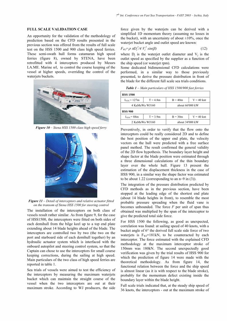
An opportunity for the validation of the methodology of prediction based on the CFD results presented in the previous section was offered from the results of full scale test on the HSS 1500 and 900 class high speed ferries. These semi-swath hull forms catamaran high speed ferries (figure 8), owned by STENA, have been retrofitted with 4 interceptors produced by Messrs LA.ME. Marine srl, to control the course keeping of the vessel at higher speeds, overriding the control of the waterjets buckets.

Figure 10 – Stena HSS 1500 class high speed ferry

Figure 11 – Detail of interceptors and relative actuator fitted on the transom of Stena HSS 1500 for steering control

The installation of the interceptors on both class of vessels result rather similar. As from figure 9, for the case of HSS1500, the interceptors were fitted on both sides of each demihull from the bilge keel up to a top end plate extending about 14 blade heights ahead of the blade. The interceptors are controlled two by two (the two on the port and starboard side of each demihull together) by an hydraulic actuator system which is interfaced with the onboard autopilot and steering control system, so that the Captain can chose to use the interceptors for small course keeping corrections, during the sailing at high speed. Main particulars of the two class of high speed ferries are reported in table 1. Sea trials of vessels were aimed to test the efficiency of the interceptors by measuring the maximum waterjets bucket which can maintain the straight course of the vessel when the two interceptors are out at their maximum stroke. According to WJ producers, the side

force given by the waterjets can be derived with a simplified 1D momentum theory (assuming no losses in the bucket), with an uncertainty of about ±10%, once the waterjet bucket angle and outlet speed are known: FWJ=ρ πDj

2/4 Vj2 sin(β) (12)

where Dj is the waterjet outlet diameter and Vj is the outlet speed as specified by the supplier as a function of the ship speed (or waterjet rpm). Some dedicated bidimensional CFD calculations were performed, in a similar way to those previously presented, to derive the pressure distribution in front of the blade for the different full scale sea trials conditions.

Table 1 – Main particulars of HSS 1500/900 fast ferries

HSS 1500

LOA = 127m T = 4.8m B = 40m V = 40 knt

4 KaMeWa WJ160 about 66'000 kW

HSS 900

LOA = 88m T = 3.9m B = 30m V = 40 knt

2 KaMeWa WJ160 about 34'000 kW

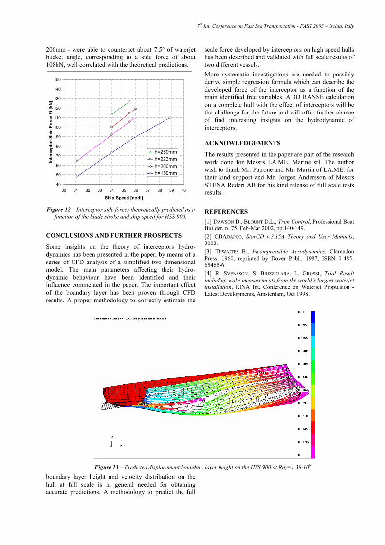
Preventively, in order to verify that the flow onto the interceptors could be really considered 2D and to define the best position of the upper end plate, the velocity vectors on the hull were predicted with a free surface panel method. The result confirmed the general validity of the 2D flow hypothesis. The boundary layer height and shape factor at the blade position were estimated through a three dimensional calculations of the thin boundary layer over the whole hull. Figure 13 present the estimation of the displacement thickness in the case of HSS 900, in a similar way the shape factor was estimated to be about 1.22 (corresponding to an n~9 in (3)). The integration of the pressure distribution predicted by CFD methods as in the previous section, have been stopped at the leading edge of the shortest end plate (about 14 blade heights in front), to resemble the most probable pressure spreading when the fluid vane is becomes unbounded. The force F per unit of span thus obtained was multiplied by the span of the interceptor to give the predicted total side force. For HSS 1500 the following, as good as unexpected, correlation was found: at sailing speed of 40 knots, with a bucket angle of 6° the derived full scale side force of two waterjets is FWJ=181kN, to be counteracted by each interceptor. The force estimated with the explained CFD methodology at the maximum interceptor stroke of 150mm was 180kN. The second unexpectedly good verification was given by the trial results of HSS 900 for which the prediction of figure 14 were made with the theoretical methodology. As from figure 14, the functional relation between the force and the ship speed is almost linear (as it is with respect to the blade stroke), probably for the momentum defect existing inside the boundary layer within the blade height. Full scale trials indicated that, at the steady ship speed of 36 knots, the interceptors - out at the maximum stroke of


200mm - were able to counteract about 7.5° of waterjet bucket angle, corresponding to a side force of about 108kN, well correlated with the theoretical predictions.

40

50

60

70

80

90

100

110

120

130

140

150

30 31 32 33 34 35 36 37 38 39 40

Ship Speed [nodi]

Inte

rcep

torS

ide

Forc

eFi

[kN]

h=259mmh=223mmh=200mmh=150mm

Figure 12 – Interceptor side forces theoretically predicted as a function of the blade stroke and ship speed for HSS 900.

CONCLUSIONS AND FURTHER PROSPECTS Some insights on the theory of interceptors hydro-dynamics has been presented in the paper, by means of a series of CFD analysis of a simplified two dimensional model. The main parameters affecting their hydro-dynamic behaviour have been identified and their influence commented in the paper. The important effect of the boundary layer has been proven through CFD results. A proper methodology to correctly estimate the

boundary layer height and velocity distribution on the hull at full scale is in general needed for obtaining accurate predictions. A methodology to predict the full

scale force developed by interceptors on high speed hulls has been described and validated with full scale results of two different vessels. More systematic investigations are needed to possibly derive simple regression formula which can describe the developed force of the interceptor as a function of the main identified free variables. A 3D RANSE calculation on a complete hull with the effect of interceptors will be the challenge for the future and will offer further chance of find interesting insights on the hydrodynamic of interceptors.

ACKNOWLEDGEMENTS

The results presented in the paper are part of the research work done for Messrs LA.ME. Marine srl. The author wish to thank Mr. Patrone and Mr. Martin of LA.ME. for their kind support and Mr. Jorgen Andersson of Messrs STENA Rederi AB for his kind release of full scale tests results.

REFERENCES [1] DAWSON D., BLOUNT D.L., Trim Control, Professional Boat Builder, n. 75, Feb-Mar 2002, pp.140-149. [2] CDADAPCO, StarCD v.3.15A Theory and User Manuals,2002. [3] THWAITES B., Incompressible Aerodynamics, Clarendon Press, 1960, reprinted by Dover Publ., 1987, ISBN 0-485-65465-6 [4] R. SVENSSON, S. BRIZZOLARA, L. GROSSI, Trial Result including wake measurements from the world’s largest waterjet installation, RINA Int. Conference on Waterjet Propulsion - Latest Developments, Amsterdam, Oct 1998.

Figure 13 – Predicted displacement boundary layer height on the HSS 900 at RnL=1.38·109

HYDRODYNAMIC ANALYSIS OF INTERCEPTORS WITH CFD METHODS

Documents