hydro chapter_5_a_by louy Al hami

10/30/2012 1

Chapter 5

Civil Engineering Department

Prof. Majed Abu-Zreig

Hydraulics and Hydrology – CE 352

Water Pumps

Definition

• Water pumps are devices designed to

convert mechanical energy to hydraulic

energy.

• They are used to move water from lower

points to higher points with a required

discharge and pressure head.

• turbines turn fluid energy into electrical or

mechanical

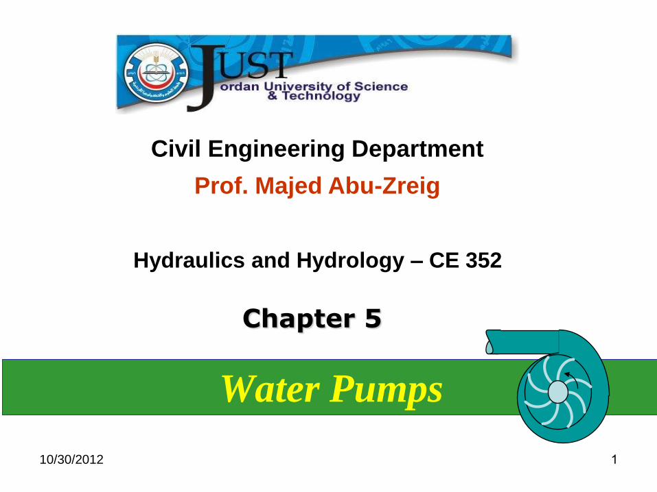
Pump Classification

• Turbo-hydraulic (kinetic) pumps

Centrifugal pumps (radial-flow pumps)

Propeller pumps (axial-flow pumps)

Jet pumps (mixed-flow pumps)

• Positive-displacement pumps

Screw pumps

Reciprocating pumps

• This classification is based on the

way by which the water leaves the

rotating part of the pump.

• In radial-flow pump the water

leaves the impeller in radial

direction,

• while in the axial-flow pump the

water leaves the propeller in the

axial direction.

• In the mixed-flow pump the water

leaves the impeller in an inclined

direction having both radial and

axial components

In a centrifugal pump flow enters along

the axis and is expelled radially. (The

reverse is true for a turbine.)

An axial-flow pump is like a propeller;

the direction of the flow is unchanged

after passing through the device.

A mixed-flow device is a hybrid device,

used for intermediate heads.

Schematic diagram of basic

elements of centrifugal

pump

Schematic diagram of axial-flow

pump arranged in vertical operation

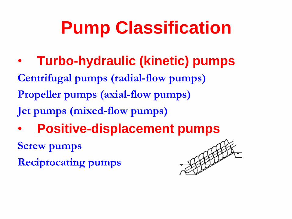
Jet pump

Screw pumps.

• In the screw pump a revolving shaft fitted with

blades rotates in an inclined trough and pushes the

water up the trough.

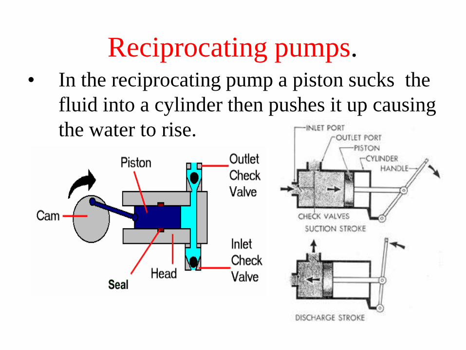
Reciprocating pumps. • In the reciprocating pump a piston sucks the

fluid into a cylinder then pushes it up causing

the water to rise.

تبارك اهلل أحسن الخالقين

RECIPROCATING INERTIA (JOGGLE)

PUMPS

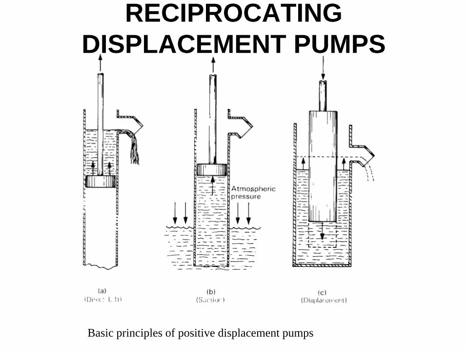
RECIPROCATING

DISPLACEMENT PUMPS

Basic principles of positive displacement pumps

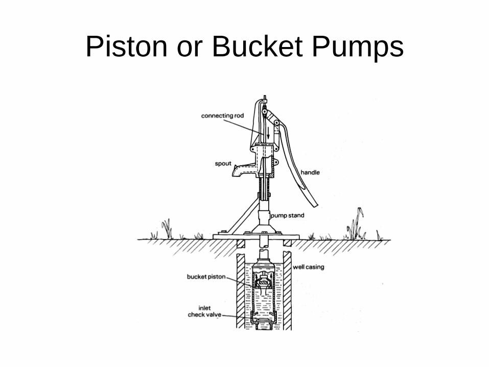
Piston or Bucket Pumps

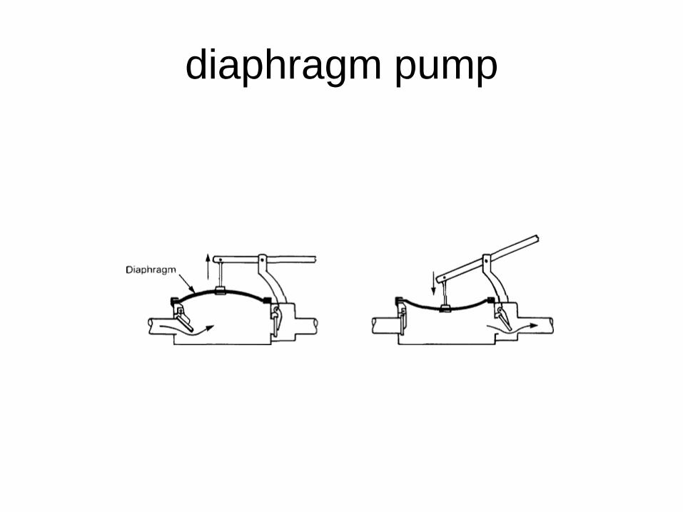
diaphragm pump

Different types of reciprocating displacement pumps

Selection of A Pump It has been seen that the efficiency of a pump depends on the discharge,

head, and power requirement of the pump. The approximate ranges of

application of each type of pump are indicated in the following Figure.

Centrifugal Pumps

• Demour’s centrifugal pump - 1730

• Theory

– conservation of angular momentum

– conversion of kinetic energy to potential energy

• Pump components

– rotating element - impeller

– encloses the rotating element and seals the pressurized

liquid inside – casing or housing

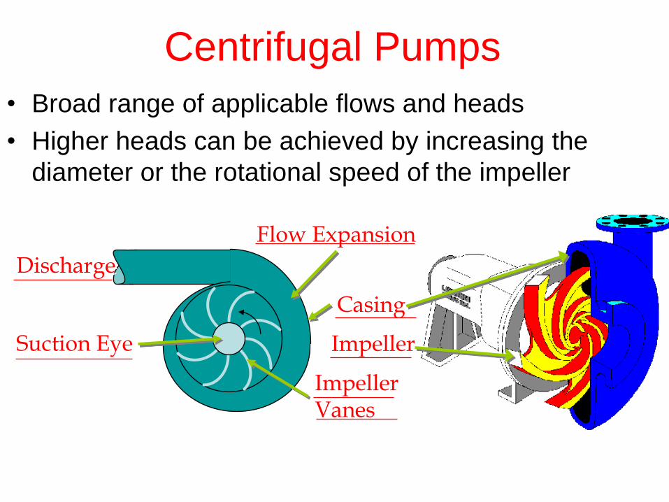
Centrifugal Pumps

Impeller Vanes

Casing

Suction Eye Impeller

Discharge

Flow Expansion

• Broad range of applicable flows and heads

• Higher heads can be achieved by increasing the

diameter or the rotational speed of the impeller

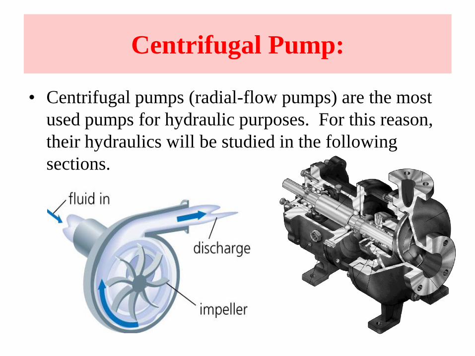
Centrifugal Pump:

• Centrifugal pumps (radial-flow pumps) are the most

used pumps for hydraulic purposes. For this reason,

their hydraulics will be studied in the following

sections.

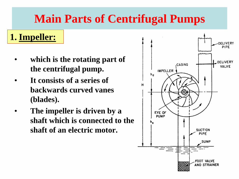
Main Parts of Centrifugal Pumps

• which is the rotating part of

the centrifugal pump.

• It consists of a series of

backwards curved vanes

(blades).

• The impeller is driven by a

shaft which is connected to the

shaft of an electric motor.

1. Impeller:

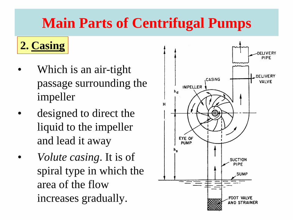
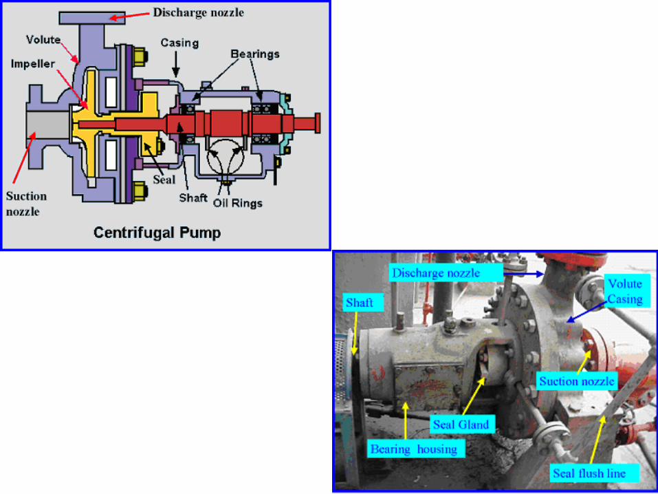
Main Parts of Centrifugal Pumps

• Which is an air-tight

passage surrounding the

impeller

• designed to direct the

liquid to the impeller

and lead it away

• Volute casing. It is of

spiral type in which the

area of the flow

increases gradually.

2. Casing

3. Suction Pipe.

4. Delivery Pipe.

5. The Shaft: which is the bar by which the

power is transmitted from the motor drive to

the impeller.

6. The driving motor: which is responsible for

rotating the shaft. It can be mounted directly

on the pump, above it, or adjacent to it.

Mechanics

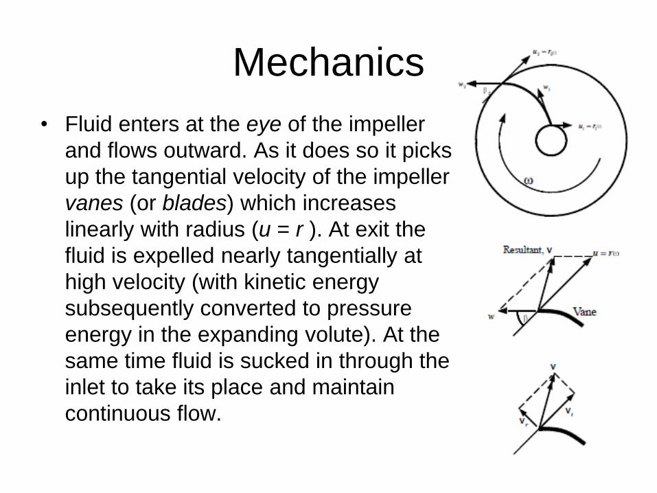
• Fluid enters at the eye of the impeller

and flows outward. As it does so it picks

up the tangential velocity of the impeller

vanes (or blades) which increases

linearly with radius (u = r ). At exit the

fluid is expelled nearly tangentially at

high velocity (with kinetic energy

subsequently converted to pressure

energy in the expanding volute). At the

same time fluid is sucked in through the

inlet to take its place and maintain

continuous flow.

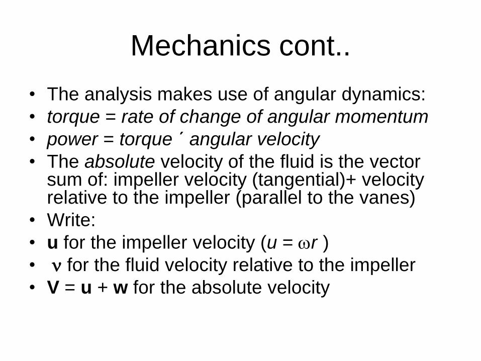
Mechanics cont..

• The analysis makes use of angular dynamics:

• torque = rate of change of angular momentum

• power = torque ´ angular velocity

• The absolute velocity of the fluid is the vector sum of: impeller velocity (tangential)+ velocity relative to the impeller (parallel to the vanes)

• Write:

• u for the impeller velocity (u = wr )

• n for the fluid velocity relative to the impeller

• V = u + w for the absolute velocity

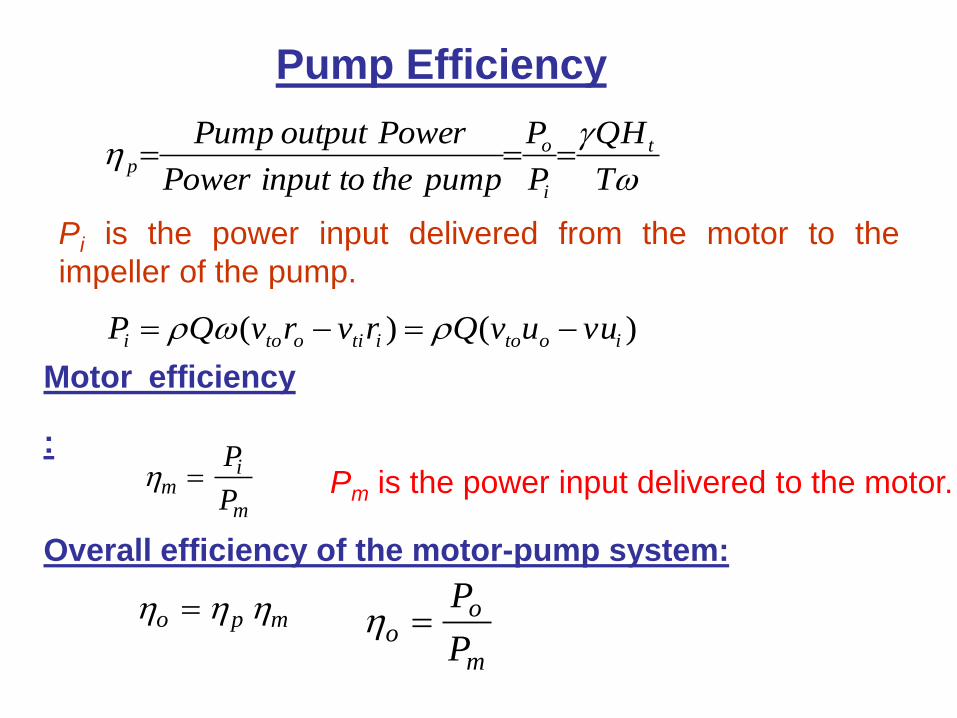
Pump Efficiency

)()(

iotoitiotoi

t

i

op

vuuvQrvrvQP

T

HQ

P

P

pumpthetoinputPower

PoweroutputPump

w

w

Pi is the power input delivered from the motor to the

impeller of the pump.

Motor efficiency

: m

i

m

P

P Pm is the power input delivered to the motor.

o p m oo

m

P

P

Overall efficiency of the motor-pump system:

Pump Efficiency

• Example.

• A pump lifts water from a large tank at a rate of

30 L/s. If the input power is 10 kW and the

pump is operating at an efficiency of 40%, find:

• (a) the head developed across the pump;

• (b) the maximum height to which it can raise

water if the delivery pipe is vertical, with D=100

mm and friction factor f = 0.015.

• Answer: (a) 13.6 m; (b) 12.2 m

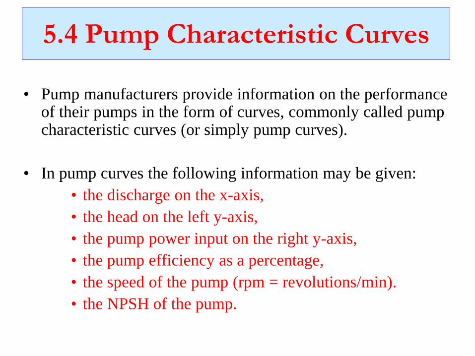
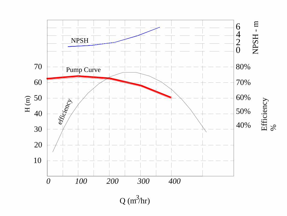
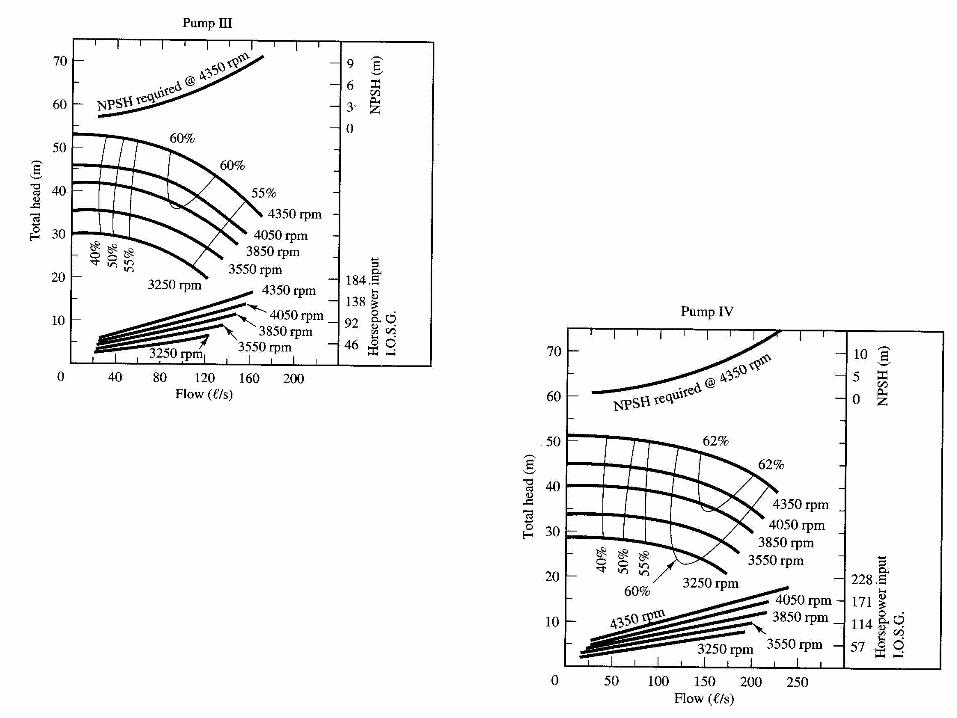
5.4 Pump Characteristic Curves

• Pump manufacturers provide information on the performance of their pumps in the form of curves, commonly called pump characteristic curves (or simply pump curves).

• In pump curves the following information may be given:

• the discharge on the x-axis,

• the head on the left y-axis,

• the pump power input on the right y-axis,

• the pump efficiency as a percentage,

• the speed of the pump (rpm = revolutions/min).

• the NPSH of the pump.

NP

SH

- m

Q (m /hr)

20

10

0 100 200

H (

m)

70

60

50

40

30

Pump Curve

NPSH

effi

cien

cy

300

3

400

6

70%

60%

50%

40%

420

Eff

icie

ncy

%

80%

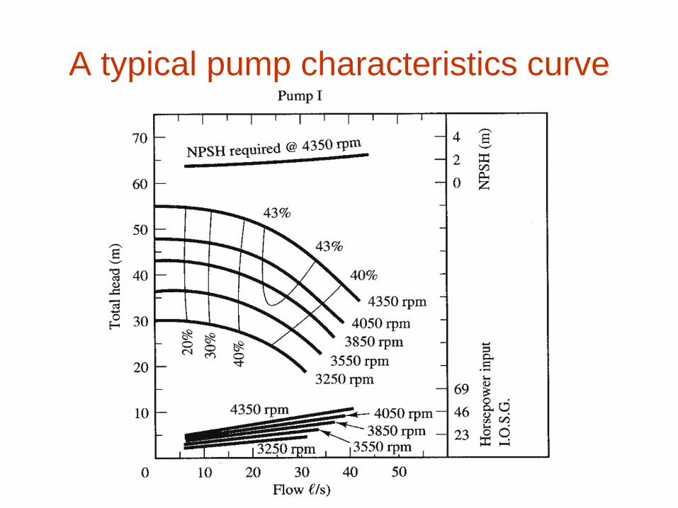
A typical pump characteristics curve

Constant- and Variable-Speed Pumps

• The speed of the pump is specified by the angular

speed of the impeller which is measured in

revolution per minutes (rpm).

• Based on this speed, N , pumps can be divided into

two types:

• Constant-speed pumps

• Variable-speed pumps

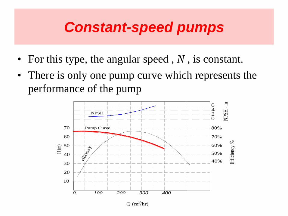
Constant-speed pumps

• For this type, the angular speed , N , is constant.

• There is only one pump curve which represents the

performance of the pump

10

0 100 300

Q (m /hr)

200

3

400

Pump Curve

30

40

50

60

70

20

H (m

)

effic

ienc

y

NPSH

Eff

icie

ncy

%

4

NPS

H -

m

80%

02

40%

50%

60%

70%

6

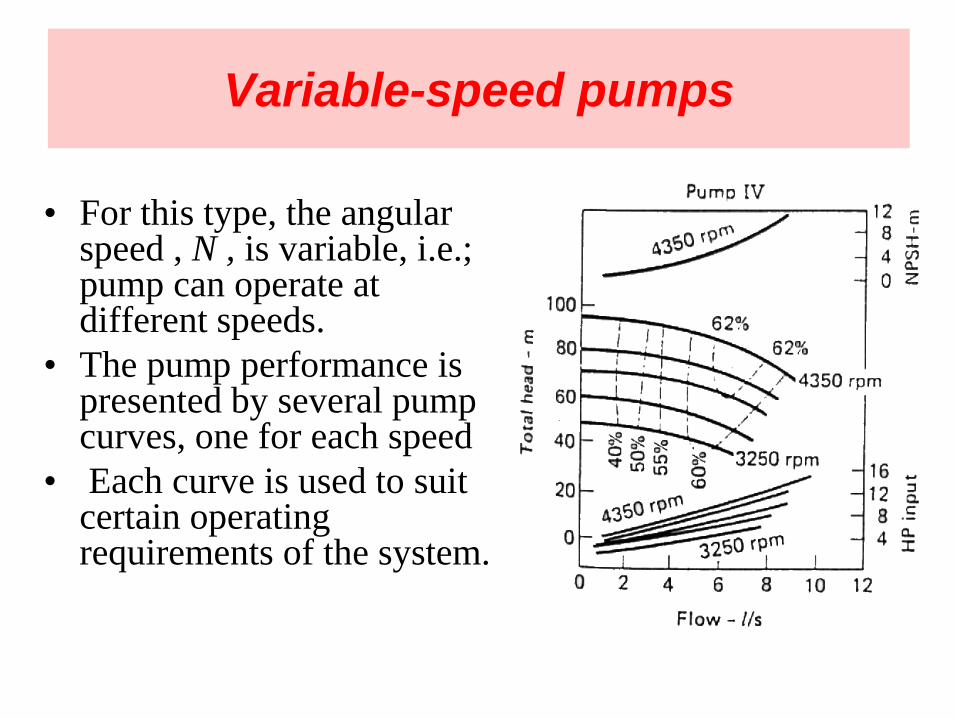
Variable-speed pumps

• For this type, the angular speed , N , is variable, i.e.; pump can operate at different speeds.

• The pump performance is presented by several pump curves, one for each speed

• Each curve is used to suit certain operating requirements of the system.

Similarity Laws:

Affinity laws

• The actual performance characteristics curves of pumps have to be determined by experimental testing.

• Furthermore, pumps belonging to the same family, i.e.; being of the same design but manufactured in different sizes and, thus, constituting a series of geometrically similar machines, may also run at different speeds within practical limits.

• Each size and speed combination will produce a unique characteristics curve, so that for one family of pumps the number of characteristics curves needed to be determined is impossibly large.

• The problem is solved by the application of dimensional analysis and by replacing the variables by dimensionless groups so obtained. These dimensionless groups provide the similarity (affinity) laws governing the relationships between the variables within one family of geometrically similar pumps.

• Thus, the similarity laws enable us to obtain a set of characteristic curves for a pump from the known test data of a geometrically similar pump.

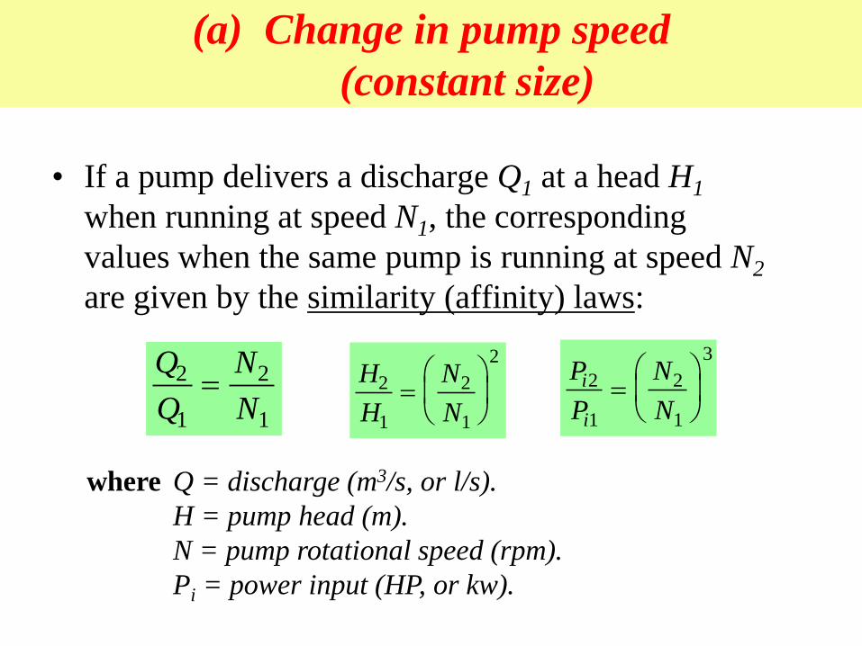
(a) Change in pump speed

(constant size)

• If a pump delivers a discharge Q1 at a head H1

when running at speed N1, the corresponding

values when the same pump is running at speed N2

are given by the similarity (affinity) laws:

Q

Q

N

N

2

1

2

1

H

H

N

N

2

1

2

1

2

P

P

N

N

i

i

2

1

2

1

3

where Q = discharge (m3/s, or l/s).

H = pump head (m).

N = pump rotational speed (rpm).

Pi = power input (HP, or kw).

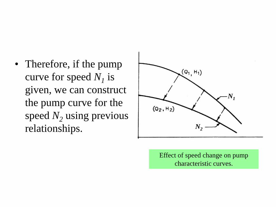
• Therefore, if the pump

curve for speed N1 is

given, we can construct

the pump curve for the

speed N2 using previous

relationships.

Effect of speed change on pump

characteristic curves.

N1

N2

(b) Change in pump size

(constant speed)

• A change in pump size and therefore, impeller

diameter (D), results in a new set of characteristic

curves using the following similarity (affinity) laws:

Q

Q

D

D

2

1

2

1

3

H

H

D

D

2

1

2

1

2

P

P

D

D

i

i

2

1

2

1

5

where D = impeller diameter (m, cm).

Note : D indicated the size of the pump

5.5 Hydraulic Analysis of Pumps and

Piping Systems

• Pump can be placed in two possible position in

reference to the water levels in the reservoirs.

• We begin our study by defining all the

different terms used to describe the pump

performance in the piping system.

Surface mounted centrifugal

pump installation

Below-surface (sump) centrifugal pump installation

Ht Dynamic Head

g

VhhhhHH

g

VhHH

dsmsfdmdfstatt

dlstatt

2

2

2

2

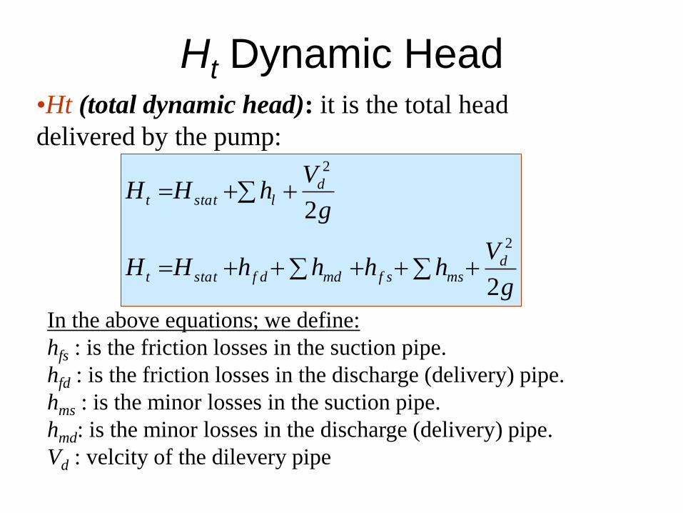
•Ht (total dynamic head): it is the total head

delivered by the pump:

In the above equations; we define:

hfs : is the friction losses in the suction pipe.

hfd : is the friction losses in the discharge (delivery) pipe.

hms : is the minor losses in the suction pipe.

hmd: is the minor losses in the discharge (delivery) pipe.

Vd : velcity of the dilevery pipe

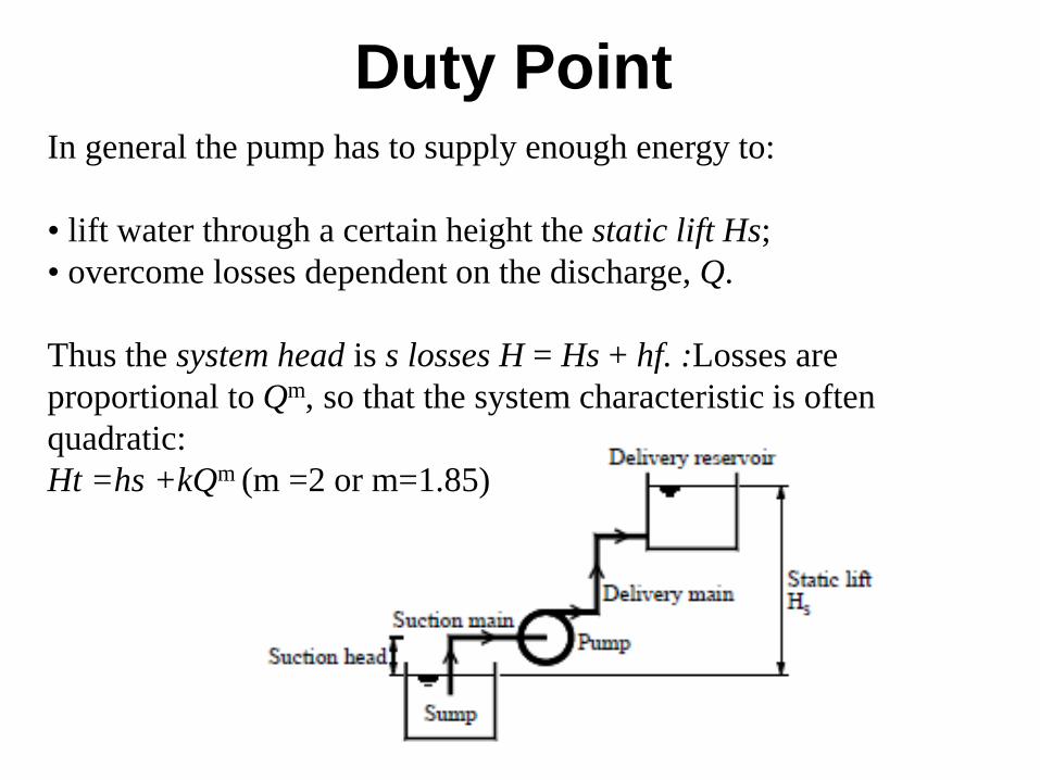
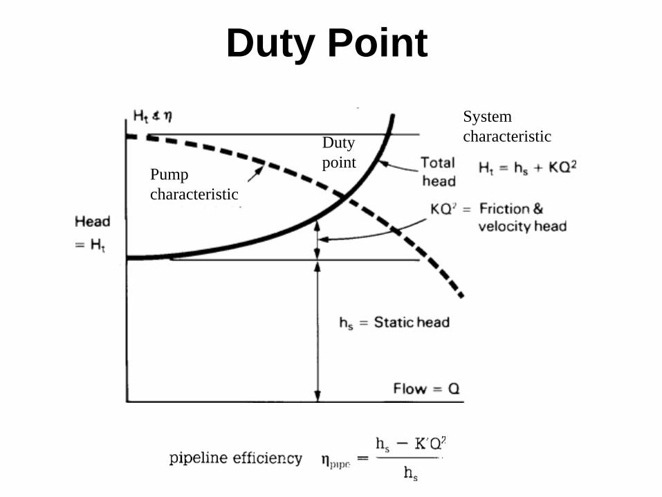
Duty Point In general the pump has to supply enough energy to:

• lift water through a certain height the static lift Hs;

• overcome losses dependent on the discharge, Q.

Thus the system head is s losses H = Hs + hf. :Losses are

proportional to Qm, so that the system characteristic is often

quadratic:

Ht =hs +kQm (m =2 or m=1.85)

Lstatt

Lt

hHH

hZZH 12

System Curve

0 3 6 9 12 15 18

10

H (m)

20

30

40

50

60

70

Q (m /hr) 3

Static head (z2-z1)=Hs

m

p kQzzH )( 12

mkQhf

Duty

point Pump

characteristic

System

characteristic

Duty Point

15

30

10

20

0 3

Q (m /hr)

6 9

3

12

Pump Curve

H (m) effi

cien

cy

70

40

50

60

System Curve

18

NP

SH

- m

420

6

40%

50%

60%

70%

Eff

icie

ncy

%

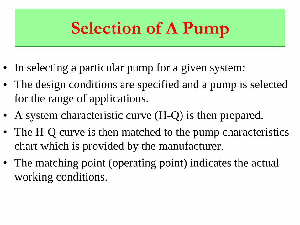
Selection of A Pump

• In selecting a particular pump for a given system:

• The design conditions are specified and a pump is selected

for the range of applications.

• A system characteristic curve (H-Q) is then prepared.

• The H-Q curve is then matched to the pump characteristics

chart which is provided by the manufacturer.

• The matching point (operating point) indicates the actual

working conditions.

• The pump characteristic curves are very important to help select the required pump for the specified conditions.

• If the system curve is plotted on the pump curves in we may produce the following Figure:

• The point of intersection is called the operating point.

• This matching point indicates the actual working conditions, and therefore the proper pump that satisfy all required performance characteristic is selected.

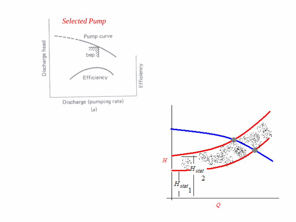
Matching the system and pump curves.

System Characteristic Curve

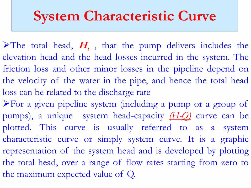
The total head, Ht , that the pump delivers includes the

elevation head and the head losses incurred in the system. The

friction loss and other minor losses in the pipeline depend on

the velocity of the water in the pipe, and hence the total head

loss can be related to the discharge rate

For a given pipeline system (including a pump or a group of

pumps), a unique system head-capacity (H-Q) curve can be

plotted. This curve is usually referred to as a system

characteristic curve or simply system curve. It is a graphic

representation of the system head and is developed by plotting

the total head, over a range of flow rates starting from zero to

the maximum expected value of Q.

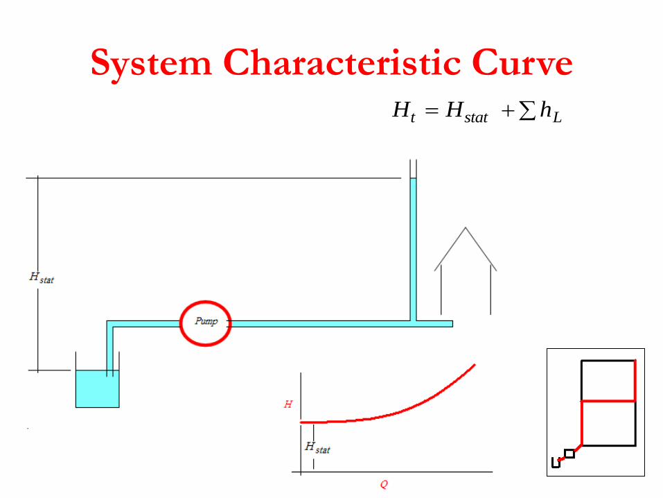
System Characteristic Curve H H ht stat L

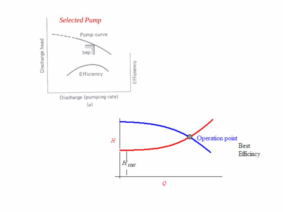
Selected Pump

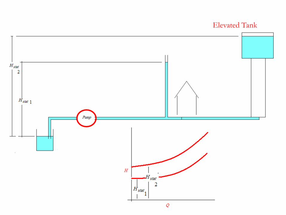
Elevated Tank

Selected Pump

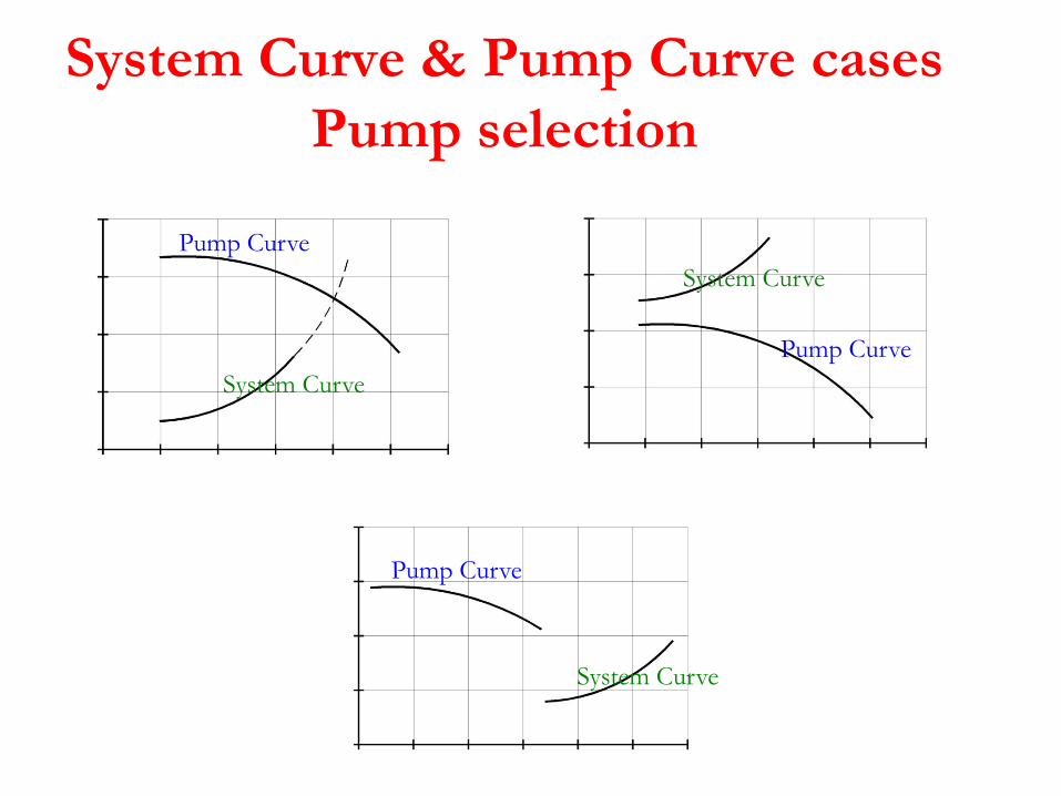
System Curve & Pump Curve cases

Pump selection

Pump Curve

Pump Curve

Pump Curve

System Curve

System Curve

System Curve

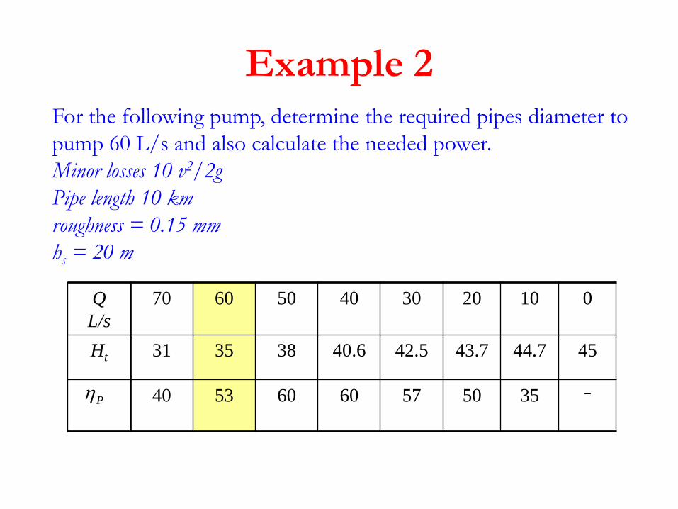
Example 2 For the following pump, determine the required pipes diameter to

pump 60 L/s and also calculate the needed power.

Minor losses 10 v2/2g

Pipe length 10 km

roughness = 0.15 mm

hs = 20 m

0 10 20 30 40 50 60 70 Q

L/s

45 44.7 43.7 42.5 40.6 38 35 31 Ht

- 35 50 57 60 60 53 40 P

To get 60 L/s from the pump hs + hL must be < 35 m

Assume the diameter = 300mm

Then:

mh

fDKR

smVmA

f

Se

32.2362.193.0

85.010000019.0

019.0,0005.0/,1025.2

/85.0,070.0

2

5

2

m

gg

Vhm 37.0

2

85.010

2

1022

mmhhh mfs 3569.43

Assume the diameter = 350mm

Then:

smVmA /624.0,0962.0 2

,48.10

0185.0,00043.0/,1093.1 5

mh

fDKR

f

Se

m

gg

Vhm 2.0

2

624.010

2

1022

mmhhh mfs 3568.30

kWWHQ

Pp

ti 87.388.38869

53.0

3581.910001000

60

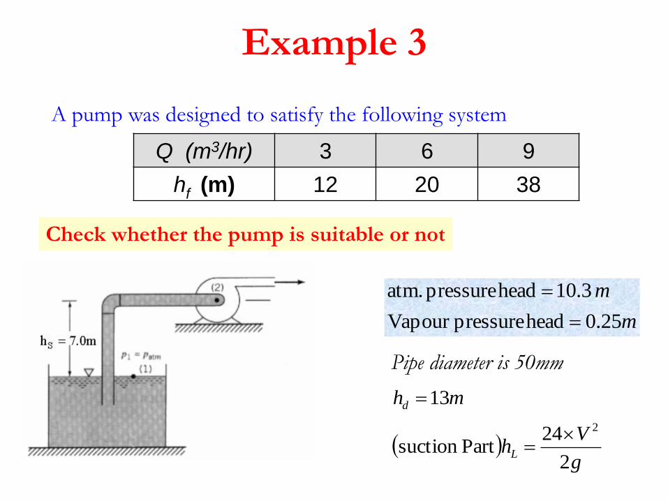
Example 3

A pump was designed to satisfy the following system

9 6 3 Q (m3/hr)

38 20 12 hf (m)

m

m

25.0head pressureVapour

3.10head pressure atm.

mhd 13

Pipe diameter is 50mm

g

VhL

2

24Partsuction

2

Check whether the pump is suitable or not

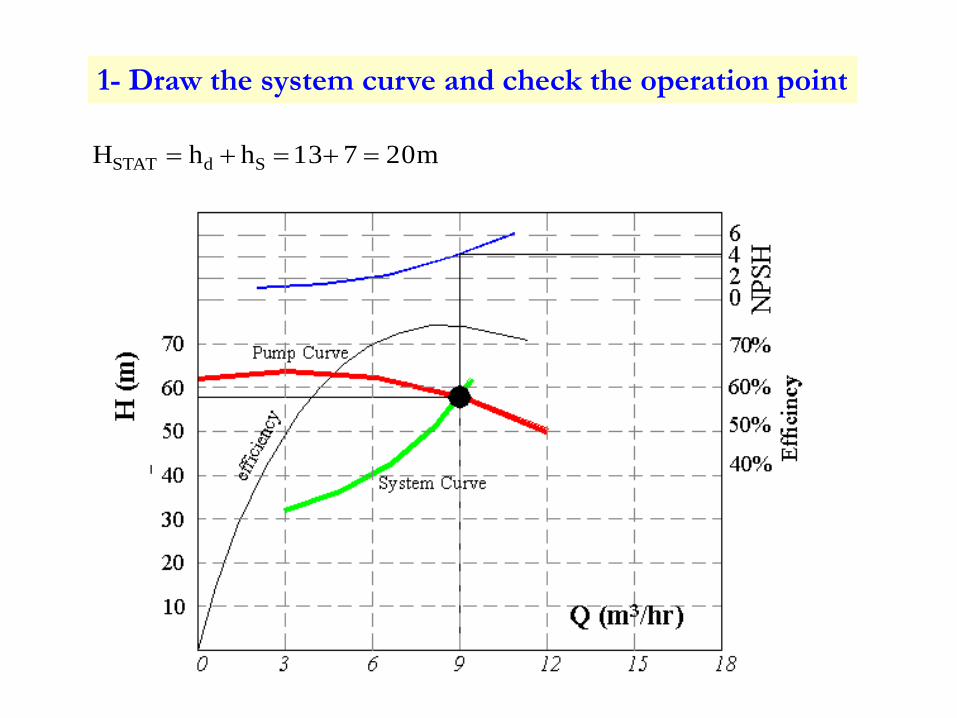
1- Draw the system curve and check the operation point

20m713hhH SdSTAT

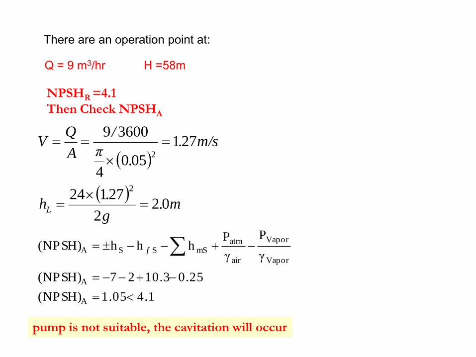
There are an operation point at:

Q = 9 m3/hr H =58m

NPSHR =4.1

Then Check NPSHA

m.

g

.h

m/s.

.π

/

A

QV

L 022

27124

271

0504

36009

2

2

4.11.05(NPSH)

0.2510.327(NPSH)

γ

P

γ

Phhh(NPSH)

A

A

Vapor

Vapor

air

atmmSS SA

f

pump is not suitable, the cavitation will occur

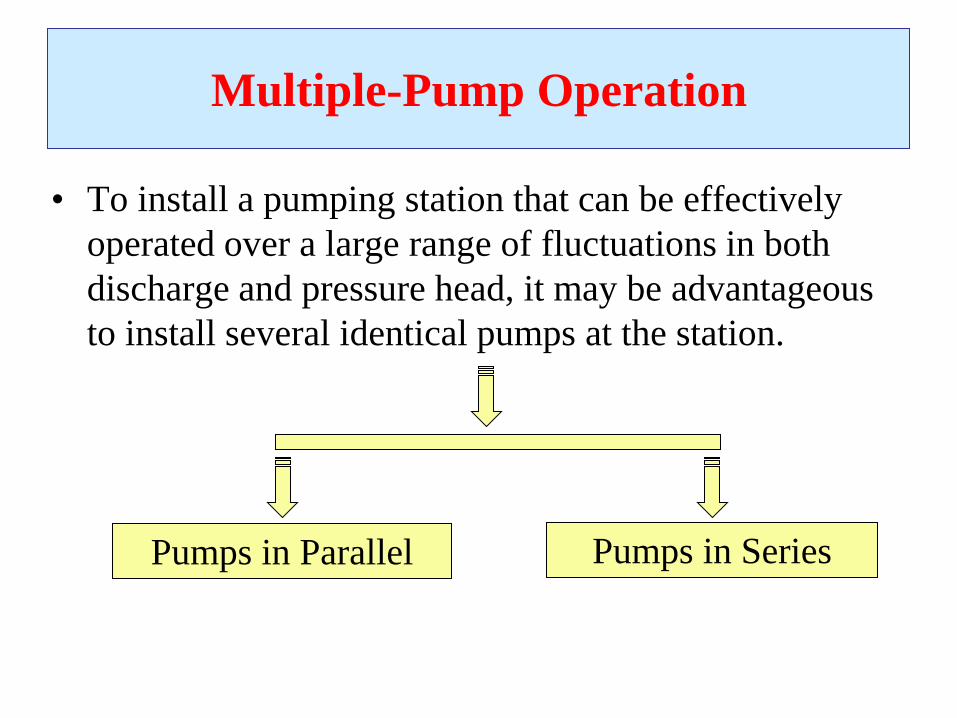
Multiple-Pump Operation

• To install a pumping station that can be effectively

operated over a large range of fluctuations in both

discharge and pressure head, it may be advantageous

to install several identical pumps at the station.

Pumps in Parallel Pumps in Series

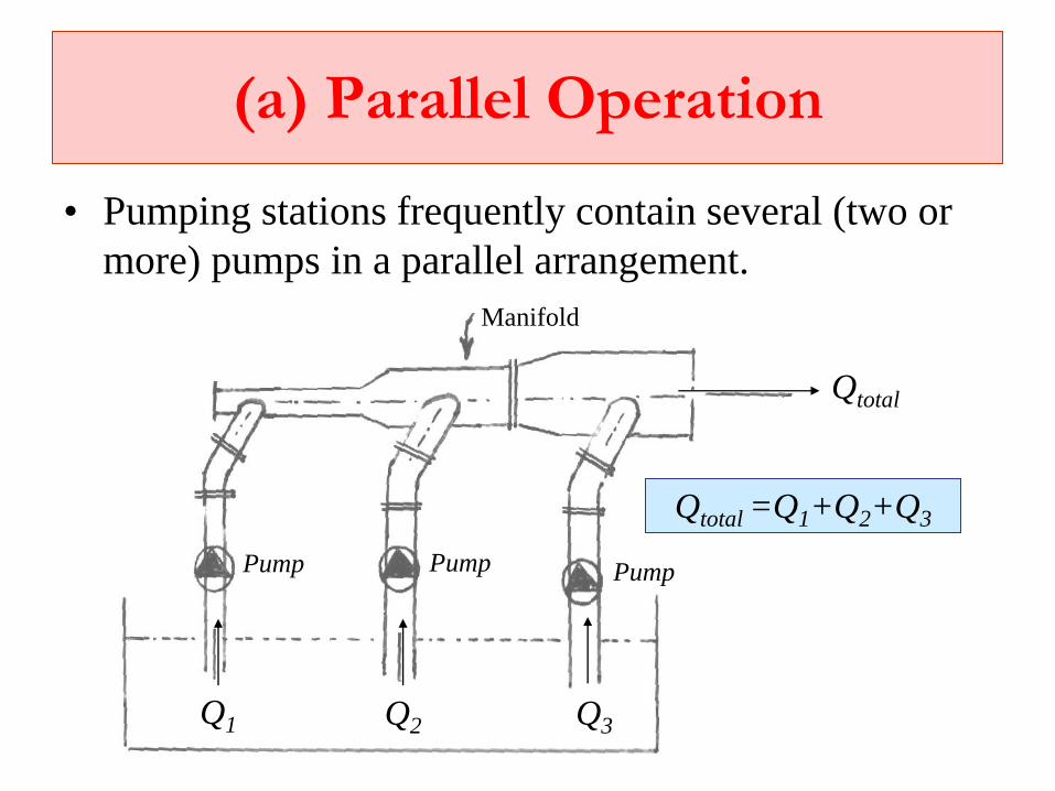
(a) Parallel Operation

• Pumping stations frequently contain several (two or

more) pumps in a parallel arrangement.

Q1 Q2 Q3

Pump Pump Pump

Manifold

Qtotal

Qtotal =Q1+Q2+Q3

• In this configuration any number of the pumps can be

operated simultaneously.

• The objective being to deliver a range of discharges,

i.e.; the discharge is increased but the pressure head

remains the same as with a single pump.

• This is a common feature of sewage pumping stations

where the inflow rate varies during the day.

• By automatic switching according to the level in the

suction reservoir any number of the pumps can be

brought into operation.

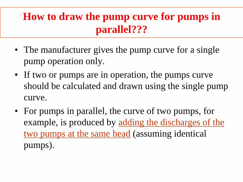
How to draw the pump curve for pumps in

parallel???

• The manufacturer gives the pump curve for a single

pump operation only.

• If two or pumps are in operation, the pumps curve

should be calculated and drawn using the single pump

curve.

• For pumps in parallel, the curve of two pumps, for

example, is produced by adding the discharges of the

two pumps at the same head (assuming identical

pumps).

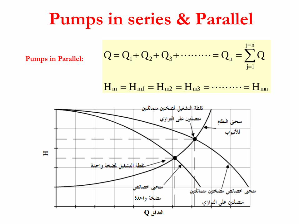
Pumps in series & Parallel

Pumps in Parallel:

mnm3m2m1m

nj

1j

n321

HHHHH

QQQQQQ

(b) Series Operation

• The series configuration which is used whenever we need to increase the pressure head and keep the discharge approximately the same as that of a single pump

• This configuration is the basis of multistage pumps; the discharge from the first pump (or stage) is delivered to the inlet of the second pump, and so on.

• The same discharge passes through each pump receiving a pressure boost in doing so

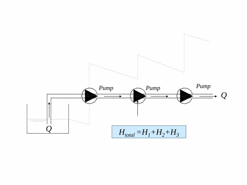
Q

Pump Pump Pump

Q

Htotal =H1+H2+H3

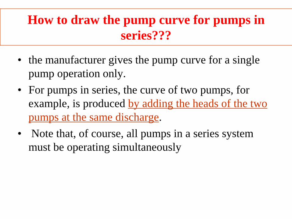
How to draw the pump curve for pumps in

series???

• the manufacturer gives the pump curve for a single

pump operation only.

• For pumps in series, the curve of two pumps, for

example, is produced by adding the heads of the two

pumps at the same discharge.

• Note that, of course, all pumps in a series system

must be operating simultaneously

H

Q

Q1

H1

H1

H1

2H1

H1

3H1

Single pump

Two pumps

in series

Three pumps

in series

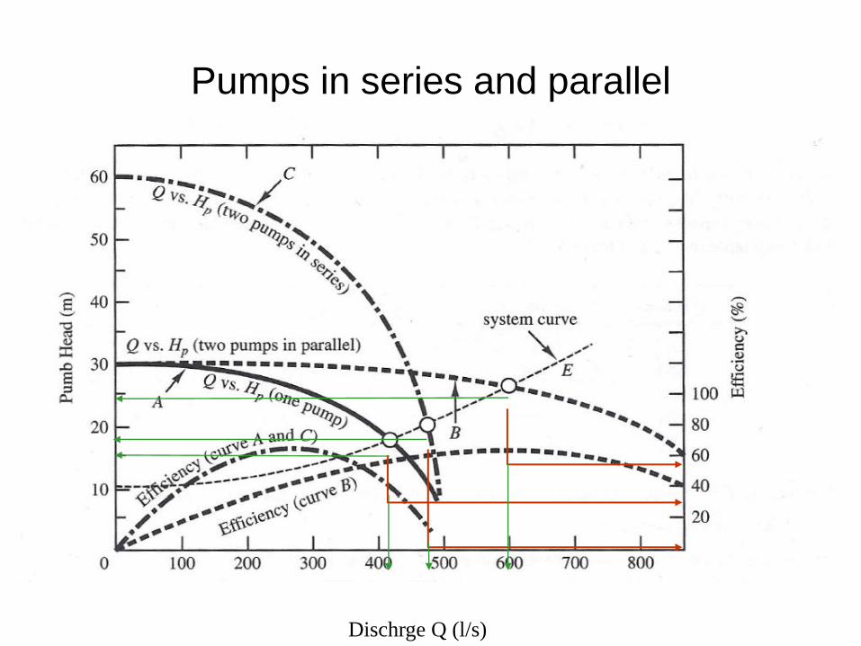
Pumps in series and parallel

Dischrge Q (l/s)

Cavitation of Pumps and NPSH

• In general, cavitation occurs when the liquid pressure

at a given location is reduced to the vapor pressure of

the liquid.

• For a piping system that includes a pump, cavitation

occurs when the absolute pressure at the inlet falls

below the vapor pressure of the water.

• This phenomenon may occur at the inlet to a pump

and on the impeller blades, particularly if the pump is

mounted above the level in the suction reservoir.

• Under this condition, vapor bubbles form (water

starts to boil) at the impeller inlet and when these

bubbles are carried into a zone of higher pressure,

they collapse abruptly and hit the vanes of the

impeller (near the tips of the impeller vanes). causing:

• Damage to the pump (pump impeller)

• Violet vibrations (and noise).

• Reduce pump capacity.

• Reduce pump efficiency

• To avoid cavitation, the pressure head at the inlet should not fall

below a certain minimum which is influenced by the further

reduction in pressure within the pump impeller.

• To accomplish this, we use the difference between the total head

at the inlet , and the water vapor pressure head g

VP ss

2

2

vaporP

How we avoid Cavitation ??

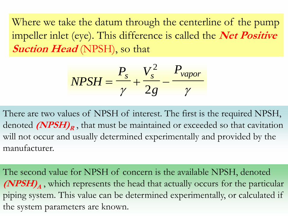
Where we take the datum through the centerline of the pump

impeller inlet (eye). This difference is called the Net Positive Suction Head (NPSH), so that

NPSHP V

g

Ps s vapor

2

2

There are two values of NPSH of interest. The first is the required NPSH,

denoted (NPSH)R , that must be maintained or exceeded so that cavitation

will not occur and usually determined experimentally and provided by the

manufacturer.

The second value for NPSH of concern is the available NPSH, denoted

(NPSH)A , which represents the head that actually occurs for the particular

piping system. This value can be determined experimentally, or calculated if

the system parameters are known.

How we avoid Cavitation ??

• For proper pump operation (no cavitation) :

(NPSH)A > (NPSH)R

Determination of

(NPSH)A

datum

hs

applying the energy equation between

point (1) and (2), datum at pump

center line

Vapor

Vapor

LS

air

atmA

Vapor

Vapor

LS

air

atm

Vapor

VaporSS

LS

air

atmSS

LSS

S

air

atm

Phh

PNPSH

Phh

PP

g

VP

hhP

g

VP

hg

VPh

P

)(

2

2

2

2

2

2

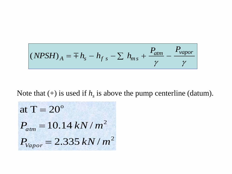
( )NPSH h h hP P

A s f s m satm vapor

Note that (+) is used if hs is above the pump centerline (datum).

2

2

o

/ 335.2

/ 14.10

20Tat

mkNP

mkNP

Vapor

atm

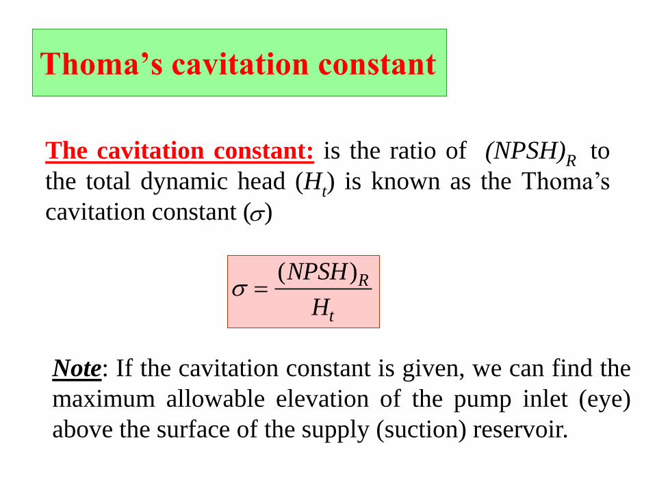
Thoma’s cavitation constant

The cavitation constant: is the ratio of (NPSH)R to

the total dynamic head (Ht) is known as the Thoma’s

cavitation constant ( )

( )NPSH

H

R

t

Note: If the cavitation constant is given, we can find the

maximum allowable elevation of the pump inlet (eye)

above the surface of the supply (suction) reservoir.

Head analysis in the suction side of the

pump

H’s

hfs

hc

V2/2g

hp

Hs

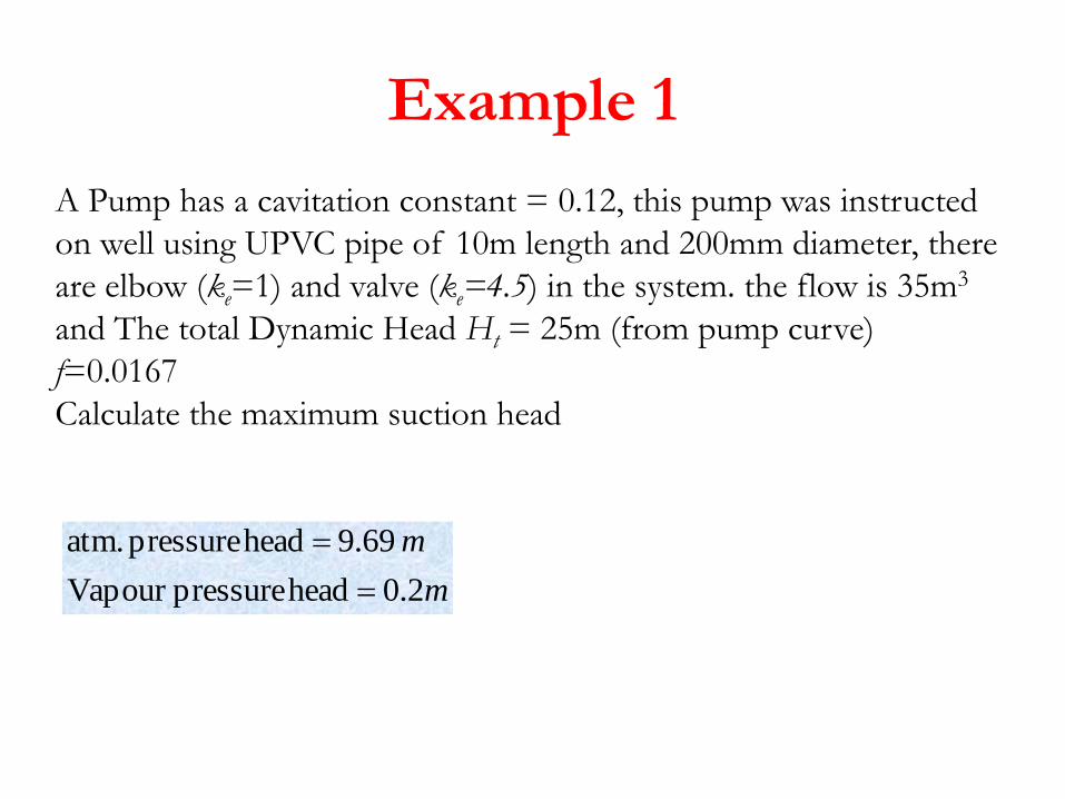
Example 1

A Pump has a cavitation constant = 0.12, this pump was instructed

on well using UPVC pipe of 10m length and 200mm diameter, there

are elbow (ke=1) and valve (ke=4.5) in the system. the flow is 35m3

and The total Dynamic Head Ht = 25m (from pump curve)

f=0.0167

Calculate the maximum suction head

m

m

2.0head pressureVapour

69.9head pressure atm.

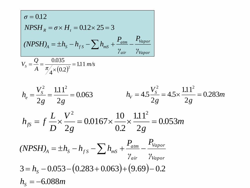
325120

120

.HσNPSH

.σ

tR

m.g

..

g

V.h S

V 28302

11154

254

22

06302

111

2

22

.g

.

g

Vh S

e

m.g

.

..

g

V

D

Lfh fS 0530

2

111

20

1001670

2

22

m.h

....h

γ

P

γ

Phhh(NPSH)

S

S

Vapor

Vapor

air

atmmSf SSA

0886

2069.90630283005303

Vapor

Vapor

air

atmmSf SSA

γ

P

γ

Phhh(NPSH)

m/s .

.π

.

A

QVS 111

204

03502

Specific Speed

• Pump types may be more explicitly defined by the

parameter called specific speed (Ns) expressed by:

Where: Q = discharge (m3/s, or l/s).

H = pump total head (m).

N = rotational speed (rpm).

NN Q

Hs 3

4

• This expression is derived from dynamical similarity

considerations and may be interpreted as the speed in

rev/min at which a geometrically scaled model would have

to operate to deliver unit discharge (1 l/s) when generating

unit head (1 m).

• The given table shows the range of Ns values for the turbo-

hydraulic pumps:

Pump type Ns range (Q - l/s, H-m)

centrifugal up to 2600

mixed flow 2600 to 5000

axial flow 5000 to 10 000

Specific speed variation

Specific Speed vs Efficiency

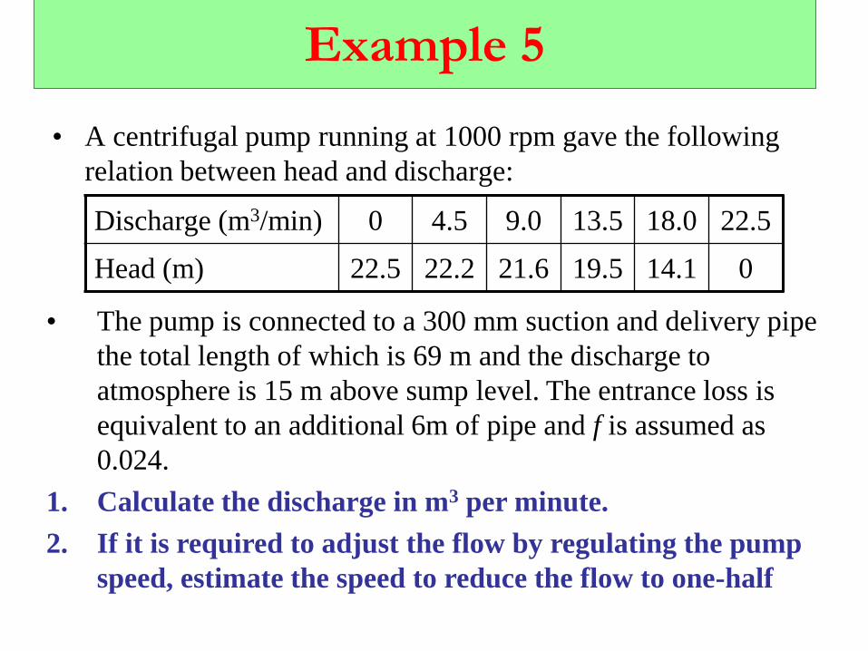
Example 5

• A centrifugal pump running at 1000 rpm gave the following

relation between head and discharge:

Discharge (m3/min) 0 4.5 9.0 13.5 18.0 22.5

Head (m) 22.5 22.2 21.6 19.5 14.1 0

• The pump is connected to a 300 mm suction and delivery pipe

the total length of which is 69 m and the discharge to

atmosphere is 15 m above sump level. The entrance loss is

equivalent to an additional 6m of pipe and f is assumed as

0.024.

1. Calculate the discharge in m3 per minute.

2. If it is required to adjust the flow by regulating the pump

speed, estimate the speed to reduce the flow to one-half

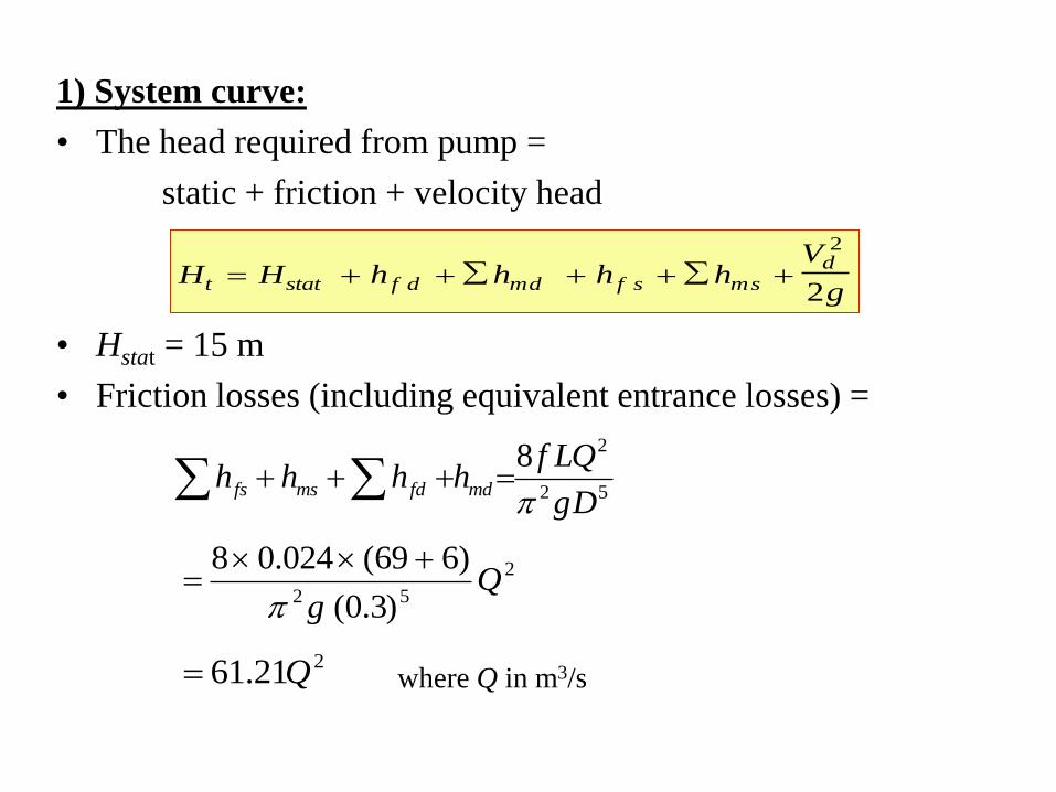
1) System curve:

• The head required from pump =

static + friction + velocity head

• Hstat = 15 m

• Friction losses (including equivalent entrance losses) =

H H h h h hV

gt stat f d md f s ms

d

2

2

52

28

Dg

QLfhhhh mdfdmsfs

2

52 )3.0(

)669(024.08Q

g

221.61 Q where Q in m3/s

• Velocity head in delivery pipe =

where Q in m3/s

Thus:

• where Q in m3/s

or

• where Q in m3/min

• From this equation and the figures given in the problem the

following table is compiled:

2

22

2.102

1

2Q

A

Q

gg

Vd

241.7115 QH t

231083.1915 QH t

Discharge (m3/min) 0 4.5 9.0 13.5 18.0 22.5

Head available (m) 22.5 22.2 21.6 19.5 14.1 0

Head required (m) 15.0 15.4 16.6 18.6 21.4 25.0

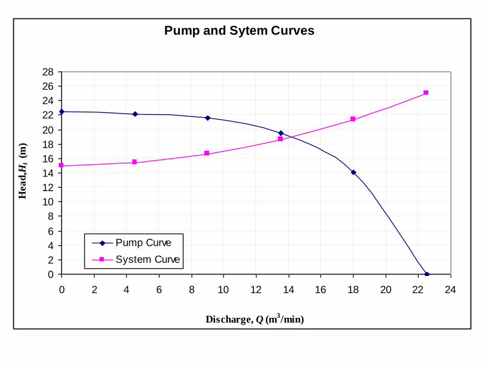
Pump and Sytem Curves

0

2

4

6

8

10

12

14

16

18

20

22

24

26

28

0 2 4 6 8 10 12 14 16 18 20 22 24

Discharge, Q (m3/min)

Hea

d, H

t (

m)

Pump Curve

System Curve

From the previous Figure, The operating point is:

• QA = 14 m3/min

• HA = 19 m

• At reduced speed: For half flow (Q = 7 m3/min) there

will be a new operating point B at which:

• QB = 7 m3/min

• HB = 16 m

• HomeWork

How to estimate the new speed ?????

Pump and Sytem Curves

0

2

4

6

8

10

12

14

16

18

20

22

24

26

28

0 2 4 6 8 10 12 14 16 18 20 22 24

Discharge, Q (m3/min)

Hea

d, H

t (

m)

Pump Curve

System CurveA

B

A

B

Q

Q

N

N

2

1

2

1

H

H

N

N

2

1

2

1

2

2

BB Q

Q

H

H

22

2327.0

7

16QQH

This curve intersects the original curve for N1 = 1000 rpm

at C where Qc= 8.2 m3/ hr and Hc= 21.9 m, then

1

2

N

N

Q

Q

C

B 10002.8

7 2N N2 = 855rpm

Pump and Sytem Curves

0

2

4

6

8

10

12

14

16

18

20

22

24

26

28

0 2 4 6 8 10 12 14 16 18 20 22 24

Discharge, Q (m3/min)

Hea

d, H

t (

m)

Pump Curve

System Curve

A

B

C

A

B

C

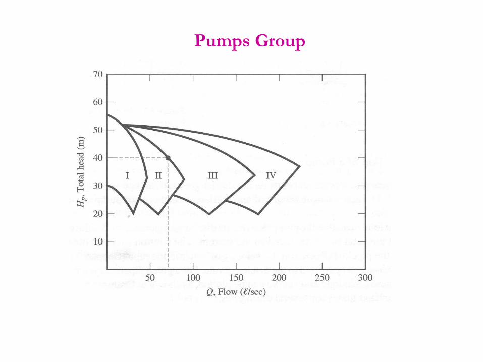
Pumps Group

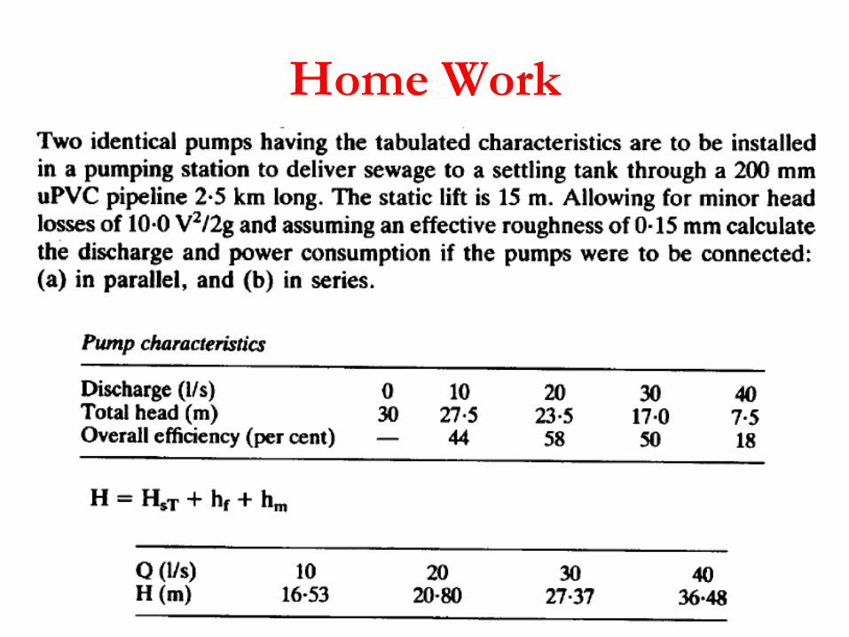
Home Work

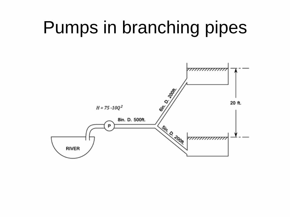
Pumps in branching pipes

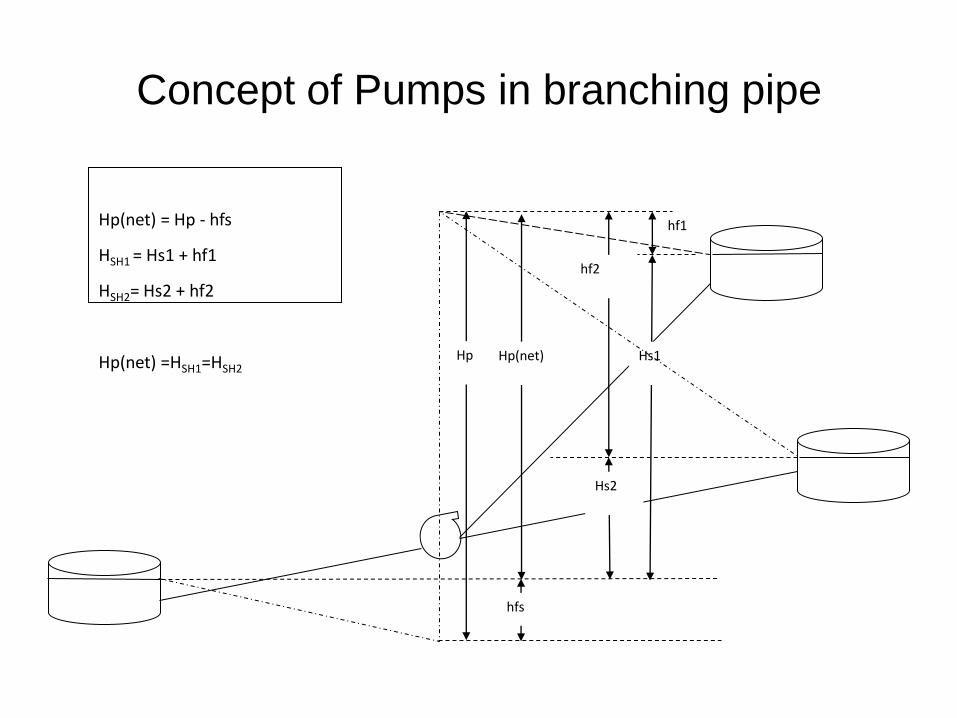
Concept of Pumps in branching pipe

Hp(net)

Hs2

Hs1

hf2

hf1

hfs

Hp

Hp(net) = Hp - hfs

HSH1 = Hs1 + hf1

HSH2= Hs2 + hf2

Hp(net) =HSH1=HSH2

Pumps in branching pipes

Example 5.5 Example 5.6

Q Hp Hsh1 Hsh2 H Q1+Q2 Net Hp

0 80 10 30 30 20 80

10 78.5 15.12 37.68 40 35 77.47

20 74 30.48 60.72 50 43 69.88

30 66.5 56.08 99.12 60 51 57.23

40 56 91.92 152.88 70 56 39.52

50 42.5 138 222 80 62 16.75

60 20 194.32 306.48

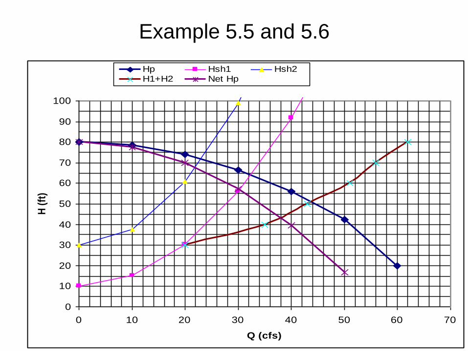
Example 5.5 and 5.6

0

10

20

30

40

50

60

70

80

90

100

0 10 20 30 40 50 60 70

Q (cfs)

H (

ft)

Hp Hsh1 Hsh2H1+H2 Net Hp