Hydraulics - Freenguyen.hong.hai.free.fr/EBOOKS/SCIENCE AND ENGINEERING...and sudden changes of velocity occur, as in certain problems associated with the rapid opening or closing

This page has been reformatted by Knovel to provide easier navigation.

5 Hydraulics

The late J Allen DSc, LLD, FICE, FRSEEmeritus Professor,University of Aberdeen

Contents

5.1 Physical properties of water 5/35.1.1 Density 5/35.1.2 Viscosity 5/35.1.3 ‘Non-Newtonian’ fluids 5/35.1.4 Compressibility 5/45.1.5 Surface tension 5/45.1.6 Capillarity 5/45.1.7 Solubility of gases in water 5/45.1.8 Vapour pressure 5/5

5.2 Hydrostatics 5/55.2.1 Force on any area 5/55.2.2 Force on plane areas 5/55.2.3 Force on curved areas 5/65.2.4 Buoyancy 5/7

5.3 Hydrodynamics 5/75.3.1 Energy 5/75.3.2 Bernoulli’s theorem 5/85.3.3 Streamline and turbulent motion 5/85.3.4 Pipes of noncircular section 5/85.3.5 Loss of head in rough pipes 5/95.3.6 Formulae for calculating pipe friction

(turbulent flow) 5/95.3.7 Deterioration of pipes 5/105.3.8 Use of additives to reduce resistance 5/10

5.3.9 Losses of head in pipes due to causesother than friction 5/10

5.3.10 Losses at pipe bends 5/115.3.11 Losses at valves 5/115.3.12 Graphical representation of pipe-flow

problems 5/115.3.13 Pipes in parallel 5/125.3.14 Siphons 5/125.3.15 Nozzle at the end of a pipeline 5/135.3.16 Multiple pipes 5/135.3.17 Flow measurement in pipes 5/145.3.18 Water hammer in pipes 5/155.3.19 Flow in open channels 5/155.3.20 Orifices 5/195.3.21 Weirs and notches 5/205.3.22 Impact of jets on smooth surfaces 5/235.3.23 Sediment transport 5/245.3.24 Vortices 5/245.3.25 Waves 5/255.3.26 Dimensional analysis 5/25

References 5/27

Bibliography 5/28

5.1 Physical properties of water

5.1.1 Density

For most purposes in hydraulic engineering, the density of freshwater may be taken to be 1000kg/m3. Correspondingly, theweight of 11 is approximately 1 kg. In more precise work,usually of a laboratory or experimental nature, the variation ofdensity with temperature may have to be taken into account inaccordance with Table 5.1.

Table 5.1 Density of fresh water at atmospheric pressure

Temperature Density(0C) (kg/m3)

O 999.94 1000.0

10 999.720 998.230 995.740 992.250 988.160 983.370 977.880 971.990 965.3

100 958.4

The density of sea water depends on the locality but forgeneral calculations the open sea may be assumed to weigh1025 kg/m3. In a tidal river the density varies appreciably fromplace to place and time to time; it is influenced by the state of thetide and by the amount of fresh water flowing into the estuaryfrom the higher reaches or from drains and other sources. Atany one spot it may also vary through the depth of the waterowing to imperfect mixing of the fresh and saline constituents.

5.1.2 Viscosity

Let us visualize a layer of a fluid as represented in Figure 5.1.The thickness of the layer is Sy and particles in the plane AB aresupposed to have a velocity v while those in CD have a different

Figure 5.1 Layer of fluid illustrating laminar flow

velocity, say v + Sv. The plan area of each plane, AB or CD, is a,say. Now the fluid bounded by AB and CD experiences aresistance to relative motion along AB analogous to shearresistance in solid mechanics. This force of resistance, dividedby the area a, will give a resistance per unit area, or a stress /.Then:

f=rj(dvldy) (5.1)

as Sy tends to zero, or as the layer assumes an infinitesimalthickness, so that dv/dy becomes the velocity gradient, i.e. therate at which the velocity changes as we proceed outwards in adirection normal to the plane AB. rj in Equation (5.1) is known

as the coefficient of viscosity. If force is defined by force =mass x acceleration then rj will have the units of f/(dv/dy}, or:

((M] x (L] x (T-2] x [L-2])/([L] x [T~>] x [L"1])

i.e. [MZrT'1], where (Af] represents mass, [L] length, and (T]time.

Thus if newtons (i.e. kilogram metres per squared second) areadopted for the force of resistance, metres for length, metressquared for area, and metres per second for velocity, then thecoefficient of viscosity takes the units kilograms per metresecond. For example, the numerical value of rj in the case ofwater at 1O0C is 0.00131 kg/m s. This is the same as0.0131 poise, i.e. 0.0131 g/cms.

5.1.2.1 Kinematic viscosity

Kinematic viscosity v is defined as the ratio of the viscosity rj tothe density p of a fluid, or:

v = rj/p (5.2)

It follows from this definition that if /7 is in kilograms per metresecond and p in kilograms per cubic metre then v will be insquare metres per second. Again, considering water at 10° C, v is1.31 x 10-6m2/s or 1.31 x 10-2cm2/s.

Typical values of rj and v, for both water and air, are given inTable 5.2, from which it will be seen that temperature has quitedifferent effects on these two fluids.

Table 5.2 Viscosities of water and dry air at atmospheric pressure

Temperature Water Air

0C 103// 106v 105// 105v(kg/m s) (m2/s) (kg/ms) (m2/s)

O 1.79* 1.79* 1.71* 1.32*5 1.52 1.52 .73 1.36

10 1.31 1.31 .76 .4115 1.14 1.14 .78 .4520 1.01 1.01 .81 .5025 0.894 0.897 .83 .5530 0.801 0.804 .86 .5935 0.723 0.727 .88 .6440 0.656 0.661 .90 .6950 0.549 0.556 .95 .7960 0.469 0.477 2.00 .8880 0.357 0.367 2.09 2.09

100 0.284 0.296 2.18 2.30

*To avoid any misinterpretation of the column headings note that, at 0° C, rj forwater is 1.79x 10~3kg/m s; v i s 1.79x 10~6m2/s; rj for air is 1.71 x l(T5kg/ms;v i s 1.32 x 10~5m2/s.

5.1.3 'Non-Newtonian' fluids

Table 5.2 implies that for water and air, the coefficient ofviscosity (sometimes called 'dynamic viscosity' or 'absoluteviscosity') varies with temperature but otherwise is a constantcoefficient in Equation (5.1), i.e. / is in simple proportion todv/dy. This is true of very many other fluids, but there exist also theso-called non-Newtonian fluids. With some of these, // decreasesas dv/dy increases; with others the reverse is true. Among theexamples of substances which, in phases of their fluid state,

behave in a 'non-Newtonian' way, are certain lubricants, e.g.grease used in bearings, plastics, and suspensions of particles.

5.1.4 Compressibility

In the vast majority of engineering calculations, water may betreated as an incompressible fluid. Exceptions arise when largeand sudden changes of velocity occur, as in certain problemsassociated with the rapid opening or closing of a valve. If weimagine a mass of water to have its volume changed from V toV— S V by an increase of pressure dp applied uniformly round itssurface, then the bulk modulus of compressibility A'is defined asthe stress or pressure intensity dp divided by the volumetricstrain produced by dp. This volumetric strain is -SV/V. Hence:

K=-dp / (SVI V) (5.3)

6 V itself being treated as negative.The value of K depends somewhat on the temperature and

absolute pressure of the water, but in round numbers it isusually sufficiently accurate to take it as 2 x 109N/m2.

5.1.5 Surface tension

Surface tension is the property which enables water and otherliquids to assume the form of drops, when it appears that thewater is bounded by an elastic skin or membrane under tension.Another important manifestation is related to small waves orripples where the form and motion are restricted or influencedby the tension in the surface. Surface tension depends on theliquid and gas in contact with one another. Suppose a portion ofthe liquid to have a bounding surface with radii of curvature intwo mutually perpendicular directions R1 and R2 as in Figure5.2. Then the excess of pressure intensity inside the boundary,over that outside it, is y(l//2, +l//?2), where y is the surfacetension, a force per unit length of the line to which it is normal.

Side view

Front viewFigure 5.2 Bounding surface of a liquid

The surface tension of mercury in contact with air at 20° C isapproximately 0.51 N/m.

Table 5.3 Surface tension of water in contact with air

(0C) O 20 40 60 80 100

y(N/m) 0.0756 0.0728 0.0700 0.0671 0.0643 0.0615

5.1.6 Capillarity

If a vertical tube is placed in a vessel containing water, the waterwill be drawn up the tube by capillary attraction. The angle a inFigure 5.3 is known as the angle of contact, and approaches thevalue zero for clean water in contact with a clean glass tube. Inthat case

h = (4 x 106 yjpdg) mm, approximately, or say (4 x 105 y)/pd(5.4)

where y is the surface tension in newtons per metre, p the densityin kilograms per cubic metre, d the bore of the tube inmillimetres, and g is in metres per second squared.

At 20° C, therefore, the elevation of the water in the glass tubeamounts to about 30/d mm. It should be emphasized, however,that capillary attraction depends to a marked degree upon thestate of cleanliness of the liquid and the tube.

Figure 5.3 Capillaryrise of water in a tube

If mercury is considered instead of water, there is a depressionof the liquid in the tube as shown in Figure 5.4. The angle /? isapproximately 53° and H, at room temperature, is about 9/d mm.

Figure 5.4 Capillary depressionof mercury in a tube

Capillary attraction may be important in connection with thetechnique of measurement. For example, if the level of water ina tank is read, for convenience, on an external gauge as depictedin Figure 5.5, the bottom of the meniscus, or curved surface ofthe water in the gauge-tube, will stand higher than in the tank.Whether the effect is serious depends, of course, upon thestandard of accuracy demanded, but it is generally advisable insuch a case, or when using a differential gauge having two limbs,to use a tube not smaller than 9.5 mm bore, and as uniform aspracticable throughout its length.

Figure 5.5 Effectof capillary attractionon measurement of height ofwater in a tank

5.1.7 Solubility of gases in water

At atmospheric pressure, water is capable of dissolving approxi-mately 3, 2 and 1% of its own volume of air at temperatures ofO, 20 and 100° C respectively. Certain other gases, such as carbondioxide, are dissolved in much greater volumes, but the presenceof air alone, together with the phenomenon of vapour pressureof water, may lead to complications in certain pipelines ormachines. To take an example, at the highest point of a siphonthe pressure is below atmospheric and it is possible for air tocome out of solution there which was originally dissolved in thewater at atmospheric pressure. This accumulation of air mayultimately reduce the flow along the siphon very appreciably, oreven break it entirely, unless precautions are taken to draw offthe air and vapour as it collects. The suction-lift of pumps is alsorestricted in practice by the difficulty of release of air and

generation of vapour so that, in practice, it is usual to limit thesuction-lift to about 8.5 m instead of the full height of the waterbarometer, say 10.4m.

5.1.8 Vapour pressure

If a liquid is contained within a closed vessel the space above itbecomes saturated with its vapour and the space is subjected toan increase of pressure, which is the vapour pressure of theliquid at the temperature then obtaining.

Table 5.4 Vapour pressure pv (N/m2) of water at varioustemperatures

(0C) O 5 10 15 20 30 4010-4/?v 0.0610 0.0875 0.123 0.170 0.235 0.423 0.736

(0C) 50 60 70 80 90 100lQ-4pv 1.23 2.00 3.09 4.76 7.00 10.1

To obtain pv in metres of water at a given temperature, divide pv, (N/m2) by gpwhere p (kg/m3) is given in Table 5.1. For example, at 10O0C, pv is(10.1xl04)/(9.81x9.58x 102), i.e. 10.8m of water.

5.2 Hydrostatics

( I ) A fluid at rest exerts a pressure which is everywhere normalto any surface immersed in it.

(2) The pressure intensity at a point P in a liquid is equal to thatat the free surface of the liquid together with pgh, where h isthe depth of P below the free surface and p is the density ofthe liquid.

5.2.1 Force on any area

In many engineering problems all pressures are treated relativeto atmospheric pressure as a datum. Adopting that system,consider the force exerted on an elementary, or infinitesimal,portion SA of an area A immersed in a liquid (see Figure 5.6).

Free surface

Figure 5.6 Elementary areabA immersed in liquid

The pressure intensity on SA is p = pgh. Hence, the force onSA is pgh-SA, where h is the vertical depth of SA.

The total force on the whole area A of which SA is an elementis the arithmetical sum of the forces on all its constituentelements, Zpgh- A= pgLh-dA, assuming p to be constantthroughout the liquid. Hence:

total force = pgH-A (5.5)

where H is the vertical depth of the centroid of the whole area.

This total force is only equal to the resultant force if the areaunder consideration is a plane one. If the area is curved, then theforces acting on its elementary portions are not all parallel toone another so their simple arithmetic sum is not the same astheir resultant.

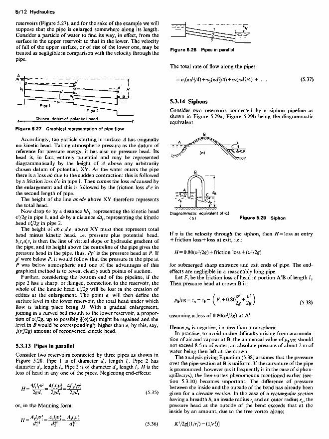
5.2.2 Force on plane areas (Figure 5.7)

Force on element = (pgz cos 9 )SA

Resultant force = total force in this case

= I,(pgzco*0)dA

= pgzAcosO (5.6)

where z is the inclined depth of centroid of A.

Figure 5.7 Plane areaimmersed in liquid

The resultant force will act through a point in the immersed areaA known as its centre of pressure and such that its inclineddepth Z is given by:

Z= f (z2 dA \ IzA = (Second moment of area A about 0O)/'zA^ ' =fJAz (5.7)

or:

Z = V0Jz (5.8)

where ^00 is the radius of gyration about OO and ^J0 = k2 + z2,where k is the radius of gyration about an axis through thecentroid parallel to 00.

Examples 5.1 to 5.6. In the following examples C is thecentroid, P the centre of pressure.

Example 5.1: Parallelogram (Figure 5.8(a)):

rw=(bd*/i2)+bd(zrZ=[bd*/l2 + bd(z2)]lbdz

= (d2!\2 + z2)/z= J d if upper edge of parallelogram is in surface.

Example 5.2: Circular area, diameter d (Figure 5.8(b)):

/00 = (7^4/64) + (7r</2/4)z2

(7T^4/64) + (7^2/4)z2

•(nd2/4)z= (J2/16 + z2)/z= 5<//8 if circle touches 00.

Example 5.3: Triangular area, apex downwards (Figure 5.8(c)):

/w = (W/36) + (6/2/2) z2

(btf/36) + (bh/2) z2 _ h2/18 + z2

(bh/2)z zwhere z = a + (h/3)

Z = A/2 if a = O.

Figure 5.8 (a) Parallelogram; (b) circular area; (c) triangular area,apex downwards; (d) triangular area, apex upwards; (e) trapezium;(f) ellipse

Example 5.4: Triangular area, apex upwards (Figure 5.8(d)):

/oo =(№/36)+ 0/1/2)?

h2l\8 + z2

z

where z = a+ (2/I)H

Z = (3/4)/*

ifa = 0.

Example 5.5: Trapezium (Figure 5.8(e)):

Z=(k2 + z2)/z

where k2 = (h2/l$)[l + 2bc/(b + c)2]

»-$$*•

Example 5.6: Ellipse (Figure 5.8(f)):

Z = (fc2 + z2)/z

where k2 = c2/\6'z = a + (c/2)

In the examples so far considered, the immersed areas havehad a vertical plane of symmetry in which it is evident that theresultant force will act. All that has been necessary, therefore,was to determine the position of the resultant force in that planeof symmetry.

5.2.2.1 Force on an unsymmetrical plane area

Choose any convenient axes OX, OY. OX may be the line ofintersection of the plane of the immersed area with the surfaceof the liquid. The elementary area 8A has coordinates x and yrelative to the chosen axes (Figure 5.9).

Figure 5.9 Unsymmetrical plane area

Let x and y be the coordinates of the centre of pressure of thewhole area relative to these same axes. Then, by using theprinciple that the moment of the resultant force is equal to thesum of the moments of the individual elementary forces:

y = (1Ly2 SA)IQLy SA) x = (fxy SA)I(Xy SA)

or:

f f>> 2 d.xdy HxydxdyJ) = LL X = JA. (5.9)

JJ>>d.xd>> JJ^djtd^

But:

Xy2SA or f f y2dxdy = Ak2

(5.10)Iy SA or Jf ydxdy = Ay0

where A is the total area, k its radius of gyration about OX andJ0 the ordinate of the centroid of the area.

5.2.3 Force on curved areas

The following examples will serve to illustrate some usefulprinciples.

Hemispherical bowl, radius r, just full of water (Figure 5.10).

Figure 5.10 Hemispherical bowl just full ofwater

Total force = arithmetical sum of forces acting on the surface= area x pressure intensity at centroid= 2nr2 x density of water x depth of centroid x g= 2nr2xpx(r/2)g= 7ir3pg

But the horizontal components of the corresponding forceson opposite sides of the vertical axis counterbalance oneanother, and:

Resultant force = weight of water contained= volume of hemisphere x density of water x g= $nr3pg

Cylindrical vessel with hemispherical end, just full of water.

(1) (Figure 5.11(a)). Force on lid due to water = O

Resultant force (vertical) on hemisphericalbase = (TiY1H + jnr3)pg

(2) (Figure 5.11(b)). Resultant force (vertical) on flatbase = nr\h + r}pgResultant force (vertically upwards) ondome = nr\h + r)pg - (nr2h + %nr3)pg = %nr3 pg

(3) (Figure 5.11(c)). Horizontal force on eitherend = nr\rp)g = nr3 pg

Figure 5.11 (a) Cylindrical vessel with hemispherical end just fullof water; (b) the same, inverted; (c) the same, lying with axishorizontal

Figure 5.12 Truncatedcone just full of water

Truncated cone, just full of water (Figure 5.12).Resultant force (vertically downwards) on base = nR2hpgVolume of water contained = ^nH(R2 + Rr + r2)Resultant force (vertically upwards) on curved side= [TiR2Hp - \nh(R2 + Rr + r2)p]g= (2STiR2H - }nRrh - }nr2h)pg

5.2.4 Buoyancy

A liquid of density p exerts a vertical upwards force Vpg on animmersed body of volume V (Figure 5.13). If the weight of the

Figure 5.13 Bodyimmersed in liquid

body is greater than Vpg it will sink. If the weight of the body isless than Vpg the body will float in such a way that the portionimmersed has a volume V which satisfies the following equa-tion:

V pg = total weight of body (5.11)

Centre of buoyancy and metacentre. The centre of gravity ofthe displaced fluid is called the centre of buoyancy. When abody is floating freely, the weight of the fluid displaced equalsthe weight of the body itself, and its centre of buoyancy, forequilibrium, must be in the same vertical as the centre of gravity

of the body. The degree of stability for angular displacementsinvolves the conception of the metacentre. In Figure 5.14, XXrepresents the vertical axis of symmetry of a floating body with acentre of gravity, owing to the distribution of its weight, wesuppose to be at G. B is the centre of buoyancy.

Figure 5.14Centre of buoyancy

Let the body be displaced so that B, becomes the new centreof buoyancy, i.e. the centre of gravity of the liquid as displacedin the new position (Figure 5.15).

Figure 5.15 Metacentre

The new force of buoyancy acts vertically upwards throughB1, to intersect the deflected line BG in M, the metacentre.Strictly speaking, the metacentre is the position assumed by Mas the angle of displacement 6 tends to zero.

If M is above G, there will be a 'righting moment'pV-GMsmO-g.

The condition for initial stability, or stability during smalldisplacements, is then that M shall be above G.

The metacentric height may be calculated from the equation:

GM = (//FV±GB (5.12)

where /= Ak2: the plus sign is used if G is below B and the minussign if G is above B.

A is the area of the water-line section and k is its radius ofgyration about the axis Oy. K is the volume of the immersedportion of body (shown in Figure 5.16).

Plan view of Figure 5.17 Mass of liquidwaterline section subjected to p N/m2 and

Figure 5.16 Metacentric height moving with velocity vm/s

5.3 Hydrodynamics

5.3.1 Energy

A liquid possesses energy by virtue of the pressure under whichit exists, its velocity and its height above some datum level of

potential energy. These three forms of energy—pressure, kineticand potential—may be expressed as quantities per unit weightof the liquid concerned. The result is the pressure, kinetic orpotential head. Thus, referring to Figure 5.17, in which a massof liquid is represented as subjected to a pressure /?N/m2,moving with a velocity v m/s and having its centre of mass at aheight z above a datum of potential energy:

total head = (p/pg} + (v2/2g) + z (5.13)

in metres, where p is the density in kilograms per cubic metre.If a gas is considered, then account should be taken of its

elasticity and the work done in compressing a given mass of it asit passes from a region of low to higher pressure.

5.3.2 Bernoulli's theorem

This states that in the streamline motion of an incompressibleand inviscid fluid the total head remains constant from sectionto section along the stream tube, i.e.:

(Pl PS) + (*>2/2g) ̂ z = constant (5.14)

The idealized circumstances envisaged in this statement wouldseem, at first sight, to render the theorem useless for the solutionof problems dealing with natural fluids, which are viscous, andespecially when such fluids are not moving in streamlines, i.e.when the motion is turbulent, as it usually is in hydraulics. Infact, however, the theorem forms the basis of the majority ofpractical calculations if and when appropriate terms are addedor coefficients introduced to allow for losses of head arisingfrom various causes. The numerical values of these terms andcoefficients are almost always the result of experiment orexperience.

5.3.3 Streamline and turbulent motion

If we concentrate attention upon one point P in the cross-sectionof a pipe or channel along which a fluid is moving at a constantrate, the motion at P may be called 'streamline' if the velocitythere is constant in magnitude and direction. On the other hand,the motion at P will be turbulent if the velocity there varies fromtime to time in magnitude and/or direction, despite the fact thatthe general rate of flow along the channel is constant. In thisturbulent motion, the instantaneous velocity at P depends uponhow the eddies are passing it at the moment under consider-ation. The eddies which characterize turbulent motion requireenergy for their creation and maintenance, and the law ofresistance in streamline (sometimes called laminar) flow is quitedifferent from that in turbulent flow.

5.3.3.1 Flow in pipes

Loss of head in smooth pipes The general equations for the lossof head in a pipe of uniform diameter d are as follows. Let h bethe loss of head in metres, / the length of pipe considered inmetres, v the mean velocity in metres per second = Qj(nd2/4), Qthe rate of discharge (in cubic metres per second) and v thekinematic viscosity of fluid (in square metres per second). Then:

H = K(Iv2 "v")/gd>-n (5.15)

where K is a coefficient.

Both K and n depend upon Re the Reynolds number, vd/v. If Reis less than 2100, K=32 and AI= 1.

These values give the equation for streamline flow, which maybe deduced mathematically:

h = 32vlv/gd2 (5.16)

Alternatively we may use the equation! commonly adopted byhydraulic engineers, i.e.:

h=flv2/2gm (5.17)

in which m represents the hydraulic mean depth or the ratio ofthe area of section to the wetted perimeter. In a cylindrical piperunning full, m = d/4.

For values of Re up to 2100:

/=16(w//v)-' (5.18)

For values of Re between 3000 and 150 000 (Davis and White1):

/=0.08(™//v)-°-25 (5.19)

Alternatively, if Re exceeds 4000, the Prandtl equation may beused:

1 /V(4/) = 2.0 Ig [/W(4/)] - 0.8 (5.20)

These relationships apply to smooth pipes of, say, glass, drawnbrass, copper or large pipes with a smooth cement finish.

In calculating Reynolds numbers, the units in which v, d and vare measured should be consistent with one another; e.g. v inmetres per second, d in metres and v in square metres persecond. Values of / for smooth pipes in the equationh=flv2j2gm are plotted against \gvdjv in Figure 5.18.2

At a temperature of 150C, v for water is 1.14 x 10~6m2/s.

Figure 5.18 Values of ffor smooth pipes. (After Stanton andPannell (1914) Phil. Trans A, 214; National Phys. Lab. Coll. Res.,11)

5.3.4 Pipes of noncircular section

There is experimental evidence showing that if the flow isturbulent, the value of/for various shapes of section is approxi-mately the same as for a cylindrical pipe at the same value ofvm/v, where m again represents the hydraulic mean depth.

The critical value of vm/v, below which the motion is nor-mally laminar, does depend to some extent, however, on theshape of the section. For a circular section it is 525 (i.e.vd/v = 2100). For rectangular sections the critical vm/v varieswith the ratio of the lengths of the sides and has approximatevalues of 525 for a square section, 590 for a section having one

t Some writers prefer to use h = A/v2/2g^/, rather than 4fv2/2qd, forcylindrical pipes. Their friction factor 1 is then 4/.

side 3 times the other, and 730 for a section in which the lengthof one side is large compared with the other.

During truly laminar or viscous motion, the loss of head h forvarious shapes of section is as follows (v being the mean velocitythrough the section):

Circular section (diameter d): h = 32vlv/gd2

Rectangular section (one side 2a, other side 2b):

/, i / / wFi 192 b ( ^na l ^na MH = 3vh/gbV~^a(ianhYb + y i a n h ^ + ' ' - ) }

Square section (each side 2a):

h = l.\2vlv/ga2

Rectangular section having a large compared with b:

h-+3vh/gb2

Circular annulus (mean velocity v through space of arean(d] -d2

0)/4):

A-W^[1 + W^+]E^]

where d\ is the outside diameter and J0 the inside diameter.

5.3.5 Loss of head in rough pipes

Here the value of/also depends upon the ratio of the hydraulicmean depth to the height of the roughening projections from thewall, as well as upon the distribution and shape of theseroughnesses. Figure 5.19 summarizes experimental resultsobtained by Nikuradse3 with sand-roughened pipes, k being themean size of the grain projecting from the wall.

Figure 5.19 Values of ffor rough pipes. (After Nikuradse (1933)Forschungsh. Ver. dtsch. Ing., No. 361)

The general tendency is for/to become constant, for a givenrough pipe, at sufficiently high Reynolds numbers. A commonlyaccepted explanation of this is that first of all the surface grainslie inside a very thin viscous layer at the wall of the pipe, evenwhen the main motion is turbulent; at higher values of Re,

however, they begin to project from this layer and to shed eddiesfor the maintenance of which additional energy is required.

Prandtl and von Karman4 have shown than Nikuradse'sresults may be made to lie within one band by plotting thequantity

l/V(4/)-21g(<//2*)

against a new Reynolds number V+k/v, in which V^ representsiN/C/72).

Again, if V^k/v exceeds 60, / becomes constant for a givenpipe, the flow then being 'fully turbulent' and the resistanceproportional to v2.

Under those conditions (F^A:/v>60):

'//="('g¥92 (5.21,A pipe may be regarded as 'hydraulically smooth' if V^k/v<3.

To take a specific example, namely, d/k = 252: for values ofthe original Reynolds number vd/v less than about 11 500, / isthe same as for a smooth pipe (see Figure 5.19), while if vd/vexceeds 250 000, / assumes a constant value of 0.007. Betweenthe two there is a curve which represents a transition and whichcovers a wide range of Reynolds numbers (11 500 to 250 000 inthe example d/k = 252).

A large proportion of the cases which occur in engineeringwill be found to lie within the zone of transition, for whichColebrook and White5 6 have evolved the equation:

./V(4/)=-2,g(4+^) (522)

5.3.6 Formulae for calculating pipe friction (turbulentflow)

With the velocities commonly encountered in water pipes, themotion is turbulent. These velocities in fact are frequentlywithin the range from 1.5 to 3.5m/s, whereas in general themotion can only be expected to be streamline, considering waterat ordinary temperatures, for velocities lower than 2.4/dm/s,where d is the pipe diameter (in millimetres).

Manning's formula. Among the many formulae which havebeen suggested from time to time, that of Manning7 is muchfavoured:

V = (W2W2In) (m/s) (5.23)

In this-form it applies to pipes and open channels.m is the hydraulic mean depth (in metres), i the virtual slope

of the pipe (i.e. h/l) or the actual slope of the open channelunder conditions of uniform flow, n depends upon the materialof which the conduit is made.

Alternatively:

V = WP12IlWn) (m/s) (5.24)

if m is expressed in millimetres.For cylindrical pipes, the Manning formula in Equation

(5.23) gives:

H = H2Iv2Jm^ (5.25)

Comparing the formulae

h = 4flv2/2gd and h = Ah2/d413

it appears that

f=(4.9\/d^)A (5.27)

or

/=31.2/i2/</"3 (5.28)

where d is in metres. If d is in millimetres:

f=(49.l/d]/*)A = 312«2/</'/3 (5.29)

Hydraulic Research Papers, Nos 1 and 2 (Ackers8), firstpublished by HMSO in 1958, contain not only a fascinatingreview of the resistance of fluids in channels and pipes but alsotables and graphs for the use of designers. The results arederived from the formula of Colebrook and White in Equation(5.22) and values of the effective roughness dimension k arequoted for a great variety of commercial pipes, while in addi-tion, a supplementary note provides information concerning theactual diameters of different classes of pipe in relation to theirnominal bores.

5.3.7 Deterioration of pipes

Pipes deteriorate with age and to allow for this reduction in theircarrying capacity Barnes9 has suggested the following (see Table5.6).

None of these values can be at all precise, since the reduction

of carrying capacity must depend not only upon the materialbut also upon the nature and velocity of the water and upon thediameter of the pipe; an increased roughness due to tubercula-tion will be more troublesome, proportionately, in small- thanin large-diameter pipes.10

5.3.8 Use of additives to reduce resistance

The literature dealing with this important subject has expandedgreatly in the last 10 or 20 years and now includes a largenumber of papers giving information not only of laboratorystudies but also of evidence adduced by full-scale applications.

Fortunately, the International Association for HydraulicResearch (IAHR) invited a panel or Task Force' consisting ofR. H. T. Sellin, J. W. Hoyt, J. Pollert and O. Scrivener tocompile a 'state-of-the-art review' and this has now beenpublished in two parts in the Association's Journal"-12

These reports deal largely with the addition of polymers andtheir observed effect in decreasing the resistance to the motionof the fluid. Attempts to explain the phenomenon are discussedand a wide range of applications are described: they include,inter alia, full-scale examples of sewers, oil pipelines, openchannels, hydro-transport of solids, hydraulic machinery, shipsand submerged bodies, in which significant reductions of resis-tance or increases of the carrying-capacity of pipes and channelshave been recorded.

5.3.9 Losses of head in pipes due to causes other thanfriction

Sudden enlargement. With sufficient accuracy for practicalpurposes, loss due to sudden enlargement (Figure5.20) = (^-z,2)

2/2g

Figure 5.20 Loss of Figure 5.21 Pipe joinedhead due to sudden to tank or reservoirenlargement

If the enlarged section is very large, as when a pipe is joined toa tank or reservoir (Figure 5.21):

loss = *;2/2g (5.31)

Gradual enlargement (Figure 5.22). Loss of head (includingfriction) may be taken as:

k(v,-V2)2JIg (5.32)

But:

m = d/4

Hence:

h = n2(4)4'\h2/d413) = 6.35n2(h2/d413) (5.26)

If we write this in the form:

h = A(Iv2Jd4^

the following are appropriate values of A for new pipes (seeTable 5.5).

Table 5.5

Material

Clean uncoated cast ironClean coated cast ironRiveted steelGalvanized ironBrass, copper or glassWood-staveSmooth concreteCement mortar finishVitrified sewer pipe

n

0.0130.0120.0150.0140.0100.0120.0120.0130.011

A = 6.35 n2

0.001 10.000 920.00140.001 20.000 640.000920.000 920.001 10.000 77

Table 5.6

Type of pipe

Uncoated cast ironAsphalted cast ironAsphalted riveted wrought

iron or steelWood-staveNeat cement or concrete

Discharge for which todesign, in terms of requireddischarge Q

1.5501.450

1.3301.0801.060

where k depends upon the angle of divergence 9 in the followingmanner (Gibson13).

Table 5.7

0 (degrees) 2 5 10 15 20 40 60 90 120 180k (circularpipe) 0.20 0.13 0.18 0.27 0.43 0.91 1.12 1.07 1.05 1.00

Sudden contraction. The loss due to sudden contraction isalmost entirely due to the subsequent re-enlargement of thecontracted stream (Figure 5.23). For practical purposes:

loss = (l/2)(*;2/2g) (5.33)

and this may be taken as the immediate loss of head experiencedas water flows from a reservoir into a pipe in which it attains avelocity v.

Figure 5.23 Loss of head dueto sudden contraction

With a reasonably rounded entrance, the loss may be reducedto about:

(\/20)(v2j2g)

If the pipe has a sharp entrance but projects into the reservoirand forms a re-entrant mouthpiece, the loss of head at theentrance is approximately 0.80*;2/2g (assuming that the piperuns full).

5.3.10 Losses at pipe bends

Owing to the many variables involved (e.g. size of pipe, radius ofbend, velocity of flow), it is impracticable at present to genera-lize with any degree of certainty, but the following data may behelpful in ordinary calculations (Figure 5.24).

Figure 5.24 Pipe bend

Defining Kv1 /2g as the loss in excess of that which would arisefrom friction in the same length of straight pipe, then approxi-mate values of K are:

RId= 1; K=0.50 for either 90° or 180° bends;RJd= 2 to 8; K= 0.30 for 90° and K= 0.35 for 180° bends.

For 90° elbows, K= 0.75 and for square, or sharp, elbows,AT= 1.25.

The motion round the bend tends to take on the characteris-tics of a free vortex, having a greater velocity at the inside thanat the outside. Correspondingly, the pressure at the inside is lessthan at the outside. Consider a section half-way round the bendand let d= Ir. If the discharge (volume per second) is Q, thevelocities at the inside and outside of the bend are approxima-tely:

= QV' 27r(«-l)r2[«-(«2-l)I /2]

= QV° 2n(n+l)r2[n-(n2-iy/2]

where n = R/r.

Correspondingly, the effect of the free vortex itself is to makethe pressure head at the outside of the bend exceed that at theinside by an amount (v2 - vfy/2g.

5.3.11 Losses at valves

These depend, of course, upon the relative size and design, butthe order of magnitude involved may be judged from Gibson'sexperiments13 for:

Figure 5.25 Circular sluice gate valve

(1) Circular sluice gate valves (Figure 5.25):

Loss = F(v2/2g) where v = velocity in pipe (5.34)

Table 5.8

F for djD

0.2 0.3 0.4 0.5 0.6 0.8 1.0

D= 50mm 30 11 4.2 2.1 0.9 0.22 OZ) = 600mm 36 11 3.0 1.6 1.0 - -

(2) Butterfly valve (Figure 5.26):

Figure 5.26 Butterfly valve

Table 5.9

0 5° 10° 20° 30° 40° 50° 60° 70°F 0.24 0.52 1.54 3.9 10.8 32.6 118 751

5.3.12 Graphical representation of pipe-flowproblems

This may be illustrated by the example of a pipeline joining two

Figure 5.22 Gradual enlargementof pipe

Included angleof cone 8

reservoirs (Figure 5.27), and for the sake of the example we willsuppose that the pipe is enlarged somewhere along its length.Consider a particle of water to find its way, in effect, from thesurface in the upper reservoir to that in the lower. The velocityof fall of the upper surface, or of rise of the lower one, may betreated as negligible in comparison with the velocity through thepipe.

Figure 5.27 Graphical representation of pipe flow

Accordingly, the particle starting in surface A has originallyno kinetic head. Taking atmospheric pressure as the datum ofreference for pressure energy, it has also no pressure head. Itshead is, in fact, entirely potential and may be representeddiagrammatically by the height of A above any arbitrarilychosen datum of potential, XY. As the water enters the pipethere is a loss ab due to the sudden contraction: this is followedby a friction loss b'c in pipe 1. Then comes the loss cd caused bythe enlargement and this is followed by the friction loss d'e inthe second length of pipe.

The height of the line abode above XY therefore representsthe total head.

Now drop be by a distance bb}, representing the kinetic headv2J2g in pipe 1, and de by a distance JJ1, representing the kinetichead v2

2/2g in pipe 2.The height of ab^c^e^ above XY must then represent total

head minus kinetic head, i.e. pressure plus potential head.blcldlel is then the line of virtual slope or hydraulic gradient ofthe pipe, and its height above the centreline of the pipe gives thepressure head in the pipe, thus, Pp' is the pressure head at P. Ifp' were below P, it would follow that the pressure in the pipe atP was below atmospheric and one of the advantages of thisgraphical method is to reveal clearly such points of suction.

Further, considering the bottom end of the pipeline, if thepipe 2 has a sharp, or flanged, connection to the reservoir, thewhole of the kinetic head v2

2/2g will be lost in the creation ofeddies at the enlargement. The point ^1 will then define thesurface level in the lower reservoir, the total head under whichflow is taking place being H. With a gradual enlargement,joining in a curved bell mouth to the lower reservoir, a propor-tion of t>2/2g, up to possibly j(^/2g) might be regained and thelevel in B would be correspondingly higher than el by this, say,j(v^/2g) amount of reconverted kinetic head.

5.3.13 Pipes in parallel

Consider two reservoirs connected by three pipes as shown inFigure 5.28. Pipe 1 is of diameter J1, length /,. Pipe 2 hasdiameter J2, length I2. Pipe 3 is of diameter J3, length I3. H is theloss of head in any one of the pipes. Neglecting end-effects:

H_4Mv2_4f2l2v2_ 4f3l3v

2

2gd, 2gd2 2gd3 (5.35)

or, in the Manning form:

„_ A1W _ A2I2V2 _ A3I3V

2

df Jf Jf (5.36)

Figure 5.28 Pipes in parallel

The total rate of flow along the pipes:

= v,(nd2/4) + v2(ndl/4) + v,(nd2/4) + ... (5.37)

5.3.14 Siphons

Consider two reservoirs connected by a siphon pipeline asshown in Figure 5.29a, Figure 5.29b being the diagrammaticequivalent.

Diagrammatic equivalent of (a)( b ) Figure 5.29 Siphon

If v is the velocity through the siphon, then H= loss at entry+ friction loss+ loss at exit, i.e.:

H= 0.80(v2/2g) + friction loss + (v2/2g)

for submerged sharp entrance and exit ends of pipe. The end-effects are negligible in a reasonably long pipe.

Let F1 be the friction loss of head in portion A'B of length /,.Then pressure head at crown B is:

ft//* = *A-*.-(* + 0.8og + g) (53g)

assuming a loss of 0.80(v2/2g) at A'.

Hence pB is negative, i.e. less than atmospheric.In practice, to avoid undue difficulty arising from accumula-

tion of air and vapour at B, the numerical value ofpjpg shouldnot exceed 8.5 m of water, an absolute pressure of about 2 m ofwater being then left at the crown.

The analysis giving Equation (5.38) assumes that the pressureover the pipe-section at B is uniform. If the curvature of the pipeis pronounced, however (as it frequently is in the case of siphon-spillways), the free-vortex phenomenon mentioned earlier (sec-tion 5.3.10) becomes important. The difference of pressurebetween the inside and the outside of the bend has already beengiven for a circular section. In the case of a rectangular sectionhaving a breadth b, an inside radius rt and an outer radius r0, thepressure head at the outside of the bend exceeds that at theinside by an amount, due to the free vortex alone:

*2/2g[(l/r?)-(l/r2)]

where K= Q/b In rjr{ and Q is the volume flowing per second.

Difficulties may arise, therefore, in bends of severe curvature,through high suction at the inside of the bend.

5.3.15 Nozzle at the end of a pipeline (Figure 5.30)

Figure 5.30 Nozzle at end of pipeline

Let H be the total head (in metres), V the velocity in the pipe (inmetres per second), v the velocity in the jet (in metres persecond), D the diameter of the pipe (in metres) and d thediameter of the nozzle end (in metres):

Discharge = v(nd2/4) m3/s. Then v = V(DId)2

Effective head behind nozzle = //—loss at entrance to pipe —friction in pipe. Hence v2/2g = H— friction head in pipe, neglect-ing entrance effect, or, more precisely:

v = C»[2g(H-Far» (5.39)

where F is the friction loss of head in pipe and CN the coefficientof the nozzle.

Although CN depends upon the Reynolds number vd/v, forpractical purposes it is usually sufficiently accurate to give it thevalue 0.98, either for elaborately streamlined nozzles or for astraight taper form ending in a cylindrical portion of length d/2and diameter d.

Writing F in the form F=4flV2/2gD:

2gC2tH

l + [4flCl/D(D/dY] (5.40)

The energy delivered in the jet = pav^/2 N m/s, where p is thedensity of water (=1000 kg/m3) and a = nd2/4.

This energy is a maximum, for a given //, if:

"2 = CV(/W) (5.41)

The velocities are then such that the friction head F is verynearly equal to ///3.

5.3.16 Multiple pipes

Consider the example shown in Figure 5.31, in which it isdesired to calculate the flow along the three pipes.

Height of A, B, C, J above some chosen datum of potential

= ZA, ZB, zc, Zj respectively.

Neglecting losses other than those due to pipe friction F:

ZA = (P JPS) + («?/2*) + z, + FI <5-42)

Z8 = (P JPK) + (vlllg) + Z1-F2 (5.43)

zc = (P J Pg) + (v\!2g) + Z1-F3 (5.44)

Also:

V1(Kd*/*) = v2(nd2/4) + v3(nd2/4) (5.45)

Calling:

F1 = (4Mv2^d1)- F2 = (4f2l2v2/2gd2)', F3 = (4f3l3v

2/2gd3)

and assigning values to/,,/2,/3, Equations (5.42) to (5.45) aresufficient for the determination of the four unknowns /?;, V19 V2,V3, and if necessary the solutions may be modified by furthercalculation should the resulting v suggest values of/,, /2, /3different from those originally assumed.

The solution of (in this example) four simultaneous equationsis, however, cumbersome and full of possibilities of arithmeticalslips. A simpler and quicker method14 is as follows.

If assumed total head difference between two ends of apipe = /i, then:

w=^vev 22gd 2gd\a) A^ (5.46)

where Q is the rate of flow = va, a is area of section = nd2/4, andK=2fllgda2.

If the correct values of h and Q are h + Sh and Q + SQ, thenSh = 2h-SQ/Q to a first approximation.

Now the error SQ for any one pipe is unknown, but the sumof the errors, Z(SQ), is known, being equal to the unbalancedflow, and:

6h = HdQ)/I,(QI2h) (5.47)

Example 5.7. zA = 30.50; z}= 12.20; zB = 6.10; zc = 3.05, all inmetres.

(These might be levels with reference to ordnance datum,say.)

Pipe 1 3.0km long, 600mm diameter,/= 0.007Pipe 2 1.5km long, 300mm diameter,/=0.007Pipe 3 1.5km long, 300mm diameter,/=0.007

Let:

H=(p/pg) + (v2/2g) + z

Steps in solution(1) Assign some value to the total head at J. Evidently it must

be less than that at A, which is 30.5 m. Hence we might firsttry Hj = 20 m, say.

(2) It then follows that:

F1 = (4 x 0.007 x 3000^)/(2 x 9.81 x 0.600) = 30.5 - 20.0 =10.5

Hence:

V1 = V(1.47)= 1.21 m/sQ1= 0.342 m3/sFigure 5.31 Multiple pipes

(3) Similarly, F2 = 20.0 - 6.1 = 13.9therefore:

4 x Q.OQ7 x 15OQ^2x9.81x0.300

z;2=1.40m/s

Q2 = 0.099 Om3/s

F3 = 20.0-3.05 =16.95therefore:

4x0.007x1500.^2x9.81x0.300

V3= 1.54m/s

£3 = 0.109m3/s

Hence, our original assumption (that total head at J = 20 m) hasled to an out-of-balance flow of 0.342-(0.099 O+ 0.109), or0.134m3/s. Hence:

I1SQ = 0.134

(4) But QlIh for pipe 1 =0.342/(2 x 10.5) = 0.016 3

therefore 1(6/2/0 = 0.0231

But Q/2H for pipe 2 = 0.0990/27.8 = 0.003 57

But Q/2H for pipe 3 = 0.109/33.9 = 0.003 22

so that T£QI\L(QI2h)] = 0.134/0.023 1 = 5.80

(5) Now it is evident that we must aim at decreasing ouroriginal estimate of Q} while increasing those of Q2 and Qr

We now try total head at J: 20.0 + 5.8 = 25.8 m:

Our new estimate of

^=°-342X V(Sf^S) =0.229m3/s

Our new estimate of Q2 = 0.099 O x J(~^\ = 0.118 m3/s

Our new estimate of Q, = 0.109 x J(^|) = 0.126m3/s

and:

S<5£ = 0.118 + 0.126-0.229 = 0.015

2/2/1 = 0.229/9.40 = 0.0244 for pipe 1

2/2/z = 0.118/39.4 = 0.0030 for pipe 2

2/2/1 = 0.126/45.5 = 0.0028 for pipe 3

Therefore:

2(2/2/?) = 0.030 2

^ = 0.015/0.0302 = 0.497

(6) Now make total head at J: 25.8-0.5 = 25.3:

Q1 then = 0.342 x v/(5.20/10.5) = 0.241

Q2 then = 0.099 0x^(19.2/13.9) = 0.116 .[ 0.241

Q3 then = 0.109 x V(22.25/16.95) = 0.125 >

The flows are now in balance; the number of steps required inthe process of successive approximation depends on the accur-acy of the original guess at the total head of J.

Having obtained a sensibly accurate balance, we may if wechoose carry out refined calculations based upon more accep-table values of/and including losses due to other causes such asthe junction J, any bends, and so forth.

The example considered above is, however, comparativelysimple. The more complicated cases frequently encountered inpractice are nowadays analysed with the aid of analogue ordigital computers.15^8

5.3.17 Flow measurement in pipes

5.3.17.1 The Venturi meter

The proportions shown in Figure 5.32 are not essential, but arefairly representative; the gently tapering divergent portion fol-lowing the convergent tube (which is the real meter) is intendedto minimize the overall loss of head due to eddies and frictionbetween 1 and 3.

Q = ̂ offiov = va=C(nd>,4)[M^Y (54g)

where h} (=pjpg) and H2 (=p2/pg) are the pressure heads atsections 1 and 2 respectively.

.̂ .̂

1 I 2 ~3~r 2v2d-^ r/*d H

Figure 5.32 Venturi meterIf the throat diameter is too small, the pressure p2 may be so

low as to encourage release of air and vapour which will causethe flow to fluctuate and will introduce an uncertainty. To avoidthis, it is advisable to use proportions which will not cause p2 tobe less than 21 x 103 N/m2); i.e. H2 not less than 2.1 m of water(absolute).

Values of C. The value of C, the coefficient of the meter, isinfluenced by the Reynolds number and for the sort of designsof meter commonly used in practice, the following are approxi-mately correct values19 (Table 5.10).

5.3.17.2 Pipe orifice as meter

The pipe orifice as a measuring device is conveniently installedat a flange joint but has the disadvantage of creating anappreciable obstruction and consequent loss of head. In Figure5.33, a and b are pressure tappings:

Q = CAJ2gh/((D/dy-l] (5.49)

where A = nD2/4, and H is the pressure head difference betweenpoints a and b. C is of the order of 0.61 for values of (d/D)2

between 0.3 and 0.6, but it should be noted that the accuracy ofthe machining is of great importance, since the quantity (D/dYoccurs in the formula. Similarly, it is important to have a highdegree of accuracy in the measurement of the diameter D of thepipe in which the plate is installed.

Figure 5.33 Pipe orifice as a meter

If a well-shaped convergent nozzle is used instead of a sharp-edged orifice plate, C has a value of 0.98 to 0.99 if (d/D)2 doesnot exceed 0.2.

5.3.17.3 General notes on meters

The pressure holes used for meters or other purposes should befinished flush with the inside of the pipe. A reasonable length ofstraight pipe should precede the meter, and, though less import-ant, should follow the meter.

For laboratory purposes it is always most satisfying tocalibrate any meter in situ by comparison with the collection of aknown weight of water in a measured time, but considerableaccuracy may be expected from observance of the recommenda-tions in the British Standard Code,20 BS 1042:1943, whichcovers Venturi tubes, orifice plates and nozzles, and pitot tubes:it deals with gases as well as liquids. The US Standard21 isASME Fluid Meters Report.

5.3.18 Water hammer in pipes

If a valve is closed suddenly, successive masses of the water inthe pipe are brought to rest; their kinetic energy is converted tostrain energy and the effect is transmitted along the pipe with thevelocity of sound waves in water. Some energy is, in fact,expended in stretching the pipe walls, thus reducing the waterhammer pressure, but if this effect is neglected the rise ofpressure p at the valve is given by:

P = Vj(Kp) (N/m2) (5.50)

where v is the velocity of flow before the valve is closed (inmetres per second), K the bulk modulus of compressibility of thewater, equal to about 2 x 109 N/m2 and p is the density of water,1000 kg/m3.

This formula leads to the result:

Water hammer pressure= 1.4 x 106y (N/m2) (5.51)

where v is the original velocity of flow (in metres per second).Pressures of this order of magnitude will result if a valve is

closed in a time not exceeding 21/Vp s, where Vp = J(KJp) is thevelocity of sound waves in the water and where / is the length ofpipe (in metres). In round numbers, Vp may be taken as 1400m/s.

If the time of closure exceeds 41/Vp the stoppage becomesgradual. Supposing the valve to be then closed in such a manneras to cause a constant retardation a m/s2 of the water column,the resulting rise of pressure will be pica N/m2, or Ia/g m head ofwater.

5.3.19 Flow in open channels

5.3.19.1 Formulae for open channels

Consider the portion of an open channel shown in Figure 5.34.AB represents the surface of a stream: section A is distance /along the channel, section B a distance /-I- 61 along, h is the depthat A, h + 6h the depth at B. v is the mean velocity at A, r thedepth of surface at A below some arbitrary datum and (r + Sr)the depth of surface at B below the same datum, m is thehydraulic mean depth, equal to the ratio of area to wettedperimeter, and/is the friction coefficient. Then:

dr/d/= (v/g)(dv/dl) +fv2/2gm (5.52)

Figure 5.34 Portion of open channel

If the flow is uniform and the mean velocity constant fromsection to section along a channel of constant cross-section, thisassumes the familiar form:

/ = slope of bed = slope of water surface

= fall per unit length

=fv2/2gm (5.53)

alternatively, as in the Chezy equation, Equation (5.53) can bewritten:

v = cj(mi) (5.54)

where c is known as the Chezy coefficient and is related to thefriction coefficient/in the formula:

friction head =flv2/2gm by c2 = 2g/f (5.55)

The numerical value of c depends on the units adopted; it hasthe units of [L*]/[T]. Consequently, in the metre second system itis measured in metres* per second. On the other hand, / isdimensionless; it has the same numerical value in either system.

Chezy's c depends upon the nature of the channel and alsoupon the hydraulic mean depth of a channel of given material.

Table 5.10

Reynolds number vd/vas measured at throat

20006000

10000100000

1 000 000

C

0.910.940.950.980.99

To some extent it also depends upon the mean velocity of thestream, although in most practical examples of open channelflow with which the engineer is concerned, this effect is of minorimportance.

Although old fashioned in the sense that it dates back to thelast century, a formula due to Bazin22 is very reliable:

c=158/(1.81+N/Vm) (mVs) (5.56)

the hydraulic mean depth m being measured in metres and TVhaving the values given in Table 5.11.

Table 5.11

Class N Application

I 0.109 Smoothed cement or planed woodII 0.290 Planks, bricks or cut stone

III 0.833 Rubble masonryIV 1.54 Earth channels of very regular surface, or

revetted with stoneV 2.35 Ordinary earth channels

VI 3.17 Exceptionally rough earth channels (bedcovered with boulders) or weed-grown sides

As one of the many proposed alternatives to the Chezy-Bazintreatment (v = cj(mi) where c = [158/(1.81 +N/Vm)], the for-mula due to Manning7 is much favoured and regarded by manyas more convenient, though giving much the same result.

For the classes of channel already described in Table 5.11 inconnection with Bazin's N, Manning's n may be taken as givenin Table 5.12 and in Equation (5.23): v = (w2/3/1/2)/« (m/s) wherem is in metres.

With rather more precision, the values of n given by Parker23

are quoted in Table 5.13.

Table 5.12

Class n

I 0.009 3II 0.0129

III 0.0182IV 0.022 5V 0.025 8

VI 0.028 4

Table 5.13

Nature of channel n

Timber, well planed and perfectly continuous 0.009Planed timber, not perfectly true 0.010Pure cement plaster 0.010Timber, unplaned and continuous; new brickwork 0.012Rubble masonry in cement, in good order 0.017Earthen channels in faultless condition 0.017Earthen channels in very good order or heavily siltedin the past 0.018Large earthen channels maintained with care 0.0225Small earthen channels maintained with care 0.025Channels in order, below the average 0.0275Channels in bad order 0.030

Note that by comparing v — c^/(mi) with v = (m2l3P/2)/n wemay obtain the result:

c = ml/6/n

or:

f=2g/c2=\9.6n2/m^ (5.57)

Incidentally the formula c = 20.7+17.71g w/A:mVs covers aremarkably wide range of both rough pipes and rough openchannels.24 Here k represents the size of roughening excres-cences.

5.3.19.2 Form of channel for maximum v and Q

Q = rate of discharge (in cubic metres per second) = vA, where Ais now the area of section (in square metres) and v is the meanvelocity (in metres per second).

Adopting the Manning formula:

Q = VA = (AmWpP)In (5.58)

for a given material of channel, and a given slope i, v is amaximum when m, or when A/P9 is a maximum, P being thewetted perimeter.

For Q to be a maximum, however, Am21* must be a maximum.Hence:

for max v, P dA - A dP = O I .5 ̂formaxQ,5PdA-2AdP = Qf ( ' }

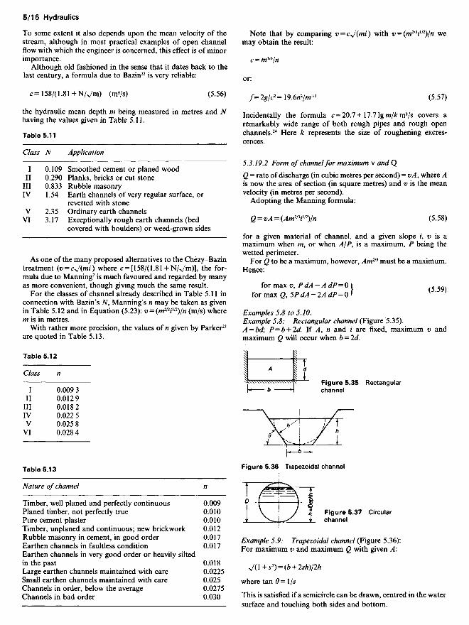
Examples 5.8 to 5.10.Example 5.8: Rectangular channel (Figure 5.35).A = bd\ P = b + 2d. If A, n and i are fixed, maximum v andmaximum Q will occur when b = 2d.

Figure 5.35 Rectangularchannel

Figure 5.36 Trapezoidal channel

Figure 5.37 Circularchannel

Example 5.9: Trapezoidal channel (Figure 5.36):For maximum v and maximum Q with given A:

J(l+s2) = (b + 2sh)/2h

where tan 0=l/s

This is satisfied if a semicircle can be drawn, centred in the watersurface and touching both sides and bottom.

Example 5.10: Circular channel (Figure 5.37).For maximum v, h = 0.813/); for maximum Q, /z = 0.938/).

5.3.19.3 Resistance of natural river channels

This resistance is complicated by the losses of energy at bendsand at relatively sudden changes of cross-sectional area. Asthese depend on the precise dimensions and shapes, it is quiteimpossible to generalize, but they are nevertheless important.For example, it has been shown that in a 13-km tortuous stretchof the River Mersey25 the textural roughness of the bed and sidesaccounts for only 25 to 50% of the total loss of head dependingon the rate of flow, the rest of the resistance being dueprincipally to the bends.

Somewhat similar conclusions have been reached in a study ofthe River Irwell.26

5.3.19.4 Velocity distribution in open channels

Side and bottom friction cause the stream to be retarded. Thehighest velocity in any vertical at a particular section is usuallyfound some distance below the surface; the mean velocity in avertical line occurs at about 60% of the depth, whether the windis blowing up- or downstream. This is the basis of one method ofstream-gauging, in which the section is considered divided intostrips of equal width and the velocity in these strips, or panels, ismeasured by current meter at 60% of the depth of eachindividual panel (Figure 5.38). The area of a strip, as found bysounding the bed, multiplied by the velocity so measured isassumed to give the flow through the strip and the addition forthe total number of strips gives the flow through the wholesection.

Figure 5.38 Measurement of velocityin open channel

5.3.19.5 Energy of a stream in an open channel, or 'specificenergy'

If D is the depth and v the mean velocity, the energy head //e,taking atmospheric pressure as the datum of pressure and thebottom of the channel as the datum of potential, is D + v2/2g, orD + Q2/2gA2.

5.3.19.6 Critical depth

Critical depth is the depth at which maximum discharge occuisfor a certain energy head, or, alternatively, the depth at which agiven discharge takes place with the minimum energy head. Itrepresents an unstable condition, often accompanied by watersurface undulations. Under these conditions D = V2Jg in arectangular channel and Q then equals (Q.544b^/g)H^2.

5.3.19.7 Nonuniform flow in open channels

If h is the depth at a distance / along the channel with slope i

AhlAl-i-W2*"*M/dl~ !-(»'/**) (5.60)

This condition of varying depth, even in a stream of constantwidth and constant rate of discharge, as here assumed, may bebrought about by obstructions or irregularities.

h is now the depth actually found at a particular section,whereas H may be called the depth which would apply underconditions of uniform flow corresponding to the simple Equa-tion (5.54). In other words, h becomes equal to H if d/z/d/=0.

Suppose now, in order to examine general trends, that the

width of the stream is large compared with its depth. In such acase the hydraulic mean depth m is approximately the same as /2,at any rate in channels having approximately uniform depthacross their width. Then:

H/,,H,-'-(M2g/0an at —=—, 7 . I Nl-(v2/gh)

and Q = vbh. Q is also equal to VbH, where V and H are thevelocity and depth which would be obtained with uniform flow.

It then follows that:

^M,- ''[1-WJQ3Id*/d/~l-(2///)(/W (5.61)

5.3.19.8 Special cases of nonuniform flow

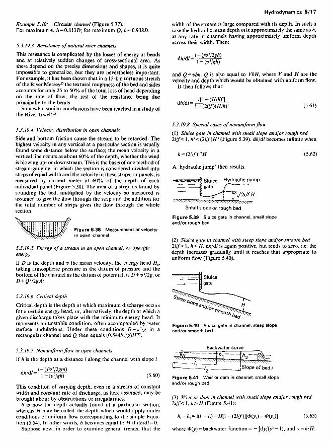
(1) Sluice gate in channel with small slope and/or rough bed2i/f< 1, /z3<(2///)//3 (Figure 5.39). d/z/d/ becomes infinite when

h = (2i/fy»H (5.62)

A 'hydraulic jump' then results.

Small slope or rough bedFigure 5.39 Sluice gate in channel, small slopeand/or rough bed

(2) Sluice gate in channel with steep slope and/or smooth bed2i/f> \,h<H. d/z/d/ is again positive, but tends to zero, i.e. thedepth increases gradually until it reaches that appropriate touniform flow (Figure 5.40).

Sluicegate

Hydraulic pump

Sluicegate

Figure 5.40 Sluice gate in channel, steep slopeand/or smooth bed

Figure 5.41 Weir or dam in channel, small slopeand/or rough bed

(3) Weir or dam in channel with small slope andjor rough bed2ijf< !,/*>// (Figure 5.41):

h, - h2 = /(/, -12) + H[I - (2/7/)][0(y,) - 0Cy2)] (5.63)

where <P(y) = backwater function= — jd^/(y3— 1), and y = h/H.

Slope of bed /

Backwater curve

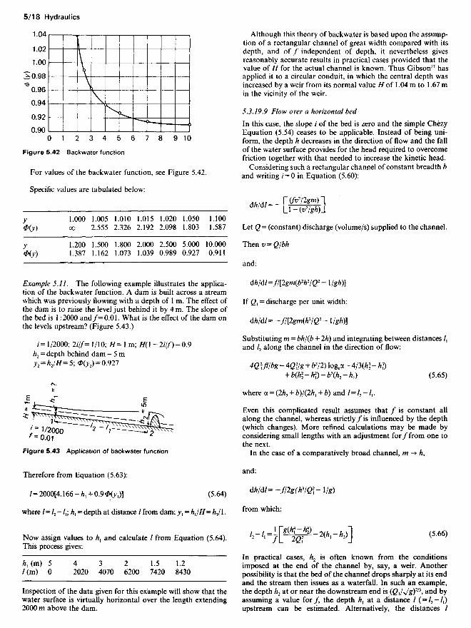
Figure 5.42 Backwater function

For values of the backwater function, see Figure 5.42.

Specific values are tabulated below:

y 1.000 1.005 1.010 1.015 1.020 1.050 1.100<£(y) oo 2.555 2.326 2.192 2.098 1.803 1.587

y 1.200 1.500 1.800 2.000 2.500 5.000 10.0000(y) 1.387 1.162 1.073 1.039 0.989 0.927 0.911

Example 5.11. The following example illustrates the applica-tion of the backwater function. A dam is built across a streamwhich was previously flowing with a depth of 1 m. The effect ofthe dam is to raise the level just behind it by 4 m. The slope ofthe bed is 1:2000 and/= 0.01. What is the effect of the dam onthe levels upstream? (Figure 5.43.)

/= 1/2000; 2///= 1/10; H= 1 m; H(I -2///) = 0.9H2 = depth behind dam = 5 my2 = H2IH= 5; <Z>(y2) = 0.927

Figure 5.43 Application of backwater function

Therefore from Equation (5.63):

/= 2000[4.166- /i, + 0.90^1)] (5.64)

where /= I2 — /,; /*, = depth at distance / from dam; y} = HJH= HJl.

Now assign values to /z, and calculate / from Equation (5.64).This process gives:

/z, (m) 5 4 3 2 1.5 1.2/(m) O 2020 4070 6200 7420 8430

Inspection of the data given for this example will show that thewater surface is virtually horizontal over the length extending2000 m above the dam.

Although this theory of backwater is based upon the assump-tion of a rectangular channel of great width compared with itsdepth, and of / independent of depth, it nevertheless givesreasonably accurate results in practical cases provided that thevalue of H for the actual channel is known. Thus Gibson27 hasapplied it to a circular conduit, in which the central depth wasincreased by a weir from its normal value H of 1.04 m to 1.67 min the vicinity of the weir.

5.3.19.9 Flow over a horizontal bed

In this case, the slope / of the bed is zero and the simple ChezyEquation (5.54) ceases to be applicable. Instead of being uni-form, the depth h decreases in the direction of flow and the fallof the water surface provides for the head required to overcomefriction together with that needed to increase the kinetic head.

Considering such a rectangular channel of constant breadth band writing / = 0 in Equation (5.60):

Ak1A,- - r(^2/2gm)1Am~ Ll-(^)J

Let Q = (constant) discharge (volume/s) supplied to the channel.

Then v = Q/bh

and:

dh/dl=f/(2gm(bWIQ2-\lgh)]

If Q1 = discharge per unit width:

dh/dl=-fl[2gm(VIQi-\lgh)]

Substituting m = bh/(b + 2h) and integrating between distances /,and I2 along the channel in the direction of flow:

4Q \fllbg = 4Q2Jg + VjI) logeot - 4/3№ - H])+ b(h\-h^-b\h2-h^ (5.65)

where a = (2H2 + b)l(2h, + b) and I=I2-I1.

Even this complicated result assumes that / is constant allalong the channel, whereas strictly/is influenced by the depth(which changes). More refined calculations may be made byconsidering small lengths with an adjustment for/from one tothe next.

In the case of a comparatively broad channel, m —> h,

and:

dh/dl=-f/2g(VIQ>-l/g)

from which:

^-/'-?Pwa-2(*'-*>)] (5-66)

In practical cases, H2 is often known from the conditionsimposed at the end of the channel by, say, a weir. Anotherpossibility is that the bed of the channel drops sharply at its endand the stream then issues as a waterfall. In such an example,the depth H2 at or near the downstream end is (2,/V£)2/3» and byassuming a value for/, the depth A1 at a distance / ( = / 2 ~A)upstream can be estimated. Alternatively, the distances /

upstream of H2 may be found for a succession of chosen values of/Z1.

5.3.19.10 The hydraulic jump (sometimes called 'standingwave')

An hydraulic jump is illustrated in Figure 5.44.

H1 - h2((h, + h2)/2 - (H1V2J h2g)] + (H2 - d/2)d= O

or, in a practically horizontal channel (W=O):

h2=-h}I2 + [(h2/4) + (2h}v2/gyi2]

Figure 5.44 Hydraulic j u m p

and:

(H2-H1) = [(A>/4) + (2htf/g)Y - 3A./2 (5.67)

For information concerning the length of channel covered informing the jump, see Allen and Hamid.28

5.3.19.11 The Venturi flume

The flume is a device for measuring rates of flow in an openchannel and is not so liable to damage as a weir and does notoffer the same obstruction to the flow. In order to preserve itssurface and its hydraulic characteristics, it is sometimes linedwith stainless steel.

It may be formed by inserting 'streamlined' humps on thesides (Figure 5.45a) and/or the bed (Figure 5.45b) of thechannel.

Figure 5.45 Venturi flume

If the discharge is 'free' as represented by the broken lines inFigure 5.45 and accompanied by the formation of a standingwave, the rate of discharge depends only upon the depthupstream of the constriction. With a throat of rectangularsection and width b, Q is approximately 0.54g*(//+ K2/2g)3/2, Vitself of course depending upon H.

The general equation is:

Q = C0(M2/!! - (b2d2lb,d№}[2g(d, - 4)11/2 (5.68)

where b2 is the breadth at throat, d2 the depth at throat, d} thedepth upstream of the constriction, b} the breadth upstream ofthe constriction, and C0 is the coefficient of discharge.

For particular designs, C0 is best found by scale-modelexperiments.

Details as to proportions, shapes and types of flow may befound in papers by Engel.29 See also Elsden.30

5.3.20 Orifices

5.3.20.1 Sharp-edged orifice (Figure 5.46)

Velocity at vena contracta=Cv*J(2gh), where Cv is the coeffi-cient of velocity, about 0.985.

Neglecting air resistance:

x2 = 4yhC2

v = 3Myh (5.69)

Discharge Q = CvacJ(2gh)

= CvCcaJ(2gh) (5.70)

where Cc is the coefficient of contraction, or:

<2=CX/(2g/0 (5.71)

where a is the area of the orifice and C' is the coefficient ofdischarge.

Figure 5.46 Sharp-edged orifice

Consideration of various published data31 indicates that fororifices of 6.35 cm diameter or over, under heads of at least0.43 m, C = 0.60, provided h < 3d, where d= diameter of orifice.Other typical results are given in Table 5.14.

It is doubtful whether a third significant figure is of any value,as a 1 % error in measuring the mean diameter of the orifice atonce makes 2% difference to the computed discharge. Theabsolute sharpness of the edge must also have some bearingupon the results.

Table 5.14 Values of C' for sharp-edged orifice

Head, h d of circular orifice, or side of square orifice

0.64 1.27 2.54 6.35 15.2 30.5(m) (cm) (cm) (cm) (cm) (cm) (cm)

0.12 - 0.64 0.63 0.61 - -0.18 0.66 0.64 0.62 0.61 0.60 -0.31 0.65 0.63 0.62 0.61 0.60 0.600.61 0.63 0.62 0.62 0.61 0.60 0.601.22 0.62 0.61 0.61 0.61 0.60 0.603.05 0.61 0.61 0.61 0.60 0.60 0.60

15.24 0.60 0.60 0.60 0.60 0.60 0.6030.48 0.60 0.60 0.60 0.60 0.60 0.60

The value of C for a rectangular orifice appears to besomewhat higher than for a circular or square one of the samearea. The difference amounts to about 2% for rectangles havinga 4:1 ratio of sides and 4% for a ratio of 10:1.

5.3.20.2 Rounded or bell-mouthed orifice

For a design such as that shown in Figure 5.47, C c=l andC' = Cv:

Q = 0.95(nd2/4)J(2gh) to 0.99(nd2/4)J(2gh) (5.72)

Figure 5.47 Rounded orifice

Figure 5.48 Submerged orifice

5.3.20.3 Submerged orifices

For a submerged orifice as shown in Figure 5.48:

Q=C'aJ(2gh) (5.73)

where C is substantially the same as for free discharge into theatmosphere.

5.3.20.4 Time of discharge through an orifice

The equation for time of discharge through an orifice from atank (Figure 5.49), without any simultaneous inflow is:

dh/dt=C(a/A)J(2gh)

or

'>-<•=-cx^C"™ (5.74)

Figure 5.49 Discharge throughan orifice

This can be solved if A can be expressed in terms of h, theinstantaneous head at time /.

If A is constant, or independent of h:

[CaJQg)/A](I2-O = 2(V//, - JH2) (5.75)

treating C' as independent of h.The time of discharge through a submerged orifice (Figure

5.50) is given by the equation:

('t~'i>°C'(\/Al + llAJaJVg)('JHt~y/H') <5-76)

Figure 5.50 Dischargethrough submergedorifice

5.3.21 Weirs and notches

The term 'notch' is used for the smaller weirs common inlaboratories, as distinct from outdoors.

5.3.21.1 Rectangular sharp-crested weir

For a rectangular weir as shown in Figure 5.51 in which 0<4//and c «3//, and H is measured at a distance 6 to 10 times Hbehind the weir, then:

Q = [0.410(2g)*](6 - ///10)//3/2 (5.77)

This formula is probably accurate within 2% for all values of Hfrom 0.08 to 0.61m provided b/H>2 and provided b is«0.305 m.

Figure 5.51 Rectangular sharp-crested weir

The effect of the velocity of the approaching stream isautomatically allowed for in this formula, as in all others to bepresented.

5.3.21.2 Suppressed rectangular weir

If a rectangular weir crest occupies the full width of the channel,the end contractions are suppressed. Under these conditions the'nappe' or stream discharging over the crest, the sides of thechannel and the front of the weir plate form the boundaries of apocket of air, some of which may be dissolved in the turbulentmass of water at the foot of the weir on its downstream side andcarried away (Figure 5.52). The effect of this would be to reducethe pressure below the nappe and, hence, to increase the

Figure 5.52 Suppressed rectangular weir

discharge for a given head. In itself this is no detriment but itintroduces an element of uncertainty and of variation. Toovercome this it is generally supposed that air vents should beprovided through the sides of the channel in communicationwith the air-pocket with the object of maintaining atmosphericpressure and preserving a standardized condition.

Under such conditions (ventilated suppressed rectangularweir of height P m above the bed of the channel), the Rehbockformula32 is perhaps accurate to within 1 or 2%; It reads:

Q- W(2gX> (0.605 +105o^-3+^) HM (m^ (5'78>

Writing this as:

2 = CV(2#)//3/2 (5.79)

values of C are as given in Table 5.15.*

Table 5.15 Values of C

P H

0.06 0.15 0.31 0.46 0.61 0.91 1.22 1.52(m) (m) (m) (m) (m) (m) (m) (m) (m)

0.15 0.436 0.461 0.512 0.565 0.617 0.724 0.831 0.9360.31 0.425 0.434 0.459 0.486 0.511 0.564 0.617 0.6720.61 0.421 0.422 0.433 0.446 0.458 0.484 0.510 0.5370.91 0.418 0.417 0.423 0.431 0.440 0.458 0.475 0.4921.52 0.416 0.413 0.416 0.421 0.426 0.436 0.446 0.4573.05 0.415 0.411 0.411 0.412 0.416 0.421 0.425 0.431

5.3.21.3 The 90-degree vee-notch (sharp-edged)

Measuring the head with reference to the point v (Figure 5.53):

<2=1.34//248 (m3/s) (5.80)

over a wide range, H being in metres.This notch is more convenient than the rectangular form for

the measurement of small quantities but it should be remem-bered that an error of 1 % in the measurement of//means 2.5%in the resulting estimate of Q, whereas with a rectangular notchthe corresponding error is 1.5%.

Figure 5.53 Sharp-edged 90° vee-notch

5.3.21.4 The Cippoletti weir (sharp-crested)

The discharge over this type of weir (Figure 5.54) is:

Q = 0.420 V(2g)6[(//+/0'-^/2] i f tan0 = i (5.81)

where h = v2/2g, v being the mean velocity in the approachchannel.

Figure 5.54 Sharp-crested Cippolettiweir

v cannot be allowed for until Q is known. Hence, as a firstapproximation, find Q from Q = 0.420(2g)i^//3/2. Then calculatev = Q/area of section of approach channel, and re-evaluate Qfrom Equation (5.81).

5.3.21.5 Weirs without sharp crests

Some typical examples are shown in Figure 5.55(a), (b), (c) and(d). The discharge Q = C(2g^bW12

5.3.21.6 Submerged weirs

If the downstream level rises above the crest of the weir, a'drowned weir' results. The effect of this upon the discharge fora given upstream head is surprisingly small: in general, thereduction in discharge will not amount to more than 2 or 3% for'downstream heads' or submergences up to 20% of theupstream head.* Q = 4.43C/>//1/2 m3/s if b and H are in metres.

5.3.21.7 Time of discharge over a weir (Figure 5.56)

The time of discharge over a weir or spillway of length b may becalculated as follows.

(1) With no inflow:

ASH=-C(2g)>bH3*dt

therefore:

j;;d<=-Ccw"'d"Or, time for head to fall from //, to H2 is:

<'>-''>-'-iCc£?""i'w

This may be solved by splitting the change between //, and H2

into stages over which mean values of A and C are applied.If A and C are treated as constant:

,--**- (-L-J-"! (5.82)bC(2g)> \JH2 JH1)

(2) Reservoir with inflow as well as outflow (Figure 5.56)Let A be the surface area of reservoir, Q the inflow and h the

instantaneous head over spillway of length b.

Then excess of inflow over outflow = Q — C(2g)*b№12. Hence:

dh/dt =[Q- C(2g)W2]/A

Let H be the head over spillway which would make the rate ofoutflow equal to the rate of inflow. Then:

Q = C(2gybH^

Let:

r = h/H and K, = C(2g)^b.

The time taken for the head to change from hl to /I2 is given by:

t2 - /, = (AfK^H)Wr2) - <£(/-,)] (5.83)

In this equation, r, = /*,///, r2 = h2/H and 0 represents Gould'sfunction33 of h/H, i.e. of r.

Detailed values of <&(r) for use when the time-interval isexpressed in the form given by Equation (5.83) (where b as wellas C*J(2g) is absorbed in AT1) have been calculated by Mathie-son.34

Figure 5.56 Discharge over a weir

Whenr<l:

•»-!(" PT^]-^ M2Sr1)-I])Whenr>l :

^H'-̂ l-̂ M^H])

Some of the values given by Mathieson are quoted below.

r O 0.1000 0.2000 0.3000 0.4000 0.5000 0.6000<£(r) O 0.1013 0.2076 0.3220 0.4482 0.5920 0.7615

r 0.7000 0.8000 0.9000 0.9900 1.0100 1.0200 1.0400<£(r) 0.9729 1.2619 1.7414 3.2925 4.4948 4.0426 3.5795

r 1.0600 1.1000 1.5000 2.0000 5.0000 10.0000 oo<£(r) 3.3202 2.9838 1.9708 1.5730 0.9155 0.6376 O

Example 5.12. A reservoir has a surface area of 2.5 km2. It isprovided with an overflow weir of length 25m, C=0.400.Initially there is a steady head of 0.25 m over the weir, butsuperimposed upon the discharge corresponding with this con-dition, additional flood water enters the reservoir as detailedbelow.

Time W 0 1 2 3 4 5 6 7 8

Additionalinflow (m3/s) O 10 35 50 40 20 10 O -2.75

Investigate the variation of water level.

K} = CbJ(2g) = 0.4 x 25.0 x 4.43 = 44.3

A/K} = 2.5 x 106/44.3 = 5.64 x 104; 360OAT1M = 0.0637

Initial inflow = initial outflow = 44.3(0.25)3/2 = 5.53 m3/s.

First hour

Mean Q = 5.53 + 5 = 10.53 m3/stherefore T/3/2= 10.53/44.3 = 0.238

and H=0.384m; JH= 0.62r, = HJH=0.25/0.384 = 0.651; tf>(r,) = 0.863

3600(s) = (5.64 x 10V0.62)[#(r2) - 0.863]<£(r2) = 0.903; r2 = 0.67

H2 = 0.67 x 0.384 = 0.258m= head over spillway at end of 1 h

Figure 5.55 Weirs without sharp crests, with corresponding H, C valuesSee also Hydraulics Research, HMSO Annual Reports, e.g. 1964 p. 15 and 1965 p. 7 (the 'Crump' weir)

(a)

H C(m)

0.15 0.4000.31 0.4260.46 0.4410.61 0.4420.91 0.4111.22 0.392

(b)

H C(m)

0.15 0.4020.31 0.4070.46 0.4240.61 0.4310.91 0.4451.22 0.455

(c)

H C(m)

0.15 0.3920.31 0.4260.46 0.4390.61 0.4500.91 0.4561.22 0.456

(d)

H C(m)

0.61 0.3680.76 0.3790.91 0.3841.07 0.3871.22 0.3861.37 0.3841.42 0.384

Second hour

Mean Q = 5.53 + 22.5 = 28.03 m3/s//3/2 = 28.03/44.3 = 0.634

// = 0.738 m;v//=0.859r, = 0.258/0.738 = 0.35; #(/-,) = 0.384

therefore 0.0637 = (l/0.859)[tf>(r2) - 0.384]0(r2) = 0.438; r2 = 0.392

and /Z2 = 0.392 x 0.738 = 0.289 m= head at end of 2 h.

Proceeding in this way, we obtain:

Hour 0 1 2 3 4 5 6 7 8

Head (m) 0.250 0.258 0.289 0.348 0.407 0.442 0.453 0.449 0.438

So the maximum head is 0.453 m at 6.10 h. This head wouldgive a maximum owrflow of 44.3(0.453)3/2, or 13.5m3/s, ascompared with the maximum /wflow of 55.5 m3/s at 3.10 h.

5.3.22 Impact of jets on smooth surfaces

5.3.22.1 Single moving vane

Let v be the absolute velocity of jet, u the absolute velocity ofvane, assumed parallel to v, and a the area of section of jet(Figure 5.57).

Figure 5.57 Impact of a jet on a single moving vaneor series of moving vanes

Velocity of jet relative to vane = z;-w.Therefore mass striking \ane = pa(v — u).This is unaltered in flow over the vane. (If roughness is taken

into account, the final relative velocity = k(v — u) where k< 1.)Initial momentum per second of ]et = pa(v — u)v<-Final momentum per second of jet = pa(v — u}[u + (v - u)

cos#]<-Therefore force exerted on vane = pa(v — u)2 (1 — cos O) <— = x,

sayWork done on vane = pa(v — u)2 (1 - cos 9}u

Initial kinetic energy of jet = pav*/2

Therefore efficiency = [2(v-u}2(\-cos 0)u]/v* (5.84)

Initial momentum per second of jet, in | direction = OFinal momentum per second of jet, in | direction = pa(v-u)2

sin<9Therefore force exerted on vane in direction l=pa(v — u)2

sin 9=y, say

Resultant force on vane = VC*2 + y2) (5.85)

5.3.22.2 Series of moving vanes

Figure 5.57 also applies. Since successive vanes intercept the jet,

the mass of water striking them per second now is pav. p is againthe density of the water.

Force exerted in direction <- = pav(v- u)( 1 -cos O) = x, sayWork done on vanes = pavu(v — u)(\— cos 6}Efficiency = 2u(v -u)(\- cos 6)/v2 (5.86)

Force exerted in direction I = pav(v — u) sin O = y, say (5.87)

Resultant force = VC*2 + /)

5.3.22.3 Cubical block resting on the bed of a stream(Figure 5.58)

Let p be the density of the material of the block (in kilogramsper cubic metre), // the coefficient of friction between the blockand bed of stream and v the velocity of stream at height y abovebed (in metres per second).

Figure 5.58 Impact of jet oncubical block resting on the bedof a stream

Resistance to overturning about P = {[(// -p)l4]/2}g

Resistance to sliding = u(p'-p)l3gwhere /j, is the coefficient of sliding friction.

Force of impact of stream against face RS = K'pi f v2 dy

where K' is a coefficient, ~0.70, to allow for the fact that not allthe forward momentum of the stream is 'destroyed'.

Therefore, block will overturn if:

*№*»**iF (^

or will slide if:

rrVd,>s<£^ (5.89)These results neglect other effects such as reduction of pressureon top and lee faces. They serve to show, however, that thestability of the block is essentially dependent upon the way inwhich the velocity is distributed through the depth of thestream.

Experiments in laboratory flumes indicate that:

v = mean velocity of stream for which block overturns (inmetres per second)= rate of discharge divided by (area of section of channel-

- area of section of block)

-T(l»-5™)[(^)']"where L is the length of block measured parallel to direction ofcurrent (in metres), / the depth of block (in metres), h the depthof water above top of block (in metres), p' the density ofmaterial of block (in kilograms per cubic metre) and p thedensity of water (in kilograms per cubic metre).

Example 5.13. A concrete cube 1 x 1 x 1 m of density 2400 kg/m3.

Total depth D Depth over cube h v(m) (m) (m/s)

2 1 3.343 2 3.534 3 3.706 5 3.99

11 10 4.56

For stability of more than one block, arranged in rows andtiers, or heaped at random, see Allen.35

5.3.22.4 Stability of flat beds and mounds of broken stoneand sand

The paper just cited35 suggests that, over a wide range includingmaterials having 'equivalent cube lengths' of 0.098 to 26.2 mmand specific gravities of 2.016 to 3.89:

V = k[(L+B)l2l]°M((j' -<7)0-22/0.22M-0.22 /,0.06 ^0.22 (5 91)

where v is the mean velocity (in metres per second) of streamflowing over a flat bed, L is the average value of maximumlength of individual grains, B the average value of maximumbreadth of individual grains, / the length of side of a cube of thesame weight as the average piece, o' the specific gravity ofmaterial, a the specific gravity of water (say unity), M theuniformity modulus of material, h the depth of stream, m thehydraulic mean depth and A; is a constant.

k is equal to 0.067 for movement of the first few particles if L,B, /, h and m are all in millimetres.

The uniformity modulus M is defined as indicated in Figure5.29.

Figure 5.59 Definition of a uniformity modulus

Similarly, for mounds:

v = 0.079(<r' - a)027/027 M-°-27 /z021 w002 (5.92)

for initial disturbance.

v = 0.083[(L + £)/2/]° •* (<jf - <r)°27 /°27 A/'027 h° -21 m0-02 (5.93)

for 'flattening the crest of the mound'.

Here v is the velocity (mean) of the stream flowing over the topof the mound and h the depth over the top (in millimetres).

Equations (5.92) and (5.93) apply to materials of irregularshape (sand or broken stone), but the case of mounds formed ofcubes laid in random fashion has also been investigated byAllen.35

Example 5.14: 1 m cubes weighing 2400 kg so that a' = 2.4.Example 5.15: Broken stone, equivalent cube length /= 1 m,

a =2.64, M= 0.9

v for initial movement(m/s)

Depth over crest of mound laid Broken stonein random fashion 1 m cubes I= 1 m, M=0.9

(m)

1 1.6 2.92 1.9 3.45 3.1 4.2

10 4.0 5.0

Note that <r f, the true specific gravity, of silica or quartz sands isusually 2.64, or very nearly so.

5.3.23 Sediment transportConsiderable effort continues to be applied to the theoreticaland experimental study of the transport of sand and suspendedsilt in both laboratory channels and natural waterways. Oneapproach used for at least 100 years has been to try to relate thebed movement to the shear stress or tractive force per unit areaexerted by the water on the bed of the channel, especially for thecritical condition necessary to initiate motion of the grains. Thisstress is pfv2/2, where/depends on the material which forms thebed and sides of the channel and on the hydraulic mean depth(see Equation (5.57)). The stress so defined has formed the basisof many theories and the means of interpreting observations ofbed movement. The results cover a wide range of complexity,one of the most elementary being to write TC, the critical shearstress required to start movement of the sand, as proportional tothe median diameter ds of the grains. For example, TC= l.2dt,where rc is in newtons per square metre if ds is in millimetres.While such a simple relationship makes no allowance for theshape of the grains, or the variation in their individual sizes, orany cohesion such as is present with fine particles, it neverthelessgives the right order of magnitude of TC if ds is not less than about0.25 mm. Thus, for ds = 0.25 mm, TC becomes 0.3 N/m2. Equatingthis to p/^2/2 and taking p for water as 1000 kg/m3, andsupposing/to be of the order of 0.003 if the depth is, say, 1 m, itthen follows that the mean velocity v in such a channel would beabout 0.5 m/s. At this velocity, grains would begin to move.

Other researchers, such as G. M. White36 and R. A. Bagnold,37

have introduced a force of upward lift on a grain in addition tothe longitudinal drag, while some methods of assessing thequantity of bed material transported by a given stream havebeen based on the amount by which the shear stress at the bedexceeds the critical shear stress TC. Yet another concept is torelate the sediment transport to the 'streampower' rv. Moredetailed accounts of these matters appear in many books andjournals, e.g. a paper by P. A. Mantz.38

5.3.24 Vortices

5.3.24.1 Forced vortices Forced vortices are of the type causedby stirring a liquid in a dish or by rotating the dish (Figure5.60).

/i = (wV2)/2g (5.94)

where CD is the angular velocity of rotation (rad/s).

5.3.24.2 Free vortices

Free vortices are of the type which results when a liquid flows

Figure 5.60 Forced vortex

through a hole in the bottom of a vessel. The water moves instream lines spirally towards the centre, where an air-core triesto form. The coefficient of discharge through the orifice isgreatly reduced as compared with its value in the absence of avortex, i.e. with larger heads.

If the hole is now closed, the vortex motion persists for a time(until damped out by viscous resistance), the lower part havingthe characteristics of a forced vortex and the upper of a freecylindrical vortex (Figure 5.61):

C1-Z = constant/2gr2 (5.95)

Figure 5.61 Free vortex

5.3.25 Waves

5 J.25.1 Waves of transmission or translation

Waves of transmission or translation are of the type formedwhen a sluice gate is suddenly opened to admit water to achannel, or when a tidal bore advances along a river.

Let h be the depth of the stream, v the velocity of the streammoving in the direction opposite to the wave, k the height of thewave crest above the surface of the stream and V the velocity ofpropagation of the wave. Then:

r 2g(h+k)^ (596)L\+h/(h + k)_\ v ^ }

If k is small compared with h

V=[g(h + kW2-v

If k is very small compared with h

V=(ghyi-v

5.3.25.2 Waves of oscillation

Waves of oscillation occur in comparatively deep water (Figure5.62).

Direction of apparent propagationFigure 5.62 Waves of oscillation

Particles in the surface describe circular orbits, giving theappearance of a wave crest advancing with velocity J(gA/2n).The period of oscillation is ^/(2n^/g). In shallower water the

orbits become distorted into approximate ellipses - a conditionintermediate between a wave of oscillation and one of transla-tion - and finally the wave breaks on the shore.

5.3.25.3 Dynamic effects on hydraulic structures

These are not confined to the direct impact of streams or waves.They may also result from eddies giving rise to periodic forcesand may become serious, e.g. with long, slender piles in deeptidal waters. An important occurrence of this phenomenon wasinvestigated at Immingham Oil Terminal.39"*1

5.3.26 Dimensional analysis

Dimensional analysis is a valuable tool in reducing the apparentchaos of experimental results involving many variables and alsoin the systematic design of experimental procedure or technique.

Consider the resistance R of a certain shape of submergedbody. Let / be any representative dimension, such as the length,v the velocity relative to the stream, p the density of fluid, ̂ theviscosity of fluid and g the acceleration due to gravity.

Suppose R depends upon /, v, /?, fj, and g (5.97)

Six quantities are involved here, and together they depend uponthe three fundamental units or quantities of mass, length andtime.

We therefore expect to find three dimensionless groups of theoriginal quantities R, /, v, /?, // and g, related to one another.

Let N be a dimensionless group.Choose any three quantities from Equation (5.97) such that

together they include mass M, length L, and time T.Suppose we choose R, /, p.

R (a force) has the dimensions of mass x acceleration, or[MLr-2]/ has the dimensions of length [L]p has the dimensions of [ML"3]

Now write N1 = R0I lb\ pc\, the last quantity v being chosen atrandom from the remaining symbols of Equation (5.97).

Now TV1 is to have no dimensions in mass, length or time.Hence, dimensionally, O = [Mai][Lfl>jr-2fli][L*i][Mc.][L-3ci][Lr-'].

Equating indices of [Af]9 [L], [T] in turn

for [M], O = C 1 -Hc 1

for [L], O = O1-I-^-Sc, + !for[71,0=-2fl ,- l

These simultaneous equations give a} = — 1/2, c, = 1/2, 6, = 1.Hence:

N1=PtIvIR1I2

Similarly, writing N2 = Ra2lh2pcifj. and remembering that theunits of// are [Af][L-1Jr-1], we should find

N^/A/ftp1*

Again, writing

N3 = Raihpcig

we should get:

N3 = R-Vpg

Now write:

TV = a function of TV2, W3 = 0(N2, N,)

i.e.

p*fo/Rll2 = &(tilftp*, Ppg/R)

which result is not invalidated if we multiply any one of thedimensionless 'groups', TV1, W2, W3, by a function of itself or ofone of the others, so long as we do not reduce the total numberof such distinctive groups.

Therefore:

RIpI2V2 = 0(vlp/n, v2/lg) (5.98)

In this, vlp/n is the so-called Reynolds number, and V2IIg is theso-called Froude number, although some writers define it asvfj(lg).

For alternative methods of dimensional analysis, see Dun-can42 and Whittington.43

5.3.26.1 Application to scale models

The principle of dynamical similarity indicates that if a model isoperated at a speed truly corresponding with the full sizeproject, then:

RJR2 = P1I2V2Jp2I

2V2

where the suffix 1 refers to the full size and the suffix 2 to itsmodel.

As far as the resistance of submerged bodies is concernedtherefore, it follows from Equation (5.98) that the Reynoldsnumber in the model should be the same as in the actual, and (atthe same time) the Froude numbers should be the same in modeland full-size project.

The one condition then requires:

V2 = Vt(IJl2)(PJpM^ (5-99)

and the other requires:

»2 = tW(/2//.) (5'10°)

These two conditions cannot, in general, be satisfied at one andthe same time and one of the features of scale model technique isto choose one or other as the more important and then todiscover, as a result of experiments on models of different scales,or by comparison of model results with prototype values, whatis the inaccuracy or 'scale effect' caused by neglect of the otherrequirement. In more complicated examples, more than tworequirements may ideally be necessary.

5.3.26.2 Ship models

In testing the resistance of a ship's hull, the model is towed at aspeed given by V2 = V1 x (1/S)I/2, where \/S represents the geome-trical scale. Its total resistance RT is then measured and from thisis subtracted the skin-frictional resistance Rs as estimated fromexperiments on long 'boards' of similar surface roughness. Theresidue (RT — RS) represents eddy and wave-making resistanceRE

RE multiplied by /?,/2 V2Jp2I2 v2, or (/Vp2)S

3

then gives the eddy and wave-making resistance of the full-sizeship at the corresponding speed ^1 = v^J S, and to this is addedthe estimated skin friction of the ship at that speed.

5.3.26.3 Falling particles - terminal velocity

A particle descending through a fluid will accelerate until itseffective weight is balanced by the resistance to its motion - itwill then have attained its terminal velocity FT.

Let P1 = density of particle, p = density of fluid, rj = viscosity offluid, and /?T = force of resistance when velocity of particlereaches its terminal value F1-.

Then, once the terminal velocity is attained,

S(P\ ~P)X volume of particle = R^.

A general treatment of the resistance to relative motion of thesolid through the fluid would involve considering inertia (arisingfrom the property of mass possessed by the fluid) and viscosity(brought about by the molecular structure of the fluid).

In his classical study of a sphere moving through a fluid, SirGeorge Gabriel Stokes assumed that at sufficiently low veloci-ties the inertia terms could be neglected and so established theresult that under such conditions the resistance would be 3nrj Vd,where V is the velocity of the sphere of diameter d relative to thefluid.

Applying this to the terminal velocity VT:

g(p,-pm/^nd^] = 3nrjV^

from which VT = (gd2/\8) (^^] -

Experiments confirm this provided that VTdp/rj does not exceedapproximately 0.5. Subject to that proviso, the formula for K1-may be used to determine: (1) the diameter of a small spherefrom its observed terminal velocity in a fluid of known viscosity;and (2) the viscosity of a fluid by measuring the terminal velocityof a small sphere of known diameter.

In more general terms, the terminal velocity, even when V^dp/rjexceeds 0.5, may be used as a measure of: (1) the size of particlesin comparison with the well-established experimental results forspheres; and (2) the capacity of particles to be lifted intosuspension by an upwards current.

(Incidentally, it will be seen that Stokes's R = 3nnVd isequivalent to RIpI2 V2 = R/pd2 V2 = 3n/(p Vdjrj), or, if A is theprojected area of the sphere, nd2/4, RJp AV2= 12/(Vd/v).)

5.3.26.4 Models of sluice-gates, weirs, etc

In models of sluice-gates, weirs and spillways, the Froudenumber is to be adopted, provided the scale is well chosen. Forexample, a model of an overflow spillway for a dam may usuallybe relied upon if the lowest head on which deductions are to bebased is not less than 6.4 mm in the model. Under heads smallerthan this, surface tension and viscosity are generally responsiblefor appreciable scale effects. With this reservation, however, ifwe call h the head observed in the model and q the discharge,then the discharge of the full-size spillway under a head of Shwill be qS512, the model scale being 1: S.

5.3.26.5 River models

River models are frequently constructed to different scaleshorizontally and vertically. Many considerations influence thescales actually to be chosen. If the horizontal scale is 1: x and thevertical scale 1 :y, there will be a vertical exaggeration, ordistortion, of scale, equal to x/y. This exaggeration is desirablein order to improve the prospects of: (1) the flow being turbulentin the model as it is in nature; (2) the water-surface slopes beingreproduced; (3) bed material being shifted by the currents

available in the model. The smaller the value of x, the smallermust be the exaggeration x/y. The nominal velocity scale forsensibly horizontal stream velocities in such a model is then1: Jy and the scale of time 1: x/Jy. If q is the rate at which wateris fed to the model in order to simulate a flow Q in nature, then qshould be equal to Q/xy3/2. Some river models have, however,been operated with such flows and velocities, discovered by trial,as to give the proper gradients and bed movements irrespectiveof these ideal conditions which should, if practicable, beobserved.

Sand or other material used on the bed of river models to givequalitative or approximately quantitative indications of scour isnot necessarily reduced to scale. Frequently such materials areof the same order of size as in nature, the feasibility of thisdepending on the fact that the scouring property of a shallowstream is greater than that of a deep one of the same meanvelocity.

5.3.26.6 Harbour models

Models of harbours specifically concerned with surface wavesproduced by storms have been successful with scales (undis-torted) in the region of 1:50, 1:100 or 1:180, and with modelwaves in the exposed area outside the harbour works about20 mm or more in height. The velocity scale of such a modelhaving a geometrical scale of 1:100 would be 1: V100; or 1:10,and its time scale would also be 1:10.

5.3.26.7 'Mathematical models'

Mathematical solutions to complex problems of fluid motionhave developed on a wide front in recent years, in conjunctionwith the increasing availability of computers. They cover arange of problems embracing the analysis of data, the study ofsurges, the hydraulic behaviour of rivers and estuaries, sedimenttransport, etc. The representation or modelling by mathematicalformulae and equations frequently contains terms and/or coeffi-cients which have been derived from observations in the field,the laboratory, or on physical models. The choice of which kindof model to use - the mathematical or the physical - depends onthe nature of the engineering problem concerned; in some cases,it is advantageous to combine the two methods, so treating oneas complementary to the other. Recent literature provides aguide, and in the particular case of estuaries, the potential andthe limitations of both kinds of model are discussed by McDow-ell and O'Connor.44

Notwithstanding the undoubted powers of the mathematicalapproach, engineers experienced in these matters are likely toendorse the view of McDowell and O'Connor that 'the greatestsingle merit of physical models is their capacity to reproduce, onan easily observed scale, the intricate three-dimensional flow ina large estuary. They are, in consequence, an aid to thought andplanning without equal... .' This applies not only to physicalmodels of rivers and estuaries but equally to those of hydraulicstructures, e.g. spillways, channels and other devices for the'dissipation' of energy.

References

1 Davis, S. J. and White, C. M. (1929) 'A review of flow in pipesand channels', Engng, 78, 71.

2 Stanton, T. E. and Pannell, J. R. (1914) Phil. Trans. A, 214, 199;National Phys. Lab. Coll. Res., 11, 293.

3 Nikuradse, J. (1933) Forschungsh. Ver. dtsch. Ing., No. 361.4 Prandtl, L. and von Karman, T. (1933/1935) Z. Ver. dtsch. Ing.,

77, 105 (1933); Proceedings, 4th international congress on appliedmechanics, Cambridge (1935).

5 Colebrook, C. F. and White, C. M. (1937) 'Experiments with fluidfriction to roughened pipes'. Proc. R. Soc. A, 161, 367.

6 Colebrook, C. F. (1939) Turbulent flow in pipes, with particularreference to the transition region between the smooth and roughpipe laws', /. Instn Civ. Engrs, 11, 133.

7 Manning, R. (1895) 'Flow of water in open channels and pipes',Trans Instn Civ. Engrs, Ireland, 20, 161 (1891); 24, 179.

8 Ackers, P. (1958) 'Resistance of fluids flowing in channels andpipes', Hydraulics Research Papers, Nos 1 and 2, HMSO, London.

9 Barnes, A. A. (1916) Hydraulic flow reviewed, Spon, London.10 Colebrook, C. F. and White, C. M. (1937) 'The reduction of

carrying capacity of pipes with age', /. Instn Civ. Engrs, 7, 99.11 Sellin, R. H. J., Hoyt, J. W. and Scrivener, O. (1982) The effect of

drag-reducing additives on fluid flows and their industrialapplications'. Part 1 'Basic aspects'. J. Hydr. Res, 20, 1, 29.

12 Sellin, R. H. J., Hoyt, J. W., Scrivener, O. and Pollert, J. (1982)'Present applications and future proposals', Part 2, /. Hydr. Res,20, 3, 235.

13 Gibson, A. H. (1910/1911) 'Loss of head in gradual enlargements',Proc. R. Soc. A, 83, 366 (1910); 'Loss at enlargements and atvalves', Trans R. Soc. Edinburgh, 48, (1911).

14 Cornish, R. J. (1939) The analysis of flow in networks of pipes',J. Instn Civ. Engrs, 13, 147.

15 Skeat, W. O. and Dangerfield, B. J. (eds) (1969) Manual of Britishwater engineering practice (4th edn) Vol. Ill, Institution WaterEngineers, London, 7 pp. 168-174.

16 Stuckey, A. T. (1969) Methods used for the analysis of pipenetworks, WWE.

17 Barlow, J. F. and Markland, E. (1969) 'Computer analysis of pipenetworks', Proc. Instn Civ. Engrs, 43, 249.

18 Al-Nassri, S. A. (1971) 'Flow in pipes and pipe networks', PhDthesis, University of Liverpool.

19 O'Brien, M. P. and Hickox, G. H. (1937) Applied fluid mechanics.McGraw-Hill, New York,

20 British Standards Institution (1943) Flow measurement (BS 1042).British Standards Institution, Milton Keynes.

21 American Society of Mechanical Engineers (1931) Fluid metersreport (4th edn). ASME, New York.

22 Bazin, H. E. (1897) Ann. des Ponts et Chaussees, 4, 20.23 Parker, P. A. M. (1915) The control of water, Routledge, London.24 Allen, J. (1943) 'Roughness factors in fluid motion through

cylindrical pipes and through open channels', J. Instn Civ. Engrs,20,91

25 Allen, J. (1939) The resistance to flow of water along a tortuousstretch of river and in a scale model of the same', /. Instn Civ.Engrs, 11, 115.

26 Allen, J. and Shahwan, A. (1954) The resistance to flow of wateralong a tortuous stretch of the river Irwell (Lancashire) - aninvestigation with the aid of scale-model experiments', Proc. InstnCiv. Engrs, Part. Ill, 3, 1, 144.

27 Gibson, A. H. (1924) Hydro-electric engineering, Blackie, London,Vol. I, p. 67.

28 Allen, J. and Hamid, H. I. (1968). The hydraulic jump and otherphenomena associated with flow under rectangular sluice-gates',Proc. Instn Civ. Engrs, 40, 345.

29 Engel, F. V. A. (1933/1934) 'Non-uniform flow of water', TheEngineer, London, 21, 28 April, 5 May (1933); The venturiflume', The Engineer, London, 3 and 10 August (1934).

30 Elsden, O. (1964) 'Flow measurement' in: Guthrie Brown (ed.)Hydro-electric engineering practice (2nd edn) Chap. 2, Vol. I.Blackie, London and Glasgow.

31 Hamilton Smith, Jr (1886) Hydraulics.Bilton, H. J. I. (1908) Victorian Inst. Engrs.Judd, H. and King, R. S. (1906) Am. Assoc. Adv. Sd.Smith, E. S. and Walker, W. H. (1923) Proc. Instn Mech. Engrs.Bond, W. N. An introduction to fluid motion. Arnold, London.

32 Rehbock, T. (1912/1929) Handbuch der Ingenieur wissenschaften,Vol. I, Part 3/2 (1912); discussion in Trans. Am. Soc. Civ. Engrs,93 (1929); also details in J. R. Freeman (ed.) Hydraulic laboratorypractice. American Society Civil Engineers, (1929).

33 Gould (1901) Engineering News.Horton, D. F. (1918) Engineering News Record.Gibson, A. H. (1924) Hydro-electric engineering, Vol. I, Blackie,London and Glasgow, p. 75.

34 Mathieson R. (1953) The generalized Gould's function', Proc.Instn Civ. Engrs, Part III, 2, 1, 142.

35 Allen, J. (1942) 'An investigation of the stability of bed materialsin a stream of water', J. Instn Civ. Engrs, 18, 1.

36 White, C. M. (1940) The equilibrium of grains on the bed of astream'; Proc. Roy. Soc. A, 174, 958, 322.

37 Bagnold, R. A. (1956) The flow of cohesionless grains in fluids';Phil Trans. Roy. Soc. A, 249, 964.

38 Mantz, P. A. (1983) 'Semi-empirical correlations for fine andcoarse cohesionless sediment transport'; Proc. Instn Civ. Engrs, 75,Part 2, 1.

39 Sainsbury, R. N. and King, D. (1971) The flow-inducedoscillation of marine structures', Proc. Instn Civ. Engrs, 49, 269.

40 Construction Industry Research and Information Association(1970/1971) Report Project 143, p.21.

41 British Transport Docks Board (1971) Docks, 8, 11,5.42 Duncan, W. J. (1953) Physical similarity and dimensional analysis.

Arnold, London.43 Whittington, R. B. (1963) 'A simple dimensional method for

hydraulic problems', J. Hydr. Div. Proc. Am. Soc. Civ. Engrs, 89,No. HY5, 1.

44 McDowell, D. M. and O'Connor, B. A. (1977) Hydraulicbehaviour of estuaries. Macmillan, London.

Bibliography

Addison, H. (1964/1940) A treatise on applied hydraulics (5th edn),Chapman and Hall, London; Hydraulic measurements, Chapmanand Hall, London.

Allen, J. (1947) Scale models in hydraulic engineering, Longman,London.

Brown, J. Guthrie (1964) Hydro-electric engineering practice (2nd edn),vol. I, Blackie, London and Glasgow.

Duncan, W. J., Thorn, A. S. and Young, A. D. (1960) The mechanicsof fluids, Arnold, London.

Fox, J. A. (1977) An introduction to engineering fluid mechanics (2ndedn), Macmillan, London.

Francis, J. R. D. (1958) A textbook of fluid mechanics for engineeringstudents, Arnold, London.

Francis, J. R. D. (1975) Fluid mechanics for engineering students (4thedn), Arnold, London.

Gibson, A. H. (1952) Hydraulics and its applications (5th edn),Constable, London.

Her Majesty's Stationery Office Hydraulics research. HMSO AnnualReports, London.

Institution Water Engineers (1969) Manual of British water engineeringpractice (3 vols) (4th edn). IWE, London.

Jaeger, C. (1956) in: Wolf (trans, and ed.), Engineering fluid mechanics,Blackie, London and Glasgow.

Jameson, A. H. (1937) An introduction to fluid mechanics, Longman,London.

King, H. W. (1954) in: Brater (ed.) Handbook of hydraulics (4th rev.ed.) McGraw-Hill, New York.

Lewitt, E. H. (1952) Hydraulics and the mechanics of fluids (9th edn),Pitman.

McDowell, D. M. and Jackson, J. D. (eds) (1970) Osborne Reynoldsand engineering science today. Manchester University Press,Manchester, and Barnes and Noble, Inc. New York.

McDowell, D. M. and O'Connor, B. A. (1977) Hydraulic behaviour ofestuaries, Macmillan, London.

Muir Wood, A. M. (1969) Coastal hydraulics, Macmillan, London.Novak, P. and Cabela, J. (1981) Models in hydraulic engineering,

Pitman, London.O'Brien, M. P. and Hickox, G. H. (1937) Applied fluid mechanics.

McGraw-Hill, New York.Pao, R. H. F. (1961) Fluid mechanics. Wiley, New York.Parker, P. a. M. (1915) The control of water. Routledge, London.Prandtl, L. (1952) The essentials of fluid dynamics. Blackie, London

and Glasgow.Raudkivi, A. J. (1967) Loose boundary hydraulics, Pergamon Press,

Oxford.Rouse, H. (1948) Elementary mechanics of fluids, Wiley, New York.Vennard, J. K. (1962) Elementary fluid mechanics (4th edn). Wiley,

New York.Webber, N. B. (1979) Fluid mechanics for civil engineers, Chapman and

Hall, London.