HYDRAULIC MODELING APPLICATIONS IN MAIN SYSTEM MANAGEMENT

HYDRAULIC MODELING APPLICATIONS IN MAIN SYSTEM MANAGEMENT

WATER MANAGEMENT SYNTHESIS II PROJECT WMS REPORT 74

HYDRAULIC MODELING APPLICATIONS IN MAIN SYSTEM MANAGEMENT

This study is an output of Water Management Synthesis II Project

under support of United States Agency for International Development

Contract AID/DAN-4127-C-00-2086-00

All reported opinions, conclusions or recommendations are the sole responsibility of the author and do not represent the official

or unofficial positions of any agency of the United States or Utah State University or the

Consortium for International Development

prepared by

Gary P. Merkley - Irrigation Engineer

Utah State University Agricultural and Irrigation Engineering Department

Logan, Utah 84322-4105

March 1988 WMS Report 74

PREFACE

This study was conducted as part of the Water Management SynthesisII Project, a program funded and assisted by the United States Agencyfor International Development through the Consortium for International Development. Utah State University, Colorado State University, and Cornell University serve as co-lead universities for the Project.

The key objective is to provide services in irrigated regions of the world for improving water management practices in the design and operation of existing and future irrigation projects and give guidancefor USAID for selecting and implementing development options and investment strategies.

For more information about the Project and any of its services, contact the Water Management Synthesis II Project.

Jack Keller, Project Co-Director Wayne Clyma, Project Co-Director Agricultural and Irrig. Engr. University Services Center Utah State University Colorado State University Logan, Utah 84322-4105 Fort Collins, Colorado 80523 (801) 750-2785 (303) 491-6991

E. Walter Coward, Project Co-Director Department of Rural Sociology Warren Hall Cornell University Ithaca, New York 14853-7801 (607) 255-5495

iii

TABLE OF CONTENTS

Page

PREFACE........................................................ iii

LIST OF TABLES .................................................. ix

LIST OF FIGURES ................................................. xi

LIST OF SYMBOLS AND NOTATION.................................... xiii

ABSTRACT.......................................................

Chapter

I. INTRODUCTION .......................................... 1

Statement of the Problem ......................... I Hydraulic Modeling ............................... 2 Objectives ....................................... 3 Scope of Study ................................... 4

II. LITERATURE REVIEW ..................................... 7

Hydraulic Modeling ............................... 7 Canal Control Logic .............................. 8 Main System Management ........................... 9

III. GATE SCHEDULING ....................................... 11

Numerical Solution ............................... 11 Control Structures ............................... 12

Filling an Empty System ..................... 15 Activated Canal Reaches ..................... 16 Deactivated Canal Reaches ................... 20

Turnout Structures ............................... 24

Status Conditions ........................... 24

IV. FIELD EVALUATION OF THE MODEL ......................... 27

Overview of Activity ............................. 27 Procedure.........................................29

Results...........................................32

Steac--State Distributions .................. 32 Stabilization Times ......................... 36

v

TABLE OF CONTENTS (cont)

Page

IV. FIELD EVALUATION OF THE MODEL (cont).................. 36

Target Level Deviations ...................... 36 Turnout Discharge Deviations ................ 39 Manual Mode Comparsions ..................... 39

Interpretation of Results ........................ 39

V. MAIN SYSTEM MANAGEMENT ISSUES ......................... 43

Implications for Lam Nam Oon ..................... 43

Seepage and Roughness ....................... 44 Infrastructure Changes ...................... 45 Time Requirements ........................... 46

System Shifting .................................. 46 Turnout Scheduling ............................... 48 Flow Level Fluctuations .......................... 50 Recovering from Modeling Errors .................. 52

Changing Physical Conditions ................ 52 Measurement Errors .......................... 54 Operational Deviations ...................... 55 Model Limitations ........................... 56

VI. HYDRAULIC MODEL SURVEY ................................ . 59

Introduction..................................... 59 Procedure ........................................ 59 Results .......................................... 61

Multiple Choice Responses ................... 61 Written Responses ........................... 64 Demographic Information ..................... 66 Analysis of Variance ........................ 67

Discussion ....................................... 69

Recommendations .................................. 72

VII. SUMMARY AND CONCLUSIONS ............................... 73

Model Development ................................ 73 Model Applications ............................... 73 Lam Nam Oon Project .............................. 76 Survey Questionnaire ............................. 77

vi

TABLE OF CONTENTS (concl)

Page

VIII. RECOMMENDLATIONS ....................................... 79

Software Maintenance ............................. 79 Software Additions ............................... 79

Computed Inflows ............................ 80 Multiple Inflows ............................ 80 Reverse Flow................................ 80 Recession ................................... 81 Structure Types ............................. 81 Branch Linkages ............................. 82

Additional Research .............................. 82

Lam Nam Oon Project.............................. 82

REFERENCES ...................................................... 85

APPENDICES ...................................................... 89

APPENDIX A. Lam Nam Oon Right Main Canal Data ........ 91 APPENDIX B. Hydraulic Model Survey Instrument ........ 97

Original English Survey Form ..................... 99 English Version Used In IIC Courses .............. 103 Spanish Version Used In IIC Courses .............. 107 Thai Version Used in Thailand.................... 111

vii

LIST OF TABLES

Table Page

1. Known, Calculated, and External Parameters at the Downstream End of a Canal Reach During Solution of the Saint-Venant Equations ............................ 13

2. Initial Steady-State Turnout Demands During Model Simulations ..................................... 30

3. Predicted Responses for Rectangular Sluice Gates with Varied Seepage Rate, Hydraulic Roughness, and Operational Mode ...................................... 33

4. Predicted Reponses for Rectangular Weirs with Varied Seepage Rate, Hydraulic Roughness, and Operational Mode ...................................... 34

5. Response Summary for Questions 1-14 ................... 61

6. Mean Responses to Questions 1-14 ...................... 63

7. Percentage Within Groups Identifying a Specific Area as a Problem .......................................... 65

8. Percentage, by Group, Responding that the Model Might Help with the Specified Problems ...................... 65

9. Breakdown of Respondent Education Levels .............. 67

10. Analysis of Variance Results with Respondent Group as the Independent Variable .......... 68

A-1. Configuration Data for the Right Main Canal of the Lam Nam Oon Irrigation Project in Thailand............ 93

A-2. Control Structure Data for the Right Main Canal of the Lam Nam Oon Irrigation Project in Thailand ............ 93

A-3. Turnout Structure Data for the Right Main Canal of the Lam Nam Oon Irrigation Project in Thailand ............ 94

A-4. Weekly Turnout Demands During a Four-Week Period in 1987 of the Dry Season at the Lam N'm Oon Irrigation Project in Thailand........................ 96

ix

LIST OF FIGURES

Figure Page

1. Map Showing the Location of the Lam Nam Oon Irrigation Project in Northeast Thailand .............. 5

2. Flow Diagram Indicating the Possible Paths to the Five Different Gate Scheduling Status Conditions for Individual Canal Reaches .......................... 14

3. Illustrated Example of Steady-State Reach Discharge Calculations During Gate Scheduling ................... 17

4. Illustrated Example of how the Model Stabilizes Over-Reaction of a Control Structure to the Closing of a Turnout .................................. 18

5. Flow Diagram Showing the Possible Program Paths for Gate Scheduling When Scheduling is Enabled for the Canal System .................................. 21

6. Schematic Side View of a Sluice Gate Defining the End of One Canal Reach and the Beginning of Another... 23

7. A Typical Example of Steady-State Flow Distributions for Sluice Gates ................... 35

8. Predicted Flow Stabilization Times for Weirs and Sluice Gates with Varied Seepage Rate, Hydraulic Roughness, and Operational Mode .................................. 37

9. Predicted Average Deviations Between Target Levels and Calculated Flow Levels for Weirs and Sluice Gates with Varied Seepage Rate, Hydraulic Roughness, and Operational Mode ....................... 38

10. Predicted Average Deviations Between Turnout Demands and Calculated Discharge Rates for Weirs and Sluice Gates with Varied Seepage Rate, Hydraulic Roughness, and Operational Mode ....................... 40

11. Response Distributions for Questions 1-14 ............. 62

12. Average Score Versus Respondent Age for Questions 1-14 .................................... 66

xi

LIST OF SYMBOIS AND NOTATION

Term

Advance Phase:

Backwater:

Branch:

Command Area:

Control Structure:

Gate:

Lag Time:

Description

This describes the time period after which water begins to flow into an empty canal reach, but before water advances to the end of the reach. The advance phase only exists during the filling of a canal reach.

This refers to the effect of a downstream control structure on the upstream flow depth in a canal reach for subcritical flow conditions. Under steady-state conditions the "backwater curve" is the same as the prevailing gradually varied flow profile.

In the model a branch consists of between one and nine canal reaches which are connected together in a serial fashion. A branch can be linked to a turnout in another branch, the end of the last reach in another branch, or the head of the canal system.

A command area, or "unit" command area, consists of one or more individual fields in an irrigated area, within which the distribution of irrigation water and maintenance of conveyance channels is the responsibility of the water users. A typical main system will have many command areas. The main system ends and a command area begins at the point, or zone, where operation and maintenance activities by project personnel end and are taken over by the usars.

This is an in-line flow control structure which is used to regulate flow rates and levels in a canal reach. Examples are sluice gates and weirs. Control structure settings may be adjustable or fixed.

Same as a control structure.

The response time of a canal system to a change in water distribution as a result of an inflow change, a control structure change, or a change in turnout discharge.

xiii

Term

Main System:

Reach:

Scheduling:

Setting:

Tail Ender:

Tertiary:

Turnout:

Description

This is the term used to describe the primary network of canals or pipelines which are used to convey and distribute water from a source to an irrigated area. The main system may also include secondary canals if these are also operated by the project, and not by the water users or groups of users. User-operated portions of the network may be referred to as "command areas". A reach is a section of canal that ends at the location of an in-line flow control structure, such as a sluice gate or a weir.

This is essentially synonymous with the term "gate stroking", which has appeared in published literature on hydraulic modeling. It refers to a simulation technique for control structure operation to achieve pre-determined upstream flow levels or flow rates.

This is the opening of a control or turnout structure. Structures may have adjustable or fixed settings.

This term refers to the farmers or water users who are located at the downstream ends of the main system, or of an individual tertiary system. These users typically bear the brunt of main system operational problems and tend to receive water in dispropor-tionately J.ower amounts, with greater flow rate and flow level fluctuations than upstream users.

The tertiary system is herein defined to be the network of conveyance and distribution canals contained within unit command areas, downstream of terminal points in the main system.

This is an off-line structure in a canal reach which is used to deliver bulk quantities of water to laterals, groups of users, or individual users. Turnouts may also be wasteway structures which release water when canal flow levels are excessively high.

xiv

ABSTRACT

The main system is the primary network of canals and flow control structures which convey and distribute irrigation water from a source to individual tertiary systems. A computerized hydraulic model was developed and applied to the simulation of transient open channel flow in main systems. The model development emphasized technical soundness, software interfaces which were designed to facilitate field application, and ease of interpretation graphical and tabular displayformats. Gate scheduling is one of the three operational modes available in the model. During gate scheduling, control structure settings are computed by the model with the objective of quickly stabilizing transient flow conditions, while maintaining flow levels at target values.

The model was applied to the scheduling of main system operations at an irrigation project in Northeast Thailand. Application of the model for this irrigation project was based on actual field data and operational conditions; the data being collected on-site during four trips over a two-year period. The model was also applied to main system training in two short courses of the International Irrigation Center in Logan, Utah. Application of the model was accompanied by the developmPnt and use of survey questionnaires in three languages. The questionnaires were designed to evaluate some of the more important institutional and sociological issues which are relevant to main system management.

xv

CHAPTER I

INTRODUCTION

Statement of the Problem

It is generally recognized that the ideal objective of a primaryirrigation delivery system, or "main system", is to convey water through canals and pipelines to farmlands in a manner which optimizesboth individual field and overall agr;icultural production. Thus an optimal main system operates without constraining on-farm cultural practices due to physical or operational deficiencies in the main system itself. Operational deficiencies can arise from differences between system design criteria and expected water distribution capacityand flexibility. Many existing irrigation systems have been designedbased on steady- .tate, peak flow criteria which preclude the ability to operate the system according to actual expectancies. Other operational shortcomings may result from inadequate operator training orexperience, especially in dealing with the inevitable extreme flow conditions which can occur from time to time.

In order to potentially maximize agricultural production at the field level it is necessary to supply water in accordance with actual crop demands rather than on a continuous flow or rotational basis. Unfortunately, on-demand delivery of irrigation water at a user­specified rate and duration is problematic from the canal managementpoint of view because of the difficulty of communicating with numerous farmers and the required frequent flow adjustments throughout the delivery system. On-demand delivery of water typically implies,therefore, nearly continuous transient flow conditions throughout the main system which complicate the job of operating the flow control structures and require greater skill on the part of the systemoperators. Under such conditions the operators may be frequentlyconfronted with system-wide flow distributions for which they are not familiar and, consequently, must exercise more judgement than is required for other more rigid delivery schemes. Additional operationalproblems often associated with the delivery of water to irrigated areas include: (1) water level fluctuations in the main system; (2) sluggishsystem response to changing demands; (3) inequitable distribution of water among the users, particularly between users on the upstream end of the system and users on the downstream end of the system; (4) too much or too little available water with respect to user needs at anygiven time; and (5) so-called "administrative" losses at the extreme downstream points of the system.

The operational transition from a rigid or semi-rigid water delivery scheme can be facilitated by providing canal operators with specific information regarding the magnitude and timing of control structure adjustments during transient flow conditions. With the availability of this type of information, less judgentent is required on

1

the part of the canal operators because they are not required to base operational decisions on past experience alone. One appropriate typeof tool that can be applied to this end is the microcomputer. In this age of global microcomputer proliferation, it is becoming increasinglyfeasible to supply operational information about transient flow conditions by means of computer-implemenced hydraulic modeling, or simulation, of main irrigation distribution and delivery systems.

Hydraulic Modeling

hydraulic modeling can be used for simulating the hydraulic response of a main system over a wide range of operating conditions. In this way it is a valuable training tool for new canal operators.They can practice making real-time operational decisions and see the outcome of their reaction to various situations. Substantial insight can be gained into the hydraulic behavior of the main system,therefore, without jeopardizing the physical system itself or disrupting service to real water users. As a training tool a model can reduce the amount of time required to familiarize new operators with the operation of a main system for effectively meeting user demands for irrigation water. Experienced operators can use a model to better understand the required operating procedures under infrequentlyencountered delivery situations for which they may not be sufficiently acquainted.

Similarly, there are many applications of a hydraulic model for analysis of the main system's performance under hypothetical or proposed flow conditions. For example, maintenance issues can be examined by modeling flow conditions with reduced capacity due to siltation or weed growth, and then comparing these conditions with those corresponding to clean canals. Economic analyses could then be made to determine at what point maintenance activities can be justified, and the effect of neglected maintenance on main systemperformance can be evaluated. Another example is to investigate the need for additional control structures, or different types of control structures, by simulaLing an existing configuration and evaluating the effect of system alterations which are under consideration. Any number of infrastructure changes can be studied with little effort using a hydraulic model to re-configure the system in terms of any of the physical parameters which describe it. In this way a model can also be used to aid in the design of main systems by means of multiplesimulations and subsequent analyses of proposed design changes. The final design would be based upon simulations of intended operationalscenarios rather than upon traditional peak flow capacity criteria. Planners will know what can be reasonably expected of the system in an operational context and can identify where plausible real operational problems are likely to develop.

The actual daily operation of a main system can be significantlyimproved via application of a hydraulic model. The ability of a model to determine appropriate control structure settings during flow changes

2

in the system can provide the exact information needed for canal operators to maintain stable flow profiles at all times. This ability can be taken advantage of in order to minimize operational.uncertainties and required travel along the canals by the operatorswhen they adjust control structures during system-wide or local flow changes. The consequence of maintaining stable flow profiles in themain system is the potential for more reliable and equitable water deliveries. Deliveries are more reliable because they conform more closely to intended distributions, both spatially and temporally.Water users are more satisfied with the service provided by the main system operators and are, therefore, less inclined to interfere with the system operation themselves in unscheduled or unauthorized ways.

In addition to improving water delivery, maintaining stable flow profiles by means of calculated control structure settings cancontribute to greater water use efficiency both in conveyance and in on-farm applications. This is because the main system can be operatedfrom a global perspective in which the individual sections of the system are controlled in a highly coordinated manner. The systemoperation is more effectual and less water is wasted in the form of spills along th, downstream terminal points of the system. Water deliveries are more closely matched to the users' needs in terms ofdelivery times and discharge rates, thus enabling a more efficient on­farm application of water in which constraints imposed by inadequate system operation are minimized.

Objectives

Hydraulic modeling can be applied to improving main systemoperation, analysis, design, and operator training. Successful application of a model can be realized with a computer program that is easy to use and that has sufficient inherent flexibility to accommodate various main system configurations. Operational applications of such a model must include consideration of the broader scope of main systemmanagement which include sociological, economic, and agronomic issues. And it is evident that existing management structures in a main system, or irrigation project, will determine to some extent the utility of a hydraulic model. That is, management acceptance of a model depends in part on the way in which a system is operated before introduction of hydraulic modeling as an additional source of operational information. Correspondingly, some changes can be expected to take place in the main system management as a result of introduction and application of a model.

The specific objectives of this study can be summarized as follows:

(1) To develop a computer software package capable of simulating the transient flow conditions which can exist in main system canals. The software should be able to generate "optimal" control structure

3

operation schedules and should employ menu-driven and interactive features to facilitate its use. Output of model results should bi in both graphical and tabular form;

(2) To investigate the effect of different types of canal operational schemes on the reduction of main system lag times;

(3) To assess the effect of neglected maintenance un main system hydraulic performance in terms of reduced flow capacity, conveyance efficiency, and system responsiveness;

(4) To evaluate the socio-institutional reaction to implementation of the model as an operational and a training tool by means of a survey questionnaire. The respondents include main system planners, managers, and operational personnel; and,

(5) To implement the hydraulic model as an operational tool for the Right Main Canal of the Lam Nam Oon Irrigation Project in Northeast Thailand.

Scope of Study

Development of the model has included graphic and tabular displays, error-trapping routines, on-screen help information, and a menu-driven, interactive user interface. These features are intended to facilitate the application of the model to real problems by engineers who do not necessarily have backgrounds in hydraulic modeling or computer programming. A separate program has been written to organize and manage the data files used by the model for rapid entry and modification of canal hydraulic data. A comprehensive user's manual has been written (Merkley, 1987) describing the various features and uses of the model, and to define the pertinent relationships for calibration of flow control and turnout structures.

After the development and testing of the model it was used to perform a series of hypothetical simulations for the Right Main Canal of the Lam Nam Oon Irrigation Project in Thailand (see Fig. 1). The simulations were designed to address such issues as system lag time and neglected maintenance as functions of operational sch ,1e,seepage loss rates, and hydraulic roughness. Actual system dimensions and configuration data were used in the ;imulations, along with real flow rates and water distributions froi. recent operations. Thus, the emphasis of this dissertation i.- on the application of the model to main system management issues, rather than on theoretical hydraulic principles and software development. The details of the numerical solution to the theoretical equations are very similar to those presented by Gichuki (1988). The opinions and views regarding the

4

1000E 105 0 E

%_ _ _ _ _ _ _ _20*N20ON ­

-. Gulf

LAOS - ,ank/n

Udorn %% ThanieSoco

LAM NAM OON Nakhon IRRIGATION PROJECT-'

ITHAILANDUbnjUbon- ,

150N Khan 6 -n Ratchathani 15ON ,.

Ka%

*Banlgkok / KL CAMBODI A

§ G1f of * Thoiland

%,*

Scale

0 50 100 150 200 km

.'MALAYSI______

100°E 105 0 E

Lam Nam Oon IrrigationFigure 1. Map Showing the Location of the Project in Northeast Thailand.

5

utility of the hydraulic model were solicited from planners, managers, and operational personnel in Thailand and in the International Irrigation Center's courses related to operation and management of main systems. This was accomplished by means of a questionnaire which was distributed to the prospective respondents. The acceptance of the model, as well as the resistance to its use, was evaluated for the different respondent groups. Recommendations for facilitatir6 future installations of the model at irrigation projects are made in a concluding chapter of this dissertation.

The model was implemented at the Lam Nam Oon Irrigation Project in Thailand during four, two-month trips by the author in the period from June, 1986 to March, 1988. System configuration and calibration data were collected in the field, and software modifications were made at the project site as part of the implementation procedure. Calioration data included control structure discharge coefficients, sluice Rate setting corrections, seepage loss rates, and hydraulic roughness values for individual canal reaches. Project personnel were trained in the use of the model, a users manual was written, and a computer was purchased with USAID/Thailand Mission funds for field application of the ii.odel.

6

CHAPTER II

LITERATURE REVIEW

Hydraulic Modeling

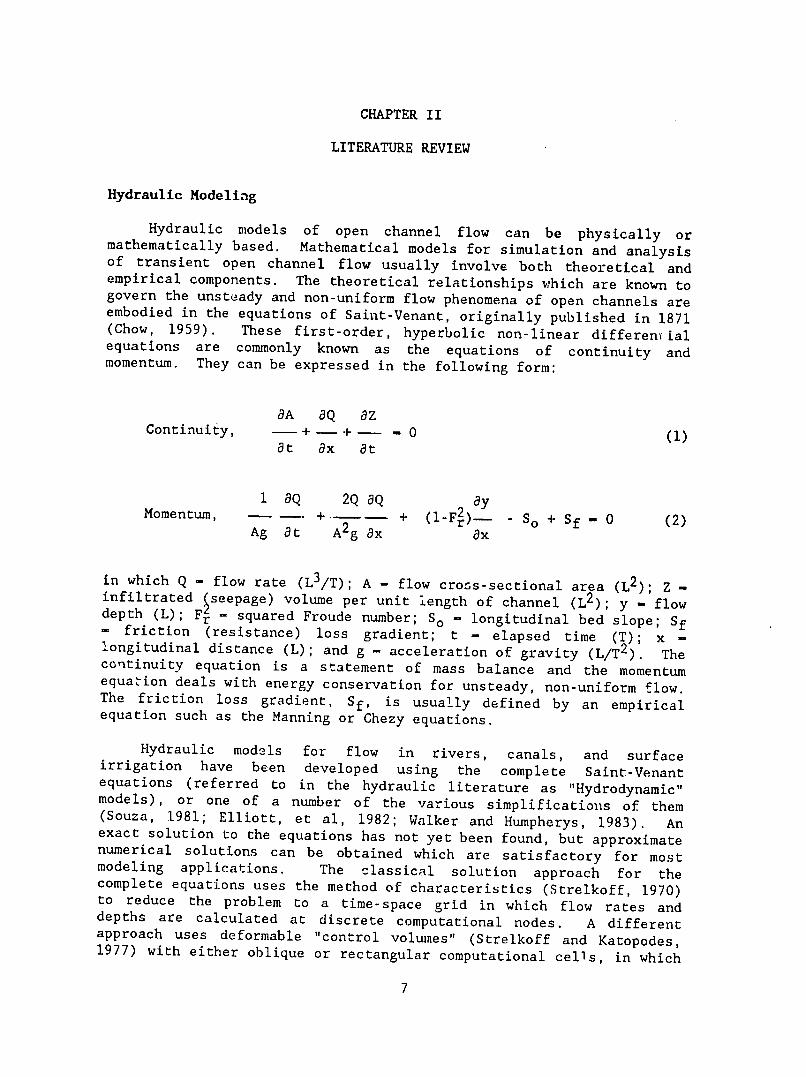
Hydraulic models of open channel flow can be physically or mathematically based. Mathematical models for simulation and analysisof transient open channel flow usually involve both theoretical and empirical components. The theoretical relationships which are known to govern the unsteady and non-uniform flow phenomena of open channels are embodied in the equations of Saint-Venant, originally published in 1871 (Chow, 1959). These first-order, hyperbolic non-linear differenyialequations are commonly known as the equations of continuity and momentum. They can be expressed in the following form:

aA aQ az Continuity, - + - +- - 0 (1)

at ax at

1 aQ 2Q aQ ayMomentum, - - +.-- + (I-Fr)- - + Sf - 0 (2)So

Ag at A2g ax ax

in which Q - flow rate (L3/T); A - flow cross-sectional area (L2); Z -infiltrated seepage) volume per unit length of channel (L2 ); y - flow depth (L); Fr - squared Froude number; So - longitudinal bed slope; Sf - friction (resistance) loss gradient; t - elapsed time (T); x ­longitudinal distance (L); and g - acceleration of gravity (L/T2 ). The continuity equation is a statement of mass balance and the momentum equa,-ion deals with energy conservation for unsteady, non-uniform flow. The friction loss gradient, Sf, is usually defined by an empirical equation such as the Manning or Chezy equations.

Hydraulic models for flow in rivers, canals, and surface irrigation have been developed using the complete Saint-Venant equations (referred to in the hydraulic literature as "Hydrodynamic"models), or one of a number of the various simplificatious of them (Souza, 1981; Elliott, et al, 1982; Walker and Humpherys, 1983). An exact solution to the equations has not yet been found, but approximatenumerical solutions can be obtained which are satisfactory for most modeling applications. The classical solution approach for the complete equations uses the method of characteristics (Strelkoff, 1970)to reduce the problem to a time-space grid in which flow rates and depths are calculated at discrete computational nodes. A different approach uses deformable "control volumes" (Strelkoff and Katopodes,1977) with either oblique or rectangular computational cells, in which

7

adjacent cells share computational nodes. This method has some numerical advantages over the method of characteristics and it has been used in the model developed for this study (Gichuki, 1988). Solution techniques are generally applicable to different types of problems, although some techniques are more suited to particular kinds of investigations. Thus, a solution of the governing equations for surface irrigation models can be perfectly acceptable for use in flood­routing or canal flow models, with each individual application employing the specific boundary conditions unique to its configuration.

Canal Control Logic

A large variety of methods for controlling flow in canals and rivers have been proposed and applied throughout the world in recent years. Some of these methods include local and system-wide automation, remote sensing and control, and hydraulic simulation through computer modeling. In general, canal regulation schemes can be classified as either upstream or downstream control. In upstream control the gates are operated to regulate the water level on the upstream side of each control structure. This is the traditional and most common type of canal control, especially in manually operated systems. With downstream control, as the name implies, gates are operated to regulate the water level on the dowr..tream side of each control structure. Downstream control has been used in irrigation canals for providing on­demand delivery of water by means of specially design control structures which operate independently of each other, and thus provide localized control (Goussard, 1987).

Long-crested weirs have been used successfully for regulation of canal flow levels in many parts of the world (Walker, 1987). These represent a simple, yet often effective, solution to canii control in which the flow control qtructures have fixed settings. However, they do require sufficient longitudinal canal slope so that they will operate under free-flow conditions. One irrigation project in New Mexico uses elaborate remote sensing and automation hardware in an extensive system of sloping canals (USBR, 1973). Such automation is currently implemented only at relatively high initial and maintenance costs, and can only be justified for a few projects. Burt (1983) used a hydraulic model to test a localized canal control concept based on maintaining constant volumes of water in individual canal reaches. Other types of localized control have appeared in the literature (CheverLau and Schwartz-Benezeth, 1987) and many have been tested in actual applications. Hydraulic modeling has also been used by the California Department of Water Resources for analyzing different operational schemes in the California Aqueduct (Reynolds and Madsen, 1967).

Global or system-wide control of canal flow has been made possible through modeling techniques which can be used to integrate the operation of individual control structures. Falvey (1979) showed how a "valve stroking" technique for controlling pipeline transients could be

8

applied to open channel flow problems. This technique was called "gatestroking" and was used with a method of characteristics solution to the Saint-Venant equations. Gichuki (1988) showed how this could be applied analogously to models employing the deformable control volume solution approach.

Most of the hydraulic models developed to this date are basicallyresearch-oriented and are only usable by the model developers or byengineers who have invested considerable time to understanding their internal workings. Corriga et al. (1980) developed a model for simulating hydraulic transients in canals with self-leveling gates.They reported that their model was applied to study the transients in a hypothetical system and that it could usedbe to improve operatingpolicies in real systems. Balogun et al (1988) presented a hydrodynamic model for the automation of canal systems using linear quadratic regulator theory. usedThey have their model to performsimulations of hypothetical canals to demonstrate the applicability for designing automatic canal control systems. Gray (1980) reviewed several finite element models for the simulation of unsteady openchannel flow and concluded that none were ready to be applied to the analysis of real canal systems.

In an effort to enhance tha utility of hydraulic models for canalcontrol, and for other applications, some models have been developedusing extensive simplifying assumptions to the complete equations (Hartet al, 1978). Others have been developed using steady-state, uniform flow assumptions. This latter group of models ignore all hydraulictransients and are essentially based upon inflow-outflow balances for water in a canal system. However, in spite of the simplifyingassumptions which may be introduced into a model of this type, the required field data for successful application are the same. That is,whether a model uses the complete Saint-Venant equations, an empiricaluniform flow equation, or anything in between, the same type uf data must be collected from the field in order to use the model.

Main System Management

Replogle (1983) states that the physical water delivery system(i.e. main system) is one of the two major factors which limit irrigation efficiency on the farm. This is typical of the current thinking on the role of the main system in influelLing agriculturalproduction practices. Khan et al (1987) write that many countries are now "shifting their attention" toward better management of existingirrigation main systems since the development of new project sites hasdiminished rapidly in recent years. The importance of improving water management through better main system operation is also emphasized byWalker and Skogerboe (1983). Rao and Sundar (1986) assert that,

9

"Although, initially people thought that the best way to improve the performance of irrigation systems was to develop the farms below the outlet, it soon became clear that better and more equitable water distribution was the prerequisite for increasing the productivity of irrigated agriculture"

Power (1986) offers the opinion that irrigation project organizations tend to have civil engineering orientations toward design and construction, with less emphasis on operations and maintenance issues. Others claim that irrigation development work around the world has traditionally over-emphasized technical solutions to water managementproblems, while ignoring sociological issues (Uphoff, et al, 1986, and Lusk, 1986).

Evidence of computer models for training main system operators can be found in the literature. Burton and Frank (1983) believe that the poor performance of many irrigation projects can be partially attributed to the quality of operational practices in th= main system. They .!so present a conceptual approach to training in main systemoperation through use of a computer-implemented model. Their model is essentially based on a "water budget" notion in which the different flow components are considered with respect to canal operation and on­farm water requirements. Johnson (1986) discusses the application of computer software to improving water resources planning and operation, including irrigation main systems. He goes on to emphasize the importance of a "user-friendly software interface" for computer models, and indicates that "considerable effort" is required to develop such an interface.

It can be concluded that most existing models for transient hydraulic analysis of canal flow are research-oriented. This means that most existing hydraulic models lack a "friendly" user interface, interactive features, menu-selectable system configuration options, and graphical output of simulation results. It is also evident from the cited literature that researchers and others believe that hydraulicmodeling can be successfully applied to design, training, and operation of main systems.

10

CHAPTER III

GATE SCHEDULING

Numerical Solution

Since no known analytical solution exists to the Saint-Venant equations, they must be dealt with using numerical approximations. The model developed for this study uses the deformable control volume approach detailed by Walker and Skogerboe (1987), which effectively reduces the momentum and continuity equations from partial differential equations to a system of non-linear algebraic equations for each canal reach. Thus, individual canal reaches are treated separately duringsolutions of the resulting equations, except at the upstream and downstream boundaries of the reach. At downstream boundaries, control structures which operate under submerged flow conditions may exist, in which case, the downstream depth is taken from the solution of the previous time step. In this way calculations are kept to a tractable level, proceeding on a reach-by-reach basis, rather than attempting to solve the-equations simultaneously for all reaches in a canal system.

The model controls the placement of computational nodes along the length of a reach to reduce the possibility of numerical instabilities, and to accommodate turnout structures at various locations. It is at computational nodes that flow rates and depths are calculated. The last node in a reach is placed at the extreme downstream end of the reach where a control structure is always located. In this model, control structures demarcate the end of one reach, and possibly, the beginning of another. At this last node three potentially variable parameters exist: (1) flow rate; (2) flow depth; and (3) control structure setting. Of course, if a reach has a non-adjustable control structure then the setting is not a variable parameter.

In order for the total number of unknown parameters to be equal to the number of independent equations one of the three variable parameters at the last node must be specified. The number of equations to be solved simultaneously is equal to twice the number of computa­tional nodes minus one. In equation form,

m - 2n-1 (3)

where, m - number of equations and n - number of computational nodes along the reach. These equations include two boundary conditions, one at the inlet to the reach and one at the outlet. Inlet boundaryconditions are usually a known hydrograph since reach flow conditions are updated individually. Downstream boundary conditions are usually a unique stage-discharge relationship defining the hydrauliccharacteristics of the control structure. Intermediate boundary

11

cnditions will also exist when one or more turnouts are located within a given canal reach. Turnout boundary conditions are similar to the downstream boundary condition; however, in this model the stage­discharge relationships for turnouts affect only the continuity equation, not the momentum equation.

Control Structures

In a pure simulation mode, the control structure setting is specified by the user and the model computes the flow rate and depth at the last node along with all other nodes in the reach. This type of mode is in effect for what are called the "manual" and "pre-set"operational modes. Both of these modes are similar in that the user specifies the settings for individual structures during a simul,'tion, or at the beginning of a simulation.

The pre-set operational mode is essentially the same as the manual mode since both use manual control structure settings. The difference is that with the pre-set mode the manual control structure movements are specified for the entire duration of the simulation before it begins, and the movements are derived from a pre-evaluated operationalscenario over the period of the simulation. If the desired manual control structure settings are already known before a simulation begins, then pre-setting the structures is useful as the simulation does not have to be interrupted each time an adjustment needs to be made. A principal application of this pre-set mode is to test the differences between using veraged or "banded" control structure setting adjustments versus using the exact adjustments from a previoussimulation for which the gate scheduling mode (described below) was in effect. Simulations with gate scheduling often produce slightfluctuations in control structure settings while the canal systemchanges from one steady-state condition and adjusts to another steady­state condition. These fluctuations can be eliminated or reduced bysimplifying the exact gate scheduling settings according to the generaltrends in calculated control structure responses to flow rate changesin the system. These trends can be identified in either graphical or tabular format from the model output after a simulation.

Averaged or "banded" control structure setting adjustments are more practical for field operation, and they represent a compromisebetween exact model solutions and the feasible operation of a real canal system. The model treats canal system operations from a centralized perspective during gate scheduling, which means that in some cases the simulation results will show simultaneous control structure movements throughout the system. Due to labor constraints and the time required to physically travel from one control structure to another, logistical adjustments of the model-generated solution maybe required. Canal operators cannot be in two places at the same time. The pre-set mode is used in this case to determine the consequences of making logistical adjustments in the operations schedule, and to confirm whether or not the adjustments are acceptable.

12

Gate scheduling is the third and most interesting operational mode in main system management. When gate schedul.ing is enabled, computations produce optimal control structure adjustmentsautomatically in an effort to maintain water onconstant levels the upstream side of each structure (the upstream side of each structure is at the downstream end of the reach in which the structure is located).This constitutes canal operation for upstream control since the control structures respond to maintain upstream conditions. Maintaining constant water levels is accomplished by calculating an appropriateflow rate for the last node in the reach by an independent criteria (see Activated Canal Reaches). In this case the control setting is calculated using the known stage-discharge relationship for the structure after the Saint-Venant equations have been solved for the current time step. In this situation it is possible to make the solution of the downstream boundary equation external to the solution of the system of Saint-Venant equations. a resultAs of making the downstream boundary an external calculation, the number of simultaneous equations becomes exactly equal to twice the number of nodes in the reach. Table 1 summarizes the differences in the solution to the Saint-Venant equations with respect to the three variable parameter7 at the downstream node.

TABLE 1. Known, Calculated, and External Parameters at the Downstream End of a Canal Reach During Solution of the Saint-Venant Equations.

Flow Rate Flow Depth Gate Setting Operational Mode (m3/s) (m) (m)

Manual or Pre-Set calculate calculate known

Scheduling: calculate calculate known Reach Deactivated (WaitSetter)

Scheduling: known calculate external Reach Activated (FlowSetter) (Ctrl_Setter)

Note: Wait Setter, FlowSetter, and CtrlSetter are procedure names for various gate scheduling computations before and after solving the Saint-Venant equations in a reach during a given time step.

13

The target water levels at the downstream end of a canal reach during gate scheduling are specified by the model user. When gate scheduling is enabled, the entire canal system will be in the gate scheduling mode. However, individual reaches may be either activated or deactivated, meaning that two separate control criteria can be used for adjustable structures during gate scheduling. These two criteria are described in the following sections. Non-adjustable control structures (e.g. culverts and fixed weirs) can never be activated since their setting cannot oe changed. Pumps as control structures can be manually operated, but incremental adjustments cannot be made since they are assumed to have constant speed motors. Therefore, pumps cannot be activated for scheduling by the model; they can only be turned on, or turned off (although multiple pumps with identical characteristics are allowed at a single location).

Of the five possible status conditions for canal reaches, four may prevail when the system is in the gate scheduling mode. These are: (1) on; (2) off; (3) fill; and (4) wait. For activated reaches the status is "on" and for reaches with non-adjustable control structures the status is "off". During the filling or advance phase the status will be "fill", and for deactivated reaches the status is "wait". The fifth status condition is "set", which indicates that the "Pre-Set" operational mode is in effect. Figure 2 shows the possible paths to different scheduling status conditions according to the operational mode in effect.

SOperational Mode

EntireCanal System

Scheduling Enable d Scheduling Disabled

hl Z chdln SchedulingAotiv.aetiv ctDectivted DdIndividualDeactivated

leduCanal Reaches

satus: Status: Stte tatus tau:Stta(1)On (2) Of f

Figure 2. Flow Diagram Indicating the Possible Paths to the Five Different Gate Scheduling Status Conditions for Individual Canal Reaches.

14

Reaches with adjustable control structures may be automaticallydeactivated at any time during a simulation when gate scheduling is enabled if some operational limitations have been encountered. Reaches can also be re-activated automatically provided that the schedulingmode is still in effect (operational modes can be changed at any time during a simulation). Re-activation occurs when a control structure setting can be changed from an extreme value, and when the water level comes close to the target level. The operational limitations which will cause a reach to be deactivated are described below.

Filling an Empty System

When gate scheduling is enabled during the filling of a canal system, the computed control structure settings remain at their initial settings at least until the next downstream reach has completed the advance phase. For example, while the water in reach four is still advancing to the end of the reach, the control structure setting in reach three will not change front its initial value. After reach four has completed the advance phase, the analysis begins showing control structure settings in reach three that would meet the objective of changing the actual water level upstream of the structure so that it approaches the target level. During filling this usually means that the actual water level must be raised up to the target level, and thac the flow through the structure and into reach four must be reduced (using the above example). If the system inflow rate is sufficientlyhigh, the actual water level will eventually come 'lose to the targetlevel. When this happens, the reach will be activated and in subsequent time steps the model will try to maintain the actual water level at the target level by "scheduling" the control structure operation.

When a reach becomes activated, its control structure begins to operate regardless of whether or not the next downstream reach has completed the advance phase. The flow condition in the next downstream reach will only be able to deterinine whether any control structure adjustments are made until an upstream reach is activated. Adjustmentsprior to reach activation usually mean the ratethat reach dischargemust be decreased (i.e. the control structure must be closed an amount)in order to raise the actual water level to the target level. However,after activation the reach discharge increases since the actual level is already at or near the target level, and the additional flow used to build the water to this desired level must now be passed downstream. Increases in discharge to a reach which is currently in the advance phase are usually not a problem, but decreases during the advance phasetend to cause numerical instabilities which can lead to failure of the simulation.

15

Activated Canal Reaches

The gate scheduling analysis attempts to maintain the actual water level on the upstream side of each adjustable control structure at the target level for all activated reaches. This is performed in an indirect way using an intermediate steady-state estimation of dischargethrough the control structure. The steady-state discharge is calculated before the transient equations (integrated forms of Eqs. 1 and 2) are solved for the current time step. Thus, during solution of the transient equations the downstream flow rate is known (fixed), and at this downstream node the only unknown quantity is the flow depth(see Table 1). The gate setting is then determined after solution of the transient equations, making it an external calculation.

Initially, a steady-state discharge rate for each reach iscalculated based upon the system inflow rate and all system outflow rates from each structure in the upstream direction. For example, if the flow conditions in reach two of branch one are being updated, and if this reach is currently activated, the steady-state discharge rate from reach two into reach three will be equal to the system inflow rate minus all turnout and seepage flows in reaches one and two. In this case wasteway weir discharges are not included in the turnout totals since under normal operation they should not be spilling water. Figure3 illustrates an example of this computation with some dischargevalues. For the purpose of calculating these steady-state discharges, the system inflow is taken to be the average of the inflo,;s from the past four time steps. This averaging slightly delays the reaction of the system to inflow changes in order to allow the reaches to adjust to the new inflow rate more smoothly. After calculating the steady-statedischarge for a reach, the difference between the current actual water level and the target level on the upstream side of the reach's control structure is checked.

A new discharge for the reach is then calculated by either increasing or decreasing the steady-state value according to the absolute magnitude of the difference in actual and target water levels. It this difference is large compared to the canal depth then the adjustment on the steady-state discharge value will be relativelylarge. And of course, if the actual water level is above the targetlevel, the new discharge must be higher than the steady-state value since the actual water level needs t. be lowered. The opposite is true when the actual water level is below the target level. When the difference between actual and target water levels becomes small, the new discharge will be close to the steady-state discharge, and the reach will actually be near a steady-state flow condition. During gatescheduling tho model is always "aiming" at a system-wide steady-state flow condition even though the system inflow rate and distribution of flows may change. In other words, the objective of gate scheduling is to quickly stabilize, or dampen, transient flow conditions.

Once this new reach discharge rate is calculated based on the steady-state discharge rate and the deviation between actual and targetwater levels, a series of checks are made. These checks compare the

16

REACH 1 Svltem

TTotal Turnout

Flow - 2.00

Total See pagLoss - 0.160

Figure 3. Illustrated Example of Steady-State Reach Discharge Calculations During Gate Scheduling.

current reach discharge with the discharges from previous time steps so that potentially problematic ifflow conditions can be avoided possible. The first check determines whether the reach outflow is fluctuating and is performed by comparing the reach discharges from the pas: two time steps to the new discharge. If the reach discharge from the previous time step is greater than both the new value and the value from two time steps before, an attempt will be made to stabilize thedischarge by taking ; weighted average of the previous and current rates and setting the new discharge equal to this average.

This averaging will always be performed for the above two conditions in which a positive or negative "spike" exists in the reach discharge hydrograph, except when the differences in computed flow rates between consecutive time steps is very small. For example, if a turnout is suddenly closed, the reach discharge must eventuallyincrease by che amount "recovered" from the turnout discharge (see Fig.4), assuming that all other turnout demands remain the same, and that the system inflow has not changed. If the induced transient is sufficiently large, the model may initially over-react, and then stabilize after a few time steps. This initial over-reaction can be lessened, and the stabilization time can be decreased, by havingfluctuations of this nature identified and corrected automatically by the model itself.

17

01=- 0.60t +0.0­Or.ICD at-i

•.....I .. ..................................................................... 0 a "

Oto

CLO -4 ar-3 Or-2E0 U

Oto =recovered turnout discharge

t-4 t-3 t-2 t-1t Elapsed Simulation Time

Figure 4. Illustrated Example of How the Model Stabilizes Over-Reaction of a Control Structure to the Closing of a Turnout.

The second check is to prevent the computed reach discharge from changing too fast in a single time step. The new discharge is compared to the average value of the discharges from the past two time steps.The acceptable range for the new discharge is then defined as this average value of the previous two steps plus or minus five percent of the design, flow capacity for the reach. The design flow capacity is defined using Manning's equation under uniform flow conditions at the target water level. If the newly computed reach outflow is not within this acceptable range, the value will be changed to either the upper or lower limit of this range, depending on whether the value is high or low. This second check tends to prevent an over-reaction to a sudden large change in the flow conditions.

The third check compares the new discharge to the extreme upper and lower flow rate limits for the reach as defined in the model. The extreme lower limit is 0.01 m3/sec. If possible, a reach discharge is not allowed to be lower than this minimum value during gate scheduling.Nor can a reach discharge exceed the design flow capacity (definedabove) of a reach while that reach is activated during gate scheduling.

18

After the new reach discharge has been calculated and the above three checks performed, the new outflow is fixed as a boundarycondition in the hydraulic equations for the current canal reach and time step. The solution to the hydraulic equations then yields a flow depth that accommodates the fixed outflow (tbh appropriate control structure setting which meets these conditioti- is computed after solution to the equations). If the flow depth on the upstream side of the structure is not at the target level, then it should at least be closer target than atto the level it was the start of the previoustime step since the fixed discharge rate through the structure was calculated in such a way as to reduce the difference between actual and target water levels. However, this may not always be true duringtransient conditions since reaches may, in effect, be competing with one another for the available water in the canal system. If the systeminflow is high enough to satisfy total system outflows, the canal system will eventually reach a steady-state condition, even thoughduring one or two time steps the actual water level may not be approaching the target level for some of the reaches.

It was mentioned previously that the model tries to maintain the actual water level at the downstream end of each reach at the targetlevel in an indirect way. The method is indirect because instead of fixing the flow depth at the downstream end of a reach to be equal to the target flow level, the reach discharge through the control structure at the downstream end of the reach is fixed. Scheduling the structure movements indirectly as such tends to significantly reduce the sensitivity of the models' reaction sudden changesto in upstream or downstream flow conditions. Scheduling in this way also tends to dampen oscillations of structure settings much quicker than if the flow depth is fixed at the downstream end of a reach. It is possible to reference the entire system back to the system inflow rate at the extreme upstream end of the canal system since the reach discharge is fixed during solution of the transient hydraulic eqtations with gate scheduling enabled.

This computational procedure integrates the operation of the entire system and eliminates the amplification of local disturbances in the downstream direction which can result from successive over­reactions to system flow changes with fixed downstream flow depths.Thus, local flow rate or flow level changes are handled by the model from a global perspective of the canal system during gate scheduling.It also tends to minimize the transfer time of flow rate changesthrough the canal system because the entire system reacts simultaneously to any flow change, even if the system is already in a steady-state condition at the time of the change.

Before a new control structure setting is accepted during gatescheduling some conditions met.final must be First of all, if the structure is an adjustable weir, the sill height cannot raise above the upstream flow depth once water has begun to discharge into the next downstream reach. This is to prevent the flow from being temporarily cut off in the downstream direction. If the structure is a sluice

19

gate, a check is made as to whether the current flow regime is free flow or submerged flow. When the structure is operating under free flow condit.'ns, the bottuai of the gate be raised above thecannot upstream wagt- level. And if the structure is operating under submerged flow conditions the bottom of the gate cannot be raised above the downstream water level. The-e conditions are intended to preservethe current flow regime if possible. Changes from one regime to another can cause abrupt changes in the computed discharge rate, which can then cause the numerical solution of the hydraulic equations to fail.

Next, the hydraulic head differential for sluice gate structures is checked. If the downstream water level is at or above the upstream water level across a sluice gate operating under submerged flow conditions, the flow rate through the structure is set equal to zero. This is to prevent the occurrence of "back flow" in which water maytemporarily go upstream through the sluice gate. Backflow conditions have proven to be troublesome to the numerical stability of the model.

Finally, the new setting is compared to the extreme maximum and minimum settings which define the operational range of the structure. If the new setting is lower than the extreme minimum setting the new setting will be set equal to this minimum value. If the new setting is higher than the extreme maximum setting the new setting will be set equal to this maximum value.

If any of the above conditions are not met, the scheduling status for the current reach will be deactivated since the model will be unable to accommodate the fixed discharge rate for which the new setting was calculated. In this case the current flow conditions are re-computed for the reach with scheduling deactivated before moving on to the next reach in the system. The model will try to bring the actual downstream water level close to the target level in subsequenttime steps by opening or closing the control structure incrementallythrough the "WaitSetter" procedure (see Fig. 5). The criteria used to make the control structure adjustments in this case is described in the following section. When the actual water level upstream of the reach's control structure is near the target level the scheduling status will be automatically reactivated.

Deactivated Canal Reaches

When the scheduling status for a reach with an adjustable control structure is deactivated the structure setting may be automaticallyadjusted in an attempt to reduce the difference between actual and target water levels at its downstream end. However, the criteria used to compute setting adjustments in the deactivated case are not the same as for activated reaches. This is because either the deviation between actual and target water levels is currently too large, or because the structure is unable to open or close enough to satisfy the schedulingrequirements. Thus, an independent criteria is used during subsequent

20

Current Reach

Activate ? Flow Setter

rate) Icomputeflow<

Solve Saint-Venant Equations

N y

WaitSetter -- Activated ? -- Ctrl Setter (compute setting) 1(compute setting)

Near Target N YCniin evel ? Acpals

Activate Deactivate

Current Reach Current Reach

Next Reach

Figure 5. Flow Diagram Showing the Possible Program Paths for Gate Scheduling When Scheduling is Enabled for the Canal System.

21

time steps until the scheduling conditions become feasible. In other words, the difference in the two situations is essentially that for activated reaches the gate adjustments are based on computations which are designed to maintain the actual water level at the target level, and for deactivated reaches the adjustments are calculated "guesses"which are designed to reduce the difference between actual and target levels.

The magnitude of a deactivated control structure adjustment is based upon the current relative absolute flow level deviation, and upon the current relative control setting. These values are relative in the sense that they are scaled to the depth of the canal lining in the reach. The relative absolute flow level deviation is defined as follows:

6 - abs Yay (4)f

where, 6 - relative absolute flow level deviation (L/L), Ya - current actual water level (L), Yt - target water level (L), and Ymax - depth of the canal lining (L). Figure 6 shows the relationship between the parameters on the right side of Eq. 4 and the control structure setting. This equation is also used for the activated reaches, but the steps following calculation of 6 differ from the procedure described below.

If at any given time step during a simulation 6 < 0.05, the reach will be activated and the control setting in subsequent time steps will be based upon the steady-state discharge criteria described in the previous section. Activation in this case is also dependent on the required new control structure setting. If the new setting is beyond either the upper or the lower operational limits then this new setting will be made equal to the appropriate limit, and the reach will remain deactivated.

If the value of 6 is not less than 0.05, the reach will remain deactivated and the new control setting will be computed as follows:

b' - (lFA)b (5)

where, b is t'ie current control setting (L), and b' is the new control setting (L). The value of A is defined as follows:

2 -2 (6)

10 Ymax

22

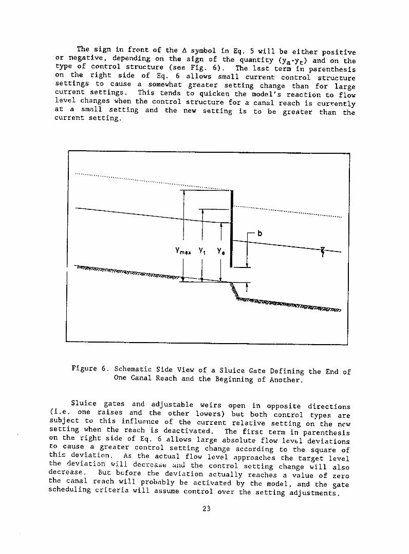
The sign in front of the A symbol in Eq. 5 will be either positiveor negative, depending on the sign of the quantity (Ya-Yt) and on the type of control structure (see Fig. 6). The last term in parenthesis on the right side of Eq. 6 allows small current control structure settings to cause a somewhat greater setting change than for largecurrent settings. This tends to quicken the model's reaction to flow level changes when the control structure for a canal reach is currentlyat a small setting and the new setting is to be greater than the current setting.

............................. ........................ ...............

.........................

max t Ya ............ .......... .......

Figure 6. Schematic Side View of a Sluice Gate Defining the End of One Canal Reach and the Beginning of Another.

Sluice gates and adjustable weirs open in opposite directions (i.e. one raises and the other lowers) but both control types aresubject to this influence of the current relative setting on the new setting when the reach is deactivated. The first term in parenthesis on the right side of Eq. 6 allows large absolute flow level deviations to cause a greater control setting change according to the square ofthis deviation. As the actual flow level approaches the target level the deviation will decrease and the control setting change will also decrease. But before the deviation actually reaches a value of zero the canal reach will probably be activated by the model, and the gatescheduling criteria will assume control over the setting adjustments.

23

Thus, a small current control structure setting and a large flow level deviation will both tend to cause a large control setting change. The effect of the current control structure setting on the magnitude of the adjustment is limited on the upper end to doubling the effect of the flow level deviation alone. This would be true when the current setting is zero. At the other extreme, the current setting would be equal to the canal lining depth and the effect of the current setting on increasing the adjustment magnitude would be nullified (see Eq. 6). The new control structure setting is checked against the extreme upper and lower operational ranges for the structure and the flow regime is checked, as for activated reaches, before the new setting is accepted by the model.

Turnout Str'ctures

When the gate scheduling mode is in effect turnout settings are also computed with the objective of matching individual turnout discharges to their demands. Turnout demands can be changed at any time during a simulation. When turnout demands change, or when canal flow levels change, the turnout settings will be appropriately modified by the model. Before attempting to solve the hydraulic equations for a canal reach, the new turnout settings will be estimated based on the flow levels from the previous time step. After solution of the equations the actual turnout discharges will be computed according to the newly calculated flow levels. The actual discharges may not ex, itly match the demand discharges for the turnouts in a reach since the flow levels may have changed. Nevertheless, the actual discharges will come very close to the demands after the flow levels have stabilized for a given steady-state condition.

Status Conditions

During simulations the status of a turnout may change depending on the flow conditions and on the type of turnout structure. Non­adjustable turnout structures (e.g. wasteway weirs) by definition have fixed settings and cannot be operated. If a turnoiut demand on an adjustable structure exceeds the flow capacity of the turnout, the structure will be opened fully, but the actual discharge will be less than the demand. When a turnout demand is changed during a simulation the new required setting is instantly made, unless the new setting is more than 0.1 meters from the previous setting. In this case the turnout setting will change in increments of 0.1 meters during subsequent time steps until the appropriate new setting is reached. Incremental turnout adjustments help insure numerical stability during flow changes which can be induced by modified turnout demands or by fluctuating flow levels.

Orifice-type turnouts can operate under free flow or submerged flow regimes, depending on the downstream water level. Downstream water levels are approximated by linear stage-discharge relationships

24

since they are external to the calculations performed by the model. Thus, downstream of turnouts the water levels are computed based on current discharge rates in order to determine the prevailing flow regime. This regime is really only an estimation since updated flow conditions may cause modified turnout discharges, making possible a change from free flow to submerged flow, or vice versa. However, turnouts normally operate under only free flow, or only submerged flow conditions. If the water level downstream of a turnout is above the upstream flow level, backflow conditions prevail. But water is not allowed to flow back into a canal reach from a turnout. Therefore,under such conditions the turnout discharge is assumed to be zero until a positive water level differential exists across the structure.

Orifice-type turnouts will never open such that the bottom of the turnout gate is above the upstream water surface. This ensures that the structure behaves as an orifice, and not as a submerged channel constriction or a contracted weir. In any case, operation of the structure with the bottom of the gate above the upstream water level will not affect the turnout discharge. If the water level in a canal reach drops below the top of an orifice turnout opening, the orifice will also close in compliance with the above operational restriction on this type of structure.

25

CHAPTER IV

FIELD EVALUATION OF THE MODEL

Overview of Activity

The emphasis of this study was not only to develop an easy to use main system hydraulic model, but to implement it at an irrigationproject site. It was decided to initially implement the model to helpimprove the operation of two irrigation projects in Northeast Thailand. They were: (1) The Northeast Small-Scale Irrigation Project (NESSI),consisting of seven small-scale systems; and (2) The Lam Nam Oon Irrigation Project. The chosen NESSI site was the Huai Aeng system,located near Roi Et. At Lam Nam Oon, data was collected from both the left and right main canals, but the model was first implemented on the right main canal.

Prior to completion of the model development two Thai engineersfrom the Royal Irrigation Department (RID) participated in the analysisof data from the two project sites mentioned above. Mr. KanchingKawsard had collected configuration and calibration data from the left main canal at Huai Aeng before arriving at Utah State University in1984 to study for an M.S. degree in Irrigation Engineering. Mr. Charoon Pojsoontorn of the Lam Nam Oon Project came to Utah State University in 1985 for twelve months of special training at the International Irrigation Center (IIC). The model was tested using data from both of these projects, and the software was modified to accommodate some of the particular features of the canal systems. The software was also developed in a modular fashion so that the model could be most easily adapted for application at other project sites with different physical and hydraulic characteristics.

The existing data from the two chosen project sites were incomplete for the purposes of hydraulic modeling. Additional data were collected during June and July of 1986 at the Huai Aeng and Lam Nam Oon sites. These additional data were collected by RID engineersand technicians as part of the field exercises for two training courses conducted by the IIC. The courses involved dimensional canal infrastructure and flow measurements for the purpose of obtaining flow structure calibrations and seepage loss rates. And, the courses were elaborated in a practical and field-oriented manner so that the participants would have the skills to perform such data collection activities at their own project sites, and train others as well. Thus,the courses served to train the participants and also providedadditional data which could be used for hydraulic modeling.

The two week duration of each of the training courses was insufficient to complete all of the required data collection for application of the model at the project sites. Further data collection was directed by Mr. Kawsard at NESSI, and by Mr. Pojsoontorn at Lam Nam

27

Oon. The writer made a second trip to Thailand in February of 1987 to resolve some computer hardware problems, review newly collected data, and make further software modifications to facilitate application of the model. By this time two microcomputers had been purchased for implementing the model in Thailand, and both were stationed at the NESSI project headquarters in Khon Kaen.

During a third trip in August of the same year, one of the computers was moved to the Lam Nam Oon project to apply the model to the operation of the right main canal. At this time calibration and seepage loss measurements were completed and the model was used to perform verification simulations. Existing operational data were used along with newly collected data to demonstrate the ability of the model to simulate the flow of water in the canals. Further training of project personnel was undertaken to answer some of the remaining details about how to use the model as a tool for improving canal operation. Additional software modifications and additions were also made to enhance the model's utility for on-site application. After thi3 third trip, the model and computers were ready for field use.

The fourth, and final, trip to Thailand was made in January of 1988 with the intert to complete any remaining field data collection work and apply the model to the actual operation of the right main canal at Lam Nam Oon. Bed slope survey data were plotted and analyzed to determine "as-constructed" longitudinal canal slopes and elevation changes across control structures. Software modifications were made to include gate setting corrections in the control structure equations for rectangular sluice gates. The use of these setting corrections al1 owed constant discharge coefficients for each of the sluice gate ("3ck structures on the right main canal (see Skogerboe et al, 1987). u ner software changes and expansions were made to improve the capability to accurately simulate the field-observed flow conditions.

Data were collected along the left main canal for use in hydraulic modeling during February of 1988. The existence of pumping stations on the left main canal. required the addition of centrifugal pumps as flow control structures to the model.. Plans were established for continued data collection along the secondary canals of both the left and right main canals after the end of this fourth trip. A utility program Wzas developed to solve for hydraulic roughness values based on gradually varied flow profiles. This was necessary since normal depth did not occur anywhere in the main canals, and it was impossible to determine roughness values by direct computation. The model was calibrated for two steady-state conditions on the right main canal, but because of some remaining field data inconsistencies the model was not actually applied to scheduling control structure operation in the field. However, considerable progress was made and with continued data collection it is anticipated that the model will be successfully applied toward improving the canal operation. The data collection and analysis activities have already made a positive impact on improving water management at the Lam Nam Oon project.

28

The writer began studying the spoken and written Thai languageduring his first trip to Thailand in June of 1986. Proficiency was attained in the language after one year, during the third trip toThailand. This ability to speak and write the language was veryhelpful in implementing the model and conducting the questionnaire survey (see Chapter VI).

Procedure

As part of the field implementation prccess, the model was used toexamine alternative configurations and operating conditions. These analyses were undertaken both to demonstrate the management options at Lam Nam Oon and to initially evaluate some of the more important main system management issues. A more general discussion of main system management issues follows in Chapter V.

The first twelve reaches of the Right Main Canal (RMC) of the LamNam Oon Irrigation Project (see Table A-l) were used to compare the simulated effects of gate scheduling; neglected maintenance, and typeof control structure on canal operation. It was necessary to use two branches since the model accommodates a maximum of nine reaches perbranch; the first six reaches were placed in the first branch, and the remaining six reaches were placed in the second. The second branch waslinked to the downstream end of the first, thus allowing the simulation of what is considered to be a single "branch" in the real system.These twelve reaches contained a total of 72 turnouts, including 10 wasteway weirs and 16 lateral turnouts. All turnouts other than wasteway weirs were constant head orifices (CHO's), most of which operated under submerged flow conditions at all times. The CHO's were actually operated as single gate structures because the second of the two gates were always wide open.

Both rectangular vertical sluice gates and rectangular sharp­crested weirs were evaluated as alternative control structures althoughthe real canal system has only sluice gates. The system was also simulated using rectangular weirs in which the crest lengths were set equal to the widths of the sluice gates for each respective canal reach. The model was used to simulate nine combinations of seepageloss rates and hydraulic roughnesses for each of the two control structure types.

Every simulation began at a steady-state condition in which the system inflow rate was sufficient to satisfy all turnout demands and seepage losses, with approximately 1.0 m3/s remaining to exit thedownstream end of the twelfth reach. Thus, most of the simulations had different inflow rates because of the differences in seepage loss ratesand hydraulic roughness. Volumetric seepage loss rates were calculated based on the seepage rate in mm/day and the calculated wetted perimeters at various points along each canal reach. The RMC of the real canal system has an additional six reaches downstream of the twelfth reach, but these reaches are not operated by the project

29

personnel. Therefore, although some flow normally passes downstream of the twelfth reach, it was taken to be a terminal point in the system for the purpose of performing hydraulic simulations.

For the purposes of this chapter, the distribution of flows in the system for the initial steady-state condition was taken from recorded turnout delivery rates for the dry season of 1987 at the Lam Nam Oon Project (see Table 2). The initial turnout demands used in all of the simulations are shown in Table A-4. At the beginning of each simulation the demands for turnouts R-16L and R-17L were increased from 0.2 m /s to 0.8 m-'/s. For the two turnouts, the total i ;.rease in demand on the system was then 1.2 m3/s. All other turnout demands remained the same as for the initial steady-state condition, and all adjustable turnouts not appearing in Table A-4 were closed at all times during every simulation. Non-adjustable turnouts were wasteway weirs.

TABLE 2. Initial Steady-State Turnout Demands During Model Simulations.

Turnout Branch Reach Turnout Demand Name Number Number Number (m3/s)

R-IL 1 2 2 0.50 R-4L 1 3 6 0.40 R-6L 1 4 3 0.80 R-9L 1 6 6 0.10 R-1lL 2 1 6 0.25 R-12L 2 2 1 0.10 R-15L 2 5 4 0.10 R-16L 2 5 8 0.20 R-17L 2 6 2 0.20

16

Note: See Table A-3 for complete turnout specifications.

Seepage losses increased in all cases as a result of the increased system inflow rate. This was because of changes in the final steady­state flow profiles, even when downstream flow levels were held constant in each reach during gate scheduling simulations. Additional flow increases were not made to account for increased seepage losses since the resulting flow profile changes could not be known in advance of the simulations. Computed seepage losses were dependeni: on wetted perimeters along each canal reach, which are a function of flow depths.

As soon as the demands on turnouts R-16L and R-17L were increased to 0.8 m3/s the system inflow rate was also increased by 1.2 m3/s to provide the additional water required to satisfy the new system demand. The system inflow rate was not changed from the initial steady-state

30

condition before these two turnout demands werj increased. This means that there was no "lead time" in anticipat- ,i of a new system demand, but that the system inflow rate change ar < the turnout demand changes were made simultaneously.

For each of the nine simulations the operational mode was changedbetween "Scheduling", "Pre-Set", "Manual #1", and "Manual #2". The scheduling mode involved the use of gate scheduling in which the model computed control structure settings in response to system flow changeswith the objective of maintaining constant downstream water levels in each reach. This was thr. cnly cperational mode for which the control structure settings could change during a simulation. The pre-set mode used constant control structure settings throughout the simulation. These settings were all made simultaneously as soon as the system flow rate was increased at the beginning of the simulation, and they were equal to the final steady-state settings as computed by the model for the scheduling mode. Thus, when the pre-set mode was in effect, the canal system was abruptly changed from a steady-state condition to a transient condition using new control structure settings which had been calculated to produce the desired final flow levels and turnout discharges.

Both of the manual modes involved increasing the system inflow rate and total turnout demand without changing any of the control structure settings. These represented an extreme operational case in which no adjustments were made on the control structure settings, even after the system flow rate changed. The first set of these simulations (Manual #1) used model-generated turnout settings which compensated for any flow level changes to maintain constant turnout discharges. For example, if the water level in a canal reach increased during a simulation the open turnouts in that reach would close an appropriateamount to eliminate deviations from the demand discharge rates. This automatic turnout operation was also in effect for the scheduling and pre-set operational. modes. The second set of simulations for the manual mode (Manual #2) used constant turnout settings in which no turnout adjustments were made to compensate for changing water levels. Therefore, if the water level in a reach increased, the turnout ir.e would also increase. And if the water level decreased, so too would the turnout discharge decrease. During this second set of simulations all turnout discharges equalled the respective demands during the initial thirty minutes of simulated time; after that all turnout settings were "frozen". This thirty-minute period allowed the model to adjust the turnouts R-16L and R-17L to the new demand of 0.8 m3/s each.

After increasing the system inflow rate by 1.2 m3/s at thebeginning of each simulation, and increasing the demands on the two downstream turnouts, the flow conditions were allowed to stabilize. Flows were considered to be stable when the total system outflow was within plus or minus one percent of the increased system inflow. The total system outflow included seepage losses, turnout discharges, and flow exiting the downstream end of the twelfth reach.

31

Results

The results for the nine combinations of seepage rate and hydraulic roughness are shown in Tables 3 and 4. Each of the four operational modes described above were simulated for each of the nine seepage and roughness combinations, for both sluice gate and weir control scructures. Thus, there were a total of 48 separatesimulations. Most of the simulations lasted longer than the twelve and one-half hour maximum period of the model. This required that many of the simulations be continued in a serial fashion so that sufficient time was allowed for the system to stabilize.

The maximum target level deviations shown in Tables 3 and 4 are for the absolute value of the difference between target level and stmulated water level at the downstream end of each reach. This corresponds to the maximum for all reaches and all time steps during the simulation. The average target level deviation is also an absolute value and is computed for all reaches and time steps. The maximum turnout deviation is the absolute value of the maximum difference between individual demands and simulated discharge rates for the end of the simulation only (i.e. after the flow in the system stabilized). Similarly, the average turnout deviation is the average of the absolute value of the differences for all adjustable turnouts with non-zero demands for the conditions at the end of the simulation.

System inflow rates for the simulations using Manning roughness values of 0.040 and seepage rates of 1000 mm/day exceeded, practically speaking, the peak flow capacity of the first canal reach. For this reason the control structure in the first reach was unable to openenough during the scheduling mode, and according to the operational restrictions imposed (see Chapter lIT). These conditions caused wasteway weir spills when such spills did not exist for the scheduling mode and other combiuations of roughness and seepage. Thus, the system could not respond satisfactorily to the flow requirements for this case and the results must be viewed with some skepticism compared to results from the other simulations.

Steady-State Distributions

An typical example of the steady-state flow rate distributions for the scheduling, pre-set, and both manual operational modes is sho,-n in Fig. 7. In this figure, the manuel mode is with turnout scheduling(corresponding to the Manual#l simulation), and it shows a more favorable situation than the corresponding simulation without turnout scheduling (i.e. Manual#2). For both the scheduling and pre-set modes the results are nearly identical. This is because the pre-set mode used the same constant control structure settings as those of the scheduling mode at the final steady-state conditions. The hydraulic transients during stabilization, and the time to stabilize the system, were not the same for the scheduling and pre-set modes. Only the final steady-state conditions were the same.

32

----------------------- ---------------------

-----------------

TABLE 3. Predicted Responses for Rectangular Sluice Gates with Varied

Seepage Rate, Hydraulic Roughness, and Operational Mode.

Case 1 2 3 4 5 6 7 8 9

Seepage 0 0 0 500 500 500 1000 1000 1000 Roughness 0.020 0.030 0.040 0.020 0.030 0.040 0.020 0.030 0.040

Flow Stabilization Time (hrs)

Sched 11.58 15.75 10.3319.33 13.83 16.83 9.25 12.25 14.33 PreSet 11.08 39.58 59.58 18.25 36.83 50.58 16.25 29.25 38.00 Manual #1 41.50 55.42 57.58 42.50 43.0841.00 37.25 34.25 36.92 Manual #2 55.17 57.67 60.67 45.83 43.17 42.75 38.83 32.25 37.67

Maximum Deviation from Target Level (m) ........

Sched 0.054 0.067 0.493 0.054 0.071 0.0400.571 0.135 0.610 PreSet 0.072 0.065 0.125 0.070 0.073 0.103 0.0670.061 0.104 Manual #1 0.798 0.787 0.767 0.741 0.7320.743 0.699 0.697 0.716 Manual #2 0.645 0.637 0.667 0.590 0.614 0.5480.642 0.584 0.617

----------------- Average Deviation from Target Level (m) -----------------

Sched 0.009 0.0250.014 0.011 0.016 0.038 0.012 0.019 0.050 PreSet 0.017 0.029 0.055 0.015 0.028 0.042 0.014 0.026 0.053 Manual #1 0.257 0.271 0.270 0.249 0.249 0.248 0.1760.233 0.221 Manual #2 0.240 0.241 0.244 0.220 0.224 0.223 0.204 0.206 0.197

3Maximum Deviation from Turnout Demand (m /s) ---------------

Sched 0.003 0.003 0.003 0.004 0.003 0.004 0.003 0.003 0.003 PreSet 0.003 0.003 0.004 0.0040.032 0,004 0.002 0.003 0.004 Manual #1 0.519 0.531 0.527 0.432 0.4580.470 0.365 0.397 0.389 Manual #2 0.384 0.403 0.411 0.340 0.366 0.371 0.310 0.335 0.338

Average Deviation from Turnout Demand (m3/s) ..............

Sched 0.001 0.001 0.002 0.001 0.001 0.002 0.001 0.001 0.001 PreSet 0.001 0.001 0.001 0.001 0.001 0.002 0.001 0.003 0.002 Manual #1 0.056 0.058 0.059 0.048 0.052 0.051 0.041 0.045 0.04J Manual #2 0.089 0.091 0.092 0.081 0.0820.084 0.075 0.077 0.071

Total Wasteway Spill Rate (m3/s) -------------------

Sched 0.000 0.000 0.000 0.000 0.000 0.000 0.000 0.000 0.063 PreSet 0.000 0.000 0.000 0.000 0.000 0.000 0.0000.000 0.086 Mdnual #1 1.003 1.054 1.076 0.746 0.747 0.742 0.444 0.439 0.457 Manual #2 0.845 0.872 0.885 0.580 0.583 0.583 0.312 0.297 0.367

--------.------------- Total Seepage Loss Rate (m3 /s) ---------------------

SchAd 0.000 0.000 1.8440.000 1.935 2.051 3.751 3.999 4.300 PreSet 0.000 0.000 0.000 1.838 1.925 2.049 3.747 3.994 4.300 Manual #1 0.000 0.000 0.000 1.961 2.1482.045 3.984 4.212 4.466 Manual #2 0.000 0.000 0.000 1.962 2.047 2.148 3.987 4.218 4.459

Note: Seepage rates are in mm/day and hydraulic roughness values are for the Manningequation. The three operational modes are scheduling, pre-set, and manual. Manual #1 is for continuously adjusted turnout settings, and Manual #2 is for unchanging turnout settings (settings remain at initial values throughout the simulation).

33

------------------ -----------------

----------------- -----------------

TABLE 4. Predicted Responses for Rectangular Weirs with Varied Seepage Rate,

Hydraulic Roughness, and Operational Mode.

Case 1 2 3 4 5 6 7 8 9

Seepage 0 0 0 500 500 500 1000 1000 1000 Roughness 0.020 0.030 0.040 0.020 0.030 0.040 0.020 0.030 0.040

----------------------- Flow Stabilization Time (hrs) ---------------------

Sched 11.58 15.75 19.33 10.42 13.83 16.83 9.25 12.92 15.08 PreSet 15.33 20.25 24.25 14.58 18.75 22.00 13.25 17.17 19.83 Manual #1 24.17 25.75 28.25 21.25 22.92 24.67 18.92 20.50 21.75 Manual #2 23.58 25.42 27.42 20.50 22.25 24.08 18.33 19.83 21.08

Maximum Deviation from Target Level (m)

Sched 0.057 0.06q 0.407 0.051 0.072 0.582 0.052 0.262 0.611 PreSet 0.073 0.120 0.193 0.068 0.120 0.0680.179 0.125 0.162 Manual #1 0.597 0.599 0.604 0.584 0.595 0.593 0.579 0.585 0.579 Manual #2 0.483 0.488 0.496 0.466 0.480 0.475 0.457 0.466 0.456

Average Deviation from Target Level (m)

Sched 0.010 0.014 0.026 0.011 0.016 0.039 0.013 0.023 0.045 PreSet 0.013 0.023 0.035 0.015 0.027 0.036 0.017 0.028 0.036 Manual #1 0.124 0.124 0.124 0.112 0.112 0.111 0.103 0.103 0.099 Manual #2 0.113 0.112 0.112 0.100 0.101 0.099 0.092 0.091 0.087

Maximum Deviation from Turnout Demand (m3/ -s)

Sched 0.003 0.003 0.003 0.004 0.003 0.004 0.003 0.003 0.003 PreSet 0.004 0.003 0.003 0.004 0.003 0.0030.004 0.004 0.003 Manual #1 0.012 0.061 0.139 0.014 0.040 0.105 0.011 0.013 0.060 Manual #2 0.168 0.204 0.236 0.155 0.196 0.223 0.146 0.186 0.208

Average Deviation from Turnout Demand (m3/s)

Sched 0.001 0.001 0.002 0.001 0.001 0.002 0.001 0.001 0.001 PreSet 0.001 0.001 0.002 0.001 0.002 0.002 0.001 0.002 0.002 Manual #1 0.002 0.004 0.009 0.002 0.004 0.007 0.003 0.002 0.005 Manual #2 0.024 0.027 0.030 0.023 6.027 0.029 0.022 0.026 0.028

--------------------- Total Wasteway Spill Rate (m3 /s) ...................

Sched 0.000 0.000 0.000 0.000 0.000 0.000 0.000 0.000 0.034 PreSet 0.000 0.000 0.000 0.000 0.000 0.000 0.000 0.000 0.034 Manual #1 0.000 0.000 0.000 0.000 0.000 0.000 0,000 0.000 0.077 Manual #2 0,000 0.000 0.000 0.000 0,000 0.00U 0.000 0.000 0.075

Total Seepage Loss Rate (m3/s)

Schad 0.000 0.000 0.000 1.844 1.935 2.051 3.751 4.001 4.309 PreSet 0.000 0.000 0.000 1.846 1.937 2.053 3.754 4.003 4.313 Manual #1 0.000 0.000 0.000 2.018 2.092 2.190 4.026 4.233 4.476 Manual #2 0.000 0.000 0.000 2.003 2.076 2.171 4.005 4.207 4.452

Note: Seepage rates are in mm/day and hydraulic roughness values are for the Manningequation. The three operational modes are scheduling, pre-set, and manual. Manual #1 is for continuously adjusted turnout settings, and Manual #2 is for unchanging turnout settings (settings remain at initial values throughout the simulation).

34

STEADY STATE FLOW RATE DDSTRBUTOONS Seepage Rate = 500 mm/day and Roughness = 0.030

086 0. tJ

'IX - --

Ei11;

SCHEDULING PRE-SET MANUAL

STurnouts EB SeepageM Wasteways CX Spillage E2 Storage

Figure 7. A Typical Example of Steady-State Flow Distributions for Sluice Gates.

For the manual mode the percentage of flow leaving through turnouts (excluding wasteway weirs) is significantly lower (see Fig.

. Also, the manual mode results show increased seepage loss, and eleven percent of the flow is lost through wasteways. Neither the scheduling or pre-set modes had any wasteway losses, at least not after the system had stabilized. However, the manual mode results indicate a decreased spillage of water out of the furthest downstream reach, compared to the scheduling mode. In this case at the Lam Nam Oon Project a decrease in spillage out of the last reach may actually be undesirable since water users exist downstream of this point. In all cases the percent of flow corresponding to system storage equals one percent of the system inflow, meaning that the system water levels were still building slightly when the simulations were terminated. This is consistent with the imposed criteria that steady-state conditions are achieved after the total system outflow is within plus or minus one percent of the system inflow rate.

Stabilization Times

In this study it is seen that the stabilization times tend to decrease with increased seepage loss rate, and increase with increased hydraulic roughness. This is shown graphically in Fig. 8. The stabilization times are minimized for most combinations of seepage and roughness when the scheduling mode is in effect. This is true for both sluice gates and weir control structures. In the few cases where the scheduling stabilization time is not a minimum for given values of seepage and roughness, it is only sl.ightly higher than the value for the pre-set operational mode. And, the pre-set mode uses the final stabilized control structure settings from the corresponding scheduling mode simulation. In all cases, the stabilization times for the two manual operational modes are significantly greater than the times for the scheduling mode. Thus, the stabilization times are essentially minimized when the scheduling mode is in effect, although in a few cases the pre-set mode has approximately the same time. It can also be seen that the times for weirs and sluice gates are virtually the same for given values of seepage and roughness when the scheduling mode is in effect. For the other three operational modes the corresponding stabilization times for weirs and sluice gates are significantly different.

Target Level Deviations

The magnitude of average absolute target level deviations tends to increase with increased seepage for the scheduling and pre-set modes,but tends to decrease with increased seepage for the manual modes, as seen in Fig. 9. This is true for both sluice gates and weirs. With increased hydraulic roughness this target level deviation tends to increase for the scheduling and pre-set modes, but remains about the same for the manual modes (for a given seepage rate value). And, as was the case for the flow stabilization times, the a'rerage target

36

Scheduling Pro-Set Manual #1 Manual #2

WEIRS " ,

a Seepage Lose Rate E CM 0 mm/day

= 500 mm/day EM 1000 mm/day0 - o-

U.

0.020 0.030 0.040 0.020 0.030 0.040 0.020 0.030 0.040 0.020Roughness Roughnass 0.030 0.040 Roughness Roughness

Scheduling Pro-Set Manuai #1 Manual #2SLUICE GATES -

E.- o. a

0

Xe

0L -",--

LLt 0.020 0.030 0.040 0.020 0.030 0.040 0.020 0.030 0.040 0.020 0.030 0.040Roughness Roughness Roughness Roughness

Fioure 8. Predicted Flow Stabilization Times for Weirs and Sluice Gates with Varied SeepageRate, Hydraulic Roughness, and Operational Mode.

o Scheduling Pre-Set Manual *1 Manual *2 0, WEIRS

Loss Rate ASeepage 00 E2 0 mm/day

M 500 o-c o­11111000mm/daymm/day

;00 0 0-.

0- 0 0

0.020 0.030 0.040 0.020 0.030 0.040 0.020 0.030 0.040 0.020 0.030 0.040Roughness Roughness Roughness Roughness

o o0

Scheduling 0 Pre-Set Manual *1 o Manual *2 0 o

" SLUICE GATES * ,00 0 0

•- eq­ - o-q

O. 0 0

0­

0.020 0.030 0.040 0.020 0.030 0.040 0.020 0.030 0.040 C.020 0.030 0.040 Roughness Rloughness Roughness Roughness

Figure 9. Predicted Average Deviations Between Target Levels and Calculated Flow Levels for Weirs and Sluice Gates with Varied Seepage Rate, Hydraulic Roughness, and Operational Mode.

deviations for scheduling mode werethe virtually the same for both weirs and sluice gates. For the manual operational modes correspondingvalues of average target level deviation are significantly different between weir and sluice gate structures. Corresponding deviations for either of the two control structure types are approximately the same for both scheduling and pre-set modes. And, these values are significantly lower than the corresponding values for either of the manual operational modes.

Turnout Discharge Deviations

The average absolute deviation from turnout demand discharges is insignificant for the scheduling and pre-set operational modes, for both weirs and sluice gates (see Fig. 10). For the manual modes the deviations are significant relative to the average turnout demand rate,and for the sluice gate control structures the corresponding deviations are higher than for the Thereweirs. is a tendency for the deviation to decrease with increased seepage loss rate, especially for the sluice gate control structures with of manual ineither the modes effect. With the Manual #2 mode and weirs the deviation increased slightly for increasing roughness, seepage loss rates being the same. With this same operational mode and sluice gate control structures, the deviation did not show any clear tendency to increase or decrease with changes in roughness.

Manual Mode Comparisons

The flow stabilization times for the Manual #1 and Manual #2 operational modes were essentially the same for correspondingcombinations of seepage and roughness, and for the same kind of control structure. For weir control structures the corresponding stabilization times were all slightly lower for the Manual #2 mode by an average of 2.8 percent. However, for the sluice gates these times were generallyhigher for the Manual #2 mode than for Manualthe #1 mode. Averageabsolute target level deviations were generally lower for the Manual #2 mode for both types of control structure, and for corresponding values of seepage and roughness. The most significant differences between the two manual modes is seen in Fig. 10 which E'iows higher average absolute deviations from turnout demand discharges for the Manual #2 mode.

Interpretation of Results

The fact that flow stabilization times tended to be minimized for the scheduling mode is logical since control structure settings were being continuously updated by the model to achieve system-wide steady­state conditions for the desired flow distribution (i.e. turnout demands). In some cases the corresponding stabilization times for the pre-set mode were comparable to those of the scheduling values, but this was at the expense of somewhat higher average absolute deviations

39

0 Sche- ding o Pro-Set Manual #1 Manual *2 .. WEIRS ­

- Seepage Loss Riste , 10 ,iE 0 mm/day

600 mm/day ° o. 1000 mm/dayBo

za 00a, q a C0

*001 01 me ~a p 0

0.020 0.030 0.040 0.020 0.030 0.040 0.020 0.030 0.040 0.020 0.030 0.040Roughness Roughness Roughness Roughness

0 Scheduling o Pro-Set a Manual *1 0 Manual *2 12 SLUICE GATES

0 0 0

0 0 0 0

0 I

0 0 0

Coi

0.020 0.030 0.040 0.020 0.030 0.040 0.020 0.030 0.040 0.020 0.030 0.040Roughness Roughness Roughness Roughness

Figure 10. Predicted Average Deviations Between Turnout Demands and Calculated Discharge Rates for Weirs and Sluice Gates with Varied Seepage Rate, Hydraulic Roughness, and Operational Mode.

in the target levels. This implies a larger average turnout dischargefluctuation during the time in which the system was stabilizing, even though the turnouts were also being operated by the model in responseto flow level changes. It is also important to recognize that the control structure settings for the pre-set mode were equal to the final settings from the scheduling mode simulation for the values ofsame seepage and roughness. Thus, when stabilization times were comparablefor the scheduling and pre-set modes it may be inferred that the scheduling changes to the control structure settings approached the final setting values relatively quickly. In general, the simulations with the scheduling mode superior the other three inwera to modes terms of th e combined effects on the flow stabilization time and average absolute deviations of target levels and turnout discharges.

The tendency for stabilization times to decrease with increased seepage rate can be partially explained by the higher flow velocities associate t with increased seepage rate. Flow velocities were higherfor increased seepage rates because the system flow rates were increased in the upper reaches so that enough water would be available to the downstream turnouts. These correspondingly higher flow velocities accelerated the response of the system in the downstream direction to the inflow changes at the beginning of each simulation. Thus, water was transferred faster to the downstream end of the systemand flow stabilization occurred somewhat faster. However, it can also be noted that the average absolute deviations from target levels increased with increasing seepage loss rate for the simulations with the scheduling mode in effect (for both sluice gates and weirs). This tends to offset the advantage of quicker stabilization times since the quicker times have relatively high water level deviations, which for the scheduling mode implies fluctuating water levels during the time for which the system was stabilizing. For the manual operational modes the average absolute target level deviations decreased with increased seepage loss rate. However, this trend was insignificant compared to the effects of other parameter variations.

The effect of increased hydraulic ruiuhness on flow stabilization time is to increase the time, although for sluice gates and manual operational mode there is no definite trend. Increased hydraulicroughnesses are flow levelsaccompanied by higher (especially on the upstream ends of canal reaches) which tend to cause higher seepagelosses. This distorts the water surface profile, even duringscheduling, and lowers average flow velocities due to increased flow cross-sectional areas. These effects combine to cause the system to react more sluggishly to flow rate changes at the head of the system.Increased hydraulic roughness also tends to increase flow level deviations for the scheduling and pre-set modes, but appears to have little effect for the manual modes. This is probably because changesin the hydraulic roughness have a greater effect at the upstream ends of reaches than at the downstream ends, and because target levels are set at the downstream end of the reaches.

41

Average absolute deviations in turnout demand flows are expectedlyminimized for the gate scheduling mode since both control structure and turnout settings are being adjusted by the model in a way that causes the system to maintain nearly constant downstream flow levels and nearly constant turnuuL discharge rates. Turnout discharge rates are,of course, affected by both water levels at the turnouts and the turnout settings. For the manual operational modes these deviations were much higher, even when the model calculated turnout settingsduring the simulation. These deviations are also significantly greaterfor sluice gates than for weirs. Weir control structures showed lower deviations in water levels and in turnout discharge rates than sluice gate structures. This is also expected because weirs are more sensitive to flow level variations than sluice gates (which are orifice-type structures) in terms of discharges through the structure.

For the Manual #2 operational mode (turnout settings constant) the turnout discharge deviations were higher than for the Manual #1 mode. This is due to the combined effect of discharges exceeding demand ratesfor turnouts at the upstream reaches of the system, and dischargeslower than the demands at the downstream end of the system. Deviations for the Manual #1 mode were due to shortages of water at the downstream end of the system only; at the upstream end the turnouts were all discharging the demand rate because of adjusted turnout settings.Downstream shortages of water for the Manual #1 mode were due to unadjusted control structure settings, which caused higher seepage loss rates in upstream reaches (when the seepage was greater than zero) and in some cases due to discharges over wasteway weirs. And, as mentioned above, these shortages were also partly caused by increased turnout discharge rates in the upstream reaches for the Manual #2 mode. This illustrates the often-observed 'tail-ender" problem which can occur in real systems when the operational mode is equivalent to the manual modes discussed here, or is inadequate in terms of control structure and turnout adjustment magnitudes and timing. The size of adjustmentsand the time at which they are made are both important to the degree of operational control over the canal system. This means that unless the system is operated correctly, the deliveries of water to doVmstream turnouts will be subject to greater fluctuations and shortages than turnouts in the upstream reaches.

In this study it has been demonstrated that the scheduling mode as implemented through hydraulic modeling can be applied to reducingsystem response times and increasing flow level stability for changesin system flow rate and distribution of flows. For the simulations which used the scheduling mode, turnout demands were substantially increased at the downstream end of the system with a simultaneous increase in system inflow. Thus, turnout increases were available immediately and with only slight water level fluctuations throughoutthe system; this shows that with correct system operation the water deliveries could be made "on demand" for significant water travel distances and significant flow rate changes.

42

CHAPTER V

MAIN SYSTEM MANAGEMENT ISSUES

Implications for Lam Nam Oon

The simulation results for the right main canal (RMC) at the Lam Nam Con Irrigation Project (see. Chapter IV) provide a basis for which an assessment of the feasibility of applying hydraulic modeling can be made. For both the scheduling and pre-set operational modes the results in terms of flow level and flow rate fluctuations were essentially the same, even though the use of the pre-set mode during the simulations was restrictive it be actualmore than would in practice. This is because the pre-set mode was used only to change the control structure settings to the final settings from the schedulingresults at the beginning of each simulation. In practice, the pre-setmode would be used to approximate the scheduling results throughout the simulation, with the tointent of making slight logistical adjustments accommodate field conditions. Therefore, even though the use of the pre-set mode in Chapter IV afforded only a rather crude approximationof the scheduling results for control structure movements, the simulation results were nearly the same.

From the above considerations it is clear that hydraulic modeling can be usefully applied to the main system operation for improving water management and water distribution equity. In operationalapplications the most valuable feature o5 the model is the pre-set mode which combines the benefit of exact model-generated operating schedules from the gate scheduling mode, and the consideration of practicaldeviations from schedule account for fie ld Withthis to conditions. some experience in using the model at a particular site, it is likelythat slight operat4onal adjustments can be made to the exact gate scheduling results without subsequently using the pre-set mode.

Referring to the results from Chapter IV, several specific reasons can be identified which support the notion that hydraulic modeling can improve operation of the main system during changes in water distribution. These reasons are:

#changes in turnout discharges can be made with effectively zero lag time;

* deviations of actual turnout discharges from intended discharges can be effectively eliminated;

* system stabilization times can be significantly lowered;

* actual water levels can be maintained close to the target levels;

43

4 field personiel can spend less time operating the canal system because they do not need to estimate control structure and turnout setting adjustments; and

* seepage losses can be controlled, and wasteway spills eliminated.

Seepage and Roughness

From an operational point of view, seepage and roughnessvariations are not very important. With the gate scheduling mode, the simulation results reveal relatively insignificant changes in stabilization times, target level deviations, and turnout dischargedeviations over a wide range of seepage loss rates and hydraulicroughness values (see Figs. 8-10). Even with the pre-set and both manual modes, the variations in these parameters with seepage and roughness are small, except for the stabilization times for sluice gates. Much more important is the way in which the canal system is operated during hydraulic transients, as is evident from a comparison of the results for the four different operational modes (see Figs. 8­10). Stabilization times for sluice gates are from one and one-half to over three times longer for the manual modes than for the scheduling mode with the same values of seepage and roughness. Average targetlevel deviations are between three and twenty eight times higher, and average turnout discharge deviations are seventy to ninety times higher. The magnitudes of these differences are much greater for variations in operational mode than for variations in seepage and roughness.

Seepage and roughness would be more important from an operationalperspective when the discharges approach the canal capacities. When the canals are operated at full capacity, any changes in either seepage or roughness are significant since flow levels and rates are at extreme limits. This does not necessarily mean that the stabilization times would be more subject to seepage and roughness changes under these conditions, but obviously target level deviations would have to be kept to a nminimum to avoid canal overflowing. The simulations performed in this study used system inflow rates of no more than about 75% of the total canal carrying capacity.

Of course, from a water management point of view, seepage and roughness variations are always important since they directly affect the conveyance efficiency of the canal system. Increased hydraulic roughness values are accompanied by increased flow levels at the upstream ends of each canal reach, which cause the seepage losses to increase as well. Thus, seepage and roughness affect the effective water carrying capacity of the canals and should be controlled through maintenance practices. At Lam Nam Oon, maintenance is a very importantactivity because of the combination of sandy soils and heavy rains, which mostly occur during the monsoon season. The effects of erosion must be mitigated through frequent maintenance surveys and repair of

44

cavities under the concrete canal lining. The author measured hydraulic roughness increases of about 30-40 percent in some reaches of the right main canal over a four-week period. These increases were due to rapid weed growth in the sediment at the bottom of the canals.

Infrastructure Changes

The hypothetical replacement of sluice gates with weirs on the right main canal for the simulations in Chapter IV shows some interesting results with regard to canal operation. Under the same conditions the system with weirs tended to stabilize faster, and with less average deviation in target flow levels. As a consequence of this, average turnout discharge deviations were also lower when weirs were used as control structures. These differences were primarily evident for the manual operational modes; for the gate scheduiing and pre-set modes the results were essentially the same for both sluice gates and weirs. This indicates a decided advantage in using weirs when canal system management is to be kept to a minimum. The advantage would be particularly significant if long crested weirs were used (see Walker, 1987). In this study the crest length of the weirs were set equal to the sluice gate widths in the real canal system.

Discharge is more sensitive to flow level changes for weirs than for sluice gates. This is due to the form of the stage-discharge relationship for these two kinds of control structures. However, with the gate scheduling mode the simulation results show identical stabilization times for both weirs and sluice gates. This exemplifies the effect that the gate scheduling mode has on reducing the influence on canal operation by two substantially different types of structures. With the gate scheduling mode, the differences in the results for weirs and sluice gates are also very small when compared in terms of average target level deviations and average turnout discharge deviations.

In the first reach of the right main canal the control structure consists of a circular culvert. Simulations and field observations snow that the installation of a sluice gate at this location would improve the ability to deliver water through the turnouts in this first reach. When the system inflows are low, as they are during much of the dry season, the water levels in the first reach may be too low to allow adequate removal through the gravity-flow turnouts. Thus, the installation of an adjustable control structure at the entrance to the culvert would allow water levels in the reach to be raised sufficiently to deliver water through the turnouts upstream of this location. The next downstream control structure is 4,700 meters from the beginning of the first reach, and the ability of that structure to control water levels in the first reach is almost non-existent.

45

Time Requirements

The feasibility of applying the model to actual canal system operation depends in part on the speed with which simulations can be performed. The principle factors affe&-ing simulation speed on the computer are: (1) system dimensions, and (2) magnitude and duration of hydraulic transients. The system dimensions include the total number of canal reaches, and the total number of turnouts. Simulations of large canal systems run slower because more computational nodes are involved, and more reaches must be updated for every time step. The effect of hydraulic transients on simulation time is to possibly require more iterations of the mathematical solution process at each time step. When the gate scheduling mode is used, the simulation time may be further prolonged if hydraulic transients are large since the model may frequently change the activated status (see Chapter III) for individual reaches in an attempt to stabilize the system.

For the right main canal at Lam Nam Oon, twelve-hour simulations typically take about twelve to fifteen minutes on ti.e IBM AT computer (with the 80287 co-processor installed). For the Hewlett-Packard 9836 computer the simulations take about ten minutes longer, even though the computer code is almost exactly the same. These simulation speeds have been deemed to be adequate to justify the use of the model in actual practice, particularly since the model user is not required to sit and monitor the progress of the simulation. Thus, a simulation can be started and the final results reviewed, in both graphical and tabular form, after the simulation automatically terminates. Faster simulation speeds would be desirable in many applications, but not necessarily for training of canal operators. Training sessions with the model generally require constant monitoring and operational adjustments as the simulation proceeds. In fact, some users of the model have remarked that simulations tend to run too fast to allow for the required interactive decision-making process during manual operation of a canal system (personal communication).

System Shifting

When the required distribution of water in a main system changes, transient flow conditions necessarily result in which system flow rates and canal reach storage volumes are potentially altered. In general, both system flow rates and reach storage volumes change to some extent in one or more reaches during changes in flow distribution. This is true whether the system was at a steady-state flow condition before the change, or whether it was already experiencing s-me hydraulic transients. The movement of water in the system under these circumstances, with the possibility of changing reach storage volumes, is herein referred to as "system shifting".

For a typical situation in which the net demand increases, a corresponding increase in system inflow rate must be routed through successive canal reaches until it arrives at the intended outlets. A

46

common way in which this might be handled by the canal operators is to maintain full supply levels manually through estimated control structure adjustments as the additional flow passed from reach to reach in the downstream direction. When an appreciable portion of this increased flow arrives at the outlet points, the turnouts can be opened to deliver the water in the intended amount. The time involved in delivering the water in this fashion may be a matter of days.

The responsiveness of the system to such a change can be evaluated in terms of the elapsed time since the beginning of the change, until full delivery can be made at the outlet points. A measure of operational performance then relatedcan be to the systemresponsiveness since the speed of the system's reaction to flow changesis an important issue to the water users. The magnitude and duration of water level fluctuations during system shifting is also an importantissue. If "improving" the system performance through reductions in response time carries the consequence of severe water level fluctuations, then the benefit of the responsiveness must correspondingly diminish as a result of reduced hydraulic control over the system. Therefore, quickening the response of the main system to changes in water delivery needs is a desirable operational objective,but it must not be achieved at the expense of losing flow level stability in the canals.

The results of the simulations for the Lam Nam Oon right main canal (RMC) show that it is possible to increase the responsiveness of the system with only marginal water level fluctuations throughapplication of the gate scheduling mode (see Fig. 8). The responsiveness with gate scheduling is better than with the typicalreach-by-reach manual operation approach described above. This is because the entire system reacts simultaneously to the change in flow distribution. Rather than waiting for water to arrive at downstream points before opening sluice gates, the storage capacity of the reaches is used to immediately avail the water to those turnouts which have an increased flow requirement. In doing so, the system is shifted in a controlled way, and the lag times for individual reaches becomes unimportant since the whole system responds as if control were centralized. However, actualthe field implementation of these scheduling results can be performed manually.

System shifting through simulated gate scheduling is fast because the model adjusts control structure settings throughout the system in response to an upstream flow change, even though the water levels mayalrpndy be steady and at the target levels. After the water levels at the downstream end of each reach subsequently deviate from the targets,the model will again react to correct this deviation by operating the adjustable control structures accordingly. Thus, the model attempts to shift the water through the system quickly, and minimize target level deviations at the same time. These two objectives are of a conflicting nature, especially when the flow change is made while the system is in a steady-state condition, but the conflicts quickly diminish as the elapsed simulated time approaches the lag time of the longest reach in

47

the system. It is for this reason that some amount of temporary departure from the target levels is required in order to shift the entire system simultaneously.

By maintaining stable flow levels during flow changes, the loss of water due to seepage can be controlled. This is especially important when the seepage loss rate is high, as is the case at the Lam Nam Oon Project. The results of the simulations for the RMC show increases in seepage loss of more than 200 liters per secona for the manual mode when compared to the gate scheduling mode under the same conditions (see Table 3). These inczeases were due to increases in flow depths above the full supply levels.

Maintaining stable flow levels can also reduce or eliminate the need to adjust turnout settings during system flow changes. This is important for providing stable turnout deliveries ti those users who have a constant demand, both before and during the changing of demands at other turnoucs in the system. When operators or users do not need to adjust turnout settings as a means to provide reliable deliveries, the system operation is simplified and the overall performance is improved. Also, by maintaining stable flow levels during system shifting it is more feasible to increase canal flow capacities by encroaching on the available freeboard. Less freeboard is required since operational uncertainties are reduced, and a smaller margin of safety is possible with respect to canals overflowing.

Turnout Scheduling

The term "turnout scheduling" refers to the calculated operation of turnout structures for constant discharge when upstream and downstream flow levels are changing at the structure. Due to physical limitations in a real canal system, the goal of maintaining constant turnout discharges can not always be achieved. For example, a constant discharge that exceeds the maximum flow capacity of a turnout structure cannot exist in practice, even if the flow levels at the turnout are constant. However, from a hydraulic modeling point of view it is entirely feasible to compute turnout operational schedules based on small water level fluctuations that may occur during normal canal operation. In fact, turnout scheduling can be performed simultaneously with transient hydraulic simulation of a canal system in which turnout structure settings change according to calculated flow levels and specified demand discharges. In this case, demcnd discharges are actually pre-determined or "arranged" turnout flows since the simulations are performed in anticipation of implementing a known change in the water distribution for a canal system. In general, a change in the water distribution can be effected by: (1) a change in the system inflow rate; (2) a change in any of the control structure settings; (3) a change in any of the turnout settings; or, (4) any combination of the above.

48

From a practical point of view it may not be feasible to schedule turnout operations as such, especially when the frequency of settingchanges is high. However, frequent changes for turnout settings to maintain a constant discharge imply significant flow level fluctuations in the main system. This in-turn implies that the main system is not being operated as well as it could be, and that scheduling the turnout operations under such conditions may actually contribute to an existingproblem related to canal hydraulic control. Therefore, scheduling the operation of turnouts is only practical when flow level fluctuations are small and infrequent. The combined effect of rapid flow level changes and consequent turnout setting adjustments typicallyintensifies and prolongs hydraulic transients. In extreme cases the transients will not dampen out appreciably for several hours.

Instead, turnout scheduling is primarily applied towards makingtimely and accurate turnout setting changes for changes in the requireddischarge through a turnout. For example, if a turnout demand is reduced and a flow level change (either upstream or downstream, or both) is associated with the reduced demand, then the new turnout setting must accommodate the total effect of these changes. It may be impossible to calculate the new required :urnout setting until the resulting hydraulic transients stabilize and a new steady-statecondition is achieved. Thus, during hydrnulic simulations the turnout setting would be adjusted incrementally until the final setting for the new conditions is determined.

Flow level changes in the main system that result from turnout discharge changes do not necessarily mean that canal operators did not adequately respond to the new distribution of flows by makingcompensating control structure adjustments. The ability of canal operators to flow turnouts by thecontrol levels at is affected hydraulic characteristics of the system, which is to say the design of the system. Flow levels at the upstream end of long canal reaches with relatively steep slopes are less affected by downstream control structure adjustments because of more fully developed flow profiles(assuming sub-critical flow). This can be an exclusively "hydraulic"problem, with no practical operational solution other than to adjustthe turnout settings in response to flow level changes in the main system.

If normal depth occurs at the upstream end of a canal reach, the operation of a downstream control structure cannot affect the upstreamflow level at all. When normal depth occurs at the upstream end of a canal reach, the flow level at the upstream end of the reach varies only as a function of the flow rate, and not according to the operationof any downstream structure. However, this situation can change if the flow level increases above the normal depth level for a new steady­state condition.

Even though normal depth may not occur in a canal reach under usual operating conditions, the regulation of water levels on the upstream end of the reach by adjustments of a control structure at the

49

downstream end of the reach may not be wholly feasible. This can occur when the backwater effects from the control structure are substantially diminished at the upstream end of the reach, and the regulation of the water level at the upstream end may carry the undesirable consequence of excessive flow levels near the downstream end of the reach. This is particularly true when the operation of the system is based on matchi;Ig a target flow level just upstream of the control structure. Thus, adequate discharge regulation for turnouts at the upstream and of a reach may require turnout setting adjustments as flow rates change in the main system. On the other hand, turnout flow near the downstream end of a reach can usually be adequately regulated by maintaining the main system flow level constant through appropriate control structure adjustments alone, and not by changing the turnout setting.

Flow Level Fluctuations

From an operational point of view, fluctuating water Ie.vels are undesirable since they complicate the task of routing water through the canal system and inherently cause conveyance inefficiencies. When water levels fluctuate the canals may also be physically endangered by sloughing in unlined sections, and lining failure in lined sections. Furthermore, flow level fluctuations are highly visible and carry the detrimental consequence of reducing user confidence in the ability of the operators to manage the system. Thus, technical solutions which can reduce flow level fluctuations will not only improve water distribution, but can also indirectly improve the working relationship between operators and users.

From a water user's point of view, fluctuating water levels are undesirable since they tend to undermine the reliability of water delivery, particularly at the downstream ends of the canal system. Upstream water level fluctuations will virtually always cause downstream fluctuations, which tend to amplify in the downstream direction when the canal cross-sections taper down in size, as they typically do in irrigation water delivery canals. When turnout delivery rates fluctuate in response to flow level fluctuations in the main system, the distribution of water in the tertiary system is complicated, and on-farm irrigation application efficiencies tend to be lower than they could potentially be. This is true whether the distribution in the tertiary system is by rotation, or by a combination of rotation and priority-based demand (or for any other type of water allocation policy). Also, unreliable turnout deliveries tend to aggravate water distribution disputes among the users within a tertiary section, and erode the organizational structure, which is often needed to support cooperative efforts for maintenance of the tertiary canals and infrastructure. When the maintenance of the tertiary system is neglected, the problem of water distribution to the individual users is further entrenched. Thus, the operation of the main system plays an important role in the quality of on-farm irrigation practices, and fluctuating water levels tend to reduce this quality.

50

Maintaining stable water levels in the main canals is not enough.Canal operators can already do this quite well with a little experienceand adequate monitoring by maintaining flow levels to "full supplylevels" which are painted on the side of the canal at the downstream

each If beend of reach. this cannot effectively accomplishedmanually, then the opt.'on exists to install automatic flow control structures that regulate local upstream water levels. However, besides maintaining stable flow levels, there must also be knowledge of flow rates at various points in the canal system so that the distribution of flows is known. When the true distribution of flows is quantified,questions of supply equity can be answered, and seepage loss rates and wasteway spills are known. Field measurement and knowledge of flow rates and conveyance losses is essential for equitable distribution of water and for legitimizing the main system operation. The existence of a canal main system is justified primarily by its ability to deliver water satisfactorily to the tertiary system interfaces - maintainingstable water levels is only an intermediate step toward achieving satisfactory flow distribution.

Maintaining constant water levels downstream of control structures through local automation can provide water "on-demand" in some cases. A main system operational policy of providing water on-demand inherently presumes adequate supply volume and canal carrying capacity.If this is not the case, then the problem of inequitable water distribution will certainly occur, just as receive"tail-enders" disproportionately less water than other users when more rigidoperational pclicies (e.g. continuous flow, rotational flow, etc.) are in effect. TZ the water supply is limited, on-demand delivery of water is not fcasible. In most irrigation projects around the world, water is limited most of the time. As agricultural development increases,

lesser the irrigation water will also intensify.

cropping intensity in developed countries competition for Thus, water management must be

steadily improved so that the available water may be used more effectively. This that mainmeans system operation must improve so that it does not restrict potential on-farm application efficiencies due to excessive conveyance losses, and due to poor control of water distribution. It also means that for many irrigation systems, the delivery of water on-demand cannot be realistically applied as an operational policy.

Irrigation main systems which supply water to large numbers of users often cannot deliver water on-demand simply because of the associated logistical difficulties. This is particularly true for systems which supply water to many small individual land-holdings that have been planted with the same crop. For example, in all of the irrigation projects in Northeast Thailand, more than 90% of the area is planted in rice during the rainy season. In these systems the demand for water tends to fluctuate for the entire irrigated area as a singleunit, rather than partially balancing out as in the dry season when cropping is much more diversified. When a heavy rain falls the entire canal system must be shut down quickly since water in the tertiarysystem is temporarily excessive, and no user wishes to accept any extra

51

water at that time. On the is no rainother hand, when there for several days, the total water demand may often exceed the capacity of the systemt. Furthermore, the water users themselves do not really know how much water they need to apply since they do not have a history of irrigated agriculture (although the situation is steadily improving because of agricultural extension services and growing farmer experience).

Therefore, on-demand distribution of water from the main system is not always a viable alternative to the more rip-! continuous flow or rotational allocation schemes. Automation for providing constant downstream (or upstream) canal flow levels is not enough to ensure equitable flow distribution to the water users. Flow levels must be regulated for hydraulic stability and minimization of conveyance losses (due to seepage and wasteway spillage), but more importantly, flow rates must also be regulated and known throughout the system for improved water management.

Recovering from Modeling Errors

During field application of the model the simulation results may often deviate from the observed flow conditions. These deviati;ns can be with respect to flow levels, flow rates, turnout settirgs, and control structure settings for steady-state conditions. For unsteady conditions the response (lag) time of the canal system is an additional parameter which may differ between model simulations and observed conditions. Although slight deviations can always be expected, significant differences between field-measured values and model­generated values should be investigated and corrected, if possible. The most likely sources of modeling errors are described below.

Changing Physical Conditions

The model has no information about the condition of the canal system other than that which is read from the configuration dada file. When the conditions of the system change, the data file contents must be updated so that the simulation results reflect the current system status. Otherwise, even though the data were at one time correct, the modeling results will be for a system status which is no longer valid.

The hydraulic roughness is a parameter which can potentially change in a relatively short time period due to physical changes in the canals. Changes in hydraulic roughness generally reflect maintenance practices, or lack of, in terms of cleaning and infrastructure repair. Cleaning of canals can be a major maintenance activity when aquatic weeds or vegetation rooted in sediment deposits on the canal beds are abundant. Hydraulic roughness in some reaches of the Right Main Canal at the Lam Nam Oon Irrigation Project in Northeast Thailand had measured increases of 30 to 40 percent over a four-week period during the dry season in 1988. These increases were attributed to rapid and

52

extensive vegetative growth. The removal of weeds can also cause a corresponding large decrease in the hydraulic roughness. Changingcanal lining conditions are another cause of hydraulic roughnesschanges. When canal lining deteriorates, the roughness must increase due to greater flow resiscance. On the other hand, subsequent repair or rehabilitation of the lining will be accompanied by lower hydraulic roughnesses.

Changes in hydraulic roughness can occur slowly or rapidly,depending on the conditions under which the canals are operated.Therefore, it is important to periodically measure the hydraulicroughness as part of the monitoring of the system so that current values are available for hydraulic modeling activities. Hydraulicroughness should be determined during steady-state flow conditions. In some cases, the hydraulic roughness can be directly calculated from a uniform flow equation (e.g. the Manning equation) after measuring flow rate and depth in a canal reach. However, when gradually varied flow profiles do not fully develop in a reach, a uniform flow analysis is not appropriate. In these later cases, an iterative approach can be used to repeatedly compute gradually varied profiles with different roughness values until observed field conditions are matched. This approach is best implemented through use of a computer program.

Monitoring of the hydraulic roughness is also important to provide a criteria for scheduling maintenance work. Hydraulic roughnesschanges do not directly affect control structure calibrations. Therefore, changing roughness values will be reflected by modeling errors in the upstream flow depths of canal reaches. Flow depths at the downstream ends of reaches notare affected by roughness changeswithin the same reach. However, changes in roughness in a downstream reach will affect the flow depth upstream of the control structure if the flow regime through the structure is submerged.

Monitoring activities should also include periodic seepage loss rate measurements in the main system. The measurement of seepage loss rates by the inflow-outflow method requires knowledge of flow rates and flow depths. Thus, both the seepage loss rate and the hydraulicroughness for a canal reach can be determined from the same set of data. Seepage loss rate changes can occur from one season to the next due to variations in local soil water and groundwater conditions. These changes can also be due to canal lining deterioration in which cracks and broken panels allow increased losses. Errors in the seepageloss rate used for hydraulic modeling will show up as deviations in volume balance or flow rate, particularly at the downstream end of the system.

Control structure and turnout calibrations may change with time, although they are usually less subject to variations when compared to hydraulic roughness and seepage loss rate. Structure deterioration in the form of breakage, rusting, or incrustation can cause the calibration coefficient to change. Erosion around structures can also be a factor. In some cases the calibration can change due to flow

53

conditions alone. For example, large eddies or vortices can sometimes develop upstream of flow control structures, thereby significantly distorting the shape of the streamlines entering the structure, and causing a shift in the calibration. Of course, clogging of a structure opening by weeds or other debris will affect the calibration. Clogging can be easily observed in some structures, but may be hidden in others (e.g. culverts and inverted siphons). When model-generated flow levels just upstream or downstream of a control structure are in error, or when computed control structure settings deviate from field-measured values, it is likely that the structure calibration is in error.

As is the case for the measurement of seepage loss rate and hydraulic roughness, hydraulic monitoring activities can be combined to include control structure calibrations. Control structures are, by definition, always located at the extreme downstream end of canal reaches, at the same point where flow rate and flow depth measurements are made for determining seepage loss rates and hydraulic roughnesses. The only additional measurement required for control structure calibrations is the gate setting. For turnouts, the flow rate and flow levels must be measured independently of seepage and roughness measurements, unless the turnout is located at the upstream or downstream end of the reach (i.e. very near a control structure). However, when turnouts are open their discharge must be taken into account for determining the seepage loss rate. Thus, the same set of data for the reach is used to compute more than one parameter as in the previously discussed cases.

Measurement Errors

Canal dimensions and slopes should always be taken from as­constructed conditions since the exact design values may not be representative. Values such as canal base width, depth, and side slope are relatively easy to measure for lined canals. For unlined canals the cross-section may not be prismatic, therefore making it necessary to approximate the dimensions with average values. Canal longitudinal be slopes should be measured from survey data of the canal bottom, and the data should be plotted on graph paper with a regression line fitted to the plotted points. All of the survey data should be referenced to the same benchmark elevation, such as mean sea level. Elevation changes across control structures should be determined from the extrapolated regression lines of adjacent canal reaches, not from local field measurements. This is because local measurements may not be representative since canal bottoms tend to have high and low spots. For the same reason, canal longitudinal bed slopes which are taken from only two or three points may be in significant error. All field measurements should be compared to as-constructed or design drawings, if possible, in order to check the data and identify any obvious errors.

Flow depth measurements should always be based on water surface elevations which are referenced to the regression slope from the canal

54

bed survey. Again, local measurements of flow depth may contain significant erroL since the model always assumes that the canal bed slope has a smooth and constant gradient. If staff gauges are used to read water surface levels, the markings should be in elevation rather than depth. This makes everything referenced to samethe benchmark, and depths can be easily computed by subtracting in regression bed elevations at the gauge location.

Control structure calibrations can easily be in error, especiallyfor orifice structures (e.g. sluice gates and radial gates) when the opening is measured indirectly at the top of the structure. For example, opening measurements based on readings taken from the threaded shaft of a sluice gate may not be accurate since a significant amount of "play" can exist in the regulating mechanism. It is best to measure the opening directly, or to make provisions for reading the amount of the opening from a pointer which is securely fastened to the gateitself. Weir sill heights should be measured from a known and marked elevation at the structure.

Probably one of the most difficult values to measure accurately is the flow rate, or flow velocity, in the canals. The use of standard or electronic current meters involves some assumptions about the true mean velocity since the measurements are actually made at individual pointswithin a flow cross-section. This is often complicated by the existence of swirling eddies and turbulence which cause unrepresentative point measurements of the flow velocity. It is preferable to measure flow rates on upstream side ofthe control structures, if possible, because the streamlines are usually much more parallel than on the downstream side.

Since the task of accurately measuring flow rates is relativelytime-consuming compared to other data collection activities, it is worthwhile to meticulously calibrate the control structures in a canal system so that these structures can be used as flow measurement devices. Once a structure is adequately calibrated by making separate measurements for different flow rates and levels, it is easy to use the results to quickly determine flow rates through the structure from a simple computation involving flow levels and the gate setting. This reduces the need for current-metering or other more expensive openchannel flow measurement techniques, and it facilitates the measurement of seepage loss rates and hydraulic roughnesses. Therefore, specialemphasis is warranted in accurately calibrating control structures as part of the field data collection activities.

Operational Deviations

One of the simplest reasons for having modeling errors is that the canal system is not operated as it is simulated, or not simulated as operated. In the former of the two cases a simulation may be entirelyvalid for the conditions under which it was performed, but the field implementation of the modeling results did not exactly follow the

55

simulated conditions. For example, in a gate scheduling application the timing or magnitude of control structure adjustments as prescribed by the model may not be executed the same way in the field. Or, the turnout flows may be different from what they were anticipated to be. Thus, modeling "errors" may in some cases be explained by adjustments in planned water distribution schedules, or by the possibility of water stealing or corruption.

If for a given steady-state condition the modeling results do not agree with the field-observed data then it can be said that the canal system is not simulated as it is operated. After calibrations, roughnesses, and seepage loss rates *are determined for individual reaches, the canal system must be tested as a whole through steady­state simulations. This final calibration procedure will match field­measured flow levels and control structure settings to simulated values by adjusting seepage loss rates, hydraulic roughnesses, and gate setting corrections (for rectangular sluice gates). This can be done on a reach-by-reach basis, beginning at the furthest upstream reach and continuing in the downstream direction until the entire system are checked. Operational supply levels in each reach can be set to the field-measured flow depths at the downstream end of the reach, and the gate scheduling mode can be used to quickly match the downstream depths to the actual values. If upstream flow depths don't match the measured values after the simulation reaches a steady-state condition, then the hydraulic roughness must be adjusted accordingly.

Model Limitations

Recognizing that the model is a mathematical idealization of what actually occurs in a real canal system, it is obvious that modeling errors can arise due to the limitations which are inherent to the specific assumptions used in its development. In spatial coordinates the model is one-dimensional and it can only account for relatively large-scale flow conditions. In reality, of course, open channel flow is always three-dimensional, with very complicated flow patterns near control structures and turnouts. Surges, bores, and hydraulic jumps are some examples of hydraulic phenomena which are not handled by the model.

One limiting assumption is that the hydraulic roughness is constant with flow rate and depth. However, hydraulic roughness is known to change to some extent with flow depth, especially in large canals. This may not be a severe limitation in riany canals, since flow depth changes are often restrictrd to within - narrow range during normal operation. Other limitIng assumptions may be more restrictive than this, and the magnitude f errors introduced by not having a variable hydraulic roughness m,_ be overshadowed by field measurement errors.

The stage-discharge relationships which the model uses to define flow characteristics of control and turnout structures are also

56

simplifications of their true hydraulic behavior. Changes between free flow and submerged flow regimes are not simulated as smoothly as what can be observed in the field. This is because each of the flow regimes uses a separate equation, potentially causing flow rate discontinuities during regime changes. This is particularly troublesome when an orifice structure suddenly becomes a submerged channel constriction, or a contracted weir, after the gate is raised such that its bottom is above the water surface.

Simple open culverts are among the most hydraulically complicated structures in open channel flow. This is because of the rather extensive variety of flow conditions which can possibly occur in such structures. The model essentially treats all culverts as submerged orifices. Under flow conditions for which this is not the case, the modeling assumptions provide only a rough approximation to what the flow regime would be in actuality. Thus, errors in filling times and flow levels at culverts can be observed when the model results are compared to a real structure.

Fixed and adjustable weirs are assumed to operate under well­aerated and free flow conditions at all times during simulations. Of course, this is not always the case in real c-anals. Weirs are also assumed to be sharp-crested, which again is not always the case. However, the discharge coefficient can often be determined such that errors are minimized for the effective operational range of a weir, even though the form of the representing equation may not be exactly correct. This is also true for sluice gates and other control structures.

57

CHAPTER VI

HYDRAULIC MODEL SURVEY

Introduction

The increasing recognition of the importance of inter­disciplinary contributions to irrigation project planning, operation,and evaluation has had a significant impact on current thinking in this area. Past development of irrigation projects, focusing heavily on design and constructijn issues, has largely given way to more emphasis on the successful operation of existing projects. This shift in focus to improve water m~a~agement in existing projects was to be expected,given that the potential sites for new development have diminished and water resources are more fully exploited. Evaluations of the performance of many existing irrigation projects throughout the world have indicated a disproportionate investment in purely technical considerations, as opposed to management, sociological, and institutional issues. Furthermore, the technical emphasis has been oninfrastructure design and construction, and not on the operation and management of the irrigation main systen.

To make the most of existing irrigati. n systems and available water resources, and designto or re-design new systems, it is now standard practice to study deveiopment and management proposals from amulti-disciplinary standpoint. This reduces the possibilities forplanning and implementation errors which, in many cases, have seemed obvious after evaluations of projects that failed or performed poorlyrelative to initial expectations. Current staffing of irrigationprojects often includes engineers, agronomists, economists, and sociologists. Combining talents from different fields of study has thepotential to make more effective use of available funding, and to maximize the utility of irrigation projects to the intended beneficiaries.

If computerized main system management is one of t.he options forimplementing a more effective management strategy, the critical issue in the short term is how to make the transition from the present to thefuture. Certainly, one theof most immediate problems is how to overcome the "inertia" in thinking and attitudes towards a new technology. To address this question, a questionnaire was developed inEnglish and translated to Spanish and Thai (see Appendix B). This chapter summarizes the evaluation of the responses over 1 three year period.

Procedure

In ".ecognition of the need for non-technical investigations in theapplication of hydraulic modeling toward improving main system

59

management, a survey questionnaire was prepared and distributed to engineers, technicians, and project managers. The questionnaire included items related to both technical and socio-institutional issues; the survey used an open-ended format where respondents were to answer individual questions in their own words. This was subsequently modified in favor of a multiple-choice format as it was found that initial respondents were reluctant to take the time necessary to complete the survey. The final instrument included fourteen multiple­choice questions and two attitudinal short-answer questions. Some of the questions were worded in a different direction to eliminate response set; that is, respondents who agree or disagree with every item without reading all of them. The revised questionnaire was easier to complete and respondents were able to finish it in about five or ten minutes.

The final instrument was given to each respondent personally by the author, and in most cases it was completed and submitted immediately. However, in some cases the survey questionnaire was picked up from the respondent one or two days after it was given to chem. The original drafts of the Thai and Spanish versions of the questionnaire were written by .he author. Back-translation of the Thai and Spanish versions were not performed; however, each of the translations from the English version were checked and revised by two or more native speakers. The persons who checked the final translations were irrigation engineers who were familiar with the technical terms used in some of the questions, and who had field experience in the operation of irrigation main systems. The author was able to clarify some of the uncertainties these reviewers had about specific wordings by giving explanations in their native language.

The Thai version of the questionnaire was distributed to engineers, technicians, and project managers during August and September of 1987 at the Northeast Small Scale Irrigation Project and the Lam Nam Oon Irrigation Project, both in Thailand. Other respondents included Royal Irrigation Department management and training personnel in Bangkok. All respondents were familiar with the USU Hydraulic Model and its intended initial applications at the two above-mentioned irrigation projects.

The English and Spanish versions of the questionnaire were given to participants in two International Irrigation Center (IIC) training courses in Logan, Utah during the Summer ard Fall of 1987. Both of these courses focused on the subject of operation and management of irrigation districts. The paiticipants heaLd presentations on the USU hydraulic model and had "hands-on" experience with it during lab sessions. The English speaking and Spanish speaking respondents were from various countries in Asia, Central America, South America, the Caribbean, Africa, and Europe. As with the Thai respondents, the IIC participants were mostly engineers, technicians, and managers involvee with irrigation project planning, operation, and evaluation.

60

Results

Multiple Choice Responses

The scaling technique used in the multiple choice questions is similar to Likert's method of sumiated ratings (Likert, 1932). Each question was intended to reflect the degree of favorableness of the respondent to each attitude object. Thus, responses were coded from one to five, where one was the most favorable response (with respect to the utility of the model) and five was the least favorable.

Seventy two individuals responded; nineteen were from the Thai group, thirty eight from the English group, and fifteen from the Spanish group. Since each response contained the same fourteen multiple-choice questions there were a total of 1008 questions answered. Of these, six questions were left unanswered, and they were later given a neutral value of three (3). The frequency distributions for the fourteen multiple-choice questions and seventy two respondents are given in Table 5 and in Fig. 11.

TABLE 5. Response Summary for Questions 1-14.

Response

Group 1 2 3 4 5 Total favorable unfavorable Responses

Thai 19% 47% 29% 2%3% 100%

_51) (126) (77) ( 7) (5) (266)

English 30% 30% 23% 8% 9% 100% (159) (162) (120) ( 41) (50) (532)

Spanish 66% 17% 4% 7% 6% 100% (138) (37) ( 8) ( 14) 1 (13) (210)

Overall 35% 32% 20% 6% 7% 100%

(348) (325) (205) ( 62) (68) (1008)

Response distributions take into account the change of direction questions which were included in the survey to identify response set. The results for individual questions with means and standard deviations for each of the three respondent grrtps are shown below in Table 6. It can be seen that the standard deviations for the Spanish-speaking group were mostly lower than for the other two groups, and that the standard deviation for the Thai group was lower than for the English-speaking group for every one of the fourteen questions. Thus, the English­speaking group showed the largest var 4iation in responses.

61

HYDRAULIC MODEL SURVEY Response Distributions From Questions 1-14

'~/ /" /1"';

////

1

/ /

THAI ENGLISH SPANISH

Figure 1I.

EZI Most Favorable Favorable

kNeutral IE Unfavorable

Least Favorable

Response Distributions for Questions 1-14.

TABLE 6. Mean Responses to Questions 1-14.

Question Mean Response Stnd Deviation Overall Rank Number Thai Engl Span Thai Engl Span Mean

1 1.79 2.00 1.80 0.63 1.09 1.37 1.90 5 2 2.05 1.87 1.47 0.85 1.04 0.83 1.83 3 3 4 5

2.37 1.63 3.00

2.21 2.87 2.84

1.60 2.00 3.53

0.90 0.68 1.00

1.04 1.40 1.10

0.83 1.51 1.68

2.13 2.36 3.03

8 11 14

6 1.95 1.71 1.27 0.62 1.01 0.46 1.68 1 7 8

2.37 2.11

2.42 3.45

1.40 2.67

0.60 1.05

1.27 1.16

0.63 1.76

2.19 2.93

9 13

9 2.63 2.71 1.60 0.96 1.16 0.93 2.46 12 10 2.21 2.29 1.47 0.85 1.23 0.74 2.10 7 11 2.42 1.84 1.07 0.61 1.15 0.26 1.83 4 12 2,00 2.18 1.80 0.82 0.98 1.26 2.06 6 13 2.26 2.74 1.13 0.73 1.35 0.52 2.28 10 14 2.11 1.95 1.00 0.66 1.21 0.00 1.79 2

Overall Mean 2.21 2.36 1.70 0.78 0.911.16 2.18

Note: Rank refers to the overall average response for individual questions. The highest rank (1) represents the most favorable overall response of the fourteen multiple­choice questions.

The ranking for individual questions in Table 6 elicit thefollowing three favorablemost responses (favorableness refers to application of the model):

(1) "The hydraulic model can be used for canal design, evaluation, or re-design".

(2) "Use of the model could cause irrigation canal operators to be more aware of farmer's water delivery needs".

(3) "The hydraulic model can be used to evaluate the operational potentials of irrigation canals".

The three least favorable responses were the following:

(1) "Hydraulic modeling may be abandoned in the future if problems arise concerning its use".

63

(2) "Use of the model would tend to concentrate operational decision-making at the management level and exclude input from farmers".

(3) "Use of the model would not encourage farmer involvement in the operation of irrigation canals".

Question number four may have been misinterpreted by many respondents in the English and Spanish groups because of the wording. This was evident upon a review which indicated that questions were answered in a consistent manner, except question number four (reverse coding was used for opposite-direction questions). The analysis of variance (in a following section) also showed significant differences in the responses for the fourth question when compared to the individual respondent groups.

Written Responses

In question fifteen the respondents were asked to list the three most important problems concerning operation and management of irrigation canals in their country. They were requested to list the problems in ranked order, with the most important being first. The respondents listed a variety of problems, some of which do not specifically concern operation and management of irrigation canals. The problems identified as important by the respondents have been grouped into eighteen categories and are shown in Table 7. The different categories were determined after a review of all responses to question sixteen. Some of the respondents listed less than three problems, and others listed the same problem twice with only a slight variation in wording. Still others listed more than three problems by including two separate issues as a single problem. Therefore, the total number of problems listed in Table 7 differ from the expected total of 216 (72 respondents times 3 problems each).

In the last question (i.e. question sixteen) the respondents were asked if they thought the model could be used to help with the problems they listed in question fifteen. The results from this last question are shown below in Table 8. can beIt seen from these results that an overwhelming majority of the respondents stated that the model could help with the specified problems. However, it should also be noted that in many cases conditions were applied to affirmative responses to this last question. Thus, respondents mostly agreed that the model could be usefully applied, but that it would not be fully effective without concurrent improvements in related areas.

64

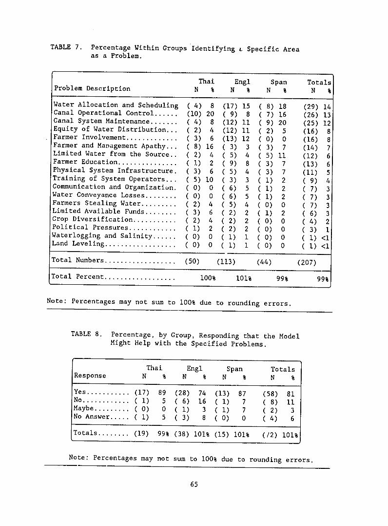
TABLE 7. Percentage Within Groups Identifying ; Specific Area as a Problem.

Problem Description Thai

N % Engl N %

Span N %

Totals N %

Water Allocation and Scheduling Canal Operational Control ......

( 4) 8 (10) 20

(17) ( 9)

15 8

(8) (7)

18 16

(29) 14 (26) 13

Canal System Maintenance ....... Equity of Water Distribution... Farmer Involvement ............. Farmer and Management Apathy Limited Water from the Source.. Farmer Education ............... Physical System Infrastructure. Training of System Operators... Communication and Organization. Water Conveyance Losses ........ Farmers Stealing Water ......... Limited Available Funds ........ Crop Diversification ........... Political Pressures ............ Waterlogging and Salinity ...... Land Leveling ..................

( 4) 8 (12) 11 (9) ( 2) 4 (12) 11 (2) 3) 6 (13) 12 (0)

( 8) 16 (3) 3 (3) (2) 4 (5) 4 (5)

1) 2 (9) 8 (3) (3) 6 (5) 4 (3) ( 5) 10 (3) 3 (1) ( 0) 0 (6) 5 (1) 0) 0 (6) 5 (1) 2) 4 (5) 4 (0) 3) 6 (2) 2 (1) 2) 4 (2) 2 (0) 1) 2 (2) 2 (0)

( 0) 0 (1) 1 (0) (0) 0 (1) 1(0)

20 5 0 7

11 7 7

2 2 2 0 2 0 0 0

0

(25) 12 (16) 8 (16) 8 (14) 7 (12) 6 (13) 6 (11) 5 ( 9) 4 ( 7) 3 ( 7) 3 ( 7) 3 (6) 3 (4) 2 (3) 1 (1) <1 () <1

Total Numbers .................. (50) (113) (44) (207)

Total Percent .................. 100% 101% 99% 99%

Note: Percentages may not sum to 100% due to rounding errors.

TABLE 8. Percentage, by Group, Responding that the Model Might Help with the Specified Problems.

Thai Engl Span Totals Response N % N % N % N %

Yes ........... (17) 89 (28) 74 (13) 87 (58) 81 No ............ (1) 5 (6) 16 (1) 7 (8) 11 Maybe ......... 0) 0 (1) 3 (1) 7 (2) 3 No Answer ..... (1) 5 (3) 8 (0) 0 (4) 6

Totals ........ (19) 99% (38) 101% (15) 101% (/2) 101%

Note: Percentages may not sum to 100% due to rounding errors.

65

Demographic Information

At the end of the survey form the respondents wer- asked to provide demographic information. Some of the respondents did not give any demographic information, and others gave only selected information. Sixty of the seventy two respondents gave their age, and the mean age was 40 years old. The mean respondent ages for each of the three groups are as follows:

Thai .......... 36.1 years English ....... 43.9 years Spanish ....... 32.8 years

The average scores given by the respondents for the first fourteen questions are plotted versus age in Fig. 12 for the sixty respondents who gave their age on the questionnaire. The range of scores Ls from one to five, corresponding to the five possible choices for each of the first fourteen questions. As previously stated, the value of one is the most favorable response toward application and use of the hydraulic model, and five is the least favorable. The dotted line in Fig. 12 is the result of a linear regression on the plotted data points. This figure suggests that the younger the respondent, the more favorible to the application of hydraulic modeling.

0

* Thai LPI& English

M Spanish B-0

4O0

a . Ec

0A

0 R . " ... .............

, oo I...... o0................................. > .... ..

Is @

26 30 35 40 45 50 55

Respondent Age (years)

Figure 12. Average Score Versus Respondent Age for

Questions 1-14.

66

More than 95% of the respondents were male. Education levels ranged from doctorates to technical school graduates (see Table 9).Most respondents also gave their position title, which included ntuni :ous engineering ranks from field engineers to executive engineers,project managers, and others. Project names were given, in addition to the place of residence prior to working at the present location. The prior residence item was included in the demographic part of the surveyin order to assess the potential effect of cultural differences on survey responses. It was thought that local people who work at an irr:igation project may tend to have a better rapport with farmers in some cases, and take a greater personal interest in main system

TABLE 9. Breakdown of Respondent Education Levels.

Education Number of Percent of Level Respondents Total

Ph.D. (2) 2.8 M.S. (17) 23.6 B.S. (34) 47.2 Less Than B.S. ( 7) 9.7 No Response (12) 16.7

Totals (72) 100.0%

operation than non-locals or persons with an urban background.However, the locations listed as prior residence were often vague, and in many cases the respondents simply listed the name of the countrywhich they are from. Therefore, no conclusions were drawn from this particular demographic item.

Analysis of Variance

A one way analysis of variance was performed for each of the fourteen multiple-choice questions in order to identify any trends in the responses for selected parameters. The three independent variables chosen were: (1) respondent group; (2) respondent age; and, (3)respondent education level. The respondent groups were Thai, English,and Spanish. The respondent education levels were categorized as follows: (1) Less than Bachelor of Science; (2) Bachelor of Science;(3) Master of Science; and, (4) Doctor of Philosophy. All of the analyses were done at the 0.05 confidence level. Significance tests were made using the least squares difference (LSD) and the Scheffe criteria. Of these, the LSD is more liberal and the Scheffe is more conservative, meaning that the LSD criteria will indicate "significant"

67

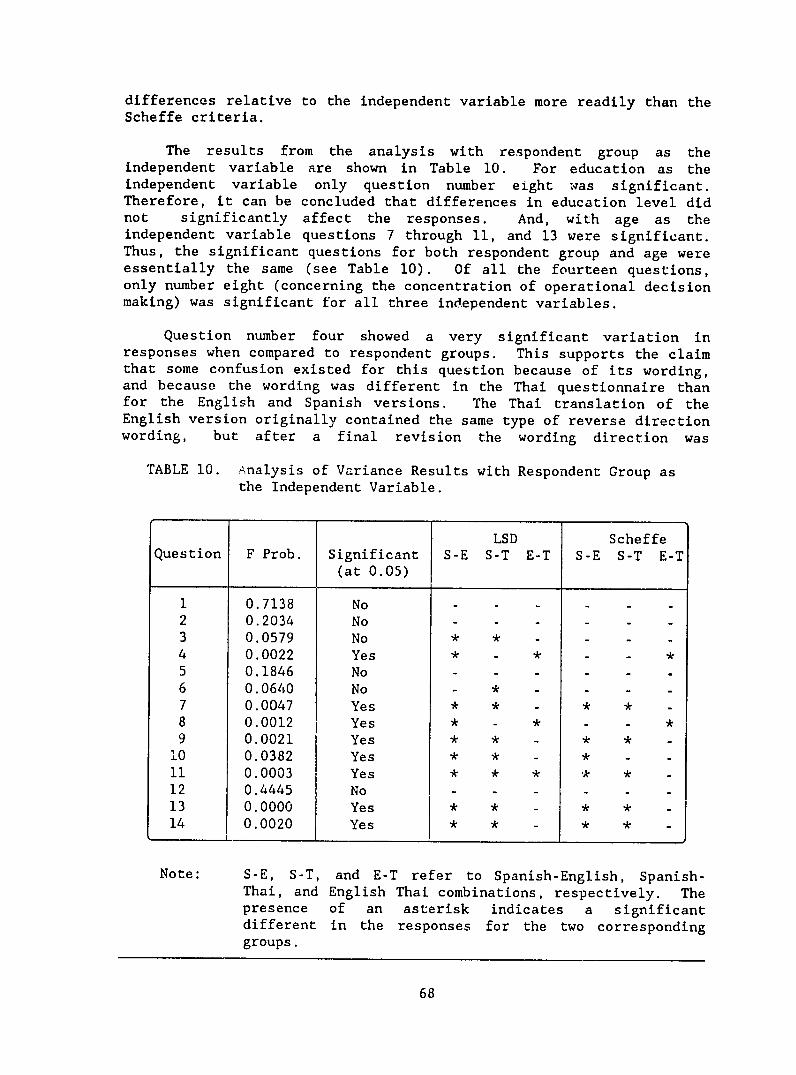
differences relative to the independent variable more readily than the Scheffe criteria.

The results from the analysis with respondent group as the independent variable are shown in Table 10. For education as the independent variable only question number eight was significant. Therefore, it can be concluded that differences in education level did not significantly affect the responses. And, with age as the independent variable questions 7 through 11, and 13 were significant. Thus, the significant questions for both respondent group and age were essentially the same (see Table 10). Of all the fourteen questions, only number eight (concerning the concentration of operational decision making) was significant for all three independent variables.

Question number four showed a very significant variation in responses when compared to respondent groups. This supports the claim that some confusion existed for this question because of its wording, and because the wording was different in the Thai questionnaire than for the English and Spanish versions. The Thai translation of the English version originally contained the same type of reverse direction wording, but after a final revision the wording direction was

TABLE 10. Analysis of Variance Results with Respondent Group as the Independent Variable.

LSD Scheffe

Question F Prob. Significant S-E S-T E-T S-E S-T E-T (at 0.05)

1 0.7138 No . . .. 2 0.2034 No . . .. 3 0.0579 No * * - ­

4 0.0022 Yes * * * 5 0.1846 No - ­6 0.0640 No * - - ­

7 0.0047 Yes * * * * ­

8 0.0012 Yes * * - * 9 0.0021 Yes * * * *

10 0.0382 Yes * * * 11 0.0003 Yes * * * * * 12 0.4445 No - - ­

13 0.0000 Yes * * * * 14 0.0020 Yes * * * *

Note: S-E, S-T, and E-T refer to Spanish-English, Spanish-Thai, and English Thai combinations, respectively. The presence of an asterisk indicates a significant different in the responses for the two corresponding groups.

68

inadvertently changed by a Thai irrigation engineer. This had not been independent variable questions 7 through 11, and 13 were significant. Thus, the significant questions for both respondent group and age were essentially the same (see Table 10). Of all the fourteen questions, only number eight (concerning the concentration of operational decision making) was significant for all three independent variables.

Question number four showed a very significant variation in responses when compared to respondent groups. This supports the claim that some confusion existed for this question because of its wording,and because the wording was different in the Thai questionnaire than for the English and Spanish versions. The Thai translation of the English version originally contained the same type of reverse direction wording, but after a final revision the wording direction was inadvertently changed by a Thai irrigation engineer. This had not been noticed until after the questionnaire was typed and photocopied iiI Thailand. Thus, there was some difference between responses to question number four with the group as an independent variable (this was taken into account for the purposes of coding the responses). Questions 7 through 11, 13 and 14 showed up the most on the analyses of variance as having significant differences in responses for the three independent variables. All of these questions contained the word "farmer", and were related to the perceived relationship between farmers and hydraulic modeling. It was these questions that were more sociologically oriented, whereas the other questions were more technically oriented. This indicates a more consistent response for the more technical questions, and greater response variation for sociological questions. Respondents showed significant differences in their views of how the introduction of hydraulic modeling might affect farmer perceptions and behavior relative to main system operation.

Discussion

The results from the first fourteen questions show the respondent opinions on the utility of the hydraulic model and some of the potential problems associated with its use. From the ranking of the questions (see Table 6) it can be seen that the greatest concern about the model is that it might be abandoned at a particular project if there were problems in applying it to operation, training, or design. This is understandable since hydraulic modeling has mostly been used by hydraulic engineers up to the present time, and not by technicians or water management personnel. Furthermore, hydraulic modeling has not been used extensively and it is still a relatively new method for improving water management in irrigation canals. Apprehension as to its application at irrigation projects is to be expected until it has been demonstrated to be successful in the field. If any one of a number of potential problems were encountered during implementation of hydraulic modeling at a given site the modeling effort could be abandoned in favor of the previous operational, training, or design methods.

69

Many of the respondents also considered that one adverse effect of the model could be to concentrate operational decision-making at the management level, and exclude input from farmers. Exclusion from decision-making could also extend to junior level operations personnel. This may be a valid concern at some projects, although it would not be true for all cases. Application of the model to improving canal operation would not necessarily remove operational decision-making from the farmers, especially when the farmers may not have any voice in the system operation under the existing management structure. In many cases operational information available to the farmers and to junior operations personnel would remain the same under application of hydraulic modeling. That is, the things that they were aware of regarding system operation before modeling was used would not change afterwards. However, it is possible that in some cases the model could be used, in effect, to conceal the basis for specific operational decisions from the farmers by the management. In this way management could conceivably use the model to justify operational decisions which were not actually based on use of the model at all. Nevertheless, farmers would in any case be able to see where the water is going in the field, at least to the extent that they were before applying the model. If water is being delivered inequitably or inefficiently the farmers will know this from field observations, regardless of what they are told about the model.

Another concern about applying the model is that the model would not encourage farmer involvement in the operation of irrigation canals. Again, this could apply to junior operations personnel as well as farmers. This is a logical assumption for many irrigation systems since the use of the model would be restricted to senior project personnel. However, farmer awareness of the existence and use of the model may introduce an added perception of legitimacy on the operation of the system, even though they may not know what a computer model is. If farmers were satisfied that the model was not being misused by the management, then they may agree that the operation of the system is more objective and fair. This in turn could encourage the farmers to accept operational decisions as being just, reducing the tendency for them to interfere with the system operation. In this way the farmers could be involved in the system operation in a positive way, even though they do not actively participate in operational decisions. Another point in favor of the model is that farmers would have few objections to model-generated operational schedules since the model is not used to determine water allocation in the system. The hydraulic model is used in an operational context by reducing system lag times and minimizing water level fluctuations for given water distributions. Thus, water allocation decisions are made external to the hydraulic model, and it is this type of decision which potentially concerns the farmers and their involvement.

Most of the respondents thought that the model could be used to help design and evaluate irrigation canal systems, and that it could make canal operators more aware of farmer's water delivery needs. "Tuning the operators in" to the farmer's perspective relative to water

70

deliveries can be an important training application of the model. This result from the survey indicates the acceptance of the raodel as a potentially useful training tool for both new and experienced canal operators. Simulations of hypothetical water delivery schemes can increase understanding of how the real system will respond, and how maximum control over the flow conditions can be successfully achieved.

The regression line shown in Fig. 12 indicates a definite tendency, in spite of the wide data scattering, for older respondents to view application of the model less favorably. This is not surprising since it is the older persons who tend to be less familiar with computers and their applications, and consequently view computer modeling with greater skepticism. Younger persons tend to be more optimistic about relatively new technologies and methods, partlybecause they are more familiar with the new developments. The results of this survey support such tendencies, although it is seen that a given response may depart significantly from this tendency. For example, a given older person may view the application of hydraulic modeling in a very favorable way, even though in general these persons tend to view its application less favorably than younger persons.

The results from questions fifteen and sixteen of the survey (seeTable 8) are indicative of the importance attached to different problems associated with operation and management of irrigation canals by the respondents. Although the respondents were asked to list the problems in ranked order, it seemed from casual observation that manyof them tended to simply list issues as they occurred to them. This led to the assumption that in general the respondents listed problemsand issues which they considered important, but that were not necessarily in ranked order. Therefore, analysis of the responses to question fifteen considered all of the listed problems on an equal basis.

The category which was most frequently cited was that of water allocation and scheduling. This category includes responses concerning decisions of how best to distribute water and how to schedule deliveries, both within the canal system and to individual fields in command areas. Listed scheduling problems included both spatial and temporal water distribution. The hydraulic model does not address these types of problems directly since they must be essentially resolved before application of the model to operational issues. However, the model can be used as a tool to analyze proposed water delivery schemes without actually imple enting them in the field. For example, the feasibility of routing water in a specified way and in a desired time frame could be assessed through hydraulic simulations of the system. Canal operational control issues was the second most frequently listed type of problem. Of course, the hydraulic model can be used to solve such problems insofar as determining operational schedules for both control structures and turnouts.

The third most frequently listed problem category was canal systemmaintenance. Maintenance issues can also be investigated with the

71

model to determine the effect of different infrastructure conditions on the hydraulic performance of the system. The fourth most frequently listed problem was that of water distribution equity, or lack of equity. Equity problems can be partially resolved through correct operation of the main system, which can be achieved through use of the model. Such problems as "tail-ender", or downstream, water level and flow rate fluctuaticns can be reduced if the system is correctly operated.

Other commonly cited issues were: farmer involvement and education, farmer and management apathy, limited available water to the system, system infrastructure deterioration, inappropriate design, or faulty construction, and training of canal operators. The results from question fifteen of the survey indicate that many of the problems which the respondents consider to be most important in canal operation and management can be reduced or eliminated by using the hydraulic model. The results from question sixteen (see Table 9) show that a majority of the respondents support this claim. Problems such as apathy on the part of project personnel or farmers are somewhat more fundamentally based than canal operation, and they cannot be solved adequately through use of the model alone.

Recommendations

As illustrated in Fig. 12 it is apparent that the older persons involved in the operation and management of irrigation canals will need to be shown more convincingly that the model can be useful for canal operation, design, and operator training. And, in most irrigation projects it is the older persons who a-e responsible for deciding whether or not canal hydraulic modeling 6hould be used. Therefore, acceptance of the model, even on a trial basis, will probably require thorough verification and demonstration, and not merely verbal or written persuasion.

The respondents' concern about concentrating operational decision­making at the management level supports the idea of interdisciplinary involvement in realizing improvements in irrigation system operation and water management. This is accentuated by the fact that virtually all of the respondents were technically trained and oriented. Implementation of the hydraulic model at new irrigation project sites must include, therefore, non-technical considerations so that the opportunities for successful application are maximized. Problems listed by respondents concerning operation and management of irrigation canals also indicate many non-technical, or partially technical, issues. These are issues such as farmer involvement, farmer education apathy, water stealing, and even political pressure. Implementation of the model must be accompanied by clear examples of how the model can assist in solving or alleviating various important problems that are related to canal operation. Such examples can highlight some of the non-technical model benefits that may be less obvious.

72

CHAPTER VII

SUMMARY AND CONCLUSIONS

Model Development

An interactive, menu-driven, hydraulicand

model has been developedtested for the simulation of transient open channel flow inirrigation main systems. The model solves the complete hydrodynamic

equations of continuity and momentum, and the results are displayed intabular and graphical form. The three user-selectable simulation modes are: (1) Manual, (2) Pre-Set, and (3) Scheduling. With the schedulingmode the model computes control structure adjustments in response tochanges in system flow distribution with the objective of maintainingconstant flow levels at the downstream end of each canal reach.

Initial installation and field testing of the model was conductedat the Lam Nam Oon Irrigation Project in Northeast Thailand (see Fig.1) during four trips from June, 1986 to March, 1988. Installationincluded collection and analysis of system configuration andcalibration data. The model was tested using steady-state andtransient flow conditions for both real and hypothetical distribution scenarios.

A series of simulations were performed comparing main systemoperational modes, hydraulic roughness, and seepage loss rates. Theresults of these simulations showed the significance of operationElmode of system response (lag) time, flow level fluctuations,deviations from intended turnout discharges.

and Hydraulic roughness and seepage loss rate variations were shown to have relatively

insignificant effects on system response time and flow level fluctuations when the scheduling mode was used.

Modeling Applications

An operational procedure for applying unsteady hydraulic analysisof branching canal flow to the computation of control structure andturnout setting adjustments has been developed in this model. Thecontrol logic contained in this procedure is implemented through use ofthe model's gate scheduling operational mode. With gate scheduling,rapid system shifting from one steady-state condition to another ispossible, while at the same time maintaining stable flow levels in thecanals. This enables centralized system operation without making anyhardware (infrastructure) changes to the canals or control structures. The modeling results can be field-implemented through manual operation.Thus, with gate scheduling, significant improvements can be made inmain system operations without requiring large expenditures forautomated control structures and related hardware. Water managementimprovements can also be realized when the system is operated in such a

73

way as to distribute water according to intended allocation plans in terms of delivery timing and rate. Furthermore, conveyance inefficiencies in the main system are reduced by maintaining stable flow conditions, even during changes in water allocation.

The operational improvements which are possible through the application of gate scheduling also include more equitable deliveries during times of water shortage, whether due to unavailability at the source, or to canal and turnout capacity limitations. Equity improvements through gate scheduling are better than that which can be obtained from canal operation by -iutomatic float-actuated gates since not only flow levels are controlled during unsteady conditions, but discharges are also known and managed. The results of simulations for the right main canal at Lam Nam Oon have shown that the application to canal operation can eliminate the often-mentioned "tail-ender" problem, in which downstream water users must typically endure most of the undesirable consequences of inadequate main system operation. With gate scheduling, the main system is more responsive to water allocation changes, and the deliveries are more reliable because of stable flow levels during ursteady hydraulic conditions.

As previously stated, implementation of the model's gatescheduling mode in operational applications provides centralized control for branching main systems. During simulations with gate scheduling, the operational strategy in the model includes referencing all control structure adjustments to the head of the system. Consequently, when local flow disturbances occur in the canals, they are treated from a global perspective so that hydraulic transients do not amplify in the downstream direction. Of course, local flow conditions are also taken into account to prevent excessive targetlevel deviations when the distribution of flow in the system is changing. This type of control is preferable to localized control methods which can generate gate adjustments that exacerbate operationalconflicts while attempting to contain local flow level or discharge fluctuations. Centralized control through gate scheduling has also been shown to significantly decrease the system's reaction time to changes in demand since gates do not respond only to local flow conditions. Thus, the advantages of applying gate scheduling results frem the model are that the main system is managed with consideration of all important operational constraints, hydraulic stability is maintained at all times, and system response times are greatly improved.

The model can be effectively used as a training tool for main system operators by enabling interactive simulation of canal flow. In two International Irrigation Center short courses on andoperation management of irrigation districts, the participants were exposed to the model in a training environment. The participants manuallyoperated a given main system with the assignment to control flow levels while routing water .- downstream outlets. They compared their manual operation to gate scheduling results and learned about effective lagtimes and the importance of control structure adjustment magnitude and

74

timing. Through of theuse model, participants in the courses were able to see the consequences of estimated control structure adjustmentson the ability of the system to deliver water -o downstream points in terms of responsiveness and hydraulic control. Canal operators at irrigation project sites also from-an benefit model simulations bylearning how to control the main system under a variety of conditions before experimenting on the real system itself.

The design of main systems can be significantly improved viaapplication of model.the These improvements come from use of themodel as a design tool in which transient hydraulic analysis is appliedto test the response of the system. The constructed system can then bebetter able to meet intended operational conditions since unsteadyhydraulic evaluations have been performed to compliment standard steady-state design criteria. For example, if a proposed design does not allow water allocations to be made within an acceptable time frame, or without excessive flow instability, then changes can be identified to correct the problem. Locations and types of control structures,canal cross sections and slopes, and other parameters can be subject todesign modification as a result of transient hydraulic analysis. Or,proposed cropping patterns may need to be changed orderin to realistically supply water in the required quantities and times.

The model can be used to provide information about the need forcanal maintenance by illustrating the operational effects of different conditions. The effect of weed growth or sediment deposition can beassessed before it becomes a major problem. Canal lining needs can be evaluated in terms of the consequence of seepage losses on main systemoperations and hydraulic roughness. For example, data collection activities at Lam Nam Oon identified large changes in hydraulicroughness over a short time period, and this illustrated the effect ofuncontrolled weed growth on effective flow capacities and lag times.Corresponding simulations showed the antiripated effects of further weed growth and provided a rational basis on which canal cleaning could be scheduled. The effect of weed growth had previously not been quantified or recognized.

The management of main system operation can be improved throughhydraulic modeling by removing the problems caused by estimated control structure adjustments. Different operators may be responsible fordifferent canal branches in large systems, and operational adjustments on control structures and turnouts may be of a conflicting naturebetween the branches. An operator in an upstream branch may over­correct for a decrease in water levels by closing control structures too much, thereby causing transients which a downstream operator must attempt to manage. Or, a downstream branch may be incorrectlyoperated, causing upstream conditions to change even though the flow was stable already. Thus, the operator in the upstream branch must make corrections, and the effect of correctionsthese will then benoticed downstream as well. However, with gate scheduling the systemis operated from a centralized perspective and conflicts of this nature are eliminated.

75

Main system management personnel can use the model to verify approved water allocations by comparing field data with simulation results. If water is actually being diverted in excess of the intended delivery rate at a turnout, the consequencz will be apparent from the modeling results. Thus, modeling is not only used to determine appropriate main system operation, but to check for problems in water distribution when intended deliveries are not met.

Lam Nam Oon Project

The conclusion from the Lam Nam Oon Irrigation Project is that the model can be successfully applied to improve main system operation through use of the scheduling and pre-set modes. Modeling results from simulations of the right main canal showed that the system can be made more responsive, with reduced flow level and turnout discharge fluctuations when the model is used to determine control structure and turnout adjustment schedules. Consequently, turnout deliveries are more timely and reliable, and operational guesswork during flow distribution changes is eliminated. Turnout deliveries can better match actual crop water needs, and limitations on agricultural production due to non-optimal operation of the main system can be minimized.

When changes in flow distribution occur in the main system, the model can be applied to "shifting" water through the system with greater responsiveness than can normally be expected. When a demand comes on-line at a downstream point in the system, a corresponding increase in inflow from the dam (ur river) is made simultaneously. Water is then immediately transferred through each canal reach by a coordinated op.eration of control structures, although downstream flow levels in each reach temporarily drop below the target levels. The system subsequently responds by recovering from the target level deviations in order to maintain hydraulic stability, and a new steady­state condition is quickly achieved. Throughout the duration of these transient flow conditions all control structure and turnout settings are known from the modeling results, and the canal operators do not need to estimate structure adjustments.

Gate scheduling through hydraulic modeling can also be successfully applied to improve canal operation for an opposite situation. When a system is at a steady-state condition and a sudden heavy and unexpected rainfall occurs, causing the system-wide demand for water to abruptly decrease, the model can then be applied to coordinate operation of the system by decreasing system inflow, calculating appropriate control structure adjustments, and using available reach storage capacity to temporarily hold excess water. Consequently, the canal infrastructure is not threatened by overtopping of the lining or berms, and the spillage of water due to inadequate operation during the routing of hydraulic transients can be eliminated.

These, and other, operational applications of hydraulic modeling are made feasible with interactive and user-friendly software, and

76

computational speed which exceeds real-time by about fifty times. The ability to generate and store steady-state flow conditions in the modelallows rapid analysis of subsequent unsteady conditions without spending any time to update the system status.

Survey Questionnaire

A survey questionnaire was prepared to assess the perceived impactof main system hydraulic modeling at irrigation projects. The questionnaire was translated to Thai. and Spanish from the originalversion in English. It was distributed in Thailand and in two short courses of the International Irrigation 'Tenter in Logan, Utah. The results from th. analysis of the questionnaire responses helped to clarify some of the most important sociological and institutional issues as related 7' application of the model. Some trends in the responses were statistically identified termsin of respondent groupand age. The importance of various vnon-technical components to engineering solutions for water managemm-n.t improvement in irrigation main systems were recognized and noted.

It is recognized that some of the responses may have been biased in favor of the model's application due to cultural reasons. It would be fair to say that many oi the respondents consider open criticism to be socially unacceptable in all but the most extreme situations. And, a few of the respondents were directly involved with the modelingeffort and, therefore, had some reason to view the model's application more favorably than they might otherwise if they had not been involved. Neverthele7ss, it is the author's opinion that, with only a few exceptions, the respondents completed the final version of the surveyin a truthful and candid way. One or two of these exceptions included respondents who submitted completed survey forms with extreme answers to all questions. The reverse direction wording on question number four identified the response set in these cases, in which respondentsdid not really read all of the questions, but only agreed or disagreed with everything unilaterally.

77

CHAPTER VIII

RECOMMENDATIONS

Software Maintenance

Large computer programs are difficult to debug completely. This model contains more than twelve thousand lines of source code and the internal interactions are complex. Many changes and additions have been made to the model over the three-year development period with the intent of improving its utility as a planning, operations, and trainingtool. Most of the changes and additions were not initially foreseen. Consequently, large sections of the source code were periodically re­written to integrate new features and organize the program structure appropriately. At this point in time even small additions or modifications to modelthe must be carefully integrated into the software so that all possible interactions with the existing code are taken into account. And, it is probable that further modifications will need to be made as part of an on-going software maintenance program.

Sustainability of this hydraulic modeling effort for irrigationmain systems, and the avoidance of repeating the same development work,will be possible if other researchers can understand and modify the source code themselves. Even if this particular model is to be discarded, an understanding of its internal workings can be usefullyapplied to the development of a new model with improved capabilities.In order for other researchers to adequately understand this model,without expending undue time and effort, it is essential that a programming manual be prepared which describes the procedures, details,and logic involved in the software. Such a manual would explain all important programming interactions, and define all of the variables used in the source code. The users' manual (Merkley, 1987) only deals with application of the model, and does not address the issue of programming structure.

Software Additions

The physical configuration and operating conditions of main systems around the world can differ substantially from one irrigationproject to another. The success of a hydraulic model for the simulation of these systems depends in part on its generality, or flexibility to accommodate the site-specific conditions of a particularmain system. The greater the number of systems that can be correctlysimulated without modifying the source code, the greater the chance that the model will be successfully applied. This kind of generalityhas been emphasized throughout the development of the model, yetcontinued expansion to include new features can be a limitless task.

79

Some suggestions for software additions which would enhance the models' generality are described below.

Computed Inflows

The system inflow is treated as an external boundary condition bythe model, meaning that it must be specified by the model user as a function of time. Thus, the user enters an inflow hydrograph based on five-minute time intervals for the duration of each simulation. In order to facilitate application as a main system operational tool, it would be desirable to compute the inflow as a function of time, rather than requiring that it be specified by the user. In this way, the inflow would be calculated on a step-by-step basis with the objectiveof matching changing demand discharges at downstream points.

The calculation of inflows could be integrated into the proceduresfor performing gate scheduling of control structures. In order to do this, a downstream condition must then be externally specified since the solution would otherwise be under-defined (in terms of mathematical simulation). For example, the discharge past the control structure in the last reach of a branch could be specified instead of the systeminflow. In this case, the discharge from the reach could be set to zero in order to eliminate one potential source of conveyance inefficiency.

Multiple Inflows

Currently, the model will only allow water to enter the main system at a single location which is the furthest upstream point in the system. In some main systems inflows at intermediate locations alongthe canal represent important contributions to the availability of water downstream. Thus, the ability to simulate multiple inflows would extend the models' applicability to a greater number of main systems.This new feacure could be incorporated into the existing capability for simulating bulk lateral outflow through turnouts from intermediate locations along the canals.

Reverse Flow

In real canals, backflow can sometimes occur through control structures and turnouts that operate under submerged flow conditions. This can happen is a result of downstream water levels temporarilybeing higher than upstream levels. The model currently does not allow this to occur; if the water surface head differential across a structure is negative, the model will assume zero flow though the structure until this differential becomes positive again. There is every expectation that this phenomena can be successfully modeled, but

80

the procedural details for doing so without causing numerical instabilities have yet to be worked out.

Recession

The model can simulate canal filling by computing advance profilesuntil water arrives at the end of a reach. This feature was adaptedfrom surface irrigation models (Walker and Skogerboe, 1987) which simulate water advance in borders, basins, and furrows. During the draining of canals an analogous event can occur in which water recedes after flow depths decrease to zero. Recession can occur at both the upstream nnd downstream ends of canal reaches. The ability to simulate recession already exists in some surface irrigation models, and it could be adapted for use in a main system hydraulic model. This feature would be particularly useful in main systems that are frequently filled and emptied.

Canals at some irrigation projects may be only partially emptied,then filled again to full supply levels. In such cases the flow rates in some reaches may decrease to zero, with a triangular "wedge" of water remaining at the downstream end of the reach. This is a special case which involves both recession and subsequent filling, althoughsome time may elapse before re-filling begins. During re-filling water will advance downstream until it meets the triangular wedge of pondedwater which has remained after recession. The numerical procedures for simulating the interaction between moving and ponded water have not yetbeen developed.

Structure Types

Additional turnout and control structure types could be included in the model to enhance its generality. New structure types could include radial gates, automatic float-actuated gates, and cross­sectional size reductions (without any structure at all). Currently,control structures are limited to circular and rectangular sluice gates, rectangular sharp-crested weirs, circular and rectangularculverts and siphons, and constant-speed centrifugal pumps. Turnouts currently include circular and rectangular orifices, rectangular sharp­crested weirs, and wasteway weirs. The simplifying assumptions and restrictions in the approximating stage-discharge relationships could be partially replaced by equations which more adequately define the true flow characteristics of a real structure. These kinds of improvements would allow for weirs which do not really behave as sharp­crested weirs, and expand the simulated operational range of sluice gates.

81

Bra ch Linkages

The model is dimensioned for a maximum of four canal branches,with nine reaches in each branch. Reaches within a branch are alwaysconsidered to be linked together in serial. This is inadequate for main systems that have more than four branches, but less that thirty­six reaches. Thus, systems with multiple canal andbifurcations relatively few reaches in series cannot be handled simultaneously bythe model ­ they must be divided into separate systems. A more generaland less restrictive approach would be to re-define branches and canal linkages in the model such that individual reaches could be linked in any way, rather than only having branch linkages.

Additional "esearch

During testing of the model over its three-year developmentperiod, several hundred simulations were performed for a wide varietyof main system configurations and operating conditions. One interesting problem that has been noticed is that canals with identical cross-sections and reach lengths tend exhibit aggravated hydraulicto instability when compared to less homogeneous systems. When reach lengths and cross-sections are the same for a number of canal reaches connected in series, hydraulic transients sometimes propagate quicklyand resist dampening. In extreme cases, apparent harmonic oscillation of flow levels and discharges occurred during simulations. The control of such recalcitrant hydraulic behavior is worthy of further study.

Another follow-up research topic is an in-depth study of canal system response times for different operational strategies and physicalconfigurations. The results of the present showstudy that it is possible to increase the responsiveness of main systems through the application of gate scheduling. However, main systems with relatively steep slopes and long reaches would be more difficult to manage since systenm shifting through simultaneous control structure adjustmentswould'cause augmented flow level fluctuations. The differences in flow distribution between scheduling both control structure and turnout adjustments, and only control structure adjustments, is a related area of concern. The results from a follow-up study on this topic should also include turnout discharge deviations, and canal conveyanceefficiencies, in terms of volumes of water relative to turnout de-ands and system inflows.

Lam Nam Oon Project

Data collection activities should be continued at Lam Nam Oon for the right and left main canals, and their laterals. These activities include measurement of configuration data and seepage losses,calculation of hydraulic roughnesses, and determination of dischargecoefficients. Much of this information has already been collected and

82

analyzed, but some of the data are of questionable accuracy and it needs to be re-checked in che field.

The remaining data collection and field measurement activities should be conducted on a regular basis so that they may be completedwithin two or three irrigation seasons. The data obtained thus far have proved to be quite valuable as information upon which maintenance and operational decisions can be partially based. This has been the case even though the hydraulic model has not yet been fully applied.After satisfactory completion of data collection the model can be used to further assist in operational and maintenance decisions.

83

REFERENCES

Balogun, 0. S., Hubbard, M., and DeVries, J. J. 1988. Automatic control of canal flow using linear quadratic regulator theory. J. Hydr. Eng., ASCE, Vol. 114, No. 1, January. pp. 75-101.

Basset, D. L., and D. W. Fitzsimmons. 1976. Simulating overland flow in border irrigation. Transactions of the ASAE 19(4):674­680.

Burt, C. M. 1983. Regulation of sloping canals by automatic downstream control. Unpublished Ph.D. dissertation, College of Engineering, Utah State University, Logan, UT.

Burton, M. A., and Franks, T. R. 1983. Simulation and modellingfor training in irrigation management. Cambridge African Monograph3: Irrigation in Tropical Africa. Cambridge Univ., London, England.

Chevereau, G., and S. Schwartz-Benezeth. 1987. Bival system for downstream control. ASCE Proceedings. Portland, Oregon, July.

Chow, Ven Te. 1959. Open Channel Flow. McGraw-Hill Book Company. New York, NY.

Corriga, G., S. Sanna, and G. Usai. 980. Frequency response and dynamic behaviour of canal networks with self-leveling gates.Appl. Math. Modelling, Vol. 4. April. pp. 125-129.

Elliott, R. L., W. R. Walker, and G. V. Skogerboe. 1982. Zero­inertia modeling of furrow irrigation advance. J. Irrig. Drain. Div., ASCE, 108(IR3):179-195.

Frederiksen, H. D. 1969. Design of California aqueduct. J. Irrig. Drain. Div., ASCE, 95(IR2):307-328.

Gichuki, F. N., W. R. Walker, and G. P. Merkley. 1987. Modelingbranching irrigation canal networks. ASCE Proceedings, Portland, Oregon, July. pp. 724-731.

Gichuki, F. N. 1988. Development of a branching canal network hydraulic model. Water Management Synthesis II Project Report#72. Dept. Ag. and Irrig. Eng., Utah State University, Logan, UT.

Goussard, j. I.; .. Neyrtec aatomatic equipment for irrigation canals. ASCE Proceedings. Portland, Oregon, July.

Gray, W. G. 1980. Do finite element models simulate surface flow?. Proc. Third International Conf. on Finite Elements in Water Res. School of Eng., Univ. of Mississippi, University, Mississippi.

85

Hart, W. E., D. L. Bassett, and T. Strelkoff. 1978. Surface irrigation hydraulics - kinematics. J. Irrig. Drain. Div., ASCE, 94(IR4):419-440.

Johnson, L. F. 1986. Water resource management decision support systems. J. Water Resources Planning and Management, ASCE, Vol. 112, No. 3, pp. 308-325. July.

Katopodes, N. D. and T. Strelkoff. 1977. Hydrodynamics of border irrigation - complete model. Proc. J. Irrig. Drain. Div., ASCE, 103(IR-3):309-324.

Khan, A. U., Murray-Rust, D. H., and Bhuiyan, S.I. 1987. What developing countries need from today's engineers. Agricultural Engineering. ASAE. January/February. pp. 14-16.

Lusk, M. W. 1986. The social dimension of irrigation and on-farm water management. Report of the International Irrigation CenLez, Dept. of Ag. and Irrig. Eng., Utah State University, Logan, UT.

Merkley, G. P. 1987. Users manual for the pascal version of the USU main system hydraulic model. Water Management Synthesis II Project Report #75. Dept. Ag. and Irrig. Eng., Utah State University, Logan, UT.

Merkley, G. P., W. R. Walker, and F. N. Gichuki. 1987. Hydraulic modeling applications in canal main systems. Abstract in ASCE Proceedings, Portland, Oregon, July. p.76 1 .

Merkley, G. P. 1988. USU irrigation main system hydraulic model: replication of modeling capability. Water Management Synthesis II Project Report. Dept. Ag. and Irrig. Eng., Utah State University, Logan, UT.

Power, J. W. 1986. Sharing irrigation know-how with developing countries. Agricultural Engineering. ASAE. September/October. pp. 15-18.

Rao, P. S. and Sundar, A. 1986. Managing main system water distribution. Management Brief. International Irrigation Management Institute, Digana Village via Kandy, Sri Lanka.

Replogle, J. A. 1983. Flexible delivery systems that encouragebetter irrigation. Paper presented at the Winter Meeting of ASAE, December 13-16, Chicago, Illinois.

Reynolds, R. R., and W. R. Madsen. 1967. Automation in California's state water project. J. Pipeline Div., ASCE, 93(PL3):15-23.

86

Skogerboe, G. V., Shafique, M. S., and Gandarillas, C. 1987. Field calibration of irrigation structures for discharge measurement. Report of the International Irrigation Center, Dept. of Ag. and Irrig. Eng., Utah State University, Logan, UT.

Souza, F. 1981. Non-linear hydrodynamic model of furrow irrigation. Unpublished Ph.D. dissertation, Department of Land,Air and Water Resources, University of California, Davis, CA.

Strelkoff, T. and N. D. Katopodes. 1977. End depth under zero­inertia conditions. J. Hydr. Div., ASCE, 103(HY-7):699-711.Uphoff, N., Meinzen-Dick, R., and St. Julien, N. 1985. Getting the process right: farmer organization and participation in irrigation water management. Water Management Synthesis II Project Report. Cornell University, Ithaca, NY.

United States Bureau of Reclamation. 1963. Lining for irrigationcanals. USBR Report. Eng. and Research Center, Denver, CO.

United States Bureau of Reclamation. 1973. Navajo indian irrigation project. USBR Report #7610-00-921-0090. Eng. and Research Center, Denver, CO.

Walker, R. E. 1987. Long crested weirs. ASCE Proceedings. Portland, Oregon, July.

Walker, W. R., and A. S. Fa'iherys. 1983. Kinematic-wave furrow irrigation model. J. Irrig. L>.ain. Div., ASCE, 109(IR4):377-392.

Walker, W. R., and G. V. Skogerboe. 1983. Proposed activities for developing an integrated strategy for improving irrigatedagriculture in northeast Thailand. Water Management Synthesis II Project Report. Dept. Ag. and Irrig. Eng., Utah State University, Logan, UT.

Walker, W. R., and C. '. Skogerboe. 1986. The theory and practiceof surface irrigation. Prentice-Hall, Inc., Englewood Cliffs, New Jersey.

87

APPENDICES

89

Appendix A. Lam Nam Oon Right Main Canal Data

91

TABLE A-I. Configuration Data for the Right Main Canal of the Lam Nam Oon Irrigation Project in Thailand.

Brnch Rch Lngth Base Side Depth Slope Rough Seep OSL Q_Des No, No. (m) (m) (m/m) (m) (m/lOOm) (n) (mm/day) (%) (cms)

1 1 1400 5.0 1.50 2.85 0.0155 0.020 750 82 14.4 1 2 3340 5.0 1.48 2.85 0.0125 0.020 750 82 14.4 1 3 5326 4.0 1.51 2.85 0.0152 0.023 750 84 12.9 1 4 4141 4.0 1.29 2.85 0.0129 0.032 750 84 12.9 1 5 4498 4.0 1.50 2.65 0.0125 0.019 750 85 11.5 1 6 3957 4.0 1.50 2.60 0.0128 0.049 750 85 11.0

2 1 3469 4.0 1.50 2.45 0.0125 0.020 750 84 9.6 2 2 5446 4.0 1.50 2.40 0.0125 0.020 750 83 9.0 2 3 2175 3.5 1.50 2.15 0.0125 0.020 750 84 6.8 2 4 1845 3.0 1.50 2.15 0.0125 0.020 750 84 6.1 2 5 3088 3.0 1.50 2.05 0.0125 0.020 750 83 5.4 2 6 565 2.0 1.50 1.70 0.0125 0.020 750 85 3.0

TABLE A-2. Control Structure Data for the Right Main Canal of the Lam Nam Oon Irrigation Project in Thailand.

Brnch Rch Dist Reach No. Width Disch Delta "b" DropNo. No. (m) Name (m) Coeff (m) (m)

1 1 1+400 Check 1 2 2.30 0.40 +0.317 Check 4 1.751 2 4+740 3 0.68 -0.020 +0.030

1 3 10+066 Check 10 3 1.75 0.82 +0.176-0.030 1 4 14+20 Check 14 3 1.75 0.76 -0.045 -0.037 1 5 18+705 Check 18 2 2.00 0.78 -0.042 +0.219 1 6 22+662 Check 22 2 2.00 0.68 +0.000 -0.030

2 1 26+131 Check 26 2 2.00 +0.0000.61 +0.290 2 2 31+577 Check 31 2 1.75 0.72 +0.000 +0.000 2 3 33+752 Check 33 3 1.50 +0.0000.45 +0.270 2 4 35+597 Check 35 2 1.75 0.81 +0.000 +0.370 2 5 38+685 Check 38 1 1.75 0.55 +0.000 -0.140 2 6 39+250 Check 39 1 1.00 0.67 +0.000 -0.550

93

TABLE A-3. Turnout Structure Data for the Right Main Canal of the Lam Nam Oon Irrigation Project in Thailand.

Brnch Rch Tnout Name Cd Width Height Posn Distn DS DS No. No, No. (m) (m) (m) (m) Depth Slope

1 1 1 Wv 1 1.83 3.00 2.40 400 .... 1 1 2 1 0.55 0.60 0.60 1.51 500 0.00 0.00 1 1 3 2 0.55 0.60 0.60 1.60 545 0.00 0.00 1 1 4 3 0.59 0.60 1.25 1.57 1310 0.00 0.00

1 2 1 4 0.61 0.60 0.60 1.81 470 0.00 0.00 1 2 2 R-lL 0.61 2.50 1.25 0.49 770 0.49 0.32 1 2 3 5 0.61 0.60 0.60 1.56 1790 0.00 0.00 1 2 4 6 0.61 0.60 0.60 1.74 2410 0.00 0.00 1 2 5 R-2L 0.60 0.80 0.80 1.13 2795 1.04 0.10 1 2 6 7 0.61 0.60 0.60 1.73 2852 0.00 0.00 1 2 7 WW 2 1.83 9.65 2.65 3040 1 2 8 8 0.61 0.60 0.60 1.60 3270 0.00 0.00

1 3 1 9 0.61 0.60 0.60 1.84 610 0.00 0.00 1 3 2 R-3L 0.55 0.60 0.60 1.12 1020 1.03 0.10 1 3 3 10-11 0.61 1.20 0.60 1.50 1835 0.00 0.00 1 3 4 12-13 0.61 1.20 0.60 1.33 3245 0.00 0.00 1 3 5 14 0.57 0.60 0.60 1.89 3860 0.00 0.00 1 3 6 R-4L 0.67 2.00 1.00 0.79 4082 0.3 0.56 1 3 7 WW 3 1.83 9.62 ---- 2.69 4660 1 3 8 15 0.57 0.60 0.60 0.07 4960 0.00 0.00 1 3 9 16 0.57 0.60 0.60 1.38 5285 0.00 0.00

1 4 1 17 0.57 0.60 0.60 0.06 1D34 0.00 0.00 1 4 2 18 0.57 0.60 0.60 -0.02 1484 0.00 0.00 1 4 3 R-6L 0.71 2.50 1.25 0.58 1869 0.55 0.08 1 4 4 19 0.57 0.60 0.60 0.02 2934 0.00 0.00 1 4 5 20 0.57 0.60 0.60 0.00 3534 0.00 0.00 1 4 6 WW 4 1.83 9.66 ---- 2.60 3774

1 5 1 21 0.57 0.60 0.60 1.67 735 0.00 0.00 1 5 2 22 0.61 0.60 0.60 1.62 2593 0.00 0.00 1 5 3 23 0.57 0.60 0.60 1.68 3193 0.00 0.00 1 5 4 24 0.61 0.60 0.60 0.00 3743 0.00 0.00 1 5 5 WW 5 1.83 8.62 ---- 2.44 4393

1 6 1 R-7L 0.64 2.00 1.00 0.64 190 0.07 0.72 1 6 2 25 0.61 0.60 0.60 1.16 645 0.00 0.00 1 6 3 R-8L 0.48 1.00 1.00 0.63 790 0.09 0.22 1 6 4 26 0.61 0.60 0.60 1.30 1515 0.00 0.00 1 6 5 27 0.57 0.60 0.60 1.72 2495 0.00 0.00 1 6 6 R-9L 0.54 2.00 1.00 0.87 2810 0.11 0.88 1 6 7 28 0.57 0.60 0.60 1.54 3895 0.00 0.00

94

TABLE A-3. (cont) Turnout Structure Data for the Right Main Canal of the Lam Nam Oon Irrigation Project in Thailand.

Brnch Rch Tnout Name Cd Width Height Posn Distn DS DS No. No. No. (m) (m) .Jm) (m) DeDth Slone

2 1 1 WW 6 1.83 10.44 ---- 2.05 538 .... 2 1 2 29 0.61 0.60 0.60 1.32 688 0.00 0.00 2 1 3 R-10L 0.61 0.60 0.60 1.01 854 0.50 0.10 2 1 4 30 0.61 0.60 0.50 1,39 888 0.00 0.00 2 1 5 31 0.61 0.60 0.60 1.39 1338 0.00 0.00 2 1 6 R-1lL 0.39 2.00 1.00 0.48 18.4 -0.12 0.46 2 1 7 32 0.61 0.60 0.60 1.41 2688 0.00 0.00 2 1 8 WW 7 1.83 9.20 ---- 2.22 3318 ---- .....

2 2 1 R-12L 0.61 0.90 0.90 0.09 271 0.01 1.41 2 2 2 34 0.61 0.60 0.6C 1.35 419 0.00 0.00 2 2 3 35-36 0.61 1.20 0.60 1.36 1119 0.00 0.00 2 2 4 37-38 0.61 1.20 0.60 1.33 0.002465 0.00 2 2 5 WW 8 1.83 9.26 ---- 2.19 ?469 .... .... 2 2 6 39-40 0.61 1.20 0.60 1.36 3609 0.00 0.00 2 2 7 41 0.61 0.60 0.60 0.02 4064 0.00 0.00 2 2 8 42 0.48 0.60 0.60 0.09 0.005409 0.00

2 3 1 43 0.48 0.60 0.60 0.99 243 0.00 0.00 2 3 2 R-13L 0.37 0.90 0.90 -0.30 285 -0.30 0.10 2 3 3 44 0.61 0.60 0.60 1.10 823 0.00 0.00 2 3 4 45 0.61 0.60 0.60 1.17 1363 .00 0.00 2 3 5 WW 9 1.83 6.34 ---- 1.97 1743 ....

2 4 1 45 0.61 0.60 0.60 1.12 278 0.00 0.00 2 4 2 47 0.61 0.60 0.60 1.09 748 0.00 0.00 2 4 3 48 0.61 0.60 0.60 1.22 1298 0.00 0.00

2 5 1 49 0.61 0.60 0.60 1.65 63 0.00 0.00 2 5 2 R-14L 0.58 0.60 0.60 0.92 0.20135 0.10 2 5 3 50-51 0.55 1.20 0.60 1.02 403 0.00 0.00 2 5 4 R-15L 0.69 1.00 1.00 0.16 526 0.00 0.10 2 5 5 52-53 0.55 1.20 0.60 0.10 1228 0.00 0.00 2 5 6 WW 10 1.83 5.03 .--- 1.83 1743 .... .... 2 5 7 54-55 0.48 1.20 0.60 0.88 2153 0.00 0.00 2 5 8 R-16L 0.63 2.50 1.25 0.35 2503 0.29 0.43 2 5 9 56.57 0.53 1.20 0.60 0.93 2706 0.00 0.00

2 6 1 58 0.48 0.60 0.60 0.69 165 0.00 0.00 2 6 2 R-17L 0.61 2.40 1.20 0.54 222 0.28 0.15 2 6 3 59 0.48 0.60 0.60 0.70 515 0.00 0.00

Notes: Turnout names beginning with "R-" are lateral turnouts. Turnout names beginning with "WW" are wasteway weirs, and all others are farm turnouts. Lateral R-5L does not exist in the real system although it was included in the original canal design.

95

TABLE A-4. Weekly Turnout Demands During a Four-Week Period in 1987 of the Dry Season at the Lam Nam Oon IrrigatioU Project.

Discharge Rate (m3/s)

Turnout Week 9 Week i0 Week 11 Week 12

R-1L 0.52 0.52 0.52 0.30 R-2L 0.00 0.07 0.00 0.00 R-4L 0.37 0.36 0.35 0.00 R-6L 0.82 0.82 0.82 0.82 R-7L 0.18 0.15 0.14 0.14 R-SL 0.05 0.05 0.05 0.05 R-9L 0.10 0.10 0.08 0.08 R-10L 0.00 0.03 0.00 0.02 R-11L 0.25 0.25 0.25 0.10 R-12L 0.10 0.10 0.10 0.05 R-13L 0.08 0.08 0.08 0.08 R-14L 0.02 0.02 0.02 0.02 R-15L 0.10 0.10 0.10 0.10 R-16L 0.80 0.80 0.80 0.80 R-17L 0.75 0.75 0.80 0.80

Total 4.14 4.20 4.11 3.36

Inflow 5.30 5.20 5.07 4.50

96

Appendix B, Hydraulic Model Survey Questionnaires

97

FIELD SURVEY QUESTIONS FOR AN ASSESSMENT OF THEPERCEPTION OF THE IMPACT OF HYDRAULIC MODELING ON THEINSTITUTIONAL ASPECTS OF IRRIGATION SYSTEM OPERATION AND MANAGEMENT

As part of the Water Management Synthesis II Project with USAIDand on behalf of the Agricultural and Irrigation Engineering Depart­ment of Utah State University, I am installing a computer model which can be used for hydraulic simulation of irrigation canal networks.This computer model is intended for use in operation, maintenance,design, and operator training issues regarding irrigation canal management. Since we expect to introduce this model in other countries we are very interested inthe opinions of people involved in the management and operation of irrigation projects inThailand. We are very interested to learn more about both the technical and the sociological issues associated with the application of hydraulicmodeling in irrigation projects.

I have prepared a series of statements which I would like you torespond to. "our reaction to these statements will be of great valueto us in the WMS II Project, and to me for use inmy Ph.D. disserta­tion which ison the subject of hydraulic modeling applications inirrigation canals. Please be assured that your responses will be held in complete confidentiality.

Gary P. Merkley June 1987

(1) Hydraulic modeling will be used on a regular basis to improve the

operation of irrigation canals in this area.

Definitely Probably Maybe Probably Not Definitely Not (2) Hydraulic modeling will actually be used to evaluate the operational potentials of irrigation canals inthis area.

Definitely Probably Maybe Probably Not Definitely Not

(3) Hydraulic modeling will be used to help analyze the maintenance needs of irrigation canals inthis area.

Definitely Probably Maybe Probably Not Definitely Not (4) Hydraulic modeling will not be used for teaching irrigation canal operation in this area?

Definitely Probably Maybe Probably Not Definitely Not

99

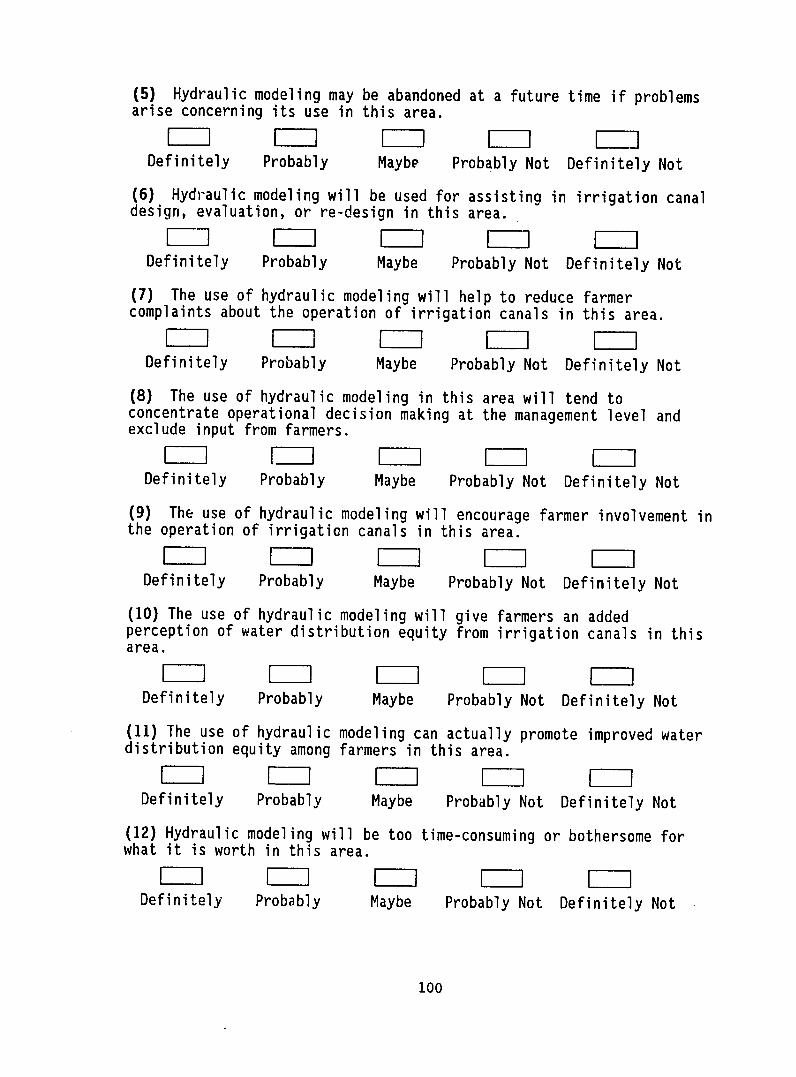
(5) Hydraulic modeling may be abandoned at a future time if problems

arise concerning its use in this area.

LI--l LI--Z LIZ L-I ] Definitely Probably Maybe Probably Not Definitely Not

(6) Hydraulic modeling will be used for assisting in irrigation canal design, evaluation, or re-design in this area.

LI]L L LIII LII-Definitely Probably Maybe Probably Not Definitely Not

(7) The use of hydraulic modeling will help to reduce farmer complaints about the operation of irrigation canals in this area.

[--- [2L1] LI-I LI---Definitely Probably Maybe Probably Not Definitely Not

(8) The use of hydraulic modeling in this area will tend to concentrate operational decision making at the management level and exclude input from farmers.

Definitely Probably Maybe Probably Not Definitely Not (9) The use of hydraulic modeling will encourage farmer involvement in the operation of irrigation canals in this area.

Definitely Probably Maybe Probably Not Definitely Not

(10) The use of hydraulic modeling will give farmers an added perception of water distribution equity from irrigation canals in this area.

Definitely Probably Maybe Probably Not Definitely Not

(11) The use of hydraulic modeling can actually promote improved water distribution equity among farmers in this area.

Definitely Probably Maybe Probably Not Definitely Not (12) Hydraulic modeling will be too time-consuming or bothersome for what it is worth in this area.

Definitely Probably Maybe Probably Not Definitely Not

100

(13) The use of hydraulic modeling will tend to reduce the difference between farmer requests and actual water deliveries from irrigationcanals in this area.

L_r L- - - L- -Definitely Probably Maybe Probably Not Definitely Not

(14) The use of hydraulic modeling will cause irrigation canal operators in this area to be more aware of the farmers' water deliveryneeds.

Definitely Probably Probably NotMaybe Definitely Not

(15) What are the three most important problems that need to beaddressed concerning the operation and management of irrigation canals in this area? Please prioritize these beginning with the most important one.

1.

2.

3.

(16) Do you believe that the use of hydraulic modeling will help in anyof these three areas? Ifyes, then how? Ifno, why not?

P12ase write any final comments or observations that you may haveconcerning the use of hydraulic modeling in this area. Use the back ofthe page if additional space is needed. Thank you very much for takingthe time to answer these questions.

Respondent Background Information:

Position Project Education

Place of Residence Pricr to Moving to This Project

Age Male Female Today's Date

101

FIELD SURVEY QUESTIONS FOR AN ASSESSMENT OF THE PERCEPTION OF THE IMPACT OF HYDRAULIC MODELING ON THE

INSTITUTIONAL ASPECTS OF IRRIGATION SYSTEM OPERATION AND MANAGEMENT

As part of the Water Management Synthesis II Project with USAIDand the Agricultural and Irrigation Engineering Department of UtahState University, a computer model which can be used for hydraulicsimulation of irrigation canal networks has been developed. Thiscomputer model is intended for use-in operation, maintenance, design,and operator training issues regarding irrigation canal management. We are very interested in the opinions of people involved in the management and operation of irrigation projects in different countries.We would like to learn more about both the technical and thesociological issues associated with the application of hydraulicmodeling in irrigation projects.

I have prepared a series of statements which I would like you torespond to. Your reaction to these statements will be of great value to us in the WMS II Project, and to me for use in my Ph.D. disserta­tion which is on the subject of hydraulic modeling applications in irrigation canals.

Gary P. Merkley July 1987

(1) Hydraulic modeling could be used ina regular basis to improve the operation of irrigation canals inyour country.

Definitely Probably Maybe Probably Not Definitely Not (2) Hydraulic modeling could actually be used to evaluate the operational potentials of irrigation canals inyour country.

Definitely Probably Probably NotMaybe Definitely Not (3) Hydraulic modeling could be used to help analyze the maintenance needs of irrigation canals inyour country.

Definitely Probably Maybe Probably Not Definitely Not

(4) Hydraulic modeling could not be used for teaching irrigation canal operation inyour country.F--I[]ZI 1111] LI[l Definitely Probably Maybe Probably Not Definitely Not

103

(5) Hydraulic modeling may be abandoned at a future time if problems

arise concerning its use in your country.

-I LI-Z F---] LI- L---I Definitely Probably Maybe Probably Not Definitely Not

(6) Hydraulic modeling could be used for assisting in irrigation canal design, evaluation, or re-design inyour country.

Definitely Probably Maybe Probably Not Definitely Not

(7) The use of hydraulic modeling could help to reduce farmer complaints about the operation of irrigation canals inyour country.

LIZ LIZ ---- ---Definitely Probably Maybe Probably Not Definitely Not

(8) The use of hydraulic modeling inyour country could tend to concentrate operational decision making at the management level and exclude input from farmers.

Definitely Probably Maybe Probably Not Definitely Not

(9) The use of hydraulic modeling could encourage farmer involvement

in the operation of irrigation canals inyour country.

Definitely Probably Maybe Probably Not Definitely Not

(10) The use of hydraulic modeling could give farmers an added perception of water distribution equity from irrigation canals inyour country.

Definitely Probably Maybe Probably Not Definitely Not

(11) The use of hydraulic modeling could actually promote improved

water distribution equity among farmers inyour country.

Definitely Probably Maybe Probably Not Definitely Not

(12) Hydraulic modeling might be too time-consuming or bothersome for what it is worth inyour country.

LIZ LZ I Definitely Probably Maybe Probably Not Definitely Not

104

(13) The use of hydraulic modeling could tend to reduce the differencebetween farmer requests and actual water deliveries from irrigationcanals inyour country.

Definitely Probably Maybe Probably Not Definitely Not

(14) The use of hydraulic modeling could cause irrigation canal operators inyour country to be more aware of the farmers' water delivery needs. 1

Definitely Probably Maybe Probably Not Definitely Not

(15) What are the three most important problems that need to beaddressed concerning the operation and management of irrigation canalsinyour country? Please prioritize these beginning with the most important one.

1.

2.

3.

(16) Do you believe that the use of hydraulic modeling can help in anyof these three areas? Ifyes, then how? Ifno, why not?

Please write any final comments or observations that you may haveconcerning the use of hydraulic modeling. Use the back of the page ifadditional space is needed. Thank you very much for taking the time to answer these questions.

Respondent Background Information:

Position Project Education

Place of Residence Prior to Moving to This Project_

Age Male Female Today's Date

105

ESTUDIO SOBRE LA PERCEPCION DEL IMPACTO DEL USO DE LA SIMULACION COMPUTARIZADA EN LA PARTE

INSTITUCIONAL DE LA OPERACION Y MANEJO DE DISTRITOS DE RIEGO

Como parte del proyecto Water Management Synthesis II (Sintesisdel Manejo de Agua II)de USAID y el Departamento de IngenieriaAgricola y Riegos de USU, un modelo hidrAulico computarizado ha sidodesarrollado con el fin de simular el flujo no-estable del agua encanales de riego. Se espera que el uso de este modelo pueda cubrir laoperaci6n, mantenimiento y diseflo, asi como la capacitaci6n de los operadores en distritos de riego.

Con el fin de darle credulidad al modelo estamos interesados en laopini6n de las personas involucradas en el manejo y operaci6n dedistritos de riego en diferentes paises acerca del modelo, asi como los efectos tdcnicos y sociales de su aplicaci6n. Por lo anterior estamossolicitando a ustedes de la manera mds atenta tengan a bien responder alas siguientes aseveraciones. Las opioniones que Ustedes viertan sersnde gran utilidad debido a que su analisis forma parte de mi disertaci6n para el grado de doctorado, la cual trata sobre el uso de este modelo.

Gary P. Merkley Julio 1987

(1) El modelo hidrdulico puede ser usado cotidianamente en elmejoramiento de la operaci6n de los canales de riego en su pais.

Si Probablemente Quizds Probablemente No No (2) El modelo hidrdulico puede ser usado en la evaluaci6n del potencial operativo de los sistemas de riego en su pais.

Si Probablemente Quizds Probablemente No No

(3) Este modelo podria ser usado en el analisis de las necesidades de mantenimiento del sistema de conducci6n en su pais.

Si Probablemente Quizds Probablemente No No

(4) El modelo no puede ser usado en la ensefianza sobre la operaci6n de los canales de riego en su pais.

Si Probablemente QuizAs Probablemente No No

107

(5) El modelo puede ser abandonado si surgen problemas en su uso.LIZ [III [, ]LI l Si Probablemente Quizas Probablemente No No

(6) Este modelo podria ser usado en la asistencia sobre evaluaci6n, disefio, y redisehio del sistema de conducci6n.

Si Probablemente Quizas Probablemente No No

(7) Este modelo podria ayudar en reducir las quejas del usuario acerca de la operaci6n del sistema en su pals.

--- El L--F-I Si Probablemente Quizds Probablemente No No

(8) El uso del modelo podria tender a concentrar el poder de decisi6n a niveles administrativos, excluyendo la opini6n de los usuarios en su pafs.

Si Probablemente Quizds Probablemente No No (9) El uso del modelo podria motivar a los usuarios a que formen parte en la operaci6n de los canales de riego en su pals.

Si Probablemente Quizds Probablemente No No

(10) El modelo podria dar a los usuarios una mejor opini6n sobre la igualdad de distribuci6n del agua de riego en su pais.

Si Probablemente Quiz~s Probablemente No No

(11) El uso del modelo realmente puede mejorar una equitativadistribuci6n del agua de riego entre los usuarios en su pals.

Si Probablemente Quizds Probablemente No No (12) El uso del modelo podria consumir mucho tiempo y como consecuencia

no valdria la pena su uso en su pais.ZII] -lI L-I Si Probablemente Quizds Probablemente No No

108

(13) El uso del modelo tenderia a reducir la diferencia entre la demanda y la entrega del agua de riego en su pais.

Si Probablemente Quizds Probablemente No No (14) El modelo podria provocar un mejor entendimiento del operador del sistema de conducci6n respecto a las necesidades del usuario.

Si Probablemente Quizds Probablemente No No

(15) jCu~les son los tres problemas m~s importantes en la operaci6n ymanejo del sistema de conducci6n? Por favor mencionelos en orden decreciente de uno a tres.

1.

2.

3.

(16) jCree Usted que el uso del modelo pueda ayudar en la soluci6n de estos tres problemas? Si es que si, jc6mo puede? Si es que no, jPorqud No?

ITiene Usted algunos comentarios u observaciones acerca de estecuestionario? Si el espacio no es suficiente puede usar la parte de atrds de la hoja. Muchas gracias por su colaboraci6n.

Informaci6n del Encuestado:

Posici6n

Nivel Educativo

Edad Sexo

Proyecto

Lugar del

Fecha

cual procede

109

~uU-j~j~utu ~i'LtJ~uiajHydraulic Model vitnnn

WMS II va USAID Ifl Agricultural and Irrigations Engineering Department

wi Utah State University 'iU in,<tLu Hydraulic Model A101't'

WM If

flh1DnflLu WM II min 'I~nIWM

Uu~~t Laum~uugmjg-u k~u~

17 F 8- f

v]F1 LUCLi 0Li ;U Li'n U1uil

dik9 ,O VRtut 131.1u-3 tol

OUIIJU'U1A;LUl

5. ueinltunu&19MA; vwt4I"i~iljllLi'g

6. tj-3=d;uNsLLaz&DnuuiAvt I;

F1 R FI ID-11% fl-IR LbUltlUl;LIIU;-)IJOVR LgU;-3U Al; AIIAVU

7. mil;lOuniud Lntm-3n-3 Av-jffunu;iuni-s0g-3,v

D

toul; v1Q ktlljl'I; tbulljUl;

a. niil;l 0 umu z wrigot Oulo;i un-rsqm wnl*m o,3J-iviiiiii-S n -Mj411e 41.4 t Au-3 L"'lulu

L;6,ueo tntm-in-s

.0

L;U;-3Aqf4 t;61 ;-3 9 SIR LOUI; 13-1v Altilulol L9UllJIU

9. ni-3141thun-i:jqim:ji-inn-szq'ul;Lnim-sn-3 ovin

LITU;Itiogn A; v D-M toul 019 AIJ14

io.

F] Fl F-1 pliu;-)Voqfq t;u;-Iu Vlq LbUl; 0-tv Aullf"WIN Aulliluol;

ii. niil;lui unim u"o-m -vm i vl;n-rj n-3::4q ut'll-i ni4-i-j Lmm-jn-3;-m Ku Ou Ili avljq wvju

ALAU -36"qm A -)fj a-IQ olul U-IR Allilmb" ULUIIA41s,

12.

E 1-1 1-1

L;U;lu4qiR L;64-10 CErIQ Aul @-lQ Oulolul; LIJU10141A

13.

El

L;U;-)U,"VFI t"', u ka u inq Lnl.!I; niq AU10141; L&101131

14.

u;,A mwj tntwim

F P F] thkau"'VA thkm Inq LlluU Div W ljlul LLISJ12,I;

112

15. &POft 3 iiri~u~~~ni~

2.

IUH~I UAAsu;u u4inq Lanuiffuldiuriiu Hydraulic Model if ;-)hmno

113

WATER MANAGEMENT SYNTHESIS PROJECT REPORTS

WMS 1 irrigation Projects Document Review

Executive Summary Appendix A: The Indian Subcontinent Appendix B: East Asia Appendix C: Near East and Africa Appendix D: Central and South America

WMS 2 Nepal/USAID: Irrigation Development Options and Investment Strategies for the 1980's

WMS 3 Bangladesh/USAID: Irrigation Development Options and Investment Strategies for the 1980's

WMS 4 Pakistan/USAID: Irrigation Development Options and Investment Strategies for the 1980's

WMS E Thailand/USAID: Irrigation Development Options and Investment Strategies for the 1980's

WMS 6 India/USAID: Irrigation Development Options and Investment Strat-gies for the 1980's

WMS 7 General Asian Overview

WMS 8 Command Area Development Authorities for Improved Water Management

WMS 9 Seneqal/USAID: Project Review for Bakel Small Irrigated Perimeters Project No. 685-0208

WMS 10 Sri Lanka/USAID: Evaluatiun Review of the Water Management Project No. 383-0057

WMS 11 Sri Lanka/USAID: Irrigation Develooment Options and Investment Strategies for the 1980's

WMS 12 Ecuador/USAID: Irrigation Sector Review

WMS 13 Maintenance Plan for the Lam Nam Oon Irrigation System in Northeast Thailand

WMS 14 Peru/USAID: Irrigation Development Options and Investment Strategies for the 1980's

WMS 15 Diagnostic Analysis of Five Deep Tubewell Irrigation Systems in Joydebpur, Bangladesh

WMS 16 System H of the Mahaweli Development Project, Sri Lanka: 1980 Diagnostic Analysis

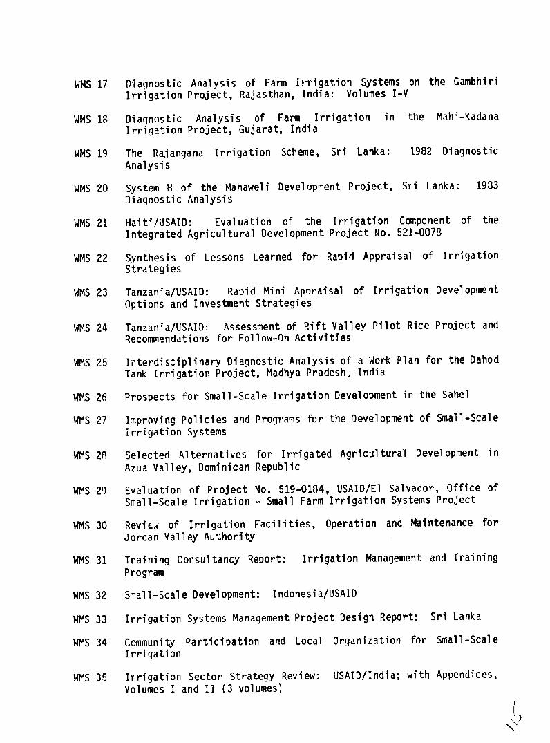
WMS 17 Diagnostic Analysis of Farm Irrigation Systems on the Gambhiri Irrigation Project, Rajasthan, India: Volumes I-V

WMS 18 Diagnostic Analysis of Farm Irrigation in the Mahi-Kadana Irrigation Project, Gujarat, India

WMS 19 The Rajangana Irrigation Scheme, Sri Lanka: 1982 Diagnostic Analysis

WMS 20 System H of the Mahaweli Development Project, Sri Lanka: 1983 Diagnostic Analysis

WMS 21 Haiti/USAID: Evaluation of the Irrigation Component of the Integrated Agricultural Development Project No. 521-0078

WMS 22 Synthesis of Lessons Learned for Rapid Appraisal of Irrigation Strategies

WMS 23 Tanzania/USAID: Rapid Mini Appraisal of Irrigation Development Options and Investment Strategies

WMS 24 Tanzania/USAID: Assessment of Rift Valley Pilot Rice Project and Recommendations for Follow-On Activities

WMS 25 Interdisciplinary Diagnostic Analysis of a Work Plan for the Dahod Tank Irrigation Project, Madhya Pradesh, India

WMS 26 Prospects for Small-Scale Irrigation Development in the Sahel

WMS 27 Improving Policies and Programs for the Development of Small-Scale irricjation Systems

WMS 28 Selected Alternatives for Irrigated Agricultural Development in Azua Valley, Dominican Republic

WMS 29 Evaluation of Project No. 519-0184, USAID/El Salvador, Office of Small-Scale Irrigation - Small Farm Irrigation Systems Project

WMS 30 ReviLA of Irrigation Facilities, Operation and Maintenance for Jordan Valley Authority

WMS 31 Training Consultancy Report: Irrigation Management and Training

Program

WMS 32 Small-Scale Development: Indonesia/USAID

Sri LankaWMS 33 Irrigation Systems Management Project Design Report:

WMS 34 Community Participation and Local Organization for Small-Scale Irrigation

WMS 35 Irrigation Sector Strategy Review: USAID/India; with Appendices, Volumes I and Ii (3 volumes)

WMS 36 Irrigation Sector Assessment: USAID/Haiti

WMS 37 African Irrigation Overview: Summary; Main Report; An Annotated Bibliography (3 volumes)

WMS 38 Diagnostic Analysis of Sirsia Irrigation System, Nepal

WMS 39 Small-Scale Irrigation: Design Issues and Government Assisted Systems

WMS 40 Watering the Shamba: Current Public and Private Sector Activities for Small-Scale Irrigation Development

WMS 41 Strategies for Irrigation Development: Chad/USAID

WMS 42 Strategies for Irrigation Development: Egypt/USAID

WMS 43 Rapid Appraisal of Nepal Irrigation Systems

WMS 44 Direction, Inducement, and Schemes: Investment Strategies for Small-Scale Irrigation Systems

WMS 45 Post 1987 Strategy for Irrigation: Pakistan/USAID

WMS 46 Irrigation Rehab: User's Manual

WMS 47 Relay Adapter Card: User's Manual

WMS 48 Small.-Scale and Smallholder Irrigation in Zimbabwe: Analysis of Opportunities for Improvement

WMS 49 Design Guidance for Shebelli Water Management Project (USAID Project No. 649-0129) Somalia/USAID

WMS 50 Farmer Irriqation Participation Project in Lam Chamuak, Thailand: Initiation Report

WMS 51 Pre-Feasibility Study of Irrigation Development in Mauritania: Mauri tani a/USAID

WMS 52 Command Water Management - Punjab Pre-Rehabilitation Diagnostic Analysis of the Niazbeg Subproject

WMS 53 Pre-Rehabilitation Diagnostic Study of Sehra Irrigation System, Sind, Pakistan

WMS 54 Framework for the Management Plan: Niazbeg Subproject Area

WMS 55 Framework for the Management Plan: Sehra Subproject Area

WMS 56 Review of Jordan Valley Authority Irrigation Facilities

WMS 57 Diaqnostic Analysis of Parakrama Samudra Scheme, Sri Lanka: 1985 Yala Discipline Report

WMS 58 Diagnostic Analysis Discipline Report

of Giritale Scheme, Sri Lanka: 1985 Yala

WMS 59 Diagnostic Analysis Discipline Report

of Minneriya Scheme, Sri Lanka: 1986 Yala

WMS 60 Diaqnostic Analysis Discipline Report

of Kaudlilla Scheme, Sri Lanka: 1986 Yala

WMS 61 Diagnostic Aalysis District, Sri Lanka:

of Four Irrigation Schemes Interdisciplinary Analysis

in Polonnaruwa

WMS 62 Workshops for Developing Policy Irrigation and Management Training.

and Strategy USAID/India

for Nationwide

WMS 63 Research on Irrigation in Africa

WMS 64 Irrigation Rehab: Africa Version

WMS 65 Revised Management Plan for the Warsak Lift Canal, Command Management Project, Northwest Frontier Province, Pakistan

Water

WMS 66 Small-Scale Irrigation--A Foundation for Rural Growth in Zimbabwe

WMS 67 Variations in Irrigation Management Intensity: Farmer-Managed Hill Irrigation Systems in Nepal

WMS 68 Experience Guatemala:

with Small-Scale Sprinkler System An Evaluation of Program Benefits

Development in

WMS 69 Linking Main and Farm Irriqation Systems (5 volumes)

in Order to Control Water

WMS 70 Integrating Strategies Management

for Improving Irrigation System Design and

WMS 71 The USU Unit Command Area Model

WMS 72 Development of a Branching Canal Network Hydraulic Model

WMS 73 User's Manual for Hydraulic Model

the FORTRAN Version of the USU Main System

WMS 74 Hydraulic Modeling Applications in Main System Management

WMS 75 User's Mdnual for Hydraulic Model

the Pascal Version of the USU Main System

WMS 76 Formulation and Evaluation of the USU Main System Allocation Model

WMS 77 Irrigated Land Use ind Irrigation Distribution Schemes in the Poloniaruwa District of Sri Lanka

Systems for Four

WMS 78 Classification of Gravity Irrigation Systems and their Operation

WMS 79 Development and Management of Small Marais

WMS 80 Baskets of Stones: Government Assista ,ce and Development of Local Irrigation in a District of Northern Sumatra

WMS 81 Implementing the Irrigation Maintenance and Operations (M & 0) Learning Process Regionally or Nationally

WMS 82 Handbook of Improved Irrigation Project Operations Practices for the Kingdom of Thailand

WMS 83 Handbook of Improved Irrigation Project Maintenance Practices for the Kingdom of Thailand

WMS 84 USU Irrigation Main System Hydraulic Model: Replication of Modeling Capability in Other Countries

WMS 85 Development of the Centre International de l'Irrigation

WMS 86 Forum on the Performance of Irrigated Agriculture in Africa: Papers and Proceedings

WMS 87 Niger Irrigation Scheme Case Studies (English & French)

WMS 88 Irrigation Management for Development

WMS 89 Bureaucratic and Farmer Participation in Irrigation Development

WMS 90 Irrigation System Management: An Interdisciplinary Synthesis of Water Management Studies

WMS 91 Assessment Report: Maharashtra Irrigation Program. USAID/India

WMS 92 Irrigation System Operation Intensity and Relative Water Supply: The Asian Case

WMS 93 Methodologies for Interdisciplinary Diagnosis of Irrigation Systems

WMS 94 Management-Focused Improvement of Irrigated Agriculture

WMS 95 Diagnostic Analysis for Improving the Management of Irrigation Systems