Gautham P. Das ENVIRONMENTAL ENGINEERING COLLECTION Francis J. Hopcroft, Collection Editor Hydraulic Engineering Fundamental Concepts

Welcome message from author
This document is posted to help you gain knowledge. Please leave a comment to let me know what you think about it! Share it to your friends and learn new things together.
Transcript

HYD
RAU
LIC EN
GIN
EERING
DA
S
EBOOKS FOR THE ENGINEERING LIBRARYCreate your own Customized Content Bundle — the more books you buy, the higher your discount!
THE CONTENT• Manufacturing
Engineering• Mechanical
& Chemical Engineering
• Materials Science & Engineering
• Civil & Environmental Engineering
• Advanced Energy Technologies
THE TERMS• Perpetual access for
a one time fee• No subscriptions or
access fees• Unlimited
concurrent usage• Downloadable PDFs• Free MARC records
For further information, a free trial, or to order, contact: [email protected]
Hydraulic EngineeringFundamental Concepts
Gautham P. Das
Hydraulic Engineering: Fundamental Concepts includes hydraulic
processes with corresponding systems and devices. The hydraulic
processes includes the fundamentals of fl uid mechanics and pres-
surized pipe fl ow systems. This book illustrates the use of appropri-
ate pipeline networks along with various devices like pumps, valves
and turbines. The knowledge of these processes and devices is ex-
tended to design, analysis and implementation.
Dr. Gautham P. Das is an associate professor of civil and environ-
mental engineering at Wentworth Institute of Technology in Boston,
Massachusetts. Prior to starting his teaching career, Dr. Das worked
for environmental consulting fi rms in North Carolina and Boston.
His expertise lies in water resources, hydraulic engineering and
environmental remediation. He is active in the Water Environment
Federation, the New England Water Environment Association and
the American Society of Civil Engineers. He has authored numer-
ous technical papers on various civil and environmental engineering
subjects that have been published in peer-reviewed journals and
presented at technical conferences. http://gauthampdas.us/
Gautham P. Das
ENVIRONMENTAL ENGINEERINGCOLLECTIONFrancis J. Hopcroft, Collection Editor
Hydraulic EngineeringFundamental Concepts

Hydraulic Engineering


Hydraulic Engineering Fundamental Concepts
Gautham P. Das

Hydraulic Engineering: Fundamental Concepts
Copyright © Momentum Press®, LLC, 2016
All rights reserved. No part of this publication may be reproduced, stored in a retrieval system, or transmitted in any form or by any means—electronic, mechanical, photocopy, recording, or any other except for brief quotations, not to exceed 250 words, without the prior permission of the publisher.
First published in 2016 by Momentum Press, LLC 222 East 46th Street, New York, NY 10017 www.momentumpress.net
ISBN-13: 978-1-60650-490-1 (print) ISBN-13: 978-1-60650-491-8 (e-book)
Collection ISSN: 2375-3625 (print) Collection ISSN: 2375-3633 (electronic)
Momentum Press Environmental Engineering Collection
DOI: 10.5643/9781606504918
Cover and interior design by S4Carlisle Publishing Services Private Ltd., Chennai, India
10 9 8 7 6 5 4 3 2 1
Printed in the United States of America.

Dedication
To my son whose strength and wisdom is infinite.


Abstract
Hydraulic Engineering: Fundamental Concepts includes hydraulic processes with corresponding systems and devices. The hydraulic processes include the fundamentals of fluid mechanics and pressurized pipe flow systems. This book illustrates the use of appropriate pipeline networks, along with various devices like pumps, valves, and turbines. The knowledge of these processes and devices is extended to design, analysis, and implementation.
Keywords
Continuity Equation, Bernoulli’s Equation, General Energy Equation, Series and Parallel Pipeline Systems, Pumps.


Contents
Preface. ................................................................................................. xi Chapter 1 Fundamental Concepts ..................................................... 1 Chapter 2 General Energy Equation ................................................ 19 Chapter 3 Types of Flow and Loss Due to Friction ......................... 33 Chapter 4 Minor Losses .................................................................. 47 Chapter 5 Series and Parallel Pipeline Systems................................. 67 Chapter 6 Pumps and Turbines....................................................... 91 Appendix A: Properties of Water .........................................................121 Appendix B: Properties of Common Liquids .........................................123 Appendix C: Dimensions of Steel Pipe .................................................125 Appendix D: Dimensions of Type K Copper Tubing .............................129 Appendix E: Conversion Factors ..........................................................131 Index .................................................................................................137


Preface The objective of this book is to present the various applications of fluid mechanics in the form of hydraulic engineering systems. Primary em-phasis is on fluid properties, flow systems, pipe networks, and pump selection. Its main purpose is to augment lecture courses and standard textbooks on fluid mechanics and hydraulic engineering by illustrating a wide array of exercise problems with solutions. This book is directed to anyone in an engineering field with the ability to apply the principles of hydraulic engineering and fluid mechanics.
The units used in this textbook are both in the metric and in English units. This will enable the student get a better understanding of practi-cal applications in the field. The reader of this textbook should have a basic understanding of algebra and calculus.

CHAPTER 1
Fundamental Concepts All matter encountered on an everyday basis exists in one of three forms: solid, liquid, or gas. Generally, these forms are distinguished by the bonds between adjacent molecules (or atoms) that compose them. Thus, the molecules that make up a solid are relatively close together and are held in place by the electrostatic bonds between the molecules. There-fore, solids tend to keep their shape, even when acted on by an external force.
By contrast, gas molecules are so far apart that the bonds are too weak to keep them in place. A gas is very compressible and always takes the shape of its container. If the container of a gas is removed, the mole-cules would expand indefinitely.
Between the extremes of solid and gas lies the liquid form of matter. In a liquid, molecules are bonded with enough strength to prevent in-definite expansion but without enough strength to be held in place. Liquids conform to the shape of their container except for the top, which forms a horizontal surface free of confining pressure except for atmospheric pressure. Liquids tend to be incompressible, and water, despite minute compressibility, is assumed to be incompressible for most hydraulic problems.
In addition to water, various oils and even molten metals are exam-ples of liquids and share the basic characteristics of liquids.
1.1 Force and Mass
An understanding of fluid properties requires a careful distinction be-tween mass and weight. The following definitions apply:
Mass is the property of a body of fluid that is a measure of its inertia or resistance to a change in motion. It is also a measure of the quantity of fluid.

2 HYDRAULIC ENGINEERING
The symbol m (for mass) is used in this book. Weight is the amount that a body of fluid weighs, that is, the force
with which the fluid is attracted toward Earth by gravitation. The symbol w (for weight) is used in this book. An equivalent unit for force is kg·m/s2, as indicated above. This is
derived from the relationship between force and mass
* F m a= (1.1)�
where a is the acceleration expressed in units of m/s2. Therefore, the derived unit for force is
2kg·m/s N F ma= = = (1.2)
Thus, a force of 1.0 N would give a mass of 1.0 kg an acceleration of 1.0 m/s2. This means that either N or kg·m/s2 may be used as the unit for force. In fact, some calculations in this book require the ability to use both or to convert from one to the other. Similarly, besides using the kg as the standard unit of mass, the equivalent unit N·s2/m may be used. This can be derived again from F = ma.
2
2
N N sm m
s
Fm
a⋅= = = (1.3)�
1.2 Surface Tension and Capillarity
All liquids have surface tension, which is manifested differently in differ-ent liquids. Surface tension results from a different molecular bonding condition at the free surface compared to bonds within the liquid. In water, surface tension results in properties called cohesion and adhesion. Cohesion enables water to resist a slight tensile stress; adhesion enables it to adhere to another body.
Capillarity is a property of liquids that results from surface tension in which the liquid rises up or is depressed down a thin tube. If adhe-sion predominates over cohesion in a liquid, as in water, the liquid will wet the surface of a tube and rise up. If cohesion predominates over ad-hesion in a liquid, as in mercury, the liquid does not wet the tube and is depressed down (Figure 1.1).

FUNDAMENTAL CONCEPTS 3
Figure 1.1 Examples of adhesion and cohesion of water and mercury
in a glass test tube
1.3 Density and Specific Weight
Density is defined as mass per unit volume and is denoted by the expression
mV
ρ = (1.4)
where � (rho) = density (kg/m3, slugs/ft3) m = mass (slugs, kg) V = volume (ft3, m3). Density varies with water as shown in Table 1.1. The slug is a unit of mass associated with Imperial units and U.S.
customary units. It is a mass that accelerates by 1 ft/s2 when a force of one pound-force (lbF) is exerted on it.
⋅= ↔⋅ =
2
2
slug ftlb s1 slug 1 1 lb 1
ft sF
F (1.5)
In general, density can be changed by changing either the pressure or the temperature. Increasing the pressure always increases the density of a material. Increasing the temperature generally decreases the density, but there are notable exceptions to this generalization. For example, the den-sity of water increases between its melting point (0 °C) and 4 °C; similar behavior is observed in silicon at low temperatures.

4 HYDRAULIC ENGINEERING
Table 1.1 Density of water at various temperatures
Temperature Density Specific WeightoF/°C slugs/ft3 g/cm3 lb/ft3 kg/l
32/0 1.94 0.99987 62.416 0.999808
39.2/4.0 1.94 1 62.424 1
40/4.4 1.94 0.99999 62.423 0.999921
50/10 1.94 0.99975 62.408 0.999681
60/15.6 1.94 0.99907 62.366 0.999007
70/21 1.94 0.99802 62.3 0.99795
80/26.7 1.93 0.99669 62.217 0.996621
90/32.2 1.92 0.9951 62.118 0.995035
100/37.8 1.92 0.99318 61.998 0.993112
120/48.9 1.94 0.9887 61.719 0.988644
140/60 1.91 0.98338 61.386 0.983309
160/71.1 1.91 0.97729 61.006 0.977223
180/82.2 1.88 0.97056 60.586 0.970495
200/93.3 1.88 0.96333 60.135 0.96327
212/100 1.88 0.95865 59.843 0.958593
The specific weight (also known as the unit weight) is the weight
per unit volume of a material. The symbol of specific weight is �.
wV
γ = (1.6)�
where � = specific weight of the material (weight per unit volume, typically
lb/ft3, N/m3 units) w = weight (lb, kg) V = volume (ft3, m3) Alternatively, specific weight can be defined by the expression
gγ ρ= (1.7)
where � = density of the material (mass per unit volume, typically kg/m3)

FUNDAMENTAL CONCEPTS 5
g = acceleration due to gravity (rate of change of velocity, given in m/s2, and on Earth usually given as 32.2 ft/s2 or 9.81 m/s2)
Since specific weight is function of density and density is dependent on temperature, the specific weight will vary with temperature as shown in Tables 1.2 and 1.3.
Table 1.2 Specific weight of water at various temperatures in °C
Temperature (°C) Specific Weight (kN/m3)0 9.805 5 9.807 10 9.804 15 9.798 20 9.789 25 9.777 30 9.765 40 9.731 50 9.69 60 9.642 70 9.589 80 9.53 90 9.467
100 9.399
Table 1.3 Specific Weight of Water at Varying Temperature in °F
Temperature (°F) Specific Weight (lb/ft3)32 62.4240 62.4350 62.4160 62.37 70 62.3 80 62.2290 62.11
100 62110 61.86120 61.71 130 61.55 140 61.38150 61.2160 61170 60.8180 60.58 190 60.36 200 60.12212 59.83

6 HYDRAULIC ENGINEERING
Quite often the specific weight of a substance must be found when its density is known and vice versa. The conversion from one to the other can be made using the following equation:
* gγ ρ= (1.8)
where g is the acceleration due to gravity. This equation can be justified by referring to the definitions of den-
sity and specific gravity and by using the equation relating mass to weight,
w mg= (1.9)
The definition of specific weight is
wV
γ = (1.10)
Multiplying both the numerator and the denominator of this equa-tion by g, yields
wgVg
γ = (1.11)
But w
mg
= (1.12)
Therefore
mgV
γ = (1.13)
Because
mV
ρ = (1.14)
gγ ρ= (1.15)
1.4 Specific Gravity
When the term specific gravity is used in this book, the reference fluid is pure water at 4 °C. At this temperature, water has its greatest density. Then, specific gravity can be defined in either of two ways:

FUNDAMENTAL CONCEPTS 7
Specific gravity is the ratio of the density of a substance to the density of water at 4 °C.
Specific gravity is the ratio of the specific weight of a substance to the specific weight of water at 4 °C.
These definitions for specific gravity (s.g.) can be shown mathemati-cally as
s s
w @ 4 C w @ 4 C
s.g. γ ρ
γ ρ° °
= = (1.16)
where the subscript s refers to the substance whose specific gravity is being determined and the subscript w refers to water. The properties of water at 4 °C are constant, having the following values:
ρ ° = 3w @4 C 1,000 kg/m ρ ° = 3
w @4 C 1.94 slugs/ft
γ ° = 3w @ 4 C 9.81 kN/m γ ° = 3
w @ 4 C 62.4 lb/ft
1.5 Pressure
Pressure (denoted as p or P) is the ratio of force to the area over which that force is distributed.
Pressure is force per unit area applied in a direction perpendicular to the surface of an object. Gage pressure is the pressure relative to the local atmospheric or ambient pressure. Pressure is measured in any unit of force divided by any unit of area. The SI unit of pressure is the newton per square meter (N/m2), which is called the Pascal (Pa). Pounds per square inch (psi) is the traditional unit of pressure in U.S. customary units.
Mathematically:
d d
F FP or p
A A= = (1.17)
where P is the pressure F is the normal force A is the area of the surface on contact
8 HYDRAULIC ENGINEERING
2 2
kgN1 Pa 1 1 m m
= = (1.18)
1 psi 6.8947 kPa=
1.6 Viscosity
Viscosity is a property arising from friction between neighboring parti-cles in a fluid that are moving at different velocities. When the fluid is forced through a tube, the particles which comprise the fluid generally move faster near the axis of the tube and more slowly near its walls: therefore some stress (such as a pressure difference between the two ends of the tube), is needed to overcome the friction between particle layers and keep the fluid moving. For the same velocity pattern, the stress re-quired is proportional to the viscosity.
Viscosity is sometimes confused with density, but it is very different. While density refers to the amount of mass per unit volume, viscosity refers to the ability of fluid molecules to flow past each other. Thus, a very dense fluid could have a low viscosity or vice versa.
The properties of viscosity and density are well illustrated by the ex-ample of oil and water. Most oils are less dense than water and therefore float on the water surface. Yet, despite its lack of density, oil is more viscous than water. This property of viscosity is called absolute viscosity. It is designated by the Greek letter mu (μ) and has the units lb·s/ft2 (kg·s/m2). Because it has been found that in many hydraulic problems, density is a factor, another form of viscosity, called kinematic viscosity, has been defined as absolute viscosity divided by density. It is usually denoted by the Greek letter nu (ν). It has the units ft2/s or m2/s.
μνρ
= (1.19)�
1.7 Flow Rate
Flow rate or rate of flow is the quantity of fluid passing through any section of pipeline or open channel per unit time. �

FUNDAMENTAL CONCEPTS 9
It can be expressed in terms of Volume flow rate Mass flow rate Weight flow rate
1.7.1 Volume Flow Rate
The volumetric flow rate (also known as volume flow rate, rate of fluid flow, or volume velocity) is the volume of fluid which passes per unit of time; usually represented by the symbol Q. The SI unit is m3/s (cubic meters per second). In U.S. customary units and British Imperial units, volumetric flow rate is often expressed as ft3/s (cubic feet per second) or gallons per minute.
Volume flow rate is defined by the limit
0
dlimdt
V VQ
t tΔ →
Δ= =Δ
(1.20)
i.e., the flow of volume of fluid V through a surface per unit time t Since this is the time derivative of volume, a scalar quantity, the vol-
umetric flow rate is also a scalar quantity. The change in volume is the amount that flows after crossing the boundary for some time duration, not simply the initial amount of volume at the boundary minus the final amount at the boundary; otherwise the change in volume flowing through the area would be zero for steady flow.
Volumetric flow rate can also be defined by
*Q v A= (1.21)
where v = flow velocity of the substance elements A = cross-sectional vector area or surface
1.7.2 Mass Flow Rate
Mass flow rate is the mass of a substance which crosses a fixed plane per unit of time.

10 HYDRAULIC ENGINEERING
The unit of mass flow rate is kilogram per second in SI units, and slug per second or pound per second in U.S. customary units. The common symbol is m� (pronounced “m-dot”)
Mass flow rate is defined by the limit
0dlim dt
m mt t
m Δ →Δ= =Δ
� (1.22)
i.e., the flow of mass m� through a plane per unit time t. Mass flow rate can be calculated as
*Qm ρ=� (1.23)
� = mass density of the fluid Q = volume flow rate
1.7.3 Weight Flow Rate
Weight flow rate is defined as the weight of any fluid passing through any section per unit time. It is denoted by the symbol W.
Weight flow rate can calculated as
*W Qγ= (1.24)
1.8 Principle of Continuity
The method of calculating the velocity of the flow of a fluid in a closed pipe system depends on the principle of continuity. If a fluid flow from section 1 to section 2 occurs at a constant rate, that is, the quantity of fluid flowing past any section in a given amount of time is constant, it is referred to as steady flow. If there is no fluid added, stored, or removed between section 1 and section 2, then the mass of the fluid flowing in section 2 will be the same as the mass of the fluid flowing in section 1. This can be expressed in terms of mass flow rate
1 2M M= (1.25)
However, M Avρ=
So Eq. (1.25) will become
( ) ( )1 2Av Avρ ρ= (1.26)
FUNDAMENTAL CONCEPTS 11
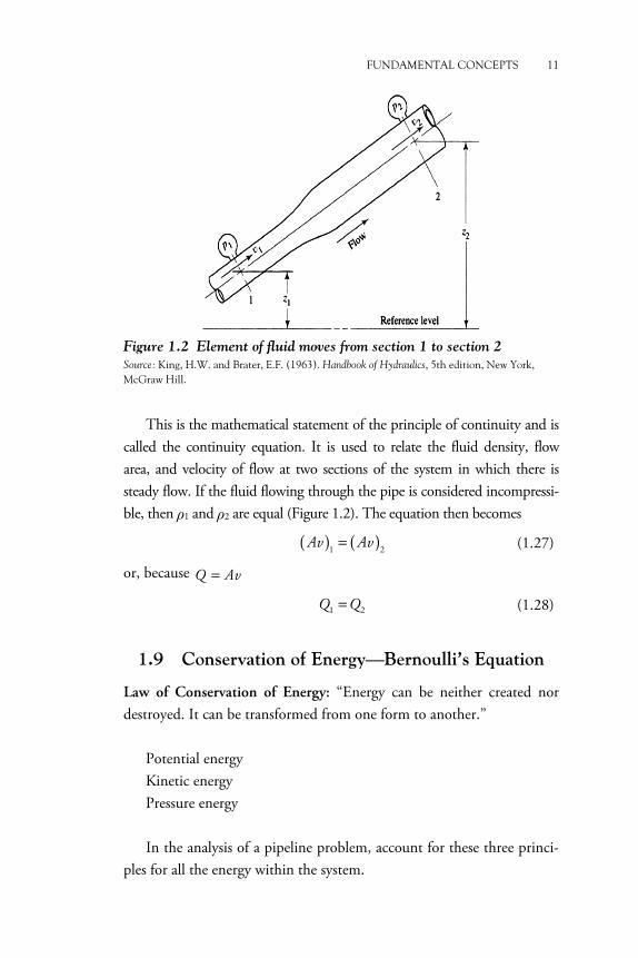
Figure 1.2 Element of fluid moves from section 1 to section 2
Source: King, H.W. and Brater, E.F. (1963). Handbook of Hydraulics, 5th edition, New York, McGraw Hill.
This is the mathematical statement of the principle of continuity and is
called the continuity equation. It is used to relate the fluid density, flow area, and velocity of flow at two sections of the system in which there is steady flow. If the fluid flowing through the pipe is considered incompressi-ble, then �1 and �2 are equal (Figure 1.2). The equation then becomes
( ) ( )1 2Av Av= (1.27)
or, because Q Av=
1 2Q Q= (1.28)
1.9 Conservation of Energy—Bernoulli’s Equation
Law of Conservation of Energy: “Energy can be neither created nor destroyed. It can be transformed from one form to another.”
Potential energy Kinetic energy Pressure energy In the analysis of a pipeline problem, account for these three princi-
ples for all the energy within the system.

12 HYDRAULIC ENGINEERING
Figure 1.3 Fluid element inside a pipe
An element of fluid, at any point inside a pipe in a flow system (Figure 1.3):
Is located at a certain elevation (z) Has a certain velocity (v) Has a certain pressure (P)
The element of fluid would possess the following forms of energy: Potential energy: Due to its elevation, the potential energy of the
element relative to some reference level is
ePE w z= (1.29)
we = weight of element z = elevation of fluid Kinetic energy: Due to its velocity, the kinetic energy of the element is
2
eKE 2
w vg
= (1.30)
Flow energy (pressure energy or flow work): Amount of work neces-sary to move an element of a fluid across a certain section against the pressure (P).
ePE w P
γ= (1.31)

FUNDAMENTAL CONCEPTS 13
Total amount of energy of these three forms possessed by the ele-ment of fluid:
PE KE FEE = + + (1.32)
2
e ee
2w v w P
E w zg γ
= + + (1.33)
Considering the fluid flow through the sections as shown in Figure 1.2
2
e 1 e 11 e 1Total energy in section1 :
2w v w P
E w zg γ
= + + (1.34)
2
e 2 e 22 e 2Total energy in section 2 :
2w v w P
E w zg γ
= + + (1.35)
If no energy is added to the fluid or lost between the sections 1 and 2, then the principle of energy requires that
2 2
e 1 e 1 e 2 e 2e 1 e 2
2 2w v w P w v w P
w z w zg gγ γ
+ + = + + (1.36)
The weight of the element is common to all terms and can be divided out, resulting in the following equation known as Bernoulli’s equation.
2 2
1 1 2 21 2
2 2v P v P
z zg gγ γ
+ + = + + (1.37)
Each term in Bernoulli’s equation is one form of the energy possessed by the fluid per unit weight of fluid flowing in the system. The units in each term are “energy per unit weight.” In the SI system, the units are N·m/N and in the U.S. customary system, the units are lb·ft/lb.
The force unit appears in both the numerator and denominator and it can be cancelled. The resulting unit thus becomes the meter (m) or foot (ft) and can be interpreted to be a height. In fluid flow analysis, the terms are typically expressed as “head” referring to a height above a reference level (Figure 1.4).
P/� = pressure head
z = elevation head Summation of the terms is called total head.
v2/2g = velocity head

14 HYDRAULIC ENGINEERING
Figure 1.4 Element of fluid moves from section 1 to section 2
Source: King, H.W. and Brater, E.F. (1963). Handbook of Hydraulics, 5th edition, New York, McGraw Hill.
1.9.1 Restrictions on Bernoulli’s Equation
It is stated only for incompressible fluids, since the specific weight of the fluid is assumed to be the same at two sections of interest.
There can be no mechanical devices between sections 1 and 2 that would add energy to or remove energy from the system, since the equa-tion states that the total energy of the fluid is constant.
There can be no heat transferred into or out of the fluid. There can be no energy loss due to friction.
Example Problem 1
Water at 10 °C is flowing from section 1 to section 2. At section 1, which is 25 mm in diameter, the gage pressure is 345 kPa and the velocity of
FUNDAMENTAL CONCEPTS 15
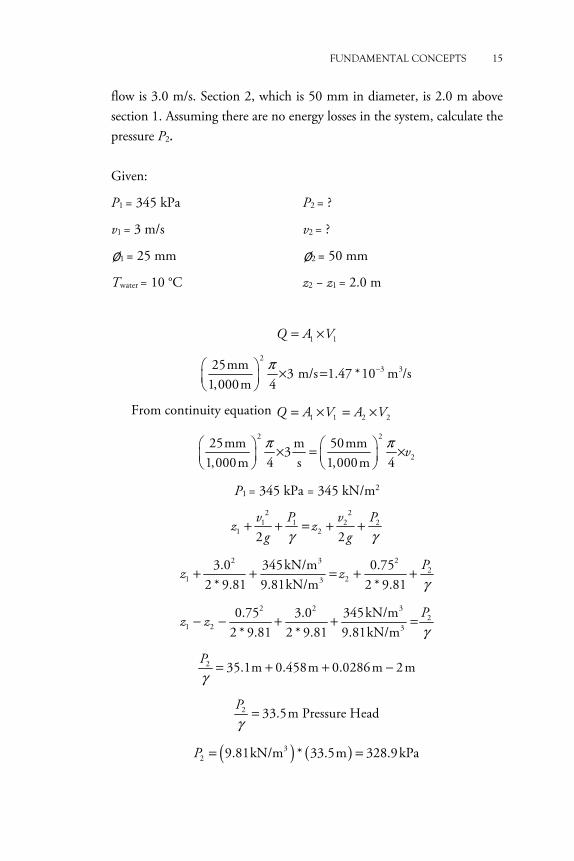
flow is 3.0 m/s. Section 2, which is 50 mm in diameter, is 2.0 m above section 1. Assuming there are no energy losses in the system, calculate the pressure P2. Given:
P1 = 345 kPa P2 = ?
v1 = 3 m/s v2 = ?
�1 = 25 mm �2 = 50 mm
Twater = 10 °C z2 − z1 = 2.0 m
1 1Q A V= × 2
3 325 mm3 m/s 1 .47 *10 m s
1,000 m 4/
π −� � × =� �� �
From continuity equation 1 1 2 2 Q A V A V= × = ×
2 2
225 mm m 50 mm3
1,000 m 4 s 1,000 m 4v
π π� � � �× = ×� � � �� � � �
P1 = 345 kPa = 345 kN/m2 2 2
1 1 2 21 2
2 2v P v P
z zg gγ γ
+ + = + +
2 3 22
1 23
3.0 345 kN/m 0.75 2 * 9.81 9.81 kN/m 2 * 9.81
Pz z
γ+ + = + +
2 2 32
1 2 3
0.75 3.0 345 kN/m2 * 9.81 2 * 9.81 9.81 kN/m
Pz z
γ− − + + =
2 35.1 m 0.458 m 0.0286 m 2 mPγ
= + + −
2 33.5 m Pressure HeadPγ
=
( ) ( )32 9.81 kN/m * 33.5 m 328.9 kPaP = =

16 HYDRAULIC ENGINEERING
Example Problem 2
A siphon draws fluid from a tank and delivers it through a nozzle at the end of the pipe (Figure 1.5).
Calculate the volume flow rate through the siphon and the pressure at points B, C, D, and E. Diameter of siphon = 40 mm
Diameter of nozzle = 25 mm Assume that there are no energy losses in the system. Reference points A and F (most convenient points)
2 2A A F F
A F 2 2v P v P
z zg gγ γ
+ + = + +
Points A and F are open to atmosphere; hence, PA = 0 and PF = 0. Velocity at point A is zero. Elevation difference between A and F = 1.8 + 1.2 = 3.0 m
A F 3.0 mz z− =
F A 3.0 mz z− = − 2
FA F
2v
z zg
= +
( )F A F ) * (2 * 9.81v z z= −
F 7.67 m/sv =
Q A V= ×
Figure 1.5 Example Problem 2
Source: Mott, R.L. (1972). Applied Fluid Mechanics, 6th Edition, Prentice Hall, New Jersey.

FUNDAMENTAL CONCEPTS 17
233 25 mm m m* 7.67 3.77 10 s1,000 m 4
Qs
π −� �= = ×� �� �
Determine the pressures between B, C, D and E. Write the Bernoulli’s equation between A and B.
2 2A A B B
B 2 2Av P v P
z zg gγ γ
+ + = + +
B BQ A v= × 2
33 B
40 mm �m3.77 10 s 1,000 m 4v− � �× = ×� �
� �
B 3.0 m/sv = 2
B(3.0)0 2 * 9.81
Pγ
= +
B 4.50 kPaP = −
(Negative sign indicates that the pressure is below atmospheric pressure.) Write the Bernoulli equation between A and C.
22C CA A
A C 2 2
v Pv Pz z
g gγ γ+ + = + +
C B : Since pipe diameter is the samev v= 2
C(3.0)3.0 m 4.2 m2 * 9.81 9.81
P= + +
C 16.27 kPaP = −
Similarly, write the Bernoulli equation between A and D. 22
D DA AA D
2 2v Pv P
z zg gγ γ
+ + = + +
D 4.50 kPaP = −
Similarly, write the Bernoulli equation between A and E. 2 2
A A E EA E
2 2v P v P
z zg gγ γ
+ + = + +
E 24.93 kPaP =

18 HYDRAULIC ENGINEERING
1.9.2 Summary of the Results of Example
1. Velocity from nozzle and therefore the volume flow rate delivered by siphon depends on the elevation difference between the free sur-face of fluid and the outlet of the nozzle.
2. The pressure at point B is below atmospheric pressure even though it is on the same level as point A, which is exposed to the atmosphere. Bernoulli’s equation shows that the pressure head at B is decreased by the amount of the velocity head. That is, some of the energy is converted.
3. The velocity of flow is the same at all points where the pipe size is the same, when steady flow exists.
4. The pressure at point C is the lowest in the system because point C is at the highest elevation.
5. The pressure at point D is the same as that at point B, because both are on the same elevation and the velocity head at both points is the same.
6. The pressure at point E is the highest in the system because point E is at the lowest elevation.
CHAPTER 2
General Energy Equation It was identified in the last chapter that the Bernoulli’s equation has a few limitations that cannot account for the flow of water through pipes. In fluid systems, there are different types of devices and components. These devices and components occur in most fluid-flow systems and they add energy to the fluid, remove energy from the fluid, or cause un-desirable losses of energy from the fluid.
In this chapter, pumps, fluid motors, friction losses as fluid flows in pipes and tubes, energy losses from changes in the size of the flow path, and energy losses from valves and fittings are discussed.
In later chapters, details about how to compute the amount of energy losses in pipes and specific types of valves and fittings are discussed. The method of using performance curves for pumps and to apply them properly is discussed in detail.
2.1 Pumps
A pump is a common example of a mechanical device that adds energy to a fluid. A pump is a device that moves fluids by mechanical action. Pumps can be classified into three major groups according to the method they use to move the fluid: direct lift, displacement, and gravity pumps.
An electric motor or some other prime power device drives a rotat-ing shaft in the pump. The pump then takes this kinetic energy and delivers it to the fluid, resulting in fluid flow and increased fluid pres-sure. Pumps operate via many energy sources, including manual opera-tion, electricity, engines, or wind power, and come in many sizes, from microscopic for use in medical applications to large industrial pumps.

20 HYDRAULIC ENGINEERING
2.2 Fluid Motors
Fluid motors, turbines, rotary actuators, and linear actuators are exam-ples of devices that take energy from a fluid and deliver it in the form of work, causing the rotation of a shaft or the linear movement of a piston. The major difference between a pump and a fluid motor is that when acting as a motor, the fluid drives the rotating elements of the device. The reverse is true for pumps.
The hydraulic motor shown in Figure 2.1 is often used as a drive for the wheels of construction equipment and trucks and for rotating components of material transfer systems, conveyors, agricultural equipment, special machines, and automation equipment. The design incorporates a stationary internal gear with a special shape. The rotating component is like an exter-nal gear, sometimes called a gerotor, which has one fewer teeth than the internal gear. The external gear rotates in a circular orbit around the center of the internal gear. High-pressure fluid entering the cavity between the two gears acts on the rotor and develops a torque that rotates the output shaft. The magnitude of the output torque depends on the pressure difference between the input and output sides of the rotating gear. The speed of rota-tion is a function of the displacement of the motor (volume per revolution) and the volume flow rate of fluid through the motor.
Figure 2.1 Rotor and external gear
2.3 Fluid Friction
A fluid in motion is subject to frictional resistance to flow. Part of the energy generated by that resistance is converted into thermal energy

GENERAL ENERGY EQUATION 21
(heat), which is dissipated through the walls of the pipe in which the fluid is flowing. The magnitude of the energy loss is dependent on the properties of the fluid, the flow velocity, the pipe size, the smoothness of the pipe wall, and the length of the pipe.
2.4 Valves and Fittings
Elements that control the direction or flow rate of a fluid in a system typically set up local turbulence in the fluid, causing energy to be dissi-pated as heat. Whenever there is a restriction, a change in flow velocity, or a change in the direction of flow, these energy losses occur. In a large system, the magnitude of losses due to valves and fittings is usually small compared with frictional losses in the pipes. Therefore, such losses are referred to as minor losses.
Energy losses and additions in a system are accounted for in this book in terms of energy per unit weight of fluid flowing in the system. This is also known as “head,” as de scribed in Chapter 6. As an abbreviation for head, symbol h is used for energy losses and additions. Specifically, the following terms are used throughout the next several chapters:
hA = Energy added to the fluid with a mechanical device such as a
pump; this is often referred to as the total head on the pump hR = Energy removed from the fluid by a mechanical device such as a
fluid motor hL = Energy losses from the system due to friction in pipes or minor
losses due to valves and fittings The magnitude of energy losses produced by fluid friction, valves,
and fittings is directly proportional to the velocity head of the fluid. This can be expressed mathematically as
2
L 2v
h Kg
� �= � �
� � (2.1)
The term K is the resistance coefficient. The value of K for fluid fric-tion can be determined using the Darcy equation. In the following

22 HYDRAULIC ENGINEERING
chapters, the various methods of calculating the value of K for many kinds of valves and fittings, and changes in flow cross section and direc-tion are provided. Most of these are found from experimental data.
2.5 General Energy Equation
The general energy equation as used in this text is an expansion of Ber-noulli’s equation, which makes it possible to solve problems in which energy losses and additions occur. The terms E�1 and E�2 denote the en-ergy possessed by the fluid per unit weight at sections 1 and 2, respec-tively. The respective energy additions (hA), removals (hR), and losses (hL) are shown. For such a system, the expression of the principle of conservation of energy is
1 A L R 2E h h h E+ − − =′ ′ (2.2)
Figure 2.2 shows how the terms of this equation are related to a typ-ical section of a pipe system.
The energy possessed per unit weight is given by the following equation:
2
2v P
E zg γ
′ = + + (2.3)
Figure 2.2 Fluid flow system demonstrating the general energy
equation
Source: Mott, R.L. (1972). Applied Fluid Mechanics, 6th Edition, Prentice Hall, New Jersey. �

GENERAL ENERGY EQUATION 23
Substituting the values from Eq. (2.2) into Eq. (2.3) yields the fol-lowing equation:
γ γ
+ + − − + = + +2 2
1 1 2 21 L R A 22 2
v P v Pz h h h z
g g (2.4)
This is the form of the energy equation that is used in this book. As with Bernoulli’s equation, each term in Eq. (2.4) represents a quantity of energy per unit weight of fluid flowing in the system. Typical SI units are N·m/N, or meters. U.S. customary system units are lb·ft/lb, or feet.
It is essential that the general energy equation be written in the direc-tion of flow, that is, from the reference point on the left side of the equa-tion to that on the right side. Algebraic signs are critical because the left side of Eq. (2.4) states that an element of fluid having a certain amount of energy per unit weight at section 1 may have energy added (+hA), energy removed (−hR), or energy lost (−hL) from it before it reaches sec-tion 2. There it contains a different amount of energy per unit weight, as indicated by the terms on the right side of the equation.
For example, in Figure 2.2, reference points are shown to be points 1 and 2 with the pressure head, elevation head, and velocity head indi-cated at each point. After the fluid leaves point 1 it enters the pump, where energy is added. A prime mover such as an electric motor drives the pump, and the impeller of the pump transfers the energy to the fluid (+hA). Then the fluid flows through a piping system composed of a valve, elbows, and the lengths of pipe, in which energy is dissipated from the fluid and is lost (−hL). Before reaching point 2, the fluid flows through a fluid motor, which removes some of the energy to drive an external device (−hR). The general energy equation accounts for all of these energies.
Example Problem 2.1
Water flows from a large reservoir at the rate of 1.20 ft3/s through a pipe system as shown in Figure 2.3. Calculate the total amount of energy lost from the system because of the valve, the elbows, the pipe entrance, and fluid friction.

24 HYDRAULIC ENGINEERING
Figure 2.3 Example Problem 2.1
Source: Mott, R.L. (1972). Applied Fluid Mechanics, 6th Edition, Prentice Hall, New Jersey
Step 1. Identify two points in the system with the most number of
known values Step 2. Points 1 and 2 are identified in the above figure as
P1 = 0:Surface of reservoir exposed to the atmosphere P2 = 0: Free stream of fluid exposed to the atmosphere v1 = 0 (approximately): Surface area of reservoir is large, and hence it can be assumed to be negligible hA = hR = 0: No mechanical device in the system
Step 3. Apply the energy equation between points 1 and 2.
2 21 1 2 2
1 L R A 2 2 2v P v P
z h h h zg gγ γ
+ + − − + = + +
Step 4. The general energy equation becomes
22
1 L 20 0 0 0 0 2v
z h zg
+ + − − + = + +
Step 5. Since the objective is to determine energy loss in the system, solve for hL.
22
L 1 2 ( )2v
h z zg
= − −
1 2 25 ftz z− =

GENERAL ENERGY EQUATION 25
Given Q = 1.20 ft3/s and 3-in. diameter pipe is 0.0491 ft2
3
2
1.20 ft / s24.0 ft/s
0.0491 ftQ
vA
= = =
( )2
L 2
(24.0 ft/s)25 ft
2(32.2 ft/s )h = −
L 25 ft 9.25 fth = −
L(lb ft)15.75 ft 15.75
lbh
⋅= =
Example Problem 2.2
The volume flow rate through the pump, as shown in Figure 2.4, is 0.014 m3/s. The fluid being pumped is oil with a specific gravity of 0.86. Calculate the energy delivered by the pump to the oil per unit weight of oil flowing in the system. Energy losses in the system are caused by the check valve and friction losses as the fluid flows through the piping. The magnitude of such losses has been determined to be 1.86 N·m/N.
Figure 2.4 Example Problem 2.2
Source: Mott, R.L. (1972). Applied Fluid Mechanics, 6th Edition, Prentice Hall, New Jersey.

26 HYDRAULIC ENGINEERING
Step 1. Objective is to determine the energy delivered by the pump, hA
Step 2. Apply energy equation
2 2A A B B
A L R A B 2 2v P v P
z h h h zg gγ γ
+ + − − + = + +
Step 3. Rewrite the equation to solve the unknown hA
γ− −= − + + + +
2 2B A B A
A B A L R( ) ( )
( )2
v v P Ph z z h h
g
Step 4. Determine specific weight
33
w
0.868.44 kN/m
9.81 kN/msgγγ
= = =
Step 5. Determine vA and vB
3
A 3 2A
(0.014)m /s2.94 m/s
(4.768 10 )mQ
vA −= = =
×
−= = =×
3
B 3 2B
(0.014)m /s 6.46 m/s(2.168 10 ) m
Qv
A
Step 6. Calculate hA
− − −= + +
+ +
2 2 2 2
A 3 3
(6.46 2.94 ) m (296 ( 28)) kN / m(1.0 m)2 * 9.81 kN / m 8.44 kN / m
1.86 N·m / N 0
h
A 1.0 m 1.69 m 38.4 m 1.86 N·m / m 0h = + + + +
A 42.9 m or 42.9 N·m/Nh =
That is, the pump delivers 42.9 N·m/N of energy to each newton of oil flowing through it.
2.6 Power Generated by Pumps
Power is defined as the rate of doing work. In fluid mechanics this statement can be modified to consider that power is the rate at which energy is being transferred. The unit for power in the SI system is watt (W), which is equivalent to 1.0 N·m/s or 1.0 joule (J)/s.

GENERAL ENERGY EQUATION 27
In Example Problem 2.2 it was determined that the pump was deliv-ering 42.9 N·m/N of energy to each newton of oil as it flowed through the pump. To calculate the power delivered to the oil, it is necessary to determine how many newtons of oil are flowing through the pump in a given amount of time. This is called the weight flow rate, W, which was defined in the previous chapter, and is expressed in units of N/s. Power is calculated by multiplying the energy transferred per newton of fluid by the weight flow rate. This is
A AP h W= (2.5)
However, from the previous chapter it was identified that
W Qγ=
Therefore
A AP h Qγ= (2.6)
Using the information from Example Problem 2.2
A 42.9 N·m/Nh = 3 3 3 8.44 kN/m 8.44 10 N/mγ = = ×
Q = 0.014 m3/s 3
3A 3
N m N m42.9 * 8.44 10 * 0.014
N m sP
⋅= ×
PA = 5069.0 N·m/s
Because 1.0 W = 1.0 N·m/s, this can be expressed in watts:
PA = 5069 W = 5.07 kW
The unit for power in the U.S. customary system is lb·ft/s. Because it is common practice to refer to power in horsepower (hp), the conver-sion factor required is
1 hp = 550 lb·ft/s
In Eq. (2.6) the energy added hA is expressed in feet of the fluid flowing in the system. Then, expressing the specific weight of the fluid in lb/ft3 and the volume flow rate in ft3/s would yield the weight flow rate Qγ in lb/s. Finally, in the power equation, A A ,P h Qγ= power would be expressed in lb·ft/s.

28 HYDRAULIC ENGINEERING
To convert these units to the SI system, the following factors are used:
l.0 lb-ft/s = 1.356 W
1 hp = 745.7 W
2.7 Mechanical Efficiency of Pumps
The term efficiency is used to denote the ratio of the power delivered by the pump to the fluid to the power supplied to the pump. Because of energy losses due to mechanical friction in pump components, fluid friction in the pump, and excessive fluid turbulence in the pump, not all of the input power is delivered to the fluid. Then, using the symbol eM for mechanical efficiency
AM
I
Power delivered to fluidPower put into pump
Pe
P= = (2.7)
The value of eM should always be less than 1.0. Continuing with the data of Example Problem 2.2, calculate the power
input to the pump if eM is known. For commercially available pumps, the value of eM is published as part of the performance data. It is assumed that for the pump in this problem the efficiency is 82 percent, then
PI = PA/eM = 5.07/0.82 = 6.18 kW
The value of the mechanical efficiency of pumps depends not only on the design of the pump, but also on the conditions under which it is operating, particularly the total head and the flow rate.
2.8 Power Delivered to Fluid Motors
The energy delivered by the fluid to a mechanical device such as a fluid motor or a turbine is denoted in the general energy equation by the term hR. This is a measure of the energy delivered by each unit weight of fluid as it passes through the device. The power delivered is found by multi-plying hR by the weight flow rate, W.
R RP h Qγ= (2.8)
where PR is power delivered by the fluid to the fluid motor.
GENERAL ENERGY EQUATION 29
2.9 Mechanical Efficiency of Fluid Motors
As was described for pumps, energy losses in a fluid motor are produced by mechanical and fluid friction. Therefore, not all the power delivered to the motor is ultimately converted to power output from the device. Mechanical efficiency is then defined as
oM
R
Power output from motorPower delivered by fluid
Pe
P= = (2.9)
Here again the value of eM should be less than 1.0.
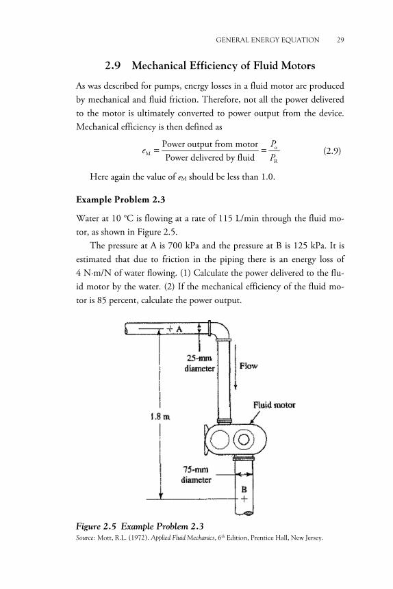
Example Problem 2.3
Water at 10 °C is flowing at a rate of 115 L/min through the fluid mo-tor, as shown in Figure 2.5.
The pressure at A is 700 kPa and the pressure at B is 125 kPa. It is estimated that due to friction in the piping there is an energy loss of 4 N·m/N of water flowing. (1) Calculate the power delivered to the flu-id motor by the water. (2) If the mechanical efficiency of the fluid mo-tor is 85 percent, calculate the power output.
Figure 2.5 Example Problem 2.3
Source: Mott, R.L. (1972). Applied Fluid Mechanics, 6th Edition, Prentice Hall, New Jersey.
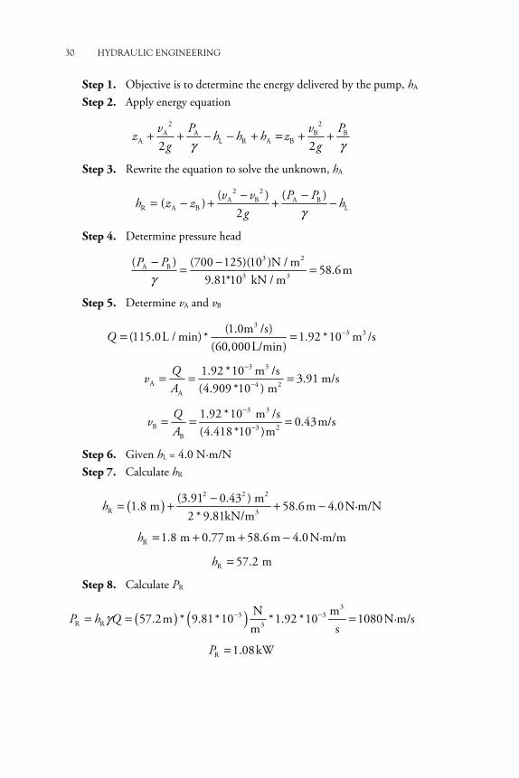
30 HYDRAULIC ENGINEERING
Step 1. Objective is to determine the energy delivered by the pump, hA
Step 2. Apply energy equation
2 2A A B B
A L R A B 2 2v P v P
z h h h zg gγ γ
+ + − − + = + +
Step 3. Rewrite the equation to solve the unknown, hA
γ− −= − + + −
2 2A B A B
R A B L)( ) ( )
(2
v v P Ph z z h
g
Step 4. Determine pressure head
γ− −= =
3 2A B
3 3
( ) (700 125)(10 )N / m 58.6 m9.81*10 kN / m
P P
Step 5. Determine vA and vB
3 3 3(1.0m /s)
(115.0 L / min)* 1.92 *10 m /s(60,000 L/min)
Q −= =
−
−= = =3 3
A 4 2A
1.92 *10 m /s 3.91 m/s(4.909 *1 0 ) m
Qv
A
−
−= = =3 3
B 3 2B
1.92 *10 m /s 0.43 m/s(4.418 *1 0 ) m
Qv
A
Step 6. Given hL = 4.0 N·m/N Step 7. Calculate hR
( )2 2 2
R 3
(3.91 0.43 ) m1.8 m 58.6 m 4.0 N·m/N
2 * 9.81kN/mh
−= + + −
R 1.8 m 0.77 m 58.6 m 4.0 N·m/mh = + + −
R 57.2 mh =
Step 8. Calculate PR
( ) ( )3
3 3R R 3
N m57.2 m * 9.81*10 *1.92 *10 1080 N·m/s
m sP h Qγ − −= = =
� R 1.08 kWP = ��

GENERAL ENERGY EQUATION 31
Step 9. Calculate the power output Efficiency (eM) is given as 85% = 0.85. PR is determined as 1.08 kW. Po is calculated as follows:
oM
R
Pe
P=
o R M*P P e=
o 0.85 *1.08 0.92 kWP = = �

�

CHAPTER 3
Types of Flow and Loss Due to Friction
Fluid flow in circular and noncircular pipes is commonly encountered in practice. Water in a city is distributed by extensive piping networks. Oil and natural gas are transported hundreds of miles by large pipelines. Blood is carried throughout our bodies by arteries and veins. The cool-ing water in an engine is transported by hoses to the pipes in the radia-tor where it is cooled as it flows. Thermal energy in a hydronic space heating system is transferred to the circulating water in the boiler, and then it is transported to the desired locations through pipes.
Fluid flow is classified as external and internal, depending on whether the fluid is forced to flow over a surface or in a conduit. Internal and external flows exhibit very different characteristics. In this chapter, inter-nal flow where the conduit is completely filled with the fluid and the flow is driven primarily by a pressure difference is explained. This should not be confused with open-channel flow where the conduit is partially filled by the fluid and thus the flow is partially bounded by solid surfaces, as in an irrigation ditch, and flow is driven by gravity alone.
3.1 Reynolds Number
Reynolds number (NR) is a dimensionless quantity that is used to help distinguish the different flow patterns in the pipe flow. The main types of flow in pipes are
a. Laminar flow b. Turbulent flow c. Critical flow
34 HYDRAULIC ENGINEERING
It has been demonstrated that the character of flow in a round pipe depends on four variables: fluid density ρ, fluid viscosity μ, pipe diame-ter D, and average velocity of flow v. Osborne Reynolds was the first to demonstrate that laminar or turbulent flow can be predicted if the mag-nitude of a dimensionless number, now called the Reynolds number (NR), is known. It is defined by the equation
RN vD vDρμ ϑ
= = (3.1)
As kinematic viscosity μϑρ
= , the variation in the formula occurs.
The Reynolds number is the ratio of the inertia force on an element of fluid to the viscous force. The inertia force is developed from New-ton’s second law of motion, F = ma.
Flows having large Reynolds numbers, typically because of high velocity and/or low viscosity, tend to be turbulent. Those fluids having high viscosity and/or moving at low velocities will have low Reynolds numbers and will tend to be laminar. The following section gives some quantitative data with which to predict whether a given flow system will be laminar or turbulent.
For practical applications in pipe flow, if the Reynolds number for the flow is less than 2,000, the flow will be laminar. If the Reynolds number is greater than 4,000, the flow can be assumed to be turbulent. In the range of Reynolds numbers between 2,000 and 4,000, it is impossible to predict which type of flow exists; therefore, this range is called the critical region. Typical applications involve flows that are well within the laminar flow range or well within the turbulent flow range, so the existence of this re-gion of uncertainty does not cause great difficulty. If the flow in a system is found to be in the critical region, the usual practice is to change the flow rate or pipe diameter to cause the flow to be definitely laminar or definitely turbulent. More precise analysis is then possible.
When NR is greater than about 4,000, a minor disturbance of the flow stream will cause the flow to suddenly change from laminar to tur-bulent. Therefore, for practical applications in this book, the following assumption is made:

TYPES OF FLOW AND LOSS DUE TO FRICTION 35
If NR < 2,000, the flow is laminar. If NR > 4,000, the flow is turbulent.
3.2 Laminar Flow
As the water flows from a faucet at a very low velocity, the flow appears to be smooth and steady. The stream has a fairly uniform diameter and there is little or no evidence of mixing of the various parts of the stream. This is called laminar flow, a term derived from the word layer, because the fluid appears to be flowing in continuous layers, with little or no mixing from one layer to the adjacent layers. Laminar flow is a flow re-gime wherein mixing is characterized by high-momentum diffusion and low-momentum convection.
When laminar flow exists, the fluid seems to flow as several layers, one on another. Because of the viscosity of the fluid, a shear stress is created between the layers of fluid. Energy is lost from the fluid by the action of overcoming the frictional forces produced by the shear stress. Because laminar flow is so regular and orderly, a relationship between the energy loss and the measurable parameters of the flow system can be derived. This relationship is known as the Hagen–Poiseuille equation:
L 2
32 Lvh
Dμ
γ= (3.2)
hL = energy loss μ = dynamic viscosity L = length of pipe D = diameter for pipe � = specific weight of fluid It should be noted that the Hagen–Poiseuille equation is valid only
for laminar flow (NR < 2,000).
3.3 Turbulent Flow
Turbulent flow is a flow regime characterized by chaotic property changes. This includes low-momentum diffusion, high-momentum convection, and rapid variation of pressure and flow velocity in space and time.
36 HYDRAULIC ENGINEERING
Although there is no theorem relating the Reynolds number (NR) to turbulence, flows at Reynolds numbers larger than 4,000 are typically turbulent. In this case, the energy losses in the energy equation are given by the Darcy equation:
2
L * *2
L vh f
D g= (3.3)
hL = energy loss due to friction f = friction factor D = diameter of pipe v = velocity of fluid g = acceleration due to gravity For turbulent flow of fluids in circular pipes it is most convenient to
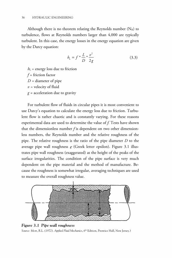
use Darcy’s equation to calculate the energy loss due to friction. Turbu-lent flow is rather chaotic and is constantly varying. For these reasons experimental data are used to determine the value of f. Tests have shown that the dimensionless number f is dependent on two other dimension-less numbers, the Reynolds number and the relative roughness of the pipe. The relative roughness is the ratio of the pipe diameter D to the average pipe wall roughness ε (Greek letter epsilon). Figure 3.1 illus-trates pipe wall roughness (exaggerated) as the height of the peaks of the surface irregularities. The condition of the pipe surface is very much dependent on the pipe material and the method of manufacture. Be-cause the roughness is somewhat irregular, averaging techniques are used to measure the overall roughness value.
Figure 3.1 Pipe wall roughness
Source: Mott, R.L. (1972). Applied Fluid Mechanics, 6th Edition, Prentice Hall, New Jersey.)

TYPES OF FLOW AND LOSS DUE TO FRICTION 37
For commercially available pipe and tubing, the design value of the av-erage wall roughness ε has been determined as shown in Table 3.1. These are only average values for new, clean pipe. Some variation should be ex-pected. After a pipe has been in service for a time, the roughness could change due to the formation of deposits on the wall or due to corrosion.
Glass tubing has an inside surface that is virtually hydraulically smooth, indicating a very small value of roughness. Therefore, the rela-tive roughness, D/ε, approaches infinity. Plastic pipe and tubing are nearly as smooth as glass, and the values of roughness are listed in the table; however, variations should be expected. Copper, brass, and some steel tubing are drawn to its final shape and size over an internal man-drel, leaving a fairly smooth surface. For standard steel pipe (such as Schedule 40 and Schedule 80) and welded steel tubing, the roughness value is listed for commercial steel or welded steel. Galvanized iron has a metallurgically bonded zinc coating for corrosion resistance. Ductile iron pipe is typically coated on the inside with a cement mortar for cor-rosion protection and to improve surface roughness.
Table 3.1 Pipe roughness—design values
Material Roughness ε (m) Roughness ε (ft) Glass Smooth Smooth Plastic 3 × 10⁻⁷ 1 × 10⁻⁶ Drawn tubing, copper, brass, steel 1.5 × 10⁻⁶ 5 × 10⁻⁶ Steel, commercial or welded 4.6 × 10⁻⁵ 1.5 × 10⁻⁴ Galvanized iron 1.5 × 10⁻⁴ 5 × 10⁻⁴ Ductile iron, coated 1.2 × 10⁻⁷ 4 × 10⁻⁴ Ductile iron, uncoated 2.4 × 10⁻⁴ 8 × 10⁻⁴ Concrete, well made 1.2 × 10⁻⁴ 4 × 10⁻⁴ Riveted steel 1.8 × 10⁻³ 6 × 10⁻³
3.4 Moody Diagram
One of the most widely used methods for evaluating the friction factor employs the Moody diagram shown in Figure 3.2. The diagram shows the friction factor f plotted versus the Reynolds number NR, with a se-ries of parametric curves related to the relative roughness D/ε. Both f and NR are plotted on logarithmic scales because of the broad range of values encountered. At the left end of the chart, for NR < 2,000, the straight line shows the relationship f = 64/NR for laminar flow. For

38 HYDRAULIC ENGINEERING
2,000 < NR < 4,000, no curves are drawn because this is the critical zone between laminar and turbulent flow, and it is not possible to predict the type of flow. The change from laminar to turbulent flow results in val-ues for friction factors within the shaded band. Beyond NR = 4,000, the family of curves for different values of D/ε is plotted. Several important observations can be made from these curves:
i. For a given Reynolds number of flow, as the relative roughness D/ε is increased, the friction factor f decreases.
ii. For a given relative roughness D/ε, the friction factor f decreases with increasing Reynolds number until the zone of complete turbulence is reached.
iii. Within the zone of complete turbulence, the Reynolds number has no effect on the friction factor.
iv. As the relative roughness D/ε increases, the value of the Reyn-olds number at which the zone of complete turbulence begins also increases.
Figure 3.2 is a simplified sketch of Moody’s diagram on which the
various zones are identified. The laminar zone at the left has already been discussed. At the right of the dashed line downward across the dia-gram is the zone of complete turbulence. The lowest possible friction factor for a given Reynolds number in turbulent flow is indicated by the smooth pipes line.
Between the smooth pipes line and the line marking the start of the complete turbulence zone is the transition zone. Here, the various D/ε lines are curved, and care must be exercised to evaluate the friction fac-tor properly. As shown in the example, the value of the friction factor for a relative roughness of 500 decreases from 0.0420 at NR = 4,000 to 0.0240 at NR = 6.0 × 10⁵, where the zone of complete turbulence starts.
Table 3.2 Example values to determine friction factor
NR D/ε f 6.7 × 10³ 150 0.0430 1.6 × 10⁴ 2,000 0.0284 1.6 × 10⁶ 2,000 0.0171 2.5 × 10⁵ 733 0.0233
Source: Mott, R.L. (1972). Applied Fluid Mechanics, 6th Edition, Prentice Hall, New Jersey

TYPES OF FLOW AND LOSS DUE TO FRICTION 39
�
Fig
ure
3.2
M
oody
dia
gram
40 HYDRAULIC ENGINEERING
3.5 Friction Factor Equations
The Moody diagram in Figure 3.2 is a convenient and sufficiently accu-rate means of determining the value of the friction factor when solving problems by manual calculations. However, additional equations are often used to determine the friction factor.
In the laminar flow zone, for values below 200, the friction factor can be found from the equation
R
64N
f = (3.4)
This relationship, developed in Figure 3.2, plots in the Moody dia-gram as a straight line on the left side of the chart. Of course, for Reyn-olds numbers from 2,000 to 4,000, the flow is in the critical range and it is impossible to predict the value of f.
The value of the friction factor for turbulent flow can be determined by
2
0.9R
0.25
1 5.74log N3.7
f
Dε
=� � � � � � � +� �
� �� � � �� � � �� � �
(3.5)
The value determined from Eq. (3.5) will be similar to the value from the Moody diagram shown in Figure 3.2.
Example Problem 3.1
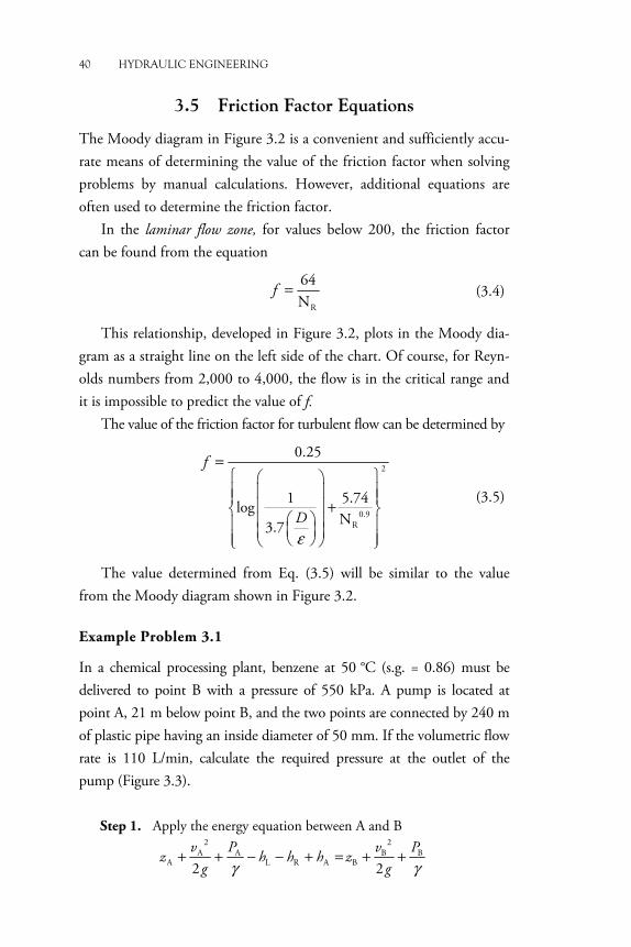
In a chemical processing plant, benzene at 50 °C (s.g. = 0.86) must be delivered to point B with a pressure of 550 kPa. A pump is located at point A, 21 m below point B, and the two points are connected by 240 m of plastic pipe having an inside diameter of 50 mm. If the volumetric flow rate is 110 L/min, calculate the required pressure at the outlet of the pump (Figure 3.3).
Step 1. Apply the energy equation between A and B
� 2 2A A B B
A L R A B 2 2v P v P
z h h h zg gγ γ
+ + − − + = + + �
TYPES OF FLOW AND LOSS DUE TO FRICTION 41
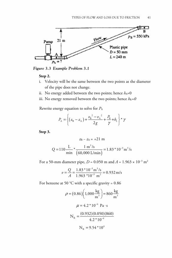
Figure 3.3 Example Problem 3.1
Step 2. i. Velocity will be the same between the two points as the diameter
of the pipe does not change. ii. No energy added between the two points; hence hA=0 iii. No energy removed between the two points; hence hR=0
Rewrite energy equation to solve for PA
( )2 2
B A BA B A L *
2v v P
P z z hg
γγ
� −= − + + +� � �
Step 3.
zB − zA = +21 m
( )3
3 3L 1 m /s110 * 1.83 *10 m /smin 60,000 L/min
Q −= =
For a 50-mm diameter pipe, D = 0.050 m and A = 1.963 × 10⁻³ m2
3 3
3 2
1.83 *10 m /s 0.932 m/s1.963 *1 0 m
Qv
A
−
−= = =
For benzene at 50 °C with a specific gravity = 0.86
( ) 3 3
kg kg0.86 1,000 860
m mρ � �= =� �
� �
44.2 *10 Pa sμ −= ⋅
R 4
(0.932)(0.050)(860)N4.2 *10−=
4RN 9.54 *10=
42 HYDRAULIC ENGINEERING
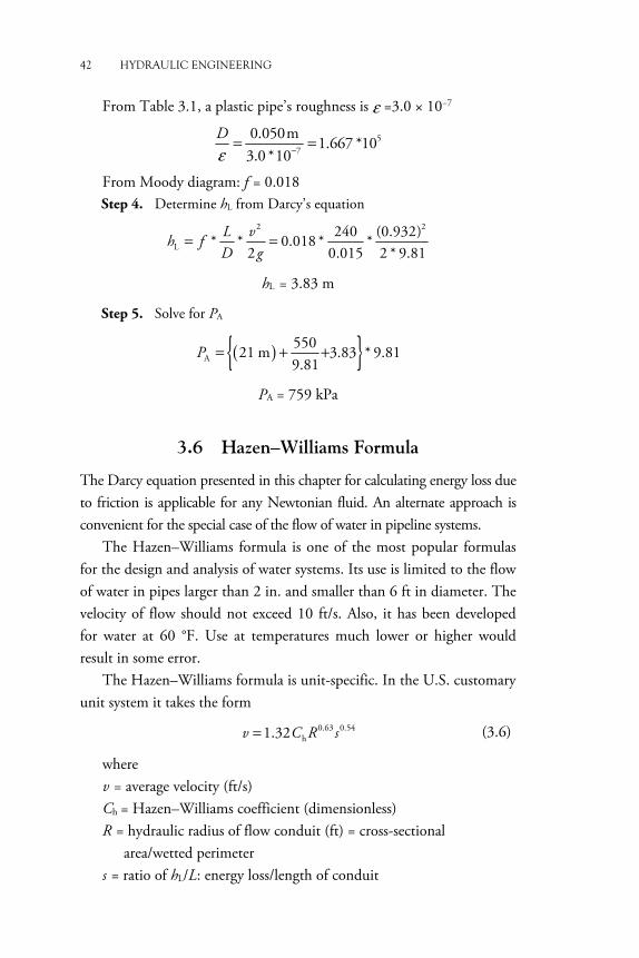
From Table 3.1, a plastic pipe’s roughness is ε =3.0 × 10⁻⁷
57
0.050 m 1.667 *1 03.0 *10
Dε −= =
From Moody diagram: f = 0.018 Step 4. Determine hL from Darcy’s equation
2 2
L240 (0.932)* * 0.018 * *
2 0.015 2 * 9.81L v
h fD g
= =
hL = 3.83 m
Step 5. Solve for PA
( ){ }A55021 m 3.83 * 9.819.81
P = + +
PA = 759 kPa
3.6 Hazen–Williams Formula
The Darcy equation presented in this chapter for calculating energy loss due to friction is applicable for any Newtonian fluid. An alternate approach is convenient for the special case of the flow of water in pipeline systems.
The Hazen–Williams formula is one of the most popular formulas for the design and analysis of water systems. Its use is limited to the flow of water in pipes larger than 2 in. and smaller than 6 ft in diameter. The velocity of flow should not exceed 10 ft/s. Also, it has been developed for water at 60 °F. Use at temperatures much lower or higher would result in some error.
The Hazen–Williams formula is unit-specific. In the U.S. customary unit system it takes the form
0.63 0.54h1.32 v C R s= (3.6)
where v = average velocity (ft/s) Ch = Hazen–Williams coefficient (dimensionless) R = hydraulic radius of flow conduit (ft) = cross-sectional
area/wetted perimeter s = ratio of hL/L: energy loss/length of conduit

TYPES OF FLOW AND LOSS DUE TO FRICTION 43
The use of the hydraulic radius in the formula allows its application to noncircular sections as well as circular pipes. Use R = D/4 for circular pipes. The coefficient Ch is dependent only on the condition of the sur-face of the pipe or conduit. Table 3.3 gives typical values. Note that some values are described as for pipe in new, clean condition, whereas the de-sign value accounts for the accumulation of deposits that develop on the inside surfaces of pipe after time, even when clean water flows through them. Smoother pipes have higher values of Ch than rougher pipes.
Table 3.3 Hazen–Williams Coefficient, Ch
Type of Pipe
Ch Average for
New, Clean Pipe Design Value
Steel, ductile iron, or cast iron with centrifugally applied cement or bituminous lining 150 140 Plastic, copper, brass, glass 140 130 Steel, cast iron, uncoated 130 100 Concrete 120 100 Corrugated steel 60 60
The Hazen–Williams formula for SI units is
0.63 0.54h0.85 v C R s= (3.7)
Example Problem 3.2
For what velocity of flow of water in a new, clean, 6-in. Schedule 40 steel pipe would an energy loss of 20 ft of head occur over a length of 1,000 ft? Compute the volumetric flow rate at that velocity. Then refigure the velocity using the design value of Ch for steel pipe.
Solution:
Part a:
Step 1. 0.63 0.54h1.32 v C R s=
Step 2. s = hL/L = (20)/(1,000 ft)= 0.02 Step 3. R = D/4 = (0.5054)/4 = 0.126 ft Step 4. Ch = 130
Step 5. ( )0.540.631.32(130)(0.126) 0.02 5.64 ft/s v = =
44 HYDRAULIC ENGINEERING
Step 6. Q = Av = (0.2006 ft2)(5.64 ft/s) = 1.13 ft3/s Part b: Reconfigure for design value
Ch =100 (design value)
The allowable volume flow rate to limit the energy loss to the same value of 20 ft per 1,000 ft of pipe length would be
v = 5.64 ft/s (100/130) = 4.34 ft/s
Q = Av = (0.2006 ft2)(4.34 ft/s) = 0.869 ft3/s
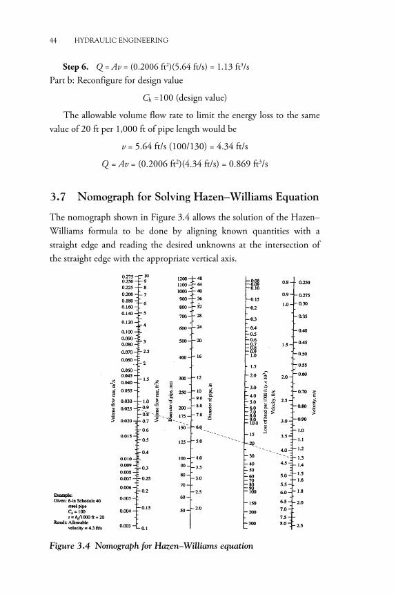
3.7 Nomograph for Solving Hazen–Williams Equation
The nomograph shown in Figure 3.4 allows the solution of the Hazen–Williams formula to be done by aligning known quantities with a straight edge and reading the desired unknowns at the intersection of the straight edge with the appropriate vertical axis.
Figure 3.4 Nomograph for Hazen–Williams equation
TYPES OF FLOW AND LOSS DUE TO FRICTION 45
Example Problem 3.3
Specify the required size of Schedule 40 steel pipe to carry 1.20 ft3/s of water with no more than 4.0 ft of head loss over a 1,000-ft length of pipe. Use the design value for Ch.
Solution:
Table 3.3 suggests Ch = 100. Using Figure 3.4, place a straight edge from Q = 1.20 ft3/s on the volume flow rate line to the value of s = 4.0 ft/1,000 ft on the energy loss line. The straight edge then intersects the pipe size line at approximately 9.7 in. The next larger standard pipe size listed in Appendix C is the nominal 10-in. pipe with an inside diameter of 10.02 in.
Returning to Figure 3.4 and slightly realigning Q = 1.20 ft3/s with D = 10.02 in., an average velocity of v = 2.25 ft/s. This is relatively low for a water distribution system, and the pipe is quite large. If the pipe-line is long, the cost for piping would be excessively large.
Hence, allow the velocity of flow to increase to approximately 6.0 ft/s for the same volume flow rate; use Figure 3.4 to show that a 6-in. pipe could be used with a head loss of approximately 37 ft per 1,000 ft of pipe. The lower cost of the pipe (in comparison with the 10-in. pipe) would have to be compared with the higher energy cost required to overcome the additional head loss.
� �

�
�

CHAPTER 4
Minor Losses Energy losses are proportional to the velocity head of the fluid as it flows around an elbow, through an enlargement or contraction of the flow section, or through a valve. Experimental values for energy losses are usually reported in terms of a resistance coefficient K as follows:
2
L 2v
h Kg
� �= � �
� � (4.1)
In Eq. (4.1), hL is the minor loss, K is the resistance coefficient, and v is the average velocity of flow in the pipe in the vicinity where the mi-nor loss occurs. In some cases, there may be more than one velocity of flow, as with enlargements or contractions. It is most important to know which velocity is to be used with each resistance coefficient.
The resistance coefficient is dimensionless because it represents a constant of proportionality between the energy loss and the velocity head. The magnitude of the resistance coefficient depends on the geom-etry of the device that causes the loss and sometimes on the velocity of flow. In the following sections, the process for determining the value of K and for calculating the energy loss for many types of minor loss condi-tions will be described.
As in the energy equation, the velocity head v2/2g in Eq. (4.1) is typ-ically in the SI units of meters (or N·m/N of fluid flowing) or in the U.S. customary units of feet (or ft·lb/lb of fluid flowing). Because K is dimensionless, the energy loss has the same units.
The different types of minor losses are the following:
1. Sudden enlargement 2. Gradual enlargement 3. Sudden contraction 4. Gradual contraction

48 HYDRAULIC ENGINEERING
5. Entrance loss 6. Exit loss 7. Resistance coefficient for valves and fittings 8. Pipe bends
4.1 Sudden Enlargement
As a fluid flows from a smaller pipe into a larger pipe through a sudden enlargement, its velocity abruptly decreases, causing turbulence, which generates an energy loss (Figure 4.1(a) and (b)). The amount of turbu-lence, and therefore the amount of energy loss, is dependent on the ratio of the sizes of the two pipes.
The minor loss is calculated from the equation
2
1L 2
vh K
g� �
= � �� �
(4.2)
Here v1 is the average velocity of flow in the smaller pipe ahead of the enlargement. Tests have shown that the value of the loss coefficient K is dependent on both the ratio of the sizes of the two pipes and the magni-tude of the flow velocity. This is illustrated graphically in Figure 4.2 and in tabular form in Table 4.1.
By making some simplifying assumptions about the character of the flow stream as it expands through the sudden enlargement, it is possible to analytically predict the value of K from the following equation:
K = [1 – (A1/A2)2 = [1–(D1/D2)2]2)] (4.3)
The subscripts 1 and 2 refer to the smaller and larger sections, respec-tively, as shown in Figure 4.1. Values for K from this equation agree well with experimental data when the velocity v1 is approximately 1.2 m/s
Figure 4.1 Sudden enlargement

MINOR LOSSES 49
(4 ft/s). At higher velocities, the actual values of K are lower than the theoretical values. We recommend that experimental values be used if the velocity of flow is known.
Figure 4.2 Resistance coefficient—sudden enlargement
Source: King, H.W. and Brater, E.F. (1963). Handbook of Hydraulics, 5th edition, New York, McGraw Hill.
Table 4.1 Resistance coefficient—sudden enlargement
Velocity 1υ
D2/D1
0.6 m/s
2 ft/s
1.2 m/s
4 ft/s
3 m/s
10 ft/s
4.5 m/s
15 ft/s
6 m/s
20 ft/s
9 m/s
30 ft/s
12 m/s
40 ft/s
1.0 0.0 0.0 0.0 0.0 0.0 0.0 0.0 1.2 0.11 0.10 0.09 0.09 0.09 0.09 0.09 1.4 0.26 0.25 0.23 0.22 0.22 0.21 0.20 1.6 0.40 0.38 0.38 0.34 0.33 0.32 0.32 1.8 0.51 0.48 0.45 0.43 0.42 0.41 0.40 2.0 0.60 0.56 0.52 0.51 0.50 0.48 0.47 2.5 0.74 0.70 0.65 0.63 0.62 0.60 0.58

50 HYDRAULIC ENGINEERING
Velocity 1υ
D2/D1
0.6 m/s
2 ft/s
1.2 m/s
4 ft/s
3 m/s
10 ft/s
4.5 m/s
15 ft/s
6 m/s
20 ft/s
9 m/s
30 ft/s
12 m/s
40 ft/s
3.0 0.83 0.78 0.73 0.70 0.69 0.67 0.65 4.0 0.92 0.87 0.80 0.78 0.76 0.74 0.72 5.0 0.96 0.91 0.84 0.82 0.80 0.77 0.75 10.0 1.00 0.96 0.89 0.86 0.84 0.82 0.80 ∞ 1.00 0.98 0.91 0.88 0.86 0.83 0.81
Source: King, H.W. and Brater, E.F. (1963). Handbook of Hydraulics, 5th edition, New York, McGraw Hll; Table 6-7.
4.2 Gradual Enlargement
If the transition from a smaller to a larger pipe can be made less abrupt than the square-edged sudden enlargement, the energy loss is reduced. This is normally done by placing a conical section between the two pipes as shown in Figure 4.3. The sloping walls of the cone tend to guide the fluid during the deceleration and expansion of the flow stream. Therefore, the size of the zone of separation and the amount of turbulence are reduced as the cone angle is reduced.
The energy loss for a gradual enlargement is calculated from
2
1L 2
vh K
g� �
= � �� �
(4.4)
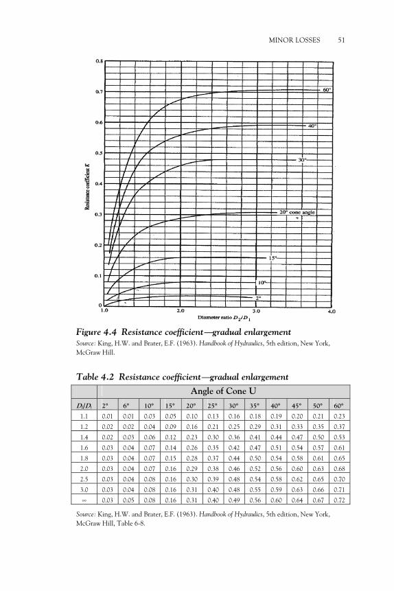
where v1 is the velocity in the smaller pipe ahead of the enlargement. The magnitude of K is dependent on both the diameter ratio D2/D1 and the cone angle θ. Data for various values of θ and D2/D1 are given in Figure 4.4 and Table 4.2.
Figure 4.3 Gradual enlargement �
MINOR LOSSES 51
Figure 4.4 Resistance coefficient—gradual enlargement
Source: King, H.W. and Brater, E.F. (1963). Handbook of Hydraulics, 5th edition, New York, McGraw Hill.
Table 4.2 Resistance coefficient—gradual enlargement � Angle of Cone U
D2/D1 2° 6° 10° 15° 20° 25° 30° 35° 40° 45° 50° 60°
1.1 0.01 0.01 0.03 0.05 0.10 0.13 0.16 0.18 0.19 0.20 0.21 0.23
1.2 0.02 0.02 0.04 0.09 0.16 0.21 0.25 0.29 0.31 0.33 0.35 0.37
1.4 0.02 0.03 0.06 0.12 0.23 0.30 0.36 0.41 0.44 0.47 0.50 0.53
1.6 0.03 0.04 0.07 0.14 0.26 0.35 0.42 0.47 0.51 0.54 0.57 0.61
1.8 0.03 0.04 0.07 0.15 0.28 0.37 0.44 0.50 0.54 0.58 0.61 0.65
2.0 0.03 0.04 0.07 0.16 0.29 0.38 0.46 0.52 0.56 0.60 0.63 0.68
2.5 0.03 0.04 0.08 0.16 0.30 0.39 0.48 0.54 0.58 0.62 0.65 0.70
3.0 0.03 0.04 0.08 0.16 0.31 0.40 0.48 0.55 0.59 0.63 0.66 0.71
∞ 0.03 0.05 0.08 0.16 0.31 0.40 0.49 0.56 0.60 0.64 0.67 0.72
Source: King, H.W. and Brater, E.F. (1963). Handbook of Hydraulics, 5th edition, New York, McGraw Hill, Table 6-8.

52 HYDRAULIC ENGINEERING
The energy loss calculated from Eq. (4.4) does not include the loss due to friction at the walls of the transition. For relatively steep cone angles, the length of the transition is short, and therefore, the wall fric-tion loss is negligible. However, as the cone angle decreases, the length of the transition increases and wall friction becomes significant. Taking both wall friction loss and the loss due to the enlargement into account, the minimum energy loss with a cone angle of about 7° is obtained.
4.2.1 Diffuser
Another term for an enlargement is a diffuser. The function of a diffuser is to convert kinetic energy (represented by the velocity head, v2/2g) to pressure energy (or otherwise called pressure head, p/�) by decelerating the fluid as it flows from the smaller to the larger pipe. The diffuser can be either sudden or gradual, but the term is most often used to describe a gradual enlargement.
An ideal diffuser is one in which no energy is lost as the flow decel-erates. Of course, no diffuser performs in the ideal fashion. If it did, the theoretical maximum pressure after the expansion could be computed from Bernoulli’s equation,
2 2A A B B
A B 2 2v P v P
z zg gγ γ
+ + = + +
If the diffuser is horizontal, the elevation terms get cancelled out. Then pressure recovery for an ideal diffuser is calculated from the equation,
2 2
A BB A
2v v
p P Pg
γ� �−Δ = − = � �� �
(4.5)
In a real diffuser, energy losses do occur and the general energy equa-tion must be used:
2 2A A B B
A L B 2 2v P v P
z h zg gγ γ
+ + − = + +
The pressure increases and becomes
2 2
A BB A L{ }
2v v
p P P hg
γ� �−Δ = − = −� �� �
(4.6)
MINOR LOSSES 53
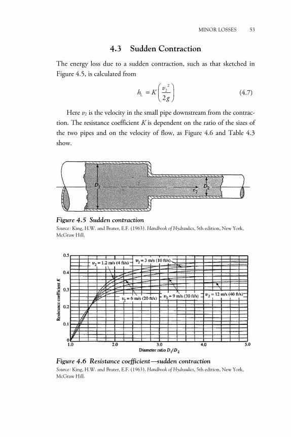
4.3 Sudden Contraction
The energy loss due to a sudden contraction, such as that sketched in Figure 4.5, is calculated from
2
2L 2
vh K
g� �
= � �� �
(4.7)
Here v2 is the velocity in the small pipe downstream from the contrac-tion. The resistance coefficient K is dependent on the ratio of the sizes of the two pipes and on the velocity of flow, as Figure 4.6 and Table 4.3 show.
Figure 4.5 Sudden contraction
Source: King, H.W. and Brater, E.F. (1963). Handbook of Hydraulics, 5th edition, New York, McGraw Hill.
Figure 4.6 Resistance coefficient—sudden contraction
Source: King, H.W. and Brater, E.F. (1963). Handbook of Hydraulics, 5th edition, New York, McGraw Hill. �

� Table
4.3
R
esis
tance
coe
ffic
ient—
sudden
con
tract
ion
�V
eloc
ity
2ν
D1/
D2
0.6m
/s
2 ft
/s
1.2
m/s
4 ft
/s
1.8
m/s
6 ft
/s
24 m
/s
8 ft
/s
3 m
/s
10 f
t/s
4.5
m/s
15 f
t/s
6 m
/s
20 f
t/s
9 m
/s
30 f
t/s
12 m
/s
40 f
t/s
1.0
0.
0
0.0
0.0
0
.0
0
.0
0
.0
0
.0
0.0
0
.0
1.1
0.03
0.
04
0.04
0.
04
0.04
0.
04
0.05
0.
05
0.06
1.
2 0.
07
0.07
0.
07
0.07
0.
08
0.08
0.
09
0.10
0.
11
1.4
0.17
0.
17
0.17
0.
17
0.18
0.
18
0.18
0.
19
0.20
1.
6 0.
26
0.26
0.
26
0.26
0.
26
0.25
0.
25
0.25
0.
24
1.8
0.34
0.
34
0.34
0.
33
0.33
0.
32
0.31
0.
29
0.27
2.
0 0.
38
0.37
0.
37
0.36
0.
36
0.34
0.
33
0.31
0.
29
2.2
0.40
0.
40
0.39
0.
39
0.38
0.
37
0.35
0.
33
0.30
2.
5 0.
42
0.42
0.
41
0.40
0.
40
0.38
0.
37
0.34
0.
31
3.0
0.44
0.
44
0.43
0.
42
0.42
0.
40
0.39
0.
36
0.33
4.
0 0.
47
0.46
0.
45
0.45
0.
44
0.42
0.
41
0.37
0.
34
5.0
0.48
0.
47
0.47
0.
46
0.45
0.
44
0.42
0.
38
0.35
10
.0
0.49
0.
48
0.48
0.
47
0.46
0.
45
0.43
0.
40
0.36
∞
0.
49
0.48
0.
48
0.47
0.
47
0.45
0.
44
0.41
0.
38
Sour
ce: K
ing,
H.W
. and
Bra
ter,
E.F.
(19
63).
Han
dboo
k of
Hyd
raul
ics ,
5th
edit
ion,
New
Yor
k, M
cGra
w H
ill.
54 HYDRAULIC ENGINEERING
MINOR LOSSES 55
2
L 2v
h kg
� �= � �
� �
Vena contracta
Turbulence zones
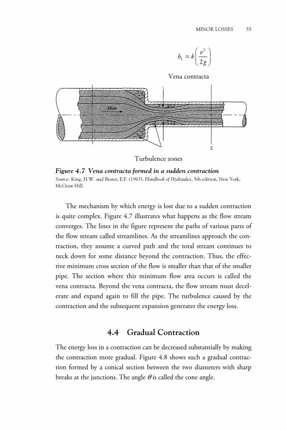
Figure 4.7 Vena contracta formed in a sudden contraction
Source: King, H.W. and Brater, E.F. (1963). Handbook of Hydraulics, 5th edition, New York, McGraw Hill.
The mechanism by which energy is lost due to a sudden contraction
is quite complex. Figure 4.7 illustrates what happens as the flow stream converges. The lines in the figure represent the paths of various parts of the flow stream called streamlines. As the streamlines approach the con-traction, they assume a curved path and the total stream continues to neck down for some distance beyond the contraction. Thus, the effec-tive minimum cross section of the flow is smaller than that of the smaller pipe. The section where this minimum flow area occurs is called the vena contracta. Beyond the vena contracta, the flow stream must decel-erate and expand again to fill the pipe. The turbulence caused by the contraction and the subsequent expansion generates the energy loss.
4.4 Gradual Contraction
The energy loss in a contraction can be decreased substantially by making the contraction more gradual. Figure 4.8 shows such a gradual contrac-tion formed by a conical section between the two diameters with sharp breaks at the junctions. The angle θ is called the cone angle.

56 HYDRAULIC ENGINEERING
Figure 4.8 Gradual contraction
Source: King, H.W. and Brater, E.F. (1963). Handbook of Hydraulics, 5th edition, New York, McGraw Hill.
Figure 4.9 shows the data for the resistance coefficient versus the
diameter ratio for several values of the cone angle. The energy loss is com-puted from Eq. (4.7), where the resistance coefficient is based on the velocity head in the smaller pipe after the contraction. These data are for Reynolds numbers greater than 1 × 10⁵. Note that for angles over the wide range of 15° to 40°, K = 0.05 or less, a very low value. For angles as high as 60°, K is less than 0.08.
As the cone angle of the contraction decreases below 15°, the resistance coefficient actually increases, as shown in Figure 4.10. The reason is that the data include the effects of both the local turbulence caused by flow separation and pipe friction. For the smaller cone angles, the transition between the two diameters is very long, which increases the friction losses.

MINOR LOSSES 57
Figure 4.9 Resistance coefficient—gradual contraction with θ ≥ 15°
Source: King, H.W. and Brater, E.F. (1963). Handbook of Hydraulics, 5th edition, New York, McGraw Hill.
Figure 4.10 Resistance coefficient—gradual contraction with θ ≤ 15°
Source: King, H.W. and Brater, E.F. (1963). Handbook of Hydraulics, 5th edition, New York, McGraw Hill.
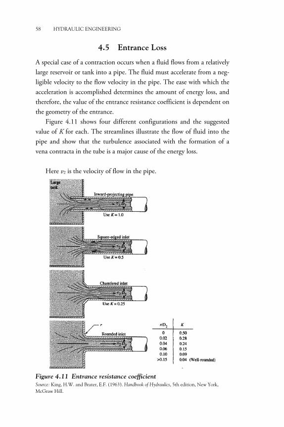
58 HYDRAULIC ENGINEERING
4.5 Entrance Loss
A special case of a contraction occurs when a fluid flows from a relatively large reservoir or tank into a pipe. The fluid must accelerate from a neg-ligible velocity to the flow velocity in the pipe. The ease with which the acceleration is accomplished determines the amount of energy loss, and therefore, the value of the entrance resistance coefficient is dependent on the geometry of the entrance.
Figure 4.11 shows four different configurations and the suggested value of K for each. The streamlines illustrate the flow of fluid into the pipe and show that the turbulence associated with the formation of a vena contracta in the tube is a major cause of the energy loss.
Here v2 is the velocity of flow in the pipe.
Figure 4.11 Entrance resistance coefficient
Source: King, H.W. and Brater, E.F. (1963). Handbook of Hydraulics, 5th edition, New York, McGraw Hill.

MINOR LOSSES 59
In summary, after selecting a value for the resistance coefficient from Figure 4.11, the energy loss at an entrance can be calculated from
2
2L 2
vh K
g� �
= � �� �
(4.8)
4.6 Exit Loss
As a fluid flows from a pipe into a large reservoir or tank, as shown in Fig-ure 4.12, its velocity is decreased to very nearly zero. In the process, the kinetic energy that the fluid possessed in the pipe, indicated by the velocity head v1
2/2g, is dissipated. Therefore, the energy loss for this condition is
2
1L 2
vh K
g� �
= � �� �
(4.9)
This is called the exit loss. The value of K = 1 is used regardless of the form of the exit where the pipe connects to the tank wall.
4.7 Resistance Coefficients for Valves and Fittings
Many different kinds of valves and fittings are available from several man-ufacturers for specification and installation into fluid flow systems. Valves are used to control the amount of flow; and they may be globe valves, angle valves, gate valves, butterfly valves, any of several types of check valves, and many more. Fittings direct the path of flow or cause a change in the size of the flow path, and these can include elbows of several de-signs, tees, reducers, nozzles, and orifices. See Figures 4.13 and 4.14.
Figure 4.12 Exit loss as the fluid flows into a static reservoir
Source: King, H.W. and Brater, E.F. (1963). Handbook of Hydraulics, 5th edition, New York, McGraw Hill.
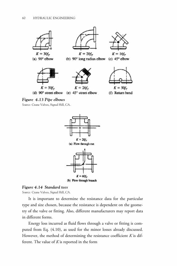
60 HYDRAULIC ENGINEERING
Figure 4.13 Pipe elbows
Source: Crane Valves, Signal Hill, CA.
Figure 4.14 Standard tees
Source: Crane Valves, Signal Hill, CA.
It is important to determine the resistance data for the particular type and size chosen, because the resistance is dependent on the geome-try of the valve or fitting. Also, different manufacturers may report data in different forms.
Energy loss incurred as fluid flows through a valve or fitting is com-puted from Eq. (4.10), as used for the minor losses already discussed. However, the method of determining the resistance coefficient K is dif-ferent. The value of K is reported in the form

MINOR LOSSES 61
eT
LK f
D� �= � �� �
(4.10)
The value of Le/D, called the equivalent length ratio, is reported in Table 4.4, and it is considered to be constant for a given type of valve or fitting. The value of Le is called the equivalent length and is the length of straight pipe of the same nominal diameter as the valve that would have the same resistance as the valve. The term D is the actual inside diameter of the pipe.
The term fT is the friction factor in the pipe to which the valve or fitting is connected, taken to be in the zone of complete turbulence. Note in Figure 3.2, the Moody diagram, that the zone of complete tur-bulence lies in the far right area where the friction factor is independent of Reynolds number. The dashed line running generally diagonally across the diagram divides the zone of complete turbulence from the transition zone to the left.
Values for fT vary with the size of the pipe and the valve, causing the value of the resistance coefficient K to also vary. Table 4.5 lists the val-ues of fT for standard sizes of new, clean, commercial steel pipes.
Some system designers prefer to compute the equivalent length of pipe for a valve and combine that value with the actual length of pipe. Equation (4.10) can be solved for Le:
e T
KDL
f� �
= � �� �
(4.11)
Table 4.4 Resistance in valves and fittings expressed as equivalent
length in pipe diameters, Le/D
Type Equivalent Length in Pipe
Diameters Le /D Globe valve—fully open 340 Angle valve—fully open 150 Gate valve—fully open 8
—¾ open 35 —½ open 160 —¼ open 900
Check valve—swing type 100 Check valve—ball type 150 Butterfly valve—fully open, 2–8 in 45
—10–14 in 35

62 HYDRAULIC ENGINEERING
Type Equivalent Length in Pipe
Diameters Le /D —16–24 in 25
Foot valve—poppet disc type 420 Foot valve—hinged disc type 75 90° standard elbow 30 90° long radius elbow 20 90° street elbow 50 45° standard elbow 16 45° street elbow 26 Close return bend 50 Standard tee—with flow through run 20
—with flow through branch 60
Source: Crane Valves, Signal Hill, CA.
Table 4.5 Friction factor in zone of complete turbulence for new,
clean, commercial steel pipes
Nominal Pipe Size (in)
Friction Factor fT
Nominal Pipe Size (in)
Friction Factor fT
½ 0.027 3½, 4 0.017 ¾ 0.025 5 0.016 1 0.023 6 0.015 1¼ 0.022 8–10 0.014 1½ 0.021 12–16 0.013 2 0.019 18–24 0.012 2½, 3 0.018
Source: Crane Valves, Signal Hill, CA.
It is given that Le = (Le/D). Note, however, that this would be valid only if the flow in the pipe is in the zone of complete turbulence.
If the pipe is made from a material different from new, clean, com-mercial steel pipe, it is necessary to compute the relative roughness D/ε, and then use the Moody diagram to determine the friction factor in the zone of complete turbulence.
4.8 Resistance Coefficient for Pipe Bends
It is frequently more convenient to bend a pipe or tube than to install a commercially made elbow. The resistance to flow of a bend is dependent on the ratio of the bend radius r to the pipe inside diameter D. Figure 4.15 shows that the minimum resistance for a 90° bend occurs when the ratio

MINOR LOSSES 63
r/D is approximately 3. The resistance is given in terms of the equivalent length ratio Le/D, and therefore, Eq. (4.10) must be used to calculate the resistance coefficient. The resistance shown in Figure 4.15 includes both the bend resistance and the resistance due to the length of the pipe in the bend.
When the r/D ratio is computed, r is defined as the radius to the centerline of the pipe or tube, called the mean radius (see Figure 4.16). That is, if Ro is the radius to the outside of the bend, Ri is the radius to the inside of the bend, and Do is the outside diameter of the pipe or tube, then
r = Ri + Do/2
r = Ro − Do/2
r = (Ro + Ri)/2
Figure 4.15 Resistance due to 90° pipe bends
Source: Beij, K.H. (1938). ‘‘Pressure Losses for Fluid Flow in 90° Pipe Bends.’’ Journal of Research of the National Bureau of Standards 21 (July): 1–18.

64 HYDRAULIC ENGINEERING
Figure 4.16 Resistance due to 90° pipe bends
Source: King, H.W. and Brater, E.F. (1963). Handbook of Hydraulics, 5th edition, New York, McGraw Hill.
Example Problem 1
Calculate the pressure in tank A, as shown in Figure 4.17. Account for all minor losses.
Solution:
Step 1. Write the energy equation
� 2 2A A B B
A L B 2 2v P v P
z h zg gγ γ
+ + − = + + �Step 2. vA = vB (pipe diameter does not change)
PB = 0 (pressure in tank B = 0, as it is open to atmosphere)
A B A L( ( ) )P z z hγ= − + �

MINOR LOSSES 65
Figure 4.17 Example 1
Step 3. Determine the hL Minor and major losses from tank A to tank B would be = en-trance loss + check valve + swing valve + friction + elbow + exit
Step 4.
hL = entrance loss + check valve + swing valve + friction + elbow + exit � L v T v T v v T v T v38
1 100 150 30 1 0.0525
h h f h f h f h f h f h= + + + + +
� L v (7.32 724 )h h f= +
From Table 4.5
fT = 0.019 (2-in. Schedule 40 steel pipe) � ( )2
v in pipe2v
hg
=
3
3 2
435 L/min 1 m /s3.344 m/s
2.168 10 m 60,000 L/minQ
vA −= = × =
×
� 2
v3.44 0.570 m
2 * 9.81h π= =

66 HYDRAULIC ENGINEERING
� ( )( )( )ρμ
ε
−
−
= = = ××
= =×
4R 3
5
3.344 0.0525 820N 8.47 10 ;
1.70 100.0525 1,141
4.60 10
vD
D
From Moody diagram
f = 0.022
Step 5.
A B A L ( ( ) )P z z hγ= − + = (0.82)(9.81 kN/m3)[4.5 m + 0.570 (7.32
+ 724(0.022))]
PA = 143.5 kPa

CHAPTER 5
Series and Parallel Pipeline Systems
As discussed in the previous chapter, fluid flow systems have numerous minor losses. In addition to these losses, pipeline systems for analysis purposes are classified into series pipeline systems and parallel pipeline systems.
5.1 Series Pipeline Systems
Series pipeline systems are those with a single flow path: all of the fluid must travel the same route. Because of that, conservation of mass and conservation of energy principles are used to develop the generalized form of the energy equation
2 21 1 2 2
1 L R A 2 2 2v P v P
z h h h zg gγ γ
+ + − − + = + +
The first three terms of the left-hand side of the equation represent the energy possessed by the fluid at point 1 in the form of pressure head, velocity head, and elevation head. The same can be applied for the terms on the right-hand side as the energy possessed by the fluid at point 2. The term hA is the energy added to the fluid by the pump, and this is termed as the total head on the pump and is used to select the different types of pumps. This will be discussed in the next chapter.
The term hL denotes the energy lost from the systems anywhere be-tween points 1 and 2. This can include major and minor losses.
2 2
L1
( )2 2
n
ii
v L vh K f
g D g=
= +� �

68 HYDRAULIC ENGINEERING
System analysis and design problems can be classified into three clas-ses as follows:
Class I: The system is completely defined in terms of the size of pipes, the types of minor losses that are present, and the volume flow rate of fluid in the system. The typical objective is to compute the pressure at some point of interest, to compute the total head on a pump, or to compute the elevation of a source of fluid to produce a desired flow rate or pressure at selected points in the system.
Steps to solve Class I problems: Flow rate (Q) and pipe diameter (D) are known; head loss (hL) is unknown.
i. Write down energy equation: P1/γ + z1 + v1
2/2g + hA – hL – hR = P2/γ + z2 + v2
2/2g ii. Identify all the terms that make up hL, such as pipe losses, hL = f
(L/D)v2/2g, and minor losses, hL = Kv2/2g. iii. By using Q, Q = v × π / 4 × D2, and D, solve for the velocity, v,
and determine the Reynolds number, NR, and the loss coeffi-cient, K.
iv. By using the Reynolds number, NR, and D/ε, determine the fric-tion factor, f, by using the Moody diagram or the appropriate friction factor equation. For minor losses, find fT (if required) by using D/ε only.
v. Determine hL and find the required output (e.g., hA, etc.).
Example Problem 1: Class I Type Problem
Calculate the power supplied to the pump, as shown in Figure 5.1, if its efficiency is 76 percent. Methyl alcohol at 25 °C is flowing at the rate of 54 m3/s. The suction line is a standard 4-in. Schedule 40 steel pipe, 15 m long. The total length of a 2-in. Schedule 40 steel pipe in the discharge line is 200 m. Assume that the entrance from reservoir 1 is through a square-edged inlet and that the elbows are standard. The valve is a fully open globe valve. The elevation difference between the two surfaces of the reservoirs was measured as 10 m.
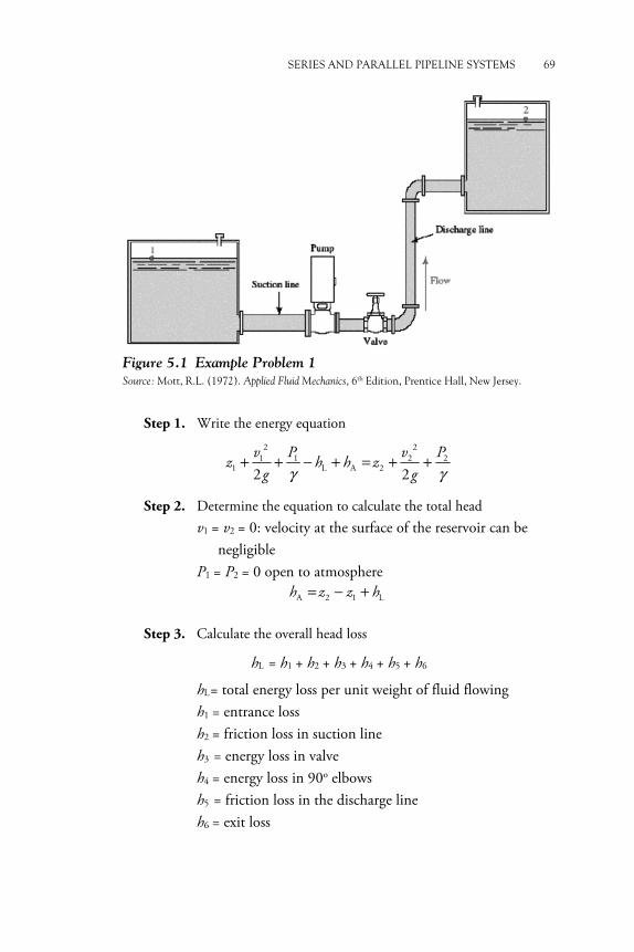
SERIES AND PARALLEL PIPELINE SYSTEMS 69
Figure 5.1 Example Problem 1
Source: Mott, R.L. (1972). Applied Fluid Mechanics, 6th Edition, Prentice Hall, New Jersey.
Step 1. Write the energy equation 2 2
1 1 2 21 L A 2
2 2v P v P
z h h zg gγ γ
+ + − + = + +
Step 2. Determine the equation to calculate the total head v1 = v2 = 0: velocity at the surface of the reservoir can be
negligible P1 = P2 = 0 open to atmosphere � A 2 1 L h z z h= − + �
Step 3. Calculate the overall head loss
hL = h1 + h2 + h3 + h4 + h5 + h6
hL= total energy loss per unit weight of fluid flowing h1 = entrance loss h2 = friction loss in suction line h3 = energy loss in valve h4 = energy loss in 90o elbows h5 = friction loss in the discharge line h6 = exit loss �

70 HYDRAULIC ENGINEERING
Step 4. Equation for energy loss 2s
1 (entrance loss)2v
h Kg
� �= � �
� �
2s
2 s ( ) (friction loss in suction line)2vL
h fD g
� �= � �
� �
2e d
3 dT (valve)2
L vh f
D g� �� �= � �� �
� �� �
2oe d
4 dT (two 90 elbows)2
L vh f
D g� �� �= � �� �
� �� �
2d
5 d ( ) (friction loss in discharge line)2vL
h fD g
� �= � �
� �
2d
6 1.0 (exit loss)2v
hg
� �= � �
� �
Step 5. Determine velocity in suction and discharge line
= × =3
354 m 1 hr 0.015 m /shr 3,600 s
Q
3
s 3 2s
0.015 m 1 1.83 m/ss 8.213*10 m
Qv
A −= = × =
2 2s (1.83 ) 0.17 m
2 2*9.81vg
= =
3
d 3 2d
0.015 m 1 6.92 m/ss 2.168*10 m
Qv
A −= = × =
2 2d (6.92 ) 2.44 m
2 2*9.81v
g= =
Step 6. Determine the friction factor in suction and discharge line Methyl alcohol at 25 oC Suction line
5R 4
(1.83)(0.1023)(789)N 2.60 *10
5.60 *10vDρ
μ −= = =

SERIES AND PARALLEL PIPELINE SYSTEMS 71
For steel pipe: ε −= × 54.6 10
224Dε
=
From Moody diagram: fs = 0.018 Discharge line
5R 4
(6.92)(0.0525)(789)N 5.12 *10
5.60 *10vDρ
μ −= = =
For steel pipe: 54.6 10−= ×
1,141Dε
=
From Moody diagram: fd = 0.020 Step 7. Determine total energy loss
h1 = 0.5(0.17 m) = 0.09 m (for a square-edged inlet, K = (0.5)(0.17))
( )2 15
0.018 0.17 0.45 m 0.1023
h � �= =� �� �
( )( ) e3 0.019 340 2.44 15.76 m ( 340 :
Dfully open globe valve)
Lh = = =
( )( ) o4 2*0.019 30 2.44 m 2.78 m (two 90 elbows)h = =
( )5 2000.020 2.44 185.9 m
0.0525h � �= =� �
� �
( )6 1.0 2.44 2.44 m (exit loss)h = =
hL = h1 + h2 + h3 + h4 + h5 + h6 = 207.4 m
Step 8. Determine total head
A 2 1 L h z z h= − +
hA = 10 m + 207.4 = 217.4 m �

72 HYDRAULIC ENGINEERING
Step 9. The power 3 3 3
A
M
2
(217.4 m)(7.74 *10 N / m )(0.015 m )Power
0.76m33.2 10 N. 33.2 kWs
h Qeγ
−
= =
= × =
Class II: The system is completely described in terms of its elevations, pipe sizes, valves and fittings, and allowable pressure drop at key points in the system. The objective is to determine the volume flow rate of the fluid that could be delivered by a given system.
Steps to solve Class II problem: Pipe diameter (D) and pressure drop, ΔP, are known; flow rate, Q, is unknown.
i. Write down the energy equation, P1/γ + z1 + v1
2/2g + hA – hL – hR = P2/γ + z2 + v2
2/2g ii. Separate known variables from unknown variables. Put the
known variables on the left-hand side of the equation and the unknowns on the right side.
iii. Identify all the terms that make up hL, such as pipe losses, hL = f(L/D)v2/2g, and minor losses, hL = Kv2/2g.
iv. Since flow rate, Q, is unknown, express hL as a function v and f, and solve for v.
v. Use D/ε to estimate an initial guess value for f, and find v. vi. Use the calculated v to determine the Reynolds number, NR, and
determine a new f value. vii. Find v (velocity) and repeat step vi until the f value converges to a
steady value. viii. Determine the flow rate, Q.
Example Problem 2: Class II Type (Iterative Method)
Hydraulic oil is flowing in a steel tube with an outside diameter of 2 in. and a wall thickness of 0.083 in (Figure 5.2). A pressure drop of 68 kPa is observed between two points in the tube 30 m apart. The oil has a specific gravity of 0.90 and dynamic viscosity of 3.0 × 10⁻³ Pa·s. Calcu-late the velocity of flow of the oil.

SERIES AND PARALLEL PIPELINE SYSTEMS 73
�Figure 5.2 Example Problem 2
Step 1. Apply the energy equation between the two points
γ γ+ + − = + +
2 21 1 2 2
1 L 22 2v P v P
z h zg g
z1 = z2: horizontal pipe
v1 = v2: same size diameter pipe
Step 2. Write the equation for head loss
( ) 22 1
L
3
kN68m 7.70 m
kN9.81 0.90m
P Ph
γ
� �� �− � �= = =
� �� �� �
2
L7.70 m 2
L vh f
D g= =
L2 2(9.81)(0.04658)(7.70) 0.235(30)
gDhv
fL f f= = =
6
0.04658 31,0531.5 10
Dε −= =
×
Step 3. Make assumptions for f and solve for v 1st Iteration: Try f = 0.03; then v = 2.80 m/s
4R 3
2.80 * 0.0468 * 900N 3.92 103 10
vDρμ −= = = ×
×
Use the Moody diagram and determine the friction factor. From the Moody diagram: f = 0.022 (new f ) 2nd Iteration: Try f = 0.022; then v = 3.27 m/s
4R 3
3.27 * 0.0468 * 900N 4.58 103 10
vDρμ −= = = ×
×
Use the Moody diagram and determine the friction factor.

74 HYDRAULIC ENGINEERING
From the Moody diagram: f = 0.0210 (new f ) 3rd Iteration: Try f = 0.0210; then v = 3.345 m/s
4R 3
3.345 * 0.0468 * 900N 4.69 103 10
vDρμ −= = = ×
×
Use the Moody diagram and determine the friction factor. From the Moody diagram: f = 0.0210 (no change) Hence, the velocity of flow of oil = 3.34 m/s.
Class III: The general layout of the system is known along with the de-sired volume flow rate. The size of the pipe required to carry a given volume flow rate of a given fluid is to be determined. Steps for Class III: Pressure drop, ΔP, and flow rate, Q, are known; D is unknown.
i. Write down the energy equation: P1/γ + z1 + v12/2g + hA – hL –
hR = P2/γ + z2 + v22/2g
ii. Separate known variables from the unknown variables. Put the known variables on the left-hand side of the equation and the unknowns on the right side.
iii. Identify all the terms that make up hL, such as pipe losses, hL = f(L/D)v2/2g, and minor losses, hL = Kv2/2g.
iv. Solve for D by using Q = v × π/4 × D2, and express it in terms of hL and f.
v. Make an initial guess value for f (between 0.01 and 0.1; f = 0.02 is usually a good initial guess), and find D.
vi. Determine NR and D/ε, and compute a new f value. vii. Find D and repeat Step vi until the f value converges to a steady
value. viii. Determine D. ix. Alternatively the flow diameter can be determined using the
equation listed below:
0.044.75 5.22
1.25 9.4
L L
0.66 LQ LD vQ
gh ghε� �� � � �� �= +� � � �� �� � � �� �
(5.1)

SERIES AND PARALLEL PIPELINE SYSTEMS 75
Example 3: Type III Problem
Compute the required size of a new Schedule 40 pipe that will carry 0.014 m3/s of water at 15 oC and limit the pressure drop to 13.79 kPa over a length of 30.5 m of horizontal pipe.
Solution:
Step 1. Write the energy equation 2 2
1 1 2 21 L 2
2 2v P v P
z h zg gγ γ
+ + − = + +
v1 = v2 z1 = z2
γ−= = =1 2
L 3
( ) 13.79 kPa 1.402 m9.81 kN/m
P Ph
Step 2. State the given information
Q = 0.014 m3/s; L = 30.5 m; g = 9.81 kN/m3
hL = 1.402 m; ε= 4.72 × 10⁻⁵ m; v = 1.15 × 10⁻⁶ m2/s
Step 3. Using Eq. (5.1) 0.044.75 5.22
1.25 9.4
L L
0.66 LQ LD vQ
gh gh
� �� � � �� �= +� � � �� �� � � �� �
−
−
� � �= � � �
� � �
����
�
� �+ × � �� �
4.7525 1.25
0.045.26 9.4
30.5 * 0.0140.66 (4.72 10 )
9.81*1.402
30.5(1.15 10 )(0.014)9.81*1.402
D
D = 0.098 m From the Appendix it is determined that D = 0.098 m would corre-
spond to a 4-in. Schedule 40 pipe.
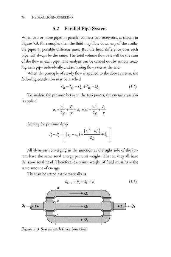
76 HYDRAULIC ENGINEERING
5.2 Parallel Pipe System
When two or more pipes in parallel connect two reservoirs, as shown in Figure 5.3, for example, then the fluid may flow down any of the availa-ble pipes at possible different rates. But the head difference over each pipe will always be the same. The total volume flow rate will be the sum of the flow in each pipe. The analysis can be carried out by simply treat-ing each pipe individually and summing flow rates at the end.
When the principle of steady flow is applied to the above system, the following conclusion may be reached
1 2 a b cQ Q Q Q Q= = + + (5.2)
To analyze the pressure between the two points, the energy equation is applied
� 2 21 1 2 2
1 L 2 2 2v P v P
z h zg gγ γ
+ + − = + + �Solving for pressure drop
� ( ) ( )2 22 1
1 2 2 1 L2
v vP P z z h
g
� �−− = − + +� �
� �� � �All elements converging in the junction at the right side of the sys-
tem have the same total energy per unit weight. That is, they all have the same total head. Therefore, each unit weight of fluid must have the same amount of energy.
This can be stated mathematically as
L1 2 a b ch h h h− = = = (5.3)
Figure 5.3 System with three branches

SERIES AND PARALLEL PIPELINE SYSTEMS 77
5.2.1 System with Two Branches
A common parallel piping system includes two branches arranged as shown in Figure 5.4. The analysis of this type of system is relatively simple and straightforward, although some iteration is typically required. Because velocities are unknown, friction factors are also unknown.
Figure 5.4 is used to illustrate the analysis of flow in two branches. The basic relationships that apply here are similar to Eqs. (5.2) and (5.3) except there are only two branches instead of three.
These relationships are
1 2 a bQ Q Q Q= = + (5.4)
L1 2 a bh h h− = = (5.5)
Below are the solution method for systems with two branches when the total flow rate and the description of the branches are known:
1. Equate the total flow rate to the sum of the flow rates in the two
branches, as stated in Eq. (5.4). Then express the branch flows as the product of the flow area and the average velocity; that is,
a a a b b b and Q A v Q A v= =
2. Express the head loss in each branch in terms of the velocity of flow in that branch and the friction factor. Include all significant losses due to friction and minor losses.
3. Compute the relative roughness for each branch, estimate the value of the friction factor for each branch, and complete the calculation of head loss in each branch in terms of the unknown velocities.
�Figure 5.4 System with two branches
78 HYDRAULIC ENGINEERING
4. Equate the expression for the head losses in the two branches to each other as stated in Eq. (5.5).
5. Solve for one velocity in terms of the other from the equation in Step 4.
6. Substitute the result from Step 5 into the flow rate equation devel-oped in Step 1, and solve for one of the unknown velocities.
7. Solve for the second unknown velocity from the relationship devel-oped in Step 5.
8. If there is doubt about the accuracy of the value of the friction fac-tor used in Step 2, compute the Reynolds number for each branch and reevaluate the friction factor from the Moody diagram or compute the values for the friction factor as described in the previ-ous sections.
9. If the values for the friction factor have changed significantly, re-peat Steps 3 to 8, using the new values for friction factor.
10. When satisfactory precision has been achieved, use the now-known velocity in each branch to compute the volume flow rate for that branch. Check the sum of the volume flow rates to ensure that it is equal to the total flow in the system.
11. Use the velocity in either branch to compute the head loss across that branch, employing the appropriate relationship from Step 3. This head loss is also equal to the head loss across the entire branched system.
Example Problem 4
In Figure 5.5, 100 gal/min of water at 60 °F is flowing in a 2-in. Schedule 40 steel pipe at section 1. The heat exchanger in branch “a” has a loss coefficient of K = 7.5 based on the velocity head in the pipe. All three valves are wide open. Branch “b” is a bypass line composed of 1¼-in. Schedule 40 steel pipe. The elbows are standard. The length of pipe be-tween points 1 and 2 in branch “b” is 6 m. Because of the size of the heat exchanger, the length of pipe in branch “a” is very short and friction losses can be neglected. For this arrangement, determine (a) the volume flow rate of water in each branch and (b) the pressure drop between points 1 and 2.

SERIES AND PARALLEL PIPELINE SYSTEMS 79
Figure 5.5 Example Problem 4
Step 1. Relate the two flow rates
1 a a b bQ A v A v= +
From the given data, Aa = 0.02333 ft2, Ab = 0.01039 ft2, and Q1 = 100 gal/min
33
1
ft1 s ft100 gal / min 0.223 s449 gal/minQ = × =
Step 2. Head losses in the two branches are equal. Considering the branch “a”
2 2a a
a 1 222 2v v
h K Kg g
� � � �= +� � � �
� � � �
where K1 = faT(Le/D) = resistance coefficient for each gate valve K2 = resistance coefficient for the heat exchanger = 7.5 (given) The following data are known: faT = 0.019 for a 2-in. Schedule 40 steel pipe faT = 8 for a fully open gate valve Then
K1 = faT(Le/D) = (0.019)(8) = 0.152
Then
( )2 2 2a a a
a 2 0.152 7.5 7.82 2 2v v v
hg g g
� � � � � �= + =� � � � � �
� � � � � �
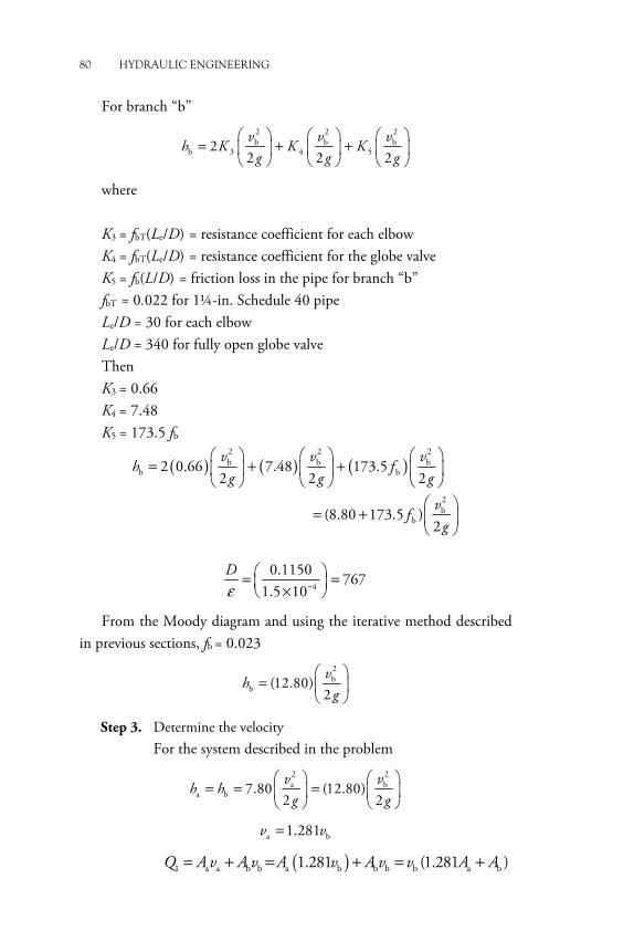
80 HYDRAULIC ENGINEERING
For branch “b” 2 2 2b b b
b 3 4 522 2 2v v v
h K K Kg g g
� � � � � �= + +� � � � � �
� � � � � �
where K3 = fbT(Le/D) = resistance coefficient for each elbow K4 = fbT(Le/D) = resistance coefficient for the globe valve K5 = fb(L/D) = friction loss in the pipe for branch “b” fbT = 0.022 for 1¼-in. Schedule 40 pipe Le/D = 30 for each elbow Le/D = 340 for fully open globe valve Then K3 = 0.66 K4 = 7.48 K5 = 173.5 fb
( ) ( ) ( )2 2 2b b b
b b
2b
b
2 0.66 7.48 173.52 2 2
(8.80 173.5 ) 2
v v vh f
g g g
vf
g
� � � � � �= + +� � � � � �
� � � � � �� �
= + � �� �
�4
0.1150 7671.5 10
Dε −
� �= =� �� �
From the Moody diagram and using the iterative method described in previous sections, fb = 0.023
2b
b (12.80) 2v
hg
� �= � �
� �
Step 3. Determine the velocity For the system described in the problem
2 2a b
a b 7.80 (12.80) 2 2v v
h hg g
� � � �= = =� � � �
� � � �
a b1.281v v=
( )1 a a b b a b b b b a b 1.281 (1.281 ) Q A v A v A v A v v A A= + = + = +

SERIES AND PARALLEL PIPELINE SYSTEMS 81
Solving for vb
( )= =
+ +
31
b 2a b
0.223 ft s(1.281 ) (1.281 0.02333 0.01039 t
/)f
Qv
A A
b 5.54 ft/sv =
aft ft1.281* 5.54 7.09s s
v = =
The calculations were made with an assumed value of fb; hence, the accuracy of the assumption needs to be checked.
b bRbN v D
ϑ=
Kinematic viscosity for water at 15 oC = 5 21.21 10 ft / sϑ −= ×
( )( ) 4Rb 5
5.54 0.1150N 5.26 10
1 .21 10−= = ××
Relative roughness was determined as 767; from the Moody diagram the new fb = 0.025. This value is significantly different from the initial assumed value. Hence
( )2 2
b bb 8.80 173.9 0.025 . 13.15
2 2v v
hg g
� �= + =� � � �� �
� �
Equating the head losses in the two branches ha = hb
2 2a b7.80 13.15 ( )
2 2v v
g g� �
=� �� �
Solving for velocities gives
va = 1.298vb
Substituting the equation for vb used earlier gives
( )( )3
b 2
0.223 ft /s 5.48 ft/s1.298 0.02333 0.01039 ft
v = =+
va = 1.298vb = 1.298(5.48) = 7.12 ft/s �

82 HYDRAULIC ENGINEERING
Recomputing the Reynolds number for branch “b”
( )( ) 4Rb 5
5.48 0.1150N 5.21 10
1 .21 10−= = ××
Using the Moody diagram, fb = 0.023 (no change). Step 4. Determine the flow rates
3
a a aft
0.02333 * 7.12 0.166 74.5 gal/mins
Q v A= = = =
3
b b bft
0.01039 * 5.48 0.057 25.5 gal/mins
Q v A= = = =
Part b: Determine the pressure drop Apply the energy equation between points 1 and 2
2 21 1 2 2
1 L 2 2 2v P v P
z h zg gγ γ
+ + − = + +
1 2L
P Ph
γ γ− =
1 2L
P Ph
γ γ− =
1 2L a bh h h−
= = 2 2a
a7.127.80 7.80 6.14 ft
2 64.4v
hg
� � � �= = =� � � �
� �� �
2
1 2 3 2
lb 1 ft62.4 6.14 ft 2.66 psi
ft 144 in.P P− = × × =
5.2.2 System with Three or More Branches
Hardy Cross Method
The Hardy Cross method is an iterative method for determining the flow in pipe network systems where the inputs and outputs are known, but the flow inside the network is unknown. The introduction of the Hardy Cross method for analyzing pipe flow networks revolutionized municipal water supply design. Before the method was introduced, solv-ing complex pipe systems for distribution was extremely difficult due to the nonlinear relationship between head loss and flow (Figure 5.6).
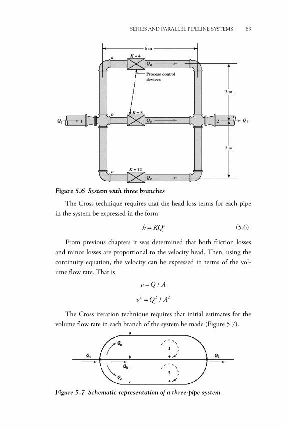
SERIES AND PARALLEL PIPELINE SYSTEMS 83
Figure 5.6 System with three branches
The Cross technique requires that the head loss terms for each pipe in the system be expressed in the form
nh KQ= (5.6)
From previous chapters it was determined that both friction losses and minor losses are proportional to the velocity head. Then, using the continuity equation, the velocity can be expressed in terms of the vol-ume flow rate. That is
/v Q A=
2 2 2/v Q A=
The Cross iteration technique requires that initial estimates for the volume flow rate in each branch of the system be made (Figure 5.7).
Figure 5.7 Schematic representation of a three-pipe system
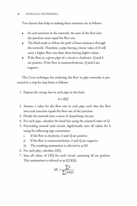
84 HYDRAULIC ENGINEERING
Two factors that help in making these estimates are as follows:
• At each junction in the network, the sum of the flow into the junction must equal the flow out.
• The fluid tends to follow the path of least resistance through the network. Therefore, a pipe having a lower value of K will carry a higher flow rate than those having higher values.
• If the flow in a given pipe of a circuit is clockwise, Q and h are positive. If the flow is counterclockwise, Q and h are negative.
The Cross technique for analyzing the flow in pipe networks is pre-
sented in a step-by-step form as follows: 1. Express the energy loss in each pipe in the form
2h KQ=
2. Assume a value for the flow rate in each pipe such that the flow into each junction equals the flow out of the junction.
3. Divide the network into a series of closed-loop circuits. 4. For each pipe, calculate the head loss using the assumed value of Q. 5. Proceeding around each circuit, algebraically sum all values for h
using the following sign convention: i. If the flow is clockwise, h and Q are positive. ii. If the flow is counterclockwise, h and Q are negative. iii. The resulting summation is referred to as �h.
6. For each pipe, calculate 2KQ. 7. Sum all values of 2KQ for each circuit, assuming all are positive.
This summation is referred to as �(2KQ).
(2 )h
KkQ
Δ = ��

SERIES AND PARALLEL PIPELINE SYSTEMS 85
8. For each pipe, calculate a new estimate for Q from
Q Q Q′ = − Δ
9. Repeat Steps 4 to 8 until �Q from Step 8 becomes negligibly small. The Q� value is used for the next cycle of iteration.
Example Problem 5
Find the flow rate of water at 60 oF in each; all pipes are 2½-in. Sched-ule 40 steel pipes, as shown in the figure below.
��For a 2½-in. Schedule 40 commercial steel pipe: D = 0.2058;
A = 0.03326 ft2 2 2
222 2
L v LQh KQ f f
D g D gA= = =
22fL
KD gA
=
Based on the length of the pipes
( )a b d e 2
(50)3,410
0.2058 (64.4)(0.03326)f
K K K K f= = = = =

86 HYDRAULIC ENGINEERING
�As described in the previous section, the clockwise flow is shown as
positive (+) sign.
( )c f 2
(30)2,046
0.2058 (64.4)(0.03326)f
K K f= = =
Values of f can be computed as
1,372Dε
=
RN vD QDAϑ ϑ
= =
For water at 60 oF: 5 21.21 10 ft /sϑ −= ×
( )5R 5
(0.2058)N 5.114 10
(0.03326)1.21 10Q
Q−= = ××
From Chapter 3, use the equation
2
0.9R
0.25
1 5.74log N3.7
f
Dε
=� � � � � � � +� �
� �� � � �� � � �� � �
2
4 0.9R
0.25
1 5.74log 1.970 10 N
f
−
=� � � +� �� �� � �

SERIES AND PARALLEL PIPELINE SYSTEMS 87
For Trial 1: Flow equation at nodes Qa + Qb = 1.2 Try Qa = 0.5 and Qb = 0.7 Qc + Qd = 0.5 Try Qc = 0.1 and Qd = 0.4 Qd – Qf = 0.3 Try Qd = 0.4 and Qf = 0.1 Qe + Qf = 0.6 Try Qf = 0.1 and Qe = 0.5 Qb + Qc = Qe + 0.3 0.7 + 0.1 = 0.5 + 0.3 (check) Compute the values of f using the equation above
Pipe f K Equation of K a 0.0197 67.18 3,410 fa b 0.0194 66.00 3,410 fb c 0.0233 47.65 2,046 fc d 0.0200 68.25 3,410 fd e 0.0197 67.18 3,410 fe f 0.0233 47.65 2,046 ff
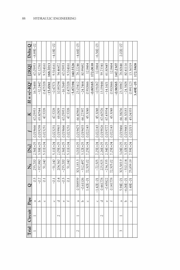
Tri
al
Cir
cuit
P
ipe
Q
NR
[NR]
f K
H
= +
/−K
Q2
[2K
Q]
Del
ta Q
1
1 a
0.5
255,
700
2.56
E+05
0.
0196
66
67.0
5953
16
.764
88
67.0
5953
−
8.89
E−02
b
−0.
7 −
357,
980
3.58
E+05
0.
0192
98
65.8
0544
−
32.2
447
92.1
2761
c 0.
1 51
,140
5.
11E+
04
0.02
3251
47
.570
8 0.
4757
08
9.51
4161
−
15.0
041
168.
7013
c −
0.1
−51
,140
5.
11E+
04
0.02
3251
47
.570
8 −
0.47
571
9.51
4161
−
4.18
E−02
2
d 0.
4 20
4,56
0 2.
05E+
05
0.01
9965
68
.080
9 10
.892
94
54.4
6472
e −
0.5
−25
5,70
0 2.
56E+
05
0.01
9666
67
.059
53
−16
.764
9 67
.059
53
f
0.1
51,1
40
5.11
E+04
0.
0232
51
47.5
708
0.47
5708
9.
5141
61
−5.
8719
4 14
0.55
26
2
1 a
0.58
8939
30
1,18
3.3
3.01
E+05
0.
0194
75
66.4
0968
23
.034
12
78.2
2246
−
4.66
E−03
b
−0.
6110
6 −
312,
497
3.12
E+05
0.
0194
35
66.2
7397
−
24.7
464
80.9
9492
c 1.
42E−
01
72,5
05.0
2 7.
25E+
04
0.02
2143
45
.304
8 0.
9106
66
12.8
464
−
0.80
165
172.
0638
c −
1.42
E−01
−
72,5
05
7.25
E+04
0.
0221
43
45.3
048
−0.
9106
7 12
.846
4 −
6.56
E−03
2
d 0.
4417
78
225,
925
2.26
E+05
0.
0198
26
67.6
0576
13
.194
44
59.7
3341
e −
0.45
822
−23
4,33
5 2.
34E+
05
0.01
9777
67
.439
34
−14
.160
1 61
.804
45
f
0.14
1778
72
,505
.02
7.25
E+04
0.
0221
43
45.3
048
0.91
0666
12
.846
4
−
0.96
565
147.
2307
3 1
a 5.
94E−
01
303,
565.
9 3.
04E+
05
0.01
9466
66
.380
36
23.3
8967
78
.806
46
2.02
E−07
b
−6.
06E−
01
−31
0,11
4 3.
10E+
05
0.01
9443
66
.301
83
−24
.380
8 80
.411
16
c
1.48
E−01
75
,859
.19
7.59
E+04
0.
0220
15
45.0
4355
0.
9911
23
13.3
6319
3.49
E−
05
172.
5808
88 HYDRAULIC ENGINEERING
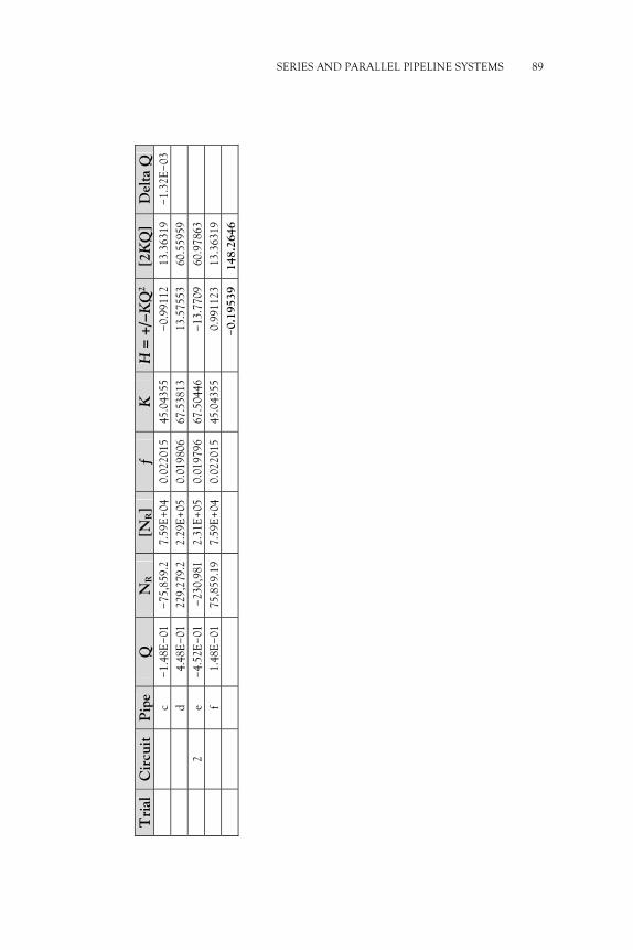
�
Tri
al
Cir
cuit
P
ipe
Q
NR
[NR]
f K
H
= +
/−K
Q2
[2K
Q]
Del
ta Q
c
−1.
48E−
01
−75
,859
.2
7.59
E+04
0.
0220
15
45.0
4355
−
0.99
112
13.3
6319
−
1.32
E−03
d
4.48
E−01
22
9,27
9.2
2.29
E+05
0.
0198
06
67.5
3813
13
.575
53
60.5
5959
2 e
−4.
52E−
01
−23
0,98
1 2.
31E+
05
0.01
9796
67
.504
46
−13
.770
9 60
.978
63
f
1.48
E−01
75
,859
.19
7.59
E+04
0.
0220
15
45.0
4355
0.
9911
23
13.3
6319
−
0.19
539
148.
2646
SERIES AND PARALLEL PIPELINE SYSTEMS 89�
90 HYDRAULIC ENGINEERING
As the �Q is negligibly small after three trials, the following Q can be accepted.
Summary of results from table: Qa = 0.594 Qb = 0.606 Qc = 0.148 Qd = 0.448 Qf = 0.148 Qe = 0.452

CHAPTER 6
Pumps and Turbines Hydraulic pumps are used in hydraulic drive systems and can be hydro-static or hydrodynamic. A hydraulic pump is a mechanical source of power that converts mechanical power into hydraulic energy (hydrostat-ic energy, i.e., flow, pressure). It generates flow with enough power to overcome pressure induced by the load at the pump outlet. When a hydraulic pump operates, it creates a vacuum at the pump inlet, which draws liquid from the reservoir into the inlet line to the pump and by mechanical action delivers this liquid to the pump outlet and forces it into the hydraulic system. In the previous chapter, the general energy equation was introduced to determine the energy added by a pump to the fluid as follows:
2 2B A B A
A B A L 2
v v P Ph z z h
g γ− −= − + + +
hA is the total head on the pump. Some pump manufacturers refer to this as the total dynamic head
(TDH). TDH is the total equivalent height that a fluid is to be pumped, tak-
ing into account friction losses in the pipe. As discussed in previous chapters, the power delivered to the fluid by
the pump can be calculated by the equation
A A P h Qγ=
The efficiency of the pump was determined by the equation
AM
I
Pe
P=

92 HYDRAULIC ENGINEERING
6.1 Types of Pumps
Pumps are categorized into two types on the response to changes in dis-charge pressure as shown in Figure 6.1. The basic difference between the two types is their response to changes in discharge pressure.
6.1.1 Dynamic Pumps
Dynamic pumps are pumps in which the energy is added to the water continuously and the water is not contained in a set volume. They are used in conditions where high volumes are required and a change in flow is not a problem. As the discharge pressure on a dynamic pump is increased, the quantity of water pumped is reduced. One type of dy-namic pump is the centrifugal pump. These are the most common pump used in water systems. Dynamic pumps can be operated for short periods of time with the discharge valve closed.
6.1.2 Displacement Pumps
Displacement pumps are pumps in which the energy is added to the water periodically and the water is contained in a set volume. Displace-ment pumps are used in conditions where relatively small, but precise, volumes are required. Displacement pumps will not change their vol-ume with a change in discharge pressure. Displacement pumps are also called positive displacement pumps. The most common positive dis-placement pump is the diaphragm pump used to pump chlorine and fluoride solutions. Operating a displacement pump with the discharge valve closed will damage the pump.
6.2 Dynamic Pumps/Centrifugal Pumps
Centrifugal pumps are used to transport fluids by the conversion of ro-tational kinetic energy to the hydrodynamic energy of the fluid flow. The rotational energy typically comes from an engine or electric motor. The fluid enters the pump impeller along or near to the rotating axis and is accelerated by the impeller, flowing radially outward into a dif-

PUMPS AND TURBINES 93
fuser or volute chamber (casing), from where it exits. Volute is a spiral-shaped casing surrounding a pump impeller that collects the liquid dis-charged by the impeller. For example, a snail shell is volute shaped as shown in Figure 6.2. The shape of the case helps to determine the direc-tion of rotation of the pump.
The direction of rotation can be determined when looking into the suction side of the volute case. For example, in Figure 6.3, the direction of rotation is counterclockwise.
Figure 6.1 Different types of pumps
Figure 6.2 Pump case or volute
Source: Grundfos Pumps, Downers Grove, IL.

94 HYDRAULIC ENGINEERING
Figure 6.3 Direction of flow
Source: Grundfos Pumps, Downers Grove, IL.
In summary, there are two theories that explain how a centrifugal pump works:
1. Energy transfer—the transfer of energy from the shaft to the impel-ler and from the impeller to the water
2. Centrifugal force—the force used to throw the water from the impeller
6.2.1 Types of Centrifugal Pumps
Centrifugal pumps can be divided into one of three classifications based on the configurations.
a. End-suction centrifugal pumps—The most common style of centrif-ugal pump. The center of the suction line is centered on the impeller eye. The impeller is attached directly onto the end of the motor shaft. End-suction centrifugal pumps are further classified as either frame-mounted or close-coupled (Figure 6.4).
Figure 6.4 End-suction centrifugal pump
Source: Grundfos Pumps, Downers Grove, IL.

PUMPS AND TURBINES 95
i Frame-mounted pumps—End-suction centrifugal pumps are designed so that the pump bearings and pump shaft are inde-pendent of the motor. This type of pump requires a coupling between the pump and the motor to transfer energy from the motor to the pump (Figure 6.5).
ii Close-coupled pumps—A close-coupled pump has only one shaft and one set of bearings: the motor shaft and bearings. The pump impeller is placed directly onto the motor shaft. Close-coupled pumps require less space and are less expensive than frame-mounted pumps (Figure 6.6).
b. Split case pumps—A centrifugal pump is designed so that the volute case is split horizontally. The case divides on a plane that cuts through the eye of the impeller. Split case pumps are unique. The case has a row of bolts that allow half of the case to be removed, providing access to the entire rotating assembly for inspection or re-moval. These pumps are normally found as fire service pumps and circulation pumps in medium-to-large communities (Figure 6.7).
Figure 6.5 Frame-mounted pump
Source: Grundfos Pumps, Downers Grove, IL.
Figure 6.6 Close-coupled pump
Source: Grundfos Pumps, Downers Grove, IL.
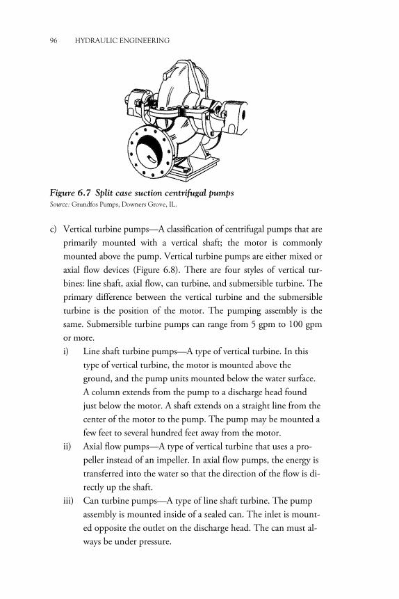
96 HYDRAULIC ENGINEERING
Figure 6.7 Split case suction centrifugal pumps
Source: Grundfos Pumps, Downers Grove, IL.
c) Vertical turbine pumps—A classification of centrifugal pumps that are primarily mounted with a vertical shaft; the motor is commonly mounted above the pump. Vertical turbine pumps are either mixed or axial flow devices (Figure 6.8). There are four styles of vertical tur-bines: line shaft, axial flow, can turbine, and submersible turbine. The primary difference between the vertical turbine and the submersible turbine is the position of the motor. The pumping assembly is the same. Submersible turbine pumps can range from 5 gpm to 100 gpm or more. i) Line shaft turbine pumps—A type of vertical turbine. In this
type of vertical turbine, the motor is mounted above the ground, and the pump units mounted below the water surface. A column extends from the pump to a discharge head found just below the motor. A shaft extends on a straight line from the center of the motor to the pump. The pump may be mounted a few feet to several hundred feet away from the motor.
ii) Axial flow pumps—A type of vertical turbine that uses a pro-peller instead of an impeller. In axial flow pumps, the energy is transferred into the water so that the direction of the flow is di-rectly up the shaft.
iii) Can turbine pumps—A type of line shaft turbine. The pump assembly is mounted inside of a sealed can. The inlet is mount-ed opposite the outlet on the discharge head. The can must al-ways be under pressure.

PUMPS AND TURBINES 97
Figure 6.8 Vertical turbine pumps
Source: Grundfos Pumps, Downers Grove, IL.
iv) Submersible turbine pumps—A style of vertical turbine pump in which the entire pump assembly and motor are submersed in the water. The motor is commonly mounted below the pump.
6.3 Positive Displacement Pumps
Although there are several different types of positive displacement pumps available, this section is limited to those commonly used in water systems.
6.3.1 Diaphragm Pumps
A diaphragm pump is operated by either electric or mechanical means (Figure 6.9). Two-valve assemblies: a suction-valve assembly and a dis-charge-valve assembly. When the diaphragm is pulled back, a vacuum is
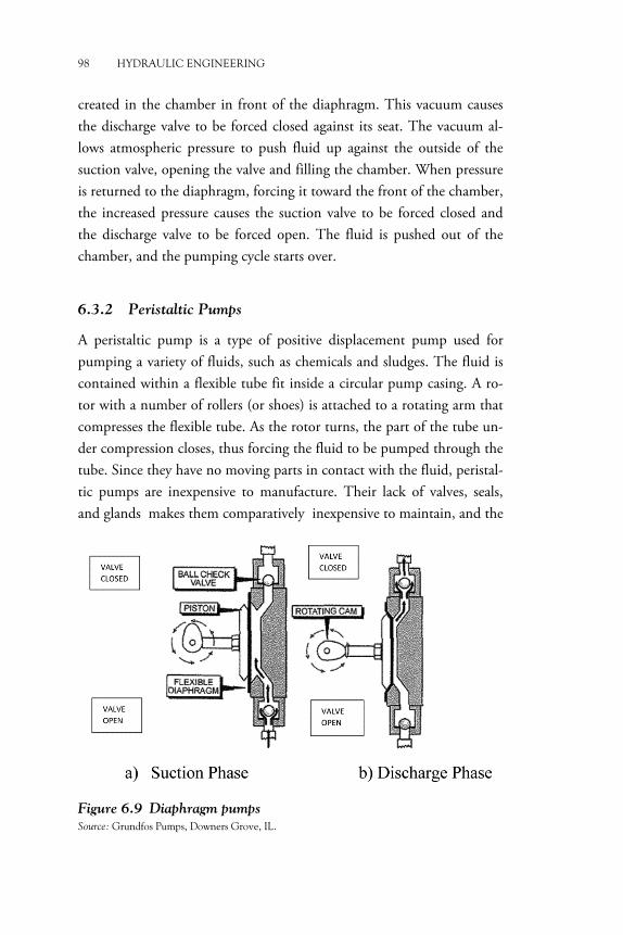
98 HYDRAULIC ENGINEERING
created in the chamber in front of the diaphragm. This vacuum causes the discharge valve to be forced closed against its seat. The vacuum al-lows atmospheric pressure to push fluid up against the outside of the suction valve, opening the valve and filling the chamber. When pressure is returned to the diaphragm, forcing it toward the front of the chamber, the increased pressure causes the suction valve to be forced closed and the discharge valve to be forced open. The fluid is pushed out of the chamber, and the pumping cycle starts over.
6.3.2 Peristaltic Pumps
A peristaltic pump is a type of positive displacement pump used for pumping a variety of fluids, such as chemicals and sludges. The fluid is contained within a flexible tube fit inside a circular pump casing. A ro-tor with a number of rollers (or shoes) is attached to a rotating arm that compresses the flexible tube. As the rotor turns, the part of the tube un-der compression closes, thus forcing the fluid to be pumped through the tube. Since they have no moving parts in contact with the fluid, peristal-tic pumps are inexpensive to manufacture. Their lack of valves, seals, and glands makes them comparatively inexpensive to maintain, and the
�Figure 6.9 Diaphragm pumps
Source: Grundfos Pumps, Downers Grove, IL.
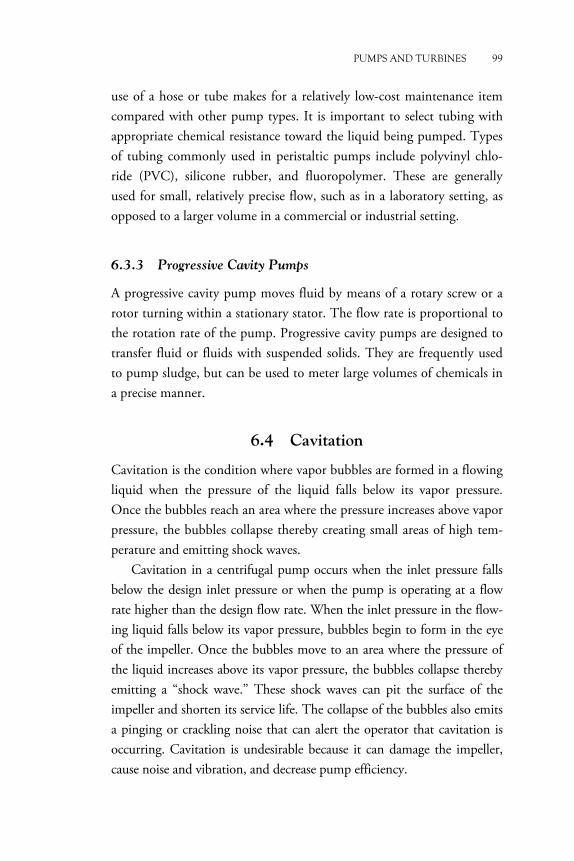
PUMPS AND TURBINES 99
use of a hose or tube makes for a relatively low-cost maintenance item compared with other pump types. It is important to select tubing with appropriate chemical resistance toward the liquid being pumped. Types of tubing commonly used in peristaltic pumps include polyvinyl chlo-ride (PVC), silicone rubber, and fluoropolymer. These are generally used for small, relatively precise flow, such as in a laboratory setting, as opposed to a larger volume in a commercial or industrial setting.
6.3.3 Progressive Cavity Pumps
A progressive cavity pump moves fluid by means of a rotary screw or a rotor turning within a stationary stator. The flow rate is proportional to the rotation rate of the pump. Progressive cavity pumps are designed to transfer fluid or fluids with suspended solids. They are frequently used to pump sludge, but can be used to meter large volumes of chemicals in a precise manner.
6.4 Cavitation
Cavitation is the condition where vapor bubbles are formed in a flowing liquid when the pressure of the liquid falls below its vapor pressure. Once the bubbles reach an area where the pressure increases above vapor pressure, the bubbles collapse thereby creating small areas of high tem-perature and emitting shock waves.
Cavitation in a centrifugal pump occurs when the inlet pressure falls below the design inlet pressure or when the pump is operating at a flow rate higher than the design flow rate. When the inlet pressure in the flow-ing liquid falls below its vapor pressure, bubbles begin to form in the eye of the impeller. Once the bubbles move to an area where the pressure of the liquid increases above its vapor pressure, the bubbles collapse thereby emitting a “shock wave.” These shock waves can pit the surface of the impeller and shorten its service life. The collapse of the bubbles also emits a pinging or crackling noise that can alert the operator that cavitation is occurring. Cavitation is undesirable because it can damage the impeller, cause noise and vibration, and decrease pump efficiency.
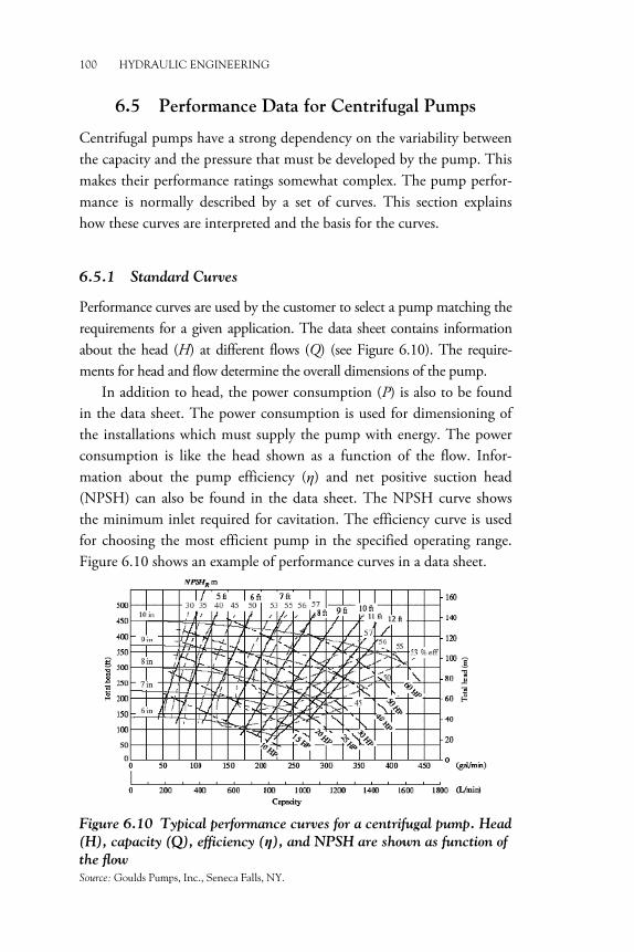
100 HYDRAULIC ENGINEERING
6.5 Performance Data for Centrifugal Pumps
Centrifugal pumps have a strong dependency on the variability between the capacity and the pressure that must be developed by the pump. This makes their performance ratings somewhat complex. The pump perfor-mance is normally described by a set of curves. This section explains how these curves are interpreted and the basis for the curves.
6.5.1 Standard Curves
Performance curves are used by the customer to select a pump matching the requirements for a given application. The data sheet contains information about the head (H) at different flows (Q) (see Figure 6.10). The require-ments for head and flow determine the overall dimensions of the pump.
In addition to head, the power consumption (P) is also to be found in the data sheet. The power consumption is used for dimensioning of the installations which must supply the pump with energy. The power consumption is like the head shown as a function of the flow. Infor-mation about the pump efficiency (�) and net positive suction head (NPSH) can also be found in the data sheet. The NPSH curve shows the minimum inlet required for cavitation. The efficiency curve is used for choosing the most efficient pump in the specified operating range. Figure 6.10 shows an example of performance curves in a data sheet.
Figure 6.10 Typical performance curves for a centrifugal pump. Head
(H), capacity (Q), efficiency (�), and NPSH are shown as function of
the flow
Source: Goulds Pumps, Inc., Seneca Falls, NY.

PUMPS AND TURBINES 101
6.5.2 Net Positive Suction Head
NPSH is a term describing conditions related to cavitation, which is undesired and harmful. Cavitation is the creation of vapor bubbles in areas where the pressure locally drops to the fluid vapor pressure. The extent of cavitation depends on how low the pressure is in the pump. Cavitation generally lowers the head and causes noise and vibration. Cavitation first occurs at the point in the pump where the pressure is lowest, which is most often at the blade edge at the impeller inlet, see Figure 6.11.
The NPSH value is absolute and always positive. Hence, it is not necessary to take the density of different fluids into account because NPSH can be stated in meters (m) or in feet (ft). Distinction is made between two different NPSH values: NPSHR and NPSHA.
NPSHA stands for NPSH available and is an expression of how close the fluid in the suction pipe is to vaporization. NPSHA is dependent on the vapor pressure of the fluid being pumped, energy losses in the suc-tion piping, the location of the fluid reservoir, and the pressure applied to the fluid in the reservoir. This can be expressed as
NPSHA = hsp ± hs − hf − hvp (6.1)
Figure 6.11 Cavitation
Source: Grundfos Pumps, Downers Grove, IL.

102 HYDRAULIC ENGINEERING
hsp = Static pressure head above the fluid in the reservoir, expressed in meters or feet of the liquid; sp /sph p γ=
psp = static pressure above the fluid in the reservoir hs = elevation difference from the level in the reservoir to the center-
line of the pump suction inlet, expressed in meters or feet If the pump is below the reservoir, hs is considered positive and if the
pump is above the reservoir, hs is considered negative. hf = head loss in the suction piping due to friction and minor losses,
expressed in meters or feet hvp = vapor pressure head of the liquid at the pumping temperature,
expressed in meters or feet; vp vp /h p γ=
pvp = vapor pressure of the liquid at the pumping temperature NPSHR is the minimum pressure required at the suction port of the
pump to keep the pump from cavitation. NPSHR is a function of the pump and must be provided by the pump manufacturer. NPSHA must be greater than NPSHR for the pump system to operate without cavita-tion and is generally given by the equation
A RNPSH 1.10 NPSH> (6.2)
The data given in pump catalogs for NPSH are for water and apply only to the listed operating speed. If the pump is operated at a different speed, the NPSH required at the new speed can be calculated from
( )2
2R 2 R 1
1
(NPSH ) NPSHNN
� �= � �� �
(6.3)
where the subscript 1 refers to catalog data and the subscript 2 refers to conditions at the new operating speed. The pump speed in rpm is N.
Example Problem 1
Determine the available NPSH for the system shown in Figure 6.12(a). The fluid reservoir is a closed tank with a pressure of −20 kPa above water at 70 °C. The atmospheric pressure is 100.5 kPa. The water level in the tank is 2.5 m above the pump inlet. The pipe is a 1.5-in. Sched-ule 40 steel pipe with a total length of 12.0 m. The elbow is standard and the valve is a fully open globe valve. The flow rate is 95 L/min.

PUMPS AND TURBINES 103
Figure 6.12 The pump suction-line details and definitions of terms for
computing NPSH
Solution:
Absolute pressure = Atmospheric pressure + Tank gage pressure
pabs = 100.5 kPa − 20 kPa = 80.5 kPa
However, it is given that
γ×= = =×
3 2
3 3
80.5 10 N/m 8.39 m9.59 10 N/m
abssp
ph
Based on the elevation of the tank
hs = + 2.5 m
To find the friction loss, we must find the velocity, Reynolds num-ber, and friction factor:
−= = × =×
3
3 2
95 L/min 1.0 m 1.21 m/s1.314 10 m 60,000 L/min
Qv
A
5R 7
1.21 0.0409N 1.20 10 (turbulent)
4.11 10vDϑ −
×= = = ××
5
0.0409889
4.6 10Dε −= =
×
From the Moody diagram, f = 0.0225; from previous chapters, fT = 0.021. From Figure 6.12(a).

104 HYDRAULIC ENGINEERING
( ) ( )2 2 2 2
h 2 30 340 1.02 2 2 2f T T
L v v v vf f f
D g g g g� � � � � �� �= + + +� � � � � �� �
� �� � � � � �
Pipe Elbow Valve Entrance
The velocity head is 2 21.21
0.0746 m2 2 9.81v
g� �
= =� �� �
Then the friction loss is
( ) ( )( )
( )( )
12h 0.0225 0.0746 2(0.021) 30 0.07460.0409
0.021 340 0.0746 0.0746
f� �= +� �� �
+ +
hf = 1.19 m
From Table 6.1: hvp = 3.25m at 70 oC
NPSHA = hsp ± hs − hf − hvp = 8.9 m + 2.5 m − 1.19m − 3.25 m = 6.45 m
It is known that NPSHA > 1.10 NPSHR
NPSHR < NPSHA/1.10
NPSHR < 6.45/1.10 = 5.86 m
Table 6.1 Vapor pressure and vapor pressure head
Temperature (°C)
Temperature (°F)
Vapor Pressure
(kPa)
Vapor Pressure
(psi)
Vapor Pressure
Head (m)
Vapor Pressure
Head (ft)
0 32 0.6113 0.08854 0.06226 0.2043 5 40 0.8726 0.1217 0.08894 0.2807 10 50 1.2281 0.1781 0.1253 0.4109 15 60 1.7056 0.2563 0.1795 0.5917 20 70 2.3388 0.3631 0.2338 0.8393 30 80 4.2455 0.5069 0.4345 1.173 40 90 7.3814 0.6979 0.758 1.618 50 100 12.344 0.9493 1.272 2.205 60 120 19.932 1.692 2.066 3.948 70 140 31.176 2.888 3.25 6.775 80 160 47.373 4.736 4.967 11.18 90 180 70.117 7.507 7.405 17.55 95 202 84.529 11.52 9.9025 27.59 100 212 101.32 14.69 10.78 35.36
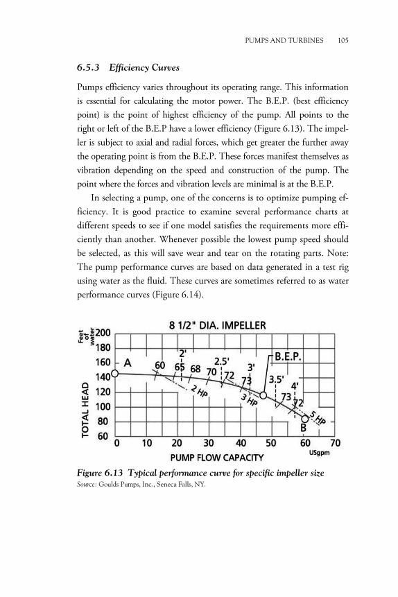
PUMPS AND TURBINES 105
6.5.3 Efficiency Curves
Pumps efficiency varies throughout its operating range. This information is essential for calculating the motor power. The B.E.P. (best efficiency point) is the point of highest efficiency of the pump. All points to the right or left of the B.E.P have a lower efficiency (Figure 6.13). The impel-ler is subject to axial and radial forces, which get greater the further away the operating point is from the B.E.P. These forces manifest themselves as vibration depending on the speed and construction of the pump. The point where the forces and vibration levels are minimal is at the B.E.P.
In selecting a pump, one of the concerns is to optimize pumping ef-ficiency. It is good practice to examine several performance charts at different speeds to see if one model satisfies the requirements more effi-ciently than another. Whenever possible the lowest pump speed should be selected, as this will save wear and tear on the rotating parts. Note: The pump performance curves are based on data generated in a test rig using water as the fluid. These curves are sometimes referred to as water performance curves (Figure 6.14).
Figure 6.13 Typical performance curve for specific impeller size
Source: Goulds Pumps, Inc., Seneca Falls, NY.
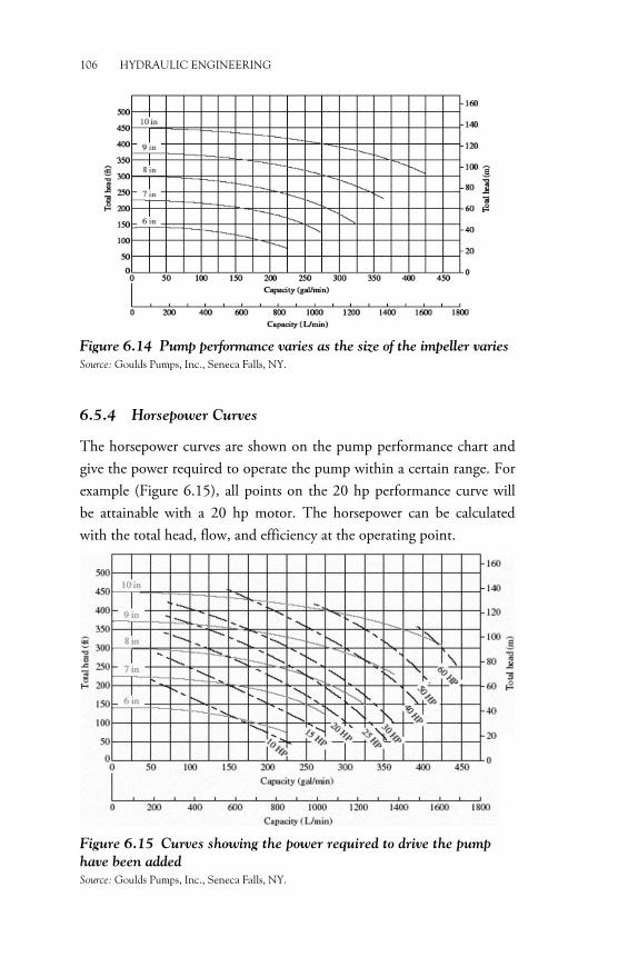
106 HYDRAULIC ENGINEERING
Figure 6.14 Pump performance varies as the size of the impeller varies
Source: Goulds Pumps, Inc., Seneca Falls, NY.
6.5.4 Horsepower Curves
The horsepower curves are shown on the pump performance chart and give the power required to operate the pump within a certain range. For example (Figure 6.15), all points on the 20 hp performance curve will be attainable with a 20 hp motor. The horsepower can be calculated with the total head, flow, and efficiency at the operating point.
Figure 6.15 Curves showing the power required to drive the pump
have been added
Source: Goulds Pumps, Inc., Seneca Falls, NY.
PUMPS AND TURBINES 107
6.5.5 Affinity Laws for Centrifugal Pumps
It is important to understand the manner in which capacity, head, and power vary when either speed or impeller diameter is varied. These rela-tionships, called affinity laws, are listed here. The symbol N refers to the rotational speed of the impeller, usually in revolutions per minute (r/min, or rpm). The affinity laws are useful as they allow prediction of the head discharge characteristic of a pump or fan from a known charac-teristic measured at a different speed or impeller diameter. The only requirement is that the two pumps or fans are dynamically similar; that is, the ratios of the fluid forced are the same.
Law 1. With impeller diameter (D) held constant: Law 1a. Flow is proportional to shaft speed:
1 1
2 2
Q NQ N
= (6.4)
Law 1b. Pressure or head is proportional to the square of shaft speed:
2
1 1
2 2
H NH N
� �= � �� �
(6.5)
Law 1c. Power is proportional to the cube of shaft speed:
3
1 1
2 2
P NP N
� �= � �� �
(6.6)
Law 2. With shaft speed (N) held constant: Law 2a. Flow is proportional to the impeller diameter:
1 1
2 2
Q DQ D
= (6.7)
Law 2b. Pressure or head is proportional to the square of impeller diameter:
2
1 1
2 2
H DH D
� �= � �� �
(6.8) �

108 HYDRAULIC ENGINEERING
Law 2c. Power is proportional to the cube of impeller diameter:
3
1 1
2 2
P DP D
� �= � �� �
(6.9)
where • Q is the volumetric flow rate (e.g., GPM or L/s), • D is the impeller diameter (e.g., in or mm), • N is the shaft rotational speed (e.g., rpm), • H is the pressure or head developed by the fan/pump (e.g.,
psi or Pascal), and • P is the shaft power (e.g., W).
These laws assume that the pump/fan efficiency remains constant,
i.e., η1 = η2, which is rarely exactly true, but can be a good approxima-tion when used over appropriate frequency or diameter ranges (i.e., a fan will not move anywhere near 1,000 times as much air when spun at 1,000 times its designed operating speed, but it may increase the flow by 99 percent when the operating speed is doubled). The exact relationship between speed, diameter, and efficiency depends on the particulars of the individual fan or pump design. Product testing or computational fluid dynamics become necessary if the range of acceptability is un-known, or if a high level of accuracy is required in the calculation. In-terpolation from accurate data is also more accurate than the affinity laws. When applied to pumps, the laws work well for the constant diameter variable speed case (Law 1) but are less accurate for the con-stant speed variable impeller diameter case (Law 2).
Example Problem 2
Assume that the pump for which the performance data are plotted in Figure 6.16 was operating at a rotational speed of 1,750 rpm and that the impeller diameter was 330 mm. First determine the head that would result in a capacity of 5,670 L/min (1,500 gal/min) and the power re-quired to drive the pump. Then, compute the performance at a speed of 1,250 rpm.

PUMPS AND TURBINES 109
Figure 6.16 Complete performance rating of a pump, superimposing
head, efficiency, and power curves and plotting all three versus
capacity
From Figure 6.16 projecting upward from Q1 = 5,670 L/min (1,500 gal/min) gives
Total head = 40 m = ha1
Power required = 37 kW = P1
When the speed is changed to 1,250 rpm, the new performance can be computed by using the affinity laws:
Capacity: Q2 = Q1 (N2/N1) = 5,670(1,250/1,750) = 4,050 L/min Head: ha2 = ha1(N2/N1)2 = 40(1,250/1,750)2 = 20.4 m Power: P2 = P1(N2/N1)3 = 37(1,250/1,750)3 = 13.5 kW
Note the significant decrease in the power required to run the pump. If the capacity and the available head are adequate, large savings in energy costs can be obtained by varying the speed of operation of a pump.
6.6 Coverage Chart for Centrifugal Pumps
A coverage chart (Figure 6.17) makes it possible to do a preliminary pump selection by looking at a wide range of pump casing sizes for a specific impeller speed. This chart helps to narrow down the choice of pumps that will satisfy the system requirements.
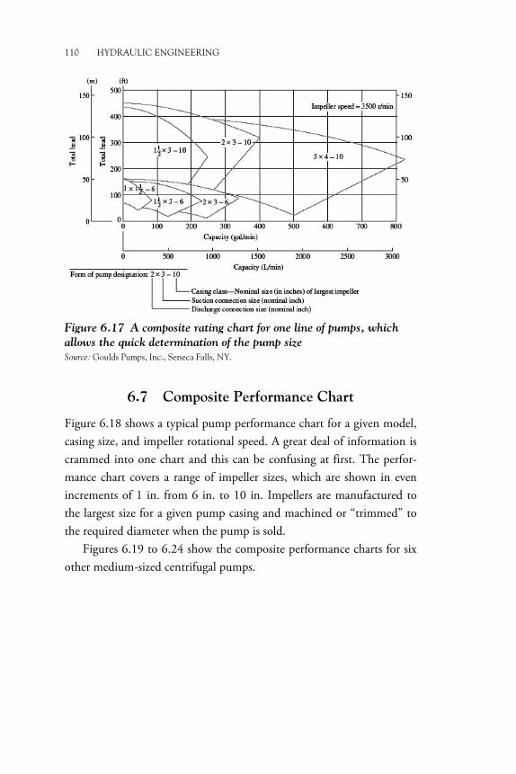
110 HYDRAULIC ENGINEERING
Figure 6.17 A composite rating chart for one line of pumps, which
allows the quick determination of the pump size
Source: Goulds Pumps, Inc., Seneca Falls, NY.
6.7 Composite Performance Chart
Figure 6.18 shows a typical pump performance chart for a given model, casing size, and impeller rotational speed. A great deal of information is crammed into one chart and this can be confusing at first. The perfor-mance chart covers a range of impeller sizes, which are shown in even increments of 1 in. from 6 in. to 10 in. Impellers are manufactured to the largest size for a given pump casing and machined or “trimmed” to the required diameter when the pump is sold.
Figures 6.19 to 6.24 show the composite performance charts for six other medium-sized centrifugal pumps.

PUMPS AND TURBINES 111
Figure 6.18 All the data are put together on one chart, so the user
can see all important parameters at the same time
Source: Goulds Pumps, Inc., Seneca Falls, NY.
Figure 6.19 The performance of a 1.5 × 3, 6 centrifugal pump at
1,750 rpm.
Source: Goulds Pumps, Inc., Seneca Falls, NY.

112 HYDRAULIC ENGINEERING
Figure 6.20 The performance of a 3 × 4, 10 centrifugal pump at
1,750 rpm
Source: Goulds Pumps, Inc., Seneca Falls, NY.)
Figure 6.21 The performance of a 3 × 4, 13 centrifugal pump at
1,750 rpm
Source: Goulds Pumps, Inc., Seneca Falls, NY.
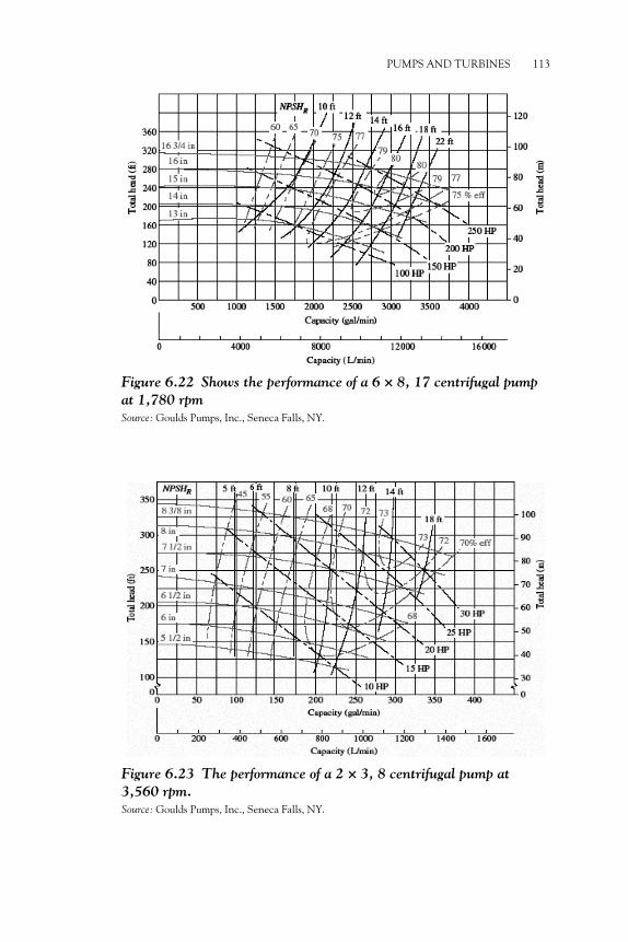
PUMPS AND TURBINES 113
Figure 6.22 Shows the performance of a 6 × 8, 17 centrifugal pump
at 1,780 rpm
Source: Goulds Pumps, Inc., Seneca Falls, NY.
Figure 6.23 The performance of a 2 × 3, 8 centrifugal pump at
3,560 rpm.
Source: Goulds Pumps, Inc., Seneca Falls, NY.

114 HYDRAULIC ENGINEERING
Figure 6.24 The performance of a 1.5 × 3, 13 centrifugal pump at
3,560 rpm
Source: Goulds Pumps, Inc., Seneca Falls, NY.
6.8 Operating Point of a Pump and Pump Selection
The operating point of a pump is defined as the volume flow rate it will deliver when installed in a given system. The total head developed by the pump is determined by the system resistance corresponding to the same volume flow rate. Figure 6.25 illustrates the concept.
Figure 6.25 Operating point of a pump �

PUMPS AND TURBINES 115
The pump is holding the fluid at the elevation of the destination point in the system and maintaining the fluid pressure at that point. This point is called the total static head, where
( )2 12 1h o
p pz z
γ−= + − (6.10)
This equation, derived from the energy equation, illustrates that the pump must develop a head equal to the pressure head difference be-tween the two reference points plus the elevation head difference before any flow is delivered. As the flow increases with its corresponding in-crease in total head, the system curve eventually intersects the pump rating curve. Where the system curve and the pump rating curve inter-sect is the true operating point of the pump in this system.
Example Problem 3
A centrifugal pump must deliver at least 945 L/min of water at a total head of 91 m (300 ft) of water. Specify a suitable pump. List its perfor-mance characteristics.
Solution:
From Figure 6.18 it can be determined that the pump with a 0.23-m (9-in.) impeller will deliver approximately 1,040 L/min (275 gal/min) at 91 m (300 ft) of head. At this operating point, the efficiency would be 57 percent, near the maximum for this type of pump. Approximately 28 kW (37 hp) would be required. The NPSHR at the suction inlet to the pump is approximately 2.8 m (9.2 ft) of water.
Example Problem 4
Figure 6.26 shows a system in which a pump is required to deliver at least 850 L/min of water at 15 °C from a lower reservoir to an elevated tank maintained at a pressure of 240 kPa gage. Length of suction line is 2.44 m and discharge line is 110 m. Design the system and specify a suitable pump.

116 HYDRAULIC ENGINEERING
Figure 6.26 Example Problem 4
Solution:
Step 1. fluid—water at 15 °C (Q = 850 L/min minimum) Source: lower reservoir; p = 0 kPa Elevation = 2.4 m above pump inlet Destination: upper reservoir; p = 240 kPa Elevation = 26.8 m above pump inlet
Step 2. Water at 15 °C:
� = 9.80 kN/m3; υ = 1.12 × 10⁻⁶ m2/s; hvp = 0.182 m.
Step 3. Figure 6.26 shows the proposed layout. Step 4. Design decisions—Suction line is 2.4 m long; discharge line is
110 m. �

PUMPS AND TURBINES 117
Step 5. Suction pipe is 3.5-in. Schedule 40 steel pipe; D = 0.09 m;
A = 6.381 × 10⁻³ m2
Discharge line is 2.5-in. Schedule 40 steel pipe; D = 0.063 m; A = 3.09 × 10⁻³ m2
Step 6. Reference point 1 is the surface of the lower reservoir. Refer-ence point 2 is the surface of the upper reservoir. Computing all the major and minor losses through the system, the head loss hL was determined to be 41.42 m. The result for the total dynamic head is given by
( ) 22 1 L 24.4 24.5 41.42 90.32 ma
ph z z h
γ= − + + = + + =
Step 7. Total static head is
( ) 2 1o 2 1
( )24.4 24.4 48.9 m
p ph z z
γ−= − + = + =
Step 8. Pump selection—From Figure 6.17: 2 × 3, 10 centrifugal pump operating at 3,500 rpm. The desired operating point lies be-tween the curves for the 8-in. and 9-in. impellers. We specify the 9-in. impeller diameter so the capacity is greater than the minimum of 850 L/min or 0.014 m3/s.
6.9 Pumps Operating in Parallel or Series
Many fluid flow systems require largely varying flow rates that are diffi-cult to provide with one pump without calling for the pump to operate far off its best efficiency point.
When two or more pumps are arranged in parallel, their resulting performance curve is obtained by adding their flow rates at the same head as indicated in Figure 6.27. Centrifugal pumps in parallel are used to overcome larger volume flows than one pump can handle alone.
When two (or more) pumps are arranged in series, their resulting pump performance curve is obtained by adding their heads at the same flow rate as indicated in the Figure 6.28. Directing the output of one pump to the inlet of a second pump allows the same capacity to be ob-tained at a total head equal to the sum of the ratings of the two pumps. This method permits operation against unusually high heads.

118 HYDRAULIC ENGINEERING
Figure 6.27 Performance of two pumps in parallel
Figure 6.28 Performance of two pumps in series
6.10 Life Cycle Cost of Pumps
The term life cycle cost (LCC) refers here to the consideration of all factors that make up the cost of acquiring, maintaining, and operating a pumped fluid system.
Good design practice seeks to minimize LCC by quantifying and computing the sum of the following factors:
PUMPS AND TURBINES 119
1. Initial cost to purchase the pump, piping, valves and other accesso-ries, and controls.
2. Cost to install the system and put it into service. 3. Energy cost required to drive the pump and auxiliary components
of the system over the expected life. 4. Operating costs related to managing the system including labor and
supervision. 5. Maintenance and repair costs over the life of the system to keep the
pump operating at design conditions. 6. Cost of lost production of a product during pump failures or when
the pump is shut down for maintenance. 7. Environmental costs created by spilled fluids from the pump or
related equipment. 8. Decommissioning costs at the end of the useful life of the pump,
including disposal of the pump and cleanup of the site. �

�
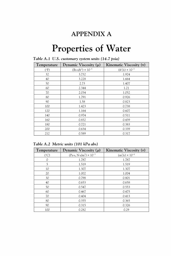
APPENDIX A
Properties of Water Table A.1 U.S. customary system units (14.7 psia)
Temperature Dynamic Viscosity (μ) Kinematic Viscosity (�) (oF) (lbf·s/ft2) × 10−5 (ft2/s) × 10−5 32 3.732 1.924 40 3.228 1.664 50 2.73 1.407 60 2.344 1.21 70 2.034 1.052 80 1.791 0.926 90 1.58 0.823
100 1.423 0.738 120 1.164 0.607 140 0.974 0.511 160 0.832 0.439 180 0.721 0.383 200 0.634 0.339 212 0.589 0.317
Table A.2 Metric units (101 kPa abs)
Temperature Dynamic Viscosity (μ) Kinematic Viscosity (�) (oC) (Pa·s, N·s/m2) × 10−3 (m2/s) × 10−6
0 1.787 1.787 5 1.519 1.519 10 1.307 1.307 20 1.002 1.004 30 0.798 0.801 40 0.653 0.658 50 0.547 0.553 60 0.467 0.475 70 0.404 0.413 80 0.355 0.365 90 0.315 0.326 100 0.282 0.29


APPENDIX B
Properties of Common Liquids
Table B.1 SI units (101 kPa and 25 °C)
Fluid
Specific Gravity (s.g.)
Specific Weight (�) (kN/m3)
Density (kg/m3)
Dynamic Viscosity
(Pa·s)
Kinematic Viscosity
(m2/s) Acetone 0.787 7.72 787 3.16E−04 4.02E−07 Ethyl alcohol 0.787 7.72 787 1.00E−03 1.27E−06 Methyl alcohol 0.789 7.74 789 5.60E−04 7.10E−07 Propyl alcohol 0.802 7.87 802 1.62E+01 2.02E−02 Aqua ammonia 0.91 8.93 910 Benzene 0.876 8.59 876 6.03E−04 6.88E−07 Carbon tetrachloride 1.59 15.60 1,590 9.10E−04 5.72E−07 Castor oil 0.96 9.42 960 6.51E−01 6.78E−04 Ethylene glycol 1.1 10.79 1,100 1.62E−02 1.47E−05 Gasoline 0.68 6.67 680 2.87E−04 4.22E−07 Glycerine 1.258 12.34 1,258 9.60E−01 7.63E−04 Kerosene 0.823 8.07 823 1.64E−03 1.99E−06 Linseed oil 0.93 9.12 930 3.31E−02 3.56E−05 Mercury 13.54 132.83 13,540 1.53E−03 1.13E−07 Propane 0.495 4.86 495 1.10E−04 2.22E−07 Seawater 1.03 10.10 1,030 1.03E−03 1.00E−06 Turpentine 0.87 8.53 870 1.37E−03 1.57E−06 Fuel oil, medium 0.852 8.36 852 2.99E−03 3.51E−06 Fuel oil, heavy 0.906 8.89 906 1.07E−01 1.18E−04
� �
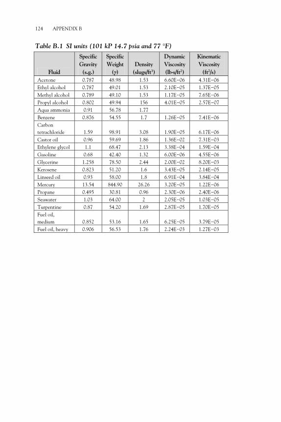
124 APPENDIX B
Table B.1 SI units (101 kP 14.7 psia and 77 °F)
Fluid
Specific Gravity (s.g.)
Specific Weight
(�) Density
(slugs/ft3)
Dynamic Viscosity (lb·s/ft2)
Kinematic Viscosity
(ft2/s) Acetone 0.787 48.98 1.53 6.60E−06 4.31E−06 Ethyl alcohol 0.787 49.01 1.53 2.10E−05 1.37E−05 Methyl alcohol 0.789 49.10 1.53 1.17E−05 7.65E−06 Propyl alcohol 0.802 49.94 156 4.01E−05 2.57E−07 Aqua ammonia 0.91 56.78 1.77 Benzene 0.876 54.55 1.7 1.26E−05 7.41E−06 Carbon tetrachloride 1.59 98.91 3.08 1.90E−05 6.17E−06 Castor oil 0.96 59.69 1.86 1.36E−02 7.31E−03 Ethylene glycol 1.1 68.47 2.13 3.38E−04 1.59E−04 Gasoline 0.68 42.40 1.32 6.00E−06 4.55E−06 Glycerine 1.258 78.50 2.44 2.00E−02 8.20E−03 Kerosene 0.823 51.20 1.6 3.43E−05 2.14E−05 Linseed oil 0.93 58.00 1.8 6.91E−04 3.84E−04 Mercury 13.54 844.90 26.26 3.20E−05 1.22E−06 Propane 0.495 30.81 0.96 2.30E−06 2.40E−06 Seawater 1.03 64.00 2 2.05E−05 1.03E−05 Turpentine 0.87 54.20 1.69 2.87E−05 1.70E−05 Fuel oil, medium 0.852 53.16 1.65 6.25E−05 3.79E−05 Fuel oil, heavy 0.906 56.53 1.76 2.24E−03 1.27E−03

Table
C.1
Sch
edu
le 4
0
Nom
inal
Pip
e Si
ze (
in.)
D
iam
eter
D
iam
eter
Fl
ow A
rea
Ext
erna
l (in
.)
Inte
rnal
E
xter
nal (
mm
) In
tern
al (
mm
) (f
t2 )
(m2 )
(i
n.)
(ft)
1/
8 0.
41
0.27
0.
0224
10
.3
6.8
0.00
0394
3.
66E−
05
1/4
0.54
0.
36
0.03
03
13.7
9.
2 0.
0007
23
6.72
E−05
3/
8 0.
68
0.49
0.
0411
17
.1
12.5
0.
0013
3 1.
24E−
04
1/2
0.84
0.
62
0.05
18
21.3
15
.8
0.00
211
1.96
E−04
3/
4 1.
05
0.82
0.
0687
26
.7
20.9
0.
0037
3.
44E−
04
1 1.
32
1.05
0.
0874
33
.4
26.6
0.
006
5.57
E−04
1¼
1.
66
1.38
0.
115
42.2
35
.1
0.01
039
9.65
E−04
1½
1.
9 1.
61
0.13
42
48.3
40
.9
0.01
414
1.31
E−03
2
2.38
2.
07
0.17
23
60.3
52
.5
0.02
333
2.17
E−03
2½
2.
88
2.47
0.
2058
73
62
.7
0.03
326
3.09
E−03
3
3.5
3.07
0.
2557
88
.9
77.9
0.
0513
2 4.
77E−
03
3½
4 3.
55
0.29
57
101.
6 90
.1
0.06
868
6.38
E−03
4
4.5
4.03
0.
3355
11
4.3
102.
3 0.
0884
8.
21E−
03
5 5.
56
5.05
0.
4206
14
1.3
128.
2 0.
139
1.29
E−02
6
6.63
6.
07
0.50
54
168.
3 15
4.1
0.20
06
1.86
E−02
8
8.63
7.
98
0.66
51
219.
1 20
2.7
0.34
72
3.23
E−02
10
10
.75
10.0
2 0.
835
273.
1 25
4.5
0.54
79
5.09
E−02
12
12
.75
11.9
4 0.
9948
32
3.9
303.
2 0.
7771
7.
22E−
02
14
14
13.1
3 1.
094
355.
6 33
3.4
0.93
96
8.73
E−02
APPENDIX C
Dimensions of Steel Pipe

Nom
inal
Pip
e Si
ze (
in.)
D
iam
eter
D
iam
eter
Fl
ow A
rea
Ext
erna
l (in
.)
Inte
rnal
E
xter
nal (
mm
) In
tern
al (
mm
) (f
t2 )
(m2 )
(i
n.)
(ft)
16
16
15
1.
25
406.
4 38
1 1.
227
1.14
E−01
18
18
16
.88
1.40
6 45
7.2
428.
7 1.
553
1.44
E−01
20
20
18
.81
1.56
8 50
8 47
7.9
1.93
1 1.
79E−
01
24
24
22.6
3 1.
886
609.
6 57
4.7
2.79
2 2.
59E−
01
� � � ��
126 APPENDIX C

Table
C.2
Sch
edu
le 8
0
Nom
inal
Pip
e Si
ze (
in.)
D
iam
eter
D
iam
eter
Fl
ow A
rea
�E
xter
nal (
in.)
In
tern
al
Ext
erna
l (m
m)
Inte
rnal
(m
m)
(ft2 )
(m
2 )
(in.
) (f
t)
1/8
0.41
0.
22
0.01
83
10.4
14
5.58
8 0.
0002
64
2.45
E−05
1/
4 0.
54
0.3
0.02
50
13.7
16
7.62
0.
0004
91
4.56
E−05
3/
8 0.
68
0.42
0.
0350
17
.272
10
.668
0.
0009
62
8.94
E−05
1/
2 0.
84
0.55
0.
0458
21
.336
13
.97
0.00
1650
1.
53E−
04
3/4
1.05
0.
74
0.06
17
26.6
7 18
.796
0.
0029
87
2.77
E−04
1
1.32
0.
96
0.08
00
33.5
28
24.3
84
0.00
5027
4.
67E−
04
1¼
1.66
1.
28
0.10
67
42.1
64
32.5
12
0.00
8936
8.
30E−
04
1½
1.9
1.5
0.12
50
48.2
6 38
.1
0.01
2272
1.
14E−
03
2 2.
38
1.94
0.
1617
60
.452
49
.276
0.
0205
27
1.91
E−03
2½
2.
88
2.32
0.
1933
73
.152
58
.928
0.
0293
56
2.73
E−03
3
3.5
2.9
0.24
17
88.9
73
.66
0.04
5869
4.
26E−
03
3½
4 3.
36
0.28
00
101.
6 85
.344
0.
0615
75
5.72
E−03
4
4.5
3.83
0.
3192
11
4.3
97.2
82
0.08
0006
7.
43E−
03
5 5.
56
4.81
0.
4008
14
1.22
4 12
2.17
4 0.
1261
88
1.17
E−02
6
6.63
5.
76
0.48
00
168.
402
146.
304
0.18
0956
1.
68E−
02
8 8.
63
7.63
0.
6358
21
9.20
2 19
3.80
2 0.
3175
24
2.95
E−02
10
10
.75
9.56
0.
7967
27
3.05
24
2.82
4 0.
4984
74
4.63
E−02
12
12
.75
11.3
8 0.
9483
32
3.85
28
9.05
2 0.
7063
36
6.56
E−02
14
14
12
.5
1.04
17
355.
6 31
7.5
0.85
2211
7.
92E−
02
16
16
14.3
1 1.
1925
40
6.4
363.
474
1.11
688
1.04
E−01
APPENDIX C 127

Nom
inal
Pip
e Si
ze (
in.)
D
iam
eter
D
iam
eter
Fl
ow A
rea
�E
xter
nal (
in.)
In
tern
al
Ext
erna
l (m
m)
Inte
rnal
(m
m)
(ft2 )
(m
2 )
(in.
)(f
t)
18
18
16.1
3 1.
3442
45
7.2
409.
702
1.41
904
1.32
E−01
20
20
17
.94
1.49
50
508
455.
676
1.75
538
1.63
E−01
24
24
21
.56
1.79
67
609.
6 54
7.62
4 2.
5352
7 2.
36E−
01
128 APPENDIX C
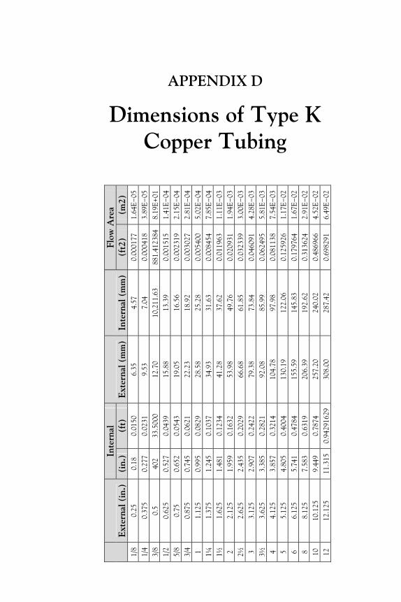
E
xter
nal (
in.)
In
tern
al
Ext
erna
l (m
m)
Inte
rnal
(m
m)
Flow
Are
a (i
n.)
(ft)
(f
t2)
(m2)
1/
8 0.
25
0.18
0.
0150
6.
35
4.57
0.
0001
77
1.64
E−05
1/
4 0.
375
0.27
7 0.
0231
9.
53
7.04
0.
0004
18
3.89
E−05
3/
8 0.
5 40
2 33
.500
0 12
.70
10,2
11.6
3 88
1.41
2384
8.
19E+
01
1/2
0.62
5 0.
527
0.04
39
15.8
8 13
.39
0.00
1515
1.
41E−
04
5/8
0.75
0.
652
0.05
43
19.0
5 16
.56
0.00
2319
2.
15E−
04
3/4
0.87
5 0.
745
0.06
21
22.2
3 18
.92
0.00
3027
2.
81E−
04
1 1.
125
0.99
5 0.
0829
28
.58
25.2
8 0.
0054
00
5.02
E−04
1¼
1.
375
1.24
5 0.
1037
34
.93
31.6
3 0.
0084
54
7.85
E−04
1½
1.
625
1.48
1 0.
1234
41
.28
37.6
2 0.
0119
63
1.11
E−03
2
2.12
5 1.
959
0.16
32
53.9
8 49
.76
0.02
0931
1.
94E−
03
2½
2.62
5 2.
435
0.20
29
66.6
8 61
.85
0.03
2339
3.
00E−
03
3 3.
125
2.90
7 0.
2422
79
.38
73.8
4 0.
0460
91
4.28
E−03
3½
3.
625
3.38
5 0.
2821
92
.08
85.9
9 0.
0624
95
5.81
E−03
4
4.12
5 3.
857
0.32
14
104.
78
97.9
8 0.
0811
38
7.54
E−03
5
5.12
5 4.
805
0.40
04
130.
19
122.
06
0.12
5926
1.
17E−
02
6 6.
125
5.74
1 0.
4784
15
5.59
14
5.83
0.
1797
64
1.67
E−02
8
8.12
5 7.
583
0.63
19
206.
39
192.
62
0.31
3624
2.
91E−
02
10
10.1
25
9.44
9 0.
7874
25
7.20
24
0.02
0.
4869
66
4.52
E−02
12
12
.125
11
.315
0.
9429
1629
30
8.00
28
7.42
0.
6982
91
6.49
E−02
�
APPENDIX D
Dimensions of Type K Copper Tubing

�

APPENDIX E
Conversion Factors
Table E.1 Conversion factors length, area, and volume Length Conversion Factors Length To convert from to multiply by mile (U.S. statute) kilometer (km) 1.609347 inch (in.) millimeter (mm) 25.4 inch (in.) centimeter (cm) 2.54 inch (in.) meter (m) 0.0254 foot (ft) meter (m) 0.3048 yard (yd) meter (m) 0.9144 Area Conversion Factors Area To convert from to multiply by square foot (sq ft) square meter (sq m) 0.09290304 square inch (sq in.) square meter (sq m) 0.00064516 square yard (sq yd) square meter (sq m) 0.83612736 acre (ac) hectare (ha) 0.4047 Volume Conversion Factors Volume To convert from to multiply by cubic inch (cu in.) cubic meter (cu m) 0.00001639 cubic foot (cu ft) cubic meter (cu m) 0.02831685 cubic yard (cu yd) cubic meter (cu m) 0.7645549 U.S. liquid gallon (gal) cubic meter (cu m) 0.00378541 gallon (gal) liter 3.785 fluid ounce (fl oz) milliliters (mL) 29.57353 fluid ounce (fl oz) cubic meter (cu m) 0.00002957

132 APPENDIX E
Table E.2 Conversion factors for force, pressure, and mass Force Conversion Factors Force To convert from to multiply by kip (1,000 lb) kilogram (kg) 453.6 kip (1,000 lb) newton (N) 4,448.22 pound (lb) avoirdupois kilogram (kg) 0.4535924 pound (lb) newton (N) 4.448222 Pressure or Stress Conversion Factors Pressure or stress To convert from to multiply by kip per square inch (ksi) megapascal (MPa) 6.894757
pound per square foot (psf) kilogram per square meter (kg/sq m) 4.8824
pound per square foot (psf) pascal (Pa) 47.88 pound per square inch (psi) pascal (Pa) 6,894.76 pound per square inch (psi) megapascal (MPa) 0.00689476 Mass Conversion Factors Mass (weight) To convert from to multiply by pound (lb) avoirdupois kilogram (kg) 0.4535924 ton, 2,000 lb kilogram (kg) 907.1848 grain kilogram (kg) 0.0000648 Mass (weight) per length kip per linear foot (klf) kilogram per meter (kg/m) 0.001488 pound per linear foot (plf) kilogram per meter (kg/m) 1.488 Mass per volume (density)
pound per cubic foot (pcf) kilogram per cubic meter (kg/cu m) 16.01846
pound per cubic yard (lb/cu yd) kilogram per cubic meter (kg/cu m) 0.5933

Table
E.3
C
onve
rsio
n f
act
ors
den
sity
M
ulti
ply
by
Con
vert
fr
om
Con
vert
to
kg/m
3 g/
cm3
oz/in
.3 oz
/gal
(i
mpe
rial
) oz
/gal
(U
.S.)
lb
/ft3
lb/in
.3 lb
/yd3
lb/g
al
(im
peri
al)
lb/g
al
(U.S
.)
ton/
yd3
kg/m
3 1
0.00
1 0.
0005
78
0.16
04
0.13
35
0.06
24
0.00
0036
1.
6855
0.
01
0.00
835
0.00
075
g/cm
3 1,
000
1 0.
578
160.
4 13
3.52
62
.43
0.03
6 1,
685.
6 10
.02
8.35
0.
752
oz/in
.3 1,
730
1.73
1
277.
4 23
1 10
8 0.
0625
2,
916
17.3
4 14
.44
1.30
2
oz/g
al
(im
peri
al)
6.24
0.
0062
0.
0036
1
0.82
7 0.
389
0.00
0225
10
.51
0.06
25
0.05
2 0.
0047
oz/g
al (
U.S
.)
7.49
0.
0074
9 0.
0043
1.
2 1
0.46
8 0.
0002
7 12
.62
0.07
5 0.
0625
0.
0056
lb/f
t3 16
.02
0.01
6 0.
0093
2.
57
2.14
1
0.00
0579
27
0.
1605
0.
134
0.01
21
lb/in
.3 27
,680
27
.68
16
4,43
8.7
3,69
6 1,
728
1 46
,656
27
7 23
1 20
.82
lb/y
d3 0.
593
0.00
059
0.00
034
0.09
5 0.
079
0.03
7 0.
0000
21
1 0.
0059
5 0.
0049
5 0.
0004
5
lb/g
al
(im
peri
al)
99.7
8 0.
0998
0.
0577
16
13
.32
6.23
0.
0036
16
8.2
1 0.
833
0.07
51
lb/g
al (
U.S
.)
119.
8 0.
12
0.06
9 19
.2
16
7.48
0.
0043
20
1.97
1.
2 1
0.09
ton/
yd3
1,32
8.9
1.32
9 0.
768
213.
1 17
7.4
82.9
6 0.
048
2,24
0 13
.32
11.1
1
APPENDIX E 133

Table
E.3
C
onve
rsio
n fact
ors
dynam
ic v
isco
sity
(m
etri
c unit
s)
Mul
tipl
y by
Con
vert
fro
m
Con
vert
to
Poi
seui
lle
(Pa·
s)
Poi
se
(dyn
e·s/
cm2 )
(g
/cm
·s)
cent
iPoi
se
kg/m
·h
kgf·s
/m2
Poi
seui
lle
(Pa·
s)
1 10
10
3 3.
63 ×
103
0.10
2
Poi
se
(dyn
e·s/
cm2 )
(g/c
ms)
0.
1 1
100
360
0.01
02
cent
iPoi
se
0.00
1 0.
01
1 3.
6 0.
0001
2
kg/m
·h
2.78
× 1
0−4
0.00
278
0.02
78
1 2.
83 ×
10−5
kgf·s
/m2
9.81
98
.1
9.81
× 1
03 3.
53 ×
104
1
lbf·s
/in.2
6.89
× 1
03 6.
89 ×
104
6.89
× 1
06 2.
48 ×
107
703
lbf·s
/ft2
47.9
47
9 4.
79 ×
104
1.72
× 1
05 0.
0488
lbf·h
/ft2
1.72
× 1
05 1.
72 ×
106
1.72
× 1
08 6.
21 ×
108
1.76
× 1
04
lb/f
t·s
1.49
14
.9
1.49
× 1
03 5.
36 ×
103
0.15
2
lb/f
t·h
4.13
× 1
0−4
0.00
413
0.41
3 1.
49
4.22
× 1
0−5
134 APPENDIX E

Table
E.4
C
onve
rsio
n f
act
ors
dyn
am
ic v
isco
sity
(E
ngl
ish
un
its)
M
ulti
ply
by
Con
vert
fro
m
Con
vert
to
lbf·s
/in.2
lbf·s
/ft2
lbf·h
/ft2
lb/f
t·s
lb/f
t·h
Poi
seui
lle (
Pa·
s)
1.45
× 1
0−4
0.02
09
5.8
× 10
−6
0.67
2 2.
42 1
03
Poi
se (
dyne
s/c
m2
= g
/cm
s)
1.45
× 1
0−5
0.00
209
5.8
× 10
−7
0.06
72
242
cent
iPoi
se
1.45
× 1
0−7
2.09
× 1
0−5
5.8
× 10
−9
0.00
0672
2.
42
kg/m
·h
4.03
× 1
0−8
5.8
× 10
−6
1.61
× 1
0−9
0.00
0187
0.
672
kgf·s
/m2
0.00
142
20.5
5.
69 ×
10−
5 6.
59
2.37
104
lbf·s
/in.2
1 14
4 0.
04
4.63
103
1.67
107
lbf·s
/ft2
0.00
694
1 0.
0002
78
32.2
1.
16 1
05
lbf·h
/ft2
25
3.6
103
1 1.
16 1
05 4.
17 1
08
lb/f
t·s
0.00
0216
0.
0311
8.
63 ×
10−
6 1
3.6
103
lb/f
t·h
6 ×
10−
8 8.
633
10−
6 2.
4 ×
10−
9 0.
0002
78
1
��
APPENDIX E 135

� �

Index
Absolute viscosity (�), 8 Acceleration(a), 2 Adhesion, 2, 3 Axial flow pumps, 96 Bernoulli’s equation, 11–14
restrictions on, 14 Best efficiency point, 105 Can turbine pumps, 96 Capillarity, 2 Cavitation, 99 Centrifugal force, 94 Centrifugal pumps, 92–97
affinity laws for, 107–109 coverage chart for, 109–110 performance data for, 100–109
Close-coupled pumps, 95 Cohesion, 2, 3 Common liquids, properties of,
123–124 Composite performance chart,
110–114 Cone angle(θ), 55 Continuity equation, 10–11 Conversion factors, 131–135 Critical region, 34 Cross iteration technique, 83–85
for analyzing flow in pipe networks, 84–85
Darcy equation, 21, 36 Density (ρ), 3–4 Diaphragm pumps, 97–98 Diffuser, 52 Displacement pump, 92 Dynamic pump, 92 Efficiency curves, 105 Elevation head, 13, 14
End-suction centrifugal pumps, 94–95 Energy additions (hA), 21 Energy losses (hR), 21
equation, 70 magnitude of, 21
Energy removals (hR), 21 Energy transfer, 94 Entrance loss, 58–59 Equivalent length ratio, 61–62 Exit loss, 59 Flow energy (FE), 12 Flow rate, 8–10
mass, 9–10 volume, 9 weight, 10
Flow, types of critical, 34 laminar, 35 turbulent, 35–37
Fluid friction, 20–21 Fluid motors, 20
mechanical efficiency of, 29 power delivered to, 28 vs. pumps, 20
Force(F ), 1–2 Frame-mounted pumps, 95 Friction factor, 61–62
equations, 40–42 for laminar flow, 40 for turbulent flow, 40 using Moody diagram, 37–39
Fundamental concepts, 1–18 Bernoulli’s equation, 11–18 density and specific weight, 3–6 flow rate, 8–10 force and mass, 1–2 law of conservation of energy, 11–18 pressure, 7–8 principle of continuity, 10–11

138 INDEX
Fundamental concepts (Continued) specific gravity, 6–7 surface tension and capillarity, 2–3 viscosity, 8
Gage pressure, 7 General energy equation, 22–26
fluid flow system demonstrating, 22–23
Gerotor, 20 Gradual contraction, 55–57 Gradual enlargement, 50–52 Hagen–Poiseuille equation, 35 Hardy Cross method, 82–90 Hazen–Williams coefficient (Ch), 43 Hazen–Williams formula, 42–43
nomograph for solving, 44 Head, 21 Horsepower curves, 106 Hydraulic engineering
fundamental concepts, 1–18 general energy equation, 22–26 minor losses, 47–66
Hydraulic motor, construction and working of, 20
Hydraulic pumps, 91 Iterative method, 72–74 Kinematic viscosity (ν), 8 Kinetic energy (KE), 12 Laminar flow, 35
value of friction factor for, 40 Law of conservation of energy, 11–14 Life cycle cost (LCC), 118–119 Line shaft turbine pumps, 96 Mass(m), 1–2 Mass flow rate, 9–10 Mechanical efficiency (eM)
of fluid motors, 29 of pumps, 28
Minor losses, 21, 47–66 entrance loss, 58–59 exit loss, 59 gradual contraction, 55–57 gradual enlargement, 50–52 pipe bends, resistance coefficient
for, 62–64 sudden contraction, 53–55 sudden enlargement, 48–50 valves and fittings, resistance
coefficients for, 59–62 Moody diagram, 37–39 Net positive suction head (NPSH),
101–104 Operating point of pump, 114–117 Parallel pipe system, 76–90 Pascal (Pa), 7 Peristaltic pumps, 98–99 Pipe bends, resistance coefficient for,
62–66 Positive displacement pumps
diaphragm, 97–98 peristaltic, 98–99 progressive cavity, 99
Potential energy (PE), 12 Power
delivered to fluid motors, 28 generated by pumps, 26–28
Pressure (P), 7–8 Pressure energy. See Flow energy Pressure head, 13, 14 Principle of continuity, 10–11 Progressive cavity pumps, 99 Pumps, 19
cavitation, 99 centrifugal, 92–97 composite performance chart,
110–114 direct lift, 19 displacement, 19 displacement, 92

INDEX 139
dynamic, 92 vs. fluid motors, 20 gravity, 19 life cycle cost of, 118–119 mechanical efficiency of, 28 operating in parallel or series, 117–
118 operating point of, 114–117 positive displacement, 97–99 power generated by, 26–28
Rate of fluid flow. See Volume flow rate
Relative roughness, of pipe, 36–37 Resistance coefficient, 21, 47
entrance loss, 58–59 exit loss, 59 gradual contraction, 56–57 gradual enlargement, 50–51 pipe bends, 62–64 sudden contraction, 53–54 sudden enlargement, 48–50 valves and fittings, 59–62
Reynolds number(NR), 33–35 Series pipeline systems, 67–75 Specific gravity, 6–7 Specific weight (γ), 4–6 Split case pumps, 95 Standard curves, 100 Steel pipe, dimensions of, 125–128 Submersible turbine pumps, 97
Sudden contraction, 53–55 Sudden enlargement, 48–50 Surface tension, 2 Total dynamic head (TDH), 91 Total energy (E), 13 Total head, 13, 14 Turbines. See Pumps Turbulent flow, 35–37
value of friction factor for, 40 Type K copper tubing, dimensions
of, 129 Unit weight. See Specific weight Valves and fittings, 21–22
resistance coefficients for, 59–62 Velocity head, 13, 14 Vena contracta, 55 Vertical turbine pumps, 96–97 Viscosity, 8
absolute, 8 kinematic, 8
Volume flow rate (Q), 9 Volume velocity. See Volume flow
rate Volute, 93 Water, properties of, 121 Weight (w), 2 Weight flow rate (W), 10


OTHER TITLES IN OUR ENVIRONMENTAL ENGINEERING COLLECTION
Francis Hopcroft, Editor
• Wastewater Treatment Concepts and Practices by Francis Hopcroft
• Small-Scale Wind Power: Design, Analysis, and Environmental Impacts
by John P. Abraham and Brian Plourde
FORTHCOMING IN THIS COLLECTION • Valuing Energy for Global Needs: A Systems Approach by Daniel M. Martínez
and Ben W. Ebenhack
• Chemistry for Environmental Engineering by Armen S. Casparian
• Geotechnical Site Characterization by Anirban De
Announcing Digital Content Crafted by LibrariansConcise e-books business students need for classroom and research
Momentum Press offers digital content as authoritative treatments of advanced engineering
topics by leaders in their fi eld. Hosted on ebrary, MP provides practitioners, researchers,
faculty, and students in engineering, science, and industry with innovative electronic content
in sensors and controls engineering, advanced energy engineering, manufacturing, and
materials science.
Momentum Press offers library-friendly terms:
• perpetual access for a one-time fee• no subscriptions or access fees required• unlimited concurrent usage permitted• downloadable PDFs provided• free MARC records included• free trials
The Momentum Press digital library is very affordable, with no obligation to buy in future years.
For more information, please visit www.momentumpress.net/library or to set up a trial in the US,
please contact [email protected].

HYD
RAU
LIC EN
GIN
EERING
DA
S
EBOOKS FOR THE ENGINEERING LIBRARYCreate your own Customized Content Bundle — the more books you buy, the higher your discount!
THE CONTENT• Manufacturing
Engineering• Mechanical
& Chemical Engineering
• Materials Science & Engineering
• Civil & Environmental Engineering
• Advanced Energy Technologies
THE TERMS• Perpetual access for
a one time fee• No subscriptions or
access fees• Unlimited
concurrent usage• Downloadable PDFs• Free MARC records
For further information, a free trial, or to order, contact: [email protected]
Hydraulic EngineeringFundamental Concepts
Gautham P. Das
Hydraulic Engineering: Fundamental Concepts includes hydraulic
processes with corresponding systems and devices. The hydraulic
processes includes the fundamentals of fl uid mechanics and pres-
surized pipe fl ow systems. This book illustrates the use of appropri-
ate pipeline networks along with various devices like pumps, valves
and turbines. The knowledge of these processes and devices is ex-
tended to design, analysis and implementation.
Dr. Gautham P. Das is an associate professor of civil and environ-
mental engineering at Wentworth Institute of Technology in Boston,
Massachusetts. Prior to starting his teaching career, Dr. Das worked
for environmental consulting fi rms in North Carolina and Boston.
His expertise lies in water resources, hydraulic engineering and
environmental remediation. He is active in the Water Environment
Federation, the New England Water Environment Association and
the American Society of Civil Engineers. He has authored numer-
ous technical papers on various civil and environmental engineering
subjects that have been published in peer-reviewed journals and
presented at technical conferences. http://gauthampdas.us/
Gautham P. Das
ENVIRONMENTAL ENGINEERINGCOLLECTIONFrancis J. Hopcroft, Collection Editor
Hydraulic EngineeringFundamental Concepts
Related Documents