Hydraulic energy recovery by replacing a control valve ...

LAPPEENRANTA UNIVERSITY OF TECHNOLOGY

LUT School of Energy Systems

Energy Technology

Jaakko Hyypiä

HYDRAULIC ENERGY RECOVERY BY REPLACING A CONTROL VALVE

WITH A CENTRIFUGAL PUMP USED AS A TURBINE

Examiners: Professor Jari Backman

D.Sc. Tero Ahonen

ABSTRACT

Lappeenranta University of Technology

LUT School of Energy Systems

Degree Programme in Energy Technology

Jaakko Hyypiä

Hydraulic energy recovery by replacing a control valve with a centrifugal pump used as a

turbine

2016

Master’s thesis.

105 pages, 69 figures and 9 tables.

Examiners: Professor Jari Backman, D.Sc. Tero Ahonen

Keywords: pump as turbine, centrifugal pump, control valve, hydraulic energy recovery, sensorless

estimate, turbine model, control model, flow control.

Reverse running centrifugal pumps as turbines (PaT’s) are used in small-scale hydropower genera-

tion mainly because of lower investment costs. Predicting the turbine mode operation point for a

centrifugal pump has a lot of uncertainties, as manufacturers do not usually publish the turbine mode

performance data. Using variable speed drives (VSD) makes it possible to operate PaT’s at different

operation points at high efficiency, and they can be used to change the operation point, if the pre-

dicted best efficiency point (BEP) for PaT is not accurate.

In many processes the flow is controlled by throttling a control valve, and the pressure loss in the

valve is dissipated. Stricter system level energy efficiency requirements may cause the flow control

methods to change. Hydraulic energy recovery with a PaT in flow control application is made pos-

sible by VSD’s.

In this thesis, the main focus is to develop models and to test a PaT as a valve replacement in flow

control application. A turbine polynomial model is created for a VSD PaT. The turbine models are

used in flow control, Maximum Power Point (MPP) tracking and for sensorless estimation. The eco-

nomic feasibility of hydraulic energy recovery with a PaT is studied. Based on 10 pumps, a minimum

scale for economically feasible hydraulic energy recovery exists at the scale of 10 - 20 kWe. With a

correctly sized PaT it is possible to recover approximately 23 – 27 % of the energy consumed by the

pressure producing pump, depending on the amount of throttling and the process.

TIIVISTELMÄ

Lappeenrannan teknillinen yliopisto

LUT School of Energy Systems

Energiatekniikan koulutusohjelma

Jaakko Hyypiä

Hydraulisen energian talteenotto käyttämällä keskipakopumppua turbiinina säätöventtiiliin

korvaamiseen

2016

Diplomityö

105 sivua, 69 kuvaa ja 9 taulukkoa.

Tarkastajat: Professori Jari Backman, tutkijatohtori Tero Ahonen

Hakusanat: pumpputurbiini, keskipakopumppu, energian talteenotto, säätöventtiili, anturiton esti-

mointi, turbiinimalli, säätömalli, virtaussäätö.

Keskipakopumppuja käytetään turbiineina erityisesti pienen kokoluokan vesivoimasovelluksissa

pienien investointikustannuksien vuoksi. Kuitenkin keskipakopumpun turbiinitoimintapisteen arvi-

ointiin liittyy paljon epävarmuutta. Käyttämällä taajuusmuuttajaa tarkan toimintapisteen arviointi ei

ole niin tärkeää, sillä sitä voidaan muuttaa pyörimisnopeutta muuttamalla.

Monissa prosesseissa virtausta säädetään säätöventtiiliä kuristamalla, jolloin venttiilin paine-ero hu-

kataan lämmöksi. Tiukemmat energiatehokkuusmääräykset voivat muuttaa tulevaisuudessa proses-

sien säätöä. Hydraulisen energian talteenotto pumpputurbiinilla on mahdollista taajuusmuuttajakäy-

töillä virtaussäätösovelluksessa.

Tässä diplomityössä kehitetään ja testataan mallit pumpputurbiinin käyttöön säätöventtiilin korvaa-

jana. Muuttuvanopeuksisen pumpputurbiinin polynomimallit kehitetään, ja niitä käytetään virtaus-

säätöön, maksimitehopisteen etsimiseen ja anturittomaan estimointiin. Hydraulisen energian talteen-

oton taloudellista kannattavuutta tutkitaan, ja minimikokoluokka taloudellisesti järkevään talteenot-

toon vaikuttaa olevan 10 - 20 kWe kokoluokassa. Oikein mitoitetulla pumpputurbiinilla on mahdol-

lista ottaa talteen 23 – 27 % painetta tuottavan pumpun tehonkulutuksesta, riippuen virtauskuristuk-

sen määrästä ja prosessista.

ACKNOWLEDGEMENTS

This Master’s thesis was conducted in Lappeenranta University of Technology between June and

November 2016 as a part of Efficient Energy Usage (EFEU) research program.

I want to thank my instructors, Tero Ahonen and Jari Backman for this opportunity. This process has

taught me a lot about energy technology but also from electrical engineering. Special thanks to Saku

Vanhala and Sami Virtanen from Sulzer for providing me information and industrial perspective to

this research.

I want to thank Armatuuri and all the fellow students who I have been studying with for all these

years. Studying in Lappeenranta has been a truly remarkable time in my life.

Finally, I want to thank my family for encouraging and supporting me in my studies.

In Lappeenranta, 14th of November, 2016.

Jaakko Hyypiä

5

CONTENTS

1 INTRODUCTION 9

1.1 Previous research 10

1.2 Outline of this thesis 11

2 CENTRIFUGAL PUMPS 12

2.1 Working principle 13

2.2 Dimensionless numbers 18

2.3 Losses 21

3 PUMP AS TURBINE 23

3.1 Velocity triangles 26

3.2 Power and losses 30

3.3 Difference to turbines 32

4 ELECTRICAL MACHINE AND FREQUENCY CONVERTER 34

4.1 Motor efficiency 36

4.2 Frequency converter 37

5 CONTROL VALVE CHARACTERISTICS 39

5.1 Installed flow characteristics 43

6 TURBINE MODEL 48

6.1 Model for turbine head 48

6.2 Model for turbine power 50

6.3 Runaway, resistance and maximum power curve 52

6.4 PaT operation area 53

6.5 Inherent valve characteristics and gain 58

6.6 Turbine and valve in series 61

6.7 Example of a PaT application 65

7 EXPERIMENTS 70

7.1 Turbine characteristics for A22-80 71

7.2 Turbine characteristics for A11-50 75

7.3 Sulzer A22-80 inherent valve characteristics 78

7.4 Turbine and valve in series 80

7.4.1 Measuring the components of the system 81

6

7.4.2 Testing the flow control 84

7.4.3 Sensorless estimation 87

8 ECONOMICAL EVALUATION 90

8.1 Example cases 90

8.2 Operation point based evaluation 97

9 CONCLUSIONS 101

9.1 Suggestions for future work 102

REFERENCES 103

7

LIST OF SYMBOLS AND ABBREVIATIONS

AC Alternating Current

BEP Best Efficiency Point

DC Direct Current

EU European Union

PaT Pump as Turbine

MEPS Minimum Energy Performance Standard

MPP Maximum Power Point

SynRM Synchronous Reluctance

VSD Variable-Speed Drive

A area [m2]

b height [m]

𝐶𝑉 valve flow coefficient [m5

2 ∙ kg−1

2]

c absolute speed [m/s]

d diameter [m]

fq impeller eyes per impeller, single-entry fq=1 [-]

G gain [-]

g acceleration due to gravitation, g = 9.81 m/s2 [m/s2]

H head [m]

h relative opening [-]

𝐾𝑉 valve capacity factor [m2]

k constant [-]

L length [m]

n rotational speed [1/s]

nq specific speed [-]

P power [W]

Q flow rate [m3/s]

r radius [m]

T torque [Nm]

t time [s]

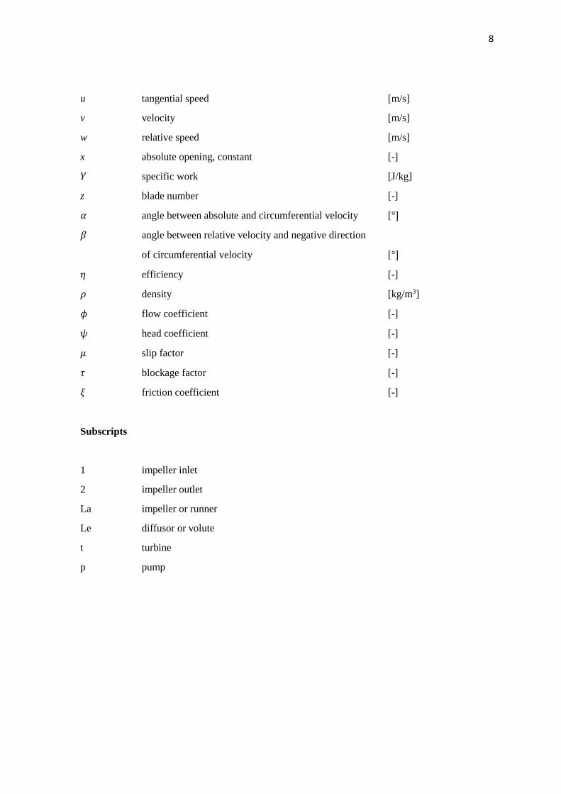
8

u tangential speed [m/s]

v velocity [m/s]

w relative speed [m/s]

x absolute opening, constant [-]

𝑌 specific work [J/kg]

z blade number [-]

𝛼 angle between absolute and circumferential velocity [°]

𝛽 angle between relative velocity and negative direction

of circumferential velocity [°]

𝜂 efficiency [-]

𝜌 density [kg/m3]

𝜙 flow coefficient [-]

𝜓 head coefficient [-]

𝜇 slip factor [-]

𝜏 blockage factor [-]

𝜉 friction coefficient [-]

Subscripts

1 impeller inlet

2 impeller outlet

La impeller or runner

Le diffusor or volute

t turbine

p pump

9

1 INTRODUCTION

Fluid handling systems are everywhere, and you cannot live a day without running into pumping

systems. Water distribution systems use pumps to deliver water to houses; a car’s engine uses a

coolant pump to keep the coolant flowing through the engine; even a human heart is a pump pumping

blood through a system.

Pumping is very energy intensive; it uses 10 % of the global electricity consumption, so the energy

savings potential in pumping systems should not be neglected (Motiva, 2011, 5). Majority of the

industrial pumps are centrifugal pumps because of their relatively simple construction, inexpensive-

ness and the possibility to throttle the flow without difficulties. (Grundfos, 2004b, 8)

Reverse running centrifugal pumps have been used as turbines for nearly a century. The earliest

recorded application is from USA from the year 1926 (Alatorre-Frenk C. 1994, 4). They have been

used especially in small-scale hydropower applications. The advantage of using pumps as turbines

(PaT’s) is the cost reduction compared to turbines, made possible by the large manufacturing vol-

umes of centrifugal pumps (Alatorre-Frenk C. 1994, 4). Even though centrifugal pumps are not pri-

marily designed to be used as turbines, they usually do work as turbines with a good efficiency.

An example of a documented PaT application can be found from Germany, near Stuttgart. Breech

water plant has the highest underground reservoir in the water supply system and its delivering drink-

ing water downhill towards Stuttgart. The pressure regulators were replaced with PaT’s starting from

1989, and nowadays there is 8 PaT’s installed in series with a maximum electrical power of 230 kW.

The control of the constant speed operated PaT’s is done with butterfly valves, and the number of

the PaT’s operating is altered depending on the flow rate. (Budris A.)

PaT’s are also used in process industry where a large pressure reduction is needed. Examples can be

found from nitrogenous fertilizer manufacturing plants and petrochemical industry. These applica-

tions can have an electrical power of 600 – 1600 kW and pump manufacturers already provide PaT’s

for these applications. (Sulzer, 2014)

This thesis is a part of Efficient Energy Usage (EFEU) research program, which aims to develop

system level energy efficiency solutions for fluid handling and regional energy systems. EFEU re-

search program partners consist of several Finnish companies and universities. Lauri Nygren (2016)

studied the use of variable speed PaT’s for hydraulic energy recovery in his thesis, which is also part

of the EFEU program. This thesis continues the research on PaT’s done in the EFEU program.

10

The aim of this thesis is to study the use of PaT’s for hydraulic energy recovery as a substitute for a

control valve. Polynomial models for a PaT are developed and used to develop methods for using a

PaT for flow control. The economic feasibility of PaT’s and energy recovery is also studied.

1.1 Previous research

There exists a lot of uncertainty about the predicting the best efficiency operation point (BEP) of a

PaT based on pump mode performance data. This has been a subject for many previous studies. For

example, Chapallaz (1992) introduces methods for PaT operation point determination based on many

previous studies conducted by Diederich (1967), Buse (1981), Lewinski-Kesslitz (1987) and several

others. Gülich (2010) has also provided equations for turbine mode performance prediction. This

research focus has been primarily driven by the fact that the pump manufacturers do not usually

publish data about their pumps turbine mode performance. A reliable method for turbine mode per-

formance prediction has not been created, and all the methods described earlier have a lot of uncer-

tainty. This is due to the fact that pumps with similar performance can be designed with different

geometric parameters, and this affects the turbine mode performance.

Nygren (2016) studied the suitability of centrifugal pumps to turbine use in his thesis. He also created

polynomial models for turbine head and power, which can be used, for example maximum power

point tracking. In Nygren’s thesis, the mechanical suitability of centrifugal pumps to turbine opera-

tion was evaluated; most pumps are suitable for turbine operation without changes, and do work as

turbines with an efficiency that is comparable to pump mode efficiency. In some cases, the turbine

mode efficiency is even higher than pump mode efficiency.

Nygren also stated that the use of variable-speed drives does make the turbine performance predic-

tion less critical, since the operation point can be altered by adjusting the rotational speed. Electricity

generation using frequency converter requires the use of four-quadrant (4Q) frequency converter,

unless common DC circuits can be used. Common DC circuits could be used between multiple fre-

quency converters, so that the motoring converters would use the electricity produced by the gener-

ating units.

11

1.2 Outline of this thesis

After this introductory chapter, this thesis consists of following chapters:

Chapter 2. Centrifugal pumps

This chapter introduces the basic theory of the centrifugal pumps. The structure, velocity triangles,

key numbers and dimensionless numbers are introduced.

Chapter 3. Pump as turbine

This chapter describes the difference of turbines to pumps. Basic turbine theory is introduced, espe-

cially by parts that differ compared to the pump theory.

Chapter 4. Electrical machine and frequency converter

This chapter introduces the electrical devices that are essential for variable speed PaT’s to be used.

Electrical motors and frequency converters are described.

Chapter 5. Control valve characteristics

The characteristics and types of control valves are described. Parts of valves, valve coefficients and

different opening characteristics are introduced.

Chapter 5. Control systems and turbine model

In this chapter, a polynomial model for PaT head and power is created. The basics of control systems

are introduced. Polynomial models are used to derive Maximum Power Point (MPP)-curve and run-

away curve of a PaT.

Chapter 6. Experiments

This chapter explains the experiments conducted in the LUT pump laboratory. The results of the

experiments are shown.

Chapter 7. Economical evaluation

This chapter focuses on the economical evaluation of PaT’s and hydraulic energy recovery in gen-

eral.

Chapter 8. Conclusions

Conclusions of the experiments and the thesis are described in this chapter.

12

2 CENTRIFUGAL PUMPS

A centrifugal pump is a device that is used for transporting liquid by raising the pressure of the fluid.

The pressure rise in centrifugal pumps is based on hydrodynamic processes between the impeller

and the fluid, and all energy differences are proportional to the square of the rotational speed (Gülich,

Johann. 2010, 39). Because the centrifugal pump work is based on kinetics, the flow can easily be

throttled or even cut off with throttling without causing damage to the pump. On the contrary, posi-

tive displacement pumps can suffer from overpressure if the flow is restricted. Centrifugal pumps

also have a continuous flow, while the flow through displacement pumps is pulsating (Grundfos,

2004b, 24).

A centrifugal pump consists of a set of rotating vanes, which are enclosed in a casing. The fluid is

forced into the impeller, and the impeller increases the absolute velocity of the flow. Energy is trans-

ferred from the impeller to the flow. After the impeller, the flow is decelerated in diffuser resulting

in a pressure rise. To maximize the pressure recovery, a carefully designed diffuser is used to recover

most of the kinetic energy of the flow after the impeller. (Gülich J. 2010, 39)

Centrifugal pumps can be divided into several groups based on their design. Most common way is

to classify pumps based on the flow direction at the impeller exit: Terms radial, mixed flow, and

axial pumps are used. Impellers can be also classified in enclosed, semi-enclosed and open impellers

based on the impeller structure. Diffusers are classified into vaneless and vaned diffusors. Based on

the diffusor flow direction, they can be radial, semi-axial or axial diffusers. Pumps are divided to

single stage and multi stage pumps depending on the number of impellers in series. Pumps can be

built with single-entry or double-entry. Double-entry pumps have two inlets built in the both sides

of the impeller (Gülich J. 2010, 39-41). End-suction pumps have inlet and outlet at 90 degree angle

to each other. In-line pumps have a direct flow direction, the angle between inlet and outlet is 180

degrees.

In addition to the parts required for the flow control, pump consists also from mechanical parts, such

as bearings, seals, shaft and motor. It is also possible to use an inducer at the pump inlet to achieve

better flow control, however, it is not commonly used. Fig. 2.1 illustrates the cutout view of an end-

suction single-stage pump with a radial flow impeller and single volute. The fluid enters the pump

from the left.

13

Fig. 2.1. A cross-section of an end-suction centrifugal pump (Sulzer, 2015, 4-5)

A variety of seals can be used to control the leakage flow from between the shaft and the casing. One

of the simplest options is the stuffing box, which controls the leakage flow from the pump and houses

a soft seal that is compressed against the shaft. Also lip seals and mechanical seals are used, and they

are more delicate options for sealing. With correctly working mechanical seal it is possible to get a

very small, even nonvisible leakage flow through the seal (Grundfos, 2009, 9). Bearings are usually

located between the seals and the motor. There are also many other possible configurations for the

placement of bearings, but this is one of the most common configurations. (Gülich J. 2010, 40)

To reduce the axial force caused by the higher pressure in the impeller outlet and on the back plate

of the impeller, a thrust balance device is used. Examples of thrust balance devices are balancing

holes, sealing gap and blades in the backside of the impeller. In double-entry pumps axial thrust

balancing is not needed because of the symmetrical impeller. (Grundfos, 2004b, 14)

2.1 Working principle

The work done in the impeller and the working principles can be described using velocity triangles.

Fig. 2.2 illustrates the velocity triangles of a radial pump impeller. The subscript 0 means state before

impeller, 1 is at the impeller inlet, and 2 at the impeller outlet. Prime means actual velocity, whereas

velocities without prime are theoretical. Theoretical velocities equal to the velocities that would fol-

low the blade angle accurately. This is however not realistic: centrifugal pumps always have a certain

14

amount of slip at the impeller exit, caused by the different pressure distribution on different blade

surfaces. No work transfer from impeller is possible if the flow is blade-congruent. (Gülich J. 2010,

76)

Fig. 2.2. Velocity triangles of a radial pump impeller (Modified from Karassik et.al. 1976)

Euler’s equation for turbomachinery describes the work done to the fluid by a turbomachine. The

specific work Y is equal to enthalpy rise Δℎ𝑡𝑜𝑡. (Gülich J. 2010, 43)

𝑌 = 𝑐2𝑢′ 𝑢2 − 𝑐1𝑢

′ 𝑢1 (2.01)

In the pump literature, it is common to use head H instead of specific work. Euler’s equation for

turbomachinery can be rewritten as (Gülich J. 2010, 43)

𝐻 =1

𝑔 (𝑐2𝑢

′ 𝑢2 − 𝑐1𝑢′ 𝑢1) (2.02)

The actual velocities can be estimated when the geometry of impeller is known. The slip factor at

impeller outlet is defined as the ratio between actual and theoretical tangential velocities (eq. 2.03)

15

𝜇 =𝑐𝑢2

′

𝑐𝑢2 (2.03)

Euler’s equation for turbomachinery (eq. 2.02) and (eq. 2.03) show that the slip decreases the work

done by the impeller. It is however not considered to be a loss, more of a fact that the amount of

work done is reduced. This has to be taken into account in impeller design. There exists a lot of

different ways to estimate the slip at impeller outlet. Most estimates are based on blade number,

blade angle and geometry. For example, Pfleiderer’s slip factor formula states (Karassik et.al 1974)

𝜇 =1

1+𝑎(1+𝛽260

)𝑟2

2

𝑧𝑆

(2.04)

where 𝛽2 is the blade exit angle in degrees, S is the static moment of the mean streamline, 𝑆 =

∫ 𝑟 𝑑𝑥𝑟2

𝑟1 and a is a coefficient that takes into account different casing designs. For volute pumps, a

= 0.65 to 0.85.

In centrifugal pumps without inlet inducer, it is usually assumed that the flow enters the impeller

with zero inlet swirl (The velocity component 𝑐𝑢1 = 0). This simplifies Euler’s equation for tur-

bomachinery into form

𝐻 =1

𝑔𝑐2𝑢

′ 𝑢2 (2.05)

It can be seen from (eq. 2.05) that the work done by impeller depends only on the exit velocity

triangle. This simplifies the analysis of centrifugal pumps noticeably. The head can be calculated

when 𝑐2𝑢′ is known. 𝑢2 is the tangential speed of impeller outlet, and it can be calculated easily when

rotational speed and impeller diameter is known.

𝑢2 = 2𝜋𝑟22 ∙ 𝑛 (2.06)

where n is the rotational speed [1/s]. The meridional velocity for incompressible fluids can be derived

from continuity and mass balance.

16

𝑐2𝑚 ∙ 𝐴2 = 𝑄 (2.07)

where 𝐴2 is the flow area, which can be estimated with (eq. 2.08)

𝐴2 = 2𝜋𝑟2 ∙ ℎ2 − 𝑧 ∙ 𝑠2 ∙ ℎ2 (2.08)

where ℎ2 is the height of impeller outlet, 𝑠2 is the blade thickness at the exit and z is the blade

number. With the help of velocity triangles, the velocity component 𝑐2𝑢 can be expressed as

𝑐2𝑢 = 𝑢2 −𝑐2𝑚

tan 𝛽2 (2.09)

The slip can be taken into account with (eq. 2.03 – eq. 2.04) and the theoretical head can be calcu-

lated. Pump useful power 𝑃𝑢 can be calculated from the specific work in (eq. 2.05) by multiplying it

with mass flow �̇� = 𝜌𝑄.

𝑃𝑢 = 𝜌𝑄𝑔𝐻 (2.10)

The efficiency of the pump is obtained by dividing the useful power with power at coupling

𝜂 =𝑃𝑢

𝑃=

𝜌𝑄𝑔𝐻

𝑃 (2.11)

The pressure rise in centrifugal pump impeller can be divided into two parts: static pressure rise

caused by deceleration of relative velocity w in the impeller, and the total pressure rise caused by

deceleration of absolute velocity c after the impeller. The relationship between these two is called as

degree of reaction (Gülich J. 2010, 75).

17

𝑅𝐺 =𝐻𝑠

𝐻 (2.12)

In order to decelerate the flow leaving the impeller, a diffuser must be used. Diffusers can be divided

to two groups: vaneless and vaned diffusers. Vaneless diffusers are simpler, they have better off-

design performance, but on the other hand, they require more space and do not reach as high peak

efficiencies as vaned diffusers. Fig. 2.3 and Fig. 2.4 illustrate vaneless and vaned diffusers and their

velocity triangles.

Fig. 2.3. Two types of vaneless diffusers. a) parallel walls, b) conical walls, c) velocities (Gülich J. 2010,

105)

Fig. 2.4. A vaned diffuser. (Gülich J. 2010, 105)

The pressure rise in vaneless diffuser can be explained using continuity and preservation of angular

momentum. If no external forces are acting on the flow, the fluid keeps moving with the same angular

momentum. Thus cu ∙ r stays constant. The diffusor element has to be designed so that they comply

with the preservation of angular momentum. (Gülich J. 2010, 103)

18

The pump characteristics as function of flow rate can be described with pump curves. Fig. 2.5 illus-

trates Sulzer AHLSTAR A11-50 pump curves at a rotational speed of 1450 rpm. The efficiencies

are also plotted in the figure. The different pump curves illustrate the characteristics on different

impeller diameters, here the 210 mm impeller is the largest possible to be used with this pump.

Fig. 2.5. Pump curves for Sulzer AHLSTAR A11-50 at 1450 rpm. (Sulzer, (a), 36)

2.2 Dimensionless numbers

A dimensionless unit specific speed is used to describe what kind of impellers are feasible to be used

at certain working cycles. There exists several different definitions of specific speed, depending on

the units used. In this thesis we use the definition of specific speed described by Sulzer (1998) and

Gülich (2010, 47). 𝑛𝑞 is commonly used in European pump literature.

𝑛𝑞 = 𝑛 √𝑄

𝐻34

(2.13)

19

Where n is the rotational speed in [rpm], Q is the flow rate in [m3/s] and H is the head in [m]. The

truly dimensionless representation, 𝜔𝑆, which uses SI units, should be preferred. However, it is rarely

used in literature (Gülich J. 2010, 47). The dependency between 𝑛𝑞 and 𝜔𝑠 is

𝜔𝑆 =𝑛𝑞

52,9 (2.14)

Fig. 2.6 illustrates the typical impeller shapes at different specific speeds. Notice that it is possible

to build impellers with different shapes for certain specific speed, but in order to achieve best effi-

ciency typical shapes are used.

Fig. 2.6. The effect of specific speed on impeller shapes. (Modified from Karassik et.al. 1974)

As can be seen from Fig. 2.6, pumps with low specific speed have radial flow impellers. With spe-

cific speeds of 20 – 100 the impellers are of mixed flow type. Impellers with higher specific speeds

are axial flow type. The limits for centrifugal pump feasible operation are at very low specific speeds

or at very high specific speeds. The achievable maximum efficiency becomes lower at low and high

specific speeds.

The efficiency will drop rapidly when 𝑛𝑞 goes below 20, and the lowest specific speeds for centrif-

ugal pumps are found around 𝑛𝑞= 5. If very low specific speeds are required by the operation point,

the problem can be solved by using multistage pumps, where the total head required is divided to

several impellers, and the specific speed per stage is higher. At very high specific speeds hydraulic

losses become higher, and the pumps with highest specific speeds can be typically found from range

of 𝑛𝑞 = 350 - 450. When the operation point requires higher specific speeds, a multi-entry pump can

be used to lower the flow rate, and therefore the specific speed of the impeller. (Gülich J. 2010, 48)

20

In addition to specific speed, several other dimensionless numbers are used to describe the head and

flow rate. Head coefficient 𝜓 is defined as (Gülich J. 2010, 134)

𝜓 =2gH

𝑢22 =

2𝑌

𝑢22 (2.15)

Flow coefficients are defined as (Gülich J. 2010, 134)

𝜙1 =𝑐1𝑚

𝑢1 (2.16)

𝜙2 =𝑄/𝑓𝑞

𝜋𝑑2𝑏𝑏2𝑢2 (2.17)

Where 𝑓𝑞 is the number of impeller eyes per impeller. 𝑓𝑞 = 1 for single-entry pumps. Subscript 1

denotes inlet of the impeller and subscript 2 outlet of the impeller. The dimensionless numbers (eq.

2.17 – eq. 2.19) can be used to compare different impellers.

Affinity laws are used to predict the operation point of a known pump at another rotational speed.

The affinity laws are described in (eq. 2.20 – eq. 2.22). Subscript 1 denotes operation point 1, while

2 is the operation point 2. The affinity law for power (eq. 2.20) does not take into account the chang-

ing efficiency of the pump, when the operation point changes to other rotational speed.

𝑄1

𝑄2=

𝑛1

𝑛2 (2.18)

𝐻1

𝐻2= (

𝑛1

𝑛2)

2 (2.19)

𝑃1

𝑃1= (

𝑛1

𝑛2)

3 (2.20)

21

2.3 Losses

The losses in centrifugal pumps can be divided into groups according to Gülich. (2010, 83):

1. Mechanical losses, which are caused by mechanical friction in the bearings and seals, and

can be described as power loss 𝑃𝑙𝑜𝑠𝑠,𝑚.

2. Leakage flow loss, which is caused by a leakage flow pumped by the impeller. Leakage flow

loss is described using volumetric efficiency 𝜂𝑣 =𝑄

𝑄+𝑄𝑙𝑒𝑎𝑘𝑎𝑔𝑒, which describes how much

more flow impeller must pump to create desired flow rate. The leakage flows include the

flows through the thrust balance holes and the leakage between impeller and the casing. The

power loss caused by leakage flow is 𝑃𝑙𝑜𝑠𝑠,𝑙 =𝜌𝑔𝐻

𝜂ℎ∙ 𝑄 (

1

𝜂𝑉− 1).

3. Disc friction loss 𝑃𝑙𝑜𝑠𝑠,𝑑𝑓, which is caused by the friction between the fluid and the rear (and

front shroud) of the impeller.

4. Hydraulic loss, caused by friction and turbulence in the pump components. Hydraulic losses

are described using hydraulic efficiency 𝜂ℎ. The dissipated power is 𝑃𝑙𝑜𝑠𝑠,ℎ =

𝜌𝑔𝐻𝑄 (1

𝜂ℎ− 1)

5. Fluid recirculation at part load 𝑃𝑙𝑜𝑠𝑠,𝑟𝑒𝑐 which is the greatest loss at partial load conditions.

Fluid recirculation loss is caused by momentum exchange between stalled and not stalled

fluid regions. Near design point this loss is minimal.

6. Friction losses caused by axial thrust balance devices 𝑃𝑙𝑜𝑠𝑠,𝑒𝑟 and leakage flows in multi-

stage pumps caused by leakages in the interstage seals 𝑃𝑙𝑜𝑠𝑠,𝑆3. The interstage seals power

loss occurs only in multistage pumps.

Fig. 2.7 summarizes these losses in the form of a Sankey-diagram.

22

Fig. 2.7. Sankey-diagram of pump losses (Modified from Gülich J. 2010, 84)

23

3 PUMP AS TURBINE

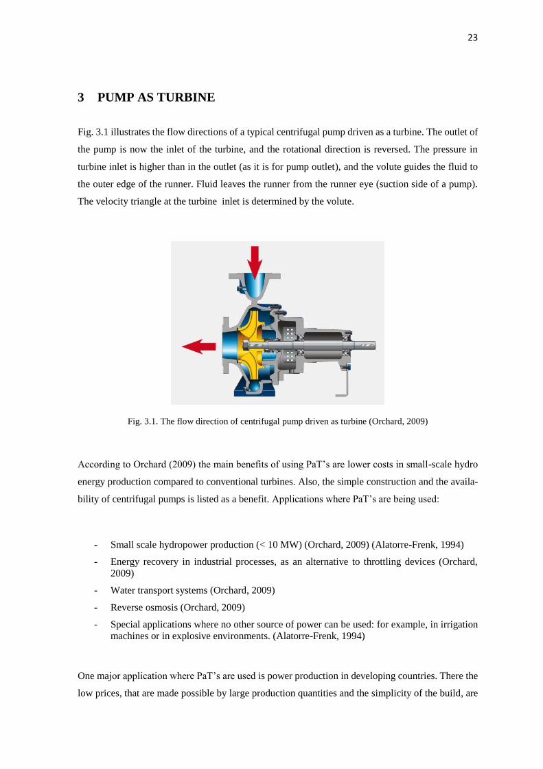
Fig. 3.1 illustrates the flow directions of a typical centrifugal pump driven as a turbine. The outlet of

the pump is now the inlet of the turbine, and the rotational direction is reversed. The pressure in

turbine inlet is higher than in the outlet (as it is for pump outlet), and the volute guides the fluid to

the outer edge of the runner. Fluid leaves the runner from the runner eye (suction side of a pump).

The velocity triangle at the turbine inlet is determined by the volute.

Fig. 3.1. The flow direction of centrifugal pump driven as turbine (Orchard, 2009)

According to Orchard (2009) the main benefits of using PaT’s are lower costs in small-scale hydro

energy production compared to conventional turbines. Also, the simple construction and the availa-

bility of centrifugal pumps is listed as a benefit. Applications where PaT’s are being used:

- Small scale hydropower production (< 10 MW) (Orchard, 2009) (Alatorre-Frenk, 1994)

- Energy recovery in industrial processes, as an alternative to throttling devices (Orchard,

2009)

- Water transport systems (Orchard, 2009)

- Reverse osmosis (Orchard, 2009)

- Special applications where no other source of power can be used: for example, in irrigation

machines or in explosive environments. (Alatorre-Frenk, 1994)

One major application where PaT’s are used is power production in developing countries. There the

low prices, that are made possible by large production quantities and the simplicity of the build, are

24

an advantage. Also spare parts are well available for most common centrifugal pumps and the

maintenance is simple. The possibility to use pumps designed for corrosive or abrasive fluids may

be an advantage in some applications. (Alatorre-Frenk, 1994)

A centrifugal pump runs as a pump when the direction of rotation and flow are positive (defined as

positive for pump operation). When the flow direction and rotational direction are reversed, it is

operating in turbine mode. In both cases the pressure difference over the device is positive (positive

head) and the torque is positive. It is possible to form altogether 16 different possible combinations

of these 4 variables. Eight of them may be observed in operation and they are illustrated in Fig. 3.2.

(Gülich J. 2010, 736)

Fig. 3.2. Eight operation modes for centrifugal machine (Gülich J. 2010, 736)

The most relevant operating modes for PaT operation are C and D. In operation area C, the pump is

working normally as turbine. Rotational direction is negative, flow is negative and torque and head

are positive. In operation area D the flow rate drops below the runaway curve, and torque changes

to negative. There the turbine is dissipating energy. The operation area B is found from below the

resistance curve, where the rotational speed changes back to positive. (Gülich J. 2010, 736)

25

Similar to pump maps, turbine characteristics can also be described using turbine maps. Turbine

head is plotted as a function of flow rate for constant rotational speed. Unlike in pump curves, the

system curve is descendent in turbine maps. Fig. 3.3 illustrates the turbine map for Sulzer A22-80

pump based on measurements done by Lauri Nygren in his master’s thesis (2016). The constant

speed lines vary from 200 rpm to 1400 rpm. The efficiency contours are turbine efficiency contours.

Fig. 3.3. Turbine map for Sulzer AHLSTAR A22-80 pump (Nygren L. 2016)

The lines, which limit turbine operation in Fig. 3.3, are the runaway curve and the resistance curve.

The red curve is the runaway curve, which means that the turbine operating point will be on this

curve, when the torque on the shaft is zero. Runaway condition occurs therefore, for example, when

the motor is not connected to the grid. Orange resistance curve is the curve with locked rotor, so that

rotor cannot turn at all. It’s also the minimum flow resistance the turbine can cause, without using

power to help accelerate the flow. Turbine can also be operated outside this area, but no power pro-

duction is possible there. The green lines are constant speed lines of the turbine; higher rotational

speeds are curves with higher head.

26

3.1 Velocity triangles

In turbine operation, the volute or the diffuser vanes determine the inflow angle 𝛼2 to the runner.

When diffusor vanes are fixed, as in most centrifugal pumps, the angle is largely independent of the

flow rate. The fluid also leaves the impeller with an angle 𝛽1 which does not depend on the flow

rate. (Gülich J. 2010, 716) Fig. 3.4 illustrates the velocity triangles of a PaT with backwards curved

vanes. The indices used are the same as in pump mode, so that 1 is the inlet of a pump, and 2 is outlet

of a pump. In turbine mode the flow direction is reversed, so that subscript 2 is the inlet of a turbine.

Fig. 3.4. PaT velocity triangles. (Gülich J. 2010, 716)

The specific work of the runner is

𝑌 = 𝑢2𝑐2𝑢 − 𝑢1𝑐1𝑢 (3.01)

The meridional velocity components 𝑐2𝑢 = 𝑐2𝑚 ∙ cot 𝛼2 and 𝑐1𝑢 = 𝑢1 − 𝑐1𝑚 ∙ cot 𝛽1 can be inserted

into (eq. 3.01) and the resulting equation for specific work is (eq. 3.02).

𝑌 = 𝑢2 ∙ 𝑐2𝑚 ∙ cot 𝛼2 − 𝑢12 + 𝑢1𝑐1𝑚 ∙ cot 𝛽1 (3.02)

27

Volute or diffuser vanes define the flow angle 𝛼2. Gülich (2010, 717) presents a way to estimate the

flow angle 𝛼3 from the volute or diffuser vanes. Fig. 3.5 illustrates the throat of a volute or diffuser

vanes. The measure 𝑡3 is the length of the throat. 𝑧𝐿𝑒 is the number of volutes or diffusor vanes: This

estimation can be used for both volutes and diffusors.

Fig. 3.5. A schematic of a throat of a diffuser. (Gülich J. 2010, 717)

The flow angle 𝛼3𝐵 can be estimated with (eq. 3.03). (Gülich J. 2010, 717)

𝛼3𝐵 = 𝑎𝑟𝑐 sin𝑎3

𝑡3 (3.03)

The total flow rate that enters the runner is reduced by the amount of the leakage flows. The flow

rate entering runner can be therefore calculated with (eq.3.04)

𝑄𝐿𝑎 = 𝑄 ∙ 𝜂𝑉 (3.04)

The meridional velocity component can be calculated with (eq. 3.05). (Gülich J. 2010, 717)

𝑐2𝑚 =𝑄 𝜂𝑉

π fq 𝑑2𝑏𝑏2 (3.05)

Where 𝑓𝑞 is the number of runner eyes per impeller (=1 for single-entry runners), 𝑑2𝑏 is the diameter

at runner entry, and 𝑏2 is the height of the vane at runner entry.

28

The velocity component in the direction of the circumferential velocity can be calculated with (eq.

3.06). In vaneless space, the momentum conservation yields 𝑐2𝑢 = 𝑐3𝑢𝑟3

𝑟2 which can be rewritten to

form (eq. 3.06).

𝑐2𝑢 =𝑟3,𝑒𝑓𝑓 𝑄 cos 𝛼3𝐵

𝑟2 𝑧𝐿𝑒 𝐴3𝑞 (3.06)

Where 𝑟3,𝑒𝑓𝑓 = 𝑟3 + 𝑒3 + 𝑘3 ∙ 𝑎3 where 𝑒3 is the thickness of diffusor vane leading edge and 𝑘3 is

an empirical coefficient. (Gülich J. 2010, 717)

The flow angles at runner inlet can be calculated from the velocity components.

tan 𝛼2 =𝑐2𝑚

𝑐2𝑢 (3.07)

tan 𝛽2 =𝑐2𝑚

𝑢2−𝑐2𝑢 (3.08)

The condition for shock-free entry in a turbine is

τ2 ∙ tan β2 = tan β2B (3.09)

Where 𝛽2𝐵 is the blade angle at runner inlet and 𝜏2 is the blockage factor. The shock-free entry

condition means that the flow angle is the same as the runner blade angle. The turbine operation

mode BEP is close to the flow rate of shock-free entry. For pumps the BEP is found when the dis-

charge flow angle 𝛽2 is much lower than the blade angle. This is because of the slip in pump mode.

(Gülich J. 2010, 718) Turbine mode BEP for volute pumps is usually found from flow rate of 0.75

to 0.9 times the shock free flow rate. (Gülich J. 2010, 730)

The runner exit angle 𝛽1 is not equal to the blade angle 𝛽1𝐵. In analogy to (eq. 3.07) and (eq. 3.08),

the angle 𝛽1 can be calculated. The throat 𝐴1𝑞 velocity is

29

𝑤1𝑞 =𝑄 𝜂𝑉

𝑓𝑞𝐴1𝑞𝑧𝐿𝑎 (3.10)

And the circumferential component is 𝑤1𝑢 = 𝑤1𝑞 ∙ cos 𝛽𝐴1. The relative velocity and absolute ve-

locity in the circumferential direction can be calculated (Gülich J. 2010, 718)

𝑤1𝑢 =𝜂𝑉𝑄𝑐𝑜𝑠𝛽𝐴1

𝑧𝐿𝑎𝑓𝑞𝐴1𝑞 (3.11)

𝑐1𝑢 = 𝑢1 −𝜂𝑉𝑄𝑐𝑜𝑠𝛽𝐴1

𝑧𝐿𝑎𝑓𝑞𝐴1𝑞 (3.12)

tan 𝛽1 =𝑧𝐿𝑎𝐴1𝑞

𝐴1𝑐𝑜𝑠𝛽𝐴1 (3.13)

𝛽𝐴1 = arcsin𝐴1𝑞

𝑏1𝑡1 (3.14)

The velocities can be substituted into Euler’s equation for turbomachinery (eq. 3.02) and the specific

work can be calculated. This yields the equation for turbine theoretical work (eq. 3.15). (Gülich J.

2010, 718)

Ysch = u22[

Q

u2zLeA3q(

r3,eff

r2cos α3B +

d1∗ ηVzLeA3q

zLafqA1qcos βA1) − d1

∗ 2] (3.15)

where 𝑑1∗ is dimensionless diameter 𝑑1

∗ =𝑑1

𝑑2. (eq. 3.15) will be used to develop the turbine head

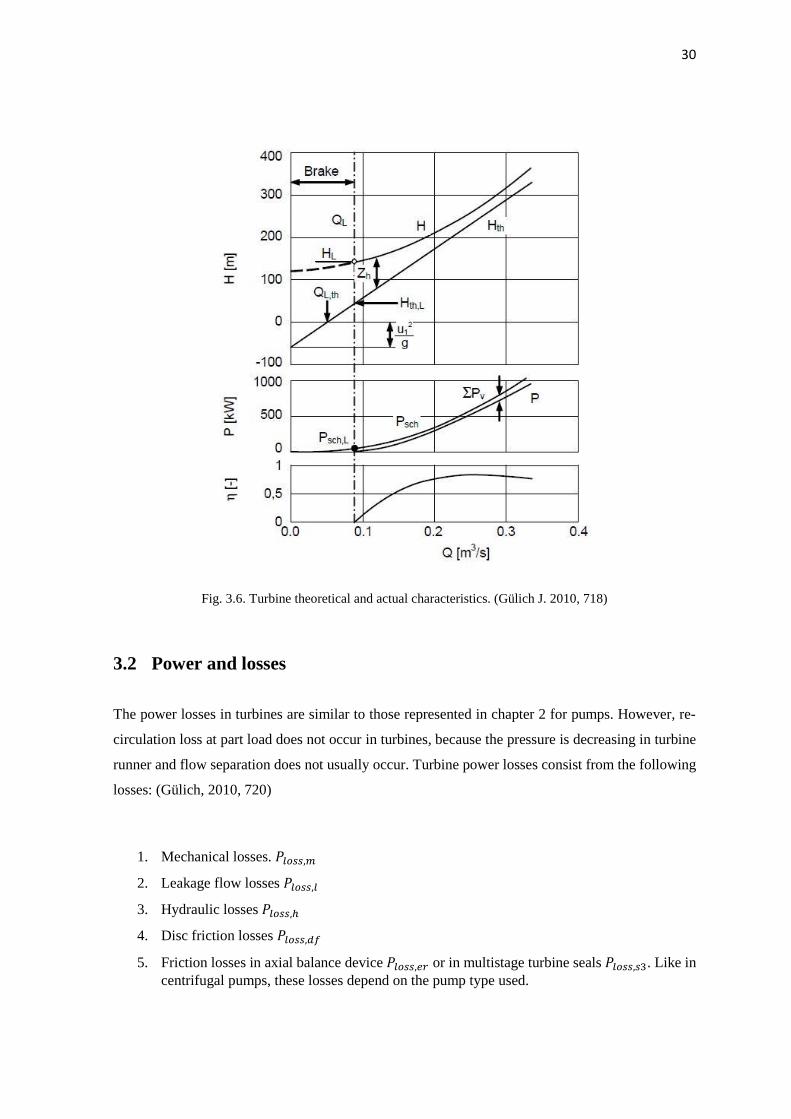
model in chapter 6.1. Fig. 3.6 illustrates the theoretical and actual turbine characteristics for constant

rotational speed. According to (eq. 3.15), the theoretical head is a straight line. The actual head is

larger because of the hydraulic losses 𝑍ℎ. The power curve 𝑃𝑠𝑐ℎ describes the theoretical work that

is absorbed in the runner. The work available at turbine coupling 𝑃 is smaller.

30

Fig. 3.6. Turbine theoretical and actual characteristics. (Gülich J. 2010, 718)

3.2 Power and losses

The power losses in turbines are similar to those represented in chapter 2 for pumps. However, re-

circulation loss at part load does not occur in turbines, because the pressure is decreasing in turbine

runner and flow separation does not usually occur. Turbine power losses consist from the following

losses: (Gülich, 2010, 720)

1. Mechanical losses. 𝑃𝑙𝑜𝑠𝑠,𝑚

2. Leakage flow losses 𝑃𝑙𝑜𝑠𝑠,𝑙

3. Hydraulic losses 𝑃𝑙𝑜𝑠𝑠,ℎ

4. Disc friction losses 𝑃𝑙𝑜𝑠𝑠,𝑑𝑓

5. Friction losses in axial balance device 𝑃𝑙𝑜𝑠𝑠,𝑒𝑟 or in multistage turbine seals 𝑃𝑙𝑜𝑠𝑠,𝑠3. Like in

centrifugal pumps, these losses depend on the pump type used.

31

𝑃𝑠𝑐ℎ is the power transmitted to the runner. It is the hydraulic power subtracted with the hydraulic

and leakage losses. (Gülich J. 2010, 720) Fig. 3.7 is a Sankey-diagram illustrating the turbine power

losses described earlier. The turbine shaft power P is calculated from the theoretical power by sub-

tracting the mechanical loss, disc friction loss, thrust balance device friction loss and the interstage

seals power loss.

Fig. 3.7. Sankey-diagram of turbine power losses (Gülich J. 2010, 720)

The applicability range of PaT’s is described by Chapallaz (1992) and this is illustrated in Fig. 3.8.

Radial flow pumps can be used as turbines to around 500 l/s flow rates and to about 150 m head,

while mixed flow pumps can be used to around 800 l/s flow rates but to only about 40 m heads.

32

Fig. 3.8. Applicability range of PaT’s based on operation point. (Nygren, 2016, 40, modified from Chapallaz,

1992)

3.3 Difference to turbines

The main difference between a PaT and a regular turbine is the lack of flow control device that

turbines have. This can be an advantage, because it makes the system cheaper and less complicated.

On the other hand, it makes the PaT less versatile because of the sensitivity of the efficiency to the

flow condition. Variable speed drives may provide an economical alternative to use PaT in different

flow conditions.

The geometry and size of a PaT and a conventional turbine differ a lot: The latter has smaller diam-

eter and opposite direction of curvature in the blades. The main reason is of course the fact, that a

PaT is primarily designed to work as a pump. A pump needs longer blades and flow channels, be-

cause there is a risk of flow separation that needs to be managed. In turbines, the flow is accelerated

in the impeller, and there is usually no risk of flow separation. The PaT’s may have typically 30 –

40 % larger impeller than a Francis-turbine for the same operation point. For same reasons, a normal

Francis-turbine would not make a good pump: It is easier to use a pump as a turbine, than the other

way around. Fig. 3.9 is a schematic of the differences of Francis-turbine impeller and a centrifugal

pump used as turbine for similar work cycle. (Alatorre-Frenk, 1994, 3)

33

Fig. 3.9. Difference of a Francis-impeller and a PaT of similar work cycle (Alatorre-Frenk, 1994,3)

34

4 ELECTRICAL MACHINE AND FREQUENCY CONVERTER

In order to utilize the power produced by PaT, the shaft has to be coupled either to an electrical

generator, or to other consumer of mechanical energy. For example, PaT may be coupled to a pump,

or even to a pump and an electrical machine as a turbopump system in some applications. In this

thesis we are studying a PaT coupled to an electrical motor, which is used as a generator.

The two electric motor types used in the test setup are AC induction motor (IM) and a synchronous

reluctance motor (SynRM). These are introduced in detail. AC induction motors, or “squirrel cage”

motors are probably the most used electric motor in industry. The AC-current is fed to the stator

coiling, which creates a rotating magnetic field. Stator phase coil number determines the pole number

of a motor. In 2-pole motor, there is 2 stator coils for each phase. For 50 Hz frequency the synchro-

nous speed of a 2-pole motor is 3000 rpm and the higher the pole number, the lower the synchronous

speed. Fig. 4.1 illustrates a view of a stator winding. The stator windings are built inside a stator

housing, and the stator itself consists of thin, stacked laminations that are made from insulated wire.

(Grundfos, 2004a, 15)

Fig. 4.1. A stator of an AC-induction motor. (Grundfos, 2004a, 15)

The rotating stator magnetic field induces currents in the rotor. In a typical, “squirrel cage” rotor, the

rotor bars induce a current because of the stator magnetic field, and this causes the rotor to turn.

More accurately, the difference between the stator magnetic field, which is rotating at synchronous

speed, and the rotor speed, which is lower than the synchronous speed, causes torque. This is called

as the slip of a motor, and it is given as percentage. The higher the load, the higher the slip. This is

also why induction motors are called asynchronous motors: The rotor speed is not the same as the

35

synchronous speed. Fig. 4.2 illustrates the build of a “squirrel cage” rotor. Rotor is made from a stack

of slotted aluminium plates, which create the bars of the squirrel cage. (Grundfos, 2004a, 16)

Fig. 4.2. (Left) A cross sectional view of rotor lamination. (Right) A view of a typical stacked rotor.

Synchronous reluctance motors (SynRM) have a similar stator coiling than induction motors. The

rotor is different from the induction motor, because of its magnetically anisotropic structure. Fig. 4.3

illustrates a rotor of a SynRM motor. The axis that has a high magnetic permeance is the d-axis,

while the q-axis has a low permeance. The torque is created because the high permeance d-axis turns

towards the magnetic field created by the stator. No rotor currents are induced, as in induction mo-

tors, and therefore the rotor has no Joule-losses and it runs cooler than an induction rotor. However,

SynRM-motors can not be operated without a frequency converter and a sophisticated control

scheme. (ABB, 2016b, 10)

Fig. 4.3. The rotor of a 4-pole SynRM motor. The q and d are the magnetic axes. (ABB, 2016b, 10)

Fig. 4.4 illustrates the operation of an induction motor with variable frequency. The relation 𝑛/𝑛𝑁

describes the rotational speed of the rotor compared to the nominal value. The electrical machine is

operating as a motor when the rotational speed of the rotor is smaller than the synchronous speed.

When the rotor speed is higher than the synchronous speed, the motor is generating. As can be seen

36

from the figure, the bolded blue curve is steep around the synchronous speed. This is important,

because a high torque is wanted with a minimal slip. (ABB, 2016c)

When operating the motor with a frequency converter, the synchronous speed can be changed and

the maximum torque can be reached at all speeds lower than the nominal speed. This is called the

constant-flux region. When the speed is higher than the nominal speed, the motor is operating in

field-weakening range and the maximum torque gets lower. Notice the analogy to Fig. 3.2 where 8

operating modes for pumps were introduced. (ABB, 2016c)

Fig. 4.4. Induction motor operation areas. (ABB, 2016c)

4.1 Motor efficiency

The single-speed, 3-phase, 50 or 60 Hz induction motor efficiency classes are defined by IEC/EN

60034-30-1:2014. The efficiency classes are named International Efficiency-classes (IE). The clas-

ses used are from IE1 to IE4, where IE4 is the highest standardized efficiency class. Fig. 4.5 illus-

trates the minimum efficiency of different IE-classes as a function of the motor output power for 4-

pole motors. (ABB, 2016c, 4)

37

Fig. 4.5. IE-classes for 4-pole induction motors (ABB, 2016c, 5)

The EU-wide aim is to increase the energy efficiency of electric motors and therefore decrease the

CO2-emissions. Therefore international Minimum Energy Performance Standard (MEPS) levels are

used. The regulations are different in different parts of the world, but European Minimum Energy

Performance Standard (EU MEPS) sets a minimum energy efficiency levels for 2-, 4- and 6-pole

single-speed, three-phase induction motors in a power range of 0.75 kW to 375 kW. The EU MEPS

is in stage 2 (after 2015), and the motors sized 7.5 kW to 375 kW must fulfill IE3 level in direct on-

line use, but they can be IE2-class if they are used with variable speed drive. In 2017 the EU MEPS

includes motors from 0.75 kW to 375 kW. (ABB, 2016c, 4)

The electric motor manufacturers do not usually publish the efficiency values for their motors in

generating mode. For high efficiency motors (eff 1, which is similar to IE2), the efficiency as gen-

erator is usually comparable to the motor efficiency. This is not the case in low efficiency motors;

for low efficiency motors the generator efficiency can be lower than the motor efficiency. An over

2 percent efficiency drop was observed in a study with an eff3-class motor. Eff3-class is old effi-

ciency class, which has minimum efficiency requirements below IE1-class. (Deprez, Wim et Al.

2006)

4.2 Frequency converter

Frequency converter is a device that alters the frequency of the voltage in the motor input. According

to ABB (2016a), the frequency converters can be divided into three groups based on their DC circuit

38

structure. Voltage-source converters are most common at low voltage applications (< 1000 V), and

they have intermediate DC-circuit with constant voltage. Current-source converters produce the out-

put by modulating the fixed DC current. Direct frequency converters produce the variable output

voltage by modulating the input voltage directly.

In this thesis we will focus on the voltage-source converters, because they are the type of frequency

converters used in the test setup. Fig. 4.6 illustrates the principle of voltage-source frequency con-

verter. In this figure the input is a diode bridge, but it is possible to use Insulated-Gate Bipolar Tran-

sistors (IGBT) for the input also. This makes it possible to feed power back to the grid from the

intermediate DC circuit and therefore to use the frequency converter for power generation. The out-

put in the figure is a Pulse-Width Modulation (PWM) inverter. The component that is responsible

for the PWM is usually Insulated-Gate Bipolar Transistor (IGBT), because of high efficiency and

current handling capacity.

Fig. 4.6. Schematic of a voltage-source frequency converter (ABB, 2016a)

The frequency converters intermediate DC circuit can be linked to other frequency converters inter-

mediate DC circuit. This makes it possible to use only one line side rectifier to supply all the DC-

AC inverters. In applications where some motors are generating, while other are motoring, it makes

it possible to use the power of the generating motors through the DC-circuit. Therefore the expensive

line side inverter is not needed, if all the power produced is consumed by the other motoring units.

(Rockwell Automation, 2005, 2)

39

5 CONTROL VALVE CHARACTERISTICS

Control valves are used in processes to control the flow rate in the process. A control valve controls

the flow rate by controlling the pressure losses across the valve. Typically a control valve causes one

third of the total pressure losses in a piping system. (Kirmanen J. et al. 2011, 11-17) Stricter energy

efficiency requirements may cause the partition of pressure drop caused by control valve to drop.

Before the use of variable speed drives, it was often the only option to use a pump which was running

at full speed, and then to throttle the flow with a control valve to produce suitable process conditions.

The use of variable speed driven pumps may make the control valve unnecessary in many applica-

tions. It is also more energy efficient, because the pump is not producing more pressure than neces-

sary, thus it is consuming less power.

Valves can be divided into sliding-stem valves and rotary-stem valves. Sliding-stems are valves that

operate by linear motion of the valve stem and valve internal components. Rotary-stem valves oper-

ate by rotating the stem and the internal components. Common control valve types based on the

internal components are ball, globe and butterfly valves.

The simplest pressure reducing valves may work without intelligent control using the fluid pressure

difference as energy source for valve actuation. A spring is holding the valve closed, and valve opens

when the pressure in secondary side of the valve is lowered, thus heightening the pressure. These

valves can operate to supply a fixed secondary pressure as long as the primary pressure is higher

than the desired pressure, or they can work as constant pressure reduction valves, which create a

constant pressure difference over the valve. (Hydraulics & Pneumatics, 2012)

In this thesis we are especially interested in pressure reducing valves and flow control valves, which

reduce the pressure of the fluid and the throttled pressure energy is lost in the valve. These valves

might be substituted with a PaT in order to recover hydraulic energy, which would otherwise be lost

in the valve pressure reduction.

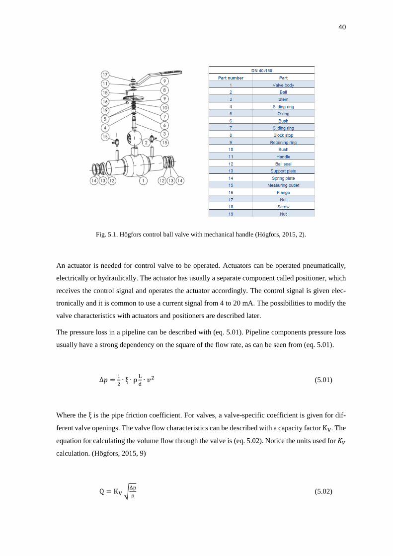
Fig. 5.1 illustrates a rotary-stem ball valve, which can be used either as on on-off valve, or as a flow

control valve with or without an actuator. There is a mechanical actuator (a handle) installed in the

picture. (Högfors, 2015)

40

Fig. 5.1. Högfors control ball valve with mechanical handle (Högfors, 2015, 2).

An actuator is needed for control valve to be operated. Actuators can be operated pneumatically,

electrically or hydraulically. The actuator has usually a separate component called positioner, which

receives the control signal and operates the actuator accordingly. The control signal is given elec-

tronically and it is common to use a current signal from 4 to 20 mA. The possibilities to modify the

valve characteristics with actuators and positioners are described later.

The pressure loss in a pipeline can be described with (eq. 5.01). Pipeline components pressure loss

usually have a strong dependency on the square of the flow rate, as can be seen from (eq. 5.01).

Δ𝑝 =1

2∙ ξ ∙ ρ

L

d∙ 𝑣2 (5.01)

Where the ξ is the pipe friction coefficient. For valves, a valve-specific coefficient is given for dif-

ferent valve openings. The valve flow characteristics can be described with a capacity factor KV. The

equation for calculating the volume flow through the valve is (eq. 5.02). Notice the units used for 𝐾𝑉

calculation. (Högfors, 2015, 9)

Q = KV √Δp

ρ (5.02)

41

Where 𝑄 is the volume flow in [m3/h], Δp is the pressure difference in [bar] and 𝜌 is the density of

fluid in [kg/m3]. Other manufacturers use a different coefficient, called the valve flow coefficient,

CV which is defined as (Niemelä I. et al, 2015, 6)

𝑄 = 𝐶𝑉 ∙ 𝑁1 ∙ √Δ𝑝 (5.03)

Where N1 is a unit specific coefficient. For [m3/h] and [bar] value of N1 is 0.865. The coefficient

𝐶𝑉 is used by American valve industry, so that the coefficient 𝑁1 is defined to be 1.0 for units [gpm]

and [psi]. Both the 𝐶𝑉 and 𝐾𝑉 values are determined for water; for 𝐶𝑉 the fluid is specified to be

room temperature water, and therefore the density of the fluid is probably absorbed in the coefficient

itself.

Inherent flow characteristics for valves are determined with a constant pressure difference over the

valve. This is not the case in real life applications; change in flow rate will cause the pressure to

change. Inherent flow characteristics are used to determine the valve throttling characteristics indi-

vidually from the pipeline characteristics.

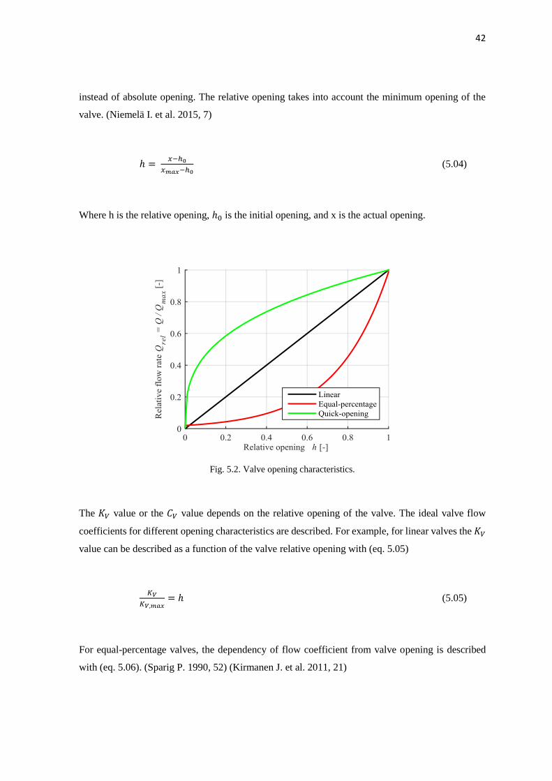
Valves can be divided into three main groups by their inherent flow characteristics. Fig. 5.2 illus-

trates the different opening characteristics. In linear opening valves, the capacity factor grows line-

arly with increasing valve opening. This means that for a constant pressure difference over the valve,

50 % relative opening equals to 50 % of the maximum flow rate. Linear inherent flow characteristics

would be ideal in application where the pressure difference over the valve stays constant. (Kirmanen

J. et al. 2011, 22) In quick opening valves the capacity factor grows faster in small openings, which

makes them ideal for use as on/off valves in applications where fast increase of flow is wanted.

Equal percentage valves work ideally so that equal increments in the valve opening cause a constant

change in relative flow rate. Equal percentage valves are designed to linearize the installed flow

characteristics in normal control valve applications, where the available pressure drop decreases with

increasing flow. (Kirmanen J. et al. 2011, 22) This makes them ideal for use in applications where

precise and linear flow control is needed. Equal percentage valves are the most common control

valves. The different valve opening characteristics are described in Fig. 5.2. (Emerson, 2005)

Some rotary type valves have a certain minimum opening. This means that a certain opening is

needed before the fluid starts flowing through the valve. Therefore relative opening is usually used

42

instead of absolute opening. The relative opening takes into account the minimum opening of the

valve. (Niemelä I. et al. 2015, 7)

ℎ = 𝑥−ℎ0

𝑥𝑚𝑎𝑥−ℎ0 (5.04)

Where h is the relative opening, ℎ0 is the initial opening, and x is the actual opening.

Fig. 5.2. Valve opening characteristics.

The 𝐾𝑉 value or the 𝐶𝑉 value depends on the relative opening of the valve. The ideal valve flow

coefficients for different opening characteristics are described. For example, for linear valves the 𝐾𝑉

value can be described as a function of the valve relative opening with (eq. 5.05)

𝐾𝑉

𝐾𝑉,𝑚𝑎𝑥= ℎ (5.05)

For equal-percentage valves, the dependency of flow coefficient from valve opening is described

with (eq. 5.06). (Sparig P. 1990, 52) (Kirmanen J. et al. 2011, 21)

43

𝐾𝑉

𝐾𝑉,𝑚𝑎𝑥= 𝑘1 ∙ 𝑒𝑘2∙ℎ (5.06)

Where 𝑘1 and 𝑘2 are valve-specific coefficients. It should be noted that ideal equal-percentage valves

have a certain minimum flow rate when the relative opening is zero. Quick-opening valves can be

described with (eq. 5.07).

𝐾𝑉

𝐾𝑉,𝑚𝑎𝑥 = ℎ1/𝑘1 (5.07)

The similar expressions can be derived for the valve flow coefficient 𝐶𝑉. There does also exist some

variation in the ways the ideal different characteristics are expressed. (eq. 5.05 – eq. 5.07) describe

the ideal valve characteristics, the real valve characteristics are always provided by the manufacturer.

Manufacturer provides the 𝐶𝑉 or 𝐾𝑉 values for their valves on different openings based on measure-

ments.

5.1 Installed flow characteristics

The control valve is usually installed as a part of a process piping. The pressure over the valve is

rarely kept constant. The pressure difference over the valve drops with increasing flow, because of

pressure losses in other components of the pipeline, for example in heat exchangers and in the pipe-

line itself. The installed flow characteristics curve for a valve is therefore dependent on the inherent

valve characteristics and also from the pipeline flow characteristics. (Kirmanen J. et al. 2011, 22)

The process pipeline characteristics can be described using a pressure ratio factor DPm (eq. 5.08),

which is defined as the ratio between the pressure difference at maximum flow rate and at zero-flow.

𝐷𝑃𝑚 =Δ𝑝𝑚

Δ𝑝0 (5.08)

Where Δ𝑝𝑚 is the pressure difference over the valve at maximum flow and Δ𝑝0 is the pressure dif-

ference when the valve is closed. Fig. 5.3 illustrates the pipeline characteristics and the available

44

pressure difference over the control valve. Here subscript 1 denotes state before valve and 2 state

after the valve. The pressure difference over the valve is Δ𝑝 = 𝑝1 − 𝑝2.

Fig. 5.3. Pipeline characteristics (Modified from Kirmanen J. et al. 2011, 23)

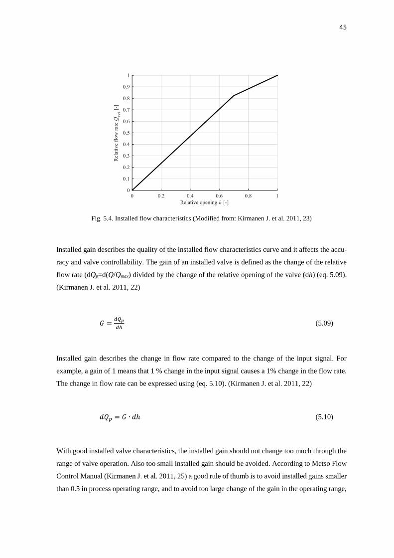
Fig. 5.4 illustrates installed flow characteristics curve where equal-percentage valve characteristics

have been combined to pipeline characteristic. The resulting installed flow characteristics curve is

almost linear. Properly selected equal-percentage valves combined with pipeline characteristics

make it possible to get nearly linear installed flow characteristics.

45

Fig. 5.4. Installed flow characteristics (Modified from: Kirmanen J. et al. 2011, 23)

Installed gain describes the quality of the installed flow characteristics curve and it affects the accu-

racy and valve controllability. The gain of an installed valve is defined as the change of the relative

flow rate (dQp=d(Q/Qmax) divided by the change of the relative opening of the valve (dh) (eq. 5.09).

(Kirmanen J. et al. 2011, 22)

𝐺 =𝑑𝑄𝑝

𝑑ℎ (5.09)

Installed gain describes the change in flow rate compared to the change of the input signal. For

example, a gain of 1 means that 1 % change in the input signal causes a 1% change in the flow rate.

The change in flow rate can be expressed using (eq. 5.10). (Kirmanen J. et al. 2011, 22)

𝑑𝑄𝑝 = 𝐺 ∙ 𝑑ℎ (5.10)

With good installed valve characteristics, the installed gain should not change too much through the

range of valve operation. Also too small installed gain should be avoided. According to Metso Flow

Control Manual (Kirmanen J. et al. 2011, 25) a good rule of thumb is to avoid installed gains smaller

than 0.5 in process operating range, and to avoid too large change of the gain in the operating range,

46

so that the relation between maximum gain and the minimum gain is below 2.0. Too large variations

in the gain will result in difficulties in the process control.

Fig. 5.5 illustrates the possibilities to modify the flow rate response by modifying the signals or the

response of the actuator in order to get linear characteristics. Signal modification can be done in the

controller or in the positioner. Inherent valve characteristics and piping characteristics are defined

by the properties of the parts used in the system, while the controller output or the positioner output

can be modified easily. Positioner output can be modified using positioners with nonlinear output

(PMW, 2002).

Fig. 5.5. Control valve characterization by modifying controller output (Kirmanen J. et al. 2011, 26)

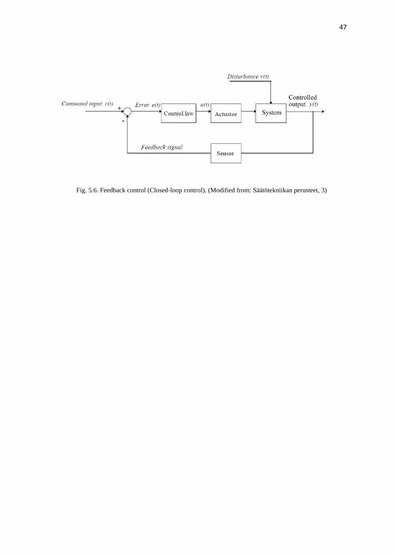
Control systems can be divided into two groups: open loop control and feedback control (closed loop

control). In open loop control, the adjustment is done by predefined model for the system, and it does

not take into account errors in the process. Feedback control measures the adjusted quantity (con-

trolled output), and can take errors in account by adjusting the command input. Fig. 5.6 illustrates

the principle of the feedback control system.

47

Fig. 5.6. Feedback control (Closed-loop control). (Modified from: Säätötekniikan perusteet, 3)

48

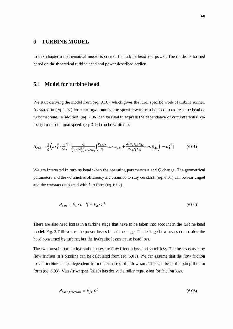
6 TURBINE MODEL

In this chapter a mathematical model is created for turbine head and power. The model is formed

based on the theoretical turbine head and power described earlier.

6.1 Model for turbine head

We start deriving the model from (eq. 3.16), which gives the ideal specific work of turbine runner.

As stated in (eq. 2.02) for centrifugal pumps, the specific work can be used to express the head of

turbomachine. In addition, (eq. 2.06) can be used to express the dependency of circumferential ve-

locity from rotational speed. (eq. 3.16) can be written as

𝐻𝑠𝑐ℎ =1

𝑔(𝜋𝑟2

2 ∙𝑛

60)

2[

𝑄

(𝜋𝑟22∙

𝑛

60)

𝑧𝐿𝑒𝐴3𝑞

(𝑟3,𝑒𝑓𝑓

𝑟2𝑐𝑜𝑠 𝛼3𝐵 +

𝑑1∗ 𝜂𝑉𝑧𝐿𝑒𝐴3𝑞

𝑧𝐿𝑎𝑓𝑞𝐴1𝑞𝑐𝑜𝑠 𝛽𝐴1) − 𝑑1

∗2] (6.01)

We are interested in turbine head when the operating parameters n and Q change. The geometrical

parameters and the volumetric efficiency are assumed to stay constant. (eq. 6.01) can be rearranged

and the constants replaced with k to form (eq. 6.02).

𝐻𝑠𝑐ℎ = 𝑘1 ∙ 𝑛 ∙ 𝑄 + 𝑘2 ∙ 𝑛2 (6.02)

There are also head losses in a turbine stage that have to be taken into account in the turbine head

model. Fig. 3.7 illustrates the power losses in turbine stage. The leakage flow losses do not alter the

head consumed by turbine, but the hydraulic losses cause head loss.

The two most important hydraulic losses are flow friction loss and shock loss. The losses caused by

flow friction in a pipeline can be calculated from (eq. 5.01). We can assume that the flow friction

loss in turbine is also dependent from the square of the flow rate. This can be further simplified to

form (eq. 6.03). Van Artwerpen (2010) has derived similar expression for friction loss.

𝐻𝑙𝑜𝑠𝑠,𝑓𝑟𝑖𝑐𝑡𝑖𝑜𝑛 = 𝑘𝑓𝑟 𝑄2 (6.03)

49

The shock loss is proportional to the difference of flow rate from the shock-free entry flow rate, and

this is assumed to be dependent on the square of the difference. This is described with (eq. 6.04).

𝐻𝑙𝑜𝑠𝑠,𝑠ℎ𝑜𝑐𝑘 = 𝑘𝑠ℎ𝑜𝑐𝑘(𝑄 − 𝑄𝑆𝐹)2 (6.04)

Gülich (2010, 728) provides an equation for calculating the shock-free entry flow rate. The equation

can be simplified with same assumptions as for (eq. 6.01). It is also assumed that the flow blockage

factor 𝜏2 does not change significantly with changing rotational speed or flow rate. This yields (eq.

6.05).

𝑄𝑆𝐹 = 𝑘𝑆𝐹𝑛 (6.05)

(Eq. 6.04 – eq. 6.05) can be combined and simplified to form (eq. 6.06).

𝐻𝑙𝑜𝑠𝑠,𝑠ℎ𝑜𝑐𝑘 = 𝑘1 ∙ 𝑄2 + 𝑘2 ∙ 𝑛 ∙ 𝑄 + 𝑘3𝑛2 (6.06)

Taking into account the theoretical head (eq. 6.02) and head losses from the theoretical head (eq.

6.03 and eq. 6.06), we can describe a polynomial model for turbine head (eq. 6.07). The constants in

loss models are absorbed to form the final constants used in the head model.

𝐻𝑡 = 𝑘ℎ1𝑄2 + 𝑘ℎ2𝑛𝑄 + 𝑘ℎ3𝑛2 (6.07)

Similar derivation of turbine head model has been done by Nygren (2016), Van Artwerpen (2010),

and several others.

50

6.2 Model for turbine power

The previously derived head model describes the total head of a turbine, when fitted to experimental

data. The turbine power model can be derived from the head model, when certain power losses are

taken into account. The available hydraulic power is

𝑃ℎ𝑦𝑑 = 𝜌𝑔𝐻𝑄 (6.08)

Fig. 3.7 illustrates the power losses of a turbine. We can use the theoretical head model and theoret-

ical power in derivation of turbine model. The theoretical power does not take into account the hy-

draulic losses or the leakage flow losses. The theoretical power is

𝑃𝑠𝑐ℎ = 𝜌𝑔𝐻𝑠𝑐ℎ𝑄 (6.09)

Taking into account (eq. 6.02) yields

𝑃𝑠𝑐ℎ = 𝜌𝑔(𝑘1𝑛𝑄 + 𝑘2𝑛2)𝑄 (6.10)

The turbine shaft power can be calculated from the theoretical power by subtracting the disc friction

and mechanical loss (eq. 6.11). The losses in interstage seals and axial thrust balance device are not

taken into account.

𝑃𝑡 = 𝑃𝑠𝑐ℎ − 𝑃𝑙𝑜𝑠𝑠,𝑑𝑓 − 𝑃𝑙𝑜𝑠𝑠,𝑚 (6.11)

The disc friction loss can be estimated for radial impellers with (eq. 6.12) (Gülich J. 2010, 136)

𝑃𝑙𝑜𝑠𝑠,𝑑𝑓 =𝑘𝑅𝑅

cos δ𝜌𝜔3𝑅5 (1 − (

𝑅𝑛

𝑅)

5) (6.12)

51

Similar equation for calculating disc friction is provided also by KSB (a). Knowing that the angular

velocity 𝜔 = 2𝜋𝑛, and assuming that the geometrical parameters, density and the friction coefficient

𝑘𝑅𝑅 are constants, (eq. 6.12) can be simplified and the resulting dependency between disc friction

and the rotational speed is presented in (eq. 6.13).

𝑃𝑙𝑜𝑠𝑠,𝑑𝑓 = 𝑘𝑑𝑓 ∙ 𝑛3 (6.13)

Mechanical losses occurring in centrifugal pumps have a dependency (eq. 6.14).

𝑃𝑙𝑜𝑠𝑠,𝑚 ~ 𝑛𝑥 (6.14)

Where x = 1.3 to 1.8. (Gülich, 2010, 101). We will use approximation x = 1 for the model derivation

from reasons of simplicity. Mechanical losses are therefore assumed to be

𝑃𝑙𝑜𝑠𝑠,𝑚 = 𝑘𝑚𝑛 (6.15)

The model for turbine power is created combining (eq. 6.10, eq. 6.11, eq. 6.13 and eq. 6.15) to form

(eq. 6.16).

𝑃𝑡 = 𝜌𝑔(𝑘1𝑛𝑄 + 𝑘2𝑛2)𝑄 − 𝑘𝑑𝑓 ∙ 𝑛3 − 𝑘𝑚 ∙ 𝑛 (6.16)

Which can be simplified by absorbing the constants to form the final polynomial model for turbine

power

𝑃𝑡 = 𝑘𝑝1𝑛𝑄2 + 𝑘𝑝2𝑛2𝑄 + 𝑘𝑝3𝑛3 + 𝑘𝑝4𝑛 (6.17)

Similar model has been derived by Nygren (2016). There is however a small difference compared to

the power model derived by Nygren. The last term 𝑘𝑝4𝑛, which describes the mechanical losses in

52

the turbine, is used in this model. It makes the model slightly more complex, but it should increase

the accuracy of the model compared to the model based on similarity laws.

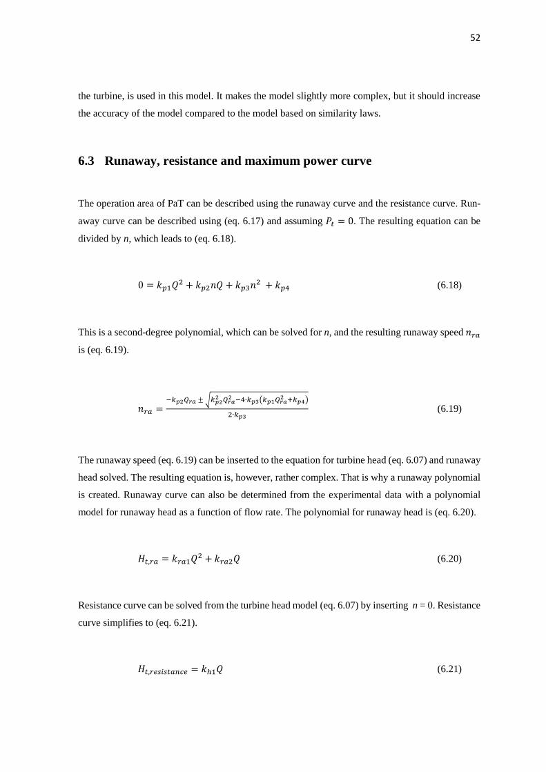
6.3 Runaway, resistance and maximum power curve

The operation area of PaT can be described using the runaway curve and the resistance curve. Run-

away curve can be described using (eq. 6.17) and assuming 𝑃𝑡 = 0. The resulting equation can be

divided by n, which leads to (eq. 6.18).

0 = 𝑘𝑝1𝑄2 + 𝑘𝑝2𝑛𝑄 + 𝑘𝑝3𝑛2 + 𝑘𝑝4 (6.18)

This is a second-degree polynomial, which can be solved for n, and the resulting runaway speed 𝑛𝑟𝑎

is (eq. 6.19).

𝑛𝑟𝑎 =−𝑘𝑝2𝑄𝑟𝑎 ± √𝑘𝑝2

2 𝑄𝑟𝑎2 −4∙𝑘𝑝3(𝑘𝑝1𝑄𝑟𝑎

2 +𝑘𝑝4)

2∙𝑘𝑝3 (6.19)

The runaway speed (eq. 6.19) can be inserted to the equation for turbine head (eq. 6.07) and runaway

head solved. The resulting equation is, however, rather complex. That is why a runaway polynomial

is created. Runaway curve can also be determined from the experimental data with a polynomial

model for runaway head as a function of flow rate. The polynomial for runaway head is (eq. 6.20).

𝐻𝑡,𝑟𝑎 = 𝑘𝑟𝑎1𝑄2 + 𝑘𝑟𝑎2𝑄 (6.20)

Resistance curve can be solved from the turbine head model (eq. 6.07) by inserting n = 0. Resistance

curve simplifies to (eq. 6.21).

𝐻𝑡,𝑟𝑒𝑠𝑖𝑠𝑡𝑎𝑛𝑐𝑒 = 𝑘ℎ1𝑄 (6.21)

53

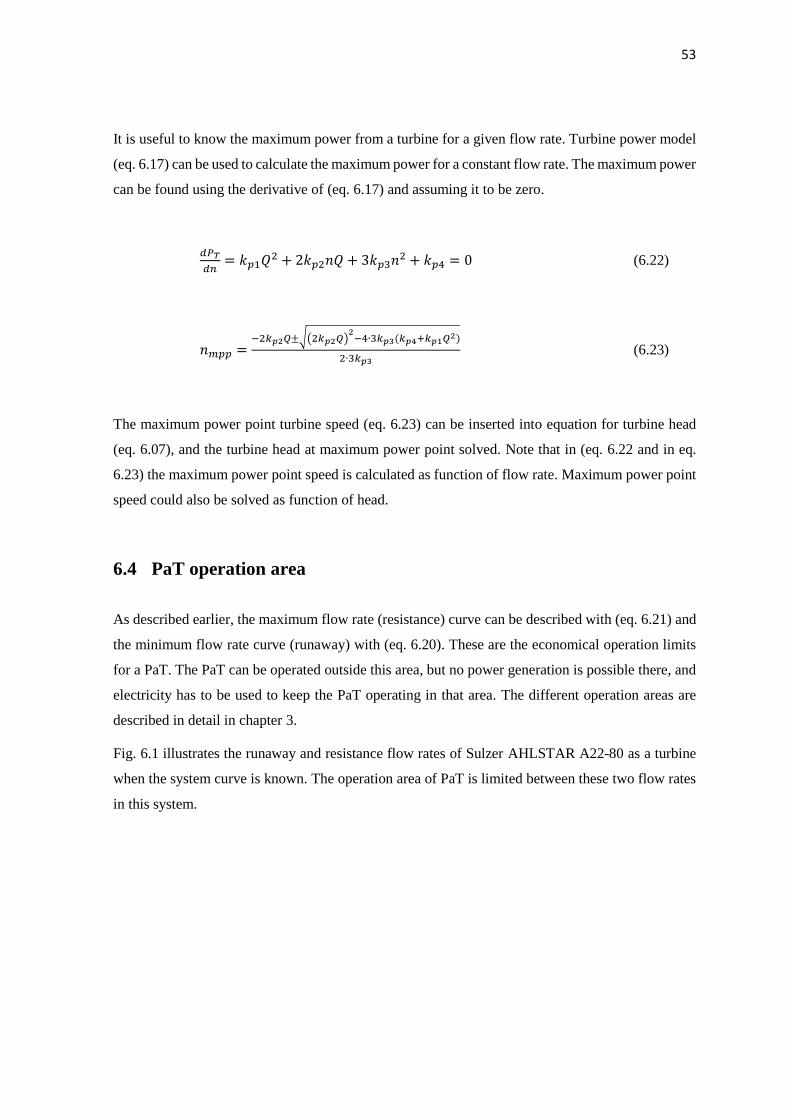
It is useful to know the maximum power from a turbine for a given flow rate. Turbine power model

(eq. 6.17) can be used to calculate the maximum power for a constant flow rate. The maximum power

can be found using the derivative of (eq. 6.17) and assuming it to be zero.

𝑑𝑃𝑇

𝑑𝑛= 𝑘𝑝1𝑄2 + 2𝑘𝑝2𝑛𝑄 + 3𝑘𝑝3𝑛2 + 𝑘𝑝4 = 0 (6.22)

𝑛𝑚𝑝𝑝 =−2𝑘𝑝2𝑄±√(2𝑘𝑝2𝑄)

2−4∙3𝑘𝑝3(𝑘𝑝4+𝑘𝑝1𝑄2)

2∙3𝑘𝑝3 (6.23)

The maximum power point turbine speed (eq. 6.23) can be inserted into equation for turbine head

(eq. 6.07), and the turbine head at maximum power point solved. Note that in (eq. 6.22 and in eq.

6.23) the maximum power point speed is calculated as function of flow rate. Maximum power point

speed could also be solved as function of head.

6.4 PaT operation area

As described earlier, the maximum flow rate (resistance) curve can be described with (eq. 6.21) and

the minimum flow rate curve (runaway) with (eq. 6.20). These are the economical operation limits

for a PaT. The PaT can be operated outside this area, but no power generation is possible there, and

electricity has to be used to keep the PaT operating in that area. The different operation areas are

described in detail in chapter 3.

Fig. 6.1 illustrates the runaway and resistance flow rates of Sulzer AHLSTAR A22-80 as a turbine

when the system curve is known. The operation area of PaT is limited between these two flow rates

in this system.

54

Fig. 6.1. Sulzer A22-80 and a system curve of 𝐻𝑠𝑡𝑎𝑡𝑖𝑐 = 15 m and 𝑘𝑠𝑦𝑠𝑡𝑒𝑚 = 0.015. The maximum and mini-

mum flow rates are marked with vertical lines.

Fig. 6.2 illustrates the maximum and minimum head of a PaT with the same system as earlier de-

scribed. Maximum pressure reduction (highest turbine head) can be achieved at runaway speed, and

the minimum pressure reduction at resistance curve (zero speed).

Fig. 6.2. Sulzer A22-80 and a system curve of 𝐻𝑠𝑡𝑎𝑡𝑖𝑐 = 15 m and 𝑘𝑠𝑦𝑠𝑡𝑒𝑚 = 0.015. The maximum and mini-

mum turbine head are marked with horizontal lines.

55

In order to simplify the use of a PaT as a control valve in simple closed loop applications, an equiv-

alent for valve opening is created. A typical valve opening is given as a percentage from 0 to 100 %,

which is transformed to a current signal which is given to a valve positioner. Typical signal for valve

positioner is a current signal from 4 mA to 20 mA. On the contrary, the control signal for the PaT

motor speed is typically a digital signal which contains a reference speed for the frequency converter.

Valve opening percentage can be changed to turbine speed reference with (eq. 6.24) when the runa-

way speed is known

𝑛 = 𝑛𝑟𝑎 (1 −𝑥

100) (6.24)

This simplifies the use of a PaT as a control valve for example in closed loop control applications,

because it introduces the operating limits of a PaT. It is worth mentioning that according to (eq.

6.24), the 0 % opening is the runaway speed of the PaT and the 100 % is zero-speed. The maximum

flow rate is achieved at 100 % opening, which corresponds to zero-speed.

As described earlier, the runaway speed of a PaT depends on the flow rate at runaway, which is,

dependent on the turbine head. When the turbine characteristics are known, depending on the system

and the measurements available there is two ways to calculate the runaway speed:

A) Calculation of the turbine head at runaway based on the known system properties.

B) Estimation of turbine head using measurements or estimate from frequency converter

With method A, the turbine head at runaway can be calculated when the system properties are known.

For example, if the system has a static head and the friction losses in the pipelines are known, the

runaway head can be calculated. The turbine head is equal to the system head, which is the system

static head subtracted with the head loss in the system pipelines at the runaway flow rate.

The pressure loss in a pipeline is described by (eq. 5.01) and this can be further modified to include

the system pipe friction coefficients and pipe geometries into one constant. The result is (eq. 6.25).

Δ𝑝 = 𝜌𝑔𝐻 =1

2𝜌𝑣2𝑘𝑙𝑜𝑠𝑠𝑒𝑠 (6.25)

Where the constant 𝑘𝑙𝑜𝑠𝑠𝑒𝑠 includes all the friction pressure losses and minor losses in the pipeline.

The acceleration due to gravity, pipe cross sectional area and the friction coefficient can be absorbed

56

in one coefficient so the equation can be rewritten to form that is easy to fit to measurement data.

(Eq. 6.26) also illustrates the system head losses dependency of the square of flow rate.

Δ𝐻 = 𝑘𝑠𝑦𝑠𝑡𝑒𝑚 ∙ 𝑄2 (6.26)

Where 𝑘𝑠𝑦𝑠𝑡𝑒𝑚 is a system specific constant which describes the pressure losses in the system pipe-

line when the pipeline remains unchanged. The system is assumed to have a static head and the head

losses in system are described with (eq. 6.26). If the whole system head is consumed by the PaT, the

turbine head can be solved with (eq. 6.27).

𝐻𝑡 = 𝐻𝑠𝑦𝑠𝑡𝑒𝑚 = 𝐻𝑠𝑡𝑎𝑡𝑖𝑐 − 𝑘𝑠𝑦𝑠𝑡𝑒𝑚 ∙ 𝑄 2 (6.27)

Turbine head can be inserted into the model for runaway head (eq. 6.20) and solved for flow rate at

runaway. The runaway speed 𝑛𝑟𝑎 can be directly solved from (eq. 6.19). Fig. 6.3 illustrates the run-

away speed determination with method A.

System static head and friction coefficient

Substitute in to model for turbine runaway head and

solve QRA

(6.20)

Solve runaway speed nRA

with (6.19)

Create an equation for turbine head (6.27)

Fig. 6.3. Method A for determining runaway speed.

57

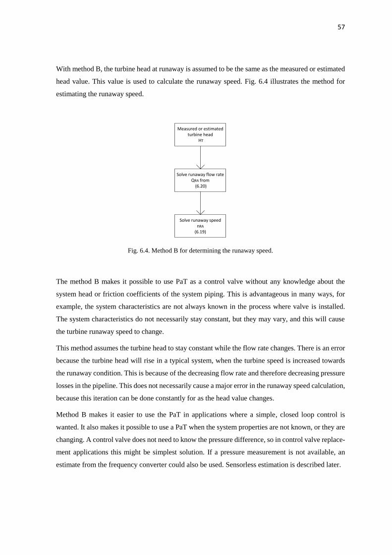
With method B, the turbine head at runaway is assumed to be the same as the measured or estimated

head value. This value is used to calculate the runaway speed. Fig. 6.4 illustrates the method for

estimating the runaway speed.

Measured or estimated turbine head

HT

Solve runaway flow rate QRA from

(6.20)

Solve runaway speed nRA

(6.19)

Fig. 6.4. Method B for determining the runaway speed.

The method B makes it possible to use PaT as a control valve without any knowledge about the

system head or friction coefficients of the system piping. This is advantageous in many ways, for

example, the system characteristics are not always known in the process where valve is installed.

The system characteristics do not necessarily stay constant, but they may vary, and this will cause

the turbine runaway speed to change.

This method assumes the turbine head to stay constant while the flow rate changes. There is an error

because the turbine head will rise in a typical system, when the turbine speed is increased towards

the runaway condition. This is because of the decreasing flow rate and therefore decreasing pressure

losses in the pipeline. This does not necessarily cause a major error in the runaway speed calculation,

because this iteration can be done constantly for as the head value changes.

Method B makes it easier to use the PaT in applications where a simple, closed loop control is

wanted. It also makes it possible to use a PaT when the system properties are not known, or they are

changing. A control valve does not need to know the pressure difference, so in control valve replace-

ment applications this might be simplest solution. If a pressure measurement is not available, an

estimate from the frequency converter could also be used. Sensorless estimation is described later.

58

6.5 Inherent valve characteristics and gain

The inherent valve characteristics for Sulzer A22-80 were calculated based on the models described

earlier and coefficients obtained from measurements in pump laboratory. The method for determin-

ing the inherent turbine characteristics from a model is described in Fig. 6.5. The results are illus-

trated in Fig. 6.6.Fig. 6.5. Determining the inherent valve characteristics for a PaT using the head

and runaway model.

Assume a static turbine head HT

Runaway flow rate QRA

(6.20)

Runaway speed nRA

(6.19)Opening

x = 0 – 100 %

Convert opening to speed reference n

(6.24)

Solve Q from head model (6.07)

Calculate relative flow rate

QREL = Q / QMAX

Plot x, QREL

Fig. 6.5. Determining the inherent valve characteristics for a PaT using the head and runaway model.

a) b)

Fig. 6.6. Inherent valve characteristics for a) Sulzer A22-80 b) A11-50 with 10 m head over the turbine

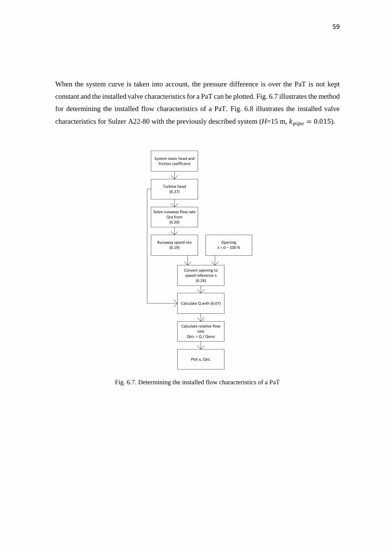
59

When the system curve is taken into account, the pressure difference is over the PaT is not kept

constant and the installed valve characteristics for a PaT can be plotted. Fig. 6.7 illustrates the method

for determining the installed flow characteristics of a PaT. Fig. 6.8 illustrates the installed valve

characteristics for Sulzer A22-80 with the previously described system (H=15 m, 𝑘𝑝𝑖𝑝𝑒 = 0.015).

System static head and friction coefficient

Turbine head (6.27)

Solve runaway flow rate Qra from

(6.20)

Opening x = 0 – 100 %

Convert opening to speed reference n

(6.24)

Calculate Q with (6.07)

Calculate relative flow rate

QREL = Q / QMAX

Plot x, QREL

Runaway speed nRA

(6.19)

Fig. 6.7. Determining the installed flow characteristics of a PaT

60

Fig. 6.8. Installed valve characteristics for Sulzer A22-80 for a system with 𝐻𝑠𝑡𝑎𝑡𝑖𝑐 = 15 m and 𝑘𝑠𝑦𝑠𝑡𝑒𝑚 =

0.015.

Because the available turbine head decreases with increasing flow rate, the maximum flow rate is

reduced compared to the inherent valve characteristics. This is why the operation area gets narrower

when the effects of system curve are taken into account. Similar turbine inherent valve characteristics

were created by Nygren (2016).

The valve gain describes the change of flow with changing the input signal (eq. 5.10). The installed

gain is calculated from the installed valve characteristics, and it is 𝐺 =d𝑄𝑟𝑒𝑙

d𝑥. Fig. 6.9 illustrates the

installed gain of Sulzer A22-80 based on Fig. 6.8.

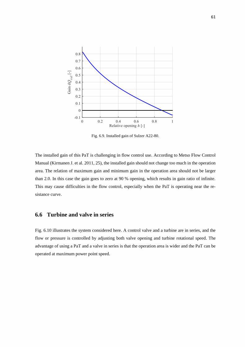
61

Fig. 6.9. Installed gain of Sulzer A22-80.

The installed gain of this PaT is challenging in flow control use. According to Metso Flow Control

Manual (Kirmanen J. et al. 2011, 25), the installed gain should not change too much in the operation

area. The relation of maximum gain and minimum gain in the operation area should not be larger

than 2.0. In this case the gain goes to zero at 90 % opening, which results in gain ratio of infinite.

This may cause difficulties in the flow control, especially when the PaT is operating near the re-

sistance curve.

6.6 Turbine and valve in series

Fig. 6.10 illustrates the system considered here. A control valve and a turbine are in series, and the

flow or pressure is controlled by adjusting both valve opening and turbine rotational speed. The

advantage of using a PaT and a valve in series is that the operation area is wider and the PaT can be

operated at maximum power point speed.

62

Fig. 6.10. Turbine and valve in series.

The following figure illustrates the effect of adding a valve in series with the turbine. The throttling

caused by valve is subtracted from the system curve and the operating point of the turbine can be

found from this curve. Fig. 6.11 illustrates Sulzer A11-50 turbine curves, a system with a static head

of 25 m and system friction coefficient of 𝑘𝑠𝑦𝑠𝑡𝑒𝑚 = 0,015. The valve is a fully open Metso Neles

RA DN80 control valve with a 𝐶𝑉 value of 160. The black line represents the turbine maximum

power point curve solved with (eq. 6.23).

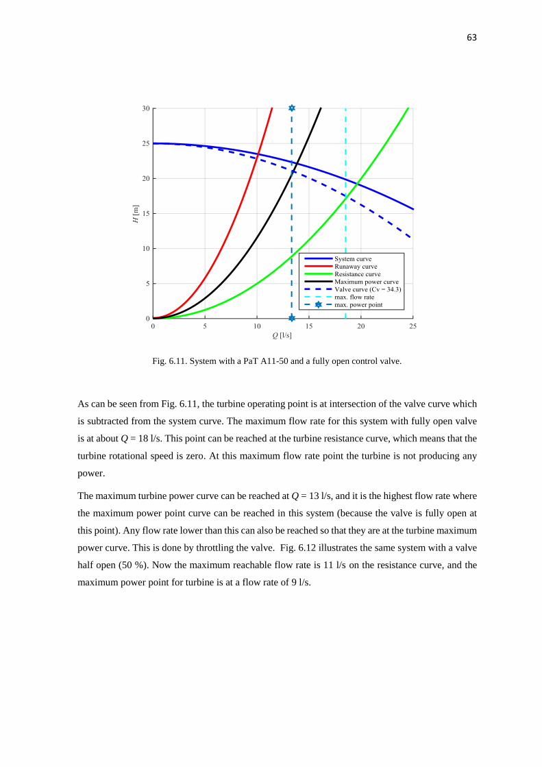
63

Fig. 6.11. System with a PaT A11-50 and a fully open control valve.

As can be seen from Fig. 6.11, the turbine operating point is at intersection of the valve curve which

is subtracted from the system curve. The maximum flow rate for this system with fully open valve

is at about Q = 18 l/s. This point can be reached at the turbine resistance curve, which means that the

turbine rotational speed is zero. At this maximum flow rate point the turbine is not producing any

power.

The maximum turbine power curve can be reached at Q = 13 l/s, and it is the highest flow rate where

the maximum power point curve can be reached in this system (because the valve is fully open at

this point). Any flow rate lower than this can also be reached so that they are at the turbine maximum

power curve. This is done by throttling the valve. Fig. 6.12 illustrates the same system with a valve

half open (50 %). Now the maximum reachable flow rate is 11 l/s on the resistance curve, and the

maximum power point for turbine is at a flow rate of 9 l/s.

64

Fig. 6.12. System with a PaT A11-50 and a 50 % open control valve.

In order to achieve maximum turbine power for a certain flow rate setting, it is always best to operate

at the maximum power curve of the turbine. The remaining throttling has to be done with the series

flow control valve. The flow control area is divided into two parts: operation at maximum power

point (MPP) curve and operation with valve fully open. For previously described system the opera-

tion on the turbine maximum power curve is possible at flow rates lower than 13 l/s. For flow rates

higher than this, the turbine maximum power point curve cannot be reached, and the valve is kept

fully open. The method for controlling a system with both valve closing and turbine rotational speed

control is illustrated in Fig. 6.13.

65

Flow rate settingQSET

Turbine head at MPP speed (6.07)

Turbine MPP speed nMPP (6.23)

HT > HSYS – HVALVE,OPEN? Yes

System characteristics (H and kPIPE)

System head HSYS at QSET

HT = HSYS – HVALVE,OPENHVALVE = HSYS - HT

Valve characteristics

Fully open valve head at QSET

No

Calculate valve opening h

Turbine speed n = nMPP, valve opening h

Calculate turbine speed from head model (6.07)

Turbine speed n, valve opening 100%

Fig. 6.13. Flow control with a valve and a turbine in series when the system is known.

6.7 Example of a PaT application

In this chapter we present an example of a process where a PaT might be used. The process consists

of a pump, system piping, and a PaT that can be bypassed. Fig. 6.14 illustrates the described system.

The system can be driven in two operating modes. When the full flow is wanted through the system,

the PaT stays closed and flow bypasses the PaT. Valve 1 is open, and valve 2 is kept closed. When

the reduced flow rate is wanted, valve 2 is opened and valve 1 is closed, the flow is forced through

the PaT and therefore the flow rate is reduced because of the throttling in the PaT. It would also be

66

possible to reach other operation points by adjusting the flow rate with valves 1 and 2, but this is not

considered in this example.

Fig. 6.14. Schematic of an application for pump and a PaT.

The components of the system are selected to illustrate the effect of adding a PaT. It is assumed that

the pumps are not variable speed driven: The flow has to be throttled to decrease the flow rate through

the system. The selected pump is Sulzer AHLSTAR A20-65 with a nominal speed of 2950 rpm and

175 mm impeller. The BEP for the pump is 𝐻 = 35.5 m and 𝑄 = 35 l/s with 𝜂 = 0.80.

It is assumed that the pump is selected so that the system resistance is such that on full flow rate

these conditions are reached: The pump nominal head is consumed by the system at the nominal

flow rate. The 100 % flow operation condition is therefore at the previously described pump BEP.

(Eq. 6.26) describes the relationship between pipe flow rate and head loss, and this is used to estimate

the behavior of the system. The system is assumed to have no static head, but the whole system head

consists of the dynamic pressure loss. The system pressure loss coefficient at 100 % flow rate can

be calculated from (eq. 6.29).

𝑘𝑠𝑦𝑠𝑡𝑒𝑚 =𝐻𝑠𝑦𝑠𝑡𝑒𝑚

𝑄2 =35.5 𝑚

(0.035𝑚3

𝑠)

2 = 28 980𝑠2

𝑚5 (6.29)

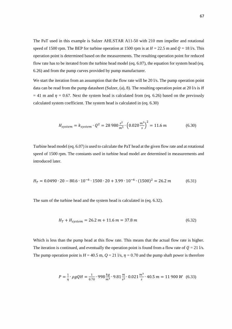
67

The PaT used in this example is Sulzer AHLSTAR A11-50 with 210 mm impeller and rotational

speed of 1500 rpm. The BEP for turbine operation at 1500 rpm is at 𝐻 = 22.5 m and 𝑄 = 18 l/s. This

operation point is determined based on the measurements. The resulting operation point for reduced

flow rate has to be iterated from the turbine head model (eq. 6.07), the equation for system head (eq.

6.26) and from the pump curves provided by pump manufacturer.

We start the iteration from an assumption that the flow rate will be 20 l/s. The pump operation point

data can be read from the pump datasheet (Sulzer, (a), 8). The resulting operation point at 20 l/s is 𝐻

= 41 m and 𝜂 = 0.67. Next the system head is calculated from (eq. 6.26) based on the previously

calculated system coefficient. The system head is calculated in (eq. 6.30)

𝐻𝑠𝑦𝑠𝑡𝑒𝑚 = 𝑘𝑠𝑦𝑠𝑡𝑒𝑚 ∙ 𝑄2 = 28 980𝑠2

𝑚5 ∙ (0.020𝑚3

𝑠)

2

= 11.6 𝑚 (6.30)

Turbine head model (eq. 6.07) is used to calculate the PaT head at the given flow rate and at rotational

speed of 1500 rpm. The constants used in turbine head model are determined in measurements and

introduced later.

𝐻𝑇 = 0.0490 ∙ 20 − 80.6 ∙ 10−6 ∙ 1500 ∙ 20 + 3.99 ∙ 10−6 ∙ (1500)2 = 26.2 𝑚 (6.31)

The sum of the turbine head and the system head is calculated in (eq. 6.32).

𝐻𝑇 + 𝐻𝑠𝑦𝑠𝑡𝑒𝑚 = 26.2 𝑚 + 11.6 𝑚 = 37.8 𝑚 (6.32)

Which is less than the pump head at this flow rate. This means that the actual flow rate is higher.

The iteration is continued, and eventually the operation point is found from a flow rate of 𝑄 = 21 l/s.

The pump operation point is H = 40.5 m, Q = 21 l/s, 𝜂 = 0.70 and the pump shaft power is therefore

𝑃 =1

𝜂∙ 𝜌𝑔𝑄𝐻 =

1

0.70∙ 998

𝑘𝑔

𝑚3 ∙ 9.81𝑚

𝑠2 ∙ 0.021𝑚3

𝑠∙ 40.5 𝑚 = 11 900 𝑊 (6.33)

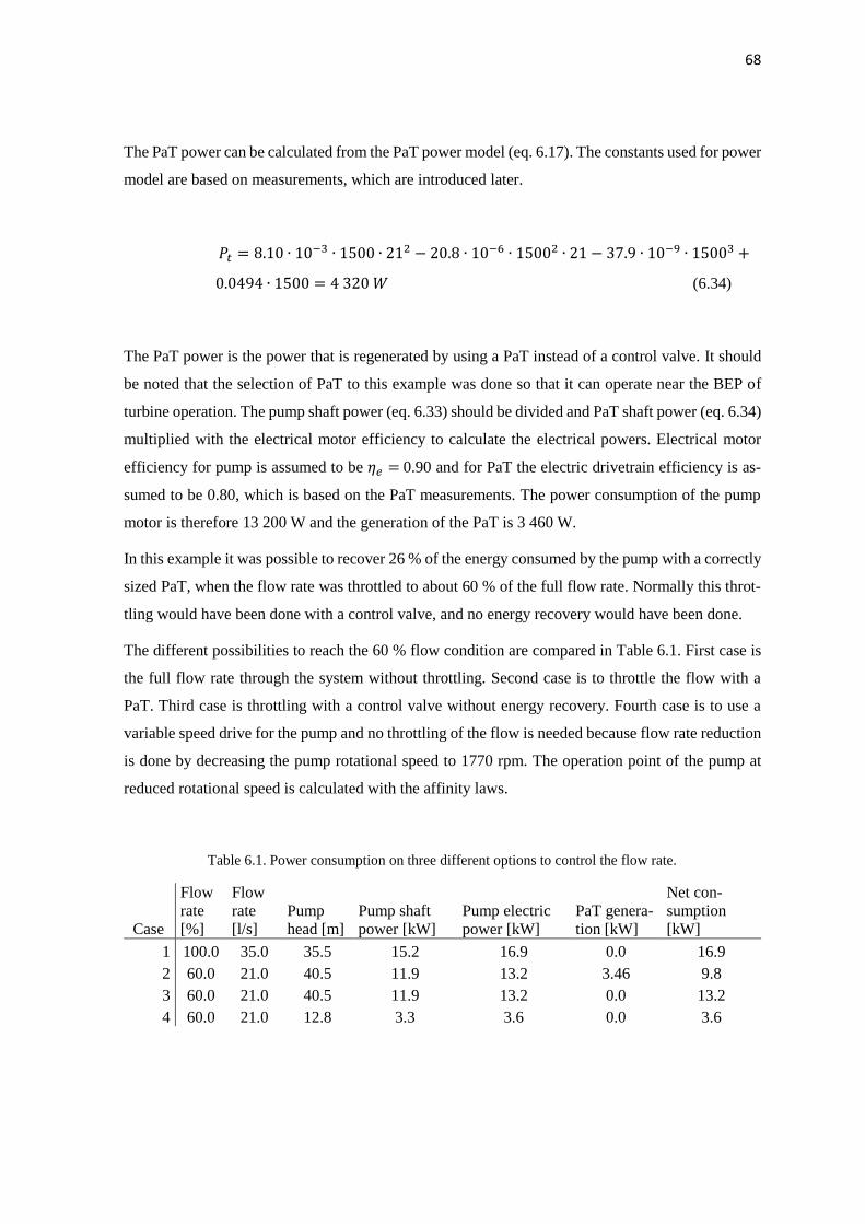
68

The PaT power can be calculated from the PaT power model (eq. 6.17). The constants used for power

model are based on measurements, which are introduced later.

𝑃𝑡 = 8.10 ∙ 10−3 ∙ 1500 ∙ 212 − 20.8 ∙ 10−6 ∙ 15002 ∙ 21 − 37.9 ∙ 10−9 ∙ 15003 +

0.0494 ∙ 1500 = 4 320 𝑊 (6.34)

The PaT power is the power that is regenerated by using a PaT instead of a control valve. It should

be noted that the selection of PaT to this example was done so that it can operate near the BEP of

turbine operation. The pump shaft power (eq. 6.33) should be divided and PaT shaft power (eq. 6.34)

multiplied with the electrical motor efficiency to calculate the electrical powers. Electrical motor

efficiency for pump is assumed to be 𝜂𝑒 = 0.90 and for PaT the electric drivetrain efficiency is as-

sumed to be 0.80, which is based on the PaT measurements. The power consumption of the pump

motor is therefore 13 200 W and the generation of the PaT is 3 460 W.

In this example it was possible to recover 26 % of the energy consumed by the pump with a correctly

sized PaT, when the flow rate was throttled to about 60 % of the full flow rate. Normally this throt-

tling would have been done with a control valve, and no energy recovery would have been done.

The different possibilities to reach the 60 % flow condition are compared in Table 6.1. First case is

the full flow rate through the system without throttling. Second case is to throttle the flow with a

PaT. Third case is throttling with a control valve without energy recovery. Fourth case is to use a

variable speed drive for the pump and no throttling of the flow is needed because flow rate reduction

is done by decreasing the pump rotational speed to 1770 rpm. The operation point of the pump at

reduced rotational speed is calculated with the affinity laws.

Table 6.1. Power consumption on three different options to control the flow rate.

Case

Flow

rate

[%]

Flow

rate

[l/s]

Pump

head [m]

Pump shaft

power [kW]

Pump electric

power [kW]

PaT genera-

tion [kW]

Net con-

sumption

[kW]

1 100.0 35.0 35.5 15.2 16.9 0.0 16.9

2 60.0 21.0 40.5 11.9 13.2 3.46 9.8

3 60.0 21.0 40.5 11.9 13.2 0.0 13.2

4 60.0 21.0 12.8 3.3 3.6 0.0 3.6

69

Table 6.1 illustrates the benefits of variable speed drives (VSD). With VSD, the power consumption

of the pump is reduced from 13.2 kW to 3.6 kW, which is only 27 % of what it would be in flow

control done with throttling. The use of a PaT reduces the net consumption from 13.2 kW to 9.8 kW,

a reduction to 74 % of the power consumption with valve throttling.

70

7 EXPERIMENTS

The experiments were conducted in LUT’s pump test facility. The pump test setup consists of three

pumps that are connected to a same water reservoir from their suction side. Pumps are variable speed

driven with a frequency converter, and the rotational speed and valve positions can be controlled

through a LabVIEW-based measurement program. The discharge pipes from the pumps connect to

a one pipe that has a control valve that can be adjusted. Fig. 7.1 is a 3D schematic of the pump test

setup used in the tests.

Fig. 7.1. LUT Pump test setup

The upper control valve in Fig. 7.1 is closed during the turbine tests, and the flow is guided from the

discharge side of the pump to the discharge side of the other pump, which is working as a turbine.

There is 3 pumps installed in the test setup, however only two are used for these tests. The pumps

used in the tests are Sulzer AHLSTAR-series centrifugal pumps with open impellers. The pump

models are Sulzer AHLSTAR A22-80 and Sulzer AHLSTAR A11-50. Table 7.1 shows the charac-

teristics of the pumps used in the test setup. The pumps are driven by electrical motors which are

driven by frequency converters. A22-80 has a ABB M3BP induction motor, while A11-50 uses a

M3AL synchronous reluctance motor. The motor specifications are described in Table 7.2.

71

Table 7.1 Properties of pumps in the test setup

Table 7.2. Properties of the electrical motors and the frequency converters used.

ABB M3BP 160MLA 4

Type Induction -

Poles 4 -

Output 11 kW

Speed 1466 rpm

Efficiency (full load) 90.4 %

Current IN 20.9 A

TN 71.6 Nm

Frequency converter ABB A800 -

ABB M3AL 90LDA 4

Type SynRM -

Poles 4 -

Output 5.5 kW

Speed 3000 rpm

Efficiency (full load) 89.2 %

Current IN 13.4 A

TN 17.5 Nm

Frequency converter ABB ACS880 -

The A22-80 pump has a torque and rotational speed measurement on the shaft between the pump

and the motor. The A11-50 pump is a close-coupled model, and it has no torque or rotational speed

measurements on the shaft. The values for rotational speed and torque are therefore based on esti-

mates provided by the frequency converter ACS880. Both pumps have temperature and pressure

measurements on both the intake and discharge sides, and the flow rate measurement is done on the

discharge side of A22-80 with a magnetic flow rate meter.

7.1 Turbine characteristics for A22-80

The following turbine curves have been created by adjusting the rotational speed of the pressure

producing pump while the turbine rotational speed is kept constant. The rotational speed of the driv-

ing pump is increased with 100-rpm increments. Runaway curve is created by letting the rotor turn

Sulzer A22-80

Impeller diameter 265.0 mm

Blade number 6 -

Nominal head 21.0 m

Nominal flow rate 38.0 l/s

Nominal efficiency 78.0 %

Nominal speed 1450.0 rpm

nq 28.8 -

Sulzer A11-50

Impeller diameter 210.0 mm

Blade number 5 -

Nominal head 14.2 m

Nominal flow rate 14.3 l/s

Nominal efficiency 70.8 %

Nominal speed 1455.0 rpm

nq 23.7 -

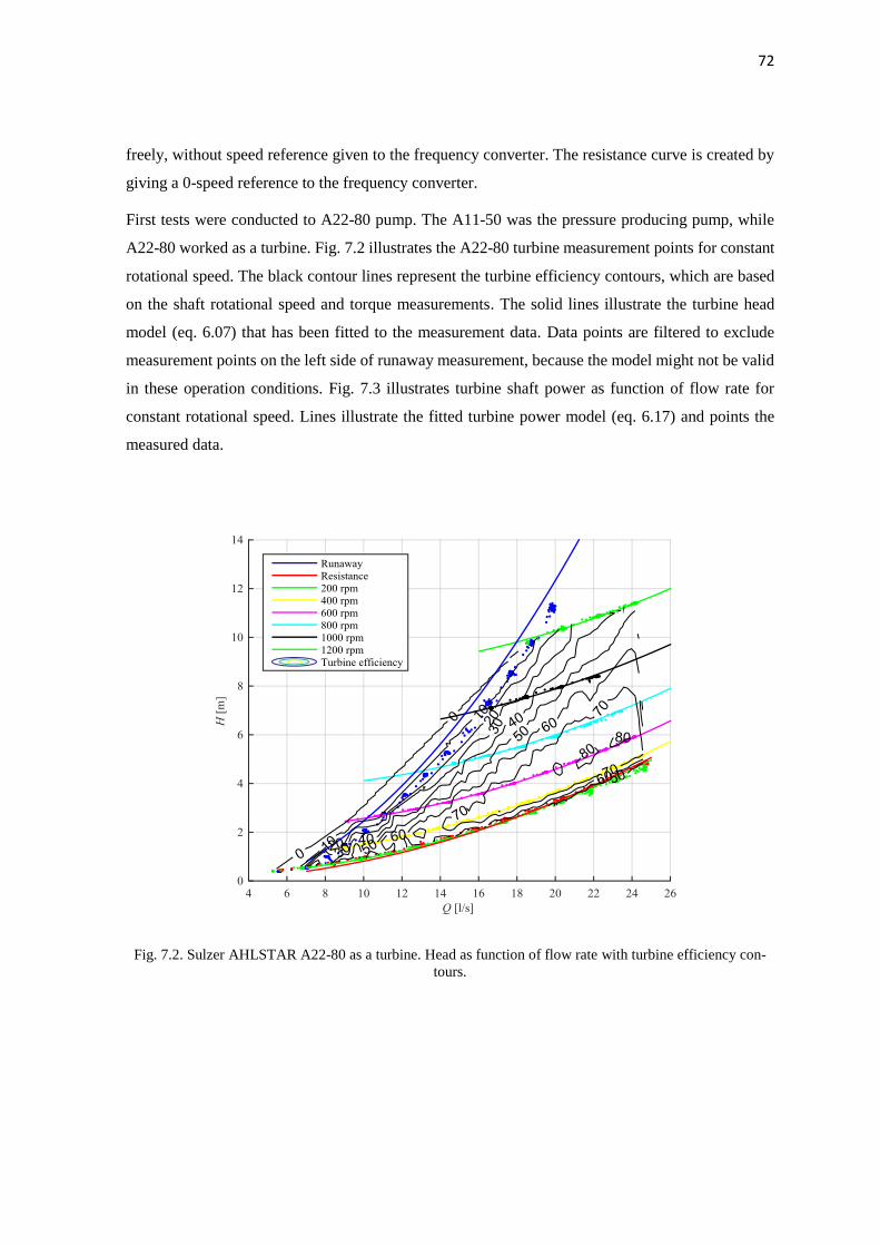
72

freely, without speed reference given to the frequency converter. The resistance curve is created by

giving a 0-speed reference to the frequency converter.

First tests were conducted to A22-80 pump. The A11-50 was the pressure producing pump, while

A22-80 worked as a turbine. Fig. 7.2 illustrates the A22-80 turbine measurement points for constant

rotational speed. The black contour lines represent the turbine efficiency contours, which are based

on the shaft rotational speed and torque measurements. The solid lines illustrate the turbine head

model (eq. 6.07) that has been fitted to the measurement data. Data points are filtered to exclude

measurement points on the left side of runaway measurement, because the model might not be valid

in these operation conditions. Fig. 7.3 illustrates turbine shaft power as function of flow rate for

constant rotational speed. Lines illustrate the fitted turbine power model (eq. 6.17) and points the

measured data.

Fig. 7.2. Sulzer AHLSTAR A22-80 as a turbine. Head as function of flow rate with turbine efficiency con-

tours.

73

Fig. 7.3. Sulzer AHLSTAR A22-80 as a turbine. Shaft power as function of flow rate.

As can be seen from Fig. 7.2, the turbine head model works well, except for runaway curve. This is

because of the torque measurement that was done at the axis between motor and the pump, and

therefore the motor friction is measured as torque in the runaway measurements. This causes a devi-

ation from the model, where the shaft power is assumed to be zero. However, because of the torque

measurement, and therefore power measurement is done on the turbine shaft, the model is independ-

ent from the electrical motor used. Therefore, the modeled runaway curve in Fig. 7.2 should illustrate

the real runaway condition for the turbine, and the runaway measurement points are not truly meas-

ured in runaway condition. This can also be seen from the efficiency contour: The zero-efficiency

contour (zero power) fits better to the modeled runaway curve.

The measured turbine curves are similar to ones measured by Nygren (2016). There is however, a

slight deviation in the measured maximum efficiency. The maximum turbine efficiency measured

here was 80.0 %, while Nygren measured an efficiency of 79.0 %. This accuracy is acceptable, and

the deviation can be explained with the accuracy of the shaft torque measurements.

The maximum efficiency point of turbine operation is found from much lower rotational speed than

the nominal rotational speed of pump operation. In these measurements it seemed to be at around

600 – 800 rpm. It seems possible that higher efficiencies might have been achieved with higher flow

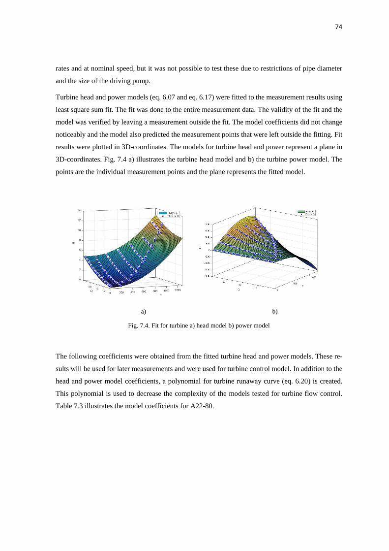
74

rates and at nominal speed, but it was not possible to test these due to restrictions of pipe diameter

and the size of the driving pump.

Turbine head and power models (eq. 6.07 and eq. 6.17) were fitted to the measurement results using

least square sum fit. The fit was done to the entire measurement data. The validity of the fit and the

model was verified by leaving a measurement outside the fit. The model coefficients did not change

noticeably and the model also predicted the measurement points that were left outside the fitting. Fit

results were plotted in 3D-coordinates. The models for turbine head and power represent a plane in

3D-coordinates. Fig. 7.4 a) illustrates the turbine head model and b) the turbine power model. The

points are the individual measurement points and the plane represents the fitted model.

a) b)

Fig. 7.4. Fit for turbine a) head model b) power model

The following coefficients were obtained from the fitted turbine head and power models. These re-

sults will be used for later measurements and were used for turbine control model. In addition to the

head and power model coefficients, a polynomial for turbine runaway curve (eq. 6.20) is created.

This polynomial is used to decrease the complexity of the models tested for turbine flow control.

Table 7.3 illustrates the model coefficients for A22-80.

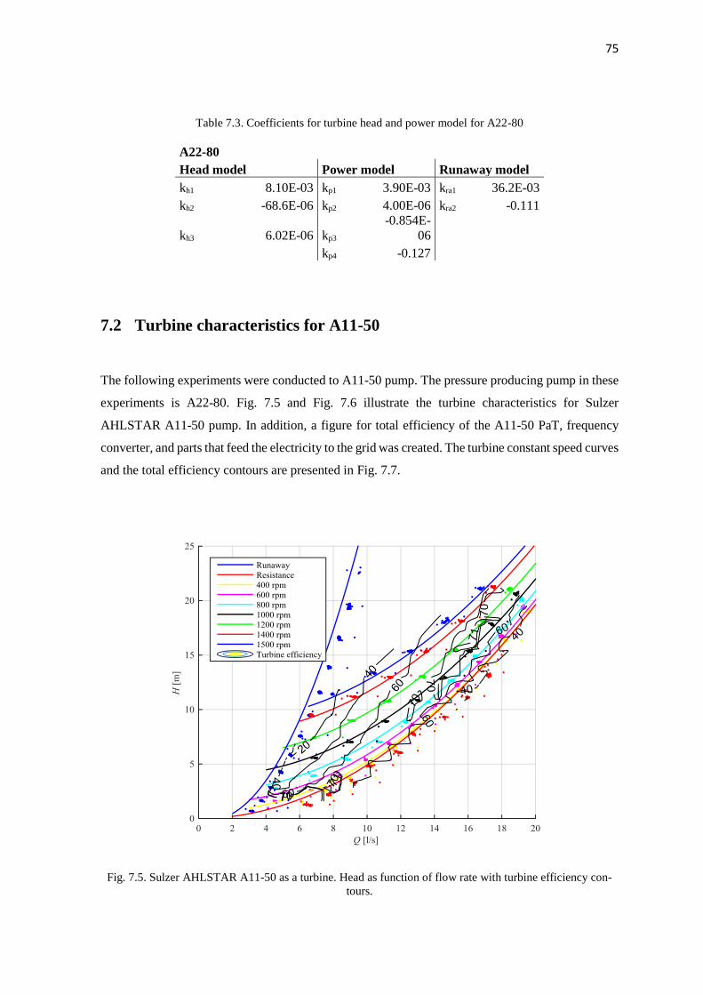
75

Table 7.3. Coefficients for turbine head and power model for A22-80

A22-80

Head model Power model Runaway model

kh1 8.10E-03 kp1 3.90E-03 kra1 36.2E-03

kh2 -68.6E-06 kp2 4.00E-06 kra2 -0.111

kh3 6.02E-06 kp3

-0.854E-

06

kp4 -0.127

7.2 Turbine characteristics for A11-50

The following experiments were conducted to A11-50 pump. The pressure producing pump in these

experiments is A22-80. Fig. 7.5 and Fig. 7.6 illustrate the turbine characteristics for Sulzer

AHLSTAR A11-50 pump. In addition, a figure for total efficiency of the A11-50 PaT, frequency

converter, and parts that feed the electricity to the grid was created. The turbine constant speed curves

and the total efficiency contours are presented in Fig. 7.7.

Fig. 7.5. Sulzer AHLSTAR A11-50 as a turbine. Head as function of flow rate with turbine efficiency con-

tours.

76

Fig. 7.6. Sulzer AHLSTAR A11-50 as a turbine. Shaft power as function of flow rate

Fig. 7.7. Sulzer AHLSTAR A11-50 as a turbine. Head as function of flow rate with total efficiency contours.

Here the lines illustrate measured constant speed curves, not the model.

77

Unlike with A22-80, in these measurements the torque measurement was not available, because the

pump is a close coupled type and the shaft could not be accessed. Therefore the turbine power is

calculated based on an estimate given by the frequency converter. This might explain the differences

between the measured runaway curve and the model. Although, the difference may have been caused

by the same reason as in A22-80 model: Because of the electrical motor friction, the runaway meas-

urements do not represent a real runaway condition for the turbine.

The resistance curve modeled deviates noticeably from the measurement results. The reason for this

is unknown, as the same model worked well for the A22-80 pump. There was also a small deviation

in Nygren’s measurements for A11-50, although not as great as in these. The different method for

model fitment might be the cause for this. Nygren (2016) fitted the model to one measurement series,

done with a single rotational speed of the turbine.

There is also a lot of scattering in the individual measurement points. Scattering seems to be caused

by the discontinuities: when the flow rate changes, the measurements are not valid because of the

fast changes. This was not observed in A22-80 measurements. The resistance condition deviation

might be caused also from the geometric differences between the pumps. Also, at low rotational

speeds high oscillation of the turbine head was observed, which might cause errors in the measure-

ments. The validity of the model was tested by leaving a measurement series outside the least square

sum fit. The model coefficients did not change remarkably; The model also predicted the data points

left outside the model accurately. The coefficients of the model are presented in Table 7.4. These

coefficients will be used in turbine flow control model and in turbine calculations.

Table 7.4. Sulzer A11-50 model coefficients.

A11-50

Head model Power model Runaway model

kh1 0.0491 kp1 8.10E-03 kra1 0.324

kh2 -83.2E-06 kp2 -21.0E-06 kra2 -0.423

kh3 4.01E-06 kp3 -37.3E-09

kp4 0.0473

These turbine curves are similar to the ones created by Nygren (2016). The efficiency contours and

measured head at different speeds seems to match the previous measurements. The maximum turbine

efficiency measured is 71.0 and the result is the same as measured by Nygren. The maximum total

efficiency was 56.5 %. The drivetrain efficiency in this point can be calculated, and the drivetrain

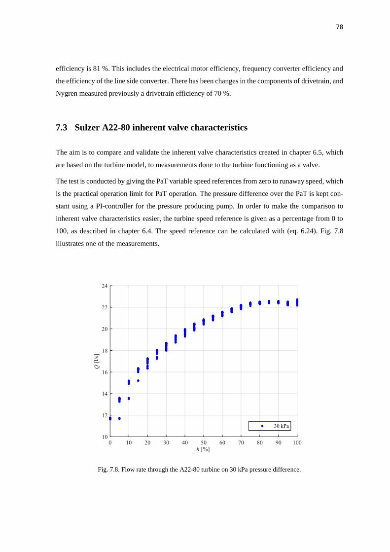
78

efficiency is 81 %. This includes the electrical motor efficiency, frequency converter efficiency and

the efficiency of the line side converter. There has been changes in the components of drivetrain, and

Nygren measured previously a drivetrain efficiency of 70 %.

7.3 Sulzer A22-80 inherent valve characteristics

The aim is to compare and validate the inherent valve characteristics created in chapter 6.5, which

are based on the turbine model, to measurements done to the turbine functioning as a valve.

The test is conducted by giving the PaT variable speed references from zero to runaway speed, which

is the practical operation limit for PaT operation. The pressure difference over the PaT is kept con-

stant using a PI-controller for the pressure producing pump. In order to make the comparison to

inherent valve characteristics easier, the turbine speed reference is given as a percentage from 0 to

100, as described in chapter 6.4. The speed reference can be calculated with (eq. 6.24). Fig. 7.8

illustrates one of the measurements.

Fig. 7.8. Flow rate through the A22-80 turbine on 30 kPa pressure difference.

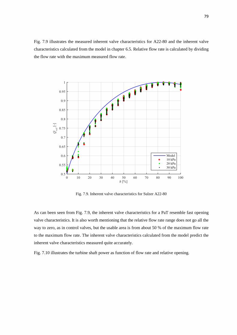
79

Fig. 7.9 illustrates the measured inherent valve characteristics for A22-80 and the inherent valve

characteristics calculated from the model in chapter 6.5. Relative flow rate is calculated by dividing

the flow rate with the maximum measured flow rate.

Fig. 7.9. Inherent valve characteristics for Sulzer A22-80

As can been seen from Fig. 7.9, the inherent valve characteristics for a PaT resemble fast opening

valve characteristics. It is also worth mentioning that the relative flow rate range does not go all the

way to zero, as in control valves, but the usable area is from about 50 % of the maximum flow rate

to the maximum flow rate. The inherent valve characteristics calculated from the model predict the

inherent valve characteristics measured quite accurately.

Fig. 7.10 illustrates the turbine shaft power as function of flow rate and relative opening.

80

Fig. 7.10. Power as a function of flow rate and signal

The accuracy of the runaway speed calculation can be estimated from Fig. 7.10. The PaT power

changes rapidly near the runaway speed, but the zero shaft power seems to be near the zero opening,

so the runaway condition is predicted with a reasonable accuracy.

The maximum power point seems to be always found from the same value of relative opening. The

specific speed values were calculated for the maximum power points at different pressure differences

and it was noticed that the specific speed of the turbine stays the same at the MPP-condition. This

could also be used for turbine control.

7.4 Turbine and valve in series

The following measurements are conducted to test the validity of the control models described in

chapter 6.6. The test setup consists of a pressure producing pump, a PaT, a control valve connected

in series with the PaT, and the piping connecting the components. All the individual components of

the system are determined and the tested model will be open-loop control model. The pressure pro-

ducing pump is kept at constant rotational speed and it forms the “static” head of the system.

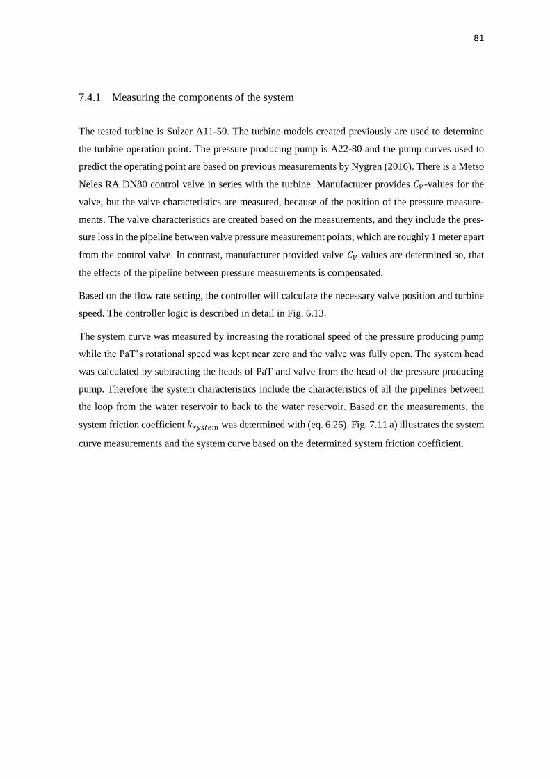
81

7.4.1 Measuring the components of the system

The tested turbine is Sulzer A11-50. The turbine models created previously are used to determine

the turbine operation point. The pressure producing pump is A22-80 and the pump curves used to

predict the operating point are based on previous measurements by Nygren (2016). There is a Metso

Neles RA DN80 control valve in series with the turbine. Manufacturer provides 𝐶𝑉-values for the

valve, but the valve characteristics are measured, because of the position of the pressure measure-

ments. The valve characteristics are created based on the measurements, and they include the pres-

sure loss in the pipeline between valve pressure measurement points, which are roughly 1 meter apart

from the control valve. In contrast, manufacturer provided valve 𝐶𝑉 values are determined so, that

the effects of the pipeline between pressure measurements is compensated.

Based on the flow rate setting, the controller will calculate the necessary valve position and turbine

speed. The controller logic is described in detail in Fig. 6.13.

The system curve was measured by increasing the rotational speed of the pressure producing pump

while the PaT’s rotational speed was kept near zero and the valve was fully open. The system head

was calculated by subtracting the heads of PaT and valve from the head of the pressure producing

pump. Therefore the system characteristics include the characteristics of all the pipelines between

the loop from the water reservoir to back to the water reservoir. Based on the measurements, the

system friction coefficient 𝑘𝑠𝑦𝑠𝑡𝑒𝑚 was determined with (eq. 6.26). Fig. 7.11 a) illustrates the system

curve measurements and the system curve based on the determined system friction coefficient.

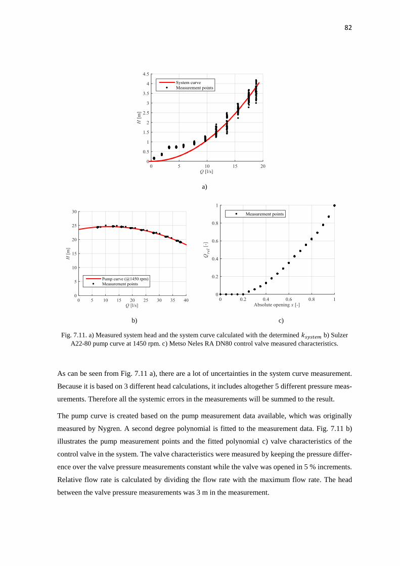
82

a)

b) c)

Fig. 7.11. a) Measured system head and the system curve calculated with the determined 𝑘𝑠𝑦𝑠𝑡𝑒𝑚 b) Sulzer

A22-80 pump curve at 1450 rpm. c) Metso Neles RA DN80 control valve measured characteristics.

As can be seen from Fig. 7.11 a), there are a lot of uncertainties in the system curve measurement.

Because it is based on 3 different head calculations, it includes altogether 5 different pressure meas-

urements. Therefore all the systemic errors in the measurements will be summed to the result.

The pump curve is created based on the pump measurement data available, which was originally

measured by Nygren. A second degree polynomial is fitted to the measurement data. Fig. 7.11 b)

illustrates the pump measurement points and the fitted polynomial c) valve characteristics of the

control valve in the system. The valve characteristics were measured by keeping the pressure differ-

ence over the valve pressure measurements constant while the valve was opened in 5 % increments.

Relative flow rate is calculated by dividing the flow rate with the maximum flow rate. The head

between the valve pressure measurements was 3 m in the measurement.

83

Fig. 7.11 c) shows that the initial opening ℎ0, which is needed before any flow passes through the

valve, is surprisingly high. A ℎ0 of 0.20 was observed. According to manufacturer provided data,

the initial opening should be 9 degrees for rotary stem valves. It means 0.10 of absolute opening for

90 degree valves. The initial opening of 0.20 is approximately 18 degrees in angular movement of

the valve. In order to create a model for valve characteristics, the relative opening h is calculated

with (eq. 5.04) and the valve characteristics are plotted in Fig. 7.12. The fitted curve is a second

degree polynomial.

Fig. 7.12. Valve and pipeline characteristics for Metso Neles RA DN80 as function of relative opening.

Now all the characteristics of the individual pieces that make the system are known. All the curves

can be plotted together as was done in chapter 6.6. Fig. 7.13 illustrates the individual components of

the system. The pressure producing pump is plotted first, and the system pressure loss and the valve

pressure loss is subtracted from it. The operating point of the turbine is found from the intersection

of turbine curve and the valve curve. Closing the valve makes the valve curve become steeper.

84

Fig. 7.13. Characteristics of the individual components of the system.

7.4.2 Testing the flow control

Based on the control logic described in Fig. 6.13, the flow control model was tested with the system.

The idea of the control is to follow the MPP-curve at small flow rates, and throttle the excess head

with the valve. When the valve is fully open, PaT speed is reduced to increase the flow rate through

the system. Maximum flow rate is reached at fully open valve and at the resistance curve of the PaT.

The valve opening and PaT speed values were calculated for each of the measurement points at 1 l/s

intervals.

Fig. 7.14 illustrates the measured heads as function of flow rate. Measured control valve head at flow

rates lower than 9 l/s is invalid. The pressure sensor before the control valve had a maximum pressure

of 2.5 bar. Fig. 7.15 shows the PaT power, power from the PaT to the grid and the power of the

pressure producing pump.

85

Fig. 7.14. Head of different components as a function of flow rate.

Fig. 7.15. Power as function of flow rate.

86

Fig. 7.16. PaT speed and valve absolute opening as function of flow rate.

Fig. 7.16 illustrates the control signals; PaT rotational speed and the valve absolute opening. It can

be seen from Fig. 7.16 that at around 10 l/s the PaT speed reaches its maximum value. This is because

of the programmed safe limits in the frequency converter, and this is also the reason why the PaT

head deviates from the MPP curve. At around 16 l/s the flow rate desired cannot be reached with the

full rotational speed of the PaT, and after this the rotational speed is reduced. The maximum flow

rate for this system is about 18 l/s, the higher flow rate cannot be reached without going over the

PaT’s resistance curve.

The control valve is fully open after 16 l/s flow rate. If the MPP curve of the PaT would have been

followed to higher rotational speeds than 1500 rpm, the control valve would have been fully open

from a smaller flow rate. Despite the deviation from the MPP curve, the PaT power increases with

increasing flow rate, and reaches a maximum value of 2370 W at 17.6 l/s. The maximum power to

the grid is 1840 W and the resulting drivetrain efficiency is 78 %. The pressure producing pump,

A22-80 had a measured shaft power of 7050 W at the same point. With an electrical motor efficiency

of 90 %, the power from grid is 7830 W, and the energy recovery percentage with the PaT is 23.5

%. If the PaT rotational speed could have been increased over 1500 rpm the energy recovery per-

centage could have been higher.

With common frequency converters intermediate DC-circuits the efficiency of the drivetrain could

be improved, and therefore the energy recovery percentage would be higher. The losses caused by

the line side inverter of the frequency converter could be therefore avoided.

The accuracy of the control is evaluated. The setting value 𝑄𝑆𝐸𝑇 is the flow rate for which the valve

position and the turbine speed were calculated. Fig. 7.17 illustrates the flow rate as function of the

87

measurement time. As can be seen, the flow rate follows the setting value fairly accurately, even

though there is uncertainties, especially with the system curve.

Fig. 7.17. Accuracy of the open loop flow control.

Fig. 7.17 shows that the open loop control works accurately, when all the characteristics of the indi-

vidual components of the system are known. The largest deviation from the flow rate setting was

around 13 l/s and the error was about 1 l/s.

7.4.3 Sensorless estimation

Sensorless estimates are used to calculate the flow properties without using measurements like flow

rate meter or pressure meter. This is done using the data available from the frequency converter. As

earlier described, the frequency converter provides values for motor rotational speed and motor

torque. Using the PaT power model (eq. 6.17), the PaT flow rate can be calculated from these values.

The estimated flow rate and the rotational speed can be used in the head model (eq. 6.07) to calculate

the PaT head. The estimated flow rate and head are compared to the measured values. The results

are plotted in Fig. 7.18.

88

a) b)

Fig. 7.18. a) The estimated flow rate and actual flow rate. b) The estimated head and the measured head.

The sensorless estimates work surprisingly accurately. The problem with the flow rate estimation at

small flow rates (4 l/s and smaller) is probably related to the zero-points of the power model. Even

though the sensorless estimates were tested as a part of the flow control model test, they do not use

any data from the system characteristics, but are based only on the frequency converter provided

data and the previously created and fitted PaT head and power models. The error between measured

and estimated flow rate and head is illustrated in Fig. 7.19.

a) b)

Fig. 7.19. Difference between measured and estimated PaT a) flow rate and b) head.

89

The head estimate has more error than the flow rate estimate. This is probably due to the fact that

turbine head is calculated by using the estimated flow rate, so the errors in flow rate cause also error

in the turbine head. Turbine head measurement has also quite a lot of fluctuations and the turbine

head measurement itself can cause part of the error. Estimated flow rate is within 0.4 l/s of the meas-

ured value and turbine head estimate is within 1 m of the measured value. More analysis would be

needed to verify the accuracy of the sensorless estimates.

90

8 ECONOMICAL EVALUATION

We are interested in the economic feasibility of using PaT’s for hydraulic energy recovery. In this

thesis, economic feasibility is evaluated using payback period. In order to evaluate costs, several

example cases are studied. Also, a graph is created for evaluating the feasibility of PaT depending

on the operation point. In the following calculations, the electricity price is assumed to be 0.071

€/kWh, which was an average electricity cost of an industrial customer in Finland in 2015. (Eurostat,

2016)

8.1 Example cases

The selection of pumps that will be evaluated is done using the pump mode BEP, which is used to

determine the turbine mode BEP. The following pumps were selected for evaluation. The pumps

prices were inquired to form the basis for the evaluation. The prices include the price of the baseplate,

coupling, motor and the pump. The pump mode BEP’s are shown in Table 8.1.

Table 8.1. Pump mode nominal operation points for cases A-E.

Case A Case B Case C Case D Case E

n [rpm] 1500 3000 1000 1500 1500

Hn,p [m] 8.4 92.5 10.6 95.3 44.7

Qn,p [l/s] 3.03 8.29 94.36 108.36 947.99

nq,p 16.7 9.2 52.2 16.2 84.5

η 0.4 0.4 0.8 0.7 0.9

These operation points can be transformed to turbine mode nominal operation points with correla-

tions given by Chapallaz (1992). Fig. 8.1 illustrates the empirical conversion factors for turbine nom-

inal operation point flow rate and head. These conversation factors are based on empirical data from

over 80 pumps. Nygren (2016) has studied turbine mode performance prediction in his thesis in

detail. It is worth mention that these correlations are empirical and valid for large number of pumps.

However, for a single pump, the turbine performance can differ noticeably from these correlations

because for example, of different geometric design. There also exists a lot of alternative correlations

for BEP prediction, for example Gülich (2010, 726)

91

a)

b)

Fig. 8.1. Conversion factors for a) flow rate and b) head. Figure is from Nygren (2016, 30), which is modi-

fied from Chapallaz (1992).

Based on the conversion factors, BEP for turbine mode were calculated. The turbine efficiency stays

usually near the same value as the pump efficiency. (Chapallaz, 1992) In these calculations the tur-

bine efficiency is assumed to be the same as the pump mode BEP efficiency. Table 8.2 shows the

turbine mode BEP’s. The efficiency of the electrical motor, which is used as generator in turbine

mode, has to be taken into account when the electrical power is calculated. The electrical motors are

selected according to the pump mode operation. The efficiencies for the electrical motors are calcu-

lated based on the motor size and the IE-classification (IE2 or IE3). The electrical motor efficiency

is assumed to be the same in the generation mode as in the motoring mode.

92

Table 8.2. Conversion factors and turbine nominal operation points for cases A-E. The turbine efficiency is

estimated to stay the same as in pump mode.

Case A Case B Case C Case D Case E

CQ 1.67 2 1.3 1.6 1.25

CH 2.05 2.5 1.35 1.85 1.35

n [rpm] 1500 3000 1000 1500 1500

Hn.t [m] 17.30 231.21 14.35 176.37 60.34

Qn.t [l/s] 5.06 16.57 122.67 173.38 1184.98

nq.t [-] 12.58 6.51 47.50 12.91 75.42

ηt [-] 0.4 0.4 0.8 0.7 0.9

Motor [kW] 0.75 22 15 160 500

ηe [-] 0.81 0.93 0.91 0.96 0.97

The turbine power in the BEP can be calculated using (eq. 8.01).

𝑃𝑡 = 𝜌𝑔𝐻𝑡𝑄𝑡𝜂𝑡 (8.01)

The electrical power can be calculated from the turbine power by multiplying it with the electrical

motor efficiency (eq. 8.02). The powers are shown in Table 8.3.

𝑃𝑒 = 𝑃𝑡 ∙ 𝜂𝑒 (8.02)

Table 8.3. Nominal power for cases A-E.

Case A Case B Case C Case D Case E

Pt [kW] 0.9 37.5 17.2 299.4 700.0

Pe [kW] 0.7 34.8 15.7 286.8 676.2

In addition to cases A-E, five more pumps were evaluated. The prices were inquired from another

manufacturer and the turbine mode BEP was calculated with the same method as for cases A-E. The

pump mode and turbine mode operation points are shown in Table 8.4.

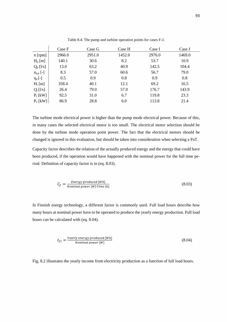
93

Table 8.4. The pump and turbine operation points for cases F-J.

Case F Case G Case H Case I Case J

n [rpm] 2966.0 2951.0 1452.0 2976.0 1469.0

Hp [m] 140.1 30.6 8.2 53.7 10.9

Qp [l/s] 13.0 63.2 40.9 142.5 104.4

nq,p [-] 8.3 57.0 60.6 56.7 79.0

ηp [-] 0.5 0.9 0.8 0.9 0.8

Ht [m] 358.4 40.1 12.1 69.2 16.5

Qt [l/s] 26.4 79.0 57.0 176.7 143.9

Pt [kW] 92.5 31.0 6.7 119.8 23.3

Pe [kW] 86.9 28.8 6.0 113.8 21.4

The turbine mode electrical power is higher than the pump mode electrical power. Because of this,

in many cases the selected electrical motor is too small. The electrical motor selection should be

done by the turbine mode operation point power. The fact that the electrical motors should be

changed is ignored in this evaluation, but should be taken into consideration when selecting a PaT.

Capacity factor describes the relation of the actually produced energy and the energy that could have

been produced, if the operation would have happened with the nominal power for the full time pe-

riod. Definition of capacity factor is in (eq. 8.03).

𝐶𝑓 =𝐸𝑛𝑒𝑟𝑔𝑦 𝑝𝑟𝑜𝑑𝑢𝑐𝑒𝑑 [𝑊ℎ]

𝑁𝑜𝑚𝑖𝑛𝑎𝑙 𝑝𝑜𝑤𝑒𝑟 [𝑊]∙𝑇𝑖𝑚𝑒 [ℎ] (8.03)

In Finnish energy technology, a different factor is commonly used. Full load hours describe how

many hours at nominal power have to be operated to produce the yearly energy production. Full load

hours can be calculated with (eq. 8.04).

𝑡𝑓𝑙 =𝑌𝑒𝑎𝑟𝑙𝑦 𝑒𝑛𝑒𝑟𝑔𝑦 𝑝𝑟𝑜𝑑𝑢𝑐𝑒𝑑 [𝑊ℎ]

𝑁𝑜𝑚𝑖𝑛𝑎𝑙 𝑝𝑜𝑤𝑒𝑟 [𝑊] (8.04)

Fig. 8.2 illustrates the yearly income from electricity production as a function of full load hours.

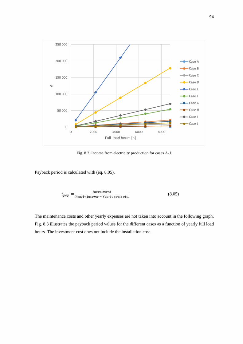
94

Fig. 8.2. Income from electricity production for cases A-J.

Payback period is calculated with (eq. 8.05).

𝑡𝑝𝑏𝑝 =𝐼𝑛𝑣𝑒𝑠𝑡𝑚𝑒𝑛𝑡

𝑌𝑒𝑎𝑟𝑙𝑦 𝑖𝑛𝑐𝑜𝑚𝑒 − 𝑌𝑒𝑎𝑟𝑙𝑦 𝑐𝑜𝑠𝑡𝑠 𝑒𝑡𝑐. (8.05)

The maintenance costs and other yearly expenses are not taken into account in the following graph.

Fig. 8.3 illustrates the payback period values for the different cases as a function of yearly full load

hours. The investment cost does not include the installation cost.

0

50 000

100 000

150 000

200 000

250 000

0 2000 4000 6000 8000

€

Full load hours [h]

Case A

Case B

Case C

Case D

Case E

Case F

Case G

Case H

Case I

Case J

95

Fig. 8.3. Payback period in years as a function of full load hours.

Fig. 8.3 shows that there exists a minimum scale where the hydraulic energy recovery is feasible.

The first example, case A, has so small operation point electrical power (0.75 kW), that even though

it would be used for the whole year, it will have a payback period of 12.2 years. On the other hand,

all the larger pumps have rather short payback periods when the full load hours are high enough. For

example, case C with 15.2 kWe has a payback period of 2.4 years when the full load hours are 4380

h (equals to a capacity factor of 50 %).

If we select the limit for economic feasibility to a payback period of 2 years at 50 % capacity factor,

we can make some estimates based on the cases A-J about the needed turbine mode operation point

power. Cases A and C have turbine mode electrical power of 0.7 kW and 15.7 kW and they do not

have the required payback period. On the other hand, cases H and B have smaller payback period

than required, and they have electrical power of 6.0 kW and 34.8 kW. Cases G and J have electrical

powers of 28.8 kW and 21.4 kW, and they are clearly below the required the payback period. The

limit seems to be at the scale of 10 – 20 kWe power in turbine mode operation point.

The amount of pumps evaluated is small, and there are only pumps from two manufacturers. More

pumps should be evaluated to make better predictions about viable scale for hydraulic energy recov-

ery with a PaT. The costs of installation and maintenance should also be considered in more accurate

estimations. One major cost not considered in this evaluation is the cost of devices related to con-

trolling the produced electricity quality and the load.

Some of the pumps selected for these evaluations are not recommended for turbine operation. Cha-

pallaz (1992) recommends that pumps with 𝑛𝑞 below 15 should not be used as turbines. They tend

0,0

2,0

4,0

6,0

8,0

10,0

12,0

14,0

16,0

18,0

20,0

0 2000 4000 6000 8000

Pay

bac

k p

erio

d [

year

s]

Full load hours [h]

Case A

Case B

Case C

Case D

Case E

Case F

Case G

Case H

Case I

Case J

96

to have low efficiencies, and their performance as turbine cannot be predicted accurately. Cases B

and F have a pump mode 𝑛𝑞 value below 15, and therefore their turbine BEP might be unreliable.

Fig. 8.3 is calculated for constant speed PaT’s. The price of frequency converter is not taken into

account in the investment cost. The prices of the frequency converters were also inquired, and the

resulting payback period for variable speed PaT’s were calculated. Fig. 8.4 illustrates the payback

period for the cases A-J with variable speed drive. The prices in this figure include pump, baseplate,

coupling, motor and a frequency converter. The electricity generation with this setup would be done

with common intermediate DC circuits between the frequency converters of generating and the mo-

toring electrical machines. Frequency converter price was not available for case E, so it is left out

from the figure.

Fig. 8.4. Payback period for the cases A-J with variable speed drive.

The effect of adding a frequency converter to the investment cost is minimal to the payback period.

For case C the payback period is 2.8 years at capacity factor of 50 %. For constant speed application

the payback period was 2.4 years. Adding a frequency converter makes the use of PaT more flexible,

and it might increase the full load hours noticeably depending on the operation point conditions.

With variable speed drives PaT’s could be used at high efficiency at different operating points, in-

stead of one operation point, as is assumed with constant speed PaT’s.

0,0

2,0

4,0

6,0

8,0

10,0

12,0

14,0

16,0

18,0

20,0

0 2000 4000 6000 8000

Pay

bac

k p

erio

d [

year

s]

Full load hours [h]

Case A

Case B

Case C

Case D

Case F

Case G

Case H

Case I

Case J

97

8.2 Operation point based evaluation

To predict the applications where PaT’s may be feasible, a different, more general approach is also

studied. We start by deriving a contour of available turbine power as a function of flow rate and

head.

The PaT selection has to be done according the operation point, and at the area of Fig. 8.6 the opti-

mum pump design will mainly be a radial single-entry and single-stage pump. We will assume that

the pump selected for turbine operation is a radial single-stage pump. It is assumed that the PaT can

be always selected so that it will operate in the BEP of turbine operation.

The efficiency of the pump selection does not stay the same through the area described in Fig. 8.6.

Gülich (2010. 114) provides a figure for single-stage, single-entry, radial pump efficiency at different

flow rates and specific speeds. Fig. 8.5 illustrates this optimal overall efficiency, and it is based on

(eq. 8.06 – eq. 8.07).

Fig. 8.5. Efficiencies of single-stage, single-entry radial pumps (Gülich, 2010, 114)

𝑚 = 0.1 ∙ 𝑎 ∙ (𝑄𝑅𝑒𝑓

𝑄)

0.15(

45

𝑛𝑞)

0.06

(8.06)

98

Where 𝑄𝑅𝑒𝑓 = 1 m3/s and 𝑎 = 1 if 𝑄 < 1 m3/s, 𝑎 = 0.5 𝑖𝑓 𝑄 > 1m3/s. The exponent m is used

for overall efficiency calculation in the following equation.

𝜂𝑜𝑝𝑡 = 1 − 0.095 ∙ (𝑄𝑅𝑒𝑓

𝑄)

𝑚− 0.3 (0.35 − log

𝑛𝑞

23)

2(

𝑄𝑅𝑒𝑓

𝑄)

0.05 (8.07)

Using the correlations (eq. 8.06 – eq. 8.07) for efficiency of radial, single-stage pumps and an as-

sumption that the electrical motor efficiency stays constant 𝜂𝑒𝑙 = 0.90, the available electrical power

in different operating points can be calculated. The pump rotational speed is 1500 rpm. This is needed

for the specific speed calculation which is used in the pump efficiency calculation. It is assumed that

the turbine mode efficiency is the same as the pump mode efficiency. The results are plotted in Fig.

8.6.

Fig. 8.6. Electrical power available as a function of head and flow rate.

The results can be referenced to the previous evaluation. For example, case C is at operation point

where an electrical power of 10 kWe is expected. The previously calculated electrical power for case

C can be read from Table 8.3, and it is 15.7 kWe. The difference is might be caused by the differences

99

in efficiency caused by the different rotational speed. Case C has a rotational speed of 1000 rpm

while Fig. 8.8 assumes a rotational speed of 1500 rpm and this effects the estimated efficiency of the

turbine.

Case J is expected to have an electrical power of about 15 kWe according to Fig. 8.6. According to

Table 8.4 the electrical power is 21.4 kWe. The accuracy of the prediction in Fig. 8.6 is not great; as

seen, a variation of more than 30 % was observed. The PaT efficiency and operation point prediction

methods have a lot of uncertainties.

Fig. 8.6 can be used to derive contours for yearly income from a PaT. However, we do not know the

full load hours, so we will assume capacity factor to be 75%. A similar figure could be derived for

any capacity factor.

Fig. 8.7. Yearly income from a PaT based on electricity price of 0.071 €/kWh and capacity factor of 0.75.

Based on the yearly income, and the equation for payback period (eq. 8.05), the cost of investment

can be calculated for a certain payback period. This illustrates the investment cost that a PaT system

can cost, to be able to reach a certain payback period in years. We have picked a payback period of

2 years for the Fig. 8.8.

100

Fig. 8.8. The cost of investment which would result in a payback period of 2 years.

Fig. 8.8 could be used to estimate the flow conditions where it is feasible to use a PaT for hydraulic

energy recovery. The figure should be used with knowledge of centrifugal pump prices, which are,

of course, manufacturer dependent.

When selecting a PaT to certain application, the turbine mode performance data should be available.

The information about the operation point where the PaT will work form the basis of the PaT selec-

tion, and the empirical coefficients for turbine mode performance prediction have a lot of uncertain-

ties.

101

9 CONCLUSIONS

The applicability of a variable speed PaT as a substitute for control valve was studied. A model for

PaT head and power was created, and the model was fitted to the pumps installed in LUT’s pump

laboratory. The typical characteristics of control valves was studied and the PaT characteristics were

compared to the typical control valve characteristics.

Control valves are used with an opening signal, which is typically a 4 – 20 mA current signal that is

changed to valve stem position in valve positioner. The use of PaT’s require knowledge about the

PaT head available because the operation area of a PaT is from runaway speed to zero speed, and the

runaway speed depends on the head available. Control signal for a PaT can be a speed reference from

runaway speed to zero speed. PaT head and power models can be used to calculate the runaway

speed when knowledge from the turbine head is available. Sensorless estimates could be used for

PaT head estimation when the measurements are unavailable.

When compared to control valves, PaT’s have a narrow operation area. In measurements conducted

to Sulzer AHLSTAR A22-80, PaT could be used to control the flow rate from 50 to 100 % of the

maximum flow rate. The results were similar to the ones predicted by the turbine models and the

runaway condition was predicted accurately with the models. To obtain broader operation area,

PaT’s could be used with a series flow control valve. Maximum power point tracking is also made

possible by using a PaT and a valve in series. The turbine maximum power point speed also depends

on the turbine head, and this can be calculated using the models created.

The use of a PaT for flow control was illustrated with a test setup consisting of a PaT and control

valve in series. The maximum energy recovery was 23.5 % of the power consumed by the pressure

producing pump. The whole operation area from zero flow to maximum flow rate was reached by

combining the valve opening and PaT rotational speed, and the PaT was operated at the MPP-curve

predicted by the turbine models.

An example of a PaT application was studied theoretically. A pump and system characteristics were

selected, and this system was assumed to be operating at two different operation points; 100 % flow

rate and 60 % flow rate. Instead of throttling the flow with a valve, a constant speed PaT was used.

PaT made it possible to reduce the overall power consumption to 74 % compared to valve throttling.

However, the use of variable speed drives is more energy efficient; with variable speed drives the

power consumption could be reduced to 27 % in comparison with the valve throttling.

The economic feasibility of PaT’s was studied with two different methods. First 10 pumps were

selected, and their payback period as PaT’s at different capacity factors was calculated based on

102

manufacturer provided prices. A minimum scale for PaT economic feasibility seems to exist; the

smallest PaT’s had a payback period of decades, while the larger pumps had a payback period of

under a year, depending on the capacity factor. The scale where 2 year payback period could be

reached at yearly capacity factor of 50 % seems to be around 10 to 20 kWe at turbine operation point

for the 10 pumps evaluated.

A contour for yearly income from a PaT at different flow conditions was created. This was used to

estimate how much PaT investment can cost, in order to be able to reach a certain payback period.

These tools provide a method for estimating the feasibility of a PaT for a certain application. The

exact limit for economic feasibility depends, of course, from the manufacturer dependent prices, the

cost of installation and most importantly, from the operation point and the yearly operation hours of

the PaT.

The accuracy of sensorless estimates from the flow rate and head of a PaT were tested using the

models created. The sensorless estimates based on the frequency converter provided data were sur-

prisingly accurate. Despite the small inaccuracies in the turbine models the estimates predicted the

flow rates at accuracy of about 0.4 l/s. The head estimate had more inaccuracy, but it predicted the

turbine head with an error of under 1 m.

9.1 Suggestions for future work

- Testing the PaT in real life application; selecting a correctly sized PaT to an application and

testing the use of PaT in flow control in process application based on the models created.

- The long time performance and the accuracy of the sensorless estimates. Does fouling and

wearing of the turbine change the coefficients of the turbine model? Can a pump manufac-

turer provide the coefficients for turbine head and power models for a certain pump model,

and are they accurate enough to be used in sensorless estimates?

- Could frequency converter use the models to keep the PaT running at maximum power point

speed at changing flow conditions without using data about the flow conditions or the system

it is attached to?

- The economic feasibility should be studied based on the power duration curves of the PaT.

103

REFERENCES

ABB. 2016a. Frequency converter. [E-document]. Retrieved 8.9.2016. From:

http://www.abb.com/product/ap/seitp322/9f10a1ecce40c4e7c125744b00273b98.aspx

ABB. 2016b. Low Voltage High Output Synchronous Reluctance motors. [Catalog]. Retrieved

8.11.2016. From: https://library.e.abb.com/pub-

lic/701cdc28cde347138222cc817c8a3dcd/HO_SynRM_04-2016_LOW.pdf

ABB. 2016c. Low Voltage Process Performance Motors. [Catalog]. Retrieved 8.11.2016. From:

https://library.e.abb.com/public/2cb08e5893494bfd853e658a738e446b/PPM_cata-

log_13042016.pdf

Alatorre-Frenk, Claudio. 1994. Cost Minimisation in Micro-Hydro Systems Using Pumps-as-Tur-

bines. [PhD Thesis]. University of Warwick. Retrieved 13.6.2016. From: http://wrap.war-

wick.ac.uk/36099/

Budris, Allan. Case History: Pumps as Turbines in Water Industry. [Web-page] WaterWorld.com

Retrieved: 11.11.2016. From: http://www.waterworld.com/articles/print/volume-27/issue-2/depart-

ments/pump-tips-techniques/case-history-pumps-as-turbines-in-the-water-industry.html

Chapallaz, J.-M. Eichenberger P. Fischer G. 1992. Manual on Pumps used as Turbines. Deutsches

Zentrum fur Entwicklungstechnologien GATE. Retrieved 8.11.2016. From:

http://www.nzdl.org/gsdlmod?e=d-00000-00---off-0hdl--00-0----0-10-0---0---0direct-10---4-------

0-1l--11-en-50---20-about---00-0-1-00-0--4----0-0-11-10-0utfZz-8-

00&cl=CL1.11&d=HASH011f05bf8734d88d1a080257.1&x=1

Deprez, Wim. Dexters, Annick. Driesen, Johan. Belmans, Ronnie. 2006. Energy Efficiency of small

Induction Machines: Comparison between Motor and Generator Mode.

Emerson Process Management. Control Valve Handbook. 4th edition. 2005. Fisher Controls Interna-

tional.

Eurostat. Electricity price statistics. [Web-page] Retrieved 9.9.2016. From: http://ec.europa.eu/eu-

rostat/statistics-explained/index.php/Electricity_price_statistics

104

Grundfos. 2004a. Motor Book. Retrieved 8.11.2016. From: http://net.grundfos.com/doc/web-

net/waterutility/assets/downloads/motorbook.pdf

Grundfos. 2004b. Pump handbook. Retrieved 8.11.2016. From: http://net.grundfos.com/doc/web-

net/mining/_downloads/pump-handbook.pdf

Grundfos, 2009. Mechanical Shaft Seals for Pumps. Retrieved 8.11.2016. From: http://net.grund-

fos.com/doc/webnet/waterutility/_assets/downloads/shaft_seals.pdf

Gülich Johann Friedrich. 2010. Centrifugal Pumps. 2nd edition. Springer. ISBN 978-3-642-12823-3

Hydraulics & Pneumatics. Engineering Essentials: Pressure Control Valves. 2012. [Web-page] Re-

trieved 8.11.2016. From: http://hydraulicspneumatics.com/200/TechZone/HydraulicValves/Arti-

cle/False/6411/TechZone-HydraulicValves?page=2

Högfors valves. 2015. Ball Control Valve of stainless steel [Product information]. [Retrieved

10.6.2016]. From: http://hogfors.com/wp-content/uploads/2016/01/467-468-ENG-17-03-2015.pdf

Karassik, Igor J. Pump Handbook. 1976. New York : McGraw-Hill. ISBN 0-07-033301-7.

Kirmanen, Jari. Niemelä, Ismo. Pyötsiä, Jouni. Simula, Markku. Hauhia, Markus. Riihilahti, Jari.

Lempinen, Vesa. Koukkuluoma, Jussi. Kanerva, Petri. 2011. Flow Control Manual. METSO Flow

Control Inc. ISBN 952-9773-12-9. Retrieved 8.11.2016. From: http://valveproducts.metso.com/doc-

uments/softwarepackages/nelprof/FlowControl_manual.pdf

KSB Aktiengesellschaft. (a) Disc friction. [Web-page]. [Retrieved 12.8.2016]. From:

https://www.ksb.com/centrifugal-pump-lexicon/disc-friction/191458

Motiva. 2011. Energiatehokkaat pumput. Retrieved 8.11.2016. From: http://www.motiva.fi/fi-

les/5343/Energiatehokkaat_pumput.pdf

Niemelä, Ismo. Lumme, Esa. Kanerva, Petri. Lempinen, Vesa. Kirmanen, Jari. Koukkuluoma, Jussi.

Räty, Toni. Taipale, Petri. 2015. Control Valve Sizing Coefficients. METSO Flow Control Inc. Re-

trieved 8.11.2016. From: http://valveproducts.metso.com/documents/neles/TechnicalBulle-

tins/en/10CV20EN.pdf

105

Nygren, Lauri. 2016. [Will be published] Variable-Speed Centrifugal Pump as Turbine for Hydraulic

Power Recovery [Master’s thesis]. Lappeenranta University of Technology

Orchard. Bryan. 2009. Pumps as turbines in the water industry [Web-page]. World pumps. Retrieved

9.6.2016. From: http://www.worldpumps.com/view/5086/pumps-as-turbines-in-the-water-industry/

PMW. 2002. EP-5 Electropneumatic positioner. [Brochure].

Rockwell Automation. 2005. Common DC Bus. [Catalog]. Retrieved: 13.11.2016. From: http://lit-

erature.rockwellautomation.com/idc/groups/literature/documents/sg/drives-sg001_-en-p.pdf

Sulzer. 1998. Centrifugal Pump Handbook. Second edition. ISBN–13: 978-0-75-068612-9 From:

http://www.sciencedirect.com/science/book/9780750686129

Sulzer. 2014. Your Partner for Hydraulic Power Recovery. [Brochure] Retrieved: 11.11.2016. From:

http://www.sulzer.com/mr/-/media/Documents/ProductsAndServices/Pumps_and_Sys-

tems/Power_Recovery/Brochures/YourPartnerForHydraulicPowerRecov-

ery_en_E10141_6_2014_WEB.pdf

Sulzer. 2015. AHLSTAR End Suction Single Stage Centrifugal Pumps. [Brochure]. Retrieved:

8.11.2016. From: http://www.sulzer.com/ne/-/media/Documents/ProductsAndSer-

vices/Pumps_and_Systems/Single_Stage_Pumps/Brochures/AHLSTAREndSuctionSingleS-

tage_E10083.pdf

Sulzer, (a). AHLSTAR A Performance curves ISO 50 Hz open impeller. [Product information]

Sparig, Pirjo. 1990. The Valve Book. Neles-Jamesbury. ISBN: 951-95409-2-X

Säätötekniikan perusteet. [Course material]. Course BL40A0200, Moodle Material. Lappeenranta

University of Technology.

Van Antwerpen, H.J. Greyvenstein, G.P. 2004. Use of turbines for simultaneous pressure regulation

and recovery in secondary cooling water systems in deep mines. North West University, South Af-

rica.