Hybrid Simulation of Seismic Wave Propagation in Laterally Inhomogeneous Media

Contents lists available at ScienceDirect

Journal of Sound and Vibration

Journal of Sound and Vibration 330 (2011) 664–684

0022-46

doi:10.1

� Cor

E-m

journal homepage: www.elsevier.com/locate/jsvi

Seismic wave propagation in laterally inhomogeneous geologicalregion via a new hybrid approach

F. Wuttke a,�, P. Dineva b, T. Schanz c

a Laboratory of Soil Mechanics, Bauhaus-University, 99421 Weimar, Germanyb Department of Continuum Mechanics, Institute of Mechanics, Bulgarian Academy of Sciences, 1113 Sofia, Bulgariac Chair of Foundation Engineering, Soil and Rock Mechanics, Ruhr-University, 44780 Bochum, Germany

a r t i c l e i n f o

Article history:

Received 15 May 2008

Received in revised form

17 August 2010

Accepted 28 August 2010

Handling Editor: A.V. Metrikinewith non-parallel layers and free surface relief. Efficient hybrid wavenumber

Available online 24 September 2010

0X/$ - see front matter & 2010 Elsevier Ltd. A

016/j.jsv.2010.08.042

responding author.

ail addresses: [email protected] (F

a b s t r a c t

2D seismic wave propagation in a local multilayered geological region rested in an

inhomogeneous half-space with a seismic source is studied. Plane strain state is

suggested. The vertical variation of the soil properties in the half-space is modelled by a

set of horizontal flat isotropic, elastic and homogeneous layers. The finite local region is

integration-boundary integral equation method (WNI-BIEM) is proposed, validated

and applied for synthesis of seismic signals in the finite soil stratum. The numerical

simulation reveals that the developed hybrid method is able to demonstrate the

sensitivity of the obtained synthetic signals to the seismic source properties, to the

heterogeneous character of the wave path and to the relief peculiarities of the local

stratified geological deposit. The advantages and disadvantages of the proposed method

are discussed.

& 2010 Elsevier Ltd. All rights reserved.

1. Introduction

A way to shed light on seismic wave propagation in complex geological profile, consists in developing of high-performance tools to simulate seismic signals. A detailed overview of the approaches developed in the field is given bySanchez-Sesma [1]. Essentially three main groups of methodologies treat the problem and they are analytical, numericaland hybrid methods. Analytical methods are mainly based on the ray theory, mode matching methods and integralrepresentation theorems. Ray theory [2] and its modifications such as the Maslov asymptotic theory [3], the Kirchhoff–Helmholtz methods [4], Gaussian beams [5], generalized ray method [6] and the Born approximation method [7] arerestricted to media with simple geometry. Mode matching techniques are based on the fact that the unknown wave fieldsare built up by superposition of normal modes of the considered medium. The problem is reduced to the evaluation of a setof coefficients needed for the expansion of the wave field by the normal nodes at a given frequency by satisfy the correctboundary conditions. The modal summation is very useful for synthesizing long-period seismograms. Alternativetechniques are the reflectivity method [8] and the generalized R/T coefficient method [9,10] as wavenumber integrationmethod (WNIM) that can compute numerical signals for both long- and short-period signals. A satisfactory agreementbetween theoretical seismograms obtained by generalized ray method and WNIM is presented in Burdik and Orcutt [11].

The modelling of seismic wave propagation in geological media includes the source, the travel path and the receivingsite (see Fig. 1a). It comprises two types of models: (a) all-in-one source–path-site single computational tool demanding an

ll rights reserved.

. Wuttke), [email protected] (P. Dineva), [email protected] (T. Schanz).

www.elsevier.com/locate/jsvi

dx.doi.org/10.1016/j.jsv.2010.08.042

mailto:[email protected]



dx.doi.org/10.1029/2000JB000082.3d

Nomenclature

Latin characters

Cij free term coefficients in BIEs depending on thelocal geometry

C vector of unknown constants of the analyticalsolution of ordinary differential equation forthe motion-stress vector

D damping ratioE known structure matrix of the layer in the

system for the motion-stress vectorL, h half-width, depth of a semi-elliptical valleylBE length of the boundary elementMij seismic moment, with ith arm and jth force

direction (i,j = x,z)M0 seismic scalar momentM number of layers in vertically inhomogeneous

half-space O0

N number of layers in laterally inhomogeneousgeological region OLGR

p traction vector, pj ¼ sijnj, where sij and nj arethe components of the stress tensor and theoutward normal of the surface element

Pj components of the seismic unit line sourcedescribed by the term DQ

P* traction fundamental solutionR modified reflection coefficient matrixbR generalized reflection coefficient matrix

(cumulative coefficient)S depth (z=S) of the seismic sourcet time variableT modified transmission coefficient matrixbT generalized transmission coefficient matrix

(cumulative coefficient)u displacement vector€u acceleration vectorU* displacement fundamental solution

Greek characters

a compressional wave velocityb shear wave velocityd dip angle of the faultr densityz wavenumbery slip or rake angle of the faultY incident angle of P-wavel, m lame constantslS length of the shear waveL common boundary between OLRG and O0

K exponential matrix in the system for themotion-stress vector

sij stress tensorR vector of stress componentsf strike angle of the faulto circle frequency

Sub- and Superscripts

(x,z) position of the observerTd/u

l transmission coefficients for plane P- andSV-waves impinging on the lth interface fromabove and below

Rd/ul reflection coefficients for plane P- and

SV-waves impinging on the lth interface fromabove and belowbT l

d=u generalized transmission coefficients for planeP- and SV-waves, including multiple reflec-tions, conversions and transmissions on thelayers above and below the lth interfacebR l

d=u generalized reflection coefficients for planeP- and SV-waves, including multiple reflec-tions, conversions and transmissions on thelayers above and below the lth interface

Kld=u the submatrices representing the upgoing/

downgoing waves within the lth layerCl

d/u the unknown coefficients of analytical solutionof ordinary differential equation for the mo-tion-stress vector inside lth layer, representingthe upgoing/downgoing waves within the lthlayer

ClPd/Pu the unknown coefficients of analytical solution

of ordinary differential equation for the mo-tion-stress vector inside lth layer, representingof upgoing/downgoing P-waves within the lthlayer

ClSd/Su the unknown coefficients of analytical solution

of ordinary differential equation for the mo-tion-stress vector inside lth layer, representingof upgoing/downgoing SV-waves within thelth layer

Abbreviations and Notations

DQ stress-discontinuity representing the seismicsource

OLGR ¼SN

i ¼ 1 Oi finite local geological region with N

non-parallel layers Oi

O0 ¼SM

k ¼ 1 Gk vertically inhomogeneous half-spacemodelled by a series of M homogeneous flatlayers Gi, parallel to free surface

BIEM boundary integral equation methodCPV integral Cauchy principal value integralFFT fast Fourier transformationMS-BIEM modal summation-boundary integral equa-

tion methodWNIM wavenumber integration methodWNI-BIEM wavenumber integration-boundary integral

equation methodMSM modal summation methodMS-FDM modal summation-finite difference methodFE-BEM finite element-boundary element method

F. Wuttke et al. / Journal of Sound and Vibration 330 (2011) 664–684 665

Seismicsource

Receiver points

LGR

Homogeneous half-space(seismic bed)

excitation

Seismicsource

Receiver points

Homogeneous half-space(seismic bed)

excitation

Receiver points

LGR

excitation

Excitation domain

External domain

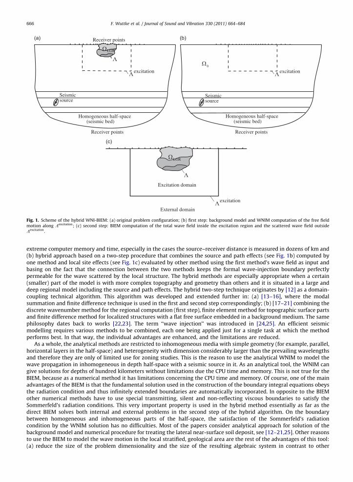
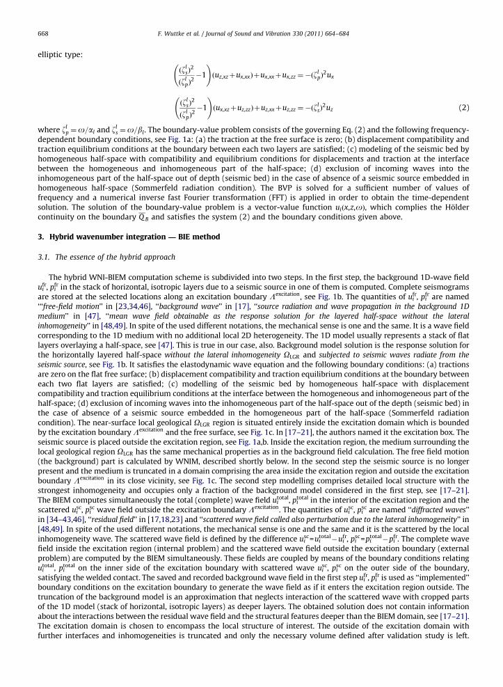
Fig. 1. Scheme of the hybrid WNI-BIEM: (a) original problem configuration; (b) first step: background model and WNIM computation of the free field

motion along Lexcitation; (c) second step: BIEM computation of the total wave field inside the excitation region and the scattered wave field outside

Lexcitation.

F. Wuttke et al. / Journal of Sound and Vibration 330 (2011) 664–684666

extreme computer memory and time, especially in the cases the source–receiver distance is measured in dozens of km and(b) hybrid approach based on a two-step procedure that combines the source and path effects (see Fig. 1b) computed byone method and local site effects (see Fig. 1c) evaluated by other method using the first method’s wave field as input andbasing on the fact that the connection between the two methods keeps the formal wave-injection boundary perfectlypermeable for the wave scattered by the local structure. The hybrid methods are especially appropriate when a certain(smaller) part of the model is with more complex topography and geometry than others and it is situated in a large anddeep regional model including the source and path effects. The hybrid two-step technique originates by [12] as a domain-coupling technical algorithm. This algorithm was developed and extended further in: (a) [13–16], where the modalsummation and finite difference technique is used in the first and second step correspondingly; (b) [17–21] combining thediscrete wavenumber method for the regional computation (first step), finite element method for topographic surface partsand finite difference method for localized structures with a flat free surface embedded in a background medium. The samephilosophy dates back to works [22,23]. The term ‘‘wave injection’’ was introduced in [24,25]. An efficient seismicmodelling requires various methods to be combined, each one being applied just for a single task at which the methodperforms best. In that way, the individual advantages are enhanced, and the limitations are reduced.

As a whole, the analytical methods are restricted to inhomogeneous media with simple geometry (for example, parallel,horizontal layers in the half-space) and heterogeneity with dimension considerably larger than the prevailing wavelengthsand therefore they are only of limited use for zoning studies. This is the reason to use the analytical WNIM to model thewave propagation in inhomogeneous in depth half-space with a seismic source in it. As an analytical tool, the WNIM cangive solutions for depths of hundred kilometers without limitations due the CPU time and memory. This is not true for theBIEM, because as a numerical method it has limitations concerning the CPU time and memory. Of course, one of the mainadvantages of the BIEM is that the fundamental solution used in the construction of the boundary integral equations obeysthe radiation condition and thus infinitely extended boundaries are automatically incorporated. In opposite to the BIEMother numerical methods have to use special transmitting, silent and non-reflecting viscous boundaries to satisfy theSommerfeld’s radiation conditions. This very important property is used in the hybrid method essentially as far as thedirect BIEM solves both internal and external problems in the second step of the hybrid algorithm. On the boundarybetween homogeneous and inhomogeneous parts of the half-space, the satisfaction of the Sommerfeld’s radiationcondition by the WNIM solution has no difficulties. Most of the papers consider analytical approach for solution of thebackground model and numerical procedure for treating the lateral near-surface soil deposit, see [12–21,25]. Other reasonsto use the BIEM to model the wave motion in the local stratified, geological area are the rest of the advantages of this tool:(a) reduce the size of the problem dimensionality and the size of the resulting algebraic system in contrast to other


numerical domain methods; (b) possibility to model lateral inhomogeneity in contrast to WNIM and other analyticalapproaches; (c) solution at each internal point in the domain is expressed in terms of boundary values without recourse todomain discretization and this main facility is very important when wave propagation problems are being solved inmultilayered solids, because only the boundaries between layers are discretized, not their volumes as it is when domaindiscretization methods as finite element or finite difference methods are used; (d) flexibility to model relief peculiarities incontrast to analytical methods and finite difference method having problems with implementing conditions on boundariesof complex geometric shapes, see [18]; (e) the possibility to obtain directly, with no other intermediate source of error, thedynamic regime — displacements and tractions; (f) the semi-analytical character of the method as far as it is based onGreen’s function of the considered problem; (g) high level of accuracy is achieved since numerical quadrature techniquesare directly applied to the boundary integral equations, which are an exact solution of the considered problem.

Although the advantages of the BIEM are well known, there is still a lack of hybrid methods that are based on thismethod. Up to now, few BIEM-based hybrid schemes, such as Bard and Bouchon [26,27], Bravo et al. [28], Kawase [29],Bouchon et al. [30], Kawase and Aki [31], Papageorgiou and Kim [32], Zhang et al. [33], Gil-Zepeda et al. [34], Nguyen andGatmiri [35] have been presented for seismic response analysis of topographic structures. The coupled BIEM with finiteelement and finite difference methods are proposed in [36–40]. In [41–43], a hybrid approach in which an internal regionincluding the valley under harmonic plane waves is modeled by finite elements, while the exterior region is modeled bythe BIE-method. The accuracy and efficiency of the hybrid indirect BIE-Born approximation method is studied in [44]. Gil-Zepeda et al. [34] proposed a hybrid indirect BIEM-discrete wavenumber method and applied it to model the groundmotion of stratified alluvial valleys under incident plane SH waves from an elastic homogeneous half-space. An efficienthybrid MS-BIE method based on the modal summation and the direct boundary integral equation technique is developedin [45].

We conclude that there is a lack of hybrid models based on BIEM that allow to take into consideration the properties ofall three components: seismic source, inhomogeneous in depth wave path and finite laterally inhomogeneous soil stratum.The majority of the computational tools use the body plane waves as input of the seismic motion in the lateralinhomogeneous geological site. That is not adequate to the real seismic scenarios.

The objective of the present paper is to combine the facilities of both analytical WNI and numerical BIE methods inorder to develop an accurate and efficient hybrid approach for synthesis of theoretical seismograms in a laterally varyingnear-surface seismic region embedded in a deep horizontally layered half-space with a seismic source in one of the layers,accounting for: (a) the seismic source characteristics; (b) the inhomogeneous wave path from the source to the area ofinterest; (c) the local geological media with the complex mechanical and geometrical properties and (d) the existence offree surface relief peculiarities.

The proposed hybrid technique is based on the WNIM for investigating wave propagation in the background structure,while BIE method is used for synthesis of theoretical seismograms on the free surface of the local finite near-surface soilstratum with or without relief. The hybrid method, as proposed in this paper is most closely resembles to the methoddiscussed in [12–21,25]. The paper has following content: Starting with the problem description in Section 2, followed bythe hybrid computational tool presented and discussed in Section 3. The validation study of the computational technique ispresented in Section 4. Finally, numerical examples for different seismic scenarios are solved and simulation study is givenin Section 5, followed by conclusions in the last Section 6.

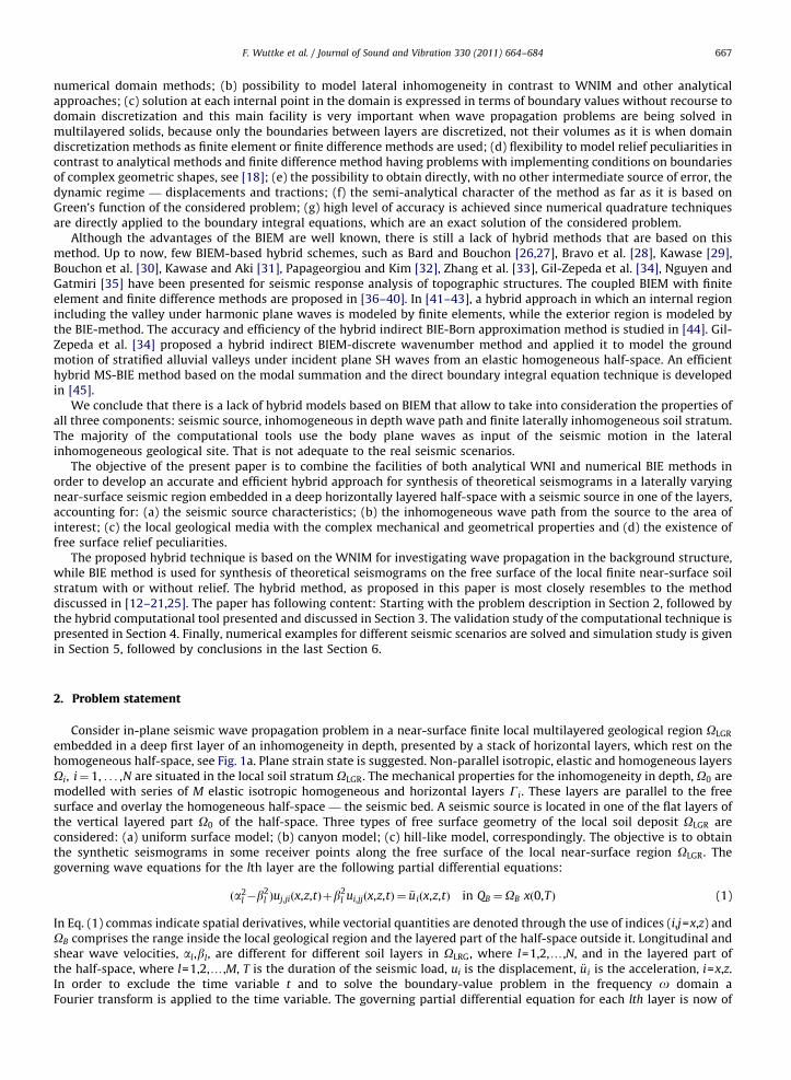
2. Problem statement

Consider in-plane seismic wave propagation problem in a near-surface finite local multilayered geological region OLGR

embedded in a deep first layer of an inhomogeneity in depth, presented by a stack of horizontal layers, which rest on thehomogeneous half-space, see Fig. 1a. Plane strain state is suggested. Non-parallel isotropic, elastic and homogeneous layersOi, i¼ 1, . . . ,N are situated in the local soil stratum OLGR. The mechanical properties for the inhomogeneity in depth, O0 aremodelled with series of M elastic isotropic homogeneous and horizontal layers Gi. These layers are parallel to the freesurface and overlay the homogeneous half-space — the seismic bed. A seismic source is located in one of the flat layers ofthe vertical layered part O0 of the half-space. Three types of free surface geometry of the local soil deposit OLGR areconsidered: (a) uniform surface model; (b) canyon model; (c) hill-like model, correspondingly. The objective is to obtainthe synthetic seismograms in some receiver points along the free surface of the local near-surface region OLGR. Thegoverning wave equations for the lth layer are the following partial differential equations:

ða2l �b

2l Þuj,jiðx,z,tÞþb2

l ui,jjðx,z,tÞ ¼ €uiðx,z,tÞ in QB ¼OB xð0,TÞ (1)

In Eq. (1) commas indicate spatial derivatives, while vectorial quantities are denoted through the use of indices (i,j=x,z) andOB comprises the range inside the local geological region and the layered part of the half-space outside it. Longitudinal andshear wave velocities, al,bl, are different for different soil layers in OLRG, where l=1,2,y,N, and in the layered part ofthe half-space, where l=1,2,y,M, T is the duration of the seismic load, ui is the displacement, €ui is the acceleration, i=x,z.In order to exclude the time variable t and to solve the boundary-value problem in the frequency o domain aFourier transform is applied to the time variable. The governing partial differential equation for each lth layer is now of


elliptic type:

ðzlsÞ

2

ðzlpÞ

2�1

!ðuz,xzþux,xxÞþux,xxþux,zz ¼�ðz

lpÞ

2ux

ðzlsÞ

2

ðzlpÞ

2�1

!ðux,xzþuz,zzÞþuz,xxþuz,zz ¼�ðz

lsÞ

2uz (2)

where zlp ¼o=al and zl

s ¼o=bl. The boundary-value problem consists of the governing Eq. (2) and the following frequency-dependent boundary conditions, see Fig. 1a: (a) the traction at the free surface is zero; (b) displacement compatibility andtraction equilibrium conditions at the boundary between each two layers are satisfied; (c) modeling of the seismic bed byhomogeneous half-space with compatibility and equilibrium conditions for displacements and traction at the interfacebetween the homogeneous and inhomogeneous part of the half-space; (d) exclusion of incoming waves into theinhomogeneous part of the half-space out of depth (seismic bed) in the case of absence of a seismic source embedded inhomogeneous half-space (Sommerfeld radiation condition). The BVP is solved for a sufficient number of values offrequency and a numerical inverse fast Fourier transformation (FFT) is applied in order to obtain the time-dependentsolution. The solution of the boundary-value problem is a vector-value function uiðx,z,oÞ, which complies the Holdercontinuity on the boundary Q B and satisfies the system (2) and the boundary conditions given above.

3. Hybrid wavenumber integration — BIE method

3.1. The essence of the hybrid approach

The hybrid WNI-BIEM computation scheme is subdivided into two steps. In the first step, the background 1D-wave fieldui

fr, pifr in the stack of horizontal, isotropic layers due to a seismic source in one of them is computed. Complete seismograms

are stored at the selected locations along an excitation boundary Lexcitation, see Fig. 1b. The quantities of uifr, pi

fr are named‘‘‘free-field motion’’ in [23,34,46], ‘‘background wave’’ in [17], ‘‘source radiation and wave propagation in the background 1D

medium’’ in [47], ‘‘mean wave field obtainable as the response solution for the layered half-space without the lateral

inhomogeneity’’ in [48,49]. In spite of the used different notations, the mechanical sense is one and the same. It is a wave fieldcorresponding to the 1D medium with no additional local 2D heterogeneity. The 1D model usually represents a stack of flatlayers overlaying a half-space, see [47]. This is true in our case, also. Background model solution is the response solution forthe horizontally layered half-space without the lateral inhomogeneity OLGR and subjected to seismic waves radiate from the

seismic source, see Fig. 1b. It satisfies the elastodynamic wave equation and the following boundary conditions: (a) tractionsare zero on the flat free surface; (b) displacement compatibility and traction equilibrium conditions at the boundary betweeneach two flat layers are satisfied; (c) modelling of the seismic bed by homogeneous half-space with displacementcompatibility and traction equilibrium conditions at the interface between the homogeneous and inhomogeneous part of thehalf-space; (d) exclusion of incoming waves into the inhomogeneous part of the half-space out of the depth (seismic bed) inthe case of absence of a seismic source embedded in the homogeneous part of the half-space (Sommerfeld radiationcondition). The near-surface local geological OLGR region is situated entirely inside the excitation domain which is boundedby the excitation boundary Lexcitation and the free surface, see Fig. 1c. In [17–21], the authors named it the excitation box. Theseismic source is placed outside the excitation region, see Fig. 1a,b. Inside the excitation region, the medium surrounding thelocal geological region OLGR has the same mechanical properties as in the background field calculation. The free field motion(the background) part is calculated by WNIM, described shortly below. In the second step the seismic source is no longerpresent and the medium is truncated in a domain comprising the area inside the excitation region and outside the excitationboundary Lexcitation in its close vicinity, see Fig. 1c. The second step modelling comprises detailed local structure with thestrongest inhomogeneity and occupies only a fraction of the background model considered in the first step, see [17–21].The BIEM computes simultaneously the total (complete) wave field ui

total, pitotal in the interior of the excitation region and the

scattered uisc, pi

sc wave field outside the excitation boundary Lexcitation. The quantities of uisc, pi

sc are named ‘‘diffracted waves’’in [34–43,46], ‘‘residual field’’ in [17,18,23] and ‘‘scattered wave field called also perturbation due to the lateral inhomogeneity’’ in[48,49]. In spite of the used different notations, the mechanical sense is one and the same and it is the scattered by the localinhomogeneity wave. The scattered wave field is defined by the difference ui

sc=uitotal�ui

fr, pisc=pi

total�pi

fr. The complete wavefield inside the excitation region (internal problem) and the scattered wave field outside the excitation boundary (externalproblem) are computed by the BIEM simultaneously. These fields are coupled by means of the boundary conditions relatingui

total, pitotal on the inner side of the excitation boundary with scattered wave ui

sc, pisc on the outer side of the boundary,

satisfying the welded contact. The saved and recorded background wave field in the first step uifr, pi

fr is used as ‘‘implemented’’boundary conditions on the excitation boundary to generate the wave field as if it enters the excitation region outside. Thetruncation of the background model is an approximation that neglects interaction of the scattered wave with cropped partsof the 1D model (stack of horizontal, isotropic layers) as deeper layers. The obtained solution does not contain informationabout the interactions between the residual wave field and the structural features deeper than the BIEM domain, see [17–21].The excitation domain is chosen to encompass the local structure of interest. The outside of the excitation domain withfurther interfaces and inhomogeneities is truncated and only the necessary volume defined after validation study is left.


So, the truncation limits the interactions between the structure of interest and the outer medium to the interaction withcontents of the incoming background wave field, i.e. it may include surface and body waves influenced by the source, wavepath and the structure around (in close vicinity of) the excitation domain. The multiple reflections of the scattered wavebetween the local structure of interest inside the excitation domain and the regional structure outside it can be modelledproperly by the optimal choice of the truncated domain based on the validation study.

3.2. WNIM–BIEM coupling

The key point of the hybrid method is the presentation of the total wave field by a sum of the free field (background)and the scattered parts: ui

total=uifr+ui

sc, pitotal=pi

fr+pisc. The total wave field is inside the excitation domain, while the

scattered wave field is propagating outside of the excitation domain. The boundary conditions relating the total wavefield on the inner side of the excitation boundary with scattered wave on the outer side of the boundary, satisfying the welded

contact. The hybrid coupling keeps the excitation boundary fully transparent in the second step. The scattered wavefield penetrates freely out of the excitation domain and, if reflected by an inhomogeneity, it freely propagates through theexcitation boundary back into the local structure. Oprsal et al. [19] discussed clearly the essence of the generalized hybridapproach of wave injection based on binding two sub-volumes treated by arbitrary wave propagation methods.The decomposition of the total wave field into a sum of free field motion and the scattered wave is commented in the samemanner in [60] for the case of the seismic response of a foundation rested in a non-homogeneous half-space.

3.3. WNIM solution for free field wave motion uifr,pi

fr

In the first step, the seismic source radiation and wave propagation in the horizontally layered background medium O0

is calculated by the WNIM, and the computed background wave field Ufr (called free-field) is recorded along the excitationboundary Lexcitation, see Fig. 1b. The WNIM solves the problem for wave propagation in horizontally layered media with aseismic source at a given level z=S and rested on homogeneous half-space, where radiation condition is satisfied. Theunknowns are displacements ui

l,fr(x,z,t) and traction pl,fri ðx,z,tÞ ¼ sl,fr

ij nj in each lth layer, where i=x,z. The basic equations (1)are decoupled by application of the Helmholtz decomposition theorem into potentials, see [8]. Since the elastic propertiesdo not depend on horizontal position, we use the Fourier transforms over time and the horizontal coordinate to reduce thepartial differential equations of motion to a set of ordinary differential equations according to the displacementul,frðz,z,o,SÞ and stress Rl,fr

ðz,z,o,SÞ vectors which depend on the frequency o , wavenumber z, location of the observer z

and source depth S. After applying the inverse Fourier transformation to the wavenumber z, unknown displacement andstresses are obtained in the frequency-space domain. The frequency-domain formulation is based on the representation ofthe complete response in terms of semi-infinite integrals with respect to the wavenumber. The integrands for eachwavenumber and frequency are determined by an efficient factorization in terms of generalized transmission andreflection coefficients which are calculated by an iterative scheme. As far as we consider the case, when the lateralinhomogeneous soil deposit is situated in the first layer of the horizontally layered half-space (see Fig. 1a) we need theWNIM solutions for displacement ul,frðx,z,oÞ and stress Rl,fr

ðx,z,oÞ vectors in the first layer l=1. Following notation andmathematical description in [9,10,52,54,55,70], these analytical expressions are given as follows:

u1,frðx,z,o,SÞ ¼1

2p

Z 1�1

ðE111K

1dbR0

uþE112K

1uÞbT1

ubT2

u . . .bTS�1

u ðBSþDS

�BS�Þ�1DQ eðizxÞ dz (3)

R1,frðx,z,o,SÞ ¼

1

2p

Z 1�1

ðE121K

1dbR0

uþE122K

1uÞbT1

ubT2

u . . .bTS�1

u ðBSþDS

�BS�Þ�1DQeðizxÞ dz (4)

The integrands in Eqs. (3) and (4) are functions of wavenumber z and depend on the characteristics of the soil stratum,frequency, the depth of the seismic source and the location of the observer. In the above equations the generalized

reflection/transmission (R/T) coefficients are denoted by bR l

u ¼ RluþTl

dbR l�1

ubT l

u and bT l

u ¼ ðI�RldbR l�1

u Þ�1Tl

u, l = 1,y,S�1 for the

layers above the source and bR l

d ¼ RldþTl

ubR lþ1

dbT l

d and bT l

d ¼ ðI�RlubR lþ1

d Þ�1Tl

d, l = M�1,y,S for the layers below the source. For

l=M the generalized reflection coefficients are bR l

d ¼ RMd and bTM

d ¼ TMd , where Rd

M and TdM are the modified R/T coefficients for

the layer M. The index l of layers is running from 1 to M, and the seismic bed is homogeneous half-space and denoted by

M+1. The term bR l�1

u ¼bR0

u is the reflection coefficient at the free surface as the upper boundary of the first layer. The seismic

line source in vertical or horizontal direction is described by the term DQ ¼ ½�Px,0�T and DQ ¼ ½0,�Pz�T , where Px and Pz are

unit line loads in horizontal and vertical directions. Matrix I describes the unit matrix, while the power of �1 means theinverse of a matrix. The matrices E contain the variables excluding exponents and amplitudes of the analytical solution foreach layer. The matrix expressions for displacements and stresses are as follows:

ul,frðz,z,oÞ ¼ El11K

ldCl

dþEl12K

luCl

u (5)

Rl,frðz,z,oÞ ¼ El

21KldCl

dþEl22K

luCl

u (6)


where the terms Kld=u describe the wave propagation in positive (down) and negative (up) directions in the lth layer. The

submatrices Kld=u and Eij

l , i=1,2, j=1,2, are functions of shear modulus ml, shear bl and compressional al wave velocities,

wavenumber z, frequency o and z 2 ðzl�1,zlÞ. The terms CPd/Pul and CSd/Su

l are the unknown constants of the solution of theordinary differential equation, in the lth layer that describe up and down going P- and SV-wave propagation, see [9,53]. Thequality factor or its inverse the dissipation factor describing the material attenuation in soil is defined by the material dampingratio that in the numerical studies here is assumed to be depth dependent. For layers embedded in a depth smaller than 1 kmthe material damping ratio is 1%, in a depth between 1 and 5 km the material damping ratio is 0.5% and for layers in a depthmore than 5 km the damping ratio is 0.25%. By following the definition of the complex velocities [9], the singular points of theintegrals in Eqs. (5) and (6) are shifted slightly from the wavenumber real axis in the complex plane. The numerical integrationalong the real wavenumber axis can be done without singularities. Finally, the displacement function in the frequency andspace domain is obtained after integration over all wavenumbers along the integration path. The displacements in the time andspace domain are obtained by inverse Fourier transformation procedure.

3.4. BIEM solution in the second step

In this second step, the BIEM computes simultaneously the total (complete) wave field in the interior of the excitationregion and the scattered wave field outside the excitation boundary. The following system of boundary integral equationsaccording to the total wave field is satisfied along the boundaries of the layers inside the excitation region:

Cijuiðx,z,oÞ ¼ZOm

U�ijðx,z,x0,z0,oÞpjðx0,z0,oÞdG�ZOm

P�ijðx,z,x0,z0,oÞujðx0,z0,oÞdG (7)

m=1,2,3,y,N here, and Cij are the constants depending on the geometry at the collocation point (x,z); (x0,z0) denotes theposition vector of the source point; GOm

is the boundary of the Om layer; ui and pj are the unknown total displacements andtractions on the boundaries GOm

; U*ij, P*ij are the displacement and traction frequency-dependent fundamental solutions ofEq. (2), given in [50]. The BIE on the external boundary Lexternal is added and it is according to the scattered wave field,which in this case is ui

sc=uitotal�ui

fr, pisc=pi

total�pi

fr.

Cijðutotalj ðx,zÞ�ufr

j ðx,zÞÞjLexternal ¼

ZLexternal

U�ijðx,z,x0,z0,oÞðptotalj ðx0,z0Þ�pfr

j ðx0,z0ÞÞdG

�

ZLexternal

P�ijðx,z,x0,z0,oÞðutotalj ðx0,z0Þ�ufr

j ðx0,z0ÞÞdG (8)

The system of BIE (7) and (8) is according to the unknown displacement uitotal and traction pi

total on the boundaries of the layers inthe local geological structure, on the boundary of the excitation region and on the observer points on the free boundary. In orderto solve this system of BIEs we need to know the free field motion ui

fr, pifr at the boundary nodes on the external boundary

Lexternal. The values for uifr, pi

fr in the boundary nodes on Lexternal are obtained as solution of the background problem by WNIM.The usual numerical procedure of BIEM is applied. The boundary is discretized into elements using piecewise polynomialapproximations of the boundary geometry, displacement and traction. The mesh discretization is made via the quadraticboundary element method. After discretization, in the Fourier transformed domain the kernels of the obtained integrals havesingularities like (a) Oð1=c7xÞ, for c 2 ½�1; þ1� that lead to the Cauchy principal value (CPV) integrals and (b) singularitieslike Oðlnðc7xÞÞ for c 2 ½�1; þ1� that lead to non-singular integrals. The regular integrals are computed employing the Gaussian32-point quadrature scheme and boundary element subdivision, while the singular integrals are solved analytically, using theasymptotics of the fundamental solutions for small arguments, see [51]. After application of discretization procedure, the systemof boundary integral equations is transformed into an algebraic system for the unknown displacement and traction in the Fourierdomain. To obtain displacements and tractions as functions of time, the inverse Fourier transformation is applied.

4. Validation study

The aim of the validation study is to establish the error bounds of the proposed hybrid tool and to evaluate its accuracyon the base of solution of several benchmark examples. The validation of the proposed hybrid solution is based on thecomparison to pure analytical or numerical methods or other hybrid computational techniques. The first example validatesthe proposed hybrid WNI-BIEM technique by solution of specially selected benchmark example which can be solved by thepure analytical methods and by the proposed hybrid method. The second and the third numerical examples validate theaccuracy of the BIEM that is one of the base components of the proposed hybrid technique.

The fourth test example concerns comparison of the numerical results obtained by the proposed WNI-BIEM with twoother hybrid techniques as modal summation-BIEM (MS-BIEM) and modal summation-finite difference method (MS-FDM).

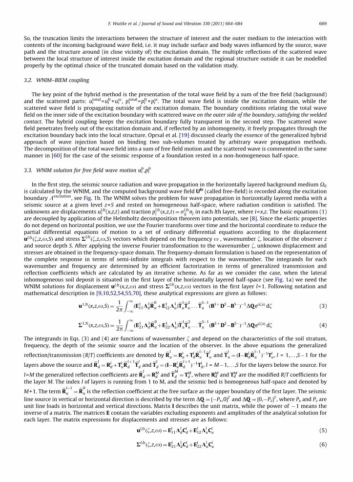
Test example 1. As a first test example a structural model given in Fig. 2a is used.

The local geological region OLGR in Fig. 2a is a valley L1R1T1P1 and it is situated in the first layer of a layered half-space.The coordinates of the corner points (in meters) are: T1(100,0), P1(�100,0), L1(110,270), R1(�110,270). The mechanicalproperties of the local geological region are the same as the first layer in the horizontally layered half-space. In this case it

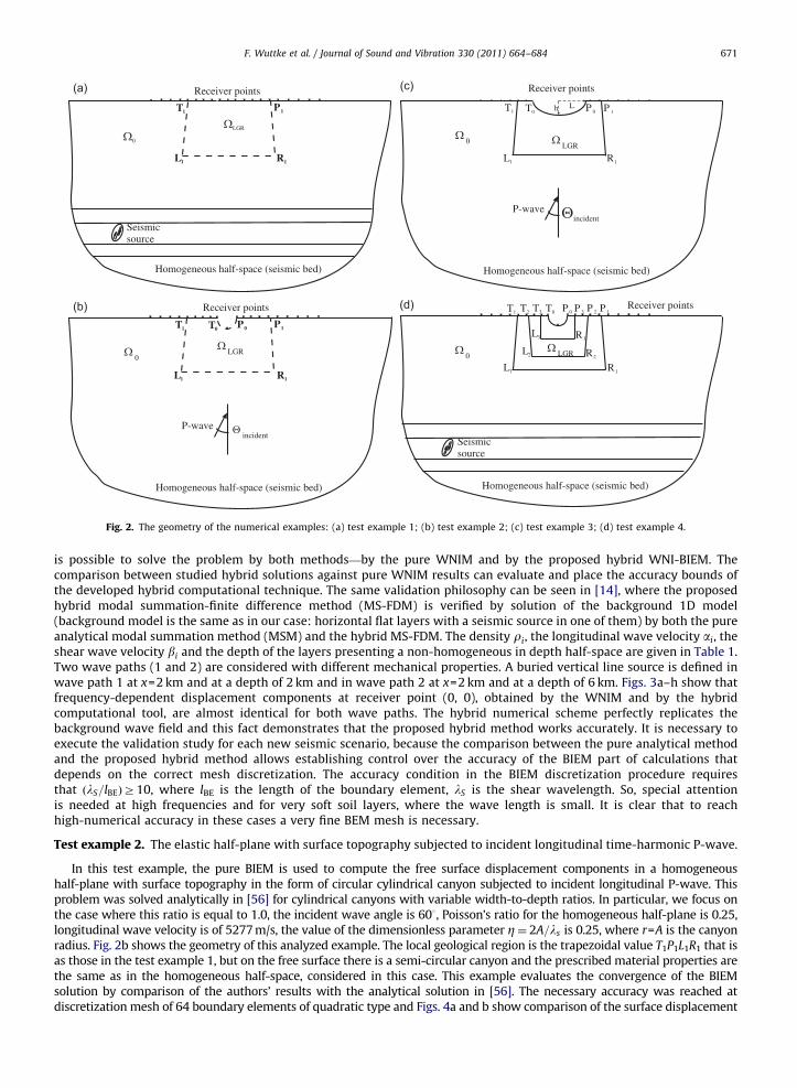
Fig. 2. The geometry of the numerical examples: (a) test example 1; (b) test example 2; (c) test example 3; (d) test example 4.


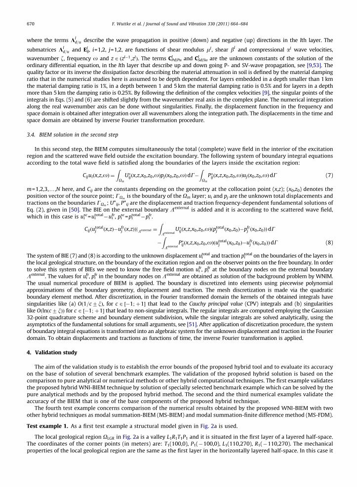
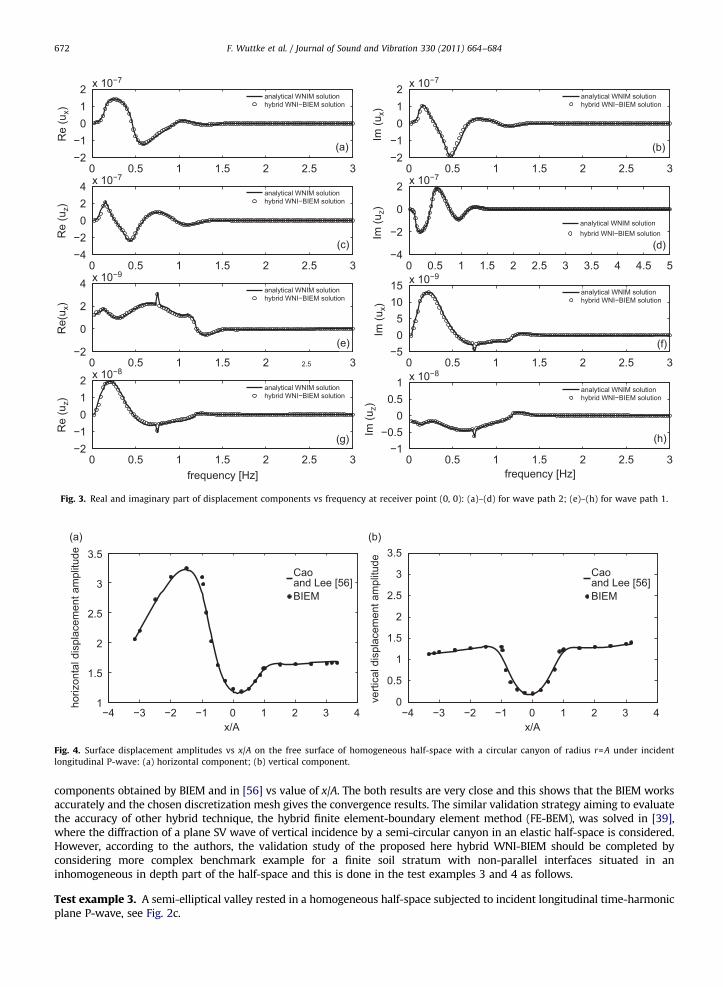
is possible to solve the problem by both methods—by the pure WNIM and by the proposed hybrid WNI-BIEM. Thecomparison between studied hybrid solutions against pure WNIM results can evaluate and place the accuracy bounds ofthe developed hybrid computational technique. The same validation philosophy can be seen in [14], where the proposedhybrid modal summation-finite difference method (MS-FDM) is verified by solution of the background 1D model(background model is the same as in our case: horizontal flat layers with a seismic source in one of them) by both the pureanalytical modal summation method (MSM) and the hybrid MS-FDM. The density ri, the longitudinal wave velocity ai, theshear wave velocity bi and the depth of the layers presenting a non-homogeneous in depth half-space are given in Table 1.Two wave paths (1 and 2) are considered with different mechanical properties. A buried vertical line source is defined inwave path 1 at x=2 km and at a depth of 2 km and in wave path 2 at x=2 km and at a depth of 6 km. Figs. 3a–h show thatfrequency-dependent displacement components at receiver point (0, 0), obtained by the WNIM and by the hybridcomputational tool, are almost identical for both wave paths. The hybrid numerical scheme perfectly replicates thebackground wave field and this fact demonstrates that the proposed hybrid method works accurately. It is necessary toexecute the validation study for each new seismic scenario, because the comparison between the pure analytical methodand the proposed hybrid method allows establishing control over the accuracy of the BIEM part of calculations thatdepends on the correct mesh discretization. The accuracy condition in the BIEM discretization procedure requiresthat ðlS=lBEÞZ10, where lBE is the length of the boundary element, lS is the shear wavelength. So, special attentionis needed at high frequencies and for very soft soil layers, where the wave length is small. It is clear that to reachhigh-numerical accuracy in these cases a very fine BEM mesh is necessary.

Test example 2. The elastic half-plane with surface topography subjected to incident longitudinal time-harmonic P-wave.

In this test example, the pure BIEM is used to compute the free surface displacement components in a homogeneoushalf-plane with surface topography in the form of circular cylindrical canyon subjected to incident longitudinal P-wave. Thisproblem was solved analytically in [56] for cylindrical canyons with variable width-to-depth ratios. In particular, we focus onthe case where this ratio is equal to 1.0, the incident wave angle is 603, Poisson’s ratio for the homogeneous half-plane is 0.25,longitudinal wave velocity is of 5277 m/s, the value of the dimensionless parameter Z¼ 2A=ls is 0.25, where r=A is the canyonradius. Fig. 2b shows the geometry of this analyzed example. The local geological region is the trapezoidal value T1P1L1R1 that isas those in the test example 1, but on the free surface there is a semi-circular canyon and the prescribed material properties arethe same as in the homogeneous half-space, considered in this case. This example evaluates the convergence of the BIEMsolution by comparison of the authors’ results with the analytical solution in [56]. The necessary accuracy was reached atdiscretization mesh of 64 boundary elements of quadratic type and Figs. 4a and b show comparison of the surface displacement

0 0.5 1 1.5 2 2.5 3−2−1

012 x 10−7

Re

(ux)

0 0.5 1 1.5 2 2.5 3−2−1

012 x 10−7

Im (u

x)

0 0.5 1 1.5 2 2.5 3−4−2

024 x 10−7

Re

(uz)

0 0.5 1 1.5 2 2.5 3 3.5 4 4.5 5−4

−2

0

2 x 10−7

Im (u

z)0 0.5 1 1.5 2 2.5 3

−2

0

2

4 x 10−9

Re(

u x)

0 0.5 1 1.5 2 2.5 3−5

05

1015 x 10−9

Im (u

x)

0 0.5 1 1.5 2 2.5 3−2−1

012 x 10−8

Re

(uz)

frequency [Hz]0 0.5 1 1.5 2 2.5 3

−1−0.5

00.5

1 x 10−8Im

(uz)

frequency [Hz]

analytical WNIM solutionhybrid WNI−BIEM solution








Fig. 3. Real and imaginary part of displacement components vs frequency at receiver point (0, 0): (a)–(d) for wave path 2; (e)–(h) for wave path 1.

−4 −3 −2 −1 0 1 2 3 41

1.5

2

2.5

3

3.5

x/A

horiz

onta

l dis

plac

emen

t am

plitu

de

Caoand Lee [56]BIEM

−4 −3 −2 −1 0 1 2 3 40

0.5

1

1.5

2

2.5

3

3.5

x/A

verti

cal d

ispl

acem

ent a

mpl

itude

Caoand Lee [56]BIEM

Fig. 4. Surface displacement amplitudes vs x/A on the free surface of homogeneous half-space with a circular canyon of radius r=A under incident

longitudinal P-wave: (a) horizontal component; (b) vertical component.


components obtained by BIEM and in [56] vs value of x/A. The both results are very close and this shows that the BIEM worksaccurately and the chosen discretization mesh gives the convergence results. The similar validation strategy aiming to evaluatethe accuracy of other hybrid technique, the hybrid finite element-boundary element method (FE-BEM), was solved in [39],where the diffraction of a plane SV wave of vertical incidence by a semi-circular canyon in an elastic half-space is considered.However, according to the authors, the validation study of the proposed here hybrid WNI-BIEM should be completed byconsidering more complex benchmark example for a finite soil stratum with non-parallel interfaces situated in aninhomogeneous in depth part of the half-space and this is done in the test examples 3 and 4 as follows.

Test example 3. A semi-elliptical valley rested in a homogeneous half-space subjected to incident longitudinal time-harmonicplane P-wave, see Fig. 2c.


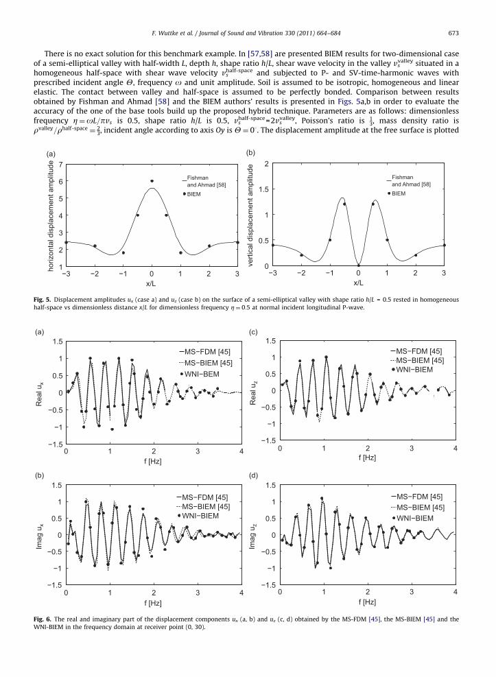
There is no exact solution for this benchmark example. In [57,58] are presented BIEM results for two-dimensional caseof a semi-elliptical valley with half-width L, depth h, shape ratio h/L, shear wave velocity in the valley vs

valley situated in ahomogeneous half-space with shear wave velocity vs

half-space and subjected to P- and SV-time-harmonic waves withprescribed incident angle Y, frequency o and unit amplitude. Soil is assumed to be isotropic, homogeneous and linearelastic. The contact between valley and half-space is assumed to be perfectly bonded. Comparison between resultsobtained by Fishman and Ahmad [58] and the BIEM authors’ results is presented in Figs. 5a,b in order to evaluate theaccuracy of the one of the base tools build up the proposed hybrid technique. Parameters are as follows: dimensionlessfrequency Z¼oL=pvs is 0.5, shape ratio h/L is 0.5, vs

half-space=2vsvalley, Poisson’s ratio is 1

3, mass density ratio isrvalley=rhalf-space ¼ 2

3, incident angle according to axis Oy is Y¼ 03. The displacement amplitude at the free surface is plotted

−3 −2 −1 0 1 2 31

2

3

4

5

6

7

x/L

horiz

onta

l dis

plac

emen

t am

plitu

de

Fishmanand Ahmad [58]

BIEM

−3 −2 −1 0 1 2 30

0.5

1

1.5

2

x/L

verti

cal d

ispl

acem

ent a

mpl

itude

Fishmanand Ahmad [58]

BIEM

Fig. 5. Displacement amplitudes ux (case a) and uz (case b) on the surface of a semi-elliptical valley with shape ratio h/L = 0.5 rested in homogeneous

half-space vs dimensionless distance x/L for dimensionless frequency Z¼ 0:5 at normal incident longitudinal P-wave.

0 1 2 3 4−1.5

−1

−0.5

0

0.5

1

1.5

f [Hz]

Rea

l ux

MS−FDM [45]MS−BIEM [45]WNI−BEM

0 1 2 3 4−1.5

−1

−0.5

0

0.5

1

1.5

f [Hz]

Imag

ux

MS−FDM [45]MS−BIEM [45]WNI−BIEM

0 1 2 3 4−1.5

−1

−0.5

0

0.5

1

1.5

f [Hz]

Rea

l uz


0 1 2 3 4−1.5

−1

−0.5

0

0.5

1

1.5

f [Hz]

Imag

uz


Fig. 6. The real and imaginary part of the displacement components ux (a, b) and uz (c, d) obtained by the MS-FDM [45], the MS-BIEM [45] and the

WNI-BIEM in the frequency domain at receiver point (0, 30).


vs the dimensionless distance x/L. It is obvious that the obtained authors’ results are in agreement with those obtained byFishman and Ahmad in [58].

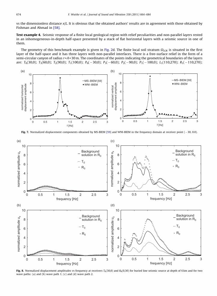
Test example 4. Seismic response of a finite local geological region with relief peculiarities and non-parallel layers restedin an inhomogeneous-in-depth half-space presented by a stack of flat horizontal layers with a seismic source in one ofthem.

The geometry of this benchmark example is given in Fig. 2d. The finite local soil stratum OLGR is situated in the firstlayer of the half-space and it has three layers with non-parallel interfaces. There is a free-surface relief in the form of asemi-circular canyon of radius r=A=30 m. The coordinates of the points indicating the geometrical boundaries of the layersare: T0(30,0); T3(60,0); T2(90,0); T1(100,0); P0(�30,0); P3(�60,0); P2(�90,0); P1(�100,0); L1(110,270); R1(�110,270);

0 0.5 1 1.5 2 2.5 30

2

4

6

8

10

frequency [Hz]

norm

aliz

ed a

mpl

itude

ux Background

solution in R0

T0

R0

0 0.5 1 1.5 2 2.5 30

2

4

6

8

10

frequency [Hz]

norm

aliz

ed a

mpl

itude

uz Background

solution in R0

T0

R0

0 0.5 1 1.5 2 2.5 30

2

4

6

8

10

frequency [Hz]

norm

aliz

ed a

mpl

itude

ux Background

solution in R0

T0

R0

0 0.5 1 1.5 2 2.5 30

2

4

6

8

10

frequency [Hz]

norm

aliz

ed a

mpl

itude

uz Background

solution in R0

T0

R0

Fig. 8. Normalized displacement amplitudes vs frequency at receivers T0(30,0) and R0(0,30) for buried line seismic source at depth of 6 km and for two

wave paths: (a) and (b) wave path 1; (c) and (d) wave path 2.

0 0.5 1 1.5 2 2.5 30

2

4

6

8

10

f [Hz]

norm

aliz

ed h

oriz

onta

ldi

spla

cem

ent a

mpl

itude

MS−BIEM [59]WNI−BIEM

0 0.5 1 1.5 2 2.5 30

2

4

6

8

10

f [Hz]

norm

aliz

ed v

ertic

aldi

spla

cem

ent a

mpl

itude

MS−BIEM [59]WNI−BIEM

Fig. 7. Normalized displacement components obtained by MS-BIEM [59] and WNI-BIEM in the frequency domain at receiver point (�30, 0.0).


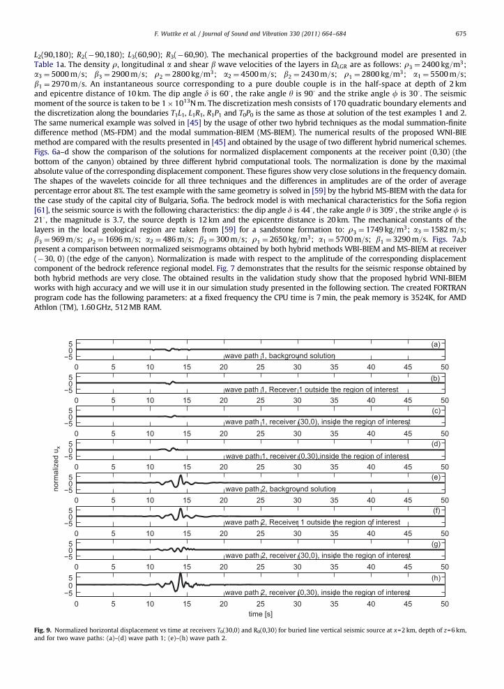
L2(90,180); R2(�90,180); L3(60,90); R3(�60,90). The mechanical properties of the background model are presented inTable 1a. The density r, longitudinal a and shear b wave velocities of the layers in OLGR are as follows: r3 ¼ 2400 kg=m3;a3 ¼ 5000 m=s; b3 ¼ 2900 m=s; r2 ¼ 2800 kg=m3; a2 ¼ 4500 m=s; b2 ¼ 2430 m=s; r1 ¼ 2800 kg=m3; a1 ¼ 5500 m=s;b1 ¼ 2970 m=s. An instantaneous source corresponding to a pure double couple is in the half-space at depth of 2 kmand epicentre distance of 10 km. The dip angle d is 603, the rake angle y is 903 and the strike angle f is 303. The seismicmoment of the source is taken to be 1�1013N m. The discretization mesh consists of 170 quadratic boundary elements andthe discretization along the boundaries T1L1, L1R1, R1P1 and T0P0 is the same as those at solution of the test examples 1 and 2.The same numerical example was solved in [45] by the usage of other two hybrid techniques as the modal summation-finitedifference method (MS-FDM) and the modal summation-BIEM (MS-BIEM). The numerical results of the proposed WNI-BIEmethod are compared with the results presented in [45] and obtained by the usage of two different hybrid numerical schemes.Figs. 6a–d show the comparison of the solutions for normalized displacement components at the receiver point (0,30) (thebottom of the canyon) obtained by three different hybrid computational tools. The normalization is done by the maximalabsolute value of the corresponding displacement component. These figures show very close solutions in the frequency domain.The shapes of the wavelets coincide for all three techniques and the differences in amplitudes are of the order of averagepercentage error about 8%. The test example with the same geometry is solved in [59] by the hybrid MS-BIEM with the data forthe case study of the capital city of Bulgaria, Sofia. The bedrock model is with mechanical characteristics for the Sofia region[61], the seismic source is with the following characteristics: the dip angle d is 443, the rake angle y is 3093, the strike angle f is213, the magnitude is 3.7, the source depth is 12 km and the epicentre distance is 20 km. The mechanical constants of thelayers in the local geological region are taken from [59] for a sandstone formation to: r3 ¼ 1749 kg=m3; a3 ¼ 1582 m=s;b3 ¼ 969 m=s; r2 ¼ 1696 m=s; a2 ¼ 486 m=s; b2 ¼ 300 m=s; r1 ¼ 2650 kg=m3; a1 ¼ 5700 m=s; b1 ¼ 3290 m=s. Figs. 7a,bpresent a comparison between normalized seismograms obtained by both hybrid methods WBI-BIEM and MS-BIEM at receiver(�30, 0) (the edge of the canyon). Normalization is made with respect to the amplitude of the corresponding displacementcomponent of the bedrock reference regional model. Fig. 7 demonstrates that the results for the seismic response obtained byboth hybrid methods are very close. The obtained results in the validation study show that the proposed hybrid WNI-BIEMworks with high accuracy and we will use it in our simulation study presented in the following section. The created FORTRANprogram code has the following parameters: at a fixed frequency the CPU time is 7 min, the peak memory is 3524K, for AMDAthlon (TM), 1.60 GHz, 512 MB RAM.

0 5 10 15 20 25 30 35 40 45 50−5

05

wave path 1, background solution

0 5 10 15 20 25 30 35 40 45 50−5

05

wave path 1, Recever 1 outside the region of interest

0 5 10 15 20 25 30 35 40 45 50−5

05

wave path 1, receiver (30,0), inside the region of interest

0 5 10 15 20 25 30 35 40 45 50−5

05

norm

aliz

ed u

x

wave path 1, receiver (0,30),inside the region of interest

0 5 10 15 20 25 30 35 40 45 50−5

05


0 5 10 15 20 25 30 35 40 45 50−5

05

wave path 2, Receiver 1 outside the region of interest

0 5 10 15 20 25 30 35 40 45 50−5

05


0 5 10 15 20 25 30 35 40 45 50−5

05

time [s]


Fig. 9. Normalized horizontal displacement vs time at receivers T0(30,0) and R0(0,30) for buried line vertical seismic source at x=2 km, depth of z=6 km,

and for two wave paths: (a)–(d) wave path 1; (e)–(h) wave path 2.


5. Numerical simulations

In order to illustrate the efficiency of the proposed hybrid method, the response of a multilayered region with geometrygiven in the test example 4 (Fig. 2d) is analyzed. Three types of the free-surface geometry relief are considered: (a) flatmodel; (b) semi-circle canyon with radius r=A=30 m; (c) semi-circle hill with radius r=A=30 m. The mechanical propertiesof the finite geological region are given in Table 2. The aim of the simulation study is to demonstrate that the syntheticsignals, obtained through the proposed hybrid WNI-BIEM, depend on: (a) wave path inhomogeneity; (b) relief existence onthe free surface; (c) mechanical properties of the local finite soil stratum and lateral inhomogeneity of the local geologicalregion; (d) seismic source characteristics. Each one of these effects is considered and discussed below.

5.1. Sensitivity of the obtained synthetic seismic signals to the wave path properties

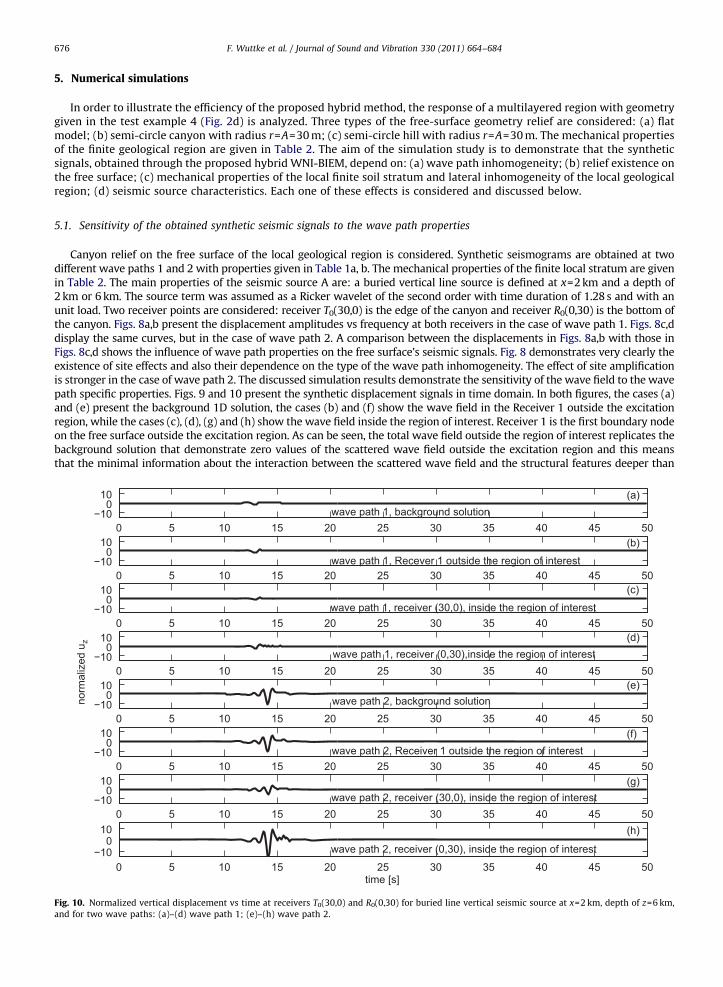
Canyon relief on the free surface of the local geological region is considered. Synthetic seismograms are obtained at twodifferent wave paths 1 and 2 with properties given in Table 1a, b. The mechanical properties of the finite local stratum are givenin Table 2. The main properties of the seismic source A are: a buried vertical line source is defined at x=2 km and a depth of2 km or 6 km. The source term was assumed as a Ricker wavelet of the second order with time duration of 1.28 s and with anunit load. Two receiver points are considered: receiver T0(30,0) is the edge of the canyon and receiver R0(0,30) is the bottom ofthe canyon. Figs. 8a,b present the displacement amplitudes vs frequency at both receivers in the case of wave path 1. Figs. 8c,ddisplay the same curves, but in the case of wave path 2. A comparison between the displacements in Figs. 8a,b with those inFigs. 8c,d shows the influence of wave path properties on the free surface’s seismic signals. Fig. 8 demonstrates very clearly theexistence of site effects and also their dependence on the type of the wave path inhomogeneity. The effect of site amplificationis stronger in the case of wave path 2. The discussed simulation results demonstrate the sensitivity of the wave field to the wavepath specific properties. Figs. 9 and 10 present the synthetic displacement signals in time domain. In both figures, the cases (a)and (e) present the background 1D solution, the cases (b) and (f) show the wave field in the Receiver 1 outside the excitationregion, while the cases (c), (d), (g) and (h) show the wave field inside the region of interest. Receiver 1 is the first boundary nodeon the free surface outside the excitation region. As can be seen, the total wave field outside the region of interest replicates thebackground solution that demonstrate zero values of the scattered wave field outside the excitation region and this meansthat the minimal information about the interaction between the scattered wave field and the structural features deeper than

0 5 10 15 20 25 30 35 40 45 50−10

010


0 5 10 15 20 25 30 35 40 45 50−10

010

wave path 1, Recever 1 outside the region of interest

0 5 10 15 20 25 30 35 40 45 50−10

010


0 5 10 15 20 25 30 35 40 45 50−10

010

norm

aliz

ed u

z

wave path 1, receiver (0,30),inside the region of interest

0 5 10 15 20 25 30 35 40 45 50−10

010


0 5 10 15 20 25 30 35 40 45 50−10

010

wave path 2, Receiver 1 outside the region of interest

0 5 10 15 20 25 30 35 40 45 50−10

010


0 5 10 15 20 25 30 35 40 45 50−10

010

time [s]


Fig. 10. Normalized vertical displacement vs time at receivers T0(30,0) and R0(0,30) for buried line vertical seismic source at x=2 km, depth of z=6 km,

and for two wave paths: (a)–(d) wave path 1; (e)–(h) wave path 2.


the excitation region have been lost. Normalization in Figs. 8–10 is made with respect to the maximal amplitude of thecorresponding displacement component, synthesized for the bedrock reference model (wave path 1). All results confirm theconclusion that wave path properties can dramatically change the character of the seismic signals.

5.2. Sensitivity of the obtained synthetic seismic signals to the free surface relief of the local geological region

The effects of surface geology can greatly enlarge the site response, exerting an important influence on the distributionof damage observed during earthquakes. In [62–64], the need of incorporating or reviewing parameters related to the localtopography to account for topographical effects in the seismic response is pointed out. The role of lateral heterogeneity in

0 0.5 1 1.5 2 2.5 30

0.5

1

1.5

frequency [Hz]

norm

aliz

ed a

mpl

itude

ux

Backgroundsolution in R0

T0

R0

Canyon relief on the surface

0 0.5 1 1.5 2 2.5 30

0.5

1

1.5

frequency [Hz]

norm

aliz

ed a

mpl

itude

ux


T0

R0

Flat free surface

0 0.5 1 1.5 2 2.5 30

0.5

1

1.5

2

frequency [Hz]

norm

aliz

ed a

mpl

itude

uz


T0

R0

Canyon relief on the surface

0 0.5 1 1.5 2 2.5 30

0.5

1

1.5

2

frequency [Hz]

norm

aliz

ed a

mpl

itude

uz


T0

R0

Flat free surface

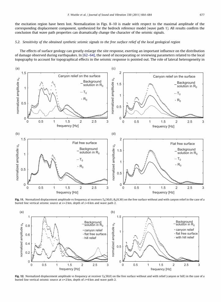
Fig. 11. Normalized displacement amplitude vs frequency at receivers T0(30,0), R0(0,30) on the free surface without and with canyon relief in the case of a

buried line vertical seismic source at x=2 km, depth of z=6 km and wave path 2.

0 0.5 1 1.5 2 2.5 30

0.2

0.4

0.6

0.8

1

frequency [Hz]

norm

aliz

ed a

mpl

itude

ux Background

solution in R0

canyon reliefflat free surfacehill relief

0 0.5 1 1.5 2 2.5 30

0.5

1

1.5

frequency [Hz]

norm

aliz

ed a

mpl

itude

uz Background

solution in R0

canyon reliefflat free surfacewith hill relief

Fig. 12. Normalized displacement amplitude vs frequency at receiver T0(30,0) on the free surface without and with relief (canyon or hill) in the case of a

buried line vertical seismic source at x=2 km, depth of z=6 km and wave path 2.


site effects, especially in small and shallow sedimentary basins has been observed in Coachella valley in California by [65],Parkway in New Zealand by [66], Colfiorito in Italy by [67,68]. The WNI-BIEM can show the influence of the relief on thecomputed seismic signals. Figs. 11 and 12 reveal the sensitivity of the seismic signals to the free surface relief.

The synthetic seismograms shown in Figs. 11 and 12 are obtained at wave path 2 and seismic source A at a depth of6 km. The mechanical properties of the local soil region are given in Table 2. Three types of the free surface geometry areconsidered: (a) flat surface; (b) canyon relief; (3) hill-like relief, correspondingly. Normalization in Figs. 11–17 is made

0 0.5 1 1.5 2 2.5 30

0.2

0.4

0.6

0.8

1

1.2

frequency [Hz]

norm

aliz

ed a

mpl

itude

ux


T0; Layer 3 is of type A

R0; Layer 3 is of type A

T0; Layer 3 is of type B

R0; Layer 3 is of type B

0 0.5 1 1.5 2 2.5 30

0.5

1

1.5

frequency [Hz]no

rmal

ized

am

plitu

de u

z


T0; Layer 3 is of type A

R0; Layer 3 is of type A

T0; Layer 3 is of type B

R0; Layer 3 is of type B

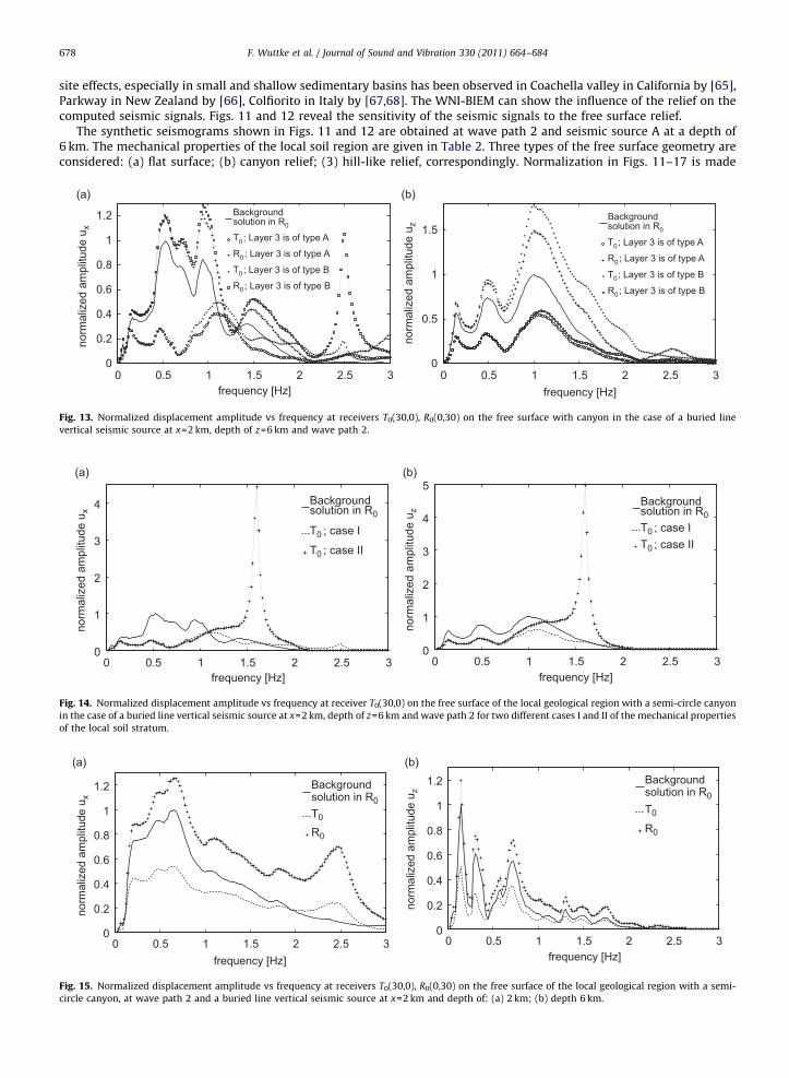
Fig. 13. Normalized displacement amplitude vs frequency at receivers T0(30,0), R0(0,30) on the free surface with canyon in the case of a buried line

vertical seismic source at x=2 km, depth of z=6 km and wave path 2.

0 0.5 1 1.5 2 2.5 30

1

2

3

4

frequency [Hz]

norm

aliz

ed a

mpl

itude

ux


T0 ; case I

T0 ; case II

0 0.5 1 1.5 2 2.5 30

1

2

3

4

5

frequency [Hz]

norm

aliz

ed a

mpl

itude

uz

Backgroundsolution in R0T0 ; case IT0 ; case II

Fig. 14. Normalized displacement amplitude vs frequency at receiver T0(30,0) on the free surface of the local geological region with a semi-circle canyon

in the case of a buried line vertical seismic source at x=2 km, depth of z=6 km and wave path 2 for two different cases I and II of the mechanical properties

of the local soil stratum.

0 0.5 1 1.5 2 2.5 30

0.2

0.4

0.6

0.8

1

1.2

frequency [Hz]

norm

aliz

ed a

mpl

itude

ux

Backgroundsolution in R0T0

R0

0 0.5 1 1.5 2 2.5 30

0.2

0.4

0.6

0.8

1

1.2

frequency [Hz]

norm

aliz

ed a

mpl

itude

uz

Backgroundsolution in R0T0

R0

Fig. 15. Normalized displacement amplitude vs frequency at receivers T0(30,0), R0(0,30) on the free surface of the local geological region with a semi-

circle canyon, at wave path 2 and a buried line vertical seismic source at x=2 km and depth of: (a) 2 km; (b) depth 6 km.


with respect to the maximal amplitude of the corresponding displacement component, synthesized for the bedrockreference model (wave path 2). Figs. 11a,b show the horizontal component of displacement amplitude in the case of localmultilayered region with canyon relief and with flat free surface, correspondingly. Figs. 11c,d show the vertical componentof displacement amplitude versus frequency for free surface with and without canyon relief. The discussed results revealthat the site effects are much stronger in the case of relief on the free surface, while in the case of flat free surface there isno clear presence of the site amplification. This can be explained with the complex diffraction wave picture in the case ofcanyon relief, i.e. with the well known edge effects. Figs. 12a,b compare the displacement amplitudes at receiver (30,0)

0 5 10 15 20 25 30 35 40 45 50−1

0

1

norm

aliz

ed u

x

source depth 6km, background solution

0 5 10 15 20 25 30 35 40 45 50−1

0

1

norm

aliz

ed u

x

source depth 6km, Receiver 1 outside the region of interest

0 5 10 15 20 25 30 35 40 45 50−1

0

1

norm

aliz

ed u

x

source depth 6km, Receiver (0,30) inside the region of interest

0 5 10 15 20 25 30 35 40 45 50−1

0

1

norm

aliz

ed u

x


time [s]

0 5 10 15 20 25 30 35 40 45 50−1

0

1

norm

aliz

ed u

x


0 5 10 15 20 25 30 35 40 45 50−1

0

1

norm

aliz

ed u

x


0 5 10 15 20 25 30 35 40 45 50−1

0

1

norm

aliz

ed u

x


0 5 10 15 20 25 30 35 40 45 50−1

0

1

time [s]

norm

aliz

ed u

x


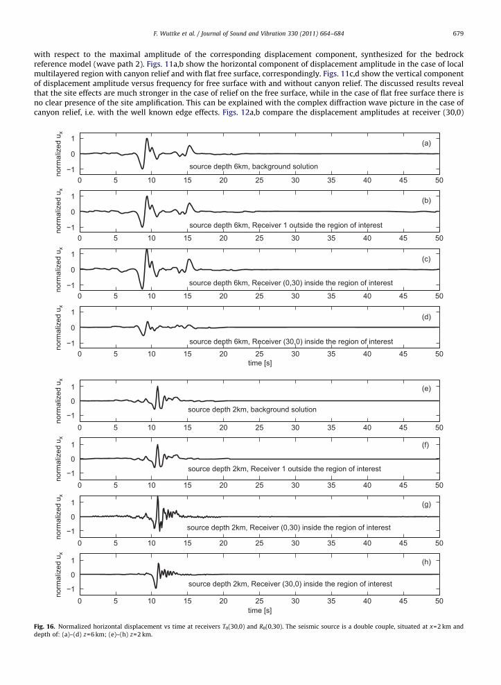
Fig. 16. Normalized horizontal displacement vs time at receivers T0(30,0) and R0(0,30). The seismic source is a double couple, situated at x=2 km and

depth of: (a)–(d) z=6 km; (e)–(h) z=2 km.


(the edge of the canyon) on the free, horizontal surface and the free surface with relief (canyon or hill). In the case ofcanyon relief the displacement amplitudes are the smallest one, while in the case of the free, horizontal surface they arethe greatest one. The complex diffraction wave picture in the case of relief peculiarities is responsible for this behavior.

5.3. Sensitivity of the obtained synthetic seismic signals to the mechanical properties of the local geological region

The mechanical properties of the local soil stratum play an important role on the specific character of the seismic signal.Fig. 13 shows displacement amplitudes at receiver T0(30,0) and receiver R0(0,30) vs frequency, at seismic source A at a

0 5 10 15 20 25 30 35 40 45 50−1

0

1

norm

aliz

ed u

z


0 5 10 15 20 25 30 35 40 45 50−1

0

1

norm

aliz

ed u

z


0 5 10 15 20 25 30 35 40 45 50−1

0

1

norm

aliz

ed u

z


0 5 10 15 20 25 30 35 40 45 50−1

0

1

norm

aliz

ed u

z


0 5 10 15 20 25 30 35 40 45 50−1

0

1

norm

aliz

ed u

z


0 5 10 15 20 25 30 35 40 45 50−1

0

1

norm

aliz

ed u

z


0 5 10 15 20 25 30 35 40 45 50−1

0

1

norm

aliz

ed u

z


0 5 10 15 20 25 30 35 40 45 50−1

0

1

time [s]

norm

aliz

ed u

z


Fig. 17. Normalized vertical displacement vs time at receivers T0(30,0) and R0(0,30). The seismic source is a double couple, situated at x=2 km and depth

of: (a)–(d) z=6 km; (e)–(h) z=2 km.


depth of 6 km and wave path 2. The mechanical properties of the local geological region are presented in Table 2. The thirdsoil layer is of type A ðb3 ¼ 800 m=s, a3 ¼ 1500 m=sÞ or of type B ðb3 ¼ 500 m=s, a3 ¼ 900 m=sÞ. Fig. 14 compares seismicsignals obtained at receiver T0 for two cases of mechanical properties of the finite soil profile: (a) case I — materialcharacteristics are as those given in Table 2; (b) case II — second and third layers change their positions, i.e. second layer iswith the properties of the third layer and vice versa . This leads to a complete different character of the syntheticseismograms. Figs. 13 and 14 reveal how important are the mechanical properties of the local seismic region for thecharacteristic peculiarities of the obtained wave signals during earthquake.

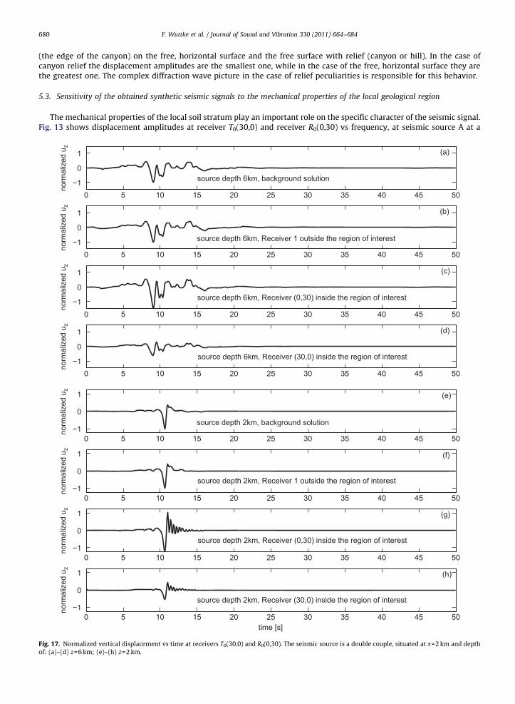
5.4. Sensitivity of the obtained synthetic seismic signals to the seismic source properties

The synthetic seismograms are obtained for seismic source B at two different depths. The rest of the data is fixed, it isconsidered wave path 2 and canyon relief on the free surface, while the mechanical properties of the local soil region aregiven in Table 2. The seismic source B used for the simulation study is the so-called double couple source. The timedependency of the seismic moment M0(t) is defined after [69]. As source parameters were chosen scalar seismic momentM0=5.98�1014 N m, corner frequency fc=5.0 Hz, strike angle j¼ 1513, dip angle d¼ 833 and rake angle y¼ 73. To show theeffects of different source depths this source is implemented in x=2 km and a depth of 2 km or 6 km. Figs. 15–17demonstrate in frequency and in time domain, respectively, how sensitive are the synthetic signals to the depth of theseismic source. The discussed numerical results in this item show that the synthetic signals and the site effects depend onall essential components of the seismic wave path: seismic source located in the half-space, inhomogeneous wave pathfrom the source to the local geological region plus the lateral inhomogeneous finite local stratum with its complexmechanical and geometrical peculiarities. The proposed, developed and validated hybrid analytically numerical tool hasthe possibility to account for all these important components of the seismic wave.

6. Concluding remarks

Efficient hybrid wavenumber integration-boundary integral equation method is developed, validated and applied insimulation studies. The hybrid approach combines analytical WNIM and numerical BIEM. PROS and CONS of the proposedhybrid tool are as follows: (a) it is possible to treat many soil layers due to the effective combination of both methods;(b) wave field can be evaluated for small and large distances; (c) body and surface waves are considered; (d) BIEM allowsmodeling of complex geometry, relief existence, non-parallel layering, inhomogeneities like cracks, inclusions, etc.;(e) capability to obtain seismograms, velocigrams and accelerograms, also response spectra, that account for the propertiesof the earthquake source, inhomogeneous wave path and laterally varying local geological region; (f) potential to accountfor geological regions with more complex mechanical behavior as anisotropy, poroelasticity, non-elasticity, etc.; (g) most ofthe papers in the literature take into account either one or two of the physical mechanisms controlling the seismic wave,while the hybrid WNI-BIEM has the potential to study simultaneously the combined effects of different physical propertiesof the system: seismic wave-geological media; (k) special attention is needed at high frequencies and for very soft soillayers, where the wavelength is small. It is clear that to reach high-numerical accuracy in these cases a very fine BEM mesh

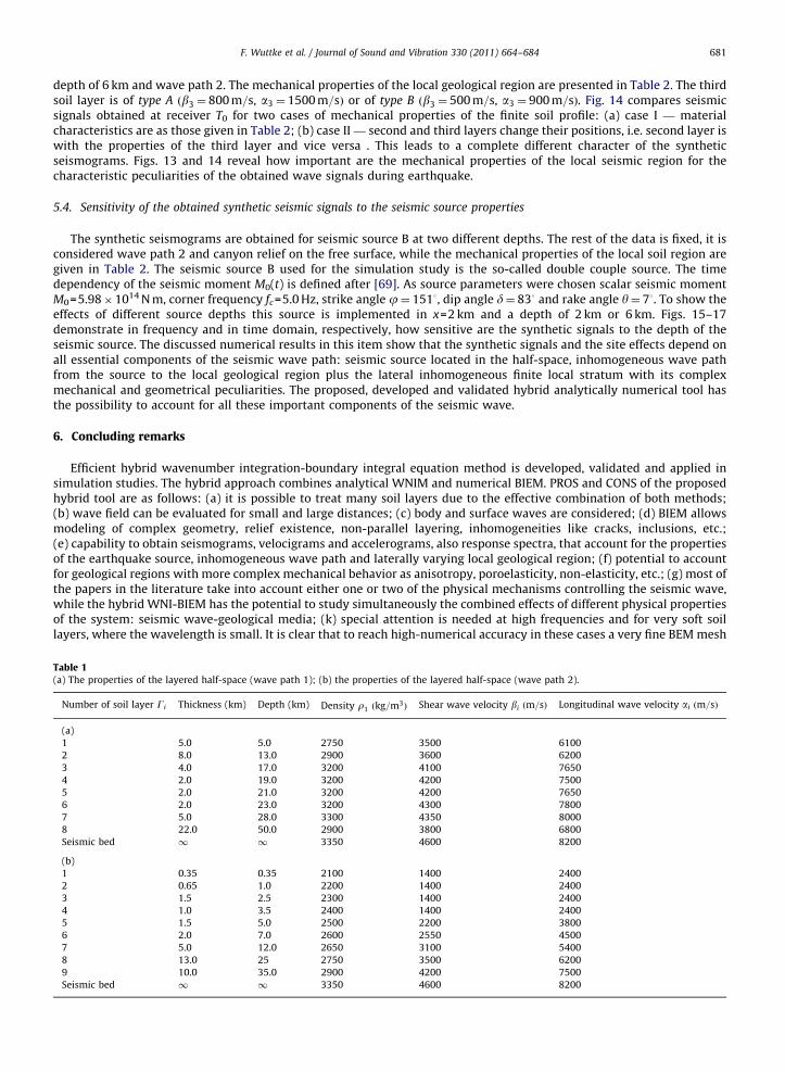
Table 1(a) The properties of the layered half-space (wave path 1); (b) the properties of the layered half-space (wave path 2).

Number of soil layer Gi Thickness (km) Depth (km) Density r1 ðkg=m3Þ Shear wave velocity bi ðm=sÞ Longitudinal wave velocity ai ðm=sÞ

(a)

1 5.0 5.0 2750 3500 6100

2 8.0 13.0 2900 3600 6200

3 4.0 17.0 3200 4100 7650

4 2.0 19.0 3200 4200 7500

5 2.0 21.0 3200 4200 7650

6 2.0 23.0 3200 4300 7800

7 5.0 28.0 3300 4350 8000

8 22.0 50.0 2900 3800 6800

Seismic bed 1 1 3350 4600 8200

(b)

1 0.35 0.35 2100 1400 2400

2 0.65 1.0 2200 1400 2400

3 1.5 2.5 2300 1400 2400

4 1.0 3.5 2400 1400 2400

5 1.5 5.0 2500 2200 3800

6 2.0 7.0 2600 2550 4500

7 5.0 12.0 2650 3100 5400

8 13.0 25 2750 3500 6200

9 10.0 35.0 2900 4200 7500

Seismic bed 1 1 3350 4600 8200

Table 2The properties of the local geological region.

Number of soil layer Density r1 ðkg=m3Þ Shear wave velocity bi ðm=sÞ Longitudinal wave velocity ai ðm=sÞ

3 1800 800 1500

2 2000 1000 1700

1 2000 1400 2400


has to be used, respective this leads to high values of CPU time and memory; (l) it is necessary to establish the limits andpossibilities of the proposed hybrid technique for each new seismic scenario and to this aim one-dimensional simulationexperiment allows us to consider the WNIM result as one of the reference benchmark examples.

The seismic signal, obtained by the hybrid technique, can be used as a necessary base for solution of the followingimportant geotechnical and civil engineering problems: (a) seismic wave propagation with accounting for the morecomplex mechanical behavior of the soil (b) soil–structure interaction and its effects on the dynamics of structures duringearthquake; (c) solution of inverse problems for dynamic site characterization and identifying the soil profiles.

Acknowledgements

The authors acknowledge the support of the NATO under the Grant number CLG982064 and the R&D-ProgrammeGEOTECHNOLOGIEN funded by the German Ministry of Education and Research (BMBF) and German Research Foundation(DFG), Grant 03G0636B with the publication no. GEOTECH - 320.

References

[1] F.J. Sanchez-Sesma, Strong ground motion and site effects, in: S.A. Anagnostopoulos, D. Beskos (Eds.), Computer Analysis and Design of EarthquakeResistant Structures, Computational Mechanics Publications, Southampton, 1996, pp. 201–239.

[2] V.M. Babich, Ray Method for the Computation of the Intensity of Wavefronts, Nauka, Moscow, 1956.[3] C.H. Chapman, R. Drummond, Body-wave seismograms in inhomogeneous media using Maslov asymptotic theory, Bulletin Seismological Society of

America 72 (1982) 277–317.[4] N. Frazer, Quadrature of wave number integrals, in: D.J. Doornbos (Ed.), Seismological Algorithms, Academic Press, 1988.[5] V. Cerveny, M.M. Popov, I. Psencik, Computation of seismic wave fields in inhomogeneous media-Gaussian beam approach, Geophysical Journal of the

Royal Astronomical Society 70 (1982) 109–128.[6] Y.H. Pao, R.G. Gajewski, The generalized ray theory and transient response of layered elastic solids, in: R.N. Thurston, W.P. Mason (Eds.), Physical

Acoustics, Academic Press, New York, 1977, pp. 183–265.[7] J.E. Gubernatis, E. Domany, J.A. Krumhansl, M. Huberman, Born approximation in the theory of scattering of elastic waves, Journal of Applied Physics

48 (1977) 2812–2819.[8] B.L.N. Kennett, Seismic Wave Propagation in Stratified Media, vol. I, Cambridge University Press, 1983.[9] Y. Hisada, An efficient method for computing Green’s functions for a layered half-space with sources and receivers at close depths (Part 1), Bulletin

Seismological Society of America 84 (5) (1994) 1456–1472.[10] Y. Hisada, An efficient method for computing Green’s functions for a layered half-space with sources and receivers at close depths (Part 2), Bulletin

Seismological Society of America 85 (4) (1995) 1080–1093.[11] L. Burdik, J. Orcutt, A comparison of the generalized ray and reflectivity methods of waveform synthesis, Geophysical Journal of the Royal Astronomical

Society 58 (1979) 261–278.[12] Z.S. Alterman, F.C. Karal, Propagation of elastic waves in layered media by finite difference methods, Bulletin of the Seismological Society of America 58

(1968) 367–398.[13] D. Fah, P. Suhadolc, G.F. Panza, Estimation of strong ground motion in laterally heterogeneous media: modal summation-finite differences,

Proceedings of the 9th European Conference of Earthquake Engineering, Moscow, USSR, vol. 4A, 11–16 September 1990, pp. 100–109.[14] D. Fah, A Hybrid Technique for the Estimation of Strong Ground Motion in Sedimentary Basins, PhD Thesis, ETH Nr. 9767, Swiss Federal Institute of

Technology, Zurich, 1992.[15] D. Fah, P. Suhadolc, G.F. Panza, Variability of seismic ground motion in complex media: the case of a sedimentary basin in the Fruili Italy area, Journal

of Applied Geophysics 30 (1993) 131–148.[16] D. Fah, P. Suhadolc, St. Muller, G.F. Panza, A hybrid method for the estimation of ground motion in sedimentary basins: quantitative modelling for

Mexico City, Bulletin of the Seismological Society of America 84 (2) (1994) 383–399.[17] J. Zahradnik, P. Moczo, Hybrid seismic modelling based on discrete wave number and finite difference methods, PAGEOPH 148 (1/2) (1996) 21–38.[18] P. Moczo, E. Bystricky, J. Kristek, M. Carcione, M. Bouchon, Hybrid modelling of P-SV seismic motion at inhomogeneous viscoelastic topographic

structures, Bulletin of the Seismological Society of America 87 (5) (1997) 1305–1323.[19] I. Oprsal, M. Pakzad, V. Plicka, J. Zahradnik, Ground motion simulation by hybrid methods, in: K. Irikura, K. Kudo, H. Okada, T. Sasatani, (Eds.),

The Effects of Surface Geology on Seismic Motion, Proceedings of ESG’98, December 1–3, 1998, Yokohama, Japan, Vol. 2, Balkema, Rotterdam, 1998,pp. 955–960. ISBN 9058090337.

[20] I. Oprsal, V. Plicka, J. Zahradnik, Kobe simulation by hybrid methods, in: K. Irikura, K. Kudo, H. Okada, T. Sasatani, (Eds.), The Effects of Surface Geologyon Seismic Motion, Proceedings of ESG’98, December 1–3, 1998, Yokohama, Japan, Vol. 3, Balkema, Rotterdam, 1999, pp. 1451–1456, ISBN9058090337.

[21] I. Oprsal, J. Zahradnik, Three-dimensional finite difference method and hybrid modelling of earthquake ground motion, Journal of GeophysicalResearch 107 (B8) (2002) 16 10.1029/2000JB000082.

[22] J. Bielak, P. Christiano, On the effective seismic input for nonlinear soil structure interaction systems, Earthquake Engineering Structural Dynamics12 (1984) 107–119.

[23] J. Bielak, K. Loukakis, Y. Hisada, Ch. Yoshimura, Domain reduction method for three-dimensional earthquake modelling in localized regions. Part I:theory, Bulletin of the Seismological Society of America 93 (2) (2003) 817–824.

[24] J.O.A. Robertsson, C.H. Chapman, An efficient method for calculating finite-difference seismograms after model alterations, Geophysics 65 (2000)907–918.

dx.doi.org/10.1029/2000JB000082.3d


[25] I. Oprsal, C. Matyska, K. Irikura, The source-box wave propagation hybrid methods: general formulation and implementation, Geophysical JournalInternational 176 (2009) 555–564.

[26] P.Y. Bard, M. Bouchon, The seismic response of sediment-filled valleys. Part I. The case of incident SH waves, Bulletin of the Seismological Society ofAmerica 70 (1980) 1263–1286.

[27] P.Y. Bard, M. Bouchon, The seismic response of sediment-filled valleys. Part II. The case of incident P and SV waves, Bulletin of the Seismological Societyof America 70 (1980) 1921–1941.

[28] M.A. Bravo, F.J. Sanchez-Sesma, F.J. Chavez-Garcia, Ground motion on stratified alluvial deposits for incident SH waves, Bulletin of the SeismologicalSociety of America 78 (1988) 436–450.

[29] H. Kawase, Time-domain response of a semicircular canyon for incident SV, P, and Rayleigh waves calculated by the discrete wavenumber boundaryelement method, Bulletin of the Seismological Society of America 78 (1988) 1415–1437.

[30] M. Bouchon, M. Campillo, S. Gaffet, A boundary integral equation discrete wavenumber representation method to study wave propagation inmultilayered media having irregular interfaces, Geophysics 54 (1989) 1134–1140.

[31] H. Kawase, K. Aki, A study on the response of a soft basin for incident S, P and Rayleigh waves with special reference to the long duration observed inMexico City, Bulletin of the Seismological Society of America 79 (1989) 136113–136182.

[32] A.S. Papageorgiou, J. Kim, Study of the propagation and amplification of seismic waves in Caracas Valley with reference to the 29 July 1967earthquake: SH waves, Bulletin of the Seismological Society of America 81 (1991) 2214–2233.

[33] B. Zhang, A.S. Papageorgiou, J.L. Tassoulas, A hybrid numerical technique, combining the finite-element and boundary-element methods, formodelling the 3D response of 2D scatters, Bulletin of the Seismological Society of America 88 (1998) 1036–1050.

[34] S.A. Gil-Zepeda, J.C. Montalvo-Arrieta, R. Vai, F.J. Sanchez-Sesma, A hybrid indirect boundary element-discrete wave number method applied tosimulate the seismic response of stratified alluvial valleys, Soil Dynamics and Earthquake Engineering 23 (2003) 77–86.

[35] K.V. Nguyen, B. Gatmiri, Evaluation of seismic ground motion induced by topographic irregularity, Soil Dynamics and Earthquake Engineering 27 (2)(2007) 183–188.

[36] G.A. Ayala, R.A. Gomes, A general procedure for solving three dimensional elasticity problems in geomechanics, in: W. Wittke (Ed.), NumericalMethods in Geomechanics, A. Balkema, Rotterdam, 1979.

[37] A.H. Shah, K.C. Wong, S.K. Datta, Diffraction of plane sh waves in a half-space, Earthquake Engineering and Structural Dynamics 10 (1982)519–528.

[38] D.M. Cole, P.P. Kosloff, J.B. Minster, A numerical boundary integral equation for elastodynamics I, Bulletin of the Seismological Society of America 68(1988) 1331–1357.

[39] B. Gatmiri, C. Arson, K.V. Nguyen, Seismic site effects by an optimized 2D BE/FE method. I. Theory, numerical optimization and application totopographical irregularities, Soil Dynamics and Earthquake Engineering 28 (8) (2008) 632–645.

[40] B. Gatmiri, C. Arson, Seismic site effects by an optimized 2D BE/FE method. II. Quantification of site effects in two-dimensional sedimentary valleys,Soil Dynamics and Earthquake Engineering 28 (8) (2008) 646–661.

[41] K.R. Khair, S.K. Datta, A.H. Shah, Amplification of oblique incident seismic waves by cylindrical alluvial valley of arbitrary cross-sectional shape: partI. Incident P and SV waves, Bulletin of the Seismological Society of America 79 (1989) 610–630.

[42] K.R. Khair, S.K. Datta, A.H. Shah, Amplification of oblique incident seismic waves by cylindrical alluvial valley of arbitrary cross-sectional shape: partII. Incident SH and Rayleigh waves, Bulletin of the Seismological Society of America 81 (1991) 346–357.

[43] S.W. Liu, S.K. Datta, M. Bouden, A.H. Shah, Scattering of oblique incident seismic waves by a cylindrical valley in a layered half-space, EarthquakeEngineering and Structural Dynamics 20 (1991) 859–870.

[44] T. Yokoi, F.J. Sanchez-Sesma, A hybrid calculation technique of the in direct boundary element method and the analytical solution for three-dimensional problems of topography, Geophysical Journal International 133 (1998) 121–139.

[45] P. Dineva, F. Vaccari, G. Panza, Hybrid modal summation — BIE method for site effect estimation of a seismic region in a laterally varying media,Journal of Theoretical and Applied Mechanics 33 (4) (2003) 55–88.

[46] F. Luzon, L. Ramirez, F.J. Sanchez-Sesma, A. Posadas, Propagation of SH elastic waves in deep sedimentary basins with an oblique velocity gradient,Wave Motion 38 (2003) 11–23.

[47] F. Luzon, V.J. Palencia, J. Morales, F.J. Sanchez-Sesma, J.M. Garcia, Evaluation of site effects in sedimentary basins, Fisica de la Tierra 14 (2002)183–214 ISSN:0214-4557.

[48] R. Zhang, L. Zhang, M. Shinozuka, Seismic waves in a laterally inhomogeneous layered medium, Part I: Theory, Transactions of the ASME 64 (1997)50–58.

[49] R. Zhang, L. Zhang, M. Shinozuka, Seismic waves in a laterally inhomogeneous layered medium, Part II: Analysis, Transactions of the ASME 64 (1997)59–65.

[50] J. Dominguez, Boundary Elements in Dynamics. Computational Mechanics, Elsevier, Southampton, Amsterdam, 1993.[51] T. Rangelov, P. Dineva, D. Gross, A hypersingular traction boundary integral equation method for stress intensity factor computation in a finite

cracked, Engineering Analysis with Boundary Elements 27 (1) (2003) 9–21.[52] X. Chen, A systematic and efficient method of computing normal modes for multilayered media, Geophysical Journal International 115 (1993)

391–409.[53] D.G. Harkrider, Surface waves in multilayered elastic media, I. Rayleigh and Love waves from buried sources in a multilayered elastic half-space,

Bulletin of the Seismological Society of America 54 (2) (1964) 627–679.[54] J.E. Luco, R.J. Apsel, On the Greens functions for layered half-space, Part I, Bulletin of the Seismological Society of America 73 (1983) 909–929.[55] R.J. Apsel, J.E. Luco, On the Greens functions for layered half-space, Part II, Bulletin of the Seismological Society of America 73 (1983) 931–951.[56] H. Cao, V.W. Lee, Scattering and diffraction of plane P waves by circular cylindrical canyons with variable depth-to-width ratios, International Journal

of Soil Dynamics and Earthquake Engineering 9 (3) (1990) 141–150.[57] M. Dravinski, T.K. Mossessian, Scattering of plane harmonic P, SV, and Rayleigh waves by dipping layers of arbitrary shape, Bulletin of the

Seismological Society of America 77 (1987) 212–235.[58] K.L. Fishman, S. Ahmad, Seismic response for alluvial valleys subjected to SH, P and SV waves, Soil Dynamics and Earthquake Engineering 14 (1995)

249–258.[59] G.F. Panza, I. Paskaleva, P. Dineva, Cr. La Mura, Earthquake site effects modeling by hybrid MS-BIEM: the case study of Sofia, Bulgaria, Rendiconti

di Scienze Fisiche by the Accademia dei Lincei 20 (2) (2009) 91–116.[60] C.A. Brebbia, Topics in Boundary Element Research (1987), C. Brebbia (Ed.), Applications in Geomechanics, Vol. 4, Springer-Verlag, 1987, p. 65.[61] I. Paskaleva, A contribution to the seismic risk assessment of the Sofia City, Report on CNR-NATO program, 65, Announcement 219.33, 2002.[62] K. Makra, D. Raptakis, F.J. Chavez-Garcia, K. Pitilakis, How important is the detailed knowledge of a 2d soil structure for site response evaluation?

in: 12th European Conference on Earthquake Engineering, London, 2002.[63] E. Faccioli, M. Vanini, L. Frassine, Complex site effects in earthquake ground motion, including topography, in: 12th European Conference on

Earthquake Engineering, London, 2002.[64] R. Paolucci, Amplification of earthquake ground motion by steep topographic irregularities, Earthquake Engineering Structural Dynamics 31 (2002)

1831–1853.[65] E.H. Field, Spectral amplification in a sediment filled valley exhibiting clear basin-edge-induced waves, Bulletin of the Seismological Society of America

86 (1996) 991–1005.[66] F. J Chavez-Garcia, W.R. Stephenson, M. Rodrigez, Lateral propagation effects observed at Parkway, New Zealand: a case history to compare 1d versus

2d side effects, Bulletin of the Seismological Society of America 89 (3) (1999) 718–732.


[67] A. Caserta, A. Rovelly, F. Marra, F. Belluci, Strong diffraction effects at the edge of the Colfiorito, central Italy, basin, in: Second InternationalSymposium on the Effects of Surface Geology on Seismic Motion, Yokohama, Balkema, 1998, pp. 435–440.

[68] A. Rovelli, L. Scognamiglio, F. Marra, A. Caserta, Edge-diffracted 1-sec surface waves observed in a small-size intermountain basin (Colfiorito, centralItaly), Bulletin of the Seismological Society of America 91 (2) (2001) 313–334.

[69] J. Miksat, Earthquake Ground Motion Modelling from Crustal and Intermediate Depth Sources, PhD Thesis, University of Karlsruhe, 2006.[70] F. Wuttke, Inverse site identification by use of surface waves, Ph.D. Thesis, Bauhaus-University Weimar, 2005.

Hybrid Simulation of Seismic Wave Propagation in Laterally Inhomogeneous Media

Documents