Hybrid Predictive Control of a Simulated Continuous-Batch Process

This article appeared in a journal published by Elsevier. The attachedcopy is furnished to the author for internal non-commercial researchand education use, including for instruction at the authors institution

and sharing with colleagues.

Other uses, including reproduction and distribution, or selling orlicensing copies, or posting to personal, institutional or third party

websites are prohibited.

In most cases authors are permitted to post their version of thearticle (e.g. in Word or Tex form) to their personal website orinstitutional repository. Authors requiring further information

regarding Elsevier’s archiving and manuscript policies areencouraged to visit:

http://www.elsevier.com/copyright

http://www.elsevier.com/copyright

Author's personal copy

A strategy for predictive control of a mixed continuous batch process

C. de Prada a, I. Grossmann b, D. Sarabia a,*, S. Cristea a

a Department of Systems Engineering and Automatic Control, University of Valladolid, Faculty of Sciences, c/Real de Burgos s/n, 47011 Valladolid, Spainb Department of Chemical Engineering, Carnegie Mellon University, Pittsburgh, PA 15213-3890, USA

Received 14 September 2006; received in revised form 9 January 2008; accepted 13 January 2008

Abstract

This paper deals with the on-line control of mixed processes composed of continuous and batch units in which some continuous vari-ables must be kept as close as possible at prescribed values and the batch units must be scheduled in order to avoid bottlenecks in pro-duction. In particular, a pilot plant is considered with product recycle involving simultaneous continuous and scheduling decisions. Theproblem is of hybrid nature and can be formulated as a hybrid predictive control model in terms of integer and continuous variables.However, as the system must be controlled in real-time, an alternative formulation is proposed based on a hierarchical view of the prob-lem and the use of flow patterns and time of occurrence of events in the batch units. The paper describes the process, the control problemformulation, and provides results of some test in the pilot plant.� 2008 Elsevier Ltd. All rights reserved.

Keywords: Hybrid predictive control; Mixed continuous-batch processes; On-line scheduling; Plant wide control

1. Introduction

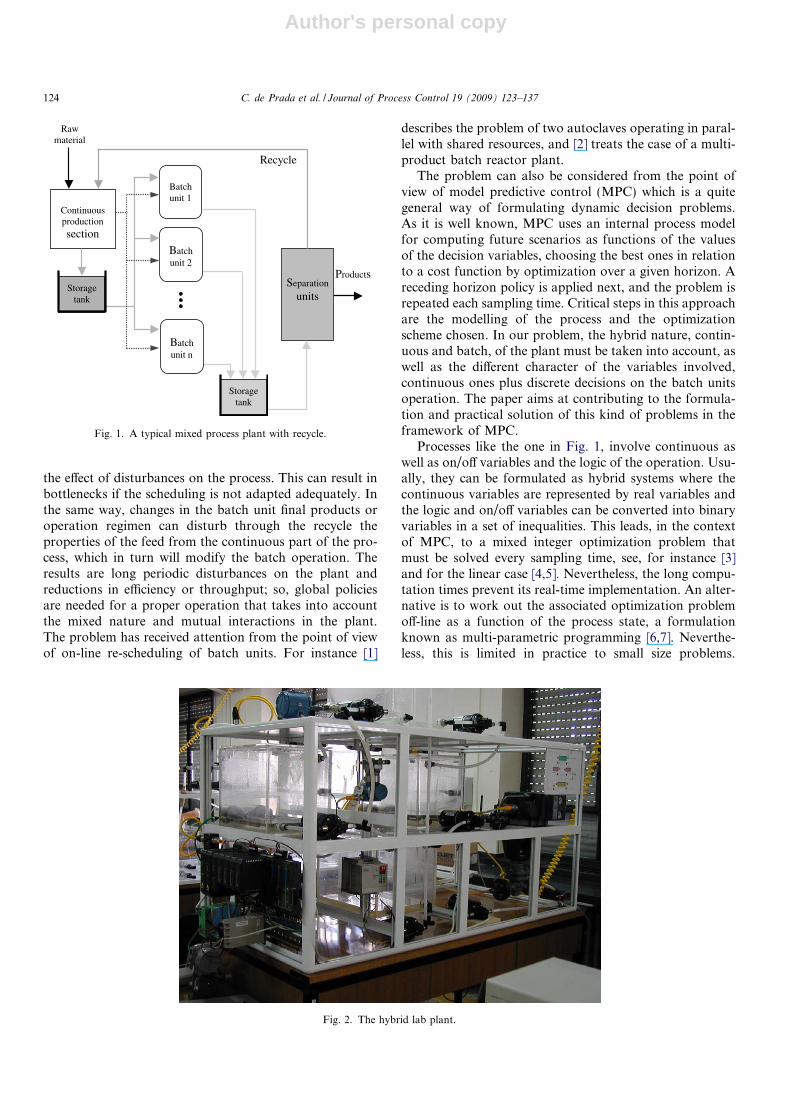
Plant-wide control has received considerable attentionin the recent past. Progressively, as the complexity of theplants increases due to mass and heat integration and thereare more strict requirements on production, the problemsof the overall dynamic behaviour (integration of operationwith control and economical optimization, etc.) of a pro-cess plant are emerging as important ones and must betaken into account besides the classical process control top-ics. These problems cover a wide range of situations,involving different types of process units and industries.In this paper we focus our attention on a special type ofhybrid plants involving continuous and batch units, suchas the one represented by the schematic of Fig. 1, that cor-responds to a configuration quite common in industry: acontinuous section, followed by a storage tank, feeds sev-eral batch units (like reactors, vacuum pans, etc.) operatingin parallel. These units discharge their products in a vessel

after which a separation process (it can be batch or contin-uous) takes place so that part of the un-reacted compo-nents are recycled. Sometimes, the continuous part alsosupplies energy to the batch section.

From the batch processes point of view, the basic char-acteristics are: single product, a fixed structure of produc-tion and the possibility of non-intermediate storage (NIS)or finite intermediate storage (FIS). Although this kind ofbatch process appears to be somewhat simple, its operationcan be very complex, in terms of sequencing, resource con-straints, batch size and batch processing time.

In this scheme there are continuous variables that mustbe kept at prescribed values in the continuous units, as wellas a sequence of operations that has to be performedsequentially in each batch unit. Both problems are stronglycoupled so that the overall coordination between them isimportant. On the one hand, the inflow to the process mustbe processed smoothly by the batch units by means ofproper scheduling. At the same time the duration of abatch unit cycle often depends on the energy and the qual-ity of the products that it receives. Hence, it is not difficultthat the synchronization of the batch units be lost due to

0959-1524/$ - see front matter � 2008 Elsevier Ltd. All rights reserved.

doi:10.1016/j.jprocont.2008.01.004

* Corresponding author. Tel.: +34 983 423162; fax: +34 983 423161.E-mail address: [email protected] (D. Sarabia).

www.elsevier.com/locate/jprocont

Available online at www.sciencedirect.com

Journal of Process Control 19 (2009) 123–137


the effect of disturbances on the process. This can result inbottlenecks if the scheduling is not adapted adequately. Inthe same way, changes in the batch unit final products oroperation regimen can disturb through the recycle theproperties of the feed from the continuous part of the pro-cess, which in turn will modify the batch operation. Theresults are long periodic disturbances on the plant andreductions in efficiency or throughput; so, global policiesare needed for a proper operation that takes into accountthe mixed nature and mutual interactions in the plant.The problem has received attention from the point of viewof on-line re-scheduling of batch units. For instance [1]

describes the problem of two autoclaves operating in paral-lel with shared resources, and [2] treats the case of a multi-product batch reactor plant.

The problem can also be considered from the point ofview of model predictive control (MPC) which is a quitegeneral way of formulating dynamic decision problems.As it is well known, MPC uses an internal process modelfor computing future scenarios as functions of the valuesof the decision variables, choosing the best ones in relationto a cost function by optimization over a given horizon. Areceding horizon policy is applied next, and the problem isrepeated each sampling time. Critical steps in this approachare the modelling of the process and the optimizationscheme chosen. In our problem, the hybrid nature, contin-uous and batch, of the plant must be taken into account, aswell as the different character of the variables involved,continuous ones plus discrete decisions on the batch unitsoperation. The paper aims at contributing to the formula-tion and practical solution of this kind of problems in theframework of MPC.

Processes like the one in Fig. 1, involve continuous aswell as on/off variables and the logic of the operation. Usu-ally, they can be formulated as hybrid systems where thecontinuous variables are represented by real variables andthe logic and on/off variables can be converted into binaryvariables in a set of inequalities. This leads, in the contextof MPC, to a mixed integer optimization problem thatmust be solved every sampling time, see, for instance [3]and for the linear case [4,5]. Nevertheless, the long compu-tation times prevent its real-time implementation. An alter-native is to work out the associated optimization problemoff-line as a function of the process state, a formulationknown as multi-parametric programming [6,7]. Neverthe-less, this is limited in practice to small size problems.

Products

Continuous productionsection

Batch unit 1

Separation

units

Recycle

Raw material

Batch unit 2

Batch unit n

Storage tank

Storage tank

Fig. 1. A typical mixed process plant with recycle.

Fig. 2. The hybrid lab plant.

124 C. de Prada et al. / Journal of Process Control 19 (2009) 123–137

https://www.researchgate.net/publication/228975046_On-line_scheduling_of_hybrid_chemical_plants_with_parallel_production_lines_and_shared_resources_a_feedback_control_implementation?el=1_x_8&enrichId=rgreq-8df33a83d6347e0d4341b54c642a0507-XXX&enrichSource=Y292ZXJQYWdlOzIyNDI5NDUzNztBUzoxNDYwNjAzMzY5NjM1ODRAMTQxMTgzNDkwNjEzMw==

https://www.researchgate.net/publication/222682015_The_Explicit_Linear_Quadratic_Regulator_for_Constrained_Systems?el=1_x_8&enrichId=rgreq-8df33a83d6347e0d4341b54c642a0507-XXX&enrichSource=Y292ZXJQYWdlOzIyNDI5NDUzNztBUzoxNDYwNjAzMzY5NjM1ODRAMTQxMTgzNDkwNjEzMw==

https://www.researchgate.net/publication/226315148_Hierarchical_Hybrid_Control_Synthesis_and_its_Application_to_a_Multiproduct_Batch_Plant?el=1_x_8&enrichId=rgreq-8df33a83d6347e0d4341b54c642a0507-XXX&enrichSource=Y292ZXJQYWdlOzIyNDI5NDUzNztBUzoxNDYwNjAzMzY5NjM1ODRAMTQxMTgzNDkwNjEzMw==


Besides formulations aimed to the scheduling of batchplants [8], applying off-line scheduling methods repetitivelyis another approach that has been tried in [9] but it doesnot solve the integration with the continuous elements.

In the paper we have explored an alternative approachusing a hierarchical point of view and separating the prob-lems that can be solved locally at a lower level from theones that require a global consideration. The paper focuseson these overall decisions, and, presents a methodologythat, within a MPC framework, reformulates the problemin terms of prescribed flow patterns and time of occurrenceof events using the ideas of the time-optimal switching con-trol theory [10,11]. This approach leads to a formulationwhere binary variables are avoided so that a NLP optimi-zation problem is solved instead.

In order to make things more specific, we have focusedour work to a lab scale approximation of the above men-tioned problem. It consist of a pilot plant that tries toreflect the main characteristics of the industrial setup,while, at the same time, being simple enough to allow asimpler development and testing of the proposed solutionmethod. The pilot plant is shown in Fig. 2 and consistsof a couple of continuous processes linked to a couple ofbatch units with recycle. The control objectives are givenin terms of processing a given flow of product while main-taining several continuous variables close to their set pointsand performing on-line the scheduling of the batch units.

The paper is organised as follows. After the introduc-tion, the control architecture that allows decomposing thecontrol tasks in a hierarchical way and the generic optimi-zation problem of this kind of processes is described in Sec-tion 2. The lab plant is presented in Section 3, which alsopresents the control objectives. Section 4 describes the sim-plifications required to develop the MPC controller and itsparticular structure. Finally, its implementation and exper-imental results in the pilot plant are given in Section 5. Thepaper ends with some brief conclusions and bibliography.

2. Control architecture and optimization problem

A common way of approaching complex problems is todecompose them in several layers or levels so that someaspects can be solved locally and only those variables ordecisions that have global impact are considered in theupper layer. In our case, we could recognize at least threeof these levels (Fig. 3):

� Local continuous SISO control (regulatory control)such as flow, temperature or pressure controllers in thecontinuous units. These can be managed by the Distrib-uted Control System (DCS) of the plant and have fastdynamics compared with the ones of the whole process.They are supposed to operate well using standardcontrollers.� Sequence control of each batch unit, which refers to exe-

cute the different stages of a batch cycle in correct orderand their associated regulatory controls, such as main-

taining the temperature at certain reaction stage for agiven period of time. The sequences of stages in a batchunit and the references of the corresponding local con-trollers in each stage are predefined and fixed parame-ters. The sequence control is assumed to perform well,completing their tasks in each cycle and is implementedin the DCS and operates according to and externalorders, such as load or unload a certain unit. Notice thatthe cycle time will depend also on the properties of thefeed.� Plant wide-control. This layer is responsible of main-

taining a proper operation of the whole section makingdecisions that have a global impact on the processdynamics: deciding when load and unload all batch unitsand the values of the set points of the local controllers inthe continuous units.

From the point of view of the plant-wide control, thelocal sequence and SISO controls layers can be seen asincluded in the process, operating in cascade over them.Hence, the internal operation of the batch units is not ofdirect interest for the plant-wide controller that sees themas some kind of black boxes where what is important isnot the inside but the interaction with the outside. Theplant-wide controller sends orders to the local sequencingcontrollers specifying when they should start or stop theoperation of a certain unit and it is the responsibility ofthe sequence control to implement the batch cycle. Plantwide controller calculates and fixes also the value of theset points of some control loops in the continuous unitsin order to fulfil the overall operating objectives, whichcan be summarized as:

� Process as smoothly as possible the incoming raw mate-rial, that is, avoiding the need of changing the flow ofraw material due to process bottlenecks and adapt theproduction to the inflow avoiding in this way bottle-necks in production.� Maintain the quality of the final product.

I/O analogical I/O analogical I/O discrete

continuousunits

batch units

Hybrid Process

regulatorycontrol

sequential control

PLANT-WIDE CONTROL

Low-level Control

regulatorycontrol

Fig. 3. Hierarchical control of the pilot plant.

C. de Prada et al. / Journal of Process Control 19 (2009) 123–137 125

https://www.researchgate.net/publication/230873381_Detection_and_Exploitation_of_the_Control_Switching_Structure_in_the_Solution_of_Dynamic_Optimization_Problems?el=1_x_8&enrichId=rgreq-8df33a83d6347e0d4341b54c642a0507-XXX&enrichSource=Y292ZXJQYWdlOzIyNDI5NDUzNztBUzoxNDYwNjAzMzY5NjM1ODRAMTQxMTgzNDkwNjEzMw==

https://www.researchgate.net/publication/222434561_State-of-the-art_review_of_optimization_methods_for_short-term_scheduling_of_batch_processes?el=1_x_8&enrichId=rgreq-8df33a83d6347e0d4341b54c642a0507-XXX&enrichSource=Y292ZXJQYWdlOzIyNDI5NDUzNztBUzoxNDYwNjAzMzY5NjM1ODRAMTQxMTgzNDkwNjEzMw==

https://www.researchgate.net/publication/231366268_A_New_Approach_for_Efficient_Rescheduling_of_Multiproduct_Batch_Plants?el=1_x_8&enrichId=rgreq-8df33a83d6347e0d4341b54c642a0507-XXX&enrichSource=Y292ZXJQYWdlOzIyNDI5NDUzNztBUzoxNDYwNjAzMzY5NjM1ODRAMTQxMTgzNDkwNjEzMw==


In spite of changes in the supply and quality flow, poweror product demands. The first objective implies selecting asuitable schedule of the batch units operation, as well asavoiding the continuous units from being either empty oroverflow. The second one implies maintaining certain mea-sures of quality of the final product, like temperature, con-centration, etc. on given target values.

The approach chosen in this paper is based on this plantwide control perspective and will be developed in the fol-lowing sections in the framework of nonlinear model pre-dictive control. As it is known, NMPC uses a model ofthe process in order to predict its future behaviour as afunction of the present and future control actions, whichare selected in order to minimize some performance index.The optimal control signals corresponding to the presenttime are applied to the process and the whole procedureis repeated in the next sampling period. So, the optimiza-tion problem can be generically defined as

minfug

J ¼Z T p

0

Xf

F f ðy; tÞdt

subject to fðx; _x; y; d; u; tÞ ¼ 0

gðx; _x; y; d; u; tÞ 6 0

xmin 6 x 6 xmax

ymin 6 y 6 ymax

umin 6 u 6 umax

d 2 f0; 1gp

ð1Þ

where x and y are the sates and controlled variables respec-tively, u, d are the decision variables, in principle and due tothe nature of the problem they can be real (references of thecontrollers) and discrete (signals to load and unload eachbatch unit). Tp is the total time of prediction, Ff(�) is a functionwhich integral has to be minimized (the cost function J) and isdefined as the quadratic error of the controlled variables(quality) and their references. f(�) corresponds with the nonlinear dynamical internal model which allow to link controlledand decision variables and it is described by differential-alge-braic equations and discrete events. Constraints on the statesor in the controlled variables, as well as inequalities expressingthe logic of operation are included in g(�) and the lower andupper limits of all variables are managed explicitly.

The optimization of cost function (1) in terms on thebinary and real variables implies to solve a dynamic MIN-LP optimization problem every sampling time if an internalnon linear model is used, or solving a MIQP optimizationproblem if an internal discrete lineal model is used, whichimplies the linearization and discretization of the nonlinearmodel f(�). Both approaches are very difficult to execute inreal time due to the use of many integer variables.

3. The pilot plant

In order to be more specific a case study will be pre-sented next. Fig. 2 shows the small scale pilot plant that

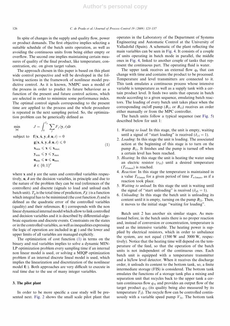
operates in the Laboratory of the Department of SystemsEngineering and Automatic Control at the University ofValladolid (Spain). A schematic of the plant reflecting themain variables can be seen in Fig. 4. It consists of a coupleof units operating in batch mode in parallel, the middleones in Fig. 4, linked to another couple of tanks that rep-resent the continuous part. The operating fluid is water.

The upper tank receives an external flow q0 that canchange with time and contains the product to be processed.Temperature and level transmitters are connected to it.This tank emulates a continuous process whose intensivevariable is temperature as well as a supply tank with a cer-tain product level. It feeds two units that operate in batchmode according to a given sequence, emulating batch reac-tors. The loading of every batch unit takes place when thecorresponding on/off pump (B11 or B12) receives an ordereither manually or from the MPC controller.

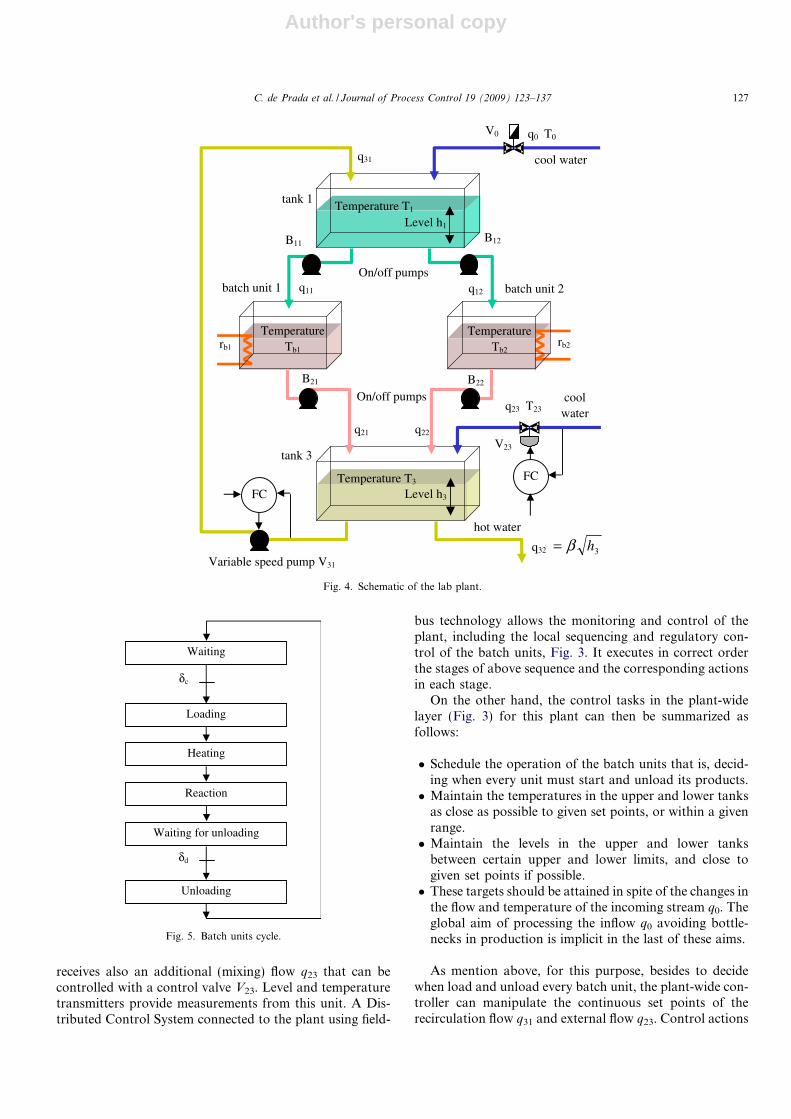
The batch units follow a typical sequence (see Fig. 5)described below for unit 1:

1. Waiting to load: In this stage, the unit is empty, waitinguntil a signal of ‘‘start loading” is received (dc1 = 1).

2. Loading: In this stage the unit is loading. The associatedaction at the beginning of this stage is to turn on thepump B11. It finishes and the pump is turned off whena certain level has been reached.

3. Heating: In this stage the unit is heating the water usingan electric resistor (rb1) until a desired temperature(Tb1max) is reached.

4. Reaction: In this stage the temperature is maintained ina value Tb1max for a given period of time Tw1max, as if areaction took place.

5. Waiting to unload: In this stage the unit is waiting untilthe signal of ‘‘start unloading” is received (dd1 = 1).

6. Unloading: In this stage the batch unit is unloading itscontent until it is empty, turning on the pump B21. Then,it moves to the initial stage ‘‘waiting for loading”.

Batch unit 2 has another six similar stages. As men-tioned before, in the batch units there is no proper reactionand, instead of conversion or concentration, temperature isused as the intensive variable. The heating power is sup-plied by electrical resistors, which in order to unbalancethe system, are not equal (1500 W and 3000 W, respec-tively). Notice that the heating time will depend on the tem-perature of the feed, so that the operation of the batchunits is not independent of the continuous ones. Eachbatch unit is equipped with a temperature transmitterand a hi/low level detector. When it receives the dischargeorder, it unloads its content to the bottom tank, so, a finiteintermediate storage (FIS) is considered. The bottom tankemulates the functions of a storage tank plus a mixing andseparation unit that recycles back to the upper tank a cer-tain continuous flow q31 and provides an output flow of thetarget product q32 (its quality being also measured by itstemperature T3). The recycle flow can be controlled contin-uously with a variable speed pump V31. The bottom tank



receives also an additional (mixing) flow q23 that can becontrolled with a control valve V23. Level and temperaturetransmitters provide measurements from this unit. A Dis-tributed Control System connected to the plant using field-

bus technology allows the monitoring and control of theplant, including the local sequencing and regulatory con-trol of the batch units, Fig. 3. It executes in correct orderthe stages of above sequence and the corresponding actionsin each stage.

On the other hand, the control tasks in the plant-widelayer (Fig. 3) for this plant can then be summarized asfollows:

� Schedule the operation of the batch units that is, decid-ing when every unit must start and unload its products.� Maintain the temperatures in the upper and lower tanks

as close as possible to given set points, or within a givenrange.� Maintain the levels in the upper and lower tanks

between certain upper and lower limits, and close togiven set points if possible.� These targets should be attained in spite of the changes in

the flow and temperature of the incoming stream q0. Theglobal aim of processing the inflow q0 avoiding bottle-necks in production is implicit in the last of these aims.

As mention above, for this purpose, besides to decidewhen load and unload every batch unit, the plant-wide con-troller can manipulate the continuous set points of therecirculation flow q31 and external flow q23. Control actions

Waiting

Loading

Heating

Reaction

Waiting for unloading

Unloading

δc

δd

Fig. 5. Batch units cycle.

q23 T23coolwater

rb1

TemperatureTb1

Temperature T3

rb2

Temperature Tb2

V0

V23

B12

B22

Temperature T1

B21

cool water

hot water

tank 1

tank 3

batch unit 1 batch unit 2

q0 T0

q11 q12

q21 q22

q31

q32

B11

Level h1

FC

FC

Level h3

3hβ=Variable speed pump V31

On/off pumps

On/off pumps

Fig. 4. Schematic of the lab plant.



should respect the logic of operation and the constraints onthe process variables. Notice that, in addition, some oper-ational rules must be taken into account. For instance, theload of a batch unit requires a minimum level in the uppertank, on the other hand, discharge of a unit requires a cer-tain empty volume in the bottom tank, and both batchunits cannot unload its products simultaneously. Thus, itis a hybrid control problem of non-linear process involvingcontinuous and discrete variables and decisions and opera-tion constraints.

4. Hybrid model predictive control

The hybrid MPC controller is responsible of the controltasks in the plant wide layer, and uses a model of the pilotplant and an optimization algorithm for decision making.The internal model is a key component in a hybrid problemlike the one we are considering, and it should be a goodcompromise between being a detailed representation ofthe process dynamics and being simple enough so thatthe associated optimization problem can be solved in a rea-sonable time according to the chosen sampling time. Twomodelling approaches will be presented next that take intoaccount the particular structure of the mixed batch-contin-uous processes.

4.1. Detailed process model

Next a detailed model of the process that combines massand energy balances of all units with the interactions anddynamics between continuous and batch units will be pre-sented. In our pilot plant, the following equations can bepostulated for the upper and lower continuous tanks:

A1

dh1

dt¼ q0 þ q31 � q11 � q12

A1h1

dT 1

dt¼ q0ðT 0 � T 1Þ þ q31ðT 3 � T 1Þ

A3

dh3

dt¼ q23 þ q21 þ q22 � q31 � q32

A3h3

dT 3

dt¼ q23ðT 0 � T 3Þ þ q21ðT b1 � T 3Þ þ q22ðT b2 � T 3Þ

ð2Þ

With reference to Fig. 4, hi represents the level, Ti thetemperature and Ai the cross section of tank i (i = 1,3).Densities and specific heat are assumed to be constant.Variables q0 and T0 are, respectively, the flow and tem-perature of the inflow and can be considered as distur-bances. Tbi (i = 1,2) corresponds to the batch reactiontemperature. q31 and q23, the recycle and mixing flows,are decision variables that can be implemented usingthe corresponding flow control loops and q32 is assumedto be proportional to the square root of level h3. Finally,Losses to the ambient have been disregarded.

On the other hand, the behaviour of levels (hb1 and hb2)and temperatures (Tb1 and Tb2) in batch units must be alsoincluded:

Ab1

dhb1

dt¼ q11 � q21

Ab1hb1

dT b1

dt¼ q11ðT 1 � T b1Þ þ

P b1

qCpþ SiUðT b1 � T envÞ

qCp

Ab2

dhb2

dt¼ q12 � q22

Ab2hb2

dT b2

dt¼ q12ðT 1 � T b2Þ þ

P b2

qCpþ SiUðT b2 � T envÞ

qCp

ð3Þ

where Abi and Pbi are the cross area and the power of elec-tric resistor of each batch unit (i = 1,2) and Cp is the heatcapacity of water and q its density. Losses to the ambienthave been included in the third term in both temperatureequations.

To complete the detailed model of the process is neces-sary to model the behaviour of the sequence control imple-mented in the DCS which drives the stages and actions ofeach batch unit. Batch unit 1 has six stages(XB1 = 1,2,3,4,5,6), see also Fig. 6:

� XB1 = 1, waiting for loading. Batch unit 1 (tank b1)is empty, pumps B11 and B21 are stopped u11 = 0and u21 = 0, electrical resistor rb1 is off r1 = 0. Nextstage is activated when the high-level control signaldc1 = 1.� XB1 = 2, loading. While hb1max = 0 pump B11 is working,

u11 = 1. When hb1max = 1 (tank full) next stage isactivated.

XB1=1 XB1=2 XB1=3 XB1=4 XB1=5 XB1=6

δc1=1

δc1=0

δd1=1

δd1=0

hb1max=1

hb1max=0

Tb1>Tb1max

Tb1≤Tb1max Twb1≤Twb1max

Twb1>Twb1max

hb1min=1

hb1min=0

Fig. 6. Sequence of stages and conditions of evolution in batch unit 1.



� XB1 = 3, heating. Pump B11 is stopped, u11 = 0. WhileTb1 6 Tb1max electric resistor rb1 is on, so r1 = 1. Nextstage is activated when Tb1 > Tb1max (temperaturereached).� XB1 = 4, reaction (simulated). In this stage rb1 is off. At

the beginning a timer Twb1 is turned on, next stage isactivated when Twb1 > Twb1max (duration time Twb1max

of this stage is reached).� XB1 = 5, waiting for loading. In this stage batch unit 1

(tank b1) is waiting for a high-level control signaldd1 = 1 to start the unloading.� XB1 = 6, unloading. In this stage, while hb1min = 1 pump

B21 is working, u21 = 1. When hb1min = 0 (tank empty)then first stage is activated.

The other batch unit 2 has a similar operation scheme.Therefore, a natural way of modeling this sequence is byusing binary decision variables dci and ddi (i = 1,2), integervariables for the current stages XBi (i = 1,2) and past stagesX�Bi (i = 1,2) defined all of them at every sampling time. So,for batch unit 1 we have

if ðX�B1 ¼ 1 and dc1 ¼ 1Þ then X B1 ¼ 2

if ðX�B1 ¼ 1 and dc1 ¼ 0Þ then X B1 ¼ 1

if ðX�B1 ¼ 2 and hb1 max ¼ 1Þ then X B1 ¼ 3

if ðX�B1 ¼ 2 and hb1 max ¼ 0Þ then X B1 ¼ 2

if ðX�B1 ¼ 3 and T b1 > T b1 maxÞ then X B1 ¼ 4

if ðX�B1 ¼ 3 and T b1 6 T b1 maxÞ then X B1 ¼ 3

if ðX�B1 ¼ 4 and T wb1 > T wb1 maxÞ then X B1 ¼ 5

if ðX�B1 ¼ 4 and T wb1 6 T wb1 maxÞ then X B1 ¼ 4

if ðX�B1 ¼ 5 and dd1 ¼ 1Þ then X B1 ¼ 6

ifðX�B1 ¼ 5 and dd1 ¼ 0Þ then X B1 ¼ 5

if ðX�B1 ¼ 6 and hb1 min ¼ 0Þ then X B1 ¼ 1

if ðX�B1 ¼ 6 and hb1 min ¼ 1Þ then X B1 ¼ 6

ð4Þ

plus a set of additional conditions that reflects the actionsto be executed in each stage, start a on/off pump (u11),on the electrical resistor (r1), turn on the timer (Twb1), etc.

u11 ¼0 if X B1 ¼ 1; 3; 4; 5; 6

1 if X B1 ¼ 2

�

r1 ¼0 if X B1 ¼ 1; 2; 4; 5; 6

1 if X B1 ¼ 3

�

dT wb1ðtÞdt

¼0 if X B1 ¼ 1; 2; 3; 5; 6

1 if X B1 ¼ 4

�

T wb1 ¼ 0 if X B1 ¼ 1; 2; 3; 5; 6

u12 ¼0 if X B1 ¼ 1; 2; 3; 4; 5

1 if X B1 ¼ 6

�

ð5Þ

Then, the conditional assignments (4) and (5) should betranslated into a set of inequalities using the usual proce-dure [12,13] eliminating the possible products of integerand continuous variables. Normally, these inequalitiescombine real and discrete auxiliary variables and they have

to be incorporated in the optimization problem as con-straints. In this way, the result is a detailed but complexmodel with several nonlinearities and many integervariables.

An alternative can be to transform the above model to ahybrid automaton [1,14] defining all operation modes ofthe process and associating each one of them with a certaincontinuous dynamic. It is also necessary define thesequence of modes and the transition conditions betweenmodes, that can be external or internal events.

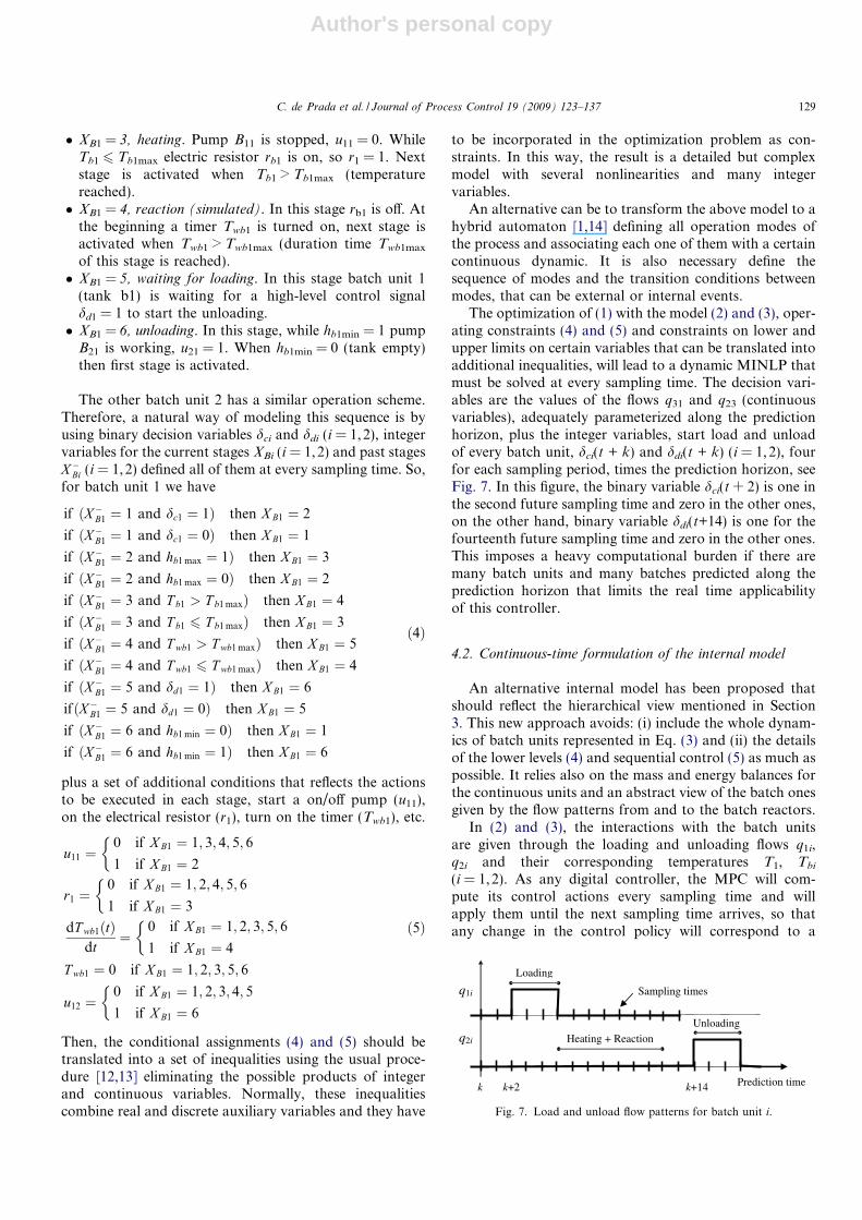
The optimization of (1) with the model (2) and (3), oper-ating constraints (4) and (5) and constraints on lower andupper limits on certain variables that can be translated intoadditional inequalities, will lead to a dynamic MINLP thatmust be solved at every sampling time. The decision vari-ables are the values of the flows q31 and q23 (continuousvariables), adequately parameterized along the predictionhorizon, plus the integer variables, start load and unloadof every batch unit, dci(t + k) and ddi(t + k) (i = 1,2), fourfor each sampling period, times the prediction horizon, seeFig. 7. In this figure, the binary variable dci(t + 2) is one inthe second future sampling time and zero in the other ones,on the other hand, binary variable ddi(t+14) is one for thefourteenth future sampling time and zero in the other ones.This imposes a heavy computational burden if there aremany batch units and many batches predicted along theprediction horizon that limits the real time applicabilityof this controller.

4.2. Continuous-time formulation of the internal model

An alternative internal model has been proposed thatshould reflect the hierarchical view mentioned in Section3. This new approach avoids: (i) include the whole dynam-ics of batch units represented in Eq. (3) and (ii) the detailsof the lower levels (4) and sequential control (5) as much aspossible. It relies also on the mass and energy balances forthe continuous units and an abstract view of the batch onesgiven by the flow patterns from and to the batch reactors.

In (2) and (3), the interactions with the batch unitsare given through the loading and unloading flows q1i,q2i and their corresponding temperatures T1, Tbi

(i = 1,2). As any digital controller, the MPC will com-pute its control actions every sampling time and willapply them until the next sampling time arrives, so thatany change in the control policy will correspond to a

q1i

Loading

Heating + ReactionUnloading

Sampling times

q2i

k k+2 k+14 Prediction time

Fig. 7. Load and unload flow patterns for batch unit i.


https://www.researchgate.net/publication/228975046_On-line_scheduling_of_hybrid_chemical_plants_with_parallel_production_lines_and_shared_resources_a_feedback_control_implementation?el=1_x_8&enrichId=rgreq-8df33a83d6347e0d4341b54c642a0507-XXX&enrichSource=Y292ZXJQYWdlOzIyNDI5NDUzNztBUzoxNDYwNjAzMzY5NjM1ODRAMTQxMTgzNDkwNjEzMw==

https://www.researchgate.net/publication/222299188_Design_of_Process_Operations_using_Hybrid_Dynamic_Optimization?el=1_x_8&enrichId=rgreq-8df33a83d6347e0d4341b54c642a0507-XXX&enrichSource=Y292ZXJQYWdlOzIyNDI5NDUzNztBUzoxNDYwNjAzMzY5NjM1ODRAMTQxMTgzNDkwNjEzMw==


sampling instant. On the other hand, as represented inFig. 8 and according to the logic of operation, the load-ing q1i will be zero except for the loading stages where itwill maintain a constant value q1imax, while the unloadingflows q2i will be zero except for the unloading periodwhere they will maintain a constant value q2imax, aftera discharge order takes place.

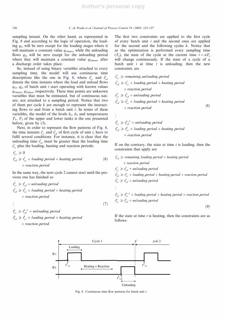
So, instead of using binary variables attached to everysampling time, the model will use continuous timedescriptions like the one in Fig. 8, where tk

i;c and tki;d

denote the time instants where the load and unload flowsq1i, q2i of batch unit i start operating with known valuesq1imax, q2imax, respectively. These time points are unknownvariables that must be estimated, but of continuous nat-ure, not attached to a sampling period. Notice that twoof them per cycle k are enough to represent the interact-ing flows to and from a batch unit i. In terms of thesevariables, the model of the levels h1, h3 and temperaturesT1, T3 of the upper and lower tanks is the one presentedbefore, given by (3).

Next, in order to represent the flow patterns of Fig. 8,the time instants t1

i;c and t1i;d of first cycle of unit i, have to

fulfil several conditions. For instance, it is clear that theunloading time t1

i;d must be greater than the loading timet1i;c plus the loading, heating and reaction periods:

t1i;c P 0

t1i;d P t1

i;c þ loading period þ heating period

þ reaction period

ð6Þ

In the same way, the next cycle 2 cannot start until the pre-vious one has finished so

t2i;c P t1

i;d þ unloading period

t2i;d P t2


þ reaction period

..

.

tki;c P tk�1


tki;d P tk


þ reaction period

ð7Þ

The first two constraints are applied to the first cycleof every batch unit i and the second ones are appliedfor the second and the following cycles k. Notice thatas the optimization is performed every sampling time(Ts), the state of the cycle at the current time t = nTs

will change continuously. If the state of a cycle of abatch unit i at time t is unloading, then the newconstraints are

t1i;c P remaining unloading period

t1i;d P t1


þ reaction period

t2i;c P t1


t2i;d P t2


þ reaction period

..

.

tki;c P tk�1


tki;d P tk


þ reaction period

ð8Þ

If on the contrary, the state at time t is loading, then theconstraints that apply are

t1i;d P remaining loading period þ heating period

þ reaction period

t1i;c P t1


t2i;d P t1

i;c þ loading period þ heating period þ reaction period

t2i;c P t2


..

.

tki;d P tk�1


tki;c P tk


ð9Þ

If the state at time t is heating, then the constraints are asfollows:

t1i,c

q1i

Loading

Heating + Reaction

Unloading

q2i

t1i,d

t2i,c

Cycle 1 C ycle 2

Fig. 8. Continuous time flow patterns for batch unit i.



t1i;d P remaining heating period þ reaction period

t1i;c P t1


t2i;d P t1


t2i;c P t2


..

.

tki;d P tk�1


þ reaction period

tki;c P tk


ð10Þ

while for the reaction

t1i;d P remaining reaction period

t1i;c P t1


t2i;d P t1


t2i;c P t2


..

.

tki;d P tk�1


þ reaction period

tki;c P tk


ð11Þ

Finally, if batch unit i at time t is in the stage waiting to un-load, we have

t1i;d P 0

t1i;c P t1


t2i;d P t1


þ reaction period

t2i;c P t2


..

.

tki;d P tk�1


þ reaction period

tki;c P tk


ð12Þ

In all cases, the first two constraints are applied to the firstcycle of every batch unit i and the next ones are appliedwithin the k cycles predicted.

Therefore, in this alternative, model constraints of thetype (4) or (5) are replaced by the ones above, and the bin-ary variables dci and ddi are replaced by the continuousvariables tk

i;c and tki;d for the time events and a different set

of constraints (6)–(12) to guarantee the correct order ofthese events along the prediction.

Loading, unloading and reaction periods are constantsand known in advance, but the heating period will dependon the temperature of the feed T1, the available power andthe temperature desired Tbimax and must be estimated. Forthis purpose, it is possible to use the model of the heating

stage of a batch unit i (i = 1,2), relating its temperatureTbi with supply power Pbi and, perhaps, losses to theambient

V biqCpdT bi

dt¼ P bi � SiUðT bi � T ambÞ; T bið0Þ ¼ T 1 ð13Þ

where Vbi is the volume of batch unit i, Cp heat capacityof water and q its density. Integrating this equationfrom initial condition Tbi(0) = T1(t) until the conditionTbi(heating_ period) = Tbimax is satisfied, will provide thevalue of the heating period. Notice that in this problem,Eq. (13) can be solved analytically and its explicit solutionis included directly in the internal model. However, in morecomplex problems where there is not analytical solution, itis necessary integrate the similar Eq. (13) for a range of sen-sible initial conditions and obtains a two-dimensional tableoff-line from which the value of the heating period can beobtained by interpolation.

So, the abstract view of the batch units given by theirloading, reaction, heating and unloading periods has beenincluded. In this way, all variables in the new model (2),(6)–(13) are continuous while, at the same time the sched-uling of the batch units has been integrated in the plant-wide model. This means that the associated optimizationis a nonlinear programming (NLP) model, so that NLPalgorithms can be used instead MINLP algorithms, savingcomputation time and resulting in a more compactformulation.

4.2.1. A compact formulation

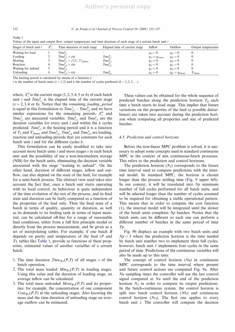
The set of constraints (6)–(13) can be incorporated intothe optimization algorithm. However, due to their nature itis more effective to incorporate them directly into the inter-nal model building the adequate inflow and outflow pat-terns. See Table 1.

We can also define the duration Cki of a certain cycle k of

every batch unit i like the sum of duration of all stages:

C0i ¼ 0

Cki ¼ Timek

i;1 þ Timeki;2 þ Timek

i;3 þ Timeki;4 þ Timek

i;5 þ Timeki;6

¼X6

s¼1

Timeki;s 8k ¼ 1; 2; 3; . . .

ð14Þ

Notice that, as the optimization is performed every sam-pling time (Ts), the state of the cycle at current timet = nTs will change continuously, so the exact events ofload tk

i;1 or unload tki;5 are defined for each unit i by

tki;1 ¼

Xk

Ck�1i þ

X1

s¼X 0i

Timeki;s � Time0

i;X 0i

tki;5 ¼

Xk

Ck�1i þ

X5

s¼X 0i

Timeki;s � Time0

i;X 0i8k ¼ 1; 2; 3; . . .

ð15Þ



where, X 0i is the current stage (1,2,3,4,5 or 6) of each batch

unit i and Time0i;s is the elapsed time of the current stage

(s = 2,3,4 or 6). Notice that the remaining_loading_ periodis equal in this formulation to Time1

i;2 � Time0i;2 and we have

similar expressions for the remaining periods. X 0i and

Time1i;s are measured variables. Timek

i;1 and Timeki;5 are the

decision variables for every unit i and within the k cyclespredicted. Timek

i;3 is the heating period and it is a functionof T1 and T2imax and Timek

i;2, Timeki;4 and Timek

i;6 are loading,reaction and unloading periods that are constants for eachbatch unit i and for the different cycles k.

This formulation can be easily modified to take intoaccount more batch units i and more stages s in each batchunit and the possibility of use a non-intermediate storage(NIS) for the batch units, eliminating the decision variableassociated with the stage ‘‘waiting to unload”. On theother hand, duration of different stages, inflow and out-flow, can also depend on the state of the feed, for examplefor a semi-batch process. The abstract view used takes intoaccount the fact that, once a batch unit starts operatingwith its local control, its behaviour is quite independentof the time evolution of the rest of the process, and its finalstate and duration can be fairly computed as a function ofthe properties of the feed only. Then the final state of abatch in terms of quality, quantity or duration, as wellas its demands to its feeding tank in terms of input mate-rial, can be calculated off-line for a range of reasonablefeed conditions, either from a full first principle model ordirectly from the process measurement, and be given as aset of interpolating tables. For example, if one batch B

depends on purity and temperature of the feed (P andT), tables like Table 1, provide as functions of these prop-erties, estimated values of another variables of a certainbatch:

1. The time duration TimeB,s(P,T) of all stages s of thebatch operation.

2. The total mass loaded MinB,s(P,T) in loading stages.Using this value and the duration of loading stage, anaverage inflow can be calculated.

3. The total mass unloaded MoutB,s(P,T) and its proper-ties: for example, the concentration of one componentCoutB,s(P,T) in the unloading stages. Also knowing themass and the time duration of unloading stage an aver-age outflow can be estimated.

These values can be obtained for the whole sequence ofpredicted batches along the prediction horizon Tp eachtime a batch starts its load stage. This implies that futurevariations on the properties of the feed (a possible distur-bance) are taken into account during the prediction hori-zon when computing all properties and size of predictedbatches.

4.3. Prediction and control horizons

Before the non-linear MPC problem is solved, it is nec-essary to adopt some concepts used in standard continuousMPC in the context of mix continuous-batch processes.This refers to the prediction and control horizons.

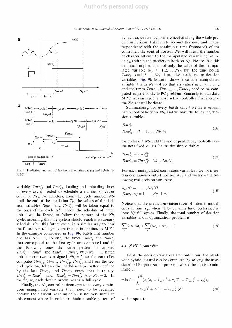
The prediction horizon (N2) corresponds to the futuretime interval used to compute predictions with the inter-nal model. In standard MPC, the horizon is chosenlonger than the process settling time (Fig. 9 upper left).In our context, it will be translated into Np minimumnumber of full cycles performed for all batch units, andwill be selected longer than the number of cycles assumedto be required for obtaining a stable operational pattern.This means that in order to compute the cost function(1), the internal model will be integrated until the slowerof the batch units completes Np batches. Notice that thebatch units can be different so each one can perform adifferent number of batches in the same period of timeTp.

Fig. 9b displays an example with two batch units andNp = 3 where the prediction horizon is the time neededby batch unit number two to implement three full cycles,however, batch unit 1 implements four cycles in the sameperiod of time. Predictions of the continuous variables willalso be made up to this time.

The concept of control horizon (Nu) in continuousMPC corresponds to the time interval where presentand future control actions are computed Fig. 9a. AfterNu sampling times the controller will use the last controlsignal computed at Nu until the end of the predictionhorizon N2 in order to compute its output predictions.In the batch-continuous system, the control horizon issplit into batch control horizon (Nbi) and continuouscontrol horizon (Ncl). The first one applies to everybatch unit i. The controller will compute the decision

Table 1Values of the input and output flow, output temperature and time duration of each stage of a certain batch unit i

Stages of batch unit i Xki Time duration of each stage Elapsed time of current stage Inflow Outflow Output temperature

Waiting for load 1 Timeki;1 – q1i = 0 q2i = 0 0

Loading 2 Timeki;2 ¼ cte Time0

i;2 q1i = q1imax q2i = 0 0Heating 3 Timek

i;3 ¼ f ðT 1; T ð2imaxÞ Time0i;3 q1i = 0 q2i = 0 0

Reaction 4 Timeki;4 ¼ cte Time0

i;4 q1i = 0 q2i = 0 0Waiting for unload 5 Timek

i;5 – q1i = 0 q2i = 0 0Unloading 6 Timek

i;6 ¼ cte Time0i;6 q1i = 0 q2i = q2imax T2imax

The heating period is calculated by means of a function f.i is the number of batch units (i = 1,2) and k the number of cycles predicted (k = 1,2,3, . . .).



variables Timeki;1 and Timek

i;5, loading and unloading timesof every cycle, needed to schedule a number of cyclesequal to Nbi. Nevertheless, from the cycle number Nbi

until the end of the prediction Tp, the values of the deci-sion variables Timek

i;1 and Timeki;5 will be taken equal to

the ones of the cycle Nbi, hence, the schedule of batchunit i will be forced to follow the pattern of the Nbi

cycle, assuming that the system should reach a stationaryschedule after this future cycle, in a similar way to howthe future control signals are treated in continuous MPC.In the example considered in Fig. 9b, batch unit numberone has Nb1 = 1, so only the times Timek

i;1 and Timeki;5

that correspond to the first cycle are computed and inthe following ones the same pattern is appliedTimek

i;1 ¼ Time1i;1 and Timek

i;5 ¼ Time1i;5 8k > Nb1 ¼ 1. Batch

unit number two is assigned Nb2 = 2, so the controllercomputes Time1

i;1, Time1i;5, Time2

i;1, Time2i;5 and from the sec-

ond cycle on, follows the load/discharge pattern definedby the last Time2

i;1 and Time2i;5 times, that is to say:

Timeki;1 ¼ Time2

i;1 and Timeki;5 ¼ Time2

i;5 8k > Nb2 ¼ 2. Inthe figure, each double arrow means a full cycle.

Finally, the Ncl control horizon applies to every contin-uous manipulated variable l but need to be redefinedbecause the classical meaning of Nu is not very useful inthis context where, in order to obtain a stable pattern of

behaviour, control actions are needed along the whole pre-diction horizon. Taking into account this need and in cor-respondence with the continuous time framework of thecontroller, the control horizon Ncl will mean the numberof changes allowed to the manipulated variable l (like q31

or q23) within the prediction horizon Np. Notice that thisdefinition implies that not only the value of the manipu-lated variable ul,j, j = 1,2, . . . ,Ncl, but the time pointsTimel,j, j = 1,2, . . . ,Ncl – 1 are also considered as decisionvariables. Fig. 9b bottom, shows a certain manipulatedvariable l with Ncl = 4 so that its values ul,1,ul,2, . . . ,ul,4

and the times Timel,1,Timel,2, . . . ,Timel,3 need to be com-puted as part of the MPC problem. Similarly to standardMPC, we can expect a more active controller if we increasethe Ncl control horizons.

Summarizing, for every batch unit i we fix a certainbatch control horizon Nbi, and we have the following deci-sion variables:

Timeki;1

Timeki;5 8k ¼ 1; . . . ;Nbi 8i

ð16Þ

for cycles k > Nbi until the end of prediction, controller usethe next fixed values for the decision variables

Timeki;1 ¼ TimeNbi

i;1

Timeki;5 ¼ TimeNbi

i;1 8k > Nbi 8ið17Þ

For each manipulated continuous variables l we fix a cer-tain continuous control horizon Ncl, and we have the fol-lowing real decision variables:

ul;j 8j ¼ 1; . . . ;Ncl 8lTimel;j 8j ¼ 1; . . . ;Ncl–1 8l

ð18Þ

Notice that the prediction (integration of internal model)ends at time Tp, when all batch units have performed atleast Np full cycles. Finally, the total number of decisionvariables in our optimization problem isX

i

2� Nbi þX

l

ðNcl þ Ncl � 1Þ ð19Þ

4.4. NMPC controller

As all the decision variables are continuous, the plant-wide hybrid control can be computed by solving the asso-ciated NLP optimization problem, where the aim is to min-imize J:

min J ¼Z Tp

0

ða1ðh1 � h1ref Þ2 þ a2ðT 1 � T 1refÞ2 þ a3ðh3

� h3refÞ2 þ a4ðT 3 � T 3refÞ2Þdt ð20Þ

with respect to

cycle 1

cycle 2cycle 1

Np=3

cycle 2 y

Nb2=2

start of prediction = t end of prediction = Tp

Timel,1

Ncl=4

batchunit 1

ul,1

cycle 4

cycle 3

Nb1=1

batchunit 2

Timel,2Timel,3

ul,2

ul,3

ul,4

past future

(k+j)

w(k)

y

u u(k+j)

t Nu =3 N2 = 7

past furure

c cle 3

a

b

y

Fig. 9. Prediction and control horizons in continuous (a) and hybrid (b)MPC.



Timek1;1; Timek

1;5 8k ¼ 1; . . . ;Nb1

Timek2;1; Timek

2;5 8k ¼ 1; . . . ;Nb2

u1;j 8j ¼ 1; . . . ;Nc1

u2;j 8j ¼ 1; . . . ;Nc1

Time1;j 8j ¼ 1; . . . ;Nc1 � 1

8>>>>>><>>>>>>:

9>>>>>>=>>>>>>;

Batch unit 1

Batch unit 2

q31

q23

q31&q23

ð21Þ

subject to path constraints

T 1 min 6 T 1 6 T 1 max; h1 min 6 h1 6 h1 max

T 3 min 6 T 3 6 T 3 max; h3 min 6 h3 6 h3 max

ð22Þ

limits of decision variables

0 6 Timek1;1 6 Timemax; 0 6 Timek

1;5 6 Timemax

0 6 Timek2;1 6 Timemax; 0 6 Timek

2;5 6 Timemax

0 6 u1;j 6 q31 max

0 6 u2;j 6 q23 max

0 6 Time1;j 6 Timemax

ð23Þ

and internal model (3) together with Table 1, and con-straints (14) and (15).

The decision variables correspond to the time durationsof all ‘‘waiting stages” of every batch unit along the controlhorizons plus the set points of flow control loops of q31

and q23 at certain times. In order to decrease the complex-ity of the optimization problem we have used the samecontrol horizon Nc1 for the manipulated variables q31

and q23. That is to say, their changes are applied at thesame times Time1,j on both of them. In this way wedecrease the number of decision variables in (Nc1 � 1).So, we have 2 � Nb1 + 2 � Nb2 + Nc1 + Nc1 + Nc1 � 1decision variables.

Measured variables at every sampling time are levels andtemperatures of upper and bottom tanks and the currentstage and elapsed time of it for every batch unit:

T 1; h1; T 3; h3; X 01; Time0

1;X 01; X 0

2; Time02;X 0

2ð24Þ

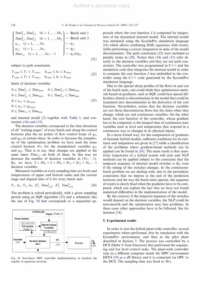
The problem is solved periodically, with a given samplingperiod using an SQP algorithm [15] and a schematic likethe one of Fig. 10 that corresponds to a sequential ap-

proach where the cost function J is computed by integra-tion of the dynamical internal model. The internal modelwas simulated using the EcosimPro simulation language[16] which allows combining DAE equations with events,while performing a correct integration in spite of the modeldiscontinuities. The path constraints (22) were included aspenalty terms in (20). Notice that (14) and (15) refer di-rectly to the decision variables and they are not path con-straints. The controller was programmed in C++ and thesimulation code that integrates the internal model in orderto compute the cost function J was embedded in the con-troller using the C++ code generated by the EcosimProsimulation language.

Due to the special sharp profiles of the flows in and outof the batch units, one could think that optimization meth-ods based on gradients, such as SQP, could face special dif-ficulties related to discontinuities in the model that could betranslated into discontinuities in the derivative of the costfunction. Nevertheless, notice that the decision variablesare not those discontinuous flows but the times when theychange, which are real continuous variables. On the otherhand, the cost function of the controller, whose gradienthas to be computed, is the integral time of continuous statevariables such as level and temperature that respond in acontinuous way to changes in its physical inputs.

In a more formal way, for the computation of gradientsof dynamic hybrid models, sufficient conditions for its exis-tence and uniqueness are given in [17] while a classificationof the problems where gradient-based methods can beapplied can be found in [18]. The main result is that sensi-tivity trajectories of a hybrid system will exist and NLPmethods can be applied subject to the constraint that thetemporal sequence of internal model switches is fix, evenif the timing of the switches changes. In the continuous-batch problem we are dealing with, due to the periodicityconstraints that we impose at the end of the predictionhorizons and the way the batch units operate, the sequenceof events is clearly fixed when the gradients have to be com-puted, which can explain the fact that we have not foundnumerical difficulties in the implementation of the model.

By the contrary if the temporal sequence of the switcheswould depend on the decision variables, the NLP could benon-smooth and the optimization may face problems. Inthese cases other approaches have to be followed. See forinstance [14].

5. Experimental results

In order to test the hybrid plant-wide controller, severalexperiments where performed, first by simulation with theEcosimPro environment, and then in the pilot plantdescribed in Section 3. The process was controlled by aDCS (Delta V from Emerson) that performed the sequenc-ing and low level control tasks. The plant-wide controllerruns in a different computer inside the MPC environmentHITO [19] as a dll library and it is connected via OPC tothe DCS. The sampling time was fixed to 30 s.

Fig. 10. Non-linear MPC controller implementation, in brackets thenumber of equations involved.



The inflow q0 to pilot plant is obtained directly from thewater network of the laboratory, so, there is much variabil-ity on it along the experiments, due to another uses of thewater network. It is also important the variations on thetemperature T0 of this flow depending on the ambient tem-perature, if it is a cloudy or sunny day, if it is turn on theheating of the laboratory room, etc.

One real experiment of 4 h is presented here, with non-measured disturbances q0 and T0. The valve associated tothe inflow q0 is always 45% opened except from the secondto third hour which is manually closed completely. How-ever, each sampling time, the hybrid controller assumesthat all disturbances are fixed in the nominal operatingconditions (q0 = 30 cm3/s, T0 = 14 �C) to make the predic-tions with these constant values. That is, there is not on-line estimation of the non measured disturbances.

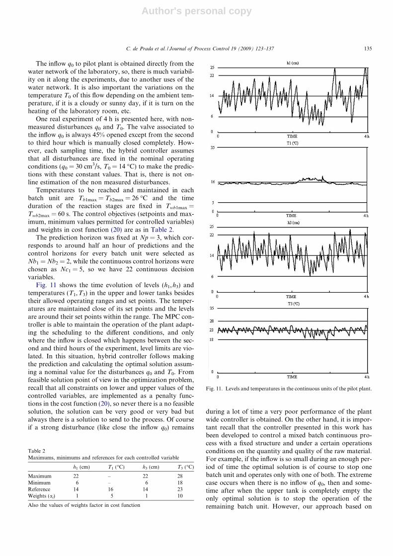
Temperatures to be reached and maintained in eachbatch unit are Tb1max = Tb2max = 26 �C and the timeduration of the reaction stages are fixed in Twb1max =Twb2max = 60 s. The control objectives (setpoints and max-imum, minimum values permitted for controlled variables)and weights in cost function (20) are as in Table 2.

The prediction horizon was fixed at Np = 3, which cor-responds to around half an hour of predictions and thecontrol horizons for every batch unit were selected asNb1 = Nb2 = 2, while the continuous control horizons werechosen as Nc1 = 5, so we have 22 continuous decisionvariables.

Fig. 11 shows the time evolution of levels (h1,h3) andtemperatures (T1,T3) in the upper and lower tanks besidestheir allowed operating ranges and set points. The temper-atures are maintained close of its set points and the levelsare around their set points within the range. The MPC con-troller is able to maintain the operation of the plant adapt-ing the scheduling to the different conditions, and onlywhere the inflow is closed which happens between the sec-ond and third hours of the experiment, level limits are vio-lated. In this situation, hybrid controller follows makingthe prediction and calculating the optimal solution assum-ing a nominal value for the disturbances q0 and T0. Fromfeasible solution point of view in the optimization problem,recall that all constraints on lower and upper values of thecontrolled variables, are implemented as a penalty func-tions in the cost function (20), so never there is a no feasiblesolution, the solution can be very good or very bad butalways there is a solution to send to the process. Of courseif a strong disturbance (like close the inflow q0) remains

during a lot of time a very poor performance of the plantwide controller is obtained. On the other hand, it is impor-tant recall that the controller presented in this work hasbeen developed to control a mixed batch continuous pro-cess with a fixed structure and under a certain operationsconditions on the quantity and quality of the raw material.For example, if the inflow is so small during an enough per-iod of time the optimal solution is of course to stop onebatch unit and operates only with one of both. The extremecase occurs when there is no inflow of q0, then and some-time after when the upper tank is completely empty theonly optimal solution is to stop the operation of theremaining batch unit. However, our approach based on

Table 2Maximums, minimums and references for each controlled variable

h1 (cm) T1 (�C) h3 (cm) T3 (�C)

Maximum 22 – 22 28Minimum 6 – 6 18Reference 14 16 14 23Weights (ai) 1 5 1 10

Also the values of weights factor in cost function

Fig. 11. Levels and temperatures in the continuous units of the pilot plant.



real decision variables and the repetition of the last cyclesuntil the prediction horizon, can not decide stop the batchunits and put them out of work. In this case the only wayto solve this situation is to include binary variables todecide if it is enough operate with one batch unit, or withtwo batch units or none of them.

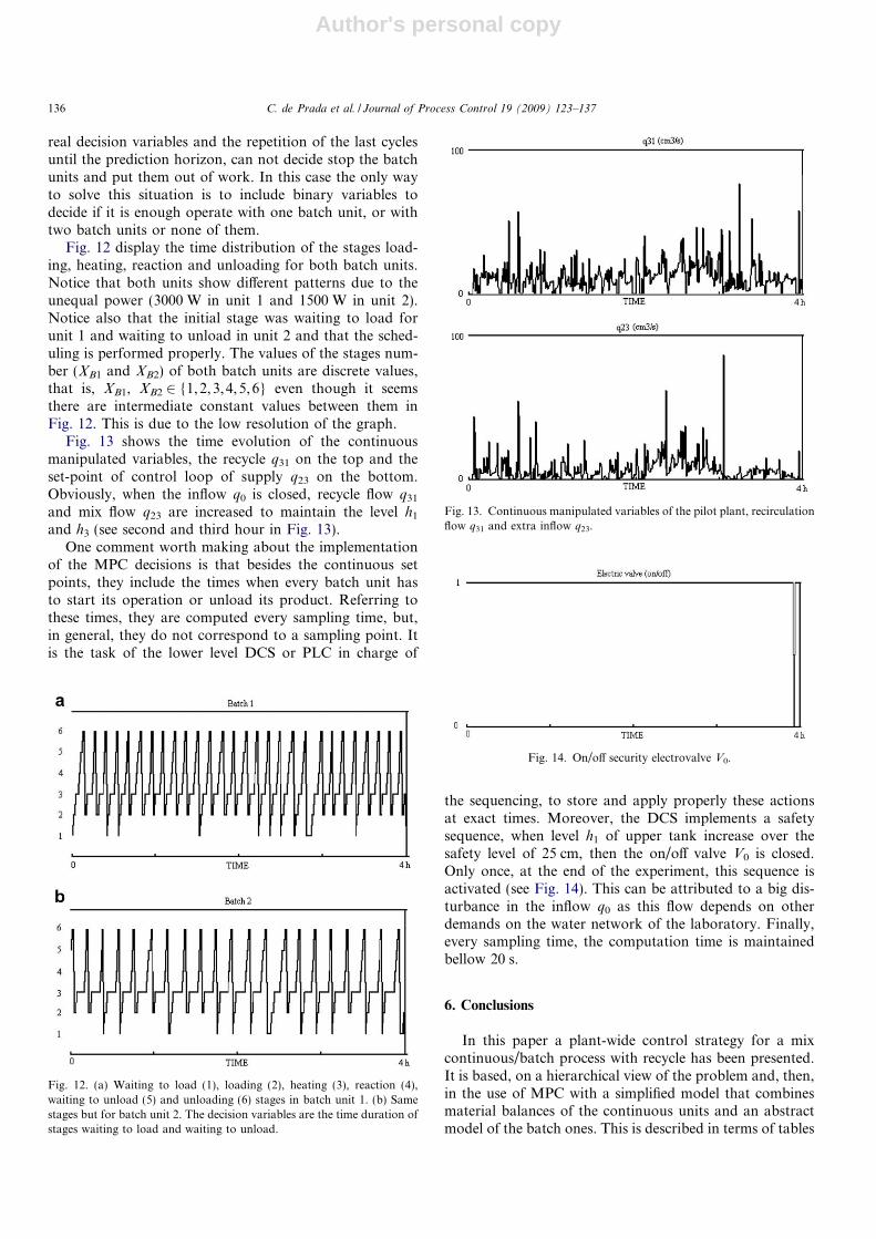
Fig. 12 display the time distribution of the stages load-ing, heating, reaction and unloading for both batch units.Notice that both units show different patterns due to theunequal power (3000 W in unit 1 and 1500 W in unit 2).Notice also that the initial stage was waiting to load forunit 1 and waiting to unload in unit 2 and that the sched-uling is performed properly. The values of the stages num-ber (XB1 and XB2) of both batch units are discrete values,that is, XB1, XB2 2 {1,2,3,4,5,6} even though it seemsthere are intermediate constant values between them inFig. 12. This is due to the low resolution of the graph.

Fig. 13 shows the time evolution of the continuousmanipulated variables, the recycle q31 on the top and theset-point of control loop of supply q23 on the bottom.Obviously, when the inflow q0 is closed, recycle flow q31

and mix flow q23 are increased to maintain the level h1

and h3 (see second and third hour in Fig. 13).One comment worth making about the implementation

of the MPC decisions is that besides the continuous setpoints, they include the times when every batch unit hasto start its operation or unload its product. Referring tothese times, they are computed every sampling time, but,in general, they do not correspond to a sampling point. Itis the task of the lower level DCS or PLC in charge of

the sequencing, to store and apply properly these actionsat exact times. Moreover, the DCS implements a safetysequence, when level h1 of upper tank increase over thesafety level of 25 cm, then the on/off valve V0 is closed.Only once, at the end of the experiment, this sequence isactivated (see Fig. 14). This can be attributed to a big dis-turbance in the inflow q0 as this flow depends on otherdemands on the water network of the laboratory. Finally,every sampling time, the computation time is maintainedbellow 20 s.

6. Conclusions

In this paper a plant-wide control strategy for a mixcontinuous/batch process with recycle has been presented.It is based, on a hierarchical view of the problem and, then,in the use of MPC with a simplified model that combinesmaterial balances of the continuous units and an abstractmodel of the batch ones. This is described in terms of tables

Fig. 12. (a) Waiting to load (1), loading (2), heating (3), reaction (4),waiting to unload (5) and unloading (6) stages in batch unit 1. (b) Samestages but for batch unit 2. The decision variables are the time duration ofstages waiting to load and waiting to unload.

Fig. 13. Continuous manipulated variables of the pilot plant, recirculationflow q31 and extra inflow q23.

Fig. 14. On/off security electrovalve V0.



computed off-line and prescribed patterns of the batchunits flows and time of occurrence of the events relatedto the batch operation, avoiding the use of integer vari-ables, which allows to use NLP algorithms avoiding heuse of MINLP methods. The strategy has proved to per-form well in a pilot plant and opens the door to practicalimplementations at industrial scale.

Acknowledgment

The authors wish to express their gratitude to the Span-ish Ministry of Education and Science (former MCYT) forits support through project DPI2003-0013, as well as to theEuropean Commission for its support through VI FP NoEHYCON.

References

[1] I. Simeonova, F. Warichet, G. Bastin, D, Dochain, Y. Pochet, On linescheduling of chemical plants with parallel production lines andshared resources: a feedback control implementation, in: Paper T5-I-76-0718, CD-Rom Proceedings IMACS World Congress, Paris,France, 2005.

[2] J. Raisch, T. Moor, Hierarchical hybrid control synthesis and itsapplication to a multiproduct batch plant, in: Nonlinear Control andObserver Design, Lecture Notes in Control and Information Sciences,vol. 322, 2005, pp. 199–210.

[3] A. Bemporad, M. Morari, Control of systems integrating logic,dynamic, and constraints, Automatica 35 (1999) 407–427.

[4] W. Colmenares, S. Cristea, C. de Prada, T. Villegas, A. Alonso, O.Perez, MLD Systems: modeling and control, Journal of Dynamics ofContinuous, Discrete and Impulsional Systems 10 (1-3) (2003) 107–121.

[5] C. Prada, D. Sarabia, S. Cristea, Modelling and control of four tanksmixed logic dynamical (MLD) system, Dynamics of Continuous,Discrete, and Impulsive Systems B: Applications and Algorithms 12(2) (2005) 243–264.

[6] A. Bemporad, M. Morari, V. Dua, E.N. Pistikopoulos, The explicitlinear quadratic regulator for constrained systems, Automatica 38 (1)(2002) 3–20.

[7] E.N. Pistikopoulos, M.C. Georgiadis, V. Dua, Multi-ParametricModel-Based Control, Wiley-VCH Verlag GmbH & Co., KGaA,Weinheim, 2007.

[8] C.A. Mendez, J. Cerda, I.E. Grossmann, I. Harjunkoski, M. Fahl,State-of-the-art review of optimization methods for short-termscheduling of batch processes, Computers & Chemical Engineering30 (2006) 913–946.

[9] J.P. Vin, M.G. Ierapetritou, A new approach for efficient reschedul-ing of multiproduct batch plants, Industrial and Engineering Chem-istry Research 39 (2000) 4228–4238.

[10] M.E. van Wissen, J. Smeets, A. Muller, P.J.T. Verheijen. Discreteevent modelling and dynamic optimisation of a sugar plant. Focapo2003, Florida, USA, 2003.

[11] M. Schlegel, W. Marquardt, Detection and exploitation of the controlswitching structure in the solution of dynamic optimization problems,Journal of Process Control 16 (3) (2006) 275–290.

[12] C.A. Floudas, Non-linear and Mix-Integer Optimization, OxfordUniv. Press, 1995.

[13] H.P. William, Model Building in Mathematical Programming, fourthed., Wiley, Chichester, 1985.

[14] P.I. Barton, C.K. Lee, Design of process operations using hybriddynamic optimization, Computers and Chemical Engineering 28 (6–7)(2004) 955–969.

[15] C.T. Lawrence, A.L. Tits, A computationally efficient feasiblesequential quadratic programming algorithm, SIAM Journal ofOptimization 11 (4) (2001) 1092–1118.

[16] EA Int., EcosimPro User Manual, 1999, <www.ecosimpro.com>.[17] S. Galan, W.F. Feehery, P.I. Barton, Parametric sensitivity functions

for hybrid discrete/continuous systems, Applied Numerical Mathe-matics 31 (1999) 17–47.

[18] P.I. Barton, R.J. Allgor, W.F. Feehery, S. Galan, Dynamic optimi-zation in a discontinuous World, Industrial & Engineering ChemistryResearch 37 (3) (1998) 966–981.

[19] C. Prada, S. Cristea, T. Alvarez, J.M. Zamarreno, T.J. Alvarez,HITO – A tool for Hierarchical Control, in: Proceedings of 7th IEEEEmerging Technologies and Factory Automation Barcelona, vol 2,1999, pp. 1177–1183.


Hybrid Predictive Control of a Simulated Continuous-Batch Process

Documents