Hybrid model predictive control of residential heating ...

University of Wollongong University of Wollongong

Research Online Research Online

University of Wollongong Thesis Collection 1954-2016 University of Wollongong Thesis Collections

2016

Hybrid model predictive control of residential heating, ventilation and air Hybrid model predictive control of residential heating, ventilation and air

conditioning systems with on-site energy generation and storage conditioning systems with on-site energy generation and storage

Massimo Fiorentini University of Wollongong

Follow this and additional works at: https://ro.uow.edu.au/theses

University of Wollongong University of Wollongong

Copyright Warning Copyright Warning

You may print or download ONE copy of this document for the purpose of your own research or study. The University

does not authorise you to copy, communicate or otherwise make available electronically to any other person any

copyright material contained on this site.

You are reminded of the following: This work is copyright. Apart from any use permitted under the Copyright Act

1968, no part of this work may be reproduced by any process, nor may any other exclusive right be exercised,

without the permission of the author. Copyright owners are entitled to take legal action against persons who infringe

their copyright. A reproduction of material that is protected by copyright may be a copyright infringement. A court

may impose penalties and award damages in relation to offences and infringements relating to copyright material.

Higher penalties may apply, and higher damages may be awarded, for offences and infringements involving the

conversion of material into digital or electronic form.

Unless otherwise indicated, the views expressed in this thesis are those of the author and do not necessarily Unless otherwise indicated, the views expressed in this thesis are those of the author and do not necessarily

represent the views of the University of Wollongong. represent the views of the University of Wollongong.

Recommended Citation Recommended Citation Fiorentini, Massimo, Hybrid model predictive control of residential heating, ventilation and air conditioning systems with on-site energy generation and storage, Doctor of Philosophy thesis, Sustainable Buildings Research Centre, University of Wollongong, 2016. https://ro.uow.edu.au/theses/4584

Research Online is the open access institutional repository for the University of Wollongong. For further information contact the UOW Library: [email protected]

https://ro.uow.edu.au/

https://ro.uow.edu.au/theses

https://ro.uow.edu.au/theses

https://ro.uow.edu.au/thesesuow

https://ro.uow.edu.au/theses?utm_source=ro.uow.edu.au%2Ftheses%2F4584&utm_medium=PDF&utm_campaign=PDFCoverPages

Hybrid Model Predictive Control of Residential Heating,

Ventilation and Air Conditioning Systems with On-site

Energy Generation and Storage

Massimo Fiorentini

B.Eng., M.Sc.Eng.

This thesis is presented as part of the requirements for the

award of the Degree of

Doctor of Philosophy

from

University of Wollongong

Sustainable Buildings Research Centre

Faculty of Engineering and Information Sciences

January 2016

3

CERTIFICATION

I, Massimo Fiorentini, declare that this thesis, submitted in fulfilment of the

requirements for the award of Doctor of Philosophy, in the Sustainable Buildings

Research Centre, Faculty of Engineering and Information Sciences, University of

Wollongong, is wholly my own work unless otherwise referenced or acknowledged.

The document has not been submitted for qualifications at any other academic

institution.

Massimo Fiorentini

27th

August 2015

4

5

To my family

6

7

ACKNOWLEDGEMENTS

First of all I would like to thank my supervisors, Prof Paul Cooper and Dr Zhenjun Ma;

I would like to thank Paul for guiding me through a big portion of my academic career,

as an engineer and as a researcher, and for being always a great mentor and example.

Paul’s contribution to my professional and personal development was crucial. I am very

grateful to Zhenjun for his help and advice throughout my PhD, for sharing his

experience and for his help shaping my work into proper research outcomes.

I would like to thank the Commonwealth Scientific & Industrial Research Organisation

(CSIRO) for their support to my project, both technical and financial. In particular I

would like to thank my CSIRO supervisor Dr Josh Wall, and all his colleagues from the

CSIRO Energy Centre that helped me during my studies. Josh’s input to my research

was very important, from both a purely academic perspective and from the point of

view of the practical implementation of the control theory and development of the

experimental facilities. I am also very grateful to Dr Julio Braslavsky, for sharing his

knowledge and giving me his advice on the MPC control theory. His help was much

appreciated; it directed my research on the right track from the very beginning, in many

of its aspects.

I would also like to thank Prof Alberto Bemporad and Dr Daniele Bernardini for having

me at the IMT in Lucca and sharing their knowledge on MPC for hybrid systems; their

advice was crucial for the successful formulation and solution of the optimal control

problem. It was a pleasure to discuss with them my research and the application of Prof

Bemporad’s work in my study.

I would like to express my gratitude to all the SBRC staff members and research

students, each one of them contributed every day in making the SBRC the best place to

work in, supporting each other in difficult times and enjoying together great moments

and achievements, like only a family does. I am glad I was ‘crazy’ enough to be part of

this group, I have learnt a lot from you all. I found good friends. I would also like to

thank all the Team UOW members, the Solar Decathlon was a tough journey, but it has

been surely one of the best. We have all achieved a lot with this project; hopefully our

8

work will keep inspiring more and more people, and contribute to shaping a better

future.

I would like thank my partner Francesca, for her constant love and support. I am glad

you have been on my side during this journey.

Lastly, but most importantly, I am and will be forever grateful to my parents and my

brother; I would not be the person that I am today without their endless encouragement,

love, and patience, they are behind all my achievements.

9

ABSTRACT

Driven by population growth and our insatiable need for energy, there is an ever

increasing trend in worldwide energy consumption and cost. Therefore, sustainability in

the energy sector has become one of the most important international strategic issues.

One approach to mitigating this trend is to reduce energy consumption in the built

environment, which contributes significantly to overall world energy demand. A

substantial reduction in consumption of fossil fuels can be achieved by increasing

building energy efficiency, as well as integrating on-site renewable electrical and

thermal energy generation, and energy storage. Such solutions are becoming more and

more cost effective, and readily available for straightforward implementation in both

new and existing buildings.

This thesis presents the design, implementation and testing of an innovative solar-

assisted residential Heating, Ventilation and Air Conditioning (HVAC) system

developed for the Team UOW ‘Illawarra Flame’ Solar Decathlon house and the design,

development and implementation of a Hybrid Model Predictive Control (HMPC)

strategy to optimise its operational performance. This novel yet practical modelling and

control approach has wide spread application in the optimisation of HVAC and

integrated renewable energy systems. The Illawarra Flame house was the winning entry

to the Solar Decathlon China 2013 competition, and its HVAC system included an air-

based Photovoltaic-Thermal (PVT) collector and a Phase Change Material (PCM)

thermal store integrated with a reverse-cycle heat pump, in a ducted air distribution

system.

The system was designed for operation during both winter and summer using daytime

solar radiation and night-time sky radiative cooling, respectively. The heated or cooled

air from the PVT collectors could be used for heating or cooling directly, or to charge

the PCM storage unit for later use to condition the space or precondition the air entering

the Air Handling Unit (AHU) of the heat pump.

Analytical models for the PVT collector and PCM unit were developed for system

performance evaluation and optimisation. The models were also implemented into the

Building Management and Control System (BMCS) developed for the ‘Illawarra Flame’

10

Solar Decathlon house. These models were validated using the experimental data

collected from the house and then utilised to simulate the performance of the system.

Preliminary simulations and experimental tests using a Rule-Based Control (RBC)

strategy showed positive and promising results from the thermal perspective. However,

potential limits that an RBC system would have, when optimising the system under

real-time weather conditions, were also revealed.

The necessary control infrastructure was also designed, implemented and commissioned

in the Illawarra Flame house, which enabled an effective integration of a Matlab

program/script with the BMCS. This allowed the Matlab script to take control of the

house HVAC system using virtually any control strategy desired.

A key outcome of this work was to formulate and implement a HMPC strategy taking

into account future internal and external disturbances and the dynamics of the building

and HVAC systems. The aim was to optimise the performance of the solar-assisted

HVAC system, while coordinating the operation of the operable windows of the house,

so as to achieve multiple goals of maintaining the indoor temperature of the house

within a comfortable range and simultaneously minimising the energy consumption of

the house.

To achieve this goal a grey box, state-space, resistance-capacitance (RC) model of the

building was developed and ‘identified’ using experimental data (i.e. the quantitative

values of components in the R-C network were determined). The model was extended

to encompass the dynamics of the solar-assisted HVAC system, using a number of

‘switchable’ linear systems.

The system model was therefore a Mixed Logical Dynamical system, and two levels of

Hybrid Model Predictive Control were developed. The high-level controller with a 24-

hour prediction horizon and a 1-hour control step was used to select the ‘operating

mode’ of the HVAC system. The low-level controllers for each HVAC operating mode,

each with a 1-hour prediction horizon and a 5-minute control step, were used to track

the trajectory defined by the high-level controller and to optimize the operating mode

selected.

11

Comparison of results from the experimental work and simulations using the same

weather data demonstrated the value of the HMPC approach in control optimisation of

the solar-assisted HVAC system implemented in the Illawarra Flame house. This

resulted in the successful selection of the appropriate operating mode and appropriate

optimisation of the thermal energy delivery to allow the PVT system and PCM unit to

achieve the best overall performance than a standard air conditioning system. The

controller was also successfully designed to utilize automatically operated, high-level

windows to naturally ventilate the building and to reduce the demand on the HVAC

system. Multiple objectives where achieved, including maintenance of indoor comfort

conditions within a defined, and potentially variable, thermal comfort band, and

optimisation of the overall energy efficiency of the system using all available on-site

energy resources.

12

TABLE OF CONTENTS

Certification ..................................................................................................................... 3

Acknowledgements ......................................................................................................... 7

Abstract ............................................................................................................................ 9

Table of contents ........................................................................................................... 12

List of figures ................................................................................................................. 18

List of tables ................................................................................................................... 26

Nomenclature ................................................................................................................ 28

1 Introduction ................................................................................................................ 32

1.1 Background and motivation ............................................................................ 32

1.2 Solar-assisted HVAC systems ........................................................................ 33

1.3 Building controls ............................................................................................. 34

1.4 Research Aim and Objectives ......................................................................... 36

1.5 Thesis Outline ................................................................................................. 37

1.6 Publications ..................................................................................................... 38

2 Literature Review ...................................................................................................... 40

2.1 Solar-assisted HVAC systems and thermal energy storage ............................ 40

2.2 Control and Energy Management in Buildings............................................... 46

2.2.1 Conventional control methods .................................................................... 48

2.2.2 Learning based approaches of artificial intelligence (AI) ........................... 49

2.2.3 Model Predictive Control ............................................................................ 51

2.3 Summary ......................................................................................................... 62

3 Case study building, HVAC Configuration design and component modelling .... 64

3.1 Case study building ......................................................................................... 64

3.1.1 Solar Decathlon Competition ...................................................................... 64

13

3.1.2 Overall design of Team UOW Solar Decathlon house ............................... 65

3.2 HVAC system development ............................................................................ 70

3.2.1 System narrative and design constraints ..................................................... 70

3.2.2 HVAC system configuration and operating modes .................................... 72

3.3 Analytical model of a PVT collector .............................................................. 75

3.3.1 Thermal Model ............................................................................................ 76

3.3.2 Airflow Model ............................................................................................. 82

3.3.3 PV panel electrical efficiency ..................................................................... 83

3.4 Analytical Model of the PCM Thermal Storage Unit ..................................... 83

3.4.1 Thermal model ............................................................................................ 83

3.4.2 Airflow model ............................................................................................. 85

3.5 PVT Collector Design ..................................................................................... 85

3.6 PCM Unit Design ............................................................................................ 94

3.7 Field Tests and Validation .............................................................................. 97

3.7.1 Experimental Facilities................................................................................ 97

3.7.2 Validation of the PVT Thermal Model ....................................................... 98

3.7.3 Experimental validation of the PCM thermal model ................................ 102

3.8 Summary ....................................................................................................... 103

4 Optimisation and Simulation Study of A Solar-Assisted HVAC System ........... 104

4.1 Optimisation of Operating Modes of the HVAC System ............................. 104

4.1.1 General considerations for the PVT and PCM units ................................. 104

4.1.2 Charging PCM unit with PVT .................................................................. 106

4.1.3 Conditioning the house with Direct PVT air supply ................................. 109

4.1.4 Conditioning the house with PCM Discharging air supply ...................... 109

4.2 System simulations ....................................................................................... 109

14

4.2.1 Building demand simulation ..................................................................... 109

4.2.2 Mode Selection strategy ............................................................................ 110

4.2.3 Case study simulations .............................................................................. 112

4.3 Initial Experimental Results .......................................................................... 115

4.3.1 Mechanical system identification .............................................................. 115

4.3.2 Thermal results .......................................................................................... 116

4.4 Summary and research needs identified ........................................................ 118

5 Design and Implementation of Practical Control System Infrastructure .......... 121

5.1 Control System Architecture ......................................................................... 121

5.2 C-Bus system description.............................................................................. 122

5.2.1 Lighting ..................................................................................................... 122

5.2.2 Operable windows..................................................................................... 123

5.2.3 HVAC control ........................................................................................... 124

5.2.4 Sensors, power distribution and monitoring and Non-Priority Line ......... 126

5.2.5 User interface and weather station ............................................................ 129

5.2.6 Interfacing with JACE controller .............................................................. 131

5.3 Niagara JACE Controller .............................................................................. 133

5.3.1 Summary of data-points linked to C-Bus units for control ....................... 133

5.3.2 Data-points on Modbus network for LG air conditioner control .............. 135

5.3.3 oBIX network for Matlab interface ........................................................... 135

5.4 Matlab HMPC Controller.............................................................................. 135

5.4.1 oBIX network interface ............................................................................. 136

6 Hybrid Model Predictive Control Formulation .................................................... 137

6.1 Control chain structure .................................................................................. 137

6.2 Building Modelling and System Identification ............................................. 139

15

6.2.1 Identification of house parameters with mechanical ventilation (windows

closed) 141

6.2.2 Identification of house parameters with natural ventilation (windows open)

142

6.3 Modelling of Solar-PVT Assisted HVAC system ........................................ 142

6.3.1 PVT system and PVT Direct Supply ........................................................ 142

6.3.2 PCM Thermal Storage unit and PCM Discharging................................... 142

6.3.3 PCM Charging with PVT .......................................................................... 144

6.4 Energy consumption of the HVAC components ........................................... 144

6.5 System Model and Control ........................................................................... 144

6.6 Formulation of the Hybrid MPC Problem .................................................... 145

6.7 High Level Controller ................................................................................... 146

6.7.1 MLD – High Level Controller .................................................................. 148

6.7.2 Constraints – High Level Controller ......................................................... 151

6.8 Low Level Controller 1 – Direct PVT and Normal Conditioning ................ 152

6.8.1 MLD – Low Level Controller 1 ................................................................ 152

6.8.2 Constraints – Low Level Controller 1 ....................................................... 153

6.9 Low Level Controller 2 – PCM Discharging and Normal Conditioning ..... 153

6.9.1 MLD – Low Level Controller 2 ................................................................ 154

6.9.2 Constraints – Low Level Controller 2 ....................................................... 154

6.10 Low Level Controller 3 – Natural Ventilation and Normal Conditioning .... 155

6.10.1 MLD – Low Level Controller 3 ............................................................ 156

6.10.2 Constraints – Low Level Controller 3 ................................................... 156

6.11 Low Level Controllers for Heating and Cooling .......................................... 156

6.12 Weather forecast............................................................................................ 157

16

6.13 Building internal loads .................................................................................. 158

6.14 Summary ....................................................................................................... 158

7 Experimental and numerical results of the HMPC Strategy ............................... 159

7.1 Building System Identification ..................................................................... 159


closed) 159


164

7.2 HVAC system control simulations ............................................................... 165

7.3 HMPC and RBC simulations ........................................................................ 166

7.3.1 Benchmark RBC and Proportional control ............................................... 166

7.3.2 HVAC simulations parameters ................................................................. 167

7.3.3 Case A, winter operation ........................................................................... 171

7.3.4 Case B, winter operation ........................................................................... 175

7.3.5 Case A, summer operation ........................................................................ 182

7.3.6 Case B, summer operation ........................................................................ 186

7.4 Natural ventilation and simulations in other climates ................................... 190

7.4.1 Case C, summer operation ........................................................................ 190

7.4.2 Case B, winter operation, Melbourne ....................................................... 193

7.4.3 Case B, summer operation, Melbourne .................................................... 195

7.4.4 Case B, winter operation, Brisbane .......................................................... 197

7.4.5 Case B, summer operation, Brisbane ....................................................... 199

7.5 HMPC Experimental results - Cooling ......................................................... 201

7.5.1 Cooling-only experiment .......................................................................... 201

7.5.2 Cooling experiment with natural ventilation ............................................ 206

17

7.6 HMPC Experimental results – Heating ......................................................... 211

7.7 Results discussion ......................................................................................... 214

8 Conclusions ............................................................................................................... 217

8.1 Summary of key results ................................................................................. 217

8.2 Recommendations for future work................................................................ 219

References .................................................................................................................... 221

18

LIST OF FIGURES

Figure 2-1: PVT collector test rig from Aste et al. (2008). ........................................... 43

Figure 2-2: EcoTerra demonstration house from Chen, Athienitis, et al. (2010) and

Chen, Galal, et al. (2010). ....................................................................................... 43

Figure 2-3: Adsorption chiller and evacuated tube solar thermal collectors installed at

the University hospital in Freiburg (Henning 2007). .............................................. 44

Figure 2-4: Solar air conditioning plant in Sevilla, Spain (Zambrano et al. 2008). ....... 45

Figure 2-5: Home+ Solar Decathlon house and its HVAC system................................. 46

Figure 2-6: RBC and PID for reverse cycle heat pump control in cooling mode. .......... 49

Figure 2-7: Direct Neural Network Controller Example from (Liang & Du 2005). ...... 50

Figure 2-8: Basic Structure of MPC (Camacho & Bordons 2004). ................................ 52

Figure 2-9: Model predictive control demonstrating the receding horizon control

approach (Camacho & Bordons 2004).................................................................... 52

Figure 2-10: Hybrid systems - Logic-based discrete dynamics and continuous dynamics

interact through events and mode switches, from (Bemporad 2012). .................... 58

Figure 2-11: Schematic of the solar air conditioning plant, Seville, Spain (Menchinelli

& Bemporad 2008).................................................................................................. 60

Figure 2-12: Buildings used for MPC application experiments by the ETH group (ETH

2010) and the CTU group (Prívara et al. 2011; Široký et al. 2011). ....................... 62

Figure 3-1: DOE Solar Decathlon, Washington, 2009 (left) and Solar Decathlon China,

Datong, 2013 (right). ............................................................................................... 65

Figure 3-2: Typical fibro house, used for the design of the Illawarra Flame house and

the Team UOW Illawarra Flame house. ................................................................. 66

Figure 3-3: Reference (pre-retrofit) fibro house floor plan (Team UOW University of

Wollongong 2013) it represents a common floor plan adopted for social housing in

NSW. ....................................................................................................................... 67

Figure 3-4: Living room of the Illawarra Flame house. .................................................. 68

19

Figure 3-5: Illawarra Flame house pods, highlighted in red (Team UOW University of

Wollongong 2013). ................................................................................................. 68

Figure 3-6: Feature thermal mass wall (Team UOW University of Wollongong 2013). 69

Figure 3-7: Schematic of the solar-assisted HVAC system where the symbols represent

the following: S/A supply air, O/A outside air, R/A return air, E/A exhaust air, F

fan and D damper, respectively ............................................................................... 73

Figure 3-8: Illustration of a) HVAC system conditioning modes and b) HVAC system

PVT modes. ............................................................................................................. 74

Figure 3-9: Overview of the PVT collector geometry as implemented on the Illawarra

Flame Solar Decathlon House. ................................................................................ 76

Figure 3-10: Thermal resistance network model of the heat exchange at a given cross-

section of the PVT collector. ................................................................................... 77

Figure 3-11: Air flow resistance network showing flow elements/resistances for flow

branches connected to the air collection manifold. V1, V2, etc. represent PVT

ducts and H1, H2, etc. represent manifold sections. ............................................... 82

Figure 3-12: Lysaght Trimdek™, from (Lysaght 2013) ................................................. 85

Figure 3-13: PVT metal flashing module: view of underside. ........................................ 87

Figure 3-14: Temperature difference between ambient (inlet) air and PVT outlet as a

function of time and flow rate through the PVT collector, Sydney, July IWEC

weather data. ........................................................................................................... 88

Figure 3-15: Simulation of the PVT thermal output in winter conditions, July IWEC

weather data, Sydney. ............................................................................................. 90

Figure 3-16: Simulation of the PVT thermal output in summer conditions. .................. 91

Figure 3-17: Photovoltaic thermal (PVT) collectors implemented on the roof of the

Illawarra Flame Solar Decathlon house. ................................................................. 92

Figure 3-18: Pressure-airflow characteristic of the ‘Illawarra Flame’ Solar Decathlon

house PVT collector. ............................................................................................... 93

Figure 3-19: PVT system on the ‘Illawarra Flame’ Solar Decathlon house. .................. 93

20

Figure 3-20: PCM unit layout, top view schematic. ....................................................... 94

Figure 3-21: PlusIce™ salt hydrate PCM ‘bricks’ .......................................................... 95

Figure 3-22: Pressure drop-airflow through the PCM thermal storage unit. .................. 96

Figure 3-23: Modelled air temperature profile along the length of the PCM thermal

storage unit under different airflow rates. ............................................................... 96

Figure 3-24: PCM unit during first assembly at iC, March 2013. .................................. 97

Figure 3-25: Comparison of the predicted and measured PVT air outlet temperatures

(11th of June 2014, Wollongong, Australia)........................................................... 98

Figure 3-26: A scatter plot of measured and predicted PVT air outlet temperature data

(11th of June 2014, Wollongong, Australia)........................................................... 99

Figure 3-27: Predicted and measured PV electrical energy generation as a function of

time (experiments conducted at Datong, China, during August 2013). ................ 100

Figure 3-28: A scatter plot of measured and predicted PVT electrical generation. ...... 101

Figure 3-29: PVT efficiency as measured during testing August 2013 at Datong, China

(η_th, η_el, η_tot are the PVT thermal, electrical and total efficiency, respectively).

............................................................................................................................... 102

Figure 3-30: Comparison between modelled UA values (line) and experimental results

(circles) of the laboratory-scale PCM thermal storage unit. ................................. 103

Figure 4-1: Variation of a) PVT heat exchange rate and b) outlet air temperature with

increasing airflow rate for example PVT collector . ............................................. 105

Figure 4-2: a) PCM thermal storage unit heat exchange rate as a function of airflow rate

and b) PCM thermal storage unit outlet temperature varying airflow rate. .......... 106

Figure 4-3: Heat transfer rate, increased electrical generation and electrical power

consumption of PCM Charging under varying air flow rate. ............................... 108

Figure 4-4: Evaluation of the benefit function under various solar radiation levels and

varying air flow rate. ............................................................................................. 108

Figure 4-5: Charge level and operating modes, July IWEC weather data, Sydney. ..... 113

21

Figure 4-6: Charge level and operating modes, January IWEC weather data, Sydney 114

Figure 4-7: Variable speed fan power as a function of air flow rate for: a) PVT Direct

Supply and b) PCM Charging modes. Note: fan power is the electrical input to the

variable speed drive (VSD) unit, which clearly has low efficiency at low fan

speeds. ................................................................................................................... 116

Figure 4-8: PVT Direct Supply heating test, June 2014. Note: the supply temperature

from PVT is meaningful only when the fan is active, since the sensor is located in

the ducting after the PVT collector plenum. ......................................................... 117

Figure 4-9: PCM Charging heating test, June 2014. Note: the supply temperature from

PVT (Tinlet_duct_pcm) is meaningful only when the fan is active, since the sensor

is located in the ducting after the PVT collector plenum, just before the PCM unit.

............................................................................................................................... 118

Figure 5-1: Schematic of control system structure. ...................................................... 122

Figure 5-2: Illawarra Flame house a) lighting system, b) programmable wall

pushbuttons, c) light relay unit and dimmers and, d) light level and occupancy

sensor. ................................................................................................................... 123

Figure 5-3: a) Operable high level windows and b) extra low voltage relay unit. ........ 124

Figure 5-4: a) Single and double blade dampers, Belimo NMU and CMU actuators, b)

Clipsal Low voltage relays and 0-10V analogue output units. ............................. 125

Figure 5-5: a) Fantech PCD354DD Centrifugal fan and b) Vacon VP10VSD Variable

speed drives. .......................................................................................................... 125

Figure 5-6: House floorplan – Temperature sensors location and Clipsal wall

temperature sensor. ............................................................................................... 127

Figure 5-7: Locations of HVAC temperature and air velocity sensors. ........................ 128

Figure 5-8: a) Clipsal Digital temperature sensor units, b) Siemens air velocity sensor

and general input units. ......................................................................................... 128

Figure 5-9: Distribution board, Clipsal current measurement units and Non-Priority Line

contactor. ............................................................................................................... 129

22

Figure 5-10: Illawarra Flame house user interface. ...................................................... 130

Figure 5-11: Davis Vantage Pro II weather station installed on the Illawarra flame

house. .................................................................................................................... 130

Figure 5-12: a) C-Bus CNI network interface and b) C-Bus Bus Couplers. ................ 131

Figure 5-13: C-Bus network diagram. .......................................................................... 132

Figure 5-14: JACE controller and IntesisBox Modbus-LG Gateway ........................... 133

Figure 5-15: University of Wollongong DELL XPS13 Laptop – Matlab and HMPC

machine ................................................................................................................. 136

Figure 6-1: Control chain structure. .............................................................................. 137

Figure 6-2: Schematic of control system architecture. ................................................. 139

Figure 6-3: Building Zone Thermal Model Schematic. ................................................ 140

Figure 6-4: PCM equivalent thermal capacitance. ........................................................ 143

Figure 6-5: High Level Controller system schematic. .................................................. 147

Figure 6-6: System schematic of Low Level Controller 1. ........................................... 152



Figure 7-1: Identification input data a) heating with heat pump b) heating with PVT c)

cooling with heat pump. ........................................................................................ 160

Figure 7-2: Comparison of identified model prediction with experimental data a)

heating with heat pump b) heating with PVT c) cooling with heat pump. ........... 162

Figure 7-3: Identification input data - natural ventilation. ............................................ 164

Figure 7-4: Comparison of identified model prediction with experimental data - natural

ventilation.............................................................................................................. 165

Figure 7-5: HMPC simulation compared to RBC simulation, Case A: temperature

profiles, winter operation. ..................................................................................... 171

Figure 7-6: HMPC simulation compared to RBC simulation, Case A: Operating modes,

winter operation. ................................................................................................... 171

23

Figure 7-7: a) HMPC simulation compared to b) RBC simulation, Case A:

instantaneous heating and COP, winter operation. ............................................... 172

Figure 7-8: HMPC simulation compared to RBC simulation, Case B: temperature

profiles, winter operation. ..................................................................................... 175

Figure 7-9: HMPC simulation compared to RBC simulation, Case B: operating modes,


Figure 7-10: a) HMPC simulation compared to b) RBC simulation, Case B:

instantaneous heating and COP, winter operation. ............................................... 176

Figure 7-11: HMPC simulation compared to HMPC perfect weather simulation, Case B:

temperature profiles, winter operation. ................................................................. 179

Figure 7-12: HMPC simulation compared to HMPC perfect weather simulation, Case B:

operating modes, winter operation. ....................................................................... 179

Figure 7-13: a) HMPC simulation compared to b) HMPC perfect weather simulation,

Case B: instantaneous heating and COP, winter operation. .................................. 180


profiles, summer operation.................................................................................... 182

Figure 7-15: HMPC simulation compared to RBC simulation, Case A: operating modes,

summer operation. ................................................................................................. 182


instantaneous cooling and COP, summer operation. ............................................ 183


profiles, summer operation.................................................................................... 186

Figure 7-18: HMPC simulation compared to RBC simulation, Case B: operating modes,

summer operation. ................................................................................................. 186


instantaneous cooling and COP, summer operation. ............................................ 187

Figure 7-20: HMPC with Natural Ventilation (Case C) simulation compared to HMPC

HVAC only (Case A) simulation: temperature profiles, summer operation. ........ 190

24

Figure 7-21: HMPC with Natural Ventilation (Case C) simulation compared to HMPC

HVAC only (Case A) simulation: operating modes, summer operation. ............. 190

Figure 7-22: a) HMPC with Natural Ventilation (Case C) simulation compared to b)

HMPC HVAC only (Case A) simulation: instantaneous cooling and COP, summer

operation................................................................................................................ 191

Figure 7-23: HMPC simulation: temperature profiles, Case B, Melbourne, winter

operation................................................................................................................ 193

Figure 7-24: HMPC simulation: operating modes, Case B, Melbourne, winter operation.

............................................................................................................................... 193

Figure 7-25: HMPC simulation: instantaneous heating and COP, Case B, Melbourne,


Figure 7-26: HMPC simulation: temperature profiles, Case B, Melbourne, summer

operation................................................................................................................ 195

Figure 7-27: HMPC simulation: operating modes, Case B, Melbourne, summer

operation................................................................................................................ 196


operation................................................................................................................ 196

Figure 7-29: HMPC simulation: temperature profiles, Case B, Brisbane, winter

operation................................................................................................................ 197

Figure 7-30: HMPC simulation: operating modes, Case B, Brisbane, winter operation.

............................................................................................................................... 197

Figure 7-31: HMPC simulation: instantaneous heating and COP, Case B, Brisbane,



operation................................................................................................................ 199

Figure 7-33: HMPC simulation: operating modes, Case B, Brisbane, winter operation.

............................................................................................................................... 199

25



Figure 7-35: HMPC experimental test compared to simulated test, HVAC only, March

2015: Temperature profiles and solar radiation. ................................................... 202


2015: a) experimental and b) simulated test operating mode selection. ............... 203


2015: a) experimental and b) simulated instantaneous cooling generation and COP.

............................................................................................................................... 204

Figure 7-38: HMPC experimental test compared to simulated test, HVAC and Natural

Ventilation, April 2015: Temperature profiles and solar radiation. ...................... 206


Ventilation, April 2015: a) experimental and b) simulated test operating mode

selection................................................................................................................. 207


Ventilation, April 2015: a) experimental and b) simulated instantaneous cooling

generation and COP. ............................................................................................. 209

Figure 7-41: HMPC experimental test compared to simulated test, heating, August

2015: temperature profiles and solar radiation...................................................... 211


2015: a) experimental and b) simulated test operating mode selection. ............... 212


2015: a) experimental and b) simulated test instantaneous heating and COP. ..... 213

26

LIST OF TABLES

Table 3-1: Values and governing equations used to determine the values of major

parameters. .............................................................................................................. 80

Table 4-1: Operating modes and logic conditions ........................................................ 111

Table 4-2: Summary of simulated performance of solar-assisted HVAC system. ....... 114

Table 5-1: Summary of JACE – C-Bus signals ............................................................ 134

Table 5-2: Summary of JACE – LG unit signals .......................................................... 135

Table 6-1: HMPCs states. ............................................................................................. 147

Table 6-2: HMPCs measured disturbances. .................................................................. 148

Table 6-3: HMPCs controlled variables........................................................................ 148

Table 7-1: Building parameters identification .............................................................. 161

Table 7-2: RBC for operating mode selection .............................................................. 167

Table 7-3: Cost function values – High Level Controller (Simulations) ...................... 168

Table 7-4: Cost function values – Low Level Controller 1 (Simulations) .................... 169

Table 7-5: Cost function values – Low Level Controller 2 (Simulations) .................... 169

Table 7-6: Cost function values – Low level controller 3 (Simulations) ...................... 169

Table 7-7: Summary of HVAC average performance using HMPC and RBC, Case A,


Table 7-8: Daily breakdown of HVAC average performance using HMPC and RBC,

Case A, winter operation. ...................................................................................... 174

Table 7-9: Summary of HVAC average performance using HMPC and RBC, Case B,



Case B, winter operation. ...................................................................................... 178

Table 7-11: Summary of HVAC average performance using HMPC compared to HMPC

perfect weather, Case B, winter operation. ........................................................... 181

27


summer operation .................................................................................................. 184


Case A, summer operation. ................................................................................... 185


summer operation .................................................................................................. 188


Case B, summer operation. ................................................................................... 189

Table 7-16: Summary of HVAC average performance using HMPC and natural

ventilation, summer operation ............................................................................... 192

Table 7-17: Summary of HVAC average performance using HMPC, winter operation,

Melbourne ............................................................................................................. 194

Table 7-18: Summary of HVAC average performance using HMPC, summer operation,

Melbourne ............................................................................................................. 196

Table 7-19: Summary of HVAC average performance using HMPC, winter operation,

Brisbane................................................................................................................. 198

Table 7-20: Summary of HVAC average performance using HMPC, summer operation,

Brisbane................................................................................................................. 200

Table 7-21: Summary of the HVAC average performance, HMPC experimental and

simulated test, HVAC only, March 2015. ............................................................. 205


simulated test, HVAC and Natural Ventilation, April 2015. ................................ 210


simulated test, August 2015. ................................................................................. 214

28

NOMENCLATURE

𝛼 = absorptivity

𝛼𝑐 = a weighting factor for electrical and thermal energy

𝐴𝑐 = cross sectional area [m2]

Ai = equivalent area of internal solar gains [m2]

Ae = equivalent area of wall solar gains [m2]

𝛽 = surface slope [rad]

𝑐𝑝 = specific heat of air [J/kg K]

Ci =indoor space equivalent capacitance [kWh/K]

Ce = effective thermal capacitance of walls [kWh/K]

Cpcm = effective capacitance of PCM unit [kWh/K]

D = PVT duct depth [m]

δm.. = discrete Boolean variables

δhp = discrete Boolean variable for heat pump activation

Dh = hydraulic diameter [m]

doy = day of the year

ε = cost associated to thermal comfort constraint softening [kW/˚C]

εsky = sky emissivity

𝜂 = electrical efficiency of PV panels

𝜂𝑓 = fans electrical efficiency

Φig = internal loads [kW]

Φhp = heat pump thermal generation [kW]

ΦPVT = PVT system thermal generation [kW]

ΦPCM = PCM unit thermal generation [kW]

𝜑 = latitude [rad]

29

𝛾 = surface azimuth [rad]

ℎ̅𝑖𝑛 = average convective heat transfer coefficient inside the duct [W/m2K]

ℎ̅𝑖𝑛𝑇 = average convective heat transfer coefficient of the bottom half inside the duct

and PV panel [W/m2K]

ℎ𝑟1 = radiative heat transfer coefficient duct -sky [W/m2 K]

ℎ𝑟2 = radiative heat transfer coefficient duct top plate-bottom plate [W/m2 K]

ℎ𝑐𝑜𝑛𝑣 = convective heat transfer coefficient between top of PV panels and air [W/m2K]

Ghr = global horizontal radiation [W/m2]

Gi = solar radiation on the tilted surface [W/m2]

Gn = direct normal radiation [W/m2]

Gd = diffuse horizontal radiation [W/m2]

k = thermal conductivity of air [W/mK]

l = duct length [m]

�̇� = mass flow rate [kg/s]

𝑁𝑢 = Nusselt number

p = pressure [Pa]

P = perimeter [m]

𝑃𝑡ℎ = heat transfer [W]

𝑃𝑒,𝑐𝑜𝑛𝑠 = fan electrical power consumption [W]

∆𝑃𝑒,𝑔𝑒𝑛 = increased electrical power generation [W]

Ψ = solar gains on building lumped capacitance surfaces [kW/m2]

𝜌 = air density [kg/m3]

𝑅𝑒 = Reynolds number

Rpcm = equivalent PCM unit thermal resistance [K/kW]

Rw = equivalent half-wall resistance [K/kW]

30

Rv = equivalent infiltration resistance, operable windows closed [K/kW]

Rvo = equivalent infiltration resistance, operable windows open [K/kW]

𝑅𝑃𝑉 = R-value of PV panel, glue and steel frame [m2 K/W]

stn = solar time number

𝑇𝑎𝑚𝑏 = ambient temperature [˚C]

𝑇𝑝𝑐𝑚,𝑖 = PCM unit inlet air temperature [˚C]

𝑇𝑝𝑐𝑚,𝑜 = PCM unit outlet air temperature [˚C]

𝑇𝑠𝑘𝑦 = sky temperature [˚C]

𝑇𝑖 = indoor temperature [˚C]

𝑇�̅� = indoor temperature upper boundary [˚C]

𝑇𝑖 = indoor temperature lower boundary [˚C]

𝑇𝑑𝑝 = dew point temperature [˚C]

𝑇𝑡𝑜𝑝 = top plate temperature [˚C]

𝑇𝑏𝑜𝑡 = bottom plate temperature [˚C]

Tmelt,b = PCM melting temperature, bottom limit [˚C]

Tmelt,t = PCM melting temperature, top limit [˚C]

𝑇𝑠𝑒𝑡 = temperature setpoint [˚C]

𝑇𝑃𝑉𝑇 = PVT outlet air temperature [˚C]

𝑈𝑖𝑛𝑡 = U-value from lower inside surface of duct to inside building [W/m2K]

𝑈𝑒𝑥𝑡 = U-value from bottom surface of PV panels to ambient [W/m2K]

�̇� = volumetric flow rate [m3/s]

Vw = wind speed [m/s]

𝜈 = kinematic viscosity of air [m2/s]

w = PVT duct width [m]

31

x = distance from the inlet [m]

32

1 INTRODUCTION

1.1 Background and motivation

The cost of energy is increasing every year and the need to reduce the consumption of

fossil fuels is becoming more and more important, thus, increasing the efficiency of new

and existing buildings will play a significant role in reducing global energy

consumption. It is critically important to reduce the cost of energy conservation

measures and reduce their payback period to aid in their extensive and effective

implementation. Installation, commissioning and fine-tuning of efficient Heating,

Ventilation and Air Conditioning (HVAC) systems and Building Management and

Control Systems (BMCS) are common strategies used for improving building energy

efficiency and sustainability (Mills 2009). However, implementation of efficient and

cost-effective strategies in HVAC systems and BMCS is one of the key challenges

faced by the building services industry in order to meet future energy efficiency targets.

Buildings of today are also expected to meet higher levels of performance than

previously in terms of energy usage, thermal comfort and air quality, and grid

interaction, and at the same time be cost-effective to build and maintain. Net-zero

energy buildings (NZEB) or even positive energy buildings (PEB) are currently subject

to extensive research related to building engineering and building physics and have been

discussed by many energy policy experts (e.g. Kolokotsa et al. 2011). The terms NZEB

and PEB describe buildings with a zero or negative net energy consumption over the

course of a year. To meet these targets with an economically viable on-site renewable

energy supply, it is critical to reduce the annual energy demand of the building.

Various innovative energy efficient technologies have been studied and could be

implemented to reduce the energy consumption of a building, including improvement of

building fabric, introduction of smart shading devices, incorporation of efficient HVAC

equipment, and intelligent energy management systems. Among the various

improvements to the building as a whole, use of solar energy to increase the efficiency

of the HVAC system and adoption of advanced control strategies in the BMCS have

been demonstrated as cost-effective options. The proper operation of building control

systems was also found to be a significant contributor to energy efficiency (Iowa

Energy Center 2002), identifying the issues associated with building controls as a cause

33

of inefficient energy usage. Current industrial practice is limited to the implementation

of Rule-Based Control (RBC) and Proportional-Integral-Derivative (PID) control

strategies, since both have shown to be able to reliably operate building systems.

However, classical control approaches on the other hand cannot accurately deal with the

requirements of modern, complex and energy efficient buildings, such as multi-

objective optimisation of energy, operational cost and comfort, complex subsystems,

renewable energy generation and energy storage.

This thesis focusses on the development and optimisation of an energy efficient solar-

assisted HVAC system, which can significantly increase the performance of standard air

conditioning units, together with the development and implementation of an advanced

control strategy that can make the HVAC system developed operates at near-optimal

conditions, guaranteeing better operational performance. This research was carried out

at the Sustainable Buildings Research Centre, University of Wollongong, with research

support from the Commonwealth Scientific & Industrial Research Organisation

(CSIRO), Newcastle.

1.2 Solar-assisted HVAC systems

One of the key targets of current building research is the achievement of net-zero

building energy consumption, whereby a grid-connected building is able to export as

much renewable energy from on-site systems as it imports from the grid over the course

of a year. To achieve this target cost-effectively, it is first necessary to reduce the

energy demand of the building through the implementation of cost effective passive

technologies. HVAC systems have been identified as one of the most critical areas in

terms of energy demand of a building, and therefore have been a key focus of current

research to increase their energy efficiency. One of the methods to increase the energy

efficiency of HVAC systems is to utilise solar thermal energy for winter heating or

radiative cooling for summer cooling. Various solutions have been investigated and

developed mainly using air or water as working fluids, including solar heaters and more

recently photovoltaic-thermal systems (Ibrahim et al. 2011; Alkilani et al. 2011; Saxena

et al. 2015). As with other renewable energy harvesting methods, one of the main issues

is the fact that the energy generation is intermittent, and therefore systems coupled with

thermal energy storage have been considered to temporarily store thermal energy

34

generated. Thermal energy storage can be achieved using sensible heat storage,

increasing or decreasing the temperature of storage material, or using latent heat

(generally fusion) through melting and solidifying the storage material. When

considering latent heat thermal energy storage, phase change materials (PCMs) with

high energy storage density and the capability to absorb or reject thermal energy at a

relatively constant temperature; PCMs have been recognized as a sustainable and

environmentally friendly technology to reduce building energy consumption and

improve indoor thermal comfort. Storage systems can be implemented ‘passively’ in

distributed building elements (e.g. PCMs embedded in the wall fabric), or actively using

a central water or PCM store that can be charged or discharged.

In this thesis modelling, development and optimisation of an innovative, air-based, solar

photovoltaic-thermal (PVT) assisted HVAC system coupled with a PCM thermal

energy storage unit are presented. These components were thermodynamically

integrated with a standard reverse-cycle heat pump AHU by means of a ducted air

distribution system. The system was designed for operation during both winter and

summer, using daytime solar radiation and night sky radiative cooling to enhance the

energy efficiency of the air-conditioning system.

1.3 Building controls

Energy efficient control of energy systems in new and existing buildings is extremely

important; modern technologies have led to new possibilities for more energy efficient

building climate control through progress on increasing computational power of

controllers, availability of low-cost sensors, high-quality weather predictions, and

development of more advanced control techniques.

Current control engineering practice in building management is Rule Based Control

(RBC). This type of control utilizes logical rules of the form “if condition, then action”

and includes a large number of threshold values and parameters that need to be

determined and possibly retuned over the life of the system. Associated with any given

RBC controller there may often be PID controllers of components of the equipment.

Indoor temperature control of a commercial HVAC system is a typical example of this

type of control, with activation of the system initiated when fixed thresholds are

reached, and which are often governed by the indoor air temperature set-point and the

35

compressor speed being controlled as a function of the temperature difference between

the set-point and the current reading. With the current increasing complexity of HVAC

systems, appropriate tuning of RBC controllers becomes more and more difficult, and

they are limited in their capacity to optimise system performance.

Current research in advanced HVAC control and energy control is following two main

directions (Prívara et al. 2013):

‘Learning’ approaches to application of artificial intelligence (AI), such as

neural networks (NNs), genetic algorithms (GAs) and fuzzy techniques; and

Model predictive control (MPC) techniques, which are based on the principles

of classical control.

Learning based techniques are usually easier to implement, but require sufficient

building data of a minimum quality to train the models. The subsequent AI models are

held to be unsuitable for optimisation (Prívara et al. 2013) as they lack a physical

insight and do not deal well with changes to the identified system (e.g. changes in

occupant behaviour, changes to the building fabric/systems, etc.).

MPC, on the other hand, is a well-established method for constrained control and has

been a research focus in the area of buildings. Due to the high computational demands,

this method has not received a great deal of attention until recently when MPC began to

be applied to various types of building systems, often using standard simulation tools,

and has been reported in practical applications including the management of various

building systems. (Prívara et al. 2011; Široký et al. 2011; Oldewurtel et al. 2012)

MPC makes use of predictions of future disturbances (e.g. internal gains due to people

and equipment, weather, etc.) given requirements and constraints, such as comfort

ranges for controlled variables. The control constraints are known in advance, or at least

estimated, for controlled variables, disturbances, control costs, etc.

Physical knowledge of the system and of the future disturbances, as well as the

possibility to optimise the models identified, allows the controller to ‘plan ahead’,

opening up possibilities for exploiting the thermal storage capacity of buildings and/or

active thermal storage systems, as well as optimising the management of renewable

36

energy resources, where generation is typically intermittent, not completely controllable

and weather dependent.

1.4 Research Aim and Objectives

The aim of this thesis is to propose, model and develop a solar-assisted HVAC system

that can improve the energy efficiency of a standard residential ducted air conditioning

system, and develop and implement a model predictive control strategy to effectively

control the system operation using objectives such as thermal comfort and the energy

consumption of the system. The author aims at demonstrating an implementable

methodology that can incorporate one of the most advanced model-based control

techniques for energy management available at a residential scale, utilising state-of-the-

art mathematical modelling of the systems, estimation of parameters from experimental

data, control design and simulations. The controller developed will be deployed and

tested in a real-world prototype house.

The specific objectives of the thesis project are as follows:

1) Development of analytical thermal and electrical models of an air-based

photovoltaic thermal system and an active PCM thermal energy store, which can

be used for system design and control optimisation;

2) Design, implementation and benchmarking of a solar PVT assisted HVAC

system integrated with a PCM thermal energy store and a ducted, reverse cycle

heat pump system;

3) Development of a Hybrid Model Predictive Control (HMPC) strategy, to near-

optimally control the HVAC system in combination with automatically operable

windows, and of a system identification strategy that uses available BMCS data

to characterize the thermodynamics characteristics of the building;

4) Design and development of infrastructure needed to implement the proposed

HMPC on a case study building;

5) Testing and evaluation of the performance of the HMPC controller through both

computer simulation and experimental investigation.

37

1.5 Thesis Outline

This chapter has provided a brief introduction to the work undertaken, aim and

objectives of this thesis. Subsequent chapters are structured as described below.

Chapter 2 gives some background on relevant research in HVAC and control systems. It

describes the research literature on development and modelling of solar-assisted HVAC

systems and thermal energy storage, their application and relevant case studies. In this

chapter, the research focussed on control and energy management of buildings is also

presented, including an overview of various control approaches, the state-of-the-art in

commercial Rule Based Control, and research in major areas such as Learning Based

Approaches and Model Predictive Control.

Chapter 3 describes the analytical models developed for PVT collectors and PCM

thermal stores. Model validation against the experimental test data is presented.

This chapter continues with an overview of the ‘Illawarra Flame’ Solar Decathlon house

project, the configuration and design of its solar-assisted HVAC system. A detailed

description of the PVT system and PCM storage unit developed and implemented on

this house is also presented.

Chapter 4 outlines the methodology for the design of the system. An EnergyPlus™

thermodynamic model of the Illawarra Flame house was used to generate the heating

and cooling demand profiles is described. Optimisation of operating modes is then

presented, followed by a description of the mode-switching strategy used in simulations.

Preliminary experimental results on the performance of the system are also presented.

Chapter 5 focusses on the design and implementation of the control system for this

HVAC system to meet the requirements for deployment of the controller described in

Chapter 6. A detailed description of the low level control system and its interface with

the high level control system is presented. Chapter 5 continues with the description of

the control and electrical infrastructure and a description of the Matlab programming

environment, toolboxes and optimisers used.

The core of Chapter 6 is the development and formulation of the Hybrid MPC problem

and its components. The grey-box building model, represented as an R-C network, is

presented, as well as a system identification strategy for its key parameters.

38

Following a brief introduction on how the whole problem has been divided into two

levels for computational and control requirements, the high level controller and low

level controllers corresponding to each operating mode are presented. The methods

used for weather forecasting and prediction of internal loads are then described.

Chapter 7 starts with presenting the results from the experimental system identification

of the building grey-box model and then focusses on the results of the application of the

HMPC strategy described in Chapter 6. Simulated system performance using the HMPC

controller is also compared with that for Rule Based Controllers. The simulation results

are then compared with experimental data of the controller in the real building.

Chapter 8 summarises conclusions and recommendations for future work.

1.6 Publications

All the publications listed in this section (excluding “other publications”) have been

fully peer reviewed and the author of this thesis was the primary contributor to the

technical content and academic insight of the papers, whereas the co-authors contributed

by reviewing content, presentation and formatting, and proof reading.

Chapters 3 and 4 of this thesis are based on the following publications:

i) Fiorentini M, Cooper P, Ma Z, Sohel MI. Implementation of A Solar PVT

Assisted HVAC system with PCM energy storage on a Net-Zero Energy

Retrofitted House.

1st Asia-Pacific Solar Research Conference, Sydney, 2014.

ii) Fiorentini M, Cooper P, Ma Z, Wall J.

(CH-15-C028) Experimental Investigation of an Innovative HVAC System with

Integrated PVT and PCM Thermal Storage for a Net-Zero Energy Retrofitted

House.

ASHRAE Winter Conference, Chicago, 2015.

39

iii) Fiorentini M, Cooper P, Ma Z.

Development and optimization of an innovative HVAC system with integrated

PVT and PCM thermal storage for a net-zero energy retrofitted house.

Energy in Buildings 2015, 94:21–32. doi:10.1016/j.enbuild.2015.02.018.

Chapters 6 and 7 are based on the following publications:

iv) Fiorentini M, Cooper P, Ma Z and Robinson D.

(seb15f-007) Hybrid Model Predictive Control of a residential HVAC system

with PVT energy generation and PCM thermal storage.

7th International Conference on Sustainability in Energy and Buildings, Lisbon,

2015

v) Fiorentini M., Wall J., Ma Z., Braslavski J., Cooper P.

Formulation and Implementation of Hybrid Model Predictive Control for an

Innovative HVAC System with Integrated PVT and PCM Thermal Storage and

Natural Ventilation

In preparation and to be submitted to Applied Energy

Other publications:

vi) Kos J. R., Fiorentini M, Cooper P., Miranda, F.

Tuning Houses through Building Management Systems

30th INTERNATIONAL PLEA CONFERENCE, 16-18 December 2014, CEPT

University, Ahmedabad.

40

2 LITERATURE REVIEW

This chapter provides some background on research undertaken in the areas of solar-

assisted Heating, Ventilation and Air conditioning (HVAC) systems, control systems

and their scope. The first part of this literature review focusses on using solar energy to

increase the efficiency of HVAC systems and the use of thermal energy storage to offset

the demand that the system has to meet. In order not to diverge from the focus of the

thesis, it does not include a more general investigation on standard HVAC systems and

their implementation. The second part of this literature review focusses on control and

energy management in buildings, reviewing current industrial practices and research

approaches and a more detailed review of some aspects and formulations of model

predictive control strategies and their application in buildings.

2.1 Solar-assisted HVAC systems and thermal energy storage

Harvesting energy from the sun is one of the ways to significantly reduce the energy

consumption of an HVAC system. HVAC systems have been identified as key energy

consumers of a building, and therefore have been a focus of current research aiming to

increase their energy efficiency. One of the methods to reduce their energy consumption

is to harvest solar energy for:

(i) winter daytime heating

(ii) summer daytime cooling

(iii) radiative cooling for summer night time cooling.

Solar radiation reaching the earth’s surface may be collected and converted into heat

and or electricity. One way to make use of this energy for winter daytime space heating

is to use a solar air heater (SAH). The first substantive SAH is thought to be that

designed and produced by E. Morse in 1881. The system a simple wall-hung, wooden-

framed cabinet for a blackened metallic sheet covered with transparent glass. This

system worked primarily using convection; the hot air generated through a solar

absorber made of steel within the cabinet (Saxena et al. 2015).

A SAH collects solar radiant energy and transforms it into heat through a fluid flowing

through the system. There are various types of SAH and the key components of these

systems are: a blackened absorber covered by a thin transparent glass sheet, ducts, an air

41

blower or fans and insulation material. SAHs with and without storage have been

studied, and it has been found that it is beneficial to have a temporary energy storage to

increase the system efficiency (Tyagi et al. 2007). Given that there is usually a

mismatch between the time of maximum solar generation and maximum thermal

demand of a building, when used for space heating, the availability and design of the

storage system becomes critical. Heat storage is also a technique to decrease building

energy use and operational cost. Thermal energy storage (TES) systems can be divided

into sensible heat storage and latent heat storage systems (Pomianowski et al. 2013).

Phase change materials (PCMs) generally with a high energy storage density and the

capability to store thermal energy at a relatively constant temperature, have been

recognized as a sustainable and environmentally friendly technology to reduce building

energy consumption and improve indoor thermal comfort (Baetens et al. 2010). PCMs

have been applied in buildings in various ways, including being integrated into

construction materials in a passive manner (e.g. in gypsum and wallboards, concrete,

bricks or composite materials) or an active manner, where the panels are thermally

activated with for example using a capillary tube system. PCMs can be also integrated

with glazing, shading systems and blinds, as well as in HVAC systems and heat

exchangers (Pomianowski et al. 2013). Phase change materials (PCMs) generally have a

high energy storage density and the capability to store thermal energy at a relatively

constant temperature, and have been recognized as a sustainable and environmentally

friendly technology to reduce building energy consumption and improve indoor thermal

comfort (Baetens et al. 2010). Coupling PCMs with solar collectors may provide an

alternative solution to increase the efficiency of traditional HVAC systems. Such

integrated systems have been investigated since the 1970s and several studies have been

performed to: evaluate the performance of air heaters coupled with PCM thermal

storage units (Jurinak & Abdel-Khalik 1979a); determinate the thermal properties of the

PCMs used (Jurinak & Abdel-Khalik 1978); and sizing of the thermal storage units

(Jurinak & Abdel-Khalik 1979b). More recent studies have tried to develop general

procedures to design an effective short term thermal energy storage (TES) system using

phase change materials, with a methodology focussed on the selection of the working

materials and the development of heat exchangers (Iten & Liu 2014). With this

technology coming to maturity a number of materials have been studied and

42

implemented in both active and passive systems integrated with buildings and building

HVAC systems, as presented by Cabeza et al. (2011).

A more recent improvement to the classical SAHs is the integration of thermal and

electrical generation within a single device, commonly defined as Photovoltaic-Thermal

(PVT) system. The combination of photovoltaic and thermal generation can be achieved

in various ways using water (or other liquids) or air as a working fluid, in a number of

different configurations (Zhang et al. 2012). A critical review by (Kumar & Rosen

2011) showed that advantages of PVT collectors include greater energy production per

unit collector area, enhanced cost-effectiveness, simultaneous production of high- and

low-grade energy products and enhanced exploitation of roof area (which is usually

limited) and higher efficiency of the system. PVT systems have been modelled and their

performance has been simulated in different system configurations, in glazed and

unglazed versions of the PVT systems (Pantic et al. 2010).

A hybrid collector has been developed as an upgrade to a conventional SAHs designed

to be integrated in common sloped roofs or vertical facades. The top part of this system

consists of a glass sandwich that includes PV cells. The cell area can cover the entire

glazed surface or can be distributed in a grid where the spacing between adjacent

columns and rows can allow direct gain of solar radiation to the absorber plate (Aste et

al. 2008).

An example of a PVT collector test rig is shown in Figure 2-1. PVT collectors have

also been studied when coupled to thermal energy storage systems, using both sensible

and latent heat of the materials. A successful example of a Building Integrated PVT

system coupled with a ventilated concrete slab, developed for a near Net-Zero Energy

house (EcoTerra demonstration house) in Canada, was presented by Chen, Athienitis, et

al. (2010) and Chen, Galal, et al. (2010) and is shown in Figure 2-2.

43

Figure 2-1: PVT collector test rig from Aste et al. (2008).

Figure 2-2: EcoTerra demonstration house from Chen, Athienitis, et al. (2010) and

Chen, Galal, et al. (2010).

Solar energy can be used for daytime cooling as well. The most direct way is to utilize

PV panels and convert the electrical energy generated into cooling by powering a

conventional vapour-compression system to condition a given building. One could

argue that every building with PV installed and an air conditioner is effectively applying

a form of solar cooling, and previous studies on how to effectively manage an air

conditioner associated with a PV array have been undertaken by authors such as

(Tanaka et al. 1994; Abdel-Rahim & Shaltout 2007; Abdel-Rahim 2010).

The other main stream of solar cooling research is on utilization of solar thermal

collectors such as flat plate, air collectors, evacuated tubes, and parabolic trough, to

44

power a thermally driven cooling device (i.e. single or two–stage absorption chillers,

adsorption chillers, liquid or solid desiccant systems). Working fluid options in these

cases are generally air and water. Each of the variants has advantages and

disadvantages, and no combination of technologies has yet been shown to be the

optimum. For example, low cost collector technologies tend to provide a low

temperature source of heat which often requires a more costly or less efficient cooling

process. Furthermore, application requirements or customer preferences may determine

a delivery method which has an impact on the selection of the cooling process and solar

collectors. However, it is claimed, using current technologies, that solar-assisted air

conditioning can lead to significant primary energy savings, if the systems are properly

designed (Henning 2007). The system presented in Figure 2-3 was installed at the

University hospital in Freiburg, Germany, and it the consisted of an adsorption chiller

with a capacity of 70 kW and evacuated tube collectors with an aperture area of 170 m2

(Henning 2007). Practical implementation of these types of systems is now becoming

more common, as shown in (Bourdoukan et al. 2009; Baniyounes et al. 2013;

Tsekouras et al. 2014).

Figure 2-3: Adsorption chiller and evacuated tube solar thermal collectors installed at

the University hospital in Freiburg (Henning 2007).

Precondition to achieve primary energy savings is a sufficient collector size and a

suitable size of energy storage in the system. When using these types of systems, it is

essential to maximize the use of solar thermal energy by supplying other services such

as space heating or domestic hot water using solar heat in order to optimize the

economics. Another practical example of a solar air conditioning system is shown in

Figure 2-4. This plant was located in Seville, Spain, and was developed under the

European Union HYCON Network of Excellence.

45

Figure 2-4: Solar air conditioning plant in Sevilla, Spain (Zambrano et al. 2008).

The system consists of a solar collector field that produces hot water to feed an

absorption machine which generates chilled water and injects it into the air conditioning

system, achieving a cooling power of 35 kW. The plant consists of a set of flat solar

collectors, a storage system, an absorption cooling machine and an auxiliary gas-fired

heater (Figure 2-4). The control of this system has been of particular interest for a

number of researchers, and it will be mentioned later in this literature review.

The final application for solar systems in cooling considered here is the utilization of

the radiative cooling principle to remove heat from a fluid using the areas exposed to

the sky. Radiative cooling systems work on the principle that a hot surface will

exchange heat to a cold surface via radiation, depending on their temperatures,

emissivities and geometrical factors. During a clear summer night, the effective sky

temperature is much cooler than the ambient air temperature, and surfaces that face the

sky will lose heat by radiation. Theoretical and experimental studies on nocturnal

radiators for space cooling have been undertaken with good results (Mihalakakou et al.

1998; Bagiorgas & Mihalakakou 2008; Dobson 2005). The night sky radiative cooling

principle can also be applied to other hybrid systems, such as PVT collectors. Recently,

new water-based PVT collectors have been studied and implemented in a residential

application, where the system was designed to produce electricity and efficient cooling

at night time (Eicker & Dalibard 2011). The water-based PVT collectors were designed

46

to exchange heat with a PCM ceiling of a house to help maintain satisfactory indoor

conditions and reduce the load on a standard air conditioning system (Figure 2 5).

Figure 2-5: Home+ Solar Decathlon house and its HVAC system.

From the literature it possible to conclude that using solar energy is an effective and

viable way to improve the efficiency of an HVAC system. Between all the possible and

attractive ways to use solar energy, the simplest and more efficient types of systems

applicable to residential buildings include the one the make use of solar energy for

daytime heating and the one based radiative cooling for summer night time cooling.

However, a major challenge for these types of system is the time mismatch between the

time of maximum generation and demand.

2.2 Control and Energy Management in Buildings

Over recent decades the use of embedded processors and of wired and wireless sensors

has increased significantly in the building sector. Modern technological advances (e.g.

increases in computational power, availability of low-cost sensors, high-quality weather

predictions, and advanced control techniques) have opened up new possibilities for

energy efficient building climate control. The flexibility of the building automation

platforms and the complexity of building systems have made control a very active area

of research and development. Living space climate regulation is a problem that has no

unique solution, since a number of variables can be included in the optimisation

process, in particular when on site generation and energy storage are implemented in the

building. In general, the goals of an intelligent management system for energy and

comfort are to:

- Achieve a high comfort level(thermal, air quality and illuminance) by learning

the comfort zone from the user’s preference;

47

- Achieve high energy efficiency, combining the comfort conditions control with

an energy saving strategy;

- Ensure air quality and manage the level of contaminants such as CO2;

- Minimize the running cost of the building, including dynamic energy pricing.

A variety of control logic approaches for building cooling and heating systems have

been proposed and reported in literature. The ASHRAE handbook (ASHRAE 2013;

ASHRAE 2015) offers a thorough review of existing control methodologies for building

energy systems. Classical control has been widely adopted in building energy systems

due to its simplicity in design and low computational complexity when determining the

control signals (ASHRAE 2013; ASHRAE 2015). The heating, ventilation, and air

conditioning subsystems are generally controlled using rule-based controllers (RBC,

“if–then–else”), which are each responsible for a specific and space-limited area. For

example, ON/OFF or bang-bang controllers are very common in old building systems

without digital control, and proportional-integral-derivative (PID) control loops are

usually implemented in more modern buildings where heating and cooling systems are

equipped with digital control and variable frequency drives (ASHRAE 2013). At the

level of the whole building, there is generally no optimisation, even though there are

often highly sophisticated local controllers. This is due to the extreme complexity that

would be required of the respective RBCs and the fact that it is practically impossible to

generalize their rules for the building level (Prívara et al. 2013). Different approaches

have been used to develop optimal control solutions, and they can be roughly classified

two main categories: learning based approaches of artificial intelligence (AI), which

include neural networks, genetic algorithms and fuzzy techniques, and Model predictive

control (MPC) techniques that are founded on the principles of classical control.

There are a number of advantages and disadvantages in the application of techniques in

both categories; while learning based techniques are usually easier to implement, a big

amount of building data is necessary to train models that lead to reliable predictions and

the AI model which is generated is generally not suitable for optimisation and it lacks a

physical insight.

48

MPC on the other hand is a well-established method, based on principles of classical

control and optimisation. It deals well with constrained control and has also been in

focus of researchers in the area of buildings.

Until the past decade the MPC framework found a difficult path to the practical

implementation, because of its high computational demand in large optimisation

problems. With the development of new processors and the exponential increase in

computational power, MPC was applied to various types of buildings systems often

using standard simulation tools (Prívara et al. 2013).

MPC has also recently found a way to practical applications (Široký et al. 2011; Bengea

et al. 2014; Ma et al. 2012).

MPC opens up possibilities of exploiting thermal storage capacities and optimisation of

on-site generation. MPC uses the prediction of future disturbances (e.g. internal gains,

weather, etc.) and given requirements such as comfort ranges for controlled variables.

Constraints on the controlled variables can be included in the optimisation process.

In the following sections a brief introduction to these techniques will be presented.

2.2.1 Conventional control methods

The main goal of the development of control systems for buildings is to ensure comfort

levels are maintained and energy consumption is minimized. Thermostats are

commonly used for feedback control of space temperature. In order to avoid frequent

changes between the two states of a thermostat, a ‘dead band’ is used. This kind of

control is called bang–bang control with a dead zone. However, overshoots in the

controlled temperature can generally not be avoided, which results in an increase in

energy consumption and potential failure to stay within the comfort band.

In order to solve this problem, Proportional–Integral–Derivative (PID) controllers have

been designed and implemented. An example of a typical Rule Based Control (RBC)

combined with PID control of an air conditioner in cooling is presented in Figure 2-6.

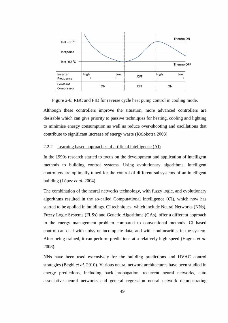
49

Figure 2-6: RBC and PID for reverse cycle heat pump control in cooling mode.

Although these controllers improve the situation, more advanced controllers are

desirable which can give priority to passive techniques for heating, cooling and lighting

to minimise energy consumption as well as reduce over-shooting and oscillations that

contribute to significant increase of energy waste (Kolokotsa 2003).

2.2.2 Learning based approaches of artificial intelligence (AI)

In the 1990s research started to focus on the development and application of intelligent

methods to building control systems. Using evolutionary algorithms, intelligent

controllers are optimally tuned for the control of different subsystems of an intelligent

building (López et al. 2004).

The combination of the neural networks technology, with fuzzy logic, and evolutionary

algorithms resulted in the so-called Computational Intelligence (CI), which now has

started to be applied in buildings. CI techniques, which include Neural Networks (NNs),

Fuzzy Logic Systems (FLSs) and Genetic Algorithms (GAs), offer a different approach

to the energy management problem compared to conventional methods. CI based

control can deal with noisy or incomplete data, and with nonlinearities in the system.

After being trained, it can perform predictions at a relatively high speed (Hagras et al.

2008).

NNs have been used extensively for the building predictions and HVAC control

strategies (Beghi et al. 2010). Various neural network architectures have been studied in

energy predictions, including back propagation, recurrent neural networks, auto

associative neural networks and general regression neural network demonstrating

50

relatively successful results. Coefficients of variation were in the range of 2–40%.

These variations in the accuracy of the predictions were primarily dependent on the

ANN architecture used, the regularity of the building operation and the accuracy of data

measurement devices (Kumar et al. 2013)

Neural network controllers have also been studied and a two-layer, multi-input, single-

output (MISO) example is shown in Figure 2-7 (Liang & Du 2005). Direct Neural

Network Controllers have been used in thermal comfort control (Liang & Du 2005) and

in the temperature control of hydronic heating systems (Kanarachos & Geramanis

1998). These controllers are practical and, in contrast to indirect neural network

controllers, do not require ‘identification’ of the dynamic model of the plant.

Figure 2-7: Direct Neural Network Controller Example from (Liang & Du 2005).

Fuzzy Logic Controllers have also been studied as a potential solution that couples and

integrates management of all the different criteria and components of an HVAC system.

Alcala et al (2003) contend that the use of Fuzzy Logic Controllers (FLCs) could enable

the implementation of multi-criteria control strategies incorporating expert knowledge,

with the caveat that rational operation and improved performance of FLCs is required

for implementing complex control techniques (Alcalá et al. 2003).

The use of smart setting and tuning techniques for such controllers could improve

energy savings and indoor comfort if used properly. Genetic Algorithms (GAs) are a

good methodology to tune these FLCs when multiple criteria are considered. In the

same paper presented by Alcalá et al. (2003), the use of GAs to develop smartly tuned

FLCs to control HVAC systems, considering both energy performance and indoor

comfort requirement was reported.

51

Even though learning based techniques have shown promising results and they are

relatively easy to implement, they still exhibit disadvantages regarding the amount of

building data is necessary to train the models and the fact that subsequent AI model is

not suitable for optimisation. The building model also lacks of physical insight, leading

to uncertainty when it is operating outside the identified system range or when it is

subject to changes during its operation.

2.2.3 Model Predictive Control

MPC is a well-established method for constrained control and has been receiving wide

attention recently from researchers in the field of building control. MPC opens up

possibilities for exploiting thermal storage capacities. It makes use of predictions of

future disturbances, such as weather and internal gains, given requirements such as

comfort ranges and physical constraints on the controlled variables.

Building control system design becomes challenging when predictions of weather,

occupancy, renewable energy availability, and energy price are used for feedback

control. Green buildings are expected to maintain occupant comfort while minimizing

energy consumption, to manage intermittency in renewable energy generation and

manage the opportunities to store thermal and electrical energy. It is particularly

challenging to develop such controllers when conventional systems are replaced by

innovative heating and cooling systems that use active storage of thermal energy with

critical operational constraints.

Several authors have hypothesised that model predictive control (MPC) is the only

control methodology that can systematically take into account future predictions during

the control design stage while satisfying the system operating constraints (e.g. Henze et

al. 2004; Liu & Henze 2006a; Liu & Henze 2006b).

Background of Model Predictive Control

A Model Predictive Controller is based on an iterative, finite horizon (constrained),

optimisation of a plant model. At each discrete sampling time k, the vector of system

states xk is measured or estimated. The MPC makes use of a cost function to determine

the performance of the controller. Using a dynamic model of the plant, the cost function

is formulated in such a way that it can describe the performance of the controller at the

52

future horizon, given the current plant states and the future controlled inputs and

predicted disturbances uk. The objective of the MPC controller is to find the sequence of

control inputs that minimises the cost function to the horizon.

Figure 2-8: Basic Structure of MPC (Camacho & Bordons 2004).

Once the resulting sequence of optimal inputs is calculated, only the first is applied and

the rest is discarded. Then the process is repeated at the next time step using new

measured state information. This type of repeated measure-predict-optimise-apply cycle

is called ‘receding horizon control’ and is shown schematically in Figure 2-8.

Figure 2-9: Model predictive control demonstrating the receding horizon control

approach (Camacho & Bordons 2004).

Camacho and Bordons (2004) proposed a useful illustration of the principles of MPC

and classic control strategies when driving a car. MPC represents the case of a driver of

53

a vehicle using the information gathered by looking through the front windshield, while

classical feedback control is more aligned with looking out of the back window or in the

rear-view mirror, trying to steer the vehicle based on the information about its past

behaviour. The approach of a real driver to driving a car is similar to a MPC, since the

latter looks forward and chooses an ideal action based on possible future outcomes,

taking the real characteristics of the car into consideration. Moreover, a classical control

hypothetical driver would not take into consideration the real limits and boundaries of

their vehicle; they would try to drive through a curve with a semi-truck, assuming it

handles just like a sports car. A real driver has a mental image of the dynamics of the

car; knowing how it can accelerate, how fast it can stop and how it handles in general.

This mental image of the car is substituted by a simplified internal mathematical model

in MPC. The portion of the road that the driver can see is represented by the prediction

horizon in MPC. A real driver continuously updates their decisions; similarly MPC

continuously updates its predictions based on the current information, and repeats this

procedure. One of the most important aspects of driving is given by the essential

requirement of not leaving the road and crashing the car. We can think of this as a type

of constraint, complemented by other constraints such as the physical properties of the

vehicle.

System Models

A reliable prediction from the identified dynamic model is crucial to ensuring good

performance of MPC. It is a well-known that development of an appropriate dynamic

model and its identification are often the most difficult and time-consuming parts of the

automation process, in particular when applying a MPC strategy. The basic conditions

that each dynamic model intended for MPC usage should satisfy are: be reasonably

simple, be relatively accurate in system dynamics and steady-state properties, as well as

satisfactory prediction capabilities (Prívara et al. 2013).

The models reported in literature can be categorized into three groups:

1) High fidelity models that involve the numerical solution of differential algebraic

equations (DAE) describing the thermal energy balance in buildings;

2) Simplified physical models based on R-C analogies;

54

3) Grey/black box models that do not rely on physical building models.

High fidelity models are usually developed for simulation purposes, generally for

prediction of loads and sizing of systems. The most common simulation programs

include EnergyPlus (Crawley et al. 2001), TRNSYS (Laboratories 2015), ESP-r (ESP-r

2016) and DOE-2 (Lawrence Berkeley National Laboratory n.d.). A number of

researchers have studied the application of optimal controllers that use high fidelity

models as the prediction tool. Henze et al. (2004) applied model predictive control of

active and passive building thermal storage elements to a test facility, in which time-

varying electricity prices without demand charges were considered. In this case, the

building was modelled using TRNSYS while Matlab and its optimisation toolbox were

interfaced with the building simulation program. The objective of the high fidelity

models was to simulate the behaviour of the building. However, as an explicit model

was not provided, therefore this approach cannot really be classified as a control

oriented modelling approach. The issues related to the use of high fidelity models for

control include the fact that the identification and validation of high fidelity models are

nontrivial processes, and require significant parameter tuning and simulation, since the

complexity and size of the predictive models quickly lead to computationally intractable

optimisation problems. Also high fidelity simulation models prevent the optimisation

solvers from exploring the sparse structure of the resulting optimisation problem (Ma

2012).

An alternative is to use statistically based, data-driven approaches, resulting in a model

in an explicit form. Physically-based parametric models are classified as statistically-

based models here since the parameters are identified using measured or simulated data

(Prívara et al. 2013).

Subspace methods belong to the black-box class of identification algorithms and

provide a model in a state space form. Prediction error methods (PEM) are the most

commonly used statistical identification techniques. Their objective is to minimize one-

step ahead prediction errors by optimizing parameters of a specified model structure.

Typically, an autoregressive moving average with external input (ARMAX) model

structure is used. These models also belong to the black-box identification algorithms.

55

These models do not require full knowledge of the system or process. They are

developed by fitting parameters of the model to historical behaviour of the system. The

parameters in these models do not generally have direct physical significance.

These types of black/grey-box models are simple to develop and implement since they

only require sufficient data to ensure accurate system representation. However, these

models cannot ensure reliable prediction for operating points outside the range covered

by the training data and thus extensive and adequate data training is needed in order to

guarantee prediction accuracy.

Semi-deterministic physical modelling (DSPM) uses a resistance capacitance (RC)

electrical network analogue to describe the thermodynamics of a system, and is often

referred to as a grey-box modelling. Usually the model parameters are estimated by

tuning to historical measurements, and this approach has been presented in a wide

variety of papers including Ma et al. (2009), Gyalistras & Gwerder (2009) and Verhelst

et al. (2012). DSPM Grey-box models are more difficult to develop compared to black-

box models, since they include dynamic models of the physical system.

Semi-probabilistic physical modelling (PSPM) (Cigler 2010) approaches the problem

using stochastic differential equations for the description of a system to be identified.

Various models with increasing complexity have been formulated based on prior

physical knowledge, and the parameters of each model are estimated using the

maximum likelihood (ML) method. A forward selection strategy is used to find the best

model by an iterative process, using the most meaningful and adequately complex

model (Bacher & Madsen 2011; Andersen et al. 2000).

Model Predictive Control for Linear Systems

Considering a linear system in its state space form:

𝑥𝑘+1 = 𝐴𝑥𝑘 + 𝐵𝑢𝑘 (2.1)

𝑦𝑘 = 𝐶𝑥𝑘 + 𝐷𝑢𝑘 (2.2)

Where A is the state matrix, B is the input matrix and C is the output matrix of

dimensions A ∈ ℝnx×nx , B ∈ ℝny×nx

and C ∈ ℝny×nx. Matrix D represents the direct input–

output feedthrough and it is generally omitted in most models of real-life systems.

56

The predictive controller iterates the state-space model n steps ahead in time (this

determines the prediction horizon) to see how the system will behave in the future for a

given set of predicted disturbances based on the current states, and adjusts the inputs, uk,

which include both the measured disturbances and controlled inputs.

A cost function is an important part the predictive controller. It determines the degree of

optimality of a dynamic response, resulting from a sequence of control inputs to be

applied to the system. A cost function is of the form:

𝐽 = 𝑓(𝑥𝑘, 𝑢𝑘) (2.3)

The optimal set of inputs is obtained by minimising the cost function J:

𝑢𝑘∗ = 𝑎𝑟𝑔 min𝑢 𝐽(𝑥𝑘, 𝑢𝑘) (2.4)

The cost function is generally built in a quadratic form:

𝐽𝑘 = ∑ (𝑥𝑘+𝑖𝑇 𝑄𝑥𝑘+𝑖 + 𝑢𝑘+𝑖

𝑇 𝑅𝑢𝑘+𝑖)𝑛𝑝−1

𝑖=1 (2.5)

This is called the finite horizon predicted cost, calculated at the time and where the

effects of inputs beyond the horizon are excluded from the optimisation altogether. A

method which approximates the cost for an infinite horizon but with a finite number of

inputs is the dual-mode control paradigm. In this case, the last state at k+np is used to

compute a so-called terminal cost, and is included in the cost function as follows:

𝐽𝑘 = ∑ (𝑥𝑘+𝑖𝑇 𝑄𝑥𝑘+𝑖 + 𝑢𝑘+𝑖

𝑇 𝑅𝑢𝑘+𝑖)𝑛𝑝−1

𝑖=1+ 𝑥𝑘+𝑛𝑝

𝑇 𝑃𝑥𝑘+𝑛𝑝 (2.6)

Model Predictive Control for Hybrid Systems

Most of the control theory and tools have been developed for systems featuring linear

on nonlinear continuous dynamics. The mathematical models of such systems are

traditionally built using differential or difference equations, typically derived from

physical laws governing the dynamics of the system under consideration. However, in

many applications the system to be controlled is also described by discrete controlled

inputs (e.g. on/off switches or valves, gears or speed selectors and evolutions dependent

on if-then-else rules) which are generally described by logic. Often, the control of these

systems is left to the schemes based on heuristic rules inferred from practical plant

57

operation. These types of systems, that feature dynamical processes of a heterogeneous

continuous and discrete nature, are classified as ‘hybrid systems’.

Discrete-time hybrid systems, also called discrete hybrid automata (DHA) (Torrisi &

Bemporad 2004), have continuous dynamics described by linear difference equations

and have discrete dynamics described by finite state machines, both synchronized by the

same clock.

Bemporad and Morari (1999) proposed a framework for modelling of systems described

by interacting physical laws, logical rules, and operating constraints. These types of

system are classified as mixed logical dynamical (MLD) systems. Bemporad developed

a systematic control design method based on model predictive control ideas, which

provides stability, tracking, and constraint fulfilment properties. The form of this class

of hybrid system is described as follows:

𝑥(𝑘 + 1) = 𝐴𝑥(𝑘) + 𝐵1𝑢(𝑘) + 𝐵2𝛿(𝑘)+𝐵3𝑧(𝑘) (2.7)

𝑦(𝑘) = 𝐶𝑥(𝑘) + 𝐷1𝑢(𝑘) + 𝐷2𝛿(𝑘)+𝐷3𝑧(𝑘) (2.8)

𝐸2𝛿(𝑘) + 𝐷3𝑧(𝑘) ≤ 𝐸1𝑢(𝑘) + 𝐸4𝑥(𝑘) + 𝐸5 . (2.9)

Where 𝑥(𝑘) = [𝑥𝑐(𝑘)

𝑥𝑙(𝑘)] is the state vector 𝑥𝑐(𝑘) ∈ ℝ𝑛𝑐

and 𝑥𝑙(𝑘) ∈ {0,1}𝑛𝑙 , 𝑦(𝑘) =

[𝑦𝑐(𝑘)

𝑦𝑙(𝑘)] ∈ ℝ𝑝𝑐 × {0,1}𝑝𝑙 is the output vector, 𝑢(𝑘) = [

𝑢𝑐(𝑘)

𝑢𝑙(𝑘)] ∈ ℝ𝑚𝑐 × {0,1}𝑚𝑙 is the

input vector, 𝑧(𝑘)∈ ℝ𝑟𝑐 and 𝛿(𝑘) ∈ {0,1}𝑟𝑙 are the auxiliary variables, A, Bi, C, Di and

Ei denote real constant matrices, E5 is a real vector, nc > 0, and pc, mc, rc, nl, pl, ml, rl ≥

0.

The MLD formulation allows the specification of the evolution of continuous variables

through linear dynamic equations of discrete variables, propositional logic statements

and automata. The approach consists of embedding the logic in the state equations by

transforming Boolean variables into 0-1 integers, and by expressing the relations as

mixed-integer linear inequalities.

Bemporad’s framework (Bemporad & Morari 1999) was used to develop the Hybrid

Model Predictive Control (HMPC) toolbox for Matlab (Bemporad 2012), which makes

use of the hybrid systems description language HYSDEL to model MLD systems.

58

Figure 2-10: Hybrid systems - Logic-based discrete dynamics and continuous dynamics

interact through events and mode switches, from (Bemporad 2012).

One of the capabilities of HMPC is that it explicitly takes into account future samples of

the reference vector and/or measured disturbance, which automatically results in a

feedforward (non-causal) control action. The most general way to change a model-based

control design method to anticipate future reference samples is to augment the

prediction model, as described in (Bemporad 2006). In (Heemels et al. 2001), the

authors establish equivalences among five classes of hybrid systems: mixed logical

dynamical (MLD) systems, linear complementarity (LC) systems, extended linear

complementarity (ELC) systems, piecewise affine (PWA) systems, and max-min-plus

scaling (MMPS) systems. These approaches allow the transfers of theoretical properties

and tools from one class to another.

Research on the optimal control of hybrid systems has been very active during the past

decade (Morari & Barić 2006; Bemporad & Giorgetti 2006; Borrelli et al. 2005), and

this type of control has been practically implemented in a number of applications. One

such area of application is the automotive industry, e.g. the application of the HMPC

framework to active suspension systems (Cairano et al. 2007) and traction control

(Borrelli et al. 2001). In both cases the systems feature a non-linear function which can

be closely approximated by piecewise affine (PWA) segments, and can therefore be

recast in a MLD formulation and treated as a hybrid system.

Only a limited amount of research has been undertaken on the application of Hybrid

MPC to buildings, building HVAC systems and solar systems with storage. In the area

of buildings Siroky (2013) presented a hybrid approach to the re-configuration of a

59

heating system of a real building that had already been used to test a different MPC

strategy at the Czech Technical University (CTU). In the area of air conditioning

systems, HMPC has been also applied to a supermarket refrigeration system (Larsen et

al. 2002) where the key components of the system were the compressors, generally

configured as compressor racks, i.e. a number of compressors connected in parallel. In

the paper presented by Ferrari-trecate et al. (2004), the short-term scheduling

optimisation of a co-generation power plant was accomplished by exploiting hybrid

systems. These plants featured discrete dynamics such as the possibility of turning the

turbines on or off, operating constraints like minimum up and down times, and the

different types of start-up behaviour of the turbines. They also featured continuous

dynamics such as power and steam output, the corresponding fuel consumption, etc.

The authors also demonstrated that HMPC is applicable for online optimisation of such

systems. HMPC has also been studied and applied to a solar air-conditioning plant

(Menchinelli & Bemporad 2008). This plant, as presented in

Figure 2-4 and Figure 2-11, located in Seville, Spain, was developed under the

European Union project HYCON Network of Excellence. A number of other different

control approaches have been trialled on the same plant (Sonntag et al. 2008; Zambrano

& Garcia-Gabin 2008; Zambrano et al. 2008; Garcia-Gabin et al. 2009), and it was of

particular interest because of its hybrid nature.

60

Figure 2-11: Schematic of the solar air conditioning plant, Seville, Spain (Menchinelli

& Bemporad 2008).

Model Predictive Control of Buildings and Building HVAC systems

MPC strategies have been applied to the control and operation of both virtual and real

buildings. It is widely accepted that the application of a MPC strategy in one of its

formulations can lead to significant energy savings when compared to the classical

control strategies. A very broad and comprehensive review of optimal supervisory

control of building HVAC systems was carried out by Wang & Ma (2008). One of the

most active groups in MPC research applied to buildings is at the University of

California, Berkeley. They have developed a range of predictive approaches to building

temperature regulation, including a distributed predictive control approach (Morosan et

al. 2010), and a fast nonlinear stochastic MPC approach (Ma & Borrelli 2012), that

would lead to an estimated energy saving of 30% compared to the baseline building

running with RBC and PID control. The same group also focussed on the design of an

MPC strategy to optimize the scheduling and operation of a building cooling system

with storage to achieve lower electricity cost and better performance. The experimental

results showed that a 19.1% improvement of the plant COP can be achieved compared

to the use of the original baseline control logic (Ma et al. 2012; Ma et al. 2009).

61

Furthermore, Aswani et al. (2012) developed an energy efficient hybrid system

Learning-Based MPC controller, which was used to control a case study building. The

controller showed a 1.5 MWh energy saving per day compared to the default

manufacturer control strategy.

A MPC strategy has also been successfully implemented in a mid-size commercial

building with substantial energy savings compared to a DDC strategy (Bengea et al.

2014).

Extensive research has been undertaken by the Czech Technical University (CTU)

(Prívara et al. 2011; Široký et al. 2011). A MPC strategy has been applied to the heating

system of the university building (Figure 2-12), with very promising practical results.

The results also demonstrated the supremacy of a predictive controller over a well-tuned

weather-compensated control system, with energy savings in the order of 17–24%. The

application of a Hybrid MPC strategy to the reconfiguration of a building heating

system has also been recently reported (Sirok 2013).

In Australia, researchers from the Commonwealth Scientific and Industrial Research

Organisation (CSIRO) recently investigated the application of a self-learning MPC

strategy to refrigeration plants (Wall et al. 2015). This was designed to intelligently

alter the operation of a refrigeration system by dynamically determining optimal

operating temperature set points and run-time schedules. The application of intelligent

control to commercial buildings across Australia has also been investigated by the same

CSIRO team (Ward et al. 2012), and their experience in the implementation of a MPC

strategy in a typical commercial office building was reported in Platt et al. (2011) and

West et al. (2014).

Work applied to buildings has also been presented by the research group from ETH

Zurich, Switzerland, which has also been working on MPC under the OptiControl

project framework (ETH 2010), which had an objective to develop and test novel,

predictive control approaches for commercial building automation systems. A number

of research case studies have been investigated through theoretical study (Oldewurtel et

al. 2012; Oldewurtel et al. 2013; Sturzenegger et al. 2013) and experimental tests

(Sturzenegger, et al. n.d.; Sturzenegger, Morari, et al. n.d.). See also Figure 2-12.

62

Figure 2-12: Buildings used for MPC application experiments by the ETH group (ETH

2010) and the CTU group (Prívara et al. 2011; Široký et al. 2011).

2.3 Summary

Given the requirements for buildings to meet higher levels of performance, in terms of

energy usage and thermal comfort, a number of different technologies have been

implemented and studied. Among the various improvements to the building as a whole,

using solar energy to increase the efficiency of the HVAC system and adopt advanced

control strategies in the BMCS have been proven to be effective options. Systems that

harvest solar energy for daytime heating and ones based on radiative cooling for

summer night time cooling are attractive. The major challenge for these types of

systems is the time lag between generation and demand, and therefore thermal energy

storage is potentially beneficial. PVT systems provide an efficient solution for

generation of both electrical and thermal energy at the same time and therefore increase

the efficiency of the whole system.

From a control perspective, the literature review highlights that the current classical

Rule-Based Control (RBC) and Proportional-Integral-Derivative (PID) control cannot

accurately deal with the requirements of modern, complex and energy efficient

buildings. More advanced control strategies have been studied and implemented,

including artificial intelligence (AI) based and Model Predictive Control (MPC) based

strategies. Adopting an MPC strategy allows the controller to make use of physical

models of the building and the energy systems to optimise their operation over a defined

prediction horizon, becoming extremely attractive for application to a solar-based

thermal generation coupled with energy storage. Its adaptability to hybrid systems gives

63

the flexibility to describe and optimise a system that features both continuous and

discrete dynamics, such as operating modes and switches.

64

3 CASE STUDY BUILDING, HVAC CONFIGURATION DESIGN AND

COMPONENT MODELLING

This chapter introduces the case study building used to undertake the research presented

in this thesis, presenting the details of the solar-assisted HVAC system and its

components, explaining their modelling, sizing and performance validation.

The author was a member of the leadership group (six students) of Team UOW Solar

Decathlon China 2013 Competition project and managed the design, construction and

commissioning of the Illawarra Flame house. The author was responsible for the

HVAC, electrical and control systems.

3.1 Case study building

3.1.1 Solar Decathlon Competition

The case study building used for this study was a Solar Decathlon house, developed by

University of Wollongong’s ‘Team UOW’ in order to compete in the Solar Decathlon

China 2013 competition. The Solar Decathlon competition was first introduced by the

US Department of Energy in 2002, aiming to inform and educate communities about the

opportunities and benefits presented by clean-energy products for buildings and design

solutions, showcasing the comfort and affordability of homes that combine energy-

efficient construction and appliances with renewable energy systems available today

(DOE 2013). The Solar Decathlon is a very important and useful vehicle for the

implementation of new technologies and the evolution of the housing stock towards

new benchmarks for building performance, such as Net-Zero Energy buildings (NZEB)

or even positive energy buildings (PEB). At the time of writing the Solar Decathlon

competition have proven to be a great success over the past decade, and has expanded to

three competitions around the world: Solar Decathlon Europe, Solar Decathlon China

2013, and the U.S. Department of Energy Solar Decathlon (Figure 3-1). Overall, more

than 12,000 students have been involved in the Solar Decathlon projects.

In a Solar Decathlon competition, university teams have to design, build, and operate

solar-powered houses that are cost-effective, energy-efficient, and attractive. They have

to compete in ten sub-contests, five of which are measured and five are judged.

65

The measured contests in the Solar Decathlon China 2013 competition included: energy

balance (the houses have to be Net-Zero Energy); thermal comfort; hot water;

appliances and home entertainment, while the judged contests included: engineering;

architecture; solar application; market appeal: and communications (DOE 2013).

Figure 3-1: DOE Solar Decathlon, Washington, 2009 (left) and Solar Decathlon China,

Datong, 2013 (right).

3.1.2 Overall design of Team UOW Solar Decathlon house

In developed countries the existing building stock is not very often replaced by new

buildings. Many of the houses built in Australia after the Second World War were

timber-framed houses, clad in fibre-cement and were hence colloquially named ‘fibro’

houses. These buildings typically have little or no thermal insulation and generally

exhibit poor thermal performance and low energy efficiency. Under the auspices of the

University of Wollongong (UOW) Sustainable Buildings Research Centre (SBRC) a

student/staff team (Team UOW) was formed with the members drawn from both the

University of Wollongong and TAFE (Technical and Further Education) NSW (New

South Wales) Illawarra Institute. Team UOW was the first team in the history of Solar

Decathlon competitions to demonstrate how to effectively upgrade and retrofit an

existing building rather than designing a new building from scratch. This approach

proved to be extremely successful and Team UOW subsequently won the Solar

Decathlon China 2013 competition with the highest overall score in the history of Solar

Decathlon competitions. Team UOW decided to develop a retrofit strategy to

demonstrate how to improve the level of thermal comfort and overall sustainability of a

‘fibro’ home through the development and application of different retrofit technologies.

Figure 3-2 shows a typical fibro house used for the design of the Team UOW Solar

66

Decathlon house (named as Illawarra Flame house) and the Team UOW Illawarra

Flame Solar Decathlon house. The name fibro derives from the "fibrous (or

fibre) cement sheet", more commonly called "asbestos cement sheet", that was widely

used in Australia as a building cladding material, due to its durability. Asbestos fibres

were often used to reinforce cement sheets, enhancing their mechanical properties.

Fibro houses generally have a timber frame, do not have or have very little insulation,

and do not have very good airtightness, making them a very good candidate for energy

efficiency building envelope retrofits.

One of the key targets in this project was to achieve net-zero energy consumption in that

the grid-connected building was to export more renewable energy (generated on-site)

than energy it imports from the grid over the course of a year. To achieve this target, it

was first necessary to reduce the energy demand of the building through the

implementation of effective passive retrofitting initiatives, such as upgrading the

envelope, glazing and shading systems, using natural ventilation, etc., followed by

retrofitting and application of advanced active systems.

Figure 3-2: Typical fibro house, used for the design of the Illawarra Flame house and

the Team UOW Illawarra Flame house.

One of the key challenges to overcome in a building retrofit project was the design of

the existing house chosen as a reference (Figure 3-3). The application of the retrofitting

options has to be logical, easily implemented and suitable for the constraints that the

existing house would impose.

http://en.wikipedia.org/wiki/Cement

http://en.wikipedia.org/wiki/Asbestos

67

Figure 3-3: Reference (pre-retrofit) fibro house floor plan (Team UOW University of

Wollongong 2013) it represents a common floor plan adopted for social housing in

NSW.

Given that the house needed to be assembled and disassembled in a short timeframe to

meet the competition requirements, Team UOW decided to design a new building that

would have the same shape and structure as the pre-retrofitted reference fibro house, but

designed for modular and fast construction. The floor, wall and roof sections were

therefore designed to include steel framing, so that each section could be structurally

self-sufficient for disassembly, shipping and assembly operations.

Inside the steel structure, the geometry of the timber framing of the typical fibro house

was replicated, so that the challenges that, for example, insulating the walls would bring

were effectively the same.

Keeping the architecture of the original building was considered important, since Team

UOW wanted to ensure that the retrofitted building would not fell out of place in its

suburban environment. However, certain features of the house were modified to

increase the functionality of the layout, such as removing the third bedroom of the

original home to make space for an open plan living and dining area, which, together

68

with the modifications to the roof structure over the living area, provided increased

natural lighting and ventilation, as shown in Figure 3-4.

Figure 3-4: Living room of the Illawarra Flame house.

The original bathroom and laundry were replaced by two pre-manufactured ‘retrofit

pods’. These not only provided structurally robust modules that protect the key tiled/wet

areas of the house during transportation, but also enhanced the easiness of

implementation of the retrofit technologies, such as the advanced services and

technological innovations of the home including the HVAC, BMCS and hot water

systems (See Figure 3-5).

Figure 3-5: Illawarra Flame house pods, highlighted in red (Team UOW University of

Wollongong 2013).

69

A typical fibro house is a lightweight construction building, with very minimal levels of

insulation and high infiltration rates. One of the primary retrofits adopted was a

relatively heavy insulation of the walls, ceiling and floors using a combination of glass-

wool bulk insulation and rigid foam insulation. The single-glazed windows were

replaced with high quality double-glazed elements, which allowed the design team to

increase the window size in certain areas. The retrofitting of the windows, combined

with the modification of the window openings allowed the penetration of the winter sun

into the interior of the house, whilst minimising the risk of summer overheating. Being

a lightweight building, thermal mass was introduced in the interior space via a feature

wall, made with recycled terracotta tiles and glass, as shown in Figure 3-6.

A window located next to the wall allows sun to shine on the passive thermal storage

surface during winter, whilst remains obscured during summer.

Figure 3-6: Feature thermal mass wall (Team UOW University of Wollongong 2013).

The development and implementation of an innovative HVAC system incorporating

advanced sustainable energy technologies was a desired outcome of the project. Solar

photovoltaic-thermal (PVT) collectors were seen as a promising technology that was

receiving wide attention. Cooling of the PV modules by the heat transfer fluid flowing

through the PVT collector leads to an increase in the electrical efficiency of the PV

panels as compared to a conventional PV system, which has higher PV cell operating

temperatures. At the same time, the heat transferred to or from the fluid may be used for

70

space heating or cooling, thereby resulting in an increase in the overall energy collection

and conversion efficiencies of the system.

3.2 HVAC system development

3.2.1 System narrative and design constraints

The design of a solar-PVT assisted HVAC system for the Illawarra Flame house was

challenging for a number of reasons. The main objectives were to efficiently harvest

solar energy and increase the generation of the PV modules, however, the design had to

accommodate the need for the system to be retrofitted to an existing building, and the

need for the house to be modular and easily assembled for the competition. The system

was designed to operate under Sydney weather conditions on a small scale residential

building, but in principle a similar system could be either installed in different building

typologies or in different climates. Furthermore, the system was to be designed to

operate both in heating and cooling conditions.

Considering just the PVT component, various design options were evaluated. The first

selection to be made was the working fluid. Generally, PVT systems are either air-based

or water-based. A water-based system would have advantages in a higher heat capacity

of the fluid, and the possibility to connect the system to the hot water generation and

have more advanced heat delivery option such as underfloor heating and ceiling

cooling. A very good example of the design and implementation of such a system was

proposed in a previous Solar Decathlon by the German team Home+. The design and a

few experimental results under the cooling operation mode were presented in (Eicker &

Dalibard 2011).

Even though very attractive from the thermal perspective, such a system would create a

number of problems when retrofitted to an existing building. Compared to an air based

system, the need of pumps, valves and proper piping creates more issues in installation

and maintenance of a system with fans, dampers and ducting (e.g. a malfunction in the

water-based system could cause water leaks that can potentially create significant

damage to the house since it has to be installed on the roof).

Another advantage of an air-based system lies in the installation and the integration with

a conventional air conditioning system; it is only necessary to create a cavity underneath

71

the solar panels, possibly using a commercially available roof profile, to create the PVT

collectors.

It is only then left to connect the outlet of the collectors to a conventional ducted system

for thermal integration. In this case a water-based system would require a more complex

installation of the collectors, and either the possibility to deliver the heating and cooling

with a hydronic system, which is not always a possibility when retrofitting an existing

building and it is also one of the most invasive retrofit options, or the integration of the

water system with the air distribution, which means that a heat exchanger is needed.

Lastly, an air-based system would not have freezing-related problems when installed in

a cold climate. For these reasons an air-based PVT was chosen for the Illawarra Flame

house HVAC system.

The second design choice to be made was whether the intake of the PVT was to be fresh

air or return air from the house. This choice was mainly driven by considerations of the

weather, and the fact is that the building designed to operate in Wollongong played a

major role in this decision. The system was intended to operate for both heating and

cooling purposes, and therefore a significant temperature difference in both cases had to

be achieved. A closed loop system would be an advantage in terms of heating, since the

PVT inlet temperature would be the temperature of the house which is generally higher

than the winter outdoor temperature. For instance, in winter the typical maximum daily

outdoor temperature in Wollongong is around 15°C-18°C.

On the other hand, a fresh air intake PVT can still guarantee a significant temperature

difference between the outlet of the PVT in winter heating conditions (at the design

airflow rate, preliminary simulations predicted an average PVT outlet temperature in

sunny conditions of 30-35°C), and utilise that the fact that in summer night time cooling

conditions the outdoor temperature naturally drops below the indoor average

temperature (the outdoor temperature is on average 16-18°C at night time in summer).

Thus, the relatively limited radiative cooling available can be used to further reduce the

outside air temperature and condition the space.

Using a fresh air intake is also beneficial in terms of air quality, since in PVT operation

the amount of fresh air introduced in the building is well above the recommended

quantities for an airtight and well-designed house.

72

The benefits of thermal storage linked to the PVT system becomes clear when

considering the fact that the PVT system generates its most useful heating (or cooling)

at times when the house generally requires it the least, if a classical set-point control

strategy is in place. To utilise a larger portion of the heating/cooling generated, either a

more advanced control strategy that can utilise the building fabric to store the energy by

over-heating or over-cooling the building or, as presented in the literature review, a

dedicated thermal energy store has to be introduced. To store thermal energy, both

sensible (Chen, Athienitis, et al. 2010) and latent heat (Jurinak & Abdel-Khalik 1979a)

of a particular material can be used.

Given the relatively narrow operating conditions and the need to utilise the system in

both heating and cooling, a single active thermal store, based on a salt-hydrate PCM

with a melting temperature of 22°C, was selected.

The overall HVAC system should have the capability to directly utilise the energy

generated by the PVT system, store the excess energy, discharge the energy stored and

have a standard air conditioner as a backup.

The configuration of the Illawarra Flame house HVAC system is presented in the next

section.

3.2.2 HVAC system configuration and operating modes

The various components of the Illawarra Flame house HVAC system were connected

by means of a combination of solid and flexible ducting. A schematic of the solar-

assisted HVAC system developed is provided in Figure 3-7. To direct the airflow along

the different flow paths, on/off dampers were used (D1, D2, D4, D6 and D7), and two

variable opening dampers (D3, D5) were located in the specific sections of the ducting

to control the amount of fresh air introduced into the building. Two fans (F2 and F3)

were utilised to charge the PCM unit and assist the heat pump’s AHU fan (F1) to

overcome the additional pressure drop introduced by the PVT system, the PCM unit and

the extra ducting. These fans were controlled by variable speed drives (VSDs) that

allowed the controller to optimise the airflow rate in the system.

73

Figure 3-7: Schematic of the solar-assisted HVAC system where the symbols represent

the following: S/A supply air, O/A outside air, R/A return air, E/A exhaust air, F fan

and D damper, respectively

The system was controlled by a residential control system with a programmable logic

controller (full details of the control system infrastructure are provided in Chapter 5).

The present author designed the system such that there were a total of five operating

modes, comprising three conditioning modes and two PVT modes.

Conditioning modes

The various operating modes that the system could utilise based on the indoor and

outdoor measured conditions are illustrated in Figure 3-8. Depending on the indoor

conditions, the system worked in either the natural ventilation mode through

automatically controlling the opening of high level windows, or the mechanical heating

and cooling mode.

74

Figure 3-8: Illustration of a) HVAC system conditioning modes and b) HVAC system

PVT modes.

In the mechanical heating and cooling mode, the system was designed to operate in

three different sub-modes, as illustrated in Figure 3-8a.

1. Direct Photovoltaic-Thermal Supply. If the generation of heating during daytime

or cooling during night time (night sky radiative cooling) occurs at the same

time as demand, then heated air/cooled air from the PVT system is directed into

the house until the demand is matched. If the demand is higher than the energy

extracted from the PVT system, the AHU will cover the remaining

heating/cooling requirement.

2. Supply Air Preconditioned Through The Phase Change Material. In this case, if

thermal energy is available in the PCM store the mixture of return air and fresh

a)

b)

75

air will be preconditioned by the PCM store, increasing or decreasing the supply

air temperature. If the demand is higher than the energy extracted from the PCM

storage unit, the AHU covers the remaining heating/cooling requirement.

3. Normal Heating and Cooling Mode. If there is no PVT thermal generation and

no thermal energy stored in the PCM, the AHU will supply the heating or the

cooling required.

PVT modes

If no conflicting operating mode is activated, the system can operate in two other

modes, as shown in Figure 3-8b.

1. PCM Charging. If there is no demand from the house, and the PCM unit is not

fully charged and it is convenient to charge it, the PVT system will charge the

PCM unit.

2. PVT Exhaust. In situations where the increase in electrical generation by the PV

panels due to their temperature decrease is higher than the energy used by the

fan, then air is drawn underneath the PV panels and exhausted directly to

ambient.

3.3 Analytical model of a PVT collector

The PVT collector studied in this paper consisted of a number of thin-film PV panels

mounted on a steel sheet ‘flashing’, which was fixed to the top of an existing sheet

metal roof profile. This system created a cavity beneath the steel flashing through which

the working fluid (i.e. air) could flow and exchange heat with the PV panel, as shown

schematically in Figure 3-9.

a) Day time thermal energy collection.

76

b) Night time heat rejection.

Figure 3-9: Overview of the PVT collector geometry as implemented on the Illawarra

Flame Solar Decathlon House.

The utilisation mode of the PVT collector generally depends on the demand of the

house. For instance, when heating is required in winter daytime, the incoming solar

radiation generates electricity through the PV modules. Part of the radiation is

reflected/reradiated, part is lost to ambient via convection and the remainder is

transferred to the heat transfer fluid (Figure 3-9a). The air mass flow rate is the key

parameter that allows the Building Management & Control System (BMCS) to control

the air temperature at the outlet of the PVT collector and also the quantity of heat

extracted from the PV modules.

Under Sydney summer conditions the house would mainly require cooling. In this case

the PVT will generate cooling during the night time, whereby the solar panels extract

heat from the air flowing through the PVT collector by emitting radiation to the sky if

the sky is at a lower temperature than the panels (see Figure 3-9b).

3.3.1 Thermal Model

An analytical quasi-steady state model was developed to describe the thermal behaviour

of the PVT collector. This model can be used for both design optimisation and control

optimisation purposes. The key assumptions used in developing this quasi-steady state

model were that: a) the transients involved in heating or cooling of the system are

relatively short compared to the time constants elsewhere in the building and HVAC

system; and b) that the conduction resistance through the upper and lower walls of the

air duct are negligible in comparison to the other convection, conduction and radiation

77

thermal resistances. These assumptions can be justified by the fact that the thin metal

flashing and the thin film solar panels have relatively low thermal mass and thermal

resistance (our experimental results indicated that the thermal time constant of the PVT

collectors was less than five minutes).

Taking an energy balance on a short, stream-wise control volume in the PVT collector

air duct, an analytical solution for the thermal performance of the collector may be

derived; the thermal resistance network for heat flow at a given cross-section of the

PVT collector/duct is illustrated in Figure 3-10.

Figure 3-10: Thermal resistance network model of the heat exchange at a given cross-

section of the PVT collector.

The energy balance on the upper and lower surfaces of the PV panel, the energy balance

on the air flowing into and out of the control volume, and the heat balance on the lower

surface of the duct may be described by Equations (3.1), (3.2) and (3.3), respectively.

𝐺𝑖 ∙ 𝛼(1 − 𝜂) = 𝑈𝑒𝑥𝑡(𝑇top − 𝑇amb) + ℎr1(𝑇top

− 𝑇sky) + ℎ̅inT(𝑇top − 𝑇𝑃𝑉𝑇) +

ℎr2(𝑇top − 𝑇bot) (3.1)

�̇� ∙ 𝜌 ∙ 𝑐𝑝 ∙𝜕𝑇𝑃𝑉𝑇

𝜕𝑥𝑑𝑥 = [ℎ̅𝑖𝑛𝑇(𝑇𝑡𝑜𝑝 − 𝑇𝑃𝑉𝑇) + ℎ̅𝑖𝑛(𝑇𝑏𝑜𝑡 − 𝑇𝑃𝑉𝑇)] ∙ 𝑤 ∙ 𝑑𝑥 (3.2)

ℎ̅in(𝑇𝑃𝑉𝑇 − 𝑇bot) = 𝑈int(𝑇bot

− 𝑇i) + ℎr2(𝑇bot − 𝑇top) , (3.3)

where �̇� is the volumetric air flow rate, ρ and cp are the density and specific heat

capacity of the air, TPVT is the local air temperature in the PVT channel, Gi is the solar

radiation on the inclined surface, Ttop and Tbot are the temperatures of the top and bottom

plates of the PVT channel, ℎ̅𝑖𝑛 and ℎ̅𝑖𝑛𝑇 are the average heat transfer coefficients on the

bottom and top inside surfaces of the channel, respectively, Uint is the overall heat

transfer coefficient between the bottom plate of the PVT channel and indoor

Gi

78

environment, Uext is the overall convective heat transfer coefficient between the top

plate of the PVT channel and ambient, hr1 is the radiative heat transfer coefficient

between the outside surface of the PV panel and the sky, hr2 is the radiative heat transfer

coefficient between the duct top and bottom surfaces, x and w are the length and the

width of the channel, respectively, Tsky is the temperature of the sky and Ti is the interior

building temperature. Combining Equations (3.1) and (3.3), the top and bottom surface

temperatures of the PVT duct can be determined from Equations (3.4) and (3.5),

respectively.

𝑇𝑡𝑜𝑝 =(ℎ̅𝑖𝑛+ℎ𝑟2+𝑈𝑖𝑛𝑡) ((𝑈𝑒𝑥𝑡+ℎ̅𝑖𝑛𝑇+ℎ𝑟1+ℎ𝑟2) (𝑇𝑃𝑉𝑇 ℎ̅𝑖𝑛+𝑈𝑖𝑛𝑡 𝑇𝑖)+𝐼𝑟 𝛼 ℎ𝑟2 (1−𝜂)+𝑈𝑒𝑥𝑡 ℎ𝑟2 𝑇𝑎𝑚𝑏+𝑇𝑃𝑉𝑇 ℎ̅𝑖𝑛𝑇 ℎ𝑟2+ℎ𝑟1 ℎ𝑟2 𝑇𝑠𝑘𝑦)

ℎ𝑟2 ((ℎ̅𝑖𝑛+ℎ𝑟2+𝑈𝑖𝑛𝑡) (𝑈+ℎ̅𝑖𝑛𝑇+ℎ𝑟1+ℎ𝑟2)−ℎ𝑟22)

−

𝑇𝑃𝑉𝑇 ℎ̅𝑖𝑛+𝑈𝑖𝑛𝑡 𝑇𝑖

ℎ𝑟2 (3.4)

𝑇𝑏𝑜𝑡 = (𝑈𝑒𝑥𝑡+ℎ̅𝑖𝑛𝑇+ℎ𝑟1+ℎ𝑟2) (𝑇𝑃𝑉𝑇 ℎ̅𝑖𝑛+𝑈𝑖𝑛𝑡 𝑇𝑖)+𝐺𝑖𝛼 ℎ𝑟2 (1−𝜂)+𝑈𝑒𝑥𝑡 ℎ𝑟2 𝑇𝑎𝑚𝑏+𝑇𝑃𝑉𝑇 ℎ̅𝑖𝑛𝑇 ℎ𝑟2+ℎ𝑟1 ℎ𝑟2 𝑇𝑠𝑘𝑦

(ℎ̅𝑖𝑛+ℎ𝑟2+𝑈𝑖𝑛𝑡) (𝑈+ℎ̅𝑖𝑛𝑇+ℎ𝑟1+ℎ𝑟2)−ℎ𝑟22 (3.5)

It is then possible to recast 𝑇𝑡𝑜𝑝 and 𝑇bot as follows:

𝑇top = 𝐶1𝑇𝑃𝑉𝑇 + 𝐶2 (3.6)

𝑇bot = 𝐶3𝑇𝑃𝑉𝑇 + 𝐶4 (3.7)

where, C1, C2, C3 and C4 are coefficients defined as follows:

𝐶1 =(ℎ̅𝑖𝑛+ℎ𝑟2+𝑈𝑖𝑛𝑡)𝐶3

ℎ𝑟2−

ℎ̅𝑖𝑛

ℎ𝑟2 (3.8)

𝐶2 =(ℎ̅𝑖𝑛+ℎ𝑟2+𝑈𝑖𝑛𝑡)𝐶4

ℎ𝑟2−

𝑈𝑖𝑛𝑡 𝑇𝑖

ℎ𝑟2 (3.9)

𝐶3 =(𝑈𝑒𝑥𝑡+ℎ̅𝑖𝑛𝑇+ℎ𝑟1+ℎ𝑟2)ℎ̅𝑖𝑛+ℎ̅𝑖𝑛𝑇ℎ𝑟2

(ℎ̅𝑖𝑛+ℎ𝑟2+𝑈𝑖𝑛𝑡) (𝑈𝑒𝑥𝑡+ℎ̅𝑖𝑛𝑇+ℎ𝑟1+ℎ𝑟2)−ℎ𝑟22 (3.10)

𝐶4 =(𝑈𝑒𝑥𝑡+ℎ̅𝑖𝑛𝑇+ℎ𝑟1+ℎ𝑟2) (𝑈𝑖𝑛𝑡 𝑇𝑖)+𝐼𝑟𝛼 ℎ𝑟2 (1−𝜂)+𝑈𝑒𝑥𝑡 ℎ𝑟2 𝑇𝑎𝑚𝑏+ℎ𝑟1 ℎ𝑟2 𝑇𝑠𝑘𝑦

(ℎ̅𝑖𝑛+ℎ𝑟2+𝑈𝑖𝑛𝑡) (𝑈𝑒𝑥𝑡+ℎ̅𝑖𝑛𝑇+ℎ𝑟1+ℎ𝑟2)−ℎ𝑟22 (3.11)

Combining Equations (3.6), (3.7) and (3.2) we then derive:

𝜕𝑇𝑃𝑉𝑇

𝜕𝑥𝑑𝑥 =

𝑤

�̇�∙𝜌∙𝑐𝑝[(ℎ̅𝑖𝑛𝐶2 + ℎ̅𝑖𝑛𝑇𝐶4) + 𝑇𝑓(ℎ̅𝑖𝑛𝑇𝐶1 + ℎ̅𝑖𝑛𝐶3 − (ℎ̅𝑖𝑛 + ℎ̅𝑖𝑛𝑇))] (3.12)

Equation (3.12) is a first order, nonhomogeneous, linear differential equation with

constant coefficients, of the form expressed in Equation (3.13) with the general solution

of Equation (3.14).

79

𝑦 ′ + 𝑎𝑦 = 𝑏 𝑦 = 𝑦(𝑥) (3.13)

𝑦 = �̅� + 𝑦∗ = 𝐶𝑒−𝑎𝑥 +𝑏

𝑎 (3.14)

From Equation (3.12) we can then derive Equation (3.15):

{𝑇𝑃𝑉𝑇

′ + 𝐴𝑇𝑃𝑉𝑇 = 𝐵

𝑇𝑃𝑉𝑇(0) = 𝑇𝑎𝑚𝑏 (3.15)

The solution of which is:

𝑇𝑃𝑉𝑇 = (𝑇𝑎𝑚𝑏 −𝐵

𝐴) 𝑒−𝐴𝑥 +

𝐵

𝐴 (3.16)

Where

𝐴 = −𝑤

�̇�∙𝜌∙𝑐𝑝(ℎ̅𝑖𝑛𝑇𝐶1 + ℎ̅𝑖𝑛𝐶3 − (ℎ̅𝑖𝑛 + ℎ̅𝑖𝑛𝑇)) (3.17)

𝐵 =𝑤

�̇�∙𝜌∙𝑐𝑝(ℎ̅𝑖𝑛𝐶2 + ℎ̅𝑖𝑛𝑇𝐶4). (3.18)

The convective heat transfer coefficient on the upper/outside surface of the PVT is

dependent on the local wind speed (Vw) and is calculated from the correlation (3.19) by

considering both the natural and forced convection components through the following

relationship (Eicker & Dalibard 2011),in which the forced convection heat transfer

coefficient ℎ𝑐𝑜𝑛𝑣,𝑓𝑜𝑟𝑐𝑒𝑑 is determined by Equation (3.20) (Duffie & Beckman 2013a):

𝑈𝑒𝑥𝑡 = √ℎ𝑐𝑜𝑛𝑣,𝑓𝑜𝑟𝑐𝑒𝑑3.5 + ℎ𝑐𝑜𝑛𝑣,𝑛𝑎𝑡𝑢𝑟𝑎𝑙

3.53.5 (3.19)

ℎ𝑐𝑜𝑛𝑣,𝑓𝑜𝑟𝑐𝑒𝑑 = 2.8 + 3.0 ∗ 𝑉𝑤 (3.20)

The natural convection coefficient on the upper surface of the PVT is calculated

according to the relationships of ASHRAE 2013 Fundamentals Handbook correlations

for natural convection on a horizontal plate (ASHRAE 2013).

The internal convective heat transfer coefficient (ℎ̅𝑖𝑛) within the duct is dependent on

the Reynolds number, which is different for laminar flow and turbulent flow. The heat

transfer coefficient of the top half of the PVT channel (ℎ̅𝑖𝑛𝑇) also includes the thermal

resistance of the PV panels:

ℎ̅𝑖𝑛𝑇 =1

1

ℎ𝑖𝑛 +𝑅𝑝𝑣

(3.21)

80

In this model, when the Reynolds number is lower than 2000, Equation (3.22) is used to

calculate the Nusselt number. Otherwise, the Dittus-Boelter relationship for turbulent

flow as shown in Equation (3.23) is used.

𝑁𝑢𝑙 = 7.541(1 − 2.61𝐴𝑅 + 4.97𝐴𝑅2 − 5.119𝐴𝑅3 + 2.702𝐴𝑅4 − 0.548𝐴𝑅5) (3.22)

𝑁𝑢𝑡 = 0.023𝑃𝑟𝑛𝑅𝑒4

5 (3.23)

where, 𝐴𝑅 is the aspect ratio (height/width) of the channel, Pr is the Prandtl number of

air and 𝑛 is equal to 0.4 when the airflow is heated and 0.3 when the airflow is cooled.

The parameters needed to calculate the instantaneous intensity of solar radiation

impinging on a tilted surface are summarised in Table 3-1, together with values and

governing equations used to determine the major parameters.

Table 3-1: Values and governing equations used to determine the values of major

parameters.

Parameters Values and governing equations used

Albedo 0.2

Hour Angle 𝜔 = 2𝜋(𝑠𝑡𝑛 − 12) ∙ 15/360

Declination 𝑑 = 23.45 ∙ 𝑠𝑖𝑛(360 ∙ (284 + 𝑑𝑜𝑦)/365) ∙ 2𝜋/360

The angle 𝜃 between the

normal to the inclined plane

and the beam radiation

cos 𝜃 = sin 𝑑 sin𝜑 cos𝛽 − sin𝛿 cos𝜑 sin𝛽 cos 𝛾 +

cos 𝛿 cos𝜑 cos𝛽 cos𝜔 + cos𝛿 sin𝜑 sin𝛽 cos 𝛾 cos𝜔 +

cos 𝛿 sin𝛽 sin𝛾 sin𝜔

The radiation on an inclined

surface

𝐺𝑖 = 𝐺𝑛 cos 𝜃 +𝐺𝑑(1+cos𝛽)

2+ 0.2(𝐺ℎ𝑟 + 𝐺𝑑)(1 −

cos𝛽) /2

In cases where only site data for global horizontal radiation is available, the horizontal

surface radiation measurement can be used to estimate the diffuse and beam

components. The coefficient Rb is used to define the ratio of beam radiation on the tilted

surface to that on a horizontal surface.

𝑅𝑏 =cos𝜃

cos𝜃𝑧 (3.24)

81

where, 𝜃𝑧 is the angle 𝜃 calculated for a horizontal surface as follows.

cos 𝜃𝑧 = cos𝜑 cos 𝛿 cos𝜔 + sin𝜑 sin 𝛿 (3.25)

The ratio between the diffused and beam radiation is calculated using the Orgill and

Hollands correlation (Duffie & Beckman 2013b).

The effective emissivity of the solar panels may be calculated using empirical or semi-

empirical correlations available in the literature (Eicker & Dalibard 2011; Berdahl &

Fromberg 1982). Most of which are valid only for clear sky conditions (Berdahl &

Fromberg 1982), and while factors to take account of cloudy conditions may be added

(Mihalakakou et al. 1998). The temperature of the sky in this study was calculated using

the relationship for night-time clear sky radiation provided by Duffie and Beckman, as

follows (Duffie & Beckman 2013b):

𝑇𝑠𝑘𝑦 = 𝑇𝑎𝑚𝑏 ∗ (0.711 + 0.0056𝑇𝑑𝑝 + 0.000073(𝑇𝑑𝑝2) + 0.013𝑐𝑜𝑠(15𝑡))1/4 (3.26)

Where the units for 𝑇𝑠𝑘𝑦 𝑎𝑛𝑑 𝑇𝑎𝑚𝑏 are Kelvin, for 𝑇𝑑𝑝 degrees Celcius, and t is the

time of day in hours.

Cloudiness has an effect on the incident radiation which can be expressed by the factor

C as shown in Equation (3.27) (Mihalakakou et al. 1998; Bagiorgas & Mihalakakou

2008) and the effective emissivity of the sky is given by (3.28).

𝐶 = (1 + 0.00224𝑛 + 0.0035𝑛2 + 0.00028𝑛3) (3.27)

휀𝑠𝑘𝑦,𝑐𝑙𝑜𝑢𝑑𝑦 = 𝐶휀𝑠𝑘𝑦,𝑐𝑙𝑒𝑎𝑟 (3.28)

The linearized radiation heat transfer coefficient between the sky and the PV panels is

defined as (3.29). Using the same methodology the radiation coefficient between the top

plate and bottom plate of the PVT channel is derived as Equation (3.30).

ℎ𝑟1 = 𝛼𝜎(𝑇𝑡𝑜𝑝2 + 𝑇𝑠𝑘𝑦

2)(𝑇𝑡𝑜𝑝 + 𝑇𝑠𝑘𝑦) (3.29)

ℎ𝑟2 = 𝛼𝜎(𝑇𝑡𝑜𝑝2 + 𝑇𝑏𝑜𝑡

2)(𝑇𝑡𝑜𝑝 + 𝑇𝑏𝑜𝑡) (3.30)

where, σ is the Boltzmann constant, 𝛼 is the absorptivity of the metal flashing, 𝑇𝑠𝑘𝑦 is

the sky temperature, and 𝑇𝑡𝑜𝑝 is the temperature of the top plate of the PVT channel,

which is calculated iteratively.

82

3.3.2 Airflow Model

To optimize the airflow rate through a PVT collector it is necessary to take into account

the fan power required to circulate the air through the PVT and ductwork system.

Firstly, the air velocity through the PVT channels, and other ductwork, and the

associated pressure drops need to be calculated. To calculate these parameters in the

Solar Decathlon House system an equivalent hydraulic resistance network was analysed

(Figure 3-11).

Figure 3-11: Air flow resistance network showing flow elements/resistances for flow

branches connected to the air collection manifold. V1, V2, etc. represent PVT ducts and

H1, H2, etc. represent manifold sections.

This analysis was important in choosing the optimal number and size of the PVT

channels and in optimising the geometry of the manifold, since a uniform air flow

velocity through the PVT channels is important to maximise the overall efficiency.

One of the assumptions made in this model is that, since the channels were uniformly

distributed across the intake manifold, the flows will be symmetrical, and it is therefore

necessary to model only one half of the system. Major and minor losses were calculated

for each of the sections of the network by first assuming the flow in the first channel it

is then possible to calculate the pressure at the manifold point where the second channel

is connected and therefore calculate the flow in the second channel. Repeating the

process the pressure drop of the whole network for a given airflow rate, and the flow

distribution across the network can be obtained. The pressure-airflow curve for this

V… V2

H1

V1

H2 H…

PVT air

intakes

Manifold

To the house HVAC

system

83

particular system can then be determined. Since the PVT collectors were constructed in

the same way on both the north- and south-facing slopes of the pitched roof, the curve

of just one side can be generated, assuming that each side of the PVT has half of the

total airflow rate. The power necessary to ideally circulate the air through the system

can then be calculated by Equation (3.31).

𝑃𝑖𝑑 = ∆𝑝 ∙ �̇� (3.31)

where ∆𝑝 is the total pressure drop and �̇� is the total airflow rate.

The electrical power consumption can be derived from Equation (3.32), using a 3rd

order relationship between the electrical consumption of the fan and the airflow rate.

This relationship, which includes the overall efficiency of the fan, can be used for

optimisation purposes.

𝑃𝑒,𝑐𝑜𝑛𝑠 = 𝑃𝑖𝑑/𝜂 = 𝛾𝑃𝑉𝑇V̇3 (3.32)

3.3.3 PV panel electrical efficiency

Drawing air underneath the solar panels has the benefit of reducing the panel

temperature and increasing their electrical conversion efficiency. This benefit can be

quantified using the temperature coefficient of the solar panels, β. Using the thermal

model developed for the air stream, presented in section 3.1, the temperature profile of

the top sheet of the PVT collector (𝑇𝑡𝑜𝑝) can be calculated. The efficiency is therefore

given by Equation (3.33).

𝜂𝑒 = 𝜂𝑒−𝑟𝑒𝑓 ∙ (1 − 𝛽 ∙ (𝑇𝑡𝑜𝑝 − 25)) (3.33)

where 𝜂𝑒−𝑟𝑒𝑓 is the efficiency under standard test conditions.

3.4 Analytical Model of the PCM Thermal Storage Unit

3.4.1 Thermal model

A number of assumptions were applied so as to facilitate derivation of an analytical

solution to reduce the computational load of the controller. These assumptions were:

- The temperature of the PCM is uniform along the entire length of the heat

exchanger at any given time (lumped mass approximation);

84

- The PCM material changes phase at a specific temperature (with no temperature

‘glide’);

- The material encapsulating the PCM brick has the same thermal conductivity as

that of the PCM material per se. Note that in the Solar Decathlon house thermal

store, the encapsulation was made of High-density polyethylene (HDPE) which

had a very similar thermal conductivity to that of the PCM (i.e. 0.46-0.52W/m∙K

and 0.54 W/m∙K respectively).

Given the assumptions above, the air temperature as a function of distance along each

channel is given by:

𝑇𝑝𝑐𝑚,𝑚 = 𝑇𝑝𝑐𝑚 − (𝑇𝑝𝑐𝑚 − 𝑇𝑝𝑐𝑚,𝑖)𝑒(−

𝑃ℎ̅ 𝑥

�̇�∙𝜌∙𝑐𝑝) (3.34)

where TPCM,m is the average temperature of the air at a distance x along the channel, Tpcm

is the surface temperature of the channel (assumed equal to the uniform internal PCM

temperature), TPCM,o is the inlet air temperature, P is the perimeter of the channel, ℎ̅ is

the average internal convective heat transfer coefficient.

Similarly, the outlet temperature at the length l can be determined by Equation (3.35).

𝑇𝑝𝑐𝑚,𝑜 = 𝑇𝑝𝑐𝑚 − (𝑇𝑝𝑐𝑚 − 𝑇𝑝𝑐𝑚,𝑖)𝑒(−

𝑃ℎ̅ 𝑙

�̇�∙𝜌∙𝑐𝑝) (3. 35)

The average internal convective heat transfer coefficient can be calculated using the

Nusselt number definition.

ℎ̅ =𝑘𝑁𝑢̅̅ ̅̅

𝐷ℎ (3. 36)

The correlations to evaluate the average Nusselt number for a fully developed laminar

flow in a rectangular duct are the same as those presented in (3.22) and (3.23).

To include the thermal resistance of the wall and PCM material in the modelling, it is

possible to rewrite the equation with the total heat transfer coefficient (Utot).

𝑅𝑐𝑜𝑛𝑣 = 1/ℎ̅ (3. 37)

𝑅𝑐𝑜𝑛𝑑 =1

𝑈𝑤𝑎𝑙𝑙+𝑃𝐶𝑀 (3. 38)

𝑈𝑡𝑜𝑡 =1

𝑅𝑐𝑜𝑛𝑑+𝑅𝑐𝑜𝑛𝑣 (3. 39)

85

This coefficient in Equation (3.39) substitutes ℎ̅ in Equations (3.34) and (3.35).

The total heat transfer can be calculated as follows:

𝑃𝑡ℎ = �̇�𝑐𝑝(𝑇𝑖𝑛 − 𝑇𝑜𝑢𝑡) (3. 40)

3.4.2 Airflow model

As for the PVT collector it is necessary to take into account the power required to drive

the air through the PCM thermal store. The material in contact with the air in this case is

plastic, with a roughness 휀 (ASHRAE 2013). Figure 3-22 shows the pressure-airflow

curve. Following the same methodology presented in Section 3.2, including the

efficiency of the fan, the resulting 3rd

order fit for the power consumption is of the same

form:

𝑃𝑒,𝑐𝑜𝑛𝑠 = 𝛾𝑃𝐶𝑀 V̇3 (3. 41)

3.5 PVT Collector Design

The PVT collector was designed to be integrated with the HVAC system of the Team

UOW Solar Decathlon house. The project objective was to demonstrate how to use

various retrofit technologies to an existing building, in this case a typical ‘fibro house’.

From preliminary studies, it was decided to design a metal flashing to be fitted to a

commercially available roof profile to create the air channels underneath the PV panels.

Figure 3-12: Lysaght Trimdek™, from (Lysaght 2013)

To maximise the output temperature of the PVT collector, the channel was designed to

be as long (upslope) as the existing roof (4.16m) (Team UOW University of

Wollongong 2013). The optimal depth for air heaters and PVT collectors was studied by

Hegazy and Bambrook in (Hegazy 1999; Bambrook & Sproul 2010), recommending a

ratio between the depth of the channel and its length of 0.0025. With a channel length of

86

4.16 m, the recommended depth of the channel would be 10.4 mm. The best

commercially available roof cladding product identified was Lysaght Trimdek™

(Figure 3-12), which provided a channel depth of 29 mm. This profile offered the best

compromise between channel height (when topped with a flat flashing to form air

channels) and suitability for a residential application.

The PVT collector was therefore designed to be fabricated using flexible thin-film PV

panels glued to a metal flashing fixed across the ‘valleys’ of the roof sheeting. Air could

therefore flow through the air duct between the PV panels/flashing and the roof sheeting

to exchange heat with the panels.

In order to select an appropriate PV module different aspects were considered:

- Arrangement for maximum coverage on available roof area;

- Ability to properly and safely fasten the flashing to the roof;

- Air-tightness;

- Aesthetics;

- Wiring routing and access;

- Security against wind forces;

- Electrical efficiency and total electrical production.

After consideration of these items, the large-format SoloPower SP3S PV module was

chosen. The height of the module allowed for two modules to be installed on each metal

flashing, and the width of the module allowed the metal flashing to span across six pans

of Trimdek™.

The module is shown in Figure 3-13 (seen from underneath), designed by Vincent

Tannahill, a summer scholarship student as part of a UOW/BlueScope research

collaboration. He designed the module to be compliant with the AS1170.2 (Structural

Design Actions Part 2: Wind Actions) standard, verifying that the resulting stiffener

layout, sizing and fastening method was sufficient to resist wind loads expected in the

final location that this system was to be installed.

87

Figure 3-13: PVT metal flashing module: view of underside.

To size the system, the heating and cooling demand of the Illawarra Flame house was

simulated using DesignBuilder over the course of a whole year, using Sydney

International Weather for Energy Calculation (IWEC) data (see Chapter 4 for details of

the model). The resulting design heating and cooling capacities of the system for

Sydney conditions were 3.3 kW in cooling and 2.1 kW in heating (Team UOW

University of Wollongong 2013).

88

An example of the simulated outlet temperature the PVT system, using Sydney IWEC

July weather data, is presented in Figure 3-14:

Figure 3-14: Temperature difference between ambient (inlet) air and PVT outlet as a

function of time and flow rate through the PVT collector, Sydney, July IWEC weather

data.

The design airflow rate of the system was taken to be equal to that of a conventional air

conditioning system sized for a similar demand, i.e. 350 L/s in this case. The outlet

temperature of the PVT system can be calculated using the model developed in

Equation (3.16) and the design thermal generation of this PVT generation is calculated

as follows:

𝑃th = �̇�𝑑𝜌𝑐𝑝(𝑇𝑃𝑉𝑇,𝑘 − 𝑇𝑠𝑝𝑎𝑐𝑒) (3.42)

The space temperature was considered to be fixed at 22°C in both heating and cooling

cases, which leads to a worst case scenario situation, since generally the design

temperature in residential applications for heating is 20°C and for cooling 25°C. The

system is also considered to run at its variable air flow rate �̇�𝑑, extracting the maximum

heat possible from the collectors, considering that it should not perform worse than a

100 150 200 250 300 350 4000

10

20

30

40

50

60

Time (h)

Tem

pera

ture

( C

)

Tpvt - 50L/s

Tpvt - 150L/s

Tpvt - 250L/s

Tpvt - 350L/s

Tpvt - 450L/s

Tambient

89

standard air conditioning system. This is introduced maximising the following benefit

function C:

𝐶(�̇�) = 𝑃𝑡ℎ(�̇�) − 𝛼𝑐 (𝑃𝑒,𝑐𝑜𝑛𝑠(�̇�)) (3.43)

Where Pe,cons is the electrical energy used by the fan, calculated using the plant curve

presented in Figure 3-18.

In this case the coefficient 𝛼𝑐 was chosen to be nominally equal to 6, since the system

needed to perform better than a standard air conditioning heat pump (with a typical

seasonal Coefficient of Performance > 3.5) also when the heating or cooling is stored in

the PCM unit, and therefore would require additional electrical energy to discharge the

unit. The choice of this coefficient was entirely dependent on the design requirements

and can vary from system to system. The simulation of a PVT system, covering with the

whole of a roof coverable with PVT collectors, using July and January Sydney weather

data, is presented in Figure 3-15 and Figure 3-16, respectively.

90

Figure 3-15: Simulation of the PVT thermal output in winter conditions, July IWEC

weather data, Sydney.

Over the month simulated the PVT system was estimated to generate a maximum (peak)

of 5 to 6 kW useful thermal power, with a total of 217 kWh of useful heating energy

generated over the month, equivalent to an average of 7 kWh/day.

50 100 150 200 250 300 350 400 4500

5

10

15

20

25

30

35T

em

pera

ture

( C

)

Time (h)

50 100 150 200 250 300 350 400 4500

500

PVT outlet temperature

Ambient temperature

Global horizontal radiation

50 100 150 200 250 300 350 400 4500

500

1000

1500

2000

2500

3000

3500

4000

4500

5000

Hea

t tr

an

sfe

r (W

) an

d A

irflo

w r

ate

(L

/s)

Time (h)

Airflow rate

Heat transfer

91

Figure 3-16: Simulation of the PVT thermal output in summer conditions.

Over January, the PVT system was simulated to be able to generate a maximum of 4

kW of useful (peak) night time cooling, providing a total of 288 kWh of useful cooling,

equivalent to an average of 9.3 kWh/day.

0 50 100 150 200 250 300 35010

15

20

25

30

35

Tem

pera

ture

( C

)

Time (h)

0 50 100 150 200 250 300 3500

500

1000

PVT outlet temperature

Ambient temperature

Global horizontal radiation

0 50 100 150 200 250 300 350

-3500

-3000

-2500

-2000

-1500

-1000

-500

0

500

Hea

t tr

an

sfe

r (W

) an

d A

irflo

w r

ate

(L

/s)

Time (h)

Airflow rate

Heat transfer

92

To optimize the system and calculate the optimal airflow rate, it was necessary to

accurately model the heat transfer into the air channels below the PV modules, the

mechanical losses in the system, and the electrical benefit of reducing the temperature

of the PV panels, and define a cost function that makes the system operate as desired.

This methodology is explained in Chapter 4.

So as to maximise the use of available roof space for PV electrical generation during the

Solar Decathlon China 2013 competition and the exposed area to the sky for radiative

cooling purposes, the PVT collector was designed to draw air from both the north and

south elevations of the pitched roof and the two air streams then mixed in a plenum at

the apex of the roof as shown in Figure 3-17.

Figure 3-17: Photovoltaic thermal (PVT) collectors implemented on the roof of the

Illawarra Flame Solar Decathlon house.

From a mechanical perspective it was necessary to ensure that the airflow rate was

equally distributed across the various PVT collector channels. The model described in

Figure 3-11 was used to determine the number of take-off spigots that the plenum was

required to have in order to have a relatively small difference between the channels with

the maximum (closest to the take-off spigot) and minimum (furthest from the take-off

spigot) airflow rate. The final design, with three equally spaced take-off spigots of

150mm of diameter each, reduced the difference in airflow in the channels to less than

93

5%. The same model was then used to determine the pressure-airflow rate curve of the

PVT system, to be used for fan sizing as well as optimisation purposes.

The calculated pressure-airflow rate curve calculated for the Solar Decathlon house

PVT system is shown in Figure 3-18.

Figure 3-18: Pressure-airflow characteristic of the ‘Illawarra Flame’ Solar Decathlon

house PVT collector.

The implementation of the PVT system on the Illawarra Flame Solar Decathlon house is

shown on the left hand side portion of the roof in Figure 3-19.

Figure 3-19: PVT system on the ‘Illawarra Flame’ Solar Decathlon house.

0 100 200 300 400 500

50

100

150

200

250

300

350

400

450

Airflow rate [L/s]

Pre

ssure

[P

a]

PVT

collectors

Conventional

1st gen. PV

PVT air

intakes

94

3.6 PCM Unit Design

The PCM thermal storage unit in the Solar Decathlon house (See Figure 3-20) was

designed to exchange heat between the PCM and the air. For practical reasons, it was

decided to use commercially available ‘bricks’ of PCM (Figure 3-21), aligned to create

a small gap between the rows of bricks to allow air to flow through and exchange heat

with the PCM.

Figure 3-20: PCM unit layout, top view schematic.

The objective was to maximise the heat exchange rate, considering that under design

conditions the unit needed to operate with an airflow rate of 350 L/s and a maximum

pressure drop of 100 Pa.

The system was designed to operate for heating and cooling conditions, therefore the

phase change temperature was designed to be in the middle of the comfort band. The

optimal phase change temperature, obtained by maximising the thermal output from the

simulation of the system presented in Chapter 4, was calculated to be 22˚C. Given the

requirements for the unit to be non-flammable and to have a relatively narrow melting

range, PlusIce™ salt hydrate PCM ‘bricks’(PCM Products 2015) were chosen as an

appropriate product. The material selected has a latent heat of fusion of 145 kJ/kg and

sensible heat capacity 2.2 kJ/ kg∙K.

Tpcm,i

Air

Inlet

Tpcm,o

Air

Outlet

PCM unit

walls

PCM

bricks

95

Figure 3-21: PlusIce™ salt hydrate PCM ‘bricks’

To offset the PVT thermal generation to meet the house demand, a total capacity of

27kWh sufficient for approximately two days of heating or cooling demand of the

house, was decided to be installed. The designed PCM thermal storage unit consisted of

120 PlusIce™ PCM ‘bricks’, placed rows so as to create channels for the air to flow

through. The dimensions of the PCM store were limited to the available space

(~600mm) underneath the suspended floor of the house. The maximum volume that

could be used for the installation of the PCM storage unit was a rectangular

parallelepiped 4m long, 1.5m wide and 0.4m high. Given the dimensions of the bricks

(0.5m long, 0.25m wide, 0.032m thick), it was decided to lay them vertically on the

long edge, in twenty rows of six. The minimum thickness of the channels that could

guarantee a sufficiently high heat transfer coefficient, while not exceeding the design

pressure drop of 100Pa at 350L/s, was found to be 16mm.

The resulting pressure-airflow rate curve of the PCM thermal energy storage unit

implemented in the Solar Decathlon house is shown in Figure 3-22.

96

Figure 3-22: Pressure drop-airflow through the PCM thermal storage unit.

The simulated air temperature profiles along the length of the PCM thermal storage unit

under various airflow rates are shown in Figure 3-23 as a function of distance from the

inlet. As expected it was found that increasing the airflow rate led to higher heat transfer

rates and higher outlet air temperature.

Figure 3-23: Modelled air temperature profile along the length of the PCM thermal

storage unit under different airflow rates.

The final design of the PCM unit consisted of a steel frame, covered and sealed using

plywood. An external layer of R=3.0 W/m2K insulation was used to limit the heat

0 50 100 150 200 250 300 350 400 450 5000

20

40

60

80

100

120

140

160

180

Airflow [L/s]

Pre

ssure

dro

p [

Pa]

0 0.5 1 1.5 2 2.5 322

23

24

25

26

27

28

29

30

Length [m]

Tem

pera

ture

[degC

]

50 L/s

150 L/s

250 L/s

350 L/s

450 L/s

97

dispersion to the ambient. Two plenums at both ends of the unit were designed to

guarantee an even flow distribution across the channels. The assembled PCM unit and

the layout of the bricks are shown in Figure 3-24.

Figure 3-24: PCM unit during first assembly at iC, March 2013.

3.7 Field Tests and Validation

In this section results from both experiments and simulations are presented. The PVT

and PCM models were implemented in Matlab and the response of the PVT collectors

were simulated. For some of these simulations, Sydney IWEC (International Weather

for Energy Calculations) weather data was used. The models were then validated using

the experimental data collected in both Datong, China, during the Solar Decathlon

China competition and later at the University of Wollongong, following the return of

the Illawarra Flame house to Australia. The parameters used for the models presented

in Sections 3.3 and 3.4 were either defined by the geometry of the PVT collector and

the PCM unit (Sections 3.5 and 3.6), or defined by the thermal characteristics of the

construction materials of the HVAC components.

3.7.1 Experimental Facilities

The PVT tests were first carried out during August 2013 in Datong, China, and then in

Wollongong, Australia, from June 2014 onwards. The PVT collector, integrated with

the HVAC system of the house, was controlled and monitored through a Clipsal C-Bus

PCM

bricks

PCM

unit

98

Building Management System. All the relevant parameters were monitored and logged

using a Tridium Niagara JACE embedded controller at a one-minute sample rate.

The weather conditions, including ambient temperature, solar radiation and wind speed

and direction, were monitored using a Davis Vantage Pro II Weather station and

integrated through an RS232 connection to the C-Bus and JACE control units. Airflow

was monitored using Siemens QVM62.1 air velocity sensors, located one third of the

duct diameter from the duct centreline. These sensors had a stated accuracy of ±0.2 m/s

+ 3% of measured values. Temperatures in the ductwork were measured using Clipsal

C-Bus Digital Temperature Sensor Units 5104DTSI with a stated accuracy of ±0.5°C in

the temperature range of -10°C to 80°C.

3.7.2 Validation of the PVT Thermal Model

The global horizontal radiation, ambient temperature, predicted PVT outlet

temperatures and measured PVT outlet temperatures in Wollongong, Australia, for June

2014 are shown in Figure 3-25.

Figure 3-25: Comparison of the predicted and measured PVT air outlet temperatures

(11th of June 2014, Wollongong, Australia).

0

100

200

300

400

500

600

700

800

900

1000

0

5

10

15

20

25

30

35

7:0

6

7:2

6

7:4

6

8:0

6

8:2

6

8:4

6

9:0

6

9:2

6

9:4

6

10:

06

10:

26

10:

46

11:

06

11:

26

11:

46

12:

06

12:

26

12:

46

13:

06

13:

26

13:

46

14:

06

14:

26

14:

46

15:

06

15:

26

15:

46

16:

06

16:

26

16:

46

17:

06

Rad

iati

on

(W

/m2)

Tem

pe

ratu

re (

˚C)

Ta (˚C) Tpvt Measured (˚C)

Tpvt Predicted (˚C) Ghr (W/m2)

99

During these experimental tests the PVT airflow rate was maintained at approximately

350 L/s. It can be seen that a very good agreement between the predicted PVT outlet

temperatures and measured values was achieved. It is also seen that the experimental

results lag the simulations by a short time, of less than five minutes, since the quasi-

steady state thermal model of the PVT does not account for the (relatively small)

thermal mass of the PVT collector.

A scatter plot of the predicted versus measured PVT outlet temperatures is shown in

Figure 3-26, which provides substantive evidence that the simulations matched

experiments with a linear regression coefficient b = 0.9911 and 𝑅2𝑎𝑑𝑗 = 0.9122.

Figure 3-26: A scatter plot of measured and predicted PVT air outlet temperature data

(11th of June 2014, Wollongong, Australia).

This is considered to be a good result noting that the scatter in the data was in part due

to the non-controlled and transient environment and that the data acquisition system has

a coarse resolution (0.5⁰C) on temperature due to the limitations of the residential

building management system employed. In addition, the assumed negligible PVT

collector thermal mass used in the thermal model also contributed somewhat to the

scatter in the data.

0 5 10 15 20 25 30 35 40 45 500

5

10

15

20

25

30

35

40

45

50

PVT outlet temperature predicted ( C)

PV

T o

utl

et

tem

pe

ratu

re m

ea

sure

d (

C)

Measured vs. Predicted PVT Outlet temperature

Linear regression

100

The measured total electrical energy generated from the PVT roof, and that modelled as

generated from both the north and south elevations of the PVT collector using the

published performance data of the CIGS solar panels and global insolation measured

during field tests, are compared in Figure 3-27.

Figure 3-27: Predicted and measured PV electrical energy generation as a function of

time (experiments conducted at Datong, China, during August 2013).

A scatter plot of the predicted versus measured PVT electrical generation is shown in

Figure 3-28, with a linear regression coefficient b = 0.9947, intercept a=-137 and

𝑅2𝑎𝑑𝑗 = 0.8904. This indicates a relatively good agreement between the two sets of

data, where the model slightly over-predicted the electrical generation.

0 50 100 150 200 250 300 350 400 450 5000

500

1000

1500

2000

2500

3000

3500

Time [min]

Pow

er

[W]

PV Generation, Model, South side

PV Generation, Model, North side

PV Generation, Model, Total

PV Generation, Measured

101

Figure 3-28: A scatter plot of measured and predicted PVT electrical generation.

The thermal efficiency, electrical efficiency and total efficiency of the PVT collector

under the experimental tests at Datong, during August 2013, are shown in Figure 3-29.

1000 1500 2000 2500 3000

1000

1500

2000

2500

3000

Modelled Generation (W)

Mea

sure

d G

ene

ratio

n (

W)

Measured vs. Model

Linear regression

102

Figure 3-29: PVT efficiency as measured during testing August 2013 at Datong, China

(η_th, η_el, η_tot are the PVT thermal, electrical and total efficiency, respectively).

It can be seen that the overall electrical efficiency of the PVT collector was relatively

constant (i.e. ~ 8.2%) and consistent with the expected efficiency, considering that the

published PV conversion efficiency was stated as 11.2% and the inverter efficiency

taken to be 95%. Even with a relatively low air flow (i.e. 160-170 L/s), the heat transfer

to the air was as high as 4.0 kW, equating to a thermal efficiency of around 9.0%. The

effect of extracting thermal energy from the PV panels was to increase the overall

system efficiency to around 17%.

3.7.3 Experimental validation of the PCM thermal model

Experimental tests on the PCM thermal storage unit were carried out on a laboratory-

scale test rig at the University of Wollongong, which was essentially a replica of the

Illawarra Flame house PCM thermal store system with the same length of 3 m, but with

a reduced number of channels. The total mass of FlatIce™ PCM in the lab-scale rig was

138 kg, as compared to 693 kg in the Solar Decathlon house per se. The same

equipment was used to measure and log the temperature and air flow data as that for the

0

500

1000

1500

2000

2500

3000

3500

4000

4500

5000

0

0.05

0.1

0.15

0.2

0.25

0.3

0.35

0.4

0.45

0 20 40 60 80 100 120 140 160 180 200 220 240 260 280 300 320 340 360 380 400 420 440 460

Po

wer

[W

] -

Rad

iati

on

[W

/m2]

Effi

cien

cy

Time [min]

η_th η_el

η_tot

Heat Transfer [W] Electrical Generation [W]

Global Horizontal Radiation [W/m2]

103

PVT tests described above. A sample rate of 15s was employed for the transient heating

and cooling tests on the PCM store.

The modelled and experimentally determined total UA values for the heat exchanger

under different flow rates are shown in Figure 3-30, where UA values for the

experimental tests were found by dividing the total heat exchange to the working fluid

by the log-mean temperature difference (LMTD).

Figure 3-30: Comparison between modelled UA values (line) and experimental results

(circles) of the laboratory-scale PCM thermal storage unit.

3.8 Summary

This chapter outlined a modelling methodology for the thermal, hydraulic and electrical

characteristics of a photovoltaic-thermal (PVT) system, and the thermal and hydraulic

behaviour of an integrated Phase Change Material (PCM) thermal storage unit. This

methodology is efficient and can be readily implemented in practice in the logic of a

Building Management & Control System (BMCS). The experimental field work and

laboratory tests using a full-scale Solar Decathlon house and a laboratory-scale PCM

thermal store test rig showed that this modelling methodology can provide sufficient

accuracy for control purposes, despite its relative simplicity.

40 60 80 100 120 140

60

80

100

120

140

160

180

200

Airflow Rate [L/s]

UA

va

lue

[W

/K]

Experimental data

Predicted UA value

104

4 OPTIMISATION AND SIMULATION STUDY OF A SOLAR-ASSISTED

HVAC SYSTEM

This chapter presents a method for the optimisation of the airflow rate in the solar-

assisted HVAC system, a simulation of its behaviour when coupled with the Illawarra

Flame Solar Decathlon house over two typical summer and winter months and a

discussion on its operational performance. Initial experimental tests in winter conditions

were undertaken, highlighting the actual performance of the two PVT-based operating

modes, and control issues that needed to be addressed in this research.

4.1 Optimisation of Operating Modes of the HVAC System

4.1.1 General considerations for the PVT and PCM units

The instantaneous optimisation of the efficiency a solar PVT assisted HVAC system is

mainly dependent on the current weather conditions (i.e. solar radiation, ambient

temperature) and system conditions (i.e. average house temperature or PCM unit

temperature).

Considering the PVT system from the energy perspective, increasing the airflow rate

will affect the thermal response of the PVT system and increase the electrical

consumption of the fan. With increasing airflow rate the heat exchange rate in the PVT

increases, due to the increase of the internal convective heat transfer coefficient ℎ̅𝑖𝑛,

while the outlet temperature of the PVT system will decrease. The results of a typical

analysis are provided in Figure 4-1 where the simulation is for a single-sided PVT of the

same size of the Illawarra Flame house (aperture of 23.7 m2) and cross-section of air

flow area of 1.6 m2, with fixed weather conditions, i.e. total incident radiation on the

tilted surface is 750W/m2, inlet (ambient) temperature is 18˚C, indoor temperature is

25˚C, and wind speed is fixed at 1.0 m/s.

105

Figure 4-1: Variation of a) PVT heat exchange rate and b) outlet air temperature with

increasing airflow rate for example PVT collector .

This will affect the heat exchange into the PCM unit or the amount of heating that can

be provided to the house, depending on the temperature of the PCM and the average

temperature of the house, respectively. In both graphs discontinuities are due to the

change in heat transfer coefficient calculation in the transition between laminar flow and

turbulent flow.

From the electrical point of view (i.e. generation of the PV panels), increasing the

airflow rate will lead to a reduction in the temperature of PV panels, increasing the

electrical efficiency and power generation. The methodology presented in the previous

chapter was used to determine the increase in power generation as the airflow rate

increases.

The PCM thermal energy storage unit, as previously presented, was designed to be the

heat exchanger to transfer heat between the PCM and the air. From the thermal

perspective, increasing the airflow rate leads to an increase in the heat exchange rate

(See Figure 4-2a), due to the increase of the internal convective heat transfer coefficient

ℎ̅𝑖𝑛. If the inlet air temperature of the PCM unit is higher than the PCM temperature,

increasing the airflow rate leads to an increase of the outlet temperature (Figure 4-2b).

The example presented in Figure 4-2 was generated through simulating the response of

the PCM unit with the inlet airflow temperature of 30˚C, and the PCM wall at 22˚C,

0 100 200 300 400 5000

1

2

3

4

5

6

7

8

9

Airflow [L/s]

Hea

t E

xcha

ng

e [

kW

]

a) b)

0 100 200 300 400 50030

35

40

45

50

55

60

65

Airflow [L/s]

Tem

pera

ture

[°C

]

106

Figure 4-2: a) PCM thermal storage unit heat exchange rate as a function of airflow rate

and b) PCM thermal storage unit outlet temperature varying airflow rate.

Increasing the airflow rate will also increase the mechanical power required to move the

air into the system and therefore the electrical consumption of the fan.

To quantify the electrical consumption of the fan for each working mode, the modelling

methodology presented in the previous chapter is used. The electrical power necessary

to move the air in the PVT system and the PCM unit follows the relationships, as

previously presented in Chapter 3 for the individual components:

𝑃𝑃𝑉𝑇 = 𝛾𝑃𝑉𝑇 V̇3 (4.1)

𝑃𝑃𝐶𝑀 = 𝛾𝑃𝐶𝑀 V̇3 (4.2)

Where, PPVT and PPCM are the power consumption of the fan to move the air in the PVT

system and the PCM unit in W. A similar coefficient γDUCT can be calculated for the

ducting that connects the different components in the different operating modes. The

sum of the relevant coefficients in each operating mode leads to the plant curve for that

specified mode.

4.1.2 Charging PCM unit with PVT

The models developed were used for the optimisation of the various control system

operating modes. Optimisation of the PCM Charging mode, for example, requires the

control system to choose an optimal airflow rate that can maximise the benefit in terms

of the heat stored in the PCM unit and the energy used by the fan. In this study, a

benefit function, Equation (4.3), was used to maximize the amount of heat stored,

0 100 200 300 400 5000

0.5

1

1.5

2

2.5

3

3.5

Airflow [L/s]

Hea

t E

xcha

ng

e [

kW

]

0 100 200 300 400 50022

22.5

23

23.5

24

24.5

Airflow [L/s]

Tem

pera

ture

[°C

]

a) b)

107

considering that this would lead to certain electrical power consumption and an increase

in the electrical generation that has to be somehow related to the heat transfer. This

function is an extension of the one used previously used to thermally size the system,

which now includes more variables for a more complete optimisation:

𝐶(�̇�) = 𝑃𝑡ℎ(�̇�) + 𝛼𝑐(∆𝑃𝑒,𝑔𝑒𝑛(�̇�) − 𝑃𝑒,𝑐𝑜𝑛𝑠(�̇�)) (4.3)

𝑃𝑡ℎ(�̇�) = 𝜌�̇�𝑐𝑝(𝑇𝑃𝑉𝑇(�̇�) − 𝑇𝑝𝑐𝑚,𝑜(�̇�)) (4.4)

Where, �̇� is the flow rate of air flowing in the system, cp is the air specific heat capacity,

ρ is the density, 𝑃𝑡ℎ is the heat transfer rate into the PCM thermal storage unit as defined

in Equation (4.4), ∆𝑃𝑒,𝑔𝑒𝑛 is the increase in electrical generation due to the cooling of

the solar panels, ∆𝑃𝑒,𝑐𝑜𝑛𝑠 is the power consumption of the fan to move the air into the

system, Tpvt and Tpcm,o are the PVT outlet temperature (which corresponds to the inlet

temperature of the PCM if the thermal losses in the ducting can be considered

negligible) and PCM storage outlet temperature, respectively, 𝛼𝑐 is a weighting factor

for the electrical energy to increase its importance relatively to the thermal energy. The

choice of this factor might be different from case to case, depending on the design

objectives.

The simulated heat transfer, increased electrical generation of the PV panels and the

electrical energy used by the fans are presented in Figure 4-3. This simulation used the

same conditions of Figure 4-1.

The heat transfer into the PCM unit can then be correlated to the electrical power

consumption of the fan and the increased electrical generation of the PV panels.

Discontinuities in Figure 4-3 due to the changes in the heat transfer coefficient

calculation between laminar flow and turbulent flow have been smoothed.

108

Figure 4-3: Heat transfer rate, increased electrical generation and electrical power

consumption of PCM Charging under varying air flow rate.

It is then possible to obtain the cost function curves (Equation 4.3) and identify the

optimal airflow rate which maximises the benefit function under the various weather

conditions (Figure 4-4).The discontinuities in this case due to the changes in the heat

transfer coefficient calculation between laminar and turbulent flow have also been

smoothed.

Figure 4-4: Evaluation of the benefit function under various solar radiation levels and

varying air flow rate.

50 100 150 200 250 300 350 400 450 5000

0.5

1

1.5

2

2.5

3

3.5

4

4.5

Airflow [L/s]

Pow

er

[kW

]

Heat Transfer, 750 W/m2

Electrical Power Consumption

Increased Electrical Generation

0 50 100 150 200 250 300 350 4000

500

1000

1500

2000

2500

3000

3500

4000

4500

5000

5500

Cost

Fu

nctio

n [

W]

Airflow [L/s]

300 W/m2

450 W/m2

600 W/m2

750 W/m2

109

4.1.3 Conditioning the house with Direct PVT air supply

Optimisation of the Direct PVT operation mode is very similar to that of the

optimisation of the PCM charging mode, using the same cost function as presented in

Equation (4.3). The heating generated of the house is calculated as Equation (4.5).

𝑃𝑡ℎ(�̇�) = 𝜌�̇�𝑐𝑝(𝑇𝑝𝑣𝑡(�̇�) − 𝑇ℎ𝑜𝑢𝑠𝑒) (4.5)

Where, Thouse is the average temperature of the house.

4.1.4 Conditioning the house with PCM Discharging air supply

As in the case of the PCM charging mode, the performance of the PCM Discharging

mode is highly dependent on the inlet temperature of the PCM thermal storage unit. In

this operating mode, the inlet temperature is a mixture of the return air from the house

and the fresh air from ambient. The ratio between the two air streams is dependent on

the decisions taken at the design stage. Since there is no electrical generation involved,

the optimisation of this working mode is to maximise the cost function below.

𝐶(�̇�) = 𝑃𝑡ℎ(�̇�) − 𝛼𝑐(𝑃𝑒,𝑐𝑜𝑛𝑠(�̇�)) (4.6)

Where, 𝑃𝑡ℎ is the heat discharged from the PCM unit and is defined as Equation (4.7).

𝑃𝑡ℎ(�̇�) = 𝜌�̇�𝑐𝑝(𝑇𝑝𝑐𝑚,𝑜(�̇�) − 𝑇𝑝𝑐𝑚,𝑖(�̇�)) (4.7)

Where, Tpcm,i is the inlet temperature of the PCM unit, which is a mixture of the return

air from the house and the fresh air.

4.2 System simulations

4.2.1 Building demand simulation

The heating and cooling demands of the house were simulated using DesignBuilder, a

building simulation software based on EnergyPlus. This task was performed by Team

UOW members as part of the final project manual submission for the Solar Decathlon

competition (Team UOW University of Wollongong 2013). The modelling was

performed as part of the competition documentation submission, before the construction

of the Illawarra Flame house.

110

The heating and cooling demands were then used as inputs to simulate the behaviour of

the HVAC system. To align with NatHERS guidelines (Nathers 2015), the minimum

temperature of the house was set at 20°C during daytime and 18°C during night time for

the winter simulations. For summer simulations the maximum temperature was set at

25°C for the entire day.

The simulations showed that the thermal energy required to meet the NatHERS

requirements is relatively low (Team UOW University of Wollongong 2013); a direct

result of the expected effective passive design of the building. The thermal energy

demand, dependant on the set points chosen by the user, has to be met by the HVAC

system. The research aim of this solar-PVT assisted HVAC system is to satisfy heating

and cooling demands greater than that resulting from these preliminary simulations of

the building.

4.2.2 Mode Selection strategy

In the simulation, a rule-based strategy was used to determine the operating mode of the

HVAC system. This was based on the indoor conditions, the HVAC status (e.g.

temperatures of the PVT and PVT, etc.) and the weather conditions.

The operating modes and the mode selection strategy are summarised in Table 1, where

HD is the house heating or cooling demand, Tpvt is the calculated PVT temperature,

Thouse is the average temperature of the house, Tpcm is the temperature of the PCM, Pth is

the heating or cooling that the selected operating mode can provide, Charge is the

charge level of the PCM unit, mCharge is the maximum charge level, which is equal to

the total latent heat capacity of the PCM, and Ts is the sampling time in hours. The

variables are evaluated at each time step k.

These operating modes have been described in the previous chapter, where they have

been divided into conditioning modes and PVT modes. In this simulation, the

conditioning modes, including those where the PVT system and the PCM unit are pre-

heating or pre-cooling for the normal air conditioning system, are represented with

numbers from Mode 1 to Mode 5. The only PVT mode considered is PCM Charging,

represented as Mode a. This information is summarised in Table 4-1.

111

Using winter heating as an example, if the PVT generation occurs at the same time as

the house demand, the preferred operating mode is Direct PVT supply. If the heating

generation is sufficient then Mode 1 will be selected. In the case where the heating

demand is higher than the generation the normal air conditioning system is used and the

PVT is to pre-heat the air for the AHU – Mode 4.

If the house requires heating when the PVT is not generating and the PCM unit is

charged, PCM Discharging is selected. Mode 2 is selected if the PCM unit can provide

enough heating. Otherwise, Mode 5 will be selected and use the normal air conditioning

system to provide the remaining required heating. If none of these two resources are

available, Normal Conditioning mode is selected (i.e. Mode 3).

Table 4-1: Operating modes and logic conditions

Mode Mode

description Logic conditions in winter Logic conditions in summer

0 Off Mode 1) 𝐻𝐷𝑘 = 0 1) 𝐻𝐷𝑘 = 0

1 Direct PVT

supply

1) 𝐻𝐷𝑘 > 0

2) 𝑇𝑝𝑣𝑡,𝑘(�̇�) > 𝑇ℎ𝑜𝑢𝑠𝑒,𝑘

3) 𝑃𝑡ℎ,𝑘(�̇�) ≥ 𝐻𝐷𝑘

1) 𝐻𝐷𝑘 < 0

2) 𝑇𝑝𝑣𝑡,𝑘(�̇�) < 𝑇ℎ𝑜𝑢𝑠𝑒,𝑘

3) 𝑃𝑡ℎ,𝑘(�̇�) ≤ 𝐻𝐷𝑘

2 PCM

Discharging

1) 𝐻𝐷𝑘 > 0

2) 𝑇𝑝𝑣𝑡,𝑘(�̇�) ≤ 𝑇ℎ𝑜𝑢𝑠𝑒,𝑘

3) 𝑃𝑡ℎ,𝑘(�̇�) ≥ 𝐻𝐷𝑘 ⋀ 𝐶ℎ𝑎𝑟𝑔𝑒𝑘 ≥ 𝐻𝐷𝑘 ∙ 𝑇𝑠

1) 𝐻𝐷𝑘 < 0

2) 𝑇𝑝𝑣𝑡,𝑘(�̇�) ≥ 𝑇ℎ𝑜𝑢𝑠𝑒,𝑘

3) 𝑃𝑡ℎ,𝑘(�̇�) ≤ 𝐻𝐷𝑘 ⋀ 𝐶ℎ𝑎𝑟𝑔𝑒𝑘 ≤ 𝐻𝐷𝑘 ∙ 𝑇𝑠

3 Normal

Conditioning

1) 𝐻𝐷𝑘 > 0


3) 𝑃𝑡ℎ,𝑘(�̇�) ≤ 0 ⋁ 𝑃𝑡ℎ,𝑘(�̇�) <

𝐻𝐷𝑘 ⋁ 𝐶ℎ𝑎𝑟𝑔𝑒𝑘 < 𝐻𝐷𝑘 ∙ 𝑇𝑠

1) 𝐻𝐷𝑘 < 0


3) 𝑃𝑡ℎ,𝑘(�̇�) ≥ 0 ⋁ 𝑃𝑡ℎ,𝑘(�̇�) >

𝐻𝐷𝑘 ⋁ 𝐶ℎ𝑎𝑟𝑔𝑒𝑘 > 𝐻𝐷𝑘 ∙ 𝑇𝑠

4

Direct PVT

supply + Air

conditioning

1) 𝐻𝐷𝑘 > 0

2) 𝑇𝑝𝑣𝑡,𝑘(�̇�) > 𝑇ℎ𝑜𝑢𝑠𝑒,𝑘

3) 𝑃𝑡ℎ,𝑘(�̇�) < 𝐻𝐷𝑘

1) 𝐻𝐷𝑘 < 0

2) 𝑇𝑝𝑣𝑡,𝑘(�̇�) < 𝑇ℎ𝑜𝑢𝑠𝑒,𝑘

3) 𝑃𝑡ℎ,𝑘(�̇�) > 𝐻𝐷𝑘

5

PCM

Discharging +

Air

conditioning

1) 𝐻𝐷𝑘 > 0


3) 0 < 𝑃𝑡ℎ,𝑘(�̇�) < 𝐻𝐷𝑘 ⋀ 𝐶ℎ𝑎𝑟𝑔𝑒𝑘 ≥ 𝐻𝐷𝑘 ∙

𝑇𝑠

1) 𝐻𝐷𝑘 < 0


3) 𝐻𝐷𝑘 < 𝑃𝑡ℎ,𝑘(�̇�) < 0 ⋀ 𝐶ℎ𝑎𝑟𝑔𝑒𝑘 ≤ 𝐻𝐷𝑘 ∙

𝑇𝑠

a PCM Charging

1) mode=0 ˄ mode=3

2) 𝑇𝑝𝑣𝑡,𝑘(�̇�) ≥ 𝑇𝑝𝑐𝑚,𝑘

3) 𝐶ℎ𝑎𝑟𝑔𝑒𝑘 < 𝑚𝐶ℎ𝑎𝑟𝑔𝑒

1) mode=0 ˄ mode=3

1) 𝑇𝑝𝑣𝑡,𝑘(�̇�) ≤ 𝑇𝑝𝑐𝑚,𝑘

2) 𝐶ℎ𝑎𝑟𝑔𝑒𝑘 > −𝑚𝐶ℎ𝑎𝑟𝑔𝑒

112

PCM Charging mode is operated independently, but can only be activated if the PVT

system can provide heating to the PCM unit and no conflicting modes are already

selected, i.e. PVT Direct Supply (Mode 1 or Mode 4) or PCM Discharging (Mode 2 or

Mode 5). The summer cooling logic is similar and reversed, as presented in Table 4-1.

4.2.3 Case study simulations

For these simulations the models and optimisation methods previously presented in this

chapter have been used. The simulations were performed on a model of the Illawarra

Flame house and its components, assuming that fans with 40% electrical to mechanical

efficiency were utilised to move the air through the system.

The ambient temperature (Ta), the global horizontal radiation (Ghr), the house demand

(HD), the operating conditioning mode selected (Mode), the PCM Charging mode

(PCMCharging) (equal to 0 when inactive and set as 5 when active) and the resulting

charge level (Charge) are presented in Figure 4-5. The charge level profile of the PCM

unit was also presented in this figure. From this figure, it is seen that the system

employed different operating modes to meet the house demand, according to the

strategies presented in Table 4-1. Throughout July the simulated HVAC system was

estimated to supply 128 kWh of heating while the house demand was 206 kWh,

achieving an average COP, defined as the ratio of thermal input to the building to

electrical power consumption, of 32.5 for Mode 1 and Mode 4, 37.2 for Mode 2 and

Mode 5, and 24.7 for PCM Charging mode. The overall COP in the heating case was

16.3 without considering the increase in electrical energy generation of the PV panels.

113

Figure 4-5: Charge level and operating modes, July IWEC weather data, Sydney.

The results from using the same rule-based logic as summarised in Table 4-1 for the

cooling case are presented in Figure 4-6. The house demand and the charge level are

presented as positive on the graph for readability purpose, but they were considered

negative in the simulation since cooling is provided to the building. It can be observed

that, compared to the winter case, there is more offset between the cooling generation

and the demand. Therefore, the system mainly employed Mode 2 and Mode 5, PCM

Discharging mode or PCM Discharging assisted by the air conditioning system,

respectively. This figure also shows that sometimes the system employed Mode 4 -

Direct PVT Supply assisted by the air conditioning system at the beginning of the night,

when there is no solar radiation but the house is still warm because of its thermal mass.

For the remainder of the night, if the PCM unit is not fully charged, the system was

switched to the PCM Charging mode.

0

100

200

300

400

500

600

0

3

6

9

12

15

18

21

24

27

191 192 193 194 195 196 197

Gh

r [

W/m

2]

Tem

peratu

re [

˚C]

- H

D [

kW

] -

Mod

e

Day of the year

Ta Mode Charge [kWh]

HD [kW] PCMCharging Ghr

Ta

HD Ghr

114

Figure 4-6: Charge level and operating modes, January IWEC weather data, Sydney

During the month of January, the simulated system was estimated to be capable of

supplying 84 kWh of cooling, while the cooling demand of the house was 109 kWh.

This was achieved at an average COP of 18.3 for Mode 1 and Mode 4, 22.9 for Mode 2

and Mode 5 and 21.1 for PCM Charging mode. The overall COP in the heating case

was 10.9 without taking into consideration the increase in electrical energy generation

efficiency of the PV panels.

The simulated performance of the HVAC system over the two months considered is

summarised in Table 4-2.

Table 4-2: Summary of simulated performance of solar-assisted HVAC system.

Items Winter – July

(Heating)

Summer – January

(Cooling)

Total thermal demand (kWh) 206.4 109.2

Thermal Energy supplied through PVT/ PCM

system (kWh)

129.0 84.8

Fan Electrical Energy (kWh) 7.91 7.75

COP Mode 1 and 4 (Direct PVT) 32.5 18.3

COP Mode 2 and 5 (PCM Discharging) 37.2 23.0

COP PCM Charging mode 24.7 21.1

COP system 16.3 10.9

COP system – including extra PV generation 27.9 10.9

0

200

400

600

800

1000

1200

0

3

6

9

12

15

18

21

24

27

30

33

36

39

9 10 11 12 13 14 15

Gh

r [

W/m

2]

Tem

peratu

re [

˚C]

- H

D [

kW

] -

Mod

e

Day of the year

Ta Mode Charge [kWh]

HD [kW] PCMCharging GhrHD Ghr

115

4.3 Initial Experimental Results

The experimental work was focussed on addressing the application of the optimisation

method proposed at the beginning of this chapter to the real system, by implementing a

rule-based strategy that tries to optimize the system at each time step. The house control

system (details in Chapter 5) employed a similar analytical equation to the one as

presented in Chapter 3 to calculate the PVT supply air temperature to the house. The

test focussed on the operating modes PVT Direct Supply and PCM Charging.

The consumption of the fans was set for discrete speed levels (Figure 4-7) for each

working mode. The current cost function C was then calculated for each speed level i:

𝐶𝑖 = 𝑃𝑡ℎ,𝑖 − 𝛼 ∙ 𝑃𝑒𝑙,𝑖 (4.8)

𝑃𝑡ℎ,𝑖 = �̇�𝑖 ∙ ρ ∙ 𝑐𝑝 ∙ (𝑇𝑃𝑉𝑇,𝑖 − 𝑇𝑖,𝑖) (4.9)

Where Pth is the heat introduced in the building, Pel is the electrical power consumption

of the fans, α is a coefficient introduced to weight electrical power compared to thermal,

�̇� is the flow rate, cp is the specific heat capacity of air at 20˚C, ρ is the density, TPVT is

the supply air temperature, and Ti is the average temperature of the house.

The fan speed level corresponding to the maximum value of C was then utilized:

�̅� = 𝑚𝑎𝑥𝑖=1,..,𝑛 𝐶𝑖 (4.10)

The same procedure was followed to optimize the PCM charging mode, substituting the

calculated outlet temperature of the PCM thermal energy storage unit, Tpcmo to Ti:

𝑃𝑡ℎ,𝑖 = �̇�𝑖 ∙ ρ ∙ 𝑐𝑝 ∙ (𝑇𝑃𝑉𝑇,𝑖 − 𝑇𝑝𝑐𝑚𝑜,𝑖) (4.11)

4.3.1 Mechanical system identification

Identification of the electrical consumption versus air flow characteristics was a key

aspect of optimisation of this HVAC system. The example curves for the Direct

Photovoltaic-Thermal Supply mode and PCM Charging mode are presented in Figure

4-7, where electrical power is that provided to the fan variable speed drive (VSD) unit.

A third order polynomial has been fitted to the experimental data, since:

𝑃𝑒𝑙 =V̇

𝜂𝑓∙ ∆𝑝 (4.12)

116

Where, 𝜂𝑓 is the fan efficiency and ∆𝑝 is the pressure drop, which is proportional to V̇2.

The experimental data points were collected while increasing the VSD level controlling

the fan from 10% to 100%, in 10% increments. The minimum energy input to the VSD

when the fan was operating was found to be approximately 35 W. However, when the

fan was ‘off’ the standby power was measured to be approximately 4 W. The results

from the mechanical system identification process have been used to compute the cost

function, C, together with the predicted supply temperature.

Figure 4-7: Variable speed fan power as a function of air flow rate for: a) PVT Direct

Supply and b) PCM Charging modes. Note: fan power is the electrical input to the

variable speed drive (VSD) unit, which clearly has low efficiency at low fan speeds.

4.3.2 Thermal results

The experimental results from a test conducted in Wollongong, on the 15th

of June

2014, where the system was operated under the PVT Direct heat supply mode, are

presented in Figure 4-8 where Tavg is the average temperature of the house, Tout the

outside temperature, COP PVT Heating is the COP of the PVT system when operating,

Ghr is the global horizontal radiation, Heating_PVT and Heating_HP are the heating

inputs of the PVT and the Heat Pump respectively, P_Fans is the electrical

consumption of the PVT Fan. It was demonstrated that the PVT system could provide a

significant amount of heating, and in this test a total of 12.9 kWh was provided to the

house, with a peak generation of 3.7 kW thermal.

0

50

100

150

200

250

300

350

400

0 100 200 300 400

Po

wer

[W]

Flow Rate [L/s]

0

50

100

150

200

250

300

350

400

0 100 200 300 400

Po

wer

[W]

FlowRate [L/s]

Experimental data 3rd order polynomial

a) b)

117

This heating was also supplied to the house at a much higher COP, than a conventional

heat pump, achieving an average COP in this test equal to 13.5 (the total electrical

energy used in this test was equal to 0.9 kWh). It was also found that the fan speed was

correctly modulated to achieve high performance throughout the day.

Figure 4-8: PVT Direct Supply heating test, June 2014. Note: the supply temperature

from PVT is meaningful only when the fan is active, since the sensor is located in the

ducting after the PVT collector plenum.

Experimental results from a test conducted in Wollongong, on the 22nd

of June 2014,

where the system was charging of the PCM thermal energy storage unit, are presented

in Figure 4-9. In this graph Tout is the outside temperature, COP PCM Charging is the

COP of the PVT system when charging the PCM unit, Ghr is the global horizontal

radiation, Heating_to_PCM is the heating stored in the PCM unit, P_Fans is the

electrical consumption of the PVT Fan, Tinlet_duct_pcm and Toutlet_duct_pcm are the

air temperatures in the ducting at the inlet and the outlet of the PCM unit, Tpcm is the

average temperature of the PCM material (average of the measured temperature in the

first and last brick of PCM material).

From Figure 4-9, it can be seen that while charging the PCM thermal storage unit on a

typical winter day, with peak radiation slightly less than 500W/m2, a total of 26.6kWh

0

1000

2000

3000

4000

5000

6000

7000

8000

0

5

10

15

20

25

30

35

12:

00 A

M

12:

37 A

M

1:1

4 A

M

1:5

1 A

M

2:2

8 A

M

3:0

5 A

M

3:4

2 A

M

4:1

9 A

M

4:5

6 A

M

5:3

3 A

M

6:1

0 A

M

6:4

7 A

M

7:2

4 A

M

8:0

1 A

M

8:3

8 A

M

9:1

5 A

M

9:5

2 A

M

10:

29 A

M

11:

06 A

M

11:

43 A

M

12:

20 P

M

12:

57 P

M

1:3

4 P

M

2:1

1 P

M

2:4

8 P

M

3:2

5 P

M

4:0

2 P

M

4:3

9 P

M

5:1

6 P

M

5:5

3 P

M

6:3

0 P

M

7:0

7 P

M

7:4

4 P

M

8:2

1 P

M

8:5

8 P

M

9:3

5 P

M

10:

12 P

M

10:

49 P

M

11:

26 P

M

Po

wer

(W

) -

Rad

iati

on

(W

/m2)

Tem

per

atu

re (

°C)

- C

OP

Tavg (°C) Tout (°C) COP PVT Heating

Supply Temperature from PVT (C) Ghr (W/m2) Heating_PVT (W)

Heating_HP (W) P_Fans (W)

118

was stored in the PCM unit, with a total electrical energy consumption of 2.5kWh of the

fan and, therefore, an average COP of 10.7.

Figure 4-9: PCM Charging heating test, June 2014. Note: the supply temperature from

PVT (Tinlet_duct_pcm) is meaningful only when the fan is active, since the sensor is

located in the ducting after the PVT collector plenum, just before the PCM unit.

Both simulation and experimental results showed promising results. However, a

significantly lower performance was observed as compared to the results of the

simulations. The reason for this mismatch is in part because of poor fan efficiency in

practice. In the simulations it was assumed that electrical-to-mechanical fan efficiency

was 40%, whereas the real system used Fantech PCD354DD centrifugal fans, which

were found to have an efficiency of less than 20%. Simulations were performed with a

higher fan efficiency to capture the performance of the system with an achievable

efficiency, not necessarily limited to the fans that Team UOW could source in the

limited time allowed for the design and construction before the competition.

4.4 Summary and research needs identified

The simulations of the system showed the potential of this solar-assisted HVAC system,

which can effectively utilise a PVT system and a PCM thermal storage unit to offset the

0

1000

2000

3000

4000

5000

6000

0

5

10

15

20

25

30

35

7:3

0 A

M

7:5

0 A

M

8:1

0 A

M

8:3

0 A

M

8:5

0 A

M

9:1

0 A

M

9:3

0 A

M

9:5

0 A

M

10:

10 A

M

10:

30 A

M

10:

50 A

M

11:

10 A

M

11:

30 A

M

11:

50 A

M

12:

10 P

M

12:

30 P

M

12:

50 P

M

1:1

0 P

M

1:3

0 P

M

1:5

0 P

M

2:1

0 P

M

2:3

0 P

M

2:5

0 P

M

3:1

0 P

M

3:3

0 P

M

3:5

0 P

M

4:1

0 P

M

4:3

0 P

M

4:5

0 P

M

5:1

0 P

M

5:3

0 P

M

5:5

0 P

M

6:1

0 P

M

6:3

0 P

M

6:5

0 P

M

7:1

0 P

M

7:3

0 P

M

Po

wer

[W

] -

Rad

iati

on

[W

/m2]

Tem

per

atu

re [

°C]

- C

OP

Tout (°C) Tpcm (°C) Tinlet_duct_pcm (°C)

Toutlet_duct_pcm (°C) COP HeatingtoPCM (W)

P_Fans (W) Ghr (W/m2)

119

demand. Even though there were factors and losses not taken into account in this study,

the system showed potential for increasing the efficiency of a standard air-conditioning

system significantly.

The experimental tests of the PVT and PCM components showed that part of the

heating demand of the house could be provided at a higher efficiency than the normal

air-conditioning system, by utilizing the thermal energy harvested from the PV panels.

The results showed that when directly heating the house with PVT system on a typical

winter day, this solar-assisted HVAC system was capable of achieving a significantly

higher efficiency than a commercial air conditioning system, providing 12.9 kWh with

an average COP of 13.5. The PVT also showed good performance when heating the

PCM thermal store, storing 26.6kWh at an average COP of 10.7.

The results also showed that effective control of the flow rate through the system can

ensure good performance throughout the day.

However, the complexity of the HVAC system creates a number of problems when it

comes to the creation an efficient rule-based control (RBC) system. The most critical

issues that an RBC system would find very difficult to deal with are as follows.

i) Given that thermal generation occurs with a significant lag compared to

demand, it is not clear what the optimal balance is between heating/cooling

energy provided directly to the house (and stored in the building fabric), and

energy directed to the PCM store.

ii) The storage of heating or cooling can be determined by measuring the

average temperature of the PCM material. The level of charge required is

highly dependent on the heating or cooling demand for the next day, and on

the time of the year and specific conditions at a given point in time. It is very

difficult to generate general rules to optimise the temperature of the store.

iii) With thermostat control the only information that the controller has is the

internal temperature of the building. To decide if the PVT system or PCM

unit are giving enough heating or cooling to satisfy the demand, and

therefore whether it is necessary to switch on the heat pump as a backup,

requires further information on the likely future 24h heating or cooling

demand.

120

iv) Generating a set of rules that determine the optimal sequence of mode

switching, including the possibility to use natural ventilation, is not trivial,

without some sort of knowledge of the system physics and a feedforward

mechanism, considering future inputs, constraints and targets.

A more advanced type of control is needed to effectively control the system, and Model

Predictive Control was identified as possibly the ideal strategy to deal with the

aforementioned issues. The approach that was taken is presented in Chapter 6.

121

5 DESIGN AND IMPLEMENTATION OF PRACTICAL CONTROL SYSTEM

INFRASTRUCTURE

This chapter presents the design and implementation of the control system infrastructure

necessary for testing and evaluation of the performance of the optimal control strategy

implemented in the case study building, the Illawarra Flame house. The infrastructure

was designed to have the flexibility to control individual components as well as

allowing a control tools such as Matlab and Simulink to interact with the system, in

order to implement any desired control strategies on the Illawarra Flame house.

5.1 Control System Architecture

The control system of the Illawarra Flame house was designed to accommodate the

objectives and constraints of the overall project, but also to satisfy additional

requirements such as: control system components being commercially available; the

system being useful in existing buildings; capable of controlling lighting systems,

operable windows, and the complex HVAC systems. The system is also to be capable of

monitor building temperatures, energy consumption and electricity generation, HVAC

temperatures and flow rates, and effectively report this information to the user via a

graphical interface.

Various control systems were considered for this task, and a number of suppliers were

considered to have products to achieve these objectives. For sourcing and project

sponsoring reasons, the Australian manufacturer and supplier Clipsal, and its

proprietary control system C-Bus were used in the project. The structure of the C-Bus

network and the utilisation of its units for the house equipment control are presented in

Section 5.2.

C-Bus was born as a lighting control system, and despite its initial specific focus it was

seen to offer a flexible programmable logic platform, based on the Pascal language.

However, it lacked flexibility in terms of data logging and interfacing with other

systems. For this reason a more advanced controller was needed to interface with the C-

Bus system, and to effectively log the house data and interface with other units on

different network typologies, such as Modbus and oBIX (OASIS 2015), as defined in

Sections 5.3 and 5.4.

122

The Tridium Niagara control system was selected as being appropriate for this task

because of its capability to utilize different communication languages, and the

availability for drivers for common C-Bus units. The JACE 6 controller was considered

to be the ideal controller for this objective.

To be able to easily implement a MPC strategy on the system, a machine running

Matlab was necessary, with the possibility to override the JACE Niagara data point in

real time. A schematic of the control system structure is presented in Figure 5-1.

Figure 5-1: Schematic of control system structure.

5.2 C-Bus system description

5.2.1 Lighting

The Illawarra Flame house was designed to have a variety of low-power lighting

product installed. These lights were used to provide adequate task and space lighting to

suit our target market while achieving the key aesthetic goals of the house including

feature lighting. Different lighting tasks and typologies required a fine segregation of

the lighting circuits and the possibility to dim some of them manually or automatically,

using light level sensors.

To achieve this objective, the system developed used programmable Clipsal C-Bus wall

pushbuttons, light and occupancy sensors installed in each room as inputs and two

Matlab – MPC platform

JACE Controller

C-Bus

oBIX Network

Network

C-Bus driver for Niagara AX

House sensors and weather station

HVAC low level control

Lighting low level control

Operable windows control

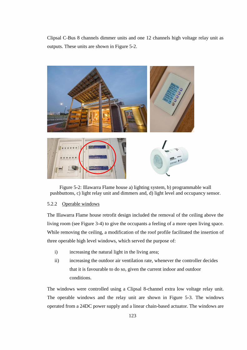
123

Clipsal C-Bus 8 channels dimmer units and one 12 channels high voltage relay unit as

outputs. These units are shown in Figure 5-2.

Figure 5-2: Illawarra Flame house a) lighting system, b) programmable wall

pushbuttons, c) light relay unit and dimmers and, d) light level and occupancy sensor.

5.2.2 Operable windows

The Illawarra Flame house retrofit design included the removal of the ceiling above the

living room (see Figure 3-4) to give the occupants a feeling of a more open living space.

While removing the ceiling, a modification of the roof profile facilitated the insertion of

three operable high level windows, which served the purpose of:

i) increasing the natural light in the living area;

ii) increasing the outdoor air ventilation rate, whenever the controller decides

that it is favourable to do so, given the current indoor and outdoor

conditions.

The windows were controlled using a Clipsal 8-channel extra low voltage relay unit.

The operable windows and the relay unit are shown in Figure 5-3. The windows

operated from a 24DC power supply and a linear chain-based actuator. The windows are

124

operated in a drive-open and drive-closed manner with only two positions, i.e. fully

open and fully closed. Controlling the windows in the intermediate positions can be

achieved by timing the control input, but this was not part of the research presented in

this thesis.

Figure 5-3: a) Operable high level windows and b) extra low voltage relay unit.

5.2.3 HVAC control

The HVAC system had to control the airflow in a ducted system, direct the air into

various flow-paths, and control the amount of air flowing in the system. A schematic of

the system presented in Figure 3-7, Chapter 3, shows the dampers and fans which were

the key components to be controlled.

Dampers

Most of the dampers were to be controlled in fully open or closed positions, and these

are, referring to Figure 3-7, D1, D2, D4, D6 and D7. Dampers D3 and D5 were for

modulating the fresh air intake to the system and had to be controlled continuously from

fully open to fully closed. The construction of the dampers was the same (rectangular

blade dampers, single or double blade), with different sizes depending on the location of

the damper in the ducting. The actuators for the operation of the dampers were either

drive-open or drive-close for the on/off dampers, or variable position actuator controlled

via a 0-10V signal for the variable dampers. In both cases the selected product was a

Belimo actuator, the non-spring return NMU24 for the on/off dampers and the variable

non-spring return CMU24 for the variable dampers (Figure 5-4). The control units for

125

these actuators were a Clipsal 8-channel extra low voltage relay unit and a 4-channel 0-

10V analogue output unit.

Figure 5-4: a) Single and double blade dampers, Belimo NMU and CMU actuators, b)

Clipsal Low voltage relays and 0-10V analogue output units.

Fans

One of the most important controlled variables that affected the performance of this

solar-assisted HVAC system was the airflow rate, which has to be optimised in real time

to maximise the efficiency of the system. The fans chosen in the design stage were

Fantech PCD354DD centrifugal fans, with a 3-phase motor and maximum power

absorption of 370 W. To dynamically control the airflow rate, the fans were driven by

Vacon VP10VSD Variable Speed Drives (Figure 5-5).

Figure 5-5: a) Fantech PCD354DD Centrifugal fan and b) Vacon VP10VSD Variable

speed drives.

126

The VSDs require two inputs from the control infrastructure, i.e. an on/off activation

signal, and a 0-10V signal, to control the variable output frequency. From a control

infrastructure perspective, these tasks were achieved using two of the channels of the

Clipsal extra low voltage relay units and the two free channels of the Clipsal 0-10V

analogue output unit, as presented in Figure 5-4.

5.2.4 Sensors, power distribution and monitoring and Non-Priority Line

A number of sensors were installed and integrated into the control system of Illawarra

Flame house, including indoor and HVAC temperature sensors, HVAC air velocity

sensors and a weather station to monitor outdoor temperature and solar radiation. The

power distribution was divided into 12 sub-circuits and each monitored using current

transformers. Some of these sub-circuits were grouped in a common non-priority line,

which can be disconnected by a contactor when the occupants leave the house.

Indoor temperature sensors

Indoor air temperatures were monitored using five Clipsal wall temperature sensors,

located in each room of the house. The locations of the temperature sensors on the floor

plan are presented in Figure 5-6. Each sensor was calibrated using a common reference,

i.e. a hand held Testo digital thermometer.

127

Figure 5-6: House floorplan – Temperature sensors location and Clipsal wall

temperature sensor.

HVAC temperature and air velocity sensors

Temperatures in the ductwork were measured using Clipsal C-Bus Digital Temperature

Sensor Units 5104DTSI with a stated accuracy of ±0.5°C in the temperature range

of -10 to 80°C. A total of 8 temperature sensors were located in various sections of the

HVAC system, as shown in Figure 5-7. Two of the temperature sensors were placed in

two of the PCM bricks, one in the first and the other in the last row, to measure the

average temperature and therefore the charge level of the PCM storage unit.

T

T

T

T

T

128

Figure 5-7: Locations of HVAC temperature and air velocity sensors.

Airflow was monitored using Siemens QVM62.1 air velocity sensors, located one third

of the duct height from the duct centreline. These sensors had a stated accuracy of ±0.2

m/s + 3% of measured values. The signals from these sensors were collected by the

Clipsal control system via Clipsal 4-channel general input units, which accepted 0-10V

inputs. These units are presented in Figure 5-8.

Figure 5-8: a) Clipsal Digital temperature sensor units, b) Siemens air velocity sensor

and general input units.

Power distribution, monitoring and Non-Priority Line

In order to be able to accurately evaluate the power consumption of the house, 240-volt

wiring was divided into 12 sub-circuits, each of being individually protected and

monitored via a current transformer linked to the Clipsal BMCS (Figure 5-9).

This sub-monitoring individually tracked the consumption of the lighting system, air

conditioner, fans, control system, power points (divided into 4 subgroups), oven,

T = Temperature sensor

V= Air Velocity sensor

T

T T

T T

T

T T

V

V

129

cooktop and low voltage equipment (such as dampers and operable windows). The

consumption of the various sub-circuits was then displayed on the touchscreen user

interface, to provide the occupants with feedback on the way they used electrical energy

in the house.

Some of the sub-circuits were grouped in a common ‘Non-Priority Line’, which could

be disconnected via a 32A contactor when the occupants leave the house (Figure 5-9).

The contactor was controlled by a spare relay channel of the 12-channel high voltage

relay unit.

Figure 5-9: Distribution board, Clipsal current measurement units and Non-Priority Line

contactor.

5.2.5 User interface and weather station

The Clipsal user interface was a 6.4 Inch colour touchscreen with customised

programing. A screenshot of the main screen of the user interface developed by the

present author is presented in Figure 5-10. This interface provided the user with

information on the house temperatures and the active operating mode. It also allowed

the user a choice of either automatic (using the MPC strategy) or manual control of the

thermal conditions in the house. The user was able to define the comfort target, and the

controller then decided, in real time, the best operating mode (or the best sequence of

operating modes) to maximise the efficiency of the system.

Clipsal current measuring units

Electrical sub-distribution board

Non-Priority Line contactor

130

Figure 5-10: Illawarra Flame house user interface.

The user was also provided with instantaneous measurements from the weather station

and the sensor placed in the HVAC system as shown in Figure 5-7.

The interface allowed the user to control the various lighting groups individually and

receive feedback from the occupancy and light level sensors. A page dedicated to

energy consumption and generation presented the overall daily and instantaneous

generation and consumption, together with a detailed breakdown of the consumption of

the various sub-circuits.

The C-Bus logic (in Pascal) was programmed into the screen, which also acted as a

local controller. The weather station (Figure 5-11) was a Davis Vantage Pro II with a

wireless Weather Envoy, connected via RS232 to the C-Bus Touch screen. This

monitored ambient temperature, humidity, global horizontal radiation, wind speed, wind

direction and rainfall.

Figure 5-11: Davis Vantage Pro II weather station installed on the Illawarra flame

house.

131

The screen was programmed to decode the messages from the serial port and convert

them to data-points to be used for the control logic of the house.

5.2.6 Interfacing with JACE controller

The JACE controller was equipped with C-Bus drivers that were capable of interacting

with most of the C-Bus units. The JACE controller accessed the C-Bus network via an

Ethernet Network Interface (C-Bus CNI unit) to read and control the C-Bus units data-

points (Figure 5-12). Unfortunately not all of the C-Bus units were compatible with

these drivers, and therefore a simple “gateway” using C-Bus bus couplers was

developed to hold the signals from non-compatible units, and allow the JACE controller

to read and write on those as well. Each bus coupler had 4 channels and 4 LED

indicators, and these were used to write and read a virtual data-point level for a total of

8 signals on each bus coupler. These were used to both integrate non-compatible units

with the C-Bus drivers for the JACE controller and integrate control signals and

variables from the C-Bus touchscreen controller with the JACE controller.

Figure 5-12: a) C-Bus CNI network interface and b) C-Bus Bus Couplers.

A more detailed diagram of the whole C-Bus network is presented in Figure 5-13.

132

Analogue Output Units

Extra Low Voltage Relay

Units

High Voltage Relay Units

Dimmer Units

Current Measurement

units

Wall Temperature

Sensors

Digital Temperature

Sensors

Wall Pushbuttons

General Input units

Occupancy and light level sensors

Bus CouplersColour

TouchscreenCNI Ethernet

PAC Pascal controller

Weather Station

Wireless Envoy

JACE 6 Controller

Dampers position Dampers power Windows open/close AHU on/off VSDs start/stop

Non Dimmable lights Non-Priority line

contactor

Dimmable lights VSDs frequency control

Variable dampers position

Indoor temperatures

PVT outlet PCM inlet/outlet PCM bricks AHU inlet/outlet Return air

Light groups control

Windows control

Air velocity sensors

Feedback from VSDs and variable dampers

Indoor occupancy and light levels

PV1/PV2 Generation

Consumption submonitoring

C-Bus CAT-5

Ethernet

RS-

232

Figure 5-13: C-Bus network diagram.

133

5.3 Niagara JACE Controller

A Tridium Niagara JACE 6 controller for high level control and data logging of the

system data-points was used in Illawarra Flame house.The controller was connected

to three different networks:

i) The University of Wollongong intranet network via its Ethernet port 1.

(The JACE controller was also linked through this network with another

JACE machine running on a server at the Sustainable Buildings Research

Centre, which could store a larger amount of information).

ii) The C-Bus network, via Ethernet Port 2. (Dedicated C-Bus drivers were

installed on the JACE controller to communicate with the compatible C-

Bus units).

iii) A Modbus Network on the RS485 port, used to control the LG air

conditioning unit via an IntesisBox Gateway. (This allowed simultaneous

or exclusive control of the LG unit via either the LG wall controller

and/or the Modbus network inputs).

These devices are shown in Figure 5-14.

Figure 5-14: JACE controller and IntesisBox Modbus-LG Gateway

5.3.1 Summary of data-points linked to C-Bus units for control

A number of data-points from the low level C-Bus system were linked to the JACE

controller, as inputs or as controllable variables. These data-points are summarised in

To LG air conditioning unit

Modbus RS485

To Clipsal CNI – C-Bus network

To UOW network

134

Table 5-1 and could be either only readable or both readable and writeable, and they

could be Numeric (N), Boolean (B), or Enumerable (E).

Table 5-1: Summary of JACE – C-Bus signals

Signal Description Read/Write Type oBIX

T1, T2, T3, T4, T5 Indoor Temperatures Read N

T_PVT PVT outlet temperature Read N

T_PCM1, T_PCM2 PCM material temperatures Read N

T_PCMduct1, T_PCMduct2 Air temperature in ducting before and after PCM unit

Read N

T_AHU1, T_AHU2, T_RET Air temperature before and after AHU, and return air

Read N

T_Setpoint Set point temperature in manual control

Read/Write N

T_Out Outdoor temperature from weather station

Read N

Ghr Global horizontal radiation from weather station

Read N

WindSpeed Wind speed from weather station Read N

Flow_PVT, Flow_PCM Airflow rate from the two air velocity sensors

Read N

Direct_PVT, PCM_ Discharging, Normal_Conditioning, PCM_Charging, Off_mode

Boolean variables that activate the corresponding C-Bus scene that sets the dampers to achieve the desired flow path

Read/Write B

PCM_Fan, PVT_Fan Fan speed (percentage for VSD) Read/Write N

Windows_open, Windows_close

Boolean variables to control the windows operation

Read/Write B

P_TOT, P_HP, P_Fans Total power consumption, Heat pump power consumption and fans power consumption

Read N

PV1, PV2 PV generation of array 1 and array 2

Read N

AM, HM, CM User request for Auto mode, Manual Heating mode, Manual Cooling mode

Read B

135

5.3.2 Data-points on Modbus network for LG air conditioner control

The JACE controller interacted with the LG unit via the IntesisBox Gateway,

connected to the JACE via a Modbus network. A summary of the controlled data-

points is presented in Table 5-2.

Table 5-2: Summary of JACE – LG unit signals

Signal Description Read/Write Type oBIX

On_Off Unit ON/OFF Read/Write B

Unit_mode Unit operation mode (heating, cooling, auto, ventilation, dehumidification

Read/Write E

Fan_speed Fan speed Read/Write E

T_set AC unit setpoint Read/Write N

Indoor_reference_temp Indoor unit reference temperature

Read N

5.3.3 oBIX network for Matlab interface

oBIX (for Open Building Information Exchange) is a standard for RESTful Web

Services-based interfaces to building control systems. oBIX is a framework designed

for building automation that allows reading and writing data over a network of

devices. In this research it was utilised to generate live communication between a

Matlab control script and the JACE controller. A summary of the signals that the

JACE controller shared on the oBIX network is presented in Table 5-1 and Table

5-2.

5.4 Matlab HMPC Controller

The Hybrid MPC controller was implemented in Matlab via a script that dynamically

interacted with the JACE controller. A number of functions developed by the present

author, based on the models previously presented in this thesis, utilise the current and

historical data-points to predict the future inputs to the system and therefore calculate

the optimal set of control actions for the HVAC system. The dynamics of the Mixed

Logical Dynamical system were formulated in the HYSDEL language (Torrisi &

Bemporad 2004) and then optimised using the Hybrid Toolbox for Matlab

(Bemporad 2012) and implemented on a DELL XPS13 Laptop, with an intel i5

136

processor and 4GB of RAM (Figure 5-15). The optimisation package used to solve

the MILP problem was Gurobi.

Figure 5-15: University of Wollongong DELL XPS13 Laptop – Matlab and HMPC

machine

5.4.1 oBIX network interface

The Matlab script was interfaced to the JACE controller using an oBIX network

interface developed by CSIRO researchers from the Newcastle Energy Centre. This

interface allowed Matlab to communicate with an oBIX device and override the data-

points on the network, sending control signals with the highest priority level on to the

JACE device, using the credential of the Niagara station administrator active on the

JACE. The data-points to be controlled were identified by their address on the JACE

station. This allowed the Matlab script to take full control the system while the

HMPC was active, and when deactivated the rule-based logic of the JACE re-gained

control of the system.

137

6 HYBRID MODEL PREDICTIVE CONTROL FORMULATION

This chapter introduces the development, formulation and implementation of Hybrid

Model Predictive control of the solar assisted HVAC system developed for the

Illawarra Flame Solar Decathlon house. The Hybrid Model Predictive Controller was

developed based on a Mixed Logical Dynamical (MLD) approach. Building

modelling, system identification procedures and the introduction of HVAC

components in the state-space models for the MPC formulation are presented.

6.1 Control chain structure

Given the complexity of the problem to be solved, the HMPC control strategy was

divided into a high-level HMPC controller and multiple low-level HMPC controllers.

A schematic of the control system structure is presented in Figure 6-1. The control

problem was divided into two levels to ensure that the optimal solution was

computed within the desired control time step of 5 minutes for each low level

controller, and half an hour for the high level controller. The author also tried to

implement a single optimisation for the whole problem, but found it was not feasible

due to the necessity of finding the optimal solution within each control time step. The

house BMCS, which consists of a C-Bus based system and a JACE controller,

collects the data from the sensors and the various devices on the network.

Figure 6-1: Control chain structure.

138

The information collected from the weather station is used for the weather forecast

and the prediction of the future PVT outlet temperature and its potential useful

thermal generation together with the system states, which are then used to compute

the optimal control action generated by the HMPCs. The first set of actions from the

optimal control sequence is then sent to the BMCS to control the individual

components and HVAC equipment.

The high-level HMPC computes the optimal solution with a control step of 1 hour

and a prediction horizon of 24 hours. The objective of the high-level HMPC is to

compute the optimal sequence of the operating modes of the innovative HVAC

system presented in Chapter 3 using an object cost function.

Once the high-level HMPC has selected the operating modes for the next hour, the

corresponding low-level HMPC controller is then activated. The objective of the

low-level HMPC controller is to optimize the particular operating mode for the time

period of concern, considering the range of fan speeds to be utilized for the PVT and

PCM store, for example. The low-level HMPC computes the optimal solution with a

control step of 5 minutes and a prediction horizon of 1 hour. Once the optimal

sequence of control actions has been computed, the first set of actions is then sent to

the JACE controller and applied to control the operation of the HVAC system

(Figure 6-2).

The use of HMPC for low level controllers is necessary to optimise the operation of

the mode selected. While the time lag of the system becomes less important, since

the low level controllers are only fed with the forecast of the weather one hour ahead,

utilisation of HMPC algorithms is crucial because of their optimisation capability,

which guarantees the selection of the best performing discrete and continuous time

variables in the defined time frame. A classic PID controller, for example, would not

be capable of optimising the heating source selection (PVT fan speed with a limited

heat delivery at a weather-dependent performance in conjunction with the operation

of the heat pump) while following an indoor temperature trajectory.

The same issue would appear when the low level controller has to operate the switch

between the heat pump and the operable windows.

139

Figure 6-2: Schematic of control system architecture.

6.2 Building Modelling and System Identification

The HMPC control strategy was developed based on a grey-box model. The

parameters of this model were estimated using the datasets of the system in its

various configurations, forcing the building with intermittent heating or cooling, and

using the average temperature of the building as the thermal response. The building

was therefore treated as a single zone. The estimation of the building parameters was

performed using a nonlinear least-square fit method.

The building was to operate in two main modes, i.e. with mechanical ventilation

(when the high level windows were completely closed), and natural ventilation (high

level windows fully open). In order to keep the system linear and easily identifiable,

natural ventilation was modelled as simply resulting in a different building

infiltration rate. The model for the natural ventilation was identical to the one with

the building with the windows closed, the only different parameter being the

infiltration resistance Rvo. The R-C model that represented the building is presented

in Figure 6-3.

140

Figure 6-3: Building Zone Thermal Model Schematic.

In this model, the states are Ti - average inside temperature (measured) and Tw -

equivalent wall temperature; the measured disturbances are Ta - ambient temperature

(measured) and Ψ – global horizontal radiation (measured); the controlled variables

are the Boolean switch δnv, that determines if the system is in mechanical ventilation

or natural ventilation, and Φh which is the heating input to the building, that can be

supplied using different sources.

The parameters subject to identification are Rw - equivalent half wall resistance, Rv -

infiltration equivalent resistance with windows closed, Rvo - infiltration equivalent

resistance with windows open, Ci - equivalent internal capacitance, Cw - equivalent

wall capacitance, Aw - equivalent windows area and – Ae equivalent external wall

area.

The system dynamics are described by the state-space relationships:

�̇�(𝑡) = 𝐴𝑥(𝑡) + 𝐵𝑢(𝑡) (6.1)

𝑦(𝑡) = 𝐶𝑥(𝑡) + 𝐷𝑢(𝑡) (6.2)

Where the state vector is x = [Ti, Tw]T , the input vector is u = [Ta, Ψ, Φh ]

T and the

time invariant matrices are:

𝐴 = [− (

1

𝑅𝑤∙𝐶𝑖+

1

𝐶𝑖∙𝑅𝑣)

1

𝑅𝑤∙𝐶𝑖

1

𝑅𝑤∙𝐶𝑤−(

2

𝑅𝑤∙𝐶𝑤)] 𝐵 = [

1

𝐶𝑖∙𝑅𝑣

𝐴𝑤

𝐶𝑖

1

𝐶𝑖

1

𝐶𝑤∙𝑅𝑤

𝐴𝑒

𝐶𝑤0] (6.3)

ψAw Cw

Rw Rw

Ta

Tw

ψAe Φh

Rvo δnv

Ci

Ti Rv

141

𝐶 = [1 0] 𝐷 = [0 00 0

] (6.4)


closed)

The building parameters had to be identified using a number of datasets from the real

operation of the building, where the indoor temperature was forced intermittently

using the PVT system, PCM unit or the air conditioning system. In the first case, the

heating introduced in the building was calculated as:

𝛷𝑃𝑉𝑇 = 𝜌�̇�𝑐𝑝(𝑇𝑝𝑣𝑡,𝑜 − 𝑇𝑖) (6.5)

𝛷𝑃𝐶𝑀 = 𝜌�̇�𝑐𝑝(𝑇𝑃𝐶𝑀,𝑜 − 𝑇𝑖) (6.6)

Where ρ is the air density at 20˚C, �̇� is the volume flow rate, cp is the specific heat

capacity of the air at 20˚C, and Tpvt,o is the PVT outlet temperature.

In the second case, since the heating or cooling input of the heat pump was not

directly measurable in the house setup, it was considered to be proportional to the

electrical consumption of the air conditioning unit (Φc,el), following the relationship:

𝛷𝐻𝑃 = 𝜂𝐻𝑃𝐶𝑂𝑃̅̅ ̅̅ ̅̅ 𝛷𝑐,𝑒𝑙 (6.7)

Where the average coefficient of performance 𝐶𝑂𝑃̅̅ ̅̅ ̅̅ was a known coefficient derived

from the specifications of the manufacturer and 𝜂𝐻𝑃 is an identifiable parameter. The

COP of the air conditioning unit was considered to be constant to simplify the

control problem, considering that the target of the controller was to optimise the

system as a whole, guaranteeing that the potentially more efficient energy sources

operated at a higher efficiency than the average one of the heat pump.

The simplified model used did not fully describe the real dynamics of a heat pump,

and it was utilised in this form to reduce the model complexity for the online

computation of the optimal solution. This simplification slightly affected the

operation of the heat pump, but the objective of this study was still fulfilled, i.e. that

the renewable energy sources operate at a higher efficiency than the average one of

the heat pump.

The effect of including a more detailed model of the heat pump in the MPC

formulation would be to give a more efficient delivery of its thermal energy, leading

142

to a further benefit in terms of general efficiency, as others have previously presented

in their studies on the optimisation of the operation of a heat pump using predictive

controllers.


The only parameter that changes in the natural ventilation mode, compared to

mechanical ventilation, is Rvo - infiltration equivalent resistance with windows open.

To quantify this parameter, the identification process was repeated using a dataset

where the operable windows have been constantly fully open. In this case, the

parameters already identified have been kept fixed, leaving only Rvo free.

6.3 Modelling of Solar-PVT Assisted HVAC system

6.3.1 PVT system and PVT Direct Supply

As described in Chapter 3, the relationship that describes the heat transfer and allows

the control system to compute the predicted outlet temperature of the PVT system

depending on the various weather conditions and the different airflow rates is of the

form:

𝑇𝑝𝑣𝑡,𝑜 = (𝑇𝑎𝑚𝑏 −𝐵

𝐴) 𝑒−𝐴𝑥 +

𝐵

𝐴 (6.8)

The heating that the PVT system can supply to the building is then determined by

Equation (6.9).

𝛷𝑃𝑉𝑇 = 𝜌�̇�𝑐𝑝(𝑇𝑝𝑣𝑡,𝑜 − 𝑇𝑖) (6.9)

6.3.2 PCM Thermal Storage unit and PCM Discharging

To effectively include the PCM storage dynamics into the HMPC formulation, the

heat exchange in the unit and the equivalent capacitance of the material have to be

modelled. As presented in Chapter 3, assuming that the wall temperature of each

channel is constant along the total length of the heat exchanger, the relationship that

describes the heat exchange is:

𝑇𝑝𝑐𝑚,𝑜 = 𝑇𝑝𝑐𝑚 − (𝑇𝑝𝑐𝑚 − 𝑇𝑖𝑛)𝑒(−

𝑝𝑒𝑟ℎ̅ 𝐿

�̇�∙𝜌∙𝑐𝑝) (6.10)

143

Where Tpcm,o is the average temperature of the air at the length L of the channel (the

outlet), Tpcm is the surface temperature of the channel, equivalent to the measured

PCM temperature, Tin is the inlet air temperature, per is the perimeter of the channel,

and ℎ̅ is the average internal convective heat transfer coefficient.

The heating that the PCM storage unit can supply to the building is equal to:

𝛷𝑃𝐶𝑀 = 𝜌�̇�𝑐𝑝(𝑇𝑝𝑐𝑚,𝑜 − 𝑇𝑖) (6.11)

The equivalent thermal capacitance of the PCM unit was calculated by interpolating

the results from the tests conducted at the Fraunhofer - Institut Für Solare

Energiesysteme in Freiburg. The test was conducted using a differential scanning

calorimeter (DSC), applying a cooling and heating rate of 0.01K/min to a

temperature range of 0-40°C. The equivalent thermal capacitance was divided into

three ranges, when the material was completely solid (Cpcm,s), when it was changing

phase (Cpcm,c), and when was is completely liquid (Cpcm,l),.

Figure 6-4: PCM equivalent thermal capacitance.

Applying a linear fit to the ranges of 0-19°C, 20-24°C and 25-40°C, the equivalent

capacitance for the entire PCM unit was calculated, resulting in Cpcm,s=0.40kWh/°C

0 5 10 15 20 25 30 35 40

-250

-200

-150

-100

-50

0

50

Temperature (C)

Enth

alp

y (

J/g

)

Interpolation

DSC cooling

DSC heating

144

for the solid range, Cpcm,c=5.10kWh/°C for the changing phase range and

Cpcm,l=0.57kWh/°C for the liquid range.

For the implementation in the HMPC, the melting range was extended to include the

transition areas, to a wider range 19-25°C, as represented in Figure 6-4.

6.3.3 PCM Charging with PVT

The PCM Charging mode is linked directly with the dynamics of PVT system and

the PCM unit. The amount of heat stored is therefore dependent on the relationships

of Equations (6.8) and (6.10), presented in the previous sections.

The total heat stored in the PCM unit is equal to:

𝛷𝐶ℎ𝑎𝑟𝑔𝑒𝑑 = 𝜌�̇�𝑐𝑝(𝑇𝑝𝑣𝑡,𝑜 − 𝑇𝑝𝑐𝑚,𝑜) (6.12)

6.4 Energy consumption of the HVAC components

Knowing the energy consumption of the system components in each operating mode

was necessary to compute the optimal solution of the controller, allocating a cost for

each energy source.

Identification of the electrical consumption versus air flow characteristics was key

aspect of the optimisation of each operating mode that involves the PVT system or

the PCM unit. The fit used was a 3rd

order polynomial of the form:

𝑃𝑓𝑎𝑛 = 𝛾𝑃𝑉𝑇_𝑆𝑢𝑝𝑝𝑙𝑦 V̇3 (6.13)

6.5 System Model and Control

It is easy to notice that the linear model used for the system identification becomes

non-linear as soon as it is attempted to model the whole system.

The system can operate in three different conditioning modes and two PVT modes.

Some of these modes cannot operate together (e.g. PCM Charging and PCM

Discharging) because of the physical constraints.

It was therefore required to introduce Boolean variables that are able to switch the

different operating modes according to defined logical constraints, in order to not

have two or more conflicting modes active at the same time.

145

Some of the operating modes, such as PVT Direct Supply and PCM Discharging, are

intrinsically bilinear. The controlled variable �̇� is multiplying one of the states, Ti.

Even considering the outlet temperature of the PVT system or the outlet temperature

of the PCM unit constant, the resulting system would be of the form:

�̇�(𝑡) = 𝐴𝑥(𝑡) + 𝐵𝑢(𝑡) + 𝑁𝑥(𝑡)𝑢(𝑡) (6.14)

Another problem to overcome in the formulation of the MPC problem is the fact that

the relationships among the PVT outlet temperature and the PCM unit outlet

temperature and the airflow rate are nonlinear.

6.6 Formulation of the Hybrid MPC Problem

One of the possible solutions to the number of issues described is the formulation of

the problem as a Hybrid Model Predictive Control problem. By definition, this type

of formulation can deal with continuous dynamics and discrete variables, finding the

optimal solution through solving a mixed integer linear or quadratic programming

problem.

In particular it is possible to describe this problem as a Mixed Logical Dynamical

(MLD) System, a class of hybrid systems has been introduced in which logic,

dynamics and constraints are integrated, of the form:

𝑥(𝑘 + 1) = 𝐴𝑥(𝑘) + 𝐵1𝑢(𝑘) + 𝐵2𝛿(𝑘)+𝐵3𝑧(𝑘) (6.15)

𝑦(𝑘) = 𝐶𝑥(𝑘) + 𝐷1𝑢(𝑘) + 𝐷2𝛿(𝑘)+𝐷3𝑧(𝑘) (6.16)

𝐸2𝛿(𝑘) + 𝐷3𝑧(𝑘) ≤ 𝐸1𝑢(𝑘) + 𝐸4𝑥(𝑘) + 𝐸5 (6.17)

Where 𝑥(𝑘) = [𝑥𝑐(𝑘)

𝑥𝑙(𝑘)] is the state vector 𝑥𝑐(𝑘) ∈ ℝ𝑛𝑐

and 𝑥𝑙(𝑘) ∈ {0,1}𝑛𝑙 , 𝑦(𝑘) =

[𝑦𝑐(𝑘)

𝑦𝑙(𝑘)] ∈ ℝ𝑝𝑐 × {0,1}𝑝𝑙 is the output vector, 𝑢(𝑘) = [

𝑢𝑐(𝑘)

𝑢𝑙(𝑘)] ∈ ℝ𝑚𝑐 × {0,1}𝑚𝑙 is

the input vector, 𝑧(𝑘)∈ ℝ𝑟𝑐 and 𝛿(𝑘) ∈ {0,1}𝑟𝑙 are the auxiliary variables, A, Bi, C,

Di and Ei denote real constant matrices, E5 is a real vector, nc > 0, and pc, mc, rc, nl,

pl, ml, rl ≥ 0.

In order to take into account future samples of the reference vector and measured

disturbance, the prediction model has to be augmented with an additional linear

146

model and to treat the vector of future references and measured disturbances as

additional states (Bemporad 2006).

Writing the problem as a MLD system with discrete fan speeds, removes the

difficulty of the aforementioned problems. This results in a number of linear systems

that can be activated by Boolean variables. For each of them the cost is fixed at the

energy used by the fan at the selected discrete speed step with the addition of the

consumption of the heat pump.

Given the number of Boolean variables and the requirement to compute the solution

in a relatively short amount of time (e.g. 5 minutes), the controller was divided into

two levels, a high level controller that selects the operating mode every hour, and

three lower level controllers that optimize the operation of each operating mode

every five minutes.

Each controller has to minimise a cost function of the form:

𝑚𝑖𝑛{𝑢,𝑑,𝑧}0𝑁−1𝐽({𝑢, 𝑑, 𝑧}0

𝑁−1, 𝑥(𝑡)) ≜ ∑ ‖𝑄𝑥(𝑥(𝑘) − 𝑥𝑟)‖𝑝𝑁−1𝑘=1 + ∑ ‖𝑄𝑢(𝑢(𝑘) −𝑁−1

𝑘=1

𝑢𝑟)‖𝑝 + ∑ ‖𝑄𝑧(𝑧(𝑘) − 𝑧𝑟)‖𝑝 + ∑ ‖𝑄𝑦(𝑦(𝑘) − 𝑦𝑟)‖𝑝

𝑁−1𝑘=1 + ‖𝑄𝑥𝑁(𝑥(𝑁|𝑡) −𝑁−1

𝑘=1

𝑥𝑟)‖𝑝 (6.18)

The values and the parameters included in the cost function vary from controller to

controller. For this study the infinity norm was used, with p = ∞.

6.7 High Level Controller

The main purpose of the High Level Controller is to determine the operating mode in

which the system is to operate. To maintain the problem relatively simple and

minimise the number of Boolean optimisation variables, each mode was considered

to operate at its nominal conditions (e.g. fan speed for PVT Direct Supply and PCM

Charging mode is considered to be at 80% of the VSD range, which corresponds to a

flow rate of approximately 300 L/s).

147

Figure 6-5: High Level Controller system schematic.

The states of the High Level Controller, the measured disturbances and the controlled

variables are summarised in Table 6-1, Table 6-2 and Table 6-3, respectively.

The resistances Rm1j and Rm2j, represent the heating and cooling delivery to the

building using the nominal air mass flow rates of mode 1 – PVT Direct Supply and 2

– PCM Discharging, and Rex,j represents the heat exchange rate into the PCM unit at

the nominal air flow rate.

Table 6-1: HMPCs states.

State Description High Level

Low Level 1

Low Level 2

Low Level 3

Ti average inside temperature

(measured)

Tw equivalent wall temperature

(estimated)

Tpcm average PCM temperature (measured)

ψAw Cw

Rw Rw

Ta

Tw

ψAe Φhp

δnv

Ci

Ti Rv

Φig

Tpvt,j Cpcm

Rm1,j Rex,j

Rm2,j

Rpcm

δm1 δm2 δc

Tpcm

Rvo

148

Table 6-2: HMPCs measured disturbances.

Measured Disturbance

Description High Level

Low Level 1

Low Level 2

Low Level 3

Ta ambient temperature

Ψ global horizontal radiation

Φig Internal loads

Tpvt,j PVT calculated outlet

temperature at fan speed j

Table 6-3: HMPCs controlled variables.

Controlled variable

Description High Level

Low Level 1

Low Level 2

Low Level 3

Ε constraint softening on

indoor temperature

Φhp thermal input to the

building provided by the heat pump

δm1j PVT Direct Supply (at fan

speed j in low level controllers)

δm2j PCM Direct Supply (at fan

speed j in low level controllers)

δc PCM Charging mode

δnv Natural ventilation mode

δhp Heat pump active

(minimum heat delivery)

6.7.1 MLD – High Level Controller

The first logical condition at which the system described by the high level controller

is subject is the temperature of the PCM. As described earlier in this chapter, the

PCM is characterised by three equivalent capacitances, depending on the temperature

of the PCM material, equal to Cpcm,s for the solid temperature range, Cpcm,c for the

changing phase temperature range and Cpcm,l for the liquid temperature range.

Given Tmelt,t and Tmelt,b the higher and lower temperature limits of the phase change

range, the equivalent capacity at each time step k equals to:

149

𝐶𝑝𝑐𝑚(𝑘) = {

𝐶𝑝𝑐𝑚,𝑠 𝑖𝑓 𝑇𝑝𝑐𝑚 < 𝑇𝑚𝑒𝑙𝑡,𝑏

𝐶𝑝𝑐𝑚,𝑐 𝑖𝑓 𝑇𝑚𝑒𝑙𝑡,𝑏 ≤ 𝑇𝑝𝑐𝑚 ≤ 𝑇𝑚𝑒𝑙𝑡,𝑡

𝐶𝑝𝑐𝑚,𝑙 𝑖𝑓 𝑇𝑝𝑐𝑚 > 𝑇𝑚𝑒𝑙𝑡,𝑡

The forecast of the next 24h of the measured disturbances Ta , Ψ, and the calculated

outlet temperature of the PVT at the fan speed j, Tpvt,j, are provided to the controller.

The Boolean variables switch among the four linear subsystems. Considering the

state vector to be x = [Ti, Tw,Tpcm]T the following possible cases can be selected:

1. in the case where the switch δm1 is closed, the PVT direct mode is

activated; the input vector is u = [Ta, Ψ, Φh,, Tpvt,j ]T

and the system

matrices are:

𝐴𝐻 =

[ − (

1


1

𝐶𝑖∙𝑅𝑣+

1

𝑅𝑚1,𝑗∙𝐶𝑖)

1

𝑅𝑤∙𝐶𝑖0

1

𝐶𝑤∙𝑅𝑤−(

1

𝐶𝑤∙𝑅𝑤+

1

𝑅𝑤∙𝐶𝑖) 0

0 0 −1

𝑅𝑝𝑐𝑚∙𝐶𝑝𝑐𝑚]

𝐵𝐻 =

[

1

𝐶𝑖∙𝑅𝑣

𝐴𝑤

𝐶𝑖

1

𝐶𝑖

1

𝑅𝑚1,𝑗∙𝐶𝑖

1

𝐶𝑤∙𝑅𝑤

𝐴𝑒

𝐶𝑤0 0

1

𝑅𝑝𝑐𝑚∙𝐶𝑝𝑐𝑚0 0 0

]

(6.19)

2. in the case where the switch δm2 is closed, the PCM Discharging mode is

activated; the input vector is u = [Ta, Ψ, Φh, ]T and the system matrices

are:

𝐴𝐻 =

[ − (

1


1

𝐶𝑖∙𝑅𝑣+

1

𝑅𝑚2,𝑗∙𝐶𝑖)

1


1


1


1


0 0 −1

𝑅𝑝𝑐𝑚∙𝐶𝑝𝑐𝑚+

1

𝑅𝑚2,𝑗∙𝐶𝑖]

𝐵𝐻 =

[

1

𝐶𝑖∙𝑅𝑣

𝐴𝑤

𝐶𝑖

1

𝐶𝑖

1

𝐶𝑤∙𝑅𝑤

𝐴𝑒

𝐶𝑤0

1

𝑅𝑝𝑐𝑚∙𝐶𝑝𝑐𝑚0 0

]

(6.20)

3. in the case where the switches δm1 , δm2, δnv are all open, the system is set

in Normal Conditioning mode; the input vector is u = [Ta, Ψ, Φh ]T and

the system matrices are:

150

𝐴𝐻 =

[ − (

1


1


1


1


1


1


0 0 −1

𝑅𝑝𝑐𝑚∙𝐶𝑝𝑐𝑚]

𝐵𝐻 =

[

1

𝐶𝑖∙𝑅𝑣

𝐴𝑤

𝐶𝑖

1

𝐶𝑖

1

𝐶𝑤∙𝑅𝑤

𝐴𝑒

𝐶𝑤0

1


]

(6.21)

If the switch δnv is closed and therefore the natural ventilation is selected,

the resistance Rv is substituted by Rvo.

If the switch δc is closed, the system is charging the PCM unit, the input

vector is u = [Ta, Ψ, Φh,, Tpvt,j ]T, the resistance Rm1,j =

1

ρc𝑝V̇𝑗, and the

matrices are:

𝐴𝐻 =

[ − (

1


1


1


1


1


1


0 0 −(1

𝑅𝑝𝑐𝑚∙𝐶𝑝𝑐𝑚+

1

𝑅𝑚1,𝑗∙𝐶𝑝𝑐𝑚)]

𝐵𝐻 =

[

1

𝐶𝑖∙𝑅𝑣

𝐴𝑤

𝐶𝑖

1

𝐶𝑖0

1

𝐶𝑤∙𝑅𝑤

𝐴𝑒

𝐶𝑤0 0

1


1

𝑅𝑚1,𝑗∙𝐶𝑝𝑐𝑚]

(6.22)

Considering the cost function in equation (6.18), in this controller, the matrices Qx

and QxN are equal to 0 since there is no cost directly associated with the states, as

well as the auxiliary variables matrix Qz and output matrix Qy. The continuous time

input variables vector is:

𝑢𝑐(𝑘) = [휀(𝑘), Φℎ𝑝(k)] (6.23)

The matrix of the costs associated with this input is:

𝑄𝑢,𝑐 = [𝐶휀 00 𝐶Φℎ𝑝

] (6.24)

The Boolean input variables vector is:

151

𝑢𝑑(𝑘) = [δ𝑚1(𝑘), δ𝑚2(k), δ𝑛𝑣(k), δ𝑐(k)] (6.25)

The matrix of the costs associated with this input is:

𝑄𝑢,𝑑 =

[ 𝐶δ𝑚1

0 0 0

0 𝐶δ𝑚20 0

0 0 𝐶δ𝑛𝑣0

0 0 0 𝐶δ𝑐]

(6.26)

Since:

𝑢(𝑘) = [𝑢𝑐(𝑘), 𝑢𝑑(𝑘)] (6.27)

The matrix 𝑄𝑢 is equal to:

𝑄𝑢 =

[ 𝐶휀 0 0 0 0 00 𝐶Φℎ𝑝

0 0 0 0

0 0 𝐶δ𝑚10 0 0

0 0 0 𝐶δ𝑚20 0

0 0 0 0 𝐶δ𝑛𝑣0

0 0 0 0 0 𝐶δ𝑐]

(6.28)

An example of the coefficients of the matrix 𝑄𝑢 is given in Table 7.3.

Since the objective of the cost function is to minimise the cost of the energy

consumption and the comfort band relaxation variable ε, the reference vector is:

𝑥𝑟 = [0, 0, 0, 0, 0, 0, 0]. (6.29)

6.7.2 Constraints – High Level Controller

The set of constraints associated to the High Level Controller are as follows:

Two conflicting modes are not activated at the same time;

The heat pump thermal input respects the physical limits of the real unit;

The comfort conditions are maintained, keeping the average indoor

temperature in the defined variable thermal comfort range.

The air conditioning thermal capacity (Φhp) limits are represented by [𝛷ℎ𝑝, 𝛷ℎ𝑝], the

allowance for the temperature to go outside the comfort band (ε) limits is represented

by [ε, 휀];

The logical conditions are:

152

~(δm2 & δm1), ~(δm2 & δnv), ~(δm1 & δnv), ~(δm2 & δc), ~(δm1 & δc), Ti <=𝑇𝑖+ ε, Ti >=𝑇𝑖

– ε .

6.8 Low Level Controller 1 – Direct PVT and Normal Conditioning

Low Level Controller 1 (Figure 6-6) is selected when the Boolean variable δm1 of the

high level controller is active. This controller sets the system in mechanical

ventilation and operates the PVT Direct Mode in conjunction with the operation of

the heat pump. This controller can select various Boolean variables that correspond

to the discrete fan speed levels. The PVT system can provide thermal energy

independently or can operate in conjunction with the heat pump (PVT Direct mode –

PVT pre-heating/pre-cooling the air for the AHU). The heat pump can also operate

without the PVT (Normal Conditioning mode).

Figure 6-6: System schematic of Low Level Controller 1.

The states of the Low Level Controller 1, the measured disturbances and the

controlled variables are summarised in Table 6-1, Table 6-2 and Table 6-3,

respectively.

Resistances Rm11, Rm12, Rm1n represent the heating/cooling delivery to the building

using the various air mass flow rates. The objective of this controller is to track a

reference temperature given by the high level controller, using the next computed

state of average indoor temperature Ti.

6.8.1 MLD – Low Level Controller 1

The Low Level Controller 1 switches among various linear systems associated to

each speed of the fan driving the PVT direct supply mode. The forecast of the next

ψAw Cw

Rw Rw

Ta

Tw

ψAe Φh

Ci

Ti

Rv

Φig

Tpvt,1

Rm11

δm12 δm1n

Rm12 Rm1n

δm11

δhp

Tpvt,2 Tpvt,n

Φhp,s

153

hour of the measured disturbances Ta , Ψ, and the calculated outlet temperature of the

PVT system at the various fan speeds j, Tpvt,1, Tpvt,2, … , Tpvt,n, are provided to the

controller.

The various systems have the same form. The states vector is x = [Ti, Tw]T and for

each linear subsystem the input vector is u = [Ta, Ψ, Φh,, Tpvt,j ]T.

The matrices AL1 and BL1 of each subsystem corresponding to the fan speed activated

have the same form as that of the high level controller ones, presented in Equation

(6.19).

6.8.2 Constraints – Low Level Controller 1

The set of constraints associated to the Low Level Controller 1 are as follows:

Two fan speeds are not activated at the same time;


The comfort conditions are maintained, following the trajectory defined by

the high level controller.

The air conditioning thermal capacity (Φhp) limits is represented by [𝛷ℎ𝑝, 𝛷ℎ𝑝].

Logical conditions are:

~(δm11 & δm12) , ~(δm11 & δm1n),…, ~(δm12 & δm1n), ~(δhp & Φhp≠0);

6.9 Low Level Controller 2 – PCM Discharging and Normal Conditioning

Low Level Controller 2 (Figure 6-7) is selected when the Boolean variable δm2 of the

high level controller is active. This controller sets the system in mechanical

ventilation and operates the PCM Discharging Mode in conjunction with the

operation of the heat pump. This controller can select between various Boolean

variables that correspond to discrete fan speed levels. The PVT system can provide

thermal energy independently or can operate in conjunction with the heat pump

(PVT Direct mode – PVT pre-heating/pre-cooling the air for the AHU). The heat

pump can also operate without the PVT (Normal Conditioning mode).

154




respectively. Resistances Rex1, Rex2, Rexn represent the heat exchange rate into PCM

unit corresponding to the various air flow and Rm21, Rm22, Rm2n represent the

heating/cooling delivery to the building using the various air mass flow rates. The

objective of this controller is to track a reference temperature given by the high level

controller, using the next computed state of average indoor temperature Ti.


Low Level Controller 2 switches between various linear systems associated to each

fan speed of the fan driving the PCM Discharging mode. The forecast of the next

hour of the measured disturbances Ta and Ψ are provided to the controller.

The various systems have the same form. The states vector is x = [Ti, Tw,Tpcm]T and

for each linear subsystem the input vector is u = [Ta, Ψ, Φh]T.


have the same form of the high level controller ones, presented in Equation (6.20).



ψAw Cw

Rw Rw

Ta

Tw

ψAe

Φhp

Ci

Ti

Rv

Φig

Cpcm

Rexn

Rm2n

Rpcm

δmn

Rex2

Rm22

δm22

Rex1

Rm21

δm21

Φhp,s

δhp

Tpcm

155

Two fan speeds are not activated at the same time;




The air conditioning thermal capacity (Φhp) limits is represented by [𝛷ℎ𝑝,𝛷ℎ𝑝].

Logical conditions are:

~(δm21 & δm22) , ~(δm21 & δm2n),…, ~(δm22 & δm2n), ~(δhp & Φhp≠0);

6.10 Low Level Controller 3 – Natural Ventilation and Normal Conditioning

Low Level Controller 3 (Figure 6-8) is selected when neither the Boolean variable

δm1 nor δm2 of the high level controller are active. This controller sets the mechanical

ventilation system in either Off Mode or Normal Conditioning Mode depending on

the value of the optimal thermal input of the air conditioner at each control step and

operates the high level operable windows of the house. This controller utilises two

Boolean variables that correspond to the operation of the building in mechanical or

natural ventilation (windows open or closed) and the activation of the heat pump.




respectively. The objective of this controller is to track a reference temperature given

Rvo

ψAw Cw

Rw Rw

Ta

Tw

ψAe Φig

δnv

Ci

Ti

Rv

Φhp

δhp

Φhp,s

156

by the high level controller, using its next computed state of average indoor

temperature Ti.


The Low Level Controller 3 manages Normal Conditioning mode and Natural

Ventilation mode. The forecast of the next hour of the measured disturbances Ta and

Ψ are provided to the controller.

The various systems have the same form. The states vector is x = [Ti, Tw]T and for

each linear subsystem the input vector is u = [Ta, Ψ, Φh]T.


have the same form of the high level controller, as presented in Equation (6.21).



Natural ventilation and air conditioning are not activated at the same time;




The air conditioning thermal capacity (Φhp) limit is represented by [𝛷ℎ𝑝,𝛷ℎ𝑝]. The

logical conditions are that natural ventilation and the air conditioning do not operate

at the same time and that heat pump cannot provide additional heating if it is not

switched on:

~(δhp & δnv); ~(δhp & Φhp≠0).

6.11 Low Level Controllers for Heating and Cooling

Given the objective of the low level controllers, it is possible that, since there is

always a mismatch between the model and the real system, the controller will

intermittently heat and cool the building to follow a certain trajectory. To avoid this

problem, that would lead to inefficient operation of the system, each low level

controller is developed in two versions, one that only allows heating and the other

that only allows cooling. The type of controller is dictated by the request for heating

157

or cooling by the high level controller and for that hour the appropriate low level

controller is selected.

6.12 Weather forecast

An adaptive weather-prediction model that can be used for on-line control of HVAC

and thermal storage systems, developed in (Ren & Wright 2002), was used to

forecast external dry-bulb temperature and solar radiation over the next 24 hours.

These predictions serve as the inputs of the building model and the PVT analytical

thermal model.

Among the various approaches presented in (Ren & Wright 2002) the Deterministic-

Stochastic method was adopted to predict both external dry-bulb temperature and

solar radiation.

The procedure for establishing the combined model consists of three steps:

i) Predict the deterministic part of the time series using either the

Exponentially Weighted Moving Average (EWMA) model, as follows:

�̂�𝑡,𝑑+1 = �̂�𝑡,𝑑 + 𝜆(𝑋𝑡,𝑑 − �̂�𝑡,𝑑) (6.30)

Where �̂�𝑡,𝑑+1 is the deterministic forecast for the next day at the time t,

�̂�𝑡,𝑑 is the deterministic forecast for the previous 24h, day d at the time t,

and 𝑋𝑡,𝑑is the temperature or global horizontal radiation observations for

the previous 24h, day d at time t. The weighting factor 𝜆 was chosen to be

equal to 0.45.

ii) Calculate the stochastic part of the time series 𝑆𝑡 from the errors in the

deterministic predictions for the previous N data samples:

𝑆𝑡 = 𝑇𝑡 − �̂�𝑡 (6.31)

t = 1, 2, ..., N (N being equal to 14 days of hourly sampled data in this

case).

iii) Predict the stochastic element of the time series , using an Autoregressive

Moving Average (ARMA) model

The temperature forecasts are the combination of the deterministic and

stochastic elements:

�̂�𝑡,𝑑+1 = �̂�𝑡,𝑑+1 − �̂�𝑡,𝑑+1 (6.32)

158

The forecast of the temperature has been performed using 24h cycles, whether the

solar radiation using 17h periodicity, according to the suggestions presented in (Ren

& Wright 2002).

6.13 Building internal loads

This study does not intend to propose any methodology for the forecast of the

internal loads. The models take into account the possibility to include the prediction

of the future internal loads for the next 24 hours, but since the tests for the validation

of the control strategy were performed without occupants, the only internal heat

generation is equivalent to the standby power of the equipment that is physically

located inside the building.

6.14 Summary

This chapter has outlined a Hybrid MPC strategy to near-optimally manage an

HVAC system that integrates solar thermal generation and an active PCM thermal

energy storage unit. The proposed control strategy has the capability to consider

natural ventilation as part of the optimisation problem, modelled as an increase in the

infiltration rate. This methodology utilises the analytical physical models of the

components integrated in the HVAC system and a low order identifiable R-C model

of the building to compute the optimal operation of the system over a 24h prediction

horizon. An offline weather forecast method was utilised in this study to predict the

future thermal generation and thermal response of the house.

159

7 EXPERIMENTAL AND NUMERICAL RESULTS OF THE HMPC

STRATEGY

This chapter presents experimental results used for the system identification of the

building and results of the operation of the solar-assisted HVAC system using the

proposed HMPC control strategy described in Chapter 6.

7.1 Building System Identification


closed)

The building parameters have been identified using a number of datasets from the

real operation of the building, where the indoor temperature was forced

intermittently using the PVT system or the air conditioning system.

The three input datasets used for this identification include intermittently heating the

building with the heat pump, heating with the PVT system and cooling with the heat

pump and are shown in Figure 7-1 a, Figure 7-1 b and Figure 7-1 c respectively,

where Ta is the ambient temperature, Ghr is the global horizontal radiation, HP_el is

the electrical consumption of the heat pump and PVT_th is the thermal input of the

PVT system to the house.

160

Figure 7-1: Identification input data a) heating with heat pump b) heating with PVT

c) cooling with heat pump.

As the system was linear and time-invariant, the in-built Matlab linear grey-box

model estimation function was used to estimate the parameters.

0

0.5

1

1.5

2

2.5

3

3.5

4

4.5

5

0

5

10

15

20

25

18 22 2 6 10 14 18 22 2 6 10 14 18 22 2 6 10 14 18 22 2 6 10 14 18 22 2 6 10 14 18 22 2 6 10 14 18 22 2 6 10

Pow

er (

kW

) -

Rad

iati

on

(k

W/m

2)

Tem

peratu

re (

˚C)

Hour of the day

Ta (˚C)

Ghr (kW/m2)

HP_el (kW)

0

0.5

1

1.5

2

2.5

3

3.5

4

4.5

5

0

5

10

15

20

25

30

0 4 8 12 16 20 0 4 8 12 16 20 0 4 8 12 16 20 0 4 8 12 16 20 0 4 8 12 16 20 0 4 8 12 16 20 0 4 8 12 16 20 0 4 8

Pow

er (

kW

) -

Ra

dia

tion

(k

W/m

2)

Tem

pera

ture (

˚C)

Hour of the day

Ta (˚C)

Ghr (kW/m2)

PVT_th (kW)

0

0.5

1

1.5

2

2.5

3

3.5

4

4.5

5

0

5

10

15

20

25

30

5 9 13 17 21 1 5 9 13 17 21 1 5 9 13 17 21 1 5 9 13 17 21 1 5 9 13 17 21 1 5 9 13 17 21 1 5 9 13 17

Pow

er (

kW

) -

Ra

dia

tion

(k

W/m

2)

Tem

pera

ture (

˚C)

Hour of the day

Ta (˚C) Ghr (kW/m2)

HP_el (kW)

a)

b)

c)

161

To achieve a parameter identification that leads to both a stable system and to

parameter values that are representative of the physical lumped resistances and

capacitances, the ‘first guess’ and boundary conditions were chosen based on the

design values of the Illawarra Flame house and commonly used minimum and

maximum design values for each parameter. The values used are summarized in

Table 7-1.

Table 7-1: Building parameters identification

Parameter First

Guess Lower Boundary Upper Boundary Identified Value

Rw (K/kW) 7.90 2 20 6.54

Ci (kWh/K) 0.76 0.06 5 3.39

Cw (kWh/K) 22 1 40 6.72

Ae (m2) 20 0.50 50 2.91

Aw (m2) 1 0.01 5 1.15

Rv (K/kW) 7 1 20 7.62

𝜂𝐻𝑃 0.90 0.60 1 0.61

The measured response of the system and the predicted responses of the identified

system are compared in Figure 7-2 a, Figure 7-2 b and Figure 7-2 c respectively. The

goodness of fit, defined as in the Matlab System Identification Toolbox, between the

measured and the predicted output was equal to 48.38%, 54.15% and 57.48%

respectively.

The goodness of fit that resulted from these identification tests is considered

acceptable (Prívara et al. 2012), considering the limitations of the model (e.g. no

influence of wind speed and direction on Rvo) and the uncertainty associated with the

experimental tests.

162

Figure 7-2: Comparison of identified model prediction with experimental data a)

heating with heat pump b) heating with PVT c) cooling with heat pump.

Time Response Comparison

20 40 60 80 100 120 140 16020

21

22

23

24

25

26

27

28

Time (h)

Tem

pera

ture

( C

)

Experimental data

Model


20 40 60 80 100 120 140 16018

19

20

21

22

23

24

25

26

27

28

Time (h)

Tem

pera

ture

( C

)

Experimental data

Model


20 40 60 80 100 120 14018

19

20

21

22

23

24

Time (h)

Tem

pera

ture

( C

)

Experimental data

model

a)

c)

b)

163

The parameter identification methodology was designed to be applicable to any

building, without knowing its thermo-physical properties beforehand. One can only

initially guess a rough value for each lumped parameter and allow a very ample

range between its minimum and maximum boundaries. For example, the volume of

air (roughly 225 m3) has a total heat capacity of roughly 0.075 kWh/K, slightly

above the lowest limit of the identification. Considering the thermal mass of the

internal walls, furniture, and feature wall, the first guess was set to 0.76 kWh/K. The

upper limit was selected to be much higher, at more than half the expected heat

capacity of the walls. This was to allow the internal capacitance value to absorb part

of the wall capacitance. The identification showed that this would be the best fit

(Table 7-1), reducing the wall capacitance from the first guess and increasing the

internal capacitance. This is due to the fact that the internal part of the walls directly

influences the air temperature and acts as an additional internal mass.

Another interesting result from the identification was the value of the overall window

and wall areas. In the physical world, they only represent the equivalent area of wall

or internal mass that gets exposed to the sun, and is capable of storing energy in the

two capacitances, internal and walls. Since the only input to this area is the global

horizontal radiation, the equivalent area is affected by other factors, such as

absorptivity of the surfaces, shading and position of the sun. Only a fraction of the

global horizontal radiation actually managed to heat the two capacitances, and the

equivalent wall and window area are representative of that value, which is

significantly lower than the total exposed area.

164


The objective of this identification is to evaluate the value of Rvo - infiltration

equivalent resistance with windows open. The input dataset used for this

identification is presented in Figure 7-3. The boundaries for the parameter Rvo were

the same as for Rv in the identification with the windows closed. The identified

infiltration equivalent resistance equals to 3.28 which is less than half of the

infiltration resistance with the windows closed and corresponds to more than double

the equivalent infiltration rate.

Figure 7-3: Identification input data - natural ventilation.

The measured response of the system and the predicted responses of the identified

system are compared in Figure 7-4. The fit between the measured and the predicted

output was equal to 46.52%.

0

200

400

600

800

1000

1200

0

5

10

15

20

25

30

35

40

14 18 22 2 6 10 14 18 22 2 6 10 14 18 22 2 6 10 14 18 22 2 6 10 14 18 22 3 7 11 15 19 23 3 7 11 15 19 23 3 7 11 15 19 23 3 7

Rad

iati

on

(kW

/m2)

Tem

per

atu

re (

˚C)

Hour of the day

Ta (˚C)

Ghr (kW/m2)

165

Figure 7-4: Comparison of identified model prediction with experimental data -

natural ventilation.

7.2 HVAC system control simulations

This section presents a number of simulations of the house and the solar PVT-

assisted HVAC system, utilising a Rule-Based Control strategy coupled with an

instantaneous optimisation of the system air flow rate, and the HMPC strategy

presented in Chapter 6, respectively.

All the simulations used the R-C model identified in Chapter 6, and the only

controlled state was the internal temperature. Humidity was not considered in this

study and this assumption might play a significant role in humid climate conditions.

Three different systems were considered in these simulations; the first two studied

systems could condition the building only using the HVAC system, one being the

standard system (Case A) and the second one a high efficiency system (Case B) are

simulated. The two controllers were simulated over the same dataset, with the same

constraints and objective. The performance of the two control strategies was

compared.

Case A considered the system with the fans operating at the identified efficiency

(Figure 4-7) and the PCM unit with an external insulation of R=3.0 W/m2K to limit

the heat losses to the ambient. In this case, the HMPC was provided with the same

offline weather forecast as that of the experimental tests, presented in section 6.12.

An identical, but more efficient system was also studied, presented as Case B. In this

case, the fans were considered to have a higher efficiency and therefore use half of


20 40 60 80 100 120 140 160 18014

16

18

20

22

24

26

28

Time (h)

Tem

pera

ture

( C

)

Experimental data

Model

166

the electrical energy to deliver the same volume flow rate as in Case A. The PCM

unit is also considered with an external insulation of R=9.0 W/m2K. In this case, the

HMPC was provided with the actual next 24 hours of weather data.

A third case, Case C, considering natural ventilation, was also studied. As an

accurate ventilation model of the building was not developed in this study, the model

considers the opening of the windows as an increased infiltration rate, as identified in

Section 7.1.2. In this case the results of the HMPC with and without the utilisation of

natural ventilation are compared.

7.3 HMPC and RBC simulations

7.3.1 Benchmark RBC and Proportional control

In order to compare the benefits of the proposed HMPC strategy, a combination of a

rule based and proportional control strategy was developed, based on the work

presented in Chapter 4.

In this strategy, the operating modes utilised the same real-time instantaneous

optimisation presented in Sections 4.1.2 and 4.1.3 for the selection of the fan speed in

the various operating modes. The fan is allowed to operate at the same discrete speed

levels as the HMPC strategy.

The control of the average indoor temperature is based on a dead band on-off control,

with a variable set-point for both the heating and cooling cases.

A Boolean heating or cooling request variable HR, is introduced. Considering the

heating case, when the average indoor temperature Ti drops below the set-point

temperature -0.5°C, HR becomes equal to 1, until Ti becomes greater than the set-

point temperature +0.5°C, and vice versa for the cooling case.

The instantaneous thermal input delivered to the house by the heat pump Φhp is

considered to be proportional to the temperature difference between the setpoint Tset

and the average indoor temperature.

The heat pump is considered to be working at full capacity, delivering 7 kW of

heating, when the indoor temperature is at the bottom of the dead band; when the

temperature is at the top of the dead band it is delivering the minimum capacity of 2

kW heating.

167

The linear relationship is used to describe the instantaneous heat delivery.

Φℎ𝑝 = 5(𝑇𝑖 − 𝑇𝑠𝑒𝑡) + 4.5 (7.1)

The cooling delivery is the opposite of the relationship used in Equation (7.1).

The operating modes are then managed according to the rules specified in Table 7-2.

Table 7-2: RBC for operating mode selection

Mode Mode description

Logic conditions in winter Heat Delivery

0 Off Mode 𝐻𝑅𝑘 = 0 -

1 Direct PVT

supply

𝐻𝑅𝑘 = 1

𝑇𝑝𝑣𝑡,𝑘(�̇�) > 𝑇𝑖,𝑘 + 1 Φℎ𝑝,𝑘 + 𝜌�̇�𝑘

∗𝑐𝑝(𝑇𝑝𝑣𝑡,𝑜 − 𝑇𝑖)

2 PCM

Discharging

𝐻𝑅𝑘 = 1

𝑇𝑝𝑣𝑡,𝑘(�̇�) ≤ 𝑇𝑖,𝑘 + 1

𝑇𝑝𝑐𝑚 ≥ 𝑇𝑖,𝑘 + 1

Φℎ𝑝,𝑘 + 𝜌�̇�𝑘∗𝑐𝑝(𝑇𝑝𝑐𝑚,𝑜 − 𝑇𝑖)

3 Normal

Conditioning

𝐻𝑅𝑘 = 1

𝑇𝑝𝑣𝑡,𝑘(�̇�) ≤ 𝑇𝑖,𝑘 + 1

𝑇𝑝𝑐𝑚 ≤ 𝑇𝑖,𝑘 + 1

Φℎ𝑝,𝑘

The cooling mode rules are the opposite of the heating ones described in Table 7-2.

The PCM temperature is controlled in a thermostat manner as well, with a setpoint of

22°C and a dead band of ±1°C for the heating mode and with a setpoint of 21°C for

the cooling mode.

PCM Charging mode is effectively active if:

- There is a request to heat the PCM;

- The outlet temperature of the PVT is greater than the PCM temperature +1°C;

- No conflicting conditioning modes are active, which are modes 1 and 2.

Once active, the PCM airflow is optimised as presented in section 4.1.4.

7.3.2 HVAC simulations parameters

The simulation is performed using a variable comfort band, which is considered as a

variable soft constraint for the average indoor temperature, where the top boundary

𝑇𝑖 and the bottom boundary 𝑇𝑖 are defined as follows:

168

𝑇𝑖,𝑘 = {24 𝑖𝑓 9 ≤ ℎ𝑜𝑢𝑟𝑘 ≤ 18

25.5 𝑜𝑡ℎ𝑒𝑟𝑤𝑖𝑠𝑒 (7.2)

𝑇𝑖,𝑘 = {20 𝑖𝑓 9 ≤ ℎ𝑜𝑢𝑟𝑘 ≤ 18

18.5 𝑜𝑡ℎ𝑒𝑟𝑤𝑖𝑠𝑒 (7.3)

The parameters used in these simulations to build the cost function of the HMPC are

presented in Table 7-3, Table 7-4, Table 7-5 and Table 7-6. These costs are relative

to the Case A simulations. Case B simulations consider half of the fan energy

consumption at the same fan speed, whereas the other costs remain identical.

The cost associated to the variable that allows the softening of the comfort constraint

on the indoor temperature, is to be chosen by the control designer. A higher

coefficient associated to 휀 increases the importance of the remaining inside of the

comfort band and not violating the comfort constraint, whether a lower one will

allow the controller to temporarily violate the constraint if this leads to an energy

saving.

In this study the cost for all the simulations is fixed at 6, which leads to a small

amount of violation of the comfort constraint, comparable but still lower in all the

tests than to the violation that a standard RBC would have in the same conditions, as

it can be noticed in the simulations presented in Chapter 7. Allowing the HMPC to

slightly violate the comfort constraint allows the results to be more comparable to the

RBC strategy also in terms of the energy consumption.

Table 7-3: Cost function values – High Level Controller (Simulations)

Variable (High Level Controller)

Type (Boolean/Continuous)

Cost (kW) Lower / Upper

limits

휀 Continuous 6 0 / 9

Φhp Continuous 0.476 -7 / 7

δm1

Boolean 0.26 (fan at 80%) 0 / 1

δm2

Boolean 0.152 (fan at 60%) 0 / 1

δnv

Boolean 0.0001 0 / 1

δc Boolean 0.26 (fan at 80%) 0 / 1

169

Table 7-4: Cost function values – Low Level Controller 1 (Simulations)

Variable (Low Level Controller 1)

Type (Boolean/Continuous) Cost (kW) Lower /

Upper limits

Ti Continuous (state - output) – high level controller next state tracking

40 0 / 40

Φhp Continuous 0.476 -7 / 7*

δm11 Boolean 0.36 (fan at 100%) 0 / 1

δm12 Boolean 0.26 (fan at 80%) 0 / 1

δ m13 Boolean 0.152 (fan at 60%) 0 / 1

δ m14 Boolean 0.73 (fan at 40%) 0 / 1

δhp Boolean 0.952 0 / 1

Table 7-5: Cost function values – Low Level Controller 2 (Simulations)

Variable (Low Level Controller 2)

Type (Boolean/Continuous) Cost (kW) Lower /

Upper limits


40 0 / 9

Φhp Continuous 0. 476 -7 / 7*

δm21 Boolean 0.36 (fan at 100%) 0 / 1

δm22 Boolean 0.26 (fan at 80%) 0 / 1

δm23 Boolean 0.152 (fan at 60%) 0 / 1

δm24 Boolean 0.73 (fan at 40%) 0 / 1

δhp Boolean 0. 952 0 / 1

Table 7-6: Cost function values – Low level controller 3 (Simulations)

Variable (Low level controller 3)

Type (Boolean/Continuous) Cost (kW) Lower / Upper

limits


40 0 / 9

Φhp Continuous 0. 476 -7 / 7*

Δnv Boolean 0.0001 0 / 1

Δhp Boolean 0. 952 0 / 1

* The simulation was performed using two low level controllers for each mode, one

is for heating only and the other is for cooling only, as described in section 6.11.

170

Based on this system, constraints and parameters, the HMPC has to dynamically

choose where to store the thermal energy, with the options of increasing or

decreasing the air temperature and store heating or cooling in the building fabric, or

utilise the PCM active thermal storage. Storing thermal energy by heating or cooling

the building has also impacted the indoor temperature, which affects the thermal

comfort, one of the objectives of the cost function of the controller.

The optimisation of the controller aims to minimise energy consumption and while

maintaining thermal comfort, therefore the best choice between overheating or

overcooling the building or storing energy in the PCM unit depends on both energy

and comfort outcomes.

Considering the house, the losses are a combination of the losses through the

equivalent wall resistance, leading to a total U-value in the order of 0.2 kW/K. The

PCM unit loses less thermal energy, with an overall U-value of roughly 0.01 kW/K.

On the other hand, storing the thermal energy from the PVT in the building fabric to

achieve a thermal comfort objective is far more efficient than storing the energy in

the PCM unit and then discharging it. This is due to the extra energy consumption of

the fan required in the discharge process, which is not required when heating the

building directly.

171

7.3.3 Case A, winter operation

This section discusses the performance of the HMPC strategy presented in Chapter 6,

compared to the RBC strategy presented in section 7.3.1. The house model used in

this simulation is the R-C model presented in

Figure 6-3, and the HVAC system models are the ones presented in Chapter 3. The

HMPC utilised at each time-step the weather forecast method presented in section

6.12. The weather used in the simulation is the July Sydney IWEC dataset.


profiles, winter operation.

Figure 7-6: HMPC simulation compared to RBC simulation, Case A: Operating

modes, winter operation.

0 8 16 24 32 40 48 56 64 72 80 88 96 104 112 120 128 136 144 152 160 168 176 184 192 200 208 216 224 232 2402

4

6

8

10

12

14

16

18

20

22

24

26

Tem

pera

ture

( o

C)

Time(h)

0 8 16 24 32 40 48 56 64 72 80 88 96 104 112 120 128 136 144 152 160 168 176 184 192 200 208 216 224 232 2400

250

500

750

1000

Sol

ar R

adia

tio

n (

W/m

2)

Comfort band upper and lower limits

HMPC Indoor Temperature

RBC Indoor Temperature

HMPC PCM Average temperature

RBC PCM Average temperature

Outdoor Temperature

Solar Radiation

0 8 16 24 32 40 48 56 64 72 80 88 96 104 112 120 128 136 144 152 160 168 176 184 192 200 208 216 224 232 240

Off

On

Off

On

Off

On

HMPC Normal Conditioning

HMPC PVT Direct Supply/PCM Charging

HMPC PCM Discharging

Time(h)

0 8 16 24 32 40 48 56 64 72 80 88 96 104 112 120 128 136 144 152 160 168 176 184 192 200 208 216 224 232 240

Off

On

Off

On

Off

On

RBC Normal Conditioning

RBC PVT Direct Supply/PCM Charging

RBC PCM Discharging

Time(h)

172

The hourly data was linearly interpolated to achieve a five minute resolution to

replicate the real operating conditions of the controllers. The controlled average

indoor temperature and average PCM temperature are presented in Figure 7-5, where

both the temperature trajectories of the HMPC and RBC controllers are plotted

together. It is noticeable that the HMPC controller tends to increase the indoor

temperature more at daytime, when compared to the RBC strategy. This is because

the direct input of thermal energy into the house using the PVT is the most efficient

way to heat the space, when PVT generation is available.


instantaneous heating and COP, winter operation.

0 8 16 24 32 40 48 56 64 72 80 88 96 104 112 120 128 136 144 152 160 168 176 184 192 200 208 216 224 232 2400

10

20

30

Hea

ting

(kW

) an

d C

OP

HMPC Time(h)

Heating PVT Direct

PCM Charging

COP PVT Direct

COP PCM Charging

0 8 16 24 32 40 48 56 64 72 80 88 96 104 112 120 128 136 144 152 160 168 176 184 192 200 208 216 224 232 2400

5

10

15

Hea

ting

(kW

)

HMPC Time(h)

Heating HP

0 8 16 24 32 40 48 56 64 72 80 88 96 104 112 120 128 136 144 152 160 168 176 184 192 200 208 216 224 232 2400

5

10

15

Hea

ting

(kW

) an

d C

OP

HMPC Time(h)

Heating PCM Discharging

COP PCM Discharging

0 8 16 24 32 40 48 56 64 72 80 88 96 104 112 120 128 136 144 152 160 168 176 184 192 200 208 216 224 232 2400

10

20

30

Coo

lin

g(k

W)

and

CO

P

RBC Time(h)

Heating PVT Direct

PCM Charging

COP PVT Direct

COP PCM Charging

0 8 16 24 32 40 48 56 64 72 80 88 96 104 112 120 128 136 144 152 160 168 176 184 192 200 208 216 224 232 2400

5

10

15

Hea

ting

(kW

) an

d C

OP

RBC Time(h)


COP PCM Discharging

0 8 16 24 32 40 48 56 64 72 80 88 96 104 112 120 128 136 144 152 160 168 176 184 192 200 208 216 224 232 2400

5

10

15

Hea

ting

(kW

)

RBC Time(h)

Heating HP

a)

b)

173

Most of the remaining heat available is then utilised to heat the PCM storage. This

behaviour is noticeable in Figure 7-6, where in the HMPC operation both the PVT

Direct mode (red line) and PCM Charging mode (dark red dashed line) are active for

longer period of time. This figure shows the conditioning mode selected at each

hourly time-step. The mode ‘selected’ did not necessarily correspond to the fans

actually delivering heat in the case of the PVT/PCM modes, or the heat pump

working for the whole period of time. Rather it represented the position of the

dampers in the HVAC system. If the Normal Conditioning mode was selected for

example, the low level controller that managed the heat delivery could only use the

heat pump to mechanically condition the building. Observing Figure 7-7 it is also

possible to better quantify the amount of heating delivered by the PVT to the house

or to the PCM unit. A summary of the average performance of the system is

presented in Table 7-7.


winter operation.

HMPC RBC

PVT Direct (kWh/day) 1.53 0.10

Average COP PVT Direct 5.67 7.72

PCM Discharge (kWh/day) 3.66 0.87

Average COP PCM Discharge 2.79 5.82

Normal Conditioning (kWh/day) 18.05 22.58

Average COP PCM Charging 12.47 9.43

PCM Charging (kWh/day) 4.36 1.90

Total Electrical Consumption (kWh/day) 10.63 11.08

Degree-hour/day outside comfort band 1.633 1.84

The results presented in Table 7-7 show that the HMPC achieves a better

performance than the RBC in terms of both electrical energy utilisation and meeting

the comfort constraints. The HMPC achieved this result by harvesting more solar

energy in both the PVT Direct Supply mode and via charging and discharging the

PCM unit. A detailed breakdown of the actual daily energy delivery to the house and

consumption is presented in Table 7-8. The table highlights in green the days where

174

the HMPC performed better than the RBC, in terms of total electrical consumption

and degree-hours outside the comfort band. The HMPC achieved better performance

in both areas and for the majority of the time period when compared to the RBC, but

it is noticeable that the HMPC strategy can result in a slightly higher energy

consumption in those days when there is a sudden change in climate conditions with

respect to the average (days two to four, where it was generally hotter), also due to

the fact that the weather forecast is imperfect and only based on the past data. A

slightly worse performance in terms of the comfort levels can be noticed in days

seven and eight, where there was a similar change is terms of climate, but in this case

the days and nights were colder.


Case A, winter operation.

Day

PVT

Direct

(kWh)

PCM

Discharge

(kWh)

Heat Pump

(kWh -

electrical)

PCM

Charging

(kWh)

Fan

Consumption

(kWh)

Degree-

Hour

Total

Electrical

Consumption

(kWh)

HMPC

1 0.79 4.94 6.73 3.12 2.62 1.06 9.35

2 1.42 3.38 8.28 6.96 2.34 1.29 10.61

3 2.90 3.16 3.99 9.27 2.31 0.33 6.30

4 0.00 0.00 0.08 1.20 0.11 0.00 0.19

5 0.52 6.19 3.09 0.84 2.48 0.24 5.57

6 5.01 2.52 12.58 4.59 1.69 1.80 14.27

7 0.30 4.46 15.82 0.00 2.69 4.48 18.50

8 0.72 0.66 15.10 2.36 0.83 3.82 15.92

9 3.31 1.83 11.31 12.80 1.86 2.11 13.17

10 0.83 7.92 7.75 4.49 3.18 1.17 10.93

11 0.00 2.86 4.02 0.00 1.05 0.59 5.07

TOT 15.80 37.92 88.74 45.62 21.16 16.89 109.89

RBC

1 0.00 0.50 9.73 0.00 0.07 2.58 9.80

2 0.08 0.23 10.46 0.00 0.05 2.27 10.51

3 0.44 0.35 5.19 7.71 0.94 1.15 6.13

4 0.00 0.00 0.00 0.00 0.00 0.28 0.00

5 0.00 1.03 6.52 0.00 0.18 1.02 6.70

6 0.19 2.15 14.40 0.00 0.41 2.29 14.80

7 0.00 0.34 20.14 0.00 0.07 1.64 20.21

8 0.00 0.21 15.75 1.39 0.27 2.48 16.02

9 0.28 0.66 12.14 10.62 1.00 2.21 13.13

10 0.09 2.19 10.71 0.00 0.33 2.36 11.05

11 0.00 1.31 5.93 0.00 0.26 0.83 6.19

TOT 1.09 8.97 110.97 19.72 3.58 19.11 114.55

175

7.3.4 Case B, winter operation

In this section, the result from the simulation of the house with the same HVAC

system is presented. The HMPC in this simulation is provided with the actual next

24h of weather, and therefore with a perfect weather prediction.


profiles, winter operation.

Figure 7-9: HMPC simulation compared to RBC simulation, Case B: operating

modes, winter operation.

Similarly to the simulation presented in the previous section the HMPC utilised the

PVT more than the RBC strategy, in particular in the Direct PVT mode, heating the

0 8 16 24 32 40 48 56 64 72 80 88 96 104 112 120 128 136 144 152 160 168 176 184 192 200 208 216 224 232 2402

4

6

8

10

12

14

16

18

20

22

24

26

Tem

pera

ture

( o

C)

Time(h)

0 8 16 24 32 40 48 56 64 72 80 88 96 104 112 120 128 136 144 152 160 168 176 184 192 200 208 216 224 232 2400

250

500

750

1000

Sol

ar R

adia

tion (

W/m

2)






Outdoor Temperature

Solar Radiation

0 8 16 24 32 40 48 56 64 72 80 88 96 104 112 120 128 136 144 152 160 168 176 184 192 200 208 216 224 232 240

Off

On

Off

On

Off

On




Time(h)

0 8 16 24 32 40 48 56 64 72 80 88 96 104 112 120 128 136 144 152 160 168 176 184 192 200 208 216 224 232 240

Off

On

Off

On

Off

On



RBC PCM Discharging

Time(h)

176

house space when the PVT can generate useful heating, as shown in Figure 7-8 and

Figure 7-9. The efficiency in the heating delivery is logically higher in the PVT

Direct Supply mode and PCM Charging and PCM Discharging modes (Table 7-10),

when compared to the previous tests. It is also noticeable in this test that the HMPC

tends to use more charging and discharging cycles; charging the PCM unit at a

higher efficiency allows for a less efficient but more extensive discharge of the unit.


instantaneous heating and COP, winter operation.

This behaviour can also be observed in the summary of the HVAC performance in

Table 7-9. It is also noticeable the implementation of more efficient fans, a better

insulated PCM unit and perfect weather forecast affects the ratio of heat delivered via

0 8 16 24 32 40 48 56 64 72 80 88 96 104 112 120 128 136 144 152 160 168 176 184 192 200 208 216 224 232 2400

10

20

30

Hea

ting

(kW

) an

d C

OP

HMPC Time(h)

Heating PVT Direct

PCM Charging

COP PVT Direct

COP PCM Charging

0 8 16 24 32 40 48 56 64 72 80 88 96 104 112 120 128 136 144 152 160 168 176 184 192 200 208 216 224 232 2400

5

10

15

Hea

ting

(kW

)

HMPC Time(h)

Heating HP

0 8 16 24 32 40 48 56 64 72 80 88 96 104 112 120 128 136 144 152 160 168 176 184 192 200 208 216 224 232 2400

5

10

15

Hea

ting

(kW

) an

d C

OP

HMPC Time(h)


COP PCM Discharging

0 8 16 24 32 40 48 56 64 72 80 88 96 104 112 120 128 136 144 152 160 168 176 184 192 200 208 216 224 232 2400

10

20

30

Coo

lin

g(k

W)

and

CO

P

RBC Time(h)

Heating PVT Direct

PCM Charging

COP PVT Direct

COP PCM Charging

0 8 16 24 32 40 48 56 64 72 80 88 96 104 112 120 128 136 144 152 160 168 176 184 192 200 208 216 224 232 2400

5

10

15

Hea

ting

(kW

) an

d C

OP

RBC Time(h)


COP PCM Discharging

0 8 16 24 32 40 48 56 64 72 80 88 96 104 112 120 128 136 144 152 160 168 176 184 192 200 208 216 224 232 2400

5

10

15

Hea

ting

(kW

)

RBC Time(h)

Heating HP

a)

b)

177

PVT Direct compared to the one via PCM discharge in favour of the PVT Direct

mode, reduces the difference between the heating delivered to the PCM unit and

useful heat delivered to the house due to the reduced losses and can reduce the

average daily electrical consumption of more than 10%, achieving a similar result in

terms of comfort.


winter operation.

HMPC RBC










The detailed breakdown of the HVAC performance is presented in Table 7-10. It can

be seen that the HMPC performed better than the RBC in terms of both energy

consumption and comfort, thanks to the perfect weather forecast given to the HMPC.

178

Table 7-10: Daily breakdown of HVAC average performance using HMPC and

RBC, Case B, winter operation.

Day

PVT

Direct

(kWh)

PCM

Discharge

(kWh)

Heat

Pump

(kWh -

electrical)

PCM

Charging

(kWh)

Fan

Consumption

(kWh)

Degree-

Hour

Total

Electrical

Consumption

(kWh)

HMPC

1 1.86 4.93 5.43 1.23 1.71 0.89 7.14

2 2.11 3.37 7.52 3.62 1.50 1.71 9.02

3 3.21 3.15 3.53 0.00 1.23 0.70 4.76

4 2.50 0.00 0.00 4.45 0.32 0.02 0.32

5 0.00 1.31 5.61 1.61 0.76 0.36 6.36

6 3.97 4.46 11.81 4.75 1.71 1.48 13.52

7 0.82 1.77 17.22 0.00 0.94 2.11 18.16

8 0.00 1.34 14.78 0.00 0.54 2.01 15.32

9 10.86 0.00 9.90 0.15 0.62 1.20 10.53

10 5.17 2.23 9.08 8.63 1.04 1.58 10.12

TOT 30.50 22.57 84.87 24.44 10.37 12.07 95.24

RBC

1 0.00 1.19 9.33 0.00 0.11 2.06 9.44

2 0.17 1.26 10.10 0.00 0.14 2.60 10.25

3 0.70 0.42 4.98 7.67 0.67 1.07 5.65

4 0.00 0.00 0.00 0.00 0.00 0.28 0.00

5 0.00 1.60 6.28 0.00 0.18 1.05 6.46

6 0.33 3.06 13.61 0.00 0.40 2.30 14.01

7 0.00 2.52 19.03 0.00 0.35 1.96 19.38

8 0.00 1.12 15.44 2.23 0.42 2.87 15.86

9 0.53 1.78 11.56 10.44 0.85 2.26 12.41

10 0.21 2.94 10.20 0.00 0.33 2.75 10.54

TOT 1.94 15.89 100.54 20.34 3.45 19.19 104.00

Example with imperfect weather prediction

The accuracy of weather prediction has a noticeable effect on the choice the model

predictive controller in terms of which resource to use (Figure 7-11, Figure 7-12 and

Figure 7-13), but overall the performance of the system using an imperfect weather

forecast is not compromised and the benefits in terms of both energy efficiency and

thermal comfort, when compared to a RBC strategy, are still preserved (Table 7-11).

179

Figure 7-11: HMPC simulation compared to HMPC perfect weather simulation, Case

B: temperature profiles, winter operation.

Because of the slightly different choices, the controller with the imperfect weather

forecast has a slightly worse performance in terms of thermal comfort, but used

slightly less electrical energy than the controller with the perfect weather forecast.

The total cost for the predictive controller, in terms of energy consumption and

degree hour (multiplied by 6), is as expected slightly in better for the controller with

perfect weather forecast, but by less than 0.5%.

Figure 7-12: HMPC simulation compared to HMPC perfect weather simulation, Case

B: operating modes, winter operation.

0 8 16 24 32 40 48 56 64 72 80 88 96 104 112 120 128 136 144 152 160 168 176 184 192 200 208 216 224 232 2402

4

6

8

10

12

14

16

18

20

22

24

26

Tem

pera

ture

( o

C)

Time(h)

0 8 16 24 32 40 48 56 64 72 80 88 96 104 112 120 128 136 144 152 160 168 176 184 192 200 208 216 224 232 2400

250

500

750

1000

Sol

ar R

adia

tion (

W/m

2)



HMPC Perfect Weather Indoor Temperature


HMPC Perfect Weather PCM Average temperature

Outdoor Temperature

Solar Radiation

0 8 16 24 32 40 48 56 64 72 80 88 96 104 112 120 128 136 144 152 160 168 176 184 192 200 208 216 224 232 240

Off

On

Off

On

Off

On




Time(h)

0 8 16 24 32 40 48 56 64 72 80 88 96 104 112 120 128 136 144 152 160 168 176 184 192 200 208 216 224 232 240

Off

On

Off

On

Off

On

HMPC Perfect Weather Normal Conditioning

HMPC Perfect Weather PVT Direct Supply/PCM Charging

HMPC Perfect Weather PCM Discharging

Time(h)

180

Figure 7-13: a) HMPC simulation compared to b) HMPC perfect weather simulation,

Case B: instantaneous heating and COP, winter operation.

0 8 16 24 32 40 48 56 64 72 80 88 96 104 112 120 128 136 144 152 160 168 176 184 192 200 208 216 224 232 2400

10

20

30

Coo

ling

(kW

) an

d C

OP

HMPC Perfect Weather Time(h)

Heating PVT Direct

PCM Charging

COP PVT Direct

COP PCM Charging

0 8 16 24 32 40 48 56 64 72 80 88 96 104 112 120 128 136 144 152 160 168 176 184 192 200 208 216 224 232 2400

5

10

15

Hea

ting

(kW

) an

d C

OP



COP PCM Discharging

0 8 16 24 32 40 48 56 64 72 80 88 96 104 112 120 128 136 144 152 160 168 176 184 192 200 208 216 224 232 2400

5

10

15

Hea

ting

(kW

)


Heating HP

0 8 16 24 32 40 48 56 64 72 80 88 96 104 112 120 128 136 144 152 160 168 176 184 192 200 208 216 224 232 2400

10

20

30

Coo

lin

g(k

W)

and

CO

P


Heating PVT Direct

PCM Charging

COP PVT Direct

COP PCM Charging

0 8 16 24 32 40 48 56 64 72 80 88 96 104 112 120 128 136 144 152 160 168 176 184 192 200 208 216 224 232 2400

5

10

15

Hea

ting

(kW

) an

d C

OP



COP PCM Discharging

0 8 16 24 32 40 48 56 64 72 80 88 96 104 112 120 128 136 144 152 160 168 176 184 192 200 208 216 224 232 2400

5

10

15

Hea

ting

(kW

)


Heating HP

a)

b)

181

Table 7-11: Summary of HVAC average performance using HMPC compared to

HMPC perfect weather, Case B, winter operation.

HMPC HMPC Perfect Weather










182

7.3.5 Case A, summer operation

This section discusses the performance comparison of the HMPC strategy with the

RBC strategy under Case A summer conditions. The HMPC utilised at each time-

step the weather forecast method presented in section 6.12. The weather file used in

the simulation was the January Sydney IWEC dataset. This test considered only the

utilisation of the HVAC system to condition the space and the possibility to naturally

ventilate the building by opening the operable windows was not considered.


profiles, summer operation.

Figure 7-15: HMPC simulation compared to RBC simulation, Case A: operating

modes, summer operation.

0 8 16 24 32 40 48 56 64 72 80 88 96 104 112 120 128 136 144 152 160 168 176 184 192 200 208 216 224 232 24016

18

20

22

24

26

28

30

Tem

pera

ture

( o

C)

Time(h)

0 8 16 24 32 40 48 56 64 72 80 88 96 104 112 120 128 136 144 152 160 168 176 184 192 200 208 216 224 232 2400

250

500

750

1000

1250

Sol

ar R

adia

tion (

W/m

2)






Outdoor Temperature

Solar Radiation

0 8 16 24 32 40 48 56 64 72 80 88 96 104 112 120 128 136 144 152 160 168 176 184 192 200 208 216 224 232 240

Off

On

Off

On

Off

On




Time(h)

0 8 16 24 32 40 48 56 64 72 80 88 96 104 112 120 128 136 144 152 160 168 176 184 192 200 208 216 224 232 240

Off

On

Off

On

Off

On



RBC PCM Discharging

Time(h)

183

The controlled average indoor temperature and average PCM temperature are

presented in Figure 7-14, the operating modes utilised to achieve these trajectories

are presented in Figure 7-15. The HMPC, compared to the RBC logic, was capable

of utilising the Direct PVT mode for efficient night time pre-cooling, whereas the

RBC logic never utilised it because the indoor temperature remained inside the

comfort band naturally until the change in set-point in the morning, when the night-

time cooling was not available. This can be seen by comparing Figure 7-14 and

Figure 7-15, where a significant drop in the indoor temperature can be noticed at the

end of most nights, even below the daytime upper comfort limit, in correspondence

with the activation of the Direct PVT mode.


instantaneous cooling and COP, summer operation.

0 8 16 24 32 40 48 56 64 72 80 88 96 104 112 120 128 136 144 152 160 168 176 184 192 200 208 216 224 232 2400

5

10

15

Coo

ling(k

W)

and

CO

P

HMPC Time(h)

Cooling PVT Direct

PCM Charging

COP PVT Direct

COP PCM Charging

0 8 16 24 32 40 48 56 64 72 80 88 96 104 112 120 128 136 144 152 160 168 176 184 192 200 208 216 224 232 2400

5

10

Coo

ling(k

W)

HMPC Time(h)

Cooling HP

0 8 16 24 32 40 48 56 64 72 80 88 96 104 112 120 128 136 144 152 160 168 176 184 192 200 208 216 224 232 2400

5

10

Coo

ling(k

W)

and

CO

P

HMPC Time(h)

Cooling PCM Discharging

COP PCM Discharging

0 8 16 24 32 40 48 56 64 72 80 88 96 104 112 120 128 136 144 152 160 168 176 184 192 200 208 216 224 232 2400

5

10

15

Coo

ling(k

W)

and

CO

P

RBC Time(h)

Cooling PVT Direct

PCM Charging

COP PVT Direct

0 8 16 24 32 40 48 56 64 72 80 88 96 104 112 120 128 136 144 152 160 168 176 184 192 200 208 216 224 232 2400

5

10

Coo

ling(k

W)

and

CO

P

RBC Time(h)


COP PCM Discharging

0 8 16 24 32 40 48 56 64 72 80 88 96 104 112 120 128 136 144 152 160 168 176 184 192 200 208 216 224 232 2400

5

10

Coo

ling(k

W)

RBC Time(h)

Cooling HP

a)

b)

184

From a PCM temperature management perspective, to achieve a good charging and

discharging performance the RBC has to maintain an average lower temperature of

the PCM unit compared to the HMPC, which also used the heat losses of the PCM

unit to achieve free cooling of the storage (see Table 7-12, where it can be noticed

that the cooling charged into the unit is less then cooling discharged to the house).

In general the HMPC tends, similarly to the winter heating case, to use the PVT

system and the PCM unit more to condition the indoor space.

Since the efficiency of these systems and the daily demand of the house are generally

lower in the cooling case than in the heating case, the performance of the HMPC

performed significantly better that the RBC in terms of the indoor thermal comfort

and just slightly better in terms of the energy consumption (Table 7-12). This is

because the weighting factor that compares the time outside the comfort band and the

energy used is the same as that utilised in the heating case, but with a lower demand,

which automatically assigns a higher priority to maintaining comfort.

Table 7-12: Summary of HVAC average performance using HMPC and RBC, Case

A, summer operation

HMPC RBC

PVT Direct (kWh/day) 1.27 0

Average COP PVT Direct 2.30 0








Observing the daily breakdown of HVAC average performance (Table 7-13), one

can notice that the management of the electrical consumption was more critical for

the HMPC. In particular the sudden variation in weather conditions, which affects

the offline weather prediction, resulted in a poorer performance of the HMPC. This

can be observed by comparing Table 7-13 and Figure 7-14: for example, in the third

test day, the HMPC extensively utilised the PVT Direct pre-cooling, but the next day

185

was colder and significantly less sunny, resulting in excessive precooling compared

to the actual need of the building. Considering a higher number of days these effects

are compensating with the more efficient days resulting in an overall better

performance of the HMPC.


RBC, Case A, summer operation.

Day

PVT

Direct

(kWh)

PCM

Discharge

(kWh)

Heat

Pump

(kWh -

electrical)

PCM

Charging

(kWh)

Fan

Consumption

(kWh)

Degree-

Hour

Total

Electrical

Consumption

(kWh)

HMPC

1 1.72 0.91 5.82 0.49 0.89 0.42 6.71

2 1.64 0.98 4.87 0.00 1.08 0.31 5.94

3 1.76 0.00 2.11 2.56 0.65 0.00 2.76

4 0.00 1.87 1.31 0.00 0.80 0.14 2.11

5 0.00 0.79 3.46 0.00 0.31 0.24 3.77

6 1.25 0.78 3.60 0.00 0.80 0.23 4.40

7 0.93 1.00 7.29 0.00 1.01 0.62 8.30

8 1.69 0.83 6.58 0.04 1.22 0.34 7.80

9 2.16 0.55 7.78 0.00 0.87 0.55 8.66

10 1.59 1.08 9.75 1.78 1.31 0.84 11.06

TOT 12.74 8.79 52.57 4.86 8.94 3.69 61.51

RBC

1 0.00 0.76 5.78 2.19 0.53 0.94 6.31

2 0.00 0.54 6.24 5.99 0.94 0.79 7.18

3 0.00 0.00 0.00 0.51 0.09 1.04 0.09

4 0.00 0.60 2.03 0.00 0.08 0.98 2.11

5 0.00 1.16 4.16 0.00 0.16 0.96 4.32

6 0.00 1.05 4.18 0.00 0.16 1.12 4.35

7 0.00 1.82 8.19 0.00 0.35 0.77 8.54

8 0.00 0.86 7.89 0.00 0.17 1.10 8.06

9 0.00 0.42 8.66 0.00 0.09 0.56 8.75

10 0.00 0.29 12.04 0.45 0.15 0.31 12.19

TOT 0.00 7.51 59.19 9.15 2.71 8.58 61.90

186

7.3.6 Case B, summer operation

In this section, the results from the simulation Case B in summer conditions are

presented. The HMPC in this simulation was provided with a perfect weather

prediction. In this case, the controller was not given the possibility to naturally

ventilate the building by opening the operable windows.


profiles, summer operation.

Figure 7-18: HMPC simulation compared to RBC simulation, Case B: operating

modes, summer operation.

Similarly to the simulation presented in section 7.3.5, the HMPC and RBC utilised

very different trajectories of the indoor temperature and PCM temperature (Figure

7-17). From this figure it is also possible to see that the HMPC tends to pre-cool the

0 8 16 24 32 40 48 56 64 72 80 88 96 104 112 120 128 136 144 152 160 168 176 184 192 200 208 216 224 232 24016

18

20

22

24

26

28

30

Tem

pera

ture

( o

C)

Time(h)

0 8 16 24 32 40 48 56 64 72 80 88 96 104 112 120 128 136 144 152 160 168 176 184 192 200 208 216 224 232 2400

250

500

750

1000

1250

Sol

ar R

adia

tio

n (

W/m

2)






Outdoor Temperature

Solar Radiation

0 8 16 24 32 40 48 56 64 72 80 88 96 104 112 120 128 136 144 152 160 168 176 184 192 200 208 216 224 232 240

Off

On

Off

On

Off

On




Time(h)

0 8 16 24 32 40 48 56 64 72 80 88 96 104 112 120 128 136 144 152 160 168 176 184 192 200 208 216 224 232 240

Off

On

Off

On

Off

On



RBC PCM Discharging

Time(h)

187

building similarly to the test presented in section 7.3.5, however it pre-cooled the

building on different days when compared to the previous test, due to the perfect

knowledge of the future 24h weather conditions. From a mode operation perspective

(Figure 7-18), the RBC still did not utilise the PVT Direct mode while the HMPC

utilised it more extensively, increasing the portion of utilisation of the PCM

Charging and PCM Discharging modes.


instantaneous cooling and COP, summer operation.

The extensive cooling delivered using HMPC via the Direct PVT mode can be also

seen in Figure 7-19, together with the higher instantaneous COP because of the

higher efficiency of the fans. It can also be noticed that the HMPC tends to charge

0 8 16 24 32 40 48 56 64 72 80 88 96 104 112 120 128 136 144 152 160 168 176 184 192 200 208 216 224 232 2400

5

10

15

20

Coo

ling(k

W)

and

CO

P

HMPC Time(h)

Cooling PVT Direct

PCM Charging

COP PVT Direct

COP PCM Charging

0 8 16 24 32 40 48 56 64 72 80 88 96 104 112 120 128 136 144 152 160 168 176 184 192 200 208 216 224 232 2400

5

10

Coo

ling(k

W)

HMPC Time(h)

Cooling HP

0 8 16 24 32 40 48 56 64 72 80 88 96 104 112 120 128 136 144 152 160 168 176 184 192 200 208 216 224 232 2400

5

10

Coo

ling(k

W)

and

CO

P

HMPC Time(h)


COP PCM Discharging

0 8 16 24 32 40 48 56 64 72 80 88 96 104 112 120 128 136 144 152 160 168 176 184 192 200 208 216 224 232 2400

5

10

15

20

25

Coo

lin

g(k

W)

and

CO

P

RBC Time(h)

Cooling PVT Direct

PCM Charging

COP PVT Direct

0 8 16 24 32 40 48 56 64 72 80 88 96 104 112 120 128 136 144 152 160 168 176 184 192 200 208 216 224 232 2400

5

10

Coo

lin

g(k

W)

and

CO

P

RBC Time(h)


COP PCM Discharging

0 8 16 24 32 40 48 56 64 72 80 88 96 104 112 120 128 136 144 152 160 168 176 184 192 200 208 216 224 232 2400

5

10

Coo

lin

g(k

W)

RBC Time(h)

Cooling HP

a)

b)

188

the PCM unit with a higher COP and discharge with a lower, when compared to the

RBC logic.

This can also be seen in the summary of the HVAC performance in Table 7-14. This

table also highlighted again a better performance of the HMPC in terms of both the

energy consumption and indoor temperature remaining inside the comfort band.

Table 7-14: Summary of HVAC average performance using HMPC and RBC, Case

B, summer operation

HMPC RBC

PVT Direct (kWh/day) 6.30 0

Average COP PVT Direct 7.42 0








Comparing the daily breakdown of the HVAC average performance in Table 7-15

with the results of the previous section, it can be seen that the number of days where

the HMPC performed better than the RBC is higher than the previous case, because

of both a higher efficiency of the PVT/PCM system and the perfect weather forecast,

which avoided excessive pre-cooling of the building.

189


RBC, Case B, summer operation.

Day

PVT

Direct

(kWh)

PCM

Discharge

(kWh)

Heat

Pump

(kWh -

electrical)

PCM

Charging

(kWh)

Fan

Consumption

(kWh)

Degree-

Hour

Total

Electrical

Consumption

(kWh)

HMPC

1 3.39 1.87 4.93 0.42 1.21 0.69 6.14

2 7.78 2.05 4.20 0.00 2.06 0.29 6.26

3 4.00 0.21 0.00 4.28 0.85 0.00 0.85

4 1.98 2.45 0.42 0.79 1.25 0.04 1.67

5 8.85 1.05 1.23 2.20 1.43 0.08 2.66

6 7.74 1.47 1.45 0.41 1.43 0.17 2.88

7 7.22 1.83 5.47 0.00 1.85 0.74 7.32

8 6.39 1.24 5.11 0.00 1.73 0.65 6.84

9 7.88 0.74 6.22 0.00 1.52 0.80 7.74

10 7.81 0.89 7.73 1.89 1.32 1.02 9.05

TOT 63.03 13.81 36.75 9.99 14.65 4.48 51.39

RBC

1 0.00 1.28 5.21 3.45 0.63 1.15 5.85

2 0.00 1.15 5.90 6.39 0.95 0.86 6.85

3 0.00 0.00 0.00 0.00 0.00 1.13 0.00

4 0.00 0.84 1.87 0.00 0.09 1.06 1.95

5 0.00 1.68 3.86 0.00 0.18 0.94 4.04

6 0.00 1.43 3.93 0.00 0.16 1.16 4.09

7 0.00 2.21 8.03 0.00 0.25 0.78 8.28

8 0.00 1.48 7.91 0.00 0.18 1.07 8.09

9 0.00 1.22 8.06 0.27 0.23 0.89 8.29

10 0.00 2.50 10.54 4.47 0.94 0.32 11.48

TOT 0.00 13.78 55.32 14.58 3.60 9.35 58.92

190

7.4 Natural ventilation and simulations in other climates

7.4.1 Case C, summer operation

This section discusses the operation of the HMPC strategy with and without the

possibility to naturally ventilate the building, via the operation of the high level

windows of the Illawarra Flame house. The window opening is modelled with an

increase of the infiltration rate, with an average value as identified in 7.1.2. Both

HMPCs, as mentioned in at the beginning of section 7.2, utilise the offline weather

forecast and therefore have an imperfect weather forecast.

Figure 7-20: HMPC with Natural Ventilation (Case C) simulation compared to

HMPC HVAC only (Case A) simulation: temperature profiles, summer operation.

Figure 7-21: HMPC with Natural Ventilation (Case C) simulation compared to

HMPC HVAC only (Case A) simulation: operating modes, summer operation.

0 8 16 24 32 40 48 56 64 72 80 88 96 104 112 120 128 136 144 152 160 168 176 184 192 200 208 216 224 232 24016

18

20

22

24

26

28

30

Tem

pera

ture

( o

C)

Time(h)

0 8 16 24 32 40 48 56 64 72 80 88 96 104 112 120 128 136 144 152 160 168 176 184 192 200 208 216 224 232 2400

250

500

750

1000

1250

Sol

ar R

adia

tion (

W/m

2)


HMPC with NV Indoor Temperature

HMPC no NV Indoor Temperature

HMPC with NV PCM Average temperature

HMPC no NV PCM Average temperature

Outdoor Temperature

Solar Radiation

0 8 16 24 32 40 48 56 64 72 80 88 96 104 112 120 128 136 144 152 160 168 176 184 192 200 208 216 224 232 240

Off

On

Off

On

Off

OnHMPC With NV Normal Conditioning/Natural Ventilation

HMPC With NV Direct Supply/PCM Charging

HMPC With NV PCM Discharging

Time(h)

0 8 16 24 32 40 48 56 64 72 80 88 96 104 112 120 128 136 144 152 160 168 176 184 192 200 208 216 224 232 240

Off

On

Off

On

Off

OnHMPC Normal Conditioning



Time(h)

191

Observing Figure 7-20 and Figure 7-21, it is noticeable that the HMPC can utilise

natural ventilation for a large amount of time, since the ambient temperature is

mostly below the average indoor temperature. This results in a lower indoor

temperature trajectory in not too hot days, but a higher indoor temperature in hotter

days that sometimes leads to a higher percentage of time outside the comfort band. In

general the HMPC that can operate the windows prioritises the utilisation of the

natural ventilation mode, since the cost associated is negligible.

Figure 7-22: a) HMPC with Natural Ventilation (Case C) simulation compared to b)

HMPC HVAC only (Case A) simulation: instantaneous cooling and COP, summer

operation.

Because of the additional cooling provided, the instantaneous and total demand of

cooling to the HVAC were reduced, as shown in Figure 7-22 and Table 7-16. The

0 8 16 24 32 40 48 56 64 72 80 88 96 104 112 120 128 136 144 152 160 168 176 184 192 200 208 216 224 232 2400

10

20

Co

oli

ng

(kW

) an

d C

OP

Time(h)

Cooling PVT Direct

PCM Charging

COP PVT Direct

COP PCM Charging

0 8 16 24 32 40 48 56 64 72 80 88 96 104 112 120 128 136 144 152 160 168 176 184 192 200 208 216 224 232 2400

5

10

Co

oli

ng

(kW

)

Time(h)

Cooling HP

0 8 16 24 32 40 48 56 64 72 80 88 96 104 112 120 128 136 144 152 160 168 176 184 192 200 208 216 224 232 2400

5

10

Co

oli

ng

(kW

) an

d C

OP

Time(h)


COP PCM Discharging

0 8 16 24 32 40 48 56 64 72 80 88 96 104 112 120 128 136 144 152 160 168 176 184 192 200 208 216 224 232 2400

10

20

Co

oli

ng

(kW

) an

d C

OP

Time(h)

Cooling PVT Direct

PCM Charging

COP PVT Direct

COP PCM Charging

0 8 16 24 32 40 48 56 64 72 80 88 96 104 112 120 128 136 144 152 160 168 176 184 192 200 208 216 224 232 2400

5

10

Co

oli

ng

(kW

) an

d C

OP

Time(h)


COP PCM Discharging

0 8 16 24 32 40 48 56 64 72 80 88 96 104 112 120 128 136 144 152 160 168 176 184 192 200 208 216 224 232 2400

5

10

Co

oli

ng

(kW

)

Time(h)

Cooling HP

a)

b)

192

average daily electrical energy consumption reduced by almost 30%, but with a

lower performance in terms of keeping the indoor temperature within the comfort

band.

Table 7-16: Summary of HVAC average performance using HMPC and natural

ventilation, summer operation

HMPC with NV HMPC










193

7.4.2 Case B, winter operation, Melbourne

In this section, the results from the simulation Case B in winter conditions in

Melbourne are presented (July IWEC weather data). Only the results of HMPC are

presented, as the scope of these sections is to provide an indication of the

performance of the ideal system in another typical Australian climate. The system

was given the same initial conditions as in the Sydney simulations.

Figure 7-23: HMPC simulation: temperature profiles, Case B, Melbourne, winter

operation.

Figure 7-24: HMPC simulation: operating modes, Case B, Melbourne, winter

operation.

Weather conditions in Melbourne are typically much colder than in Sydney in July

(Figure 7-23). The HMPC system in Melbourne tended to overheat the building

considerably less compared to the Sydney case, as well as charging the PCM unit

0 8 16 24 32 40 48 56 64 72 80 88 96 104 112 120 128 136 144 152 160 168 176 184 192 200 208 216 224 232 2402

4

6

8

10

12

14

16

18

20

22

24

26

Tem

pera

ture

( oC

)

Time(h)

0 8 16 24 32 40 48 56 64 72 80 88 96 104 112 120 128 136 144 152 160 168 176 184 192 200 208 216 224 232 2400

250

500

750

1000

So

lar

Rad

iati

on

(W

/m2)




Outdoor Temperature

Solar Radiation

0 8 16 24 32 40 48 56 64 72 80 88 96 104 112 120 128 136 144 152 160 168 176 184 192 200 208 216 224 232 240

Off

On

Off

On

Off

On




Time(h)

194

less of the time. This is due to both a smaller amount of heating being available by

the PVT system and the attempt of the system to minimise the heat losses. The

instantaneous heating generation is shown in Figure 7-25, highlighting a similar

pattern to the Sydney simulation in terms of heat delivery, but with a smaller fraction

of heat provided by the PVT/PCM system.

Figure 7-25: HMPC simulation: instantaneous heating and COP, Case B, Melbourne,

winter operation.

This information is also evident in the summary of the HVAC performance in Table

7-17. The PVT and PCM system still maintained a higher efficiency than for the

conventional heat pump, but the useful heating provided to the house is significantly

less than the Sydney simulation.

Table 7-17: Summary of HVAC average performance using HMPC, winter

operation, Melbourne

HMPC

PVT Direct (kWh/day) 1.58

Average COP PVT Direct 7.98

PCM Discharge (kWh/day) 1.14

Average COP PCM Discharge 2.94

Normal Conditioning (kWh/day) 32.0

PCM Charging (kWh/day) 0.731

Average COP PCM Charging 12.48

Total Electrical Consumption (kWh/day) 15.25

Degree-hour/day outside comfort band 2.7

0 8 16 24 32 40 48 56 64 72 80 88 96 104 112 120 128 136 144 152 160 168 176 184 192 200 208 216 224 232 2400

20

40

Heati

ng

(kW

) an

d C

OP

Time(h)

Heating PVT Direct

PCM Charging

COP PVT Direct

COP PCM Charging

0 8 16 24 32 40 48 56 64 72 80 88 96 104 112 120 128 136 144 152 160 168 176 184 192 200 208 216 224 232 2400

5

10

15

Heati

ng

(kW

)

Time(h)

Heating HP

0 8 16 24 32 40 48 56 64 72 80 88 96 104 112 120 128 136 144 152 160 168 176 184 192 200 208 216 224 232 2400

5

10

15

Heati

ng

(kW

) an

d C

OP

Time(h)


COP PCM Discharging

195

7.4.3 Case B, summer operation, Melbourne

This section presents the results from the simulation of the system in Melbourne, in

summer conditions (January IWEC weather data). The climate conditions in this case

are also colder than the Sydney conditions in the same month, as shown in Figure

7-26. As a result, the average indoor temperature naturally remained inside the

comfort band for most of the time, resulting in a minimal cooling demand to be

provided by the HVAC system. The PCM temperature remained relatively constant

(maximum variation was 0.46°C), since very little amount of charging and

discharging of the unit is required.

Figure 7-26: HMPC simulation: temperature profiles, Case B, Melbourne, summer

operation.

0 8 16 24 32 40 48 56 64 72 80 88 96 104 112 120 128 136 144 152 160 168 176 184 192 200 208 216 224 232 24010

12

14

16

18

20

22

24

26

28

30

Tem

pera

ture

( oC

)

Time(h)

0 8 16 24 32 40 48 56 64 72 80 88 96 104 112 120 128 136 144 152 160 168 176 184 192 200 208 216 224 232 2400

250

500

750

1000

So

lar

Rad

iati

on

(W

/m2)




Outdoor Temperature

Solar Radiation

0 8 16 24 32 40 48 56 64 72 80 88 96 104 112 120 128 136 144 152 160 168 176 184 192 200 208 216 224 232 240

Off

On

Off

On

Off

On




Time(h)

196


operation.

The reduced utilisation of the system is also noticeable from Figure 7-27 and Figure

7-28.


operation.

A very little amount of pre-cooling using the PVT system was performed before a

couple of hot days, together with a minor utilisation of the PCM unit and the heat

pump. For the majority of the time the systems are inactive, this is also summarised

in Table 7-18.

Table 7-18: Summary of HVAC average performance using HMPC, summer

operation, Melbourne

HMPC










0 8 16 24 32 40 48 56 64 72 80 88 96 104 112 120 128 136 144 152 160 168 176 184 192 200 208 216 224 232 2400

10

20

Co

oli

ng

(kW

) an

d C

OP

HMPC Time(h)

Cooling PVT Direct

PCM Charging

COP PVT Direct

COP PCM Charging

0 8 16 24 32 40 48 56 64 72 80 88 96 104 112 120 128 136 144 152 160 168 176 184 192 200 208 216 224 232 2400

5

10

Co

oli

ng

(kW

)

HMPC Time(h)

Cooling HP

0 8 16 24 32 40 48 56 64 72 80 88 96 104 112 120 128 136 144 152 160 168 176 184 192 200 208 216 224 232 2400

5

10

Co

oli

ng

(kW

) an

d C

OP

HMPC Time(h)


COP PCM Discharging

197

7.4.4 Case B, winter operation, Brisbane

In this section, the results from the simulation Case B in winter conditions in

Brisbane are presented (January IWEC weather data). Brisbane has a subtropical

climate, with hotter winter days compared to Sydney, as shown in Figure 7-29. As a

result the HMPC utilised the PVT system extensively to keep the indoor conditions

inside the comfort band, both via overheating the building directly with the PVT and

keeping a high PCM temperature to be able to discharge it at the end of the night

(Figure 7-30).


operation.

Figure 7-30: HMPC simulation: operating modes, Case B, Brisbane, winter

operation.

0 8 16 24 32 40 48 56 64 72 80 88 96 104 112 120 128 136 144 152 160 168 176 184 192 200 208 216 224 232 2402

4

6

8

10

12

14

16

18

20

22

24

26

Tem

pera

ture

( oC

)

Time(h)

0 8 16 24 32 40 48 56 64 72 80 88 96 104 112 120 128 136 144 152 160 168 176 184 192 200 208 216 224 232 2400

250

500

750

1000

So

lar

Rad

iati

on

(W

/m2)




Outdoor Temperature

Solar Radiation

0 8 16 24 32 40 48 56 64 72 80 88 96 104 112 120 128 136 144 152 160 168 176 184 192 200 208 216 224 232 240

Off

On

Off

On

Off

On




Time(h)

198

The extensive utilisation of the PVT/PCM system can be also noticed in Figure 7-31.

Because of the higher ambient temperature and solar radiation, the PVT can operate

at a higher efficiency (generating more useful heat at the same airflow rate). From

this graph it is also evident that HMPC tended to minimise the utilisation of the

conventional heat pump.


winter operation.

The summary of the daily average performance of the system is presented in Table

7-19.

Table 7-19: Summary of HVAC average performance using HMPC, winter

operation, Brisbane

HMPC










0 8 16 24 32 40 48 56 64 72 80 88 96 104 112 120 128 136 144 152 160 168 176 184 192 200 208 216 224 232 2400

20

40

60

Heati

ng

(kW

) an

d C

OP

Time(h)

Heating PVT Direct

PCM Charging

COP PVT Direct

COP PCM Charging

0 8 16 24 32 40 48 56 64 72 80 88 96 104 112 120 128 136 144 152 160 168 176 184 192 200 208 216 224 232 2400

10

20

Heati

ng

(kW

)

Time(h)

Heating HP

0 8 16 24 32 40 48 56 64 72 80 88 96 104 112 120 128 136 144 152 160 168 176 184 192 200 208 216 224 232 2400

10

20

Heati

ng

(kW

) an

d C

OP

Time(h)


COP PCM Discharging

199

7.4.5 Case B, summer operation, Brisbane

This section includes a discussion of the performance of Case B in summer

conditions in Brisbane (July IWEC weather data). This case represents the operation

of the system under the hottest weather conditions in this study (Figure 7-32). For

most of the time, the indoor temperature remained at the top of the comfort band and

the PCM also was maintained at higher temperatures. Since the ambient temperature

remained consistently high, this makes it difficult for the PVT/PCM system to

operate efficiently.


operation.

Figure 7-33: HMPC simulation: operating modes, Case B, Brisbane, winter

operation.

0 8 16 24 32 40 48 56 64 72 80 88 96 104 112 120 128 136 144 152 160 168 176 184 192 200 208 216 224 232 24010

12

14

16

18

20

22

24

26

28

30

32

34

36

38

40

Tem

pera

ture

( oC

)

Time(h)

0 8 16 24 32 40 48 56 64 72 80 88 96 104 112 120 128 136 144 152 160 168 176 184 192 200 208 216 224 232 2400

250

500

750

1000

So

lar

Rad

iati

on

(W

/m2)




Outdoor Temperature

Solar Radiation

0 8 16 24 32 40 48 56 64 72 80 88 96 104 112 120 128 136 144 152 160 168 176 184 192 200 208 216 224 232 240

Off

On

Off

On

Off

On




Time(h)

200

As it can be noticed in Figure 7-33 and Figure 7-34, the PVT system can provide a

limited amount of cooling to the house and PCM unit, and can deliver it at a

relatively low efficiency compare to the previous cases.


winter operation.

This can also be noticed in Table 7-20, where it is highlighted that the PVT/PCM

system can provide only a small fraction of the cooling required by the house,

leaving most the demand to the conventional heat pump.

Table 7-20: Summary of HVAC average performance using HMPC, summer

operation, Brisbane

HMPC










0 8 16 24 32 40 48 56 64 72 80 88 96 104 112 120 128 136 144 152 160 168 176 184 192 200 208 216 224 232 2400

10

20

Co

oli

ng

(kW

) an

d C

OP

HMPC Time(h)

Cooling PVT Direct

PCM Charging

COP PVT Direct

COP PCM Charging

0 8 16 24 32 40 48 56 64 72 80 88 96 104 112 120 128 136 144 152 160 168 176 184 192 200 208 216 224 232 2400

5

10

Co

oli

ng

(kW

)

HMPC Time(h)

Cooling HP

0 8 16 24 32 40 48 56 64 72 80 88 96 104 112 120 128 136 144 152 160 168 176 184 192 200 208 216 224 232 2400

5

10

Co

oli

ng

(kW

) an

d C

OP

HMPC Time(h)


COP PCM Discharging

201

7.5 HMPC Experimental results - Cooling

The experiments were conducted at University of Wollongong Innovation Campus,

Wollongong, in March and April 2015. Two HMPC tests were conducted, one where

only mechanical ventilation was used to condition the building, always keeping the

windows closed, and a second one where the natural ventilation mode was included

in the optimisation strategy.

In both tests a variable comfort band was adopted as a target for the controller, 20-

24°C during the daytime and 18.5-25.5°C during the night time. In the first test the

daytime period was 9am to 5pm, in the second test the daytime period was extended

to 6pm. The equipment used for these tests was presented in Chapter 5.

After the test were conducted, the same weather data was used in a simulated

environment, where the models of the building and equipment were the same as

previously presented as part of the HMPC formulation using the same weather

forecasting methodology.

The experimental and simulated tests were conducted using the identified parameters

of consumption of the heat pump and the fans operating at the various fan speeds

(e.g. Figure 4-7) to determine the cost function of the HMPC controller. Most the

parameters of the HMPC used in this test are the same as used in the previous

simulations, presented in Table 7-3, Table 7-4, Table 7-5 and Table 7-6. In these

tests only 휀 differs from the value in Table 7-3, and it is set to be equal to ten, giving

a slightly stricter constraint in keeping the temperature in the comfort band.

The simulated controller had to deal with the same mismatch in the weather

prediction, but had no mismatch in the models compared to the one implemented in

the controller.

In both tests the controller did not activate the mode PCM Charging, and therefore is

not presented in the following graphs.

7.5.1 Cooling-only experiment

This test was conducted between the 6th

and the 11th

of March 2015. To stay inside

the defined comfort band, cooling was mostly required.

202

The experimental and simulated indoor temperature profiles, outdoor temperature,

global horizontal radiation and the objective temperature range are presented in

Figure 7-35. One can notice that both the simulated and experimental controllers lead

to similar indoor temperature profiles, where it is noticeable the attempt to pre-cool

the building at the end of the night, and drift as much as possible inside the comfort

band.

The reason for this choice is that the most efficient generation of cooling comes from

the Direct PVT supply mode, especially at the end of the night, when the temperature

difference between the indoor and outdoor becomes greater.

Figure 7-35: HMPC experimental test compared to simulated test, HVAC only,

March 2015: Temperature profiles and solar radiation.

When the precooling provided by the PVT is not sufficient, the discharging of the

PCM unit and the normal air conditioner are compensating to keep the temperature

inside the comfort band. The profile of the activation of the various operating modes

(coinciding with the activation of the three low level controllers) is presented in

Figure 7-36. Also in this case it is noticeable that both of the controllers try to

achieve their objective with a similar sequence of selected operating modes.

0 4 8 12 16 20 24 28 32 36 40 44 48 52 56 60 64 68 72 76 80 84 8814

16

18

20

22

24

26

28

30

Tem

pera

ture

( oC

)

Time(h)

0 4 8 12 16 20 24 28 32 36 40 44 48 52 56 60 64 68 72 76 80 84 880

200

400

600

800

1000

1200

So

lar

Rad

iati

on

(W

/m2)


Measured Indoor Temperature

Simulated Indoor Temperature

Measured PCM Average temperature

Measured PVT outlet temperature

Measured Outdoor Temperature

Solar Radiation

203


March 2015: a) experimental and b) simulated test operating mode selection.

From a thermal generation perspective, during the experimental test the HVAC

system has provided a total of 45.2 kWh of cooling to the building, 14.9 kWh with

the Direct PVT mode, 4.7 kWh discharging the PCM unit and 25.6kWh using the air

conditioning unit. The average COP of the PVT system over the whole test, defined

as cooling provided divided by the electrical energy used by the fan, was equal to

5.04, and the average COP of the PCM discharging was equal to 4.48. In both cases

the controller was successful in keeping the performance above the reference COP of

the air conditioning system, identified to be equal to 2.1 on average.

The simulated test generated similar results, with a total of 41.2 kWh of cooling

provided to the building. In this case the PVT supplied 13.9 kWh of cooling, the

PCM unit supplied 4.7kWh and the air conditioning unit 22.6 kWh. Also in this case

the COP of the PVT system and the PCM unit discharging were higher than the

reference COP, equal to 4.59 and 4.55 respectively.

The instantaneous cooling generation and COP of the various operating modes,

experimental and simulated, are presented in Figure 7-37.

From these graphs it can be seen that cooling of the house by both the PVT and PCM

occurs in similar ways in both the experimental and the simulated tests, keeping the

instantaneous COP of both the systems well above the given reference.

0 4 8 12 16 20 24 28 32 36 40 44 48 52 56 60 64 68 72 76 80 84 88

Off

On

Off

On

Off

OnE Air Conditioning

E PVT Direct Supply

E PCM Discharging

Time(h)

0 4 8 12 16 20 24 28 32 36 40 44 48 52 56 60 64 68 72 76 80 84 88

Off

On

Off

On

Off

OnS Air Conditioning

S PVT Direct Supply

S PCM Discharging

Time(h)

a)

b)

204


March 2015: a) experimental and b) simulated instantaneous cooling generation and

COP.

Similar overall performance of the experimental and simulated tests can also be seen

in the summary in Table 7-21.

0 4 8 12 16 20 24 28 32 36 40 44 48 52 56 60 64 68 72 76 80 84 880

5

10

Co

oli

ng

(kW

) an

d C

OP

E Time(h)

Cooling PVT

COP PVT

0 4 8 12 16 20 24 28 32 36 40 44 48 52 56 60 64 68 72 76 80 84 880

5

10

Co

oli

ng

(kW

)

E Time(h)

Cooling HP

0 4 8 12 16 20 24 28 32 36 40 44 48 52 56 60 64 68 72 76 80 84 880

5

10

Co

oli

ng

(kW

) an

d C

OP

E Time(h)

Cooling PCM

COP PCM

0 4 8 12 16 20 24 28 32 36 40 44 48 52 56 60 64 68 72 76 80 84 880

5

10

Co

oli

ng

(kW

) an

d C

OP

S Time(h)

Cooling PVT

COP PVT

0 4 8 12 16 20 24 28 32 36 40 44 48 52 56 60 64 68 72 76 80 84 880

5

10

Co

oli

ng

(kW

) an

d C

OP

S Time(h)

Cooling PCM

COP PCM

0 4 8 12 16 20 24 28 32 36 40 44 48 52 56 60 64 68 72 76 80 84 880

5

10

Co

oli

ng

(kW

)

S Time(h)

Cooling HP

a)

b)

205


simulated test, HVAC only, March 2015.

Experimental Simulated







206

7.5.2 Cooling experiment with natural ventilation

A similar experiment was undertaken, including natural ventilation in the control

optimisation. The cost associated with windows open is very small so that the

controller will see the condition of having the house free-running with the windows

closed preferable compared to the option with the windows open, unless opening the

windows results to be necessary in terms of remaining inside the comfort band.

The portion of the test presented was collected between the 14th

and the 16th

of April

2015. The experimental and simulated indoor temperature profiles, outdoor

temperature, global horizontal radiation and the objective temperature range are

presented in Figure 7-38.

It can be found that in this case the simulated and the experimental trajectories are

similar, with the controller capable to manage effectively the indoor temperature

even in very hot conditions.

Figure 7-38: HMPC experimental test compared to simulated test, HVAC and

Natural Ventilation, April 2015: Temperature profiles and solar radiation.

Compared to the case where only the HVAC system was used, the controller used the

Low Level Controller 3 more extensively, associated to normal conditioning and

natural ventilation modes. The possibility to cool using natural ventilation is

preferred by the controller, since the cost associate to this mode is negligible

0 4 8 12 16 20 24 28 32 36 40 44 4814

16

18

20

22

24

26

28

30

32

34

36

Tem

pera

ture

( oC

)

Time(h)

0 4 8 12 16 20 24 28 32 36 40 44 480

100

200

300

400

500

600

700

800

900

So

lar

Rad

iati

on

(W

/m2)


Measured Indoor Temperature

Simulated Indoor Temperature

Measured PCM Average temperature

Measured Outdoor Temperature

Solar Radiation

207

compared to any other cooling means. This behaviour of the controller can be

observed in Figure 7-39. Comparing the two graphs it is possible to notice that both

of them used mostly Normal Conditioning/Natural Ventilation mode. The

experimental test used the PCM Discharging mode at the end of the second day (hour

24 to 27), mostly because of a mismatch between the model and the real system, and

the need to correct the trajectory to keep the temperature in the comfort band. The

simulated HMPC, differed from the experimental one, deciding to activate PVT

direct supply at the end of the second night, whereas the experimental one used

natural ventilation. This is again due to a very slight mismatch between the model

and the system, but with a minimal difference in the cooling supplied: even though

PVT direct supply was activated, a very minimal amount of cooling was supplied –

see Figure 7-40.


Natural Ventilation, April 2015: a) experimental and b) simulated test operating

mode selection.

During the experimental test the HVAC system provided a total of 12.9 kWh of

cooling to the building, 4.9 kWh by discharging the PCM unit (at an average COP of

7.1) and 8.0 kWh using the air conditioning unit. Direct PVT mode was not used.

The natural ventilation mode kept the operable windows open for a total of 76 five

minute control steps (6 hours and 20 minutes) over the whole test, which was 50

hours and 30 minutes long.

0 4 8 12 16 20 24 28 32 36 40 44 48

Off

On

Off

On

Off

OnE NC/NV

E PVT Direct Supply

E PCM Discharging

Time(h)

0 4 8 12 16 20 24 28 32 36 40 44 48

Off

On

Off

On

Off

OnS NC/NV

S PVT Direct Supply

S PCM Discharging

Time(h)

a)

b)

208

In the simulated test, the HVAC system provided 11.9 kWh of cooling, 0.2 kWh with

Direct PVT mode (at an average COP of 3.1), 3.2 kWh by discharging the PCM unit

(at an average COP of 5.5), and 8.5 kWh using the air conditioning unit. During this

simulated test, the Natural Ventilation mode was active for 99 five minute control

steps (8 hours and 15 minutes).

The instantaneous cooling generation and COP of the various operating modes,

experimental and simulated, are presented in Figure 7-40.

Also in this case, the experimental and simulated test resulted in a similar pattern in

the utilisation of the various resources, using most of the natural ventilation mode

during the night and during the day when the temperature is below the current indoor

average temperature (e.g. around hour 24). The controller did not have a logical

condition that required the outdoor temperature to be lower than the average indoor

temperature to open the windows. This was to allow the controller to utilise the

windows also for heating in winter, in case the outdoor temperature was higher than

the indoor for some portions of the day.

In this specific case, the windows could have opened for some fraction of the time

because the Low Level Controller 3 was only tracking the temperature reference that

the High Level Controller has set for it. If because of a mismatch between the model

and the real system, or because the weather was colder than predicted, the indoor

temperature was lower than the objective temperature, the Low Level Controller 3

could utilise the window opening (which came at a negligible cost for it) to adjust the

temperature to better track the trajectory chosen by the High Level Controller.

Both of the tests utilised PCM discharging during the last hot day, but it was utilised

as well in the experimental between hour 24 and 28 to correct the indoor temperature

trajectory.

209


Natural Ventilation, April 2015: a) experimental and b) simulated instantaneous

cooling generation and COP.

The summary of the performance of the system in the experimental and simulated

test is presented in Table 7-22.

0 4 8 12 16 20 24 28 32 36 40 44 480

5

10

Co

oli

ng

(kW

) an

d C

OP

E Time(h)

Cooling PVT

0 4 8 12 16 20 24 28 32 36 40 44 480

5

10

Co

oli

ng

(kW

)

E Time(h)

Cooling HP

Windows open

0 4 8 12 16 20 24 28 32 36 40 44 480

5

10

Co

oli

ng

(kW

) an

d C

OP

E Time(h)

Cooling PCM

COP PCM

0 4 8 12 16 20 24 28 32 36 40 44 480

5

10

Co

oli

ng

(kW

) an

d C

OP

S Time(h)

Cooling PVT

COP PVT

0 4 8 12 16 20 24 28 32 36 40 44 480

5

10

Co

oli

ng

(kW

) an

d C

OP

S Time(h)

Cooling PCM

COP PCM

0 4 8 12 16 20 24 28 32 36 40 44 480

5

10

Co

oli

ng

(kW

)

S Time(h)

Cooling HP

Windows open

a)

b)

210


simulated test, HVAC and Natural Ventilation, April 2015.


PVT Direct (kWh/day) 0 0.10

Average COP PVT Direct 0 3.10





211

7.6 HMPC Experimental results – Heating

The experiments were conducted at Innovation Campus, Wollongong, between the

1st and the 4

th of August 2015.

The comfort band and the HMPC parameters used in this test were the same as

previously used in the simulations in Section 7.3.2 and in Table 7-3,Table 7-4, Table

7-5 and Table 7-6, with no variations.

After the test was conducted, the same weather data was used in a simulated

environment, where the models of the building and equipment were the same as

previously presented as part of the HMPC formulation using the same weather

forecasting methodology.

To stay inside the defined comfort band during this test, heating was mostly required.

The experimental and simulated indoor temperature profiles, outdoor temperature,

global horizontal radiation and the objective temperature range are presented in

Figure 7-41. It is possible to notice that the behaviour of the experimental and

simulated HMPCs in terms of management of the indoor temperature is similar, since

both tried to over-heat the building when energy is directly available through the

PVT system (Figure 7-41). The trajectories of the indoor temperature are similar, but

following a slightly different path, mostly due to model limitations and mismatch.


2015: temperature profiles and solar radiation.

0 8 16 24 32 40 48 56 64 722

4

6

8

10

12

14

16

18

20

22

24

26

28

30

32

34

Tem

pera

ture

( o

C)

Time(h)

0 8 16 24 32 40 48 56 64 720

250

500

750

1000

Sol

ar R

adia

tio

n (

W/m

2)


Experimental Indoor Temperature

Simulation Indoor Temperature

Experimental PCM Average temperature

Simulation PCM Average temperature

PVT Temperature

Outdoor Temperature

Solar Radiation

212

The experimental and simulated indoor temperature trajectories are relatively close

(average difference between the trajectories is 0.78°C) while the PCM temperature

profiles are not as close (average difference 1.62°C).

Even though during the experiment the system provided more heat to the PCM unit

and extracted less heat from it as compared to that during the simulation, the PCM

temperature dropped much more quickly in the experiments, also limiting the amount

of time where the PCM Discharging mode could have been used. This was mainly

due to the difficulties in implementing the target R3 insulation on the PCM unit,

which could not be fully achieved and is affecting the PCM heat losses of this test.

This can be noticed also in Figure 7-42, where it can be seen that in both the

experimental and simulated tests the PVT was extensively used to both heat directly

the building and the PCM unit, but the PCM Discharging mode was utilised

significantly less during the experimental test.


2015: a) experimental and b) simulated test operating mode selection.

In terms of heating delivery, during the experimental test the HVAC system has

provided a total of 34.0 kWh of heating to the building, 10.9 kWh with the Direct

PVT mode, 1.3 kWh discharging the PCM unit and 21.8 kWh using the air

conditioning unit. The average COP of the PVT Direct Supply mode was equal to

9.3, and the average COP of the PCM Discharging was equal to 2.4. The PCM unit

received 20 kWh during the whole test, at an average COP of 9.2.

0 8 16 24 32 40 48 56 64 72

Off

On

Off

On

Off

OnExperimental Normal Conditioning

Experimental PVT Direct Supply/PCM Charging

Experimental PCM Discharging

Time(h)

0 8 16 24 32 40 48 56 64 72

Off

On

Off

On

Off

OnSimulation Normal Conditioning

Simulation PVT Direct Supply/PCM Charging

Simulation PCM Discharging

Time(h)

a)

b)

213

The simulated test generated similar results, with a total of 36.4 kWh of heating

provided to the building. In this case the PVT supplied 9.2 kWh of heating, the PCM

unit supplied 10.45 kWh and the air conditioning unit 16.75 kWh. Also in this case

the COP of the PVT system and the PCM unit discharging were higher than the

reference COP, equal to 7.8 and 4.04 respectively. The PCM unit received 14.0 kWh

during the whole test, at an average COP of 15.9.

The instantaneous heat delivery and COP of both tests are presented in Figure 7-43.


2015: a) experimental and b) simulated test instantaneous heating and COP.

This test highlighted the good performance of the HMPC, and at the same time the

importance of having the proper design insulation on an active thermal energy

storage unit. While the controller was able to compensate using different energy

0 8 16 24 32 40 48 56 64 720

10

20

Heati

ng

(kW

) an

d C

OP

Time(h)

Heating PVT Direct

PCM Charging

COP PVT Direct

COP PCM Charging

0 8 16 24 32 40 48 56 64 720

5

10

Heati

ng

(kW

)

Time(h)

Heating HP

0 8 16 24 32 40 48 56 64 720

5

10

Heati

ng

(kW

) an

d C

OP

Time(h)


COP PCM Discharging

0 8 16 24 32 40 48 56 64 720

10

20

Co

oli

ng

(kW

) an

d C

OP

Time(h)

Heating PVT Direct

PCM Charging

COP PVT Direct

COP PCM Charging

0 8 16 24 32 40 48 56 64 720

5

10

Heati

ng

(kW

) an

d C

OP

Time(h)


COP PCM Discharging

0 8 16 24 32 40 48 56 64 720

5

10

Heati

ng

(kW

)

Time(h)

Heating HP

a)

b)

214

sources, the performance of the charging and discharging cycles was significantly

affected by the heat losses to the ambient.

The summary results for this experimental and simulated heating test are presented in

Table 7-23.


simulated test, August 2015.










7.7 Results discussion

The simulations and experimental tests presented in this chapter have highlighted the

differences and the benefits of adopting a HMPC strategy over a RBC strategy.

The main benefit of HMPC is the ability to optimise the operation of the system,

utilising the knowledge of the system dynamics and future inputs.

This was demonstrated in both the heating and cooling simulations and experiments.

Under heating in winter, the HMPC tended to utilise the most efficient energy

source, which in most cases was the PVT in Direct Supply mode, whenever possible.

Compared to the RBC strategy, the HMPC did not stop heating the building when the

set-point was reached, but kept harvesting the heat from the PVT overheating the

space and storing heat in the building fabric.

A similar anticipative behaviour could be clearly noticed also in the summer cases,

where the HMPC pre-cooled the building utilising the fact that bringing fresh air

further cooled by the PVT system can lower the temperature of the indoor air and

building fabric more efficiently than the heat pump. In these summer simulations the

RBC strategy never activated the Direct PVT mode for cooling, since the indoor

215

temperature never went above the set-point at night time, and the RBC did not have

the capability to predict the future need for cooling.

The fact that an energy storage device is integrated in the system allows the RBC

strategy to offset part of the generation to meet a later demand, even though it did not

have the capability to anticipate the heating or cooling requirement of the house; this

allowed the system to harvest a good portion of the heating available in winter at

daytime and cooling the PCM unit at night time in summer for daytime needs.

The HMPC knowledge of the system future dynamics allowed it to better manage the

available resources; The HMPC offered in all the cases studied a better performance

than the RBC, with both perfect and imperfect weather forecasts and with a more

efficient or less efficient version of the same HVAC system.

This performance was also translated to similar results in the experimental tests,

where the real and a simulated controller behaviour were compared, offering a

similar outcome in terms of control of the system.

The HMPC strategy also demonstrated the capability to effectively utilise natural

ventilation as a free resource in both the experimental tests and simulated

environment, giving priority to window opening for cooling purposes when

available, and when this could help meet the building demands. It also showed an

extensive opening of the windows at night-time, as a rule-based system would

include a ‘night purge’ period.

The experimental results were mostly in line with the simulations, highlighting that

even though the thermal models were kept relatively simple, so as to reduce the

computational effort of the optimisation, they were suitable for control purpose and

online optimisation.

The experimental results also highlighted the direct benefits and the areas of the

system that have to be carefully designed, constructed and commissioned to achieve

a significant improvement on the efficiency of a standard reverse cycle heat pump.

Limiting the consumption of the fans when achieving a required design airflow rate

is crucial, at least as important as ensuring that the heat losses in the system are

minimised, especially in the thermal storage unit.

216

Having appropriate insulation of an active PCM unit is crucial; Excessive heat losses

prevented the system having efficient charging and discharging cycles. Experimental

results showed that only a fraction of the heat was discharged from the PCM unit

compared to the simulations, mainly because the target external insulation rating was

not achieved in practice. On the other hand, if the target PCM temperature is above

the average summer temperature swing and the unit is not exposed to the sun, a

lower level insulation will allow the unit to naturally exchange some of the heat

collected from the house during the daytime with the ambient, reducing the need of

forced charging using the PVT system.

Overall, the system showed promising results from both the thermal and control

perspective all-year round. The system developed can be utilised in other climates,

and its performance was simulated in a significantly colder and significantly hotter

climate. Even though the system was beneficial and the HMPC was able to manage it

in different weather conditions compared to the system’s design climate, the author

believes that the physical design of the system should be replicated for heating

dominated and cooling dominated climates, as the system presented in this study is

specifically designed for Sydney’s climate.

Modifications to the system (e.g. recirculating the house air into the PVT in a cold

climate, selecting a different PCM temperature, etc.) could have a significant impact

on the performance of this system when utilised in another climate.

217

8 CONCLUSIONS

8.1 Summary of key results

This thesis outlines the development of a modelling methodology for the thermal,

hydraulic and electrical characteristics of a photovoltaic-thermal (PVT) system, and

the thermal and hydraulic behaviours of an integrated Phase Change Material (PCM)

thermal storage unit. The resulting models were then used to design and implement a

novel solar assisted HVAC system on the Team UOW Illawarra Flame house, overall

winner of the 2013 Solar Decathlon China competition.

This was efficiently implemented in practice through an off-the-shelf residential

Building Management and Control System (BMCS), which allows the integration of

more complexed control algorithms, such as Model Predictive Control. In particular,

the use of the analytical thermal models of the PVT and PCM systems developed

during the current project reduced computational effort compared to computational

models with full numerical models of individual components.

Comprehensive experimental control infrastructure was designed, installed and

commissioned in the Illawarra Flame house, allowing the implementation of virtually

any typology of control strategy on the house systems, via the integration of the

BMCS with a Matlab script.

The experimental field work and laboratory tests using the full-scale Illawarra Flame

house and a laboratory-scale PCM thermal store test rig showed that this modelling

methodology can provide sufficient accuracy for control purposes, despite its relative

simplicity. An instantaneous optimisation methodology of the operating modes that

involve these components is also presented, as well as a Rule-Based Control (RBC)

mode switching strategy to be used in combination with a simulation of the heating

and cooling demand of the house.

The behaviour of this system was simulated over two typical winter and summer

months in Sydney, the results showed the potential of increasing the efficiency of a

standard air-conditioning system significantly in both heating and cooling.

Preliminary experiments showed promising results from the efficiency perspective,

but also highlighted problems in the application of a rule-based logic to control the

system.

218

In this study a model predictive control strategy was developed and the simulated

and experimental application of this strategy for the management of the system

explored, so as to optimise both the selection of the optimal sequence of operating

modes as well as optimising the operation of each operating mode.

Describing the building and HVAC system dynamics and operating modes as a

Mixed Logical Dynamical (MLD) system the author was able to apply a Hybrid

MPC strategy for the optimisation of the system. Separating the control problem into

two levels ensured that the optimal solution was computed within the control time

step, allowing a real time implementation of the HMPC strategy.

The results from the simulations showed that the HMPC could outperform an

optimised RBC logic in both minimising the energy consumption of the system as

well as better management of the average indoor temperatures within a desired

comfort band. In the best case scenarios, the HMPC strategy used 8.3% less energy

than the RBC strategy in the heating case and 12.9% less energy in the cooling case.

Experimental results showed good performance of the system, generally in

agreement with the simulations, producing the same anticipative actions typical of a

predictive controller. From a thermal perspective the PVT system in the experiments

could supply directly to the building 3.2 kWh/day of heating at a COP of 9.3 in

winter and 3.97 kWh/day of cooling at a COP of 5.0. Simulations indicated that the

COP in heating and cooling could be realistically increased to 16.4 and 7.4,

respectively, if more efficient fans were to be installed in practice, as compared to

those currently in the Illawarra Flame house.

The rate of supply of heat from the PCM store was extremely limited during the

experimental winter test (0.37 kWh/day at a COP of 2.4) because of poor practical

performance of the PCM unit insulation. In the cooling test this was not such a

crucial issue, since the ambient temperature swing was more favourable in respect of

PCM unit thermal energy storage. Tests showed that the PCM unit could provide

1.25 kWh/day of cooling at a COP of 4.48 in the test undertaken in March and 2.35

kWh/day of cooling at a COP of 7.10 in the test undertaken in April.

Charging of the PCM unit was not operated during the cooling tests, however, in the

heating test 6.0 kWh/day of thermal energy was added to the store at an average COP

219

of 9.2. Simulations with a more effectively insulated system indicated that the PCM

store COP might increase to approximately 25.8 when heating the store and to

around 11.3 when cooling.

This study therefore also highlighted important areas in the design, installation and

commissioning of the solar-PVT-assisted HVAC system, and the potential threats

that fan efficiency and excessive heat losses pose to the effectiveness of such a

system.

From the control perspective, the results presented in this thesis demonstrate that the

methodology proposed by the author, which is possibly one of the most advanced

model-based control techniques for energy management available at a residential

scale, is implementable and promising. An important advantage of MPC techniques

is that they enable the use of real-time measurements and forecasts to optimise

performance when confronted with changing conditions and disturbances, which is

particularly important when efficient, solar-driven generation is implemented on site

and it is only available at certain times of the day. Exploitation of the hybrid nature

of the system allowed the controller to effectively coordinate the charging and

discharging cycles of an active energy storage unit.

The methodology presented in this thesis was validated though a comprehensive

study. This included state-of-the-art mathematical modelling, ‘identification’ of key

building performance parameters from experimental data, and control design, all of

which was tested through numerical simulations and then deployed in a real-world,

prototype, net-zero energy houses.

8.2 Recommendations for future work

This study was a significant ‘first attempt’ in many areas, such as utilising a Hybrid

Model Predictive Control to optimise the 24 hours operation of a building with solar

thermal generation and storage. The author chose this specific approach, but the

same problem could be solved either using other methods, or minor changes could be

made to the same methodology (e.g. linearizing the PVT output temperature and heat

exchange to the house when varying the airflow rate, resulting in linear low level

MPCs that can use the whole continuous range of VSD fan regulation, instead of a

limited number of speeds).

220

For simplicity and to achieve an offline, directly implementable control strategy, a

off-line (local) weather forecast method was used, which had some limitations that

could be overcome using the data fed from an internet weather forecast source.

Including an online weather forecast could potentially increase the accuracy of future

predictions of key parameters, especially under weather conditions that might

suddenly change at a local scale.

A method to include natural ventilation in the HMPC formulation was proposed in

this study. While this method was shown to be effective, it could be enhanced to

include a more explicit prediction of infiltration, or ventilation, as a function of wind

speed, wind direction and window/opening locations and characteristics.

Furthermore, the system described in this study was designed primarily for the

climate of Sydney, and experimentally tested under these conditions. The

performance of the same house and HVAC system in other Australian climates was

simulated, but not validated by experiment. Modifications to the system could be

made to increase its performance in climates with more extreme weather.

Finally, the author believes that the HMPC approach could be directly applicable to

the optimisation of residential HVAC demand response, when the system is subject

to demand response signals from the utility grid. This is particularly relevant in

Australia given the imminent introduction of ‘cost-reflective pricing’ tariffs, as well

as widespread implementation of AS4755 demand response enabled residential air

conditioning systems and demand response programmes.

This is particularly useful in emerging smart grids, in which a significant number of

buildings provide a form of distributed renewable energy generation, possibly

integrating on-site energy storage (electrical and thermal) which are also becoming

increasingly cost-effective.

MPC also helps in managing peak loads during extreme periods of hot and cold

weather which can increase infrastructure costs and the cost of electricity to

households, helping in managing power quality when distributed generation and

storage already have a significant impact on the grid.

221

REFERENCES

Abdel-Rahim, N.M.B., 2010. Adjustable-speed Unsymmetrical Two-phase Induction

Motor Drive for Photovoltaic Powered Air Conditioners. Electric Power

Components and Systems, 38(March 2015), pp.865–880.

Abdel-Rahim, N.M.B. & Shaltout, a, 2007. Analysis and Design of Photovoltaic

Powered Air Conditioners Using Slip-frequency Control Scheme. Electric

Power Components and Systems, 35(March 2015), pp.81–95.

Alcalá, R. et al., 2003. Fuzzy control of HVAC systems optimized by genetic

algorithms. Applied Intelligence, 18, pp.155–177.

Alkilani, M.M. et al., 2011. Review of solar air collectors with thermal storage units.

Renewable and Sustainable Energy Reviews, 15(3), pp.1476–1490. Available

at: http://dx.doi.org/10.1016/j.rser.2010.10.019.

Andersen, K.K. (Dtu), Madsen, H. (Dtu) & Hansen, L.H. (Risø), 2000. Modelling the

heat dynamics of a building using stochastic differential equations. Energy and

Buildings, 31, pp.13–24. Available at:

http://www.scopus.com/scopus/inward/record.url?eid=2-s2.0-

0033890632&partnerID=40.

ASHRAE, 2013. 2013 ASHRAE Handbook - Fundamentals (SI Edition), American

Society of Heating, Refrigerating and Air-Conditioning Engineers, Inc.

ASHRAE, 2015. 2015 ASHRAE handbook - HVAC Applications,

Aste, N., Chiesa, G. & Verri, F., 2008. Design, development and performance

monitoring of a photovoltaic-thermal (PVT) air collector. Renewable Energy,

33, pp.914–927.

Aswani, A. et al., 2012. Energy-efficient building HVAC control using hybrid

system LBMPC. IFAC Proceedings Volumes (IFAC-PapersOnline), 4, pp.496–

501.

Bacher, P. & Madsen, H., 2011. Identifying suitable models for the heat dynamics of

buildings. Energy and Buildings, 43(7), pp.1511–1522. Available at:

http://dx.doi.org/10.1016/j.enbuild.2011.02.005.

Baetens, R., Jelle, B.P. & Gustavsen, A., 2010. Phase change materials for building

applications: A state-of-the-art review. Energy and Buildings, 42(2010),

pp.1361–1368.

Bagiorgas, H.S. & Mihalakakou, G., 2008. Experimental and theoretical

investigation of a nocturnal radiator for space cooling. Renewable Energy, 33,

pp.1220–1227.

Bambrook, S. & Sproul, A., 2010. Experimental PVT Air System for Residential

Dwellings. In 48th AuSES Annual Conference.

Baniyounes, A.M., Rasul, M.G. & Khan, M.M.K., 2013. Experimental assessment of

a solar desiccant cooling system for an institutional building in subtropical

Queensland, Australia. Energy and Buildings, 62, pp.78–86. Available at:


Beghi, A. et al., 2010. Load forecasting for the efficient energy management of

HVAC systems. 2010 IEEE International Conference on Sustainable Energy

222

Technologies (ICSET), pp.1–6.

Bemporad, a. & Giorgetti, N., 2006. Logic-based solution methods for optimal

control of hybrid systems. IEEE Transactions on Automatic Control, 51(6),

pp.963–976.

Bemporad, A., 2012. Hybrid Toolbox User ’ s Guide.

Bemporad, A., 2006. Model Predictive Control Design : New Trends and Tools. , (1),

pp.6678–6683.

Bemporad, A. & Morari, M., 1999. Control of systems integrating logic, dynamics,

and constraints. Automatica, 35, pp.407–427.

Bengea, S.C. et al., 2014. Implementation of model predictive control for an HVAC

system in a mid-size commercial building. HVAC&R Research, 20(February

2014), pp.121–135. Available at:

http://www.scopus.com/inward/record.url?eid=2-s2.0-

84893103966&partnerID=tZOtx3y1.

Berdahl, P. & Fromberg, R., 1982. The thermal radiance of clear skies. Solar Energy,

29(4), pp.299–314.

Borrelli, F. et al., 2001. A Hybrid Approach to Traction Control. , pp.162–174.

Borrelli, F. et al., 2005. Dynamic programming for constrained optimal control of

discrete-time linear hybrid systems ଁ . , 41, pp.1709–1721.

Bourdoukan, P., Wurtz, E. & Joubert, P., 2009. Experimental investigation of a solar

desiccant cooling installation. Solar Energy, 83(11), pp.2059–2073. Available

at: http://dx.doi.org/10.1016/j.solener.2009.08.005.

Cabeza, L.F. et al., 2011. Materials used as PCM in thermal energy storage in

buildings: A review. Renewable and Sustainable Energy Reviews, 15(3),

pp.1675–1695. Available at: http://dx.doi.org/10.1016/j.rser.2010.11.018.

Cairano, S. Di et al., 2007. Model predictive control of magnetically actuated mass

spring dampers for automotive applications. International Journal of Control,

80(March 2015), pp.1701–1716.

Camacho, E.F. & Bordons, C., 2004. Model Predictive Control, Springer London.

Available at: http://books.google.com.au/books?id=Sc1H3f3E8CQC.

Chen, Y., Athienitis, a. K. & Galal, K., 2010. Modeling, design and thermal

performance of a BIPV/T system thermally coupled with a ventilated concrete

slab in a low energy solar house: Part 1, BIPV/T system and house energy

concept. Solar Energy, 84(11), pp.1892–1907. Available at:

http://dx.doi.org/10.1016/j.solener.2010.06.013.

Chen, Y., Galal, K. & Athienitis, a. K., 2010. Modeling, design and thermal

performance of a BIPV/T system thermally coupled with a ventilated concrete

slab in a low energy solar house: Part 2, ventilated concrete slab. Solar Energy,

84(11), pp.1908–1919. Available at:


Cigler, J. (Čvut/Fel), 2010. Issues in nonlinear stochastic grey box identification.

International Journal of Adaptive Control and Signal Processing, 9, pp.465–

490. Available at: http://doi.wiley.com/10.1002/acs.4480090603.

223

Crawley, D.B. et al., 2001. EnergyPlus: Creating a new-generation building energy

simulation program. Energy and Buildings, 33, pp.319–331.

Dobson, R.T., 2005. Thermal modelling of a night sky radiation cooling system.

Journal of Energy in Southern Africa, 16(2), pp.20–31. Available at:

http://www.eri.uct.ac.za/jesa/volume16/16-2jesa-dobson.pdf.

DOE, 2013. DOE Solar Dechatlon. Available at:

http://www.solardecathlon.gov/about.html [Accessed April 16, 2015].

Duffie, J.A. & Beckman, W.A., 2013a. Solar Engineering of Thermal Processes,

Wiley. Available at: http://books.google.com.au/books?id=5uDdUfMgXYQC.

Duffie, J.A. & Beckman, W.A., 2013b. Solar Engineering of Thermal Processes,

Wiley.

Eicker, U. & Dalibard, A., 2011. Photovoltaic-thermal collectors for night radiative

cooling of buildings. Solar Energy, 85(7), pp.1322–1335. Available at:


ESP-r, 2016. ESP-r. Available at: http://www.esru.strath.ac.uk/Programs/ESP-r.htm.

ETH, 2010. OptiControl. Available at: http://www.opticontrol.ethz.ch/ [Accessed

March 27, 2015].

Ferrari-trecate, G. et al., 2004. Modeling and Control of Co-Generation Power

Plants : A Hybrid System Approach. , 12(5), pp.694–705.

Garcia-Gabin, W., Zambrano, D. & Camacho, E.F., 2009. Sliding mode predictive

control of a solar air conditioning plant. Control Engineering Practice, 17,

pp.652–663.

Gyalistras, D. & Gwerder, M., 2009. Use of weather and occupancy forecasts for

optimal building climate control (OptiControl): Two years progress report,

Available at:

http://scholar.google.com/scholar?hl=en&btnG=Search&q=intitle:Use+of+Wea

ther+and+Occupancy+Forecasts+For+Optimal+Building+Climate+Control+(+

OptiControl+):+Two+Years+Progress+Report#0.

Hagras, H. et al., 2008. An intelligent agent based approach for energy management

in commercial buildings. 2008 IEEE International Conference on Fuzzy

Systems (IEEE World Congress on Computational Intelligence), pp.156–162.

Available at: http://ieeexplore.ieee.org/xpl/freeabs_all.jsp?arnumber=4630359.

Heemels, W., Schutter, B. De & Bemporad, A., 2001. Equivalence of hybrid

dynamical models. Automatica, 37, pp.1085–1091. Available at:

http://www.sciencedirect.com/science/article/pii/S0005109801000590.

Hegazy, A. a, 1999. Optimum channel geometry for solar air heaters of conventional

design and constant flow operation. Energy Conversion and Management, 40,

pp.757–774.

Henning, H.M., 2007. Solar assisted air conditioning of buildings - an overview.

Applied Thermal Engineering, 27, pp.1734–1749.

Henze, G.P., Felsmann, C. & Knabe, G., 2004. Evaluation of optimal control for

active and passive building thermal storage. International Journal of Thermal

Sciences, 43, pp.173–183.

224

Ibrahim, A. et al., 2011. Recent advances in flat plate photovoltaic/thermal (PV/T)

solar collectors. Renewable and Sustainable Energy Reviews, 15(1), pp.352–

365. Available at: http://dx.doi.org/10.1016/j.rser.2010.09.024.

Iowa Energy Center, 2002. Building Energy Use and Control Problems: Defining the

Connection. National Building Controls Information Program.

Iten, M. & Liu, S., 2014. A work procedure of utilising PCMs as thermal storage

systems based on air-TES systems. Energy Conversion and Management, 77,

pp.608–627. Available at: http://dx.doi.org/10.1016/j.enconman.2013.10.012.

Jurinak, J.J. & Abdel-Khalik, S.I., 1979a. On the performance of air-based solar

heating systems utilizing phase-change energy storage. Energy, 4, pp.503–522.

Jurinak, J.J. & Abdel-Khalik, S.I., 1978. Properties optimization for phase-change

energy storage in air-based solar heating systems. Solar Energy, 21, pp.377–

383.

Jurinak, J.J. & Abdel-Khalik, S.I., 1979b. Sizing phase-change energy storage units

for air-based solar heating systems. Solar Energy, 22, pp.355–359.

Kanarachos, a. & Geramanis, K., 1998. Multivariable control of single zone

hydronic heating systems with neural networks. Energy Conversion and

Management, 39(13), pp.1317–1336.

Kolokotsa, D. et al., 2011. A roadmap towards intelligent net zero- and positive-

energy buildings. Solar Energy, 85(12), pp.3067–3084. Available at:


Kolokotsa, D., 2003. Comparison of the performance of fuzzy controllers for the

management of the indoor environment. Building and Environment, 38,

pp.1439–1450.

Kumar, R., Aggarwal, R.K. & Sharma, J.D., 2013. Energy analysis of a building

using artificial neural network: A review. Energy and Buildings, 65, pp.352–

358. Available at:

http://www.sciencedirect.com/science/article/pii/S0378778813003459.

Kumar, R. & Rosen, M. a., 2011. A critical review of photovoltaic-thermal solar

collectors for air heating. Applied Energy, 88(11), pp.3603–3614. Available at:

http://dx.doi.org/10.1016/j.apenergy.2011.04.044.

Laboratories, T.E.S.S., 2015. Transient System Simulation Tool. Available at:

http://www.trnsys.com/.

Larsen, L.F.S., Geyer, T. & Morari, M., 2002. Hybrid Model Predictive Control in

Supermarket Refrigeration Systems.

Lawrence Berkeley National Laboratory, DOE-2. Available at:

http://www.doe2.com/.

Liang, J. & Du, R., 2005. Thermal comfort control based on neural network for

HVAC application. Proceedings of 2005 IEEE Conference on Control

Applications, 2005. CCA 2005., pp.819–824. Available at:

http://ieeexplore.ieee.org/lpdocs/epic03/wrapper.htm?arnumber=1507230.

Liu, S. & Henze, G.P., 2006a. Experimental analysis of simulated reinforcement

learning control for active and passive building thermal storage inventory: Part

225

1. Theoretical foundation. Energy and Buildings, 38, pp.142–147.

Liu, S. & Henze, G.P., 2006b. Experimental analysis of simulated reinforcement

learning control for active and passive building thermal storage inventory: Part

2: Results and analysis. Energy and Buildings, 38, pp.148–161.

López, a. et al., 2004. An evolutionary algorithm for the off-line data driven

generation of fuzzy controllers for intelligent buildings. Conference

Proceedings - IEEE International Conference on Systems, Man and

Cybernetics, 1, pp.42–47.

Lysaght, 2013. Trimdek: Design and Installation Guide.

Ma, Y., 2012. Model Predictive Control for Energy Efficient Buildings. University of

California, Berkeley.

Ma, Y. et al., 2012. Model Predictive Control for the Operation of Building Cooling

Systems. Control Systems Technology, IEEE Transactions on, 20(3), pp.796–

803.

Ma, Y. & Borrelli, F., 2012. Fast stochastic predictive control for building

temperature regulation. American Control Conference (ACC), 2012, pp.3075–

3080.

Ma, Y.M.Y. et al., 2009. Model Predictive Control of thermal energy storage in

building cooling systems. Proceedings of the 48h IEEE Conference on Decision

and Control (CDC) held jointly with 2009 28th Chinese Control Conference.

Menchinelli, P. & Bemporad, A., 2008. Hybrid Model Predictive Control of a Solar

Air Conditioning Plant. European Journal of Control, (April), pp.1–15.

Mihalakakou, G., Ferrante, a. & Lewis, J.O., 1998. The cooling potential of a

metallic nocturnal radiator. Energy and Buildings, 28, pp.251–256.

Mills, E., 2009. Building Commissioning: A Golden Opportunity for Reducing

Energy Costs and Greenhouse Gas Emissions,

Morari, M. & Barić, M., 2006. Recent developments in the control of constrained

hybrid systems. Computers & Chemical Engineering, 30, pp.1619–1631.

Morosan, P.-D. et al., 2010. Distributed model predictive control for building

temperature regulation. American Control Conference (ACC), 2010, pp.3174–

3179.

Nathers, 2015. Nathers Guidelines.

OASIS, 2015. oBIX. Available at: http://www.obix.org/ [Accessed August 28,

2015].

Oldewurtel, F. et al., 2012. Use of model predictive control and weather forecasts for

energy efficient building climate control. Energy and Buildings, 45, pp.15–27.

Available at: http://dx.doi.org/10.1016/j.enbuild.2011.09.022.

Oldewurtel, F., Sturzenegger, D. & Morari, M., 2013. Importance of Long-Term

Occupancy Information - A Validation with Real Occupancy Data. Clima -

RHEVA World Congress, 101, pp.521–532. Available at:

http://www.eeh.ee.ethz.ch/uploads/tx_ethpublications/2013_07_02_Sturzenegge

rOldewurtel_RHEVA2013.pdf\nhttp://linkinghub.elsevier.com/retrieve/pii/S030

6261912004564.

226

Pantic, S., Candanedo, L. & Athienitis, a. K., 2010. Modeling of energy

performance of a house with three configurations of building-integrated

photovoltaic/thermal systems. Energy and Buildings, 42(10), pp.1779–1789.

Available at: http://dx.doi.org/10.1016/j.enbuild.2010.05.014.

PCM Products, 2015. PCM Products.

Platt, G., Ward, J. & Wall, J., 2011. Optimal supervisory HVAC control:

Experiences in Australia. HVAC&R Research, 17(3), pp.297–308.

Pomianowski, M., Heiselberg, P. & Zhang, Y., 2013. Review of thermal energy

storage technologies based on PCM application in buildings. Energy and

Buildings, 67, pp.56–69. Available at:


Prívara, S. et al., 2013. Building modeling as a crucial part for building predictive

control. Energy and Buildings, 56, pp.8–22.

Prívara, S. et al., 2012. Building modeling: Selection of the most appropriate model

for predictive control. Energy and Buildings, 55, pp.341–350.

Prívara, S. et al., 2011. Model predictive control of a building heating system: The

first experience. Energy and Buildings, 43, pp.564–572.

Ren, M.J. & Wright, J. a., 2002. Adaptive Diurnal Prediction of Ambient Dry-Bulb

Temperature and Solar Radiation. HVAC&R Research, 8, pp.383–401.

Saxena, A., Varun & El-Sebaii, a. a., 2015. A thermodynamic review of solar air

heaters. Renewable and Sustainable Energy Reviews, 43, pp.863–890. Available

at: http://linkinghub.elsevier.com/retrieve/pii/S1364032114009988.

Sirok, J., 2013. Hybrid MPC approach to reconfiguration of building heating system.

European Control Conference, pp.2675–2680.

Široký, J. et al., 2011. Experimental analysis of model predictive control for an

energy efficient building heating system. Applied Energy, 88, pp.3079–3087.

Sonntag, C., Ding, H. & Engell, S., 2008. Supervisory Control of a Solar Air

Conditioning Plant with Hybrid Dynamics. European Journal of Control, 14,

pp.451–463.

Sturzenegger, D., Member, S., et al., Model Predictive Climate Control of a Swiss

Office Building : Implementation , Results and Cost-Benefit Analysis. , pp.1–

11.

Sturzenegger, D., Control, A. & Zurich, E.T.H., 2013. Bilinear Modeling of an Air

Handling Unit for Model Predicitive Control Technical Report.

Sturzenegger, D., Morari, M. & Smith, R.S., MODELING , IDENTIFICATION

AND CONTROL OF BUILDING THERMAL SYSTEMS Automatic Control

Laboratory , ETH Zurich , Switzerland Corresponding e-mail address :

[email protected] SIMULATIONS , EXPERIMENTS AND

SOFTWARE. , pp.10–11.

Tanaka, K. et al., 1994. Residential Solar-Powered Air Conditioners. Electrical

Engineering in Japan, 114-3, pp.144–150.

Team UOW University of Wollongong, 2013. PROJECT MANUAL ILLAWARRA

FLAME,

227

Torrisi, F.D. & Bemporad, A., 2004. HYSDEL — A Tool for Generating

Computational Hybrid Models for Analysis and Synthesis Problems. , 12(2),

pp.235–249.

Tsekouras, P. et al., 2014. Experimental results of a solar absorption cooling plant in

Greece. International Journal of Sustainable Energy, (March 2015), pp.1–14.

Available at:

http://www.tandfonline.com/doi/abs/10.1080/14786451.2014.899229.

Tyagi, V.. et al., 2007. Comparative study based on exergy analysis of solar air

heater collector using thermal energy storage. International journal of energy

research, 36(2012), pp.724–736.

Verhelst, C. et al., 2012. Study of the optimal control problem formulation for

modulating air-to-water heat pumps connected to a residential floor heating

system. Energy and Buildings, 45, pp.43–53. Available at:


Wall, J. et al., 2013. Case Study : Predictive Control of Refrigerated Facilities for

Improved Energy Management Application to Commercial Refrigeration

Systems. Conference of the Australian Institute of Refrigeration,

Airconditioning and Heating.

Wang, S. & Ma, Z., 2008. Supervisory and Optimal Control of Building HVAC

Systems: A Review. HVAC&R Research, 14(March 2015), pp.3–32.

Ward, J.K., Wall, J. & Perfumo, C., 2012. Environmentally active buildings: the

controls challenge. Architectural Science Review, 55(1), pp.26–34.

Zambrano, D. et al., 2008. Model development and validation of a solar cooling

plant. International Journal of Refrigeration, 31, pp.315–327.

Zambrano, D. & Garcia-Gabin, W., 2008. Hierarchical Control of a Hybrid Solar Air

Conditioning Plant. European Journal of Control, 14(April), pp.464–483.

Zhang, X. et al., 2012. Review of R&D progress and practical application of the solar

photovoltaic/thermal (PV/T) technologies. Renewable and Sustainable Energy

Reviews, 16, pp.599–617. Available at:

http://dx.doi.org/10.1016/j.rser.2011.08.026.

Hybrid model predictive control of residential heating ...

Documents