HY539: Mobile Computing and Wireless Networks Basic Statistics / Data Preprocessing Tutorial: November 21, 2006 Elias Raftopoulos Prof. Maria Papadopouli.

HY539: Mobile Computing and Wireless Networks

Basic Statistics / Data Preprocessing

Tutorial: November 21, 2006

Elias Raftopoulos

Prof. Maria Papadopouli Assistant Professor

Department of Computer Science University of North Carolina at Chapel Hill

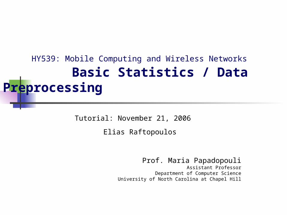
Basic Terminology

An Element of a sample or population is a specific subject or object (for example, a person, firm, item, state, or country) about which the information is collected.

A Variable is a characteristic under study that assumes different values for different elements.

An Observation is the value of a variable for an element.

Data set is a collection of observations on one or more variables.

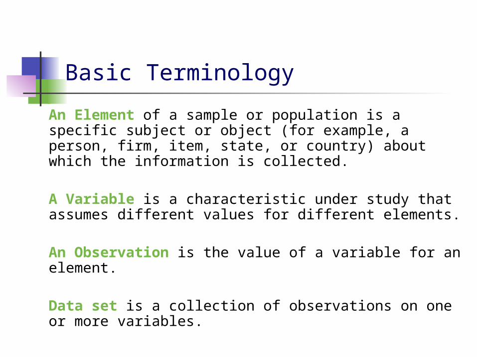
Measures of Central Tendency

Mean: Sum of all values divided by the number of cases.

Median: The value of the middle term in a data set that has been ranked in increasing order. 50% of the data lies below this value and 50% above.

Mode: is the value that occurs with the highest frequency in a data set.

Measures of Dispersion

The square root of the average squared deviations from the mean

This measure how the data values differ from the mean. A small standard deviation implies most values are near

the average The large standard deviation indicates that values are

widely spread above and below the average Range = Largest value – Smallest Value

The range, like the mean has the disadvantage of being influenced by outliers

Percentiles Values that divide cases below which certain percentages

of values fall Standard Error (SE): Standard deviation of the

mean.

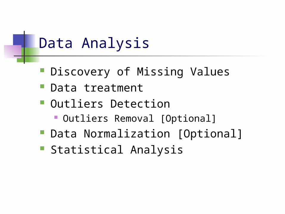
Data Analysis

Discovery of Missing Values Data treatment Outliers Detection

Outliers Removal [Optional] Data Normalization [Optional] Statistical Analysis

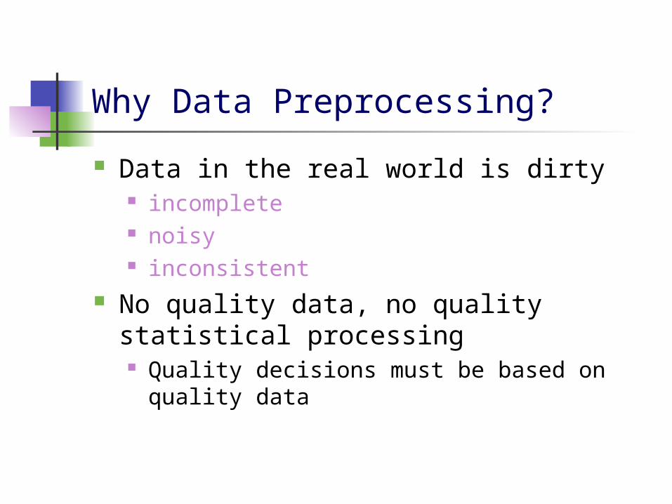
Why Data Preprocessing?

Data in the real world is dirty incomplete noisy inconsistent

No quality data, no quality statistical processing Quality decisions must be based on quality

data

Data Cleaning Tasks

Handle missing values, due to Sensor malfunction Random disturbances Network Protocol [eg UDP]

Identify outliers, smooth out noisy data

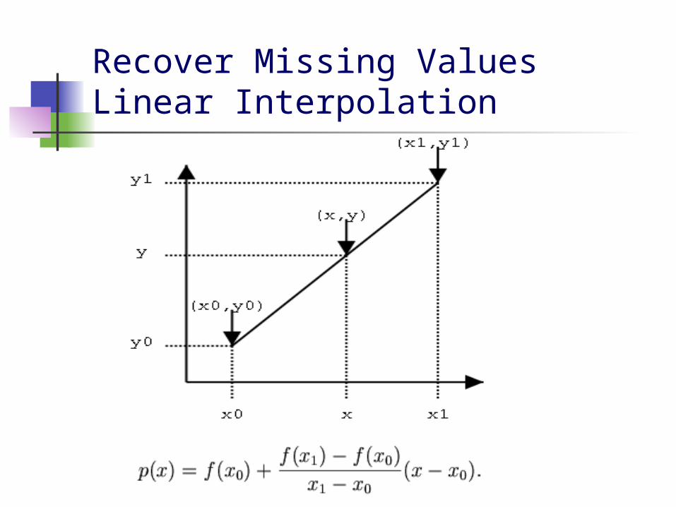
Recover Missing ValuesLinear Interpolation

Recover Missing Values Moving Average

A simple moving average is the unweighted mean of the previous n data points in the time series

A weighted moving average is a weighted mean of the previous n data points in the time series

A weighted moving average is more responsive to recent movements than a simple moving average

An exponentially weighted moving average (EWMA or just EMA) is an exponentially weighted mean of previous data points

The parameter of an EWMA can be expressed as a proportional percentage - for example, in a 10% EWMA, each time period is assigned a weight that is 90% of the weight assigned to the next (more recent) time period

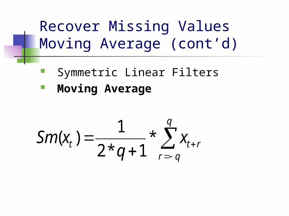
Recover Missing Values Moving Average (cont’d)

Symmetric Linear Filters Moving Average

q

qrrtt x

qxSm *

1*2

1)(

What are outliers in the data?

An outlier is an observation that lies an abnormal distance from other values in a random sample from a population It is left to the analyst (or a consensus

process) to decide what will be considered abnormal

Before abnormal observations can be singled out, it is necessary to characterize normal observations

What are outliers in the data? (cntd)

An outlier is a data point that comes from a distribution different (in location, scale, or distributional form) from the bulk of the data

In the real world, outliers have a range of causes, from as simple as

operator blunders equipment failures day-to-day effects batch-to-batch differences anomalous input conditions warm-up effects

Scatter Plot: Outlier

Scatter plot here reveals A basic linear relationship between X and Y for most of the data A single outlier (at X = 375)

Symmetric Histogram with Outlier

A symmetric distribution is one in which the 2 "halves" of the histogram appear as mirror-images of one another.

The above example is symmetric with the exception of outlying data near Y = 4.5

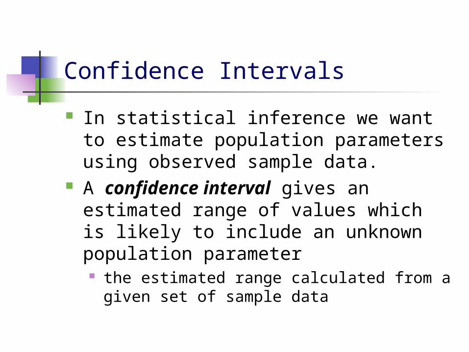
Confidence Intervals

In statistical inference we want to estimate population parameters using observed sample data.

A confidence interval gives an estimated range of values which is likely to include an unknown population parameter the estimated range calculated from a given

set of sample data

Confidence Intervals

Common choices for the confidence level C are 0.90, 0.95, and 0.99

Levels correspond to percentages of the area of the normal density curve

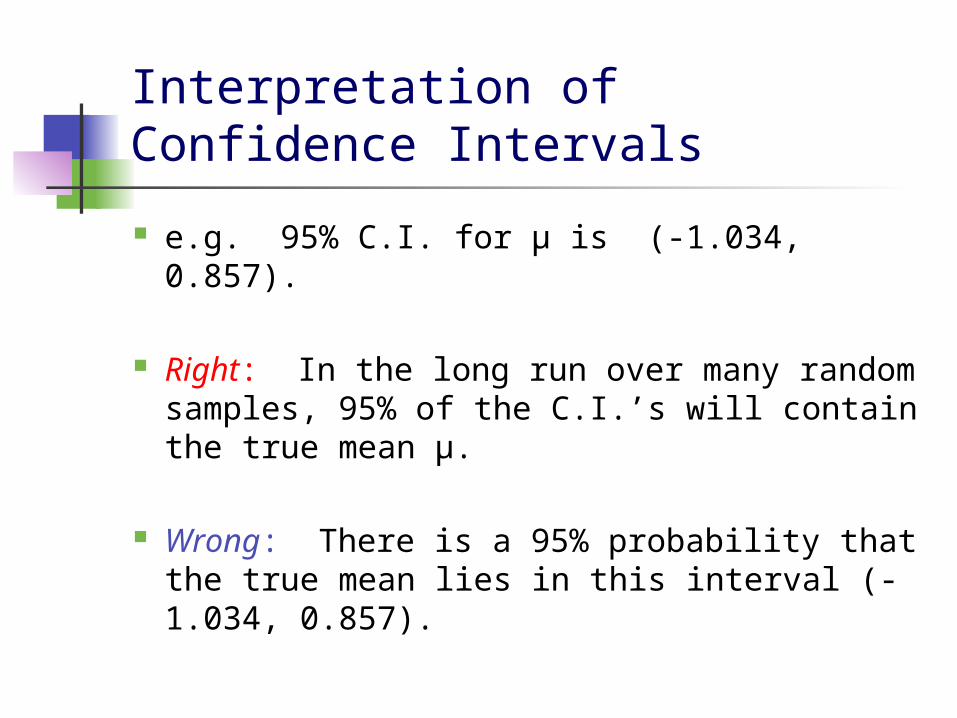
Interpretation of Confidence Intervals

e.g. 95% C.I. for µ is (-1.034, 0.857).

Right: In the long run over many random samples, 95% of the C.I.’s will contain the true mean µ.

Wrong: There is a 95% probability that the true mean lies in this interval (-1.034, 0.857).

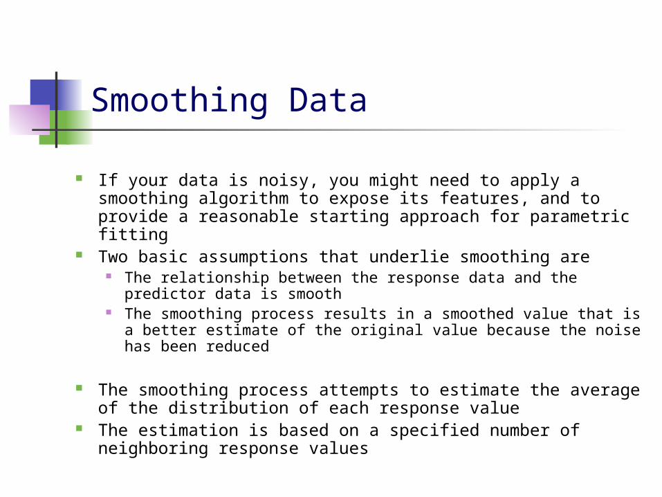
Smoothing Data

If your data is noisy, you might need to apply a smoothing algorithm to expose its features, and to provide a reasonable starting approach for parametric fitting

Two basic assumptions that underlie smoothing are The relationship between the response data and the predictor

data is smooth The smoothing process results in a smoothed value that is a

better estimate of the original value because the noise has been reduced

The smoothing process attempts to estimate the average of the distribution of each response value

The estimation is based on a specified number of neighboring response values

Smoothing Data (cntd)

Moving average filtering Lowpass filter that takes the average of

neighboring data points Lowess and loess

Locally weighted scatter plot smooth Savitzky-Golay filtering

A generalized moving average where you derive the filter coefficients by performing an unweighted linear least squares fit using a polynomial of the specified degree

Smoothing Data (eg Robust Lowess)

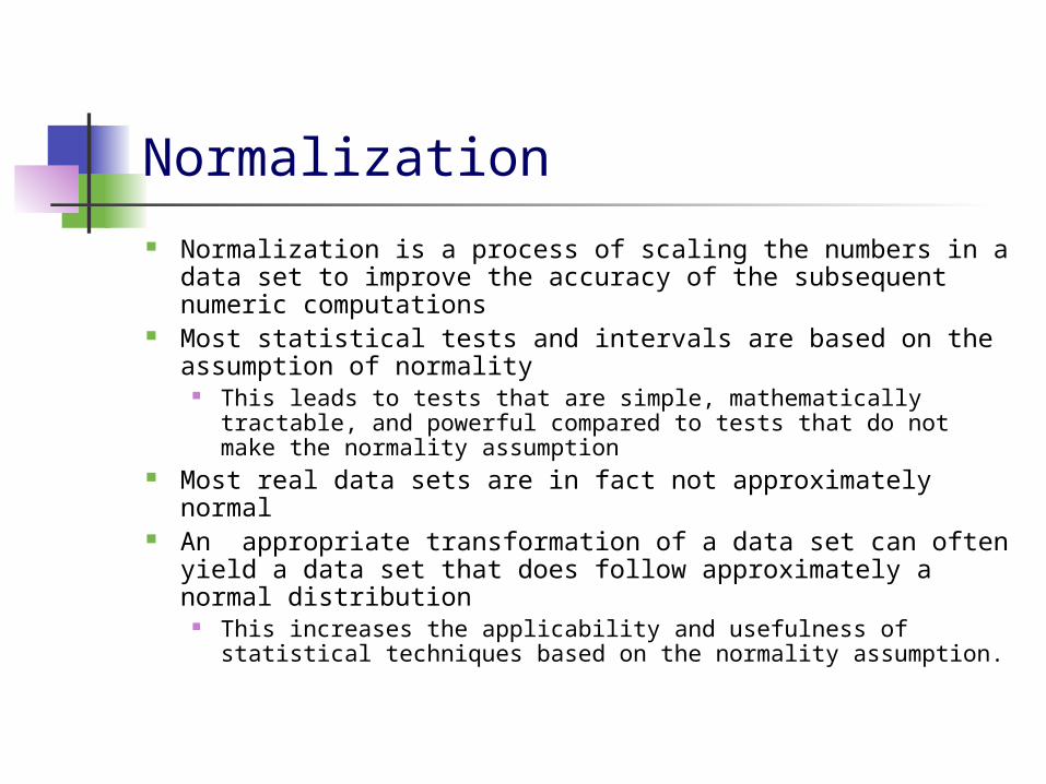
Normalization

Normalization is a process of scaling the numbers in a data set to improve the accuracy of the subsequent numeric computations

Most statistical tests and intervals are based on the assumption of normality

This leads to tests that are simple, mathematically tractable, and powerful compared to tests that do not make the normality assumption

Most real data sets are in fact not approximately normal An appropriate transformation of a data set can often

yield a data set that does follow approximately a normal distribution

This increases the applicability and usefulness of statistical techniques based on the normality assumption.

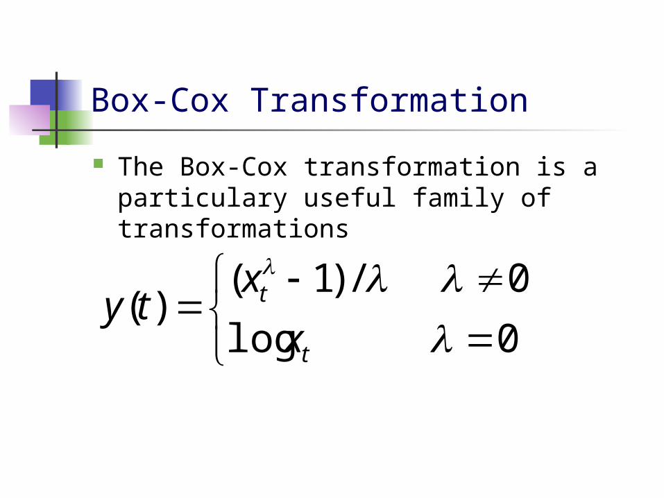
Box-Cox Transformation

The Box-Cox transformation is a particulary useful family of transformations

0log

0/)1()(

t

t

x

xty

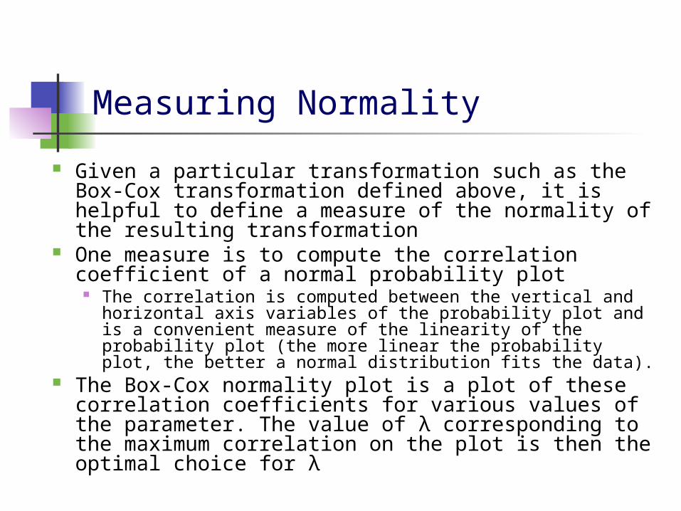
Measuring Normality

Given a particular transformation such as the Box-Cox transformation defined above, it is helpful to define a measure of the normality of the resulting transformation

One measure is to compute the correlation coefficient of a normal probability plot

The correlation is computed between the vertical and horizontal axis variables of the probability plot and is a convenient measure of the linearity of the probability plot (the more linear the probability plot, the better a normal distribution fits the data).

The Box-Cox normality plot is a plot of these correlation coefficients for various values of the parameter. The value of λ corresponding to the maximum correlation on the plot is then the optimal choice for λ

Measuring Normality (cont’d)

The histogram in the upper left-hand corner shows a data set that has significant right skewness

And so does not follow a normal distribution

The Box-Cox normality plot shows that the maximum value of the correlation coefficient is at = -0.3

The histogram of the data after applying the Box-Cox transformation with = -0.3 shows a data set for which the normality assumption is reasonable

This is verified with a normal probability plot of the transformed data.

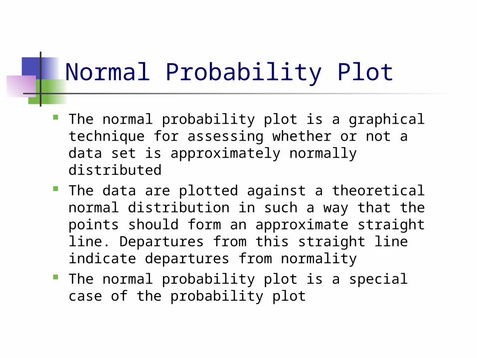
Normal Probability Plot

The normal probability plot is a graphical technique for assessing whether or not a data set is approximately normally distributed

The data are plotted against a theoretical normal distribution in such a way that the points should form an approximate straight line. Departures from this straight line indicate departures from normality

The normal probability plot is a special case of the probability plot

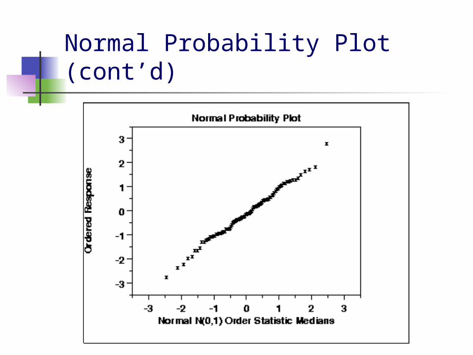
Normal Probability Plot (cont’d)

PDF Plot

Probability density function (pdf) represents a probability distribution in terms of integrals

A probability density function is non-negative everywhere and its integral from −∞ to +∞ is equal to 1

If a probability distribution has density f(x), then intuitively the infinitesimal interval [x, x + dx] has probability f(x) dx

CDF Plot

Plot of empirical cumulative distribution function

Percentiles

percentiles provide a way of estimating proportions of the data that should fall above and below a given value

The pth percentile is a value, Y(p), such that at most (100p)% of the measurements are less than this value and at most 100(1- p)% are greater

The 50th percentile is called the median Percentiles split a set of ordered data into

hundredths For example, 70% of the data should fall below the 70th

percentile.

Interquartile Range Quartiles are three summary measures that divide a

ranked data set into four equal parts

Second quartile is the same as the median of a data set

First quartile is the value of the middle term among the observations that are less than the median

Third quartile is the value of the middle term among the observations that are greater than the median

Interquartile range: The difference between the third and first quartiles or

equivalently the middle 50% of the data