HURDLE AND “SELECTION” MODELS Jeff Wooldridge Michigan State University BGSE/IZA Course in Microeconometrics July 2009 1. Introduction 2. A General Formulation 3. Truncated Normal Hurdle Model 4. Lognormal Hurdle Model 5. Exponential Type II Tobit Model 1

Welcome message from author
This document is posted to help you gain knowledge. Please leave a comment to let me know what you think about it! Share it to your friends and learn new things together.
Transcript
HURDLE AND “SELECTION” MODELS
Jeff WooldridgeMichigan State University
BGSE/IZA Course in MicroeconometricsJuly 2009
1. Introduction2. A General Formulation3. Truncated Normal Hurdle Model4. Lognormal Hurdle Model5. Exponential Type II Tobit Model
1
1. Introduction
∙ Consider the case with a corner at zero and a continuous distribution
for strictly positive values.
∙ Note that there is only one response here, y, and it is always observed.
The value zero is not arbitrary; it is observed data (labor supply,
charitable contributions).
∙ Often see discussions of the “selection” problem with corner solution
outcomes, but this is usually not appropriate.
2
∙ Example: Family charitable contributions. A zero is a zero, and then
we see a range of positive values. We want to choose sensible, flexible
models for such a variable.
∙ Often define w as the binary variable equal to one if y 0, zero if
y 0. w is a deterministic function of y. We cannot think of a
counterfactual for y in the two different states. (“How much would the
family contribute to charity if it contributes nothing to charity?” “How
much would a woman work if she is out of the workforce?”)
3
∙ Contrast previous examples with sound counterfactuals: How much
would a worker in if he/she participates in job training versus when
he/she does not? What is a student’s test score if he/she attends
Catholic school compared with if he/she does not?
∙ The statistical structure of a particular two-part model, and the
Heckman selection model, are very similar.
4
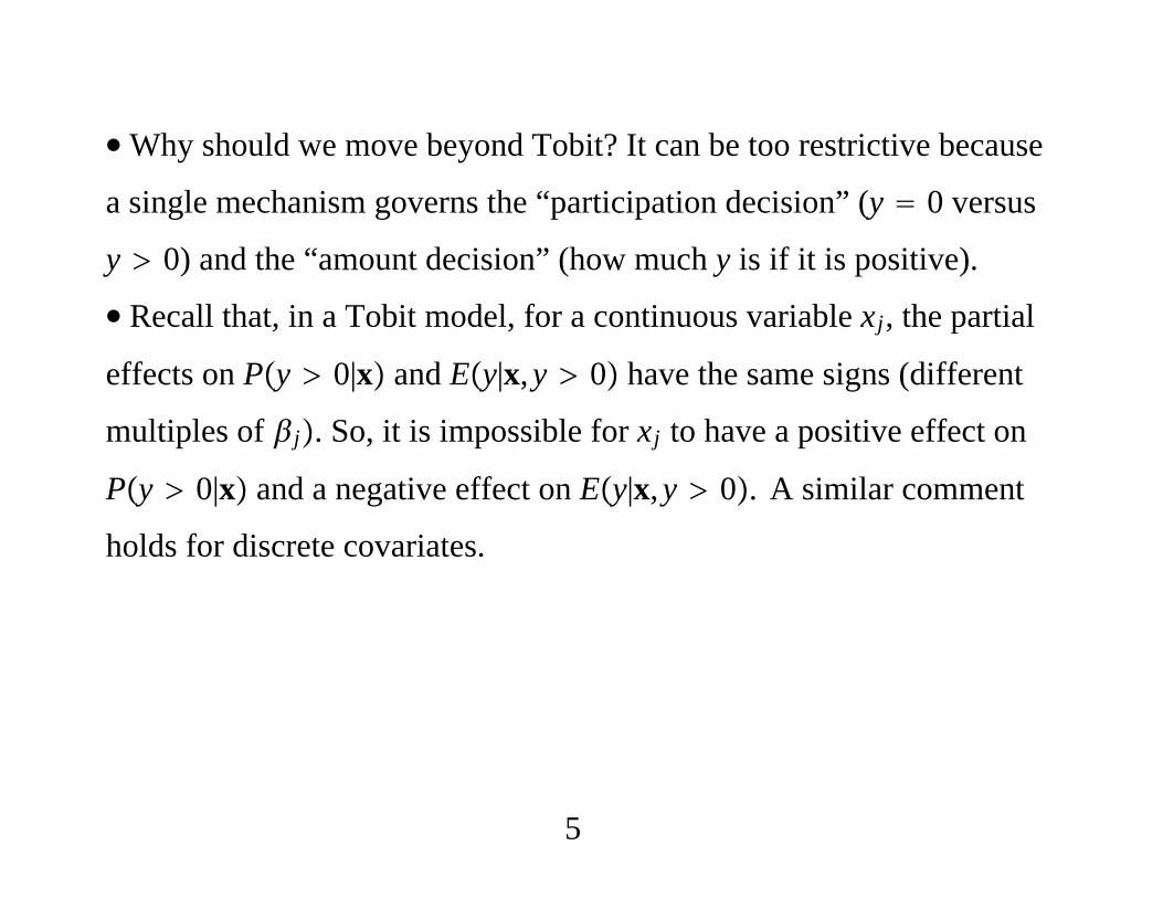
∙Why should we move beyond Tobit? It can be too restrictive because
a single mechanism governs the “participation decision” (y 0 versus
y 0) and the “amount decision” (how much y is if it is positive).
∙ Recall that, in a Tobit model, for a continuous variable xj, the partial
effects on Py 0|x and Ey|x,y 0 have the same signs (different
multiples of j. So, it is impossible for xj to have a positive effect on
Py 0|x and a negative effect on Ey|x,y 0. A similar comment
holds for discrete covariates.
5
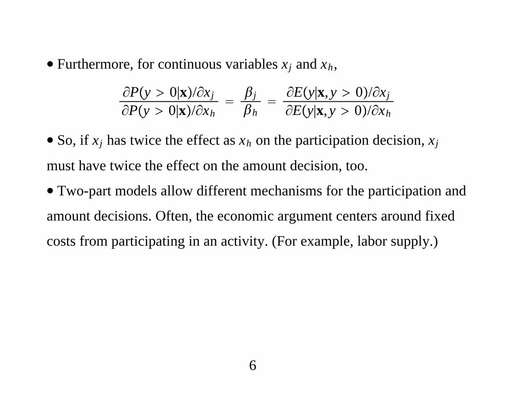
∙ Furthermore, for continuous variables xj and xh,
∂Py 0|x/∂xj
∂Py 0|x/∂xh
jh
∂Ey|x,y 0/∂xj
∂Ey|x,y 0/∂xh
∙ So, if xj has twice the effect as xh on the participation decision, xj
must have twice the effect on the amount decision, too.
∙ Two-part models allow different mechanisms for the participation and
amount decisions. Often, the economic argument centers around fixed
costs from participating in an activity. (For example, labor supply.)
6
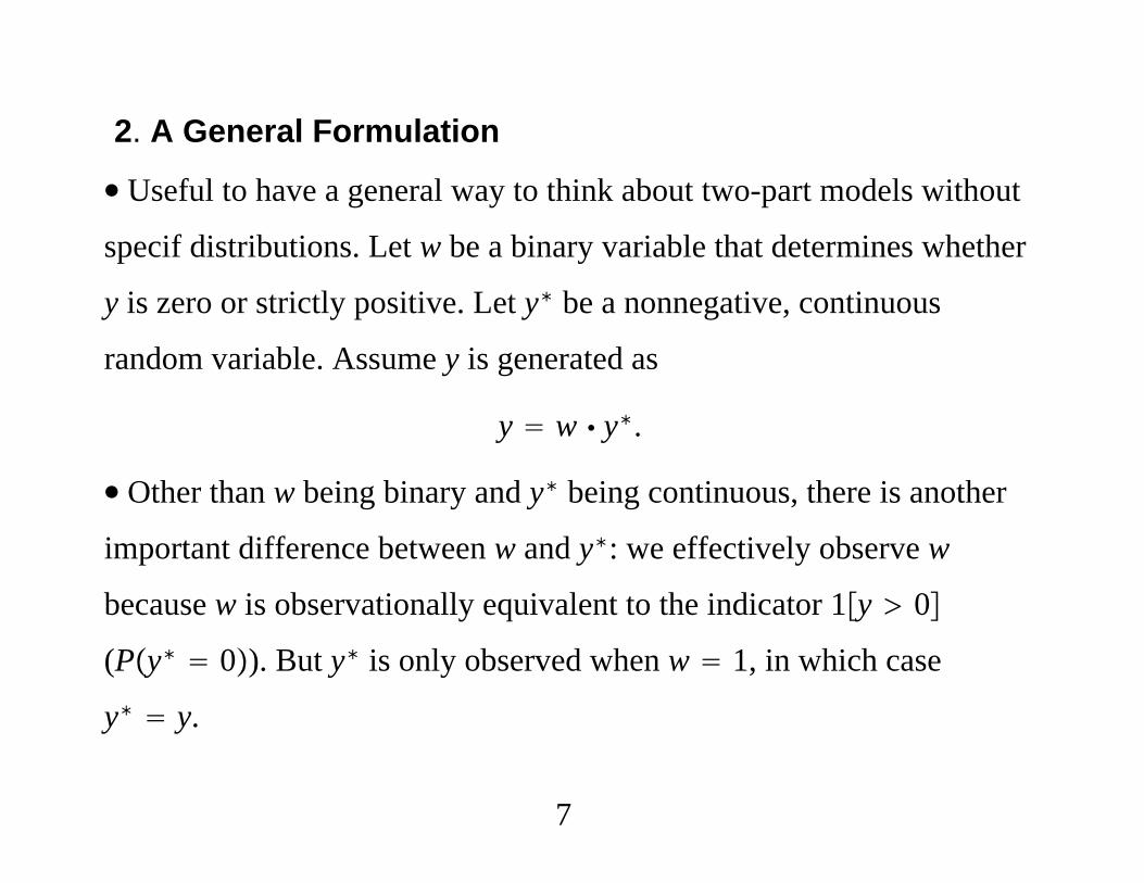
2. A General Formulation
∙ Useful to have a general way to think about two-part models without
specif distributions. Let w be a binary variable that determines whether
y is zero or strictly positive. Let y∗ be a nonnegative, continuous
random variable. Assume y is generated as
y w y∗.
∙ Other than w being binary and y∗ being continuous, there is another
important difference between w and y∗: we effectively observe w
because w is observationally equivalent to the indicator 1y 0
(Py∗ 0). But y∗ is only observed when w 1, in which case
y∗ y.
7
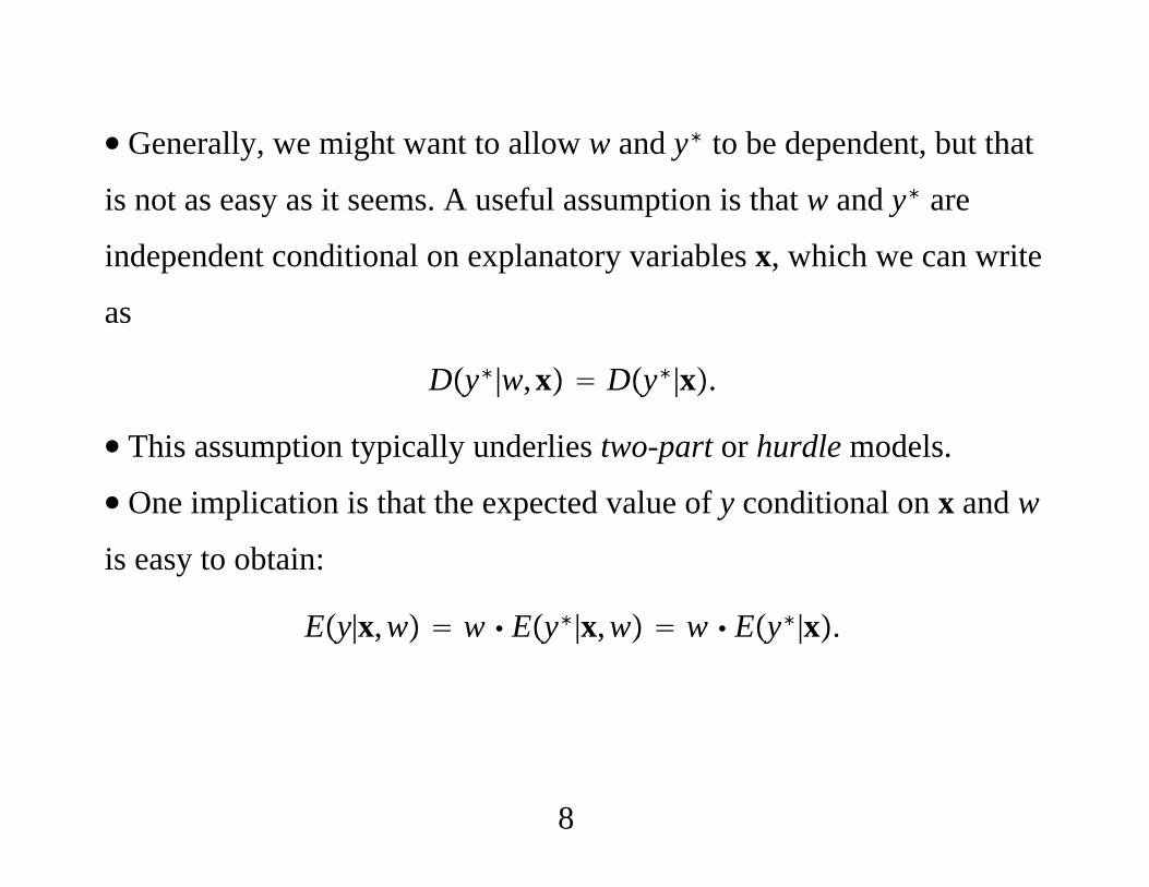
∙ Generally, we might want to allow w and y∗ to be dependent, but that
is not as easy as it seems. A useful assumption is that w and y∗ are
independent conditional on explanatory variables x, which we can write
as
Dy∗|w,x Dy∗|x.
∙ This assumption typically underlies two-part or hurdle models.
∙ One implication is that the expected value of y conditional on x and w
is easy to obtain:
Ey|x,w w Ey∗|x,w w Ey∗|x.
8
∙ Sufficient is conditional mean independence,
Ey∗|x,w Ey∗|x.
∙When w 1, we can write
Ey|x,y 0 Ey∗|x,
so that the so-called “conditional” expectation of y (where we condition
on y 0) is just the expected value of y∗ (conditional on x).
∙ The so-called “unconditional” expectation is
Ey|x Ew|xEy∗|x Pw 1|xEy∗|x.
9
∙ A different class of models explicitly allows correlation between the
participation and amount decisions Unfortunately, called a selection
model. Has led to considerable conclusion for corner solution
responses.
∙Must keep in mind that we only observe one variable, y (along with
x. In true sample selection environments, the outcome of the selection
variable (w in the current notation) does not logically restrict the
outcome of the response variable. Here, w 0 rules out y 0.
∙ In the end, we are trying to get flexible models for Dy|x.
10
3. Truncated Normal Hurdle Model
∙ Cragg (1971) proposed a natural two-part extension of the type I
Tobit model. The conditional independence assumption is assumed to
hold, and the binary variable w is assumed to follow a probit model:
Pw 1|x x.
∙ Further, y∗ is assumed to have a truncated normal distribution with
parameters that vary freely from those in the probit. Can write
y∗ x u
where u given x has a truncated normal distribution with lower
truncation point −x.
11
∙ Because y y∗ when y 0, we can write the truncated normal
assumption in terms of the density of y given y 0 (and x):
fy|x,y 0 x/−1y − x//, y 0,
where the term x/−1 ensures that the density integrates to unity
over y 0.
∙ The density of y given x can be written succinctly as
fy|x 1 − x1y0xx/−1y − x//1y0,
where we must multiply fy|x,y 0 by Py 0|x x.
12
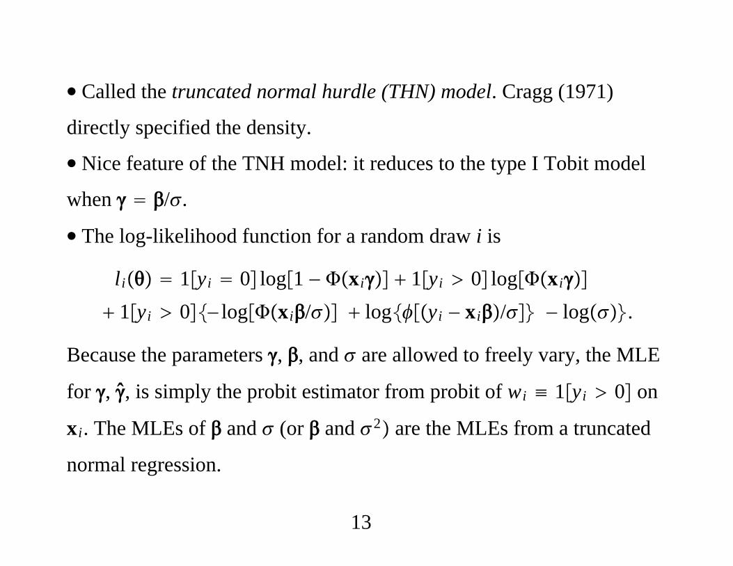
∙ Called the truncated normal hurdle (THN) model. Cragg (1971)
directly specified the density.
∙ Nice feature of the TNH model: it reduces to the type I Tobit model
when /.
∙ The log-likelihood function for a random draw i is
li 1yi 0 log1 − xi 1yi 0 logxi
1yi 0− logxi/ logyi − xi/ − log.
Because the parameters , , and are allowed to freely vary, the MLE
for , , is simply the probit estimator from probit of wi ≡ 1yi 0 on
xi. The MLEs of and (or and 2 are the MLEs from a truncated
normal regression.
13
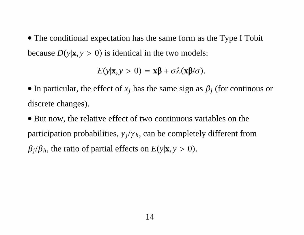
∙ The conditional expectation has the same form as the Type I Tobit
because Dy|x,y 0 is identical in the two models:
Ey|x,y 0 x x/.
∙ In particular, the effect of xj has the same sign as j (for continous or
discrete changes).
∙ But now, the relative effect of two continuous variables on the
participation probabilities, j/h, can be completely different from
j/h, the ratio of partial effects on Ey|x,y 0.
14
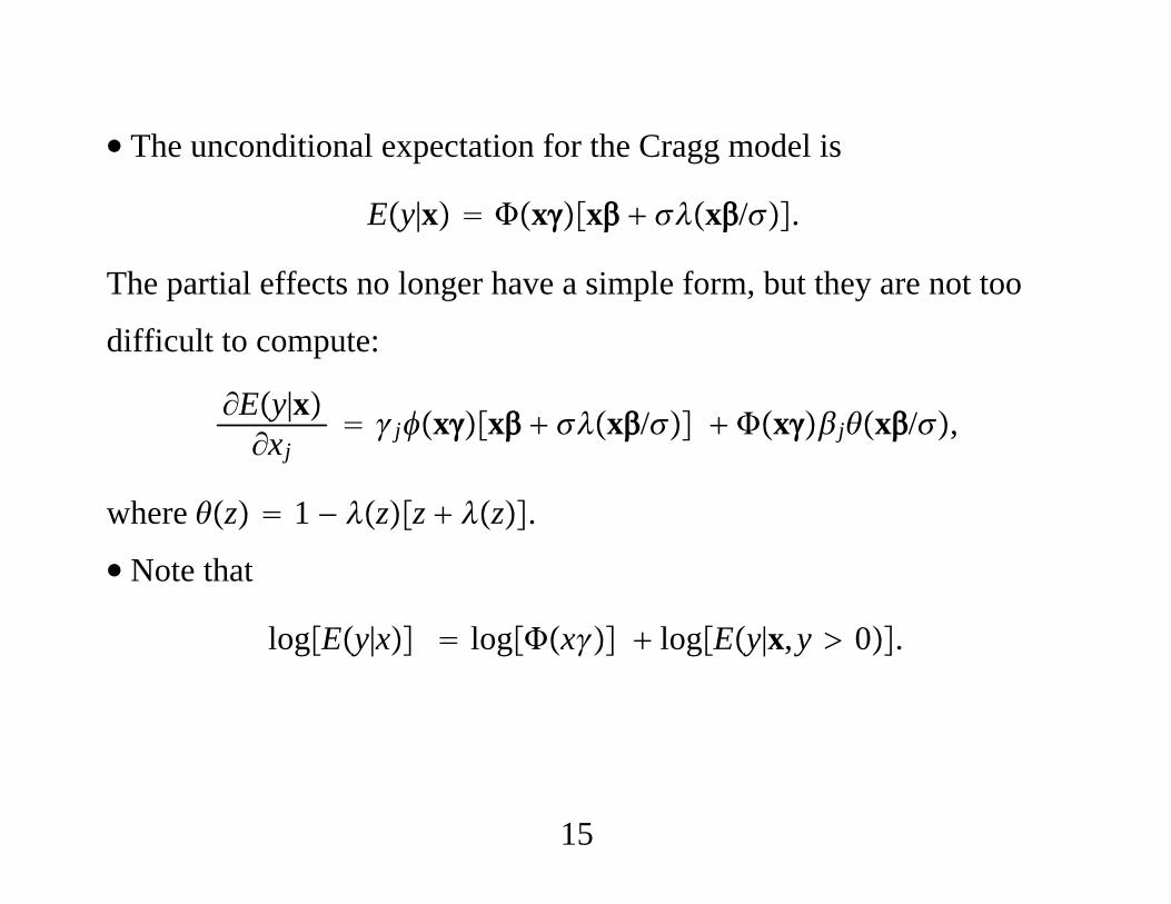
∙ The unconditional expectation for the Cragg model is
Ey|x xx x/.
The partial effects no longer have a simple form, but they are not too
difficult to compute:
∂Ey|x∂xj
jxx x/ xjx/,
where z 1 − zz z.
∙ Note that
logEy|x logx logEy|x,y 0.
15
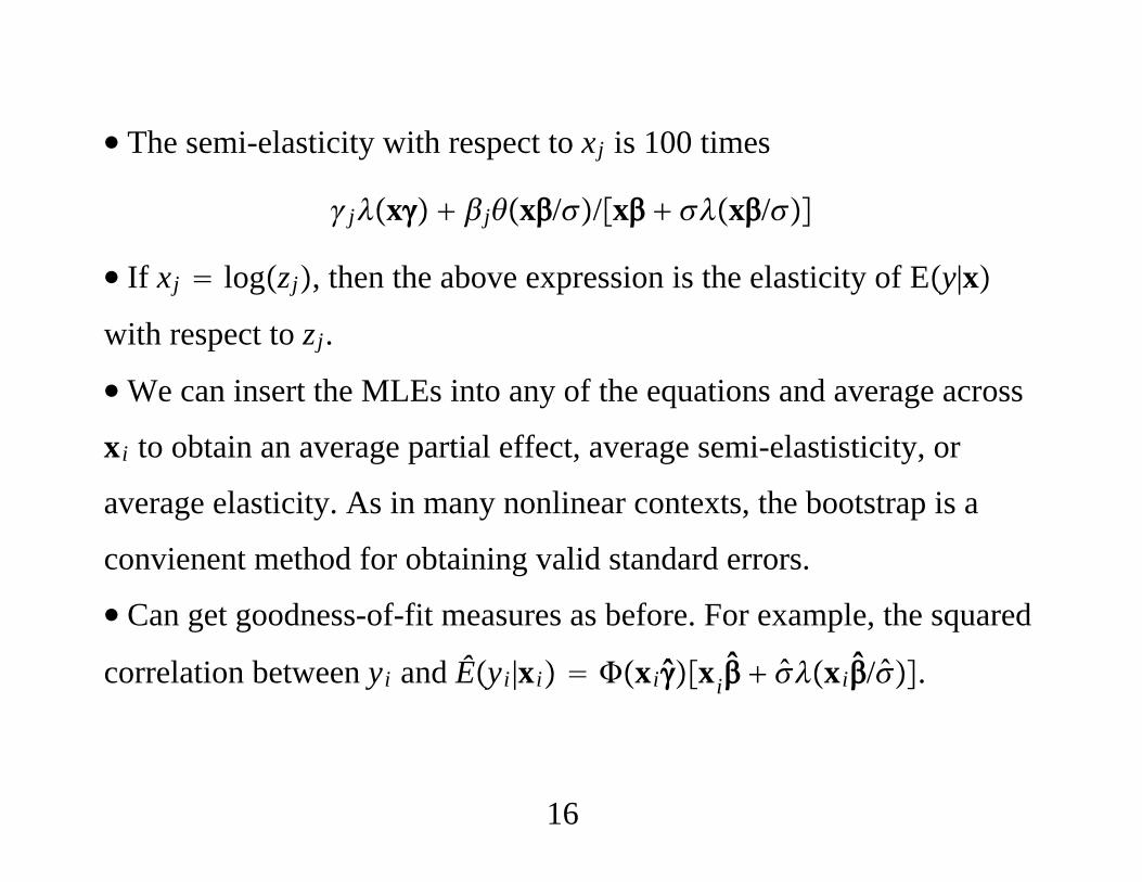
∙ The semi-elasticity with respect to xj is 100 times
jx jx//x x/
∙ If xj logzj, then the above expression is the elasticity of Ey|x
with respect to zj.
∙We can insert the MLEs into any of the equations and average across
xi to obtain an average partial effect, average semi-elastisticity, or
average elasticity. As in many nonlinear contexts, the bootstrap is a
convienent method for obtaining valid standard errors.
∙ Can get goodness-of-fit measures as before. For example, the squared
correlation between yi and Êyi|xi xixi xi/.
16
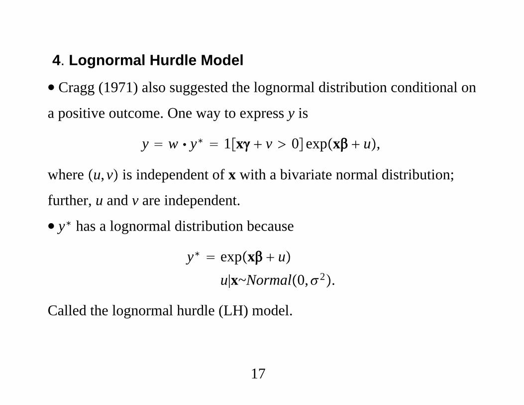
4. Lognormal Hurdle Model
∙ Cragg (1971) also suggested the lognormal distribution conditional on
a positive outcome. One way to express y is
y w y∗ 1x v 0expx u,
where u,v is independent of x with a bivariate normal distribution;
further, u and v are independent.
∙ y∗ has a lognormal distribution because
y∗ expx uu|x~Normal0,2.
Called the lognormal hurdle (LH) model.
17
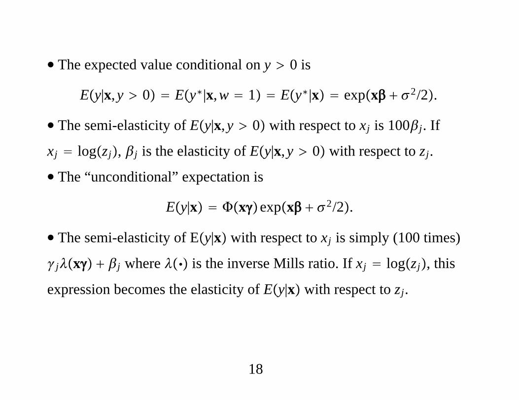
∙ The expected value conditional on y 0 is
Ey|x,y 0 Ey∗|x,w 1 Ey∗|x expx 2/2.
∙ The semi-elasticity of Ey|x,y 0 with respect to xj is 100j. If
xj logzj, j is the elasticity of Ey|x,y 0 with respect to zj.
∙ The “unconditional” expectation is
Ey|x xexpx 2/2.
∙ The semi-elasticity of Ey|x with respect to xj is simply (100 times)
jx j where is the inverse Mills ratio. If xj logzj, this
expression becomes the elasticity of Ey|x with respect to zj.
18
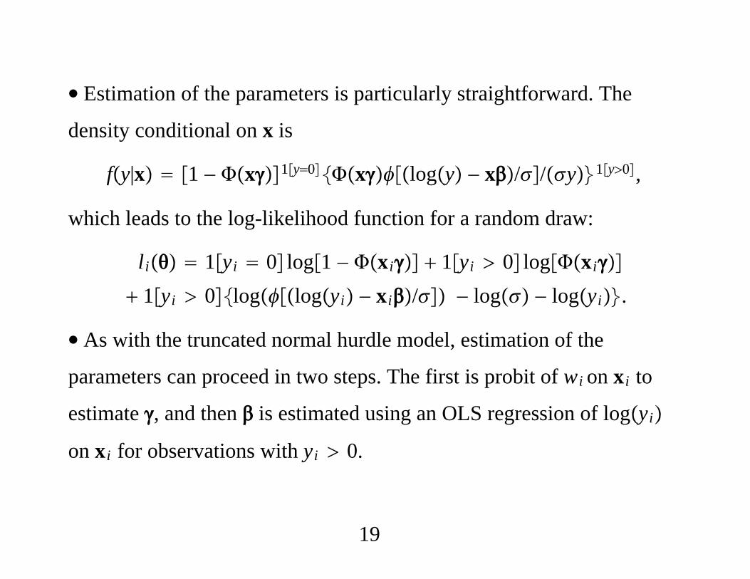
∙ Estimation of the parameters is particularly straightforward. The
density conditional on x is
fy|x 1 − x1y0xlogy − x//y1y0,
which leads to the log-likelihood function for a random draw:
li 1yi 0 log1 − xi 1yi 0 logxi
1yi 0loglogyi − xi/ − log − logyi.
∙ As with the truncated normal hurdle model, estimation of the
parameters can proceed in two steps. The first is probit of wi on xi to
estimate , and then is estimated using an OLS regression of logyi
on xi for observations with yi 0.
19
∙ The usual error variance estimator (or without the degrees-of-freedom
adjustment), 2, is consistent for 2.
∙ In computing the log likelihood to compare fit across models, must
include the terms logyi. In particular, for comparing with the TNH
model.
∙ Can relax the lognormality assumption if we are satisfied with
estimates of Py 0|x, Ey|x,y 0, and Ey|xare easy to obtain.
20
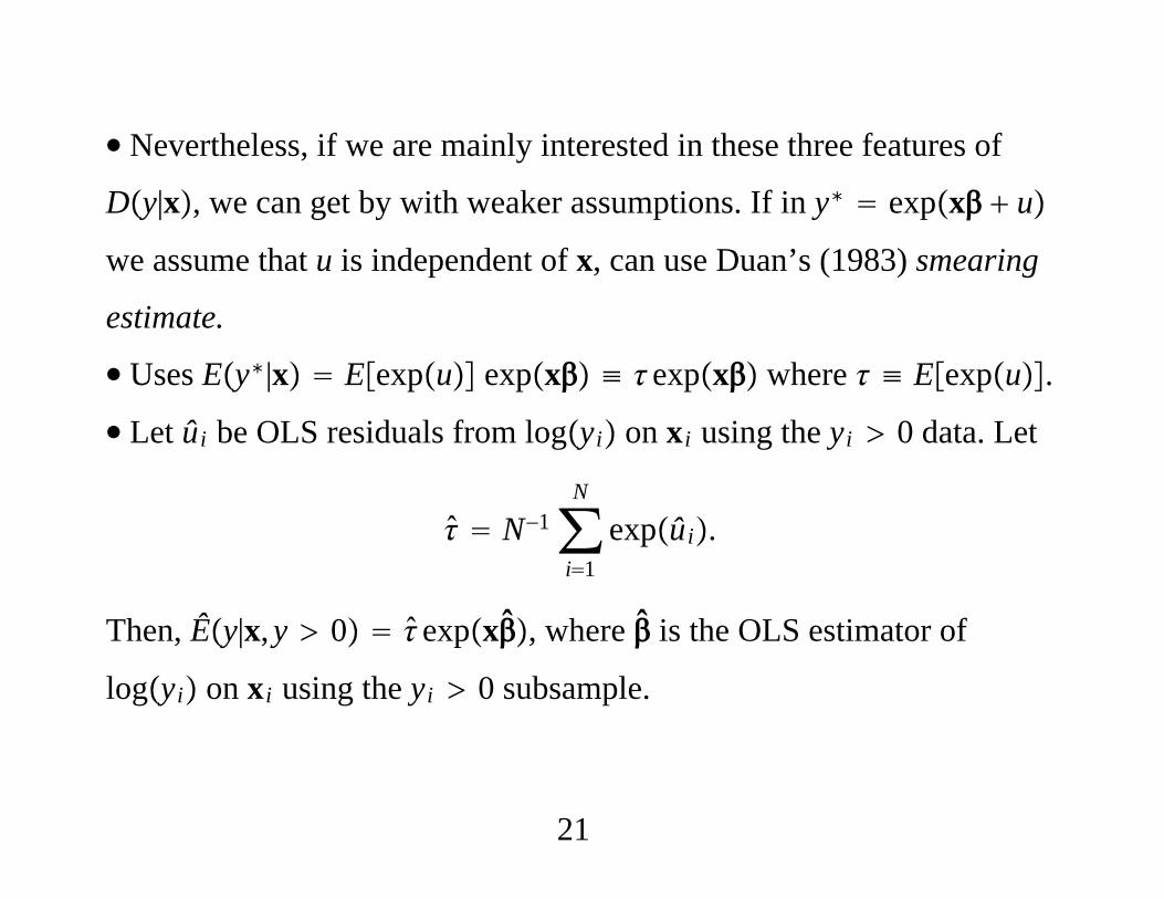
∙ Nevertheless, if we are mainly interested in these three features of
Dy|x, we can get by with weaker assumptions. If in y∗ expx u
we assume that u is independent of x, can use Duan’s (1983) smearing
estimate.
∙ Uses Ey∗|x Eexpu expx ≡ expx where ≡ Eexpu.
∙ Let ûi be OLS residuals from logyi on xi using the yi 0 data. Let
N−1∑i1
N
expûi.
Then, Êy|x,y 0 expx, where is the OLS estimator of
logyi on xi using the yi 0 subsample.
21
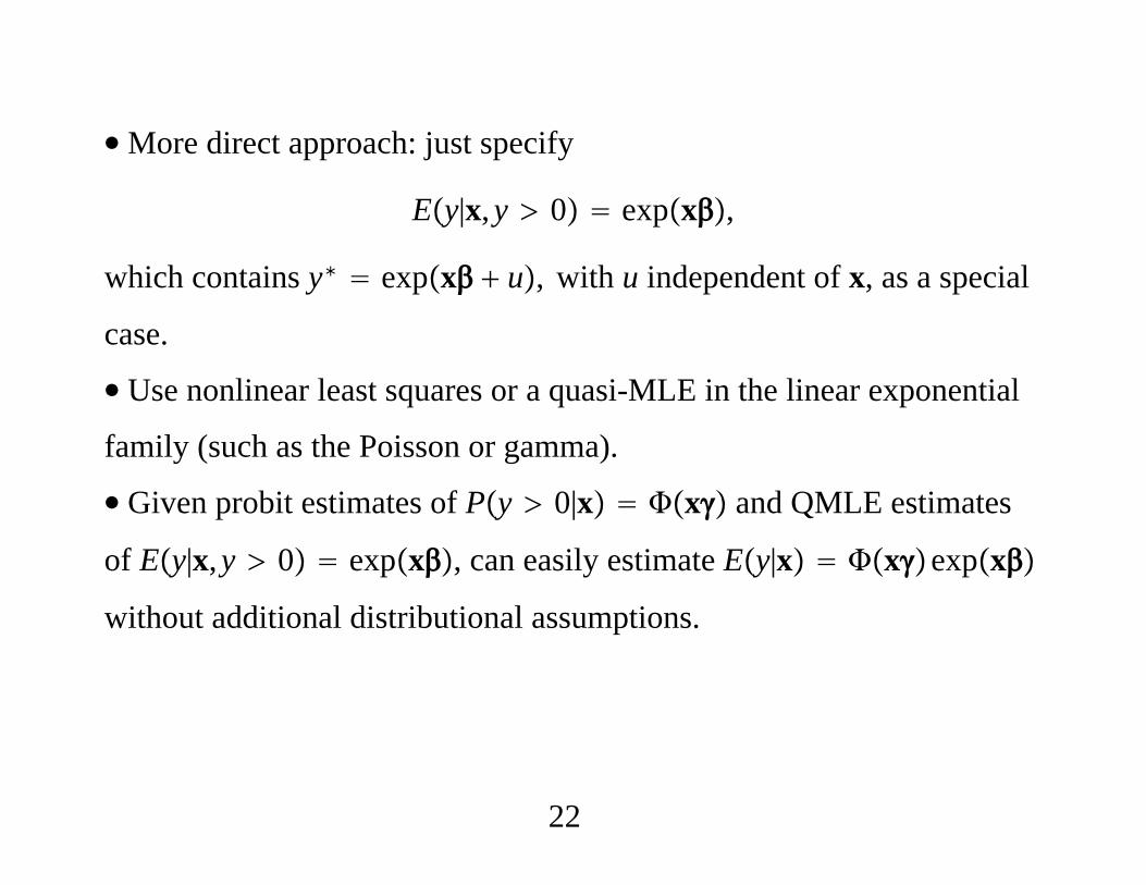
∙More direct approach: just specify
Ey|x,y 0 expx,
which contains y∗ expx u, with u independent of x, as a special
case.
∙ Use nonlinear least squares or a quasi-MLE in the linear exponential
family (such as the Poisson or gamma).
∙ Given probit estimates of Py 0|x x and QMLE estimates
of Ey|x,y 0 expx, can easily estimate Ey|x xexpx
without additional distributional assumptions.
22
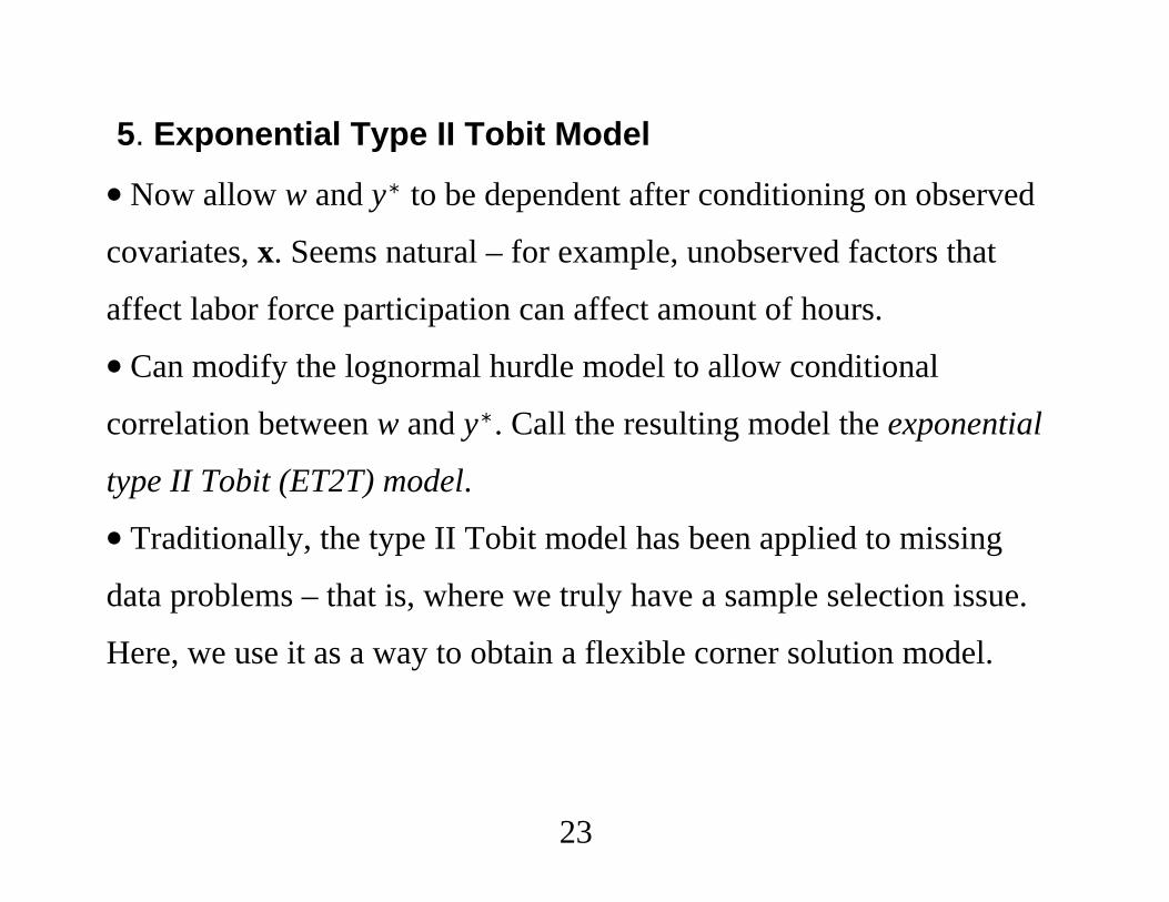
5. Exponential Type II Tobit Model
∙ Now allow w and y∗ to be dependent after conditioning on observed
covariates, x. Seems natural – for example, unobserved factors that
affect labor force participation can affect amount of hours.
∙ Can modify the lognormal hurdle model to allow conditional
correlation between w and y∗. Call the resulting model the exponential
type II Tobit (ET2T) model.
∙ Traditionally, the type II Tobit model has been applied to missing
data problems – that is, where we truly have a sample selection issue.
Here, we use it as a way to obtain a flexible corner solution model.
23
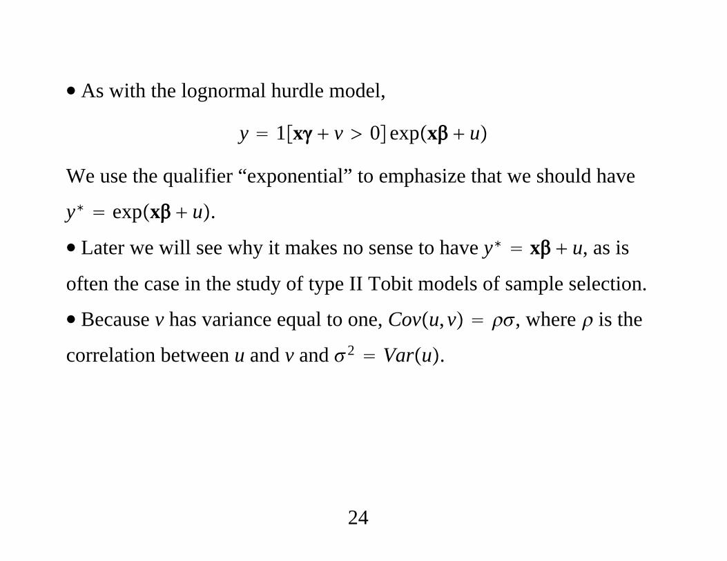
∙ As with the lognormal hurdle model,
y 1x v 0expx u
We use the qualifier “exponential” to emphasize that we should have
y∗ expx u.
∙ Later we will see why it makes no sense to have y∗ x u, as is
often the case in the study of type II Tobit models of sample selection.
∙ Because v has variance equal to one, Covu,v , where is the
correlation between u and v and 2 Varu.
24
∙ Obtaining the log likelihood in this case is a bit tricky. Let
m∗ logy∗, so that Dm∗|x is Normalx,2. Then
logy m∗when y 0. We still have Py 0|x 1 − x.
∙ To obtain the density of y (conditional on x) over strictly positive
values, we find fy|x,y 0 and multiply it by Py 0|x x.
∙ To find fy|x,y 0, we use the change-of-variables formula
fy|x,y 0 glogy|x,y 0/y, where g|x,y 0 is the density of
m∗ conditional on y 0 (and x).
25
∙ Use Bayes’ rule to write
gm∗|x,w 1 Pw 1|m∗,xhm∗|x/Pw 1|x where hm∗|x is
the density of m∗ given x. Then,
Pw 1|xgm∗|x,w 1 Pw 1|m∗,xhm∗|x.
∙Write w 1x v 0 1x /u e 0, where
v /u e and e|x,u~Normal0, 1 − 2. Because u m∗ − x,
we have Pw 1|m∗,x x /m∗ − x1 − 2−1/2.
26
∙ Further, we have assumed that hm∗|x is Normalx,2. Therefore,
the density of y given x over strictly positive y is
fy|x x /y − x1 − 2−1/2logy − x//y.
∙ Combining this expression with the density at y 0 gives the log
likelihood as
li 1yi 0 log1 − xi
1yi 0logxi /logyi − xi1 − 2−1/2
loglogyi − xi/ − log − logyi.
27
∙Many econometrics packages have this estimator programmed,
although the emphasis is on sample selection problems. To use
Heckman sample selection software, one defines logyi as the variable
where the data are “missing” when yi 0) When 0, we obtain the
log likelihood for the lognormal hurdle model from the previous
subsection.
28
∙ For a true missing data problem, the last term in the log likelihood,
logyi, is not included. That is because in sample selection problems
the log-likelihood function is only a partial log likelihood. Inclusion of
logyi does not affect the estimation problem, but it does affect the
value of the log-likelihood function, which is needed to compare across
different models.)
29
∙ The ET2T model contains the conditional lognormal model from the
previous subsection. But the ET2T model with unknown can be
poorly identified if the set of explanatory variables that appears in
y∗ expx u is the same as the variables in w 1x v 0.
∙ Various ways to see the potential problem. Can show that
Elogy|x,y 0 x x
where is the inverse Mills ratio and .
30
∙We know we can estimate by probit, so this equation nominally
identifies and . But identification is possible only because is a
nonlinear function, but is roughly linear over much of its range.
∙ The formula for Elogy|x,y 0 suggests a two-step procedure,
usually called Heckman’s method or Heckit. First, from probit of wi
on xi. Second, and are obtained from OLS of logyi on xi, xi
using only observations with yi 0.
31
∙ The correlation between i can often be very large, resulting in
imprecise estimates of and .
∙ Can be shown that the unconditional expectation is
Ey|x x expx 2/2,
which is exactly of the same form as in the LH model (with 0
except for the presence of . Because x always should include a
constant, is not separately identified by Ey|x (and neither is 2/2).
32
∙ If we based identification entirely on Ey|x, there would be no
difference between the lognormal hurdle model and the ET2T model
when the same set of regressors appears in the participation and amount
equations.
∙ Still, the parameters are technically identified, and so we can always
try to estimate the full model with the same vector x appearing in the
participation and amount equations.
33
∙ The ET2T model is more convincing when the covariates determining
the participation decision strictly contain those affecting the amount
decision. Then, the model can be expressed as
y 1x v ≥ 0 expx11 u,
where both x and x1 contain unity as their first elements but x1 is a
strict subset of x. If we write x x1,x2, then we are assuming
2 ≠ 0.
∙ Given at least one exclusion restriction, we can see from
Elogy|x,y 0 x11 x that 1 and are better identified
because x is not an exact function of x1.
34
∙ Exclusion restrictions can be hard to come by. Need something
affecting the fixed cost of participating but not affecting the amount.
∙ Cannot use y rather than logy in the amount equation. In the TNH
model, the truncated normal distribution of u at the value −x ensures
that y∗ x u 0.
∙ If we apply the type II Tobit model directly to y, we must assume
u,v is bivariate normal and independent of x. What we gain is that u
and v can be correlated, but this comes at the cost of not specifying a
proper density because the T2T model allows negative outcomes on y.
35
∙ If we apply the “selection” model to y we would have
Ey|x,y 0 x x.
∙ Possible to get negative values for Ey|x,y 0, especially when
0. It only makes sense to apply the T2T model to logy in the
context of two-part models.
∙ Example of Two-Part Models: Married Women’s Labor Supply
36
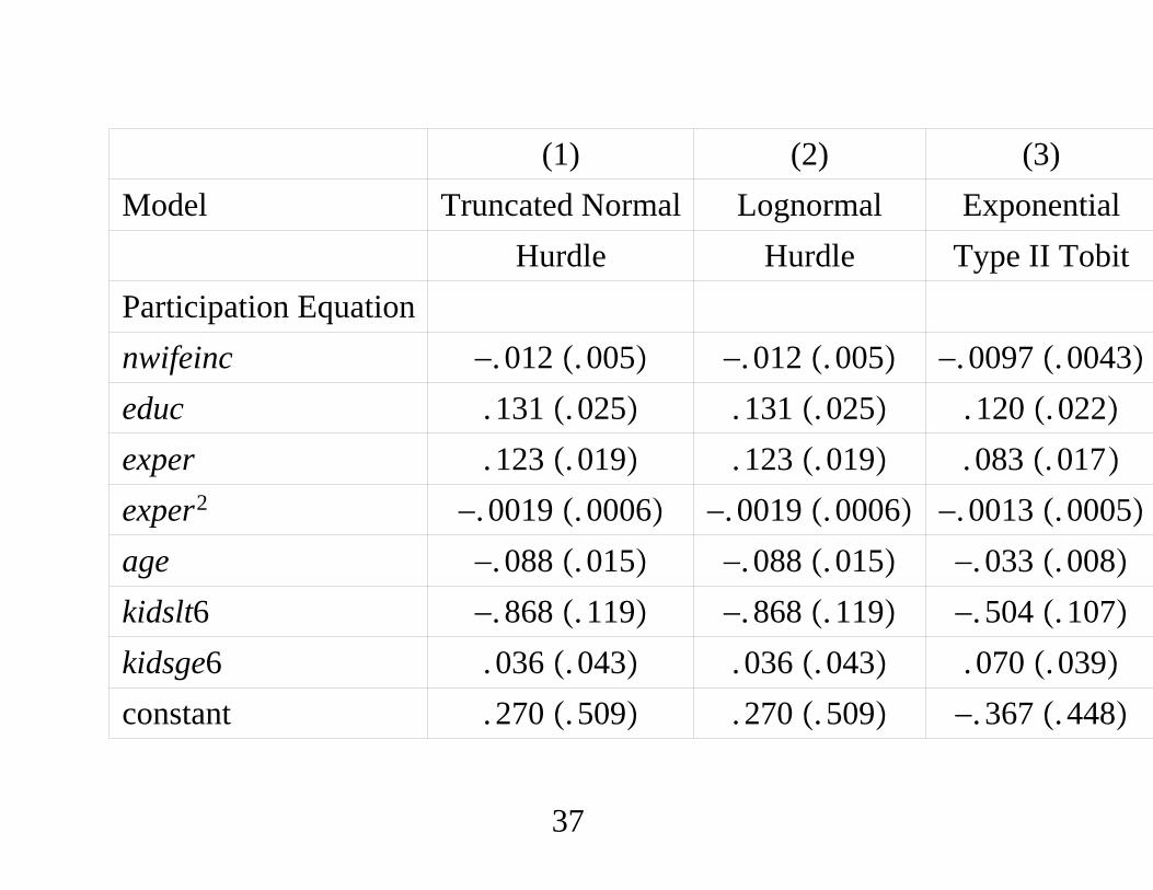
(1) (2) (3)Model Truncated Normal Lognormal Exponential
Hurdle Hurdle Type II TobitParticipation Equationnwifeinc −. 012 . 005 −. 012 . 005 −. 0097 . 0043educ . 131 . 025 . 131 . 025 . 120 . 022exper . 123 . 019 . 123 . 019 . 083 . 017exper2 −. 0019 . 0006 −. 0019 . 0006 −. 0013 . 0005age −. 088 . 015 −. 088 . 015 −. 033 . 008kidslt6 −. 868 . 119 −. 868 . 119 −. 504 . 107kidsge6 .036 . 043 . 036 . 043 . 070 . 039constant . 270 . 509 . 270 . 509 −. 367 . 448
37
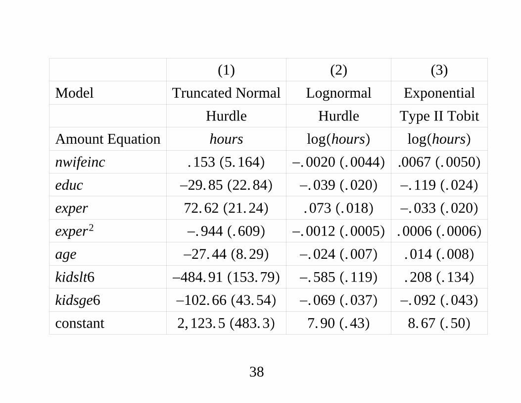
(1) (2) (3)Model Truncated Normal Lognormal Exponential
Hurdle Hurdle Type II TobitAmount Equation hours loghours loghoursnwifeinc . 153 5.164 −. 0020 . 0044 .0067 . 0050educ −29.85 22.84 −. 039 . 020 −. 119 . 024exper 72.62 21.24 . 073 . 018 −. 033 . 020exper2 −. 944 . 609 −. 0012 . 0005 . 0006 . 0006age −27.44 8.29 −. 024 . 007 . 014 . 008kidslt6 −484.91 153.79 −. 585 . 119 . 208 . 134kidsge6 −102.66 43.54 −. 069 . 037 −. 092 . 043constant 2, 123.5 483.3 7.90 . 43 8.67 . 50
38
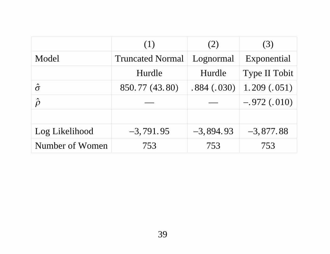
(1) (2) (3)Model Truncated Normal Lognormal Exponential
Hurdle Hurdle Type II Tobit 850.77 43.80 . 884 . 030 1.209 . 051 — — −. 972 . 010
Log Likelihood −3,791.95 −3,894.93 −3,877.88Number of Women 753 753 753
39
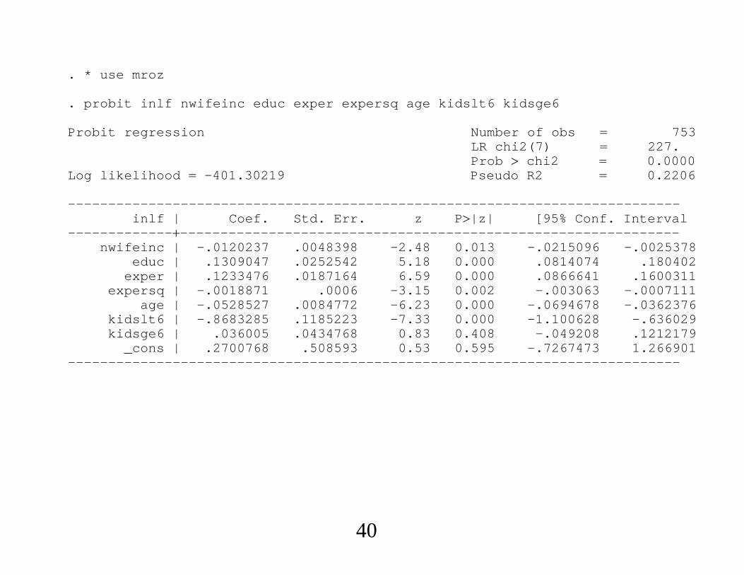
. * use mroz
. probit inlf nwifeinc educ exper expersq age kidslt6 kidsge6
Probit regression Number of obs 753LR chi2(7) 227.Prob chi2 0.0000
Log likelihood -401.30219 Pseudo R2 0.2206
----------------------------------------------------------------------------inlf | Coef. Std. Err. z P|z| [95% Conf. Interval
---------------------------------------------------------------------------nwifeinc | -.0120237 .0048398 -2.48 0.013 -.0215096 -.0025378
educ | .1309047 .0252542 5.18 0.000 .0814074 .180402exper | .1233476 .0187164 6.59 0.000 .0866641 .1600311
expersq | -.0018871 .0006 -3.15 0.002 -.003063 -.0007111age | -.0528527 .0084772 -6.23 0.000 -.0694678 -.0362376
kidslt6 | -.8683285 .1185223 -7.33 0.000 -1.100628 -.636029kidsge6 | .036005 .0434768 0.83 0.408 -.049208 .1212179
_cons | .2700768 .508593 0.53 0.595 -.7267473 1.266901----------------------------------------------------------------------------
40
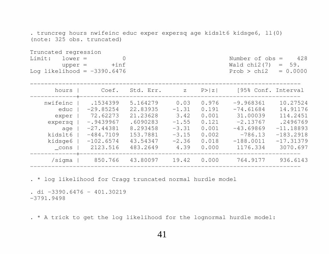
. truncreg hours nwifeinc educ exper expersq age kidslt6 kidsge6, ll(0)(note: 325 obs. truncated)
Truncated regressionLimit: lower 0 Number of obs 428
upper inf Wald chi2(7) 59.Log likelihood -3390.6476 Prob chi2 0.0000
----------------------------------------------------------------------------hours | Coef. Std. Err. z P|z| [95% Conf. Interval
---------------------------------------------------------------------------nwifeinc | .1534399 5.164279 0.03 0.976 -9.968361 10.27524
educ | -29.85254 22.83935 -1.31 0.191 -74.61684 14.91176exper | 72.62273 21.23628 3.42 0.001 31.00039 114.2451
expersq | -.9439967 .6090283 -1.55 0.121 -2.13767 .2496769age | -27.44381 8.293458 -3.31 0.001 -43.69869 -11.18893
kidslt6 | -484.7109 153.7881 -3.15 0.002 -786.13 -183.2918kidsge6 | -102.6574 43.54347 -2.36 0.018 -188.0011 -17.31379
_cons | 2123.516 483.2649 4.39 0.000 1176.334 3070.697---------------------------------------------------------------------------
/sigma | 850.766 43.80097 19.42 0.000 764.9177 936.6143----------------------------------------------------------------------------
. * log likelihood for Cragg truncated normal hurdle model
. di -3390.6476 - 401.30219-3791.9498
. * A trick to get the log likelihood for the lognormal hurdle model:
41
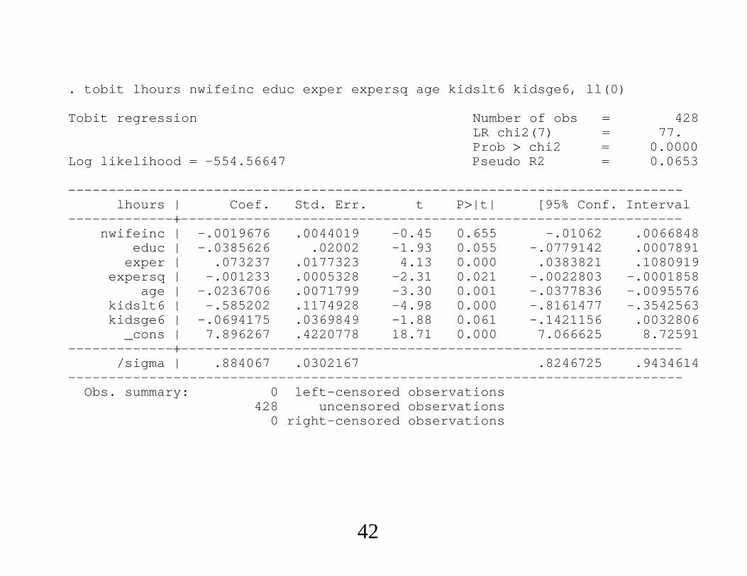
. tobit lhours nwifeinc educ exper expersq age kidslt6 kidsge6, ll(0)
Tobit regression Number of obs 428LR chi2(7) 77.Prob chi2 0.0000
Log likelihood -554.56647 Pseudo R2 0.0653
----------------------------------------------------------------------------lhours | Coef. Std. Err. t P|t| [95% Conf. Interval
---------------------------------------------------------------------------nwifeinc | -.0019676 .0044019 -0.45 0.655 -.01062 .0066848
educ | -.0385626 .02002 -1.93 0.055 -.0779142 .0007891exper | .073237 .0177323 4.13 0.000 .0383821 .1080919
expersq | -.001233 .0005328 -2.31 0.021 -.0022803 -.0001858age | -.0236706 .0071799 -3.30 0.001 -.0377836 -.0095576
kidslt6 | -.585202 .1174928 -4.98 0.000 -.8161477 -.3542563kidsge6 | -.0694175 .0369849 -1.88 0.061 -.1421156 .0032806
_cons | 7.896267 .4220778 18.71 0.000 7.066625 8.72591---------------------------------------------------------------------------
/sigma | .884067 .0302167 .8246725 .9434614----------------------------------------------------------------------------
Obs. summary: 0 left-censored observations428 uncensored observations
0 right-censored observations
42
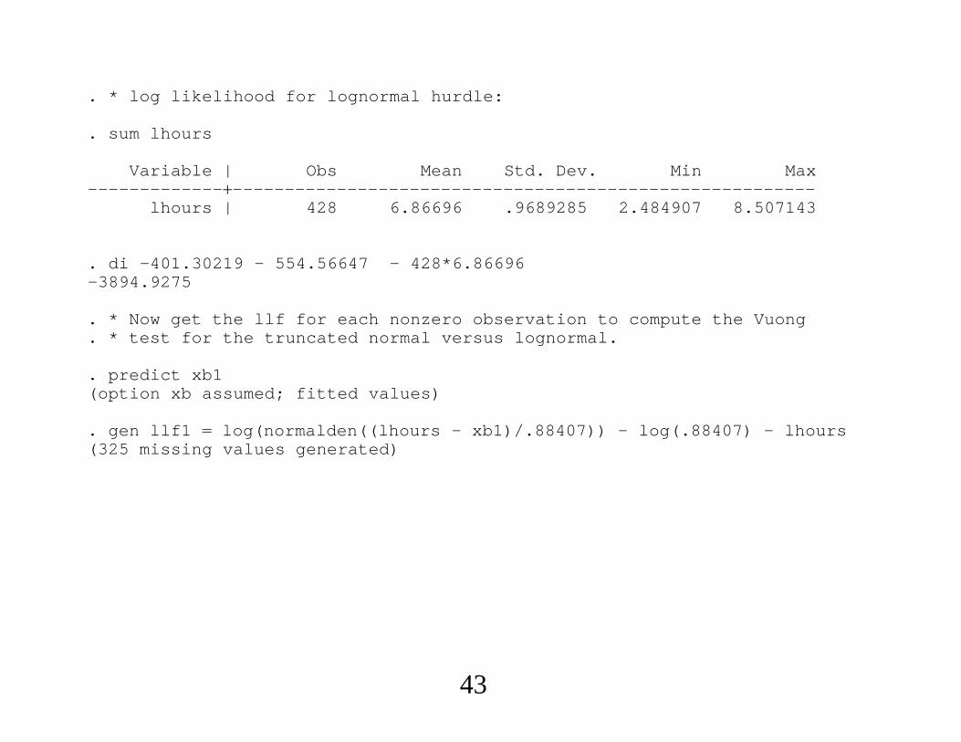
. * log likelihood for lognormal hurdle:
. sum lhours
Variable | Obs Mean Std. Dev. Min Max---------------------------------------------------------------------
lhours | 428 6.86696 .9689285 2.484907 8.507143
. di -401.30219 - 554.56647 - 428*6.86696-3894.9275
. * Now get the llf for each nonzero observation to compute the Vuong
. * test for the truncated normal versus lognormal.
. predict xb1(option xb assumed; fitted values)
. gen llf1 log(normalden((lhours - xb1)/.88407)) - log(.88407) - lhours(325 missing values generated)
43
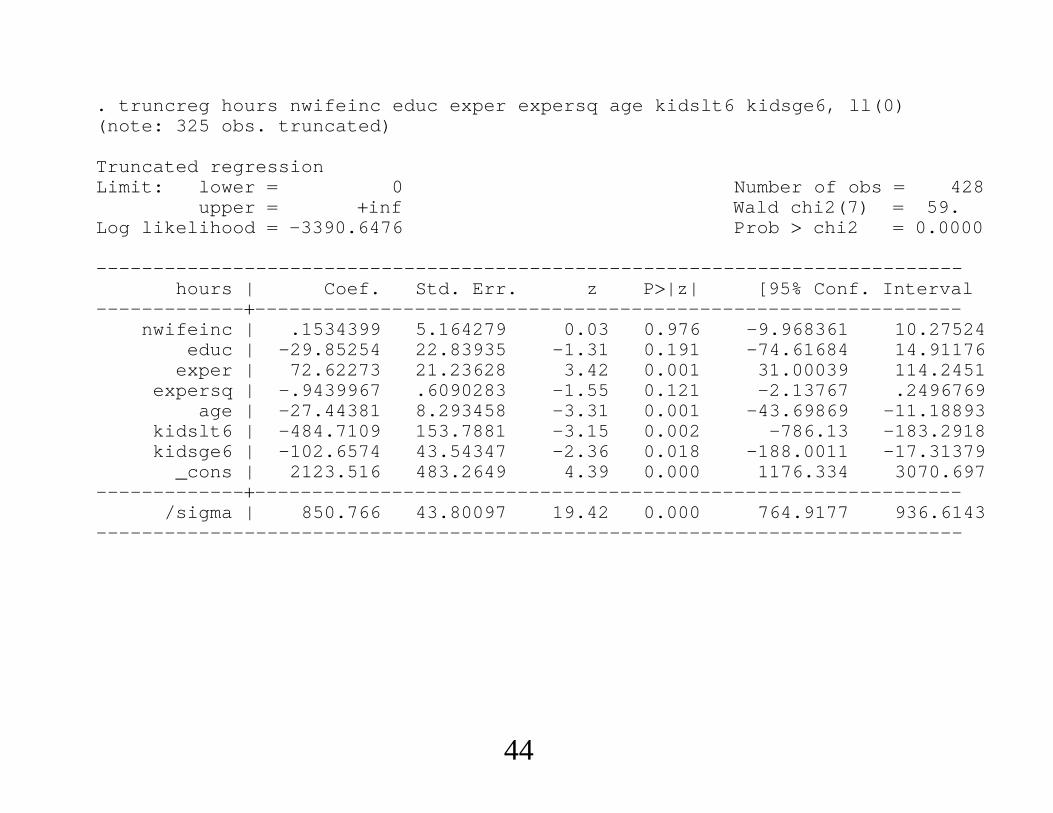
. truncreg hours nwifeinc educ exper expersq age kidslt6 kidsge6, ll(0)(note: 325 obs. truncated)
Truncated regressionLimit: lower 0 Number of obs 428
upper inf Wald chi2(7) 59.Log likelihood -3390.6476 Prob chi2 0.0000
----------------------------------------------------------------------------hours | Coef. Std. Err. z P|z| [95% Conf. Interval
---------------------------------------------------------------------------nwifeinc | .1534399 5.164279 0.03 0.976 -9.968361 10.27524
educ | -29.85254 22.83935 -1.31 0.191 -74.61684 14.91176exper | 72.62273 21.23628 3.42 0.001 31.00039 114.2451
expersq | -.9439967 .6090283 -1.55 0.121 -2.13767 .2496769age | -27.44381 8.293458 -3.31 0.001 -43.69869 -11.18893
kidslt6 | -484.7109 153.7881 -3.15 0.002 -786.13 -183.2918kidsge6 | -102.6574 43.54347 -2.36 0.018 -188.0011 -17.31379
_cons | 2123.516 483.2649 4.39 0.000 1176.334 3070.697---------------------------------------------------------------------------
/sigma | 850.766 43.80097 19.42 0.000 764.9177 936.6143----------------------------------------------------------------------------
44
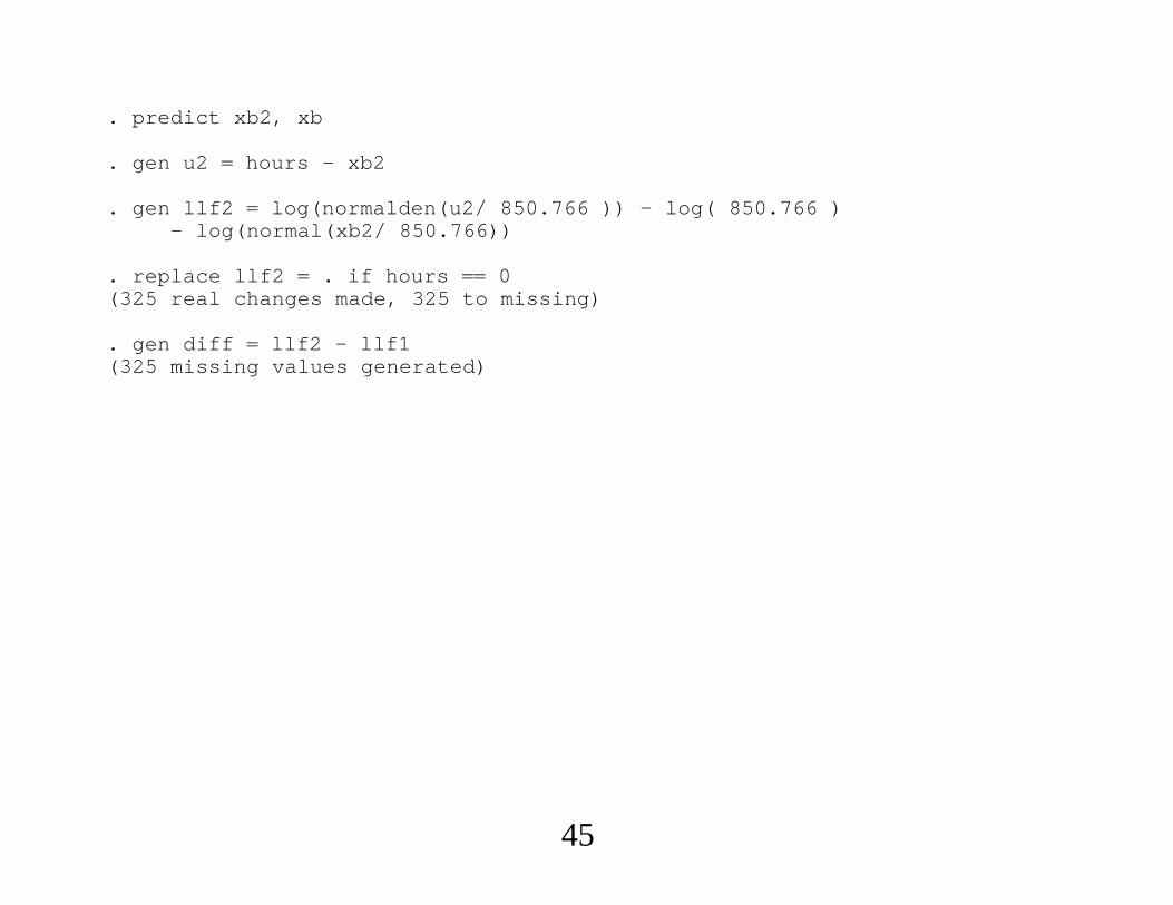
. predict xb2, xb
. gen u2 hours - xb2
. gen llf2 log(normalden(u2/ 850.766 )) - log( 850.766 )- log(normal(xb2/ 850.766))
. replace llf2 . if hours 0(325 real changes made, 325 to missing)
. gen diff llf2 - llf1(325 missing values generated)
45
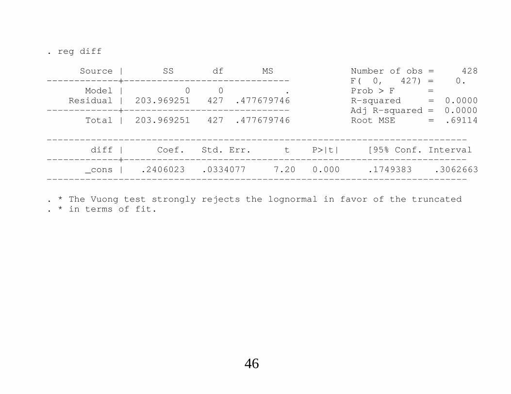
. reg diff
Source | SS df MS Number of obs 428------------------------------------------- F( 0, 427) 0.
Model | 0 0 . Prob F Residual | 203.969251 427 .477679746 R-squared 0.0000
------------------------------------------- Adj R-squared 0.0000Total | 203.969251 427 .477679746 Root MSE .69114
----------------------------------------------------------------------------diff | Coef. Std. Err. t P|t| [95% Conf. Interval
---------------------------------------------------------------------------_cons | .2406023 .0334077 7.20 0.000 .1749383 .3062663
----------------------------------------------------------------------------
. * The Vuong test strongly rejects the lognormal in favor of the truncated
. * in terms of fit.
46
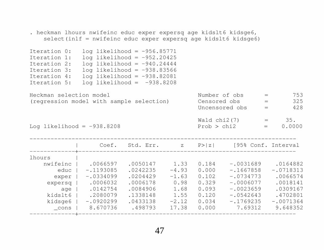
. heckman lhours nwifeinc educ exper expersq age kidslt6 kidsge6,select(inlf nwifeinc educ exper expersq age kidslt6 kidsge6)
Iteration 0: log likelihood -956.85771Iteration 1: log likelihood -952.20425Iteration 2: log likelihood -940.24444Iteration 3: log likelihood -938.83566Iteration 4: log likelihood -938.82081Iteration 5: log likelihood -938.8208
Heckman selection model Number of obs 753(regression model with sample selection) Censored obs 325
Uncensored obs 428
Wald chi2(7) 35.Log likelihood -938.8208 Prob chi2 0.0000
----------------------------------------------------------------------------| Coef. Std. Err. z P|z| [95% Conf. Interval
---------------------------------------------------------------------------lhours |
nwifeinc | .0066597 .0050147 1.33 0.184 -.0031689 .0164882educ | -.1193085 .0242235 -4.93 0.000 -.1667858 -.0718313
exper | -.0334099 .0204429 -1.63 0.102 -.0734773 .0066574expersq | .0006032 .0006178 0.98 0.329 -.0006077 .0018141
age | .0142754 .0084906 1.68 0.093 -.0023659 .0309167kidslt6 | .2080079 .1338148 1.55 0.120 -.0542643 .4702801kidsge6 | -.0920299 .0433138 -2.12 0.034 -.1769235 -.0071364
_cons | 8.670736 .498793 17.38 0.000 7.69312 9.648352---------------------------------------------------------------------------
47
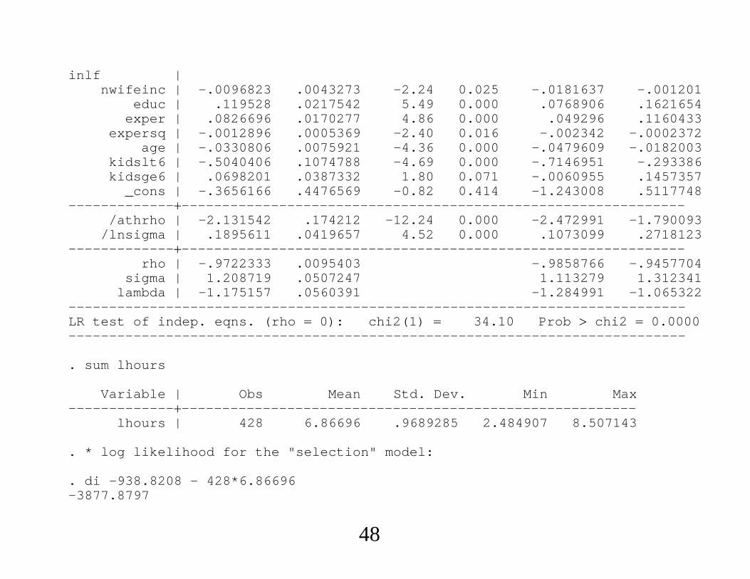
inlf |nwifeinc | -.0096823 .0043273 -2.24 0.025 -.0181637 -.001201
educ | .119528 .0217542 5.49 0.000 .0768906 .1621654exper | .0826696 .0170277 4.86 0.000 .049296 .1160433
expersq | -.0012896 .0005369 -2.40 0.016 -.002342 -.0002372age | -.0330806 .0075921 -4.36 0.000 -.0479609 -.0182003
kidslt6 | -.5040406 .1074788 -4.69 0.000 -.7146951 -.293386kidsge6 | .0698201 .0387332 1.80 0.071 -.0060955 .1457357
_cons | -.3656166 .4476569 -0.82 0.414 -1.243008 .5117748---------------------------------------------------------------------------
/athrho | -2.131542 .174212 -12.24 0.000 -2.472991 -1.790093/lnsigma | .1895611 .0419657 4.52 0.000 .1073099 .2718123
---------------------------------------------------------------------------rho | -.9722333 .0095403 -.9858766 -.9457704
sigma | 1.208719 .0507247 1.113279 1.312341lambda | -1.175157 .0560391 -1.284991 -1.065322
----------------------------------------------------------------------------LR test of indep. eqns. (rho 0): chi2(1) 34.10 Prob chi2 0.0000----------------------------------------------------------------------------
. sum lhours
Variable | Obs Mean Std. Dev. Min Max---------------------------------------------------------------------
lhours | 428 6.86696 .9689285 2.484907 8.507143
. * log likelihood for the "selection" model:
. di -938.8208 - 428*6.86696-3877.8797
48
Related Documents