Human alteration of groundwater–surface water interactions (Sagittario River, Central Italy): implication for flow regime, contaminant fate and invertebrate response

1

HUMAN ALTERATION OF GROUNDWATER-SURFACE WATER INTERACTIONS 1 (SAGITTARIO RIVER, CENTRAL ITALY): IMPLICATION FOR FLOW REGIME, CONTAMINANT 2 FATE AND INVERTEBRATE RESPONSE 3 4 5 Mariachiara Caschetto1, Maurizio Barbieri1, Diana M. P. Galassi2, Lucia Mastrorillo3, Sergio Rusi4, 6 Fabio Stoch2, Alessia Di Cioccio2, Marco Petitta1 7 8 9 1Dipartimento di Scienze della Terra, Università di Roma “La Sapienza”, P.le Aldo Moro 5, 00185 Roma, Italy 10 11 2Dipartimento della Vita, della Salute e delle Scienze Ambientali, Università de L’Aquila, Via Vetoio, Coppito 12 67100 L'Aquila, Italy 13 14 3Dipartimento di Scienze Geologiche, Università “Roma Tre”, Largo San Leonardo Murialdo, 00146 Roma, 15 Italy 16 17 4Dipartimento di Ingegneria e Geologia (INGEO) Sezione di Geologia, Università G. d'Annunzio, Via dei 18 Vestini 30, 66013 Chieti, Italy 19 20 21 22 23 24 25 26 27 28 Corresponding author: Marco Petitta 29 E-mail: [email protected] 30 Phone: 0039-06-49914834 31 Fax: 0039-06-4454729 32 33 34 35 36 37 38 39 40

41

2

ABSTRACT 42

Many rivers world-wide are undergoing severe man-induced alterations which are reflected also in 43

changes of the degree of connectivity between surface waters and groundwater. Pollution, 44

irrigation withdrawal, alteration of freshwater flows, road construction, surface water diversion, soil 45

erosion in agriculture, deforestation and dam building have led to some irreversible species losses 46

and severe changes in community composition of freshwater ecosystems. 47

Taking into account the impact of damming and flow diversion on natural river discharge, the 48

present study is aimed at (i) evaluating the effects of anthropogenic changes on 49

groundwater/surface water interactions; (ii) analysing the fate of nitrogenous pollutants at the 50

floodplain scale; and (iii) describing the overall response of invertebrate assemblages to such 51

changes. 52

Hydrogeological, geochemical, and isotopic data revealed short- and long-term changes in 53

hydrology, allowing the assessment of the hydrogeological setting and the evaluation of potential 54

contamination by nitrogen compounds. Water isotopes allowed distinguishing a shallow aquifer 55

locally fed by zenithal recharge and river losses, and a deeper aquifer/aquitard system fed by 56

surrounding carbonate aquifers. This system was found to retain ammonium and, through the 57

shallow aquifer, release it in surface running waters via the hyporheic zone of the river bed. All 58

these factors influenced river ecosystem health. As many environmental drivers entered in action 59

offering a multiple - component artificial environment, a clear relationship between river flow 60

alteration and benthic and hyporheic invertebrate diversity was not found, being species response 61

driven by the combination of three main stressors: ammonium pollution, man-induced changes in 62

river morphology and altered discharge regime. 63

64

Key words: river, nitrogen cycle, stable isotope, surface/groundwater interaction, GDE, Italy 65

66

67

3

INTRODUCTION 68

The key role of hydrological processes on ecological functioning in rivers is largely emphasized 69

and the cause-effect relationship between them already described in the Water Framework 70

Directive (WFD) of the European Community (EC, 2000). Nevertheless, there is still great 71

uncertainty in assessing a clear link between flow alteration and ecological response, in part 72

because along with man-induced flow alteration, several other environmental parameters may 73

change and not always as “dependent variables.” Additionally, if alteration of river flow may lead to 74

bank and riverbed sediment erosions with severe changes in river bed sediment composition, there 75

are other factors that contribute to the alteration of the abiotic facies of rivers. For instance, 76

agriculture, urbanization and industrialization determine the pollution of soil and water in both 77

surface-flowing water and groundwater. 78

Dams lead to severe changes in river discharge regimes, altering the natural distribution and timing 79

of stream flow by high-magnitude peaks during dam release, with a cascade effect on river 80

morphology, alteration of riffle-pools sequences, and an increase in sediment and bank erosion 81

downstream (Boulton et al., 1998; Salem et al., 2012). These man-induced alterations co-occur in 82

the Sagittario River floodplain in central Italy with indiscriminate land use for urbanization, 83

agriculture and industrialization. Moreover, water diversion for irrigation coexists with damming, 84

further altering the natural flow regime, and urbanization and agriculture in the floodplain increases 85

the nitrogenous contamination. 86

Hydropower dams release high-discharge water downstream, leading to floods in the alluvial plain, 87

where urban and agricultural settlements are located (May et al., 2011). In these areas, local 88

authorities introduce additional interference by means of river course rectification and 89

channelization by erasing riparian vegetation. Moreover, where discharge is very high and the river 90

flows close to roads, railways and urbanized areas, the river flow is moved out of its original 91

topology, making parts of the river artificially perched. Changes in river hydrology and dynamics 92

can directly or indirectly influence the chemical characteristics of surface water and groundwater 93

(EC, 2012; Rao et al., 2012) by altering the connectivity between the river and the underlying 94

aquifer that has become disconnected in the artificial perched stretch, as in the Sagittario River 95

4

(Banks et al., 2011). This condition alters the topology of the groundwater-dependent ecosystems 96

(GDEs) (Eamus and Froend, 2006), consequently affecting freshwater invertebrate biodiversity 97

(Poff et al., 2010) at the interface between surface water and groundwater, in the so-called 98

hyporheic zone of the riverbed sediments, and on the surface benthic macroinvertebrate 99

communities. Moreover, understanding how hydrological and biological processes in the floodplain 100

and in the hyporheic zone may control the concentration and fate of nitrogen compounds in 101

watersheds is crucial (Landers et al., 2008; Di Lorenzo et al., 2012). In particular, nitrate 102

attenuation depends on the capacity of riparian vegetation and microbial communities to intercept 103

pollutants moving in surface runoff and groundwater flow (Hill, 1996; Cey et al., 1999; Petitta et al., 104

2009; Keskin, 2010; Wexler et al., 2011).In a groundwater multi-layer system (Stanford and Ward, 105

1992), as in the case under study, the interactions between groundwater and surface water that 106

are influenced by the alteration of river discharge and morphology can generate impacts on GDEs 107

(e.g., in terms of nitrogen contamination and invertebrate community compositions). 108

An integrated multidisciplinary monitoring approach was applied to man-altered stretches of the 109

Sagittario River (central Italy). This study was focused on assessing (i) surface water-groundwater 110

interactions, (ii) the influence of surface water and groundwater interactions on the nitrogen cycle 111

at the floodplain scale, and (iii) freshwater benthic and hyporheic invertebrate responses to multiple 112

disturbances. 113

114

STUDY AREA 115

The Sulmona Basin, a Pleistocene intramontane plain surrounded by carbonate ridges in central 116

Italy, is characterized by a complex hydrogeological setting where several high-discharge springs 117

feed the Aterno-Pescara hydrological basin, including the Sagittario River (Celico, 1978; Boni et 118

al., 1986; Conese et al., 2001; Barbieri et al., 2005; Desiderio et al., 2012). 119

The Sagittario River valley is the southern part of the Sulmona Basin, which extends over 120

approximately 143 km2 in the SSE-NNW direction (Fig. 1). It is a large depression filled with thick 121

(up to 500 m) fluvio-lacustrine deposits of Pleistocene-Holocene age and completely surrounded 122

by carbonate ridges (Miccadei et al., 1998). Previous studies (Desiderio et al., 2003, 2005b, 2012) 123

5

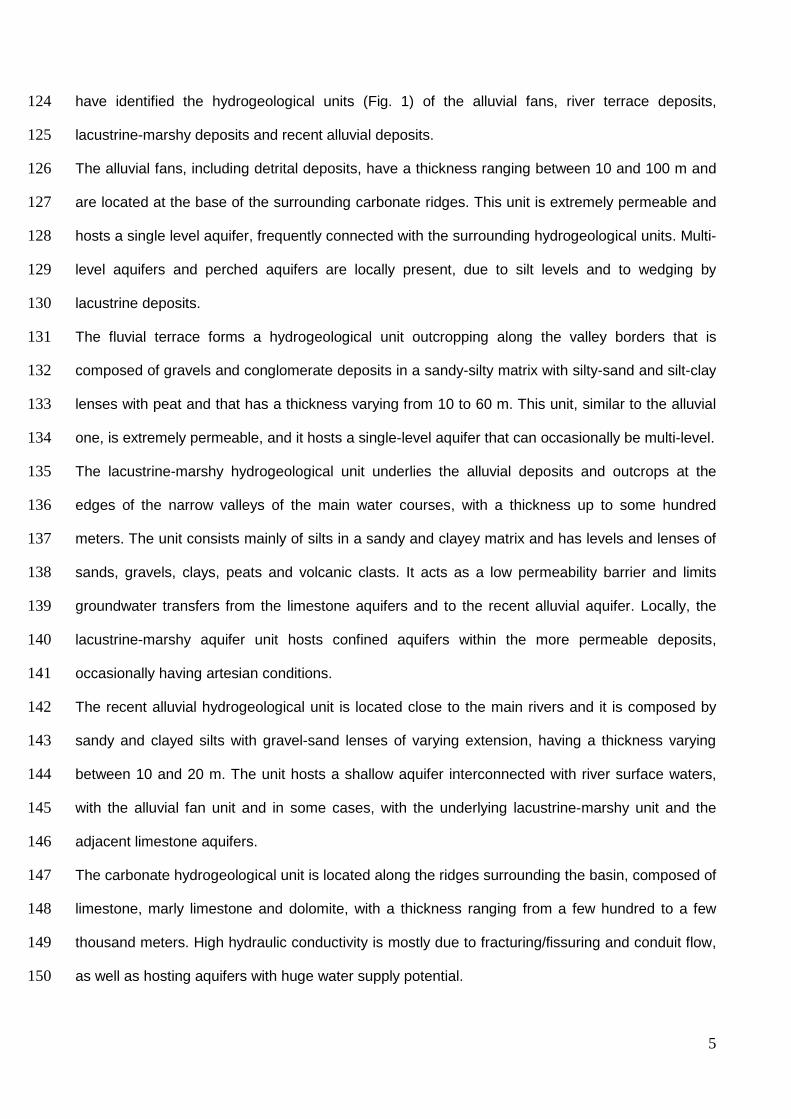
have identified the hydrogeological units (Fig. 1) of the alluvial fans, river terrace deposits, 124

lacustrine-marshy deposits and recent alluvial deposits. 125

The alluvial fans, including detrital deposits, have a thickness ranging between 10 and 100 m and 126

are located at the base of the surrounding carbonate ridges. This unit is extremely permeable and 127

hosts a single level aquifer, frequently connected with the surrounding hydrogeological units. Multi-128

level aquifers and perched aquifers are locally present, due to silt levels and to wedging by 129

lacustrine deposits. 130

The fluvial terrace forms a hydrogeological unit outcropping along the valley borders that is 131

composed of gravels and conglomerate deposits in a sandy-silty matrix with silty-sand and silt-clay 132

lenses with peat and that has a thickness varying from 10 to 60 m. This unit, similar to the alluvial 133

one, is extremely permeable, and it hosts a single-level aquifer that can occasionally be multi-level. 134

The lacustrine-marshy hydrogeological unit underlies the alluvial deposits and outcrops at the 135

edges of the narrow valleys of the main water courses, with a thickness up to some hundred 136

meters. The unit consists mainly of silts in a sandy and clayey matrix and has levels and lenses of 137

sands, gravels, clays, peats and volcanic clasts. It acts as a low permeability barrier and limits 138

groundwater transfers from the limestone aquifers and to the recent alluvial aquifer. Locally, the 139

lacustrine-marshy aquifer unit hosts confined aquifers within the more permeable deposits, 140

occasionally having artesian conditions. 141

The recent alluvial hydrogeological unit is located close to the main rivers and it is composed by 142

sandy and clayed silts with gravel-sand lenses of varying extension, having a thickness varying 143

between 10 and 20 m. The unit hosts a shallow aquifer interconnected with river surface waters, 144

with the alluvial fan unit and in some cases, with the underlying lacustrine-marshy unit and the 145

adjacent limestone aquifers. 146

The carbonate hydrogeological unit is located along the ridges surrounding the basin, composed of 147

limestone, marly limestone and dolomite, with a thickness ranging from a few hundred to a few 148

thousand meters. High hydraulic conductivity is mostly due to fracturing/fissuring and conduit flow, 149

as well as hosting aquifers with huge water supply potential. 150

6

Unconfined aquifers recognized in the alluvial units and within the multi-layer aquifer in the 151

lacustrine-marshy deposits are recharged by rain, runoff, and irrigation as well (Desiderio et al. 152

2003, 2012). Locally, the deeper levels are fed by regional carbonate aquifers. Available δ18O and 153

δD data (Desiderio et al., 2005a) indicate that sand-gravel aquifers are recharged at average 154

isotopic altitudes of 800 m a.s.l. The flow path of the alluvial aquifer moves from the alluvial fans 155

toward the terrace edges. The main aquifer drainage pathways are along some paleo-riverbeds 156

into recent alluvial deposits. The Sagittario River acts as the final destination for groundwater (Fig. 157

1). 158

A hydrological gauging station (Capocanale site) has been recording the discharge of the 159

Sagittario River since 1927. The monthly discharge regime shows two peaks in April and in 160

December (with a mean highest discharge of 8 m3s-1), with the lowest values from June to August 161

(from 2.5 to 4 m3s-1), demonstrating the base flow contribution from groundwater. In the last two 162

decades, the lowest mean discharge values were measured along the hydrologic year. The natural 163

regime of the river has been highly affected since the first half of the 20th century by a hydropower 164

dam located upstream, as shown by daily hydrographs (Fig. 2) related to years 2006, 2008, 2010 165

and 2011. In the first half of the year and in the last months of the year, weekly changes 166

correspond to the use of hydropower, which is active during weekdays, causing peaks in 167

discharge. Conversely, during the weekend, there is no overflow, and water is stocked in the dam, 168

as reflected in a shortage of approximately 50% of the river discharge. This artificial regime has 169

been employed for several years, but during 2010, the hydropower plant was stopped. As a result, 170

the 2010 hydrograph represents a more "natural" discharge, with peaks corresponding to runoff 171

contribution and low-discharge phases during dry summer periods. In addition, from June to 172

September, river diversions for irrigation purposes are active along the river, are concentrated 173

downstream from the gauging station, and are limitedly affecting the discharge hydrographs at the 174

Capocanale station. The selected years can be considered representative of rainy (2006), average 175

(2010-2011) and dry years (2008). 176

177

178

7

METHODS 179

A multidisciplinary approach has been adopted for evaluating the hydrological, hydrochemical and 180

biological status of the Sagittario River according to EU requirements (EC, 2012) by analyzing the 181

degree of connectivity between surface flowing waters and the underlying aquifers, its influence on 182

the nitrogen cycle and the response of freshwater invertebrate fauna. Three sampling surveys 183

were performed in different hydrological and environmental conditions along the hydrological year: 184

(1) between November and December 2010, when runoff and groundwater discharges are 185

progressively increasing the river discharge (initial recharge phase); (2) in June 2011, when the 186

highest river discharge is recorded (peak phase) and influenced by snow melting and abundant 187

runoff (Fig. 2); and (3) between August and October 2011, corresponding to the minimum 188

discharge value (exhaustion phase), which persists until fall, when the new rainfall season starts. 189

To assess the relationship between the Sagittario River and the water table, for each sampling 190

time, river discharge was measured with a portable flow meter at five gauging stations (Fig. 3). 191

Water samples were collected along the riverbed in 19 sites. Groundwater from 13 springs (S) and 192

3 wells (W) located in the Sagittario River alluvial plain was sampled (Fig. 3, Table 1). Due to the 193

limited availability of wells in the study area, 3 new monitoring wells (MW) were drilled close to the 194

Sagittario River (up to 300 m away, Fig. 3), to a depth of 26, 30 and 24 m. MW1 showed an 195

artesian condition, flushing groundwater up to 2 m above ground level. 196

Groundwater from monitoring wells MW2 and MW3 was sampled using Solinst straddle inflatable 197

packers for depth profiles. Three depths were monitored for each well: MW2 was investigated at 7, 198

12 and 18 m below the groundwater table (b.g.t.) and MW3 at 6, 14, and 20 m b.g.t. Temperature, 199

oxidation reduction potential (ORP), pH and electrical conductivity (EC) were measured using the 200

Oxi 349i/SET multiparametric probe. In the monitoring wells MW2 and MW3, vertical logs of the 201

same parameters were also obtained using a Hydrolab Reporter multiprobe 5.0. 202

Laboratory analyses including major ions δ18O and δD were performed. For chemical analysis, 50 203

mL of water were collected in PVS bottles, filtered (0.45 µm Millipore Filters) and then acidified with 204

0.1 N HNO3 to pH≤ 5. 205

8

Major ions analyses were performed by chromatographic technique (Metrohm 761 Compact IC) 206

with an analytical precision of ±0.5%. Groundwater and surface water samples (100 mL) for δ18O 207

and δD were analyzed at the Isotope Lab at the University of Parma. The international standard 208

used was the Vienna Standard Mean Ocean Water (VSMOW) for oxygen and hydrogen isotopes. 209

The analytical error was ±0.1‰ and ±1‰, respectively. The normalization procedure followed the 210

two-points or multi-point method based on a linear regression. The raw measured delta values for 211

at least two different analyzed standards were plotted on the x-axis, and the “true” commonly 212

accepted delta values, expressed in VSMOW scale, were plotted on the y-axis, a regression line 213

that covers a different range of delta values depending on the delta values of the standards 214

analyzed. During the normalization process, the raw delta value of the sample (measured versus 215

the working gas standard) was multiplied by the slope, and the value of the intercept was then 216

added (Skrzypek, 2013). 217

Samples for water chemistry from both surface flowing waters and hyporheic sites were collected 218

and stored in polyethylene bottles and kept refrigerated until analyzed by A.R.T.A. Abruzzo 219

(Department of L’Aquila). Dissolved oxygen, temperature, pH, oxygen concentration, and electrical 220

conductivity were measured in the field with a multiparametric probe (YSI 556 MPS). 221

The invertebrate sampling was conducted along with the hydrological and hydrochemical 222

monitoring surveys. Sampling sites were located as close as possible to the corresponding 223

discharge measurement sites. Faunal samples were collected at five sites along the Sagittario 224

River downstream of the dam (Fig. 3) by selecting an additional “reference site” (site B0) in a river 225

stretch that did not undergo rectification, river bank concretion, or riparian devegetation. Site B1 226

was placed at the terminal fan of the river-gaining sector where several alterations co-occurred, 227

such as rectification, river bank concretion, and riparian devegetation; site B2 was located in the 228

most altered river stretch, where the river path underwent diversion, was artificially perched, and 229

riparian vegetation was completely erased; B3 was located 500 m downstream of B2, where the 230

river comes back to its natural path after an artificial waterfall (Fig. 3); and B4 was located 1 km 231

upstream from the confluence to the Aterno River, river banks had consistent riparian vegetation 232

but rectification was still present. Sites B3 and B4 were the ones less affected by changes in river 233

9

morphology. To assess spatial and temporal biodiversity patterns in the hyporheic zone, each site 234

was sampled at 50 cm below the river bed and samples were taken using a Bou-Rouch pump (Bou 235

and Rouch, 1967) and mobile pipes were hammered at each sampling point-depth. For each site, 236

three spatial replicates were taken for three times along the hydrological year to maximize the 237

measured species richness along habitat heterogeneity for each transect. The piezometric head 238

was measured at each sampling date and site using the T-bar (Malard et al., 2002). 239

Faunal samples were extracted by filtering 10 L samples of water and fine sediments collected 240

through a hand net (mesh size of 60 μm) and then preserved in 60% ethyl alcohol in the field. All 241

fauna samples were accompanied by physicochemical analyses. The Crustacea Copepoda 242

resulted in the most abundant group in the hyporheic sites by far, and for this reason, they were 243

selected as the target group. Copepods were sorted, counted, identified to species level, and 244

assigned to two ecological categories (obligate groundwater dwellers, i.e., stygobionts, and non-245

obligate groundwater dwellers, i.e., non-stygobionts) according to the definition given by Galassi 246

(2001) and Galassi et al. (2009). Supplementary samples were also taken at the benthic surface of 247

riverbed sediments by sampling 25 x 25 cm2 on three different microhabitats recognizable along 248

the transect, to cover the highest habitat heterogeneity at each site. Benthic samples were filtered 249

through a drift net and preserved in 60% ethyl alcohol on the field. Individuals, predominantly 250

belonging to insect orders and macrocrustaceans, were sorted and identified at the species level 251

when achievable. The Margalef’s index (Margalef, 1958) was calculated from the total number of 252

species counted and their abundance from both hyporheic and benthic samples by cumulating 253

abundances and species richness of spatial replicates and sampling dates per sampling site. 254

255

RESULTS 256

River discharge 257

In the first survey, the highest value of 7.7 m3s-1 was measured downstream (Q4), upstream from 258

the confluence with the Aterno River, and the lowest value of 4.9 m3s-1 was measured at Q3 (Fig. 259

4). During the second survey, the highest discharge value of approximately 10.7 m3s-1 was 260

measured at Q2, at the confluence with the Velletta stream, and the lowest value at Q3. Q4 261

10

showed the highest discharge value, even in the third survey (3.4 m3s-1), whereas in Q1, close to 262

the Acqua Chiara spring (SA, Fig. 3), the lowest value of 1.8 m3s-1 was observed. According to the 263

hydrological cycle in central Italy, the seasonal variability among collected data showed a 264

significant increase in discharge between the first two surveys, followed by a decrease in the third 265

survey. In addition, data related to Q3 were collected 500 m downstream from the Capocanale 266

gauging station. A comparison between the measured values and the calculated values were 267

similar, with an error for each survey below 10% (Fig. 2). 268

In the first two surveys, discharge differences along monitoring sites followed the same scheme, 269

with alternation of increase and decrease of river discharge having comparable magnitude and 270

highlighting a similar response in terms of surface water-groundwater exchanges. The third survey 271

values are affected both by natural lower discharge and by additional human diversions for 272

agricultural purposes; consequently, discharge changes along the river showed a lower magnitude, 273

becoming negligible. Furthermore, it was possible to identify small-scale differences in river 274

discharge, where local river discharge increased or decreased (Fig. 4). In upstream stretches close 275

to the SA spring, up to Q2, the Sagittario River discharge increased at an average of approximately 276

0.7 m3s-1; from Q2 to Q3 the discharge decreases of approximately 2.7 m3s-1 (33% of the total river 277

discharge). Downstream from Q3, where the artificial waterfall is located, the discharge increased 278

to 2.6 m3s-1, with lower values during the third survey. Between Q4 and Q5, upstream from the 279

confluence with the Aterno River, local mean discharge lowered to approximately 1.1 m3s-1. 280

281

Water chemistry 282

All sampled waters in wells, springs and monitoring wells showed pH values close to neutrality or 283

slightly alkaline (from 6.84 to 8.02) (Table 1), except for the well WC during the second survey in 284

June 2011. Seasonal changes were observed in surface water temperature, with an average of 285

6.9°C in the first survey, and 14.7°C in the second and third surveys. Groundwater showed a less 286

pronounced variation, between 7.9°C in the first survey and 12.5°C in the second and third 287

surveys. The electrical conductivity ranged between 255 and 790 µScm-1 in springs, and between 288

478 and 693 µScm-1 in groundwater, including vertical logs. ORP ranged from +37 to +231 mV in 289

11

spring, as expected for oxygenated waters, except for SC in the second survey. Wells (W) and 290

monitoring wells (MW) were locally characterized by low ORP values until -188 mV, indicating a 291

reducing environment. Vertical data logs of MW2 and MW3 (Fig. 5) showed sharp changes in pH, 292

ORP, and electrical conductivity between 17 and 22 m b.g.l. 293

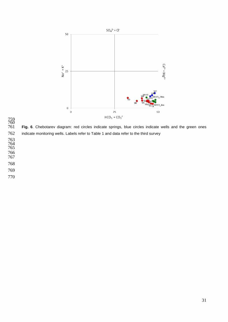
The geochemical facies (Fig. 6) of groundwater and surface water is mainly a Ca-HCO3 type. 294

Slight variations of measured values of SO42-, Ca2+, Mg2+, Na+ and K+ were also detected both 295

among the three seasonal surveys and across different sampling sites. Wells WB and WC showed 296

a steady chemical facies during the whole sampling period. Conversely, marked differences of 297

Ca2+ (65.9 mgL-1 in WB and 47.8 mgL-1 in WC during the third survey) and Cl- concentrations (11.9 298

mgL-1 in WB and 5.8 mgL-1 in WC during the third survey) were recorded in the same samples. WA 299

showed an intermediate chemical composition and a sharp seasonal variability. Differences in 300

spring waters were observed between the group SA-SC-SF close to the river bed and those at 301

higher elevation (SM, SN, SO) that showed a higher SO42-, Cl-, Na+, and K+ content. Monitoring 302

wells (MW) did not show chemical variation through vertical sampling, except MW3, which at the 303

deepest sampling point had a significant increase in HCO3-, K+ and NH4

+ content. MW3 showed 304

higher values of NH4+ and PO4

3- (up to 30.6 and 1.2 mgL-1, respectively), whereas the same ions 305

have not been found in MW1 and MW2. MW1 had a unique chemical composition, showing the 306

highest values of Ca2+ (68.9 mgL-1), SO42- (10.1 mgL-1) and Cl- (18.5 mgL-1). 307

During the three seasonal surveys, no clear trends were observed in nitrate concentration, ranging 308

from 0.1 to 100.9 mgL-1. Therefore, wide variability among springs, wells and monitoring wells was 309

proved by standard deviation (Table 2). The lowest average value was detected during the second 310

survey. The monitoring wells did not show differences along the water column at the temporal 311

scale. Conversely, slight differences among springs at different elevation were observed (Fig. 7). 312

All springs located on the left side of the Sagittario River (between 340 and 1200 m a.s.l.) showed 313

remarkable concentrations of nitrate. A similar trend, even if less pronounced, was observed in 314

wells located on the right border. 315

Ammonium concentrations showed the similar standard deviation values to the averages (Table 2). 316

Values ranged from under the instrumental detection limits to 30.9 mgL-1 of NH4+ observed in few 317

12

springs. Detectable ammonium concentrations were found only in SC (1.3 mgL-1, first survey) and 318

SE (2.5 mgL-1, second survey). Some wells and monitored wells revealed significant ammonium 319

concentration, reaching 21 and 14 mgL-1 in WB and WC, respectively. Low ammonium 320

concentrations were measured in MW1 and MW2 during the second survey, but they were under 321

the instrumental detection limits in October. MW3 showed high ammonium concentrations along 322

the entire sampling survey, with the maximum value measured at the deepest screen sampled (up 323

to 30 mgL-1). At the spatial scale (Fig. 8), the highest ammonium concentrations were measured 324

close to the river bed, mostly along the right bank, especially in wells and monitoring wells. 325

326 Isotope approach 327

The isotopic compositions of the sampled waters collected during all monitoring surveys showed a 328

variability range between -59.5/-74.8‰ for δD, and -8.6/-11.3‰ for δ18O (Table 3). Differences in 329

isotopic composition among sampling points were also observed over time, in particular from 330

springs SA, SC, SE and SF. 331

The isotopic data are consistent with the literature relationships for the global average (GML, 332

Rozanski et al., 1993), central Italy (cIML, Longinelli and Selmo, 2003) and the Abruzzi region 333

(RML, Barbieri et al., 2003). Moreover, such a straight line (Fig. 9) is also consistent with the 334

equation (δD = 5.05 δ18O – 16.04) concerning samples of the upper valley of the Sagittario River 335

(Petitta et al., 2010). Three different isotope signals representative of the study area were found in 336

groundwater samples (Fig. 9). A group of waters including spring SI and well WC showed the less 337

enriched δ18O and δD values: -10.9‰ and -71.4 in SI, -11.3‰ and -74.8‰ in WC (third survey). 338

More enriched values referred to a different group of springs (SN, SO and SM) (-8.6‰ δ18O, -339

59.5‰ δD in SN, third survey) and well WB (-9.1‰ δ18O, -63.5‰ δD, third survey). The third group 340

included springs and monitoring wells characterized by intermediate signals (-10‰ δ18O, -66.9‰ 341

δD in SC). No significant variations were detected among the vertical logs in MW2 and MW3. 342

343 344

345

13

Species diversity and abundance of freshwater invertebrates 346

The distribution pattern of benthic and hyporheic invertebrate fauna along the Sagittario River from 347

the third survey (Fig. 10) showed significant differences. Both benthic macroinvertebrates and 348

hyporheic copepods displayed higher species diversity (expressed as Margalef’s index) in the 349

uppermost stretch (B0), characterized by the presence of a consistent riparian buffer strip. 350

Although located downstream from the dam, the stretch showed microhabitat diversification, with 351

riffle-pool sequences, macrophytes, and mosses close to river banks, where current velocity was 352

lower. Macroinvertebrate diversity dramatically decreased in site B1, where river channel 353

rectification, bank concretion, very high current velocity, and the total absence of riparian 354

vegetation contributed to an impoverishment of microhabitats. Moreover, the erosion of bed 355

sediments created a benthic habitat inhospitable for almost all the macroinvertebrate taxa. 356

Conversely, the highest stygobiotic copepod species richness was found at this site. In 357

downstream river stretches (from B2 to B4), there was a significant decrease of both surface and 358

hyporheic diversity, which reached the lowest values in the terminal stretch (site B4), upstream 359

from the confluence with the Aterno River. 360

361 DISCUSSION 362

Surface water and groundwater interactions 363

According to the data of this study along the Sagittario River, in the upstream stretch between Q1 364

and Q2, an average increase in discharge of approximately 0.7 m3s-1 was recorded, whereas in the 365

second stretch, between Q2 and Q3, a water loss of approximately 33% of the total river discharge 366

was estimated (up to 2.7 m3s-1). Downstream, in the third stretch (Q3-Q4), immediately after the 367

artificial perched sector and downstream from the artificial waterfall occurrence, the river regained 368

nearly all the previous water loss. In the fourth stretch, between Q4 and Q5, a new downwelling 369

zone showed a water loss of approximately 1.1 m3s-1, with an average discharge of 5.4 m3s-1 (Fig. 370

4). 371

Along the river, two discharge peaks were observed, in correspondence with Q2 and Q4, with 372

particular reference to the first and second surveys (Fig. 4). The second survey showed higher 373

14

values for Q1 and Q2 in comparison to the first survey; nevertheless, the downstream sites Q3 and 374

Q4 showed identical values and trends. 375

The correspondence of exchanges values from Q3 to Q5, starting from different upstream values, 376

demonstrates that discharge in these stretches is largely affected by river modifications (e.g., the 377

artificial waterfall), which forces the hydraulic gradient between surface waters and water table. 378

Consequently, along this river stretch, the exchange amount of up to 2.5 m3s-1km-1 was magnified 379

by artificial riverbed elevation and morphology, which enhanced river-aquifer interactions, at 380

seasonal and annual scales. In the summer season (third survey), the lower discharge of the river 381

did not allow high-rate exchanges between Q2 and Q3, but the relationships among the river and 382

the groundwater table remained unchanged in downstream stretches, indicating a gaining sector 383

between Q3-Q4 and a losing sector in the last stretch Q4-Q5. 384

385

Groundwater conceptual model 386

Groundwater flow paths were consistent with a complex multilayer system; in fact, the study area is 387

characterized by (I) a shallow alluvial aquifer, fed by zenithal recharge and river losses, (II) a local 388

perched terraced aquifer and (III) a deep carbonate aquifer. They are separated by a lacustrine-389

marshy aquitard with sand and gravel lenses with high permeability (Fig. 11). Nevertheless, along 390

the river, the shallow aquifer interacts with both surface water and the hyporheic zone, immediately 391

below the river bed, as supported by multi-level sampling results. A high hydrological connectivity 392

has been identified between the Sagittario River and this complex groundwater system, 393

determined by exchanges between the river and the shallow alluvial aquifer. The deep aquifer-394

aquitard system, fed by high-altitude surrounding carbonate aquifers, contributed to river discharge 395

in upwelling zones where shallow and deep groundwater contributions were mixed due to a limited 396

thickness and/or higher permeability deposits of the aquitard (Fig. 11). Similarly, hydraulic 397

interactions also allowed the river to feed water back to the water table artificially disconnected 398

from the river, just as upstream the waterfall in the perched stretch between Q2 and Q3 (Figs. 3, 399

4). 400

15

Environmental isotopes, δ18O and δD, provided evidence of different recharge areas. The more 401

depleted isotope values (WC) indicated the existence of a deep flow path related to the carbonate 402

aquifer, having a similar recharge altitude of the spring SI, which was located in the upper terrace 403

on the right river bank (1275 m a.s.l.). A second group showing more enriched isotope signals 404

included surface water and groundwater coming from local and perched springs (SN, SO, SM) and 405

a WB well denoted a local recharge effect related to the terraced aquifer. The group showing 406

intermediate isotope signals, such as the monitoring wells and WA, suggests potential mixing 407

processes are occurring through the lacustrine-marshy deposits between the deep and shallow 408

aquifers. 409

410

The nitrogen cycle at floodplain scale 411

In this hydrogeological framework, it was possible to determine the source and fate of nitrogen 412

compounds in groundwater and surface water (Fig. 11). High nitrate concentrations were detected 413

in springs located on the terraced aquifer (up to 100 mgL-1 NO3-) at an elevation higher than the 414

Sagittario River alluvial plain. The nitrogen load is due to anthropogenic activities, mainly related to 415

agricultural activities occurring at the floodplain scale, using synthetic fertilizers and/or livestock 416

wastes. Nitrogenous compounds can transfer toward the plain through infiltration and/or leaching 417

processes following the shallow groundwater flow paths (Fig. 11), reaching wells and springs 418

closer to the riverbed (maximum concentrations: 100 mgL-1 NO3- and 31 mgL-1 NH4

+). The pollution 419

of surface river waters was prevented upstream, where the riparian buffer strips were still present. 420

Conversely, in the downstream stretches, river waters in upwelling zones (Fig. 11U) received 421

nitrogen from the shallow aquifer and from the deep flow path, reaching a maximum value of 422

approximately 5.4 and 1 mgL-1 of nitrate and ammonium (1.2 mgL-1 as N-NO3-, 0.6 mgL-1 as N-423

NH4+), respectively (Fig. 12). Nitrogen compounds detected in river water are likely due to 424

anthropogenic practices that, to manage the plain against flood risks, caused the eradication of 425

riparian vegetation (which is useful in lowering nitrogen contamination). In deeper flow paths, 426

however, the nitrogen content affecting groundwater can reach deep wells and monitoring wells as 427

ammonium, according to the lithology of the deep aquifer-aquitard, where peat and clay deposits 428

16

determine anoxic conditions, reduce infiltration processes and most likely increase denitrification. 429

Moreover, ammonium from the deep aquifer can locally transfer to the shallow aquifer too, where 430

the aquitard thickness lowers or disappears. As a result, a mixing between nitrates and ammonium 431

having different origins was observed (e.g., in WB). Ammonium can also reach river waters, along 432

the upwelling zones (due to the high content of organic matter, such as peat, in lacustrine deposits: 433

Desiderio et al., 2010). Following groundwater flowpaths, in downwelling zones located 434

downstream (Fig. 11L), nitrogen-enriched surface waters can transfer nitrates to the shallow 435

aquifer, increasing nitrogen content of local springs fed mainly by losses of surface water. 436

Consequently, the complex hydrogeological setting may explain nitrate or ammonium pollution at 437

the subsurface, as ammonium is uncommon in oxidized environments. Thus, the ecological 438

conditions of the Sagittario River in some upwelling zones can be affected by the presence of a 439

non-negligible concentration of nitrogen compounds. 440

441

Preliminary evaluation of freshwater invertebrate response 442

The distribution pattern of benthic and hyporheic invertebrate fauna along the Sagittario River (Fig. 443

10) predominantly followed the broad-scale pattern of water pollution as derived from the increase 444

in nitrate and ammonium concentrations. Both benthic macroinvertebrates and hyporheic 445

copepods displayed high species diversity, as measured by Margalef’s index, in the gaining sector 446

of the river (B0), characterized by higher microhabitat diversification, presence of riparian 447

vegetation and low concentrations of nitrate and ammonium. Macroinvertebrate diversity 448

decreased in site B1, and the Margalef’s index became half of that measured in site B0, due to 449

microhabitat impoverishment as a reflection of river channel rectification and concretion and very 450

high current velocity. Conversely, hyporheic copepod species richness was increased slightly in 451

site B1 by groundwater upwelling from the shallow aquifer, which enriched the site in stygobionts 452

(species which complete the entire life cycle in true groundwater habitats), such as the cyclopoids 453

Diacyclops italianus, Diacyclops maggii, and Eucyclops intermedius and the harpacticoids 454

Parastenocaris sp., Nitocrella psammophila, and Parapseudoleptomesochra italica. In downstream 455

river stretches, there was a significant decrease of macroinvertebrate diversity, with the lowest 456

17

species richness and abundance measured at site B4 (Fig. 10 a, b). The worsening of water quality 457

due to the input of nitrogenous compounds (especially ammonium) from the hypoxic aquifer 458

highlighted a continuous increase of the overall environmental alteration along an upstream-459

downstream gradient. In downstream stretches, the input of ammonium in the hyporheic zone 460

caused a higher response to pollution by hyporheic copepods, which almost disappeared at site B4 461

(Fig. 10 c, d). 462

Epibenthic macroinvertebrates and copepod assemblages were sensitive to both water pollution 463

and hydraulic alteration of the analyzed stretches, i.e., they were able to integrate the 464

environmental information derived from all stressors together. Hydraulic change among river 465

stretches was the major explanatory parameter for variation in total abundances; macrobenthic 466

abundances markedly increased in the perched stretch of B3 and therefore decoupled from 467

species richness, and the dominance of a single eurytopic species, the amphipod 468

Echinogammarus tibaldii, was observed. Hyporheic copepod abundances showed a marked 469

decrease in the same stretch of B3, where only a few stygoxene species were present. The low 470

abundances of the hyporheos were related to the reduced availability of subsurface habitats that 471

resulted in unsuitable colonization by surface copepods due to the aggressive erosion of 472

sediments. In addition, the losing facies of this artificial perched site determined an interruption in 473

connectivity between surface and groundwater, as reflected in the total absence of stygobiotic 474

species. The deterioration of the environmental conditions did not allow a recovery in assemblage 475

structure complexity, which remained compromised along the whole downstream river sector. 476

In the present study, nitrogen content also represented dependent variables following groundwater 477

and surface water exchanges. This study demonstrated that in river stretches with high ammonium 478

concentration (B3-Q5, Figs. 3, 4, 10, 12) and persistence (B4), the effects on abundance of 479

hyporheic meiofauna and epibenthic macroinvertebrates were evident. Hyporheic assemblages 480

were also sensitive in terms of species richness more than surface benthic invertebrates because 481

lower oxygen concentration in the hyporheic zone maintained over longer time reduced the 482

nitrogenous compounds, which were notoriously more toxic than the oxidized forms (Camargo and 483

Alonso, 2006; Dehedin et al., 2013). Conversely, nitrate contamination in the shallow aquifer was 484

18

negligible due to the peculiar conditions of the groundwater flow path, and its detrimental effect on 485

meiofauna was observed only at very high concentrations (Di Lorenzo and Galassi, in press). 486

487

CONCLUSIONS 488

This study analyzed the interaction among river flow alteration, the degree of connectivity between 489

surface flowing waters and the underlying aquifers, and the amount of water pollution by 490

nitrogenous compounds, and it included a preliminary evaluation of the large-scale response of 491

freshwater invertebrate fauna among stretches downstream from a hydropower plant. 492

The hydrological and hydrochemical information gathered in the present study provided information 493

to advance a conceptual model explaining the relationships between groundwater coming from a 494

multilayer aquifer-aquitard system, and surface water affected by morphological and discharge 495

regime disturbances. This hydrogeological setting has significant effects on the distribution of 496

nitrogen pollution along the stretches analyzed and on the invertebrate riverine biota. This altered 497

situation was heavily reflected in the worsening of the ecological status of the Sagittario River, as 498

measured by benthic and hyporheic invertebrate diversity and abundance, especially in gaining 499

stretches where groundwater is polluted by nitrogenous compounds. The GDEs are known to be 500

highly sensitive to such alterations (Dole-Olivier, 2011). 501

The alternation of gaining and losing stretches along the Sagittario River, even if allowing 502

significant water exchanges with the shallow alluvial aquifer, was obscured by anthropogenic 503

changes having both short- and long-time frequencies. Processes that lead to river-aquifer 504

interactions affecting river discharge are forced by anthropogenic practices concerning 505

geomorphologic disturbance and hydrologic regime alteration, mainly due to rectification of the 506

river path, artificial perched riverbed stretch (e.g., the artificial waterfall), summer withdrawals due 507

to channel diversions for agricultural use, and hydropower dam activity. At the floodplain scale, the 508

nitrogen cycle was affected by the complex groundwater flow system and also by anthropogenic 509

changes. The nitrogen content in groundwater and surface water did not reach high contamination 510

levels; conversely, significant concentrations of ammonium reached surface waters in downstream 511

stretches, fed by the hypoxic deep aquifer enriched of reduced nitrogenous compounds via the 512

19

hyporheic zone. This hydrogeological scenario, superimposed to nitrogen loads entering the 513

aquifer, was inexorably reflected on the biological integrity of local GDEs (Stanford and Ward, 514

1993). The integrity of the GDEs was thus threatened by multi-faceted pressures, as suggested by 515

the degree of occurrence of copepods in the hyporheic zone among stretches, and a similar trend, 516

although less marked, was also observed in the macroinvertebrate benthic fauna. Artificial perched 517

stretches are detrimental in dammed rivers for several reasons and determine a worsening of the 518

ecological status of river waters, as indicated by the severe decline of invertebrate biodiversity both 519

above and below the riverbed surface. Only tolerant species may survive in such conditions, 520

becoming dominant, if not the only “pioneer” species able to colonize the river in such extreme 521

conditions (such as, in this case, Echinogammarus tibaldii). 522

The interaction between groundwater and surface water in rivers by means of upwelling, outwelling 523

and downwelling exchanges represents a crucial “dimension” in urgent need to be evaluated for a 524

correct integrated approach to river management issues (Boulton et al., 1998; Tomlinson and 525

Boulton, 2010; Dole-Olivier, 2011; Di Lorenzo et al., 2013). 526

527

528

ACKNOWLEDGEMENTS 529

This study was supported by a project granted by Provincia dell’Aquila. We are much indebted to 530

Valerio Saladini, Lorenzo Pasqualini, Nicola Tirozzi and Matteo Mammone for field work 531

assistance. The Regional Agency for Environmental Protection (A.R.T.A.), Department of L’Aquila, 532

is greatly acknowledged for having supported the chemical monitoring. 533

534

REFERENCES 535

Banks EW, Simmons CT, Love AJ, Shand P (2011) Assessing spatial and temporal connectivity 536

between surface water and groundwater in a regional catchment: Implications for regional scale 537

water quantity and quality. J Hydrol 404:30–49 538

Barbieri M, D’ Amelio L, Desiderio G, Rusi S, Marchetti A, Nanni T, Petitta M, Rusi S, Tallini M 539

(2003) Gli isotopi ambientali (18O, 2H and 87/86Sr) nelle acque sorgive dell’Appennino Abruzzese: 540

20

considerazioni sui circuiti sotterranei negli acquiferi carbonatici. Atti I° Congresso Nazionale AIGA, 541

Chieti, 19-20 February 2003, pp 69–81 542

Barbieri M, Boschetti T, Tallini M (2005) Stable isotopes (2H, 18O and 87/86Sr) and hydrochemistry 543

monitoring for groundwater hydrodynamics analysis in a karst aquifer (Gran Sasso, Central Italy). 544

Appl Geochem 20(11):2063–2081 545

Boni C, Bono P, Capelli G (1986) Schema Idrogeologico dell’Italia Centrale. Mem Soc Geol It 546

36:991–1012 547

Bou C, Rouch R (1967) Un nouveau champ de recherches sur la faune aquatique souterraine. C R 548

Acad Sci 265:369–370 549

Boulton AJ, Findlay S, Marmonier P, Stanley EH, Valett HM (1998) The functional significance of 550

the hyporheic zone in streams and rivers. Ann Rev Ecol Syst 29:59–81 551

Camargo JA, Alonso Á (2006) Ecological and toxicological effects of inorganic nitrogen pollution in 552

aquatic ecosystems: A global assessment. Environ Int 32:831–849 553

Celico P (1978) Schema idrogeologico dell’Appennino carbonatico centro-meridionale. Memorie e 554

Note dell’Istituto di Geologia Applicata, Università di Napoli 14:5–97 555

Cey EE, Rudolph DL, Aravena R, Parking G (1999) Role of the riparian zone in controlling the 556

distribution and fate of agricultural nitrogen near a small stream in southern Ontario. J Contam 557

Hydrol 37:45–67 558

Conese M, Nanni T, Peila C, Rusi S, Salvati R (2001) Idrogeologia della Montagna del Morrone 559

(Appennino abruzzese): dati preliminari. Mem Soc Geol It 56:181–196 560

Dehedin A, Maazouzi C, Puijalon S, Marmonier P, Piscart C (2013) The combined effects of water 561

level reduction and an increase in ammonia concentration on organic matter processing by key 562

freshwater shredders in alluvial wetlands. Global Change Biol 19:763–774 563

Desiderio G, Rusi S, Nanni T (2003) Idrogeologia e qualità delle acque degli acquiferi della conca 564

intramontana di Sulmona (Abruzzo) Atti del 1° Convegno Nazionale dell’AIGA, 19 – 20 February 565

3003, Chieti, pp 315–342 566

21

Desiderio G, Ferracuti L, Rusi S, Tatangelo F (2005a) Il contributo degli isotopi naturali 18O e 2H 567

nello studio delle idrostrutture carbonatiche abruzzesi e delle acque mineralizzate nell’area 568

abruzzese e molisana. Giornale di Geologia Applicata 2:453–458 569

Desiderio G, Nanni T, Rusi S (2005b) Hydrogeology, aquifer vulnerability and potenzial hazard of 570

the Sulmona plain (Central Apennine, Italy) Fourth Congress on the Protection and Management of 571

Groundwater, Colorno, 21-23/9/2005, GEA Torino, pp 1–7 572

Desiderio G, Rusi S, Tatangelo F (2010) Caratterizzazione idrogeochimica delle acque sotterranee 573

abruzzesi e relative anomalie. Ital J Geosci 129(2):207–222 574

Desiderio G, Folchi Vici D'Arcevia C, Nanni T, Rusi S (2012) Hydrogeological mapping of the 575

highly anthropogenically influenced Peligna Valley intramontane basin (Central Italy). J Maps 576

8(2):165–168 577

Di Lorenzo T, Brilli M, Del Tosto D, Galassi DMP, Petitta M (2012) Nitrate source and fate at the 578

catchment scale of the Vibrata River and aquifer (Central Italy): an analysis by integrating 579

component approaches and nitrogen isotopes. Environ Earth Sci 67:2383–2398 580

Di Lorenzo T, Galassi DMP (in press) Agricultural impact in Mediterranean alluvial aquifers: do 581

groundwater communities respond? Fundam Appl Limnol. 582

Di Lorenzo T, Stoch F, Galassi DMP (2013) Incorporating the hyporheic zone within the river 583

discontinuum: Longitudinal patterns of subsurface copepod assemblages in an Alpine stream. 584

Limnologica. doi: 10.1016/j.limno.2012.12.003 585

Di Marzio WD, Castaldo D, Pantani C, Di Cioccio A, Di Lorenzo T, Sàenz ME, Galassi DMP (2009) 586

Relative Sensitivity of Hyporheic Copepods to Chemicals. Bull Environ Contam Toxicol 82:488–587

491 588

Dole–Olivier M-J (2011) The hyporheic refuge hypothesis reconsidered: a review of hydrological 589

aspects. Mar Freshw Res 62(11):1281–1302 590

Eamus D, Froend R (2006) Groundwater-dependent ecosystems: the where, what and why of 591

GDEs. Aust J Bot 54:91–96 592

22

EC - European Commission (2000) Directive 2000/60/EC of the European Parliament and of the 593

Council of 23 October 2000 establishing a framework for Community action in the field of water 594

policy. Off J Eur Commun L 327:1–72 595

EC- European Commission (2012) Communication from the commission to the European 596

Parliament, the Council, the European economic and social committee and the committee of the 597

regions. A blueprint to Safeguard Europe's Water Resources. Brussels 598

Galassi DMP (2001) Groundwater copepods: diversity patterns over ecological and evolutionary 599

scales. Hydrobiologia 453/454:227–253 600

Galassi DMP, Huys R, Reid JW (2009) Diversity, ecology and evolution of groundwater copepods. 601

Freshwater Biol 54:691–708 602

Hill AR (1996) Nitrate removal in stream riparian zones. J Environ Qual 25:743–755 603

Keskin TE (2010) Nitrate and heavy metal pollution resulting from agricultural activity: a case study 604

from Eskipazar (Karabuk, Turkey). Environ Earth Sci 61(4): 703–721 605

Landers DH, Simonich SL, Jaffe DA, Geiser LH, Campbell DH, Schwindt AR, Schreck CB, Kent 606

ML, Hafner WD, Taylor HE, Hageman KJ, Usenko S, Ackerman LK, Schrlau JE, Rose NL, Blett 607

TF, Erway MM (2008) The Fate, Transport, and Ecological Impacts of Airborne Contaminants in 608

Western National Parks (USA). EPA/600/R-07/138. US Environmental Protection Agency, Office of 609

Research and Development, NHEERL, Western Ecology Division, Corvallis, Oregon 610

Longinelli A, Selmo E (2003) Isotopic composition of precipitation in Italy; a first overall map. J 611

Hydrol 270:75–88 612

Malard F, Dole–Olivier M–J, Mathieu J, Stoch F (2002) Sampling Manual for the Assessment of 613

Regional Groundwater Biodiversity. Available at: http://www.pascalis-project.com (last accessed on 614

17 October 2008) 615

Margalef R (1958) Temporal succession and spatial heterogeneity in phytoplankton. In: 616

Perspectives in Marine biology, Buzzati-Traverso (ed.), Univ. Calif. Press, Berkeley, pp 323–347 617

May R, Jinno K, Tsutsumi A (2011) Influence of flooding on groundwater flow in central Cambodia. 618

Environ Earth Sci 63(1):151–161 619

23

Miccadei E, Barberi R, Cavinato G (1998) La geologia della Conca di Sulmona (Abruzzo, Italia 620

Centrale). Geologica Romana 34:59–86 621

Petitta M, Fracchiolla D, Aravena R, Barbieri M (2009) Application of isotopic and geochemical 622

tools for the evaluation of nitrogen cycling in an agricultural basin, the Fucino Plain, central Italy. J 623

Hydrol 372:124–135 624

Petitta M, Scarascia Mugnozza G, Barbieri M, Bianchi Fasani G, Esposito C (2010) Hydrodynamic 625

and isotopic investigations for evaluating the mechanisms and amount of groundwater seepage 626

through a rockslide dam. Hydrol Process 24(24):3510–3520 627

Poff NL, Richter BD, Arthington AH, Bunn SE, Naiman RJ, Kendy E, Acreman M, Apse C, Bledsoe 628

BP, Freeman MC, Henriksen J, Jacobson RB, Kennen JG, Merritt DM, O’keeffe JH, Olden JD, 629

Rogers K, Tharme RE, Warner A (2010) The ecological limits of hydrologic alteration (ELOHA): a 630

new framework for developing regional environmental flow standards. Freshwater Biol 55(1):147–631

170 632

Rao NS, Subrahmanyam A, Kumar SR, Srinivasulu N, Rao GB, Rao PS, Reddy GV (2012) 633

Geochemistry and quality of groundwater of Gummanampadu sub-basin, Guntur District, Andhra 634

Pradesh, India. Environ Earth Sci 67(5):1451–1471 635

Rozanski K, Araguás-Araguás L, Gonfiantini R (1993) Isotopic patterns in modern global 636

precipitation. Geophys Monogr Ser 78:1–36 637

Salem SBH, Chkir N, Zouari K, Cognard-Plancq AL, Valles V, Marc V (2012) Natural and artificial 638

recharge investigation in the Zeroud Basin, Central Tunisia: impact of Sidi Saad Dam storage. 639

Environ Earth Sci 66(4):1099–1110 640

Skrzypek G (2013) Normalization procedures and reference material selection in stable HCNOS 641

isotope analyses: an overview. Anal Bioanal Chem 405:2815–2823 642

Stanford JA, Ward JV (1992) Management of aquatic resources in large catchments: Recognizing 643

interactions between ecosystem connectivity and environmental disturbance In: Naiman, RJ (ed.) 644

Watershed Management. Springer-Verlag, New York, pp 91–124 645

Stanford JA, Ward JV (1993) An ecosystem perspective of alluvial rivers: connectivity and the 646

hyporheic corridor. J N Am Benthol Soc 12:48–60 647

24

Tomlinson M, Boulton AJ (2010) Ecology and management of subsurface groundwater dependent 648

ecosystems in Australia: a review. Mar Freshw Res 61:936–949 649

Wexler SK, Hiscock KM, Dennis PF (2011) Catchment-scale quantification of hyporheic 650

denitrification using an isotopic and solute flux approach. Environ Sci Technol 45:3963–3973 651

652

25

653

654 655

Fig. 1. Geolithological and hydrogeological scheme (modified from Desiderio et al., 2012). 656 a: Regional geolithological map. A- Carbonatic sequence (Meso-Cenozoic); B- “Argille varicolori” formation 657 (Cretaceous-Miocene); C– Terrigenous and evaporitic deposits (Miocene); D- Pelagic clayey deposits (Plio-658 Pleistocene); E- Alluvial deposits (Holocene); F- Thrusts; G- Faults. The rectangle indicates the area detailed 659 in b. b: Hydrogeological scheme. 1- Alluvial fan, 2- Lacustrine and marshy deposits, 3- Ancient fluvial 660 deposits, 4- Recent fluvial deposits, 5- Travertine deposits, 6- Carbonatic deposits, 7- piezometric contour 661 lines, 8- main groundwater flow lines of the alluvial plain, 9- groundwater flow divide 662

663

26

664 665 Fig. 2. Comparison of daily discharge (m3s-1) for 2006, 2008, 2010 and 2011 at the Capocanale gauging 666 station. Circles refer to direct discharge measurements: first survey in red, second survey in yellow and third 667 survey in black 668

669

27

670

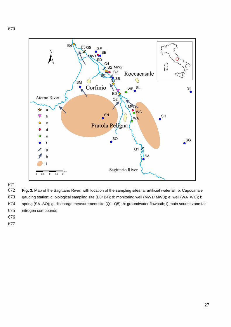
671 Fig. 3. Map of the Sagittario River, with location of the sampling sites; a: artificial waterfall; b: Capocanale 672 gauging station; c: biological sampling site (B0÷B4); d: monitoring well (MW1÷MW3); e: well (WA÷WC); f: 673 spring (SA÷SO); g: discharge measurement site (Q1÷Q5); h: groundwater flowpath; i) main source zone for 674 nitrogen compounds 675 676

677

28

Table 1. Physico-chemical parameters. Data refer to the third survey. (n.a.: not available) 678 (T: Temperature; EC: Electrical conductivity; ORP: Oxidation Reduction Potential; m a.s.l.: meter above sea 679 level; m b.g.l.: meter below ground level) 680

681 682 683 684 685 686 687 688 689

690 691 692 693 694 695 696 697 698 699 700 701

702 703 704

705 706

707 708 709 710 711 712 713 714 715 716 717 718 719 720 721 722 723 724 725 726 727 728

Id Elevation Well depth

Water table depth

T pH EC 25°C ORP

m a.s.l. m b.g.l. m b.g.l. °C μS cm-1 mV

SA 314 16.7 7.4 385 130 SC 261 16.3 7.7 378 152 SD 256 15.0 7.5 398 139 SE 257 15.7 7.6 405 137 SF 253 21.7 7.1 578 121 SG 366 22.4 7.6 304 189 SH 359 16.2 7.0 613 223 SI 1275 19.6 7.1 255 231 SL 333 14.2 7.2 436 241 SM 350 16.7 7.7 633 156 SN 351 15.4 7.0 788 176 SO 343 15.6 7.7 749 177 WA 286 4 -1 19.0 7.2 502 -91 WB 274 45 n.a. 25.0 6.9 640 -91 WC 285 58 0 14.5 7.6 515 -188 MW1 255 26 +2 14.2 7.0 603 -60 MW2_7m 265 29 -2 14.0 6.9 508 -125 MW2_12m 265 29 -2 13.8 6.9 509 -134 MW2_18m 265 29 -2 13.6 6.9 510 -141 MW3_6m 287 24 -2 14.2 6.8 551 -93 MW3_14m 287 24 -2 13.8 6.9 551 -100 MW3_20m 287 24 -2 13.7 6.8 681 -126

29

729 730 731 732

733 734 735 Fig. 4. River discharge measured along three seasonal surveys. Horizontal axis approximately corresponds 736 to distance (km), vertical axis to river discharge (m3s-1). Q1÷ Q5 refer to Fig. 3 737 738 739 740 741 742 743 744 745 746 747 748 749 750 751 752

753

30

754 755

Fig. 5. Vertical Logs. Blue line refers to MW2, red line refers to MW3. a: circles refer to CE (µScm-1), squares 756 to temperature (°C). b: rhombus refers to ORP (mV), triangles refer to pH. Location of MW2 and MW3 is 757 shown in Fig. 3 758

31

759 760

Fig. 6. Chebotarev diagram: red circles indicate springs, blue circles indicate wells and the green ones 761 indicate monitoring wells. Labels refer to Table 1 and data refer to the third survey 762

763 764

765 766 767 768 769

770

32

771 Table 2. Statistical parameters of nitrate and ammonium concentrations (mgL-1) during the three sampling 772 surveys (u.d.l: under detection limits; #: number of samples; SD: standard deviation) 773

774 775 776 . 777 778 779 780 781 782 783 784 785 786 787 788 789 790 791 792 793 794 795 796 797 798 799 800 801 802 803 804 805 806 807 808

Survey # Average SD Min 1° Quartile Median 3° Quartile Max

NO3-

I 9 10 20 u.d.l. 2 3 4 63

II 16 2 1 1 1 2 3 4

III 22 10 22 u.d.l. 0 2 6 101

NH4+

I 9 3 6 u.d.l. 0 u.d.l. 1 16

II 16 3 5 u.d.l. 0 u.d.l. 4 19

III 22 4 9 u.d.l. 0 u.d.l. 0 31

33

809

810 811 812 Fig. 7. Map of distribution of nitrate concentrations for each sampling site (third survey). For monitoring wells, 813 the values showed in the map refer to the shallowest screen monitored 814 815 816 817

818

34

819 820 821 Fig. 8. Map of distribution of ammonium concentrations for each sampling site (third survey). For monitoring 822 wells, the values showed in the map refer to the shallowest screen monitored 823 824 825

826 827

828

829

830

831

832

833

834

35

Table 3. δ18O and δD data. S: springs, W: wells, MW: monitoring wells. Data refer to the international 835 standard, Vienna Standard Mean Ocean Water (VSMOW). Location is shown in Fig. 3. (n.a.: data not 836 available) 837 838

839 840 841 842

843

36

844 845 Fig. 9. δ18O and δD plot; S: springs, W: wells, MW: monitoring wells. Blue line from Petitta et al. (2010) is 846 related to the upper valley of the Sagittario River. Red line from Rosanski et al. (1993) is related to Global 847 Meteoric Line, green line from Barbieri et al. (2003) is related to the Abruzzi region and the Orange line from 848 Longinelli and Selmo (2003) is related to Central Italy Meteoric Line 849 850

851

852

853

854

855

856

857

858

859

860

861 862

37

863 864

865 866 867 Fig.10. Longitudinal changes of benthic macroinvertebrates (a, b) and hyporheic copepods (c, d) along the 868 Sagittario River. a, c: abundance; b, d: species diversity measured as Margalef’s index (Margalef, 1998), 869 both calculated on cumulative abundance and species richness of spatial and temporal replicates. B0÷B4 870 location is shown in Fig.3 871 872 873 874 875 876 877 878 879 880 881 882 883 884 885 886 887 888 889 890 891

38

892 893

894 895 896 Fig. 11. Conceptual model of groundwater flow system and nitrogen cycle. U: upstream section 897 representative of upwelling zones; L: downstream section representative of downwelling zones. a: alluvial 898 fan aquifer, b: alluvial shallow aquifer, c: local terraced aquifer, d: lacustrine-marshy aquitard with high 899 permeability lenses, e: deep carbonate aquifer, f: groundwater flow direction, g: recharge area, h: water 900 table, i: monitoring well, l: nitrogen transport in groundwater 901 902 903 904 905

39

906 Fig. 12. Nitrogen and ammonium concentrations in river waters. Data refer to the third survey. Blue line 907 represents nitrate (as N-NO3

- mgL-1), red line ammonium (as N-NH4+ mgL-1). B0÷B4 refer to Fig. 3 908

909