hud utilities demonstration - NIST Technical Series Publications

Volume 13 HUD UTILITIESDEMONSTRATIONSERIES

PERFORMANCE ANALYSIS OFTHE JERSEY CITY TOTALENERGY SITE:

FINAL REPORT

U.S. DEPARTMENT OF COMMERCENational Bureau of StandardsNational Engineering Laboratory

Center for Building TechnologyWashington, DC 20234

o miusMODULAR INTEGRATED UTILITY SYSTEMSimproving community utility services — supplying

electricity, heating, cooling, and water/ processing

liquid and solid wastes/ conserving energy and

natural resources/ minimizing environmental impact

— QC

AUGUST 1982, Ujo

o2-2474

19u2

Prepared for:

Department of Housing and Urban DevelopmentBuilding Technology Division

Office of Policy Development and ResearchWashington, DC 20410

NBSIR 82-2474

atiunal hura-au

Qf STANDARD*UBtAIT

JUL 2 \J m2

PERFORMANCE ANALYSIS OF

THE JERSEY CITY TOTALENERGY SITE: q&'«

FINAL REPORT

C. W Hurley

J. D. Ryan

C W. Phillips

U.S. DEPARTMENT OF COMMERCENational Bureau of Standards

National Engineering Laboratory

Center for Building Technology

Washington, DC 20234

August, 1 982

Prepared for:

Department of Housing and Urban DevelopmentBuilding Technology Division

Office of Policy Development and Research

Washington, DC 20410

U.S. DEPARTMENT OF COMMERCE. Malcolm Baldrige, Secretary

NATIONAL BUREAU OF STANDARDS, Ernest Ambler, Director

ABSTRACT

Under the sponsorship of the Department of Housing and Urban Development (HUD),

the National Bureau of Standards (NBS) gathered engineering, economic, environ-mental, and reliability data from a 486 unit apartment/commercial complexlocated on a 6.35 acre (2.6 hectare) site in Jersey City, New Jersey. The

complex consists of four medium to high rise apartment buildings, a 46,000 ft-

(4300 m^) commercial building, a school (kindergarten through third grade), a

swimming pool, and a central equipment building.

The construction of the complex was started in 1971, and a decision was made by

HUD to design the central equipment building to meet both the thermal and elec-trical energy demands of the site. The necessary equipment was installed to

recover the waste heat from diesel engines driving the generators making thecentral equipment building a total energy (TE) plant. Absorption type chillerswere also installed in the central equipment building. This TE plant has beenserving the complex since January 1974.

The National Bureau of Standards was responsible for designing and installingthe instrumentation and a data acquisition system (DAS) to determine fundamentalengineering data from the plant and site buildings. The DAS was put on line, inApril 1975. The raw data from the DAS was processed by a minicomputer at NBSto obtain a broad spectrum of engineering results. This report describes thesesystems and presents the appropriate data and a performance analysis of the

plant and site. The analysis of the data indicates a significant savings infuel is possible by minor modifications in plant procedures.

This report also includes the results of an analysis of the quality of utilityservices supplied to the consumers on the site and an analysis of a series of

environmental tests made for the effects of the plant on air quality and noise.In general, these analyses reflected favorable results for the total energyplant

.

Economic and energy analyses are presented for the plant as operated during theperiod of the study and on a comparative basis with twelve alternative systemdesigns applicable for providing the tenants on the site with equivalent util-ity services. In general, although those systems utilizing the total energyconcept showed a significant savings in fuel, such systems do not representattractive investments compared to conventional systems, with fuel costs of1977 .

Key Words: Absorption chiller; boiler performance; diesel engine performance;engine-generator efficiency; integrated utility system; totalenergy systems-economic and engineering analysis; waste heatrecovery.

iii

DISCLAIMER

Certain commercial equipment, names, and instrumentation are identified by namein this report in order to adequately describe the capabilities and technicalfeatures of hardware use in this project. In no case does such identificationimply recommendation or endorsement by the National Bureau of Standards, nordoes it imply that the material or equipment identified is necessarily the best

available for the purpose.

iv

SI CONVERSIONS

In view of the presently accepted practice of the building industry in the

United States and the structure of the computer software used in this project,common U.S. units of measurement have been used in this report. In recognitionof the United States as a signatory to the General Conference of Weights andMeasures, which gave official status to the SI system of units in 1960, appro-priate conversion factors have been provided in the table below. The readerinterested in making further use of the coherent system of SI units is referredto: NBS SP330, 1972 Edition, ’’The International System of Units," or E380-72,ASTM Metric Practice Guide (American National Standard 2210.1).

Metric Conversion Factors

Length

Area

Volume

1 inch (in) = 25.4 millimeters (mm)

1 foot (ft) = 0.3048 meter (m)

1 ft 2 » 0.092903 m 2

1 ft 3 = 0.028317 m3

Temperature

TemperatureInterval

Mass

Mass Per UnitVolume

Energy

Specific Heat

Gallon

F = 9/5 C + 32

1 F = 5/9 C or K

1 pound (lb) = 0.453592 kilogram (kg)

1 lb/ ft 3 = 16.0185 kg/m3

1 3tu = 1.05506 kilojoules (kJ)

1 Btu/ [ ( lb) ( °F) ]= 4.1868 kJ./[(kg)(K)]

1 gallon = 0.0037854 m3

v

TABLE OF CONTENTS

Page

ABSTRACT iiiDISCLAIMER iv

SI CONVERSIONS v

1. INTRODUCTION 1

1.1 TOTAL ENERGY DEVELOPMENT IN THE UNITED STATES 1

1.2 HUD ROLE IN TOTAL ENERGY 2

1.3 HISTORY OF JCTE DEMONSTRATION 3

1.4 REFERENCES - SECTION 1 4

2. SITE DESCRIPTION 6

2.1 PHYSICAL DESCRIPTION OF THE SITE BUILDINGS 6

2.2 PHYSICAL DESCRIPTION OF THE PLANT 15

2.3 PNEUMATIC TRASH COLLECTION SYSTEM 25


3. PLANT AND SITE MEASUREMENTS 31

3.1 MEASUREMENT OBJECTIVES 31

3.2 DESCRIPTION OF THE INSTRUMENTATION AND DATA ACQUISITIONSYSTEM 32

3.3 DESCRIPTION OF THE DATA PROCESSING 33

3.4 ACCURACY OF DATA 37


4. ENGINEERING DATA-PLANT ‘AND SITE BUILDINGS 39

4.1 THERMAL AND ELECTRICAL MEASUREMENTS FROM THE PLANT 39

4.1.1 Thermal Energy Input and Output of the Plant 39

4.1.2 Electrical Energy Values for the Plant 44

4.1.3 Fuel Consumption 46

4.1.4 Component and Plant Performance 48

4.1.5 Thermal Energy - Primary Hot Water Loop 50

4.1.6 Profiles of Plant Loads 50

4.2 THERMAL AND ELECTRICAL LOAD DATA FOR THE SITE BUILDINGS 62

4.2.1 Thermal Loads of Site Buildings 62

4.2.2 Electrical Loads of Site Buildings 62


5. ENGINEERING ANALYSIS- PLANT COMPONENTS, SUBSYSTEMS, AND SYSTEMS 71

5.1 OVERALL ENERGY BALANCE FOR THE PLANT 71

5.2 PERFORMANCE ANALYSIS OF PLANT COMPONENTS 71

5.2.1 Engine Generator Performance 71

5. 2. 1.1 Thermal Losses from Idle Engines 73

5. 2. 1.2 Thermal Losses from Deposits in the ExhaustHeat Exchangers 7 5

5. 2. 1.3 Variations in Engine-Generator Efficiencywith Load 81

vi

TABLE OF CONTENTS (Cont.)

Page

5.2.2 Boiler Performance 86

5.2.3 Chiller Performance 86

5.2.4 Dry Cooler Losses 89

5.3 SITE DISTRIBUTION LOSSES 94

5.3.1 Site Thermal Losses 94

5.3.2 Site Electrical Losses 101

5.4 SUMMARY 101


6. ALTERNATIVE SYSTEMS FOR ENERGY SUPPLY 104

6.1 INTRODUCTION 104

6.2 SELECTION OF ALTERNATIVE SYSTEMS 104

6.3 DESCRIPTION OF ALTERNATIVE SYSTEMS 105

6.4 UTILITY POWER PLANT CHARACTERISTICS ' 110

6.4.1 Marginal New Plants and Displaced Plants Ill

6.4.2 Power Plant Efficiency 112

6.4.3 Fuel Utilization 112


7. ENERGY ANALYSIS OF ALTERNATIVE SYSTEMS 118


7.2 SIMULATION PROGRAM DESCRIPTION 118

7.2.1 Selection 118

7.2.2 TRACE Program ? 118

7.2.3 Selection of TRACE 119

7.3 PROGRAM VALIDATION 120

7.3.1 Data Periods for Comparison 120

7.3.2 Comparison of Loads 123

7.3.3 Comparison of Equipment Performance 125

7.3.4 Comparison of Fuel Consumption 125

7.4 SIMULATION OF ALTERNATIVE SYSTEMS 127

7.4.1 Equipment Performance Input Data 127

7.5 ENERGY CONSUMPTION RESULTS 127

7.5.1 Baseline Simulation Data 127

7.5.2 Adjustments to Baseline Data 129

7.5.3 Comparisons of Energy Consumption 129

7.5.4 Comparison of Fuel Use 1307.6 SENSITIVITY TO CENTRAL POWER STATION EFFICIENCY 137


8. JCTE COST DATA AND ANALYSIS 140


8.2 OPERATION AND MAINTENANCE COSTS 140

8.2.1 Cost Collection Methodology 1408.2.2 Cost Accounting Procedure 141

8. 2. 2.1 Prorated Expenses 143

8. 2. 2.

2

Subsystem Cost Separation 144

vii


Page

8. 2. 2.

3

O&M Cost Categories 144

8.2.3 Actual O&M Cost Data 145

8.3 CAPITAL COSTS 145

8.3.1 Capital Costs for Equipment 145

8.3.2 Subsystem Cost Separation 145

8.4 OWNING COSTS 145

8.5 UNIT ENERGY COSTS 151

8.6 DISCUSSION OF DATA AND ASSESSMENT OF TYPICALITY 153

8.6.1 Inflation and Other Temporal Effects 154

8.6.2 Plant Loads 154

8.6.3 Equipment Performance 159

8.6.4 Operation and Maintenance 160

8.6.5 Management and Institutional Factors 162

8.6.6 Capital Costs - Design Factors 165

8.7 TYPICAL COSTS 168


9. ECONOMIC EVALUATION OF ALTERNATIVE SYSTEMS 170

9.1 BASIC ECONOMIC DATA 170

9.1.1 Capital Costs 170

9.1.2 Operational and Maintenance Costs 173

9.1.3 Fuel and Energy Costs 176

9.1.4 Comparison of Actual Costs to System 1 Costs 177

9.2 OTHER ESTIMATED COSTS 180

9.3 EVALUATION METHODOLOGY 181

9.3.1 Investment Viability Measures 181

9.3.2 Cash Flow Streams 181

9.4 EVALUATION RESULTS 187

9.4.1 Simple Payback and Initial Investment Premium 187

9.4.2 Return on Investment 188

9.5 SENSITIVITY ANALYSIS 189

9.5.1 Investment Tax Credit 189

9.5.2 Relative Cost of Fuel Oil and Electricity 190


10. RESULTS OF ENVIRONMENTAL TESTS 196

10.1

AIR QUALITY ASSESSMENT 196

10.1.1 Scope of Study 196

10.1.2 Plant Combustion Exhaust System 198

10.1.3 Combustion Emissions 198

10.1.3.1 Engine Emissions 198

10.1.3.2 Boiler Emissions 205

10.1.3.3 Comparison of Engine and Boiler EmissionRates 205

10.1.4 Site Description Characteristics 206

10.1.4.1 Local Wind 207

10.1.4.2 Engine Exhaust Plume Observations 207

viii


Page

10.1.5 Ground-Level Air Quality 211

10.1.5.1 Data Collection/Monitoring Appro _h 211

10.1.5.2 Statistical Summary of Air Quality Data 211

10.1.5.3 Evaluation of General Site Air Quality 213

10.1.5.4 Contribution of TE Plant to N0X Concentration . 219

10.1.5.5 Ground-Level Concentration Distribution 221

10.1.6 Summary and Conclusion 221

10.2 NOISE LEVEL ASSESSMENT 223


10.2.2 Data Collection 22310.2.2.1 Pre-Construction Period 223

10.2.2.2 Operational Period 224

10.2.3 Results 224

10.2.4 Comparison with Local Standards 22610.2.5 Summary and Conclusions 227

10.3 COOLING TOWER ASSESSMENT 228


10.3.2 Cooling Tower Operation 228

10.3.2.1 Description 228

10.3.2.2 Operation Conditions 22810.3.2.3 Chemical Treatment 229

10.3.2.4 Heat Rejection Load 23010.3.3 Measurements 230

10.3.3.1 Cooling Tower Drift Source 23010.3.3.2 Ground-Level Measurements 231

10.3.4 Results 231

10.3.4.1 Cooling Tower Drift Source Results 231

10.3.4.2 Drift Deposition Results 23210.3.5 Conclusions 233


11. RELIABILITY EVALUATION 235

11.1 SCOPE AND DEFINITION 235

11.2 ELECTRICAL SERVICE AVAILABILITY 235

11.2.1 Electrical System Design Features 23511.2.2 Sources of Availability Data 237

11.2.3 Service Availability Methodology 23711.2.4 Availability Data Summary 240

11.2.5 Temporal Trends 24011.2.6 Outage Causes 241

11.2.7 Sources of Comparative Data 24411.2.8 Evaluation 245

11.2.9 Conclusions , , 24811.3 ELECTRICAL SERVICE QUALITY 249

11.3.1 TE Plant Data 24911.3.2 Sources of Comparative Criteria and Data 249

11.3.3 Comparison of Results 251

ix


Page

11.4 HOT WATER AND CHILLED WATER AVAILABILITY AND QUALITY 252


ACKNOWLEDGMENTS 256

APPENDICES

x

LIST OF FIGURES

Figure Page

2.1 Overall view of total energy site 7

2.2 Relative location of individual buildings at the Jersey City

total energy site 7

2.3 Commercial, Camci,and Descon buildings 8

2.4 Descon building (11-story section) 9

2.5 Elementary school 11

2.6 Elementary school, swimming pool, and pavilion 12

2.7 Shelley "A" and Shelley "B" buildings 13

2.8 Central equipment building 14

2.9 All five of the 600 kW engine-generators 16

2.10 One of the five 600 kW engine-generators 17

2.11 Two 13.4 MBtu per hour (4.0 MW) fire-tube hot water boilers .... 18

2.12 Two 546-ton (1.9 MW) absorption-type chillers 19

2.13 Central equipment building control room 20

2.14 Master control panel 21

2.15 Scale model of the central equipment building 22

2.16 Schematic of the primary hot water loop 23

2.17 The central equipment building roof showing the cooling towersand the dry coolers for control of PHW and engine lubricatingoil temperatures 24

2.18 Pneumatic Trash Collection master control panel 26

2.19 Two Pneumatic Trash Collection 150 hp (112 kW) exhausters 27

2.20 Air separator and trash holding hopper in the centralequipment building 28

2.21 The trash hopper and compactor located in the centralequipment building 29

2.22 Front view of the central equipment building showing the

loading dock with the trash containers 30

3.1 Data acquisition system located in the plant 34

3.2 One of the eight remote DAS stations located in the sitebuildings 35

3.3 Impact printer for registering real-time data 36

3.4 Simplified flow diagram of data processing. For furtherdetails see reference [3-2] 38

4.1 Plant primary hot water loop 40

4.2 Major energy flow diagram for the plant 43

4.3 Thermal energy recovered from the engines and boilers 52

4.4 Output of the absorption chillers at the plant 54

4.5 Thermal energy leaving the plant for the site in the form of

secondary hot water 554.6 Seasonal profiles of site hot water demand, thermal energy

recovered from the engines, and chiller input from the

primary hot water loop. These profiles denote the thermaldemands of the plant relative to the thermal energy recoveredfrom the engines 56

xi

LIST OF FIGURES

Figure

4.7 Profiles of site hot water demand, thermal energy recoveredfrom the engines, and chiller input from the primary hotwater loop for one day of each of the four seasons of the

year4.8 Thermal energy recovered from each of the boilers during one of

the colder months of record. The boilers are rated at 13.4

MBtu per hour (3.9MW). However, the controls apparentlylimited the output to 10 MBtu per hour (2.9MW)

4.9 Gross and net output of engine-generators during 1977. The

net output is calculated as being representative of the elec-trical energy that would be purchased from the grid if the

plant were not generating electrical power4.10 Hourly electrical damands of the site and plant for four

days during each of the four seasons of the year4.11 Profiles of hourly electrical energy demands of the site for

one day of each of the four seasons of the year4.12 Seasonal profiles of electrical loads for the Shelley B

residential building4.13 Seasonal profiles of electrical loads for the commercial

building

5.1 Profile of monthly plant energy effectiveness (see section 4.4

for definition) and heating and cooling degree-days5.2 Profiles of the gross electrical output and the net thermal

energy recovered from the engines. Two days are shown:November 4, 1977 is representative of one of the lower elec-trical energy demand days of the plant while July 9, 1977

represents one of the higher electrical demand days of the

plant. In both cases, the exhaust heat exchangers had not

been cleaned for a period of over 30 days5.3 The thermal energy recovered (or lost) from engine No. 2 under

three modes of operation: on line, off line and valved out of

the PHW loop5.4 Temperature of exhaust gases from engine No. 2 entering and

leaving the exhaust heat exhanger. The unit was taken off

line January 3, 1978, the exchanger cleaned and the unit put

back on line January 4, 1978. The rapid accumulation of

deposits in the tubes of the exhanger are indicated by the

increase in the outlet temperature5.5 Thermal energy recovered from engine No. 2. The accumulation

of deposits in the tubes of the exhaust heat exchanger is

reflected in curves 1 and 3

xii

Page

57

58

59

60

61

67

68

72

74

76

77

78

LIST OF FIGURES

Figure Page

5.6 Gross electrical output of the three on-line units and net

thermal energy recovered from the entire bank, of engines. The

exhaust gas heat exchangers were cleaned during the periodDecember 26, 1977 through January 3, 1978. On the January 25

and 26, the on-line engines were changed. Two engines withless deposits in their exhaust gas heat exchanger were put on

line and consequently a rise in the net thermal energyrecovered from the engines is indicated. The overall effectsof the deposits in the exhaust gas heat exchangers arereflected in these curves. The jackets and exhaust gas heatexchangers of all five engines were in the PHW loop during the

period shown 805.7 Gross electrical and net thermal output of all engines. On

January 5, 1978, the electrical system was operating withthree exhaust heat exchangers with two days or less of serviceafter cleaning. On January 3, 1978, the system was operatingwith exchangers having from 13 to 27 days of service aftercleaning. The jackets and exhaust gas heat exchangers of allfive engines were in the PHW loop for the two days shown 83

5.8 Efficiency-load curve for engine generator No. 2. This curvereflects data taken on an hourly basis during a 24-hour periodin January 1978 34

5.9 Diurnal profile of electrical efficiency of engine-generatorNo. 2. This curve reflects data taken on a hourly basisduring a 24-hour period in January 1978. 85

5.10 Profiles of thermal input and output of the chillers inSeptember 1976. The erratic functioning of the chillers is

indicated during the first half of the month. On September 21,

1976, a factory representative restored the units to "normal"operation 88

5.11 Dry cooler convective heat loss experiment performed October 19,

1976. The natural convective flow through the ducts wasrestricted using glass fiber mats. The results are shown in

figure 5.12 91

5.12 Results of dry cooler natural convective heat loss experiment.The dry cooler outlets were fully covered at hour 16. Thedotted line indicates loss expected if the outlets wereuncovered 92

5.13

Louvers, designed to open from force generated by the fans in

the dry coolers, were installed February 16, 1978. When the

fans are not activated, the louvers close by gravity. One or

more pair of fans were apparently manually activated onFebruary 18, 19, 21, 22, 1978 to release excess heat whilerepairs were being made in the secondary loops. The profilerepresents the thermal energy removed from the PHW by the drycoolers 93

xi ii

LIST OF FIGURES

Figure Page5.14

Hourly profile of thermal energy from the plant to the westsite second hot water loop. Ground water was pumped out of

distribution pits on July 22 , 1977 . 95

5.15

Thermal energy in the chilled water in west site distributionloop. Profile number 1 is the summation of thermal energyconsumed by the individual buildings on the west loop. Profilenumber 2 is the thermal energy produced by the plant for the

west loop. Ground water was pumped out of distribution pits

July 22, 1977 98

5.16

Thermal energy in secondary hot water systems. Profile number

1 is the summation of the thermal energy consumed by the sitebuildings. Profile number 2 represents the total thermalenergy leaving the plant in the secondary hot water system 100

6.1 Trend to the use of electric space heating in single-familyhomes 106

6.2 Alternative energy systems - TE and conventional centralsystems 107

6.3 Alternative energy systems - conventional building andindividual unit systems 108

6.4 Forcasted PSE&G fuel use based on a study made in 1978 115

7.1 Program validation logic 121

7.2 Comparison of electrical loads for program validation 124

7.3 Comparison of fuel consumption for program validation 126

7.4 Comparison of annual energy consumption for twelve alternativesystems. These data include the adjustments of table 7.4 133

7.5 Relative energy consumption of twelve alternative systemscompared to System 1 134

7.6 Relative source energy consumption for alternative systems 136

7.7 Effect of utility power station heat rate on relative energysavings. System 8 is representative of System 5 throughSystem 8; System 12 is representative of Systems 9, 10, and 12. . 138

8.1 Organizational cash flow for the operation of tne Jersey City

Total Energy site 142

8.2 Major components of the O&M cost 155

8.3 Total annual O&M costs 156

8.4 Unit cost of fuel oil delivered, 1974 - 1977 157

8.5 Total labor-related O&M costs 163

9.1 Comparison of total costs: J CTE actual vs. estimated for

System 1 179

9.2 Effect of electricity and fuel-oil unit costs on investmentattractiveness of a Total Energy System 194

10.1 Summit Plaza site. This shows the TE plant surrounded by tallerbuildings 197

xiv

LIST OF FIGURES

Figure Page

10.2 Roof area of the TE plant. This shows the various componentsof the combustion exhaust system 199

10.3 Engine-generator carbon monoxide emission rates 201

10.4 Engine-generator nitrogen oxides emission rates 202

10.5 Engine-generator hydrocarbon emission rates 20310.6 Engine-generator particulate emission rates 20410.7 Wind rose: summer monitoring period, 1977 20810.8 Wind rose: winter monitoring period, 1977 208

10.9 Diesel engine exhaust plume with 2-4 mph (0.9 -1.8 m/s)southerly wind. Visibility of the plume was enhanced by meansof a smoke bomb dropped into the stack 209

10.10 Diesel engine exhaust plume with 3-8 mph (1.3 - 3.6 m/s)

southerly wind. Visibility of the plume was enhanced by meansof a smoke bomb dropped into the stack 209

10.11 Diesel engine exhaust plume with 9-12 mph (4. 0-5. 4 m/s) southerlywind. Visibility of the plume was enhanced by means of a smokebomb dropped into the stack 210

10.12 Air quality monitoring station locations 21210.13 Average nitrogen oxide concentrations ~210 ft (65 m) from the

TE plant 21810*14 TE plant and background average N0X concentrations when wind

blew toward a stationary sampler 22010.15 Noise levels in dB(A) around the Central Equipment Building

during 8-9 a.m.,August 4, 1977 225

10.16 Ceil designation for TE plant cooling tower 229

11.1 Relative priority of areas for reliability evaluation 23611.2 Accounting procedure for partial interruptions 23911.3 Typical failure rate for a TE plant as a function of time 242

xv

LIST OF TABLES

Table Page

4.1 Monthly Thermal Values (millions of Btu) 42

4.2 Monthly Accumulated Electrical Values (Megawatt-hours) 45

4.3 Monthly Fuel Values 47

4.4 Monthly Component and Plant Performance 49

4.5 1976, 1977 Monthly Thermal Values for the PHW Loop (millionsof Btu) 51

4.6 Monthly Hot Water Energy Use for the Site Buildings on the EastSecondary Hot Water Loop (millions of Btu) 63

4.7 Monthly Hot Water Energy Use for the Site Buildings on the WestSecondary Hot Water Loop (millions of Btu) 64

4.8 Monthly Chilled Water Energy Use for the Site Buildings on

Chilled Water Loops and the Plant (millions of Btu) 65

4.9 Monthly Electrical Energy Consumption for the Shelley B andCommercial Building (killowatt - hours) 66

5.1 Output of Engine No. 2, January 1978 79

5.2 SHW Thermal Energy to the West Zone in July 1977 96

5.3 Chilled Water Thermal Energy to the West Zone in July 1977 97

5.4 Summary of Estimated Annual Fuel Savings Which Would Resultfrom Selected Individual Changes in Equipment, Operation,and/or Maintenance of Plant and Site 102

6.1 Summary of Alternative Energy Systems and Their Components 109

6.2 PSE&G New Power Plant Characteristics Ill

6.3 Displaced Plant Characteristics 112

6.4 Heat Rate of Utility-Supplied Power from Reference [6-5, 6-6

and 6-7] 113

6.5 Utility Heat Rates for Use in Overall Evaluation 114

6.6 PSE&G and National Average Electrical Generation by Fuel Type ... 116

7.1 Selection of Month for Comparison of Simulation Results and JCTEData 122

7.2 Comparison of Heating and Cooling Loads for Program Validation .. 123

7.3 Equipment Performance of Alternative Energy Systems 128

7.4 Annual Energy Consumption Adjustments for Load Discrepancies .... 131

7.5 Annual Energy Consumption of Alternative Systems 132

7.6 Source Energy Consumption of Alternative Systems 135

7.7 Relative Source Energy Consumption of Alternative Systems 135

7.8 Energy Consumption Variations with Utility Power Plant HeatRate 137

8.1 Direct 0&M Costs - 1974 Summary (March 1974 - November 1974) .... 146

8.2 Direct O&M Costs - 1975 Summary (December 1974 - November 1975) . 147



8.5 Capital Cost Summary 150

8.6 Qualitative Seasonal Load Variations 153

xvi

LIST OF TABLES

Table Page

8.7 Unit Cost of Site Thermal and Electrical Energy March 1, 1974

through November 30, 1977 154

8.8 Actual Weather Patterns, 1974-1977 159

8.9 Cost Impacts of Improved Equipment Performance 160

8.10 Labor Costs by Category, January through June 1977 164

8.11 Atypical Costs: Travel and Profit 165

8.12 Summary of Recommended Cost Adjustments for Atypicalities 168

9.1 Summary of Capital Costs 171

9.2 Comparison of Initial Cost Estimates with Actual Costs 173

9.3 Estimated Annual Operation and Maintenance Costs for

Alternative Systems 17 5

9.4 Energy Cost for Alternative Systems 178

9.5 Actual Cash Flow Data for Alternative Systems 183

9.6 Incremental Cash Flow Data for Alternative Systems 184

9.7 Example of an Incremental Constant - Dollar Cash Flow Streamfor an Alternative System 185

9.8 Example of an Incremental Cash Flow Stream for an AlternativeSystem in Current-Year (Inflated) Dollars 186

9.9 Comparison of Alternative Systems Using Several IncrementalInvestment Measures 187

9.10 Effect of Investment Tax Credit on Investment Premium andPayback Period 190

9.11 Unit Cost of Electricity for Several Ownership/Ra te ScheduleScenarios 191

9.12 Effect of Owners hip /Rate Schedule Scenarios on Simple Paybackof Alternative Systems 192

10.1 Boiler Exhaust Concentrations and Emission Rates at 17 percentof Full Load 20 5

10.2 Engine and Boiler Emission Rates at an Annual Average LoadLevel 206

10.3 Summary of Measured Air Quality Data-Summer Period 214

10.4 Summary of Measured Air Quality Data-Winter Period 21510.5 Summary of Downwind Nitrogen Oxides (N0X ) Concentrations 216

10.6 Federal Air Quality Standards 217

11.1 Summit Plaza Total Energy Plant Electrical ServiceAvailability 240

11.2 Number of Interruptions by Outage Cause for the Period 1974

through 1977 24311.3 Summary of Generic Utility Availability Targets 246

11.4 Summary of Actual Utility Availability 247

11.5 TE Plant vs. Utility Availability 24811.6 Effects of Unattended Operation on Duration of Total

Interruptions 249

11.7 Comparative Data for Electrical Service Quality 252

xvii

LIST OF TABLES

Tables Page

11.8 Hot and Chilled Water Service Quality 253

xviii

1. INTRODUCTION

The thermal energy normally wasted in the generation of electrical power and

the potential for the recovery and use of this energy for heating and coolingare widely recognized. In the most efficient electrical generation systems,only 40 percent or less of the energy in the coal, oil, or gas is converted

into electrical energy. The remaining 60 percent or more of the input is

usually rejected into the environment as waste heat.

In the total energy (TE) concept, efforts are made to recover this normallywasted heat and utilize it for space heating, domestic hot water, and space

cooling using absorption-type chillers. The use of this normally wasted heat

conserves the additional conventional energy normally required to meet these

needs. Since the total energy concept requires the generation of electricalpower to be near the area of the utilization of the waste heat, the applicationof on-site electrical generation systems is encouraged.

1.1 TOTAL ENERGY DEVELOPMENT IN THE UNITED STATES

The general history of the TE concept in the United States is fairly well known.The decade 1962 through 1971 saw the installation of approximately 500 TE

plants. Intense promotion by natural-gas utilities was a major factor in thisdevelopment. Many of the early TE installations were in gas company facilitiesto familiarize gas utility engineers with the equipment and to "demonstrate"the concept. As late as 1969, one-quarter of all TE installations were stillin buildings and plants owned by gas utilities. Gas industry interest wasspurred by the need to equalize the seasonal demand for gas by creating a

year-round load. Also it was hoped that TE would provide an effective meansof combating promotion of the all-electric building concept by the electricuti lities

.

Since 1972, little promotion of TE has occurred by the gas industry primarilydue to growing concern about unavailability of natural gas supplies. The

petroleum industry had not mounted a strong TE market development effort in

part because natural gas held a significant economic advantage over oil in mostareas. Equipment manufacturers likewise had not developed a strong promotionalforce for TE largely because TE represented a small part of their businessand/or the conventional (non-TE) equipment could also be supplied by the samemanufacturers. In the last ten years then, private-sector promotion and

development of the TE concept has largely waned. The 'energy crisis' andincreased interest in energy conservation has again spurred interest in TotalEnergy - this time largely as part of the Federal R&D activities.

It is of interest to recap the experience of TE development as it stood in

1971-72. TE plants were typically small - by 1972, 40 percent of all installa-tions were under 600 kW total capacity although larger plants were increasinglybecoming the norm. Counting the "captive" gas company installations, three-quarters of all TE installations served industrial or commercial facilities.Residential applications accounted for less than 10 percent of the total.

1

Natural gas was the principal fuel for TE and was used in over 90 percent of

all installations in 1972 [1-2]*.

Although the number of plants installed in the promotional days of TE is

impressive, there has been little unbiased feedback in terms of actual oper-ating experience. In particular, there is little identification of the typesof problems and their extent so that R&D plans could be formulated. There is,

however, some general agreement as to the recurring reasons for TE systemproblems and failures and the major unanswered technical questions regardingTE:

0 maintenance requirements and costs0 viability of unattended or semi-attended operation0 inflexibility to meet changes in level of demand (i.e., expansion of

facilities or last-minute changes)° adequacy of controls and auxiliary equipment reliability

1.2 HUD ROLE IN TOTAL ENERGY

One of the purposes of the U.S. Department of Housing and Urban Development(HUD) is to assist sound development of the Nation's communities and metropoli-tan areas. The goals are decent housing and a suitable living environment at

reasonable cost. Space heating and cooling, domestic water heating, and powerfor lighting and home appliances are elements of decent housing. Clean air andwater and the reduction or elimination of pollution contribute to a suitableliving environment. Housing at a reasonable cost demands economy of effort,better use of resources, and correction of wasteful and expensive practices[1-3].

These considerations led HUD in 1969 to sponsor studies of the use of wasteheat from central power plants for heating and cooling large cities. This

work, conducted by the Oak Ridge National Laboratory, indicated that signifi-cant economies could be achieved in this manner if cities were built to conformto the requirements of the power plant and thermal distribution system.Unfortunately, community development does not occur in this way.

The question then is, if cities are not developed to meet power plant

requirements, can power plants be developed to match urban growth and stillmake the most efficient use of energy.

This question led to the examination by HUD of the total energy concept. The

interest in the total energy concept by HUD is two-fold. First, on-site powergeneration (with or without heat recovery) affords the potential to add neededgenerating capacity at a rate consistent with residential development.Secondly, with heat recovery, i.e., the total energy approach, significantsavings in primary fuel consumption can be realized.

Numbers in brackets refer to references at the end of each section.

2

HUD’s evaluation of the TE concept could have focused on one or more of the

existing 500 TE plants in operation. In 1971 there were 28 separate installa-tions of total energy plants serving residential facilities [1-4]. Four of

these were combined residential and shopping center or office building complexes.Of the 24 purely residential installations, nine were luxury rental developmentsin the Kansas City, Kansas, metropolitan area. A HUD/NBS team visited these

plants, the developer, and a maintenance contractor in 1970. Instrumentationof these plants was found to be minimal. Hard data on total capital cost,

reliability, energy utilization, operating costs, and maintenance costs were

not available. The same was also generally true for the nineteen other plants

serving residential facilities.

An alternative to collecting and analyzing spare and suspect data from actualexisting plants was the building and operating of a total energy plant for a

residential development. By taking such a step, under HUD control and direc-tion, the plant could be fully documented as to cost and problems, from initialconcept through long-term operation.

This approach was selected by HUD after careful consideration of all factorsinvolved

.

1.3 HISTORY OF JCTE DEMONSTRATION

At the time of HUD's growing interest in TE and the recognition of a need for a

full-scale TE demonstration, there was a large-scale program underway at HUD to

demonstrate industrialized housing, called OPERATION BREAKTHROUGH. This pro-gram had identified eleven sites around the country for potential developmentand demonstration.

The BREAKTHROUGH sites were owned by HUD and were to be developed undercontracts with developers and industrialized housing producers.

The existence of the BREAKTHROUGH program provided an excellent opportunity for

HUD to demonstrate Total Energy with a minimum of risk and delay by using oneof the BREAKTHROUGH sites. The sites were eventually to be sold by HUD to

private sector owners so that operation of the TE plant would be in the overallcontext of a viable commercial venture.

NBS was deeply involved in the housing technology aspects of BREAKTHROUGH, and,

under contract to HUD, was brought into the TE demonstration effort. In April1970, NBS initiated investigations of the technical aspects of residential TEand the selection of one of the BREAKTHROUGH sites for the HUD demonstration.Two feasibility studies were prepared by NBS evaluating and comparing TotalEnergy and the conventional systems for six of the BREAKTHROUGH sites [1-5,1-6

]

.

Based on the results of these studies and other factors, HUD chose the JerseyCity BREAKTHROUGH site as the location of the TE Demonstration. The JerseyCity site was recommended by NBS partly because it had the largest number ofdwelling units of the available sites, high spatial density, and a large amountof commercial space.

3

Jersey City was also preferred because its relative standing among the availablesites improved greatly if oil was considered as the fuel to be used. Also theJersey City site developer was interested in the use of Total Energy.

HUD sponsored the design of the TE plant at Jersey City. A contract was awardedto Gamze-Korobkin-Caloger (GKC) for complete design and preliminary analysis.MBS prepared a performance specification [1-7] which was referenced in the

contract documents for the design. This specification addressed the areas ofdesign equipment, selection, reliability, economics, stability of electricalservice, maintenance requirements, noise and vibration control, air pollutioncontrol, plant space conditioning, aesthetics, safety, future expansion andquality assurance.

Construction at the Jersey City site started in November 1971 and the TE plantbegan operations in December 1973 - January 1974. A description of the siteand plant are presented in section 2 of this report.

In parallel with site activities, MBS designed and built an instrumentation and

data acquisition system and developed the methods and procedures to be used in

the evaluation of the demonstration. Preliminary drafts of an evaluation planwere prepared in June 1973 and used to elicit comments from people knowledge-able in research and engineering/design fields related to Total Energy. Thisincluded the American Society of Heating, Refrigerating and Air ConditioningEngineers (ASHRAE) task force on Total Energy Systems.

The entire site (TE plant and apartment/coramercial buildings) is owned by a

private real estate corporation, Starrett Housing Corporation. The site is

now known as Summit Plaza. This name will be used throughout this report to

designate the entire site, including the energy conversion equipment.

1 .4 REFERENCES - SECTION 1

1-1. Echols, H. M.,"Problems of Total Energy Systems," Actual Specifying

Engineer, pp. 60-63, November 1970.

1-2. Federal Council on Science and Technology, "Total Energy Systems, UrbanEnergy Systems, Residential Energy Consumption," NTIS #PB-221 374,October 1972.

1-3. U.S. Department of Housing and Urban Development, "Total Energy System,"HUD-381-PDR, p. 8, December 1974.

1-4. "Total Energy's Plant Directory," Total Energy, Vol. 9, No. 1, pp. 34-61,January 1972.

1-5. Achenbach, P. R.,Coble, J. B., Cadoff, B. C. ,

and Kusuda, T., "A

Feasibility Study of Total Energy Systems for BREAKTHROUGH Housing Sites,"National Bureau of Standards Report 10402, August 12, 1971.

4

,J. B. and Achenbach, P. R.

, "Site Analysis and Fieldrumentation for an Apartment Application of a Total Energy Plant,”

ional Bureau of Standards Report NBSIR 75-711, May 1975.

chenbach, P. R. and Coble, J. B. "A Performance Specification for a

Total Energy Plant at the Jersey City BREAKTHROUGH I Site,” NationalBureau of Standards Report 10313, December 28, 1970.

5

2. SITE DESCRIPTION

2.1 PHYSICAL DESCRIPTION OF THE SITE BUILDINGS

The Summit Plaza site occupies an area of 6.35 acres (2.6 hectares) andcontains a central equipment building (CEB), four apartment buildings, an

elementary school, a swimming pool, a commerical building, and parking spacefor the tenants. Figure 2.1 is an aerial view of the site and its surroundingsand figure 2.2 is the plan layout of the individual buildings contained on the

site

.

The commercial building, figure 2.3, is brick-faced, three stories in height,and contains approximately 46,000 ft^ (4,274 m^) of rentable area; consistingof 25,500 ft^ (2369 m^) of office space and 20,500 f t ^ (1905 m^) of storespace. All commercial store front space is on the first (ground) floor andoffice space is located on the third floor. The second floor contains a 72-

space parking garage which is accessable by a ramp. The main mechanical equip-ment rooms are located on the first floor. The structure was designed byBeyer, Blinder, and Belle (architects and planners) in collaboration withLanger, Polise (consulting engineers); Zoldas

,Silman (Structural Engineers);

and Howard Branstan (Lighting Consultant).

The Camci Building, figure 2.3, is 16 stories in height, of modularconstruction, and contains 150 dwellings units consisting of one and two-bedroom apartments. All dwelling units are located on the second throughfifteenth floors.

The first floor (ground level) contains, in addition to the mechanical andelectrical equipment rooms, a laundry and entrance lobby. The mail room and

additional utility and storage rooms are also located on the ground level.

Camci, Inc. and Modular Communities, Inc. were the Building Manufacturer and

General Contractor, respectively; utilizing the services of Skidmore, Owningsand Merrill (architects); I.B.S. Industrial Buildings, Inc. (Systems Consul-tants); Paul Weidlinger (Structural Engineer); and Cosentini Associates(Mechanical Engineers).

The Descon building (figures 2.3 and 2.4) is L-shaped, contains a total of 122

dwelling units, and consists of three distinct sections:

1. The first section (figure 2.3) has six two-floor apartments over a

parking area. The upper floor is three floors above ground level.

2. The second section (figure 2.3) has 12 two-floor apartments builtabove a parking area, automobile drive through passage, and the

mechanical and pump room which services all three sections of the

Descon building. The upper floor is six floors above ground level.

3. The third section (figure 2.4) is an eleven-story high-rise containing104 dwelling units (20 of these have 1-1/2 times as much floor area as

the other units and 4 have between 2 and 3 times as much floor area).

6

Figure 2.1 Overall view of total energy site

Figure 2.2 Relative location of individual buildings at the

Jersey City total energy site

7

Figure 2.3 Commercial, Caraci, and Descon buildings

8

Figure 2.4 Descon building (11-story section)

9

This section contains two elevators, a laundry room (on the groundfloor), a main electrical equipment room, and an entrance lobby.

The building general contractor was Descon/Concordia Systems, Ltd. withGeorge E. Buchanan, Jr. as architect. Gamze-Korobkin-Caloger and StorchEngineers served as engineering consultants.

The elementary school (figures 2.5 and 2.6) (Preschool through Grade 3) is a

brick-faced, two-story structure and contains a small playground adjacent to

the building. The building contains approximately 15,700 ft^ (4790 m^).

The first floor consists of an auditorium (multi-purpose room), administrativeoffices, and the mechanical and electrical equipment rooms. The second floorconsists of one large open area with movable room dividers which extend to the

ceiling. Several offices as well as a kitchen are also located on the secondfloor. Beyer, Blinder, and Bess served as architects for the building.

The outdoor swimming pool and pavilion (figure 2.6) were designed by Beyer,Blinder, and Bell (architects and planners) with Langes, Polise acting as

consulting engineers and Zoldos, Silman as structural engineers.

The swimming pool is 25 ft. wide by 45 ft. long (7.6 m by 14 m) and contains a

diving board. The pavilion contains two locker rooms, an instructor's office,storage room, and a mechanical and electrical equipment room. The entire poolis surrounded by either the pavilion, a brick-faced fence, or a metal-typefence

.

Shelley B (figure 2.7) is nine stories in height with eight floors above groundand one below. The building contains 40 two-story dwelling units and fourlevels of lighted parking area. All dwelling units are located on the fourththrough the ninth floors. The mechanical and electrical equipment rooms are onthe second and third floors. The second floor (ground level) contains anentrance foyer and access to the elevator. Shelley B is of modular construc-tion and was designed by Shelley Systems, Inc.

Shelley A (figure 2.7) contains 18 stories above ground and has 152 dwellingunits, a laundry, entry foyer, and space for up to 14 store-front offices. Abasement area contains the mechanical and electrical equipment necessary to

service the building. This building is the tallest (and largest) building onthe site and is served by two elevators. The Shelley A building is of modularconstruction and was designed by Shelley Systems, Inc.

The three-story central equipment building (CEB) (figure 2.8) contains all of

the equipment necessary to produce and control the electrical and thermalenergy required by the Summit Plaza site. In addition, the CEB contains facil-ities for collecting and processing site refuse. An office and rest room areais located on an upper level of the building. The details of the varioussystems and components contained in the CEB are described in the followingsection.

10

Figure 2.5 Elementary school

11

Figure 2.6 Elementary school, swimming pool, and pavilion

12

13

Figure 2.8 Central equipment building

14

2.2 PHYSICAL DESCRIPTION OF THE PLANT

The Total Energy plant is housed in the three-story central equipment building(figure 2.8). Electrical power is generated by five Caterpillar 600 kW dieselengine-generators (figures 2.9 and 2.10). Thermal energy for space heating and

domestic hot water production is recovered from both the water jackets of the

engines and from their exhausts. Supplementary thermal energy is supplied by

two Cleaver-Brooks 1.34 MBtu per hour (4.0 MW) hot-water boilers (figure 2.11).During the air-conditioning season, the thermal energy is also used by two

Trane 546 ton (6.6 MBtu per hour) (1.9 MW) absorption chillers (figure 2.12)

to produce chilled water. The engines and boilers both burn No. 2 fuel oil

which is stored in three 25,000 gallon (95 m^) underground tanks. The totalenergy plant was designed to be completely automatic, allowing for unattendedovernight and weekend operation. Figures 2.13 and 2.14 show the CEB controlroom and the master control panel, respectively. During the period of thisstudy, the plant was operated by Gamze-Korobkin-Caloger , Inc., Chicago, Illi-nois, under contract to HUD. Figure 2.15 illustrates the physical relationshipof the various mechanical and electrical components making up the CEB.

Heat is recovered from the engine-generators and utilized in a primary hotwater (PHW) loop (figure 2.16). Primary hot water at a temperature rangingfrom 180°F to 230°F (82°C to 110°C) is pumped at a rate of approximately 11,000pounds (5000 kg) per minute, transferring heat from the engines and boilers to

the chillers and site hot water system. From the engines, the PHW passesthrough two 25 hp (19 kW) circulation pumps and then through the boilers whereadditional heat can be added if necessary. During the summer the PHW is routedthrough the two 546 ton (1.9 MW) absorption chillers which provide 45°F (7°C)

chilled water for the site. The PHW then passes through two water-to-waterheat exchangers transferring heat to the site secondary hot water system. Whenboth heating and cooling demands are extremedy low, a forced-circulation, dry-surface heat exchanger (dry coolers) (figure 2.17) releases the excess PHW heatto the atmosphere to control the upper limit of the PHW temperature. Anemergency water-to-water heat exchanger can also release excess PHW heat.

Electricity, hot water, and chilled water are delivered to the site viaunderground conduits. Two sets of 480-volt, three-phase feeders (one normaland one essential bus) are used for electric power distribution to each sitebuilding. In the event of a complete total energy plant electrical outage,power is automatically supplied from the local utility only to the essentialbus network to preserve operation of emergency lighting, fire protection sys-tems, and at least one elevator in each building. Hot and chilled water arecirculated by a four-pipe system (hot water supply and return, and chilledwater supply and return). Heat exchangers in the buildings transfer heat to

and from building loops designed for space heating and cooling and domestichot water production. A more complete description of the plant is provided inreference [2.1].

15

Figure 2.9 All five of the 600 kW engine-generators

16

Figure 2.10 One of the five 600 kW engine-generators

17

Figure 2.11 Two 13.4 MBtu per hour (4.0 MW) fire-tube hot water boilers

18

Figure 2.12 Two 546-ton (1.9 MW) absorption-type chillers

19

Figure 2*13 Central equipment building control room

20

Figure 2.14 Master control panel

21

Dry

cooJers

Control

room

22

Figure

2.15

Scale

model

of

the

central

equipment

building

23

Figure

2.16

Schematic

of

the

primary

hot

water

loop

Figure 2.17 The central equipment building roof showing the cooling towersand the dry coolers for control of PHW and engine lubricatingoil temperatures

24

2.3 PNEUMATIC TRASH COLLECTION SYSTEM

The site is equipped with a pneumatic trash collection system (PTC) which pullstrash from the site buildings into a single, compactor-type receptacle locatedin the central equipment building. This system consists of a collector chutein each building which holds accumulated refuse until such time that the con-

trols (located in the CEB) (figure 2.18) are actuated to transfer the trash to

the CEB. Once the request (automatic or manual) for transfer is made, one oftwo 150 hp (112 kW) exhausters (figure 2.19) is started. This motor is onlystarted if sufficient on-line reserve electrical power exists in the electricalplant. If sufficient power does not exist, an additional engine-generator is

automatically started and put on-line before the exhauster is started.

Trash is transferred in sequential order from the individual buildings througha tube to a holding hopper in the CEB. This transfer takes place through the

movement of air (caused by a partical vacuum on the CEB end) created by theexhauster in the transfer pipe. Figure 2.20 shows the end of the trash holdinghopper in the CEB. When the trash transfer is complete, the exhauster isautomatically turned off and the electrical generating plant returns to itsnormal reserve condition.

The next stage of the trash sequence consists of its compaction into speciallydesigned containers for subsequent transfer off of the site. These containersare mounted on tracks to facilitate positioning.

Figure 2.21 shows the trash compactor (which is located in the CEB below thehopper) and figure 2.22 shows the CEB loading dock with .the containers readyfor pickup.

2.4 REFERENCES - SECTION 2

2-1. Gamze-Korobkin-Caloger, Inc., "Final Report, Design and Installation,

Total Energy Plant - Central Equipment Building, Summit Plaza Apartments,Operation BREAKTHROUGH Site, Jersey City, New Jersey," HUD UtilitiesDemonstration Series, Vol. 12, February 1977.

25

Figure 2.18 Pneumatic Trash Collection master control panel

26

Figure 2.19 Two Pneumatic Trash Collection 150 hp (112 kW) exhausters

27

Figure 2.20 Air separator and trash holding hopper in the centralequipment building

28

Figure 2.21 The trash hopper and compactor located in the central

equipment building

29

Figure 2.22 Front view of the central equipment building showing the loadingdock with the trash containers

30

3. PLANT AND SITE MEASUREMENTS

Plant analysis and evaluation required collection of actual operational datafrom the plant. Beginning with plant start-up in January 1974 and continuing

through December 1977, several types of data were collected for HUD, These

data included:

0 continuous therraal/electrical measurements of 225 plant and sitevariables beginning in April 1975

0 economic data (operation and maintenance expenses) from the time

of plant start-up

0 environmental data during three separate data collection periods in

1977

These data supported economic, environmental, and reliability analyses as wellas being the foundation for thermal performance and energy analysis efforts.Additionally, these measurements provided the data for monthly reports of plantperformance to the sponsor and provided hourly, daily, and monthly data as

requested to aid the plant operator in his efforts to maximize the plant’seffectiveness

.

The system used to collect and process the site engineering data containedapproximately 225 transducers in the plant and site buildings, a data acquisi-tion system (DAS) which sampled and recorded signals from the transducers at

five-minute intervals, and a digital computer which processed the site data.

This section describes the system used by NBS to collect JCTE engineering dataand discusses the accuracy of the data collection system.

3 . 1 MEASUREMENT OBJECTIVES

The engineering measurements performed at the site, their frequency, their

accuracy, and the duration of the monitoring were determined by the datarequirements of the JCTE evaluation activities. These activities includedplant and site energy use studies, plant component performance evaluations,and an assessment of the quality of the utility services supplied to the sitebuildings

.

The energy study plan sought to account for all energies supplied to the plant,the energy used by the plant for its operation, the energy supplied to thesite, and that energy discarded from the plant as waste energy. These datawere used to calculate an overall plant energy effectiveness as a function oftime. The data required for this study included:

° fuel consumed by the engine-generators and boilers° electrical energy generated° heat recovered from the engines and boilers° heat used by the absorption chillers° chilled water produced

31

° electrical energy, hot water, and chilled water supplied to the site,and that lost in the site distribution systems

° electrical energy and chilled water used in the plant0 heat discarded by the plant

The measurement of energy used by the site required continuous monitoring of

the electrical energy, heating, cooling, and domestic hot water demands of eachof the site buildings, as well as complete weather information. These measure-ments were used to establish a data base of demands and demand profiles of

urban residential and commercial buildings. This information is valuable forfuture TE system design. The reliability and quality of the utilities producedby the JCTE plant could be determined from these measurements.

The plant component performance evaluation activity focused on measuring the

seasonal operating performance of the major plant components. These componentsincluded the engine-generators, the boilers, the chillers, the water-to-waterheat exchangers located in the plant, and the water-to-air heat exchangers (drycooling) located on the roof of the plant. ' These measurements involved contin-uous monitoring of the applicable input, output, and parasitic energyrequirements of the components.

Details of the plant data and site data are presented in section 4 of this

report

.

3.2 DESCRIPTION OF THE INSTRUMENTATION AND DATA ACQUISITION SYSTEM

The instrumentation and data acquisition system monitored approximately 225

plant and site variables at five-minute intervals on a continuous year-roundbasis. The system stored these data on magnetic tape for shipment to NBS forprocessing. Data could also be transmitted to NBS in real-time by a modem linkover a telephone line from the DAS at the Summit Plaza site to the computer at

NBS.

The data recorded by the DAS originated from monitoring transducers located in

the plant and site buildings. These transducers did not affect plant operationand were completely separate from the operational instrumentation used by the

plant operator. The monitoring transducers included turbine and nutating-diskflowmeters and venturies with differential-pressure cells to measure fuel andwater flow rates, copper/constantan and iron/constantan thermocouples withice-point references to measure temperatures, multi-junction thermopiles to

measure temperature differences, Hall-effect meters to measure instantaneouselectrical power, pressure cells for pressure measurements, and seven types of

weather instrumentation. Signal conditioning circuitry was used where neces-sary to scale voltage levels and to shape pulse signals. Integration wasrequired to convert instantaneous electrical power signals (kilowatts) to elec-trical energy signals (kilowatt-hours) and to provide analog signals from the

pulsatile-output signals from the turbine flow-meters. Signals were also takenfrom the engine-generators' malfunction transducers. Unlike the previously men-tioned instrumentation, the engine-generator malfunction transducers were partof the operational plant equipment. Recording of these signals by the DaS did

not affect the operation of the plant.

32

Signals from the instrumentation were sampled and recorded by the data

acquisition system (figure 3.1). The central station of the DAS was located

in the central equipment building and was connected by shielded cables to

approximately 135 pieces of plant instrumentation and to eight remote DAS

stations located in the site buildings (figure 3.2).

Each of the remote DAS stations was controlled by the central DAS so that the

five to thirteen transducers connected to each remote station could be sequen-tially recorded by the central DAS. The central DAS sampled, digitized, and

recorded all instrumentation signals once every five minutes. This processrequired approximately thirty seconds. Data were recorded on reels of magnetictape which could store up to two weeks of data. At aproximately weekly inter-vals the reel of tape was changed and sent to NBS in Gaithersburg, Md. forcomputer processing.

Two modes of real-time data output were available from the instrumentation anddata acquisition system. The first mode was a line printer located in the

plant control room (figure 3.3). This printer could print out a list of allrealtime signals from the instrumentation in millivolts. This listing capabil-ity was valuable for instrumentation maintenance, calibration, or repair. Thesecond real-time output mode was a modem link between the DAS and the NBS dataprocessing computer. This mode allowed complete scans to be sent over a tele-phone line to the NBS computer where raw millivolt instrumentation data wereconverted into engineering data and printed out for a five-minute period. Themodem capability was used to routinely check on the functioning of the instru-mentation and DAS, and to provide the plant operator with very recent plantdata as requested. For example, during the summer of 1977 extensive adjust-ments were performed on the absorption chillers to improve their performance.After these adjustments were made, chiller COP was checked daily using themodem link. Erratic operation of the chillers could be quickly detected andthe plant operator informed by telephone. As a result of this cooperativeeffort, some chiller malfunctions were detected and repaired.

A detailed description of the instrumentation and DAS can be found in reference[3-1].

3.3 DESCRIPTION OF THE DATA PROCESSING

Magnetic tapes containing data from the DAS were sent periodically from thesite to NBS for computer processing. Processing began by converting the rawmillivolt data stored on the tape into engineering units, using transducer andinstrumentation calibration data. Then, all five-minute engineering datarecorded for each channel during each one-hour period were accumulated to createa single hourly data point for each channel. These hourly values were storedon monthly computer disks. Data requiring information from several channelsfor calculation, call derived variables (as for example, heat transfer is equalto flow rate times temperature difference) , were also stored on the disk.Thus, the end results of computer processing were the conversion of five-minutemillivolt data stored on magnetic tape into hourly engineering data stored onmonthly disks. Daily and monthly average values were also stored on each

33

lip

34

Figure 3.2 One of the eight remote DAS stations located in the

site buildings

35

Figure 3.3 Impact printer for registering real-time data

36

month's disk. Examples of hourly, daily, and monthly data output from the

computer disks are included in appendix A. In addition, all daily valueswere stored on a separate disk for up to a twenty-month period to facilitatethe analysis of seasonal trends.

Versatile data output software permitted easy access and analysis of datastored on the monthly and yearly disks. This software permitted hourly, daily,or monthly data to be presented in tabular or graphical form. The graphicaloutput capability allowed plotting of up to five variables over any time scalefrom one day to an entire month or year. Examples of the graphical outputs areshown in section 4. A simplified flow diagram of the data processing is shownin figure 3.4.

Detailed descriptions of the data processing software and facilities are

contained in reference [3-2].

3.4 ACCURACY OF DATA

The accuracy of data presented in this report is primarily dependent upon theaccuracy of the measurement instrumentation. For data dependent upon only onemeasurement (for example, gross electrical power), measurement accuracy dependson only one piece of instrumentation. For data which were calculated fromseveral measurements (for example, thermal energy recovered from the engines),accuracy depends on the combined accuracies of the several pieces of measure-ment instrumentation.

The accuracies for the various types of monitoring instrumentation, and theaccuracies of derived engineering values obtained from more than one datachannel are presented in appendix B of this report. All engineering datapresented in this report are subject to uncertainities . This should be kept in

mind when using the data presented in this report for comparative purposes or

when extrapolating the data for applications beyond the limits imposed by the

JCTE plant and site.


3-1. Bulik, C., Rippey, W., Hurley, C., and Rorrer, D., "Description of the

Data Acquisition and Instrumentation Systems: Jersey City Total EnergyProject," National Bureau of Standards Report NBSIR 79-1709, March 1979.

3-2. Rorrer, D. E., Rippey, W. , and Chang, Y., "Data Reduction Processes forthe Jersey City Total Energy Project", National Bureau of StandardsReport NBSIR 79-1757, May 1979.

37

KASBBENEIT

FKLSAMPLES

i

'

LABORATORYANALYSIS

ILABORATORY

IEP0RT

OPERATOR

Figure 3.4

MEIICALBISPLAY

'

CNABACTEICWVERT

BATA CNECK l'

BKMEERING OBITS

_CALCBUT#B__RAGGEBEIATIIN

ENGINEERING

UNIT

CALCULATIONS

NUMERICALDISPLAY

EKMEEINIG•BITS

MAGNETIC

TAPE

ANALYSIS BBS

IAHA RLE IAME TESTS

JWOILT* CALEBLA_T 10 N s’

BEIIVEB VARIABLE

__ CALCULATIONS

T _CALC»LAI»MJ _UNTIL Y CALCULATIONS

Simplified flow diagram of data processing. For furtherdetails see reference [3-2].

38

4. ENGINEERING DATA - PLANT AND SITE BUILDINGS

This section reports the monthly DAS accumulated engineering measurementscollected in the plant and in the individual site buildings. For the 33-monthperiod covered by continuous data collection (April 1975-December 1977), the

results of calculated eneirgy flow in the forms of electricity, space heating,space cooling, domestic hot water, fuel, etc., are tabulated in monthly incre-

ments. The performance of the major components of the plant and the loads of

the individual site buildings are also tabulated. In general, all engineeringvalues listed were taken directly from the output of the data processing systemwith no adjustment. Performance data were calculated directly from these

values. In several cases when adequate data were not available from the DAS,

projected values are tabulated. Each such value is clearly noted in the tables.

The accuracy of the reported values is briefly discussed in section 3.4 and a

more comprehensive accuracy analysis is given in appendix B. The data presentedin this section are analyzed in section 5.

4.1 THERMAL AND ELECTRICAL MEASUREMENTS FROM THE PLANT

4.1.1 Thermal Energy Input and Output of the Plant

A schematic design showing the relative position of the major components in the

plant with respect to a primary hot water loop is presented in figure 4.1.

The broad line represents the primary hot water (PHW) loop. This is a closedloop with the pumps continually circulating approximately 11,000 pounds (5000kg) of water per minute around the loop. The water passes through one or two

boilers in series, depending upon how many boilers the plant engineer has online. The valving of the boilers is such that one or two boilers can be put on

line with either boiler in the leading position.

The balance cock shown on the schematic diagram adjacent to the boilers is in a

normally-closed position thereby forcing all water through the boilers.

When the chillers are on line, water from the PHW loop is pumped through the

absorption chillers. The chillers are connected to the PHW loop in a parallelfashion designed with balance cocks to allow thermal energy to be extractedfrom the loop at equal rates when both chillers are on line. The site heatexchanger shown on the schematic actually consists of two independent heatexchangers. They are connected in the loop using balance cocks whichessentially allow equal rates of flow through each exchanger.

The PHW loop then continues through a balance cock which diverts a portion ofthe PHW to flow through the forced convection water-to-air heat exchangersshown as the dry cooler. The dry cooler has four pairs of fans which areautomatically energized in sequential order in the event that the temperatureof the water in the loop reaches a high enough level to activate the controls.This temperature level is usually preset to about 230 °F which approaches themaximum recommended operating temperature of the diesel engines. The emergencyheat exchanger which follows in the loop is a water- to-water heat exchanger.If a condition should exist where the dry cooler could not shed the excessthermal energy from the loop, valves on a 4-inch (10-cm) city water line are

39

ELECTRIC

POWER

TO

PLANT

AND

SITE

40

Figure

4.1

PLant

primary

hot

'vater

loop

automatically opened and the thermal energy is released from the PHW to citywater passing through this water-to-water heat exchanger. This heat exchanger

is located inside the plant and is well-insulated. In general, negligibleamounts of thermal energy are lost in the emergency heat exchanger. The losses

in the dry cooler are discussed in detail in section 5.

The PHW loop then passes through the jackets of all five engines in parallel.A portion of the water passing through each engine jacket is routed through its

respective exhaust gas heat exchanger. The quantities of water passing throughthe exhaust gas heat exchangers are controlled by balance cocks. ^rom theseheat exchangers, the PHW returns to the common loop.

Table 4.1 lists the accumulated monthly values of the thermal energy outputsand inputs of the major components of the plant. Figure 4.2 shows the energyflow in the primary hot water loop and between the major components of the

plant. This schematic diagram has been simplified to indicate the basic ther-mal energy inputs and outputs of the plant. A review of this diagram will

assist the reader in understanding the relative significance of the accumulatedmonthly values listed in table 4.1 and are defined as follows:

Heat recovered from engines is the accumulated monthly net thermal energyrecovered by the PHW loop from the jackets and exhaust heat exchangers of the

diesel engines. The term "net" is used in this definition because the thermallosses from the idle engines reduce the available thermal gain from the enginebank.

Heat recovered from boilers is the net thermal energy added to the PHW loop bythe boilers. This variable was calculated using the DAS measurements of thePHW flow rate through the boilers and the difference in temperature across the

boilers. Since this is an accumulated monthly value, the losses through the

idle boiler(s) were automatically subtracted.

PHW heat to chillers is the accumulated monthly value of thermal energy removedfrom the PHW loop by the absorption chillers.

PHW heat to secondary hot water exchangers is the accumulated monthly value of

thermal energy removed from the PHW loop by the water-to-water heat exchangerstransferring thermal energy to the two secondary hot water loops which circu-late from the plant to the site buildings. The values reported were calculatedusing the DAS measurements of the PHW flow rate and the temperature differencein the PHW across the exchangers.

PHW dry cooler and piping losses is the difference between the accumulatedmonthly value of the thermal energy supplied to the PHI'/ loop by the boilersand engines and the heat removed by the hot water heat exchangers and theabsorption chillers.

Plant cooling load is the accumulated monthly value of the thermal energyabsorbed by the large chilled-water fan-coil unit controlling the temperaturein the engine room plus the thermal energy absorbed by the small fan-coil unitsin the office and control room areas of the plant. The large unit controlling

41

Table 4.1 Monthly Thermal Values (millions of Btu)

All values taken from DAS monthly printouts unless otherwise noted

Recovered Recovered PHW heat PWH heat PHW dryfrom from to to secondary cooler and cooling load

Month engines boilers chillers HW exchangers piping losses plant site

1975

April 1728 3075 0 4096 707 0 0

Mayl 1744 1471 760 1884 571 0 100June 2198 3891 3488 904 16972 336 1000

July^ 2428 2631 4020 800 239 356 1804

August 2556 3888 5357 802 285 468 2133

September 1839 1087 783 1003 11402 84 128

October 1751 1062 0 2266 547 0 0

November 1863 1986 0 3362 487 0 0

December 2028 4144 0 5544 628 0 0

1976January 1753 5635 0 6904 484 0 0

February 1797 3825 0 5158 464 0 0

March 1922 2897 0 4421 398 0 0

April 1930 1252 0 2867 315 0 0

May 1994 559 396 1766 391 1 87

June 2433 4622 5233 1155 6672 297 1864

July 2592 4469 5760 1084 217 396 2294

August 2641 5666 6937 1091 27 9 412 2334

September 2613 3575 4763 1130 395 268 1285

October 2011 1724 313 2957 465 33 140

November 1981 3229 0 4737 473 0 0

December 2001 5032 0 6520 513 0 0

Total 1976 25668 42485 23402 39790 5061 1407 8004

1977January 2184 6038 0 7630 592 0 0

February 1798 4023 0 5391 430 0 0

March 1935 2566 0 4128 373 0 0

April 1920 1301 0 2891 330 0 0

May 2096 1540 1606 1765 265 101 490

June 2234 2394 3264 1138 226 254 1366

July 2656 3856 5378 890 244 398 2679

A.ugust^ 2524 3855 5210 985 184 460 2452

September 2216 3747 4525 1144 294 350 1263

October 1953 1536 314 2744 431 38 83

November 1867 2865 0 4236 496 0 0

December 2066 4925 0 6453 538 0 0

Total 1977 25449 38646 20297 39395 4403 1601 8333

1. Data calculated from daily DAS data because of fragmentation of DAS operation and short

duration of chiller operation.

2. Excessive losses confirmed in other related data. Apparent malfunction of dry cooler/

boiler controls.3. Only 5.6 days of DAS data available; however, DAS data was found to be representative

for entire month.4. DAS data adjusted to account for DAS downtime during changing weather.

42

LOSS

43

the temperature in the engine room represents approximately 90 percent of theplant cooling load.

Site cooling load is the accumulated monthly value of the thermal energyabsorbed by the two secondary chilled-water loops supplying the site buildings.These quantities were calculated using DAS measurements of water flow rates andtemperature differences.

4.1.2 Electrical Energy Values for the Plant

The electrical energy consumed by the site and various plant subsystems arepresented in this section. The majority of the loads of the various plant sub-systems were computed since they were not directly monitored. The rationaleused in the calculations is different for the fixed and variable loads. Fixedloads were derived from manual measurements of the electrical energy consumedby each of the major plant subsystems (boilers, chillers, fan-coil units, etc.)when they were in operation. Variable loads were determined on the basis of

manual measurements and calculations of the percentage of the electrical energyconsumed by each of the motor control centers (DAS monitored) for supplying the

energy for the major plant subsystems (electrical operations, cooling, andheating). During the processing of the data, the various instrumented plantparameters such as the status (ON/OFF) of each of the major components in theplant was determined. Once the status of the overall plant was known, the

electrical energy consumed by the heating components, the cooling components,and that used in the generation of electrical energy was computed.

Table 4.2 contains the accumulated monthly values of electrical energy directlymeasured or calculated as described above. The column headings are definedas follows:

Gross generated is the monthly accumulated electrical energy produced by the

generators. A kilowatt-hour meter connected to the main bus bars from the

generators was used to confirm the DAS data and to supply data during DASdowntime

.

Allocated to heating is the monthly accumulated electrical energy consumed by

the heating components of the plant.

Allocated to cooling is the monthly accumulated electrical energy consumed by

the cooling components of the plant including the cooling towers.

Total Allocated to HVAC in plant is the sum of the two previous columns andrepresents the total electrical energy consumed by the plant each month for the

operation of the boilers, chillers, and their auxiliary equipment.

PTC load is the monthly accumulated electrical energy consumed by the PTCexhausters. The electrical energy consumed by the compactor and other auxiliaryPTC equipment was not directly monitored. The additional electrical energy for

this auxiliary equipment has been calculated and found to be less than 10

percent of the values listed for the exhausters.

44

Table 4.2 Monthly Accumulated Electrical Values (Megawatt-hours)

All values taken from DAS monthly printouts unless otherwise noted

Gross Allocated Allocated Allocated to PTC^- Site NetMonth generated to heating to cooling HVAC in plant load load generated

1975April 531.5 55.7 0 55.7 6.7 403.2 465.6May 542.2 43.8 14.3 58.1 3.8 416.3 478.2June 638.5 26.0 150.3 176.3 3.

5

459.8 640.4July 2 740.3 27.5 175.6 203.1 3.2 3 487.1 693.4August 758.0 28.7 179.1 207.7 3. 2 3 498.1 709.0September^ 637.4 41.8 42.4 84.4 3.8 466.9 555.1October 576.9 46.5 0 46.5 3.1 465.0 514.6November 593.5 52.2 0 52.2 2.5 495.2 550.9December 652.1 55.4 0 55.4 2.7 541.2 599.3

1976

January 674.9 57.8 0 57.3 2.9 557.0 617.8February 621.2 52.2 0 52.2 2.4 506.6 561.2''larch 650.6 56.6 0 56 .

6

6.1 523.2 585.9April 607.0 47.3 0

*47.3 7.6 478.4 533.3

May 634.0 39.0 22.8 61.8 8.4 482.1 552.2June 790.7 28.2 152.6 180.8 4.9 542.4 728.4July 822.8 29.3 179.2 208.5 3.

5

565.3 776.8August 850.2 31.

C

200.6 231.6 3.0 567.5 802.1September 309.5 29.0 182.3 211.3 3.1 544.4 758.8October 662.4 49.3 15.2 64.4 3.1 530.2 597.7November 639.3 56.2 0 56.2 3.4 523.2 582.7December 676.4 56.9 0 56.9 3.9 558.1 618.9Total 1976 8439.0 532.8 752.7 1285.4 52.3 6378.9 7715.8

1977January 689.8 55.6 0 55.6 3.1 574.6 633.3February 607.8 48.9 0 48.9 2.8 501.9 553.6March 641.1 53.4 0 53.4 3.3 520.8 577.5April 617.2 46.7 0 46.7 3.2 499.0 548.9May 664.4 35.8 63.9 99.6 4.0 494.3 597.9June 723.9 26.6 134.4 161.0 3.4 510.3 674.7July 334.6 30.8 178.1 208.9 3.4 570.0 782.2August 821.7 29.5 156.5 186.0 3.7 580.5 770.2September 739.3 25.5 140.9 166.3 3.3 522.3 691.9October 630.4 44.6 19.4 64.9 4.0 499.8 568.7November 606.2 55.1 0 55.1 4.5 498.3 555.0December 662.7 56.8 0 56.8 3.5 547.9 608.2Total 1977 8239.1 509.3 693.2 1203.2 42.2 6319.7 7562.1

1. The values listed represent the DAS recorded values for the exhauster only . The compactorand other PTC accessories are less than 10 percent of the exhauster values listed

.

2. Insufficent3. Insufficient

DAS data,

DAS data.values adjustedaverage values

to equate with manual kWhfor 1975 inserted.

meter reading.

4. Insufficientadj usted

.

DAS data, values adjusted to equate with manual kWh reading; PTC values not

45

Site load is the accumulated monthly electrical energy leaving the plant for

site consumption. The site load was not directly monitored. It was computedby subtracting all measured plant loads and the PTC exhauster loads from the

gross electrical energy generated.

Net generated is the accumulated monthly net electrical energy required by the

site, PTC, and HVAC equipment in the plant. It is the electrical energy whichwould have to be purchased from the grid if the engine-generators were notused

.

4.1.3 Fuel Consumption

The monthly values of the fuel consumption are listed in table 4.3. Four fuelvariables are reported: fuel consumed by engines, fuel consumed by boilers,total fuel consumed, and higher heating values of the fuel. With minor excep-tions, the quantities reported for the engines and the total are measuredquantities since May 1976. The values reported for months prior to that dateand for the month of October 1976, were determined from models using the mea-

sured outputs of the engine-generators and boilers. The engine-generatormodel assumes an efficiency of 32 percent for the gross electrical energyfor the month. The boiler model is described in detail in appendix C of this

report

.

The measured quantities were taken from two manually-read nutating disc metersmounted on the input lines to the "day tanks." One meter registers the totalinput to the 1000 gallon (3.8 ra^) day tanks supplying fuel to the boilers andthe engines. The second meter registers the input to the tank supplying the

engines only. The fuel consumed by the boilers was calculated by substractingthe engine fuel consumption from the total consumption. During normal opera-tion of the plant, these day tanks were automatically filled from 3 to 5 timeseach hour to maintain a constant level within + 30 gallons ( + 0.1 m^).

The meters were calibrated prior to installation in the fuel lines. Acorrection factor was used for each meter as determined during calibration.Although these meters were found to have an uncertainty less than 1 percent,the uncertainty of the values reported for the boilers depends upon the rela-tive consumption of the engines and boilers. For months during which the con-sumption of the boilers and engines were equal, the maximum probable error for

the boiler values is 2 percent. However, for months of mild weather when the

consumption of the boilers was less than that of the engines, this probableerror increases. For example, during mild weather when the boiler consumptionwas one-quarter to one-tenth of the engine consumption, the theoretical proba-

ble uncertainty of the boiler consumption becomes 6 percent to 15 percent,respectively

.

In correlating the measured (after April 1976) and the calculated (ApriL 1976

and earlier) total fuel consumption with the total fuel deliveries and storagetank records for the 33-month period covered in this report, the difference was

less than 0.2 percent. This correlation and the consistency of the engine and

boiler performances increase confidence in the monthly values reported for

components

.

46

Table 4.3 Monthly Fuel Values

Month

Consumed byengines(gallons)

Consumed byboilers(gallons)

Total fuelconsumed(gallons

)

Higher heatingvalue (Btuper gallon)

No . of

boilerson-line

DegreeHeating°F*day

Days^Cooling°F *day

1975

April* 40,652 27,490 68,142 139,400 2 524 0

May* 41,470 13,833 55,303 139,400 2 84 117

June* 52,061 34,316 86,378 139,580 2 6 211July* 56,143 23,537 79,680 140,600 2 0 375

August* 57,485 34,180 91,665 140,600 2 1 321September* 48,335 10,423 58,758 140,600 2 59 46

October* 44,352 10,392 54,744 138,703 2 195 20

November* 45,786 18,348 64,134 138,200 2 400 10December* 49,938 36,706 86,644 139,226 2 913 0

1976

January* 51,623 49,394 101,017 139,400 2 1170 0

February* 47,369 33,752 81,121 139,824 2 738 0

March* 49,552 25,900 75,451 140,000 2 645 0April* 46,227 , 11,371 58,098 140,000 2 338 50May 48,361 5,455 53,816 138,970 1.5 141 30 0June 60,267 41,505 101,772 138,440 1 17 281July 62,824 36,794 99,618 138,665 1 0 317August 64,586 47,618 112,204 138,890 1 4 305September 61,906 29,450 91,356 138,967 1 56 110October 1 50,749 15,384 66,133 139,168 1 381 6

November 49,532 25,937 75,469 139,665 1 745 0DecemberTotal 1976

51,927644,923

40,835363,895

92,7621,008,817

139,500 1.7 11075342

0

1099

1977

January 52,010 50,531 102,541 139,060 2 1361 0February 46,220 32,923 79,143 139,096 2 895 0March 49,807 20,722 70,529 139,000 2 563 6

April 47,788 10,816 58,604 139,400 2 352 18May 51,407 13,663 65,070 138,935 1.3 89 111June 54,703 20,022 74,726 138,320 1 24 191July 63,171 34,623 97,794 139,355 1 0 414August 62,463 33,506 95,969 139,640 1 0 321September 56,745 30,830 87,575 139,640 1.5 50 146October 47,791 14,836 62,627 139,640 2 319 1November 46,936 26,367 73,303 139,000 2 527 0DecemberTotal 1977

50,653629,694

43,530332,369

94,183962,064

139,000 2 975

51550

1208

* Fuel consumption data based on 32 percent engine—generator efficiency and boiler model.

1. Meters inadvertantly by-passed by plant personnel. Models used to generate fuel data.2. Values taken from National Oceanic and Atmospheric Administration summary of local

climatological data from the weather station located at the Newark, N.J. InternationalAirport (approximately 6 miles from site).

47

The higher heating values listed were determined from averaging the valuesdetermined by laboratory testing of fuel samples normally taken from the twiceeach month. ASTM test procedures D1552, D874, D95, and D287 were used.

The average number of boilers on-line for each month are listed in table 4.3.The heating and cooling degree-days are also listed for each month. Thesequantities as well as the thermal outputs of the various components in theplant are of interest in analyzing the fuel consumption. The degree-day dataare also of interest in analyzing the site data. The values listed were takenfrom the local climatological data for the weather station of the NationalOceanic and Atmospheric Administration (NOAA) located at the Newark, N.J.International Airport (approximately 6 miles from the site) and are based on65°F

.

Several weather station transducers at the site were put on line late in thedata reporting period. The data were only used for occasional comparison withthe Newark NOAA data and are not included in this report.

4.1.4 Component and Plant Performance

Table 4.4 lists the performance of the major components of the plant and the

overall performance of the plant. The efficiency values reported for the

engine-generators and boilers prior to May 1976 and for October 1976 are basedupon the output/input models for these components as previously mentioned. Thechiller/COP values are computed directly from measured thermal values for theentire 33-month period. The terms used in table 4.4 are defined as follows:

Engine gross electrical efficiency values were computed by dividing the grosselectrical energy output of the engine-generators by the thermal energy of the

fuel consumed by the engines using the same units (i.e., the kilowatt-hour valueswere multiplied by 3412 to convert the kWh to Btu). The monthly higher heatingvalues listed for the fuel were used in computing these values.

Engine gross electrical plus thermal efficiency values were computed by dividingthe gross electrical energy output plus the thermal energy recovered from the

engine jackets and exhaust gas heat exchangers by the thermal energy of the

fuel consumed by the engines (again all terms had the same units).

Boiler efficiency values were computed by dividing the net thermal energyrecovered from the boilers by the thermal energy of the fuel consumed by the

boilers

.

Chiller COP values were computed by dividing the thermal energy absorbed in the

chilled water output of the chillers by the thermal energy extracted from the

PHW loop. These values do not include the electrical energy required for the

operation of the absorption chillers, cooling tower fan and pump motors, etc.

Engine generator heat rate (Btu per net kWh) is a measure of the net efficiencyof the engine-generators and is expressed by dividing the thermal energy of fuel

consumed by the engines by the net electrical energy generated by the plant.

48

Table 4.4 Monthly Component and Plant Performance

Engine gross Engine gross Engine-generatorelectrical electrical plus Boiler heat rate Flantefficiency thermal efficiency efficiency Chiller (Btu per energy

Month % % % COP net kWh) effectiveness

1975

April* 32.0% 62.5% 80.2% - 12,170 57.6%May* 32.0% 62.2% 76.3% .132 12,090 44.2%June* 32.0% 62.3% 81.2% .383 11,347 28.8%July* 32.0% 62.8% 79.5% .537 11,383 38.1%Augus t* 32.0% 63.6% 80.9% .486 11,399 36.1%September* 32.0% 59.1% 74.2% .271 12,243 33.0%October* 32.0% 60.5% 73.7% - 11,954 50.7%November* 32.0% 61.4% 78.3% - 11,487 57.0%December* 32.0% 61.2% 81.1% - 11,602 61.3%

1976January* 32.0% 56.4 % 81.8% - 11,649 62.6%February* 32.0% 59.1% 81.0% - 11,803 60.8%March* 32.0% 59.7% 79.9% - 11,841 58.6%April* 32.0% 61.8% 75.3%

»

12,136 55.3%May 32.2% 61.9% 73.7% .245 12,171 46.6%June 32.3% 60.3% 80.4% .413 11,454 34.5%July 32.2% 62.0% 87.6% .467 11,214 38.4%August 32.3% 61.8% 85.7% .396 11,184 34.6%September 32.1% 62.5% 87.4% .326 11,338 33 . 6%October* 32.0% 60.5% 80.5% .553 11,816 53.3%November 31.5% 60.2 % 89.1% - 11,872 61 . 9%December 31.3% 59.5% 88.3% - 11,703 65.1%

1977

January 32.5% 62.7% 85.9% - 11,420 67.2%February 32.3% 60.2% 37.8% - 12,048 64.5%March 31.6% 59.5% 89.1% - 11,988 60.2%April 31.7% 60.4% 86.3% - 12,136 56.2%May 31.7% 61.1% 81.1% .368 11 ,945 43.6%June 32.6% 62.2% 86.4% .496 11,214 41.1%July 32.3% 62 . 5% 79 . 9% .572 11,254 40.5 %August 1- 32.1% 61.1% 82.4% .559 11,325 40.4%Septeraber 31.8% 59.8% 87.0% .356 11,452 34.3%October 32.2% 61.5% 74.1% .385 11,734 51 . 3%November 31.7% 60.3% 78 . 2% - 11,755 60 . 2%December 32.1% 61.5% 31.4% - 11,576 63.6%

* Fuel consumption basedappendix C.

on 32.0 percent engine-generator efficiency and boiler model in

1. DAS data adjusted to account for DAS downtime during changing weather •

49

Plant energy effectiveness is a measure of net efficiency of the plant in

supplying the needs of the site. The values listed in table 4.4 were calculatedby dividing the sum of the energy demands of the site (site electrical energy,

site hot water, and site chilled water) by the energy content of the fuel

consumed by the plant. The reported values were based on measurements made at

the plant and therefore include losses in the distribution systems between the

plant and site buildings. It should be noted that a specific definition forthe energy effectiveness of a total energy system has not been universallyadopted to date.

4.1.5 Thermal Energy - Primary Hot Water Loop

Table 4.5 lists the individually-measured thermal inputs and outputs of the PHWloop for the calendar years 1976 and 1977. Although some of the basic datalisted in this table are also listed in table 4.1, table 4.5 is presented for

the convenience of the reader interested in comparing input/output values for a

heat balance or for a comparison with other measured values used in this report.The thermal energy values listed in table 4.5 are based upon the flow measure-ments using the venturi in the PHW loop and the appropriate thermopiles andthermocouples in the loop. All data listed in table 4.5 were taken directlyfrom the monthly computer printout of the processed data recorded by the DAS.

The accumulated monthly values listed in table 4.5 are defined in section 4.1.1with the following exceptions:

Total thermal input is the sum of the heat recovered from the engines and the

heat recovered from the boilers.

PHW dry cooler losses are the losses from' the dry cooler in the PHW loop.These values do not include any other losses from the PHW loop.

Total thermal output is the sum of the measured outputs from the PHW loop.These outputs include the PHW dry cooler losses, the thermal energy removed

by the secondary hot water heat exchangers, and the thermal energy removed bythe absorption chillers.

4.1.6 Profiles of Plant Loads

Figures 4.3 through 4.11 present a series of profiles describing the thermal

and electrical outputs of the plant during 1977. Figure 4.3 shows the dailyoutputs of the boiler and the daily thermal energy recovered from the enginesfor the year 1977. The increase in the thermal energy recovered from the

engines during the summer months when the electrical energy demand is increasedby the loads imposed by the absorption chiller system is worthy of note. Alsothe drop in boiler demand during the spring and fall seasons indicate the capa-bility of the thermal energy recovered from the engines in meeting the demandsof the site during limited periods. Gaps or breaks in any profile shown in

this report represented periods during which one or more of the channels in the

DAS was not capable of producing the data to calculate the values.

50

Table A. 5 1976, 1977 Monthly Thermal Values for the PHW Loop (millions of Btu)

All values taken from DAS monthly printouts

PHW heatPHW dry PHW heat to secondary Total thermal Total (

D

Month cooler losses to chillers HW exchangers output thermal input

1976

January NA 0 6904 NA 7388February NA 0 5158 NA 5619March NA 0 4421 NA 4819April 225 0 2867 3092 3182May 264 396 1766 2426 2553June 59 L 5233 1155 6979 7055July 241 5760 1085 7086 7060August 299 6937 1071 8327 8307September 259 4763 1130 6152 6188October 345 313 2956 3614 3735November 371 0 4736 5107 5210December 443 0 6520 6863 7033

1977

January 500 0 7630 8130 8222February 372 0 5391 5763 5821March 348 0 4128 4476 4501April 281 0 2891 3172 3221May 262 1606 1765 3633 3636June 239 3264 1138 4641 4628July 237 5378 890 6505 6512August 258 4300 985 5543 5469September 334 4525 1144 6003 5963October 374 314 2744 3432 3489November 399 0 4236 4635 4731December 428 0 6453 6881 6991

Note: NA =

1 . Sum o f

Not available

the thermal energy recovered from the engines and the boilers shown in table 4.1.

PHW loop input and output values were determined from independent data channel measurements.Comparison of the input and output totals demonstrates the consistency of the measured data.See appendix B for an explantation of those months when the thermal output slightly exceeds thethermal input. Note the correlation of the small and negative differences with the lowdemands from the secondary HW exchangers.

51

CN

I

°1 %tQ

>os

oh

ooo

LOCN

oCN

in un

AVQ 333 HIS V03K

52

Figure

A.

3

Thermal

energy

recovered

from

the

engines

and

boilers

Figure 4.4 is a profile of the daily output of the chillers during the 1977

season. It should be noted that the chillers are put in service about the

middle of May each year and taken off line during the early part of October.

Figure 4.5 is a profile showing the thermal energy leaving the plant In the

form of secondary hot water. The seasonal periods are indicated and the

continuing demand of the site for hot water throughout the summer months can be

noted

.

Figure 4.6 presents profiles of 4 days from each of the four seasons of the

year 1977, showing the of the hourly demand of the plant for site hot water,the thermal recovery from the engines and the thermal demand of the chillersfrom the primary hot water (PHW) loop. During the spring season, the thermaloutput of the engines often slightly exceeds the demand from the site. How-ever, line losses in the site distribution systems (see section 5) consumethis excess thermal output. Figure 4.7 presents the profiles for one of thefour days shown in figure 4.6 for each of the four seasons. It is interestingto note that only the diurnal pattern of the heat recovered from the enginesfollow any similarity from day to day or season to season.

Figure 4.8 shows the thermal output of the boilers for the month of

January 1977. This month was chosen because it is one of the colder months of

record, dating back to the year 1938. The 1361 heating degree-days at the

site during January 1977 were 31 percent higher than the normal heating degree-days reported for the month of January. The Cleaver-Brooks boilers at this

plant are rated at 13.39 MBtu per hour (3.9 MV) at altitudes up to 3,000 feet

(900 m) with water operating temperatures up to 250°F (120°C). The profilesin figure 4.8 indicate that the leading boiler controls were set to limit the

output of the boiler to about 10 MBtu per hour (2.9 MW). The profiles in fig-ure 4.3 further indicate that either one of the boilers alone operating withinrated capacity could have met the demands of the plant during the extremeweather conditions of January 1977.

Figure 4.9 presents the daily profiles of the gross and net electrical energyduring the year 1977. The typical lower site demands in the spring and fallseasons are indicated as well as the higher loads in the summer months requiredto operate the auxiliary absorption chiller equipment.

Figure 4.10 shows the hourly electrical energy demands of the site and plantfor four days of each of the four seasons of the year. The lower demands ofthe site in the spring and fall seasons are again reflected. However, theincrease in demand of the plant during the summer season is the more signifi-cant change and is reflected in the gross generated profile. Figure 4.11presents the profiles for one of the four days in each season in figure 4.10.Unlike the thermal diurnal profiles, the electrical profiles show a generalsimilarity, the slight differences denoting the shorter days of the wintermonths and the longer days of the spring season.

53

S-j

3txC

CO vO co

iva H3d nia voaw

54

MAY

JUNE

JULY

AUGUST

SEPTEMBER

OCTOBER

55

secondary

hot

water

Thermal

TO •

3 aL o o1) O 4->

> rHO 0)

o 3 >3 0) -Hl-l 4-1 4J

to to

>> 3 r-i

00 0)l 4-1 La; 03 -C JJ3 c^ 3

I“—( i—I I—

I

to to c.s sL «H 01

i> l „ct"* GC— 4—• •

4J to

3 cl 3" -c O c

TO 4-1 •Hc CO bC<0 E to 3c o 3 a;

5 L cO

TO 04 g 30! .3

L 4J X) 4-1

0) 34J Oh 1—-1 Eto 3 to O3 •H E L

l *4-1

4-1 Li a;

O 3 -3 TO,3 r-4 4_) 3

L1' —4 d) 34-1 -3 -3 >•H U 4—

J

Oco 3

TO 3 3*4—i 3 4J Lo 3 O

3CO - 3 bOa> CO -TO L—j 3 3—4 3 CO 3*4-1 •H 0) 30 boL 3 -H i—H

a. CU U4 3o p=

f—

*

1) L Lto j3 a. 3c 4J r~

c a) 4-1

to E co

to O 0) 33 L JZ r-

CO *44 E-1 U

0

a;

1

tN 00 co <r cn o bC•HCl4

dnoH Had nig voaw

56

CO

T3 S-i

0) 0)

^ rH"O <D '—

I

C > 'HCO O JSB a o C 4J

>-i c *h a1) CO 00 60 4-10

"3o

CN 00 cnj o

nnoH H3d nia vosk

57

Figure

4.7

Profiles

of

site

hot

water

demand,

thermal

energy

recover

from

the

engines,

and

chiller

input

from

the

primary

hot

water

loop

for

one

day

of

each

of

the

four

seasons

of

the

year

Boiler

No.

Boiler

No.

i—I CN

II II

rH CN

HflOH Had Oia V33H

o3

<4-1 4-1 3c CC X

co 01

S 4-1

CN r-* <r T3o • 3m 4J

vC M •HCN C £

•H 4-1 •HS_ CD rH3•3 TJ tH

CN 3 rHCD 4H 4-1

Cl CD C0) S-i 3

CN I—

<

in

CN •H 3 CD

o u Q.X CD CL

o CD

CN 01 CD

X S-i CD

u 3 rHrH O

CC <4-1 •pH S-l

r—

1

Cv o o 4-1 •

r—l

XX 3 ^

O n?o 3 o £

'vCCD X

— r—

*

0) Eh 3 CT\

x •

£ e 4-1 CM*

*

03 0 • v—/

• rH c -o<4-1 )-i S-I S-I

Q 3 3

CN 3U3

> O3 X

r—

1

s-i S-i s3 O S-I

> <4-1 no 3

10oo3C

o

CD

x

a• 3

/H 4-1

CO Sh4_)

3S CC£ s

bC O O'c e • o3 C^ rHC S-i N '

vO 3 3r to

rH rH 33 o O JHt= o X 3Sh CL3 3 Sl 4-1

X x 3 3Eh 4H Q. O

CN

00

3u3bfl

58

Note:

Boiler

No.

1was

changed

from

lagging

to

leading

position

January

4,

1977

Gross

Output

59

Figure

4.9

Gross

and

net

output

of

the

engine-generators

during

1977.

The

net

output

is

calculated

as

being

representative

of

the

electri-

cal

energy

that

would

be

purchased

from

the

grid

if

the

plant

were

not

generating

electrical

power

CNCN r-^

uaqCM

oCN

uOJ

-AOUCJ

ccO

Cm

Cl.

ON TO mrH £ cO

?0 0)

0)rH HI <UCN •H X

CO H

3 CMO r'- oCN t". ""S H)

On M COrH 0) U-l c

on e o o—1 >, E COrH 3 co cO

3 CO TO 0)s»^ co

00 COrH fl M

V 3"C O

4HrH >>

m be cu

H Xo H

MO c«—

1

/-N 0) 4-4

00 oc rH

r^. •H CO Xuo g\ H O or—1 r—

1

Q. •H CO

CO Hi 0)'-H Hi

-<r co o bo•H S 0) c

H •H0J H

3r—

i

>N "CCN rH

H CO

3 >>O 0 CO

CN CTN X T3rH x—s

HON >, <D O’r-1 H Hi rH

<3 3 •

3 •H <rC s

CO CO v—

'

a;r-l I-) u

3b0•H

o UH

s^^hmoxt^

60

T30)

CO TO

f"-

ON

cCN

CO J-4 r—

I

T5 ,OC g10 H E-o 33 ^ 50O r—*

N—

'

S 3

r^r-^ ^—.

O'. 50r—1 3

*> -HCO i-i

"O i-H 3.c COos CO

S

ONr—

1

oc î—

i MCO cu

T3 J-J

CO U 30) CO *H3 3 3H 3

3

61

Figure

4.1L

Profiles

of

hourly

electrLcal

energy

demands

of

the

site

for

one

day

of

each

of

the

four

seasons

of

the

year

4.2 THERMAL AND ELECTRICAL LOAD DATA FOR THE SITE BUILDINGS

Another task of the Summit Plaza total energy project was to collect datadescribing the individual site building demands for electrical energy and for

the thermal energy for space heating, space cooling, and domestic hot water.These data establish a body of information which is useful to future designersand planners of total energy sites as well as providing data for the assessmentof the present system and the building loads predicted by various methods priorto erection. The DAS recording the plant data was put in service April 1975.

The remote DAS units were put in service November 1975.

4.2.1 Thermal Loads of Site Buildings

The four-pipe hot and chilled water circulation loops contain valved "bridgecircuits" enclosed in pits outside the buildings. These valved bridge circuitsprevent changes in plant line pressures from significantly affecting the bal-ancing of flow within the several remote buildings. Also the bridge circuitsallow the flow in the site distribution systems to be independent of the flowin the distribution systems within the buildings. A valved bridge circuit is

simply a restricted bypass or "short circuit" between the plant supply andreturn lines with a balance cock installed to limit the flow in the bypass.The supply and return lines for the hot and chilled water for each building are

connected to their representative bypasses on a manifold located on the higherpressure (plant supply line) side of the balance cock. In general, separatebypasses with a balance cock are installed in the hot water and chilled waterloops to supply each building. •

Tables 4.6 and 4.7 list the thermal energy consumed by the site buildings onthe east and west distribution loops, respectively. Table 4.8 lists the ther-mal energy released to the chilled water loops by the site buildings. Problemswith the venturis measuring the flow of space heating and cooling water invali-dated much of the data for the Shelley A building. Unscheduled changes in

capacities of other building circulation pumps and subsequent delay in the

delivery of replacement differential pressure cells to accommodate the flowincrease or decrease through the venturis were the primary cause for the

excessive loss of other valid data.

The values for the swimming pool are not listed in the tables because the

environment at the pool did not permit the instrumentation (thermal and elec-trical) to be satisfactorily maintained without undue effort. However, onlyminute quantities of thermal and electrical energy were required by the pool.

4.2.2 Electrical Loads of Site Buildings

The electrical loads of Shelley B and the commercial building are listed in

table 4.9. Seasonal profiles of the electrical loads for Shelley "B" and the

commercial building are shown in figures 4.12 and 4.13. The tabular data andthe profiles are comprised of two parts; i.e., the electrical energy consumedfrom the normal bus and that consumed by the essential bus. The essential bus

serves hall and stairway lighting, water pumps, the operation one elevator, andany other items necessary in the event of a failure of the site power plant.

62

Table 4.6 Monthly Hot Water Energy Use for the Site Buildings on the EastSecondary Hot Water Loop (millions of 3tu)

Shelley "A" Shelley "B" School

Month

Domestichotwater

Spaceheating Total

Domestichot

waterSpace

heating Total

Domestichot

waterSpace

heating Total

1975

November 363 555 918 100 368 468 NA NA NADecember NA NA NA 107 458 567 NA NA NA

1976January 470 1290 1760 127 670 689 NA NA NAFebruary 419 873 1292 104 328 432 NA NA NAMarch 404 740 1154 88 327 415 NA NA NAApril 314 • 653 967 57 184 241 NA NA NAMajf 349 376 725 98 NA NA NA NA NAJune 322 0 322 90 0 90 .5 0 .5

July 277 0 277 88 0 88 .5 0 .5

August 260 0 260 87 0 87 .5 0 .5

September 257 0 257 80 0 80 .6 0 .6

October 288 NA NA 82 237 319 .6 80 30.6November 375 NA NA 101 401 502 .6 160 161December 448 NA NA 113 NA NA .6 222 223

1977

January 421 1492 1913 120 527 647 .6 234 235February 345 NA NA 112 NA NA ,6 197 178March 394 NA NA 124 705 829 .6 104 105April 322 NA NA 117 247 364 .6 62 63May 330 NA NA 106 61 167 .6 11 12June 305 0 305 91 0 91 .5 0 .5

July 327 0 237 75 0 75 .5 0 .5

August NA 0 NA NA 0 NA .5 0 .5

September 132 0 132 NA 0 NA .5 0 S• —t

October NA NA NA 129 173 302 NA NA NANovember 268 853 1139 112 284 396 NA NA NADecember 354 1410 1764 121 492 613 NA NA NA

NA = Data not available. See text.

63

Table 4.7 Monthly Hot Water Energy Use for the Site Buildings on the WestSecondary Hot Water Loop (millions of Btu)

Descon Camci Commercial Building

Month

Domestichot

waterSpace

heating Total

Domestichot

waterSpace

heating Total

Domestichot

waterSpace

heating Total

1975November 156 364 520 219 454 673 NA NA NA

December 185 700 885 213 786 999 NA NA NA

1976

January 204 745 949 248 1173 1421 NA NA NAFebruary 179 523 702 225 648 873 1 537 538

March 172 455 627 233 576 809 1 475 476

April 163 271 434 240 339 579 1 247 248

May 178 126 304 193 97 290 1 NA NAJune 169 0 169 158

'

0 15*8 1 0 1

July 112 0 112 158 0 158 1 0 1

August 138 0 138 110 0 110 1 0 1

September 111 0 111 139 0 139 1 0 1

October 132 323 455 181 397 578 1 270 271

November 152 487 639 239 648 887 1 445 445

December 159 643 802 299 905 1204 1 564 565

1977January 175 780 955 268 1220 1488 1 623 624

February 148 722 870 240 NA NA 1 NA NA

March 161 576 737 272 437 709 1 322 323

April 139 292 431 253 291 544 1 225 226

May 123 69 192 266 53 319 1 173 174

June 109 NA 109 253 0 253 1 0 1

July 102 NA 102 251 0 251 1 0 1

August NA NA NA NA 0 NA 1 0 1

September 165 NA 165 NA 0 NA 1 0 _ 1

October 120 350 470 NA NA NA 1 142 143

November 103 602 705 173 730 903 1 298 299

December 153 1061 1214 233 233 1359 NA NA NA


64

Table 4.8 Monthly Chilled Water Energy Use for the Site Buildings on

Chilled Water Loops and the Plant (millions of Btu)

Month Shelley A^ Shelley B School

PlantCooling Fan coilcoil units Descon Camci

Commericalbuilding

1976May NA NA NA 10 0 NA NA NAJune NA 161 NA 297 0 233 925 NAJuly NA 199 NA 396 0 260 358 107

August NA 2C6 NA 401 11 308 373 417September NA 65 50 232 30 129 116 340October NA 9 NA 29 4 NA NA NA

1977May NA NA NA NA NA NA NA NAJune NA 142 46 219 36 191 249 308July NA 251 60 358 40 313 577 383August NA NA NA 346 34 NA NA NASeptember NA NA NA 317 33 976 NA NAOctober NA NA NA 32 . 6 NA NA NA


^ Flow rate measurements problems in Shelley A mechanical room negated all Shelley A data.

65

Table 4.9 Monthly Electrical Energy Consumption for the

Shelley B and Commercial Building (kilowatt - hours)

Month PE

Shelley B

PN TotalCommercial BuildingPE PN Total

1975November 5145 51185 56330 NA NA NADecember 5320 58084 63404 NA NA NA

1976

January 5748 60186 65734 2399 43261 45660February 5386 54711 60097 2157 42739 44896March 5318 55178 60496 2256 47787 50043April 4117 50557 55674 2228 48235 47937May 5152 56397 55549 2272 45889 50463June 5003 52662 57665 2272 53572 48161July 5239 53492 58731 2203 52758 55784August 5244 50807 56051 2203 51131 54961September NA NA NA 2390 58770 53338October 5188 55279 50467 2378 46525 51160November 5231 52081 62081 2248 56744 48903December 6608 62623 69231 2145 47713 49192

1977

January 6263 63785 70048 2010 44997 50058February 5442 57213 62655 2363 47365 47007March 5614 58083 63697 2360 48726 49725April 5258 53178 58436 2380 52064 51106May 5189 49428 54617 2455 52064 54519June 4807 48874 53681 1911 52167 54078July 4931 41099 46030 1904 55491 57395August NA NA NA NA NA NA

September NA NA NA NA NA NAOctober 5422 51040 56462 1777 47418 51195November 5108 53231 58339 1625 48055 49680December 5528 58364 63892 NA NA NA

NA = Data not availablePN = Normal busPE = Essential bus

66

Bus

r-'-

cn

0) rH31 r-l

O G3

•Ul 0uCJ

O

$-

cn aji—i =

£>> 3

r-J on

r-- o

c

o> C

C-i

e.on

CI—

1

cu

4-1

e•H3''w'

cC3

S^^BWOXT^

67

Figure

4.12

Seasonal

profiles

of

electrical

loads

for

the

Shelley

B

residential

building

120

CM

CMCM

OCM

r-

d) r-

£> ct

O fa.u

ao

vO

C\

rH I3 3

'-) m

s:neaoT;-rfl

68

Figure

4.13

Seasonal

profiles

of

electrical

loads

for

the

commercial

building

During such an event, the essential circuits in the site buildings and the

necessary power panels in the plant required to put the plant back on normal

operation are automatically switched over to the local utility lines. When the

plant is put back in service, the essential bus is switched back on the plant's

power system. The normal bus is designed to carry all other circuits.

The seasonal profiles of the electrical loads indicate a diurnal pattern on the

normal bus. These profiles are of special interest for the comparison of sea-

sonal loads and because they show the relatively high load factors for the

residential and commercial buildings. The high load factors of the normal bus

in the residential buildings as well as the commercial building indicate that

the essential bus is carrying only a small portion of the electrical energynormally consumed during typical plant operation.

The Shelley "B" building during the year 1977 had four levels of parking areasilluminated 24 hours each day. However, these lamps represent slightly less

than 7 kW (8 percent) of the load. Following the monitoring period covered by

this report, a timing switch was put on these lights and they no longer function24 hours each day.

The most significant factor accounting for the high load factor in Shelley B is

the load of the pumps, fans, etc. in the mechanical room and other areas of the

building. Reference [4-1] lists a design load of 60 kW for this equipment with a

total of 80 kW connected. The seasonal diurnal profiles shown in figure 4.12

reflects this reference value.

Another feature of interest is the weekly pattern for the commercial building.Each of the four seasonal prof iles “shown in figure 4.13 are for Wednesday,Thursday, Friday, and Saturday.

The electrical loads for the remote buildings are presented in a limited formin this section. Diagrams of the electrical system are shown in detail in

reference [4-2]. The instrumentation for the electrical systems is also dis-cussed in detail in this reference. Only three of the six site buildings(Shelley B, Commercial, and School) were properly instrumented because of

misinformation about the electrical design when the instrumentation was beingdeveloped and installed. The entire site, including the plant, operates on a

three-phase, four-wire "Y" configuration and requires monitoring of all threephases for unbalanced loads. An incorrect specification issued during theconstruction phase of the Summit Plaza project resulted in instrumentation inseveral buildings having only two of the three phases monitored with resultanterroneous data. Monitoring only two phases of a three-phase, 4-wire system is

accurate only for balance phase loads (reference [5-8]). In March 1977, theloads on the phases of the lines in the various buildings were periodicallymonitored using portable test equipment. Some of the measurements indicatedthat the ratio of the loads on the individual phases varied as much as 2 to 1.

Although the electrical supply to the school was monitored on each of the threephases, the data is limited because of an unavoidable delay in getting theschool remote DAS station on-line with the recording DAS. The data availablefrom the school indicated that less than 3 percent of the electrical energy

69

consumed by the site buildings was consumed by the school. For these reasons,the data presented in table 4.9 are limited to the Shelley B and the commercialbuildings

.


4-1. H.D. Nottingham and Associates, Inc., "Design, Cost and Operating Datafor Alternative Energy Systems for the Summit Plaza Complex, JerseyCity, N.J.," National Bureau of Standards Report GCR 79-164, May 1979.

4-2. Bulik, C., Rippey, W.,Hurley, C., and Rorrer, D., "Description of the

Data Acquisition and Instrumentation System; Jersey City Total EnergyProject," National Bureau of Standards Report NBSIR 79-1709, March 1979.

70

5. ENGINEERING ANALYSIS - PLANT COMPONENTS, SUBSYSTEMS, AND SYSTEM

This section presents analyses of the flow of energy through the Summit Plaza

Total Energy System and its major components and subsystems for the 33-monthperiod covered by the DAS data. Descriptions of energy flows in the system are

presented in such a manner that the effect of present and modified systemoperation on energy use can be more readily understood.

This section also presents information on the engineering performance of the

major plant components and subsystems from an energy point of view. Analysesof mean efficiencies and losses are reported for the engine-generators, boilers,chillers, primary hot water loop, and the site distribution systems. Operationalconsiderations relevant to the energy usage of the components and subsystemsare also discussed.

5.1 OVERALL ENERGY BALANCE FOR THE PLANT

The overall energy effectiveness of the plant in meeting the demands of site,

including site distribution losses, can be expressed by dividing the totalenergy leaving the plant (electrical and the thermal) by the total energy of

the fuel oil consumed by the plant (using the higher heating value of the fuel

oil). The monthly values of this quotient are listed as percentages in table4.4. The profile of these values for the 33-month period is presented infigure 5.1. It should be noted that the seasonal demands of the site and the

performance of the plant components are reflected in figure 5.1. During thecolder months, the relatively high efficiency of the boilers together with thethermal energy recovered from the engines result in the higher peaks of the

plant energy effectiveness profile. However, during the warmer months the COPof the absorption chillers and the additional electrical energy required to

operate the chillers result in lower values for the plant energy effectiveness.

More detailed analyses of the performance of the individual components andsubsystems follow in this section. The overall plant energy effectivenessprofile is presented here to assist the reader in correlating the relativesignificance of the component and subsystem performance with the overall energybalance profile for the plant.

5.2 PERFORMANCE ANALYSIS OF PLANT COMPONENTS

5.2.1 Engine Generator Performance

The electrical* and thermal efficiencies of the engine-generators of a totalenergy plant are crucial to the energy efficiency and the economic well-beingof the plant. At the Summit Plaza site, five 600-kW diesel engine-generatorunits are installed to supply all of the electrical energy for the site. Threeof these units are capable of supplying the total load at any one time. Fiveunits were installed at the time of construction to allow one unit to be avail-able as a standby while a second unit was being serviced.

These Caterpillar Tractor Co. model D-398, V-12 diesel engines with thegenerators attached were purchased by the plant designer. The units were

71

j-1500

8ut-[oo3 - - - J8UT5B3H

s^BQ-aa ;t8aQ

(iNaonaa)ssaNaAiioaaaa Aoaawa iNvaa

r--.

o>

vO

m

72

Figure

5.1

Profile

of

monthly

plant

energy

effectiveness

(see

section

4.4

for

definition)

and

heating

and

cooling

degree-days

factory-tested simulating anticipated plant conditions under the direction of

NBS prior to installation at the Summit Plaza plant. The results of these

tests are given in detail in references [ 5—1 jand [5-2]. The four-stroke cycle

engines are designed to operate at 1200 RPM and are equipped with turbochargersand aftercoolers. The electrical generators are designed to deliver 600 kW at

480 volts, threephase, and 60 hertz for normal industrial use. For energyservice using higher temperature cooling water, the manufacturer rates these

engine-generator units at 475 kW.

The average monthly electrical efficiency of the engine-generators for 1977, as

shown in table 4.4, was 32.1 percent which is slightly higher than the value of

31.2 percent reported in the factory tests of the units prior to installation.In addition to good electrical efficiency, one of the major features determin-ing the success of a total energy installation is the recovery and use of the

thermal energy normally rejected by the engines driving the generators. At the

Summit Plaza plant, the five engines are connected in parallel in the primaryhot water loop with approximately equal rates of hot water flowing through eachengine. The primary hot water flows in series through the water jacket andexhaust heat exchanger of each engine. The thermal energy values listed in

table 4.1 as "recovered from the engines" represent the net thermal energygained by the primary hot water (PHW) loop from the entire bank of five engines.This net value includes the thermal losses from the engines both on and offline. Note that water flows continuously through all engine regardless of

whether they are on or off line. A series of electrical load profiles arepresented in section 4 (figures 4.9 through 4-11) which are representative of

the electrical energy produced in the plant.

Figure 5.2 presents the gross electrical output and the net thermal energyrecovered from the bank of the five engines during one of the lower electricalenergy demand days and one of the higher electrical energy demand days duringthe year 1977. These profiles indicate that the net thermal energy recoveredfrom the bank of engines tends to follow the gross electrical output; the

recovered thermal energy being slightly less than the gross electrical outputfor the condition of the exhaust gas heat exchangers on the days shown.The accumulated values of the electrical energy and recovered thermal energyare listed in figure 5.2 for each of the two days.

Analysis of the data indicated three major areas in which energy losses inthe engine-generators could be avoided or significantly reduced:

(1) thermal losses from idle engines,

(2) reduced heat recovery caused by the accumulation of deposits inthe exhaust heat exchangers on each engine, and

(3) operation of the engines at low loads.

Each of these three areas is discussed in following subsections.

5. 2. 1.1 Thermal Losses from Idle Engines

Figure 5.3 presents the thermal energy recovered (or lost from engine number 2

under the three basic modes of operation: (1) the engine on line producing

73

Kilowatts

Figure 5.2 Profiles of the gross electrical output and the net thermal energyrecovered from the engines. Two days are shown: November 4, 1977is representative of one of the lower electrical energy demand daysof the plant while July 9, 1977 represents one of the higher elec-trical demand days of the plant. In both cases, the exhaust heatexchangers had not been cleaned for a period of over 30 days.

74

electrical and thermal energy; (2) the engine not running but remaining in the

PHW loop in parallel with the other four engines; and (3) the engine valved

out of the PHW loop for minor repairs. Figures 5.3 indicates that engine

number 2 was taken off line on May 12, 1977 and put back on line on May 19,

1977. It was valved out of the PHW loop on May 16, 1977. While the enginewas valved out of the PHW loop, the thermal output of the engine was zero.

However, when the engine was not running and the PHW was flowing through the

jacket and exhaust gas heat exchanger, there were thermal energy losses fromthese idle components. Using the daily values accumulated by the DAS for

engine number 2 on May 15, 1977, the loss from the exhaust gas heat exchangerwas 964.5 kBtu (1017 MJ) per day. The loss from the jacket was 1431 kBtu

(1510 MJ) per day making the total loss 2396 kBtu (2528 MJ) per day or 874.6

MBtu (922.7 GJ) per year for each idle engine in the PHW loop.

Over 7,600 gallons (28.8 m^) of fuel oil are required per year by the boilersto make up the thermal losses from each idle engine, assuming a boiler effi-ciency of 83.3 percent and a HHV of 139,000 Btu per gallon for number 2 fuel

oil.

Since the maximum plant load requires only three engines, the fourth enginecould remain in the PHW loop as a stand-by while the fifth engine is valved outof the PHW loop. Aspects other than fuel savings must be considered in thedecision to bypass one or more of the idle engines. The primary concern wouldbe that a valve failure could cause damage to the engine. The reliability andcosts of a control system to accommodate this concern must be considered in the

cost/benefit analysis for this retrofit. A second concern would be the timerequired to bring a "cold" engine up to the required temperature before puttingthe unit on line.

An optional concept in reducing the losses from the idle engines is by-passingthe exhaust gas heat exchangers on all idle engines. This technique could be

accomplished by automatic valving and still allow the jackets of all idleengines to remain in the PHW loop at all times. Since over 40 percent of the

total losses from the idle engines are from the exhaust gas heat exchangers,over 6,000 gallons (22.7 m^) of fuel oil could be saved annually. Thisconcept reduces the costs and risks involved in valving off an entire engine.Installation of automatic by-pass valves appears to present minimal risk.

5. 2. 1.2 Thermal Losses from Deposits in the Exhaust Heat Exchangers

The second major area of energy loss identified in the analysis of theenginegenerator thermal data was the rapid decrease in thermal energy recoveredfrom the two-pass fire-tube exhaust heat exchangers in relatively few daysafter the tubes were cleaned. Figures 5.4 and 5.5 are representative of a

typical cycle.

Engine 2 was taken off line on January 3, 1978, and after the tubes werecleaned, put back on line the following day. Figure 5.4 indicates a relativelyconsistent diurnal pattern for the temperature of the exhaust gases entering theheat exchanger. However, the temperature of the outlet gases from the heatexchangers show a rapid increase with operating time after the tubes werecleaned

.

75

kBtu

per

hour

1 - Thermal output of No. 2 exhaust heat exchanger2 = Thermal output of engine No. 2 jacket

May 1977

Figure 5.3 The thermal energy recovered (or lost) from engine No. 2 underthree modes of operation: on line, off line and valved out of

the PHW loop. See text for details.

76

Degree

Fahrenheit

Temperature of exhaust gases entering exchangerTemperature of exhaust gases at outlet of heat exchanger

i—t—i—i—i—i—i—I—»—l—«—«—I—I—»—l—I—»—»—

—

i———*—•————*

—

1—

'

20 25 30

Figure 5.4 Temperature of exhaust gases from engine No. 2 entering andleaving the exhaust gas heat exchanger. The unit was takenoff line January 3, 1978, the exchanger cleaned and the unitput back on line January 4, 1978. The rapid accumulation of

deposits in the tubes of the exchanger are indicated by the

increase in the outlet temperature.

77

kBtu

per

hour

1600

1500

1400

1300

1200

1100

1000

900

800

700

600

500

400

300

200

100

0

1 = Thermal energy recovered from engine No. 2

exhaust gas heat exchanger2 = Thermal energy recovered from engine No. 2 jacket3 = Total thermal energy recovered from engine No. 2.

January 1978

Figure 5.5 Thermal energy recovered from engine No. 2. The accumulationof deposits in the tubes of the exhaust heat exchanger isreflected in curves 1 and 3.

78

Figure 5.5 presents the thermal outputs of engine no. 2 during the same period

as shown in figure 5.4. While the diurnal pattern of the thermal output of the

engine jacket remains at a relatively constant level, the output of the exhaustheat exchanger reflects the changes indicated in the temperature profiles shown

in figure 5.4. An analysis of the daily thermal values from the DAS for engineno. 2 is shown in table 5.1.

Table 5.1 Output of Engine No. 2, January 1978

Electrical output Thermal OutputDate gross Exhaust heat exchanger Jacket Total

0L 6790 kWh 4.121 MBtu 17.13 MBtu 21.25 MBtu5 7133 kWh 8.924 MBtu 17.74 MBtu 26.67 MBtu

15 7132 kWh 6.795 MBtu 17.72 MBtu 23.52 MBtu31 6939 kWh 4.535 MBtu 17.68 MBtu 22.22 MBtu

The thermal output of the engine no. 2 exhaust heat exchanger was increased by

a factor of 2.2 by the cleaning of the unit on January 4. However, within 26

days the thermal output dropped to 52 percent of the output of the clean unit.These values indicate over 25 percent increase in the total thermal output ofengine no. 2 after cleaning the exhaust heat exchanger and, after 25 days, a

drop of over 16 percent in the total thermal output.

The net effects of cleaning all of the exhaust gas heat exchangers are shown in

figure 5.6 where the daily values from the DAS of the gross electrical energygenerated by the three on-line engine-generators are plotted together with the

daily values of the net thermal energy recovered from the entire bank of enginejackets and exhaust heat exchangers. The thermal profiles reflect the thermallosses from the idle engines as well as the effects of accumulation of matterin the tubes of the exhaust gas heat exchangers.

Using the same DAS values used to produce the profiles in figure 5.6, the netthermal energy recovered from the engines was calculated to be approximately7.6 percent greater than the electrical energy on January 5. On that day, thesystem was operating with three exhaust heat exchangers having two days orless of service after cleaning. During the period January 25 to January 27,the on-line engines were changed and consequently an increase in thermal energyrecovery from exhaust gas heat exchangers is indicated. On January 31, theheat exchangers on the bank of five engines had from 8 to 27 days of serviceafter cleaning. The three engines on line on that date had from 13 to 27 daysof service after cleaning. However, the net thermal energy recovered from thebank of engines had fallen approximately from 7.6 percent greater than theelectrical output to 8.6 percent less than the electrical output. Figure 5.7shows the gross electrical output of the three on-line units and net thermaloutput of the entire bank of engines on January 5 and January 31, 1978.

Since many parameters affect the net thermal output of the engines (e.g., thePHW loop temperature, the ambient temperature of the engine room, the individual

79

Megawatt-hours

per

day

25Gross electrical output

Figure 5.6 Gross electrical output of the three on-line units and net thermalenergy recovered from the entire bank of engines. The exhaust gasheat exchangers were cleaned during the period December 26, 1977through January 3, 1978. On the January 25 and 26, the on-lineengines were changed. Two engines with less deposits in theirexhaust gas heat exchanger were put on line and consequently a rise

in the net thermal energy recovered from the engines is indicated.The overall effects of the deposits in the exhaust gas heatexchangers are reflected in these curves. The jackets and exhaustgas heat exchangers of all five engines were in the PHW loop duringthe period shown.

80

electrical/thermal characteristics of the on-line engines, the number of doors

open in the engine room during periods of repair, etc.), the quantative daily

values of thermal energy shown in figures 5.2 and 5.7 should not be used for a

rigorous comparative analysis. If such an analysis is desired, the hourlydata should be examined for the period of interest. From an analysis of data

for the month of January 1978, an estimate of the annual fuel savings can be

projected based on the known parameters for this month. Such parameters includethe recorded dates of the cleaning of the exhaust gas heat exchangers and the

on- and off-line periods of the engines.

Using the month of January 1978 as a model and computing savings for eachmonth of 1977, using the appropriate electrical output, boiler efficiency, and

high heating value (HHV) of the fuel oil, an annual savings of over 37,000gallons (140 m^) are indicated by operating engines with four or less days

of service after the exhaust gas heat exchangers have been cleaned.

In general, these savings can be accomplished by cleaning three exhaust gas

heat exchangers every four days, or less than one per day if a simple scheduleis followed based upon the number of hours an engine has been on line since the

last date of cleaning. Considering the present design of the exhaust gas heatexchangers at the Summit Plaza plant, minor modifications would be required to

facilitate this procedure. For example, a fast and simple method of openingand closing the access doors to the units (such as used on an autoclave) and a

vacuum/ brush combination or other type of abrasive cleaning device with a vacuumunit to collect the ash deposits could be utilized in the procedure (such unitsare now commercially available). These items would minimize the labor requiredfor brushing operations and cleanup, and reduce the cost to accomplish the

cleaning

.

If the shorter interval of regular cleaning were accomplished, additionalbenefits would be obtained. For example, the porous nature of excessive depo-sits in the tubes of the exchangers have other negative effects such as allow-ing the flue gas to come in contact with the metal under somewhat static condi-tions. This gas is cooled below the dew-point temperature by the water on theother side of the tubes. The resulting moisture in combination with the acidash promotes rapid corrosion under the coating even though the temperature of

the gas leaving the exchanger may be at an elevated temperature [ 5—3 J • Thisknown action is an additional incentive for keeping the exhaust heat exchangersclean. A second example is the reduction in each cleaning effort due to thesmaller quantity of deposits.

5. 2. 1.3 Variations in Engine-Generator Efficiency with Load

With the exception of a short period (less than 2 months) during the 33 monthsof data collection covered by this report, the plant was operated using threeengine-generators on line 24 hours each day. During the short period theplant was operated part time using two engine-generators, the third unit wastaken off line after the last cycle of the pneumatic trash collector (PTC)(which at that time was at midnight) and put back on line the next morningbefore the first PTC cycle. Using their rated capacity of 600 kW, it will benoted from figures 5.2 and 5.7 that two engines are capable of operating the

81

plant the vast majority of the time. Figure 5.2 indicates that for only oneor two hours on exceptionally high demand days did the load slightly exceed1200 kW. However, the plant was operated using a maximum level of 480 kW pergenerator, leaving ”120 kW per generator to handle transient loads” [5-4].

Several problems were involved in determining the most practical method of

analyzing the engine-generator operation. First were the concerns of the plantoperator relative to adequate reserve for "transient loads” typical of a sitesuch as Summit Plaza [5-4]. Second were the transient loads of the PTC systemwhich automatically starts and runs a 150 hp (112 kW) motor 15 to 17 timeseach day for a five-minute period each hour from 7:00 a.m. to 11:00 p.m. (The

scheduling for this automatic operation has been varied from time to time.)Probably the most significant of these items is the PTC transient load whichis the largest and can usually be predicted, except when problems occur in the

PTC system and manual operation is necessary.

Using the 480 kW value as a maximum steady-state rating for the unitsestablished in reference [5-4], and observing figures 4.9 and 4.10, it can be

seen that the plant could have been operated part time during the winter andfall season and throughout the spring season on two units. The additionalelectrical loads of the absorption chiller system during the summer monthsrequire three units, using 480 kW as the steady-state maximum.

During those periods when the electrical load is low enough to be carried bytwo units but three units are on line, the ef f iciency/load curve shown in

figure 5.8 and the diurnal profile of the efficiency of engine-generator unitno. 2 shown in figure 5.9 clearly indicate a reduction in the efficiency as the

units are operated at the lighter loads. These numbers are further confirmedby the pre-installation tests at the factory reported in reference [5-1*].

In analyzing these data, one month was selected for each of the four seasons of

the year 1977. Each hour of the selected month was scanned for electricalloads, using 960 kW (2 x 480 kW) as the maximum steady-state load between the

hours of 7:00 a.m. and midnight, and 848 kW (960 kW - 112 kW to operate the

PTC) as the maximum steady-state load been midnight and 7:00 a.m. Approxi-mately 7300 gallons (27.6 m^) of fuel could have been saved in 1977 by takingthe third engine-generator off line when the maximum steady-state load fellbelow the established values within the given time frames. These fuel savingsare considered to be conservative since the PTC load is a short-term load (5

minutes each hour) (in addition to its starting load) and could be dividedbetween two engine-generators units operating at 480 kW or less without damage,

still allowing reserve up to 600 kW for transients (including the startingtransient of the PTC itself).

In addition to the conservation of fuel oil, the total engine running hourswould be reduced by approximately 2200 engine-hours per year. This reductionwould reduce maintenance costs and extend the life of the engines. In general,for 8 months of the year the plant can be operated with an average of 9 hoursper day with two engines and an average of 15 hours per day with three engines.

82

Kilowatts

1 = Gross Electrical Output2 = Net Thermal Energy Recoveres

Figure 5.7 Gross electrical and net thermal output of all engines. On

January 5, 1978, the electrical system was operating with threeexhaust heat exchangers with two days or less of service aftercleaning. On January 3, 1978, the system was operating withexchangers having from 13 to 27 days of service after cleaning.The jackets and exhaust gas heat exchangers of all five engineswere in the PHW loop for the two days shown.

83

32.

(juao jacj) AouaxoT jjg

84

Figure

3.8

Efficiency-load

curve

for

engine

generator

No.

2.

This

curve

reflects

data

taken

on

an

hourly

basis

during

a

24-hour

period

in

January

1978.

Efficiency

(Percent)

Hour of DayJanuary 31, 1978

Figure 5.9 Diurnal profile of electrical efficiency of engine-generatorNo. 2. This curve reflects data taken on a hourly basisduring a 24-hour period in January 1978.

85

The remaining 4 months of the year (June, July, August, and September) would

not require the continuous operation of 3 engines. However, the average time

per day the plant could operate on 2 engines is very low (0 to 4 hours) and

the complications relative to excessive starting, wear on the starting motors,controls, etc., would not justify the shorter periods of 2-engine operation.

5.2.2 Boiler Performance

The Summit Plaza Total Energy Plant is equipped with two Cleaver-Brooks 13.4MBtu (3.9MW) oil-fired, hot water boilers capable of meeting the thermal

demands of the PHW loop even without the thermal energy recovered from the

engines. The two boilers are piped and valved so both, either, or neitherboiler is in the PHW loop. When both boilers are in use they are connected in

series in the PHW loop. The valving and controls are so arranged that eitherboiler can put in the lead position using the lagging boiler to operate onlywhen the lead boiler cannot meet the load. This happens only at extreme condi-tions such as those shown in figure 4.8 for the month of January 1977, one ofthe coldest months on record for this area.

DAS data indicated that an idle boiler continually losses an average of 100kBtu per hour (29 kW) of primary loop thermal energy to the surroundingenvironment in the plant. When both boilers are connected to the PHW loop,the losses of the idle boiler must be made up by the operating boiler. At the

boiler firing efficiency of 84 percent (see appendix C),the operating boiler

would consume approximately an additional 7500 gallons (28.4 m^) of fuel oil

each year if the lagging boiler is left on line during months when it is

possible that peak demands can be met by a single boiler.

Valving a boiler in and out of the PHW loop in the present design of the plantrequires manual intervention. An analysis of the DAS data performed after 1976indicated that the output of a single boiler could meet the demand of the site

even under the most severe weather conditions. The profiles shown in figure4.8 indicate that the controls on the leading boiler did not allow the outputof the leading boiler to exceed approximately 75 percent of its rated capacitybefore firing the lagging boiler. During the severe weather conditions of

1976/1977, it was probably advisable to have both boilers on line in case of

malfunction. However, for the 33-raonth period, the DAS data indicated that

both boilers were on line for a total of 22 months, only 4 months of whichappear to warrant having the two boilers on line (see table 4.3). With the

exception of those months when it is advisable to have both boilers on line in

case the leading boiler should malfunction, the ease of valving off a boilerand the fuel saved make it advisable to keep only one boiler on line. It

should be noted that detailed data analysis was performed too late for

immediate system correction.

5.2.3 Chiller Performance

During the 33-month period covered by this report, the two Trane 546-ton,single-stage, absorption chillers did not meet the expected COP of 0.60 whichis normally experienced in building installations and is in accordance withthe manufacturer's specifications. The COP of these chillers is defined for

86

this report as the total thermal energy removed from the chilled water divided

by the PHW thermal energy consumed by the chillers. The electrical energy for

chilled-water pump motors, condensate pump motors, and cooling tower fan motors

is not included. During the cooling season, the chiller PHW heat demands are

larger than that recovered from the engines and relatively large outputs from

the boiler are required to meet these demands. The efficient operation of the

chillers is vital in maintaining an acceptable level of plant energyeffectiveness

.

For three cooling seasons in the 33-month period covered by the DAS data (1975,

1976, and 1977), the measured seasonal thermal OOP's of the chiller system were

0.401, 0.402, and 0.489, respectively. An analysis of the DAS data and the

daily plant logs for these three cooling seasons indicated initial problems in

the seasonal and routine servicing and adjustments, most of which were performedunder contract. For example, at the end of the 1975 cooling season it was dis-covered that several large gaskets in the chillers had been improperly installedduring routine contractor servicing at the end of the previous cooling season.Fragments of these shredded gaskets may have restricted flows inside the

chillers. During the 1976 cooling season, the chillers appeared to operate in

a somewhat erratic manner indicating faulty control and/or adjustment. Periodsof extremely low OOP's (0.2 to 0.3) were experienced for several days which werefollowed by short periods of higher COP (0.50) which were still below the

expected levels.

On September 21, 1976, a factory representative restored the chillers to "normal"operation by making several adjustments in the controls. Figure 5.10 shows theprofiles of the PHW thermal input to the chillers and the thermal output from thechillers for the month of September 1976. The results of the adjustments areclearly indicated.

The 1977 cooling season yielded higher OOP's during the months of June, Julyand August (0.496, 0.572, and 0.559, respectively) than previously experienced.These higher values are reflected in the monthly plant energy effectiveness pro-file shown in figure 5.1. In August 1977, it was discovered that the nozzlesin the cooling towers were clogging from matter within the cooling water(appeared to be scaling from the inside of pipes) and the nozzles were removedfor cleaning. This action improved the effectiveness of the towers. However,the COP of the chillers dropped to 0.356 due to the reasons given in thefollowing paragraph.

Analysis of the 1977 cooling data revealed excessive delays in turning offthe respective cooling tower pumps when the second chilling unit was taken offline. It was also noted that the second chiller was taken off line severaltimes prior to the reduction in the site cooling load. Apparently the secondunit was taken off line as the weather changed and not as the demand for chilledwater was reduced. Taking the second unit off line prior to the reduction inthe chilled water thermal demand resulted in a rise in the temperature of thechilled water and a drop in the thermal COP of the chiller system.

The seasonal COP of the chillers for 1977 was 0.489. Fuel savings of over32,000 gallons (121 m^) would have been experienced in 1977 if the chillers

87

MBtu

per

hour

1 - Thermal Input

September. 1976

Figure 5.10 Profiles of thermal input and output of the chillers inSeptember 1976. The erratic functioning of the chillers isindicated during the first half of the month. On September 21,1976, a factory representative restored the units to "normal"operation

.

88

had been functioning at the expected COP of 0.6. Occasional periods of

operation with COP values in excess of 0.6 were experienced during the 1978

season when this report was being prepared, indicating that the system can meet

the manufacturer's specifications with proper operation, maintenance, and

adjustment. The estimate for the 1977 fuel savings resulting from proper

chiller performance would be supplemented by additional savings in the reduc-

tion of the electrical energy required to operate the chiller system pumps and

fans

.

An analysis of the data presented in table 4.1 of this report indicates that

about 16 percent of the total cooling load was that imposed by plant cooling.

Further analysis of the data indicated that the majority of this portion of the

cooling load was attributed to the cooling coils in the ventilation system

serving the engine-generator and other component areas of the plant. Severalconditions existed at the time of the design of the plant which prompted the

decision to provide cooling for the plant machinery areas. These conditionsincluded the necessity to "seal" the engine room to reduce the noise level

outside the plant, to minimize ventilation air filtering, and to make the plant

more comfortable for the maintenance personnel and for the numerous groups of

visitors expected to visit and tour the plant. If the machinery areas werenot cooled, an estimated annual savings of 23,000 gallons (87 m^) of fuel

oil could be realized, assuming operation of the chillers at a COP of 0.60.If cooling were not provided, modification of the plant ventilation systemwould be required.

5.2.4 Dry Cooler Losses

The dry cooler (water-to-air heat exchanger) shown in the PHW loop in figure 4.1is located on the roof of the plant. The eight-fan unit shown in the foregroundon figure 2.17 is the dry cooler. The second unit shown in the background of

figure 2.17 is used primarily to control the temperature of the lubricating oilin the engines. The dry cooler in the PHW loop functions to release thermalenergy whenever the temperature of the water in the PHW loop exceeds a presetlimit. This limit is set at a value to prevent overheating of the engines.When the PHW exceeds the preset value, the dry cooler fans are activated andforced air convection transfers thermal energy from the PHW passing through the

finned coils of the dry cooler to the atmosphere. Under normal conditions the

fans would operate only infrequently during the spring or fall seasons when thethermal recovery from the engines exceeds the site demands.

Incorrect settings and malfunctions of the dry cooler fan controllers have, onoccasion, caused large quantities of thermal energy to be released to the

atmosphere which had to be made up by the boiler. Table 4.1 indicates theperiods during which these conditions existed. During 1977, the data do notindicate any malfunctioning of the dry cooler fan controllers.

The dry cooler also continually lost thermal energy to the atmosphere vianatural convection. During the 33-month period covered by DAS data, a draftwas induced by the continuous high temperature of the finned coils causing theambient air to flow from below the units and out the top ducts. Analysis ofthe DAS data indicates that from 237 MBtu to 500 MBtu (250 GJ to 530 GJ) were

89

lost each month in 1977 from the PHW loop through the dry coolers (see table4.5).

An experiment was performed on October 19, 1976 to determine the potential forreducing PHW dry cooler losses by restricting the natural convection acrossthe finned coils. In this experiment, the dry cooler air outlets were coveredwith 3.5 inch (9 cm) glass fiber mats to simulate louvers installed in the drycooler. Figure 5.11 shows the outlets being covered with the glass fiber mats.Figure 5.12, using DAS data, indicates that the PHW dry cooler losses werereduced by more than 50 percent during the test when the outlets were covered.

Louvers were installed during the period this report was being prepared. Thelouvers were designed to open from the force generated by the fans. When thefans are not activated, the louvers close by gravity. The thermal energytransferred to the louvers from the finned coils of the dry coolers preventice and snow from obstructing the action of the louvers.

A profile of the PHW dry cooler losses for the month of February 1978, is

shown in figure 5.13 as recorded by the DAS. The profile clearly shows the daythe louvers were installed. An analysis of the available data from the DASbefore and after the installation of the louvers indicates a possible annualsavings of 11,000 gallons (41.6 m^) of fuel oil.

Although the DAS data did not indicate any extensive losses caused by

malfunctioning dry cooler fan controls during the year 1977, it can be notedfrom figure 5.13 that one or more pair of the fans were apparently activatedduring the month of February 1978, after the installation of the louvers. On

several occasions, it has been necessary for the plant operator to manuallyactive the dry cooler fans to remove heat from the PHW loop while repairs werebeing made in the secondary systems. The periods of possible fan operationafter February 16, 1978, as shown on figure 5.13, may represent such conditions.The calculation of the 11,000 gallons (41.6 m^) of annual fuel oil savings wasbased on actual losses from the dry coolers before and after the installationof the louvers and includes any short service-oriented periods of fan activa-tion. However, excessive losses from malfunctioning controls such as shown in

table 4.2 for the months of June and September 1975, and May 1976, were not

included in the calculation.

Other approaches could be considered in the reduction of dry cooler losses.For example, if the dry coolers could be completely valved out of the PHW loop,

the savings would exceed 30,000 gallons (114 m^) of fuel oil annually. However,the valving must be fail-safe and activated so PHW would flow through the finned

coils only when the release of excess thermal energy is necessary. This

approach would require measures to prevent the water from freezing in the coilswhile they are valved out of the PHW loop. Such measures are feasible if the

design of the two dry cooling units were coordinated to allow the thermal energy

at the lower temperatures being released from the dry cooling unit in the raw

water loop to be used for this purpose. The primary objective of the raw waterloop is to remove heat from the engine lubrication oil and aftercoolers.

90

Figure 5.11 Dry cooler convective heat loss experiment performed October 19,1976. The natural convective flow through the ducts wasrestricted using glass fiber mats. The results are shown infigure 5.12.

91

kBtu

per

hour

October 19, 1976

Figure 5.12 Results of dry cooler natural convective heat loss experiment.The dry cooler outlets were fully covered at hour 16. Thedotted line indicates loss expected if the outlets wereuncovered

.

92

kBtu

per

hour

Figure 5.13 Louvers, designed to open from force generated by the fans in the

dry coolers, were installed February 16, 1978. When the fans are

not activated, the louvers close by gravity. One or more pair of

fans were apparently manually activated on February 18, 19, 21,

22, 1978 to release excess heat while repairs were being made in

the secondary loops. The profile represents the thermal energyremoved from the PHW by the dry coolers.

93

5.3 SITE DISTRIBUTION LOSSES

In this report, distribution losses are defined as the differences between the

thermal and electrical energy outputs of the plant and the thermal and electri-cal energy used by the buildings. The data for the thermal and electricaloutputs of the plant are based upon measurements made at the plant. The datafor the energy used by the site buildings are based upon the measurements madeat each building.

5.3.1 Site Thermal Losses

The thermal energy consumed by each of the site buildings for space heating,cooling, and for domestic hot water were computed from the raw data collectedby the DAS from transducers located in the individual buildings. The collec-tion of raw data via the DAS to produce the tables listed in section 4 of thisreport began in November 1975. After processing two or three months of remotedata (data from the site buildings)

,it was observed that the summations of

the thermal energy being consumed by the site buildings were considerably lowerthan those leaving the plant. Considerable effort over a period of severalmonths was undertaken to determine whether or not the data were correct. The

results verified that the instrumentation and software were correct, that the

data reflected real losses, and that the thermal distribution system itself wasthe cause of these losses.

An investigation of the site distribution system showed that, with oneexception, the underground distribution pits outside the buildings were foundto have water standing in them high enough to cover all pipes, butterfly valves,and balance cocks located in each pit. Samples of water from each pit wereanalyzed and found to be free of ethylene glycol (used in the site water loop),

indicating that the water came from surface or ground sources. While examiningthe pits, the temperature of water in the pits was found to be from 126°F to

153°F (52°C to 67°C), while the ambient temperature was 33°F (1°C). The higherwater temperatures were found in the pits outside the Shelley A and Desconbuildings. The distribution pit serving the Camci and commercial buildingswas not accumulating water at the time of this inspection. The samples of

water appeared to be relatively clear. All manholes on the site were locatedin areas with adequate drainage of surface water. These findings and numerousreports of water in the pits noted in the plant engineer's log, indicated that

ground water was entering the pits from the top, bottom, or sides of the pits.The fact that the pits had been pumped out several times in the past furtherconfirmed this indication.

On July 15, 1977 portable sump pumps were delivered to the site by the plantoperator. On July 22, 1977, the distribution pits on the west secondary systemwere pumped out by site maintenance personnel. Figure 5.14 shows the resultsof this action. Using the daily computer values of the thermal energy leavingthe plant via the secondary hot water (SHW) to the west zone and the summationof the thermal energy consumed by the west SHW loop for the period July 19-28,

1977, table 5.2 was produced.

94

Kilo

Btu

per

hour

JULY 1977

Figure 5.14 Hourly profile of thermal energy from the plant to the west site

second hot water loop. Ground water was pumped out of distri-bution pits on July 22, 1977.

95

Table 5.2 SHW Thermal Energy to the West Zone in July 1977

Day of month 19 20 21 22 23 24 25 26 27 28

Plant outputto west loop

(MBtu/day)17.8 17.8 17.8 15.2 13.1 12.5 16.7 19.2 19.3 20.3

Consumption byWest buildings(MBtu/ day)

10.9 11.0 11.4 11.0 11.9 11.4 11.3 11.3 11.3 11.1

Loss (MBtu/day) 6.9 6.8 6.4 4.2 1.2 1.1 5.4 8.1 8.0 9.2

Percent loss 39.8 38.2 35.9 27.6 9.2 8.8 32.3 42.2 41.4 45.3

Table 5.2 and the information received from the plant engineer indicated thatthe pits were filling rapidly after being pumped out. The higher losses indi-cated for the period July 25-28 should be noted. By this time, ground waterhad reentered the pits and covered the pipes and valves. Site maintenance wastaking place in two of the east site buildings at this time and preventedobtaining similar data for the east secondary loop.

•

The distribution losses in the chilled water loop serving the west sidebuildings were also reflected in the daily energy data for this same period.The cooling demand of the buildings is related to the cooling degree days for

each day and, because the weather changed during the period after the pits werepumped out, less energy was required for cooling. Table 5.3 was obtained usingthe cooling degree days for the area, the daily computer values for the plantchilled water output to the west chilled water loop, and the chilled waterdemand by the buildings.

Table 5.3 and figure 5.15 reflect the distribution losses in the chilled waterloop serving the west buildings. The losses affected by the water in the pits

are indicated by the reduction in the percentage loss during the periodimmediately following the removal of ground water from the pits on July 22.

The effect of the rapid refilling of pits is also indicated.

With respect to tables 5.2 and 5.3, it was important to note the number of pitson the east and the west loops. The distribution loop supplying the buildingson the east side of the site includes three pits, all of which had water at a

level which covered the pipes when inspected in March 1977. The distributionloop supplying the buildings on the west side of the site has two pits, onlyone of which had water covering the pipes. Therefore, the losses shown for the

west loop in tables 5.2 and 5.3 are a small portion of the total losses causedby water in pits.

96

Table 5.3 Chilled Water Thermal Energy to the West Zone in July 1977

Day of month 19 20 21 22 23 24 25 26 27 28

Cooling degree-days (65°F base) 24 18 25 13 3 14 9 6 3 4

Plant output to

west loop(MBtu/ day)

75.1 75.9 75.4 64.1 46.8 50.0 44.6 38.5 33.9 35.9

Consumption byWest buildings(MBtu/ day)

58.1 61.4 58.5 53.7 38.2 40.4 35.0 28.9 24.9 26.6

Loss (MBtu/day) 17.0 14.5 15.9 10.4 6 .

6

9.6 9.6 9.6 9.0 9.3

Percent loss 22.6 19.1 22.4 16.2 14.1 19.2 21.5 24.9 26.5 25.9

The weather reports from the National Weather Service office at the NewarkInternational Airport for the time period of these observations indicate only a

"trace" of precipitation at midnight on July 25, 1977. The lack of traces of

ethylene glycol in the pit water, the local weather reports, and a review of

the plant log of the minimal quantities of water put into the secondary systemsduring this period, lead to the conclusion that the pits refilled from leakageof ground water through the pit walls.

At New Brunswick, N.J., earth temperatures of 44 0 F"(7 0C), 47°F (8°C), 63°F

(17°C), and 61°F (16°C) have been reported for the winter, spring, summer andautumn seasons, respectively [5-5]. An annual average value of 54°F (12°C) is

reported. These values are in considerable contrast to the measured tempera-tures of the water in the pits.

By reviewing the tables in section 4 of this report, it is apparent thatrelatively large quantities of thermal energy were lost in the distributionsystem during the winter seasons. However, the ratio of the losses to thethermal output of the plant increased during the periods of less demand. Forexample, in January 1977, the losses in the secondary hot water loops (east andwest) were 1435 MBtu (1514 GJ) or 19.6 percent of the plant output. Figure5.16 shows the profiles of the daily values of the thermal energy leaving theplant via the SHW system and the summation of the thermal energy consumed bythe site buildings in January 1977.

In May 1977, the losses in the west secondary hot water loop were 322 MBtu(340 GJ) or 32.0 percent of the plant output to the west loop. In July 1977,the losses in both east and west secondary hot water loops were 266 MBtu (281GJ) or 28.6 percent of the plant output. The losses in the west chilled watercirculation loop for July 1977 were 351 MBtu (370 GJ) or 21.7 percent of theCEB output to the west loop.

97

90

80

70

60

50

40

30

20

10

0

JULY, 1977

5.15 Thermal energy in the chilled water in west site distributionloop. Profile number 1 is the summation of thermal energy con-sumed by the individual buildings on the west loop. Profilenumber 2 is the thermal energy produced by the plant for the westloop. Ground water was pumped out of distribution pits July 22,

1977.

98

The 1977 annual distribution losses were calculated using existing valid

monthly values from the DAS for the east and west loops and buildings and

inserting estimated values for those periods for which valid data were not

available. The estimated values were based upon extrapolation of existing

valid monthly data. The annual distribution losses in the SHW system were

estimated to be 8400 MBtu (8862 GJ) for 1977.

Using the factors and techniques given in reference [5-5], nominal or expectedlosses were calculated for the underground distribution system at the Summit

Plaza site. The data used were the average values for the size of the pipes,

thickness and type of insulation, and the length of each size of pipe. The

nominal loss for the SHW system was calculated to be 815 MBtu (860 GJ) peryear. Substracting this computed nominal value from the estimated annual

losses results in an annual excessive loss of 7585 MBtu (8002 GJ). Using the

average higher heating value for the fuel and the average boiler efficiencyfor the year 1977, the annual estimated fuel savings that would be possible if

these excessive losses were eliminated in the SHW system is:

7585 x 10 6 Btu139174 Btu/gal x .833

= 65,426 gallons of fuel oil.

The same basic procedure was followed for the chilled water distributionsystem. The lengths of the various sizes of pipe, the average temperature of

the chilled water, and the annual time period were adjusted to fit the actualconditions at the Summit Plaza site. The total seasonal losses for 1977 wereestimated to be 1554 MBtu (1640 GJ) . The computation of the nominal losses forthe chilled water system using the techniques given in reference [5-5] resultedin a value of 47 MBtu (50 GJ) for the 1,977 season, leaving an excess seasonalloss of 1507 MBtu (1590 GJ). Using the same basic equation to determine the

possible fuel savings:

1507 x 106 Btu139,239 x .839 x .489

26,380 gallons fuel oil,

The higher heating value of the fuel and the boiler efficiency were adjustedto reflect summer performance. The COP of the chillers for the 1977 coolingseason was used in the equation.

The above equation only addresses the thermal energy required by the boiler/chiller system to compensate for the excess cooling losses in the chilledwater distribution system. Auxiliary electrical energy is required for theboiler/chiller system operation. This energy was not considered in the equa-tion because of its sensitivity to the mode of plant operation. Therefore,the possible fuel savings shown are considered to be conservative.

In general, the excessive distribution losses in the SHW and chilled watersystems for the year 1977 are conservatively estimated to be equivalent to

approximately 91,000 gallons (345 m^) of fuel oil. It must be emphasizedthat all of these excessive losses were not necessarily directly related tothe ground water in the distribution pits. City water added to the SHW andcooling water distribution systems (excessive at times), reported breaks in

99

MBtu

per

day

JANUARY ,1977

Figure 5.16 Thermal energy in secondary hot water systems. Profile number 1

is the summation of the thermal energy consumed by the site

buildings. Profile number 2 represents the total thermal energyleaving the plant in the secondary hot water system.

190

the systems, extremely wet soil adjacent to the distribution pits, etc., must

all be considered as contributing factors. However, when the thermal data

listed in section 4 were compared to the losses and calculations were made

using the equations developed in reference [5-6], it is felt obvious that the

majority of the losses were directly related to the water conditions found in

the pits.

5.3.2 Site Electrical Losses

Determination of the electrical losses from measured values was not possiblebecause of the problems of inadequate monitoring of the building loads as

stated in section 4. Monitoring only two phases of a three-phase, 4-wire sys-tem is accurate only for balanced phase loads (reference [5-8]). In March

1977, the loads on the phases of the lines in the various buildings were peri-odically monitored using portable test equipment. Some of the measurementsindicated that the ratio of the loads on the individual phases varied as muchas 2 to 1.

5 . 4 SUMMARY

Section 5 of this report covers a broad spectrum of system and componentperformance including some of the operational and maintenance procedures usedfor the plant and site. Although the analysis of several areas indicate fuelsavings by minor modifications in operation and/or maintenance procedures, the

fuel savings for all of the individual areas are not necessarily additive dueto the interaction of plant components. For example, if the large distributionlosses were reduced to the nominal value, the thermal load on the chillerswould be reduced. Operating at a reduced level, the fuel savings from theimprovement of the chiller operation would also be reduced proportionally.Several other examples will become apparent by reviewing the list in table5.4.

Although the fuel savings from several areas covered in this section are notdirectly additive, it will be noted that the calculations for all fuel savingswere based upon the plant and site loads for the calendar year 1977. If anestimate of a total annual fuel savings is desired, the loads on the varioussystems and components must be adjusted to values based on the seasonalweather conditions and, most important, any changes or improvements made in

the system, components, operation, and/or maintenance procedures.


5-1. Coble, J. B., Kuklewicz,M. E., Hebrank, J. H.

,"Performance of the

Engine - Generators Used in the Jersey City Total Energy Plant," NationalBureau of Standards Report NBSIR 77-1207, October 1976.

5-2. Kitson, C. E., et al., "Exhaust Emission Evaluation of Three CaterpillarTractor D-398 Diesel-Electric Sets," National Bureau of Standards ReportGCR 77-104, November 1977.

5-3. de Lorenzi, 0., "Combustion Engineering," Combustion Engineering-Superheater,Inc., The Riverside Press, Cambridge, Massachusetts, 1950.

101

Table 5.4 Summary of Estimated Annual Fuel Savings Which Would Result fromSelected Individual Changes in Equipment, Operation, and/orMaintenance of Plant and Site

ItemPossible Savings

Gallons of Fuel Oil

1. Bypass one idle engine

Alternate - bypass two idle exhaustheat exchangers

2. More frequent cleaning of exhaustheat exchangers

3. Use of minimum practical number of

engine-generators(Additional savings of 2200 engine-hours per year)

4. Bypassing idle boiler

5. Improved chiller operation andmaintenance

6. Eliminate use of chilled water to

cool plant ventilation air

7. Install louvers on PHW drycooler

Alternate - Valve dry coolers out

of PHW loop

8. Correct site conditions causingexcessive distribution losses

Secondary hot water

Chilled water

* Assumes chiller COP of 0.6

7,500

( 6 , 000 )

37.000

7,300

7,500

32.000

23,000*

11.000(Note: This has

been accomplished)

(30,000)

65.000

26.000

Values shown in parenthesis indicate savings if the "alternate" action is taken.

102

5-4. Gamze-Korobkin-Caloger ,Inc., "Final Report, Design and Installation,

Total Energy Plant-Central Equipment Building, Summit Plaza Apartments,Operation BREAKTHROUGH Site, Jersey City, New Jersey,” HUD UtilitiesDemonstration Series, Volume 12, February 1977.

5-5. Kusuda, T., et al., “Heat Transfer Analysis of Underground HeatDistribution Systems," NBS Report 10194, April 9, 1970.

5-6. Eckert, E.R.G., et al., "Heat and Mass Transfer,” McGraw-Hill BookCompany, Inc., New York, N.Y., 1963.

5-7, Bulik, C., Rippey, W.,Hurley, C., and Rorrer, D., "Description of the

Data Acquisition and Instrumentation Systems: Jersey City Total EnergyProject," National Bureau of Standards Report NBSIR 79-1709, March 1979.

5-3. Dawes, C. L., "A Course in Elecrical Engineering, Volume II, AlternatingCurrents," McGraw-Hill Book Company, Inc., New York, N.Y., 1947.

103

6. ALTERNATIVE SYSTEMS FOR ENERGY SUPPLY

6.1 INTRODUCTION

As part of this demonstration project at the Jersey City Summit Plaza, a seriesof comparative analyses were completed. These analyses examined the differencesin energy, economic, environmental, and reliability performance between the

existing JCTE plant and a number of other ways of providing equivalent energyservices to the Summit Plaza buildings.

To develop the data necessary to carry out the comparative evaluations,substantial effort was directed toward the selection, design, and analysis of

alternatives energy systems which could be used at Summit Plaza. The analysisnot only considered the energy conversion equipment installed at the site but

also the utility systems which would supply electricity from remote locationsto the site for the use of non-TE (i.e., "conventional") systems.

This section provides the rationale for selecting the alternative systems,describes the on-site systems, and provides basic data for an electric utilitysystem. More detailed data regarding the predicted performance and operationof the alternative systems is discussed in section 7.

6.2 SELECTION OF ALTERNATIVE SYSTEMS

Twelve different designs of energy systems were postulated for the Summit Plazasite. The systems were chosen as being within a representative range of tech-nical options for the buildings at Summit Plaza. In the case of conventionalsystems, the selections were based on the following criteria:

° construction trends at the time the HVAC systems for Summit Plaza werebeing designed (1971-1972),

° construction trends at the time of the completion of the project(1977-1978),

0 optimum systems based on energy use and economics, irrespective of HVACconstruction practice.

A brief investigation was conducted in early 1977 by Mathtech, Inc., undercontract to HUD, to identify typical HVAC systems being installed in newconstruction at the time Summit Plaza was built. Mathtech used data preparedby the U.S. Bureau of the Census and presented in their 1973 Annual HousingSurvey. Numerous contacts with local A/E firms, equipment suppliers, buildingcode officials, and utilities were also made. Although the sample size for

the northeast census region was admittedly small, the following conclusionsconcerning mid- to high-rise residential buildings were drawn [6-1]:

0 heating would likely be provided by a gas or oil-fired boilerdistributing hot water or steam within the building.

104

0 cooling would be provided by individual room units for mid-risebuildings (7-15 stories) while a central system with absorption or

perhaps centrifugal chillers would predominate in buildings over 12

stories. A large percentage of buildings would have no air condition-ing installed by the builder but probably would have provisions for

individual room air conditioners.

° central forced-air systems would not likely be used in the northeast.

It was felt that conventional systems which were probable candidates at the

completion of the project (1978) should also be included in the study to give

a proper "then vs now" perspective to the case study. Trends in recent yearshave been to wider use of all-electric systems. Data on the use of electricityfor space heating in single-family dwellings are shown in figure 6.1 for the

nation as a whole and for the northeast census region. Available data on

multi-family dwellings show even greater proportions of electric space heating[6-2]. The actual JCTE design was selected as one of the 12 systems and usedfor validation as well as a hypothetical alternative design.

6.3 DESCRIPTION OF ALTERNATIVE SYSTEMS

Each of the twelve energy systems examined for Summit Plaza are brieflydescribed below. Figures 6.2 and 6.3 show a schematic representation of theenergy flows for each of the systems and table 6.1 provides a summary of the

systems and types of equipment installed in each system. Additional conceptualdesign information is contained in appendix D, including narrative discussionsand example schematics. This information is obtained from reference [6.3].

Total Energy Systems

System No.

1. The existing Total Energy plant at Jersey City including: Caterpillardiesel engine-generators, oil-fired boilers, and absorption chillers.

2. The existing JCTE plant with utility interconnection to allow selling ofpower to Public Services Electric and Gas Co. (PSE&G), the local electricalutility at the site.

3. Same as system 1 except using medium-speed, high-efficiency diesel enginesinstead of the existing high-speed Caterpillar units.

4. Same as system 1 except using both absorption and compressionchillers; the absorption chillers being powered with recovered heat.

Conventional Central Systems

5.

A central plant similar to system 1 without on-site power generation andwith electrically-driven compression chillers. Electrical energy would bepurchased

.

105

Suxsnoq asu jo % ‘oxxioaxa TTV

106

Figure

6.1

Trend

to

the

use

of

electric

space

heating

in

single-family

homes

HW HW

Heat

Cool

EL

1 & 3 Total energy : Absorptioncooling 4 Total energy : Centrifugal and

absorption cooling

2 Total energy : Absorption cooling

HW

Heat

Cool

EL

5 Central conventional fuel-firedheating and absorption cooling

HW

-W Heat

-fc. Cool

EL

6 Central conventional : Fuel-firedheating, compressive cooling 7 Central conventional : diesel-

driven compressive plus absorptioncooling

Figure 6.2 Alternative energy systems - TE and conventional central systemsNote: See legend on figure 6.3

107

EL

S Building conventional: fuelfired heating, compressive cooling 9 Building conventional:

resistance heating andcompressive cooling (all electric)

10 £* 12 Dwelling unit: resistanceheating and compressive cooling(all electric)

11 Dwelling unit: heat pump withsupplement resistance heating (all

electric)

Legend - Figures 6-2 & 6-3

F - fuel

B - boiler

E/G - engine - generator

A - absorption chiller

HW - domestic hot water

Heat - space heating

Cool - space cooling

EL - electricity

C - motor-driven compressive chiller

Figure 6.3 Alternative energy systems - conventional building andindividual unit systems

I

108

Table 6.1 Summary of Alternative Energy Systems and Their Components

System Number 123456 7 8 9 10 11 12

System type:

TE x x x x

Conventional central x x X

Conventional building X X

Individual unit X XX

Electricity:

On-site generation x x x x

Purchased x x X X X X XX

Diesel engines x x x x X

Cooling Equipment:

Absorption chillers x x x x x X

Compression chillers x x XXXIndividual airconditioners

X X

Heat pumps X

Heating equipment:

Oil-fired boilers x x x x x x X XElectric boilers X

Individual resistanceheaters

X

Resistance furnaces XHeat pumps X

Domestic hot water

Building heat exchanger x x x x x x X X

Electric water heaters XX XX

109

6. Similar to system 5 except using absorption chillers instead of compressionchillers

.

7. Similar to systems 5 and 6 except using diesel-driven compression chillersand absorption chillers driven by recovered heat.

Conventional Building Systems

8. An individual system for each building using electrically-driven chillers,oil-fired boilers, and hydronic distribution.

9. Similar to system 8 except using electric boilers.

Individual Unit Systems

10. Self-contained through-the-wall terminal air conditioners with electricresistance heat for each apartment.

11. A single heat pump for each apartment with forced-air distribution.

12. A single, split-system air conditioner and resistance heater for eachapartment with forced air distribution.

6.4 UTILITY POWER PLANT CHARACTERISTICS

In order to make proper comparisons between alternative systems, the

characteristics of the electric utility system must be included along with the

on-site equipment for those alternatives using purchased power. These charac-teristics include energy, economic, reliability, and environmental factors for

both the central station generating plants as well as for the utility systemas a whole. This section will present energy and environmental characteristicsto be used in the comparisons.

Several approaches are possible for doing such an analysis depending onassumptions made regarding power plant operations. It could be based on a case

study, regional, or national data. For the case study approach, the character-istics of the PSE&G power plants and systems would be used. The otherapproaches would use aggregated average data on a regional or notational basis.

Although emphasis will be placed on presenting detailed PSE&G data in this

section to support the case study analysis of sections 7 and 8.4, regional andnational data are also provided for comparative purposes.

Various assumptions are also possible regarding how the Summit Plaza load is

served and which plant capacity and/or energy production capability is dis-placed by the TE plant. The analysis could be based on the displacement of

marginal new plant capacity, average system facilities, or facilities displacedbecause of high operating costs. Data are provided in this section for the

several possible approaches. This is done for comparison purposes even thoughall approaches were not utilized in analysis described in sections 7 and 8.4

of this report.

110

6.4.1 Marginal New Plants and Displaced Plants

The PSE&G plants whose service dates are nearest to the service date for the TE

plant (January 1974) are listed in table 6.2 [6-4]. Actual design and operating

data for these plants were used as the characteristics of the displaced marginalnew plant capacity in the case study.

Table 6.2 PSE&G New Power Plant Characteristics

SummerCapacity, MW

Generating Unit PSE&G Unit Fuel ServiceStation no

.

Type sharea ) capacity type Location date

Conemaugh 1 Steam 191 820 Coal W. Wheatfield 5/21/70Township, Pa.

2 Steam 191 &20 Coal W. Wheatfield 5/27/71Township, Pa.

---------------- JCTE service data ------------- 1/10/74

Peach 2 Nuclear 446 1065 Nuclear Peach Bottom, 7/05/74Bottom Pa.

3 Nuclear 440 1065 Nuclear Peach Bottom, 12/23/74Pa.

a ) Jointly-owned plants

An analysis was also made to identify the specific PSE&G plants whose energyproduction the TE plant would logically displace in a plant-displacing situa-tion. First, four typical days from 1976 and 1977 where chosen based on weatherconditions to represent each of the four seasons. Data were obtained fromPSE&G on the hourly output for every generating plant for these four days in

order to identify those plants in an intermediate and peaking mode. Thisassessment was further corroborated by data on the relative ranking of theseplants in terms of production expenses as provided in reference [6-5]. Theplants identified were largely older steam plants with higher heat rates,using oil as fuel and therefore having higher production expenses. Theseplants are identified in table 6.3, along with data supporting their selection.

A determination of marginal new and displaced plant characteristics for a

national and/or regional analysis was not made. It was felt that the PSE&Gmarginal new plant capacity could serve as a good proxy for marginal new plantsin such an analysis. The displaced plant analysis is considerably less usefulunless an effort is made to identify such plants over a particular region ofinterest. Such an effort would be a substantial undertaking and was consideredoutside the scope of the JCTE evaluation.

Ill

Table 6.3 Displaced Plant Characteristics

1977 Operating DataPlant Installed Connected Capacity Productionname Type Fuel capacity to load factor expenses

MW Hrs % mills/kWh

Essex Steam Oil 117 3481 19.8 48.0

Kearny Steam Oil 314 7966 30.2 35.1

Burlngton Steam Oil 455 8674 27.0 32.6

6.4.2 Power Plant Efficiency

The efficiency of power supply from utility sources is determined by the

efficiency of generation plus consideration of distribution losses. The gener-ation efficiency for the PSE&G marginal, system average, and displaced powerplant capacity is shown in terms of heat rate in table 6.4 [6-5, 6-6, and 6-7].

Data are also presented for the average distribution loss which is defined as

the difference between energy produced (including net interchanged energy) and

energy sales. The average delivered heat rate for the various approaches is

also shown. Several years of data were used to calculate the heat rates so that

anomalous conditions in the specific plants would not distort the value.

On a national scale, average heat rates at the power plant were virtuallyconsta'nt for the 1970's at about 10,410 Btu/kWh. For Federal Power Commission(FPC) Region 1 (which includes New Jersey), the 1975 average heat rate was

10,446, somewhat lower than in prior years. The average heat rates for the

eight FPC regions in 1975 varied from 10,155 to 11,241 [6-6, table 9],

An analysis was made of FPC data in reference [6-8] showing relatively stableand uniform values for losses, which in 1975 were about 7.2 percent nationallyand 8.0 percent in FPC Region 1, (excluding Maine, New Hampshire and Vermont).As was the case for the specific PSE&G analysis, these losses must be includedin the plant heat rates above to obtain energy consumption per kWh delivered to

the customer. Therefore, the appropriate average heat rate for use in compara-tive evaluations are 11,160 Btu/kWh on a national basis and 11,280 Btu/kWh for

regional analyses. These values are shown in table 6.5 along with the valuesfor the PSE&G case study plants from table 6.4.

6.4.3 Fuel Utilization

Section 6.4.2 provided data on the efficiency of utility power plant stations,in terms of Btu of source energy consumption per kW delivered to the costomers.It is of importance to further define what specific types of fuel resources are

actually cunsumed since comparisons between on-site TE plants and utility-supplied electricity will invaribly involve different types of fuel. There

112

Table 6.4 Heat Rate of Utility-Supplied Powerfrom Reference [6-5, 6-6 and 6-7]

Type of analysisand plant

1974-1977 Average heat rate

Generated Delivered

Btu/kWh Btu/kWh

Marginal new plant

ConemaughPeach BottomAverage3 )

9,97211,04510,675 11,530

System average

Displaced plant

10,657 11,515

EssexKearnyBurlingtonAverage 3 )

15,05312,04011,57512,080 13,050

70 Losses 8.05

3 ) Weighted by kWh produced.

113

Table 6.5 Utility Heat Rates for Use in Overall Evaluation

Evaluation ScopeType of

AnalysisCase study

( PSE&G) Regional National

Btu/kWh c ) Btu/kWh°) Btu/kWhc )

Marginalnew plant 11,350 a) a)

Systemaverage 11,515 11,280 11,160

Displacedplant 13,927 b) b)

a ) assumed to be the same as the case study approachb) not determined

all values are for delivered heat reates, includingtransmission & distribution losses.

should be a distinction between scarce (oil and gas) and non-scarce fuels(coal, nuclear and hydro).

Actual and projected data were obtained from PSE&G in terms of the percentageelectrical energy generated by fuel type. Ignoring minor differences in trans-mission losses and plant efficiency for the various fuels, these data can be

used for fuel resource consumption at the power plant. References [6-9 through6-11] provided actual data through 1978, estimated data for 1979, and officialprojections (made in 1978) from 1980 through 1994. (The projected data repre-sent 1978 PSE&G data, including the effect of an early 1979 decision not to

construct off-shore nuclear power plants.) Figure 6.4 displays the data.

As can be seen from figure 6.4, PSE&G's extensive use of gas and oil in 1974(totaling 57 percent) is expected to significantly decline in future yearsthrough the increased use of nuclear power, which will rise to more than 50

percent of the total used for generation by 1986. In terms of a twenty-yearaverage (1974 through 1993, equivalent to the expected life of the JCTE plant)

the total fuel consumption was projected as follows:

Nuclear 39.6 percentCoal 30.5 percentOil 28.9 percentGas 1.0 percent

The above data were appropriate for a "System Average" analysis made in 1978.

An analysis based on displacement of marginal new plant capacity for the plants

114

100

occ

c c\0 <T

CDCs|

asn isnj =, 9 AT 5 BT T l ultl3

115

Figure

6.4

Forecasted

PSIi&O

fuel

use

based

on

a

study

made

in

1978

shown in table 6.2, weighted by PSE&G share, would show twenty-year data as

follows

:

Nuclear 70 percentOil 30 percent

An analysis based on actual plant capacity displaced would require forecasting,for each year over the twenty-year period, the mix of generation capacity and

the plants operating at the least margin of profit. However, in 1973 it was

clear that these plants would likely be nearly 100 percent oil-fired.

In terms of a national analysis, it is useful to compare the PSE&G fuel sharevalues with actual and projected national data. National average data arecompared with PSE&G data in table 6.6 [6-12, 6-13] based on studies made in

1977.

Table 6.6 PSE&G and National Average Electrical Generationby Fuel Type

1975 1986Fuel type National PSE&G National PSE&G

Non-scarce(coal, nuclear,

%

69.3

l

55.1

%

82.6

%

81.5

hydro)

Scarce(gas & oil) 30.7 44.9 17.4 18.5

Table 6.6 clearly shows that, while the nation as a whole used significantlygreater portions of non-scarce fuels to generate electricity in 1975, PSE&Gappeared in 1978 to be rapidly nearing the national average. If analyses wereconducted for only the scarce and non-scarce categories, the national analysisand case study analysis would be virtually the same beyond 1986 using the sta-tistical values available in 1978. If specific fuels were to be examined,significant difference would remain.


6-1. Mathtech, Inc., "Alternative Energy System Configurations to the JerseyCity Total Energy Demonstration Project,” unpublished reportsubmitted to HUD, March 21, 1977.

6-2. U.S. Bureau of Census, "Characteristics of New Housing,” ConstructionReports C25-75-13, 1975.

116

6-3. H.D. Nottingham and Associates, Inc., "Design, Cost and Operating Datafor Alternative Energy Systems for the Summit Plaza Complex, JerseyCity, N.J.," National Bureau of Standards Report GCR 79-164, May 1979.

6-4. Public Service Electric and Gas Co., "Public Service Electric and Gas

Co. Electric System Generator Statistics," Exhibit P-4, Schedule 35 of

Docket No. 761-8, March 1, 1976.

6-5. Public Service Electric and Gas Co., "Annual Report of Public ServiceElectric and Gas Co. to the Federal Regulatory Commission for the YearEnded December 31, 1977," F.P.C. Form No. 1.

6-6. Energy Information Administration, "Steam-Electric Plant ConstructionCost and Annual Production Expenses, 1975," U.S. Dept of Energy,DoE/EIA-0033/1, January 1978.

6-7. Public Service Electric and Gas Company, "1977 Annual Report," Report to

Stockholders

.

6-8. Federal Power Commission, "Statistics of Privately Owned ElectricUtilities in the United States, 1975," F.P.C. Report S-260.

6-9. Public Service Electric and Gas Co., "PSE&G Forecaster Generation by

Fuel Type," Fuel data for 1980 through 1994 obtained through privatecommunication with PSE&G, 1979.

6-10. Public Service Electric and Gas Co., "Financial & Statistical Review,1965-1975", 1976.

6-11. Private Communication with PSE&G, Fuel data for the years 1976 through1979.

6-12. Federal Power Commission, "Annual Summary of the Cost and Quality of

Electric Utility Plant Fuels, 1976," Bureau of Power, May 1977.

6-13. National Electric Reliability Council, "Fossil and Nuclear Fuel forElectric Utility Generation, Requirements and Constraints, 1977-1986,"August 1977.

117

7. ENERGY ANALYSIS OF ALTERNATIVE SYSTEMS

7.1 INTRODUCTION

The energy consumption of each of the alternative systems described in Section6.2 is presented and compared in this section. Energy consumption, in terms of

both fuel and electricity consumed on-site, was predicted using a commercially-available computer program. The program simulated in detail the performanceand operation of each of the alternative systems in response to diurnal siteload variations.

The energy consumption data are basic not only to the energy analysis but alsoto the economic and environmental impact analyses. These analyses, describedlater in the report, depended heavily on the energy consumption data producedby the simulation program.

This section describes the simulation program methodology, a program validationeffort based on actual JCTE data, and the results.

7.2 SIMULATION PROGRAM DESCRIPTION

7.2.1 Selection

Of the 19 computer programs available for HVAC energy analysis, at least 8 werestrong candidates for the JCTE alternative systems’ simulation effort. Thecontractor for the simulation effort chose one of these, the Trane Air Condi-tioning Economics (TRACE) program, with which he was familiar.

•

The following section describes the TRACE program and its major features. Asubsequent section describes the rationale used in selecting and utilizingTRACE.

7.2.2 TRACE Program

This section provides a brief description of the TRACE program in terms of its

general approach, its unique features, and its suitability for the JCTE systemsanalysis. A more complete narrative and schematic description of the programis given in appendix E, while full documentation can be found in reference[7-1], available to qualified users from the Trane Company.

The general TRACE program structure consists of five parts which correspond to

the analytical steps performed in a complete energy/economic analysis of HVACsystems for buildings. This approach was typical of other state-of-the-artsimulation programs in 1978. The five parts are: Load, Design, SystemSimulation, Equipment Simulation, Economic Analysis.

In the Load phase, a unique feature of TRACE is its use of 864 hours of load

data to represent an entire year. The 864 hours are based on three typicaldays per month; a weekday, a Saturday, and a Sunday. These days all have the

same weather for a given month but differ in internal loads (lighting, people,

etc.). This approach has been shown by the Trane Company to be as accurate as

118

a simulation based on a full 8760-hour year in a case study for a selectedbuilding and HVAC system [7-1]. Whether this is true for a wide range of con-

figurations and climates including complex TE systems has not been determined.This approach is also used in the ESOP program developed by NASA for the HUD-

MIUS program.

The key to the TRACE 864 hour simulation is the use of a weather reductionsubroutine which accepts 8760 hour data from weather tapes and reduces this

data analytically into 12 typical 24-hour days, one for each month.

The Design and System Simulation phases contain subroutines for 20 differenttypes of air-side systems. These "systems" (not to be confused with the Alter-native Energy Systems) represent most of the possible configurations for air

handling and control within a building. These can be applied individually to

different zones within the building.

The TRACE program contains a comprehensive file of equipment characteristicsto simulate almost any conceivable item of equipment. Full-load and part-loadperformance data are available for each piece of equipment in this file and the

subroutines simulate their operating characteristics as well as those of the

necessary auxiliary equipment. The list below shows the approximate number of

different items of equipment which are available for use [7-3]:

primary cooling equipment - 58 itemsprimary heting equipment - 19 itemstotal energy equipment - 27 itemsprimary air handling equipment - 13 itemsaccessory/auxiliary equipment - 43 items

7.2.3 Selection of TRACE

Six criteria for selecting a simulation program were established. These were:methodology, flexibility, adaptability, availabilty, cost, and stature. Thepossible trade-offs considered when selecting the TRACE program are statedbelow for each of the criteria:

Methodology - The use of an 864-hour analysis is probably not as desirable forsimulating TE systems as an 8760-hour analysis. Until conclusively provenotherwise, it must be assumed that some accuracy is lost in using this type of

analysis. On the positive side, the TRACE program has extensive models forair-side systems and primary conversion equipment.

Flexibility - The program can simulate all the conventional systems, includingthe diesel-driven compressive/absorption system under consideration in thisstudy. As with most other programs, simulation of the more complex TE systems(combined absorption-compression chilling and grid interconnection) requiresprogram modifications. Modifications also are required for specifying equip-ment performance which is different than that available in the equipment file.

Adaptability - Modifications have to be made by the Trane Company in LaCrosse,Wisconsin and cannot be made by the user.

119

Availability - The source program is not available to the user and must be

input (due to modifications) at the Trane Company in LaCrosse, Wisconsin.

Cost - The cost of running is comparable to other programs.

Stature - The program is widely-used by leading HVAC A/E firms across the

country. It is probably not as widely-used as other simulation programs whendoing detailed TE studies,

7.3 PROGRAM VALIDATION

The availability of actual measured data from the JCTE site afforded the

opportunity to "fine-tune” the computer simulation to accurately model the

existing plant (i.e., alternative system no. 1). Obtaining an accurate modelof system 1 also improved the accuracy of modelling the other alternativesystems since the site loads and many system components are common to the

other alternative systems.

The validation process could have been conducted so as to model the JCTEperformance as actually operated. This approach would have required modelingseveral anomalous situations described in section 5 in order to obtain a closematch. This approach was not undertaken due to the difficulty and time

required in program modification and data analysis.

The validation was conducted using nominal component performances and siteloads for system 1 consistent with those indicated in section 5 under non-anomalous conditions.

The logic of the validation process is shown schematically in figure 7.1. The

process included selecting periods of actual JCTE data for comparison and

adjusting the simulation model so that plant loads and component performanceclosely approximated the actual/nominal levels for the JCTE plant.

The validation was actually carried out by a comparison of computer predictedvs. actual fuel consumption. Final adjustments to fuel consumption resultswere made to account for any small residual discrepancies in loads or componentperformance levels.

7.3.1 Data Periods for Comparison

Since building space conditioning loads are in part determined by the weather,this had to be a consideration in selecting the specific months from the 33

months of measured data. DAS availability also affected in the selection of

specific months.

The degree-days were calculated for the reduced "typical" day used by TRACE as

a proxy for an entire month's weather. This was then compared to actual degreedays determined at Newark Airport by the National Oceanic & Atmospheric Admini-stration (NOAA) for each corresponding month available from the 33. The degreedays considered to be "normal" for Newark did not enter into the comparisonfor validation purposes.

120

Figure 7.1 Program validation logic

121

The availability of the DAS (on-line time) was considered important as a

determinant of the accuracy of the measured data. DAS availability data werecombined with the degree-day comparison to identify the appropriate month onwhich to base the comparison. The results of this process are shown in

table 7.1.

Table 7.1 Selection of Month for Comparison of Simulation Results and JCTEData

Heating degree days/DAS availability (%)Month TRACE NOAA: 197 5 1976 1977

January 1097 864/0 1177/95 1361/89February 907 832/0 738/93 894/99March 753 775/0 645/79 563/94April 529 524/86 338/77 352/99May 217 84/33 141/92 89/100

September 55 59/47 56/95 50/70October 318 195/75 381/99 319/ 51 a )

November 501 400/87 745/96 527/88December 911 913/98 1107/57 975/98

Total 5288 4646 5328 5131 52 59 b ^

Cooling degree days/DAS availability (%)

Month TRACE NOAA: 1975 1976 1977

May 6 117/33 30/92 111/100June 261 211/98 281/77 191/63July 430 375/18 317/23 414/99Augus t 324 321/72 a ) 305/91 321/ 44 a )

September 83 46/47 110/95 146/70

Total 1104 1070 1043 1183 1140 b )

a ) Month with closet degree days but rejected because of low DAS availability.b) Season total for selected months.

122

7.3.2 Comparison of Loads

Loads for secondary hot water, chilled water, site electricity, and plant

electricity for the specific months chosen in section 7.3.1 were obtained from

tables 4.1 through 4.4. These actual measured data were compared to loads

calculated by the TRACE program.

Differences were expected in the heating and cooling loads due to the large

site distribution losses, the magnitude of which was not known accurately at

the time the computer program was run. The results of the analysis in section

5 in this report determined the approximate magnitude of the losses and these

values were used to normalize the actual JCTE data as shown in table 7.2 to

provide a proper comparison.

Table 7.2 Comparison of Heating and Cooling Loads for Program Validation

Heating and DHW Load Annual Cooling LoadJCTE Trace JCTE Trace

10 6Btu 10 6Btu 10 6 Btu 10 6Btu

Measured value 39,100 9760

Adj ustedlosses

for

-7,580 -1510

Nominal/calculated 31,520 27,916 8250 10,180

% difference — -11.4% — +23%

Direct monthly comparisons were not made for heating and cooling leads due to

the difficulty in determining accurate monthly values for the distributionsystem losses.

Electrical load comparisons were undertaken for the site load, the plantauxiliary load, and the total load. These load components are shown on anannual basis in figure 7.2 for both the actual measured data (for the selectedmonths) and for the computer-calculated values. The site load at the JCTE was6240 MWh while the computer calculated value was 5,610, a difference of 10percent

.

Differences in plant auxiliaries are also evident. Chiller auxiliary loaddetermined by computer calculation was 8.2 percent lower than actual measuredvalues. About half of this difference was due to the computer simulation notcalling for cooling during May or October. The computer analysis was notcapable of calculations for periods of less than 1 month.

123

-oai

a) 4-1

4J d3 r—\ns= CJ

O rHa d

O

qM 0001 - uoT^duinsuoo ot.r:joaia xHnuuV

124

Figure

7.2

Comparison

of

electrical

loads

for

program

validation

Differences in other plant auxiliaries are significant on a percentage basis,

the computer predictions being more than 35 percent less than actual measuredvalues. This may be partly because the model of the TE plant was based on an

ebulliently-cooled engine-generator configuration.

Due to the above discrepancies in site load and auxiliary load, the total plant

electrical load by computer simulation was about 15 percent too low, as shown

in figure 7.2.

Additional adjustments to the computer simulation could perhaps have reduced the

size of the load discrepancies.

7.3.3 Comparison of Equipment Performance

Since the equipment performance for major components in the TE plant was usedin the computer simulation, only minor differences between the computer and

actual, values resulted for the engine-generator and boilers. The differencesin seasonal performance for these components were due to part load effects and

differences in equipment loads as described above. Large difference existedfor the heat recovery from the engines and COP of the the chillers. These are

due to the "typical” performance approach taken in the computer simulation and

the fact that conditions encountered in actual operation at JCTE were muchdifferent as described in section 5.

7.3.4 Comparison of Fuel Consumption

The differences between computer-predicted and actual loads described aboveneed to be accounted for when comparing results. Also, when determining the

fuel consumption of all alternative systems, these differences should be takeninto account. The validation should also account for differences in componentperformance due to "typical" versus "anomalous” operating conditions.

The computer-calculated results for System 1 showed a total annual fuel

consumption of 715,000 gallons (2706 m3) . The necessary adjustment to accountfor the load discrepancies noted above is an increase of 75,000 gallons (284 m3),bringing the total adjusted value to 790,000 gallons (2990 m3).

Actual measured fuel consumption at JCTE for the selected 12 months totaled987,000 gallons (3740 m3). The calculated adjustments for anomalous conditionsfrom table 5.1 totalled 215,000 gallons (814 m3) which were subtracted from themeasured data for comparison with the computer results. The resultant correctedannual fuel consumption at JCTE (under normal operation) was 772,000 gallons(2922 m^) (see section 5.4). The adjusted computer-calculated value of 790,000gallons (2990 mJ

) was only 2.3 percent greater. The results of these calcula-tions are shown in figure 7.3.

From the preceding results, it is readily apparent that the computer predictions(as adjusted) agree very closely with the actual measured JCTE data (as adjustedfor anomalous conditions). This level of agreement is well within the uncer-tainty of the calculations. Thus, the computer-calculated results (as adjusted)serve as an excellent basis for determining the relative fuel consumption andcosts for all alternative systems.

125

1000s

of

gallons

Figure 7.3 Comparison of fuel consumption for program validation

126

7.4 SIMULATION OF ALTERNATIVE SYSTEMS

7.4.1 Equipment Performance Input Data

The assumptions for equipment performance for all systems were formulated from

a number of data sources:

° actual measured JCTE data0 measured JCTE data adjusted for anomalous conditions0 manufacturer's data0 TRACE equipment files

Table 7.3 provides the significant equipment performance assumptions usedin the system simulations. Additional details on equipment performance are

provided in appendix E of reference [7-4],

7.5 ENERGY CONSUMPTION RESULTS

This section presents a comparison of the total estimated annual energyconsumption of the 12 alernative systems described in section 6.

The validated computer program described in section 7.2 was used to calculateenergy consumption (fuel & electricity) for each system. A baseline wasdeveloped for comparison from adjusted computer-calculated results. Thiscomparison includes the fuel consumption of any on-site fuel-burning equipmentplus the equivalent energy consumption at the off-site utility power plant dueto consumption of utility-supplied power. The sensitivity of these results to

variations in the efficiency of the utility power plant are then êxamined

.

Finally, the results are translated into equivalent fuel resource consumptionin section 7.5.3 and further comparisons are made.

7.5.1 Baseline Simulation Data

The computer simulations were undertaken to determine energy and operational datafor the alternative systems (including the existing TE system) on an equivalentbasis. For energy consumption comparisons, equivalency means that typicalcomponent performance and typical loads were assumed the same for every system.The results of the simulations which are contained in reference [7-4] were usedas the basis for the energy comparison with one exception described below.

Because of inaccuracies in the simulation unique to the combined compression/absorption chiller TE system (System 4), the fuel consumption of this system hadto be estimated by adjustments to the simulation results for System 1. AppendixF gives the methodology and calculations for the adjustment procedure. Theresults for System 4 are felt to be as accurate as for the other simulations,partly because the adjustment affected only a small part of the results (i.e.,that portion of the chiller load met by boiler-produced heat in System 1).

The TRACE program calculates the fuel energy consumption for on-site combustionequipment. Such equipment is included in Systems 1 through 8. The programalso calculates the energy used in the form of electricity, but does not

127

Table 7.3 Equipment Performance of Alternative Energy Systems

Equipment Performance measureFullload

Seasonalaverage

600 hp diesel electrical efficiency, % 31.4 30.5engine -gene rat or heat recovery, Btu/kWh 4860 4280

overal efficiency, % 76.2 67.5

400 hp boiler thermal efficiency, % 81 80

500 T absorption COP 0.641d ) 0.74d >

chiller

615 hp high- electrical efficiency, % 39.0 35.6

efficiency diesel heat recovery, Btu/kWh 2900 3070engine-generator overall efficiency, % 72.3 67.6

400T diesel- COP n/a 1.49

centrifugal andabsorption chiller

500T centrifugal COP 4.83 5.10chiller

building centrifugal COP 4.83 4.61

chiller

( 85-238T)

2T air-air heatpump a ^k^

CO pcooling 1.95 1.89

^Pheating 2.58 1.40

2T incremental^ 0 )

^^cooling 1.75 1.89cooling unit COPfieating 1.00 0.88

a

)

Full load performance is for ambient temperatures as follows: 95°F

(35°C) for cooling and 45°F (7°C) and 20°F (-7°C) for heating.

b) Seasonal performance includes indoor and outdoor fans and supplementaryresistance heat (for the heat pump).

c ) Full load cooling performance is for 95°F (35°C) ambient.

d ) Values taken from manufacturer publications.

128

calculate the fuel energy needed at the central power station. Electricityis used in all conventional systems (i.e., Systems 5 through 12). For these

systems, data on power plant efficiency from section 6.3 were used to convert

the electricity consumption of reference [7-4] to fuel energy consumption.

For the baseline analysis in this section, the PSE&G system average heat rate

(11,515 Btu/kWh) was used for the conversion. Other heat rates are included

for purposes of a sensitivity analysis in the following section.

The TRACE program calculated loads which vary from those determined to be

typical for the Summit Plaza site (since 1978). The computer results of ref-

erence [7-4] required some adjustment in order to account for this difference.These adjustments are described below.

7.5.2 Adjustments to Baseline Data

In section 7.3.4, the adjustments made to the fuel consumption results for the

System 1 simulation to account for differences between predicted and actualplant loads were described. By means of the adjustments, computer-predictedfuel consumption results were shown to closely agree with typical JCTE opera-tional results. To carry out the comparison of all alternative systems on the

same basis, similar load adjustments were made to the computer-predicted energyconsumption results for all alternative systems.

The adjustments in the hot and chilled water loads were made on the basis of the

percentage load differences shown in table 7.2 and were the same for all sys-tems. The adjustments for electrical load were also made on the basis of the

data of figure 7.2. In this case, the total energy alternative systems wereadjusted for the total 14.9 percent difference shown in figure 7.2 while con-ventional plants were adjusted for differences in the site load (10.1 percent).The different adjustments for TE and conventional systems had the effect of

increasing energy consumption for TE systems more than conventional systems.

The magnitude of the adjustment was determined separately for each system bymanual calculations. Consideration was given to the basic conversion equipmentinvolved and its seasonal efficiency from the computer simulations (as modifiedby part-load shifts, heat recovery effects, etc.). The uncertainty of the

adjustments is judged to be + 10 percent.

These calculated adjustments (for both on-site fuel consumption and purchasedelectrical energy) were added to the computer-calculated results from reference[7-4] as shown in table 7.4. The adjustments varied from +3 percent to +15percent for fuel oil consumption and from + 7 percent to +10 percent forelectrical energy consumption, depending on the system.

7.5.3 Comparisons of Energy Consumption

Total fuel energy consumption data are shown in table 7.4. Electrical energyconsumption is also shown so that the effect of different central stationefficiencies can be examined separately. Monthly energy consumption data foreach system are provided in appendix G (from the computer simulations, andhence without adjustments for load discrepancies).

129

As shown in table 7.5 and also in figure 7.4, the lower energy consumption of

the TE systems is substantial and attractive. The figure also indicates the

relative contributions of the on-site combustion equipment (diesel engines andboilers) and the off-site electric power generating station.

Figure 7.4 shows that the 12 systems can be placed into 3 distinct groupsaccording to energy consumption. The first group is comprised of the TE systems(Systems 1 through 4) and have total energy consumptions averaging 96.2 x 10^

Btu/year (101.5 GJ/year). The second group is comprised of the conventionalcentral systems (Systems 5 through 7) and the building plant using oil-firedboilers (System 8). This group's fuel consumption averages 128.4 x 10^ Btu/year(135.5 GJ/year). The third group is comprised of the all-electric systems(Systems 9, 10, and 12) with fuel consumptions averaging 187.8 x 10^ Btu/year(198.1 GJ/year). System 11, using individual apartment heat pumps, fallsbetween the second and third groups with an annual consumption of 164.5 x 10^

Btu/year (173.6 GJ/year).

Figure 7.5 shows the relative energy savings of various systems using theexisting TE plant as a baseline. Conventional systems use from 24 percent to

88 percent more energy than the existing plant. Only the more optimal TE plantdesigns save energy over the existing TE plant - by up to 10 percent. This

figure also shows the three energy consumption groups more distinctly.

Viewing TE as a generic concept for comparison, the most energy efficient TE

system could be used as a baseline. In this case, the conventional systems usefrom 39 percent to 110 percent more energy than TE (i.e.. System 3).

7.5.4 Comparison of Fuel Use

The previous section showed that the TE alternative systems saved significantamounts of energy compared with conventional alternatives. It is also impor-tant to examine the types of fuel resources used by each system.

The data of section 6.4.3 enable the electric power plant portion of the sourceenergy consumption for each system to be broken down by fuel types. For a life-cycle analysis of the TE plant, the average PSE&G fuel share data was appliedto the energy data of table 7.5. The fuel used on site, whether in a TE plantor by a conventional alternative system, was considered to be oil. This analy-sis produced the data of table 7.6.

It should also be noted that the oil used at central power plant stations (i.e.,residual oil) is quite different than that being used at JCTE (No. 2 distillate).However this distinction is not of major importance because market forces con-tinually change the relative availability of these fuels and because residualoil could be used in on-site combustion systems if necessary.

Most concern is expressed over the consumption of the scarce fuel resources, oil

and natural gas. The advantage of systems which use less these fuel resourceswould seem to partly offset any attendant higher total energy consumption.Table 7.7 and figure 7.6 compare both the relative scarce fuel consumption of

the representative systems and their overall energy resource consumption relativeto System 1.

130

Table 7.4 Annual Energy Consumption Adjustments for Load Discrepancies

SystemNo.

Computer - calculated Adj ustments Final value

Fuel Electricity Fuel Electricity Fuel Electricity

1000 gal MWh 1000 gal MWh 1000 gal MWh

1 715.3 0 74.8 0 790.1 0

2 1164.1 ( 7,016) a > 18.0 1253 1182.1 (5763) a >

3 658.8 0 68.7 0 727.5 0

4 676.5 0 86.8 0 763.3 0

5 248.2 7,744 36.0 526 284.2 8,270

6 363.1 7,319 12.6 636 375.7 7,955

7 296.9 7,333 26.7 636 323.6 7,969

8 248.2 8,013 36.0 514 284.2 8,527

9 0 » 16,200 0 1690 0 17,890

10 0 16,240 0 1550 0 17,790

11 0 14,210 0 970 0 15,180

12 0 16,240 0 1550 0 17,790

a ) Electricity transferred to Utility.

131

Table 7.5 Annual Energy Consumption of Alternative Systems

SystemNo.

Fuel oil a )

consumedEnergy content^)

of fuel oilElectricity3 )

purchasedSource energy0 )

consumed

1000 gal 10 9 Btu 10 3 kWh 10 9 Btu

1 790.1 109.8 0 109.8

2 1182.1 164.3 ( 5 , 763) d ) 97.4

3 727.5 101.1 0 101.1

4 763.3 106.1 0 106.1

5 284.2 39.5 8,270 134.7

6 375.7 52.22 7,955 143.8

“7

! 323.6 44.98 7,969 136.7

8 284.2 39.50 8,527 137.7

9 0 0 17,890 206.0

10 0 0 17,790 204.9

11 0 0 15,180 174.8

12 0 0 17,790 204.9

a ) From table 7.4, "Final value".

b) Converted at 139,000 Btu/gallon.

°) Electrical energy converted at 11,515 Btu/kWh (29.6 percent efficiency),

d) Electricity sold to Utility; counted as energy credit at power plant.

132

Energy

consumpt

ion/year

,

Btu

Figure 7.4 Comparison of annual energy consumption for twelve alternativesystems. These data include the adjustments of table 7.4.

133

134

Figure

7.5

Relative

energy

consumption

of

twelve

alternative

systems

compared

to

System

1

Table 7.6 Source Energy Consumption of Alternative Systems

System No.

Fuel Type 1 3 8 11 12

10 9Btu 109Btu 10 9Btu 10 9Btu 10 9Btu

Oil

on-site 109.8 101.1 39.5 0 0

power station 0 0 28.4 50.5 59.2

Coal 0 0 29.9 53.3 62.5

Gas 0 0 1.0 1.8 2.1Nuclear 0 0 38.9 69.2 81.1

Total 109.8 101.1 137.7 174.8 204.9

Table 7.7 Relative Source Energy Consumption of Alternative Systems

System No.

Scarce Fuel ConsumptionRelative to System 1

ResourceTotal EnergyConsumption Relativeto System 1

3

%

-7.9

%

-7.9

8 -37.2 +25.4

11 -52.4 +59.2

12 -44.2 +86.2

135

CM

CO

ma 6 oi- NoadwnsNOO AK13N3 3oanos

Figure 7.6 Relative source energy consumption for alternative systems

136

SYSTEM

NO.

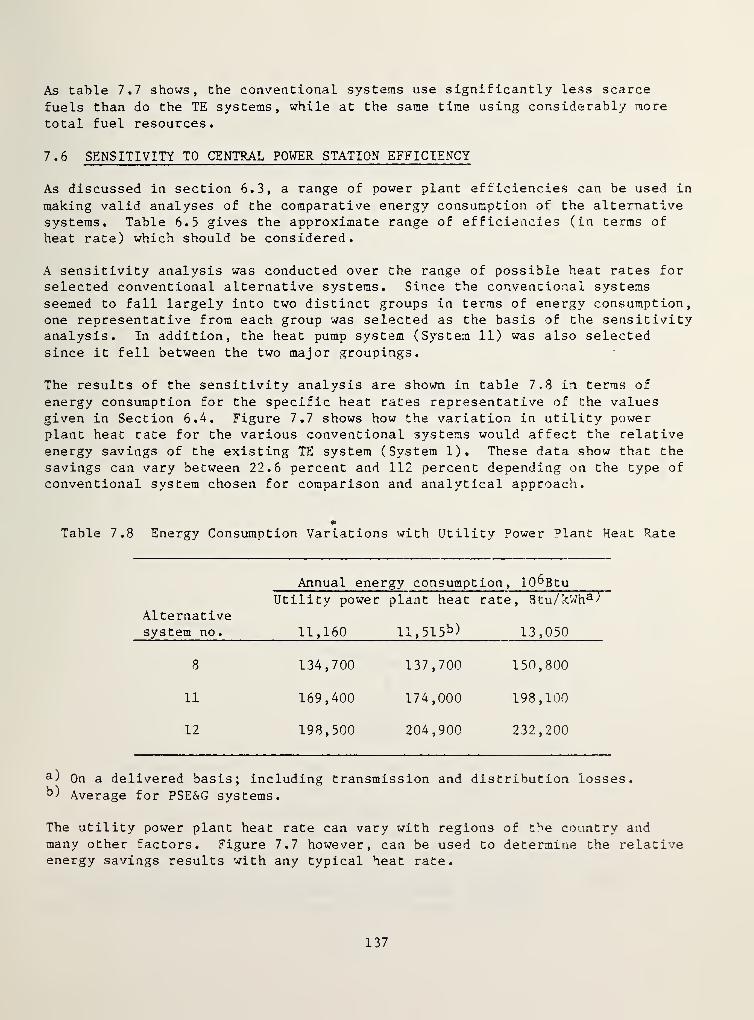
As table 7.7 shows, the conventional systems use significantly less scarce

fuels than do the TE systems, while at the same time using considerably more

total fuel resources.

7.6 SENSITIVITY TO CENTRAL POWER STATION EFFICIENCY

As discussed in section 6.3, a range of power plant efficiencies can be used in

making valid analyses of the comparative energy consumption of the alternativesystems. Table 6.5 gives the approximate range of efficiencies (in terms of

heat rate) which should be considered.

A sensitivity analysis was conducted over the range of possible heat rates for

selected conventional alternative systems. Since the conventional systems

seemed to fall largely into two distinct groups in terms of energy consumption,one representative from each group was selected as the basis of the sensitivityanalysis. In addition, the heat pump system (System 11) was also selectedsince it fell between the two major groupings.

The results of the sensitivity analysis are shown in table 7.8 in terms of

energy consumption for the specific heat rates representative of the valuesgiven in Section 6.4. Figure 7.7 shows how the variation in utility powerplant heat rate for the various conventional systems would affect the relativeenergy savings of the existing TE system (System 1). These data show that the

savings can vary between 22.6 percent and 112 percent depending on the type of

conventional system chosen for comparison and analytical approach.

©

Table 7.8 Energy Consumption Variations with Utility Power Plant Heat Rate

Alternativesystem no.

Annual energy consumpt ion, 10 b Btu

Utility power

11,160

plant heat

ll,515 b )

rate, Btu/kWha 7

13,050

8 134,700 137,700 150,800

11 169,400 174,000 198,100

12 198,500 204,900 232,200

a ) On a delivered basis; including transmission and distribution losses.b ) Average for PSE&G systems.

The utility power plant heat rate can vary with regions of the country andmany other factors. Figure 7.7 however, can be used to determine the relativeenergy savings results with any typical heat rate.

137

energy

savings

of

system

Figure 7.7 Effect of utility power station heat rate on relative energysavings. System 8 is representative of System 5 throughSystem 8; System 12 is representative of Systems 9, 10, and 12,

138


7-1. The Trane Company, "TRACE Documentation Manual", 1976.

7-2. Patterson, N.R.,"TRACE Weather Reduction Accuracy," Internal Memo,

A.P.O #1431-249, The Trane Company, April 23, 1975.

7-3. The Trane Company, "TRACE Program Input Version 200," TRACE 2, included as

part of reference 7-1, December 1976.

7-4. H.D. Nottingham and Associates, Inc., "Design, Cost and Operating Data for

Alternate Energy Systems for the Summit Plaza Complex, Jersey City, N.J.,"National Bureau of Standards Report GCR 79-164, May 1979.

139

8. JCTE COST DATA AND ANALYSIS

8.1 INTRODUCTION

The actual economic data collected for the Summit Plaza TE plant are presentedand analyzed in this section in order to develop data for use in the systemcomparisons described in section 9. Other possible uses for the data includeinput for evaluating other projects for which specific economic data may nototherwise be available.

This section also presents an analysis of the effect of anomalous conditionsat JCTE on the economic data. Anomolous conditions include equipment perfor-mance problems, improper or non-optimum operating and maintenance practices,unique institutional factors, etc. A forecast of costs is presented for a

"typical" (i.e. non-anomalous ) TE situation. Unit costs were also developed,based on the actual "raw" cost data, as a convenient means of presenting the

data and as an aid in making direct comparisons with known data from otherplants

.

This section presents all the actual costs that have been incurred as a resultof designing, constructing, owning, and operating the total energy plant at

Summit Plaza. The following types of costs were considered:

1. Operation and Maintenance (O&M) costs from initial plant start-up in

January 1974 through November 1977.

2. Initial capital costs incurred beginning in late 1971 and capitalimprovements since plant start-up.

3. -Owning costs' other than capital investment (i.e., property insuranceand taxes).

Indirect revenues from providing utilities to tenants and income tax effectswere not considered.

The analysis includes both direct and indirect costs. Direct costs are the

costs associated with goods, services, or capital equipment for which actualpayment is made to a supplier. These direct costs are separated into compo-nents for the electrical, heating, cooling, and PTC subsystems. Indirect costsare the costs associated with transfers of energy between subsystems within the

TE plant and for which no actual monetary transaction is made. Indirect costsare a means of further allocating direct costs to the subsystems so that unit

costs can be calculated. This further allocation of costs is discussed in

appendix I of this report.

8.2 OPERATION AND MAINTENANCE COSTS

8.2.1 Cost Collection Methodology

The firm of Gamze-Korobkin-Caloger, Inc. of Chicago, Illinois (GKC) had the

responsibility for operating, maintaining, and improving the JCTE plant for the

140

entire period covered by this report. GKC employees operated and main-tained the plant, made fuel and materials purchases, and obtained contractlabor services. Even incidential items such as telephone service, remotemonitoring by security service, standby electric service

setc., were purchased

by GKC. In short, all plant operating expenses, with the exception of one

minor O&M cost item discussed below, were incurred by GKC. Owning costs were

incurred by the site owner, not GKC.

Cost data were submitted to NBS by GKC on a monthly basis in the form of recordsof individual disbursements to other companies and of charges made by themselves

for operating the plant. These data were also reported to HUD by GKC in accor-dance with GKC/HUD accounting procedures. NBS had full access to GKC disburse-ment records (including internal labor, overhead (OH), and assessed fee) as

well as cost reports sent to HUD for reimbursement.

Payment to GKC for these operating and maintenance expenses was shared by HUDand Starrett Housing Corporation (SHC) (owner of the entire Summit Plaza site,

including the Total Energy Plant). The cost sharing was based on a formula in

which SHC’s share of the expenses increased year-by-year until no support was

to be provided by HUD after 8 years.

The flow of money through the various organizations to pay for O&M expenses is

shown in figure 8.1. This figure emphasizes the fact that even though HUD and

SHC were sharing O&M costs for the project, this did not in any way influencethe cost data being collected by NBS . This was due to the fact that NBS col-lected total disbursement data from GKC, the plant operator, and not from HUDor SHC. GKC, a private consulting mechanical engineering firm, did not subsi-dize plant operation, expected to get fully reimbursed for its disbursements,and in fact intended to collect a fee for carrying out its responsibilities.

Only one O&M cost item was not directly reported by GKC. This is the cost of

water consumed by the plant. Water was supplied to the entire Summit Plazasite by the City of Jersey City and invoices rendered to the site owner did notseparately show the water consumption of the plant. A portion of the water for

the plant was separately metered by the plant operator for the water consumed.The water was primarily for make-up in the cooling tower, the heat transfercircuits within the plant, and losses in the site distribution systems. For

this report, the total monthly water consumption based on measurements and cal-culations was used along with the appropriate city water rate (1978) to developmonthly O&M cost data for this item. The annual cost for this item was quitesmall, 2.4 percent of the total O&M costs excluding fuel costs.

The monthly cost data include all expenditures as they occurred since January1974. With the four exceptions treated in the next section, this reportincludes data on individual expenditures directly in terms of magnitude of

expenditure and the actual time of occurrence during the year.

8.2.2 Cost Accounting Procedure

Cost data were collected monthly and the raw data were kept in a monthly database for reduction and analysis. Prior to utilizing the raw data in any wav,

141

03 V03 3aj G03 C03 U 03 03

CJ 3 <3

CJ <3 <D •Hu U 4—1 i

—1

•

3 rH u c C- CJ

PL, 0) r- *H 3. w3 o 03 3 •H

( CJ T* zn

142

Figure

8.1

Organizational

cash

flow

for

the

operation

of

the

Jersey

City

Total

Energy

site

several adjustments were made to the raw data to improve accuracy or to

facilitate comparisons. First, adjustments were made to prorate expenses to

more accurately reflect the magnitude and time occurrence of four individualcost items. Second, individual disbursement items were allocated to the vari-ous subsystems within the plant and aggregated into seasonal periods in orderto calculate unit costs. In all but one case, these adjustments did not change

the total yearly cost in any way, but improved the accuracy of the unit cost

and seasonal data presentations. The adjustments are described in the

following subsections.

8. 2. 2.1 Prorated Expenses

Four large expenditure items occurred in such a way as to substantially distortmonth-to-month costs if they were used directly in terms of time of occurrence.One of these items (engine overhauls) was spread over a multi-year time periodand appropriate monthly costs were assessed (based on 1979 forecasts). Two of

these expenditures (lube oil and insurance) were prorated so that, for eachmonth, a cost was incurred which is equivalent to one-twelfth of the appropriateannual cost. The expenditure for fuel oil was based on actual monthly fuel use,

which varied from month to month. By means of these adjustments, the monthlyand trimester cost data in this report more accurately reflect the actual levelof plant production and maintenance in each period. The engine overhaul andfuel cost prorating schemes are further described below:

Engine overhauls - The overhaul schedule which was projected at the timeof plant start-up consisted of three overhauls, two minor and one major,for each engine during the running time of 36,000 hours. When initialminor overhauls on two engines were conducted in January and August 1976(at 11,800 and 19,900 hours of operation, respectively), the condition of

the engines indicated that an extended overhaul schedule should be putinto practice. This new schedule called for two overhauls, one minor and

one major over a 50,000 hour cycle. The validity of this schedule wasconfirmed by an inspection performed on an additional engine in December1977. This approach tc overhauls was applied to each individual engineto predict the engine running time and elapsed time at which overhaulswould be experienced. Based on this forecast, it was expected to take anaverage of 116 months (9.6 years) for an engine to complete the firstoverhaul cycle.

The costs actually incurred during the 47 months of operation throughNovember 1977 did not include any major overhauls because none were per-formed. (The maximum running time for a single engine at the time was

21,900 hours.) If only actual incurred costs were reported, the costdata would not reflect the true costof operation. Therefore, the totalcost for the projected (revised) overhaul cycle was estimated based onthe actual cost of minor overhauls performed through November 1977 and theestimated cost of a future major overhaul provided by the overhaul con-tractor in 1978. The individual cost items shown here were not escalatedfor inflation nor discounted. To develop monthly engine cost data, thistotal estimated cost was divided by the number of months it was expectedto take an engine to reach major overhaul.

143

The actual cost of overhauls experienced during the 47-month period was

$32,300, or $687 per month. This was for the minor overhauls and inspec-tions described earlier. This monthly cost for overhauls was increasedto $1505 to properly reflect the projected costs for the entire 50,000hour overhaul cycle. This is approximately half of the projected monthlycosts under the original 36,000 hour overhaul cycle. This change is theonly case in which data ajdustments changed the actual total yearly costsof the TE plant.

Fuel Oil . Expenditures for fuel were made monthly but fuel deliveries andinvoicing were somewhat irregular. For example, a substantial deliverycould be made/billed on the last day of a month for fuel which would beused in the following month. Since fuel cost is a significant single item

(56 percent of the total O&M costs), a more accurate representation of

monthly fuel costs was desired. Therefore, monthly cost data for thisreport were developed from the fuel actually consumed by the plant duringthe month (as determined by measurements) and the average unit cost of

fuel for the month. Checks were made to insure that the total cost of

fuel for a year calculated in this way very nearly equaled the totalactual disbursement.

8. 2. 2. 2 Subsystem Cost Separation

Each direct cost item was assigned to the subsystem to which it pertained,except when a single item pertained to two or more subsystems. For theseitems, the cost was divided between the subsystems either by estimation or by

use of secondary data. In some cases, the cost was divided between subsystemsaccording to an estimated fixed percentage. These percentages were estimatedby the plant operator and reviewed by NBS. In other cases, secondary dataallowed accurate division of cost items between subsystems.

For example, the direct expenditure for fuel oil was charged to the electricaland heating subsystems according to the actual fuel consumption of each, as

registered by the NBS data acquisition system.

8. 2. 2.

3

O&M Cost Categories

After the individual monthly expenditures were assigned to the subsystems to

which they were attributable, they were condensed into the following categories

1. Fuel2. Contract maintenance3. Direct labor and overhead4. Plant burden5. Direct material6. Miscellaneous

The plant burden category includes those services which are incidential to

plant operation and generally not associated with a particular subsystem.Examples are: telephone service, insurance, standby power, and GKC operatingfee

.

144

Direct material includes non-capital operation and maintenance items not

provided by contract maintenance services. Examples are: chemicals for watertreatment, lubrication oil, tools, and spare parts.

8.2.3 Actual O&M Cost Data

The basic O&M data were collected on a monthly basis and the adjustmentsdescribed above were carried out on the monthly data. For presentation and

analysis purposes, it is more convenient to deal with longer periods.

The O&M costs for each of the four subsystems (electrical, heating, cooling, and

PTC) for each of the six cost categories are given in table 8.1 for the periodMarch through November 1974, and in tables 8.2 through 8.4 for the three "years"(December-November ) of 1973, 1976, and 1977. These 12-month periods were chosento be consistent with the seasonal periods for which unit costs were calculated(i.e., a "year" commences at the beginning of a winter season on December 1).

8.3 CAPITAL COSTS

8.3.1 Capital Costs for Equipment

Capital equipment costs represent the initial investment as well as capitalimprovements and replacements during the life of the plant. The initial invest-ment was for all energy and PTC equipment external to the buildings and is

reported in the following cost categories:

engine-generatorsmechanical system

e electrical systemdistributioncentral equipment buildingdesign fee

These initial costs are presented in table 8.5. These costs were incurredduring plant construction which took place from November 1971 through mid-1974.The cost of land occupied by the CEB is not included.

8.3.2 Subsystem Cost Separation

In table 8.5, the capital costs are assigned to the four subsystems on thebasis of the function of each piece of equipment. Costs for equipment sharedbetween two or more subsystems were apportioned by relevant indices. Forexample, fuel storage costs were apportioned by annual average boiler andengine fuel consumption and CEB envelope costs were proportioned by squarefeet of floor area.

8.4

OWNING COSTS

Owning costs other than capital financing consist of expenditures for propertytaxes and property insurance by the site owner, Starrett Housing Corporation.Invoices for these items are based on the entire Summit Plaza complex and donot separately include the TE plant.

145

ON CM 00 CM CM o• • • • • • •

rH 06 CO c 00 00 O o03 m CM o4H rHOHH -nt <r p^ o o CNc m JO cn CM o03 m ON 00 o ON m 00rH </> — r — r r

CH rH ON o rH ON cnO' 1 rH mi CN rH <rrH CN

4—

\

o O ON CO nO o• • • • • • •

on o o rH CN o orH \C CN rH o

rHSh CJCU HJ3 CUS o o rH CN O' m r*^

1) cn o CM o> </> m NO rHc r

25

|

CN

1

o CM cn 'sO 00 rH o« • • • • • •

G> o NO 00 o cn rH or—

1

m CM iH o60 rH

j3 2O •HH rH03 O o o vO it o m coZ o 00 <r 00 nVw/ cj </> ON rH CM rH rH p^

r

£ cn CM nH cu

03 4-i

c cd

§ >43 CD <r CM ^d* cn rH oCO JO • • • • • • •

3 cn O o CO n«. O o<r CO VsO CN o

60 o rHC

rH •H4-1

1 CO o m o rH nO o CM01 o rn ON o cn m n-

X 35 rH rH •mO in 00 cnHJ <y> * r * - —

Cfl CN CO n n3" nDO <r rH nO

2<5 r^. o rH CN 00 CM oO • • • • • • »

rH CM r^. O o4H C0 lT) iH rH oo CJ 1—

1

0) •HS-4 SH

•H 4J

Q 0! <T CM r^ m o m0) n NO rH n ON m cnrH <r CO <r cn CM CM NO

rH Cd </> r r * — *• ON 00 m rH CM

CO 00 rH CN rH H nrH

0)

rHJO 0)

03 cj

H dco

T30) C3 rH4H 03 cO

>N c •H CD

•H H C S-4 dc CO O 0) as oCO a hO "O 4_> as

0J cd H CO d4H 4H rH •a 3 a cO

to O CO rQ rHCJ co U a) 4H rH rH

S-4 CJ jd 4J CJ as cd

4-1 rH 4H a) S-4 3 OS CJ uCD 0) c H as cd Sj CD oo 3 o •H > rH •H •H HCJ Ph CJ Q o CH Q 2

• . # • . .

rH CM cn <1* m nO

146

Table

8.2

Direct

O&M

Costs

-

1975

Summary

(December

1974

-

November

1975)

a-

a0)

J-l

1

03

>xX

1-03

C/0

I

S'?

</>

S'?

S'?

S'?

S'?

I

I

I

;nu0to0)

J-l

33cj

j-i

01

oo

O' co co o CO CN o• • • • • • •

O' m 50 on O om rH oiH

o 00 O' r-H 50 co CMCO co o co co in inco O' 'T o on C—

S

CM* * r. rx r ox rr

ON 00 cO CT\ CO rH cnCO cO O' 04 rH coCM -cT

o r-' rH rH rH rH o• • • • » • •

o co ox r«x 50 rH ovO CN o

rH

o CM Q 04 CN on oc CM r-H m cnCsi CO rH on m

— r.

CO r—< m

o ox xO P—| 50 r^ o• • • * * • •

o m m cn m o o—j in rH rH o

rH

o O' xC -s 50 X O'uo 00 <n o on rHo •£> on o rH CN

r» r

o CM on OnrH rH

o xO 00 on CN o• • • • • • •

o m, xO m 04 o or'~- o

rH

co LT> CO on 50 O'.o VC CTX on r-J m mO' o o 0‘s* CM cn <r

rx rx IX r AO' r~~ on oc on CNO' on Mt

rH

o m rH m CM o• > • # • » •

o co CM m on o oo —

j

rH orH

CN HT 50 rH Cx XrH O o CN CM <r

<r vO cm <r 00 in o* r M r A

05 co CO rH xOoo m CO rH rH rHf—J on

0)

CJ

33a T3cu rHHJ 33 3C3 •H 03

•H u r Hi 3o 5 1)

a -O *3 OH s33 H 3 c

•U >H -O 3 a 35

CJ 03 J2 rH03 j_l 0) AJ rH iHU o jr 4J a 03 33

r-H u 1) H C a) CJ U rH •H •H E—

i

Ch CJ Q o CU 2

• # • • # ,

r-H CN on m o

147

Table

8.3

Direct

O&M

Costs

-

1976

Summary

(December

1975

-

November

1977)

o J5 J2 un o• • • • • • •

rH 00 ON 00 un o oCO un H o4-1 rHOHHI O' un o> <r o rHc CM cn ON O CN o O'to ON un un unrH <J> — * *CM JO 00 o m CN CN

<r LO H cn O'cn H un

o o H m. in o. • • • • • •

o o vO H o H o50 CN rH o

HcjHCH

o o o cn un rûn 00 CN O

un CO H cn* r

un H co

o 00 ON 00 CTi 50 o• • • • • • •

o CN o CN CN o oCN <r H CN o

SO HC•HrHO o CN O <J* CO Ho r-- 'sO O O ON <rCJ CN o H cn rH ON

— * a

a m cn <r H0) H cnHIcn

OnX <T> rH ON oo oo un OrO • • • • • • •

3 50 CN a> c50 cn O o

CO 50 H * oso He•HHI

cO CN cn H o 50 ON01 CN cn ON on cn CN ONX n- 50 o ON 50

- * *

cn 50 CN 1

—

unCN cn rH coH H

on CTi o CN cn O• • • • • • •

rH ON CN m m <r o oCO in rH H oCJ (H•HUHI

o CN r>- cn o01 O cn ON JO ON unrH rH cn 00 CN CN 50W </> * - * r * - *

CN m un \0 r*^ rH oCN nr un CN HCN cn

0)

ocCO

e "O0) s HHI CO 03

>, c H cn

H •H Hi C H 3O CO O 01 0) OSO a J3 "3 4-J 01

01 CO Hi 03 cHI HI rH -a 3 s cO

CO O cO .a rHo cO HI 01 4-J rH rH

l-i O J3 HI a 0) <3

HI rH HI 01 H £ OJ o uX 0) rj Hi 0) 3 H cn Oo 3 o •H > rH H rH HCJ EH CJ a o Ou s

® • . • •

rH CN cn <r un JO

148

TabLe

8.4

Direct

O&M

Costs

-

1977

Summary

(December

1976

-

November

1977)

CU

4-1

o

S'?

5^

6C

W

S'?

5s?

S'?

I

I

|

I

j

l

3300)

4-1

<c

CJ

I

i

co

qcj

rH r^ CN CN cn O• • • • • • •

O'. o> v£> C <r o om fH rH orH

t-H o C CO fH in L

n

O' On OC CO rH PM coc iH <r vO O' O'.

A A * * r p»

PO »H <fr vO r*

l

Hn. vO o vO CN COm pH vC

o On O) CC c• • • • « •

o CO CN LO c oCN <r CN c-

o 0s CO CN MO n.H <r <r O' Oco CN vc vO O'A * * *

co uo CN HrH

o vC CO LO cc 00 o• • • • • • «

c <r O vO o oCN CO CN ^-4 c

l—l

o co O' r^ c <r CMpH H <r i—

i

CN o> vO CN] po POa * p> * r

0s CO vOrH po !

I". oc cr 00 LO co C• • • • • . .

in m vC oc CN o O<c H n

i—l

<T 00 CN CO oc pn00 CO v£> CN Ov in OCs.

o

CN o> rH oc inA * a ps PS * 1

H CN <0 <rJCN ^4 CO H as

i—

i

rH

<r <r uo 00 CN O• • • • • • •

m co O' CO C ovo H o

pH

r-r CN 0 VC r—4 CN 00O r*«. o> CN CN<r v£> o o cc O' O'— p» PS * PS

m CN <r o-<r co UO CO rH 00Psl CO

i

UCJ

Cctf

d 030) d »Hxj 03 03H H COH u d U 3C3 O 0) 0) Ce pQ 03 XJ 0)

1

03 u 03 cXJ H 03 3 S to

CJ 03 pO t"“41

03 xj 0) i-j rH 1 rHu CJ pC 4-J CJ a)

1 to

i—

j

u D U £ D o | 4J

<v*-r H 0) 03 u co | o

3 o H > rH *H rH 1 Ei 1

fa. CJ o o 0^ o

• • • • •

H CN co LPi M3 1

I

149

Table 8.5 Capital Cost Summary

Actual construction costs including overhead and profit

Thousands of Dollars

SubsystemCost category Electrical Heating Cooling PTC Total

Engine-generator $ 316 — — — $ 316

Mechanical 132 553 714 85 1,484

Electrical 213 — — — 213

Distribution 214 86 110 713 1,123

CEB envelope 208 130 148 109 595

Design fee 52 39 49 Includedabove

140

Totals $ 1,135 $ 808 $ 1,021 $ 907 $ 3,871

150

Real estate for the Summit Plaza complex is paid pursuant to New Jersey statutes,

NJ3A 55.14 J-l,

et . seq., as set forth in an agreement with the City of Jersey

City. This agreement provides that the real estate taxes payable for the com-plex will be 15 percent of annual "shelter rent" of the complex. This means of

paying real estate taxes is very common in the New York City and adjacent New

Jersey areas. Therefore, the actual expenditures for real estate taxes do not

directly depend on the value of equipment used for providing utility services.In presenting the actual costs as experienced for the JCTE plant, this report

includes no portion of the total Summit Plaza cost for real estate taxes.

3.5 UNIT ENERGY COSTS

Unit costs for each of the energy commodities provided by the plant were

calculated using the actual O&M and capital cost data of sections 3.2 and 3.3.

The unit costs are reported as follows:

electricity <£/kWh

hot water S/10 6 Btu

chiller water $/10°Btu or i/Ton-hr

The energy quantity used in the denominator is the energy delivered to the site.

Unit costs for JCTE are provided here primarily as a convenient,widely-understood means of presenting the actual cost data. These data can be

used for:

3 comparing the cost of supplying utility services to the 'Summit *

Plaza Complex with different means of supplying the same services

3 comparing the cost with actual data from similar existing plantcomplexes

Either of the above comparisons is not considered a method for comprehensiveeconomic evaluation. Nevertheless, such comparisons may prove useful in somecircumstances provided that a cautious approach is employed. Some items of

particular concern are cited below. If comparisons are to be made using JCTEunit costs, care must be excercised to insure that:

3 all relevant costs are included or that similar physical/costaccounting boundaries are drawn so that comparable cost items areincluded

the building complexes being compared have somewhat similar loadpatterns

J anomalous conditions are considered including differences in thecurrent costs and economic forecasts compared with those of 1973/19 T 9.

If comparisons with other published data is considered, then the limitations ofthose data should be recognized. In general:

151

° most published cost data do not completely separate HVAC andelectrical system costs from other operating costs for the buildingsas was done here.

° there are usually inherent variations among the sampled buildings in

terms of size, age, type of HVAC system, usage, etc.

0 there are a variety of ways costs are reported (even within a fairlyrigid accounting system) which can lead to significant differences in

reported costs.

0 there may be small sample sizes for some cost items

Because of the significant variations in subsystem loads with the season,it is appropriate to present unit costs on other than annual basis. The timeperiods chosen here were based on plant operating conditions. Specifically,a year was divided into three unequal periods as follows:

Summer - included all days for which the chiller was operating (generallythe last week of May through the first week of October).

Winter - the three months of December, January and February.

Spring/Fall - all other days of the year.

This approach allowed expenses for the chiller to be confined to a singleperiod. It further allowed costs during the periods of low thermal loads in

Spring and Fall to be separated from periods of higher loads. The differencesin plant loads for these periods were significant. In qualitative terms, plantload differences were as shown in table 8.6.

Monthly O&M costs aggregated into seasons for the purpose of calculating unitcosts. These data also provide a more detailed look at the actual data, pre-viously shown as yearly aggregations in tables 8.1 through 8.4. The seasonaldata can be found in appendix H.

The seasonal data and the unit costs include a capital cost component in

addition to O&M costs. In order to combine these two types of costs the ini-tial capital costs of table 8.5 were converted to an equivalent annual basis.To accomplish this conversion, the initial capital costs were multiplied by an

appropriate uniform capital recovery (UCR) factor. The UCR factor depends on

the interest rate and the assumed life of the plant which are developed and

described in appendix H.

The methodology used to calculate unit costs accounts for the energy transfersbetween subsystems internal to the plant. This is necessary because of the

significant indirect costs associated with these energy transfers. The needto include these energy transfers and their costs in the calculation of unitcosts resulted in development of a fairly complex calculation methodology.This methodology is fully discussed in appendix J.

152

Table 8.6 Qualitative Seasonal Load Variations

Load SummerSpring/

Fall Winter

1. Gross electrical output high moderate moderate2. Boiler output high low high3. Site hot water consumption low moderate high4. Plant auxiliary electrical

consumptionhigh moderate moderate

5. Site electrical consumption moderate moderate moderate

The unit costs results are shown in table 8.7 as an aggregated 3-year summaryof subsystem unit costs. Year-by-year data do not vary significantly from the

aggregated values. More detailed yearly and seasonal data are contained in

appendix H. In all cases, the cost components of fuel, other O&M, and capitalrecovery are provided to facilitate comparisons with other data which may not

include capital recovery or which may be based on different unit costs for

fuel

.

The unit cost data clearly show a very high cost for chilled water andmoderately high unit costs for electricity and hot water. The high cost for

chilled water is due in large part to the high capital recovery associatedwith a system which operates only four months of the year. For example, in an

officfe building, with a year-round need for chilled water, the capital recoveryportion alone could be cut from nearly $19/10^Btu to approximately $10/10^Btu.

8.6 DISCUSSION OF DATA AND ASSESSMENT OF TYPICALITY

The purpose of this section is to discuss the cost data of section 8.2, to

identify the major variables which affected actual plant costs, to conduct an

assessment of the typicality of the cost data, and to provide adjustments so

that the costs can be considered typical.

The assessment typicality of is vital if this demonstration is to provide an

understanding of TE plant economics beyond the particular case study which has

been completed at Summit Plaza. The typicality of JCTE economic data should be

a consideration in analyses which directly use JCTE overall economic resultsfor comparison or which use the JCTE individual cost component data to estimatecosts for other TE plants.

The data of tables 8.1 through 8.4 gives O&M costs by component. Figure 8.2shows the relative contribution of these components during the 1975-1977period. The analysis of these cost data will be by component as indicated infigure 8.2 by emphasizing effects of fuel costs with slightly less emphasis ondirect labor and maintenance and only cursory analysis of the significantelements of the other cost components. The first five parts of the discussion(sections 8.6.1 through 8.6.5) deal exclusively with O&M costs; capitalcosts are discussed in section 8.6.6.

153

Table 8.7 Unit Cost of Site Thermal and Electrical EnergyMarch 1, 1974 through November 30, 1977

Cost category Electricity Hot water Chilled water

6kWh $/MBtu $/MBtu

Fuel 1.92 3.90 10.08Other O&M 1.22 2.60 6.80Capital recovery 1.02 2.87 18.86

Totals 4.16 9.37 35.74Site energydelivered

,

MWh or MBtu 18,210 112,000 21,540

8.6.1 Inflation and Other Temporal Effects

The total O&M cost of JCTE has continuously increased since January 1974, as

shown for fuel and non-fuel components in figure 8.3. Fuel cost increaseshave resulted from both increased fuel usage and from rising unit costs for

fuel (see figure 8.4). Fuel usage is largely affected by site/plant loads,discussed in section 8.6.2, and by equipment performance, discussed in section8.6.3.

For non-fuel O&M costs, general increases in costs for on-site labor, contractmaintenance, and material costs have been experienced since January 1974.

The combined cost for on-site labor and contract maintenance has also changedover time as the various O&M tasks have been performed either by in-house or by

contract personnel and by the number of plant personnel employed. This is

discussed further in section 8.6.4.

8.6.2 Plant Loads

The magnitude of the thermal and electrical loads imposed on the plant has a

major influence on costs. When these loads increase, total costs rise largelybecause more fuel is burned, while unit costs (e.g., <jr/kWh) are reduced becausefixed costs remain constant.

JCTE cost data can be compared directly with other systems which serve similarloads, irrespective of the type of facility being served or the climate. This

approach usually results in the most accurate comparisons. It may also be

desired to make comparisons between JCTE costs and costs for services to othersimilar complexes for which load data are not available. (Similar complexesmeans approximately the same number of apartments, and/or the same conditionedarea, the same building types, the same climates, etc.) In this latter case,

it is important to know whether the JCTE loads are typical for this generaltype of application. TE plant loads are primarily influenced by the following:

154

a

a0

vy

u r>. CNcc a\ cn

SI! m vC

'•<3

o

<jy </> </>

rH m rûo On o> CT>

H rH r—i r-H

155

Figure

8.2

Major

components

of

the

O&M

cost

IT90

ianj

r^

>-

m oc_

>d*

r-*

OOco

ocvC

oc oo

<N

(0001$ x)

S^soo Hô

156

Figure

8.3

Total

annual

O&M

costs

nagw j;ad s^BXToa

o V.

C

r—

i

cn CTn <r o rH

o CO r-* in <T CM rH o CC

cn CN CN CNl CN CN CN CN pH pH

r^-

m

oooo oooooo oo c

uoxiBo s.iexI 0Q

157

Figure

8.4

Unit

cost

of

fuel

oil

delivered,

1974

-

1977

0 percent site occupancy0 distribution system performance° weather0 occupant conservation efforts0 building characteristics

The following paragraphs discuss each of these items in turn.

The apartment buildings reached full occupancy in September 1974. The schoolhad its first session beginning in September 1976. However, the commercialbuilding was only partially occupied during the period covered by this report.The hot water, chilled water, and electrical loads at the TE plant would be

increased only slightly (less than 5 percent) by a fully occupied commercialbuilding

.

The thermal distribution system has been a source of very significant energyThe thermal distribution system has been a source of very significant energylosses, as discussed in section 5.3.1, and has therefore increased plant hotwater and chilled water loads accordingly. The excess in hot water load dueto the inefficient distribution system was estimated to be 19.6 percent in

January 1977 and 28.6 percent in July 1977. Section 5.3.1 also contains an

estimate of the annual reduction in fuel oil consumption which would result if

the excess losses were eliminated in both hot and chilled water circuits:

91,000 gallon (344 m^) which is equivalent to a cost savings of $32,300 at

the 1976 average fuel cost. This should be taken into account in use of thisdata for comparisons.

Peak loads, also affected by the losses, have an effect on boiler capacity andcapital costs as discussed in sectin 8.6.6.

Weather patterns exert a direct and significant effect on building spaceconditioning loads, and therefore an evaluation of the typicality of the weatherduring the four years covered by this report was performed. Data obtainedfrom the National Oceanic and Atmospheric Administration (NOAA) shows both the

actual and normal degreedays for heating and cooling. These data are shownin table 8.8 for the Newark Airport weather station which is 6 miles fromSummit Plaza [8-1]. These data show that heating loads were somewhat higherthan normal during the first 2-1/2 years of operation and somewhat less thannormal during the last 1-1/2 years. Cooling loads were consistently higher (7

percent to 18 percent) than normal during the entire 4-year period. For this

report it was not considered necessary to develop O&M cost adjustments to

account for these relatively minor deviations from typical weather patterns in

view of the large distribution system losses. The larger cooling loads due to

the weather was somewhat offset by the low commercial building load.

Occupant conservation efforts are very difficult to assess and depend at least

in part on the degree of economic incentive. The site contains no individualmetering of either electrical or thermal commodities for the purpose of directlybilling to the tenants. Under this "master-metered" situation, no significantoccupant conservation efforts are likely. Insofar as cost comparisons areconcerned where specific load data are not available, Summit Plaza TE costsshould be compared only with costs of other complexes which are also

"master-metered"

.

158

Table 8.8 Actual Weather Patterns, 1974-1977

Heating Cooling

Season Degree-daysa ) % Dev.k) Year Degree-aays a ) % Dev.k)

1974 c ) 2903 -11 1974 1125 t—

*

o

1974-75 4811 - 4 1975 1100 + 7

1975-76 4624 - 8 1976 1099 + 7

1976-77 5577 +11 1977 1208 +18

1977 d ) 1871 + 5

Normalseason 5304

Normalyear 1024

a ) base = 65°F

b)% Dev. * actual-normal

x 1Q0normal

c ) January through June only, normal = 3252 degree-days

d) September through* December only, normal = 1787 degree-days

Building characteristics at Summit Plaza are somewhat atypical. All apartmentbuildings are of modular construction. The school and commercial buildings,however, generally have typical construction characteristics. The impact of

modular construction on apartment building space heating and cooling loads is

not known and was not part of this TE demonstration evaluation. All apartmentbuildings except Decson have double-glazed windows which is somewhat atypicalfor buildings designed in 1972. In general, it is felt that the buildingcharacteristics should not be a factor in comparisons of data.

8.6.3 Equipment Performance

Section 5.2 identified a number of conditions at the site which causedincreased fuel usage. The increased fuel use can be translated directly to

increase costs. Of the six items listed in section 5.2, all but one appearsto be atypical in the sense that either equipment did not function as it doesin most plants, or that the conditions could have been easily and inexpensivelyrectified

.

Table 5.1 provided the possible annual fuel savings for the conditions had theybeen rectified. Taking the more conservative fuel saving values from thistable when more than one approach to improvement is provided, the fuel and costsavings for rectifying the five atypical conditions are shown in table 8.9.

159

The exhaust heat exchangers and dry coolers would possibly require some addedinvestment to realize the above cost savings. However, it is felt that anysuch costs would be rapidly repaid through the fuel savings, thereby justifyingthe inclusions of these improvements. For example in February 1978, louverswere actually installed on the dry coolers at a cost of $91,000. Unit fuelcosts for the first five months of 1978 averaged 39.27<^/gal. At this fuel costand the annual fuel savings indicated in table 8.9, the investment in drycooler louvers had a payback period of 2.1 years.

Table 8.9 Cost Impacts of Improved Equipment Performance

ItemAnnual

Fuel SavingsAnnual

Cost Savings 3 )

gallon $

Exhaust heat exchangers 37,000 12,720Engine-generator operation 7,300 2,510Idle boiler bypass 7,500 2,580Chiller performance 32,000 11,000Dry cooler losses 11,000 3,780

Total 94,800 32,590

a ) Based on 1976 average fuel cost of 34.37 <^/gal.

Optimizing the engine-generator schedule reduced fuel costs because the

engine-generators were allowed to operate at a higher part-load conditionwhere efficiency is somewhat greater. As discussed in section 5. 2. 1.3, anotherbenefit was also obtained: a savings of 2200 engine-hours per year. In terms

of the overhauling the engine-generator alone, this saves an addition $1500per year.

8.6.4 Operation and Maintenance

The operating approach envisioned in the design of the plant was carried out

and was not changed during the first four years. That approach calls for anoperator to be at the plant on a one-shift, 40-hour per week basis. In theevening and on weekends, the plant is completely unattended. A second operatorwas added during the daytime primarily to assist with maintenance tasks and to

provide a back-up to the principal operator in case of sickness or emergencycalls .

The single-shift operating approach obviously reduces cost to a minimum. On

the negative side are some added costs due to running excessive engines and

some loss of reliability. Whether a generic plant should incorporate greateroperator attendance cannot be clearly stated on economic grounds. The amountof cost increase for a generic plant with two-shift or three-shift attendanceis uncertain since the Summit Plaza plant has added controls which would not be

160

r

needed in a fully-attended plant. For a small plant like this one, the

unattended approach is viable and likely the most cost effective; therefore,

no atypicality appears to be present in this area.

The maintenance approach has evolved through three distinct phases. The first

phase, from plant start-up through mid-1975, was oriented toward plant shake-down, familiarizing the principal operator with the plant, establishing proce-dures, etc. In this phase, maintenance functions were almost completely per-formed by outside contractors (i.e., those firms which had supplied equipmentand who also affected contract maintenance services). This was to allow the

operator to give proper attention to operational shake-down rather than be

burdened with maintenance chores. Equipment warranty provisions also made it

advisable to have maintenance well-documented and performed by recognized,qualified service personnel.

A second maintenance phase from mid-1975 through 1976, was based on a

transition from contracted maintenance to in-house maintenance. It was felt

that cost reductions could be affected by the in-house approach. During the

transition phase, two additional plant O&M personnel were added (for a totalof three) and an effort at maintenance development and on-the-job training was

undertaken. Contract maintenance was retained during the transition period at

nearly the same level as if no additional in-house personnel were available.Obviously there were substantial added costs during the transition period forhaving both contract maintenance and in-house personnel.

The approach during the third phase was to gradually take over the previously-contracted maintenance task with the added in-house personnel and to terminatemany of the maintenance contracts. Contract maintenance support was stillcalled upon for major maintenance operations.

Figure 8.5 shows the total labor-related O&M costs for the three maintenancephases. During the first phase, direct labor was relatively constant whilecontract maintenance steadily increased as maintenance needs developed for the

new equipment. The second phase saw a significant increase in labor costs anda slackening in the increase in contract maintenance costs.

Labor costs as a percentage of total labor + contract maintenance costsremained nearly constant at 50 percent in the second phase. During the thirdphase, in-house labor costs did not increase greatly.

In-house labor costs as a percentage of total labor-related O&M costs was 84

percent in the first phase, 56 percent in the second phase, and 78 percent in

the third phase.

The magnitude of cost savings with in-house maintenance versuscontractor-performed maintenance was difficult to quantify. However, the

total cost trend shown in figure 8.5 clearly shows the three phases. Theadded cost of the second phase is quite obvious and appears to have been about$14,000 per year.

The overall maintenance approach implemented in the three phases appears to bevery reasonable and a viable approach for any TE plant. No atypical factors

161

were noted in the general approach. The maintenance costs for the third phaseshould be considered most representative of a typical plant.

Specific maintenance situations did exist, however, which resulted in atypicalequipment performance. The most significant was the lack of monitoring andmaintenance of the cooling tower and chillers which did lead to poor chillerCOP's. Proper maintenance of these items would not have increased the O&Mcosts in any significant way.

O&M costs for labor were also influenced by the high local wage rates (highrelative to the national average). This effect is more fully described in

section 8.6.6. The cost impact for a 9.2 percent labor premium in the JerseyCity area considering in-house labor only was $9,000. It would have been evenhigher including contract maintenance which is very labor-intensive.

8.6.5 Management and Institutional Factors

From a management and institutional standpoint, the design, construction, andoperation of the TE plant in the context of the Summit Plaza development wasunique in a number of significant ways. Those management and institutionalfactors which had an impact on O&M costs are as follows:

° the multiplicity of organizations involved in management, design,construction, and operation of the TE plant and site buildings

° operation of the TE plant under a HUD contract by an engineering firmindependent of the site owner •

0 HUD financial support to the developer for operating the TE plant

0 HUD requirements for accounting and reporting costs for the TE plantand for public relations support by the operating firm.

These non-technical aspects and their impact on costs are discussed in the

following paragraphs.

The multiplicity of organizations involved in the design and construction of

the site was necessitated by the nature of the HUD objectives under the Opera-tion BREAKTHROUGH program. Four different firms had lead responsibility for

the various site buildings while the site distribution, the PTC, and the TE

plant each were the responsibility of separate firms. This situation is

described in more detailed in reference [8-3]. The impact of this situationwas difficult to determine, but it appears that it may have been the basiccause of other technical problems such as discrepancies between actualand predicted loads, early operating problems with electrical service, etc.

The TE plant was operated by Gamze-Korobkin-Caloger,under a contract with HUD

who, in turn, billed the site owners for part of this cost. The site ownershad responsibility for all electrical and mechanical equipment outside the TE

buildings, including site distribution and in-building HVAC equipment. This

three-party responsibility probably led to the following atypical conditions:

162

(0001$ X) 3SO0 TBIOI

163

figure

8.5

Total

labor-related

O&M

costs

0 maintenance and operation of site hydronic equipment without fullappreciation for impacts on the TE plant

° lack of direct impacts of plant/site O&M practices on costs to the siteowner, since HUD assumed plant costs above a certain limit

0 lack of direct cost accountability between the site owner and the TEplant operator.

Specific technical problems with a major cost impact can be traced to thismanagement situation, including site distribution losses, chiller performance,and other obvious and correctible plant problems.

Aside from the issue of cost consciousness and having only indirectresponsibility, the approach of having an engineering firm based in Chicagooperating a single plant in New Jersey would appear to incur added overheadcosts for accounting, engineering, travel, etc., in addition to possible diffi-culties in technical monitoring.

An examination of actual JCTE labor costs is indicative in this respect, as

shown in table 8.10. These data for January through June 1977, show that

34.9 percent of total labor costs were incurred in Chicago, at the engineeringfirm's office. Contributing to this high percentage was the fact that Chicagohome-office overhead rates were over twice the overhead for plant personnel.

Table 8.10 Labor Costs by Category, January through June 1977

Total CostLocation Labor category (with OH)

Jersey City, N.J. Plant operator $ 10,703Ass ' t operators 19,700

$ 30,403

Chicago, Illinois Principal 8,716Engineer 5,572Clerical 1,993

$ 16,281

Whether this level of management and engineering effort was warranted or not

depends on many factors and was not determined in this analysis. The costimpact, however, is reflected in the data. -

Two quantifiable atypical costs resulting from management and institutionalfactors were travel and profit. Travel would not have been incurred if the

plant had been operated by local firms or by the site owners. Profit likewisewould not have been included if site owners had operated the plant.

Cost data on these two elements are shown in table 8.11. These atypical costelements are snail but noteworthy impacts on costs and should be considered

164

when using the JCTE data. An average value of $20,000 reduction is recommendedfor this adjustment.

8.6.6 Capital Costs - Design Factors

Capital costs are influenced by the basic design approach, by government-imposedplant design requirements, by local construction practices, and by institutionalfactors such as general construction/procurement requirements for government-funded projects.

The basic design approach was quite typical of the TE design practices in use

in 1970-72. Several specific design decisions can be identified which mayhave influenced costs relative to other viable design approaches. In the

design stage, combined absorption and compression chillers were identified as

having lower life-cycle costs but were rejected primarily because of expectedreliability problems with engine-driven centrifugal chillers and, secondarilybecause of limited experience with this design approach [8-3].

Table 8.11 Atypical Costs: Travel and Profit

Year a )

CostTravel

elementProfit Total

% of total yearly^)non-fuel O&M

1974 3,113 5,310 8,423 7.5

1975 5,211 5,853 11,064 5.7

1976 6,734 13,578 20,312 8.1

1977 . 4,245 14,826 19,071 7.4

19,303 39,567 58,870 7.2

a ) December through Novemberb) Yearly cost from tables 7.1 through 7.4, excluding fuel

It does not appear that electric-driven centrifugal chillers were considered as

part of combined chiller scheme. This approach, while sacrificing some thermalefficiency compared to direct drive, seems attractive when a standby-generatoris considered for the chiller drive thereby obviating any added generator units.This approach is equivalent to alternative system 4, described in section 6.

The cost impact of this approach will be described in section 9.

A second major design decision was the use of hot water cooling of enginejackets instead of the more widely-used ebullient cooling. The choice betweenthese modes of cooling is a complex issue involving engine tolerance for ebul-lient cooling, water treatment requirements, pumping power, and ease of control.Although there has been a measurable cost impact due to added auxiliary powerusage with hot water cooling at Summit Plaza, it cannot be stated definitely

165

that ebullient cooling would result in lower costs when all factors areconsidered.

A third design decision was to use chilled water to cool the ventilation airfor the equipment areas in the plant instead of using larger quantities of out-side ambient air without mechanical cooling. The reasons for this decision wereatypical and not economically justified. The capital cost of this approach wassmall because no added chilled capacity was installed to meet this load. How-ever, the operating cost impacts have been significant. As indicated in sec-tion 5.2.3, 23,000 gallons (87 m^) of fuel oil (valued at $8,200) could be savedannually. This savings would be slightly offset by the added electrical energyfor distributing larger quantities of ventilation air.

In making adjustments so that the data represents a typical situation, it is

recommended that the fuel oil reduction be included and that capital costreductions due to elimination of the heating and cooling coils be considered to

be offset by larger fans and ducts.

The HUD demonstration imposed several significant design requirements on theplant which are definitely atypical. These requirements were:

a parallel HUD demonstration at Summit Plaza of pneumatic trashcollection (PTC) as described in section 2.3

0to minimize possible future government liability in case the TE"experiment" failed, the non-TE components were designed so thatthe engine-generators could be shut down and the remainder of the

plant operate as a conventional central HVAC system

° to permit future experimentation with novel electrical generationequipment, spare room was left in the plant to install a generatingunit of the size of the existing units.

The impact of each of these three items is discussed in the following paragraphs.

From table 4.1, the PTC's electrical energy consumption totaled about 45,000kWh annually, which can be ignored as having any significant effect on planteconomics. The PTC has, however, been a major factor in determining engine-generator operational practices (i.e., "three-engine" operation) as describedin section 5 and reference [8-3]. Elimination of the PTC would furtherincrease the time two-engine operation would be valid and might allow consider-ation of a plant with only four engines installed. A four-engine plant withspace for adding a fifth engine would have reduced costs by at least $63,200for the engines alone, not including savings for heat recovery unit, controls,and piping.

In a typical TE plant design, the capital cost of the PTC would not be incurred.From table 8.5, the capital cost allocated to the PTC is $907,000. Thearchitectural/structural design of the CEB was also heavily influenced by the

requirements of the PTC and although the data of table 8.5 includes the PTCshare of these capital costs, it is possible that a more efficient overallplant design would have been executed without the PTC, thereby reducing capital

166

costs below the allocated costs shown. The magnitude of any such capital cost

reduction could not be determined without added study and therefore no specific

costs adjustments for a typical design are recommended in this report.

The required design approach to leave extant a self-sufficient central

conventional HVAC plant in the event of termination of the electric generationrequired that the boiler capacity be determined without regard for availableengine heat [8-3]. As shown in figure 4.8 and discussed in section 5.2.2, the

capacity of just one boiler can handle the entire thermal load. The excessiveboiler capacity should be considered in using the capital cost data.

Table 1 of reference [8-3] provides the total peak heat demand ( 12 . lxlO^Btu/h(12.8 GJ/h)) of the buildings with no diversity. With no consideration of

engine heat, a two-boiler design would require 253 boiler hp (2480 kW) for eachunit [8-4]. Figure 15 of reference [2-3] provides the predicted minimum engineheat output on a typical winter day - approximately 2.6 x 10^Btu/h (2.7 GJ/h).This heat output can be considered 100 percent available because of back-upengine generator units. Therefore in determining boiler capacity, this outputshould be subtracted from the load rather than counted as a boiler unit of

equivalent capacity. To meet the resulting maximum expected boiler load (9.5 x

10^Btu/h (10 GJ/h)), two boilers of at least 200 hp (1960 kW) or three boilersof at least 100 hp (980 kW)

,would be required [8-4],

Thus consideration of engine heat can achieve an equivalent maximum reductionin boiler capacity (each of two boilers) of 21 percent. An approximate esti-mate of the total cost savings from reference [8-5] is $5,500. (This ''redesign”

analysis ignores two (atypical) occurrences which were unforseen in the actualdesign of the TE plant; excessive distribution losses and poor exhaust heatexchanger performance.)

The overcapacity in the existing plant is not solely due to ignoring engineheat. Two 400 hp (3920 kW) units are installed compared to a required capacityof 253 hp (2480 kW) when no consideration is given to engine heat. A signifi-cant cost savings would result from use of 200 hp (1960 kW) boilers. Thisapproach is valid according to the sizing procedures of reference [8-4] (whichinclude excess capacity for contingencies when (1) consideration is given to

engine heat and (2) when site distribution heat losses are minimized by propermaintenance). Such an approach would reduce capital costs by $11,000.

The extra space in the CEB for an additional engine-generator was a requirementof HUD for future experimentation. This situation appears atypical althoughsuch extra space is often provided in TE plant design for commercial-onlyapplications where large load increases can be imposed on the system by a changein tenants. For a primarily residential site like Summit Plaza and in view ofthe excess electrical capacity provided in the basic design, extra space appearsunwarranted. A reduction in CEB floor space of about 6.1 percent and a reduction$33,376 in total capital costs would result from elimination of the extra bay.

Local construction practices and wage rates also influenced the capital costsof the TE plant. Reference [8-6] indicates that the average skilled trade wagerate in Jersey City in 1974 was 9.2 percent greater than an average of 30 majorU.S. cities. This factor should be taken into account when utilizing the JCTE

167

data. Labor costs were 22.6 percent of total JCTE plant construction costs[8-7], Therefore, generic data should reflect a 2.1 percent decrease in capitalcosts for wage rates, or $62,200.

8.7 TYPICAL COSTS

This section gives typical costs for an optimum design approach, typicalweather, and typical equipment performance in a plant built, owned and operatedby a typical private organization. This is based on accounting for the atypi-cal features identified in section 8.6. Table 8.12 lists all atypical featuresidentified in section 8.6 along with the recommended cost reductions, if any.

In terms of capital costs, the cost of the plant exclusive of the PTC was

$2,964,000. This should be reduced by $169,900 (5.7 percent) to reflect the

atypicalities present in the existing design. Thus construction cost for a

typical plant like that at Summit Plaza which would have begun operation inJanuary 1974, would have been $2,794,000.

In terms of O&M costs, the recommended cost adjustments for all factors in

table 8.12 totals $94,800, or about 16 percent of total O&M costs for 1976.Therefore a typical plant operating at Summit Plaza in 1976 would have incurredO&M costs of $501,800 for the year.

Table 8.12 Summary of Recommended Cost Adjustments for Atypicalities

RecommendedO&M Cost Impacts Cost Adjustments

1 . Plant loads

1.1 Occupancy +$23,7001.2 Distribution system -$32,3001.3 Weather None1.4 Occupant conservation None1.5 Building characteristics None

2. Equipment performance2.1 Fuel costs (see table 8.9) -$32,6002.3 Engine-generator overhauls - 1,500

3. Operation and maintenance factors3.1 Maintenance evolution - $ -$14,000a )

3.2 Labor wage rates -$9,900

4. Management and institutional factors4.1 Multiplicity of organizations None4.2 HUD /ope rat or /ownership relations None4.3 HUD requirements of operator None4.4 Remote, contracted operation -$20,000

5. Design factors5.1 Plant cooling -$8,2005.2 PTC electrical load None

O&M total -$94,800

(Continued next page)

168

Table 8.12 Summary of Recommended Cost Adjustments for Atypicalities(continued)

Capital Cost Impacts

1. PTC

2. Miscellaneous2.1 Spare engine bay

2.2 Boiler capacity2.3 Labor wages rates2.4 Four engines only

-$33,400-$ 11,100-$62,200-$63,200

Capital total

-$907,000

-$169,900

- $1,076,900

a) adjustment to 1976 costs only


8-1. National Oceanic and Atmospheric Administration, "Local ClimatologicalData, Annual Summary with Comparative Data - 1977, Newark, New Jersey."

8-2. Kennedy, D.,et. al

. ,"Alternative Strategies of Naval Bases, Volume III:

Assessment of Total Energy Systems Applications at Naval Facilities,"NTIS Report No. AD/A-003 590, November 20, 1974.

8-3. Gamze-Korobkin-Caloger,Inc., "Final Report, Design and Installation,

Total Energy Plant - Central Equipment Building, Summit Plaza Apartments,Operation BREAKTHROUGH Site, Jersey City, New Jersey,” HUD UtilitiesDemonstration Series, Vol. 12, February 1977.

8-4. U.S. Department of Housing and Urban Development, "HUD Minimum PropertyStandards - Multifamily Housing," HUD Publication 4910, 1973.

8-5. Richardson Engineering Services, Inc., "Commercial-Industrial ConstructionEstimating and Engineering Standards," Vol. 2, Sect. 15100-20, 1974.

8-6. R. S. Means Co., Inc., "1976 Labor Rates for the Construction Industrv,"1976.

8-7. H. D. Nottingham and Associates, Inc., "Design, Cost and Operating Data forAlternative Energy Systems for the Summit Plaza Complex, Jersey City,N.J.," National Bureau of Standards Report GCR 79-164, December 1974.

8-8. Hebrank, J., Hurley, C. W., Ryan, J., Obright

,W., and Rippey, W.

,

"Performance Analysis of the Jersey City Total Energy Site," NationalBureau of Standards Report NBSIR 77-1243, July 1977.

169

9. ECONOMIC EVALUATION OF ALTERNATIVE SYSTEMS

The relative economics of the Summit Plaza TE plant are presented here bycomparing its costs with the estimated costs for the twelve alternativesystems described in section 6. The capital cost of each of these systems wasestimated from quantity take-offs from a preliminary design. Operation andmaintenance costs were estimated using JCTE data for operating labor and plantburden and from cost quotations from vendors on service contracts for majorpieces of equipment. Fuel and electricity costs were based on results of the

computer simulations described in section 7.

The capital cost and maintenance cost data along with basic fuel and electricityconsumption data for the evaluation were taken directly from references [9-1]

and [9-2]. Unit energy costs, operating labor requirements and costs, taxes,and insurance costs were estimated by NBS.

The evaluation was carried out using an engineering-economic approach utilizingdiscounted cash flow techniques. Several evaluation criteria were used includ-ing return-on-investment and payback period. The baseline analysis consideredthe project to be solely financed from equity while the effect of debt finan-cing is shown in a sensitivity analysis.

A sensitivity analysis was also conducted to determine the variability of the

comparative results to changes in assumptions in the economic analysis, energyprice levels, and escalating rates.

9.1 BASIC ECONOMIC DATA

9.1.1 Capital Costs

The capital costs of each alternative system were estimated in reference [9-1]

based on a detailed quantity take-off from the preliminary design. Each pieceof mechanical and electrical equipment in the plant was identified as to type,

size, and quantity and was costed from estimating handbooks and manufacturer’sdata. These data were based on the cost levels current as of January 1, 1976.

A summary of the capital cost data is provided in table 9.1. Appendix K providesadditional cost detail for each of the systems. These data clearly show that

the twelve systems fall into four groups which are equivalent to the four basicdesign approaches. The categories and their approximate initial capital costsare

:

total energy system - approximately $7.3 millionconventional central systems - approximately $5.9 millionindividual building systems - approximately $5.0 millionindividual apartment systems - approximately $4.1 million

The capital costs of table 9.1 include all elements of the Summit Plaza site

which change with changes in energy systems. In the case of the central systemsthe data include costs for all relevant mechanical and electrical equipmentwithin the buildings as well as within the CEB itself. Therefore the cost of

170

Table 9.1 Summary of Capital Costs

SystemNo. Description

Cos t

,

1975 Dollars

InitialInvestment $ 1000s

1 Total energy - existing $ 7,3312 Total energy - existing-selling power $ 7,3313 Total energy - high efficiency engines $ 7,9484 Total energy - diesel and absorption chillers $ 7,3185 Central plant - electric chiller-oil burner $ 5,8366 Central plant - absorption chiller-oil burner $ 5,8617 Central plant - diesel and electric chillers $ 6,6218 Building plant - electric chiller-oil burner $ 5,0279 Building plant - electric chiller and boiler $ 4,963

10 Individual apartment - through-the-wall airconditioners with electric resistance heat

$ 4,120

11 Individual apartment - central heat pump S 4,19712

ReplacementCost

Individual apartment - central air conditionerand electric resistance heat

$ 3,989

10 Individual apartment - through-the-wall airconditioners with electric resistance heat

$ 1,294

11 Individual apartment - central heat pump $ 1,12512 Individual apartment - central air conditioner

and electric resistance heat$ 919

171

System 1 in table 9.1 is not just the cost of the "total energy system" andcannot be directly compared to the actual TE cost data of table 8.5.

An effort was made to validate the initial capital cost estimates for allsystems. This was accomplished by first validating the costs of System 1 andsecondly, by validating the cost relationship between the other systems andSystem 1.

The actual cost of the TE plant was compared to the estimated cost of System 1.

Reference [9-2] shows an estimated total cost of $3,638,000 (in January 1976)for the CEB, the CEB equipment, and the site distribution system. The equiva-lent cost (less the PTC allocation and design fee) of the TE plant from table

8.5, is $2,824,000 which can be considered to have occurred in January 1973.The 1976 cost shows a 29 percent increase over the 1973 cost, or an averageannual escalation of 8.83 percent. This escalation rate appears reasonablefor the 1973-1976 time period, thereby serving to validate the estimated costsas a good measure of actual 1976 construction costs .

A cost comparison between a limited number of conventional system configurationsand the TE plant was made in December 1972 for HUD [9-3]. The cost estimatefor the TE plant in that comparison is used here to validate the general accu-racy of estimated costs without having to consider the effect of annual escala-tion. The December 1972 cost estimate for the TE system exclusive of the CEBbuilding envelope was $2,133,000 [9-4]. The equivalent actual cost from table

8.5 is $2,338,000. The 8.8 percent difference in these values shows very closeagreement in view of the uncertainties involved in allocating common costs to

the PTC subsystem (in the cas£ of the actual data).

A second cost comparison was conducted to validate the cost relationship of the

alternative systems to the actual TE plant. Cost estimates for alternativeSystems 5 and 6 were compared to the cost estimates for equivalent systems usedin the December 1972 design studies. (Systems equivalent to 5 and 6 were the

only conventional systems studied in reference [9-3] which could be directlycompared to the alternative systems of reference [9-1]). This comparison, in

table 9.2, shows that Systems 5 and 6 have very nearly the same relationshipto System 1 as the equivalent systems had to the early estimate of TE plantcosts. The fact that two independent cost estimates of hypothetical alterna-tives conducted five years apart show similar results serves to validate the

relationship of costs between the systems.

In reviewing the results of the above validation effort, it appears that the

initial capital costs are within 8-10 percent of actual construction costsand that the relative costs between systems is likely to be within 5 percent.The higher accuracy for the relative costs is partly because many of the

alternative systems contain a great deal of identical equipment.

An important factor in economic analyses is equipment life. Large differencesin the life of major equipment items should be accounted for either by means of

replacement cost during the time span of the analysis or by considering salvagevalues for equipment items which outlast the study period. Replacements of

172

Table 9.2 Comparison of Initial Cost Estimates with Actual Costs

Conventional central systems

Cost TE Absorption Compressionsource system chili e r chiller

$ 1000 $ 1000 % of TE $ 1000 % of TE

GKCa ) 2132 1279 60.0 1236 58.0

HDN&Ab ) 3036 1332 60.3 1806 59.5

a ) Gamze-Korobkin-Caloger;January 1973 cost estimates,

reference [ 9-3 ]

.

b) H.D. Nottingham and Associates; January 1976 cost estimates,reference [9-1], from appendix K.

minor equipment (pumps, valves, etc.) can be viewed as routine maintenance and

accounted for accordingly.

The three individual apartment systems (Systems 10, 11, and 12) were the onlysystems in which major equipment items were judged to have lives grealty dif-ferent from the others [9-1]. The relatively small through-the-wall incrementalheating and cooling units in System 10, heat pump units in System 11, and self-contained heating and cooling units in System 12 were considered to have equip-ment lives of approximately 10 years compared to the 20-year life of the large,industrial-oriented equipment in the other systems [9-4, 9-5]. The replacementcosts for this equipment was estimated in reference [9-1]. These costs wereincluded by means of the equivalent first-year costs.

9.1.2 Operational and Maintenance Costs

Estimates of maintenance costs for each alternative systems were developed andare described in appendix H of reference [9-1]. These estimates were based on

quotations provided by maintenance service contractors for the specific majorequipment items used in each of the alternative systems. For each system, allequipment was considered in developing the maintenance costs including the

building distribution and terminal units for the central systems. These dataare an excellent source of relative costs between alternative systems. Thesedata do not include onsite operating labor, labor overhead, and plant burden.The costs for these items were estimated from actual JCTE data and addedseparately as discussed later in this section.

The estimated maintenance costs were validated by comparing equivalent costsfrom the System 1 estimate with actual JCTE costs. Equivalent costs are thoserelated to CEB equipment for strictly maintenance tasks. For the System 1

estimate of reference [9-1], the maintenance costs for site distribution, sitebuilding equipment, and overhead were subtracted from the total for the

173

comparison.D The actual JCTE cost data for the validation comparison do notinclude plant burden, fuel, operating labor, labor overhead, or any of the

PTC-allocated costs.

Taken as whole, the equivalent data for System 1 in reference [9-1] agreeclosely with actual cost data from Summit Plaza. For example, in 1976 the

actual maintenance costs totaled $93,000. The equivalent estimated cost fromreference [9-1] is $91,000. The total maintenance cost estimate for System1 also includes $33,100 for maintenance of site building and distributionequipment, for a total of 124,200. This value and the comparable costs for

all systems are shown in the first column of table 9.3.

The values for maintenance cost shown in table 9.3 were taken directly fromappendix H of reference [9-1] with two exceptions. First, appendix H of the

reference included an "overhead" item which is deleted from the value of table

9.3, since all overheads are separately included (based on actual JCTE data) in

either the "labor" or "plant burden" categories, depending on the nature of the

overhead cost. The second exception was for System 2. The maintenance costsfor the engine-generators was reduced for two reasons: 1) the near-doubling of

these costs over those of System 1 was felt to be excessive and 2) the amountof extra electrical production for export to the utility was reduced over that

calculated in reference [9-1] because of electrical load adjustments to allsystems as explained in section 7.3. The engine-generator maintenance cost for

System 2 was reduced from $78,900 (196 percent of System 1 cost) to $61,000(152 percent of System 1 cost).

Relevant maintenance cost differences between systems includes plant burden in

addition to strictly maintenance costs. Plant burden, as reported in section8.2 includes standby power, travel, GKC operating fee, liability insurance, andother non-maintenance costs. With the exception of travel and fee, these itemsshould be included in total 0&M costs in a typical scenario. Table 8.3 shows a

total of $43,650 for plant burden exclusive of the PTC in 1976. Travel and fee

(from table 8.1) totaled $20,310 for the year, while standby power was $11,040.Thus, the total estimated maintenance cost from reference [9-1] should be

increased by approximately $23,300 (i.e., $43,650 - $20,310) for TE systems andincreased by $12,300 (i.e., 23,320 - $11,040) for conventional systems to

account for plant burden. Plant burden for each system is shown in the secondcolumn of table 9.3. It is important to note that the difference between the

systems for plant burden is due to the cost for standby power. The absolutelevel is not as important as the relative differences. The absolute levelcould vary considerably depending on which of the "plant burden" costs wereassumed to be repeated in a typical owning/operating scenario.

The first two items were not included since they are not a part of the GKCdata base. Site building maintenance personnel handle these tasks.The overhead item was likewise deleted since this was separately accountedfor either in labor overhead or plant burden, which were separatelydeveloped from actual JCTE costs.

174

Table 9.3 Estimated Annual Operation and Maintenance Costsfor Alternative Systems

Systemnumber

Maintenance 3 ^

costPlant^)burden

Operating 0 )

labor cost Miscellaneous^)

Total O&M cost,

less fuel andelectricity

$ 1,000 $ 1,000 S 1,000 $ 1,000 S 1,000

1 124.2 23.3 85.0 18.6 251.1

2 145.0 23.3 85.0 21.1 274.5

3 124.2 23.3 85.0 19.0 251.5

4 124.2 23.3 85.0 17.7 250.2

5 80.6 12.3 73.9 12.4 179.2

6 80.6 12.3 73.9 14.6 181.4

7 87.4 12.3 73.9 15.4 189.0

8 83.7 12.3 55.4 11.1 162.5

9 82.4 12.3 55.4 10.1 160.2

10 80.0 12.3 18.5 8.5 119.3

11 70.4 12.3 18.5 8.1 109.3

12 68.1 12.3 18.5 7.8 106.7

a ) From appendix H of reference [9-1] less "overhead", which is included eitherin plant burden or operating labor.

t>) Based on JCTE data.

°) Including labor overhead, based on JCTE data and trends,

d) Consists of property insurance and plant water use.

175

The maintenance cost data of reference [9-1] did not include "operating labor”which is defined as any in-house labor required for equipment operation and

surveillance and/or for minor housekeeping and maintenance not provided by the

outside service contracts. Staffing requirements and skill levels were consid-ered in developing such costs for each alternative system. The cost for System1 was developed from the actual cost data and staffing levels, adjusted to

reflect a typical balance between in-house and contract maintenance services.Data from tables 8.2, 8.3, and 8.4 with consideration of the factors stated in

section 8.6.4 and figure 8.7, indicated a cost of $85,000 would be appropriatefor System 1. The simpler central, building, and individual systems were assessedproportionately less operating labor costs. The operating labor data are shownin the third column of table 9.3.

Two additional 0&M cost items were included in each alternative system. First,

property insurance for physical damage to the facilities were included based on

the costs paid by Summit Plaza owners for the entire plant. It was assumedthat premiums would vary in direct proportion to the total value of the site,including the energy systems. The annual premium being paid by the site ownersis 1.7 percent of the total value of the Summit Plaza property. This percent-age was applied to the initial capital costs of each of the energy systems.The second item is the cost of water consumed by the energy systems. The costof water for each system was based on the computercalculated water consumptiondata in reference [9-1] and the local New Jersey water rate. The combined cost

for property insurance and water is shown in table 9.3, column four.

9.1.3 Fuel and Energy Costs

The quantity of fuel and electrical energy consumed by the alternative systemswas previously presented in section 7.5. These data, when combined with unit

energy costs ($/10 6 Btu or / kWh ) ,give the total annual energy costs for each

of the alternative systems.

Baseline unit energy cost for the No. 2 distillate fuel used in on-sitecombustion equipment (System 1 through 8) was based on the actual unit cost of

fuel used by the TE plant. For calendar year 1975 and half of 1976, the aver-age delivered cost was very stable at about $2.40/10^Btu (2.27/GJ) (see figure8.2). This value was used for the unescalated fuel costs.

Significant regional differences in the cost of oil can exist and should be

considered when analyzing systems for other parts of the nation. In 1976 forexample, the national average cost of fuel oil which utilities purchased for

combustion turbine and internal combustion power generation (i.e., distillatefuel similar to the fuel used at JCTE) was $2 . 37/lO^Btu (S2.25/GJ). Regionalaverages varied from $2.24/10^Btu (S2.12/GJ) to $2 . 56/106Btu ($2.43/GJ) (a 14.6

percent variation) over nine geographic regions comprising the 48 contiguousstates. At the same time, the state-by-state averages varied from $2.14($2.03) to $2.69/10^Btu (S2.55/GJ) (a 25.6 percent variation) [9-6]. Suchvariations will be accounted for in section 9.5 in the sensitivity analysis.

For the baseline analysis using a case study approach and system average costs,

the unit cost of electricity was based on PSE&G rate schedules in effect on

176

January 1, 1976. The rate schedule used was the Large Power & Lighting (LPL)

schedule and a single service entry and meter for the entire site was assumed.

This afforded the lowest-cost energy available from PSE&G (except for High-Tension service) for the site. This schedule was chosen for two reasons.First, the site is currently supplied with standby service under the LPL rate.

Second, the LPL rate would provide the lowest-cost energy to the site and thus

would be preferred by a site owner when utilities are included in the monthlyrent. The site appears to qualify for the LPL rate as restrictions on its

applicability are rather minimal.

Within the context of the case study/average cost approach, there can be

significant variations in electric energy unit cost. Use of other than LPL

rate or use of individual building metering or individual apartment meteringcan be valid under various institutional assumptions within the PSE&G system.On a broader scale, the regional average unit costs for large-user service canvary from 6 . 0<j:/kWh to 2.46 <j:/kWh, with the national average being 3.44<£/kWh [9-7], The effect of variations in the unit cost of electricity are

examined in section 9.5 in the sensitivity analysis.

Use of the PSE&G LPL rate for the conventional alternative systems entailed notonly incorporation of the usual demand, consumption, and energy adjustment compo-nents which are different for each system, but also consideration of summer andwinter differences, night-use adjustments, and building heating service adjust-ments for systems using electric heating equipment. In addition, the purchaseof standby ("Breakdown") service capacity had to be included for the TE systems.A computer program was developed to account for all these factors in calculatingthe cost of electricity for each system.

Energy cost data for the baseline analysis are shown in table 9.4. The fueloil and electricity energy cost components are shown separately as well as the

total cost. As also shown in the table, the average annual unit cost for elec-tricity for the conventional systems varied from 3.2 to 3,5 cj: / kWh . (Such dif-ferences are due to the factors mentioned in the previous paragraph.) The unitcost for fuel oil was the same for all systems, 2.40 $/Btu ($2.2 7 /GJ), or about33.6 ^/gallon (8.9 <j:/liter). The energy consumption quantities used to

calculate these costs are those of table 7.5 and appendix G.

9.1.4 Comparison of Actual Costs to System 1 Costs

A comparison of actual 1976 JCTE costs with the estimated costs for the System 1

is shown in figure 9.1. As shown, adjustments of both fuel and 1976 JCTE 0&Mcosts had to be made for an equivalent comparison with System 1. Fuel costswere adjusted for anomalous conditions and for slight differences in fuelquantity (by selecting months from several years for comparison) and fuel costs(1976 average = 34.4 ^/gallon (9.1 <£/liter) while System 1 (January 1976) = 33.6^/gallon (8.9 <j:/liter)). After these fuel adjustments, very close agreementbetween JCTE and System 1 was obtained. This result is not surprising in viewof the close agreement in fuel quantities shown in figure 7.3.

177

Table 9.4 Energy Cost for Alternative Systems

SystemNo.

On-sitefuel cost a )

Utilityelectricity cost

Unit costof electricity

Total energycost

$ 1,000 $ 1,000 c/kWTi $ 1,000

1 263.5 -0- n/

a

263.5

2 394.3 145.

3

b ) 2.52 b > 249.0

3 242.6 -0- n/ a 242.6

4 254.6 -0- n/

a

254.6

5 94.8 289.9 3.51 384.7

6 125.3 277.4 3.49 402.7

7 107.9 277.9 3.49 385.8

8 94.8 297.1 3.48 391.9

9 -0- 572.2 3.20 572.2

10 -0- 574.2 3.23 574.2

11 -0- 497.1 3.27 497.1

12 -0- 574.2 3.23 574.2

a ) Unit cost of on-site fuel is the same for all systems, $2.40/10 bBtu

( $2 . 27/GJ)

.

b) Credit for electrical energy sales; "Unit cost of electricity" is the

sales price.

178

fuel

other O&M

1976 actual system 1

JCTE costs estimated costs

Figure 9.1 Comparison of total costs: JCTE actual vs. estimated for System 1.

Note that all costs are in SlOOO's

179

O&M costs for JCTE were adjusted for the PTC (not included in System 1), andthose previously-identified anomalous O&M cost items except local wage rateswhich were included in the alternative systems. Systems 1 costs also had to beadjusted to delete the costs for site building maintenance, property insuranceand water (not included in actual JCTE costs). These adjustments are clearlyshown in figure 9.1.

As described earlier, the estimated maintenance cost for System 1 from reference[9-1] agrees very closely with actual costs, as shown in figure 9.1. Plantburden for System 1 was developed directly from JCTE data and agrees nearlyexactly. Labor and overhead for System 1 is $20,000 less than the actual mea-sured data for JCTE due to adjustments for "typical-year" data, supported byJCTE data trends through mid-1978.

In summary, the actual 1976 JCTE total annual costs on an equivalent basis forcomparison purposes, including both fuel and O&M, was $482,000. The System 1

costs total was $463,000 (or 4 percent lower), the difference being in thelabor cost category.

The labor cost difference could also have been deleted from the JCTE data onthe basis of anomalous conditions. However, the labor cost trends are some-what less well-defined compared to the rather clear anomalies in equipment per-formance and operating conditions which led to the deletion of $72,000 in

anomalous fuel costs and $20,000 in anomalous O&M costs.

9 .2 OTHER ESTIMATED COSTS

In addition to the amount of capital, O&M, and fuel costs, the amount of

property taxes, insurance costs, income taxes, and debt financing costs shouldbe considered for each of the systems. The method of calculation of each of

these items will be discussed in this section.

Federal and state income taxes were included as expenses for each system. Therelevant Federal income tax rate was 48 percent and the state rate was 7.5

percent. The combined rate was computed as follows:

c = s + (1-s) f

where c = the combined tax ratef = the federal tax rates = the state tax rate

For the federal tax rates given above, the combined federal plus state tax ratewas 51.9 percent.

The taxable income for each system was comprised of the net income lessdepreciation and interest expense. Depreciation was based on the double-ratedeclining-balance method while the baseline analysis was conducted on a 100percent equity basis, so that no deductions for interest were possible.

180

The sensitivity analysis considered the effect of financing methods wherein debt

expenses were equal annual payments made up of both principal amortization and

interest expenses.

The Federal investment tax credit cannot be applied to equipment which is a

part of a building or otherwise appurtenanced to a non-industrial building. In

the case where the owner of the site building at Summit Plaza also owns the TF

plant, the investment tax credit cannot be applied. However under a hypotheti-

cal scenario whereby a utility company would own a central TE plant or hot and

chilled water plant, the investment tax credit may be applicable, but only to

the central plant equipment, not the in-building equipment. For the purposeof this study, no investment tax credit was taken, but the effect of the creditunder utility ownership was addressed in the sensitivity analysis.

9.3 EVALUATION METHODOLOGY

The economic evaluation was carried out by first calculating the value of

several measures of economic viability for each alternative system. The com-parative values for each measure were then compared relative to thresholdcriteria for project acceptance. These criteria were based in part on criteriacommonly used in actual practice. The basic data are provided however, so that

any criteria could be utilized in the comparison.

9.3.1 Investment Viability Measures

Four measures of investment viability were considered in conducting thet

comparative economic evaluation:

Initial Investment PremiumSimple Payback PeriodReturn on InvestmentPresent Worth

The first of these, initial investment premium, was not used by itself to

evaluate viability, but was subjectively combined with one of the other mea-sures. It should be noted that the first two measures are not based on dis-counted cash flow analysis. Both Return on Investment (ROI) and Present Worth(PW) use a discounted cash flow analysis and consider the year-by-year cashflow stream over the entire period of analysis. While these latter two mea-sures are most theoretically correct in evaluating alternatives, the initialinvestment premium and simple payback period are useful and widely-usedmeasures

.

9.3.2 Cash Flow Streams

In order to utilize the rate of return and payback measures for evaluatingalternative utility systems where there is no revenue from sales, the cashflow streams have to be formatted on an incremental basis. This means thatthe system with the lowest first cost is taken as a baseline from which the

first cost and annual cost for all other systems are compared. This enablesthe calculation of those measures which require that an annual income be

181

realized for every investment. When formatted on an incremental basis this

"income" is the reduction in the annual disbursements for the higher first cost

systems

.

The basic cash flow data consists of capital investment costs and annual costsfor each of the alternative systems. These data are shown in table 9.5. Cap-ital investment costs in this table are based on the data of table 9.1 andinclude the present worth of the replacement cost for Systems 10, 11 and 12.

Annual costs in table 9.5 are the sum of total O&M costs (less fuel and

electricity) from table 9.3 and energy costs from table 9.4.

The capital investment costs and annual costs are shown on an incrementalbasis in table 9.6. Both tables 9.5 and 9.6 show O&M costs in the first yearof operation. Income tax payments and/or effects of financing are excludedfrom the tables. The effect of inflation on annual costs in future years is

also excluded.

Calculations for the ROI and PW measures were based on all costs over the

period of evaluation. These measures therefore required that the annual costsbe forecasted over the entire period for each alternative system.

This forecast was made by two different methods. In the first, the life cyclecash flow streams consisted of equal annual before-tax income amounts expressedin terms of constant (year zero) dollars. Because income taxes were calculatedusing other than a straight-line depreciation schedule, the total after-taxincome amounts vary from year to year. An example of thi£ type of cash flowstream showing the year-by-year method of income tax calculation is shown in

table 9.7. Appendix L* contains the yearly unescalated cash flows for each of

the systems. The ROI calculated using these cash flow streams is called the

real ROI.

The second cash flow forecast consisted of annual values of current year dollarswhich included a constant annual inflation rate over the entire period. Energycosts (both fuel and electricity) were inflated at a 12 percent annual ratewhile all other O&M were inflated at an 8 percent rate. Income taxes were againbased on an accelerated depreciation schedule. An example of this type of cashflow stream with the tax calculations is shown in table 9.8. Appendix L containsa similar set of data for each of the alternative systems. The ROI calculatedusing these cash flow streams is called the nominal ROI.

The cash flow streams were calculated by an economic analysis computer programwhich also directly calculated the investment viability measures for the compara-tive evaluation. This program was developed by the Alabama Power Company andis called Financial Analysis for Capital Expenditures. The computer program is

based in part on the Edison Electric Institute's (EEI) AXCESS energy/econoraicanalysis manual developed for the EEI by Price, Waterhouse and Co. and later usedas the basis for the financial analysis portion of the AXCESS energy analysiscomputer program.

182

Table 9.5 Actual Cash. Flow Data for Alternative Systems

System No. Capital investments3 ) Annual cost before taxes*5 )

$ 1,000 $ 1,000

1 7,331 514.6

2 7,331 542.2

3 7,947 494.1

4 7,318 504.8

5 5,836 563.9

6 5,861 584.1

7 6,621 574.8

8 5,027 554.4

9 4,963 732.4

10 5,414 693.5

11 5,321 606.4

12 4,908 680.9

a ) Values for Systems 10 through 12 include the value of capitalreplacements in year 10.

k) First year cost; from tables 9.3 and 9.4.

183

Table 9.6 Incremental Cash Flow Data for Alternative Systems

System No.

Incremental caj

investment 3 -

)ital)b)

Incremental annualbefore taxes

incomeb)c)

$ 1,000 S 1,000

1 2,423 166.3

2 2,423 138.7

3 3,039 186.8

4 2,410 176.1

5 927.8 117.0

6 953.2 96.8

7 1,713 106.1

8 118.9 126.5

9 55.1 -51.6

10 505.8 -12.7

11 413.2 74.5

12 0 0

a' Includes the present worth of capital replacements in year 10

for systems 10, 11, and 12.

b) Baseline system is System 12.

c ) First year incremental cost.

184

Table 9.7 Example of an Incremental Constant - Dollar Cash Flow Streamfor an Alternative System

This cash flow stream is for System 1 with an initialincremental investment of $2,423,000.

o Income tax rate = 51.9 percento Double-declining balance depreciation with change to

straight-line at the break-even point.

YearAnnualincome

Tax

depreciationTaxableincome Income tax Cash flow3

1

$ 1000s $ 1000s $ 1000s $ 1000s $ 1000s

1 168.6 242.3 -73.7 -38.2 206.92 168.6 218.1 -49.5 -25.7 194.3

3 168.6 196.3 -27.6 -14.3 183.04 168.6 176.7 -8.0 -4.2 172.85 168.6 159.0 9.6 5.0 163.66 168.6 143.1 25.5 13.3 155.47 168.6 128.8 39.9 20.7 148.08 168.6 115.9 52.7 27.4 141.39 168.6 104.3 64.3 33.4 135.3

10 168.6 93.9 74.8 38.8 129.811 168.6 84.5 84.1 43.7 125.012 168.6 84.5 84.1 43.7 125.013 168.6 84.5 84.1 43.7 125.014 168.6 84.5 84.1 43.7 125.015 168.6 84.5 84.1 43.7 125.016 168.6 84.5 84.1 43.7 125.017 168.6 84.5 84.1 43.7 125.018 168.6 84.5 84.1 43.7 125.019 168.6 84.5 84.1 43.7 125.020 168.6 84.5 84.1 43.7 125.0

a) Cash flow = annual income income tax.

135

Table 9.8 Example of an Incremental Cash Flow Stream for an AlternativeSystem in Current-Year (Inflated) Dollars.

This cash flow stream is for System 1 with an initialincremental investment of $2,423,000.

o Income tax rate = 51.9 percento Double declining balance depreciation with change to straight-

line at break-even pointo Inflation rates: 12 percent for energy costs, 8 percent for other costs.

YearAnnualIncome

TaxDepreciation

TaxableIncome Income Tax Cash flow3 )

$ 1000s $ 1000s $ 1000s $ 1000s $ 1000s

1 168.6 242.3 -73.7 -38.2 206.92 194.6 218.1 -23.5 -12.2 206.83 224.0 196.3 27.8 14 .

4

209.64 257.6 176.7 80.9 42.0 215.65 295.6 158.9 136.6 70.9 224.7

6 338.8 143.1 195.7 101.6 237.27 387.8 128.8 259.0 134.4 253.48 443.4 115.9 327.5 170.0 273.49 506.3 104.3 402.0 208.6 297.7

10 577.6 93.9 483.7 251.1 326.611 658.3 84.5 573.8 297.8 360.512 749.5 84.5 665.1 345.2 404.413 852.7 84.5 768.2 398.7 454.014 969.4 84.5 884.9 459.3 510.1

15 1101.2 84.5 1016.7 527.6 573.516 1249.9 84.5 1165.5 604.9 645.1

17 1418.0 84.5 1333.5 692.1 725.9

18 1607.6 84.5 1523.1 790.5 817.119 1821.6 84.5 1737.1 901.5 920.020 2062.9 84.5 1978.4 1026.8 1036.1

a ) Cash flow = annual income income tax

9.4 EVALUATION RESULTS

Results of the calculation of the three primary investment measures are shownin table 9.9. These results will be compared to general investment criteriain this section to determine the viability of the incremental investmentsfor the alternative systems.

Table 9.9 Comparison of Alternative Systems Using SeveralIncremental Investment Measures

System

No.

Inititalinves tment

premium

Simple-^paybackperiod

Discounted Return-

Real

R0I c )

-on- Inves tment^)NominalR0I d )

V/o years % %

1 49.4 14.6 1.9 11.8

2 49.4 17.5 0.1 10.3

3 61.9 16,3 1.2 10.64 49.1 13.7 2.3 12.2

5 18.9 7.9 6.5 17.2

6 19.4 9.8 4.7 15.37 34.9 16.2 1.2 10.7

8 2.4 0.9 56.0 68.8

9 1.1 — — —10 10.3 — — —11 8.4 5.5 10.0 19.9

12 0 — — —

a ) Before income taxesb) Including income taxes

Without inflationd) With inflation

9.4.1 Simple Payback and Initial Investment Premium

Preliminary evaluation criteria for these investmentcommonly-used criteria tailored so as not to excludesystems. These criteria are:

PaybackPeriod

attractive 0-5 yearsmarginally attractive 5-10 yearsunattractive over 10 years

measures are based on

any potentially viable

Inves tment

Premium

0-20 percent20-50 percentover 50 percent

187

The investment premium criteria are used as a secondary guideline only; paybackperiod is the primary evaluation measure.

The data of table 9.9 clearly show that in terms of simple payback and initialinvestment premium, the alternative systems fall into four distinct groups:

° System 8, which has a very low investment premium compared to System12 and a very attractive payback period of 0.9 years.

0 Systems 11, 5, and 6, which have low to moderate investment premiumscompared to System 12 and marginally attractive payback periods of

5.5, 7.9, and 9.8 years, respectively.

° Systems 4, 1, 7, 3, and 2, which have high investment premiumscompared to System 12 and somewhat unattractive payback periods of

13.7 to 17.5 years.

0 Systems 9 and 10, which are definitely inferior investments sinceboth investment cost and annual operating cost is higher than thatof System 12.

The best of the total energy systems, System 4, has an investment premium of

49.1 percent and a payback period of 13.7 years. This is unattractive in

almost any business enterprise, whether it be a regulated public utility,private utility, or developer.

System 8, using fuel-oil boilers for space heating and domestic hot waterproduction and electric-driven centrifugal chillers, is clearly an attractiveinvestment. The added investments for System 11 (individual heat pumps),System 5 (central plant - electric chiller and oil boiler) can be attractiveunder certain business conditions.

The sensitivity analysis of section 9.5 will show how the assumptions andconditions have influenced these results and will show that other conclusionsare possible under various other assumptions.

Initial investment premiums range from 1.1 percent to 61.9 percent of the

baseline energy system (System 12). It may also be useful to express invest-ment premium as a percentage of the total cost for the entire Summit Plazacomplex. This was calculated by using a 1976 value of $10,350,000 for totalSummit Plaza costs, including all site buildings and the baseline energy system.

In this approach, investment premiums for the energy systems range from 0.3percent to 15.7 percent.

9.4.2 Return on Investment

Investment criteria for real and nominal ROI are not as well established as the

criteria for payback period. Attractive values for real ROI can be as low as 2

percent or in excess of 10 percent. A general inflation rate of 8 percent was

used in developing the current-dollar for the alternative systems.

188

Referring to table 9.9, an arbitrary criterion of 3 to 4 percent real ROI is

met or exceeded by only four of the alternative systems: System 8, with an

ROI of 56 percent, System 11 (ROI = 10 percent), System 5 (ROI = 6.5 percent)and System 6 (ROI = 4.7 percent).

A nominal ROI criterion of 11 to 12 percent is met by System 4 (ROI = 12.2

percent) and System 1 (ROI = 11.8 percent) in addition to the same systems

which met the real ROI criterion.

The ROI criteria appear less restrictive than the payback criteria in that

they include up to six systems as being acceptable investments. However it is

clear from the ROI data of table 9.9 that the TE systems represent marginallyattractive investments at best.

9.5 SENSITIVITY ANALYSIS

The sensitivity of the results of section 9.4 are examined here in relation to

several important factors/assumptions. These factors are:

° investment tax credit0 changes in the relative cost of fuel oil and electricity° consideration of debt financing in the economic analysis° improved utilization of TE plant equipment.

9.5.1 Investment Tax Credit

In section 9.2, it was indicated that under certain circumstances the Federalinvestment tax credit could be applied to the central facilities. This wouldbe true under any scenario where a separate organization owned the centralfacilities and supplied services to Summit Plaza as its principle businessactivity. There may also be other cost differences involved in such the owner-ship in an actual case. For example, property taxes would be directly appliedto the central plant equipment.

Consideration of the tax credit would only be applicable to the separate centralfacilities and distribution systems for Systems 1 through 7. The in-buildingequipment would not be eligible for the credit. The credit would amount to 10

percent (for the 1975-76 tax years) and would be applied in the analysis as a

reduction to the capital cost.

Appendix K includes the cost of the central equipment building and distributionsystems for each of the seven systems. These facilities to which the credit

-'

would apply average 43 percent of the total cost of the TE systems (Systems 1

through 4) and 33 percent of the total cost of the conventional central systems(Systems 5 through 7).

Table 9.10 compares the initial investment premium and payback periods with andwithout the investment tax credit. As the data show, no significant differencesin the systera-to-system comparisons result from including the investment taxcredit in the analysis. With the credit, the best of the total energy systemsobtain a 12.0 year payback, which is still unattractive. The best of the

189

Table 9.10 Effect of Investment Tax Credit on Investment Premiumand Payback Period

Systemno

.

Initial Investment Premium Simple Payback Period

Withoutcredit

Withcredit

Withoutcredit

Withcredit

X X years years

1 49.4 43.2 14.6 12.7

2 49.4 43.2 17.5 15.3

3 61.9 54.5 16.3 14.34 49.1 42.9 13.7 12.05 18.9 15.2 7.9 6.4

6 19.4 15.7 9.8 8.07 34.9 29.9 16.2 13.88 2.4 n/ a 0.9 n/

a

9 1.1 n/a — —10 10.3 n/a — —11 8.4 n/a 5.5 n/

a

12 — — —

conventional central systems, System 5, achieves a 6.4 year payback and a 15.2percent investment premium with the credit which allows it to approach the

"attractive" range.

9.5.2 Relative Cost of Fuel Oil and Electricity

Section 9.1.3 briefly introduced several factors influencing fuel oil and

electricity costs. One of these factors was the particular electric ratechosen for the analysis. The appropriate rate depends on the type of systemand the ownership scenario. It is clear that the central TE and conventionalsystems (Systems 1 through 7) would be most likely applied to a site owned andoperated as a single entity as in the actual Summit Plaza case. In this case,the Large Power and Lighting (LPL) rate is appropriate as was used in the

analyses of section 9.1.3.

In cases where the individual buildings or apartments are owned/operatedseparately and the energy system are likewise decentralized (i.e., Systems 8

through 12) other rates could be applied. Other available rates are the Resi-dential Services (RS), General Lighting and Power (GLP), and Residential HeatingService (RHS) rates.

For residential buildings as individual customers of electric power, the LPL

electric rates would still be available although residential rates, adjustedfor multi-family occupancy, could also be applied. These PSE&G residential

190

rates are the RS or RHS rates. For the commercial and school buildings, the

GLP rate could be applied instead of the LPL rates. The LPL rate would offer

lower cost electric service than either RS,RHS, or GLP service, providing it

were available for this class of customers.

The individual apartment systems (Systems 10, 11 and 12) also allow metering to

be applied to each separate apartment using the RHS rate. This would result in

the same rate structure as applying the RHS rate to the entire building as an

entity since in the latter case, the rate would be adjusted in direct propor-tion to the number of apartments in the building [9-8]. However, the possibil-ity would exist for conservation efforts to reduce the consumption levelsbecause the customer would be billed and pay directly for service. The

magnitude of this reduction has been estimated to be as much as 30 percent

[9-9].

An analysis was conducted for three of the conventional alternative systemsusing the various rate schedule/owernship scenarios described above. OnlySystems 8, 11, and 12 were included in the analysis since the energy consumptionpatterns for Systems 9, 10 and 12 were nearly identical. Table 9.11 shows the

applied rate schedule and average annual unit of electricity for each scenario.

Table 9.11 Unit Cost of Electricity for Several Ownership/RateSchedule Scenarios

System numberScenario 8 » 11 12

Wholesite

Rate scheduleunit cost a /

U/kWh)

LPL3.48

LPL3.27

LPL3.23

Individualbuildings

Rate scheduleunit cost

(i/kWh)

LPL

3.74LPL3.60

LPL3.55

Individualbuildings


U/kWh)

RS/ GLP5.05

RHS/ GLP4.41

RHS/GLP4.19

Individualapartments^)


(<fc/kWh)

RS/ GLP5.10

RHS/GLP4.49

RHS/GLP4.26

a ) Same as table 9 .4

b) Includes effect of 20 percent reduction in consumption forapartments

.

191

As shown in the table, significant differences in average unit cost (andtherefore total annual electricity cost), result when different approaches aretaken to metering and ownership. It should be noted that the individual build-ing approach using the residential small-user rates would produce nearly thesame cost results as an individual apartment metering scenario withoutoccupant conservation efforts. As a means of validation, the rates of

table 9.11 were compared to the average rate in 1976 for three classes of

PSE&G customers. These rates were as follows: residential - 5.74 <j:/kWh,

commercial - 4.99 <j:/kWh, industrial - 3.5 <j:/kWh [9-11].

The impact of the hypothetical scenario on the comparative economic viabilityof the alternative systems was also determined. Table 9.12 shows the effect onthe simple payback period.

Table 9.12 Effect of Onwership/Rate Schedule Scenarios on SimplePayback of Alternative Systems

Scenariodescription

Wholesitea )

Individualbuildings

Individualbuildings^)

Individualapartments

Rateschedule( s

)

LPL LPL RS/RHS/GLP RS/RHS/GLP

years years years years

System 1 14.6 10.8 7.2 10.7

System 4 13.7 10.3 6.9 10.2

System 8 0.9 0.7 0.7 1.0

System 11 5.5 5.0 5.6 6.8

a ) Results from table 9.9.

b) Results equivalent to individual apartments without occupant conservation.

Not unexpectedly, dramatic changes in payback periods would be produced fromchanges in the ownership/operating approach. It must be emphasized that thesechanges would not be produced by temporal changes in electric rates (inflation),nor changes in the utility, but rather institutional changes in how electricrates would be applied and the type of ownership inherent in the facilitybeing served.

Obviously, a large number of electric and fuel-oil rates are possible once the

analysis is broadened beyond the PSE&G Summit Plaza. Rather than try to treatthese possibilities directly, a set of data have been developed which displaysthe effect of the relative cost of electricity and fuel oil on the payback

192

period of the TE system, System 1. This relationship is shown in figure 9.2.

It is important here to highlight the set of electricity/ fuel-oil rates of

1977/1978 which would have made the TE investment "marginally attractive,"and "attractive", thus the payback periods of 5 years and 10 years have been

shown in figure 9.2.

As shown in the figure, the attractiveness of Total Energy is highly dependenton the relative costs of electricity. The 5 and 10-year payback lines in the

figure have a slope of approximately 22.5. This means that the cost of fuel-oil must increase approximately 2.25 times as fast as the cost of electricityin order to maintain a constant payback (i.e., a constant level of investmentattractiveness)

.


1. H. D. Nottingham and Associates, Inc., "Design, Cost and Operating Datafor Alternate Energy Systems for the Summit Plaza Complex, Jersey City,N.J.," National Bureau of Standards Report GCR 79-164, May 1979.

2. H. D. Nottingham and Associates, Inc., "Detailed Initial Cost Data for

Alternate Energy Systems for the Summit Plaza Complex, Jersey City,New Jersey," National Bureau of Standards Report NBS GCR 79-165,May 1979.

3. Gamze-Korobkin-Caloger,Inc. "Estimated Owning, Operating and Maintenance

Cost for a Conventional Central Equipment Building at OperationBREAKTHROUGH Jersey City, New Jersey Site," Unpublished report, 1973.

4. The American Society of Heating, Refrigerating and Air-ConditioningEngineers, Inc., "ASHRAE Handbook and Product Directory, 1976 Systems,"Chapter 44, ASHRAE, Atlanta, Ga., 1976. This provides general indicationof the variation in equipment life between large and small air conditioningsystems

.

5. Gordian Associates, Inc., "Heat Pump Technology," U.S. Department of EnergyReport HCP/M2121-01, June 1978.

6. Federal Power Commission, "Annual Summary of Cost and Quality of ElectricUtility Plant Fuels, 1976," FPC Staff Report, May 1977.

7. Federal Power Commission, "Typical Electric Bills, 1975," FPC Report R86,1975.

3. Public Service Electric and Gas Corapnay, "Tariff for Electric Service,"November 3, 1975.

9. Midwest Research Institute, "Energy Conservation Implications of MasterMetering," Vol. I and Vol. II, NTIS Nos. PB 254 322 and PB 254 323, October1975.

193

cost

of

fuel

oil

approximately

p/gallon

cost of electricity approximately c/kWh

Figure 9.2 Effect of electricity and fuel-oil unit costs on investmentattractiveness of a Total Energy System

194

10. Public Service Electric and Gas Company, "1976 Annual Report," February 10,

1977.

195

10. RESULTS OF ENVIRONMENTAL TESTS

This section presents a summary of environmental data and an impact analysis of

the Total Energy plant on air quality, noise and as a result of cooling tower

emissions. In addition to environmental data collected during plant operations,two types of data were collected prior to plant start-up: combustion emissionsfrom the diesel engine-generators and baseline noise data for the site prior to

construction. On-site measurements after the start of plant operations wereconducted during calendar year 1977 by the Oak Ridge National Laboratory (ORNL)

and its subcontractors, the University of Tennessee (Knoxville) for air qualityand noise and the Environmental Systems Corporation for cooling tower emissions(see reference [10-1]).

Environmental data were not collected on a continuous basis as were the

thermal/electrical data presented in sections 4 and 5. The capability to do

so was not designed into the automatic DAS. It was felt that short-durationfield measurements at Summit Plaza could adequately characterize basic equip-ment emissions and site dispersion characteristics and that the continuousload and weather data from the DAS would enable annual weather data to be

produced, if desired.

Summit Plaza is located in a heavily-developed commercial, high densityresidential sector of Jersey City, New Jersey. The demonstration site, shownin the aerial view in figure 10.1, is bounded on the three sides by SummitAvenue, Kennedy Blvd . and Newark Avenue, carrying a high rate of automobile,bus, and truck traffic. In addition to the immediate traffic activity adjacentto the site, the general urban environment of Jersey City includes heavy traf-fic activity, large industrial manufacturing and petrochemical plants, andcoal and oil-fired electrical generating plants. From an environmental stand-point, the Jersey City environs represent high background levels of atmosphericpollutants and noise. These background conditions must be recognized in

assessing the environmental impact of the operation of the TE plant.

10.1 AIR QUALITY ASSESSMENT

10.1.1 Scope of Study

The scope of the air quality effort was to measure and characterize the

combustion emissions from the TE plant, to determine the general behavior of

plume dispersion from the TE plant, and to determine the effect of the plantcombustion emissions on local air quality within 350 ft. (107 m) of the TEplant

.

Background information on the diesel engine and auxiliary boiler loads coupledwith general engine emission characteristics indicated that the diesel engineswould be the dominant source of combustion emissions. Therefore, the majoreffort in emission measurements were related to the diesel engine exhaust.

The Central Equipment Building (CEB) is located among taller apartment buildingswhich affect the wind flow and hence the dispersion characteristics of the

exhaust plumes from the TE plant (see figure 10.1). With low wind speeds, the

196

197

Figure

10.1

Summit

Plaza

site.

This

shows

the

TE

plant

surrounded

by

taller

buildings.

exhaust plume can rise and escape the building downwash influence in the wakeof the CEB and other up-stream buildings. With a completely undisturbed plumerise, calculations showed that the exhaust plume from the TE plant could travelmore than a kilometer before reaching ground level

,and that ground level pollu-

tant concentrations from the CEB at that point would be indistinguishable frombackground concentrations [10-1]. Therefore, the on-site effort concentratedon determining the local wind conditions and resulting dispersion conditionsfrom the exhaust plumes.

The pollutants of interest were those for which Federal air quality standardshave been promgulated: particulates, sulfur oxides (S02 ) s

carbon monoxide(CO), hydrocarbons (HC) and nitrogen oxides (N0X ) [10-2]. The N0X pollutantwas further characterized by the separate constituents NO, NO 2 as well as thetotal N0X »

The air quality measurements included three periods of on-site data collection.The first period, June 13-18, 1977, was a short-term study to perform initialmeasurements of wind, emission rates, and ground-level air quality. Two long-term periods of measurements of six weeks each were conducted from July 5 toAugust 19, 1977, and from November 6, 1977 to January 3, 1978. The latterperiods were to obtain data during summer and winter conditions.

10.1.2 Plant Combustion Exhaust System

The exhaust gases from the operating diesel engines are collected in an exhaustduct and discharged through a common stack. The 4.0 ft (1.22 m) diameter stackextends 3.0 ft (0.91 m) above the top of the 60 ft (18.3 m) tall CEB. Thediesel engine exhaust is diluted with air in a ratio of about 3 to 1 and givenadditional momentum by a 75 hp (56 kW) stack dilution fan. The total air plusengine exhaust flow downstream of the dilution fan is 29,000 cfm (13.7 m^/s)yielding an average velocity of 38.2 ft/s (11.7 m/s) at the stack discharge.

The two boilers each have a 2.0 ft (0.61 m) inside diameter stack extending 3.0ft (0.91 ra) above the top of the CEB. No dilution of the boiler exhaust occursbefore it is discharged to the atmosphere. The combustion exhaust system is

shown in figure 10.2.

10.1.3 Combustion Emissions

Substantial data were collected to characterize the diesel engine and boilerexhaust emissions. This was done to provide basic data on component performanceas a direct contribution to available data and also to support the furtheranalysis of ground level air quality impacts from the TE plant.

10.1.3.1 Engine Emissions

Combustion emissions first received attention during the testing of the dieselengine-generators at the factory in June 1972. In this series of test, threeof the engine-generators were instrumented for exhaust emissions. Data werecollected on CO, N0X , HC, and particulates over the full load range of theengines; zero to 660 kW (110 percent load) output. One or two sets of these

198

199

Figure

10.2

Roof

area

of

the

TE

plant.

This

shows

the

various

components

of

the

combustion

exhaust

system

*

measurements were made on each engine at each load. Except in the caseof CO, these tests utilized measurement methods in accordance with reference[10-3] with minor deviations necessitated by the physical conditions of thetest stand. CO was measured by detector tubes in order to obtain the requiredsensitivity at the low concentrations encountered. The full results of theemissions testing on the test stand are published in reference [10-4].

On-site measurements at Summit Plaza of N0X ,SO2 , CO, total hydrocarbons (THC),

and particulates were made on individual engine stacks downstream of the exhaustheat exchanger and just prior to discharge into the common intake duct for theexhaust gas dilution fan. The measurement method used for particulates was the

recommended method of reference [10-3]. For all other pollutants, analyses weremade by automatic analyzer equipment.

On-site measurements were made while the engines were operating normally inresponse to load variations. Therefore the range of engine loads was much lessthan for the factory tests. However, in the field tests many more sets of mea-surements were taken for each engine over the narrower range of loads. Engineloads ranged from 215 to 390 kW, or 36 to 65 percent of full rated load of 600kW/engine. This range of engine loads nearly covers the entire normal operatingrange for the plant (i.e., three engines meeting electrical loads from 650 to

1,170 kW) [10-1]

.

Both the factory tests and field tests showed significant engine-to-enginevariations in emissions. For the factory test, these variations largely occur-red only in extremes of the engines' load range. In comparing the test standand field results, the field test data showed an increase of 14 percent inexhaust gas flow rate over the test stand data. For equivalent concentrations(ppm) of pollutants in the exhaust streams, the higher flow rate produced com-paratively greater mass emission rates (gms/h) for the field tests. The reasonfor the difference in flow rate was not clear.

With this basic difference in mind, comparisons of test stand and field resultsfor total emissions showed fairly close agreement in the case of CO and N0X ,

as

shown in figures 10.3 and 10.4. The results for THC and particulates infigures 10.5 and 10.6 show significant discrepancies. The reasons for thesediscrepancies could not be fully identified.

SO2 , which was not measured on the test stand, had a concentration of 45 ppm at

50 percent load with 0.24 weight % sulfur in the fuel.

The results for particulates are noteworthy. The average level of particulatemass emissions in the field was twice that of the factory tests. In addition,the field results showed a much greater variation between tests than did the

factory tests. This variation could have been caused by the presence of anexhaust gas heat exchanger which normally removes condensible hydrocarbons but

which also can release bursts of particulate material leading to highly vari-able particulate emission rates [10-1]. Reasons for the higher overall level of

particulates were not given in reference [10-1] but one possible cause was wearor improper adjustment of the engines, particularly the diesel fuel injectionsystem.

200

CO

emissions

(gm/h

/engine

Figure 10.3 Engine-generator carbon nonoxide emission rates

201

Figure 10.4 Engine-generator nitrogen oxides emission rates

202

Hydrocarbon

emissions

(gm/h/eng

ine)

Figure 10.5 Engine-generator hydrocarbon emission rates

203

Particulate

emissions

(gm/h/engine)

f ield

Figure 10.6 Engine-generator particulate emission rates

204

10.1.3,2 Boiler Emissions

The boilers were not subject to performance or emission tests prior to their

installation at Summit Plaza as was the case for the diesel engine-generators.Therefore, comparisons between field and test stand emissions are not made.

Only one set of exhaust emission measurements was made on the boilers in the

field. Emissions of SO 2 ,CO, and N0X were measured at a heat output rate of

2.3 x 10°Btu/h (674 kW),or approximately 17 percent of the rated boiler

output. The volume concentrations and mass emission rates for this part load

condition are presented in table 10.1.

Table 10.

1

Boiler Exhaust Concentrationsat 17 percent of Full Load

and Emission Rates

Pollutant Exhaust Concentration Mass Emission Rate

ppm gm/h

N0X 74 604

so 2 27 307

CO 18 89

Particulate and hydrocarbon emissions were not measured. However, from genericdata on oil-fibred boiler emissions in reference [10-5], the total hydrocarbonsemission rates is estimated to be about the same as that for CO, and the parti-culate emission rate is about one sixth of the N0V rate, or approximately 100

gm/h [10-1]

.

10.1.3.3 Comparison of Engine and Boiler Emission Rates

The emission rates for the diesel engines (figures 10.3 through 10.6) and forthe boilers (table. 10.2) allow a comparison of emission rates and a determina-tion made of the total combined pollutant emissions for a typical year. Thebasis for the comparison is an electric load of 1,000 kW provided by threeengines operating at 55 percent of full load and a boiler load of 4.6 x lO^Btu/h(1347 kW) thermal output provided by one boiler operating at 34 percent of ratedcapacity. These loads are approximately the average annual loads for thesecomponents (see tables 4.1 and 4.2).

In order to obtain values for boiler emissions at an output of 4.6 x 10^Btu/h(1347 kW) a change in boiler mass emissions directly proportional to changes inload was assumed and this was applied to the measured emissions at the 17

percent load.

Engine emission rates were based on figure 10.3 through 10.6. Both test standand field results were used for THC and particulates, where significantunresolved discrepancies existed.

205

Results of the comparison are shown in table 10.2 and indicate that only in the

case of SO 2 and THC are the boiler emissions significant relative to the engineemissions. However, in the peak winter months, the monthly average boiler loadcan be as much as twice the annual average with no significant change in engineload. Under these conditions, again assuming proportionality between boileremissions and load, the boiler emission rates for all pollutants, exceptpossibly N0X ,

are significant relative to engine emission rates.

Table 10.2 Engine and Boiler Emission Rates at an AnnualAverage Load Level

Pollutant

Emission Rate (gms/h)

Engines Boiler

N0X 10,000 1200

so2 800 600

CO 500 180

THC 50 (150) a ) 180 b >

Particulates 1,200 (550) a ) 200b )

a ) Numbers in parentheses are test stand results.

b) Estimated values.

The relative importance of each of these pollutants which respect to groundlevel air quality is discussed in section 10.1.5.

10.1.4 Site Dispersion Characteristics

One element of the ground-level air quality analysis was to characterize the

exhaust gas plume behavior in the vicinity of the CEB with respect to the con-ditions under which aerodynamic downwash of the plume occurs. The methodologyemployed (1) photographing of smoke-traced diesel engine exhaust plumes and

(2) collecting wind data at the exhaust stack. The wind data provide the keyinterpretive tool for evaluating the plume observations and the effect of the

TE plant operation on local air quality. This section, which describes the

plume analysis, is based entirely on material in reference [10-1],

206

10.1.4.1 Local Wind

The local wind speed and direction were monitored with a Climatronics Mark III

wind sensor located 15 ft (4.5 m) above the top of the CEB. Figures 10.7 and

10.8 represent wind roses for the summer and winter monitoring periods of 1977,

The summer period had a high frequency of southerly and westerly winds; whereasthe winter period has a more uniform distribution with high wind frequenciesfrom the east-northeast and north directions. Wind speeds were generally lower

during the summer period ranging up to 12 mph (5.4 m/s) compared to winterperiod wind speeds that ranged to more than 25 mph (11.2 m/s).

Hourly wind speed and direction data from the sensor above the CEB were obtainedto correlate with ground level air quality data. In addition, the local hori-zontal plume dispersion condition was estimated from the range of the lateralwind direction over time intervals between 15 minutes to one hour. The rangeof the lateral wind direction was translated to an equivalent Pasquill atmo-spheric stability category to aid in correlating short-term, ground-level airquality results.

10.1.4.2 Engine Exhaust Plume Observations

Visual plume observations were obtained by injecting white smoke bombs into the

engine exhaust duct and photographing the visible plume. The objectives of

these observations were to determine the wind speed* conditions at whichincipient building downwash occurred and the character of the plume rise anddispersion in the downwash condition. The engine exhaust was chosen for thisobservation as the engines are the dominant source of emissions, primarily N0X ,

from the TE plant.

The majority of the plume observations were made with southerly and westerlywinds as these winds dominated the summer period when these observations veremade. The main result of these observations was that no evidence of plumedownwash existed with an average wind speed less than about 3-4 mph (1.3 -

1.8 m/s). Such plume behavior is shown in figure 10.9 with a southerly 2-4 mph(0.9 - 1.8 m/s) wind. As the wind speed increased to 3-8 mph (1.3 - 3.6 m/s),the plume rise was limited to 20-30 ft (6-9 m) and the plume partly dispersedinto the wake of the CEB. Figure 10.10 shows this condition for a southerlywind. With a 9-12 mph (4.0 - 5.4 m/s) wind speed, the plume was significatlydispered in the CEB wake. Figure 10.11 shows this wind condition for a

southerly wind. In general, the observations with southerly winds indicatedthat as the wind speed increased above the threshold for downwash, the plumerise was reduced and an increasing fraction of the plume was pulled into theCEB wake

.

The most systematic plume observations were made with southerly winds, and thesame type of plume rise behavior occurred with winds from other directions as

* The "wind speed" refers to the measured wind condition 15 ft (4.5 m) fromthe CEB, not the wind speed at higher altitudes unaffected by the buildingtopography

.

207

WIND SPEED IN KNOTS ^

Figure 10.7 Wind rose: Summer monitoring period, 1977

Figure 10.8 Wind rose: winter monitoring period, 1977

208

Figure 10.9 Diesel engine exhaust plume with 2-4 mph (0.9 - 1.8 m/s)

southerly wind. Visibility of the plume was enhanced by

means of a smoke bomb dropped into the stack.

f

Figure 10.10 Diesel engine exhaust plume with 3-8 mph (1.3 - 3.6 m/s)southerly wind. Visibility of the plume was enhanced bymeans of a smoke bomb dropped into the stack.

209

Figure 10.11 Diesel engine exhaust plume with 9-12 mph (4. 0-5. 4 m/s)southerly wind. Visability of the plume was enhanced bymeans of a smoke bomb dropped into the stack.

above the threshold for downwash, the plume rise was reduced and an increasingfraction of the plume was pulled into the CEB wake.

The most systematic plume observations were made with southerly winds, and thesame type of plume rise behavior occurred with winds from other directions aswith southerly winds. However, the amount of the plume down-wash into thebuilding cavity (i.e., brought to ground-level directly behind the CEB)appeared qualitatively to be higher for northerly and westerly winds of 8-12mph (3. 6-5. 4 m/s) than for southerly winds.

The plume observations fulfilled the primary objectives of determining that thethreshold wind speed for the inception of plume downwash was approximately 3.4mph (1.5 m/s). Analysis of the wind data of figures 10.7 and 10.8 show thatwind speeds above this threshold occurred 40 percent and 60 percent of the timeduring the summer and winter monitoring periods, respectively.

In addition, the observations indicated that the transition of plume downwashfrom the building wake to the building cavity* occurred with wind speed above8-12 mph (3. 6-5. 4 m/s).

The "building cavity" is the area directly behind the building which containsrecirculating air currents and which exhibits the greatest potential for sig-nificant pollutant concentrations should the exhaust plume become entrainedin this area.

210

10.1.5 Ground-Level Air Quality

The purpose of the ground level air quality monitoring was to measure and

separate the TE plant source ground level contribution from the backgroundcontribution for specific pollutants. In addition to monitoring of pollutantsboth in exhaust gases and at the ground level, sulfur hexafluoride (SF 5 ) was

utilized as a tracer in the exhaust in short term tests to support and validatethe separation of source contribution from the background contribution to air-

quality. This section, which describes the ground level air quality data and

analysis, is based entirely on material in reference [ 10- 1 ],

10.1.5.1 Data Collection/Monitoring Approach

The monitoring began with a one week period to determine whether typical engineemissions could be detected at ground level by air quality monitoring instru-ments. This exploratory effort served to direct the primary monitoring effortwhich consisted of a six-week period in the summer and again in the winter.Based on the results of the preliminary one-week monitoring period, it was con-cluded that it was not necessary to monitor all pollutants at all times. Emis-sion data and ambient air quality N0X data taken during the preliminary periodindicated that the maximum N0X emission rate from each diesel engine would be

less than 3b00 grams/hour while the maximum incremental ground-level concentra-tions of N0

xduring the one-week period was 0.06 ppm (112 yg/m^) above back-

ground. Based on this observed dilution for N0X ,the maximum hourly concentra-

tions expected for other pollutants were estimated as follows: CO < 0.001 ppm;

SO 2 < 0.001 ppm; and THC < 0.0001 ppm. The maximum 24-hour concentration of

particulates was estimated to be 12 yg/m^.

When these maximum concentrations from the TE plant were compared with thecapabilities of standard air monitoring instrumentation, it was concluded thatthe TE plant contribution for CO, SO 2 ,

THC, and particulates could not be

detected even with a zero background concentration and that the sensitivity of

the instrumentation was not sufficient to delineate between the general back-ground and the contribution from the CEB. Thus, monitoring for CO, SO 2 ,

andTHC was conducted only at the continuously monitoring van 224 ft (68 m) to

the east of the CEB (see figure 10.12) to obtain general area air quality data.NO, NO 2 ,

and N0X were also monitored at the van. At 6 other locations on thesite from 30 to 260 ft (9 to 80 m) from the CEB, air samples were taken andlater analyzed at the van for NO, NO 2 , and N0X . These 6 other locations areshown in figure 10 . 12 .

10.1.5.2 Statistical Summary of Air Quality Data

Cumulative frequency distributions of one-hour average concentrations wereprepared for ground-level concentrations of NO, NO 2 ,

and N0X for each loca-tion for the two monitoring periods. Distributions of SO 2 ,

CO, and THC* werealso prepared (summer period, van only). Total pollutant concentrations arepresented in tables 10.3 and 10.4 in terms of (1) C 5 Q, the 50 percentile value,(2) 099 . 939 ,

t îe projected_ 99.989 percentile value, equivalent to the annualone-hour peak value, (3) C, the arithmetic average value of all measurements,and (4) Cmax ,

the maximum observed value.

211

ST

JOHNS

I

MAYFAIR

APTS

APTS

U3co

03

Oo

co

03

4J

cn

SOC

uoui

•Hcos

4-1

03

3cr

T-i

•Hc

3

212

NEWARK

AVENUE

In addition to the concentrations for the entire sampling period, total and

above-background nitrogen oxide concentrations were determined at several

sample locations when they were downwind of the TE plant. The results of this

sub-set of data from the total summer and winter sampling periods are presentedin table 10.5.

The NO2 concentrations relative to NO concentrations in tables 10.3 through10.5 are probably higher than actually occurred for all locations except the

east (van) samples because NO can partially convert to NO 2 in the sampling bags

prior to analysis. This conversion would tend to lead to higher NO 2 resultsfor the samplers. The data show the opposite, with uniformly lower relative

NO 2 values at the samplers than at the van. This dichotomy is not resolved in

reference [10-1]. For the air quality analysis using Federal Air QualityStandards, only the van data will be used.

The measured concentrations in tables 10.3 through 10.5 form the basis for

assessing the overall air quality during the summer and winter monitoringperiods of 1977.

10.1.5.3 Evaluation of General Site Air Quality

It has already been concluded that the contributions of the TE plant to ambientconcentrations of CO, THC, and SO 2 were below the lower detectable limit of the

monitoring instruments utilized. Thus, contributions of CO, THC, and SO 2 fromthe TE plant are insignificant even with a zero ambient concentration fromother sources

.

Concentrations for CO, THC, and SO 2 at the Summit Plaza site can be assessed by

comparing concentrations in table 10.3 with allowable concentrations from the

Federal Air Quality Standards in table 10.6. For CO, the highest measured andhighest projected hourly concentrations of 9.2 and 12.5 ppm are well under the

maximum one-hour allowable concentration of 35 ppm. For THC, the arithmeticaverage concentration, C, of 1.90 ppm exceeds the maximum three-hour (6 to 9

a.m.) allowable concentration for non-methane hydrocarbons by a factor of 8.

The allowable concentration for non-methane hydrocarbons could therefore be

exceeded if methane contributed less than ~ 88 percent of the THC concentra-tion, which is likely. For SO 2 ,

the C of 0.042 ppm exceeds the allowableannual arithmetic average (secondary) by about a factor of 2. Therefore, forCO, THC, and SO 2 ,

only CO ambient concentrations at the Jersey City site areclearly within allowable limits in accordance with the Federal Air QualityStandards based on the data obtained during the summer of 1977.

For nitrogen oxides, NO, and NO2 ,the average concentrations for the two

monitoring periods at the monitoring sites 200 to 260 ft (60 to 80 m) fromthe CEB are shown in comparison with the allowable annual arithmetic averagefor NO2 in figure 10.13. Average NO 2 concentrations exceeded the allowableconcentration of 0.05 ppm only in the east direction from the TE plant.

THC = total hydrocarbons as methane.

213

Table 10.3 Summary of Measured Air Quality Data-Summer Period

Monitoringsite Pollutant

c 50

ppm

c99.989ppm

C

ppm

<-Tnax

ppm

Van NO .0228 1.1 0.0384 .53

(east) NO 2 .0538 0.27 0.0556 .19

N0X .0810 0.72 0.0939 .63

Van S0 2 .037 0.34 0.0420 .18

(east) CO 2.700 12.50 2.100 9.20THC 1.500 13.20 1.900 7.60

Station C

(north)NO

no2

N0X

.045

0.01600.061

0.510.0610.540

0.05800.01660.0749

0.340.0640.360

Station B NO 0.0154 0.490 0.0263 0.198(west) no 2 0.012 0.033 0.0132 0.023

N0X 0.0307 0.560 0.0395 0.153

•

Station F NO 0.0354 0.640 0.0624 0.329(south) no2 0.018 0.162 0.0191 0.124

N0X 0.055 0.550 0.0803 0.348

214

Table 10.4 Summary of Measured Air Quality Data-Winter Period

Monitoring c50 c99.989 C ^maxsite Pollutant ppm ppm ppm ppm

Van NO 0.055 0.9 0.082 0.54(east) no 2 0.069 0.36 0.079 0.33

N0X 0.133 0.91 0.162 0.70

Station C NO 0.06 0.82 0.085 0.43(north) no 2 0.023 0.98 0.022 0.05

N0X 0.085 1.10 0.110 0.46

Station B NO 0.064 1.20 0.100 0.54no 2 0.020 0.08 0.021 0.50N0X 0.089 1.30 0.121 0.62

Station G NO 0.064 0.40 0.074 0.22(north-close NOo 0.0175 0.041 0.018 0.035in) N0X 0.074 0.400 0.093 0.240

Station H NO 0.081 0.950 0.110 0.48(east-close no 2 0.025 0.062 0.026 0.043in) N0X 0.106 0.950 0.137 0.510

215

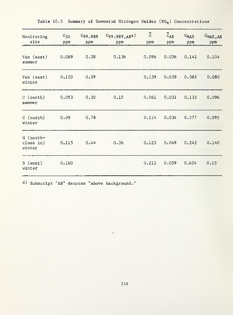
Table 10.5 Summary of Downwind Nitrogen Oxides (N0X ) Concentrations

Monitoringsite

c 50

ppm

c99 .989

ppm

c99 .989 ,ABa )

ppm

C

ppm

CABppm

CMAXppm

CMAX,ABppm

Van (east)summer

0.089 0.28 0.136 0.096 0.036 0.142 0.104

Van (east)

winter0.120 0.39 0.139 0.039 0.385 0.080

C (north)summer

0.053 0.30 0.15 0.061 0.031 0.133 0.096

C (north)winter

0.09 0.78 0.114 0.034 0.277 0.095

G (north-close in)

winter0.115 0.44 0.36 0.125 0.049 0.242 0.140

B (west)winter

0.160 0.212 0.059 0.624 0.15

a ) Subscript ”AB" denotes "above background."

216

Table 10.6 Federal Air Quality Standards

Primary SecondaryEnforcement by No time limit on

summer 1975 enforcement

ParticulatesAnnual geometric meanMaximum 24-hr concentration3 '

Sulfur oxidesAnnual arithmetic averageMaximum 24-hr concentration3 )

Maximum 3-hr concentration3 )

Carbon monoxide0 )



Photochemical oxidantsMaximum 3-hr concentration3 ''

HydrocarbonsMaximum 3-hr concentration3 )

(6-9 am)

Nitrogen oxidesAnnual arithmetic averageMaximum 24-hr average

ug/m 3 (ppm) ug/m~3 (ppm)

75 60

260 150

80 (0.03) 60 (0.02)365 (0.14) 260 (0.1)

b ) 1300 (0.5)

10 (9) 10 (9)

40 (35) 50 (35)

160 (0.08) 150 (0.08)

160 (0.24) 160 (0.24)

100 (0.05) 100 (0.05)b) b)

3 ) Not to be exceeded more than once a year,

b) No standard proposed.

°) Values for CO are in mg/m^.

217

Nitrogen

oxide

cone

(ppm)

Figure 10.13 Average nitrogen oxide concentrations -210 ft (65

from the TE plant

218

This is particularly significant in view of the greater accuracy of the east

(continuously-monitoring van) NOg data. Total nitrogen oxide concentration (NO

+ NO2 ) exceeded the allowable levels in all directions except the west duringthe summer period. Therefore, with eventual conversion of NO to NO 2 ,

the

potential existed for NO 2 concentrations to exceed the allowable annual arith-metic average concentration of 0.05 ppm to the north and south directionsduring the summer period plus the west direction during the winter period.

10.1.5.4 Contribution of TE Plant to N0X Concentration

During the summer period, the 0.04 ppm N0X concentration in the west direction(see table 10.3) serves as an estimate of the average background concentrationsince the frequency of easterly winds was almost zero (see figure 10.7).Assuming a 0.04 ppm average background concentration, the average N0X contribu-tion from the TE plant ranged from 0.035 to 0.055 ppm according to the data of

table 10.3.

An additional estimate of the TE plant contribution to N0X concentrations can

be made from the results for sampling periods when the wind generally blewtoward a stationary sampler. The average N0X concentration results from table10.4 are shown graphically in figure 10.14 for the north, east, and west direc-tions from the TE plant. The TE plant contribution to the average N0X concen-tration were similar for the summer and winter periods in the north and eastdirections. However, in the west direction, the TE plant N0X contribution was

greater for the winter period as the summer period contribution was essentiallyzero. The TE contribution to the average N0X concentration when the wind blewtoward a sampler ranged from 0.03 to 0.06 ppm, similar to the range estimatedusing the summer period data.

Figures 10.13 and 10.14 show that the average N0X concentrations during thewinter period were significantly higher than during the summer period. Themain reason for the higher winter N0X concentrations is that the backgroundconcentrations in the winter period were 0.04 to 0.05 ppm higher than in the

summer period at the north and east samplers and reached 0.15 ppm at the westsampler during the winter period (see figure 10.14).

Maximum one-hour nitrogen oxide concentrations observed (Cmax ) andstatistically projected "once per year" ( 099 , 939 ) in tables 10.3 through10.5 show that observed N0X concentrations range up to 0.63 and 0.70 ppm inthe summer and winter periods, respectively, while the corresponding valuesfor projected one-hour concentrations range up to 0.72 and 1.1 ppm. Tables10.3 and 10.4 show that in most cases, maximum NO 9 concentrations were lowcompared with the maximum NO or N0X concentrations with the exception of the

north samplers during the winter period.

Finally, it is important to address the question of whether the TE plant N0X is

the main cause of the maximum short-term concentrations of N0X . The maximumobserved N0X concentrations in table 10.5 range from 0.16 to 0.62 ppm, whilethe corresponding above-background concentrations were 0.07 to 0.15 ppm. Theprojected values for the "once per year" concentration above background intable 10.5 are less reliable (hence were not estimated at most samplers) than

219

TE

contribution

Figure

10.14

TE

plant

and

background

average

N0

X

concentrations

when

wind

blew

toward

a

stationary

sampler

the projected total concentration, 099 . 939 ,in tables 10.3 and 10.4 since data

in table 10.5 are based on a relatively small sample sice. Hence the question

of whether or not the TE plant or the background causes the maximum projected

N0X concentration cannot be directly answered. However, several pieces of

evidence lead to the conclusion that the background is the major cause of the

maximum N0 X concentrations. First, the maximum observed N0X concentration of

0.4 to 0.6 ppm were caused by winter background concentrations of 0.3 to 0.45

ppm (see table 10 . 5 ); secondly the 099.939 value for the west sampler in the

summer, a backgrond station, was essentially the same as for the north and

south samplers; finally the higher C99.939 in the winter than in the summer is

consistent with the significantly higher average background concentration in

the winter than in the summer (see figure 10.14;

.

10.1.5.5 Ground-Level Concentration Distribution

Ground-level concentration studies were conducted to describe the variation in

above-background N0X concentrations from the TE plant in the general path of

downwash plumes from the plant. The main technique used was a horizontal pro-file consisting of a 30 to 60 minute run - an array of 12 to 16 portable air

bag samples positioned from 50 to 300 ft (15 to 100 m) from the plant stacks.The horizontal profile data was supplemented by above-background N0 X data fromthe stationary samplers; NO x data from these samplers were correlated with windspeed data and engine rates estimated from the engine load. In addition to

determining the concentration of N0 X above background for a given wind condi-tion, the stacx- to-ground dilution was characterized in terms of values,where x = ground-level mass concentration, micrograms/m^

, Q = aass emissionrate, gm/ s ,

and m = mean wind speed, m/ s . The reason the parameter -r1

^ is

* used to characterize plume dilution rather than the specific concentration,is that the first order "ventilating" dilution effect of wind speed is removedleaving mechanical and atmospheric turbulence as the dominant mechanisms of

plume dilution. The data were calculated from NQ Xemission and ground-

level concentration data using the estimated N0 X emission rate for the engineload and for some profiles using the SF 5 tracer gas technique.

The horizontal profile results typically showed widely-scattered data and patternsof multiple concentration peaks as opposed to any clearly discernable or uniformconcentration pattern. Such non-uniform ground-level concentrations apparentlyresult from the random eddy motion in the downwashed plumes that exposes specificlocations to different peak concentrations over a sampling period as short as

60 minutes. Because of the scattered nature of the basic horizontal profiledata, little confidence can be placed in results based on calculated andtherefore strong conclusions about the site dispersion characteristics 'could

not be developed in reference[ 10- 1 ].

10.1.6 Summary and Conclusion

The results of the air quality assessment of the Jersey City Total EnergySite can be presented at two levels. The first level of results deals with thegeneral characteristics of pollutant dispersion from this distillate oil-fueled,diesel-combustion process emitting 3-5 kg/h of gaseous pollutants, predominantlynitrogen oxides, from exhaust stacks lower tuan the height of surrounding

221

buildings. The general characteristics of interest are (1) the degree of plumedownwash, (2) the TE plant pollutants that contribute significantly to groundlevel concentrations, and (3) the general level of background pollutants andTE plant contributions at 200 - 260 ft (60-80 m) from the TE plant. The secondlevel of results deals with the micro-scale behavior of the exhaust plume inthe complicated building topography surrounding the TE plant. All the resultsare based on two six-week monitoring periods in 1977, one summer and one winter.As such the results are limited by the range of wind conditions, controllingthe dispersion of exhaust emissions, that occurred during the two monitoringperiods

.

The general results are summarized as follows:

1. Plume downwash begins with average wind speeds of 3.5 mph (1.6 m/s), andan increasing fraction of the plume is drawn into the wake of the CEB withincreasing wind speed. Local wind speeds above the 3.5 mph (1.6 m/s)

threshold occurred about 50 percent of the time.

2. Of all the combustion pollutants, only nitrogen oxides, N0X , were detectableat ground level. The diesel engines were the major contributor, greaterthan 90 percent of the N0X emissions during a winter month.

3. Concentration of N0X from the TE plant at ground level averaged from 0.03to 0.05 ppm at distances of about 230 ft (70 m) from the CEB. These con-centrations represent from 60 to 100 percent of the allowable annualaverage concentration, 0.05 ppm, for NO 2 in accordance with the Federal AirQuality Standards (FAQS). In addition, background levels of N0X rangedfrom about 0.04 ppm during the summer to about 0.08 ppm during the winter.The combination of the TE plant emission and the local background createsthe potential for the average NO 2 concentration to exceed the allowable NO 2

concentration of 0.05 ppm in the air within about 210 ft’ (65 m) of the CEB.

Maximum one-hour N0X concentrations projected for once per year reach about

1 ppm.

4. The background levels of SO 2 exceeded the allowable annual average FAQSvalues by 100 percent during the summer period. The maximum CO level was

well below the applicable one-hour allowable FAQS value. The averagehydrocarbon concentration was at the allowable maximum three-hour concen-tration (6-9 a.m.) if methane is less than 88 percent of the total hydro-carbon concentration.

The combination of exhaust plume observations and horizontal profile measurementsof ground-level pollutant distribution indicate the following relative dispersionbehavior in the area of 33 to 295 ft (10 to 90 m) from the CEB:

1. For moderate wind speeds 6 mph (2.7 m/s) dilution is lowest to the south of

the CEB - in the area bounded by Shelley B, Descon-Corcondia,and the

school - and highest to the north of the CEB.

2. Except for the area to the south of the CEB, specific concentrationsdecrease significantly with distance at intermediate wind speeds of 3.5 to

8 mph (1.6 to 3.6 m/s) in the area of 195 to 295 ft (60 to 90 m) from the CEB.

222

3. The TE plant exhaust plumes do contribute detectable N0X concentrations

up to 33 ft (10 m) from the CEB even at low wind speeds of 3.5 raph

(1.6 m/s). The behavior is caused by part of the plume being caught in

random eddies generated by the wind flow around the CEB and other up-wind

buildings. This random wind behavior persists for winds up to 12 mph(5.4 m/s) as opposed to complete trapping of the exhaust plume into the

cavity of the CEB.

As a result of the air quality monitoring and assessment at the Jersey CityTotal Energy Site, several general conclusions are drawn that pertain to the

siting of diesel engine TE plants in urban areas:

1. The general level of N0X and total oxidants in the background is importantin assessing the potential air quality impact of a TE plant.

2. For a TE plant with exhaust discharged at a height comparable to surroundingbuildings, the average N0X concentration increase within 295 ft (90 m) of

the TE plant can be a significant fraction of the allowable annual arithme-tic average concentration for NO 2 of 0.05 ppm. Since the allowable concen-tration for NO 2 is based on limiting the formation of photo-chemical smog,

the observed N0X levels are of concern only during periods of high back-ground levels of non-methane hydrocarbons and ozone to catalize the smogformation reaction.

10.2 NOISE LEVEL ASSESSMENT


The purpose of the noise assessment was to determine the general impact of

normal TE plant activities on the Summit Plaza site and adjacent areas.- Fivediesel-engine generators, a stack dilution fan, the solid waste disposal system(truck transfer), and the cooling towers were the main sources of noise fromthe CEB. All these activities are continuous in nature except the transfer of

solid waste from the site which was done by diesel truck approximately twice a

week. No noise survey data were obtained during this operation.

10.2.2 Data Collection

10.2.2.1 Pre-Construction Period

Noise data were collected in September 1970, prior to any construction activityon the Summit Plaza site. This pre-construction noise survey consisted of

around-the clock, sequential measurements at seven locations on the vacantsite. Data were collected in the form of three-minute tape recordings and sub-sequently subjected to statistical analysis by digital computer. A completedescription of the methods and results of these tests are contained in reference

[ 10-6 ]

.

The pre-construction noise survey provides valid data on background trafficnoise levels near the streets bordering the Summit Plaza site. Assuming nosignificant change in traffic density or patterns, these 1970 data are appli-cable during the operating period. The pre-construction survey also provided

223

data interior to the site, but since the site itself substantially changed withthe new buildings, the applicability of these data as measures of backgroundnoise levels in the absence of the TE plant is somewhat limited.

10.2.2.2 Operational Period

Noise data were also collected during July and August of 1977 in five one-hoursampling periods between 8:00 a.m. and 9:00 p.m. During these tests, threeengines were operating at electrical loads between 1075 and 1275 kW. Windvaried in direction and speed; however, average wind speeds during all surveyswere no greater than 8 raph (3.5 m/s). The stack dilution fan and the coolingtower fans were operating during all surveys [10-1].

The south wall of the CEB has five pairs of doors, one opposite each engine,that provide access during minor and major overhaul. These doors are openedoccasionally during routine maintenance in hot weather to improve the comfortof maintenance personnel. It was anticipated that this would cause a signifi-cant increase in sound levels in the area south of the CEB and therefore, a

survey was performed with two doors open. The frequency with which one or moredoors are opened in actual practice is less than once per week, i.e., less fre-quently than the solid waste pickup. Thus this condition is somewhat anomalousand is trated as such in the noice impact evaluation.

Sound level measurements were made with a hand-held, "A" weighted frequencyresponse Gen. Rad. 1981-B Precision Sound-Level Meter yielding sound levels in

dB(A). Measurements were made four feet (1.22 m) above the ground in the areasgenerally to the north and south of the CEB. Recorded sound level valuesexcluded transient contributions from individual trucks, planes, or humans.

10.2.3 Results

Each of five surveys during the operating period showed essentially similarresults. Figure 10.15, taken from reference [10-1] shows typical estimatedsound level isopleths in the area within 200 ft (61 m) of the CEB.

As one might expect, the engine-generators are the major source of noise fromthe TE plant operation. The maximum sound levels on the south face of the CEB

directly opposite the operating engines were 74-75 dB(A) with the engine doors

closed and up to 85 dB(A) with a pair of doors open opposite one of the three

operating engines. The open doors also raised the sound level from 8-10 db(A)

in the area between the north end of the Descon-Concordia building and the westend of the Shelley B building [10-1].

Figure 10.5 shows that the site is dominated by two noise sources, the CEB

(engine-generators) at 74-75 dB(A) and the Newark Avenue street traffic at 70

dB(A). Prior to site construction, traffic generated noise was measured at an

average value of 61 dB(A) for the daytime and an average 57 dB(A) for the night.

At the time, peak traffic noise values of at least 65 dB(A) during the daytimeand 60(A) at night were experienced 10 percent of the time [10-6]. Thus the TE

plant could potentially have a greater impact on site noise levels than the

traffic on Newark Avenue.

224

225

igure

10.15

Noise

levels

in

dli(A)

around

the

Central

Equipment

Building

during

8-9

a.

in.,

August

4,

1977

A given increment in noise above background levels would be most acutely sensedin the courtyard area of Summit Plaza where people recreate and where the win-dows and balconies of the Shelley B and Descon apartment buildings face. Anexamination of the noise levels in the courtyard (bounded by Shelley B, Descon,the school, and the pool) as shown in figure 10.15 indicates a maximum noise con-tribution from the CEB of about 4 dB(A) since the noise levels continuouslydecrease from 62 to 58 dB(A) with increasing distance from the CEB.

Other detectable noise sources from the CEB are the absorption chillers in the

east end of the CEB and the exhaust stack dilution fan mounted below the engineexhaust stack. The chillers cause an approximate 66 dB(A) peak on the southwall, west end, of the CEB while the dilution fan causes approximately a 66

dB(A) peak sound level in the parking lot north of the CEB (see figure 10.15).However, the dilution fan contribution blends into the background at the nearproximity of the Mayfair and St. John's Apartments, resulting in rather minimalimpact on outdoor recreational areas and no impacts on the interior buildingenvironment

.

Careful examination of figure 10.15 and similar data in reference [10-1]

indicates that the positioning of the TE plant on the site in relation to the

other buildings has minimized overall noise impacts. The close proximity of

the Shelley B and Descon buildings permit a relatively narrow path for trans-mission of CEB noise into the Summit Plaza courtyard. In addition, the endwalls of these two apartment buildings facing the CEB are windowless exceptfor corridor windows in Shelley B. Thus the noise levels of 64 to 66 dB(A) atthese walls should have minimal impact on interior noise levels. Also the sit-ing of the TE plant adjacent to the open parking lot allows peak noise levelson the north side of the plant to be dissipated before reaching the MayfairApartments as previously stated.

10.2.4 Comparison with Local Standards

In 1978, a noise control code was established for certain municipalities inHudson County, which includes Jersey City. The sound level limit in the codeis 65 dB(A) for residential, public space, or open space between 7:00 a.m. and10:00 p.m. Between 1:00 p.m. and 7:00 a.m., the limit is 50 dB(A). For com-mercial or business land-use categories, the sound level limit is 65 d3(A) at

all times [10-7 ]

.

The results of the surveys with all doors on the CEB south wall closed show thedaytime 65 dB(A) limit is exceeded from the TE plant only in the limited areawithin about 75 ft (23 m) south of the CEB. It should also be noted that the65 dB(A) daytime limit was also exceeded on the south side of the Summit Plazasite from traffic activity on Newark Avenue (see figure 10.15).

With regard to the nighttime residential limit of 50 dB(A), no data during the

operational period was taken past 9:00 p.m. However, the operational datataken in the early evening (8:00 p.m.) and the nighttime pre-construction data

indicate that the background noise from traffic far exceeds this level and thatthe sound level in the courtyard at Summit Plaza also exceeded this level by up

226

to 5 dB(A). At the time the data was taken, the incremental impact of the TE

plant appeared to be a maximum of about 4 dB(A) in the courtyard [10-1].

10.2.5 Summary and Conclusions

This brief study of noise levels at the Summit Plaza mainly addressed the

contribution of continuous operations of the Central Equipment Building (CEB)

and the urban surroundings. The major findings of this study are summarizedas follows:

1. Of the continuous operations, the engine-generators cause the highestnoise levels, predominantly to the south of the CEB. The second highestnoise level source is the engine exhaust fan motor causing increasingnoise levels predominantly to the north of the CEB. Traffic-generatednoise is intermediate between the two major CEB sources.

2. During normal operation, with all doors closed on the south wall of the

CEB, the maximum noise level is 74-75 dB(A) at the south wall of the CEB

regardless of which engines operate or the total engine load. The maximumnoise level increased to 85 dB(A) with two doors open on the south wallopposite the engines.

3. The area exposed to noise levels greater than 65 dB(A), the daytime limitof the local noise ordinance, is limited to about 75 ft (23 m) south of

the CEB

.

4. The nighttime background noise level in the interior of Summit Plaza fromsurrounding urban activities is approximately 55 dB(A).

The major conclusions of this study are as follows:

1. The noise contribution from the CE3 does not exceed the 65 dB(A) daytimelimit of the local noise ordinance at the exterior walls of any adjacentresidential buildings under normal operating conditions (with the doors of

the CEB closed).

2. The nighttime noise level limit of 50 dB(A) for residential space is

probably exceeded at Summit Plaza from the surrounding urban activitiesalone

.

3. The TE plant appears to increase noise levels in the courtyard of theSummit Plaza site by a maximum of 4 dB(A) and in the parking lot of the

adjacent Mayfield Apartments by a maximum of 6-8 dB(A).

4. If the TE plant had been constructed on Newark Avenue (i.e., on the partof the site with the highest background noise concentration), its impactmay have been lessened.

5. Overall site design including the juxtaposition of the CE3, Shelley B, andDescon buildings and the location of the CEB adjacent to a parking lotcombined to minimize its noise impact on Summit Plaza recreational areasand building interior noise levels

.

227

10.3 COOLING TOWER ASSESSMENT


Two wet cooling towers are used in the TE plant for heat rejection from theabsorption chillers during the summer cooling season. The types of potentialenvironmental effects from the cooling towers are chemical toxicity and aesthe-tic in nature — plume visibility and nuisance effects of drift deposition.Since the cooling tower water is treated with a chemically benign additive andthe plume is rarely visible during the warm summer season, the main considera-tion became the aesthetic nuisance effects of drift transport deposition.Therefore, the drift emission characteristics of the cooling towers was mea-sured as a prerequisite for the possible calculation of drift transport anddeposition. Also, field measurements of drift deposition and concentrationwere made in the area within 200 ft (60 m) of the CEB.

Subsequent to cooling tower emission measurements, the combustion emissionstudy results showed that the complicated wind flow in the area of the CEBwould require a significantly greater effort than was planned for modelingdrift transport by the cooling tower plume during building downwash conditions.Since the nuisance effects from the drift deposition were fairly obvious duringthe on-site monitoring period, a drift transport modeling effort for this uni-que cooling tower installation was not justified. The remainder of this sec-tion presents a summary of the results of drift emission measurements obtainedbetween August 2-12, 1979. The nusiance effects of the observed drift condi-tions are also discussed. The material in this section is derived exclusivelyfrom reference [10-1].

10.3.2 Cooling Tower Operation

10.3.2.1 Description

The towers under investigation are two Baltimore Aircoil Co., Inc., Model No.

VST-1050S counter flow, forced draft cooling towers with three cells each and a

design circulation water flowrate for the total system of 4440 gpm (0.28 m-Vs).The towers employ three-break galvanized steel drift eliminator blades withhooked trailing edges. In addition, sound attenuation panels are located abovein the plane of the drift eliminators.

The towers are located next to one another atop the CEB and are separated by

approximately 3.5 ft (1.1 m) . The updraft air exit plane of the towers is

located approximately 23 ft (7 m) above the central roof section of the CEB. Atop view schematic of the two towers is shown in figure 10.16 with the indivi-dual cell designations included. The lines in each cell represent the struc-tural members supporting the sound attenuation panels.

10.3.2.2

Operating Conditions

Each cell has a constant speed fan mounted underneath the tower creating a

vertical flow of air to remove heat from the tower water. During the period of

the drift measurements, the fans for all cells except cell no. 6 were on

continuously.

228

WEST TOWER EAST TOWER

6

CELL NO 5

CELL NO. 4

Figure 10.16 Cell designation for TE plant cooling tower

Prior to the measurement period, excessive drift of large droplets had been

noted particularly from the west cells, nos. 1, 2, and 3. The plant operatingstaff determined that debris had accumulated in the distribution headers and in

the nozzles that normally direct the water flow downward against the air flow.

In some cases, the nozzles had plugged and been forced out of the distributionheaders. The water flow then discharged horizontally, resulting in much largerdroplet size distribution and much greater drift loss from each cell. Duringthe period of the drift measurements, the plant operating staff removed the

debris from the distribution headers and replaced most of the plugged or

restricted nozzles with new nozzles. This action returned the water distribu-tion in the headers to normal; however, the drift loss was still abnormallyhigh in certain locations where replacement nozzles were not available.

As a result of the cleaning maintenance performed on the cooling towers, driftmeasurements were made before and after the maintenance allowing a comparisonof drift characteristics to be made.

10.3.2.3 Chemical Treatment

Metallic cooling towers require addition of a chemical to prevent corrosion andmineral scale deposition on the metal surfaces of the tower. The treatmentchemical used at the TE plant is a proprietary Calgon Corporation product,designated "CLD-709," which contains the organic phosphonate, amino methyalenephospanate (AMD). The chemical is biodegradable and low in toxicity, contain-ing no chromates and used in the ph range of 7.0 to 8.2.

229

10.3.2.4 Heat Rejection Load

The heat rejection load of the cooling tower is coupled to the operation of theabsorption chillers that provided chilling water for space cooling from May to

September. The space cooling load and heat rejected to the cooling tower variesdiurnally with the mean ambient temperature. The heat rejection rate of the

cooling towers was normally monitored by the NBS Data Acquisition System (DAS).

Because of an outage of the DAS during the drift measurement period, directmeasurement of the tower heat rejection rate was not available. However, an

estimate was made based on other periods of similar maximum and average ambienttemperatures of 85-90°F and 79-82°F, respectively. The heat rejection rate wasestimated to be from 14 to 18 x 10^Btu/h (4.1 to 5.3 MW) during the latemorning to afternoon when drift measurements were made.

10.3.3 Measurements

10.3.3.1 Cooling Tower Drift Source

The objective of the cooling tower drift source measurements was to characterizethe cooling tower drift effluent at or near the fan stack exit plane withacquisition of the following parameters:

1. the rate of liquid drift mass emission2. drift liquid mass emission rate as a function of droplet diameter3. drift mineral mass emission rate4. updraft air speed, and5. updraft air temperature.

In addition, samples of circulating water were required for determination of

its mineral concentration.

In order to meet this objective, the following instruments were employed:

1. ESC* PILLS II (Particulate Înstrumentation by _Laser _Light Scattering)electro-optical monitor for determination of the rate of liquid drift massemission and its distribution over the droplet diameters.

2. ESC Sensitive Paper (SP) System for determination of the rate of liquiddrift mass emission and its distribution over the droplet diameters (a

technique complementary to the PILLS System).

3. ESC Heated Glass Bead I_sok.inetic (IK) Sampling System for determinationof the drift mineral mass emission rate.

4. Propeller anemometer for measurement of updraft air velocity.

5. An electronic psychrometer for determination of the wet and dry-bulbtemperatures of the updraft air.

ESC = Environmental Systems Corporation.

230

10.3.3.2 Ground-Level Measurements

The objective of these measurements was to characterize the cooling tower drift

deposition characteristics at ground level from plume transported drift rather

than the largest drift droplets that were transported by exit momentum from the

tower. The rationale for this measurement strategy was that the high drift

fallout close to the CEB was a temporary situation that would be remedied by

cooling tower maintenance work. This strategy was verified by observing a

significant reduction in drift fallout close to the CEB after the maintenancework was concluded.

In order to characterize the drift transported away from the cooling towers,

five mobile ground-level data acquisition stations were employed. These sta-tions were located from 65 to 100 ft (20 to 30 m) from the cooling towers.

Each station was capable of acquiring the following parameters:

1. airborne droplet mass concentration as a function of droplet size,

2. airborne drift mineral mass concentration,3. droplet mass deposition flux as a function of droplet size, and,

4. drift mineral mass deposition flux.

The measurements of mineral mass were directed at suitable elements present in

the cooling tower circulating water (Na in the form of salts, and Z n in the

form of oxides of zinc) just as with the mineral mass emission at the towerexit plane.

Concentration measurements were acquired by using ESC Airborne Particle Sampler(APS) units. The APS unit consists of motor-driven arms which sweep samplingelements through the air, collecting droplets and minerals through inertialimpaction. A meter counts arm revolutions to determine air volume sampled and

a fan assures fresh air input even under calm conditions.

Deposition flux measurements of water and minerals were made by two separatetechniques. Droplet mass deposition flux and droplet size was determined by a

sensitive paper (SP) technique. Mineral deposition was measured by sample col-lection on a clear surface with a subsequent distilled water wash and finalanalysis by flame emission spectophotometr y

.

10.3.4 Results

This section presents the major results of the measurements performed to

characterize the cooling tower drift source and the drift deposition characte-ristics. The major conclusions with regard to the nuisance effects from thecooling tower operation are also presented.

10.3.4.1 Cooling Tower Drift Source Results

Average updraft air velocity measurements on the tower were quite consistentfrom cell to cell varying only + 0.3 ft/s (+ 0.1 m/s), about an average value of14.4 ft/s (4.4 m/s). The total volumetric air flow rate of the tower wascalculated to be 6957 ft Vs (197 mV s )

,

a value within 4 percent of thedesign air flow rate of 6712 ftVs (190.1 mVs).

231

In general, most wet and dry-bulb updraft air temperature readings were the

same (within the uncertainty of the instruments) indicating saturated air. Widevariation was exhibited in the air temperature from point to point within cellswith maximum differences between points in a cell varying from 39°F to 48°F(3.7°C to 9.2°C). The average temperature difference between cells, was in

general, less than the variation in temperature observed within a cell.

Liquid drift measurements performed on five cells showed individual cellemission values ranging from 2.30 gm/ s (#3 "before") to 0.0466 gm/ s (#5 "after")corresponding to drift fractions of .00493 percent and .0000956 percent,respectively, of the design circulating water flow rate. Mass median diametersof the droplet emissions varied from 484 pm to 758 pm and were two or threetimes the values commonly measured on induced drift cooling towers. The con-current maintenance of the cooling tower water distribution headers affordedthe opportunity for "before" and "after" measurements on cell #3 with the

"after" measurements showing an improvement (decrease) in drift emission ofover one twentieth of the "before" value. Total tower emissions characteristicof conditions after maintenance were calculated to be 1.63 gm/s; however, it is

believed that substantial improvement could be made in this figure with a com-bination of the maintenance work which was ongoing during the measurements andsome work on sealing gaps between the drift eliminator panels.

Analysis of the cooling tower basin water for sodium and zinc showed the sodiumconcentration during the test period varying between 408 and 545 ppm while the

zinc concentration steadily decreased from 5.45 to 1.28 ppm. Measurements of

mineral mass emission of the individual cells show sodium emissions varying from1776 pg/sec (cell #3, 8/5-6/77) to 205 pg/sec (cell #4, 8/8/77). Total mineralemission for the tower was calculated to be 1804 pg/s for Na and 190 pg/s for

Zn. Again, the sodium was in the form of salts and the zinc in the form of

oxides of zinc.

10.3.4.2 Drift Deposition Results

Measurements of the airborne mineral concentrations (Na and Zn) varied across allstation locations only within + 15 percent of the average daily concentrationfor each day's run. On August 5, a much larger average sodium concentration(1.33 pg/^) was observed than on other days (0.115 to 0.224 pg/m^)

,which may

be due to the fluctuating ambient sodium concentration. The range of measuredvalues over all runs ranged from 0.095 to 1.53 pg/m^ for sodium and from 0.012to 0.22 pg/m^ for zinc.

Unlike the mineral mass concentration measurements, droplet mass concentrationsvaried as much as 2 to 3 orders of magnitude between all stations of a singleday's run. Measured concentrations over all runs ranged from 0.023 to 132.6pg/m-, and mass median droplet diameters ranged from 41 to 840 pm.

Of the mineral mass deposition measurements, 32 percent of the sodium and 20

percent of the zinc samples were less than the average background. Averagedover all samples, the collected amounts were about twice the respective average

backgrounds. Sodium deposits fluxes ranged from 8.78 to 250 kg/km^.mo over all

runs, and zinc deposition fluxes ranged from 0.104 to 17.1 kg/km^.mo.

232

Droplet mass deposition flux measurements vary up to 3 orders of magnitudeacross all stations for a day's run. Measured values over all runs ranged from

114 to 426,000 kg/km^ •mo, and mass median droplet diameters range from 117 to

613 pm.

Two quantitative measurements of drift transport from individual time periodswere compared at upwind and downwind sampler stations. These comparisons indi-cated that in general no significant amount of cooling tower drift material was

detectable above the background concentrations or deposition fluxes.

In contrast to the inconsequential quantitative results from the AirborneParticle Samplers and deposition collectors, the qualitative observation of

drift fallout within about 50 ft (15 m) was equivalent to a light drizzlingrain before the maintenance work was performed on the cooling tower. The

dramatic, although not complete, reduction in drift loss, after the cleaning of

the distribution headers and nozzles, resulted in a reduction in drift falloutto the point that the fallout was barely detectable to a person downwind of the

towers. Additionally, the reduction in drift deposition also eliminated the

noticable accumulation of a residue on cars parked within about 50 ft north of

the CEB when southerly winds prevailed. This deposition on cars belonging to

residents of the adjacent St. John's apartment complex was the most significantnuisance effect of the degraded CEB cooling tower performance.

10.3.5 Conclusions

The major conclusions of this study of the cooling tower operation at theJersey City Total Energy Plant are as follows:

1. The cooling towers require occasional maintenance to preserve good flowdistribution and drift loss characteristics.

2. The drift loss obtained with these cooling towers can be a very acceptablelevel of 1 x lCT 4 percent when properly cleaned and drift eliminators arepositioned correctly.

3. Drift deposition from transport by the cooing tower plume wasindistinguishable from ambient concentrations of moisture and minerals (Naand Zn) .

4. The major nuisance effect from the abnormally high drift loss, prior to themaintenance work on the cooling towers, was from a spotty deposition onparked cars to the north of the CEB. This situation, which is preventableby proper maintenance, could result in significant ill-feelings towards theowner/operator of the TE plant. Therefore, adequate justification existsfor periodic inspection and maintenance procedures to be developed and fol-lowed to keep the cooling tower drift loss characteristics within acceptablelimits

.

233


10-1. Davis, W. K. and Kolb, J. 0., "Environmental Assessment of Air Quality,Noise, and Cooling Tower Drift from the Jersey City Total Energy Demon-stration," HUD Utilities Demonstration Series, Vol. 11, National Bureauof Standards Report GCR 80-252, Oak Ridge National Laboratory, July 1980.

10-2. "National Primary and Secondary Ambient Air Quality Standards," 40 CFR

50, July 1, 1977.

10-3. "Standards of Performance for New Stationary Sources," 40 CFR 60, AppendixA, July 1, 1977.

10-4. Kitson, C. E. and Egdall, R. S., "Exhaust Emission Evaluation of ThreeCaterpillar Tractor D-398 Diesel-Electric Sets," National Bureau of Stan-dards Report GCR-77-104, York Research Corporation, Stamford, Connecticut,November 1977.

10-5. U. S. Environmental Protection Agency, "Complication of Air PollutantEmission Factors," EPA Publication AP-42, 3rd Edition, August 1977.

10-6. Qunidry, T. L., Fisher, R. L. and Blomquist, D. S., "Noise Survey of the

Jersey City Operation BREAKTHROUGH Prototype Site,” National Bureau of

Standards Report 10219, Revised, October 1972.

10-7. "Noise Ordinance of the Hudson Regional Health Commission," February 1,

1978.

234

11. RELIABILITY EVALUATION

11.1 SCOPE AND DEFINITION

Two aspects of reliability are considered in this evaluation: "availability"and "quality of service." Availability refers to the continuity of function of

service. It can be examined from the standpoint of plant components and/orfrom a customer service standpoint. The availability of each type of equipment

(e.g., boilers, engine-generators) and of each utility service (hot and chilledwater and electricity) must be evaluated separately. Major emphasis is placedon electrical reliability in this section since the electrical subsystem is

the key subsystem in the TE plant to distinguish it from more conventionalsystems for supplying the same services to the site.

The major emphasis for the availability analysis was from the customers'standpoint. This "service availability' analysis was carried out by measuringinterruptions of utility service to the customer. The performance of indivi-dual components within the plant (analyzed by measuring equipment outages) wasexamined only in a cursory manner.

Quality of service refers to the degree of excellence or acceptability of the

service when examined from the customer's standpoint. This investigation is

only relevant for periods during which the utility service is fully available.The evaluation of quality of service for Summit Plaza must include hot water,chilled water, and electricity. Again, major emphasis is placed on the qualityof electrical service.

Figure 11.1 shows the relative priorities described above for the reliabilityevaluation

.

11.2 ELECTRICAL SERVICE AVAILABILITY

Electrical service availability was evaluated by determining the number, extantand causes of interruptions of customer service. Several types of electricalservice interruptions are currently defined (see appendix M) and are applicableto Summit Plaza. However, before the means used to measure service interrup-tions are discussed, additional information is given on the design of the TEelectrical system and the available sources of interruption data.

11.2.1 Electrical System Design Features

Electrical Distribution - The electrical distribution system at Summit Plaza is

a configuration specially designed for the use with on-site power generation.Two sets of 480-volt, three-phase feeders are used to every building. One setof feeders supplies "essential" loads within the building such as emergencylighting, fire protection, and one elevator. The other, "normal", feeder supp-lies all other loads. During normal plant operation, power to both sets offeeders is supplied by the TE plant. When a total plant outage occurs, powerto the essential feeder only is supplied by the local utility company.

235

J3uo•H33

II

33

e3•H-oa;

sII

s

5o4II

hJ

CO

a)

o•HS-i

Q.

0)

>

cfl

ai

ad

236

Figure

11.1

Relative

priority

of

areas

for

reliability

evaluation

Control System - The automatic control system for the engine-generatorscontains a load shedding capability which can interrupt service to varioussegments of the load. Need for this can occur during an overload condition or

through equipment malfunction whenever a standby engine-generator is not

brought on line rapidly enough to provide adequate capacity [11-2].

The site is divided into ten (10) load segments which can be sequentiallyinterrupted after an initial voltage reduction of 10 percent. Load segmentsinclude auxiliary loads within the TE plant as well as the individual build-

ings. The essential load circuit is the last segment to be shed from plant

generation. When the essential load is disconnected from the plant supply, it

is automatically connected to the utility standby service, thereby receivingvirtually uninterrupted service.

11.2.2 Sources of Availability Data

DAS - The DAS began collecting data in April 1975 for the TE plant only.

Collection of data for individual buildings began in November 1975. For

monitoring of electrical service availability, the DAS provided basic data suchas kWh and voltage at various points within the TE plant and at each of the

individual buildings. Deviations in gross energy production at the TE plant

indicated probable interruption events. The data for individual buildingsquantified partial interruptions more fully in terms of specific buildings and

magnitude of load loss. Since the DAS recorded data every 5 minutes, the

duration of interruptions could be determined within +2.5 minutes.

kW Record - Prior to the start-up of the DAS (and during periods in which the

DAS was inoperative) other sources of data had to be utilized. First, a

continous-str ip chart recording of gross kW production covered the entireperiod from 1974 to the present. This strip chart was maintained by plantpersonnel and provided a primary source of data. The strip chart recordingsalso helped to identify when interruptions had occurred so that the DAS datacould be more efficiently accessed. The strip chart could not, however, showthe duration of total interruptions since it was not powered from the essentialservice line.

Narrative Logs - Principal sources of data for identifying the causes of the

equipment outages which resulted in service interruptions were found in variousnarrative log books kept by the plant operator and NBS. Often these also pro-vided some indication of the duration of interruptions in the absence of DASdata

.

Utility Bills - As a final cross-reference, the monthly bills from the electricutility were used. In addition to charges for standby service, these billsalso registered the quantity and cost of any energy used. This source therebygave an approximate indication of total interruptions for each month.

11.2-3 Service Availability Methodology

Availability Measures - A number of measures have been developed for evaluatingthe availability of electric utility systems from the standpoint of customerservice [11-3, 11-4], Four basic measures were selected for this evaluation:

237

° number of interruptions in a given time period (e.g., year)0 total duration of interruptions in a given time period, minutes° average duration of interruptions

,minutes

0 maximum duration of any one interruption, minutes.

These measures quantify the three important aspects of interruptions: frequency,duration, and magnitude. A basic building-block in developing these measureswas a "customer interruption."

Accounting Approach - For the Summit Plaza TE plant, two means of accountingfor service interruptions were possible depending on how a "customer" wasdefined, and how partial interruptions (see appendix M) were handled. First,each of the individual buildings could have been considered a single customer.For partial interruptions, an accounting would have been made of those build-ings without service. Data would then have been presented using the esta-blished measures as if the TE plant were a utility supplying six customers(the four apartment buildings, plus the commercial and school facilities).Three problems were inherent in this approach:

0 accounting for partial interruptions which involved only TE plantequipment

° an assumed customer equivalence in terms of load magnitude0 difficulty in identifying the buildings curtailed during partial

interruptions prior to November 1975.

These problems were overcome by using a second approach which considered the

site as a single customer. Partial interruptions were treated as an "equivalent"total interruption, using plant kW output as the basic measure of service. Thisaccounted for differences in the load demand of the various buildings, includ-ing in-plant loads. In generic terms, this was equivalent to the aforementionedapproach in the special case where all customers had the same kW demand. Thisapproach is further explained below

Partial Interruptions - Partial interruptions were classified based oncoincidence with total interruptions (see appendix M) . This was necessarybecause a partial interruption which was an extension of a total interruptionwas not counted as an additional interruption event.

In accounting for partial interruptions, the duration and number of individualpartial interruptions were adjusted to an equivalent total interruption basisas shown in figure 11.2. The equivalent duration of a partial interruption(both coincident and isolated) was defined as the duration of a total interrup-tion which would have resulted in the same energy curtailment. This calculationentailed determining the energy curtailment of a partial interruption in kW-minand dividing this value by the "normal" cr uninterrupted power demand (in kW)

of the total site during the interruption.

The equivalent number of isolated partial interruptions was calculated by the

actual power demand curtailed as a fraction of the normal power demand. For

example, a partial interruption which resulted in an actual load curtailment(in kW) of 50 percent of the normal power demand would be counted as 0.50interruption.

238

T3I.H

.. I

pi

vj!

;>

o

!l I!

>

T-0

(ppi) undone aaîod

239

AecouuLiug

procedure

Lol'

parLial

LaLei:

r

apt

ions

11.2.4 Availability Data Summary

All interruptions occurring during the period from plant start-up in January1974 through December 1977, were examined. The duration, cause, and type ofinterruption were noted and the appropriate measures described above calculated.For the period prior to September 1974, some data could not be accurately deter-mined and therefore, some uncertainty exists in the aggregated measures of

reliability.

Three interruptions stemming from outages occasioned by NBS actions were deletedfrom the analysis. These interruptions were assumed to be atypical for commer-cial TE plants not subject to third party data collection efforts. Momentaryinterruptions (for a definition, see appendix M) were also not included in the

analysis, since these are not normally included in utility system outage data.

Table 11.1 presents yearly aggregated data for electric service availability at

the Summit Plaza site. For the year 1976, table 11.1 also includes data con-sidering forced interruptions only since scheduled interruptions (not likely to

be repeated in the future) significantly affected overall availability levelsin that year.

Table 11.1 Summit Plaza Total Energy PlantElectrical Service Availability

YearNo . of

InterruptionsInterruption Duration

,Minutes

Total Average Maximum

1974 12.8 2474 193 1869

1975 0.6 5 - -

1976 11.6 992 86 2491976a > 9.6 591 62 135

1977 2.4 116 48 55

a ) Forced interruptions only, scheduled interruptions not included.

This table clearly shows that the availability record of the TE plant has variedconsiderably. Two of the four years (1974 and 1976) had poor availability whiletwo years (1975 and 1977) were considerably better. The year 1975, with its

nearly perfect availability record, is particularly noteworthy.

11.2.5 Temporal Trends

It is expected that a TE system will exhibit changing levels of availabilitywith time. Figure 11.3 illustrates a typical life-cycle availability trendwhich a TE plant might be expected to follow. The trend includes an earlydebugging phase with higher failure rates and a normal operating phase with a

240

lower failure rate which is nearly constant over a significant portion of the

operating life. An effort was made to relate the early interruption pattern of

the TE plant to the first two phases of the life-cycle trend.

The causes for the significant unreliability experienced in both 1974 and 1976

are typical of a plant debugging phase. This was indicated by both the causesof the outages resulting in the interruptions and the nature of plant changesundertaken to prevent reocurrence. Unreliable components were identified and

replaced. Sytem capabilities and limitations were identified. Operating and

maintenance practices were adjusted. Improved record-keeping procedures wereinstituted. These interruptions also provided a means for the plant operatorsto "come up the learning curve" regarding equipment and procedures.

The extended interruptions of 1974 are revealing in several respects. First,

a number of individual problems combined to cause massive interruptions.Second, there was difficulty in restoring proper plant operation after the

interruptions had occurred. Third, there was a high probability that theseinterruptions were completely preventable, or at the very least, could havebeen reduced in severity by more rigorous debugging phase procedures.

The data collected indicates that the debugging phase for the electricalsubsystem continued at least through the Summer of 1976 when a scheduledinterruption was experienced to modify electrical controls to improveavailability

.

Although only two total interruptions and one isolated partial interruptionoccurred during 1977, it cannot yet be concluded that the relatively constantreliability level which is characteristic of normal operation (see figure 11.3)had been reached. It is believed that at least another year of availabilitydata were needed to firmly established this trend.

11.2.6 Outage Causes

The causes of equipment outages which resulted in interruptions were identifiedfrom operator logs and NBS observations. The outage cause data, shown in table

11.2, clearly shows that the electrical controls were the single major contri-buting factor. The uncertain outage causes largely stem from the period priorto mid-1974 during which detailed plant logs were not kept.

The electrical control system can be divided into two groups of equipment. Onegroup consists of electrical and mechanical controls for each individual engine-generator and which are physically located thereon. The other group is the

automatic control system located in a temperature-controlled room separate fromthe engine-generators. These two groups of components interact with each otherto affect proper operation of the electrical subsystem.

The engine controls group consists of several components including:

° sensors for determining 14 malfunction/alarm conditionsa governor system, including an actuator for maintaining proper fuel

flow to the engine0 generator exciter.

241

<u

M—

<

CO

cu

c

33BX sjnxxBi

242

Figure

11.3

Typical

failure

rate

for

a

TE

plant

as

a

function

of

time

Table 11.2 Number of Interruptions by Outage Cause for the Period1974 through 1977

Type of interruptionOutage Forced Scheduled Total

cause Total Period (All total) Number

Electricalcontrols 13

Fuel supplysystem 2

Operator error 2

Other 0

Uncertain __2_

Total 19

4 2 19

0 0 2

0 0 2Oil_6 _0 _8

10 3 32

The automatic control system group consists of the following functionalcomponents

:

0 engine-generator controls »

speed control (frequency)load divisionvoltage regulationunit start-stopalarm indicators

0 master control

unit sequencingparallelingload sheddingload demand and capacity matchingessential load control (utility standby)time reference

Components in both groups were the cause of outages resulcing in interruptions.The malfunction/alarm sensors and actuators in the engine group and the voltageregulators in the automatic control group were the primary sources of outages.

In a few cases, operator inexperience and maintenance oversights played a

contributory role in causing interruptions, particularly in 1974.

243

The load shedding feature is particularly noteworthy. This system was notoriginally designed to deal with an unexpected loss of one of the engine-generators. It was mainly intended to cope with lesser electrical imbalancessuch as load increases which would necessitate an additional engine-generatorbeing brought on-line. Thus the many outages which occurred are not an indict-ment of the load-shedding feature as designed . Conversely, this feature didnot materially assist in achieving high reliability levels.

11.2.7 Sources of Comparative Data

Design Target - The measured availability of the TE plant should be comparedfirst against what was expected or specified in the design phase. In 1970, NBSprepared a performance specification which was used as a basis for system designand component procurement for the Summit Plaza TE plant [11-5] . This specifica-tion defined the minimum acceptable levels of performance for the plant. In

the area of electrical service availability, these were as follows:

The specification did not distinguish between total and partial interruptions.

Utility Experience - It was desired to make a comparison of the TE plantavailability with that of an electric utility. Actual measured data for util-ity electric service reliability are not readily available. Data are generallynot published and in most cases do not have to be reported to regulatory com-missions except for large-scale interruptions. Direct contacts with individualutilities, along with a few known sources of published data were utilized to

obtain data for the comparisons. Three approaches to these comparisons weredeveloped depending on the source of measured utility data. These approachesand the data sources are described below.

Individual Utility Data - A specific case study approach was taken by usingdata from the local electric utility company serving the Jersey City area, the

Public Service Electric and Gas Co. (PSE&G) . These data were obtained directlyfrom PSE&G for 1976 for two cases as follows:

° for the distribution circuit which would have supplied Summit Plazain any non-TE scheme (the same circuit which has supplied the site

with standby service) . This circuit is entirely underground and is

highly reliable.

° for an average PSE&G customer (as calculated by PSE&G). This includesrural as well as urban/suburban areas.

A somewhat broader approach was also taken in utilizing data from two otherutility companies servicing urbanized areas. The Duquesne Light Company (DLC),

serving the Pittsburgh area, has published service reliability data on 4-kV and

23-kV circuits for the years 1964 through 1971 [11-6] and for 23-kV circuits

total interruptions timetotal no. of interruptionsmaximum duration of any one

interruption

8 hours per year

12 per year

4 hours

244

only for 1973-1976 [11-7]. These data give a somewhat optimistic picture of

the overall DLC system reliability because the published data do not includethe unreliability of power supply to the distribution circuits.

Data were also obtained directly from the Boston Edison Co. (BECo) for the years1974-1977. These were average data for the entire BECo service territory.

National Average Da ta - A comparison with national average reliability data was

also possible by using data collected by the Edison Electric Institute (EEI)

[11-8]. The EEI collected such data from 1956 through 1967. These data weregathered on the basis of individual customer interruptions of 5 minutes or more.Therefore, these data were quite different than the data on large-scale elec-tric power disturbances reported to the state regulatory agencies and the

Federal Economic Regulatory Commission [11-9].

The EEI data show a nearly constant trend in service reliability over the

12-year period. Therefore, these data were felt to be a good representation of

reliability levels.

Generic Targets for Availability - Target values or rules-of -thumb for

electrical service availability also were used an an adjunct to measured data.Two sources supplied published data on such generic "national” availabilitytargets [11-10, 11-11],

The actual data obtained from the sources described above are summarized in

table 11.4. Generic data and design criteria are shown in table 11.3. Therecan be a wide range of service availability especially when individual circuitsare examined. The 4-kV DLC data, the BECo data, and EEI average data however,are narrowly grouped around the generic or target values. PSE&G appears to

have considerably better availability than the average utility.

11.2.8 Evaluation

Comparison of Data - A comparison was made between the availability of theSummit Plaza TE system (i.e,, table 11.1) and the other data described above.

This comparison is shown in table 11.5. The following points should be noted:

0of the 4 years of plant operation, only two years completely met the

requirements of the NBS performance specifications.

0 both the PSE&G typical system and the circuit serving the adjacent areahave a high level of availability which the TE plant has only met inone year.

0 the TE plant appears to have exceeded the availability record of theaverage utility in one year (1975) and has nearly met it in another(1977). In the two remaining years, the availability was much worsethan the general utility.

245

Table 11.3 Summary of Generic Utility Availability Targets

Unavailability Frequency

Source Date Ref min . / year interr ./year

Generic data:

Electrical World 1977 [11-10] £ 60-90 i 1,5

REA 1972 [11-11] < 60 urban —< 120 suburban —

Design criteria:

REA 1972 [11-11] <_ 300 —

DL Co. 1978 [11-7] < 60 1.5

246

Table 11.4 Summary of Actual Utility Availability

Availability Measure a)

Source Unavailability Frequency Duration

Co. Level Year Ref min . / year interr . / year min . / interr

PSENG Summitplaza

74-77 0 0 0

PSE&G Systemaverage

74-77 33.2 .489 67.9

BE Co

.

4-kVcircuits

74-77 93.0 .983 94.7

DL Co. 4-kVcircuits

67-71 [11-6] 79 .9°) - -

23-kVcircuits

67-71 [11-6] 182°) - -

23-kVcircuits

73-76 [11-7] 210 2.88

9

72.9

EEI Nationalsurvey

66-67 [11-8] 71.5 - -

a ) Unavailability = 525,600 x Service Unavailability Index'3)

Frequency = System Interruption Frequency Index°'Duration = Customer Interruption Duration Index^)

Indices are defined per IEEE paper A75 588-4

Does not include unreliability of power supply to distribution circuits;other data includes all system components.

247

Table 11.5 TE Plant vs. Utility Availability

Actual Utility Dataa )

TE Plant PSE & G

1975 1977 Summit Plaza Typical Other

Total interruptionduration (minutes/year)

5 116 0 33 60-90

Number of

interruptions peryear

0.5 2.4 0 0.5 1.5

a ) annual average

Unattended Operation - The plant was specifically designed for partly-attendedoperation to minimize operation labor costs. In actual practice, the plant has

been staffed with two people on a single-shift, 40-hour per week basis.

It is obvious that restoration of service will take longer if an interruptionoccurs during a period when the plant is unattended than when it is attended.Data on individual interruptions were analyzed to determine the impact of this

difference in restoration time.

Only total, forced interruption events were considered. The extendedinterruptions of August 1974 were not considered because they are anomaloussituations and would distort the data. Four early 1974 interruptions were alsonot considered because of uncertainties in duration and operator attendance.

Table 11.6 shows the results of this analysis and indicates a significant effectof unattended operation. Particularly significant is the minimum equivalentdurations: 10 minutes for attended operation (achieved on 2 occasions) and 54

minutes for unattended operation. It is also noteworthy that the total numberof interruptions did not vary between attended and unattended operation periodseven though the plant was in an unattended mode 76 percent of the time. Perhapsthis is because the lower electrical load levels during the night resulted in

more plant flexibility to adjust to outage conditions.

Whether labor attendance on greater than a one-shift basis would be warranteddepends on the economic costs of additional operators weighed agains the benefitsof increased availability.

11.2.9 Conclusions

The measured data show that the TE plant has the capability of being highlyreliable and within the availability targets set, and achieved, by many electricutility companies.

248

Table 11.6 Effect of Unattended Operation on Duration of

Total Interruptions

Plant StatusAttended Unattended

No. of Interruptions 3 ^ 7 6

Interruption Duration(minutes

)

minimum 10 54

maximum 86 135

average 27 83

a ) Interruptions include those from plant start-upthrough December 1977, for which attendance datawere available.

The Summit Plaza TE plant did not appear as of 1977, from the measured data, to

be fully out of the debugging phase of plant operation. Thus, "normal" avail-ability levels were then not yet attained.

The electrical control system was the principal source of equipment outageswhich Droduced service interruotions . To the extent that the Summit Plaza TE

plant serves as a model for TE technology, it appears that electrical controlsare a fruitful area for R&D and/or product improvements.

The partly-attended operating status of the plant had an adverse affect on

availability, to the extent of a three-fold increase in average interruptionduration.

11.3 ELECTRICAL SERVICE QUALITY

Service quality measures relevant to supply systems consist primarily of voltageand frequency. Power factor and phase-to-phase voltage unbalance are largelyload-dependent and are therefore of less importance.

11.3.1 TE Plant Data

The Summit Plaza demonstration was instrumented for the following parameters:

Plant Site

Power factor of CE3 busFrequency of CEB busVoltage of CEB bus

Voltage of PSE&G feeder

Voltage of Shelley A normal bus

Voltage of Shelley B normal busVoltage of School normal bus

Voltage of Descon A3 normal bus

249

Voltage of Descon A1 and A2 normal busVoltage of Camci normal bus

Voltage of Commercial normal bus

In this case the main interest was directed to the performance of the TE plantand not the site distribution system, individual building equipment, or loadcharacteristics. Therefore, the two TE plant parameters of voltage and fre-quency was the basis of electrical service quality evaluations. The PSE&Gfeeder voltage was also valuable as a basis for comparison.

Nominal values for these parameters are 480 volts and 60 hertz. The DAS datacould be scanned on either an hourly or, if necessary, a 5-minute basis to

determine variations from the nominal values. The distribution of the valuesabout nominal or mean values were then used to completely describe the qualitylevels. It is useful to first identify existing criteria or comparative datafor voltage and frequency as a means of directly determining from the DAS howwell the TE plant service quality compared with conventional service.

11.3.2 Sources of Comparative Criteria and Data

As with the service interruption evaluation, several sources of service qualitydata were examined to develop data for comparisons. These sources and dataare described in the following paragraphs.

The NBS Performance Specification [11-5] and the GKC Design Report [11-2]

provide criteria for allowable voltage and frequency variations. Although the

latter report contains some apparent inconsistences, the intent of thesereports was to establish limits on voltage of about + 1 percent under steadyload conditions at the plant bus. Frequency limits were + 0.25 percent (+ 0.15hertz) at steady-load conditions. The plant was designed with the capabilityto meet these levels of service quality.

The Public Service Electric & Gas Co. (PSE5cG) has developed criteria for

voltage and frequency variations but no data are available on actual systemperformance. PSE&G strives to maintain frequency at 60 Hz + 0.02 Hz undernormal conditions. This variation may increase under "unusual or emergency"conditions. When the system nominal frequency drops 0.7 Hz, automatic loadshedding relays will initiate load shedding. This situation is clearly an

emergency condition, not likely to be experienced. No data are available to

indicate how often variations up to 0.7 Hz occur.

PSE&G maintains standards for voltage variations at their customer’s meters.These standards vary with the type of circuit and customer. For service to

Summit Plaza, the standards are + 4 percent, -3 percent of nominal voltage.Again, these limits are applicable under normal operating conditions.

The New Jersey Department of Public Utilities administers a regulationpertaining to voltage and frequency variations. A maximum variation of + 4

percent for a period greater than 5 minutes is specified, although this onlypertains to service supplied at 150 volts or below. (Service to Summit Plazawould be at 480 volts.) No quantitative limits on frequency are specified in

the regulation [11-12].

250

An analysis of data collected by the National Association of Regulatory UtilityCommissioners (NARUC) indicates that 29 local regulatory agencies (State public

utility commissions or equivalent) utilize numercial limits on voltage varia-tions. Twenty-one of these use + 6 percent or less as a limit, with eleven

using + 5 percent [11-13]. These data include some cases in which the limits

apply only to residential and lighting loads; limits for industrial and non-

lighting loads (when they are specified separately) are generally less

restrictive

.

The NARUC does not summarize regulations applying to frequency limits. As

indicated by the New Jersey regulations (and as corroborated by review of

several other states' regulations), frequency variations are generally not the

subject of quantitative criteria.

Perhaps the most detailed voltage criteria are promgulated by the AmericanNational Standards Institute (ANSI). The relevant standard recognizes that

there is a distribution characteristic for voltage which is likely to be

Guassian, that the voltage variation depends on what point in the electricsystem is being considered, and that the variations depend on whether"desirable"/ "allowable" levels or "normal/short-term" conditions are beingconsidered [11-14].

The ANSI Standard provides the following voltage variation for 480-volt nominalsupply

:

allowable +28v., -40 v.

desirable +24v., -24 v.

(The terms "allowable" and "desirable" are not in the ANSI Standard and havebeen coined for use in this report as descriptors for the two voltage ranges in

the Standard.)

The voltage and frequency criteria described above are summarized in table11.7. The PSE&G and ANSI voltage criteria were chosen as the basis of compari-son with the TE plant data. These criteria are appropriate for specific andgeneric comparisons, respectively. Clearly, the NBS-GKC design specificationvoltage limits are much too restrictive. The New Jersey limits are very nearlythe same as PSE&G is while the NARUC limits are between the PSE&G and ANSIlimits and therefore attainment can be estimated by interpolation.

For frequency comparison with the TE plant data, the PSE&G "normal” level of

+0.02 Hz, the NBS/GKC design target of +0.15 Hz and an intermediate level of

+0.10 Hz were chosen as appropriate.

11.3.3 Comparison of Results

Because of the rapid fluctuation of frequency and voltage, it was desirablethat service quality evaluations be carried out using the 5-minute DAS data.Special software routines were developed to access and reduce the 5-minute data.

The general objective was to determine the total duration that the parameterwas outside the criteria established in the preceeding section.

251

Table 11.7 Comparative Data for Electrical Service Quality

Source Reference Voltage Limits Frequency Limits

NBS 11-5 +1% +0.15 Hz b )

GKC 11-2 +1% +0.15 Hz b >

PSE&G +4%, -3%a ) +0.02 Hzb )

N.J. 11-12 +4% -

NARUC 11-13 + 6% or less -

ANSI 11-14 allowable +6%, -8%a -*

desirable +5%, -5%a -)

-

a ) Voltage levels chosen for comparative analysisb) Frequency levels chosen for comparative analysis.

One major factor which influenced results of this study was the adequacy of

sensor calibration for the parameters. Throughout the data collection effort,the thermal and electrical measurements relating to energy flows were given a

higher priority for instrumentation maintenance than those relating to qualityof service. The result was that the average recorded values for some of the

parameters were substantially different from the nominal value (i.e., 480 v or

60 Hz).

The analysis of frequency variation shows a fairly stable electrical supplyfrom the TE plant. The frequency exceeded PSE&G limits 11.0 percent of the

time and exceeded design specification limits 0.9 percent of the time.

The analysis of voltage variation for the TE plant shows that the stability wasexcellent. Out of the 15 months for which voltage data were available, only in

three months was there any occurrence of voltage excursions beyond either the

PSE&G or ANSI limits. These excursions were limited in duration to less than 2

percent of the time in the month.

Similarly, the monitoring of PSE&G voltage at the plant essential bus showedexcellent stability. In only two months was there any occurrence of voltagevariation. These excursions were of negligible duration.

11.4 HOT WATER AND CHILLED WATER AVAILABILITY AND QUALITY

The reliability of thermal energy supply can either include or exclude the

distribution system. As described in section 5.3, the thermal losses of the

distribution system were excessively high. Aside from questions regardingenergy efficiency and economics, the capability of the energy system to ade-quately heat and cool the buildings may have been adversely impacted by these

252

losses. Since this situation is clearly atypical, it is considered more useful

to evaluate the performance of the TE plant itself in this regard. The avail-

ability of hot and chilled water supply was evaluated by examining 5-minute DASdata for periods of zero flow in the four secondary flow loops.

0 SHW flow in site East zone0 SHW flow in site West zone0 CHW flow in site East zone0 CHW flow in site West zone.

For all data examined, there were no periods of zero flow in the flow loops.

Service quality of the hot water and chilled water was measured by the tempera-ture of the supply leaving the plant. For chilled water, two quality levelswere established, at temperatures of 45°F (72°C) and 50°F (10°C). The designchilled water supply temperature was 45°F (72°C) [11-2]. For hot water, upperand lower limits were established. The lower limit of 180°F (82.2°C) was felt

to be the minimum to adequately meet space heating needs, although this limitcould vary during the year. The upper limit of 200°F (93.3°C) was establishedby the designer [11-2]

.

Analysis of the 5-minute DAS data by means of special computer routinesproduced the data of table 11.8 for hot and chilled water service quality. As

can be seen, chilled water service quality was relatively poor. Chilled watersupply temperature leaving the plant exceeded 45

3F 59.5 percent of the time

and exceeded 50°F 26.4 percent of the time. This is not unexpected in view of

the operational problems of the chillers as discussed in section 5.2.3. Hot

water service quality, was excellent, with negligible excursions beyond the

temperature limits.

Table 11.8 Hot and Chilled Water Service Quality

Chilled Water 1975Year1976 1977

TotalPeriod

% time > 45°

F

53 65 59 59

% time > 50°F 27 26 26 26

Hot Water

% time < 180°

F

0 0 .10 .04

% time > 200°

F

.01 0 .02 .01


11-1. The Institute of Electrical and Electronic Engineers, 'IEEE StandardDefinitions in Power Operations Terminology Including Terms for Report-ing and Analyzing Outages of Electrical Transmission and DistributionFacilities and Interruptions to Customers Service,” IEEE Standard346-1973, November 2, 1973.

253

11-2. Gamze-Korobkin-Caloger,Inc., Final Report, "Design and Installation,

Total Energy Plant-Central Equipment Building, Summit Plaza Apartments,Operation BREAKTHROUGH Site, Jersey City, New Jersey,” HUD UtilitiesDemonstration Series, Vol. 12, February 1977.

11-3. Gaver, D. P., Montmeat,F. E., Patton, A. D., "Power System Reliability

I - Measures of Reliability and Methods of Calulation," IEEE Transactionson Power Apparatus and Systems, Vol. 83, p. 727, July 1964.

11-4. Working Group on Performance Records for Optimizing System Design,

"Definitions of Customer and Load Reliability Indices for EvaluatingElectric Power System Performance," IEEE Paper No. A75 588-4, presentedat the IEEE Power Engineering Society Summer Meeting, San Francisco,California, July 20-25, 1975.

11-5. Achenbach, P. R. and Coble, J. B., "A Performance Specification for a TotalEnergy Plant at the Jersey City BREAKTHROUGH I Site," National Bureau of

Standards Report 10313, December 28, 1970.

11-6. Koepfinger, J. L., "Automation Improves Reliability," Electrical World;Vol. 179, No. 6, pp. 80-82, March 15, 1973.

11-7. Koepfinger, J. L., "Automation and Reliability - High VoltageDistribution Circuits," paper presented at a meeting of the PennsylvaniaElectrical Association, at Seven Springs, May 16-18, 1978.

11-8. Edison Electric Institute, "The Reliability of Electric Service," EEIPublication 68-52, June 1968. This document is the only publishedrecord of the reliability data collected by EEI. Additional (unpub-lished) details beyond that provided in this reference was obtaineddirectly from EEI for this report.

11-9. FPC Order No. 331-1 requires electric system to report all interruptionsof bulk power supply caused by the outage of any generating unit or elec-tric facility operating at a nominal voltage of 69 kilovolts or higherand resulting in a load loss for 15 minutes or longer of at least 100

megawatts, or for smaller systems, half or more of the annual system peakload.

11-10. Beaty, H. W.,"Automated Distribution; Improves System Operations and

Reliability," Electrical World, Vol. 188, No. 2, p. 41, July 15, 1977.

11-11. Rural Electrification Administration, "Interruption Reporting andService Continuity Standards for Electric Distribution Systems,” REABulletin 161-1, March 1972.

11-12. State of New Jersey, "New Jersey Administrative Code - Adequacy of

Service," N. J .A.C.

,

14:5-2.3, May 11, 1976.

254

11-13.

11-14.

National Association of Regulatory Utility Commissioners, "1976 AnnualReport on Utility and Carrier Regulation," p. 480 and 572, November

1, 1977.

American National Standards Institute, "Voltage Ratings for ElectricPower Systems and Equipment (60 Hz)," ANSI C84. 1-1977, February 4, 1977.

255

ACKNOWLEDGMENTS

This project from its conception to the end of the NBS participation, wasspread over more than a seven-year period. During this time many NBS engineersand managers have contributed towards its progress. Those whose contributionshave been particularly significant during one or more phases are mentionedbelow as an expression of the authors' gratitude.

For technical management and direction:

P. R. Achenbach, Division ChiefD. A. Didion, Section Chief, Mechanical Systems SectionL. Galowin, Section Chief, Building Services SectionJ. Snell, Manager, Energy Conservation Programs

For project leadership during the construction phase of the project:

J. B. Coble

For conceptual design of the instrumentation system:

L. D. BallardR. CarpenterM. E. KuklewiczP. J. ReynoldsJ. Filippelli

For installation and checkout support:

J. BrammerJ. CohenB. Shomaker

The authors also wish to extend a special thanks and appreciation to

Mr. D. Rorrer, C. Bulik, and W. Rippey, for their continuous hard work and

outstanding cooperation in making the instrumentation system functional and

for interfacing the system with the software used in the analysis of the

data recorded from the instrumentation.

We would also like to express special thanks to Ulesia Gray and Brenda Thompsonfor the typing of this manuscript.

256

APPENDIX A

Examples of Hour l)7

,Daily, and Monthly

Printouts from Computer Disks

FAGE 1HOURLY SUMMARY FOP MAY 2. 1277, 700- 800TOTAL DATA TIME 60 MI MUTES, ACTUhL time 122 7 0MBSLOC UALUE UNITS TIME DEP UALUE UNITS TIME

19 57 773 PS I 60 1010 — 006 MINUTES 601 1 74? P6 I 60 1011 00G MINUTES 6012 1 467 PS I 60 1 0 1

2

000 MINUTES 6013 - 020 PS I 6O 1 O 1 3 o2 466 KWH'". INS > 6014 - 019 PS I 60 1 0 1 4 000 KWH< INS > 6015 1 1908 242 LE, MIN 60 1015 000 KWH'" INS > 6016 2558 168 LB - M I

N

60 1016 007 466 KWH' INS

?

6017 2436 6 1

0

LB - M I

N

60 1 0 1

8

000 KWH-; INS > 6oIS 000 LB''MIN 60 1019 14 609 KWH'" INS > 601 9 7155 236 LE MIN 60 1020 1 06 463 KWH'" INS 6020 6057 763 LB MIN 60 1 02

1

36 658 K WH-: INS .1 6.0

21 000 LB.- MIN 6 *? 1022 000 KWH', INS ' 60O T*<— — 000 LB MIN 60 1 023 000 KWH' INS > 60O’?L ' 000 LB 'MIN 60 1025 832 C;C7

I UH-" AUG > 6024 000 LB' MIN 60 1 026 000 KWH' A* *G 60

crlLJ 000 LB -'M I

N

60 1027 000 kwh*-. aug 6.0

26 2879 825 LB MIN 60 1028 832 853 KWH'" AUG :• 60O ^7 000 LB -'MIN 60 1 030 000 KWH' hUG > 602# 000 LB 'MIN 60 1031 14 985 KWH< AUG 1 6029 0G0 LB/MIN 60 1032 113 035 KWH< h 1 'L > 60•30 000 GPM < hUI- 60 1033

-7 CT-* -J 471 KWH<: AUG '> 60

31 crJ 763 GF'M <AU> 60 1 034 000 K WH'" AUG ' 60

--2crJ 436 GPM < AU

>

60 1035 000 K WH-: At »G > 60000 GF'M C AU > 60 1836 16 947 K WH'.. AUG > SO

34 000 GPM < AU } 60 10.37 129 0 7*7 KWH- AUG > 6.0

35 000 GPM <AU> 60 1038 146 221 KWH' AUG > 6036 000 GPM < AU

>

60 1039 f 236 KWH< AUG '• 60_j r . 000 GPM <• AU > 60 1040 65 399 KWH< AUG '• 6038 . 000 GPM < AU :> 60 1041 72 636 KWH'" AUG > 60

A-

1

HOURLY SUMMARY FOP MhY 700- SO0 PAGE 2MBSLOG UALUE UN I

T

q T I ME DER UHLUE UNITS TIME

39 000 GPM < HU 1 60 1042. GOO KWH< Ht 'L ) 60

40 000 GF'M < HU •1 60 1 043 568 KWH<. HUG ) 60

41 o*23 466 KW '" INS > 60 1044 OO 017 WH< HUG 6042 000 KW : INS > 60 1045 30 584 KWH0 H'- 'G > 6043 000 KW •: INS ' 60 1046 000 KWH'. AUG > 044 000 KW < INS i 60 1047 “7 “7

,395 KWH 1' HUG > 6045 14 3 KW C INS > 60 1 048 000 K WH', HUG > D46 136 483 KW C ins ;• 60 1049 q-7 126 K.UHC HUG > 604? <6 65P, KW ( ins :« 60 1050 000 KWH- HUG 048 000 KW < INS > 60 1051 "7~7 lCOO i- 1 K WH( HUG

>

604

'3 000 K W < ins ; 60 1052 r> cr bH 3 1 WH'. H< 'G 60i

50 175 360 DEG F 60 1053 119 341 K WH' HUG )

51 1 "5 03G DEG F 60 1 054 1) 300 KWH': HUG ' 60C~ ~t 174 Q36 DEL . F 60 1055 62 300 KWH-: HUG .' 6057 173 4ll3 DEG F 60 1056 65 600 KWH'. hUl 1 6054 172 684 El F . 60 1 059 163 491 l WH'. HUG > 60'

55 181 498 DEG F 60 1 060 46 0010 KWH' hUG . 6056 181 319 DEG p 60 1061

—* cr

. 178 K WHv HUG • 60C ~7

i 175 689 DEG. F . 60 1062 000 KWHC HUG

>

60C7JO 1 79 131 DEG. F 60 1063 OO 313 K.WH-r HUG 1 6059 175 293 DEG F . 60 1 364

—*cr1 17S KWH', HUG > 60

60 175 446 DEG F 60 1065 . 0100 KWH'.' HUG > 606 1 89 480 DEG . F 60 1 066 669 361 KWH' hi iL > 6062 OO 635 DEG F 60 1G67 744 53? K WH 1

- HUl > 60i

63 90 12 ? DEL F 60 1073 70 353 K WH', HUG > 6064 nr.bo 286 DEG F 60 1074 26 . 751 \ WH- HUG > 60i

65 74 274 DEG F 60 1075 97 . 605 K WH', HUG ;< 6066 oo *7* CT “7

.5 •_» _9 DEG F 60 1 076 147 . 983 KWH'' HUG : 60i

67 31 106 DEG F 60 1077 . 010101 KWH'- HUG :.' O68 74 090 DEG F 60 1078 2'j 017 K WH' HI 'G > 60

HOURLY summary fMBSLOC UHLUE UNITS T I ME

68 74 04*5 DEG F 6070 7? cr ,3.

J DEG F. 6871 74 080 DEG . F 60l' uL 1' V*1 123 DEG F 60i 108 ' 16 DEG F 6074 81 541 DEG F 6075 81 . 183 DEG F 6076 88 104 DEG F 60

'

f I 83 7 1 6 DEG F. 607C* -'CT 723 DEG F. 6079 0 i£ 185 DEG F 6080 156 146 DEG F 6081 177 407 DEu F 60O j 115 6 1

3

DEG . F 60C; T

1 20 1 9 1 DEG P 60c 4 1 19 941 DEG F 609.5 113 79 DEG F 608b -

. 378 DL DEG.F 6087 - 381 DL DEG.F 60r,<~>OO 1 052 DL DEG F 6809 ~3

•-> h, 7 h, DL DEG F 6880 -1 113 DL DEG.F 671

81 -. 67

6

DL DEG.F 6082 Cm 424 DL DEG F 6033 403 DL DEG.F 60>

34 5 500 DL DEG.F 6035 . 103 DL DEG.F 603b . 388 DL DEG.F 60i

87 331 DL DEG F 6098 -If 109 DL DEG F 60

708- 3G0 PAGE 3

' ‘hLUE ur i I TS T I ME

65 . 399 K l JH-, HUG ) 60129. 7 —

—

KUH< HUG > 6001001 Kl JHC h"G > 00001 KNH< H>. ‘G 00001 P T U 6001001 CD

L.' T U 6001 01 01 B T l_l

.

60-38986 672 B T IJ

.

6001001 B T

I . !J 60-dBBc-id 672 e T IJ bO38386 7.72 B T u 60

0001 B T IJ 0113576 944 P T

\ . 601 13576 844 B T IJ

.

601

0i 0n_i B T 0-43175 148 B T .

IJ

.

60i

-43135 1 48 B T u . 6 Q—50626 234 B T IJ 60-58164 377 B T 60-58164 377 B T 60i

-53092 633 0 T IJ

.

60crc-co

r j 9 531 B T IJ 60-55753 531 B T 60

000 B T u Q171741 3 1

2

B T 601

171741 812 B T IJ

’

6Q01001 B T u 01

-98894 68 7 B T 60— 98 0 9 4 687 B T IJ

.

600001 B T IJ 0

MhY 2

DER

10721 §80108110821 0811 0881 0821G9010811 0821087.1 1 0011011 1 821 1 031 1041 1 051 1 081 1071 1 0811081 1 1011111 1 121 1 131 1 141 1 151 1 161 1 171 1 18

A-

3

HOURLY SUMMER'- FOP MNBSLOG UAL.UE UNITS TIME

99 { . 106 DL DEG F 60 1

100 947 DL DEG . F 60 1

101 000 OL DEG F 60 ]_

102 0 01

0

DL DEG c '

60 £

103 000 DL DEG . F 60 1

104 -1 342 DL DEG F 60 1

105 000 DL DEG F 60 1

1 06 320 DL DEG F 60 14-

107 er 160 DL DEG F 60 1

lOS 081 DL DEG F 60 1

1

10Q - 000 DL DEG F 60 1

1 10 0O w.cr -7

K U t AUG > 60 1

1 1 1 000 KW < AUG > 68 1

112 000 KW < AUG > 60 1

113 000 KW AUG > 60 1

114 14 .

QO=i KW < AUG > '68 1

1 15 1 17 035 KW < AUG :• 60116 T cr

1- U 471 KW < AUG 60 1

1 17 OOG KW < AUG .) 60 i1 18 000 KW < AUG > 60 1

120 002 250 ON--OFF 68 1

121 202 917 ON -OFF 60 i

122 203 000 ON OFF 60 i

123 203 733 ON--OFF 60 i

124 203 417 ON- -OFF 60 i

125 203 667 ON 'OFF 60 i

126 203 917 ON OFF 60 i

127 204 . 083 ON -OFF 60 i

123 204 333 ON--OFF 60 i

129 204 “T “7 *7ON--OFF 60 i

r c2 1 9_'7

: 7 00- 800 PAGE 4

ER UALIJE UNITS TIME

i 'r* 2868515 000 B .

*T4 60

20 23685 1

5

000 B . T . u

.

6021 2597879 000 e T . U 60w 22 -66104 516 C; T 602-j -75903 750 p T ij

. 6024 -66104

.

500 0 T u 602 C; —66 1 04 500 B T IJ

.

6026 1731748 000 B T IJ 60

"“7

1655844

.

250 B XIJ

. 60;:-o

1 665643 5iTu'i B T u 609Q 1665643 500 B T IJ 6038 000 B T IJ

. 60000 E ; T u 60

“TO 000 r>C .

T IJ.

607*7 4022542 000 E T IJ

.

6034 3929768 500 B T IJ 60*7«=r 3929768 5G0 B T IJ 6036 283264. 062 B . T IJ

. 6037 292514 o87 B T 1 1u . 68*rq 2925 1

4

637 B . T IJ .60

39 -47599 531 B T IJ 6040 -132201

.

531 B T u h041 4121521 000 B T u

.

6042 4131320 000 B T IJ . 6043 4131328 000 B T 6044 4258206 0001 6 T 6u45 4174683 000 B T u 6046 4174683 000 B T IJ 6U47 — t 7.66.W5 000 B . T IJ . 6048 -43363 000 B T 60

ix

D:

1

1

i

i

i

i

l

l

. l

, i

l

L

. 1

1

. i

. i

. l

. i

. i

.1

. 1

. 1

.-1

. 1

. 1

. 1

. 1

. 1

L 1

L 1

A-

4

HOURLY SUMMARY F UrMBSLOG UALUE UNITS T I ME

140 422 6PM <: 0N > 0141 425 GPM v HU ’> 0142 41

1

6PM < H 1 1 : yi

143 4 1 8 GPM < AU 0144 77 ,3 -3 GPM < HU • 0145 979 GPM CPU) 0146 947 GPM hU > 0160 497 75U UOLTS 6Q163 463 500 UOLTS 60172 4 It' 0 MINUTES 69173 000 MINUTES174 000 MINUTES 60177 698 PUP FACT 601 78 59 994 HERTZ >£i.j

179 f 536 DL DEG F 60180 000 LB MIN 60133 C-

•J 239 K U < AUG ) 6u187 267 cr -7

«— DEG F. 6u193 er<~»

i* » 6-88 DL DEG F 6U194 000 LB/M IN 60195 - 148 DL DEG F £0196 000 LB/M IN 60197 12 . 453 DL DEG.F 60198 . 000 GPM < AU :> Li

1 99 28 017 KW < AUG

>

68200 568 KW CAUG? 60201 2o0 . 475 UOLTS 602Q2 40 133 DEG . F

.

60203 130 922 DEG F 60204 132 855 DEG F . 60 -

UALUE UNITS TIME

-43363. 000 B T IJ 68

3939752 000 B T U 60fTflfl D T ij_ 6S000 B T 60

25828 1

2

500 B T Ij.

- 681356939 750 E T 6Q1356939 750 B T u 63

P-27Q0 000 B T IJ

.

6 0-9983 500 B T IJ 60-9983 500 B T u . 60

000 0 Ti IJ 60

000 B T IJ 60000 B T _L! p i7l

000 T u . 60000 B T u 60000 B T IJ 60

. 000 B T IJ . 6 0. 000 B T

1

1

6u, 000 B T 60. 000 e T 60000 B T U . 6u

. 000 B T u 6u000 B T IJ

.

6Q- 008 B T IJ

.

6U. 0Q8 E: T IJ 60000 B T IJ 60

— 7643 331 B T IJ. 60- 549 B T 60-- 549 B T IJ

.

607638 1 08 B T IJ 60

MhY 2

GEE

1 14?1 1 q|1 1 5611571 1 581 1 591 1 6011611 1 621 1 631170117111721 1731 1741 1751 1 76117711781 1 791 1801 1811 1 321 1331 1341 1 8511911 1 921 1 931194

A-

5

HOURLY SUMMARY FCNBSLGC UALUE UNITS T I ME

207 4 805 DL DEG F 60203 90 1 875 LB "MIN 60299 -13 163 DL DEG F 60210 000 LB -'MIN 60211 "7 7CC

,__r

;

DL DEG F 60212 4 306 GPM < HU > 60213 62 300 KN (HUG) 60214 *7 300 KW c; HUG 60213 192 7 “7O UQLTS 60217 93 197 DEG . F 60218 187 y

• DEG F 60219 183 035 DEG F 60221 190 C CM2 ' MN 60OO T'

.— <_•

*— . 038 C' CM2. MN 60223 . 000 DEGREES 60224 131 . 0U0 M I LE 3 HR 60225 31 . 800 I

N

. HG . 60226 199 . 990 DEG F 60223 1 00 . Q00 PER-CENT 60o oo 150 530 DEG . F

.

60235 r 595 DL DEG F 68OTtT

C*o—O i 953 LB- MIN 60

O *7 “7*1. •_» i . 735 DL DEG F 60j7C;

. 000 LB-'M I

N

60232 5 530 DL DEG F 68240 533 687 LB MIN 60241 85 399 KW (HUG) 60242 —>

( . 236 KW < HUG

>

60243 120 417 UQLTS; 60244 85 . 734 DEG F 60

hV d > 19T 70O- 800 PHGE 6

DER URLUE UNITS TIME

195 944676 000 B T U 681 96 944670 750 B T U . 60197 944670 50U B T .

IJ 601 Yd 952313 T — cr

\ , . j g T 631 99 952313 375 0 T IJ

. 60200 14047 639 B T u 60201 33986 672 B T IJ

.

68202 cr cr “7 -

~ J-JC. jb 333, p T IJ 68203 236983 231 p T IJ 68204 709332 250 0 T IJ 68205 3894 -* 4 "7 “7C*

-• » J g T IJ 60236 339434 « —.cr

1 HL J C; T IJ 68207 397077 000 P, T M 68203 397077 00H P T IJ 602Q3 389434

.

125 £: T ij. 60

210 897077 000 T . 60211 397Q77 000 B T . IJ

. 60212 999904 —

1

crO 1 J B T IJ 60213 -110470 500 B T IJ 60214 -110470 750 B T . 6021° -102827

.

*“*1 crO 1 B T .IJ

. 69216 -102827 875 B T 60217 -1 10470 750 B T 68213 -102827

.

875 B T IJ 60219 -102827

.

375 B T IJ 60O cr 000 6 T . 0226 000 B T u Q24

1

1 000 B T u 02b3 000 B T IJ

.

0229 000 B T u 0

Ml

1

1

1

1

1

1

1

1

1

1

1i

I

1

1

1

I

1

1

1

1

1

1

1

1

1

1

1

1

1

1

HOURLY SUMMAPY FNBSLOC UhLUE UNITS T I ME

245 172 360 DEG F 60246 173 169 DEG . F 60249 21 89? DL DEG.F 60250 570 000 LB Til

N

60251 “7 199 DL DEG F 60252 1279 313 LB- TIIM 60253 Q 431 DL DEG.F 60254 573 196 LB' MIN 6U255 123 1 1' KW ( hUG > 60256 1

6

947 KN (AUG' r.0257 497 713 'JOLTS 60259 96 876 DEG F 60260 175 140 DEG F 60261 174 630 DEG . F 60263 14 68 2 DL DEG F 60264 979 60? LB T1IN 60265 -4 593 DL DEG F 6026p 000 LB- 'MIN 60267 13 798 DL DEG F 60263 642 759 LB MIN 60263 35 683 KW < AUG > 60270 “7*7 658 KW ( hUG > 60271 473 . 460 'JOLTS 60~J

m7 “7— i —1 39 206 DEG F 6Q274 174 093 DEG F. 60-i -?cr 173 509 DEG F . 60277 1 526 DL DEG.F 60273 5034 198 LB MIN 60279 “7

. 228 DL DEG F 60280 1713 415 LB.-'MIN 60

Hi <1 • 1977 700- 3Q0 PHGZ T

DER. L'hL UE Ml ilro

-.7 TIME

230 000 B T u 023

1

000 B T u . 33 t 3 000 B T

1 u 0

726405 .187 B r . u . 63234 422557 062 B T u . 63235 748962 250 B T ij 60336 195426 094 B T

I IJ 63v “7"|7

1 1 0625 344 B“T*

1 (J 603 - O 30605

1

4 37 B T u hM241 000 B T !_l 60i

242 0 01 01 B T IJ.

601

243 00M 6 . T IJ 0244 000 p T _u 0245 000 B T IJ 0246 000 B T

. u . o247 8001 B T

.IJ

. 0243 331347 £25 B T IJ . 60249 46.6503 500 B T . u . 6

1

250 798351 125 B T IJ 6Q251 53 1 909 375 B T 1

1

60252 331054 000 B T . u. 60253 66-496'P 7?c

— ' 1

C;L_* T u 60

254 967' 300 e T IJ 60255 orp-’-pp 312 B . T IJ

.60

256 259760 625 B . T . u 60dcr—»

wl .J i 1921075 0001 B . T IJ . 60253 36 1 737 500 B . T u 60259 000 B T u . 0260 000 B T IJ

.

0261 000 B T

. IJ 0

Mi

I

1 ,

1,

1

1

1

1

1

1

1

1

1

1

1

1

i

1

1

1

1

1

1

1

1

1

1

1

1

1

1

1

HOURLY SUMMARY 1 FOR MAY' 2 ? 7O0- 300 PAGE 3MBSLOG UALUE UNITS TIME DEF 1 UrUJE UNITS TIME

281 000 KW < HUG 0 1262 000 B T u 0232 38 395 KW ' hUG > 60 1263 . 000 B . T u . 0233 "7*7 126 KW v HUG

J

60 i 26^ 000 B T u 0284 43? 20 UOLT.S 60 1265 000 B T u 0235 123 635 UOLTS 60 1 266 000 B T !J 60286 1 64 321 EG F 60 1267 . 000 B . T IJ 60007

1 175 446 EG .F 60 1 268 . 000 B T U 60

238 000 •SUM- UINT 60 1263 000 e . T IJ 60289 000 SUM- WINT 60 1270 . 000 B T u . 60315 *-4 000 KW < hUG ) 60 1271 000 B T IJ 60316 ,

•' 000 SUM- W I NT 60 1272 . 000 B T IJ 6Q31? 500 PER-CENT 60 1 273 000 B .

T IJ 60313 i O0O EFF 60 1274 000 B T u . 6031

8

35 000 DEG. HP I 60 1 -, 7,cr

. 000 B T u 60320 139480 000 BTU'- GHL 6G 1276 . 000 B . T u 60

1277 . 000 B T IJ 601273 . 000 B T u . 681279 . 000 B . T IJ

. 601235 . 000 B T IJ . 01286 . Q00 B T 1

1

01287 . 000 B T u 01238 . 000 B T IJ 01233 000 B T IJ 01230 000 B . T u 01231 000 B . T IJ 01232 000 B . T u 01234 000 GALLONS 01235 000 GhLLOHS 01 L96 000 GALLONS 01 233 . 000 GALLONS A

NESLOC

ENTER

HOURLY SUMMARY FOR MAY 2 .. 1577 ; 700- 800 PAGE 5

TIME

M00

606060606060

A-

9

UALUE units TIME DER UALUE UNITS

1 299 . 000 GALLONS1 COO 000 GALLONS1 701 000 GALLONS1 702 000 GALLONS* T T

. 800 Gallons1 304 . 000 GALLONS1 704 000 GALLONS1 707 . 000 GALLONS1 70S . 000 GALLONS1 709 000 GALLONS'1 7 1

0

000 GALLONS1311 . 000 GALLONS1312 000 GALLONS1317 000 GALLONSi “7 « crI -• 1 J 4a 000 1 W < AUG

>

1716 .

•' 000 SUM MINT1317 - 500 PER-CENT1318 1 000 EFF1719 35 0001 EG API1320 1 39480 0010 BTU GaL

COMMAND

;>

QOo

©ocO

QQ©q

DhILt SUMMAP 1

FuF 1 MhY 2 • 1 971" PHGE 1

TOTAL DATA r I ME 1420 MINUTES. ACTUAL TIME 122 3 0NBoLOG UALUE UNITS TIME DER UALIJE UNITS T I ME

10 59 648 PSI 1420 1010 .221 MINUTES 14201 1 000 PSI 1440 1011 6 057 MINUTES 142312 35 917 PSI 1440 1012 156 . 701 MINUTES 142013 00 1 PSI 1 420 1013 19615 g24 KWH< INS -' 142914 092 PSI 1440 1014 22 259 KWH'.; INS - 142015 11931 836 LB.-'MIN 1420 1 01 1

5

42 J ~J. 692 KWPK INS > 1 420

1

6

ii* j-jb . 083 LB -MIN 1420 1016 15370 -7*7—_> i i KWH' INS > 1 420

17 2423 839 LB'- MIN 1420 1018 000 KWH'- INS :• 142018 000 LB - MIN 1 440 1019 370 510 KWH' INS - 1 42019 7164 501 LB- MIN 1420 1 020 2474 . 698 KWH*- INS > 142020 5870 330 LS-'M IN 1 420 1021 O -, cr

r _J 432 1 WH' INS '>

1 42021 0100 LB MIN 1440 1022 000 KWH'! INS ' 1420. 000 LB MIN 1 4401 1 023 132 71 c

1- 1 J KWH'! INS 1428_•

. 000 LB MIN 144Q 1025 1 9922 . 672 KWH'I HUG 142024 . 0010 LB-- MIN 1 4401 1026 12 115 KWH' hi 'G 1420O cr O00 LB MIN 1 440 1 027 4238 . 705 K WH' A i,- !G ' 142326 287

4

046 LB - MIN 1420 1028 15671 . 854 KUPK HUG 1420£- i . 000 LB- MIN 1440 1030 000 KWH'I AUG > 1420O 000 LB--MIN 1440 1031 *7 “70 .931 KWH 1 ’ AUG 1420

29 . 000 LB- MIN 1440 1032 2633 189 KWH'- AUG ' 142030 000 GPM CAM) 1440 1033 847 . 874 KWH 1'. h ( !G -' 142031 000 GPM •: hi > > 0 1Q34 000 KWH*- AUG > 142032 . 000 GPM < AU 1 0 1035 152 517 KWH' AUG > 1420*7 "7 000 GPM (. hU > 0 1036 385 968 KWH': AUG 1 42034 000 GPM ( AU ) Q 1037 3250 010 KWH- AUG 142035 000 GPM C AU ' 0 1038 3635 977 K WHv HUG 142036 000 GPM < hU

>

0 103? 168 086 KWH'- HUG > 1 420-7-7

. 0010 GPM <AU> 0 1040 1584 561 KWH' AUG > 142038 . 000 GPM < AU

>

0 1041 1752 . 647 KWH'. HUG 1420

A- 10

DAILY SUMMrPY FOR MAY 2 , 1377 PAGc. 2NBSLOG UALUE UN 1

7

C; TIME DER UALUE UNITS TIME

39 000 6PM < hU ' 0 1842 000 KWH' HUG > 144040 000 6PM ( AM 0 1043 52 007

l_'< 1 KWH'. HUG > 142041 817 305 KW C INS ? 1 420 1 044 303 598 KWH') HUG ) 142042 32 q -.cr KW 142043 603 K X V I MS > 900 1046 000 KWH0 H'.ltj 044 000 KW < IMS > 0 104 7 593 QQQ KWH'. AUG > 142045 15 433 KW I NS > 142G 1043 000 KWH' AUG :• 046 103 1 12 KW c IMS) 1 420 1 049 690 653 KWH< HUG ; 142047 3b 476 KW ' I NS :• 1420 1 050 000 KNH< AUG > 046 000 K W C. INS 0 1051 S19 i>77 KWH' AUG : 142049 i r*i KW 8S0 1 852 2148 108 KWH' hUG > 1 42050 175 664 DEG p 1428 1853 485 KWH' AUG > 1 42 01

51 175 ~7 ' CE'j F 1420 1054 7*? 208 KWh' AL G 144052 178 731 L EG F 1420 1855 1725 C; cr cr KWH' H 1

,. G ' 1 4<_UCT "7 173 747 DEG F 1428 1 056 1 SG5 055 h NH’ Hi >G ' 1 42054 131 663 DEG r-

r 1428 1059 4012 560 KWH*: H' >G > 1420cr cr ISO I'

• DEG F 1428 1 068 1 1 04 000 K WH< Al !G > 144056 ISO 22

1

DEG F 1420 1061 1330 219 K WH<.; HUG ' 1420cr_• 1 175 963 DEG F . 1420 1 862 . 0G0 KWH'.: HUG 144056 179 759 DEG F . 142G 1 063 2529 . 324 K.WH 1

-' HUG ' 142059 175 566 DEG. F . 142Q 1 064 1330 .219 KWH'. AUG •' 1 42060 175 770 DEG F . 1428 1065 152 .517 K WH', AUG -' 142061 32 265 DEG F 1428 1 866 15910 189 f WH-: aug : 1420b2 977 DEG F 1428 1 867 17392 . 844 KWH' A*. !G > 142063 93 901 DEG F 1420 1073 1492 cr — cr

. -J f J [ WHC AUG 142064 92 739 DEG F. 142G 1 074 606 . 877 KWH' hUG > 142065 74 834 DEG F 1428 1875 2899 . 453 K WH' H*. '6 > 142066 33 746 DEG p 1 428 1076 3865 ib,-?, KWH' AUG > 142067 84 301 DEG F 1429 1077 000 KWH' HUG > 068 77 705 DEG F

. 1428 1078 308 . 596 KWH' HUG : 1420

A-l 1

MBSLOG UALUE UNI T TIME

59 \ \£7k DEG F 1420

70 C* 7? 240 DEG F 1 42071 i r 8 "7 DEG F 1 42070 125 704 DEG p 50

-Jj 153 528 DEu F 142074 84 791 DEG F . 142075 o4 258 DEG F 1 4207 89 434 DEG . F 1420r i 91 207 DEG . F 142070 O'?

•_» s 154 DEG F 142G73 97 542 DEG F 142080 157 77 c DEG p 1 420O 155 457 DEG c 1420*c' i_e 14-' 447 DEG F 1420o J- 390 432 DEG p 142G84 131 934 DEG F 1420ClC"

213 151 DEG F 1420O^* - 373 DL DEG F 1420B r

"7 855 DL DEG F 1420r -. i~«oo 7;o DL DEG F 1 4207 913 DL DEG F 1420

90 -1 035 DL DEG F 142091 4 435 DL DEG F 142092 712 DL DEG F 142093 395 DL DEG F 142094 4 124 DL DEG F 142095 000 DL DEG F 144095 —^ DL DEG F 1 42097 644 DL DEG F 1 42098 2 742 DL DEG F 1420

R Mh 7 2 197’ PAGE 3

PER UALUE UNITS TINE

079 1534 561 K WHC HUG ? 1420y80 3250 0 1 0 KWH'- AUG

;

1420031 000 KlJH0 AUG

:

0082 000 Ki 1H0 AUG

:

0087 0010 B T IJ

. 1440088 0010 e T . u 144y039 000 B T u

.

1440090 -297563 0i62 B T .

IJ 1420091 . 000 B T . IJ 142Q092 33 7 0 n-y 062 B T u 1420093 297563 062 B T IJ

.

14201 00 .

01010 g T IJ 01

101 -2521914 500 B T !J 1 4201

102 —382 1914 500 B Ti u •420i

103 *

.00101 B T IJ

.01

1 04 47567Q7 000 B T !J 1 420105 4766707 . 0100 O T u

.

1420105 - 1 365 1 00 000 B T IJ

.

1 4201

107 -1373763 500 B T u

.

1420108 -1373763 5010 B T . IJ 1420109 10685568 00101 B T IJ 14201 10 10633472 ,

010101 B T IJ 14201 1

1

10683472 . 0010 B T. IJ

.

14201 12 01010 B T .

IJ

.

01 13 -3995634 000 B T IJ 14201 14 -799‘=iFF;4

. 000 e Ti IJ

.

14201 15 010101 B T IJ 01 16 1 5450 1 SO 0100 B T IJ 14201 17 1 5450 1 SG 000 B T IJ 14201 13 000 B T IJ 0

Pi

1

1

1

1

1i

1

1

1

1

1iL

14.

1

1

1

1

1

1

1

1

1

1

1

1

1

1

1

1

1

A- 12

DAILY SUMMARY FuF MhY 2 - 12*77 PAGE 4MBSLOC UALUE UNITS TIME DEP UALUE !_!>.; T TS TIME

99 4 392 DL DEG F 1420 111? cr cr —»p o* O O 000 E T IJ. 1420

100 000 DL DEG F 1440 1 120 55732334 000 B T ij. 1420

101 000 DL DEG F 1440 1121 67236:336 000 r- tCD . 1 IJ . 1420

104: 000 DL DEG .

F

1440 1122 -1162823 250 B J !J . 1420103 000 DL DEG F 1440 1 1 23 -1673950 750 B T !j , 1420104 -4 265 DL DEG F 1420 1 124 - 1 162322 500 B T IJ 14201 05 000 DL DEG.F 1440 1125 -1162322 500 6 T y 1420106 - 31? DL DEG.F 1420 1 126 12230464 000 B T IJ 1 428107 crJ 330 DL DEG.F 1420 1127 10556514 000 B T u 1420103 133 DL DEG F 1420 1 1 23 1 1 mr . 763

6

000 B T IJ 1 420109 002 DL DEG F 1420 1 12? 1 1 06 763

6

000 P T IJ 1 4201 10 330 1 1 1 KW AUG .:* 1 420 1 1 30 000 B . T IJ 1 4401 1

1

17 920 KW AUG 40 1131 000 B T u 14401 12 j

~~' 2Lj 656 KU ( AUij > 900 1 i "T O 0 00 B T IJ 1 440

113 000 1 W < hUG •> 0 1 1 33 73165152 000 P T IJ 1426114 15 73

1

KW v AUG > 1420 1134 70852443 000 E T ij. 1 420

115 1 09 716 K w hUG > 1420 1135 70352443 000 E T u . 142Q116 "7op KW 1 hUG

>

1420 1 1 36 6315565 000 B T u i 42Q117 000 KW < AUG

>

0 1 137 673681

1

000 B T !J . 14 201 13 10 254 KW < AUG :* 830 1 1 33 673631

1

000 B . T 1 ! 1 4201 20 000 ON-OFF 0 113? - 1 635045 500 e t U 1420121 000 ON -OFF O 1 1 40 -31 13629 000 B. T u 1 420122 000 ON-OFF 0 1141 74673744 000 B . T IJ 1420123 000 ON-OFF 0 1142 75 1 90880 000 B T I.J 1426124 000 ON OFF 0 1143 75 1 90880 000 B T u 1420125 000 ON. 'OFF 0 1144 73295646'- 000 B . T IJ . 1426126 000 ON. OFF 0 1 145 75954224 0601 B T u 142U127 000 ON- OFF 0 1146 75954224 000 B T IJ 1 426123 000 ON OFF 0 1 147 -36 1 5394 000 B T IJ 1 420129 000 ON-OFF 0 1 1 43 -763325 “7 -7CTO _! B T !J . 1420

A- 13

PAGEDAILY SUMMARY FuR MAYHBSLOG UALUE UNITS TIME DEP UrtLUE UNITS TIME

140 000 GPM < AU > 0 1 1 49 —76Y325 e T U 1420141 452 GPM c. AU > 730 1 1 55 70127232 000 B . T . U . 1420142 000 GPM < AU :• 0 1 1 56 000 B T IJ 1440143 000 GPM < AU

>

0 1 157 0M0 fcl T U 1440144 000 GPM ( AU

>

0 1 1 40 41361392 000 B T IJ

.

1420145 000 GPM < hU 0 1 1 59 23765816 000 r*i

fc . T u 1420146 600 GPM hU > 0 1 1 66 287658 1

6

000 B . T IJ 14201 60 495 731 UOLTS 1420 1161 3837937 000 B . T . 1J

,

1420163 471 6 7 y UOLTS 1420 1 1 62 725250 750 B T .

IJ

.

1 4201 72 5 000 MINUTES 1.420 1 1 63 725250 - 50 B T IJ 14201 "7 “7s i _• 747 MINUTES 40 1170 000 B X

1

1

14401 7 4 ... CT O MINUTES 900 1171 000 B . 1 . IJ 1 448i

-?—>i. • ( 700 PUP FACT 1420 1 1^2 000 p T*

) . u 1 440173 60 009 HERTZ 1420 1173 000 B T IJ 1 4401 79 . 000 DL DEG.F 1440 1 i 74 000 B . i . i 44^1 80 . 0O0 LB- MIN 1 440 1 1 75 000 B T IJ 1440163 . 000 KW AUG ,* 1440 1176 000 B T IJ 1440187 . 000 DEG . F 0 1177 000 B T

. I . IJ 1440193 000 DL DEG F 0 1 178 000 B . T . u 1440194 6

. 437 LB Ml IN 940 1 179 000 B T . IJ

.

1440195 . 000 DL DEG.F 1440 1 1 30 000 B . T u 14401 96 000 LB 'MIN 1440 1181 000 B T u 1440197 8 170 DL DEG F 1120 i 182 000 B . T 1440193 . 000 GPM < A'J ) 0 1 1 33 000 B T . u 1440199 12 C*cr o KN < AUG J 1 420 1 184 000 B T .

IJ 1440200 201 KW < AUG > 1420 1185 000 B T . u 1440201 281 351 UOLTS 1420 1191 -

1 1 89 1

8

750 B . T. 1420202 37 .513 DEG F. 830 1 1 92 9231 066 B T 1 420203 . 000 DEG F. 0 1 1 93 9231 066 B . T IJ 1420204 . 000 DEG . F

.

0 1 1 94 613845 625 B T IJ 1 420

Dpi ly SUMMARY FDR MAY *— • i . i i PAGE 6MBSLOG UpLUE UNITS T I ME DER UhLUE HI IT TIME

207 3 225 DL DEG F 142Q 1125 222 0i'250i4 0100 E :

. T l_i. 1420

208 807 52:2 LE. MIN 1420 1 1 2b 229014436 000 B T IJ. 1420

209 000 DL DEG F 1440 1 127 229014436 000 •p T . u

.

14202 1 0 000 LE' MIN 1440 1 1 28 2301325801 000 p T

IJ 142021 1

T 545 DL DEG.F 1 420* 1192 2301325801 000 B T .IJ 1420

212 312 lPm ; hu 1 1 88 1 200 548937 750 D . T U 1420213 71 21 1 KW < AUG 1420 1201 297568 fib2 p T U . 1 4202 i 4

*7 300 ku chug:- 1440 1202 -1319970 250 B T U 1420215 121 247 UOLTS 1420 1203 470190127 000 g T IJ

.

1420017 25 71 1 DEG F. 142U 1204 1 9068848 000 g T IJ 1420218 i 63 008 DEG F . 1420 1 205 21584468 0001 E T IJ

. 1 420218 1 t-G 202 DEG F. 1 420 1 206 21584460 01010 c? . T IJ 1420

' 000 C-' CM2 - MM 0 1 207 2171 26 1

6

000 B T .IJ 1420

000 C-CM2,'MN 0 ® 1208 2171 26 1 *z> 000 p T u

.

1 420OO "7c— c 1 000 DEGREES Cl 1 202 d. 1 5844601 000 e T IJ i 420224 000 MILES 'HR 01 1218 2171261

6

0010 B*r*

i .IJ 1 4201

" c 31 000 IN HG. 1420 1211 21712616 0010 B T IJ

.

142022b 0001 DEG.F 01 1212 24224364 0001 B T IJ

.

1 428227 0010 PER-CENT 0 1213 -2639907 500 B T IJ 1420t~ . 0010 DEG F . 0 1214 -2639910 500 PLJ . T IJ 14207> "T cr

l 6 625 DL DEG F 1 420 1215 -2511761 0100 B T . u . 1420236 46 674 LB MIN 1 000 1216 -2511761 0010 B T IJ 1420O "7 "7

0001 DL DEG.F 1440 1217 -2639910 500 B . T IJ 1420Po 0010 LB "MIN 1440 1218 -251 1761 0100 B T IJ 1420

232 It 817 DL DEG F 1420 1212 -2511761 01010 B T. LJ 1428240 COO O e;q

_< J J7 LB-"MIN 1420 1225 000 e T . u 0241 66 0i23 KW 0 PUG ) 1420 1 226 0010 B T u 0.842 T* 0014 KW ChUG) 1420 1227 010101 B T .

IJ 0243 112 219 UOLTS 1420 1228 000 B T IJ . 900244 86 182 DEG . F 1420 1229 39517280 000 B T IJ 780

A- 15

1977 PAGE 7drily summary fop may 2HBSLOG c I>rHE UNITS TIME DEF UhLUE IT ITS TIME

245 172 9G6 DEG . F 1420 1 230 00M B T u 0246 173 717 DEG F 1420 1271 000 B T U . 0249 20 176 DL DEG F 1 420 i. *1 3 000 C; T

i IJ . 0250 578 . 000 LB 'MIN 144U 1 22 2 -2*

—* -7 cr - cr, -7 cr 000 P T 1420251 0Q0 DL DEG F 1440 1234 9175156 000 P T u

.

1420252 000 LB MIN 1440 1275 16527732 000 c>u T IJ 1420253 O 913 DL DEG F 1420 1276 3265221 50G B T IJ 1420254 cr —

*

__i ^2. 550 LB- MIN 1420 1237 2923907 500 F T 1

1

1 000-e'er<3. _» -J

135

'

417 KW ( hUG : 1420 1278 6163333 000 e T u

.

10002^6 16 032 KW AUG ’i 1420 1241 000 P: T IJ 1440Oe*7<A- w> 1 495 154 UOLTS 1420 1242 000 e T .

IJ

.

1 120259 ,

97 . 31

1

DEG . F 1 420 1247 000 B T IJ

.

026Q 175 433 DEG . F 1420 1244 000 0 T . u 0261 174 96 1 DEG F 1420 1245 000 B T U . 0263 1 1 240 DL DEG F 1420 1246 000 g T . *J . 0264 909 406 LB - M I

N

1420 1247 000 f"ib . T . IJ 0265 000 DL DEG F 1440 1243 434Q226 000 B T . IJ 1420266 000 LB MIN 1440 1249 19293332 000 B . T IJ

. 7002R'7 1 335 L DEG F 1 420 1250 1 4056330 000 B . T 700268 643 343 LB MIN 1420 1251 7324324 000 B . T . IJ . 1420269 c'3 171 KW < RUG

>

1420 1252 7235313 000 B Ti IJ 1420

270 34 141 KW < hUG > 142© 1253 14559638 000 B T 1420271 476 707 UOLT 3 1420 1254 9675 264 B . T

'

IJ. 1420

p *7 *7 99 133 DEG . F 142Q 1255 5157530 000 B T 1420274 174 249 DEG F 1420 1256 5167256 000 B T 1 420275 174 032 DEG F. 1420 1257 33342420 000 B T IJ 700

1 f 1 637 DL DEG.F 700 1253 10319356 000 B T 700273 4o33 720 LB 'MIN 700 1259 000 B T IJ 0279 1 762 DL DEG.F 1420 1260 000 B T u 02S0 1712 G53 LB Ml IN 1426 1261 000 e T IJ 0

A- 16

1.1i—i

<1l.J SUMMhRMBSLOC UALUE UNITS TIME

231 000 KW * HUE 0232 24 750 KW < AUG

>

1420233 23 r » i KW (’ hUG > 1420234 485 .315 UULT3 1420333 143 146 UGLTS 1 240286 164 980 DEG F 1420007 175 Ô 3' DEG . F 1420opo

. 000 SUM- N I NT y26 '3 000 SUM -W I NT 0315 46 . 000 h U AUG ?' 1440316 s' 000 SUM. WINT 1440317 500 PEP-C ENT 1440313 1 000 EFr 1440313 “7cr

. 000 DEG API 1440320 1 39430 000 BTU- LhL 1 440

R MAY 2, 1 877 PAGE 3

DEP UALUE UN I T TIME

262 . 000 6 . T . u

,

0T . 000 B T u 540264 000 e T u 0265 . 000 r~,

. T u 0266 . 000 B T u 1 440267 . 000 Ei . T IJ

.

. 1440266 000 B T . u 1440.w 2 . 0Q0 B T . u

.

1 44o270 000 B T . IJ

.

1 440271 . 000 B T I_l

.

1440"0 "7 O 000 B T . IJ

.1440

0 7 7. 000 & . T !_!

. 14402 74 000 E: T |J 1440- —, e- 000 B ~r

\ 1 | 1 440276 000 B *r

i IJ . 1 440! 1 . 000 B . T IJ 1 440

278 . 000 B T ij 1440o 000 B T IJ . 144000*7 000 B T IJ

. 0286 . 000 B . T . IJ . 0287 000 p. T . u 0288 000 B T u . Q289 . 000 B . T u 0290 . 000 B T . u .

0291 . 000 6: T IJ 0292 000 B T . IJ

.

0294 . 000 GALLONS 0235 000 GHLLONS 540236 000 GALL ON3 0298 . 000 GALLOWS 0

Qi

1a <

1

1

1

i

1

1

1

1

1

1

ii.

1

1

1

1

1

1

1

1

1

1

1

1

1

1

i

i

A- 17

NBSLOC UALUE

ENTER COMMAND

DAILY SUMMARY FOR MAY S' 197 PAGE 9

DER UA JJE UNITS TIME

1 29? . 000 GALLONS 01 30O .

000 GALLONS 01301 000 GALLONS 01302 . 000 GALLONS 31 303 . 000 GALLONS 01 304 000 GALLONS 01 3Q? 000 GALLON'S 01307 . 000 GALLO! < 6 9001 70S 641 793 GALLONS 7S01 309 000 GALLONS 01310 000 GALLONS 01311 000 GALLONS 01312 000 GALLONS 01313 000 GALLONS 01313 1 1 04 000 KM 1 aUg

>

1 4401316 lL 000 SUM "MINT 1 4401317' 300 PER-CENT 14401318 1 000 EFF . 1 4401319 33 000 DEG . API 14401320 139480 . 000 BTU'GAL 1440

A- 18

TOTALMBS

DATA TIMEMONTHLY SU

44465 MINUTES,MMARY FuP MAYACTUAL TIME

1977121 0 0

PAGE 1

LOG UHLUE UN ITS T I ME DEP UALUE UNITS TIME

10 64 7.AS PS I 43145 1 0 1

0

3 037 MINUTES 444651

1

242 PSI 44580 1 0 1 1 1322 . 031 MINUTES 4444512 43 1 ^7 PS I 44505 1012 5915 030 MINUTES 4444513 00 1 PSI 4456© 1 0 1

3

6 -“ 4820 . 125 KWH' INS '> 4446514 158 PSI 445G5 1014 874 304 KWH' INS ) 4446515 11769 934 LB- MIN 44465 1015 163707 68 ^ KWH'' INS) 444651 G 2575 360 LB-"MIN 44465 1016 434233

.

312 KWHC INS

)

4446517 2353 363 LB- MIN 41325 1 0 1

3

00 ij KWH' INS • 444651 o 1893 077 LB- MIN 44475 1 0 1

9

1 1637 80*5 KWH'.' INS 1 4446519 7 1 83 840 LB--MIN 44465 1 0201 77346 141 KWH' I N z• j 4^-46520 58 1

6

"7 *7 “7LB- -MIN 44465 1021 34773 437 KWH' INS ) *4 *-4 ^ r~,

v 1 5622 133 LB MIN 40340 1 022 37 *7 cr cr 3 .

P. 1 KWH' INS 4- -4 4-

22 7107 . 9 1

3

LB-TUN 44415 1023 3462 . 838 KWH' If To > 444650*7<L_ 297 295 LB 'MIN 44295 1 025 664365 375 AUG ) *.

-i444524 4949 562 LB- MIN 44415 1026 933 236 KWH', h' !G 44445ocLL J 2190

“7 cr —

»

i LB T1IN 43040 1 927 1 70667 Q69 KWH' HUG 1 4444526 2864 914 LB 'MIN 44465 1023 432708 250 KWH' hug :• 44445'“» “7

r 189 376 LB--'MIN 33730 1030 000 KWH'! AUG • 44445c-O 2380 646 LB-T1IN 444 1

5

1031 1 1338

.

476 K WH' AUG ) 4444529 2662 541 LB--MIN 44475 1 032 82023

.

578 KWH' hO!G ) 4444530 000 GPM AU > 26640 1033 34042

.

^'73 K WH 1, AUG > 44445

31 . 000 GPM '.AU) 0 1034 38 1 43 070 K WH' HUG > 44500.2. 000 GPM < AU ) 0 1035 395b 219 KWH' AUG > 44445

-7 "7-) . 000 GPM ' AU > 0 103b 1 1 937 637 KWH 1-' AUG :• 4444534 000 GPM < AU> 0 1037 97434 406 KWH'. h"G > 4444535 000 GPM <au:> 0 1038 99422 031 KWH' AUG ) 4444536 . 000 GPM C AU > 0 1039 5183. 187 KWH'. AUG > 4444537 . 000 GPM CAU> 0 1 04O 49423 492 KWH'. AUG 4444538 . 000 GPM < AU ) 0 1041 54617

.

703 KWH' AUG

>

44445

A- 19

MONTHLY SUMMmP.Y FOP MrY 1977 PAGE 2MBSLOG UALUE UNIT T I ME DEP UAL UE UNITS TIME

39 000 GPM K hN 1 0 1042 1247 . 812 KMH< HUG

>

4452540 000 GPM < HU > 0 1043 1 697 *™*Q

-J » KWH< HUG

>

4444541 880 . 007 KM ( IMS; > 44465 1044 3503 443 KMH r

, hUg 1 4444542 153 712 KM •; INS 340 1 045 102O6

.

0 1

8

KMH f HUG 4444543 3U8 . 977 kw <: Iris : 32805 1046 35279 57Q K M H-, AUG .> 65044 000 KM < INS; :• 0 1047 13562 859 K MH 1

. hUG 1 4444545 15 642 KM •: INS •' 44445 1048 59060 930 KMH< AUG > 65049 103 953 KM (. I NS ) 44465 1049 SD 1 lZ "7-h-lOu . 023 KWH 1

,AUij j 44445

47 46 739 KM i. INS :> 44465 1 050 77391 141 KWH*: rUG 65048 124 307 KM < INS 17955 1051 25217 855 KMH'" H"G .• 4444549 o cr O ~

’

JO i KM < INS > 24090 1052 67939 437 KMH f. hUG ' 4444t)

50 137

.

lib DEG F 44465 1053 93207

.

250 KMHr RUG .• 444455 1 1 :r- b 738 DEG F 444^.5 1054 2455 300 KMH*. HUG 44570cr 189 686 DEG. F 42125 1055 52064 234. KMH* AUG ' 4444553 185 DEM F 44465 1 056 54519 w -• KMH 1

, HUG .' 6444M54 191

'^'3’ cri 1>-J DEG F . 44465 1059 1 70049

- —cr.3! ._! KMH' A'. JG 44445

55 194 1 9.1 DEG F . 44465 1 060 34224 000 KMH 1' h’ 'G 4453058 191 022 DEG . F 44465 1 06

1

35793 172 KMH': hUG • 4444557 137 519 DEG

.

F 44465 1062 63351 367 KWH*: AUG 1 4452558 191 273 DEG F . 44465 1063 664 1

6

125 KMH*:. AUG '* 4444559 187 018 DEG F .

4446,5 1 064 936,44 500 KMH'. hUG ' 4444560 1 o7 405 DEG F . 44465 1 065 3 ci56 219 K MH* HUG 1 4444561 74 927 DEG . F 44465 1 066 494315 625 KWH*" h< 'G • 4444562 72 880 DEG F 44465 1 067 597916 125 KMH' AUG • 4444563 79 00b DEG F . 44405 1073 46236 0 1

6

KMH'. AUG 4444564 71 426 DEG. F 44465 1074 13874 "*38 KMH' AUG ' 44445m5 70 124 DEG F 33930 1075 65 1 1

0

422 r MH' AUG "' 44445b6 85 274 DEG. F 44465 1076 120053 £72 KMH 1

- AUG > 4444567 35 183 DEG F 44465 1077 53 fc»U *3 805 KMH' AUG;* 65068 31 132 DEG F 44465 1073 9756 256 KMH- hUG > 44445

A-20

MONTHLY SUMMARY FOR MHY 1977 PAGE 3NB3oc UHUJE UNITS T I ME DER UhL IJE UNITS TIME

69 31 103 DEG F . 44465 1079 49423 492 KUH«: hUG > 4444570 O "7 153 DEG F . 44465 1 080 87434 406 KWH'- HUG ;• 44.44571 81 . 353 DEG . F .

44465 1081 230563 562 KWH< HUG > 650< cL 122 353 DEL. F 1.2330 1 032 *7 cr q cr p 1 ^ ~.cr KWH' HUG > 65 3

\ si* 163 G14 DEG F . 44465 1Q87 463406080 000 B T. IJ. 4 1 1 0

74 89

.

1 32 DEG F 44465 1 033 1353331323 000 £ T. IJ 4447575 83 . 425 DEu F 44465 1 033 2377310203 000 B T IJ 4 1 "201

75 33 133 DEG .F 44465 1 030 2 1 40723332

.

000 B T IJ, 29795

r r 94 993 DEG . F . 44465 1031 30441 15.34 000 £ . T 3375070 S3 229 DEG F . 44465 1092 4262730 000 £ . T IJ 430S579 90 443 DEG F 44465 1 093 2773556323 000 £ . T 9 1 95sa 131 031 DEG F 44465 1 1 G0 000 B T IJ . 031 172 0 p 7 DEG F 44465 1101 -32881424 000 £ T !J 44*^7'C- T*

1 28 3 1

1

DEG F 44465 1 1 02 — 3 L 80 1 4 0 4 000 E T 44-16587 464 102 DEG F .

44465 1 1 03 000 £ T IJ 034 13-i bo 1 DEG . F . 44465 1 1 04 137723768 000 £ T IJ . 4Q9 0U85 310 351 DEG F 44465 1 1 05 137723763 000 B T IJ 4U9258b - 334 DL DEG F 44465 1 1 06 -43563416 000 B . T IJ 44465O

f 4 379 DL DEG F 40985 1 1 07 -44014563 000 B T u 44465c'*o 776 DL DEG F 44465 1108 —•4 *40

1

45*8 000 B T IJ

.

4446539 "7 990 DL DEG F 44465 1 1 09 432630960 000 6 . T 420059u -i 10b DL DEG F 44465 1 1 10 4444 1 9323 000 B . T IJ 4092591 c*

J 713 DL DEG F 411G5 1111 43 1 63 1 920 000 B . T u 420Oi592 765 DL DEG F 44465 1112 000 B T IJ 093 497 DL DEG F 44465 1 1 13 -1263 16O00 000 B T IJ 4446594 ”7 352 DL DEG F 44465 1 1 14 - 1 263 1 60U0 000 B . T IJ

.

4446595 cr cr -?

j j r DL DEG F 44535 1 1 15 000 B T 096 t> 629 DL DEG F 44465 1 1 16 532534272 000 B - T 4104597 Cm 940i DL DEG F 44465 1 1 17 532534272 000 B T 410459P. O 371 DL DEG F 44465 1 1 13 000 B T 0

A-21

MONT HLV SU:ihhRy for MhY 19" POGE 4NBSLOG 08LUE UNITS T I ME DER OhL UE IJf JIT 60 TIME

93 7 8 7 ° DL DEG F 44465 1119 1 6 4 4 2 4 1 1 ~j 2 000 B T u 41045100 - 778 DL DEG F •350701 1 1 20 1644241 152 010101 0 : T u 41045101 191 DL DEG F 32735 1 121 209555 1 2 32 000 P; T I

1 44465102 1

1 566 DL DEG F 44475 1122 1 134332292 000 3 T u 44465103 “7

. 68

1

DL DEG . F 3 9 5 1 0i 1 123 1 122771200 000 B T . IJ

.

44465184 -1 037 DL DEG F 41330 1124 1134382592 010101 6 T .

!_! 44465105 . 34 7 DL DEG F 44475 1 125 1134332592 000 B T IJ 4446510b - 1' <— -z* DL DEG . F 44465 1 126 4016043776 010101 B T

. u 444651G7 cr

J 738 DL DEG .F 43145 1 127 1528315104 010101 B . T 1 ! 44465

1 Q8 193 DL DEG . F 43085 1 128 1 5401426240 0010 B . T IJ 44465109 006 DL DEG F 44465 1 129 1 540426240 0Q0 £ T IJ

.

444651 10 892 .314 KU ( HOG > 4444-5 1130 428171 136 00101 B i IJ 444751 1

1

•* “'*“7

3 1

6

KU HOG ' 340 1131 1 175254272 000 B . T IJ. 44475

112 310 716 KU i HOG 32790 1132 1 60630 7328 010101 B T IJ 44535113 000 KU < HOG > 0 1133 18442421 76 0001 g T IJ 44465114 15 979 KU 0 HOG > 44445 1134 176529Q496

.

000 B T ij 444p-5115 1 10 244 KU < hOG "> 44445 1135 1 7652901496 000 B T IJ 44465118 45 .747 KU Hi. 'G > 44445 1136 263617356 0100 B. 7 .

IJ 44465117 127 . 628 KU < AUG i 1 7880 1137 261507104 0001 B T ij

.

444651 IS 9 . 533 KU < AUG > 24735 1138 261507104

.

0010 b‘ T IJ

.

44465120 . 0010 ON- 'OFF Q 1139 -5 1 526264 0001 0 T IJ

. 44465121 000 UN •'OFF 01 1140 -88291872 010101 B T IJ j

122 . 0100 ON.•OFF 0 1141 3536074240 000 B T. u 44465

123 000 ON. OFF 0 1142 3547635376 000 e T IJ 44465124 000 ON 'OFF 0 1143 3547685376 010101 B T . IJ 44465125 0100 ON 'OFF 0 1 144 3662645240 00101 C; T IJ 44465126 000 ON OFF 0 1 145 3581584384 01001 B T IJ 44465127 010101 ON 'OFF 0 1146 3581584384 00101 B T IJ 44465123 0010 ON •OFF 0 1147 -126571936 000 B T IJ 44465129 000 ON.'OFF 0 1148 -33898632 01001 B T u

.

44465

A-22

monthly SUMMhPY FOR MHY 1-377 PAGE 5MBSLOC UALUE UNITS T I ME DBF UhLUE UNITS TIME

148 qtk3 GPM CATO 8400 1149 -33898632 000 B T IJ 44465141 394 gpm t. r'-.i 3S19G 1155 1768941824 000 0 T 44465142 473 GPM AU : 7005 1 1 56 000 B T .

l_l

.

44580143 457 GPM '4' 1560 1157 000 E: T IJ 44580144 456 GPM ( HU ;• 7305 1158 1007241216 000 B T. IJ

. 44465145 539 GPM ( hU 1 7* S 4. •

5

1 1-9 761 700864 000 eT"\ .

IJ 44465146 000 GPM <Ri..O 0 J 1 60 761700864 000 B T . U 44465160 49b 123 UOLTS 44465 1161 753O0240 Q00 B T .

IJ

.

444651 63 450 949 UOLTS 44465 1 1 62 -365 1 082 000 B T . U

.

44465172 cr 000 MINUTES 44445 1 1 63 -3651032 000 B T IJ 44465173 O 414 MINUTES v 7 "j

«=;1 170 000 B T IJ

.

43040174 696 MINUTES 32850 1171 6 883665 6

0

000 f' T u 4 3040177 697 PNP FhCT 1172 61 lo?Ti 44 000 B

7"u . 4 3y4y

173 6u 004 HERTZ 444h j 1 173 936423SO 000 B T IJ•7 •-> cr —

•

,

- J f T9

173 2 699 DL DEG F 44535 1174 6630605 800 B T*I . IJ 3591 0

1 BO 1 S99 LB-MIN 26880 1175 000 g T IJ 2 *51 4 0183 1

i.74 KW 1 HUH 1 44525 1 1 76 4 j 3199744 000 g T1 IJ 44535

187 000 DEG . F 0 1177 453199744 000 B T IJ 44535193 1 092 DL DEG F 217* 7**5 1 178 -36337720 000 B T 30710194 64 703 LB •'TUN 28500 1 1 79 60553416 000 B T IJ

“7 ' ”7 cr4- 1 J

195 475 DL DEG F 38850 1 1 80 000 B T IJ 26640196 266 549 LB •71 IN 40215 1 181 438665344 000 g T IJ

137 8 1 1 1 DL DEG F 37330 1 182 433665344 000 B T u . 32735198 1 022 GPM < HU I* 22915 1 1 S3 000 B T u . 26640199 1

1

428 KW < AUG 1 44445 1164 144939744 000 C-L_' T 32195

200 y 282 KM CHUG;' 44445 1165 144939744 000 B T IJ

.

32 1 95201 231 250 UOLTS 44465 1191 -3698765 000 B T 44465202 49 963 DEG . F

.

19975 1192 830746 •7 -'•cr_• r _» p T IJ 444k j

203 150 266 DEG F 1 3345 1 1 93 838746 -7 —’cr B TIJ 44465

204 150 070•w* l <L_ DEG F 13165 1194 3260 1 008 000 B T 44465

A-23

MONTHLY SUMONBSLOG UALUE UNITS T I ME

207 4 586 OL DEG F 41110208 070

•-> *— w' t

’ 2L LB 'MIN 44460209 1 . 103 L DEG F 441702 1 O 888 018 LB. 'MIN 4447021 1

*7 207 DL DEG F 41230212 543 GPM -sHU) 39830

69 . 868 k:w < hug 44440214 “7 300 K'U < HUG > 44070210 181 348 DOLTS 44460217 O '7 048 DEG F 44285218 1 73 crcr -

_i _i O. DEL . F 386602 i 8 170 333 DEG F 38300

l OQ0 C- CM2 MN 0-71 000 C CM2- MN 0

O "Tc_ H _ 000 DEGREES * ft

224 000 MILES- HR 07)

*7. 31 . 000 IN HG. 44465226 000 DEG . F 07 *^1 —

»

000 PER-CENT 0. 2! ZL*8 000 DEG . F

.

0230 0 242 DL DEG F 44460236 1 67 346 LB 'MIN 363002_ *j

1 829 DL DEG F 39930,

“ 3 022 937 LB--MIN 37005238 4 040 DL DEG F 44460240i 008 371 LB 'M I

N

44000241 66 440 KU • hUG > 44445242 6 97 *=; KW <AUG> 44440243 11 ? 910 •JOLTS 44465244 78 907 DEG F 44465

V FOP Mo r - Q -*"1 Hi : J. _• 1 > F8GE 5

DEF UhLUE ur IT C TIME

195 7403773 1

2

00Q B T U 44465196 7697794 06 000 P; T U 44465197 769778406 000 B T U 4446

0

1 98 77 4 703864 000 3 T u 44465199 774308864 000 g T . u

.

444802Q0 23261212 000 B . T IJ 43035201 4262730 000 B T u 43035202 -41397734 000 B . T u

.

44460203 1 4121 3343 000 B . T IJ

.

444652Q4 63 1 63463

8

000 r~<

C* . T IJ 43140200 72733 1 600 000 B . T .

IJ 44460206 72738 1472 000 E

1

. T IX 4H4c 5207 732411003 00Q p T

!J 44465203 73*41 1008 000 E : T . u

.

44468209 72771 9296 000 E T . 44283210

^7" -cr no Ofi 000 B T IJ

.

44290211 732250330 000 B . T IJ . 44290212 309107712 000 B . T .

IJ 429 1 5213 "33337648 000 B . T . 42915214 -83337760 000 B . T IJ 429 1

5

210 -7390U864 000 B T IJ 42910216 -73900864 000 B T 42910217 —33337760 000 B .

-rIJ 429 1

0

218 -78900864 000 B T .IJ 429 1

0

219 -73900864 000 B . T 4 j9 1

0

225 000 e

.

T 0226 000 B T . u 0<12. 1 000 B T u

.

0•7. 7. 7. 9797914 000 B . T IJ 4260022,‘S* 2170918092 000 B T IJ 42390

A-24

h.F

i

1i

i

l

l

1

1

1

l

1

l

l

i

l

1

1

1

l

l

l

1

1

1

1

1

l

l

l

l

1

l

fv

ro

ro

ro

nro

ro

ro

ro

ro

ro

ro

ro

ro

ro

ru

ro

(>j

k>

ro

ro

ro

ro

ro

ro

ro

r>

ro

ro

ro

CO

-

J-vj

-

J--j

-'J

-

J'-i

J,

<7.

>Ti

IT,

IT,

it,

cti

.r,

c.r

,LH

lH

lH

>J)

CJ1

>J\

tH

01U1

4*

o'0

'X1

j'.n-P*-

to

*-*

'H1'v

co

jit,cn

4-

•>]

c>

*£j0,

i.n

4-

c-j

ro

•—

£•

*£>

(Jt

cn

NBSLOG

MONTHLY SUMMARY FOR MhY 1377 PAGE 7

UBLUE UNITS T I ME OER UHL UE IJ> I T TIME

1 S3 . 938 DEG F. 43505 1230 1 058 1 33320 000 6 . T ij 17745184 569 DEG F 43565 1231 235603520 000 B . T (J 1 752014 652 DL DEG F 377O0 1232 638358752 00U B T I.J 24 705

359 7 C “*

LB- M I

N

44530 1233 - 77 ~ .< ccri «

w i' 1' -+ _i

.

jU4 000 fcl T IJ 4393504 2 DL DEG F 31055 1234 133045664 000 H T

1

1

37T’O0366 . 430 LB' MIN 44535 1235 3632 8

6

65

6

000 B . T u 38000Q_ 388 DL DEG.F 43385 1236 1 06 1 53643 000 g T IJ . 44465

559 867 LB- MIN 44465 1 237 60 3 1 566

4

000 B r IJ 36305117 530 KN < HUG > 44445 1 238 167441383 000 E

T1 IJ 36305

16 i 13 KM v hUG ' 444-15 1241 354333

.

562 r~ T Ij•* •< — CT

, .

‘“cF J

494 746 i.'ULTS 44465 1242 1 33205 4 2; 7 s T ij, 37315

97 143 DEG F. 43630 1243 2 67823S3 •inn B T ij 21775187 j 8 8 DEG F *4^ w. 1 w.^4 1 1 m305 - H 000 E 1 1 5425186 * **< cr

i wl J DEG .F 44105 1245 430.811712 000 T u 12450

11 231 DL DEG F 44345 1 24<3 420811712 000 p T .IJ 12450

701 427 LB. MIN 43445 1247 265379803 000 B T .ij

. 12450710 DL DEG F 42980 1243 136255232 000 6 T . u

.

\ ; k.1 Ij

1055 297 LB-' MIN 42975 1249 144456672

.

0010 B T» . IJ 26955

12 273 DL DEG.F 43865 1250 285 1 34332 000 B T IJ 2015O*529 254 LB Mil

N

44465 1251 265661600

.

0001 B T1 IJ

.

43 ij6591 334 KN (hUG) 44445 1252 51643203

.

0100 B T .Ij 43745

~7 ~7 396 KW GhUG> 44445 1 253 3 1 9068 1 60 010101 B T .IJ 44345

475 2£3 U0LT3 44465 1254 307361 625 B T U 41215*Z> cL 966 DEG . F

.

44235 1255 171723616 00101 B Ti IJ

. 40 375185 LG « DEG F 44165 1 256 173816256 0100 CD

' T IJ 41U5135 122 DEG F. 44105 1257 735336576 000 8 T U 18650

- 297 DL DEG.F 261G 1

0

1 258 262579040 01001 B T .IJ 1 3650

4705 LB 'MIN 22715 1259 1068222208 010101 B T ij. 7665

1> 012 DL DEG F 37705 1 260 502696320 000 B T tj. 7665

1236 537 LB-- MIN 33895 1261 3859614720 01001 B T IJ. 17335

A-25

MBSLOG UAL.UE LIMITS T I MET

281 47 41? KW ’-PMG > 850~ o o

i_2 *4 94 1 KW 1 h ! ,'G’> 4444 5

283 78 9 KW ( R I !G 4 4448284 494 950 UGLTS 44485285 137 96 i MOLTS 31220286 122 l 8 8 DEG F 44110237 187 289 DEG F 44745283 000 SUM' MINT 0288 000 SUM-- MINT 0315 48 000 KW (. AUG > 44840318 1

crq —SUM- MINT 44440

317 50© PEP—CENT 44t,40

318 1 000 EFF 4 46 40319 34 >53 x DEG . API 440.40320 1 38935

.

125 BTU- GAL 44840

V FOP MAY 1977 PAGE 8

DEP UAL UE UN I TS TIME

2iS2l 1 42028O320 000 B . T u . 10785^ 5j 000 B . T U . 2356040 1 42O230320 0Q0 B T . IJ 10725285 JLi 8o0a .JtlO 000 3 T u 10725206 2302909 500 8 T u 31055287 £8209492 000 8 . T u 39930*2.'

^T'C 1 000 B T IJ 4458020 ? 1 b-582040 000 8 T U 4311027u 000 B T

. u. 400- 4 01

271 000 3 T IJ . 4 0.0 4 0000 B T IJ 09 <*40

" ~7 “7J. r^.

i 0 * 01 000 8 T IJ 43035274 89985504 000 B T . IJ

.

429801~i “?cr

1 12475280 000 B T IJ

.

44 175278 4085724 1 b 000 B . T . IJ

.

42380i_L ( 1 20O312352 000 B . T . IJ 42380Z> “70i__ 1 gy 000 B T . u . 2604027? 000 3 . T u 20.0.401

2PM 000 6 T IJ 0286 000 B T IJ 020 i 00Q e t u 0288 000 B T IJ 023? 000 B . T IJ 0290 000 B T IJ 0291 000 B . T u 0292 000 B 1 .

IJ

.

0294 10267 40b gallons 10785295 000 gallons 28560129b 10267

.

406 GALLONS 10725298 000 gallons 0

A-26

hP

1

1

1

1

1

1

1

1

1

i

i

i

li

1

l

i

i

l

1

1

l

l

l

l

1

l

l

1

l

l

l

MONTHLY SUMMARY FOR MAY 1977 PAGE 9MBSLOC UALUE UNITS TIME DEE UaLUE UNITS TIME

1 299 000 GALLONS 01 SCO 0001 GALLONS 01301 000 GALLONS 01 302 000 GALLONS. 01 303 000 GALLONS 01304

. 000 GALLONS 01305 000 GALLUf 13 01307 70 246 GALLONS 426001 30S 15663 . 543 GALLONS 4 _i 39O1 309 7649 o34 GALLONS 177451310 1 703 .211 gallons 175201311 5052 .148 gallons 247051312 2790

1

707 GALLONS i— — er

i 1 _/

1313 50 1 5 ^ 1 89 GALLONS 107251315 34224 000 KU ' AUG ’ 446401316 1 597 SUM HINT 446401317 500 PER-CENT 44o 4 O1318 1 . 000 EFF 4464 O1319 34 698 DEG API 446401 320 133935 125 BTU'GaL 44640

ENTEP COMMAND

A-27

APPENDIX 3

UNCERTAINTY OF CALCULATED VALUES

B.l INTRODUCTION

Instrumentation for the JCTE project was selected to provide maximum,

measurement accuracy and a high degree of reliability. Because the programrequired long-term monitoring in a field environment, laboratory instrumenta-tion and instruments requiring frequent calibration or maintenance wereavoided. To meet these requirements, thermocouples were selected for

temperature measurements; venturis and turbine flowmeters were selected for

flow measurements; and Hall-effect meters were selected for electrical powermeasurements. The measurement accuracies of these instruments as they were

connected to the DAS are given in detail in reference [ B— 1 ] .

B . 2 UNCERTAINTY OF MULT I-MEASUREMENT VALUES

The uncertainty of multi-measurement data can be calculated using the root

mean square (RMS) technique, also called the statistical bounds technique.The RMS technique states that a given variable, s, is calculated from severalmeasurements (say x, y, and z) according to the equation:

s = f (x,y ,z) ( B-i)

The RMS uncertainty, ds,

of the calculated Variable, s, is:

^ ^ 21/2ds = [di.dx) (i£-dy) + (i!.dz) ]

dx dy dz

For the case of a plant component in the primary hot water loop, thermal energyvalues were calculated from flow rate, temperature difference, and specific heataccording to the following equation:

E = F • AT* Cp (B-3)

where

:

E is the rate of thermal energy input or output of the component of interest,

F is the water flow rate,

AT is the difference in temperature of the water entering and leaving the

component of interest, and

Gp is the specific heat of the water in the loop.

B-l

is expressed by:The uncertainty of the calculated energy, dE,

'P

where

:

dE = [ (dF *AT*C )2 + (dAT-F*C )

24- (dC «?«AT) 2

]

1/2( "Q — A ^

dE is the uncertainty in the thermal energydF is the uncertainty in the rate of flowdAT is the uncertainty in the temperature difference, anddCD is the uncertainty in the specific heat

.

By dividing equation (3-4) throughout by the thermal energy, E, or

equation ( B— 3 )

:

dE (dF*AT*C )'

P4-

(F *AT*C r)'

— P

(dAT *F»C )

^

P

(F *AT *Cp

)2

4-

which reduces to:

dE

E~J

dF

I

Fh-1 2 dAT

AT + fh 1Cp _

1/2

(dC • F*AT) 2!

P|

(F-AT.Gp

)

2

^

r- 1/2

(3-5)

wnere

:

dE is the ratio of the uncertainty of E with respect to the computedE value of the the rmal energy, E;

dF is the ratio of the uncertainty of F with respect to the measuredF value of F;

dAT is the ratio of the uncertainty of AT,with respect to the measured

AT of AT; and

dh is the ratio of the uncertainty of cp

with respect to the assumedGP

value of C D .

V

Reducing equation (B-5) to a simplified form:

Rp

= rp2 + rAT

" 4- rc^

(B-6)

Inserting typical instrumentation uncertainties from reference [B-l], where an

uncertainty of the flow rates in the CEB was 1.1 percent (rp = .011), the

0 2uncertainty in the AT measurement was 0.2°F (0.1°C) (r AT = ——) ,and the

AT

uncertainty in the assumed value of the specific heat was 1 percent ( r^ = .01)P

the uncertainty in the thermal energy is (for a typical value of AT of 5°F

(0.3°C) for a component in the primary hot water loop):

B-2

/ 2 9 2 2

R = / .011 + (*r) + .01p 3

Rn = .0427 or 4.27%

Assuming typical condit'.ons for a component in the primary hot water loop whenthe rate of flow of water was 11,000 pounds per minute (83.2 kg/s), the IT was

5°F (3°C). and a 1 percent uncertainty in the assumed specific heat, the Rp of

4.27 percent is equivalent to 2,348 Btu per minute (41.26 kW) or 104.8 ‘13 tu

(110.6 GJ) per month.

The data sometime indicated slightly higher output values of the insulated hotwater heat exchangers in the primary loop than the input, (see table 4.3) whichof course is impossible. In these calculations, the thermal outputs of the two

secondary heating loops were often directly compared with the thermal input fromthe primary hot water loop. Neglecting losses, the following equation applies:

E s i + S s2 - Ep = 0 (B-7)

where:

E-rj is the thermal energy removed from the primary hot water loop,

E s i is the thermal output of one secondary loop, and

E 3 2 is the thermal output of the other secondary loop. »

Each of the three energy values noted in equation (3-7) were be calculated usingthree independent sets of variables similar to those described above. Using thesame derivation used to obtain equations (3-5) and (3-6), the total uncertaintyis equal to the RMS of the uncertainties of each variable involved:

% -< \

2 + Xsl2 + r

s22

< 3- 8)

whe re

:

Rq- is the uncertainty in the sum of the values in equation (B-7)

Rp is the uncertainty in the thermal energy input from the primary hot waterloop obtained from equation (B-6),

R g q is the uncertainty of the thermal energy output from one secondary outputloop, and

Rs 2 is the uncertainty of the thermal energy output from the second secondaryloop

.

Using the same value of AT for the calculation of Rs q and Rs 2 that was used incalculating Rp, equation (B-8) becomes:

B-3

itj = / .0427 2 + . 0427 2 + .0427 2

R-p = .074 or + 7.4%.

In !:his example, the uncertainty would be + 7.4 percent of the sum of the

three quantities, E g q, E s 2 and Ep. Because the losses from the heat exchangerwere quite small in comparison with the average thermal exchange, the

uncertainty occasionally caused the data to indicate an impossible value.

B .3 SPECIAL FACTORS IN COMPUTING UNCERTAINTIES

Two variables involved in the above examples should be given special attentionwhen calculating of an uncertainty for a specific case. First, the valueof AT was set to 5°F (3°C) for all calculations. In reality, these valuesvaried from 0.7°F (0.4°C) to 10°F (6°C) on both sides of the exchanger depend-ing upon the thermal demands of the secondary loops. In randomly observingactual AT readings for the primary and the two secondary loops, they were foundto be 1.8°F (1°C), 0.7°F (0.4°C), and 2.6°F (1.4°C) respectively, for a five-minute period during the month of July, 1977 and 9.0°F (5.0°C), 6.0°F (3.3°C)and L0°F (6°C) respectively, for a similar period during the month of February,1978. Since the uncertainty of the AT was given as a tolerance instead of a

ratio, the vast differences in the value of r^-p in equation (3-6) will sig-nificantly affect the uncertainties found by using equations ( B— 6 ) and (

3— 7 )

.

The second variable that should be noted is the assumed value of the specificheat of the fluid in the loops. It is noted in reference [3-3] that the

specific weight of the fluids were computed for each venturi in the primary andsecondary loops for every five-minute period. However, the specific heat of

the fluid was considered to be unity in the thermal energy calculations made in

the existing software. An uncertainty of 1 percent for the specific heat, Cp

,

was introduced in the calculation of the uncertainty of thermal energy becauseof the known increase in specific heat of water as the temperature increases,and the known decrease in the specific heat of the fluid as ethylene glycoland other additives are introduced (see reference [ B—4 ] ) . Since the additivesin each loop were introduced in a somewhat random fashion to slightly reducethe freezing point of the fluid and to prevent internal corrosion of the pipes,the specific heat of the fluid was decreased by an unknown factor. Informationobtained from the plant engineer and from laboratory tests of samples of the

fluids indicated a 1 percent to 3 percent decrease in the specific heat at

ambient temperatures. Based upon these factors the ratio of .01 or 1 percentwas established for the specific heat.

B .4 AVAILABILITY OF DAS DATA

The accuracy of monthly data is affected by the percentage of time data wererecorded by the DAS for a given month. Data for those months during which less

than 60 percent of the total data were recorded should be used with caution.The two months during the year when the chillers were put on-line or takenoff-line by the plant engineer, denotes a change in the mode of operation of

B-4

the plant from winter to summer or from summer to winter, respectively. Datafor these two months (usually May and October) are presented in this report

and should used keeping the date of the change in mode of operation in mind.

The plant thermal energy data for May, 1975, are an excellent example. Themonthly plant data listed for May 1975, were based on calculations from DAS

daily summaries due to the fragmented data and the short chiller on-time.

The accuracy of the daily data is not necessarily affected b\ the percentage o

time data were recorded for the month in which a given day appears. However,

before using the daily data, the total time of data collection during the dayof interest should be observed. If one or more hours were absent from the

data channel or derived variable of interest, ic is advisable to selectanother day. This same philosphy applies to the use of the hourly data. In

the monthly, daily, and hourly printouts from the computer, the time of

recorded valid data are shown in a column adjacent to the engineering unitsfor each DAS channel and each derived variable. Typical examples of monthly,daily, and hourly data are shown in appendix A.

3.4.1 Problems Affecting DAS On-Line Time

Table B.l shows the percentage of DAS on-line time for each of the 33 monthscovered by this study. Figure 3.1 is a bar graph of the values listed in thistable. Routine monitoring and preventive maintenance minimized DAS malfunc-tions that would have otherwise resulted in the loss of large banks of data.However, problems were experienced which reflected on the DAS on-line time.Lighting was the apparent cause of severe damage to the DAS in July 1975 andin August 1977. Restoration of the DAS operation on each of these occasionsinvolved the replacement of more than 60 integrated circuit chips in the DAS,all specially-designed operational amplifiers, many of the power supplies,and several integrated circuit chips in the remote DAS units. The requiredreplacement of the operational amplifiers in the remote DAS stations necessi-tated extended periods of off-line time for the remote data. The long timedelay experienced in obtaining manufacturer’s repair and/or supply of newoperational amplifiers occasioned redesign of these units in an attempt to

minimize this problem in the future.

A mechanical failure of the cooling units in the DAS room in July 1976 allowedthe system to become overheated and record data erraticly. An additional airconditioner was- installed as a standby to the two existing cooling units to

avoid future problems of this type.

One additional problem was experienced which reflected on the availability of

data. The tape recording system malfunctioned several times causing the lossof as much as 12 days of data at one time. Although the recorder was cleaned,rebuilt, and realigned after over 2-1/2 years of continuous satisfactoryservice, occasional mechanical and electrical problems continued to create DAStapes or sections of DAS tapes that could not be processed.

B-5

B .5 REFERENCES - APPENDIX B

S-l .

B-2.

Bulik, C., Rippey, W.,Hurley, C, and Rorrer, D., "Description of the

Data Acquisition and Instrumentation Systems: Jersey City Total EnerProject", National Bureau of Standards Report NBSIR 79-1709, March 19

Grumpier, T. B, and Yoe, J. H.,"Chemical Computations and Errors",

John Wiley and Sons,Inc., New York, New York, Chapter 10, 1940.

/y

.

3-3. Rorrer, D, E., Rippey, W.,and Chang, Y., "Data Reduction Processes for

the Jersey City Total Energy Project", National Bureau of StandardsReport NBSIR 79-1759, May 1979.

B-4. Baumeister, T., "Marks Standard Handbook for Mechanical Engineers",Seventh Edition, McGraw-Hill Book Company, New York, New York.

3-6

bo

r

able 3.1 DAS On-Line Time*

1975 1976 1977

January — 94.8% 89 .0%

February — 92.8% 98.6%

March — 79.0 % 94.4%

April 85.7% 7 7.1% 93.8%

May 32.7% 91.8% 99.6%

June 97.8% 77.4% 63.1%

July 18.0% 22.9% 99.0%

August 72.4% 91.2% 43.6%

September 46.3% 95.0% 69.5%

October 74.5% 98.9% 51.0%

Novembe

r

86.9% 96.1% 87 . 5%

December • 97.9% 57.1% 98.0%

*Represents percentage of time data were recorded by the DASfor each month. Individual channel time may be less than theDAS on-line time.

B-7

1975 I 1976 I 1977

Figure B.l Percentage of monthly data recorded and processed by NBS

B-8

APPENDIX C - BOILER EUEL CONSUMPTION MODEL

A mathematical boiler model was used to determine the boiler fuel consumptionfor months when fuel data was unavailable. This model predicted the fuel

consumed by the boiler(s) from monthly DAS measurements of the total boiler(s)

output

.

The boilers at the JCTE site are fire-tube,hot-water boilers having a rated

full-load capacity of 13.4 MBtu per hour (3.9 MW). Unless a boiler is

bypassed, primary hot water continuously flows through it. The constructionof a fire-tube boiler is such that the boiler shell inner walls are maintainedat the temperature of the boiler water while the endplates are. heated by the

combustion gases.

The mathematical boiler model is described by two terms. The first term

accounts for a fixed percentage of the combusted fuel’s heat content beingtransferred to the boiler mechanisms which carefully regulates the fuel/airmixture and due to boiler controls which only allows firing at rates greaterthan 30 percent full-load. The second term accounts for the heat losses fromthe boiler's shell. The shell is held at a relatively constant temperature by

the primary hot water flowing through the boiler. The boiler model is

expressed by the equation:

BO = (mf )(HV)(F) - (L) (T) (N) (C-l)

where:

BO is the DAS measurement of boiler output for the time period T,

aif is the constant boiler firing efficiency,

HV is the higher heating value of one gallon of fuel oil,

F is the gallons of fuel oil consumed in the time period T,

L is the constant boiler loss rate, andN is the number of boilers connected into the primary loop during time

interval T.

Note that the boiler firing efficiency is different from the boiler operatingefficiency which includes shell losses.

Numerical values for the two terms of the boiler model were determined fromDAS measurements and boiler fuel measurements. From DAS measurements of idleboiler PHW heat, the constant loss term was found to be approximately 100 kBtuper hour (29.3 kW). Using a regression analysis based on equation (C-i) andspecific periods of boiler output and boiler fuel data when data wereavailable, the average firing efficiency was determined to be 84 percent.

The manufacturer's data sheet which describes boiler part-load operatingefficiency is in agreement with this model. The model predicts operatingefficiencies of 83.3 percent at 100 percent load and 82.0 percent at 30 percentsteady-state load. These values are within 1 percent of the performance datagiven by the manufacturer.

C-l

Computation of boiler fuel consumption using the model required only data for

the total boiler output and the duration that the boiler (s) were valved into

the primary loop (generally this was all or none of a month). To compute fuel

consumption, the boiler') s) loss rate was multiplied by the duration of time that

each boiler was "waived in" and added to the measured total boiler(s) output.This quantity was divided by the boiler firing efficiency and the fuel's heatcontent. This computation is represented by the following rearrangement of

equation ( C— 1 )

:

F = BO + (L)(T)(N), or

(HV)(mf )

F(gallons) = BO(Btu) + [100 kBtu/ h ][ T( hours )] [N

]

[ . 84 ] [HV( Btu/'gallon) ]

The operating efficiencies of the boiler(s) were determined by dividing the

measured boiler output by the fuel consumption times the fuel heat content.Measured fuel consumption data were used when available; however, when measureddata were not available, the boiler model was used to determine fuel data. Duethe constant loss term, the monthly operating efficiency of the boiler(s)dropped below 80 percent during low output months.

C-2

APPENDIX D - DETAILED DESCRIPTION OF ALTERNATIVE ENERGY SYSTEMS

D < 1 INTRODUCTION

This appendix describes in detail each of the twelve alternative, systems

which were used in the comparative systems analysis. Each of the twelve is

described in terms of major equipment, functional relationships, design param-eters, and operating approach. Where individual buildings differ in equipment

type and/or size, this is clearly indicated along with key design parametersfor each building.

Table D.l provides a summary description of the alternatives systems in terms

of basic equipment and system type. It should be noted that none of the

alternative energy systems include the pneumatic trash collection system.

D.2 SYSTEM 1 - TOTAL ENERGY SYSTEM

The total energy system is based on the on-site generation of electrical powerby five diesel-electric sets rated at 640 kW in conventional form, derated to

^•75 kW for high temperature jacket water conditions'. These generators arelocated in the Central Equipment Building (CEB). Waste heat is recovered by

the primary hot water system which consists of engine jacket cooling and water-cooled exhaust gas mufflers. When required by site demand, additional heat is

provided to the primary hot water system by two 400 horsepower (3.9 MW) oil-fired boilers. Fuel for both the generators and boilers is No. 2 fuel oil witha higher heating value of 140,000 Btu per gallon (560 GJ/m^). The generatorsfeed a main switchboard bus ra*ted at 4000A, three-phase, which serves the CEBand radial feeders to the site. The average load is handled by three of the

generators which are alternated in their use.

During the cooling season, the primary hot water system provides heat to two546 ton (1.9 MW) absorption chillers. The chillers may be operated indepen-dently or in parallel, depending on site demand. The chilled water systemprovides 44°F (6.7°C) water to the site buildings for cooling purposes. Thechiller condenser water systems consist of two roof-mounted cooling towers,each having the capacity to provide 2,220 gpm (8.40 m^/min) of water at 85°F(2.9°C) to the chiller condensers.

During the heating season, the primary hot water system provides heat to thebuilding heating hot water system through two water-to-water heat exchangers,each with the capacity to exchange 16 x 10^ Btu per hour (16.9 GJ/h)

.

Building heating hot water at approximately 200°F (93°C) is pumped to theindividual buildings by three 500 gpm (1.9 nP/min) pumps through the sitedistribution system.

Some buildings' heating hot water is used throughout the year for generationof domestic hot water at each building.

D-l

Table D-l Summary of System Components

System Number

Component Description 1 2 3 5 6 7 8 9 i ni u 11 12

Energy System:

Central SystemIndividual BuildingIndividual Apartment

X X X V"A. X X X

X XX X X

Electricity:

Diesel Generators X X X X

Sell ElectricityPurchase Electricity

XX X X X X X X X

Cooling

:

Absorption Chillers X X X X X X

Electric Motor ChillersIncremental Thru-the-Wall Units

X X X XX

Heat Pump UnitsDiesel Driven ChillersSelf-Contained Cooling Units

X

X

X

Heating

:

i

Oil-Fired BoilersElectric BoilersIncremental Thru-the-Wall Units

X X X X X X X X

XX

Heat Pump UnitsElectric Resistance Furnace

X

X

Domestic Hot Water:

Oil-Fired BoilersElectric HW Heaters

X X X X X X X XX X X X

D-2

The primary hot water passes through a dry cooler to reject any excess

heat and to maintain its temperature to approximately 190°F (88°C) beforereturning to the diesel engine.

Additional engine heat is recovered by the lube oil cooling system. Heat is

collected from the engine oil coolers and aftercoolers, and is used to provideheat to the air handling unit and the fan coil units in the CEB„ Unused lube

oil cooling system heat is discharged through a roof-mounted roof cooler.

Intake air for the diesel engines is provided by a 40,000 cfm (19 ra-Vs) -sir

handling unit in the CEB. The unit is provided with a heating coil suppliedfrom the lub oil cooling water system and a cooling coil supplied from the

cniller water system. The unit also provides air for general air conditioningof the CEB. Fan coil units provide heating and cooling for the CEB officeand control room.

Hot water, chilled water, and electricity are provided to the site buildings by

the site distribution systems. The chilled water and hot water systems consistof underground piping runs connected to each building's hot water and chilledwater supply. Valve pits are provided to insulate any building from the system.The electrical distribution is via underground duct banks to an electricalequipment room at each building.

Each of the four apartment buildings is provided with a mechanical room whichcontains pumps, an air handler, and a domestic hot water generator. Individualapartments are heated and cooled by two-pipe fan coil units. Hot water orchilled water (depending on season) from the site distribution system is

pumped to the fan coil units from mechanical rooms. The fan coil units areindividually controlled in each apartment. Conditioned air is supplied to

corridors, lobbies, and other central areas of each building by air handlingunits which are supplied with hot water and chilled water for temperaturecontrol. Ventilation is provided by individual apartment kitchen and bathroomexhaust fans and by a centralized corridor exhaust system. Hot wacer from the

site distribution system also provides the heating medium for the domestic hotwater heaters located in each building mechanical room. City water for domesticuse is supplied to each building from the city mains.

Each building (except the swimming pool) receives one normal power feeder (PN)and one essential power feeder (PE). The essential feeder is tied to the publicutility (Public Service Electrical and Gas Company) and is for loads such as exitlights, elevators, and fire pumps. The essential feeder receives power fromthe generator bus and usually functions as a normal feeder, and is transferredto the utility source only when there is a generator bus outage. The electricalroom at each building houses all of the major equipment for the normal andessential service, for transforming to 480/272V or 208/120V, and distributionthroughout the building.

The commercial building consists of two occupied floors separated by a parkinglevel. The upper floor office area is heated and cooled by a central airhandling unit and four-pipe fan coil units located on the perimeter. The lowerfloor is designed for retail shops and is provided with hot water and chilled

D-3

water supply taps for tenant connections. Hot water and chilled water for the

building is supplied from the site distribution system. The hot water suppliedis used for both building heating and domestic hot water generation.

The school building is heated and cooled by four-pipe fan coil units locatedthroughout the building, again served from the site distribution system. Thehot water is used for domestic hot water generation, as well. The swimmingpool bath house uses hot water from the site distribution system to generatedomestic hot water only.

D .3 SYSTEM 2 - TOTAL ENERGY SYSTEM SELLING POWER

All equipment for System 2 is identical to that used for System 1; however,the operation of System 2 differs from that of System 1. While the generatorsin System 1 are operated to match the site electrical power demand, in System2 the generators are operated such that the total site heat requirement is

matched by the heat rejected from the diesel engines and any excess electricalpower generated in this operating mode is sold to the local power company.This operating mode minimizes the auxiliary heat energy input by the oil-firedboilers into the primary hot water loop, since auxiliary heat is required onlywhen the site heat energy requirement is greater than the capacity of the

diesel engine heat recovery system (approximately 660 hours per year).

The local power company, Public Service Electric and Gas Company, indicatedthat it would accept all of the electrical power that the Jersey City TotalEnergy Plant could produce during the utility system's peak, load hours, 3:00a.m. and 10:00 p.m. During the hours between 10:00 p.m. and 8:00 a.m.

,

System 2 will be operated in a manner identical to System 1.

D . 4 SYSTEM 3 - TOTAL ENERGY SYSTEM WITH HIGH EFFICIENCY ENGINE-GENERATORS

System 3 utilizes large, medium-speed, high-efficiency, engine-generators inthe total energy system. Except for the substitution of these engine-generatorsfor the standard units used in System 1, all equipment and operating modes areidentical to System 1.

D .5 SYSTEM 4 - TOTAL ENERGY SYSTEM WITH ELECTRIC-DRIVEN CENTRIFUGAL CHILLERSAND ABSORPTION CHILLERS

System 4 is a total energy system utilizing absorption water chillers andelectric-driven compression water chillers. In this system, the site chilledwater demand is met first by an absorption water chiller fueled by hot waterrecovered from the diesel-generators. Increases in the chilled water demandgreater than the output of the absorption machine at this heat input rate aremet by the electric-driven centrifugal water chiller. Starting the electric-driven centrifugal chiller results in additional heat recovery from the diesel-generator sets. This additional heat recovery is used by the absorption machineto increase its output. Approximately one ton of additional cooling is generatedat the absorption machine for each four tons of cooling generated by the

electric-driven centrifugal chiller. This system minimizes the firing of theboiler to meet chilled water demand as is required in System 1.

D-4

Relative to System 1, this system substitutes a 550 ton (1.9 MW) compression

water chiller and its associated electrical service in place of one of the

absorption units and substitutes a smaller cooling tower for one of the System

l units. All other equipment and operating modes are identical to System 1.

D . 6 SYSTEM 5 - CENTRAL PLANT WITH ELECTRIC CHILLER AND OIL BOILER

System 5 is based on the central utility plant concept without total energycapability. The CEB, in this scheme, provides hot water for heating and chilledwater for cooling to the buildings on the site. Electrical power is purchasedfrom the local utility and is distributed to the site buildings from the CEB.

Hot water and chilled water are supplied to the buildings on the site by an

underground distribution system as in System 1. The hot water heating systemcontains two 210 hp (2.1 MW) oil-fired boilers, and hot water heating pumps.The hot water, as in System 1, is used during the winter for space heating and

throughout the year for domestic hot water generation. The chilled water systemconsists of two 550-ton (1.9 MW) electric motor-driven centrifugal chillers

delivering chilled water to the buildings on the site. The chillers are cooledby a condenser water system containing two 660-ton (2.3 MV/) cooling towers

located on the roof of the CEB.

As in System 1, the primary heating and cooling of the site buildings is done

by fan coil units. The description of the System 1 includes a detaileddescription of the site buildings' mechanical and electrical systems which are

unchanged for System 5.

The normal electrical power is purchased from the local utility company at 480V,

three-phase. There is one incoming service to the main stitchgear in. the CEB

where it is then distributed to the two 620 HP (460 kW) chillers, the CEB, and

the buildings on the site via a radial distribution system.

The site distribution, the site building loads, and the internal buildingdistribution is similar to System 1.

Emergency power for the essential circuit is provided by a diesel engine-drivengenerator located in the CEB, which is interconnected to the main switchboardand the site feeders in the same manner as it was in System 1. The only differ-ence is the physical location of the emergency supply is at the CEB rather thanDescon-Concordia.

D.7 SYSTEM 6 - CENTRAL PLANT WITH ABSORPTION CHILLER AND OIL BOILER

System 6 is a central utility plant without total energy capability and is

similar to System 5.. In System 6, two 550 ton (1.9 MW) absorp-tion water chillers are substituted for the electric-driven centrifugal waterchillers used in System 5. The electrical distribution in the CEB is similarto System 5 although it differs in that there is no requirement to feed electric

D-5

motor-driven chillers as in System 5. All other equipment and operating modes

are identical to that of System 5.

0 , 8 SYSTEM 7 - CENTRAL PLANT WITH DIESEL-DRIVEN ABSORPTION CHILLERS ANDOIL 30ILERS

System 7 is based on the central utility plant concept without total energycapability similar to System 5 and System 6.

Chilled water in this system is produced by an engine-driven centrifugal and

absorption chiller arrangement. Two 400-ton (1.4 MW) centrifugal chillers aredriven by diesel engines having a waste heat recovery system consisting of

engine jacket cooling and exhaust gas cooling. The waste heac from theseengines is recovered by the primary hot water system and is used to drive two

150-ton (0.5 MW) absorption chillers to produce additional chilled water. Whenrequired by the absorption chillers, supplemental heat is provided to the sys-tem by the hot water heating system through a water-to-water heat exchanger.The system is designed to provide up to 1000 tons (3.5 MW) of cooling withoutthe addition of supplemental heat. At part load conditions, the system is

designed to be balanced so that the heat demand of the absorption chillers is

equal to the heat recovered from the diesel engines. At cooling loads from1000 tons (3.5 MW) to the design load of 1100 tons (3.8 MW), supplemental heatis required for the absorption chillers The diesel engines are rated at 415bhp (310 kW) at 1200 rpm. At peak operating conditions, fuel consumption perengine is 25.1 gallons per hour (0.095 m^/h) of No. 2 fuel oil with a heatingvalue of 140,000 Btu per gallon (560 GJ/m^).

•

The centrifugal chillers operate at 3600 rpm thereby requiring the use of 3:1

speed increasing gears between the engines and chillers.

All other equipment and operating modes are similar to System 6.

D . 9 SYSTEM 8 - INDIVIDUAL PLANT WITH ELECTRIC CHILLERS AND OIL BOILERS

In System 8, each site building is provided with its own independent heating andcooling system. There is no central utility plant as in the previous systems.Each building has an enlarged mechanical room housing the equipment required to

generate hot water and chilled water for the heating, cooling, and domestic hotwater requirements of the building. Electrical service is purchased from thelocal utility and is supplied to each building. The use of the hot water,chilled water, and electrical service within each building under System 8 is

the same as in System 1; heating and cooling for the conditioned spaces is

provided by fan-coil units and central area handling units.

Shelley A, Camci, and Descon-Concordia each contain electric motor-drivencentrifugal water chillers, roof-mounted cooling towers, and oil-fired boilers.(Equipment sizes are shown in table D.2). Hot water and chilled water is

circulated through the buildings as in previous systems. The condenser wateris pumped from the mechanical room to the roof-mounted cooling tower. Fuel oilis stored in underground storage tanks located adjacent to each building.

D-6

Shelley B contains an electric motor-driven reciprocating chiller, a

roof-raounted cooling tower, and an oil-fired boiler.

The commercial building uses an electric motor-driven centrifugal chiller,

roof-mounted cooling tower, and an electric hot water heating boiler.

The school building has an air-cooled roof-mounted reciprocating water chiller

and an electric hot water boiler. Both the commercial building and the school,

have 15 kW electric domestic hot water heaters.

Space for the additional air conditioning and heating equipment is obtained by-

converting portions of the parking areas to mechanical rooms in Shelley 3,

Descon-Concordia,and the commercial building. New floor space must be provided

in Shelley A and Camci . The roof of the school is utilized for the location of

the added equipment.

Table D.2 Equipment sizes for System 8

Chillersize

Condense r

water pumpheat

Boilersize

Circulatingpump head

ton ft ft

Shelley A 350 170 130 hp 4 5

Shelley B 96 70 40 hp 35

Camci 225 150 100 hp 45

Descon-Concordia 238 110 110 hp 95

Commercial 136 35 400 kW 60

School 85 - 170 kW 50

The 480V, three-phase, electrical service could be metered separately at eachbuilding or master-metered for the entire site. All buildings have sufficientdemand to qualify for the Large Power and Lighting (LPL) Schedule of PSE&G.

Additional electrical equipment has been installed for the cooling systems, but

the remainder of the internal building distribution is the same as System 1.

Diesel engine-driven emergency generators and transfer switches have been addedat each building. These have small day tanks that are filled from the under-ground fuel tanks. The generators are mounted in the electrical rooms or on

outside pads.

D.10 SYSTEM 9 - INDIVIDUAL PLANT WITH ELECTRIC CHILLERS AND ELECTRIC BOILERS

System 9 involves independent building systems as did System 8 except thatheating is provided by electric hot water boilers. Each building generates itsown hot water and chilled water and purchases electrical service. The occupiedareas are heated and cooled in the same manner as in Systems 1 through 8, bythe use of fan coil units and central air handling units.

D-7

Shelley A, Camel,

and Descon-Concordia are provided with electric motor-drivencentrifugal chillers and Shelley 3 is provided with an electric motor-drivenreciprocating chiller. All four buildings have roof-mounted cooling towers,

electric hot water boilers for heating, and electric domestic hot water heaters.Equipment sices are shown in table D.3 . The commercial building and the schoolhave the same systems as used in System 8.

The 480V, three-phase, electrical service could be metered separately at each

building, ill buildings have a large enough demand to qualify for the LPLrate schedule

,

Additional electrical equipment has been installed for the heating, cooling and

domestic hot water systems, but the remainder of the internal building distri-bution is the same as System 1. Although the electrical equipment would be

slightly larger, additional floor space requirements would be minimal, and

space as provided in System 1 is sufficient.

Diesel engine-driven emergency generators and transfer switches have been addedat each building. These have underground fuel oil tanks located outside the

building. The generators would be mounted in the electrical rooms or on outsidepads .

Table D.3 Equipment sizes for System 9

Chillersize

Condenserpump head

Boilersize

Circulatingpump head

Domes tic

hot waterheater

ton ft kW ft kW

Shelley A 350 170 1300 45 190

Shelley 3 96 70 300 85 50

Camci 225 150 720 45 190

Descon-Concordia 238 110 880 95 170

Commercial 136 35 400 60 15

School 85 - 170 50 15

D.ll SYSTEM 10 - INDIVIDUAL AIR-COOLED HEATING AND COOLING UNITS

In System 10, the building hydronic heating and cooling concept is eliminated.The system is based on the use of numerous all-electric, thru-the-wall air

conditioning units. Each unit provides approximately 9,000 Btu/h (9.5 MJ/h)of heating and cooling. Units are located in each apartment and throughout

the commercial building and school. Central zones in the apartment buildingsand the commercial building are heated and cooled by all-electric rooftop air

conditioning units. Table D.4 indicates the quantity of the thru-the-wallunits required for each building. In addition, each apartment is provided with

an electric domestic hot water heater with sizes ranging from three kW to ninekW. The commercial building and the school each have electric domestic hot

water heaters. The cooling capacities of the rooftop air conditioning units

D-8

for the central area are 20 tons (70 kW) in Shelley B, 30 tons (105 kW) in

Shelley A, Camci,and Descon-Concordia

,and 70 tons (246 kW) in the commercial

building. Building ventilation for the school is accomplished by use of roof-

top exhaust fans. The thru-the-wall units in the school are larger than in

the other buildings, each providing 12,000 Btu/h (12.7 MJ/h) of heating and

cooling. All rooftop units in the other buildings, as well as all thru-the-wall units, contain electric resistance heating elements. The capacity of the

heating elements in the rooftop units are 100 kW in Shelley A, Camci,and

Oescon-Ccncordia, 40 kW in Shelley B, and 200 kW in the commercial building.

Table D.4 Number of individual air conditioningunits per building

Building No. of Units

Camci 368

Commercial 87

Descon-Concordia 404

School 70

Shelley A 576

Shelley B 180

Total 1,685

Electrical service is 480V, three-phase, from the public utility company and

is metered separately at each building. All buildings have sufficient demandto qualify for the LPL rate schedule, and qualify under that rate's provisionsfor space heating service for a reduced demand charge during the months of

November through May.

Additional electrical equipment is required to accomodate the individualheating-cooling units and domestic water heaters. This consists mainly of

circuit breakers, feeders, panelboards, and increased transformer sizes whererequired. The remainder of the building distribution is the same as System 1.

Deisel engine-driven emergency generators and transfer switches are providedat each building as in System 9.

Although there is additional electrical equipment, the electrical room floorspace for this system will be. no greater than in System 1.

D . 1 2 SYSTEM 11 - INDIVIDUAL AIR-COOLED HEAT PUMP UNITS

System 11 provides heating and cooling by use of self-contained packaged heatpump units. Apartment units have a cooling capacity of approximately 25,000Btu/h (26 MJ/h) each and each unit contains 5.3 kW of supplemental electricresistance heat which is required for heating when the outside temperaturefalls below 28°F (-2°C). The air-to-air units are completely self-containedand are connected to ducted air distribution systems in each apartment. Theunits are located on the balconies (where available) inside utility closets.Where no balcony exists, the units are mounted in the exterior wall and the

D-9

utility closet is located inside the apartment. The return air systems consistof return grills mounted in each utility closet wall. Common areas of the

apartment buildings are heated and cooled by rooftop air conditioning units, as

in System 10. The rooftop unit capacities in Shelley A, Camci,

and Descon-Concordia are 30-tons (105 kW) each and in Shelley B are 20-tons (70 kW) . The

heating capacities are 100 kW in Shelley A, Camci, and Descon-Concordia and 60

kW in Shelley 3. Each apartment contains an electric domestic hot water heateras in System 10.

The commercial building is heated and cooled by similar self-contained heatpump units and a 50-ton (175 kW) rooftop air conditioning unit (200 kW heatingcapacity). The heat pumps provide all the heating and cooling for the firstfloor and for the perimeter of the third floor. The heat pump capacities are

54,000 Btu/h (57 MJ/h) on the first floor and 25,000 Btu/h (26 MJ/h) on the

third floor. The building is provided with one 15 kW electric domestic hot

water heater.

The school is heated and cooled by 60,000 Btu/h (63.3 MJ/h) heat pumps locatedon the perimeter of the first floor and on the roof. There is no centralrooftop air conditioning unit for the school. These units contain 10.6 kW of

supplemental resistance heat, which is required when the outdoor temperaturefalls below 25°F (4°C).

The number of units in each building is given in table D.4. The floor spaceused for mechanical rooms in previous systems is used for additional storage or

parking in^ this system.

Table D.5 Number of heat pump units per building

Building No. of Units

Camci 153

Commercial 24

Descon-Concordia 141

School 12

Shelley A 152

Shelley B 140

Total 522

Electrical service is 480V, three-phase, from the public utility company and is meters

separately at each building. All buildings have sufficient demand to qualifyfor the LPL rate schedule, and as in system 10, they receive a reduced demand

rate during the months of November through May.

Additional electrical equipment is required to accommodate the heat pump units

and domestic water heaters. This consists mainly of circuit breakers, feeders,panel boards, and increased transformer sizes where required. The remainder of

the building distribution is the same as System 1.

D-10

Diesel engine-driven emergency generators and transfer switches have been added

at each building as in System 9.

Although there is additional electrical equipment, the electrical room floor

space for this System will be no greater than System 1.

D . 1 3 SYSTEM 12 - INDIVIDUAL AIR-COOLED SELF-CONTAINED AIR CONDITIONING UNITSWITH ELECTRIC FURNACES

System 12 substitutes individual air-cooled self-contained air conditioningunits and electric furnaces for the individual heat pumps used in System 11.

The System 12 units are physically similar to the heat pumps of System 11

except that they have no heating capability. Heating is provided solely be

electric resistance heaters located within the unit discharge ductwork.

All other equipment and operating modes are similar to System 11. Theperformance of the system is assumed equal to System 10, the only differencebeing initial capital costs.

D— 1

1

APPENDIX S TRACE PROGRAM DESCRIPTION

E.l PROGRAM ORGANIZATION (See figure E.l)

The TRACE program has five major parts or phases, each with a specificfunction that must be performed to provide a complete energy and economicanalysis. The names of these phases are load, design, system simulation,equipment simulation, and economic analysis.

The building heating/cooling load calculation procedures, used in the load

phase of the program, are of sufficient detail to permit the evaluation of the

effect of variables such as building orientation, size, shape and mass, as

well as hourly climatic data. The calculation procedures used to simulate the

operation of the building and its systems through a full year are of sufficientdetail to permit the evaluation of the effect of system design and mechanicalequipment operating characteristics on annual energy use. Manufacturers' dataare used in the program for the simulation of all systems and equipment. Theseprocedures use techniques recommended in appropriate ASHRAE publications or

produce results which are consistent with the recommended techniques.

The documentation in the TRACE manual shows that the calculation proceduresin the program explicitly account for the following items:

- Climatic data, including coincident hourly data for temperature, solarradiation, wind, and humidity of typical days of the year, representingseasonal variations. In total, the TRACE program calculates building heatgains and losses, by zone, for 864 hours of the year.

- Building orientation, size, shape, mass, and heat transfer characteristics.

- Building operational characteristics, accounting for changes in interiortemperature, humidity, ventilation, illumination, and control modes foroccupied and unoccupied hours.

- Mechanical operational characteristics, taking into account capacity underdesign conditions, part load performance, and effects of ambient dry bulband wet bulb temperature on equipment performance.

- Internal heat generation from illumination, equipment, and the number ofpeople in occupied spaces during both occupied and unoccupied hours.

E-l

AIR CONDITIONINGECONOMICS flowchart

Building

DESCRIPTION

• LOCATION f• ZONES

• DESIGN DATA

SYSTEMSDESCRIPTION w

• SYSTEM TYPES|

• ECONOMIZER

4EQUIPMENT

DESCRIPTION

• EQUIPMENT TYPES f• PUMP HEADS

ECONOMICDATA _k• MORTGAGE LIFE

• ECONOMIC FACTORS• FIRST COST

• MAINTENANCE COST

LOADPHASE

PEAK & HOURLY LOADS BY ZONE

DESIGN

PHASEWEATHERTAPE

CFM & SUPPLY AIR DRY BULB BY ZONE

SYSTEMSIMULATION

PHASEEQUIPMENT LOADS BY SYSTEM BY HOUR

EQUIPMENTSIMULATION

PHASEENERGY CONSUMPTION BY SOURCE

ECONOMICANALYSIS

PHASE

[]ECONOMIC COMPARISONS OF ALTERNATIVES

EQUIPMENTPERFORMANCE

TAPE

Figure E.l TRACE flowchart

E.2 LOAD PHASE (See figure E.2)

In the load phase of the program, conventional load data describing building

construction, orientation, and location are required input. In addition, the

use profile of the building, including lighting schedules, occupancy schedules,and miscellaneous load schedules are required.

From the building location, the program automatically selects a full year of

weather for the city closest to the building location. Building loads are

then calculated by zone, by hour.

E . 3 DESIGN PHASE (See figure E.3)

The second major phase of the program is the design phase. The purpose of this

phase is to establish the building design load. The type of mechanical system

to be used is required input as well as the relationship between the roof,wall, and lights and the return air. In addition, the outside air quantitiesunder design conditions are required.

The program then determines design cooling load, heating load, outside air

quantity, total air quantity, and the supply air dry bulb temperature. The

air quantities and supply air dry bulb temperature in the cooling mode aredetermined psychrometrically using standard procedures outlined in the ASHRAEHandbook of Fundamentals. Design loads determined in this phase are based on

100 percent of design input values, even though the coincident design valuesof weather affected loads may not actually occur during the weather year. Theaforementioned design values are determined for both the perimeter* and interiorsystems

.

E.4 AIR SIDE SYSTEM SIMULATION PHASE (See figure E.4)

The next major phase of the program is the air-side system simulation phase.Its k.ey function in the program is to translate building heating and coolingloads on an hourly basis into equipment loads, by system, utilizing all of thehourly building variables that affect the system operation. In this phase,the program tracks the air around the complete air-side system loop, pickingup and cancelling gains and losses along the path of each system.

The output from the system simulation phase is the equipment load, by system,by hour. This phase of the program is perhaps the most complicated. Complica-tions arise from the fact that each major system or system combination mustutilize separate individual system subroutines to reflect the actual operationand control of that system. The program contains subroutines for 20 differentsystem types that form innumerable combinations of perimeter and interiorsystems to handle the building comfort requirements.

E.5 EQUIPMENT SIMULATION (See figure E.5)

The equipment loads, by system, by hour, are then provided to the equipmentsimulation phase, along with a description of the equipment to be used in thesystem. The previously described weather information is input to this phase

E-3

AIR CONDITIONINGECONOMICS- oad phase

EXTERNAL LOADS INTERNAL L0AD8

Composition/Orientation

WEATHER SOLAR CONSTRUCTION" L 1

1

WALL LOAD ROOF1 1

LOAD GLASS LOAD FLOOR LOAD

Liahts/People/Misc. Weekday/Saturday/SundayDESIGN VALUES UTILIZATION

|1

Ii

1 PEOPLE MISC1

PEOPLE

“1MISC.

LIGHTS SENSIBLE SENSIBLE LATENT LATENT

Figure E.2 Load phase

design phase

SYSTEM8 BLOCK LOADS PEAK LOADS BY ZONE ROOM DESIGN

SUPPLY AIRDRY BULBCALCULATION

CFM/ZONECALCULATION

DESIGN TONSAND HEATINGCAPACITYCALCULATION

Figure E.3 Design phase

also. Regardless of whether the equipment has air-cooled or water-cooledcondensing, the weather affects the overall part-load efficiencies of equipment •

performance

.

The essential function of the equipment simulation phase is to translateequipment loads, by system, by hour, into energy consumption by source. Theloads are translated into kilowatt hours of electricity, therms of gas, oil,

district hot water or district chilled water; even to the extent of calculatingthe total gallons of make-up water required by a cooling tower or the energyconsumed by the crackcase heaters of a reciprocating compressor. The inputrequirements for this phase consist only of the equipment types for heating,cooling, and air moving as well as pump heads and pump motor efficiencies for

each system where hydronic pumping is involved. These data are utilized withinthe program to call the performance information for the various pieces of

equipment from the equipment library. This information is used to convertsystem loads into energy consumption for subsequent processing in the economicanalysis phase.

It is important to note that it is not necessary for the user to input the part-load performance of equipment accessories into the program. They are alreadycontained in the separate equipment library.

E . 6 ECONOMIC ANALYSIS PHASE (See figure E.6)

The final major phase of the program is the economic analysis phase. Thisphase utilizes user input such as the utility rates and system installed costdata along with other economic information such as mortgage life, cost of

capital, etc., to compute annual owing and operating costs. It also calculatesthe various financial measurements of an investment such as cash flow effect,profit and loss effect, payout period, and return on additional investmentbetween alternatives.

In very simple terms, the program determines how much it costs to operate onesystem compared with another. It then computes the present worth of the savingsand the incremental return on the additional investment. It is keyed to provideinformation that the owner needs to make his final economic decision, includingmonthly and yearly utility costs over the life of the building.

E-6

AIR CONDITIONINGECONOMICS

EXHAUSTAIR

RETURN AIRCFM, DB, OP

ADD RETURNAIR LOAD

SYSTEM 1

OUTSIDEAIRCFM, DB, DP

MIXCFMDB. OP

rm mamm mam

1 1

fJib 1 fclVl I

!

L «J

CFM. DB. DP

COOLING LOAD ON REFRIGERATION EQUIPHEATING LOAD ON HEATING EQUIP.HUMIDIFICATION LOADCFM OF SUPPLY FANCFM OF RETURN FAN

SYSTEM 2

OUTSIDEAIRCFM, DB. DP

*

MIXCFMDB, DP

r 1i >

SYSTEM 2 n

fjf t

Lm mmm mmm mmm JCOOLING LOAD ON REFRIGERATION EQUIPHEATING LOAD ON HEATING EQUIP.HUMIDIFICATION LOADCFM OF SUPPLY FANCFM OF RETURN FAN

KNOWN DATA:Load per zone per hour

Design values for each system

cfm/systemcfm/zone

supply air dry bulb

ZONESUPPLY AIRCFM. DB

RETURN AIRCFM, DB, DP

SYSTEM 1 ZONELOAD. DB. DP

ZONESUPPLY AIR

I CFM. DB

RETURN AIRCFM, DB. DP

SYSTEM 2 ZONELOAD. DB. DP

ZONESUPPLY AIRCFM. DB

Weather data per hour

dry bulb

dew point

OTHERZONES

Figure E.4 System simulation phase

HOURLY LOADS USER WEATHER EQUIPMENTImpult COO

Amv.ovmcJ'NG

INPUT DATA DATA PERFORMANCE OATA

Caloafiaftnona

OunitpMft

COOLING HE/1 TING AIR MOVING

ENERGY CONSUMPTIONSBY MONTH

>u

Figure E.5 Equipment simulation phase

IAIR CONDITIONINGECONOMICS

UTILITY RATE MAINTENANCE INSTALLED ECONOMIC

CONSUMPTION STRUCTURE COST COST FACTORS

OPERATINGCOST

OWNINGCOST

CASH FLOW EFFECT,PROFIT AND LOSS EFFECT

BY ALTERNATIVES

COMPARISONOF ALTERNATIVES

Figure E.6 Economic phase

E-9

APPENDIX F

/

- FUEL ADJUSTMENT FOR COMBINED CHILLER OPERATION

F.l PROBLEM IDENTIFICATION

System 4 of the alternative systems consists of a combined compression/absorption chilling system, whereby recovered heat from site electrical genera-tion is used. This system could not be handled by the TRACE program withoutspecial internal modifications. These modifications were attempted, but subse-quent analysis showed that simulation results were incorrect or at the very

least corresponded to an unoptimized system.

Table F.l shows a comparison of the chiller auxiliaries for System 1 and 4

from computer printouts in appendix I of reference [ F— 1 ] . The data show consi-derably more electrical energy consumption for the chilled water and condenserpumps for System 4. This is clearly not possible since these pumps are exactlythe same for both systems. Likewise, the larger electrical consumption for

the cooling tower fan in System 4 is not probable in a properly optimizedsystem because the cooling towers are smaller and reject less heat than in

System 1.

Since only the chiller system is changed between System 1 and System 4, theother components should perform identically during the non-cooling months. As

table F.2 illustrates, the boiler fuel consumption for System 4 is considerablydifferent (+13.6 percent) in the non-cooling months. Differences during the

non-cooling months can also be seen for other components as well.

Clearly, the attempt to simulate this system with the TRACE program was not

successful. With additional efforts, the program could probably be correctlymodified to produce an accurate simulation of such a system in the future. Forthe Summit Plaza study, it was desirable that an approximate calculation of theperformance of System 4 be made. This would be based on System 1, withappropriate adjustments to account for the combined chiller approach. Thefollowing sections describe the equations used for the adjustment and give thefuel adjustment results.

F.2 GENERAL EQUATIONS FOR ADJUSTMENTS

Given: 1) System 1 - all-absorption system using waste heat from enginegenerators and additional boiler-produced heat to produce chilledwater for plant and site purposes.

2) System 4 - combined compression/absorption system using waste heatfrom engine-generators in absorption chillers and motor-drivencentrifugal chillers to produce chilled water. Boiler-producedheat is not used for input to the chillers.

3) Total chilled water load and the base absorption chiller load inSystem 1 is known from appendix I of reference [ F— 1 ]

.

F-l

Table F. 1 Comparison of energy use for chiller auxiliaries,System 1 vs System 4

Combining Chilling (System 4)

a) Absorp t ion Comp i* es 3io n

(550'r) (550'D Total

5501 Chilled water pump 134,635 kWh 131,118 kWh 16 5,803 kWh5012 Condenser pump 10 3 , 105 kWh 157,901 kWh 361 ,006 kWh5102 Cooling tower fan 206,785 kWh 115,281 kWh 322,066 kWh5301 Controls 16,425 kWh 8,760 kWh 25,185 kWh5050 pumps

/V'/*w /}

29,900 kWh — 29,900 kWh590,900 kWh 413,060 kWh 1 ,003,960 kWh

5401 Make-up water 2,962,020 gal 1,971 ,396 gal 4,933,416 gal

Absorption Chilling only (System 1)

Unit 7/1 (550T) Unit #1 '

( 550T) Total

5001 Chilled water pump 134,685 kWh 12,445 kWh 156,140 kWh5012 Condenser pump 203,105 kWh 32,356 kWh 235,461 kWh5102 Cooling tower fan 206,785 kWh 32,942 kWh 239,727 kWh

5301 Controls 16,425 kWh 3,285 kWh 19,710 kWh5050 Solution pumps 29,900 kWh 4,761 kWh 34,661 kWh

590 ,900 kWh 94,799 kWh 695,699 kWh

540 Make-up water 6,682,087•

gal 222,682 gal 6,904,769 gal

a -> Numbers refer to TRACE equipment identification numbers in the computerprintouts of appendix B of reference [

F— 1

]

F-2

Table F.2 Boiler fuel oil consumption,System 1 vs. System 4, from Appendix I of reference [ F— 1

]

System 1 'B" System 4

gal Ions gallons

J 3 5 , 8 6 <3 39,593

F 25,517 28 ,606

M 15,794 18,087

A 8,603 10,016

M 2,010 2,753

J 17 ,532 122

J 25,513 0

A 21,422 0

S 3,941 1,168

0 4,372 5,482

N 9,900 11,556

D 26,503 30,022

TOTAL 196,975 147,400

non-cooling

TOTAL 128,567 146,110

F-3

Objective: Determine the fuel consumption of System 4.

Approach: Convert the boiler fuel consumption in June through Septemberinto chilled water load. Calculate the incremental engine-generator fuel necessary to meet this load in a combined chillerscheme. Calculate changes in chiller auxiliary electricconsumption.

Step 1 . Calculate the thermal chiller load generated from boiler-producedheat in System 1. (see Nomenclature in Section F.4 of this Appendix)

^âbs,in =âbs,b = r b * 4b

âbs,out = âbs,in * ^ Fabs

therefore:

^âbSjOut ~ f b * 4b CCJâbs (F-l)

Step 2 . Calculate the incremental chiller load in a combined chiller system (System

4) in terms of engine fuel.

The incremental electrical output is used solely by the centrifugal chiller:

^cent,out= ^F e • y e • C0P cent

The incremental absorption chiller load in system 4 is met by incrementalrecovered heat:

âbs,out ^ F e * 4 recov • COPabs

The total incremental chiller load is:

^c.out =^cent.out + âbs.out

(F-2)

^c,out = ^F e * 4g * C0I?cent + AF e • Precov * C0Pabs

Step 3 . Calculate the incremental engine-generator fuel necessary to meet thechiller load in System 1.

Equate AHabs out for System 1 (equation F-l) and AHC out for System 4

(equation F-i) and solve for AF e :

AT? _Fb

* 4b * COPabs

4 e * CO^cent + 4 re cov * ^^âbs

(F-3)

Appropriate values for all parameters (based on non-anomalous plant conditions)were well-established at JCTE and were incorporated into the TRACE computeranalysis. On an annual average basis these values are as follows [F-l]:

F-4

y b— 0.80, COP abg 0.74, y recov 0.35,

y 3= 0.31, 00P cen j- = 5.1

Using the above values, equation ( F— 3 ) becomes:

AFe = 0.322Fb (F-4)

Step 4. Calculate the differences in cooling tower heat rejection, the resultantchange in electric load for cooling tower auxiliaries, and the change in enginefuel (AF e )

.

The total neat rejection in System 1 is:

^rej, total= âbs,in ( ^ + C0Pabs ) li - 5)

The base heat rejection due to base absorption chiller load (met by recovered hea

from site electric generation) is:

^rej,base =^rej

,total “ ^rej

,boiler

= âbs,in 0OP abs )

= F b • u b (1 + 0OP abg )

= (1 + C0Pabs ) (Habg>an - F b y b )

The incremental heat rejection from the combined chiller system:

A^rej ,c= ^cent,in + ^cent,out + ^âSs,in + ^âbs #,out

^cent,in (1 + C0P cent-) + AHabg> -j_ n (1 + C0Pabg )

= AF e • y e (1 + C0P cen t) + AFe • d recov ( 1 + COPabg )

The total heat rejection in System 4 is:

^rej =^rej ,base + ^^rej ,c

= (1 + C0P abg ) (Habs>an - F b • y b ) + A Fe • u e (1 + CO^cent' +

Aê • y recov C 1 + C0P abg )

- (1 + C0Pabs ) (habSjan - F b • y b + AF b • y recov

)

(1 + COP cent ) AF e • p e ( F— 6

)

The fractional difference in heat rejection in System 4 relative to System 1 is:

^^rej ,syst 4

Hrej ,syst

equation (F-5) - equation (F-6)

equation (F-5)

F-5

Substituting previous values from reference [ F— 1 ] ,and GOP and p, and expressing

AF^ in terms of F b from equation ( F— 4 )

:

AHrej ,syst 4 _U 1nrej , syst i

0 . 609Fiq

‘ âbs ,in

0 .356?^

aatis,m

(F-7)

This indicates that in System I, 1.71 of the boiler heat produced to operatethe chillers is rejected in the cooling tower, whereas in System 4, only .967

(i.e., 1.71- • ^P.2.) of this amount of heat is rejected; the base heat rejectionPb

remaining constant.

The change in total auxiliary load can bechange in tower auxiliaries as a function

assumed to be approximately a linearof heat rejection. Therefore:

af =Ect AHrej,syst 4

UE,aux nrej

,s y s t 1

iF , .&Eaux ,

E ct 0-356Fb

ê ê âbs,iri

(F-8)

Step 5 . It is also necessary to consider the effect of the decrease in EauX onthe base heat rejection from the engine and the added engine fuel (AFg) neededto make up the resultant loss in base chiller production.

A âbs , base, out AP e ^0PabsPrecov

AA^c,out “ Aâbs , base , out

- AAF e * p e • ^0Pcen {- + AAr e

absAFg =

AF" =

recov

ê(" l')Pcent

+^recov ^ P abs

^recov ^^Pabs

Pc COP„ ar,,-H e cent ^recov ^^Pabs

‘recov COPabs

(F-9)

Using values from reference [F-l] as listed under Step 3:

AF"—f = 0.133AFg

(F-10)

Step 6 . The total change in fuel consumption can be found from the variouscomponents F b ,

AF e ,AFg and AFg

AFuel = -Fb + AF

e - AFe + AF

0

F-6

Fcr a general case

Ect ‘equation (F-7)

AFuel = -F^ + equation ( F— 3 ) (1 - equation (F-9)) ( F— 1 1

)

y e «equation (F-5)

For the values in reference [F—

1

]

AFuel = -F-0 + equation (F-4) - equation (F-8) [1 - equation ( F— 10)]

E . 0 . 356F

,

= -Fb + 0.326Fb - D (1-0.133)ê âbs , in

= F, (-0.674 - Q - 305) (F-12)

D TJ

abs ,in

F . 3 ADJUSTMENT OF SYSTEM 1 RESULTS FOR SYSTEM 4 OPERATION

Using equation (F-12), only three values from the System 1 simulation are needed:F b ,

the boiler fuel used solely to generate hot water for the chiller; Habs qn ,

the total heat (boiler and engine) used as input to the chiller and E ct ,the

cooling tower auxiliary electrical energy.

F b can be found from the data in the table F.2:

total System 1 output 68,408 therms

less that needed 1 , 290 thermsfor space heating

67,118 therms = Fb

âbs,in = 137, 443 therms (from appendix I of reference [ F— 1 ]

)

E tc = condenser pump and c.t. fan

= 235,461 + 239,727 kWh (from appendix I of reference [ F— 1 J

)

= 16,218 therms

Substituting into each of terms of equation (F-12),

1) Boiler fuel eliminated = F b

= -67 ,118 therms

2) Added engine fuel for combined chiller load = 0.326 Fb

= 0.326 (67,118) = 21,880 therms

3) change in c.t. auxiliaries

F-7

h e âbs , in

= -16,213 0.356 (67,113)0.31 137,443

= -9,095 Charms

4) Added fuel for reduced base electrical load

= +0.133 (9095)

= +1210 therms

5) Total AFuel = -67 ,118

+21 ,880

-9,095

+1,210

-53,123 tnerms = -5,312 x 10^ Btu

This is the total annual difference in fuel consumption between System 1 andSystem 4. At 139,000 Btu/gal, the total fuel consumption for System 4 is 38,216gallons less than System 1.

F . 4 NOMENCLATURE

COP Coefficient of performance of chiller system

E Electrical consumption, kWh

F Fuel input, Btu

H Heat energy (enthalpy),Btu

p Efficiency

A Indicates an incremental value for a component which is already carryinga base load in System 1

Subscripts

abs absorption chiller

adj adjustment

aux auxiliary

F-8

b

base

c

cent

e

in

out

recov

rej

ct

boiler

base consumption where rejected heat from electrical production for

plant and site uses is used to generate chilled water

chiller system (abs + cent)

centrifugal chiller

electrical

into component (input)

out of component (output)

recovered

raj ected

cooling tower

F-9

F . 5 REFERENCES APPENDIX F

F-l. H.D. Nottingham and Associates, Inc., "Design, Cost and Operating Datafor Alternative Energy Systems for the Summit Plaza Complex, Jersey City,N.J." National Bureau of Standards Report GCR 79-164, May 1979.

F-10

APPENDIX G - MONTHLY ENERGY CONSUMPTION DATA FOR ALTERNATIVE SYSTEMS

G.l INTRODUCTION

The data provided in tables G.l through G.12 is taken directly from reference[ G— 1 ] . These tables consist of monthly energy purchases (fuel oil andelectricity), energy consumption (3tu), electrical demand (kW)

,and make-up

water requirements (gallons) for all 12 alternative systems. Tables G.10 andG.12 (for Systems 10 and 12, respectively) are identical since, the performanceof these systems was assumed to be the same.

The energy content of the fuel oil was determined in these tables by assuming a

higher heating value (HHV) of 140,000 Btu/gal. The conversion of electricalenergy to source energy consumption was accomplished by assuming a power plantdelivered heat rate of 11,570 Btu/kWh or 29.5 percent overall thermal effici-ency. The total source energy consumed is the sum of the energy content of

the fuel oil and the equivalent source energy consumption for the productionof electric energy. The conversion factors used in the tables of this appendixare slightly different from those used in the body of the report (i.e.,

11,515 Btu/kWh and 139,000 Btu/gal).

%

G-l

s044-1

co

>,xuo

u-t

oo

B3co

cj

oo

Xs_

3Cid

o0)rHX3H

O- 3

1UX

3 0) o_id 4J o3 3 oX S

330)

B0) 3O CO

S-J c3 OC CJcn

>"xEd

0)

cw

XO

l-i 35u 3O 3<D Ei—I 0)

Ed £2

4-1

30)4-1

3O

c X O'r-.

xO'.CN

xr~~

x O' CO<r04

04

CNx

X!

uo o <3* inO' — —•* X COCC Ol CC X CO CO

O' oc X X O'

CN x<r

O' -H

uo CO CN CN<r CN X UOUO X O' X

X X X

l I io o cI I I

IcI

Io Io oI

I01

I Ic oI I

!o Io Io I Ic oI I

I01

I

01

Ic!

I

o

Cd 4-J O x O <T X CN UO CN CN CN O'CQ O' X CO X <3

* CO X UO <r?o 04 X CN X X X X X X O' XX 3 ' O1-1 Cti o O' X X X O' o X X X ooj *—

1

o3 <4-4 rHEd O

rH 33•H s 04 u Ed

>4 td X Ed 3 04

Ej c« 4-1 B 04 X X rH 3X 3 3 X rH 3 1) X 6 s Ct3 rH4J 3 id o •H 04 >» 3 U O 04 04 3 3o 3 X Ed Ed En 3 rH X a 4J > CJ C uo 3 04 3 CC eg 3 3 3 04 a O 04 3 Os >-} Ph S < S l“3 *3) C X O 2 a < H

O'<T

oc

IoI

Io

a) a)

O l-i

S 3o crx CD

G-2

energy

consumed

per

conditioned

square

foot

(573,780

ft^)

=

174,500

Btu

per

year

per

C- CC

£3 1 bC rr\ X X X cn O'* CC X o co Xi

1 L i in —

1

<r X CN X CN X OJ ON <r1 4 4) a co <T x O'. X <r CO X c1 „£ u ' o ** r * *

3 cc|o —J CN CN CO

1

Xide

i

i

X 3c to

1- 3 X <r X CN vC CN _ X vC r>^

|

3 O u cn m O' CN CN —

»

rv o X O CNC O' 35 V.

C

<r X X c X X X c CN X -H Xor:

*

CN >n C X X X CN X X X ac ON— bC O X

s 3 Li 1—H

4 m X4-1 C C03 E- W>>V3

Co rHTn CCJ-J oCl •HE L T3 i i i 1 1 i 1 1 i 1 1 i 1

M C 3 o c o o o o o o o o o o o03 O cc X i 1 1 1 1 1 i i 1 1 I 1 I

4' 65 r“H <Drj W Q>ntoLl tn4 4-1

rj 1-c "3 /—N /N /-N /r-N /-V /^*N ^"N r-N /T-N

Ci3 CJ 4 cc X X O' O' CN <r o X X X•H C/3 x o X X <3* m r-H CN m <rUi cc co CN in X X un CO X CN

CN LJ -3 2« 4 <J X CO X —

H

X CO O ON in r-H in

o ai l CN X m i~~h CO rH o o CN CO ^H CO rH-H 3 u

D

in X X X UO m X in X X X O4 td Dm 'w' v—/ N—

S

'— S— ^

'

V-/ s-/ •n ^ r>

r-l r—X4H

ontent

Oil

3o 4J X X x 1^ X o> X m ON X

rH cc On o o X rH X o X X CN ON4 CC o r-* X X o X o X <r r^N

bO 3 o r.

L &L o X <r "d" X X X X <r CO co X X o4 rH rH rH rH rH r“H >-H ^H »—H i-H

C 4-1

W O

-H XT-l 4 cn o o o o O o o o o o o o oC E c m X X <3* o X X X o CO X X

3 o m o /-"n X o^ ^H o X X o X ONi-c co r—

1

4 C rH x o un X X rs CO X o av3 O cc r-H o o O' O' O' o o ON ON ON r-H r-H

ft. O be. r-H rH ^H r-H CN

Li r-H

4 Li Li

5n Ll X u 4 4L eg 4-1 E 4 X X i—I toX cC 3 X rH ca 4 X E s «3 x

4-1 3 Li o •H 4 tn 3 4—1 O 4 4 3 CO

c 3 3D u Li 5n C rH to CL 4-) > O C jjo cO 4 3 CL 3 3 3 3 4 o O 4 c os X S < S X X C X o 2 a < E-1

4

u34

4 4O Li

Sj eg

3 3O o*X CO

G-3

energy

consumed

per

conditioned

square

foot

(373,780

ft“)

=

156,200

Btu

per

Table

G-3.

EiTergy

consumption

for

System

oo

14-1

cn

n-4]

Pl. CT2'—• Kr,

1 s- 1

V 3 0j

4-1

3 0X

"C

%VCJ c

n

*H c 32 0 4—1

0 ro X 1

GC !

bnXr-^ be C

h •—

1

4_> 3O 3c_ ca

r-^

CT3

CJ

•HU T54-> C r-y

0 3 X|<V S(“H O)

w 0

cn4-1

— T3O 3—4 3u 3 X'4-1 X HO O 2D urH 3w 0u

4-1

034-1 rHc •H0 O 3u 4-1

rH pabn Ol

bd 3^0i-l Ph 00)

3 <4Hw O

rH T3•H 3 cn

0 s c3 0

rH CO rHa) 3 rH3 O 3C*4 U bC

XI4-1

c0s

—

-

00 CC O in CN CNr—

I

oc CM On in X 00CT5 CN X CN X O'

0 in in oc 0

CO 0^ CO CCi-H 0 CN <r CCO' <T 0 X CNJ

O' X m X CO 92

,

•—

H

00 00 0 m eg CN cn cn CCf-H 00 CN o' X X 00 f-H 0 CN <r CN

O' CN X CN X o' cn *<r c X CN

O' r^* in m 00 0 O' X X X X CNO'

O CN CN X O' <r X O'X cn cn r>* 0 X O' m <r X

cn 0 X X X 00 X O' LTl 0o' r-* <-H 0 —

(

00 0 CO cn f—t XX X in cn X cn <r X inX

14

bn 3 u HCn u X u 3 3H eg 4-J E 3 X X rH 33 X pH 3 3 X E B CTj rH3 H 0 •H 3 Cn 3 4J O 3 3 3 33 X S-4 1-1 Cn 3 r—

1

bO a, 4-J > 3 C 4-»

3 3 frt a eg 3 3 3 3 0 O 3 3 0l—

5 I-H s < s l-3

l~) C CO 0 Z a < t->

G-4

energy

consumed

per

conditioned

square

foot

(573,780

ft^)

=

160,700

Btu

per

CO

>,CO

3O

cofa•U

oo

so33cfa

St

o0)

X3H

I!->

0) 0)

CJ CO, 3

0 XJ o LO —r-x fa CN CM in u

o CJ ec as •—

*

—

H

oc CM X UO — Xx

PsX00 CN X X co

*X C CO

r^rH SC O X rn X no cc <5* o•U

33

CO CN Cn

3CJ

fa3 TOU CCJ CO

0) SrX 3fa o

•h t:O 0)

fa CO

lx CO

4-1 JZ3 30) lx

-x 3fa d.

C34-1

oCJ)

co>s 3SO 3 tolx faai

C MXw o

fa CJ

X CTn

rsfaOsCM

stfa

IO

IoI

Io

IoI

I Io oI I

I

c Io o o

IcI

Ic Io cI

I I IcooI I I

cI

I01

CO

Stas

i

o

cnCO

sO

X

fa CO

cO fa3 C0

C 4_>

3 O< H

3Co

stX

00rs

PsLO

oU-J

crco

”33eo

srcoCJ

lx

3fa

333e3CO

303

SOlx 4J

3 O3 O01 <4X

3 33 3

£ §O crCO CO

e34J

CO

>vCO

CO

3

3s3CO

G-5

Calculated

by

adjustment

to

System

I

per

Appendix

uo

eu4-1

co

Soxco

G.e3CO

cOo

SobO

3

£c3

noOJ

^-4

X3

~I Si

OJ 3 o

!

X 3—1

llo o

I i

! IO CI ! CO

O'O'3"'

oI

1!

3So

o 3 1

4-1 O' . n cc n^ cc-- X cc CN CN rH

=5

4-J

o cj S2 ! cc n- i-H r-H t—

\ vo r-H CN n ccCO

So LC|

co CN O' O' 1 X o CN <r cc CN COo

be C co «—

<

cc n- o *—

1

>—

i

O' oc O' CN <r o34J

o

dOJ

c

-1 CN n^

vCH Sd

H -a O' O' X CN CN c uO <3" CC -<r CNU c 3 CO n- 40 m m 00 -h X o m in X r—

<

o 3 44 O' O' O' O' O' n- O' X O' O' O'. 0s

0) E *• * r* rs

rH 

o a 44 X CN CN e* m n^ O' * X <r o OJ <d* CO0) d O' co <r <r X CN X m <r X <r

r—

J

3 LO m m m uO r>. O' X X U0 in m now 0-

no

uc34-J rH3 *HO o 3a 4-J o O' o co o CO CO CN n- CN CN

rH cc O' o O' CM o O' r-H CM O' X X Xso CD <r o n*. 40 O' O' O' Osl o o <r nbO 3 X a *» r* r* r* •*

U Eh o X m <r 04 *-H r-H CN X n0) *—

H

coc <4-1

Cd O

r—

1

T3•H 0) CO O' <r CO o <r CN O' CO CO UO CNo E 3 LO O' r-H 40 m n^ CN O' CO O' X

3 o CO <r CN <r of o uO UO CN] X X ^H r-H

l“H CO rH<u C i—

1

X 40 O' O' r-H X X O' r-H O' X3 o <TJ <r co CN r-H <-H CN CO •od*

Cx-| CO bo

d

CN

So D d dSo d X d 01 <V

d •3 4—1 e 01 X X rH CO

43 3 3 -3 rH CO CD X s s cd rHu 3 d CJ •H o 3 Xo cd CD eg a eg 3 3 3 a) o o OJ 3 oS *-0 Eh x <3 S H C X o z o C

0) 0)

o d

3 go orCO CO

G-6

energy

consumed

per

conditioned

square

foot

(573,780

ft

Table

G.b

Energy

consumption

System

x

i

i

i

I

i

i

I

CL 03

cc : be i 1! 1 X X o- i ! 1

UO

1 t-i CD o O O o 0C CO O' X a O G o2) 2J c 1 1 1 1 1 X CO O' X i 1 1

v> AJ '—

'

* * r

ct CC c r—

•

CN •—H XS ^

1

i—

H

-3U

3 3CJ CO

u c3 Cj i-J 00 f-H <r cc X O' o X <r X CN *“H COO CJ pa On x o X O O' O' uo f-H CO <r coCO co CN On CO O' CO CO CO X <t O"' CN UO

SN £5i—i be o co i-H o ac CN uo o X O' CN uoCO J i-H *—

H

i-H f-H r—4 —

H

i-H «—H f-H XX 0)

o aH Ed

i—

H

i—

^

CO

o•HLi T3 00 00 <r CO CO X X O' X CO X XLi 3 2 CO o* X m in X X CN uo uo X XO CO Jri O' O' O' O' O' <r CN O' O' O' <3*

V 6 * •s * * r>

i—1 <D

Ed Cf-H ^H

cl

ty

ed o CNI UO CO X CN o- X X o^ x O' o O' co CN CO CO CN CO CO On ou CO .-H X <r tn X o CN »-H CN X X C^X JZ « ^

O O X uo p-H f-H O' <3* X c < CN O) O' -H col O'o; i- O' x On co X X uo <r -vT X f-H

i— 3 X m in m uO X On O-o X X uo uo COEd a. r

On

ontent

Oil

3CJ 4-J O O' O CO o X CN CN <d- X

oa a\ o O' CN o X CN O' CN uo X X CN>> 0)

c^H o On X O' CO X CN o o <r X

bo 3 rL o x m <r CN •-H <f X m CO CN CO X oEne

of

•—H UO

-T3

•H «D CO On 00 o m CN X X UO X X <r O'o a c x O' i-H X m CO o O' On X

3 o CO <r CM <f <r CM X o X X i-H oiH CO rH ft

(u c rH x £5 ON O' i—H m m o CO r-H O' X3 O 03 co CN r-H f-H X CN t—

H

CN CO XCl O bC

Li

X

Co 0) u Li

Li X Li 0) OJ

3 4J e 3 Li a •H a; So 3 4-J o 0) a> 3 cfl

3 LX £3 Li Li So o rH bO CL AJ > u 3 XO cd 0) J3 CL co 3 3 3 a) o o OJ 3 OE ’-a U-i E < E •o <3 X o z Q < H

0)

CL

Li

3

Xcr—

5

CN

XXCN

CN

0) 0)

O Li

3 3O o“CO CO

G-7

energy

consumed

per

conditioned

square

foot

(573,780

ft

rHCL 3

be 1 1i ! !

UO NO UO X 1 1 1 CNV ^ o O c o <T o o0) 3 o 1 1 1 I I <r cr 1 i 1 eN> O r r *

3 CO O f—

>

CN rH X

0)

<U 33 XH C 3r c 4-1 x On CO NO nO CM CM X o o rHo 33 00 X) r

H

rH CM O- X CO CM <r LOx co CM ON UO <r CO X X <r co CM O’"'

bMo *1 rH bC o co «—1 cr X a CM rH ON X O'. CN X

« H rH f-h rH rH rH rH rH rH CM6 u a) rH

3 o cJ-> H w03

>n03

rHO 3cu o

•Hc H T3 ON ON nO <r On rH CM UO X <r t—4

c u C! s 00 NO un UO NO ON X CM uO UO X ON*H 3 CO ON ON CN CN ON CM ON ON ON4-) 03 e r * * rCu r—| <D i—

H

rH rH rH rH

s fa! Q3Wco bno 4-1

•H Tnbn CJ 0) o CM UO X >—

(

X rH OJ X X XbC *H W CM CM CO UO X rH X UO X ro o • -MrH J-i cd _C rH <r <r U0 o X uo uo X XI X3 hi x *

c CJ CJ X M0 CM CN o UO CO CO co <3 OJ <r CMfa! 3 Ci on CO <r x X uo <r uO X COx 3 uo uO x uO uO NO X uO X X X

fa! CL, r

r-

ci4-1

a; crH 3x HI iH3 3 -HH O O 3

u 4-1 o ON c <r on CN CM X X CN orH CO ON o ON CM o rH X X in X X X

bn HI

b0 3' D<r o nO cn ON o o <r X

Hi Ch o X x CN rH CN cn CN CM CN co X rH

Ene of

rH

rH -a•H 01 CO on 00 o <r o rH X X co X <r oc s 3 x ON rH NO x nO X X rH ON X

3 o cn <r CM <r ^d* NO X rH X X X rH XrH Cfi rH0) c rH X) NO ON ON rH CO rH X rH ON X3 O cd <r CO CN rH rH rH CN CM rH rH CN CO ONfa CJ b0

Hi

CN

bn 0) Hi Hi

bn Hi X Hi 3 33 3 4J s 3 X X i—1 03

X cd 3 X rH 03 3 X s s cd »h4-1 3 Hi CJ •H 3 >N 3 4-1 o 3 3 3 33 3 X Hi Hi >N 3 rH bO Cl 4—1 > 3 3 HI

O 3 0) 3 a jg 3 3 3 3 3 O 3 3 Os *-3 Eh S <l 2 H < X o z a *3 H

Hi

3

uCS

3>N

Hi

3 33 Hi

'i §O crC/3 03

G-8

energy

consumed

per

conditioned

square

foot

(573,780

ft^)

=

220,300

Btu

pe

Table

G.8

Energy

consumption

for

System

oc

l—

4

CL co

b£ 1! ! \ i

cn O' n. cn1 ! 1 CN

1 H 3 O O o o <r C5 CD O o in03 <v c I 1 ! i 1 00 — C7> <r i 1 1

<5*

4-3 O' r r

03 03 o —

4

cn2: 3

I

T30)

ET1) 3O cn

h c 33 O 4-J CN <r O' cn fN 00 CO —4 cn cn IN oo u PQ —4 —4 o c <r —

H

i—4 cn in IN IN "d“

cn CN —

4

LO 00 n cn CC cn cn CN r—

4

o <r©

t—1 bC c cn 1—

'

o CC in — CN CN 3 oc O' CN NcO H i—

H

i—4 1-H f—4 -H —4 —

i

—4 CV|

HI 0) i—

*

o cH Ed

iHcC

o•Hin TD O' O'. v© in cn IN CO 00 <r cn4-J C v© m <r cn cn n i—

H

V© O' cn cn NO —4CJ CO O' O'. O' O' O' in O' CC m O' O' O' o© CN O' o4-3 jr 3O CJ Hi r-H i—4 fn © O cn O'. IN cn m oc O' . CN03 S-I CO CO m CN cn CO CN N N cn CN NO —rH 3 LO in m m in CC 3 O' IN in in m oEd O. n

00

4-3

cit

•U i-l

C -HO O 3cj 4-3 o O' o <r cn o cn CO CN IN CN "d" CN

r-

i

P3 O' o O' CN o O' i—4 CN O' m vO 00 ^d“>1 0) <r i—

H

o in N3 O'. O' O' CN o c <r INbO 3JO * * * rs *H Eh o v© in CN —

4

»—4 CN co in0) *—

4

cnC MhM O

rH 73•H 03 CO <r <d“ CO o <T CN O' co CO in CNo s c m O' i—4 N3 in in CN O' co O' IN

i

—

NO3 o co •<r CN <r o m m CN NO 00 i—4 i—

H

rH U3 rH03 3 i-H '•£> N3 O' O' r-H in v© NO O' ^“4 O' CO3 O 03 <r co CN »—

4

^H —4 CN CO <dEh O bO CN

In

>, 0) H HSh u JO H a; 0)

Hi 4-J S 03 -O J3 rH in

jC CO 3 JC rH cn 3 J3 S e cdHI 3 In O •H 03 Oh 3 4-3 O 03 03 3 CO

3 C -Q H Ul to 3 rH bo a 4-J > O C 4-J

O c0 0) eg a eg 3 3 3 3 CJ O 0) c o2 *—> pH 2 < 2 •“j <3 CO o 2 Q < Eh

v

CNCNCN

G-9

Source

energy

consumed

per

conditioned

square

foot

(573,780

ft

square

foot

Table

G.9

Energy

consumption

for

System

ON

I

|

I

|

rHp 3ZD SO i 1

ii

!co CTs CO

!! i CN

i c o o c o o vO cr <r o o m3 3 O 1 1 i J 00 —4 ao I 1 i

**^* Hi

4-J O '* * 303 *—

H

co CLs 3 rH

Li

30)

T3u U

33 H CLV 3Ui C H 3Zj c 4J CN CO o o 3 cr O'* —

<

cc f—i o c*n uc o CQ p—4 -H uo CO O' CO c go CC ao ccCO vc o vO LO X CN <r g0 m,

>v goi-H 00 o <r c CO CN <3* m CN f-h <r —

H

\C3 c •H CN CN fH -H *H r—

1

—

i

f—

H

•H -h —

•

CN 00 cc4-> 0) —

H

*

o c gow CN

Ci

J_>

o3

»--t

w

T333E0)

o

3: I

*£I

m o 00 o o CN CO CO O' CN invO CN CN CN in m 00 r^> o goin CO cc CO X o —1 —

*

00 CO <r o mco m CN CN —< eg CN CM -1 —i CN CO ro

0-,

4-J

•H -a uo CN in X O CO r-H go co <r Ou 0) \C in <r m P-H go O' in O o> m in•H CO •—H <3* C-' o N" m o go X CO CNLi

uCC

jr £ <r CO av m rs go <r LOo u CN m CN go o o co oo —H in c3 m f-h LO —4 CO i-H CN —H o C CN X CNr—j 3w OL, CN pH f-H 1 —: •-H F—

1

i-H p-4 —H F-H goF_l

4Jc0)4J »H3 •Ho o 3CJ 4-1

m 1 i 1 1 1 i 1 1 1 1 1 1 1

01 o o o O o o O o o o O o o00 3' D 1 i 1 1 1 i 1 1 I 1 1 1 1

S-I Lh XD0) pH

s CMw o

hH -a0) c/d

o E c3 o 1 i 1 1 1 i 1 1 1 1 1 1 1

?H CO rH o o o o o o o o o o o o o0) 3 rH 1 1 1 1 1 1 1 1 1 1 1 1 1

3 O 3Eh CJ 00

u>. V S-i (-1

>, M JO M 0) 3M 4-1 E 3 -3 -3 rH C/D

J3 cC 3 -3 rH CO <v -3 E s 3 rH4J 3 M O •H <y » 3 4-1 O 3 3 3 3c 3 U3 M M >•> 3 *H 00 a 4-J > CJ 3 4-J

o 3 3 eg &. eg 3 3 3 3 CJ O 3 3 o2 *”3 2 C 2 H c CO c 2 a H

3 3O S-I

M 33 3O orCO M

G-10

energy

consumed

per

conditioned

square

foot

(573,780

ft

Table

G.IO

Energy

consumption

for

System

10

—

,

c. 3a X 11 i i i 1

11 1 i 1 1 i

i>- o o o c o o a O c o o o

03 3 C 1 i ! i ! 1 i 1 1 i 1 1 1

- w 'wcn 3

oj

aD 3CJ x

3 3 4-* o 00 -H O' X m CM in CM O'C CJ ch X r—l CN rH m r—

1

O' CM cn O' i-H

CO CM <r x <3" -H X O' CM in <r o>v3

r—• bC C in o cn o cn cn r-H —•> <r CM3 i-j —H CM CN ^H i—

i

i-H i-H p—

)

p~H r-H p-H i—4 CN X4-1 0)

C 3E- W

rHcn

CJ

•Hin T3 cn CN X —H X m o •-H p-H O' cn.u C 12 00 CN o n- in O' X X X O' X X XCJ CO X O' cn X m r-v m X O' <r •-H X0) SrH <D

w am cn CM CM -1 CN CM oj CN cn cn

>>4-1

•H X m cn O' O' X <r O' X cn CNCJ 03 CN m o r-H O' in X o X m in•H CO —

-

CH o <r C^> r*^ X c —

H

in <rU 03

u Si § O O' c X <f X X O'CJ CJ Jxi oc rv. cn X »—

•

X X O' oa) u p—

i

in —

H

00 —

H

CN p-H O' O' CN O' CNi—i 3 * * * A *• ** ** *K 0- CM —

H

p—

1

p—*4 —

H

p-H <—

i

p-4 X’ 1

4-1

ca)

4-1 rH3 *HO O 3cj 4-1

rH 33 1 1 1 1 i 1 1 l 1 1 i 1 1

5^ at

b0 3'Do

1

O1

o1

o1

o1

oi

O1

o1

o1

o1

01

o1

o1

l-i OEne of

X XX 03 03

c s 33 O 1 1 1 ! 1 i 1 I 1 1 i 1 1

-h cn rH o o o O o o o o c o o o o03 c rH 1 1 1 1 1 1 1 1 1 1 1 1 1

3 o cn

fa CJ b0

1-1

03 u 1-1

1-1 X >-l 0) 0)

1-1 03 4-1 s 03 X X x cn

-3 cn 3 J3 rH cn ai X £ s cd «h4-1 3 1-4 CJ X 0) S*' 3 4-J O 0) 03 3 33 3 -3 l-i U >> 3 rH bo a 4-J > CJ C 4-J

O cn 0) m a crt 3 3 3 03 CJ o 0) 3 Os X Eh S <3 s X *3 <3 X O 2 a < H

0) 0)

CJ u

3 3o o*C/3 X

G-l 1

energy

consumed

per

conditioned

square

foot

(573,780

ft

z)

-

327,502

Btu

per

year

per

foot

Table

G.1L

Energy

consumption

for

System

11

o. 3

3 03

T3. 0)

3 5CJ CD

S-i c3 OO 0J30

3m|0<H to03 l-i

4_> 3O CH M

1

OI

01

Io

3sm

<rnoO'

CMCM

nO 30 O <r CM co CO H CM cm -J

-o CM m CO r—

1

r—

<

CO o m vO —

<

32m to —

<

On m <r 'JO

CO o ON CM CO o on —

<

1 NO —

<

•—

1

*—

•

—

h

—1 1 nO

S-I T3 CM CO O' CO N to m o NO nO ON CM4-> 3 to o to CM CO ON sO to X m o r-H X3 03 to nO O' nO CM CO in to <r to CO Xcu ai—1 <3J CO CO »—

»

1—

1

r-H CM cm CM r—

H

< r—

1

CO XW Q

5m4-J

*H -O to CM —

1

ON ON >—

H

nO O oCJ 0) I/O o o —

<

CO m NO CM uo NO ON X•H tfl nO CO nj o X i—

H

C^SJ 03

4-) _c: o CM i—

1

in —

»

o CO <r PN m to CM mO CJ to m CO O' o to CO CM in ON CM —

i

a s-4 ON m , i—

»

03 » •—H CM r—

(

C5 to CN CM—1 3 *» * *> r* * * *

W 2- *—

<

—

H

r-H «-H »—

H

4-J 0

334-> i-H

3 -Ho o 3CJ 4-J

rH S3 1 i 1 1 i 1 l 1i 1 1 1 1

5m 0) o o O o o o o O o o o o oto 3 o 1 l 1 1 1 1 1 1 i 1 I 1 1

l-i Cn o3 I—

^

3 14-1

cc o

>-4 -a•H 0) co

o a 33 o 1 i 1 1 1 1 1 1 i 1 1 1 1

r-l CD rH o o o o o o o o o o o o o3 3 rH 1 1 1 1 1 1 1 1 1 1 1 1 1

3 O 3Cn CJ to

S-I

>4 3 Sj 1-1

>N S-i -3 S-I 3 3S-I 3 4-1 S 3 -3 -3 1—1 CD

-C 3 3 1— rH UD 3 -3 B a H4-J 3 l-i u •H 3 3m 3 4-) O 3 3 3 33 3 J3 1-1 l-i 3m 3 <H to a 4-J > 3 3 4-1

O 3 3 3 O. 3 3 3 3 3 o O 3 3 O£ £ <2 £ l—

3l—

3 c CO o £ Q <3 H

nOtoCM

0) 0)

o sj

S-i 33 3o crcn cn

G-12

energy

consumed

per

conditioned

square

foot

(573,780

ft^)

foot

Table

G.12

Energy

consumption

for

System

12

rHa- 3

~-T| I i 1 | } 1 1 1 | 1 1 i

i U o o o o rr O o oV Q) o 1 1 i 1 1 1 i 1 i 1 ! | i

a X oX x /—

'

S 3:

-3

3

3 5"3 05

S- 3 33 C 4-> o a —

H

O' X uO <r CM UO CM O' <Tc u a co a rH CM r-J uO rH rH O' CM CO O'C/5 CM CO <r rH X O' CM m o O'

>N3 r

x to o uo o CO O CM <r X rH rH CM3 X cm CM rH rH rH rH r-H rH rH rH rH CM X4-1 0) rH

O 3E- a

rH3CJ

•HX T3 x CM X rH r- X X O rH rH O' CO4-J 3 3 a CM o 1^- uo O' X X X O' X X XCJ 3 a X MT O' CO X X UO oo O' <r rH XO) £

r-H Qj X x CM CM rH CM CM X rH rH CM X COM Q

>>uh-J T3 —

1

uo x O' O' X MT O' X X CMCJ 0) CM uo o rl c\ uo X o o X 'JO UO

CO rH CO o <3* CO r*- X rH o XX 3 a -.u O o O' o <r o X <r X X O'CJ cj a » x x r-H X X O' <r o CO3 x m rH X rH CM rH O' O' CM O' CMa 3 * r * r r r r •* r r»

M CU CN rH rH rH rH rH rH rH rH X~1

4-J

c3X a3 t-4

o o 3o 4-1

r-H m 1 1 1 1 1 1 1 1 1 t 1 1 i

Sn 0) o o o o o O O O o o o O oto 3 o 1 i 1 1 1 1 1 1 i 1 1 1 1

n a o3 rH3 aa o

i-l 33*H Q) CO

o a 33 o 1 i 1 1 1 1 ! 1 i 1 1 1 1

rH CO r—

4

o o o o o o O o o o o o o0) c rH 1 1 1 1 1 1 1 1 1 l 1 1 1

3 O 3a a to

X>> 3 X X

O'. 1-1 X X 3 3X 3 X £ 3 X X rH CO

a 3 3 H rH 05 3 X a £ CTj rH4-» 3 l-i cj a 3 3 4-J O 3 3 3 33 3 a 1-1 x 3 rH to a X > CJ 3 xO 3 3 3 Cu 3 3 3 3 3 CJ O 3 3 OS H PH S <fi a l—

5 H c X o 2 X C H

v

>>bOX X0) oc oa; >x

3 a>

o t-i

x 33 3o crC/5 05

G-13

consumed

per

conditioned

square

foot

(573,780

ft^)

=

327,502

Rtu

pe

G .2 REFERENCES — APPENDIX G

G-l. H.D. Nottingham and Associates, Inc.. "Design, Cost and Operating Data for

Alternative Energy Systems for the Summit Plaza Complex, Jersey City,

N.J." National 3ureau of Standards Report GCR 79-164, May 1979.

c

G-l 4

APPENDIX H - SEASONAL DIRECT COST AND DETAILED UNIT COST DATA

H.i SEASONAL DIRECT COST DATA

Econonic data collected at JCTE on a monthly basis were aggregated into seasonalperiods so that unit costs could be calculated on a similar basis. The seasonaldata include the effect of prorating annual expenses as described in section8.2.2. 1. One other aspect of prorating, not described previously, also had to

be applied to the seasonal data. Costs for chiller maintenance were proratedover the period of chiller operation regardless of the time-occurrence of the

maintenance. This was necessary since some chiller maintenance was performedin the winter but could only be meaningfully applied to the period in whichthe chiller operated.

As briefly mentioned in section 8.5, capital costs are included in the unitcost data. The capital costs had to be converted to an equivalent annual basis

so that they could be combined with the annual unit cost data. This conversionwas done by means of the Uniform Capital Recovery (UCR) factor, which dependson the interest rate and the life of the plant (or other appropriate time

period for study)

.

When dealing with actual cost data for several years following a capitalinvestment, the interest rate should be the nominal rate (i.e. includinginflation). This approach puts the capital recovery costs on the same basis as

the actual annual costs (which, by nature, include inflation). Since 0 & Mcosts are expected to increase with inflation each year while capital recoveryis fixed, the relationship between capital and 0 £ M costs can be expected to

change each year. The unit costs provided in this report are thus unique to

the particular years being presented and in fact, capital recovery is a some-what greater proportion of total unit costs than would be the case in lateryears

.

The interest rate for determining the UCR factor was based on financing theplant with 100 percent debt at a nominal interest rate which was typical of

early 1973 when the present owner purchased the entire Summit Plaza site. Atthat time, industrial and public utility A-rated bond yields were approximately7.3 percent and 7.8 percent, respectively representing a lower limit for interestrates [ H— 1 ] . Major insurance company financing of income-producing multi-familyand non-residential mortgages in the same time period averaged 8.6 percent [ H— 2 ]

.

Housing developers, however, when financing a partly subsidized housing projectsuch as Summit Plaza usually obtained federally-guaranteed loans at an interestrate less than they could obtain under normal circumstances. For this report,an interest rate of 8.0 percent was used in determining the UCR factor.

The time period for determining the UCR factor was based on the expected lifetimeof the equipment installed at JCTE. Electric utilities generally use a servicelife of 30 years in estimating capital recovery of conventional large steamgenerating equipment [ H—3 ] . This equipment should outlast a diesel TE facilityand therefore represents an upper limit for equipment life. The minimum useful

H-l

life of chillers, boilers and engines for depreciation purposes is generallyestimated at 20 years [ H—4 ] . Therefore the life span of the JCTE plant for

capital recovery purposes was conservatively assumed to be 20 years.

Applying a life of 20 years and the interest rate of 8.0 percent, UCR factorwas calculated as follows [H-5]:

(UCR, i, n) =

(l+i) n_1

where: i = interest rate

n = time period for capital recovery= equipment life

(UCR, 0.08, 20) = 0.10185

This is equivalent to an annual fixed charge rate of 10.185% of the initialcapital costs. Monthly costs for capital recovery are one- twelfth of the annualcosts

.

Certain equipment replacement and improvement items, which occurred during the

first three years of operation were considered to be capital expenses and werethus included in the reported capital recovery cost entries. These capitalexpense items were individually reported by GKC as they occurred. Examples of

such expenses were: pump replacement, control system modifications, etc. The

capital cost entries were determined in the same manner as for initial capitalcosts. They were based on the year in which the expense was incurred, the

remaining life of the plant, and the same interest rates as for the initialcapital investment. For example, capital improvement items occurring in the

second year of plant operation (1975) were annualized by a UCR factorcorresponding to 8.0 percent and an 18-year life.

This analysis did did not include a forecast of future replacement orimprovement items. Also, in assuming that the prior rep la cement /improvementitems were capitalized in the year in which the expense occurred and haveuseful lives equal to the remaining plant life, the data in this report have

a slightly lower level of capital recovery during the years prior to the

incurring of such costs.

Seasonal cost data are presented in tables H-l tnrough H-9. These data areconsistent with the annual cost data of tables 8-2 through 8-4. The "Other 0 &

M" category in tables H-l through H-9 is the total of the five non-fuel categor-ies of section 8. The Capital Recovery category is a linear prorating of the

annualized capital recovery amount (i.e. the capital recovery of a 3-monthlized capital recovery amount (i.e. the capital recovery of a 3-monthperiod is one-fourth of the annualized capital recovery determined by the UCRfactor)

.

H.2 DETAILED UNIT COST DATA

The data of tables H.l through H.9 were used as input to the unit costcalculation methodology described in appendix I. The results of these calcula-tions are shown in tables H.10 through H.13.

H-2

Table H.l Total Direct Costs - Season SummaryWinter, 1975 (December 1974 - February 1975)

SubsystemPlant TotalCost Category Electric Heating Cooling PTC

5 $ s $ s

F uel 41,904 32,924 - 0 74,328Other 0 & M 28,476 11,048 -

1 ,026 40,550Capital recovery 29,431 20,948 - 23,095 73,474

TOTALS 99,811 64,920 — 24,121 188,852

Table H.2 Total Direct Costs - SeasonSummer-Fall, 1975 (March 1 - May 28 & September

Summary28 - November 30)

SubsystemCost Category Electric Heating Cooling PTC Plant Total

$ $ $ $ $

Fuel 74,828 31,865 0 106,693Other 0 & M 54,472 25,782 2,364 82,618Capital recovery 49,054 39,911 38,491 122,456

TOTALS 178,354 92,538 40,855 311,767

Table H.3 Total Direct CostsSummer, 1975 (May 29 -

- SeasonSeptember

Summary27)


$ $ $ $ $

F uel 72,745 35,114 0 0 107,359Other 0 & M 43,624 5,721 19,216 2,140 70,701Capital recovery 39,244 27,931 105,580 30,792 203,547

TOTALS 155,613 68,766 124,796 32,932 382,107

H-3

Table H.4 Total Direct Costs - Season SummaryWinter, 1976 (December 1975 - February 1976)


$ $ 3 $ S

Fuel 51,424 41,375 — 0 92,799Other 0 4 M 42,014 18,577 - 1,987 62,578Capital recovery 29,431 20,948 - 23,095 73,474

TOTALS 122,869 80,900 — 25,082 228,851

Spring -Table H.5 Total Direct CostsFall, 1976 (March 1 - May 25

- Season& October

Summary3 - November 30)


$ $ $ $ 3

Fuel 79,484 28,443 — 0 107,927Other 0 & M 61,606 34,829 - 3,544 99,979Capital recovery 46,111 32,817 - 36,181 115,109

TOTALS 187,201 96,089 __ 39,725 323,015

Table H.6 Total Direct Costs

Summer, 1976 (May 26 -- Season SummaryOctober 2)


3 3 3 3 $

Fuel 91,199 54,504 0 0 145,703Other 0 & M 44,917 7,970 31,941 2,777 87,605Capital recovery 42,187 30,026 105,580 33,102 210,895

TOTALS 178,303 92,500 137,521 35,879 444,203

H-4

Table H.7 Total Direct Costs - Season SummaryWinter, 1977 (December 1976 - February 1977)


$ $ $ $ S

Fuel 56,281 46,564 — 0 102,845

Other 0 & M 31,109 19,493 - 5,010 55,612Capital recovery 29,431 20,947 - 23,095 73,473

TOTALS 1 16,821 87,004 __ 28,105 231,930

Table H.8 Total Direct Costs - Season SummarySpring - Fall, 1977 (March 1 - May 18 & October 4 - November 30)


$ $ $ $ $

Fuel 85,411 31,324 - 0 116,735Other 0 & H 51 ,384 34,966 - 3,295 89,645Capital recovery 44,149 31,421 - 34,641 110,211

TOTALS 180,944 97,71

1

37 ,936 316,591

Table H.9 Total Direct Costs - Season SummarySummer

,

1977 (May 19 - October 3)


$ $ $ $ $

Fuel 103,715 49,796 0 0 153,511Other 0 & M 60,078 12,344 37,362 3,602 113,386Capital recovery 44,149 31,422 105,580 34,642 215,793

TOTALS 207,942 93,562 142,942 38,244 482,690

H-5

Table H.10 Cost of Site Thermal and Electrical Energy-

March 1, 1974 through November 30, 1977

Cost Category Electricity Hot Water Chilled Water4:/ kWh $/MStu $/MBtu

1975 1976 1977 1975 1976 1977 1975 1976 1977

Fuel 1.79 1.87 2.07 3.91 3.73 4.07 10.99 10.08 9.52Other 0 & M 1.39 1 .31 1.19 2.24 2.77 2.73 6.69 6.17 7.48Capital recovery 1.14 0.98 0.97 3.24 2.73 2.68 25.61 16.94 16.52

TOTALS 4.32 4.16 4.23 9.39 9.23 9.48 43.29 33.19 33.52

Site energydelivered

,

MWh or MBtu5,520 6,362 6,330 33,760 38,780 39,460 5,160 8,044 8,333

Table H.ll Cost of Site Electrical Energy

Electrical energy c/kWhCost Category 1975 1976 . 1977

Wtr

.

Spg. Fall Sum

.

Wtr. Spg. Fall Sum. Wtr. Spg. Fall Sum.

Fuel 1.80 1.70 1.89 1.87 1.79 1.95 .2.02 1.99 2.18Other 0 & M 1.53 1.15 1.58 1.86 0.95 1.31 1.25 0.64 1.65

Capital recovery 1.43 0.86 1.27 1.22 0.65 1.15 1.22 0.68 1.08

TOTALS 4.76 3.71 4.74 4.95 3.39 4.41 4.49 3.31 4.91

Site EnergyDelivered, MWh 1 ,359 2,269 1 ,891 1,605 2,383 2,374 1,635 2,257 2,439

H-6

Table H.12 Cost of Site Hot Water Energy

Cost CategoryHot Water

,$/MBtu

1975 1976 1977

Wtr

.

Spg . Fall Sum. Wtr. Spg. Fall Sum. Wtr. Spg. Fall Sum.

Fuel 3.43 4.35 3.97 3.56 4.05 3.31 3.56 4 . 84 3.77

Other 0 & M 1.27 3.46 0.92 1.73 4.60 0.63 1.54 4.38 1.44

Capital recovery 2.11 4.14 3.96 1.74 3.94 2.38 1.55 4.08 2.93

TOTALS 6.81 11.95 8.35 7.03 12.59 6.32 6.65 13.80 7.84

Site EnergyDelivered, MWh 14,650 15,570 3,545 17,620 16,030 5,140 19,540 14,740 5,179

Table H.13 Cost of Site Chilled Water Energy

Chilled Water, $/MBtuCost Category Summer 1975 Summer 1976 Summer 1977

Fuel 10.99 10.08 9.52Other 0 4 M 6.64 6.17 7 .48

Capital Recovery 25.61 16.94 16.52

TOTALS 43.29 33.19 33.52

Site EnergyDelivered, MWh 5,163 8,044 8,333

Tables H-10 shows yearly values for the unit costs for each of the energycommodities as well as the site energy delivered. Tables H.ll and H.12provide data on a seasonal basis.

H.3 REFERENCES - APPENDIX H

H-l. "Industrial Bond Yields", Public Utilities Fortnightly, Vol. 98, No. 4,

pg. 41, August 12, 1976, and "Public Utility Bond Yields", PublicUtilities Fortnightly, Vol. 98, No. 6, p. 33, September 9, 1976.

H-2 . American Council of Life Insurance, "Survey of Mortgage Commitments on

Multi-family and Nonresidential Properties Reported by 15 Life InsuranceCompanies - Second Quarter, 1976", Investment Bulletin, No. 755, p.3,November 3, 1976.

H-3. Federal Power Commission, "The 1970 National Power Survey," p. 1-19-6,

December 1971.

H-4. American Society of Heating, Refrigeration and Air Conditioning EngineerInc., "ASHRAE Handbook and Product Directory - 1976 Systems," Chapter 44

1976.

H-5. Grant, E.L., Ireson, W.G., and Leavenworth, R.S., "Principles of

Engineering Economy," 6th ed., p. 34, Ronald Press Co., 1976.

APPENDIX I - UNIT COST CALCULATION METHODOLOGY

1 . 1 INTRODUCTION

The quantity of utility services supplied to the site is not the sane as that

produced by the subsystems due to energy flows internal to the plant betweensubsystems. In order to calculate unit costs of utility services supplied to

the site, direct subsystem costs had to be allocated between subsystems to

account for these internal energy flows. Energy flows requiring considerationare as follows:

0 thermal energy recovered from engines and used in the heating andcooling subsystems,

0 electrical energy used for the heating, cooling, and PTC subsystems,0 heat used by the chillers for production of chilled water,0 chilled water used to cool plant office and equipment areas, and° supplementary heating for plant office area.

The recovered heat from the engine generators is provided entirely to the

heating subsystem, even though in the summer the vast majority of all heat,including recovered heat, is utilized by the cooling subsystem. Forbookkeeping purposes only, the heating subsystem was considered to be respon-sible for all PHW heat production, recovery, and losses. This helped to

streamline the cost separation formulations.

For the most part, allocating costs between subsystems was relativelystraightforward once basic ground rules were established. However, in the caseof the recovered heat from the diesel engines, the allocation process wasconceptually complex.

1.2 HEAT RECOVERY FROM ENGINES

A number of techniques can be devised for electrical/thermal cost separation.There appears to be no concensus among engineers and economists regarding costseparation from dual-purpose diesel energy systems.

At least two general approaches are possible:

1) from the viewpoint of the electrical subsystem: determine total heatand electrical energy output from the electrical subsystem and allocateelectrical subsystem costs, in part or in whole, based on the thermo-dynamic equivalence of the two commodities, or

2) from the viewpoint of the heating subsystem: determine the cost of a

unit of boiler-produced heat and apply this unit cost to the quantityof by-product heat to determine allocated cost.

Cost allocation formulas for both of these approaches are given in thisappendix. The approach from the electrical subsystem viewpoint is called the"Cost Separation" approach and is analyzed first. The heating subsystemviewpoint is called the "Heat Value" approach and is dealt with later in thisappendix.

1-1

Significant thermal and economic accounting questions bearing on the

implementation of either of these approaches are:

0 what heat commodity will be used as a basis for cost transfer:potentially available heat, recovered heat, utilized heat, or the

equivalent energy input to the boilers necessary to produce the utilizedheat? How should heat losses be accounted for?

0 Which cost elements are separable? Should fixed and variable costs be

treated differently?

The following two sections will address these questions in turn.

1.2.1 Heat Accounting

The economics of total energy are based on efficient recovery of by-productheat from the diesel exhaust. Dif f iciencies in design, operation, or mainten-ance of either the diesel engines or the heat recovery units may be a sourceof inefficiency. Considering the heat recovery units as part of the heatingsubsystem, it is not immediately clear whether capture of less than the maximumpotential exhaust heat should be a penalty to the heating subsystem or to the

electrical subsystem. Baseline data in this report is presented using actualheat recovered, while the maximum potential heat recovery case is analyzed on

the basis of a sensitivity analysis. The baseline data therefore, are somewhatin favor of low heat unit costs at the expense of higher electrical unit costs.

After heat is added to the PHW system, certain losses occur before the heat is

utilized. These losses are either inadvertent (and undesired) or deliberate.Inadvertent losses include convection heat loss from piping and heat rejectionunits. Deliberate losses consists of operation of heat rejection equipmentduring periods of low heat demand for site use.

Inadvertent losses occur entirely within the heating subsystem and, therefore,should influence the unit cost of heat but not the unit cost of electricity.Deliberate heat losses should be partly reflected in the unit cost of electri-city since it is the basic inflexibility of this subsystem that causes diurnalmismatches between heat and electricity demands.

The majority of the heat losses at JCTE during the period for which thermaldata are available were the inadvertent type. Therefore, no adjustment of the

recovered heat was made tar account for the heat losses.

A further question is how to properly measure thermodynamic equivalence of heatand electricity: on the basis of energy or availability. For this report,availability measures were used.

1.2.2 Cost Accounting

The Cost Separation approach is based on electrical subsystem costs while the

Heat Value approach uses heating subsystem costs to develop allocated cost.

1-2

Particularly with regard to capital costs, it is not clear which of the

subsystem costs to include when determining the allocated cost by eitherapproach. For example, it may seem that only fuel-related costs should be

included instead of total fixed and variable costs. In a system where an

integrated design has resulted in a capital cost reduction for boilers

on the basis of the heat producing capacity of the engine-generators, it is

appropriate to include capital costs in the allocated cost in both approaches.This is especially true in a system which has an operating mode which virtuallyassures an uninterrupted supply of recovered heat.

For this report, both fixed and variable costs for the relevant subsystem wereincluded in determining the cost of recovered heat whether using the Heat Valueapproach or the Cost Separation approach. Any other costs accounting method(e.g. one based on variable costs only) would result in lower costs for

recovered heat.

In the JCTE case, boiler capacity was determined based on a condition where no

heat was available from the engine generators [

I

-1 ] » The added capital costs

are reflected in higher heat costs, but were not considered a oasis for

neglecting capital costs in determining the value of recovered heat,

1.3 OTHER INTERSUBSYSTEM ENERGY TRANSFERS

In developing an approach for cost separation for other than recovered heat, a

basic assumption is that the unit cost of a particular energy product at the

producing subsystem is the same regardless whether it is used by anothersubsystem o^ transported to site buildings. Thus, all uses of an energyproduct share proportionately in the fixed and variable expenses of the producingsubsystem. Allocating fixed costs (i.e., capital recovery) to energy commoditiesused within the plant also arises from the fact that these energy outputs arenot optional outputs bearing only incremental production costs. This approachis consistent with that of the recovered heat energy transfer.

The cost of energy commodities as provided to the site buildings is the relevantunit cost. In cost accounting for the intersubsystem energy transfers, sitedistribution costs were not included in plant subsystem direct costs. Sitecosts were applied only to the energy quantities delivered to the site. This wasdone because distribution costs are a significant portion (approximately 10

percent) of the costs of their respective subsystems but only relate to energyproducts delivered to the site. For this reason, the unit cost of each energyproduct as delivered to the site is slightly higher than the plant unit costused for cost accounting between subsystems.

The following two major sections develop the methodology for determining firstthe unit costs at the plant and second, the unit costs at the site buildings.

1.4 FORMULATION OF PLANT UNIT COSTS

In formulating the cost separation, the following basic equation was used:

Direct cost + indirect cost of energy from other subsystems= cost of products ( 1

-1 )

1-3

The direct cost is that cost already described in section 7, i.e., the reportedcosts before cost separation. Applying this equation to each subsystemresulted in a set of equations which were solved simultaneously. This provideda basis for solving the cost separation problem. In applying equation (1-1)

the following notation was used:

»

= total direct cost of subsystem i, less distribution costs. Thisitem is primed to indicate "as reported" costs, before costseparation

.

Ej_j

= quantity of product energy transferred from subsystem i to

subsystem j

.

c^ = unit cost of energy produced at plant subsystem i.

for i: e = electrical; h = heating; c = cooling;

p = pneumatic trash collection

1.4.1 Equations for the Cost Separation Approach

For the electrical subsystem, the net cost of energy from other subsystemsconsists of the added cost of the chilled water energy used to cool the plantelectrical area and the reduction in cost due to heat recovery. The reductionin cost due to recovered thermal energy is the total electrical subsystem cost(including the cost of chilled water energy) multiplied by a heat recoveryfactor, (denoted by "x"). Thus, for the electrical subsystem, equation (1-1)

becomes

:

C' + E • c - y(C' + Ee c,e c e c,e c ) = E • c

c' e,n e

or

where

:

(1-X) CC' + Ec.e O = Ee ,n ( 1

- 2 )

,n ê,s + ê,c + ê,h + ê,

;

The heat recovery factor can be formulated in several ways; however, section1.2.1 provides the approach for this report which results in the following:

X= for the baseline case, and

X=

Ap + Ac

for the sensitivity analysis.

where: Ar = availability of actual recovered heat

Ae = availability of elecricity produced, and

Ap = availability of potential recovered heat

This formulation differs for that in the first report on this project which wasbased solely on energy equivalence [1-2].

1-4

For the heating subsystem, the net cost of energy from other subsystems consists

of the added cost of recovered heat plus the added cost due to electric energyconsumption by the heating subsystem plus the added cost of chilled water used co

cool the boiler area. Thus, for the heating subsystem, equation (1-1) becomes:

<=i + x (c: +c ,e

Sc } + J

e ,h+

c,h cc

=Jh,n 'h

( 1- 3 )

where: £h,n ^h,s + ^h,c

For the cooling subsystem, the cost of energy from other subsystems consists of

the added cost due to use of hot water energy in the absorption chillers plusthe added cost due to electric energy consumption.

Equation (1-1) for the cooling subsystem becomes:

C* + E,c h ,c

cu +E • c = E • ch e,c e c,n c

where

:

^c,n ^c,s + ic,e + ^c,h + ^c,p

(1-4)

For the pneumatic trash collection system, the cost of electric energy and

space cooling are the elements to be considered in addition to the direct costs.Equation (1-1) becomes:

C + EP e,p c + E

e c,pc = Cc p

Equations (1-2) through (1-4) represent a system of three equations in threeunknowns for the Cost Separation approach. The unknowns are the unit costs

'e ’c, and c ,

h cAssuming consistency and independence of thi's set of

equations, the solution is a straightforward matter. Moreover, negative unitcosts or other anomalous solutions are unlikely because costs are separated inproportion to energy flows which are reasonable and consistent.

The Cost Separation approach was used earlier in JCTE unit cost calculationswith the heat recovery factor calculated in terms of the energy equivalence of

heat and electricity rather than availability equivalence [1-2]. This resultedin a heat recovery factor equal to 0.47. This value is subject to some varia-tion depending on the exact thermal assumptions made in response to the firstquestion in section J.2. The magnitude of the variation for JCTE was approxi-mately 0.41 to 0.57.

When evaluating the equivalence of heat and electricity by availabilitymeasures, significantly greater variation than that expressed above is possible.This occurs because significant quantities of availability are consumed by eachof the components in question (diesel engine, heat recovery unit, and boiler)relative to their availability output. The magnitude of the variation in theheat recovery factor for JCTE in this case was approximately 0.21 to 0.43. Thevariation in this case was large enough to cause concern about using the CostSeparation approach to produce meaningful results. In any case, it is necessaryto display unit cost results parametrically, for a range of values of the heatrecovery factor, thus diminishing the usefulness of the unit cost data.

1-5

1.4.2 Equations for the Heat Value Approach

Following the approach taken in the previous section for the unit cost

electricity, the net cost of energy from other subsystems includes the heatenergy recovered valued at the unit cost of boiler-produced heat. The unitcost of boiler-produced heat is not the same as the unit cost of heatingsubsystem heat. Equation (1-1) becomes:

C T

e&e ,n

1-5)

where: Er = energy recovered

c K = unit cost of boiler-produced heat

+ E= Ch

+ Ee,h‘ c J

c ,h

^h,n + ^losses ^r

For the heating subsystem, the net cost of energy must include the cost of

recovered heat which was subtracted from electrical subsystem costs. Thus,equation (1-1) becomes:

Ch + E, + Ee ,h

+ Ec ,h ( 1

- 6 )

For the cooling subsystem, the approach is unchanged from the Cost SeparationApproach and equation (1-4) is appropriate.

Equations (1-4), (1-5) and (1-6) represent the series of simultaneous equationsfor solving the cost separation problem for the Heat Value approach. Theseequations were used to produce the unit cost data of section 8 in this report.

1.4.3 Unit Cost Components

Since published data often provide only 0 & M costs for comparison purposes, it

was felt desirable to provide site unit costs for the JCTE plant showing 0 & M andcapital recovery components separately. For the Heat Value approach, the setof equations (1-4) through (1-6) were used three times to calculate the threeunit cost components: fuel, other 0 & M, and capital. By this process, each of

the direct cost components of a particular subsystem was allocated to othersubsystems in proportion to the amount of energy utilized. This procedure also

guaranteed that the cost structure of a particular energy commodity was the samewhether used as a final site product or as an input to another subsystem.Taking the fuel cost component as an example, equation (1-4) for the coolingsubsytem becomes:

C' . + E.c,f h,c c, c + E

h,f e,cc ^ — Ef c

,n "c,f

C r

c f, the direct fuel cost for the cooling subsystem, is zero (see for exampletable 8-8) since the chillers consume no fuel directly. However, the electricenergy and hot water energy used by the cooling subsystem have fuel cost

1-6

components associated with them and thus the fully allocated unit cost for

cooling contains a fuel component. This is c, f .

The data for these equations are readily available from the direct cost data of

section 8 and from production quantities reported in section 4.

I . 5 UNIT GOST SITE ENERGY

3y combining the direct costs for site distribution with the unit costs of

energy products at the plant, the unit cost for energy products delivered to

the site buildings were calculated.

Conceivably, the site distribution costs could include both capital recoveryand 0 & M components. The reported data of section 8 does not separately show0 4 M costs for site distribution. The plant operator's responsibility theo-retically ends at the TE plant building wall and maintenance of distributionequipment on the site grounds and inside site buildings is the responsibilityof the site owner/operator. This division of responsibility has not alwaysbeen adhered to, resulting in some plant labor being expended on site distri-bution 0 & M activities. These activities were minor except for the PTCsubsystem and only a small percentage of plant labor has been involved. Thusan assumption of zero 0 4 M costs for site distribution of energy products up

to the site building wall was made.

Equations were developed for the cost of site energy commodities using thefollowing basic equation:

site unit cost = plant unit cost + site distribution unit cost (1-7)

In applying equation (1-7), the following notation was used:

ci k j

= the cost f° r subsystem energy product i, of cost component kprovided to j .

C'i k = direct cost for subsystem i of cost component k (plant costonly)

C' i ,k , j

= as above except denotes added direct cost for j

for i: subsystem e, h, c are defined as beforefor k: f = fuel cost; o = other 0 & M; d = capital recoveryfor j: s = site; p = plant

and other notations as before.

Since there are no reported 0 & M costs for site distribution, both the fueland 0 & M site unit costs components are the same as the plant. Therefore,equation (1-7) for fuel and 0 & M unit costs for each site energy commoditybecomes the following:

1-7

electrical

-P o~

e,

j.,s

Ce,f ,p(1-8)

ce ,o ,s

ce,o,p(1-9)

heating

ch,f,s= Hh,f ,p

(1-10)

ch,o,s ch,o,p (1-11)

cooling

cc,f,s cc,f ,p(1-12)

cc,o,s cc, 0 ,p

(1-13)

The capital costs for site distribution are separately reported in section 7 of

this report. Equation (1-7) for capital recovery unit costs for each siteenergy commodity becomes:

electrical

ce,d,s ue,d,p + E e,d,s/ Ee,s

heating

ch,d,s= ch,d,p

+ C 'h,d,s/ Eh,s

cooling

(1-14)

Cl— 1 5

)

c j =Cj + C ' , /Ec,d,s c,d,p c,d,s/ c,s(1-16)

In addition to yearly unit cost data, seasonal unit costs were developed to

provide additional insight into the effects of plant operation. It should be

noted, however, that it was not possible to produce the yearly unit costs by any

simple weighted averaging of seasonal unit costs. Due to the form of the cost

separation equations, the allocation of total costs to the site energy commodi-ties depends on whether the cost separation is done monthly, quarterly, or

yearly. The total allocated cost data presented were based on applying the costseparation equation to 12-month periods. Legitimate differences of up to 10

percent between seasonal and yearly values can be obtained by summing seasonalcosts obtained by applying the equations seasonally.

1-8

1.6 REFERENCES - APPENDIX I

1-1 Gamze-Korobkin-Caloger,Inc., "Final Report, Design and Installation,

Total Energy Plant-Central Equipment Building, Summit Plaza Apartments,Operation BREAKTHROUGH Site, Jersey City, New Jersey", HUD UtilitiesDemonstration Series, Vol. 12, February, 1977.

1-2 Hebrank, J., Hurley, C. W.,Ryan, J., Obright, W.

,and Rippey, W.

,

"Performance Analysis of the Jersey City Total Energy Site," NationalBureau of Standards Report NBSIR 77-1243, July 1977.

1-9

APPENDIX J - DETAILED INITIAL COST DATA FOR ALTERNATIVE SYSTEMS

J.l INTRODUCTION

This appendix presents detailed capital cost data for each of the alternativeenergy systems. For each system, the data are subdivided by each site building,the distribution system, and 03^ mechanical and electrical elements. The cost of

the floor space occupied by each system was also assessed as a cost elementbecause substantial difference between systems was expected in this area. Theinitial cost data were obtained from reference [J-lj.

*

J-l

Table J.l Summary cost estimate for Systems 1 and 2

Item Mechanical Cost Electrical Cost Total Cost

Central Equipment Building $2,335,802 $ 203,164 $2,538,966Site Distribution System 303,344 194,237 497,581Camci 414,602 475,673 890,275Commercial Building 260 ,065 80,207 340,272Descon-Concordia 415 ,021 450,115 865,136School 77,857 69,975 147,832Shelley A 490,508 499,400 989,908Shelley B 147 ,013 151 ,498 298,511Building floor space — — 762,810

TOTAL $4,444,212 $2 , 124,269 $7,331,291

Note: Unit Cost = $7,331 ,291 t 573,780 ft 2 = $12. 77/ft 2

Item

Table J.2 Summary cost estimate for System 3

Mechanical Cost Electrical Cost Total Cost

Central Equipment BuildingSite Distribution SystemCaraci

Commercial BuildingDescon-ConcordiaSchoolShelley AShelley B

Building floor space

TOTAL

$2,952,006 $

303,344*

*

414,602*260,065*415,021*77,857*

490,508*147,013*

$5,060,416 $2

203,164* $3,155,170194,237* 497,581*475,673* 890,275*80,207* 340,272*

450,115* 865,136*69,975* 147,832*

499,400* 989,908*151,498* 298,511*— 762,810*

124,269 $7,947,495

Note: Unit Cost = $7,947,495 i 573,780 ft 2 = $13. 85/ft 2

* Cost identical to System 1

J-2



Central Equipment BuildingSite Distributing SystemCamciCommercial BuildingDescon-ConcocdiaSchoolShelley AShelley B


$2,313,991303,344*414,602*260,065*415,021*77,357*

490,508*147,013*

$ 206,389194,237*475,673*80,207*450,115*69,975*

499 ,400*

151 ,498*

$2,525,880497,531*390,275*340,272*365 ,136*

147,832*989,908*298,511*762,810*

TOTAL $4,427,401 $2,127,994 $7,318,205

Note: Unit Cost = $7,318,205 r 573,780 ft 2 = $12. 75/ft 2


Table J .4 Summary cost estimate for System 5


Central Equipment BuildingSite Distribution SystemCamciCommercial BuildingDescon-ConoordiaSchoolShelley AShelley B


$1,028,420303,344*414,602*260,065*415,021*77,857*

490,508*147 ,013*

$ 280,442194,237*475,673*80,207*

446,30669,975*499,400*151,498*

$1,308,862497,531*890,275*340,272*861,327147,832*989,908*298,511*501,310

TOTAL $3,136,830 $2,197,738 $5,835,878

Note: Unit Cost = $5,835,878 * 573,780 ft 2 = $10. 17/ft 2


J-3

Table J Summary cost estimate for System 6


Central Equipment BuildingSite Distribution SystemCamciCommercial BuildingDescon-ConcordiaSchoolShelley AShelley B


$1,063,309303,344*414,602*260,065*415,021*77 ,357*

490,508*147,013*

$ 270,933194,237*475,673*80,207*446,306**69,975*

499 ,400*

151,498*

$1,334,242497,581*890,275*340,272*861,327147,832*989,908*298,511*501,310

TOTAL $3,171,719 $2 ,188,229 $5,861,258

Note: Unit Cost = $5 ,851?258 r 573,780 ft 2 = $10. 22/ft 2


** Cost identical to System 1 unless emergency switchboard


Item Me chanical Cost Electrical Cost Total Cost

Central Equipment BuildingSite Distribution SystemCamciCommercial BuildingDescon-ConcordiaSchoolShelley AShelley B


$1,673,353303,344*414,602*260,065*415,021*77,857*

490,508*147,013*

$ 270,933194,237*475,673*80,207*

446,30669,975*

499,400*151,498*

$1,944,286497,581*890,275*340,272*861,327147,832*989,908*298,511*651,310

TOTAL $3,781,763 52, 188,229 $6,621,302

Note: Unit Cost = $6,621,302 t 573,780 ft 2 = $11. 54/ft 2


J-4



Site Distribution System $ 194,237 $ 194 ,237

Camci $ 606,842 513,024 1,119,866

Commercial Building 339,806 95,038 434,844Descon-Concordia 616,305 484,511 1,100,816School 128,040 78,875 206,915

Shelley A 712,563 534,701 1,247,264Shelley B 247,909 174,879 422,788Building floor space — — 300,260

TOTAL $2,651,465 $2,075,265 $5,026,990

Note: Unit Cost = $5,026 ,990 v 573,780 ft 2 = S3, 76/ft 2



Site Distribution System __ ___$ 194,237 $ 194,237

Camci $ 580,128 527,272 1,107,400Commercial Building 339,806 95,038 434,344Descon-Concordia 582,726 495,647 1,078,373School 128,040 78,875 206,915Shelley A 678,988 545,340 1,224,328Shelley B 237,511 179,309 416,820Building floor space — — 300,260

TOTAL $2,547,199 $2,115,718 $4,963,177

Note: Unit Cost = $4,963,177 f 573,780 ft 2 = $8. 65/ft 2

J-5



Site Distribution SystemCamciCommercial BuildingDescon-Conco rdiaSchoolShelley A

Shelley B


$ 194,237

$ 349,441 - 591,234119,934 104,734

358,756 614,06245,067 85,739

501,123 678,898161,282 229,902

$ 194,237940,675224,668972,313130,856

1 , 180,021391,18485,080

TOTAL $1,535,603 $2,498,856 $4,119,539

Note: Unit Cost = $4,119,539 v 573,780 ft 2 = $7. 18/ft 2



Site Distribution System — $ 194,237 $ 194,237Camci . $ 361,613 • 623,859 985,472Commercial Building 138,757 99,832 238,589Descon-Conco rdia 463,384 604,082 1,067,466School 60,745 31,763 142,508Shelley A 498,893 643,327 1,142,220Shelley 3 145,870 195,066 340,936Building floor space — — 85,080

TOTAL $1,669,262 $2,442,166 $4,196,508

Note: Unit Cost = $4,196,508 t 573,780 ft 2 = $7. 31/ft 2

J-6

Table J.ll Summary cost estimate for System 12


Site Distribution System ———$ 194,240 $ 194,240

Camci $ 318,390 623,860 942,2.50

Commercial Building 128,590 99,830 293 Aon

Descon-Concordia 392,440 604,080 996,520School 55,660 81,760 13 7

, 423Shelley A 437,870 643,330 1,081,200Shelley B 128,920 195,070 323,990Building floor space — — 85,080

TOTAL $1 ,461,870 $2,442,170 $3,989,120

Note: Unit Cost = $3,989,120 f 573,780 ft2 = $6 . 95/ ft

2

J-7

REFERENCES APPENDIX J

H.D. Nottingham and Associates, Inc., "Detailed Initial Cost Data forAlternative Energy Systems for the Summit Plaza Complex, Jersey City,N.J," National Bureau of Standards Report GCR 79-165, May 1979.

J-8

APPENDIX K - ANNUAL CASH FLOW STREAMS FOR ALTERNATIVE SYSTEMS

K.l INTRODUCTION AND ASSUMPTIONS

Use of Rate-of-Return (ROI) and Present Worth analysis to judge the economicviability of the incremental investments for the alternative energy systemsrequired that cash flow streams be formulated for each }f the alternative

systems over the entire period of analysis. These cash flow streams take the

form of a total net incremental cash flow for each year during the 20-yearanalysis period. The net cash flows were based on a number of assumptions in

the area of plant operation, non-racurring capital replacement costs, depreci-ation for tax purposes, income tax rate, and debt financing.

Total annual disbursements before taxes consist of plant operation expenses and

capital replacement expenses. Annual disbursements for plant operation (i.e.

before taxes) in constant dollars are expected to remain constant throughoutthe period. This is based on the assumption that a typical year was used in

the computer energy analysis and the results would not, on the average, changefrom year-to-year. The constant capital disbursements were based on two

simplifications: (1) Systems 10, 11, and 12, which incur large non-recurringcapital replacement costs in year 10, could be adequately modelled by includingthe present value of these replacements in the initial cost and (2) all Systemsincur minor capital replacement and improvement costs nearly every year andthese could be adequately handled by including a constant (real dollar) amountin the annual disbursements for plant operation.

Depreciation for tax purposes represents an allowable deduction from annualincremental income in order to determine the income on which taxes are computed.The depreciation schedule used for all systems is a combination of the double-declining balance and straight line methods. The double-declining balancemethod was used for the initial years of the period up to the point where the

depreciation deduction was less than that which would result from using thestraight line method for the remaining undepreciated balance over the remaininganalysis period. This combined approach is allowable under Federal income taxlaws and results in full depreciation of the initial incremental investmentwith no salvage value (undepreciated balance) at the end of the period.

Because of the high depreciation deduction incurred in the first few years whenusing the double-declining balance method, negative income taxes are shown inthe cash flow stream. It was assumed that these could be applied to other tax-able income by the owner of the Summit Plaza site/plant and therefore werelegitimate as additions to the total net income. The alternative means ofanalysis (based on carry-forward of the negative tax) would have produced verynearly the same results.

Because other than a simple straight-line depreciation schedule was used, thecash flows after taxes, in constant dollars, are not constant from year-to-yeareven though the incremental income is constant. This variation in cash flowevery year virtually requires a computerized analysis to determine discountedcash flow measures such as ROI and Present Worth.

K-l

The income tax rate used in determining the cash flow streams was based on the

combined Federal and State tax rates applicable to large business enterprises.The tax rate is uniform for all systems and all years in the analysis at 51.9

percent of taxable income. The income tax amount was subtracted from annualoperating income before taxes to determine total net income taxes (i.e. annualcs s a t lows )

.

Debt financing was not considered in the baseline analysis, but was brieflyexamined in sensitivity analyses. Appropriate debt financing calculations were

based on the percent of the investment which is debt financed and the interestrate for the debt. In order to formulate cash flows, the total debt/mortgagepayments had to be separated into principle and interest amounts so that

interest effects could be included in yearly tax calculations. This complexseries of calculations was made with the computer program used by MBS for the

sensitivity analysis. No cash flow data is provided in this appendix for the

debt financing analysis because it was felt these data and general evaluationapproach was not particularly relevant to investment decisions.

Two sets of cash flow streams were generated for the economic analysis, onebased on constant dollars and one based on consideration of inflation. Thesetwo aporoaches and the cash flow data are discussed in the following two

sections

.

K.2 CASH FLOW STREAMS WITHOUT INFLATION

Tables K.l through K.9 provide the incremental cash flow streams for Systems 1

through 8 and System 11. Cash flow streams for Systems 9 and 10 were not

calculated because all values would be negative (i.e. these systems had both an

increase in first cost and an increase in operating cost compared to the baselinesystem. System 12, the baseline system, was not included in the cash flowstreams since all values would be zero.

All data in tables K.l through K.9 are in terms of constant (1976) dollars .

This is a common approach to economic analysis but does contain one discrepancy:depreciation amounts were calculated on a constant investment expressed in 1976

dollars. However, since depreciation deductions are actually taken in lateryears, they are, in their basic form, in current-year (i.e. inflated) dollars.This could be accounted for by including an annual de-escalator to depreciationdeductions so that they also would be in terms of constant dollars.

K. 3 CASH FLOW STREAMS INCLUDING INFLATION

The data in tables K.10 through K.18 are cash flows in current dollar (1976)terms. These inflated values were based on an 8 percent nominal inflation ratefor all disbursements other than energy and a 12 percent nominal inflation ratefor energy purchases (i.e. fuel oil and electricity).

While the data in tables K.10 through K.18 solve the problem of depreciationdeductions which was inherent in the data of tables K.l through K.9, it raisesa potentially more difficult problem. This problem concerns the proper infla-tion rate to use in developing the cash flow streams. The inflation rates

K-2

chosen were based on the need to investigate what was felt to be a maximum(average) inflation rate above the general level of inflation for energy com-

modities to compare with the constant-dollar data in tables K.l through K.9wherein energy commodities are expected to increase only at the same rata as

the general level of inflation.

Other assumptions concerning inflation rates can be

cash flows streams for analysis or by interpolatingresults produced from using uninflated and inflated

made by formulatingbetwen the two sets

cash flow data.

newof

K-3

na'(N<rcoco(r)<rn'OHcoc^^^rsH'J’COCOCOin^^l/iniNHHCOCNCSNgso

(-nnHHcONnrtsj>jHinOinNa'\omu-iococor—iv^cNG''p'-vO'sOr^râocoa,

>aO^mmcNCN^Hr-IOOOOCOOOOO ON

cnO rH

o > cn x <2D co

— x CO <D co IP

— LO — — hN

iP P 3 co

CC . -O IP »*1

nr n-o-oO''1 '^-0 '"'

mo 3- T ~ ^ c f ™ Z. t— -c r* -o -o‘ ~ * rt*' "

O O O O

r <V<| —o - ™

c o =

O cP v£> r** rP

CO rv O COvC sO '-P

CN CN C'J .N

<r in (N ^X) CN X iP Xn cn X' >j vO ir, <r

-X p- co m r". ON CO ^ I— 03 CN O O <-P r— p^cNCNCNCNcNrinvjstmin

3 —i ipi o O'lo r>*

CN r—p^ co

I

o m -o p- r****>

CO n -0 CD n ® CN

03 ^ ‘N rirwo >0 CP iP 3* P* ‘"'J ô a O — cNimiP r^w-%'-'ww--(S(

i

(NrM(NM'^^^ <^ M,n|

:3" ;rJ1 '^

T HI N 0" N O ^ l-'1 N ni

Îfl O O - >

<3 O X y O n L-Un N 0-0O lP — CN, O

“ o

• • • •

o o a o a o a o o o o

*A

|

i

* '

!

i

IT -C iT O' O' x -o x p IP -0

X — a cc a X 3- -0 T vP O'

t£ <N <N®X O' O' IP 3- O' -c OCC CN 3- — a — X o cc —O — — T P o ^ o c P O'

* •— (N CN CN

j j

a CO if >o r* — CD

I

I

n a n co

' O' • n ip o* cm n 3- cz —• CN CD

*o ift p x 'O p* c 3- a; t*j n o r o * IP CT cn n n

M CN O cc n o* iP ‘"n * p*

-• •

1

1 i- — P n 3 3 lT|

a •i

• •1

• • •i

• • •

I

o o o a o o oj

u\r

co i

uj 1

> i

z

-— wo x cr o — 3- <r

o 3" cn C -p

lp pm C o cr- Ox ir» -o -o p- o* O

3 I

O,

I

zo

I

*! o

i

J=>

ICt)

CN CC

(M [N N a>, -O

c- —- x cc 1 cc

X IP — a «*.

ifi n r-> co

^ c -'O niNfr,'

,s

f^.c.a — oiirrîO*~

r

""

i i

o o c o oaoaoaac»-J ^ w v-j

• • • • • >. 3..

Lfl* N H l/l O* O ~ ^ r-lCN

cvj o co ji Q o* ® Q ®n C cn o O* C N C* occ

"'-T

~

m tn o oO O^ O'3- 3*. 3*

y 31 y

<0 OCH O-

x 3-3-3-13-

< U»- LJ 3-

Q3 CN

aa

U_ ~*J ^— o in y cn"" — c 0* CO cc cc CD CO cc co cc cc

1

• • • » • • • • • • • « • • • •

lf> T CO - -O ~ C> ~C — O — rP

fO tPOlP — CN CN 03 OC®3"•O; lP C if.

â.CQOO'OCNirtfico'TTNUiccscn «or^ CD Oo O' CO 3* CMfl 3-

N O >0 i/>

m N Lft CD

fN> <P — 0'

(N O — OtP 'O Q 3*

o o— 3-

o 'C

co p.

uTi <c

- O <*J *c

Z z - — CN CN «N n r X P iP *0 * °{

O' — <n y -O CC=

mm —

1

CNXo

< -• X

« S d X1,

« « % r v" a - 3 3

. ..0

PWFS

WORTH

TOTAL

cash

flow

n

t ?

* t

1 K 3 \

cr o-c -J — *C — rv m O' X O X _» fM CM O' in O' in X o

•

1

u o m m rv O' c m X X fSl Pv < rv — in o X rv,x• r- p- «A CL IT —

«

X — «e CM O' wO O' PS' m mm O' O' CP C CMo U u in

! i

in _J c rv >0 O' m O' P^ in in m X o m o a mm X X —

«

a. CL crl

iuj < o in m cu o o o o o o mm mm mm CM CM cm m

>- cr >-

o c o CL cO' o rs

1;

h-

• o1

1

— •

in CD

| X 3t* >- c

IT X -J — -0 — m O' X »** o X — CM CM O' in O' in X oZ • ! o u o m m rw. O' o m < x X CM Pv vO in o X rv X

• — •!

1 cc in — CD — <- rv fM O' in O' CM O' O' O' O CM

UJ • >- rv c r^. «c O' m O' Pv in in m X o m o X mm X X• z • i . in < in m <M — o o o c o o •M mm mm CM CM CM n

<r •I LL

• Z • cr oH CL

• u t- UJ

UJ UJj

-

D p-

-J CD in

< UJ <1

2 •

> 3 o fS) CL CM -C X — X m X in — pv in CM O' rv m xu. -J O' in X (M m m Pv O' m m >0 X pv m o — O X

UJ Z oin

< u. o — O ffl 'O < O O o if’ fM m in in m X — d> XIT UJ o - %fc in m X fv X X a IT — — — o pv in — in c in m< K UJ ibJ O X CD cc X X O' o — m m X — in O' X o ^ X m CM> < UJ u. i*

in —

-

— — — — (S fU CM fM fN m m m X m in >0 rv X O'

-J X l- |< c< <- —

J

jh- UJin X cr

< 3 IQ3 - >- UJ z

3UJ in - '< >- • •- UJ UJ < z o fSJ X n. -£ X — X m pv X in — pv in fM O' pv pv X=> z cr z *-• 1 z -J — O' in X fSl m m n* pv O' m m o Pv X rv m o — O XCL o UJ •— o 3 u. o o -• o X o -0 3 o o X m fM m in in m X — in mZ UJ >- - CL •— o «A lO m x hs. X X X LT. >c — — o pv in in o in xo z z in z X UJ CD X cc X O' o — m If X in O' X O P' X m cm xUJ •—

1

UJ o Z < in CNJ CM eg <N fM m m m X m in o rv X O' aft

UJ < o X- > !UJ UJ o< UJ UJ— 'X •

• • h- UJ X ‘CL c:O' X UJ UJ UJ < UJ z

IR X — 0. CL cr UJ 3 oX CM — CL X ~

in o oCD • •

CM

czLJ Z— cin z>- —IT, U.

I I

U Zz o< —z -

• in• UJ>z

z —UJz cP- UIT 3uj c>z

C I

-J cr cc r zUj IT K -C LL CL

3 cr uj u.

< . c cin

t C L' •

C Z CL—

I UJP- > C CL

Z < H —u inr H p-

p- cr z —in o u ouj z UJ

> Uj — CT

z z in' o•— c u X

— <. c . z

~ z *- zz z m

j < uj in

< Uj vJp- O cr >C > UJ zP- < u. ~

'UJ £io

:z uj•< 2

'< -JICL

lur x

z «<

i— cr

j *-

1 Uj if

iUc c

UJu-

'3 12'3 Z•cjC X

UJz t*

CO 00000000000,00000 oo

<. •—

1

iTXOv mcfM^co — ruxif o CiT-COOChr^f^n-n >c c r r fv— pv r (\ cr <,' om — —i l

o' n n cp cr

cr 1 N T hn -c C r c— — c\ fm cm

Z

<x cr t lt n « in - *vo-xxo-0'0'*ofna. NaiNorr^j'N- — o cd n n n ê *cxcm— O'lrrvirO'O-cxrvx — O'O'xcstnxxrvtnrv-miPCUXG: x in Ps. p*»

— Cv N N N M CC T -<2lNLrru'lN-'CT--iNnnrir<Noo-n— — i i

x!£L

I

J

p- m n n ifi o* C ^ n n n n n r r< INJ 0 CLb~X 0 C30 — X O' O' O' O*

— mCfM'CO-CP-O'f^CLixxxxu: *- cm x -^5 c cc a: ltc ^ y cr a-yUJ 7“— O'h'inxN — Ccr

CL CL CD

r- x m O' x m cm gj x O' »n —n^nNCpnN'>C'OC- —n t c c o O < or cr uT —

t* m ur cr o- m — x m cp x ‘C c*

n r h > pi n - -C' - ff j nn \ r, n r r l*i c — x u“ m < o inm cp in pm c o cp —n n r it o < cm (p

o- m'C LT.

in cr

a x2- ->C

if] Pv

-i-

ooocooac occcqcoooc ao

m mm mm> ^ cp o o*

3- X X X 2“ 3“

3" 3“ 3" 2" XXcl a: x cr an cl

in inCJ X

o c-* CM

I

|

• 1

P-1

2:

UJzminUJ> !

Z

Da

o3

Sitef $

PRES

WORTH

TOTAL

CAS|l

ELOW

-

7H

732

S9.

RETURN

ON

TOTAL

INVESTMENT

»

I0.

30

H*

u u wCl cl cl

>-

o c oO IN

• C

in

33 inUJ <Q.

lu

3 oa

> < Id lu

to x <r

< Q3 P- >- aJUJ (/> -

u u <r r i ra. o uj —z idc z z in

w — — UJ

! !

oQ-

Z,o z

I

<r

o*

inUJcr(L

^ N N C X X «n n o — X M C M O "0 >o <c x ; -c

IP - NOCNtTr-C r-iC CXO.*OiP^CÔ* m T C nj i/, — a. r N n r c x — C c — O -c ' C

3" — n co fs > ivicLmc^curoipMO- - iî i/i n orsi o® «o tr x x n f, o n ^ n n n x x x x inM M M M

x n. r-* ox®iT — cnn. x o

<* X — rnNrf C CC

<*N ,-N —

lO —m o

>0 (N, o — CO CN c- ^ ciPX'OX-OCCXXx rr is» m m <z x — c:n cc i/i ^ in ^ _r r** *>

x n r n ^ m r—

I

-O CO V -0

u'. r** x o- m -c O

to in n oX X X P

— x lt (\ r n» ip m Olt<x x n ip iT C f> _n 3 xjie^^r»riniNec«cr

— 'XOO’-,''C<NC,'^3x x p -o n- cc — m -o o x c <^NiNCNNNî^nxX U^tf

CTN'Ô^-OTPs.iNfNX>mX:0

<

H- X — X l0 <N X—

’ iP <*\ X N ,P lP3 up ® -o — xGf (A ® O n N - i*l

uj x x x tn >c

^ ncop® x xo C Pcd —. n

P Xo o

og oO x

'M<NC-4<N<Nr>J<NmrnmxXI ]

C CD ^ ON N (N X ?>

-o x oc oin p

p -o. xx o x x ox n* 'n x o.

a n* -c m <n— o o co <n

rs- ® Oi —

• • H- >— Id Ô id u Uj < id

ip IP o a. a. o: uj o3: X X m a. cr

O o ® o o UJ ffl: o:

-J UJ r~> •o • • Q|

uj

u. a a a “ H»o r~) uJ < Lu

r u U <in • M 9* Z Uj< rr < Z *o a. • >— -J — o

*r UJ • z • :< -j -J1

U- c c UJ • — £ u.

o w * z • >- "9 F— • -J 15 X X

Lu 9 X • z z u? in

-1 c o u • o <3 z > • z < id

C UJ 2 b- z • a: — cr

UJ *“ z •—i • < -J N- _j

3 IT z U • lu uj in <L. >- — r c • > u- oin in u. — UJ • c o z

1 1 x. o • - - zUJ o • cr. UJ !•«

lu z > < • cr — u-r O z • -• ID 19 u.< *— r • U- Z Z c2 p“ c i c -l,

1

•a -J o: O »- O X Xp- <x U. Uj 3 u h-u c — UJ UJ cr

ju - IT 2 X cj“3 M Z < K K

a z — Z ITcr •— H* — Uj 3 »-

i

a. -J U. > z 1

cl Z) Z IdUJ in - *» mc UJ CD Uj

x. uj lu a:< c c CL

ina: UJ •

c Z CD K*- Id

»- > O CL

z < >- *»

UJ inr - ->— cr z —

•

O UJ OUJ 2 UJ

|> UJ - a:

z z in Id•— O UJ

UJ > X|

-j 2 2 *c

< M — »-

—J u. -— C O z3 UJ

mm Z H- Xz z H-

-1 < UJ in-X M UJ

1

f- o q: >1

c > u 2

1

1

»- < a.

o o o a o 3 ooaooo oooocooo

u'coi/i--Nnui c o' x cn a c n-

o' r- p — O — >c — cr pm cc — -go: —— rv lT 'O X T-<N-NC-'0'CfNO — <T >0 — CC(I«CO->XCt\cn .-nôO^r^rs-c— ^(n.O'CPI — —< — rjtNooxxinu:

O U’ cO x oo o a?<N (\t

P N OX 0-1 —

I

uj mZ IP

c o-

U W» Xz — in

i

x p — o m —

<3 O X CD IP

o in <n no <r x og x o — — (vjccoiPin-o>o cn cn m c: O er-N'0 (N-îrc rn c -c -o x *o<xip'Cco‘'nxx

<N x P x <N — —» — <n p o iprn r ps n— — (N r, r if >o n ao o a ng x -o <ra —I

poaoao ooooac c o a c a o a o

\

—

i

»

— im<» Xl

CM« u rn

K U aK na.

1

|

INI

-J UJ a<x Z CM3 a 9» cr*

z ui :a

2 2< -

cd

>

— -a

in o-

p —

n o* <o a in a- a oooooo-cnor«N. {Nr^rniPr^p^Kr^^vp^^p^rsf^XPOCON-OOOOOOOC-O-OO -“PGMppppppppppm «oxn — acaocoooao

njHj<M0^^P^*XN03® ^ -O (N C ai — —

<

O P*>,(NX»*Oun - iT'NCDfNNOa' Q -O rs O r*)

^•00 X 00“ NON® ® Nh X (N C (Nin cc in n in ^

rjr^- > -o n- x— T ® (N Npn CN fN n n x x 'O N ffi Ol

I

— og x o aip G O X x 03

o <n n n cp

(Nnxirt'OHcco' o-*<vjnxip-opN®o-

i i

n 1

>z

zo

za:

3;K

UJ|

a:

i

!iP :

xo

5

oeuj i

<

,

u

cr

c5

inUJcr

CL

9 9 0 9

PReS

WORTH

total

cash

FLOW

303VH53.

RETURN

ON

TOTAL

INVEST

rtENT

«

10.634*

I

'%

I

i:

I

1

i

§

I

I(

.X 1

1

- 3i

j

CE Oc 3 cn CD C r-> If — rs ac ® r*i y co < — ® rs .in2 Lu rv lr mm O- in lt CM Ct* CO cm rs O' a — O' - in —

• 3 3 IA c c CM C0 (M ® — C IT CM IT. in i/' o CD — co fs o yc u U in in 3 c CO CM 0- O fM r**. CM O' rs m m in in in x0 >0 xC rsjrs

CL CL CE UJ < <> lP rn cn CM — — c o o c o o o O o C O o3 cr y-

c C o CL oIO* o CM y-

• o•

m ttX 3

to y— o• * 15 • CE 3 O' n- c o in — cc co y co 'O — cc rs — ^ ro• • X • c Lu fM in — m in CM O' CO <3 cm rs O' cc — O' — in mm

• — • 5 c o fM O' fM cc — cd in cm in in m xC CE — CO rs o y• 3 • >* m CD CE CM cn O CM ^ CM O' rs in m m in m x0 X© o rs rs

• • X • in t- C «o IT m r-> CM — — o o o o c o o o o o c o• • < • Lu’

• • X • X 3• • M CL Cr

• u 3 Uu • UJ3 • 3 in-1 • CD in< • 3 < X •

> • o o C 3“ fM m r> m co cn m <M O' xC y cm m O' X© cc• Lu 3 3 r» S' O CC -n 0 in — —

•

rs y co in rs CM UO fM ro co fM

u X O O'1 <5 3 c in l- to — — U*» — — tT CM C0 O' o- y c — o m O ro ffi y if)

< h* UJ UJ C X — — CM n ® o CO o ro rs cm rs co O' rs uo y m rs

> -

3 bJ 3 < X c y- 3" o 3* <N *n m co ro fM O' 'O y fM in O' -0 ®ro X CE r M X — cn o cc in O' in — — rs y co uo rs fM m cm CO CO fN

G. o 3 — o 3 u 3 o if) — rs. — ro in o cm rs CO CD o CD O GO r> ©> ••

r u 3 *—

X0- mm (X to — — IT — —

>

in rv C0 O' cr y o — o in O co © y in

o X X ini

y- X UJ — — — CM m 3" CO o CO rs cm rs CO O' rs in y in rs

u mm M u o X < in CM CM CM ^M fM fM fM co co fO y y in m o rs ® O' o at

mm u < o S to

y- > u o y- o rs

< u UJ IN oM i cr . fM

• 3 3 <J * Cl fM •

fo co 3 3 UJ < Ul z — CN

in o CD CL CL CE UJ o o:* 3- O' 0. CE y—

•0•0o c ® O o LJ CL CE y- X O C o o o o o 00 00 00 o o 00 o »

-j 3 fM • • O 1 LJ < 3u o 3- ® y- y- rsj X to z

o rN LJ * UJ 3X 3 U < >- c z Xin • to to X UJ cr Cl i: r- Ul

< CE < X o in ru • 3 -J — o r 3 3

cr 3 • X < 3 3 < > in

u O C • u. — c u Z UJ

o u . z~ >- y- >i . 3 3 15 z T

CO fMZ

L- 3" • in X L5 IT, u LT cr 3 rs «n. 3- rs ^3 y c~ rv — sC c fM CC c V-J o • o U- M <* X > y cc 3“ CM r- c ^ fM CC fM rs *C 'C rs fM — 3 cr o o >-

X> X > X < LJ o c r". 3" 3* C CD in y CO O a 3- fM CM ro rs fs co _l

o 3 2 3 X a: CE LJ y~ CS •J* f> O' — y m co CM CC — fM fM rs y o O' 3 •<

3 f— < X c —

J

mi X m ; CM 3" — y c: rs, >c — •c — CC if) <- fM rs co xC O 3X in z u 3 LJ IT, < — i • — — — CsJ CM CO co y y IT xT rs CD O' a U' O3 >- CL U u 3 3if. IT u. Lu C C X X

1 • m o 3 y- X c Xo in Uj < c

3 > < O Lu Xr C X M a L5 U UJ 3 'O *JP rv fM — <o r- fM O' S co •jo rs rs mm uo — — CE X< r Lu 3 X c X (N. r> J" cc y •*o j- CM fs in cl — C fM o CE Ci y X cr

c t C < Cl G r^- — r- a c cr — rs rs. rs co — <M ro C CO y O' < y r- X< .J C: C >- C X I < 3 to — u* r" »r cr o -c — y o- sC rs y cr cm CE C U 3

- o < X u y— X X >0 — 3- o lT — rs y fM — o O' o rs — O' CD — X© CE 3o c _ 3 UJ CE < 1 t « rv <n m y in >c *C CL O' O fM CO in cr c cr

u 1- ij: Z x z C m* m~ m* m- m. (V

|

i -) •_ 2* «3 L— h~ •

* c z — X m mm •1

ic: — — UJ j 1- <C co

CL -J Lu > z — X©

c —

j

X i LJ y— mo c

cLu IT. 3 —

i IT- in 3 o c c C O C u0 c c o a C 3 a n c — oc Lu e

; LJ U’ 15 y —cr UJ Lu CE X or <* rs f

1< C C CL u< <. fM

1i in y— X

i

ce u> 3 X 3I c X cc y- •- «

— u >j

1 - > c Cu

i ! X -a 3 —|

3 IT X =1 1 1 r 3 y- c cr

t— CE X mm 3 olu' o c IT n" — d < rs c •J rs fS fsu rs rs rs rs rs ts. rs —

j

uj X c — IM X 3- — 'T rsi

n

rs co CO CO CO co co co co r CO o U1

> k— CEi

X o O rs r- — c fM fs- co C o C C C C C •-

in U' c 3 to J* lT c rv CC' if c~ y y y y y y y y 3- y Xc Lu ! y— 3 3“ — tr 3- in — c O' CL cc a cc CE a cr co cr a in

i

!3 > X. i lX Nrf c <

!!

2T z < CL mJ u< — — (

—

u_ ^7 3

! y— X C; i _ c c 2:

cn 3i

! z —

.

o o- L2 a: a- 3 rs c y cs C y o fM y y cc fM C CD < oi Z r o- c 3 c a c. IN D C > - O' fM in y -c fM CM cr* — 3 3

X y- c X c K LP If fx <M C if if y — ro ro ^ IT C xc if!

_j <. in1 x C tfc <x lT < — or*. J- C 3“ CC r~ X — CL cm -r CO y y X X

! 1 C L_ x 3 !*v c — if. C sC C- CD cc CC O' — y C O' rs C' r- >-

r» v X fN im rs. r- ^ y y 3 -c < <s CC C ro y -o cc mrn cr CE

c > Lu. X c fM o oi

i- «c Cu — X

i in ini -

; CE rs r- T 1/ o f-' cc ir c - CM r~ lt so rs CO O' c U 3-> rs cr C

j

|

Q. a -

j

i

i

£ ? x : i x : £ £ t a a 8 s a 8 3

rf*

i

r r f r f r ( f ( f f f 4 t e e # «?

I

I

J

i

I

I

i

I

i

I

1

1

I

i

i

i

• >-

|

i

o u »-? in

a. X X 1

>-

c c co o C*4

• o—

«

•

in X

•

* • zz A

• • •— •

• • u •

• • 2 •

• • < •

• • 2• • —

•

• U. XUJ • uj

3 • 0*. 1

-j • X! (/»

< • UJ <> • Q

•

UJ 2 okS UJ O< — UJ> < UJ u.

-J X H-

< < -J

in X X< a

ji a - V- «ij

UJ in t-— UJ u < 23 r X X —a. 3 UJ —

*

Ox u> r- *- XO 2 2 \n 2

i u — UJ O 21

UJI X >i

«T U!i

• • K x U V-0 ID O UJ X «€'

in X 04 X X X UJx X CO —« X Xo o. O' o o UJ CO-j UJ <N m • • au» Q o P h-

O UJ <X L> i

in • tA 2 UJ<x X < 2u Q- • — -i

cr UJ • 2 -JU. o C • UJ — CO u. • X X —

• H- —

J

15 2u. P • in 2 2 O-J c • UJ O •- •—

3 X > 2 •a

c UJ 2 h- 2 cr •— XUJ — < X < -J r—

X in z UJ u» U ino >- I C > XU“. P u. h- lu o c

i • in Cl x H*

UJ CJ in UJUw 2 > < X X UJX o z -* CO oc r D 2X c ! o <.

< —

J

X o X a 2 ;

u- < u. UJ. 2 OG o — u UJ

j

u -J - 15 * r jrj

J M 2 xo 2 •-* 2 in Mla: — - — UJQ- -J X >

Q 3 2UJ in h-

o UJ 03

o X M<

in* C

X KD UJ •

o 2 ac HM UJ>— > o X2 < - r-'

Uj inX *- X— X z •—

in o u* cUJ X UJ> UJ »- X2 r in uM c UJ

u > XJi2 2 •*1

< •— —

i

>-M^ -J u.•— < o 22 3 UJM 2 - X

2 2 X-J << UJ in i

o > UJ 2>- < ou —

i i

i X oc -J o rn T* rr D X X O' c CM X X O' — o O 0- P

i

Ip •> M — O' X — IP X o* x x — «o 00 N 3 c X (N

IT X T c iP X >0 O' Ip in O' X O' p 04 c X -0 Pi cn -J > X X X > *o X — O' X G X X CN O' X r*1 X •'t <n o. X. >0 IP o o Pi c X u. > — Cr r. — iP X O' X X — G c O •3 3 X IN

T ~T-7" o O iP X o O' •p if O' X o p 04 3 X 3 P

> w O X C X > o X — O' X G T X 04 — > z r *

in X aj •v o- m IP •T 3* X X 4-1 X X X X X X 04 04 f«4

UJ —i X 3

X C*

!

X1

|

o CO X X o< X O' -O X X OI 04 X P-J ~ > 7- — T X 3 -G X lP X — o p N s 3 o« X

> N 'N co 04 lP O' >C X o -0 C X o G r^ X X Xin l— Co > X X CD IT 04 04 >p X p — G P o XX c X c o M X X in G X c 04 IP X o. < •3 P — X pX “ in 04 04 04 rn X X X P p -c

< c>— X'

!a2< X

o X CO O -0 X X X > rr -G X 04 X o G X CO 04 04 X •p

M — o rn 7" rn 3- X O G X P X O p 04 r* a 04 XC X ZD o o. OJ CD 04 P > -o X >o G G X a 04 •o r» X XM 3 £~ ai rn Cr X X o in 04 04 p X p G o. p 3 X

X X o O — 04 X IP •G X 3 04 P X OI G o P — X p< in —

»

—• —

•

—

-

—

•

04 04 04 04 X X X X p P G— -X aiu XX'

j

X 1

XUJ 2o o 1

•— XX X 2 o a c a c o a C a o o o o o 3 O O c c oUJ X>- 04 2 tA

1;x — X< X c

i X 0-!

I o'O r !

'-J < 1 !

Xi

'Xtn u. r* ro o OI — X X X c — O 04 X P < c X X —< X X o T X X m X in c — X — P p CL X X — -o >c

UJ c C tA o o. c X o X X X O' p X O- X X X c Oi o. —• u X m <0 -0 Cm c O' o X O' X X 04 — X X O' — 3

2 — O* T If X o c X •p X o X X — p o p fN 0*

< — — 04 04 OI X X X X P p O! d22

1 j

•<1

1

'X U U CD OD c o X U5 X O' G O' M — Or OI G 04 a X o X,o .j 21 Oi 04 3“ cr X X 04 X X X P — X 04 p •c X p1

O w m — IT C — 04 c O' G X — O' — o — X 04 04 04< X c* IT — O X a 3- o. G G — c p o X X X X O' —

jf- X 2 »^4. in X 3 3" X p O X o o OI 3 X o X G X O'

X < — — 04 X X X X x p < <3 o X c 04

:c *-1

— —

»-2 1

X X in •

ir in X O c c o a o q O c o 0 0 a o a o c o a oX X v5

|X X X wc. X

X 22 u

1

1!

j

1

a. . 4 • a • < • J . J . • • • • , •

X r in IT o m cc O' X c G 04 04 O o. o IN 04 o, 04 Ol

x, o lP rn X X 3 X X X p P p p p P P p >A pX “t r*v; Ip — o X X x X O' O' X x X X X X X X X X< X W* 04 X 1/ X c 3* o- X o IP 04 04 N X vN OI 04 Oi o fNX X X X < IP x X X X X r> X X X X X X X X

01ujo

|

. . J

OJ IP 0* 04 3- X X >0 IP X X —4 X CO X IN p CO G-J X rn 04 X 04 04 O* o X O' <n a G X o a CP 3< r a o — O- O' lP X X IT 04 P X X X G p -0

3 O t* X Ip 'C C ac G >0 -0 o. X OI X X <0 c o G -4 X2 X m lP X C 04 O' X X X O' it X M — X r OI

2 2 — M — o 04 04 04 X X X x p G CO Or O H X

Oir'jXp'OfNCCOÔ-- 04 X c ^ o—• — oi

I

I

I

i

:

t t t c t i a » » M 3

PRES

WORTH

CASH

FLOW

TO

EQUITY-

927836

.

RETURN

ON

EQUITY

INVESTMENT-

17

.

1S9»

I I

Xs

a: O0 -J O' c « n O' 0 in *- CM — 0 in — in f CM CO

3 U. y 0 « in 0 cn c in «c •- »M rv in rv — CD rv CD 0• 1- K *> cc f m O' nj 3* r~i N- O in in IT rv O' C CM y rv

0 <d U in tn —

J

0 3" 0 3 0 CM O' y O — 0 O' cc rv 0 'C 5- fCL CL x Id c CL 'O -0 in m 3- y y y y y ft f) ft ft n ft

>- <r N-

C, C c CL OO' O f'* -• O—

•

•CD

1 3M »- O• • O • X _» O' CO CL O' C in — CM — c in — in n CM — CD• • Z • O u. y «c CO If 0 m •O in < — — CM rv m rv ® rv a> C• • • 3 CD rn CO O' rv 3* O CD fv 0 m m in *c rv O' 0 CM T rv

• <d • x- m T- 0 O •c CM O' O y cn — 0 O' CO rv 0 -0 m y ft• • z • in H* eo fv 0 m in 3" y y y y y f) ft ft ro f 0 ft• • « • id• • 2 • la: O• • CL cr

• L. - Id

UJ • Ld

X • O mi

1 -J • CD in• Id < 3 #

1> O O c 0 O CM O' O 0 O O' ft •• CM IT 0 y c <> 0u. -J _J —

•

y in — CM 0 — CM y CO O' 3 O 0 — m in ~cId z 0 < L. O' 0 O' cc ld cc CO m 'O 0* —

«

in in rv ® -0 0* 1

IT Id 0 in »- 0 CO (N r«* 3" y 0 O' O' y m in — (N CD 0 O' in !

«x d- id Id O X 0 O' O C CM y 0 O' CM if cc CM >0 0 —

r

«Ci> < id U. X t- in CM fM CM ft ft y y m in

X — < < 1

< _J H- L-»j

in >c X< O Q

0 t- d- Id zLd in'*- L- «x 3 >-

u Ld < z C - CO «6 O CM O' >0 0 0 O' m — O CM m -0 y 0 0O X X 2: - 12 -l — — O' in — CM O — CM y CD O' c 0 c — in in «oCL 0 Ld — 0 IO Li. O rv O' -0 O' CD in CD CD ft rv — m in in rv co •0 O'

E Id N— C? tc 0 CO r>J O' 3" 0 y -C O' O' y O in — CM cc 0 O' in1

I

<d — ~ Id

O lT— <

Id <JCL CL

ft >0 c o

I—kd(WcrCL

Xtn

— < ©O' O' o c - n n t ON O' CM m CC CM >0 0-0 —

®

o oocoooo oo ooooooooooId in in • • 3 |UJ <r Ld3 O' y r- l»- rv X

1 O id < ju. XLd W < — <• * z Id X Q.X < Z 1

3

0Ll 4r — -J jo XId • z —I -J <c • id — u.

» X >- r-1

9 k- —1 X IX*0 • m z z 15 in Ll' < c c IS 0 CM — cc C rs rv rv O' O CM Lf in 0

L. c — — <r r X c O' lP in — m m rv in m rv f rv C CC y O' y O'

zz > z <r ’id c < td if- — y y y lT 0 rv f c m •n f) O' (M f cc fLJ 2*

1- z X •— X id »— y «V — >c rv CJ cr 0 rn O' >c fv — lT Lf — y v>— <. 21 < —

J

r- ,_J z — (NJ y IT rv O' C 'p Lf rv c m rv m O fM O'

IT Z u. UJ *d IT < — — — — — rs CM CM y m y y m m> .1 c >- • ~cr. u. - u c c ; z1 • IT c r- - z

u. c m Id <L > c X Ll i

X 0 z -• 15 il. Ll' Ld CM f — rv -O 3 in in O' CD — y y — CD — rn

C - X Ll 22 iO -J X c in O rv O' in — y o- 3 If CM o- y m if c >0 —z c 1 c < c c 0 f 3 CD >C rv Lr 3 c c O' rs CM C y if 0 CM —

*T _j rr c “ 3 X |x < Id CM rv rs; O CD O — *c LO c rv y 0 y c O' — O'— Ld C U. UJ z OI'-

X z rs un rv c f rv — lT O' y O' m CM O' CD ® CD yId C id u. < — rs <m CM f r-i y IT in < rv a a —u >- C r 7 2'

,

c — —3 z <3 r~ l- aC 2T — z m •— 1

X h~ — Ld ac. -J L- > IZ

C 3 ZjLl r- IT

Ll. in — —1

in IT UJ O O O C c c a C Q c c C a O c c c 0 a cc Ll CL Ll'

i

X UJ Lli

X X X tfi

cr k-

Id

O CL

f\ —*- -X —id cX id»- Xin id

Id> X.2' <*- X

2o

cm o o o — -c

cm c: — cc y ccm n n r ji N

» m i" n o- cm <C*- CL N O O if

o o rv rv rv rv pv rv rv ^ fvj rv

f f oomo m o m o o oCO- rwrvrs,fs/rvj(N(\/fN*r^c\;—. >C f O O f* r -

) o r", O r"| o3-0 00 r"„ O O O r*1 m f*7 rn

ii

. i ; i

1- _i U. *-

id in

<d Ld

Ld XL_ ~

y cm — >d y cm cc

id n r C o r r vX K* — — f rs C —O w © r c e- — -c r-

<d O — rr y rv o

a O' in cd ^ — —• o it in cc cf\ N O' Lr <T rv C IT' 3" O' IT— o- —•yinrsorvcrrvyr''n rs o- — o n n n n n r NO' f n n ^ l" n - - n t c

n r\ n r 'nyyj-'OrvcnO'CT —

— CMf^yifl'CrvcDO'C — (Nor- it < rv ® O' C

€

PRfS

WORTH

TOTAL

CASm

FLOW

VS

3216.

RETURN

ON

TOTAL

INVESTMENT

-

IS.3R7*

SCHEDULE

OF

CASH

FLOWS

FOR

prqjfCT

namf

-system

r

I0CATI0N

-

F1NAN

0

DEPR.CODE

H

• ft- ft-

o u u» inQL Q. o:

>-

c c c0* 3 CN• O— •

mw• •

w • z •

• • •— •

• • u •

• • z •

• • <t •

• • z •

• u. ft—

UJ • UJ

3 • ft— m-J • 3 m< • UJ <> • Q

• uUJ Z o

UJ C< — UJ> < UJ u.

-J Q£ ft— —< < -Jm X <r

< oQ >— — UJUJ in ft-

>— UJ UJ <3 X CC Xa. o UJ —X u -o z z mu UJ

• >- -o fN u u»xC O Q. CL

<N CO

n m O O—

«

o* • •

X

cA w

• H-• z• UJ —• r >-

• - -J• in z• UJ o>

A— z cr

z — <UJ ur c >»

Ujm C >—

UJ a IT

> <x Xz —•— X u.

c 1

-j QZ Q ft-

< U. UJ z— U UJ»-

i^ z Xz < ft-

z z in— ft- — UJ

u >c 3 zUJ IT ft-

a UJ tr

Q a: UJ u.< c cm

c: s9 UJ •

o c ft-

— u> Oj X

z < *- —u_ inX *-1 ft-

ft- z 2 —in o UJ oUJ z UJ> UJ ft- a:

z X uM O UJu > X

-J z Z << - ft-

ft- -J »- ft-

M O zz 3 UiM z X

z ft-

—

J

«< UJ V)<t u UJft- a: >o > U 2- < Qj

I© VjId z'

?is*Ksre' / /

Xft- XX OO _JX U.

CD COCD ®

W O' P**

o o X G3 OG

M O* N «0 C*o pn m in cox oco^ — O O* D « ® ^

c O N N CO C 1/1 l/l N - O’

cd — — *•> c — cnrMPxr^n n -o r n in 'N n t -o

Omxm*0r^0D0*O —r^rx-r^r^r^rv r>. r** co oj

— mm ro

O ON(N XCO • CD

> « < cn

-OC— x>oCO<Nr.xCD -C C C T X — — m C

m m co x o co -o in x i/i

<n — o > x X gd ^

C m lT. <N — m—. m <n n rv

n, cn (N n x xO

O N CCOO —r*- r>» r** p**-. 03 co

cn xX co

1

i—

J

! < L_in ft—

Ui o XX ft— m< <

1

ft-

i

u1

aj

z ;

!< X >-

z, o —— Z -1 —o o u 3X Jm cr

z ft— X Ui

o z < in— UJ < Oft- > u» Uft ft-

< UJ UI—t

Xj 1u iC 0-1

UJ < UJ z|

cr UJ a oa. X — ft—

UJ 3 X ft— zo UJ < uj

ft— fsi Xu »

u < ft- <z UJ

1 X Q-< Z' X o-J — o r< -j -I -

IT XZ ISP in u.

< 3 vz -

nxj'-'1'nc>o:mxrN300*CNO'CO* COM^X X-CX r-> X X X IT «c

m xOo c

G s t~l f*x

x x o fo

O C> X Xm m 3 o*

lP X 'N S>(^4 CN O

rv —. CD O CO

x 3 3n n >

t r i/ui 1 >o

O -23-o - n if xoxr^fNCOxoa-'. m r** — <rfN x mm cn-ooco xioxxxxo rncNxCxr^xJ^XfN300>4Dj*'X^10>XXXOD— CO

woo' o^r^xxxo ONcc'jii/ioo'pÔ'ivnx r? x x xlP xOf'x o- o rs/Lfix n ui cm or"X

— — ——-*— — M IN n n XXlDiJVxO

ooaoooaooooooooooocxo

I i

C-P^ X/N<fSX — C xxr- XO ^^C— N'OlPNX — 0 0“ rNXr**® C3xO(NCO'fN.r^XO C N -— o if if OCOlP O-CO - C P P C ^ <T O' 1 n<-> m — O CO CD 0*> — -OfN — — X— 3 X X \ 0“— -nii1hC(\lj'in-XCDNNNCCl/>N

I

— — — — <N(\j<v.<nrix x up. *0

f~l —1 1 I

O O <N O«*>' xO O iPo xO c o

w m c n oxO **n

• ii

i in n axuifN-ocomoo-oOf^CNOxXTNLnX xrv n N -X <NO N - in N N C C IT N -— fNU“'<NXaxOOOi^XNX— mo xo* m 3 r^. x (v — — ro— — — <N<N<^XXimxOO®0*

inUi

,Xu.

qooo cococcacc

I

<1 X -w

xO rvxO (No mm mxO —c (N

a c a c a o

o. xo a m o lt.

o xo m x m rv

t - ao s ncn — — — <n xC

CO CD CD CD CD CC CO CD CD COro f*7 ^ po p*1 f*i ro

p^r^r^rN n n o n n nOOOOOiOOxOOtO*o*a oxommmmmmmmu' m

-J uj<i x'3 aZ VJ

Z

1i

2

*0' x xo r**

0° fN X X<n in cd <c

^ rsj n — inCiPMX<CD — XO—'0 ——* — — —— Csir^fNr^rO

•o x m o o^^cxxQco®XC<NxOX<NxOO*fNCO— «D

-OOrO^xOOQxOa — fNX-C ^ C CD N

- n r •ONCDOC-ANn

s ft i : i : e

/ /

3 » 31 5

**jo

o

zUJx

in

UJ

3OUJ

S;(N

DO

Xin

*,

Q. ,

PRES

WORTH

TOTAL

CASh

FLOW

-

1713260.

RETURN

ON

TOTAL

INVESTMENT

-

10.700*

ir. z>- —in l

*- LJLJ CL _

O !U LJ 1/1

cl cl a:>-coo

jo- O CM• o

IIT «

i

.1i

UJir ; lj

UJ>- <J>

CD (SI

LU <o

u.

z oo

I

t- 2z —

IT) C.LJ Q> *3

z— x

c

0 o1 ir.

c l.Q a:<

in

cr ir

c z

Lb. (S'

x

Ii

_i cr —< < —Ila x cr

< oO h l yu in -H LJ LJ <o x <r xCL O LU —x u »- -O Z Z LA

u — — u

tt ifl u ur n Cl cl

0 Lfl

1 - o O— O • •

- m

! o

L"

jo zI— UJI*- >< LU

|U *ILU <cr LL

.a. cr

lUJ CO

joj

u-

UJ <

Z LJ< z

:< 3cc

K‘12 XjZ O

z <•— cr

-J H-

, lj in

Lb.

iC c

i

c >-

LU ZVU LJX X< -Z Ln— UJ

L. >z

b- —eLU U.

c c

I CO \D

jo zc <IC X

z ~Lj OX LJ»- cr

LA LJ

-J z z <

— «? c zZ X

j

LJ- z >- a:

z z H-

-i < L in< LJ Lh* O £ >O > LI Z*- < L —

!X*- *a: oo —

j

5 Lin -jLI <cr >-

a_ o

I

O o l/> M a —•! y Cr C0 o CO -O CC (SP'1 l/) AlTlIflNl/l OyNcc ^ C O A O'

* O 3- I^«c k - Tjn 1/1 O «e r rvcsi —0*0 N-NulAN-.-T M - -

I

!

x 3•- o«r -jO L

>-

m -LJ —

.

* 2.a. o

3O

I

•| .fvj©cm —

I

I

l/l PM A* — —30 ^ <C O CO -O C NAlfliPMfi OTNa C O PA O'1/1 >£1 n - T n 1/1 O < T fO IS -

•

r^ — f*.in«A|CM — —

r*.! wcm, —

n n cd n n - c tv n cc o*iTO'<n — <nco<m03

I ITi Lu

I*

;oz

o* 3 pv — O' o u*i

uD fA l\ lT> fS J1 l/1 «0 OO- <tp*- iT 3 3 >00*3“ - - rs k

CO O' o •— PA L*1 N O' —

— O C o* pa 3 3 QO<o ji m n < i/i od pa coL/i a n n a: th < — r*>

3* N - IT > y C N1 Trs n «v n n a x in ir -o

!I

i > •:•••••••••••O — ^ N ® N A - ttfrNCOiflO>N - N tt N O ?_J — 3" 3* &> T N ^ ^ lA T K — O O O' PA 3 3 OOL O Lfl P*1 N J1 MlP l/i <o o O a i/I N n >o l/l CD Pâo

X t* ir 33003 — — Ps^v ^ n p^ n co o o —* ro

X LI -C N CD O — PA i/i ^ O — 3 — t/> O' 3 O fN-' 3MNN^niATiniflO

Iill— < o

cr1 LI

zo

z oLJX •*

O O O O O O

cr CL

5 I

o o o o o o o o o o o p o

3- 3- pnlt. minocroa: n c n - in o O' o* cri c3- î/“. p-N-rr-C'f

o ^ iT *C — P^. 3 J- o f\ r Ac O cn,**> — crÔ'PACTC<, < CTO* CPSPALfr^C^<

— — — — — PV.rv.CN PN

i/i s r t cc Oino*O-3"C0>Cir3-O^ —3“ O tr C PM — O

PS CD 3" —r 3- 1/ o >c

z. z

>C 3- IN)

N - <

< LJ if 3- lT

x z - n i/i

i/i cr l/i

lt < cr < lt O' u"

cr r n -o r t -N O O O X 3“ O'

— PN CN f\

CC 3* CD O' O O'<n — rs

O' 3" PA if Cr-, a; <n «o

r r, r r if if < n

3- 0 3"

O' C— —C If lTrs ini 3-

cr O' C

p^-

— 3"

— cr

O- O'P^ IN)

o, cooccacooocooooooco

XLJ

— i/i/i/ — s-r- — 0'OccNNr>C O' CPArv 3 IN)CNXPN' 03- 3-3— CP^>0 'CCi:OPA>Cl tf> - c O' cr -c lt

N N N N s fs

t j r r jir

1/ 3- 3- 3-3 3 33333*3I

P^< OP^CD'OCbfAn'C — L'l'CA'C — N — ccr^j lu ccc<fr-coyo<ci:N'CNMrnirin^< z: if. cc-ycCN--CL' 3 -fMf>i'-N(No-X Otfih-U' 3 P^rMCPA 0-O'CC*OCN-CC 3 O 0'PAfAx L f\i 3 'CC— 3 f^CLf10' 3 Of'' 3 XfNrn 3 C0 PA

2 Z —. *. — — r^rblN rf n A r u" / -C N C O' X —< —

II I

NP^ 3 l0 -<PlCCO'C-M1 Iin'CN«O-C

II

I

9

I

I

I

I

I

rRfS

WORTH

CASH

flow

TO

EQUITY-

1189

MB.

RETURN

on

EQUITY

INVESTMENT-

68

.

77

M*

PRES

WORTH

CASH

FLOW

TO

EQUITY*

*413171.

RETURN

ON

EQUITY

INVESTMENT*

19.8514

I

!

i

i

i

f

I

i

i

i

i

i

i

- i

i

*ri|

!

O'

ini\

L->‘

zu. cc u.

U

1

oo

uj zH- <in z>• —in u.i i

u. zx oc —z •-

acc

"XI

• * 8-

o w L0.

c ao 0• a••m «

M•

»•

•

••

JzH

•

•••0a

• •

• • z* • TUJ • *1

D • u--J • O< • UJ> •

“=1

UJ zo L* <3

1

> ui-J Z P^<m X. «

c-r1

o - -UJ iA- UJ UI

3 £ cCL O UJX Uo z zo

j

• • Hi

o in Uy r~> zPM -O

m a aOI i o «

y —

•

|

rv

«A *P- 1

z •

Ui •

z «

«

in •

UJ •

> •

H- z *

z — •

Uj «

r c •

— u. •

in o •

u. c c

> < *

z ••— X •

c-J z a< u. lu— Uh- c 2— z <z — z•— p-

-J Uo oUJ in HI

c UJ CD

© z UJ

<1 O

zin

O uic z «- > az < HUJ m

Ir P-u- z ztnt o UJUJ X> Ui p-

c u2*

—

J

z< •— —

*

i

p- -j Ui•— < O

35- z H»

-J < U< 14P— 0 zo ' > UJp— c c.

Ui

- Kc

2 lom • 2 iz

s — u/

H2oi

aa

- M:

Kj *1

Ui’

ziUJ 03

ZPHin

o

lx )

*-*i

;cr o'

13 uj

1«w -j1UJ <c

•*z p-~

CL ©j

*0 oo| MOi ©OI

y -cy ô nn 3rv 4>

1

j ] T rn-j

3iOi

|tn

l<1^

t 2U.in

, z‘CL

• • • • *

-0 cv y in 0• • • « • 4n 4 n (SM»1

® ® cv y c ^ — rv 43 ® rin N OB > -1 rv m n a n h<2- —« (?• a -0 a n -f o- 1-— 0 a 0- c O Ot ® i

JJ

Itn Hc

M OOtv

- ^ «0 T ITO 7 ^ (D Ifl

rv O <•* O ON O O ^ CD® N *o T n

0* 4) NriflNN’On.NN**h-crsNTa^ -• r* ^ ® rCQ N <n N CD c- H (N l/l N o t~>^-TN-(h<Q< y <N -• O INncv-oqo‘ 04 C' cn gd oc

I

t

p_l -1< u.

in t-UJ 0 I>c N. (A<H* u

Oz< a -

0-j

c u.mm /

H- X< in

 -0 -0 4> 43 43 4) 4'«l n o n «o nowNo?-op«> o* o* op ch o

4 *ci t n n n i/» H — it ^ yi r 3i r y t t t jn m n n n n« n < in ? t

o* ^col O

. yOi o*

-o 4

N N N N M

T K X N -• Pn (V ® -O -C-043*^4>4>'04X > (N N l^ 4 l/l pn -o 4> 4) 43 < <C 4 <o ^>N«on^Nw®?-cpoio>(>0'^&NNPUflfS-iflfrXTTy X9 N 41 i/1 X? X n NMNP<j(SNNPiNPi

2Uix: »

1

- -1

!

1

I

! .

.

c c1

O c 0 c 0 c •u•0 0 c 0 c 0 c 0 c

< t£ rs. 4

Oy -o

'i —y

O iP ® 43 CD O 43

O n o n « nv/i m c o ac— fN <s h> y

H- 0> O*

O' <t 4)H- 4)

C 0* ^ O* O- o-

4) 4 4 4 4 44> 4> 4) 45 -0 43•«-» r-' r")

xt y yI

i

o* o4) 4)

43 4>

»n hj r->

rrCD O' X O 43 -J*l TMMnfHN.NNMNISNpiNo|iny<Myyul'n<Ncnyyyyyyyyyy-O' y

«A H»j O'

PM 3“

tI

8

4in«NPlN-o if. o pj x y y

I

<N •") IP -O COs* yC0 e ® CD ffl X

u OCOOOQQOOOQCQOCCOOOO

i/l! w ^ i/i o C >• n n m n » p) r)M 0* CO./lCCO'COO— ®0*0 0*0“f*?* O CN -C O C ^ 0* n c J T y 7'v cc < -o c m cb m y <-.• y y y y

O* CC s UJ W

f-> o0* O

r**3 m3* O

x ry rc c c <r x ®

rv; cs — — — — ~ I

u“ ip. if- in in in ui ui in ui m in 1/1 uir. (^1 i*1 r, r’, il f'l O r^» /*-. «*1 r*^

'C- 4, O 4: 4! 4 4 4-440444orxccccxcx c c c x c<\ *2 < 4> 4» 41 4» 43 4? 4 4> 45 45

LTj L*n r^,

< 43

J1 UI Jl Lfl

f*', m r* ^4 4 4 4

x c c c a c4 4 4 4 4 4

-wrvr^yui-CM-arcr c — fvpnyir. 4>pnxo*C

i

r i t r r

PRES

WORTH

CASH

FLOW

TO

EQUITY-

2R23?‘I9.

RETURN

ON

EQUITY

INVESTMENT*

1.879*

SCHEDULE

OF

CASH

FLOWS

FOR

PROJECT

NAME

-SYSTEM

2

LOCATION

.FINAN

0

DEPR

t

COOE

1

O U UI Aa. a. z

>-

c c o> O <N• o

p- XX oO -J

A -J

Li <Z H-

GL O

«A O A ^(/lO>Cl^«NTQNT PN o -o X —NOU'UlO-Olfl-rt’OTin'O O ® ® O O -•

WO (N n X — X n4^Q-O^XN -O A X X <AX <V Q O — IN A ® <N p* fV N - - —«s<iiiroN--oooc oo a o o o a

z •

u. >-

UiP- (ACO AUi <a

u.Ui z oO Ui o^ P- Ui> < y u.-j x —< < mJ

I/I x x<: a

a - p-

Uiz c

Uia aUi o> <z— z

c-J X

p- <r

— zz —

O 3u (A

C Ui

O X<

(A

X oo zp- >

Ui •CD P-

VJO X

Q O

3 3O

V'C -i ^ i3ifll>L0Q6»3l/l«^*rGNTN>i)T-OX N C in 'J> t' «fl O', - ^ 3' Ifl N O « > 3 -•

:* o <n x -• u <a «o a a -» a o x p* -o a x x .-a

> nr <n c) o-is/' fflN^c. n--«- — — — —n i- a in v (v -• — ocjOCooqcocoui — — — — — — — — — — — —X 3X 17

Ui

AX

oz

N < O — o <-» Oo ~» <> ^ y a ^ nO ui » 3 S ui — X

l A {x — — — pa <30

x c p* p*- p** /•>* p* p** r«» p*» r*<o A r* p** p^p^ r- r%. p» p*» js*

pa x <a pa <a rn rn <a <a <a a mo z cc r^<3 axiain — — oaoo ao ooooo

(A P- p- < 3C >•

Ui Ui < z Q rsi A <3 o -*• O PA > X o />• P% r* A* PV

r z r mm Z «i —

•

o — o T ® <0 P*- -0 A i— r** p%* r* P* rv A* P^

o ui — o a LW 3 o A •• o A -• X X 3Ui p- >- a. M. or W A (N — —

•

— PA o PA ® A PA PA iA PA iA PA PA PA PA

z z m z 1— X Ui ® <3 A X PA IN — — a a a o o o O 3 a o amm — Ui o z < A

— Ui < a 1

P- > u <J> ;•;

< Ui Ui I

1

•- <r• U- fr- u» Cu

f*- u u» Ui < Ui Z'IA Q. CL cc Ui a oiA a. z mm- P-

iA a a Ui 3 z ¥m z o a o a a 3 a o o a 0 0 o o o o 3 o o aIN • • a Ui < U.I

mm P*U zUi < w >-

UI »»- • _i •-3 X XIA • 2 Z i3 A LU A X o CN X «N -0 X IA C C 3 c c c C c c cUi • O — mm < z X A r- A w A A P*» X o -o «o -0 <3 <3 c 'O o -0

> • z < Ui o < •• — ® A IN « X ® IN

z • x mm z — O r^. P“ « 3 IN A O A 3 3 o o o 3 3 o c a-w • < mi p- -J z <3 X o N — — • — IN IN CN IN IN IN IN CN CN IN

• Ui u/ IA < — 1 1 i J 1 1

3zz

• — 3 Ui ui ® A o X IN

• U. 3 z c mi z X A X A1 C < X o o o (A O

C P- a X X < UI ® X IN PA AUi z U z — o PN. A iA

U Ui z < •— —

*

1 s 1 P

r z X c If

< H- H* 2Z A— Ui 2 H-u. > zz Ui p- (/I

p-> — A A Ui c c a o cX Ui Ui oUi Urn z z z VI

c o a. L. <

x x x Ar ^ n aix x c xa p^ o o1 — (X

X X X x XX X X x XCCIlCx x x ao «A A A P) n

X X X X XX X X X Xx x ec x xCO X CD CD XA A A A A

aoocco occoo

! !

Ui (A

- as z —l/l O u QUi Z Ui> ui p- zZ Z A U— O Ui

U> > X-J z z «<-—->

h» -i3 NAlTÔ — AANAAA< INOXAXoXS — XiOOC1-

— lAOrM-OOCÔPAXXXXv*/ *» cn x < o®/axax<axxxUizCL

Uia

x — >N N «

A A A A A A PAO O O O O O OX X X X x x XX X X X

N If- X N -*00 ® X ® ® X ® ® ® ®®

— < o zZ 3 Ui— z p- z

z z P-

«i < ui IA

< UI Uip- va z >o > Ui zp- < a. —

f^p*-p*->»r**P‘*p*r*r*-r*»P'*>-p*p*r*p*p-p'*.rx.«i Li a <a pa pa o ia p-y m a a a o a a a a <a pa

3 O W <A IA IA A A A rA <A <A <A «A *A 0 n PA lA <A A AZ UI MNNNNN(\(\N.N(M<N(\NISNN(\N(MZ Z

z — in pa x a o x o O — <n x a a* x e* cPReS

WORTH

CaSh

flow

TO

EQOjTY-

2923299.

RETURN

ON

EQUITY

INVESTMENT-

.091*

in2O

Xin«<

Jr

L. oo u.

UJoo

UJ 20 <la 2>- —(A U.I I

u zr o

0 UU> oL _J"5

Ocr

CL

\ z !

— —..

——

t

—\ ; 0 X

0 o1

i o 0 ^ ^ ^ ^ ® y 0 •* — in y o a- o m — 0 0®X w — — <n in o- e- o ® — O y 0 y •« o ^ y 0 y •o

• 0 0 M 0 y o — o ® 0 0 O o in o in — •O 0 « y oQ u ucn i CA 0 in 0 -w ^0 m -• o •• w in ® *0 in 0 0 o a 0 «c in

CL CL X Ui < T* pa -w o cs 0 ^ in y 0 0 0 0 0 0 0 — aw — m

m

V- 0 0 fa pa pu —o o o 0 o0 o pa 0• om m

z X¥1 0 o• • is •

|

0 0 ® ^ *a ^ ® v 0 < — m y o y o m — 0 0 co• • z • 1 o 0 — - n in p o* o CD — O y 0 y o o *c y 0 y *0

1

t

• • •«* • X 0 y o 0» — o ® 0 0 O o m o m — •O 0 ® y o i

• • O • 0 » m *» — -c o — o -Nin ® •o m 0 0 o 0 0 -o m• • 2 • CA 0 y N - P ® 0 -c in y 0 0 0 0 0 0 0 — aw — aw• • < • i 0 aw pa 0 ru —- — ww — 1

• • 2 •*

i 0 3 :j

1i

• • WW 0. o !:

1

I

• U. 0 UJ

Ui • UJ i

3 • 0 la i•

-J • ffi CA< • UJ • o o 0 9 «w 0 y th in o o 00 ® CD ® ® s ® ffi ffi ffi i

• u. 0 0 in 0 ® O O i/» 0 in — 0 o o o o o o o o o o *

Ui z o < 0 <6 ® -O y O 0 0 ® o 0 O 0 0 0 0 0 0 0o UJ .o CA 0 ¥1 CD 0 ® cn y y* y 'C ® 0 m m m m m in m l/l IT in

1< 0i Li UJ O X y 0 — O O* ® 0 «c in m y y y y y y y y y y 1

> < Ui w X 0 CA pa 0 0 0 -w — —-J Z 0 — < »

•< < -i 0 w1

(A X (E< Q o

1

o K h U zUi in 0 0 < X 00 y u < z o 0 0 ® — 0 0 y ^ moo ® ® ® ® ® ® ® ® co ffi

3 i k r aw z wJ •— in ^•0 0 0 1/'*^ m — 0 o o o o o o o o o oCL o u« o o 0 3 <6 « 'O ^ y o 0 0 ® o o o O 0 0 0 0 0 0 0r u 0 0 0. 3 «* CD n « in t r r < ® 0 m m m m m m m i/i i/i mo z z i/i z 0 r 0 y 0 -• O O* « 0 -o in in y y y y y y y y y y 1

w — — UJ O z < CA 0 2*aw UJ aw « O y *0 > V 0 0 • 0 y< Ui Ui — 0— 0

j

• ••• • 0 0 u X 0 — •0 N U U Ui X Ui z —m 0 CL CL 0 UJ o oy 0 0 0 aw 00 <ooo Ui 0 0 0 z o o o o o o o o o o o o 00 o 00 00 o0 co • • o Ui < 0 *- •o aw 0 0 ha X z0 u < 0 — 0

il

Ui p-1 u < 0 <

ir z

¥1 ¥K z Ui 0 0 1 - Ui•< z X o CA 2

• 0 -J — o 2 Ui 0• 2 • < -J -1 LA• UJ • — 0 0 1

z UI• r • >- 0 aw >• 0 • -1 l? X X 2• IT • 2 2 3 (A 0 —

•

O- mm — CD 0 0 0 0 y y y y y y y y y y 0 aw• Ui • O aw aw < 2 X cc ffi — — <-n in 0 ® 0 X X ® X X ® CD CD X © —> • 2 < w O < tf> -c c «0 o y ^ N — e- c 2 2 C 2 C o C O c w -J

0 2*0 aw 0 0 0 Ch n P < if y y 0 C -O #A m 0 0 0 0 0 0 0 0 2 •<

2 — • < -J 0 .J 2 iT. t fM - » — 0 /A 0 y y y y y y y y y y 3 0UI • UJ u CA < a- 1 1 t 1 UJ or C • 0 u 2 00 U • c O 2 2tn C • 0 0 2 O 2UJ O * CA UJ < O> < • cr _J UJ 22 • aw CD u? 0 0 0 0 > y t* 0 in 0 -o y 0 <A 0 0 0 0 0 0 0 0 0 CE 2— r • w 2 z O 0 2 in in o ® 0 — -c — in 0 — — — — — — — — — — 2 X

C 1 O < 0 C & in m in y in r •0—0 c c o c c o c o c c 2-J 0 C 0 Q z 2 «< 0 y 0 0 o ©* 0 0 ® — m 0 0 0 0 0 0 0 0 0 Ui 0< k UJ 2 w 0 X Z -• co m 0 — 0 y m 0 X ® X X X X X ffi ffi ffi cc Ui— UJ UJ 0 < — — itii X0 C Z 2 2 C 0 i

— 2 < 0 0 X 02 — 2 CA w

i0 •

— 0 — UJ X 0 in 0_J U > zz y m

C 3 Z 0 0 LA 0 yUi CA 0 ~ LA CA 0 c c o o o o c 000 C o 0 0 o 00 0 0 o 0 0o Ui c 0 0 U5 O 0o 0 UI u 0 0 IE ui 0 Oc o c 0 0 < 0

CA 0 Xcr 15 UI • 2 uc 2 0*- a- •

— U >-

0 > o u2 < 0 —UJ CA 2 22 0 0 C 3 30 0 2 — — UI ocr cue 0 IT — <, -c e- 0 ^ o ® m 0 0 0 0 0 0 0 0 0 0 -JUI 2 UJ c r* ^ p \ - N ^ 0 0 in 0 0 0 0 0 0 0 0 0 o u.> UJ 0 X X — in - in y y in 0 CD 0 0 0 0 0 0 0 0 0 0 0 0

I in u <. 0 * O 0 X cr o 0 0 0 — — — c <u 2 2 < 0 —

J

«£ WrM H 0 u.•— c -J0 -J u 0 2 <— •< C 2 LA 02 2 UJ IN 0 04 0 0 0 0 0 0 0 0 0 0 0 0 0 0 0 0 0 < o— 2 0 2 0 0 O'- O* P* O' P* c* c*- o 0 0 0 0 0 0 0 0 0 0 UJ 0

^ 2 U < E P O D- 0^ cv ^ O' 0 0 0 0 0 0 0 0 0 0 0 0< UJ CA 3 C 0 CD C ffi ® OD ® ® £ CD X X X X X X X X X X ffi 2 2

< UJ Ui 2 0 X r cr a cc ® c ace X c X X X cc X X ffi CD — 00 O 0 > n X XC > ui z c — o o0 < 0 — 5 3

IA LAcr 00 y in, 0 X O' 2 — 0 0 y in O 0 ffi 0 c Ui Ui

d)rH

03

H

schedule

OF

cash

flows

for

PROJfCT

nahf

-SVSTEM

tOC

ATION

-FlNAN

0

DEPR

,CODE

U U 1/1

Q. L XX

o o oO O CM• o

Z < I- —

o -J o <M rn n o CM — x — m ui >o 'O <1 x yX U. *4 l/l o N -fl T — -0 -0 — y X x — a y CM Lf» CM y

* n X O CD 3U1 — 'O a CM a X cn y tn CM CM CM r> y1/1 -i -o o y — a o a — y X — ® x y CM a ® X y CM

Ui < o ® x -ouin -*i CM — a o O o o O o ® 3 © CO

m «r z— o

• o * X -i

• z • C X« — • z• u • ‘

;

> M• z • -|

Ui• Ui• X 1/1

• 3 t/i

• Ui •< z• a o• u. -i -J

z o i « XUi o in r- a»

*- Ui Ui O' X< Ui C* X X l/t

as - — «< << -i

! i

H-;

°X K I .

t

*< 3 3X X Id Z

</» x - < z Ûi Ui < z o -r as r — Z -i —O Ui — o o X 3XXX GL —Z Z C/l Z X X— — Ui o z <. m

— Ui < or- > u u.< Ui Ui

X• X X u u: a.a x x Ui -< Ui zO 0. CL. as u 3 o'O Z X —- frM

® a o Ui (& X X zrv • 3 Ui <. UIMi H- K N- I »

Ui < U»u •< A— <

« Z ui X X< z o.

*— -J — o X-z • < ~J -d <Ui • — 3 u»r • >- H-

• -i X X1/1 • 2 z o cn Xuj a — Mi «c X X> * z •» u. 3Ui • 3 O Za • h* » ZQ*l/> Ui X^ • a: •i Ui

• Mi 3 a u» X Xr • u. 3 Z o X rO 1 O < 3 Cas a - C X X z

3 Z Ui X C/1

l/t — C/1 C/1 XUi 3 Ui x oZ Ui u. X X X3 O X X <

l/l X xV5 Ui z uZ 3 » —— U> O Q.< —C/1 z

H- otr z — —O Ui 3 X2 Ui <

Ui H» Z X —r in u < X c*

O Ui X XKJ > X XZ Z -C X

3 X (N yO^^-fM — X— '''I J'l'O<M Ifio N *0 r - -O 4 - T 03 rs —<•1 x 0 «oot/i— -ocMOxuiy«o o* y — o o a — y x — ® -a y0 3^ Ov/1«n<no4—CO^>‘>

'J ^ -o r -o -^ ji n r

^ ^ in <n rIN a (5 -O r (N> > i u 2 a)

x > — >On-o>ô —r"> NN '•1 <N — M X ;> — -O -O -O -0 >0 -O -O ^3-0-03 tfi <m — o ® y x x r ift ai ^ i/i til ui ji ui ul al— ® x xcct>cML/ioy<>oi>o'>ooo>>— « NÛlJ>Tn^<NNN(N(N<NNNN(N

x o — ^‘O^'Oo-o — uiinuiuiLn'/iaiifluiiiicn cm x mru — cmx>— -O’O-O'O'O'O o -o «o -o

liioi -*o®rNNrii)^ li)uio)aiaiuiai^— ® x x©^*(Muio»'y>o<>‘y»^fr‘0 3*os*— O 00 N’OU)rflT<*>'*1IN (V*NNfN(NNNNNCM — — — —— — —— — — — — — — — — — — —

o — — c x t— T>^ ina''jiuiL0uii/iinu3r*l «D |T NN 4 « >r^-N(ViNM(NNfNNNN

CM O ffl

m — i

I I

— O® -O (M 00 y > 0*

— — 04 tn m y y y0000*0y y y y y

•O i/i n oo<Myi*ioi/i rri r'i ,*i ,',i<''ionmr-i<nincm (N«n cd in n o-»t— vnuii/ia)i/iir ui ui in ui**i cm lt 0‘Lr^'Cy^*»^'C'C'0'C^>«w:«c>o^3^j<m ffl -o cNO'CC<^yvpyyyyyyyyyT>

-O cn — (NOli1’ONCDI>0*>>(>(h>>0ÎII.I

aaaooaoaoaooooooo

x x x x x x x'O iii m — — co -ors.OLnp%.rv— — <M a #n — ® Mn n '’i 1*1

o O <M x — <*1 O (M X r*>CCCOOO cooo— -o if- i/ixcMXi/ir^myyyyyyyyyyy — c* Nifrcg-Qîffixciii a:®®CM CM — —• — — — — —

0tO®CM

ZId

x—y»

Id

aaiu

aaUi

— < o z2 3 Ui— z >- r

Z Z “*

_» < ua tn•< X UiK »5 K >O > Ui 2h* < a. —

o oo aoooaoacaaaoocoooJ Ui OOOOOOOOOOOOOOOOOOOO< Jl 'C •O'O 'O-O'O'O 'O'O'O'O'O'O 'O'O'O-CÔ'O-O3 O C* co ® CC D <33 C X ®CiI®®CD(I®®(ti33fO2 x h* cm xxxxxxxxxxxxxxxxx

Zl/l

xoz

a: - m 3* if -O N ® O o— CM^y^-cxcO OXQL

PReS

WORTH

total

CASH

FLOW

-

?S10163.

RETURN

ON

TOTAL

INVESTMENT

•

2.286*

wQ LJ U

CL 0. X>*

o c o0* O o#• o

cr oO -J

2 u.

a: n*

cl o

— ajf* e* — — 0- ^ O «•> ® — 04 •*> o* Ors, 40. 0-^-0®^® y OiflO>m NNTiryONo- N ® 1/1 T ? ÎJn

03 Cb — 3-C0 *-»®^C-0 yO4 O® < *^ flN 0

in

oao

if)

cxLJ Zb- <IT Z> •—

IT L.

I I

LJ Zx o

H* LJ

LJ C

• o• z• u• z

LJ • LJ

O • ^ U1_i • ® <*

< • UJ <> • Q

• Ikui z oo ui,

o

< — Ui> ^H U U <3 X X £a. o ui —X li “ *-

o z z ui

z z*- oX ~i

o t. rs,* O- ^ 2)0 c _ ^ -O CD IN CO 3-0 ir, c

ym O ® O* IMP T T Tn^nnNNNNNN

0 CO m 1/1 «0 — N N o

X & 04 04

>. * a ® O'

UI *- 0- CD

Li,

—tt XX or

u

Xo ®

-1-1 — o -0

<* U. •>

O' ifO' wf

— r* « m — o o N (/I IT 01 tA U) cO uO lil Lfl ifl

a*i vf> i/i ifi uO iP in wn i/> wn

o zb- in

' u

y own -*® wnn*on*.in rn*"i /,', ','i ,n '*' r’>r’'> ^*2

o oo-o*®

X '

o 3- o- ^ 3- y 3" y y 3~ y

oCL

XO’

Zin

— o-o < fi o* in ^ ^ fMininintnwninininin*/Ja* — <

l 3" Oo 0 0- 0*®®

i <o < ai p* ui (t» w u > w w — — — -------^ ®<-n — ^ o- y 3-inininwninwninwnmi/i

iwn — « r> m oI

n> 0*® ® ® ^fvfuNNN^^ ^ N N N

— LJ 1«• < o

H- > O w —. * Li Li

| mm K 1

• • H* - U ic CL

*o fM LJ LJ Li < Li Z

'

y «— CL

OCL CC LJ

a. cr

a ob-

n* CD O O Li CC* cc z

LJ 04 — • • • Q Li•ui

LJ3“

O QOOOOOOOOOOOOOOOOOQO' —

• X * >-

• b- • -J• in • z• Li • C> •

>- Z • CC

Z — • <L. •Lir c • >b- u •

wn O • *-

Lu o • tn

> < • ®z • —— x • u-

c i

«j tr c -< L kJ Z— Li LJ

K c ? r— z < *-

z — z in— — — LJ

-J L. >OX 2Li in b- —C LJ Co cr lj l.

<t c cin

a is ui •

O Z CD »“

uZ Li< z

O XZ 15

lj in

ife

o ob-

Li__ L.

£ v5X Zc ^c xu

Xin

cr cl,

or

y (h^nT^N^^-NCCCCCCl®®®o OX3-IT — in — — oînininwTifirir. if

tftC 0*fS— >o<ro<Nu'iin 3' 3' 3" 5‘ 3' y’ T Z Z#n fN --o <?* <s.in<E 0 ^ 3'^* ?" y

.

— ..NNNnnnr y y y y y ^ ^ 3*yy

cc ®If if

Li Li

-J Xc. C

*- x£T Xc *-

® fK.înp*uy‘^y<Ni^cXXX 3 XOCOOO

*ir TNCNncncNîrir.iriMMfiririr^ fSi^ywnwn^C'Or^r^®®®®®®®®'53 ®®

0*

T

>-Zai

XH»mu7>Z

Xa

o*y

LJcl—inu>z

zLJ

in

LL

cr

CL

*- in

in lj

Li l—

x cr

Li <

oooooococccocooccoo>

^:

Hi

r~l

&Cfl

H

h- > O CL

z < - —lj mr »- *-

- x z —in c lj oui X Li

> L. *- ®2 x in lj

— c LJU > X

-J z 2 << — — H-

— < o z2 X LJ

- 2 *- X

J c > u; zL- < X —

— kH U“j wf cc o-

cc D iO n r*. eD 3s iT, - «c c s n

tfcrL^Lf^CyOcr *o «c if 3"

c rL <N) cs rsj rv <% rv><Nrs»sy in if. it- wn in -si m wn wn in

>y. r*, f~ f~)

u'; CN Tn Pv N ^x m ^ f—< rn n m f') o

CL

LJC

(C rs fC iCrCfClfCrCiNrMMM-MtN'N'N

2 LJ— — — — — ^ I I I — — • — — —

< —

— fSifnywfi'O^® 0“ X — is; f~i y if. -c

I

it

f’HC'’

VJnHTH

CASH

riOVJ

TO

EQUITY

SCHFOULF

OF

CASH

FLOWS

FOR

PRO

Jr

CT

NAME

-SYSTEM

t>

IOC

ATION

-FINaN

0

PEPH.COOE

H

—*

.

o —* r- jy 03 o in o®as~o > T ® oI 2 U. > ^ — rv o a x c«n co t c a -o — o <*> pg

« rO p. — <*ix — « — »-coiMin>xa -o m o ®i/» j <n <n«oô5co o ui 04 as n ai <n n - o* ® PM LI

a. a. x UJ < > -4 -4 UI HI T* X y <»1 <n <•! (*1 ® CM CM CMX *-

i

c c c a. o>> C <M P-

• O— •

x\ ®X 2

75 P- O •

» * 1*3 • 2-1 'X l; o op^ > 'ji 3 b b -o o T ® o• • 2 • O U. » 3" — r>. a G X >. o N CO X X 23-0 — (N a o CM

X <o N -i*ir-<,i-rC?cNij‘i^r o -o .-n a ®# • u • > «*Oi 1*1-0 > ^ B PI > J1NBNJ1i-)!N — ® r* L>« • 2 • Jt K 9» 4 -O ijl lil T 3" cr ^ n PI /*) n (N CM CM CM

* • < • Ui —• • 2 • ' X 2

|

; !

a., o|

! ii i

• L. fc- ! Li

W • Li3 *>-</>

• aui!

< « LJ •<> • a o 33 c® - T B N B !N (N -O-O-O-O-O-O -0 o o o

• L» -J -J — N--QjiPiar-o>>>>> > o > >I

Ui 3 0 i < u. <•» r-«*i n n r Jl > ji r y2-r-^3-r- y a- r* 3*

VJ Li O VO K -O — P^ T T T T Y 3" ^ T* T T< »- Li Li OX ^ > <2J aj fs Ps |s fs -0 -O -O -0 -O -O -O <» -O o o o> < yu. X to

_l X H. — 1 < < ii!'<C < -i

'1 P— Vi 1

I,

i

li x x<• o { a i i ia^-f u 2

iu yi p» <H UJ LJ < 2 OP- ® c® — ^®^®CN 0i-0 -0 ’0 -0 *0-0 -0 o o o3 X X 3 2 -t — — s - - ill n 3 j* — i>oi>0“00 o o1 O UJ- o L» 3 r* a-

X vj - a. (3 — P^ <1 > LJ O a ® -0 ^ T" yo z z m 2 X UI 0“ op® ® pn. pv p^ r^, ^ l3 -o -o -o -o 'O >o -o o o oVJ — — Li O 2 X (O trt

— Li mm « o PM

P-> > VJ VJ - ®< Li Li

1 1 1

O— X i

‘

1•

* • L- VJ * CL ;

' XO ^ VJ VJ Li < Li r •

; i

- N LQ. X Li a o(M <M a. a:

» o o Li <n X H- Z O aa 0000000.000000 o 00 o i

L5 ^ • Q Li < Li >—

> — — n r • 2Li < L» — >* ui

VJ <• p- < X* <* 2 LJ X X

11 ! !

p-

< 2 i o lTI

» P— -J — c r LJ• 2 • < -i ml < !

;

1 >* Li • — cc Urn 1 2« i • > P— —• • ml V? 2 X •

• tO • 2 • 2 O to La ^ ••OPIC'OP'DMNBI I a: B ® x X X ® >-

• Li • C M —• <r X X c LlO — 04-0® — CO — M (N M N N % cs CM CM Pw> • 2 < VJ c < LI TO O J1 -O cn Ofi'NNNNP»N Pv p*. PS —

m Z • « — 2 UP- — -oa T*x — B" PuO — mmmrnrnro cn tn ri O2 — • < -J P- -J — — (N (N (N INPTPinPlflPlPl <-1 n <-» <*1 cyLi • Li VJ VO < — LiX C • >• L.w lj • c o 2 2 x • a. mi Li 22 • — CD a L. UJ Ui <N J1 3* UI PI <33 -O CM — p^ fM PS. PS X— r • l. 2 2 O _l X c mm rn®FO -^|—

) &• & ®X Xx®® ® X ® ® 3C 1 O < x c o rCNOiT'O - <so*oO'<>o^ ^ o o p-

_J « o a x r 2 CM

0 3 Z Li mUj in H *• to in ui O oc ccooooooaocaoa 00 o tf>

C LJ X Li L- O >O X Ul U. X X X <•

< c c X La <to p— X

tr ^ uj • 2 VJ

o 2 e>- a— vj : 1>-

— =» o c. p-

2 < - — mm

Li LI 2r >- h* C c»- X 2 ~ Lito c tu a H- Oi oow- — ^jxpui-iCf'r-f^f'.p^r-r^ PS p^

ui r ijj < GO mm & T CD L5 O m rn mrnrim n <*» C*l O> Li - (r X — ^ rv(M a-uTCMOLi O o (mpmcmtmpmcm rg CM CM cm p-

z r in u < VJ » IP lT o ^ O Q \s. — -CPIi-TT^r— mmro <n o- o y P- LJ O x p^ -o-OLii/ia" m <n <*> r+1 3

VJ •> ‘M X 1 O_J 2 2 < CL mlX — — 1— Li L.mm OP— —J L» f*

1—I

i

• i X— < o z UI2 3 UJ X3‘3"3*r3-3-X3-3-XX3*3-3-y T* T T <— 2 - X _l u. M CM <N CM (N CM CM CM P>W CM CM CM CM CM CM CM PM CM CM (M VJ

2 2 *- < X 04 CM CM CM CM CM CM CM CS CM CVCMCMPMCMCM rM CM CM «Mml < Li *1 X O CD X® XXXXXXXXXXXXX x X X ® X«c u Li z u 0- o o oooooooooooooo Oa o p->- 13 X > 2 2 XO > LJ 2 < — o- < 0- —

toX — CM *~l T \f. OP)*<r>0 — <M<n^-|/J-0 p^ ® o c Li>* — — — — —— — — — — cm x

CLPR

f5

WORTH

TOTAL

CASh

FLOW

-

953216

.

RETURN

ON

TOTAL

INVESTMENT

•

4.

682

*

'

z o • • • • • • • • • • • • • • • • • • • m

o -J — #n in eo m fv m —

•

CD ® <4 •M #n o 0v in m — ^2 W IP tv CD — 04 04 m tv C •O « o X 3* mm o ® rv

• P- - «• cc — « 3* rv Ov 3* — -» 04 3* in <c 9 a mm m ina u u m in ® O on 43 o in o *o 04 — o 9 rv rv 4 in 3*

a. a. Z UJ < « 04 •• — o O' 9 qd rv fv rv rv -o 9 -e 9 4 4 4z —

o o o 1

CL o i

o 04 -• o

•

Ifl CD

z 24 p— o •• • 13 • z -J — in ® on fv in — CD ® 43 mm fv O in on mm O'• • z • o U. IP fv w — N 04 on rv o O ® O y O' 3- —

•

o- 9 rv• • > M • 2 CD y mm CD 3* fv on 3“ — mm 04 3“ in *c ® o mm on m• • UJ • 1 >- w CC CD & o on -C o m O >0 04 —• o 9 »v rv 4 u> 3*

• • z • in h» 04 mm — o o ® ® 0- rv fv rv 'O 4) •c 4 4 4 4• • > 4 • i UJ• • z • z 3 i

• »« ••| a. 3

1 1 1

1 !

• lu - j UJI

ji

UJ • UJ ii

X • in-J • ffi m |

< • UJ < 1 ! 2 •> • o o «o 3- mm 04 fv 3* ^

• «o — on o 43 43 43 -0 43 4 4 4 4UJ z o ; u. in 43 "O 3* —

•

O' — ^ — o -O •O 4) 43 4 4 4 4o UJ o in p- ¥1 o ro -C CO T' « 3“ 0- o 04 rv 04 04 rv 04 IN 04 04 044 u» UJ UJ o X 3- m 04 — o c a- ® ® CD ® ® 9 9 ® 9 9 9 CD> <- UJ u X in —-J z - •o i < <

1 i< < -Jl

1 p- u 1 i

l

in X CCj

•< a O 11o t- r— UJ i z 1 I

UJ in u* f- < 2•— UJ UJ < Z o >m * 3" •m O' fv on 04 fv 3- O3 X z X mm z -J mm fU CD ffl rv o- ^0 -• ® on o *0 43 'O o 4) «o 4 4 4 4a. o us — o o L> X Lf> -0 43 3- ^ -• O' — > — 4) 4) -o 4) 4> 4 4 4 4X u> u* 0. 3 »*0 <» on ^ O 3- CD 3“ ^ *c 04 rv 04 04 04 04 04 04 <M 04

o z z m z H- X w S" «n 04 — O a O' CD ® CD 00 ® 9 9 9 9 9 9 9u — —

•

UJ o z < in—

•

UJ M < o ii

t— > u oX Ui Ui

1' z !

i

!

|»• • u- l- u X X i

o 4 UJ u UJ < UJ 2m <4 O' 0. CL z UJ o O* 3“ 04 on X z «o on rv o o UJ ffi z Z 3 o o 0 0 Q a 3 00 a O o O o o o O 0 0-j UJ — o • • a UJ X UJu Q rv — u u 04 X 1*

O — UJ < Lu — >» ,

X u - u*

• o- • -J 13 z XUJ rv • in • 2 z IT in Ui c cr m O'! _ 3- 0- rv C IT in in m m in IT in in m-J c • u • C — — • 2 <« u c < t# — 04 04 O *c 04 3“ 04 3“ 04 rv rv rv O' rv rv fv fv rv rv

c Ui z z • 2 —• z UJ U- <*! 3* CP 04 rî cc m fv — 3- 3* 3" 3" 3* X 3* 3* 3" 3*

Ui L- < 2 — • •a -J H- -i z *Ni — J f — — 04 04 04 04 04 04 04 04 04 04 04

z IT z UJ • UJ U in X *— i 1 t

u >- — 2 c • >» u zin in u — u • c c 2

» 1 m c • >- H- 2UJ o • in Uj <

lu 2 > X • a: j Ur O 2 • M ® o u UJ uj c tv —• — O 43 — 43 — CD ® ® ® ® ac ® ® ffl ®«« — — X • u X z o mJ x O O rv o — f*-, 3* u“i 3- 04 m lT. in in in in in in in in

2 c 1 c < CC C CP fv or IT C K on 3- 43 C 43 «c -c < 4 4 4 4 4X —J ir c » c X z < O * n-, -C — rv i/i <> < m m — rv fv rv 0* rv rv rv fv rv rv

- kJ 3 3* on — 1 — 04 on x T 3“ 3" 3- r 3* O’ 3“ y yO o — o Uj cr < — 1 1 f l

k- VJT r 7 z cX — z <L H- -c z — 2 in •—

CL — P- — UI p-

CL -J U > ro z 2 UI u m •

UJ in r- «- m m uj a o c c c c C c c c C C c c o o O C c cc UJ cc u u oc a: UJ u cr z zc c c CL fc*. «7.

in » Xcc c L» • 2 uc z X •-

— uF— > c CL

z < - —Ui in 22 u Cu a: 2 —

»

ID c uj a U 43 o-i 3- p*- r** •4 c in c in c ® ® ® 9 ® CL CD CD CD

UJ z UJ <3 “Nj Co Ov O- c uTi 3* in rv m PP on op op on m op op op

> u k- a: X <— F"" — rv rz z~ —

«

X O P*. O' rv rv rv p» rv fv rv rv rv rv

z X in u •5 >* — ~ CL r- n, — — — O* 4. CP CP CP CP CP CP CP CP CP

— c u LL J" m Ov — c CP c rv IT in. «n in in m in in in mu > X CL —

-J 2 2 <3 CL

< — = Ui— at— -J u—

>

< o z2 z Ui <3 -0 4* <• c -C o 43 4D 4) 43 43 4) 43 43 43 4 4 4— 2 - X -J w CP > O CP Co CP > CP O' CP c- CP CP CP O CP CP CP CP 0“

z 2 H- < x m o* •**“ •n (-*• O' r. r- ^ r~ rp *— O' -n O' r*. o- op O'

_J < IT, z C K o. rv rv rv -V rv rv -V rv rv rv rv rv rv rv rv rv

o > U 2 < —t- < CL —

>- — — — — — —— —— — rv*

pops

worth

cash

flow

to

foimtv-

i7i32

&n.

return

on

equ

itv

"

I

nvestmeNT-

I.

2*»2*

tot

al

initial

investmfnT

or

added

initial

investment

i

computed

Salvage

value

*

o.

avg

annual

income

or

savings

result^,

from

added

investment

*

127587.

income

Tax

hate

si.vo

pct

PERCENT

OF

INVESTMENT

TO

RE

DEBT

FINANCED

«U

PCT

INTEREST

RATE

ON

DC

bT

FINANCING

8.000

PCT

INVESTMENT

Tax

CREDIT

|PCT.

of

INVESTmENT-F

|RST

year

ONLY!

*0

Pel

ESTIMATED

life

of

asset

.......

20YRS

ft m y OOS' wo -i m^ 0*0®

V* r>4 in r — o in ® oo — p*» r — -l/| Ol f** Ow -N r N - -

T ^ —Ui <a: s-

0- o

x 3*

>- ocr .jc u.

>-

in >—

o ui r n (*4 -o i<l — o* rv o-o—o< ^ - tCT-C-X NO)«N'PNTNO>IN®J'f,)(N-04 01 y — o u

1

) ® ® — pn y »-i — —H PI N o. — PN y 0* — —

3- CV —

ft m 3 OOlPCNN*NNN-N(MiS

O Xin0'0'0^'0'<?'0-0'0-'0

oZO 2r«, U/.

P- »< Ui

w *Ui XOL Uia. xUi (0

o

2 Ui< Z-0 —< -J

QZ<

zo

VJ

UiXXUioXUi—be<

3:

C-4be

o ~v 01 a a a 01 o 04 pn — 04 04 04 04 04 Oi 04 04 04 04

-J — y 04 p* 04 — ui 04 04 o 04 04 04 04 04 04 04 04 04 <N

u* x in > <-i 3) y X o <-1 o IN. 01 01 01 01 01 01 01 01 01 01o o 01 in 01 y y y ft ft ft i-1 <-1 1-1 ft •-1 i-1 oi

X Ui o o o O o o -o o o o o 'O -o -o -a •c -0 -0 -0 -o

m<*. OUi K-

zoH- Z< Uifu XH- <at . ol.

ox

oo a aoaoooaooooooaaaa

ITm

zL

J

r

i? rz o

— X-J

u m

UJ rN'ONONNi/C’CiriPU*. iPlPlPlPlP3 X 3“ -O — — Oo.rO-OOOT-O'COO-O'OOOOOc <«c-crgp^ — wnofNiinxccccoccccou p> Co — — iNNNnPiflTTTrrTTrrrZ O-C-O'O-O-O'O-O-O'O-O-O'O-O-O-C-O-O-O-O

XCJ

c cu-

Uiw UiX '5

X Zo ^C X

SJ

X

!•

!

ui ui n 04 n -o^ô®ps.o aoooooxooo-J X O-cOiT. — <B-0«C>'0PNyyyyyyyyyya. C < CC <> D*r*ir 04 <X.yG‘yyyyyyy 3-yy< u¥MT'-ON«^C-* — (^(^ff fffffflfftX z — — — — —.04O4fM(M(V|(MO4O4(NO4<MC^(NO4(N

h- inin uiUi 13

X XUi <M* Xz u»

oaa cooaoocaooocaocoo

<X —

ue-Xu.

Uio

it m m — y y —• o c®nnnnnnnmô* 0‘*iPNOOi04®04<3yyyyyyyyyco in o o co c^n-o— o — — — *— — — — — —

<* — Co* © r** fN-ciPinyyyyyyyyyy

<r rX cz Uz z

p»fc re. pv n nCD <C CC CD (Sin ui m in m

«J p^. pv p^ r*. f»v

04 O* 04 CM r*

NNNNrvNNNr^NreNNN®aicD®®®®®cni(3D®>o oin in in in in m m m in m in m in inrvpvpvp«*f«^r^rvr*p^rvp^^.rv^04NNNt\MN(N^(\N(S(S

Q: — 04 T If. O P^ ® O* C — 04 T lT «0 N I J CPRES

WORTH

TOTaL

CaSh

FLOW

-

118948.

RETURN

ON

TOTAL

INVESTMENT

-

55.V93X

2 CM — — O' CM O' -O cc O' cc

o- t- m tr cm c o* cd c ^c->o^'nxoO'Co*«ncMo:rxoc^

3 ZQ UjUl x

o w u m m -J — m o* X O fM X CD «C in CM O X X X X 'O

Q. Q. K Ui < in X X x cm CM CM — -»• — — mm mm —X a: X

o © O 8L oO' O «* X• o— •

IT 60= 2

VI x o• • o • QC -J x CM 60 X X X O 'n o in *c o X — X in CM CM• • z • c u. CM — — O' X CM O' < X X X m o X <n X o o X• • — • 2 O' X CD O' CO CM o X X o * X <n CM m X X o o• • VJ • • X VI — m O' X O X — X 'O in r~l CM — o X X X X X• • z • in X in X x x x CM CM CM• • < • UJ —• • z • a: 3 1

• • mm : a. o I

• u. xj

u I

1

Ui • UJ1

1

3 • x in 1

=J • co in< • UJ < 3> • o o — 'O o O' <6 O' <n m co in* X X X X X X X X X X

• u» -j -J X o *0 cm >0 in o> in CM o x CM rs. X X X XUI 2 O • < u. — 0 o x p". o o X X oIP UI o in x VI x X X o* X in X X m cn r~) rn <n «n o n cn

< X UJ UJ o X m in m in X X X X 3- 3-. X X X X X X X X X. X> < Ui u. X x m-J QD X — < i

< <!

» uin X K

i 1< O aa K X Ui : zUI in x X < xX Ui UJ < z o x — o O' *0 O' <n x in X X X X X X X X X- X3 z QC Z — z -J — X Ch <o CM o in O' in CM O X fM r*. X X X Xa. o UJ — o o u= 3 — O o X 3 X X or u X X 0. — <3 VI X X o- X fM in X X n n m rn <n n ro rr oo z 2 m z X X Ui in in in in X X X X X X X X X X X X X X X X

- T U UX — CL CL.— CM*-» y o a

O Z— uiX >< Ui

uj XUi <tr ujcl a:

Ui ffi

Q

O > Li 2X < X —

uUicr

a.uioa:

UizUJocooooooococoooooooo

o X x X IMo UJ •< u. —u Li < X• VI VI. Z UJ X

a: < z!

2 oa. • X -J — o rUJ • z » < -J ml <o * Ui — 60 u.

• z • X X• X • -J o X X• m • Z z IP in Ui

c • UJ • o — — < z> • 2 w c

z X z • a: — tr UJ<*r z — • < -j X -J zZ UJ • Ui u> m < —— X c • X Ui 3u X Uj • c c Z

i in c • X X zUj c in UJ <

z > «. • a: J UIo Z • — CD o u UJ— — z • u 3 z c -JX c i C < cr

mJ c: C X o X Xu < u. uj Z UJ X Xo — u> u tr *4

X IT r r z c X— Z « x X 2Z — Z in —— X — u 2 X

-J u > zc 3 z UJ Xu m X — in in

c u c Ui UJ

a tr uJ U. CD z< c c C. X

in Xo: c u • Zc z a. x —— Ui

X > C CL

z < X —UJ in

r X XX tr Z —IT, c Ui cUJ Z UJ> UJ x cr XZ z IT O c— c u. X

u > Xz Z

< — — XX J u. x— c c zZ 3 Ui— z x z X

z Z x c-J <. i— IT, 3

n c e o it — — •co'cecccoccccX — 3“:D 3'ir<M*CCD 03' 3' 3' 3' 3" 3' 3' 3‘ 3‘ 3‘

v» c cm — cd r cc — rMrMrvCCCCCCCCCOx o* — cMs-inxccoC— —— — — — — —— —— — <NfMrs,tvrwfNcs^. xxrnxxxxxrix

N^NT^K^NffiNCDCOflCDSCDO' CM 3“ O' c — in in CM c c o cCC c n. c — CC CM 3“ y rv a a crCM C 3“ fv o rv 3" <5 a o o oo X O' 3“ T- 3"

in iT. in in m in wH

<s

Z

X CC CD Xc o o c cx x x x xo o o o o

ooccoccoocoocoocaaoo

iT c X x c- C -O N C ^x — y — — m

*—r^xc*^:r —x r n n \ n n

-cxcccoocooco

x y y y yyyyyyyyyyyyy y y y

Cm tMCMfMCMCMCNrMCMfurM.NCMCMCMCMfMrMCMfM'X yyyyyyyyyyyyyyyyyyy

pNk rN.rsN r,vrvrvps.p>.ps»r>.f,^rv#-x?»*.p**.rvf^.rvr^

«*

COya

zUIzxin

ui>

3auzc

UJX

in

 C

9

PPfS

WOHTM

TOT

al

cA

H

FLOW

-

HI3I7I•

RETURN

ON

TOTAL

INVESTMENT

I0.0H8*

APPENDIX L - DEFINITION OF TERMS FOR ELECTRICAL SERVICE RELIABILITY

The definitions below are standard definitions developed by the Institute

of Electrical and Electronics Engineers (IEEE).

0 Interruption - an interruption is the loss of service to one or more

consumers and is the result of one or more component outages.

0 Interruption duration - the period from the initiation of an interruptionto a consumer until service has been restored to that consumer.

Classification of interruption by type of outage:

0 Forced interruption - an interruption caused by an outage that resultsfrom energy conditions directly associated with a component requiringthat it be taken out of service, immediately or an outage caused byimproper operation of equipment or human error.

° Scheduled interruption - an interruption caused by an outage that resultswhen a component is deliberately taken out of service at a selectedtime, usually for purposes of construction, preventative maintenance, or

repair

.

Classification of interruptions by duration:

° Momentary interruption - an interruption of duration limited to the

period required to restore service by automatic or supervisorycontrolled switching operations or by manual switching at locationswhere an operator is immediately available. Note: such switchingoperations must be completed.

° Sustained interruption - an interruption not classified as a momentaryinterruption.

The definitions below were developed specially for the TE evaluation to

facilitate calculations of reliability indices:

Classification of interruptions by portion of site curtailed:

0 Total interruption - an interruption affecting the entire Summit Plazasite wherein the plant is not generating any electrical energy and thebuildings are served by only the essential load circuit from the utilityconnection.

° Partial interruption - an interruption affecting one or more buildingson the Summit Plaza site, but less than the entire site. This includessituations in which only the auxiliary loads within the plant wereinterrupted.

L-l

Glassification of partial interruptions by coincidence with a totalinterruption:

3 coincident partial interruption - a partial interruption occurring at

the beginning or end of a total interruption and due to the same causeas the total interruption. A typical example of such an interruptionis shown in figure L.l.

isolated partial interruption - a partial interruption which does notimmediately precede or follow a total interruption. This class of

interruption is immediately preceded and followed by periods of normaloperation. An example of such an interruption is shown in figure L.2.

L-2

power

output

-

kW

power

output

shaded area indicated a single coincidentpartial interruption

figure L.

1

Coincident partial interruption

Figure L.2 Isolated partial interruption

L-3

NBS-114A [REV. 2-8C)

U.S. DEPT. OF COMM.

BIBLIOGRAPHIC DATA

1. PUBLICATION ORREPORT NO.

2. Performing Organ. Report No. 3. Publication Date

SHEET (See instructions) NBSIR 82-2474

4. TITLE AND SU3TITLE

PERFORMANCE ANALYSIS OF THE JERSEY CITY TOTAL ENERGY SITE: Final Report

5. AUTHOR(S)

C. W. Hurley; J. D. Ryan; and C. W. Phillips

6. PE RFO RMI NG ORGAN I ZATI ON (If join t or other in on N 6 S , see instruction s)

national bureau of standardsDEPARTMENT OF COMMERCEWASHINGTON, D.C. 20234

7. Contract/Grant No.

8. Type of Report & Period Covered

9.

SPONSORING ORGANIZATION NAME AND COMPLETE ADDRESS (Street. City. State. ZIP)

Office of the Assistant Secy for Policy Development and Research

Department of Housing and Urban Development451 7th St., S.W., Washington, D.C. 20410

10.

SUPPLEMENTARY NOTES

_jDocument describes a computer program; SP-185, FIPS Software Summary, is attached.

11. ABSTRACT (A 200-word or less fcctual summary of most significant 1 n formation . If document includes a significantbibliography or literature survey, mention it here)

Under the sponsorship of the Department of Housing and Urban Development (HUD)

,

the National Bureau of Standards* (NBS) gathered engineering, economic, environmental,

and reliability data from a 486 unit apartment/commercial complex located on a 6.35

acre (2.6 hectare) site in Jersey City, New Jersey. The complex consists of four

medium to high rise apartment buildings, a 46,000 ft 2 (4300 m") commercial building,

a school (kindergarten through third grade), a swimming pool, and a central equipmentbuilding

.

The construction of the complex was started in 1971, and a decision was made by

HUD to design the central equipment building to meet both the thermal and electricalenergy demands of the site. The necessary equipment was installed to recover thewaste heat from diesel engines driving the generators making the central equipmentbuilding a total energy (TE) plant. Absorption type chillers were also installed in

the central equipment building. This TE plant has been serving the complex since

January 1974.The National Bureau of Standards was responsible for designing and installing

the instrumentation and a data acquisition system (DAS) to determine fundamentalengineering data from the plant and site buildings. The DAS was put on line in

April 1975. The raw data from the DAS was processed by a minicomputer at NBS to

obtain a broad spectrum of engineering results. This report describes these (contd.)

12. KEY WORDS (Six to twelve entries; alphabetical order; capitali ze only proper names; and separate key words by semicolons)

Absorption chillers; boiler performance; central utility plant; diesel engine performanceengine-generator efficiency; environmental impact; heat recovery; total energy system.

13.

AVAILABILITY

jxxj Unlimited

I |For Official Distribution, Do Not Release to NTIS

f 1Order From Superintendent of Documents, U.S. Government Printing Office, Washington, D.C.20402.

Order From National Technical Information Service (NTIS), Springfield, VA. 22161

14. NO. OFPRINTED PAGES

15. Price

U S COMM- O C 6043-P80

systems and presents the appropriate data and a performance analysis of the

plant and site. The analysis of the data indicates a significant savings in

fuel is possible by minor modifications in plant procedures.

This report also includes the results of an analysis of the quality of

utility services supplied to the consumers on the site and an analysis of a

series of environmental tests made for the effects of the plant on air qualityand noise. In general, these analyses reflected favorable results for the totalenergy plant

.

Economic and energy analyses are presented for the plant as operated

during the period of the study and on a comparative basis with twelve alterna-tive system designs applicable for providing the tenants on the site with equiv-

alent utility services. In general, although those systems utilizing the totalenergy concept showed a significant savings in fuel, such systems do not repre-sent attractive investments compared to conventional systems, with fuel costsof 1977.