Hubble Space Telescope Observations of Nine High-Redshift ESSENCE Supernovae

arX

iv:a

stro

-ph/

0508

681v

1 3

1 A

ug 2

005

Hubble Space Telescope Observations of Nine High-Redshift

ESSENCE Supernovae1,2,3

Kevin Krisciunas,4 Peter M. Garnavich,4 Peter Challis,5 Jose Luis Prieto,6 Adam G.

Riess,7 Brian Barris,8 Claudio Aguilera,9 Andrew C. Becker,10 Stephane Blondin,11 Ryan

Chornock,12 Alejandro Clocchiatti,13 Ricardo Covarrubias,10 Alexei V. Filippenko,12 Ryan

J. Foley,12 Malcolm Hicken,5 Saurabh Jha,12 Robert P. Kirshner,5 Bruno Leibundgut,11

Weidong Li,12 Thomas Matheson,14 Anthony Miceli,15 Gajus Miknaitis,15 Armin Rest,9

Maria Elena Salvo,16 Brian P. Schmidt,16 R. Chris Smith,9 Jesper Sollerman,17 Jason

Spyromilio,11 Christopher W. Stubbs,18 Nicholas B. Suntzeff,9 John L. Tonry8 and W.

Michael Wood-Vasey5

– 2 –

ABSTRACT

1Based in part on observations with the NASA/ESA Hubble Space Telescope, obtained at the Space

Telescope Science Institute, which is operated by the Association of Universities for Research in Astronomy,

Inc. (AURA) under NASA contract NAS 5-26555. This research is associated with proposal GO-9860.

2Based in part on observations taken at the Cerro Tololo Inter-American Observatory, National Optical

Astronomy Observatory, which is operated by the Association of Universities for Research in Astronomy,

Inc. (AURA) under cooperative agreement with the National Science Foundation.

3Based in part on observations taken with the Very Large Telescope under ESO program 170.A-0519.

4University of Notre Dame, Department of Physics, 225 Nieuwland Science Hall, Notre Dame, IN 46556-

5670; [email protected], [email protected]

5Harvard-Smithsonian Center for Astrophysics, 60 Garden Street, Cambridge, MA 02138; pchal-

[email protected], [email protected], [email protected], [email protected]

6Ohio State University, Department of Astronomy, 4055 McPherson Laboratory, 140 W. 18th Ave.,

Columbus, Ohio 43210; [email protected]

7Space Telescope Science Institute, 3700 San Martin Drive, Baltimore, MD 21218; [email protected]

8Institute for Astronomy, University of Hawaii, 2680 Woodlawn Drive, Honolulu, HI 96822; bar-

[email protected], [email protected]

9Cerro Tololo Inter-American Observatory, Casilla 603, La Serena, Chile; [email protected],

[email protected], [email protected], [email protected]

10University of Washington, Department of Astronomy, Box 351580, Seattle, WA 98195-1580;

[email protected], [email protected]

11European Southern Observatory, Karl-Schwarzschild-Strasse 2, Garching, D-85748, Germany;

[email protected], [email protected], [email protected]

12University of California, Department of Astronomy, 601 Campbell Hall, Berkeley, CA 94720-3411;

[email protected], [email protected], [email protected], [email protected],

[email protected]

13Pontificia Universidad Catolica de Chile, Departamento de Astronomia y Astrofisica, Casilla 306, San-

tiago 22, Chile; [email protected]

14National Optical Astronomy Observatory, 950 N. Cherry Ave., Tucson, AZ 85719; [email protected]

15University of Washington, Department of Physics, Box 351560, Seattle, WA 98195-1560; am-

[email protected], [email protected]

16The Research School of Astronomy and Astrophysics, The Australian National University, Mount

Stromlo and Siding Spring Observatories, via Cotter Rd, Weston Creek PO 2611, Australia;

[email protected], [email protected]

17Stockholm Observatory, AlbaNova, SE-106 91 Stockholm, Sweden; [email protected]

18Department of Physics and Department of Astronomy, 17 Oxford Street, Harvard University, Cambridge

– 3 –

We present broad-band light curves of nine supernovae ranging in redshift

from 0.5 to 0.8. The supernovae were discovered as part of the ESSENCE project,

and the light curves are a combination of Cerro Tololo 4-m and Hubble Space

Telescope (HST ) photometry. On the basis of spectra and/or light-curve fitting,

eight of these objects are definitely Type Ia supernovae, while the classification

of one is problematic. The ESSENCE project is a five-year endeavor to discover

about 200 high-redshift Type Ia supernovae, with the goal of tightly constrain-

ing the time average of the equation-of-state parameter [w = p/(ρc2)] of the

“dark energy.” To help minimize our systematic errors, all of our ground-based

photometry is obtained with the same telescope and instrument. In 2003 the

highest-redshift subset of ESSENCE supernovae was selected for detailed study

with HST. Here we present the first photometric results of the survey. We find

that all but one of the ESSENCE SNe have slowly declining light curves, and the

sample is not representative of the low-redshift set of ESSENCE Type Ia super-

novae. This is unlikely to be a sign of evolution in the population. We attribute

the decline-rate distribution of HST events to a selection bias at the high-redshift

edge of our sample and find that such a bias will infect other magnitude-limited

SN Ia searches unless appropriate precautions are taken.

Subject headings: galaxies: distances and redshifts — cosmology: distance scale

— supernovae: general

1. Introduction

Type Ia supernovae (SNe Ia) are outstanding probes for cosmology (see Filippenko 2004,

2005, for extensive reviews). Hamuy et al. (1996b) and Riess, Press, & Kirshner (1996)

demonstrated that precise values of the Hubble constant can be obtained using SNe Ia as

distance calibrators, and that Hubble’s law is linear to a high degree of accuracy at small

redshifts. Garnavich et al. (1998a) showed, also using a small sample of high-redshift SNe Ia,

that the matter density of the Universe must be considerably less than the critical value

in an Einstein-de Sitter universe. Riess et al. (1998) and Perlmutter et al. (1999) found,

surprisingly, that SNe Ia at high redshift are systematically “too distant” (by ∼0.25 mag in

distance modulus at a redshift of 0.5 compared to a model of the Universe with ΩM = 0.3,

ΩΛ = 0.0), implying that the Universe is expanding at a progressively greater rate.

MA 02138; [email protected]

– 4 –

This deduction is straightforward to understand. Let us first consider the general form

of the “effective” distance19 of a galaxy (in megaparsecs) (e.g., Longair 1984, Eq. 15.49):

deff =2c

H0Ω2M

(1 + z)

(ΩM − 2)[

(1 + ΩMz)1

2 − 1]

+ ΩMz

, (1)

where c is the speed of light in km s−1, H0 is the Hubble constant in km s−1 Mpc−1, ΩM is

the mass density of the Universe compared to the critical density, and z is the redshift. The

relation assumes a cosmological constant (Λ) of zero. For an empty universe this becomes

lim(ΩM→0)deff =cz

H0

(1 + z

2)

(1 + z). (2)

The observed flux (F ) of a light source, measured in energy units per unit area per unit

time, is related to the luminosity L, effective distance, and redshift as follows:

F =L

4πd2eff(1 + z)2

. (3)

The first factor of (1 + z) arises because photons produced at frequency ν are observed at

frequency ν/(1 +z); that is, they lose energy due to the redshift. We need a second factor

of (1 + z) because of time dilation of the arrival of the photons.

We may thus define the “luminosity distance” (in Mpc) to be

dlum = deff(1 + z) . (4)

The distance modulus is related to the luminosity distance by the standard equation

m − M = 5 log (dlum × 106) − 5 = 5 log (dlum) + 25 , (5)

where the factor of 106 is used because cosmological distance is commonly measured in Mpc,

not pc.

For SNe, we determine the extinction along their lines of sight and their extinction-

corrected rest-frame apparent magnitudes (m) at maximum brightness, and then deduce

19Carroll, Press, & Turner (1992, Eq. 20) refer to this as the “proper motion distance.” A derivation of

Eq. 1 above is given by Krisciunas (1993, Appendix C).

– 5 –

from the light curves the absolute magnitudes (M) at maximum. The calibration of the

absolute magnitudes is anchored using nearby SNe Ia whose luminosities and distances are

consistent with the value of the Hubble constant used above.20

In units of c/H0, an Einstein-de Sitter universe (ΩM = 1, ΩΛ = 0) gives luminosity

distances which increase as z + 14z2 over the redshift range of the ESSENCE survey. In

the empty-universe model the luminosity distances increase as z + 12z2. In a universe with

ΩM ≈ 0, ΩΛ ≈ 1 the luminosity distances increase approximately as z + z2. Note the

progression of the coefficients of z2 and the order of the consequent luminosity distances.

The point is that, depending on the cosmological parameters, the loci fan out in the Hubble

diagram, and if the observed distance moduli are larger than one obtains with the empty-

universe model, one must consider a positive cosmological constant.

In practice, we plot the differential distance moduli (i.e., observed values minus those

for an empty-universe model) vs. the redshift. Distance moduli of SNe up to z ≈ 1.2 are

observed to be systematically larger than we would expect to obtain in an empty-universe

model. Riess et al. (2004, Fig. 6) find that SNe Ia have distance modulus differentials which

peak at a redshift of 0.46 ± 0.13. The simplest deduction is that the Universe must contain

matter and some form of “dark energy” with a significant negative pressure. The dark energy

behaves like a non-zero vacuum energy and causes an acceleration of the expansion.

Grey dust along the line of sight (e.g., Aguirre 1999) or SN Ia evolution in average

luminosity over several billion years could explain the implied faintness of SNe at z ∼ 0.5.

Another concern would be selection effects in the discovery of high-redshift SNe. Li, Fil-

ippenko, & Riess (2001) and Benetti et al. (2005) discuss the diversity of SNe Ia and how

the relative numbers of the different sub-types are affected in magnitude limited surveys.

Clocchiatti et al. (2000) and Homeier (2005) discuss the effect of contamination in cosmo-

logical surveys by Type Ibc SNe. Examples such as SN 1992ar were even brighter than the

brightest SNe Ia at maximum light, but, on average, stripped core SNe are two magnitudes

fainter than SNe Ia. Without high quality spectra or three (or more) filter photometry (see,

for example, Poznanski et al. 2002; Gal-Yam et al. 2004) it might be difficult to distinguish

between Types Ia and Ibc. Since the ESSENCE project relies primarily on two-band pho-

tometry and rather “grassy” spectra, our ability to distinguish between SNe Ia and Type

Ibc SNe is limited; these limitations apply to other surveys too.

Recently, however, Tonry et al. (2003), Knop et al. (2003), and Barris et al. (2004) have

20In point of fact, we determine the distance ratio of a high-redshift SN to the low-redshift limit of the

nearby sample. This effectively eliminates the need to know the Hubble constant and the absolute magnitude

of a typical SN Ia in the analysis.

– 6 –

tested supernova systematics out to z ≈ 1, confirming and strengthening the evidence for

an acceleration. Riess et al. (2001) and Riess et al. (2004) have pushed the boundary for SN

discoveries out to a redshift of z ≈ 1.7 using the Hubble Space Telescope (HST ). At z & 1.2

the SNe are brighter on average than one would expect compared to the empty-universe

model. On this basis we can reject the notion of a significant amount of grey dust along the

line of sight, as its effect would presumably be even greater at higher redshifts. At z & 1.2

we observe the Universe when it was small enough that the gravitational attraction of all the

matter exceeded the repulsive effective of the dark energy; the Universe was therefore decel-

erating. Indeed, Riess et al. (2004) find that the transition from deceleration to acceleration

could have occurred as recently as z ≈ 0.5.

A key part of the present-day concordance model of the Universe is some form of dark

energy. If the equation-of-state parameter w ≡ p/(ρc2) = −1, where p is the pressure and ρ

is the density, then the dark energy is in the form of a standard cosmological constant (e.g.,

Peebles & Ratra 2003).

Dark-energy models with w 6= −1 require internal degrees of freedom, or the presence of

non-adiabatic stress perturbations, to remain gravitationally stable (Hu 2005). If w > −1,

the dark-energy density slowly decreases as the Universe expands; w ≥ −1 is required by the

“weak energy condition” of general relativity (Garnavich et al. 1998b). The case of w < −1

was discussed by Carroll (2004). It results in an ever-faster expansion, leading to a “Big

Rip.” Such an energy was postulated by Caldwell (2002) and dubbed a “phantom field.”

Upadhye, Ishak, & Steinhardt (2005) present an excellent summary of the current

constraints and forecasts for dark energy. They characterize the form of the equation-of-state

parameter as w = w0+w1z out to z = 1 and find that existing data for the cosmic microwave

background, SNe Ia, and the galaxy power spectrum give w0 = −1.38+0.30−0.55 (2σ), and w1 =

1.2+0.64−1.06 (2σ). After discussing ongoing and planned experiments, they conclude that, “unless

we are lucky enough to find a dark energy that is very different from the cosmological constant

[w ≡ −1], new kinds of measurements or an experiment more sophisticated than those yet

conceived will be needed in order to settle the dark-energy issue.”

What is the mass density of the Universe? Eisenstein et al. (2005) investigate the large-

scale structure of the Universe using nearly 47,000 luminous red galaxies from the Sloan

Digital Sky Survey (SDSS). They find that ΩM = 0.273 ± 0.025 + 0.123(1+w0) + 0.137ΩK ,

and that the curvature term ΩK is statistically equal to zero (−0.010 ± 0.009). However,

Cole et al. (2005) derive a lower value of the mass density; their revised result from over

220,000 galaxy redshifts in the Two-degree Field (2dF) redshift survey is ΩMh = 0.168 ±

0.016. With h ≡ H0/100 = 0.72 ± 0.06 from Freedman et al. (2001), we obtain ΩM = 0.233

± 0.030.

– 7 –

The first results from the Wilkinson Microwave Anisotropy Probe (WMAP) have shown

that the spatial geometry of the Universe is flat (Bennett et al. 2003); the total energy density

of the Universe corresponds to Ωtot = ΩM + ΩΛ = 1.02 ± 0.02. Tegmark et al. (2004) use

data from WMAP and SDSS to constrain the Hubble constant H0 = 70+4−3 km s−1 Mpc−1,

the matter component of the Universe ΩM = 0.30 ± 0.04, and neutrino masses to less than

0.6 eV. The addition of SNe Ia to the mix gives an age of the Universe of t0 = 14.1+1.0−0.9 Gyr.

Ever since the luminosities at maximum of SNe Ia were first convincingly shown to be

related to the post-maximum rate of decline (Phillips 1993), SNe Ia have come to be regarded

as the most common reliable cosmic beacons with which to determine extragalactic distances

beyond 20 Mpc. Hamuy et al. (1996c), Phillips et al. (1999), Germany et al. (2004), and

Prieto, Rest, & Suntzeff (2005) have refined the ∆m15(B) method, where the decline-rate

parameter is defined to be the number of B-band magnitudes that a SN Ia declines in the first

15 days after maximum. This method previously used the BV I light curves and now uses

R-band photometry as well. The “stretch method” (Perlmutter et al. 1997; Goldhaber et

al. 2001) scales B-band and V -band templates in the time domain to fit actual light curves.

The Multi-color Light-Curve Shape (MLCS) method of Riess, Press, & Kirshner (1996)

and Riess et al. (1998) uses the BV RI light curves to give a parameter ∆, the number of

magnitudes that a SN Ia is brighter than (∆ < 0) or fainter than (∆ > 0) a fiducial light

curve. Jha (2002) and Jha, Riess, & Kirshner (2005) expand the MLCS method to include

U -band data. This is very important for studies of high-redshift SNe, because photometry

of objects at z > 0.8 observed in the R band corresponds to rest-frame photometry in the U

band. Finally, Wang et al. (2003) have shown that useful information such as reddening can

be derived from plots of the filter-by-filter magnitudes vs. the photometric colors (instead

of vs. time), using data from the month after maximum light.

The ESSENCE project has as its prime objective the measurement of the time average

of the equation-of-state parameter w to an accuracy of ±10%. A description of the strategy

and methodology of the project is given by Miknaitis et al. (2005). Briefly stated, over a

five-year period we shall discover roughly 200 SNe Ia at z = 0.2–0.8 using the facility CCD

mosaic camera on the 4-m Blanco telescope at Cerro Tololo Inter-American Observatory

(CTIO). In the past we have observed individual SNe with up to seven telescope/camera

combinations. By obtaining all of the ground-based ESSENCE photometry with a single

telescope and camera, we should be able to better control systematic photometric errors.

In this paper we present a small fraction of our eventual sample of 200 SNe Ia. Each

object presented here was observed with the CTIO 4-m telescope through the R and I bands,

and with HST using the Advanced Camera for Surveys (ACS) and its F625W, F775W,

and F850LP filters. The nine objects presented here were members of our highest redshift

– 8 –

subsample. Since one of the goals of the ESSENCE project is to identify and minimize

sources of systematic error, observing some of our highest redshift objects with HST had

obvious practical advantages since HST gave the highest S/N photometry.

Spectra of the SNe themselves and/or the host galaxies are being obtained with the two

Keck telescopes, the VLT, Gemini North and South, both Magellan telescopes, the MMT,

and at the Fred L. Whipple Observatory (Mt. Hopkins). Matheson et al. (2005) describe the

spectroscopic aspects of the SN search and discuss results obtained thus far using the spectral

cross-correlation program SNID (Tonry et al. 2005, in preparation). Suntzeff et al. (2005)

have shown that there are insignificant systematic differences (∼0.02 mag) between HST

photometry with WFPC and ground-based photometry. We assume that HST/ACS has

been tested and calibrated sufficiently well that publicly available photometric zeropoints

and filter profiles allow us to combine ACS data and ground-based photometry without

problems. For one of our objects we also obtained three orbits of data with the HST

infrared camera NICMOS.

2. Observations

In the first two seasons of the ESSENCE project we discovered 46 definite SNe Ia, 6

likely SNe Ia, 5 core-collapse SNe, plus a number of candidates that were neither confirmed

nor rejected as SNe; see Matheson et al. (2005) for a thorough discussion. In the third year

of the ESSENCE project we discovered 45 additional SNe, of which 30 are definitely SNe Ia,

10 are possible SNe Ia, and 5 are core-collapse SNe.

Are these relative numbers sensible? Dahlen et al. (2004) considered rates of SNe found

in the Great Observatories Origins Deep Survey (GOODS). These authors found 17 SNe Ia

to z = 1.0 and 16 core-collapse SNe (Types II and Ibc) to z = 0.9. Given that GOODS

found SNe Ia to z = 1.6, we may consider GOODS close to being volume limited at the

lower redshifts just stated. This is what is being found with nearby SNe discovered by the

Katzman Automatic Imaging Telescope (Leaman, Li, & Filippenko 2004) − comparable

numbers of SNe Ia and core-collapse SNe are found in a volume limited sample. ESSENCE,

however, is a magnitude limited survey. On average, core collapse SNe are at least 2 mag

fainter at maximum compared to SNe Ia. If we discover SNe Ia out to z ∼ 0.8, we discover

core-collapse SNe to about z ∼ 0.45. ESSENCE should be finding between 10 and 20 times

as many SNe Ia compared to core-collapse SNe on the basis of the relative volumes being

sampled. Since our experiment has as its goal the discovery of 200 SNe Ia, we even try to

select against Type II SNe by imposing a color cut on the candidates flagged as potential

objects of interest. Since Type II SNe are very blue prior to maximum light, we ignore

– 9 –

candidates with R − I < 0. This increases the chance that a spectrum of a candidate will

reveal a SN Ia. Thus, the low percentage of core-collapse SNe found in our survey is a

measure of our success.

In this paper we report photometry of nine objects discovered in October, November,

and December 2003 which were also observed with HST/ACS (using the Wide Field Cam-

era). The goal of the HST observations was to observe the highest-redshift end of the

ESSENCE sample since photometry becomes difficult with the CTIO 4-m as they fade. In

Table 1 we list the nine objects. Their redshifts were obtained from observations with Keck

I + LRIS, Gemini + GMOS, VLT + FORS1, or Magellan (Baade + IMACS). Spectroscopic

details are given by Matheson et al. (2005).

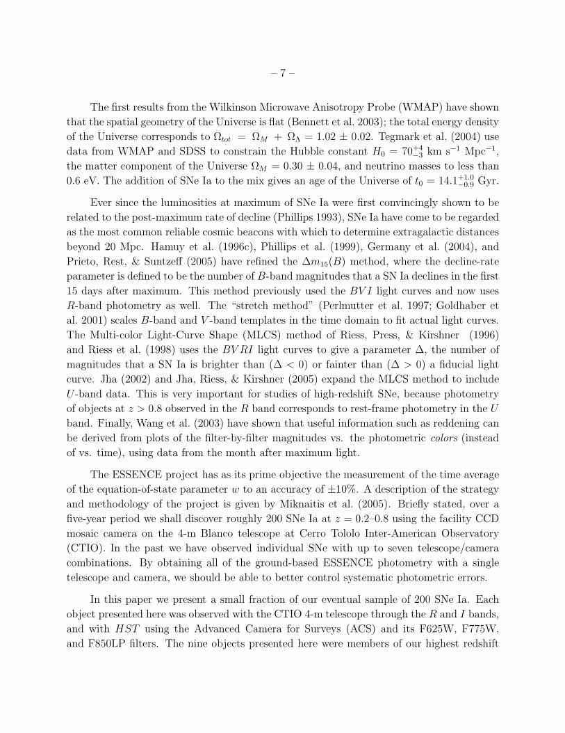
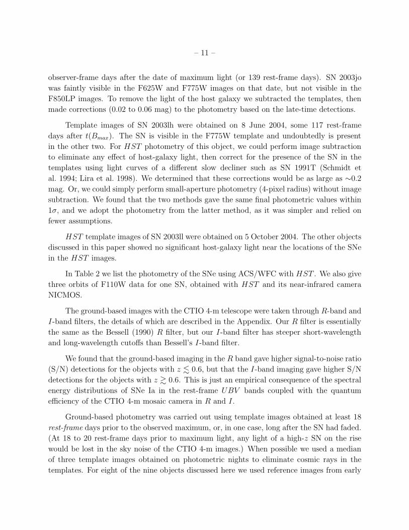
Figure 1 shows HST/ACS images, taken through the F775W filter, of the nine SNe

discussed in this paper. Each represents the combination of two integrations per date and

from four to six dates per object. The total integration times were 3700 s (e510), 5100 s

(SN 2003jo), and 4400 s (the other seven SNe). As one can see, only SN 2003jo, SN 2003ll, and

SN 2003li were hosted by galaxies sufficiently large and bright to show significant structure.

It is not entirely clear that the galaxy near SN 2003kv is the host of that SN. Several of our

objects were effectively “hostless” SNe, meaning that the hosts, if they exist, have surface

brightness too low to be detected in HST and ground-based images.

The program SNID indicates that SN 2003ku is a SN Ia, but there is ambiguity regarding

its true redshift. While the most likely redshift on the basis of the spectrum is 0.79, the next

most likely redshift is 0.41; see § 3.3 and Matheson et al. (2005) for more comments.

We observed supernova e510 spectroscopically on 29 November 2003 (UT dates are used

throughout this paper). We obtained one 1800 s spectrum with Gemini North + GMOS,

but were then shut down by high humidity, and we were unable to obtain a redshift from

the nearly featureless spectrum. We also attempted to get spectra with Keck, but were

hampered by high humidity and clouds. In mid-October 2004, long after the SN had faded,

we attempted to get a redshift from spectra of the faint host galaxy. We took three 1800 s

spectra with Gemini North + GMOS, but there was insufficient signal to extract a usable

spectrum which would provide a redshift. However, following the guidelines of Riess et al.

(2001) and Barris & Tonry (2004), one can derive a redshift-independent distance to a set

of SNe Ia, provided one has sufficiently good photometric coverage in more than a single

passband. For any individual object the results are understandably somewhat uncertain.

Analysis using the code of Prieto, Rest, & Suntzeff (2005) gives a minimum reduced χ2

value of the light-curve fits at a redshift of 0.68 for e510. However, any redshift between 0.64

and 0.84 will give a reduced χ2 value less than 1.0 for this object. It is best if we eliminate

it from further consideration. Because there is no spectral information for e510, it never

– 10 –

received an IAU designation.

Matheson et al. (2005) indicate that SN 2003kv was probably a SN Ia, but the spec-

troscopic identification was not certain. Photometric analysis (below) is entirely consistent

with the notion that SN 2003kv was a SN Ia.

The ESSENCE supernovae were not observed as “targets of opportunity” (TOOs) with

HST since these are very disruptive to the scheduling of the telescope. Instead, a “pseudo-

TOO” method was employed which was pioneered by the high-redshift supernova search

teams several years ago. We specify months before observation (in the Phase II submission)

the region on the sky to be searched, and we specify dates that exact supernova positions

will be available for insertion into the HST schedule. Usually it is five days to a week before

HST begins observing the supernovae after the coordinates have been delivered.

Generally we have a number of supernovae in each field from which to choose for HST

observations, but there are times when a non-optimal target must be inserted at the deadline.

Also, because of the delays between the supernova discovery, spectral confirmation, and the

HST schedule upload, the supernovae are rarely observed before maximum light with HST .

Since HST was meant to improve the quality of photometry at late times for our faintest

targets, this delay is not a major problem for this study.

Our HST/ACS data were obtained using the F625W, F775W, and F850LP filters,

which are essentially the same as the r′, i′, and z′ filters of the SDSS photometric system

(Smith et al. 2002). The throughput transmission curves with HST/ACS are shown in the

Appendix. One of our objects was observed in the near-infrared with NICMOS and its

F110W filter (similar to a J-band filter).

HST/ACS photometric calibration is based on the zeropoint values of Sirianni et al.

(2005), which in turn are based on the Vega spectrophotometric calibration of Bohlin &

Gilliland (2004). For an aperture of 50-pixel radius, the Vegamag zeropoints are zpF625W =

25.731, zpF775W = 25.256, and zpF850LP = 24.326 mag (Sirianni et al. 2005, Table 11).

Our HST/ACS magnitudes are based on small-aperture photometry (4-pixel radius),

using aperture corrections to r = 50 pixels consistent with the radial profiles delineated in

Table 3 of Sirianni et al. (2005). This aperture photometry was done using the apphot

package within IRAF.21

In the case of SN 2003jo we obtained HST template images on 22 May 2004, some 212

21IRAF is distributed by the National Optical Astronomy Observatory, which is operated by AURA, Inc.

under cooperative agreement with the National Science Foundation.

– 11 –

observer-frame days after the date of maximum light (or 139 rest-frame days). SN 2003jo

was faintly visible in the F625W and F775W images on that date, but not visible in the

F850LP images. To remove the light of the host galaxy we subtracted the templates, then

made corrections (0.02 to 0.06 mag) to the photometry based on the late-time detections.

Template images of SN 2003lh were obtained on 8 June 2004, some 117 rest-frame

days after t(Bmax). The SN is visible in the F775W template and undoubtedly is present

in the other two. For HST photometry of this object, we could perform image subtraction

to eliminate any effect of host-galaxy light, then correct for the presence of the SN in the

templates using light curves of a different slow decliner such as SN 1991T (Schmidt et

al. 1994; Lira et al. 1998). We determined that these corrections would be as large as ∼0.2

mag. Or, we could simply perform small-aperture photometry (4-pixel radius) without image

subtraction. We found that the two methods gave the same final photometric values within

1σ, and we adopt the photometry from the latter method, as it was simpler and relied on

fewer assumptions.

HST template images of SN 2003ll were obtained on 5 October 2004. The other objects

discussed in this paper showed no significant host-galaxy light near the locations of the SNe

in the HST images.

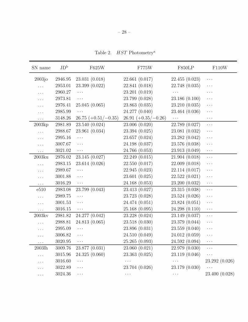
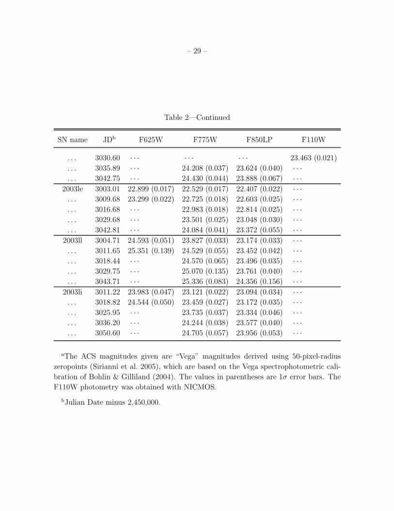
In Table 2 we list the photometry of the SNe using ACS/WFC with HST . We also give

three orbits of F110W data for one SN, obtained with HST and its near-infrared camera

NICMOS.

The ground-based images with the CTIO 4-m telescope were taken through R-band and

I-band filters, the details of which are described in the Appendix. Our R filter is essentially

the same as the Bessell (1990) R filter, but our I-band filter has steeper short-wavelength

and long-wavelength cutoffs than Bessell’s I-band filter.

We found that the ground-based imaging in the R band gave higher signal-to-noise ratio

(S/N) detections for the objects with z . 0.6, but that the I-band imaging gave higher S/N

detections for the objects with z & 0.6. This is just an empirical consequence of the spectral

energy distributions of SNe Ia in the rest-frame UBV bands coupled with the quantum

efficiency of the CTIO 4-m mosaic camera in R and I.

Ground-based photometry was carried out using template images obtained at least 18

rest-frame days prior to the observed maximum, or, in one case, long after the SN had faded.

(At 18 to 20 rest-frame days prior to maximum light, any light of a high-z SN on the rise

would be lost in the sky noise of the CTIO 4-m images.) When possible we used a median

of three template images obtained on photometric nights to eliminate cosmic rays in the

templates. For eight of the nine objects discussed here we used reference images from early

– 12 –

in the 2003 observing season. In the case of SN 2003jo we used reference images from 28

November 2002 (R band) and 11 October 2004 (I band).

For the rotation, alignment, kernel matching, and difference imaging of the ground-

based images we used two packages of scripts written by one of us (BPS). The result is

point-spread function (PSF) magnitudes of field stars and the SNe themselves. The scripts

rely on the kernel-matching algorithm of Alard & Lupton (1998). For reasonably high

S/N detections of the SNe, we adopted the 1σ symmetrical error bars in magnitudes from

dophot. For faint signals, the error bars in magnitude space are not symmetrical. We then

chose a medium-sized number (20) of random locations in the subtracted images (avoiding

obvious image defects) to derive the sky noise, and derived 1σ error bars in flux space, which

we then converted to asymmetrical upper and lower errors in magnitude space. In the case

of the CTIO 4-m R-band images, the sky noise is roughly 250 analog-to-digital units (ADUs,

or counts, where 1 ADU ≈ 1.8 e−) in 200 s exposures (templates and data images) on clear,

moonless nights. 400 s I-band images give corresponding sky noise of about 450 ADUs in

the subtracted images. A SN Ia at maximum light and z ≈ 0.5 typically gives a signal of

4000 ADUs in corresponding R-band and I-band exposures obtained with the CTIO 4-m

telescope.

We used data from the early data release of the SDSS to obtain R-band and I-band

magnitudes for the field stars near the SNe discussed in this paper, relying on the transforma-

tions given in Table 7 of Smith et al. (2002). We avoided using field stars with r′ − i′ > 0.95

mag, as many stars this red are variable and the scatter in the photometric transformation

becomes large.

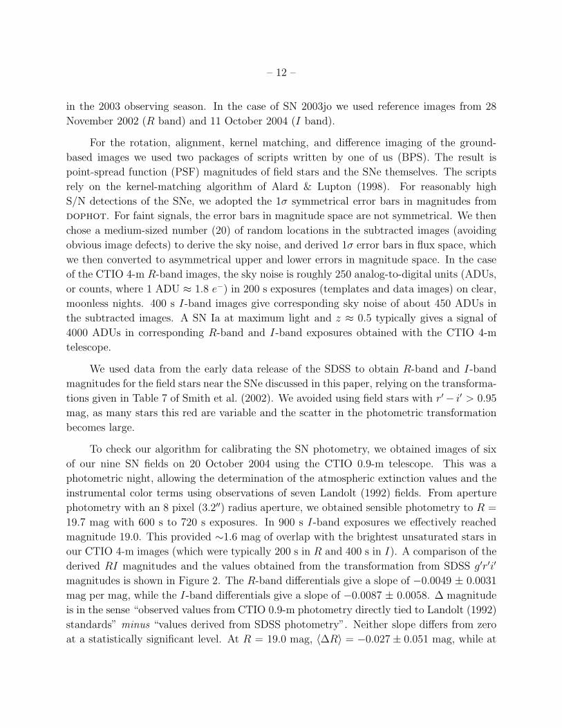
To check our algorithm for calibrating the SN photometry, we obtained images of six

of our nine SN fields on 20 October 2004 using the CTIO 0.9-m telescope. This was a

photometric night, allowing the determination of the atmospheric extinction values and the

instrumental color terms using observations of seven Landolt (1992) fields. From aperture

photometry with an 8 pixel (3.2′′) radius aperture, we obtained sensible photometry to R =

19.7 mag with 600 s to 720 s exposures. In 900 s I-band exposures we effectively reached

magnitude 19.0. This provided ∼1.6 mag of overlap with the brightest unsaturated stars in

our CTIO 4-m images (which were typically 200 s in R and 400 s in I). A comparison of the

derived RI magnitudes and the values obtained from the transformation from SDSS g′r′i′

magnitudes is shown in Figure 2. The R-band differentials give a slope of −0.0049 ± 0.0031

mag per mag, while the I-band differentials give a slope of −0.0087 ± 0.0058. ∆ magnitude

is in the sense “observed values from CTIO 0.9-m photometry directly tied to Landolt (1992)

standards” minus “values derived from SDSS photometry”. Neither slope differs from zero

at a statistically significant level. At R = 19.0 mag, 〈∆R〉 = −0.027 ± 0.051 mag, while at

– 13 –

I = 19.0 mag, 〈∆I〉 = −0.025 ± 0.046 mag. Neither differs significantly from zero. We are

trying to account for all sources of systematic error greater than 0.01 mag in the ESSENCE

photometry. Hence, a more robust test involving more fields and nights is warranted.

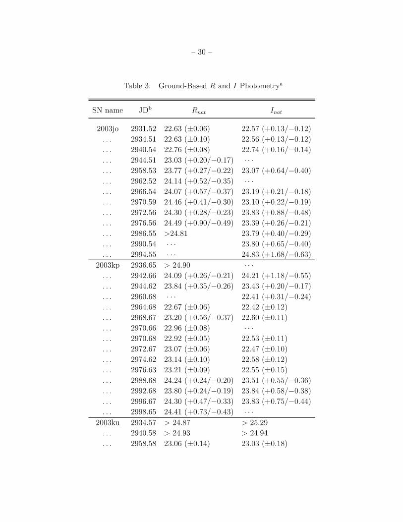
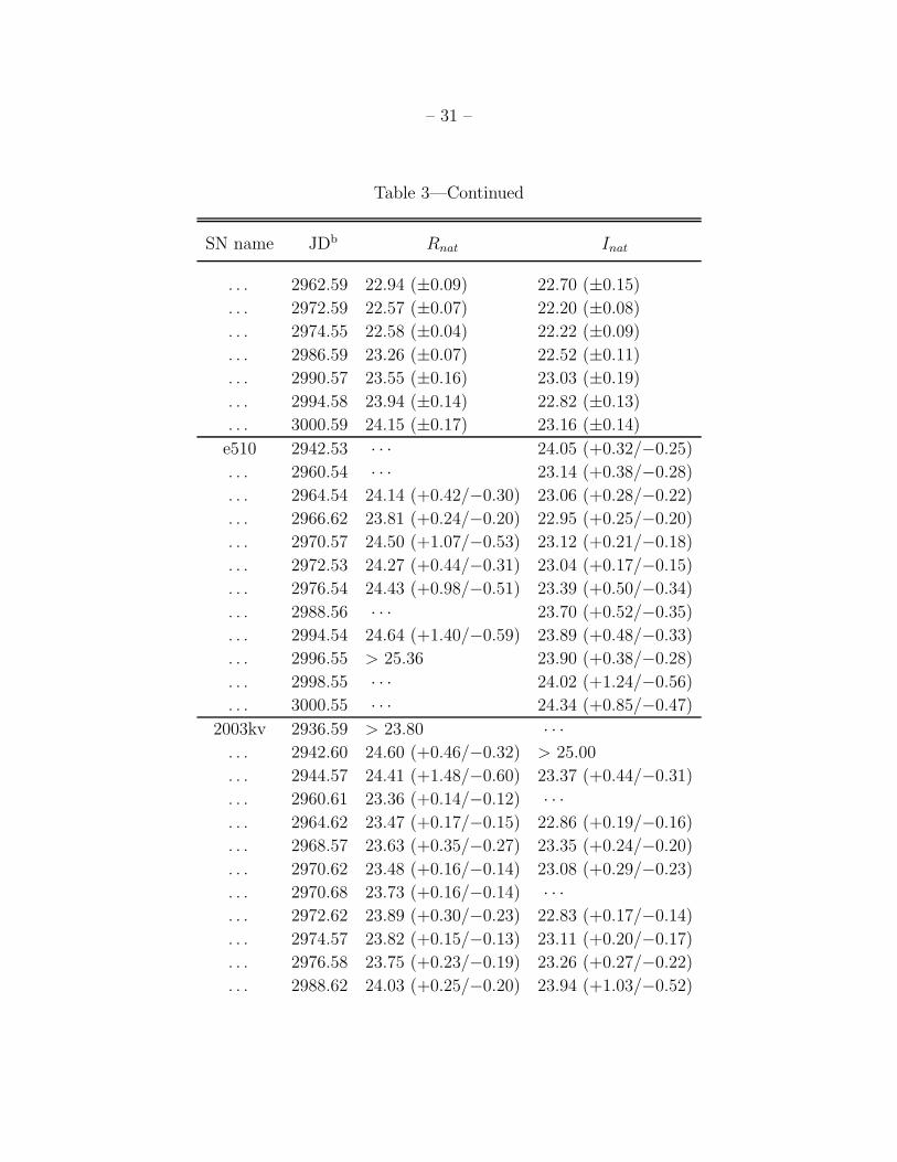
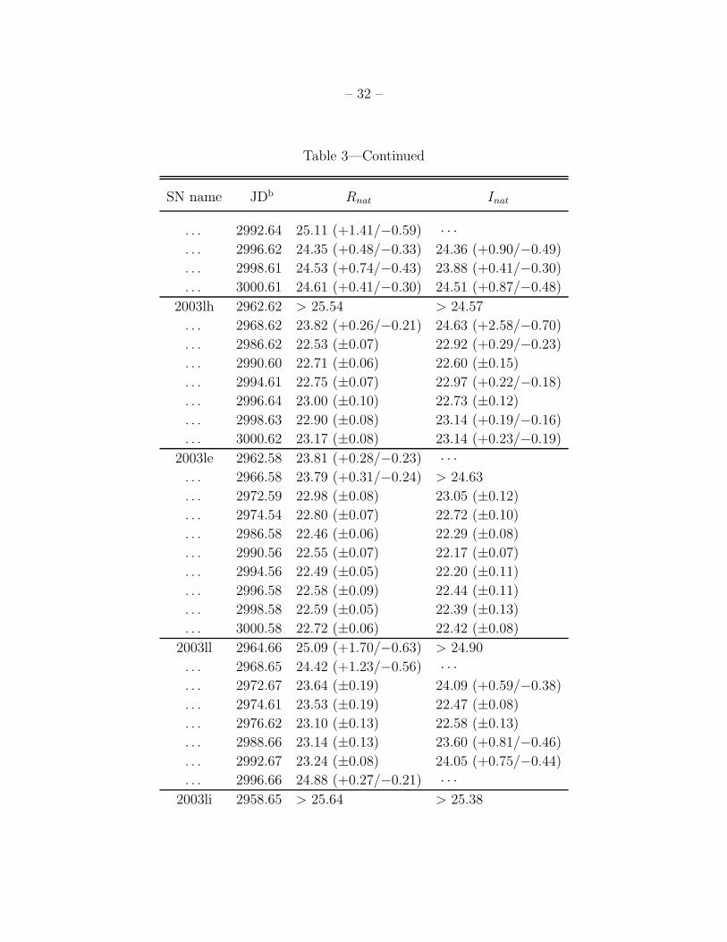
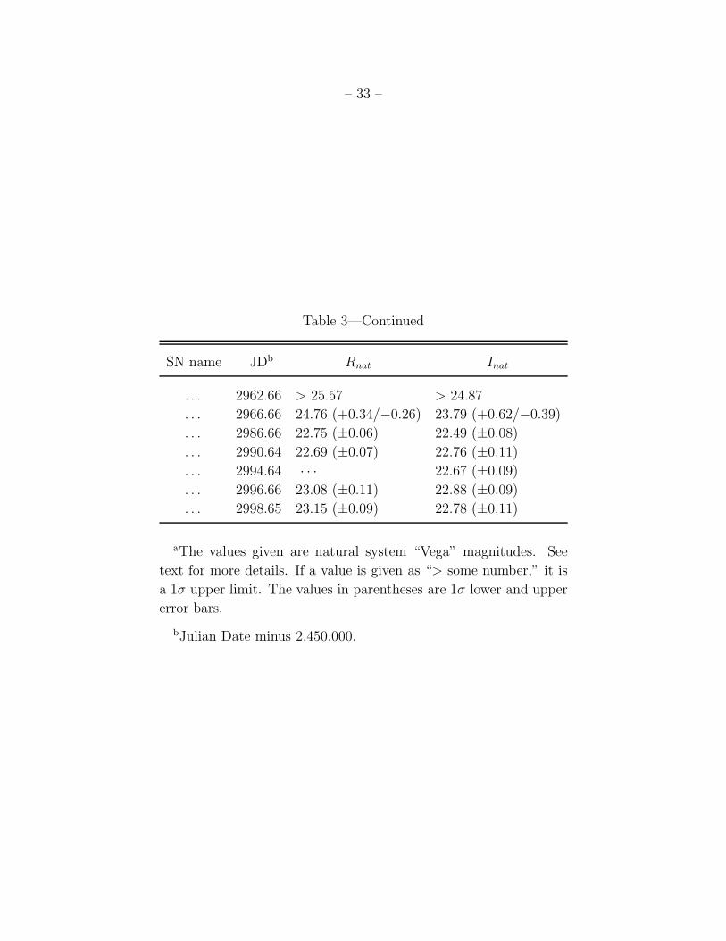
In Table 3 we give the photometry of the SNe using the CTIO 4-m telescope and its

facility mosaic camera. We list the R and I magnitudes in the natural magnitude system of

the telescope/filter/detector transmission function, with a zero point based on the Landolt

(1992) system. To force the zero point of the natural system to that of Landolt, we plot

(Rnat − RLandolt) as a function of (V − R) and (Inat − ILandolt) as a function of (V − I). By

forcing (Rnat −RLandolt) and (Inat − ILandolt) to be 0.00 where (V −R) and (V − I) are zero,

we transfer the zero point of the Landolt system onto the natural system. See the Appendix

of Schmidt et al. (1998).

In Figures 3 and 4 we show the observed light curves of the nine SNe discussed here.

Because the central wavelengths of the R-band and F625W filters are similar, we would

expect that photometry in those bands would be reasonably similar. Also, the I-band

photometry should be similar to the F775W and F850LP photometry. An exception occurs

with R-band and F625W photometry if we are observing a SN Ia with z ≈ 0.8; the flux of

the SN just longward of the Ca II H & K lines is included in the R-band photometry but

excluded from the F625W band. This can make a difference of ∼0.3 mag three weeks after

maximum light in the observer’s frame.

3. Discussion

3.1. Light-Curve Fits and a Composite Spectrum

Seven of the nine objects discussed in this paper have unambigous redshifts on the basis

of spectra (Matheson et al. 2005). We were unable to obtain a redshift of e510 from the SN

itself when it was visible, or from the faint host galaxy the following year, so it was never

assigned an official name by the IAU. But its light-curve shapes and maximum magnitudes

are completely compatible with those of other high-redshift SNe Ia. The case of SN 2003ku

is discussed below.

In order to derive the distances of the SNe, we first K-corrected the ground-based and

space-based photometry to rest-frame U , B, V , or R photometric bands. For the MLCS

method of Jha, Riess, & Kirshner (2005, hereafter MLCS2k2) and the ∆m15(B) analysis

(Prieto, Rest, & Suntzeff 2005), if z ≤ 0.6 the ground-based R-band and F625W data were

K-corrected to rest-frame B, ground-based I-band and F775W data were transformed to rest-

frame V , and F850LP data were transformed to rest-frame R. Photometry of SN 2003kp was

– 14 –

transformed to B and V . For SN 2003kv we transformed the photometry to UBV instead

of BV R.

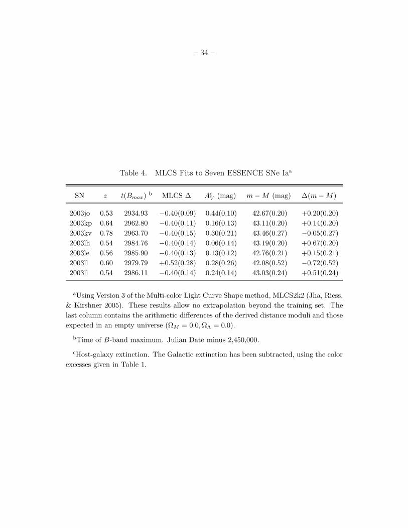
In Tables 4, 5, and 6, we give the light-curve fits using MLCS2k2, the Bayesian Adapted

Template Method (BATM; Tonry et al. 2003, and Tonry et al. 2005, in preparation), and

the ∆m15(B) method of Prieto, Rest, & Suntzeff (2005), respectively. Our derived distance

moduli are consistent within the errors using the three light-curve fitting methods. In all

three tables we give the differences of the derived distance moduli and the corresponding

values in an empty universe (ΩM = 0.0, ΩΛ = 0.0).

Since the light curve decline of SN 2003jo was covered by the ground based data, we

also fit this object without the HST data. Using just the CTIO RI data, the method of

Prieto, Rest, & Suntzeff (2005) gives ∆m15(B) = 0.84 ± 0.17, E(B − V ) = 0.05 ± 0.05,

and (m − M) = 42.77 ± 0.20 (on an H0 = 65 scale). These values are consistent with the

solution given in Table 6, which used the combined CTIO 4-m and HST data.

The ∆m15(B) values given in Table 6 indicate that all but one of the objects discussed

here are slow decliners. The slowest declining template object in the Prieto et al. training

set is SN 1999aa, with ∆m15(B) = 0.81 ± 0.04. Thus, our objects are near, but not beyond,

the limit of the ∆m15(B) system.

The MLCS fits were done in two ways. First, we assumed a prior that no light curve

could be slower than MLCS ∆ = −0.4, the mimimum value of the MLCS training set. In

this case we found that the data systematically deviated from the fits at late times. The

actual light curves were slower than the slowest declining objects in the training set. We

then fit the light curves with no constraint on the possible values of ∆. In this case we had

to extrapolate beyond the training set. In §3.4 we discuss the cosmological effects of using

the prior or not using it.

In Figure 5 we show the ∆m15(B) light-curve fits in the rest-frame bands for 7 SNe. In

Figure 6 we also show the K-corrected, extinction-corrected I-band data of SN 2003lh, our

only data obtained with NICMOS. For comparison we show the I-band data of SN 1999aa

(Krisciunas et al. 2000; Jha 2002), the slowest decliner in the nearby sample used by Prieto,

Rest, & Suntzeff (2005), and the I-band data of the prototypical slow decliner SN 1991T

(Lira et al. 1998). The photometry of SN 1999aa has been adjusted in magnitude space

to the brightness of SN 2003lh using the ∆m15(B) distance modulus given in Table 6 and

assuming an absolute magnitude MI(max) = −19.1 for the slowest-declining SN Ia studied

by Nobili et al. (2005). For H0 = 65 km s−1 Mpc−1, the value used for the ∆m15(B) system,

this becomes MI = −19.32 mag. The maximum of SN 1991T is made to coincide with that

of SN 1999aa. At face value the I-band secondary hump of SN 2003lh was weaker than that

– 15 –

of SNe 1991T and 1999aa. As we pointed out in a previous paper (Krisciunas et al. 2001,

Fig.18), SNe Ia with identical decline rates in B and V can have significantly different I-band

secondary maxima. Whatever is the appropriate adjustment of the SN 2003lh photometry in

Figure 6, we can say that its secondary I-band hump occurred earlier than that of SN 1999aa.

As a measure of our systematics, we show in Figure 7 the residuals of the K-corrected

CTIO 4-m and HST data compared to the rest-frame MLCS2k2 light-curve fits. In Figure 8

we show analogous plots of the residuals of the ∆m15(B) fits shown in Figure 5. In these two

figures a differential magnitude greater than zero means that a rest-frame datum is fainter

than the fit, and a differential magnitude less than zero means that a rest-frame datum is

brighter than the fit.

Figures 7 and 8 show that there are no statistically significant trends in the residuals

of the K-corrected data compared to the light-curve fits, and that the mean residual is close

to zero, as expected.

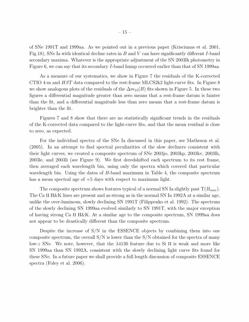
For the individual spectra of the SNe Ia discussed in this paper, see Matheson et al.

(2005). In an attempt to find spectral peculiarities of the slow decliners consistent with

their light curves, we created a composite spectrum of SNe 2003jo, 2003kp, 2003kv, 2003lh,

2003le, and 2003li (see Figure 9). We first deredshifted each spectrum to its rest frame,

then averaged each wavelength bin, using only the spectra which covered that particular

wavelength bin. Using the dates of B-band maximum in Table 4, the composite spectrum

has a mean spectral age of +5 days with respect to maximum light.

The composite spectrum shows features typical of a normal SN Ia slightly past T(Bmax).

The Ca II H&K lines are present and as strong as in the normal SN Ia 1992A at a similar age,

unlike the over-luminous, slowly declining SN 1991T (Filippenko et al. 1992). The spectrum

of the slowly declining SN 1999aa evolved similarly to SN 1991T, with the major exception

of having strong Ca II H&K. At a similar age to the composite spectrum, SN 1999aa does

not appear to be drastically different than the composite spectrum.

Despite the increase of S/N in the ESSENCE objects by combining them into one

composite spectrum, the overall S/N is lower than the S/N obtained for the spectra of many

low-z SNe. We note, however, that the λ4130 feature due to Si II is weak and more like

SN 1999aa than SN 1992A, consistent with the slowly declining light curve fits found for

these SNe. In a future paper we shall provide a full length discussion of composite ESSENCE

spectra (Foley et al. 2006).

– 16 –

3.2. Decline Rates of Supernovae

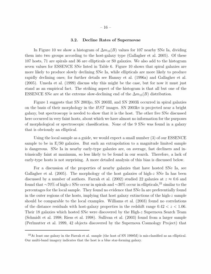
In Figure 10 we show a histogram of ∆m15(B) values for 107 nearby SNe Ia, dividing

them into two groups according to the host-galaxy type (Gallagher et al. 2005). Of these

107 hosts, 71 are spirals and 36 are ellipticals or S0 galaxies. We also add to the histogram

seven values for ESSENCE SNe listed in Table 6. Figure 10 shows that spiral galaxies are

more likely to produce slowly declining SNe Ia, while ellipticals are more likely to produce

rapidly declining ones; for further details see Hamuy et al. (1996a) and Gallagher et al.

(2005). Umeda et al. (1999) discuss why this might be the case, but for now it must just

stand as an empirical fact. The striking aspect of the histogram is that all but one of the

ESSENCE SNe are at the extreme slow-declining end of the ∆m15(B) distribution.

Figure 1 suggests that SN 2003jo, SN 2003ll, and SN 2003li occurred in spiral galaxies

on the basis of their morphology in the HST images. SN 2003kv is projected near a bright

galaxy, but spectroscopy is needed to show that it is the host. The other five SNe discussed

here occurred in very faint hosts, about which we have almost no information for the purposes

of morphological or spectroscopic classification. None of the 9 SNe was found in a galaxy

that is obviously an elliptical.

Using the local sample as a guide, we would expect a small number (3) of our ESSENCE

sample to be in E/S0 galaxies. But such an extrapolation to a magnitude limited sample

is dangerous. SNe Ia in nearby early-type galaxies are, on average, fast decliners and in-

trinsically faint at maximum, so less likely to be found in our search. Therefore, a lack of

early-type hosts is not surprising. A more detailed analysis of this bias is discussed below.

For a discussion of the properties of nearby galaxies that have hosted SNe Ia, see

Gallagher et al. (2005). The morphology of the host galaxies of high-z SNe Ia has been

discussed by a number of authors. Farrah et al. (2002) studied 22 galaxies at z ≈ 0.6 and

found that ∼70% of high-z SNe occur in spirals and ∼30% occur in ellipticals,22 similar to the

percentages for the local sample. They found no evidence that SNe Ia are preferentially found

in the outer regions of the hosts, implying that host galaxy extinctions of the high-z sample

should be comparable to the local examples. Williams et al. (2003) found no correlations

of the distance residuals with host-galaxy properties in the redshift range 0.42 < z < 1.06.

Their 18 galaxies which hosted SNe were discovered by the High-z Supernova Search Team

(Schmidt et al. 1998; Riess et al. 1998). Sullivan et al. (2003) found from a larger sample

(Perlmutter et al. 1999, 42 objects discovered by the Supernova Cosmology Project) that

22At least one galaxy in the Farrah et al. sample (the host of SN 1998M) is mis-classified as an elliptical.

Our multi-band imagery indicates that the host is a blue star-forming galaxy.

– 17 –

there is evidence for a larger scatter of the absolute magnitudes for the high-z SNe occurring

in spirals. They also found that SNe occurring in spirals are on average marginally less

luminous than those in E/S0 galaxies, by 0.14 ± 0.09 mag. But this is opposite of what is

seen at low redshifts (Hamuy et al. 1996a).

These analyses do not lead us to believe that there are significant differences between

the hosts of low-z and our high-z SNe Ia or between the SNe Ia themselves. Why, then, do

all but one of the ESSENCE objects discussed in this paper have such slow decline rates?

Some of the issues involved have already been discussed by Li, Filippenko, & Riess (2001). It

is important to note that the SNe Ia in this paper not typical of ESSENCE SNe in general.

They were chosen to be at the highest redshift end of the ESSENCE distribution for HST

follow-up.

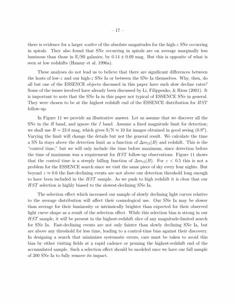
In Figure 11 we provide an illustrative answer. Let us assume that we discover all the

SNe in the R band, and ignore the I band. Assume a fixed magnitude limit for detection;

we shall use R = 23.0 mag, which gives S/N ≈ 10 for images obtained in good seeing (0.9′′).

Varying the limit will change the details but not the general result. We calculate the time

a SN Ia stays above the detection limit as a function of ∆m15(B) and redshift. This is the

“control time,” but we will only include the time before maximum, since detection before

the time of maximum was a requirement for HST follow-up observations. Figure 11 shows

that the control time is a steeply falling function of ∆m15(B). For z < 0.5 this is not a

problem for the ESSENCE search since we visit the same piece of sky every four nights. But

beyond z ≈ 0.6 the fast-declining events are not above our detection threshold long enough

to have been included in the HST sample. As we push to high redshift it is clear that our

HST selection is highly biased to the slowest-declining SNe Ia.

The selection effect which increased our sample of slowly declining light curves relative

to the average distribution will affect their cosmological use. Our SNe Ia may be slower

than average for their luminosity or intrinsically brighter than expected for their observed

light curve shape as a result of the selection effect. While this selection bias is strong in our

HST sample, it will be present in the highest-redshift slice of any magnitude-limited search

for SNe Ia. Fast-declining events are not only fainter than slowly declining SNe Ia, but

are above any threshold for less time, leading to a control-time bias against their discovery.

In designing a search that minimizes systematic errors, care must be taken to avoid this

bias by either visiting fields at a rapid cadence or pruning the highest-redshift end of the

accumulated sample. Such a selection effect should be modeled once we have our full sample

of 200 SNe Ia to fully remove its impact.

– 18 –

3.3. The Strange Case of SN 2003ku

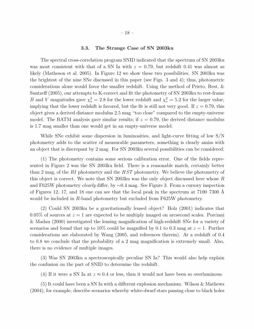
The spectral cross-correlation program SNID indicated that the spectrum of SN 2003ku

was most consistent with that of a SN Ia with z = 0.79, but redshift 0.41 was almost as

likely (Matheson et al. 2005). In Figure 12 we show these two possibilities. SN 2003ku was

the brightest of the nine SNe discussed in this paper (see Figs. 3 and 4); thus, photometric

considerations alone would favor the smaller redshift. Using the method of Prieto, Rest, &

Suntzeff (2005), our attempts to K-correct and fit the photometry of SN 2003ku to rest-frame

B and V magnitudes gave χ2ν

= 2.8 for the lower redshift and χ2ν

= 5.2 for the larger value,

implying that the lower redshift is favored, but the fit is still not very good. If z = 0.79, this

object gives a derived distance modulus 2.5 mag “too close” compared to the empty-universe

model. The BATM analysis gave similar results; if z = 0.79, the derived distance modulus

is 1.7 mag smaller than one would get in an empty-universe model.

While SNe exhibit some dispersion in luminosities, and light-curve fitting of low S/N

photometry adds to the scatter of measurable parameters, something is clearly amiss with

an object that is discrepant by 2 mag. For SN 2003ku several possibilities can be considered:

(1) The photometry contains some serious calibration error. One of the fields repre-

sented in Figure 2 was the SN 2003ku field. There is a reasonable match, certainly better

than 2 mag, of the RI photometry and the HST photometry. We believe the photometry of

this object is correct. We note that SN 2003ku was the only object discussed here whose R

and F625W photometry clearly differ, by ∼0.4 mag. See Figure 3. From a cursory inspection

of Figures 12, 17, and 18 one can see that the local peak in the spectrum at 7100–7300 A

would be included in R-band photometry but excluded from F625W photometry.

(2) Could SN 2003ku be a gravitationally lensed object? Holz (2001) indicates that

0.05% of sources at z = 1 are expected to be multiply imaged on arcsecond scales. Porciani

& Madau (2000) investigated the lensing magnification of high-redshift SNe for a variety of

scenarios and found that up to 10% could be magnified by 0.1 to 0.3 mag at z = 1. Further

considerations are elaborated by Wang (2005, and references therein). At a redshift of 0.4

to 0.8 we conclude that the probability of a 2 mag magnification is extremely small. Also,

there is no evidence of multiple images.

(3) Was SN 2003ku a spectroscopically peculiar SN Ia? This would also help explain

the confusion on the part of SNID to determine the redshift.

(4) If it were a SN Ia at z ≈ 0.4 or less, then it would not have been so overluminous.

(5) It could have been a SN Ia with a different explosion mechanism. Wilson & Mathews

(2004), for example, describe scenarios whereby white-dwarf stars passing close to black holes

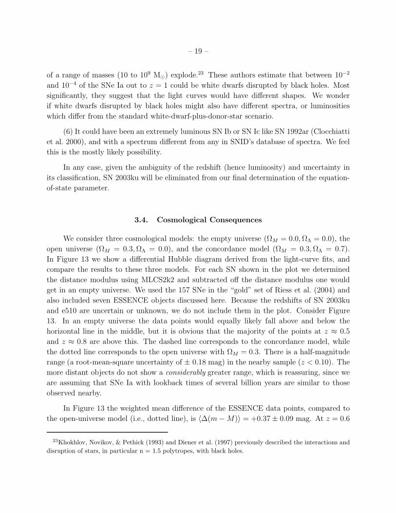
– 19 –

of a range of masses (10 to 109 M⊙) explode.23 These authors estimate that between 10−2

and 10−4 of the SNe Ia out to z = 1 could be white dwarfs disrupted by black holes. Most

significantly, they suggest that the light curves would have different shapes. We wonder

if white dwarfs disrupted by black holes might also have different spectra, or luminosities

which differ from the standard white-dwarf-plus-donor-star scenario.

(6) It could have been an extremely luminous SN Ib or SN Ic like SN 1992ar (Clocchiatti

et al. 2000), and with a spectrum different from any in SNID’s database of spectra. We feel

this is the mostly likely possibility.

In any case, given the ambiguity of the redshift (hence luminosity) and uncertainty in

its classification, SN 2003ku will be eliminated from our final determination of the equation-

of-state parameter.

3.4. Cosmological Consequences

We consider three cosmological models: the empty universe (ΩM = 0.0, ΩΛ = 0.0), the

open universe (ΩM = 0.3, ΩΛ = 0.0), and the concordance model (ΩM = 0.3, ΩΛ = 0.7).

In Figure 13 we show a differential Hubble diagram derived from the light-curve fits, and

compare the results to these three models. For each SN shown in the plot we determined

the distance modulus using MLCS2k2 and subtracted off the distance modulus one would

get in an empty universe. We used the 157 SNe in the “gold” set of Riess et al. (2004) and

also included seven ESSENCE objects discussed here. Because the redshifts of SN 2003ku

and e510 are uncertain or unknown, we do not include them in the plot. Consider Figure

13. In an empty universe the data points would equally likely fall above and below the

horizontal line in the middle, but it is obvious that the majority of the points at z ≈ 0.5

and z ≈ 0.8 are above this. The dashed line corresponds to the concordance model, while

the dotted line corresponds to the open universe with ΩM = 0.3. There is a half-magnitude

range (a root-mean-square uncertainty of ± 0.18 mag) in the nearby sample (z < 0.10). The

more distant objects do not show a considerably greater range, which is reassuring, since we

are assuming that SNe Ia with lookback times of several billion years are similar to those

observed nearby.

In Figure 13 the weighted mean difference of the ESSENCE data points, compared to

the open-universe model (i.e., dotted line), is 〈∆(m − M)〉 = +0.37 ± 0.09 mag. At z = 0.6

23Khokhlov, Novikov, & Pethick (1993) and Diener et al. (1997) previously described the interactions and

disruption of stars, in particular n = 1.5 polytropes, with black holes.

– 20 –

the difference between the concordance model (dashed line) and the open-universe model is

+0.23 mag. In a flat universe, as ΩM becomes smaller and ΩΛ increases, the curve bows

upward at z = 0.6. Thus, if the geometry of the Universe is flat, the ESSENCE data alone

would stipulate that the mass density of the Universe is ΩM < 0.3 and the dark energy has

ΩΛ > 0.7.

Using the MLCS2k2 fits and a nearby sample to establish the zeropoint of the dis-

tance moduli, we obtain cosmological constraints for a cosmological constant based on the

ESSENCE supernovae. In Figure 14 we have plotted constraints assuming a prior limiting

the decline rate of the slowest supernovae, and constraints based on no prior which allow

an extrapolation by MLCS. Clearly the choice of a prior affects the cosmological results and

points to the need to avoid a selection bias that preferentially discovers slowly declining

supernovae at the limits of the decline rate range of the local sample. Using the 2dF mass

constraint of Cole et al. (2005) (ΩMh = 0.168 ± 0.016), the Hubble constant of Freedman

et al. (2001), and with the prior on MLCS ∆ we find ΩΛ = 1.26 ± 0.18 for the sample of

ESSENCE plus nearby SNe. Without the prior we find ΩΛ = 0.99 ± 0.21.

In Figures 15 and 16 we show constraints obtained for ΩΛ and w using the entire “gold”

set of 157 SNe from Riess et al. (2004) plus seven ESSENCE SNe discussed in this paper.

We have assumed w = −1 for Figure 15 and have used two different matter constraints: the

2dF mass constraint of Cole et al. (2005) coupled with the Hubble constant from Freedman

et al. (2001), and the SDSS large-scale structure result of ΩM = 0.273 ± 0.025 + 0.137ΩK

(Eisenstein et al. 2005). Figure 15 shows that the standard model is recovered at the 1σ

level if we use the full “gold” SN sample, the seven ESSENCE objects from Table 4, and

either matter constraint. From Figure 16 we find w = −0.88 ± 0.11 with the prior on

MLCS ∆ for the ESSENCE sample. Without the prior we find w = −0.90 ± 0.12. This is

a significant shift in w considering only 7 of 164 SNe Ia were affected by the change of prior.

This demonstrates the importance of the selection bias at the high-z end of any survey.

4. Conclusions

We have presented photometry of nine supernovae from the ESSENCE project. Ground-

based photometry allowed us to cover the maxima in the rest-frame B and V light curves

of all the objects discussed here, while the photometry obtained with HST/ACS allowed

us to characterize the light-curve tails. The light-curve fitting of seven objects with reliable

redshifts, carried out with three different methods, gave distance moduli consistent within

the errors.

– 21 –

On the basis of the values of ∆m15(B) derived for the ESSENCE SNe, all but one are

slow decliners compared to the local sample and their light curves are as slow as the slowest

found in the local set of well-observed supernovae. We show that the SNe selected to be

observed with HST were at the high-z end of our distribution of redshifts and probably

represent a selection bias for slow-declining events.

The ESSENCE project is being carried out every other night on the CTIO 4-m telescope

during the months of October, November, and December. After three years of the ESSENCE

project we have discovered roughly 100 SNe and SN candidates. Eventually, with ∼200

spectroscopically confirmed ESSENCE SNe Ia, all observed with the same ground-based

telescope and filter system, we should be able to determine the time average of the equation-

of-state parameter of the Universe to ±10%.

We observe two sets of fields on alternating observing nights. The resulting cadence

of light-curve points every four observer-frame days is clearly sufficient to characterize the

light curves. For SNe Ia with z ≈ 0.5, we obtain apparent magnitudes at maximum with

an uncertainty of ±0.06 mag. For further details on the project strategy see Miknaitis et al.

(2005).

The 157 “gold” SNe Ia of Riess et al. (2004), along with seven high-redshift SNe dis-

cussed here, give contours in the ΩM − ΩΛ plane consistent with a positive cosmological

constant and flat geometry. Further cosmological tests await the acquisition of larger self-

consistent data sets.

The ESSENCE Project is supported primarily by NSF grants AST-0206329 and AST-

0443378. We are also grateful for NASA grants GO-9860 and AR-9925 from the Space

Telescope Science Institute (STScI), which is operated by AURA, Inc., under NASA contract

NAS 5-26555. P.M.G. is supported in part by NASA Long Term Space Astrophysics grant

NAGS-9364. We thank Galina Soutchkova of STScI for her help in scheduling our pseudo-

TOO observations with HST . Some of the results presented herein were obtained at the

W. M. Keck Observatory, which is operated as a scientific partnership among the California

Institute of Technology, the University of California, and NASA; the Observatory was made

possible by the generous financial support of the W. M. Keck Foundation. VLT observations

were part of program 170.A-0519. We also utilized the SDSS early data release. A.V.F. is

grateful for the support of NSF grant AST-0307894, and for a Miller Research Professorship

at UC Berkeley during which part of this work was completed. We thank Jorge Araya

for tracing filters in the lab, Sean Points for further analysis of those traces, and George

Jacoby for providing his program for simulating the filter-transmission profiles of the RI

filters appropriate to the focal ratio of the CTIO 4-m telescope. We acknowledge Joseph

– 22 –

Gallagher for providing his database of supernova properties. Lou Strolger kindly derived

the F110W photometry of one of our supernovae. K.K. thanks David Spergel for many

stimulating discussions. Finally, we thank an anonymous referee for constructive suggestions

and references to other work.

5. Appendix: Filters for Supernova Photometry

In Figure 17 we show the effective throughput (i.e., combination of filter transmission

and quantum efficiency as a function of wavelength) of the three filters used with HST/ACS.

We used laboratory hardware and software produced by Ocean Optics to make trans-

mission-curve traces of the R-band and I-band filters, which were used with the CTIO 4-m

telescope and its facility mosaic camera. The traces were taken with the incidence angle

of the input laser beam ranging from 0 to 11. We subsequently used the data files and

a program kindly provided by G. Jacoby to simulate the filter traces appropriate for the

f/2.7 beam of the CTIO 4-m telescope and its Mosaic camera. As the I-band filter is an

interference filter, this is particularly important. The effective I-band filter profile for an

f/2.7 beam has half-power points shifted roughly 30 A toward the blue from the 0 incidence

angle tracing.

The RI filter transmission curves can be obtained in graphical and tabular form at

website http://www.ctio.noao.edu/∼points/FILTERS. Our effective RI filter transmission

curves are shown in Figure 18. They include the effects of reflection off the primary mir-

ror, the quantum efficiency of the CCD chips as a function of wavelength, the atmospheric

extinction, and the major telluric absorption lines.

REFERENCES

Aguirre, A. N. 1999, ApJ, 512, L19

Alard, C., & Lupton, R. H. 1998, ApJ, 503, 325

Barris, B. J., & Tonry, J. L. 2004, ApJ, 613, L21

Barris, B. J., et al. 2004, ApJ, 602, 571

Benetti, S., et al. 2005, ApJ, 623, 1011

Bennett, C. L., et al. 2003, ApJS, 148, 1

– 23 –

Bessell, M. S. 1990, PASP, 102, 1181

Bohlin, R. C., & Gilliland, R. 2004, AJ, 127, 3508

Caldwell, R. R. 2002, Physics Letters B, 545, 23

Carroll, S. M., Press, W. P., & Turner, E. L. 1992, ARA&A, 30, 499

Carroll, S. M. 2004, in Carnegie Observatories Astrophysics Series 2, Measuring and Model-

ing the Universe, ed. W. L. Freedman (Cambridge: Cambridge Univ. Press), 235

Clocchiatti, A., et al. 2000, ApJ, 529, 661

Cole, S., et al. 2005, MNRAS, in press (astro-ph/0501174)

Dahlen, T., et al. 2004, ApJ, 613, 189

Diener, P., Frolov, V. P., Khokhlov, A. M., Novikov, I. D., & Pethick, C. J. 1997, ApJ, 479,

164

Eisenstein, D. J., et al. 2005, ApJ, in press (astro-ph/0501171)

Farrah, D., Meikle, W. P. S., Clements, D., Rowan-Robinson, M., & Mattila, S. 2002,

MNRAS, 336, L17

Filippenko, A. V., et al. 1992, ApJ, 384, L15

Filippenko, A. V. 2004, in Carnegie Observatories Astrophysics Series, Vol. 2: Measuring and

Modeling the Universe, ed. W. L. Freedman (Cambridge: Cambridge Univ. Press),

270

Filippenko, A. V. 2005, in White Dwarfs: Probes of Galactic Structure and Cosmology,

ed. E. M. Sion, H. L. Shipman, and S. Vennes (Dordrecht: Kluwer), in press (astro-

ph/0410609)

Foley, R. J., et al. 2006, in preparation

Freedman, W., et al. 2001, ApJ, 553, 47

Gallagher, J. S., Garnavich, P. M., Challis, P., Berlind, P., Jha, S., & Kirshner, R. P. 2005,

ApJ, in press, astro-ph/0508180

Gal-Yam, A., Poznanski, D., Maoz, D., Filippenko, A. V., & Foley, R. J. 2004, PASP, 116,

597

– 24 –

Garnavich, P. M., et al. 1998a, ApJ, 509, 74

Garnavich, P. M., et al. 1998b, ApJ, 493, L53

Germany, L. M., Reiss, D. J., Schmidt, B. P., Stubbs, C. W., & Suntzeff, N. B. 2004, A&A,

415, 863

Goldhaber, G., et al. 2001, ApJ, 558, 359

Hamuy, M., Phillips, M. M., Suntzeff, N. B., Schommer, R. A., Maza, J., & Aviles, R. 1996a,

AJ, 112, 2391

Hamuy, M., Phillips, M. M., Suntzeff, N. B., Schommer, R. A., Maza, J., & Aviles, R. 1996b,

AJ, 112, 2398

Hamuy, M., Phillips, M. M., Suntzeff, N. B., Schommer, R. A., Maza, J., Smith, R. C., Lira,

P., & Aviles, R. 1996c, AJ, 112, 2438

Holz, D. E. 2001, ApJ, 556, L71

Homeier, N. L. 2005, ApJ, 620, 12

Hu, W. 2005, Phys. Rev. D71, 047301

Jha, S. 2002, PhD thesis, Harvard University

Jha, S., Riess, A. G., & Kirshner, R. P. 2005, in preparation (MLCS2k2)

Khokhlov, A., Novikov, I. D., & Pethick, C. J. 1993, ApJ, 418, 163

Knop, R. A., et al. 2003, ApJ, 598, 102

Krisciunas, K. 1993, in Encyclopedia of Cosmology, ed. N. Hetherington (New York and

London: Garland), 218, errata in astro-ph/9308025

Krisciunas, K., Hastings, N. C., Loomis, K., McMillan, R., Rest, A., Riess, A. G., & Stubbs,

C. 2000, ApJ, 539, 658

Krisciunas, K., et al. 2001, AJ, 122, 1616

Landolt, A. U. 1992, AJ, 104, 340

Leaman, J., Li, W., & Filippenko, A. 2004, BAAS, 36, 1464 (#71.02)

Li, W., Filippenko, A. V., & Riess, A. G. 2001, ApJ, 546, 719

– 25 –

Lira, P., et al. 1998, AJ, 115, 234

Longair, M. 1984, Theoretical Concepts in Physics (Cambridge: Cambridge Univ. Press), p.

334

Matheson, T., et al. 2005, AJ, 129, 2352

Miknaitis, G., et al. 2005, in preparation

Nobili, S., et al. 2005, A&A, in press (astro-ph/0504139)

Peebles, P. J. E., & Ratra, B. 2003, Rev. Mod Phys., 75, 559

Perlmutter, S., et al. 1997, ApJ, 483, 565

Perlmutter, S., et al. 1999, ApJ, 517, 565

Phillips, M. M. 1993, ApJ, 413, L105

Phillips, M. M., Lira, P., Suntzeff, N. B., Schommer, R. A., Hamuy, M., & Maza, J. 1999,

AJ, 118, 1766

Porciani, C., & Madau, P. 2000, ApJ, 532, 679

Poznanski, D., Gal-Yam, A., Maoz, D., Filippenko, A. V., Leonard, D. C., & Matheson, T.

2002, PASP, 114, 833

Prieto, J. L., Rest, A., & Suntzeff, N. B. 2005, ApJ, in press

Riess, A. G., Press, W. H., & Kirshner, R. P. 1996, ApJ, 473, 88

Riess, A. G., et al. 1998, AJ, 116, 1009

Riess, A. G., et al. 2001, ApJ, 560, 49

Riess, A. G., et al., 2004, ApJ, 607, 665

Schlegel, D. J., Finkbeiner, D. P., & Davis, M. 1998, ApJ, 500, 525

Schmidt, B. P., Kirshner, R. P., Leibundgut, B., Wells, L. A., Porter, A. C., Ruiz-Lapuente,

P., Challis, P., & Filippenko, A. V. 1994, ApJ, 434, L19

Schmidt, B. P., et al. 1998, ApJ, 507, 46

Sirianni, M., et al. 2005, PASP, in press, astro-ph/0507614

– 26 –

Smith, J. A., et al. 2002, AJ, 123, 2121

Sullivan, M., et al. 2003, MNRAS, 340, 1057

Suntzeff, N. B., et al. 2005, in preparation

Tegmark, M., et al. 2004, Phys. Rev. D, 69, 103501

Tonry, J. L., et al. 2003, ApJ, 594, 1

Umeda, H., Nomoto, K., Koyayashi, C., Hachisu, I., & Kato, M. 1999, ApJ, 522, L43

Upadhye, A., Ishak, M., & Steinhardt, P. J. 2005 (astro-ph/0411803)

Wang, L., Goldhaber, G., Aldering, G., & Perlmutter, S. 2003, ApJ, 590, 944

Wang, Y. 2005, J. of Cosmology and Astroparticle Physics, 3, 5

Williams, B. F., et al. 2003, AJ, 126, 2608

Wilson, J. R., & Mathews, G. J. 2004, ApJ, 610, 368

This preprint was prepared with the AAS LATEX macros v5.2.

– 27 –

Table 1. High-Redshift Supernovae: Basic Data

IAU name ESSENCE α(J2000) δ(J2000) Redshifta E(B − V )b

Gal

SN 2003jo d033 23:25:24.03 −09:26:00.6 0.53 0.036

SN 2003kp e147 02:31:02.64 −08:39:50.8 0.64 0.032

SN 2003ku e315 01:08:36.25 −00:33:20.8 0.79c 0.036

· · · e510 23:30:59.97 −08:37:34.4 0.68d 0.032

SN 2003kv e531 02:09:42.52 −03:46:48.6 0.78 0.023

SN 2003lh f011 02:10:19.51 −04:59:32.3 0.54 0.020

SN 2003le f041 01:08:08.73 +00:27:09.7 0.56 0.029

SN 2003ll f216 02:35:41.19 −08:06:29.6 0.60 0.033

SN 2003li f244 02:27:47.29 −07:33:46.2 0.54 0.027

aObtained from the spectra of the SNe themselves, rather than the host galax-

ies. We used our program SNID (Tonry et al. 2005, in preparation).

bFrom the reddening maps of Schlegel et al. (1998); magnitude units.

cSee text and Matheson et al. (2005) for a discussion of the redshift of this

object.

dThe minimum reduced χ2 value of the light-curve fits is obtained for z = 0.68;

no spectroscopic redshift was obtained.

– 28 –

Table 2. HST Photometrya

SN name JDb F625W F775W F850LP F110W

2003jo 2946.95 23.031 (0.018) 22.661 (0.017) 22.455 (0.023) · · ·

. . . 2953.01 23.399 (0.022) 22.841 (0.018) 22.748 (0.035) · · ·

. . . 2960.27 · · · 23.201 (0.019) · · · · · ·

. . . 2973.81 · · · 23.799 (0.028) 23.186 (0.100) · · ·

. . . 2976.41 25.045 (0.065) 23.863 (0.035) 23.210 (0.035) · · ·

. . . 2985.99 · · · 24.277 (0.040) 23.464 (0.036) · · ·

. . . 3148.26 26.75 (+0.51/−0.35) 26.91 (+0.35/−0.26) · · · · · ·

2003kp 2981.89 23.540 (0.024) 23.006 (0.020) 22.789 (0.027) · · ·

. . . 2988.67 23.961 (0.034) 23.394 (0.025) 23.081 (0.032) · · ·

. . . 2995.16 · · · 23.657 (0.024) 23.282 (0.042) · · ·

. . . 3007.67 · · · 24.198 (0.037) 23.576 (0.038) · · ·

. . . 3021.02 · · · 24.766 (0.053) 23.913 (0.049) · · ·

2003ku 2976.02 23.145 (0.027) 22.249 (0.015) 21.904 (0.018) · · ·

. . . 2983.15 23.614 (0.026) 22.550 (0.017) 22.009 (0.018) · · ·

. . . 2989.67 · · · 22.945 (0.023) 22.114 (0.017) · · ·

. . . 3001.88 · · · 23.601 (0.025) 22.522 (0.021) · · ·

. . . 3016.29 · · · 24.168 (0.053) 23.200 (0.032) · · ·

e510 2983.08 23.799 (0.043) 23.413 (0.027) 23.315 (0.038) · · ·

. . . 2989.75 · · · 23.723 (0.028) 23.524 (0.026) · · ·

. . . 3001.53 · · · 24.474 (0.051) 23.824 (0.051) · · ·

. . . 3016.15 · · · 25.168 (0.095) 24.298 (0.110) · · ·

2003kv 2981.82 24.277 (0.042) 23.228 (0.024) 23.149 (0.037) · · ·

. . . 2988.81 24.813 (0.065) 23.518 (0.030) 23.379 (0.044) · · ·

. . . 2995.09 · · · 23.896 (0.031) 23.559 (0.040) · · ·

. . . 3006.82 · · · 24.510 (0.049) 24.012 (0.059) · · ·

. . . 3020.95 · · · 25.265 (0.093) 24.592 (0.094) · · ·

2003lh 3009.76 23.877 (0.031) 23.060 (0.021) 22.979 (0.030) · · ·

. . . 3015.96 24.325 (0.060) 23.363 (0.025) 23.119 (0.046) · · ·

. . . 3016.60 · · · · · · · · · 23.292 (0.026)

. . . 3022.89 · · · 23.704 (0.026) 23.179 (0.030) · · ·

. . . 3024.36 · · · · · · · · · 23.400 (0.028)

– 29 –

Table 2—Continued

SN name JDb F625W F775W F850LP F110W

. . . 3030.60 · · · · · · · · · 23.463 (0.021)

. . . 3035.89 · · · 24.208 (0.037) 23.624 (0.040) · · ·

. . . 3042.75 · · · 24.430 (0.044) 23.888 (0.067) · · ·

2003le 3003.01 22.899 (0.017) 22.529 (0.017) 22.407 (0.022) · · ·

. . . 3009.68 23.299 (0.022) 22.725 (0.018) 22.603 (0.025) · · ·

. . . 3016.68 · · · 22.983 (0.018) 22.814 (0.025) · · ·

. . . 3029.68 · · · 23.501 (0.025) 23.048 (0.030) · · ·

. . . 3042.81 · · · 24.084 (0.041) 23.372 (0.055) · · ·

2003ll 3004.71 24.593 (0.051) 23.827 (0.033) 23.174 (0.033) · · ·

. . . 3011.65 25.351 (0.139) 24.529 (0.055) 23.452 (0.042) · · ·

. . . 3018.44 · · · 24.570 (0.065) 23.496 (0.035) · · ·

. . . 3029.75 · · · 25.070 (0.135) 23.761 (0.040) · · ·

. . . 3043.71 · · · 25.336 (0.083) 24.356 (0.156) · · ·

2003li 3011.22 23.983 (0.047) 23.121 (0.022) 23.094 (0.034) · · ·

. . . 3018.82 24.544 (0.050) 23.459 (0.027) 23.172 (0.035) · · ·

. . . 3025.95 · · · 23.735 (0.037) 23.334 (0.046) · · ·

. . . 3036.20 · · · 24.244 (0.038) 23.577 (0.040) · · ·

. . . 3050.60 · · · 24.705 (0.057) 23.956 (0.053) · · ·

aThe ACS magnitudes given are “Vega” magnitudes derived using 50-pixel-radius

zeropoints (Sirianni et al. 2005), which are based on the Vega spectrophotometric cali-

bration of Bohlin & Gilliland (2004). The values in parentheses are 1σ error bars. The

F110W photometry was obtained with NICMOS.

bJulian Date minus 2,450,000.

– 30 –

Table 3. Ground-Based R and I Photometrya

SN name JDb Rnat Inat

2003jo 2931.52 22.63 (±0.06) 22.57 (+0.13/−0.12)

. . . 2934.51 22.63 (±0.10) 22.56 (+0.13/−0.12)

. . . 2940.54 22.76 (±0.08) 22.74 (+0.16/−0.14)

. . . 2944.51 23.03 (+0.20/−0.17) · · ·

. . . 2958.53 23.77 (+0.27/−0.22) 23.07 (+0.64/−0.40)

. . . 2962.52 24.14 (+0.52/−0.35) · · ·

. . . 2966.54 24.07 (+0.57/−0.37) 23.19 (+0.21/−0.18)

. . . 2970.59 24.46 (+0.41/−0.30) 23.10 (+0.22/−0.19)

. . . 2972.56 24.30 (+0.28/−0.23) 23.83 (+0.88/−0.48)

. . . 2976.56 24.49 (+0.90/−0.49) 23.39 (+0.26/−0.21)

. . . 2986.55 >24.81 23.79 (+0.40/−0.29)

. . . 2990.54 · · · 23.80 (+0.65/−0.40)

. . . 2994.55 · · · 24.83 (+1.68/−0.63)

2003kp 2936.65 > 24.90 · · ·

. . . 2942.66 24.09 (+0.26/−0.21) 24.21 (+1.18/−0.55)

. . . 2944.62 23.84 (+0.35/−0.26) 23.43 (+0.20/−0.17)

. . . 2960.68 · · · 22.41 (+0.31/−0.24)

. . . 2964.68 22.67 (±0.06) 22.42 (±0.12)

. . . 2968.67 23.20 (+0.56/−0.37) 22.60 (±0.11)

. . . 2970.66 22.96 (±0.08) · · ·

. . . 2970.68 22.92 (±0.05) 22.53 (±0.11)

. . . 2972.67 23.07 (±0.06) 22.47 (±0.10)

. . . 2974.62 23.14 (±0.10) 22.58 (±0.12)

. . . 2976.63 23.21 (±0.09) 22.55 (±0.15)

. . . 2988.68 24.24 (+0.24/−0.20) 23.51 (+0.55/−0.36)

. . . 2992.68 23.80 (+0.24/−0.19) 23.84 (+0.58/−0.38)

. . . 2996.67 24.30 (+0.47/−0.33) 23.83 (+0.75/−0.44)

. . . 2998.65 24.41 (+0.73/−0.43) · · ·

2003ku 2934.57 > 24.87 > 25.29

. . . 2940.58 > 24.93 > 24.94

. . . 2958.58 23.06 (±0.14) 23.03 (±0.18)

– 31 –

Table 3—Continued

SN name JDb Rnat Inat

. . . 2962.59 22.94 (±0.09) 22.70 (±0.15)

. . . 2972.59 22.57 (±0.07) 22.20 (±0.08)

. . . 2974.55 22.58 (±0.04) 22.22 (±0.09)

. . . 2986.59 23.26 (±0.07) 22.52 (±0.11)

. . . 2990.57 23.55 (±0.16) 23.03 (±0.19)

. . . 2994.58 23.94 (±0.14) 22.82 (±0.13)

. . . 3000.59 24.15 (±0.17) 23.16 (±0.14)

e510 2942.53 · · · 24.05 (+0.32/−0.25)

. . . 2960.54 · · · 23.14 (+0.38/−0.28)

. . . 2964.54 24.14 (+0.42/−0.30) 23.06 (+0.28/−0.22)

. . . 2966.62 23.81 (+0.24/−0.20) 22.95 (+0.25/−0.20)

. . . 2970.57 24.50 (+1.07/−0.53) 23.12 (+0.21/−0.18)

. . . 2972.53 24.27 (+0.44/−0.31) 23.04 (+0.17/−0.15)

. . . 2976.54 24.43 (+0.98/−0.51) 23.39 (+0.50/−0.34)

. . . 2988.56 · · · 23.70 (+0.52/−0.35)

. . . 2994.54 24.64 (+1.40/−0.59) 23.89 (+0.48/−0.33)

. . . 2996.55 > 25.36 23.90 (+0.38/−0.28)

. . . 2998.55 · · · 24.02 (+1.24/−0.56)

. . . 3000.55 · · · 24.34 (+0.85/−0.47)

2003kv 2936.59 > 23.80 · · ·

. . . 2942.60 24.60 (+0.46/−0.32) > 25.00

. . . 2944.57 24.41 (+1.48/−0.60) 23.37 (+0.44/−0.31)

. . . 2960.61 23.36 (+0.14/−0.12) · · ·

. . . 2964.62 23.47 (+0.17/−0.15) 22.86 (+0.19/−0.16)

. . . 2968.57 23.63 (+0.35/−0.27) 23.35 (+0.24/−0.20)

. . . 2970.62 23.48 (+0.16/−0.14) 23.08 (+0.29/−0.23)

. . . 2970.68 23.73 (+0.16/−0.14) · · ·

. . . 2972.62 23.89 (+0.30/−0.23) 22.83 (+0.17/−0.14)

. . . 2974.57 23.82 (+0.15/−0.13) 23.11 (+0.20/−0.17)

. . . 2976.58 23.75 (+0.23/−0.19) 23.26 (+0.27/−0.22)

. . . 2988.62 24.03 (+0.25/−0.20) 23.94 (+1.03/−0.52)

– 32 –

Table 3—Continued

SN name JDb Rnat Inat

. . . 2992.64 25.11 (+1.41/−0.59) · · ·

. . . 2996.62 24.35 (+0.48/−0.33) 24.36 (+0.90/−0.49)

. . . 2998.61 24.53 (+0.74/−0.43) 23.88 (+0.41/−0.30)

. . . 3000.61 24.61 (+0.41/−0.30) 24.51 (+0.87/−0.48)

2003lh 2962.62 > 25.54 > 24.57

. . . 2968.62 23.82 (+0.26/−0.21) 24.63 (+2.58/−0.70)

. . . 2986.62 22.53 (±0.07) 22.92 (+0.29/−0.23)

. . . 2990.60 22.71 (±0.06) 22.60 (±0.15)

. . . 2994.61 22.75 (±0.07) 22.97 (+0.22/−0.18)

. . . 2996.64 23.00 (±0.10) 22.73 (±0.12)

. . . 2998.63 22.90 (±0.08) 23.14 (+0.19/−0.16)

. . . 3000.62 23.17 (±0.08) 23.14 (+0.23/−0.19)

2003le 2962.58 23.81 (+0.28/−0.23) · · ·

. . . 2966.58 23.79 (+0.31/−0.24) > 24.63

. . . 2972.59 22.98 (±0.08) 23.05 (±0.12)

. . . 2974.54 22.80 (±0.07) 22.72 (±0.10)

. . . 2986.58 22.46 (±0.06) 22.29 (±0.08)

. . . 2990.56 22.55 (±0.07) 22.17 (±0.07)

. . . 2994.56 22.49 (±0.05) 22.20 (±0.11)

. . . 2996.58 22.58 (±0.09) 22.44 (±0.11)

. . . 2998.58 22.59 (±0.05) 22.39 (±0.13)

. . . 3000.58 22.72 (±0.06) 22.42 (±0.08)

2003ll 2964.66 25.09 (+1.70/−0.63) > 24.90

. . . 2968.65 24.42 (+1.23/−0.56) · · ·

. . . 2972.67 23.64 (±0.19) 24.09 (+0.59/−0.38)

. . . 2974.61 23.53 (±0.19) 22.47 (±0.08)

. . . 2976.62 23.10 (±0.13) 22.58 (±0.13)

. . . 2988.66 23.14 (±0.13) 23.60 (+0.81/−0.46)

. . . 2992.67 23.24 (±0.08) 24.05 (+0.75/−0.44)

. . . 2996.66 24.88 (+0.27/−0.21) · · ·

2003li 2958.65 > 25.64 > 25.38

– 33 –

Table 3—Continued

SN name JDb Rnat Inat

. . . 2962.66 > 25.57 > 24.87

. . . 2966.66 24.76 (+0.34/−0.26) 23.79 (+0.62/−0.39)

. . . 2986.66 22.75 (±0.06) 22.49 (±0.08)

. . . 2990.64 22.69 (±0.07) 22.76 (±0.11)

. . . 2994.64 · · · 22.67 (±0.09)

. . . 2996.66 23.08 (±0.11) 22.88 (±0.09)

. . . 2998.65 23.15 (±0.09) 22.78 (±0.11)

aThe values given are natural system “Vega” magnitudes. See

text for more details. If a value is given as “> some number,” it is

a 1σ upper limit. The values in parentheses are 1σ lower and upper

error bars.

bJulian Date minus 2,450,000.

– 34 –

Table 4. MLCS Fits to Seven ESSENCE SNe Iaa

SN z t(Bmax) b MLCS ∆ AcV

(mag) m − M (mag) ∆(m − M)

2003jo 0.53 2934.93 −0.40(0.09) 0.44(0.10) 42.67(0.20) +0.20(0.20)

2003kp 0.64 2962.80 −0.40(0.11) 0.16(0.13) 43.11(0.20) +0.14(0.20)

2003kv 0.78 2963.70 −0.40(0.15) 0.30(0.21) 43.46(0.27) −0.05(0.27)

2003lh 0.54 2984.76 −0.40(0.14) 0.06(0.14) 43.19(0.20) +0.67(0.20)

2003le 0.56 2985.90 −0.40(0.13) 0.13(0.12) 42.76(0.21) +0.15(0.21)

2003ll 0.60 2979.79 +0.52(0.28) 0.28(0.26) 42.08(0.52) −0.72(0.52)

2003li 0.54 2986.11 −0.40(0.14) 0.24(0.14) 43.03(0.24) +0.51(0.24)

aUsing Version 3 of the Multi-color Light Curve Shape method, MLCS2k2 (Jha, Riess,

& Kirshner 2005). These results allow no extrapolation beyond the training set. The

last column contains the arithmetic differences of the derived distance moduli and those

expected in an empty universe (ΩM = 0.0,ΩΛ = 0.0).

bTime of B-band maximum. Julian Date minus 2,450,000.

cHost-galaxy extinction. The Galactic extinction has been subtracted, using the color

excesses given in Table 1.

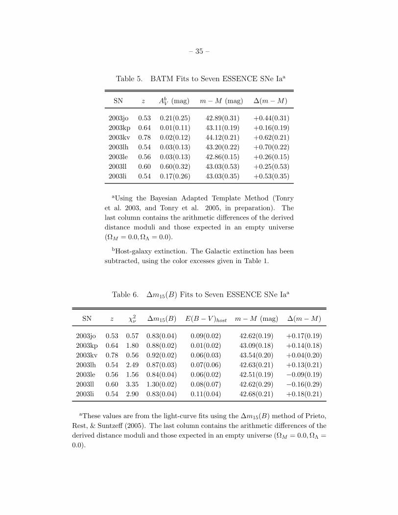
– 35 –

Table 5. BATM Fits to Seven ESSENCE SNe Iaa

SN z AbV

(mag) m − M (mag) ∆(m − M)

2003jo 0.53 0.21(0.25) 42.89(0.31) +0.44(0.31)

2003kp 0.64 0.01(0.11) 43.11(0.19) +0.16(0.19)

2003kv 0.78 0.02(0.12) 44.12(0.21) +0.62(0.21)

2003lh 0.54 0.03(0.13) 43.20(0.22) +0.70(0.22)

2003le 0.56 0.03(0.13) 42.86(0.15) +0.26(0.15)

2003ll 0.60 0.60(0.32) 43.03(0.53) +0.25(0.53)

2003li 0.54 0.17(0.26) 43.03(0.35) +0.53(0.35)

aUsing the Bayesian Adapted Template Method (Tonry

et al. 2003, and Tonry et al. 2005, in preparation). The

last column contains the arithmetic differences of the derived

distance moduli and those expected in an empty universe

(ΩM = 0.0,ΩΛ = 0.0).

bHost-galaxy extinction. The Galactic extinction has been

subtracted, using the color excesses given in Table 1.

Table 6. ∆m15(B) Fits to Seven ESSENCE SNe Iaa

SN z χ2ν ∆m15(B) E(B − V )host m − M (mag) ∆(m − M)

2003jo 0.53 0.57 0.83(0.04) 0.09(0.02) 42.62(0.19) +0.17(0.19)

2003kp 0.64 1.80 0.88(0.02) 0.01(0.02) 43.09(0.18) +0.14(0.18)

2003kv 0.78 0.56 0.92(0.02) 0.06(0.03) 43.54(0.20) +0.04(0.20)

2003lh 0.54 2.49 0.87(0.03) 0.07(0.06) 42.63(0.21) +0.13(0.21)

2003le 0.56 1.56 0.84(0.04) 0.06(0.02) 42.51(0.19) −0.09(0.19)

2003ll 0.60 3.35 1.30(0.02) 0.08(0.07) 42.62(0.29) −0.16(0.29)

2003li 0.54 2.90 0.83(0.04) 0.11(0.04) 42.68(0.21) +0.18(0.21)

aThese values are from the light-curve fits using the ∆m15(B) method of Prieto,

Rest, & Suntzeff (2005). The last column contains the arithmetic differences of the

derived distance moduli and those expected in an empty universe (ΩM = 0.0,ΩΛ =

0.0).

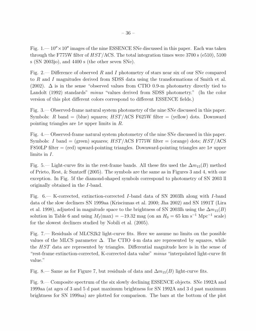
– 36 –

Fig. 1.— 10′′×10′′ images of the nine ESSENCE SNe discussed in this paper. Each was taken

through the F775W filter of HST/ACS. The total integration times were 3700 s (e510), 5100

s (SN 2003jo), and 4400 s (the other seven SNe).

Fig. 2.— Difference of observed R and I photometry of stars near six of our SNe compared

to R and I magnitudes derived from SDSS data using the transformations of Smith et al.

(2002). ∆ is in the sense “observed values from CTIO 0.9-m photometry directly tied to

Landolt (1992) standards” minus “values derived from SDSS photometry.” (In the color

version of this plot different colors correspond to different ESSENCE fields.)

Fig. 3.— Observed-frame natural system photometry of the nine SNe discussed in this paper.

Symbols: R band = (blue) squares; HST/ACS F625W filter = (yellow) dots. Downward

pointing triangles are 1σ upper limits in R.

Fig. 4.— Observed-frame natural system photometry of the nine SNe discussed in this paper.

Symbols: I band = (green) squares; HST/ACS F775W filter = (orange) dots; HST/ACS

F850LP filter = (red) upward-pointing triangles. Downward-pointing triangles are 1σ upper

limits in I.

Fig. 5.— Light-curve fits in the rest-frame bands. All these fits used the ∆m15(B) method

of Prieto, Rest, & Suntzeff (2005). The symbols are the same as in Figures 3 and 4, with one

exception. In Fig. 5f the diamond-shaped symbols correspond to photometry of SN 2003 ll

originally obtained in the I-band.

Fig. 6.— K-corrected, extinction-corrected I-band data of SN 2003lh along with I-band

data of the slow decliners SN 1999aa (Krisciunas et al. 2000; Jha 2002) and SN 1991T (Lira

et al. 1998), adjusted in magnitude space to the brightness of SN 2003lh using the ∆m15(B)

solution in Table 6 and using MI(max) = −19.32 mag (on an H0 = 65 km s−1 Mpc−1 scale)

for the slowest decliners studied by Nobili et al. (2005).

Fig. 7.— Residuals of MLCS2k2 light-curve fits. Here we assume no limits on the possible

values of the MLCS parameter ∆. The CTIO 4-m data are represented by squares, while

the HST data are represented by triangles. Differential magnitude here is in the sense of

“rest-frame extinction-corrected, K-corrected data value” minus “interpolated light-curve fit

value.”

Fig. 8.— Same as for Figure 7, but residuals of data and ∆m15(B) light-curve fits.

Fig. 9.— Composite spectrum of the six slowly declining ESSENCE objects. SNe 1992A and

1999aa (at ages of 3 and 5 d past maximum brightness for SN 1992A and 3 d past maximum

brightness for SN 1999aa) are plotted for comparison. The bars at the bottom of the plot

– 37 –

show the wavelength range of each object’s spectrum used for the composite spectrum.

Fig. 10.— Histogram of decline-rate values [∆m15(B)] for 107 nearby SNe Ia (Gallagher et

al. 2005) and values for seven ESSENCE SNe from Table 6. Clearly, most of the ESSENCE

objects have slow decline rates compared to the local sample.

Fig. 11.— Typical pre-maximum detection window for SNe Ia discovered with the CTIO

4-m telescope. We assume 0.9′′ seeing, S/N & 10, and a detection threshold of R = 23.0

mag. ESSENCE fields are typically imaged (or “visited”) every 4 days. Under typical seeing

conditions, most of the SNe Ia discovered with z & 0.60 will have slow decline rates.

Fig. 12.— Spectra of two nearby SNe Ia, redshifted by the indicated amounts, and super-

imposed on the spectrum of SN 2003ku. “Normalized flux” means that a pseudo-continuum

has been subtracted from the spectra.

Fig. 13.— Differential Hubble diagram for SNe Ia. For each object we plot the distance

modulus derived from the light curves minus the distance modulus in an empty universe vs.

the redshift. See Table 4. The yellow dots are the “gold” data set of 157 SNe Ia from Riess et

al. (2004). The ESSENCE SNe Ia are represented by larger squares. SN 2003ll is represented

by a red square having a distance modulus 0.72 mag brighter than the empty-universe model.

The dashed line is the concordance model (ΩM = 0.3, ΩΛ = 0.7). The solid horizontal line

corresponds to distance moduli in the empty-universe model. The dotted line corresponds

to an open universe with ΩM = 0.3 and ΩΛ = 0.0.

Fig. 14.— Constraints on the dark energy (ΩΛ) using the nearby SNe Ia of the “gold” set of

Riess et al. (2004), plus seven ESSENCE SNe Ia. We show sets of 1σ, 2σ, and 3σ contours.

The solid lines use a constraint that MLCS ∆ ≥ −0.40. The dashed contours assume no

constraints on MLCS ∆.

Fig. 15.— Constraints on the dark energy (ΩΛ) using the entire gold set of 157 SNe Ia from

Riess et al. (2004), plus 7 ESSENCE SNe Ia. We show sets of 1σ, 2σ, and 3σ contours. The

thin lines come from the SN constraints only and assume the prior constraint that MLCS

∆ ≥ −0.40. The thick lines include a matter density constraint of ΩM = 0.233 ± 0.030, in

accord with the results of Cole et al. (2005) and H0 = 72 km s−1Mpc−1 (Freedman et al.

2001). The dashed contours include a different matter constraint, that of Eisenstein et al.

(2005), namely ΩM = 0.273 ± 0.025 + 0.137ΩK . We assume w = −1.

Fig. 16.— Constraints on the equation-of-state parameter w using the Riess et al. (2004)

gold set of 157 SNe Ia, plus 7 ESSENCE SNe Ia. We show sets of 1σ, 2σ, and 3σ contours.

The thin lines come from the SN constraints only, while the thick lines are constrained by

– 38 –

SNe plus a matter density of ΩM = 0.233 ± 0.030 (Cole et al. 2005), which implies H0 =

72 km s−1Mpc−1 (Freedman et al. 2001). The dashed contours show the effect of using no

prior contraint on the allowable range of MLCS ∆.

Fig. 17.— The throughput of the F625W, F775W, and F850LP filters as used with the

HST/ACS. The curves include the filter transmission functions multiplied by the quantum

efficiency as a function of wavelength.

Fig. 18.— Effective filter transmission curves of the R and I filters used for ground-based

photometry with the CTIO 4-m telescope. These curves show the fractional transmission

as a function of wavelength. We included the filter transmission functions determined in

the laboratory, one aluminum reflection for the effect of the primary mirror, the quantum

efficiency of the CCDs, the atmospheric extinction, and the major telluric absorption lines.

To obtain the curves used by Bessell (1990) one must multiply these curves by the wavelength.

– 39 –

Krisciunas et al. Fig. 1

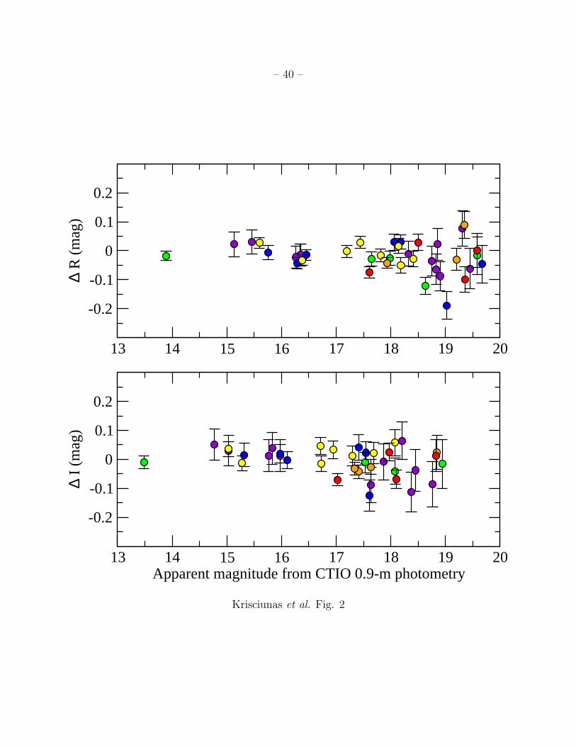
– 40 –

13 14 15 16 17 18 19 20

-0.2

-0.1

0

0.1

0.2

∆ R

(m

ag)

13 14 15 16 17 18 19 20Apparent magnitude from CTIO 0.9-m photometry

-0.2

-0.1

0

0.1

0.2

∆ I (

mag

)

Krisciunas et al. Fig. 2

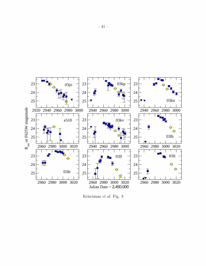
– 41 –

2920 2940 2960 2980 3000

23

24

25

2940 2960 2980 3000

23

24

25

2940 2960 2980 3000

23

24

25

2960 2980 3000 3020

23

24

25

Rna

t or

F62

5W m

agni

tude

2940 2960 2980 3000

23

24

25

2960 2980 3000 3020

23

24

25

2960 2980 3000 3020

23

24

25

2960 2980 3000 3020Julian Date − 2,450,000

23

24

25

2960 2980 3000 3020

23

24

25

03jo 03kp

03ku

e510 03kv

03lh

03le

03ll 03li

Krisciunas et al. Fig. 3

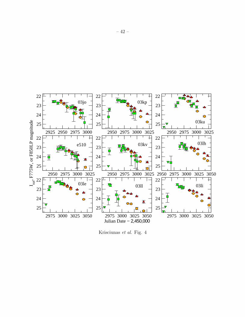
– 42 –

2925 2950 29753000

22

23

24

25

2950 2975 3000 3025

22

23

24

25

2950 2975 3000 3025

22

23

24

25

2950 2975 3000 3025

22

23

24

25

I nat, F

775W

, or

F85

0LP

mag

nitu

de

2950 2975 3000 3025

22

23

24

25

2950 2975 3000 3025 3050

22

23

24

25

2975 3000 3025 3050

22

23

24

25

2975 3000 3025 3050Julian Date − 2,450,000

22

23

24

25

2975 3000 3025 3050

22

23

24

25

03jo 03kp

03ku

e510 03kv 03lh

03le 03ll 03li

Krisciunas et al. Fig. 4

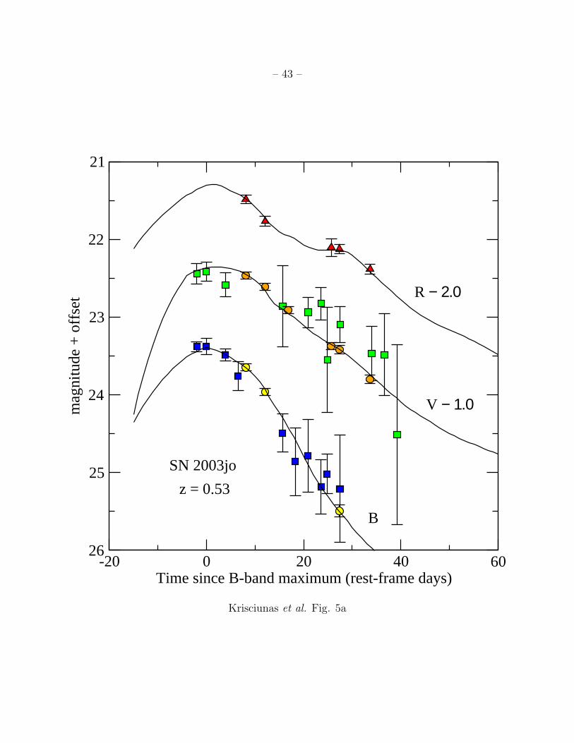
– 43 –

-20 0 20 40 60Time since B-band maximum (rest-frame days)

21

22

23

24

25

26

mag

nitu

de +

offs

et

SN 2003jo

z = 0.53

B

V − 1.0

R − 2.0

Krisciunas et al. Fig. 5a

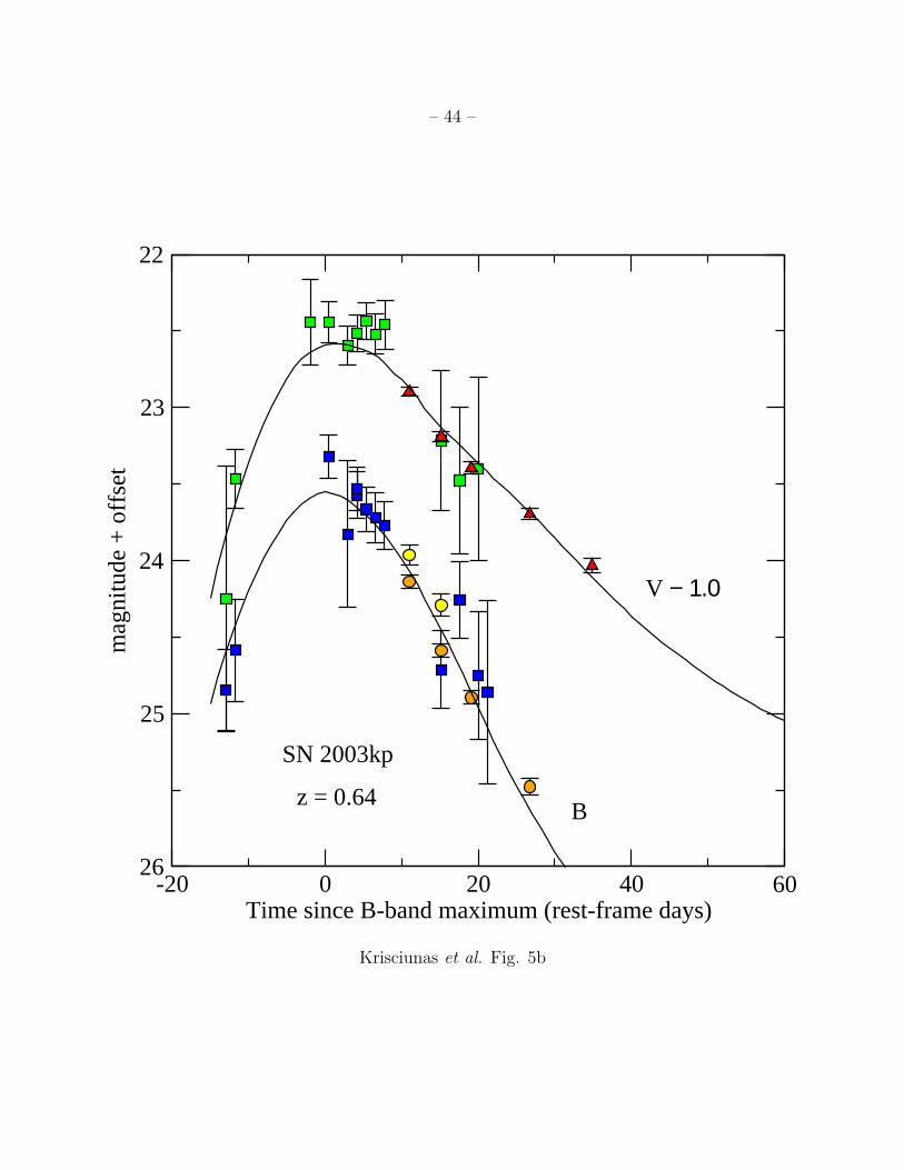
– 44 –

-20 0 20 40 60Time since B-band maximum (rest-frame days)

22

23

24

25

26

mag

nitu

de +

offs

et

SN 2003kp

z = 0.64

V − 1.0

B

Krisciunas et al. Fig. 5b

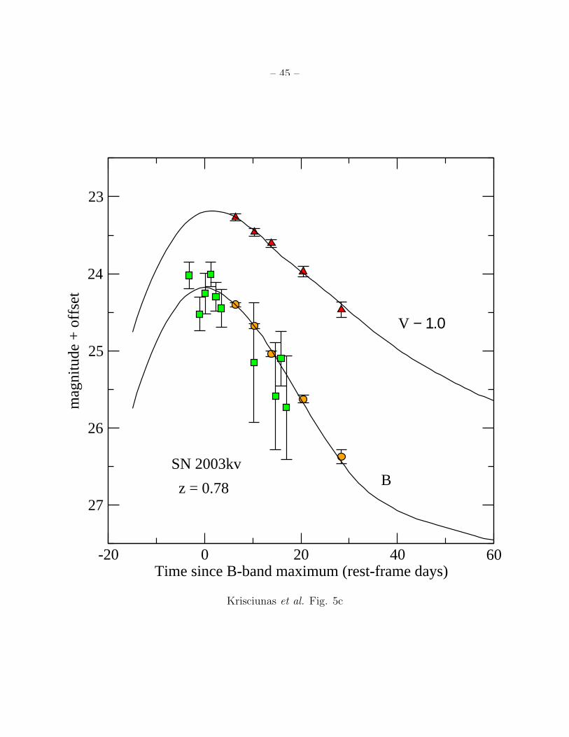
– 45 –

-20 0 20 40 60Time since B-band maximum (rest-frame days)

23

24

25

26

27

mag

nitu

de +

offs

et

SN 2003kv

z = 0.78

V − 1.0

B

Krisciunas et al. Fig. 5c

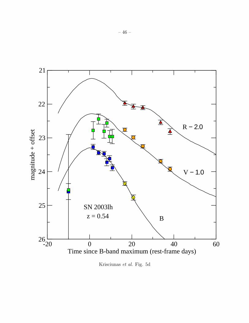
– 46 –

-20 0 20 40 60Time since B-band maximum (rest-frame days)

21

22

23

24

25

26

mag

nitu

de +

offs

et

SN 2003lhz = 0.54 B

V − 1.0

R − 2.0

Krisciunas et al. Fig. 5d

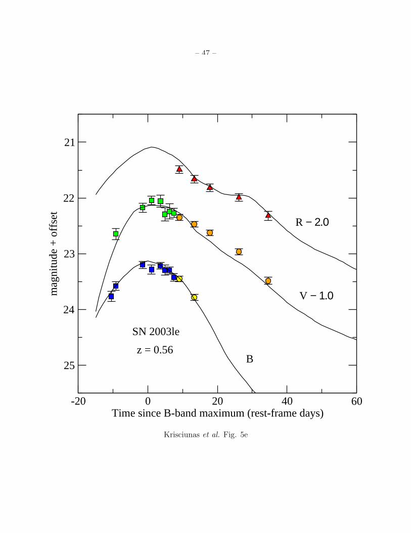
– 47 –

-20 0 20 40 60Time since B-band maximum (rest-frame days)

21

22

23

24

25

mag

nitu

de +

offs

et

SN 2003le

z = 0.56B

V − 1.0

R − 2.0

Krisciunas et al. Fig. 5e

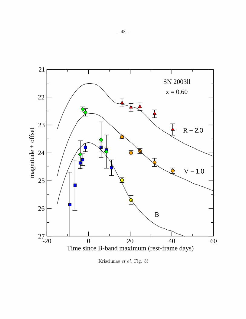
– 48 –

-20 0 20 40 60Time since B-band maximum (rest-frame days)

21

22

23

24

25

26

27

mag

nitu

de +

offs

et

SN 2003ll

z = 0.60

B

V − 1.0

R − 2.0

Krisciunas et al. Fig. 5f

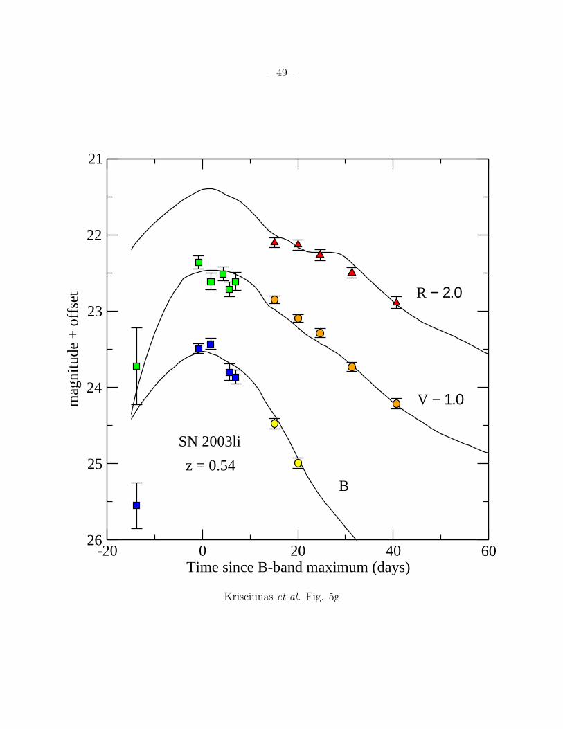
– 49 –

-20 0 20 40 60Time since B-band maximum (days)

21

22

23

24

25

26

mag

nitu

de +

offs

et

SN 2003li

z = 0.54B

V − 1.0

R − 2.0

Krisciunas et al. Fig. 5g

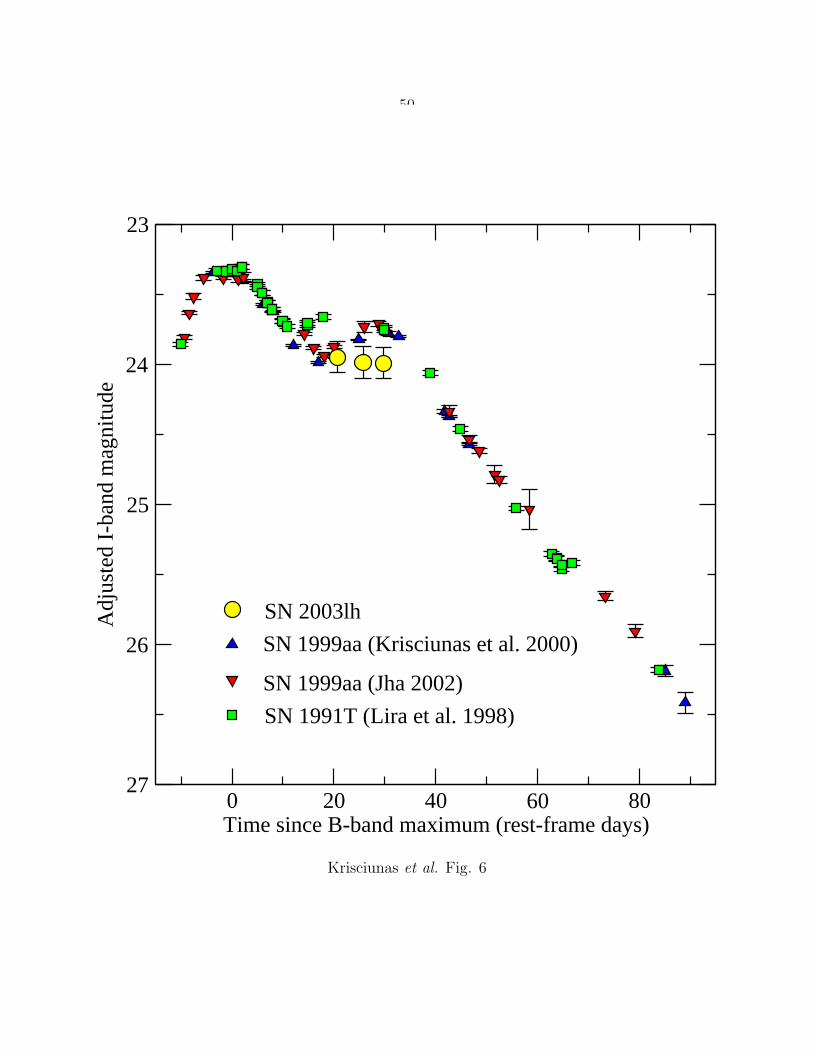
– 50 –

0 20 40 60 80Time since B-band maximum (rest-frame days)

23

24

25

26

27

Adj

uste

d I-

band

mag

nitu

de

SN 2003lh

SN 1999aa (Krisciunas et al. 2000)

SN 1999aa (Jha 2002)

SN 1991T (Lira et al. 1998)

Krisciunas et al. Fig. 6

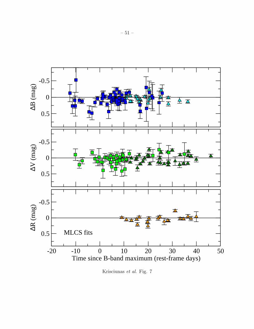
– 51 –

-0.5

0

0.5

∆B (

mag

)

-0.5

0

0.5

∆V (

mag

)

-20 -10 0 10 20 30 40 50Time since B-band maximum (rest-frame days)

-0.5

0

0.5

∆R (

mag

)

MLCS fits

Krisciunas et al. Fig. 7

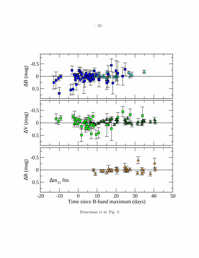
– 52 –

-0.5

0

0.5

∆B (

mag

)

-0.5

0

0.5

∆V (

mag

)

-20 -10 0 10 20 30 40 50Time since B-band maximum (days)

-0.5

0

0.5

∆R (

mag

)

∆m15

fits

Krisciunas et al. Fig. 8

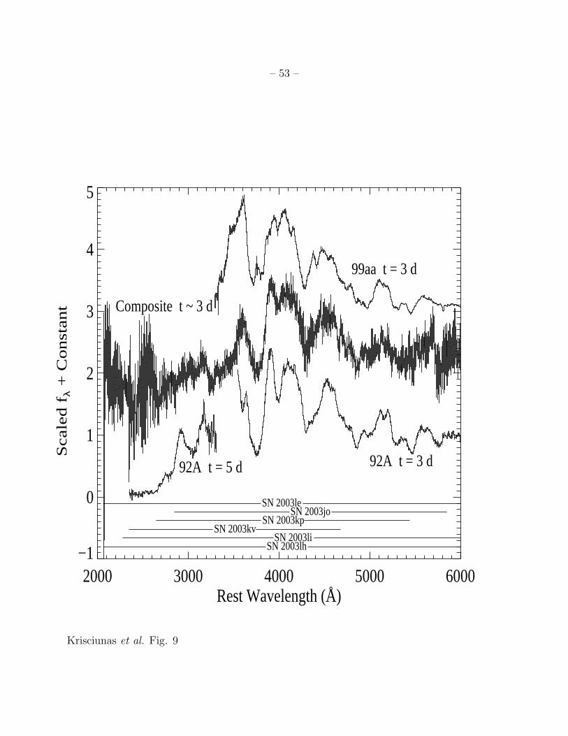
– 53 –

2000 3000 4000 5000 6000Rest Wavelength (Å)

−1

0

1

2

3

4

5

Sca

led

f λ +

Co

nsta

nt

SN 2003lhSN 2003li

SN 2003kvSN 2003kp

SN 2003joSN 2003le

99aa t = 3 d

92A t = 3 d92A t = 5 d

Composite t ~ 3 d

Krisciunas et al. Fig. 9

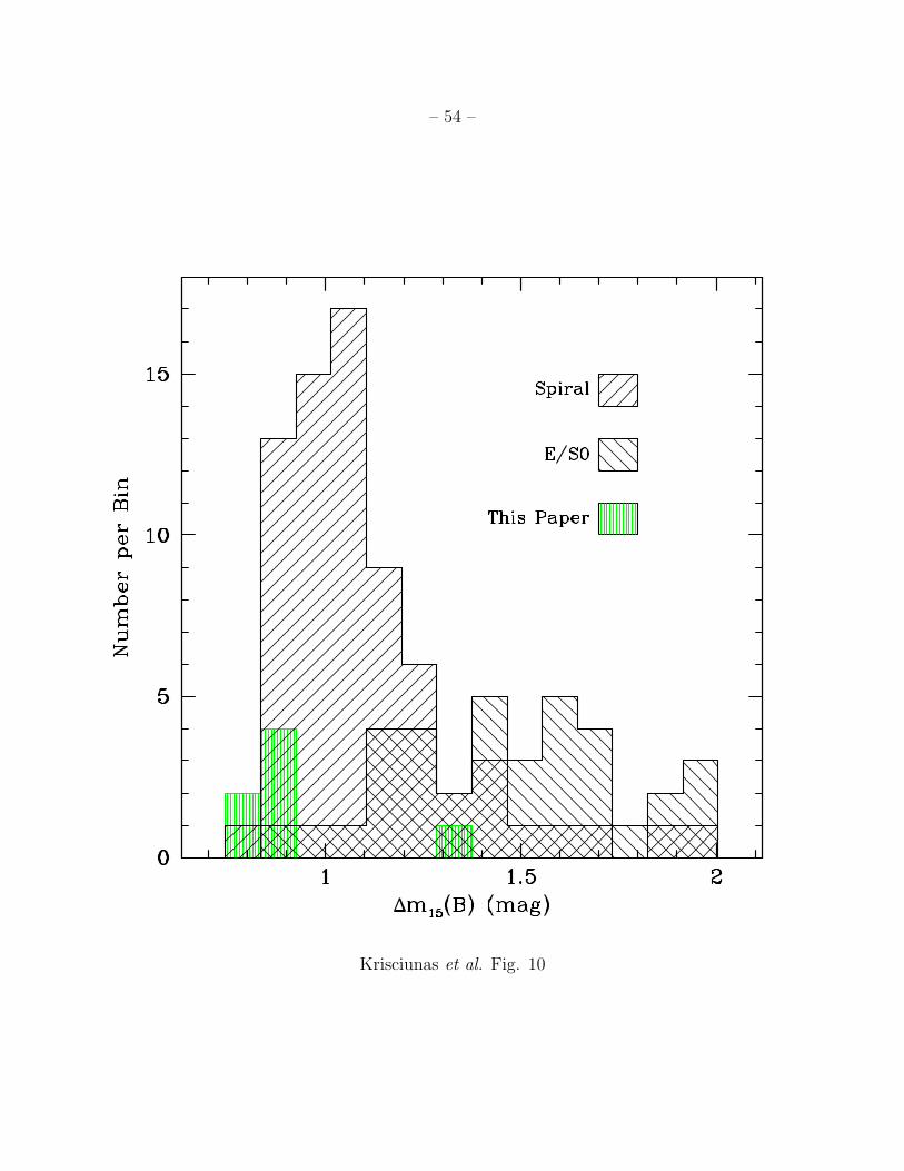
– 54 –

Krisciunas et al. Fig. 10

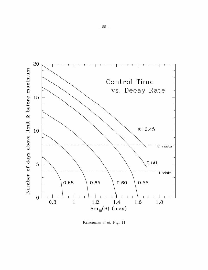
– 55 –

Krisciunas et al. Fig. 11

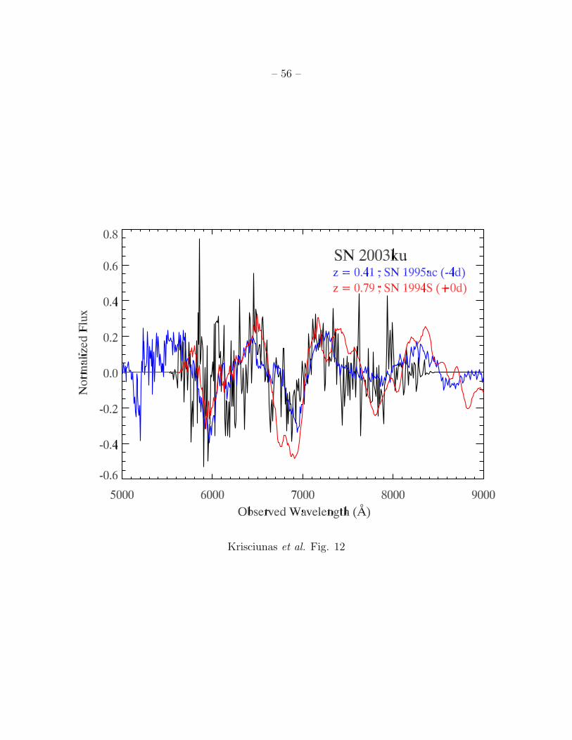
– 56 –

Krisciunas et al. Fig. 12

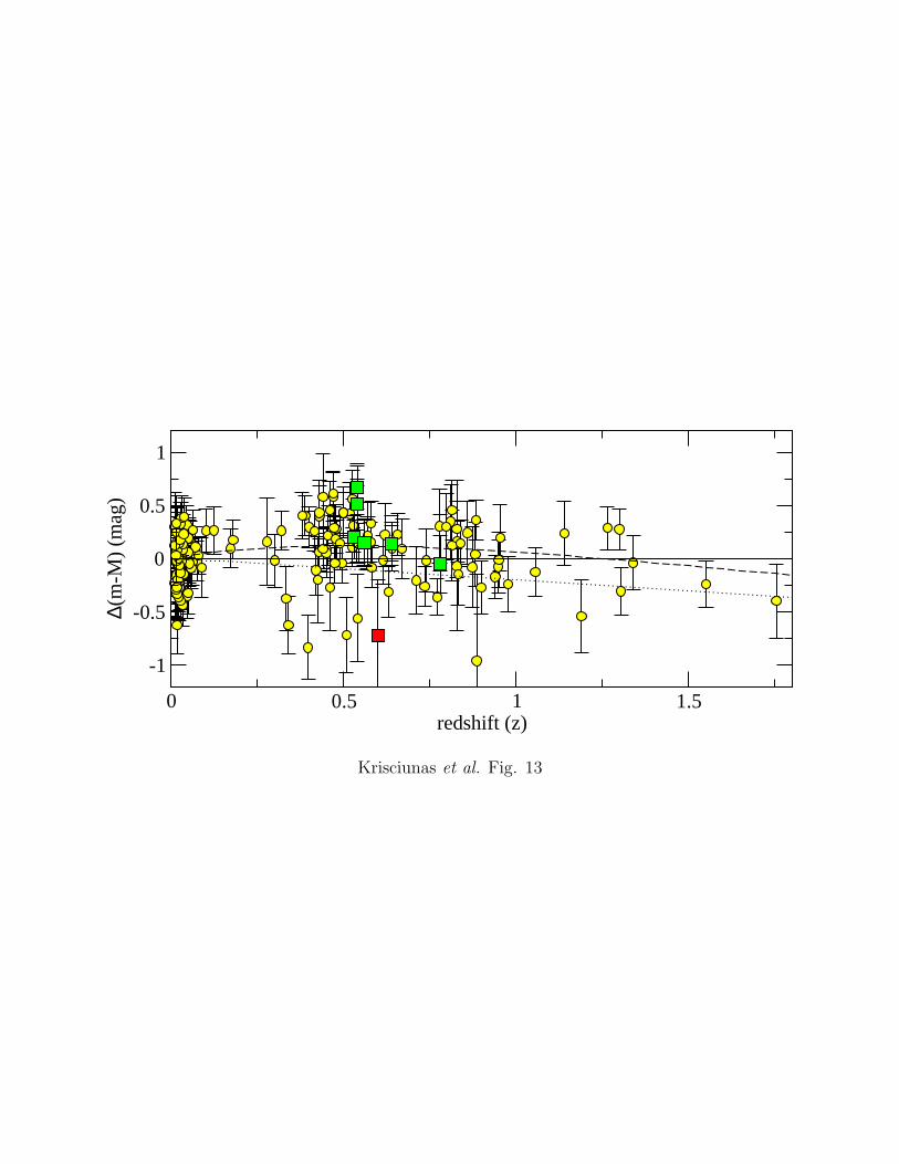
– 57 –

0 0.5 1 1.5redshift (z)

-1

-0.5

0

0.5

1

∆(m

-M)

(mag

)

Krisciunas et al. Fig. 13

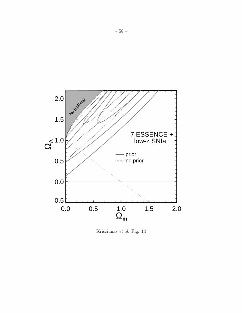
– 58 –

0.0 0.5 1.0 1.5 2.0-0.5

0.0

0.5

1.0

1.5

2.0

Ωm

ΩΛ

7 ESSENCE +low-z SNIa

priorno prior

No Big

Bang

Krisciunas et al. Fig. 14

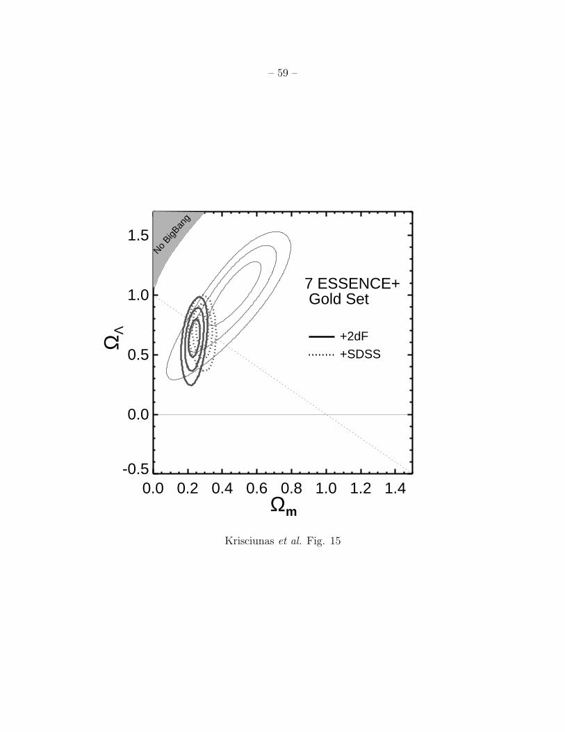
– 59 –

0.0 0.2 0.4 0.6 0.8 1.0 1.2 1.4-0.5

0.0

0.5

1.0

1.5

Ωm

ΩΛ

7 ESSENCE+Gold Set

+2dF

+SDSS

No Big

Bang

Krisciunas et al. Fig. 15

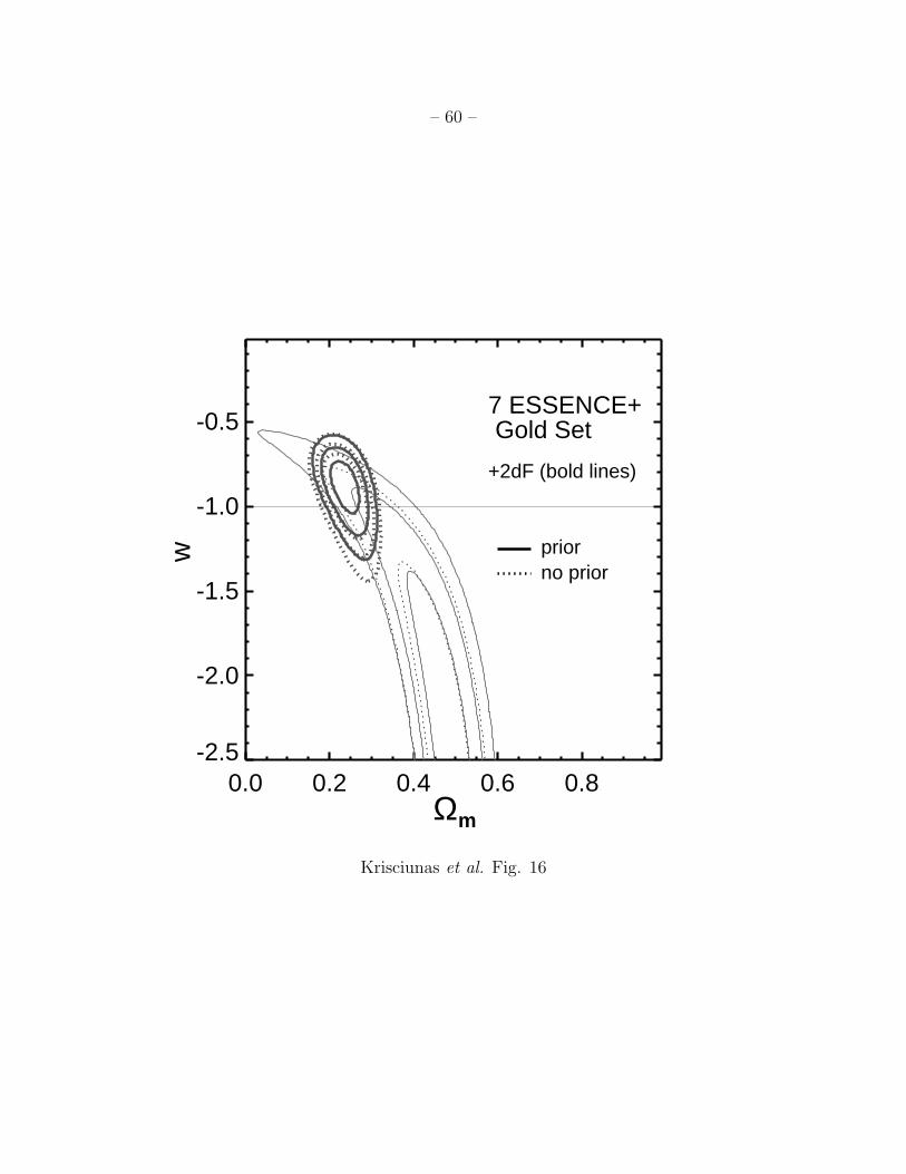
– 60 –

0.0 0.2 0.4 0.6 0.8-2.5

-2.0

-1.5

-1.0

-0.5

Ωm

w

7 ESSENCE+Gold Set

+2dF (bold lines)

prior no prior

Krisciunas et al. Fig. 16

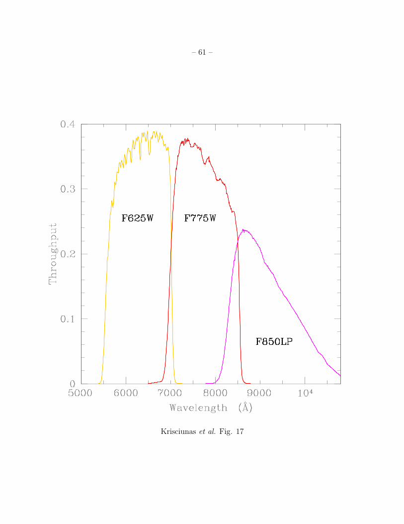
– 61 –

Krisciunas et al. Fig. 17

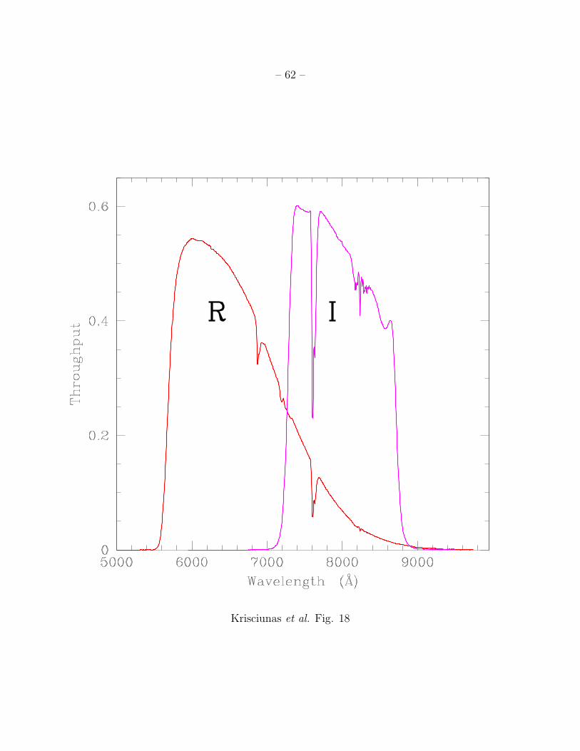
– 62 –

Krisciunas et al. Fig. 18