Https jyx jyu fi dspace bitstream handle 123456789 13594 URN NBN fi jyu-2007600

The Role of Timbre in the Memorization of Microtonal

Intervals

Pro GraduRafael Ferrer Flores

Department of MusicUniversity of Jyväskylä

September 2007

JYVÄSKYLÄN YLIOPISTO

Tiedekunta - Faculty

Humanities

Laitos - Department

Music

Tekijä - Author

Rafael Ferrer Flores

Työn nimi - Title

The Role of Timbre in the Memorization of Microtonal Intervals

Oppiaine - Subject

Music, Mind and Technology

Työn laji - Level

Master's Thesis

Aika - Month and year

September 2007

Sivumäärä - Number of pages

68

Tiivistelmä - Abstract

The aim of this thesis was to determine if timbre has any effect in the memorization of

melodic intervals. For this purpose, a test was developed in which 23 subjects heard

an interval, and after 7 seconds of silence were played three options from which they

had to select the original interval. The sound samples composing each target interval,

had one control and three degrees of timbral modification. Such modifications

consisted in altering the original partial structure of the sound samples. Spectral

Modelling and Additive Synthesis techniques were used to realize these modifications.

Results suggest that is possible to enhance or impair the ability of extracting cues for

memorizing intervals by altering timbral structure.

Asiasanat - Keywords

timbre, memory, ear training

Säilytyspaikka - Depository

Muita tietoja - Additional information

Abstract

The aim of this thesis was to determine if timbre has any effect in the

memorization of melodic intervals. For this purpose, a test was developed in which 23

subjects heard an interval, and after 7 seconds of silence were played three options from

which they had to select the original interval. The sound samples composing each target

interval, had one control and three degrees of timbral modification. Such modifications

consisted in altering the original partial structure of the sound samples. Spectral

Modelling and Additive Synthesis techniques were used to realize these modifications.

Results suggest that is possible to enhance or impair the ability of extracting cues for

memorizing intervals by altering timbral structure.

Table of Contents

1 Introduction........................................................................................................7

2 Theoretical considerations...............................................................................10

2.1 Music education..........................................................................................12

2.1.1 Ear training....................................................................................13

2.1.2 Intervals.........................................................................................14

2.2 Timbre.........................................................................................................15

2.2.1 Timbre and scales..........................................................................18

2.2.1.1Spectral shape..............................................................................18

2.2.1.2Consonance / Dissonance.............................................................19

2.2.1.3Scales...........................................................................................20

2.2.1.4Relations between timbre, consonance and scale........................21

2.3 Memory......................................................................................................24

2.3.1 A three stages in one.....................................................................24

2.3.1.1Sensory memory..........................................................................24

2.3.1.2Short-term memory......................................................................25

2.3.1.3Long-term memory......................................................................26

2.3.1.4Working memory.........................................................................26

2.3.2 Memory for timbre........................................................................26

3 Empirical approach..........................................................................................28

3.1 Method........................................................................................................28

3.1.1 Design...........................................................................................28

3.1.2 Participants....................................................................................29

3.1.3 Materials........................................................................................30

3.1.3.1Stimuli..........................................................................................30

Selection..................................................................................................30

Discrimination.........................................................................................31

Analysis...................................................................................................31

Synthesis.................................................................................................35

3.1.3.2Apparatus.....................................................................................41

3.1.4 Procedure.......................................................................................42

3.1.5 Results...........................................................................................42

3.2 Discussion...................................................................................................46

3.2.1 Adaptability...................................................................................48

3.2.2 Timbre descriptors.........................................................................50

4 Conclusions.......................................................................................................57

References..............................................................................................................59

Appendix A. Instructive of the experiment............................................................67

Appendix B. Questionnaire....................................................................................68

Index of Illustrations

Figure 1. Representation of sensory dissonance by Plompt & Levelt...........................21

Figure 2. Roughness and ratios......................................................................................22

Figure 3. Example of dissonance curve computed with Sethares' algorithm................23

Figure 4. Design of the experiment...............................................................................29

Figure 5. Minima hits from 73 dissonance curves.........................................................32

Figure 6. Mean dissonance curve for a set of 73 different timbres...............................33

Figure 7. Representation of timbre in relation with the steps of different scales..........37

Figure 8. Example of adjustment of timbral structure...................................................38

Figure 9. Synthesis types...............................................................................................40

Figure 10. Appearance of the experimental interface....................................................41

Figure 11. Accuracy per interval....................................................................................44

Figure 12. Accuracy per Synthesis Type.......................................................................45

Figure 13. Accuracy per Instrument Type.....................................................................46

Figure 14. Tendency of responses .................................................................................47

Figure 15. Histogram of responses................................................................................47

Figure 16. Adaptability per interval...............................................................................49

Figure 17. Overall Adaptability.....................................................................................50

Figure 18. One-way ANOVA between timbres of two synthesis groups 'ad' & 'sq'......51

Figure 19. One-way ANOVA between timbres of two synthesis groups, two data sets53

Figure 20. Correlation between behavioural and acoustical data..................................54

Figure 21. Scatter plots of relevant timbral descriptors and behavioural data..............55

Index of Tables and Formulas

Table 1.   Convergence of ratios from different sources..................................................22

Table 2.   Tabulated frequencies for interval selection....................................................34

Table 3.   Example of selection of candidates..................................................................36

Table 4.   Different combination of subsets to test syntheses type with one­way ANOVA

.........................................................................................................................................45

Formula 1.   Computation of ratios for a 12 tone equally tempered system....................20

Formula 2.   Relation of partials and steps of a scale......................................................36

7

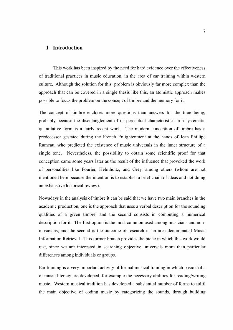
1 Introduction

This work has been inspired by the need for hard evidence over the effectiveness

of traditional practices in music education, in the area of ear training within western

culture. Although the solution for this problem is obviously far more complex than the

approach that can be covered in a single thesis like this, an atomistic approach makes

possible to focus the problem on the concept of timbre and the memory for it.

The concept of timbre encloses more questions than answers for the time being,

probably because the disentanglement of its perceptual characteristics in a systematic

quantitative form is a fairly recent work. The modern conception of timbre has a

predecessor gestated during the French Enlightenment at the hands of Jean Phillipe

Rameau, who predicted the existence of music universals in the inner structure of a

single tone. Nevertheless, the possibility to obtain some scientific proof for that

conception came some years later as the result of the influence that provoked the work

of personalities like Fourier, Helmholtz, and Grey, among others (whom are not

mentioned here because the intention is to establish a brief chain of ideas and not doing

an exhaustive historical review).

Nowadays in the analysis of timbre it can be said that we have two main branches in the

academic production, one is the approach that uses a verbal description for the sounding

qualities of a given timbre, and the second consists in computing a numerical

description for it. The first option is the most common used among musicians and non-

musicians, and the second is the outcome of research in an area denominated Music

Information Retrieval. This former branch provides the niche in which this work would

rest, since we are interested in searching objective universals more than particular

differences among individuals or groups.

Ear training is a very important activity of formal musical training in which basic skills

of music literacy are developed, for example the necessary abilities for reading/writing

music. Western musical tradition has developed a substantial number of forms to fulfil

the main objective of coding music by categorizing the sounds, through building

8

minimal construction blocks and creating a taxonomy for its physical characteristics.

Within this mentioned forms we picked one that can be presumed as generic, because it

can be found in the basic steps of most methodologies. It consists in the identification

of melodic intervals, which can be defined as the perceptual distance between two

consecutive musical tones.

In this task of identifying morphologies such as a claimed distance between two fixed

points, the role of memory is the central matter, because just as another perceptual

categories like the visual stimuli evoked by an sculpture and which has its dominion

over a constant space, the auditive stimuli resulting from music exists only in the

ephemeral present. Implying with this that music has its dominion over time and

proposing that memory can be seen as a human capability meant to recreate past

experiences and project them in the future; just as it is the purpose of learning.

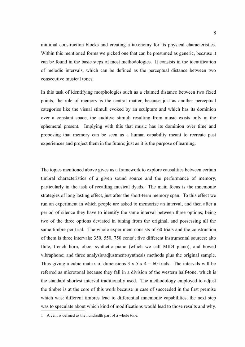
The topics mentioned above gives us a framework to explore causalities between certain

timbral characteristics of a given sound source and the performance of memory,

particularly in the task of recalling musical dyads. The main focus is the mnemonic

strategies of long lasting effect, just after the short-term memory span. To this effect we

run an experiment in which people are asked to memorize an interval, and then after a

period of silence they have to identify the same interval between three options; being

two of the three options deviated in tuning from the original, and possessing all the

same timbre per trial. The whole experiment consists of 60 trials and the construction

of them is three intervals: 350, 550, 750 cents1; five different instrumental sources: alto

flute, french horn, oboe, synthetic piano (which we call MIDI piano), and bowed

vibraphone; and three analysis/adjustment/synthesis methods plus the original sample.

Thus giving a cubic matrix of dimensions 3 x 5 x 4 = 60 trials. The intervals will be

referred as microtonal because they fall in a division of the western half-tone, which is

the standard shortest interval traditionally used. The methodology employed to adjust

the timbre is at the core of this work because in case of succeeded in the first premise

which was: different timbres lead to differential mnemonic capabilities, the next step

was to speculate about which kind of modifications would lead to those results and why.

1 A cent is defined as the hundredth part of a whole tone.

9

The main strategy consisted in subtracting the target intervals from the timbral structure

of the tones, but the entire process is explained in detail in section 3.1.3.1.

The text is divided mainly in two parts, being the first the theoretical framework which

provides a general overview and in some cases a plain summary of some works related

with music education, timbre and memory. The second is a rigorous empirical

approach, which explains step by step the experiment done for this work, from the

design, participants and materials to the procedure, results and discussion.

10

2 Theoretical considerations

A substantial amount of academic production in music analysis is focused in

written music, and most musicologists would agree that the invention of a set of

symbols to code music represented the most important advance in the history of western

music. It allowed the rapid evolution of music because the separation of human and

epistemic objects (Bent & Pople, 2006). Nevertheless, that code has also a disadvantage,

because it is just a gross representation of the actual sound itself.

The unveiling of structure and form is the outcome of analysis, therefore is generally

admitted that music structure relies on rhythm, pitch and timbre. Other categories can

be considered as the result of the combination of these three features, as it is the case for

melody and harmony.

The set of symbols written in a score fitted very well to study the cognitive processes

involved in music in terms of rhythm and pitch, but unfortunately that was not the case

for music outside those symbols, for example the music that makes use of timbre as the

main aesthetic resource (Fales, 2002, p.57).

Signal processing technology is related from its semantic origin to communication and

codification. This technology can be seen as a new way to represent sounds in a more

accurate way, for instance, it is possible to visualize timbre changes as a function of

time, which has permitted speculation about music structure focusing on timbre features

(Wessel, 1979), and which goes beyond the symbolic representation of a sound in a

score, opening the possibility to understand the role of timbre in learning music.

With the use of new technologies in music education, it is common to find electronic

devices in the classroom producing synthetic sounds, for example in the ear training

class in which some teachers also send their students to self-study practices with

software made for that specific purpose. At this point one can speculate about the

effectiveness of training the ear with one synthetic sound or another, or to be more

specific to understand the characteristics of that sound in order to improve the

applications. On the other hand it is important to understand that the relevance of ear

11

training relies on the fact that it is not the ear that it is actually trained, but the cognitive

schema which takes the form of an image in the brain of each individual. Thus to train

the ear can be explained as the improvement of precision in music imagery within a

particular tonal schema, because before reading, writing, performing or analysing music

one has to make an image of it in the mind (Pitt & Crowder, 1992; Gordon, 1997).

The perception of different timbres must lead to the acquisition of different images, but

is there a set of characteristics in timbre that can imprint in mind better than others? Can

we find a good set of timbres to improve the ear training? Is timbre a relevant feature in

the optimization of learning music? Is there any especially commendable instrument to

teach the most basic aspects of tonal schema?

Although research in musical timbre has a relatively short history, there is crescent

empirical evidence of its relevance for the perception of music. In traditional music

education in the western culture, the most closely related topic to the study of timbre

can be found in the courses of orchestration, but the approach is bounded to its aesthetic

origins, which undoubtedly is the result of many years of evolution in seeking for

functionality for the senses (Helmholtz, 1954). Nevertheless that argued functionality

has been reached through unconscious processes, and the stress in pedagogical

applications has been left unattended. There are of course exemplar efforts like the

work of Jaques-Dalcroze, Kodály, and Orff, whom specified in their pedagogical

methodologies the timbres to be used in the early stages of musical development

(Choksy, Abramson, Gillespie, Woods, York, 2001). Though this area remains

unquestioned in a systematic way, since there is a lack of literature dealing for instance,

with the differential musical abilities acquired by using only voice or the instrumental

set suggested by Orff. Furthermore in the area of music education for adults it is urgent

to understand how different instruments could optimize the musical learning, for

example in those countries were the official curricula does not contemplate musical

training as an indispensable part of education for the plenary development of the

individuals.

In the process of learning viewed from the cognitive perspective, memory has a central

role not as a container of information, but as a dynamic unit capable of systematize the

perception (Pantev, 2001, p.301). Auditory memory is divided in three different

12

categories according with the span of retention of perceived phenomena. These three

categories are not isolated blocks of processing, instead, they actually work together at

any given instant, and this interaction receives the name of working memory. The first

category is the echoic memory, and it is related with events happening in no more than

few seconds. The second is referred to as short-term memory and studies the

phenomena happening after the echoic memory and within a time span of approximately

8 seconds. And the third is the long-term memory, which can be considered the most

stable because the qualities of the information it ‘retains’, that can be reconstruction of

events that had happen in the past beyond the domain of short-term memory, or

conditions that had been rehearsed several times. Long-term memory is also related

with the idea of schema, which is a kind of superior learning controlling the perception

of new phenomena (Leman, 1995; Snyder, 2000).

2.1 Music education

Learning has two sides; one is the biological fact of genetic heritage, and the

other has to be with the sophistication of strategies to take advantage of that genetic

heritage. Music has these two sides when it is learned (Papoušek, 2003), and for that

reason there is no need to receive any special instruction to understand music, although

in order to communicate particular ways to organize sounds we actually do.

In western culture for example, the degree of systematization of music has evolved in

schools specialized in the teaching of music, and music education is subject to certain

conventions depicted in the contents of the curricula and in the role of music and

musicians in every society. However, among the obvious differences between each

society, one idea has been preserved since the foundations of western culture: not all the

individuals in the society are supposed to become producers of music, therefore, it can

be expected that among the three main musical activities; composition, performance and

analysis (Choksy, Abramson, Gillespie, Woods, York, 2001), every person must posses a

fair knowledge in at least one of them. Consequently it can be presumed that

alphabetized individuals in western world have a minimum skill to analyse music

(Serafine, 1988).

13

Western culture and its idea of music education has spread in many parts of the world,

but in each geographical region there is a particular set of instruments used, as well as

the time dedicated to learn music as a part of general education (Hargreaves & North,

2001).

By considering the immense diversity of musical sound sources, it is unavoidable to

question if there is no other better way to be educated musically than with the traditional

practices gestated in central Europe during the last millennium. Moreover, it is

imperative to acknowledge that technology is introducing in a very fast manner new

sounds and aesthetic forms, and that we must be prepared to understand how they will

affect our perception of music in the near future.

2.1.1 Ear training

There are two main sources of music education; the proper music education that

is realized in the institutions dedicated specifically to education or as a complement of

general education, and the music education implicit in the oral tradition of music. In the

institutionalized music education ear training is at the core of the curricula for example

in Germany (Hargreaves & North, 2001, p.47), Italy where one of the main aims is “to

sharpen perceptive abilities” (p.79) and Poland (p.139). A relevant data in the case of

Germany is that 13% of the teachers surveyed in 1995 had experience with MIDI

technology in the classroom.

Computer assisted instruction is an approach in ear training, that has been growing for

more than a quarter of century, like GUIDO, which was presented as an Interactive

Computer-Based system for Improvement of Instruction and Research in Ear-Training

(Hofstetter, 1975). More recent methods which being printed material also include the

possibility to access through internet to auditive media, like the Benward & Kolosick

method (2005), use a recorded piano to play the exercises. Also recent versions of

software dedicated to ear training use synthetic sounds reproduced with a MIDI capable

device, for instance Ear Master 5 (2007). But again, the documentation related with the

qualities of sound source or timbre is poor or unexistent.

As stated by Sloboda (2005), ear training is an area in which teachers are used to

14

discuss “developing a good ear”, although from the scientific point of view most

people’s ears function excellently, and there is nothing one can do to enhance their

functioning. The idea is to find out what needs to happen in the brain to produce the

behaviour that musicians would associate with a “good ear” (p.176). For that effect, the

music learning theory developed by Edwin E. Gordon (1997) fits very well; in his book

entitled Learning Sequences in Music the main focus of attention is in the concept of

audiation. Gordon explains that audiation happens when we assimilate music that we

have heard or performed, and also when we assimilate and comprehend in our minds the

music that comes from a symbolic representation of it (p.4); through this description of

the concept it is easy to understand that the term audiation refers the same phenomena

that Crowder & Pitt (1992) described as “imagery in music”. They attract the work of

Hebb (Concerning Imagery, 1968) to explain that “imagery representation is the

activation of the same central neural systems that played a role in the original event, but

this time in the absence of the original sensory activity” (p.30). Imagery is linked to

perception, and in the particular case of timbre it has demonstrated a high correlation by

using behavioural and neural data (Halpern, Zatorre, Bouffard & Johnson, 2004).

2.1.2 Intervals

The plain definition of a musical interval is referred as the distance between two

tones, but this definition brings some complexities if one think about the perceptual

meaning of a distance in the world of sounds, and even more if we involve the nature of

a tone. So in order to disentangle a functional definition of interval that would be useful

for the present project it becomes necessary to bring the concept of pitch as a

“morphoporic medium” (Shepard, 2001). By using this concept, and just as exemplified

by Shepard, it can be argued that the specific visual idea we have of a triangle does not

change if this triangle changes its position in space; which implies that visual space is

also a morphoporic medium. In the same sense, the perceived pitch space has

morphophoric qualities in a manner that ideas of auditive forms, such as the triangle,

can be sketched. Furthermore, melodies could be regarded as those forms, as could be

scales, which from a reductionist point of view, are nothing else than sets of intervals.

In this thesis, the aim is to investigate how different timbres affect the memorization of

15

intervals, so it is useful to think about intervals as sound units with particular

morphological characteristics.

The most relevant issue in the perception of intervals is related with the re-cognition of

patterns, but how this phenomena takes place involves a physiological system and its

capabilities. A tone in a musical context outside the controlled environment of a

laboratory, should be conceived as the sum of multiple pitches, which excite the

hearing system in a manner that makes it to convey an analysis of such pitches, as well

as a reduction of them into a single most salient feature known as pitch. Further

explanations on how this analysis & reduction takes place had revealed that many areas

on the physiological and neurological domain are involved, and these had been

extensively studied during the past 20 years (Burns, 1999). For instance, it is known

that humans are able to discriminate approximately 1,400 different frequencies, in

discrimination tasks that involve the comparison of sounds at two frequencies in

immediate succession (Handel, 1989).

According to the model described by Deutsch (1999), pitch is only one subdivision of

the argued analysis realized by the hearing system, which is processed and stored in

parallel areas with interval size and timbre, among other patterns like loudness and

duration. Furthermore, it is expected that these argued subdivisions have interaction

between them; in fact some evidence suggest that the perception of interval size tend to

be distorted depending on timbral variations (Warrier, Zatorre, 2002; Russo, Thompson,

2005).

2.2 Timbre

Timbre is still at the beginning of 21st century an elusive concept, perhaps

because the necessity for an accurate description of it can be seen as a fairly new task.

It might be possible that the quest for an accurate conception of timbre is the result of

the separation of the sound from its source, which was a consequence of the industrial

revolution, and with it also the becoming of recording technology (Schafer, 1977). This

separation brought new sounds that were not necessarily the result of an acoustic source

but sometimes a crude signal created with a wave generator. Furthermore, the relevance

16

of recording technology for our recent conception of timbre and musical meaning is as

strong as it is also unattended by consumers outside the circle of the expertise, and it

must be underlined that the sophistication of recording techniques pursues an aesthetic

ideal (Zagorski-Thomas, 2005) rather than being an expression of other means, like for

example pedagogical efficiency.

The advantage of counting with an acoustic source as reference, was the possibility of

associate a certain timbre with its source in terms of visual or verbal domains, in such a

way that the description of the sound was made easy, for instance the expression: “this

sounds like a... -something you have experienced before-”. This verbal expression

encloses several cues for memory (Rogers, 2005), which by some means completes the

information that could satisfy the description of a sound. Or not, in the case of those

sounds that are so strange and new that a visual reference can be only fictional. But so

far, this kind of verbal descriptions has been the constant through history, at least in the

western culture, even for music experts being them instrumentalists, composers or

musicologists. In the case of these experts, it can be found a very elaborated language

to discuss for example about the desired sounding result of a particular piece of music.

Nevertheless this code shared by musicians is far to be homogeneous, and in some cases

it can be also contradictory at a metaphorical level depending on the sub-cultural

context.

An etymological approach for the word timbre reveals its French origins and according

to Fales (2005), the concept in the sense of sound quality is the result of a process of

evolution occurred during the eighteenth century. It was implicit in several acceptations

which were actual metaphors of the timbre itself, such as consonance or unison, which

referred indirectly to a “new” separation of this qualia of sound. The problem since

then has been to find a descriptive vocabulary to parse a sound into perceptual

phenomena.

In this intend there are some references that are worth to mention, one of them was

published in 1765, and it is included in the volume XV of the Encyclopédie written by

Rosseau in his article about sound. This is supposed to be the first definition of timbre

in the modern sense, but by judging the similarities it has with the definition of the

International Standards Organization published in 1960, we can confirm that it has not

17

changed too much in nearly 200 years; although the former includes a note which makes

an explicit reference to the spectrum of the sound, the similarities consist in that both

describe what timbre is not, rather than postulating objective facts about what timbre

actually is. Another group of publications correspond to those quoted by Huron (2001)

as theoretical approaches, in reference to the work of Slawson (1985) and McAdams

(1995)2. Schaeffer's Traité des objets musicaux (1968) could also be considered as an

antecedent of this group although his work could be described in general terms as a

taxonomical approach created for music pedagogy purposes. A third group constitutes

perhaps a foundation in the field of music cognition due the discovering of a

multidimensional perceptual space for timbre (Grey, 1977; Wessel, 1979; McAdams,

Weinsberg, Donadieu, De Soete, Krimphoff, 1995).

Obligated to this effort, because we rely on it, is to point to the work of Lartillot &

Toiviainen (2007), whom had been developing a computational approach that can be

regarded as a compendium of quantitative timbre descriptors, which are taken from the

work of many researches in the area of music cognition. The nature of the tool makes

possible the processing of a sound by modules that emulate the physiological and

neurological particularities of the human auditory system, thus providing an accurate

idea of how the sound is “making sense” to the brain. These descriptors could have any

verbal labels but their quantifiable result makes them excellent in terms of reliability

because the measurement will always be the same for a particular sound sample. These

measurements represent the best solution to make connections between data extracted

from an audio signal and behavioural or neural data gathered from people, because they

provide quantifiable ground to formulate statistical inferences. With this computational

tools we believe that the old problem of non homogeneous and subjective description of

timbre is gradually starting to disappear, and is leaving in its place new attractive

problems related with the perceptual subtleties of timbre.

2 the year of this reference has been changed from 1986, because it is not clear which is the specific work Huron is pointing at.

18

2.2.1 Timbre and scales

2.2.1.1 Spectral shape

To concede that timbre can be computed from a sound signal implies that we

posses a special way to represent the sound phenomena which is useful, among other

things, to apply different forms of analysis on it. This representation also known as

digital sound is essentially an arrangement of binary ciphers encoding a sound wave.

Although there is a standard principle, which consists in encoding the situation of a

group of particles in small portions of time and space, there has been a considerable

increment in the amount of mathematical algorithms that seek to achieve this principle

in a more efficient way.

By having a representation of a sound wave in a bi dimensional form, we can figure out

that the wider the wave means more displacement of particles and so more energy3, and

the amount of repetitions of a wave in a fixed time span is related with the frequency of

that sound (or pitch). But this analysis of periodicities of a wave only works in an ideal

scenario, because the truth of music relies in the complexity of its waves, in such a way

that if we want to go beyond the superficial knowledge about volume or pitch, it

becomes necessary a more detailed analysis, one that perhaps by looking for

periodicities in the superficial periodicities would reveal a three or multidimensional

form to represent the sound. This problem of decomposing a complex wave into the

sum of its simpler components was solved by Jean-Baptiste Joseph Fourier (1768-

1830), and this decomposition applied to sound is known as spectral analysis.

In a detailed analysis of the spectrum of a sound, it can be observed that there are

certain components that has more power than others, such components are referred as

principal components of the spectrum, and the distribution and differentiated power of

these components are unique for each sound, but some part of this components remain

unchanged in sounds that come from the same source, thus drawing a certain shape.

Timbre could be regarded as this non-variant shape drawn by the principal components

in the spectrum. In other words, timbre can be found in the spectrum of a sound but this

3 or volume of particles displaced

19

imply that the spectrum will not contain relevant information concerning other qualities

of that sound, like pitch for example.

This is actually a confirmation for the predictions of Jean Phillipe Rameau (1863-1764),

who asked: “Can it really be that we hear three sounds every time we hear one?”, in

relation to the spectral components he could hear, and several of his colleagues could

not. Or it was not the case that they would not really hear them but as a matter of

perceptual grouping they heard not the principal components, but the timbre itself

(Fales, 2005).

2.2.1.2 Consonance / Dissonance

The special segmentation done by Rameau made him suspicious about the role

of those components for the entire harmonic system as it was conceived at his time, and

the way the rules of composition had been settled along years of evolution as a

consequence of constant experimentation in the quest for an aesthetic ideal. This

discovering made him and his successors to have a new consciousness about the inner

structure of a sound, though this could not be proven by scientific methodologies until

the time of Helmholtz (1821-1894).

In his work Die Lehre von den Tonenmfindungen, Helmolzt established the

mechanical and physiological basis for the concepts of consonance/dissonance, by

analysing the phenomena of sounding two tones simultaneously, keeping one at a fixed

frequency, and sounding the second at different frequencies. In that way he claimed that

the difference between consonant and dissonant phenomena was related with the

difference of their frequency, but specifically with the sound produced by the

combination of the spectral shape of one tone with the spectral shape of the other; if the

principal spectral components4 of one sound resembled the other under a certain

threshold (33 Hz), then the interval5 could be considered dissonant, and if this

resemblance was outside this threshold, and additionally had a numerical relation close

to an integer then interval could be considered as consonant. This was later studied and

rectified later by Plomp & Levelt (1965), whom added that such threshold was in fact a

4 also referred as overtones or partials.5 see a definition in section 2.1.2.

20

curve which changes as a function of frequency, this curve is contained within two

linear boundaries which they called critical bandwidth. The area between these lines is

wider at lower frequencies and narrower at higher frequencies; “Simple-tone intervals

are evaluated as consonant for frequency differences exceeding this bandwidth.

Whereas the most dissonant intervals correspond with frequency differences of about a

quarter of this bandwidth” (p. 548).

2.2.1.3 Scales

There is one interval which is the most important because can be found in the

music of many cultures as a boundary for a scale (Krumhansl, 1990), and in western

tradition has been considered the most consonant in second place just below the unison:

the octave (Fux, 1966). If two tones are sounding in unison that means that the salient

frequencies of their spectrum are so similar that the relation of distance can be

expressed as 1:1, in other words, for the most salient frequency of the spectrum in one

tone, there is another sounding at the same frequency in the other tone. In the case of

the octave the relation is expressed as 2:1, because the salient frequency of the second

tone doubles the salient frequency of the first. This numerical relations are known as

ratios, and this is a synonym of interval, in such a way that a scale could be seen as a set

of ratios of frequency within an octave. There might be as many scales as are languages

in the world, but the most popular scale used in western culture is one that divides the

interval of an octave in twelve even parts, its ratios can be obtained by the formula:

Ratio i=2 i12

were i is an index with values from 0 to 12 indicating the corresponding subdivision of

the octave6, the traditional names for this twelve subdivisions are: unison, minor second,

major second, minor third, major third, just fourth, tritone (augmented fourth or

diminished fifth), just fifth, minor sixth, major sixth, minor seven, major seven and

octave. This scale will be referred in this thesis as the twelve tone equally tempered (12

tone equally tempered) scale, and for practical reasons this will be our reference scale.

6 Further subdivisions of the octave can be computed with the same formula by changing the number 12 for the desired number.

21

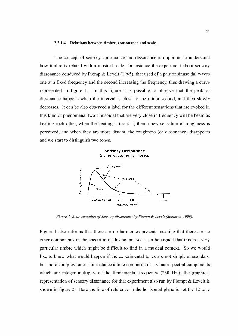
2.2.1.4 Relations between timbre, consonance and scale.

The concept of sensory consonance and dissonance is important to understand

how timbre is related with a musical scale, for instance the experiment about sensory

dissonance conduced by Plomp & Levelt (1965), that used of a pair of sinusoidal waves

one at a fixed frequency and the second increasing the frequency, thus drawing a curve

represented in figure 1. In this figure it is possible to observe that the peak of

dissonance happens when the interval is close to the minor second, and then slowly

decreases. It can be also observed a label for the different sensations that are evoked in

this kind of phenomena: two sinusoidal that are very close in frequency will be heard as

beating each other, when the beating is too fast, then a new sensation of roughness is

perceived, and when they are more distant, the roughness (or dissonance) disappears

and we start to distinguish two tones.

Figure 1. Representation of Sensory dissonance by Plompt & Levelt (Sethares, 1999).

Figure 1 also informs that there are no harmonics present, meaning that there are no

other components in the spectrum of this sound, so it can be argued that this is a very

particular timbre which might be difficult to find in a musical context. So we would

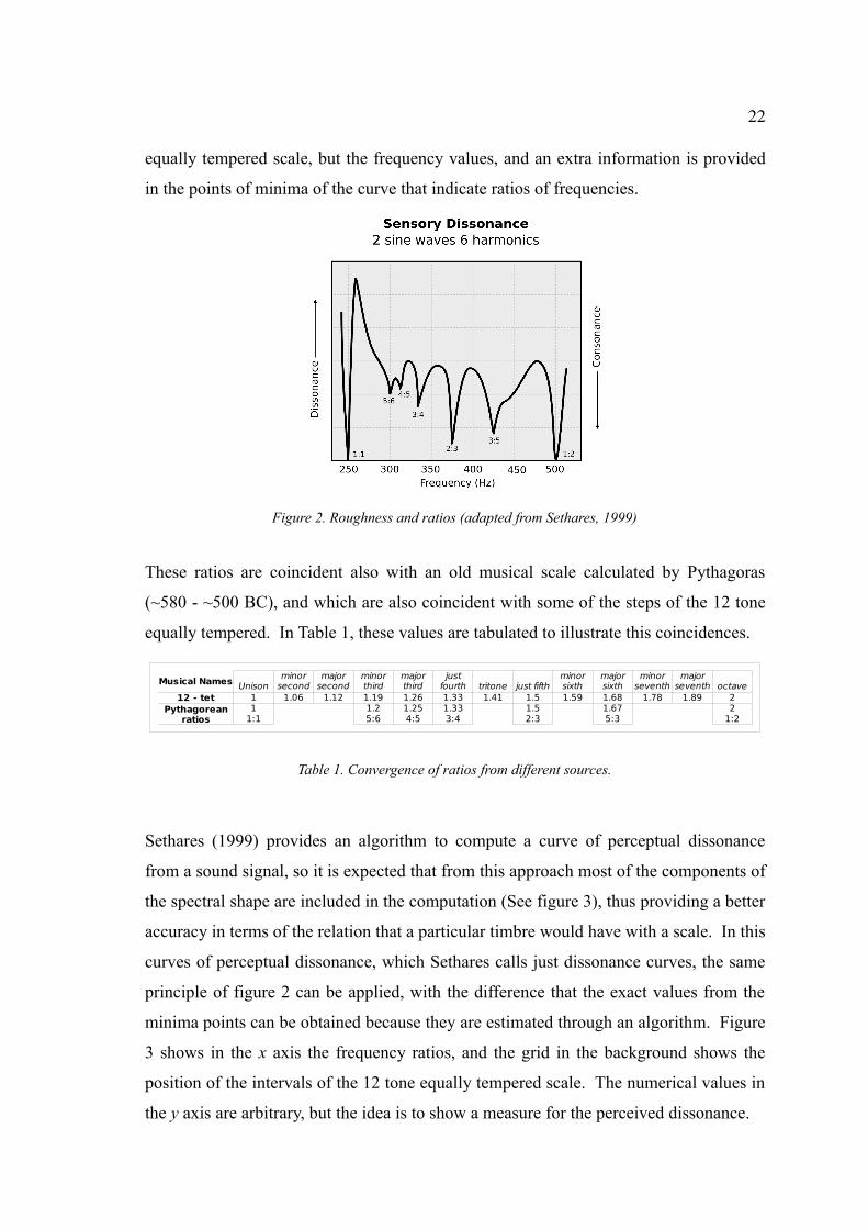
like to know what would happen if the experimental tones are not simple sinusoidals,

but more complex tones, for instance a tone composed of six main spectral components

which are integer multiples of the fundamental frequency (250 Hz.); the graphical

representation of sensory dissonance for that experiment also run by Plompt & Levelt is

shown in figure 2. Here the line of reference in the horizontal plane is not the 12 tone

22

equally tempered scale, but the frequency values, and an extra information is provided

in the points of minima of the curve that indicate ratios of frequencies.

Figure 2. Roughness and ratios (adapted from Sethares, 1999)

These ratios are coincident also with an old musical scale calculated by Pythagoras

(~580 - ~500 BC), and which are also coincident with some of the steps of the 12 tone

equally tempered. In Table 1, these values are tabulated to illustrate this coincidences.

Table 1. Convergence of ratios from different sources.

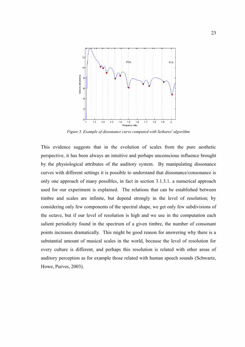
Sethares (1999) provides an algorithm to compute a curve of perceptual dissonance

from a sound signal, so it is expected that from this approach most of the components of

the spectral shape are included in the computation (See figure 3), thus providing a better

accuracy in terms of the relation that a particular timbre would have with a scale. In this

curves of perceptual dissonance, which Sethares calls just dissonance curves, the same

principle of figure 2 can be applied, with the difference that the exact values from the

minima points can be obtained because they are estimated through an algorithm. Figure

3 shows in the x axis the frequency ratios, and the grid in the background shows the

position of the intervals of the 12 tone equally tempered scale. The numerical values in

the y axis are arbitrary, but the idea is to show a measure for the perceived dissonance.

Musical Names Unison just fifth octave1 1.06 1.12 1.19 1.26 1.33 1.41 1.5 1.59 1.68 1.78 1.89 21 1.2 1.25 1.33 1.5 1.67 2

1:1 5:6 4:5 3:4 2:3 5:3 1:2

minor second

major second

minor third

major third

just fourth tritone

minor sixth

major sixth

minor seventh

major seventh

12 - tetPythagorean

ratios

23

Figure 3. Example of dissonance curve computed with Sethares' algorithm

This evidence suggests that in the evolution of scales from the pure aesthetic

perspective, it has been always an intuitive and perhaps unconscious influence brought

by the physiological attributes of the auditory system. By manipulating dissonance

curves with different settings it is possible to understand that dissonance/consonance is

only one approach of many possibles, in fact in section 3.1.3.1. a numerical approach

used for our experiment is explained. The relations that can be established between

timbre and scales are infinite, but depend strongly in the level of resolution; by

considering only few components of the spectral shape, we get only few subdivisions of

the octave, but if our level of resolution is high and we use in the computation each

salient periodicity found in the spectrum of a given timbre, the number of consonant

points increases dramatically. This might be good reason for answering why there is a

substantial amount of musical scales in the world, because the level of resolution for

every culture is different, and perhaps this resolution is related with other areas of

auditory perception as for example those related with human speech sounds (Schwartz,

Howe, Purves, 2003).

24

2.3 Memory

2.3.1 A three stages in one

In this section is briefly reviewed a three stages model presented by Bob Snyder

(2001) in his book entitled “Music and Memory”. This model divides the memory in

three main sections according to their capabilities to process information within certain

time span. These are the sensory, short-term and long-term memory. This taxonomical

approach does not imply that the brain is actually processing information in three

different parts, but rather those three converge in one referred as working memory.

2.3.1.1 Sensory memory

In the sensory memory (also called the echoic memory), the auditory

information is organized in a very basic way. The input consists of impulses from nerve

cells produced in the ear and each of the ‘features’ like pitch and spectrum is extracted

by a group of neurons that are specialized in a biologically significant form to respond

to that particular specific feature. These extractors may be established genetically

because they appear to be innate and no learned or different for different species.

Sensory memory is the most basic kind of auditory categorical perception (Evans,

1982).

At this point the information becomes categorical, which means that it is no longer a

continuous sensory representation. An auditory event is a basic form of association, and

it occurs when particular features occur together, for example the perception of a note

duration, timbre and pitch. In the echoic memory some basic non-verbal representation

(imaging) happens, and also the matching of long-term memory content to current

perceptual experience called pattern recognition. Habituation is a special form of

recognition that occurs at a less conscious awareness level. It is a phenomena that

makes the output of the neurons less active over time, when their input is repeatedly an

identical stimulus (Snyder, 2001, p. 24). This decreasing of activity is also called

adaptation response; in other words, if a the same impulse like an ambient noise is

25

repeated over and over again, it is unlikely that every next repetition attracts our

attention.

2.3.1.2 Short-term memory

Short-term memory lasts from three to five seconds on average, depending on

the novelty and complexity of the material to be remembered. It differs from the long-

term memory in that does not cause permanent anatomical or chemical changes in the

connections between neurons. It is a type of memory process whit a certain degree of

specialization, so there is probably more than one short-term memory, for instance: for

language, for visual object recognition, spatial relations, non- linguistic sounds and

physical movement (p. 47).

Short-term memory has a close link with two concepts: rehearsal and chunking.

Rehearsal is necessary to maintain information temporarily as short-term memory, it is

also necessary to store information into long-term memory and is a consciousness

process, tough it can happen also in a less conscious way. In general terms, any

repetition of elements in a pattern of experience constitutes a kind of rehearsal.

Chunking refers to small groupings (of elements) associated with each other and

capable of forming higher level units; it is the consolidation of small groups of

associated memory elements and leads to the creation of structured hierarchies of

associations. Short-term memory is associated with the level of melodic and rhythmic

grouping, this is the level at which the ´local’ order of music is perceived (p. 52-56).

This types of memory are our primary way of comprehending the time sequences of

events in our experience, although the capacity if this memory is very small; 7±2

elements with conscious rehearsal, 3 or 4 elements without conscious rehearsal, 25

elements with repetition patterns that fit time limits of short-term memory. In terms of

time span, it varies from 3 to 5 seconds to 10 to 12, depending on the type of

information (p. 50).

26

2.3.1.3 Long-term memory

Long-term memory manages patterns and relationships between events on a

time scale larger than 3 to 5 seconds. Memories need to be unconscious in order to

leave room for the notion of present, they are thoughts that are formed when repeated

stimulation changes the strength of connections between simultaneously activated

neurons. The connections between groups of simultaneously activated neurons are

called associations, and this process is referred to as cueing. There are three types of

cueing: recollection when we intentionally try to cue a memory; reminding where an

event in the environment automatically cues an associated memory of something else;

and recognition, where an event in the environment automatically acts as its own cue.

Long-term memory is not at all static, but highly dynamic. The creation of long-term

memories is often refereed to as “coding”, remembering is a process of reconstruction

rather than reproduction (p. 69-71).

2.3.1.4 Working memory

The process in which semi-activated long-term memory becomes highly

activated and conscious, and short-term memory fading in from perception and out (to

prime new memory associations) is called working memory. The conceptual difference

consists in, while short-term memory can be understood as storage, working memory

must be considered as a process. Working memory deals with immediate perceptions

and related activated long-term memories, also with contextual information that resides

semi-activated, but not in consciousness, and also with information that had just been in

consciousness (p. 47-49).

2.3.2 Memory for timbre

Among other information discerned at the few milliseconds after having

exposed to a sound, there is the timbre. It has been experimentally dissociated from

pitch, which is believed to be processed independently in auditory short-term memory

(Semal, Demany, 1991; 1993). Some research has been focused in recognition, where it

has been discovered a differential capability to recognize a given timbre when some

27

aspects of the spectral shape had been altered (Berger, 1964), and also when the

experimental task demands the recognition of timbre under different contextual

situations (Krumhansl, 1992).

Other approach that seems very promising to study the effects of timbre on memory, is

the neurological, because it has provided evidence of auditory cortical enhancement as a

possible result of training with an specific instrumental timbre (Pantev, Roberts, Schulz,

Engelien, Ross, 2001), and plastic changes in the auditory cortex in frequency

discrimination experiments (Pantev, Wollbrink, Roberts, Engelien, Lütkenhöner, 1999;

Menning, Roberts, Pantev, 2000).

28

3 Empirical approach

This chapter contains a detailed description of the different stages in which this project

was involved towards the gathering of data and the consequent testing of statistical

inferences related to the problem of the effects of timbre on the recalling of microtonal

intervals.

3.1 Method

3.1.1 Design

The design is oriented towards the comparison of performance in memorizing-recalling

intervals played with different timbres, so it can be described as a Repeated Measures

design, where the independent variables are Synthesis type, Instrument name and

Interval length, and the dependent variable is the degree of accuracy in recalling a given

interval performed by a subject, measured in number of errors. The main test involves

analysis of variance of different groups of timbral characteristics and origins, but in the

obtained data is also possible to observe the tendency of the response, and to speculate

about a possible learning function. The decision of studying timbre effects by asking

subjects to focus on another task, was made with the intention of establishing an

homogeneous status in the way working memory is controlling the attention among all

subjects (Hall & Blasko, 2005).

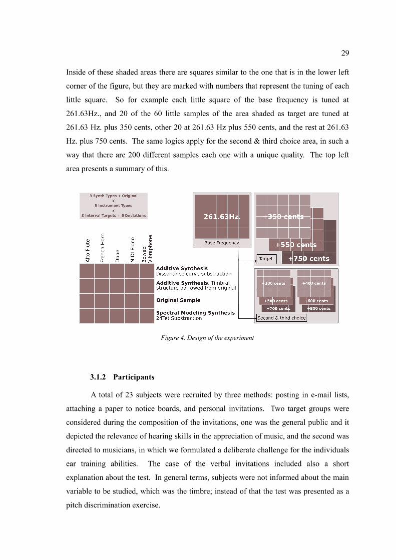
In figure 4, there is a graphical explanation of how is designed the experiment. In the

lower left corner of the figure, there is a square segmented in 20 parts, each little square

represents a sound sample with two unique qualities: one instrumental origin and one

type of timbral modification (5 Instrument types and 3 Synthesis types plus no

modification). The right side of this diagram shows three shaded backgrounds labelled

as Base Frequency, Target, and Second & third choice, which purpose is to illustrate that

there are three intervals per trial, one that is made between the base frequency and the

target, and the other two between the base frequency and the second and third choice.

29

Inside of these shaded areas there are squares similar to the one that is in the lower left

corner of the figure, but they are marked with numbers that represent the tuning of each

little square. So for example each little square of the base frequency is tuned at

261.63Hz., and 20 of the 60 little samples of the area shaded as target are tuned at

261.63 Hz. plus 350 cents, other 20 at 261.63 Hz plus 550 cents, and the rest at 261.63

Hz. plus 750 cents. The same logics apply for the second & third choice area, in such a

way that there are 200 different samples each one with a unique quality. The top left

area presents a summary of this.

Figure 4. Design of the experiment

3.1.2 Participants

A total of 23 subjects were recruited by three methods: posting in e-mail lists,

attaching a paper to notice boards, and personal invitations. Two target groups were

considered during the composition of the invitations, one was the general public and it

depicted the relevance of hearing skills in the appreciation of music, and the second was

directed to musicians, in which we formulated a deliberate challenge for the individuals

ear training abilities. The case of the verbal invitations included also a short

explanation about the test. In general terms, subjects were not informed about the main

variable to be studied, which was the timbre; instead of that the test was presented as a

pitch discrimination exercise.

30

There were 8 female and 15 males, with mean age of ages between 20 and 40 years old

(Mean = 28.6, SD = 5.2). They were asked to fill a questionnaire after the experiment

whose purpose was to collect information about their musical background and habits.

3.1.3 Materials

3.1.3.1 Stimuli

The design of the stimuli involved two main processes: selection/discrimination

of collections and samples, and analysis/synthesis.

Selection

For the selection of samples three sources were analysed: “McGill University

Master Samples 2.0” (Opolko & Wapnick, 2006), “Native Instruments: Kontakt 2

Sample Library”(Haver & Schmitt, 2006), and a Microsoft MIDI wave-table synthesizer

played with a Realtek ALC259 software. The objective was to obtain sounds with a

certain degree of ecological validity in terms of how widely are they used, so the first

one (McGill) was picked because it has been widely used by researchers in

musicological studies, and also because during the development of this project we were

involved in another research that investigated the possible relations between timbre and

emotions and used them as well. The Native Instruments option was used because it

was already available at the Music Department of the University of Jyväskylä, and also

because of the orientation of this product, which is directed to the home studio or semi

professional market, which means that samples are almost ready to be used for creative

purposes because of the equalization of loudness and classification of sounds, as well as

the software interface to play them; this last qualities in contrast to the McGill collection

which needs a substantial post processing work before it can be used. The third option

was selected because of its availability, popularity and use particularly in music training

software or web sites that rely on it.

31

Discrimination

For the discrimination of instrumental sets, the criterion was first to find all

instrumental sets containing the 13 samples of the central octave, MIDI 60-72 (C4-C5).

In second place and with the aid of MIRToolbox (Lartillot & Toiviainen, 2007) a script

was developed in Matlab which we called “Antagonist Finder”. This script was aimed

to analyse the samples, by computing a general description of them, like duration,

amplitude and timbral values. This script helped to discriminate those samples that

were not well processed by the toolbox because of particular complexities contained in

their structure. For example all the instrumental sets containing samples whose pitch

were under or above estimated for more than a 10% of error by the “mirpitch” algorithm

(using default options), were discarded. By doing this, the objective was to find

realistic sounds which could be easily treated in posterior processing. Another strategy

included in the “Antagonist Finder” consisted in comparisons of specific timbral

descriptors, to discover instruments whose values are in the lower or higher ends of a

comparison table. For example, in the initial stages of this project we were particularly

interested in brightness, so by applying this strategy on brightness, in a manner that a

pair of instrumental sets, one with a bright sound quality and other with a dark sound

quality could be included in the final experimental set. This searching of opposites was

also used with other descriptors, such as inharmonicity and roughness.

At the end, only five instrumental sets were included: French Horn, Alto Flute and

Bowed Vibraphone from the McGill collection, an Oboe from Native Instruments and a

Piano from the Microsoft table. This final decision was difficult to make, because we

were looking for including at least one instrumental set per analysed collection, and

because for practical reasons in terms of duration of the experiment, some timbres that

had attractive and interesting sounds had to be discarded.

Analysis

In his work, Sethares (1999) explains in detail a technique to compute the ratios

of a new scale that suits best to make music with better consonance for a given timbre.

In the first part of this technique is involved the computation of the spectral shape of the

target timbre to extract the most relevant partials and its amplitudes. Then, with that

32

information a dissonance curve is computed and it is argued that the minimas of that

curve pinpoint the ratios which are components of that “new scale”.

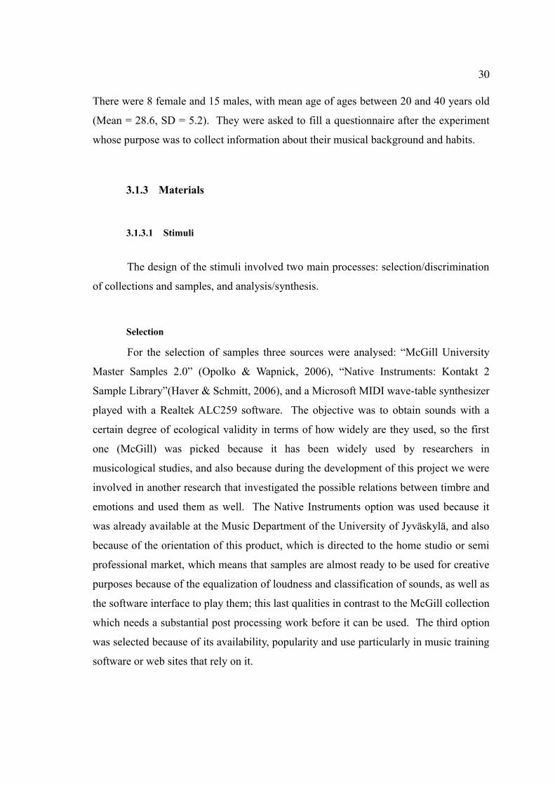
By doing these steps in a systematic form for a set of multiple timbres, we found that

the minimas for those timbres are predominantly in the same ratios, thus giving ground

for a generic scale. In figure 5, it is possible to observe a visual pattern of the minima

hits for a set of 73 samples from the McGuill Collection. Each sample has a different

timbre, all of them with a duration of 1 sec. and tuned at D#4 ~ 311 Hz. The grid in the

background depicts the location of the steps of the 12 tone equally tempered scale steps,

just for reference.

Figure 5. Minima hits from 73 dissonance curves

The pattern of incidence of minima points for 73 dissonance curves on particular ratios

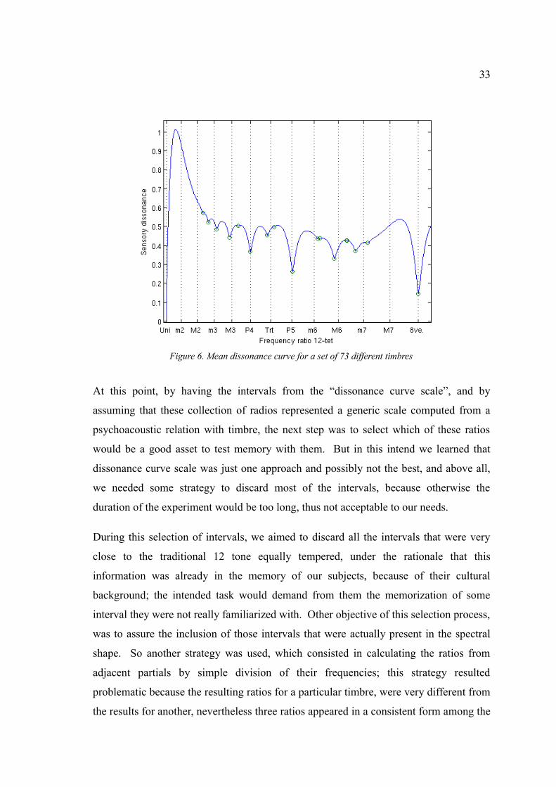
revealed in a visual way in figure 5, leads to the next representation (figure 6), which is

the curve resulting from computing the mean of those 73 curves, and the green circles

represent the steps chosen as ratios for a “new scale” that will be referred in this project

as the Dissonance Curve Scale. This mean curve shows a total of 16 points,

nevertheless some of them are not considered for further computations because in some

cases they were almost overlapped in terms of frequency. Note that the label in the

horizontal plane in figure 6. contains the expression 12-tet, which is an abbreviation of

twelve tone equally tempered system.

33

Figure 6. Mean dissonance curve for a set of 73 different timbres

At this point, by having the intervals from the “dissonance curve scale”, and by

assuming that these collection of radios represented a generic scale computed from a

psychoacoustic relation with timbre, the next step was to select which of these ratios

would be a good asset to test memory with them. But in this intend we learned that

dissonance curve scale was just one approach and possibly not the best, and above all,

we needed some strategy to discard most of the intervals, because otherwise the

duration of the experiment would be too long, thus not acceptable to our needs.

During this selection of intervals, we aimed to discard all the intervals that were very

close to the traditional 12 tone equally tempered, under the rationale that this

information was already in the memory of our subjects, because of their cultural

background; the intended task would demand from them the memorization of some

interval they were not really familiarized with. Other objective of this selection process,

was to assure the inclusion of those intervals that were actually present in the spectral

shape. So another strategy was used, which consisted in calculating the ratios from

adjacent partials by simple division of their frequencies; this strategy resulted

problematic because the resulting ratios for a particular timbre, were very different from

the results for another, nevertheless three ratios appeared in a consistent form among the

34

same 73 timbres used for the estimation of the mean dissonance curve, and were

considered useful for our purpose. But from this former strategy, getting only three

ratios was not really satisfactory, so we decided to incorporate a third set of intervals,

which had already being used in music but in a not so common or popular matter. By

exploring the music and ideas of authors like Charles Ives (1874-1954) and Julián

Carrillo (1875-1965), among others, we found that they had used a 24 tones equally

tempered scale, so this represented another set of intervals with a high degree of

ecological validity.

With these three sets of intervals in mind: dissonance curve scale, adjacent partials

consistent ratios and quarter tone scale (or 24 tones equally tempered), the final decision

of which intervals would be used, was made by comparing the tabulated frequencies. In

the comparison it was found that some interval distances were below or very close to

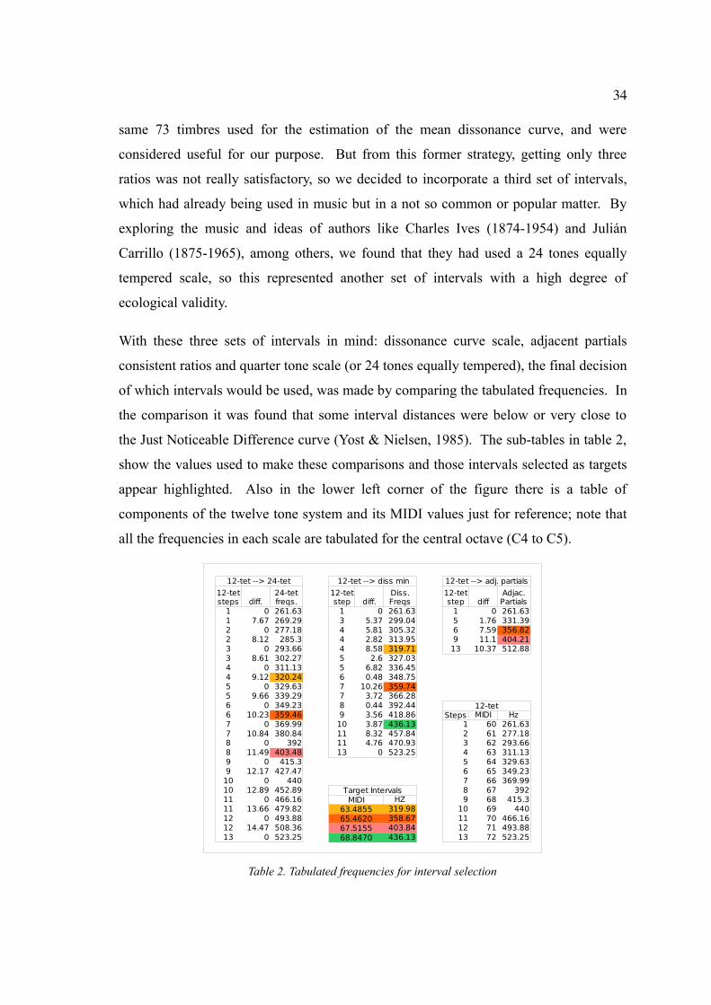
the Just Noticeable Difference curve (Yost & Nielsen, 1985). The sub-tables in table 2,

show the values used to make these comparisons and those intervals selected as targets

appear highlighted. Also in the lower left corner of the figure there is a table of

components of the twelve tone system and its MIDI values just for reference; note that

all the frequencies in each scale are tabulated for the central octave (C4 to C5).

Table 2. Tabulated frequencies for interval selection

1 0 261.63 1 0 261.63 1 0 261.631 7.67 269.29 3 5.37 299.04 5 1.76 331.392 0 277.18 4 5.81 305.32 6 7.59 356.822 8.12 285.3 4 2.82 313.95 9 11.1 404.213 0 293.66 4 8.58 319.71 13 10.37 512.883 8.61 302.27 5 2.6 327.034 0 311.13 5 6.82 336.454 9.12 320.24 6 0.48 348.755 0 329.63 7 10.26 359.745 9.66 339.29 7 3.72 366.286 0 349.23 8 0.44 392.446 10.23 359.46 9 3.56 418.86 Steps MIDI Hz7 0 369.99 10 3.87 436.13 1 60 261.637 10.84 380.84 11 8.32 457.84 2 61 277.188 0 392 11 4.76 470.93 3 62 293.668 11.49 403.48 13 0 523.25 4 63 311.139 0 415.3 5 64 329.639 12.17 427.47 6 65 349.23

10 0 440 7 66 369.9910 12.89 452.89 Target Intervals 8 67 39211 0 466.16 MIDI HZ 9 68 415.311 13.66 479.82 63.4855 319.98 10 69 44012 0 493.88 65.4620 358.67 11 70 466.1612 14.47 508.36 67.5155 403.84 12 71 493.8813 0 523.25 68.8470 436.13 13 72 523.25

12-tet --> 24-tet 12-tet --> diss min 12-tet --> adj. partials

12-tet steps diff.

24-tet freqs.

12-tet step diff.

Diss. Freqs

12-tet step diff

Adjac. Partials

12-tet

35

Initially, four intervals were chosen: three because of its incidence on the three scales

and the fourth one because we observed its importance for the dissonance scale. This

fourth one, was the third most consonant ratio in the dissonance curve scale (as can be

observed in the figure 6), but because of its closeness to the Major 6th from the 12 tone

equally tempered scale, it was discarded. Furthermore, as it can be observed in the little

table located in the central lower edge of table 2 headed as “Target intervals”, which

contains the average of coincident values, the MIDI values revealed that the three first

values are almost in the middle of an integer MIDI value, which means that if the

distance from one MIDI integer to the following is half tone in the 12 tone equally

tempered system, three of our targets were really close to the quarter of tone and one

not. Thus the final decision of target intervals were three: 350 cents (MIDI= 63.49),

550 cents (MIDI=65.46) and 750 cents (MIDI=67.52).

A minor compromise must be declared, which consisted in the rounding of this values to

one decimal in a manner that at the end the shorter interval involved in this research

would be the quarter of tone of the 12 tone equally tempered system.

Synthesis

With the aid of the Spectral Modelling Toolbox (Johnson, 2002), a sound signal

is processed with a Short Time Fourier Transform, and then the output is made of three

vectors containing the values of frequency, amplitude and phase of the sound signal as a

function of time. From this operation it is possible to identify the peaks in the values of

frequency and their evolution on time, which, according to the idea of Xavier Serra

(1990), can be accommodated in tracks. Those tracks can be seen as the partials7 of a

tone and their small fluctuations (within a given threshold) of pitch in the evolution of

time.

In our hypothesis the presence or absence of particular partials would lead to an

enhanced or impaired extraction of cues for memory. In order to make those particular

partials to be “absent”, an adjustment must be done, which starts by assuming that each

partial of a given tone has a numerical relation with each step of a given scale. So the

7 along the whole text the expressions: overtone and main spectral components, are used as a synonym of partials.

36

objective of the adjustments was to take out of the partial structure those partials that

were numerically related to the target intervals; in other words, to remove the intervals

which were going to be used in the memory trials, from the inner structure of the tones;

thus applying a modification on timbre.

The method consisted of dividing the mean frequency of each track ( p ) by the

frequency of each step of the target scale ( f ).

ratioij=pi

f j

From this operation we obtain a matrix of ratios which expresses the proximity of each

pair of data; the first row and column would express the numerical relation between the

first partial and the first step of the scale, the second column of the same row would

express the relation between the first partial and the second step of the scale, and so on.

Thus if each row represents a numerical relation between that partial and all the steps of

a scale, the only thing that remains is to identify the best candidate, which can be found

by looking in the fractional part of those numerical relations, for the value that is closer

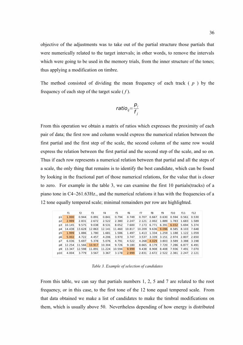
to zero. For example in the table 3, we can examine the first 10 partials(tracks) of a

piano tone in C4~261.63Hz., and the numerical relations it has with the frequencies of a

12 tone equally tempered scale; minimal remainders per row are highlighted.

Table 3. Example of selection of candidates

From this table, we can say that partials numbers 1, 2, 5 and 7 are related to the root

frequency, or in this case, to the first tone of the 12 tone equal tempered scale. From

that data obtained we make a list of candidates to make the timbral modifications on

them, which is usually above 50. Nevertheless depending of how energy is distributed

f1 f2 f3 f4 f5 f6 f7 f8 f9 f10 f11 f12

p1 1.000 0.944 0.891 0.841 0.794 0.749 0.707 0.667 0.630 0.594 0.561 0.530

p2 2.999 2.831 2.672 2.522 2.380 2.247 2.121 2.002 1.889 1.783 1.683 1.589

p3 10.145 9.575 9.038 8.531 8.052 7.600 7.173 6.771 6.391 6.032 5.694 5.374

p4 14.438 13.628 12.863 12.141 11.460 10.817 10.209 9.636 9.096 8.585 8.103 7.648

p5 1.999 1.886 1.780 1.681 1.586 1.497 1.413 1.334 1.259 1.188 1.122 1.059

p6 5.002 4.722 4.457 4.206 3.970 3.747 3.537 3.339 3.151 2.974 2.807 2.650

p7 6.036 5.697 5.378 5.076 4.791 4.522 4.268 4.029 3.803 3.589 3.388 3.198

p8 12.254 11.566 10.917 10.304 9.726 9.180 8.665 8.179 7.720 7.286 6.877 6.491

p9 13.347 12.598 11.891 11.224 10.594 9.999 9.438 8.908 8.408 7.936 7.491 7.070

p10 4.004 3.779 3.567 3.367 3.178 2.999 2.831 2.672 2.522 2.381 2.247 2.121

37

in the spectrum it could reach a maximum of 500 (this threshold is specified in the

function that converts peaks to tracks from the SMToolbox). At this point is worth to

mention that early intends on this matter of modifying timbre, were aimed at displacing

partials from its original position; to stretch them by changing their main frequency.

The idea was abandoned because the audible result was too far from the original sample

in terms of quality.

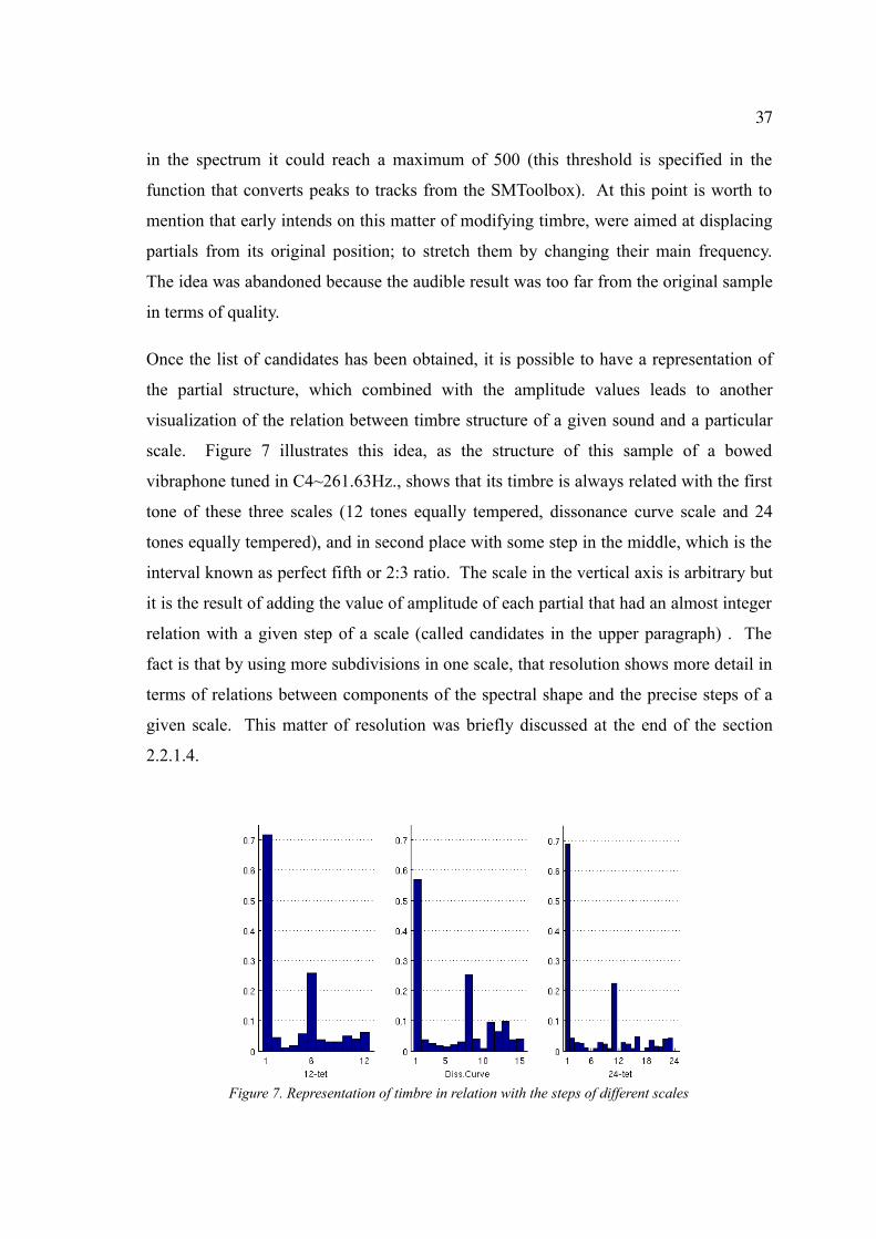
Once the list of candidates has been obtained, it is possible to have a representation of

the partial structure, which combined with the amplitude values leads to another

visualization of the relation between timbre structure of a given sound and a particular

scale. Figure 7 illustrates this idea, as the structure of this sample of a bowed

vibraphone tuned in C4~261.63Hz., shows that its timbre is always related with the first

tone of these three scales (12 tones equally tempered, dissonance curve scale and 24

tones equally tempered), and in second place with some step in the middle, which is the

interval known as perfect fifth or 2:3 ratio. The scale in the vertical axis is arbitrary but

it is the result of adding the value of amplitude of each partial that had an almost integer

relation with a given step of a scale (called candidates in the upper paragraph) . The

fact is that by using more subdivisions in one scale, that resolution shows more detail in

terms of relations between components of the spectral shape and the precise steps of a

given scale. This matter of resolution was briefly discussed at the end of the section

2.2.1.4.

Figure 7. Representation of timbre in relation with the steps of different scales

38

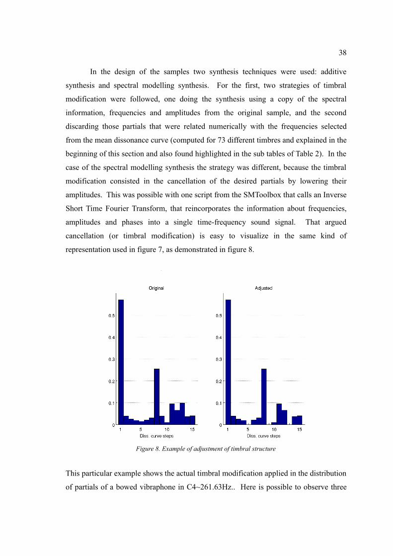
In the design of the samples two synthesis techniques were used: additive

synthesis and spectral modelling synthesis. For the first, two strategies of timbral

modification were followed, one doing the synthesis using a copy of the spectral

information, frequencies and amplitudes from the original sample, and the second

discarding those partials that were related numerically with the frequencies selected

from the mean dissonance curve (computed for 73 different timbres and explained in the

beginning of this section and also found highlighted in the sub tables of Table 2). In the

case of the spectral modelling synthesis the strategy was different, because the timbral

modification consisted in the cancellation of the desired partials by lowering their

amplitudes. This was possible with one script from the SMToolbox that calls an Inverse

Short Time Fourier Transform, that reincorporates the information about frequencies,

amplitudes and phases into a single time-frequency sound signal. That argued

cancellation (or timbral modification) is easy to visualize in the same kind of

representation used in figure 7, as demonstrated in figure 8.

Figure 8. Example of adjustment of timbral structure

This particular example shows the actual timbral modification applied in the distribution

of partials of a bowed vibraphone in C4~261.63Hz.. Here is possible to observe three

39

“holes” at 5th, 9th and 13th steps, which correspond to the intervals of 349, 546 and 752

cents of the scale extracted from the mean dissonance curve.

The final set is made of three different synthesis strategies plus the original sample,

which conform four sets of timbres that in subsequent sections we refer as “synthesis

type” variable.

All samples were equalized in loudness and converted from two to one channel, they

had a duration of 1200 ms and a linear envelope for the first 10 ms. and the last 200ms.,

which purpose is to take the amplitude from silence to the normalization level and then

back. For this processing the software named “Sox” by Bagwell (2006) was used.

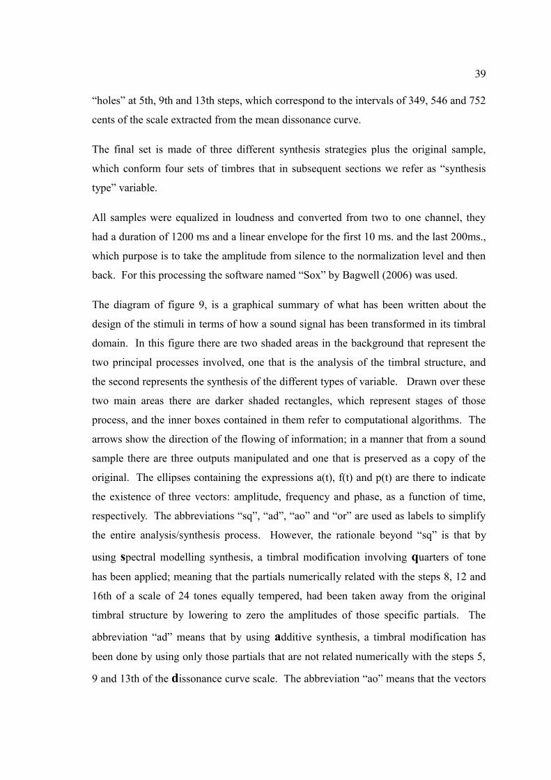
The diagram of figure 9, is a graphical summary of what has been written about the

design of the stimuli in terms of how a sound signal has been transformed in its timbral

domain. In this figure there are two shaded areas in the background that represent the

two principal processes involved, one that is the analysis of the timbral structure, and

the second represents the synthesis of the different types of variable. Drawn over these

two main areas there are darker shaded rectangles, which represent stages of those

process, and the inner boxes contained in them refer to computational algorithms. The

arrows show the direction of the flowing of information; in a manner that from a sound

sample there are three outputs manipulated and one that is preserved as a copy of the

original. The ellipses containing the expressions a(t), f(t) and p(t) are there to indicate

the existence of three vectors: amplitude, frequency and phase, as a function of time,

respectively. The abbreviations “sq”, “ad”, “ao” and “or” are used as labels to simplify

the entire analysis/synthesis process. However, the rationale beyond “sq” is that by

using spectral modelling synthesis, a timbral modification involving quarters of tone

has been applied; meaning that the partials numerically related with the steps 8, 12 and

16th of a scale of 24 tones equally tempered, had been taken away from the original

timbral structure by lowering to zero the amplitudes of those specific partials. The

abbreviation “ad” means that by using additive synthesis, a timbral modification has

been done by using only those partials that are not related numerically with the steps 5,

9 and 13th of the dissonance curve scale. The abbreviation “ao” means that the vectors

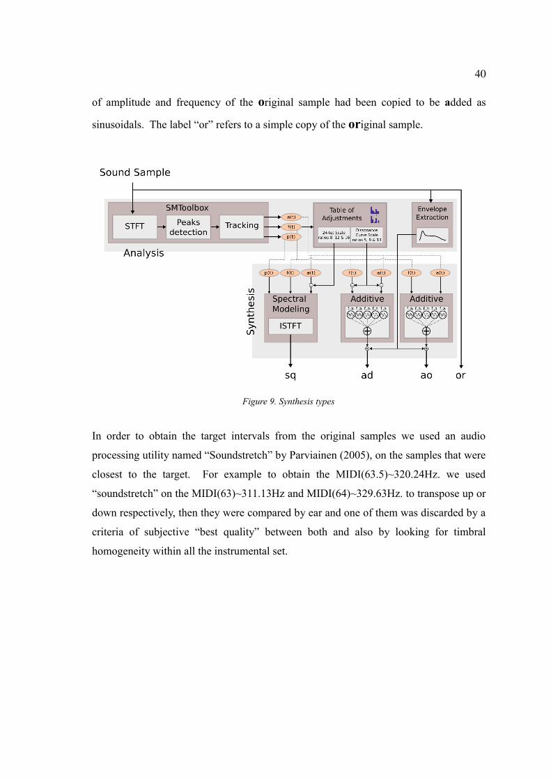
40

of amplitude and frequency of the original sample had been copied to be added as

sinusoidals. The label “or” refers to a simple copy of the original sample.

Figure 9. Synthesis types

In order to obtain the target intervals from the original samples we used an audio

processing utility named “Soundstretch” by Parviainen (2005), on the samples that were

closest to the target. For example to obtain the MIDI(63.5)~320.24Hz. we used

“soundstretch” on the MIDI(63)~311.13Hz and MIDI(64)~329.63Hz. to transpose up or

down respectively, then they were compared by ear and one of them was discarded by a

criteria of subjective “best quality” between both and also by looking for timbral

homogeneity within all the instrumental set.

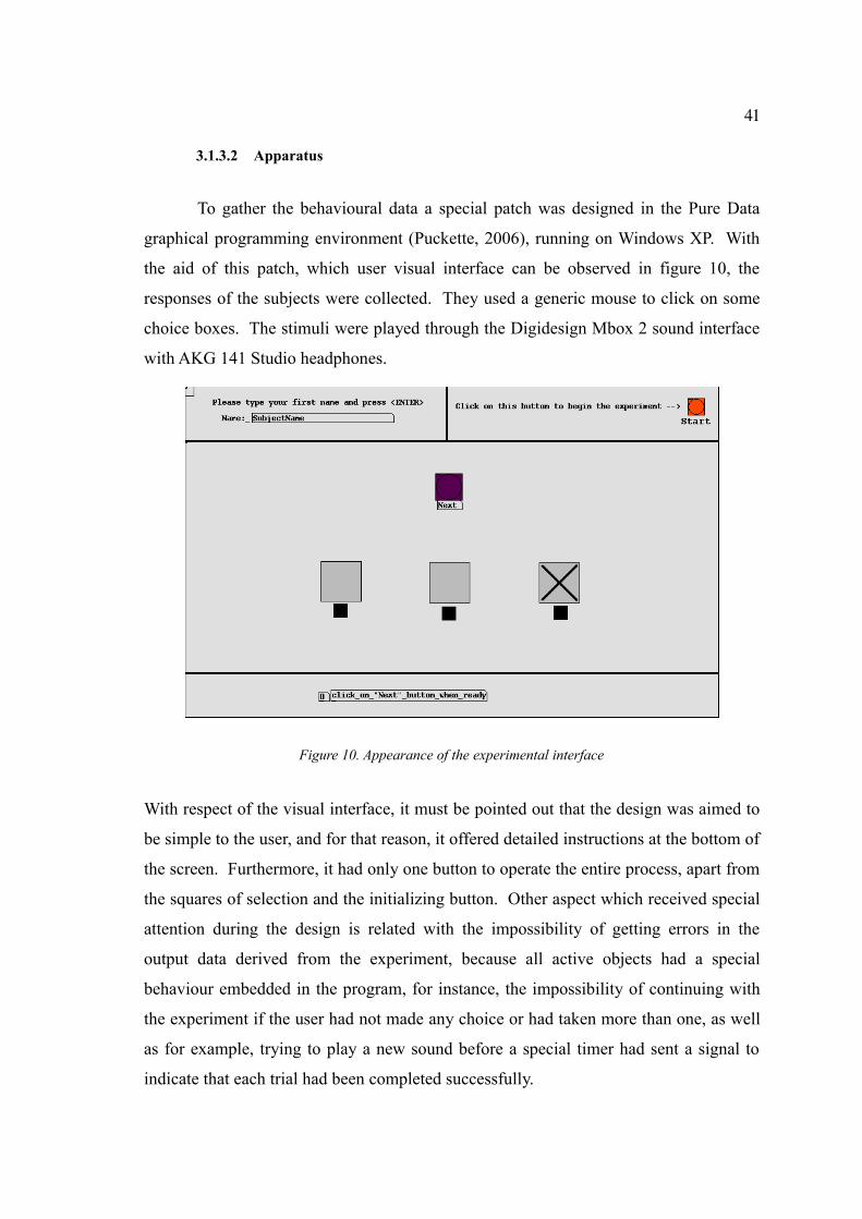
41

3.1.3.2 Apparatus

To gather the behavioural data a special patch was designed in the Pure Data

graphical programming environment (Puckette, 2006), running on Windows XP. With

the aid of this patch, which user visual interface can be observed in figure 10, the

responses of the subjects were collected. They used a generic mouse to click on some

choice boxes. The stimuli were played through the Digidesign Mbox 2 sound interface

with AKG 141 Studio headphones.

Figure 10. Appearance of the experimental interface

With respect of the visual interface, it must be pointed out that the design was aimed to

be simple to the user, and for that reason, it offered detailed instructions at the bottom of

the screen. Furthermore, it had only one button to operate the entire process, apart from

the squares of selection and the initializing button. Other aspect which received special

attention during the design is related with the impossibility of getting errors in the

output data derived from the experiment, because all active objects had a special

behaviour embedded in the program, for instance, the impossibility of continuing with

the experiment if the user had not made any choice or had taken more than one, as well

as for example, trying to play a new sound before a special timer had sent a signal to

indicate that each trial had been completed successfully.

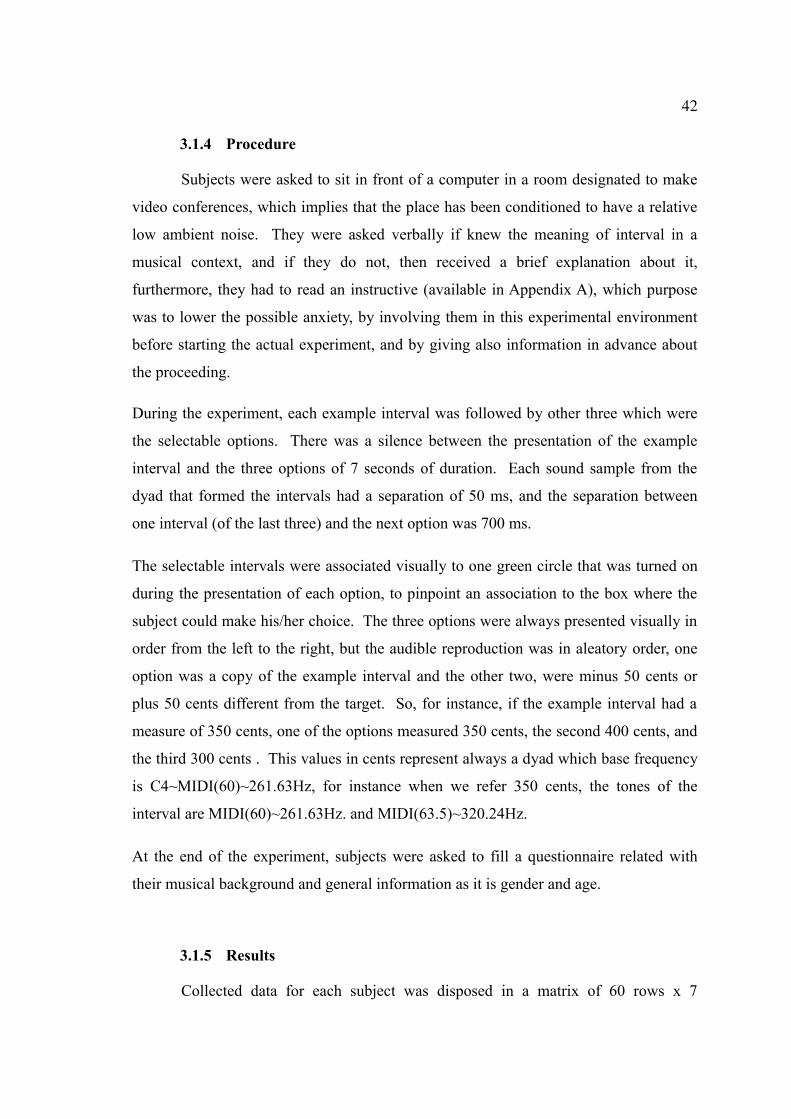
42

3.1.4 Procedure

Subjects were asked to sit in front of a computer in a room designated to make

video conferences, which implies that the place has been conditioned to have a relative

low ambient noise. They were asked verbally if knew the meaning of interval in a

musical context, and if they do not, then received a brief explanation about it,

furthermore, they had to read an instructive (available in Appendix A), which purpose

was to lower the possible anxiety, by involving them in this experimental environment

before starting the actual experiment, and by giving also information in advance about

the proceeding.

During the experiment, each example interval was followed by other three which were

the selectable options. There was a silence between the presentation of the example

interval and the three options of 7 seconds of duration. Each sound sample from the

dyad that formed the intervals had a separation of 50 ms, and the separation between

one interval (of the last three) and the next option was 700 ms.

The selectable intervals were associated visually to one green circle that was turned on

during the presentation of each option, to pinpoint an association to the box where the

subject could make his/her choice. The three options were always presented visually in

order from the left to the right, but the audible reproduction was in aleatory order, one

option was a copy of the example interval and the other two, were minus 50 cents or

plus 50 cents different from the target. So, for instance, if the example interval had a

measure of 350 cents, one of the options measured 350 cents, the second 400 cents, and

the third 300 cents . This values in cents represent always a dyad which base frequency

is C4~MIDI(60)~261.63Hz, for instance when we refer 350 cents, the tones of the

interval are MIDI(60)~261.63Hz. and MIDI(63.5)~320.24Hz.

At the end of the experiment, subjects were asked to fill a questionnaire related with

their musical background and general information as it is gender and age.

3.1.5 Results

Collected data for each subject was disposed in a matrix of 60 rows x 7

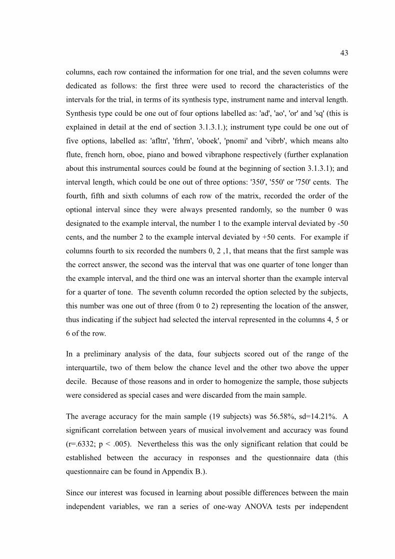
43

columns, each row contained the information for one trial, and the seven columns were

dedicated as follows: the first three were used to record the characteristics of the

intervals for the trial, in terms of its synthesis type, instrument name and interval length.

Synthesis type could be one out of four options labelled as: 'ad', 'ao', 'or' and 'sq' (this is

explained in detail at the end of section 3.1.3.1.); instrument type could be one out of

five options, labelled as: 'afltn', 'frhrn', 'oboek', 'pnomi' and 'vibrb', which means alto

flute, french horn, oboe, piano and bowed vibraphone respectively (further explanation

about this instrumental sources could be found at the beginning of section 3.1.3.1); and

interval length, which could be one out of three options: '350', '550' or '750' cents. The

fourth, fifth and sixth columns of each row of the matrix, recorded the order of the

optional interval since they were always presented randomly, so the number 0 was

designated to the example interval, the number 1 to the example interval deviated by -50

cents, and the number 2 to the example interval deviated by +50 cents. For example if

columns fourth to six recorded the numbers 0, 2 ,1, that means that the first sample was

the correct answer, the second was the interval that was one quarter of tone longer than

the example interval, and the third one was an interval shorter than the example interval

for a quarter of tone. The seventh column recorded the option selected by the subjects,

this number was one out of three (from 0 to 2) representing the location of the answer,

thus indicating if the subject had selected the interval represented in the columns 4, 5 or

6 of the row.

In a preliminary analysis of the data, four subjects scored out of the range of the

interquartile, two of them below the chance level and the other two above the upper

decile. Because of those reasons and in order to homogenize the sample, those subjects

were considered as special cases and were discarded from the main sample.

The average accuracy for the main sample (19 subjects) was 56.58%, sd=14.21%. A

significant correlation between years of musical involvement and accuracy was found

(r=.6332; p < .005). Nevertheless this was the only significant relation that could be

established between the accuracy in responses and the questionnaire data (this

questionnaire can be found in Appendix B.).

Since our interest was focused in learning about possible differences between the main

independent variables, we ran a series of one-way ANOVA tests per independent

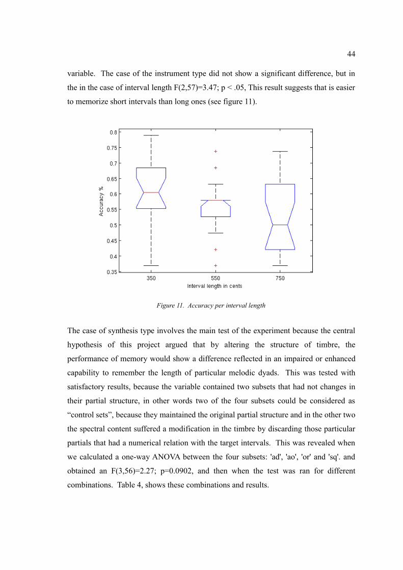
44

variable. The case of the instrument type did not show a significant difference, but in

the in the case of interval length F(2,57)=3.47; p < .05, This result suggests that is easier

to memorize short intervals than long ones (see figure 11).

Figure 11. Accuracy per interval length

The case of synthesis type involves the main test of the experiment because the central

hypothesis of this project argued that by altering the structure of timbre, the

performance of memory would show a difference reflected in an impaired or enhanced

capability to remember the length of particular melodic dyads. This was tested with

satisfactory results, because the variable contained two subsets that had not changes in

their partial structure, in other words two of the four subsets could be considered as

“control sets”, because they maintained the original partial structure and in the other two

the spectral content suffered a modification in the timbre by discarding those particular

partials that had a numerical relation with the target intervals. This was revealed when

we calculated a one-way ANOVA between the four subsets: 'ad', 'ao', 'or' and 'sq'. and

obtained an F(3,56)=2.27; p=0.0902, and then when the test was ran for different

combinations. Table 4, shows these combinations and results.

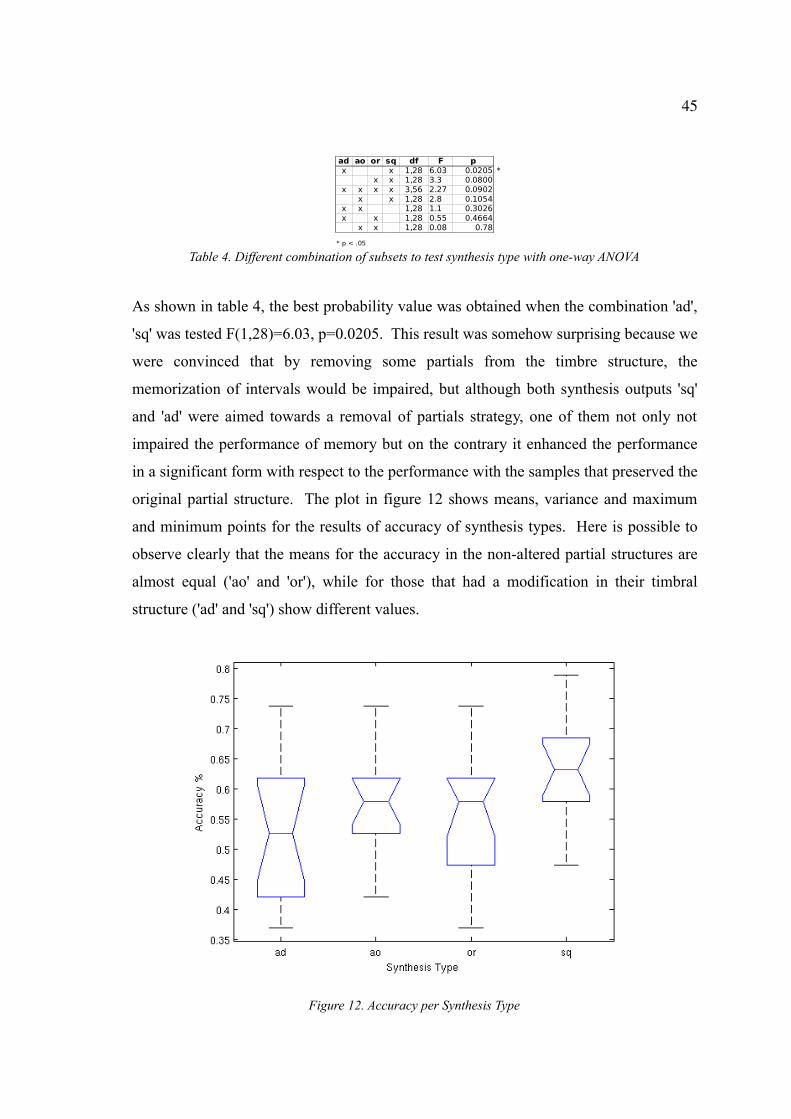
45

Table 4. Different combination of subsets to test synthesis type with one-way ANOVA

As shown in table 4, the best probability value was obtained when the combination 'ad',

'sq' was tested F(1,28)=6.03, p=0.0205. This result was somehow surprising because we

were convinced that by removing some partials from the timbre structure, the

memorization of intervals would be impaired, but although both synthesis outputs 'sq'

and 'ad' were aimed towards a removal of partials strategy, one of them not only not

impaired the performance of memory but on the contrary it enhanced the performance

in a significant form with respect to the performance with the samples that preserved the

original partial structure. The plot in figure 12 shows means, variance and maximum

and minimum points for the results of accuracy of synthesis types. Here is possible to

observe clearly that the means for the accuracy in the non-altered partial structures are

almost equal ('ao' and 'or'), while for those that had a modification in their timbral

structure ('ad' and 'sq') show different values.

Figure 12. Accuracy per Synthesis Type

ad or sq F px x 1,28 6.03 0.0205 *

x x 1,28 3.3 0.0800x x x x 3,56 2.27 0.0902

x x 1,28 2.8 0.1054x x 1,28 1.1 0.3026x x 1,28 0.55 0.4664

x x 1,28 0.08 0.78

* p < .05

ao df

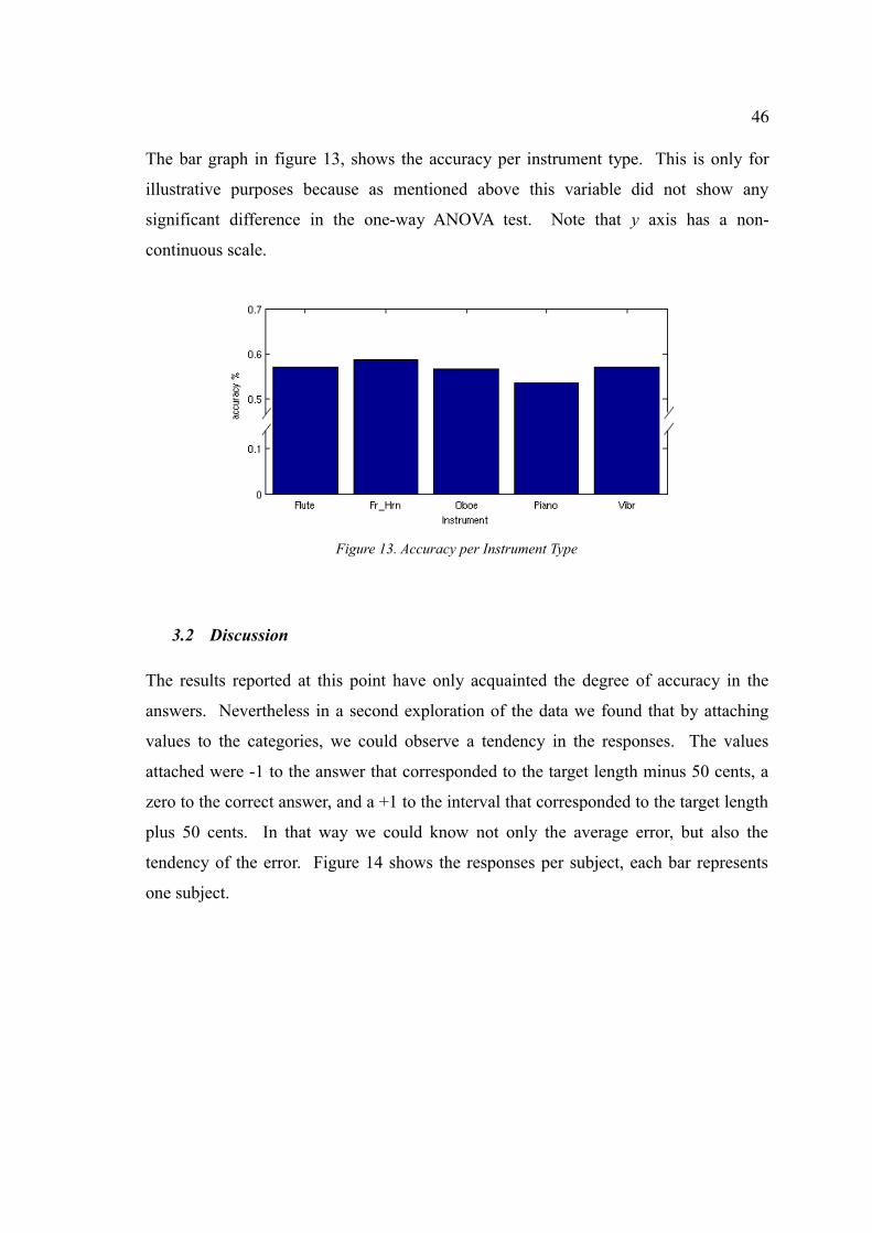
46

The bar graph in figure 13, shows the accuracy per instrument type. This is only for

illustrative purposes because as mentioned above this variable did not show any

significant difference in the one-way ANOVA test. Note that y axis has a non-

continuous scale.

Figure 13. Accuracy per Instrument Type

3.2 Discussion

The results reported at this point have only acquainted the degree of accuracy in the

answers. Nevertheless in a second exploration of the data we found that by attaching

values to the categories, we could observe a tendency in the responses. The values

attached were -1 to the answer that corresponded to the target length minus 50 cents, a

zero to the correct answer, and a +1 to the interval that corresponded to the target length

plus 50 cents. In that way we could know not only the average error, but also the

tendency of the error. Figure 14 shows the responses per subject, each bar represents

one subject.

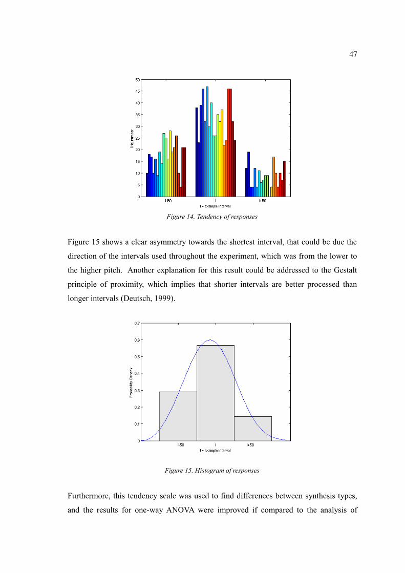
47

Figure 14. Tendency of responses

Figure 15 shows a clear asymmetry towards the shortest interval, that could be due the

direction of the intervals used throughout the experiment, which was from the lower to

the higher pitch. Another explanation for this result could be addressed to the Gestalt

principle of proximity, which implies that shorter intervals are better processed than

longer intervals (Deutsch, 1999).

Figure 15. Histogram of responses

Furthermore, this tendency scale was used to find differences between synthesis types,

and the results for one-way ANOVA were improved if compared to the analysis of

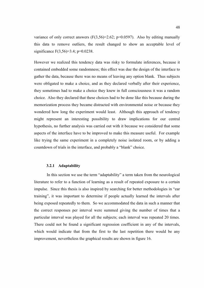
48

variance of only correct answers (F(3,56)=2.62; p=0.0597). Also by editing manually

this data to remove outliers, the result changed to show an acceptable level of

significance F(3,56)=3.4; p=0.0238.

However we realized this tendency data was risky to formulate inferences, because it

contained embedded some randomness; this effect was due the design of the interface to

gather the data, because there was no means of leaving any option blank. Thus subjects

were obligated to make a choice, and as they declared verbally after their experience,

they sometimes had to make a choice they knew in full consciousness it was a random

choice. Also they declared that these choices had to be done like this because during the

memorization process they became distracted with environmental noise or because they

wondered how long the experiment would least. Although this approach of tendency

might represent an interesting possibility to draw implications for our central

hypothesis, no further analysis was carried out with it because we considered that some

aspects of the interface have to be improved to make this measure useful. For example

like trying the same experiment in a completely noise isolated room, or by adding a

countdown of trials in the interface, and probably a “blank” choice.

3.2.1 Adaptability

In this section we use the term “adaptability” a term taken from the neurological

literature to refer to a function of learning as a result of repeated exposure to a certain

impulse. Since this thesis is also inspired by searching for better methodologies in “ear

training”, it was important to determine if people actually learned the intervals after

being exposed repeatedly to them. So we accommodated the data in such a manner that

the correct responses per interval were summed giving the number of times that a

particular interval was played for all the subjects; each interval was repeated 20 times.

There could not be found a significant regression coefficient in any of the intervals,

which would indicate that from the first to the last repetition there would be any

improvement, nevertheless the graphical results are shown in figure 16.

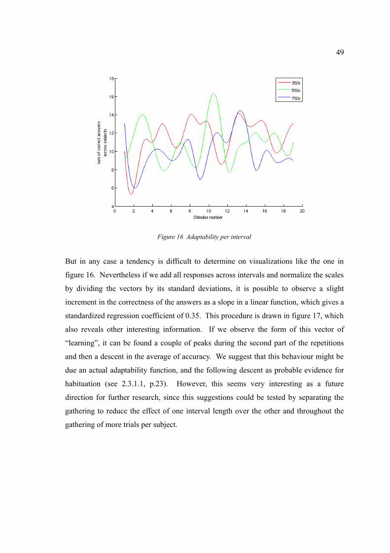
49

Figure 16 Adaptability per interval

But in any case a tendency is difficult to determine on visualizations like the one in

figure 16. Nevertheless if we add all responses across intervals and normalize the scales

by dividing the vectors by its standard deviations, it is possible to observe a slight

increment in the correctness of the answers as a slope in a linear function, which gives a

standardized regression coefficient of 0.35. This procedure is drawn in figure 17, which

also reveals other interesting information. If we observe the form of this vector of

“learning”, it can be found a couple of peaks during the second part of the repetitions

and then a descent in the average of accuracy. We suggest that this behaviour might be

due an actual adaptability function, and the following descent as probable evidence for

habituation (see 2.3.1.1, p.23). However, this seems very interesting as a future

direction for further research, since this suggestions could be tested by separating the

gathering to reduce the effect of one interval length over the other and throughout the

gathering of more trials per subject.

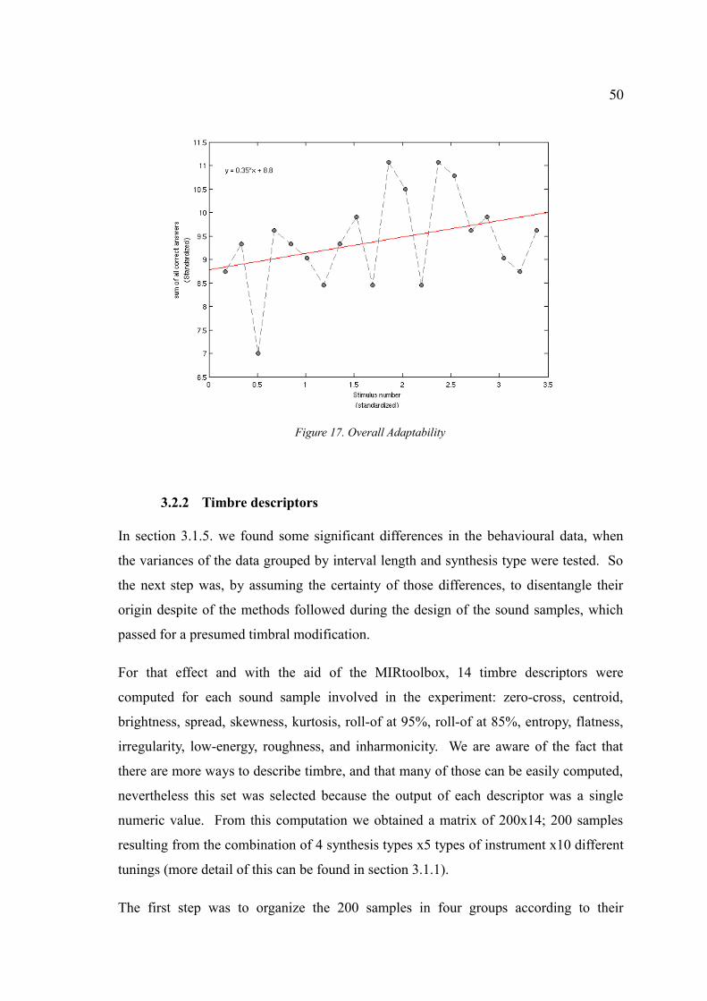
50

Figure 17. Overall Adaptability

3.2.2 Timbre descriptors

In section 3.1.5. we found some significant differences in the behavioural data, when

the variances of the data grouped by interval length and synthesis type were tested. So

the next step was, by assuming the certainty of those differences, to disentangle their

origin despite of the methods followed during the design of the sound samples, which

passed for a presumed timbral modification.

For that effect and with the aid of the MIRtoolbox, 14 timbre descriptors were

computed for each sound sample involved in the experiment: zero-cross, centroid,

brightness, spread, skewness, kurtosis, roll-of at 95%, roll-of at 85%, entropy, flatness,

irregularity, low-energy, roughness, and inharmonicity. We are aware of the fact that

there are more ways to describe timbre, and that many of those can be easily computed,

nevertheless this set was selected because the output of each descriptor was a single

numeric value. From this computation we obtained a matrix of 200x14; 200 samples

resulting from the combination of 4 synthesis types x5 types of instrument x10 different

tunings (more detail of this can be found in section 3.1.1).

The first step was to organize the 200 samples in four groups according to their

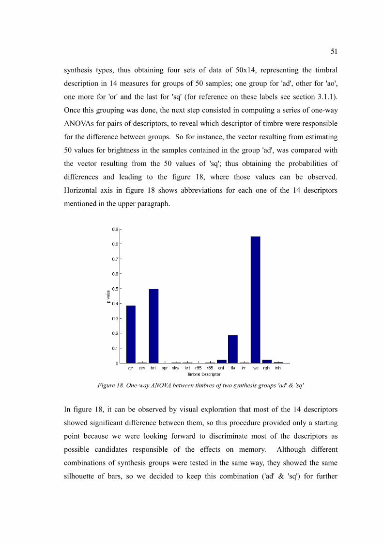
51

synthesis types, thus obtaining four sets of data of 50x14, representing the timbral

description in 14 measures for groups of 50 samples; one group for 'ad', other for 'ao',

one more for 'or' and the last for 'sq' (for reference on these labels see section 3.1.1).

Once this grouping was done, the next step consisted in computing a series of one-way

ANOVAs for pairs of descriptors, to reveal which descriptor of timbre were responsible

for the difference between groups. So for instance, the vector resulting from estimating

50 values for brightness in the samples contained in the group 'ad', was compared with

the vector resulting from the 50 values of 'sq'; thus obtaining the probabilities of

differences and leading to the figure 18, where those values can be observed.

Horizontal axis in figure 18 shows abbreviations for each one of the 14 descriptors

mentioned in the upper paragraph.

Figure 18. One-way ANOVA between timbres of two synthesis groups 'ad' & 'sq'

In figure 18, it can be observed by visual exploration that most of the 14 descriptors

showed significant difference between them, so this procedure provided only a starting

point because we were looking forward to discriminate most of the descriptors as

possible candidates responsible of the effects on memory. Although different

combinations of synthesis groups were tested in the same way, they showed the same

silhouette of bars, so we decided to keep this combination ('ad' & 'sq') for further

52

analysis because it had demonstrated the most meaningful difference in the behavioural

results (p < 0.02, see table 4).

Acknowledged that there were meaningful statistical differences between particular

timbral descriptors computed from sound samples with specific levels of modification,

the following gathering was to learn if such modifications expressed in acoustical data,

had some relation with the responses given by the subjects in the experiment. To realize

this comparison, a simple correlation between the responses of the subjects and each

one of the descriptors would fit. Nevertheless there was one problem, because the

matrix of responses was composed of 60 rows (trials), and the vectors of descriptors had

200 values, one per sample involved in the experiment. To solve this problem, the set of

200 samples x 14 descriptors had to be reduced, so this method consisted in computing

means for each timbre measure among all the pitches that were involved in one trial,

thus computing means for groups of pitches: MIDI(60)-(63)-(63.5)-(64), MIDI(60)-

(65)-(65.5)-(66), and MIDI(60)-(67)-(67.5)-(68). With that method of reduction from

10 pitches to 3, and then multiplied by the number of instrument types(5) and the

synthesis types(4) gave 14 vectors of 60 values, which could then be correlated.

Furthermore, to check the reliability of this reduction we computed again series of one-

way ANOVAs for pairs ('ad' & 'sq' synthesis types) of descriptors, but with this set of 60

values, and the results showed almost the same pattern, except for the spectral roll-off at

85% and the spectral entropy. By operating a reduction of this nature, we interpret that

effects of pitch were also reduced, thus revealing statistical differences between groups

slightly out of that dimension.

In the left side of figure 19 it can be observed the same results of figure 18, but with the

scale of the vertical axis offering a zoom. The right side of the same figure (19) shows

the results of the same computation of ANOVAs for the groups 'ad'-'sq', but within the

set of values that had been reduced to correlate with subjects responses.

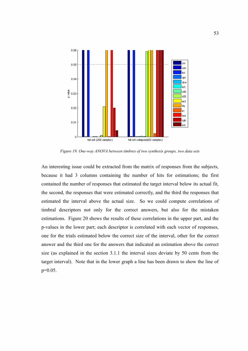
53

Figure 19. One-way ANOVA between timbres of two synthesis groups, two data sets

An interesting issue could be extracted from the matrix of responses from the subjects,

because it had 3 columns containing the number of hits for estimations; the first

contained the number of responses that estimated the target interval below its actual fit,

the second, the responses that were estimated correctly, and the third the responses that

estimated the interval above the actual size. So we could compute correlations of

timbral descriptors not only for the correct answers, but also for the mistaken

estimations. Figure 20 shows the results of these correlations in the upper part, and the

p-values in the lower part; each descriptor is correlated with each vector of responses,

one for the trials estimated below the correct size of the interval, other for the correct

answer and the third one for the answers that indicated an estimation above the correct

size (as explained in the section 3.1.1 the interval sizes deviate by 50 cents from the

target interval). Note that in the lower graph a line has been drawn to show the line of

p=0.05.

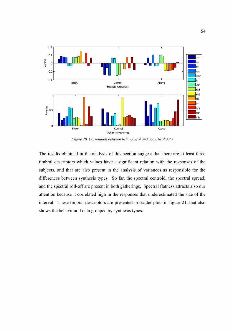
54

Figure 20. Correlation between behavioural and acoustical data

The results obtained in the analysis of this section suggest that there are at least three

timbral descriptors which values have a significant relation with the responses of the

subjects, and that are also present in the analysis of variances as responsible for the

differences between synthesis types. So far, the spectral centroid, the spectral spread,

and the spectral roll-off are present in both gatherings. Spectral flatness attracts also our

attention because it correlated high in the responses that underestimated the size of the

interval. These timbral descriptors are presented in scatter plots in figure 21, that also

shows the behavioural data grouped by synthesis types.

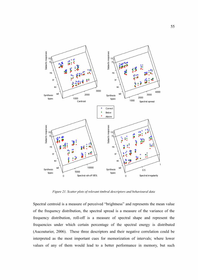
55

Figure 21. Scatter plots of relevant timbral descriptors and behavioural data

Spectral centroid is a measure of perceived “brightness” and represents the mean value

of the frequency distribution, the spectral spread is a measure of the variance of the

frequency distribution, roll-off is a measure of spectral shape and represent the

frequencies under which certain percentage of the spectral energy is distributed

(Aucouturier, 2006). These three descriptors and their negative correlation could be

interpreted as the most important cues for memorization of intervals; where lower

values of any of them would lead to a better performance in memory, but such

56

affirmation should be considered in a new experiment since too many variables are

involved in this experimental set, and would be sources of statistical noise.

Spectral Flatness is defined as the radio of the geometric mean of the power spectrum to

the arithmetic mean of the power spectrum, and is a measure of “noisiness” (Johnston,

1988). The high correlation found in the under-estimation vector would suggest that

high levels of noisiness measured with spectral flatness would probably be a source of

memory impairment. Nevertheless, more empirical evidence is necessary to make such

a claim.

57

4 Conclusions

Some of the results presented here are only partial and deserve more attention

and further analysis. For example we could not establish a connection for the effects of

every compromise, such as the decision to round the intervals for the design of the

experiment that was not applied during the analysis/synthesis of the stimuli; this

disparity could be responsible of some distortion in the results. Also the fact that

accuracy per instrument did not show a significant difference from groups of instrument

types could be explained as an inconsistency in the experimental design due the low

number of cases per instrument. Other explanation could be that the timbres selected

did not have enough contrast in those timbral aspects that resulted relevant for the cuing

of memory for intervals, thus suggesting a failure in the discrimination stage,

particularly in the script that was developed for this purpose which we called

“Antagonist Finder”. Nevertheless a positive aspect are the results obtained for the

synthesis type variable, which could be regarded as synthetic instruments, and their

timbral characteristics were used to balance the other inconsistencies. Although these

synthetic timbres were chosen from a palette of at least 10 different methodologies in an

almost arbitrary way, just by exploring visually the spectrograms of very few samples,

they proved to be useful in the timbral descriptors analysis.

The experimental setting had some aspects that must be improved, such as a counter in

the patch, a properly sound isolated place, and the recruitment of more subjects. Other

thing that could be improved is the questionnaire about the musical background, to

include information on other auditive abilities such as number of spoken languages.

The entire design of this project is an intend to link the perspectives and concepts of a

traditional western academic minded musician with the conceptualization of the nature

of music from a scientific perspective, and the matter of this link has been the definition

of timbre. This effort represent in our understanding a conceptual bridge between a

macro and a micro perspective of the nature of music: a single tone and the universe

contained in it.

58

A relevant issue explored in this project is that selection of timbre to memorize intervals

should be considered carefully for music educators in ear training exercises, because it

might be that certain timbres would optimize the task. However this suggestion must be

supported by more empirical evidence because there are many variables that are not

considered, such as individual preferences.

Future directions for this research would consist in applying more complex trials, such

as harmonic dyads and triads, and short sequences of tones or melodies, as well as the

role of timbre and emotions in memory performance.

59

References

Aucouturier, J. J. (2006). Ten experiments on the modelling of polyphonic timbre, from 

http://www.jj­aucouturier.info/papers/PHD­2006.pdf

Baars, B. J. (1988). A cognitive theory of consciousness. Cambridge University Press.

Bagwell, C. (2001). Sox ­ sound eXchange, from http://sox.sourceforge.net/ 

Bent, I. D., & Pople, A. (2006). Analysis. In L. Macy (Ed.), Grove music online. 

Retrieved May 13, 2006, from http://www.grovemusic.com

Benward, B., & Kolosick, J. T. (2005). Ear training: A technique for listening. McGraw­

Hill Higher Education.

Berger, K. W. (1964). Some factors in the recognition of timbre. The Journal of the  

Acoustical Society of America, 36, 1888. 

Burns, E. M. (1999). Intervals, scales, and tuning. (pp. 215–264)Academic Press.

Choksy, L., Abramson, R. Gillespie, A., Woods, D., & York, F. (2001). Teaching music  

in the twenty­first century. Prentice Hall Upper Saddle River, NJ.

Crowder, R. G., & Pitt, M. A. (1992). Research on Memory/Imagery for musical timbre. 

In D. E. D. T. Reisberg (Ed.), Auditory imagery Lawrence Erlbaum Assoc Inc.

60

Deutsch, D. (1999). The psychology of music (2nd. ed.)Academic Press.

Evans, E. F. (1982). Functional anatomy of the auditory system. In H. B. Barlow, & J. D. 

Mollon (Eds.), The senses (pp. 251­306). Great Britain: Cambridge University 

Press.

Fales, C. (2002). The paradox of timbre. Ethnomusicology, 46(1), 56­95. 

Fales, C. (2005). Listening to timbre during the french enlightenment. Paper presented 

at the Proceedings of the Conference on Interdisciplinary Musicology (CIM05),  

Montréal (Québec) Canada. Retrieved April 24, 2006, from 

http://www.oicm.umontreal.ca/cim05/cim05_articles/FALES_C_CIM05.pdf

Fux, J. J. (1966). Gradus ad parnassum. Broude.

Gordon, E. (1988). Learning sequences in music: Skill, content, and patterns (1997th 

ed.). USA: GIA Publications.

Grey, J. M. (1977). Multidimensional perceptual scaling of musical timbres. The  

Journal of the Acoustical Society of America, 61, 1270. 

Hall, M. D., & Blasko, D. G. (2005). Attentional interference in judgements of musical 

timbre: Individual differences in working memory. The Journal of general  

psychology, 132(1), 94­112. 

61

Halpern, A. R., Zatorre, R. J., Bouffard, M., & Johnson, J. A. (2004). Behavioral and 

neural correlates of perceived and imagined musical timbre. Neuropsychologia,  

42(9), 1281­1292. 

Handel, S. (1989). Listening: An introduction to the perception of auditory events. MIT 

Press.

Hargreaves, D. J., & North, A. C. (2001). Musical development and learning: The  

international perspective. Great Britain: Colin Brock.

Haver, D., & Schmitt , S. (2006). Native instruments kontakt 2 sample library

Helmholtz, H. (1954). On the sensations of tone as a physiological basis for the theory  

of music(A. J. Ellis Trans.).Dover Publications New York.

Hofstetter, F. T. (1975). GUIDO: An interactive computer­based system for improvement 

of instruction and research in ear­training. Journal of Computer­Based Instruction,  

1(4), 100­106. 

Huron, D. (2001). Toward a theory of timbre. Paper presented at the Music Theory Mid­

West Conference. New Theories for 20th Century Music, Cincinnati, Ohio. 

Retrieved May 14, 2006, from http://www.music­cog.ohio­

state.edu/Huron/Talks/SMTmidwest.2001/index.html

62

Johnson, M. (2002). Spectral modelling toolbox

Johnston, J. D. (1988). Transform coding of audio signals using perceptual noise 

criteria. Selected Areas in Communications, IEEE Journal on, 6(2), 314­323. 

Krumhansl, C. L. Cognitive foundations of musical pitch. Oxford University Press, New 

York and Oxford (1990).

Krumhansl, C. L., & Iverson, P. (1992). Perceptual interactions between musical pitch 

and timbre. Journal of experimental psychology. Human perception and  

performance, 18(3), 739­751. 

Lartillot, O., & Toiviainen, P. (2007). MIR toolbox. Jyväskylä University.

Leman, M. (1995). Music and schema theory: Cognitive foundations of systematic  

musicology. Springer.

McAdams, S. (2006). Psychology of music, §II,3:Perception & cognition of timbre. In 

L. Macy (Ed.), Grove music online . Retrieved May 10, 2006, from 

http://www.grovemusic.com

McAdams, S., & Bigand, E. (1993). Thinking in sound: The cognitive psychology of  

human audition. Oxford; New York: Clarendon Press; Oxford University Press.

McAdams, S., Winsberg, S., Donnadieu, S., De Soete, G., & Krimphoff, J. (1995). 

63

Perceptual scaling of synthesized musical timbres: Common dimensions, 

specificities, and latent subject classes. Psychological research, 58(3), 177­192. 

Menning, H., Roberts, L. E., & Pantev, C. (2000). Plastic changes in the auditory cortex 

induced by intensive frequency discrimination training. Neuroreport, 11(4), 817­

822. 

Opolko, F., & Wapnick, J. (2006). McGuill university master samples

Pantev, C., Engelien, A., Candia, V., & Elbert, T. (2001). Representational cortex in 

musicians. plastic alterations in response to musical practice. Ann NY Acad Sci,  

930, 300­314. 

Pantev, C., Roberts, L. E., Schulz, M., Engelien, A., & Ross, B. (2001). Timbre­specific 

enhancement of auditory cortical representations in musicians. Neuroreport, 12(1), 

169­174. 

Pantev, C., Wollbrink, A., Roberts, L. E., Engelien, A., & Lutkenhoner, B. (1999). 

Short­term plasticity of the human auditory cortex. Brain Res, 842(1), 192­199. 

Papoušek, H. (1996). Musicality in infancy research: Biological and cultural origins of 

early musicality. (2003rd ed., pp. 37­55). USA.

Parviainen, O. (2005). Soundstretch

64

Pitt, M. A., & Crowder, R. G. (1992). The role of spectral and dynamic cues in imagery 

for musical timbre. J Exp Psychol Hum Percept Perform, 18(3), 728­738. 

Plomp, R., & Levelt, W. J. (1965). Tonal consonance and critical bandwidth. The  

Journal of the Acoustical Society of America, 38(4), 548­560. 

Puckette, M. (2006). Pure data

Rogers, N. (2005). Verbal labels affect memory for musical timbre. Paper presented at 

the Proceedings of the Conference on Interdisciplinary Musicology (CIM05),  

Montréal (Québec) Canada. Retrieved April 20, 2006, from 

http://www.oicm.umontreal.ca/cim05/cim05_articles/ROGERS_N_CIM05.pdf

Russo, F. A., & Thompson, W. F. (2005). An interval size illusion: The influence of 

timbre on the perceived size of melodic intervals. Perception & psychophysics,  

67(4), 559­568. 

Schafer, R. M. (1977). The tuning of the world. Knopf.

Schwartz, D. A., Howe, C. Q., & Purves, D. (2003). The statistical structure of human 

speech sounds predicts musical universals. Journal of Neuroscience, 23(18), 7160­

7168. 

Semal, C., & Demany, L. (1991). Dissociation of pitch from timbre in auditory short­

65

term memory. The Journal of the Acoustical Society of America, 89(5), 2404­2410. 

Semal, C., & Demany, L. (1993). Further evidence for an autonomous processing of 

pitch in auditory short­term memory. The Journal of the Acoustical Society of  

America, 94(3 Pt 1), 1315­1322. 

Serafine, M. L. (1988). Music as cognition: The development of thought in sound.  

Columbia University Press.

Serra, X., & Smith III, J. (1990). Spectral modelling synthesis: A sound 

Analysis/Synthesis system based on a deterministic plus stochastic decomposition. 

Computer Music Journal, 14(4), 12­24. 

Sethares, W. A. (1999). Tuning, timbre, spectrum, scale. Great Britain: Springer.

Shepard, R. (2001). Cognitive psychology and music. Music, cognition and  

computerized sound: An introduction to psychoacoustics (pp. 21­35). USA: Cook, 

P.R.

Slawson, W. (1985). Sound color. USA: University of California Press Berkeley.

Sloboda, J. A. (2005). Exploring the musical mind: Cognition, emotion, ability, function  

Oxford University Press

Snyder, B. (2001). Music and memory: An introduction. USA: MIT Press.

66

Warrier, C. M., & Zatorre, R. J. (2002). Influence of tonal context and timbral variation 

on perception of pitch. Perception & psychophysics, 64(2), 198­207. 

Wessel, D. (1979). Timbre space as a musical control structure. Computer Music  

Journal, 3(2), 45–52. 

Yost, W. A., & Nielsen, D. W. (1985). Fundamentals of hearing.Holt.

Zagorski­Thomas, S. (2005). Shouting quietly: Changing musical meaning by changing 

timbre with recording technology. Paper presented at the Proceedings of the  

Conference on Interdisciplinary Musicology (CIM05), Montréal (Québec) Canada. 

Retrieved April 20, 2006, from 

http://www.oicm.umontreal.ca/cim05/cim05_articles/ZAGORSKI­TS_CIM05.pdf

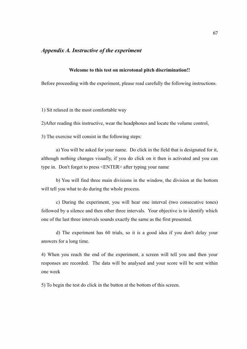
67

Appendix A. Instructive of the experiment

Welcome to this test on microtonal pitch discrimination!!

Before proceeding with the experiment, please read carefully the following instructions.

1) Sit relaxed in the most comfortable way

2)After reading this instructive, wear the headphones and locate the volume control,

3) The exercise will consist in the following steps:

a) You will be asked for your name. Do click in the field that is designated for it,

although nothing changes visually, if you do click on it then is activated and you can

type in. Don't forget to press <ENTER> after typing your name

b) You will find three main divisions in the window, the division at the bottom

will tell you what to do during the whole process.

c) During the experiment, you will hear one interval (two consecutive tones)

followed by a silence and then other three intervals. Your objective is to identify which

one of the last three intervals sounds exactly the same as the first presented.

d) The experiment has 60 trials, so it is a good idea if you don't delay your

answers for a long time.

4) When you reach the end of the experiment, a screen will tell you and then your

responses are recorded. The data will be analysed and your score will be sent within

one week

5) To begin the test do click in the button at the bottom of this screen.

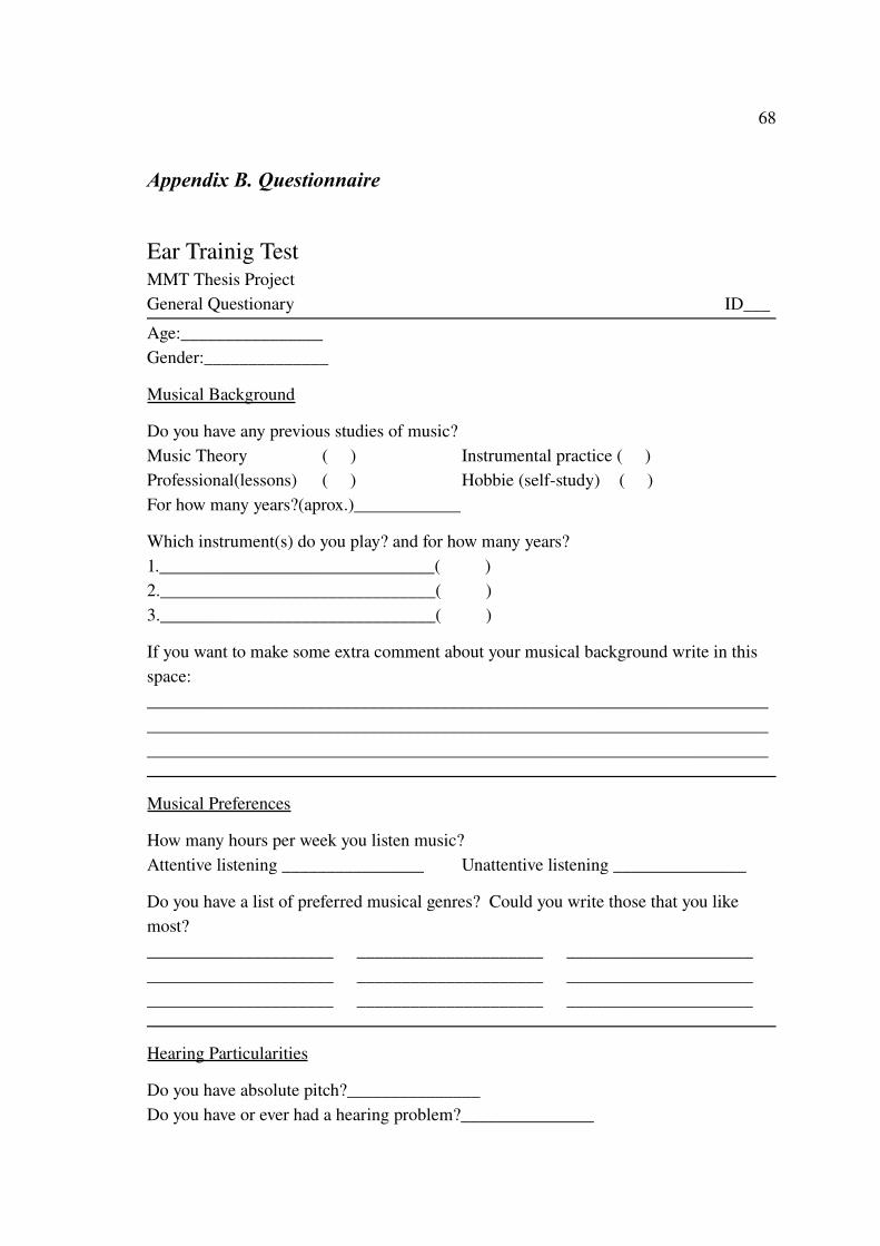
68

Appendix B. Questionnaire

Ear Trainig TestMMT Thesis ProjectGeneral Questionary             ID___Age:________________Gender:______________

Musical Background

Do you have any previous studies of music?Music Theory     (     ) Instrumental practice (     )Professional(lessons)     (     ) Hobbie (self­study) (     )For how many years?(aprox.)____________

Which instrument(s) do you play? and for how many years?1._______________________________(          )2._______________________________(          )3._______________________________(          )

If you want to make some extra comment about your musical background write in this space:__________________________________________________________________________________________________________________________________________________________________________________________________________________

Musical Preferences

How many hours per week you listen music?Attentive listening ________________ Unattentive listening _______________

Do you have a list of preferred musical genres?  Could you write those that you like most?_____________________ _____________________ __________________________________________ _____________________ __________________________________________ _____________________ _____________________

Hearing Particularities

Do you have absolute pitch?_______________Do you have or ever had a hearing problem?_______________