Cyprus Advanced HPC Workshop Winter 2012. Tracking: FH6190763 Feb/2012 Handling Parallelisation in OpenFOAM Hrvoje Jasak [email protected] Faculty of Mechanical Engineering and Naval Architecture University of Zagreb, Croatia Handling Parallelisation in OpenFOAM – p. 1

Welcome message from author
This document is posted to help you gain knowledge. Please leave a comment to let me know what you think about it! Share it to your friends and learn new things together.
Transcript
Cyprus Advanced HPC Workshop Winter 2012. Tracking: FH6190763 Feb/2012
Handling Parallelisation in OpenFOAMHrvoje Jasak
Faculty of Mechanical Engineering and Naval Architecture
University of Zagreb, Croatia
Handling Parallelisation in OpenFOAM – p. 1
Cyprus Advanced HPC Workshop Winter 2012. Tracking: FH6190763 Feb/2012
Parallelisation in OpenFOAM
Objective
• Present the approach and implementation of massively parallel discretisation andsolution method support in the OpenFOAM
Topics
• Background on architecture and massive parallelism
• Components
• Parallel communications library: Pstream
• Domain decomposition and reconstruction
• Zero halo layer discretisation support: processor boundary type
• Discretisation and Algorithmic issues
• Cell- and point-based algorithms: FVM and FEM
• Linear solvers and preconditioners
• Parallelisation of Lagrangian particle tracking
• Running OpenFOAM in parallel
• Summary
Handling Parallelisation in OpenFOAM – p. 2
Cyprus Advanced HPC Workshop Winter 2012. Tracking: FH6190763 Feb/2012
Background
Massively Parallel Computing
• Today, most large-scale CFD solvers rely on distributed-memory parallel computerarchitectures for all medium-sized and large simulations
• Parallelisation of commercial solvers is completed: if the algorithm does notparallelise well, it is not used calculation
• Current development work aimed at bottle-necks: parallel mesh generation
Parallel Computer Architecture
• Parallel CCM software operates almost exclusively in domain decompositionmode: a large loop (e.g. cell-face loop in the FVM solver) is split into bits andgiven to a separate CPU. Data dependency is handled explicitly by the software
• Similar to high-performance architecture, parallel computers differ in how eachnode (CPU) can see and access data (memory) on other nodes:
◦ Shared memory machines: single node sees complete memory
◦ Distributed memory machines: each node is a self-contained unit.Node-to-node communication involves considerable overhead
• For distributed memory machines, a node can be an off-the-shelf PC or a servernode: cheap, but limited by speed of (network) communication
Handling Parallelisation in OpenFOAM – p. 3
Cyprus Advanced HPC Workshop Winter 2012. Tracking: FH6190763 Feb/2012
Components
Parallel Components and Functionality
1. Parallel communication wrapper
• Basic information about the run-time environment: serial or parallel execution,number of processors, process IDs etc.
• Passing information in transparent and protocol-independent manner
• Global gather-scatter communication operations
2. Mesh-related operations• Mesh and data decomposition and reconstruction
• Global mesh information, e.g. global mesh size• Handling patched pairwise communications
• Processor topology communication scheduling data
3. Discretisation support• Processor data updates across processors: data consistency• Matrix assembly: executing discretisation operations in parallel
4. Linear equation solver support
5. Auxiliary operations, e.g. messaging or algorithmic communications, non-fieldalgorithms (e.g. particle tracking), data input-output
Handling Parallelisation in OpenFOAM – p. 4

Cyprus Advanced HPC Workshop Winter 2012. Tracking: FH6190763 Feb/2012
Parallel Communications
Stream-Based Parallel Communication Library
• In C++, functional communication is replaced by a stream-based system
int a = 7;// Some C programming, using ellipsis argumentsprintf("Hello World, for the %ith time", a);
// Strongly checked, object-oriented C++ waycout << "Hello, World " << a << endl;
• Stream-based system separates class-dependent part from communications
• A stream is responsible for handling the data in a stream-dependent way.Example: graph in a file or on a screen
• In OpenFOAM, all relevant classes contain Istream constructor andoperator<<() (write operation)
• Parallel communication protocol is-a stream: Pstream
OPstream toNeighb(procPatch.neighbProcNo());toNeighb << patchInfo;
IPstream fromNeighb(procPatch.neighbProcNo());fromNeighb >> nbrPatchInfo;
Handling Parallelisation in OpenFOAM – p. 5
Cyprus Advanced HPC Workshop Winter 2012. Tracking: FH6190763 Feb/2012
Parallel Communications
Stream-Based Parallel Communication Library
• Parallel communications library holds basic run-time information
• Since Pstream is derived from IOstream, no object-level changes are required:sending a floating point array and a mesh object is of same complexity
• Buffered and compressed transfer are specified as Pstream settings
Implementation
• Most Pstream data and behaviour is generic (does not depend on the underlyingcommunications algorithm): create and destroy, manage buffers, record processorIDs etc.
• The part which is communication-dependent is limited to a few functions: initialise,exit, send data and receive data
• OpenFOAM implements a single Pstream class, but protocol-dependent library isimplemented separately: run-time linkage changes the communication protocol!
• Easy porting to new communication platform: re-implementing calls in a library
• . . . and no changes are required anywhere else in the code
• Communication protocol is chosen by picking the shared library: libPstream
• Optional use of compression on send/receive to speed up communication
Handling Parallelisation in OpenFOAM – p. 6
Cyprus Advanced HPC Workshop Winter 2012. Tracking: FH6190763 Feb/2012
Domain Decomposition Approach
Parallel FVM Simulation
• Computational domain is split up into meshes, each associated with a singleprocessor:
◦ Allocation of cells to processors
◦ Physical decomposition of the mesh in the native solver format
This step is termed domain decomposition
• A mechanism for data transfer between processors needs to be devised: astandard interface to a wrapped communications package
• Solution algorithm is analysed to establish the inter-dependence and points ofsynchronisation
• Mesh partitioning constraints◦ Load balance: all processing units should have approximately the same
amount of work between communication and synchronisation points
◦ Minimum communication, relative to local work. Performing localcomputations is orders of magnitude faster than communicating the data
Data Reconstruction
• Operate in the opposite direction: reconstruct decomposed mesh and data
• Longer term, this should be avoided: parallelisation of the complete simulation
Handling Parallelisation in OpenFOAM – p. 7
Cyprus Advanced HPC Workshop Winter 2012. Tracking: FH6190763 Feb/2012
Parallel Algorithms
Mesh Support
• For purposes of algorithmic analysis, we shall recognise that each cell belongs toone and only one processor: no inherent overlap for computational points
• In FVM, mesh faces can be grouped as follows
◦ Internal faces, within a single processor mesh
◦ Boundary faces
◦ Inter-processor boundary faces: faces used to be internal but are nowseparate and represented on 2 CPUs. No face may belong to more than 2sub-domains
• FEM (and cell-to-point interpolation) operates on vertices in a similar manner but avertex may be multiply shared between processors: overlap is unavoidable
• Algorithmically, there is no change for objects internal to the mesh and on theprocessor boundary: this is the source of parallel speed-up
• The challenge is to repeat the operations for objects on inter-processor boundaries
Handling Parallelisation in OpenFOAM – p. 8
Cyprus Advanced HPC Workshop Winter 2012. Tracking: FH6190763 Feb/2012
Parallel Algorithms
Halo Layer Approach
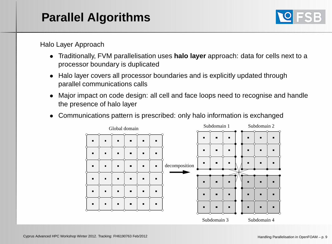
• Traditionally, FVM parallelisation uses halo layer approach: data for cells next to aprocessor boundary is duplicated
• Halo layer covers all processor boundaries and is explicitly updated throughparallel communications calls
• Major impact on code design: all cell and face loops need to recognise and handlethe presence of halo layer
• Communications pattern is prescribed: only halo information is exchanged
decomposition
Global domain Subdomain 1
Subdomain 3 Subdomain 4
Subdomain 2
Handling Parallelisation in OpenFOAM – p. 9

Cyprus Advanced HPC Workshop Winter 2012. Tracking: FH6190763 Feb/2012
Parallel Algorithms
Zero Halo Layer Approach
• Algorithmically, halo is an inconsistent approach: coupled boundary without-of-core addressing exists in other places in the code
• Example: cyclic and periodic “boundary conditions” pose the same problem
yx
y x
P
N’
N
• Implementation principle: introduce implicit updated boundaries with “out-of core”addressing
• Specific types: cyclic, periodic, processor (= cyclic with communication), GGI
• Processor boundary update encapsulates communication to do evaluation. Virtualfunction mechanism does the rest: no impact in the rest of the code!
• Difference between parallel and serial execution is the presence of processorboundary type and serial or parallel deployment (mpirun)
Handling Parallelisation in OpenFOAM – p. 10
Cyprus Advanced HPC Workshop Winter 2012. Tracking: FH6190763 Feb/2012
FVM Discretisation
Explicit FVM Operators: Gradient Calculation
• Using Gauss’ theorem, we need to evaluate face values of the variable. Forinternal faces, this is done trough interpolation:
φf = fx φP + (1− fx)φN
Once calculated, face value may be re-used until cell-centred φ changes
• In parallel, φP and φN live on different processors. Assuming φP is local, φN canbe fetched through communication: this is once-per-solution cost and obtained bypairwise communication
• Note that all processors perform identical duties: thus, for a processor boundarybetween domain A and B, evaluation of face values can be done in 3 steps:
1. Collect a subset internal cell values from local domain and send the values tothe neighbouring processor
2. Receive neighbour values from neighbouring processor
3. Evaluate local processor face value using interpolation
Handling Parallelisation in OpenFOAM – p. 11

Cyprus Advanced HPC Workshop Winter 2012. Tracking: FH6190763 Feb/2012
FVM Discretisation
Finite Volume Matrix Assembly
• Similar to gradient calculation above, assembly of matrix coefficients on processorboundaries can be done using simple pairwise communication
• In order to assemble the coefficient, we need geometrical information and someinterpolated data: all readily available, maybe with some communication
• Example: off-diagonal coefficient of a Laplace operator
aN = |sf |γf
|df |
where γf is the interpolated diffusion coefficient and the rest are geometry-relatedproperties. In actual implementation, geometry is calculated locally andinterpolation factors are cached to minimise communication
• Discretisation of a convection term is similarly simple
• Sources, sinks and temporal schemes all remain unchanged: each cell belongs toonly one processor
Handling Parallelisation in OpenFOAM – p. 12

Cyprus Advanced HPC Workshop Winter 2012. Tracking: FH6190763 Feb/2012
FEM Discretisation
Supporting FEM Discretisation
• Unlike the FVM, FEM computational points are present on multiple processors
• Since discretisation is element-based, matrix assembly is completed by combiningcontribution from various processors
• Parallel communication pattern may now be more complex: n processors sharingthe same point
• . . . but for consistency FEM must operate on the same domain decomposition
• In order to avoid communications overheads of many small messages in acomplex connectivity graph, a 2-tier update is used
◦ Pairwise patch-based communications: long messages, similar to FVM
◦ Collapse all globally shared communication into a single gather-scatteroperation: avoid small messages and complex comms pattern
Handling Parallelisation in OpenFOAM – p. 13
Cyprus Advanced HPC Workshop Winter 2012. Tracking: FH6190763 Feb/2012
Linear Solver Algorithms
Linear Equation Solvers
• Major impact of parallelism in linear equation solvers is in choice of algorithm.Only algorithms that can operate on a fixed local matrix slice created by localdiscretisation will give acceptable performance
• In terms of code organisation, each sub-domain creates its own numberingspace: locally, equation numbering always starts with zero and one cannot rely onglobal numbering: it breaks parallel efficiency
• Coefficients related to processor interfaces are kept separate and multipliedthrough in a separate matrix update
• Impact of processor boundaries will be seen in:◦ Every matrix-vector multiplication operation
◦ Every Gauss-Seidel or similar smoothing sweep
. . . but nowhere else!
Handling Parallelisation in OpenFOAM – p. 14
Cyprus Advanced HPC Workshop Winter 2012. Tracking: FH6190763 Feb/2012
Linear Solver Algorithms
Processor Interface Updates
• Data dependency in out-of-core vector- matrix multiplication is identical to explicitevaluation of shared data during discretisation
• This appears for all implicitly coupled boundary conditions: virtual base classinterface needed
• lduCoupledInterface handles all out-of-core updates. It is updated after everyvector-matrix operation or smoothing sweep processorLduCoupledInterfaceis a derived class, using Pstream for communications and processorFvPatchfor addressing
Parallel Algebraic Multigrid (AMG)
• As a rule, Krylov space solvers parallelise naturally: global updates on scalingand residual combined with local vector-matrix operations
• In Algebraic Multigrid care needs to be given to coarsening algorithms
◦ Aggregative AMG (AAMG) work naturally on matrices without overlap (FVM)
◦ For cases with overlap (FEM), Selective AMG works better
• Currently, all algorithms assume uniform communications performance across themachine. For very large clusters, AMG suffers due to lack of scaling: coarse levelserialises the work and boosts communications latency issues
Handling Parallelisation in OpenFOAM – p. 15
Cyprus Advanced HPC Workshop Winter 2012. Tracking: FH6190763 Feb/2012
Parallel Algorithms
Synchronisation
• Parallel domain decomposition solvers operate such that all processors followidentical execution path in the code. In order to achieve this, some decisionsand control parameters need to be synchronised across all processor
• Example: convergence tolerance. If one of the processors decides convergence isreached and others do not, they will attempt to continue with iterations andsimulation will lock up waiting for communication
• Global reduce operations synchronise decision-making and appear throughouthigh-level code. This is built into reduction operators: gSum, gMax, gMin etc.
• Communications in global reduce is of gather-scatter type: all CPUs send theirdata to CPU 0, which combines the data and broadcasts it back
• Actual implementation is more clever: using native gather-scatter functionalityoptimised for type of inter-connect, or hierarchical communications
vector force = sum(
mesh.Sf().boundaryField()[patchI]*p.boundaryField()[patchI]);reduce(force, sumOp<vector>());
Handling Parallelisation in OpenFOAM – p. 16

Cyprus Advanced HPC Workshop Winter 2012. Tracking: FH6190763 Feb/2012
Lagrangian Particle Tracking
Parallelisation of Particle Tracking
• Particle tracking algorithm operates on each segment of decomposed mesh bytracking local particles
• Tracking class implements boundary interaction: what happens when a particlehits a boundary face is handled through virtual functions
• Processor boundary interaction: answering the virtual function interface, aparticle is migrated to connecting processor
• Issues with load balancing: loss of performance for cases where particles are notuniformly distributed in the domain
Handling Parallelisation in OpenFOAM – p. 17
Cyprus Advanced HPC Workshop Winter 2012. Tracking: FH6190763 Feb/2012
Running OpenFOAM in Parallel
Case Preparation
• Typically, the case will be prepared in one piece: serial mesh generation
• decomposePar: parallel decomposition tool, controlled by decomposeParDict
• Options in the dictionary allow choice of decomposition and auxiliary data
• Upon decomposition, processorNN directories are created with decomposedmesh and fields; solution controls, model choice and discretisation parameters areshared. Each CPU may use local disk space
• decomposePar may output cell-to-processor decomposition
• Manual decomposition (debugging): provide cell-to-processor file
Parallel Execution
• Top-level code does not change between serial and parallel execution: operationsrelated to parallel support are embedded in the library
• Launch executable using mpirun (or equivalent) with -parallel option
• Data in time directories is created on a per-processor basis
• It is possible to visualise a single CPU data (but we do not do it often): there maybe problems with processor boundaries
• Field initialisation may also be run in parallel: trivial parallelisation
Handling Parallelisation in OpenFOAM – p. 18
Cyprus Advanced HPC Workshop Winter 2012. Tracking: FH6190763 Feb/2012
Running OpenFOAM in Parallel
On-the-Fly Data Analysis
• Sampling, graphing and post-processing tools will execute correctly in parallel:location of probes is reduced over CPUs
• In parallel decomposition, all patches are present on all CPUs (even with zerosize). This allows global reduction of patch-based data
Graphical Post-Processing
• Used most often: reconstruct the data to a single CPU: reconstructPar
• Reconstructed data can be re-decomposed to a different number of CPUs
• Dynamic load balancing and some mesh handling features are work-in-progress
• For large data sets, sampling tools may be executed in parallel: extract and mergeiso-surfaces for visualisation
Handling Parallelisation in OpenFOAM – p. 19

Cyprus Advanced HPC Workshop Winter 2012. Tracking: FH6190763 Feb/2012
Summary
Parallelisation in OpenFOAM
• Parallel communications are wrapped in Pstream library to isolate communicationdetails from library use
• Discretisation uses the domain decomposition with zero halo layer approach
• Parallel updates are a special case of coupled discretisation and linear algebrafunctionality: the code transparently implements parallel coupling
◦ processorFvPatch and equivalent FEM/FAM class for coupleddiscretisation updates
◦ processorLduInterface and field for linear algebra updates
Conclusion
• OpenFOAM is a mature and validated object-oriented implementation of domaindecomposition parallelism
• There are no specific top-level parallelisation requirements: identical codeoperates in serial and parallel execution
• Porting to new communication protocols is easy
• Future work involves chasing performance with non-trivial communication setupand dynamic load balancing
Handling Parallelisation in OpenFOAM – p. 20
Related Documents