SECOND EDITION HOW ARD DEVOE

Welcome message from author
This document is posted to help you gain knowledge. Please leave a comment to let me know what you think about it! Share it to your friends and learn new things together.
Transcript

8/12/2019 Howard Devoe Thermodynamic and Chemical
http://slidepdf.com/reader/full/howard-devoe-thermodynamic-and-chemical 1/532
SECOND EDITION
HOWARD DEVOE

8/12/2019 Howard Devoe Thermodynamic and Chemical
http://slidepdf.com/reader/full/howard-devoe-thermodynamic-and-chemical 2/532
Thermodynamicsand Chemistry
Second EditionVersion 4, March 2012
Howard DeVoeAssociate Professor of Chemistry Emeritus
University of Maryland, College Park, Maryland
8/12/2019 Howard Devoe Thermodynamic and Chemical
http://slidepdf.com/reader/full/howard-devoe-thermodynamic-and-chemical 3/532
The rst edition of this book was previously published by Pearson Education, Inc. It wascopyright ©2001 by Prentice-Hall, Inc.
The second edition, version 4 is copyright ©2012 by Howard DeVoe.
This work is licensed under a Creative Commons Attribution-NonCommercial-NoDerivsLicense, whose full text is at
http://creativecommons.org/licenses/by-nc-nd/3.0You are free to read, store, copy and print the PDF le for personal use. You are not allowedto alter, transform, or build upon this work, or to sell it or use it for any commercial purposewhatsoever, without the written consent of the copyright holder.
The book was typeset using the L ATEX typesetting system and the memoir class. Most of the gures were produced with PSTricks, a related software program. The fonts are AdobeTimes, MathTime, Helvetica, and Computer Modern Typewriter.
I thank the Department of Chemistry and Biochemistry, University of Maryland, CollegePark, Maryland ( http://www.chem.umd.edu ) for hosting the Web site for this book. Themost recent version can always be found online at
http://www.chem.umd.edu/thermobook
If you are a faculty member of a chemistry or related department of a college or uni-versity, you may send a request to [email protected] for a complete Solutions Manualin PDF format for your personal use. In order to protect the integrity of the solutions,requests will be subject to verication of your faculty status and your agreement not toreproduce or transmit the manual in any form.
8/12/2019 Howard Devoe Thermodynamic and Chemical
http://slidepdf.com/reader/full/howard-devoe-thermodynamic-and-chemical 4/532
SHORT CONTENTS
Biographical Sketches 15
Preface to the Second Edition 16
From the Preface to the First Edition 17
1 Introduction 19
2 Systems and Their Properties 27
3 The First Law 56
4 The Second Law 102
5 Thermodynamic Potentials 135
6 The Third Law and Cryogenics 150
7 Pure Substances in Single Phases 164
8 Phase Transitions and Equilibria of Pure Substances 193
9 Mixtures 223
10 Electrolyte Solutions 286
11 Reactions and Other Chemical Processes 303
12 Equilibrium Conditions in Multicomponent Systems 367
13 The Phase Rule and Phase Diagrams 419
14 Galvanic Cells 450
Appendix A Denitions of the SI Base Units 471
4
8/12/2019 Howard Devoe Thermodynamic and Chemical
http://slidepdf.com/reader/full/howard-devoe-thermodynamic-and-chemical 5/532
S HORT C ONTENTS 5
Appendix B Physical Constants 472
Appendix C Symbols for Physical Quantities 473
Appendix D Miscellaneous Abbreviations and Symbols 477
Appendix E Calculus Review 480
Appendix F Mathematical Properties of State Functions 482
Appendix G Forces, Energy, and Work 487
Appendix H Standard Molar Thermodynamic Properties 505
Appendix I Answers to Selected Problems 508
Bibliography 512
Index 521
Thermodynamics and Chemistry , second edition, version 4 © 2012 by Howard DeVoe. Latest version: www.chem.umd.edu/thermobook
8/12/2019 Howard Devoe Thermodynamic and Chemical
http://slidepdf.com/reader/full/howard-devoe-thermodynamic-and-chemical 6/532
C ONTENTS
Biographical Sketches 15
Preface to the Second Edition 16
From the Preface to the First Edition 17
1 Introduction 191.1 Units . . . . . . . . . . . . . . . . . . . . . . . . . . . . . . . . . . . . . 19
1.1.1 Amount of substance and amount . . . . . . . . . . . . . . . . . . 211.2 Quantity Calculus . . . . . . . . . . . . . . . . . . . . . . . . . . . . . . 221.3 Dimensional Analysis . . . . . . . . . . . . . . . . . . . . . . . . . . . . 24Problem . . . . . . . . . . . . . . . . . . . . . . . . . . . . . . . . . . . . . . . 26
2 Systems and Their Properties 272.1 The System, Surroundings, and Boundary . . . . . . . . . . . . . . . . . . 27
2.1.1 Extensive and intensive properties . . . . . . . . . . . . . . . . . . 282.2 Phases and Physical States of Matter . . . . . . . . . . . . . . . . . . . . . 302.2.1 Physical states of matter . . . . . . . . . . . . . . . . . . . . . . . 302.2.2 Phase coexistence and phase transitions . . . . . . . . . . . . . . . 312.2.3 Fluids . . . . . . . . . . . . . . . . . . . . . . . . . . . . . . . . . 322.2.4 The equation of state of a uid . . . . . . . . . . . . . . . . . . . . 332.2.5 Virial equations of state for pure gases . . . . . . . . . . . . . . . . 342.2.6 Solids . . . . . . . . . . . . . . . . . . . . . . . . . . . . . . . . . 36
2.3 Some Basic Properties and Their Measurement . . . . . . . . . . . . . . . 362.3.1 Mass . . . . . . . . . . . . . . . . . . . . . . . . . . . . . . . . . 362.3.2 Volume . . . . . . . . . . . . . . . . . . . . . . . . . . . . . . . . 372.3.3 Density . . . . . . . . . . . . . . . . . . . . . . . . . . . . . . . . 382.3.4 Pressure . . . . . . . . . . . . . . . . . . . . . . . . . . . . . . . . 382.3.5 Temperature . . . . . . . . . . . . . . . . . . . . . . . . . . . . . 40
2.4 The State of the System . . . . . . . . . . . . . . . . . . . . . . . . . . . 452.4.1 State functions and independent variables . . . . . . . . . . . . . . 452.4.2 An example: state functions of a mixture . . . . . . . . . . . . . . 462.4.3 More about independent variables . . . . . . . . . . . . . . . . . . 47
6
8/12/2019 Howard Devoe Thermodynamic and Chemical
http://slidepdf.com/reader/full/howard-devoe-thermodynamic-and-chemical 7/532
C ONTENTS 7
2.4.4 Equilibrium states . . . . . . . . . . . . . . . . . . . . . . . . . . 482.4.5 Steady states . . . . . . . . . . . . . . . . . . . . . . . . . . . . . 50
2.5 Processes and Paths . . . . . . . . . . . . . . . . . . . . . . . . . . . . . . 502.6 The Energy of the System . . . . . . . . . . . . . . . . . . . . . . . . . . 52
2.6.1 Energy and reference frames . . . . . . . . . . . . . . . . . . . . . 53
2.6.2 Internal energy . . . . . . . . . . . . . . . . . . . . . . . . . . . . 53Problems . . . . . . . . . . . . . . . . . . . . . . . . . . . . . . . . . . . . . . 55
3 The First Law 563.1 Heat, Work, and the First Law . . . . . . . . . . . . . . . . . . . . . . . . 56
3.1.1 The concept of thermodynamic work . . . . . . . . . . . . . . . . 573.1.2 Work coefcients and work coordinates . . . . . . . . . . . . . . . 593.1.3 Heat and work as path functions . . . . . . . . . . . . . . . . . . . 603.1.4 Heat and heating . . . . . . . . . . . . . . . . . . . . . . . . . . . 613.1.5 Heat capacity . . . . . . . . . . . . . . . . . . . . . . . . . . . . . 623.1.6 Thermal energy . . . . . . . . . . . . . . . . . . . . . . . . . . . . 62
3.2 Spontaneous, Reversible, and Irreversible Processes . . . . . . . . . . . . . 64
3.2.1 Reversible processes . . . . . . . . . . . . . . . . . . . . . . . . . 643.2.2 Irreversible processes . . . . . . . . . . . . . . . . . . . . . . . . . 663.2.3 Purely mechanical processes . . . . . . . . . . . . . . . . . . . . . 66
3.3 Heat Transfer . . . . . . . . . . . . . . . . . . . . . . . . . . . . . . . . . 673.3.1 Heating and cooling . . . . . . . . . . . . . . . . . . . . . . . . . 673.3.2 Spontaneous phase transitions . . . . . . . . . . . . . . . . . . . . 69
3.4 Deformation Work . . . . . . . . . . . . . . . . . . . . . . . . . . . . . . 693.4.1 Gas in a cylinder-and-piston device . . . . . . . . . . . . . . . . . 703.4.2 Expansion work of a gas . . . . . . . . . . . . . . . . . . . . . . . 723.4.3 Expansion work of an isotropic phase . . . . . . . . . . . . . . . . 733.4.4 Generalities . . . . . . . . . . . . . . . . . . . . . . . . . . . . . . 74
3.5 Applications of Expansion Work . . . . . . . . . . . . . . . . . . . . . . . 753.5.1 The internal energy of an ideal gas . . . . . . . . . . . . . . . . . . 753.5.2 Reversible isothermal expansion of an ideal gas . . . . . . . . . . . 753.5.3 Reversible adiabatic expansion of an ideal gas . . . . . . . . . . . . 753.5.4 Indicator diagrams . . . . . . . . . . . . . . . . . . . . . . . . . . 773.5.5 Spontaneous adiabatic expansion or compression . . . . . . . . . . 783.5.6 Free expansion of a gas into a vacuum . . . . . . . . . . . . . . . . 79
3.6 Work in a Gravitational Field . . . . . . . . . . . . . . . . . . . . . . . . . 803.7 Shaft Work . . . . . . . . . . . . . . . . . . . . . . . . . . . . . . . . . . 82
3.7.1 Stirring work . . . . . . . . . . . . . . . . . . . . . . . . . . . . . 833.7.2 The Joule paddle wheel . . . . . . . . . . . . . . . . . . . . . . . . 84
3.8 Electrical Work . . . . . . . . . . . . . . . . . . . . . . . . . . . . . . . . 863.8.1 Electrical work in a circuit . . . . . . . . . . . . . . . . . . . . . . 863.8.2 Electrical heating . . . . . . . . . . . . . . . . . . . . . . . . . . . 883.8.3 Electrical work with a galvanic cell . . . . . . . . . . . . . . . . . 89
3.9 Irreversible Work and Internal Friction . . . . . . . . . . . . . . . . . . . . 913.10 Reversible and Irreversible Processes: Generalities . . . . . . . . . . . . . 95Problems . . . . . . . . . . . . . . . . . . . . . . . . . . . . . . . . . . . . . . 97
Thermodynamics and Chemistry , second edition, version 4 © 2012 by Howard DeVoe. Latest version: www.chem.umd.edu/thermobook

8/12/2019 Howard Devoe Thermodynamic and Chemical
http://slidepdf.com/reader/full/howard-devoe-thermodynamic-and-chemical 8/532
C ONTENTS 8
4 The Second Law 1024.1 Types of Processes . . . . . . . . . . . . . . . . . . . . . . . . . . . . . . 1024.2 Statements of the Second Law . . . . . . . . . . . . . . . . . . . . . . . . 1034.3 Concepts Developed with Carnot Engines . . . . . . . . . . . . . . . . . . 106
4.3.1 Carnot engines and Carnot cycles . . . . . . . . . . . . . . . . . . 106
4.3.2 The equivalence of the Clausius and Kelvin–Planck statements . . . 1094.3.3 The efciency of a Carnot engine . . . . . . . . . . . . . . . . . . 1114.3.4 Thermodynamic temperature . . . . . . . . . . . . . . . . . . . . . 114
4.4 Derivation of the Mathematical Statement of the Second Law . . . . . . . 1164.4.1 The existence of the entropy function . . . . . . . . . . . . . . . . 1164.4.2 Using reversible processes to dene the entropy . . . . . . . . . . . 1204.4.3 Some properties of the entropy . . . . . . . . . . . . . . . . . . . . 123
4.5 Irreversible Processes . . . . . . . . . . . . . . . . . . . . . . . . . . . . . 1244.5.1 Irreversible adiabatic processes . . . . . . . . . . . . . . . . . . . 1244.5.2 Irreversible processes in general . . . . . . . . . . . . . . . . . . . 125
4.6 Applications . . . . . . . . . . . . . . . . . . . . . . . . . . . . . . . . . 1264.6.1 Reversible heating . . . . . . . . . . . . . . . . . . . . . . . . . . 1274.6.2 Reversible expansion of an ideal gas . . . . . . . . . . . . . . . . . 1274.6.3 Spontaneous changes in an isolated system . . . . . . . . . . . . . 1284.6.4 Internal heat ow in an isolated system . . . . . . . . . . . . . . . 1284.6.5 Free expansion of a gas . . . . . . . . . . . . . . . . . . . . . . . . 1294.6.6 Adiabatic process with work . . . . . . . . . . . . . . . . . . . . . 129
4.7 Summary . . . . . . . . . . . . . . . . . . . . . . . . . . . . . . . . . . . 1304.8 The Statistical Interpretation of Entropy . . . . . . . . . . . . . . . . . . . 130Problems . . . . . . . . . . . . . . . . . . . . . . . . . . . . . . . . . . . . . . 133
5 Thermodynamic Potentials 1355.1 Total Differential of a Dependent Variable . . . . . . . . . . . . . . . . . . 135
5.2 Total Differential of the Internal Energy . . . . . . . . . . . . . . . . . . . 1365.3 Enthalpy, Helmholtz Energy, and Gibbs Energy . . . . . . . . . . . . . . . 1385.4 Closed Systems . . . . . . . . . . . . . . . . . . . . . . . . . . . . . . . . 1405.5 Open Systems . . . . . . . . . . . . . . . . . . . . . . . . . . . . . . . . 1415.6 Expressions for Heat Capacity . . . . . . . . . . . . . . . . . . . . . . . . 1435.7 Surface Work . . . . . . . . . . . . . . . . . . . . . . . . . . . . . . . . . 1445.8 Criteria for Spontaneity . . . . . . . . . . . . . . . . . . . . . . . . . . . . 145Problems . . . . . . . . . . . . . . . . . . . . . . . . . . . . . . . . . . . . . . 148
6 The Third Law and Cryogenics 1506.1 The Zero of Entropy . . . . . . . . . . . . . . . . . . . . . . . . . . . . . 1506.2 Molar Entropies . . . . . . . . . . . . . . . . . . . . . . . . . . . . . . . 152
6.2.1 Third-law molar entropies . . . . . . . . . . . . . . . . . . . . . . 1526.2.2 Molar entropies from spectroscopic measurements . . . . . . . . . 1556.2.3 Residual entropy . . . . . . . . . . . . . . . . . . . . . . . . . . . 156
6.3 Cryogenics . . . . . . . . . . . . . . . . . . . . . . . . . . . . . . . . . . 1576.3.1 Joule–Thomson expansion . . . . . . . . . . . . . . . . . . . . . . 1576.3.2 Magnetization . . . . . . . . . . . . . . . . . . . . . . . . . . . . 159
Thermodynamics and Chemistry , second edition, version 4 © 2012 by Howard DeVoe. Latest version: www.chem.umd.edu/thermobook
8/12/2019 Howard Devoe Thermodynamic and Chemical
http://slidepdf.com/reader/full/howard-devoe-thermodynamic-and-chemical 9/532
C ONTENTS 9
Problem . . . . . . . . . . . . . . . . . . . . . . . . . . . . . . . . . . . . . . . 163
7 Pure Substances in Single Phases 1647.1 Volume Properties . . . . . . . . . . . . . . . . . . . . . . . . . . . . . . 1647.2 Internal Pressure . . . . . . . . . . . . . . . . . . . . . . . . . . . . . . . 1667.3 Thermal Properties . . . . . . . . . . . . . . . . . . . . . . . . . . . . . . 168
7.3.1 The relation between C V; m and C p; m . . . . . . . . . . . . . . . . . 1687.3.2 The measurement of heat capacities . . . . . . . . . . . . . . . . . 1697.3.3 Typical values . . . . . . . . . . . . . . . . . . . . . . . . . . . . 174
7.4 Heating at Constant Volume or Pressure . . . . . . . . . . . . . . . . . . . 1757.5 Partial Derivatives with Respect to T , p , and V . . . . . . . . . . . . . . . 177
7.5.1 Tables of partial derivatives . . . . . . . . . . . . . . . . . . . . . 1777.5.2 The Joule–Thomson coefcient . . . . . . . . . . . . . . . . . . . 180
7.6 Isothermal Pressure Changes . . . . . . . . . . . . . . . . . . . . . . . . . 1817.6.1 Ideal gases . . . . . . . . . . . . . . . . . . . . . . . . . . . . . . 1817.6.2 Condensed phases . . . . . . . . . . . . . . . . . . . . . . . . . . 181
7.7 Standard States of Pure Substances . . . . . . . . . . . . . . . . . . . . . 182
7.8 Chemical Potential and Fugacity . . . . . . . . . . . . . . . . . . . . . . . 1827.8.1 Gases . . . . . . . . . . . . . . . . . . . . . . . . . . . . . . . . . 1837.8.2 Liquids and solids . . . . . . . . . . . . . . . . . . . . . . . . . . 186
7.9 Standard Molar Quantities of a Gas . . . . . . . . . . . . . . . . . . . . . 186Problems . . . . . . . . . . . . . . . . . . . . . . . . . . . . . . . . . . . . . . 189
8 Phase Transitions and Equilibria of Pure Substances 1938.1 Phase Equilibria . . . . . . . . . . . . . . . . . . . . . . . . . . . . . . . 193
8.1.1 Equilibrium conditions . . . . . . . . . . . . . . . . . . . . . . . . 1938.1.2 Equilibrium in a multiphase system . . . . . . . . . . . . . . . . . 1948.1.3 Simple derivation of equilibrium conditions . . . . . . . . . . . . . 195
8.1.4 Tall column of gas in a gravitational eld . . . . . . . . . . . . . . 1968.1.5 The pressure in a liquid droplet . . . . . . . . . . . . . . . . . . . 1988.1.6 The number of independent variables . . . . . . . . . . . . . . . . 1998.1.7 The Gibbs phase rule for a pure substance . . . . . . . . . . . . . . 200
8.2 Phase Diagrams of Pure Substances . . . . . . . . . . . . . . . . . . . . . 2008.2.1 Features of phase diagrams . . . . . . . . . . . . . . . . . . . . . . 2018.2.2 Two-phase equilibrium . . . . . . . . . . . . . . . . . . . . . . . . 2048.2.3 The critical point . . . . . . . . . . . . . . . . . . . . . . . . . . . 2068.2.4 The lever rule . . . . . . . . . . . . . . . . . . . . . . . . . . . . . 2078.2.5 Volume properties . . . . . . . . . . . . . . . . . . . . . . . . . . 210
8.3 Phase Transitions . . . . . . . . . . . . . . . . . . . . . . . . . . . . . . . 2128.3.1 Molar transition quantities . . . . . . . . . . . . . . . . . . . . . . 2128.3.2 Calorimetric measurement of transition enthalpies . . . . . . . . . 2148.3.3 Standard molar transition quantities . . . . . . . . . . . . . . . . . 214
8.4 Coexistence Curves . . . . . . . . . . . . . . . . . . . . . . . . . . . . . . 2148.4.1 Chemical potential surfaces . . . . . . . . . . . . . . . . . . . . . 2158.4.2 The Clapeyron equation . . . . . . . . . . . . . . . . . . . . . . . 2168.4.3 The Clausius–Clapeyron equation . . . . . . . . . . . . . . . . . . 219
Thermodynamics and Chemistry , second edition, version 4 © 2012 by Howard DeVoe. Latest version: www.chem.umd.edu/thermobook
8/12/2019 Howard Devoe Thermodynamic and Chemical
http://slidepdf.com/reader/full/howard-devoe-thermodynamic-and-chemical 10/532
C ONTENTS 10
Problems . . . . . . . . . . . . . . . . . . . . . . . . . . . . . . . . . . . . . . 221
9 Mixtures 2239.1 Composition Variables . . . . . . . . . . . . . . . . . . . . . . . . . . . . 223
9.1.1 Species and substances . . . . . . . . . . . . . . . . . . . . . . . . 2239.1.2 Mixtures in general . . . . . . . . . . . . . . . . . . . . . . . . . . 2239.1.3 Solutions . . . . . . . . . . . . . . . . . . . . . . . . . . . . . . . 2249.1.4 Binary solutions . . . . . . . . . . . . . . . . . . . . . . . . . . . 2259.1.5 The composition of a mixture . . . . . . . . . . . . . . . . . . . . 226
9.2 Partial Molar Quantities . . . . . . . . . . . . . . . . . . . . . . . . . . . 2269.2.1 Partial molar volume . . . . . . . . . . . . . . . . . . . . . . . . . 2279.2.2 The total differential of the volume in an open system . . . . . . . . 2299.2.3 Evaluation of partial molar volumes in binary mixtures . . . . . . . 2319.2.4 General relations . . . . . . . . . . . . . . . . . . . . . . . . . . . 2339.2.5 Partial specic quantities . . . . . . . . . . . . . . . . . . . . . . . 2359.2.6 The chemical potential of a species in a mixture . . . . . . . . . . . 2369.2.7 Equilibrium conditions in a multiphase, multicomponent system . . 236
9.2.8 Relations involving partial molar quantities . . . . . . . . . . . . . 2389.3 Gas Mixtures . . . . . . . . . . . . . . . . . . . . . . . . . . . . . . . . . 239
9.3.1 Partial pressure . . . . . . . . . . . . . . . . . . . . . . . . . . . . 2409.3.2 The ideal gas mixture . . . . . . . . . . . . . . . . . . . . . . . . . 2409.3.3 Partial molar quantities in an ideal gas mixture . . . . . . . . . . . 2409.3.4 Real gas mixtures . . . . . . . . . . . . . . . . . . . . . . . . . . . 243
9.4 Liquid and Solid Mixtures of Nonelectrolytes . . . . . . . . . . . . . . . . 2469.4.1 Raoult’s law . . . . . . . . . . . . . . . . . . . . . . . . . . . . . 2469.4.2 Ideal mixtures . . . . . . . . . . . . . . . . . . . . . . . . . . . . . 2489.4.3 Partial molar quantities in ideal mixtures . . . . . . . . . . . . . . 2499.4.4 Henry’s law . . . . . . . . . . . . . . . . . . . . . . . . . . . . . . 250
9.4.5 The ideal-dilute solution . . . . . . . . . . . . . . . . . . . . . . . 2539.4.6 Solvent behavior in the ideal-dilute solution . . . . . . . . . . . . . 2559.4.7 Partial molar quantities in an ideal-dilute solution . . . . . . . . . . 256
9.5 Activity Coefcients in Mixtures of Nonelectrolytes . . . . . . . . . . . . 2589.5.1 Reference states and standard states . . . . . . . . . . . . . . . . . 2589.5.2 Ideal mixtures . . . . . . . . . . . . . . . . . . . . . . . . . . . . . 2599.5.3 Real mixtures . . . . . . . . . . . . . . . . . . . . . . . . . . . . . 2599.5.4 Nonideal dilute solutions . . . . . . . . . . . . . . . . . . . . . . . 261
9.6 Evaluation of Activity Coefcients . . . . . . . . . . . . . . . . . . . . . . 2629.6.1 Activity coefcients from gas fugacities . . . . . . . . . . . . . . . 2629.6.2 Activity coefcients from the Gibbs–Duhem equation . . . . . . . 2659.6.3 Activity coefcients from osmotic coefcients . . . . . . . . . . . 2669.6.4 Fugacity measurements . . . . . . . . . . . . . . . . . . . . . . . . 268
9.7 Activity of an Uncharged Species . . . . . . . . . . . . . . . . . . . . . . 2709.7.1 Standard states . . . . . . . . . . . . . . . . . . . . . . . . . . . . 2709.7.2 Activities and composition . . . . . . . . . . . . . . . . . . . . . . 2729.7.3 Pressure factors and pressure . . . . . . . . . . . . . . . . . . . . . 273
9.8 Mixtures in Gravitational and Centrifugal Fields . . . . . . . . . . . . . . 275
Thermodynamics and Chemistry , second edition, version 4 © 2012 by Howard DeVoe. Latest version: www.chem.umd.edu/thermobook

8/12/2019 Howard Devoe Thermodynamic and Chemical
http://slidepdf.com/reader/full/howard-devoe-thermodynamic-and-chemical 11/532
C ONTENTS 11
9.8.1 Gas mixture in a gravitational eld . . . . . . . . . . . . . . . . . . 2759.8.2 Liquid solution in a centrifuge cell . . . . . . . . . . . . . . . . . . 277
Problems . . . . . . . . . . . . . . . . . . . . . . . . . . . . . . . . . . . . . . 281
10 Electrolyte Solutions 28610.1 Single-ion Quantities . . . . . . . . . . . . . . . . . . . . . . . . . . . . . 28710.2 Solution of a Symmetrical Electrolyte . . . . . . . . . . . . . . . . . . . . 28910.3 Electrolytes in General . . . . . . . . . . . . . . . . . . . . . . . . . . . . 292
10.3.1 Solution of a single electrolyte . . . . . . . . . . . . . . . . . . . . 29210.3.2 Multisolute solution . . . . . . . . . . . . . . . . . . . . . . . . . 29310.3.3 Incomplete dissociation . . . . . . . . . . . . . . . . . . . . . . . 294
10.4 The Debye–H uckel Theory . . . . . . . . . . . . . . . . . . . . . . . . . . 29510.5 Derivation of the Debye–H uckel Equation . . . . . . . . . . . . . . . . . . 29810.6 Mean Ionic Activity Coefcients from Osmotic Coefcients . . . . . . . . 300Problems . . . . . . . . . . . . . . . . . . . . . . . . . . . . . . . . . . . . . . 302
11 Reactions and Other Chemical Processes 303
11.1 Mixing Processes . . . . . . . . . . . . . . . . . . . . . . . . . . . . . . . 30311.1.1 Mixtures in general . . . . . . . . . . . . . . . . . . . . . . . . . . 30411.1.2 Ideal mixtures . . . . . . . . . . . . . . . . . . . . . . . . . . . . . 30411.1.3 Excess quantities . . . . . . . . . . . . . . . . . . . . . . . . . . . 30611.1.4 The entropy change to form an ideal gas mixture . . . . . . . . . . 30711.1.5 Molecular model of a liquid mixture . . . . . . . . . . . . . . . . . 30911.1.6 Phase separation of a liquid mixture . . . . . . . . . . . . . . . . . 311
11.2 The Advancement and Molar Reaction Quantities . . . . . . . . . . . . . . 31311.2.1 An example: ammonia synthesis . . . . . . . . . . . . . . . . . . . 31411.2.2 Molar reaction quantities in general . . . . . . . . . . . . . . . . . 31611.2.3 Standard molar reaction quantities . . . . . . . . . . . . . . . . . . 319
11.3 Molar Reaction Enthalpy . . . . . . . . . . . . . . . . . . . . . . . . . . . 31911.3.1 Molar reaction enthalpy and heat . . . . . . . . . . . . . . . . . . . 31911.3.2 Standard molar enthalpies of reaction and formation . . . . . . . . 32011.3.3 Molar reaction heat capacity . . . . . . . . . . . . . . . . . . . . . 32311.3.4 Effect of temperature on reaction enthalpy . . . . . . . . . . . . . . 324
11.4 Enthalpies of Solution and Dilution . . . . . . . . . . . . . . . . . . . . . 32511.4.1 Molar enthalpy of solution . . . . . . . . . . . . . . . . . . . . . . 32511.4.2 Enthalpy of dilution . . . . . . . . . . . . . . . . . . . . . . . . . 32711.4.3 Molar enthalpies of solute formation . . . . . . . . . . . . . . . . . 32811.4.4 Evaluation of relative partial molar enthalpies . . . . . . . . . . . . 329
11.5 Reaction Calorimetry . . . . . . . . . . . . . . . . . . . . . . . . . . . . . 33411.5.1 The constant-pressure reaction calorimeter . . . . . . . . . . . . . 33411.5.2 The bomb calorimeter . . . . . . . . . . . . . . . . . . . . . . . . 33611.5.3 Other calorimeters . . . . . . . . . . . . . . . . . . . . . . . . . . 341
11.6 Adiabatic Flame Temperature . . . . . . . . . . . . . . . . . . . . . . . . 34211.7 Gibbs Energy and Reaction Equilibrium . . . . . . . . . . . . . . . . . . . 343
11.7.1 The molar reaction Gibbs energy . . . . . . . . . . . . . . . . . . . 34311.7.2 Spontaneity and reaction equilibrium . . . . . . . . . . . . . . . . 343
Thermodynamics and Chemistry , second edition, version 4 © 2012 by Howard DeVoe. Latest version: www.chem.umd.edu/thermobook
8/12/2019 Howard Devoe Thermodynamic and Chemical
http://slidepdf.com/reader/full/howard-devoe-thermodynamic-and-chemical 12/532
8/12/2019 Howard Devoe Thermodynamic and Chemical
http://slidepdf.com/reader/full/howard-devoe-thermodynamic-and-chemical 13/532
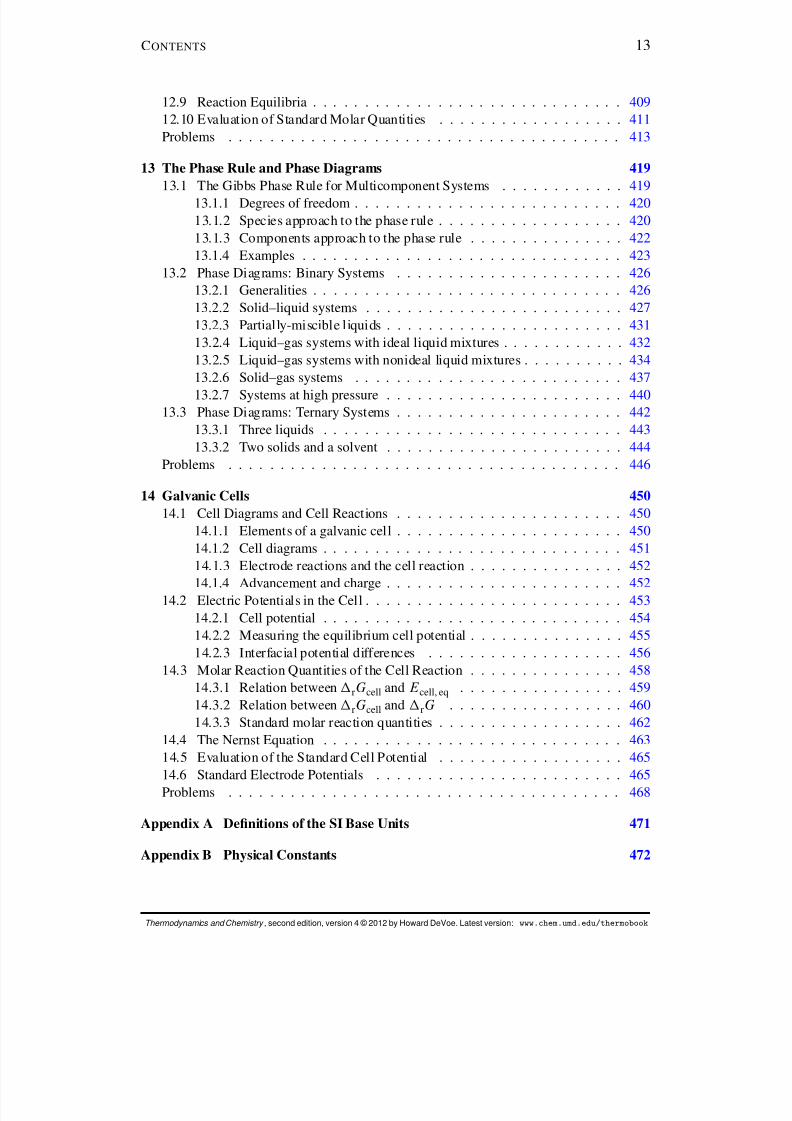
C ONTENTS 13
12.9 Reaction Equilibria . . . . . . . . . . . . . . . . . . . . . . . . . . . . . . 40912.10 Evaluation of Standard Molar Quantities . . . . . . . . . . . . . . . . . . 411Problems . . . . . . . . . . . . . . . . . . . . . . . . . . . . . . . . . . . . . . 413
13 The Phase Rule and Phase Diagrams 41913.1 The Gibbs Phase Rule for Multicomponent Systems . . . . . . . . . . . . 419
13.1.1 Degrees of freedom . . . . . . . . . . . . . . . . . . . . . . . . . . 42013.1.2 Species approach to the phase rule . . . . . . . . . . . . . . . . . . 42013.1.3 Components approach to the phase rule . . . . . . . . . . . . . . . 42213.1.4 Examples . . . . . . . . . . . . . . . . . . . . . . . . . . . . . . . 423
13.2 Phase Diagrams: Binary Systems . . . . . . . . . . . . . . . . . . . . . . 42613.2.1 Generalities . . . . . . . . . . . . . . . . . . . . . . . . . . . . . . 42613.2.2 Solid–liquid systems . . . . . . . . . . . . . . . . . . . . . . . . . 42713.2.3 Partially-miscible liquids . . . . . . . . . . . . . . . . . . . . . . . 43113.2.4 Liquid–gas systems with ideal liquid mixtures . . . . . . . . . . . . 43213.2.5 Liquid–gas systems with nonideal liquid mixtures . . . . . . . . . . 43413.2.6 Solid–gas systems . . . . . . . . . . . . . . . . . . . . . . . . . . 437
13.2.7 Systems at high pressure . . . . . . . . . . . . . . . . . . . . . . . 44013.3 Phase Diagrams: Ternary Systems . . . . . . . . . . . . . . . . . . . . . . 442
13.3.1 Three liquids . . . . . . . . . . . . . . . . . . . . . . . . . . . . . 44313.3.2 Two solids and a solvent . . . . . . . . . . . . . . . . . . . . . . . 444
Problems . . . . . . . . . . . . . . . . . . . . . . . . . . . . . . . . . . . . . . 446
14 Galvanic Cells 45014.1 Cell Diagrams and Cell Reactions . . . . . . . . . . . . . . . . . . . . . . 450
14.1.1 Elements of a galvanic cell . . . . . . . . . . . . . . . . . . . . . . 45014.1.2 Cell diagrams . . . . . . . . . . . . . . . . . . . . . . . . . . . . . 45114.1.3 Electrode reactions and the cell reaction . . . . . . . . . . . . . . . 452
14.1.4 Advancement and charge . . . . . . . . . . . . . . . . . . . . . . . 45214.2 Electric Potentials in the Cell . . . . . . . . . . . . . . . . . . . . . . . . . 45314.2.1 Cell potential . . . . . . . . . . . . . . . . . . . . . . . . . . . . . 45414.2.2 Measuring the equilibrium cell potential . . . . . . . . . . . . . . . 45514.2.3 Interfacial potential differences . . . . . . . . . . . . . . . . . . . 456
14.3 Molar Reaction Quantities of the Cell Reaction . . . . . . . . . . . . . . . 45814.3.1 Relation between rGcell and E cell, eq . . . . . . . . . . . . . . . . 45914.3.2 Relation between rGcell and rG . . . . . . . . . . . . . . . . . 46014.3.3 Standard molar reaction quantities . . . . . . . . . . . . . . . . . . 462
14.4 The Nernst Equation . . . . . . . . . . . . . . . . . . . . . . . . . . . . . 46314.5 Evaluation of the Standard Cell Potential . . . . . . . . . . . . . . . . . . 46514.6 Standard Electrode Potentials . . . . . . . . . . . . . . . . . . . . . . . . 465Problems . . . . . . . . . . . . . . . . . . . . . . . . . . . . . . . . . . . . . . 468
Appendix A Denitions of the SI Base Units 471
Appendix B Physical Constants 472
Thermodynamics and Chemistry , second edition, version 4 © 2012 by Howard DeVoe. Latest version: www.chem.umd.edu/thermobook

8/12/2019 Howard Devoe Thermodynamic and Chemical
http://slidepdf.com/reader/full/howard-devoe-thermodynamic-and-chemical 14/532
C ONTENTS 14
Appendix C Symbols for Physical Quantities 473
Appendix D Miscellaneous Abbreviations and Symbols 477D.1 Physical States . . . . . . . . . . . . . . . . . . . . . . . . . . . . . . . . 477D.2 Subscripts for Chemical Processes . . . . . . . . . . . . . . . . . . . . . . 478D.3 Superscripts . . . . . . . . . . . . . . . . . . . . . . . . . . . . . . . . . . 479
Appendix E Calculus Review 480E.1 Derivatives . . . . . . . . . . . . . . . . . . . . . . . . . . . . . . . . . . 480E.2 Partial Derivatives . . . . . . . . . . . . . . . . . . . . . . . . . . . . . . 480E.3 Integrals . . . . . . . . . . . . . . . . . . . . . . . . . . . . . . . . . . . . 481E.4 Line Integrals . . . . . . . . . . . . . . . . . . . . . . . . . . . . . . . . . 481
Appendix F Mathematical Properties of State Functions 482F.1 Differentials . . . . . . . . . . . . . . . . . . . . . . . . . . . . . . . . . 482F.2 Total Differential . . . . . . . . . . . . . . . . . . . . . . . . . . . . . . . 482F.3 Integration of a Total Differential . . . . . . . . . . . . . . . . . . . . . . 484
F.4 Legendre Transforms . . . . . . . . . . . . . . . . . . . . . . . . . . . . . 485
Appendix G Forces, Energy, and Work 487G.1 Forces between Particles . . . . . . . . . . . . . . . . . . . . . . . . . . . 488G.2 The System and Surroundings . . . . . . . . . . . . . . . . . . . . . . . . 491G.3 System Energy Change . . . . . . . . . . . . . . . . . . . . . . . . . . . . 493G.4 Macroscopic Work . . . . . . . . . . . . . . . . . . . . . . . . . . . . . . 494G.5 The Work Done on the System and Surroundings . . . . . . . . . . . . . . 496G.6 The Local Frame and Internal Energy . . . . . . . . . . . . . . . . . . . . 496G.7 Nonrotating Local Frame . . . . . . . . . . . . . . . . . . . . . . . . . . . 500G.8 Center-of-mass Local Frame . . . . . . . . . . . . . . . . . . . . . . . . . 500G.9 Rotating Local Frame . . . . . . . . . . . . . . . . . . . . . . . . . . . . 503G.10 Earth-Fixed Reference Frame . . . . . . . . . . . . . . . . . . . . . . . . 504
Appendix H Standard Molar Thermodynamic Properties 505
Appendix I Answers to Selected Problems 508
Bibliography 512
Index 521
Thermodynamics and Chemistry , second edition, version 4 © 2012 by Howard DeVoe. Latest version: www.chem.umd.edu/thermobook

8/12/2019 Howard Devoe Thermodynamic and Chemical
http://slidepdf.com/reader/full/howard-devoe-thermodynamic-and-chemical 15/532
B IOGRAPHICAL SKETCHES
Benjamin Thompson, Count of Rumford . . . . . . . . . . . . . . . . . . . . . . . . 63James Prescott Joule . . . . . . . . . . . . . . . . . . . . . . . . . . . . . . . . . . 85Sadi Carnot . . . . . . . . . . . . . . . . . . . . . . . . . . . . . . . . . . . . . . . 107Rudolf Julius Emmanuel Clausius . . . . . . . . . . . . . . . . . . . . . . . . . . . 110
William Thomson, Lord Kelvin . . . . . . . . . . . . . . . . . . . . . . . . . . . . . 115Max Karl Ernst Ludwig Planck . . . . . . . . . . . . . . . . . . . . . . . . . . . . . 117Josiah Willard Gibbs . . . . . . . . . . . . . . . . . . . . . . . . . . . . . . . . . . 139Walther Hermann Nernst . . . . . . . . . . . . . . . . . . . . . . . . . . . . . . . . 151William Francis Giauque . . . . . . . . . . . . . . . . . . . . . . . . . . . . . . . . 160Benoit Paul Emile Clapeyron . . . . . . . . . . . . . . . . . . . . . . . . . . . . . . 218William Henry . . . . . . . . . . . . . . . . . . . . . . . . . . . . . . . . . . . . . . 251Gilbert Newton Lewis . . . . . . . . . . . . . . . . . . . . . . . . . . . . . . . . . . 271Peter Josephus Wilhelmus Debye . . . . . . . . . . . . . . . . . . . . . . . . . . . . 296Germain Henri Hess . . . . . . . . . . . . . . . . . . . . . . . . . . . . . . . . . . . 322Francois-Marie Raoult . . . . . . . . . . . . . . . . . . . . . . . . . . . . . . . . . 380
Jacobus Henricus van’t Hoff . . . . . . . . . . . . . . . . . . . . . . . . . . . . . . 383
15
8/12/2019 Howard Devoe Thermodynamic and Chemical
http://slidepdf.com/reader/full/howard-devoe-thermodynamic-and-chemical 16/532
P REFACE TO THE SECOND EDITION
This second edition of Thermodynamics and Chemistry is a revised and enlarged versionof the rst edition published by Prentice Hall in 2001. The book is designed primarily as atextbook for a one-semester course for graduate or undergraduate students who have alreadybeen introduced to thermodynamics in a physical chemistry course.
The PDF le of this book contains hyperlinks to pages, sections, equations, tables,gures, bibliography items, and problems. If you are viewing the PDF on a computerscreen, tablet, or color e-reader, the links are colored in blue.
Scattered through the text are sixteen one-page biographical sketches of some of thehistorical giants of thermodynamics. A list is given on the preceding page. The sketchesare not intended to be comprehensive biographies, but rather to illustrate the human side of thermodynamics—the struggles and controversies by which the concepts and experimentalmethodology of the subject were developed.
The epigraphs on page 18 are intended to suggest the nature and importance of classi-cal thermodynamics. You may wonder about the conversation between Alice and HumptyDumpty. Its point, particularly important in the study of thermodynamics, is the need to pay
attention to denitions—the intended meanings of words.I welcome comments and suggestions for improving this book. My e-mail address ap-pears below.
Howard [email protected]
16

8/12/2019 Howard Devoe Thermodynamic and Chemical
http://slidepdf.com/reader/full/howard-devoe-thermodynamic-and-chemical 17/532
F ROM THE PREFACE TO THE F IRST
E DITION
Classical thermodynamics, the subject of this book, is concerned with macroscopic aspects of theinteraction of matter with energy in its various forms. This book is designed as a text for a one-semester course for senior undergraduate or graduate students who have already been introduced tothermodynamics in an undergraduate physical chemistry course.
Anyone who studies and uses thermodynamics knows that a deep understanding of this subjectdoes not come easily. There are subtleties and interconnections that are difcult to grasp at rst. Themore times one goes through a thermodynamics course (as a student or a teacher), the more insightone gains. Thus, this text will reinforce and extend the knowledge gained from an earlier exposureto thermodynamics. To this end, there is fairly intense discussion of some basic topics, such as thenature of spontaneous and reversible processes, and inclusion of a number of advanced topics, suchas the reduction of bomb calorimetry measurements to standard-state conditions.
This book makes no claim to be an exhaustive treatment of thermodynamics. It concentrateson derivations of fundamental relations starting with the thermodynamic laws and on applicationsof these relations in various areas of interest to chemists. Although classical thermodynamics treatsmatter from a purely macroscopic viewpoint, the book discusses connections with molecular prop-erties when appropriate.
In deriving equations, I have strived for rigor, clarity, and a minimum of mathematical complex-ity. I have attempted to clearly state the conditions under which each theoretical relation is validbecause only by understanding the assumptions and limitations of a derivation can one know whento use the relation and how to adapt it for special purposes. I have taken care to be consistent in theuse of symbols for physical properties. The choice of symbols follows the current recommendationsof the International Union of Pure and Applied Chemistry (IUPAC) with a few exceptions made toavoid ambiguity.
I owe much to J. Arthur Campbell, Luke E. Steiner, and William Moftt, gifted teachers whointroduced me to the elegant logic and practical utility of thermodynamics. I am immensely gratefulto my wife Stephanie for her continued encouragement and patience during the period this book went from concept to reality.
I would also like to acknowledge the help of the following reviewers: James L. Copeland,
Kansas State University; Lee Hansen, Brigham Young University; Reed Howald, Montana StateUniversity–Bozeman; David W. Larsen, University of Missouri–St. Louis; Mark Ondrias, Universityof New Mexico; Philip H. Rieger, Brown University; Leslie Schwartz, St. John Fisher College; AllanL. Smith, Drexel University; and Paul E. Smith, Kansas State University.
17

8/12/2019 Howard Devoe Thermodynamic and Chemical
http://slidepdf.com/reader/full/howard-devoe-thermodynamic-and-chemical 18/532
A theory is the more impressive the greater the simplicity of itspremises is, the more different kinds of things it relates, and the moreextended is its area of applicability. Therefore the deep impressionwhich classical thermodynamics made upon me. It is the only physicaltheory of universal content concerning which I am convinced that,within the framework of the applicability of its basic concepts, it willnever be overthrown.
Albert Einstein
Thermodynamics is a discipline that involves a formalization of a largenumber of intuitive concepts derived from common experience.
J. G. Kirkwood and I. Oppenheim, Chemical Thermodynamics , 1961
The rst law of thermodynamics is nothing more than the principle of the conservation of energy applied to phenomena involving theproduction or absorption of heat.
Max Planck, Treatise on Thermodynamics , 1922
The law that entropy always increases—the second law of thermodynamics—holds, I think, the supreme position among the lawsof Nature. If someone points out to you that your pet theory of theuniverse is in disagreement with Maxwell’s equations—then so muchthe worse for Maxwell’s equations. If it is found to be contradicted byobservation—well, these experimentalists do bungle things sometimes.But if your theory is found to be against the second law of thermodynamics I can give you no hope; there is nothing for it but tocollapse in deepest humiliation.
Sir Arthur Eddington, The Nature of the Physical World , 1928
Thermodynamics is a collection of useful relations between quantities,
every one of which is independently measurable. What do suchrelations “tell one” about one’s system, or in other words what do welearn from thermodynamics about the microscopic explanations of macroscopic changes? Nothing whatever. What then is the use of thermodynamics? Thermodynamics is useful precisely because somequantities are easier to measure than others, and that is all.
M. L. McGlashan, J. Chem. Educ. , 43, 226–232 (1966)
“When I use a word,” Humpty Dumpty said, in rather a scornful tone,“it means just what I choose it to mean—neither more nor less.”
“The question is,” said Alice,“whether you can make words meanso many different things.”
“The question is,” said Humpty Dumpty, “which is to be master—that’s all.”
Lewis Carroll, Through the Looking-Glass
8/12/2019 Howard Devoe Thermodynamic and Chemical
http://slidepdf.com/reader/full/howard-devoe-thermodynamic-and-chemical 19/532
C HAPTER 1
I NTRODUCTION
Thermodynamics is a quantitative subject. It allows us to derive relations between thevalues of numerous physical quantities. Some physical quantities, such as a mole fraction,are dimensionless; the value of one of these quantities is a pure number. Most quantities,however, are not dimensionless and their values must include one or more units . Thischapter reviews the SI system of units, which are the preferred units in science applications.The chapter then discusses some useful mathematical manipulations of physical quantitiesusing quantity calculus, and certain general aspects of dimensional analysis.
1.1 UNITS
There is international agreement that the units used for physical quantities in science andtechnology should be those of the International System of Units, or SI (standing for theFrench Syst eme International d’Unit es). The Physical Chemistry Division of the Inter-national Union of Pure and Applied Chemistry, or IUPAC, produces a manual of recom-mended symbols and terminology for physical quantities and units based on the SI. Themanual has become known as the Green Book (from the color of its cover) and is referredto here as the IUPAC Green Book. This book will, with a few exceptions, use symbols rec-ommended in the third edition (2007) of the IUPAC Green Book; 1 these symbols are listedfor convenient reference in Appendices C and D.
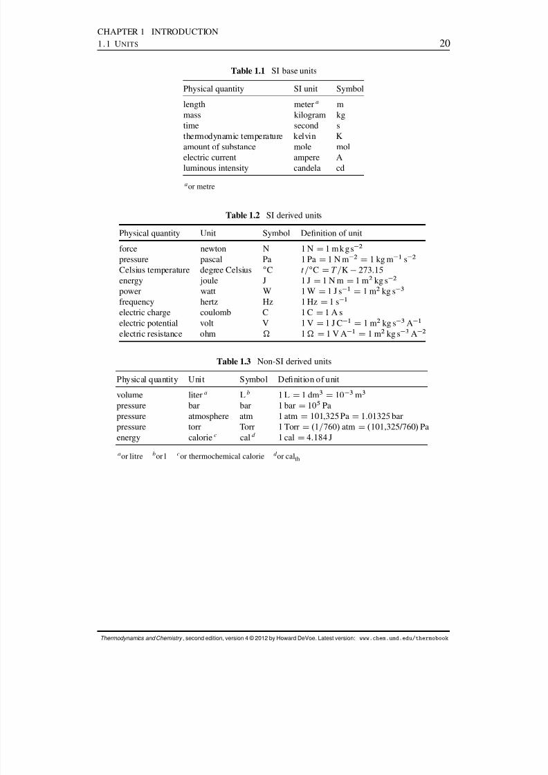
The SI is built on the seven base units listed in Table 1.1 on the next page . These baseunits are independent physical quantities that are sufcient to describe all other physicalquantities. One of the seven quantities, luminous intensity, is not used in this book and isusually not needed in thermodynamics. The ofcial denitions of the base units are givenin Appendix A .
Table 1.2 lists derived units for some additional physical quantities used in thermody-namics. The derived units have exact denitions in terms of SI base units, as given in the
last column of the table.The units listed in Table 1.3 are sometimes used in thermodynamics but are not part
of the SI. They do, however, have exact denitions in terms of SI units and so offer noproblems of numerical conversion to or from SI units.
1Ref. [ 36]. The references are listed in the Bibliography at the back of the book.
19
8/12/2019 Howard Devoe Thermodynamic and Chemical
http://slidepdf.com/reader/full/howard-devoe-thermodynamic-and-chemical 20/532
CHAPTER 1 INTRODUCTION1.1 U NITS 20
Table 1.1 SI base units
Physical quantity SI unit Symbol
length meter a mmass kilogram kgtime second s
thermodynamic temperature kelvin Kamount of substance mole molelectric current ampere Aluminous intensity candela cd
a or metre
Table 1.2 SI derived units
Physical quantity Unit Symbol Denition of unit
force newton N 1 N D 1 mk g s 2
pressure pascal Pa 1 Pa D 1 N m 2 D 1 kg m 1 s 2
Celsius temperature degree Celsius ı
C t=ıC D T =K 273:15
energy joule J 1 J D 1 N m D 1 m2 kg s 2
power watt W 1 W D 1 J s 1 D 1 m2 kg s 3
frequency hertz Hz 1 Hz D 1 s 1
electric charge coulomb C 1 C D 1 A selectric potential volt V 1 V D 1 J C 1 D 1 m2 kg s 3 A 1
electric resistance ohm 1 D 1 V A 1 D 1 m2 kg s 3 A 2
Table 1.3 Non-SI derived units
Physical quantity Unit Symbol Denition of unit
volume liter a L b 1 L D 1 dm3 D 10 3 m3
pressure bar bar 1 bar D 105
Papressure atmosphere atm 1 atm D 101,325 Pa D 1:01325 barpressure torr Torr 1 Torr D .1=760/ atm D . 101,325/760 / Paenergy calorie c cal d 1 cal D 4:184 J
a or litre bor l cor thermochemical calorie d or cal th
Thermodynamics and Chemistry , second edition, version 4 © 2012 by Howard DeVoe. Latest version: www.chem.umd.edu/thermobook

8/12/2019 Howard Devoe Thermodynamic and Chemical
http://slidepdf.com/reader/full/howard-devoe-thermodynamic-and-chemical 21/532
CHAPTER 1 INTRODUCTION1.1 U NITS 21
Table 1.4 SI prexes
Fraction Prex Symbol Multiple Prex Symbol
10 1 deci d 10 deka da10 2 centi c 102 hecto h10 3 milli m 103 kilo k 10 6 micro 10 6 mega M10 9 nano n 109 giga G10 12 pico p 1012 tera T10 15 femto f 1015 peta P10 18 atto a 1018 exa E10 21 zepto z 1021 zetta Z10 24 yocto y 1024 yotta Y
Any of the symbols for units listed in Tables 1.1–1.3 , except kg and ı C, may be precededby one of the prex symbols of Table 1.4 to construct a decimal fraction or multiple of theunit. (The symbol g may be preceded by a prex symbol to construct a fraction or multipleof the gram.) The combination of prex symbol and unit symbol is taken as a new symbolthat can be raised to a power without using parentheses, as in the following examples:
1 mg D 1 10 3 g
1 cm D 1 10 2 m
1 cm 3 D .1 10 2 m/ 3 D 1 10 6 m3
1.1.1 Amount of substance and amount
The physical quantity formally called amount of substance is a counting quantity for par-ticles, such as atoms or molecules, or for other chemical entities. The counting unit is
invariably the mole , dened as the amount of substance containing as many particles as thenumber of atoms in exactly 12 grams of pure carbon-12 nuclide, 12 C. See Appendix A forthe wording of the ofcial IUPAC denition. This denition is such that one mole of H 2 Omolecules, for example, has a mass of 18:0153 grams (where 18:0153 is the relative molec-ular mass of H 2 O) and contains 6:02214 1023 molecules (where 6:02214 1023 mol 1 isthe Avogadro constant to six signicant digits). The same statement can be made for anyother substance if 18:0153 is replaced by the appropriate atomic mass or molecular massvalue.
The symbol for amount of substance is n . It is admittedly awkward to refer to n(H 2 O)as “the amount of substance of water.” This book simply shortens “amount of substance” toamount , a common usage that is condoned by the IUPAC. 2 Thus, “the amount of water inthe system” refers not to the mass or volume of water, but to the number of H
2O molecules
in the system expressed in a counting unit such as the mole.
2Ref. [ 117 ]. An alternative name suggested for n is “chemical amount.”
Thermodynamics and Chemistry , second edition, version 4 © 2012 by Howard DeVoe. Latest version: www.chem.umd.edu/thermobook
8/12/2019 Howard Devoe Thermodynamic and Chemical
http://slidepdf.com/reader/full/howard-devoe-thermodynamic-and-chemical 22/532
CHAPTER 1 INTRODUCTION1.2 Q UANTITY C ALCULUS 22
1.2 QUANTITY CALCULUS
This section gives examples of how we may manipulate physical quantities by the rules of algebra. The method is called quantity calculus , although a better term might be “quantityalgebra.”
Quantity calculus is based on the concept that a physical quantity, unless it is dimen-sionless, has a value equal to the product of a numerical value (a pure number) and one ormore units :
physical quantity = numerical value units (1.2.1)
(If the quantity is dimensionless, it is equal to a pure number without units.) The physicalproperty may be denoted by a symbol, but the symbol does not imply a particular choice of units. For instance, this book uses the symbol for density, but can be expressed in anyunits having the dimensions of mass divided by volume.
A simple example illustrates the use of quantity calculus. We may express the densityof water at 25 ı C to four signicant digits in SI base units by the equation
D 9:970 102 kg m 3 (1.2.2)
and in different density units by the equation
D 0:9970 g cm 3 (1.2.3)
We may divide both sides of the last equation by 1 g cm 3 to obtain a new equation
= g cm 3 D 0:9970 (1.2.4)
Now the pure number 0:9970 appearing in this equation is the number of grams in onecubic centimeter of water, so we may call the ratio = g cm 3 “the number of grams percubic centimeter.” By the same reasoning, = kg m 3 is the number of kilograms per cubicmeter. In general, a physical quantity divided by particular units for the physical quantity isa pure number representing the number of those units.
Just as it would be incorrect to call “the number of grams per cubic centimeter,”because that would refer to a particular choice of units for , the common practice of calling n “the number of moles” is also strictly speaking not correct. It is actually theratio n=mol that is the number of moles.
In a table, the ratio = g cm 3 makes a convenient heading for a column of densityvalues because the column can then show pure numbers. Likewise, it is convenient to use= g cm 3 as the label of a graph axis and to show pure numbers at the grid marks of theaxis. You will see many examples of this usage in the tables and gures of this book.
A major advantage of using SI base units and SI derived units is that they are coherent .That is, values of a physical quantity expressed in different combinations of these units havethe same numerical value.
Thermodynamics and Chemistry , second edition, version 4 © 2012 by Howard DeVoe. Latest version: www.chem.umd.edu/thermobook

8/12/2019 Howard Devoe Thermodynamic and Chemical
http://slidepdf.com/reader/full/howard-devoe-thermodynamic-and-chemical 23/532
CHAPTER 1 INTRODUCTION1.2 Q UANTITY C ALCULUS 23
For example, suppose we wish to evaluate the pressure of a gas according to the idealgas equation 3
p D nRT
V (1.2.5)
(ideal gas)
In this equation, p , n , T , and V are the symbols for the physical quantities pressure, amount(amount of substance), thermodynamic temperature, and volume, respectively, and R is thegas constant.
The calculation of p for 5:000 moles of an ideal gas at a temperature of 298:15 kelvins,in a volume of 4:000 cubic meters, is
p D .5:000 mol /.8:3145 J K 1 mol 1 /.298:15 K/
4:000 m3 D 3:099 103 J m 3 (1.2.6)
The mole and kelvin units cancel, and we are left with units of J m 3 , a combination of an SI derived unit (the joule) and an SI base unit (the meter). The units J m 3 must havedimensions of pressure, but are not commonly used to express pressure.
To convert J m 3 to the SI derived unit of pressure, the pascal (Pa), we can use thefollowing relations from Table 1.2:
1 J D 1 N m 1 Pa D 1 N m 2 (1.2.7)
When we divide both sides of the rst relation by 1 J and divide both sides of the secondrelation by 1 N m 2 , we obtain the two new relations
1 D .1 N m =J/ .1 Pa=N m 2 / D 1 (1.2.8)
The ratios in parentheses are conversion factors . When a physical quantity is multipliedby a conversion factor that, like these, is equal to the pure number 1, the physical quantity
changes its units but not its value. When we multiply Eq. 1.2.6 by both of these conversionfactors, all units cancel except Pa:
p D .3:099 103 J m 3 / .1 N m =J/ .1 Pa=N m 2 /
D 3:099 103 Pa (1.2.9)
This example illustrates the fact that to calculate a physical quantity, we can simplyenter into a calculator numerical values expressed in SI units, and the result is the numericalvalue of the calculated quantity expressed in SI units. In other words, as long as we useonly SI base units and SI derived units (without prexes), all conversion factors are unity .
Of course we do not have to limit the calculation to SI units. Suppose we wish toexpress the calculated pressure in torrs, a non-SI unit. In this case, using a conversion factorobtained from the denition of the torr in Table 1.3 , the calculation becomes
p D .3:099 103 Pa/ .760 Torr =101; 325 Pa/
D 23:24 Torr (1.2.10)
3This is the rst equation in this book that, like many others to follow, shows conditions of validity in parenthe-ses immediately below the equation number at the right. Thus, Eq. 1.2.5 is valid for an ideal gas.
Thermodynamics and Chemistry , second edition, version 4 © 2012 by Howard DeVoe. Latest version: www.chem.umd.edu/thermobook
8/12/2019 Howard Devoe Thermodynamic and Chemical
http://slidepdf.com/reader/full/howard-devoe-thermodynamic-and-chemical 24/532
CHAPTER 1 INTRODUCTION1.3 D IMENSIONAL A NALYSIS 24
1.3 DIMENSIONAL ANALYSIS
Sometimes you can catch an error in the form of an equation or expression, or in the dimen-sions of a quantity used for a calculation, by checking for dimensional consistency. Hereare some rules that must be satised:
both sides of an equation have the same dimensions
all terms of a sum or difference have the same dimensions
logarithms and exponentials, and arguments of logarithms and exponentials, are di-mensionless
a quantity used as a power is dimensionlessIn this book the differential of a function, such as d f , refers to an innitesimal quantity.
If one side of an equation is an innitesimal quantity, the other side must also be. Thus,the equation d f D a dx Cb dy (where ax and by have the same dimensions as f ) makesmathematical sense, but d f D ax Cb dy does not.
Derivatives, partial derivatives, and integrals have dimensions that we must take intoaccount when determining the overall dimensions of an expression that includes them. Forinstance:
the derivative d p= dT and the partial derivative .@p=@T /V have the same dimensionsas p=T
the partial second derivative .@2 p=@T 2 / V has the same dimensions as p=T 2
the integral R T dT has the same dimensions as T 2
Some examples of applying these principles are given here using symbols described inSec. 1.2 .
Example 1. Since the gas constant R may be expressed in units of J K 1 mol 1 , it hasdimensions of energy divided by thermodynamic temperature and amount. Thus, RT hasdimensions of energy divided by amount, and nRT has dimensions of energy. The products
RT and nRT appear frequently in thermodynamic expressions.Example 2. What are the dimensions of the quantity nRT ln.p=p ı / and of p ı in
this expression? The quantity has the same dimensions as nRT (or energy) because thelogarithm is dimensionless. Furthermore, p ı in this expression has dimensions of pressurein order to make the argument of the logarithm, p=p ı , dimensionless.
Example 3. Find the dimensions of the constants a and b in the van der Waals equation
p D nRT V nb
n2 aV 2
Dimensional analysis tells us that, because nb is subtracted from V , nb has dimensionsof volume and therefore b has dimensions of volume/amount. Furthermore, since the right
side of the equation is a difference of two terms, these terms have the same dimensionsas the left side, which is pressure. Therefore, the second term n2 a=V 2 has dimensions of pressure, and a has dimensions of pressure volume 2 amount 2 .
Example 4. Consider an equation of the form
@ln x@T p D
yR
Thermodynamics and Chemistry , second edition, version 4 © 2012 by Howard DeVoe. Latest version: www.chem.umd.edu/thermobook

8/12/2019 Howard Devoe Thermodynamic and Chemical
http://slidepdf.com/reader/full/howard-devoe-thermodynamic-and-chemical 25/532
CHAPTER 1 INTRODUCTION1.3 D IMENSIONAL A NALYSIS 25
What are the SI units of y ? ln x is dimensionless, so the left side of the equation has thedimensions of 1=T , and its SI units are K 1 . The SI units of the right side are thereforealso K 1 . Since R has the units J K 1 mol 1 , the SI units of y are J K 2 mol 1 .
Thermodynamics and Chemistry , second edition, version 4 © 2012 by Howard DeVoe. Latest version: www.chem.umd.edu/thermobook

8/12/2019 Howard Devoe Thermodynamic and Chemical
http://slidepdf.com/reader/full/howard-devoe-thermodynamic-and-chemical 26/532
CHAPTER 1 INTRODUCTIONPROBLEM 26
PROBLEM
1.1 Consider the following equations for the pressure of a real gas. For each equation, nd thedimensions of the constants a and b and express these dimensions in SI units.
(a) The Dieterici equation:
p D RT e.an=VRT/
.V=n/ b
(b) The Redlich–Kwong equation:
p D RT
.V=n/ b an 2
T 1=2 V .V Cnb/
Thermodynamics and Chemistry , second edition, version 4 © 2012 by Howard DeVoe. Latest version: www.chem.umd.edu/thermobook
8/12/2019 Howard Devoe Thermodynamic and Chemical
http://slidepdf.com/reader/full/howard-devoe-thermodynamic-and-chemical 27/532
C HAPTER 2
SYSTEMS AND THEIR PROPERTIES
This chapter begins by explaining some basic terminology of thermodynamics. It discussesmacroscopic properties of matter in general and properties distinguishing different physicalstates of matter in particular. Virial equations of state of a pure gas are introduced. Thechapter goes on to discuss some basic macroscopic properties and their measurement. Fi-nally, several important concepts needed in later chapters are described: thermodynamicstates and state functions, independent and dependent variables, processes, and internal en-ergy.
2.1 THE SYSTEM, SURROUNDINGS, AND BOUNDARY
Chemists are interested in systems containing matter—that which has mass and occupiesphysical space. Classical thermodynamics looks at macroscopic aspects of matter. It dealswith the properties of aggregates of vast numbers of microscopic particles (molecules,atoms, and ions). The macroscopic viewpoint, in fact, treats matter as a continuous ma-terial medium rather than as the collection of discrete microscopic particles we know areactually present. Although this book is an exposition of classical thermodynamics, at timesit will point out connections between macroscopic properties and molecular structure andbehavior.
A thermodynamic system is any three-dimensional region of physical space on whichwe wish to focus our attention. Usually we consider only one system at a time and call itsimply “the system.” The rest of the physical universe constitutes the surroundings of thesystem.
The boundary is the closed three-dimensional surface that encloses the system andseparates it from the surroundings. The boundary may (and usually does) coincide withreal physical surfaces: the interface between two phases, the inner or outer surface of thewall of a ask or other vessel, and so on. Alternatively, part or all of the boundary may be
an imagined intangible surface in space, unrelated to any physical structure. The size andshape of the system, as dened by its boundary, may change in time. In short, our choice of the three-dimensional region that constitutes the system is arbitrary—but it is essential thatwe know exactly what this choice is.
We usually think of the system as a part of the physical universe that we are able toinuence only indirectly through its interaction with the surroundings, and the surroundings
27
8/12/2019 Howard Devoe Thermodynamic and Chemical
http://slidepdf.com/reader/full/howard-devoe-thermodynamic-and-chemical 28/532

8/12/2019 Howard Devoe Thermodynamic and Chemical
http://slidepdf.com/reader/full/howard-devoe-thermodynamic-and-chemical 29/532
CHAPTER 2 SYSTEMS AND THEIR PROPERTIES2.1 T HE S YSTEM , SURROUNDINGS , AND B OUNDARY 29
Table 2.1 Symbols and SI units for some com-mon properties
Symbol Physical quantity SI unit
E energy Jm mass kgn amount of substance molp pressure PaT thermodynamic temperature KV volume m 3
U internal energy J density kg m 3
Sometimes a more restricted denition of an extensive property is used: The propertymust be not only additive, but also proportional to the mass or the amount when inten-sive properties remain constant. According to this denition, mass, volume, amount,and energy are extensive, but surface area is not.
If we imagine a homogeneous region of space to be divided into two or more parts of arbitrary size, any property that has the same value in each part and the whole is an intensiveproperty ; for example density, concentration, pressure (in a uid), and temperature. Thevalue of an intensive property is the same everywhere in a homogeneous region, but mayvary from point to point in a heterogeneous region—it is a local property.
Since classical thermodynamics treats matter as a continuous medium, whereas matteractually contains discrete microscopic particles, the value of an intensive property at a pointis a statistical average of the behavior of many particles. For instance, the density of a gas atone point in space is the average mass of a small volume element at that point, large enoughto contain many molecules, divided by the volume of that element.
Some properties are dened as the ratio of two extensive quantities. If both extensivequantities refer to a homogeneous region of the system or to a small volume element, the ra-tio is an intensive property. For example concentration, dened as the ratio amount =volume,is intensive. A mathematical derivative of one such extensive quantity with respect to an-other is also intensive.
A special case is an extensive quantity divided by the mass, giving an intensive specicquantity ; for example
Specic volume D V m D
1 (2.1.1)
If the symbol for the extensive quantity is a capital letter, it is customary to use the cor-responding lower-case letter as the symbol for the specic quantity. Thus the symbol for
specic volume is v.Another special case encountered frequently in this book is an extensive property for a
pure, homogeneous substance divided by the amount n . The resulting intensive property iscalled, in general, a molar quantity or molar property. To symbolize a molar quantity, thisbook follows the recommendation of the IUPAC: The symbol of the extensive quantity isfollowed by subscript m, and optionally the identity of the substance is indicated either by
Thermodynamics and Chemistry , second edition, version 4 © 2012 by Howard DeVoe. Latest version: www.chem.umd.edu/thermobook

8/12/2019 Howard Devoe Thermodynamic and Chemical
http://slidepdf.com/reader/full/howard-devoe-thermodynamic-and-chemical 30/532
CHAPTER 2 SYSTEMS AND THEIR PROPERTIES2.2 P HASES AND P HYSICAL S TATES OF M ATTER 30
a subscript or a formula in parentheses. Examples are
Molar volume D V n D V m (2.1.2)
Molar volume of substance i
D V
n i D V m;i (2.1.3)
Molar volume of H 2 O D V m(H 2 O) (2.1.4)
In the past, especially in the United States, molar quantities were commonly denotedwith an overbar (e.g., V i ).
2.2 PHASES AND PHYSICAL STATES OF MATTER
A phase is a region of the system in which each intensive property (such as temperature andpressure) has at each instant either the same value throughout (a uniform or homogeneousphase), or else a value that varies continuously from one point to another. Whenever thisbook mentions a phase, it is a uniform phase unless otherwise stated. Two different phasesmeet at an interface surface , where intensive properties have a discontinuity or changeover a small distance.
Some intensive properties (e.g., refractive index and polarizability) can have directionalcharacteristics. A uniform phase may be either isotropic , exhibiting the same values of theseproperties in all directions, or anisotropic , as in the case of some solids and liquid crystals.A vacuum is a uniform phase of zero density.
Suppose we have to deal with a nonuniform region in which intensive properties varycontinuously in space along one or more directions—for example, a tall column of gas ina gravitational eld whose density decreases with increasing altitude. There are two wayswe may treat such a nonuniform, continuous region: either as a single nonuniform phase,or else as an innite number of uniform phases, each of innitesimal size in one or more
dimensions.
2.2.1 Physical states of matter
We are used to labeling phases by physical state, or state of aggregation. It is commonto say that a phase is a solid if it is relatively rigid, a liquid if it is easily deformed andrelatively incompressible, and a gas if it is easily deformed and easily compressed. Sincethese descriptions of responses to external forces differ only in degree, they are inadequateto classify intermediate cases.
A more rigorous approach is to make a primary distinction between a solid and a uid ,based on the phase’s response to an applied shear stress, and then use additional criteriato classify a uid as a liquid , gas , or supercritical uid . Shear stress is a tangential forceper unit area that is exerted on matter on one side of an interior plane by the matter on theother side. We can produce shear stress in a phase by applying tangential forces to parallelsurfaces of the phase as shown in Fig. 2.1 on the next page .
A solid responds to shear stress by undergoing momentary relative motion of its parts,resulting in deformation —a change of shape. If the applied shear stress is constant andsmall (not large enough to cause creep or fracture), the solid quickly reaches a certain
Thermodynamics and Chemistry , second edition, version 4 © 2012 by Howard DeVoe. Latest version: www.chem.umd.edu/thermobook
8/12/2019 Howard Devoe Thermodynamic and Chemical
http://slidepdf.com/reader/full/howard-devoe-thermodynamic-and-chemical 31/532
CHAPTER 2 SYSTEMS AND THEIR PROPERTIES2.2 P HASES AND P HYSICAL S TATES OF M ATTER 31
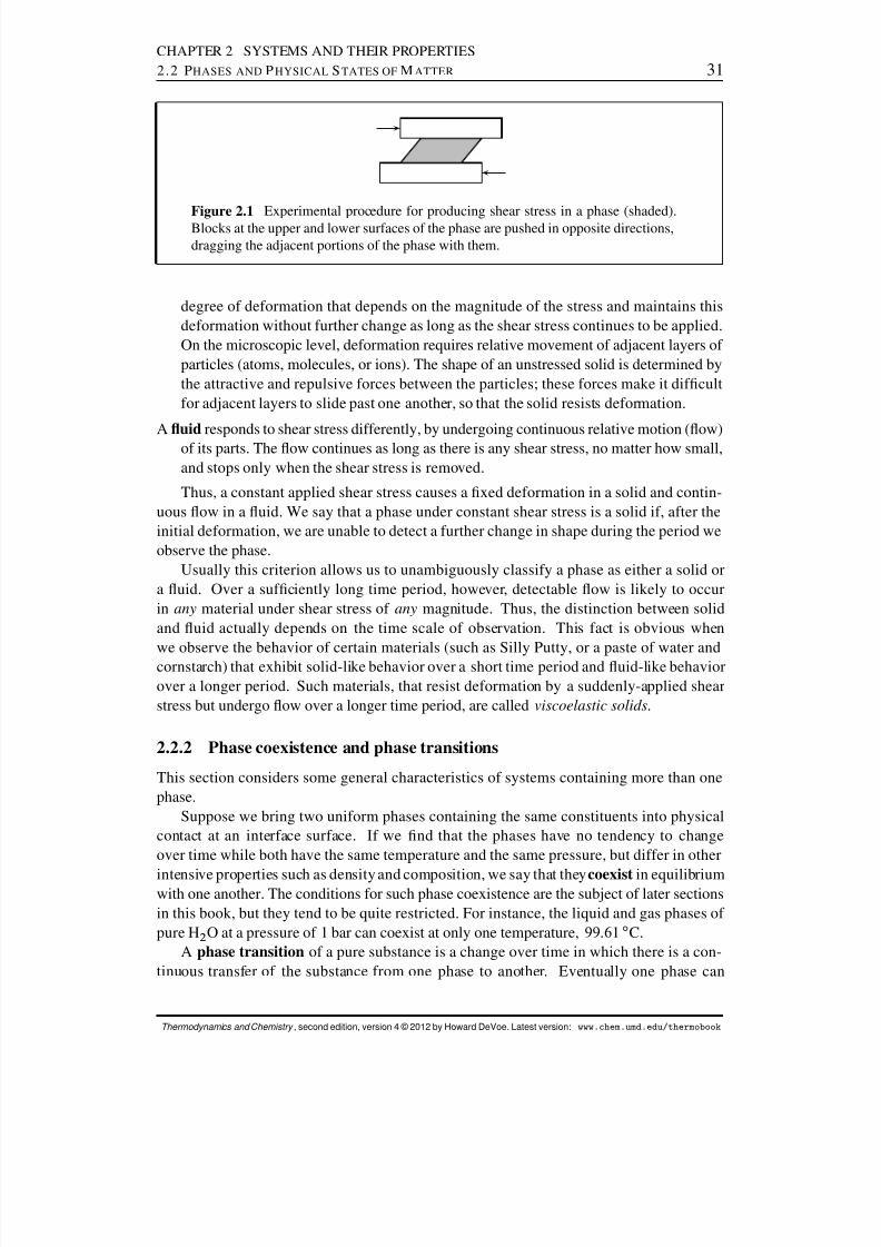
Figure 2.1 Experimental procedure for producing shear stress in a phase (shaded).Blocks at the upper and lower surfaces of the phase are pushed in opposite directions,dragging the adjacent portions of the phase with them.
degree of deformation that depends on the magnitude of the stress and maintains thisdeformation without further change as long as the shear stress continues to be applied.On the microscopic level, deformation requires relative movement of adjacent layers of particles (atoms, molecules, or ions). The shape of an unstressed solid is determined bythe attractive and repulsive forces between the particles; these forces make it difcultfor adjacent layers to slide past one another, so that the solid resists deformation.
A uid responds to shear stress differently, by undergoing continuous relative motion (ow)of its parts. The ow continues as long as there is any shear stress, no matter how small,and stops only when the shear stress is removed.
Thus, a constant applied shear stress causes a xed deformation in a solid and contin-uous ow in a uid. We say that a phase under constant shear stress is a solid if, after theinitial deformation, we are unable to detect a further change in shape during the period weobserve the phase.
Usually this criterion allows us to unambiguously classify a phase as either a solid ora uid. Over a sufciently long time period, however, detectable ow is likely to occurin any material under shear stress of any magnitude. Thus, the distinction between solidand uid actually depends on the time scale of observation. This fact is obvious when
we observe the behavior of certain materials (such as Silly Putty, or a paste of water andcornstarch) that exhibit solid-like behavior over a short time period and uid-like behaviorover a longer period. Such materials, that resist deformation by a suddenly-applied shearstress but undergo ow over a longer time period, are called viscoelastic solids .
2.2.2 Phase coexistence and phase transitions
This section considers some general characteristics of systems containing more than onephase.
Suppose we bring two uniform phases containing the same constituents into physicalcontact at an interface surface. If we nd that the phases have no tendency to changeover time while both have the same temperature and the same pressure, but differ in other
intensive properties such as density and composition, we say that they coexist in equilibriumwith one another. The conditions for such phase coexistence are the subject of later sectionsin this book, but they tend to be quite restricted. For instance, the liquid and gas phases of pure H 2 O at a pressure of 1 bar can coexist at only one temperature, 99:61 ı C.
A phase transition of a pure substance is a change over time in which there is a con-tinuous transfer of the substance from one phase to another. Eventually one phase can
Thermodynamics and Chemistry , second edition, version 4 © 2012 by Howard DeVoe. Latest version: www.chem.umd.edu/thermobook
8/12/2019 Howard Devoe Thermodynamic and Chemical
http://slidepdf.com/reader/full/howard-devoe-thermodynamic-and-chemical 32/532
CHAPTER 2 SYSTEMS AND THEIR PROPERTIES2.2 P HASES AND P HYSICAL S TATES OF M ATTER 32
tp
cp
solid
liquid
gas
supercriticaluid
A
B C
D
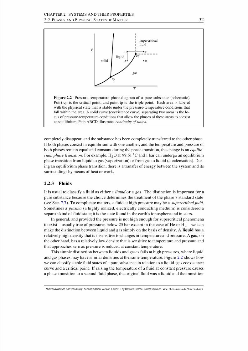
Figure 2.2 Pressure–temperature phase diagram of a pure substance (schematic).Point cp is the critical point, and point tp is the triple point. Each area is labeledwith the physical state that is stable under the pressure-temperature conditions thatfall within the area. A solid curve (coexistence curve) separating two areas is the lo-cus of pressure-temperature conditions that allow the phases of these areas to coexist
at equilibrium. Path ABCD illustrates continuity of states .
completely disappear, and the substance has been completely transferred to the other phase.If both phases coexist in equilibrium with one another, and the temperature and pressure of both phases remain equal and constant during the phase transition, the change is an equilib-rium phase transition . For example, H 2 O at 99:61 ı C and 1 bar can undergo an equilibriumphase transition from liquid to gas (vaporization) or from gas to liquid (condensation). Dur-ing an equilibrium phase transition, there is a transfer of energy between the system and itssurroundings by means of heat or work.
2.2.3 FluidsIt is usual to classify a uid as either a liquid or a gas . The distinction is important for apure substance because the choice determines the treatment of the phase’s standard state(see Sec. 7.7 ). To complicate matters, a uid at high pressure may be a supercritical uid .Sometimes a plasma (a highly ionized, electrically conducting medium) is considered aseparate kind of uid state; it is the state found in the earth’s ionosphere and in stars.
In general, and provided the pressure is not high enough for supercritical phenomenato exist—usually true of pressures below 25 bar except in the case of He or H 2 —we canmake the distinction between liquid and gas simply on the basis of density. A liquid has arelatively high density that is insensitive to changes in temperature and pressure. A gas , onthe other hand, has a relatively low density that is sensitive to temperature and pressure and
that approaches zero as pressure is reduced at constant temperature.This simple distinction between liquids and gases fails at high pressures, where liquid
and gas phases may have similar densities at the same temperature. Figure 2.2 shows howwe can classify stable uid states of a pure substance in relation to a liquid–gas coexistencecurve and a critical point. If raising the temperature of a uid at constant pressure causesa phase transition to a second uid phase, the original uid was a liquid and the transition
Thermodynamics and Chemistry , second edition, version 4 © 2012 by Howard DeVoe. Latest version: www.chem.umd.edu/thermobook

8/12/2019 Howard Devoe Thermodynamic and Chemical
http://slidepdf.com/reader/full/howard-devoe-thermodynamic-and-chemical 33/532
CHAPTER 2 SYSTEMS AND THEIR PROPERTIES2.2 P HASES AND P HYSICAL S TATES OF M ATTER 33
occurs at the liquid–gas coexistence curve . This curve ends at a critical point , at whichall intensive properties of the coexisting liquid and gas phases become identical. The uidstate of a pure substance at a temperature greater than the critical temperature and a pressuregreater than the critical pressure is called a supercritical uid .
The term vapor is sometimes used for a gas that can be condensed to a liquid by increas-
ing the pressure at constant temperature. By this denition, the vapor state of a substanceexists only at temperatures below the critical temperature.The designation of a supercritical uid state of a substance is used more for convenience
than because of any unique properties compared to a liquid or gas. If we vary the tempera-ture or pressure in such a way that the substance changes from what we call a liquid to whatwe call a supercritical uid, we observe only a continuous density change of a single phase,and no phase transition with two coexisting phases. The same is true for a change froma supercritical uid to a gas. Thus, by making the changes described by the path ABCDshown in Fig. 2.2, we can transform a pure substance from a liquid at a certain pressureto a gas at the same pressure without ever observing an interface between two coexistingphases! This curious phenomenon is called continuity of states .
Chapter 6 will take up the discussion of further aspects of the physical states of puresubstances.
If we are dealing with a uid mixture (instead of a pure substance) at a high pressure, itmay be difcult to classify the phase as either liquid or gas. The complexity of classicationat high pressure is illustrated by the barotropic effect , observed in some mixtures, in whicha small change of temperature or pressure causes what was initially the more dense of twocoexisting uid phases to become the less dense phase. In a gravitational eld, the twophases switch positions.
2.2.4 The equation of state of a uid
Suppose we prepare a uniform uid phase containing a known amount n i of each constituent
substance i , and adjust the temperature T and pressure p to denite known values. Weexpect this phase to have a denite, xed volume V . If we change any one of the propertiesT , p , or ni , there is usually a change in V . The value of V is dependent on the otherproperties and cannot be varied independently of them. Thus, for a given substance ormixture of substances in a uniform uid phase, V is a unique function of T , p , and fn ig,where fn ig stands for the set of amounts of all substances in the phase. We may be ableto express this relation in an explicit equation: V D f.T;p; fn ig/ . This equation (or arearranged form) that gives a relation among V , T , p , and fn ig, is the equation of state of the uid.
We may solve the equation of state, implicitly or explicitly, for any one of the quantitiesV , T , p , and n i in terms of the other quantities. Thus, of the 3 Cs quantities (where s isthe number of substances), only 2
Cs are independent.
The ideal gas equation , p D nRT=V (Eq. 1.2.5 on page 23 ), is an equation of state.It is found experimentally that the behavior of any gas in the limit of low pressure, astemperature is held constant, approaches this equation of state. This limiting behavior isalso predicted by kinetic-molecular theory.
If the uid has only one constituent (i.e., is a pure substance rather than a mixture), thenat a xed T and p the volume is proportional to the amount. In this case, the equation of
Thermodynamics and Chemistry , second edition, version 4 © 2012 by Howard DeVoe. Latest version: www.chem.umd.edu/thermobook
8/12/2019 Howard Devoe Thermodynamic and Chemical
http://slidepdf.com/reader/full/howard-devoe-thermodynamic-and-chemical 34/532
CHAPTER 2 SYSTEMS AND THEIR PROPERTIES2.2 P HASES AND P HYSICAL S TATES OF M ATTER 34
state may be expressed as a relation among T , p , and the molar volume V m D V =n. Theequation of state for a pure ideal gas may be written p D RT=V m .
The Redlich–Kwong equation is a two-parameter equation of state frequently used todescribe, to good accuracy, the behavior of a pure gas at a pressure where the ideal gasequation fails:
p D RT V m b
aV m .V m Cb/T 1=2 (2.2.1)
In this equation, a and b are constants that are independent of temperature and depend onthe substance.
The next section describes features of virial equations, an important class of equationsof state for real (nonideal) gases.
2.2.5 Virial equations of state for pure gases
In later chapters of this book there will be occasion to apply thermodynamic derivations tovirial equations of state of a pure gas or gas mixture. These formulas accurately describethe gas at low and moderate pressures using empirically determined, temperature-dependent
parameters. The equations may be derived from statistical mechanics, so they have a theo-retical as well as empirical foundation. There are two forms of virial equations for a puregas: one a series in powers of 1=V m :
pV m D RT 1 C BV m C
C V 2m C (2.2.2)
and the other a series in powers of p :
pV m D RT 1 CBp p CC p p 2 C (2.2.3)
The parameters B , C , : : : are called the second , third , : : : virial coefcients , and the pa-rameters Bp , C p , : : : are a set of pressure virial coefcients. Their values depend on thesubstance and are functions of temperature. (The rst virial coefcient in both power se-
ries is 1, because pV m must approach RT as 1=V m or p approach zero at constant T .)Coefcients beyond the third virial coefcient are small and rarely evaluated.
The values of the virial coefcients for a gas at a given temperature can be determinedfrom the dependence of p on V m at this temperature. The value of the second virial coef-cient B depends on pairwise interactions between the atoms or molecules of the gas, andin some cases can be calculated to good accuracy from statistical mechanics theory and arealistic intermolecular potential function.
To nd the relation between the virial coefcients of Eq. 2.2.2 and the parameters Bp ,C p , : : : in Eq. 2.2.3 , we solve Eq. 2.2.2 for p in terms of V m
p D RT 1V m C
BV 2m C (2.2.4)
and substitute in the right side of Eq. 2.2.3 :
pV m D RT "1 CBp RT 1V m C
BV 2m C
CC p .RT/ 2 1V m C
BV 2m C
2
C # (2.2.5)
Thermodynamics and Chemistry , second edition, version 4 © 2012 by Howard DeVoe. Latest version: www.chem.umd.edu/thermobook
8/12/2019 Howard Devoe Thermodynamic and Chemical
http://slidepdf.com/reader/full/howard-devoe-thermodynamic-and-chemical 35/532
CHAPTER 2 SYSTEMS AND THEIR PROPERTIES2.2 P HASES AND P HYSICAL S TATES OF M ATTER 35
Then we equate coefcients of equal powers of 1=V m in Eqs. 2.2.2 and 2.2.5 (since bothequations must yield the same value of pV m for any value of 1=V m ):
B D RTBp (2.2.6)
C
D Bp RT B
CC p .RT/ 2
D .RT / 2 .B 2
p
CC p / (2.2.7)
In the last equation, we have substituted for B from Eq. 2.2.6 .At pressures up to at least one bar, the terms beyond Bp p in the pressure power series
of Eq. 2.2.3 are negligible; then pV m may be approximated by RT .1 CBp p/ , giving, withthe help of Eq. 2.2.6 , the simple approximate equation of state 3
V m RT
p CB (2.2.8)(pure gas, p 1 bar)
The compression factor (or compressibility factor) Z of a gas is dened by
Z def
D pV
nRT D pV m
RT (2.2.9)
(gas)
When a gas at a particular temperature and pressure satises the ideal gas equation, thevalue of Z is 1. The virial equations rewritten using Z are
Z D 1 C BV m C
C V 2m C (2.2.10)
Z D 1 CBp p CC p p 2 C (2.2.11)
These equations show that the second virial coefcient B is the initial slope of the curve of a plot of Z versus 1=V m at constant T , and Bp is the initial slope of Z versus p at constantT .
The way in which Z varies with p at different temperatures is shown for the case of carbon dioxide in Fig. 2.3 (a) on the next page.
A temperature at which the initial slope is zero is called the Boyle temperature , whichfor CO 2 is 710 K. Both B and Bp must be zero at the Boyle temperature. At lower temper-atures B and Bp are negative, and at higher temperatures they are positive—see Fig. 2.3(b).This kind of temperature dependence is typical for other gases. Experimentally, and alsoaccording to statistical mechanical theory, B and Bp for a gas can be zero only at a singleBoyle temperature.
The fact that at any temperature other than the Boyle temperature B is nonzero issignicant since it means that in the limit as p approaches zero at constant T and the
gas approaches ideal-gas behavior, the difference
between the actual molar volume V mand the ideal-gas molar volume RT=p does not approach zero. Instead, V m RT=papproaches the nonzero value B (see Eq. 2.2.8). However, the ratio of the actual andideal molar volumes, V m =.RT=p/ , approaches unity in this limit.
Virial equations of gas mixtures will be discussed in Sec. 9.3.4 .
3Guggenheim (Ref. [ 71]) calls a gas with this equation of state a slightly imperfect gas .
Thermodynamics and Chemistry , second edition, version 4 © 2012 by Howard DeVoe. Latest version: www.chem.umd.edu/thermobook

8/12/2019 Howard Devoe Thermodynamic and Chemical
http://slidepdf.com/reader/full/howard-devoe-thermodynamic-and-chemical 36/532
CHAPTER 2 SYSTEMS AND THEIR PROPERTIES2.3 S OME BASIC P ROPERTIES AND T HEIR M EASUREMENT 36
/bar
.
K
K
K
(a)
/K
.
/ c m
m o l
(b)
Figure 2.3 (a) Compression factor of CO 2 as a function of pressure at three temper-atures. At 710 K, the Boyle temperature, the initial slope is zero.(b) Second virial coefcient of CO 2 as a function of temperature.
2.2.6 Solids
A solid phase responds to a small applied stress by undergoing a small elastic deformation .When the stress is removed, the solid returns to its initial shape and the properties return tothose of the unstressed solid. Under these conditions of small stress, the solid has an equa-tion of state just as a uid does, in which p is the pressure of a uid surrounding the solid(the hydrostatic pressure) as explained in Sec. 2.3.4 . The stress is an additional independentvariable. For example, the length of a metal spring that is elastically deformed is a uniquefunction of the temperature, the pressure of the surrounding air, and the stretching force.
If, however, the stress applied to the solid exceeds its elastic limit, the response is plastic
deformation . This deformation persists when the stress is removed, and the unstressed solidno longer has its original properties. Plastic deformation is a kind of hysteresis, and iscaused by such microscopic behavior as the slipping of crystal planes past one another in acrystal subjected to shear stress, and conformational rearrangements about single bonds ina stretched macromolecular ber. Properties of a solid under plastic deformation depend onits past history and are not unique functions of a set of independent variables; an equationof state does not exist.
2.3 SOME BASIC PROPERTIES AND THEIR MEASUREMENT
This section macroscopic discusses aspects of the macroscopic properties mass, volume,
density, pressure, and temperature, with examples of how these properties can be measured.
2.3.1 Mass
We may measure the mass of an object with a balance utilizing the downward force ex-erted on the object by the earth’s gravitational eld. The classic balance has a beam andknife-edge arrangement to compare the gravitational force on the body of interest with the
Thermodynamics and Chemistry , second edition, version 4 © 2012 by Howard DeVoe. Latest version: www.chem.umd.edu/thermobook
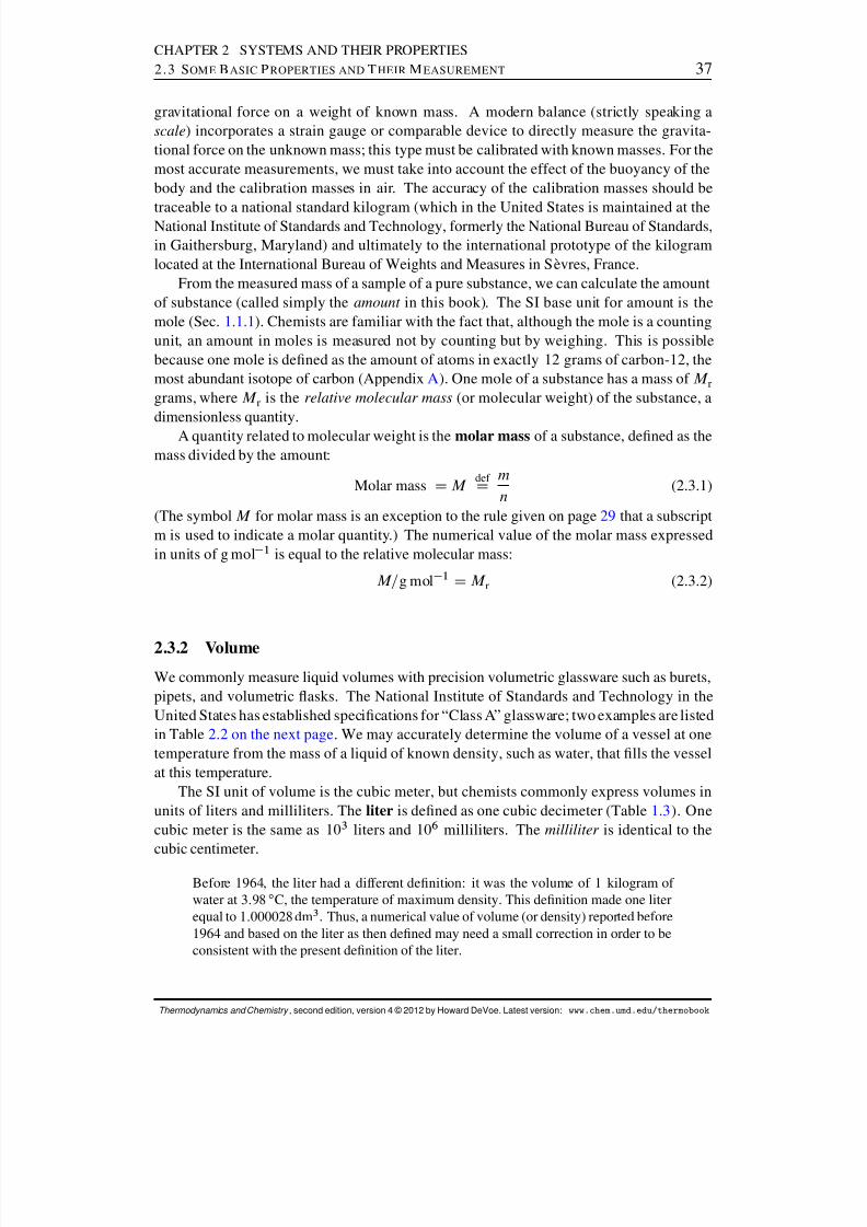
8/12/2019 Howard Devoe Thermodynamic and Chemical
http://slidepdf.com/reader/full/howard-devoe-thermodynamic-and-chemical 37/532
CHAPTER 2 SYSTEMS AND THEIR PROPERTIES2.3 S OME BASIC P ROPERTIES AND T HEIR M EASUREMENT 37
gravitational force on a weight of known mass. A modern balance (strictly speaking ascale ) incorporates a strain gauge or comparable device to directly measure the gravita-tional force on the unknown mass; this type must be calibrated with known masses. For themost accurate measurements, we must take into account the effect of the buoyancy of thebody and the calibration masses in air. The accuracy of the calibration masses should be
traceable to a national standard kilogram (which in the United States is maintained at theNational Institute of Standards and Technology, formerly the National Bureau of Standards,in Gaithersburg, Maryland) and ultimately to the international prototype of the kilogramlocated at the International Bureau of Weights and Measures in S evres, France.
From the measured mass of a sample of a pure substance, we can calculate the amountof substance (called simply the amount in this book). The SI base unit for amount is themole (Sec. 1.1.1 ). Chemists are familiar with the fact that, although the mole is a countingunit, an amount in moles is measured not by counting but by weighing. This is possiblebecause one mole is dened as the amount of atoms in exactly 12 grams of carbon-12, themost abundant isotope of carbon (Appendix A ). One mole of a substance has a mass of M rgrams, where M r is the relative molecular mass (or molecular weight) of the substance, adimensionless quantity.
A quantity related to molecular weight is the molar mass of a substance, dened as themass divided by the amount:
Molar mass D M def
D m
n (2.3.1)
(The symbol M for molar mass is an exception to the rule given on page 29 that a subscriptm is used to indicate a molar quantity.) The numerical value of the molar mass expressedin units of g mol 1 is equal to the relative molecular mass:
M= g mol 1 D M r (2.3.2)
2.3.2 VolumeWe commonly measure liquid volumes with precision volumetric glassware such as burets,pipets, and volumetric asks. The National Institute of Standards and Technology in theUnited States has established specications for “Class A” glassware; two examples are listedin Table 2.2 on the next page . We may accurately determine the volume of a vessel at onetemperature from the mass of a liquid of known density, such as water, that lls the vesselat this temperature.
The SI unit of volume is the cubic meter, but chemists commonly express volumes inunits of liters and milliliters. The liter is dened as one cubic decimeter (Table 1.3 ). Onecubic meter is the same as 103 liters and 106 milliliters. The milliliter is identical to thecubic centimeter.
Before 1964, the liter had a different denition: it was the volume of 1 kilogram of water at 3:98 ı C, the temperature of maximum density. This denition made one literequal to 1:000028 dm 3 . Thus, a numerical value of volume (or density) reported before1964 and based on the liter as then dened may need a small correction in order to beconsistent with the present denition of the liter.
Thermodynamics and Chemistry , second edition, version 4 © 2012 by Howard DeVoe. Latest version: www.chem.umd.edu/thermobook

8/12/2019 Howard Devoe Thermodynamic and Chemical
http://slidepdf.com/reader/full/howard-devoe-thermodynamic-and-chemical 38/532
CHAPTER 2 SYSTEMS AND THEIR PROPERTIES2.3 S OME BASIC P ROPERTIES AND T HEIR M EASUREMENT 38
Table 2.2 Representative measurement methods
PhysicalMethod
Typical Approximatequantity value uncertainty
Mass analytical balance 100 g 0:1 mgmicrobalance 20 mg 0:1 g
Volume pipet, Class A 10 mL 0:02 mLvolumetric ask, Class A 1 L 0:3 mL
Density pycnometer, 25-mL capacity 1 g mL 1 2 mgmL 1
magnetic oat densimeter 1 g mL 1 0:1 mgmL 1
vibrating-tube densimeter 1 g mL 1 0:01 mgmL 1
Pressure mercury manometer or barometer 760 Torr 0:001 Torrdiaphragm gauge 100 Torr 1 Torr
Temperature constant-volume gas thermometer 10 K 0:001 Kmercury-in-glass thermometer 300 K 0:01 Kplatinum resistance thermometer 300 K 0:0001 Kmonochromatic optical pyrometer 1300 K 0:03 K
2.3.3 Density
Density, an intensive property, is dened as the ratio of the two extensive properties massand volume:
def
D mV
(2.3.3)
The molar volume V m of a homogeneous pure substance is inversely proportional to itsdensity. From Eqs. 2.1.2 , 2.3.1 , and 2.3.3 , we obtain the relation
V m D M
(2.3.4)
Various methods are available for determining the density of a phase, many of thembased on the measurement of the mass of a xed volume or on a buoyancy technique.Three examples are shown in Fig. 2.4 on the next page . Similar apparatus may be used forgases. The density of a solid may be determined from the volume of a nonreacting liquid(e.g., mercury) displaced by a known mass of the solid, or from the loss of weight due tobuoyancy when the solid is suspended by a thread in a liquid of known density.
2.3.4 Pressure
Pressure is a force per unit area. Specically, it is the normal component of stress exertedby an isotropic uid on a surface element. 4 The surface can be an interface surface between
the uid and another phase, or an imaginary dividing plane within the uid.Pressure is usually a positive quantity. Because cohesive forces exist in a liquid, it maybe possible to place the liquid under tension and create a negative pressure. For instance,the pressure is negative at the top of a column of liquid mercury suspended below the closed
4A liquid crystal and a polar liquid in a electric eld are examples of uids that are not isotropic—that is, thathave different macroscopic properties in different directions.
Thermodynamics and Chemistry , second edition, version 4 © 2012 by Howard DeVoe. Latest version: www.chem.umd.edu/thermobook
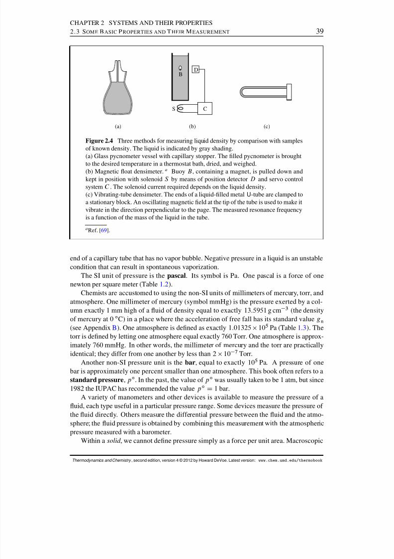
8/12/2019 Howard Devoe Thermodynamic and Chemical
http://slidepdf.com/reader/full/howard-devoe-thermodynamic-and-chemical 39/532
CHAPTER 2 SYSTEMS AND THEIR PROPERTIES2.3 S OME BASIC P ROPERTIES AND T HEIR M EASUREMENT 39
(a)
C
DB
S
(b) (c)
Figure 2.4 Three methods for measuring liquid density by comparison with samplesof known density. The liquid is indicated by gray shading.(a) Glass pycnometer vessel with capillary stopper. The lled pycnometer is broughtto the desired temperature in a thermostat bath, dried, and weighed.(b) Magnetic oat densimeter. a Buoy B , containing a magnet, is pulled down andkept in position with solenoid S by means of position detector D and servo controlsystem C . The solenoid current required depends on the liquid density.
(c) Vibrating-tube densimeter. The ends of a liquid-lled metal U-tube are clamped toa stationary block. An oscillating magnetic eld at the tip of the tube is used to make itvibrate in the direction perpendicular to the page. The measured resonance frequencyis a function of the mass of the liquid in the tube.
a Ref. [ 69].
end of a capillary tube that has no vapor bubble. Negative pressure in a liquid is an unstablecondition that can result in spontaneous vaporization.
The SI unit of pressure is the pascal . Its symbol is Pa. One pascal is a force of onenewton per square meter (Table 1.2 ).
Chemists are accustomed to using the non-SI units of millimeters of mercury, torr, andatmosphere. One millimeter of mercury (symbol mmHg) is the pressure exerted by a col-umn exactly 1 mm high of a uid of density equal to exactly 13:5951 g cm 3 (the densityof mercury at 0 ı C) in a place where the acceleration of free fall has its standard value gn(see Appendix B). One atmosphere is dened as exactly 1:01325 105 Pa (Table 1.3 ). Thetorr is dened by letting one atmosphere equal exactly 760 Torr. One atmosphere is approx-imately 760 mmHg. In other words, the millimeter of mercury and the torr are practicallyidentical; they differ from one another by less than 2 10 7 Torr.
Another non-SI pressure unit is the bar , equal to exactly 105 Pa. A pressure of onebar is approximately one percent smaller than one atmosphere. This book often refers to astandard pressure , p ı . In the past, the value of p ı was usually taken to be 1 atm, but since
1982 the IUPAC has recommended the value pı
D 1 bar.A variety of manometers and other devices is available to measure the pressure of auid, each type useful in a particular pressure range. Some devices measure the pressure of the uid directly. Others measure the differential pressure between the uid and the atmo-sphere; the uid pressure is obtained by combining this measurement with the atmosphericpressure measured with a barometer.
Within a solid , we cannot dene pressure simply as a force per unit area. Macroscopic
Thermodynamics and Chemistry , second edition, version 4 © 2012 by Howard DeVoe. Latest version: www.chem.umd.edu/thermobook
8/12/2019 Howard Devoe Thermodynamic and Chemical
http://slidepdf.com/reader/full/howard-devoe-thermodynamic-and-chemical 40/532
CHAPTER 2 SYSTEMS AND THEIR PROPERTIES2.3 S OME BASIC P ROPERTIES AND T HEIR M EASUREMENT 40
forces at a point within a solid are described by the nine components of a stress tensor. Thestatement that a solid has or is at a certain pressure means that this is the hydrostatic pressureexerted on the solid’s exterior surface. Thus, a solid immersed in a uniform isotropic uidof pressure p is at pressure p ; if the uid pressure is constant over time, the solid is atconstant pressure.
2.3.5 Temperature
Temperature scales
Temperature and thermometry are of fundamental importance in thermodynamics. Unlikethe other physical quantities discussed in this chapter, temperature does not have a singleunique denition. The chosen denition, whatever it may be, requires a temperature scaledescribed by an operational method of measuring temperature values. For the scale to beuseful, the values should increase monotonically with the increase of what we experiencephysiologically as the degree of “hotness.” We can dene a satisfactory scale with anymeasuring method that satises this requirement. The values on a particular temperaturescale correspond to a particular physical quantity and a particular temperature unit.
For example, suppose you construct a simple liquid-in-glass thermometer with equallyspaced marks along the stem and number the marks consecutively. To dene a temperaturescale and a temperature unit, you could place the thermometer in thermal contact with abody whose temperature is to be measured, wait until the indicating liquid reaches a stableposition, and read the meniscus position by linear interpolation between two marks. 5
Thermometry is based on the principle that the temperatures of different bodies maybe compared with a thermometer. For example, if you nd by separate measurements withyour thermometer that two bodies give the same reading, you know that within experimentalerror both have the same temperature. The signicance of two bodies having the sametemperature (on any scale) is that if they are placed in thermal contact with one another,they will prove to be in thermal equilibrium with one another as evidenced by the absenceof any changes in their properties. This principle is sometimes called the zeroth law of thermodynamics , and was rst stated as follows by J. C. Maxwell (1872): “Bodies whosetemperatures are equal to that of the same body have themselves equal temperatures.” 6
Two particular temperature scales are used extensively. The ideal-gas temperaturescale is dened by gas thermometry measurements, as described on page 42. The ther-modynamic temperature scale is dened by the behavior of a theoretical Carnot engine,as explained in Sec. 4.3.4 . These temperature scales correspond to the physical quanti-ties called ideal-gas temperature and thermodynamic temperature, respectively. Althoughthe two scales have different denitions, the two temperatures turn out (Sec. 4.3.4 ) to beproportional to one another. Their values become identical when the same unit of temper-ature is used for both. Thus, the kelvin is dened by specifying that a system containing
the solid, liquid, and gaseous phases of H 2 O coexisting at equilibrium with one another(the triple point of water) has a thermodynamic temperature of exactly 273:16 kelvins. We
5Of course, placing the thermometer and body in thermal contact may affect the body’s temperature. Themeasured temperature is that of the body after thermal equilibrium is achieved.6Turner (Ref. [ 158 ]) argues that the “zeroth law” is a consequence of the rst and second laws and therefore isnot a separate assumption in the axiomatic framework of thermodynamics. The term “law” for this principle isalso questioned by Redlich (Ref. [ 140 ]).
Thermodynamics and Chemistry , second edition, version 4 © 2012 by Howard DeVoe. Latest version: www.chem.umd.edu/thermobook
8/12/2019 Howard Devoe Thermodynamic and Chemical
http://slidepdf.com/reader/full/howard-devoe-thermodynamic-and-chemical 41/532
CHAPTER 2 SYSTEMS AND THEIR PROPERTIES2.3 S OME BASIC P ROPERTIES AND T HEIR M EASUREMENT 41
set the ideal-gas temperature of this system equal to the same value, 273:16 kelvins. Thetemperatures measured on the two scales are then identical.
Formally, the symbol T refers to thermodynamic temperature. Strictly speaking, a dif-ferent symbol should be used for ideal-gas temperature. Since the two kinds of temperatureshave identical values, this book will use the symbol T for both and refer to both physical
quantities simply as “temperature” except when it is necessary to make a distinction.Why is the temperature of the triple point of water taken to be 273:16 kelvins? Thisvalue is chosen arbitrarily to make the steam point approximately one hundred kelvinsgreater than the ice point.
The ice point is the temperature at which ice and air-saturated water coexist in equilib-rium at a pressure of one atmosphere. The steam point is the temperature at which liquidand gaseous H 2 O coexist in equilibrium at one atmosphere. Neither of these temperatureshas sufcient reproducibility for high-precision work. The temperature of the ice-water-air system used to dene the ice point is affected by air bubbles in the ice and by varyingconcentrations of air in the water around each piece of ice. The steam point is uncertain be-cause the temperature of coexisting liquid and gas is a sensitive function of the experimentalpressure.
The obsolete centigrade scale was dened to give a value of exactly 0 degrees centi-grade at the ice point and a value of exactly 100 degrees centigrade at the steam point, andto be a linear function of an ideal-gas temperature scale.
The centigrade scale has been replaced by the Celsius scale , which is based on thetriple point of water rather than on the less reproducible ice point and steam point. The Cel-sius scale is the thermodynamic (or ideal-gas) temperature scale shifted by exactly 273:15kelvins. The temperature unit is the degree Celsius ( ı C), identical in size to the kelvin.Thus, Celsius temperature t is related to thermodynamic temperature T by
t=ı C D T =K 273:15 (2.3.5)
On the Celsius scale, the triple point of water is exactly 0:01ı
C. The ice point is 0ı
C towithin 0:0001 ı C, and the steam point is 99:97 ı C.
The International Temperature Scale of 1990
The International Temperature Scale of 1990 (abbreviated ITS-90) is the most recent scaledevised for practical high-precision temperature measurements. 7 This scale denes thephysical quantity called international temperature, with symbol T 90 . Each value of T 90 isintended to be very close to the corresponding thermodynamic temperature T .
The ITS-90 is dened over a very wide temperature range, from 0:65 K up to at least1358 K. There is a specied procedure for each measurement of T 90 , depending on therange in which T falls: vapor-pressure thermometry ( 0:65–5:0 K), gas thermometry ( 3:0–
24:5561 K), platinum-resistance thermometry ( 13:8033 –1234:93 K), or optical pyrometry(above 1234:93 K). For vapor-pressure thermometry, the ITS-90 provides formulas for T 90in terms of the vapor pressure of the helium isotopes 3He and 4He. For the other meth-ods, it assigns values of several xed calibration temperatures. The xed temperatures areachieved with the reproducible equilibrium systems listed in Table 2.3 on the next page .
7Refs. [ 113 ] and [134 ].
Thermodynamics and Chemistry , second edition, version 4 © 2012 by Howard DeVoe. Latest version: www.chem.umd.edu/thermobook
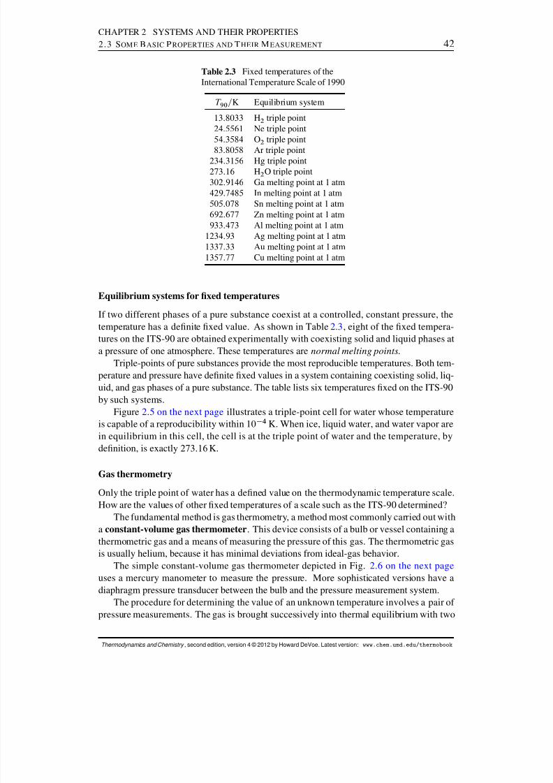
8/12/2019 Howard Devoe Thermodynamic and Chemical
http://slidepdf.com/reader/full/howard-devoe-thermodynamic-and-chemical 42/532
CHAPTER 2 SYSTEMS AND THEIR PROPERTIES2.3 S OME BASIC P ROPERTIES AND T HEIR M EASUREMENT 42
Table 2.3 Fixed temperatures of theInternational Temperature Scale of 1990
T 90 =K Equilibrium system
13:8033 H2 triple point24:5561 Ne triple point54:3584 O2 triple point83:8058 Ar triple point
234:3156 Hg triple point273:16 H2 O triple point302:9146 Ga melting point at 1 atm429:7485 In melting point at 1 atm505:078 Sn melting point at 1 atm692:677 Zn melting point at 1 atm933:473 Al melting point at 1 atm
1234:93 Ag melting point at 1 atm1337:33 Au melting point at 1 atm1357:77 Cu melting point at 1 atm
Equilibrium systems for xed temperatures
If two different phases of a pure substance coexist at a controlled, constant pressure, thetemperature has a denite xed value. As shown in Table 2.3 , eight of the xed tempera-tures on the ITS-90 are obtained experimentally with coexisting solid and liquid phases ata pressure of one atmosphere. These temperatures are normal melting points .
Triple-points of pure substances provide the most reproducible temperatures. Both tem-perature and pressure have denite xed values in a system containing coexisting solid, liq-uid, and gas phases of a pure substance. The table lists six temperatures xed on the ITS-90by such systems.
Figure 2.5 on the next page illustrates a triple-point cell for water whose temperatureis capable of a reproducibility within 10 4 K. When ice, liquid water, and water vapor arein equilibrium in this cell, the cell is at the triple point of water and the temperature, bydenition, is exactly 273:16 K.
Gas thermometry
Only the triple point of water has a dened value on the thermodynamic temperature scale.How are the values of other xed temperatures of a scale such as the ITS-90 determined?
The fundamental method is gas thermometry, a method most commonly carried out witha constant-volume gas thermometer . This device consists of a bulb or vessel containing athermometric gas and a means of measuring the pressure of this gas. The thermometric gasis usually helium, because it has minimal deviations from ideal-gas behavior.
The simple constant-volume gas thermometer depicted in Fig. 2.6 on the next pageuses a mercury manometer to measure the pressure. More sophisticated versions have adiaphragm pressure transducer between the bulb and the pressure measurement system.
The procedure for determining the value of an unknown temperature involves a pair of pressure measurements. The gas is brought successively into thermal equilibrium with two
Thermodynamics and Chemistry , second edition, version 4 © 2012 by Howard DeVoe. Latest version: www.chem.umd.edu/thermobook
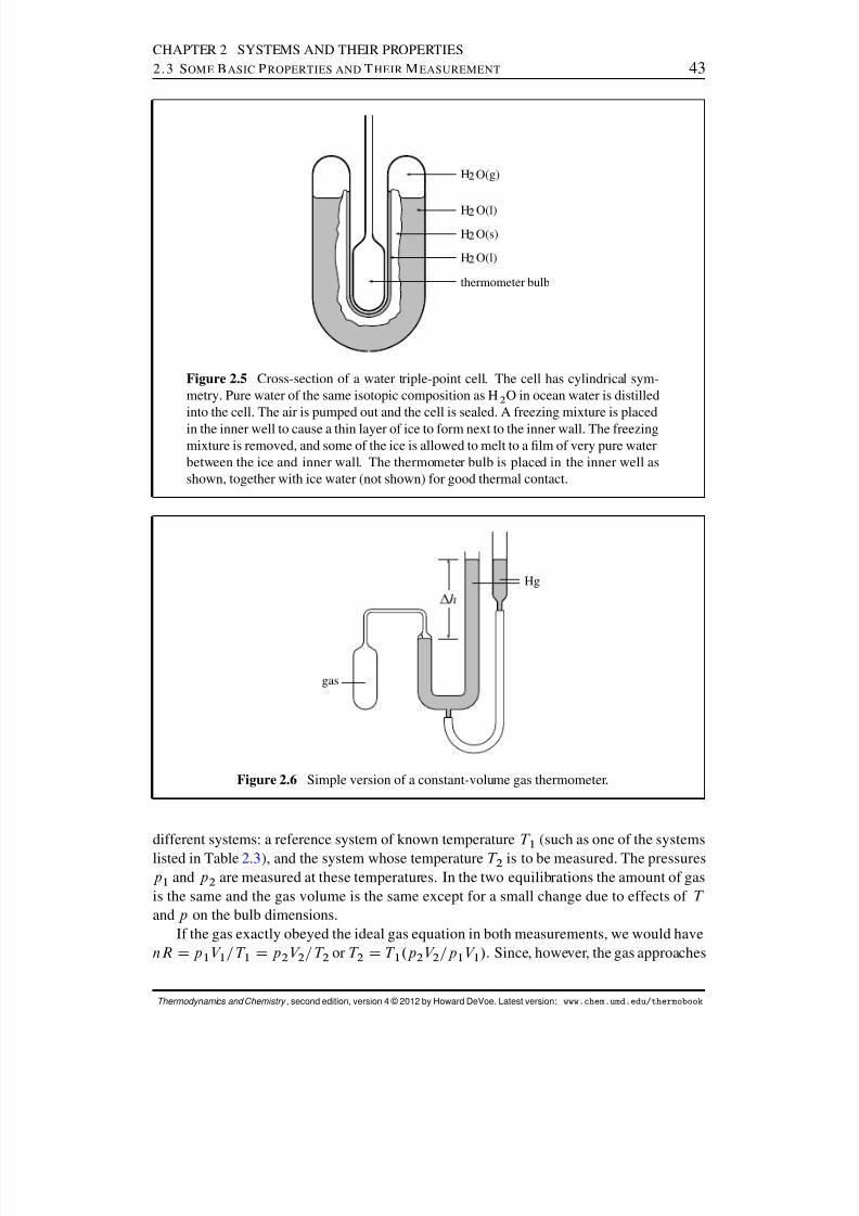
8/12/2019 Howard Devoe Thermodynamic and Chemical
http://slidepdf.com/reader/full/howard-devoe-thermodynamic-and-chemical 43/532
CHAPTER 2 SYSTEMS AND THEIR PROPERTIES2.3 S OME BASIC P ROPERTIES AND T HEIR M EASUREMENT 43
H
O(g)
H O(l)H
O(s)
H
O(l)
thermometer bulb
Figure 2.5 Cross-section of a water triple-point cell. The cell has cylindrical sym-metry. Pure water of the same isotopic composition as H 2 O in ocean water is distilledinto the cell. The air is pumped out and the cell is sealed. A freezing mixture is placedin the inner well to cause a thin layer of ice to form next to the inner wall. The freezingmixture is removed, and some of the ice is allowed to melt to a lm of very pure waterbetween the ice and inner wall. The thermometer bulb is placed in the inner well asshown, together with ice water (not shown) for good thermal contact.
gas
Hg
Figure 2.6 Simple version of a constant-volume gas thermometer.
different systems: a reference system of known temperature T 1 (such as one of the systemslisted in Table 2.3 ), and the system whose temperature T 2 is to be measured. The pressuresp 1 and p 2 are measured at these temperatures. In the two equilibrations the amount of gasis the same and the gas volume is the same except for a small change due to effects of T and p on the bulb dimensions.
If the gas exactly obeyed the ideal gas equation in both measurements, we would havenR D p 1 V 1 =T 1 D p 2 V 2 =T 2 or T 2 D T 1 .p 2 V 2 =p 1 V 1 / . Since, however, the gas approaches
Thermodynamics and Chemistry , second edition, version 4 © 2012 by Howard DeVoe. Latest version: www.chem.umd.edu/thermobook
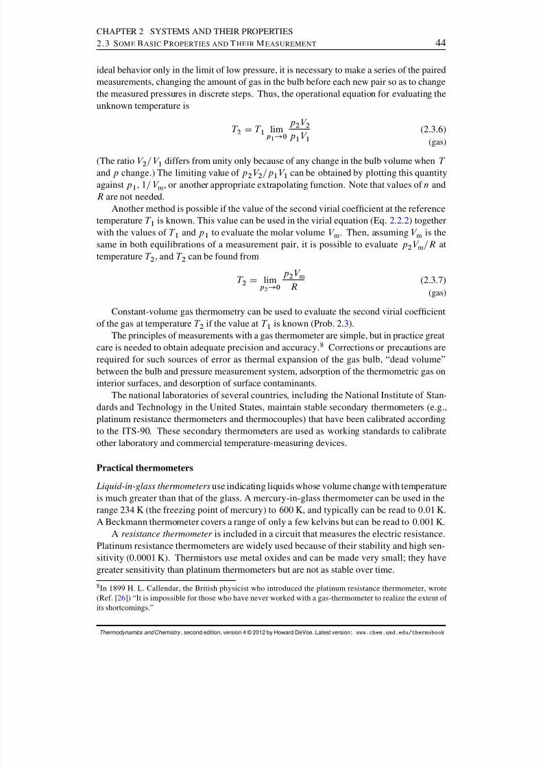
8/12/2019 Howard Devoe Thermodynamic and Chemical
http://slidepdf.com/reader/full/howard-devoe-thermodynamic-and-chemical 44/532
CHAPTER 2 SYSTEMS AND THEIR PROPERTIES2.3 S OME BASIC P ROPERTIES AND T HEIR M EASUREMENT 44
ideal behavior only in the limit of low pressure, it is necessary to make a series of the pairedmeasurements, changing the amount of gas in the bulb before each new pair so as to changethe measured pressures in discrete steps. Thus, the operational equation for evaluating theunknown temperature is
T 2 D
T 1
limp 1 ! 0
p 2 V 2p 1 V 1
(2.3.6)(gas)
(The ratio V 2 =V 1 differs from unity only because of any change in the bulb volume when T and p change.) The limiting value of p 2 V 2 =p 1 V 1 can be obtained by plotting this quantityagainst p 1 , 1=V m , or another appropriate extrapolating function. Note that values of n andR are not needed.
Another method is possible if the value of the second virial coefcient at the referencetemperature T 1 is known. This value can be used in the virial equation (Eq. 2.2.2 ) togetherwith the values of T 1 and p 1 to evaluate the molar volume V m . Then, assuming V m is thesame in both equilibrations of a measurement pair, it is possible to evaluate p 2 V m=R attemperature T 2 , and T 2 can be found from
T 2 D limp 2 ! 0
p 2 V mR
(2.3.7)(gas)
Constant-volume gas thermometry can be used to evaluate the second virial coefcientof the gas at temperature T 2 if the value at T 1 is known (Prob. 2. 3).
The principles of measurements with a gas thermometer are simple, but in practice greatcare is needed to obtain adequate precision and accuracy. 8 Corrections or precautions arerequired for such sources of error as thermal expansion of the gas bulb, “dead volume”between the bulb and pressure measurement system, adsorption of the thermometric gas oninterior surfaces, and desorption of surface contaminants.
The national laboratories of several countries, including the National Institute of Stan-dards and Technology in the United States, maintain stable secondary thermometers (e.g.,platinum resistance thermometers and thermocouples) that have been calibrated accordingto the ITS-90. These secondary thermometers are used as working standards to calibrateother laboratory and commercial temperature-measuring devices.
Practical thermometers
Liquid-in-glass thermometers use indicating liquids whose volume change with temperatureis much greater than that of the glass. A mercury-in-glass thermometer can be used in therange 234 K (the freezing point of mercury) to 600 K, and typically can be read to 0:01 K.A Beckmann thermometer covers a range of only a few kelvins but can be read to 0:001 K.
A resistance thermometer is included in a circuit that measures the electric resistance.Platinum resistance thermometers are widely used because of their stability and high sen-sitivity ( 0:0001 K). Thermistors use metal oxides and can be made very small; they havegreater sensitivity than platinum thermometers but are not as stable over time.
8In 1899 H. L. Callendar, the British physicist who introduced the platinum resistance thermometer, wrote(Ref. [ 26]) “It is impossible for those who have never worked with a gas-thermometer to realize the extent of its shortcomings.”
Thermodynamics and Chemistry , second edition, version 4 © 2012 by Howard DeVoe. Latest version: www.chem.umd.edu/thermobook
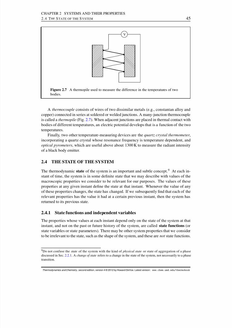
8/12/2019 Howard Devoe Thermodynamic and Chemical
http://slidepdf.com/reader/full/howard-devoe-thermodynamic-and-chemical 45/532
CHAPTER 2 SYSTEMS AND THEIR PROPERTIES2.4 T HE S TATE OF THE S YSTEM 45
V
Figure 2.7 A thermopile used to measure the difference in the temperatures of twobodies.
A thermocouple consists of wires of two dissimilar metals (e.g., constantan alloy and
copper) connected in series at soldered or welded junctions. A many-junction thermocoupleis called a thermopile (Fig. 2.7). When adjacent junctions are placed in thermal contact withbodies of different temperatures, an electric potential develops that is a function of the twotemperatures.
Finally, two other temperature-measuring devices are the quartz crystal thermometer ,incorporating a quartz crystal whose resonance frequency is temperature dependent, andoptical pyrometers , which are useful above about 1300 K to measure the radiant intensityof a black body emitter.
2.4 THE STATE OF THE SYSTEM
The thermodynamic state of the system is an important and subtle concept.9
At each in-stant of time, the system is in some denite state that we may describe with values of themacroscopic properties we consider to be relevant for our purposes. The values of theseproperties at any given instant dene the state at that instant. Whenever the value of anyof these properties changes, the state has changed. If we subsequently nd that each of therelevant properties has the value it had at a certain previous instant, then the system hasreturned to its previous state.
2.4.1 State functions and independent variables
The properties whose values at each instant depend only on the state of the system at thatinstant, and not on the past or future history of the system, are called state functions (orstate variables or state parameters). There may be other system properties that we considerto be irrelevant to the state, such as the shape of the system, and these are not state functions.
9Do not confuse the state of the system with the kind of physical state or state of aggregation of a phasediscussed in Sec. 2.2.1 . A change of state refers to a change in the state of the system, not necessarily to a phasetransition.
Thermodynamics and Chemistry , second edition, version 4 © 2012 by Howard DeVoe. Latest version: www.chem.umd.edu/thermobook
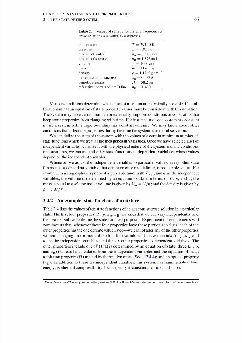
8/12/2019 Howard Devoe Thermodynamic and Chemical
http://slidepdf.com/reader/full/howard-devoe-thermodynamic-and-chemical 46/532
CHAPTER 2 SYSTEMS AND THEIR PROPERTIES2.4 T HE S TATE OF THE S YSTEM 46
Table 2.4 Values of state functions of an aqueous su-crose solution (A = water, B = sucrose)
temperature T D 293:15 Kpressure p D 1:01 baramount of water nA D 39:18 mol
amount of sucrose nB D 1:375 molvolume V D 1000 cm 3
mass m D 1176:5 gdensity D 1:1765 g cm 3
mole fraction of sucrose xB D 0:03390osmotic pressure ˘ D 58:2 barrefractive index, sodium D line nD D 1:400
Various conditions determine what states of a system are physically possible. If a uni-form phase has an equation of state, property values must be consistent with this equation.The system may have certain built-in or externally-imposed conditions or constraints that
keep some properties from changing with time. For instance, a closed system has constantmass; a system with a rigid boundary has constant volume. We may know about otherconditions that affect the properties during the time the system is under observation.
We can dene the state of the system with the values of a certain minimum number of state functions which we treat as the independent variables . Once we have selected a set of independent variables, consistent with the physical nature of the system and any conditionsor constraints, we can treat all other state functions as dependent variables whose valuesdepend on the independent variables.
Whenever we adjust the independent variables to particular values, every other statefunction is a dependent variable that can have only one denite, reproducible value. Forexample, in a single-phase system of a pure substance with T , p , and n as the independent
variables, the volume is determined by an equation of state in terms of T , p , and n; themass is equal to nM ; the molar volume is given by V m D V =n; and the density is given by
D nM=V .
2.4.2 An example: state functions of a mixture
Table 2.4 lists the values of ten state functions of an aqueous sucrose solution in a particularstate. The rst four properties ( T , p , nA , nB) are ones that we can vary independently, andtheir values sufce to dene the state for most purposes. Experimental measurements willconvince us that, whenever these four properties have these particular values, each of theother properties has the one denite value listed—we cannot alter any of the other propertieswithout changing one or more of the rst four variables. Thus we can take T , p , n A , and
nB as the independent variables, and the six other properties as dependent variables. Theother properties include one ( V ) that is determined by an equation of state; three ( m , ,and xB) that can be calculated from the independent variables and the equation of state;a solution property ( ˘ ) treated by thermodynamics (Sec. 12.4.4 ); and an optical property(nD). In addition to these six independent variables, this system has innumerable others:energy, isothermal compressibility, heat capacity at constant pressure, and so on.
Thermodynamics and Chemistry , second edition, version 4 © 2012 by Howard DeVoe. Latest version: www.chem.umd.edu/thermobook
8/12/2019 Howard Devoe Thermodynamic and Chemical
http://slidepdf.com/reader/full/howard-devoe-thermodynamic-and-chemical 47/532
CHAPTER 2 SYSTEMS AND THEIR PROPERTIES2.4 T HE S TATE OF THE S YSTEM 47
We could make other choices of the independent variables for the aqueous sucrose sys-tem. For instance, we could choose the set T , p , V , and xB , or the set p , V , , and xB .If there are no imposed conditions, the number of independent variables of this system isalways four. (Note that we could not arbitrarily choose just any four variables. For instance,there are only three independent variables in the set p , V , m , and because of the relation
D m=V .)If the system has imposed conditions, there will be fewer independent variables. Sup-pose the sucrose solution is in a closed system with xed, known values of nA and nB ; thenthere are only two independent variables and we could describe the state by the values of just T and p .
2.4.3 More about independent variables
A closed system containing a single substance in a single phase has two independent vari-ables, as we can see by the fact that the state is completely dened by values of T and p orof T and V .
A closed single-phase system containing a mixture of several nonreacting substances,
or a mixture of reactants and products in reaction equilibrium, also has two independentvariables. Examples are
air, a mixture of gases in xed proportions; an aqueous ammonia solution containing H 2 O, NH 3 , NH 4
C , HC , OH , and probablyother species, all in rapid continuous equilibrium.
The systems in these two examples contain more than one substance, but only one com- ponent . The number of components of a system is the minimum number of substances ormixtures of xed composition needed to form each phase. 10 A system of a single pure sub-stance is a special case of a system of one component. In an open system, the amount of each component can be used as an independent variable.
Consider a system with more than one uniform phase. In principle, for each phase we
could independently vary the temperature, the pressure, and the amount of each substanceor component. There would then be 2 CC independent variables for each phase, where C is the number of components in the phase.
There usually are, however, various equilibria and other conditions that reduce the num-ber of independent variables. For instance, each phase may have the same temperature andthe same pressure; equilibrium may exist with respect to chemical reaction and transferbetween phases (Sec. 2.4.4 ); and the system may be closed. (While these various condi-tions do not have to be present, the relations among T , p , V , and amounts described by anequation of state of a phase are always present.) On the other hand, additional independentvariables are required if we consider properties such as the surface area of a liquid to berelevant. 11
We must be careful to choose a set of independent variables that denes the statewithout ambiguity. For a closed system of liquid water, the set p and V might be a
10 The concept of the number of components is discussed in more detail in Chap. 13.11 The important topic of the number of independent intensive variables is treated by the Gibbs phase rule, whichwill be discussed in Sec. 8.1.7 for systems of a single substance and in Sec. 13.1 for systems of more than onesubstance.
Thermodynamics and Chemistry , second edition, version 4 © 2012 by Howard DeVoe. Latest version: www.chem.umd.edu/thermobook

8/12/2019 Howard Devoe Thermodynamic and Chemical
http://slidepdf.com/reader/full/howard-devoe-thermodynamic-and-chemical 48/532
CHAPTER 2 SYSTEMS AND THEIR PROPERTIES2.4 T HE S TATE OF THE S YSTEM 48
poor choice because the molar volume of water passes through a minimum as T isvaried at constant p . Thus, the values p D 1:000 bar and V D 18:016 cm3 woulddescribe one mole of water at both 2 ı C and 6 ı C, so these values would not uniquelydene the state. Better choices of independent variables in this case would be either T and p , or else T and V .
How may we describe the state of a system that has nonuniform regions? In this case wemay imagine the regions to be divided into many small volume elements, each small enoughto be essentially uniform but large enough to contain many molecules. We then describethe state by specifying values of independent variables for each volume element. If there isinternal macroscopic motion (e.g., ow), then velocity components can be included amongthe independent variables. Obviously, the quantity of information needed to describe acomplicated state may be enormous.
We can imagine situations in which classical thermodynamics would be completelyincapable of describing the state. For instance, turbulent ow in a uid or a shock wave ina gas may involve inhomogeneities all the way down to the molecular scale. Macroscopicvariables would not sufce to dene the states in these cases.
Whatever our choice of independent variables, all we need to know to be sure a systemis in the same state at two different times is that the value of each independent variable isthe same at both times .
2.4.4 Equilibrium states
An equilibrium state is a state that, when present in an isolated system, remains unchangedindenitely as long as the system remains isolated. (Recall that an isolated system is onethat exchanges no matter or energy with the surroundings.) An equilibrium state of anisolated system has no natural tendency to change over time. If changes do occur in anisolated system, they continue until an equilibrium state is reached.
A system in an equilibrium state may have some or all of the following kinds of internalequilibria:Thermal equilibrium : each phase has the same temperature.
Mechanical equilibrium : each phase has the same pressure.
Transfer equilibrium : there is equilibrium with respect to the transfer of each speciesfrom one phase to another.
Reaction equilibrium : every possible chemical reaction is at equilibrium.A homogeneous system has a single phase of uniform temperature and pressure, and so
has thermal and mechanical equilibrium. It is in an equilibrium state if it also has reactionequilibrium.
A heterogeneous system is in an equilibrium state if each of the four kinds of internalequilibrium is present.
The meaning of internal equilibrium in the context of an equilibrium state is that noperceptible change of state occurs during the period we keep the isolated system underobservation. For instance, a system containing a homogeneous mixture of gaseous H 2 andO2 at 25 ı C and 1 bar is in a state of reaction equilibrium on a time scale of hours or days; butif a measurable amount of H 2 O forms over a longer period, the state is not an equilibrium
Thermodynamics and Chemistry , second edition, version 4 © 2012 by Howard DeVoe. Latest version: www.chem.umd.edu/thermobook

8/12/2019 Howard Devoe Thermodynamic and Chemical
http://slidepdf.com/reader/full/howard-devoe-thermodynamic-and-chemical 49/532
CHAPTER 2 SYSTEMS AND THEIR PROPERTIES2.4 T HE S TATE OF THE S YSTEM 49
state on this longer time scale. This consideration of time scale is similar to the one weapply to the persistence of deformation in distinguishing a solid from a uid (Sec. 2.2.1 ).
Even if a system is not in internal equilibrium, it can be in an equilibrium state if achange of state is prevented by an imposed internal constraint or the inuence of an externaleld. Here are ve examples of such states.
A system with an internal adiabatic partition separating two phases can be in an equi-librium state that is not in thermal equilibrium. The adiabatic partition allows the twophases to remain indenitely at different temperatures. If the partition is rigid, it canalso allow the two phases to have different pressures, so that the equilibrium statelacks mechanical equilibrium.
An experimental system used to measure osmotic pressure (Fig. 12.2 on page 373 )has a semipermeable membrane separating a liquid solution phase and a pure solventphase. The membrane prevents the transfer of solute from the solution to the puresolvent. In the equilibrium state of this system, the solution has a higher pressure thanthe pure solvent; the system is then in neither transfer equilibrium nor mechanicalequilibrium.
In the equilibrium state of a galvanic cell that is not part of a closed electrical circuit(Sec. 3.8.3 ), the separation of the reactants and products and the open circuit areconstraints that prevent the cell reaction from coming to reaction equilibrium.
A system containing mixed reactants of a reaction can be in an equilibrium statewithout reaction equilibrium if we withhold a catalyst or initiator or introduce aninhibitor that prevents reaction. In the example above of a mixture of H 2 and O 2gases, we could consider the high activation energy barrier for the formation of H 2 Oto be an internal constraint. If we remove the constraint by adding a catalyst, thereaction will proceed explosively.
An example of a system inuenced by an external eld is a tall column of gas in a
gravitational eld (Sec. 8.1.4 ). In order for an equilibrium state to be established inthis eld, the pressure must decrease continuously with increasing elevation.
Keep in mind that regardless of the presence or absence of internal constraints andexternal elds, the essential feature of an equilibrium state is this: if we isolate the systemwhile it is in this state, the state functions do not change over time .
Three additional comments can be made regarding the properties of equilibrium states.
1. It should be apparent that a system with thermal equilibrium has a single value of T , and one with mechanical equilibrium has a single value of p , and this allows thestate to be described by a minimal number of independent variables. In contrast, thedenition of a nonequilibrium state with nonuniform intensive properties may requirea very large number of independent variables.
2. Strictly speaking, during a time period in which the system exchanges energy with thesurroundings its state cannot be an equilibrium state. Energy transfer at a nite ratecauses nonuniform temperature and pressure within the system and prevents internalthermal and mechanical equilibrium. If, however, the rate of energy transfer is small,then at each instant the state can closely approximate an equilibrium state. This topicwill be discussed in detail in the next chapter.
Thermodynamics and Chemistry , second edition, version 4 © 2012 by Howard DeVoe. Latest version: www.chem.umd.edu/thermobook
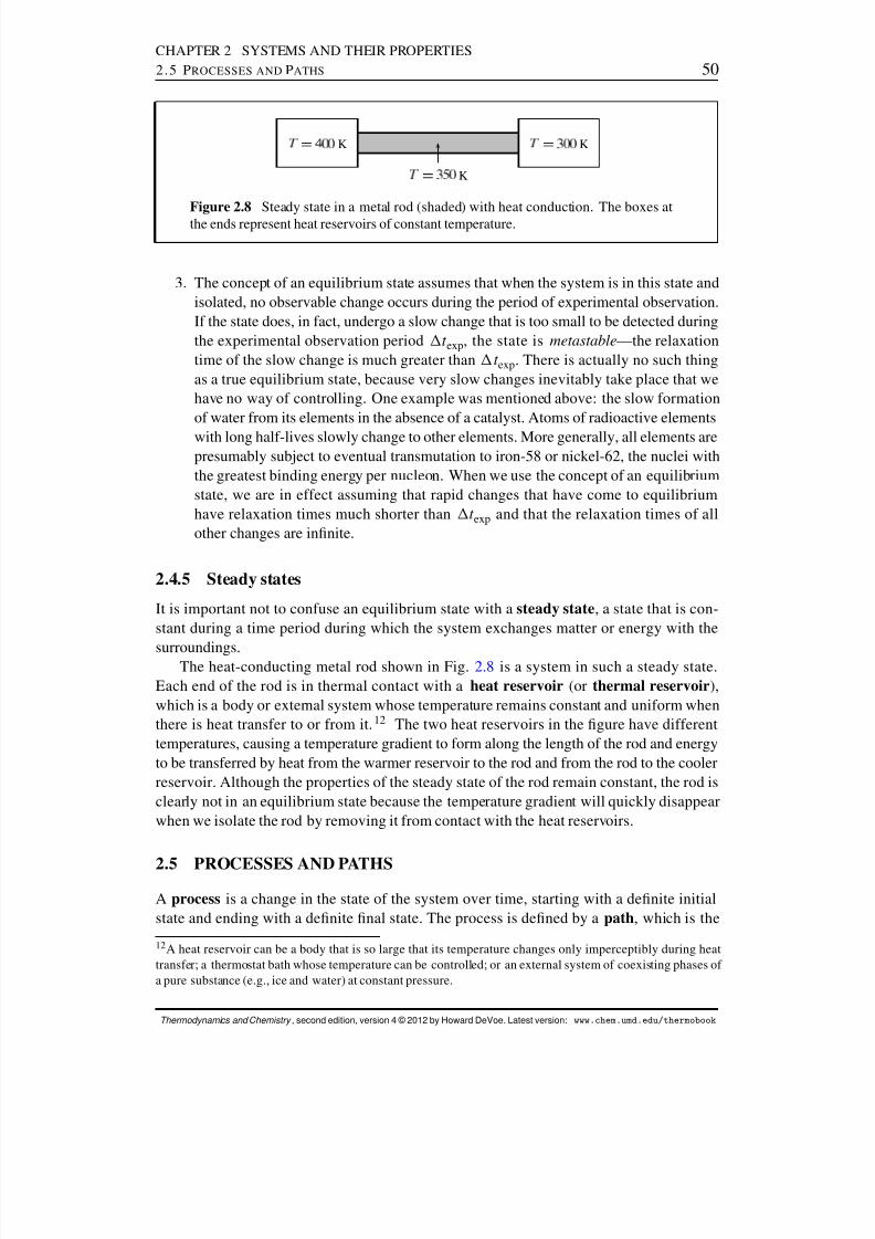
8/12/2019 Howard Devoe Thermodynamic and Chemical
http://slidepdf.com/reader/full/howard-devoe-thermodynamic-and-chemical 50/532
CHAPTER 2 SYSTEMS AND THEIR PROPERTIES2.5 P ROCESSES AND PATHS 50
K
K
K
Figure 2.8 Steady state in a metal rod (shaded) with heat conduction. The boxes atthe ends represent heat reservoirs of constant temperature.
3. The concept of an equilibrium state assumes that when the system is in this state andisolated, no observable change occurs during the period of experimental observation.If the state does, in fact, undergo a slow change that is too small to be detected duringthe experimental observation period t exp , the state is metastable —the relaxationtime of the slow change is much greater than t exp . There is actually no such thingas a true equilibrium state, because very slow changes inevitably take place that wehave no way of controlling. One example was mentioned above: the slow formationof water from its elements in the absence of a catalyst. Atoms of radioactive elementswith long half-lives slowly change to other elements. More generally, all elements arepresumably subject to eventual transmutation to iron-58 or nickel-62, the nuclei withthe greatest binding energy per nucleon. When we use the concept of an equilibriumstate, we are in effect assuming that rapid changes that have come to equilibriumhave relaxation times much shorter than t exp and that the relaxation times of allother changes are innite.
2.4.5 Steady states
It is important not to confuse an equilibrium state with a steady state , a state that is con-stant during a time period during which the system exchanges matter or energy with the
surroundings.The heat-conducting metal rod shown in Fig. 2.8 is a system in such a steady state.
Each end of the rod is in thermal contact with a heat reservoir (or thermal reservoir ),which is a body or external system whose temperature remains constant and uniform whenthere is heat transfer to or from it. 12 The two heat reservoirs in the gure have differenttemperatures, causing a temperature gradient to form along the length of the rod and energyto be transferred by heat from the warmer reservoir to the rod and from the rod to the coolerreservoir. Although the properties of the steady state of the rod remain constant, the rod isclearly not in an equilibrium state because the temperature gradient will quickly disappearwhen we isolate the rod by removing it from contact with the heat reservoirs.
2.5 PROCESSES AND PATHSA process is a change in the state of the system over time, starting with a denite initialstate and ending with a denite nal state. The process is dened by a path , which is the
12 A heat reservoir can be a body that is so large that its temperature changes only imperceptibly during heattransfer; a thermostat bath whose temperature can be controlled; or an external system of coexisting phases of a pure substance (e.g., ice and water) at constant pressure.
Thermodynamics and Chemistry , second edition, version 4 © 2012 by Howard DeVoe. Latest version: www.chem.umd.edu/thermobook
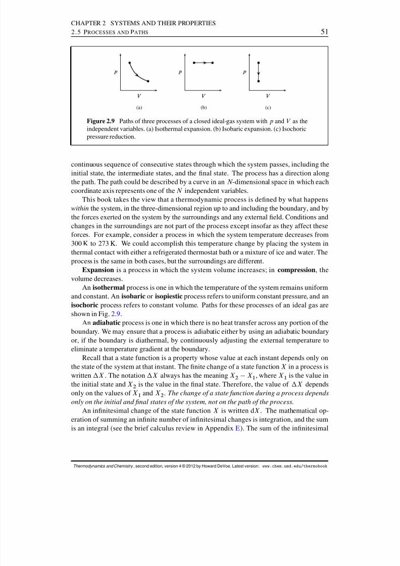
8/12/2019 Howard Devoe Thermodynamic and Chemical
http://slidepdf.com/reader/full/howard-devoe-thermodynamic-and-chemical 51/532
CHAPTER 2 SYSTEMS AND THEIR PROPERTIES2.5 P ROCESSES AND PATHS 51
V
p
(a)
V
p
(b)
V
p
(c)
Figure 2.9 Paths of three processes of a closed ideal-gas system with p and V as theindependent variables. (a) Isothermal expansion. (b) Isobaric expansion. (c) Isochoricpressure reduction.
continuous sequence of consecutive states through which the system passes, including theinitial state, the intermediate states, and the nal state. The process has a direction alongthe path. The path could be described by a curve in an N -dimensional space in which eachcoordinate axis represents one of the N independent variables.
This book takes the view that a thermodynamic process is dened by what happenswithin the system, in the three-dimensional region up to and including the boundary, and bythe forces exerted on the system by the surroundings and any external eld. Conditions andchanges in the surroundings are not part of the process except insofar as they affect theseforces. For example, consider a process in which the system temperature decreases from300 K to 273 K. We could accomplish this temperature change by placing the system inthermal contact with either a refrigerated thermostat bath or a mixture of ice and water. Theprocess is the same in both cases, but the surroundings are different.
Expansion is a process in which the system volume increases; in compression , thevolume decreases.
An isothermal process is one in which the temperature of the system remains uniform
and constant. An isobaric or isopiestic process refers to uniform constant pressure, and anisochoric process refers to constant volume. Paths for these processes of an ideal gas areshown in Fig. 2.9 .
An adiabatic process is one in which there is no heat transfer across any portion of theboundary. We may ensure that a process is adiabatic either by using an adiabatic boundaryor, if the boundary is diathermal, by continuously adjusting the external temperature toeliminate a temperature gradient at the boundary.
Recall that a state function is a property whose value at each instant depends only onthe state of the system at that instant. The nite change of a state function X in a process iswritten X . The notation X always has the meaning X 2 X 1 , where X 1 is the value inthe initial state and X 2 is the value in the nal state. Therefore, the value of X depends
only on the values of X
1 and X
2 . The change of a state function during a process depends
only on the initial and nal states of the system, not on the path of the process.An innitesimal change of the state function X is written d X . The mathematical op-
eration of summing an innite number of innitesimal changes is integration, and the sumis an integral (see the brief calculus review in Appendix E). The sum of the innitesimal
Thermodynamics and Chemistry , second edition, version 4 © 2012 by Howard DeVoe. Latest version: www.chem.umd.edu/thermobook
8/12/2019 Howard Devoe Thermodynamic and Chemical
http://slidepdf.com/reader/full/howard-devoe-thermodynamic-and-chemical 52/532
CHAPTER 2 SYSTEMS AND THEIR PROPERTIES2.6 T HE E NERGY OF THE S YSTEM 52
changes of X along a path is a denite integral equal to X :
Z X 2
X 1dX D X 2 X 1 D X (2.5.1)
If d X obeys this relation—that is, if its integral for given limits has the same value regardless
of the path—it is called an exact differential . The differential of a state function is alwaysan exact differential.A cyclic process is a process in which the state of the system changes and then returns
to the initial state. In this case the integral of d X is written with a cyclic integral sign: H dX .Since a state function X has the same initial and nal values in a cyclic process, X 2 is equalto X 1 and the cyclic integral of d X is zero:
I dX D 0 (2.5.2)
Heat ( q ) and work ( w ) are examples of quantities that are not state functions. They arenot even properties of the system; instead they are quantities of energy transferred acrossthe boundary over a period of time. It would therefore be incorrect to write “ q ” or “ w .”Instead, the values of q and w depend in general on the path and are called path functions .
This book uses the symbol ¶ (the letter “d” with a bar through the stem) for an innites-imal quantity of a path function. Thus, ¶q and ¶w are innitesimal quantities of heat andwork. The sum of many innitesimal quantities of a path function is not the difference of two values of the path function; instead, the sum is the net quantity:
Z ¶q D q Z ¶w D w (2.5.3)
The innitesimal quantities ¶q and ¶w , because the values of their integrals depend on thepath, are inexact differentials .13
There is a fundamental difference between a state function (such as temperature or
volume) and a path function (such as heat or work): The value of a state function refers toone instant of time; the value of a path function refers to an interval of time .
The difference between a state function and a path function in thermodynamics isanalogous to the difference between elevation and trail length in hiking up a mountain.Suppose a trailhead at the base of the mountain has several trails to the summit. Thehiker at each instant is at a denite elevation above sea level. During a climb from thetrailhead to the summit, the hiker’s change of elevation is independent of the trail used,but the trail length from base to summit depends on the trail.
2.6 THE ENERGY OF THE SYSTEM
A large part of classical thermodynamics is concerned with the energy of the system. Thetotal energy of a system is an extensive property whose value at any one instant cannot bemeasured in any practical way, but whose change is the focus of the rst law of thermody-namics (Chap. 3).
13 Chemical thermodynamicists often write these quantities as d q and dw . Mathematicians, however, frown onusing the same notation for inexact and exact differentials. Other notations sometimes used to indicate that heatand work are path functions are D q and Dw , and also ıq and ıw .
Thermodynamics and Chemistry , second edition, version 4 © 2012 by Howard DeVoe. Latest version: www.chem.umd.edu/thermobook
8/12/2019 Howard Devoe Thermodynamic and Chemical
http://slidepdf.com/reader/full/howard-devoe-thermodynamic-and-chemical 53/532
CHAPTER 2 SYSTEMS AND THEIR PROPERTIES2.6 T HE E NERGY OF THE S YSTEM 53
2.6.1 Energy and reference frames
Classical thermodynamics ignores microscopic properties such as the behavior of individualatoms and molecules. Nevertheless, a consideration of the classical mechanics of particleswill help us to understand the sources of the potential and kinetic energy of a thermody-namic system.
In classical mechanics, the energy of a collection of interacting point particles is thesum of the kinetic energy 1
2 mv 2 of each particle (where m is the particle’s mass and v isits velocity), and of various kinds of potential energies. The potential energies are denedin such a way that if the particles are isolated from the rest of the universe, as the particlesmove and interact with one another the total energy (kinetic plus potential) is constant overtime. This principle of the conservation of energy also holds for real atoms and moleculeswhose electronic, vibrational, and rotational energies, absent in point particles, are addi-tional contributions to the total energy.
The positions and velocities of particles must be measured in a specied system of coordinates called a reference frame . This book will use reference frames with Cartesianaxes. Since the kinetic energy of a particle is a function of velocity, the kinetic energy
depends on the choice of the reference frame. A particularly important kind is an inertialframe, one in which Newton’s laws of motion are obeyed (see Sec. G.1 in Appendix G).
A reference frame whose axes are xed relative to the earth’s surface is what this book will call a lab frame . A lab frame for all practical purposes is inertial (Sec. G.10 onpage 504 ). It is in this kind of stationary frame that the laws of thermodynamics havebeen found by experiment to be valid.
The energy E of a thermodynamic system is the sum of the energies of the particlescontained in it and the potential energies of interaction between these particles. Just as foran individual particle, the energy of the system depends on the reference frame in which itis measured. The energy of the system may change during a process, but the principle of the conservation of energy ensures that the sum of the energy of the system, the energy of the surroundings, and any energy shared by both, all measured in the same reference frame,remains constant over time.
This book uses the symbol E sys for the energy of the system measured in a speciedinertial frame. The system could be located in a weightless environment in outer space, andthe inertial frame could be one that is either xed or moving at constant velocity relative tolocal stars. Usually, however, the system is located in the earth’s gravitational eld, and theappropriate inertial frame is then an earth-xed lab frame.
If during a process the system as a whole undergoes motion or rotation relative to theinertial frame, then E sys depends in part on coordinates that are not properties of the system.In such situations E sys is not a state function, and we need the concept of internal energy.
2.6.2 Internal energy
The internal energy , U , is the energy of the system measured in a reference frame thatallows U to be a state function—that is, at each instant the value of U depends only on thestate of the system. This book will call a reference frame with this property a local frame .A local frame may also be, but is not necessarily, an earth-xed lab frame.
Thermodynamics and Chemistry , second edition, version 4 © 2012 by Howard DeVoe. Latest version: www.chem.umd.edu/thermobook
8/12/2019 Howard Devoe Thermodynamic and Chemical
http://slidepdf.com/reader/full/howard-devoe-thermodynamic-and-chemical 54/532
CHAPTER 2 SYSTEMS AND THEIR PROPERTIES2.6 T HE E NERGY OF THE S YSTEM 54
Here is a simple illustration of the distinction between the energy E sys of a systemmeasured in a lab frame and the internal energy U measured in a local frame. Let the systembe a xed amount of water contained in a glass beaker. (The glass material of the beakeris part of the surroundings.) We can dene the state of this system by two independentvariables: the temperature, T , and pressure, p , of the water. The most convenient local
frame in which to measure U in this case is a frame xed with respect to the beaker. When the beaker is at rest on the lab bench, the local frame is a lab frame; then theenergies E sys and U are equal and depend only on T and p .
If we place the beaker on a laboratory hot plate and use the hot plate to raise thetemperature of the water, the values of E sys and U increase equally.
Suppose we slide the beaker horizontally along the lab bench while T and p stayconstant. While the system is in motion, its kinetic energy is greater in the lab framethan in the local frame. Now E sys is greater than when the beaker was at rest, althoughthe state of the system and the value of U are unchanged.
If we slowly lift the beaker above the bench, the potential energy of the water in the
earth’s gravitational eld increases, again with no change in T
and p
. The value of E sys has increased, but there has been no change in the state of the system or the valueof U .
Section 3.1.1 will show that the relation between changes of the system energy and theinternal energy in this example is E sys D E k CE p CU , where E k and E p are thekinetic and potential energies of the system as a whole measured in the lab frame.
Our choice of the local frame used to dene the internal energy U of any particularsystem during a given process is to some extent arbitrary. Three possible choices are asfollows.
If the system as a whole does not move or rotate in the laboratory, a lab frame is anappropriate local frame. Then U is the same as the system energy E sys measured in
the lab frame. If the system’s center of mass moves in the lab frame during the process, we can letthe local frame be a center-of-mass frame whose origin moves with the center of massand whose Cartesian axes are parallel to the axes of the lab frame.
If the system consists of the contents of a rigid container that moves or rotates in thelab, as in the illustration above, it may be convenient to choose a local frame that hasits origin and axes xed with respect to the container.
Is it possible to determine a numerical value for the internal energy of a system? Thetotal energy of a body of mass m when it is at rest is given by the Einstein relation E D mc 2
0 ,where c0 is the speed of light in vacuum. In principle, then, we could calculate the internalenergy U of a system at rest from its mass, and we could determine U for a processfrom the change in mass. In practice, however, an absolute value of U calculated from ameasured mass has too much uncertainty to be of any practical use. For example, the typicaluncertainty of the mass of an object measured with a microbalance, about 0:1 g (Table2.2 ), would introduce the enormous uncertainty in energy of about 1010 joules. Only valuesof the change U are useful, and these values cannot be calculated from m because thechange in mass during an ordinary chemical process is much too small to be detected.
Thermodynamics and Chemistry , second edition, version 4 © 2012 by Howard DeVoe. Latest version: www.chem.umd.edu/thermobook
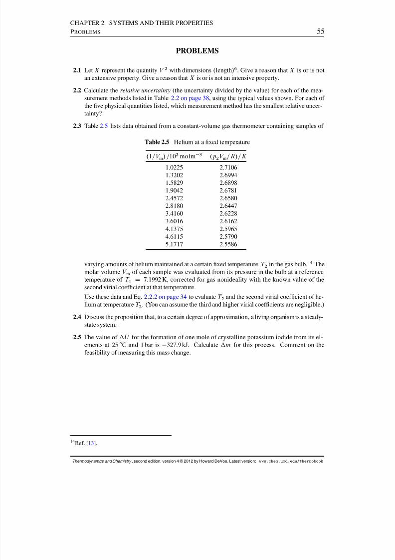
8/12/2019 Howard Devoe Thermodynamic and Chemical
http://slidepdf.com/reader/full/howard-devoe-thermodynamic-and-chemical 55/532
CHAPTER 2 SYSTEMS AND THEIR PROPERTIESPROBLEMS 55
PROBLEMS
2.1 Let X represent the quantity V 2 with dimensions . length / 6 . Give a reason that X is or is notan extensive property. Give a reason that X is or is not an intensive property.
2.2 Calculate the relative uncertainty (the uncertainty divided by the value) for each of the mea-
surement methods listed in Table 2.2 on page 38 , using the typical values shown. For each of the ve physical quantities listed, which measurement method has the smallest relative uncer-tainty?
2.3 Table 2.5 lists data obtained from a constant-volume gas thermometer containing samples of
Table 2.5 Helium at a xed temperature
.1=V m / =10 2 molm 3 .p 2 V m=R/=K
1.0225 2.71061.3202 2.69941.5829 2.68981.9042 2.67812.4572 2.65802.8180 2.64473.4160 2.62283.6016 2.61624.1375 2.59654.6115 2.57905.1717 2.5586
varying amounts of helium maintained at a certain xed temperature T 2 in the gas bulb. 14 Themolar volume V m of each sample was evaluated from its pressure in the bulb at a referencetemperature of T 1 D 7:1992 K, corrected for gas nonideality with the known value of thesecond virial coefcient at that temperature.
Use these data and Eq. 2.2.2 on page 34 to evaluate T 2 and the second virial coefcient of he-lium at temperature T 2 . (You can assume the third and higher virial coefcients are negligible.)
2.4 Discuss the proposition that, to a certain degree of approximation, a living organismis a steady-state system.
2.5 The value of U for the formation of one mole of crystalline potassium iodide from its el-ements at 25 ı C and 1 bar is 327:9 kJ. Calculate m for this process. Comment on thefeasibility of measuring this mass change.
14 Ref. [ 13].
Thermodynamics and Chemistry , second edition, version 4 © 2012 by Howard DeVoe. Latest version: www.chem.umd.edu/thermobook
8/12/2019 Howard Devoe Thermodynamic and Chemical
http://slidepdf.com/reader/full/howard-devoe-thermodynamic-and-chemical 56/532
C HAPTER 3
T HE F IRST LAW
In science, a law is a statement or mathematical relation that concisely describes repro-ducible experimental observations. Classical thermodynamics is built on a foundation of three laws, none of which can be derived from principles that are any more fundamental.This chapter discusses theoretical aspects of the rst law; gives examples of reversible andirreversible processes and the heat and work that occur in them; and introduces the extensivestate function heat capacity .
3.1 HEAT, WORK, AND THE FIRST LAW
The box below gives two forms of the rst law of thermodynamics .
In a closed system:dU D ¶q C¶w U D q Cwwhere U is the internal energy of the system, a state function;
q is heat; andw is thermodynamic work.
The equation d U D ¶q C¶w is the differential form of the rst law, and U D q Cw isthe integrated form.
The heat and work appearing in the rst law are two different modes of energy transfer.They can be dened in a general way as follows.
Heat refers to the transfer of energy across the boundary caused by a temperature gradientat the boundary.
Work refers to the transfer of energy across the boundary caused by the displacement of amacroscopic portion of the system on which the surroundings exert a force, or becauseof other kinds of concerted, directed movement of entities (e.g., electrons) on which anexternal force is exerted.
An innitesimal quantity of energy transferred as heat at a surface element of the bound-ary is written ¶q , and a nite quantity is written q (Sec. 2.5 ). To obtain the total nite heatfor a process from q DR ¶q (Eq. 2.5.3 ), we must integrate over the total boundary surfaceand the entire path of the process.
56
8/12/2019 Howard Devoe Thermodynamic and Chemical
http://slidepdf.com/reader/full/howard-devoe-thermodynamic-and-chemical 57/532
CHAPTER 3 THE FIRST LAW3.1 H EAT , WORK , AND THE F IRST L AW 57
An innitesimal quantity of work is ¶w , and a nite quantity is w DR ¶w . To obtainw for a process, we integrate all kinds of work over the entire path of the process.
Any of these quantities for heat and work is positive if the effect is to increase theinternal energy, and negative if the effect is to decrease it. Thus, positive heat is energyentering the system, and negative heat is energy leaving the system. Positive work is work
done by the surroundings on the system, and negative work is work done by the system onthe surroundings.The rst-law equation U D qCw sets up a balance sheet for the energy of the system,
measured in the local frame, by equating its change during a process to the net quantity of energy transferred by means of heat and work. Note that the equation applies only to aclosed system. If the system is open, energy can also be brought across the boundary by thetransport of matter.
An important part of the rst law is the idea that heat and work are quantitative energytransfers. That is, when a certain quantity of energy enters the system in the form of heat,the same quantity leaves the surroundings. When the surroundings perform work on thesystem, the increase in the energy of the system is equal in magnitude to the decrease inthe energy of the surroundings. The principle of conservation of energy is obeyed: thetotal energy (the sum of the energies of the system and surroundings) remains constant overtime. 1
Heat transfer may occur by conduction, convection, or radiation. 2 We can reduce con-duction with good thermal insulation at the boundary, we can eliminate conduction andconvection with a vacuum gap, and we can minimize radiation with highly reective sur-faces at both sides of the vacuum gap. The only way to completely prevent heat during aprocess is to arrange conditions in the surroundings so there is no temperature gradient atany part of the boundary. Under these conditions the process is adiabatic, and any energytransfer in a closed system is then solely by means of work.
3.1.1 The concept of thermodynamic work
Appendix G gives a detailed analysis of energy and work based on the behavior of a collec-tion of interacting particles moving according to the principles of classical mechanics. Theanalysis shows how we should evaluate mechanical thermodynamic work. Suppose the dis-placement responsible for the work comes from linear motion of a portion of the boundaryin the Cx or x direction of the local frame. The differential and integrated forms of thework are then given by 3
¶w D F surx dx w DZ
x2
x 1
F surx dx (3.1.1)
Here F surx is the component in the Cx direction of the force exerted by the surroundings on
the system at the moving portion of the boundary, and d x is the innitesimal displacementof the boundary in the local frame. If the displacement is in the same direction as the force,¶w is positive; if the displacement is in the opposite direction, ¶w is negative.
1Strictly speaking, it is the sum of the energies of the system, the surroundings, and any potential energy sharedby both that is constant. The shared potential energy is usually negligible or essentially constant (Sec. G.5 ).2Some thermodynamicists treat radiation as a separate contribution to U , in addition to q and w .3These equations are Eq. G.6.11 with a change of notation.
Thermodynamics and Chemistry , second edition, version 4 © 2012 by Howard DeVoe. Latest version: www.chem.umd.edu/thermobook
8/12/2019 Howard Devoe Thermodynamic and Chemical
http://slidepdf.com/reader/full/howard-devoe-thermodynamic-and-chemical 58/532
CHAPTER 3 THE FIRST LAW3.1 H EAT , WORK , AND THE F IRST L AW 58
The kind of force represented by F surx is a short-range contact force. Appendix G shows
that the force exerted by a conservative time-independent external eld, such as a gravita-tional force, should not be included as part of F sur
x . This is because the work done by thiskind of force causes changes of potential and kinetic energies that are equal and opposite insign, with no net effect on the internal energy (see Sec. 3.6).
Newton’s third law of action and reaction says that a force exerted by the surroundingson the system is opposed by a force of equal magnitude exerted in the opposite direction bythe system on the surroundings. Thus the expressions in Eq. 3.1.1 can be replaced by
¶w D F sysx dx w D Z
x2
x 1
F sysx dx (3.1.2)
where F sysx is the component in the Cx direction of the contact force exerted by the system
on the surroundings at the moving portion of the boundary.
An alternative to using the expressions in Eqs. 3.1.1 or 3.1.2 for evaluating w is toimagine that the only effect of the work on the system’s surroundings is a change inthe elevation of a weight in the surroundings. The weight must be one that is linkedmechanically to the source of the force F sur
x . Then, provided the local frame is a sta-
tionary lab frame, the work is equal in magnitude and opposite in sign to the changein the weight’s potential energy: w D mg h where m is the weight’s mass, g is theacceleration of free fall, and h is the weight’s elevation in the lab frame. This inter-pretation of work can be helpful for seeing whether work occurs and for deciding onits sign, but of course cannot be used to determine its value if the actual surroundingsinclude no such weight.
The procedure of evaluating w from the change of an external weight’s potentialenergy requires that this change be the only mechanical effect of the process on thesurroundings, a condition that in practice is met only approximately. For example,Joule’s paddle-wheel experiment using two weights linked to the system by strings andpulleys, described latter in Sec. 3.7.2 , required corrections for (1) the kinetic energygained by the weights as they sank, (2) friction in the pulley bearings, and (3) elasticity
of the strings (see Prob. 3. 10 on page 100).
In the rst-law relation U D qCw , the quantities U , q , and w are all measured in anarbitrary local frame. We can write an analogous relation for measurements in a stationarylab frame:
E sys D qlab Cw lab (3.1.3)
Suppose the chosen local frame is not a lab frame, and we nd it more convenient to measurethe heat qlab and the work w lab in a lab frame than to measure q and w in the local frame.What corrections are needed to nd q and w in this case?
If the Cartesian axes of the local frame do not rotate relative to the lab frame, then theheat is the same in both frames: q D qlab .4
The expressions for ¶wlab
and wlab
are the same as those for ¶w and w in Eqs. 3.1.1and 3.1.2 , with d x interpreted as the displacement in the lab frame. There is an especiallysimple relation between w and w lab when the local frame is a center-of-mass frame—onewhose origin moves with the system’s center of mass and whose axes do not rotate relativeto the lab frame: 5
w D w lab 12 m v2
cm mg z cm (3.1.4)
4Sec. G.7 . 5Eq. G.8.12 on page 503 .
Thermodynamics and Chemistry , second edition, version 4 © 2012 by Howard DeVoe. Latest version: www.chem.umd.edu/thermobook

8/12/2019 Howard Devoe Thermodynamic and Chemical
http://slidepdf.com/reader/full/howard-devoe-thermodynamic-and-chemical 59/532
CHAPTER 3 THE FIRST LAW3.1 H EAT , WORK , AND THE F IRST L AW 59
In this equation m is the mass of the system, vcm is the velocity of its center of mass inthe lab frame, g is the acceleration of free fall, and zcm is the height of the center of massabove an arbitrary zero of elevation in the lab frame. In typical thermodynamic processesthe quantities vcm and zcm change to only a negligible extent, if at all, so that usually to agood approximation w is equal to wlab .
When the local frame is a center-of-mass frame, we can combine the relations U Dq Cw and q D qlab with Eqs. 3.1.3 and 3.1.4 to obtain
E sys D E k CE p CU (3.1.5)
where E k D 12 mv 2
cm and E p D mgz cm are the kinetic and potential energies of the systemas a whole in the lab frame.
A more general relation for w can be written for any local frame that has no rotationalmotion and whose origin has negligible acceleration in the lab frame: 6
w D w lab mg z loc (3.1.6)
Here zloc is the elevation in the lab frame of the origin of the local frame. z loc is usuallysmall or zero, so again w is approximately equal to wlab . The only kinds of processesfor which we may need to use Eq. 3.1.4 or 3.1.6 to calculate a non-negligible differencebetween w and wlab are those in which massive parts of the system undergo substantialchanges in elevation in the lab frame.
Simple relations such as these between q and qlab , and between w and wlab , do not existif the local frame has rotational motion relative to a lab frame.
Hereafter in this book, thermodynamic work w will be called simply work . For allpractical purposes you can assume the local frames for most of the processes to be describedare stationary lab frames. The discussion above shows that the values of heat and work measured in these frames are usually the same, or practically the same, as if they weremeasured in a local frame moving with the system’s center of mass. A notable exceptionis the local frame needed to treat the thermodynamic properties of a liquid solution in acentrifuge cell. In this case the local frame is xed in the spinning rotor of the centrifugeand has rotational motion. This special case will be discussed in Sec. 9.8.2 .
3.1.2 Work coefcients and work coordinates
If a process has only one kind of work, it can be expressed in the form
¶w D Y dX or w DZ X 2
X 1Y dX (3.1.7)
where Y is a generalized force called a work coefcient and X is a generalized displace-ment called a work coordinate . The work coefcient and work coordinate are conjugatevariables. They are not necessarily actual forces and displacements. For example, we shallsee in Sec. 3.4.2 that reversible expansion work is given by ¶w D p dV ; in this case, thework coefcient is p and the work coordinate is V .
6Eq. G.7.3 on page 500 .
Thermodynamics and Chemistry , second edition, version 4 © 2012 by Howard DeVoe. Latest version: www.chem.umd.edu/thermobook

8/12/2019 Howard Devoe Thermodynamic and Chemical
http://slidepdf.com/reader/full/howard-devoe-thermodynamic-and-chemical 60/532
CHAPTER 3 THE FIRST LAW3.1 H EAT , WORK , AND THE F IRST L AW 60
water
weight
stop
Figure 3.1 System containing an electrical resistor and a paddle wheel immersed inwater. Dashed rectangle: system boundary. Cross-hatched area: removable thermalinsulation.
A process may have more than one kind of work, each with its own work coefcientand conjugate work coordinate. In this case the work can be expressed as a sum over the
different kinds labeled by the index i :
¶w DXi
Y i dX i or w DXi Z X i;2
X i;1Y i dX i (3.1.8)
3.1.3 Heat and work as path functions
Consider the apparatus shown in Fig. 3.1 . The system consists of the water together withthe immersed parts: stirring paddles attached to a shaft (a paddle wheel) and an electricalresistor attached to wires. In equilibrium states of this system, the temperature and pressureare uniform and the paddle wheel is stationary. The system is open to the atmosphere, sothe pressure is constrained to be constant. We may describe the equilibrium states of thissystem by a single independent variable, the temperature T . (The angular position of theshaft is irrelevant to the state and is not a state function for equilibrium states of this system.)
Here are three experiments with different processes. Each process has the same initialstate dened by T 1 D 300:0 K, and each has the same nal state.
Experiment 1: We surround the system with thermal insulation as shown in the gure andrelease the external weight, which is linked mechanically to the paddle wheel. Theresulting paddle-wheel rotation causes turbulent churning of the water and an increase inits temperature. Assume that after the weight hits the stop and the paddle wheel comesto rest, the nal angular position of the paddle wheel is the same as at the beginningof the experiment. We can calculate the work done on the system from the differencebetween the potential energy lost by the weight and the kinetic energy gained beforeit reaches the stop. 7 We wait until the water comes to rest and the system comes tothermal equilibrium, then measure the nal temperature. Assume the nal temperatureis T 2 D 300:10 K, an increase of 0:10 kelvins.
7This calculation is an example of the procedure mentioned on page 58 in which the change in elevation of anexternal weight is used to evaluate work.
Thermodynamics and Chemistry , second edition, version 4 © 2012 by Howard DeVoe. Latest version: www.chem.umd.edu/thermobook

8/12/2019 Howard Devoe Thermodynamic and Chemical
http://slidepdf.com/reader/full/howard-devoe-thermodynamic-and-chemical 61/532
CHAPTER 3 THE FIRST LAW3.1 H EAT , WORK , AND THE F IRST L AW 61
Experiment 2: We start with the system in the same initial state as in experiment 1, andagain surround it with thermal insulation. This time, instead of releasing the weight weclose the switch to complete an electrical circuit with the resistor and allow the samequantity of electrical work to be done on the system as the mechanical work done inexperiment 1. We discover the nal temperature ( 300:10 K) is exactly the same as at the
end of experiment 1. The process and path are different from those in experiment 1, butthe work and the initial and nal states are the same.
Experiment 3: We return the system to its initial state, remove the thermal insulation, andplace the system in thermal contact with a heat reservoir of temperature 300:10 K. En-ergy can now enter the system in the form of heat, and does so because of the temper-ature gradient at the boundary. By a substitution of heat for mechanical or electricalwork, the system changes to the same nal state as in experiments 1 and 2.
Although the paths in the three experiments are entirely different, the overall change of state is the same. In fact, a person who observes only the initial and nal states and hasno knowledge of the intermediate states or the changes in the surroundings will be ignorantof the path. Did the paddle wheel turn? Did an electric current pass through the resistor?
How much energy was transferred by work and how much by heat? The observer cannottell from the change of state, because heat and work are not state functions. The change of state depends on the sum of heat and work. This sum is the change in the state function U ,as expressed by the integrated form of the rst law, U D q Cw .
It follows from this discussion that neither heat nor work are quantities possessed by thesystem. A system at a given instant does not have or contain a particular quantity of heator a particular quantity of work. Instead, heat and work depend on the path of a processoccurring over a period of time. They are path functions.
3.1.4 Heat and heating
In thermodynamics, the technical meaning of the word “heat” when used as a noun is energytransferred across the boundary because of a temperature gradient at the boundary .
In everyday speech the noun heat is often used somewhat differently. Here are threestatements with similar meanings that could be misleading:
“Heat is transferred from a laboratory hot plate to a beaker of water.”“Heat ows from a warmer body to a cooler body.”“To remove heat from a hot body, place it in cold water.”Statements such as these may give the false impression that heat is like a substance that
retains its identity as it moves from one body to another. Actually heat, like work, does notexist as an entity once a process is completed. Nevertheless, the wording of statements suchas these is embedded in our everyday language, and no harm is done if we interpret themcorrectly. This book, for conciseness, often refers to “heat transfer” and “heat ow,” instead
of using the technically more correct phrase “energy transfer by means of heat.”Another common problem is failure to distinguish between thermodynamic “heat” and
the process of “heating.” To heat a system is to cause its temperature to increase. A heated system is one that has become warmer. This process of heating does not necessarily involvethermodynamic heat; it can also be carried out with work as illustrated by experiments 1and 2 of the preceding section.
Thermodynamics and Chemistry , second edition, version 4 © 2012 by Howard DeVoe. Latest version: www.chem.umd.edu/thermobook

8/12/2019 Howard Devoe Thermodynamic and Chemical
http://slidepdf.com/reader/full/howard-devoe-thermodynamic-and-chemical 62/532
CHAPTER 3 THE FIRST LAW3.1 H EAT , WORK , AND THE F IRST L AW 62
The notion of heat as an indestructible substance was the essence of the caloric the-ory. This theory was nally disproved by the cannon-boring experiments of BenjaminThompson (Count Rumford) in the late eighteenth century, and in a more quantitativeway by the measurement of the mechanical equivalent of heat by James Joule in the1840s (see Sec. 3.7.2).
3.1.5 Heat capacity
The heat capacity of a closed system is dened as the ratio of an innitesimal quantity of heat transferred across the boundary under specied conditions and the resulting innitesi-mal temperature change:
heat capacity def
D ¶qdT
(3.1.9)(closed system)
Since q is a path function, the value of the heat capacity depends on the specied conditions,usually either constant volume or constant pressure. C V is the heat capacity at constant volume and C p is the heat capacity at constant pressure . These are extensive state functionsthat will be discussed more fully in Sec. 5.6 .
3.1.6 Thermal energy
It is sometimes useful to use the concept of thermal energy , the contribution to the system’sinternal energy due to its temperature. Thermal energy has no exact denition, but generallyspeaking it includes the kinetic energy of the random translational motions of microscopicparticles (atoms and molecules) as well as the vibrational and rotational energies (if any) of these particles. When the temperature of a body increases, so do these energies.
If the transfer of energy across the boundary of a closed system is solely by means of
heat, the thermal energy change may be the same as the quantity of energy transferred. Thisis not always the case. For example, when there is slow heat transfer into an equilibriumsystem of ice and water at constant pressure, the ice partially melts without an increase ineither temperature or thermal energy. It is intermolecular potential energy that has increasedin this case, rather than thermal energy.
When an innitesimal quantity of energy ¶q is transferred as heat into a body or a closedsingle-phase system without work, volume change, or chemical reaction, we can assume allof the transferred energy goes into increasing the thermal energy: d E thermal D ¶q . Underthese conditions of zero work, the rst law becomes d U D ¶q . The heat capacity at constantvolume for such a system, as dened by Eq. 3.1.9 , is then C V D dU= dT , and the changein thermal energy is given by
dE thermal D C V dT (3.1.10)(closed single-phase system,
no reaction)
Because thermal energy by denition depends only on T , Eq. 3.1.10 is an expression for itsinnitesimal change that is valid for a closed single-phase system without reaction regard-less of whether or not the volume is constant.
Thermodynamics and Chemistry , second edition, version 4 © 2012 by Howard DeVoe. Latest version: www.chem.umd.edu/thermobook
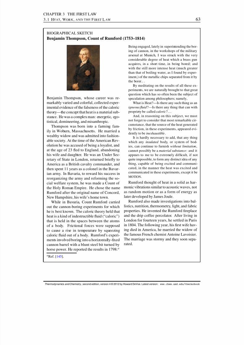
8/12/2019 Howard Devoe Thermodynamic and Chemical
http://slidepdf.com/reader/full/howard-devoe-thermodynamic-and-chemical 63/532
CHAPTER 3 THE FIRST LAW3.1 H EAT , WORK , AND THE F IRST L AW 63
BIOGRAPHICAL SKETCHBenjamin Thompson, Count of Rumford (1753–1814)
Benjamin Thompson, whose career was re-markably varied and colorful, collected exper-imental evidence of the falseness of the calorictheory—the concept that heat is a material sub-stance. He was a complex man: energetic, ego-tistical, domineering, and misanthropic.
Thompson was born into a farming fam-ily in Woburn, Massachusetts. He married awealthy widow and was admitted into fashion-able society. At the time of the American Rev-olution he was accused of being a loyalist, andat the age of 23 ed to England, abandoninghis wife and daughter. He was an Under Sec-retary of State in London, returned briey toAmerica as a British cavalry commander, andthen spent 11 years as a colonel in the Bavar-ian army. In Bavaria, to reward his success inreorganizing the army and reforming the so-cial welfare system, he was made a Count of the Holy Roman Empire. He chose the nameRumford after the original name of Concord,New Hampshire, his wife’s home town.
While in Bavaria, Count Rumford carriedout the cannon-boring experiments for whichhe is best known. The caloric theory held thatheat is a kind of indestructible uid (“caloric”)that is held in the spaces between the atomsof a body. Frictional forces were supposedto cause a rise in temperature by squeezingcaloric uid out of a body. Rumford’s experi-
ments involved boring into a horizontally-xedcannon barrel with a blunt steel bit turned byhorse power. He reported the results in 1798: a
Being engaged, lately in superintending the bor-ing of cannon, in the workshops of the militaryarsenal at Munich, I was struck with the very
considerable degree of heat which a brass gunacquires, in a short time, in being bored; andwith the still more intense heat (much greaterthan that of boiling water, as I found by exper-iment,) of the metallic chips separated from it bythe borer.. .
By meditating on the results of all these ex-periments, we are naturally brought to that greatquestion which has so often been the subject of speculation among philosophers; namely,
What is Heat?—Is there any such thing as anigneous uid ?—Is there any thing that can withpropriety be called caloric ? . . .
And, in reasoning on this subject, we must
not forget to consider that most remarkable cir-cumstance, that the source of the heat generatedby friction, in these experiments, appeared evi-dently to be inexhaustible .
It is hardly necessary to add, that any thingwhich any insulated body, or system of bod-ies, can continue to furnish without limitation ,cannot possibly be a material substance : and itappears to me to be extremely difcult, if notquite impossible, to form any distinct idea of anything, capable of being excited and communi-cated, in the manner the heat was excited andcommunicated in these experiments, except it beMOTION .
Rumford thought of heat in a solid as har-monic vibrations similar to acoustic waves, notas random motion or as a form of energy aslater developed by James Joule.
Rumford also made investigations into bal-listics, nutrition, thermometry, light, and fabricproperties. He invented the Rumford replaceand the drip coffee percolator. After living inLondon for fourteen years, he settled in Parisin 1804. The following year, his rst wife hav-ing died in America, he married the widow of the famous French chemist Antoine Lavoisier.The marriage was stormy and they soon sepa-rated.
a Ref. [ 145 ].
Thermodynamics and Chemistry , second edition, version 4 © 2012 by Howard DeVoe. Latest version: www.chem.umd.edu/thermobook
8/12/2019 Howard Devoe Thermodynamic and Chemical
http://slidepdf.com/reader/full/howard-devoe-thermodynamic-and-chemical 64/532
CHAPTER 3 THE FIRST LAW3.2 S PONTANEOUS , REVERSIBLE , AND IRREVERSIBLE P ROCESSES 64
3.2 SPONTANEOUS, REVERSIBLE, AND IRREVERSIBLE PROCESSES
A spontaneous process is a process that can actually occur in a nite time period underthe existing conditions. Any change over time in the state of a system that we observeexperimentally is a spontaneous process.
A spontaneous process is sometimes called a natural process, feasible process, possibleprocess, allowed process, or real process.
3.2.1 Reversible processes
A reversible process is an important concept in thermodynamics. This concept is neededfor the chain of reasoning that will allow us to dene entropy changes in the next chapter,and will then lead on to the establishment of criteria for spontaneity and for various kindsof equilibria.
Before reversible processes can be discussed, it is necessary to explain the meaning of the reverse of a process. If a particular process takes the system from an initial state Athrough a continuous sequence of intermediate states to a nal state B, then the reverse of
this process is a change over time from state B to state A with the same intermediate statesoccurring in the reverse time sequence. To visualize the reverse of any process, imaginemaking a movie lm of the events of the process. Each frame of the lm is a “snapshot”picture of the state at one instant. If you run the lm backward through a movie projector,you see the reverse process: the values of system properties such as p and V appear tochange in reverse chronological order, and each velocity changes sign.
The concept of a reversible process is not easy to describe or to grasp. Perhaps themost confusing aspect is that a reversible process is not a process that ever actually occurs,but is only approached as a hypothetical limit. During a reversible process the systempasses through a continuous sequence of equilibrium states. These states are ones that canbe approached, as closely as desired, by the states of a spontaneous process carried outsufciently slowly. As the spontaneous process is carried out more and more slowly, itapproaches the reversible limit. Thus, a reversible process is an idealized process with asequence of equilibrium states that are those of a spontaneous process in the limit of inniteslowness.
This book has many equations expressing relations among heat, work, and state func-tions during various kinds of reversible processes. What is the use of an equation for aprocess that can never actually occur? The point is that the equation can describe a sponta-neous process to a high degree of accuracy, if the process is carried out slowly enough forthe intermediate states to depart only slightly from exact equilibrium states. For example,for many important spontaneous processes we will assume the temperature and pressure areuniform throughout the system, which strictly speaking is an approximation.
A reversible process of a closed system, as used in this book, has all of the followingcharacteristics:
It is an imaginary, idealized process in which the system passes through a continuoussequence of equilibrium states. That is, the state at each instant is one that in anisolated system would persist with no tendency to change over time. (This kind of process is sometimes called a quasistatic process.)
Thermodynamics and Chemistry , second edition, version 4 © 2012 by Howard DeVoe. Latest version: www.chem.umd.edu/thermobook

8/12/2019 Howard Devoe Thermodynamic and Chemical
http://slidepdf.com/reader/full/howard-devoe-thermodynamic-and-chemical 65/532
CHAPTER 3 THE FIRST LAW3.2 S PONTANEOUS , REVERSIBLE , AND IRREVERSIBLE P ROCESSES 65
The sequence of equilibrium states can be approximated, as closely as desired, bythe intermediate states of a real spontaneous process carried out sufciently slowly.The reverse sequence of equilibrium states can also be approximated, as closely asdesired, by the intermediate states of another spontaneous process carried out suf-ciently slowly. (This requirement prevents any spontaneous process with hysteresis,
such as plastic deformation or the stretching of a metal wire beyond its elastic limit,from having a reversible limit.) During the approach to innite slowness, very slowchanges of the type described in item 3 on page 50 must be eliminated, i.e., preventedwith hypothetical constraints.
The spontaneous process of a closed system that has a reversible limit must be aprocess with heat, or work, or both—the system cannot be an isolated one. It must bepossible for an experimenter to use conditions in the surroundings to control the rateat which energy is transferred across the boundary by means of heat and work, andthus to make the process go as slowly as desired.
If energy is transferred by work during a reversible process, the work coefcient Y in the expression ¶w D Y dX must be nite (nonzero) in equilibrium states of the
system. For example, if the work is given by ¶w D F sysx dx (Eq. 3.1.2 ), the force
F sysx exerted by the system on the surroundings must be present when the system is
in an equilibrium state.
When a spontaneous process with a reversible limit is proceeding slowly enough forits states to closely approximate those of the reversible process, a small change inforces exerted on the system by the surroundings or in the external temperature at theboundary can change the process to one whose states approximate the sequence of states of the reverse process. In other words, it takes only a small change in externalconditions at the boundary, or in an external eld, to reverse the direction of theprocess.
In the reversible limit, dissipative effects within the system such as internal frictionvanish. This is a consequence of the fact that only equilibrium states are present inthis limit.
When any innitesimal step of a reversible process takes place in reverse, the magni-tudes of the heat ¶q and work ¶w are unchanged and their signs are reversed. Thus,energy transferred by heat in one direction across the boundary during a reversibleprocess is fully recovered as energy transferred by heat in the opposite direction inthe reverse process. Energy transferred by work is recovered in the same way.
We must imagine the reversible process to proceed at a nite rate, otherwise there wouldbe no change of state over time. The precise rate of the change is not important. Imagine agas whose volume, temperature, and pressure are changing at some nite rate while the tem-
perature and pressure magically stay perfectly uniform throughout the system. This is anentirely imaginary process, because there is no temperature or pressure gradient—no phys-ical “driving force”—that would make the change tend to occur in a particular direction.This imaginary process is a reversible process—one whose states of uniform temperatureand pressure are approached by the states of a real process as the real process takes placemore and more slowly.
Thermodynamics and Chemistry , second edition, version 4 © 2012 by Howard DeVoe. Latest version: www.chem.umd.edu/thermobook
8/12/2019 Howard Devoe Thermodynamic and Chemical
http://slidepdf.com/reader/full/howard-devoe-thermodynamic-and-chemical 66/532
CHAPTER 3 THE FIRST LAW3.2 S PONTANEOUS , REVERSIBLE , AND IRREVERSIBLE P ROCESSES 66
It is a good idea, whenever you see the word “reversible,” to think “in the reversiblelimit.” Thus a reversible process is a process in the reversible limit, reversible work is work in the reversible limit, and so on.
The reverse of a reversible process is itself a reversible process. As explained above,the quantities of energy transferred across the boundary by heat and work during areversible process are fully recovered when the reversible process is followed by thereverse process. This characteristic of a reversible process is sometimes described bythe statement that after a reversible change occurs, it is possible to restore both thesystem and the local surroundings to their original states with no further changes any-where. This statement, however, is misleading, because during the period in questionspontaneous changes inevitably occur outside the system. At the very least, the ex-ternal operations needed to control the rates and directions of energy transfer acrossthe boundary by heat and work, carried out by a human investigator or by some sortof automated mechanism, are highly spontaneous in nature and dissipate energy in thesurroundings.
3.2.2 Irreversible processesAn irreversible process is a spontaneous process whose reverse is neither spontaneous norreversible. That is, the reverse of an irreversible process can never actually occur and isimpossible . If a movie is made of a spontaneous process, and the time sequence of the eventsdepicted by the lm when it is run backward could not occur in reality, the spontaneousprocess is irreversible.
A good example of a spontaneous, irreversible process is experiment 1 on page 60 , inwhich the sinking of an external weight immersed in water causes a paddle wheel to rotateand the temperature of the water to increase. During this experiment mechanical energy isdissipated into thermal energy. Suppose you insert a thermometer in the water and make amovie lm of the experiment. Then when you run the lm backward in a projector, you willsee the paddle wheel rotating in the direction that raises the weight, and the water becomingcooler according to the thermometer. Clearly, this reverse process is impossible in the realphysical world, and the process occurring during the experiment is irreversible. It is notdifcult to understand why it is irreversible when we consider events on the microscopiclevel: it is extremely unlikely that the H 2 O molecules next to the paddles would happento move simultaneously over a period of time in the concerted motion needed to raise theweight.
3.2.3 Purely mechanical processes
There is a class of spontaneous processes that are also spontaneous in reverse; that is, spon-
taneous but not irreversible. These are purely mechanical processes involving the motion of perfectly-elastic macroscopic bodies without friction, temperature gradients, viscous ow,or other irreversible changes.
A simple example of a purely mechanical process and its reverse is shown in Fig. 3.2 .The ball can move spontaneously in either direction. Another example is a ywheel withfrictionless bearings rotating in a vacuum.
Thermodynamics and Chemistry , second edition, version 4 © 2012 by Howard DeVoe. Latest version: www.chem.umd.edu/thermobook
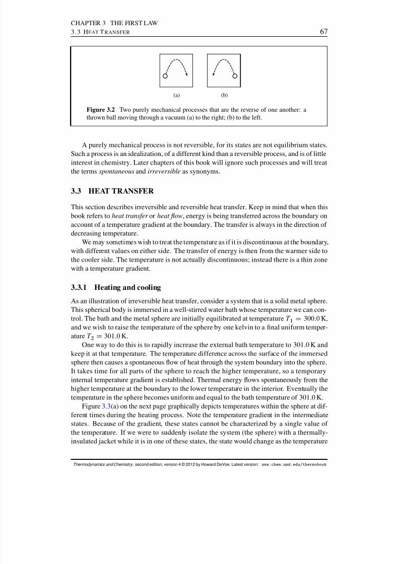
8/12/2019 Howard Devoe Thermodynamic and Chemical
http://slidepdf.com/reader/full/howard-devoe-thermodynamic-and-chemical 67/532
CHAPTER 3 THE FIRST LAW3.3 H EAT T RANSFER 67
(a) (b)
Figure 3.2 Two purely mechanical processes that are the reverse of one another: athrown ball moving through a vacuum (a) to the right; (b) to the left.
A purely mechanical process is not reversible, for its states are not equilibrium states.Such a process is an idealization, of a different kind than a reversible process, and is of littleinterest in chemistry. Later chapters of this book will ignore such processes and will treatthe terms spontaneous and irreversible as synonyms.
3.3 HEAT TRANSFER
This section describes irreversible and reversible heat transfer. Keep in mind that when thisbook refers to heat transfer or heat ow , energy is being transferred across the boundary onaccount of a temperature gradient at the boundary. The transfer is always in the direction of decreasing temperature.
We may sometimes wish to treat the temperature as if it is discontinuous at the boundary,with different values on either side. The transfer of energy is then from the warmer side tothe cooler side. The temperature is not actually discontinuous; instead there is a thin zonewith a temperature gradient.
3.3.1 Heating and cooling
As an illustration of irreversible heat transfer, consider a system that is a solid metal sphere.This spherical body is immersed in a well-stirred water bath whose temperature we can con-trol. The bath and the metal sphere are initially equilibrated at temperature T 1 D 300:0 K,and we wish to raise the temperature of the sphere by one kelvin to a nal uniform temper-ature T 2 D 301:0 K.
One way to do this is to rapidly increase the external bath temperature to 301:0 K andkeep it at that temperature. The temperature difference across the surface of the immersedsphere then causes a spontaneous ow of heat through the system boundary into the sphere.It takes time for all parts of the sphere to reach the higher temperature, so a temporaryinternal temperature gradient is established. Thermal energy ows spontaneously from thehigher temperature at the boundary to the lower temperature in the interior. Eventually thetemperature in the sphere becomes uniform and equal to the bath temperature of 301:0 K.
Figure 3.3(a) on the next page graphically depicts temperatures within the sphere at dif-ferent times during the heating process. Note the temperature gradient in the intermediatestates. Because of the gradient, these states cannot be characterized by a single value of the temperature. If we were to suddenly isolate the system (the sphere) with a thermally-insulated jacket while it is in one of these states, the state would change as the temperature
Thermodynamics and Chemistry , second edition, version 4 © 2012 by Howard DeVoe. Latest version: www.chem.umd.edu/thermobook

8/12/2019 Howard Devoe Thermodynamic and Chemical
http://slidepdf.com/reader/full/howard-devoe-thermodynamic-and-chemical 68/532
CHAPTER 3 THE FIRST LAW3.3 H EAT T RANSFER 68
0 1 2 3 4 5 699:8
100:0
100:2
100:4
100:6
100:8
101:0
101:2
299:8
300:0
300:2
300:4
300:6
300:8
301:0
301:2
r=cm
(a)
T = K
initial state
2 s
4 s
6 s
8 s10 s
nal state
0 1 2 3 4 5 699:8
100:0
100:2
100:4
100:6
100:8
101:0
101:2
299:8
300:0
300:2
300:4
300:6
300:8
301:0
301:2
r=cm
(b)
T = K
initial state
nal state
0 1 2 3 4 5 699:8
100:0
100:2
100:4
100:6
100:8
101:0
101:2
299:8
300:0
300:2
300:4
300:6
300:8
301:0
301:2
r=cm
(c)
T = K
nal state
10 s8 s
6 s
4 s
2 s
initial state
Figure 3.3 Temperature proles in a copper sphere of radius 5 cm immersed in awater bath. The temperature at each of the times indicated is plotted as a function of r , the distance from the center of the sphere. The temperature at distances greater than5 cm, to the right of the vertical dashed line in each graph, is that of the external waterbath.(a) Bath temperature raised at the rate of 0:10 K s 1 .(b) Bath temperature raised innitely slowly.(c) Bath temperature lowered at the rate of 0:10 K s 1 .
gradient rapidly disappears. Thus, the intermediate states of the spontaneous heating pro-cess are not equilibrium states, and the rapid heating process is not reversible.
To make the intermediate states more nearly uniform in temperature, with smaller tem-perature gradients, we can raise the temperature of the bath at a slower rate. The sequenceof states approached in the limit of innite slowness is indicated in Fig. 3.3 (b). In each in-termediate state of this limiting sequence, the temperature is perfectly uniform throughoutthe sphere and is equal to the external bath temperature. That is, each state has thermalequilibrium both internally and with respect to the surroundings. A single temperature nowsufces to dene the state at each instant. Each state is an equilibrium state because it wouldhave no tendency to change if we isolated the system with thermal insulation. This limitingsequence of states is a reversible heating process.
The reverse of the reversible heating process is a reversible cooling process in which thetemperature is again uniform in each state. The sequence of states of this reverse process isthe limit of the spontaneous cooling process depicted in Fig. 3.3(c) as we decrease the bathtemperature more and more slowly.
In any real heating process occurring at a nite rate, the sphere’s temperature could notbe perfectly uniform in intermediate states. If we raise the bath temperature very slowly,however, the temperature in all parts of the sphere will be very close to that of the bath. At
any point in this very slow heating process, it would then take only a small decrease in thebath temperature to start a cooling process; that is, the practically-reversible heating processwould be reversed.
The important thing to note about the temperature gradients shown in Fig. 3.3(c) for thespontaneous cooling process is that none resemble the gradients in Fig. 3.3 (a) for the sponta-neous heating process—the gradients are in opposite directions. It is physically impossible
Thermodynamics and Chemistry , second edition, version 4 © 2012 by Howard DeVoe. Latest version: www.chem.umd.edu/thermobook
8/12/2019 Howard Devoe Thermodynamic and Chemical
http://slidepdf.com/reader/full/howard-devoe-thermodynamic-and-chemical 69/532
CHAPTER 3 THE FIRST LAW3.4 D EFORMATION W ORK 69
for the sequence of states of either process to occur in the reverse chronological order, forthat would have thermal energy owing in the wrong direction along the temperature gra-dient. These considerations show that a spontaneous heat transfer is irreversible. Only inthe reversible limits do the heating and cooling processes have the same intermediate states;these states have no temperature gradients.
Although the spontaneous heating and cooling processes are irreversible, the energytransferred into the system during heating can be fully recovered as energy transferred back to the surroundings during cooling, provided there is no irreversible work. This recover-ability of irreversible heat is in distinct contrast to the behavior of irreversible work.
3.3.2 Spontaneous phase transitions
Consider a different kind of system, one consisting of the liquid and solid phases of a puresubstance. At a given pressure, this kind of system can be in transfer equilibrium at onlyone temperature: for example, water and ice at 1:01 bar and 273:15 K. Suppose the systemis initially at this pressure and temperature. Heat transfer into the system will then causea phase transition from solid to liquid (Sec. 2.2.2 ). We can carry out the heat transfer by
placing the system in thermal contact with an external water bath at a higher temperaturethan the equilibrium temperature, which will cause a temperature gradient in the system andthe melting of an amount of solid proportional to the quantity of energy transferred.
The closer the external temperature is to the equilibrium temperature, the smaller arethe temperature gradients and the closer are the states of the system to equilibrium states.In the limit as the temperature difference approaches zero, the system passes through asequence of equilibrium states in which the temperature is uniform and constant, energy istransferred into the system by heat, and the substance is transformed from solid to liquid.This idealized process is an equilibrium phase transition, and it is a reversible process.
3.4 DEFORMATION WORK
This and the four following sections (Secs. 3.5–3.8 ) describe some spontaneous, irreversibleprocesses with various kinds of work and illustrate the concept of a reversible limit for theprocesses that have such a limit.
The deformation of a system involves changes in the position, relative to the local frame,of portions of the system boundary. At a small surface element of the boundary, the work of deformation is given in general by the expression 8
¶w D F sur cos ˛ ds (3.4.1)
where F sur is the magnitude of the contact force exerted by the surroundings on the surface
element, d s is the innitesimal displacement of the surface element in the local frame, and˛ is the angle between the directions of the force and the displacement. If the displacementis entirely parallel to the x axis, the expression becomes equivalent to that already given byEq. 3.1.1 on page 57 : ¶w D F sur
x dx .
8From Eq. G.6.10 on page 499 .
Thermodynamics and Chemistry , second edition, version 4 © 2012 by Howard DeVoe. Latest version: www.chem.umd.edu/thermobook
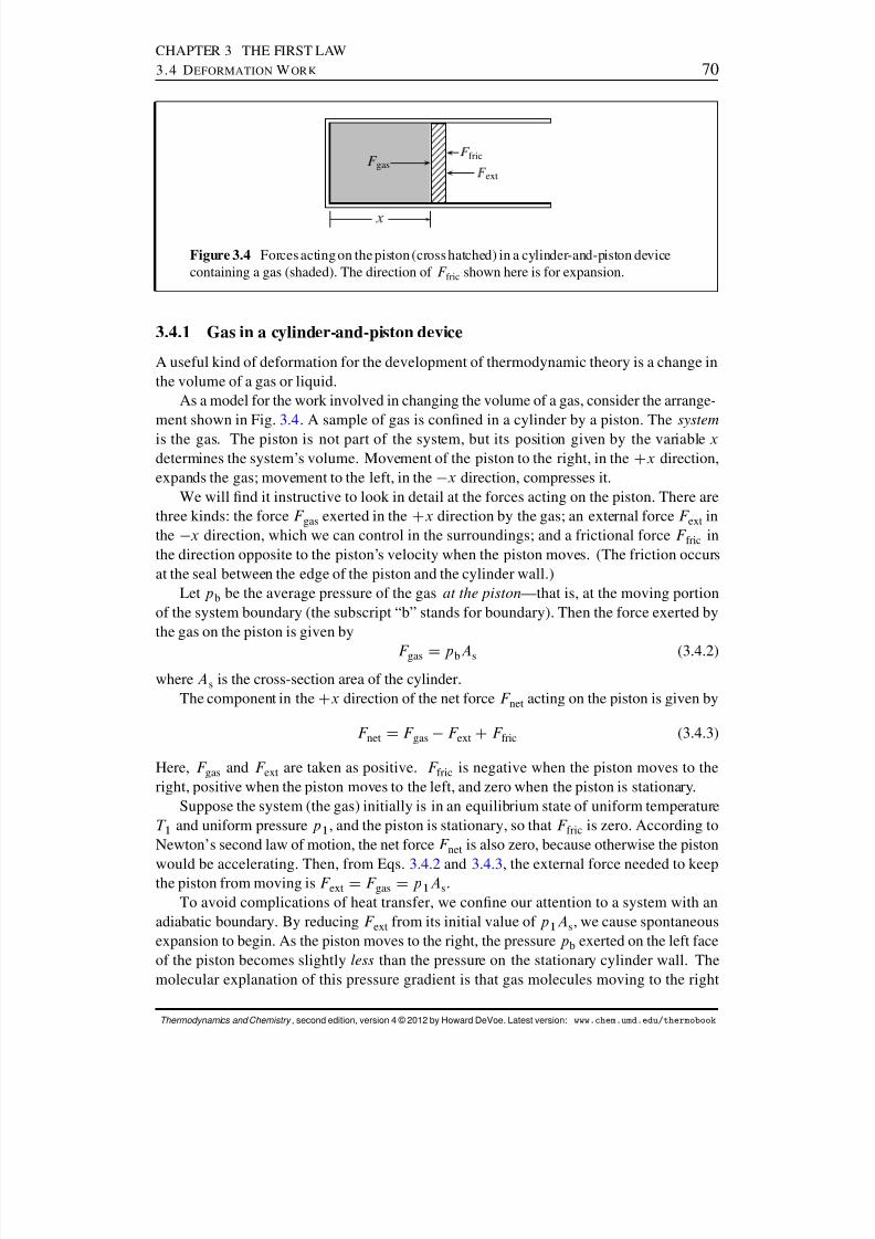
8/12/2019 Howard Devoe Thermodynamic and Chemical
http://slidepdf.com/reader/full/howard-devoe-thermodynamic-and-chemical 70/532
CHAPTER 3 THE FIRST LAW3.4 D EFORMATION W ORK 70
gas fric
ext
Figure 3.4 Forces acting on the piston (cross hatched) in a cylinder-and-piston devicecontaining a gas (shaded). The direction of F fric shown here is for expansion.
3.4.1 Gas in a cylinder-and-piston device
A useful kind of deformation for the development of thermodynamic theory is a change inthe volume of a gas or liquid.
As a model for the work involved in changing the volume of a gas, consider the arrange-ment shown in Fig. 3.4 . A sample of gas is conned in a cylinder by a piston. The systemis the gas. The piston is not part of the system, but its position given by the variable xdetermines the system’s volume. Movement of the piston to the right, in the Cx direction,expands the gas; movement to the left, in the x direction, compresses it.
We will nd it instructive to look in detail at the forces acting on the piston. There arethree kinds: the force F gas exerted in the Cx direction by the gas; an external force F ext inthe x direction, which we can control in the surroundings; and a frictional force F fric inthe direction opposite to the piston’s velocity when the piston moves. (The friction occursat the seal between the edge of the piston and the cylinder wall.)
Let p b be the average pressure of the gas at the piston —that is, at the moving portionof the system boundary (the subscript “b” stands for boundary). Then the force exerted bythe gas on the piston is given by
F gas D p bAs (3.4.2)where A s is the cross-section area of the cylinder.
The component in the Cx direction of the net force F net acting on the piston is given by
F net D F gas F ext CF fric (3.4.3)
Here, F gas and F ext are taken as positive. F fric is negative when the piston moves to theright, positive when the piston moves to the left, and zero when the piston is stationary.
Suppose the system (the gas) initially is in an equilibrium state of uniform temperatureT 1 and uniform pressure p 1 , and the piston is stationary, so that F fric is zero. According toNewton’s second law of motion, the net force F net is also zero, because otherwise the piston
would be accelerating. Then, from Eqs. 3.4.2 and 3.4.3 , the external force needed to keepthe piston from moving is F ext D F gas D p 1 As .To avoid complications of heat transfer, we conne our attention to a system with an
adiabatic boundary. By reducing F ext from its initial value of p 1 As , we cause spontaneousexpansion to begin. As the piston moves to the right, the pressure p b exerted on the left faceof the piston becomes slightly less than the pressure on the stationary cylinder wall. Themolecular explanation of this pressure gradient is that gas molecules moving to the right
Thermodynamics and Chemistry , second edition, version 4 © 2012 by Howard DeVoe. Latest version: www.chem.umd.edu/thermobook

8/12/2019 Howard Devoe Thermodynamic and Chemical
http://slidepdf.com/reader/full/howard-devoe-thermodynamic-and-chemical 71/532
CHAPTER 3 THE FIRST LAW3.4 D EFORMATION W ORK 71
approach the moving piston at lower velocities relative to the piston than if the piston werestationary, so that they collide with the piston less frequently and with a smaller transfer of momentum in each collision. The temperature and pressure within the gas become nonuni-form, and we cannot describe intermediate states of this spontaneous process with singlevalues of T and p . These intermediate states are not equilibrium states.
The more slowly we allow the adiabatic expansion to take place, the more nearly uni-form are the temperature and pressure. In the limit of innite slowness, the gas passesthrough a continuous sequence of equilibrium states of uniform temperature and pressure.
Let p 2 be the pressure in the nal state of the innitely-slow expansion. In this state,F ext is equal to p 2 As. By increasing F ext from this value, we cause spontaneous compres-sion to begin. The gas pressure p b at the piston now becomes slightly greater than at thestationary cylinder wall, because the piston is moving to the left toward the molecules thatare moving to the right. A different pressure gradient develops than during expansion. Thestates approached in the limit as we carry out the compression more and more slowly areequilibrium states, occurring in the reverse sequence of the states for expansion at inniteslowness. The sequence of equilibrium states, taken in either direction, is a reversible pro-cess.
The magnitude of the effect of piston velocity on p b can be estimated with the help of the kinetic-molecular theory of gases. This theory, of course, is not part of classicalmacroscopic thermodynamics.
Consider an elastic collision of a gas molecule of mass m with the left side of thepiston shown in Fig. 3.4. Assume the piston moves at a constant velocity u (positive forexpansion and negative for compression), and let the x component of the molecule’svelocity as it approaches the piston be vx (a positive value). After the collision, the xcomponent of the molecule’s velocity is vx C2u , and the momentum that has beentransferred to the piston is 2m.v x u/ . With the assumption that the x componentof the molecule’s velocity remains unchanged between consecutive collisions with thepiston, the time interval between two collisions is 2l=.v x u/ where l is the internalcylinder length at the time of the earlier collision.
The average force exerted by one molecule on the piston is equal to the momentumtransferred to the piston by a collision, divided by the time interval between collisions.The total pressure exerted by the gas on the piston is found by summing the averageforce over all molecules and dividing by the piston area A s D V =l:
p b D nM
V ˝v2x˛ 2u hvx i Cu 2 (3.4.4)
(The angle brackets denote averages.) The pressure at the stationary wall of the cylin-der is p D .nM=V / ˝v
2x˛. Accordingly, the pressure at the moving piston is given
by9
p b D p 1 2u hvx i
˝v2
x
˛ C
u2
˝v2
x
˛! (3.4.5)
From kinetic-molecular theory, the averages are given by hvx i D .2RT= M/ 1=2 and
˝v2x D RT=M .
Suppose the piston moves at the considerable speed of 10 m s 1 and the gas in thecylinder is nitrogen (N 2 ) at 300 K; then Eq. 3.4.5 predicts the pressure p b exerted on
9An equivalent formula is derived in Ref. [ 9], Eq. 7. A formula that yields similar values of p b appears in Ref.[14].
Thermodynamics and Chemistry , second edition, version 4 © 2012 by Howard DeVoe. Latest version: www.chem.umd.edu/thermobook
8/12/2019 Howard Devoe Thermodynamic and Chemical
http://slidepdf.com/reader/full/howard-devoe-thermodynamic-and-chemical 72/532
CHAPTER 3 THE FIRST LAW3.4 D EFORMATION W ORK 72
the piston by the gas is only about 5% lower than the pressure p at the stationary wallduring expansion, and about 5% higher during compression. At low piston speeds thepercentage difference is proportional to the piston speed, so this example shows thatfor reasonably-slow speeds the difference is quite small and for practical calculationscan usually be ignored.
3.4.2 Expansion work of a gas
We now consider the work involved in expansion and compression of the gas in the cylinder-and-piston device of Fig. 3.4 . This kind of deformation work, for both expansion and com-pression, is called expansion work or pressure-volume work.
Keep in mind that the system is just the gas. The only moving portion of the boundary of this system is at the inner surface of the piston, and this motion is in the Cx or x direction.The x component of the force exerted by the system on the surroundings at this portion of the boundary, F sys
x , is equal to F gas . (The other forces shown in Fig. 3.4 are within thesurroundings.) Applying the differential form of Eq. 3.1.2 , we have ¶w D F gas dx which,with the substitution F gas D p bAs (from Eq. 3.4.2 ), becomes
¶w D p bAs dx (3.4.6)
It will be convenient to change the work coordinate from x to V . The gas volume isgiven by V D A sx so that an innitesimal change d x changes the volume by d V D A s dx .The innitesimal quantity of work for an innitesimal volume change is then given by
¶w D p b dV (3.4.7)(expansion work,
closed system)
and the nite work for a nite volume change, found by integrating from the initial to thenal volume, is
w D Z V 2
V 1p b dV (3.4.8)
(expansion work,closed system)
During expansion (positive d V ), ¶w is negative and the system does work on the surround-ings. During compression (negative d V ), ¶w is positive and the surroundings do work onthe system.
When carrying out dimensional analysis, you will nd it helpful to remember that theproduct of two quantities with dimensions of pressure and volume (such as p b dV ) has
dimensions of energy, and that 1 Pa m3
is equal to 1 J.
The integral on the right side of Eq. 3.4.8 is a line integral (Sec. E.4 on page 481 ). Inorder to evaluate the integral, one must be able to express the integrand p b as a function of the integration variable V along the path of the expansion or compression process.
If the piston motion during expansion or compression is sufciently slow, we can withlittle error assume that the gas has a uniform pressure p throughout, and that the work can
Thermodynamics and Chemistry , second edition, version 4 © 2012 by Howard DeVoe. Latest version: www.chem.umd.edu/thermobook
8/12/2019 Howard Devoe Thermodynamic and Chemical
http://slidepdf.com/reader/full/howard-devoe-thermodynamic-and-chemical 73/532
CHAPTER 3 THE FIRST LAW3.4 D EFORMATION W ORK 73
be calculated as if the process has reached its reversible limit. Under these conditions, Eq.3.4.7 becomes
¶w D p dV (3.4.9)(reversible expansionwork, closed system)
and Eq. 3.4.8 becomes
w D Z V 2
V 1p dV (3.4.10)
(reversible expansionwork, closed system)
The appearance of the symbol p in these equations, instead of p b , implies that the equationsapply only to a process in which the system has at each instant a single uniform pressure.As a general rule, an equation containing the symbol of an intensive property not assigned to a specic phase is valid only if that property is uniform throughout the system , and this
will not be explicitly indicated as a condition of validity.
Some texts state that expansion work in a horizontal cylinder-and-piston device likethat shown in Fig. 3.4 should be calculated from w D R p ext dV , where p ext is apressure in the surroundings that exerts the external force F ext on the piston. However,if the system is the gas the correct general expression is the one given by Eq. 3.4.8 :w D R p b dV . This is because it is the force F gas D p bAs that is exerted by thesystem on the surroundings, whereas the force F ext D p ext As is exerted by one part of the surroundings on another part of the surroundings.
In other words, if the integrals R F gas dx and R F ext dx have different values, it is therst of these two integrals that should be used to evaluate the work: w D R F gas dx .Both integrals are equal if the expansion or compression process is carried out re-versibly . This is because in the limit of innite slowness the piston has neither friction(F fricD0) nor acceleration ( F netD0), and therefore according to Eq. 3.4.3 , F gas and F extare equal throughout the process. Another situation in which the two integrals areequal is when the piston is frictionless and is stationary in the initial and nal states,because then both F fric and R F net dx are zero. (The integral R F net dx can be shown tobe equal to the change in the kinetic energy of the piston, by a derivation similar tothat leading to Eq. G.1.5 on page 489 .) In the general irreversible case, however, theintegrals R F gas dx and R F ext dx are not equal. 10
3.4.3 Expansion work of an isotropic phase
Expansion work does not require a cylinder-and-piston device. Suppose the system is anisotropic uid or solid phase, and various portions of its boundary undergo displacements
in different directions. Figure 3.5 on the next page shows an example of compression ina system of arbitrary shape. The deformation is considered to be carried out slowly, sothat the pressure p of the phase remains uniform. Consider the surface element of theboundary, with area A s; , indicated in the gure by a short thick curve. Because the phase
10 For an informative discussion of this topic see Ref. [ 6]; also comments in Refs. [ 29], [7], [94], [8], and [ 120 ];also Ref. [ 92].
Thermodynamics and Chemistry , second edition, version 4 © 2012 by Howard DeVoe. Latest version: www.chem.umd.edu/thermobook

8/12/2019 Howard Devoe Thermodynamic and Chemical
http://slidepdf.com/reader/full/howard-devoe-thermodynamic-and-chemical 74/532
CHAPTER 3 THE FIRST LAW3.4 D EFORMATION W ORK 74
sur
sys
(a)
d
s
(b)
Figure 3.5 Deformation of an isotropic phase (shaded) conned by a wall.(a) Equal and opposite forces exerted by the surroundings and system at surface ele-ment (thick curve) of the system boundary.(b) Change from initial volume (dotted curve) to a smaller volume.
is isotropic, the force F sys D pA s; exerted by the system pressure on the surroundings
is perpendicular to this surface element; that is, there is no shearing force. The force F sur
exerted by the surroundings on the system is equal in magnitude to F sys and is directedin the opposite direction. The volume change for an innitesimal displacement d s thatreduces the volume is d V D As; ds , so that the work at this surface element (from Eq.3.4.1 with ˛ D0) is ¶w D p dV .
By summing the work over the entire boundary, we nd the total reversible expan-sion work is given by the same expression as for a gas in a piston-and-cylinder device:¶w D p dV . This expression can be used for deformation caused by reversible displace-ments of a conning wall, or for a volume change caused by slow temperature changesat constant pressure. It is valid if the system is an isotropic uid phase in which otherphases are immersed, provided the uid phase contacts all parts of the system boundary.The expression is not necessarily valid for an anisotropic uid or solid, because the angle
˛ appearing in Eq. 3.4.1 might not be zero.
3.4.4 Generalities
The expression ¶w D p dV for reversible expansion work of an isotropic phase is theproduct of a work coefcient, p , and the innitesimal change of a work coordinate, V .In the reversible limit, in which all states along the path of the process are equilibriumstates, the system has two independent variables, e.g., p and V or T and V . The number of independent variables is one greater than the number of work coordinates. This will turn outto be a general rule: The number of independent variables needed to describe equilibriumstates of a closed system is one greater than the number of independent work coordinates for reversible work .
Another way to state the rule is as follows: The number of independent variables is onegreater than the number of different kinds of reversible work, where each kind i is given byan expression of the form ¶w i D Y i dX i .
Thermodynamics and Chemistry , second edition, version 4 © 2012 by Howard DeVoe. Latest version: www.chem.umd.edu/thermobook
8/12/2019 Howard Devoe Thermodynamic and Chemical
http://slidepdf.com/reader/full/howard-devoe-thermodynamic-and-chemical 75/532
CHAPTER 3 THE FIRST LAW3.5 A PPLICATIONS OF E XPANSION W ORK 75
3.5 APPLICATIONS OF EXPANSION WORK
This book uses expansion work as a general term that includes the work of both expansionand compression of an isotropic phase.
3.5.1 The internal energy of an ideal gasThe model of an ideal gas is used in many places in the development of thermodynamics.For examples to follow, the following denition is needed: An ideal gas is a gas
1. whose equation of state is the ideal gas equation, pV D nRT ; and2. whose internal energy in a closed system is a function only of temperature. 11
On the molecular level, a gas with negligible intermolecular interactions fullls both of these requirements. Kinetic-molecular theory predicts that a gas containing noninteractingmolecules obeys the ideal gas equation. If intermolecular forces (the only forces that dependon intermolecular distance) are negligible, the internal energy is simply the sum of theenergies of the individual molecules. These energies are independent of volume but dependon temperature.
The behavior of any real gas approaches ideal-gas behavior when the gas is expandedisothermally. As the molar volume V m becomes large and p becomes small, the averagedistance between molecules becomes large, and intermolecular forces become negligible.
3.5.2 Reversible isothermal expansion of an ideal gas
During reversible expansion or compression, the temperature and pressure remain uniform.If we substitute p D nRT= V from the ideal gas equation into Eq. 3.4.10 and treat n and T as constants, we obtain
w D nRT
Z V 2
V 1
dV V D nRT ln
V 2V
1
(3.5.1)
(reversible isothermalexpansion work, ideal gas)
In these expressions for w the amount n appears as a constant for the process, so it is notnecessary to state as a condition of validity that the system is closed.
3.5.3 Reversible adiabatic expansion of an ideal gas
This section derives temperature-volume and pressure-volume relations when a xed amountof an ideal gas is expanded or compressed without heat.
First we need a relation between internal energy and temperature. Since the value of the internal energy of a xed amount of an ideal gas depends only on its temperature (Sec.
3.5.1 ), an innitesimal change d T will cause a change d U that depends only on T and d T :
dU D f .T / dT (3.5.2)
11 A gas with this second property is sometimes called a “perfect gas.” In Sec. 7.2 it will be shown that if a gashas the rst property, it must also have the second.
Thermodynamics and Chemistry , second edition, version 4 © 2012 by Howard DeVoe. Latest version: www.chem.umd.edu/thermobook

8/12/2019 Howard Devoe Thermodynamic and Chemical
http://slidepdf.com/reader/full/howard-devoe-thermodynamic-and-chemical 76/532
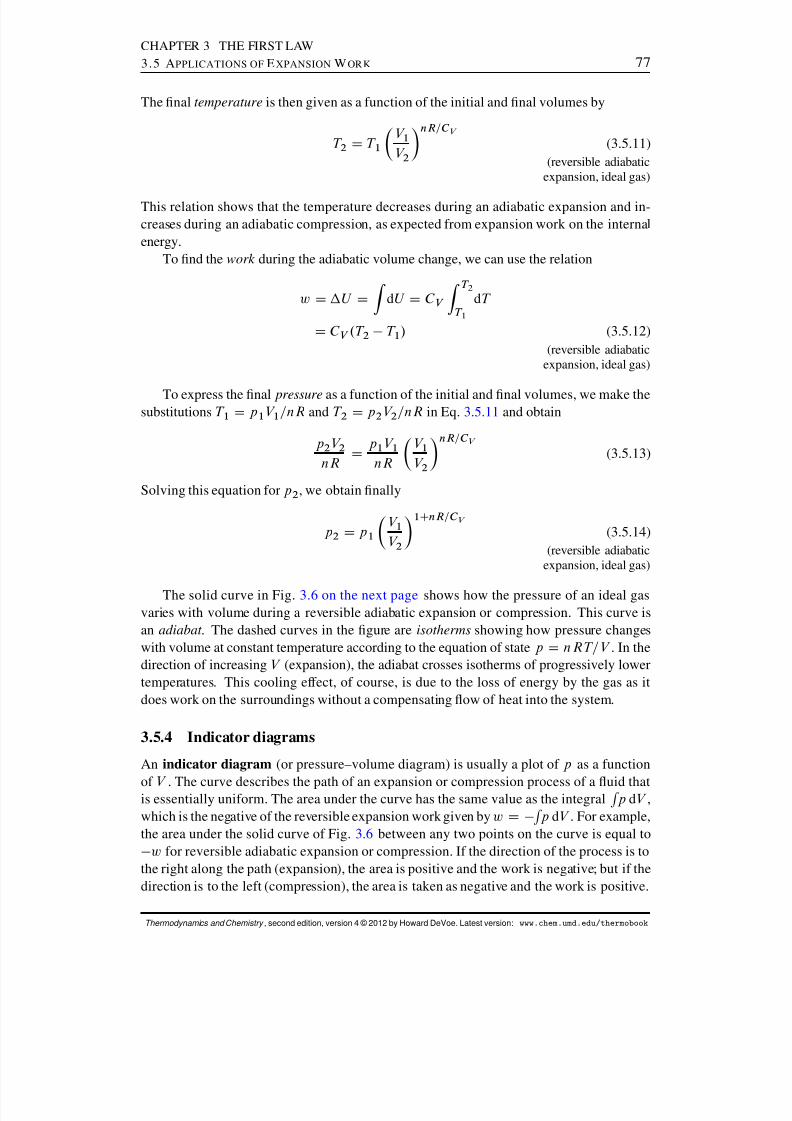
8/12/2019 Howard Devoe Thermodynamic and Chemical
http://slidepdf.com/reader/full/howard-devoe-thermodynamic-and-chemical 77/532
CHAPTER 3 THE FIRST LAW3.5 A PPLICATIONS OF E XPANSION W ORK 77
The nal temperature is then given as a function of the initial and nal volumes by
T 2 D T 1V 1V 2
nR=C V
(3.5.11)(reversible adiabatic
expansion, ideal gas)
This relation shows that the temperature decreases during an adiabatic expansion and in-creases during an adiabatic compression, as expected from expansion work on the internalenergy.
To nd the work during the adiabatic volume change, we can use the relation
w D U DZ dU D C V Z T 2
T 1dT
D C V .T 2 T 1 / (3.5.12)(reversible adiabatic
expansion, ideal gas)
To express the nal pressure as a function of the initial and nal volumes, we make thesubstitutions T 1 D p 1 V 1 =nR and T 2 D p 2 V 2 =nR in Eq. 3.5.11 and obtain
p 2 V 2nR D
p 1 V 1nR
V 1V 2
nR=C V
(3.5.13)
Solving this equation for p 2 , we obtain nally
p 2 D p 1V 1V 2
1C nR=C V
(3.5.14)(reversible adiabatic
expansion, ideal gas)
The solid curve in Fig. 3.6 on the next page shows how the pressure of an ideal gasvaries with volume during a reversible adiabatic expansion or compression. This curve isan adiabat . The dashed curves in the gure are isotherms showing how pressure changeswith volume at constant temperature according to the equation of state p D nRT=V . In thedirection of increasing V (expansion), the adiabat crosses isotherms of progressively lowertemperatures. This cooling effect, of course, is due to the loss of energy by the gas as itdoes work on the surroundings without a compensating ow of heat into the system.
3.5.4 Indicator diagrams
An indicator diagram (or pressure–volume diagram) is usually a plot of p as a function
of V . The curve describes the path of an expansion or compression process of a uid thatis essentially uniform. The area under the curve has the same value as the integral R p dV ,which is the negative of the reversible expansion work given by w D R p dV . For example,the area under the solid curve of Fig. 3.6 between any two points on the curve is equal to
w for reversible adiabatic expansion or compression. If the direction of the process is tothe right along the path (expansion), the area is positive and the work is negative; but if thedirection is to the left (compression), the area is taken as negative and the work is positive.
Thermodynamics and Chemistry , second edition, version 4 © 2012 by Howard DeVoe. Latest version: www.chem.umd.edu/thermobook
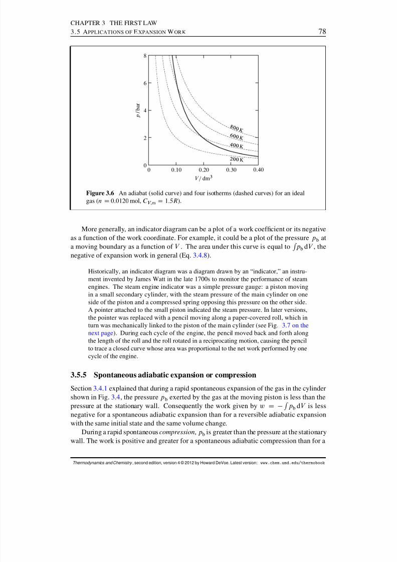
8/12/2019 Howard Devoe Thermodynamic and Chemical
http://slidepdf.com/reader/full/howard-devoe-thermodynamic-and-chemical 78/532
CHAPTER 3 THE FIRST LAW3.5 A PPLICATIONS OF E XPANSION W ORK 78
2 0 0 K
4 0 0 K
6 0 0 K
8 0 0 K
0 0:10 0:20 0:300
2
4
6
8
0:40V =dm 3
p / b
a r
Figure 3.6 An adiabat (solid curve) and four isotherms (dashed curves) for an idealgas (n D 0:0120 mol, C V; m D 1:5R ).
More generally, an indicator diagram can be a plot of a work coefcient or its negativeas a function of the work coordinate. For example, it could be a plot of the pressure p b ata moving boundary as a function of V . The area under this curve is equal to R p b dV , thenegative of expansion work in general (Eq. 3.4.8 ).
Historically, an indicator diagram was a diagram drawn by an “indicator,” an instru-ment invented by James Watt in the late 1700s to monitor the performance of steamengines. The steam engine indicator was a simple pressure gauge: a piston moving
in a small secondary cylinder, with the steam pressure of the main cylinder on oneside of the piston and a compressed spring opposing this pressure on the other side.A pointer attached to the small piston indicated the steam pressure. In later versions,the pointer was replaced with a pencil moving along a paper-covered roll, which inturn was mechanically linked to the piston of the main cylinder (see Fig. 3.7 on thenext page ). During each cycle of the engine, the pencil moved back and forth alongthe length of the roll and the roll rotated in a reciprocating motion, causing the pencilto trace a closed curve whose area was proportional to the net work performed by onecycle of the engine.
3.5.5 Spontaneous adiabatic expansion or compression
Section 3.4.1 explained that during a rapid spontaneous expansion of the gas in the cylindershown in Fig. 3.4 , the pressure p b exerted by the gas at the moving piston is less than thepressure at the stationary wall. Consequently the work given by w D R p b dV is lessnegative for a spontaneous adiabatic expansion than for a reversible adiabatic expansionwith the same initial state and the same volume change.
During a rapid spontaneous compression , p b is greater than the pressure at the stationarywall. The work is positive and greater for a spontaneous adiabatic compression than for a
Thermodynamics and Chemistry , second edition, version 4 © 2012 by Howard DeVoe. Latest version: www.chem.umd.edu/thermobook
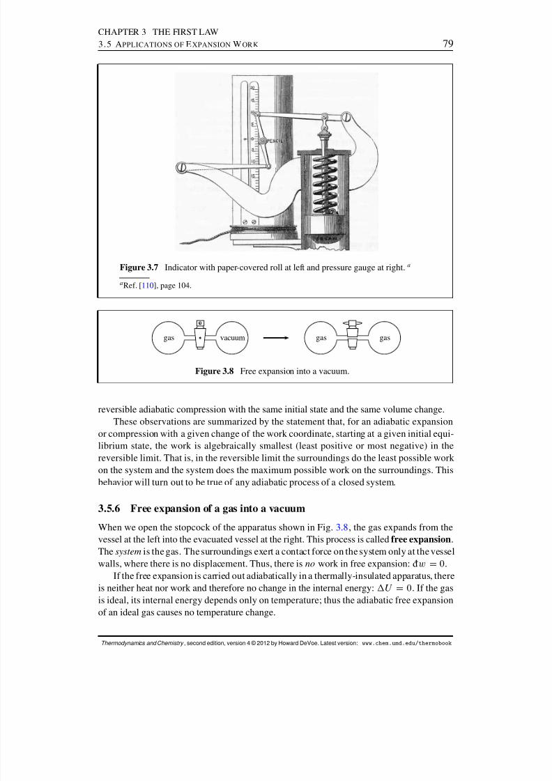
8/12/2019 Howard Devoe Thermodynamic and Chemical
http://slidepdf.com/reader/full/howard-devoe-thermodynamic-and-chemical 79/532
CHAPTER 3 THE FIRST LAW3.5 A PPLICATIONS OF E XPANSION W ORK 79
Figure 3.7 Indicator with paper-covered roll at left and pressure gauge at right. a
a Ref. [ 110 ], page 104.
gas vacuum gas gas
Figure 3.8 Free expansion into a vacuum.
reversible adiabatic compression with the same initial state and the same volume change.These observations are summarized by the statement that, for an adiabatic expansion
or compression with a given change of the work coordinate, starting at a given initial equi-librium state, the work is algebraically smallest (least positive or most negative) in thereversible limit. That is, in the reversible limit the surroundings do the least possible work on the system and the system does the maximum possible work on the surroundings. Thisbehavior will turn out to be true of any adiabatic process of a closed system.
3.5.6 Free expansion of a gas into a vacuum
When we open the stopcock of the apparatus shown in Fig. 3.8 , the gas expands from thevessel at the left into the evacuated vessel at the right. This process is called free expansion .The system is the gas. The surroundings exert a contact force on the system only at the vesselwalls, where there is no displacement. Thus, there is no work in free expansion: ¶w D 0.
If the free expansion is carried out adiabatically in a thermally-insulated apparatus, thereis neither heat nor work and therefore no change in the internal energy: U D 0. If the gasis ideal, its internal energy depends only on temperature; thus the adiabatic free expansionof an ideal gas causes no temperature change.
Thermodynamics and Chemistry , second edition, version 4 © 2012 by Howard DeVoe. Latest version: www.chem.umd.edu/thermobook

8/12/2019 Howard Devoe Thermodynamic and Chemical
http://slidepdf.com/reader/full/howard-devoe-thermodynamic-and-chemical 80/532
CHAPTER 3 THE FIRST LAW3.6 W ORK IN A G RAVITATIONAL F IELD 80
buoy fric
uid
(a)
buoy fric
str
uid
(b)
Figure 3.9 Spherical body (shaded) in a gravitational eld. The arrows indicate thedirections and magnitudes of contact and gravitational forces exerted on the body.(a) The body falls freely through a uid in a vessel.(b) The body is lowered on a string through the uid.
3.6 WORK IN A GRAVITATIONAL FIELD
Figure 3.9 depicts a spherical body, such as a glass marble, immersed in a liquid or gas inthe presence of an external gravitational eld. The vessel is stationary on a lab bench, andthe local reference frame for work is a stationary lab frame. The variable z is the body’selevation above the bottom of the vessel. All displacements are parallel to the vertical z axis.From Eq. 3.1.1 , the work is given by ¶w D F sur
z dz where F surz is the upward component
of the net contact force exerted by the surroundings on the system at the moving portion of the boundary. There is also a downward gravitational force on the body, but as explained inSec. 3.1.1 , this force does not contribute to F sur
z .Consider rst the simple process in Fig. 3.9(a) in which the body falls freely through
the uid. This process is clearly spontaneous. Here are two choices for the denition of thesystem:
The system is the combination of the spherical body and the uid. The system bound-ary is where the uid contacts the air and the vessel walls. Because there is no dis-placement of this boundary, no work is being done on or by the system: ¶w D 0.(We ignore expansion work caused by the small temperature increase.) If the processis adiabatic, the rst law tells us the system’s internal energy remains constant: asthe body loses gravitational potential energy, the system gains an equal quantity of kinetic and thermal energy.
The system is the body; the uid is in the surroundings. The upward componentsof the forces exerted on the body are (1) a gravitational force mg , where m is the
body’s mass and g is the acceleration of free fall; (2) a buoyant force 12 F buoy D V 0g ,where is the uid density and V 0 is the volume of the body; and (3) a frictional dragforce F fric of opposite sign from the velocity v D dz= d t . As mentioned above, thegravitational force is not included in F sur
z . Therefore the gravitational work is given
12 The buoyant force is a consequence of the pressure gradient that exists in the uid in a gravitational eld (seeSec. 8.1.4 ). We ignore this gradient when we treat the uid as a uniform phase.
Thermodynamics and Chemistry , second edition, version 4 © 2012 by Howard DeVoe. Latest version: www.chem.umd.edu/thermobook
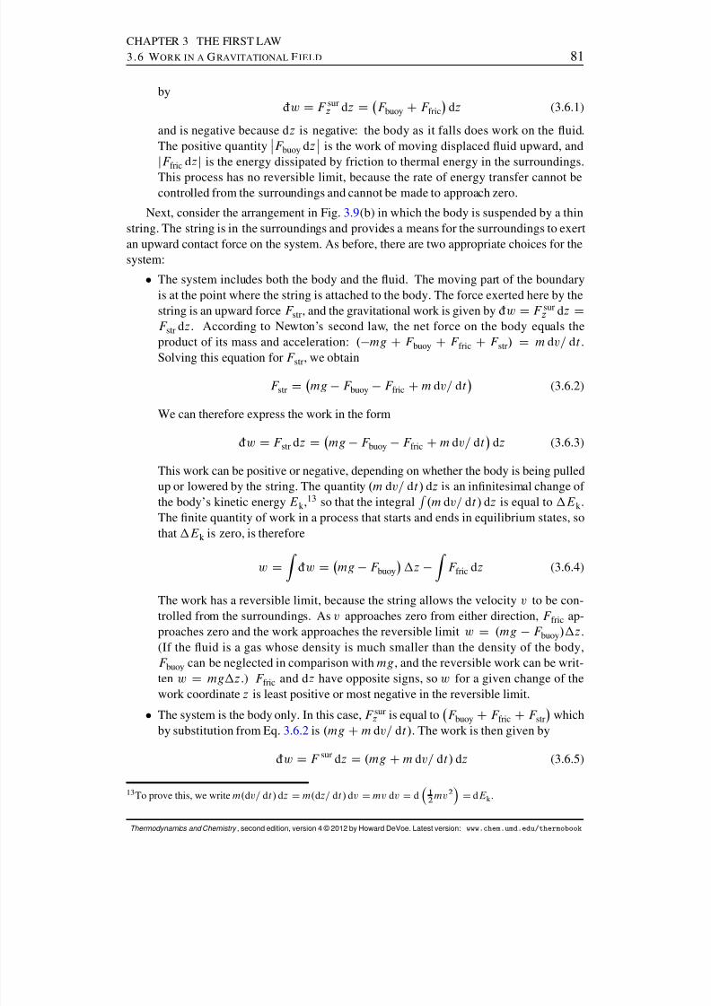
8/12/2019 Howard Devoe Thermodynamic and Chemical
http://slidepdf.com/reader/full/howard-devoe-thermodynamic-and-chemical 81/532
CHAPTER 3 THE FIRST LAW3.6 W ORK IN A G RAVITATIONAL F IELD 81
by¶w D F sur
z dz D F buoy CF fric dz (3.6.1)
and is negative because d z is negative: the body as it falls does work on the uid.The positive quantity
ˇF buoy dz
ˇ is the work of moving displaced uid upward, and
jF fric dz
j is the energy dissipated by friction to thermal energy in the surroundings.
This process has no reversible limit, because the rate of energy transfer cannot becontrolled from the surroundings and cannot be made to approach zero.
Next, consider the arrangement in Fig. 3.9 (b) in which the body is suspended by a thinstring. The string is in the surroundings and provides a means for the surroundings to exertan upward contact force on the system. As before, there are two appropriate choices for thesystem:
The system includes both the body and the uid. The moving part of the boundaryis at the point where the string is attached to the body. The force exerted here by thestring is an upward force F str , and the gravitational work is given by ¶w D F sur
z dz DF str dz . According to Newton’s second law, the net force on the body equals theproduct of its mass and acceleration: . mg
C F buoy
C F fric
C F str /
D m dv= d t .
Solving this equation for F str , we obtain
F str D mg F buoy F fric Cm dv= d t (3.6.2)
We can therefore express the work in the form
¶w D F str dz D mg F buoy F fric Cm dv= d t dz (3.6.3)
This work can be positive or negative, depending on whether the body is being pulledup or lowered by the string. The quantity .m dv= d t / dz is an innitesimal change of the body’s kinetic energy E k ,
13 so that the integral
R .m dv= d t / dz is equal to E k .
The nite quantity of work in a process that starts and ends in equilibrium states, sothat E k is zero, is therefore
w DZ ¶w D mg F buoy z Z F fric dz (3.6.4)
The work has a reversible limit, because the string allows the velocity v to be con-trolled from the surroundings. As v approaches zero from either direction, F fric ap-proaches zero and the work approaches the reversible limit w D .mg F buoy / z .(If the uid is a gas whose density is much smaller than the density of the body,F buoy can be neglected in comparison with mg , and the reversible work can be writ-ten w D mg z .) F fric and d z have opposite signs, so w for a given change of thework coordinate z is least positive or most negative in the reversible limit.
The system is the body only. In this case, F surz is equal to F buoy CF fric CF str which
by substitution from Eq. 3.6.2 is .mg Cm dv= d t / . The work is then given by
¶w D F sur dz D .mg Cm dv= d t / dz (3.6.5)
13 To prove this, we write m. dv= d t / dz D m. dz= d t / dv D mv dv D d 12 mv 2 D dE k .
Thermodynamics and Chemistry , second edition, version 4 © 2012 by Howard DeVoe. Latest version: www.chem.umd.edu/thermobook
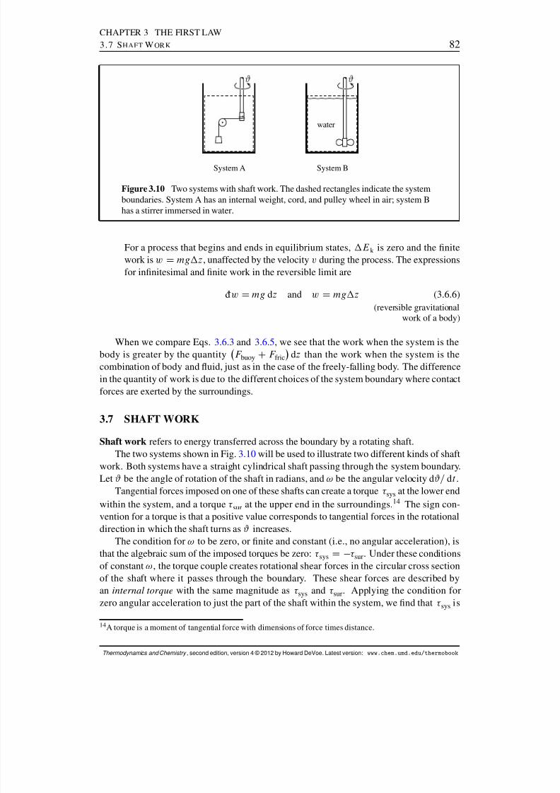
8/12/2019 Howard Devoe Thermodynamic and Chemical
http://slidepdf.com/reader/full/howard-devoe-thermodynamic-and-chemical 82/532
CHAPTER 3 THE FIRST LAW3.7 S HAFT W ORK 82
System A
water
System B
Figure 3.10 Two systems with shaft work. The dashed rectangles indicate the systemboundaries. System A has an internal weight, cord, and pulley wheel in air; system Bhas a stirrer immersed in water.
For a process that begins and ends in equilibrium states, E k is zero and the nitework is w D mg z , unaffected by the velocity v during the process. The expressionsfor innitesimal and nite work in the reversible limit are
¶w D mg dz and w D mg z (3.6.6)(reversible gravitational
work of a body)
When we compare Eqs. 3.6.3 and 3.6.5 , we see that the work when the system is thebody is greater by the quantity F buoy CF fric dz than the work when the system is thecombination of body and uid, just as in the case of the freely-falling body. The differencein the quantity of work is due to the different choices of the system boundary where contactforces are exerted by the surroundings.
3.7 SHAFT WORK
Shaft work refers to energy transferred across the boundary by a rotating shaft.The two systems shown in Fig. 3.10 will be used to illustrate two different kinds of shaft
work. Both systems have a straight cylindrical shaft passing through the system boundary.Let # be the angle of rotation of the shaft in radians, and ! be the angular velocity d #= d t .
Tangential forces imposed on one of these shafts can create a torque sys at the lower endwithin the system, and a torque sur at the upper end in the surroundings. 14 The sign con-vention for a torque is that a positive value corresponds to tangential forces in the rotationaldirection in which the shaft turns as # increases.
The condition for ! to be zero, or nite and constant (i.e., no angular acceleration), is
that the algebraic sum of the imposed torques be zero: sys D sur . Under these conditionsof constant ! , the torque couple creates rotational shear forces in the circular cross sectionof the shaft where it passes through the boundary. These shear forces are described byan internal torque with the same magnitude as sys and sur . Applying the condition forzero angular acceleration to just the part of the shaft within the system, we nd that sys is
14 A torque is a moment of tangential force with dimensions of force times distance.
Thermodynamics and Chemistry , second edition, version 4 © 2012 by Howard DeVoe. Latest version: www.chem.umd.edu/thermobook
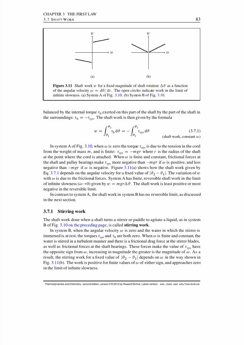
8/12/2019 Howard Devoe Thermodynamic and Chemical
http://slidepdf.com/reader/full/howard-devoe-thermodynamic-and-chemical 83/532
CHAPTER 3 THE FIRST LAW3.7 S HAFT W ORK 83
(a)
(b)
Figure 3.11 Shaft work w for a xed magnitude of shaft rotation # as a functionof the angular velocity ! D d#= d t . The open circles indicate work in the limit of innite slowness. (a) System A of Fig. 3.10. (b) System B of Fig. 3.10.
balanced by the internal torque b exerted on this part of the shaft by the part of the shaft inthe surroundings: b
D sys . The shaft work is then given by the formula
w DZ # 2
# 1
b d# D Z # 2
# 1
sys d# (3.7.1)(shaft work, constant ! )
In system A of Fig. 3.10 , when ! is zero the torque sys is due to the tension in the cordfrom the weight of mass m , and is nite: sys D mgr where r is the radius of the shaftat the point where the cord is attached. When ! is nite and constant, frictional forces atthe shaft and pulley bearings make sys more negative than mgr if ! is positive, and lessnegative than mgr if ! is negative. Figure 3.11 (a) shows how the shaft work given byEq. 3.7.1 depends on the angular velocity for a xed value of j# 2 # 1j. The variation of wwith ! is due to the frictional forces. System A has nite, reversible shaft work in the limitof innite slowness ( ! ! 0) given by w D mgr # . The shaft work is least positive or mostnegative in the reversible limit.
In contrast to system A, the shaft work in system B has no reversible limit, as discussedin the next section.
3.7.1 Stirring work
The shaft work done when a shaft turns a stirrer or paddle to agitate a liquid, as in systemB of Fig. 3.10 on the preceding page , is called stirring work .
In system B, when the angular velocity ! is zero and the water in which the stirrer isimmersed is at rest, the torques sys and b are both zero. When ! is nite and constant, the
water is stirred in a turbulent manner and there is a frictional drag force at the stirrer blades,as well as frictional forces at the shaft bearings. These forces make the value of sys havethe opposite sign from ! , increasing in magnitude the greater is the magnitude of ! . As aresult, the stirring work for a xed value of j# 2 # 1j depends on ! in the way shown inFig. 3.11 (b). The work is positive for nite values of ! of either sign, and approaches zeroin the limit of innite slowness.
Thermodynamics and Chemistry , second edition, version 4 © 2012 by Howard DeVoe. Latest version: www.chem.umd.edu/thermobook
8/12/2019 Howard Devoe Thermodynamic and Chemical
http://slidepdf.com/reader/full/howard-devoe-thermodynamic-and-chemical 84/532
CHAPTER 3 THE FIRST LAW3.7 S HAFT W ORK 84
Stirring work is an example of dissipative work . Dissipative work is work that ispositive for both positive and negative changes of the work coordinate, that vanishes as therate of change of the work coordinate approaches zero, and that therefore cannot be carriedout reversibly. Energy transferred into the system by dissipative work is not recovered aswork done on the surroundings when the work coordinate is reversed. In the case of stirring
work, if the shaft rotates in one direction work is done on the system; if the rotation directionis reversed, still more work is done on the system. The energy transferred to the system bystirring work is converted by friction within the system into the random motion of thermalenergy: the energy is completely dissipated .
Because energy transferred to the system by dissipative work is converted to thermalenergy, we could replace this work with an equal quantity of positive heat and producethe same overall change. The replacement of stirring work with heat was illustrated byexperiment 3 on page 61.
The shaft rotation angle # , which is the work coordinate for stirring work, is a propertyof the system but is not a state function, as we can see by the fact that the state of the systemcan be exactly the same for # D 0 and # D 2 . The work coordinate and work coefcientof work with a reversible limit are always state functions, whereas the work coordinate of any kind of dissipative work is not a state function.
In system B of Fig. 3.10 , there is in addition to the stirring work the possibility of expansion work given by ¶w D p dV . When we take both kinds of work into account,we must treat this system as having two work coordinates: # for stirring work and V forexpansion work. Only the expansion work can be carried out reversibly. The number of independent variables in equilibrium states of this system is two, which we could choose asT and V . Thus, the number of independent variables of the equilibrium states is one greaterthan the number of work coordinates for reversible work, in agreement with the general rulegiven on page 74.
3.7.2 The Joule paddle wheel
A good example of the quantitative measurement of stirring work is the set of experimentsconducted by James Joule in the 1840s to determine the “mechanical equivalent of heat.”In effect, he determined the quantity of dissipative stirring work that could replace the heatneeded for the same temperature increase.
Joule’s apparatus contained the paddle wheel shown in Fig. 3.12 on page 86 . It consistedof eight sets of metal paddle arms attached to a shaft in a water-lled copper vessel. Whenthe shaft rotated, the arms moved through openings in four sets of stationary metal vanesxed inside the vessel, and churned the water. The vanes prevented the water from simplymoving around in a circle. The result was turbulent motion (shearing or viscous ow) in thewater and an increase in the temperature of the entire assembly.
The complete apparatus is depicted in Fig. 3.13 on page 87 . In use, two lead weightssank and caused the paddle wheel to rotate. Joule evaluated the stirring work done on thesystem (the vessel, its contents, and the lid) from the change of the vertical position h of theweights. To a rst approximation, this work is the negative of the change of the weights’potential energy: w D mg h where m is the combined mass of the two weights. Joulemade corrections for the kinetic energy gained by the weights, the friction in the connecting
Thermodynamics and Chemistry , second edition, version 4 © 2012 by Howard DeVoe. Latest version: www.chem.umd.edu/thermobook
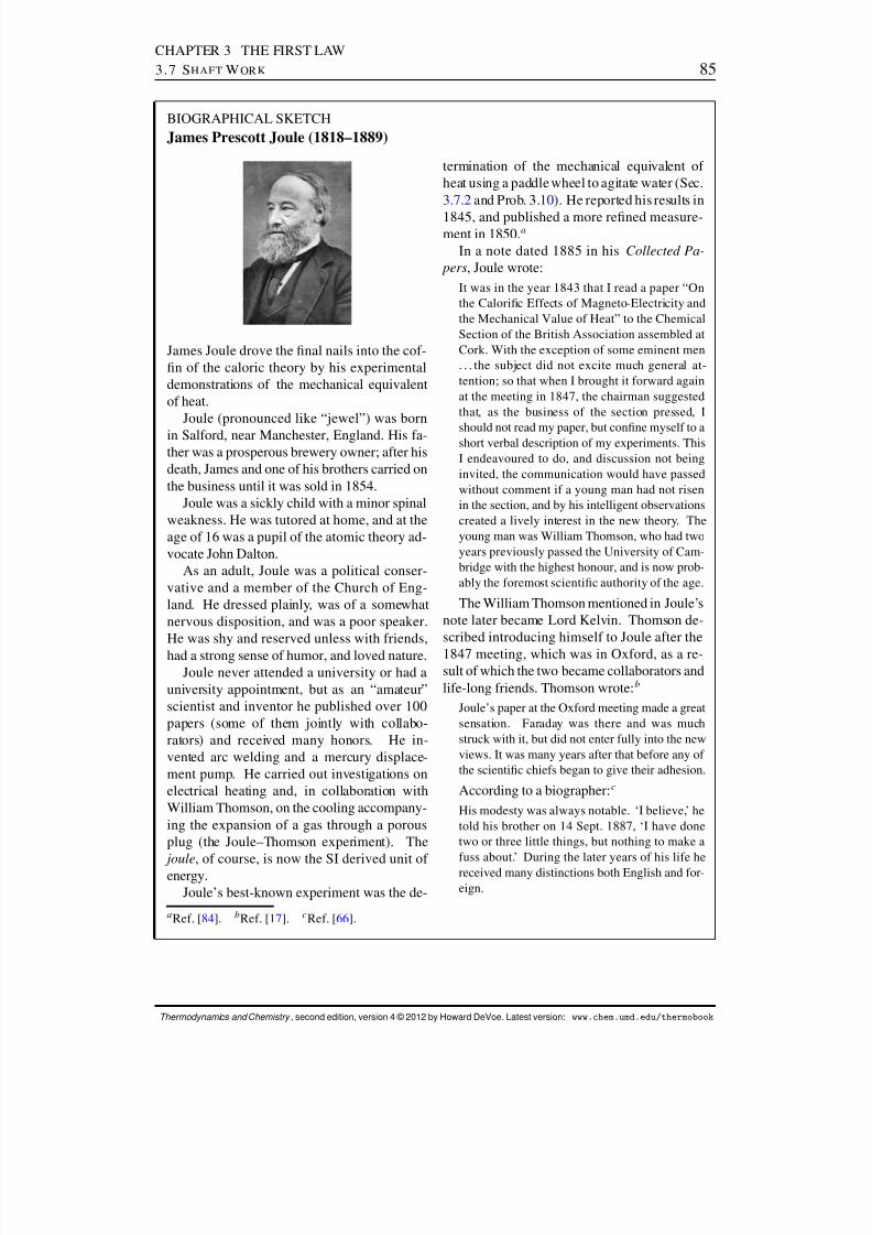
8/12/2019 Howard Devoe Thermodynamic and Chemical
http://slidepdf.com/reader/full/howard-devoe-thermodynamic-and-chemical 85/532
CHAPTER 3 THE FIRST LAW3.7 S HAFT W ORK 85
BIOGRAPHICAL SKETCHJames Prescott Joule (1818–1889)
James Joule drove the nal nails into the cof-n of the caloric theory by his experimentaldemonstrations of the mechanical equivalentof heat.
Joule (pronounced like “jewel”) was bornin Salford, near Manchester, England. His fa-ther was a prosperous brewery owner; after hisdeath, James and one of his brothers carried onthe business until it was sold in 1854.
Joule was a sickly child with a minor spinalweakness. He was tutored at home, and at theage of 16 was a pupil of the atomic theory ad-vocate John Dalton.
As an adult, Joule was a political conser-vative and a member of the Church of Eng-land. He dressed plainly, was of a somewhatnervous disposition, and was a poor speaker.He was shy and reserved unless with friends,had a strong sense of humor, and loved nature.
Joule never attended a university or had auniversity appointment, but as an “amateur”scientist and inventor he published over 100papers (some of them jointly with collabo-rators) and received many honors. He in-vented arc welding and a mercury displace-ment pump. He carried out investigations onelectrical heating and, in collaboration withWilliam Thomson, on the cooling accompany-ing the expansion of a gas through a porousplug (the Joule–Thomson experiment). The
joule , of course, is now the SI derived unit of energy.Joule’s best-known experiment was the de-
termination of the mechanical equivalent of heat using a paddle wheel to agitate water (Sec.3.7.2 and Prob. 3. 10). He reported his results in
1845, and published a more rened measure-ment in 1850. a
In a note dated 1885 in his Collected Pa- pers , Joule wrote:
It was in the year 1843 that I read a paper “Onthe Caloric Effects of Magneto-Electricity andthe Mechanical Value of Heat” to the ChemicalSection of the British Association assembled atCork. With the exception of some eminent men. . . the subject did not excite much general at-tention; so that when I brought it forward againat the meeting in 1847, the chairman suggestedthat, as the business of the section pressed, I
should not read my paper, but conne myself to ashort verbal description of my experiments. ThisI endeavoured to do, and discussion not beinginvited, the communication would have passedwithout comment if a young man had not risenin the section, and by his intelligent observationscreated a lively interest in the new theory. Theyoung man was William Thomson, who had twoyears previously passed the University of Cam-bridge with the highest honour, and is now prob-ably the foremost scientic authority of the age.
The William Thomson mentioned in Joule’snote later became Lord Kelvin. Thomson de-scribed introducing himself to Joule after the1847 meeting, which was in Oxford, as a re-sult of which the two became collaborators andlife-long friends. Thomson wrote: b
Joule’s paper at the Oxford meeting made a greatsensation. Faraday was there and was muchstruck with it, but did not enter fully into the newviews. It was many years after that before any of the scientic chiefs began to give their adhesion.
According to a biographer: c
His modesty was always notable. ‘I believe,’ hetold his brother on 14 Sept. 1887, ‘I have donetwo or three little things, but nothing to make afuss about.’ During the later years of his life hereceived many distinctions both English and for-eign.
a Ref. [ 84]. bRef. [ 17]. cRef. [ 66].
Thermodynamics and Chemistry , second edition, version 4 © 2012 by Howard DeVoe. Latest version: www.chem.umd.edu/thermobook
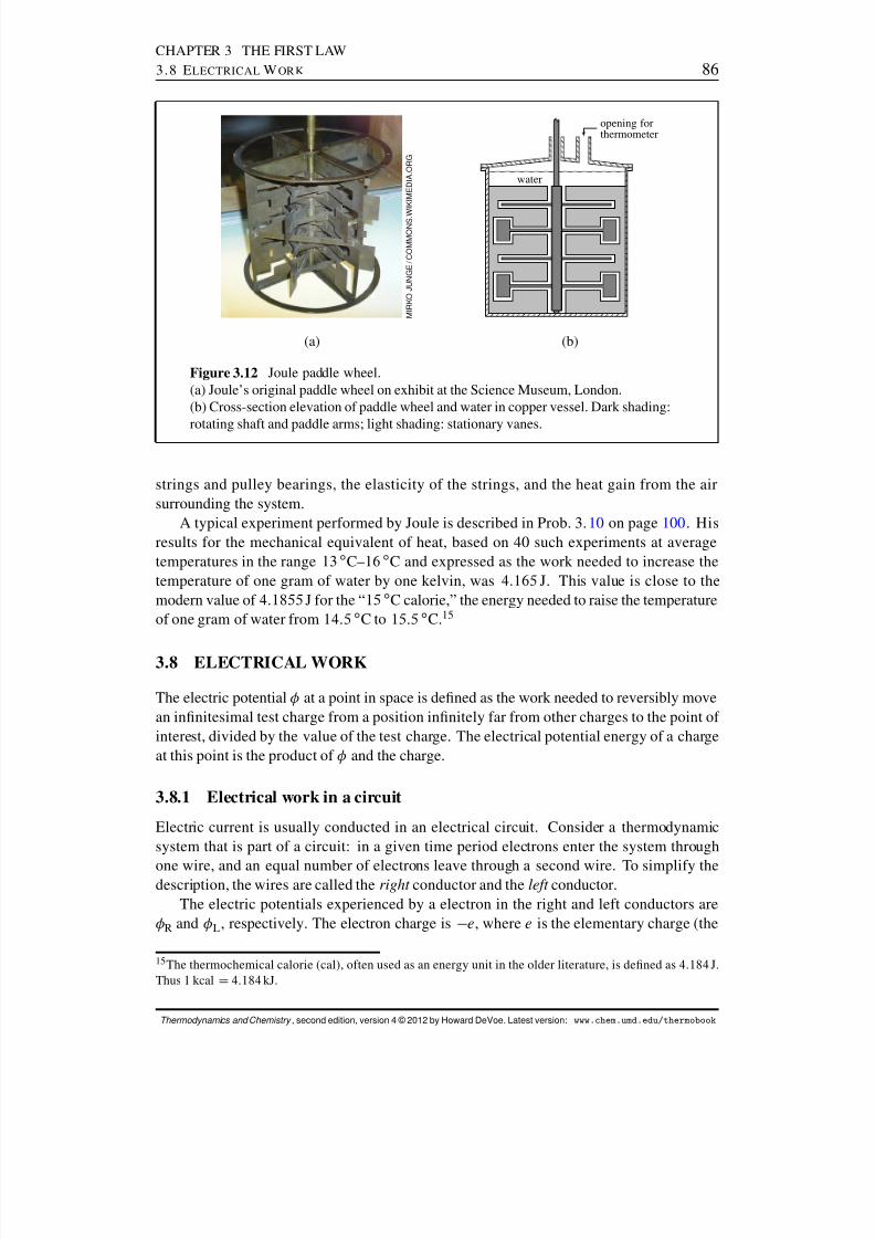
8/12/2019 Howard Devoe Thermodynamic and Chemical
http://slidepdf.com/reader/full/howard-devoe-thermodynamic-and-chemical 86/532
CHAPTER 3 THE FIRST LAW3.8 E LECTRICAL W ORK 86
(a)
M I R K O J U N G E / C O M M O N S . W I K I M E D I A
. O R G
water
opening forthermometer
(b)
Figure 3.12 Joule paddle wheel.(a) Joule’s original paddle wheel on exhibit at the Science Museum, London.(b) Cross-section elevation of paddle wheel and water in copper vessel. Dark shading:rotating shaft and paddle arms; light shading: stationary vanes.
strings and pulley bearings, the elasticity of the strings, and the heat gain from the airsurrounding the system.
A typical experiment performed by Joule is described in Prob. 3. 10 on page 100 . Hisresults for the mechanical equivalent of heat, based on 40 such experiments at averagetemperatures in the range 13 ı C–16 ı C and expressed as the work needed to increase thetemperature of one gram of water by one kelvin, was 4:165 J. This value is close to themodern value of 4:1855 J for the “ 15 ı C calorie,” the energy needed to raise the temperatureof one gram of water from 14:5 ı C to 15:5 ı C.15
3.8 ELECTRICAL WORK
The electric potential at a point in space is dened as the work needed to reversibly movean innitesimal test charge from a position innitely far from other charges to the point of interest, divided by the value of the test charge. The electrical potential energy of a chargeat this point is the product of and the charge.
3.8.1 Electrical work in a circuit
Electric current is usually conducted in an electrical circuit. Consider a thermodynamicsystem that is part of a circuit: in a given time period electrons enter the system through
one wire, and an equal number of electrons leave through a second wire. To simplify thedescription, the wires are called the right conductor and the left conductor.
The electric potentials experienced by a electron in the right and left conductors areR and L , respectively. The electron charge is e , where e is the elementary charge (the
15 The thermochemical calorie (cal), often used as an energy unit in the older literature, is dened as 4:184 J.Thus 1 kcal D 4:184 kJ.
Thermodynamics and Chemistry , second edition, version 4 © 2012 by Howard DeVoe. Latest version: www.chem.umd.edu/thermobook

8/12/2019 Howard Devoe Thermodynamic and Chemical
http://slidepdf.com/reader/full/howard-devoe-thermodynamic-and-chemical 87/532
CHAPTER 3 THE FIRST LAW3.8 E LECTRICAL W ORK 87
cm
A
B
C
D
E
F G
H I
J K
Figure 3.13 Joule’s apparatus for measuring the mechanical equivalent of heat (re-drawn from a gure in Ref. [ 84]).Key: A—paddle wheel and vessel (see Fig. 3.12); B—wood thermal insulator; C—pinused to engage paddle wheel shaft to roller; D—roller; E—crank used to wind up theweights; F, G—strings; H, I—pulley wheels; J, K—weights (round lead disks, viewedhere edge-on).
charge of a proton). Thus the electrical potential energy of an electron is Re in the rightconductor and Le in the left conductor. The difference in the energies of an electron inthe two conductors is the difference in the electrical potential energies.
The sum of charges of a small number of electrons can be treated as an innitesimalnegative charge. During a period of time in which an innitesimal charge ¶Q sys entersthe system at the right conductor and an equal charge leaves at the left conductor, the
contribution of the electric current to the internal energy change is the energy difference. R ¶Q sys L ¶Q sys / D . R L / ¶Q sys . (The notation is ¶Q sys instead of d Q sys , be-cause Q sys is a path function.) This internal energy change is called electrical work . Thusthe general formula for an innitesimal quantity of electrical work when the system is partof an electrical circuit is
¶w el D ¶Q sys (3.8.1)(electrical work in a circuit)
where is the electric potential difference dened by
def
D R L (3.8.2)
Note that in the expression . R ¶Q sys L ¶Q sys / for the energy difference, the termR ¶Q sys does not represent the energy transferred across the boundary at the right
conductor, and L ¶Q sys is not the energy transferred at the left conductor. Theseenergies cannot be measured individually, because they include not just the electricalpotential energy but also the energy of the rest mass of the electrons. The reason we canwrite Eq. 3.8.1 for the electrical work in a circuit is that equal numbers of electrons
Thermodynamics and Chemistry , second edition, version 4 © 2012 by Howard DeVoe. Latest version: www.chem.umd.edu/thermobook
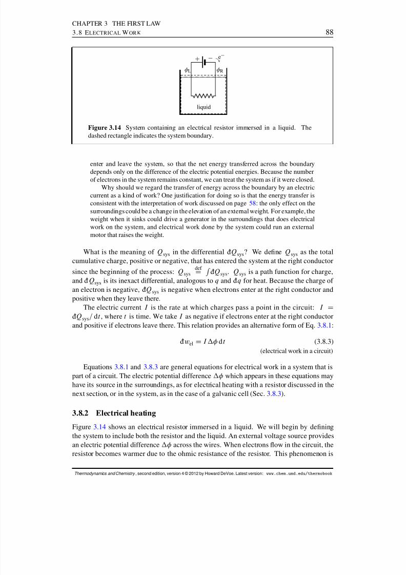
8/12/2019 Howard Devoe Thermodynamic and Chemical
http://slidepdf.com/reader/full/howard-devoe-thermodynamic-and-chemical 88/532
CHAPTER 3 THE FIRST LAW3.8 E LECTRICAL W ORK 88
liquid
L
C
R
e
Figure 3.14 System containing an electrical resistor immersed in a liquid. Thedashed rectangle indicates the system boundary.
enter and leave the system, so that the net energy transferred across the boundarydepends only on the difference of the electric potential energies. Because the numberof electrons in the system remains constant, we can treat the system as if it were closed.
Why should we regard the transfer of energy across the boundary by an electriccurrent as a kind of work? One justication for doing so is that the energy transfer isconsistent with the interpretation of work discussed on page 58: the only effect on thesurroundings could be a change in the elevation of an external weight. For example, theweight when it sinks could drive a generator in the surroundings that does electricalwork on the system, and electrical work done by the system could run an externalmotor that raises the weight.
What is the meaning of Q sys in the differential ¶Q sys ? We dene Q sys as the totalcumulative charge, positive or negative, that has entered the system at the right conductor
since the beginning of the process: Q sysdef
DR ¶Q sys . Q sys is a path function for charge,and ¶Q sys is its inexact differential, analogous to q and ¶q for heat. Because the charge of an electron is negative, ¶Q sys is negative when electrons enter at the right conductor andpositive when they leave there.
The electric current I is the rate at which charges pass a point in the circuit: I D¶Q sys = d t , where t is time. We take I as negative if electrons enter at the right conductorand positive if electrons leave there. This relation provides an alternative form of Eq. 3.8.1 :
¶w el D I d t (3.8.3)(electrical work in a circuit)
Equations 3.8.1 and 3.8.3 are general equations for electrical work in a system that ispart of a circuit. The electric potential difference which appears in these equations mayhave its source in the surroundings, as for electrical heating with a resistor discussed in thenext section, or in the system, as in the case of a galvanic cell (Sec. 3.8.3 ).
3.8.2 Electrical heating
Figure 3.14 shows an electrical resistor immersed in a liquid. We will begin by deningthe system to include both the resistor and the liquid. An external voltage source providesan electric potential difference across the wires. When electrons ow in the circuit, theresistor becomes warmer due to the ohmic resistance of the resistor. This phenomenon is
Thermodynamics and Chemistry , second edition, version 4 © 2012 by Howard DeVoe. Latest version: www.chem.umd.edu/thermobook

8/12/2019 Howard Devoe Thermodynamic and Chemical
http://slidepdf.com/reader/full/howard-devoe-thermodynamic-and-chemical 89/532
CHAPTER 3 THE FIRST LAW3.8 E LECTRICAL W ORK 89
el
Figure 3.15 Work of electrical heating with a xed magnitude of Q sys as a functionof the electric current I D ¶Q sys = d t . The open circle indicates the limit of inniteslowness.
variously called electrical heating, Joule heating, ohmic heating, or resistive heating. Theheating is caused by inelastic collisions of the moving electrons with the stationary atoms of the resistor, a type of friction. If the resistor becomes warmer than the surrounding liquid,
there will be a transfer of thermal energy from the resistor to the liquid.The electrical work performed on this system is given by the expressions ¶w el D ¶Q sys and ¶w el D I d t (Eqs. 3.8.1 and 3.8.3 ). The portion of the electrical circuit
inside the system has an electric resistance given by R el D =I (Ohm’s law). Making thesubstitution D IR el in the work expressions gives two new expressions for electricalwork in this system:
¶w el D IR el ¶Q sys (3.8.4)
¶w el D I 2 R el d t (3.8.5)
The integrated form of Eq. 3.8.4 when I and Rel are constant is wel D IR elQ sys .When the source of the electric potential difference is in the surroundings, as it is here, I and Q
sys have the same sign, so w
el is positive for nite current and zero when there is
no current. Figure 3.15 shows graphically how the work of electrical heating is positivefor both positive and negative changes of the work coordinate Q sys and vanishes as I , therate of change of the work coordinate, approaches zero. These are the characteristics of irreversible dissipative work (page 84). Note the resemblance of Fig. 3.15 to Fig. 3.11 (b)on page 83 for dissipative stirring work—they are the same graphs with different labels.
Suppose we redene the system to be only the liquid. In this case, electric current passesthrough the resistor but not through the system boundary. There is no electrical work, andwe must classify energy transfer between the resistor and the liquid as heat .
3.8.3 Electrical work with a galvanic cell
A galvanic cell is an electrochemical system that, when isolated, exhibits an electric poten-tial difference between the two terminals at the system boundary. The potential differencehas its source at the interfaces between phases within the cell.
Consider the combination of galvanic cell and electrical resistor in Fig. 3.16 on the nextpage , and let the system be the cell. When an electric current passes through the cell ineither direction, a cell reaction takes place in one direction or the other.
Thermodynamics and Chemistry , second edition, version 4 © 2012 by Howard DeVoe. Latest version: www.chem.umd.edu/thermobook
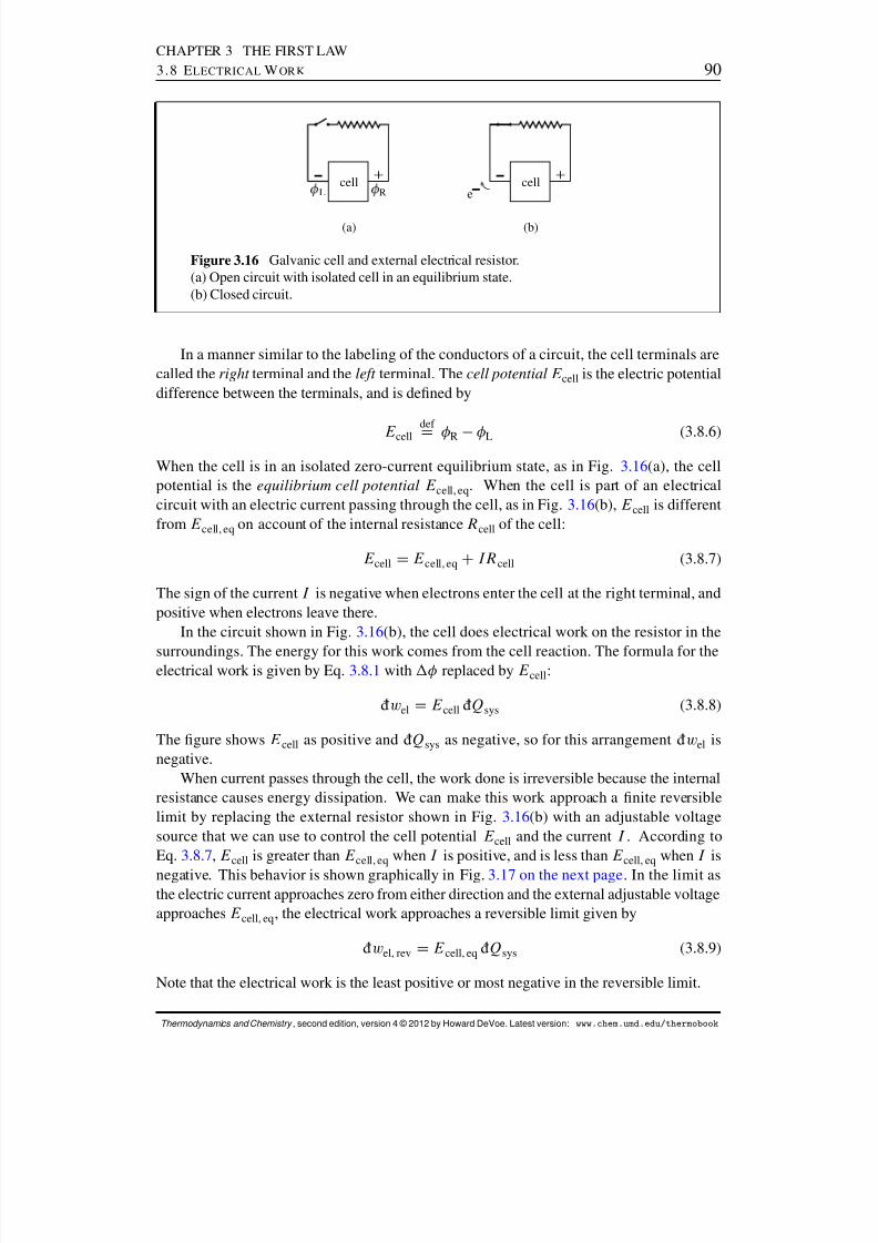
8/12/2019 Howard Devoe Thermodynamic and Chemical
http://slidepdf.com/reader/full/howard-devoe-thermodynamic-and-chemical 90/532
CHAPTER 3 THE FIRST LAW3.8 E LECTRICAL W ORK 90
cell
L
R
(a)
celle
(b)
Figure 3.16 Galvanic cell and external electrical resistor.(a) Open circuit with isolated cell in an equilibrium state.(b) Closed circuit.
In a manner similar to the labeling of the conductors of a circuit, the cell terminals arecalled the right terminal and the left terminal. The cell potential E cell is the electric potentialdifference between the terminals, and is dened by
E celldef
D R L (3.8.6)
When the cell is in an isolated zero-current equilibrium state, as in Fig. 3.16(a), the cellpotential is the equilibrium cell potential E cell, eq . When the cell is part of an electricalcircuit with an electric current passing through the cell, as in Fig. 3.16(b), E cell is differentfrom E cell, eq on account of the internal resistance R cell of the cell:
E cell D E cell, eq CIR cell (3.8.7)
The sign of the current I is negative when electrons enter the cell at the right terminal, andpositive when electrons leave there.
In the circuit shown in Fig. 3.16(b), the cell does electrical work on the resistor in the
surroundings. The energy for this work comes from the cell reaction. The formula for theelectrical work is given by Eq. 3.8.1 with replaced by E cell :
¶w el D E cell ¶Q sys (3.8.8)
The gure shows E cell as positive and ¶Q sys as negative, so for this arrangement ¶w el isnegative.
When current passes through the cell, the work done is irreversible because the internalresistance causes energy dissipation. We can make this work approach a nite reversiblelimit by replacing the external resistor shown in Fig. 3.16(b) with an adjustable voltagesource that we can use to control the cell potential E cell and the current I . According toEq. 3.8.7 , E cell is greater than E cell, eq when I is positive, and is less than E cell, eq when I isnegative. This behavior is shown graphically in Fig. 3.17 on the next page . In the limit asthe electric current approaches zero from either direction and the external adjustable voltageapproaches E cell, eq , the electrical work approaches a reversible limit given by
¶w el, rev D E cell, eq ¶Q sys (3.8.9)
Note that the electrical work is the least positive or most negative in the reversible limit.
Thermodynamics and Chemistry , second edition, version 4 © 2012 by Howard DeVoe. Latest version: www.chem.umd.edu/thermobook

8/12/2019 Howard Devoe Thermodynamic and Chemical
http://slidepdf.com/reader/full/howard-devoe-thermodynamic-and-chemical 91/532
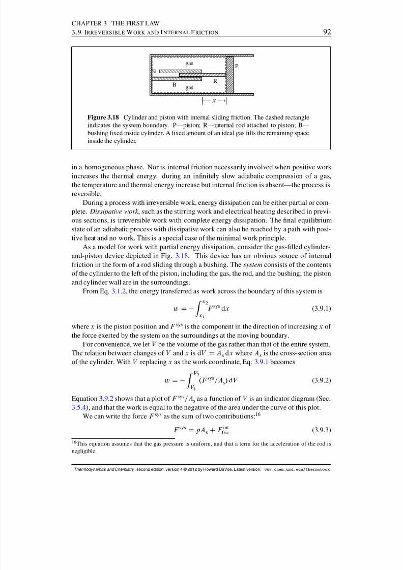
8/12/2019 Howard Devoe Thermodynamic and Chemical
http://slidepdf.com/reader/full/howard-devoe-thermodynamic-and-chemical 92/532
CHAPTER 3 THE FIRST LAW3.9 I RREVERSIBLE W ORK AND INTERNAL F RICTION 92
gas
gasB R
P
Figure 3.18 Cylinder and piston with internal sliding friction. The dashed rectangleindicates the system boundary. P—piston; R—internal rod attached to piston; B—bushing xed inside cylinder. A xed amount of an ideal gas lls the remaining spaceinside the cylinder.
in a homogeneous phase. Nor is internal friction necessarily involved when positive work increases the thermal energy: during an innitely slow adiabatic compression of a gas,the temperature and thermal energy increase but internal friction is absent—the process isreversible.
During a process with irreversible work, energy dissipation can be either partial or com-plete. Dissipative work , such as the stirring work and electrical heating described in previ-ous sections, is irreversible work with complete energy dissipation. The nal equilibriumstate of an adiabatic process with dissipative work can also be reached by a path with posi-tive heat and no work. This is a special case of the minimal work principle.
As a model for work with partial energy dissipation, consider the gas-lled cylinder-and-piston device depicted in Fig. 3.18 . This device has an obvious source of internalfriction in the form of a rod sliding through a bushing. The system consists of the contentsof the cylinder to the left of the piston, including the gas, the rod, and the bushing; the pistonand cylinder wall are in the surroundings.
From Eq. 3.1.2 , the energy transferred as work across the boundary of this system is
w D Z x2
x 1
F sys dx (3.9.1)
where x is the piston position and F sys is the component in the direction of increasing x of the force exerted by the system on the surroundings at the moving boundary.
For convenience, we let V be the volume of the gas rather than that of the entire system.The relation between changes of V and x is dV D A s dx where A s is the cross-section areaof the cylinder. With V replacing x as the work coordinate, Eq. 3.9.1 becomes
w D Z V 2
V 1.F sys =As/ dV (3.9.2)
Equation 3.9.2 shows that a plot of F sys
=As as a function of V is an indicator diagram (Sec.3.5.4 ), and that the work is equal to the negative of the area under the curve of this plot.
We can write the force F sys as the sum of two contributions: 16
F sys D pA s CF intfric (3.9.3)
16 This equation assumes that the gas pressure is uniform, and that a term for the acceleration of the rod isnegligible.
Thermodynamics and Chemistry , second edition, version 4 © 2012 by Howard DeVoe. Latest version: www.chem.umd.edu/thermobook

8/12/2019 Howard Devoe Thermodynamic and Chemical
http://slidepdf.com/reader/full/howard-devoe-thermodynamic-and-chemical 93/532
CHAPTER 3 THE FIRST LAW3.9 I RREVERSIBLE W ORK AND INTERNAL F RICTION 93
Here p is the gas pressure, and F intfric is the force on the rod due to internal friction with sign
opposite to that of the piston velocity d x=d t . Substitution of this expression for F sys in Eq.3.9.2 gives
w D Z V 2
V 1p dV Z
V 2
V 1.F int
fric =As/ dV (3.9.4)
The rst term on the right is the work of expanding or compressing the gas. The second termis the frictional work: w fric D R .F int
fric =As/ dV . w fric is positive or zero, and represents theenergy dissipated within the system by internal sliding friction.
Consider the situation when the piston moves very slowly in one direction or the other.In the limit of innite slowness 17 F int
fric and w fric vanish, and the process is reversible withexpansion work given by w D R p dV .
The situation is different when the piston moves at an appreciable nite rate. The fric-tional work wfric is then positive. As a result, the irreversible work of expansion is lessnegative than the reversible work for the same volume increase, and the irreversible work of compression is more positive than the reversible work for the same volume decrease. Theseeffects of piston velocity on the work are consistent with the minimal work principle.
The piston velocity, besides affecting the frictional force on the rod, has an effecton the force exerted by the gas on the piston as described in Sec. 3.4.1 . At largenite velocities, this latter effect tends to further decrease F sys during expansion andincrease it during compression, and so is an additional contribution to internal friction.If turbulent ow is present within the system, that would also be a contribution.
Figure 3.19 on the next page shows indicator diagrams for adiabatic expansion andcompression with internal friction. The solid curves are for irreversible processes at niterates, and the dashed curves are for reversible processes with the same initial states as theirreversible processes. The areas under the curves conrm that the work for expansion is lessnegative along the irreversible path than along the reversible path, and that for compression
the work is more positive along the irreversible path than along the reversible path.Because of these differences in work, the nal states of the irreversible processes havegreater internal energies and higher temperatures and pressures than the nal states of thereversible processes with the same volume change, as can be seen from the positions onthe indicator diagrams of the points for the nal equilibrium states. The overall changeof state during the irreversible expansion or compression is the same for a path in whichthe reversible adiabatic volume change is followed by positive heat at constant volume.Since U must be the same for both paths, the heat has the same value as the excess work wex D wirr wrev . The excess work and frictional work are not equal, because the thermalenergy released by frictional work increases the gas pressure, making wex less than wfric forexpansion and greater than wfric for compression. There seems to be no general method bywhich the energy dissipated by internal friction can be evaluated, and it would be even moredifcult for an irreversible process with both work and heat.
Figure 3.20 on the next page shows the effect of the rate of change of the volume on theadiabatic work for a xed magnitude of the volume change. Note that the work of expansionand the work of compression have opposite signs, and that it is only in the reversible limit
17 The contact between the rod and bushing is assumed to be lubricated to allow the piston to move at velocitiesinnitesimally close to zero.
Thermodynamics and Chemistry , second edition, version 4 © 2012 by Howard DeVoe. Latest version: www.chem.umd.edu/thermobook

8/12/2019 Howard Devoe Thermodynamic and Chemical
http://slidepdf.com/reader/full/howard-devoe-thermodynamic-and-chemical 94/532
CHAPTER 3 THE FIRST LAW3.9 I RREVERSIBLE W ORK AND INTERNAL F RICTION 94
0 0:10 0:20 0:300
2
4
6
8
V =dm 3
. F s y s = A
s / / b
a r
(a)
0 0:10 0:20 0:300
2
4
6
8
V =dm 3
. F s y s = A
s / / b
a r
(b)
Figure 3.19 Indicator diagrams for the system of Fig. 3.18.Solid curves: F sys =As for irreversible adiabatic volume changes at nite rates in thedirections indicated by the arrows.Dashed curves: F sys =As D p along a reversible adiabat.Open circles: initial and nal equilibrium states.(a) Adiabatic expansion.(b) Adiabatic compression.
d d
compression
expansion
Figure 3.20 Adiabatic expansion work with internal friction for a xed magnitude of V , as a function of the average rate of volume change. The open circles indicate thereversible limits.
that they have the same magnitude . The gure resembles Fig. 3.17 for electrical work of a galvanic cell with the horizontal axis reversed, and is typical of irreversible work withpartial energy dissipation.
Thermodynamics and Chemistry , second edition, version 4 © 2012 by Howard DeVoe. Latest version: www.chem.umd.edu/thermobook

8/12/2019 Howard Devoe Thermodynamic and Chemical
http://slidepdf.com/reader/full/howard-devoe-thermodynamic-and-chemical 95/532
CHAPTER 3 THE FIRST LAW3.10 R EVERSIBLE AND IRREVERSIBLE P ROCESSES : GENERALITIES 95
3.10 REVERSIBLE AND IRREVERSIBLE PROCESSES:GENERALITIES
This section summarizes some general characteristics of processes in closed systems. Someof these statements will be needed to develop aspects of the second law in Chap. 4.
Innitesimal quantities of work during a process are calculated from an expression of the form ¶w DPi Y i dX i , where X i is the work coordinate of kind of work i andY i is the conjugate work coefcient.
The work coefcients and work coordinates of reversible work are state functions.
Energy transferred across the boundary by work in a reversible process is fully recov-ered as work of the opposite sign in the reverse reversible process. It follows fromthe rst law that heat is also fully recovered in the reverse process.
When work occurs irreversibly at a nite rate, there is partial or complete dissipationof energy. The dissipation consists of an increase of thermal energy within the systemdue to frictional effects.
Dissipative work is positive work with complete energy dissipation. In this type of work, the work coefcient vanishes in the limit of innite slowness, and the work coordinate is not a state function. Examples are stirring work (Sec. 3.7.1 ) and thework of electrical heating (Sec. 3.8.2 ).
If a process is carried out adiabatically, the work for a given initial equilibrium stateand a given change in the work coordinate is least positive or most negative in thereversible limit. Since dissipative work is positive and vanishes in the limit of inniteslowness, dissipative work can be thought of as a special case of the same principle.The way in which work depends on the rate of change of the work coordinate isshown graphically for dissipative work by Figs. 3.11 (b) and 3.15 , and for work withpartial energy dissipation by Figs. 3.11 (a), 3.17 , and 3.20 .
The number of independent variables needed to describe equilibrium states of aclosed system is one greater than the number of independent work coordinates forreversible work. 18 Thus, we could choose the independent variables to be each of thework coordinates and in addition either the temperature or the internal energy. 19 Thenumber of independent variables needed to describe a nonequilibrium state is greater(often much greater) than this.
Table 3.1 on the next page lists general formulas for various kinds of work, includingthose that were described in detail in Secs. 3.4–3.8 .
18 If the system has internal adiabatic partitions that allow different phases to have different temperatures inequilibrium states, then the number of independent variables is equal to the number of work coordinates plusthe number of independent temperatures.19 There may be exceptions to this statement in special cases. For example, along the triple line of a puresubstance the values of V and T , or of V and U , are not sufcient to determine the amounts in each of the threepossible phases.
Thermodynamics and Chemistry , second edition, version 4 © 2012 by Howard DeVoe. Latest version: www.chem.umd.edu/thermobook
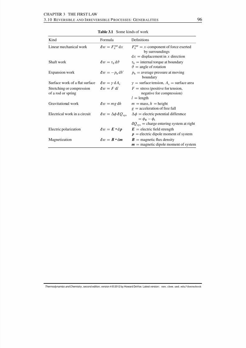
8/12/2019 Howard Devoe Thermodynamic and Chemical
http://slidepdf.com/reader/full/howard-devoe-thermodynamic-and-chemical 96/532
CHAPTER 3 THE FIRST LAW3.10 R EVERSIBLE AND IRREVERSIBLE P ROCESSES : GENERALITIES 96
Table 3.1 Some kinds of work
Kind Formula Denitions
Linear mechanical work ¶w D F surx dx F sur
x D x -component of force exertedby surroundings
dx
Ddisplacement in x direction
Shaft work ¶w D b d# b Dinternal torque at boundary# Dangle of rotation
Expansion work ¶w D p b dV pb Daverage pressure at movingboundary
Surface work of a at surface ¶w D dAs Dsurface tension, A s Dsurface areaStretching or compression ¶w D F dl F Dstress (positive for tension,of a rod or spring negative for compression)
l DlengthGravitational work ¶w D mg dh m Dmass, h Dheight
g Dacceleration of free fallElectrical work in a circuit ¶w D ¶Q sys Delectric potential difference
D R L
¶Q sys Dcharge entering system at rightElectric polarization ¶w DE dp E Delectric eld strength
p Delectric dipole moment of systemMagnetization ¶w DB dm B Dmagnetic ux density
m Dmagnetic dipole moment of system
Thermodynamics and Chemistry , second edition, version 4 © 2012 by Howard DeVoe. Latest version: www.chem.umd.edu/thermobook
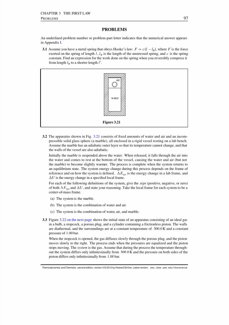
8/12/2019 Howard Devoe Thermodynamic and Chemical
http://slidepdf.com/reader/full/howard-devoe-thermodynamic-and-chemical 97/532
CHAPTER 3 THE FIRST LAWPROBLEMS 97
PROBLEMS
An underlined problem number or problem-part letter indicates that the numerical answer appearsin Appendix I.
3.1 Assume you have a metal spring that obeys Hooke’s law: F D c .l l0 / , where F is the forceexerted on the spring of length l , l0 is the length of the unstressed spring, and c is the springconstant. Find an expression for the work done on the spring when you reversibly compress itfrom length l0 to a shorter length l 0.
water
air
Figure 3.21
3.2 The apparatus shown in Fig. 3.21 consists of xed amounts of water and air and an incom-pressible solid glass sphere (a marble), all enclosed in a rigid vessel resting on a lab bench.Assume the marble has an adiabatic outer layer so that its temperature cannot change, and thatthe walls of the vessel are also adiabatic.
Initially the marble is suspended above the water. When released, it falls through the air intothe water and comes to rest at the bottom of the vessel, causing the water and air (but notthe marble) to become slightly warmer. The process is complete when the system returns toan equilibrium state. The system energy change during this process depends on the frame of reference and on how the system is dened. E sys is the energy change in a lab frame, andU is the energy change in a specied local frame.
For each of the following denitions of the system, give the sign (positive, negative, or zero)of both E sys and U , and state your reasoning. Take the local frame for each system to be acenter-of-mass frame.
(a) The system is the marble.
(b) The system is the combination of water and air.
(c) The system is the combination of water, air, and marble.
3.3 Figure 3.22 on the next page shows the initial state of an apparatus consisting of an ideal gasin a bulb, a stopcock, a porous plug, and a cylinder containing a frictionless piston. The wallsare diathermal, and the surroundings are at a constant temperature of 300:0 K and a constantpressure of 1:00 bar.
When the stopcock is opened, the gas diffuses slowly through the porous plug, and the pistonmoves slowly to the right. The process ends when the pressures are equalized and the pistonstops moving. The system is the gas. Assume that during the process the temperature through-out the system differs only innitesimally from 300:0 K and the pressure on both sides of thepiston differs only innitesimally from 1:00 bar.
Thermodynamics and Chemistry , second edition, version 4 © 2012 by Howard DeVoe. Latest version: www.chem.umd.edu/thermobook
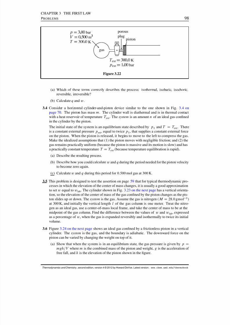
8/12/2019 Howard Devoe Thermodynamic and Chemical
http://slidepdf.com/reader/full/howard-devoe-thermodynamic-and-chemical 98/532
CHAPTER 3 THE FIRST LAWPROBLEMS 98
gas
ext K ext bar
bar m
K
porousplug
piston
Figure 3.22
(a) Which of these terms correctly describes the process: isothermal, isobaric, isochoric,reversible, irreversible?
(b) Calculate q and w .
3.4 Consider a horizontal cylinder-and-piston device similar to the one shown in Fig. 3.4 on
page 70 . The piston has mass m . The cylinder wall is diathermal and is in thermal contactwith a heat reservoir of temperature T ext . The system is an amount n of an ideal gas connedin the cylinder by the piston.
The initial state of the system is an equilibrium state described by p 1 and T D T ext . Thereis a constant external pressure p ext , equal to twice p 1 , that supplies a constant external forceon the piston. When the piston is released, it begins to move to the left to compress the gas.Make the idealized assumptions that (1) the piston moves with negligible friction; and (2) thegas remains practically uniform (because the piston is massive and its motion is slow) and hasa practically constant temperature T D T ext (because temperature equilibration is rapid).
(a) Describe the resulting process.
(b) Describe how you could calculate w and q during the period needed for the piston velocityto become zero again.
(c) Calculate w and q during this period for 0:500 mol gas at 300 K.
3.5 This problem is designed to test the assertion on page 59 that for typical thermodynamic pro-cesses in which the elevation of the center of mass changes, it is usually a good approximationto set w equal to w lab . The cylinder shown in Fig. 3.23 on the next page has a vertical orienta-tion, so the elevation of the center of mass of the gas conned by the piston changes as the pis-ton slides up or down. The system is the gas. Assume the gas is nitrogen ( M D 28:0 gmol 1 )at 300 K, and initially the vertical length l of the gas column is one meter. Treat the nitro-gen as an ideal gas, use a center-of-mass local frame, and take the center of mass to be at themidpoint of the gas column. Find the difference between the values of w and w lab , expressedas a percentage of w , when the gas is expanded reversibly and isothermally to twice its initialvolume.
3.6 Figure 3.24 on the next page shows an ideal gas conned by a frictionless piston in a verticalcylinder. The system is the gas, and the boundary is adiabatic. The downward force on thepiston can be varied by changing the weight on top of it.
(a) Show that when the system is in an equilibrium state, the gas pressure is given by p Dmgh=V where m is the combined mass of the piston and weight, g is the acceleration of free fall, and h is the elevation of the piston shown in the gure.
Thermodynamics and Chemistry , second edition, version 4 © 2012 by Howard DeVoe. Latest version: www.chem.umd.edu/thermobook

8/12/2019 Howard Devoe Thermodynamic and Chemical
http://slidepdf.com/reader/full/howard-devoe-thermodynamic-and-chemical 99/532
CHAPTER 3 THE FIRST LAWPROBLEMS 99
gas l
Figure 3.23
weightvacuum
idealgas
h
Figure 3.24
(b) Initially the combined mass of the piston and weight is m1 , the piston is at height h1 , andthe system is in an equilibrium state with conditions p 1 and V 1 . The initial temperatureis T 1 D p 1 V 1 =nR . Suppose that an additional weight is suddenly placed on the piston,so that m increases from m1 to m2 , causing the piston to sink and the gas to be com-pressed adiabatically and spontaneously. Pressure gradients in the gas, a form of friction,eventually cause the piston to come to rest at a nal position h 2 . Find the nal volume,V 2 , as a function of p 1 , p 2 , V 1 , and C V . (Assume that the heat capacity of the gas, C V ,is independent of temperature.) Hint: The potential energy of the surroundings changesby m2 g h ; since the kinetic energy of the piston and weights is zero at the beginningand end of the process, and the boundary is adiabatic, the internal energy of the gas mustchange by m2 g h D m2 g V=A s D p 2 V .
(c) It might seem that by making the weight placed on the piston sufciently large, V 2 couldbe made as close to zero as desired. Actually, however, this is not the case. Find ex-pressions for V 2 and T 2 in the limit as m2 approaches innity, and evaluate V 2 =V 1 in thislimit if the heat capacity is C V D .3=2/nR (the value for an ideal monatomic gas at roomtemperature).
3.7 The solid curve in Fig. 3.6 on page 78 shows the path of a reversible adiabatic expansion orcompression of a xed amount of an ideal gas. Information about the gas is given in the gure
Thermodynamics and Chemistry , second edition, version 4 © 2012 by Howard DeVoe. Latest version: www.chem.umd.edu/thermobook

8/12/2019 Howard Devoe Thermodynamic and Chemical
http://slidepdf.com/reader/full/howard-devoe-thermodynamic-and-chemical 100/532
CHAPTER 3 THE FIRST LAWPROBLEMS 100
caption. For compression along this path, starting at V D 0:3000 dm 3 and T D 300:0 K andending at V D 0:1000 dm 3 , nd the nal temperature to 0:1 K and the work.
gas vacuum
ext K
bar m
K
m
Figure 3.25
3.8 Figure 3.25 shows the initial state of an apparatus containing an ideal gas. When the stopcock is opened, gas passes into the evacuated vessel. The system is the gas. Find q , w, and U under the following conditions.
(a) The vessels have adiabatic walls.
(b) The vessels have diathermal walls in thermal contact with a water bath maintained at300: K, and the nal temperature in both vessels is T D 300: K.
3.9 Consider a reversible process in which the shaft of system A in Fig. 3.10 makes one revolutionin the direction of increasing # . Show that the gravitational work of the weight is the same asthe shaft work given by w D mgr # .
Table 3.2 Data for Problem 3. 10. The values are from Joule’s 1850 paper a
and have been converted to SI units.
Properties of the paddle wheel apparatus:combined mass of the two lead weights. . . . . . . . . . . . . . . . 26:3182 kgmass of water in vessel . . . . . . . . . . . . . . . . . . . . . . . . . . . . . . . 6:04118 kgmass of water with same heat capacity
as paddle wheel, vessel, and lid b . . . . . . . . . . . . . . . . . . . 0:27478 kgMeasurements during the experiment:
number of times weights were wound up and released . . . 20change of elevation of weights during each descent . . . . . 1:5898 mnal downward velocity of weights during descent . . . . . . 0:0615 m s 1
initial temperature in vessel . . . . . . . . . . . . . . . . . . . . . . . . . . . 288:829 Knal temperature in vessel . . . . . . . . . . . . . . . . . . . . . . . . . . . . 289:148 Kmean air temperature . . . . . . . . . . . . . . . . . . . . . . . . . . . . . . . . 289:228 K
a Ref. [ 84], p. 67, experiment 5.bCalculated from the masses and specic heat capacities of the materials.
3.10 This problem guides you through a calculation of the mechanical equivalent of heat using datafrom one of James Joule’s experiments with a paddle wheel apparatus (see Sec. 3.7.2). Theexperimental data are collected in Table 3.2.
In each of his experiments, Joule allowed the weights of the apparatus to sink to the oortwenty times from a height of about 1:6 m, using a crank to raise the weights before eachdescent (see Fig. 3.13 on page 87 ). The paddle wheel was engaged to the weights through the
Thermodynamics and Chemistry , second edition, version 4 © 2012 by Howard DeVoe. Latest version: www.chem.umd.edu/thermobook
8/12/2019 Howard Devoe Thermodynamic and Chemical
http://slidepdf.com/reader/full/howard-devoe-thermodynamic-and-chemical 101/532
CHAPTER 3 THE FIRST LAWPROBLEMS 101
roller and strings only while the weights descended. Each descent took about 26 seconds, andthe entire experiment lasted 35 minutes. Joule measured the water temperature with a sensitivemercury-in-glass thermometer at both the start and nish of the experiment.
For the purposes of the calculations, dene the system to be the combination of the vessel, itscontents (including the paddle wheel and water), and its lid. All energies are measured in alab frame. Ignore the small quantity of expansion work occurring in the experiment. It helpsconceptually to think of the cellar room in which Joule set up his apparatus as being effectivelyisolated from the rest of the universe; then the only surroundings you need to consider for thecalculations are the part of the room outside the system.
(a) Calculate the change of the gravitational potential energy E p of the lead weights duringeach of the descents. For the acceleration of free fall at Manchester, England (whereJoule carried out the experiment) use the value g D 9:813 m s 2 . This energy changerepresents a decrease in the energy of the surroundings, and would be equal in magnitudeand opposite in sign to the stirring work done on the system if there were no other changesin the surroundings.
(b) Calculate the kinetic energy E k of the descending weights just before they reached theoor. This represents an increase in the energy of the surroundings. (This energy wasdissipated into thermal energy in the surroundings when the weights came to rest on theoor.)
(c) Joule found that during each descent of the weights, friction in the strings and pulleysdecreased the quantity of work performed on the system by 2:87 J. This quantity repre-sents an increase in the thermal energy of the surroundings. Joule also considered theslight stretching of the strings while the weights were suspended from them: when theweights came to rest on the oor, the tension was relieved and the potential energy of thestrings changed by 1:15 J. Find the total change in the energy of the surroundings duringthe entire experiment from all the effects described to this point. Keep in mind that theweights descended 20 times during the experiment.
(d) Data in Table 3.2 show that change of the temperature of the system during the experimentwas
T
D .289:148 288:829/ K
D C0:319 K
The paddle wheel vessel had no thermal insulation, and the air temperature was slighterwarmer, so during the experiment there was a transfer of some heat into the system. Froma correction procedure described by Joule, the temperature change that would have oc-curred if the vessel had been insulated is estimated to be C0:317 K.Use this information together with your results from part (c) to evaluate the work neededto increase the temperature of one gram of water by one kelvin. This is the “mechanicalequivalent of heat” at the average temperature of the system during the experiment. (Asmentioned on p. 86, Joule obtained the value 4:165 J based on all 40 of his experiments.)
3.11 Refer to the apparatus depicted in Fig. 3.1 on page 60 . Suppose the mass of the external weightis m D 1:50 kg, the resistance of the electrical resistor is R el D 5:50 k , and the accelerationof free fall is g D 9:81 m s 2 . For how long a period of time will the external cell need to
operate, providing an electric potential difference j j D 1:30 V, to cause the same change inthe state of the system as the change when the weight sinks 20:0 cm without electrical work?Assume both processes occur adiabatically.
Thermodynamics and Chemistry , second edition, version 4 © 2012 by Howard DeVoe. Latest version: www.chem.umd.edu/thermobook
8/12/2019 Howard Devoe Thermodynamic and Chemical
http://slidepdf.com/reader/full/howard-devoe-thermodynamic-and-chemical 102/532
C HAPTER 4
T HE SECOND LAW
The second law of thermodynamics concerns entropy and the spontaneity of processes. Thischapter discusses theoretical aspects and practical applications.
We have seen that the rst law allows us to set up a balance sheet for energy changesduring a process, but says nothing about why some processes occur spontaneously andothers are impossible. The laws of physics explain some spontaneous changes. For instance,unbalanced forces on a body cause acceleration, and a temperature gradient at a diathermalboundary causes heat transfer. But how can we predict whether a phase change, a transfer of solute from one solution phase to another, or a chemical reaction will occur spontaneouslyunder the existing conditions? The second law provides the principle we need to answerthese and other questions—a general criterion for spontaneity in a closed system.
4.1 TYPES OF PROCESSES
Any conceivable process is either spontaneous, reversible, or impossible. These three pos-sibilities were discussed in Sec. 3.2 and are summarized below.
A spontaneous process is a real process that can actually take place in a nite timeperiod.
A reversible process is an imaginary, idealized process in which the system passesthrough a continuous sequence of equilibrium states. This sequence of states can beapproached by a spontaneous process in the limit of innite slowness, and so also canthe reverse sequence of states.
An impossible process is a change that cannot occur under the existing conditions,even in a limiting sense. It is also known as an unnatural or disallowed process. Some-times it is useful to describe a hypothetical impossible process that we can imaginebut that does not occur in reality. The second law of thermodynamics will presently
be introduced with two such impossible processes.The spontaneous processes relevant to chemistry are irreversible . An irreversible pro-
cess is a spontaneous process whose reverse is an impossible process.There is also the special category, of little interest to chemists, of purely mechanical
processes. A purely mechanical process is a spontaneous process whose reverse is alsospontaneous.
102
8/12/2019 Howard Devoe Thermodynamic and Chemical
http://slidepdf.com/reader/full/howard-devoe-thermodynamic-and-chemical 103/532
CHAPTER 4 THE SECOND LAW4.2 S TATEMENTS OF THE S ECOND L AW 103
It is true that reversible processes and purely mechanical processes are idealized pro-cesses that cannot occur in practice, but a spontaneous process can be practically reversibleif carried out sufciently slowly, or practically purely mechanical if friction and temperaturegradients are negligible. In that sense, they are not impossible processes. This book willreserve the term “impossible” for a process that cannot be approached by any spontaneous
process, no matter how slowly or how carefully it is carried out.
4.2 STATEMENTS OF THE SECOND LAW
A description of the mathematical statement of the second law is given in the box below.
dS D ¶q=T b for a reversible change of a closed system;dS > ¶q=T b for an irreversible change of a closed system;where S is an extensive state function, the entropy, and
¶q is an innitesimal quantity of energy transferredby heat at a portion of the boundary where the
thermodynamic temperature is T b .
The box includes three distinct parts. First, there is the assertion that a property calledentropy , S , is an extensive state function. Second, there is an equation for calculatingthe entropy change of a closed system during a reversible change of state: d S is equal to¶q=T b .1 Third, there is a criterion for spontaneity: d S is greater than ¶q=T b during anirreversible change of state. The temperature T b is a thermodynamic temperature, whichwill be dened in Sec. 4.3.4 .
Each of the three parts is an essential component of the second law, but is somewhatabstract. What fundamental principle, based on experimental observation, may we takeas the starting point to obtain them? Two principles are available, one associated withClausius and the other with Kelvin and Planck. Both principles are equivalent statements of the second law. Each asserts that a certain kind of process is impossible, in agreement withcommon experience.
Consider the process depicted in Fig. 4.1 (a) on the next page. The system is isolated,and consists of a cool body in thermal contact with a warm body. During the process, energyis transferred by means of heat from the cool to the warm body, causing the temperature of the cool body to decrease and that of the warm body to increase. Of course, this processis impossible; we never observe heat ow from a cooler to a warmer body. (In contrast,the reverse process, heat transfer from the warmer to the cooler body, is spontaneous andirreversible.) Note that this impossible process does not violate the rst law, because energyis conserved.
Suppose we attempt to bring about the same changes in the two bodies by interposing adevice of some sort between them, as depicted in Fig. 4.1(b). Here is how we would like thedevice to operate in the isolated system: Heat should ow from the cool body to the device,
1During a reversible process, the temperature usually has the same value T throughout the system, in which casewe can simply write d S D ¶q=T . The equation d S D ¶q=T b allows for the possibility that in an equilibriumstate the system has phases of different temperatures separated by internal adiabatic partitions.
Thermodynamics and Chemistry , second edition, version 4 © 2012 by Howard DeVoe. Latest version: www.chem.umd.edu/thermobook

8/12/2019 Howard Devoe Thermodynamic and Chemical
http://slidepdf.com/reader/full/howard-devoe-thermodynamic-and-chemical 104/532
CHAPTER 4 THE SECOND LAW4.2 S TATEMENTS OF THE S ECOND L AW 104
(a)
cool
warm
(b)
cool
device
warm
Figure 4.1 Two impossible processes in isolated systems.(a) Heat transfer from a cool to a warm body.(b) The same, with a device that operates in a cycle.
an equal quantity of heat should ow from the device to the warm body, and the nal stateof the device should be the same as its initial state. In other words, we want the device totransfer energy quantitatively by means of heat from the cool body to the warm body whileoperating in a cycle . If the device could do this, there would be no limit to the quantity of energy that could be transferred by heat, because after each cycle the device would be readyto repeat the process. But experience shows that it is impossible to build such a device ! Theproposed process of Fig. 4.1 (b) is impossible even in the limit of innite slowness.
The general principle was expressed by Rudolph Clausius 2 in the words: “Heat cannever pass from a colder to a warmer body without some other change, connected there-with, occurring at the same time.” For use in the derivation to follow, the statement can bereworded as follows.
The Clausius statement of the second law: It is impossible to construct a device whoseonly effect, when it operates in a cycle, is heat transfer from a body to the device andthe transfer by heat of an equal quantity of energy from the device to a warmer body.
Next consider the impossible process shown in Fig. 4.2 (a) on the next page. A Joulepaddle wheel rotates in a container of water as a weight rises. As the weight gains potentialenergy, the water loses thermal energy and its temperature decreases. Energy is conserved,so there is no violation of the rst law. This process is just the reverse of the Joule paddle-wheel experiment (Sec. 3.7.2 ) and its impossibility was discussed on page 66.
We might again attempt to use some sort of device operating in a cycle to accomplishthe same overall process, as in Fig. 4.2(b). A closed system that operates in a cycle anddoes net work on the surroundings is called a heat engine . The heat engine shown in Fig.4.2 (b) is a special one. During one cycle, a quantity of energy is transferred by heat froma heat reservoir to the engine, and the engine performs an equal quantity of work on aweight, causing it to rise. At the end of the cycle, the engine has returned to its initialstate. This would be a very desirable engine, because it could convert thermal energy intoan equal quantity of useful mechanical work with no other effect on the surroundings. 3 The
2Ref. [ 32], page 117.3This hypothetical process is called “perpetual motion of the second kind.”
Thermodynamics and Chemistry , second edition, version 4 © 2012 by Howard DeVoe. Latest version: www.chem.umd.edu/thermobook
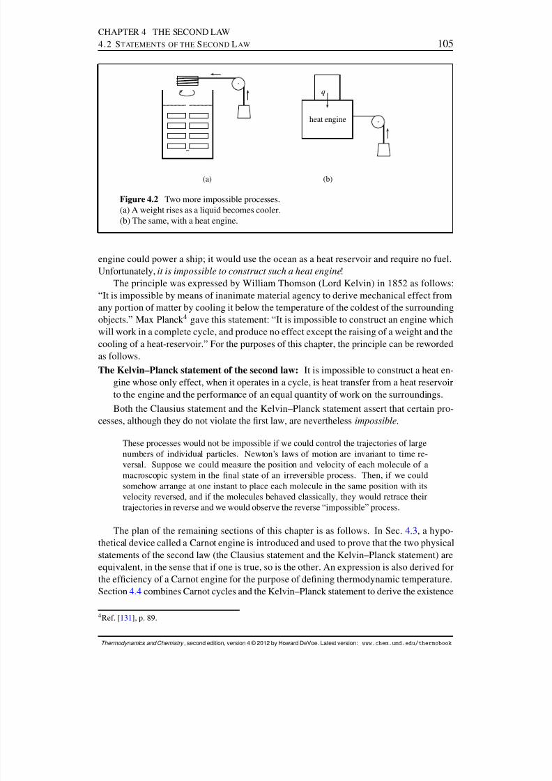
8/12/2019 Howard Devoe Thermodynamic and Chemical
http://slidepdf.com/reader/full/howard-devoe-thermodynamic-and-chemical 105/532
CHAPTER 4 THE SECOND LAW4.2 S TATEMENTS OF THE S ECOND L AW 105
(a)
heat engine
q
(b)
Figure 4.2 Two more impossible processes.(a) A weight rises as a liquid becomes cooler.(b) The same, with a heat engine.
engine could power a ship; it would use the ocean as a heat reservoir and require no fuel.
Unfortunately, it is impossible to construct such a heat engine !The principle was expressed by William Thomson (Lord Kelvin) in 1852 as follows:
“It is impossible by means of inanimate material agency to derive mechanical effect fromany portion of matter by cooling it below the temperature of the coldest of the surroundingobjects.” Max Planck 4 gave this statement: “It is impossible to construct an engine whichwill work in a complete cycle, and produce no effect except the raising of a weight and thecooling of a heat-reservoir.” For the purposes of this chapter, the principle can be rewordedas follows.The Kelvin–Planck statement of the second law: It is impossible to construct a heat en-
gine whose only effect, when it operates in a cycle, is heat transfer from a heat reservoirto the engine and the performance of an equal quantity of work on the surroundings.
Both the Clausius statement and the Kelvin–Planck statement assert that certain pro-cesses, although they do not violate the rst law, are nevertheless impossible .
These processes would not be impossible if we could control the trajectories of largenumbers of individual particles. Newton’s laws of motion are invariant to time re-versal. Suppose we could measure the position and velocity of each molecule of amacroscopic system in the nal state of an irreversible process. Then, if we couldsomehow arrange at one instant to place each molecule in the same position with itsvelocity reversed, and if the molecules behaved classically, they would retrace theirtrajectories in reverse and we would observe the reverse “impossible” process.
The plan of the remaining sections of this chapter is as follows. In Sec. 4.3, a hypo-
thetical device called a Carnot engine is introduced and used to prove that the two physicalstatements of the second law (the Clausius statement and the Kelvin–Planck statement) areequivalent, in the sense that if one is true, so is the other. An expression is also derived forthe efciency of a Carnot engine for the purpose of dening thermodynamic temperature.Section 4.4 combines Carnot cycles and the Kelvin–Planck statement to derive the existence
4Ref. [ 131 ], p. 89.
Thermodynamics and Chemistry , second edition, version 4 © 2012 by Howard DeVoe. Latest version: www.chem.umd.edu/thermobook

8/12/2019 Howard Devoe Thermodynamic and Chemical
http://slidepdf.com/reader/full/howard-devoe-thermodynamic-and-chemical 106/532
CHAPTER 4 THE SECOND LAW4.3 C ONCEPTS D EVELOPED WITH C ARNOT E NGINES 106
m
.
P a
A
B
B
CC
D
Figure 4.3 Indicator diagram for a Carnot engine using an ideal gas as the workingsubstance. In this example, T h D 400 K, T c D 300 K, D 1=4, C V; m D .3=2/R ,
n D 2:41 mmol. The processes of paths A ! B and C! D are isothermal; those of paths B ! C, B0! C0, and D! A are adiabatic. The cycle A ! B! C! D! A has network w D 1:0 J; the cycle A ! B0! C0! D! A has net work w D 0:5 J.
and properties of the state function called entropy. Section 4.5 uses irreversible processesto complete the derivation of the mathematical statements given in the box on page 103,Sec. 4.6 describes some applications, and Sec. 4.7 is a summary. Finally, Sec. 4.8 brieydescribes a microscopic, statistical interpretation of entropy.
Carnot engines and Carnot cycles are admittedly outside the normal experience of chemists, and using them to derive the mathematical statement of the second law may
seem arcane. G. N. Lewis and M. Randall, in their classic 1923 book Thermodynam-ics and the Free Energy of Chemical Substances ,5 complained of the presentation of “ ‘cyclical processes’ limping about eccentric and not quite completed cycles.” Thereseems, however, to be no way to carry out a rigorous general derivation without in-voking thermodynamic cycles. You may avoid the details by skipping Secs. 4.3–4.5 .(Incidently, the cycles described in these sections are complete!)
4.3 CONCEPTS DEVELOPED WITH CARNOT ENGINES
4.3.1 Carnot engines and Carnot cycles
A heat engine, as mentioned in Sec. 4.2, is a closed system that converts heat to work
and operates in a cycle. A Carnot engine is a particular kind of heat engine, one thatperforms Carnot cycles with a working substance. A Carnot cycle has four reversiblesteps, alternating isothermal and adiabatic; see the examples in Figs. 4.3 and 4.4 in whichthe working substances are an ideal gas and H 2 O, respectively.
5Ref. [ 103 ], p. 2.
Thermodynamics and Chemistry , second edition, version 4 © 2012 by Howard DeVoe. Latest version: www.chem.umd.edu/thermobook

8/12/2019 Howard Devoe Thermodynamic and Chemical
http://slidepdf.com/reader/full/howard-devoe-thermodynamic-and-chemical 107/532
CHAPTER 4 THE SECOND LAW4.3 C ONCEPTS D EVELOPED WITH C ARNOT E NGINES 107
BIOGRAPHICAL SKETCHSadi Carnot (1796–1832)
Sadi Carnot was the eldest son of LazareCarnot, a famous French anti-royalist politi-cian, one of Napoleon’s generals with a greatinterest in mathematics. As a boy Sadi was
shy and sensitive. He studied at the EcolePolytechnique, a training school for army en-gineers, and became an army ofcer.
Carnot is renowned for the one book hewrote: a treatise of 118 pages entitled Reec-tions on the Motive Power of Fire and on Ma-chines Fitted to Develop that Power . This waspublished in 1824, when he was 28 and hadretired from the army on half pay.
The book was written in a nontechnicalstyle and went virtually unnoticed. Its purposewas to show how the efciency of a steam en-gine could be improved, a very practical matter
since French power technology lagged behindthat of Britain at the time: a
Notwithstanding the work of all kinds done bysteam-engines, notwithstanding the satisfactorycondition to which they have been brought today,their theory is very little understood, and the at-tempts to improve them are still directed almostby chance.
. . . We can easily conceive a multitude of ma-chines tted to develop the motive power of heatthrough the use of elastic uids; but in whateverway we look at it, we should not lose sight of thefollowing principles:
(1) The temperature of the uid should bemade as high as possible, in order to obtain agreat fall of caloric, and consequently a largeproduction of motive power.
(2) For the same reason the cooling should be
carried as far as possible.(3) It should be so arranged that the passage
of the elastic uid from the highest to the lowest
temperature should be due to increase of volume;that is, it should be so arranged that the coolingof the gas should occur spontaneously as the re-sult of rarefaction [i.e., adiabatic expansion].
Carnot derived these principles from the ab-stract reversible cycle now called the Carnotcycle. He assumed the validity of the calorictheory (heat as an indestructible substance),which requires that the net heat in the cycle bezero, whereas today we would say that it is thenet entropy change that is zero.
Despite the aw of assuming that heat isconserved, a view which there is evidence he
was beginning to doubt, his conclusion wasvalid that the efciency of a reversible cycleoperating between two xed temperatures isindependent of the working substance. Hebased his reasoning on the impossibility of theperpetual motion which would result by com-bining the cycle with the reverse of a more ef-cient cycle. Regarding Carnot’s accomplish-ment, William Thomson (later Lord Kelvin)wrote:
Nothing in the whole range of Natural Philoso-phy is more remarkable than the establishmentof general laws by such a process of reasoning.
A biographer described Carnot’s personal-ity as follows: b
He was reserved, almost taciturn, with a hatredof any form of publicity. . . . his friends all spokeof his underlying warmth and humanity. Pas-sionately fond of music, he was an excellent vi-olinist who preferred the classical Lully to the“moderns” of the time; he was devoted to litera-ture and all the arts.
Carnot came down with scarlet fever and,while convalescing, died—probably of thecholera epidemic then raging. He was only 36.
Two years later his work was brought topublic attention in a paper written by EmileClapeyron (page 218), who used indicator dia-grams to explain Carnot’s ideas.
a Ref. [ 27]. bRef. [ 114 ], page x.
Thermodynamics and Chemistry , second edition, version 4 © 2012 by Howard DeVoe. Latest version: www.chem.umd.edu/thermobook
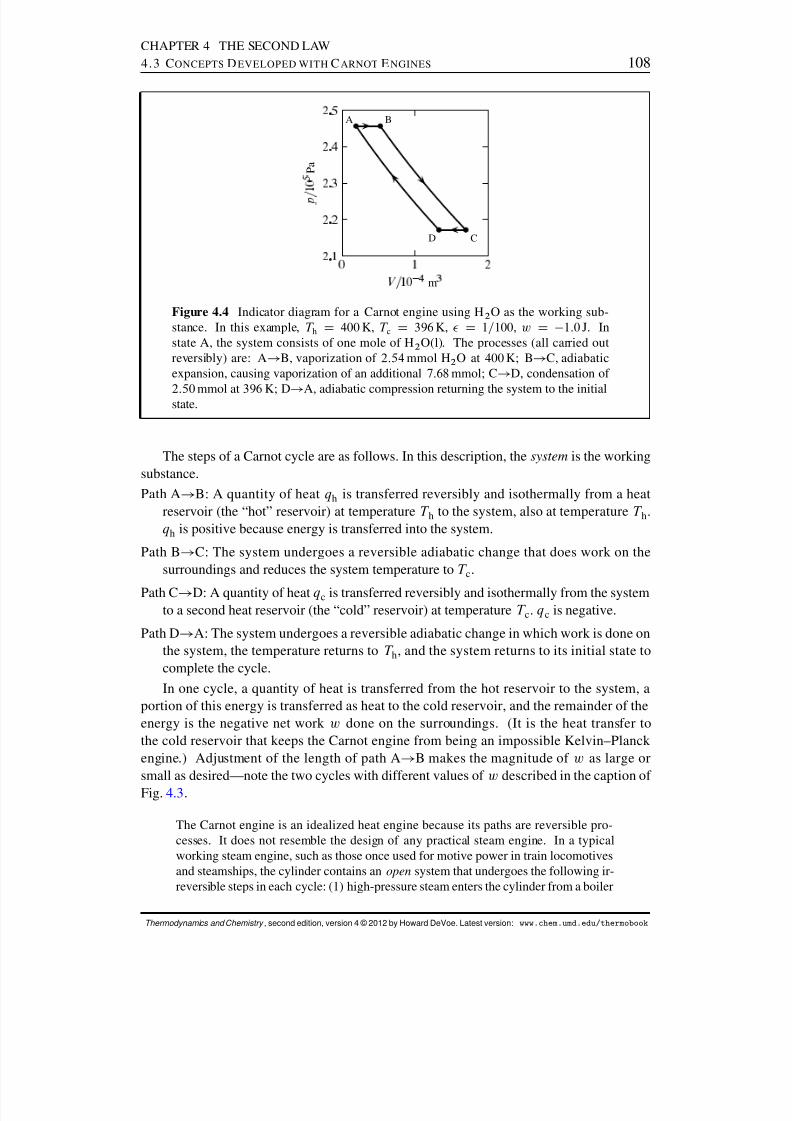
8/12/2019 Howard Devoe Thermodynamic and Chemical
http://slidepdf.com/reader/full/howard-devoe-thermodynamic-and-chemical 108/532
CHAPTER 4 THE SECOND LAW4.3 C ONCEPTS D EVELOPED WITH C ARNOT E NGINES 108
m
P a
A B
D C
Figure 4.4 Indicator diagram for a Carnot engine using H 2 O as the working sub-stance. In this example, T h D 400 K, T c D 396 K, D 1=100, w D 1:0 J. Instate A, the system consists of one mole of H 2 O(l). The processes (all carried outreversibly) are: A ! B, vaporization of 2:54 mmol H 2 O at 400 K; B! C, adiabaticexpansion, causing vaporization of an additional 7:68 mmol; C ! D, condensation of
2:50 mmol at 396 K; D! A, adiabatic compression returning the system to the initialstate.
The steps of a Carnot cycle are as follows. In this description, the system is the workingsubstance.Path A ! B: A quantity of heat qh is transferred reversibly and isothermally from a heat
reservoir (the “hot” reservoir) at temperature T h to the system, also at temperature T h .qh is positive because energy is transferred into the system.
Path B ! C: The system undergoes a reversible adiabatic change that does work on thesurroundings and reduces the system temperature to T c .
Path C ! D: A quantity of heat qc is transferred reversibly and isothermally from the systemto a second heat reservoir (the “cold” reservoir) at temperature T c . qc is negative.
Path D ! A: The system undergoes a reversible adiabatic change in which work is done onthe system, the temperature returns to T h , and the system returns to its initial state tocomplete the cycle.In one cycle, a quantity of heat is transferred from the hot reservoir to the system, a
portion of this energy is transferred as heat to the cold reservoir, and the remainder of theenergy is the negative net work w done on the surroundings. (It is the heat transfer tothe cold reservoir that keeps the Carnot engine from being an impossible Kelvin–Planck engine.) Adjustment of the length of path A ! B makes the magnitude of w as large orsmall as desired—note the two cycles with different values of w described in the caption of Fig. 4.3 .
The Carnot engine is an idealized heat engine because its paths are reversible pro-cesses. It does not resemble the design of any practical steam engine. In a typicalworking steam engine, such as those once used for motive power in train locomotivesand steamships, the cylinder contains an open system that undergoes the following ir-reversible steps in each cycle: (1) high-pressure steam enters the cylinder from a boiler
Thermodynamics and Chemistry , second edition, version 4 © 2012 by Howard DeVoe. Latest version: www.chem.umd.edu/thermobook

8/12/2019 Howard Devoe Thermodynamic and Chemical
http://slidepdf.com/reader/full/howard-devoe-thermodynamic-and-chemical 109/532
CHAPTER 4 THE SECOND LAW4.3 C ONCEPTS D EVELOPED WITH C ARNOT E NGINES 109
(a)
4
T h
1
3
T c
(b)
4
T h
1
3
T c
Figure 4.5 (a) One cycle of a Carnot engine that does work on the surroundings.(b) The same system run in reverse as a Carnot heat pump.Figures 4.5–4.7 use the following symbols: A square box represents a system (aCarnot engine or Carnot heat pump). Vertical arrows indicate heat and horizontalarrows indicate work; each arrow shows the direction of energy transfer into or out of the system. The number next to each arrow is an absolute value of q /J or w /J in thecycle. For example, (a) shows 4 joules of heat transferred to the system from the hotreservoir, 3 joules of heat transferred from the system to the cold reservoir, and 1 jouleof work done by the system on the surroundings.
and pushes the piston from the closed end toward the open end of the cylinder; (2) thesupply valve closes and the steam expands in the cylinder until its pressure decreasesto atmospheric pressure; (3) an exhaust valve opens to release the steam either to theatmosphere or to a condenser; (4) the piston returns to its initial position, driven eitherby an external force or by suction created by steam condensation.
The energy transfers involved in one cycle of a Carnot engine are shown schematicallyin Fig. 4.5 (a). When the cycle is reversed, as shown in Fig. 4.5 (b), the device is called aCarnot heat pump . In each cycle of a Carnot heat pump, qh is negative and qc is positive.
Since each step of a Carnot engine or Carnot heat pump is a reversible process, neitherdevice is an impossible device.
4.3.2 The equivalence of the Clausius and Kelvin–Planck statements
We can use the logical tool of reductio ad absurdum to prove the equivalence of the Clausiusand Kelvin–Planck statements of the second law.
Let us assume for the moment that the Clausius statement is incorrect, and that the de-vice the Clausius statement claims is impossible (a “Clausius device”) is actually possible.If the Clausius device is possible, then we can combine one of these devices with a Carnotengine as shown in Fig. 4.6(a) on page 111 . We adjust the cycles of the Clausius device andCarnot engine to transfer equal quantities of heat from and to the cold reservoir. The com-bination of the Clausius device and Carnot engine is a system. When the Clausius deviceand Carnot engine each performs one cycle, the system has performed one cycle as shownin Fig. 4.6 (b). There has been a transfer of heat into the system and the performance of anequal quantity of work on the surroundings, with no other net change. This system is a heatengine that according to the Kelvin–Planck statement is impossible.
Thus, if the Kelvin–Planck statement is correct, it is impossible to operate the Clausius
Thermodynamics and Chemistry , second edition, version 4 © 2012 by Howard DeVoe. Latest version: www.chem.umd.edu/thermobook
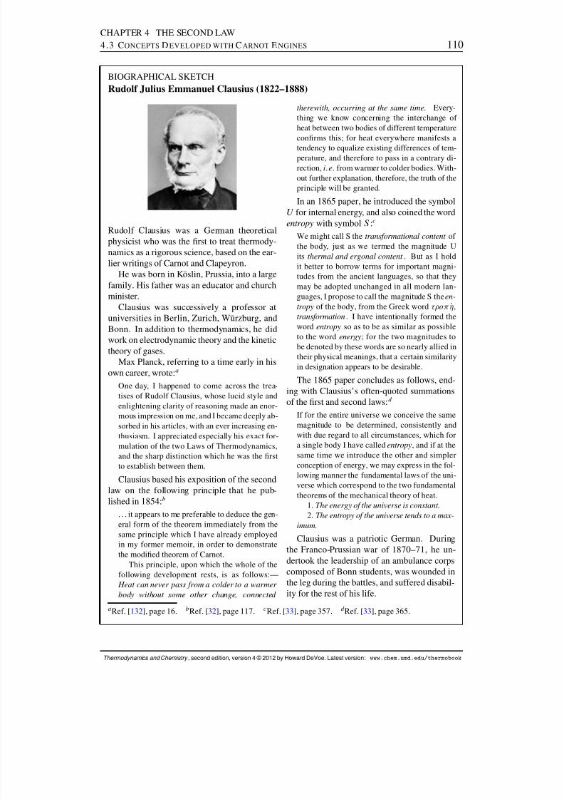
8/12/2019 Howard Devoe Thermodynamic and Chemical
http://slidepdf.com/reader/full/howard-devoe-thermodynamic-and-chemical 110/532
CHAPTER 4 THE SECOND LAW4.3 C ONCEPTS D EVELOPED WITH C ARNOT E NGINES 110
BIOGRAPHICAL SKETCHRudolf Julius Emmanuel Clausius (1822–1888)
Rudolf Clausius was a German theoreticalphysicist who was the rst to treat thermody-namics as a rigorous science, based on the ear-lier writings of Carnot and Clapeyron.
He was born in K¨oslin, Prussia, into a largefamily. His father was an educator and churchminister.
Clausius was successively a professor atuniversities in Berlin, Zurich, W¨ urzburg, andBonn. In addition to thermodynamics, he didwork on electrodynamic theory and the kinetictheory of gases.
Max Planck, referring to a time early in hisown career, wrote: a
One day, I happened to come across the trea-tises of Rudolf Clausius, whose lucid style andenlightening clarity of reasoning made an enor-
mous impression on me, and I became deeply ab-sorbed in his articles, with an ever increasing en-thusiasm. I appreciated especially his exact for-mulation of the two Laws of Thermodynamics,and the sharp distinction which he was the rstto establish between them.
Clausius based his exposition of the secondlaw on the following principle that he pub-lished in 1854: b
. . . it appears to me preferable to deduce the gen-eral form of the theorem immediately from thesame principle which I have already employedin my former memoir, in order to demonstratethe modied theorem of Carnot.
This principle, upon which the whole of thefollowing development rests, is as follows:— Heat can never pass from a colder to a warmer body without some other change, connected
therewith, occurring at the same time. Every-thing we know concerning the interchange of heat between two bodies of different temperature
conrms this; for heat everywhere manifests atendency to equalize existing differences of tem-perature, and therefore to pass in a contrary di-rection, i.e. from warmer to colder bodies. With-out further explanation, therefore, the truth of theprinciple will be granted.
In an 1865 paper, he introduced the symbolU for internal energy, and also coined the wordentropy with symbol S :c
We might call S the transformational content of the body, just as we termed the magnitude Uits thermal and ergonal content . But as I holdit better to borrow terms for important magni-
tudes from the ancient languages, so that theymay be adopted unchanged in all modern lan-guages, I propose to call the magnitude S the en-tropy of the body, from the Greek word o J,transformation . I have intentionally formed theword entropy so as to be as similar as possibleto the word energy ; for the two magnitudes tobe denoted by these words are so nearly allied intheir physical meanings, that a certain similarityin designation appears to be desirable.
The 1865 paper concludes as follows, end-ing with Clausius’s often-quoted summationsof the rst and second laws: d
If for the entire universe we conceive the samemagnitude to be determined, consistently andwith due regard to all circumstances, which fora single body I have called entropy , and if at thesame time we introduce the other and simplerconception of energy, we may express in the fol-lowing manner the fundamental laws of the uni-verse which correspond to the two fundamentaltheorems of the mechanical theory of heat.
1. The energy of the universe is constant.2. The entropy of the universe tends to a max-
imum.
Clausius was a patriotic German. Duringthe Franco-Prussian war of 1870–71, he un-
dertook the leadership of an ambulance corpscomposed of Bonn students, was wounded inthe leg during the battles, and suffered disabil-ity for the rest of his life.
a Ref. [ 132 ], page 16. bRef. [ 32], page 117. cRef. [ 33], page 357. d Ref. [ 33], page 365.
Thermodynamics and Chemistry , second edition, version 4 © 2012 by Howard DeVoe. Latest version: www.chem.umd.edu/thermobook
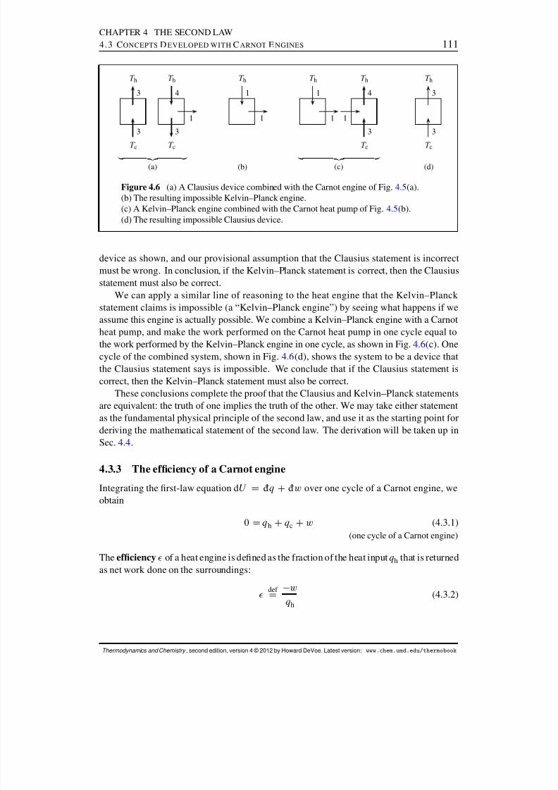
8/12/2019 Howard Devoe Thermodynamic and Chemical
http://slidepdf.com/reader/full/howard-devoe-thermodynamic-and-chemical 111/532
CHAPTER 4 THE SECOND LAW4.3 C ONCEPTS D EVELOPED WITH C ARNOT E NGINES 111
„ ƒ‚ …
(a)
3
T h
3
T c
4
T h
1
3
T c
(b)
1
T h
1
„ ƒ‚ …
(c)
1
T h
1
4
T h
1
3
T c
(d)
3
T h
3
T c
Figure 4.6 (a) A Clausius device combined with the Carnot engine of Fig. 4.5(a).(b) The resulting impossible Kelvin–Planck engine.(c) A Kelvin–Planck engine combined with the Carnot heat pump of Fig. 4.5(b).(d) The resulting impossible Clausius device.
device as shown, and our provisional assumption that the Clausius statement is incorrectmust be wrong. In conclusion, if the Kelvin–Planck statement is correct, then the Clausiusstatement must also be correct.
We can apply a similar line of reasoning to the heat engine that the Kelvin–Planck statement claims is impossible (a “Kelvin–Planck engine”) by seeing what happens if weassume this engine is actually possible. We combine a Kelvin–Planck engine with a Carnotheat pump, and make the work performed on the Carnot heat pump in one cycle equal tothe work performed by the Kelvin–Planck engine in one cycle, as shown in Fig. 4.6(c). Onecycle of the combined system, shown in Fig. 4.6 (d), shows the system to be a device thatthe Clausius statement says is impossible. We conclude that if the Clausius statement iscorrect, then the Kelvin–Planck statement must also be correct.
These conclusions complete the proof that the Clausius and Kelvin–Planck statementsare equivalent: the truth of one implies the truth of the other. We may take either statementas the fundamental physical principle of the second law, and use it as the starting point forderiving the mathematical statement of the second law. The derivation will be taken up inSec. 4.4 .
4.3.3 The efciency of a Carnot engine
Integrating the rst-law equation d U D ¶q C¶w over one cycle of a Carnot engine, weobtain
0 D qh Cqc Cw (4.3.1)(one cycle of a Carnot engine)
The efciency of a heat engine is dened as the fraction of the heat input qh that is returnedas net work done on the surroundings:
def
D wqh
(4.3.2)
Thermodynamics and Chemistry , second edition, version 4 © 2012 by Howard DeVoe. Latest version: www.chem.umd.edu/thermobook

8/12/2019 Howard Devoe Thermodynamic and Chemical
http://slidepdf.com/reader/full/howard-devoe-thermodynamic-and-chemical 112/532
CHAPTER 4 THE SECOND LAW4.3 C ONCEPTS D EVELOPED WITH C ARNOT E NGINES 112
„ ƒ‚ …
(a)
4
T h
1
3
T c
5
T h
1
4
T c
(b)
1
T h
1
T c
„ ƒ‚ …
(c)
3
T h
1
2
T c
4
T h
1
3
T c
(d)
1
T h
1
T c
Figure 4.7 (a) A Carnot engine of efciency D 1=4 combined with a Carnot engineof efciency D 1=5 run in reverse.(b) The resulting impossible Clausius device.(c) A Carnot engine of efciency D 1=3 combined with the Carnot engine of ef-ciency D 1=4 run in reverse.(d) The resulting impossible Clausius device.
By substituting for w from Eq. 4.3.1 , we obtain
D 1 C qc
qh(4.3.3)
(Carnot engine)
Because qc is negative, qh is positive, and qc is smaller in magnitude than qh , the efciencyis less than one. The example shown in Fig. 4.5 (a) is a Carnot engine with D 1=4.
We will be able to reach an important conclusion regarding efciency by considering aCarnot engine operating between the temperatures T h and T c , combined with a Carnot heatpump operating between the same two temperatures. The combination is a supersystem, andone cycle of the engine and heat pump is one cycle of the supersystem. We adjust the cycles
of the engine and heat pump to produce zero net work for one cycle of the supersystem.Could the efciency of the Carnot engine be different from the efciency the heat pump
would have when run in reverse as a Carnot engine? If so, either the supersystem is animpossible Clausius device as shown in Fig. 4.7 (b), or the supersystem operated in reverse(with the engine and heat pump switching roles) is an impossible Clausius device as shownin Fig. 4.7 (d). We conclude that all Carnot engines operating between the same two tem- peratures have the same efciency .
This is a good place to pause and think about the meaning of this statement in light of the fact that the steps of a Carnot engine, being reversible changes, cannot take place ina real system (Sec. 3.2). How can an engine operate that is not real? The statement isan example of a common kind of thermodynamic shorthand. To express the same idea
more accurately, one could say that all heat engines (real systems) operating betweenthe same two temperatures have the same limiting efciency, where the limit is thereversible limit approached as the steps of the cycle are carried out more and moreslowly. You should interpret any statement involving a reversible process in a similarfashion: a reversible process is an idealized limiting process that can be approachedbut never quite reached by a real system.
Thermodynamics and Chemistry , second edition, version 4 © 2012 by Howard DeVoe. Latest version: www.chem.umd.edu/thermobook
8/12/2019 Howard Devoe Thermodynamic and Chemical
http://slidepdf.com/reader/full/howard-devoe-thermodynamic-and-chemical 113/532
CHAPTER 4 THE SECOND LAW4.3 C ONCEPTS D EVELOPED WITH C ARNOT E NGINES 113
Thus, the efciency of a Carnot engine must depend only on the values of T c and T hand not on the properties of the working substance. Since the efciency is given by D1 Cqc=qh , the ratio qc=qh must be a unique function of T c and T h only. To nd this functionfor temperatures on the ideal-gas temperature scale, it is simplest to choose as the workingsubstance an ideal gas.
An ideal gas has the equation of state pV D nRT . Its internal energy change in aclosed system is given by d U D C V dT (Eq. 3.5.3 ), where C V (a function only of T ) isthe heat capacity at constant volume. Reversible expansion work is given by ¶w D p dV ,which for an ideal gas becomes ¶w D .nRT=V / dV . Substituting these expressions fordU and ¶w in the rst law, d U D ¶q C¶w , and solving for ¶q , we obtain
¶q D C V dT C nRT
V dV (4.3.4)
(ideal gas, reversibleexpansion work only)
Dividing both sides by T gives
¶qT D
C V dT T CnR
dV T (4.3.5)
(ideal gas, reversibleexpansion work only)
In the two adiabatic steps of the Carnot cycle, ¶q is zero. We obtain a relation among thevolumes of the four labeled states shown in Fig. 4.3 by integrating Eq. 4.3.5 over these stepsand setting the integrals equal to zero:
Path B ! C: Z ¶qT DZ
T c
T h
C V dT T CnR ln
V CV B D 0 (4.3.6)
Path D ! A:
Z ¶q
T D
Z
T h
T c
C V dT T CnR ln
V AV D D 0 (4.3.7)
Adding these two equations (the integrals shown with limits cancel) gives the relation
nR lnV AV CV BV D D 0 (4.3.8)
which we can rearrange to
ln .V B=V A / D ln.V D=V C / (4.3.9)(ideal gas, Carnot cycle)
We obtain expressions for the heat in the two isothermal steps by integrating Eq. 4.3.4 withdT set equal to 0.
Path A ! B W qh D nRT h ln.V B=V A / (4.3.10)
Path C ! D W qc D nRT c ln.V D=V C / (4.3.11)
The ratio of qc and qh obtained from these expressions is
qc
qh D T cT h
ln.V D=V C /ln.V B=V A /
(4.3.12)
Thermodynamics and Chemistry , second edition, version 4 © 2012 by Howard DeVoe. Latest version: www.chem.umd.edu/thermobook

8/12/2019 Howard Devoe Thermodynamic and Chemical
http://slidepdf.com/reader/full/howard-devoe-thermodynamic-and-chemical 114/532
CHAPTER 4 THE SECOND LAW4.3 C ONCEPTS D EVELOPED WITH C ARNOT E NGINES 114
By means of Eq. 4.3.9 , this ratio becomes
qc
qh D T cT h
(4.3.13)(Carnot cycle)
Accordingly, the unique function of T c and T h we seek that is equal to qc=qh is the ratioT c=T h . The efciency, from Eq. 4.3.3 , is then given by
D 1 T cT h
(4.3.14)(Carnot engine)
In Eqs. 4.3.13 and 4.3.14 , T c and T h are temperatures on the ideal-gas scale. As we haveseen, these equations must be valid for any working substance; it is not necessary to specifyas a condition of validity that the system is an ideal gas.
The ratio T c=T h is positive but less than one, so the efciency is less than one as deducedearlier on page 112 . This conclusion is an illustration of the Kelvin–Planck statement of thesecond law: A heat engine cannot have an efciency of unity—that is, it cannot in onecycle convert all of the energy transferred by heat from a single heat reservoir into work.The example shown in Fig. 4.5 on page 109 , with D 1=4, must have T c=T h D 3=4 (e.g.,T c D 300 K and T h D 400 K).
Keep in mind that a Carnot engine operates reversibly between two heat reservoirs. Theexpression of Eq. 4.3.14 gives the efciency of this kind of idealized heat engine only. If any part of the cycle is carried out irreversibly, dissipation of mechanical energy will causethe efciency to be lower than the theoretical value given by Eq. 4.3.14 .
4.3.4 Thermodynamic temperature
The negative ratio qc=qh for a Carnot cycle depends only on the temperatures of the two heat
reservoirs. Kelvin (1848) proposed that this ratio be used to establish an “absolute” temper-ature scale. The physical quantity now called thermodynamic temperature is dened bythe relation
T cT h D
qc
qh(4.3.15)
(Carnot cycle)
That is, the ratio of the thermodynamic temperatures of two heat reservoirs is equal, bydenition, to the ratio of the absolute quantities of heat transferred in the isothermal stepsof a Carnot cycle operating between these two temperatures. In principle, a measurement of qc=qh during a Carnot cycle, combined with a dened value of the thermodynamic tempera-ture of one of the heat reservoirs, can establish the thermodynamic temperature of the otherheat reservoir. This dened value is provided by the triple point of H 2 O; its thermodynamictemperature is dened as exactly 273:16 kelvins (page 40).
Just as measurements with a gas thermometer in the limit of zero pressure establishthe ideal-gas temperature scale (Sec. 2.3.5 ), the behavior of a heat engine in the reversiblelimit establishes the thermodynamic temperature scale. Note, however, that a reversibleCarnot engine used as a “thermometer” to measure thermodynamic temperature is only a
Thermodynamics and Chemistry , second edition, version 4 © 2012 by Howard DeVoe. Latest version: www.chem.umd.edu/thermobook
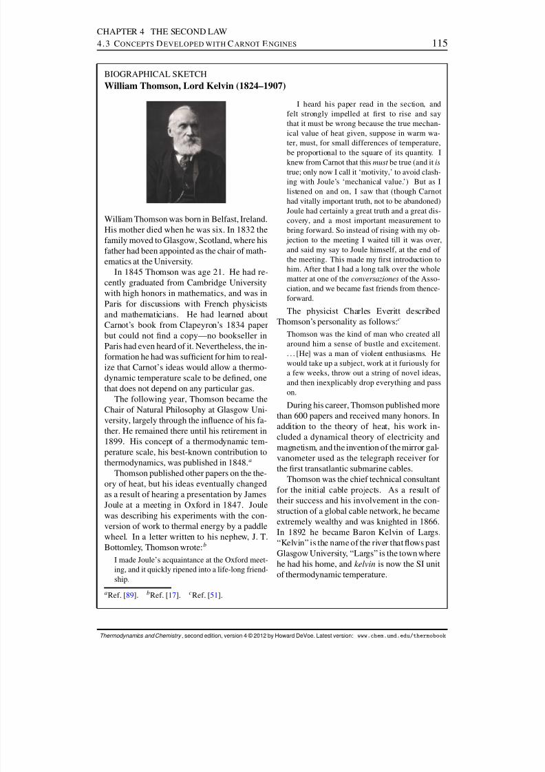
8/12/2019 Howard Devoe Thermodynamic and Chemical
http://slidepdf.com/reader/full/howard-devoe-thermodynamic-and-chemical 115/532
CHAPTER 4 THE SECOND LAW4.3 C ONCEPTS D EVELOPED WITH C ARNOT E NGINES 115
BIOGRAPHICAL SKETCHWilliam Thomson, Lord Kelvin (1824–1907)
William Thomson was born in Belfast, Ireland.His mother died when he was six. In 1832 thefamily moved to Glasgow, Scotland, where hisfather had been appointed as the chair of math-ematics at the University.
In 1845 Thomson was age 21. He had re-cently graduated from Cambridge Universitywith high honors in mathematics, and was inParis for discussions with French physicistsand mathematicians. He had learned aboutCarnot’s book from Clapeyron’s 1834 paperbut could not nd a copy—no bookseller inParis had even heard of it. Nevertheless, the in-formation he had was sufcient for him to real-ize that Carnot’s ideas would allow a thermo-dynamic temperature scale to be dened, onethat does not depend on any particular gas.
The following year, Thomson became theChair of Natural Philosophy at Glasgow Uni-versity, largely through the inuence of his fa-ther. He remained there until his retirement in1899. His concept of a thermodynamic tem-perature scale, his best-known contribution tothermodynamics, was published in 1848. a
Thomson published other papers on the the-ory of heat, but his ideas eventually changedas a result of hearing a presentation by JamesJoule at a meeting in Oxford in 1847. Joulewas describing his experiments with the con-version of work to thermal energy by a paddle
wheel. In a letter written to his nephew, J. T.Bottomley, Thomson wrote: b
I made Joule’s acquaintance at the Oxford meet-ing, and it quickly ripened into a life-long friend-ship.
I heard his paper read in the section, andfelt strongly impelled at rst to rise and saythat it must be wrong because the true mechan-
ical value of heat given, suppose in warm wa-ter, must, for small differences of temperature,be proportional to the square of its quantity. Iknew from Carnot that this must be true (and it istrue; only now I call it ‘motivity,’ to avoid clash-ing with Joule’s ‘mechanical value.’) But as Ilistened on and on, I saw that (though Carnothad vitally important truth, not to be abandoned)Joule had certainly a great truth and a great dis-covery, and a most important measurement tobring forward. So instead of rising with my ob- jection to the meeting I waited till it was over,and said my say to Joule himself, at the end of the meeting. This made my rst introduction to
him. After that I had a long talk over the wholematter at one of the conversaziones of the Asso-ciation, and we became fast friends from thence-forward.
The physicist Charles Everitt describedThomson’s personality as follows: c
Thomson was the kind of man who created allaround him a sense of bustle and excitement.. . . [He] was a man of violent enthusiasms. Hewould take up a subject, work at it furiously fora few weeks, throw out a string of novel ideas,and then inexplicably drop everything and passon.
During his career, Thomson published morethan 600 papers and received many honors. Inaddition to the theory of heat, his work in-cluded a dynamical theory of electricity andmagnetism, and the invention of the mirror gal-vanometer used as the telegraph receiver forthe rst transatlantic submarine cables.
Thomson was the chief technical consultantfor the initial cable projects. As a result of their success and his involvement in the con-struction of a global cable network, he becameextremely wealthy and was knighted in 1866.In 1892 he became Baron Kelvin of Largs.“Kelvin” is the name of the river that ows pastGlasgow University, “Largs” is the town wherehe had his home, and kelvin is now the SI unitof thermodynamic temperature.
a Ref. [ 89]. bRef. [ 17]. cRef. [ 51].
Thermodynamics and Chemistry , second edition, version 4 © 2012 by Howard DeVoe. Latest version: www.chem.umd.edu/thermobook
8/12/2019 Howard Devoe Thermodynamic and Chemical
http://slidepdf.com/reader/full/howard-devoe-thermodynamic-and-chemical 116/532
CHAPTER 4 THE SECOND LAW4.4 D ERIVATION OF THE M ATHEMATICAL S TATEMENT OF THE S ECOND L AW 116
theoretical concept and not a practical instrument, since a completely-reversible processcannot occur in practice.
It is now possible to justify the statement in Sec. 2.3.5 that the ideal-gas temperaturescale is proportional to the thermodynamic temperature scale. Both Eq. 4.3.13 and Eq.4.3.15 equate the ratio T c=T h to qc=qh; but whereas T c and T h refer in Eq. 4.3.13 to the
ideal-gas temperatures of the heat reservoirs, in Eq. 4.3.15 they refer to the thermodynamictemperatures. This means that the ratio of the ideal-gas temperatures of two bodies is equalto the ratio of the thermodynamic temperatures of the same bodies, and therefore the twoscales are proportional to one another. The proportionality factor is arbitrary, but must beunity if the same unit (e.g., kelvins) is used in both scales. Thus, as stated on page 41, thetwo scales expressed in kelvins are identical.
4.4 DERIVATION OF THE MATHEMATICAL STATEMENT OF THESECOND LAW
4.4.1 The existence of the entropy function
This section derives the existence and properties of the state function called entropy.Consider an arbitrary cyclic process of a closed system. To avoid confusion, this system
will be the “experimental system” and the process will be the “experimental process” or “ex-perimental cycle.” There are no restrictions on the contents of the experimental system—itmay have any degree of complexity whatsoever. The experimental process may involvemore than one kind of work, phase changes and reactions may occur, there may be temper-ature and pressure gradients, constraints and external elds may be present, and so on. Allparts of the process must be either irreversible or reversible, but not impossible.
We imagine that the experimental cycle is carried out in a special way that allows us toapply the Kelvin–Planck statement of the second law. The heat transferred across the bound-ary of the experimental system in each innitesimal path element of the cycle is exchanged
with a hypothetical Carnot engine. The combination of the experimental system and theCarnot engine is a closed supersystem (see Fig. 4.8 on page 118 ). In the surroundings of the supersystem is a heat reservoir of arbitrary constant temperature T res . By allowing thesupersystem to exchange heat with only this single heat reservoir, we will be able to applythe Kelvin–Planck statement to a cycle of the supersystem. 6
We assume that we are able to control changes of the work coordinates of the experi-mental system from the surroundings of the supersystem. We are also able to control theCarnot engine from these surroundings, for example by moving the piston of a cylinder-and-piston device containing the working substance. Thus the energy transferred by work across the boundary of the experimental system, and the work required to operate the Carnotengine, is exchanged with the surroundings of the supersystem.
During each stage of the experimental process with nonzero heat, we allow the Carnotengine to undergo many innitesimal Carnot cycles with innitesimal quantities of heat andwork. In one of the isothermal steps of each Carnot cycle, the Carnot engine is in thermalcontact with the heat reservoir, as depicted in Fig. 4.8(a). In this step the Carnot enginehas the same temperature as the heat reservoir, and reversibly exchanges heat ¶q 0 with it.
6This procedure is similar to ones described in Ref. [ 1], Chap. 5, and Ref. [ 97], p. 53.
Thermodynamics and Chemistry , second edition, version 4 © 2012 by Howard DeVoe. Latest version: www.chem.umd.edu/thermobook
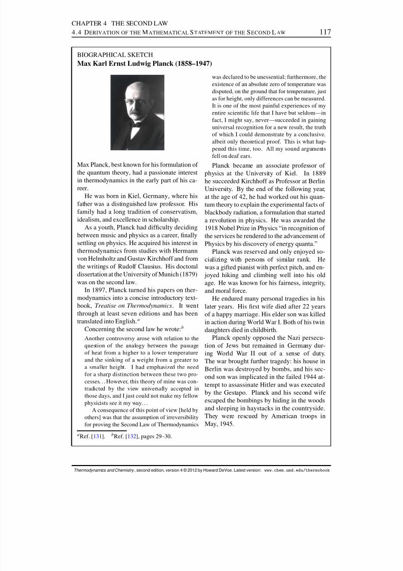
8/12/2019 Howard Devoe Thermodynamic and Chemical
http://slidepdf.com/reader/full/howard-devoe-thermodynamic-and-chemical 117/532
CHAPTER 4 THE SECOND LAW4.4 D ERIVATION OF THE M ATHEMATICAL S TATEMENT OF THE S ECOND L AW 117
BIOGRAPHICAL SKETCHMax Karl Ernst Ludwig Planck (1858–1947)
Max Planck, best known for his formulation of the quantum theory, had a passionate interestin thermodynamics in the early part of his ca-reer.
He was born in Kiel, Germany, where hisfather was a distinguished law professor. Hisfamily had a long tradition of conservatism,idealism, and excellence in scholarship.
As a youth, Planck had difculty decidingbetween music and physics as a career, nallysettling on physics. He acquired his interest inthermodynamics from studies with Hermannvon Helmholtz and Gustav Kirchhoff and fromthe writings of Rudolf Clausius. His doctoraldissertation at the University of Munich (1879)was on the second law.
In 1897, Planck turned his papers on ther-
modynamics into a concise introductory text-book, Treatise on Thermodynamics . It wentthrough at least seven editions and has beentranslated into English. a
Concerning the second law he wrote: b
Another controversy arose with relation to thequestion of the analogy between the passageof heat from a higher to a lower temperatureand the sinking of a weight from a greater toa smaller height. I had emphasized the needfor a sharp distinction between these two pro-cesses. . . However, this theory of mine was con-tradicted by the view universally accepted inthose days, and I just could not make my fellowphysicists see it my way. . .
A consequence of this point of view [held byothers] was that the assumption of irreversibilityfor proving the Second Law of Thermodynamics
was declared to be unessential; furthermore, theexistence of an absolute zero of temperature wasdisputed, on the ground that for temperature, just
as for height, only differences can be measured.It is one of the most painful experiences of myentire scientic life that I have but seldom—infact, I might say, never—succeeded in gaininguniversal recognition for a new result, the truthof which I could demonstrate by a conclusive,albeit only theoretical proof. This is what hap-pened this time, too. All my sound argumentsfell on deaf ears.
Planck became an associate professor of physics at the University of Kiel. In 1889he succeeded Kirchhoff as Professor at BerlinUniversity. By the end of the following year,
at the age of 42, he had worked out his quan-tum theory to explain the experimental facts of blackbody radiation, a formulation that starteda revolution in physics. He was awarded the1918 Nobel Prize in Physics “in recognition of the services he rendered to the advancement of Physics by his discovery of energy quanta.”
Planck was reserved and only enjoyed so-cializing with persons of similar rank. Hewas a gifted pianist with perfect pitch, and en- joyed hiking and climbing well into his oldage. He was known for his fairness, integrity,and moral force.
He endured many personal tragedies in hislater years. His rst wife died after 22 yearsof a happy marriage. His elder son was killedin action during World War I. Both of his twindaughters died in childbirth.
Planck openly opposed the Nazi persecu-tion of Jews but remained in Germany dur-ing World War II out of a sense of duty.The war brought further tragedy: his house inBerlin was destroyed by bombs, and his sec-ond son was implicated in the failed 1944 at-tempt to assassinate Hitler and was executedby the Gestapo. Planck and his second wife
escaped the bombings by hiding in the woodsand sleeping in haystacks in the countryside.They were rescued by American troops inMay, 1945.
a Ref. [ 131 ]. bRef. [ 132 ], pages 29–30.
Thermodynamics and Chemistry , second edition, version 4 © 2012 by Howard DeVoe. Latest version: www.chem.umd.edu/thermobook
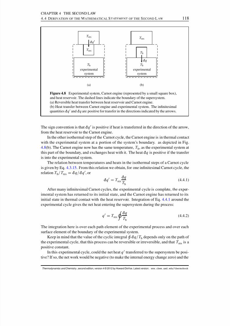
8/12/2019 Howard Devoe Thermodynamic and Chemical
http://slidepdf.com/reader/full/howard-devoe-thermodynamic-and-chemical 118/532
CHAPTER 4 THE SECOND LAW4.4 D ERIVATION OF THE M ATHEMATICAL S TATEMENT OF THE S ECOND L AW 118
(a)
T bexperimental
system
T res
T res
¶q 0
(b)
T bexperimental
system
T b
¶q
T res
Figure 4.8 Experimental system, Carnot engine (represented by a small square box),and heat reservoir. The dashed lines indicate the boundary of the supersystem.(a) Reversible heat transfer between heat reservoir and Carnot engine.(b) Heat transfer between Carnot engine and experimental system. The innitesimalquantities ¶q 0 and ¶q are positive for transfer in the directions indicated by the arrows.
The sign convention is that ¶q 0 is positive if heat is transferred in the direction of the arrow,from the heat reservoir to the Carnot engine.
In the other isothermal step of the Carnot cycle, the Carnot engine is in thermal contactwith the experimental system at a portion of the system’s boundary. as depicted in Fig.4.8 (b). The Carnot engine now has the same temperature, T b , as the experimental system atthis part of the boundary, and exchanges heat with it. The heat ¶q is positive if the transferis into the experimental system.
The relation between temperatures and heats in the isothermal steps of a Carnot cycleis given by Eq. 4.3.15 . From this relation we obtain, for one innitesimal Carnot cycle, therelation T b=T res D ¶q=¶q 0, or
¶q 0 D T res¶qT b
(4.4.1)
After many innitesimal Carnot cycles, the experimental cycle is complete, the exper-imental system has returned to its initial state, and the Carnot engine has returned to itsinitial state in thermal contact with the heat reservoir. Integration of Eq. 4.4.1 around theexperimental cycle gives the net heat entering the supersystem during the process:
q0 D T res I ¶qT b
(4.4.2)
The integration here is over each path element of the experimental process and over eachsurface element of the boundary of the experimental system.Keep in mind that the value of the cyclic integral H ¶q=T b depends only on the path of
the experimental cycle, that this process can be reversible or irreversible, and that T res is apositive constant.
In this experimental cycle, could the net heat q0 transferred to the supersystem be posi-tive? If so, the net work would be negative (to make the internal energy change zero) and the
Thermodynamics and Chemistry , second edition, version 4 © 2012 by Howard DeVoe. Latest version: www.chem.umd.edu/thermobook

8/12/2019 Howard Devoe Thermodynamic and Chemical
http://slidepdf.com/reader/full/howard-devoe-thermodynamic-and-chemical 119/532
CHAPTER 4 THE SECOND LAW4.4 D ERIVATION OF THE M ATHEMATICAL S TATEMENT OF THE S ECOND L AW 119
supersystem would have converted heat from a single heat reservoir completely into work,a process the Kelvin–Planck statement of the second law says is impossible. Therefore it isimpossible for q0 to be positive, and from Eq. 4.4.2 we obtain the relation
I ¶qT b
0 (4.4.3)
(cyclic process of a closed system)
This relation is known as the Clausius inequality . It is valid only if the integration is takenaround a cyclic path in a direction with nothing but reversible and irreversible changes—thepath must not include an impossible change, such as the reverse of an irreversible change.The Clausius inequality says that if a cyclic path meets this specication, it is impossiblefor the cyclic integral H .¶q=T b/ to be positive.
If the entire experimental cycle is adiabatic (which is only possible if the process isreversible), the Carnot engine is not needed and Eq. 4.4.3 can be replaced by H .¶q=T b/ D 0.
Next let us investigate a reversible nonadiabatic process of the closed experimentalsystem. Starting with a particular equilibrium state A, we carry out a reversible process inwhich there is a net ow of heat into the system, and in which ¶q is either positive or zero in
each path element. The nal state of this process is equilibrium state B. If each innitesimalquantity of heat ¶q is positive or zero during the process, then the integral R
BA .¶q=T b/ must
be positive. In this case the Clausius inequality tells us that if the system completes a cycleby returning from state B back to state A by a different path, the integral R
AB .¶q=T b/ for
this second path must be negative. Therefore the change B ! A cannot be carried out by anyadiabatic process.
Any reversible process can be carried out in reverse. Thus, by reversing the reversiblenonadiabatic process, it is possible to change the state from B to A by a reversible processwith a net ow of heat out of the system and with ¶q either negative or zero in each elementof the reverse path. In contrast, the absence of an adiabatic path from B to A means that itis impossible to carry out the change A ! B by a reversible adiabatic process.
The general rule, then, is that whenever equilibrium state A of a closed system can bechanged to equilibrium state B by a reversible process with nite “one-way” heat (i.e., theow of heat is either entirely into the system or else entirely out of it), it is impossible for thesystem to change from either of these states to the other by a reversible adiabatic process.
A simple example will relate this rule to experience. We can increase the temperatureof a liquid by allowing heat to ow reversibly into the liquid. It is impossible toduplicate this change of state by a reversible process without heat—that is, by usingsome kind of reversible work. The reason is that reversible work involves the changeof a work coordinate that brings the system to a different nal state. There is nothingin the rule that says we can’t increase the temperature irreversibly without heat, as wecan for instance with stirring work.
States A and B can be arbitrarily close. We conclude that every equilibrium state of aclosed system has other equilibrium states innitesimally close to it that are inaccessible bya reversible adiabatic process . This is Carath eodory’s principle of adiabatic inaccessibility. 7
7Constantin Carath´ eodory in 1909 combined this principle with a mathematical theorem (Carath´ eodory’s the-orem) to deduce the existence of the entropy function. The derivation outlined here avoids the complexities of that mathematical treatment and leads to the same results.
Thermodynamics and Chemistry , second edition, version 4 © 2012 by Howard DeVoe. Latest version: www.chem.umd.edu/thermobook

8/12/2019 Howard Devoe Thermodynamic and Chemical
http://slidepdf.com/reader/full/howard-devoe-thermodynamic-and-chemical 120/532
CHAPTER 4 THE SECOND LAW4.4 D ERIVATION OF THE M ATHEMATICAL S TATEMENT OF THE S ECOND L AW 120
Next let us consider the reversible adiabatic processes that are possible. To carry outa reversible adiabatic process, starting at an initial equilibrium state, we use an adiabaticboundary and slowly vary one or more of the work coordinates. A certain nal temperaturewill result. It is helpful in visualizing this process to think of an N -dimensional spacein which each axis represents one of the N independent variables needed to describe an
equilibrium state. A point in this space represents an equilibrium state, and the path of areversible process can be represented as a curve in this space.A suitable set of independent variables for equilibrium states of a closed system of uni-
form temperature consists of the temperature T and each of the work coordinates (Sec.3.10 ). We can vary the work coordinates independently while keeping the boundary adi-abatic, so the paths for possible reversible adiabatic processes can connect any arbitrarycombinations of work coordinate values.
There is, however, the additional dimension of temperature in the N -dimensional space.Do the paths for possible reversible adiabatic processes, starting from a common initialpoint, lie in a volume in the N -dimensional space? Or do they fall on a surface describedby T as a function of the work coordinates? If the paths lie in a volume, then every pointin a volume element surrounding the initial point must be accessible from the initial pointby a reversible adiabatic path. This accessibility is precisely what Carath´ eodory’s principleof adiabatic inaccessibility denies. Therefore, the paths for all possible reversible adiabaticprocesses with a common initial state must lie on a unique surface . This is an .N 1/ -dimensional hypersurface in the N -dimensional space, or a curve if N is 2. One of thesesurfaces or curves will be referred to as a reversible adiabatic surface .
Now consider the initial and nal states of a reversible process with one-way heat (i.e.,each nonzero innitesimal quantity of heat ¶q has the same sign). Since we have seen thatit is impossible for there to be a reversible adiabatic path between these states, the points forthese states must lie on different reversible adiabatic surfaces that do not intersect anywherein the N -dimensional space. Consequently, there is an innite number of nonintersectingreversible adiabatic surfaces lling the N -dimensional space. (To visualize this for N
D 3,
think of a exed stack of printer paper; each sheet represents a different adiabatic surfacein three-dimensional space.) A reversible, nonadiabatic process with one-way heat is rep-resented by a path beginning at a point on one reversible adiabatic surface and ending at apoint on a different surface. If q is positive, the nal surface lies on one side of the initialsurface, and if q is negative, the nal surface is on the opposite side.
4.4.2 Using reversible processes to dene the entropy
The existence of reversible adiabatic surfaces is the justication for dening a new statefunction S , the entropy . S is specied to have the same value everywhere on one of thesesurfaces, and a different, unique value on each different surface. In other words, the re-versible adiabatic surfaces are surfaces of constant entropy in the N -dimensional space.The fact that the surfaces ll this space without intersecting ensures that S is a state func-tion for equilibrium states, because any point in this space represents an equilibrium stateand also lies on a single reversible adiabatic surface with a denite value of S .
We know the entropy function must exist, because the reversible adiabatic surfaces exist.For instance, Fig. 4.9 on the next page shows a family of these surfaces for a closed systemof a pure substance in a single phase. In this system, N is equal to 2, and the surfaces
Thermodynamics and Chemistry , second edition, version 4 © 2012 by Howard DeVoe. Latest version: www.chem.umd.edu/thermobook
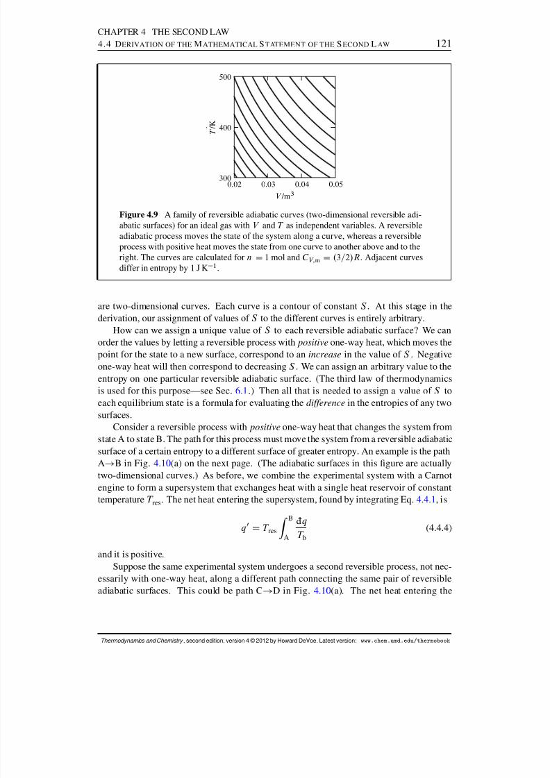
8/12/2019 Howard Devoe Thermodynamic and Chemical
http://slidepdf.com/reader/full/howard-devoe-thermodynamic-and-chemical 121/532
CHAPTER 4 THE SECOND LAW4.4 D ERIVATION OF THE M ATHEMATICAL S TATEMENT OF THE S ECOND L AW 121
0:02 0:03 0:04 0:05300
400
500
V /m 3
. T / K
Figure 4.9 A family of reversible adiabatic curves (two-dimensional reversible adi-abatic surfaces) for an ideal gas with V and T as independent variables. A reversibleadiabatic process moves the state of the system along a curve, whereas a reversibleprocess with positive heat moves the state from one curve to another above and to theright. The curves are calculated for n D 1 mol and C V; m D .3=2/R . Adjacent curves
differ in entropy by 1 J K1
.
are two-dimensional curves. Each curve is a contour of constant S . At this stage in thederivation, our assignment of values of S to the different curves is entirely arbitrary.
How can we assign a unique value of S to each reversible adiabatic surface? We canorder the values by letting a reversible process with positive one-way heat, which moves thepoint for the state to a new surface, correspond to an increase in the value of S . Negativeone-way heat will then correspond to decreasing S . We can assign an arbitrary value to theentropy on one particular reversible adiabatic surface. (The third law of thermodynamicsis used for this purpose—see Sec. 6.1 .) Then all that is needed to assign a value of S toeach equilibrium state is a formula for evaluating the difference in the entropies of any twosurfaces.
Consider a reversible process with positive one-way heat that changes the system fromstate A to state B. The path for this process must move the system from a reversible adiabaticsurface of a certain entropy to a different surface of greater entropy. An example is the pathA! B in Fig. 4.10(a) on the next page. (The adiabatic surfaces in this gure are actuallytwo-dimensional curves.) As before, we combine the experimental system with a Carnotengine to form a supersystem that exchanges heat with a single heat reservoir of constanttemperature T res . The net heat entering the supersystem, found by integrating Eq. 4.4.1 , is
q0 D T res
Z
B
A
¶qT b
(4.4.4)
and it is positive.Suppose the same experimental system undergoes a second reversible process, not nec-
essarily with one-way heat, along a different path connecting the same pair of reversibleadiabatic surfaces. This could be path C ! D in Fig. 4.10(a). The net heat entering the
Thermodynamics and Chemistry , second edition, version 4 © 2012 by Howard DeVoe. Latest version: www.chem.umd.edu/thermobook

8/12/2019 Howard Devoe Thermodynamic and Chemical
http://slidepdf.com/reader/full/howard-devoe-thermodynamic-and-chemical 122/532
CHAPTER 4 THE SECOND LAW4.4 D ERIVATION OF THE M ATHEMATICAL S TATEMENT OF THE S ECOND L AW 122
A
B
C
D
! V
!
T
(a)
A
B
C
D
! V
!
T
(b)
Figure 4.10 Reversible paths in V –T space. The thin curves are reversible adiabaticsurfaces.(a) Two paths connecting the same pair of reversible adiabatic surfaces.(b) A cyclic path.
supersystem during this second process is q00:
q00D T res Z D
C
¶qT b
(4.4.5)
We can then devise a cycle of the supersystem in which the experimental system undergoesthe reversible path A ! B! D! C! A, as shown in Fig. 4.10(b). Step A ! B is the rst pro-cess described above, step D ! C is the reverse of the second process described above, andsteps B ! D and C ! A are reversible and adiabatic. The net heat entering the supersystemin the cycle is q0 q00. In the reverse cycle the net heat is q00 q0. In both of these cycles the
heat is exchanged with a single heat reservoir; therefore, according to the Kelvin–Planck statement, neither cycle can have positive net heat. Therefore q0 and q00must be equal, andEqs. 4.4.4 and 4.4.5 then show the integral R .¶q=T b/ has the same value when evaluatedalong either of the reversible paths from the lower to the higher entropy surface.
Note that since the second path (C ! D) does not necessarily have one-way heat, itcan take the experimental system through any sequence of intermediate entropy values,provided it starts at the lower entropy surface and ends at the higher. Furthermore, since thepath is reversible, it can be carried out in reverse resulting in reversal of the signs of S and R .¶q=T b/ .
It should now be apparent that a satisfactory formula for dening the entropy change of a reversible process in a closed system is
S DZ ¶qT b
(4.4.6)(reversible process,
closed system)
This formula satises the necessary requirements: it makes the value of S positive if theprocess has positive one-way heat, negative if the process has negative one-way heat, and
Thermodynamics and Chemistry , second edition, version 4 © 2012 by Howard DeVoe. Latest version: www.chem.umd.edu/thermobook
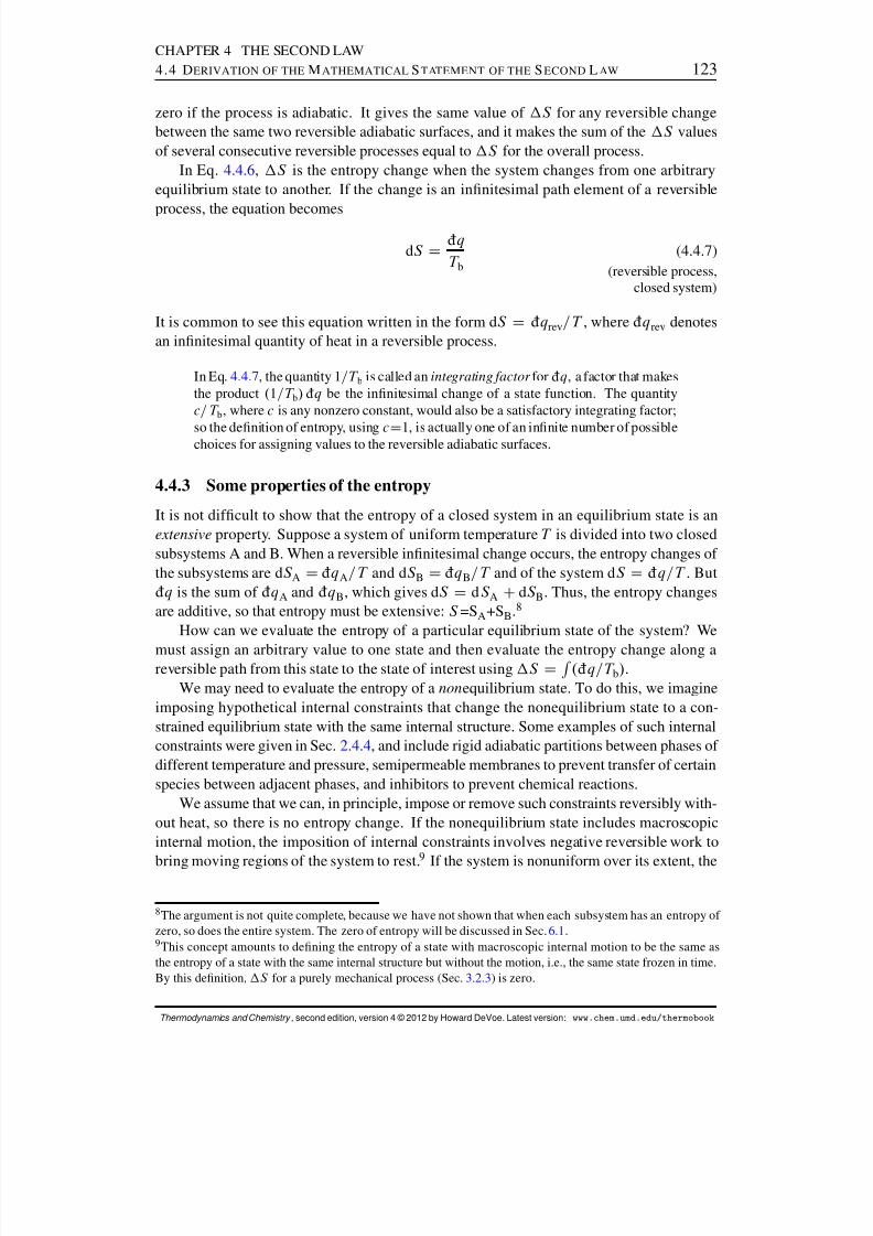
8/12/2019 Howard Devoe Thermodynamic and Chemical
http://slidepdf.com/reader/full/howard-devoe-thermodynamic-and-chemical 123/532
CHAPTER 4 THE SECOND LAW4.4 D ERIVATION OF THE M ATHEMATICAL S TATEMENT OF THE S ECOND L AW 123
zero if the process is adiabatic. It gives the same value of S for any reversible changebetween the same two reversible adiabatic surfaces, and it makes the sum of the S valuesof several consecutive reversible processes equal to S for the overall process.
In Eq. 4.4.6 , S is the entropy change when the system changes from one arbitraryequilibrium state to another. If the change is an innitesimal path element of a reversible
process, the equation becomes
dS D ¶qT b
(4.4.7)(reversible process,
closed system)
It is common to see this equation written in the form d S D ¶q rev=T , where ¶q rev denotesan innitesimal quantity of heat in a reversible process.
In Eq. 4.4.7 , the quantity 1=T b is called an integrating factor for ¶q , a factor that makesthe product .1=T b/ ¶q be the innitesimal change of a state function. The quantityc= T b , where c is any nonzero constant, would also be a satisfactory integrating factor;
so the denition of entropy, using cD1, is actually one of an innite number of possiblechoices for assigning values to the reversible adiabatic surfaces.
4.4.3 Some properties of the entropy
It is not difcult to show that the entropy of a closed system in an equilibrium state is anextensive property. Suppose a system of uniform temperature T is divided into two closedsubsystems A and B. When a reversible innitesimal change occurs, the entropy changes of the subsystems are d S A D ¶q A=T and dS B D ¶q B=T and of the system d S D ¶q=T . But¶q is the sum of ¶q A and ¶q B , which gives d S D dS A CdS B . Thus, the entropy changesare additive, so that entropy must be extensive: S =S A +S B .8
How can we evaluate the entropy of a particular equilibrium state of the system? We
must assign an arbitrary value to one state and then evaluate the entropy change along areversible path from this state to the state of interest using S DR .¶q=T b/ .
We may need to evaluate the entropy of a non equilibrium state. To do this, we imagineimposing hypothetical internal constraints that change the nonequilibrium state to a con-strained equilibrium state with the same internal structure. Some examples of such internalconstraints were given in Sec. 2.4.4 , and include rigid adiabatic partitions between phases of different temperature and pressure, semipermeable membranes to prevent transfer of certainspecies between adjacent phases, and inhibitors to prevent chemical reactions.
We assume that we can, in principle, impose or remove such constraints reversibly with-out heat, so there is no entropy change. If the nonequilibrium state includes macroscopicinternal motion, the imposition of internal constraints involves negative reversible work to
bring moving regions of the system to rest.9
If the system is nonuniform over its extent, the
8The argument is not quite complete, because we have not shown that when each subsystem has an entropy of zero, so does the entire system. The zero of entropy will be discussed in Sec. 6.1 .9This concept amounts to dening the entropy of a state with macroscopic internal motion to be the same asthe entropy of a state with the same internal structure but without the motion, i.e., the same state frozen in time.By this denition, S for a purely mechanical process (Sec. 3.2.3 ) is zero.
Thermodynamics and Chemistry , second edition, version 4 © 2012 by Howard DeVoe. Latest version: www.chem.umd.edu/thermobook
8/12/2019 Howard Devoe Thermodynamic and Chemical
http://slidepdf.com/reader/full/howard-devoe-thermodynamic-and-chemical 124/532
CHAPTER 4 THE SECOND LAW4.5 I RREVERSIBLE P ROCESSES 124
internal constraints will partition it into practically-uniform regions whose entropy is addi-tive. The entropy of the nonequilibrium state is then found from S DR .¶q=T b/ using areversible path that changes the system from an equilibrium state of known entropy to theconstrained equilibrium state with the same entropy as the state of interest. This procedureallows every possible state (at least conceptually) to have a denite value of S .
4.5 IRREVERSIBLE PROCESSES
We know that during a reversible process of a closed system, each innitesimal entropychange d S is equal to ¶q=T b and the nite change S is equal to the integral R .¶q=T b/—but what can we say about d S and S for an irreversible process?
The derivation of this section will show that for an innitesimal irreversible change of a closed system, d S is greater than ¶q=T b , and for an entire process S is greater than
R .¶q=T b/ . That is, the equalities that apply to a reversible process are replaced, for anirreversible process, by inequalities .
The derivation begins with irreversible processes that are adiabatic, and is then extendedto irreversible processes in general.
4.5.1 Irreversible adiabatic processes
Consider an arbitrary irreversible adiabatic process of a closed system starting with a par-ticular initial state A. The nal state B depends on the path of this process. We wish toinvestigate the sign of the entropy change S A! B . Our reasoning will depend on whetheror not there is work during the process.
If there is work along any innitesimal path element of the irreversible adiabatic process(¶w ¤ 0), we know from experience that this work would be different if the work coor-dinate or coordinates were changing at a different rate, because energy dissipation frominternal friction would then be different. In the limit of innite slowness, an adiabatic pro-
cess with initial state A and the same change of work coordinates would become reversible,and the net work and nal internal energy would differ from those of the irreversible pro-cess. Because the nal state of the reversible adiabatic process is different from B, there isno reversible adiabatic path with work between states A and B.
All states of a reversible process, including the initial and nal states, must be equilib-rium states. There is therefore a conceptual difculty in considering reversible pathsbetween two states if either of these states are nonequilibrium states. In such a casewe will assume that the state has been replaced by a constrained equilibrium state of the same entropy as described in Sec. 4.4.3.
If, on the other hand, there is no work along any innitesimal path element of the irre-
versible adiabatic process ( ¶w D0), the process is taking place at constant internal energy U in an isolated system. A reversible limit cannot be reached without heat or work (page 65).Thus any reversible adiabatic change from state A would require work, causing a change of U and preventing the system from reaching state B by any reversible adiabatic path.
So regardless of whether or not an irreversible adiabatic process A ! B involves work,there is no reversible adiabatic path between A and B. The only reversible paths between
Thermodynamics and Chemistry , second edition, version 4 © 2012 by Howard DeVoe. Latest version: www.chem.umd.edu/thermobook
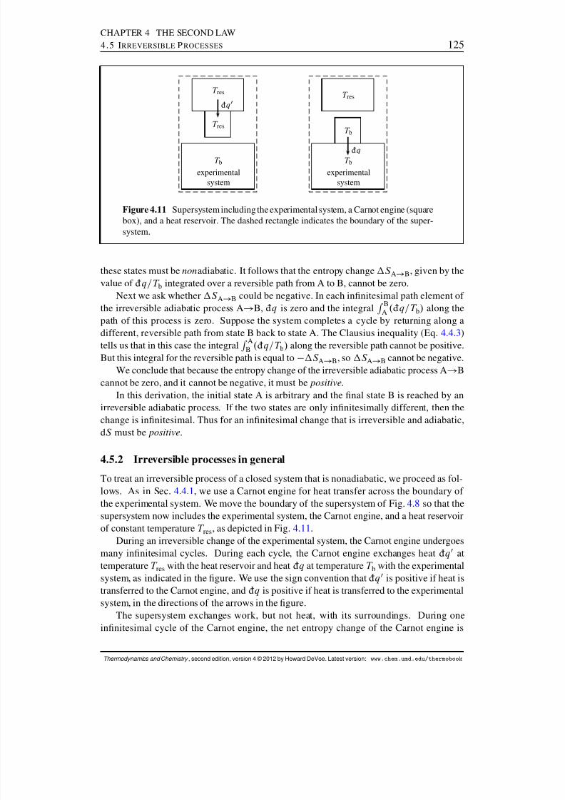
8/12/2019 Howard Devoe Thermodynamic and Chemical
http://slidepdf.com/reader/full/howard-devoe-thermodynamic-and-chemical 125/532
CHAPTER 4 THE SECOND LAW4.5 I RREVERSIBLE P ROCESSES 125
T bexperimental
system
T res
T res
¶q 0
T bexperimental
system
T b
¶q
T res
Figure 4.11 Supersystem including the experimental system, a Carnot engine (squarebox), and a heat reservoir. The dashed rectangle indicates the boundary of the super-system.
these states must be non adiabatic. It follows that the entropy change S A! B , given by thevalue of ¶q=T b integrated over a reversible path from A to B, cannot be zero.
Next we ask whether S A! B could be negative. In each innitesimal path element of the irreversible adiabatic process A ! B, ¶q is zero and the integral R
BA .¶q=T b/ along the
path of this process is zero. Suppose the system completes a cycle by returning along adifferent, reversible path from state B back to state A. The Clausius inequality (Eq. 4.4.3 )tells us that in this case the integral R
AB .¶q=T b/ along the reversible path cannot be positive.
But this integral for the reversible path is equal to S A! B , so S A! B cannot be negative.We conclude that because the entropy change of the irreversible adiabatic process A ! B
cannot be zero, and it cannot be negative, it must be positive .In this derivation, the initial state A is arbitrary and the nal state B is reached by an
irreversible adiabatic process. If the two states are only innitesimally different, then the
change is innitesimal. Thus for an innitesimal change that is irreversible and adiabatic,dS must be positive .
4.5.2 Irreversible processes in general
To treat an irreversible process of a closed system that is nonadiabatic, we proceed as fol-lows. As in Sec. 4.4.1 , we use a Carnot engine for heat transfer across the boundary of the experimental system. We move the boundary of the supersystem of Fig. 4.8 so that thesupersystem now includes the experimental system, the Carnot engine, and a heat reservoirof constant temperature T res , as depicted in Fig. 4.11 .
During an irreversible change of the experimental system, the Carnot engine undergoesmany innitesimal cycles. During each cycle, the Carnot engine exchanges heat ¶q 0 attemperature T res with the heat reservoir and heat ¶q at temperature T b with the experimentalsystem, as indicated in the gure. We use the sign convention that ¶q 0 is positive if heat istransferred to the Carnot engine, and ¶q is positive if heat is transferred to the experimentalsystem, in the directions of the arrows in the gure.
The supersystem exchanges work, but not heat, with its surroundings. During oneinnitesimal cycle of the Carnot engine, the net entropy change of the Carnot engine is
Thermodynamics and Chemistry , second edition, version 4 © 2012 by Howard DeVoe. Latest version: www.chem.umd.edu/thermobook
8/12/2019 Howard Devoe Thermodynamic and Chemical
http://slidepdf.com/reader/full/howard-devoe-thermodynamic-and-chemical 126/532
CHAPTER 4 THE SECOND LAW4.6 A PPLICATIONS 126
zero, the entropy change of the experimental system is d S , the heat transferred between theCarnot engine and the experimental system is ¶q , and the heat transferred between the heatreservoir and the Carnot engine is given by ¶q 0 D T res ¶q=T b (Eq. 4.4.1 ). The heat transferbetween the heat reservoir and Carnot engine is reversible, so the entropy change of the heatreservoir is
dS res D ¶q 0
T res D ¶qT b (4.5.1)
The entropy change of the supersystem is the sum of the entropy changes of its parts:
dS ss D dS CdS res D dS ¶qT b
(4.5.2)
The process within the supersystem is adiabatic and includes an irreversible change withinthe experimental system, so according to the conclusions of Sec. 4.5.1 , dS ss is positive.Equation 4.5.2 then shows that d S , the innitesimal entropy change during the irreversiblechange of the experimental system, must be greater than ¶q=T b:
dS > ¶qT b
(4.5.3)(irreversible change, closed system)
This relation includes the case of an irreversible adiabatic change, because it shows that if ¶q is zero, d S is greater than zero.
By integrating both sides of Eq. 4.5.3 between the initial and nal states of the irre-versible process, we obtain a relation for the nite entropy change corresponding to manyinnitesimal cycles of the Carnot engine:
S > Z ¶qT b
(4.5.4)(irreversible process, closed system)
4.6 APPLICATIONS
The lengthy derivation in Secs. 4.3–4.5 is based on the Kelvin–Planck statement describingthe impossibility of converting completely into work the energy transferred into the sys-tem by heat from a single heat reservoir. The derivation has now given us all parts of themathematical statement of the second law shown in the box on page 103 . The mathemati-cal statement includes an equality, d S D ¶q=T b , that applies to an innitesimal reversiblechange, and an inequality, d S > ¶q=T b , that applies to an innitesimal irreversible change.It is convenient to combine the equality and inequality in a single relation that is a generalmathematical statement of the second law:
dS ¶qT b
(4.6.1)( irrev
rev , closed system)
The inequality refers to an irreversible change and the equality to a reversible change, asindicated by the notation irrev
rev in the conditions of validity. The integrated form of this
Thermodynamics and Chemistry , second edition, version 4 © 2012 by Howard DeVoe. Latest version: www.chem.umd.edu/thermobook
8/12/2019 Howard Devoe Thermodynamic and Chemical
http://slidepdf.com/reader/full/howard-devoe-thermodynamic-and-chemical 127/532
CHAPTER 4 THE SECOND LAW4.6 A PPLICATIONS 127
relation is
S Z ¶qT b
(4.6.2)( irrev
rev , closed system)
During a reversible process, the states are equilibrium states and the temperature isusually uniform throughout the system. The only exception is if the system happens to haveinternal adiabatic partitions that allow phases of different temperatures in an equilibriumstate. As mentioned in the footnote on page 103, when the process is reversible and thetemperature is uniform, we can replace d S D ¶q=T b by dS D ¶q=T .
The rest of Sec. 4.6 will apply Eqs. 4.6.1 and 4.6.2 to various reversible and irreversibleprocesses.
4.6.1 Reversible heating
The denition of the heat capacity C of a closed system is given by Eq. 3.1.9 on page 62 :
C def
D ¶q= dT . For reversible heating or cooling of a homogeneous phase, ¶q is equal to
T dS and we can write
S DZ T 2
T 1
C T
dT (4.6.3)
where C should be replaced by C V if the volume is constant, or by C p if the pressure isconstant (Sec. 3.1.5 ). If the heat capacity has a constant value over the temperature rangefrom T 1 to T 2 , the equation becomes
S D C lnT 2T 1
(4.6.4)
Heating increases the entropy, and cooling decreases it.
4.6.2 Reversible expansion of an ideal gas
When the volume of an ideal gas, or of any other uid, is changed reversibly and adiabati-cally , there is of course no entropy change.
When the volume of an ideal gas is changed reversibly and isothermally , there is expan-sion work given by w D nRT ln.V 2 =V 1 / (Eq. 3.5.1 ). Since the internal energy of an idealgas is constant at constant temperature, there must be heat of equal magnitude and oppositesign: q D nRT ln.V 2 =V 1 / . The entropy change is therefore
S D nR lnV 2V 1
(4.6.5)(reversible isothermal volume
change of an ideal gas)
Isothermal expansion increases the entropy, and isothermal compression decreases it.Since the change of a state function depends only on the initial and nal states, Eq. 4.6.5
gives a valid expression for S of an ideal gas under the less stringent condition T 2 D T 1 ; itis not necessary for the intermediate states to be equilibrium states of the same temperature.
Thermodynamics and Chemistry , second edition, version 4 © 2012 by Howard DeVoe. Latest version: www.chem.umd.edu/thermobook
8/12/2019 Howard Devoe Thermodynamic and Chemical
http://slidepdf.com/reader/full/howard-devoe-thermodynamic-and-chemical 128/532
CHAPTER 4 THE SECOND LAW4.6 A PPLICATIONS 128
4.6.3 Spontaneous changes in an isolated system
An isolated system is one that exchanges no matter or energy with its surroundings. Anychange of state of an isolated system that actually occurs is spontaneous, and arises solelyfrom conditions within the system, uninuenced by changes in the surroundings—the pro-cess occurs by itself, of its own accord. The initial state and the intermediate states of the
process must be nonequilibrium states, because by denition an equilibrium state would notchange over time in the isolated system.
Unless the spontaneous change is purely mechanical, it is irreversible. According tothe second law, during an innitesimal change that is irreversible and adiabatic, the entropyincreases. For the isolated system, we can therefore write
dS > 0 (4.6.6)(irreversible change, isolated system)
In later chapters, the inequality of Eq. 4.6.6 will turn out to be one of the most useful forderiving conditions for spontaneity and equilibrium in chemical systems: The entropy of anisolated system continuously increases during a spontaneous, irreversible process until it reaches a maximum value at equilibrium .
If we treat the universe as an isolated system (although cosmology provides no assur-ance that this is a valid concept), we can say that as spontaneous changes occur in theuniverse, its entropy continuously increases. Clausius summarized the rst and second lawsin a famous statement: Die Energie der Welt ist constant; die Entropie der Welt strebt einem Maximum zu (the energy of the universe is constant; the entropy of the universe strivestoward a maximum).
4.6.4 Internal heat ow in an isolated system
Suppose the system is a solid body whose temperature initially is nonuniform. Provided
there are no internal adiabatic partitions, the initial state is a nonequilibrium state lackinginternal thermal equilibrium. If the system is surrounded by thermal insulation, and volumechanges are negligible, this is an isolated system. There will be a spontaneous, irreversibleinternal redistribution of thermal energy that eventually brings the system to a nal equilib-rium state of uniform temperature.
In order to be able to specify internal temperatures at any instant, we treat the systemas an assembly of phases, each having a uniform temperature that can vary with time. Todescribe a region that has a continuous temperature gradient, we approximate the regionwith a very large number of very small phases, each having a temperature innitesimallydifferent from its neighbors.
We use Greek letters to label the phases. The temperature of phase ’ at any given
instant is T ’
. We can treat each phase as a subsystem with a boundary across which therecan be energy transfer in the form of heat. Let ¶q ’“ represent an innitesimal quantity of heat transferred during an innitesimal interval of time to phase ’ from phase “ . The heattransfer, if any, is to the cooler from the warmer phase. If phases ’ and “ are in thermalcontact and T ’ is less than T “ , then ¶q ’“ is positive; if the phases are in thermal contactand T ’ is greater than T “ , ¶q ’“ is negative; and if neither of these conditions is satised,¶q ’“ is zero.
Thermodynamics and Chemistry , second edition, version 4 © 2012 by Howard DeVoe. Latest version: www.chem.umd.edu/thermobook
8/12/2019 Howard Devoe Thermodynamic and Chemical
http://slidepdf.com/reader/full/howard-devoe-thermodynamic-and-chemical 129/532
CHAPTER 4 THE SECOND LAW4.6 A PPLICATIONS 129
To evaluate the entropy change, we need a reversible path from the initial to the nalstate. The net quantity of heat transferred to phase ’ during an innitesimal time intervalis ¶q ’ DP“ ¤ ’ ¶q ’“ . The entropy change of phase ’ is the same as it would be for thereversible transfer of this heat from a heat reservoir of temperature T ’ : dS ’ D ¶q ’ =T ’ .The entropy change of the entire system along the reversible path is found by summing over
all phases:
dS DX’dS ’ DX’
¶q ’
T ’ DX’ X“ ¤ ’
¶q ’“
T ’
DX’ X“>’
¶q ’“
T ’ C¶q “’
T “ (4.6.7)
There is also the condition of quantitative energy transfer, ¶q “’ D ¶q ’“ , which we useto rewrite Eq. 4.6.7 in the form
dS D
X’
X“>’
1T ’
1T “
¶q ’“ (4.6.8)
Consider an individual term of the sum on the right side of Eq. 4.6.8 that has a nonzerovalue of ¶q ’“ due to nite heat transfer between phases ’ and “ . If T ’ is less than T “ , thenboth ¶q ’“ and .1=T ’ 1=T “ / are positive. If, on the other hand, T ’ is greater than T “ ,both ¶q ’“ and .1=T ’ 1=T “ / are negative. Thus each term of the sum is either zero orpositive, and as long as phases of different temperature are present, d S is positive.
This derivation shows that during a spontaneous thermal equilibration process in an iso-lated system, starting with any initial distribution of the internal temperatures, the entropycontinuously increases until the system reaches a state of thermal equilibrium with a singleuniform temperature throughout. 10 The result agrees with Eq. 4.6.6 .
4.6.5 Free expansion of a gas
Consider the free expansion of a gas shown in Fig. 3.8 on page 79 . The system is the gas.Assume that the vessel walls are rigid and adiabatic, so that the system is isolated. When thestopcock between the two vessels is opened, the gas expands irreversibly into the vacuumwithout heat or work and at constant internal energy. To carry out the same change of statereversibly, we conne the gas at its initial volume and temperature in a cylinder-and-pistondevice and use the piston to expand the gas adiabatically with negative work. Positiveheat is then needed to return the internal energy reversibly to its initial value. Because thereversible path has positive heat, the entropy change is positive.
This is an example of an irreversible process in an isolated system for which a reversiblepath between the initial and nal states has both heat and work.
4.6.6 Adiabatic process with work
In general (page 95), an adiabatic process with a given initial equilibrium state and a givenchange of a work coordinate has the least positive or most negative work in the reversible
10 Leff, in Ref. [ 98], obtains the same result by a more complicated derivation.
Thermodynamics and Chemistry , second edition, version 4 © 2012 by Howard DeVoe. Latest version: www.chem.umd.edu/thermobook
8/12/2019 Howard Devoe Thermodynamic and Chemical
http://slidepdf.com/reader/full/howard-devoe-thermodynamic-and-chemical 130/532
CHAPTER 4 THE SECOND LAW4.7 S UMMARY 130
limit. Consider an irreversible adiabatic process with work w irr . The same change of statecan be accomplished reversibly by the following two steps: (1) a reversible adiabatic changeof the work coordinate with work wrev , followed by (2) reversible transfer of heat qrev withno further change of the work coordinate. Since wrev is algebraically less than wirr , qrevmust be positive in order to make U the same in the irreversible and reversible paths.
The positive heat increases the entropy along the reversible path, and consequently theirreversible adiabatic process has a positive entropy change. This conclusion agrees withthe second-law inequality of Eq. 4.6.1 .
4.7 SUMMARY
Some of the important terms and denitions discussed in this chapter are as follows.
Any conceivable process is either spontaneous, reversible, or impossible.
A reversible process proceeds by a continuous sequence of equilibrium states.
A spontaneous process is one that proceeds naturally at a nite rate.
An irreversible process is a spontaneous process whose reverse is impossible.
A purely mechanical process is an idealized process without temperature gradients,and without friction or other dissipative effects, that is spontaneous in either direction.This kind of process will be ignored in the remaining chapters of this book.
Except for a purely mechanical process, the terms spontaneous and irreversible areequivalent.
The derivation of the mathematical statement of the second law shows that during areversible process of a closed system, the innitesimal quantity ¶q=T b equals the innites-imal change of a state function called the entropy, S . Here ¶q is heat transferred at theboundary where the temperature is T b .
In each innitesimal path element of a process of a closed system, d S is equal to ¶q=T bif the process is reversible, and is greater than ¶q=T b if the process is irreversible, as sum-marized by the relation d S ¶q=T b .
Consider two particular equilibrium states 1 and 2 of a closed system. The system canchange from state 1 to state 2 by either a reversible process, with S equal to the integral
R .¶q=T b/ , or an irreversible process, with S greater than R .¶q=T b/ . It is important tokeep in mind the point made by Fig. 4.12 on the next page : because S is a state function, itis the value of the integral that is different in the two cases, and not the value of S .
The second law establishes no general relation between entropy changes and heat in anopen system, or for an impossible process. The entropy of an open system may increase ordecrease depending on whether matter enters or leaves. It is possible to imagine differentimpossible processes in which d S is less than, equal to, and greater than ¶q=T b .
4.8 THE STATISTICAL INTERPRETATION OF ENTROPY
Because entropy is such an important state function, it is natural to seek a description of itsmeaning on the microscopic level.
Entropy is sometimes said to be a measure of “disorder.” According to this idea, theentropy increases whenever a closed system becomes more disordered on a microscopic
Thermodynamics and Chemistry , second edition, version 4 © 2012 by Howard DeVoe. Latest version: www.chem.umd.edu/thermobook

8/12/2019 Howard Devoe Thermodynamic and Chemical
http://slidepdf.com/reader/full/howard-devoe-thermodynamic-and-chemical 131/532
CHAPTER 4 THE SECOND LAW4.8 T HE S TATISTICAL INTERPRETATION OF E NTROPY 131
state 1 state 2
reversible
R ¶q=T b D S
irreversible
R ¶q=T b < S
Figure 4.12 Reversible and irreversible paths between the same initial and nal equi-librium states of a closed system. The value of S is the same for both paths, but thevalues of the integral R .¶q=T b/ are different.
scale. This description of entropy as a measure of disorder is highly misleading. It does notexplain why entropy is increased by reversible heating at constant volume or pressure, orwhy it increases during the reversible isothermal expansion of an ideal gas. Nor does it seemto agree with the freezing of a supercooled liquid or the formation of crystalline solute in asupersaturated solution; these processes can take place spontaneously in an isolated system,yet are accompanied by an apparent decrease of disorder.
Thus we should not interpret entropy as a measure of disorder. We must look elsewherefor a satisfactory microscopic interpretation of entropy.
A rigorous interpretation is provided by the discipline of statistical mechanics , whichderives a precise expression for entropy based on the behavior of macroscopic amounts of microscopic particles. Suppose we focus our attention on a particular macroscopic equilib-rium state. Over a period of time, while the system is in this equilibrium state, the systemat each instant is in a microstate , or stationary quantum state, with a denite energy. Themicrostate is one that is accessible to the system—that is, one whose wave function is com-patible with the system’s volume and with any other conditions and constraints imposedon the system. The system, while in the equilibrium state, continually jumps from one ac-
cessible microstate to another, and the macroscopic state functions described by classicalthermodynamics are time averages of these microstates.
The fundamental assumption of statistical mechanics is that accessible microstates of equal energy are equally probable, so that the system while in an equilibrium state spends anequal fraction of its time in each such microstate. The statistical entropy of the equilibriumstate then turns out to be given by the equation
S stat D k ln W CC (4.8.1)
where k is the Boltzmann constant k D R=N A , W is the number of accessible microstates,and C is a constant.
In the case of an equilibrium state of a perfectly-isolated system of constant internalenergy U , the accessible microstates are the ones that are compatible with the constraintsand whose energies all have the same value, equal to the value of U .
It is more realistic to treat an equilibrium state with the assumption the system is in ther-mal equilibrium with an external constant-temperature heat reservoir. The internal energythen uctuates over time with extremely small deviations from the average value U , and theaccessible microstates are the ones with energies close to this average value. In the language
Thermodynamics and Chemistry , second edition, version 4 © 2012 by Howard DeVoe. Latest version: www.chem.umd.edu/thermobook
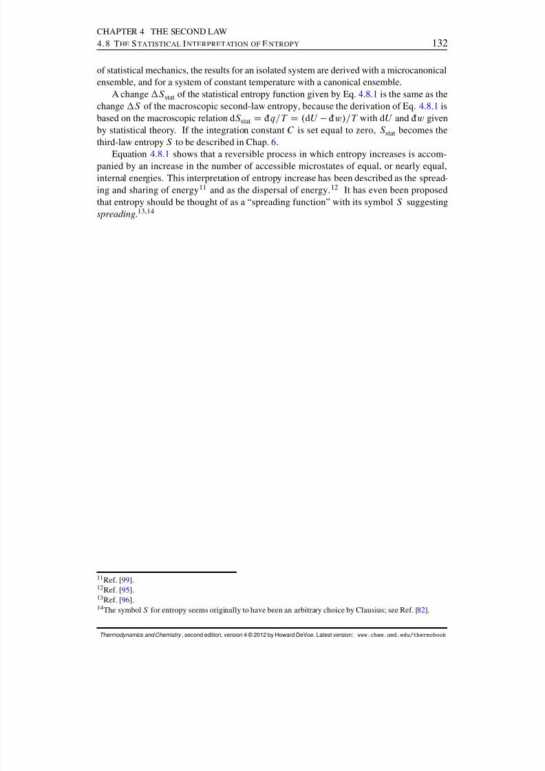
8/12/2019 Howard Devoe Thermodynamic and Chemical
http://slidepdf.com/reader/full/howard-devoe-thermodynamic-and-chemical 132/532
CHAPTER 4 THE SECOND LAW4.8 T HE S TATISTICAL INTERPRETATION OF E NTROPY 132
of statistical mechanics, the results for an isolated system are derived with a microcanonicalensemble, and for a system of constant temperature with a canonical ensemble.
A change S stat of the statistical entropy function given by Eq. 4.8.1 is the same as thechange S of the macroscopic second-law entropy, because the derivation of Eq. 4.8.1 isbased on the macroscopic relation d S stat D ¶q=T D . dU ¶w/=T with d U and ¶w given
by statistical theory. If the integration constant C is set equal to zero, S stat becomes thethird-law entropy S to be described in Chap. 6.Equation 4.8.1 shows that a reversible process in which entropy increases is accom-
panied by an increase in the number of accessible microstates of equal, or nearly equal,internal energies. This interpretation of entropy increase has been described as the spread-ing and sharing of energy 11 and as the dispersal of energy. 12 It has even been proposedthat entropy should be thought of as a “spreading function” with its symbol S suggestingspreading .13,14
11 Ref. [ 99].12 Ref. [ 95].13 Ref. [ 96].14 The symbol S for entropy seems originally to have been an arbitrary choice by Clausius; see Ref. [ 82].
Thermodynamics and Chemistry , second edition, version 4 © 2012 by Howard DeVoe. Latest version: www.chem.umd.edu/thermobook
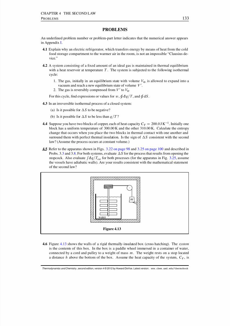
8/12/2019 Howard Devoe Thermodynamic and Chemical
http://slidepdf.com/reader/full/howard-devoe-thermodynamic-and-chemical 133/532
CHAPTER 4 THE SECOND LAWPROBLEMS 133
PROBLEMS
An underlined problem number or problem-part letter indicates that the numerical answer appearsin Appendix I.
4.1 Explain why an electric refrigerator, which transfers energy by means of heat from the coldfood storage compartment to the warmer air in the room, is not an impossible “Clausius de-vice.”
4.2 A system consisting of a xed amount of an ideal gas is maintained in thermal equilibriumwith a heat reservoir at temperature T . The system is subjected to the following isothermalcycle:
1. The gas, initially in an equilibrium state with volume V 0 , is allowed to expand into avacuum and reach a new equilibrium state of volume V 0.
2. The gas is reversibly compressed from V 0 to V 0 .
For this cycle, nd expressions or values for w , H ¶q=T , and H dS .
4.3 In an irreversible isothermal process of a closed system:
(a) Is it possible for S to be negative?
(b) Is it possible for S to be less than q=T ?
4.4 Suppose you have two blocks of copper, each of heat capacity C V D 200:0 J K 1 . Initially oneblock has a uniform temperature of 300:00 K and the other 310:00 K. Calculate the entropychange that occurs when you place the two blocks in thermal contact with one another andsurround them with perfect thermal insulation. Is the sign of S consistent with the secondlaw? (Assume the process occurs at constant volume.)
4.5 Refer to the apparatus shown in Figs. 3.22 on page 98 and 3.25 on page 100 and described inProbs. 3. 3 and 3.8. For both systems, evaluate S for the process that results from opening thestopcock. Also evaluate R ¶q=T ext for both processes (for the apparatus in Fig. 3.25, assumethe vessels have adiabatic walls). Are your results consistent with the mathematical statementof the second law?
water
Figure 4.13
4.6 Figure 4.13 shows the walls of a rigid thermally-insulated box (cross hatching). The systemis the contents of this box. In the box is a paddle wheel immersed in a container of water,connected by a cord and pulley to a weight of mass m . The weight rests on a stop locateda distance h above the bottom of the box. Assume the heat capacity of the system, C V , is
Thermodynamics and Chemistry , second edition, version 4 © 2012 by Howard DeVoe. Latest version: www.chem.umd.edu/thermobook
8/12/2019 Howard Devoe Thermodynamic and Chemical
http://slidepdf.com/reader/full/howard-devoe-thermodynamic-and-chemical 134/532
CHAPTER 4 THE SECOND LAWPROBLEMS 134
independent of temperature. Initially the system is in an equilibrium state at temperature T 1 .When the stop is removed, the weight irreversibly sinks to the bottom of the box, causing thepaddle wheel to rotate in the water. Eventually the system reaches a nal equilibrium statewith thermal equilibrium. Describe a reversible process with the same entropy change as thisirreversible process, and derive a formula for S in terms of m, h, C V , and T 1 .
Thermodynamics and Chemistry , second edition, version 4 © 2012 by Howard DeVoe. Latest version: www.chem.umd.edu/thermobook
8/12/2019 Howard Devoe Thermodynamic and Chemical
http://slidepdf.com/reader/full/howard-devoe-thermodynamic-and-chemical 135/532
C HAPTER 5
T HERMODYNAMIC POTENTIALS
This chapter begins with a discussion of mathematical properties of the total differentialof a dependent variable. Three extensive state functions with dimensions of energy are in-troduced: enthalpy, Helmholtz energy, and Gibbs energy. These functions, together withinternal energy, are called thermodynamic potentials .1 Some formal mathematical ma-nipulations of the four thermodynamic potentials are described that lead to expressions forheat capacities, surface work, and criteria for spontaneity in closed systems.
5.1 TOTAL DIFFERENTIAL OF A DEPENDENT VARIABLE
Recall from Sec. 2.4.1 that the state of the system at each instant is dened by a certainminimum number of state functions, the independent variables. State functions not treatedas independent variables are dependent variables. Innitesimal changes in any of the inde-pendent variables will, in general, cause an innitesimal change in each dependent variable.
A dependent variable is a function of the independent variables. The total differen-tial of a dependent variable is an expression for the innitesimal change of the variable interms of the innitesimal changes of the independent variables. As explained in Sec. F.2of Appendix F, the expression can be written as a sum of terms, one for each independentvariable. Each term is the product of a partial derivative with respect to one of the indepen-dent variables and the innitesimal change of that independent variable. For example, if thesystem has two independent variables, and we take these to be T and V , the expression forthe total differential of the pressure is
dp D@p@T V
dT C@p@V T
dV (5.1.1)
Thus, in the case of a xed amount of an ideal gas with pressure given by p D nRT=V ,the total differential of the pressure can be written
dp D nR
V dT
nRT V 2
dV (5.1.2)
1The term thermodynamic potential should not be confused with the chemical potential , , to be introduced onpage 137 .
135
8/12/2019 Howard Devoe Thermodynamic and Chemical
http://slidepdf.com/reader/full/howard-devoe-thermodynamic-and-chemical 136/532
CHAPTER 5 THERMODYNAMIC POTENTIALS5.2 T OTAL D IFFERENTIAL OF THE INTERNAL E NERGY 136
5.2 TOTAL DIFFERENTIAL OF THE INTERNAL ENERGY
For a closed system undergoing processes in which the only kind of work is expansion work,the rst law becomes d U D ¶q C¶w D ¶q p b dV . Since it will often be useful to makea distinction between expansion work and other kinds of work, this book will sometimeswrite the rst law in the form
dU D ¶q p b dV C¶w 0 (5.2.1)(closed system)
where ¶w 0 is nonexpansion work —that is, any thermodynamic work that is not expansionwork.
Consider a closed system of one chemical component (e.g., a pure substance) in a singlehomogeneous phase. The only kind of work is expansion work, with V as the work variable.This kind of system has two independent variables (Sec. 2.4.3 ). During a reversible processin this system, the heat is ¶q D T dS , the work is ¶w D p dV , and an innitesimalinternal energy change is given by
dU D T dS p dV (5.2.2)(closed system, C D1,
P D1, ¶w 0D0)
In the conditions of validity shown next to this equation, C D1 means there is one compo-nent ( C is the number of components) and P D1 means there is one phase ( P is the numberof phases).
The appearance of the intensive variables T and p in Eq. 5.2.2 implies, of course, thatthe temperature and pressure are uniform throughout the system during the process. If theywere not uniform, the phase would not be homogeneous and there would be more than twoindependent variables. The temperature and pressure are strictly uniform only if the process
is reversible; it is not necessary to include “reversible” as one of the conditions of validity.A real process approaches a reversible process in the limit of innite slowness. For all
practical purposes, therefore, we may apply Eq. 5.2.2 to a process obeying the conditionsof validity and taking place so slowly that the temperature and pressure remain essentiallyuniform—that is, for a process in which the system stays very close to thermal and mechan-ical equilibrium.
Because the system under consideration has two independent variables, Eq. 5.2.2 is anexpression for the total differential of U with S and V as the independent variables. Ingeneral, an expression for the differential d X of a state function X is a total differential if
1. it is a valid expression for d X , consistent with the physical nature of the system andany conditions and constraints;
2. it is a sum with the same number of terms as the number of independent variables;
3. each term of the sum is a function of state functions multiplied by the differential of one of the independent variables.
Note that the work coordinate of any kind of dissipative work—work without a re-versible limit—cannot appear in the expression for a total differential, because it is not astate function (Sec. 3.10).
Thermodynamics and Chemistry , second edition, version 4 © 2012 by Howard DeVoe. Latest version: www.chem.umd.edu/thermobook

8/12/2019 Howard Devoe Thermodynamic and Chemical
http://slidepdf.com/reader/full/howard-devoe-thermodynamic-and-chemical 137/532
CHAPTER 5 THERMODYNAMIC POTENTIALS5.2 T OTAL D IFFERENTIAL OF THE INTERNAL E NERGY 137
As explained in Appendix F, we may identify the coefcient of each term in an expres-sion for the total differential of a state function as a partial derivative of the function. Weidentify the coefcients on the right side of Eq. 5.2.2 as follows:
T D@U @S V
p D@U @V S
(5.2.3)
Now let us consider some of the ways a system might have more than two independentvariables. Suppose the system has one phase and one substance, with expansion work only, and is open so that the amount n of the substance can vary. Such a system has threeindependent variables. Let us write the formal expression for the total differential of U withS , V , and n as the three independent variables:
dU D@U @S V;n
dS C@U @V S;n
dV C@U @n S;V
dn (5.2.4)(pure substance,
P D1, ¶w 0D0)
We have seen above that if the system is closed , the partial derivatives are .@U=@S/V
D T
and .@U=@V /S D p . Since both of these partial derivatives are for a closed system inwhich n is constant, they are the same as the rst two partial derivatives on the right side of Eq. 5.2.4 .
The quantity given by the third partial derivative, .@U=@n/S;V , is represented by thesymbol (mu). This quantity is an intensive state function called the chemical potential .
With these substitutions, Eq. 5.2.4 becomes
dU D T dS p dV C dn (5.2.5)(pure substance,
P D1, ¶w 0D0)
and this is a valid expression for the total differential of U under the given conditions.If a single-phase system contains a mixture of s different substances, and the amount of
each substance can be varied independently, there are 2 Cs independent variables and thetotal differential of U can be written
dU D T dS p dV Cs
Xi D 1i dn i (5.2.6)
(P D1, ¶w 0D0)
The coefcient i is the chemical potential of substance i . We identify it as the partialderivative .@U=@ni / S;V;n j ¤ i
.Suppose that in addition to expansion work, other kinds of reversible work are possible.
Each work coordinate adds an additional independent variable. Thus, for a closed systemof one component in one phase, with reversible nonexpansion work given by ¶w 0 D Y dX ,the total differential of U becomes
dU D T dS p dV CY dX (5.2.7)(closed system,
C D1, P D1)
Thermodynamics and Chemistry , second edition, version 4 © 2012 by Howard DeVoe. Latest version: www.chem.umd.edu/thermobook
8/12/2019 Howard Devoe Thermodynamic and Chemical
http://slidepdf.com/reader/full/howard-devoe-thermodynamic-and-chemical 138/532
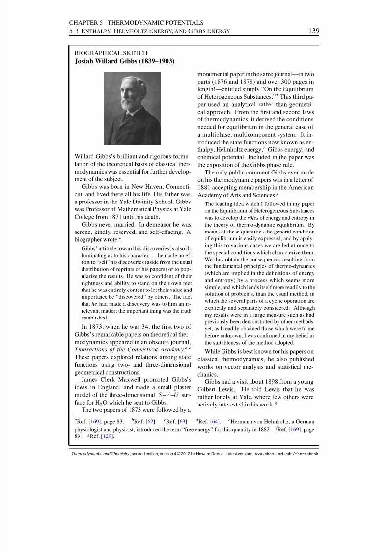
8/12/2019 Howard Devoe Thermodynamic and Chemical
http://slidepdf.com/reader/full/howard-devoe-thermodynamic-and-chemical 139/532
CHAPTER 5 THERMODYNAMIC POTENTIALS5.3 E NTHALPY , HELMHOLTZ E NERGY , A ND G IBBS E NERGY 139
BIOGRAPHICAL SKETCHJosiah Willard Gibbs (1839–1903)
Willard Gibbs’s brilliant and rigorous formu-lation of the theoretical basis of classical ther-modynamics was essential for further develop-ment of the subject.
Gibbs was born in New Haven, Connecti-cut, and lived there all his life. His father wasa professor in the Yale Divinity School. Gibbswas Professor of Mathematical Physics at YaleCollege from 1871 until his death.
Gibbs never married. In demeanor he wasserene, kindly, reserved, and self-effacing. Abiographer wrote: a
Gibbs’ attitude toward his discoveries is also il-luminating as to his character. . . . he made no ef-fort to “sell” his discoveries (aside from the usualdistribution of reprints of his papers) or to pop-ularize the results. He was so condent of theirrightness and ability to stand on their own feet
that he was entirely content to let their value andimportance be “discovered” by others. The factthat he had made a discovery was to him an ir-relevant matter; the important thing was the truthestablished.
In 1873, when he was 34, the rst two of Gibbs’s remarkable papers on theoretical ther-modynamics appeared in an obscure journal,Transactions of the Connecticut Academy .b ,c
These papers explored relations among statefunctions using two- and three-dimensionalgeometrical constructions.
James Clerk Maxwell promoted Gibbs’sideas in England, and made a small plastermodel of the three-dimensional S –V –U sur-face for H 2 O which he sent to Gibbs.
The two papers of 1873 were followed by a
monumental paper in the same journal—in twoparts (1876 and 1878) and over 300 pages inlength!—entitled simply “On the Equilibrium
of Heterogeneous Substances.” d This third pa-per used an analytical rather than geometri-cal approach. From the rst and second lawsof thermodynamics, it derived the conditionsneeded for equilibrium in the general case of a multiphase, multicomponent system. It in-troduced the state functions now known as en-thalpy, Helmholtz energy, e Gibbs energy, andchemical potential. Included in the paper wasthe exposition of the Gibbs phase rule.
The only public comment Gibbs ever madeon his thermodynamic papers was in a letter of 1881 accepting membership in the AmericanAcademy of Arts and Sciences: f
The leading idea which I followed in my paperon the Equilibrium of Heterogeneous Substanceswas to develop the r oles of energy and entropy inthe theory of thermo-dynamic equilibrium. Bymeans of these quantities the general conditionof equilibrium is easily expressed, and by apply-ing this to various cases we are led at once tothe special conditions which characterize them.We thus obtain the consequences resulting fromthe fundamental principles of thermo-dynamics(which are implied in the denitions of energyand entropy) by a process which seems more
simple, and which lends itself more readily to thesolution of problems, than the usual method, inwhich the several parts of a cyclic operation areexplicitly and separately considered. Althoughmy results were in a large measure such as hadpreviously been demonstrated by other methods,yet, as I readily obtained those which were to mebefore unknown, I was conrmed in my belief inthe suitableness of the method adopted.
While Gibbs is best known for his papers onclassical thermodynamics, he also publishedworks on vector analysis and statistical me-chanics.
Gibbs had a visit about 1898 from a youngGilbert Lewis. He told Lewis that he wasrather lonely at Yale, where few others wereactively interested in his work. g
a Ref. [ 169 ], page 83. bRef. [ 62]. cRef. [ 63]. d Ref. [ 64]. eHermann von Helmholtz, a Germanphysiologist and physicist, introduced the term “free energy” for this quantity in 1882. f Ref. [ 169 ], page89. gRef. [ 129 ].
Thermodynamics and Chemistry , second edition, version 4 © 2012 by Howard DeVoe. Latest version: www.chem.umd.edu/thermobook

8/12/2019 Howard Devoe Thermodynamic and Chemical
http://slidepdf.com/reader/full/howard-devoe-thermodynamic-and-chemical 140/532
CHAPTER 5 THERMODYNAMIC POTENTIALS5.4 C LOSED S YSTEMS 140
Thus, in a process at constant pressure (d p D 0) with expansion work only ( ¶w 0D0), wehave
dH D ¶q (5.3.7)(closed system, constant p ,
¶w 0
D0)
The enthalpy change under these conditions is equal to the heat. The integrated form of thisrelation is R dH DR ¶q , or
H D q (5.3.8)(closed system, constant p ,
w0D0)
Equation 5.3.7 is analogous to the following relation involving the internal energy, ob-tained from the rst law:
dU D ¶q (5.3.9)(closed system, constant V ,
¶w 0D0)
That is, in a process at constant volume with expansion work only, the internal energychange is equal to the heat.
5.4 CLOSED SYSTEMS
In order to nd expressions for the total differentials of H , A, and G in a closed systemwith one component in one phase, we must replace d U in Eqs. 5.3.4 –5.3.6 with
dU D T dS p dV (5.4.1)
to obtaindH D T dS CV dp (5.4.2)
dA D S dT p dV (5.4.3)
dG D S dT CV dp (5.4.4)
Equations 5.4.1 –5.4.4 are sometimes called the Gibbs equations . They are expressionsfor the total differentials of the thermodynamic potentials U , H , A , and G in closed sys-tems of one component in one phase with expansion work only. Each equation shows howthe dependent variable on the left side varies as a function of changes in two independentvariables (the natural variables of the dependent variable) on the right side.
By identifying the coefcients on the right side of Eqs. 5.4.1 –5.4.4 , we obtain the fol-
lowing relations (which again are valid for a closed system of one component in one phasewith expansion work only):
from Eq. 5.4.1 :@U @S V D T (5.4.5)
@U @V S D p (5.4.6)
Thermodynamics and Chemistry , second edition, version 4 © 2012 by Howard DeVoe. Latest version: www.chem.umd.edu/thermobook

8/12/2019 Howard Devoe Thermodynamic and Chemical
http://slidepdf.com/reader/full/howard-devoe-thermodynamic-and-chemical 141/532
8/12/2019 Howard Devoe Thermodynamic and Chemical
http://slidepdf.com/reader/full/howard-devoe-thermodynamic-and-chemical 142/532
CHAPTER 5 THERMODYNAMIC POTENTIALS5.5 O PE N S YSTEMS 142
dA D S dT p dV C dn (5.5.3)
dG D S dT CV dp C dn (5.5.4)
Note that these are the same as the four Gibbs equations (Eqs. 5.4.1 –5.4.4 ) with the additionof a term dn to allow for a change in the amount of substance.
Identication of the coefcient of the last term on the right side of each of these equa-tions shows that the chemical potential can be equated to four different partial derivatives:
D@U @n S;V D
@H @n S;p D
@A@n T;V D
@G@n T;p
(5.5.5)
All four of these partial derivatives must have the same value for a given state of the system;the value, of course, depends on what that state is.
The last partial derivative on the right side of Eq. 5.5.5 , .@G=@n/T;p , is especially in-teresting because it is the rate at which the Gibbs energy increases with the amount of sub-stance added to a system whose intensive properties remain constant. Thus, is revealedto be equal to Gm , the molar Gibbs energy of the substance.
Suppose the system contains several substances or species in a single phase (a mixture)whose amounts can be varied independently. We again assume the only work is expansionwork. Then, making use of Eq. 5.2.6 , we nd the total differentials of the thermodynamicpotentials are given by
dU D T dS p dV CXii dn i (5.5.6)
dH D T dS CV dp CXii dn i (5.5.7)
dA D S dT p dV CXii dn i (5.5.8)
dG D S dT CV dp CXii dn i (5.5.9)
The independent variables on the right side of each of these equations are the natural vari-ables of the corresponding thermodynamic potential. Section F.4 shows that all of the infor-mation contained in an algebraic expression for a state function is preserved in a Legendretransform of the function. What this means for the thermodynamic potentials is that anexpression for any one of them, as a function of its natural variables, can be converted toan expression for each of the other thermodynamic potentials as a function of its naturalvariables.
Willard Gibbs, after whom the Gibbs energy is named, called Eqs. 5.5.6 –5.5.9 the fun-damental equations of thermodynamics, because from any single one of them not only the
other thermodynamic potentials but also all thermal, mechanical, and chemical propertiesof the system can be deduced. 2 Problem 5. 4 illustrates this useful application of the totaldifferential of a thermodynamic potential.
2Ref. [ 64], p. 86.
Thermodynamics and Chemistry , second edition, version 4 © 2012 by Howard DeVoe. Latest version: www.chem.umd.edu/thermobook

8/12/2019 Howard Devoe Thermodynamic and Chemical
http://slidepdf.com/reader/full/howard-devoe-thermodynamic-and-chemical 143/532
CHAPTER 5 THERMODYNAMIC POTENTIALS5.6 E XPRESSIONS FOR H EAT C APACITY 143
In Eqs. 5.5.6 –5.5.9 , the coefcient i is the chemical potential of species i . The equa-tions show that i can be equated to four different partial derivatives, similar to the equali-ties shown in Eq. 5.5.5 for a pure substance:
i D@U @ni S;V;n j ¤ i
D@H @ni S;p;n j ¤ i
D @A@ni T;V;n j ¤ i
D@G@ni T;p;n j ¤ i
(5.5.10)
The partial derivative .@G=@ni / T;P;n j ¤ i is called the partial molar Gibbs energy of species
i , another name for the chemical potential as will be discussed in Sec. 9.2.6 .
5.6 EXPRESSIONS FOR HEAT CAPACITY
As explained in Sec. 3.1.5 , the heat capacity of a closed system is dened as the ratio of an innitesimal quantity of heat transferred across the boundary under specied conditions
and the resulting innitesimal temperature change: heat capacity def
D ¶q= dT . The heatcapacities of isochoric (constant volume) and isobaric (constant pressure) processes are of particular interest.
The heat capacity at constant volume , C V
, is the ratio ¶q= dT for a process in a closedconstant-volume system with no nonexpansion work—that is, no work at all. The rst lawshows that under these conditions the internal energy change equals the heat: d U D ¶q(Eq. 5.3.9 ). We can replace ¶q by dU and write C V as a partial derivative:
C V D@U @T V
(5.6.1)(closed system)
If the closed system has more than two independent variables, additional conditionsare needed to dene C V unambiguously. For instance, if the system is a gas mixturein which reaction can occur, we might specify that the system remains in reactionequilibrium as T changes at constant V .
Equation 5.6.1 does not require the condition ¶w 0
D0, because all quantities ap-
pearing in the equation are state functions whose relations to one another are xed bythe nature of the system and not by the path. Thus, if heat transfer into the systemat constant V causes U to increase at a certain rate with respect to T , and this rate isdened as C V , the performance of electrical work on the system at constant V willcause the same rate of increase of U with respect to T and can equally well be used toevaluate C V .
Note that C V is a state function whose value depends on the state of the system—thatis, on T , V , and any additional independent variables. C V is an extensive property: thecombination of two identical phases has twice the value of C V that one of the phases hasby itself.
For a phase containing a pure substance, the molar heat capacity at constant volumeis dened by C V; m
def
D C V =n . C V; m is an intensive property.If the system is an ideal gas, its internal energy depends only on T , regardless of whether
V is constant, and Eq. 5.6.1 can be simplied to
C V D dU dT
(5.6.2)(closed system, ideal gas)
Thermodynamics and Chemistry , second edition, version 4 © 2012 by Howard DeVoe. Latest version: www.chem.umd.edu/thermobook

8/12/2019 Howard Devoe Thermodynamic and Chemical
http://slidepdf.com/reader/full/howard-devoe-thermodynamic-and-chemical 144/532

8/12/2019 Howard Devoe Thermodynamic and Chemical
http://slidepdf.com/reader/full/howard-devoe-thermodynamic-and-chemical 145/532
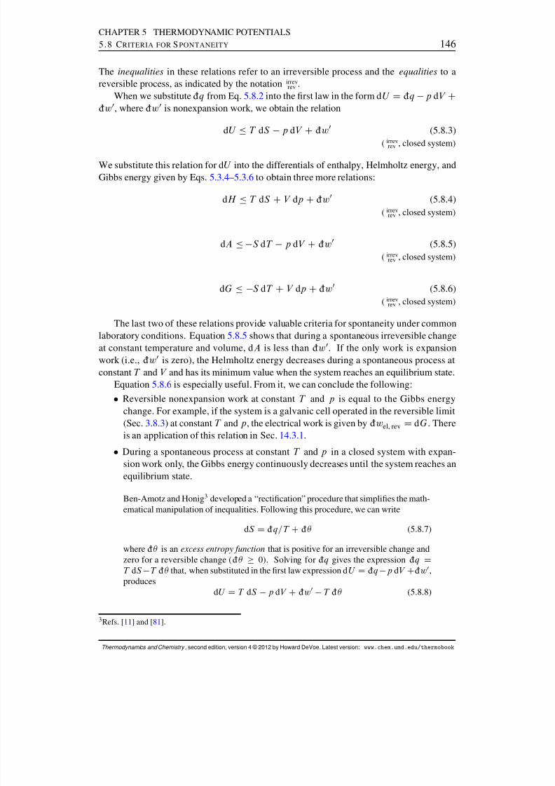
8/12/2019 Howard Devoe Thermodynamic and Chemical
http://slidepdf.com/reader/full/howard-devoe-thermodynamic-and-chemical 146/532
CHAPTER 5 THERMODYNAMIC POTENTIALS5.8 C RITERIA FOR S PONTANEITY 146
The inequalities in these relations refer to an irreversible process and the equalities to areversible process, as indicated by the notation irrev
rev .When we substitute ¶q from Eq. 5.8.2 into the rst law in the form d U D ¶q p dV C
¶w 0, where ¶w 0 is nonexpansion work, we obtain the relation
dU
T dS
p dV
C¶w 0 (5.8.3)
( irrevrev , closed system)
We substitute this relation for d U into the differentials of enthalpy, Helmholtz energy, andGibbs energy given by Eqs. 5.3.4 –5.3.6 to obtain three more relations:
dH T dS CV dp C¶w 0 (5.8.4)( irrev
rev , closed system)
dA S dT p dV C¶w 0 (5.8.5)( irrev
rev , closed system)
dG S dT CV dp C¶w 0 (5.8.6)( irrev
rev , closed system)
The last two of these relations provide valuable criteria for spontaneity under commonlaboratory conditions. Equation 5.8.5 shows that during a spontaneous irreversible changeat constant temperature and volume, d A is less than ¶w 0. If the only work is expansionwork (i.e., ¶w 0 is zero), the Helmholtz energy decreases during a spontaneous process atconstant T and V and has its minimum value when the system reaches an equilibrium state.
Equation 5.8.6 is especially useful. From it, we can conclude the following: Reversible nonexpansion work at constant T and p is equal to the Gibbs energy
change. For example, if the system is a galvanic cell operated in the reversible limit(Sec. 3.8.3 ) at constant T and p , the electrical work is given by ¶w el, rev D dG . Thereis an application of this relation in Sec. 14.3.1 .
During a spontaneous process at constant T and p in a closed system with expan-sion work only, the Gibbs energy continuously decreases until the system reaches anequilibrium state.
Ben-Amotz and Honig 3 developed a “rectication” procedure that simplies the math-ematical manipulation of inequalities. Following this procedure, we can write
dS D ¶q=T C¶ (5.8.7)
where ¶ is an excess entropy function that is positive for an irreversible change andzero for a reversible change ( ¶ 0). Solving for ¶q gives the expression ¶q DT dS T ¶ that, when substituted in the rst law expression d U D ¶q p dV C¶w 0,produces
dU D T dS p dV C¶w 0 T ¶ (5.8.8)
3Refs. [ 11 ] and [81].
Thermodynamics and Chemistry , second edition, version 4 © 2012 by Howard DeVoe. Latest version: www.chem.umd.edu/thermobook
8/12/2019 Howard Devoe Thermodynamic and Chemical
http://slidepdf.com/reader/full/howard-devoe-thermodynamic-and-chemical 147/532
CHAPTER 5 THERMODYNAMIC POTENTIALS5.8 C RITERIA FOR S PONTANEITY 147
The equality of this equation is equivalent to the combined equality and inequality of Eq. 5.8.3 . Then by substitution of this expression for d U into Eqs. 5.3.4–5.3.6 , weobtain equalities equivalent to Eqs. 5.8.4–5.8.6 , for example
dG D S dT CV dp C¶w 0 T ¶ (5.8.9)
Equation 5.8.9 tells us that during a process at constant T
and p
, with expansion work only ( ¶w 0D0), dG has the same sign as T ¶ : negative for an irreversible changeand zero for a reversible change.
Thermodynamics and Chemistry , second edition, version 4 © 2012 by Howard DeVoe. Latest version: www.chem.umd.edu/thermobook
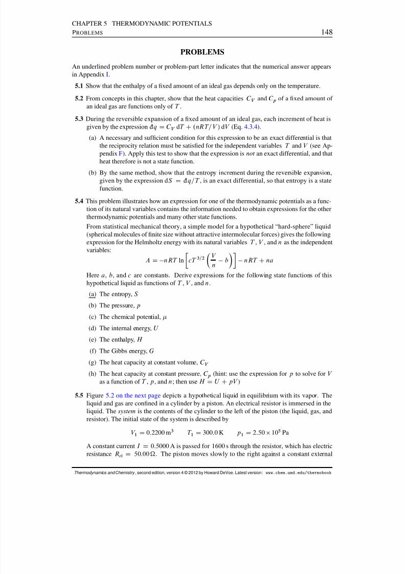
8/12/2019 Howard Devoe Thermodynamic and Chemical
http://slidepdf.com/reader/full/howard-devoe-thermodynamic-and-chemical 148/532
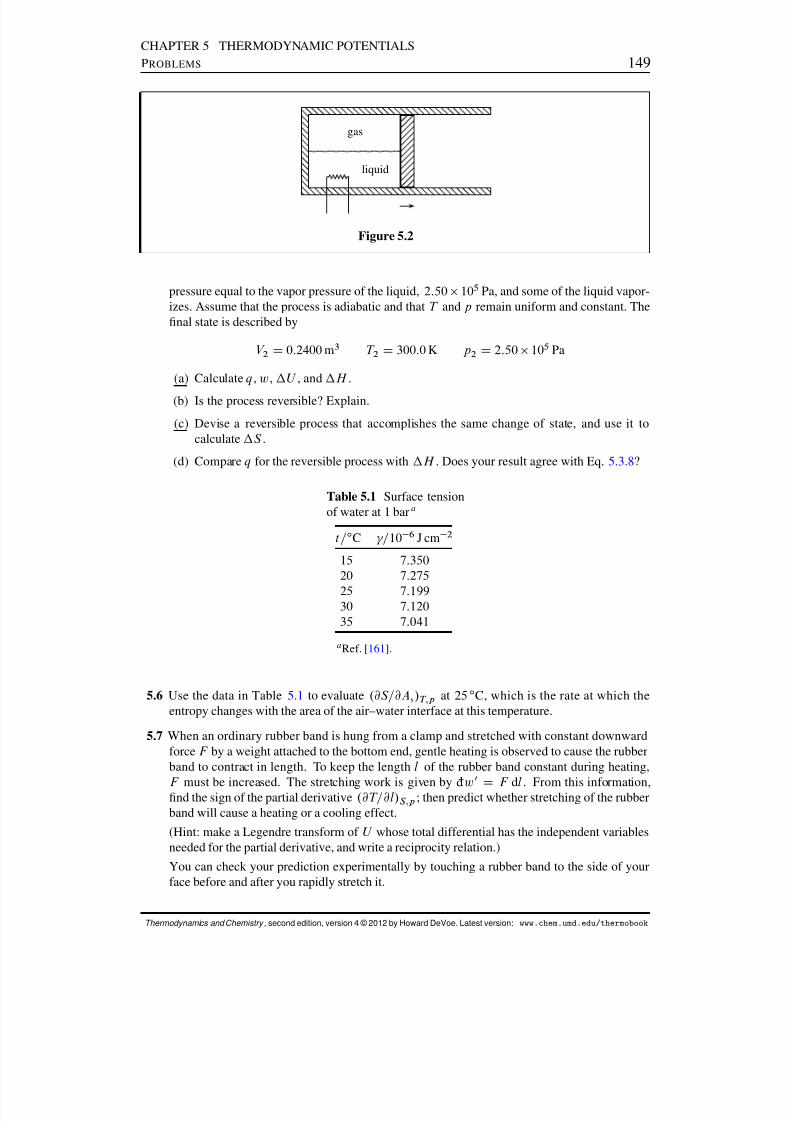
8/12/2019 Howard Devoe Thermodynamic and Chemical
http://slidepdf.com/reader/full/howard-devoe-thermodynamic-and-chemical 149/532
CHAPTER 5 THERMODYNAMIC POTENTIALSPROBLEMS 149
liquid
gas
Figure 5.2
pressure equal to the vapor pressure of the liquid, 2:50 105 Pa, and some of the liquid vapor-izes. Assume that the process is adiabatic and that T and p remain uniform and constant. Thenal state is described by
V 2 D 0:2400 m3 T 2 D 300:0 K p 2 D 2:50 105 Pa
(a) Calculate q , w , U , and H .
(b) Is the process reversible? Explain.
(c) Devise a reversible process that accomplishes the same change of state, and use it tocalculate S .
(d) Compare q for the reversible process with H . Does your result agree with Eq. 5.3.8?
Table 5.1 Surface tensionof water at 1 bar a
t=ı C =10 6 J cm 2
15 7:35020 7:27525 7:19930 7:12035 7:041
a Ref. [ 161 ].
5.6 Use the data in Table 5.1 to evaluate .@S=@As/ T;p at 25 ı C, which is the rate at which theentropy changes with the area of the air–water interface at this temperature.
5.7 When an ordinary rubber band is hung from a clamp and stretched with constant downwardforce F by a weight attached to the bottom end, gentle heating is observed to cause the rubberband to contract in length. To keep the length l of the rubber band constant during heating,
F must be increased. The stretching work is given by ¶w0
D F dl . From this information,nd the sign of the partial derivative .@T=@l/S;p ; then predict whether stretching of the rubberband will cause a heating or a cooling effect.
(Hint: make a Legendre transform of U whose total differential has the independent variablesneeded for the partial derivative, and write a reciprocity relation.)
You can check your prediction experimentally by touching a rubber band to the side of yourface before and after you rapidly stretch it.
Thermodynamics and Chemistry , second edition, version 4 © 2012 by Howard DeVoe. Latest version: www.chem.umd.edu/thermobook
8/12/2019 Howard Devoe Thermodynamic and Chemical
http://slidepdf.com/reader/full/howard-devoe-thermodynamic-and-chemical 150/532
C HAPTER 6
T HE THIRD LAW AND CRYOGENICS
The third law of thermodynamics concerns the entropy of perfectly-ordered crystals at zerokelvins.
When a chemical reaction or phase transition is studied at low temperatures, and allsubstances are pure crystals presumed to be perfectly ordered, the entropy change is foundto approach zero as the temperature approaches zero kelvins:
limT ! 0
S D 0 (6.0.1)(pure, perfectly-ordered crystals)
Equation 6.0.1 is the mathematical statement of the Nernst heat theorem 1 or third law of thermodynamics . It is true in general only if each reactant and product is a pure crystalwith identical unit cells arranged in perfect spatial order.
6.1 THE ZERO OF ENTROPY
There is no theoretical relation between the entropies of different chemical elements. Wecan arbitrarily choose the entropy of every pure crystalline element to be zero at zerokelvins. Then the experimental observation expressed by Eq. 6.0.1 requires that the entropyof every pure crystalline compound also be zero at zero kelvins, in order that the entropychange for the formation of a compound from its elements will be zero at this temperature.
A classic statement of the third law principle appears in the 1923 book Thermodynamicsand the Free Energy of Chemical Substances by G. N. Lewis and M. Randall: 2
“If the entropy of each element in some crystalline state be taken as zero at theabsolute zero of temperature: every substance has a nite positive entropy, but at the absolute zero of temperature the entropy may become zero, and does sobecome in the case of perfect crystalline substances .”
1 Nernst preferred to avoid the use of the entropy function and to use in its place the partialderivative .@A=@T /V (Eq. 5.4.9 ). The original 1906 version of his heat theorem was in the formlim T ! 0 .@ A=@T / V D0 (Ref. [ 39]).2Ref. [ 103 ], p. 448.
150
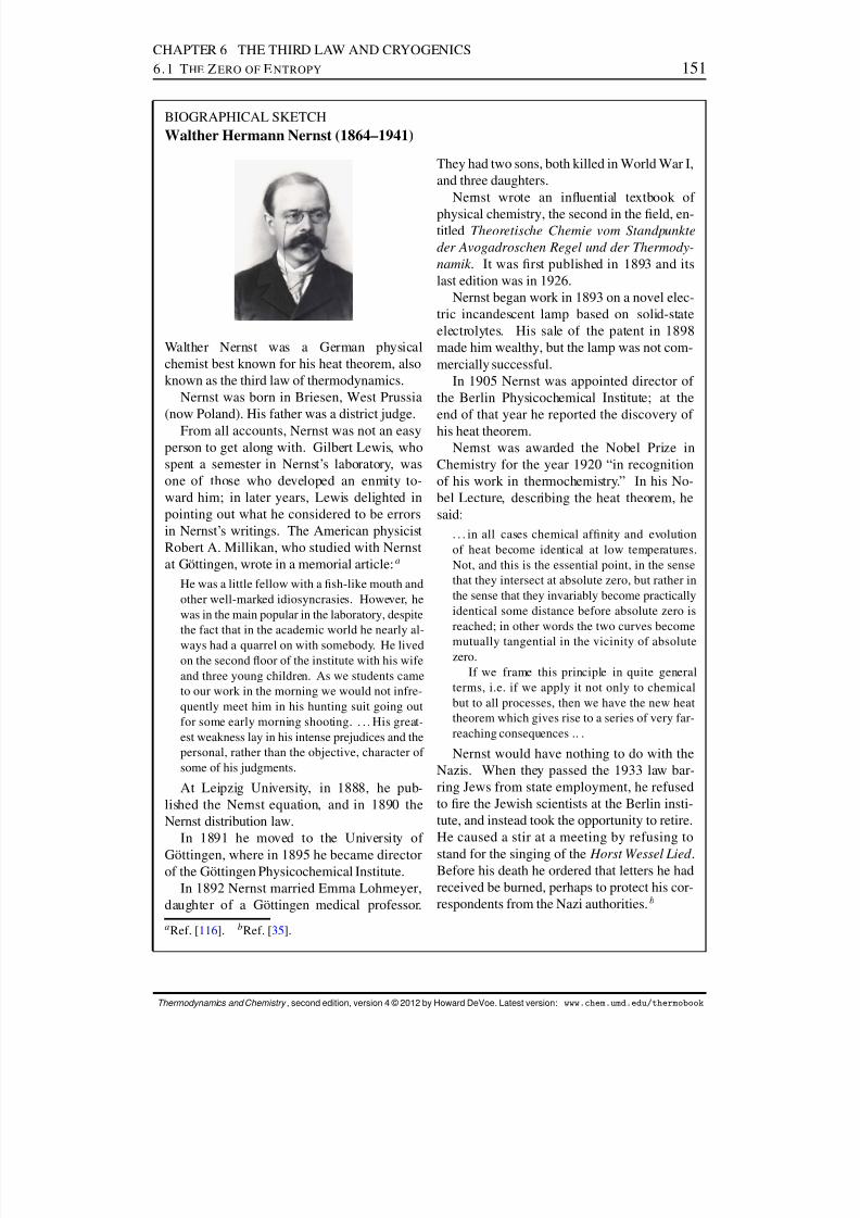
8/12/2019 Howard Devoe Thermodynamic and Chemical
http://slidepdf.com/reader/full/howard-devoe-thermodynamic-and-chemical 151/532
CHAPTER 6 THE THIRD LAW AND CRYOGENICS6.1 T HE Z ERO OF E NTROPY 151
BIOGRAPHICAL SKETCHWalther Hermann Nernst (1864–1941)
Walther Nernst was a German physicalchemist best known for his heat theorem, alsoknown as the third law of thermodynamics.
Nernst was born in Briesen, West Prussia(now Poland). His father was a district judge.
From all accounts, Nernst was not an easyperson to get along with. Gilbert Lewis, whospent a semester in Nernst’s laboratory, wasone of those who developed an enmity to-ward him; in later years, Lewis delighted inpointing out what he considered to be errorsin Nernst’s writings. The American physicistRobert A. Millikan, who studied with Nernstat Gottingen, wrote in a memorial article: a
He was a little fellow with a sh-like mouth andother well-marked idiosyncrasies. However, hewas in the main popular in the laboratory, despitethe fact that in the academic world he nearly al-ways had a quarrel on with somebody. He livedon the second oor of the institute with his wifeand three young children. As we students cameto our work in the morning we would not infre-quently meet him in his hunting suit going outfor some early morning shooting. . . . His great-est weakness lay in his intense prejudices and thepersonal, rather than the objective, character of some of his judgments.
At Leipzig University, in 1888, he pub-lished the Nernst equation, and in 1890 theNernst distribution law.
In 1891 he moved to the University of
Gottingen, where in 1895 he became directorof the G ottingen Physicochemical Institute.
In 1892 Nernst married Emma Lohmeyer,daughter of a G¨ottingen medical professor.
They had two sons, both killed in World War I,and three daughters.
Nernst wrote an inuential textbook of
physical chemistry, the second in the eld, en-titled Theoretische Chemie vom Standpunkteder Avogadroschen Regel und der Thermody-namik . It was rst published in 1893 and itslast edition was in 1926.
Nernst began work in 1893 on a novel elec-tric incandescent lamp based on solid-stateelectrolytes. His sale of the patent in 1898made him wealthy, but the lamp was not com-mercially successful.
In 1905 Nernst was appointed director of the Berlin Physicochemical Institute; at theend of that year he reported the discovery of his heat theorem.
Nernst was awarded the Nobel Prize inChemistry for the year 1920 “in recognitionof his work in thermochemistry.” In his No-bel Lecture, describing the heat theorem, hesaid:
. . . in all cases chemical afnity and evolutionof heat become identical at low temperatures.Not, and this is the essential point, in the sensethat they intersect at absolute zero, but rather inthe sense that they invariably become practicallyidentical some distance before absolute zero isreached; in other words the two curves become
mutually tangential in the vicinity of absolutezero.
If we frame this principle in quite generalterms, i.e. if we apply it not only to chemicalbut to all processes, then we have the new heattheorem which gives rise to a series of very far-reaching consequences .. .
Nernst would have nothing to do with theNazis. When they passed the 1933 law bar-ring Jews from state employment, he refusedto re the Jewish scientists at the Berlin insti-tute, and instead took the opportunity to retire.He caused a stir at a meeting by refusing to
stand for the singing of the Horst Wessel Lied .Before his death he ordered that letters he hadreceived be burned, perhaps to protect his cor-respondents from the Nazi authorities. b
a Ref. [ 116 ]. bRef. [ 35].
Thermodynamics and Chemistry , second edition, version 4 © 2012 by Howard DeVoe. Latest version: www.chem.umd.edu/thermobook
8/12/2019 Howard Devoe Thermodynamic and Chemical
http://slidepdf.com/reader/full/howard-devoe-thermodynamic-and-chemical 152/532
CHAPTER 6 THE THIRD LAW AND CRYOGENICS6.2 M OLAR E NTROPIES 152
According to this principle, every substance (element or compound) in a pure, perfectly-ordered crystal at 0 K, at any pressure, 3 has a molar entropy of zero:
S m(0 K) D 0 (6.1.1)(pure, perfectly-ordered crystal)
This convention establishes a scale of absolute entropies at temperatures above zero kelvinscalled third-law entropies , as explained in the next section.
6.2 MOLAR ENTROPIES
With the convention that the entropy of a pure, perfectly-ordered crystalline solid at zerokelvins is zero, we can establish the third-law value of the molar entropy of a pure substanceat any temperature and pressure. Absolute values of S m are what are usually tabulated forcalculational use.
6.2.1 Third-law molar entropies
Suppose we wish to evaluate the entropy of an amount n of a pure substance at a certaintemperature T 0 and a certain pressure. The same substance, in a perfectly-ordered crystal atzero kelvins and the same pressure, has an entropy of zero. The entropy at the temperatureand pressure of interest, then, is the entropy change S DR
T 0
0 ¶q=T of a reversible heatingprocess at constant pressure that converts the perfectly-ordered crystal at zero kelvins to thestate of interest.
Consider a reversible isobaric heating process of a pure substance while it exists in asingle phase. The denition of heat capacity as ¶q= dT (Eq. 3.1.9 ) allows us to substituteC p dT for ¶q , where C p is the heat capacity of the phase at constant pressure.
If the substance in the state of interest is a liquid or gas, or a crystal of a differentform than the perfectly-ordered crystal present at zero kelvins, the heating process willinclude one or more equilibrium phase transitions under conditions where two phases arein equilibrium at the same temperature and pressure (Sec. 2.2.2 ). For example, a reversibleheating process at a pressure above the triple point that transforms the crystal at 0 K to a gasmay involve transitions from one crystal form to another, and also melting and vaporizationtransitions.
Each such reversible phase transition requires positive heat qtrs . Because the pressureis constant, the heat is equal to the enthalpy change (Eq. 5.3.8 ). The ratio qtrs=n is calledthe molar heat or molar enthalpy of the transition, trs H (see Sec. 8.3.1 ). Because thephase transition is reversible, the entropy change during the transition is given by trs S Dqtrs=nT trs where T trs is the transition temperature.
With these considerations, we can write the following expression for the entropy change
of the entire heating process:
S DZ T 0
0
C pT
dT CX n trsH
T trs(6.2.1)
3The entropy becomes independent of pressure as T approaches zero kelvins. This behavior can be deducedfrom the relation .@S=@p/T D ˛V (Table 7.1 on page 178 ) combined with the experimental observation thatthe cubic expansion coefcient ˛ approaches zero as T approaches zero kelvins.
Thermodynamics and Chemistry , second edition, version 4 © 2012 by Howard DeVoe. Latest version: www.chem.umd.edu/thermobook
8/12/2019 Howard Devoe Thermodynamic and Chemical
http://slidepdf.com/reader/full/howard-devoe-thermodynamic-and-chemical 153/532
CHAPTER 6 THE THIRD LAW AND CRYOGENICS6.2 M OLAR E NTROPIES 153
The resulting operational equation for the calculation of the molar entropy of the substanceat the temperature and pressure of interest is
S m .T 0/ D S
n DZ T 0
0
C p; m
T dT CX
trs H T trs
(6.2.2)(pure substance,
constant p )
where C p; m D C p =n is the molar heat capacity at constant pressure. The summation is overeach equilibrium phase transition occurring during the heating process.
Since C p; m is positive at all temperatures above zero kelvins, and trsH is positivefor all transitions occurring during a reversible heating process, the molar entropy of asubstance is positive at all temperatures above zero kelvins.
The heat capacity and transition enthalpy data required to evaluate S m .T 0/ using Eq.6.2.2 come from calorimetry. The calorimeter can be cooled to about 10 K with liquidhydrogen, but it is difcult to make measurements below this temperature. Statistical me-chanical theory may be used to approximate the part of the integral in Eq. 6.2.2 betweenzero kelvins and the lowest temperature at which a value of C p; m can be measured. The ap-propriate formula for nonmagnetic nonmetals comes from the Debye theory for the latticevibration of a monatomic crystal. This theory predicts that at low temperatures (from 0 K toabout 30 K), the molar heat capacity at constant volume is proportional to T 3 : C V; m D aT 3 ,where a is a constant. For a solid, the molar heat capacities at constant volume and at con-stant pressure are practically equal. Thus for the integral on the right side of Eq. 6.2.2 wecan, to a good approximation, write
Z T 0
0
C p; m
T dT D a Z
T 00
0T 2 dT CZ
T 0
T 00
C p; m
T dT (6.2.3)
where T 00is the lowest temperature at which C p; m is measured. The rst term on the right
side of Eq. 6.2.3 isa Z
T 00
0T 2 dT D .aT 3 =3/ˇ
T 00
0 D a.T 00/ 3 =3 (6.2.4)
But a.T 00/ 3 is the value of C p; m at T 00, so Eq. 6.2.2 becomes
S m .T 0/ DC p; m .T 00/
3 CZ T 0
T 00
C p; m
T dT CX
trs H T trs
(6.2.5)(pure substance,
constant p )
In the case of a metal, statistical mechanical theory predicts an electronic contributionto the molar heat capacity, proportional to T at low temperature, that should be added
to the Debye T 3 term: C p; m D aT 3 CbT . The error in using Eq. 6.2.5 , which ignoresthe electronic term, is usually negligible if the heat capacity measurements are madedown to about 10 K.
We may evaluate the integral on the right side of Eq. 6.2.5 by numerical integration.We need the area under the curve of C p; m=T plotted as a function of T between some low
Thermodynamics and Chemistry , second edition, version 4 © 2012 by Howard DeVoe. Latest version: www.chem.umd.edu/thermobook
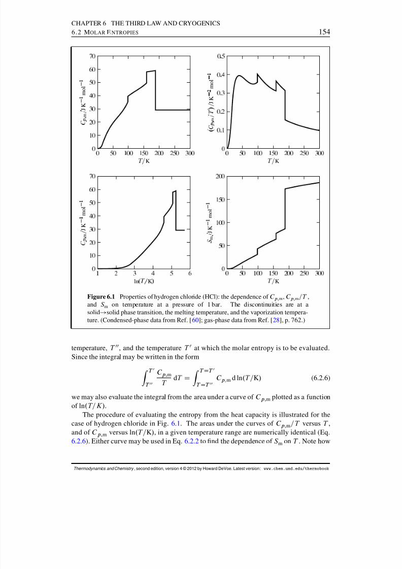
8/12/2019 Howard Devoe Thermodynamic and Chemical
http://slidepdf.com/reader/full/howard-devoe-thermodynamic-and-chemical 154/532
CHAPTER 6 THE THIRD LAW AND CRYOGENICS6.2 M OLAR E NTROPIES 154
K
m
J K
m o l
K
m
J K
m o l
ln
K
m
J K
m o l
K
m
J K
m o l
Figure 6.1 Properties of hydrogen chloride (HCl): the dependence of C p; m , C p; m=T ,and S m on temperature at a pressure of 1 bar. The discontinuities are at asolid! solid phase transition, the melting temperature, and the vaporization tempera-ture. (Condensed-phase data from Ref. [ 60]; gas-phase data from Ref. [ 28], p. 762.)
temperature, T 00, and the temperature T 0 at which the molar entropy is to be evaluated.Since the integral may be written in the form
Z T 0
T 00
C p; m
T dT DZ
T D T 0
T D T 00C p; m d ln .T =K/ (6.2.6)
we may also evaluate the integral from the area under a curve of C p; m plotted as a functionof ln .T=K/ .
The procedure of evaluating the entropy from the heat capacity is illustrated for thecase of hydrogen chloride in Fig. 6.1. The areas under the curves of C p; m=T versus T ,and of C p; m versus ln .T =K/ , in a given temperature range are numerically identical (Eq.6.2.6 ). Either curve may be used in Eq. 6.2.2 to nd the dependence of S m on T . Note how
Thermodynamics and Chemistry , second edition, version 4 © 2012 by Howard DeVoe. Latest version: www.chem.umd.edu/thermobook

8/12/2019 Howard Devoe Thermodynamic and Chemical
http://slidepdf.com/reader/full/howard-devoe-thermodynamic-and-chemical 155/532
CHAPTER 6 THE THIRD LAW AND CRYOGENICS6.2 M OLAR E NTROPIES 155
the molar entropy increases continuously with increasing T and has a discontinuity at eachphase transition.
As explained in Sec. 6.1 , by convention the zero of entropy of any substance refers tothe pure, perfectly-ordered crystal at zero kelvins. In practice, experimental entropyvalues depart from this convention in two respects. First, an element is usually a
mixture of two or more isotopes, so that the substance is not isotopically pure. Second,if any of the nuclei have spins, weak interactions between the nuclear spins in thecrystal would cause the spin orientations to become ordered at a very low temperature.Above 1 K, however, the orientation of the nuclear spins become essentially random,and this change of orientation is not included in the Debye T 3 formula.
The neglect of these two effects results in a practical entropy scale , or conventionalentropy scale, on which the crystal that is assigned an entropy of zero has randomly-mixed isotopes and randomly-oriented nuclear spins, but is pure and ordered in otherrespects. This is the scale that is used for published values of absolute “third-law”molar entropies. The shift of the zero away from a completely-pure and perfectly-ordered crystal introduces no inaccuracies into the calculated value of S for anyprocess occurring above 1 K, because the shift is the same in the initial and nal states.That is, isotopes remain randomly mixed and nuclear spins remain randomly oriented.
6.2.2 Molar entropies from spectroscopic measurements
Statistical mechanical theory applied to spectroscopic measurements provides an accuratemeans of evaluating the molar entropy of a pure ideal gas from experimental molecularproperties. This is often the preferred method of evaluating S m for a gas. The zero of entropy is the same as the practical entropy scale—that is, isotope mixing and nuclear spininteractions are ignored. Intermolecular interactions are also ignored, which is why theresults apply only to an ideal gas.
The statistical mechanics formula writes the molar entropy as the sum of a translationalcontribution and an internal contribution: S
m D S
m;trans C S
m;int. The translational
contribution is given by the Sackur–Tetrode equation:
S m;trans D R ln.2 M/ 3=2 .RT/ 5=2
ph 3 N 4A C.5=2/R (6.2.7)
Here h is the Planck constant and N A is the Avogadro constant. The internal contribu-tion is given by
S m;int D R ln qint CRT . d ln qint = dT / (6.2.8)
where qint is the molecular partition function dened by
qint DXi
exp . i =kT/ (6.2.9)
In Eq. 6.2.9, i is the energy of a molecular quantum state relative to the lowest en-ergy level, k is the Boltzmann constant, and the sum is over the quantum states of onemolecule with appropriate averaging for natural isotopic abundance. The experimentaldata needed to evaluate qint consist of the energies of low-lying electronic energy lev-els, values of electronic degeneracies, fundamental vibrational frequencies, rotationalconstants, and other spectroscopic parameters.
Thermodynamics and Chemistry , second edition, version 4 © 2012 by Howard DeVoe. Latest version: www.chem.umd.edu/thermobook
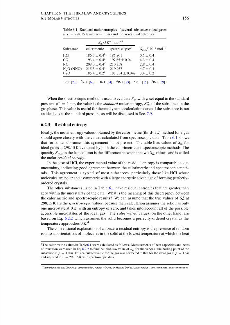
8/12/2019 Howard Devoe Thermodynamic and Chemical
http://slidepdf.com/reader/full/howard-devoe-thermodynamic-and-chemical 156/532
CHAPTER 6 THE THIRD LAW AND CRYOGENICS6.2 M OLAR E NTROPIES 156
Table 6.1 Standard molar entropies of several substances (ideal gasesat T D 298:15 K and p D 1 bar) and molar residual entropies
S ım=J K 1 mol 1
Substance calorimetric spectroscopic a S m,0 =J K 1 mol 1
HCl 186:3 ˙ 0:4b
186:901 0:6 ˙ 0:4CO 193:4 ˙ 0:4c 197:65 ˙ 0:04 4:3 ˙ 0:4NO 208:0 ˙ 0:4d 210:758 2:8 ˙ 0:4N2 O (NNO) 215:3 ˙ 0:4e 219:957 4:7 ˙ 0:4H2 O 185:4 ˙ 0:2 f 188:834 ˙ 0:042 3:4 ˙ 0:2
a Ref. [ 28]. bRef. [ 60]. cRef. [ 34]. d Ref. [ 83]. eRef. [ 15]. f Ref. [ 59].
When the spectroscopic method is used to evaluate S m with p set equal to the standardpressure p ı D 1 bar, the value is the standard molar entropy, S ım , of the substance in thegas phase. This value is useful for thermodynamic calculations even if the substance is not
an ideal gas at the standard pressure, as will be discussed in Sec. 7.9 .
6.2.3 Residual entropy
Ideally, the molar entropy values obtained by the calorimetric (third-law) method for a gasshould agree closely with the values calculated from spectroscopic data. Table 6.1 showsthat for some substances this agreement is not present. The table lists values of S ım forideal gases at 298:15 K evaluated by both the calorimetric and spectroscopic methods. Thequantity S m,0 in the last column is the difference between the two S ım values, and is calledthe molar residual entropy .
In the case of HCl, the experimental value of the residual entropy is comparable to itsuncertainty, indicating good agreement between the calorimetric and spectroscopic meth-ods. This agreement is typical of most substances, particularly those like HCl whosemolecules are polar and asymmetric with a large energetic advantage of forming perfectly-ordered crystals.
The other substances listed in Table 6.1 have residual entropies that are greater thanzero within the uncertainty of the data. What is the meaning of this discrepancy betweenthe calorimetric and spectroscopic results? We can assume that the true values of S ım at298:15 K are the spectroscopic values, because their calculation assumes the solid has onlyone microstate at 0 K, with an entropy of zero, and takes into account all of the possibleaccessible microstates of the ideal gas. The calorimetric values, on the other hand, arebased on Eq. 6.2.2 which assumes the solid becomes a perfectly-ordered crystal as thetemperature approaches 0 K.4
The conventional explanation of a nonzero residual entropy is the presence of randomrotational orientations of molecules in the solid at the lowest temperature at which the heat
4The calorimetric values in Table 6.1 were calculated as follows. Measurements of heat capacities and heatsof transition were used in Eq. 6.2.2 to nd the third-law value of S m for the vapor at the boiling point of thesubstance at p D 1 atm. This calculated value for the gas was corrected to that for the ideal gas at p D 1 barand adjusted to T D 298:15 K with spectroscopic data.
Thermodynamics and Chemistry , second edition, version 4 © 2012 by Howard DeVoe. Latest version: www.chem.umd.edu/thermobook
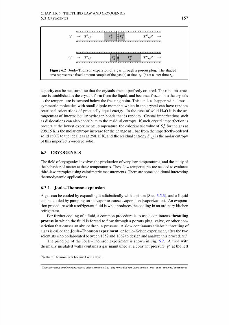
8/12/2019 Howard Devoe Thermodynamic and Chemical
http://slidepdf.com/reader/full/howard-devoe-thermodynamic-and-chemical 157/532
CHAPTER 6 THE THIRD LAW AND CRYOGENICS6.3 C RYOGENICS 157
(a)
(b)
Figure 6.2 Joule–Thomson expansion of a gas through a porous plug. The shadedarea represents a xed-amount sample of the gas (a) at time t1 ; (b) at a later time t2 .
capacity can be measured, so that the crystals are not perfectly ordered. The random struc-ture is established as the crystals form from the liquid, and becomes frozen into the crystalsas the temperature is lowered below the freezing point. This tends to happen with almost-symmetric molecules with small dipole moments which in the crystal can have randomrotational orientations of practically equal energy. In the case of solid H 2 O it is the ar-rangement of intermolecular hydrogen bonds that is random. Crystal imperfections suchas dislocations can also contribute to the residual entropy. If such crystal imperfection ispresent at the lowest experimental temperature, the calorimetric value of S ım for the gas at298:15 K is the molar entropy increase for the change at 1 bar from the imperfectly-orderedsolid at 0 K to the ideal gas at 298:15 K, and the residual entropy S m,0 is the molar entropyof this imperfectly-ordered solid.
6.3 CRYOGENICS
The eld of cryogenics involves the production of very low temperatures, and the study of the behavior of matter at these temperatures. These low temperatures are needed to evaluatethird-law entropies using calorimetric measurements. There are some additional interestingthermodynamic applications.
6.3.1 Joule–Thomson expansion
A gas can be cooled by expanding it adiabatically with a piston (Sec. 3.5.3 ), and a liquidcan be cooled by pumping on its vapor to cause evaporation (vaporization). An evapora-tion procedure with a refrigerant uid is what produces the cooling in an ordinary kitchenrefrigerator.
For further cooling of a uid, a common procedure is to use a continuous throttlingprocess in which the uid is forced to ow through a porous plug, valve, or other con-
striction that causes an abrupt drop in pressure. A slow continuous adiabatic throttling of a gas is called the Joule–Thomson experiment , or Joule–Kelvin experiment, after the twoscientists who collaborated between 1852 and 1862 to design and analyze this procedure. 5
The principle of the Joule–Thomson experiment is shown in Fig. 6.2. A tube withthermally insulated walls contains a gas maintained at a constant pressure p 0 at the left
5William Thomson later became Lord Kelvin.
Thermodynamics and Chemistry , second edition, version 4 © 2012 by Howard DeVoe. Latest version: www.chem.umd.edu/thermobook
8/12/2019 Howard Devoe Thermodynamic and Chemical
http://slidepdf.com/reader/full/howard-devoe-thermodynamic-and-chemical 158/532
CHAPTER 6 THE THIRD LAW AND CRYOGENICS6.3 C RYOGENICS 158
side of a porous plug and at a constant lower pressure p 00at the right side. Because of thepressure difference, the gas ows continuously from left to right through the plug. The owis slow, and the pressure is essentially uniform throughout the portion of the tube at eachside of the plug, but has a large gradient within the pores of the plug.
After the gas has been allowed to ow for a period of time, a steady state develops in
the tube. In this steady state, the gas is assumed to have a uniform temperature T 0
at the leftside of the plug and a uniform temperature T 00(not necessarily equal to T 0) at the right sideof the plug.
Consider the segment of gas whose position at times t1 and t2 is indicated by shadingin Fig. 6.2 . This segment contains a xed amount of gas and expands as it moves throughthe porous plug from higher to lower pressure. We can treat this gas segment as a closed system . During the interval between times t1 and t2 , the system passes through a sequenceof different states, none of which is an equilibrium state since the process is irreversible. Theenergy transferred across the boundary by heat is zero , because the tube wall is insulatedand there is no temperature gradient at either end of the gas segment. We calculate theenergy transferred by work at each end of the gas segment from ¶w D p bAs dx , wherep b is the pressure (either p 0 or p 00) at the moving boundary, A s is the cross-section area of the tube, and x is the distance along the tube. The result is
w D p 0.V 02 V 01 / p 00.V 002 V 00
1 / (6.3.1)
where the meaning of the volumes V 01 , V 02 , and so on is indicated in the gure.The internal energy change U of the gas segment must be equal to w , since q is zero.
Now let us nd the enthalpy change H . At each instant, a portion of the gas segment is inthe pores of the plug, but this portion contributes an unchanging contribution to both U andH because of the steady state. The rest of the gas segment is in the portions on either sideof the plug, with enthalpies U 0Cp 0V 0 at the left and U 00Cp 00V 00at the right. The overallenthalpy change of the gas segment must be
H D U C.p 0V 02 Cp 00V 002 / .p 0V 01 Cp 00V 001 / (6.3.2)
which, when combined with the expression of Eq. 6.3.1 for w D U , shows that H is zero . In other words, the gas segment has the same enthalpy before and after it passesthrough the plug: the throttling process is isenthalpic .
The temperatures T 0 and T 00can be measured directly. When values of T 00versus p 00
are plotted for a series of Joule–Thomson experiments having the same values of T 0 andp 0 and different values of p 00, the curve drawn through the points is a curve of constantenthalpy. The slope at any point on this curve is equal to the Joule–Thomson coefcient(or Joule–Kelvin coefcient) dened by
JTdef
D@T @p H
(6.3.3)
For an ideal gas, JT is zero because the enthalpy of an ideal gas depends only on T (Prob.5.1); T cannot change if H is constant. For a nonideal gas, JT is a function of T andp and the kind of gas. 6 For most gases, at low to moderate pressures and at temperatures
6See Sec. 7.5.2 for the relation of the Joule–Thomson coefcient to other properties of a gas.
Thermodynamics and Chemistry , second edition, version 4 © 2012 by Howard DeVoe. Latest version: www.chem.umd.edu/thermobook
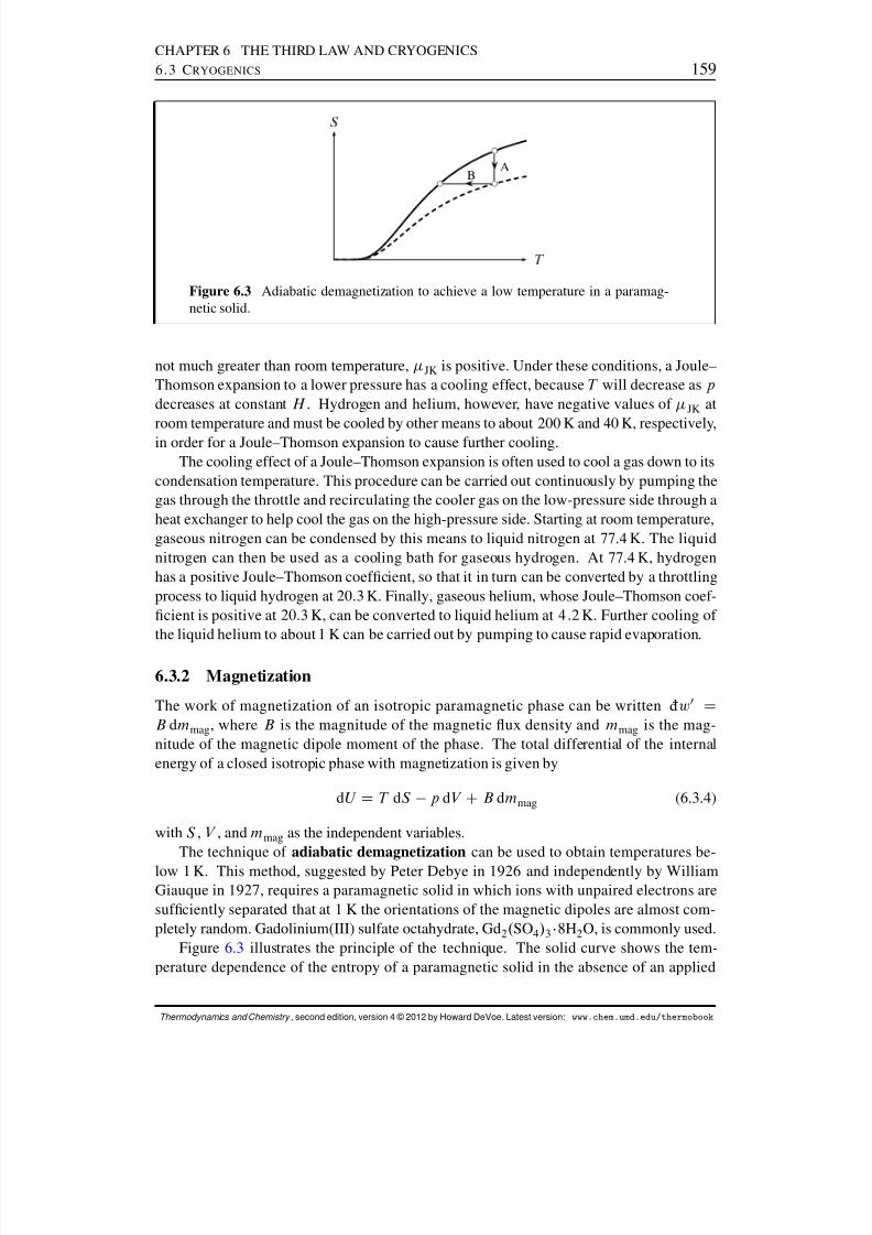
8/12/2019 Howard Devoe Thermodynamic and Chemical
http://slidepdf.com/reader/full/howard-devoe-thermodynamic-and-chemical 159/532
CHAPTER 6 THE THIRD LAW AND CRYOGENICS6.3 C RYOGENICS 159
AB
Figure 6.3 Adiabatic demagnetization to achieve a low temperature in a paramag-netic solid.
not much greater than room temperature, JK is positive. Under these conditions, a Joule–Thomson expansion to a lower pressure has a cooling effect, because T will decrease as pdecreases at constant H . Hydrogen and helium, however, have negative values of JK atroom temperature and must be cooled by other means to about 200 K and 40 K, respectively,in order for a Joule–Thomson expansion to cause further cooling.
The cooling effect of a Joule–Thomson expansion is often used to cool a gas down to itscondensation temperature. This procedure can be carried out continuously by pumping thegas through the throttle and recirculating the cooler gas on the low-pressure side through aheat exchanger to help cool the gas on the high-pressure side. Starting at room temperature,gaseous nitrogen can be condensed by this means to liquid nitrogen at 77:4 K. The liquidnitrogen can then be used as a cooling bath for gaseous hydrogen. At 77:4 K, hydrogenhas a positive Joule–Thomson coefcient, so that it in turn can be converted by a throttlingprocess to liquid hydrogen at 20:3 K. Finally, gaseous helium, whose Joule–Thomson coef-cient is positive at 20:3 K, can be converted to liquid helium at 4 :2 K. Further cooling of the liquid helium to about 1 K can be carried out by pumping to cause rapid evaporation.
6.3.2 Magnetization
The work of magnetization of an isotropic paramagnetic phase can be written ¶w 0 DB dmmag , where B is the magnitude of the magnetic ux density and mmag is the mag-nitude of the magnetic dipole moment of the phase. The total differential of the internalenergy of a closed isotropic phase with magnetization is given by
dU D T dS p dV CB dmmag (6.3.4)
with S , V , and mmag as the independent variables.The technique of adiabatic demagnetization can be used to obtain temperatures be-
low 1 K. This method, suggested by Peter Debye in 1926 and independently by WilliamGiauque in 1927, requires a paramagnetic solid in which ions with unpaired electrons aresufciently separated that at 1 K the orientations of the magnetic dipoles are almost com-pletely random. Gadolinium(III) sulfate octahydrate, Gd 2 . SO 4/ 3 8H 2O, is commonly used.
Figure 6.3 illustrates the principle of the technique. The solid curve shows the tem-perature dependence of the entropy of a paramagnetic solid in the absence of an applied
Thermodynamics and Chemistry , second edition, version 4 © 2012 by Howard DeVoe. Latest version: www.chem.umd.edu/thermobook

8/12/2019 Howard Devoe Thermodynamic and Chemical
http://slidepdf.com/reader/full/howard-devoe-thermodynamic-and-chemical 160/532
CHAPTER 6 THE THIRD LAW AND CRYOGENICS6.3 C RYOGENICS 160
BIOGRAPHICAL SKETCHWilliam Francis Giauque (1895–1982)
A I P E M I L I O S E G R ` E V I S U A L A R C H I V E S
B R I T T L E B O O K S C O L L E C T I O N
William Giauque was an American chemistwho made important contributions to the eldof cryogenics. He received the 1949 NobelPrize in Chemistry “for his contributions in theeld of chemical thermodynamics, particularlyconcerning the behaviour of substances at ex-tremely low temperatures.”
Giauque was born in Niagara Falls, On-tario, Canada, but as his father was a citizen of the United States, William was able to adoptAmerican citizenship. His father worked as aweighmaster and station agent for the Michi-gan Central Railroad in Michigan.
Giauque’s initial career goal after highschool was electrical engineering. After work-ing for two years at the Hooker Electrochem-ical Company in Niagara Falls, New York, heleft to continue his education with the idea of becoming a chemical engineer. Hearing of thescientic reputation of G. N. Lewis, the chairof the chemistry department at the Universityof California at Berkeley (page 271 ), and mo-tivated by the free tuition there, he enrolled in-stead in that department. a
Giauque spent the rest of his life in thechemistry department at Berkeley, rst as anundergraduate; then as a graduate student; andnally, after receiving his Ph.D. in 1922, asa faculty member. Some of his undergradu-ate courses were in engineering, which later
helped him in the design and construction of the heavy equipment for producing the highmagnetic elds and the liquid hydrogen andhelium needed in his research.
Beginning in 1928, with the help of his
graduate students and collaborators, he beganto publish papers on various aspects of thethird law. b The research included the evalua-
tion of third-law molar entropies and compar-ison to molar entropies calculated from spec-troscopic data, and the study of the residualentropy of crystals. Faint unexplained linesin the absorption spectrum of gaseous oxygenled him to the discovery of the previously un-known 17 O and 18 O isotopes of oxygen.
Giauque’s best-known accomplishment ishis invention and exploitation of cooling tovery low temperatures by adiabatic demagne-tization. In 1924, he learned of the unusualproperties of gadolinium sulfate octahydrate atthe temperature of liquid helium. In his NobelLecture, he said: c
I was greatly surprised to nd, that the applica-tion of a magnetic eld removes a large amountof entropy from this substance, at a temperatureso low that it had been thought that there waspractically no entropy left to remove. . . . Thosefamiliar with thermodynamics will realize thatin principle any process involving an entropychange may be used to produce either cooling orheating. Accordingly it occurred to me that adia-batic demagnetization could be made the basis of a method for producing temperatures lower thanthose obtainable with liquid helium.
It wasn’t until 1933 that he was able to buildthe equipment and publish the results from hisrst adiabatic demagnetization experiment, re-porting a temperature of 0:25 K.d
He was married to a botanist and had twosons. According to one biography: e
Giauque’s students remember pleasant Thanks-giving dinners at the Giauque home, with Muriel[his wife] as cook and Frank (as she called him)as raconteur, with a keen sense of humor. Thestories he most enjoyed telling were those inwhich the joke was on him. . . . Giauque’s con-servatism was legendary. He always appeared at
the university dressed in an iron-gray tweed suit.. . . A dominant personality himself, Giauque notonly tolerated but respected students who dis-agreed with him, and he was especially pleasedwhen they could prove their point.
a Ref. [ 130 ]. bRef. [ 152 ]. cRef. [ 61]. d Ref. [ 58]. eRef. [ 130 ].
Thermodynamics and Chemistry , second edition, version 4 © 2012 by Howard DeVoe. Latest version: www.chem.umd.edu/thermobook
8/12/2019 Howard Devoe Thermodynamic and Chemical
http://slidepdf.com/reader/full/howard-devoe-thermodynamic-and-chemical 161/532
CHAPTER 6 THE THIRD LAW AND CRYOGENICS6.3 C RYOGENICS 161
magnetic eld, and the dashed curve is for the solid in a constant, nite magnetic eld. Thetemperature range shown is from 0 K to approximately 1 K. At 0 K, the magnetic dipolesare perfectly ordered. The increase of S shown by the solid curve between 0 K and 1 K isdue almost entirely to increasing disorder in the orientations of the magnetic dipoles as heatenters the system.
Path A represents the process that occurs when the paramagnetic solid, surrounded bygaseous helium in thermal contact with liquid helium that has been cooled to about 1 K, isslowly moved into a strong magnetic eld. The process is isothermal magnetization , whichpartially orients the magnetic dipoles and reduces the entropy. During this process there isheat transfer to the liquid helium, which partially boils away. In path B, the thermal contactbetween the solid and the liquid helium has been broken by pumping away the gas sur-rounding the solid, and the sample is slowly moved away from the magnetic eld. This stepis a reversible adiabatic demagnetization. Because the process is reversible and adiabatic,the entropy change is zero, which brings the state of the solid to a lower temperature asshown.
The sign of .@T=@B/S;p is of interest because it tells us the sign of the temperaturechange during a reversible adiabatic demagnetization (path B of Fig. 6.3 on page 159 ).To change the independent variables in Eq. 6.3.4 to S , p , and B , we dene the Legendretransform
H 0 def
D U CpV Bm mag (6.3.5)
(H 0 is sometimes called the magnetic enthalpy .) From Eqs. 6.3.4 and 6.3.5 we obtain thetotal differential
dH 0 D T dS CV dp mmag dB (6.3.6)
From it we nd the reciprocity relation
@T @B S;p D
@mmag
@S p;B(6.3.7)
According to Curie’s law of magnetization, the magnetic dipole moment mmag of aparamagnetic phase at constant magnetic ux density B is proportional to 1= T . This lawapplies when B is small, but even if B is not small mmag decreases with increasing T . Toincrease the temperature of a phase at constant B , we allow heat to enter the system, and S then increases. Thus, .@mmag =@S/p;B is negative and, according to Eq. 6.3.7 , .@T=@B/S;pmust be positive. Adiabatic demagnetization is a constant-entropy process in which Bdecreases, and therefore the temperature also decreases .
We can nd the sign of the entropy change during the isothermal magnetization processshown as path A in Fig. 6.3 on page 159 . In order to use T , p , and B as the independent
variables, we dene the Legendre transform G 0 def
D H 0 TS . Its total differential is
dG 0 D S dT CV dp mmag dB (6.3.8)
From this total differential, we obtain the reciprocity relation
@S @B T;p D
@mmag
@T p;B(6.3.9)
Thermodynamics and Chemistry , second edition, version 4 © 2012 by Howard DeVoe. Latest version: www.chem.umd.edu/thermobook
8/12/2019 Howard Devoe Thermodynamic and Chemical
http://slidepdf.com/reader/full/howard-devoe-thermodynamic-and-chemical 162/532
CHAPTER 6 THE THIRD LAW AND CRYOGENICS6.3 C RYOGENICS 162
Since mmag at constant B decreases with increasing T , as explained above, we see that theentropy change during isothermal magnetization is negative .
By repeatedly carrying out a procedure of isothermal magnetization and adiabatic de-magnetization, starting each stage at the temperature produced by the previous stage, it hasbeen possible to attain a temperature as low as 0:0015 K. The temperature can be reduced
still further, down to 16 microkelvins, by using adiabatic nuclear demagnetization. How-ever, as is evident from the gure, if in accordance with the third law both of the entropycurves come together at the absolute zero of the kelvin scale, then it is not possible to attaina temperature of zero kelvins in a nite number of stages of adiabatic demagnetization. Thisconclusion is called the principle of the unattainability of absolute zero .
Thermodynamics and Chemistry , second edition, version 4 © 2012 by Howard DeVoe. Latest version: www.chem.umd.edu/thermobook
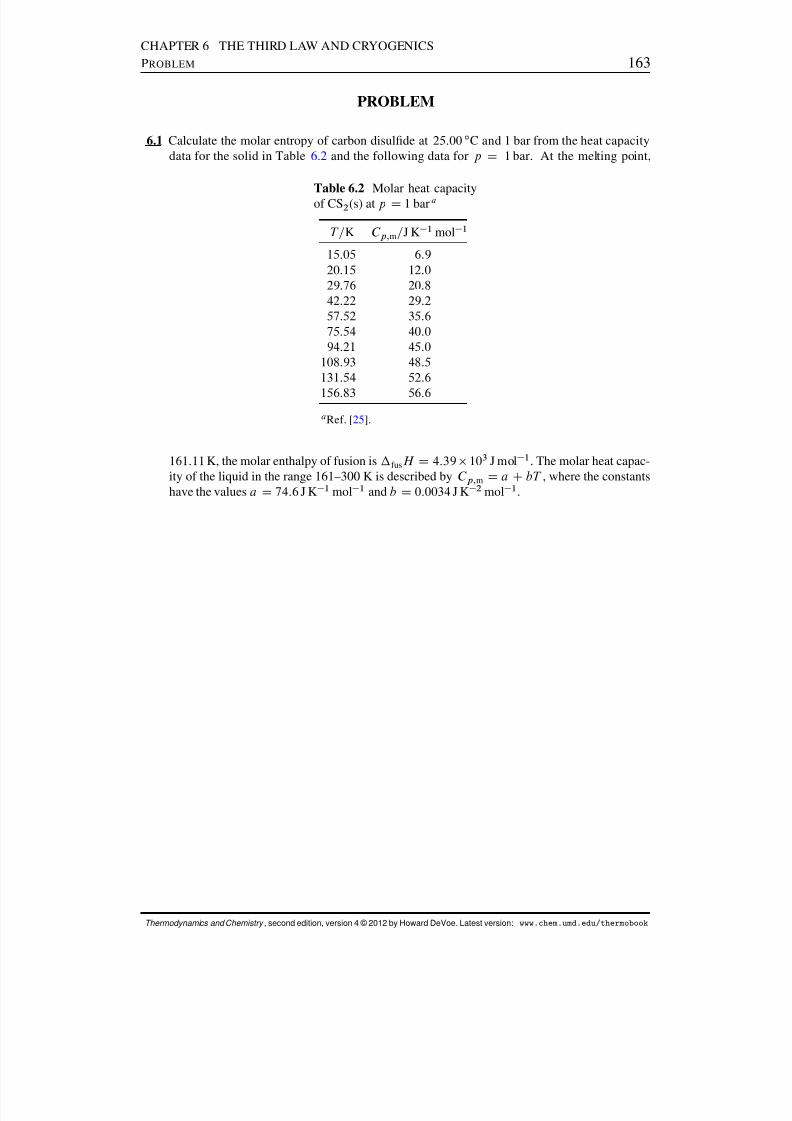
8/12/2019 Howard Devoe Thermodynamic and Chemical
http://slidepdf.com/reader/full/howard-devoe-thermodynamic-and-chemical 163/532
CHAPTER 6 THE THIRD LAW AND CRYOGENICSPROBLEM 163
PROBLEM
6.1 Calculate the molar entropy of carbon disulde at 25:00 ı C and 1 bar from the heat capacitydata for the solid in Table 6.2 and the following data for p D 1 bar. At the melting point,
Table 6.2 Molar heat capacityof CS 2 (s) at p D 1 bar a
T =K C p; m=J K 1 mol 1
15:05 6:920:15 12:029:76 20:842:22 29:257:52 35:675:54 40:094:21 45:0
108:93 48:5131:54 52:6
156:83 56:6a Ref. [ 25].
161:11 K, the molar enthalpy of fusion is fus H D 4:39 103 J mol 1 . The molar heat capac-ity of the liquid in the range 161–300 K is described by C p; m D a CbT , where the constantshave the values a D 74:6 J K 1 mol 1 and b D 0:0034 J K 2 mol 1 .
Thermodynamics and Chemistry , second edition, version 4 © 2012 by Howard DeVoe. Latest version: www.chem.umd.edu/thermobook
8/12/2019 Howard Devoe Thermodynamic and Chemical
http://slidepdf.com/reader/full/howard-devoe-thermodynamic-and-chemical 164/532
C HAPTER 7
P URE SUBSTANCES IN SINGLE PHASES
This chapter applies concepts introduced in earlier chapters to the simplest kind of system,one consisting of a pure substance or a single component in a single phase. The system hasthree independent variables if it is open, and two if it is closed. Relations among variousproperties of a single phase are derived, including temperature, pressure, and volume. Theimportant concepts of standard states and chemical potential are introduced.
7.1 VOLUME PROPERTIES
Two volume properties of a closed system are dened as follows:
cubic expansion coefcient ˛ def
D 1V
@V @T p
(7.1.1)
isothermal compressibility T def
D 1V
@V @p T
(7.1.2)
The cubic expansion coefcient is also called the coefcient of thermal expansion andthe expansivity coefcient. Other symbols for the isothermal compressibility are ˇ and T .
These denitions show that ˛ is the fractional volume increase per unit temperatureincrease at constant pressure, and T is the fractional volume decrease per unit pressureincrease at constant temperature. Both quantities are intensive properties. Most substanceshave positive values of ˛ ,1 and all substances have positive values of T , because a pressureincrease at constant temperature requires a volume decrease.
If an amount n of a substance is in a single phase, we can divide the numerator anddenominator of the right sides of Eqs. 7.1.1 and 7.1.2 by n to obtain the alternative expres-
sions1The cubic expansion coefcient is not always positive. ˛ is negative for liquid water below its temperatureof maximum density, 3:98 ı C. The crystalline ceramics zirconium tungstate (ZrW 2 O8 ) and hafnium tungstate(HfW 2 O8 ) have the remarkable behavior of contracting uniformly and continuously in all three dimensionswhen they are heated from 0:3 K to about 1050 K; ˛ is negative throughout this very wide temperature range(Ref. [ 109 ]). The intermetallic compound YbGaGe has been found to have a value of ˛ that is practically zeroin the range 100–300 K (Ref. [ 146 ]).
164
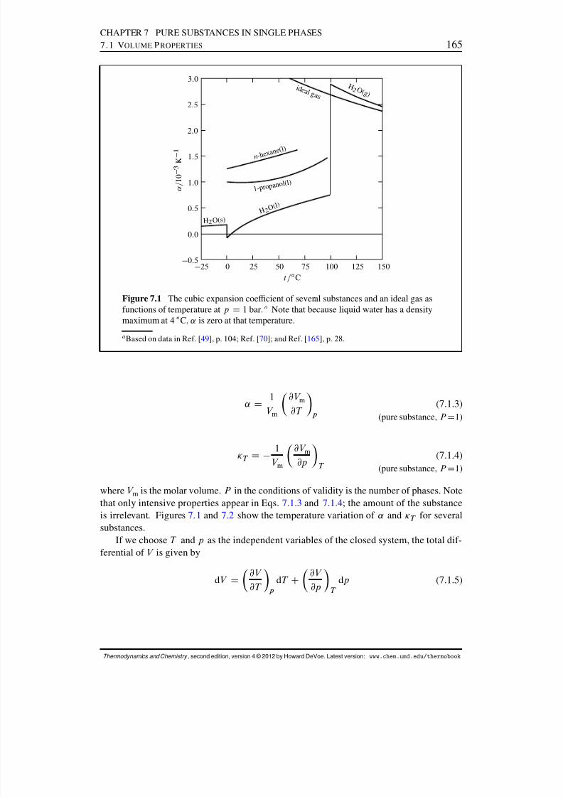
8/12/2019 Howard Devoe Thermodynamic and Chemical
http://slidepdf.com/reader/full/howard-devoe-thermodynamic-and-chemical 165/532
CHAPTER 7 PURE SUBSTANCES IN SINGLE PHASES7.1 V OLUME P ROPERTIES 165
n - h e x a n e ( l )
1 - p r o p a n o l( l )
H2 O(s ) H 2 O ( l )
H 2 O ( g ) i d e a l g a s
25 0 25 50 75 100 125 1500:5
0:0
0:5
1:0
1:5
2:0
2:5
3:0
t=ı
C
.
˛ = 1 0
3
K
1
Figure 7.1 The cubic expansion coefcient of several substances and an ideal gas asfunctions of temperature at p D 1 bar. a Note that because liquid water has a densitymaximum at 4 ı C, ˛ is zero at that temperature.
a Based on data in Ref. [ 49], p. 104; Ref. [ 70]; and Ref. [ 165 ], p. 28.
˛ D 1V m
@V m
@T p(7.1.3)
(pure substance, P D1)
T D 1V m
@V m
@p T (7.1.4)
(pure substance, P D1)
where V m is the molar volume. P in the conditions of validity is the number of phases. Notethat only intensive properties appear in Eqs. 7.1.3 and 7.1.4 ; the amount of the substanceis irrelevant. Figures 7.1 and 7.2 show the temperature variation of ˛ and T for severalsubstances.
If we choose T and p as the independent variables of the closed system, the total dif-ferential of V is given by
dV D@V @T p
dT C@V @p T
dp (7.1.5)
Thermodynamics and Chemistry , second edition, version 4 © 2012 by Howard DeVoe. Latest version: www.chem.umd.edu/thermobook
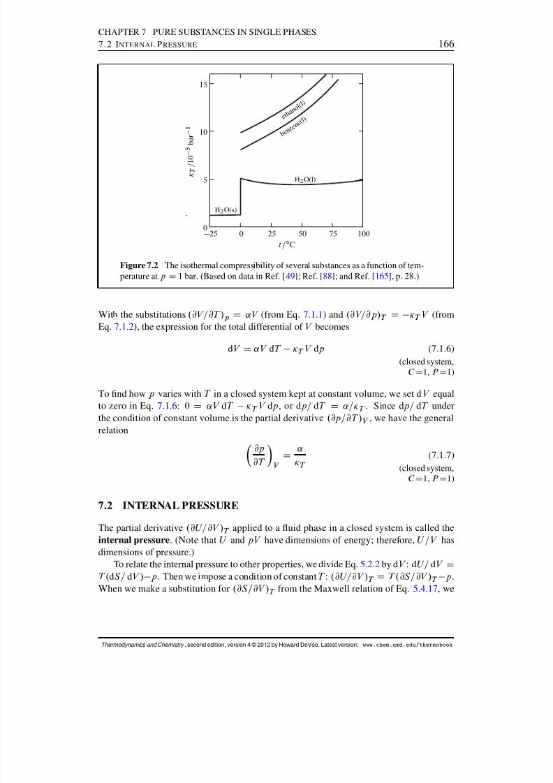
8/12/2019 Howard Devoe Thermodynamic and Chemical
http://slidepdf.com/reader/full/howard-devoe-thermodynamic-and-chemical 166/532
CHAPTER 7 PURE SUBSTANCES IN SINGLE PHASES7.2 I NTERNAL P RESSURE 166
b e n z
e n e ( l ) e t h a n
o l ( l )
H 2 O(s )
H 2 O(l)
25 0 25 50 75 1000
5
10
15
t=ı C
.
T
= 1 0
5 b
a r
1
Figure 7.2 The isothermal compressibility of several substances as a function of tem-perature at p D 1 bar. (Based on data in Ref. [ 49]; Ref. [ 88]; and Ref. [ 165 ], p. 28.)
With the substitutions .@V =@T /p D ˛V (from Eq. 7.1.1 ) and .@V=@p/T D T V (fromEq. 7.1.2 ), the expression for the total differential of V becomes
dV D ˛V dT T V dp (7.1.6)(closed system,
C D1, P D1)
To nd how p varies with T in a closed system kept at constant volume, we set d V equalto zero in Eq. 7.1.6 : 0
D ˛V dT
T V dp , or dp= dT
D ˛=
T . Since d p= dT under
the condition of constant volume is the partial derivative .@p=@T /V , we have the generalrelation
@p@T V D
˛
T (7.1.7)
(closed system,C D1, P D1)
7.2 INTERNAL PRESSURE
The partial derivative .@U=@V /T applied to a uid phase in a closed system is called theinternal pressure . (Note that U and pV have dimensions of energy; therefore, U =V hasdimensions of pressure.)
To relate the internal pressure to other properties, we divide Eq. 5.2.2 by dV : dU= dV DT . dS= dV / p . Then we impose a condition of constant T : .@U=@V /T D T .@S=@V /T p .When we make a substitution for .@S=@V /T from the Maxwell relation of Eq. 5.4.17 , we
Thermodynamics and Chemistry , second edition, version 4 © 2012 by Howard DeVoe. Latest version: www.chem.umd.edu/thermobook
8/12/2019 Howard Devoe Thermodynamic and Chemical
http://slidepdf.com/reader/full/howard-devoe-thermodynamic-and-chemical 167/532
CHAPTER 7 PURE SUBSTANCES IN SINGLE PHASES7.2 I NTERNAL P RESSURE 167
obtain
@U @V T D T
@p@T V
p (7.2.1)(closed system,
uid phase, C D1)
This equation is sometimes called the “thermodynamic equation of state” of the uid.For an ideal-gas phase, we can write p D nRT=V and then
@p@T V D
nRV D
pT
(7.2.2)
Making this substitution in Eq. 7.2.1 gives us
@U @V T D 0 (7.2.3)
(closed system of an ideal gas)
showing that the internal pressure of an ideal gas is zero.
In Sec. 3.5.1 , an ideal gas was dened as a gas (1) that obeys the ideal gas equation, and(2) for which U in a closed system depends only on T . Equation 7.2.3, derived fromthe rst part of this denition, expresses the second part. It thus appears that the secondpart of the denition is redundant, and that we could dene an ideal gas simply as agas obeying the ideal gas equation. This argument is valid only if we assume the ideal-gas temperature is the same as the thermodynamic temperature (Secs. 2.3.5 and 4.3.4)since this assumption is required to derive Eq. 7.2.3 . Without this assumption, we can’tdene an ideal gas solely by pV D nRT , where T is the ideal gas temperature.
Here is a simplied interpretation of the signicance of the internal pressure. Whenthe volume of a uid increases, the average distance between molecules increases and thepotential energy due to intermolecular forces changes. If attractive forces dominate, as theyusually do unless the uid is highly compressed, expansion causes the potential energy toincrease . The internal energy is the sum of the potential energy and thermal energy. Theinternal pressure, .@U=@V /T , is the rate at which the internal energy changes with volumeat constant temperature. At constant temperature, the thermal energy is constant so that theinternal pressure is the rate at which just the potential energy changes with volume. Thus,the internal pressure is a measure of the strength of the intermolecular forces and is positiveif attractive forces dominate. 2 In an ideal gas, intermolecular forces are absent and thereforethe internal pressure of an ideal gas is zero.
With the substitution .@p=@T /V D ˛= T (Eq. 7.1.7 ), Eq. 7.2.1 becomes
@U @V T D
˛T
T p (7.2.4)
(closed system,
uid phase, C D1)
The internal pressure of a liquid at p D 1 bar is typically much larger than 1 bar (see Prob.7.6). Equation 7.2.4 shows that, in this situation, the internal pressure is approximatelyequal to ˛T= T .
2These attractive intermolecular forces are the cohesive forces that can allow a negative pressure to exist in aliquid; see page 38.
Thermodynamics and Chemistry , second edition, version 4 © 2012 by Howard DeVoe. Latest version: www.chem.umd.edu/thermobook

8/12/2019 Howard Devoe Thermodynamic and Chemical
http://slidepdf.com/reader/full/howard-devoe-thermodynamic-and-chemical 168/532
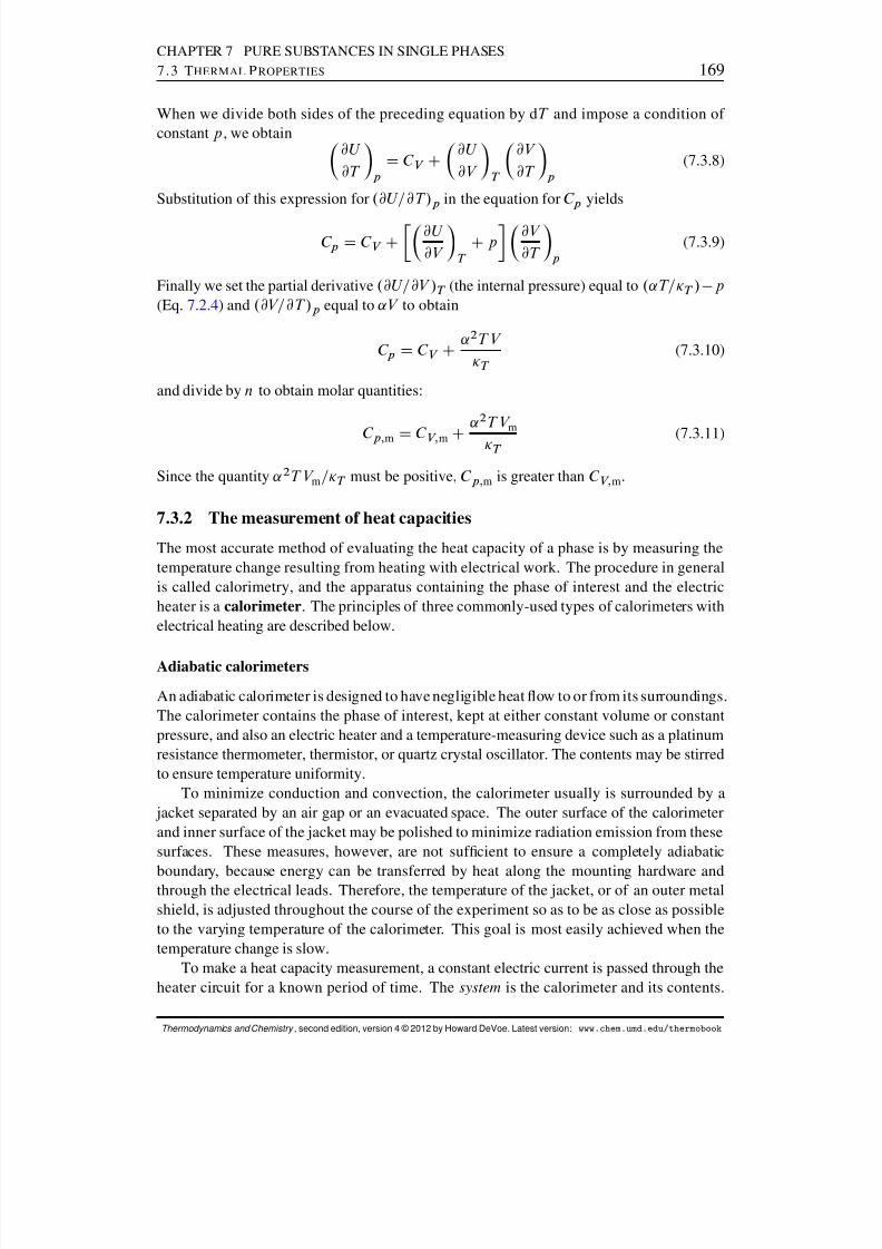
8/12/2019 Howard Devoe Thermodynamic and Chemical
http://slidepdf.com/reader/full/howard-devoe-thermodynamic-and-chemical 169/532
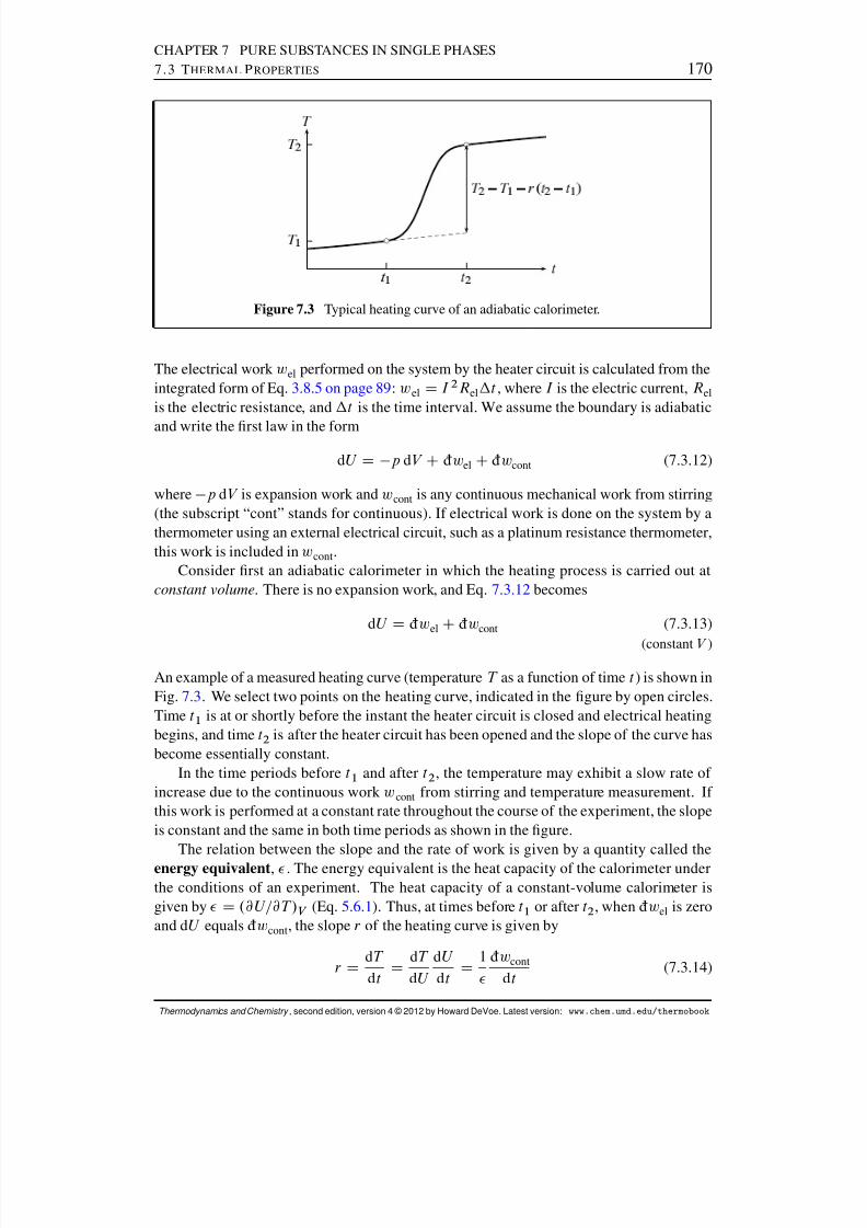
8/12/2019 Howard Devoe Thermodynamic and Chemical
http://slidepdf.com/reader/full/howard-devoe-thermodynamic-and-chemical 170/532
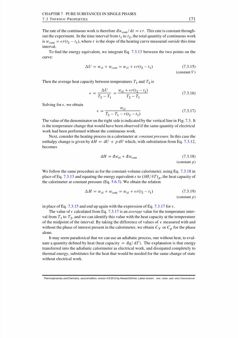
8/12/2019 Howard Devoe Thermodynamic and Chemical
http://slidepdf.com/reader/full/howard-devoe-thermodynamic-and-chemical 171/532
CHAPTER 7 PURE SUBSTANCES IN SINGLE PHASES7.3 T HERMAL P ROPERTIES 171
The rate of the continuous work is therefore ¶w cont = d t D r . This rate is constant through-out the experiment. In the time interval from t1 to t2 , the total quantity of continuous work is wcont D r.t 2 t1 / , where r is the slope of the heating curve measured outside this timeinterval.
To nd the energy equivalent, we integrate Eq. 7.3.13 between the two points on the
curve:U D wel Cwcont D wel C r.t 2 t1 / (7.3.15)
(constant V )
Then the average heat capacity between temperatures T 1 and T 2 is
D U T 2 T 1 D
wel C r.t 2 t1 /T 2 T 1
(7.3.16)
Solving for , we obtain
D wel
T 2 T 1 r .t 2 t1 / (7.3.17)
The value of the denominator on the right side is indicated by the vertical line in Fig. 7.3 . Itis the temperature change that would have been observed if the same quantity of electricalwork had been performed without the continuous work.
Next, consider the heating process in a calorimeter at constant pressure . In this case theenthalpy change is given by d H D dU Cp dV which, with substitution from Eq. 7.3.12 ,becomes
dH D ¶w el C¶w cont (7.3.18)(constant p )
We follow the same procedure as for the constant-volume calorimeter, using Eq. 7.3.18 in
place of Eq. 7.3.13 and equating the energy equivalent to .@H=@T /p , the heat capacity of the calorimeter at constant pressure (Eq. 5.6.3 ). We obtain the relation
H D wel Cwcont D wel C r.t 2 t1 / (7.3.19)(constant p )
in place of Eq. 7.3.15 and end up again with the expression of Eq. 7.3.17 for .The value of calculated from Eq. 7.3.17 is an average value for the temperature inter-
val from T 1 to T 2 , and we can identify this value with the heat capacity at the temperatureof the midpoint of the interval. By taking the difference of values of measured with andwithout the phase of interest present in the calorimeter, we obtain C V or C p for the phasealone.
It may seem paradoxical that we can use an adiabatic process, one without heat, to eval-uate a quantity dened by heat (heat capacity D ¶q= dT ). The explanation is that energytransferred into the adiabatic calorimeter as electrical work, and dissipated completely tothermal energy, substitutes for the heat that would be needed for the same change of statewithout electrical work.
Thermodynamics and Chemistry , second edition, version 4 © 2012 by Howard DeVoe. Latest version: www.chem.umd.edu/thermobook
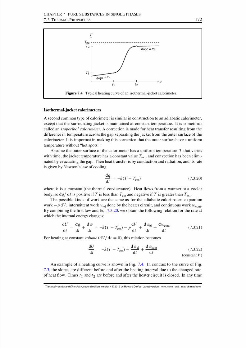
8/12/2019 Howard Devoe Thermodynamic and Chemical
http://slidepdf.com/reader/full/howard-devoe-thermodynamic-and-chemical 172/532
CHAPTER 7 PURE SUBSTANCES IN SINGLE PHASES7.3 T HERMAL P ROPERTIES 172
s l o p e =
slope =
Figure 7.4 Typical heating curve of an isothermal-jacket calorimeter.
Isothermal-jacket calorimeters
A second common type of calorimeter is similar in construction to an adiabatic calorimeter,except that the surrounding jacket is maintained at constant temperature. It is sometimescalled an isoperibol calorimeter . A correction is made for heat transfer resulting from thedifference in temperature across the gap separating the jacket from the outer surface of thecalorimeter. It is important in making this correction that the outer surface have a uniformtemperature without “hot spots.”
Assume the outer surface of the calorimeter has a uniform temperature T that varieswith time, the jacket temperature has a constant value T ext , and convection has been elimi-nated by evacuating the gap. Then heat transfer is by conduction and radiation, and its rateis given by Newton’s law of cooling
¶q
d t D k.T
T ext / (7.3.20)
where k is a constant (the thermal conductance). Heat ows from a warmer to a coolerbody, so ¶q= d t is positive if T is less than T ext and negative if T is greater than T ext .
The possible kinds of work are the same as for the adiabatic calorimeter: expansionwork p dV , intermittent work wel done by the heater circuit, and continuous work wcont .By combining the rst law and Eq. 7.3.20 , we obtain the following relation for the rate atwhich the internal energy changes:
dU d t D
¶qd t C
¶wd t D k.T T ext / p
dV d t C
¶w el
d t C ¶w cont
d t (7.3.21)
For heating at constant volume (dV=d t D 0), this relation becomes
dU d t D k.T T ext / C
¶w el
d t C ¶w cont
d t (7.3.22)
(constant V )
An example of a heating curve is shown in Fig. 7.4. In contrast to the curve of Fig.7.3 , the slopes are different before and after the heating interval due to the changed rateof heat ow. Times t1 and t2 are before and after the heater circuit is closed. In any time
Thermodynamics and Chemistry , second edition, version 4 © 2012 by Howard DeVoe. Latest version: www.chem.umd.edu/thermobook
8/12/2019 Howard Devoe Thermodynamic and Chemical
http://slidepdf.com/reader/full/howard-devoe-thermodynamic-and-chemical 173/532
CHAPTER 7 PURE SUBSTANCES IN SINGLE PHASES7.3 T HERMAL P ROPERTIES 173
interval before time t1 or after time t2 , the system behaves as if it is approaching a steadystate of constant temperature T 1 (called the convergence temperature), which it wouldeventually reach if the experiment were continued without closing the heater circuit. T 1 isgreater than T ext because of the energy transferred to the system by stirring and electricaltemperature measurement. By setting d U= d t and ¶w el= d t equal to zero and T equal to
T 1 in Eq. 7.3.22 , we obtain ¶w cont = d t D k.T 1 T ext / . We assume ¶w cont = d t is constant.Substituting this expression into Eq. 7.3.22 gives us a general expression for the rate atwhich U changes in terms of the unknown quantities k and T 1 :
dU d t D k.T T 1 / C
¶w el
d t (7.3.23)
(constant V )
This relation is valid throughout the experiment, not only while the heater circuit is closed.If we multiply by d t and integrate from t1 to t2 , we obtain the internal energy change in thetime interval from t1 to t2 :
U D k
Z t2
t1
.T T 1 / d t Cwel (7.3.24)
(constant V )All the intermittent work wel is performed in this time interval.
The derivation of Eq. 7.3.24 is a general one. The equation can be applied alsoto a isothermal-jacket calorimeter in which a reaction is occurring. Section 11.5.2will mention the use of this equation for an internal energy correction of a reactioncalorimeter with an isothermal jacket.
The average value of the energy equivalent in the temperature range T 1 to T 2 is
D U
T 2 T 1 D
.k= / Z t2
t1
.T T 1 / d t Cwel
T 2 T 1(7.3.25)
Solving for , we obtain
D wel
.T 2 T 1 / C.k= / Z t2
t1
.T T 1 / d t(7.3.26)
The value of wel is known from wel D I 2 R el t , where t is the time interval during whichthe heater circuit is closed. The integral can be evaluated numerically once T 1 is known.
For heating at constant pressure , dH is equal to d U Cp dV , and we can write
dH d t
D
dU d t
Cp
dV d t
D k.T
T ext /
C
¶w el
d t
C
¶w cont
d t (7.3.27)
(constant p )
which is analogous to Eq. 7.3.22 . By the procedure described above for the case of constantV , we obtain
H D k Z t2
t1
.T T 1 / d t Cwel (7.3.28)(constant p )
Thermodynamics and Chemistry , second edition, version 4 © 2012 by Howard DeVoe. Latest version: www.chem.umd.edu/thermobook
8/12/2019 Howard Devoe Thermodynamic and Chemical
http://slidepdf.com/reader/full/howard-devoe-thermodynamic-and-chemical 174/532
CHAPTER 7 PURE SUBSTANCES IN SINGLE PHASES7.3 T HERMAL P ROPERTIES 174
At constant p , the energy equivalent is equal to C p D H=.T 2 T 1 / , and the nal expres-sion for is the same as that given by Eq. 7.3.26 .
To obtain values of k= and T 1 for use in Eq. 7.3.26 , we need the slopes of the heatingcurve in time intervals (rating periods) just before t1 and just after t2 . Consider the case of constant volume . In these intervals, ¶w el= d t is zero and d U= d t equals k.T T 1 / (from
Eq. 7.3.23 ). The heat capacity at constant volume is C V D dU= dT . The slope r in generalis then given by
r D dT d t D
dT dU
dU d t D .k= /.T T 1 / (7.3.29)
Applying this relation to the points at times t1 and t2 , we have the following simultaneousequations in the unknowns k= and T 1 :
r1 D .k= /.T 1 T 1 / r 2 D .k= /.T 2 T 1 / (7.3.30)
The solutions are
.k= / D r1 r2
T 2 T 1T 1 D
r1 T 2 r2 T 1r1 r2
(7.3.31)
Finally, k is given byk D .k= / D
r1 r2
T 2 T 1 (7.3.32)
When the pressure is constant, this procedure yields the same relations for k= , T 1 , and k .
Continuous-ow calorimeters
A ow calorimeter is a third type of calorimeter used to measure the heat capacity of a uidphase. The gas or liquid ows through a tube at a known constant rate past an electricalheater of known constant power input. After a steady state has been achieved in the tube,
the temperature increase T at the heater is measured.If ¶w el= d t is the rate at which electrical work is performed (the electric power) anddm= d t is the mass ow rate, then in time interval t a quantity w D .¶w el= d t/ t of work is performed on an amount n D .dm= d t/ t=M of the uid (where M is the molarmass). If heat ow is negligible, the molar heat capacity of the substance is given by
C p; m D wn T D
M.¶w el= d t /T . dm= d t /
(7.3.33)
To correct for the effects of heat ow, T is usually measured over a range of ow ratesand the results extrapolated to innite ow rate.
7.3.3 Typical valuesFigure 7.5 on the next page shows the temperature dependence of C p; m for several sub-stances. The discontinuities seen at certain temperatures occur at equilibrium phase transi-tions. At these temperatures the heat capacity is in effect innite, since the phase transitionof a pure substance involves nite heat with zero temperature change.
Thermodynamics and Chemistry , second edition, version 4 © 2012 by Howard DeVoe. Latest version: www.chem.umd.edu/thermobook
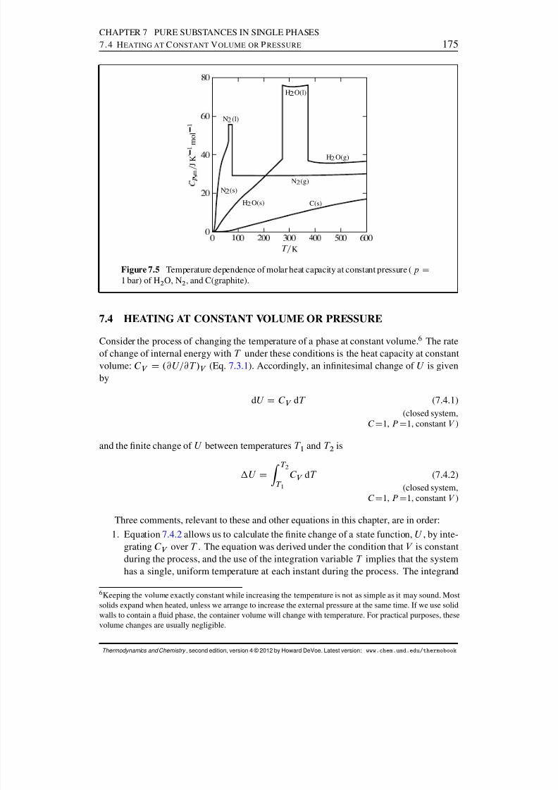
8/12/2019 Howard Devoe Thermodynamic and Chemical
http://slidepdf.com/reader/full/howard-devoe-thermodynamic-and-chemical 175/532
CHAPTER 7 PURE SUBSTANCES IN SINGLE PHASES7.4 H EATING AT C ONSTANT V OLUME OR P RESSURE 175
N
(s)
N
(l)
N
(g)
H
O(s)
H
O(l)
H
O(g)
C(s)
K
.
m
J K
m o l
Figure 7.5 Temperature dependence of molar heat capacity at constant pressure ( p
D1 bar) of H 2 O, N2 , and C(graphite).
7.4 HEATING AT CONSTANT VOLUME OR PRESSURE
Consider the process of changing the temperature of a phase at constant volume. 6 The rateof change of internal energy with T under these conditions is the heat capacity at constantvolume: C V D .@U=@T /V (Eq. 7.3.1 ). Accordingly, an innitesimal change of U is givenby
dU D C V dT (7.4.1)
(closed system,C D1, P D1, constant V )
and the nite change of U between temperatures T 1 and T 2 is
U DZ T 2
T 1C V dT (7.4.2)
(closed system,C D1, P D1, constant V )
Three comments, relevant to these and other equations in this chapter, are in order:1. Equation 7.4.2 allows us to calculate the nite change of a state function, U , by inte-
grating C V over T . The equation was derived under the condition that V is constantduring the process, and the use of the integration variable T implies that the systemhas a single, uniform temperature at each instant during the process. The integrand
6Keeping the volume exactly constant while increasing the temperature is not as simple as it may sound. Mostsolids expand when heated, unless we arrange to increase the external pressure at the same time. If we use solidwalls to contain a uid phase, the container volume will change with temperature. For practical purposes, thesevolume changes are usually negligible.
Thermodynamics and Chemistry , second edition, version 4 © 2012 by Howard DeVoe. Latest version: www.chem.umd.edu/thermobook
8/12/2019 Howard Devoe Thermodynamic and Chemical
http://slidepdf.com/reader/full/howard-devoe-thermodynamic-and-chemical 176/532
CHAPTER 7 PURE SUBSTANCES IN SINGLE PHASES7.4 H EATING AT C ONSTANT V OLUME OR P RESSURE 176
C V may depend on both V and T , and we should integrate with V held constant andC V treated as a function only of T .
2. Suppose we want to evaluate U for a process in which the volume is the same in theinitial and nal states ( V 2 D V 1 ) but is different in some intermediate states, and thetemperature is not uniform in some of the intermediate states. We know the change
of a state function depends only on the initial and nal states, so we can still use Eq.7.4.2 to evaluate U for this process. We integrate with V held constant, although V was not constant during the actual process.In general: A nite change X of a state function, evaluated under the conditionthat another state function Y is constant, is the same as X under the less stringentcondition Y 2 D Y 1 . (Another application of this principle was mentioned in Sec.4.6.2 .)
3. For a pure substance, we may convert an expression for an innitesimal or nitechange of an extensive property to an expression for the change of the correspondingmolar property by dividing by n . For instance, Eq. 7.4.1 becomes
dU m D
C V; m
dT (7.4.3)
and Eq. 7.4.2 becomes
U m DZ T 2
T 1C V; m dT (7.4.4)
If, at a xed volume and over the temperature range T 1 to T 2 , the value of C V is essen-tially constant (i.e., independent of T ), Eq. 7.4.2 becomes
U D C V .T 2 T 1 / (7.4.5)(closed system, C D1,
P D1, constant V and C V )
An innitesimal entropy change during a reversible process in a closed system is givenaccording to the second law by d S D ¶q=T . At constant volume, ¶q is equal to d U whichin turn equals C V dT . Therefore, the entropy change is
dS D C V
T dT (7.4.6)
(closed system,C D1, P D1, constant V )
Integration yields the nite change
S DZ T 2
T 1
C V
T dT (7.4.7)
(closed system,C D1, P D1, constant V )
If C V is treated as constant, Eq. 7.4.7 becomes
S D C V lnT 2T 1
(7.4.8)(closed system, C D1,
P D1, constant V and C V )
Thermodynamics and Chemistry , second edition, version 4 © 2012 by Howard DeVoe. Latest version: www.chem.umd.edu/thermobook
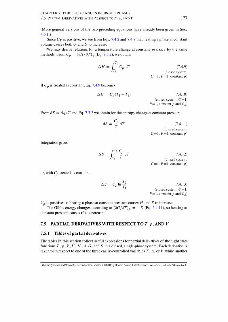
8/12/2019 Howard Devoe Thermodynamic and Chemical
http://slidepdf.com/reader/full/howard-devoe-thermodynamic-and-chemical 177/532
CHAPTER 7 PURE SUBSTANCES IN SINGLE PHASES7.5 PARTIAL D ERIVATIVES WITH R ESPECT TO T , p , A ND V 177
(More general versions of the two preceding equations have already been given in Sec.4.6.1 .)
Since C V is positive, we see from Eqs. 7.4.2 and 7.4.7 that heating a phase at constantvolume causes both U and S to increase.
We may derive relations for a temperature change at constant pressure by the same
methods. From C p D .@H=@T /p (Eq. 7.3.2 ), we obtain
H DZ T 2
T 1C p dT (7.4.9)
(closed system,C D1, P D1, constant p )
If C p is treated as constant, Eq. 7.4.9 becomes
H D C p .T 2 T 1 / (7.4.10)(closed system, C D1,
P D1, constant p and C p )
From d S D ¶q=T and Eq. 7.3.2 we obtain for the entropy change at constant pressure
dS DC pT
dT (7.4.11)(closed system,
C D1, P D1, constant p )
Integration gives
S DZ T 2
T 1
C pT
dT (7.4.12)(closed system,
C D1, P D1, constant p )
or, with C p treated as constant,
S D C p lnT 2T 1
(7.4.13)(closed system, C D1,
P D1, constant p and C p )
C p is positive, so heating a phase at constant pressure causes H and S to increase.The Gibbs energy changes according to .@G=@T /p D S (Eq. 5.4.11 ), so heating at
constant pressure causes G to decrease.
7.5 PARTIAL DERIVATIVES WITH RESPECT TO T , p , AND V 7.5.1 Tables of partial derivatives
The tables in this section collect useful expressions for partial derivatives of the eight statefunctions T , p , V , U , H , A , G , and S in a closed, single-phase system. Each derivative istaken with respect to one of the three easily-controlled variables T , p , or V while another
Thermodynamics and Chemistry , second edition, version 4 © 2012 by Howard DeVoe. Latest version: www.chem.umd.edu/thermobook
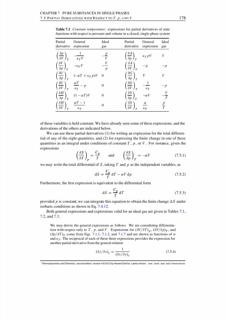
8/12/2019 Howard Devoe Thermodynamic and Chemical
http://slidepdf.com/reader/full/howard-devoe-thermodynamic-and-chemical 178/532
CHAPTER 7 PURE SUBSTANCES IN SINGLE PHASES7.5 PARTIAL D ERIVATIVES WITH R ESPECT TO T , p , A ND V 178
Table 7.1 Constant temperature : expressions for partial derivatives of statefunctions with respect to pressure and volume in a closed, single-phase system
Partial General Ideal Partial General Idealderivative expression gas derivative expression gas
@p@V T
1
T V pV
@A@p T
T pV V
@V @p T
T V V p
@A@V T
p p
@U @p T
. ˛T C T p/V 0@G@p T
V V
@U @V T
˛T
T p 0
@G@V T
1
T p
@H @p T
.1 ˛T /V 0@S @p T
˛V V T
@H @V T
˛T 1
T 0
@S @V T
˛
T
pT
of these variables is held constant. We have already seen some of these expressions, and thederivations of the others are indicated below.
We can use these partial derivatives (1) for writing an expression for the total differen-tial of any of the eight quantities, and (2) for expressing the nite change in one of thesequantities as an integral under conditions of constant T , p , or V . For instance, given theexpressions
@S @T p D
C pT
and@S @p T D ˛V (7.5.1)
we may write the total differential of S , taking T and p as the independent variables, as
dS DC pT
dT ˛V dp (7.5.2)
Furthermore, the rst expression is equivalent to the differential form
dS DC pT
dT (7.5.3)
provided p is constant; we can integrate this equation to obtain the nite change S underisobaric conditions as shown in Eq. 7.4.12 .
Both general expressions and expressions valid for an ideal gas are given in Tables 7.1 ,7.2 , and 7.3 .
We may derive the general expressions as follows. We are considering differentia-tion with respect only to T , p , and V . Expressions for .@V=@T /p , .@V=@p/T , and.@p=@T /V come from Eqs. 7.1.1, 7.1.2 , and 7.1.7 and are shown as functions of ˛and T . The reciprocal of each of these three expressions provides the expression foranother partial derivative from the general relation
.@y=@x/z D 1
.@x=@y/z(7.5.4)
Thermodynamics and Chemistry , second edition, version 4 © 2012 by Howard DeVoe. Latest version: www.chem.umd.edu/thermobook

8/12/2019 Howard Devoe Thermodynamic and Chemical
http://slidepdf.com/reader/full/howard-devoe-thermodynamic-and-chemical 179/532
CHAPTER 7 PURE SUBSTANCES IN SINGLE PHASES7.5 PARTIAL D ERIVATIVES WITH R ESPECT TO T , p , A ND V 179
Table 7.2 Constant pressure : expressions for partial derivatives of state func-tions with respect to temperature and volume in a closed, single-phase system
Partial General Ideal Partial General Idealderivative expression gas derivative expression gas
@T @V p
1˛V
T V
@A@T p
˛pV S pV T S
@V @T p
˛V V
T @A@V p
p S ˛V p
TS V
@U @T p
C p ˛pV C V @G@T p
S S
@U @V p
C p˛V p
C V T V
@G@V p
S ˛V
TS V
@H @T p
C p C p@S @T p
C pT
C pT
@H @V p
C p˛V
C p T V
@S @V p
C p˛T V
C pV
Table 7.3 Constant volume : expressions for partial derivatives of state functions withrespect to temperature and pressure in a closed, single-phase system
Partial General Ideal Partial General Idealderivative expression gas derivative expression gas
@T @p V
T
˛T p
@A@T V
S S
@p@T V
˛
T
pT
@A@p V
T S ˛
TS p
@U @T V C V C V
@G@T V
˛V
T S pV
T S @U @p V
T C p˛ ˛T V
T C V
p@G@p V
V T S
˛ V
TS p
@H @T V
C p C ˛V
T .1 ˛T / C p
@S @T V
C V
T C V
T @H @p V
T C p˛ CV .1 ˛T /
C p T p
@S @p V
T C p˛T ˛V
C V
p
This procedure gives us expressions for the six partial derivatives of T , p , and V .The remaining expressions are for partial derivatives of U , H , A , G , and S . We
obtain the expression for .@U=@T /V from Eq. 7.3.1, for .@U=@V /T from Eq. 7.2.4 ,for .@H=@T /p from Eq. 7.3.2 , for .@A=@T /V from Eq. 5.4.9 , for .@A=@V /T from Eq.5.4.10 , for .@G=@p/T from Eq. 5.4.12 , for .@G=@T/p from Eq. 5.4.11 , for .@S=@T /V from Eq. 7.4.6, for .@S=@T /p from Eq. 7.4.11 , and for .@S=@p/T from Eq. 5.4.18 .
We can transform each of these partial derivatives, and others derived in latersteps, to two other partial derivatives with the same variable held constant and thevariable of differentiation changed. The transformation involves multiplying by an
Thermodynamics and Chemistry , second edition, version 4 © 2012 by Howard DeVoe. Latest version: www.chem.umd.edu/thermobook
8/12/2019 Howard Devoe Thermodynamic and Chemical
http://slidepdf.com/reader/full/howard-devoe-thermodynamic-and-chemical 180/532
CHAPTER 7 PURE SUBSTANCES IN SINGLE PHASES7.5 PARTIAL D ERIVATIVES WITH R ESPECT TO T , p , A ND V 180
appropriate partial derivative of T , p , or V . For instance, from the partial derivative.@U=@V /T D .˛T= T / p , we obtain
@U @p T D
@U @V T
@V @p T D
˛T
T p . T V / D . ˛T C T p/ V (7.5.5)
The remaining partial derivatives can be found by differentiating U
D H
pV , H
DU C pV , A D U T S , and G D H T S and making appropriate substitutions.Whenever a partial derivative appears in a derived expression, it is replaced with anexpression derived in an earlier step. The expressions derived by these steps constitutethe full set shown in Tables 7.1, 7.2, and 7.3.
Bridgman 7 devised a simple method to obtain expressions for these and manyother partial derivatives from a relatively small set of formulas.
7.5.2 The Joule–Thomson coefcient
The Joule–Thomson coefcient of a gas was dened in Eq. 6.3.3 on page 158 by JT D.@T=@p/H . It can be evaluated with measurements of T and p during adiabatic throttlingprocesses as described in Sec. 6.3.1 .
To relate JT to other properties of the gas, we write the total differential of the enthalpyof a closed, single-phase system in the form
dH D@H @T p
dT C@H @p T
dp (7.5.6)
and divide both sides by d p :
dH dp D
@H @T p
dT dp C
@H @p T
(7.5.7)
Next we impose a condition of constant H ; the ratio d T = dp becomes a partial derivative:
0 D@H @T p
@T @p H C
@H @p T
(7.5.8)
Rearrangement gives@T @p H D
.@H=@p/T
.@H=@T /p(7.5.9)
The left side of this equation is the Joule–Thomson coefcient. An expression for the partialderivative .@H=@p/T is given in Table 7.1 , and the partial derivative .@H=@T /p is the heatcapacity at constant pressure (Eq. 5.6.3 ). These substitutions give us the desired relation
JT D .˛T 1/V
C p D .˛T 1/V m
C p; m(7.5.10)
7Ref. [ 22]; Ref. [ 21], p. 199–241.
Thermodynamics and Chemistry , second edition, version 4 © 2012 by Howard DeVoe. Latest version: www.chem.umd.edu/thermobook
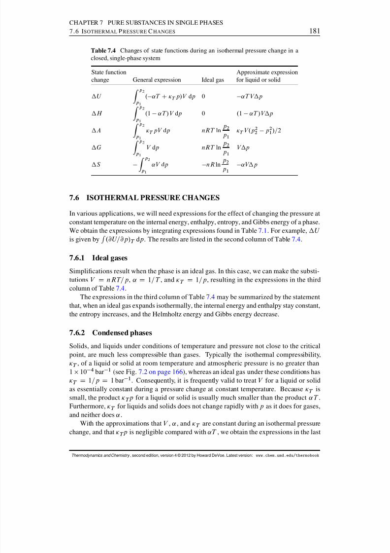
8/12/2019 Howard Devoe Thermodynamic and Chemical
http://slidepdf.com/reader/full/howard-devoe-thermodynamic-and-chemical 181/532
CHAPTER 7 PURE SUBSTANCES IN SINGLE PHASES7.6 I SOTHERMAL P RESSURE C HANGES 181
Table 7.4 Changes of state functions during an isothermal pressure change in aclosed, single-phase system
State function Approximate expressionchange General expression Ideal gas for liquid or solid
U Z p 2
p 1. ˛T C T p/V dp 0 ˛T V p
H Z p 2
p 1
.1 ˛T /V dp 0 .1 ˛T /V p
A Z p 2
p 1
T pV dp nRT lnp 2
p 1T V .p 2
2 p 21 /=2
G Z p 2
p 1
V dp nRT lnp 2
p 1V p
S Z p 2
p 1
˛V dp nR lnp 2
p 1˛V p
7.6 ISOTHERMAL PRESSURE CHANGES
In various applications, we will need expressions for the effect of changing the pressure atconstant temperature on the internal energy, enthalpy, entropy, and Gibbs energy of a phase.We obtain the expressions by integrating expressions found in Table 7.1 . For example, U is given by R .@U=@p/T dp . The results are listed in the second column of Table 7.4 .
7.6.1 Ideal gases
Simplications result when the phase is an ideal gas. In this case, we can make the substi-tutions V D nRT=p , ˛ D 1=T , and T D 1=p , resulting in the expressions in the third
column of Table 7.4 .The expressions in the third column of Table 7.4 may be summarized by the statementthat, when an ideal gas expands isothermally, the internal energy and enthalpy stay constant,the entropy increases, and the Helmholtz energy and Gibbs energy decrease.
7.6.2 Condensed phases
Solids, and liquids under conditions of temperature and pressure not close to the criticalpoint, are much less compressible than gases. Typically the isothermal compressibility,
T , of a liquid or solid at room temperature and atmospheric pressure is no greater than1 10 4 bar 1 (see Fig. 7.2 on page 166 ), whereas an ideal gas under these conditions has
T
D 1=p
D 1 bar 1 . Consequently, it is frequently valid to treat V for a liquid or solid
as essentially constant during a pressure change at constant temperature. Because T issmall, the product T p for a liquid or solid is usually much smaller than the product ˛T .Furthermore, T for liquids and solids does not change rapidly with p as it does for gases,and neither does ˛ .
With the approximations that V , ˛ , and T are constant during an isothermal pressurechange, and that T p is negligible compared with ˛T , we obtain the expressions in the last
Thermodynamics and Chemistry , second edition, version 4 © 2012 by Howard DeVoe. Latest version: www.chem.umd.edu/thermobook

8/12/2019 Howard Devoe Thermodynamic and Chemical
http://slidepdf.com/reader/full/howard-devoe-thermodynamic-and-chemical 182/532
CHAPTER 7 PURE SUBSTANCES IN SINGLE PHASES7.7 S TANDARD S TATES OF P URE S UBSTANCES 182
column of Table 7.4 .
7.7 STANDARD STATES OF PURE SUBSTANCES
It is often useful to refer to a reference pressure, the standard pressure , denoted p ı . The
standard pressure has an arbitrary but constant value in any given application. Until 1982,chemists used a standard pressure of 1 atm ( 1:01325 105 Pa). The IUPAC now recom-mends the value p ı D 1 bar (exactly 105 Pa). This book uses the latter value unless statedotherwise. (Note that there is no dened standard temperature .)
A superscript degree symbol ( ı ) denotes a standard quantity or standard-state condi-tions. An alternative symbol for this purpose, used extensively outside the U.S., is a super-script Plimsoll mark ( ). 8
A standard state of a pure substance is a particular reference state appropriate for thekind of phase and is described by intensive variables. This book follows the recommenda-tions of the IUPAC Green Book 9 for various standard states.
The standard state of a pure gas is the hypothetical state in which the gas is at pressure
pı
and the temperature of interest, and the gas behaves as an ideal gas. The molarvolume of a gas at 1 bar may have a measurable deviation from the molar volumepredicted by the ideal gas equation due to intermolecular forces. We must imaginethe standard state in this case to consist of the gas with the intermolecular forcesmagically “turned off” and the molar volume adjusted to the ideal-gas value RT=p ı .
The standard state of a pure liquid or solid is the unstressed liquid or solid at pres-sure p ı and the temperature of interest. If the liquid or solid is stable under theseconditions, this is a real (not hypothetical) state.
Section 9.7 will introduce additional standard states for constituents of mixtures.
7.8 CHEMICAL POTENTIAL AND FUGACITY
The chemical potential , , of a pure substance has as one of its denitions (page 142)
def
D Gm D Gn
(7.8.1)(pure substance)
That is, is equal to the molar Gibbs energy of the substance at a given temperature andpressure. (Section 9.2.6 will introduce a more general denition of chemical potential thatapplies also to a constituent of a mixture.) The chemical potential is an intensive statefunction.
The total differential of the Gibbs energy of a xed amount of a pure substance in a
single phase, with T and p as independent variables, is d G D S dT CV dp (Eq. 5.4.4 ).
8The Plimsoll mark is named after the British merchant Samuel Plimsoll, at whose instigation Parliament passedan act in 1875 requiring the symbol to be placed on the hulls of cargo ships to indicate the maximum depth forsafe loading.9Ref. [ 36], p. 61–62.
Thermodynamics and Chemistry , second edition, version 4 © 2012 by Howard DeVoe. Latest version: www.chem.umd.edu/thermobook
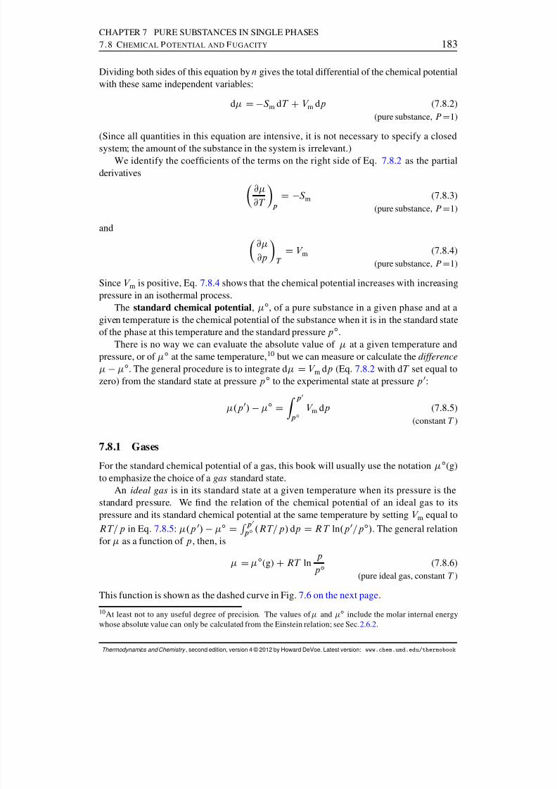
8/12/2019 Howard Devoe Thermodynamic and Chemical
http://slidepdf.com/reader/full/howard-devoe-thermodynamic-and-chemical 183/532
CHAPTER 7 PURE SUBSTANCES IN SINGLE PHASES7.8 C HEMICAL P OTENTIAL AND F UGACITY 183
Dividing both sides of this equation by n gives the total differential of the chemical potentialwith these same independent variables:
d D S m dT CV m dp (7.8.2)(pure substance, P D1)
(Since all quantities in this equation are intensive, it is not necessary to specify a closedsystem; the amount of the substance in the system is irrelevant.)
We identify the coefcients of the terms on the right side of Eq. 7.8.2 as the partialderivatives
@@T p D S m (7.8.3)
(pure substance, P D1)
and
@@p T D V m (7.8.4)
(pure substance, P D1)
Since V m is positive, Eq. 7.8.4 shows that the chemical potential increases with increasingpressure in an isothermal process.
The standard chemical potential , ı , of a pure substance in a given phase and at agiven temperature is the chemical potential of the substance when it is in the standard stateof the phase at this temperature and the standard pressure p ı .
There is no way we can evaluate the absolute value of at a given temperature andpressure, or of ı at the same temperature, 10 but we can measure or calculate the difference
ı . The general procedure is to integrate d D V m dp (Eq. 7.8.2 with d T set equal tozero) from the standard state at pressure p ı to the experimental state at pressure p 0:
.p 0/ ı
DZ p 0
p ıV
m dp (7.8.5)
(constant T )
7.8.1 Gases
For the standard chemical potential of a gas, this book will usually use the notation ı (g)to emphasize the choice of a gas standard state.
An ideal gas is in its standard state at a given temperature when its pressure is thestandard pressure. We nd the relation of the chemical potential of an ideal gas to itspressure and its standard chemical potential at the same temperature by setting V m equal toRT=p in Eq. 7.8.5 : .p 0/ ı D
R
p 0
p ı .RT=p/ dp D RT ln.p 0=p ı / . The general relationfor as a function of p , then, is
D ı (g) CRT lnpp ı (7.8.6)
(pure ideal gas, constant T )
This function is shown as the dashed curve in Fig. 7.6 on the next page .
10 At least not to any useful degree of precision. The values of and ı include the molar internal energywhose absolute value can only be calculated from the Einstein relation; see Sec. 2.6.2 .
Thermodynamics and Chemistry , second edition, version 4 © 2012 by Howard DeVoe. Latest version: www.chem.umd.edu/thermobook
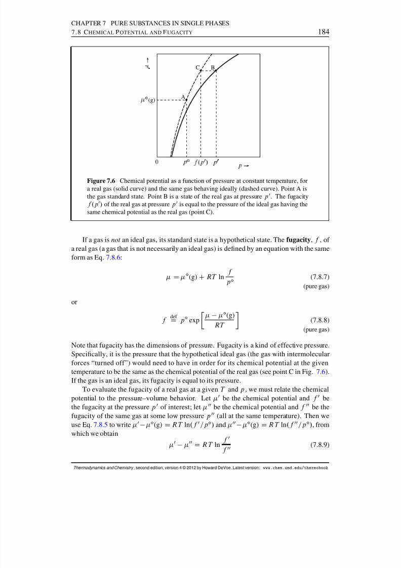
8/12/2019 Howard Devoe Thermodynamic and Chemical
http://slidepdf.com/reader/full/howard-devoe-thermodynamic-and-chemical 184/532
CHAPTER 7 PURE SUBSTANCES IN SINGLE PHASES7.8 C HEMICAL P OTENTIAL AND F UGACITY 184
Æ
Æ
(g)
A
BC
Figure 7.6 Chemical potential as a function of pressure at constant temperature, fora real gas (solid curve) and the same gas behaving ideally (dashed curve). Point A is
the gas standard state. Point B is a state of the real gas at pressure p0
. The fugacityf .p 0/ of the real gas at pressure p 0 is equal to the pressure of the ideal gas having thesame chemical potential as the real gas (point C).
If a gas is not an ideal gas, its standard state is a hypothetical state. The fugacity , f , of a real gas (a gas that is not necessarily an ideal gas) is dened by an equation with the sameform as Eq. 7.8.6 :
D ı (g) CRT lnf p ı (7.8.7)
(pure gas)
or
f def
D p ı expı (g)
RT (7.8.8)
(pure gas)
Note that fugacity has the dimensions of pressure. Fugacity is a kind of effective pressure.Specically, it is the pressure that the hypothetical ideal gas (the gas with intermolecularforces “turned off”) would need to have in order for its chemical potential at the giventemperature to be the same as the chemical potential of the real gas (see point C in Fig. 7.6).If the gas is an ideal gas, its fugacity is equal to its pressure.
To evaluate the fugacity of a real gas at a given T and p , we must relate the chemical
potential to the pressure–volume behavior. Let 0 be the chemical potential and f 0 bethe fugacity at the pressure p 0 of interest; let 00be the chemical potential and f 00be thefugacity of the same gas at some low pressure p 00(all at the same temperature). Then weuse Eq. 7.8.5 to write 0 ı (g) D RT ln.f 0=p ı / and 00 ı (g) D RT ln.f 00=p ı / , fromwhich we obtain
0 00D RT lnf 0
f 00 (7.8.9)
Thermodynamics and Chemistry , second edition, version 4 © 2012 by Howard DeVoe. Latest version: www.chem.umd.edu/thermobook
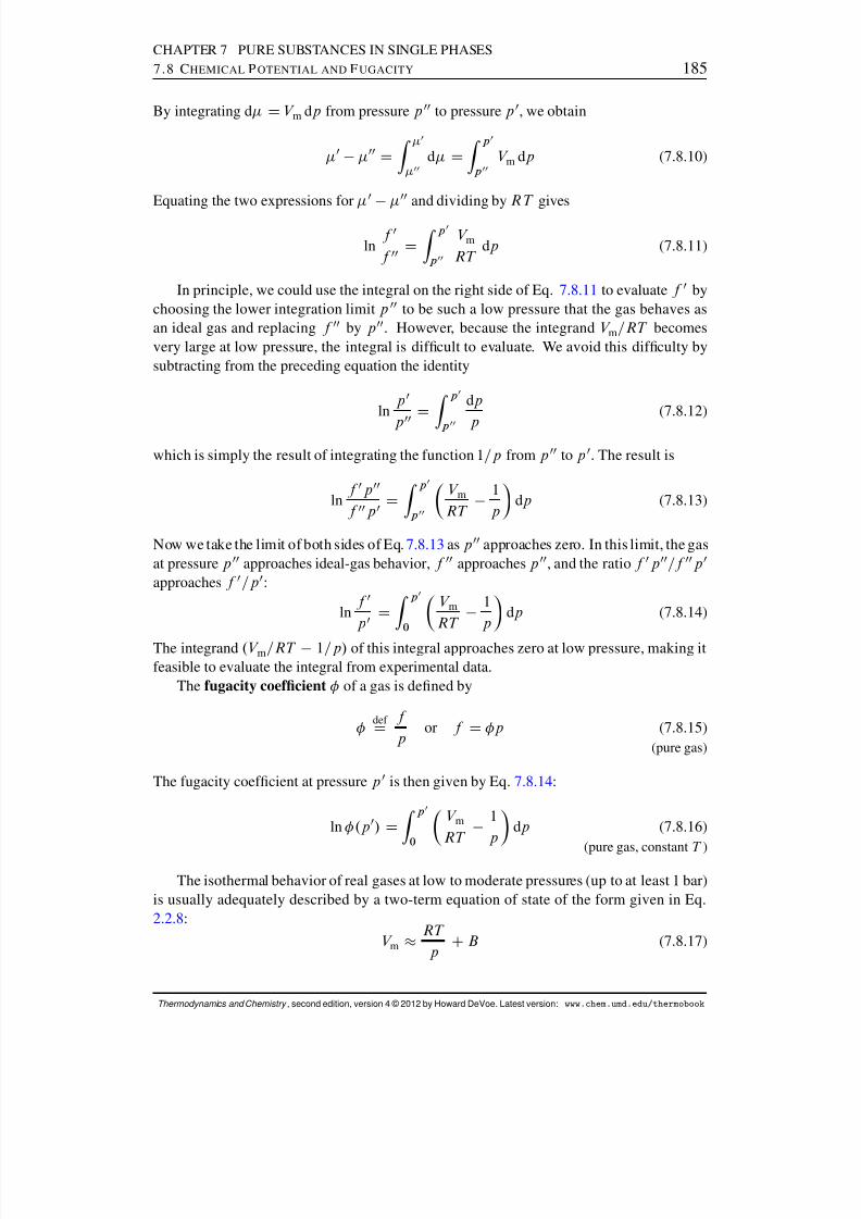
8/12/2019 Howard Devoe Thermodynamic and Chemical
http://slidepdf.com/reader/full/howard-devoe-thermodynamic-and-chemical 185/532
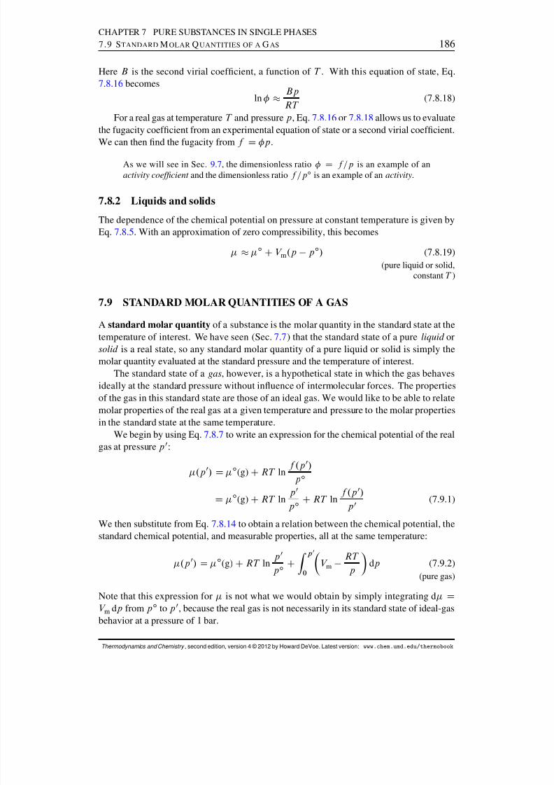
8/12/2019 Howard Devoe Thermodynamic and Chemical
http://slidepdf.com/reader/full/howard-devoe-thermodynamic-and-chemical 186/532
CHAPTER 7 PURE SUBSTANCES IN SINGLE PHASES7.9 S TANDARD M OLAR Q UANTITIES OF A G AS 186
Here B is the second virial coefcient, a function of T . With this equation of state, Eq.7.8.16 becomes
ln BpRT
(7.8.18)
For a real gas at temperature T and pressure p , Eq. 7.8.16 or 7.8.18 allows us to evaluatethe fugacity coefcient from an experimental equation of state or a second virial coefcient.We can then nd the fugacity from f D p .
As we will see in Sec. 9.7, the dimensionless ratio D f =p is an example of anactivity coefcient and the dimensionless ratio f =p ı is an example of an activity .
7.8.2 Liquids and solids
The dependence of the chemical potential on pressure at constant temperature is given byEq. 7.8.5 . With an approximation of zero compressibility, this becomes
ı CV m .p p ı / (7.8.19)(pure liquid or solid,
constant T )
7.9 STANDARD MOLAR QUANTITIES OF A GAS
A standard molar quantity of a substance is the molar quantity in the standard state at thetemperature of interest. We have seen (Sec. 7.7 ) that the standard state of a pure liquid orsolid is a real state, so any standard molar quantity of a pure liquid or solid is simply themolar quantity evaluated at the standard pressure and the temperature of interest.
The standard state of a gas , however, is a hypothetical state in which the gas behavesideally at the standard pressure without inuence of intermolecular forces. The propertiesof the gas in this standard state are those of an ideal gas. We would like to be able to relate
molar properties of the real gas at a given temperature and pressure to the molar propertiesin the standard state at the same temperature.
We begin by using Eq. 7.8.7 to write an expression for the chemical potential of the realgas at pressure p 0:
.p 0/ D ı (g) CRT lnf .p 0/
p ı
D ı (g) CRT lnp 0
p ı CRT lnf .p 0/
p 0 (7.9.1)
We then substitute from Eq. 7.8.14 to obtain a relation between the chemical potential, thestandard chemical potential, and measurable properties, all at the same temperature:
.p 0/ D ı (g) CRT lnp 0
p ı CZ p 0
0V m
RT p
dp (7.9.2)(pure gas)
Note that this expression for is not what we would obtain by simply integrating d DV m dp from p ı to p 0, because the real gas is not necessarily in its standard state of ideal-gasbehavior at a pressure of 1 bar.
Thermodynamics and Chemistry , second edition, version 4 © 2012 by Howard DeVoe. Latest version: www.chem.umd.edu/thermobook
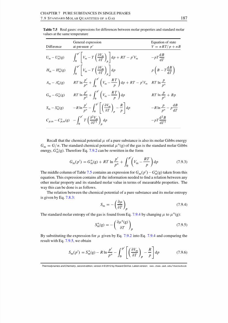
8/12/2019 Howard Devoe Thermodynamic and Chemical
http://slidepdf.com/reader/full/howard-devoe-thermodynamic-and-chemical 187/532
CHAPTER 7 PURE SUBSTANCES IN SINGLE PHASES7.9 S TANDARD M OLAR Q UANTITIES OF A G AS 187
Table 7.5 Real gases: expressions for differences between molar properties and standard molarvalues at the same temperature
General expression Equation of stateDifference at pressure p 0 V D nRT=p CnB
U m U ım (g) Z p 0
0 "V m T @V m@T p #dp CRT p 0V m pT dBdT
H m H ım (g) Z
p 0
0 "V m T @V m
@T p #dp p B T dBdT
Am Aım(g) RT ln
p 0
p ı CZ p 0
0V m
R T p
dp CRT p 0V m RT lnpp ı
Gm G ım (g) RT ln
p 0
p ı CZ p 0
0V m
R T p
dp RT lnpp ı CBp
S m S ım (g) R lnp 0
p ı
Z p 0
0
"@V m
@T p
Rp
#dp R ln
pp ı p
dBdT
C p; m C ıp; m (g) Z p 0
0T
@2 V m@T 2 p
dp pT d2 BdT 2
Recall that the chemical potential of a pure substance is also its molar Gibbs energyGm D G=n . The standard chemical potential ı (g) of the gas is the standard molar Gibbsenergy, G ı
m (g). Therefore Eq. 7.9.2 can be rewritten in the form
Gm .p 0/ D G ım (g) CRT ln
p 0
p ı CZ p 0
0V m
RT p
dp (7.9.3)
The middle column of Table 7.5 contains an expression for Gm .p 0/ G ım(g) taken from this
equation. This expression contains all the information needed to nd a relation between anyother molar property and its standard molar value in terms of measurable properties. Theway this can be done is as follows.
The relation between the chemical potential of a pure substance and its molar entropyis given by Eq. 7.8.3 :
S m D @@T p
(7.9.4)
The standard molar entropy of the gas is found from Eq. 7.9.4 by changing to ı (g):
S ım (g) D
@ ı (g)
@T p (7.9.5)
By substituting the expression for given by Eq. 7.9.2 into Eq. 7.9.4 and comparing theresult with Eq. 7.9.5 , we obtain
S m .p 0/ D S ım (g) R lnp 0
p ı Z p 0
0 "@V m
@T p
Rp #dp (7.9.6)
Thermodynamics and Chemistry , second edition, version 4 © 2012 by Howard DeVoe. Latest version: www.chem.umd.edu/thermobook

8/12/2019 Howard Devoe Thermodynamic and Chemical
http://slidepdf.com/reader/full/howard-devoe-thermodynamic-and-chemical 188/532
CHAPTER 7 PURE SUBSTANCES IN SINGLE PHASES7.9 S TANDARD M OLAR Q UANTITIES OF A G AS 188
The expression for S m S ım(g) in the middle column of Table 7.5 comes from this equation.The equation, together with a value of S m for a real gas obtained by the calorimetric methoddescribed in Sec. 6.2.1 , can be used to evaluate S ım(g).
Now we can use the expressions for Gm and S m to nd expressions for molar quantitiessuch as H m and C p; m relative to the respective standard molar quantities. The general
procedure for a molar quantity X m is to write an expression for X m as a function of Gm andS m and an analogous expression for X ım(g) as a function of G ım(g) and S ım (g). Substitutions
for Gm and S m from Eqs. 7.9.3 and 7.9.6 are then made in the expression for X m , and thedifference X m X ım (g) taken.
For example, the expression for U m U ım(g) in the middle column Table 7.5 was derivedas follows. The equation dening the Gibbs energy, G D U TS CpV , was divided bythe amount n and rearranged to
U m D Gm CTS m pV m (7.9.7)
The standard-state version of this relation is
U ım (g) D G
ım (g) CTS
ım(g) p
ı
V ı
m (g) (7.9.8)
where from the ideal gas law p ı V ım (g) can be replaced by RT . Substitutions from Eqs. 7.9.3and 7.9.6 were made in Eq. 7.9.7 and the expression for U ım(g) in Eq. 7.9.8 was subtracted,resulting in the expression in the table.
For a real gas at low to moderate pressures, we can approximate V m by .RT=p/ CBwhere B is the second virial coefcient (Eq. 7.8.17 ). Equation 7.9.2 then becomes
ı (g) CRT lnpp ı CBp (7.9.9)
The expressions in the last column of Table 7.5 use this equation of state. We can see whatthe expressions look like if the gas is ideal simply by setting B equal to zero. They show thatwhen the pressure of an ideal gas increases at constant temperature, Gm and Am increase,S m decreases, and U m , H m , and C p; m are unaffected.
Thermodynamics and Chemistry , second edition, version 4 © 2012 by Howard DeVoe. Latest version: www.chem.umd.edu/thermobook

8/12/2019 Howard Devoe Thermodynamic and Chemical
http://slidepdf.com/reader/full/howard-devoe-thermodynamic-and-chemical 189/532
CHAPTER 7 PURE SUBSTANCES IN SINGLE PHASESPROBLEMS 189
PROBLEMS
An underlined problem number or problem-part letter indicates that the numerical answer appearsin Appendix I.
7.1 Derive the following relations from the denitions of ˛ , T , and :
˛ D 1 @
@T pT D
1 @@p T
7.2 Use equations in this chapter to derive the following expressions for an ideal gas:
˛ D 1=T T D 1=p
7.3 For a gas with the simple equation of state
V m D RT
p CB
(Eq. 2.2.8), where B is the second virial coefcient (a function of T ), nd expressions for ˛ ,T , and .@U m =@V /T in terms of d B= dT and other state functions.
7.4 Show that when the virial equation pV m D RT .1 CBp p CC p p2
C / (Eq. 2.2.3) adequatelyrepresents the equation of state of a real gas, the Joule–Thomson coefcient is given by
JT DRT 2 ŒdBp = dT C. dC p = dT /p C
C p; m
Note that the limiting value at low pressure, RT 2 . dBp = dT/=C p; m , is not necessarily equal tozero even though the equation of state approaches that of an ideal gas in this limit.
7.5 The quantity .@T=@V /U is called the Joule coefcient . James Joule attempted to evaluatethis quantity by measuring the temperature change accompanying the expansion of air into avacuum—the “Joule experiment.” Write an expression for the total differential of U with T and V as independent variables, and by a procedure similar to that used in Sec. 7.5.2 show thatthe Joule coefcient is equal to
p ˛T= T
C V
7.6 p –V –T data for several organic liquids were measured by Gibson and Loefer. 11 The follow-ing formulas describe the results for aniline.
Molar volume as a function of temperature at p D 1 bar (298–358 K):
V m D a CbT CcT 2 CdT 3
where the parameters have the values
a D 69:287 cm3 mol 1 c D 1:0443 10 4 cm 3 K 2 mol 1
b D 0:08852 cm 3 K 1 mol 1 d D 1:940 10 7 cm 3 K 3 mol 1
Molar volume as a function of pressure at T D 298:15 K (1–1000 bar):
V m D e f ln.g Cp= bar /
where the parameter values are
e D 156:812 cm3 mol 1 f D 8:5834 cm 3 mol 1 g D 2006:6
11 Ref. [ 65].
Thermodynamics and Chemistry , second edition, version 4 © 2012 by Howard DeVoe. Latest version: www.chem.umd.edu/thermobook
8/12/2019 Howard Devoe Thermodynamic and Chemical
http://slidepdf.com/reader/full/howard-devoe-thermodynamic-and-chemical 190/532
CHAPTER 7 PURE SUBSTANCES IN SINGLE PHASESPROBLEMS 190
(a) Use these formulas to evaluate ˛ , T , .@p=@T /V , and .@U=@V /T (the internal pressure)for aniline at T D 298:15 K and p D 1:000 bar.
(b) Estimate the pressure increase if the temperature of a xed amount of aniline is increasedby 0:10 K at constant volume.
7.7 (a) From the total differential of H with T and p as independent variables, derive the relation
.@C p; m=@p/T D T .@2 V m =@T 2 / p .(b) Evaluate .@C p; m =@p/T for liquid aniline at 300:0 K and 1 bar using data in Prob. 7. 6.
7.8 (a) From the total differential of V with T and p as independent variables, derive the relation.@˛=@p/T D .@ T =@T /p .
(b) Use this relation to estimate the value of ˛ for benzene at 25 ı C and 500 bar, given thatthe value of ˛ is 1:2 10 3 K 1 at 25 ı C and 1 bar. (Use information from Fig. 7.2 onpage 166 .)
7.9 Certain equations of state supposed to be applicable to nonpolar liquids and gases are of theform p D Tf .V m / a=V 2m , where f .V m / is a function of the molar volume only and a is aconstant.
(a) Show that the van der Waals equation of state .p Ca=V 2m /.V m b/ D RT (where a andb are constants) is of this form.
(b) Show that any uid with an equation of state of this form has an internal pressure equalto a=V 2m .
7.10 Suppose that the molar heat capacity at constant pressure of a substance has a temperaturedependence given by C p; m D a CbT CcT 2 , where a , b , and c are constants. Consider theheating of an amount n of the substance from T 1 to T 2 at constant pressure. Find expressionsfor H and S for this process in terms of a , b , c , n , T 1 , and T 2 .
7.11 At p D 1 atm, the molar heat capacity at constant pressure of aluminum is given by
C p; m D a CbT
where the constants have the values
a D 20:67 J K 1 mol 1 b D 0:01238 J K 2 mol 1
Calculate the quantity of electrical work needed to heat 2:000 mol of aluminum from 300:00 Kto 400:00 K at 1 atm in an adiabatic enclosure.
7.12 The temperature dependence of the standard molar heat capacity of gaseous carbon dioxide inthe temperature range 298 K– 2000 K is given by
C ıp; m D a CbT C cT 2
where the constants have the values
a D 44:2 J K 1 mol 1 b D 8:8 10 3 J K 2 mol 1 c D 8:6 105 JKmol 1
Calculate the enthalpy and entropy changes when one mole of CO 2 is heated at 1 bar from300:00 K to 800:00 K. You can assume that at this pressure C p; m is practically equal to C ıp; m .
7.13 This problem concerns gaseous carbon dioxide. At 400 K, the relation between p and V m atpressures up to at least 100 bar is given to good accuracy by a virial equation of state truncated
Thermodynamics and Chemistry , second edition, version 4 © 2012 by Howard DeVoe. Latest version: www.chem.umd.edu/thermobook

8/12/2019 Howard Devoe Thermodynamic and Chemical
http://slidepdf.com/reader/full/howard-devoe-thermodynamic-and-chemical 191/532
CHAPTER 7 PURE SUBSTANCES IN SINGLE PHASESPROBLEMS 191
at the second virial coefcient, B . In the temperature range 300 K–800 K the dependence of Bon temperature is given by
B D a 0Cb0T Cc0T 2 Cd 0T 3
where the constants have the values
a 0
D 521 cm 3 mol 1
b0 D 2:08 cm 3 K 1 mol 1
c0 D 2:89 10 3 cm 3 K 2 mol 1
d 0 D 1:397 10 6 cm 3 K 3 mol 1
(a) From information in Prob. 7. 12, calculate the standard molar heat capacity at constantpressure, C ıp; m , at T D 400:0 K.
(b) Estimate the value of C p; m under the conditions T D 400:0 K and p D 100:0 bar.
7.14 A chemist, needing to determine the specic heat capacity of a certain liquid but not having anelectrically heated calorimeter at her disposal, used the following simple procedure known asdrop calorimetry . She placed 500:0 g of the liquid in a thermally insulated container equippedwith a lid and a thermometer. After recording the initial temperature of the liquid, 24:80 ı C,she removed a 60:17-g block of aluminum metal from a boiling water bath at 100:00 ı C andquickly immersed it in the liquid in the container. After the contents of the container hadbecome thermally equilibrated, she recorded a nal temperature of 27:92 ı C. She calculatedthe specic heat capacity C p =m of the liquid from these data, making use of the molar mass of aluminum ( M D 26:9815 gmol 1 ) and the formula for the molar heat capacity of aluminumgiven in Prob. 7. 11 .
(a) From these data, nd the specic heat capacity of the liquid under the assumption that itsvalue does not vary with temperature. Hint: Treat the temperature equilibration processas adiabatic and isobaric ( H D 0), and equate H to the sum of the enthalpy changesin the two phases.
(b) Show that the value obtained in part (a) is actually an average value of C p =m over thetemperature range between the initial and nal temperatures of the liquid given by
Z T
2
T 1.C p =m/ dT
T 2 T 1
7.15 Suppose a gas has the virial equation of state pV m D RT .1 CBp p CC p p 2 / , where Bp andC p depend only on T , and higher powers of p can be ignored.
(a) Derive an expression for the fugacity coefcient, , of this gas as a function of p .
(b) For CO 2 (g) at 0:00 ı C, the virial coefcients have the values Bp D 6:67 10 3 bar 1
and C p D 3:4 10 5 bar 2 . Evaluate the fugacity f at 0:00 ı C and p D 20:0 bar.
7.16 Table 7.6 on the next page lists values of the molar volume of gaseous H 2 O at 400:00 ı C and12 pressures.
(a) Evaluate the fugacity coefcient and fugacity of H 2 O(g) at 400:00ıC and 200 bar.
(b) Show that the second virial coefcient B in the virial equation of state, pV m D RT .1 CB=V m CC=V 2m C / , is given by
B D RT limp ! 0
V mRT
1p
where the limit is taken at constant T . Then evaluate B for H2 O(g) at 400:00 ı C.
Thermodynamics and Chemistry , second edition, version 4 © 2012 by Howard DeVoe. Latest version: www.chem.umd.edu/thermobook

8/12/2019 Howard Devoe Thermodynamic and Chemical
http://slidepdf.com/reader/full/howard-devoe-thermodynamic-and-chemical 192/532
CHAPTER 7 PURE SUBSTANCES IN SINGLE PHASESPROBLEMS 192
Table 7.6 Molar volume of H 2 O(g) at 400:00 ı C a
p=10 5 Pa V m=10 3 m3 mol 1 p=10 5 Pa V m =10 3 m3 mol 1
1 55:896 100 0:4757510 5:5231 120 0:3797620 2:7237 140 0:3102040 1:3224 160 0:2569960 0:85374 180 0:2144780 0:61817 200 0:17918
a based on data in Ref. [ 70]
Thermodynamics and Chemistry , second edition, version 4 © 2012 by Howard DeVoe. Latest version: www.chem.umd.edu/thermobook

8/12/2019 Howard Devoe Thermodynamic and Chemical
http://slidepdf.com/reader/full/howard-devoe-thermodynamic-and-chemical 193/532

8/12/2019 Howard Devoe Thermodynamic and Chemical
http://slidepdf.com/reader/full/howard-devoe-thermodynamic-and-chemical 194/532
CHAPTER 8 PHASE TRANSITIONS AND EQUILIBRIA OF PURE SUBSTANCES8.1 P HASE E QUILIBRIA 194
5. The conditions for an equilibrium state are those that make the innitesimal entropychange, d S , equal to zero for all innitesimal changes of the independent variablesof the isolated system.
8.1.2 Equilibrium in a multiphase system
In this section we consider a system of a single substance in two or more uniform phaseswith distinctly different intensive properties. For instance, one phase might be a liquid andanother a gas. We assume the phases are not separated by internal partitions, so that there isno constraint preventing the transfer of matter and energy among the phases. (A tall columnof gas in a gravitational eld is a different kind of system in which intensive properties of an equilibrium state vary continuously with elevation; this case will be discussed in Sec.8.1.4 .)
Phase ’ 0 will be the reference phase. Since internal energy is extensive, we can writeU D U ’
0
CP’ ¤ ’ 0 U ’ and d U D dU ’0
CP’ ¤ ’ 0 dU ’ . We assume any changes are slowenough to allow each phase to be practically uniform at all times. Treating each phase as anopen subsystem with expansion work only, we use the relation d U
D T dS
p dV
Cdn
(Eq. 5.2.5 ) to replace each d U ’ term:
dU D .T ’ 0dS ’
0p ’ 0
dV ’0
C ’ 0dn ’ 0
/
CX’ ¤ ’ 0
.T ’ dS ’ p ’ dV ’ C ’ dn ’ / (8.1.1)
This is an expression for the total differential of U when there are no constraints.We isolate the system by enclosing it in a rigid, stationary adiabatic container. The
constraints needed to isolate the system, then, are given by the relations
dU D 0 (constant internal energy) (8.1.2)
dV ’ 0
CX’ ¤ ’ 0dV
’
D 0 (no expansion work) (8.1.3)
dn ’ 0
CX’ ¤ ’ 0
dn ’ D 0 (closed system) (8.1.4)
Each of these relations is an independent restriction that reduces the number of independentvariables by one. When we substitute expressions for d U , dV ’
0, and d n ’ 0
from these re-lations into Eq. 8.1.1 , make the further substitution d S ’
0
D dS P’ ¤ ’ 0 dS ’ , and collectterm with the same differentials on the right side, we obtain
0 D T ’0dS C
X’ ¤ ’0
.T ’ T ’0/ dS ’
X’ ¤ ’0
.p ’ p ’ 0/ dV ’
CX’ ¤ ’ 0
. ’ ’ 0/ dn ’ (8.1.5)
Thermodynamics and Chemistry , second edition, version 4 © 2012 by Howard DeVoe. Latest version: www.chem.umd.edu/thermobook
8/12/2019 Howard Devoe Thermodynamic and Chemical
http://slidepdf.com/reader/full/howard-devoe-thermodynamic-and-chemical 195/532
CHAPTER 8 PHASE TRANSITIONS AND EQUILIBRIA OF PURE SUBSTANCES8.1 P HASE E QUILIBRIA 195
Solving for d S , we obtain
dS DX’ ¤ ’ 0
T ’0
T ’
T ’ 0 dS ’ X’ ¤ ’ 0
p ’ 0p ’
T ’ 0 dV ’
CX’ ¤ ’ 0
’ 0 ’
T ’ 0 dn’
(8.1.6)
This is an expression for the total differential of S in the isolated system.In an isolated system, an equilibrium state cannot change spontaneously to a differ-
ent state. Once the isolated system has reached an equilibrium state, an imagined nitechange of any of the independent variables consistent with the constraints (a so-called vir-tual displacement ) corresponds to an impossible process with an entropy decrease. Thus,the equilibrium state has the maximum entropy that is possible for the isolated system. Inorder for S to be a maximum, d S must be zero for an innitesimal change of any of theindependent variables of the isolated system.
This requirement is satised in the case of the multiphase system only if the coefcientof each term in the sums on the right side of Eq. 8.1.6 is zero. Therefore, in an equilibriumstate the temperature of each phase is equal to the temperature T ’
0of the reference phase,
the pressure of each phase is equal to p ’ 0, and the chemical potential in each phase is equal
to ’ 0. That is, at equilibrium the temperature, pressure, and chemical potential are uniform
throughout the system. These are, respectively, the conditions described in Sec. 2.4.4 of thermal equilibrium , mechanical equilibrium , and transfer equilibrium . These conditionsmust hold in order for a multiphase system of a pure substance without internal partitions tobe in an equilibrium state, regardless of the process by which the system attains that state.
8.1.3 Simple derivation of equilibrium conditions
Here is a simpler, less formal derivation of the three equilibrium conditions in a multiphasesystem of a single substance.It is intuitively obvious that, unless there are special constraints (such as internal parti-
tions), an equilibrium state must have thermal and mechanical equilibrium. A temperaturedifference between two phases would cause a spontaneous transfer of heat from the warmerto the cooler phase; a pressure difference would cause spontaneous ow of matter.
When some of the substance is transferred from one phase to another under conditionsof constant T and p , the intensive properties of each phase remains the same including thechemical potential. The chemical potential of a pure phase is the Gibbs energy per amountof substance in the phase. We know that in a closed system of constant T and p withexpansion work only, the total Gibbs energy decreases during a spontaneous process andis constant during a reversible process (Eq. 5.8.6 ). The Gibbs energy will decrease onlyif there is a transfer of substance from a phase of higher chemical potential to a phase of lower chemical potential, and this will be a spontaneous change. No spontaneous transferis possible if both phases have the same chemical potential, so this is a condition for anequilibrium state.
Thermodynamics and Chemistry , second edition, version 4 © 2012 by Howard DeVoe. Latest version: www.chem.umd.edu/thermobook
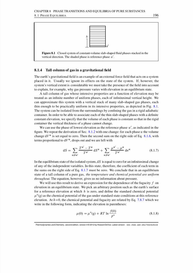
8/12/2019 Howard Devoe Thermodynamic and Chemical
http://slidepdf.com/reader/full/howard-devoe-thermodynamic-and-chemical 196/532
CHAPTER 8 PHASE TRANSITIONS AND EQUILIBRIA OF PURE SUBSTANCES8.1 P HASE E QUILIBRIA 196
Figure 8.1 Closed system of constant-volume slab-shaped uid phases stacked in thevertical direction. The shaded phase is reference phase ’ 0.
8.1.4 Tall column of gas in a gravitational eld
The earth’s gravitational eld is an example of an external force eld that acts on a systemplaced in it. Usually we ignore its effects on the state of the system. If, however, thesystem’s vertical extent is considerable we must take the presence of the eld into accountto explain, for example, why gas pressure varies with elevation in an equilibrium state.
A tall column of gas whose intensive properties are a function of elevation may betreated as an innite number of uniform phases, each of innitesimal vertical height. Wecan approximate this system with a vertical stack of many slab-shaped gas phases, eachthin enough to be practically uniform in its intensive properties, as depicted in Fig. 8.1.The system can be isolated from the surroundings by conning the gas in a rigid adiabaticcontainer. In order to be able to associate each of the thin slab-shaped phases with a deniteconstant elevation, we specify that the volume of each phase is constant so that in the rigidcontainer the vertical thickness of a phase cannot change.
We can use the phase of lowest elevation as the reference phase ’ 0, as indicated in thegure. We repeat the derivation of Sec. 8.1.2 with one change: for each phase ’ the volumechange d V ’ is set equal to zero. Then the second sum on the right side of Eq. 8.1.6 , withterms proportional to d V ’ , drops out and we are left with
dS DX’ ¤ ’ 0
T ’0
T ’
T ’ 0 dS ’ CX’ ¤ ’ 0
’ 0 ’
T ’ 0 dn ’ (8.1.7)
In the equilibrium state of the isolated system, d S is equal to zero for an innitesimal changeof any of the independent variables. In this state, therefore, the coefcient of each term inthe sums on the right side of Eq. 8.1.7 must be zero. We conclude that in an equilibriumstate of a tall column of a pure gas, the temperature and chemical potential are uniformthroughout . The equation, however, gives us no information about pressure.
We will use this result to derive an expression for the dependence of the fugacity f onelevation in an equilibrium state. We pick an arbitrary position such as the earth’s surface
for a reference elevation at which h is zero, and dene the standard chemical potentialı (g) as the chemical potential of the gas under standard state conditions at this reference
elevation. At hD0, the chemical potential and fugacity are related by Eq. 7.8.7 which wewrite in the following form, indicating the elevation in parentheses:
.0/ D ı (g) CRT lnf.0/p ı (8.1.8)
Thermodynamics and Chemistry , second edition, version 4 © 2012 by Howard DeVoe. Latest version: www.chem.umd.edu/thermobook
8/12/2019 Howard Devoe Thermodynamic and Chemical
http://slidepdf.com/reader/full/howard-devoe-thermodynamic-and-chemical 197/532
8/12/2019 Howard Devoe Thermodynamic and Chemical
http://slidepdf.com/reader/full/howard-devoe-thermodynamic-and-chemical 198/532
CHAPTER 8 PHASE TRANSITIONS AND EQUILIBRIA OF PURE SUBSTANCES8.1 P HASE E QUILIBRIA 198
If we treat the gas as ideal, so that the fugacity equals the pressure, this equation becomes
p.h/ D p.0/e Mgh=RT (8.1.13)(pure ideal gas at equilibrium
in gravitational eld)
Equation 8.1.13 is the barometric formula for a pure ideal gas. It shows that in the equi-librium state of a tall column of an ideal gas, the pressure decreases exponentially withincreasing elevation.
This derivation of the barometric formula has introduced a method that will be used inSec. 9.8.1 for dealing with mixtures in a gravitational eld. There is, however, a shorterderivation based on Newton’s second law and not involving the chemical potential. Con-sider one of the thin slab-shaped phases of Fig. 8.1 . Let the density of the phase be , thearea of each horizontal face be As , and the thickness of the slab be •h . The mass of the phaseis then m D A s•h . The pressure difference between the top and bottom of the phase is •p .Three vertical forces act on the phase: an upward force pA s at its lower face, a downwardforce .p C•p/A s at its upper face, and a downward gravitational force mg D A sg•h .
If the phase is at rest, the net vertical force is zero: pA s .p C•p/A s A sg•h D 0, or•p D g•h . In the limit as the number of phases becomes innite and •h and •p becomeinnitesimal, this becomes
dp D g dh (8.1.14)(uid at equilibrium
in gravitational eld)
Equation 8.1.14 is a general relation between changes in elevation and hydrostatic pressurein any uid. To apply it to an ideal gas, we replace the density by D nM=V D M=V m DMp=RT and rearrange to d p=p D .gM=RT / dh . Treating g and T as constants, weintegrate from h
D0 to an arbitrary elevation h and obtain the same result as Eq. 8.1.13 .
8.1.5 The pressure in a liquid droplet
The equilibrium shape of a small liquid droplet surrounded by vapor of the same substance,when the effects of gravity and other external forces are negligible, is spherical. This is theresult of the surface tension of the liquid–gas interface which acts to minimize the ratio of surface to volume. The interface acts somewhat like the stretched membrane of an inatedballoon, resulting in a greater pressure inside the droplet than the pressure of the vapor inequilibrium with it.
We can derive the pressure difference by considering a closed system containing aspherical liquid droplet and surrounding vapor. We treat both phases as open subsystems.An innitesimal change d U of the internal energy is the sum of contributions from the liq-uid and gas phases and from the surface work dAs , where is the surface tension of theliquid–gas interface and A s is the surface area of the droplet (Sec. 5.7):
dU D dU l CdU g C dAs
D T l dS l p l dV l C l dn l
CT g dS g p g dV g C g dng C dAs (8.1.15)
Thermodynamics and Chemistry , second edition, version 4 © 2012 by Howard DeVoe. Latest version: www.chem.umd.edu/thermobook

8/12/2019 Howard Devoe Thermodynamic and Chemical
http://slidepdf.com/reader/full/howard-devoe-thermodynamic-and-chemical 199/532
CHAPTER 8 PHASE TRANSITIONS AND EQUILIBRIA OF PURE SUBSTANCES8.1 P HASE E QUILIBRIA 199
Note that Eq. 8.1.15 is not an expression for the total differential of U , because V l andAs are not independent variables. A derivation by a procedure similar to the one used inSec. 8.1.2 shows that at equilibrium the liquid and gas have equal temperatures and equalchemical potentials, and the pressure in the droplet is greater than the gas pressure by anamount that depends on r :
pl
D pg
C 2
r (8.1.16)
Equation 8.1.16 is the Laplace equation . The pressure difference is signicant if r is small,and decreases as r increases. The limit r!1 represents the at surface of bulk liquid withp l equal to p g .
The derivation of Eq. 8.1.16 is left as an exercise (Prob. 8. 1). The Laplace equationis valid also for a liquid droplet in which the liquid and the surrounding gas may both bemixtures (Prob. 9. 3 on page 281 ).
The Laplace equation can also be applied to the pressure in a gas bubble surroundedby liquid. In this case the liquid and gas phases switch roles, and the equation becomesp g D p l C2 =r .
8.1.6 The number of independent variables
From this point on in this book, unless stated otherwise, the discussions of multiphase sys-tems will implicitly assume the existence of thermal, mechanical, and transfer equilibrium.Equations will not explicitly show these equilibria as a condition of validity.
In the rest of this chapter, we shall assume the state of each phase can be described bythe usual variables: temperature, pressure, and amount. That is, variables such as elevationin a gravitational eld, interface surface area, and extent of stretching of a solid, are notrelevant.
How many of the usual variables of an open multiphase one-substance equilibrium sys-tem are independent? To nd out, we go through the following argument. In the absence of
any kind of equilibrium, we could treat phase ’ as having the three independent variablesT ’ , p ’ , and n’ , and likewise for every other phase. A system of P phases without thermal,mechanical, or transfer equilibrium would then have 3P independent variables.
We must decide how to count the number of phases. It is usually of no thermodynamicsignicance whether a phase, with particular values of its intensive properties, is con-tiguous. For instance, splitting a crystal into several pieces is not usually considered tochange the number of phases or the state of the system, provided the increased surfacearea makes no signicant contribution to properties such as internal energy. Thus, thenumber of phases P refers to the number of different kinds of phases.
Each independent relation resulting from equilibrium imposes a restriction on the sys-
tem and reduces the number of independent variables by one. A two-phase system withthermal equilibrium has the single relation T “ D T ’ . For a three-phase system, there aretwo such relations that are independent, for instance T “ D T ’ and T ” D T ’ . (The addi-tional relation T ” D T “ is not independent since we may deduce it from the other two.) Ingeneral, thermal equilibrium gives P 1 independent relations among temperatures.
Thermodynamics and Chemistry , second edition, version 4 © 2012 by Howard DeVoe. Latest version: www.chem.umd.edu/thermobook

8/12/2019 Howard Devoe Thermodynamic and Chemical
http://slidepdf.com/reader/full/howard-devoe-thermodynamic-and-chemical 200/532
CHAPTER 8 PHASE TRANSITIONS AND EQUILIBRIA OF PURE SUBSTANCES8.2 P HASE D IAGRAMS OF P URE S UBSTANCES 200
By the same reasoning, mechanical equilibrium involves P 1 independent relationsamong pressures, and transfer equilibrium involves P 1 independent relations amongchemical potentials.
The total number of independent relations for equilibrium is 3.P 1/ , which we subtractfrom 3P (the number of independent variables in the absence of equilibrium) to obtain
the number of independent variables in the equilibrium system: 3P 3.P 1/ D 3.Thus, an open single-substance system with any number of phases has at equilibrium threeindependent variables . For example, in equilibrium states of a two-phase system we mayvary T , n’ , and n“ independently, in which case p is a dependent variable; for a given valueof T , the value of p is the one that allows both phases to have the same chemical potential.
8.1.7 The Gibbs phase rule for a pure substance
The complete description of the state of a system must include the value of an extensivevariable of each phase (e.g., the volume, mass, or amount) in order to specify how much of the phase is present. For an equilibrium system of P phases with a total of 3 independentvariables, we may choose the remaining 3 P variables to be intensive . The number of these
intensive independent variables is called the number of degrees of freedom or variance ,F , of the system:
F D 3 P (8.1.17)(pure substance)
The application of the phase rule to multicomponent systems will be taken up in Sec.13.1 . Equation 8.1.17 is a special case, for C D 1, of the more general Gibbs phaserule F D C P C2.
We may interpret the variance F in either of two ways: F is the number of intensive variables needed to describe an equilibrium state, inaddition to the amount of each phase;
F is the maximum number of intensive properties that we may vary independentlywhile the phases remain in equilibrium.
A system with two degrees of freedom is called bivariant , one with one degree of free-dom is univariant , and one with no degrees of freedom is invariant . For a system of apure substance, these three cases correspond to one, two, and three phases respectively.For instance, a system of liquid and gaseous H 2 O (and no other substances) is univariant(F D 3 P D 3 2 D 1); we are able to independently vary only one intensive property,such as T , while the liquid and gas remain in equilibrium.
8.2 PHASE DIAGRAMS OF PURE SUBSTANCESA phase diagram is a two-dimensional map showing which phase or phases are able to existin an equilibrium state under given conditions. This chapter describes pressure–volume andpressure–temperature phase diagrams for a single substance, and Chap. 13 will describenumerous types of phase diagrams for multicomponent systems.
Thermodynamics and Chemistry , second edition, version 4 © 2012 by Howard DeVoe. Latest version: www.chem.umd.edu/thermobook

8/12/2019 Howard Devoe Thermodynamic and Chemical
http://slidepdf.com/reader/full/howard-devoe-thermodynamic-and-chemical 201/532
CHAPTER 8 PHASE TRANSITIONS AND EQUILIBRIA OF PURE SUBSTANCES8.2 P HASE D IAGRAMS OF P URE S UBSTANCES 201
8.2.1 Features of phase diagrams
Two-dimensional phase diagrams for a single-substance system can be generated as projec-tions of a three-dimensional surface in a coordinate system with Cartesian axes p , V =n, andT . A point on the three-dimensional surface corresponds to a physically-realizable combi-nation of values, for an equilibrium state of the system containing a total amount n of the
substance, of the variables p , V =n, and T .The concepts needed to interpret single-substance phase diagrams will be illustrated
with carbon dioxide.Three-dimensional surfaces for carbon dioxide are shown at two different scales in
Fig. 8.2 on the next page and in Fig. 8.3 on page 203 . In these gures, some areas of the surface are labeled with a single physical state: solid, liquid, gas, or supercritical uid.A point in one of these areas corresponds to an equilibrium state of the system containinga single phase of the labeled physical state. The shape of the surface in this one-phase areagives the equation of state of the phase (i.e., the dependence of one of the variables on theother two). A point in an area labeled with two physical states corresponds to two coex-isting phases. The triple line is the locus of points for all possible equilibrium systems of
three coexisting phases, which in this case are solid, liquid, and gas. A point on the tripleline can also correspond to just one or two phases (see the discussion on page 203 ).
The two-dimensional projections shown in Figs. 8.2 (b) and 8.2 (c) are pressure–volumeand pressure–temperature phase diagrams. Because all phases of a multiphase equilibriumsystem have the same temperature and pressure, 2 the projection of each two-phase areaonto the pressure–temperature diagram is a curve, called a coexistence curve or phaseboundary , and the projection of the triple line is a point, called a triple point .
How may we use a phase diagram? The two axes represent values of two independentvariables, such as p and V =n or p and T . For given values of these variables, we place apoint on the diagram at the intersection of the corresponding coordinates; this is the systempoint . Then depending on whether the system point falls in an area or on a coexistencecurve, the diagram tells us the number and kinds of phases that can be present in the equi-librium system.
If the system point falls within an area labeled with the physical state of a single phase,only that one kind of phase can be present in the equilibrium system. A system containing apure substance in a single phase is bivariant ( F D 3 1 D 2), so we may vary two intensiveproperties independently. That is, the system point may move independently along twocoordinates ( p and V=n, or p and T ) and still remain in the one-phase area of the phasediagram. When V and n refer to a single phase, the variable V =n is the molar volume V min the phase.
If the system point falls in an area of the pressure–volume phase diagram labeled withsymbols for two phases, these two phases coexist in equilibrium. The phases have the samepressure and different molar volumes. To nd the molar volumes of the individual phases,we draw a horizontal line of constant pressure, called a tie line , through the system pointand extending from one edge of the area to the other. The horizontal position of each endof the tie line, where it terminates at the boundary with a one-phase area, gives the molarvolume in that phase in the two-phase system. For an example of a tie line, see Fig. 8.9 onpage 209 .
2This statement assumes there are no constraints such as internal adiabatic partitions.
Thermodynamics and Chemistry , second edition, version 4 © 2012 by Howard DeVoe. Latest version: www.chem.umd.edu/thermobook
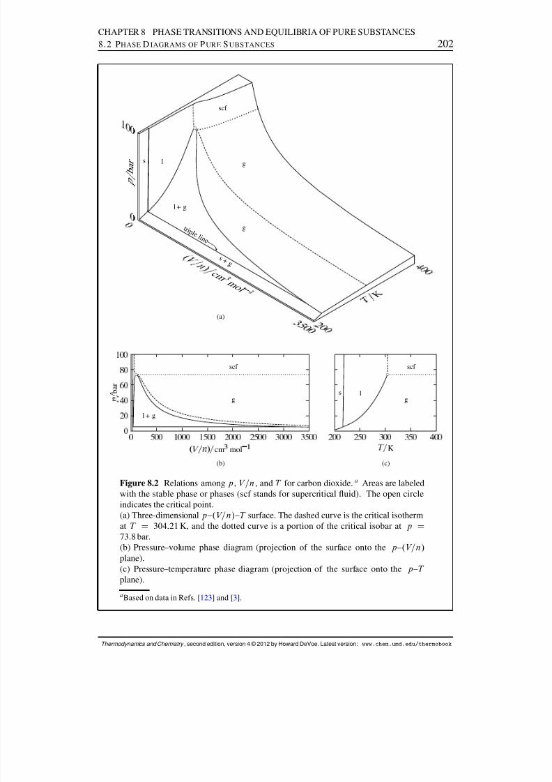
8/12/2019 Howard Devoe Thermodynamic and Chemical
http://slidepdf.com/reader/full/howard-devoe-thermodynamic-and-chemical 202/532
CHAPTER 8 PHASE TRANSITIONS AND EQUILIBRIA OF PURE SUBSTANCES8.2 P HASE D IAGRAMS OF P URE S UBSTANCES 202
s l g
g
l + g
scf
s + g
t r i p l e l i n e
c m
m o l
K
b a r
(a)
cm mol
.
b a r
l + g
g
scf
(b)
K
lsg
scf
(c)
Figure 8.2 Relations among p , V =n, and T for carbon dioxide. a Areas are labeledwith the stable phase or phases (scf stands for supercritical uid). The open circleindicates the critical point.(a) Three-dimensional p –.V=n/ –T surface. The dashed curve is the critical isothermat T D 304:21 K, and the dotted curve is a portion of the critical isobar at p D73:8 bar.
(b) Pressure–volume phase diagram (projection of the surface onto the p –.V=n/plane).(c) Pressure–temperature phase diagram (projection of the surface onto the p –T plane).
a Based on data in Refs. [ 123 ] and [3].
Thermodynamics and Chemistry , second edition, version 4 © 2012 by Howard DeVoe. Latest version: www.chem.umd.edu/thermobook

8/12/2019 Howard Devoe Thermodynamic and Chemical
http://slidepdf.com/reader/full/howard-devoe-thermodynamic-and-chemical 203/532
CHAPTER 8 PHASE TRANSITIONS AND EQUILIBRIA OF PURE SUBSTANCES8.2 P HASE D IAGRAMS OF P URE S UBSTANCES 203
s
l
g
gl + g
scf
s + l
s + g
t r i p l e l i n e
c m
m o l
K
b a r
Figure 8.3 Three-dimensional p –.V=n/ –T surface for CO 2 , magnied along theV=n axis compared to Fig. 8.2. The open circle is the critical point, the dashed curveis the critical isotherm, and the dotted curve is a portion of the critical isobar.
The triple line on the pressure–volume diagram represents the range of values of V =nin which three phases (solid, liquid, and gas) can coexist at equilibrium. 3 A three-phaseone-component system is invariant ( F D 3 3 D 0); there is only one temperature (thetriple-point temperature T tp ) and one pressure (the triple-point pressure p tp ) at which thethree phases can coexist. The values of T tp and p tp are unique to each substance, and
are shown by the position of the triple point on the pressure–temperature phase diagram.The molar volumes in the three coexisting phases are given by the values of V=n at thethree points on the pressure–volume diagram where the triple line touches a one-phasearea. These points are at the two ends and an intermediate position of the triple line. If thesystem point is at either end of the triple line, only the one phase of corresponding molarvolume at temperature T tp and pressure p tp can be present. When the system point is on thetriple line anywhere between the two ends, either two or three phases can be present. If thesystem point is at the position on the triple line corresponding to the phase of intermediatemolar volume, there might be only that one phase present.
At high pressures, a substance may have additional triple points for two solid phases andthe liquid, or for three solid phases. This is illustrated by the pressure–temperature phase
diagram of H 2 O in Fig. 8.4 on the next page , which extends to pressures up to 30 kbar. (Onthis scale, the liquid–gas coexistence curve lies too close to the horizontal axis to be visible.)The diagram shows seven different solid phases of H 2 O differing in crystal structure and
3Helium is the only substance lacking a solid–liquid–gas triple line. When a system containing the coexistingliquid and gas of 4 He is cooled to 2:17 K, a triple point is reached in which the third phase is a liquid calledHe-II, which has the unique property of superuidity. It is only at high pressures ( 10 bar or greater) that solidhelium can exist.
Thermodynamics and Chemistry , second edition, version 4 © 2012 by Howard DeVoe. Latest version: www.chem.umd.edu/thermobook

8/12/2019 Howard Devoe Thermodynamic and Chemical
http://slidepdf.com/reader/full/howard-devoe-thermodynamic-and-chemical 204/532
CHAPTER 8 PHASE TRANSITIONS AND EQUILIBRIA OF PURE SUBSTANCES8.2 P HASE D IAGRAMS OF P URE S UBSTANCES 204
200 250 300 350 4000
5
10
15
20
25
30
T =K
p = k b a r
liquid
I
II III
V
VI
VIIVIII
Figure 8.4 High-pressure pressure–temperature phase diagram of H 2 O. a The romannumerals designate seven forms of ice.
a
Based on data in Refs. [ 49], Table 3.5, and [ 128 ].
designated ice I, ice II, and so on. Ice I is the ordinary form of ice, stable below 2 bar. Onthe diagram are four triple points for two solids and the liquid and three triple points forthree solids. Each triple point is invariant. Note how H 2 O can exist as solid ice VI or iceVII above its standard melting point of 273 K if the pressure is high enough (“hot ice”).
8.2.2 Two-phase equilibrium
A system containing two phases of a pure substance in equilibrium is univariant. Bothphases have the same values of T and of p , but these values are not independent becauseof the requirement that the phases have equal chemical potentials. We may vary only oneintensive variable of a pure substance (such as T or p ) independently while two phasescoexist in equilibrium.
At a given temperature, the pressure at which solid and gas or liquid and gas are inequilibrium is called the vapor pressure or saturation vapor pressure of the solid orliquid. 4 The vapor pressure of a solid is sometimes called the sublimation pressure . Wemay measure the vapor pressure of a liquid at a xed temperature with a simple devicecalled an isoteniscope (Fig. 8.5 on the next page ).
At a given pressure, the melting point or freezing point is the temperature at whichsolid and liquid are in equilibrium, the boiling point or saturation temperature is thetemperature at which liquid and gas are in equilibrium, and the sublimation temperature
or sublimation point is the temperature at which solid and gas are in equilibrium.
4In a system of more than one substance, vapor pressure can refer to the partial pressure of a substance in a gasmixture equilibrated with a solid or liquid of that substance. The effect of total pressure on vapor pressure willbe discussed in Sec. 12.8.1 . This book refers to the saturation vapor pressure of a liquid when it is necessary toindicate that it is the pure liquid and pure gas phases that are in equilibrium at the same pressure.
Thermodynamics and Chemistry , second edition, version 4 © 2012 by Howard DeVoe. Latest version: www.chem.umd.edu/thermobook

8/12/2019 Howard Devoe Thermodynamic and Chemical
http://slidepdf.com/reader/full/howard-devoe-thermodynamic-and-chemical 205/532
CHAPTER 8 PHASE TRANSITIONS AND EQUILIBRIA OF PURE SUBSTANCES8.2 P HASE D IAGRAMS OF P URE S UBSTANCES 205
bath
Figure 8.5 An isoteniscope. The liquid to be investigated is placed in the vessel andU-tube, as indicated by shading, and maintained at a xed temperature in the bath. Thepressure in the side tube is reduced until the liquid boils gently and its vapor sweepsout the air. The pressure is adjusted until the liquid level is the same in both limbs of the U-tube; the vapor pressure of the liquid is then equal to the pressure in the sidetube, which can be measured with a manometer.
K
.
b a r
s l g
triple point
standardmelting point
standardboiling point
Figure 8.6 Pressure–temperature phase diagram of H 2 O. (Based on data in Ref.[123 ].)
The relation between temperature and pressure in a system with two phases in equilib-rium is shown by the coexistence curve separating the two one-phase areas on the pressure–temperature diagram (see Fig. 8.6 ). Consider the liquid–gas curve. If we think of T as the
independent variable, the curve is a vapor-pressure curve showing how the vapor pressureof the liquid varies with temperature. If, however, p is the independent variable, then thecurve is a boiling-point curve showing the dependence of the boiling point on pressure.
The normal melting point or boiling point refers to a pressure of one atmosphere, andthe standard melting point or boiling point refers to the standard pressure. Thus, the normalboiling point of water ( 99:97 ı C) is the boiling point at 1 atm; this temperature is also known
Thermodynamics and Chemistry , second edition, version 4 © 2012 by Howard DeVoe. Latest version: www.chem.umd.edu/thermobook

8/12/2019 Howard Devoe Thermodynamic and Chemical
http://slidepdf.com/reader/full/howard-devoe-thermodynamic-and-chemical 206/532
CHAPTER 8 PHASE TRANSITIONS AND EQUILIBRIA OF PURE SUBSTANCES8.2 P HASE D IAGRAMS OF P URE S UBSTANCES 206
as the steam point . The standard boiling point of water ( 99:61 ı C) is the boiling point at theslightly lower pressure of 1 bar.
Coexistence curves will be discussed further in Sec. 8.4 .
8.2.3 The critical point
Every substance has a certain temperature, the critical temperature , above which only oneuid phase can exist at any volume and pressure (Sec. 2.2.3 ). The critical point is the pointon a phase diagram corresponding to liquid–gas coexistence at the critical temperature, andthe critical pressure is the pressure at this point.
To observe the critical point of a substance experimentally, we can evacuate a glassvessel, introduce an amount of the substance such that V =n is approximately equal to themolar volume at the critical point, seal the vessel, and raise the temperature above thecritical temperature. The vessel now contains a single uid phase. When the substance isslowly cooled to a temperature slightly above the critical temperature, it exhibits a cloudyappearance, a phenomenon called critical opalescence (Fig. 8.7 on the next page ). Theopalescence is the scattering of light caused by large local density uctuations. At the
critical temperature, a meniscus forms between liquid and gas phases of practically thesame density. With further cooling, the density of the liquid increases and the density of thegas decreases.
At temperatures above the critical temperature and pressures above the critical pressure,the one existing uid phase is called a supercritical uid . Thus, a supercritical uid of apure substance is a uid that does not undergo a phase transition to a different uid phasewhen we change the pressure at constant temperature or change the temperature at constantpressure. 5
A uid in the supercritical region can have a density comparable to that of the liquid,and can be more compressible than the liquid. Under supercritical conditions, a substanceis often an excellent solvent for solids and liquids. By varying the pressure or temperature,
the solvating power can be changed; by reducing the pressure isothermally, the substancecan be easily removed as a gas from dissolved solutes. These properties make supercriticaluids useful for chromatography and solvent extraction.
The critical temperature of a substance can be measured quite accurately by observingthe appearance or disappearance of a liquid–gas meniscus, and the critical pressure can bemeasured at this temperature with a high-pressure manometer. To evaluate the density atthe critical point, it is best to extrapolate the mean density of the coexisting liquid and gasphases, . l C g/=2 , to the critical temperature as illustrated in Fig. 8.8 on page 208 . Theobservation that the mean density closely approximates a linear function of temperature, asshown in the gure, is known as the law of rectilinear diameters , or the law of Cailletetand Matthias. This law is an approximation, as can be seen by the small deviation of themean density of SF
6 from a linear relation very close to the critical point in Fig. 8.8(b). This
failure of the law of rectilinear diameters is predicted by recent theoretical treatments. 6
5If, however, we increase p at constant T , the supercritical uid will change to a solid. In the phase diagramof H 2 O, the coexistence curve for ice VII and liquid shown in Fig. 8.4 extends to a higher temperature than thecritical temperature of 647 K. Thus, supercritical water can be converted to ice VII by isothermal compression.6Refs. [ 164 ] and [10].
Thermodynamics and Chemistry , second edition, version 4 © 2012 by Howard DeVoe. Latest version: www.chem.umd.edu/thermobook
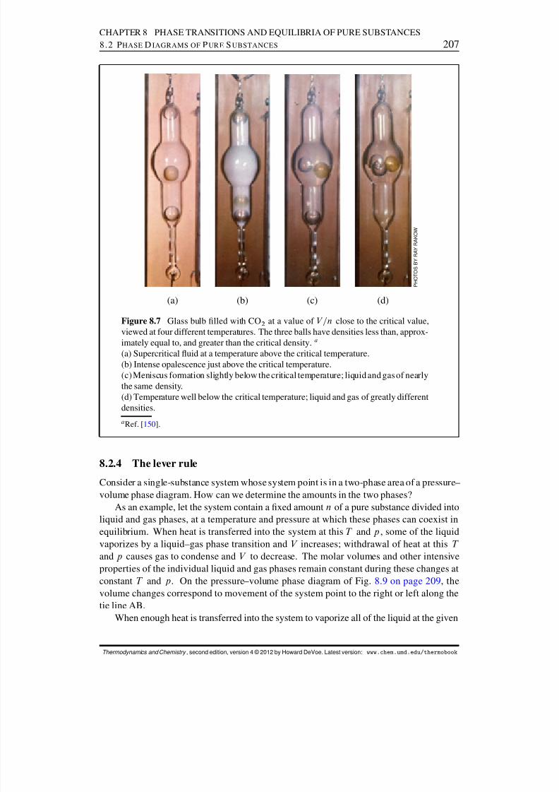
8/12/2019 Howard Devoe Thermodynamic and Chemical
http://slidepdf.com/reader/full/howard-devoe-thermodynamic-and-chemical 207/532
CHAPTER 8 PHASE TRANSITIONS AND EQUILIBRIA OF PURE SUBSTANCES8.2 P HASE D IAGRAMS OF P URE S UBSTANCES 207
(a) (b) (c) (d)
P H O T O S B Y R A Y R A K O W
Figure 8.7 Glass bulb lled with CO 2 at a value of V =n close to the critical value,viewed at four different temperatures. The three balls have densities less than, approx-imately equal to, and greater than the critical density. a
(a) Supercritical uid at a temperature above the critical temperature.(b) Intense opalescence just above the critical temperature.(c)Meniscus formation slightly below the critical temperature; liquid and gasof nearlythe same density.(d) Temperature well below the critical temperature; liquid and gas of greatly differentdensities.a Ref. [ 150 ].
8.2.4 The lever rule
Consider a single-substance system whose system point is in a two-phase area of a pressure–volume phase diagram. How can we determine the amounts in the two phases?
As an example, let the system contain a xed amount n of a pure substance divided intoliquid and gas phases, at a temperature and pressure at which these phases can coexist inequilibrium. When heat is transferred into the system at this T and p , some of the liquidvaporizes by a liquid–gas phase transition and V increases; withdrawal of heat at this T
and p causes gas to condense and V to decrease. The molar volumes and other intensiveproperties of the individual liquid and gas phases remain constant during these changes atconstant T and p . On the pressure–volume phase diagram of Fig. 8.9 on page 209 , thevolume changes correspond to movement of the system point to the right or left along thetie line AB.
When enough heat is transferred into the system to vaporize all of the liquid at the given
Thermodynamics and Chemistry , second edition, version 4 © 2012 by Howard DeVoe. Latest version: www.chem.umd.edu/thermobook
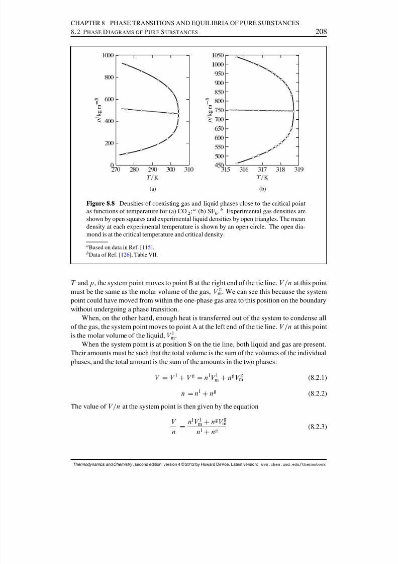
8/12/2019 Howard Devoe Thermodynamic and Chemical
http://slidepdf.com/reader/full/howard-devoe-thermodynamic-and-chemical 208/532
CHAPTER 8 PHASE TRANSITIONS AND EQUILIBRIA OF PURE SUBSTANCES8.2 P HASE D IAGRAMS OF P URE S UBSTANCES 208
K
k g m
(a)
K
k g m
(b)
Figure 8.8 Densities of coexisting gas and liquid phases close to the critical pointas functions of temperature for (a) CO 2 ; a (b) SF 6 . b Experimental gas densities areshown by open squares and experimental liquid densities by open triangles. The meandensity at each experimental temperature is shown by an open circle. The open dia-mond is at the critical temperature and critical density.
a Based on data in Ref. [ 115 ].bData of Ref. [ 126 ], Table VII.
T and p , the system point moves to point B at the right end of the tie line. V =n at this pointmust be the same as the molar volume of the gas, V gm . We can see this because the systempoint could have moved from within the one-phase gas area to this position on the boundarywithout undergoing a phase transition.
When, on the other hand, enough heat is transferred out of the system to condense allof the gas, the system point moves to point A at the left end of the tie line. V =n at this pointis the molar volume of the liquid, V lm .
When the system point is at position S on the tie line, both liquid and gas are present.Their amounts must be such that the total volume is the sum of the volumes of the individualphases, and the total amount is the sum of the amounts in the two phases:
V D V l CV g D n lV lm CngV gm (8.2.1)
n D nl
Cng
(8.2.2)The value of V =n at the system point is then given by the equation
V n D
nlV lm CngV gmn l Cng (8.2.3)
Thermodynamics and Chemistry , second edition, version 4 © 2012 by Howard DeVoe. Latest version: www.chem.umd.edu/thermobook
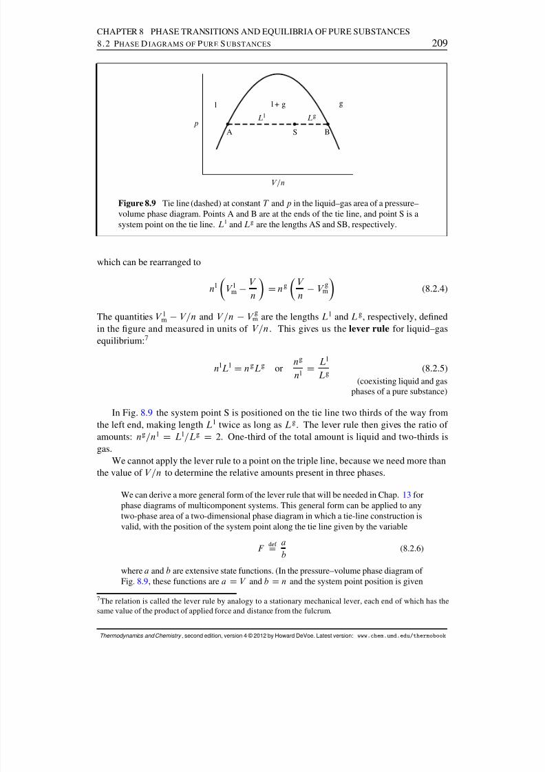
8/12/2019 Howard Devoe Thermodynamic and Chemical
http://slidepdf.com/reader/full/howard-devoe-thermodynamic-and-chemical 209/532
CHAPTER 8 PHASE TRANSITIONS AND EQUILIBRIA OF PURE SUBSTANCES8.2 P HASE D IAGRAMS OF P URE S UBSTANCES 209
A S B
p
V =n
l l + g g
L l L g
Figure 8.9 Tie line (dashed) at constant T and p in the liquid–gas area of a pressure–volume phase diagram. Points A and B are at the ends of the tie line, and point S is asystem point on the tie line. L l and L g are the lengths AS and SB, respectively.
which can be rearranged to
n l V lm V n D ng V
n V gm (8.2.4)
The quantities V lm V=n and V =n V gm are the lengths L l and L g , respectively, denedin the gure and measured in units of V =n. This gives us the lever rule for liquid–gasequilibrium: 7
n lL l D ngL g orng
n l D L l
L g (8.2.5)(coexisting liquid and gas
phases of a pure substance)
In Fig. 8.9 the system point S is positioned on the tie line two thirds of the way fromthe left end, making length L l twice as long as L g . The lever rule then gives the ratio of amounts: ng=n l D L l=L g D 2. One-third of the total amount is liquid and two-thirds isgas.
We cannot apply the lever rule to a point on the triple line, because we need more thanthe value of V =n to determine the relative amounts present in three phases.
We can derive a more general form of the lever rule that will be needed in Chap. 13 forphase diagrams of multicomponent systems. This general form can be applied to anytwo-phase area of a two-dimensional phase diagram in which a tie-line construction isvalid, with the position of the system point along the tie line given by the variable
F def
D ab
(8.2.6)
where a and b are extensive state functions. (In the pressure–volume phase diagram of Fig. 8.9, these functions are a D V and b D n and the system point position is given
7The relation is called the lever rule by analogy to a stationary mechanical lever, each end of which has thesame value of the product of applied force and distance from the fulcrum.
Thermodynamics and Chemistry , second edition, version 4 © 2012 by Howard DeVoe. Latest version: www.chem.umd.edu/thermobook
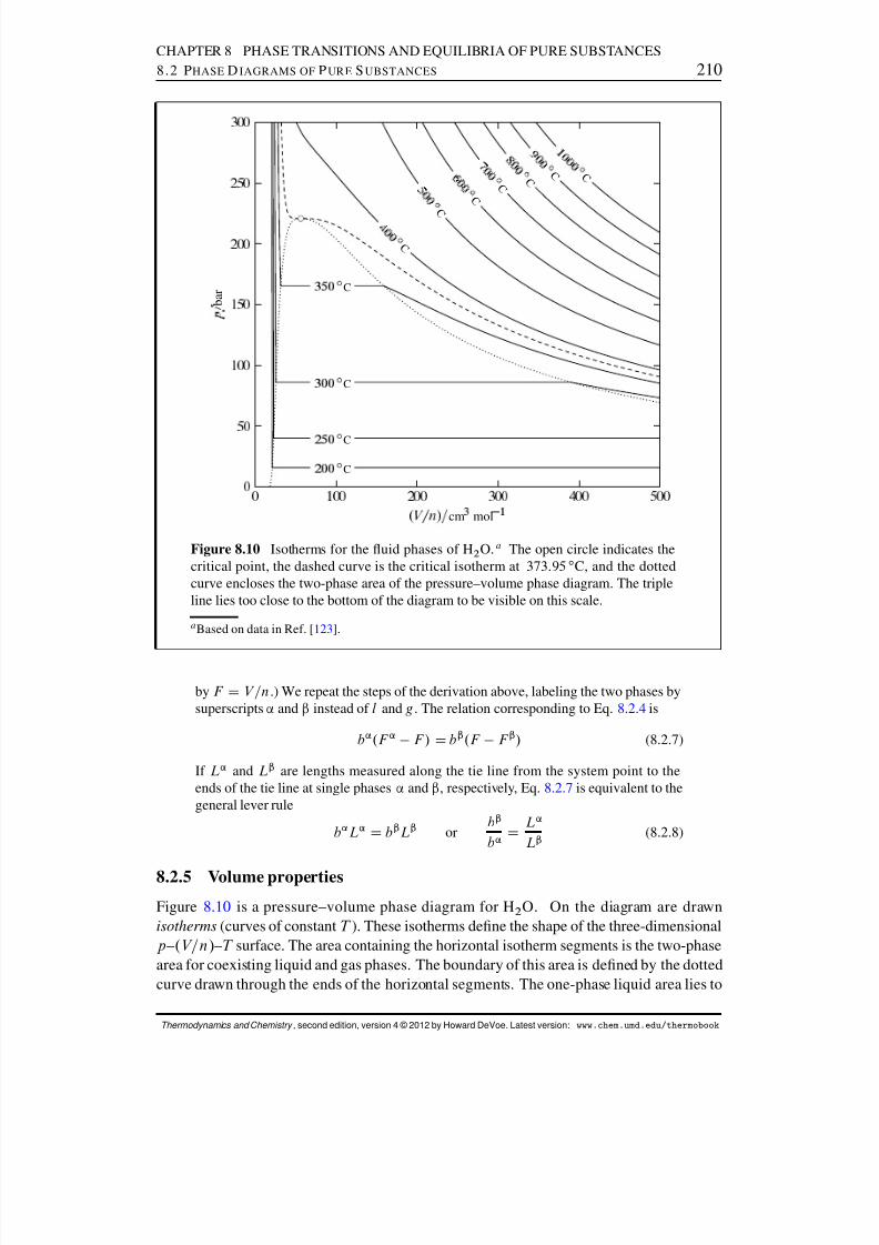
8/12/2019 Howard Devoe Thermodynamic and Chemical
http://slidepdf.com/reader/full/howard-devoe-thermodynamic-and-chemical 210/532
CHAPTER 8 PHASE TRANSITIONS AND EQUILIBRIA OF PURE SUBSTANCES8.2 P HASE D IAGRAMS OF P URE S UBSTANCES 210
cm mol
.
b a r
Æ C
Æ C
Æ C
Æ C
Æ
C
Æ
C
Æ
C
Æ
C
Æ
C
Æ
C
Æ
C
Figure 8.10 Isotherms for the uid phases of H 2 O. a The open circle indicates thecritical point, the dashed curve is the critical isotherm at 373:95 ı C, and the dottedcurve encloses the two-phase area of the pressure–volume phase diagram. The tripleline lies too close to the bottom of the diagram to be visible on this scale.
a Based on data in Ref. [ 123 ].
by F D V =n.) We repeat the steps of the derivation above, labeling the two phases bysuperscripts ’ and “ instead of l and g . The relation corresponding to Eq. 8.2.4 is
b ’ .F ’ F / D b“ .F F “ / (8.2.7)
If L ’ and L “ are lengths measured along the tie line from the system point to theends of the tie line at single phases ’ and “ , respectively, Eq. 8.2.7 is equivalent to thegeneral lever rule
b ’ L ’ D b“ L “ orb“
b ’ D L ’
L “ (8.2.8)
8.2.5 Volume properties
Figure 8.10 is a pressure–volume phase diagram for H 2 O. On the diagram are drawnisotherms (curves of constant T ). These isotherms dene the shape of the three-dimensionalp –.V=n/ –T surface. The area containing the horizontal isotherm segments is the two-phasearea for coexisting liquid and gas phases. The boundary of this area is dened by the dottedcurve drawn through the ends of the horizontal segments. The one-phase liquid area lies to
Thermodynamics and Chemistry , second edition, version 4 © 2012 by Howard DeVoe. Latest version: www.chem.umd.edu/thermobook
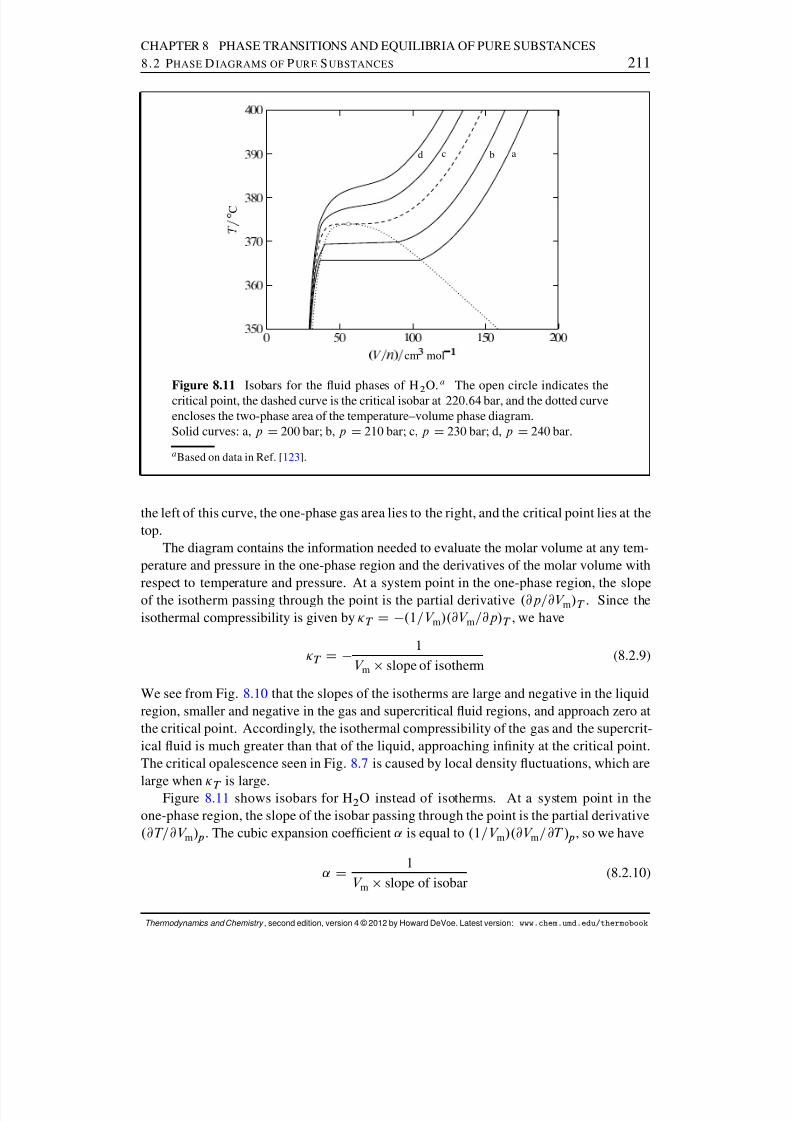
8/12/2019 Howard Devoe Thermodynamic and Chemical
http://slidepdf.com/reader/full/howard-devoe-thermodynamic-and-chemical 211/532
CHAPTER 8 PHASE TRANSITIONS AND EQUILIBRIA OF PURE SUBSTANCES8.2 P HASE D IAGRAMS OF P URE S UBSTANCES 211
cm mol
Æ
C
abcd
Figure 8.11 Isobars for the uid phases of H2
O. a The open circle indicates thecritical point, the dashed curve is the critical isobar at 220:64 bar, and the dotted curveencloses the two-phase area of the temperature–volume phase diagram.Solid curves: a, p D 200 bar; b, p D 210 bar; c, p D 230 bar; d, p D 240 bar.
a Based on data in Ref. [ 123 ].
the left of this curve, the one-phase gas area lies to the right, and the critical point lies at thetop.
The diagram contains the information needed to evaluate the molar volume at any tem-perature and pressure in the one-phase region and the derivatives of the molar volume with
respect to temperature and pressure. At a system point in the one-phase region, the slopeof the isotherm passing through the point is the partial derivative .@p=@V m / T . Since theisothermal compressibility is given by T D .1=V m /.@V m=@p/T , we have
T D 1
V m slope of isotherm(8.2.9)
We see from Fig. 8.10 that the slopes of the isotherms are large and negative in the liquidregion, smaller and negative in the gas and supercritical uid regions, and approach zero atthe critical point. Accordingly, the isothermal compressibility of the gas and the supercrit-ical uid is much greater than that of the liquid, approaching innity at the critical point.The critical opalescence seen in Fig. 8.7 is caused by local density uctuations, which are
large when T is large.Figure 8.11 shows isobars for H 2 O instead of isotherms. At a system point in theone-phase region, the slope of the isobar passing through the point is the partial derivative.@T=@V m /p . The cubic expansion coefcient ˛ is equal to .1=V m /.@V m=@T /p , so we have
˛ D 1
V m slope of isobar(8.2.10)
Thermodynamics and Chemistry , second edition, version 4 © 2012 by Howard DeVoe. Latest version: www.chem.umd.edu/thermobook
8/12/2019 Howard Devoe Thermodynamic and Chemical
http://slidepdf.com/reader/full/howard-devoe-thermodynamic-and-chemical 212/532
CHAPTER 8 PHASE TRANSITIONS AND EQUILIBRIA OF PURE SUBSTANCES8.3 P HASE T RANSITIONS 212
The gure shows that the slopes of the isobars are large and positive in the liquid region,smaller and negative in the gas and supercritical uid regions, and approach zero at thecritical point. Thus the gas and the supercritical uid have much larger cubic expansioncoefcients than the liquid. The value of ˛ approaches innity at the critical point, meaningthat in the critical region the density distribution is greatly affected by temperature gradients.
This may account for the low position of the middle ball in Fig. 8.7 (b).
8.3 PHASE TRANSITIONS
Recall (Sec. 2.2.2 ) that an equilibrium phase transition of a pure substance is a process inwhich some or all of the substance is transferred from one coexisting phase to another atconstant temperature and pressure.
8.3.1 Molar transition quantities
The quantity vap H is the molar enthalpy change for the reversible process in which liquidchanges to gas at a temperature and pressure at which the two phases coexist at equilibrium .
This quantity is called the molar enthalpy of vaporization .8 Since the pressure is constantduring the process, vap H is equal to the heat per amount of vaporization (Eq. 5.3.8 ).Hence, vap H is also called the molar heat of vaporization .
The rst edition of this book used the notation vap H m , with subscript m, in order tomake it clear that it refers to a molar enthalpy of vaporization. The most recent editionof the IUPAC Green Book 9 recommends that p be interpreted as an operator symbol:
pdef
D @=@ p , where “p” is the abbreviation for a process at constant T and p (inthis case “vap”) and p is its advancement. Thus vap H is the same as .@H=@ vap / T;pwhere vap is the amount of liquid changed to gas.
Here is a list of symbols for the molar enthalpy changes of various equilibrium phasetransitions:
vap H molar enthalpy of vaporization (liquid ! gas)
sub H molar enthalpy of sublimation (solid ! gas)fus H molar enthalpy of fusion (solid ! liquid)trsH molar enthalpy of a transition between any two phases in general
Molar enthalpies of vaporization, sublimation, and fusion are positive . The reverse pro-cesses of condensation (gas ! liquid), condensation or deposition (gas ! solid), and freezing(liquid ! solid) have negative enthalpy changes.
The subscripts in the list above are also used for other molar transition quantities. Thus,there is the molar entropy of vaporization vap S , the molar internal energy of sublimation
sub U , and so on.
A molar transition quantity of a pure substance is the change of an extensive propertydivided by the amount transferred between the phases. For example, when an amount nin a liquid phase is allowed to vaporize to gas at constant T and p , the enthalpy change is
8Because vap H is an enthalpy change per amount of vaporization, it would be more accurate to call it the“molar enthalpy change of vaporization.”9Ref. [ 36], p. 58.
Thermodynamics and Chemistry , second edition, version 4 © 2012 by Howard DeVoe. Latest version: www.chem.umd.edu/thermobook

8/12/2019 Howard Devoe Thermodynamic and Chemical
http://slidepdf.com/reader/full/howard-devoe-thermodynamic-and-chemical 213/532
CHAPTER 8 PHASE TRANSITIONS AND EQUILIBRIA OF PURE SUBSTANCES8.3 P HASE T RANSITIONS 213
H D nH gm nH l
m and the molar enthalpy of vaporization is
vap H D H
n D H gm H l
m (8.3.1)(pure substance)
In other words, vap H is the enthalpy change per amount vaporized and is also the differ-ence between the molar enthalpies of the two phases.A molar property of a phase, being intensive, usually depends on two independent in-
tensive variables such as T and p . Despite the fact that vap H is the difference of the twomolar properties H g
m and H lm , its value depends on only one intensive variable, because the
two phases are in transfer equilibrium and the system is univariant. Thus, we may treat
vap H as a function of T only. The same is true of any other molar transition quantity.The molar Gibbs energy of an equilibrium phase transition, trsG , is a special case. For
the phase transition ’ ! “ , we may write an equation analogous to Eq. 8.3.1 and equate themolar Gibbs energy in each phase to a chemical potential (see Eq. 7.8.1 ):
trsG
D G “
m G ’m
D “ ’ (8.3.2)
(pure substance)
But the transition is between two phases at equilibrium, requiring both phases to have thesame chemical potential: “ ’ D 0. Therefore, the molar Gibbs energy of any equilib-rium phase transition is zero:
trs G D 0 (8.3.3)(pure substance)
Since the Gibbs energy is dened by G D H TS , in phase ’ we have G ’m D G ’ =n ’ D
H ’m TS ’m . Similarly, in phase “ we have G “
m D H “m TS “m . When we substitute these
expressions in trsG D G“m G
’m (Eq. 8.3.2 ) and set T equal to the transition temperatureT trs , we obtain
trsG D .H “m H ’
m / T trs .S “m S ’m /
D trsH T trs trs S (8.3.4)
Then, by setting trsG equal to zero, we nd the molar entropy and molar enthalpy of theequilibrium phase transition are related by
trsS D trs H
T trs(8.3.5)
(pure substance)
where trs S and trsH are evaluated at the transition temperature T trs .
We may obtain Eq. 8.3.5 directly from the second law. With the phases in equilibrium,the transition process is reversible. The second law gives S D q=T trs D H=T trs .Dividing by the amount transferred between the phases gives Eq. 8.3.5 .
Thermodynamics and Chemistry , second edition, version 4 © 2012 by Howard DeVoe. Latest version: www.chem.umd.edu/thermobook
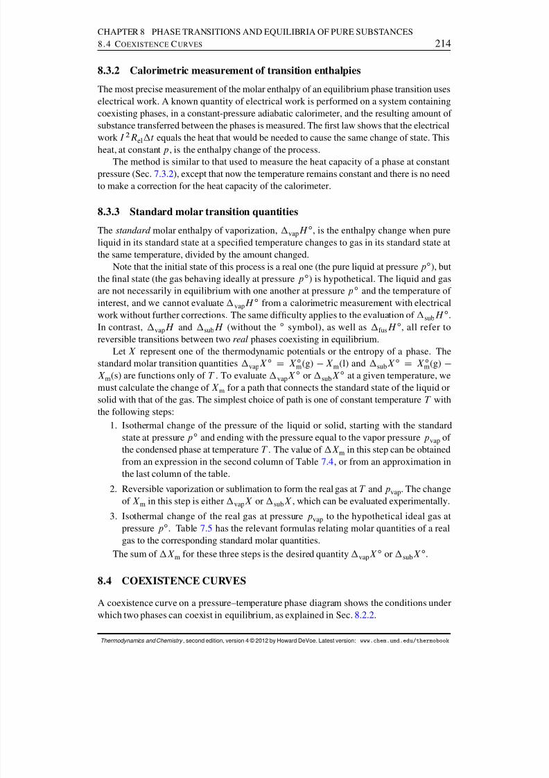
8/12/2019 Howard Devoe Thermodynamic and Chemical
http://slidepdf.com/reader/full/howard-devoe-thermodynamic-and-chemical 214/532
CHAPTER 8 PHASE TRANSITIONS AND EQUILIBRIA OF PURE SUBSTANCES8.4 C OEXISTENCE C URVES 214
8.3.2 Calorimetric measurement of transition enthalpies
The most precise measurement of the molar enthalpy of an equilibrium phase transition useselectrical work. A known quantity of electrical work is performed on a system containingcoexisting phases, in a constant-pressure adiabatic calorimeter, and the resulting amount of substance transferred between the phases is measured. The rst law shows that the electrical
work I 2 R el t equals the heat that would be needed to cause the same change of state. Thisheat, at constant p , is the enthalpy change of the process.
The method is similar to that used to measure the heat capacity of a phase at constantpressure (Sec. 7.3.2 ), except that now the temperature remains constant and there is no needto make a correction for the heat capacity of the calorimeter.
8.3.3 Standard molar transition quantities
The standard molar enthalpy of vaporization, vap H ı , is the enthalpy change when pureliquid in its standard state at a specied temperature changes to gas in its standard state atthe same temperature, divided by the amount changed.
Note that the initial state of this process is a real one (the pure liquid at pressure p ı ), butthe nal state (the gas behaving ideally at pressure p ı ) is hypothetical. The liquid and gasare not necessarily in equilibrium with one another at pressure p ı and the temperature of interest, and we cannot evaluate vap H ı from a calorimetric measurement with electricalwork without further corrections. The same difculty applies to the evaluation of sub H ı .In contrast, vap H and sub H (without the ı symbol), as well as fus H ı , all refer toreversible transitions between two real phases coexisting in equilibrium.
Let X represent one of the thermodynamic potentials or the entropy of a phase. Thestandard molar transition quantities vap X ı D X ım (g) X m (l) and sub X ı D X ım(g) X m(s) are functions only of T . To evaluate vap X ı or sub X ı at a given temperature, wemust calculate the change of X m for a path that connects the standard state of the liquid orsolid with that of the gas. The simplest choice of path is one of constant temperature T withthe following steps:
1. Isothermal change of the pressure of the liquid or solid, starting with the standardstate at pressure p ı and ending with the pressure equal to the vapor pressure p vap of the condensed phase at temperature T . The value of X m in this step can be obtainedfrom an expression in the second column of Table 7.4 , or from an approximation inthe last column of the table.
2. Reversible vaporization or sublimation to form the real gas at T and p vap . The changeof X m in this step is either vap X or sub X , which can be evaluated experimentally.
3. Isothermal change of the real gas at pressure p vap to the hypothetical ideal gas atpressure p ı . Table 7.5 has the relevant formulas relating molar quantities of a real
gas to the corresponding standard molar quantities.The sum of X m for these three steps is the desired quantity vap X ı or sub X ı .
8.4 COEXISTENCE CURVES
A coexistence curve on a pressure–temperature phase diagram shows the conditions underwhich two phases can coexist in equilibrium, as explained in Sec. 8.2.2 .
Thermodynamics and Chemistry , second edition, version 4 © 2012 by Howard DeVoe. Latest version: www.chem.umd.edu/thermobook
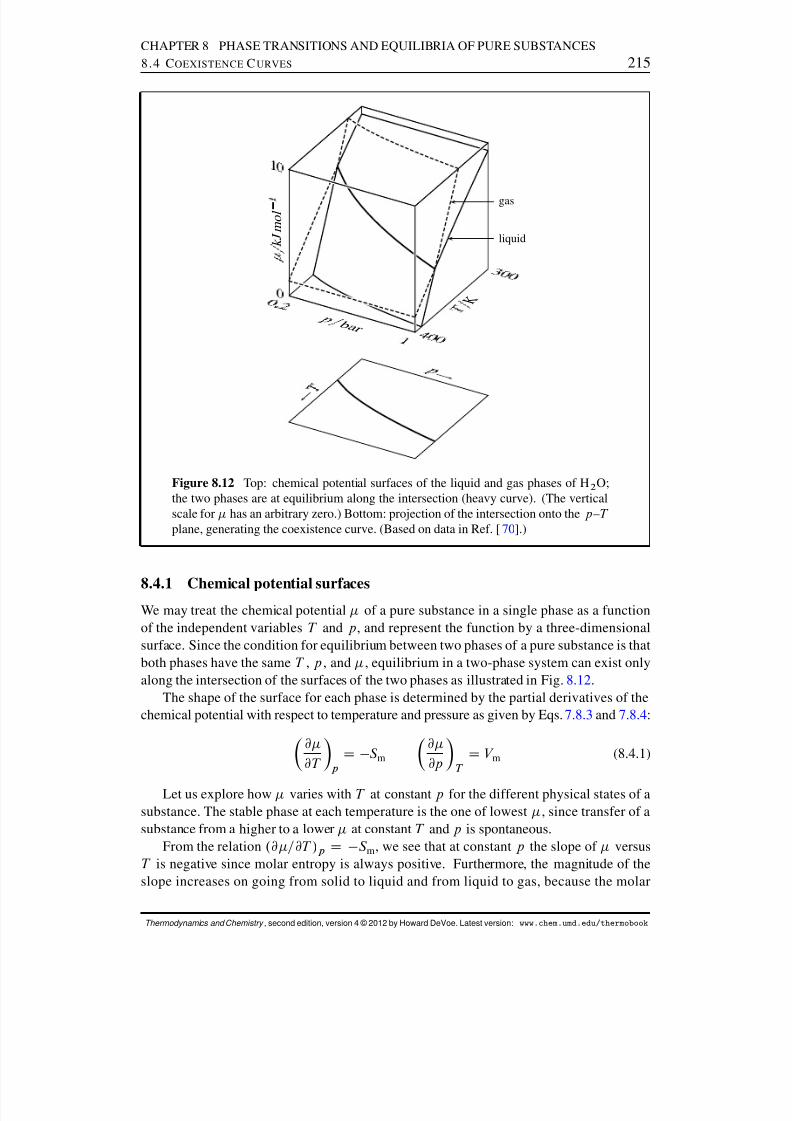
8/12/2019 Howard Devoe Thermodynamic and Chemical
http://slidepdf.com/reader/full/howard-devoe-thermodynamic-and-chemical 215/532
8/12/2019 Howard Devoe Thermodynamic and Chemical
http://slidepdf.com/reader/full/howard-devoe-thermodynamic-and-chemical 216/532
CHAPTER 8 PHASE TRANSITIONS AND EQUILIBRIA OF PURE SUBSTANCES8.4 C OEXISTENCE C URVES 216
A
B
Cs o l i d
l i q u i d
g a s ,
0 : 0
3 b a r
g a s , 0 : 0
0 3 b a r
250 260 270 280 290 300 3100
1
2
3
4
5
T =K
(a)
.
= k J m o l
1
AB
Ctriple point
solid liquid gas
250 260 270 280 290 300 3100
0:01
0:02
0:03
0:04
T =K
(b)
p = b a r
Figure 8.13 Phase stability of H 2 O. a
(a) Chemical potentials of different physical states as functions of temperature. (Thescale for has an arbitrary zero.) Chemical potentials of the gas are shown at 0:03 barand 0:003 bar. The effect of pressure on the curves for the solid and liquid is negligi-ble. At p D 0:03 bar, solid and liquid coexist at T D 273:16 K (point A) and liquidand gas coexist at T D 297:23 K (point B). At p D 0:003 bar, solid and gas coexist atT D 264:77 K (point C).(b) Pressure–temperature phase diagram with points corresponding to those in (a).
a Based on data in Refs. [ 70] and [87].
entropies of sublimation and vaporization are positive. This difference in slope is illustratedby the curves for H 2 O in Fig. 8.13(a). The triple-point pressure of H 2 O is 0:0062 bar. Ata pressure of 0:03 bar, greater than the triple-point pressure, the curves for solid and liquidintersect at a melting point (point A) and the curves for liquid and gas intersect at a boilingpoint (point B).
From .@ =@p/T D V m , we see that a pressure reduction at constant temperature low-ers the chemical potential of a phase. The result of a pressure reduction from 0:03 bar to0:003 bar (below the triple-point pressure of H 2 O) is a downward shift of each of the curvesof Fig. 8.13(a) by a distance proportional to the molar volume of the phase. The shifts of the solid and liquid curves are too small to see ( is only 0:002 kJ mol 1 ). Becausethe gas has a large molar volume, the gas curve shifts substantially to a position where itintersects with the solid curve at a sublimation point (point C). At 0:003 bar, or any otherpressure below the triple-point pressure, only a solid–gas equilibrium is possible for H 2 O.
The liquid phase is not stable at any pressure below the triple-point pressure, as shown bythe pressure–temperature phase diagram of H 2 O in Fig. 8.13(b).
8.4.2 The Clapeyron equation
If we start with two coexisting phases, ’ and “, of a pure substance and change the tem-perature of both phases equally without changing the pressure, the phases will no longer be
Thermodynamics and Chemistry , second edition, version 4 © 2012 by Howard DeVoe. Latest version: www.chem.umd.edu/thermobook

8/12/2019 Howard Devoe Thermodynamic and Chemical
http://slidepdf.com/reader/full/howard-devoe-thermodynamic-and-chemical 217/532
CHAPTER 8 PHASE TRANSITIONS AND EQUILIBRIA OF PURE SUBSTANCES8.4 C OEXISTENCE C URVES 217
in equilibrium, because their chemical potentials change unequally. In order for the phasesto remain in equilibrium during the temperature change d T of both phases, there must bea certain simultaneous change d p in the pressure of both phases. The changes d T and dpmust be such that the chemical potentials of both phases change equally so as to remainequal to one another: d ’ D d “ .
The innitesimal change of in a phase is given by d D S m dT CV m dp (Eq. 7.8.2 ).Thus, the two phases remain in equilibrium if d T and dp satisfy the relation
S ’m dT CV ’m dp D S “m dT CV “m dp (8.4.2)
which we rearrange todpdT D
S “m S ’mV “m V ’m
(8.4.3)
ordpdT D
trsS
trs V (8.4.4)
(pure substance)
Equation 8.4.4 is one form of the Clapeyron equation , which contains no approximations.We nd an alternative form by substituting trsS D trsH= T trs (Eq. 8.3.5 ):
dpdT D
trs H T trsV
(8.4.5)(pure substance)
Equations 8.4.4 and 8.4.5 give the slope of the coexistence curve, d p= dT , as a functionof quantities that can be measured. For the sublimation and vaporization processes, both
trsH and trs V are positive. Therefore, according to Eq. 8.4.5 , the solid–gas and liquid–gas coexistence curves have positive slopes. For the fusion process, however, fus H ispositive, but fus V may be positive or negative depending on the substance, so that theslope of the solid–liquid coexistence curve may be either positive or negative. The absolute
value of fus V is small, causing the solid–liquid coexistence curve to be relatively steep;see Fig. 8.13(b) for an example.
Most substances expand on melting, making the slope of the solid–liquid coexistencecurve positive. This is true of carbon dioxide, although in Fig. 8.2(c) on page 202 thecurve is so steep that it is difcult to see the slope is positive. Exceptions at ordinarypressures, substances that contract on melting, are H 2 O, rubidium nitrate, and theelements antimony, bismuth, and gallium.
The phase diagram for H 2 O in Fig. 8.4 on page 204 clearly shows that the coex-istence curve for ice I and liquid has a negative slope due to ordinary ice being lessdense than liquid water. The high-pressure forms of ice are more dense than the liq-uid, causing the slopes of the other solid–liquid coexistence curves to be positive. Theice VII–ice VIII coexistence curve is vertical, because these two forms of ice haveidentical crystal structures, except for the orientations of the H 2 O molecule; therefore,within experimental uncertainty, the two forms have equal molar volumes.
We may rearrange Eq. 8.4.5 to give the variation of p with T along the coexistencecurve:
dp D trsH
trsV dT
T (8.4.6)
Thermodynamics and Chemistry , second edition, version 4 © 2012 by Howard DeVoe. Latest version: www.chem.umd.edu/thermobook
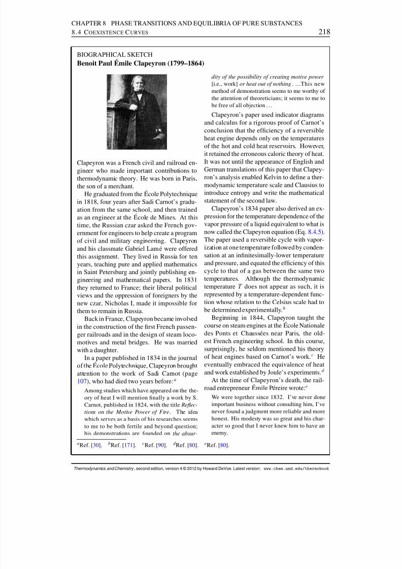
8/12/2019 Howard Devoe Thermodynamic and Chemical
http://slidepdf.com/reader/full/howard-devoe-thermodynamic-and-chemical 218/532
CHAPTER 8 PHASE TRANSITIONS AND EQUILIBRIA OF PURE SUBSTANCES8.4 C OEXISTENCE C URVES 218
BIOGRAPHICAL SKETCHBenoit Paul Emile Clapeyron (1799–1864)
Clapeyron was a French civil and railroad en-gineer who made important contributions tothermodynamic theory. He was born in Paris,the son of a merchant.
He graduated from the Ecole Polytechniquein 1818, four years after Sadi Carnot’s gradu-ation from the same school, and then trainedas an engineer at the Ecole de Mines. At thistime, the Russian czar asked the French gov-ernment for engineers to help create a programof civil and military engineering. Clapeyronand his classmate Gabriel Lam e were offeredthis assignment. They lived in Russia for tenyears, teaching pure and applied mathematicsin Saint Petersburg and jointly publishing en-gineering and mathematical papers. In 1831they returned to France; their liberal politicalviews and the oppression of foreigners by thenew czar, Nicholas I, made it impossible forthem to remain in Russia.
Back in France, Clapeyron became involvedin the construction of the rst French passen-ger railroads and in the design of steam loco-motives and metal bridges. He was marriedwith a daughter.
In a paper published in 1834 in the journalof the Ecole Polytechnique, Clapeyron broughtattention to the work of Sadi Carnot (page107 ), who had died two years before: a
Among studies which have appeared on the the-
ory of heat I will mention nally a work by S.Carnot, published in 1824, with the title Reec-tions on the Motive Power of Fire . The ideawhich serves as a basis of his researches seemsto me to be both fertile and beyond question;his demonstrations are founded on the absur-
dity of the possibility of creating motive power [i.e., work] or heat out of nothing . ...This newmethod of demonstration seems to me worthy of
the attention of theoreticians; it seems to me tobe free of all objection . . .
Clapeyron’s paper used indicator diagramsand calculus for a rigorous proof of Carnot’sconclusion that the efciency of a reversibleheat engine depends only on the temperaturesof the hot and cold heat reservoirs. However,it retained the erroneous caloric theory of heat.It was not until the appearance of English andGerman translations of this paper that Clapey-ron’s analysis enabled Kelvin to dene a ther-modynamic temperature scale and Clausius tointroduce entropy and write the mathematicalstatement of the second law.
Clapeyron’s 1834 paper also derived an ex-pression for the temperature dependence of thevapor pressure of a liquid equivalent to what isnow called the Clapeyron equation (Eq. 8.4.5).The paper used a reversible cycle with vapor-ization at one temperature followed by conden-sation at an innitesimally-lower temperatureand pressure, and equated the efciency of thiscycle to that of a gas between the same twotemperatures. Although the thermodynamictemperature T does not appear as such, it isrepresented by a temperature-dependent func-tion whose relation to the Celsius scale had tobe determined experimentally. b
Beginning in 1844, Clapeyron taught thecourse on steam engines at the Ecole Nationaledes Ponts et Chauss ees near Paris, the old-est French engineering school. In this course,surprisingly, he seldom mentioned his theoryof heat engines based on Carnot’s work. c Heeventually embraced the equivalence of heatand work established by Joule’s experiments. d
At the time of Clapeyron’s death, the rail-road entrepreneur Emile P ereire wrote: e
We were together since 1832. I’ve never doneimportant business without consulting him, I’venever found a judgment more reliable and morehonest. His modesty was so great and his char-acter so good that I never knew him to have anenemy.
a Ref. [ 30]. bRef. [ 171 ]. cRef. [ 90]. d Ref. [ 80]. eRef. [ 80].
Thermodynamics and Chemistry , second edition, version 4 © 2012 by Howard DeVoe. Latest version: www.chem.umd.edu/thermobook

8/12/2019 Howard Devoe Thermodynamic and Chemical
http://slidepdf.com/reader/full/howard-devoe-thermodynamic-and-chemical 219/532
CHAPTER 8 PHASE TRANSITIONS AND EQUILIBRIA OF PURE SUBSTANCES8.4 C OEXISTENCE C URVES 219
Consider the transition from solid to liquid (fusion). Because of the fact that the cubicexpansion coefcient and isothermal compressibility of a condensed phase are relativelysmall, fus V is approximately constant for small changes of T and p . If fus H is alsopractically constant, integration of Eq. 8.4.6 yields the relation
p 2 p 1 fus H
fus V ln
T 2T 1 (8.4.7)
or
T 2 T 1 exp fus V .p 2 p 1 /
fus H (8.4.8)
(pure substance)
from which we may estimate the dependence of the melting point on pressure.
8.4.3 The Clausius–Clapeyron equation
When the gas phase of a substance coexists in equilibrium with the liquid or solid phase,and provided T and p are not close to the critical point, the molar volume of the gas ismuch greater than that of the condensed phase. Thus, we may write for the processes of vaporization and sublimation
vap V D V gm V lm V gm sub V D V gm V sm V gm (8.4.9)
The further approximation that the gas behaves as an ideal gas, V gm RT=p , then changesEq. 8.4.5 to
dpdT
p trs H RT 2 (8.4.10)
(pure substance,vaporization or sublimation)
Equation 8.4.10 is the Clausius–Clapeyron equation . It gives an approximate expres-sion for the slope of a liquid–gas or solid–gas coexistence curve. The expression is not validfor coexisting solid and liquid phases, or for coexisting liquid and gas phases close to thecritical point.
At the temperature and pressure of the triple point, it is possible to carry out all threeequilibrium phase transitions of fusion, vaporization, and sublimation. When fusion is fol-lowed by vaporization, the net change is sublimation. Therefore, the molar transition en-thalpies at the triple point are related by
fus H C vap H D sub H (8.4.11)
Since all three of these transition enthalpies are positive, it follows that sub H is greaterthan vap H at the triple point. Therefore, according to Eq. 8.4.10 , the slope of the solid–gas coexistence curve at the triple point is slightly greater than the slope of the liquid–gascoexistence curve.
We divide both sides of Eq. 8.4.10 by p ı and rearrange to the form
d.p=p ı /p=p ı
trs H R
dT T 2
(8.4.12)
Thermodynamics and Chemistry , second edition, version 4 © 2012 by Howard DeVoe. Latest version: www.chem.umd.edu/thermobook
8/12/2019 Howard Devoe Thermodynamic and Chemical
http://slidepdf.com/reader/full/howard-devoe-thermodynamic-and-chemical 220/532
CHAPTER 8 PHASE TRANSITIONS AND EQUILIBRIA OF PURE SUBSTANCES8.4 C OEXISTENCE C URVES 220
Then, using the mathematical identities d .p=p ı /=.p=p ı / D d ln.p=p ı / and dT =T 2 Dd.1=T / , we can write Eq. 8.4.12 in three alternative forms:
d ln .p=p ı /dT
trs H RT 2 (8.4.13)
(pure substance,
vaporization or sublimation)
d ln .p=p ı / trs H R
d.1=T / (8.4.14)(pure substance,
vaporization or sublimation)
d ln .p=p ı /d.1=T /
trs H R
(8.4.15)(pure substance,
vaporization or sublimation)
Equation 8.4.15 shows that the curve of a plot of ln .p=p ı / versus 1=T (where p is thevapor pressure of a pure liquid or solid) has a slope at each temperature equal, usually toa high degree of accuracy, to vap H=R or sub H=R at that temperature. This kind of plot provides an alternative to calorimetry for evaluating molar enthalpies of vaporizationand sublimation.
If we use the recommended standard pressure of 1 bar, the ratio p=p ı appearing inthese equations becomes p= bar. That is, p=p ı is simply the numerical value of pwhen p is expressed in bars. For the purpose of using Eq. 8.4.15 to evaluate trs H , wecan replace p ı by any convenient value. Thus, the curves of plots of ln .p= bar / versus1=T , ln.p= Pa / versus 1= T , and ln .p= Torr / versus 1= T using the same temperatureand pressure data all have the same slope (but different intercepts) and yield the samevalue of trs H .
If we assume vap H or sub H is essentially constant in a temperature range, we mayintegrate Eq. 8.4.14 from an initial to a nal state along the coexistence curve to obtain
lnp 2
p 1 trsH R
1T 2
1T 1
(8.4.16)(pure substance,
vaporization or sublimation)
Equation 8.4.16 allows us to estimate any one of the quantities p 1 , p 2 , T 1 , T 2 , or trsH ,given values of the other four.
Thermodynamics and Chemistry , second edition, version 4 © 2012 by Howard DeVoe. Latest version: www.chem.umd.edu/thermobook
8/12/2019 Howard Devoe Thermodynamic and Chemical
http://slidepdf.com/reader/full/howard-devoe-thermodynamic-and-chemical 221/532
CHAPTER 8 PHASE TRANSITIONS AND EQUILIBRIA OF PURE SUBSTANCESPROBLEMS 221
PROBLEMS
An underlined problem number or problem-part letter indicates that the numerical answer appearsin Appendix I.
8.1 Consider the system described in Sec. 8.1.5 containing a spherical liquid droplet of radius rsurrounded by pure vapor. Starting with Eq. 8.1.15 , nd an expression for the total differentialof U . Then impose conditions of isolation and show that the equilibrium conditions are T g DT l, g D l, and p l D p g C2 =r , where is the surface tension.
8.2 This problem concerns diethyl ether at T D 298:15 K. At this temperature, the standard molarentropy of the gas calculated from spectroscopic data is S ım (g) D 342:2 J K 1 mol 1 . Thesaturation vapor pressure of the liquid at this temperature is 0:6691 bar, and the molar enthalpyof vaporization is vap H D 27:10 kJmol 1 . The second virial coefcient of the gas at thistemperature has the value B D 1:227 10 3 m3 mol 1 , and its variation with temperature isgiven by d B= dT D 1:50 10 5 m3 K 1 mol 1 .
(a) Use these data to calculate the standard molar entropy of liquid diethyl ether at 298:15 K.A small pressure change has a negligible effect on the molar entropy of a liquid, so that itis a good approximation to equate S ım(l) to S m (l) at the saturation vapor pressure.
(b) Calculate the standard molar entropy of vaporization and the standard molar enthalpy of vaporization of diethyl ether at 298:15 K. It is a good approximation to equate H ı
m (l) toH m(l) at the saturation vapor pressure.
8.3 Explain why the chemical potential surfaces shown in Fig. 8.12 are concave downward; thatis, why .@ =@T/p becomes more negative with increasing T and .@ =@p/T becomes lesspositive with increasing p .
8.4 Potassium has a standard boiling point of 773 ı C and a molar enthalpy of vaporization vap H D84:9 kJmol 1 . Estimate the saturation vapor pressure of liquid potassium at 400: ı C.
8.5 Naphthalene has a melting point of 78:2 ı C at 1 bar and 81:7 ı C at 100 bar. The molar volumechange on melting is fus V D 0:019 cm3 mol 1 . Calculate the molar enthalpy of fusion totwo signicant gures.
8.6 The dependence of the vapor pressure of a liquid on temperature, over a limited temperaturerange, is often represented by the Antoine equation , log10 .p= Torr / D A B=.t CC / , wheret is the Celsius temperature and A, B , and C are constants determined by experiment. Avariation of this equation, using a natural logarithm and the thermodynamic temperature, is
ln.p= bar / D a b
T Cc
The vapor pressure of liquid benzene at temperatures close to 298 K is adequately representedby the preceding equation with the following values of the constants:
a D 9:25092 b D 2771:233 K c D 53:262 K
(a) Find the standard boiling point of benzene.
(b) Use the Clausius–Clapeyron equation to evaluate the molar enthalpy of vaporization of benzene at 298:15 K.
8.7 At a pressure of one atmosphere, water and steam are in equilibrium at 99:97 ı C (the normalboiling point of water). At this pressure and temperature, the water density is 0:958 g cm 3 , thesteam density is 5:98 10 4 g cm 3 , and the molar enthalpy of vaporization is 40:66 kJ mol 1 .
Thermodynamics and Chemistry , second edition, version 4 © 2012 by Howard DeVoe. Latest version: www.chem.umd.edu/thermobook
8/12/2019 Howard Devoe Thermodynamic and Chemical
http://slidepdf.com/reader/full/howard-devoe-thermodynamic-and-chemical 222/532
CHAPTER 8 PHASE TRANSITIONS AND EQUILIBRIA OF PURE SUBSTANCESPROBLEMS 222
(a) Use the Clapeyron equation to calculate the slope d p= dT of the liquid–gas coexistencecurve at this point.
(b) Repeat the calculation using the Clausius–Clapeyron equation.
(c) Use your results to estimate the standard boiling point of water. (Note: The experimentalvalue is 99:61 ı C.)
8.8 At the standard pressure of 1 bar, liquid and gaseous H 2 O coexist in equilibrium at 372:76 K,the standard boiling point of water.
(a) Do you expect the standard molar enthalpy of vaporization to have the same value as themolar enthalpy of vaporization at this temperature? Explain.
(b) The molar enthalpy of vaporization at 372:76 K has the value vap H D 40:67 kJ mol 1 .Estimate the value of vap H ı at this temperature with the help of Table 7.5 and the fol-lowing data for the second virial coefcient of gaseous H 2 O at 372:76 K:
B D 4:60 10 4 m3 mol 1 dB= dT D 3:4 10 6 m3 K 1 mol 1
(c) Would you expect the values of fus H and fus H ı to be equal at the standard freezingpoint of water? Explain.
8.9 The standard boiling point of H 2 O is 99:61 ı C. The molar enthalpy of vaporization at thistemperature is vap H D 40:67 kJ mol 1 . The molar heat capacity of the liquid at temperaturesclose to this value is given by
C p; m D a Cb.t c/
where t is the Celsius temperature and the constants have the values
a D 75:94 J K 1 mol 1 b D 0:022 J K 2 mol 1 c D 99:61 ı C
Suppose 100:00 mol of liquid H 2 O is placed in a container maintained at a constant pressureof 1 bar, and is carefully heated to a temperature 5:00 ı C above the standard boiling point, re-sulting in an unstable phase of superheated water. If the container is enclosed with an adiabaticboundary and the system subsequently changes spontaneously to an equilibrium state, whatamount of water will vaporize? (Hint: The temperature will drop to the standard boiling point,and the enthalpy change will be zero.)
Thermodynamics and Chemistry , second edition, version 4 © 2012 by Howard DeVoe. Latest version: www.chem.umd.edu/thermobook

8/12/2019 Howard Devoe Thermodynamic and Chemical
http://slidepdf.com/reader/full/howard-devoe-thermodynamic-and-chemical 223/532

8/12/2019 Howard Devoe Thermodynamic and Chemical
http://slidepdf.com/reader/full/howard-devoe-thermodynamic-and-chemical 224/532
8/12/2019 Howard Devoe Thermodynamic and Chemical
http://slidepdf.com/reader/full/howard-devoe-thermodynamic-and-chemical 225/532
CHAPTER 9 MIXTURES9.1 C OMPOSITION VARIABLES 225
9.1.4 Binary solutions
We may write simplied equations for a binary solution of two substances, solvent A andsolute B. Equations 9.1.1 –9.1.4 become
xB
D
nB
nA Cn B
(9.1.5)(binary solution)
wB D nBM B
n AM A CnBM B(9.1.6)
(binary solution)
cB D nB
V D nB
nAM A CnBM B(9.1.7)
(binary solution)
mB D nB
nAM A (9.1.8)(binary solution)
The right sides of Eqs. 9.1.5 –9.1.8 express the solute composition variables in terms of theamounts and molar masses of the solvent and solute and the density of the solution.
To be able to relate the values of these composition variables to one another, we solveeach equation for nB and divide by nA to obtain an expression for the mole ratio nB=n A :
from Eq. 9.1.5nB
nA D xB
1 xB(9.1.9)
(binary solution)
from Eq. 9.1.6nB
nA D
M AwB
M B .1 wB / (9.1.10)
(binary solution)
from Eq. 9.1.7nB
nA D M AcB
M BcB(9.1.11)
(binary solution)
from Eq. 9.1.8nB
nA D M AmB (9.1.12)(binary solution)
These expressions for nB=n A allow us to nd one composition variable as a function of another. For example, to nd molality as a function of concentration, we equate the expres-sions for nB=n A on the right sides of Eqs. 9.1.11 and 9.1.12 and solve for mB to obtain
mB D c
BM BcB(9.1.13)
Thermodynamics and Chemistry , second edition, version 4 © 2012 by Howard DeVoe. Latest version: www.chem.umd.edu/thermobook

8/12/2019 Howard Devoe Thermodynamic and Chemical
http://slidepdf.com/reader/full/howard-devoe-thermodynamic-and-chemical 226/532
CHAPTER 9 MIXTURES9.2 PARTIAL M OLAR Q UANTITIES 226
A binary solution becomes more dilute as any of the solute composition variables be-comes smaller. In the limit of innite dilution, the expressions for nB=n A become:
nB
nA D xB
D M AM B wB
D M A
AcB D V m;AcB
D M AmB (9.1.14)(binary solution at
innite dilution)
where a superscript asterisk ( ) denotes a pure phase. We see that, in the limit of innitedilution, the composition variables xB , wB , cB , and mB are proportional to one another.These expressions are also valid for solute B in a multi solute solution in which each soluteis very dilute; that is, in the limit xA
!1.
The rule of thumb that the molarity and molality values of a dilute aqueous solutionare approximately equal is explained by the relation M AcB= A D M AmB (from Eq.9.1.14 ), or cB= A D mB , and the fact that the density A of water is approximately1 kg L 1 . Hence, if the solvent is water and the solution is dilute, the numerical valueof cB expressed in mol L 1 is approximately equal to the numerical value of m B ex-pressed in mol kg 1 .
9.1.5 The composition of a mixture
We can describe the composition of a phase with the amounts of each species, or with anyof the composition variables dened earlier: mole fraction, mass fraction, concentration, or
molality. If we use mole fractions or mass fractions to describe the composition, we needthe values for all but one of the species, since the sum of all fractions is unity.
Other composition variables are sometimes used, such as volume fraction, mole ratio,and mole percent. To describe the composition of a gas mixture, partial pressures can beused (Sec. 9.3.1 ).
When the composition of a mixture is said to be xed or constant during changes of temperature, pressure, or volume, this means there is no change in the relative amounts ormasses of the various species. A mixture of xed composition has xed values of molefractions, mass fractions, and molalities, but not necessarily of concentrations and partialpressures. Concentrations will change if the volume changes, and partial pressures in a gasmixture will change if the pressure changes.
9.2 PARTIAL MOLAR QUANTITIES
The symbol X i , where X is an extensive property of a homogeneous mixture and the sub-script i identies a constituent species of the mixture, denotes the partial molar quantity
Thermodynamics and Chemistry , second edition, version 4 © 2012 by Howard DeVoe. Latest version: www.chem.umd.edu/thermobook
8/12/2019 Howard Devoe Thermodynamic and Chemical
http://slidepdf.com/reader/full/howard-devoe-thermodynamic-and-chemical 227/532
CHAPTER 9 MIXTURES9.2 PARTIAL M OLAR Q UANTITIES 227
of species i dened by
X idef
D@X @ni T;p;n j ¤ i
(9.2.1)(mixture)
This is the rate at which property X changes with the amount of species i added to themixture as the temperature, the pressure, and the amounts of all other species are keptconstant. A partial molar quantity is an intensive state function. Its value depends on thetemperature, pressure, and composition of the mixture.
Keep in mind that as a practical matter, a macroscopic amount of a charged species (i.e.,an ion) cannot be added by itself to a phase because of the huge electric charge that wouldresult. Thus if species i is charged, X i as dened by Eq. 9.2.1 is a theoretical concept whosevalue cannot be determined experimentally.
An older notation for a partial molar quantity uses an overbar: X i . The notation X 0iwas suggested in the rst edition of the IUPAC Green Book, 2 but is not mentioned inlater editions.
9.2.1 Partial molar volume
In order to gain insight into the signicance of a partial molar quantity as dened by Eq.9.2.1 , let us rst apply the concept to the volume of an open single-phase system. Volumehas the advantage for our example of being an extensive property that is easily visualized.Let the system be a binary mixture of water (substance A) and methanol (substance B), twoliquids that mix in all proportions. The partial molar volume of the methanol, then, is therate at which the system volume changes with the amount of methanol added to the mixtureat constant temperature and pressure: V B D .@V=@nB / T;p;n A
.At 25 ı C and 1 bar, the molar volume of pure water is V m;A D 18:07 cm 3 mol 1 and that
of pure methanol is V m;B D
40:75 cm 3 mol 1 . If we mix 100:0 cm 3 of water at 25 ı C with100:0 cm 3 of methanol at 25 ı C, we nd the volume of the resulting mixture at 25 ı C is notthe sum of the separate volumes, 200:0 cm 3 , but rather the slightly smaller value 193:1 cm 3 .The difference is due to new intermolecular interactions in the mixture compared to the pureliquids.
Let us calculate the mole fraction composition of this mixture:
nA D V AV m;A D
100:0 cm 3
18:07 cm 3 mol 1 D 5:53 mol (9.2.2)
nB D V BV m;B D
100:0 cm 3
40:75 cm 3 mol 1 D 2:45 mol (9.2.3)
xB D nB
nA CnB D 2:45 mol5:53 mol C2:45 mol D 0:307 (9.2.4)
Now suppose we prepare a large volume of a mixture of this composition ( xB D 0:307)and add an additional 40:75 cm 3 (one mole) of pure methanol, as shown in Fig. 9.1 (a). If
2Ref. [ 118 ], p. 44.
Thermodynamics and Chemistry , second edition, version 4 © 2012 by Howard DeVoe. Latest version: www.chem.umd.edu/thermobook
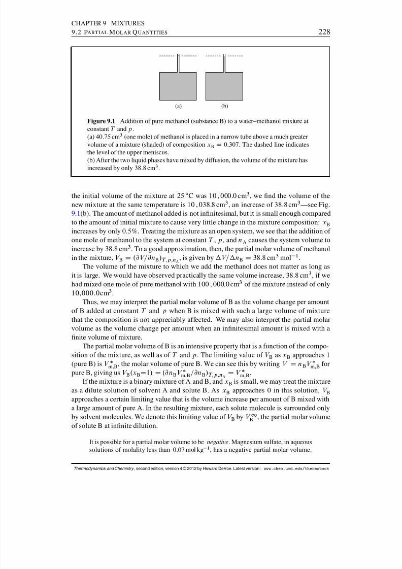
8/12/2019 Howard Devoe Thermodynamic and Chemical
http://slidepdf.com/reader/full/howard-devoe-thermodynamic-and-chemical 228/532
CHAPTER 9 MIXTURES9.2 PARTIAL M OLAR Q UANTITIES 228
(a) (b)
Figure 9.1 Addition of pure methanol (substance B) to a water–methanol mixture atconstant T and p .(a) 40:75 cm3 (one mole) of methanol is placed in a narrow tube above a much greatervolume of a mixture (shaded) of composition xB D 0:307 . The dashed line indicatesthe level of the upper meniscus.(b) After the two liquid phases have mixed by diffusion, the volume of the mixture hasincreased by only 38:8 cm 3 .
the initial volume of the mixture at 25ı
C was 10 , 000.0 cm3
, we nd the volume of thenew mixture at the same temperature is 10 , 038.8 cm 3 , an increase of 38.8 cm 3 —see Fig.9.1 (b). The amount of methanol added is not innitesimal, but it is small enough comparedto the amount of initial mixture to cause very little change in the mixture composition: xBincreases by only 0:5%. Treating the mixture as an open system, we see that the addition of one mole of methanol to the system at constant T , p , and nA causes the system volume toincrease by 38:8 cm 3 . To a good approximation, then, the partial molar volume of methanolin the mixture, V B D .@V=@nB / T;p;n A
, is given by V= n B D 38:8 cm 3 mol 1 .The volume of the mixture to which we add the methanol does not matter as long as
it is large. We would have observed practically the same volume increase, 38:8 cm 3 , if wehad mixed one mole of pure methanol with 100 , 000.0 cm 3 of the mixture instead of only10,000.0cm 3 .
Thus, we may interpret the partial molar volume of B as the volume change per amountof B added at constant T and p when B is mixed with such a large volume of mixturethat the composition is not appreciably affected. We may also interpret the partial molarvolume as the volume change per amount when an innitesimal amount is mixed with anite volume of mixture.
The partial molar volume of B is an intensive property that is a function of the compo-sition of the mixture, as well as of T and p . The limiting value of V B as xB approaches 1(pure B) is V m;B , the molar volume of pure B. We can see this by writing V D n BV m;B forpure B, giving us V B .x BD1/ D .@nBV m;B=@nB/ T;p;n A D V m;B .
If the mixture is a binary mixture of A and B, and xB is small, we may treat the mixtureas a dilute solution of solvent A and solute B. As xB approaches 0 in this solution, V Bapproaches a certain limiting value that is the volume increase per amount of B mixed witha large amount of pure A. In the resulting mixture, each solute molecule is surrounded onlyby solvent molecules. We denote this limiting value of V B by V 1B , the partial molar volumeof solute B at innite dilution.
It is possible for a partial molar volume to be negative . Magnesium sulfate, in aqueoussolutions of molality less than 0:07 mol kg 1 , has a negative partial molar volume.
Thermodynamics and Chemistry , second edition, version 4 © 2012 by Howard DeVoe. Latest version: www.chem.umd.edu/thermobook
8/12/2019 Howard Devoe Thermodynamic and Chemical
http://slidepdf.com/reader/full/howard-devoe-thermodynamic-and-chemical 229/532
CHAPTER 9 MIXTURES9.2 PARTIAL M OLAR Q UANTITIES 229
Physically, this means that when a small amount of crystalline MgSO 4 dissolves atconstant temperature in water, the liquid phase contracts. This unusual behavior is dueto strong attractive water–ion interactions.
9.2.2 The total differential of the volume in an open system
Consider an open single-phase system consisting of a mixture of nonreacting substances.How many independent variables does this system have?
We can prepare the mixture with various amounts of each substance, and we are ableto adjust the temperature and pressure to whatever values we wish (within certain limitsthat prevent the formation of a second phase). Each choice of temperature, pressure, andamounts results in a denite value of every other property, such as volume, density, andmole fraction composition. Thus, an open single-phase system of C substances has 2 CC independent variables. 3
For a binary mixture ( C D 2), the number of independent variables is four. We maychoose these variables to be T , p , n A , and n B , and write the total differential of V in thegeneral form
dV D@V @T p;n A ;n B
dT C@V @p T;n A ;n B
dp
C @V @nA T;p;n B
dnA C @V @nB T;p;n A
dnB (9.2.5)(binary mixture)
We know the rst two partial derivatives on the right side are given by 4
@V @T p;n A ;n B
D ˛V @V @p T;n A ;n B
D T V (9.2.6)
We identify the last two partial derivatives on the right side of Eq. 9.2.5 as the partial molarvolumes V A and V B . Thus, we may write the total differential of V for this open system inthe compact form
dV D ˛V dT T V dp CV A dnA CV B dnB (9.2.7)(binary mixture)
If we compare this equation with the total differential of V for a one-component closed system, d V D ˛V dT T V dp (Eq. 7.1.6 ), we see that an additional term is required foreach constituent of the mixture to allow the system to be open and the composition to vary.
When T and p are held constant, Eq. 9.2.7 becomes
dV D V A dnA CV B dnB (9.2.8)(binary mixture,constant T and p )
3C in this kind of system is actually the number of components . The number of components is usually thesame as the number of substances, but is less if certain constraints exist, such as reaction equilibrium or a xedmixture composition. The general meaning of C will be discussed in Sec. 13.1 .4See Eqs. 7.1.1 and 7.1.2 , which are for closed systems.
Thermodynamics and Chemistry , second edition, version 4 © 2012 by Howard DeVoe. Latest version: www.chem.umd.edu/thermobook
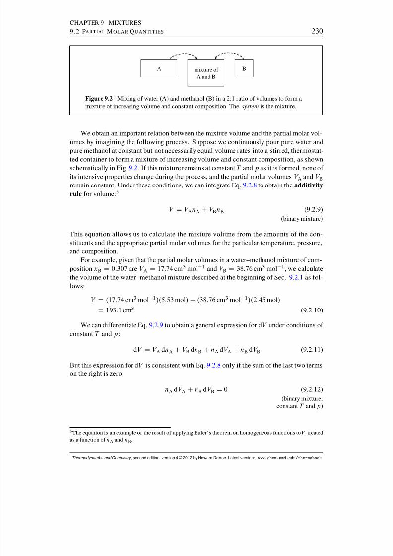
8/12/2019 Howard Devoe Thermodynamic and Chemical
http://slidepdf.com/reader/full/howard-devoe-thermodynamic-and-chemical 230/532
CHAPTER 9 MIXTURES9.2 PARTIAL M OLAR Q UANTITIES 230
A mixture of
A and B
B
Figure 9.2 Mixing of water (A) and methanol (B) in a 2:1 ratio of volumes to form amixture of increasing volume and constant composition. The system is the mixture.
We obtain an important relation between the mixture volume and the partial molar vol-umes by imagining the following process. Suppose we continuously pour pure water andpure methanol at constant but not necessarily equal volume rates into a stirred, thermostat-ted container to form a mixture of increasing volume and constant composition, as shownschematically in Fig. 9.2. If this mixture remains at constant T and p as it is formed, none of its intensive properties change during the process, and the partial molar volumes V A and V Bremain constant. Under these conditions, we can integrate Eq. 9.2.8 to obtain the additivity
rule for volume:5
V D V AnA CV BnB (9.2.9)(binary mixture)
This equation allows us to calculate the mixture volume from the amounts of the con-stituents and the appropriate partial molar volumes for the particular temperature, pressure,and composition.
For example, given that the partial molar volumes in a water–methanol mixture of com-position xB D 0:307 are V A D 17:74 cm 3 mol 1 and V B D 38:76 cm 3 mol 1 , we calculatethe volume of the water–methanol mixture described at the beginning of Sec. 9.2.1 as fol-lows:
V D .17:74 cm 3 mol 1 /.5:53 mol / C.38:76 cm 3 mol 1 /.2:45 mol /
D 193:1 cm 3 (9.2.10)
We can differentiate Eq. 9.2.9 to obtain a general expression for d V under conditions of constant T and p :
dV D V A dnA CV B dnB CnA dV A CnB dV B (9.2.11)
But this expression for d V is consistent with Eq. 9.2.8 only if the sum of the last two termson the right is zero:
nA dV A CnB dV B D 0 (9.2.12)(binary mixture,
constant T and p )
5The equation is an example of the result of applying Euler’s theorem on homogeneous functions to V treatedas a function of nA and nB .
Thermodynamics and Chemistry , second edition, version 4 © 2012 by Howard DeVoe. Latest version: www.chem.umd.edu/thermobook
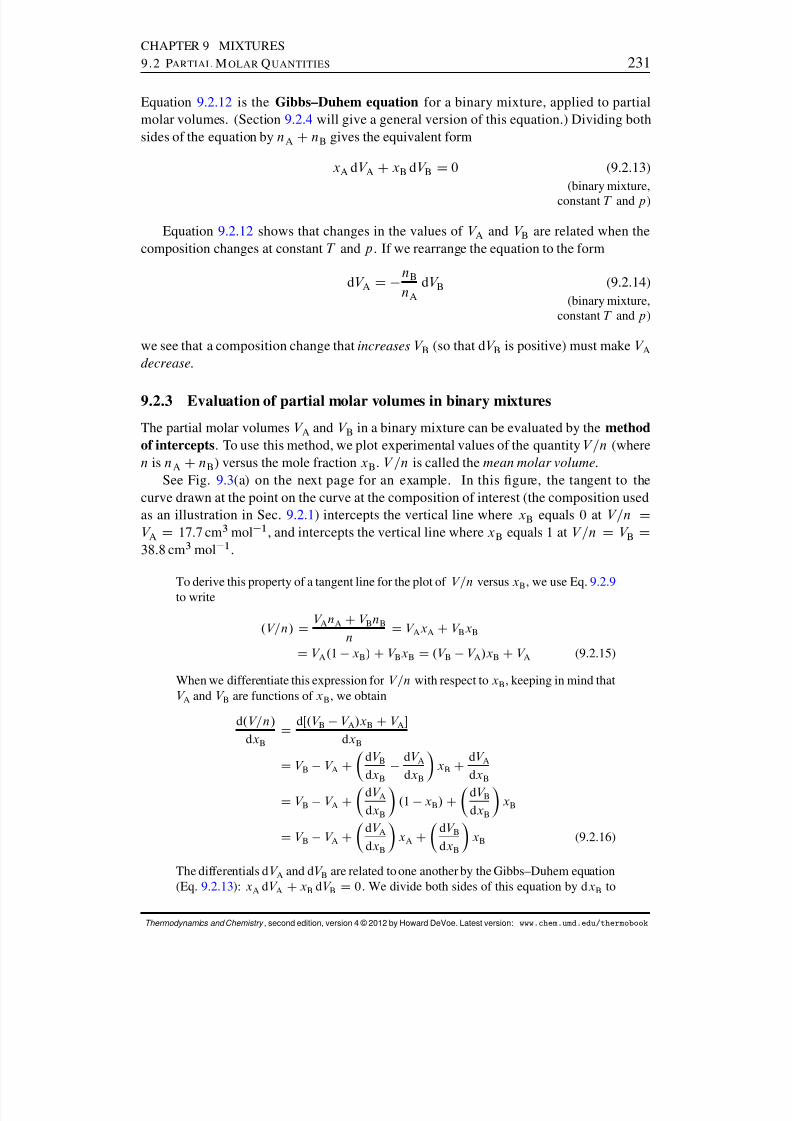
8/12/2019 Howard Devoe Thermodynamic and Chemical
http://slidepdf.com/reader/full/howard-devoe-thermodynamic-and-chemical 231/532
CHAPTER 9 MIXTURES9.2 PARTIAL M OLAR Q UANTITIES 231
Equation 9.2.12 is the Gibbs–Duhem equation for a binary mixture, applied to partialmolar volumes. (Section 9.2.4 will give a general version of this equation.) Dividing bothsides of the equation by nA CnB gives the equivalent form
xA dV A CxB dV B D 0 (9.2.13)(binary mixture,
constant T and p )
Equation 9.2.12 shows that changes in the values of V A and V B are related when thecomposition changes at constant T and p . If we rearrange the equation to the form
dV A D nB
nAdV B (9.2.14)
(binary mixture,constant T and p )
we see that a composition change that increases V B (so that d V B is positive) must make V Adecrease .
9.2.3 Evaluation of partial molar volumes in binary mixtures
The partial molar volumes V A and V B in a binary mixture can be evaluated by the methodof intercepts . To use this method, we plot experimental values of the quantity V =n (wheren is nA CnB) versus the mole fraction xB . V =n is called the mean molar volume .
See Fig. 9.3(a) on the next page for an example. In this gure, the tangent to thecurve drawn at the point on the curve at the composition of interest (the composition usedas an illustration in Sec. 9.2.1 ) intercepts the vertical line where xB equals 0 at V=n DV A D 17:7 cm 3 mol 1 , and intercepts the vertical line where xB equals 1 at V =n D V B D38:8 cm 3 mol 1 .
To derive this property of a tangent line for the plot of V=n versus xB
, we use Eq. 9.2.9to write
.V=n/ D V AnA CV BnB
n D V AxA CV BxB
D V A .1 xB / CV BxB D .V B V A /x B CV A (9.2.15)
When we differentiate this expression for V=n with respect to xB , keeping in mind thatV A and V B are functions of xB , we obtain
d.V=n/dxB D
dŒ.V B V A /x B CV AdxB
D V B V A CdV BdxB
dV AdxB
xB C dV AdxB
D V B V A CdV AdxB
.1 xB / CdV BdxB
xB
D V B V A CdV AdxB
xA CdV BdxB
xB (9.2.16)
The differentials d V A and dV B are related to one another by the Gibbs–Duhem equation(Eq. 9.2.13 ): xA dV A CxB dV B D 0. We divide both sides of this equation by d xB to
Thermodynamics and Chemistry , second edition, version 4 © 2012 by Howard DeVoe. Latest version: www.chem.umd.edu/thermobook
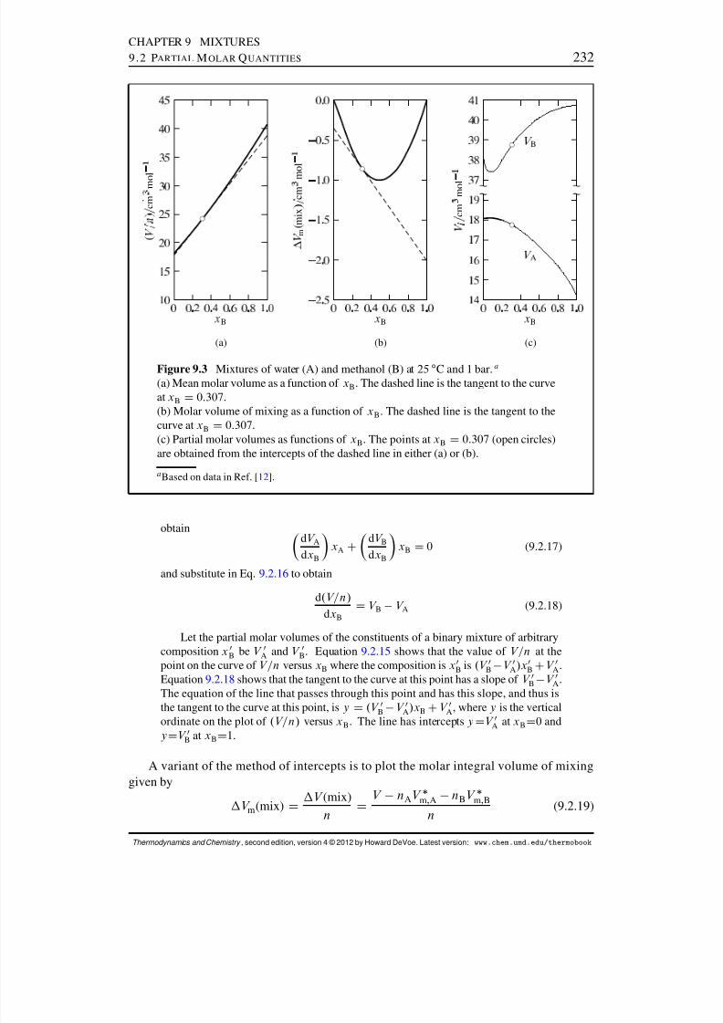
8/12/2019 Howard Devoe Thermodynamic and Chemical
http://slidepdf.com/reader/full/howard-devoe-thermodynamic-and-chemical 232/532
CHAPTER 9 MIXTURES9.2 PARTIAL M OLAR Q UANTITIES 232
B
.
c m
m o l
(a)
B
m
m i x
c m
m
o l
(b)
B
A
B
c m
m o l
(c)
Figure 9.3 Mixtures of water (A) and methanol (B) at 25 ı C and 1 bar. a
(a) Mean molar volume as a function of xB . The dashed line is the tangent to the curveat xB D 0:307 .(b) Molar volume of mixing as a function of xB . The dashed line is the tangent to thecurve at xB D 0:307 .(c) Partial molar volumes as functions of xB . The points at xB D 0:307 (open circles)are obtained from the intercepts of the dashed line in either (a) or (b).
a Based on data in Ref. [ 12].
obtain
dV AdxB
xA C dV BdxB
xB D 0 (9.2.17)
and substitute in Eq. 9.2.16 to obtain
d.V=n/dxB D V B V A (9.2.18)
Let the partial molar volumes of the constituents of a binary mixture of arbitrarycomposition x 0
B be V 0A and V 0B . Equation 9.2.15 shows that the value of V=n at thepoint on the curve of V=n versus xB where the composition is x 0
B is .V 0B V 0A /x 0
B CV 0A .Equation 9.2.18 shows that the tangent to the curve at this point has a slope of V 0B V 0A .The equation of the line that passes through this point and has this slope, and thus isthe tangent to the curve at this point, is y
D .V 0
B V 0A /x B
CV 0A , where y is the vertical
ordinate on the plot of .V=n/ versus xB . The line has intercepts yDV 0A at xBD0 andyDV 0B at xBD1.
A variant of the method of intercepts is to plot the molar integral volume of mixinggiven by
V m (mix) D V (mix)
n DV nAV m;A nBV m;B
n (9.2.19)
Thermodynamics and Chemistry , second edition, version 4 © 2012 by Howard DeVoe. Latest version: www.chem.umd.edu/thermobook

8/12/2019 Howard Devoe Thermodynamic and Chemical
http://slidepdf.com/reader/full/howard-devoe-thermodynamic-and-chemical 233/532
CHAPTER 9 MIXTURES9.2 PARTIAL M OLAR Q UANTITIES 233
versus xB , as illustrated in Fig. 9.3(b). V (mix) is the integral volume of mixing—thevolume change at constant T and p when solvent and solute are mixed to form a mixture of volume V and total amount n (see Sec. 11.1.1 ). The tangent to the curve at the compositionof interest has intercepts V A V m;A at xBD0 and V B V m;B at xBD1.
To see this, we write
V m(mix) D .V=n/ xAV m;A xBV m;B
D .V=n/ .1 xB /V m;A xBV m;B (9.2.20)
We make the substitution .V=n/ D .V B V A /x B CV A from Eq. 9.2.15 and rearrange:
V m(mix) D V B V m;B V A V m;A xB C V A V m;A (9.2.21)
Differentiation with respect to xB yields
d V m (mix)dxB D V B V m;B V A V m;A C
dV BdxB
dV AdxB
xB C dV AdxB
D V B V m;B V A V m;A CdV AdxB .1 xB / C
dV BdxB xB
D V B V m;B V A V m;A CdV AdxB
xA CdV BdxB
xB
(9.2.22)
With a substitution from Eq. 9.2.17 , this becomes
d V m (mix)dxB D V B V m;B V A V m;A (9.2.23)
Equations 9.2.21 and 9.2.23 are analogous to Eqs. 9.2.15 and 9.2.18 , with V =n re-placed by V m (mix), V A by .V A V m;A / , and V B by .V B V m;B / . Using the samereasoning as for a plot of V=n versus xB , we nd the intercepts of the tangent to a
point on the curve of V m (mix) versus xB are at V A V m;A and V B V m;B .
Figure 9.3 shows smoothed experimental data for water–methanol mixtures plotted inboth kinds of graphs, and the resulting partial molar volumes as functions of composition.Note in Fig. 9.3 (c) how the V A curve mirrors the V B curve as xB varies, as predicted by theGibbs–Duhem equation. The minimum in V B at xB 0:09 is mirrored by a maximum in V Ain agreement with Eq. 9.2.14 ; the maximum is much attenuated because nB=n A is muchless than unity.
Macroscopic measurements are unable to provide unambiguous information about mo-lecular structure. Nevertheless, it is interesting to speculate on the implications of theminimum observed for the partial molar volume of methanol. One interpretation is thatin a mostly aqueous environment, there is association of methanol molecules, perhapsinvolving the formation of dimers.
9.2.4 General relations
The discussion above of partial molar volumes used the notation V m;A and V m;B for themolar volumes of pure A and B. The partial molar volume of a pure substance is the same as
Thermodynamics and Chemistry , second edition, version 4 © 2012 by Howard DeVoe. Latest version: www.chem.umd.edu/thermobook
8/12/2019 Howard Devoe Thermodynamic and Chemical
http://slidepdf.com/reader/full/howard-devoe-thermodynamic-and-chemical 234/532
CHAPTER 9 MIXTURES9.2 PARTIAL M OLAR Q UANTITIES 234
the molar volume, so we can simplify the notation by using V A and V B instead. Hereafter,this book will denote molar quantities of pure substances by such symbols as V A , H B , andS i .
The relations derived above for the volume of a binary mixture may be generalized forany extensive property X of a mixture of any number of constituents. The partial molar
quantity of species i , dened by
X idef
D@X @ni T;p;n j ¤ i
(9.2.24)
is an intensive property that depends on T , p , and the composition of the mixture. Theadditivity rule for property X is
X DXi
n i X i (9.2.25)(mixture)
and the Gibbs–Duhem equation applied to X can be written in the equivalent forms
Xi
n i dX i D 0 (9.2.26)(constant T and p )
and
Xi
x i dX i D 0 (9.2.27)(constant T and p )
These relations can be applied to a mixture in which each species i is a nonelectrolyte sub-stance, an electrolyte substance that is dissociated into ions, or an individual ionic species.In Eq. 9.2.27 , the mole fraction xi must be based on the different species considered tobe present in the mixture. For example, an aqueous solution of NaCl could be treated asa mixture of components A=H 2 O and B=NaCl, with xB equal to nB=.n A C n B/ ; or theconstituents could be taken as H 2 O, Na C , and Cl , in which case the mole fraction of Na C
would be xC D nC =.n A CnC Cn / .A general method to evaluate the partial molar quantities X A and X B in a binary mixture
is based on the variant of the method of intercepts described in Sec. 9.2.3 . The molar mixingquantity X (mix) =n is plotted versus xB , where X (mix) is .X nAX A nBX B / . On thisplot, the tangent to the curve at the composition of interest has intercepts equal to X A X Aat xBD0 and X B X B at xBD1.
We can obtain experimental values of such partial molar quantities of an unchargedspecies as V i , C p;i , and S i . It is not possible, however, to evaluate the partial molar quanti-ties U i , H i , A i , and G i because these quantities involve the internal energy brought into the
system by the species, and we cannot evaluate the absolute value of internal energy (Sec.2.6.2 ). For example, while we can evaluate the difference H i H i from calorimetric mea-surements of enthalpies of mixing, we cannot evaluate the partial molar enthalpy H i itself.We can, however, include such quantities as H i in useful theoretical relations.
As mentioned on page 227 , a partial molar quantity of a charged species is somethingelse we cannot evaluate. It is possible, however, to obtain values relative to a reference
Thermodynamics and Chemistry , second edition, version 4 © 2012 by Howard DeVoe. Latest version: www.chem.umd.edu/thermobook

8/12/2019 Howard Devoe Thermodynamic and Chemical
http://slidepdf.com/reader/full/howard-devoe-thermodynamic-and-chemical 235/532
CHAPTER 9 MIXTURES9.2 PARTIAL M OLAR Q UANTITIES 235
ion. Consider an aqueous solution of a fully-dissociated electrolyte solute with theformula M
CX , where C and are the numbers of cations and anions per solute
formula unit. The partial molar volume V B of the solute, which can be determinedexperimentally, is related to the (unmeasurable) partial molar volumes V C and V of the constituent ions by
V B D C V C C V (9.2.28)
For aqueous solutions, the usual reference ion is H C , and the partial molar volume of this ion at innite dilution is arbitrarily set equal to zero: V 1
HC D 0.For example, given the value (at 298:15 K and 1 bar) of the partial molar volume
at innite dilution of aqueous hydrogen chloride
V 1HCl D 17:82 cm 3 mol 1 (9.2.29)
we can nd the so-called “conventional” partial molar volume of Cl ion:
V 1Cl D V 1HCl V 1HC D 17:82 cm3 mol 1 (9.2.30)
Going one step further, the measured value V 1NaCl D 16:61 cm 3 mol 1 gives, for Na C
ion, the conventional value
V 1Na C D V 1NaCl V 1Cl D .16:61 17:82/ cm 3 mol 1 D 1:21 cm 3 mol 1 (9.2.31)
9.2.5 Partial specic quantities
A partial specic quantity of a substance is the partial molar quantity divided by the molarmass, and has dimensions of volume divided by mass. For example, the partial specicvolume vB of solute B in a binary solution is given by
vB D V BM B D
@V @m.B/ T;p;m. A/
(9.2.32)
where m. A/ and m. B/ are the masses of solvent and solute.Although this book makes little use of specic quantities and partial specic quantities,
in some applications they have an advantage over molar quantities and partial molar quanti-ties because they can be evaluated without knowledge of the molar mass. For instance, thevalue of a solute’s partial specic volume is used to determine its molar mass by the methodof sedimentation equilibrium (Sec. 9.8.2 ).
The general relations in Sec. 9.2.4 involving partial molar quantities may be turnedinto relations involving partial specic quantities by replacing amounts by masses, molefractions by mass fractions, and partial molar quantities by partial specic quantities. Usingvolume as an example, we can write an additivity relation V DPi m.i/v i , and Gibbs–Duhem relations
Pi m.i/ dvi D 0 and
Pi w i dvi D 0. For a binary mixture of A and B,
we can plot the specic volume v versus the mass fraction wB
; then the tangent to the curveat a given composition has intercepts equal to vA at wBD0 and vB at wBD1. A variant of this plot is v wAvA wBvB versus wB ; the intercepts are then equal to vA vA andvB vB .
Thermodynamics and Chemistry , second edition, version 4 © 2012 by Howard DeVoe. Latest version: www.chem.umd.edu/thermobook
8/12/2019 Howard Devoe Thermodynamic and Chemical
http://slidepdf.com/reader/full/howard-devoe-thermodynamic-and-chemical 236/532
8/12/2019 Howard Devoe Thermodynamic and Chemical
http://slidepdf.com/reader/full/howard-devoe-thermodynamic-and-chemical 237/532
CHAPTER 9 MIXTURES9.2 PARTIAL M OLAR Q UANTITIES 237
of species and energy between the phases, and that effects of gravity and other externalforce elds are negligible.
The system consists of a reference phase, ’ 0, and other phases labeled by ’ ¤’ 0. Speciesare labeled by subscript i . Following the procedure of Sec. 8.1.1 , we write for the totaldifferential of the internal energy
dU D dU ’ 0 CX’ ¤ ’ 0
dU ’
D T ’0dS ’
0p ’ 0
dV ’0
CXi
’ 0
i dn ’ 0
i
CX’ ¤ ’ 0
T ’ dS ’ p ’ dV ’ CXi
’i dn ’
i ! (9.2.37)
The conditions of isolation are
dU D 0 (constant internal energy) (9.2.38)
dV ’ 0
CX’ ¤ ’ 0dV
’
D 0 (no expansion work) (9.2.39)
For each species i :
dn ’ 0
i CX’ ¤ ’ 0
dn ’i D 0 (closed system) (9.2.40)
We use these relations to substitute for d U , dV ’0, and d n ’ 0
i in Eq. 9.2.37 . After making thefurther substitution d S ’
0
D dS P’ ¤ ’ 0 dS ’ and solving for d S , we obtain
dS D
X’ ¤ ’0
T ’0
T ’
T ’ 0 dS ’
X’ ¤ ’0
p ’ 0p ’
T ’ 0 dV ’
CXi X’ ¤ ’ 0
’ 0
i ’i
T ’ 0 dn ’i (9.2.41)
This equation is like Eq. 8.1.6 on page 195 with provision for more than one species.In the equilibrium state of the isolated system, S has the maximum possible value, d S
is equal to zero for an innitesimal change of any of the independent variables, and thecoefcient of each term on the right side of Eq. 9.2.41 is zero. We nd that in this state eachphase has the same temperature and the same pressure, and for each species the chemicalpotential is the same in each phase.
Suppose the system contains a species i 0 that is effectively excluded from a particular
phase, ’00
. For instance, sucrose molecules dissolved in an aqueous phase are not accommo-dated in the crystal structure of an ice phase, and a nonpolar substance may be essentiallyinsoluble in an aqueous phase. We can treat this kind of situation by setting d n ’ 00
i 0 equal tozero. Consequently there is no equilibrium condition involving the chemical potential of this species in phase ’ 00.
To summarize these conclusions: In an equilibrium state of a multiphase, multicompo-nent system without internal partitions, the temperature and pressure are uniform throughout
Thermodynamics and Chemistry , second edition, version 4 © 2012 by Howard DeVoe. Latest version: www.chem.umd.edu/thermobook
8/12/2019 Howard Devoe Thermodynamic and Chemical
http://slidepdf.com/reader/full/howard-devoe-thermodynamic-and-chemical 238/532
CHAPTER 9 MIXTURES9.2 PARTIAL M OLAR Q UANTITIES 238
the system, and each species has a uniform chemical potential except in phases where it isexcluded.
This statement regarding the uniform chemical potential of a species applies to both asubstance and an ion, as the following argument explains. The derivation in this sectionbegins with Eq. 9.2.37 , an expression for the total differential of U . Because it is a total
differential, the expression requires the amount n i of each species i in each phase to bean independent variable. Suppose one of thephases is the aqueous solution of KCl usedas an example at the end of the preceding section. In principle (but not in practice),the amounts of the species H 2 O, KC , and Cl can be varied independently, so that itis valid to include these three species in the sums over i in Eq. 9.2.37 . The derivationthen leads to the conclusion that K C has the same chemical potential in phases thatare in transfer equilibrium with respect to K C , and likewise for Cl . This kind of situation arises when we consider a Donnan membrane equilibrium (Sec. 12.7.3 ) inwhich transfer equilibrium of ions exists between solutions of electrolytes separatedby a semipermeable membrane.
9.2.8 Relations involving partial molar quantitiesHere we derive several useful relations involving partial molar quantities in a single-phasesystem that is a mixture. The independent variables are T , p , and the amount n i of eachconstituent species i .
From Eqs. 9.2.26 and 9.2.27 , the Gibbs–Duhem equation applied to the chemical po-tentials can be written in the equivalent forms
Xi
n i d i D 0 (9.2.42)(constant T and p )
and
Xi
x i d i D 0 (9.2.43)(constant T and p )
These equations show that the chemical potentials of different species cannot be variedindependently at constant T and p .
A more general version of the Gibbs–Duhem equation, without the restriction of con-stant T and p , is
S dT V dp CXi
n i d i D 0 (9.2.44)
This version is derived by comparing the expression for d G given by Eq. 9.2.34 with thedifferential d G
DPi
i dn
i CPi n
i d
i obtained from the additivity rule G
DPi
in
i.
The Gibbs energy is dened by G D H TS . Taking the partial derivatives of bothsides of this equation with respect to n i at constant T , p , and nj ¤ i gives us
@G@ni T;p;n j ¤ i
D@H @ni T;p;n j ¤ i
T @S @ni T;p;n j ¤ i
(9.2.45)
Thermodynamics and Chemistry , second edition, version 4 © 2012 by Howard DeVoe. Latest version: www.chem.umd.edu/thermobook
8/12/2019 Howard Devoe Thermodynamic and Chemical
http://slidepdf.com/reader/full/howard-devoe-thermodynamic-and-chemical 239/532

8/12/2019 Howard Devoe Thermodynamic and Chemical
http://slidepdf.com/reader/full/howard-devoe-thermodynamic-and-chemical 240/532
CHAPTER 9 MIXTURES9.3 G AS M IXTURES 240
9.3.1 Partial pressure
The partial pressure p i of substance i in a gas mixture is dened as the product of its molefraction in the gas phase and the pressure of the phase:
p idef
D yi p (9.3.1)
(gas mixture)
The sum of the partial pressures of all substances in a gas mixture is Pi p i DPi y i p Dp Pi y i . Since the sum of the mole fractions of all substances in a mixture is 1, this sumbecomes
Xi
p i D p (9.3.2)(gas mixture)
Thus, the sum of the partial pressures equals the pressure of the gas phase. This statementis known as Dalton’s Law . It is valid for any gas mixture, regardless of whether or not thegas obeys the ideal gas equation.
9.3.2 The ideal gas mixture
As discussed in Sec. 3.5.1 , an ideal gas (whether pure or a mixture) is a gas with negligibleintermolecular interactions. It obeys the ideal gas equation p D nRT=V (where n in amixture is the sum Pi n i ) and its internal energy in a closed system is a function only of temperature. The partial pressure of substance i in an ideal gas mixture is p i D yi p Dy i nRT=V ; but y i n equals n i , giving
p i D ni RT
V (9.3.3)
(ideal gas mixture)
Equation 9.3.3 is the ideal gas equation with the partial pressure of a constituent sub-stance replacing the total pressure, and the amount of the substance replacing the totalamount. The equation shows that the partial pressure of a substance in an ideal gas mixtureis the pressure the substance by itself, with all others removed from the system, would haveat the same T and V as the mixture. Note that this statement is only true for an ideal gasmixture. The partial pressure of a substance in a real gas mixture is in general differentfrom the pressure of the pure substance at the same T and V , because the intermolecularinteractions are different.
9.3.3 Partial molar quantities in an ideal gas mixture
We need to relate the chemical potential of a constituent of a gas mixture to its partialpressure. We cannot measure the absolute value of a chemical potential, but we can evaluateits value relative to the chemical potential in a particular reference state called the standardstate.
The standard state of substance i in a gas mixture is the same as the standard state of the pure gas described in Sec. 7.7 : It is the hypothetical state in which pure gaseous i hasthe same temperature as the mixture, is at the standard pressure p ı , and behaves as an ideal
Thermodynamics and Chemistry , second edition, version 4 © 2012 by Howard DeVoe. Latest version: www.chem.umd.edu/thermobook
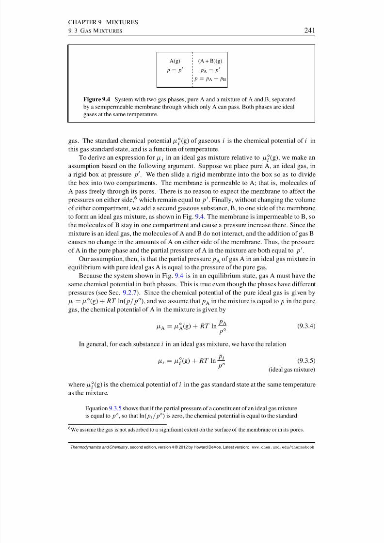
8/12/2019 Howard Devoe Thermodynamic and Chemical
http://slidepdf.com/reader/full/howard-devoe-thermodynamic-and-chemical 241/532
CHAPTER 9 MIXTURES9.3 G AS M IXTURES 241
A(g)
p D p0
(A + B)(g)
p A D p0
p D p A C p B
Figure 9.4 System with two gas phases, pure A and a mixture of A and B, separatedby a semipermeable membrane through which only A can pass. Both phases are idealgases at the same temperature.
gas. The standard chemical potential ıi (g) of gaseous i is the chemical potential of i in
this gas standard state, and is a function of temperature.To derive an expression for i in an ideal gas mixture relative to ı
i (g), we make anassumption based on the following argument. Suppose we place pure A, an ideal gas, ina rigid box at pressure p 0. We then slide a rigid membrane into the box so as to dividethe box into two compartments. The membrane is permeable to A; that is, molecules of
A pass freely through its pores. There is no reason to expect the membrane to affect thepressures on either side, 6 which remain equal to p 0. Finally, without changing the volumeof either compartment, we add a second gaseous substance, B, to one side of the membraneto form an ideal gas mixture, as shown in Fig. 9.4 . The membrane is impermeable to B, sothe molecules of B stay in one compartment and cause a pressure increase there. Since themixture is an ideal gas, the molecules of A and B do not interact, and the addition of gas Bcauses no change in the amounts of A on either side of the membrane. Thus, the pressureof A in the pure phase and the partial pressure of A in the mixture are both equal to p 0.
Our assumption, then, is that the partial pressure p A of gas A in an ideal gas mixture inequilibrium with pure ideal gas A is equal to the pressure of the pure gas.
Because the system shown in Fig. 9.4 is in an equilibrium state, gas A must have the
same chemical potential in both phases. This is true even though the phases have differentpressures (see Sec. 9.2.7 ). Since the chemical potential of the pure ideal gas is given by
D ı (g) CRT ln.p=p ı / , and we assume that p A in the mixture is equal to p in the puregas, the chemical potential of A in the mixture is given by
A D ıA(g) CRT ln
p A
p ı (9.3.4)
In general, for each substance i in an ideal gas mixture, we have the relation
i D ıi (g) CRT ln
p i
p ı (9.3.5)(ideal gas mixture)
where ıi (g) is the chemical potential of i in the gas standard state at the same temperature
as the mixture.
Equation 9.3.5 shows that if the partial pressure of a constituent of an ideal gas mixtureis equal to p ı , so that ln .p i =p ı / is zero, the chemical potential is equal to the standard
6We assume the gas is not adsorbed to a signicant extent on the surface of the membrane or in its pores.
Thermodynamics and Chemistry , second edition, version 4 © 2012 by Howard DeVoe. Latest version: www.chem.umd.edu/thermobook
8/12/2019 Howard Devoe Thermodynamic and Chemical
http://slidepdf.com/reader/full/howard-devoe-thermodynamic-and-chemical 242/532
CHAPTER 9 MIXTURES9.3 G AS M IXTURES 242
chemical potential. Conceptually, a standard state should be a well-dened state of thesystem, which in the case of a gas is the pure ideal gas at p Dp ı . Thus, although aconstituent of an ideal gas mixture with a partial pressure of 1 bar is not in its standardstate, it has the same chemical potential as in its standard state.
Equation 9.3.5 will be taken as the thermodynamic denition of an ideal gas mixture.Any gas mixture in which each constituent i obeys this relation between i and p i at allcompositions is by denition an ideal gas mixture. The nonrigorous nature of the assump-tion used to obtain Eq. 9.3.5 presents no difculty if we consider the equation to be the basicdenition.
By substituting the expression for i into .@ i =@T /p; fn ig D S i (Eq. 9.2.48 ), weobtain an expression for the partial molar entropy of substance i in an ideal gas mixture:
S i D @ ı
i (g)@T p; fn ig
R lnp i
p ı
D S ıi R lnp i
p ı (9.3.6)(ideal gas mixture)
The quantity S ıi D Œ@ıi (g)=@Tp; fn ig is the standard molar entropy of constituent i . It
is the molar entropy of i in its standard state of pure ideal gas at pressure p ı .Substitution of the expression for i from Eq. 9.3.5 and the expression for S i from Eq.
9.3.6 into H i D i CTS i (from Eq. 9.2.46 ) yields H i D ıi (g) CTS ıi , which is equivalent
to
H i D H ıi (9.3.7)
(ideal gas mixture)
This tells us that the partial molar enthalpy of a constituent of an ideal gas mixture at a giventemperature is independent of the partial pressure or mixture composition; it is a functiononly of T .
From .@ i =@p/T; fn ig D V i (Eq. 9.2.49 ), the partial molar volume of i in an ideal gasmixture is given by
V i D@ ı
i (g)@p T; fn ig
CRT @ln.p i =p ı /
@p T; fn ig(9.3.8)
The rst partial derivative on the right is zero because ıi (g) is a function only of T . For
the second partial derivative, we write p i =p ı D y i p=p ı . The mole fraction y i is constantwhen the amount of each substance is constant, so we have Œ@ln .y i p=p ı /=@p T; fn ig D 1=p .The partial molar volume is therefore given by
V i D RT
p (9.3.9)
(ideal gas mixture)
which is what we would expect simply from the ideal gas equation. The partial molarvolume is not necessarily equal to the standard molar volume, which is V ıi D RT=p ı foran ideal gas.
Thermodynamics and Chemistry , second edition, version 4 © 2012 by Howard DeVoe. Latest version: www.chem.umd.edu/thermobook
8/12/2019 Howard Devoe Thermodynamic and Chemical
http://slidepdf.com/reader/full/howard-devoe-thermodynamic-and-chemical 243/532
CHAPTER 9 MIXTURES9.3 G AS M IXTURES 243
From Eqs. 9.2.50 , 9.2.52 , 9.3.7 , and 9.3.9 we obtain the relations
U i D U ıi (9.3.10)(ideal gas mixture)
and
C p;i D C ıp;i (9.3.11)(ideal gas mixture)
Thus, in an ideal gas mixture the partial molar internal energy and the partial molar heatcapacity at constant pressure, like the partial molar enthalpy, are functions only of T .
The denition of an ideal gas mixture given by Eq. 9.3.5 is consistent with the criteriafor an ideal gas listed at the beginning of Sec. 3.5.1 , as the following derivation shows.From Eq. 9.3.9 and the additivity rule, we nd the volume is given by V DPi n i V i DPi n i RT=p D nRT=p , which is the ideal gas equation. From Eq. 9.3.10 we haveU D
Pi n i U i D
Pi n i U ıi , showing that U is a function only of T in a closed
system. These properties apply to any gas mixture obeying Eq. 9.3.5, and they are theproperties that dene an ideal gas according to Sec. 3.5.1 .
9.3.4 Real gas mixtures
Fugacity
The fugacity f of a pure gas is dened by D ı (g) C RT ln.f=p ı / (Eq. 7.8.7 onpage 184 ). By analogy with this equation, the fugacity f i of substance i in a real gasmixture is dened by the relation
i D ıi (g) CRT ln
f ip ı or f i
def
D p ı exp i ıi (g)
RT (9.3.12)
(gas mixture)
Just as the fugacity of a pure gas is a kind of effective pressure, the fugacity of a constituentof a gas mixture is a kind of effective partial pressure. That is, f i is the partial pressuresubstance i would have in an ideal gas mixture that is at the same temperature as the realgas mixture and in which the chemical potential of i is the same as in the real gas mixture.
To derive a relation allowing us to evaluate f i from the pressure–volume propertiesof the gaseous mixture, we follow the steps described for a pure gas in Sec. 7.8.1 . Thetemperature and composition are constant. From Eq. 9.3.12 , the difference between thechemical potentials of substance i in the mixture at pressures p 0 and p 00is
0i
00i D RT ln
f 0i
f 00i (9.3.13)
Integration of d i D V i dp (from Eq. 9.2.49 ) between these pressures yields
0i 00
i DZ p 0
p 00V i dp (9.3.14)
Thermodynamics and Chemistry , second edition, version 4 © 2012 by Howard DeVoe. Latest version: www.chem.umd.edu/thermobook
8/12/2019 Howard Devoe Thermodynamic and Chemical
http://slidepdf.com/reader/full/howard-devoe-thermodynamic-and-chemical 244/532
CHAPTER 9 MIXTURES9.3 G AS M IXTURES 244
When we equate these two expressions for 0i 00
i , divide both sides by RT , subtract theidentity
lnp 0
p 00 DZ p 0
p 00
dpp
(9.3.15)
and take the ideal-gas behavior limits p 00
!0 and f 00
i
!y i p 00
D .p 0
i =p 0/p 00, we obtain
lnf 0
i
p 0i DZ
p 0
0
V iRT
1p
dp (9.3.16)(gas mixture, constant T )
The fugacity coefcient i of constituent i is dened by
f idef
D i p i (9.3.17)(gas mixture)
Accordingly, the fugacity coefcient at pressure p 0 is given by
ln i .p 0/ DZ p 0
0
V iRT
1p dp (9.3.18)
(gas mixture, constant T )
As p 0 approaches zero, the integral in Eqs. 9.3.16 and 9.3.18 approaches zero, f 0i ap-proaches p 0
i , and i .p 0/ approaches unity.
Partial molar quantities
By combining Eqs. 9.3.12 and 9.3.16 , we obtain
i .p 0/ D ıi (g) CRT ln
p 0i
p ı C
Z
p 0
0V i
R T p
dp (9.3.19)(gas mixture,
constant T )
which is the analogue for a gas mixture of Eq. 7.9.2 for a pure gas. Section 7.9 describesthe procedure needed to obtain formulas for various molar quantities of a pure gas fromEq. 7.9.2 . By following a similar procedure with Eq. 9.3.19 , we obtain the formulas fordifferences between partial molar and standard molar quantities of a constituent of a gasmixture shown in the second column of Table 9.1 on the next page . These formulas areobtained with the help of Eqs. 9.2.46 , 9.2.48 , 9.2.50 , and 9.2.52 .
Equation of state
The equation of state of a real gas mixture can be written as the virial equation
pV=n D RT 1 C B.V=n/ C
C .V=n/ 2 C (9.3.20)
This equation is the same as Eq. 2.2.2 for a pure gas, except that the molar volume V m isreplaced by the mean molar volume V=n, and the virial coefcients B; C ; : : : depend oncomposition as well as temperature.
Thermodynamics and Chemistry , second edition, version 4 © 2012 by Howard DeVoe. Latest version: www.chem.umd.edu/thermobook
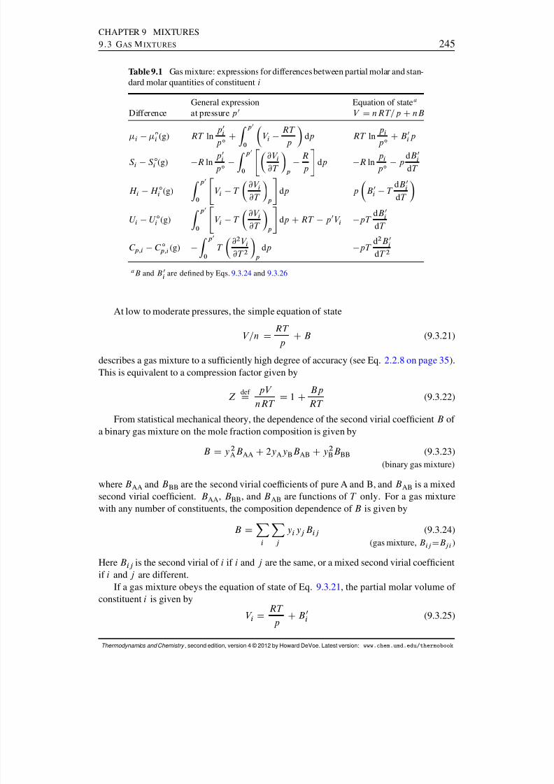
8/12/2019 Howard Devoe Thermodynamic and Chemical
http://slidepdf.com/reader/full/howard-devoe-thermodynamic-and-chemical 245/532
CHAPTER 9 MIXTURES9.3 G AS M IXTURES 245
Table 9.1 Gas mixture: expressions for differences between partial molar and stan-dard molar quantities of constituent i
General expression Equation of state a
Difference at pressure p 0 V D nRT=p CnB
i ıi (g) RT ln
p 0i
p ı CZ p 0
0 V i RT
p dp RT lnp i
p ı CB0i p
S i S ıi (g) R lnp 0
i
p ı Z p 0
0 "@V i
@T p
Rp #dp R ln
p i
p ı pdB 0
i
dT
H i H ıi (g) Z
p 0
0 "V i T @V i
@T p #dp p B 0i T
dB 0i
dT
U i U ıi (g) Z p 0
0 "V i T @V i
@T p #dp CRT p 0V i pT dB 0
i
dT
C p;i C ıp;i (g) Z p 0
0T
@2 V i@T 2 p
dp pT d2 B 0
i
dT 2
aB and B
0i are dened by Eqs. 9.3.24 and 9.3.26
At low to moderate pressures, the simple equation of state
V=n D RT
p CB (9.3.21)
describes a gas mixture to a sufciently high degree of accuracy (see Eq. 2.2.8 on page 35 ).This is equivalent to a compression factor given by
Z def
D pV nRT D 1 C
BpRT
(9.3.22)
From statistical mechanical theory, the dependence of the second virial coefcient B of a binary gas mixture on the mole fraction composition is given by
B D y 2ABAA C2y AyBBAB Cy 2
BBBB (9.3.23)(binary gas mixture)
where BAA and BBB are the second virial coefcients of pure A and B, and BAB is a mixedsecond virial coefcient. BAA , BBB , and BAB are functions of T only. For a gas mixturewith any number of constituents, the composition dependence of B is given by
B D
Xi
Xj
y i yj B ij (9.3.24)(gas mixture, B ij
DBj i )
Here B ij is the second virial of i if i and j are the same, or a mixed second virial coefcientif i and j are different.
If a gas mixture obeys the equation of state of Eq. 9.3.21 , the partial molar volume of constituent i is given by
V i D RT
p CB 0i (9.3.25)
Thermodynamics and Chemistry , second edition, version 4 © 2012 by Howard DeVoe. Latest version: www.chem.umd.edu/thermobook
8/12/2019 Howard Devoe Thermodynamic and Chemical
http://slidepdf.com/reader/full/howard-devoe-thermodynamic-and-chemical 246/532
CHAPTER 9 MIXTURES9.4 L IQUID AND S OLID M IXTURES OF N ONELECTROLYTES 246
where the quantity B 0i , in order to be consistent with V i D .@V=@ni / T;p;n j ¤ i
, is found tobe given by
B 0i D 2Xj
yj B ij B (9.3.26)
For the constituents of a binary mixture of A and B, Eq. 9.3.26 becomes
B 0A D BAA C. BAA C2B AB BBB /y 2
B (9.3.27)(binary gas mixture)
B 0B D BBB C. BAA C2B AB BBB /y 2
A (9.3.28)(binary gas mixture)
When we substitute the expression of Eq. 9.3.25 for V i in Eq. 9.3.18 , we obtain a relationbetween the fugacity coefcient of constituent i and the function B 0
i :
ln i
D
B 0i p
RT (9.3.29)
The third column of Table 9.1 gives formulas for various partial molar quantities of constituent i in terms of B 0
i and its temperature derivative. The formulas are the same as theapproximate formulas in the third column of Table 7.5 for molar quantities of a pure gas,with B 0
i replacing the second virial coefcient B .
9.4 LIQUID AND SOLID MIXTURES OF NONELECTROLYTES
Homogeneous liquid and solid mixtures are condensed phases of variable composition.Most of the discussion of condensed-phase mixtures in this section focuses on liquids.The same principles, however, apply to homogeneous solid mixtures, often called solid
solutions. These solid mixtures include most metal alloys, many gemstones, and dopedsemiconductors.
The relations derived in this section apply to mixtures of nonelectrolytes—substancesthat do not dissociate into charged species. Solutions of electrolytes behave quite differentlyin many ways, and will be discussed in the next chapter.
9.4.1 Raoult’s law
In 1888, the French physical chemist Francois Raoult published his nding that when adilute liquid solution of a volatile solvent and a nonelectrolyte solute is equilibrated with agas phase, the partial pressure p A of the solvent in the gas phase is proportional to the molefraction xA of the solvent in the solution:
p A D xAp A (9.4.1)
Here p A is the saturation vapor pressure of the pure solvent (the pressure at which the pureliquid and pure gas phases are in equilibrium).
In order to place Raoult’s law in a rigorous thermodynamic framework, consider thetwo systems depicted in Fig. 9.5 on the next page . The liquid phase of system 1 is a binary
Thermodynamics and Chemistry , second edition, version 4 © 2012 by Howard DeVoe. Latest version: www.chem.umd.edu/thermobook

8/12/2019 Howard Devoe Thermodynamic and Chemical
http://slidepdf.com/reader/full/howard-devoe-thermodynamic-and-chemical 247/532
CHAPTER 9 MIXTURES9.4 L IQUID AND S OLID M IXTURES OF N ONELECTROLYTES 247
system 1
(A+B+C)(g)
A B C
A A
(A+B)(l) A
system 2
(A+C)(g)
A C
A
A
A(l)
Figure 9.5 Two systems with equilibrated liquid and gas phases.
solution of solvent A and solute B, whereas the liquid in system 2 is the pure solvent. Insystem 1, the partial pressure p A in the equilibrated gas phase depends on the temperatureand the solution composition. In system 2, p A depends on the temperature. Both p A and
p A have a mild dependence on the total pressure p , which can be varied with an inert gasconstituent C of negligible solubility in the liquid.
Suppose that we vary the composition of the solution in system 1 at constant temper-ature, while adjusting the partial pressure of C so as to keep p constant. If we nd thatthe partial pressure of the solvent over a range of composition is given by p A D xAp A ,where p A is the partial pressure of A in system 2 at the same T and p , we will say that thesolvent obeys Raoult’s law for partial pressure in this range. This is the same as the origi-nal Raoult’s law, except that p A is now the vapor pressure of pure liquid A at the pressurep of the liquid mixture. Section 12.8.1 will show that unless p is much greater than p A ,p A is practically the same as the saturation vapor pressure of pure liquid A, in which caseRaoult’s law for partial pressure becomes identical to the original law.
A form of Raoult’s law with fugacities in place of partial pressures is often more useful:f A D xAf A , where f
A is the fugacity of A in the gas phase of system 2 at the same T andp as the solution. If this relation is found to hold over a given composition range, we willsay the solvent in this range obeys Raoult’s law for fugacity .
We can generalize the two forms of Raoult’s law for any constituent i of a liquid mix-ture:
p i D x i p i (9.4.2)(Raoult’s law for partial pressure)
f i D x i f i (9.4.3)
(Raoult’s law for fugacity)
Here x i is the mole fraction of i in the liquid mixture, and p i and f i are the partial pressure
and fugacity in a gas phase equilibrated with pure liquid i at the same T and p as the liquidmixture. Both p A and f i are functions of T and p .
These two forms of Raoult’s law are equivalent when the gas phases are ideal gas mix-tures. When it is necessary to make a distinction between the two forms, this book will referspecically to Raoult’s law for partial pressure or Raoult’s law for fugacity.
Thermodynamics and Chemistry , second edition, version 4 © 2012 by Howard DeVoe. Latest version: www.chem.umd.edu/thermobook
8/12/2019 Howard Devoe Thermodynamic and Chemical
http://slidepdf.com/reader/full/howard-devoe-thermodynamic-and-chemical 248/532
CHAPTER 9 MIXTURES9.4 L IQUID AND S OLID M IXTURES OF N ONELECTROLYTES 248
Raoult’s law for fugacity can be recast in terms of chemical potential. Section 9.2.7showed that if substance i has transfer equilibrium between a liquid and a gas phase, itschemical potential i is the same in both equilibrated phases. The chemical potential inthe gas phase is given by i D ı
i (g) CRT ln f i =p ı (Eq. 9.3.12 ). Replacing f i by x i f i
according to Raoult’s law, and rearranging, we obtain
i D ıi (g) CRT ln f i
p ı CRT ln x i (9.4.4)
The expression in brackets is independent of the mixture composition. We replace thisexpression by a quantity i , a function of T and p , and write
i D i CRT ln x i (9.4.5)
Equation 9.4.5 is an expression for the chemical potential in the liquid phase when Raoult’slaw for fugacity is obeyed. By setting xi equal to 1, we see that i represents the chemicalpotential of pure liquid i at the temperature and pressure of the mixture. Because Eq. 9.4.5is valid for any constituent whose fugacity obeys Eq. 9.4.3 , it is equivalent to Raoult’s lawfor fugacity for that constituent.
9.4.2 Ideal mixtures
Depending on the temperature, pressure, and identity of the constituents of a liquid mixture,Raoult’s law for fugacity may hold for constituent i at all liquid compositions, or over onlya limited composition range when xi is close to unity.
An ideal liquid mixture is dened as a liquid mixture in which, at a given temperatureand pressure, each constituent obeys Raoult’s law for fugacity (Eq. 9.4.3 or 9.4.5 ) over theentire range of composition. Equation 9.4.3 applies only to a volatile constituent, whereasEq. 9.4.5 applies regardless of whether the constituent is volatile.
Few liquid mixtures are found to approximate the behavior of an ideal liquid mixture.
In order to do so, the constituents must have similar molecular size and structure, and thepure liquids must be miscible in all proportions. Benzene and toluene, for instance, satisfythese requirements, and liquid mixtures of benzene and toluene are found to obey Raoult’slaw quite closely. In contrast, water and methanol, although miscible in all proportions,form liquid mixtures that deviate considerably from Raoult’s law. The most commonlyencountered situation for mixtures of organic liquids is that each constituent deviates fromRaoult’s law behavior by having a higher fugacity than predicted by Eq. 9.4.3 —a positivedeviation from Raoult’s law.
Similar statements apply to ideal solid mixtures. In addition, a relation with the sameform as Eq. 9.4.5 describes the chemical potential of each constituent of an ideal gas mix-ture, as the following derivation shows. In an ideal gas mixture at a given T and p , thechemical potential of substance i is given by Eq. 9.3.5 :
i D ıi (g) CRT ln
p i
p ı D ıi (g) CRT ln
y i pp ı (9.4.6)
Here yi is the mole fraction of i in the gas. The chemical potential of the pure ideal gas(y i D1) is
i D ıi (g) CRT ln
pp ı (9.4.7)
Thermodynamics and Chemistry , second edition, version 4 © 2012 by Howard DeVoe. Latest version: www.chem.umd.edu/thermobook
8/12/2019 Howard Devoe Thermodynamic and Chemical
http://slidepdf.com/reader/full/howard-devoe-thermodynamic-and-chemical 249/532
CHAPTER 9 MIXTURES9.4 L IQUID AND S OLID M IXTURES OF N ONELECTROLYTES 249
By eliminating ıi (g) between these equations and rearranging, we obtain Eq. 9.4.5 with xi
replaced by y i .Thus, an ideal mixture , whether solid, liquid, or gas, is a mixture in which the chemical
potential of each constituent at a given T and p is a linear function of the logarithm of themole fraction:
i D i CRT ln x i (9.4.8)(ideal mixture)
9.4.3 Partial molar quantities in ideal mixtures
With the help of Eq. 9.4.8 for the chemical potential of a constituent of an ideal mixture,we will now be able to nd expressions for partial molar quantities. These expressions ndtheir greatest use for ideal liquid and solid mixtures.
For the partial molar entropy of substance i , we have S i D .@ i =@T /p; fn ig (from Eq.9.2.48 ) or, for the ideal mixture,
S i D
@ i
@T pR ln x
i D S
i R ln x
i (9.4.9)
(ideal mixture)
Since ln x i is negative in a mixture, the partial molar entropy of a constituent of an idealmixture is greater than the molar entropy of the pure substance at the same T and p .
For the partial molar enthalpy, we have H i D i CTS i (from Eq. 9.2.46 ). Using theexpressions for i and S i gives us
H i D i CTS i D H i (9.4.10)(ideal mixture)
Thus, H i in an ideal mixture is independent of the mixture composition and is equal to themolar enthalpy of pure i at the same T and p as the mixture. In the case of an ideal gas
mixture, H i is also independent of p , because the molar enthalpy of an ideal gas dependsonly on T .
The partial molar volume is given by V i D .@ i =@p/T; fn ig (Eq. 9.2.49 ), so we have
V i D@ i
@p T D V i (9.4.11)(ideal mixture)
Finally, from Eqs. 9.2.50 and 9.2.52 and the expressions above for H i and V i , we obtain
U i D H i pV i D U i (9.4.12)(ideal mixture)
andC p;i D .@H i =@T/p; fn ig D C p;i (9.4.13)
(ideal mixture)
Note that in an ideal mixture held at constant T and p , the partial molar quantities H i , V i ,U i , and C p;i do not vary with the composition. This is basically because of the absence of intermolecular forces in an ideal mixture.
Thermodynamics and Chemistry , second edition, version 4 © 2012 by Howard DeVoe. Latest version: www.chem.umd.edu/thermobook
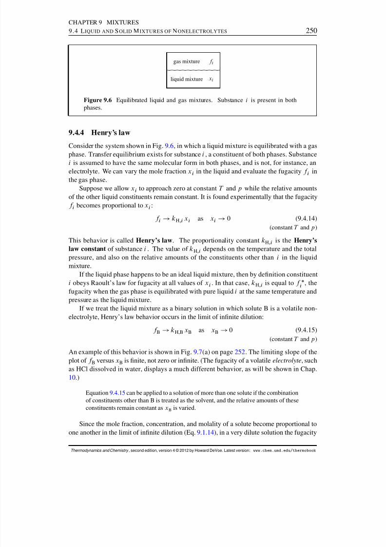
8/12/2019 Howard Devoe Thermodynamic and Chemical
http://slidepdf.com/reader/full/howard-devoe-thermodynamic-and-chemical 250/532
CHAPTER 9 MIXTURES9.4 L IQUID AND S OLID M IXTURES OF N ONELECTROLYTES 250
gas mixture f i
liquid mixture xi
Figure 9.6 Equilibrated liquid and gas mixtures. Substance i is present in bothphases.
9.4.4 Henry’s law
Consider the system shown in Fig. 9.6 , in which a liquid mixture is equilibrated with a gasphase. Transfer equilibrium exists for substance i , a constituent of both phases. Substancei is assumed to have the same molecular form in both phases, and is not, for instance, anelectrolyte. We can vary the mole fraction x i in the liquid and evaluate the fugacity f i inthe gas phase.
Suppose we allow x i to approach zero at constant T and p while the relative amountsof the other liquid constituents remain constant. It is found experimentally that the fugacityf i becomes proportional to x i :
f i ! kH;i x i as xi ! 0 (9.4.14)(constant T and p )
This behavior is called Henry’s law . The proportionality constant kH;i is the Henry’slaw constant of substance i . The value of kH;i depends on the temperature and the totalpressure, and also on the relative amounts of the constituents other than i in the liquidmixture.
If the liquid phase happens to be an ideal liquid mixture, then by denition constituenti obeys Raoult’s law for fugacity at all values of x
i. In that case, k
H;i is equal to f
i , the
fugacity when the gas phase is equilibrated with pure liquid i at the same temperature andpressure as the liquid mixture.
If we treat the liquid mixture as a binary solution in which solute B is a volatile non-electrolyte, Henry’s law behavior occurs in the limit of innite dilution:
f B ! kH,B xB as xB ! 0 (9.4.15)(constant T and p )
An example of this behavior is shown in Fig. 9.7 (a) on page 252 . The limiting slope of theplot of f B versus xB is nite, not zero or innite. (The fugacity of a volatile electrolyte , suchas HCl dissolved in water, displays a much different behavior, as will be shown in Chap.10.)
Equation 9.4.15 can be applied to a solution of more than one solute if the combinationof constituents other than B is treated as the solvent, and the relative amounts of theseconstituents remain constant as xB is varied.
Since the mole fraction, concentration, and molality of a solute become proportional toone another in the limit of innite dilution (Eq. 9.1.14 ), in a very dilute solution the fugacity
Thermodynamics and Chemistry , second edition, version 4 © 2012 by Howard DeVoe. Latest version: www.chem.umd.edu/thermobook

8/12/2019 Howard Devoe Thermodynamic and Chemical
http://slidepdf.com/reader/full/howard-devoe-thermodynamic-and-chemical 251/532
CHAPTER 9 MIXTURES9.4 L IQUID AND S OLID M IXTURES OF N ONELECTROLYTES 251
BIOGRAPHICAL SKETCHWilliam Henry (1774–1836)
William Henry was a British chemist, trainedas a physician, who is best known for his for-mulation of what is now called Henry’s law.
Henry was born in Manchester, England.His father was an apothecary and industrialchemist who established a protable businessmanufacturing such products as magnesiumcarbonate (used as an antacid) and carbonatedwater. At the age of ten, Henry was severelyinjured by a falling beam and was plagued bypain and ill health for the rest of his life.
Henry began medical studies at the Univer-sity of Edinburgh in 1795. He interrupted thesestudies to do chemical research, to assist hisfather in general medical practice, and to helprun the family chemical business. He nallyreceived his diploma of Doctor in Medicine in1807. In 1809, in recognition of his researchpapers, he was elected a Fellow of the RoyalSociety.
In 1801 the rst edition of his inuentialchemistry textbook appeared, originally called An Epitome of Chemistry and in later editions Elements of Experimental Chemistry . Thebook went through eleven editions over a pe-riod of 28 years.
Henry investigated the relation between thepressure of a gas and the volume of the gas,measured at that pressure, that was absorbedinto a given volume of water. He used a simple
apparatus in which the water and gas were con-ned over mercury in a graduated glass vessel,and the contents agitated to allow a portion of
the gas to dissolve in the water. His ndingswere presented to the Royal Society of Londonin 1802 and published the following year: a
The results of a series of at least fty experi-ments, on carbonic acid, sulphuretted hydrogengas, nitrous oxide, oxygenous and azotic gases, b
with the above apparatus, establish the follow-ing general law: that, under equal circumstancesof temperature, water takes up, in all cases, thesame volume of condensed gas as of gas un-der ordinary pressure. But, as the spaces oc-cupied by every gas are inversely as the com-pressing force, it follows, that water takes up, of gas condensed by one, two, or more additionalatmospheres, a quantity which, ordinarily com- pressed, would be equal to twice, thrice, &c. thevolume absorbed under the common pressure of the atmosphere.
Henry later conrmed a suggestion made byhis close friend John Dalton, that the amountof a constituent of a gaseous mixture that is ab-sorbed is proportional to its partial pressure. c
Henry carried out other important work,chiey on gases, including the elemental com-positions of hydrogen chloride, ammonia, andmethane.
Because of his poor health and unsuccess-ful surgery on his hands, Henry was unable tocontinue working in the lab after 1824. Twelve
years later, suffering from pain and depression,he committed suicide.In a biography published the year after
Henry’s death, his son William Charles Henrywrote: d
In the general intercourse of society, Dr. Henrywas distinguished by a polished courtesy, by anintuitive propriety, and by a considerate fore-thought and respect for the feelings and opinionsof others.. . His comprehensive range of thoughtand knowledge, his proneness to general spec-ulation in contradistinction to detail, his readycommand of the renements of language and theliveliness of his feelings and imagination ren-dered him a most instructive and engaging com-panion.
a Ref. [ 75]. bThese gases are respectively CO 2 , H2S, N 2O, O 2 , and N 2 . cRef. [ 76]. d Quoted in Ref.[154 ].
Thermodynamics and Chemistry , second edition, version 4 © 2012 by Howard DeVoe. Latest version: www.chem.umd.edu/thermobook
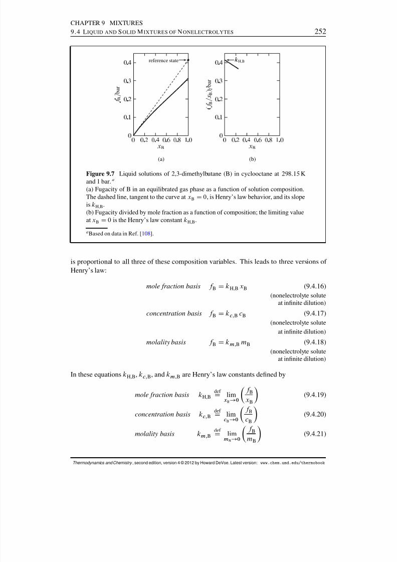
8/12/2019 Howard Devoe Thermodynamic and Chemical
http://slidepdf.com/reader/full/howard-devoe-thermodynamic-and-chemical 252/532
CHAPTER 9 MIXTURES9.4 L IQUID AND S OLID M IXTURES OF N ONELECTROLYTES 252
reference state
B
(a)
.
B
b a r
H,B
B
(b)
B
B
b a r
Figure 9.7 Liquid solutions of 2,3-dimethylbutane (B) in cyclooctane at 298:15 Kand 1 bar. a
(a) Fugacity of B in an equilibrated gas phase as a function of solution composition.
The dashed line, tangent to the curve at xB D 0, is Henry’s law behavior, and its slopeis kH,B .(b) Fugacity divided by mole fraction as a function of composition; the limiting valueat xB D 0 is the Henry’s law constant kH,B .
a Based on data in Ref. [ 108 ].
is proportional to all three of these composition variables. This leads to three versions of Henry’s law:
mole fraction basis f B D kH,B xB (9.4.16)
(nonelectrolyte soluteat innite dilution)
concentration basis f B D kc; B cB (9.4.17)(nonelectrolyte solute
at innite dilution)
molality basis f B D km; B mB (9.4.18)(nonelectrolyte solute
at innite dilution)
In these equations kH,B , kc; B , and km; B are Henry’s law constants dened by
mole fraction basis kH,B def D limx B ! 0
f B
xB (9.4.19)
concentration basis kc; Bdef
D limcB ! 0
f BcB
(9.4.20)
molality basis km; Bdef
D limm B ! 0
f BmB
(9.4.21)
Thermodynamics and Chemistry , second edition, version 4 © 2012 by Howard DeVoe. Latest version: www.chem.umd.edu/thermobook
8/12/2019 Howard Devoe Thermodynamic and Chemical
http://slidepdf.com/reader/full/howard-devoe-thermodynamic-and-chemical 253/532
CHAPTER 9 MIXTURES9.4 L IQUID AND S OLID M IXTURES OF N ONELECTROLYTES 253
Note that the Henry’s law constants are not dimensionless, and are functions of T and p .To evaluate one of these constants, we can plot f B divided by the appropriate compositionvariable as a function of the composition variable and extrapolate to innite dilution. Theevaluation of kH,B by this procedure is illustrated in Fig. 9.7 (b).
Relations between these Henry’s law constants can be found with the use of Eqs. 9.1.14
and 9.4.16 –9.4.18 : kc; B D V A kH,B km; B D M A kH,B (9.4.22)
9.4.5 The ideal-dilute solution
An ideal-dilute solution is a real solution that is dilute enough for each solute to obeyHenry’s law. On the microscopic level, the requirement is that solute molecules be suf-ciently separated to make solute–solute interactions negligible.
Note that an ideal-dilute solution is not necessarily an ideal mixture. Few liquid mix-tures behave as ideal mixtures, but a solution of any nonelectrolyte solute becomes an ideal-dilute solution when sufciently dilute.
Within the composition range that a solution effectively behaves as an ideal-dilute
solution, then, the fugacity of solute B in a gas phase equilibrated with the solution isproportional to its mole fraction xB in the solution. The chemical potential of B in thegas phase, which is equal to that of B in the liquid, is related to the fugacity by B Dı
B(g) C RT ln.f B=p ı / (Eq. 9.3.12 ). Substituting f B D kH,B xB (Henry’s law) into thisequation, we obtain
B D ıB(g) CRT ln
kH,B xB
p ı
D ıB(g) CRT ln
kH,B
p ı CRT ln xB (9.4.23)
where the composition variable xB is segregated in the last term on the right side.The expression in brackets in Eq. 9.4.23 is a function of T and p , but not of xB , and
represents the chemical potential of B in a hypothetical solute reference state. This chemicalpotential will be denoted by ref
x; B , where the x in the subscript reminds us that the referencestate is based on mole fraction. The equation then becomes
B .T;p/ D ref x; B .T;p/ CRT ln xB (9.4.24)
(ideal-dilute solutionof a nonelectrolyte)
Here the notation emphasizes the fact that B and ref x; B are functions of T and p .
Equation 9.4.24 , derived using fugacity, is valid even if the solute has such low volatil-ity that its fugacity in an equilibrated gas phase is too low to measure. In principle, nosolute is completely nonvolatile, and there is always a nite solute fugacity in the gasphase even if immeasurably small.
It is worthwhile to describe in detail the reference state to which ref x; B refers. The
general concept is also applicable to other solute reference states and solute standardstates to be encountered presently. Imagine a hypothetical solution with the sameconstituents as the real solution. This hypothetical solution has the magical property
Thermodynamics and Chemistry , second edition, version 4 © 2012 by Howard DeVoe. Latest version: www.chem.umd.edu/thermobook

8/12/2019 Howard Devoe Thermodynamic and Chemical
http://slidepdf.com/reader/full/howard-devoe-thermodynamic-and-chemical 254/532
CHAPTER 9 MIXTURES9.4 L IQUID AND S OLID M IXTURES OF N ONELECTROLYTES 254
that it continues to exhibit the ideal-dilute behavior described by Eq. 9.4.24 , even whenxB increases beyond the ideal-dilute range of the real solution. The reference state isthe state of this hypothetical solution at xBD1. It is a ctitious state in which the molefraction of B is unity and B behaves as in an ideal-dilute solution, and is sometimescalled the ideal-dilute solution of unit solute mole fraction .
By setting xB equal to unity in Eq. 9.4.24 , so that ln xB is zero, we see that ref x; B
is the chemical potential of B in the reference state. In a gas phase equilibrated withthe hypothetical solution, the solute fugacity f B increases as a linear function of xB allthe way to xBD1, unlike the behavior of the real solution (unless it happens to be anideal mixture). In the reference state, f B is equal to the Henry’s law constant kH,B ; anexample is indicated by the lled circle in Fig. 9.7(a).
By similar steps, combining Henry’s law based on concentration or molality (Eqs.9.4.17 and 9.4.18 ) with the relation B D ı
B(g) CRT ln.f B=p ı / , we obtain for the solutechemical potential in the ideal-dilute range the equations
B D ıB(g) CRT ln
kc; B cB
p ı cı
c ı
D ıB(g) CRT ln kc; B c ı
p ı CRT ln cB
c ı (9.4.25)
B D ıB(g) CRT ln
km; B mB
p ı mı
m ı
D ıB(g) CRT ln
km; B m ı
p ı CRT lnmB
m ı (9.4.26)
Note how in each equation the argument of a logarithm is multiplied and divided by aconstant, c ı or m ı , in order to make the arguments of the resulting logarithms dimension-less. These constants are called standard compositions with the following values:standard concentration cı
D 1 mol dm 3 (equal to one mole per liter, or one molar)
standard molality mı D 1 mol kg 1 (equal to one molal)Again in each of these equations, we replace the expression in brackets, which depends
on T and p but not on composition, with the chemical potential of a solute reference state:
B .T;p/ D ref c; B .T;p/ CRT ln
cB
c ı (9.4.27)(ideal-dilute solution
of a nonelectrolyte)
B .T;p/ D ref m; B .T;p/ CRT ln
mB
m ı (9.4.28)(ideal-dilute solution
of a nonelectrolyte)
The quantities ref c; B and ref
m; B are the chemical potentials of the solute in hypothetical refer-ence states that are solutions of standard concentration and standard molality, respectively,in which B behaves as in an ideal-dilute solution. Section 9.7.1 will show that when thepressure is the standard pressure, these reference states are solute standard states.
Thermodynamics and Chemistry , second edition, version 4 © 2012 by Howard DeVoe. Latest version: www.chem.umd.edu/thermobook
8/12/2019 Howard Devoe Thermodynamic and Chemical
http://slidepdf.com/reader/full/howard-devoe-thermodynamic-and-chemical 255/532
CHAPTER 9 MIXTURES9.4 L IQUID AND S OLID M IXTURES OF N ONELECTROLYTES 255
For consistency with Eqs. 9.4.27 and 9.4.28 , we can rewrite Eq. 9.4.24 in the form
B .T;p/ D ref x; B .T;p/ CRT ln
xB
x ı (9.4.29)
with x ı , the standard mole fraction , given by x ı D 1.
9.4.6 Solvent behavior in the ideal-dilute solution
We now use the Gibbs–Duhem equation to investigate the behavior of the solvent in anideal-dilute solution of one or more nonelectrolyte solutes. The Gibbs–Duhem equation ap-plied to chemical potentials at constant T and p can be written Pi x i d i D 0 (Eq. 9.2.43 ).We use subscript A for the solvent, rewrite the equation as xA d A CPi ¤ A x i d i D 0,and rearrange to
d A D 1xA Xi ¤ A
x i d i (9.4.30)(constant T and p )
This equation shows how changes in the solute chemical potentials, due to a compositionchange at constant T and p , affect the chemical potential of the solvent.
In an ideal-dilute solution, the chemical potential of each solute is given by i D ref x;i C
RT ln x i and the differential of i at constant T and p is
d i D RT d ln x i D RT dx i =xi (9.4.31)
(Here the fact has been used that ref x;i is a constant at a given T and p .) When we substitute
this expression for d i in Eq. 9.4.30 , we obtain
d A D RT xA Xi ¤ A
dx i (9.4.32)
Now since the sum of all mole fractions is 1, we have the relation Pi ¤ A x i D 1 xA whosedifferential is Pi ¤ A dx i D dxA . Making this substitution in Eq. 9.4.32 gives us
d A D RT
xAdxA D RT d ln xA (9.4.33)
(ideal-dilute solutionof nonelectrolytes)
Consider a process in an open system in which we start with a xed amount of puresolvent and continuously add the solute or solutes at constant T and p . The solvent molefraction decreases from unity to a value x0
A , and the solvent chemical potential changesfrom A to 0
A . We assume the solution formed in this process is in the ideal-dilute solution
range, and integrate Eq. 9.4.33 over the path of the process:
Z 0
A
A
d A D RT Z xA D x 0
A
x A D 1d ln xA (9.4.34)
The result is 0A A D RT ln x 0
A , or in general
A D A CRT ln xA (9.4.35)
Thermodynamics and Chemistry , second edition, version 4 © 2012 by Howard DeVoe. Latest version: www.chem.umd.edu/thermobook
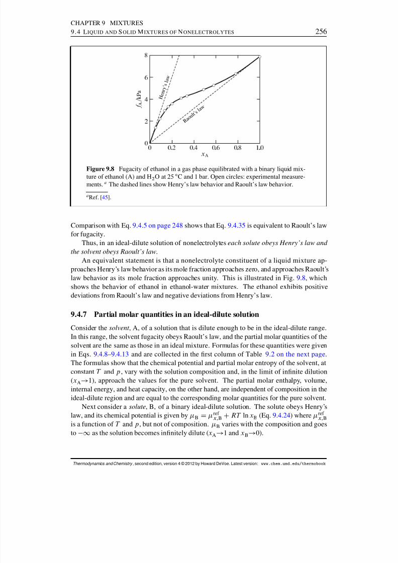
8/12/2019 Howard Devoe Thermodynamic and Chemical
http://slidepdf.com/reader/full/howard-devoe-thermodynamic-and-chemical 256/532
CHAPTER 9 MIXTURES9.4 L IQUID AND S OLID M IXTURES OF N ONELECTROLYTES 256
R a o u
l t ’ s l a w
H e n r y ’ s
l a w
A
A
k P a
Figure 9.8 Fugacity of ethanol in a gas phase equilibrated with a binary liquid mix-ture of ethanol (A) and H 2 O at 25 ı C and 1 bar. Open circles: experimental measure-ments. a The dashed lines show Henry’s law behavior and Raoult’s law behavior.
a Ref. [ 45].
Comparison with Eq. 9.4.5 on page 248 shows that Eq. 9.4.35 is equivalent to Raoult’s lawfor fugacity.
Thus, in an ideal-dilute solution of nonelectrolytes each solute obeys Henry’s law and the solvent obeys Raoult’s law .
An equivalent statement is that a nonelectrolyte constituent of a liquid mixture ap-proaches Henry’s law behavior as its mole fraction approaches zero, and approaches Raoult’slaw behavior as its mole fraction approaches unity. This is illustrated in Fig. 9.8, whichshows the behavior of ethanol in ethanol-water mixtures. The ethanol exhibits positive
deviations from Raoult’s law and negative deviations from Henry’s law.
9.4.7 Partial molar quantities in an ideal-dilute solution
Consider the solvent , A, of a solution that is dilute enough to be in the ideal-dilute range.In this range, the solvent fugacity obeys Raoult’s law, and the partial molar quantities of thesolvent are the same as those in an ideal mixture. Formulas for these quantities were givenin Eqs. 9.4.8 –9.4.13 and are collected in the rst column of Table 9.2 on the next page .The formulas show that the chemical potential and partial molar entropy of the solvent, atconstant T and p , vary with the solution composition and, in the limit of innite dilution(xA! 1), approach the values for the pure solvent. The partial molar enthalpy, volume,internal energy, and heat capacity, on the other hand, are independent of composition in theideal-dilute region and are equal to the corresponding molar quantities for the pure solvent.
Next consider a solute , B, of a binary ideal-dilute solution. The solute obeys Henry’slaw, and its chemical potential is given by B D ref
x; B CRT ln xB (Eq. 9.4.24 ) where ref x; B
is a function of T and p , but not of composition. B varies with the composition and goesto 1 as the solution becomes innitely dilute ( xA! 1 and xB! 0).
Thermodynamics and Chemistry , second edition, version 4 © 2012 by Howard DeVoe. Latest version: www.chem.umd.edu/thermobook

8/12/2019 Howard Devoe Thermodynamic and Chemical
http://slidepdf.com/reader/full/howard-devoe-thermodynamic-and-chemical 257/532
CHAPTER 9 MIXTURES9.4 L IQUID AND S OLID M IXTURES OF N ONELECTROLYTES 257
Table 9.2 Partial molar quantities of solvent and non-electrolyte solute in an ideal-dilute solution
Solvent Solute
A D A CRT ln xA B D ref x; B CRT ln xB
D ref
c; B CRT ln.c
B=cı /
D ref m; B CRT ln.m B=m ı /
S A D S A R ln xA S B D S ref x; B R ln xB
D S ref c; B R ln.c B=cı /
D S ref m; B R ln.m B=m ı /
H A D H A H B D H 1B
V A D V A V B D V 1BU A D U A U B D U 1BC p; A D C p; A C p; B D C 1p; B
For the partial molar entropy of the solute, we use S B D .@ B=@T/p; fn ig (Eq. 9.2.48 )and obtain
S B D @ ref
x; B
@T !p
R ln xB (9.4.36)
The term .@ ref x; B=@T /p represents the partial molar entropy S ref
x; B of B in the ctitiousreference state of unit solute mole fraction. Thus, we can write Eq. 9.4.36 in the form
S B D S ref x; B R ln xB (9.4.37)
(ideal-dilute solutionof a nonelectrolyte)
This equation shows that the partial molar entropy varies with composition and goes to
C1 in the limit of innite dilution. From the expressions of Eqs. 9.4.27 and 9.4.28 , we canderive similar expressions for S B in terms of the solute reference states on a concentrationor molality basis.
The relation H B D B CTS B (from Eq. 9.2.46 ), combined with Eqs. 9.4.24 and 9.4.37 ,yields
H B D ref x; B CTS ref
x; B D H ref x; B (9.4.38)
showing that at constant T and p , the partial molar enthalpy of the solute is constantthroughout the ideal-dilute solution range. Therefore, we can write
H B D H 1B (9.4.39)
(ideal-dilute solutionof a nonelectrolyte)
where H 1B is the partial molar enthalpy at innite dilution. By similar reasoning, usingEqs. 9.2.49 –9.2.52 , we nd that the partial molar volume, internal energy, and heat capacityof the solute are constant in the ideal-dilute range and equal to the values at innite dilution.The expressions are listed in the second column of Table 9.2 .
When the pressure is equal to the standard pressure p ı , the quantities H 1B , V 1B , U 1B ,
and C 1p; B are the same as the standard values H ıB , V ıB , U ıB , and C ıp; B .
Thermodynamics and Chemistry , second edition, version 4 © 2012 by Howard DeVoe. Latest version: www.chem.umd.edu/thermobook
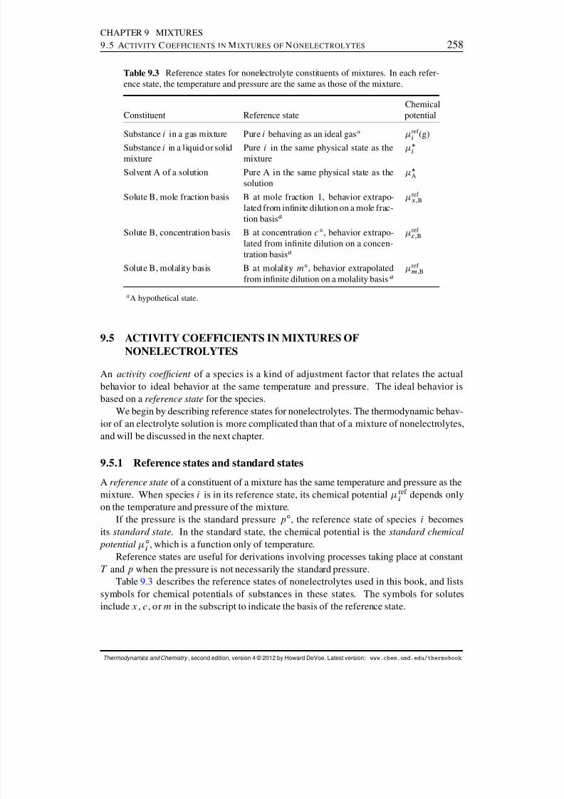
8/12/2019 Howard Devoe Thermodynamic and Chemical
http://slidepdf.com/reader/full/howard-devoe-thermodynamic-and-chemical 258/532
CHAPTER 9 MIXTURES9.5 A CTIVITY C OEFFICIENTS IN M IXTURES OF N ONELECTROLYTES 258
Table 9.3 Reference states for nonelectrolyte constituents of mixtures. In each refer-ence state, the temperature and pressure are the same as those of the mixture.
ChemicalConstituent Reference state potential
Substance i in a gas mixture Pure i behaving as an ideal gas a ref
i (g)
Substance i in a liquid or solidmixture
Pure i in the same physical state as themixture
i
Solvent A of a solution Pure A in the same physical state as thesolution
A
Solute B, mole fraction basis B at mole fraction 1, behavior extrapo-lated from innite dilution on a mole frac-tion basis a
ref x; B
Solute B, concentration basis B at concentration c ı , behavior extrapo-lated from innite dilution on a concen-tration basis a
ref c; B
Solute B, molality basis B at molality mı , behavior extrapolated
from innite dilution on a molality basisa
ref m; B
a A hypothetical state.
9.5 ACTIVITY COEFFICIENTS IN MIXTURES OFNONELECTROLYTES
An activity coefcient of a species is a kind of adjustment factor that relates the actualbehavior to ideal behavior at the same temperature and pressure. The ideal behavior isbased on a reference state for the species.
We begin by describing reference states for nonelectrolytes. The thermodynamic behav-ior of an electrolyte solution is more complicated than that of a mixture of nonelectrolytes,and will be discussed in the next chapter.
9.5.1 Reference states and standard states
A reference state of a constituent of a mixture has the same temperature and pressure as themixture. When species i is in its reference state, its chemical potential ref
i depends onlyon the temperature and pressure of the mixture.
If the pressure is the standard pressure p ı , the reference state of species i becomesits standard state . In the standard state, the chemical potential is the standard chemical potential ı
i , which is a function only of temperature.
Reference states are useful for derivations involving processes taking place at constantT and p when the pressure is not necessarily the standard pressure.Table 9.3 describes the reference states of nonelectrolytes used in this book, and lists
symbols for chemical potentials of substances in these states. The symbols for solutesinclude x , c , or m in the subscript to indicate the basis of the reference state.
Thermodynamics and Chemistry , second edition, version 4 © 2012 by Howard DeVoe. Latest version: www.chem.umd.edu/thermobook
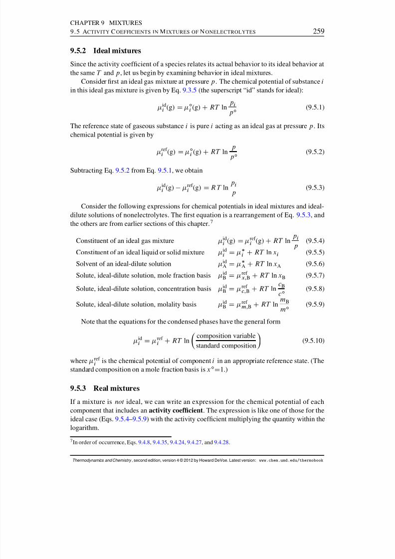
8/12/2019 Howard Devoe Thermodynamic and Chemical
http://slidepdf.com/reader/full/howard-devoe-thermodynamic-and-chemical 259/532
CHAPTER 9 MIXTURES9.5 A CTIVITY C OEFFICIENTS IN M IXTURES OF N ONELECTROLYTES 259
9.5.2 Ideal mixtures
Since the activity coefcient of a species relates its actual behavior to its ideal behavior atthe same T and p , let us begin by examining behavior in ideal mixtures.
Consider rst an ideal gas mixture at pressure p . The chemical potential of substance iin this ideal gas mixture is given by Eq. 9.3.5 (the superscript “id” stands for ideal):
idi (g) D ı
i (g) CRT lnp i
p ı (9.5.1)
The reference state of gaseous substance i is pure i acting as an ideal gas at pressure p . Itschemical potential is given by
ref i (g) D ı
i (g) CRT lnpp ı (9.5.2)
Subtracting Eq. 9.5.2 from Eq. 9.5.1 , we obtain
idi (g) ref
i (g)
D RT ln
p i
p
(9.5.3)
Consider the following expressions for chemical potentials in ideal mixtures and ideal-dilute solutions of nonelectrolytes. The rst equation is a rearrangement of Eq. 9.5.3 , andthe others are from earlier sections of this chapter. 7
Constituent of an ideal gas mixture idi (g) D ref
i (g) CRT lnp i
p (9.5.4)
Constituent of an ideal liquid or solid mixture idi D i CRT ln x i (9.5.5)
Solvent of an ideal-dilute solution idA D A CRT ln xA (9.5.6)
Solute, ideal-dilute solution, mole fraction basis idB D ref
x; B CRT ln xB (9.5.7)
Solute, ideal-dilute solution, concentration basis id
B D ref
c;B C
RT lncB
c ı (9.5.8)
Solute, ideal-dilute solution, molality basis idB D ref
m; B CRT lnmB
m ı (9.5.9)
Note that the equations for the condensed phases have the general form
idi D ref
i CRT lncomposition variablestandard composition
(9.5.10)
where ref i is the chemical potential of component i in an appropriate reference state. (The
standard composition on a mole fraction basis is x ı D1.)
9.5.3 Real mixturesIf a mixture is not ideal, we can write an expression for the chemical potential of eachcomponent that includes an activity coefcient . The expression is like one of those for theideal case (Eqs. 9.5.4 –9.5.9 ) with the activity coefcient multiplying the quantity within thelogarithm.
7In order of occurrence, Eqs. 9.4.8 , 9.4.35 , 9.4.24 , 9.4.27 , and 9.4.28 .
Thermodynamics and Chemistry , second edition, version 4 © 2012 by Howard DeVoe. Latest version: www.chem.umd.edu/thermobook
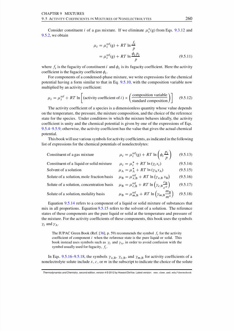
8/12/2019 Howard Devoe Thermodynamic and Chemical
http://slidepdf.com/reader/full/howard-devoe-thermodynamic-and-chemical 260/532
CHAPTER 9 MIXTURES9.5 A CTIVITY C OEFFICIENTS IN M IXTURES OF N ONELECTROLYTES 260
Consider constituent i of a gas mixture. If we eliminate ıi (g) from Eqs. 9.3.12 and
9.5.2 , we obtain
i D ref i (g) CRT ln
f ip
D ref i (g) CRT ln
i p i
p (9.5.11)
where f i is the fugacity of constituent i and i is its fugacity coefcient. Here the activitycoefcient is the fugacity coefcient i .
For components of a condensed-phase mixture, we write expressions for the chemicalpotential having a form similar to that in Eq. 9.5.10 , with the composition variable nowmultiplied by an activity coefcient:
i D ref i CRT ln . activity coefcient of i /
composition variablestandard composition
(9.5.12)
The activity coefcient of a species is a dimensionless quantity whose value dependson the temperature, the pressure, the mixture composition, and the choice of the referencestate for the species. Under conditions in which the mixture behaves ideally, the activitycoefcient is unity and the chemical potential is given by one of the expressions of Eqs.9.5.4 –9.5.9 ; otherwise, the activity coefcient has the value that gives the actual chemicalpotential.
This book will use various symbols for activity coefcients, as indicated in the followinglist of expressions for the chemical potentials of nonelectrolytes:
Constituent of a gas mixture i D ref i (g) CRT ln i
p i
p (9.5.13)
Constituent of a liquid or solid mixture i D i CRT ln . i x i / (9.5.14)
Solvent of a solution A
D A
CRT ln . AxA / (9.5.15)
Solute of a solution, mole fraction basis B D ref x; B CRT ln x; B xB (9.5.16)
Solute of a solution, concentration basis B D ref c; B CRT ln c; B
cB
c ı (9.5.17)
Solute of a solution, molality basis B D ref m; B CRT ln m; B
mB
m ı (9.5.18)
Equation 9.5.14 refers to a component of a liquid or solid mixture of substances thatmix in all proportions. Equation 9.5.15 refers to the solvent of a solution. The referencestates of these components are the pure liquid or solid at the temperature and pressure of the mixture. For the activity coefcients of these components, this book uses the symbols i and A .
The IUPAC Green Book (Ref. [ 36], p. 59) recommends the symbol f i for the activitycoefcient of component i when the reference state is the pure liquid or solid. Thisbook instead uses symbols such as i and A , in order to avoid confusion with thesymbol usually used for fugacity, f i .
In Eqs. 9.5.16 –9.5.18 , the symbols x; B , c; B , and m; B for activity coefcients of anonelectrolyte solute include x , c , or m in the subscript to indicate the choice of the solute
Thermodynamics and Chemistry , second edition, version 4 © 2012 by Howard DeVoe. Latest version: www.chem.umd.edu/thermobook
8/12/2019 Howard Devoe Thermodynamic and Chemical
http://slidepdf.com/reader/full/howard-devoe-thermodynamic-and-chemical 261/532
CHAPTER 9 MIXTURES9.5 A CTIVITY C OEFFICIENTS IN M IXTURES OF N ONELECTROLYTES 261
reference state. Although three different expressions for B are shown, for a given solutioncomposition they must all represent the same value of B , equal to the rate at which theGibbs energy increases with the amount of substance B added to the solution at constant T and p . The value of a solute activity coefcient, on the other hand, depends on the choiceof the solute reference state.
You may nd it helpful to interpret products appearing on the right sides of Eqs. 9.5.13 –9.5.18 as follows. i p i is an effective partial pressure.
i x i , AxA , and x; BxB are effective mole fractions.
c; BcB is an effective concentration.
m; BmB is an effective molality.In other words, the value of one of these products is the value of a partial pressure orcomposition variable that would give the same chemical potential in an ideal mixture asthe actual chemical potential in the real mixture. These effective composition variablesare an alternative way to express the escaping tendency of a substance from a phase; they
are related exponentially to the chemical potential, which is also a measure of escapingtendency.A change in pressure or composition that causes a mixture to approach the behavior of
an ideal mixture or ideal-dilute solution must cause the activity coefcient of each mixtureconstituent to approach unity:
Constituent of a gas mixture i ! 1 as p ! 0 (9.5.19)
Constituent of a liquid or solid mixture i ! 1 as xi ! 1 (9.5.20)
Solvent of a solution A ! 1 as xA ! 1 (9.5.21)
Solute of a solution, mole fraction basis x; B ! 1 as xB ! 0 (9.5.22)
Solute of a solution, concentration basis c; B ! 1 as cB ! 0 (9.5.23)
Solute of a solution, molality basis m; B ! 1 as mB ! 0 (9.5.24)
9.5.4 Nonideal dilute solutions
How would we expect the activity coefcient of a nonelectrolyte solute to behave in adilute solution as the solute mole fraction increases beyond the range of ideal-dilute solutionbehavior?
The following argument is based on molecular properties at constant T and p .We focus our attention on a single solute molecule. This molecule has interac-
tions with nearby solute molecules. Each interaction depends on the intermoleculardistance and causes a change in the internal energy compared to the interaction of the
solute molecule with solvent at the same distance. 8 The number of solute moleculesin a volume element at a given distance from the solute molecule we are focusingon is proportional to the local solute concentration. If the solution is dilute and the
8In Sec. 11.1.5 , it will be shown that roughly speaking the internal energy change is negative if the averageof the attractive forces between two solute molecules and two solvent molecules is greater than the attractiveforce between a solute molecule and a solvent molecule at the same distance, and is positive for the oppositesituation.
Thermodynamics and Chemistry , second edition, version 4 © 2012 by Howard DeVoe. Latest version: www.chem.umd.edu/thermobook
8/12/2019 Howard Devoe Thermodynamic and Chemical
http://slidepdf.com/reader/full/howard-devoe-thermodynamic-and-chemical 262/532
CHAPTER 9 MIXTURES9.6 E VALUATION OF A CTIVITY C OEFFICIENTS 262
interactions weak, we expect the local solute concentration to be proportional to themacroscopic solute mole fraction. Thus, the partial molar quantities U B and V B of thesolute should be approximately linear functions of xB in a dilute solution at constantT and p .
From Eqs. 9.2.46 and 9.2.50 , the solute chemical potential is given by B D U B CpV B TS B . In the dilute solution, we assume U B and V B are linear functions of xB
as explained above. We also assume the dependence of S B on xB is approximately thesame as in an ideal mixture; this is a prediction from statistical mechanics for a mixturein which all molecules have similar sizes and shapes. Thus we expect the deviationof the chemical potential from ideal-dilute behavior, B D ref
x; B CRT ln xB , can bedescribed by adding a term proportional to xB : B D ref
x; B CRT ln xB Ckx xB , wherekx is a positive or negative constant related to solute-solute interactions.
If we equate this expression for B with the one that denes the activity coef-cient, B D ref
x; B CRT ln. x; B xB / (Eq. 9.5.16 ), and solve for the activity coefcient,we obtain the relation 9 x; B D exp .k x xB=RT/ . An expansion of the exponential inpowers of xB converts this to
x; B D 1 C.k x =RT /x B C (9.5.25)
Thus we predict that at constant T and p , x; B is a linear function of x B at low x B .An ideal-dilute solution, then, is one in which xB is much smaller than RT=k x so that x; B is approximately 1. An ideal mixture requires the interaction constant kx to bezero.
By similar reasoning, we reach analogous conclusions for solute activity coef-cients on a concentration or molality basis. For instance, at low mB the chemicalpotential of B should be approximately ref
m; B CRT ln.m B=m ı / Ckm mB , where km isa constant at a given T and p ; then the activity coefcient at low mB is given by
m; B D exp .k m mB=RT/ D 1 C.k m =RT /m B C (9.5.26)
The prediction from the theoretical argument above, that a solute activity coefcient in adilute solution is a linear function of the composition variable, is borne out experimentallyas illustrated in Fig. 9.10 on page 265 . This prediction applies only to a nonelectrolytesolute; for an electrolyte, the slope of activity coefcient versus molality approaches 1at low molality (page 291 ).
9.6 EVALUATION OF ACTIVITY COEFFICIENTS
This section describes several methods by which activity coefcients of nonelectrolyte sub-stances may be evaluated. Section 9.6.3 describes an osmotic coefcient method that is alsosuitable for electrolyte solutes, as will be explained in Sec. 10.6 .
9.6.1 Activity coefcients from gas fugacities
Suppose we equilibrate a liquid mixture with a gas phase. If component i of the liquidmixture is a volatile nonelectrolyte, and we are able to evaluate its fugacity f i in the gasphase, we have a convenient way to evaluate the activity coefcient i in the liquid. Therelation between i and f i will now be derived.
9This is essentially the result of the McMillan–Mayer solution theory from statistical mechanics.
Thermodynamics and Chemistry , second edition, version 4 © 2012 by Howard DeVoe. Latest version: www.chem.umd.edu/thermobook
8/12/2019 Howard Devoe Thermodynamic and Chemical
http://slidepdf.com/reader/full/howard-devoe-thermodynamic-and-chemical 263/532
CHAPTER 9 MIXTURES9.6 E VALUATION OF A CTIVITY C OEFFICIENTS 263
When component i is in transfer equilibrium between two phases, its chemical potentialis the same in both phases. Equating expressions for i in the liquid mixture and theequilibrated gas phase (from Eqs. 9.5.14 and 9.5.11 , respectively), and then solving for i ,we have
i CRT ln . i x i / D ref i (g) CRT ln .f i =p/ (9.6.1)
i D exp "ref i (g) i
RT # f ix i p
(9.6.2)
On the right side of Eq. 9.6.2 , only f i and x i depend on the liquid composition. We cantherefore write
i D C if ix i
(9.6.3)
where C i is a factor whose value depends on T and p , but not on the liquid composition.Solving Eq. 9.6.3 for C i gives C i D i x i =f i .
Now consider Eq. 9.5.20 on page 261 . It says that as xi approaches 1 at constant T andp , i also approaches 1. We can use this limit to evaluate C i :
C i D limx i ! 1
i x i
f i D 1f
i(9.6.4)
Here f i is the fugacity of i in a gas phase equilibrated with pure liquid i at the temperatureand pressure of the mixture. Then substitution of this value of C i (which is independent of x i ) in Eq. 9.6.3 gives us an expression for i at any liquid composition:
i D f ix i f
i(9.6.5)
We can follow the same procedure for a solvent or solute of a liquid solution. We re-place the left side of Eq. 9.6.1 with an expression from among Eqs. 9.5.15 –9.5.18 , thenderive an expression analogous to Eq. 9.6.3 for the activity coefcient with a composition-independent factor, and nally apply the limiting conditions that cause the activity coef-cient to approach unity (Eqs. 9.5.21 –9.5.24 ) and allow us to evaluate the factor. When wetake the limits that cause the solute activity coefcients to approach unity, the ratios f B=xB ,f B=cB , and f B=m B become Henry’s law constants (Eqs. 9.4.19 –9.4.21 ). The resulting ex-pressions for activity coefcients as functions of fugacity are listed in Table 9.4 on the nextpage .
Examples
Ethanol and water at 25 ı C mix in all proportions, so we can treat the liquid phase as a liquid
mixture rather than a solution. A plot of ethanol fugacity versus mole fraction at xed T and p , shown earlier in Fig. 9.8, is repeated in Fig. 9.9(a) on the next page. Ethanolis component A. In the gure, the lled circle is the pure-liquid reference state at xAD1where f A is equal to f
A . The open circles at xA D 0:4 indicate f A , the actual fugacity ina gas phase equilibrated with a liquid mixture of this composition, and xAf
A , the fugacitythe ethanol would have if the mixture were ideal and component A obeyed Raoult’s law.The ratio of these two quantities is the activity coefcient A .
Thermodynamics and Chemistry , second edition, version 4 © 2012 by Howard DeVoe. Latest version: www.chem.umd.edu/thermobook
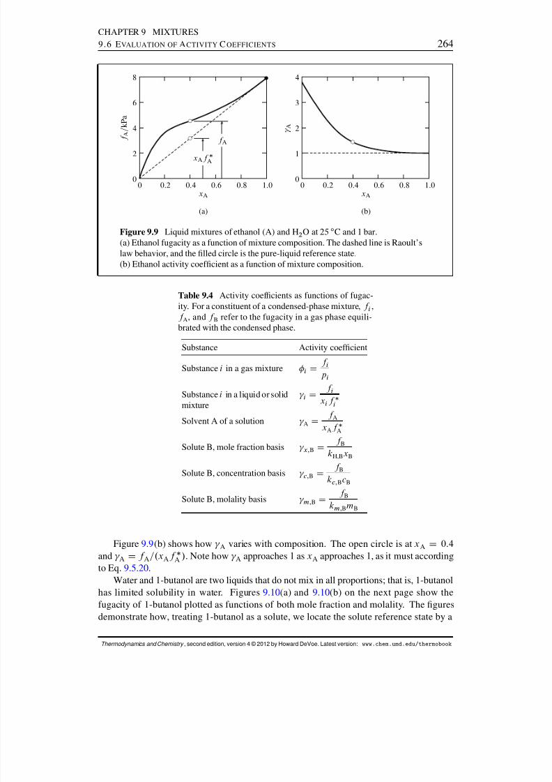
8/12/2019 Howard Devoe Thermodynamic and Chemical
http://slidepdf.com/reader/full/howard-devoe-thermodynamic-and-chemical 264/532
CHAPTER 9 MIXTURES9.6 E VALUATION OF A CTIVITY C OEFFICIENTS 264
f A
xA f
A
0 0:2 0:4 0:6 0:8 1:00
2
4
6
8
xA
f A
= k P a
(a)
0 0:2 0:4 0:6 0:8 1:00
1
2
3
4
xA
A
(b)
Figure 9.9 Liquid mixtures of ethanol (A) and H 2 O at 25 ı C and 1 bar.(a) Ethanol fugacity as a function of mixture composition. The dashed line is Raoult’slaw behavior, and the lled circle is the pure-liquid reference state.(b) Ethanol activity coefcient as a function of mixture composition.
Table 9.4 Activity coefcients as functions of fugac-ity. For a constituent of a condensed-phase mixture, f i ,f A , and f B refer to the fugacity in a gas phase equili-brated with the condensed phase.
Substance Activity coefcient
Substance i in a gas mixture i D f ip i
Substance i in a liquid or solidmixture
i D f ix i f
i
Solvent A of a solution A D f AxA f
A
Solute B, mole fraction basis x; B D f BkH,B xB
Solute B, concentration basis c; B D f Bkc; BcB
Solute B, molality basis m; B D f B
km; BmB
Figure 9.9 (b) shows how A varies with composition. The open circle is at xA D 0:4and A D f A=.x Af A / . Note how A approaches 1 as xA approaches 1, as it must according
to Eq. 9.5.20 .Water and 1-butanol are two liquids that do not mix in all proportions; that is, 1-butanol
has limited solubility in water. Figures 9.10(a) and 9.10(b) on the next page show thefugacity of 1-butanol plotted as functions of both mole fraction and molality. The guresdemonstrate how, treating 1-butanol as a solute, we locate the solute reference state by a
Thermodynamics and Chemistry , second edition, version 4 © 2012 by Howard DeVoe. Latest version: www.chem.umd.edu/thermobook
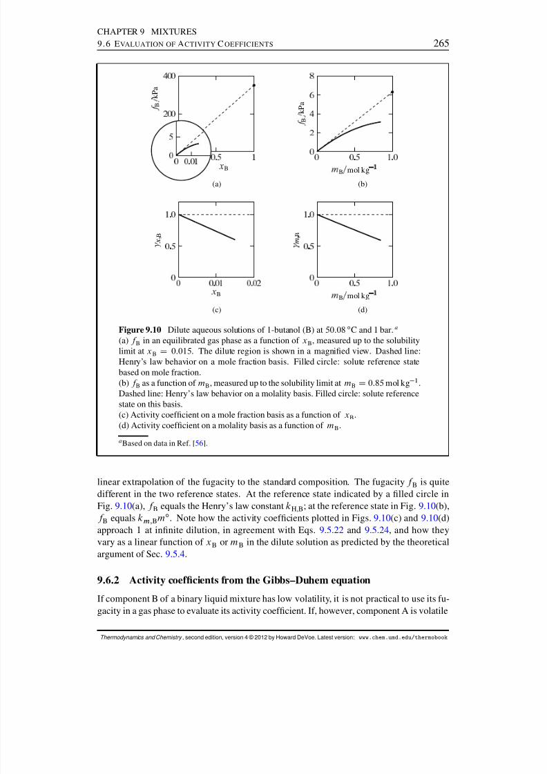
8/12/2019 Howard Devoe Thermodynamic and Chemical
http://slidepdf.com/reader/full/howard-devoe-thermodynamic-and-chemical 265/532
CHAPTER 9 MIXTURES9.6 E VALUATION OF A CTIVITY C OEFFICIENTS 265
B
B
k P a
(a)
B mol kg
B
k P a
(b)
B
B
(c)
B mol kg
B
(d)
Figure 9.10 Dilute aqueous solutions of 1-butanol (B) at 50:08 ı C and 1 bar. a
(a) f B in an equilibrated gas phase as a function of xB , measured up to the solubilitylimit at x B D 0:015 . The dilute region is shown in a magnied view. Dashed line:Henry’s law behavior on a mole fraction basis. Filled circle: solute reference statebased on mole fraction.(b) f B as a function of mB , measured up to the solubility limit at mB D 0:85 mol kg 1 .Dashed line: Henry’s law behavior on a molality basis. Filled circle: solute reference
state on this basis.(c) Activity coefcient on a mole fraction basis as a function of xB .(d) Activity coefcient on a molality basis as a function of mB .
a Based on data in Ref. [ 56].
linear extrapolation of the fugacity to the standard composition. The fugacity f B is quitedifferent in the two reference states. At the reference state indicated by a lled circle inFig. 9.10(a), f B equals the Henry’s law constant kH,B ; at the reference state in Fig. 9.10(b),f B equals km; Bm ı . Note how the activity coefcients plotted in Figs. 9.10(c) and 9.10(d)approach 1 at innite dilution, in agreement with Eqs. 9.5.22 and 9.5.24 , and how they
vary as a linear function of xB or mB in the dilute solution as predicted by the theoreticalargument of Sec. 9.5.4 .
9.6.2 Activity coefcients from the Gibbs–Duhem equation
If component B of a binary liquid mixture has low volatility, it is not practical to use its fu-gacity in a gas phase to evaluate its activity coefcient. If, however, component A is volatile
Thermodynamics and Chemistry , second edition, version 4 © 2012 by Howard DeVoe. Latest version: www.chem.umd.edu/thermobook

8/12/2019 Howard Devoe Thermodynamic and Chemical
http://slidepdf.com/reader/full/howard-devoe-thermodynamic-and-chemical 266/532
CHAPTER 9 MIXTURES9.6 E VALUATION OF A CTIVITY C OEFFICIENTS 266
enough for fugacity measurements over a range of liquid composition, we can instead usethe Gibbs–Duhem equation for this purpose.
Consider a binary mixture of two liquids that mix in all proportions. We assume thatonly component A is appreciably volatile. By measuring the fugacity of A in a gas phaseequilibrated with the binary mixture, we can evaluate its activity coefcient based on a pure-
liquid reference state: A D f A=.x Af A / (Table 9.4). We wish to use the same fugacitymeasurements to determine the activity coefcient of the nonvolatile component, B.
The Gibbs–Duhem equation for a binary liquid mixture in the form given by Eq. 9.2.43is
xA d A CxB d B D 0 (9.6.6)
where d A and d B are the chemical potential changes accompanying a change of com-position at constant T and p . Taking the differential at constant T and p of A D A CRT ln. AxA / (Eq. 9.5.14 ), we obtain
d A D RT d ln A CRT d ln xA D RT d ln A C RT
xAdxA (9.6.7)
For component B, we obtain in the same way
d B D RT d ln B C R T
xBdxB D RT d ln B
RT xB
dxA (9.6.8)
Substituting these expressions for d A and d B in Eq. 9.6.6 and solving for d ln B , weobtain the following relation:
d ln B DD xA
xBd ln A (9.6.9)
Integration from xB D 1, where B equals 1 and ln B equals 0, to composition x 0B gives
ln B .x 0B / D Z xB D x
0B
x B D 1
xA
xBd ln A (9.6.10)
(binary mixture,constant T and p )
Equation 9.6.10 allows us to evaluate the activity coefcient of the nonvolatile component,B, at any given liquid composition from knowledge of the activity coefcient of the volatilecomponent A as a function of composition.
Next consider a binary liquid mixture in which component B is neither volatile nor ableto mix in all proportions with A. In this case, it is appropriate to treat B as a solute andto base its activity coefcient on a solute reference state. We could obtain an expressionfor ln x; B similar to Eq. 9.6.10 , but the integration would have to start at xB
D0 where the
integrand xA=xB would be innite. Instead, it is convenient in this case to use the methoddescribed in the next section.
9.6.3 Activity coefcients from osmotic coefcients
It is customary to evaluate the activity coefcient of a nonvolatile solute with a functionm called the osmotic coefcient , or osmotic coefcient on a molality basis. The osmotic
Thermodynamics and Chemistry , second edition, version 4 © 2012 by Howard DeVoe. Latest version: www.chem.umd.edu/thermobook

8/12/2019 Howard Devoe Thermodynamic and Chemical
http://slidepdf.com/reader/full/howard-devoe-thermodynamic-and-chemical 267/532
CHAPTER 9 MIXTURES9.6 E VALUATION OF A CTIVITY C OEFFICIENTS 267
coefcient of a solution of nonelectrolyte solutes is dened by
mdef
D A A
RT M A Xi ¤ A
m i
(9.6.11)(nonelectrolyte solution)
The denition of m in Eq. 9.6.11 has the following signicance. The sum Pi ¤ A m i isthe total molality of all solute species. In an ideal-dilute solution, the solvent chemicalpotential is A D A CRT ln xA . The expansion of the function ln xA in powers of .1 xA / gives the power series ln xA D .1 xA / .1 xA / 2 =2 .1 xA / 3 =3 .Thus, in a very dilute solution we have ln xA .1 xA / D Pi ¤ A x i . In the limitof innite dilution, the mole fraction of solute i becomes x i D M Am i (see Eq. 9.1.14 ).In the limit of innite dilution, therefore, we have
ln xA D M A Xi ¤ A
m i (9.6.12)(innite dilution)
and the solvent chemical potential is related to solute molalities by
A D A RT M A Xi ¤ A
m i (9.6.13)(innite dilution)
The deviation of m from unity is a measure of the deviation of A from innite-dilution behavior, as we can see by comparing the preceding equation with a rear-rangement of Eq. 9.6.11 :
A D A m RT M A Xi ¤ A
m i (9.6.14)
The reason m is called the osmotic coefcient has to do with its relation to the osmoticpressure ˘ of the solution: The ratio ˘ =m B is equal to the product of m and thelimiting value of ˘=m B at innite dilution (see Sec. 12.4.4 ).
Evaluation of m
Any method that measures A A , the lowering of the solvent chemical potential causedby the presence of a solute or solutes, allows us to evaluate m through Eq. 9.6.11 .
The chemical potential of the solvent in a solution is related to the fugacity in an equili-brated gas phase by A D ref
A (g) CRT ln.f A=p/ (from Eq. 9.5.11 ). For the pure solvent,this relation is A D ref
A (g) C RT ln.f A =p/ . Taking the difference between these two
equations, we obtain
A A D RT lnf
A
f A(9.6.15)
which allows us to evaluate m from fugacity measurements.Osmotic coefcients can also be evaluated from freezing point and osmotic pressure
measurements that will be described in Sec. 12.2 .
Thermodynamics and Chemistry , second edition, version 4 © 2012 by Howard DeVoe. Latest version: www.chem.umd.edu/thermobook
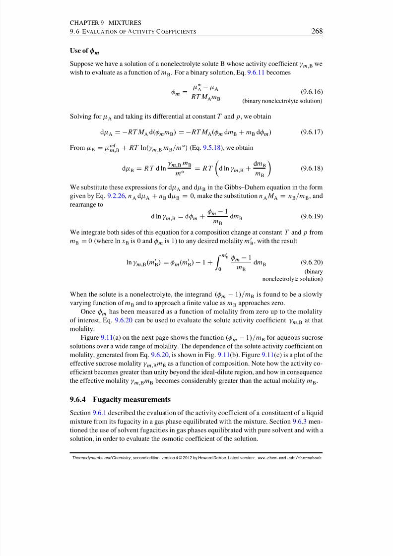
8/12/2019 Howard Devoe Thermodynamic and Chemical
http://slidepdf.com/reader/full/howard-devoe-thermodynamic-and-chemical 268/532
CHAPTER 9 MIXTURES9.6 E VALUATION OF A CTIVITY C OEFFICIENTS 268
Use of m
Suppose we have a solution of a nonelectrolyte solute B whose activity coefcient m; B wewish to evaluate as a function of mB . For a binary solution, Eq. 9.6.11 becomes
m
D A A
RT M AmB(9.6.16)
(binary nonelectrolyte solution)
Solving for A and taking its differential at constant T and p , we obtain
d A D RT M A d. m mB / D RT M A . m dmB CmB d m / (9.6.17)
From B D ref m; B CRT ln. m; B mB=m ı / (Eq. 9.5.18 ), we obtain
d B D RT d ln m; B mB
m ı D RT d ln m; B C dmB
mB (9.6.18)
We substitute these expressions for d A and d B in the Gibbs–Duhem equation in the form
given by Eq. 9.2.26 , nA d A CnB d B D 0, make the substitution nAM A D nB=m B , andrearrange to
d ln m; B D d m C m 1
mBdmB (9.6.19)
We integrate both sides of this equation for a composition change at constant T and p frommB D 0 (where ln xB is 0 and m is 1) to any desired molality m0
B , with the result
ln m; B .m 0B/ D m .m 0
B / 1 CZ m0
B
0
m 1mB
dmB (9.6.20)(binary
nonelectrolyte solution)
When the solute is a nonelectrolyte, the integrand . m 1/=m B is found to be a slowlyvarying function of mB and to approach a nite value as mB approaches zero.
Once m has been measured as a function of molality from zero up to the molalityof interest, Eq. 9.6.20 can be used to evaluate the solute activity coefcient m; B at thatmolality.
Figure 9.11 (a) on the next page shows the function . m 1/=m B for aqueous sucrosesolutions over a wide range of molality. The dependence of the solute activity coefcient onmolality, generated from Eq. 9.6.20 , is shown in Fig. 9.11 (b). Figure 9.11 (c) is a plot of theeffective sucrose molality m; BmB as a function of composition. Note how the activity co-efcient becomes greater than unity beyond the ideal-dilute region, and how in consequencethe effective molality m; BmB becomes considerably greater than the actual molality mB .
9.6.4 Fugacity measurements
Section 9.6.1 described the evaluation of the activity coefcient of a constituent of a liquidmixture from its fugacity in a gas phase equilibrated with the mixture. Section 9.6.3 men-tioned the use of solvent fugacities in gas phases equilibrated with pure solvent and with asolution, in order to evaluate the osmotic coefcient of the solution.
Thermodynamics and Chemistry , second edition, version 4 © 2012 by Howard DeVoe. Latest version: www.chem.umd.edu/thermobook
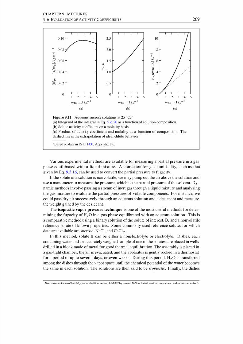
8/12/2019 Howard Devoe Thermodynamic and Chemical
http://slidepdf.com/reader/full/howard-devoe-thermodynamic-and-chemical 269/532
CHAPTER 9 MIXTURES9.6 E VALUATION OF A CTIVITY C OEFFICIENTS 269
0 1 2 3 4 50
0:02
0:04
0:06
0:08
0:10
mB=mol kg 1
Π. m
1 / = m B
= k g m o l
1
(a)
0 1 2 3 4 50
0:5
1:0
1:5
2:0
2:5
mB=mol kg 1
m
; B
(b)
0 1 2 3 4 50
2
4
6
8
10
mB=mol kg 1
m
; B m B
= m o l k g
1
(c)
Figure 9.11 Aqueous sucrose solutions at 25 ı C. a
(a) Integrand of the integral in Eq. 9.6.20 as a function of solution composition.(b) Solute activity coefcient on a molality basis.(c) Product of activity coefcient and molality as a function of composition. Thedashed line is the extrapolation of ideal-dilute behavior.
a Based on data in Ref. [ 143 ], Appendix 8.6.
Various experimental methods are available for measuring a partial pressure in a gasphase equilibrated with a liquid mixture. A correction for gas nonideality, such as thatgiven by Eq. 9.3.16 , can be used to convert the partial pressure to fugacity.
If the solute of a solution is nonvolatile, we may pump out the air above the solution anduse a manometer to measure the pressure, which is the partial pressure of the solvent. Dy-namic methods involve passing a stream of inert gas through a liquid mixture and analyzingthe gas mixture to evaluate the partial pressures of volatile components. For instance, wecould pass dry air successively through an aqueous solution and a desiccant and measurethe weight gained by the desiccant.
The isopiestic vapor pressure technique is one of the most useful methods for deter-mining the fugacity of H 2 O in a gas phase equilibrated with an aqueous solution. This isa comparative method using a binary solution of the solute of interest, B, and a nonvolatilereference solute of known properties. Some commonly used reference solutes for whichdata are available are sucrose, NaCl, and CaCl 2 .
In this method, solute B can be either a nonelectrolyte or electrolyte. Dishes, each
containing water and an accurately weighed sample of one of the solutes, are placed in wellsdrilled in a block made of metal for good thermal equilibration. The assembly is placed ina gas-tight chamber, the air is evacuated, and the apparatus is gently rocked in a thermostatfor a period of up to several days, or even weeks. During this period, H 2 O is transferredamong the dishes through the vapor space until the chemical potential of the water becomesthe same in each solution. The solutions are then said to be isopiestic . Finally, the dishes
Thermodynamics and Chemistry , second edition, version 4 © 2012 by Howard DeVoe. Latest version: www.chem.umd.edu/thermobook

8/12/2019 Howard Devoe Thermodynamic and Chemical
http://slidepdf.com/reader/full/howard-devoe-thermodynamic-and-chemical 270/532
CHAPTER 9 MIXTURES9.7 A CTIVITY OF AN U NCHARGED S PECIES 270
are removed from the apparatus and weighed to establish the molality of each solution. TheH2 O fugacity is known as a function of the molality of the reference solute, and is the sameas the H 2 O fugacity in equilibrium with the solution of solute B at its measured molality.
The isopiestic vapor pressure method can also be used for nonaqueous solutions.
9.7 ACTIVITY OF AN UNCHARGED SPECIESThe activity a i of uncharged species i (i.e., a substance) is dened by the relation
a idef
D exp i ıi
RT (9.7.1)
(uncharged species)
or
i D ıi CRT ln a i (9.7.2)
(uncharged species)
where ıi is the standard chemical potential of the species. 10 The activity of a species in agiven phase is a dimensionless quantity whose value depends on the choice of the standardstate and on the intensive properties of the phase: temperature, pressure, and composition.
The quantity a i is sometimes called the relative activity of i , because it depends on thechemical potential relative to a standard chemical potential. An important application of theactivity concept is the denition of equilibrium constants (Sec. 11.8.1 ).
For convenience in later applications, we specify that the value of a i is the same inphases that have the same temperature, pressure, and composition but are at different ele-vations in a gravitational eld, or are at different electric potentials. Section 9.8 10.1 willdescribe a modication of the dening equation i D ı
i C RT ln a i for a system withphases of different elevations, and Sec. 10.1 will describe the modication needed for a
charged species.
9.7.1 Standard states
The standard states of different kinds of mixture components have the same denitions asthose for reference states (Table 9.3 ), with the additional stipulation in each case that thepressure is equal to the standard pressure p ı .
When component i is in its standard state, its chemical potential is the standard chemicalpotential ı
i . It is important to note from Eq. 9.7.2 that when i equals ıi , the logarithm
of a i is zero and the activity in the standard state is therefore unity.The following equations in the form of Eq. 9.7.2 show the notation used in this book
for the standard chemical potentials and activities of various kinds of uncharged mixture
10 Some chemists dene the activity by i D ref i CRT ln a i . The activity dened this way is not the same as
the activity used in this book unless the phase is at the standard pressure.
Thermodynamics and Chemistry , second edition, version 4 © 2012 by Howard DeVoe. Latest version: www.chem.umd.edu/thermobook
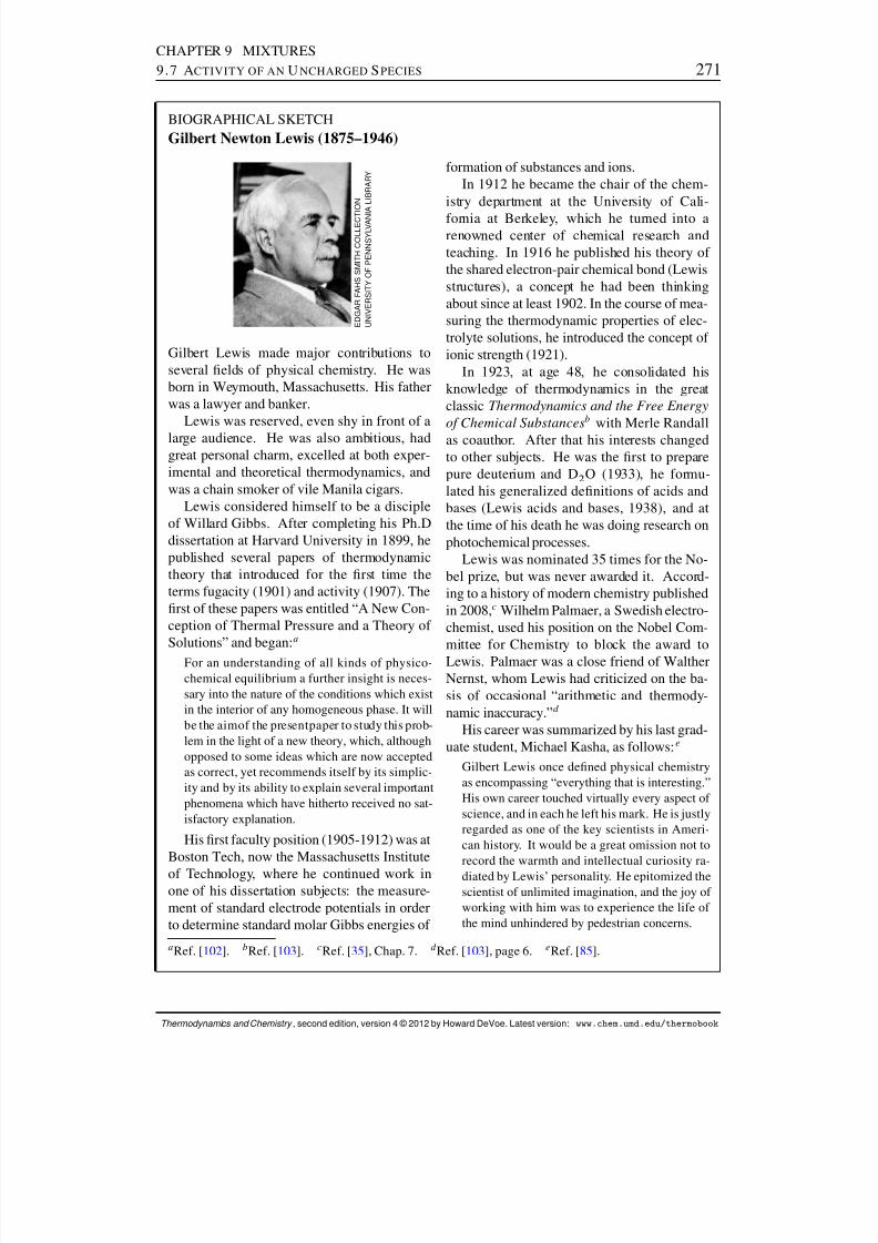
8/12/2019 Howard Devoe Thermodynamic and Chemical
http://slidepdf.com/reader/full/howard-devoe-thermodynamic-and-chemical 271/532
CHAPTER 9 MIXTURES9.7 A CTIVITY OF AN U NCHARGED S PECIES 271
BIOGRAPHICAL SKETCHGilbert Newton Lewis (1875–1946)
E D G A R F A H S S M I T H C O L L E C T I O N
U N I V E R S I T Y O F P E N N S Y L V A N I A L I B R A R Y
Gilbert Lewis made major contributions toseveral elds of physical chemistry. He wasborn in Weymouth, Massachusetts. His fatherwas a lawyer and banker.
Lewis was reserved, even shy in front of alarge audience. He was also ambitious, hadgreat personal charm, excelled at both exper-imental and theoretical thermodynamics, andwas a chain smoker of vile Manila cigars.
Lewis considered himself to be a discipleof Willard Gibbs. After completing his Ph.Ddissertation at Harvard University in 1899, hepublished several papers of thermodynamictheory that introduced for the rst time theterms fugacity (1901) and activity (1907). Therst of these papers was entitled “A New Con-ception of Thermal Pressure and a Theory of Solutions” and began: a
For an understanding of all kinds of physico-chemical equilibrium a further insight is neces-sary into the nature of the conditions which existin the interior of any homogeneous phase. It willbe the aimof the presentpaper to study this prob-lem in the light of a new theory, which, althoughopposed to some ideas which are now acceptedas correct, yet recommends itself by its simplic-ity and by its ability to explain several importantphenomena which have hitherto received no sat-isfactory explanation.
His rst faculty position (1905-1912) was atBoston Tech, now the Massachusetts Instituteof Technology, where he continued work inone of his dissertation subjects: the measure-ment of standard electrode potentials in orderto determine standard molar Gibbs energies of
formation of substances and ions.In 1912 he became the chair of the chem-
istry department at the University of Cali-
fornia at Berkeley, which he turned into arenowned center of chemical research andteaching. In 1916 he published his theory of the shared electron-pair chemical bond (Lewisstructures), a concept he had been thinkingabout since at least 1902. In the course of mea-suring the thermodynamic properties of elec-trolyte solutions, he introduced the concept of ionic strength (1921).
In 1923, at age 48, he consolidated hisknowledge of thermodynamics in the greatclassic Thermodynamics and the Free Energyof Chemical Substances b with Merle Randallas coauthor. After that his interests changedto other subjects. He was the rst to preparepure deuterium and D 2 O (1933), he formu-lated his generalized denitions of acids andbases (Lewis acids and bases, 1938), and atthe time of his death he was doing research onphotochemical processes.
Lewis was nominated 35 times for the No-bel prize, but was never awarded it. Accord-ing to a history of modern chemistry publishedin 2008, c Wilhelm Palmaer, a Swedish electro-chemist, used his position on the Nobel Com-mittee for Chemistry to block the award toLewis. Palmaer was a close friend of WaltherNernst, whom Lewis had criticized on the ba-sis of occasional “arithmetic and thermody-namic inaccuracy.” d
His career was summarized by his last grad-uate student, Michael Kasha, as follows: e
Gilbert Lewis once dened physical chemistryas encompassing “everything that is interesting.”His own career touched virtually every aspect of science, and in each he left his mark. He is justlyregarded as one of the key scientists in Ameri-can history. It would be a great omission not torecord the warmth and intellectual curiosity ra-diated by Lewis’ personality. He epitomized thescientist of unlimited imagination, and the joy of working with him was to experience the life of the mind unhindered by pedestrian concerns.
a Ref. [ 102 ]. bRef. [ 103 ]. cRef. [ 35], Chap. 7. d Ref. [ 103 ], page 6. eRef. [ 85].
Thermodynamics and Chemistry , second edition, version 4 © 2012 by Howard DeVoe. Latest version: www.chem.umd.edu/thermobook
8/12/2019 Howard Devoe Thermodynamic and Chemical
http://slidepdf.com/reader/full/howard-devoe-thermodynamic-and-chemical 272/532
CHAPTER 9 MIXTURES9.7 A CTIVITY OF AN U NCHARGED S PECIES 272
components:
Substance i in a gas mixture i D ıi (g) CRT ln a i (g) (9.7.3)
Substance i in a liquid or solid mixture i D ıi CRT ln a i (9.7.4)
Solvent A of a solution A D ıA CRT ln a A (9.7.5)
Solute B, mole fraction basis B D ıx; B CRT ln a x; B (9.7.6)
Solute B, concentration basis B D ıc; B CRT ln a c; B (9.7.7)
Solute B, molality basis B D ım; B CRT ln a m; B (9.7.8)
9.7.2 Activities and composition
We need to be able to relate the activity of component i to the mixture composition. Wecan do this by nding the relation between the chemical potential of component i in itsreference state and in its standard state, both at the same temperature. These two chemicalpotentials, ref
i and ıi , are equal only if the mixture is at the standard pressure p ı .
It will be useful to dene the following dimensionless quantity:
idef
D expref i ı
i
RT ! (9.7.9)
The symbol i for this quantity was introduced by Pitzer and Brewer. 11 They called itthe activity in a reference state . To see why, compare the denition of activity given by
i D ıi CRT ln a i with a rearrangement of Eq. 9.7.9 : ref
i D ıi CRT ln i .
At a given temperature, the difference ref i ı
i depends only on the pressure p of themixture, and is zero when p is equal to p ı . Thus i is a function of p with a value of 1when p is equal to p ı . This book will call i the pressure factor of species i .
To understand how activity is related to composition, let us take as an example theactivity am; B of solute B based on molality. From Eqs. 9.5.18 and 9.7.8 , we have
B D ref m; B CRT ln m; B
mB
m ı
D ım; B CRT ln a m; B (9.7.10)
The activity is then given by
ln a m; B Dref m; B
ım; B
RT Cln m; BmB
m ı
D ln m; B Cln m; BmB
m ı (9.7.11)
a m; B D m; B m; BmB
m ı (9.7.12)
The activity of a constituent of a condensed-phase mixture is in general equal to the productof the pressure factor, the activity coefcient, and the composition variable divided by thestandard composition.
Table 9.5 on the next page gives explicit expressions for the activities of various kindsof nonelectrolyte substances.
11 Ref. [ 104 ], p. 249.
Thermodynamics and Chemistry , second edition, version 4 © 2012 by Howard DeVoe. Latest version: www.chem.umd.edu/thermobook

8/12/2019 Howard Devoe Thermodynamic and Chemical
http://slidepdf.com/reader/full/howard-devoe-thermodynamic-and-chemical 273/532
CHAPTER 9 MIXTURES9.7 A CTIVITY OF AN U NCHARGED S PECIES 273
Table 9.5 Expressions for activities of nonelectrolytes. For a con-stituent of a condensed-phase mixture, f i , f A , and f B refer to thefugacity in a gas phase equilibrated with the condensed phase.
Substance Activity
Pure gas a (g) D (g) D f p ı
Pure liquid or solid a D
Substance i in a gas mix-ture
a i (g) D i (g) ip i
p D f ip ı
Substance i in a liquid orsolid mixture
a i D i i x i D if if
i
Solvent A of a solution aA D A A xA D Af Af
A
Solute B, mole fraction
basis
a x; B D x; B x; B xB D x; Bf B
kH,B
Solute B, concentrationbasis
a c; B D c; B c; BcB
c ı D c; Bf B
kc; Bc ı
Solute B, molality basis am; B D m; B m; BmB
m ı D m; Bf B
km; Bm ı
9.7.3 Pressure factors and pressure
At a given temperature, the pressure factor i of component i of a mixture is a functiononly of pressure. To derive the pressure dependence of i for various kinds of mixturecomponents, we need expressions for . ref
i
ıi / as functions of pressure to substitute in
the dening equation i D exp Œ . ref i ıi /=RT .For component i of a gas mixture , the reference state is pure gas i at the pressure of
the mixture, behaving as an ideal gas. The chemical potential of a pure ideal gas dependson its pressure according to Eq. 7.8.6 : D ı (g) C RT ln .p=p ı / . Thus the chemicalpotential of the reference state of gas component i is ref
i (g) D ıi (g) C RT ln .p=p ı / ,
and ref i (g) ı
i (g) is equal to RT ln .p=p ı / . This gives us the following expression for thepressure dependence of the pressure factor:
i (g) D pp ı (9.7.13)
For a mixture in a condensed phase , we will make use of .@ i =@p/T; fn ig D V i (Eq.
9.2.49 ). The relation between changes of i and p at constant temperature and composi-tion is therefore d i D V i dp . Recall (Sec. 9.1.5 ) that “constant composition” means thatthe mole fraction or molality of each component, but not necessarily the concentration, isconstant.
Consider a process in which the system initially consists of a phase with component iin its standard state. We change the pressure isothermally from p ı to the pressure p 0 of the mixture of interest. For a pure-liquid, pure-solid, or solvent reference state, or a solute
Thermodynamics and Chemistry , second edition, version 4 © 2012 by Howard DeVoe. Latest version: www.chem.umd.edu/thermobook
8/12/2019 Howard Devoe Thermodynamic and Chemical
http://slidepdf.com/reader/full/howard-devoe-thermodynamic-and-chemical 274/532
CHAPTER 9 MIXTURES9.7 A CTIVITY OF AN U NCHARGED S PECIES 274
reference state based on mole fraction or molality, this process brings the system to thereference state of component i at pressure p 0. The change of i in this case is given byintegration of d i D V i dp :
ref i .p 0/ ı
i
DZ p 0
pı
V i dp (9.7.14)
The appropriate partial molar volume V i is the molar volume V i or V A of the pure sub-stance, or the partial molar volume V 1B of solute B at innite dilution.
Suppose we want to use a reference state for solute B based on concentration. Becausethe isothermal pressure change involves a small change of volume, cB changes slightlyduring the process, so that the right side of Eq. 9.7.14 is not quite the correct expression for
ref c; B .p 0/ ı
c; B .
We can derive a rigorous expression for ref c; B .p 0/ ı
c; B as follows. Consider an ideal-dilute solution of solute B at an arbitrary pressure p , with solute chemical potentialgiven by B D ref
c; B CRT ln.c B=cı / (Table 9.2). From this equation we obtain
@ B
@p T; f n i gD
@ ref c; B
@p !T
CRT @ln .c B=cı /
@p T; f n i g(9.7.15)
The partial derivative .@ B=@p/T; f n i g is equal to the partial molar volume V B (Eq.9.2.49 ), which in the ideal-dilute solution has its innite-dilution value V 1B . Werewrite the second partial derivative on the right side of Eq. 9.7.15 as follows:
@ln.c B=cı /@p T; f n i g
D 1cB
@cB@p T; f n i g
D 1nB=V
@.nB=V /@p T; fn i g
D V @.1=V /
@p T; f n i gD
1V
@V @p T; f n i g
D T (9.7.16)
Here T is the isothermal compressibility of the solution, which at innite dilution is1T , the isothermal compressibility of the pure solvent. Equation 9.7.15 becomes
V 1B D@ ref
c; B
@p !T
CRT 1T (9.7.17)
Solving for d ref c; B at constant T , and integrating from p ı to p 0, we obtain nally
ref c; B .p 0/ ı
c; B DZ p 0
p ıV 1B RT 1
T dp (9.7.18)
We are now able to write explicit formulas for i for each kind of mixture component.They are collected in Table 9.6 on the next page .
Considering a constituent of a condensed-phase mixture, by how much is the pressurefactor likely to differ from unity? If we use the values p ı D 1 bar and T D 300 K, andassume the molar volume of pure i is V i D 100 cm 3 mol 1 at all pressures, we nd that i is 0:996 in the limit of zero pressure, unity at 1 bar, 1:004 at 2 bar, 1:04 at 10 bar, and
Thermodynamics and Chemistry , second edition, version 4 © 2012 by Howard DeVoe. Latest version: www.chem.umd.edu/thermobook

8/12/2019 Howard Devoe Thermodynamic and Chemical
http://slidepdf.com/reader/full/howard-devoe-thermodynamic-and-chemical 275/532
CHAPTER 9 MIXTURES9.8 M IXTURES IN G RAVITATIONAL AND C ENTRIFUGAL F IELDS 275
Table 9.6 Expressions for the dependence of pressure factors of nonelectrolytes on pressure. Theapproximate expressions assume the phase is incompressible, or the solute partial molar volume isindependent of pressure.
Substance Pressure factor at pressure p 0
Substance i in a gas mixture, or thepure gas
i (g) D p0
p ı
Substance i in a liquid or solidmixture, or the pure liquid or solid
i D exp Z p 0
p ı
V iRT
dp! expV i .p 0 p ı /
RT
Solvent A of a solution A D exp Z p 0
p ı
V ART
dp! expV A .p 0 p ı /
RT
Solute B, mole fraction or molalitybasis
x; B D m; B D exp Z p 0
p ı
V 1BRT
dp! expV 1B .p 0 p ı /
RT
Solute B, concentration basis c; B D exp "Z
p 0
p ı
V 1BRT
1T dp# exp
V 1B .p 0 p ı /RT
1:49 at 100 bar. For a solution with V 1B D 100 cm 3 mol 1 , we obtain the same values asthese for x; B , m; B , and c; B . These values demonstrate that it is only at high pressuresthat the pressure factor differs appreciably from unity. For this reason, it is common to seeexpressions for activity in which this factor is omitted: a i D i x i , a m; B D m; BmB=m ı ,and so on.
In principle, we can specify any convenient value for the standard pressure p ı . For achemist making measurements at high pressures, it would be convenient to specify avalue of p ı within the range of the experimental pressures, for example p ı
D 1 kbar,
in order that the value of each pressure factor be close to unity.
9.8 MIXTURES IN GRAVITATIONAL AND CENTRIFUGAL FIELDS
A tall column of a gas mixture in a gravitational eld, and a liquid solution in the cellof a spinning centrifuge rotor, are systems with equilibrium states that are nonuniform inpressure and composition. This section derives the ways in which pressure and compositionvary spatially within these kinds of systems at equilibrium.
9.8.1 Gas mixture in a gravitational eld
Consider a tall column of a gas mixture in an earth-xed lab frame. Our treatment willparallel that for a tall column of a pure gas in Sec. 8.1.4 . We imagine the gas to be dividedinto many thin slab-shaped phases at different elevations in a rigid container, as in Fig. 8.1on page 196 . We want to nd the equilibrium conditions reached spontaneously when thesystem is isolated from its surroundings.
Thermodynamics and Chemistry , second edition, version 4 © 2012 by Howard DeVoe. Latest version: www.chem.umd.edu/thermobook

8/12/2019 Howard Devoe Thermodynamic and Chemical
http://slidepdf.com/reader/full/howard-devoe-thermodynamic-and-chemical 276/532
CHAPTER 9 MIXTURES9.8 M IXTURES IN G RAVITATIONAL AND C ENTRIFUGAL F IELDS 276
The derivation is the same as that in Sec. 9.2.7 , with the additional constraint that foreach phase ’ , dV ’ is zero in order that each phase stays at a constant elevation. The resultis the relation
dS DX’ ¤ ’ 0
T ’0
T ’
T ’ 0 dS ’ CXi X’ ¤ ’ 0
’ 0
i ’i
T ’ 0 dn ’i (9.8.1)
In an equilibrium state, S is at a maximum and d S is zero for an innitesimal change of any of the independent variables. This requires the coefcient of each term in the sums onthe right side of Eq. 9.8.1 to be zero. The equation therefore tells that at equilibrium thetemperature and the chemical potential of each constituent are uniform throughout the gasmixture . The equation says nothing about the pressure.
Just as the chemical potential of a pure substance at a given elevation is dened inthis book as the molar Gibbs energy at that elevation (page 197 ), the chemical potential of substance i in a mixture at elevation h is the partial molar Gibbs energy at that elevation.
We dene the standard potential ıi (g) of component i of the gas mixture as the chem-
ical potential of i under standard state conditions at the reference elevation hD0. At thiselevation, the chemical potential and fugacity are related by
i .0/ D ıi (g) CRT ln
f i .0/p ı (9.8.2)
If we reversibly raise a small sample of mass m of the gas mixture by an innitesimaldistance d h , without heat and at constant T and V , the fugacity f i remains constant. Thegravitational work during the elevation process is ¶w 0 D mg dh . This work contributes tothe internal energy change: d U D T dS p dV CPi i dn i Cmg dh . The total differentialof the Gibbs energy of the sample is
dG D d.U TS CpV /
D S dT
CV dp
CXii dn i
Cmg dh (9.8.3)
From this total differential, we write the reciprocity relation
@ i
@h T;p; fn igD
@mg@ni T;p;n j ¤ i ;h
(9.8.4)
With the substitution m DPi n i M i in the partial derivative on the right side, the partialderivative becomes M i g . At constant T , p , and composition, therefore, we have d i DM i g dh . Integrating over a nite elevation change from h D 0 to h D h0, we obtain
i .h0
/ i .0/ DZ h0
0 M i g dh D M i gh0
(9.8.5)(f i .h 0/Df i .0/ )
The general relation between i , f i , and h that agrees with Eqs. 9.8.2 and 9.8.5 is
i .h/ D ıi (g) CRT ln
f i .h/p ı CM i gh (9.8.6)
Thermodynamics and Chemistry , second edition, version 4 © 2012 by Howard DeVoe. Latest version: www.chem.umd.edu/thermobook
8/12/2019 Howard Devoe Thermodynamic and Chemical
http://slidepdf.com/reader/full/howard-devoe-thermodynamic-and-chemical 277/532
CHAPTER 9 MIXTURES9.8 M IXTURES IN G RAVITATIONAL AND C ENTRIFUGAL F IELDS 277
In the equilibrium state of the tall column of gas, i .h/ is equal to i .0/ . Equation 9.8.6shows that this is only possible if f i decreases as h increases. Equating the expressionsgiven by this equation for i .h/ and i .0/ , we have
ıi (g) CRT ln
f i .h/p ı CM i gh D ı
i (g) CRT lnf i .0/
p ı (9.8.7)
Solving for f i .h/ gives
f i .h/ D f i .0/e M i gh=RT (9.8.8)(gas mixture at equilibrium)
If the gas is an ideal gas mixture, f i is the same as the partial pressure p i :
p i .h/ D p i .0/e M i gh=RT (9.8.9)(ideal gas mixture at equilibrium)
Equation 9.8.9 shows that each constituent of an ideal gas mixture individually obeys thebarometric formula given by Eq. 8.1.13 on page 198 .
The pressure at elevation h is found from p.h/
DPi p i .h/ . If the constituents have
different molar masses, the mole fraction composition changes with elevation. For example,in a binary ideal gas mixture the mole fraction of the constituent with the greater molar massdecreases with increasing elevation, and the mole fraction of the other constituent increases.
9.8.2 Liquid solution in a centrifuge cell
This section derives equilibrium conditions of a dilute binary solution conned to a cellembedded in a spinning centrifuge rotor.
The system is the solution. The rotor’s angle of rotation with respect to a lab frameis not relevant to the state of the system, so we use a local reference frame xed in therotor as shown in Fig. 9.12(a) on the next page. The values of heat, work, and energychanges measured in this rotating frame are different from those in a lab frame (Sec. G.9in Appendix G). Nevertheless, the laws of thermodynamics and the relations derived fromthem are obeyed in the local frame when we measure the heat, work, and state functions inthis frame (page 499 ).
Note that an equilibrium state can only exist relative to the rotating local frame; anobserver xed in this frame would see no change in the state of the isolated solution overtime. While the rotor rotates, however, there is no equilibrium state relative to the lab frame,because the system’s position in the frame constantly changes.
We assume the centrifuge rotor rotates about the vertical z axis at a constant angularvelocity ! . As shown in Fig. 9.12 (a), the elevation of a point within the local frame is givenby z and the radial distance from the axis of rotation is given by r .
In the rotating local frame, a body of mass m has exerted on it a centrifugal forceF centr D m! 2 r directed horizontally in the outward Cr radial direction (Sec. G.9 ).12 The12 There is also a Coriolis force that vanishes as the body’s velocity in the rotating local frame approaches zero.The centrifugal and Coriolis forces are apparent or ctitious forces, in the sense that they are caused by theacceleration of the rotating frame rather than by interactions between particles. When we treat these forces as if they are real forces, we can use Newton’s second law of motion to relate the net force on a body and the body’sacceleration in the rotating frame (see Sec. G.6 ).
Thermodynamics and Chemistry , second edition, version 4 © 2012 by Howard DeVoe. Latest version: www.chem.umd.edu/thermobook
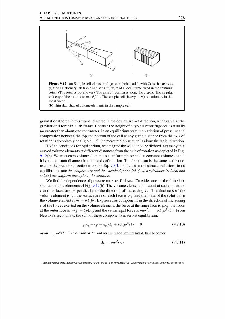
8/12/2019 Howard Devoe Thermodynamic and Chemical
http://slidepdf.com/reader/full/howard-devoe-thermodynamic-and-chemical 278/532
CHAPTER 9 MIXTURES9.8 M IXTURES IN G RAVITATIONAL AND C ENTRIFUGAL F IELDS 278
(a) (b)
Figure 9.12 (a) Sample cell of a centrifuge rotor (schematic), with Cartesian axes x ,y , z of a stationary lab frame and axes x 0, y 0, z of a local frame xed in the spinningrotor. (The rotor is not shown.) The axis of rotation is along the z axis. The angularvelocity of the rotor is ! D d#= d t . The sample cell (heavy lines) is stationary in thelocal frame.(b) Thin slab-shaped volume elements in the sample cell.
gravitational force in this frame, directed in the downward z direction, is the same as thegravitational force in a lab frame. Because the height of a typical centrifuge cell is usuallyno greater than about one centimeter, in an equilibrium state the variation of pressure andcomposition between the top and bottom of the cell at any given distance from the axis of rotation is completely negligible—all the measurable variation is along the radial direction.
To nd conditions for equilibrium, we imagine the solution to be divided into many thincurved volume elements at different distances from the axis of rotation as depicted in Fig.9.12 (b). We treat each volume element as a uniform phase held at constant volume so thatit is at a constant distance from the axis of rotation. The derivation is the same as the one
used in the preceding section to obtain Eq. 9.8.1 , and leads to the same conclusion: in anequilibrium state the temperature and the chemical potential of each substance (solvent and solute) are uniform throughout the solution .
We nd the dependence of pressure on r as follows. Consider one of the thin slab-shaped volume elements of Fig. 9.12(b). The volume element is located at radial positionr and its faces are perpendicular to the direction of increasing r . The thickness of thevolume element is •r , the surface area of each face is A s, and the mass of the solution inthe volume element is m D A s•r . Expressed as components in the direction of increasingr of the forces exerted on the volume element, the force at the inner face is pA s, the forceat the outer face is .p C•p/A s, and the centrifugal force is m! 2 r D A s!
2 r•r . FromNewton’s second law, the sum of these components is zero at equilibrium:
pA s .p C•p/A s CA s! 2 r•r D 0 (9.8.10)
or •p D ! 2 r•r . In the limit as •r and •p are made innitesimal, this becomes
dp D ! 2 r dr (9.8.11)
Thermodynamics and Chemistry , second edition, version 4 © 2012 by Howard DeVoe. Latest version: www.chem.umd.edu/thermobook
8/12/2019 Howard Devoe Thermodynamic and Chemical
http://slidepdf.com/reader/full/howard-devoe-thermodynamic-and-chemical 279/532
CHAPTER 9 MIXTURES9.8 M IXTURES IN G RAVITATIONAL AND C ENTRIFUGAL F IELDS 279
We will assume the density is uniform throughout the solution. 13 Then integration of Eq.9.8.11 yields
p 00 p 0 DZ p 00
p 0dp D ! 2Z
r 00
r 0r dr D
! 2
2 hr 00 2 r 0 2i (9.8.12)
where the superscripts 0 and 00denote positions at two different values of r in the cell. Thepressure is seen to increase with increasing distance from the axis of rotation.
Next we investigate the dependence of the solute concentration cB on r in the equi-librium state of the binary solution. Consider a small sample of the solution of mass m.Assume the extent of this sample in the radial direction is small enough for the variation of the centrifugal force eld to be negligible. The reversible work in the local frame neededto move this small sample an innitesimal distance d r at constant z, T , and p , using anexternal force F centr that opposes the centrifugal force, is
¶w 0 D F sur dr D . F centr / dr D m! 2 r dr (9.8.13)
This work is a contribution to the change d U of the internal energy. The Gibbs energy of the small sample in the local frame is a function of the independent variables T , p , nA , nB ,and r , and its total differential is
dG D d.U TS CpV /
D S dT CV dp C A dnA C B dnB m! 2 r dr (9.8.14)
We use Eq. 9.8.14 to write the reciprocity relation
@ B
@r T;p;n A ;n BD ! 2 r
@m@nB T;p;n A ;r
(9.8.15)
Then, using m D nAM A CnBM B , we obtain@ B
@r T;p;n A ;n BD M B! 2 r (9.8.16)
Thus at constant T , p , and composition, which are the conditions that allow the activitya c; B to remain constant, B for the sample varies with r according to d B D M B! 2 r dr .We integrate from radial position r 0 to position r 00to obtain
B .r 00/ B .r 0/ D M B! 2 Z r 00
r 0r dr
D 12 M B! 2
hr 00 2 r 0 2
i (9.8.17)
(a c; B .r 00/Da c; B .r 0/ )
Let us take r 0 as a reference position, such as the end of the centrifuge cell farthest fromthe axis of rotation. We dene the standard chemical potential ı
c; B as the solute chemical
13 In the centrifugal eld, this assumption is strictly true only if the solution is incompressible and its density isindependent of composition.
Thermodynamics and Chemistry , second edition, version 4 © 2012 by Howard DeVoe. Latest version: www.chem.umd.edu/thermobook
8/12/2019 Howard Devoe Thermodynamic and Chemical
http://slidepdf.com/reader/full/howard-devoe-thermodynamic-and-chemical 280/532
CHAPTER 9 MIXTURES9.8 M IXTURES IN G RAVITATIONAL AND C ENTRIFUGAL F IELDS 280
potential under standard state conditions on a concentration basis at this position. The solutechemical potential and activity at this position are related by
B .r 0/ D ıc; B CRT ln a c; B .r 0/ (9.8.18)
From Eqs. 9.8.17 and 9.8.18 , we obtain the following general relation between B and a c; B
at an arbitrary radial position r00
:
B .r 00/ D ıc; B CRT ln a c; B .r 00/ 1
2 M B! 2 hr 00 2r 0 2i (9.8.19)
We found earlier that when the solution is in an equilibrium state, B is independentof r —that is, B .r 00/ is equal to B .r 0/ for any value of r 00. When we equate expressionsgiven by Eq. 9.8.19 for B .r 00/ and B .r 0/ and rearrange, we obtain the following relationbetween the activities at the two radial positions:
lna c; B .r 00/a c; B .r 0/ D
M B! 2
2RT hr 00 2 r 0 2i (9.8.20)(solution in centrifuge
cell at equilibrium)
The solute activity is related to the concentration cB by ac; B D c; B c; B cB=cı . Weassume the solution is sufciently dilute for the activity coefcient c; B to be approximatedby 1. The pressure factor is given by c; B exp V 1B .p p ı /=RT (Table 9.6 ). Theserelations give us another expression for the logarithm of the ratio of activities:
lna c; B .r 00/a c; B .r 0/ D
V 1B .p 00 p 0/RT Cln
cB .r 00/cB .r 0/
(9.8.21)
We substitute for p 00 p 0 from Eq. 9.8.12 . It is also useful to make the substitution V 1B DM Bv1
B , where v1B is the partial specic volume of the solute at innite dilution (page 235).
When we equate the two expressions for ln Œac; B .r 00/=a c; B .r 0/ , we obtain nally
lncB .r 00/cB .r 0/ D
M B 1 v1B ! 2
2RT hr 00 2 r 0 2i (9.8.22)(solution in centrifuge
cell at equilibrium)
This equation shows that if the solution density is less than the effective solute density1=v1
B , so that v1B is less than 1, the solute concentration increases with increasing distance
from the axis of rotation in the equilibrium state. If, however, is greater than 1=v1B , the
concentration decreases with increasing r . The factor 1 v1B is like a buoyancy factor
for the effect of the centrifugal eld on the solute.Equation 9.8.22 is needed for sedimentation equilibrium , a method of determining the
molar mass of a macromolecule. A dilute solution of the macromolecule is placed in the cellof an analytical ultracentrifuge, and the angular velocity is selected to produce a measurablesolute concentration gradient at equilibrium. The solute concentration is measured opticallyas a function of r . The equation predicts that a plot of ln .c B=cı / versus r 2 will be linear,with a slope equal to M B 1 v1
B ! 2 =2RT . The partial specic volume v1B is found
from measurements of solution density as a function of solute mass fraction (page 235). Bythis means, the molar mass M B of the macromolecule is evaluated.
Thermodynamics and Chemistry , second edition, version 4 © 2012 by Howard DeVoe. Latest version: www.chem.umd.edu/thermobook

8/12/2019 Howard Devoe Thermodynamic and Chemical
http://slidepdf.com/reader/full/howard-devoe-thermodynamic-and-chemical 281/532
CHAPTER 9 MIXTURESPROBLEMS 281
PROBLEMS
An underlined problem number or problem-part letter indicates that the numerical answer appearsin Appendix I.
9.1 For a binary solution, nd expressions for the mole fractions xB and x A as functions of thesolute molality mB .
9.2 Consider a binary mixture of two liquids, A and B. The molar volume of mixing, V (mix) =n ,is given by Eq. 9.2.19 .
(a) Find a formula for calculating the value of V (mix) =n of a binary mixture from valuesof xA , xB , M A , M B , , A , and B .
Table 9.7 Molar volumes of mixing of binary mixtures of 1-hexanol (A)and 1-octene (B) at 25 ı C. a
xB ΠV (mix) =n =cm 3 mol 1 xB ΠV (mix) =n =cm 3 mol 1
0 0 0:555 0:0050:049 0:027 0:597 0:0110:097
0:050 0:702 0:029
0:146 0:063 0:716 0:0350:199 0:077 0:751 0:0480:235 0:073 0:803 0:0560:284 0:074 0:846 0:0580:343 0:065 0:897 0:0570:388 0:053 0:944 0:0490:448 0:032 1 00:491 0:016
a Ref. [ 156 ].
(b) The molar volumes of mixing for liquid binary mixtures of 1-hexanol (A) and 1-octene(B) at 25 ı C have been calculated from their measured densities. The data are in Table9.7 . The molar volumes of the pure constituents are V A D 125:31 cm 3 mol 1 and V B D157:85 cm 3 mol 1 . Use the method of intercepts to estimate the partial molar volumes of both constituents in an equimolar mixture ( xA D xB D 0:5), and the partial molar volumeV 1B of B at innite dilution.
9.3 Extend the derivation of Prob. 8. 1, concerning a liquid droplet of radius r suspended in a gas,to the case in which the liquid and gas are both mixtures. Show that the equilibrium conditionsare T g D T l, g
i D li (for each species i that can equilibrate between the two phases), and
p l D p gC2 =r , where is the surface tension. (As in Prob. 8. 1, the last relation is the Laplaceequation.)
9.4 Consider a gaseous mixture of 4:0000 10 2 mol of N 2 (A) and 4:0000 10 2 mol of CO 2
(B) in a volume of 1:0000 103
m3
at a temperature of 298:15 K. The second virial coef-cients at this temperature have the values 14
BAA D 4:8 10 6 m3 mol 1
BBB D 124:5 10 6 m3 mol 1
BAB D 47:5 10 6 m3 mol 1
14 Refs. [ 3], [47], and [ 48].
Thermodynamics and Chemistry , second edition, version 4 © 2012 by Howard DeVoe. Latest version: www.chem.umd.edu/thermobook
8/12/2019 Howard Devoe Thermodynamic and Chemical
http://slidepdf.com/reader/full/howard-devoe-thermodynamic-and-chemical 282/532
CHAPTER 9 MIXTURESPROBLEMS 282
Compare the pressure of the real gas mixture with that predicted by the ideal gas equation. SeeEqs. 9.3.20 and 9.3.23 .
9.5 At 25 ı C and 1 bar, the Henry’s law constants of nitrogen and oxygen dissolved in water arekH,N 2 D 8:64 104 bar and k H,O 2 D 4:41 104 bar. 15 The vapor pressure of water at thistemperature and pressure is p H2 O D 0:032 bar. Assume that dry air contains only N 2 andO
2 at mole fractions y
N2 D 0:788 and y
O2 D 0:212 . Consider liquid–gas systems formed by
equilibrating liquid water and air at 25 ı C and 1:000 bar, and assume that the gas phase behavesas an ideal gas mixture.
Hint: The sum of the partial pressures of N 2 and O2 must be .1:000 0:032/ bar D 0:968 bar.If the volume of one of the phases is much larger than that of the other, then almost all of theN2 and O2 will be in the predominant phase and the ratio of their amounts in this phase mustbe practically the same as in dry air.
Determine the mole fractions of N 2 and O2 in both phases in the following limiting cases:
(a) A large volume of air is equilibrated with just enough water to leave a small drop of liquid.
(b) A large volume of water is equilibrated with just enough air to leave a small bubble of gas.
9.6 Derive the expression for m; B given in Table 9.4, starting with Eq. 9.5.18 .
9.7 Consider a nonideal binary gas mixture with the simple equation of state V D nRT=p CnB(Eq. 9.3.21 ).
(a) The rule of Lewis and Randall states that the value of the mixed second virial coefcientBAB is the average of B AA and B BB . Show that when this rule holds, the fugacity coef-cient of A in a binary gas mixture of any composition is given by ln A D B AA p=RT .By comparing this expression with Eq. 7.8.18 for a pure gas, express the fugacity of A inthe mixture as a function of the fugacity of pure A at the same temperature and pressureas the mixture.
(b) The rule of Lewis and Randall is not accurately obeyed when constituents A and B arechemically dissimilar. For example, at 298:15 K, the second virial coefcients of H
2O
(A) and N 2 (B) are B AA D 1158 cm 3 mol 1 and B BB D 5 cm3 mol 1 , respectively,whereas the mixed second virial coefcient is BAB D 40 cm 3 mol 1 .
When liquid water is equilibrated with nitrogen at 298:15 K and 1 bar, the partial pressureof H2 O in the gas phase is p A D 0:03185 bar. Use the given values of B AA , B BB , andBAB to calculate the fugacity of the gaseous H 2 O in this binary mixture. Compare thisfugacity with the fugacity calculated with the value of BAB predicted by the rule of Lewisand Randall.
9.8 Benzene and 1-octanol are two liquids that mix in all proportions. Benzene has a measurablevapor pressure, whereas 1-octanol is practically nonvolatile. The data in Table 9.8 on the nextpage were obtained by Platford 16 using the isopiestic vapor pressure method.
(a) Use numerical integration to evaluate the integral on the right side of Eq. 9.6.10 at eachof the values of xA listed in the table, and thus nd B at these compositions.
(b) Draw two curves on the same graph showing the effective mole fractions AxA and BxBas functions of xA . Are the deviations from ideal-mixture behavior positive or negative?
15 Ref. [ 170 ]. 16Ref. [ 133 ].
Thermodynamics and Chemistry , second edition, version 4 © 2012 by Howard DeVoe. Latest version: www.chem.umd.edu/thermobook

8/12/2019 Howard Devoe Thermodynamic and Chemical
http://slidepdf.com/reader/full/howard-devoe-thermodynamic-and-chemical 283/532
CHAPTER 9 MIXTURESPROBLEMS 283
Table 9.8 Activity coefcient of ben-zene (A) in mixtures of benzene and1-octanol at 20 ı C. The reference stateis the pure liquid.
xA A xA A
0 2:0 a 0:7631 1:1830:1334 1:915 0:8474 1:1010:2381 1:809 0:9174 1:0460:4131 1:594 0:9782 1:0050:5805 1:370
a extrapolated
Table 9.9 Liquid and gas compositions in the two-phase sys-tem of methanol (A) and benzene (B) at 45 ı C a
xA yA p=kPa xA yA p= kPa
0 0 29:894 0:4201 0:5590 60:0150:0207 0:2794 40:962 0:5420 0:5783 60:4160:0314 0:3391 44:231 0:6164 0:5908 60:4160:0431 0:3794 46:832 0:7259 0:6216 59:8680:0613 0:4306 50:488 0:8171 0:6681 58:3210:0854 0:4642 53:224 0:9033 0:7525 54:6920:1811 0:5171 57:454 0:9497 0:8368 51:0090:3217 0:5450 59:402 1 1 44:608
a Ref. [ 155 ].
9.9 Table 9.9 lists measured values of gas-phase composition and total pressure for the binarytwo-phase methanol–benzene system at constant temperature and varied liquid-phase compo-sition. xA is the mole fraction of methanol in the liquid mixture, and yA is the mole fraction of methanol in the equilibrated gas phase.
(a) For each of the 16 different liquid-phase compositions, tabulate the partial pressures of Aand B in the equilibrated gas phase.
(b) Plot p A and p B versus xA on the same graph. Notice that the behavior of the mixture is farfrom that of an ideal mixture. Are the deviations from Raoult’s law positive or negative?
(c) Tabulate and plot the activity coefcient B of the benzene as a function of x A using apure-liquid reference state. Assume that the fugacity f B is equal to p B , and ignore theeffects of variable pressure.
(d) Estimate the Henry’s law constant kH,A of methanol in the benzene environment at 45ı
Cby the graphical method suggested in Fig. 9.7(b). Again assume that f A and p A are equal,and ignore the effects of variable pressure.
9.10 Consider a dilute binary nonelectrolyte solution in which the dependence of the chemical po-tential of solute B on composition is given by
B D ref m; B CRT ln
mB
m ı Ckm mB
Thermodynamics and Chemistry , second edition, version 4 © 2012 by Howard DeVoe. Latest version: www.chem.umd.edu/thermobook
8/12/2019 Howard Devoe Thermodynamic and Chemical
http://slidepdf.com/reader/full/howard-devoe-thermodynamic-and-chemical 284/532
CHAPTER 9 MIXTURESPROBLEMS 284
where ref m; B and km are constants at a given T and p . (The derivation of this equation is
sketched in Sec. 9.5.4 .) Use the Gibbs–Duhem equation in the form d A D .n B=n A / d B toobtain an expression for A A as a function of mB in this solution.
9.11 By means of the isopiestic vapor pressure technique, the osmotic coefcients of aqueous so-lutions of urea at 25 ı C have been measured at molalities up to the saturation limit of about20 mol kg 1 .17 The experimental values are closely approximated by the function
m D 1:00 0:050 m B=m ı
1:00 C0:179 m B=m ı
where mı is 1 mol kg 1 . Calculate values of the solvent and solute activity coefcients Aand m; B at various molalities in the range 0– 20 mol kg 1 , and plot them versus mB=m ı . Useenough points to be able to see the shapes of the curves. What are the limiting slopes of thesecurves as mB approaches zero?
9.12 Use Eq. 9.2.49 to derive an expression for the rate at which the logarithm of the activity coef-cient of component i of a liquid mixture changes with pressure at constant temperature andcomposition: .@ln i =@p/T; f n i g D‹
9.13 Assume that at sea level the atmosphere has a pressure of 1:00 bar and a composition given byyN2 D 0:788 and yO2 D 0:212 . Find the partial pressures and mole fractions of N 2 and O2 ,and the total pressure, at an altitude of 10:0 km, making the (drastic) approximation that theatmosphere is an ideal gas mixture in an equilibrium state at 0 ı C. For g use the value of thestandard acceleration of free fall listed in Appendix B.
9.14 Consider a tall column of a dilute binary liquid solution at equilibrium in a gravitational eld.
(a) Derive an expression for ln ΠcB .h/=c B .0/ , where cB .h/ and cB .0/ are the solute concen-trations at elevations h and 0. Your expression should be a function of h , M B , T , , andthe partial specic volume of the solute at innite dilution, v 1
B . For the dependence of pressure on elevation, you may use the hydrostatic formula d p D g dh (Eq. 8.1.14 onpage 198 ) and assume the solution density is the same at all elevations. Hint: use thederivation leading to Eq. 9.8.22 as a guide.
(b) Suppose you have a tall vessel containing a dilute solution of a macromolecule solute of molar mass M B D 10:0 kg mol 1 and partial specic volume v1
B D 0:78 cm 3 g 1 . Thesolution density is D 1:00 g cm 3 and the temperature is T D 300 K. Find the height hfrom the bottom of the vessel at which, in the equilibrium state, the concentration cB hasdecreased to 99 percent of the concentration at the bottom.
9.15 FhuA is a protein found in the outer membrane of the Escherichia coli bacterium. From theknown amino acid sequence, its molar mass is calculated to be 78:804 kgmol 1 . In aqueoussolution, molecules of the detergent dodecyl maltoside bind to a FhuA molecule to form anaggregate that behaves as a single solute species. Figure 9.13 on the next page shows datacollected in a sedimentation equilibrium experiment with a dilute solution of the aggregate. 18
In the graph, A is the absorbance measured at a wavelength of 280 nm (a property that is alinear function of the aggregate concentration) and r is the radial distance from the axis of rotation of the centrifuge rotor. The experimental points fall very close to the straight lineshown in the graph. The sedimentation conditions were ! D 838 s 1 and T D 293 K. Theauthors used the values v1
B D 0:776 cm 3 g 1 and D 1:004 g cm 3 .
(a) The values of r at which the absorbance was measured range from 6:95 cm to 7:20 cm.Find the difference of pressure in the solution between these two positions.
17 Ref. [ 148 ]. 18Ref. [ 18].
Thermodynamics and Chemistry , second edition, version 4 © 2012 by Howard DeVoe. Latest version: www.chem.umd.edu/thermobook

8/12/2019 Howard Devoe Thermodynamic and Chemical
http://slidepdf.com/reader/full/howard-devoe-thermodynamic-and-chemical 285/532
CHAPTER 9 MIXTURESPROBLEMS 285
48 49 50 51 522:5
2:0
1:5
1:0
0:5
0:0
0:5
r 2 /cm 2
l n A
Figure 9.13 Sedimentation equilibrium of a dilute solution of the FhuA-dodecyl mal-toside aggregate.
(b) Find the molar mass of the aggregate solute species, and use it to estimate the mass bind-ing ratio (the mass of bound detergent divided by the mass of protein).
Thermodynamics and Chemistry , second edition, version 4 © 2012 by Howard DeVoe. Latest version: www.chem.umd.edu/thermobook
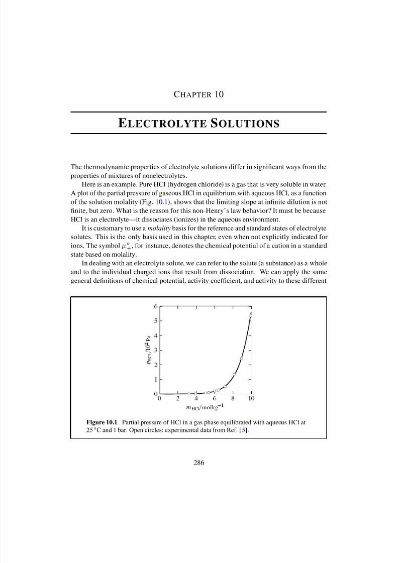
8/12/2019 Howard Devoe Thermodynamic and Chemical
http://slidepdf.com/reader/full/howard-devoe-thermodynamic-and-chemical 286/532

8/12/2019 Howard Devoe Thermodynamic and Chemical
http://slidepdf.com/reader/full/howard-devoe-thermodynamic-and-chemical 287/532
CHAPTER 10 ELECTROLYTE SOLUTIONS10.1 S INGLE - ION Q UANTITIES 287
species, but only the activity coefcient and activity of the solute as a whole can be evaluatedexperimentally.
10.1 SINGLE-ION QUANTITIES
Consider a solution of an electrolyte solute that dissociates completely into a cation speciesand an anion species. Subscripts C and will be used to denote the cation and anion,respectively. The solute molality mB is dened as the amount of solute formula unit dividedby the mass of solvent.
We rst need to investigate the relation between the chemical potential of an ion speciesand the electric potential of the solution phase.
The electric potential in the interior of a phase is called the inner electric potential , orGalvani potential . It is dened as the work needed to reversibly move an innitesimal testcharge into the phase from a position innitely far from other charges, divided by the valueof the test charge. The electrical potential energy of a charge in the phase is the product of
and the charge.Consider a hypothetical process in which an innitesimal amount d nC of the cation is
transferred into a solution phase at constant T and p . The quantity of charge transferredis ıQ D zC F dnC , where zC is the charge number ( C1, C2, etc.) of the cation, and F is the Faraday constant. 1 If the phase is at zero electric potential, the process causes nochange in its electrical potential energy. However, if the phase has a nite electric poten-tial , the transfer process changes its electrical potential energy by ıQ D zC F dnC .Consequently, the internal energy change depends on according to
dU. / D dU.0/ CzC F dnC (10.1.1)
where the electric potential is indicated in parentheses. The change in the Gibbs energy of the phase is given by d G D d.U TS CpV / , where T , S , p , and V are unaffected by the
value of . The dependence of d G on is therefore
dG. / D dG.0/ CzC F dnC (10.1.2)
The Gibbs fundamental equation for an open system, d G D S dT CV dp CPi i dn i(Eq. 9.2.34 ), assumes the electric potential is zero. From this equation and Eq. 10.1.2 , theGibbs energy change during the transfer process at constant T and p is found to depend on
according todG. / D C .0/ CzC F dnC (10.1.3)
The chemical potential of the cation in a phase of electric potential , dened by the partialmolar Gibbs energy Œ@G. /=@nC T;p , is therefore given by
C . / D C .0/ CzC F (10.1.4)
The corresponding relation for an anion is
. / D .0/ Cz F (10.1.5)
1The Faraday constant (page 453 ) is the charge per amount of protons.
Thermodynamics and Chemistry , second edition, version 4 © 2012 by Howard DeVoe. Latest version: www.chem.umd.edu/thermobook

8/12/2019 Howard Devoe Thermodynamic and Chemical
http://slidepdf.com/reader/full/howard-devoe-thermodynamic-and-chemical 288/532
CHAPTER 10 ELECTROLYTE SOLUTIONS10.1 S INGLE - ION Q UANTITIES 288
where z is the charge number of the anion ( 1, 2, etc.). For a charged species in general,we have
i . / D i .0/ Czi F (10.1.6)
We dene the standard state of an ion on a molality basis in the same way as for anonelectrolyte solute, with the additional stipulation that the ion is in a phase of zero electric
potential. Thus, the standard state is a hypothetical state in which the ion is at molality mıwith behavior extrapolated from innite dilution on a molality basis, in a phase of pressurep D p ı and electric potential D0.
The standard chemical potential ıC or ı of a cation or anion is the chemical potential
of the ion in its standard state. Single-ion activities a C and a in a phase of zero electricpotential are dened by relations having the form of Eq. 9.7.8 :
C .0/ D ıC CRT ln a C .0/ D ı CRT ln a (10.1.7)
As explained on page 270, aC and a should depend on the temperature, pressure, andcomposition of the phase, and not on the value of .
From Eqs. 10.1.4 , 10.1.5 , and 10.1.7 , the relations between the chemical potential of acation or anion, its activity, and the electric potential of its phase, are found to be
C D ıC CRT ln a C CzC F D ı CRT ln a Czi F (10.1.8)
These relations are denitions of single-ion activities in a phase of electric potential .For a charged species in general, we can write 2
i D ıi CRT ln a i Czi F (10.1.9)
Note that we can also apply this equation to an uncharged species, because the chargenumber zi is then zero and Eq. 10.1.9 becomes the same as Eq. 9.7.2 on page 270 .
Of course there is no experimental way to evaluate either C or relative to a refer-ence state or standard state, because it is impossible to add cations or anions by themselvesto a solution. We can nevertheless write some theoretical relations involving C and .
For a given temperature and pressure, we can write the dependence of the chemicalpotentials of the ions on their molalities in the same form as that given by Eq. 9.5.18 for anonelectrolyte solute:
C D ref C CRT ln C
mC
m ı D ref CRT ln mm ı (10.1.10)
Here ref C and ref are the chemical potentials of the cation and anion in solute reference
states. Each reference state is dened as a hypothetical solution with the same temperature,pressure, and electric potential as the solution under consideration; in this solution, themolality of the ion has the standard value mı , and the ion behaves according to Henry’s lawbased on molality. C and are single-ion activity coefcients on a molality basis.
2Some thermodynamicists call the quantity . ıi CRT ln a i / , which depends only on T , p , and composition,
the chemical potential of ion i , and the quantity . ıi CRT ln a i Czi F / the electrochemical potential with
symbol Qi .
Thermodynamics and Chemistry , second edition, version 4 © 2012 by Howard DeVoe. Latest version: www.chem.umd.edu/thermobook
8/12/2019 Howard Devoe Thermodynamic and Chemical
http://slidepdf.com/reader/full/howard-devoe-thermodynamic-and-chemical 289/532
CHAPTER 10 ELECTROLYTE SOLUTIONS10.2 S OLUTION OF A S YMMETRICAL E LECTROLYTE 289
The single-ion activity coefcients approach unity in the limit of innite dilution:
C ! 1 and ! 1 as mB ! 0 (10.1.11)(constant T , p , and )
In other words, we assume that in an extremely dilute electrolyte solution each individual
ion behaves like a nonelectrolyte solute species in an ideal-dilute solution. At a nite solutemolality, the values of C and are the ones that allow Eq. 10.1.10 to give the correctvalues of the quantities . C
ref C / and . ref / . We have no way to actually measure
these quantities experimentally, so we cannot evaluate either C or .We can dene single-ion pressure factors C and as follows:
Cdef
D expref C ı
C
RT ! expV 1C .p p ı /
RT (10.1.12)
def
D expref ı
RT expV 1 .p p ı /
RT (10.1.13)
The approximations in these equations are like those in Table 9.6 for nonelectrolyte solutes;they are based on the assumption that the partial molar volumes V C and V are independentof pressure.
From Eqs. 10.1.7 , 10.1.10 , 10.1.12 , and 10.1.13 , the single-ion activities are related tothe solution composition by
a C D C CmC
m ı a D mm ı (10.1.14)
Then, from Eq. 10.1.9 , we have the following relations between the chemical potentials andmolalities of the ions:
C
D ı
C
CRT ln. C C mC =m ı /
CzC F (10.1.15)
D ı CRT ln. m =m ı / Cz F (10.1.16)
Like the values of C and , values of the single-ion quantities a C , a , C , and cannot be determined by experiment.
10.2 SOLUTION OF A SYMMETRICAL ELECTROLYTE
Let us consider properties of an electrolyte solute as a whole. The simplest case is that of abinary solution in which the solute is a symmetrical strong electrolyte—a substance whoseformula unit has one cation and one anion that dissociate completely. This condition will beindicated by
D 2, where is the number of ions per formula unit. The solute with equal
to 2 might be a 1:1 salt such as NaCl, a 2:2 salt such as MgSO 4 , or a strong monoproticacid such as HCl.
In this binary solution, the chemical potential of the solute as a whole is dened in theusual way as the partial molar Gibbs energy
Bdef
D @G@nB T;p;n A
(10.2.1)
Thermodynamics and Chemistry , second edition, version 4 © 2012 by Howard DeVoe. Latest version: www.chem.umd.edu/thermobook

8/12/2019 Howard Devoe Thermodynamic and Chemical
http://slidepdf.com/reader/full/howard-devoe-thermodynamic-and-chemical 290/532
CHAPTER 10 ELECTROLYTE SOLUTIONS10.2 S OLUTION OF A S YMMETRICAL E LECTROLYTE 290
and is a function of T , p , and the solute molality mB . Although B under given conditionsmust in principle have a denite value, we are not able to actually evaluate it because wehave no way to measure precisely the energy brought into the system by the solute. Thisenergy contributes to the internal energy and thus to G . We can, however, evaluate thedifferences B
ref m; B or B
ım; B .
We can write the additivity rule (Eq. 9.2.25 ) for G as eitherG D nA A CnB B (10.2.2)
or
G D nA A CnC C Cn (10.2.3)
A comparison of these equations for a symmetrical electrolyte ( nB D nC D n ) gives usthe relation
B D C C (10.2.4)( D2)
We see that the solute chemical potential in this case is the sum of the single-ion chemicalpotentials.
The solution is a phase of electric potential . From Eqs. 10.1.4 and 10.1.5 , the sumC C appearing in Eq. 10.2.4 is
C . / C . / D C .0/ C .0/ C.z C Cz /F (10.2.5)
For the symmetrical electrolyte, the sum .z C Cz / is zero, so that B is equal to C .0/ C.0/ . We substitute the expressions of Eq. 10.1.10 , use the relation ref
m; B D ref C C ref
with reference states at D0, set the ion molalities mC and m equal to mB , and obtain
B
D ref
m; B CRT ln C
mB
m ı
2 (10.2.6)
( D2)
The important feature of this relation is the appearance of the second power of mB=m ı ,instead of the rst power as in the case of a nonelectrolyte. Also note that B does notdepend on , unlike C and .
Although we cannot evaluate C or individually, we can evaluate the product C .This product is the square of the mean ionic activity coefcient ˙ , dened for a symmet-rical electrolyte by
˙def
D p C (10.2.7)( D2)
With this denition, Eq. 10.2.6 becomes
B D ref m; B CRT ln . ˙ / 2 mB
m ı
2 (10.2.8)
( D2)
Since it is possible to determine the value of B ref m; B for a solution of known molality,
˙ is a measurable quantity.
Thermodynamics and Chemistry , second edition, version 4 © 2012 by Howard DeVoe. Latest version: www.chem.umd.edu/thermobook
8/12/2019 Howard Devoe Thermodynamic and Chemical
http://slidepdf.com/reader/full/howard-devoe-thermodynamic-and-chemical 291/532
CHAPTER 10 ELECTROLYTE SOLUTIONS10.2 S OLUTION OF A S YMMETRICAL E LECTROLYTE 291
If the electrolyte (e.g., HCl) is sufciently volatile, its mean ionic activity coefcient ina solution can be evaluated from partial pressure measurements of an equilibrated gasphase. Section 10.6 will describe a general method by which ˙ can be found fromosmotic coefcients. Section 14.5 describes how, in favorable cases, it is possible toevaluate ˙ from the equilibrium cell potential of a galvanic cell.
The activity a m; B of a solute substance on a molality basis is dened by Eq. 9.7.8 onpage 272 :
B D ım; B CRT ln a m; B (10.2.9)
Here ım; B is the chemical potential of the solute in its standard state, which is the solute
reference state at the standard pressure. By equating the expressions for B given by Eqs.10.2.8 and 10.2.9 and solving for the activity, we obtain
a m; B D m; B . ˙ / 2 mB
m ı
2(10.2.10)
( D2)
where m; B is the pressure factor dened by
m; Bdef
D expref m; B ım; B
RT ! (10.2.11)
We can use the appropriate expression in Table 9.6 on page 275 to evaluate m; B at anarbitrary pressure p 0:
m; B .p 0/ D exp Z p 0
p ı
V 1BRT
dp! expV 1B .p 0 p ı /
RT (10.2.12)
The value of m; B is 1 at the standard pressure, and close to 1 at any reasonably lowpressure (page 275). For this reason it is common to see Eq. 10.2.10 written as am; B D 2˙ .m B=m ı / 2 , with m; B omitted.
Equation 10.2.10 predicts that the activity of HCl in aqueous solutions is proportional,in the limit of innite dilution, to the square of the HCl molality. In contrast, the activityof a nonelectrolyte solute is proportional to the rst power of the molality in this limit.This predicted behavior of aqueous HCl is consistent with the data plotted in Fig. 10.1on page 286 , and is conrmed by the data for dilute HCl solutions shown in Fig. 10.2 (a).The dashed line in Fig. 10.2 (a) is the extrapolation of the ideal-dilute behavior given bya m; B D .m B=m ı / 2 . The extension of this line to mB D mı establishes the hypotheticalsolute reference state based on molality, indicated by a lled circle in Fig. 10.2 (b). (Sincethe data are for solutions at the standard pressure of 1 bar, the solute reference state shownin the gure is also the solute standard state.)
The solid curve of Fig. 10.2 (c) shows how the mean ionic activity coefcient of HCl
varies with molality in approximately the same range of molalities as the data shown inFig. 10.2 (b). In the limit of innite dilution, ˙ approaches unity. The slope of the curveapproaches 1 in this limit, quite unlike the behavior described in Sec. 9.5.4 for the activitycoefcient of a nonelectrolyte solute.
For a symmetrical strong electrolyte, ˙ is the geometric average of the single-ionactivity coefcients C and . We have no way of evaluating C or individually, evenif we know the value of ˙ . For instance, we cannot assume that C and are equal.
Thermodynamics and Chemistry , second edition, version 4 © 2012 by Howard DeVoe. Latest version: www.chem.umd.edu/thermobook

8/12/2019 Howard Devoe Thermodynamic and Chemical
http://slidepdf.com/reader/full/howard-devoe-thermodynamic-and-chemical 292/532
CHAPTER 10 ELECTROLYTE SOLUTIONS10.3 E LECTROLYTES IN G ENERAL 292
B mol kg
B
(a)
B mol kg
B
(b)
B mol kg
(c)
Figure 10.2 Aqueous HCl at 25 ı C and 1 bar. a
(a) HCl activity on a molality basis as a function of molality squared. The dashed lineis the extrapolation of the ideal-dilute behavior.(b) Same as (a) at a greatly reduced scale; the lled circle indicates the solute referencestate.(c) Mean ionic activity coefcient of HCl as a function of molality.
a Curves based on experimental parameter values in Ref. [ 74], Table 11-5-1.
10.3 ELECTROLYTES IN GENERAL
The formula unit of a non symmetrical electrolyte solute has more than two ions. Generalformulas for the solute as a whole are more complicated than those for the symmetrical casetreated in the preceding section, but are derived by the same reasoning.
Again we assume the solute dissociates completely into its constituent ions. We denethe following symbols:
C
Dthe number of cations per solute formula unit
Dthe number of anions per solute formula unit
Dthe sum C CFor example, if the solute formula is Al 2 (SO 4 )3 , the values are C D2, D3, and D5.
10.3.1 Solution of a single electrolyte
In a solution of a single electrolyte solute that is not necessarily symmetrical, the ion mo-lalities are related to the overall solute molality by
mC D C mB m D mB (10.3.1)
From the additivity rule for the Gibbs energy, we have
G D nA A CnB B
D nA A C C nB C C nB (10.3.2)
giving the relationB D C C C (10.3.3)
Thermodynamics and Chemistry , second edition, version 4 © 2012 by Howard DeVoe. Latest version: www.chem.umd.edu/thermobook
8/12/2019 Howard Devoe Thermodynamic and Chemical
http://slidepdf.com/reader/full/howard-devoe-thermodynamic-and-chemical 293/532
CHAPTER 10 ELECTROLYTE SOLUTIONS10.3 E LECTROLYTES IN G ENERAL 293
in place of Eq. 10.2.4 . The cations and anions are in the same phase of electric potential .We use Eqs. 10.1.4 and 10.1.5 to obtain
C C . / C . /
D C C .0/ C .0/ C. C zC C z /F (10.3.4)
Electrical neutrality requires that . C zC C z / be zero, giving
B D C C .0/ C .0/ (10.3.5)
By combining Eq. 10.3.5 with Eqs. 10.1.10 , 10.3.1 , and 10.3.3 , we obtain
B D ref B CRT lnh C
C CC
mB
m ı i (10.3.6)
where ref B D C
ref C C ref is the chemical potential of the solute in the hypothetical
reference state at D0 in which B is at the standard molality and behaves as at innitedilution. Equation 10.3.6 is the generalization of Eq. 10.2.6 . It shows that although C and
depend on , B does not.The mean ionic activity coefcient ˙ is dened in general by
˙ D CC (10.3.7)
or
˙ D CC
1=(10.3.8)
Thus ˙ is a geometric average of C and weighted by the numbers of the cations andanions in the solute formula unit. With a substitution from Eq. 10.3.7 , Eq. 10.3.6 becomes
B
D ref
B
CRT ln
hC
C ˙mB
mı
i (10.3.9)
Since Bref B is a measurable quantity, so also is ˙ .
The solute activity, dened by B D ım; B CRT ln a m; B , is
a m; B DC
C m; B ˙mB
m ı (10.3.10)
where m; B is the pressure factor that we can evaluate with Eq. 10.2.12 . Equation 10.3.10 isthe generalization of Eq. 10.2.10 . From Eqs. 10.1.12 , 10.1.13 , and 10.2.11 and the relations
ref B D C
ref C C ref and ı
B D CıC C ı , we obtain the relation
m; B
D
CC (10.3.11)
10.3.2 Multisolute solution
Equation 10.3.3 relates the chemical potential of electrolyte B in a binary solution to thesingle-ion chemical potentials of its constituent ions:
B D C C C (10.3.12)
Thermodynamics and Chemistry , second edition, version 4 © 2012 by Howard DeVoe. Latest version: www.chem.umd.edu/thermobook
8/12/2019 Howard Devoe Thermodynamic and Chemical
http://slidepdf.com/reader/full/howard-devoe-thermodynamic-and-chemical 294/532
CHAPTER 10 ELECTROLYTE SOLUTIONS10.3 E LECTROLYTES IN G ENERAL 294
This relation is valid for each individual solute substance in a multisolute solution, evenwhen two or more of the electrolyte solutes have an ion species in common.
As an illustration of this principle, consider a solution prepared by dissolving amountsnB of BaI 2 and n C of CsI in an amount n A of H2 O. Assume the dissolved salts are com-pletely dissociated into ions, with the I ion common to both. The additivity rule for the
Gibbs energy of this solution can be written in the formG D nA A CnB B CnC C (10.3.13)
and also, using single-ion quantities, in the form
G D nA A CnB . Ba2C / C2n B . I / CnC . CsC / CnC . I / (10.3.14)
Comparing Eqs. 10.3.13 and 10.3.14 , we nd the following relations must exist betweenthe chemical potentials of the solute substances and the ion species:
B D . Ba2C / C2 . I / C D . CsC / C . I / (10.3.15)
These relations agree with Eq. 10.3.12 . Note that . I / , the chemical potential of the ioncommon to both salts, appears in both relations.The solute activity am; B is dened by the relation B D ı
B CRT ln a m; B (Eq. 10.2.9 ).Using this relation together with Eqs. 10.1.7 and 10.1.14 , we nd that the solute activity isrelated to ion molalities by
a m; B D m; B ˙mC
m ı
C
mm ı (10.3.16)
where the pressure factor m; B is dened in Eq. 10.2.11 . The ion molalities in this ex-pression refer to the constituent ions of solute B, which in a multisolute solution are notnecessarily present in the same stoichiometric ratio as in the solute substance.
For instance, suppose we apply Eq. 10.3.16 to the solution of BaI 2 and CsI used aboveas an illustration of a multisolute solution, letting a m; B be the activity of solute substanceBaI 2 . The quantities mC and m in the equation are then the molalities of the Ba 2C and Iions, and ˙ is the mean ionic activity coefcient of the dissolved BaI 2 . Note that in thissolution the Ba 2C and I ions are not present in the 1:2 ratio found in BaI 2 , because I is aconstituent of both solutes.
10.3.3 Incomplete dissociation
In the preceding sections of this chapter, the electrolyte solute or solutes have been assumedto be completely dissociated into their constituent ions at all molalities. Some solutions,however, contain ion pairs —closely associated ions of opposite charge. Furthermore, in so-
lutions of some electrolytes (often called “weak” electrolytes), an equilibrium is establishedbetween ions and electrically-neutral molecules. In these kinds of solutions, the relationsbetween solute molality and ion molalities given by Eq. 10.3.1 are no longer valid. Whendissociation is not complete, the expression for B given by Eq. 10.3.9 can still be used.However, the quantity ˙ appearing in the expression no longer has the physical signi-cance of being the geometric average of the activity coefcients of the actual dissociatedions, and is called the stoichiometric activity coefcient of the electrolyte.
Thermodynamics and Chemistry , second edition, version 4 © 2012 by Howard DeVoe. Latest version: www.chem.umd.edu/thermobook
8/12/2019 Howard Devoe Thermodynamic and Chemical
http://slidepdf.com/reader/full/howard-devoe-thermodynamic-and-chemical 295/532
CHAPTER 10 ELECTROLYTE SOLUTIONS10.4 T HE D EBYE –H UCKEL T HEORY 295
10.4 THE DEBYE–H UCKEL THEORY
The theory of Peter Debye and Erich H¨ uckel (1923) provides theoretical expressions forsingle-ion activity coefcients and mean ionic activity coefcients in electrolyte solutions.The expressions in one form or another are very useful for extrapolation of quantities thatinclude mean ionic activity coefcients to low solute molality or innite dilution.
The only interactions the theory considers are the electrostatic interactions betweenions. These interactions are much stronger than those between uncharged molecules, andthey die off more slowly with distance. If the positions of ions in an electrolyte solutionwere completely random, the net effect of electrostatic ion–ion interactions would be zero,because each cation–cation or anion–anion repulsion would be balanced by a cation–anionattraction. The positions are not random, however: each cation has a surplus of anions inits immediate environment, and each anion has a surplus of neighboring cations. Each iontherefore has a net attractive interaction with the surrounding ion atmosphere. The resultfor a cation species at low electrolyte molality is a decrease of C compared to the cationat same molality in the absence of ion–ion interactions, meaning that the single-ion activitycoefcient C becomes less than 1 as the electrolyte molality is increased beyond the ideal-
dilute range. Similarly, also becomes less than 1.According to the Debye–H uckel theory, the single-ion activity coefcient i of ion i in
a solution of one or more electrolytes is given by
ln i D ADH z2
i p I m1 CBDH ap I m
(10.4.1)
where
zi Dthe charge number of ion i (C1, 2, etc.);
I m Dthe ionic strength of the solution on a molality basis, dened by 3
I m def D 12 Xall ions
mj z2j (10.4.2)
ADH and BDH are dened functions of the kind of solvent and the temperature;
a is an adjustable parameter, equal to the mean effective distance of closest approach of other ions in the solution to one of the i ions.
The denitions of the quantities ADH and BDH appearing in Eq. 10.4.1 are
ADHdef
D N 2A e3 =8 2 A1=2
. r 0 RT / 3=2 (10.4.3)
BDHdef
D N Ae 2 A1=2 . r 0 RT / 1=2 (10.4.4)
where N A is the Avogadro constant, e is the elementary charge (the charge of a proton),A and r are the density and relative permittivity (dielectric constant) of the solvent,
and 0 is the electric constant (or permittivity of vacuum).
3 Lewis and Randall (Ref. [ 101 ]) introduced the term ionic strength , dened by this equation, two years beforethe Debye–H uckel theory was published. They found empirically that in dilute solutions, the mean ionic activitycoefcient of a given strong electrolyte is the same in all solutions having the same ionic strength.
Thermodynamics and Chemistry , second edition, version 4 © 2012 by Howard DeVoe. Latest version: www.chem.umd.edu/thermobook
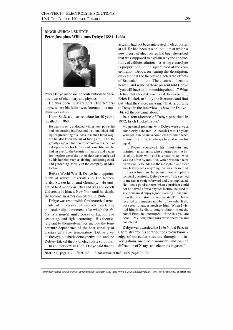
8/12/2019 Howard Devoe Thermodynamic and Chemical
http://slidepdf.com/reader/full/howard-devoe-thermodynamic-and-chemical 296/532
CHAPTER 10 ELECTROLYTE SOLUTIONS10.4 T HE D EBYE –H UCKEL T HEORY 296
BIOGRAPHICAL SKETCHPeter Josephus Wilhelmus Debye (1884–1966)
Peter Debye made major contributions to vari-ous areas of chemistry and physics.
He was born in Maastricht, The Nether-lands, where his father was foreman in a ma-chine workshop.
Henri Sack, a close associate for 40 years,recalled in 1968: a
He was not only endowed with a most powerfuland penetrating intellect and an unmatched abil-ity for presenting his ideas in a most lucid way,but he also knew the art of living a full life. Hegreatly enjoyed his scientic endeavors, he hada deep love for his family and home life, and hehad an eye for the beauties of nature and a tastefor the pleasure of the out-of-doors as manifestedby his hobbies such as shing, collecting cacti,and gardening, mostly in the company of Mrs.Debye.
Before World War II, Debye held appoint-ments at several universities in The Nether-lands, Switzerland, and Germany. He emi-grated to America in 1940 and was at CornellUniversity in Ithaca, New York until his death.He became an American citizen in 1946.
Debye was responsible for theoretical treat-ments of a variety of subjects, includingmolecular dipole moments (for which the de-bye is a non-SI unit), X-ray diffraction andscattering, and light scattering. His theoriesrelevant to thermodynamics include the tem-perature dependence of the heat capacity of crystals at a low temperature (Debye crys-tal theory), adiabatic demagnetization, and theDebye–H uckel theory of electrolyte solutions.
In an interview in 1962, Debye said that he
actually had not been interested in electrolytesat all. He had been at a colloquium at which anew theory of electrolytes had been described
that was supposed to explain why the conduc-tivity of a dilute solution of a strong electrolyteis proportional to the square root of the con-centration. Debye, on hearing this description,objected that the theory neglected the effectsof Brownian motion. The discussion becameheated, and some of those present told Debye“you will have to do something about it.” WhatDebye did about it was to ask his assistant,Erich H uckel, to study the literature and ndout what they were missing. That, accordingto Debye in the interview, is how the Debye–Huckel theory came about. b
In a reminiscence of Debye published in1972, Erich H uckel wrote: c
My personal relations with Debye were alwayscompletely care-free. Although I was 12 yearsyounger than he and a complete freshman whenI came to Z urich, he always treated me as hisequal.
. . .Debye conceived his work—in myopinion—as an artist who operates on the ba-sis of joy in his work and its creations, and whowas led often by intuition, which was then lateron rationally founded in the most plain and clearway leaving out everything that was unessential.
. . . I never found in Debye any interest in philo-sophical questions. Debye’s way of life seemedto me rather straightforward and uncomplicated.He liked a good dinner: when a problem couldnot be solved after a physics lecture, he used tosay: “one must enjoy a good evening dinner andthen the inspiration comes by itself”. . . Debyereceived an immense number of awards. It didnot seem to matter much to him. When I vis-ited him in Berlin to congratulate him on theNobel Prize, he interrupted: “Fine that you arehere.” My congratulations were therefore notcompleted.
Debye was awarded the 1936 Nobel Prize inChemistry “for his contributions to our knowl-edge of molecular structure through his in-vestigations on dipole moments and on thediffraction of X-rays and electrons in gases.”
a Ref. [ 57], page 232. bRef. [ 43]. cTranslation in Ref. [ 159 ], pages 73–74.
Thermodynamics and Chemistry , second edition, version 4 © 2012 by Howard DeVoe. Latest version: www.chem.umd.edu/thermobook

8/12/2019 Howard Devoe Thermodynamic and Chemical
http://slidepdf.com/reader/full/howard-devoe-thermodynamic-and-chemical 297/532
8/12/2019 Howard Devoe Thermodynamic and Chemical
http://slidepdf.com/reader/full/howard-devoe-thermodynamic-and-chemical 298/532
CHAPTER 10 ELECTROLYTE SOLUTIONS10.5 D ERIVATION OF THE D EBYE –H UCKEL E QUATION 298
The ionic strength I m is calculated from Eq. 10.4.2 with the molalities of all ions in thesolution, not just the molality of the ion or solute whose activity coefcient we are interestedin. This is because, as explained above, the departure of C and from the ideal-dilutevalue of 1 is caused by the interaction of each ion with the ion atmosphere resulting fromall other ions in the solution.
In a binary solution of a single electrolyte solute, assumed to be completely dissociated,the relation between the ionic strength and the solute molality depends on (the number of ions per solute formula unit) and the charge numbers zC and z . The ionic strength is givenby I m D .1=2/ Pi m i z 2
i D .1=2/. C z 2C C z2 /m B . With the help of the electroneutrality
condition C zC D . z / , this becomes
I m D 12 Π. z /z C . C zC /z m B
D 12 Π. C C /z C z m B
D 12 ˇzC z ˇmB (10.4.9)
We nd the following relations hold between I m and mB in the binary solution, dependingon the stoichiometry of the solute formula unit:
For a 1:1 electrolyte, e.g., NaCl or HCl: I m D mB
For a 1:2 or 2:1 electrolyte, e.g., Na 2 SO 4 or CaCl 2 : I m D 3mB
For a 2:2 electrolyte, e.g., MgSO 4 : I m D 4mB
For a 1:3 or 3:1 electrolyte, e.g., AlCl 3 : I m D 6 mB
For a 3:2 or 2:3 electrolyte, e.g., Al 2 (SO 4 )3 : I m D 15m B
Figure 10.4 on the next page shows ln ˙ as a function of p I m for aqueous HCl andCaCl 2 . The experimental curves have the limiting slopes predicted by the Debye–H uckellimiting law (Eq. 10.4.8 ), but at a low ionic strength the curves begin to deviate signicantlyfrom the linear relations predicted by that law. The full Debye–H¨ uckel equation (Eq. 10.4.7 )
ts the experimental curves over a wider range of ionic strength.
10.5 DERIVATION OF THE DEBYE–H UCKEL EQUATION
Debye and H¨uckel derived Eq. 10.4.1 using a combination of electrostatic theory, statis-tical mechanical theory, and thermodynamics. This section gives a brief outline of theirderivation.
The derivation starts by focusing on an individual ion of species i as it moves throughthe solution; call it the central ion. Around this central ion, the time-average spatial dis-tribution of any ion species j is not random, on account of the interaction of these ions of species j with the central ion. (Species i and j may be the same or different.) The distribu-
tion, whatever it is, must be spherically symmetric about the central ion; that is, a functiononly of the distance r from the center of the ion. The local concentration, c0
j , of the ions of species j at a given value of r depends on the ion charge zj e and the electric potential atthat position. The time-average electric potential in turn depends on the distribution of allions and is symmetric about the central ion, so expressions must be found for c0
j and asfunctions of r that are mutually consistent.
Thermodynamics and Chemistry , second edition, version 4 © 2012 by Howard DeVoe. Latest version: www.chem.umd.edu/thermobook
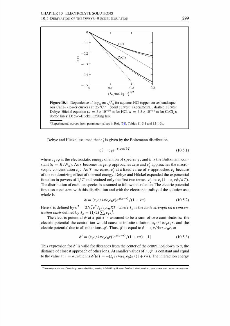
8/12/2019 Howard Devoe Thermodynamic and Chemical
http://slidepdf.com/reader/full/howard-devoe-thermodynamic-and-chemical 299/532
CHAPTER 10 ELECTROLYTE SOLUTIONS10.5 D ERIVATION OF THE D EBYE –H UCKEL E QUATION 299
HCl
CaCl 2
0 0:1 0:20:5
0:4
0:3
0:2
0:1
0:3
0
I m =mol kg 1 1=2
l n ˙
Figure 10.4 Dependence of ln ˙ on p I m for aqueous HCl (upper curves) and aque-ous CaCl 2 (lower curves) at 25 ı C. a Solid curves: experimental; dashed curves:Debye–H uckel equation ( a
D 5 10 10 m for HCl, a
D 4:5 10 10 m for CaCl 2 );
dotted lines: Debye–H uckel limiting law.
a Experimental curves from parameter values in Ref. [ 74], Tables 11-5-1 and 12-1-3a.
Debye and H uckel assumed that c0j is given by the Boltzmann distribution
c0j D cj e
zj e =kT (10.5.1)
where zj e is the electrostatic energy of an ion of species j , and k is the Boltzmann con-stant ( k D R=N A). As r becomes large, approaches zero and c0
j approaches the macro-
scopic concentration cj . As T increases, c0j at a xed value of r approaches cj becauseof the randomizing effect of thermal energy. Debye and H uckel expanded the exponential
function in powers of 1= T and retained only the rst two terms: c0j cj .1 zj e =kT/ .
The distribution of each ion species is assumed to follow this relation. The electric potentialfunction consistent with this distribution and with the electroneutrality of the solution as awhole is
D .z i e=4 r 0 r /e .a r/ =.1 C a/ (10.5.2)
Here is dened by 2 D 2N 2A e2 I c = r 0 RT , where I c is the ionic strength on a concen-tration basis dened by I c D .1=2/ Pi ci z 2
i .The electric potential at a point is assumed to be a sum of two contributions: the
electric potential the central ion would cause at innite dilution, zi e=4 r 0 r , and the
electric potential due to all other ions, 0. Thus,
0is equal to zi e=4 r 0 r , or
0 D .z i e=4 r 0 r/Œe.a r/ =.1 C a/ 1 (10.5.3)
This expression for 0 is valid for distances from the center of the central ion down to a , thedistance of closest approach of other ions. At smaller values of r , 0 is constant and equalto the value at r D a , which is 0.a/ D .z i e=4 r 0 / =.1 Ca/ . The interaction energy
Thermodynamics and Chemistry , second edition, version 4 © 2012 by Howard DeVoe. Latest version: www.chem.umd.edu/thermobook

8/12/2019 Howard Devoe Thermodynamic and Chemical
http://slidepdf.com/reader/full/howard-devoe-thermodynamic-and-chemical 300/532
CHAPTER 10 ELECTROLYTE SOLUTIONS10.6 M EAN IONIC A CTIVITY C OEFFICIENTS FROM O SMOTIC C OEFFICIENTS 300
between the central ion and the surrounding ions (the ion atmosphere) is the product of thecentral ion charge and 0.a/ .
The last step of the derivation is the calculation of the work of a hypothetical reversibleprocess in which the surrounding ions stay in their nal distribution, and the charge of thecentral ion gradually increases from zero to its actual value zi e . Let ˛z i e be the charge at
each stage of the process, where ˛ is a fractional advancement that changes from 0 to 1.Then the work w0 due to the interaction of the central ion with its ion atmosphere is 0.a/integrated over the charge:
w 0 D Z ˛ D 1
˛ D 0Œ.˛zi e=4 r 0 / =.1 C a/ d.˛z i /
D .z 2i e
2 =8 r 0 / =.1 C a/ (10.5.4)
Since the innitesimal Gibbs energy change in a reversible process is given by d G DS dT C V dp C ¶w 0 (Eq. 5.8.6 ), this reversible nonexpansion work at constant T and
p is equal to the Gibbs energy change. The Gibbs energy change per amount of speciesi is w 0N A D .z 2
i e2 N A=8 r 0 / =.1 C a/ . This quantity is G=n i for the process in
which a solution of xed composition changes from a hypothetical state lacking ion–ioninteractions to the real state with ion–ion interactions present. G=n i may be equated tothe difference of the chemical potentials of i in the nal and initial states. If the chemicalpotential without ion–ion interactions is taken to be that for ideal-dilute behavior on a mo-lality basis, i D ref
m;i CRT ln.m i =m ı / , then .z 2i e
2 N A=8 r 0 / =.1 C a/ is equal to
i Œ ref m;i CRT ln.m i =m ı / D RT ln m;i . In a dilute solution, ci can with little error be
set equal to Am i , and I c to A I m . Equation 10.4.1 follows.
10.6 MEAN IONIC ACTIVITY COEFFICIENTS FROM OSMOTICCOEFFICIENTS
Recall that ˙
is the mean ionic activity coefcient of a strong electrolyte, or the stoichio-metric activity coefcient of an electrolyte that does not dissociate completely.
The general procedure described in this section for evaluating ˙ requires knowledgeof the osmotic coefcient m as a function of molality. m is commonly evaluated bythe isopiestic method (Sec. 9.6.4 ) or from measurements of freezing-point depression (Sec.12.2 ).
The osmotic coefcient of a binary solution of an electrolyte is dened by
mdef
D A A
RT M A m B(10.6.1)
(binary electrolyte solution)
That is, for an electrolyte the sum
Pi ¤ A m i appearing in the denition of m for a nonelec-
trolyte solution (Eq. 9.6.11 on page 267 ) is replaced by m B , the sum of the ion molalitiesassuming complete dissociation. It will now be shown that m dened this way can be usedto evaluate ˙ .
The derivation is like that described in Sec. 9.6.3 for a binary solution of a nonelec-trolyte. Solving Eq. 10.6.1 for A and taking the differential of A at constant T and p , weobtain
d A D RT M A . m dmB CmB d m / (10.6.2)
Thermodynamics and Chemistry , second edition, version 4 © 2012 by Howard DeVoe. Latest version: www.chem.umd.edu/thermobook
8/12/2019 Howard Devoe Thermodynamic and Chemical
http://slidepdf.com/reader/full/howard-devoe-thermodynamic-and-chemical 301/532
8/12/2019 Howard Devoe Thermodynamic and Chemical
http://slidepdf.com/reader/full/howard-devoe-thermodynamic-and-chemical 302/532
CHAPTER 10 ELECTROLYTE SOLUTIONSPROBLEMS 302
PROBLEMS
An underlined problem number or problem-part letter indicates that the numerical answer appearsin Appendix I.
10.1 The mean ionic activity coefcient of NaCl in a 0.100 molal aqueous solution at 298:15 Khas been evaluated with measurements of equilibrium cell potentials, 4 with the result ln ˙
D0:2505 . Use this value in Eq. 10.6.9 , together with the values of osmotic coefcients inTable 10.1, to evaluate ˙ at each of the molalities shown in the table; then plot ˙ as afunction of mB .
Table 10.1 Osmotic coefcients of aqueous NaCl at298:15 K a
mB=mol kg 1m mB=mol kg 1
m
0.1 0.9325 2.0 0.98660.2 0.9239 3.0 1.04850.3 0.9212 4.0 1.11770.5 0.9222 5.0 1.1916
1.0 0.9373 6.0 1.26881.5 0.9598
a Ref. [ 31].
10.2 Rard and Miller 5 used published measurements of the freezing points of dilute aqueous so-lutions of Na 2 SO 4 to calculate the osmotic coefcients of these solutions at 298:15 K. Usetheir values listed in Table 10.2 to evaluate the mean ionic activity coefcient of Na 2 SO 4 at298:15 K and a molality of mB D 0:15 mol kg 1 . For the parameter a in the Debye–H¨uckelequation (Eq. 10.4.7 ), use the value a D 3:0 10 10 m.
Table 10.2 Osmotic coefcients of aqueous Na 2 SO 4at 298:15 K
mB=mol kg 1m mB=mol kg 1
m
0.0126 0.8893 0.0637 0.81110.0181 0.8716 0.0730 0.80360.0228 0.8607 0.0905 0.79270.0272 0.8529 0.0996 0.78870.0374 0.8356 0.1188 0.77800.0435 0.8294 0.1237 0.77600.0542 0.8178 0.1605 0.76160.0594 0.8141
4Ref. [ 143 ], Table 9.3. 5Ref. [ 139 ].
Thermodynamics and Chemistry , second edition, version 4 © 2012 by Howard DeVoe. Latest version: www.chem.umd.edu/thermobook
8/12/2019 Howard Devoe Thermodynamic and Chemical
http://slidepdf.com/reader/full/howard-devoe-thermodynamic-and-chemical 303/532
C HAPTER 11
R EACTIONS AND OTHER CHEMICAL
P ROCESSES
This chapter discusses the thermodynamics of mixing processes and processes describedby reaction equations (chemical equations). It introduces the important concepts of molarmixing and reaction quantities, advancement, and the thermodynamic equilibrium constant.The focus is on chemical processes that take place in closed systems at constant pressure,with no work other than expansion work. Under these conditions, the enthalpy change isequal to the heat (Eq. 5.3.7 ). The processes either take place at constant temperature, orhave initial and nal states of the same temperature.
Most of the processes to be described involve mixtures and have intermediate states thatare nonequilibrium states. At constant temperature and pressure, these processes proceedspontaneously with decreasing Gibbs energy (Sec. 5.8).1 When the rates of change are slowenough for thermal and mechanical equilibrium to be maintained, the spontaneity is dueto lack of transfer equilibrium or reaction equilibrium. An equilibrium phase transition of a pure substance, however, is a special case: it is a reversible process of constant Gibbs
energy (Sec. 8.3 ).
11.1 MIXING PROCESSES
A mixing process is a process in which a mixture is formed from pure substances. In theinitial state the system has two or more separate phases, each containing a different puresubstance at the same temperature and pressure. The nal state is a single-phase mixture atthis temperature and pressure.
The process is illustrated schematically in Fig. 11.1 on the next page . When the partitionis withdrawn, the two pure liquids mix spontaneously at constant pressure to form a singlehomogeneous phase. If necessary, heat transfer is used to return the phase to the initial
temperature.
1Processes in which G decreases are sometimes called exergonic .
303
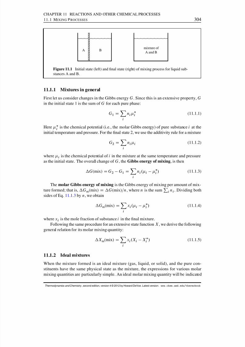
8/12/2019 Howard Devoe Thermodynamic and Chemical
http://slidepdf.com/reader/full/howard-devoe-thermodynamic-and-chemical 304/532
CHAPTER 11 REACTIONS AND OTHER CHEMICAL PROCESSES11.1 M IXING P ROCESSES 304
A B mixture of
A and B
Figure 11.1 Initial state (left) and nal state (right) of mixing process for liquid sub-stances A and B.
11.1.1 Mixtures in general
First let us consider changes in the Gibbs energy G . Since this is an extensive property, Gin the initial state 1 is the sum of G for each pure phase:
G1 D
Xi
n i i (11.1.1)
Here i is the chemical potential (i.e., the molar Gibbs energy) of pure substance i at theinitial temperature and pressure. For the nal state 2, we use the additivity rule for a mixture
G2 DXi
n i i (11.1.2)
where i is the chemical potential of i in the mixture at the same temperature and pressureas the initial state. The overall change of G , the Gibbs energy of mixing , is then
G (mix) D G2 G1 DXi
n i . i i / (11.1.3)
The molar Gibbs energy of mixing is the Gibbs energy of mixing per amount of mix-ture formed; that is, G m(mix) D G (mix) =n , where n is the sum Pi n i . Dividing bothsides of Eq. 11.1.3 by n , we obtain
G m(mix) DXi
x i . i i / (11.1.4)
where xi is the mole fraction of substance i in the nal mixture.Following the same procedure for an extensive state function X , we derive the following
general relation for its molar mixing quantity:
X m(mix)
DXi
x i .X i
X i / (11.1.5)
11.1.2 Ideal mixtures
When the mixture formed is an ideal mixture (gas, liquid, or solid), and the pure con-stituents have the same physical state as the mixture, the expressions for various molarmixing quantities are particularly simple. An ideal molar mixing quantity will be indicated
Thermodynamics and Chemistry , second edition, version 4 © 2012 by Howard DeVoe. Latest version: www.chem.umd.edu/thermobook
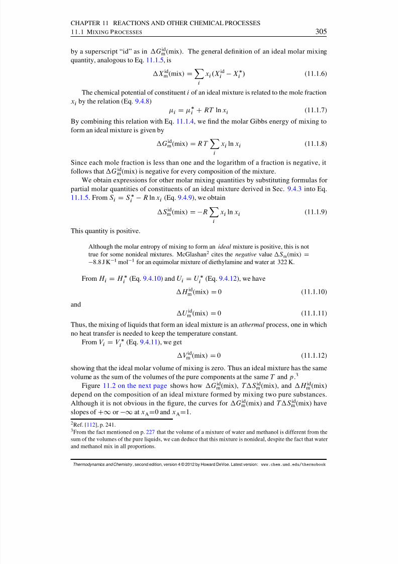
8/12/2019 Howard Devoe Thermodynamic and Chemical
http://slidepdf.com/reader/full/howard-devoe-thermodynamic-and-chemical 305/532
CHAPTER 11 REACTIONS AND OTHER CHEMICAL PROCESSES11.1 M IXING P ROCESSES 305
by a superscript “id” as in G idm (mix). The general denition of an ideal molar mixing
quantity, analogous to Eq. 11.1.5 , is
X idm (mix) DXi
x i .X idi X i / (11.1.6)
The chemical potential of constituent i of an ideal mixture is related to the mole fractionx i by the relation (Eq. 9.4.8 )
i D i CRT ln x i (11.1.7)
By combining this relation with Eq. 11.1.4 , we nd the molar Gibbs energy of mixing toform an ideal mixture is given by
G idm (mix) D RT Xi
x i ln x i (11.1.8)
Since each mole fraction is less than one and the logarithm of a fraction is negative, itfollows that G id
m (mix) is negative for every composition of the mixture.We obtain expressions for other molar mixing quantities by substituting formulas for
partial molar quantities of constituents of an ideal mixture derived in Sec. 9.4.3 into Eq.
11.1.5 . From S i D S i R ln x i (Eq. 9.4.9 ), we obtain
S idm (mix) D R Xi
x i ln x i (11.1.9)
This quantity is positive.
Although the molar entropy of mixing to form an ideal mixture is positive, this is nottrue for some nonideal mixtures. McGlashan 2 cites the negative value S m (mix) D8:8 J K 1 mol 1 for an equimolar mixture of diethylamine and water at 322 K.
From H i D H i (Eq. 9.4.10 ) and U i D U i (Eq. 9.4.12 ), we have
H id
m(mix)
D 0 (11.1.10)
andU id
m (mix) D 0 (11.1.11)
Thus, the mixing of liquids that form an ideal mixture is an athermal process, one in whichno heat transfer is needed to keep the temperature constant.
From V i D V i (Eq. 9.4.11 ), we get
V idm (mix) D 0 (11.1.12)
showing that the ideal molar volume of mixing is zero. Thus an ideal mixture has the samevolume as the sum of the volumes of the pure components at the same T and p .3
Figure 11.2 on the next page shows how G idm (mix), T S id
m (mix), and H idm (mix)
depend on the composition of an ideal mixture formed by mixing two pure substances.Although it is not obvious in the gure, the curves for G id
m (mix) and T S idm (mix) have
slopes of C1 or 1 at xAD0 and xAD1.2Ref. [ 112 ], p. 241.3From the fact mentioned on p. 227 that the volume of a mixture of water and methanol is different from thesum of the volumes of the pure liquids, we can deduce that this mixture is nonideal, despite the fact that waterand methanol mix in all proportions.
Thermodynamics and Chemistry , second edition, version 4 © 2012 by Howard DeVoe. Latest version: www.chem.umd.edu/thermobook
8/12/2019 Howard Devoe Thermodynamic and Chemical
http://slidepdf.com/reader/full/howard-devoe-thermodynamic-and-chemical 306/532
CHAPTER 11 REACTIONS AND OTHER CHEMICAL PROCESSES11.1 M IXING P ROCESSES 306
idm (mix)
idm (mix)
idm (mix)
A
q u a n t i t y / k J m o
l
Figure 11.2 Molar mixing quantities for a binary ideal mixture at 298:15 K.
11.1.3 Excess quantities
An excess quantity X E of a mixture is dened as the difference between the value of theextensive property X of the real mixture and X id , the value for a hypothetical ideal mixtureat the same temperature, pressure, and composition.
An excess molar quantity X Em is the excess quantity divided by n , the total amount of all constituents of the mixture. Examining the dependence of excess molar quantities oncomposition is a convenient way to characterize deviations from ideal-mixture behavior.
Excess molar quantities are related to molar mixing quantities as follows:
X Em D .X X id /=n D Xi
n i X i Xi
n i X idi !=n
DXi
x i X i X idi
DXi
x i .X i X i / Xi
x i .X idi X i /
D X m(mix) X idm (mix) (11.1.13)
By substituting expressions for X idm (mix) from Eqs. 11.1.8 –11.1.12 in Eq. 11.1.13 , we ob-
tain the following expressions for the excess molar Gibbs energy, entropy, enthalpy, internal
energy, and volume:G E
m D G m(mix) RT Xi
x i ln x i (11.1.14)
S Em D S m(mix) CR Xi
x i ln x i (11.1.15)
H Em D H m(mix) (11.1.16)
Thermodynamics and Chemistry , second edition, version 4 © 2012 by Howard DeVoe. Latest version: www.chem.umd.edu/thermobook
8/12/2019 Howard Devoe Thermodynamic and Chemical
http://slidepdf.com/reader/full/howard-devoe-thermodynamic-and-chemical 307/532
CHAPTER 11 REACTIONS AND OTHER CHEMICAL PROCESSES11.1 M IXING P ROCESSES 307
U Em D U m (mix) (11.1.17)
V Em D V m (mix) (11.1.18)
By substitution from Eqs. 9.5.14 and 11.1.4 in Eq. 11.1.14 , we can relate the excess molarGibbs energy to the activity coefcients of the mixture constituents based on pure-liquid
reference states: G Em D RT Xi
x i ln i (11.1.19)
It is also possible to derive the useful relation
"@ nG Em
@ni #T;p;n j ¤ i
D RT ln i (11.1.20)
To derive Eq. 11.1.20 , consider innitesimal changes in the mixture composition atconstant T and p . From Eq. 11.1.19 , we write
d nG Em D RT
Xi
d.n i ln i / D RT
Xi
n i d ln i CRT
Xi
. ln i / dn i (11.1.21)
From i D i CRT ln. i x i / , we have d i D RT . d ln i Cdx i =xi / . Substitution inthe Gibbs–Duhem equation, Pi x i d i D 0, gives
Xi
x i d ln i CXi
dx i D 0 (11.1.22)
In Eq. 11.1.22 , we set the sum Pi dx i equal to zero (because Pi x i equals 1) andmultiply by the total amount, n , resulting in Pi n i d ln i D 0. This turns Eq. 11.1.21into
d nG Em D RT Xi
. ln i / dn i (11.1.23)
from which Eq. 11.1.20 follows.
11.1.4 The entropy change to form an ideal gas mixture
When pure ideal gases mix at constant T and p to form an ideal gas mixture, the molarentropy change S id
m (mix) D R Pi y i ln y i (Eq. 11.1.9 ) is positive.Consider a pure ideal-gas phase. Entropy is an extensive property, so if we divide this
phase into two subsystems with an internal partition, the total entropy remains unchanged.The reverse process, the removal of the partition, must also have zero entropy change. De-spite the fact that the latter process allows the molecules in the two subsystems to inter-mingle without a change in T or p , it cannot be considered “mixing” because the entropydoes not increase. The essential point is that the same substance is present in both of the
subsystems, so there is no macroscopic change of state when the partition is removed.From these considerations, one might conclude that the fundamental reason the entropyincreases when pure ideal gases mix is that different substances become intermingled. Thisconclusion would be mistaken, as we will now see.
The partial molar entropy of constituent i of an ideal gas mixture is related to its partialpressure p i by Eq. 9.3.6 :
S i D S ıi R ln .p i =p ı / (11.1.24)
Thermodynamics and Chemistry , second edition, version 4 © 2012 by Howard DeVoe. Latest version: www.chem.umd.edu/thermobook
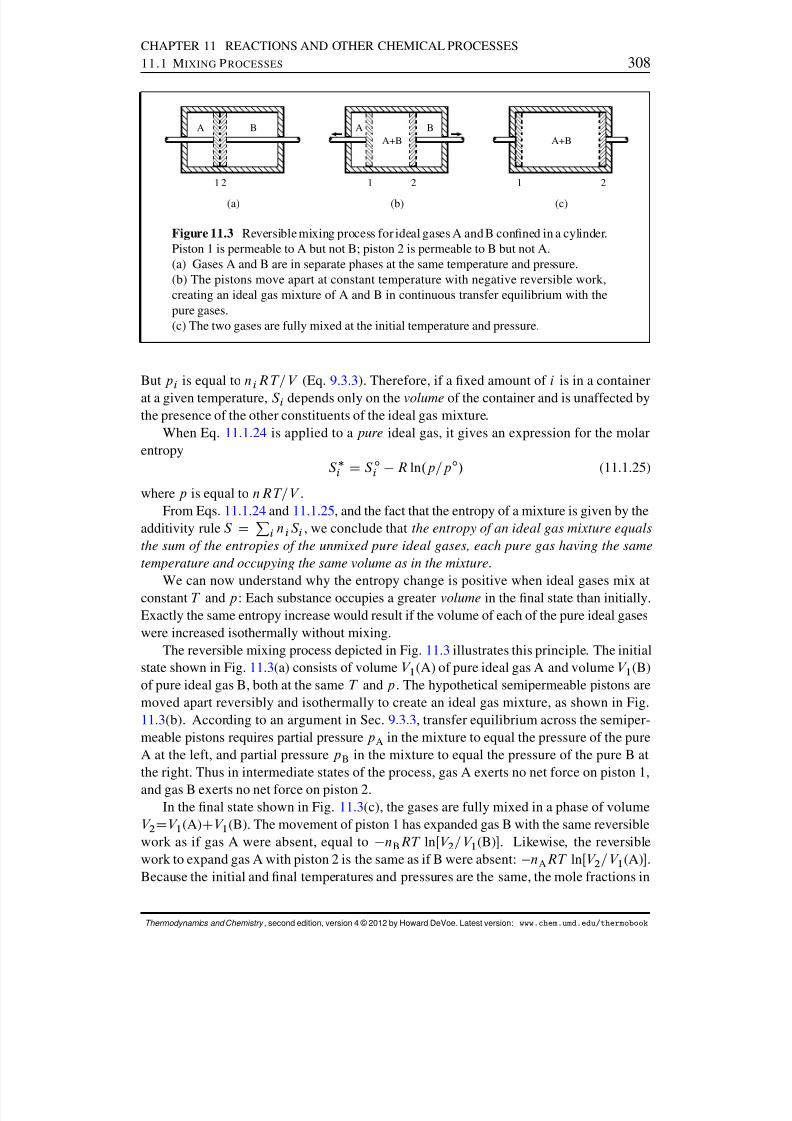
8/12/2019 Howard Devoe Thermodynamic and Chemical
http://slidepdf.com/reader/full/howard-devoe-thermodynamic-and-chemical 308/532
CHAPTER 11 REACTIONS AND OTHER CHEMICAL PROCESSES11.1 M IXING P ROCESSES 308
1 2
(a)
A B
1 2
(b)
AA+B
B
1 2
(c)
A+B
Figure 11.3 Reversible mixing process for ideal gases A and B conned in a cylinder.Piston 1 is permeable to A but not B; piston 2 is permeable to B but not A.(a) Gases A and B are in separate phases at the same temperature and pressure.(b) The pistons move apart at constant temperature with negative reversible work,creating an ideal gas mixture of A and B in continuous transfer equilibrium with thepure gases.(c) The two gases are fully mixed at the initial temperature and pressure.
But p i is equal to n i RT=V (Eq. 9.3.3 ). Therefore, if a xed amount of i is in a containerat a given temperature, S i depends only on the volume of the container and is unaffected bythe presence of the other constituents of the ideal gas mixture.
When Eq. 11.1.24 is applied to a pure ideal gas, it gives an expression for the molarentropy
S i D S ıi R ln .p=p ı / (11.1.25)
where p is equal to nRT=V .From Eqs. 11.1.24 and 11.1.25 , and the fact that the entropy of a mixture is given by the
additivity rule S DPi n i S i , we conclude that the entropy of an ideal gas mixture equalsthe sum of the entropies of the unmixed pure ideal gases, each pure gas having the sametemperature and occupying the same volume as in the mixture .
We can now understand why the entropy change is positive when ideal gases mix atconstant T and p : Each substance occupies a greater volume in the nal state than initially.Exactly the same entropy increase would result if the volume of each of the pure ideal gaseswere increased isothermally without mixing.
The reversible mixing process depicted in Fig. 11.3 illustrates this principle. The initialstate shown in Fig. 11.3 (a) consists of volume V 1 (A) of pure ideal gas A and volume V 1 (B)of pure ideal gas B, both at the same T and p . The hypothetical semipermeable pistons aremoved apart reversibly and isothermally to create an ideal gas mixture, as shown in Fig.11.3 (b). According to an argument in Sec. 9.3.3 , transfer equilibrium across the semiper-meable pistons requires partial pressure p A in the mixture to equal the pressure of the pureA at the left, and partial pressure p B in the mixture to equal the pressure of the pure B atthe right. Thus in intermediate states of the process, gas A exerts no net force on piston 1,and gas B exerts no net force on piston 2.
In the nal state shown in Fig. 11.3 (c), the gases are fully mixed in a phase of volumeV 2DV 1 (A)CV 1 (B). The movement of piston 1 has expanded gas B with the same reversiblework as if gas A were absent, equal to nBRT lnŒV 2 =V 1 (B) . Likewise, the reversiblework to expand gas A with piston 2 is the same as if B were absent: nART lnŒV 2 =V 1 (A) .Because the initial and nal temperatures and pressures are the same, the mole fractions in
Thermodynamics and Chemistry , second edition, version 4 © 2012 by Howard DeVoe. Latest version: www.chem.umd.edu/thermobook
8/12/2019 Howard Devoe Thermodynamic and Chemical
http://slidepdf.com/reader/full/howard-devoe-thermodynamic-and-chemical 309/532
CHAPTER 11 REACTIONS AND OTHER CHEMICAL PROCESSES11.1 M IXING P ROCESSES 309
the nal mixture are yA D V 1 (A) =V 2 and yB D V 1 (B) =V 2 . The total work of the reversiblemixing process is therefore w D nART ln yA CnBRT ln yB , the heat needed to keep theinternal energy constant is q D w , and the entropy change is
S D q=T D nAR ln yA nBR ln yB (11.1.26)
It should be clear that isothermal expansion of both pure gases from their initial volumesto volume V 2 without mixing would result in the same total work and the same entropychange.
When we divide Eq. 11.1.26 by n D nA CnB , we obtain the expression for the molarentropy of mixing given by Eq. 11.1.9 with xi replaced by y i for a gas.
11.1.5 Molecular model of a liquid mixture
We have seen that when two pure liquids mix to form an ideal liquid mixture at the same T and p , the total volume and internal energy do not change. A simple molecular model of a binary liquid mixture will elucidate the energetic molecular properties that are consistent
with this macroscopic behavior. The model assumes the excess molar entropy, but notnecessarily the excess molar internal energy, is zero. The model is of the type sometimescalled the quasicrystalline lattice model , and the mixture it describes is sometimes calleda simple mixture. Of course, a molecular model like this is outside the realm of classicalthermodynamics.
The model is for substances A and B in gas and liquid phases at a xed temperature.Let the standard molar internal energy of pure gaseous A be U ıA (g). This is the molarenergy in the absence of intermolecular interactions, and its value depends only on themolecular constitution and the temperature. The molar internal energy of pure liquid A islower because of the attractive intermolecular forces in the liquid phase. We assume theenergy difference is equal to a sum of pairwise nearest-neighbor interactions in the liquid.Thus, the molar internal energy of pure liquid A is given by
U A D U ıA (g) CkAA (11.1.27)
where kAA (approximately the negative of the molar internal energy of vaporization) is theinteraction energy per amount of A due to A–A interactions when each molecule of A issurrounded only by other molecules of A.
Similarly, the molar internal energy of pure liquid B is given by
U B D U ıB (g) CkBB (11.1.28)
where kBB is for B–B interactions.We assume that in a liquid mixture of A and B, the numbers of nearest-neighbor mole-
cules of A and B surrounding any given molecule are in proportion to the mole fractions xAand xB .4 Then the number of A–A interactions is proportional to nAxA , the number of B–B
4This assumption requires the molecules of A and B to have similar sizes and shapes and to be randomly mixedin the mixture. Statistical mechanics theory shows that the molecular sizes must be approximately equal if theexcess molar entropy is to be zero.
Thermodynamics and Chemistry , second edition, version 4 © 2012 by Howard DeVoe. Latest version: www.chem.umd.edu/thermobook
8/12/2019 Howard Devoe Thermodynamic and Chemical
http://slidepdf.com/reader/full/howard-devoe-thermodynamic-and-chemical 310/532
CHAPTER 11 REACTIONS AND OTHER CHEMICAL PROCESSES11.1 M IXING P ROCESSES 310
interactions is proportional to nBxB , and the number of A–B interactions is proportional tonAxB CnBxA . The internal energy of the liquid mixture is then given by
U (mixt) D nAU ıA (g) CnBU ıB (g)
CnAxAkAA CnBxBkBB C.n AxB Cn BxA /k AB (11.1.29)
where kAB is the interaction energy per amount of A when each molecule of A is surroundedonly by molecules of B, or the interaction energy per amount of B when each molecule of B is surrounded only by molecules of A.
The internal energy change for mixing amounts n A of liquid A and nB of liquid B isnow
U (mix) D U (mixt) nAU A nBU B
D nAxAkAA CnBxBkBB C.n AxB CnBxA /k AB nAkAA nBkBB
D nA .x A 1/k AA CnB .x B 1/k BB C.n AxB CnBxA /k AB (11.1.30)
With the identities xA 1 D xB , xB 1 D xA , and nAxB D nBxA D nAnB=n(where n is the sum nA
CnB), we obtain
U (mix) D nAnB
n .2k AB kAA kBB / (11.1.31)
If the internal energy change to form a mixture of any composition is to be zero, as it is foran ideal mixture, the quantity .2k AB kAA kBB / must be zero, which means kAB mustequal .k AA CkBB /=2 . Thus, one requirement for an ideal mixture is that an A–B interactionequals the average of an A–A interaction and a B–B interaction .
If we write Eq. 11.1.29 in the form
U (mixt) D nAU ıA (g) CnBU ıB (g) C 1
nA CnB.n 2
AkAA C2n AnBkAB Cn2BkBB / (11.1.32)
we can differentiate with respect to nB
at constant nA
to evaluate the partial molar internalenergy of B. The result can be rearranged to the simple form
U B D U B C.2k AB kAA kBB / .1 xB / 2 (11.1.33)
where U B is given by Eq. 11.1.28 . Equation 11.1.33 predicts that the value of U B decreaseswith increasing xB if kAB is less negative than the average of kAA and kBB , increases for theopposite situation, and is equal to U B in an ideal liquid mixture.
When the excess molar volume and entropy are set equal to zero, the model describeswhat is called a regular solution .5 The excess molar Gibbs energy of a mixture is G E
m DU Em CpV E
m TS Em . Using the expression of Eq. 11.1.31 with the further assumptions thatV Em and S Em are zero, this model predicts the excess molar Gibbs energy is given by
G Em D U (mix)
n D xAxB .2k AB kAA kBB / (11.1.34)
This is a symmetric function of xA and xB . It predicts, for example, that coexisting liquidlayers in a binary system (Sec. 11.1.6 ) have the same value of xA in one phase as the valueof xB in the other.
5Ref. [ 79].
Thermodynamics and Chemistry , second edition, version 4 © 2012 by Howard DeVoe. Latest version: www.chem.umd.edu/thermobook
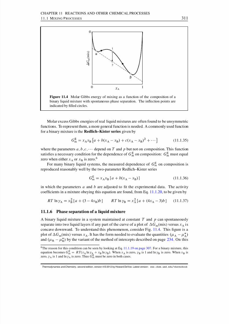
8/12/2019 Howard Devoe Thermodynamic and Chemical
http://slidepdf.com/reader/full/howard-devoe-thermodynamic-and-chemical 311/532
CHAPTER 11 REACTIONS AND OTHER CHEMICAL PROCESSES11.1 M IXING P ROCESSES 311
A
m ( m
i x )
1
2
Figure 11.4 Molar Gibbs energy of mixing as a function of the composition of abinary liquid mixture with spontaneous phase separation. The inection points areindicated by lled circles.
Molar excess Gibbs energies of real liquid mixtures are often found to be unsymmetricfunctions. To represent them, a more general function is needed. A commonly used functionfor a binary mixture is the Redlich–Kister series given by
G Em D xAxB a Cb.x A xB / Cc.x A xB / 2 C (11.1.35)
where the parameters a; b;c; depend on T and p but not on composition. This functionsatises a necessary condition for the dependence of G E
m on composition: GEm must equal
zero when either xA or xB is zero. 6
For many binary liquid systems, the measured dependence of GEm on composition is
reproduced reasonably well by the two-parameter Redlich–Kister series
G Em D xAxB ΠaCb.x A xB / (11.1.36)
in which the parameters a and b are adjusted to t the experimental data. The activitycoefcients in a mixture obeying this equation are found, from Eq. 11.1.20 , to be given by
RT ln A D x 2B ΠaC.3 4x B /b RT ln B D x 2
A ΠaC.4x A 3/b (11.1.37)
11.1.6 Phase separation of a liquid mixture
A binary liquid mixture in a system maintained at constant T and p can spontaneouslyseparate into two liquid layers if any part of the curve of a plot of G
m(mix) versus x
A is
concave downward. To understand this phenomenon, consider Fig. 11.4 . This gure is aplot of G m(mix) versus xA . It has the form needed to evaluate the quantities . A A /and . B B / by the variant of the method of intercepts described on page 234 . On this
6The reason for this condition can be seen by looking at Eq. 11.1.19 on page 307 . For a binary mixture, thisequation becomes G E
m D RT.x A ln A CxB ln B / . When xA is zero, B is 1 and ln B is zero. When xB iszero, A is 1 and ln A is zero. Thus G E
m must be zero in both cases.
Thermodynamics and Chemistry , second edition, version 4 © 2012 by Howard DeVoe. Latest version: www.chem.umd.edu/thermobook
8/12/2019 Howard Devoe Thermodynamic and Chemical
http://slidepdf.com/reader/full/howard-devoe-thermodynamic-and-chemical 312/532
CHAPTER 11 REACTIONS AND OTHER CHEMICAL PROCESSES11.1 M IXING P ROCESSES 312
plot, the tangent to the curve at any given composition has intercepts equal to . B B / atxAD0 and . A A / at xAD1.
In order for two binary liquid phases to be in transfer equilibrium, A must be thesame in both phases and B must also be the same in both phases. The dashed line in thegure is a common tangent to the curve at the points labeled ’ and “. These two points
are the only ones having a common tangent, and what makes the common tangent possibleis the downward concavity (negative curvature) of a portion of the curve between thesepoints. Because the tangents at these points have the same intercepts, phases ’ and “ of compositions x ’
A and x “A can be in equilibrium with one another: the necessary conditions
’A D “
A and ’B D “
B are satised.Now consider point 1 on the curve. A phase of this composition is unstable. It will
spontaneously separate into the two phases of compositions x ’A and x “
A , because the Gibbsenergy per total amount then decreases to the extent indicated by the vertical arrow frompoint 1 to point 2. We know that a process in which G decreases at constant T and p in aclosed system, with expansion work only, is a spontaneous process (Sec. 5.8 ).
To show that the arrow in Fig. 11.4 represents the change in G=n for phase separa-tion, we let y represent the vertical ordinate and write the equation of the dashed linethrough points ’ and “ (y as a function of xA ):
y D y ’ Cy “ y ’
x “A x ’
A!.x A x ’
A / (11.1.38)
In the system both before and after phase separation occurs, xA is the mole fraction of component A in the system as a whole. When phases ’ and “ are present, containingamounts n ’ and n“ , xA is given by the expression
xA D x ’
A n ’ Cx “A n “
n ’ Cn“ (11.1.39)
By substituting this expression for x A in Eq. 11.1.38 , after some rearrangement andusing n ’ Cn“ D n , we obtain
y D 1n
n ’ y ’ Cn“ y “ (11.1.40)
which equates y for a point on the dashed line to the Gibbs energy change for mixingpure components to form an amount n’ of phase ’ and an amount n“ of phase “,divided by the total amount n . Thus, the difference between the values of y at points1 and 2 is the decrease in G=n when a single phase separates into two equilibratedphases.
Any mixture with a value of xA between x ’A and x “
A is unstable with respect to separation
into two phases of compositions x ’A and x “
A . Phase separation occurs only if the curve of
the plot of G m(mix) versus xA is concave downward, which requires the curve to have atleast two inection points. The compositions of the two phases are not the compositions atthe inection points, nor in the case of the curve shown in Fig. 11.4 are these compositionsthe same as those of the two local minima.
By varying the values of parameters in an expression for the excess molar Gibbs energy,we can model the onset of phase separation caused by a temperature change. Figure 11.5shows the results of using the two-parameter Redlich–Kister series (Eq. 11.1.36 ).
Thermodynamics and Chemistry , second edition, version 4 © 2012 by Howard DeVoe. Latest version: www.chem.umd.edu/thermobook

8/12/2019 Howard Devoe Thermodynamic and Chemical
http://slidepdf.com/reader/full/howard-devoe-thermodynamic-and-chemical 313/532
CHAPTER 11 REACTIONS AND OTHER CHEMICAL PROCESSES11.2 T HE A DVANCEMENT AND M OLAR R EACTION Q UANTITIES 313
A
(a)
m ( m i x
)
1 1
2
3
A
(b)
A
3
2
1
Figure 11.5 Binary liquid mixtures at 1 bar. The curves are calculated from the two-parameter Redlich–Kister series using the following parameter values.
Curve 1: a D b D 0 (ideal liquid mixture).Curve 2: a=RT D 1:8, b=RT D 0:36.Curve 3: a=RT D 2:4, b=RT D 0:48.(a) Molar Gibbs energy of mixing as a function of composition.(b) Activity of component A (using a pure-liquid standard state) as a function of com-position.
If the properties of the mixture are such that G Em is positive at each mixture composition
(except at the extremes xAD0 and xAD1 where it must be zero), and no portion of thecurve of G m(mix) versus xA is concave downward, there can be no phase separation andthe activity a A increases monotonically with xA . This case is illustrated by curve 2 in Figs.11.5 (a) and 11.5 (b).
If a portion of the G m(mix)– xA curve is concave downward, the condition neededfor phase separation, then a maximum appears in the curve of aA versus xA . This caseis illustrated by curve 3, and the compositions of the coexisting phases are indicated byopen circles. The difference of the compositions at the two circles is a miscibility gap . Theportion of curve 3 between these compositions in Fig. 11.5 (b) is dashed to indicate it de-scribes unstable, nonequilibrium states. Although the two coexisting phases have differentcompositions, the activity aA is the same in both phases, as indicated in Fig. 11.5 (b) by thehorizontal dashed line. This is because component A has the same standard state and thesame chemical potential in both phases.
Coexisting liquid phases will be discussed further in Secs. 12.6 and 13.2.3 .
11.2 THE ADVANCEMENT AND MOLAR REACTION QUANTITIES
Many of the processes of interest to chemists can be described by balanced reaction equa-tions, or chemical equations, for the conversion of reactants into products. Thus, for the
Thermodynamics and Chemistry , second edition, version 4 © 2012 by Howard DeVoe. Latest version: www.chem.umd.edu/thermobook
8/12/2019 Howard Devoe Thermodynamic and Chemical
http://slidepdf.com/reader/full/howard-devoe-thermodynamic-and-chemical 314/532
8/12/2019 Howard Devoe Thermodynamic and Chemical
http://slidepdf.com/reader/full/howard-devoe-thermodynamic-and-chemical 315/532
CHAPTER 11 REACTIONS AND OTHER CHEMICAL PROCESSES11.2 T HE A DVANCEMENT AND M OLAR R EACTION Q UANTITIES 315
The notation fn ig stands for the set of amounts of all substances in the mixture, and thequantities H N2
, H H2, and H NH 3
are partial molar enthalpies. For example, H N2 is dened
by
H N2 D @H @nN2
!T;p;n H2
;n NH 3
(11.2.2)
If the system is closed , the amounts of the three substances can still change because of the reaction N 2 + 3 H 2 ! 2 NH 3 , and the number of independent variables is reduced fromve to three. We can choose them to be T , p , and a variable called advancement.
The advancement (or extent of reaction), , is the amount by which the reaction de-ned by the reaction equation has advanced in the forward direction from specied initialconditions. The quantity has dimensions of amount of substance, the usual unit being themole.
Let the initial amounts be nN2 ;0 , n H2 ;0 , and nNH 3 ;0 . Then at any stage of the reactionprocess in the closed system, the amounts are given by
nN2 D nN2 ;0 n H2 D nH2 ;0 3 n NH 3 D nNH 3 ;0 C2 (11.2.3)
These relations come from the stoichiometry of the reaction as expressed by the stoichio-metric coefcients in the reaction equation. The second relation, for example, expressesthe fact that when one mole of reaction has occurred ( D 1 mol), the amount of H 2 in theclosed system has decreased by three moles.
Taking the differentials of Eqs. 11.2.3 , we nd that innitesimal changes in the amountsare related to the change of as follows:
dnN2 D d dnH2 D 3 d dnNH 3 D 2 d (11.2.4)
These relations show that in a closed system, the changes in the various amounts are notindependent. Substitution in Eq. 11.2.1 of the expressions for d nN2
, dnH2, and d nNH 3
gives
dH D @H @T p;dT C @H @p T;
dp
C H N2 3H H2 C2H NH 3d (11.2.5)
(closed system)
(The subscript fn ig on the partial derivatives has been replaced by to indicate the samething: that the derivative is taken with the amount of each species held constant.)
Equation 11.2.5 gives an expression for the total differential of the enthalpy with T , p ,and as the independent variables. The coefcient of d in this equation is called the molarreaction enthalpy , or molar enthalpy of reaction, rH :
rH
D H N2
3H H2
C2H NH 3
(11.2.6)
We identify this coefcient as the partial derivative
rH D@H @ T;p
(11.2.7)
That is, the molar reaction enthalpy is the rate at which the enthalpy changes with theadvancement as the reaction proceeds in the forward direction at constant T and p .
Thermodynamics and Chemistry , second edition, version 4 © 2012 by Howard DeVoe. Latest version: www.chem.umd.edu/thermobook

8/12/2019 Howard Devoe Thermodynamic and Chemical
http://slidepdf.com/reader/full/howard-devoe-thermodynamic-and-chemical 316/532
CHAPTER 11 REACTIONS AND OTHER CHEMICAL PROCESSES11.2 T HE A DVANCEMENT AND M OLAR R EACTION Q UANTITIES 316
The partial molar enthalpy of a species is the enthalpy change per amount of the speciesadded to an open system. To see why the particular combination of partial molarenthalpies on the right side of Eq. 11.2.6 is the rate at which enthalpy changes withadvancement in the closed system, we can imagine the following process at constantT and p : An innitesimal amount d n of N2 is removed from an open system, threetimes this amount of H 2 is removed from the same system, and twice this amount of
NH 3 is added to the system. The total enthalpy change in the open system is d H D. H N23H H2 C2H NH 3
/ dn . The net change in the state of the system is equivalent toan advancement d D dn in a closed system, so d H= d in the closed system is equalto . H N2
3H H2 C2H NH 3/ in agreement with Eqs. 11.2.6 and 11.2.7 .
Note that because the advancement is dened by how we write the reaction equation,the value of rH also depends on the reaction equation. For instance, if we change thereaction equation for ammonia synthesis from N 2 + 3 H 2 ! 2 NH 3 to
12 N2 C 3
2 H2 ! NH3
then the value of rH is halved.
11.2.2 Molar reaction quantities in general
Now let us generalize the relations of the preceding section for any chemical process in aclosed system. Suppose the stoichiometric equation has the form
a A CbB D d D CeE (11.2.8)
where A and B are reactant species, D and E are product species, and a , b, d , and e are thecorresponding stoichiometric coefcients. We can rearrange this equation to
0 D a A bB Cd D CeE (11.2.9)
In general, the stoichiometric relation for any chemical process is
0 DXii A i (11.2.10)
where i is the stoichiometric number of species A i , a dimensionless quantity taken asnegative for a reactant and positive for a product. In the ammonia synthesis example of the previous section, the stoichiometric relation is 0 D N2 3H2 C2NH 3 and the sto-ichiometric numbers are N2 D 1, H2 D 3, and NH 3 D C2. In other words, eachstoichiometric number is the same as the stoichiometric coefcient in the reaction equation,except that the sign is negative for a reactant.
The amount of reactant or product species i present in the closed system at any instantdepends on the advancement at that instant, and is given by
n i D n i;0 C i (11.2.11)(closed system)
Thermodynamics and Chemistry , second edition, version 4 © 2012 by Howard DeVoe. Latest version: www.chem.umd.edu/thermobook
8/12/2019 Howard Devoe Thermodynamic and Chemical
http://slidepdf.com/reader/full/howard-devoe-thermodynamic-and-chemical 317/532
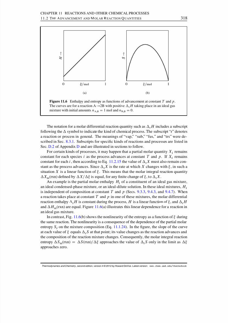
8/12/2019 Howard Devoe Thermodynamic and Chemical
http://slidepdf.com/reader/full/howard-devoe-thermodynamic-and-chemical 318/532
CHAPTER 11 REACTIONS AND OTHER CHEMICAL PROCESSES11.2 T HE A DVANCEMENT AND M OLAR R EACTION Q UANTITIES 318
mol
(a)
mol
(b)
Figure 11.6 Enthalpy and entropy as functions of advancement at constant T and p .The curves are for a reaction A ! 2B with positive rH taking place in an ideal gasmixture with initial amounts nA;0
D 1 mol and nB;0
D 0.
The notation for a molar differential reaction quantity such as rH includes a subscriptfollowing the symbol to indicate the kind of chemical process. The subscript “r” denotesa reaction or process in general. The meanings of “vap,” “sub,” “fus,” and “trs” were de-scribed in Sec. 8.3.1 . Subscripts for specic kinds of reactions and processes are listed inSec. D.2 of Appendix D and are illustrated in sections to follow.
For certain kinds of processes, it may happen that a partial molar quantity X i remainsconstant for each species i as the process advances at constant T and p . If X i remainsconstant for each i , then according to Eq. 11.2.15 the value of rX must also remain con-stant as the process advances. Since rX is the rate at which X changes with , in such asituation X is a linear function of . This means that the molar integral reaction quantityX m (rxn) dened by X= is equal, for any nite change of , to rX .
An example is the partial molar enthalpy H i of a constituent of an ideal gas mixture,an ideal condensed-phase mixture, or an ideal-dilute solution. In these ideal mixtures, H iis independent of composition at constant T and p (Secs. 9.3.3 , 9.4.3 , and 9.4.7 ). Whena reaction takes place at constant T and p in one of these mixtures, the molar differentialreaction enthalpy rH is constant during the process, H is a linear function of , and rH and H m (rxn) are equal. Figure 11.6 (a) illustrates this linear dependence for a reaction inan ideal gas mixture.
In contrast, Fig. 11.6 (b) shows the nonlinearity of the entropy as a function of duringthe same reaction. The nonlinearity is a consequence of the dependence of the partial molar
entropy S i on the mixture composition (Eq. 11.1.24 ). In the gure, the slope of the curveat each value of equals rS at that point; its value changes as the reaction advances andthe composition of the reaction mixture changes. Consequently, the molar integral reactionentropy S m(rxn) D S (rxn) = approaches the value of rS only in the limit as approaches zero.
Thermodynamics and Chemistry , second edition, version 4 © 2012 by Howard DeVoe. Latest version: www.chem.umd.edu/thermobook
8/12/2019 Howard Devoe Thermodynamic and Chemical
http://slidepdf.com/reader/full/howard-devoe-thermodynamic-and-chemical 319/532
CHAPTER 11 REACTIONS AND OTHER CHEMICAL PROCESSES11.3 M OLAR R EACTION E NTHALPY 319
11.2.3 Standard molar reaction quantities
If a chemical process takes place at constant temperature while each reactant and productremains in its standard state of unit activity, the molar reaction quantity rX is called thestandard molar reaction quantity and is denoted by rX ı . For instance, vap H ı is astandard molar enthalpy of vaporization (already discussed in Sec. 8.3.3 ), and rG
ı is the
standard molar Gibbs energy of a reaction.From Eq. 11.2.15 , the relation between a standard molar reaction quantity and the stan-
dard molar quantities of the reactants and products at the same temperature is
rX ı def
DXii X ıi (11.2.18)
Two comments are in order.1. Whereas a molar reaction quantity is usually a function of T , p , and , a standard
molar reaction quantity is a function only of T . This is evident because standard-stateconditions imply that each reactant and product is in a separate phase of constantdened composition and constant pressure p ı .
2. Since the value of a standard molar reaction quantity is independent of , the standardmolar integral and differential quantities are identical (page 318 ):
X ım(rxn) D rX ı (11.2.19)
These general concepts will now be applied to some specic chemical processes.
11.3 MOLAR REACTION ENTHALPY
Recall that H m(rxn) is a molar integral reaction enthalpy equal to H (rxn) = , and thatrH is a molar differential reaction enthalpy dened by
Pi i H i and equal to .@H=@ /T;p .
11.3.1 Molar reaction enthalpy and heat
During a process in a closed system at constant pressure with expansion work only, theenthalpy change equals the energy transferred across the boundary in the form of heat:dH D ¶q (Eq. 5.3.7 ). Thus for the molar reaction enthalpy rH D .@H=@ /T;p , whichrefers to a process not just at constant pressure but also at constant temperature, we canwrite
rH D ¶qd
(11.3.1)(constant T and p , ¶w 0D0)
Note that when there is nonexpansion work ( w0), such as electrical work, the enthalpychange is not equal to the heat. For example, if we compare a reaction taking place in a
galvanic cell with the same reaction in a reaction vessel, the heats at constant T and p fora given change of are different, and may even have opposite signs. The value of rH isthe same in both systems, but the ratio of heat to advancement, ¶q= d , is different.
An exothermic reaction is one for which rH is negative, and an endothermic reactionis one for which rH is positive. Thus in a reaction at constant temperature and pressure
Thermodynamics and Chemistry , second edition, version 4 © 2012 by Howard DeVoe. Latest version: www.chem.umd.edu/thermobook
8/12/2019 Howard Devoe Thermodynamic and Chemical
http://slidepdf.com/reader/full/howard-devoe-thermodynamic-and-chemical 320/532
CHAPTER 11 REACTIONS AND OTHER CHEMICAL PROCESSES11.3 M OLAR R EACTION E NTHALPY 320
with expansion work only, heat is transferred out of the system during an exothermic processand into the system during an endothermic process. If the process takes place at constantpressure in a system with thermally-insulated walls, the temperature increases during anexothermic process and decreases during an endothermic process.
These comments apply not just to chemical reactions, but to the other chemical pro-
cesses at constant temperature and pressure discussed in this chapter.
11.3.2 Standard molar enthalpies of reaction and formation
A standard molar reaction enthalpy , rH ı , is the same as the molar integral reaction en-thalpy H m(rxn) for the reaction taking place under standard state conditions (each reactantand product at unit activity) at constant temperature (page 319 ).
At constant temperature, partial molar enthalpies depend only mildly on pressure. It istherefore usually safe to assume that unless the experimental pressure is much greater thanp ı , the reaction is exothermic if rH ı is negative and endothermic if rH ı is positive.
The formation reaction of a substance is the reaction in which the substance, at a giventemperature and in a given physical state, is formed from the constituent elements in their
reference states at the same temperature. The reference state of an element is usually chosento be the standard state of the element in the allotropic form and physical state that is stableat the given temperature and the standard pressure. For instance, at 298:15 K and 1 bar thestable allotrope of carbon is crystalline graphite rather than diamond.
Phosphorus is an exception to the rule regarding reference states of elements. Althoughred phosphorus is the stable allotrope at 298:15 K, it is not well characterized. Instead, thereference state is white phosphorus (crystalline P 4 ) at 1 bar.
At 298:15 K, the reference states of the elements are the following: For H 2 , N2 , O2 , F2 , Cl2 , and the noble gases, the reference state is the ideal gas at1 bar.
For Br 2 and Hg, the reference state is the liquid at 1 bar.
For P, as mentioned above, the reference state is crystalline white phosphorus at 1 bar.
For all other elements, the reference state is the stable crystalline allotrope at 1 bar.The standard molar enthalpy of formation (or standard molar heat of formation),
f H ı , of a substance is the enthalpy change per amount of substance produced in theformation reaction of the substance in its standard state. Thus, the standard molar enthalpyof formation of gaseous methyl bromide at 298:15 K is the molar reaction enthalpy of thereaction
C(s, graphite, p ı ) C 32 H2 (ideal gas, p ı ) C 1
2 Br2 (l, p ı ) ! CH3 Br(ideal gas, p ı )
The value of f H ı for a given substance depends only on T . By denition, f H ı for thereference state of an element is zero.
A principle called Hess’s law can be used to calculate the standard molar enthalpy of formation of a substance at a given temperature from standard molar reaction enthalpies atthe same temperature, and to calculate a standard molar reaction enthalpy from tabulatedvalues of standard molar enthalpies of formation. The principle is an application of thefact that enthalpy is a state function. Therefore, H for a given change of the state of the
Thermodynamics and Chemistry , second edition, version 4 © 2012 by Howard DeVoe. Latest version: www.chem.umd.edu/thermobook
8/12/2019 Howard Devoe Thermodynamic and Chemical
http://slidepdf.com/reader/full/howard-devoe-thermodynamic-and-chemical 321/532
CHAPTER 11 REACTIONS AND OTHER CHEMICAL PROCESSES11.3 M OLAR R EACTION E NTHALPY 321
system is independent of the path and is equal to the sum of H values for any sequenceof changes whose net result is the given change. (We may apply the same principle to achange of any state function.)
For example, the following combustion reactions can be carried out experimentally in abomb calorimeter (Sec. 11.5.2 ), yielding the values shown below of standard molar reaction
enthalpies (at T D 298:15 K, p D pı
D 1 bar):C(s, graphite) CO2 (g) ! CO2 . g/ rH ı D 393:51 kJ mol 1
CO(g) C 12 O2 (g) ! CO2 . g/ rH ı D 282:98 kJ mol 1
(Note that the rst reaction, in addition to being the combustion reaction of graphite, isalso the formation reaction of carbon dioxide.) The change resulting from the rst reactionfollowed by the reverse of the second reaction is the formation reaction of carbon monoxide:
C(s, graphite) C 12 O2 (g) ! CO(g)
It would not be practical to measure the molar enthalpy of this last reaction by allowinggraphite to react with oxygen in a calorimeter, because it would be difcult to prevent theformation of some CO 2 . From Hess’s law, the standard molar enthalpy of formation of COis the sum of the standard molar enthalpies of the reactions that have the formation reactionas the net result:
f H ı (CO, g, 298:15 K) D . 393:51 C282:98/ kJ mol 1
D 110:53 kJ mol 1 (11.3.2)
This value is one of the many standard molar enthalpies of formation to be found incompilations of thermodynamic properties of individual substances, such as the table inAppendix H. We may use the tabulated values to evaluate the standard molar reaction en-thalpy rH ı of a reaction using a formula based on Hess’s law. Imagine the reaction to takeplace in two steps: First each reactant in its standard state changes to the constituent ele-ments in their reference states (the reverse of a formation reaction), and then these elementsform the products in their standard states. The resulting formula is
rH ı DXii f H ı .i / (11.3.3)
(Hess’s law)
where f H ı .i / is the standard molar enthalpy of formation of substance i . Recall that thestoichiometric number i of each reactant is negative and that of each product is positive, soaccording to Hess’s law the standard molar reaction enthalpy is the sum of the standard mo-lar enthalpies of formation of the products minus the sum of the standard molar enthalpiesof formation of the reactants. Each term is multiplied by the appropriate stoichiometriccoefcient from the reaction equation.
A standard molar enthalpy of formation can be dened for a solute in solution to use inEq. 11.3.3 . For instance, the formation reaction of aqueous sucrose is
12 C(s, graphite) C11 H 2 (g) C 112 O2 (g) ! C12 H22 O11 (aq)
and f H ı for C 12 H22 O11 (aq) is the enthalpy change per amount of sucrose formed whenthe reactants and product are in their standard states. Note that this formation reaction does
Thermodynamics and Chemistry , second edition, version 4 © 2012 by Howard DeVoe. Latest version: www.chem.umd.edu/thermobook

8/12/2019 Howard Devoe Thermodynamic and Chemical
http://slidepdf.com/reader/full/howard-devoe-thermodynamic-and-chemical 322/532
CHAPTER 11 REACTIONS AND OTHER CHEMICAL PROCESSES11.3 M OLAR R EACTION E NTHALPY 322
BIOGRAPHICAL SKETCHGermain Henri Hess (1802–1850)
Hess was a Russian chemist and physicianwhose calorimetric measurements led him toformulate the law of constant heat summation,now known as Hess’s law. His given name hadseveral versions: “Germain Henri” in French,as shown above; “Hermann Heinrich” in Ger-man; and “German Iwanowitsch” in Russian.
He was born in Geneva, Switzerland, theson of an artist. The family moved to Rus-sia when he was three years old; his fatherhad found work there as a tutor on an es-tate. Hess studied medicine at the Universityof Tartu in Estonia (then part of the Russianempire) and received his doctor of medicinedegree in 1825. In addition to his medical stud-ies, Hess took courses in chemistry and geol-ogy and wrote a doctoral dissertation on thecomposition of mineral waters in Russia. a
Hess was more interested in chemistry thanmedicine. He briey studied with the fa-mous Swedish chemist J ons Jakob Berzeliusin Stockholm, and they became life-longfriends. Hess then practiced medicine inIrkutsk, Siberia, while continuing his interestsin mineral chemistry and chemical analysis.
In 1829, after being being elected an adjunctmember of the St. Petersburg Academy of Sci-ences, he gave up his medical practice and be-gan teaching chemistry at various institutionsof higher learning in St. Petersburg. He wrote
a two-volume textbook, Fundamentals of PureChemistry , in 1831, followed by a one-volumeabridgment in 1834 that became the standardRussian chemistry textbook and went through
seven editions. He became a full member of the St. Petersburg Academy Academy in 1834.
Hess published the results of his thermo-
chemical research between 1839 and 1842.His 1840 paper b describes his measurementsof the heat evolved when pure sulfuric acid,H2 SO 4 , is mixed with various amounts of wa-ter, and another series of measurements of theheat evolved when the acid in H 2 SO 4 -watermixtures is neutralized with aqueous ammo-nia. The following table from this paper is of historical interest, although it is a bit difcultto decipher:
Acid Heat evolved by Sumammonia water
PH «S 595:8 595:8
PH2 «S 518:9 77:8 596:7
PH3 «S 480:5 116:7 597:2
PH6 «S 446:2 155:6 601:8Average 597:9
The rst column gives the relative amounts of acid and water in the notation of Berzelius: PHis H2 O, «S is SO 3 , and PH «S is H2 SO 4 . Thus
PH3 «S, for example, is H 2SO 4 C2H 2O. The sec-ond and third columns show the heat evolved( q) in units of calories per gram of the SO 3moiety of the H 2 SO 4 . The near-equality of thesums in the last column for the overall reaction
H2SO 4 . l/ C 2 NH 3 . aq/ ! .NH 4/ 2SO 4 . aq/demonstrates Hess’s law of constant heat sum-mation, which he stated in the words: c
The amount of heat evolved during the formationof a given compound is constant, independent of whether the compound is formed directly or in-directly in a series of steps.
Hess conrmed this law with similar exper-iments using other acids such as HCl(aq) andother bases such as NaOH(aq) and CaO(s).
After 1848 Hess’s health began to deterio-rate. He was only 48 when he died. His roleas the real founder of thermochemistry waslargely forgotten until the inuential Germanphysical chemist Wilhelm Ostwald drew atten-tion to it about forty years after Hess’s death.
a Refs. [ 93] and [100 ]. bRef. [ 77]. cRef. [ 77]; translation in Ref. [ 41].
Thermodynamics and Chemistry , second edition, version 4 © 2012 by Howard DeVoe. Latest version: www.chem.umd.edu/thermobook
8/12/2019 Howard Devoe Thermodynamic and Chemical
http://slidepdf.com/reader/full/howard-devoe-thermodynamic-and-chemical 323/532
CHAPTER 11 REACTIONS AND OTHER CHEMICAL PROCESSES11.3 M OLAR R EACTION E NTHALPY 323
not include the formation of the solvent H 2 O from H 2 and O 2 . Instead, the solute onceformed combines with the amount of pure liquid water needed to form the solution. If theaqueous solute is formed in its standard state, the amount of water needed is very large soas to have the solute exhibit innite-dilution behavior.
There is no ordinary reaction that would produce an individual ion in solution from its
element or elements without producing other species as well. We can, however, preparea consistent set of standard molar enthalpies of formation of ions by assigning a value toa single reference ion. 7 We can use these values for ions in Eq. 11.3.3 just like values of
f H ı for substances and nonionic solutes. Aqueous hydrogen ion is the usual referenceion, to which is assigned the arbitrary value
f H ı (H C ,aq) D 0 (at all temperatures) (11.3.4)
To see how we can use this reference value, consider the reaction for the formation of aqueous HCl (hydrochloric acid):
12 H2 . g/ C 1
2 Cl2 . g/ ! HC . aq / CCl . aq /
The standard molar reaction enthalpy at 298:15 K for this reaction is known, from reaction
calorimetry, to have the value rH ı D 167:08 kJ mol 1 . The standard states of thegaseous H 2 and Cl 2 are, of course, the pure gases acting ideally at pressure p ı , and thestandard state of each of the aqueous ions is the ion at the standard molality and standardpressure, acting as if its activity coefcient on a molality basis were 1. From Eq. 11.3.3 , weequate the value of rH ı to the sum
12 f H ı (H 2 , g) 1
2 f H ı (Cl 2 , g) C f H ı (H C ,aq) C f H ı (Cl , aq)
But the rst three terms of this sum are zero. Therefore, the value of f H ı (Cl ,aq) is167:08 kJ mol 1 .
Next we can combine this value of f H ı (Cl , aq) with the measured standard molarenthalpy of formation of aqueous sodium chloride
Na . s/ C 12 Cl2 . g/ ! NaC . aq / CCl . aq /to evaluate the standard molar enthalpy of formation of aqueous sodium ion. By continuingthis procedure with other reactions, we can build up a consistent set of f H ı values of various ions in aqueous solution.
11.3.3 Molar reaction heat capacity
The molar reaction enthalpy rH is in general a function of T , p , and . Using the relationsrH DPi i H i (from Eq. 11.2.15 ) and C p;i D .@H i =@T /p; (Eq. 9.2.52 ), we can write
@ rH @T p; D
@
Pi i H i@T p; D
Xi
i C p;i D rC p (11.3.5)
where rC p is the molar reaction heat capacity at constant pressure, equal to the rate atwhich the heat capacity C p changes with at constant T and p .
Under standard state conditions, Eq. 11.3.5 becomes
d rH ı = dT D rC ıp (11.3.6)
7This procedure is similar to that described on page 235 for partial molar volumes of ions.
Thermodynamics and Chemistry , second edition, version 4 © 2012 by Howard DeVoe. Latest version: www.chem.umd.edu/thermobook

8/12/2019 Howard Devoe Thermodynamic and Chemical
http://slidepdf.com/reader/full/howard-devoe-thermodynamic-and-chemical 324/532
CHAPTER 11 REACTIONS AND OTHER CHEMICAL PROCESSES11.3 M OLAR R EACTION E NTHALPY 324
(rxn,
)
(rxn, )
Figure 11.7 Dependence of reaction enthalpy on temperature at constant pressure.
11.3.4 Effect of temperature on reaction enthalpy
Consider a reaction occurring with a certain nite change of the advancement in a closedsystem at temperature T 0 and at constant pressure. The reaction is characterized by a changeof the advancement from
1 to
2, and the integral reaction enthalpy at this temperature is
denoted H (rxn, T 0). We wish to nd an expression for the reaction enthalpy H (rxn, T 00)for the same values of 1 and 2 at the same pressure but at a different temperature, T 00.
The heat capacity of the system at constant pressure is related to the enthalpy by Eq. 5.6.3on page 144 : C p D .@H=@T /p; . We integrate d H D C p dT from T 0 to T 00at constant pand , for both the nal and initial values of the advancement:
H. 2 ; T 00/ D H . 2 ; T 0/ CZ T 00
T 0C p . 2 / dT (11.3.7)
H. 1 ; T 00/ D H . 1 ; T 0/ C
Z
T 00
T 0C p . 1 / dT (11.3.8)
Subtracting Eq. 11.3.8 from Eq. 11.3.7 , we obtain
H (rxn, T 00) D H (rxn, T 0) CZ T 00
T 0C p dT (11.3.9)
where C p is the difference between the heat capacities of the system at the nal and initialvalues of , a function of T : C p D C p . 2 / C p . 1 / . Equation 11.3.9 is the Kirchhoff equation .
When C p is essentially constant in the temperature range from T 0 to T 00, the Kirchhoff equation becomes
H (rxn, T 00)
D H (rxn, T 0)
CC p .T 00 T 0/ (11.3.10)
Figure 11.7 illustrates the principle of the Kirchhoff equation as expressed by Eq.11.3.10 . C p equals the difference in the slopes of the two dashed lines in the gure, andthe product of C p and the temperature difference T 00 T 0 equals the change in the valueof H (rxn). The gure illustrates an exothermic reaction with negative C p , resulting ina more negative value of H (rxn) at the higher temperature.
Thermodynamics and Chemistry , second edition, version 4 © 2012 by Howard DeVoe. Latest version: www.chem.umd.edu/thermobook
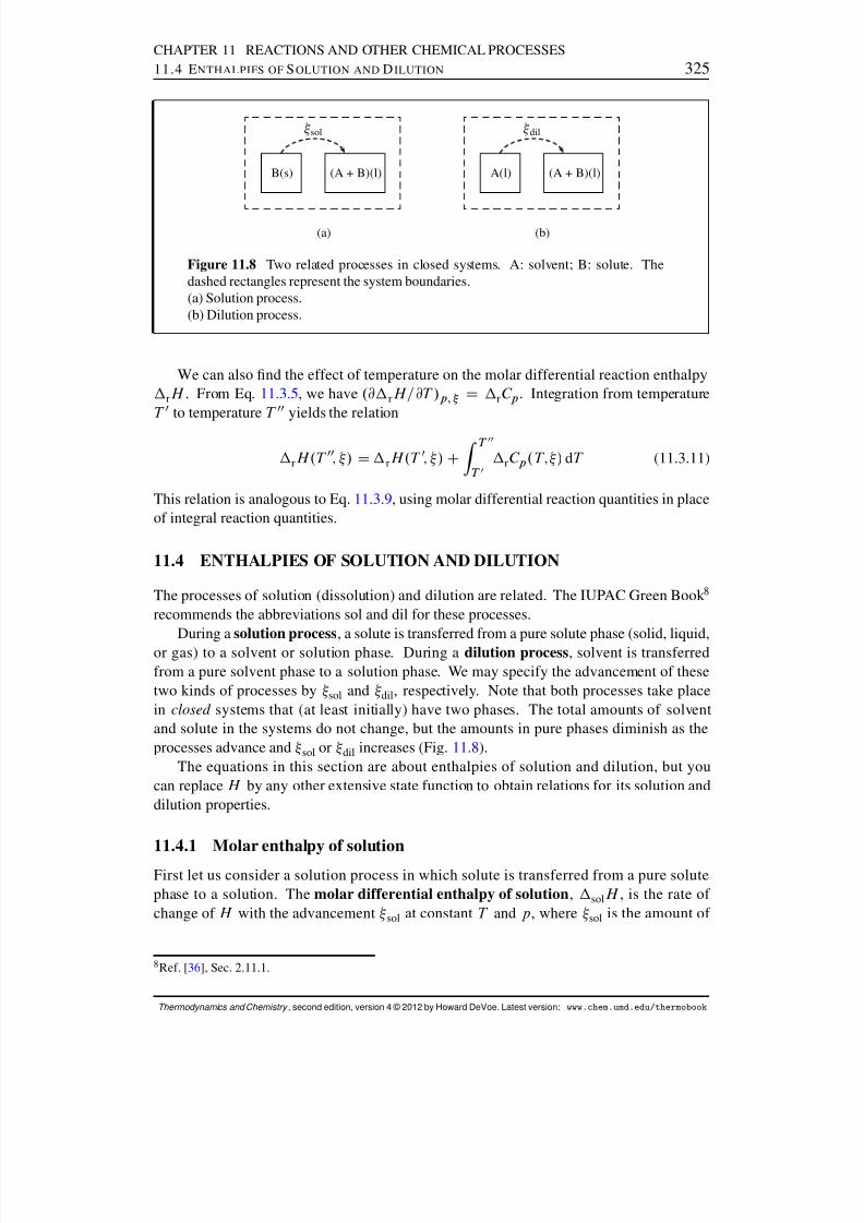
8/12/2019 Howard Devoe Thermodynamic and Chemical
http://slidepdf.com/reader/full/howard-devoe-thermodynamic-and-chemical 325/532
CHAPTER 11 REACTIONS AND OTHER CHEMICAL PROCESSES11.4 E NTHALPIES OF S OLUTION AND D ILUTION 325
B(s) (A + B)(l)
sol
(a)
A(l) (A + B)(l)
dil
(b)
Figure 11.8 Two related processes in closed systems. A: solvent; B: solute. Thedashed rectangles represent the system boundaries.(a) Solution process.(b) Dilution process.
We can also nd the effect of temperature on the molar differential reaction enthalpyrH . From Eq. 11.3.5 , we have .@ rH=@T /p; D rC p . Integration from temperature
T 0 to temperature T 00yields the relation
rH.T 00; / D rH.T 0; / CZ T 00
T 0rC p .T; / dT (11.3.11)
This relation is analogous to Eq. 11.3.9 , using molar differential reaction quantities in placeof integral reaction quantities.
11.4 ENTHALPIES OF SOLUTION AND DILUTION
The processes of solution (dissolution) and dilution are related. The IUPAC Green Book 8
recommends the abbreviations sol and dil for these processes.During a solution process , a solute is transferred from a pure solute phase (solid, liquid,
or gas) to a solvent or solution phase. During a dilution process , solvent is transferredfrom a pure solvent phase to a solution phase. We may specify the advancement of thesetwo kinds of processes by sol and dil , respectively. Note that both processes take placein closed systems that (at least initially) have two phases. The total amounts of solventand solute in the systems do not change, but the amounts in pure phases diminish as theprocesses advance and sol or dil increases (Fig. 11.8 ).
The equations in this section are about enthalpies of solution and dilution, but youcan replace H by any other extensive state function to obtain relations for its solution anddilution properties.
11.4.1 Molar enthalpy of solution
First let us consider a solution process in which solute is transferred from a pure solutephase to a solution. The molar differential enthalpy of solution , sol H , is the rate of change of H with the advancement sol at constant T and p , where sol is the amount of
8Ref. [ 36], Sec. 2.11.1.
Thermodynamics and Chemistry , second edition, version 4 © 2012 by Howard DeVoe. Latest version: www.chem.umd.edu/thermobook
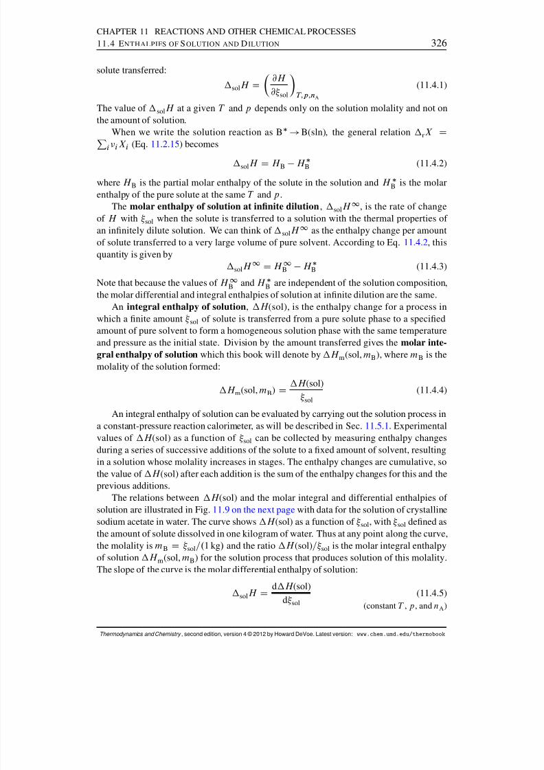
8/12/2019 Howard Devoe Thermodynamic and Chemical
http://slidepdf.com/reader/full/howard-devoe-thermodynamic-and-chemical 326/532
CHAPTER 11 REACTIONS AND OTHER CHEMICAL PROCESSES11.4 E NTHALPIES OF S OLUTION AND D ILUTION 326
solute transferred:
sol H D @H @ sol T;p;n A
(11.4.1)
The value of sol H at a given T and p depends only on the solution molality and not onthe amount of solution.
When we write the solution reaction as B ! B(sln), the general relation rX DPi i X i (Eq. 11.2.15 ) becomes
sol H D H B H B (11.4.2)
where H B is the partial molar enthalpy of the solute in the solution and H B is the molarenthalpy of the pure solute at the same T and p .
The molar enthalpy of solution at innite dilution , sol H 1 , is the rate of changeof H with sol when the solute is transferred to a solution with the thermal properties of an innitely dilute solution. We can think of sol H 1 as the enthalpy change per amountof solute transferred to a very large volume of pure solvent. According to Eq. 11.4.2 , thisquantity is given by
sol H 1
D H 1B H B (11.4.3)
Note that because the values of H 1B and H B are independent of the solution composition,
the molar differential and integral enthalpies of solution at innite dilution are the same.An integral enthalpy of solution , H (sol), is the enthalpy change for a process in
which a nite amount sol of solute is transferred from a pure solute phase to a speciedamount of pure solvent to form a homogeneous solution phase with the same temperatureand pressure as the initial state. Division by the amount transferred gives the molar inte-gral enthalpy of solution which this book will denote by H m (sol, mB), where mB is themolality of the solution formed:
H m(sol, mB) D H (sol)
sol(11.4.4)
An integral enthalpy of solution can be evaluated by carrying out the solution process ina constant-pressure reaction calorimeter, as will be described in Sec. 11.5.1 . Experimentalvalues of H (sol) as a function of sol can be collected by measuring enthalpy changesduring a series of successive additions of the solute to a xed amount of solvent, resultingin a solution whose molality increases in stages. The enthalpy changes are cumulative, sothe value of H (sol) after each addition is the sum of the enthalpy changes for this and theprevious additions.
The relations between H (sol) and the molar integral and differential enthalpies of solution are illustrated in Fig. 11.9 on the next page with data for the solution of crystallinesodium acetate in water. The curve shows H (sol) as a function of sol , with sol dened asthe amount of solute dissolved in one kilogram of water. Thus at any point along the curve,the molality is mB D sol =.1 kg / and the ratio H (sol) = sol is the molar integral enthalpyof solution H m (sol, mB) for the solution process that produces solution of this molality.The slope of the curve is the molar differential enthalpy of solution:
sol H D d H (sol)
d sol(11.4.5)
(constant T , p , and nA )
Thermodynamics and Chemistry , second edition, version 4 © 2012 by Howard DeVoe. Latest version: www.chem.umd.edu/thermobook
8/12/2019 Howard Devoe Thermodynamic and Chemical
http://slidepdf.com/reader/full/howard-devoe-thermodynamic-and-chemical 327/532
CHAPTER 11 REACTIONS AND OTHER CHEMICAL PROCESSES11.4 E NTHALPIES OF S OLUTION AND D ILUTION 327
a
bc
sol
mol
.
s o
l
k J
Figure 11.9 Enthalpy change for the dissolution of NaCH 3 CO 2 (s) in one kilogramof water in a closed system at 298:15 K and 1 bar, as a function of the amount sol of dissolved solute. a The open circle at solD15 mol indicates the approximate satura-
tion limit; data to the right of this point come from supersaturated solutions. At thecomposition mBD15 mol kg 1 , the value of H m (sol, mB) is the slope of line a andthe value of sol H is the slope of line b. The value of sol H 1 is the slope of line c.
a Data from Ref. [ 163 ], page 2-315.
The slope of the curve at solD0 is sol H 1 , the molar enthalpy of solution at innitedilution. If the measurements are made at the standard pressure, sol H 1 is the same asthe standard molar enthalpy of solution, sol H ı , because the standard molar enthalpy of asolute is the molar enthalpy at p Dp ı and innite dilution.
11.4.2 Enthalpy of dilutionNext let us consider a dilution process in which solvent is transferred from a pure solventphase to a solution phase. The molar differential enthalpy of dilution is the rate of changeof H with the advancement dil at constant T and p of the dilution process, where dil is theamount of solvent transferred:
dil H D @H @ dil T;p;n B
(11.4.6)
For the dilution reaction A ! A(sln), the general relation rX DPi i X i becomes
dilH
D H
AH
A (11.4.7)
where H A is the partial molar enthalpy of the solvent in the solution. In the limit of innitedilution, H A must approach the molar enthalpy of pure solvent, H A ; then Eq. 11.4.7 showsthat dil H approaches zero in this limit.
An integral enthalpy of dilution , H (dil), refers to the enthalpy change for transferof a nite amount of solvent from a pure solvent phase to a solution, T and p being the
Thermodynamics and Chemistry , second edition, version 4 © 2012 by Howard DeVoe. Latest version: www.chem.umd.edu/thermobook
8/12/2019 Howard Devoe Thermodynamic and Chemical
http://slidepdf.com/reader/full/howard-devoe-thermodynamic-and-chemical 328/532
CHAPTER 11 REACTIONS AND OTHER CHEMICAL PROCESSES11.4 E NTHALPIES OF S OLUTION AND D ILUTION 328
same before and after the process. The molar integral enthalpy of dilution is the ratio of H (dil) and the amount of solute in the solution. For a dilution process at constant soluteamount nB in which the molality changes from m0
B to m00B , this book will use the notation
H m . dil, m0B! m00
B / :
H m . dil, m0B
!m00
B /
D
H (dil)
nB
(11.4.8)
The value of H m . dil, m0B! m00
B / at a given T and p depends only on the initial and nalmolalities m0
B and m00B .
There is a simple relation between molar integral enthalpies of solution and dilution,as the following derivation demonstrates. Consider the following two ways of preparing asolution of molality m00
B from pure solvent and solute phases. Both paths are at constant T and p in a closed system.Path 1: The solution forms directly by dissolution of the solute in the solvent. The en-
thalpy change is nB H m . sol, m00B / , where the molality of the solution is indicated in
parentheses.
Path 2: Starting with the unmixed solvent and solute, the solute dissolves in a portion of
the solvent to form a solution of composition m0B (more concentrated than m
00B). The
enthalpy change is nB H m . sol, m0B / . In a second step of this path, the remaining pure
solvent mixes with the solution to dilute it from m0B to m00
B . The enthalpy change of thesecond step is nB H m . dil, m0
B! m00B / .
Since both paths have the same initial states and the same nal states, both have the sameoverall enthalpy change:
nB H m . sol, m00B / D nB H m . sol, m0
B/ CnB H m . dil, m0B! m00
B / (11.4.9)
orH m . sol, m00
B / D H m . sol, m0B/ CH m . dil, m0
B! m00B / (11.4.10)
Equation 11.4.10 is the desired relation. It shows how a measurement of the molar integral
enthalpy change for a solution process that produces solution of a certain molality canbe combined with dilution measurements in order to calculate molar integral enthalpies of solution for more dilute solutions. Experimentally, it is sometimes more convenient to carryout the dilution process than the solution process, especially when the pure solute is a gasor solid.
11.4.3 Molar enthalpies of solute formation
Molar integral enthalpies of solution and dilution are conveniently expressed in terms of molar enthalpies of formation. The molar enthalpy of formation of a solute in solution isthe enthalpy change per amount of solute for a process at constant T and p in which thesolute, in a solution of a given molality, is formed from its constituent elements in theirreference states. The molar enthalpy of formation of solute B in solution of molality mBwill be denoted by f H (B, mB).
As explained in Sec. 11.3.2 , the formation reaction of a solute in solution does notinclude the formation of the solvent from its elements. For example, the formation reactionfor NaOH in an aqueous solution that has 50 moles of water for each mole of NaOH is
Na(s) C 12 O2 (g) C 1
2 H2 (g) C50 H2 O(l) ! NaOH in 50 H2 O
Thermodynamics and Chemistry , second edition, version 4 © 2012 by Howard DeVoe. Latest version: www.chem.umd.edu/thermobook
8/12/2019 Howard Devoe Thermodynamic and Chemical
http://slidepdf.com/reader/full/howard-devoe-thermodynamic-and-chemical 329/532
CHAPTER 11 REACTIONS AND OTHER CHEMICAL PROCESSES11.4 E NTHALPIES OF S OLUTION AND D ILUTION 329
Consider a solution process at constant T and p in which an amount nB of pure solute(solid, liquid, or gas) is mixed with an amount nA of pure solvent, resulting in solution of molality mB . We may equate the enthalpy change of this process to the sum of the enthalpychanges for the following two hypothetical steps:
1. An amount nB of the pure solute decomposes to the constituent elements in their
reference states. This is the reverse of the formation reaction of the pure solute.2. The solution is formed from these elements and an amount nA of the solvent.
The total enthalpy change is then H (sol) D nB f H (B ) CnB f H (B, mB). Dividingby nB , we obtain the molar integral enthalpy of solution:
H m (sol, mB) D f H (B, mB) f H (B ) (11.4.11)
By combining Eqs. 11.4.10 and 11.4.11 , we obtain the following expression for a molarintegral enthalpy of dilution in terms of molar enthalpies of formation:
H m . dil, m0B! m00
B / D f H (B, m00B) f H (B, m0
B) (11.4.12)
From tabulated values of molar enthalpies of formation, we can calculate molar integralenthalpies of solution with Eq. 11.4.11 and molar integral enthalpies of dilution with Eq.11.4.12 . Conversely, calorimetric measurements of these molar integral enthalpies can becombined with the value of f H (B ) to establish the values of molar enthalpies of soluteformation in solutions of various molalities.
11.4.4 Evaluation of relative partial molar enthalpies
Although it is not possible to determine absolute values of partial molar enthalpies, we canevaluate H A and H B relative to appropriate solvent and solute reference states.
The relative partial molar enthalpy of the solvent is dened by
L A def D H A H A (11.4.13)
This is the partial molar enthalpy of the solvent in a solution of given composition relativeto pure solvent at the same temperature and pressure.
L A can be related to molar differential and integral enthalpies of solution as follows.The enthalpy change to form a solution from amounts nA and nB of pure solvent and soluteis given, from the additivity rule, by H (sol) D .n AH A CnBH B / .n AH A CnBH B / . Werearrange and make substitutions from Eqs. 11.4.2 and 11.4.13 :
H (sol) D nA .H A H A / CnB .H B H B /
D nAL A CnB sol H (11.4.14)
H (sol) is also given, from Eq. 11.4.4 , by
H (sol) D nB H m(sol, mB) (11.4.15)
Equating both expressions for H (sol), solving for L A , and replacing n B=n A by M AmB ,we obtain
L A D M AmB ΠH m(sol, mB) sol H (11.4.16)
Thermodynamics and Chemistry , second edition, version 4 © 2012 by Howard DeVoe. Latest version: www.chem.umd.edu/thermobook
8/12/2019 Howard Devoe Thermodynamic and Chemical
http://slidepdf.com/reader/full/howard-devoe-thermodynamic-and-chemical 330/532

8/12/2019 Howard Devoe Thermodynamic and Chemical
http://slidepdf.com/reader/full/howard-devoe-thermodynamic-and-chemical 331/532
CHAPTER 11 REACTIONS AND OTHER CHEMICAL PROCESSES11.4 E NTHALPIES OF S OLUTION AND D ILUTION 331
H (sol) D sol H m(sol, mB) and take the derivative of the expression with respect to sol :
sol H D d Πsol H m (sol, mB)
d sol
D H m(sol, mB) C sold H m (sol, mB)
d sol
(11.4.20)
At constant nA , mB is proportional to sol , so that d sol = sol can be replaced by d mB=m B .When we combine the resulting expression for sol H with Eq. 11.4.19 , we get the follow-ing expression for the relative partial molar enthalpy of the solute:
L B D H m (sol, mB) CmBd H m(sol, mB)
dmBsol H 1 (11.4.21)
It is convenient to dene the quantity
˚ Ldef
D H m(sol, mB) sol H 1 (11.4.22)
known as the relative apparent molar enthalpy of the solute
. Because sol H 1
is indepen-dent of mB , the derivative d ˚ L = dmB is equal to d H m (sol, mB)= dmB . We can thereforewrite Eq. 11.4.21 in the compact form
L B D ˚ L CmBd˚ L
dmB(11.4.23)
(constant T and p )
Equation 11.4.23 allows us to evaluate L B at any molality from the dependence of ˚ L onmB , with ˚ L obtained from experimental molar integral enthalpies of solution according toEq. 11.4.22 .
Once ˚ L and L B have been evaluated for a given molality, it is a simple matter tocalculate L A at that molality. By combining Eqs. 11.4.16 and 11.4.22 , we obtain the relation
L A D M AmB .˚ L L B / (11.4.24)
For an electrolyte solute, a plot of H m(sol, mB) versus mB has a limiting slope of C1at mBD0, whereas the limiting slope of H m(sol, mB) versus p mB is nite and can bepredicted from the Debye–H uckel limiting law. Accordingly, a satisfactory procedure is toplot H m(sol, mB) versus p mB , perform a linear extrapolation of the experimental pointsto p mBD0, and then shift the origin to the extrapolated intercept. The result is a plot of ˚ Lversus p mB . An example for aqueous NaCl solutions is shown in Fig. 11.10 (a) on the nextpage.
We can also evaluate ˚ L from experimental enthalpies of dilution. From Eqs. 11.4.10and 11.4.22 , we obtain the relation
˚ L .m 00B / ˚ L .m 0
B / D H m . dil, m0B! m00
B / (11.4.25)
We can measure the enthalpy changes for diluting a solution of initial molality m0B to various
molalities m00B , plot the values of H m . dil, m0
B! m00B / versus p mB , extrapolate the curve to
p mBD0, and shift the origin to the extrapolated intercept, resulting in a plot of ˚ L versusp mB .
Thermodynamics and Chemistry , second edition, version 4 © 2012 by Howard DeVoe. Latest version: www.chem.umd.edu/thermobook

8/12/2019 Howard Devoe Thermodynamic and Chemical
http://slidepdf.com/reader/full/howard-devoe-thermodynamic-and-chemical 332/532
CHAPTER 11 REACTIONS AND OTHER CHEMICAL PROCESSES11.4 E NTHALPIES OF S OLUTION AND D ILUTION 332
0 0.5 1.0 1.5 2.0
B mol kg
(a)
m
s o l
k J m o l
k J m o l
B mol kg
(b)
B
k J m o l
Figure 11.10 Thermal properties of aqueous NaCl at 25:00 ı C.(a) Left axis: molar integral enthalpy of solution to produce solution of molality mB .a
The dashed line has a slope equal to the theoretical limiting value of the slope of thecurve. Right axis: relative apparent molar enthalpy of the solute.(b) Relative partial molar enthalpy of the solute as a function of molality. b
a Calculated from molar enthalpy of formation values in Ref. [ 163 ], p. 2-301.bBased on data in Ref. [ 125 ], Table X.
In order to be able to use Eq. 11.4.23 , we need to relate the derivative d ˚ L = dmB to theslope of the curve of ˚ L versus p mB . We write
dp mB D 1
2p mBdmB dmB D 2p mB dp mB (11.4.26)
Substituting this expression for d mB into Eq. 11.4.23 , we obtain the following operationalequation for evaluating L B from the plot of ˚ L versus p mB :
L B D ˚ L Cp mB
2d˚ L
dp mB(11.4.27)
(constant T and p )
The value of ˚ L goes to zero at innite dilution. When the solute is an electrolyte, thedependence of ˚ L on mB in solutions dilute enough for the Debye–H uckel limiting law toapply is given by
˚ L D C Lp mB (11.4.28)
(very dilute solution)
For aqueous solutions of a 1:1 electrolyte at 25 ı C, the coefcient C L
has the value 10
C L D 1:988 103 J kg 1=2 mol 3=2 (11.4.29)
10 Thefact that C L
is positive means, according to Eq. 11.4.25 , that dilution of a very dilute electrolyte solutionis an exothermic process.
Thermodynamics and Chemistry , second edition, version 4 © 2012 by Howard DeVoe. Latest version: www.chem.umd.edu/thermobook
8/12/2019 Howard Devoe Thermodynamic and Chemical
http://slidepdf.com/reader/full/howard-devoe-thermodynamic-and-chemical 333/532
CHAPTER 11 REACTIONS AND OTHER CHEMICAL PROCESSES11.4 E NTHALPIES OF S OLUTION AND D ILUTION 333
C L
is equal to the limiting slope of ˚ L versus p mB , of H m (sol, mB) versus p mB ,and of H m . dil, m0
B! m00B / versus p m0
B . The value given by Eq. 11.4.29 can be used forextrapolation of measurements at 25 ı C and low molality to innite dilution.
Equation 11.4.28 can be derived as follows. For simplicity, we assume the pressureis the standard pressure p ı . At this pressure H 1
B is the same as H ı
B, and Eq. 11.4.17
becomes L B D H B H ıB . From Eqs. 12.1.3 and 12.1.6 in the next chapter, we can
write the relations
H B D T 2@. B=T /
@T p; f n i gH ı
B D T 2d. ı
m; B=T /
dT (11.4.30)
Subtracting the second of these relations from the rst, we obtain
H B H ıB D T 2
@. Bım; B /=T
@T p; f n ig(11.4.31)
The solute activity on a molality basis, a m; B , is dened by B ım; B D RT ln a m; B .
The activity of an electrolyte solute at the standard pressure, from Eq. 10.3.10 , is given
by a m; B D .C
C / ˙ .m B=m ı / . Accordingly, the relative partial molar enthalpyof the solute is related to the mean ionic activity coefcient by
L B D RT 2 @ln ˙
@T p; f n i g(11.4.32)
We assume the solution is sufciently dilute for the mean ionic activity coefcientto be adequately described by the Debye–H¨ uckel limiting law, Eq. 10.4.8 : ln ˙ DADH jzC z jp I m , where A DH is a temperature-dependent quantity dened on page295 . Then Eq. 11.4.32 becomes
L B D RT 2 jzC z j
p I m
@ADH
@T p; f n i g(11.4.33)
(very dilute solution)
Substitution of the expression given by Eq. 10.4.9 on page 298 for I m in a solution of a single completely-dissociated electrolyte converts Eq. 11.4.33 to
L B D"RT 2
p 2@AADH
@T p; f n i gjzC z j
3=2#p mB
D C L Bp mB (11.4.34)
(very dilute solution)
The coefcient C L B(the quantity in brackets) depends on T , the kind of solvent, and
the ion charges and number of ions per solute formula unit, but not on the solutemolality.
Let C ˚ L
represent the limiting slope of ˚L
versus
p m
B. In a very dilute solution
we have ˚ L D C L p mB , and Eq. 11.4.27 becomes
L B D ˚ L Cp mB
2d˚ L
dp mB D C Lp mB C
p mB
2 C
L (11.4.35)
By equating this expression for L B with the one given by Eq. 11.4.34 and solving forC
L, we obtain C
L D .2=3/C L Band ˚ L D .2=3/C L B
p mB .
Thermodynamics and Chemistry , second edition, version 4 © 2012 by Howard DeVoe. Latest version: www.chem.umd.edu/thermobook
8/12/2019 Howard Devoe Thermodynamic and Chemical
http://slidepdf.com/reader/full/howard-devoe-thermodynamic-and-chemical 334/532
CHAPTER 11 REACTIONS AND OTHER CHEMICAL PROCESSES11.5 R EACTION C ALORIMETRY 334
11.5 REACTION CALORIMETRY
Reaction calorimetry is used to evaluate the molar integral reaction enthalpy H m (rxn) of areaction or other chemical process at constant temperature and pressure. The measurementactually made, however, is a temperature change.
Sections 11.5.1 and 11.5.2 will describe two common types of calorimeters designed forreactions taking place at either constant pressure or constant volume. The constant-pressuretype is usually called a reaction calorimeter , and the constant-volume type is known as abomb calorimeter or combustion calorimeter .
In either type of calorimeter, the chemical process takes place in a reaction vessel sur-rounded by an outer jacket. The jacket may be of either the adiabatic type or the isothermal- jacket type described in Sec. 7.3.2 in connection with heat capacity measurements. Atemperature-measuring device is immersed either in the vessel or in a phase in thermalcontact with it. The measured temperature change is caused by the chemical process, in-stead of by electrical work as in the determination of heat capacity. One important way inwhich these calorimeters differ from ones used for heat capacity measurements is that work is kept deliberately small, in order to minimize changes of internal energy and enthalpy
during the experimental process.
11.5.1 The constant-pressure reaction calorimeter
The contents of a constant-pressure calorimeter are usually open to the atmosphere, so thistype of calorimeter is unsuitable for processes involving gases. It is, however, a convenientapparatus in which to study a liquid-phase chemical reaction, the dissolution of a solid orliquid solute in a liquid solvent, or the dilution of a solution with solvent.
The process is initiated in the calorimeter by allowing the reactants to come into contact.The temperature in the reaction vessel is measured over a period of time starting before theprocess initiation and ending after the advancement has reached a nal value with no furtherchange.
The heating or cooling curve (temperature as a function of time) is observed over aperiod of time that includes the period during which changes. For an exothermic reactionoccurring in an adiabatic calorimeter, the heating curve may resemble that shown in Fig. 7.3on page 170 , and the heating curve in an isothermal-jacket calorimeter may resemble thatshown in Fig. 7.4 on page 172 . Two points are designated on the heating or cooling curve:one at temperature T 1 , before the reaction is initiated, and the other at T 2 , after has reachedits nal value. These points are indicated by open circles in Figs. 7.3 and 7.4 .
Figure 11.11 on the next page depicts three paths at constant pressure. The enthalpychange of the experimental process, in which reactants at temperature T 1 change to productsat temperature T 2 , is denoted H (expt).
The value of H (expt) at constant pressure would be zero if the process were perfectlyadiabatic and the only work were expansion work, but this is rarely the case. There may beunavoidable work from stirring and from electrical temperature measurement. We can eval-uate H (expt) by one of the methods described in Sec. 7.3.2 . For an adiabatic calorimeter,the appropriate expression is H (expt) D r.t 2 t1 / (Eq. 7.3.19 on page 171 with welset equal to zero), where is the energy equivalent of the calorimeter, r is the slope of theheating curve when no reaction is occurring, and t1 and t2 are the times at temperatures T 1
Thermodynamics and Chemistry , second edition, version 4 © 2012 by Howard DeVoe. Latest version: www.chem.umd.edu/thermobook
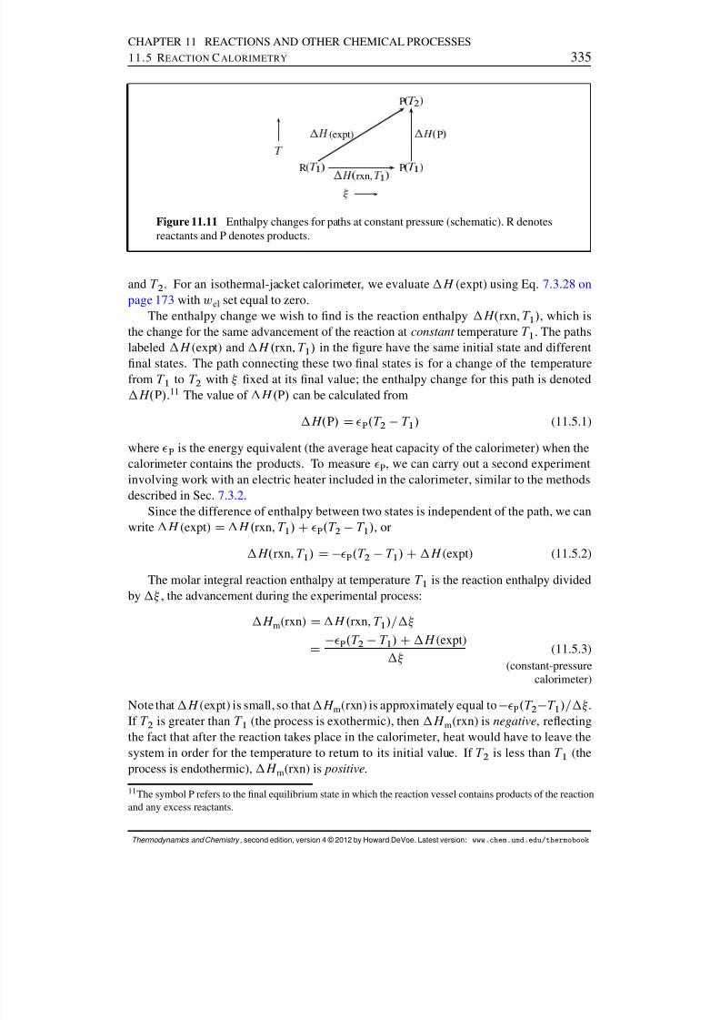
8/12/2019 Howard Devoe Thermodynamic and Chemical
http://slidepdf.com/reader/full/howard-devoe-thermodynamic-and-chemical 335/532
CHAPTER 11 REACTIONS AND OTHER CHEMICAL PROCESSES11.5 R EACTION C ALORIMETRY 335
R
P
P
(expt)
rxn,
P
Figure 11.11 Enthalpy changes for paths at constant pressure (schematic). R denotesreactants and P denotes products.
and T 2 . For an isothermal-jacket calorimeter, we evaluate H (expt) using Eq. 7.3.28 onpage 173 with wel set equal to zero.
The enthalpy change we wish to nd is the reaction enthalpy H. rxn, T 1 / , which isthe change for the same advancement of the reaction at constant temperature T 1 . The pathslabeled H (expt) and H . rxn, T 1 / in the gure have the same initial state and differentnal states. The path connecting these two nal states is for a change of the temperaturefrom T 1 to T 2 with xed at its nal value; the enthalpy change for this path is denotedH. P/ .11 The value of H. P/ can be calculated from
H. P/ D P .T 2 T 1 / (11.5.1)
where P is the energy equivalent (the average heat capacity of the calorimeter) when thecalorimeter contains the products. To measure P , we can carry out a second experimentinvolving work with an electric heater included in the calorimeter, similar to the methodsdescribed in Sec. 7.3.2 .
Since the difference of enthalpy between two states is independent of the path, we canwrite H (expt)
D H . rxn, T 1 /
CP .T 2 T 1 / , or
H. rxn, T 1 / D P .T 2 T 1 / CH (expt) (11.5.2)
The molar integral reaction enthalpy at temperature T 1 is the reaction enthalpy dividedby , the advancement during the experimental process:
H m(rxn) D H . rxn, T 1 /=
D P .T 2 T 1 / CH (expt)
(11.5.3)(constant-pressure
calorimeter)
Note that H (expt) is small, so that H m(rxn) is approximately equal to P .T 2 T 1 /= .If T 2 is greater than T 1 (the process is exothermic), then H m (rxn) is negative , reectingthe fact that after the reaction takes place in the calorimeter, heat would have to leave thesystem in order for the temperature to return to its initial value. If T 2 is less than T 1 (theprocess is endothermic), H m(rxn) is positive .
11 The symbol P refers to the nal equilibrium state in which the reaction vessel contains products of the reactionand any excess reactants.
Thermodynamics and Chemistry , second edition, version 4 © 2012 by Howard DeVoe. Latest version: www.chem.umd.edu/thermobook
8/12/2019 Howard Devoe Thermodynamic and Chemical
http://slidepdf.com/reader/full/howard-devoe-thermodynamic-and-chemical 336/532
CHAPTER 11 REACTIONS AND OTHER CHEMICAL PROCESSES11.5 R EACTION C ALORIMETRY 336
Most reactions cause a change in the composition of one or more phases, in which caseH m(rxn) is not the same as the molar differential reaction enthalpy, rH D .@H=@ /T;p ,unless the phase or phases can be treated as ideal mixtures (see Sec. 11.2.2 ). Correc-tions, usually small, are needed to obtain the standard molar reaction enthalpy rH ı fromH m(rxn).
11.5.2 The bomb calorimeter
A bomb calorimeter typically is used to carry out the complete combustion of a solid orliquid substance in the presence of excess oxygen. The combustion reaction is initiated withelectrical ignition. In addition to the main combustion reaction, there may be unavoidableside reactions, such as the formation of nitrogen oxides if N 2 is not purged from the gasphase. Sometimes auxiliary reactions are deliberately carried out to complete or moderatethe main reaction.
From the measured heating curve and known properties of the calorimeter, reactants,and products, it is possible to evaluate the standard molar enthalpy of combustion, cH ı ,of the substance of interest at a particular temperature called the reference temperature, T ref .
(T ref is often chosen to be 298:15 K, which is 25:00 ı C.) With careful work, using temper-ature measurements with a resolution of 1 10 4 K or better and detailed corrections, theprecision of cH ı can be of the order of 0:01 percent.
Bomb calorimetry is the principal means by which standard molar enthalpies of com-bustion of individual elements and of compounds of these elements are evaluated. Fromthese values, using Hess’s law, we can calculate the standard molar enthalpies of formationof the compounds as described in Sec. 11.3.2 . From the formation values of only a few com-pounds, the standard molar reaction enthalpies of innumerable reactions can be calculatedwith Hess’s law (Eq. 11.3.3 on page 321 ).
Because of their importance, the experimental procedure and the analysis of the datait provides will now be described in some detail. A comprehensive problem (Prob. 11. 7)
based on this material is included at the end of the chapter.There are ve main steps in the procedure of evaluating a standard molar enthalpy of combustion:
1. The combustion reaction, and any side reactions and auxiliary reactions, are carriedout in the calorimeter, and the course of the resulting temperature change is observed.
2. The experimental data are used to determine the value of U. IBP ; T 2 / , the internalenergy change of the isothermal bomb process at the nal temperature of the reaction.The isothermal bomb process is the idealized process that would have occurred if the reaction or reactions had taken place in the calorimeter at constant temperature.
3. The internal energy change of the isothermal bomb process is corrected to yieldU. IBP ; T ref / , the value at the reference temperature of interest.
4. The standard molar internal energy of combustion, cU ı .T ref / , is calculated. Thiscalculation is called reduction to standard states .
5. The standard molar enthalpy of combustion, cH ı .T ref / , is calculated.These ve steps are described below.
Thermodynamics and Chemistry , second edition, version 4 © 2012 by Howard DeVoe. Latest version: www.chem.umd.edu/thermobook
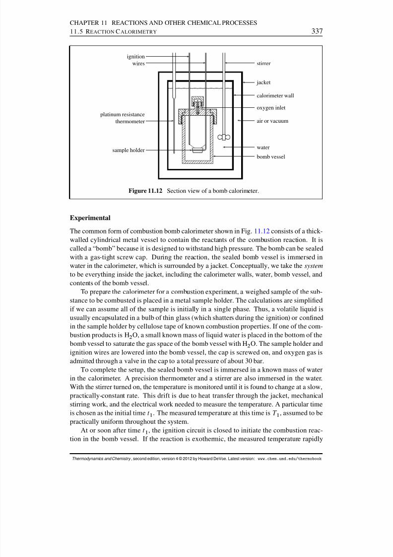
8/12/2019 Howard Devoe Thermodynamic and Chemical
http://slidepdf.com/reader/full/howard-devoe-thermodynamic-and-chemical 337/532
CHAPTER 11 REACTIONS AND OTHER CHEMICAL PROCESSES11.5 R EACTION C ALORIMETRY 337
ignitionwires
platinum resistancethermometer
sample holder
stirrer
jacket
calorimeter walloxygen inlet
air or vacuum
water
bomb vessel
Figure 11.12 Section view of a bomb calorimeter.
Experimental
The common form of combustion bomb calorimeter shown in Fig. 11.12 consists of a thick-walled cylindrical metal vessel to contain the reactants of the combustion reaction. It iscalled a “bomb” because it is designed to withstand high pressure. The bomb can be sealedwith a gas-tight screw cap. During the reaction, the sealed bomb vessel is immersed inwater in the calorimeter, which is surrounded by a jacket. Conceptually, we take the systemto be everything inside the jacket, including the calorimeter walls, water, bomb vessel, andcontents of the bomb vessel.
To prepare the calorimeter for a combustion experiment, a weighed sample of the sub-stance to be combusted is placed in a metal sample holder. The calculations are simpliedif we can assume all of the sample is initially in a single phase. Thus, a volatile liquid isusually encapsulated in a bulb of thin glass (which shatters during the ignition) or connedin the sample holder by cellulose tape of known combustion properties. If one of the com-bustion products is H 2 O, a small known mass of liquid water is placed in the bottom of thebomb vessel to saturate the gas space of the bomb vessel with H 2 O. The sample holder andignition wires are lowered into the bomb vessel, the cap is screwed on, and oxygen gas isadmitted through a valve in the cap to a total pressure of about 30 bar.
To complete the setup, the sealed bomb vessel is immersed in a known mass of waterin the calorimeter. A precision thermometer and a stirrer are also immersed in the water.
With the stirrer turned on, the temperature is monitored until it is found to change at a slow,practically-constant rate. This drift is due to heat transfer through the jacket, mechanicalstirring work, and the electrical work needed to measure the temperature. A particular timeis chosen as the initial time t1 . The measured temperature at this time is T 1 , assumed to bepractically uniform throughout the system.
At or soon after time t1 , the ignition circuit is closed to initiate the combustion reac-tion in the bomb vessel. If the reaction is exothermic, the measured temperature rapidly
Thermodynamics and Chemistry , second edition, version 4 © 2012 by Howard DeVoe. Latest version: www.chem.umd.edu/thermobook

8/12/2019 Howard Devoe Thermodynamic and Chemical
http://slidepdf.com/reader/full/howard-devoe-thermodynamic-and-chemical 338/532
CHAPTER 11 REACTIONS AND OTHER CHEMICAL PROCESSES11.5 R EACTION C ALORIMETRY 338
R
P
R
(expt) R
IBP
Figure 11.13 Internal energy changes for paths at constant volume in a bomb calo-rimeter (schematic). R denotes reactants and P denotes products.
increases over the course of several minutes as chemical energy is converted to thermal en-ergy. For a while the temperature in the system is far from uniform, as energy is transferredby heat through the walls of the bomb vessel walls to the water outside.
When the measured temperature is again observed to change at a slow and practicallyconstant rate, the reaction is assumed to be complete and the temperature is assumed oncemore to be uniform. A second time is now designated as the nal time t2 , with nal tem-perature T 2 . For best accuracy, conditions are arranged so that T 2 is close to the desiredreference temperature T ref .
Because the jacket is not gas tight, the pressure of the water outside the bomb vesselstays constant at the pressure of the atmosphere. Inside the bomb vessel, the changes intemperature and composition take place at essentially constant volume, so the pressure in-side the vessel is not constant. The volume change of the entire system during the processis negligible.
The isothermal bomb process
The relations derived here parallel those of Sec. 11.5.1 for a constant-pressure calorimeter.
The three paths depicted in Fig. 11.13 are similar to those in Fig. 11.11 on page 335 , exceptthat instead of being at constant pressure they are at constant volume. We shall assume thecombustion reaction is exothermic, with T 2 being greater than T 1 .
The internal energy change of the experimental process that actually occurs in thecalorimeter between times t1 and t2 is denoted U (expt) in the gure. Conceptually, theoverall change of state during this process would be duplicated by a path in which the tem-perature of the system with the reactants present increases from T 1 to T 2 ,12 followed by theisothermal bomb process at temperature T 2 . In the gure these paths are labeled with theinternal energy changes U. R/ and U. IBP ; T 2 / , and we can write
U (expt) D U. R/ CU. IBP ; T 2 / (11.5.4)
To evaluate U. R/ , we can use the energy equivalent R of the calorimeter with reac-tants present in the bomb vessel. R is the average heat capacity of the system between T 1and T 2 —that is, the ratio q=.T 2 T 1 / , where q is the heat that would be needed to change
12 When one investigates a combustion reaction, the path in which temperature changes without reaction is besttaken with reactants rather than products present because the reactants are more easily characterized.
Thermodynamics and Chemistry , second edition, version 4 © 2012 by Howard DeVoe. Latest version: www.chem.umd.edu/thermobook

8/12/2019 Howard Devoe Thermodynamic and Chemical
http://slidepdf.com/reader/full/howard-devoe-thermodynamic-and-chemical 339/532
CHAPTER 11 REACTIONS AND OTHER CHEMICAL PROCESSES11.5 R EACTION C ALORIMETRY 339
the temperature from T 1 to T 2 . From the rst law, with expansion work assumed negligible,the internal energy change equals this heat, giving us the relation
U. R/ D R .T 2 T 1 / (11.5.5)
The initial and nal states of the path are assumed to be equilibrium states, and there may
be some transfer of reactants or H 2 O from one phase to another within the bomb vesselduring the heating process.
The value of R is obtained in a separate calibration experiment. The calibration isusually carried out with the combustion of a reference substance, such as benzoic acid,whose internal energy of combustion under controlled conditions is precisely known fromstandardization based on electrical work. If the bomb vessel is immersed in the same massof water in both experiments and other conditions are similar, the difference in the valuesof R in the two experiments is equal to the known difference in the heat capacities of theinitial contents (reactants, water, etc.) of the bomb vessel in the two experiments.
The internal energy change we wish to nd is U. IBP ; T 2 / , that of the isothermal bombprocess in which reactants change to products at temperature T 2 , accompanied perhaps bysome further transfer of substances between phases. From Eqs. 11.5.4 and 11.5.5 , we obtain
U. IBP ; T 2 / D .T 2 T 1 / CU (expt) (11.5.6)
The value of U (expt) is small. To evaluate it, we must look in detail at the possiblesources of energy transfer between the system and the surroundings during the experimentalprocess. These sources are
1. electrical work wign done on the system by the ignition circuit;
2. heat transfer, minimized but not eliminated by the jacket;
3. mechanical stirring work done on the system;
4. electrical work done on the system by an electrical thermometer.The ignition work occurs during only a short time interval at the beginning of the process,and its value is known. The effects of heat transfer, stirring work, and temperature mea-surement continue throughout the course of the experiment. With these considerations, Eq.11.5.6 becomes
U. IBP ; T 2 / D .T 2 T 1 / Cw ign CU 0(expt) (11.5.7)
where U 0(expt) is the internal energy change due to heat, stirring, and temperature mea-surement. U 0(expt) can be evaluated from the energy equivalent and the observed ratesof temperature change at times t1 and t2 ; the relevant relations for an isothermal jacket areEq. 7.3.24 (with wel set equal to zero) and Eq. 7.3.32 .
Correction to the reference temperatureThe value of U . IBP ; T 2 / evaluated from Eq. 11.5.7 is the internal energy change of theisothermal bomb process at temperature T 2 . We need to correct this value to the desiredreference temperature T ref . If T 2 and T ref are close in value, the correction is small and canbe calculated with a modied version of the Kirchhoff equation (Eq. 11.3.10 on page 324 ):
U. IBP ; T ref / D U. IBP ; T 2 / CΠC V (P) C V (R) .T ref T 2 / (11.5.8)
Thermodynamics and Chemistry , second edition, version 4 © 2012 by Howard DeVoe. Latest version: www.chem.umd.edu/thermobook
8/12/2019 Howard Devoe Thermodynamic and Chemical
http://slidepdf.com/reader/full/howard-devoe-thermodynamic-and-chemical 340/532
CHAPTER 11 REACTIONS AND OTHER CHEMICAL PROCESSES11.5 R EACTION C ALORIMETRY 340
Here C V (P) and C V (R) are the heat capacities at constant volume of the contents of thebomb vessel with products and reactants, respectively, present.
Reduction to standard states
We want to obtain the value of cU ı .T ref / , the molar internal energy change for the maincombustion reaction at the reference temperature under standard-state conditions. Once wehave this value, it is an easy matter to nd the molar enthalpy change under standard-stateconditions, our ultimate goal.
Consider a hypothetical process with the following three isothermal steps carried out atthe reference temperature T ref :
1. Each substance initially present in the bomb vessel changes from its standard state tothe state it actually has at the start of the isothermal bomb process.
2. The isothermal bomb process takes place, including the main combustion reactionand any side reactions and auxiliary reactions.
3. Each substance present in the nal state of the isothermal bomb process changes to
its standard state.The net change is a decrease in the amount of each reactant in its standard state and anincrease in the amount of each product in its standard state. The internal energy change of step 2 is U. IBP ; T ref / , whose value is found from Eq. 11.5.8 . The internal energy changesof steps 1 and 3 are called Washburn corrections .13
Thus, we calculate the standard internal energy change of the main combustion reactionat temperature T ref from
U ı . cmb ; T ref / D U. IBP ; T ref / C(Washburn corrections) Xi
i rU ı .i / (11.5.9)
where the sum over i is for side reactions and auxiliary reactions if present. Finally, we
calculate the standard molar internal energy of combustion from
cU ı .T ref / D U ı . cmb ; T ref /
c(11.5.10)
where c is the advancement of the main combustion reaction in the bomb vessel.
Standard molar enthalpy change
The quantity cU ı .T ref / is the molar internal energy change for the main combustion reac-tion carried out at constant temperature T ref with each reactant and product in its standardstate at pressure p ı . From the relations cH D
Pi i H i (Eq. 11.2.15 ) and H i D U i CpV i
(from Eq. 9.2.50 ), we get
cH ı .T ref / D cU ı .T ref / Cp ı Xii V ıi (11.5.11)
13 Ref. [ 168 ].
Thermodynamics and Chemistry , second edition, version 4 © 2012 by Howard DeVoe. Latest version: www.chem.umd.edu/thermobook

8/12/2019 Howard Devoe Thermodynamic and Chemical
http://slidepdf.com/reader/full/howard-devoe-thermodynamic-and-chemical 341/532
CHAPTER 11 REACTIONS AND OTHER CHEMICAL PROCESSES11.5 R EACTION C ALORIMETRY 341
Molar volumes of condensed phases are much smaller than those of gases, and to a goodapproximation we may write
cH ı .T ref / D cU ı .T ref / Cp ı Xi
gi V ıi (g) (11.5.12)
where the sum includes only gaseous reactants and products of the main combustion reac-tion. Since a gas in its standard state is an ideal gas with molar volume equal to RT=p ı ,the nal relation is
cH ı .T ref / D cU ı .T ref / CXi
gi RT ref (11.5.13)
Washburn corrections
The Washburn corrections needed in Eq. 11.5.9 are internal energy changes for certainhypothetical physical processes occurring at the reference temperature T ref involving thesubstances present in the bomb vessel. In these processes, substances change from theirstandard states to the initial state of the isothermal bomb process, or change from the nal
state of the isothermal bomb process to their standard states.For example, consider the complete combustion of a solid or liquid compound of car-bon, hydrogen, and oxygen in which the combustion products are CO 2 and H 2 O and thereare no side reactions or auxiliary reactions. In the initial state of the isothermal bomb pro-cess, the bomb vessel contains the pure reactant, liquid water with O 2 dissolved in it, anda gaseous mixture of O 2 and H 2 O, all at a high pressure p 1 . In the nal state, the bombvessel contains liquid water with O 2 and CO 2 dissolved in it and a gaseous mixture of O 2 ,H2 O, and CO 2 , all at pressure p 2 . In addition, the bomb vessel contains internal parts of constant mass such as the sample holder and ignition wires.
In making Washburn corrections, we must use a single standard state for each substancein order for Eq. 11.5.9 to correctly give the standard internal energy of combustion. Inthe present example we choose the following standard states: pure solid or liquid for thereactant compound, pure liquid for the H 2 O, and pure ideal gases for the O 2 and CO 2 , eachat pressure p ı D 1 bar.
We can calculate the amount of each substance in each phase, in both the initial stateand nal state of the isothermal bomb process, from the following information: the inter-nal volume of the bomb vessel; the mass of solid or liquid reactant initially placed in thevessel; the initial amount of H 2 O; the initial O 2 pressure; the water vapor pressure; thesolubilities (estimated from Henry’s law constants) of O 2 and CO 2 in the water; and thestoichiometry of the combustion reaction. Problem 11. 7 on page 362 guides you throughthese calculations.
11.5.3 Other calorimeters
Experimenters have used great ingenuity in designing calorimeters to measure reactionenthalpies and to improve their precision. In addition to the constant-pressure reactioncalorimeter and bomb calorimeter described above, three additional types will be brieymentioned.
A phase-change calorimeter has two coexisting phases of a pure substance in thermalcontact with the reaction vessel and an adiabatic outer jacket. The two coexisting phases
Thermodynamics and Chemistry , second edition, version 4 © 2012 by Howard DeVoe. Latest version: www.chem.umd.edu/thermobook
8/12/2019 Howard Devoe Thermodynamic and Chemical
http://slidepdf.com/reader/full/howard-devoe-thermodynamic-and-chemical 342/532
CHAPTER 11 REACTIONS AND OTHER CHEMICAL PROCESSES11.6 A DIABATIC F LAME T EMPERATURE 342
constitute a univariant subsystem that at constant pressure is at the xed temperature of the equilibrium phase transition. The thermal energy released or absorbed by the reaction,instead of changing the temperature, is transferred isothermally to or from the coexistingphases and can be measured by the volume change of the phase transition. A reaction en-thalpy, of course, can only be measured by this method at the temperature of the equilibrium
phase transition. The well-known Bunsen ice calorimeter uses the ice–water transition at0 ı C. The solid–liquid transition of diphenyl ether has a relatively large volume change andis useful for measurements at 26:9 ı C. Phase-transition calorimeters are especially usefulfor slow reactions.
A heat-ow calorimeter is a variation of an isothermal-jacket calorimeter. It uses a ther-mopile (Fig. 2.7 ) to continuously measure the temperature difference between the reactionvessel and an outer jacket acting as a constant-temperature heat sink. The heat transfer takesplace mostly through the thermocouple wires, and to a high degree of accuracy is propor-tional to the temperature difference integrated over time. This is the best method for anextremely slow reaction, and it can also be used for rapid reactions.
A ame calorimeter is a ow system in which oxygen, uorine, or another gaseousoxidant reacts with a gaseous fuel. The heat transfer between the ow tube and a heat sink can be measured with a thermopile, as in a heat-ow calorimeter.
11.6 ADIABATIC FLAME TEMPERATURE
With a few simple approximations, we can estimate the temperature of a ame formed ina owing gas mixture of oxygen or air and a fuel. We treat a moving segment of the gasmixture as a closed system in which the temperature increases as combustion takes place.We assume that the reaction occurs at a constant pressure equal to the standard pressure,and that the process is adiabatic and the gas is an ideal-gas mixture.
The principle of the calculation is similar to that used for a constant-pressure calorimeteras explained by the paths shown in Fig. 11.11 on page 335 . When the combustion reaction
in the segment of gas reaches reaction equilibrium, the advancement has changed by and the temperature has increased from T 1 to T 2 . Because the reaction is assumed to beadiabatic at constant pressure, H (expt) is zero. Therefore, the sum of H . rxn ; T 1 / andH. P/ is zero, and we can write
cH ı .T 1 / CZ T 2
T 1C p . P/ dT D 0 (11.6.1)
where cH ı .T 1 / is the standard molar enthalpy of combustion at the initial temperature,and C p . P/ is the heat capacity at constant pressure of the product mixture.
The value of T 2 that satises Eq. 11.6.1 is the estimated ame temperature. Problem11. 9 presents an application of this calculation. Several factors cause the actual temperaturein a ame to be lower: the process is never completely adiabatic, and in the high temperatureof the ame there may be product dissociation and other reactions in addition to the maincombustion reaction.
Thermodynamics and Chemistry , second edition, version 4 © 2012 by Howard DeVoe. Latest version: www.chem.umd.edu/thermobook
8/12/2019 Howard Devoe Thermodynamic and Chemical
http://slidepdf.com/reader/full/howard-devoe-thermodynamic-and-chemical 343/532
CHAPTER 11 REACTIONS AND OTHER CHEMICAL PROCESSES11.7 G IBBS E NERGY AND R EACTION E QUILIBRIUM 343
11.7 GIBBS ENERGY AND REACTION EQUILIBRIUM
This section begins by examining the way in which the Gibbs energy changes as a chemicalprocess advances in a closed system at constant T and p with expansion work only. Auniversal criterion for reaction equilibrium is derived involving the molar reaction Gibbsenergy.
11.7.1 The molar reaction Gibbs energy
Applying the general denition of a molar differential reaction quantity (Eq. 11.2.15 ) to theGibbs energy of a closed system with T , p , and as the independent variables, we obtainthe denition of the molar reaction Gibbs energy or molar Gibbs energy of reaction, rG:
rG def
DXii i (11.7.1)
Equation 11.2.16 shows that this quantity is also given by the partial derivative
rG D @G@ T;p
(11.7.2)(closed system)
The total differential of G is then
dG D S dT CV dp C rG d (11.7.3)(closed system)
11.7.2 Spontaneity and reaction equilibrium
In Sec. 5.8 , we found that the spontaneous direction of a process taking place in a closed
system at constant T and p , with expansion work only, is the direction of decreasing G . Inthe case of a chemical process occurring at constant T and p , rG is the rate at which Gchanges with . Thus if rG is positive, spontaneously decreases; if rG is negative, spontaneously increases. During a spontaneous process d and rG have opposite signs. 14
Note how the equality of Eq. 11.7.3 agrees with the inequality d G < S dT CV dp ,a criterion of spontaneity in a closed system with expansion work only (Eq. 5.8.6 onpage 146 ). When d and rG have opposite signs, rG d is negative and d G D. S dT CV dp C rG d / is less than . S dT CV dp/ .
If the system is closed and contains at least one phase that is a mixture, a state of reactionequilibrium can be approached spontaneously at constant T and p in either direction of the
reaction; that is, by both positive and negative changes of . In this equilibrium state,therefore, G has its minimum value for the given T and p . Since G is a smooth function
14 Sometimes reaction spontaneity at constant T and p is ascribed to the “driving force” of a quantity calledthe afnity of reaction , dened as the negative of rG . increases spontaneously if the afnity is positive anddecreases spontaneously if the afnity is negative; the system is at equilibrium when the afnity is zero.
Thermodynamics and Chemistry , second edition, version 4 © 2012 by Howard DeVoe. Latest version: www.chem.umd.edu/thermobook
8/12/2019 Howard Devoe Thermodynamic and Chemical
http://slidepdf.com/reader/full/howard-devoe-thermodynamic-and-chemical 344/532
CHAPTER 11 REACTIONS AND OTHER CHEMICAL PROCESSES11.7 G IBBS E NERGY AND R EACTION E QUILIBRIUM 344
of , its rate of change with respect to is zero in the equilibrium state. The condition forreaction equilibrium , then, is that rG must be zero:
rG DXii i D 0 (11.7.4)
(reaction equilibrium)
It is important to realize that this condition is independent of whether or not reactionequilibrium is approached at constant temperature and pressure. It is a universal criterionof reaction equilibrium. The value of rG is equal to Pi i i and depends on the state of the system. If the state is such that rG is positive, the direction of spontaneous changeis one that, under the existing constraints, allows rG to decrease. If rG is negative,the spontaneous change increases the value of rG . When the system reaches reactionequilibrium, whatever the path of the spontaneous process, the value of rG becomes zero.
11.7.3 General derivation
We can obtain the condition of reaction equilibrium given by Eq. 11.7.4 in a more general
and rigorous way by an extension of the derivation of Sec. 9.2.7 , which was for equilibriumconditions in a multiphase, multicomponent system.
Consider a system with a reference phase, ’ 0, and optionally other phases labeled by’ ¤ ’ 0. Each phase contains one or more species labeled by subscript i , and some or all of the species are the reactants and products of a reaction.
The total differential of the internal energy is given by Eq. 9.2.37 on page 237 :
dU D T ’0dS ’
0p ’ 0
dV ’0
CXi
’ 0
i dn ’ 0
i
C
X’ ¤ ’ 0
T ’ dS ’ p ’ dV ’ C
Xi
’i dn ’
i ! (11.7.5)
The conditions of isolation are
dU D 0 (constant internal energy) (11.7.6)
dV ’0
CX’ ¤ ’ 0
dV ’ D 0 (no expansion work) (11.7.7)
For each species i :
dn ’ 0
i CX’ ¤ ’ 0
dn ’i D i d (closed system) (11.7.8)
In Eq. 11.7.8 , dn ’ 00
i0 should be set equal to zero for a species i 0 that is excluded from phase
’ 00, and i 00 should be set equal to zero for a species i 00that is not a reactant or product of the reaction.
Thermodynamics and Chemistry , second edition, version 4 © 2012 by Howard DeVoe. Latest version: www.chem.umd.edu/thermobook
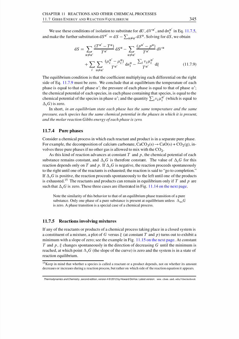
8/12/2019 Howard Devoe Thermodynamic and Chemical
http://slidepdf.com/reader/full/howard-devoe-thermodynamic-and-chemical 345/532
CHAPTER 11 REACTIONS AND OTHER CHEMICAL PROCESSES11.7 G IBBS E NERGY AND R EACTION E QUILIBRIUM 345
We use these conditions of isolation to substitute for d U , dV ’0, and d n ’ 0
i in Eq. 11.7.5 ,and make the further substitution d S ’
0
D dS P’ ¤ ’ 0 dS ’ . Solving for d S , we obtain
dS DX’ ¤ ’ 0
.T ’ 0T ’ /
T ’ 0 dS ’ X’ ¤ ’ 0
.p ’ 0p ’ /
T ’ 0 dV ’
CXi X’ ¤ ’ 0
. ’ 0i ’
i /T ’ 0 dn ’
i Pi i ’ 0i
T ’ 0 d (11.7.9)
The equilibrium condition is that the coefcient multiplying each differential on the rightside of Eq. 11.7.9 must be zero. We conclude that at equilibrium the temperature of eachphase is equal to that of phase ’ 0; the pressure of each phase is equal to that of phase ’ 0;the chemical potential of each species, in each phase containing that species, is equal to thechemical potential of the species in phase ’ 0; and the quantity Pi i
’ 0
i (which is equal to
rG ) is zero.In short, in an equilibrium state each phase has the same temperature and the same
pressure, each species has the same chemical potential in the phases in which it is present,
and the molar reaction Gibbs energy of each phase is zero .
11.7.4 Pure phases
Consider a chemical process in which each reactant and product is in a separate pure phase.For example, the decomposition of calcium carbonate, CaCO 3 (s) ! CaO(s) + CO 2 (g), in-volves three pure phases if no other gas is allowed to mix with the CO 2 .
As this kind of reaction advances at constant T and p , the chemical potential of eachsubstance remains constant, and rG is therefore constant. The value of rG for thisreaction depends only on T and p . If rG is negative, the reaction proceeds spontaneouslyto the right until one of the reactants is exhausted; the reaction is said to “go to completion.”If
rG is positive, the reaction proceeds spontaneously to the left until one of the products
is exhausted. 15 The reactants and products can remain in equilibrium only if T and p aresuch that rG is zero. These three cases are illustrated in Fig. 11.14 on the next page .
Note the similarity of this behavior to that of an equilibrium phase transition of a puresubstance. Only one phase of a pure substance is present at equilibrium unless trs Gis zero. A phase transition is a special case of a chemical process.
11.7.5 Reactions involving mixtures
If any of the reactants or products of a chemical process taking place in a closed system isa constituent of a mixture, a plot of G versus (at constant T and p ) turns out to exhibit aminimum with a slope of zero; see the example in Fig. 11.15 on the next page . At constantT and p , changes spontaneously in the direction of decreasing G until the minimum isreached, at which point rG (the slope of the curve) is zero and the system is in a state of reaction equilibrium.
15 Keep in mind that whether a species is called a reactant or a product depends, not on whether its amountdecreases or increases during a reaction process, but rather on which side of the reaction equation it appears.
Thermodynamics and Chemistry , second edition, version 4 © 2012 by Howard DeVoe. Latest version: www.chem.umd.edu/thermobook
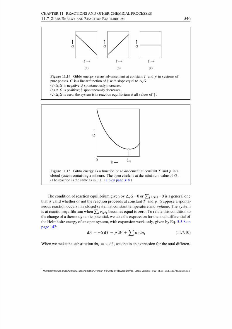
8/12/2019 Howard Devoe Thermodynamic and Chemical
http://slidepdf.com/reader/full/howard-devoe-thermodynamic-and-chemical 346/532
CHAPTER 11 REACTIONS AND OTHER CHEMICAL PROCESSES11.7 G IBBS E NERGY AND R EACTION E QUILIBRIUM 346
G
G
G
(a) (b) (c)
Figure 11.14 Gibbs energy versus advancement at constant T and p in systems of pure phases. G is a linear function of with slope equal to rG .(a) rG is negative; spontaneously increases.(b) rG is positive; spontaneously decreases.(c) rG is zero; the system is in reaction equilibrium at all values of .
eq
Figure 11.15 Gibbs energy as a function of advancement at constant T and p in aclosed system containing a mixture. The open circle is at the minimum value of G .(The reaction is the same as in Fig. 11.6 on page 318 .)
The condition of reaction equilibrium given by rGD0 or Pi i i D0 is a general onethat is valid whether or not the reaction proceeds at constant T and p . Suppose a sponta-neous reaction occurs in a closed system at constant temperature and volume . The systemis at reaction equilibrium when Pi i i becomes equal to zero. To relate this condition tothe change of a thermodynamic potential, we take the expression for the total differential of the Helmholtz energy of an open system, with expansion work only, given by Eq. 5.5.8 onpage 142 :
dA D S dT p dV CXii dn i (11.7.10)
When we make the substitution d n i D i d , we obtain an expression for the total differen-
Thermodynamics and Chemistry , second edition, version 4 © 2012 by Howard DeVoe. Latest version: www.chem.umd.edu/thermobook
8/12/2019 Howard Devoe Thermodynamic and Chemical
http://slidepdf.com/reader/full/howard-devoe-thermodynamic-and-chemical 347/532
CHAPTER 11 REACTIONS AND OTHER CHEMICAL PROCESSES11.7 G IBBS E NERGY AND R EACTION E QUILIBRIUM 347
tial of A in a closed system with a chemical reaction:
dA D S dT p dV C Xii i!d (11.7.11)
We identify the coefcient of the last term on the right as a partial derivative:
Xii i D
@A@ T;V
(11.7.12)
This equation shows that as the reaction proceeds spontaneously at constant T and V , itreaches reaction equilibrium at the point where .@A=@ /T;V is zero. This is simply an-other way to express the criterion for spontaneity stated on page 146: If the only work isexpansion work, the Helmholtz energy of a closed system decreases during a spontaneousprocess at constant T and V and has its minimum value when the system attains an equilib-rium state.
11.7.6 Reaction in an ideal gas mixture
Let us look in detail at the source of the minimum in G for the case of a reaction occurring inan ideal gas mixture in a closed system at constant T and p . During this process the systemhas only one independent variable, which it is convenient to choose as the advancement .The additivity rule (Eq. 9.2.25 ) for the Gibbs energy is
G DXi
n i i (11.7.13)
where both n i and i depend on . Thus, G is a complicated function of .For the chemical potential of each substance, we write i D ı
i (g) CRT ln.p i =p ı /
(Eq. 9.3.5 ), where p i is the partial pressure of i in the mixture. Substitution in Eq. 11.7.13gives, for the Gibbs energy at any value of ,
G. / DXi
n iıi (g) CRT ln
p i
p ı (11.7.14)
At D 0, the amounts and partial pressures have their initial values n i;0 and p i;0 :
G.0/ DXi
n i;0ıi (g) CRT ln
p i;0
p ı (11.7.15)
The difference between these two expressions is
G. / G.0/ DXi
.n i n i;0 / ıi (g)
CRT Xi
n i lnp i
p ı RT Xi
n i;0 lnp i;0
p ı (11.7.16)
Thermodynamics and Chemistry , second edition, version 4 © 2012 by Howard DeVoe. Latest version: www.chem.umd.edu/thermobook
8/12/2019 Howard Devoe Thermodynamic and Chemical
http://slidepdf.com/reader/full/howard-devoe-thermodynamic-and-chemical 348/532
CHAPTER 11 REACTIONS AND OTHER CHEMICAL PROCESSES11.7 G IBBS E NERGY AND R EACTION E QUILIBRIUM 348
Converting partial pressures to mole fractions with p i D y i p and p i;0 D y i;0 p gives
G. / G.0/ DXi
.n i n i;0 / ıi (g) CRT Xi
n i ln y i
RT
Xi
n i;0 ln y i;0 CRT
Xi
.n i n i;0 / lnpp ı (11.7.17)
With the substitution n i n i;0 D i (Eq. 11.2.11 ) in the rst and last terms on the rightside of Eq. 11.7.17 , the result is
G. / G.0/ D Xii
ıi (g) CRT Xi
n i ln y i
RT Xi
n i:0 ln y i;0 CRT Xii! ln
pp ı (11.7.18)
The sum
Pi i
ıi (g) in the rst term on the right side of Eq. 11.7.18 is rG
ı , thestandard molar reaction Gibbs energy. Making this substitution gives nally
G. / G.0/ D rGı CRT Xi
n i ln y i RT Xi
n i;0 ln y i;0
CRT Xii! ln
pp ı (11.7.19)
(ideal gas mixture)
There are four terms on the right side of Eq. 11.7.19 . The rst term is the Gibbs en-ergy change for the reaction of pure reactants to form pure products under standard-stateconditions, the second is a mixing term, the third term is constant, and the last term is anadjustment of G from the standard pressure to the pressure of the gas mixture. Note that
the rst and last terms are proportional to the advancement and cannot be the cause of aminimum in the curve of the plot of G versus . It is the mixing term RT Pi n i ln y i thatis responsible for the observed minimum. 16 This term divided by nDPi n i is G id
m (mix),the molar differential Gibbs energy of mixing to form an ideal mixture (see Eq. 11.1.8 onpage 305 ); the term is also equal to nT S id
m (mix) (Eq. 11.1.9 ), showing that the minimumis entirely an entropy effect.
Now let us consider specically the simple reaction
A. g/ ! B. g/
in an ideal gas mixture, for which A is 1 and B is C1. Let the initial state be one of pureA: n B;0 D0. The initial mole fractions are then yA;0 D1 and y B;0 D0. In this reaction, the
total amount n D nA CnB is constant. Substituting these values in Eq. 11.7.19 gives17
G. / G.0/ D rGı CnRT.y A ln yA CyB ln yB / (11.7.20)
16 This term also causes the slope of the curve of G. / G.0/ versus to be 1 and C1 at the left and rightextremes of the curve.17 Note that although ln yA approaches 1 as yA approaches zero, the product y A ln yA approaches zero inthis limit. This behavior can be proved with l’Hospital’s rule (see any calculus textbook).
Thermodynamics and Chemistry , second edition, version 4 © 2012 by Howard DeVoe. Latest version: www.chem.umd.edu/thermobook
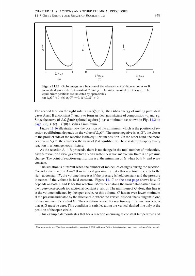
8/12/2019 Howard Devoe Thermodynamic and Chemical
http://slidepdf.com/reader/full/howard-devoe-thermodynamic-and-chemical 349/532
CHAPTER 11 REACTIONS AND OTHER CHEMICAL PROCESSES11.7 G IBBS E NERGY AND R EACTION E QUILIBRIUM 349
0 1= n A ;0
G
(a)
0 1= n A ;0
G
(b)
0 1= n A ;0
G
(c)
Figure 11.16 Gibbs energy as a function of the advancement of the reaction A ! Bin an ideal gas mixture at constant T and p . The initial amount of B is zero. Theequilibrium positions are indicated by open circles.(a) rG ı < 0 . (b) rG ı D 0. (c) rG ı > 0 .
The second term on the right side is n G idm (mix), the Gibbs energy of mixing pure ideal
gases A and B at constant T and p to form an ideal gas mixture of composition yA and yB .Since the curve of G id
m (mix) plotted against has a minimum (as shown in Fig. 11.2 onpage 306 ), G. / G.0/ also has a minimum.
Figure 11.16 illustrates how the position of the minimum, which is the position of re-action equilibrium, depends on the value of rG
ı . The more negative is rGı , the closer
to the product side of the reaction is the equilibrium position. On the other hand, the morepositive is rG
ı , the smaller is the value of at equilibrium. These statements apply to any
reaction in a homogeneous mixture.As the reaction A ! B proceeds, there is no change in the total number of molecules,
and therefore in an ideal gas mixture at constant temperature and volume there is no pressurechange. The point of reaction equilibrium is at the minimum of G when both V and p areconstant.
The situation is different when the number of molecules changes during the reaction.Consider the reaction A ! 2 B in an ideal gas mixture. As this reaction proceeds to theright at constant T , the volume increases if the pressure is held constant and the pressureincreases if the volume is held constant. Figure 11.17 on the next page shows how Gdepends on both p and V for this reaction. Movement along the horizontal dashed line inthe gure corresponds to reaction at constant T and p . The minimum of G along this line is
at the volume indicated by the open circle. At this volume, G has an even lower minimumat the pressure indicated by the lled circle, where the vertical dashed line is tangent to oneof the contours of constant G . The condition needed for reaction equilibrium, however, isthat rG must be zero. This condition is satised along the vertical dashed line only at theposition of the open circle.
This example demonstrates that for a reaction occurring at constant temperature and
Thermodynamics and Chemistry , second edition, version 4 © 2012 by Howard DeVoe. Latest version: www.chem.umd.edu/thermobook
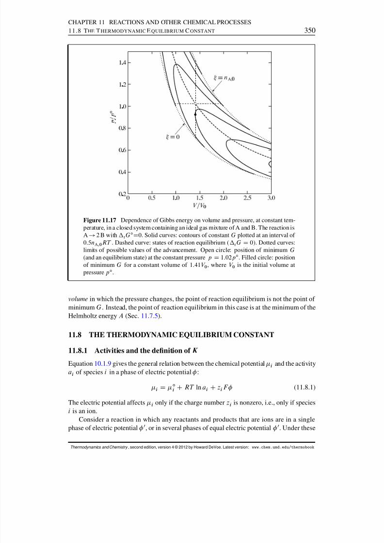
8/12/2019 Howard Devoe Thermodynamic and Chemical
http://slidepdf.com/reader/full/howard-devoe-thermodynamic-and-chemical 350/532
CHAPTER 11 REACTIONS AND OTHER CHEMICAL PROCESSES11.8 T HE T HERMODYNAMIC E QUILIBRIUM C ONSTANT 350
A,
Æ
Figure 11.17 Dependence of Gibbs energy on volume and pressure, at constant tem-perature, in a closed system containing an ideal gas mixture of A and B. The reaction isA ! 2 B with rG ı D0. Solid curves: contours of constant G plotted at an interval of 0:5n A;0 RT . Dashed curve: states of reaction equilibrium ( rG D 0). Dotted curves:limits of possible values of the advancement. Open circle: position of minimum G(and an equilibrium state) at the constant pressure p D 1:02p ı . Filled circle: positionof minimum G for a constant volume of 1:41V 0 , where V 0 is the initial volume atpressure p ı .
volume in which the pressure changes, the point of reaction equilibrium is not the point of minimum G . Instead, the point of reaction equilibrium in this case is at the minimum of theHelmholtz energy A (Sec. 11.7.5 ).
11.8 THE THERMODYNAMIC EQUILIBRIUM CONSTANT
11.8.1 Activities and the denition of K
Equation 10.1.9 gives the general relation between the chemical potential i and the activitya i of species i in a phase of electric potential :
i D ıi CRT ln a i Czi F (11.8.1)
The electric potential affects i only if the charge number zi is nonzero, i.e., only if speciesi is an ion.
Consider a reaction in which any reactants and products that are ions are in a singlephase of electric potential 0, or in several phases of equal electric potential 0. Under these
Thermodynamics and Chemistry , second edition, version 4 © 2012 by Howard DeVoe. Latest version: www.chem.umd.edu/thermobook
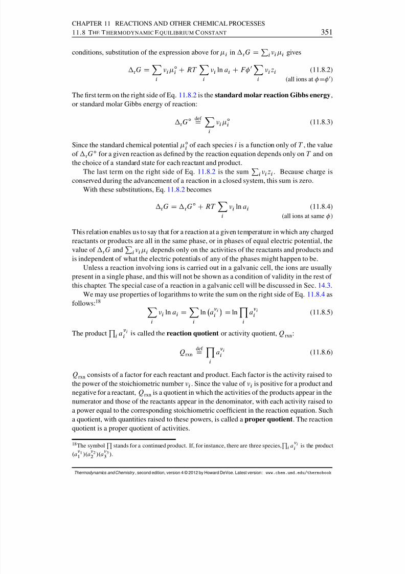
8/12/2019 Howard Devoe Thermodynamic and Chemical
http://slidepdf.com/reader/full/howard-devoe-thermodynamic-and-chemical 351/532
CHAPTER 11 REACTIONS AND OTHER CHEMICAL PROCESSES11.8 T HE T HERMODYNAMIC E QUILIBRIUM C ONSTANT 351
conditions, substitution of the expression above for i in rG DPi i i gives
rG DXii
ıi CRT Xi
i ln a i CF 0Xii zi (11.8.2)
(all ions at D 0)
The rst term on the right side of Eq. 11.8.2 is the standard molar reaction Gibbs energy ,or standard molar Gibbs energy of reaction:
rGı def
DXii
ıi (11.8.3)
Since the standard chemical potential ıi of each species i is a function only of T , the value
of rGı for a given reaction as dened by the reaction equation depends only on T and on
the choice of a standard state for each reactant and product.The last term on the right side of Eq. 11.8.2 is the sum Pi i zi . Because charge is
conserved during the advancement of a reaction in a closed system, this sum is zero.With these substitutions, Eq. 11.8.2 becomes
rG D rGı CRT Xi
i ln a i (11.8.4)(all ions at same )
This relation enables us to say that for a reaction at a given temperature in which any chargedreactants or products are all in the same phase, or in phases of equal electric potential, thevalue of rG and Pi i i depends only on the activities of the reactants and products andis independent of what the electric potentials of any of the phases might happen to be.
Unless a reaction involving ions is carried out in a galvanic cell, the ions are usuallypresent in a single phase, and this will not be shown as a condition of validity in the rest of this chapter. The special case of a reaction in a galvanic cell will be discussed in Sec. 14.3 .
We may use properties of logarithms to write the sum on the right side of Eq. 11.8.4 asfollows: 18
Xii ln a i DXi
ln a ii D ln Yi
a ii (11.8.5)
The product Qi ai
i is called the reaction quotient or activity quotient, Q rxn :
Q rxndef
DYi
a ii (11.8.6)
Q rxn consists of a factor for each reactant and product. Each factor is the activity raised tothe power of the stoichiometric number i . Since the value of i is positive for a product andnegative for a reactant, Q rxn is a quotient in which the activities of the products appear in the
numerator and those of the reactants appear in the denominator, with each activity raised toa power equal to the corresponding stoichiometric coefcient in the reaction equation. Sucha quotient, with quantities raised to these powers, is called a proper quotient . The reactionquotient is a proper quotient of activities.
18 The symbol Q stands for a continued product. If, for instance, there are three species, Qi ai
i is the product.a 1
1 /.a 22 /.a 3
3 /.
Thermodynamics and Chemistry , second edition, version 4 © 2012 by Howard DeVoe. Latest version: www.chem.umd.edu/thermobook

8/12/2019 Howard Devoe Thermodynamic and Chemical
http://slidepdf.com/reader/full/howard-devoe-thermodynamic-and-chemical 352/532
CHAPTER 11 REACTIONS AND OTHER CHEMICAL PROCESSES11.8 T HE T HERMODYNAMIC E QUILIBRIUM C ONSTANT 352
For instance, for the ammonia synthesis reaction N 2 (g )+3H 2 (g) ! 2 NH 3 (g) the reac-tion quotient is given by
Q rxn Da 2
NH 3
a N2a 3
H2
(11.8.7)
Q rxn is a dimensionless quantity. It is a function of T , p , and the mixture composition, soits value changes as the reaction advances.
The expression for the molar reaction Gibbs energy given by Eq. 11.8.4 can now bewritten
rG D rGı CRT ln Q rxn (11.8.8)
The value of Q rxn under equilibrium conditions is the thermodynamic equilibrium con-stant , K . The general denition of K is
K def
DYi
.a i / ieq (11.8.9)
where the subscript eq indicates an equilibrium state. Note that K , like Q rxn , is dimension-
less.
The IUPAC Green Book 19 gives K as an alternative symbol for the thermodynamicequilibrium constant, the appended superscript denoting “standard.” An IUPAC Com-mission on Thermodynamics 20 has furthermore recommended the name “standardequilibrium constant,” apparently because its value depends on the choice of stan-dard states. Using this alternative symbol and name could cause confusion, since thequantity dened by Eq. 11.8.9 does not refer to reactants and products in their standardstates but rather to reactants and products in an equilibrium state.
Substituting the equilibrium conditions rGD0 and Q rxnDK in Eq. 11.8.8 gives an im-portant relation between the standard molar reaction Gibbs energy and the thermodynamic
equilibrium constant:rG
ı D RT ln K (11.8.10)
We can solve this equation for K to obtain the equivalent relation
K D exp rGı
RT (11.8.11)
We have seen that the value of rGı depends only on T and the choice of the standard
states of the reactants and products. This being so, Eq. 11.8.11 shows that the value of K fora given reaction depends only on T and the choice of standard states. No other condition,neither pressure nor composition, can affect the value of K . We also see from Eq. 11.8.11that K is less than 1 if rG
ı is positive and greater than 1 if rGı is negative. At a xed
temperature, reaction equilibrium is attained only if and only if the value of Q rxn becomesequal to the value of K at that temperature.
The thermodynamic equilibrium constant K is the proper quotient of the activities of species in reaction equilibrium. At typical temperatures and pressures, an activity cannot be
19 Ref. [ 36], p. 58.20 Ref. [ 52].
Thermodynamics and Chemistry , second edition, version 4 © 2012 by Howard DeVoe. Latest version: www.chem.umd.edu/thermobook
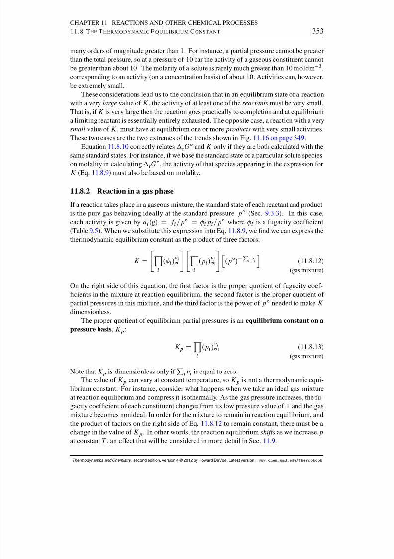
8/12/2019 Howard Devoe Thermodynamic and Chemical
http://slidepdf.com/reader/full/howard-devoe-thermodynamic-and-chemical 353/532
CHAPTER 11 REACTIONS AND OTHER CHEMICAL PROCESSES11.8 T HE T HERMODYNAMIC E QUILIBRIUM C ONSTANT 353
many orders of magnitude greater than 1. For instance, a partial pressure cannot be greaterthan the total pressure, so at a pressure of 10 bar the activity of a gaseous constituent cannotbe greater than about 10. The molarity of a solute is rarely much greater than 10 moldm 3 ,corresponding to an activity (on a concentration basis) of about 10. Activities can, however,be extremely small.
These considerations lead us to the conclusion that in an equilibrium state of a reactionwith a very large value of K , the activity of at least one of the reactants must be very small.That is, if K is very large then the reaction goes practically to completion and at equilibriuma limiting reactant is essentially entirely exhausted. The opposite case, a reaction with a verysmall value of K , must have at equilibrium one or more products with very small activities.These two cases are the two extremes of the trends shown in Fig. 11.16 on page 349 .
Equation 11.8.10 correctly relates rGı and K only if they are both calculated with the
same standard states. For instance, if we base the standard state of a particular solute specieson molality in calculating rG
ı , the activity of that species appearing in the expression forK (Eq. 11.8.9 ) must also be based on molality.
11.8.2 Reaction in a gas phase
If a reaction takes place in a gaseous mixture, the standard state of each reactant and productis the pure gas behaving ideally at the standard pressure p ı (Sec. 9.3.3 ). In this case,each activity is given by a i (g) D f i =p ı D i p i =p ı where i is a fugacity coefcient(Table 9.5 ). When we substitute this expression into Eq. 11.8.9 , we nd we can express thethermodynamic equilibrium constant as the product of three factors:
K D"Yi
. i / ieq#"Yi
.p i / ieq#h.p ı / Pi i i (11.8.12)
(gas mixture)
On the right side of this equation, the rst factor is the proper quotient of fugacity coef-
cients in the mixture at reaction equilibrium, the second factor is the proper quotient of partial pressures in this mixture, and the third factor is the power of p ı needed to make K dimensionless.
The proper quotient of equilibrium partial pressures is an equilibrium constant on apressure basis , K p :
K p DYi
.p i / ieq (11.8.13)
(gas mixture)
Note that K p is dimensionless only if Pi i is equal to zero.The value of K p can vary at constant temperature, so K p is not a thermodynamic equi-
librium constant. For instance, consider what happens when we take an ideal gas mixtureat reaction equilibrium and compress it isothermally. As the gas pressure increases, the fu-gacity coefcient of each constituent changes from its low pressure value of 1 and the gasmixture becomes nonideal. In order for the mixture to remain in reaction equilibrium, andthe product of factors on the right side of Eq. 11.8.12 to remain constant, there must be achange in the value of K p . In other words, the reaction equilibrium shifts as we increase pat constant T , an effect that will be considered in more detail in Sec. 11.9 .
Thermodynamics and Chemistry , second edition, version 4 © 2012 by Howard DeVoe. Latest version: www.chem.umd.edu/thermobook
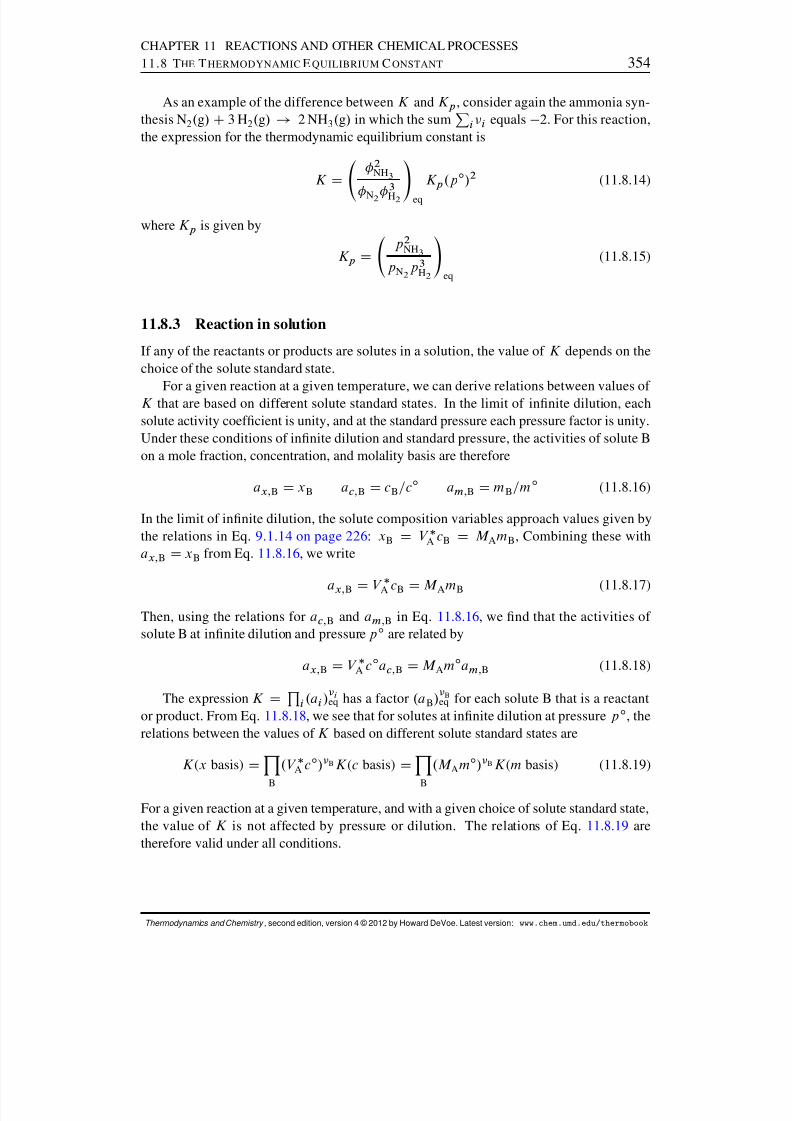
8/12/2019 Howard Devoe Thermodynamic and Chemical
http://slidepdf.com/reader/full/howard-devoe-thermodynamic-and-chemical 354/532
CHAPTER 11 REACTIONS AND OTHER CHEMICAL PROCESSES11.8 T HE T HERMODYNAMIC E QUILIBRIUM C ONSTANT 354
As an example of the difference between K and K p , consider again the ammonia syn-thesis N 2 . g/ C3 H 2 . g/ ! 2 NH 3 . g/ in which the sum Pi i equals 2. For this reaction,the expression for the thermodynamic equilibrium constant is
K
D
2NH 3
N2
3H2
!eq
K p .p ı / 2 (11.8.14)
where K p is given by
K p D p 2
NH 3
p N2p 3
H2!
eq
(11.8.15)
11.8.3 Reaction in solution
If any of the reactants or products are solutes in a solution, the value of K depends on thechoice of the solute standard state.
For a given reaction at a given temperature, we can derive relations between values of K that are based on different solute standard states. In the limit of innite dilution, eachsolute activity coefcient is unity, and at the standard pressure each pressure factor is unity.Under these conditions of innite dilution and standard pressure, the activities of solute Bon a mole fraction, concentration, and molality basis are therefore
a x; B D xB ac; B D cB=cı a m; B D mB=m ı (11.8.16)
In the limit of innite dilution, the solute composition variables approach values given bythe relations in Eq. 9.1.14 on page 226 : xB D V A cB D M AmB , Combining these witha x; B D xB from Eq. 11.8.16 , we write
a x; B D V A cB D M AmB (11.8.17)
Then, using the relations for ac; B and am; B in Eq. 11.8.16 , we nd that the activities of solute B at innite dilution and pressure p ı are related by
a x; B D V A c ı a c; B D M Am ı a m; B (11.8.18)
The expression K DQi .a i / ieq has a factor .a B / B
eq for each solute B that is a reactantor product. From Eq. 11.8.18 , we see that for solutes at innite dilution at pressure p ı , therelations between the values of K based on different solute standard states are
K (x basis) D
YB
.V A c ı / B K (c basis) D
YB
.M Am ı / B K (m basis) (11.8.19)
For a given reaction at a given temperature, and with a given choice of solute standard state,the value of K is not affected by pressure or dilution. The relations of Eq. 11.8.19 aretherefore valid under all conditions.
Thermodynamics and Chemistry , second edition, version 4 © 2012 by Howard DeVoe. Latest version: www.chem.umd.edu/thermobook
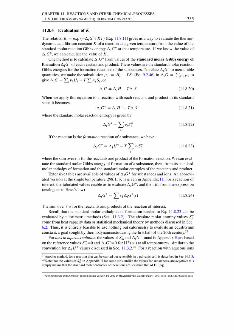
8/12/2019 Howard Devoe Thermodynamic and Chemical
http://slidepdf.com/reader/full/howard-devoe-thermodynamic-and-chemical 355/532
CHAPTER 11 REACTIONS AND OTHER CHEMICAL PROCESSES11.8 T HE T HERMODYNAMIC E QUILIBRIUM C ONSTANT 355
11.8.4 Evaluation of K
The relation K D exp . rGı =RT/ (Eq. 11.8.11 ) gives us a way to evaluate the thermo-
dynamic equilibrium constant K of a reaction at a given temperature from the value of thestandard molar reaction Gibbs energy rG
ı at that temperature. If we know the value of rG
ı , we can calculate the value of K .One method is to calculate rG ı from values of the standard molar Gibbs energy of
formation f Gı of each reactant and product. These values are the standard molar reaction
Gibbs energies for the formation reactions of the substances. To relate f Gı to measurable
quantities, we make the substitution i D H i TS i (Eq. 9.2.46 ) in rG DPi i i togive rG DPi i H i T Pi i S i , or
rG D rH T rS (11.8.20)
When we apply this equation to a reaction with each reactant and product in its standardstate, it becomes
rGı D rH ı T rS ı (11.8.21)
where the standard molar reaction entropy is given by
rS ı DXii S ıi (11.8.22)
If the reaction is the formation reaction of a substance, we have
f Gı D f H ı T Xi
i S ıi (11.8.23)
where the sum over i is for the reactants and product of the formation reaction. We can eval-uate the standard molar Gibbs energy of formation of a substance, then, from its standardmolar enthalpy of formation and the standard molar entropies of the reactants and product.
Extensive tables are available of values of f Gı
for substances and ions. An abbrevi-ated version at the single temperature 298:15 K is given in Appendix H. For a reaction of interest, the tabulated values enable us to evaluate rG
ı , and then K , from the expression(analogous to Hess’s law)
rGı DXi
i f Gı .i / (11.8.24)
The sum over i is for the reactants and products of the reaction of interest.Recall that the standard molar enthalpies of formation needed in Eq. 11.8.23 can be
evaluated by calorimetric methods (Sec. 11.3.2 ). The absolute molar entropy values S ıicome from heat capacity data or statistical mechanical theory by methods discussed in Sec.6.2 . Thus, it is entirely feasible to use nothing but calorimetry to evaluate an equilibriumconstant, a goal sought by thermodynamicists during the rst half of the 20th century. 21
For ions in aqueous solution , the values of S ım and f Gı found in Appendix H are based
on the reference values S ımD0 and f Gı D0 for H C (aq) at all temperatures, similar to the
convention for f H ı values discussed in Sec. 11.3.2 .22 For a reaction with aqueous ions
21 Another method, for a reaction that can be carried out reversibly in a galvanic cell, is described in Sec. 14.3.3 .22 Note that the values of S ım in Appendix H for some ions, unlike the values for substances, are negative ; thissimply means that the standard molar entropies of these ions are less than that of H C (aq).
Thermodynamics and Chemistry , second edition, version 4 © 2012 by Howard DeVoe. Latest version: www.chem.umd.edu/thermobook

8/12/2019 Howard Devoe Thermodynamic and Chemical
http://slidepdf.com/reader/full/howard-devoe-thermodynamic-and-chemical 356/532
CHAPTER 11 REACTIONS AND OTHER CHEMICAL PROCESSES11.9 E FFECTS OF T EMPERATURE AND P RESSURE ON E QUILIBRIUM P OSITION 356
as reactants or products, these values correctly give rS ı using Eq. 11.8.22 , or rGı using
Eq. 11.8.24 .
The relation of Eq. 11.8.23 does not apply to an ion, because we cannot write a for-mation reaction for a single ion. Instead, the relation between f G ı , f H ı and S ım ismore complicated.
Consider rst a hypothetical reaction in which hydrogen ions and one or moreelements form H 2 and a cation M z C with charge number zC :
zC HC (aq) Celements ! .z C =2/ H2 (g) CMz C (aq)
For this reaction, using the convention that f H ı , S ım , and f G ı are zero for theaqueous H C ion and the fact that f H ı and f G ı are zero for the elements, we canwrite the following expressions for standard molar reaction quantities:
rH ı D f H ı . Mz C / (11.8.25)
rS ı D .z C =2/S ım . H2 / CS ım . Mz C / Xelements
S ıi (11.8.26)
rGı
D f G
ı . Mz C / (11.8.27)
Then, from rG ı D rH ı T rS ı , we nd
f Gı . Mz C / D f H ı . Mz C /
T "S ım . Mz C / Xelements
S ıi C.z C =2/S ım . H2 /# (11.8.28)
For example, the standard molar Gibbs energy of the aqueous mercury(I) ion is foundfrom
f Gı . Hg 2
2C / D f H ı . Hg 22C / TS ım . Hg 2
2C /
C2TS ım . Hg / 22 TS ım . H2 / (11.8.29)
For an anion Xz
with negative charge number z , using the hypothetical reaction
jz =2jH2 (g) Celements ! j z jHC (aq) CXz (aq)
we nd by the same method
f Gı . Xz / D f H ı . Xz /
T "S ım . Xz / Xelements
S ıi jz =2jS ım . H2 /# (11.8.30)
For example, the calculation for the nitrate ion is
f Gı . NO 3 / D f H ı . NO 3 / TS ım . NO 3 /
C 12 TS
ım . N2 / C
32 TS
ım . O2 / C
12 TS
ım . H2 / (11.8.31)
11.9 EFFECTS OF TEMPERATURE AND PRESSURE ONEQUILIBRIUM POSITION
The advancement of a chemical reaction in a closed system describes the changes in theamounts of the reactants and products from specied initial values of these amounts. We
Thermodynamics and Chemistry , second edition, version 4 © 2012 by Howard DeVoe. Latest version: www.chem.umd.edu/thermobook
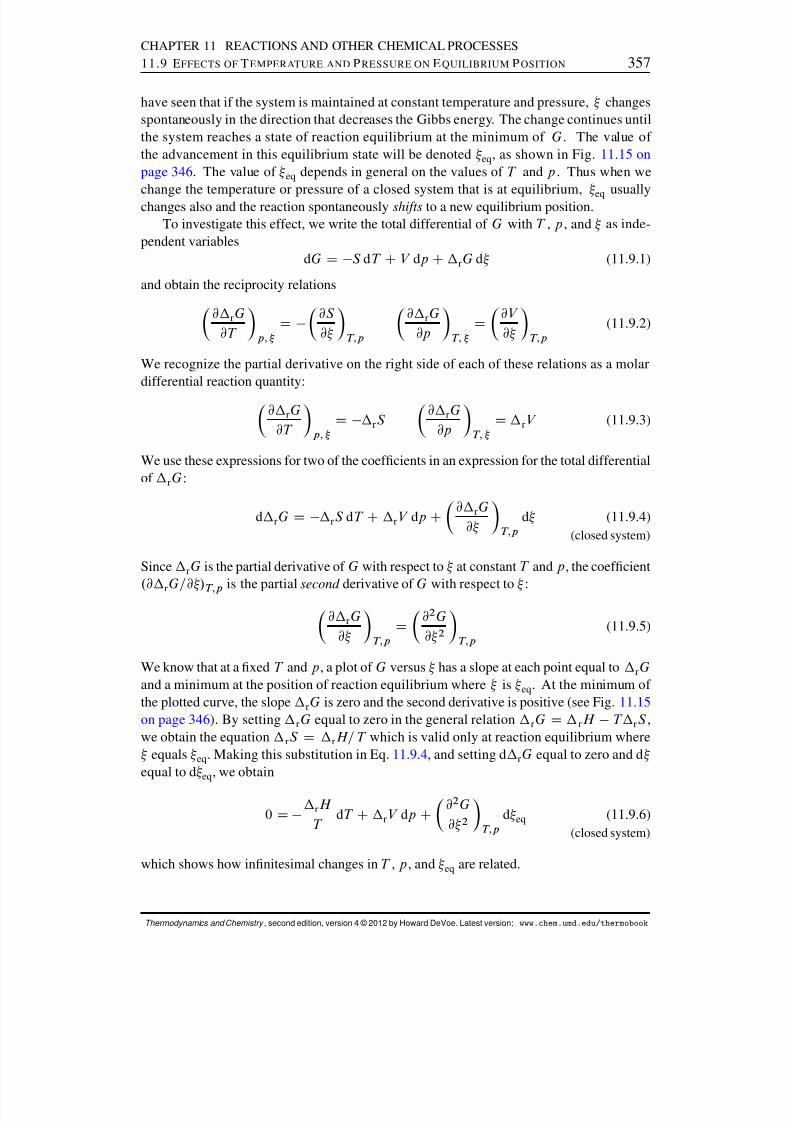
8/12/2019 Howard Devoe Thermodynamic and Chemical
http://slidepdf.com/reader/full/howard-devoe-thermodynamic-and-chemical 357/532
CHAPTER 11 REACTIONS AND OTHER CHEMICAL PROCESSES11.9 E FFECTS OF T EMPERATURE AND P RESSURE ON E QUILIBRIUM P OSITION 357
have seen that if the system is maintained at constant temperature and pressure, changesspontaneously in the direction that decreases the Gibbs energy. The change continues untilthe system reaches a state of reaction equilibrium at the minimum of G . The value of the advancement in this equilibrium state will be denoted eq , as shown in Fig. 11.15 onpage 346 . The value of eq depends in general on the values of T and p . Thus when we
change the temperature or pressure of a closed system that is at equilibrium, eq usuallychanges also and the reaction spontaneously shifts to a new equilibrium position.To investigate this effect, we write the total differential of G with T , p , and as inde-
pendent variablesdG D S dT CV dp C rG d (11.9.1)
and obtain the reciprocity relations
@ rG@T p; D
@S @ T;p
@ rG@p T; D
@V @ T;p
(11.9.2)
We recognize the partial derivative on the right side of each of these relations as a molardifferential reaction quantity:
@ rG@T p; D rS
@ rG@p T; D rV (11.9.3)
We use these expressions for two of the coefcients in an expression for the total differentialof rG :
d rG D rS dT C rV dp C@ rG
@ T;pd (11.9.4)
(closed system)
Since rG is the partial derivative of G with respect to at constant T and p , the coefcient
.@ rG=@ /T;p is the partial second derivative of G with respect to :
@ rG@ T;p D
@2 G@ 2 T;p
(11.9.5)
We know that at a xed T and p , a plot of G versus has a slope at each point equal to rGand a minimum at the position of reaction equilibrium where is eq . At the minimum of the plotted curve, the slope rG is zero and the second derivative is positive (see Fig. 11.15on page 346 ). By setting rG equal to zero in the general relation rG D rH T rS ,we obtain the equation rS D rH= T which is valid only at reaction equilibrium where equals eq . Making this substitution in Eq. 11.9.4 , and setting d rG equal to zero and d equal to d eq , we obtain
0 D rH T
dT C rV dp C@2 G@ 2 T;p
d eq (11.9.6)(closed system)
which shows how innitesimal changes in T , p , and eq are related.
Thermodynamics and Chemistry , second edition, version 4 © 2012 by Howard DeVoe. Latest version: www.chem.umd.edu/thermobook
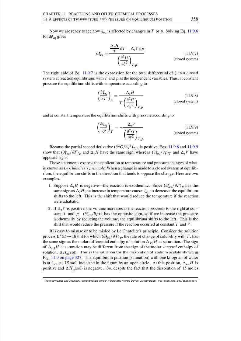
8/12/2019 Howard Devoe Thermodynamic and Chemical
http://slidepdf.com/reader/full/howard-devoe-thermodynamic-and-chemical 358/532
CHAPTER 11 REACTIONS AND OTHER CHEMICAL PROCESSES11.9 E FFECTS OF T EMPERATURE AND P RESSURE ON E QUILIBRIUM P OSITION 358
Now we are ready to see how eq is affected by changes in T or p . Solving Eq. 11.9.6for d eq gives
d eq DrH T
dT rV dp
@2
G@ 2 T;p
(11.9.7)
(closed system)
The right side of Eq. 11.9.7 is the expression for the total differential of in a closedsystem at reaction equilibrium, with T and p as the independent variables. Thus, at constantpressure the equilibrium shifts with temperature according to
@ eq
@T p D rH
T @2 G@ 2 T;p
(11.9.8)(closed system)
and at constant temperature the equilibrium shifts with pressure according to
@ eq
@p T D rV
@2 G@ 2 T;p
(11.9.9)(closed system)
Because the partial second derivative .@2 G=@ 2 / T;p is positive, Eqs. 11.9.8 and 11.9.9show that .@ eq=@T /p and rH have the same sign, whereas .@ eq =@p/T and rV haveopposite signs.
These statements express the application to temperature and pressure changes of whatis known as Le Ch ˆ atelier’s principle : When a change is made to a closed system at equilib-rium, the equilibrium shifts in the direction that tends to oppose the change. Here are two
examples.1. Suppose rH is negative—the reaction is exothermic. Since .@ eq=@T /p has the
same sign as rH , an increase in temperature causes eq to decrease: the equilibriumshifts to the left. This is the shift that would reduce the temperature if the reactionwere adiabatic.
2. If rV is positive, the volume increases as the reaction proceeds to the right at con-stant T and p . .@ eq=@p/T has the opposite sign, so if we increase the pressureisothermally by reducing the volume, the equilibrium shifts to the left. This is theshift that would reduce the pressure if the reaction occurred at constant T and V .
It is easy to misuse or to be misled by Le Ch atelier’s principle. Consider the solutionprocess B (s)
!B(sln) for which .@
eq=@T/
p, the rate of change of solubility with T , has
the same sign as the molar differential enthalpy of solution sol H at saturation. The signof sol H at saturation may be different from the sign of the molar integral enthalpy of solution, H m(sol). This is the situation for the dissolution of sodium acetate shown inFig. 11.9 on page 327 . The equilibrium position (saturation) with one kilogram of wateris at sol 15 mol, indicated in the gure by an open circle. At this position, sol H ispositive and H m(sol) is negative. So, despite the fact that the dissolution of 15 moles
Thermodynamics and Chemistry , second edition, version 4 © 2012 by Howard DeVoe. Latest version: www.chem.umd.edu/thermobook
8/12/2019 Howard Devoe Thermodynamic and Chemical
http://slidepdf.com/reader/full/howard-devoe-thermodynamic-and-chemical 359/532
8/12/2019 Howard Devoe Thermodynamic and Chemical
http://slidepdf.com/reader/full/howard-devoe-thermodynamic-and-chemical 360/532
CHAPTER 11 REACTIONS AND OTHER CHEMICAL PROCESSESPROBLEMS 360
PROBLEMS
An underlined problem number or problem-part letter indicates that the numerical answer appearsin Appendix I.
11.1 Use values of f H ı and f G ı in Appendix H to evaluate the standard molar reaction enthalpyand the thermodynamic equilibrium constant at 298:15 K for the oxidation of nitrogen to formaqueous nitric acid:
12 N2 . g/ C 5
4 O2 . g/ C 12 H2O. l/ ! HC . aq/ CNO 3 . aq/
11.2 In 1982, the International Union of Pure and Applied Chemistry recommended that the valueof the standard pressure p ı be changed from 1 atm to 1 bar. This change affects the values of some standard molar quantities of a substance calculated from experimental data.
(a) Find the changes in H ım , S ım , and G ı
m for a gaseous substance when the standard pressureis changed isothermally from 1:01325 bar (1 atm) to exactly 1 bar. (Such a small pressurechange has an entirely negligible effect on these quantities for a substance in a condensedphase.)
(b) What are the values of the corrections that need to be made to the standard molar enthalpyof formation, the standard molar entropy of formation, and the standard molar Gibbsenergy of formation of N 2 O4 (g) at 298:15 K when the standard pressure is changed from1:01325 bar to 1 bar?
11.3 From data for mercury listed in Appendix H, calculate the saturation vapor pressure of liquidmercury at both 298:15 K and 273:15 K. You may need to make some reasonable approxima-tions.
11.4 Given the following experimental values at T D 298:15 K, p D 1 bar:
HC (aq) COH (aq) ! H2 O(l) rH ı D 55:82 kJ mol 1
Na(s) CH2 O(l) ! NaC (aq / COH (aq) C 12 H2 (g) rH ı D 184:52 kJmol 1
NaOH(s)
! NaOH(aq) sol H 1
D 44:75 kJmol 1
NaOH in 5 H 2 O ! NaOH in 1 H2 O H m(dil) D 4:93 kJ mol 1
NaOH(s) f H ı D 425:61 kJmol 1
Using only these values, calculate:
(a) f H ı for Na C (aq), NaOH(aq), and OH (aq);
(b) f H for NaOH in 5 H 2 O;
(c) H m(sol) for the dissolution of 1 mol NaOH(s) in 5 mol H 2 O.
Thermodynamics and Chemistry , second edition, version 4 © 2012 by Howard DeVoe. Latest version: www.chem.umd.edu/thermobook

8/12/2019 Howard Devoe Thermodynamic and Chemical
http://slidepdf.com/reader/full/howard-devoe-thermodynamic-and-chemical 361/532
CHAPTER 11 REACTIONS AND OTHER CHEMICAL PROCESSESPROBLEMS 361
Table 11.1 Data for Problem 11. 5 a
Substance f H /kJ mol 1 M /g mol 1
H2 O(l) 285:830 18:0153Na 2S2O3 5H2O. s/ 2607:93 248:1828Na2 S2 O3 in 50 H2 O
1135:914
Na2 S2 O3 in 100 H2 O 1133:822Na2 S2 O3 in 200 H2 O 1132:236Na2 S2 O3 in 300 H2 O 1131:780
a Ref. [ 163 ], pages 2-307 and 2-308.
11.5 Table 11.1 lists data for water, crystalline sodium thiosulfate pentahydrate, and several sodiumthiosulfate solutions. Find H to the nearest 0:01 kJ for the dissolution of 5:00 g of crystallineNa 2S2O3 5H2O in 50:0 g of water at 298:15 K and 1 bar.
Table 11.2 Data for Problem 11. 6. Molar in-tegral enthalpies of dilution of aqueous HCl(m0
B D 3:337 mol kg 1 ) at 25 ı C.a
m00B=mol kg 1 H m . dil, m0
B! m00B /=kJ mol 1
0:295 2:8830:225 2:9990:199 3:0410:147 3:1430:113 3:2170:0716 3:3250:0544 3:3810:0497 3:4120:0368
3:466
0:0179 3:5740:0128 3:621
a Ref. [ 153 ].
11.6 Use the experimental data in Table 11.2 to evaluate L A and L B at 25 ı C for an aqueous HClsolution of molality mB D 0:0900 mol kg 1 .
Thermodynamics and Chemistry , second edition, version 4 © 2012 by Howard DeVoe. Latest version: www.chem.umd.edu/thermobook

8/12/2019 Howard Devoe Thermodynamic and Chemical
http://slidepdf.com/reader/full/howard-devoe-thermodynamic-and-chemical 362/532
CHAPTER 11 REACTIONS AND OTHER CHEMICAL PROCESSESPROBLEMS 362
Table 11.3 Data for Problem 11. 7. The values of intensive properties arefor a temperature of 298:15 K and a pressure of 30 bar unless otherwisestated. Subscripts: A = H 2 O, B = O 2 , C = CO 2 .
Properties of the bomb vessel:internal volume . . . . . . . . . . . . . . . . . . . . . . . 350:0 cm 3
mass of n-hexane placed in bomb. . . . . . . 0:6741 gmass of water placed in bomb . . . . . . . . . . 1:0016 g
Properties of liquid n-hexane:molar mass . . . . . . . . . . . . . . . . . . . . . . . . . . . M D 86:177 gmol 1
d e n s i t y . . . . . . . . . . . . . . . . . . . . . . . . . . . . . . . D 0:6548 g cm 3
cubic expansion coefcient. . . . . . . . . . . . . ˛ D 1:378 10 3 K 1
Properties of liquid H 2 O:molar mass . . . . . . . . . . . . . . . . . . . . . . . . . . . M D 18:0153 gmol 1
d e n s i t y . . . . . . . . . . . . . . . . . . . . . . . . . . . . . . . D 0:9970 g cm 3
cubic expansion coefcient. . . . . . . . . . . . . ˛ D 2:59 10 4 K 1
standard molar energy of vaporization . . . vap U ı D 41:53 kJ mol 1
Second virial coefcients, 298:15 K:
BAA . . . . . . . . . . . . . . . . . . . . . . . . . . . . . . . . . 1158 cm3
mol1
BBB . . . . . . . . . . . . . . . . . . . . . . . . . . . . . . . . . . 16 cm 3 mol 1
dBBB = dT . . . . . . . . . . . . . . . . . . . . . . . . . . . . 0:21 cm 3 K 1 mol 1
BCC . . . . . . . . . . . . . . . . . . . . . . . . . . . . . . . . . . 127 cm3 mol 1
dBCC = dT . . . . . . . . . . . . . . . . . . . . . . . . . . . . 0:97 cm 3 K 1 mol 1
BAB . . . . . . . . . . . . . . . . . . . . . . . . . . . . . . . . . 40 cm 3 mol 1
BAC . . . . . . . . . . . . . . . . . . . . . . . . . . . . . . . . . . 214 cm3 mol 1
BBC . . . . . . . . . . . . . . . . . . . . . . . . . . . . . . . . . . 43:7 cm 3 mol 1
dBBC = dT . . . . . . . . . . . . . . . . . . . . . . . . . . . . 0:4 cm3 K 1 mol 1
Henry’s law constants at 1 bar (solvent = H 2 O):O2 . . . . . . . . . . . . . . . . . . . . . . . . . . . . . . . . . . . km; B D 796 bar kg mol 1
CO 2 . . . . . . . . . . . . . . . . . . . . . . . . . . . . . . . . . km; C D 29:7 bar kg mol 1
Partial molar volumes of solutes in water:O2 . . . . . . . . . . . . . . . . . . . . . . . . . . . . . . . . . . . V 1B D 31 cm 3 mol 1
CO 2 . . . . . . . . . . . . . . . . . . . . . . . . . . . . . . . . . V 1C D 33 cm 3 mol 1
Standard molar energies of solution (solvent = H 2 O):O2 . . . . . . . . . . . . . . . . . . . . . . . . . . . . . . . . . . . sol U ı D 9:7 kJmol 1
CO 2 . . . . . . . . . . . . . . . . . . . . . . . . . . . . . . . . . sol U ı D 17:3 kJmol 1
11.7 This 16-part problem illustrates the use of experimental data from bomb calorimetry and othersources, combined with thermodynamic relations derived in this and earlier chapters, to eval-uate the standard molar combustion enthalpy of a liquid hydrocarbon. The substance underinvestigation is n-hexane, and the combustion reaction in the bomb vessel is
C6H14 . l/ C 192 O2 . g/ ! 6 CO 2 . g/ C7 H 2O. l/
Assume that the sample is placed in a glass ampoule that shatters at ignition. Data needed forthis problem are collected in Table 11.3 .
States 1 and 2 referred to in this problem are the initial and nal states of the isothermal bombprocess. The temperature is the reference temperature of 298:15 K.
Thermodynamics and Chemistry , second edition, version 4 © 2012 by Howard DeVoe. Latest version: www.chem.umd.edu/thermobook
8/12/2019 Howard Devoe Thermodynamic and Chemical
http://slidepdf.com/reader/full/howard-devoe-thermodynamic-and-chemical 363/532
CHAPTER 11 REACTIONS AND OTHER CHEMICAL PROCESSESPROBLEMS 363
(a) Parts (a)–(c) consist of simple calculations of some quantities needed in later parts of theproblem. Begin by using the masses of C 6 H14 and H2 O placed in the bomb vessel, andtheir molar masses, to calculate the amounts (moles) of C 6 H14 and H2 O present initiallyin the bomb vessel. Then use the stoichiometry of the combustion reaction to nd theamount of O 2 consumed and the amounts of H 2 O and CO 2 present in state 2. (There isnot enough information at this stage to allow you to nd the amount of O 2 present, just
the change.) Also nd the nal mass of H 2 O. Assume that oxygen is present in excessand the combustion reaction goes to completion.
(b) From the molar masses and the densities of liquid C 6 H14 and H2 O, calculate their molarvolumes.
(c) From the amounts present initially in the bomb vessel and the internal volume, nd thevolumes of liquid C 6 H14 , liquid H 2 O, and gas in state 1 and the volumes of liquid H 2 Oand gas in state 2. For this calculation, you can neglect the small change in the volume of liquid H 2 O due to its vaporization.
(d) When the bomb vessel is charged with oxygen and before the inlet valve is closed, thepressure at 298:15 K measured on an external gauge is found to be p 1 D 30:00 bar. To agood approximation, the gas phase of state 1 has the equation of state of pure O 2 (sincethe vapor pressure of water is only 0:1 % of 30:00 bar). Assume that this equation of stateis given by V m D RT=p CBBB (Eq. 2.2.8), where B BB is the second virial coefcientof O2 listed in Table 11.3 . Solve for the amount of O 2 in the gas phase of state 1. Thegas phase of state 2 is a mixture of O 2 and CO 2 , again with a negligible partial pressureof H 2 O. Assume that only small fractions of the total amounts of O 2 and CO 2 dissolvein the liquid water, and nd the amount of O 2 in the gas phase of state 2 and the molefractions of O 2 and CO 2 in this phase.
(e) You now have the information needed to nd the pressure in state 2, which cannot be mea-sured directly. For the mixture of O 2 and CO 2 in the gas phase of state 2, use Eq. 9.3.23on page 245 to calculate the second virial coefcient. Then solve the equation of state of Eq. 9.3.21 on page 245 for the pressure. Also calculate the partial pressures of the O 2 andCO 2 in the gas mixture.
(f) Although the amounts of H 2 O in the gas phases of states 1 and 2 are small, you need toknow their values in order to take the energy of vaporization into account. In this part,you calculate the fugacities of the H 2 O in the initial and nal gas phases, in part (g) youuse gas equations of state to evaluate the fugacity coefcients of the H 2 O (as well as of the O 2 and CO 2 ), and then in part (h) you nd the amounts of H 2 O in the initial and nalgas phases.The pressure at which the pure liquid and gas phases of H 2 O are in equilibrium at 298:15 K(the saturation vapor pressure of water) is 0:03169 bar. Use Eq. 7.8.18 on page 186 to es-timate the fugacity of H 2 O(g) in equilibrium with pure liquid water at this temperatureand pressure. The effect of pressure on fugacity in a one-component liquid–gas system isdiscussed in Sec. 12.8.1 ; use Eq. 12.8.3 on page 401 to nd the fugacity of H 2 O in gasphases equilibrated with liquid water at the pressures of states 1 and 2 of the isothermalbomb process. (The mole fraction of O 2 dissolved in the liquid water is so small that you
can ignore its effect on the chemical potential of the water.)(g) Calculate the fugacity coefcients of H 2 O and O 2 in the gas phase of state 1 and of H 2 O,
O2 , and CO 2 in the gas phase of state 2.For state 1, in which the gas phase is practically-pure O 2 , you can use Eq. 7.8.18 onpage 186 to calculate O2
. The other calculations require Eq. 9.3.29 on page 246 , withthe value of B 0
i found from the formulas of Eq. 9.3.26 or Eqs. 9.3.27 and 9.3.28 (yA is sosmall that you can set it equal to zero in these formulas).
Thermodynamics and Chemistry , second edition, version 4 © 2012 by Howard DeVoe. Latest version: www.chem.umd.edu/thermobook
8/12/2019 Howard Devoe Thermodynamic and Chemical
http://slidepdf.com/reader/full/howard-devoe-thermodynamic-and-chemical 364/532
8/12/2019 Howard Devoe Thermodynamic and Chemical
http://slidepdf.com/reader/full/howard-devoe-thermodynamic-and-chemical 365/532
CHAPTER 11 REACTIONS AND OTHER CHEMICAL PROCESSESPROBLEMS 365
the gas phase present in state 1. Use the approximate expression for U m U ım(g) in Table7.5 to calculate U D U.p 1 / nU ım (g); a value of d B= dT for pure O 2 is listed in Table11.3 .The other internal energy change is for a process in which the gas phase of state 2 atpressure p 2 is expanded until the pressure is low enough for the gas to behave ideally,and the mixture is then separated into ideal-gas phases of pure O 2 and CO 2 . The molar
internal energies of the separated low-pressure O 2 and CO 2 gases are the same as thestandard molar internal energies of these gases. The internal energy of unmixing idealgases is zero (Eq. 11.1.11 ). The dependence of the internal energy of the gas mixture isgiven, to a good approximation, by U DPi U ıi (g) npT dB= dT , where B is the secondvirial coefcient of the gas mixture; this expression is the analogy for a gas mixture of theapproximate expression for U m U ım(g) in Table 7.5 . Calculate the value of d B= dT forthe mixture of O 2 and CO 2 in state 2 (you need Eq. 9.3.23 on page 245 and the values of dB ij = dT in Table 11.3 ) and evaluate U DPi n i U ıi (g) U.p 2 / for the gas expansion.
(n) Add the internal energy changes you calculated in parts (j)–(m) to nd the total internalenergy change of the Washburn corrections. Note that most of the corrections occur inpairs of opposite sign and almost completely cancel one another. Which contributions arethe greatest in magnitude?
(o) The internal energy change of the isothermal bomb process in the bomb vessel, correctedto the reference temperature of 298:15 K, is found to be U . IBP ; T ref / D 32:504 kJ.Assume there are no side reactions or auxiliary reactions. From Eqs. 11.5.9 and 11.5.10 ,calculate the standard molar internal energy of combustion of n-hexane at 298:15 K.
(p) From Eq. 11.5.13 , calculate the standard molar enthalpy of combustion of n-hexane at298:15 K.
11.8 By combining the results of Prob. 11. 7(p) with the values of standard molar enthalpies of formation from Appendix H, calculate the standard molar enthalpy of formation of liquid n-hexane at 298:15 K.
11.9 Consider the combustion of methane:
CH 4 . g/ C2 O 2 . g/ ! CO2 . g/ C2 H 2O. g/
Suppose the reaction occurs in a owing gas mixture of methane and air. Assume that thepressure is constant at 1 bar, the reactant mixture is at a temperature of 298:15 K and hasstoichiometric proportions of methane and oxygen, and the reaction goes to completion withno dissociation. For the quantity of gaseous product mixture containing 1 mol CO 2 , 2 mol H 2 O,and the nitrogen and other substances remaining from the air, you may use the approximateformula C p . P/ D a CbT , where the coefcients have the values a D 297:0 J K 1 and b D8:520 10 2 J K 2 . Solve Eq. 11.6.1 for T 2 to estimate the ame temperature to the nearestkelvin.
11.10 The standard molar Gibbs energy of formation of crystalline mercury(II) oxide at 600:00 K hasthe value f G ı D 26:386 kJmol 1 . Estimate the partial pressure of O 2 in equilibrium with
HgO at this temperature: 2 HgO(s) • 2 Hg(l) CO2 (g).11.11 The combustion of hydrogen is a reaction that is known to “go to completion.”
(a) Use data in Appendix H to evaluate the thermodynamic equilibrium constant at 298:15 Kfor the reaction
H2 . g/ C 12 O2 . g/ ! H2O. l/
Thermodynamics and Chemistry , second edition, version 4 © 2012 by Howard DeVoe. Latest version: www.chem.umd.edu/thermobook
8/12/2019 Howard Devoe Thermodynamic and Chemical
http://slidepdf.com/reader/full/howard-devoe-thermodynamic-and-chemical 366/532
CHAPTER 11 REACTIONS AND OTHER CHEMICAL PROCESSESPROBLEMS 366
(b) Assume that the reaction is at equilibrium at 298:15 K in a system in which the partialpressure of O 2 is 1:0 bar. Assume ideal-gas behavior and nd the equilibrium partialpressure of H 2 and the number of H 2 molecules in 1:0 m3 of the gas phase.
(c) In the preceding part, you calculated a very small value (a fraction) for the number of H 2
molecules in 1:0 m3 . Statistically, this fraction can be interpreted as the fraction of a givenlength of time during which one molecule is present in the system. Take the age of theuniverse as 1:0 1010 years and nd the total length of time in seconds, during the age of the universe, that a H 2 molecule is present in the equilibrium system. (This hypotheticalvalue is a dramatic demonstration of the statement that the limiting reactant is essentiallyentirely exhausted during a reaction with a large value of K .)
11.12 Let G represent carbon in the form of graphite and D represent the diamond crystal form. At298:15 K, the thermodynamic equilibrium constant for G • D, based on a standard pressurep ı D 1 bar, has the value K D 0:31. The molar volumes of the two crystal forms at thistemperature are V m . G/ D 5:3 10 6 m3 mol 1 and V m . D/ D 3:4 10 6 m3 mol 1 .
(a) Write an expression for the reaction quotient Q rxn as a function of pressure. Use theapproximate expression of the pressure factor given in Table 9.6.
(b) Use the value of K to estimate the pressure at which the D and G crystal forms are inequilibrium with one another at 298:15 K. (This is the lowest pressure at which graphitecould in principle be converted to diamond at this temperature.)
11.13 Consider the dissociation reaction N 2O4 . g/ ! 2 NO 2 . g/ taking place at a constant tempera-ture of 298:15 K and a constant pressure of 0:0500 bar. Initially (at D 0) the system contains1:000 mol of N 2 O4 and no NO 2 . Other needed data are found in Appendix H. Assume ideal-gas behavior.
(a) For values of the advancement ranging from 0 to 1 mol, at an interval of 0:1 mol orless, calculate ΠG. / G.0/ to the nearest 0:01 kJ. A computer spreadsheet would be aconvenient way to make the calculations.
(b) Plot your values of G. / G.0/ as a function of , and draw a smooth curve through thepoints.
(c) On your curve, indicate the estimated position of eq . Calculate the activities of N 2 O4 andNO 2 for this value of , use them to estimate the thermodynamic equilibrium constant K ,and compare your result with the value of K calculated from Eq. 11.8.11 .
Thermodynamics and Chemistry , second edition, version 4 © 2012 by Howard DeVoe. Latest version: www.chem.umd.edu/thermobook
8/12/2019 Howard Devoe Thermodynamic and Chemical
http://slidepdf.com/reader/full/howard-devoe-thermodynamic-and-chemical 367/532
C HAPTER 12
E QUILIBRIUM CONDITIONS IN
M ULTICOMPONENT SYSTEMS
This chapter applies equilibrium theory to a variety of chemical systems of more than onecomponent. Two different approaches will be used as appropriate: one based on the relation
’i D “
i for transfer equilibrium, the other based on Pi i i D 0 or K DQi ai
i forreaction equilibrium.
12.1 EFFECTS OF TEMPERATURE
For some of the derivations in this chapter, we will need an expression for the rate at whichthe ratio i =T varies with temperature in a phase of xed composition maintained at con-stant pressure. This expression leads, among other things, to an important relation betweenthe temperature dependence of an equilibrium constant and the standard molar reactionenthalpy.
12.1.1 Variation of i =T with temperature
In a phase containing species i , either pure or in a mixture, the partial derivative of i =T with respect to T at constant p and a xed amount of each species is given by 1
@ . i =T /@T p; fn ig
D 1T
@ i
@T p; fn ig
i
T 2 (12.1.1)
This equality comes from a purely mathematical operation; no thermodynamics is involved.The partial derivative .@ i =@T /p; fn ig is equal to S i (Eq. 9.2.48 ), so that Eq. 12.1.1 be-comes
@ . i =T /
@T p; fn ig
D S iT
i
T 2 D TS i C i
T 2 (12.1.2)
The further substitution i D H i TS i (Eq. 9.2.46 ) gives nally
@ . i =T /@T p; fn ig
D H iT 2
(12.1.3)
1This relation is obtained from the formula d .uv/= dx D u. dv= dx/ Cv. du= dx/ (Appendix E), where u is1=T , v is i , and x is T .
367
8/12/2019 Howard Devoe Thermodynamic and Chemical
http://slidepdf.com/reader/full/howard-devoe-thermodynamic-and-chemical 368/532
CHAPTER 12 EQUILIBRIUM CONDITIONS IN MULTICOMPONENT SYSTEMS12.1 E FFECTS OF T EMPERATURE 368
For a pure substance in a closed system, Eq. 12.1.3 when multiplied by the amount nbecomes
@.G=T/@T p D
H T 2
(12.1.4)
This is the Gibbs–Helmholtz equation .
12.1.2 Variation of ıi =T with temperature
If we make the substitution i D ıi CRT ln a i in Eq. 12.1.3 and rearrange, we obtain
d. ıi =T /
dT D H iT 2 R
@ln a i
@T p; fn ig(12.1.5)
Because ıi =T is a function only of T , its derivative with respect to T is itself a function
only of T . We can therefore use any convenient combination of pressure and compositionin the expression on the right side of Eq. 12.1.5 in order to evaluate d . ı
i =T/= dT at a giventemperature.
If species i is a constituent of a gas mixture, we take a constant pressure of the gas thatis low enough for the gas to behave ideally. Under these conditions H
i is the standard molar
enthalpy H ıi (Eq. 9.3.7 ). In the expression for activity, a i (g) D i (g) i p i =p (Table 9.5 ),
the pressure factor i (g) is constant when p is constant, the fugacity coefcient i for theideal gas is unity, and p i =p D yi is constant at constant fn ig, so that the partial derivativeŒ@ln a i (g)=@Tp; fn ig is zero.
For component i of a condensed-phase mixture, we take a constant pressure equal tothe standard pressure p ı , and a mixture composition in the limit given by Eqs. 9.5.20 –9.5.24 in which the activity coefcient is unity. H i is then the standard molar enthalpy H ı
i ,and the activity is given by an expression in Table 9.5 with the pressure factor and activitycoefcient set equal to 1: a i Dx i , a ADxA , a x; BDxB , a c; BDcB=cı , or a m; BDmB=m ı .2 Withthe exception of a c; B , these activities are constant as T changes at constant p and fn ig.
Thus for a gas-phase species, or a species with a standard state based on mole fractionor molality, Œ@ln a i (g)=@Tp; fn ig is zero and Eq. 12.1.5 becomes
d. ıi =T /
dT D H ı
i
T 2 (12.1.6)(standard state not based
on concentration)
Equation 12.1.6 , as the conditions of validity indicate, does not apply to a solute stan-dard state based on concentration, except as an approximation. The reason is the volumechange that accompanies an isobaric temperature change. We can treat this case by consid-ering the following behavior of ln .c B=cı / :
@ln .c B=cı /
@T p; fn ig D
1
cB
@cB
@T p; fn ig D
1
nB=V
@.nB=V /
@T p; fn ig
D V @.1=V /
@T p; fn igD
1V
@V @T p; fn ig
D ˛ (12.1.7)
2If solute B is an electrolyte, am; B is given instead by Eq. 10.3.10 ; like am; B for a nonelectrolyte, it is constantas T changes at constant p and fn ig.
Thermodynamics and Chemistry , second edition, version 4 © 2012 by Howard DeVoe. Latest version: www.chem.umd.edu/thermobook
8/12/2019 Howard Devoe Thermodynamic and Chemical
http://slidepdf.com/reader/full/howard-devoe-thermodynamic-and-chemical 369/532
CHAPTER 12 EQUILIBRIUM CONDITIONS IN MULTICOMPONENT SYSTEMS12.1 E FFECTS OF T EMPERATURE 369
Here ˛ is the cubic expansion coefcient of the solution (Eq. 7.1.1 ). If the activity coef-cient is to be unity, the solution must be an ideal-dilute solution, and ˛ is then ˛ A , the cubicexpansion coefcient of the pure solvent. Eq. 12.1.5 for a nonelectrolyte becomes
d. ıc; B=T /
dT D H ı
B
T 2 CR˛ A (12.1.8)
12.1.3 Variation of ln K with temperature
The thermodynamic equilibrium constant K , for a given reaction equation and a givenchoice of reactant and product standard states, is a function of T and only of T . By equat-ing two expressions for the standard molar reaction Gibbs energy, rG
ı DPi iıi and
rGı D RT ln K (Eqs. 11.8.3 and 11.8.10 ), we obtain
ln K D 1RT Xi
iıi (12.1.9)
The rate at which ln K varies with T is then given by
d ln K dT D
1R Xi
id. ı
i =T /dT
(12.1.10)
Combining Eq. 12.1.10 with Eqs. 12.1.6 or 12.1.8 , and recognizing that Pi i H ıi is the
standard molar reaction enthalpy rH ı , we obtain the nal expression for the temperaturedependence of ln K :
d ln K dT D
rH ı
RT 2 ˛ A Xsolutes,conc. basis
i (12.1.11)
The sum on the right side includes only solute species whose standard states are based onconcentration. The expression is simpler if all solute standard states are based on molefraction or molality:
d ln K dT D
rH ı
RT 2 (12.1.12)(no solute standard states
based on concentration)
We can rearrange Eq. 12.1.12 to
rH ı D RT 2d ln K
dT (12.1.13)(no solute standard states
based on concentration)
We can convert this expression for rH ı to an equivalent form by using the mathematicalidentity d .1=T / D .1=T 2 / dT :
rH ı D R d ln K d.1=T /
(12.1.14)(no solute standard states
based on concentration)
Thermodynamics and Chemistry , second edition, version 4 © 2012 by Howard DeVoe. Latest version: www.chem.umd.edu/thermobook
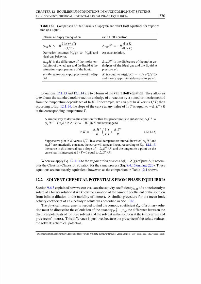
8/12/2019 Howard Devoe Thermodynamic and Chemical
http://slidepdf.com/reader/full/howard-devoe-thermodynamic-and-chemical 370/532
CHAPTER 12 EQUILIBRIUM CONDITIONS IN MULTICOMPONENT SYSTEMS12.2 S OLVENT C HEMICAL P OTENTIALS FROM P HASE E QUILIBRIA 370
Table 12.1 Comparison of the Clausius–Clapeyron and van’t Hoff equations for vaporiza-tion of a liquid.
Clausius–Clapeyron equation van’t Hoff equation
vap H
R
d ln .p=p ı /
d.1=T /
vap H ı
D R
d ln K
d.1=T /Derivation assumes V m(g) V m (l) andideal-gas behavior.
An exact relation.
vap H is the difference of the molar en-thalpies of the real gas and the liquid at thesaturation vapor pressure of the liquid.
vap H ı is the difference of the molar en-thalpies of the ideal gas and the liquid atpressure p ı .
p is the saturation vapor pressure of the liq-uid.
K is equal to a (g)=a(l) D .f=p ı /= (l),and is only approximately equal to p=p ı .
Equations 12.1.13 and 12.1.14 are two forms of the van’t Hoff equation . They allow usto evaluate the standard molar reaction enthalpy of a reaction by a noncalorimetric methodfrom the temperature dependence of ln K . For example, we can plot ln K versus 1=T ; thenaccording to Eq. 12.1.14 , the slope of the curve at any value of 1=T is equal to rH ı =Rat the corresponding temperature T .
A simple way to derive the equation for this last procedure is to substitute rG ı DrH ı T rS ı in rG ı D RT ln K and rearrange to
ln K D rH ı
R 1T C
rS ı
R (12.1.15)
Suppose we plot ln K versus 1=T . In a small temperature interval in which rH ı andrS ı are practically constant, the curve will appear linear. According to Eq. 12.1.15 ,
the curve in this interval has a slope of rH ı=R , and the tangent to a point on the
curve has its intercept at 1=T D0 equal to rS ı =R .
When we apply Eq. 12.1.14 to the vaporization process A(l) ! A(g) of pure A, it resem-bles the Clausius–Clapeyron equation for the same process (Eq. 8.4.15 on page 220 ). Theseequations are not exactly equivalent, however, as the comparison in Table 12.1 shows.
12.2 SOLVENT CHEMICAL POTENTIALS FROM PHASE EQUILIBRIA
Section 9.6.3 explained how we can evaluate the activity coefcient m; B of a nonelectrolytesolute of a binary solution if we know the variation of the osmotic coefcient of the solutionfrom innite dilution to the molality of interest. A similar procedure for the mean ionicactivity coefcient of an electrolyte solute was described in Sec. 10.6 .
The physical measurements needed to nd the osmotic coefcient m of a binary solu-tion must be directed to the calculation of the quantity A A , the difference between thechemical potentials of the pure solvent and the solvent in the solution at the temperature andpressure of interest. This difference is positive, because the presence of the solute reducesthe solvent’s chemical potential.
Thermodynamics and Chemistry , second edition, version 4 © 2012 by Howard DeVoe. Latest version: www.chem.umd.edu/thermobook
8/12/2019 Howard Devoe Thermodynamic and Chemical
http://slidepdf.com/reader/full/howard-devoe-thermodynamic-and-chemical 371/532
CHAPTER 12 EQUILIBRIUM CONDITIONS IN MULTICOMPONENT SYSTEMS12.2 S OLVENT C HEMICAL P OTENTIALS FROM P HASE E QUILIBRIA 371
To calculate m from A A , we use Eq. 9.6.16 on page 268 for a nonelectrolytesolute, or Eq. 10.6.1 on page 300 for an electrolyte solute. Both equations are representedby
m D A A
RT M A m B(12.2.1)
where for a nonelectrolyte is 1 and for an electrolyte is the number of ions per formulaunit.
The sequence of steps, then, is (1) the determination of A A over a range of molalityat constant T and p , (2) the conversion of these values to m using Eq. 12.2.1 , and (3) theevaluation of the solute activity coefcient 3 by a suitable integration from innite dilutionto the molality of interest.
Sections 12.2.1 and 12.2.2 will describe freezing-point and osmotic-pressure measure-ments, two much-used methods for evaluating A A in a binary solution at a given T andp . The isopiestic vapor-pressure method was described in Sec. 9.6.4 . The freezing-pointand isopiestic vapor-pressure methods are often used for electrolyte solutions, and osmoticpressure is especially useful for solutions of macromolecules.
12.2.1 Freezing-point measurements
This section explains how we can evaluate A A for a solution of a given compositionat a given T and p from the freezing point of the solution combined with additional dataobtained from calorimetric measurements.
Consider a binary solution of solvent A and solute B. We assume that when this solutionis cooled at constant pressure and composition, the solid that rst appears is pure A. Forexample, for a dilute aqueous solution the solid would be ice. The temperature at whichsolid A rst appears is T f , the freezing point of the solution. This temperature is lowerthan the freezing point T f of the pure solvent, a consequence of the lowering of A by thepresence of the solute. Both T f and T f can be measured experimentally.
Let T 0 be a temperature of interest that is equal to or greater than T f . We wish todetermine the value of A . l; T 0/ A . sln ; T 0/ , where A . l; T 0/ refers to pure liquid solventand A . sln ; T 0/ refers to the solution.
Figure 12.1 on the next page explains the principle of the procedure. The gure shows
A=T for the solvent in the pure solid phase, in the pure liquid phase, and in the xed-composition solution, plotted as functions of T at constant p . Since A is the same in thesolution and solid phases at temperature T f , and is the same in the pure liquid and solidphases at temperature T f , the curves intersect at these temperatures as shown.
Formulas for the slopes of the three curves, from Eq. 12.1.3 on page 367 , are includedin the gure. The desired value of A . l; T 0/ A . sln ; T 0/ is the product of T 0 and thedifference of the values of A=T at points e and a. To nd this difference, we integrate the
3A measurement of A A also gives us the solvent activity coefcient, based on the pure-solvent referencestate, through the relation A D A CRT ln. A xA / (Eq. 9.5.15 ).
Thermodynamics and Chemistry , second edition, version 4 © 2012 by Howard DeVoe. Latest version: www.chem.umd.edu/thermobook
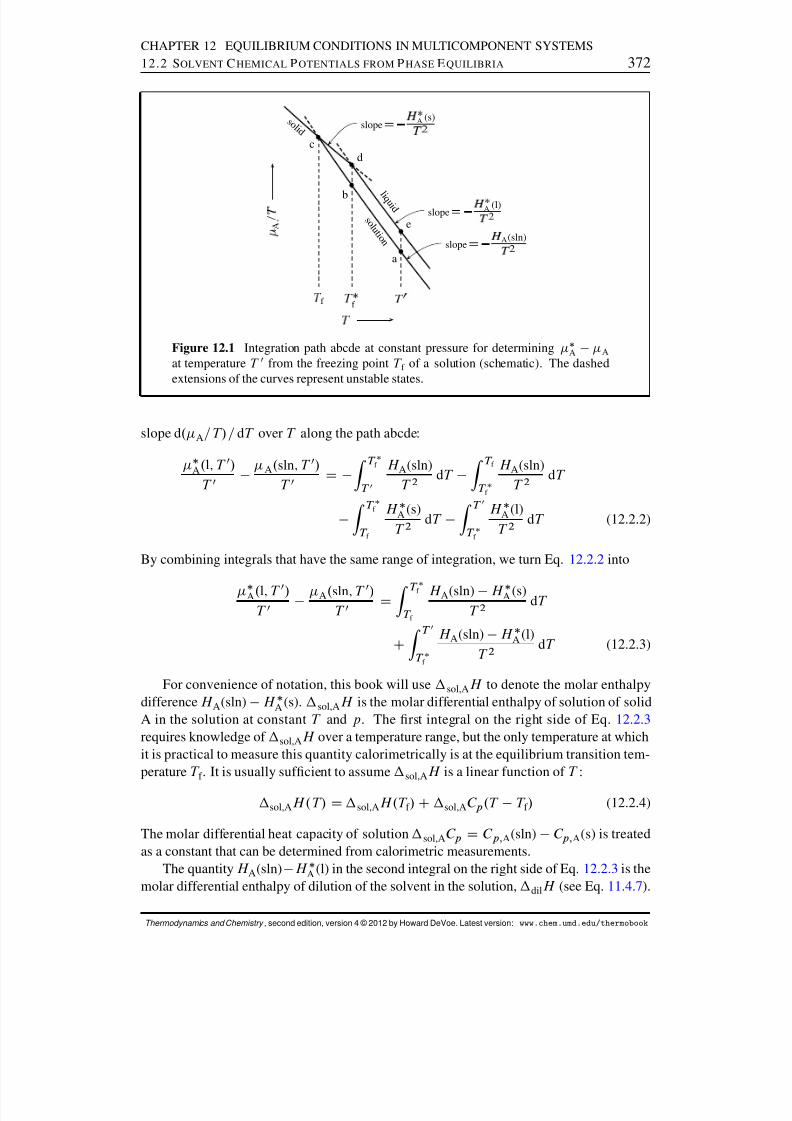
8/12/2019 Howard Devoe Thermodynamic and Chemical
http://slidepdf.com/reader/full/howard-devoe-thermodynamic-and-chemical 372/532
CHAPTER 12 EQUILIBRIUM CONDITIONS IN MULTICOMPONENT SYSTEMS12.2 S OLVENT C HEMICAL P OTENTIALS FROM P HASE E QUILIBRIA 372
a
b
cd
e
f
f
A
s o l i d
l i q u i d s o l u t i o n
slope
A (s)
slope
A (l)
slope
A(sln)
Figure 12.1 Integration path abcde at constant pressure for determining A Aat temperature T 0 from the freezing point T f of a solution (schematic). The dashedextensions of the curves represent unstable states.
slope d . A=T/= dT over T along the path abcde:
A . l; T 0/T 0
A . sln ; T 0/T 0 D Z
T f
T 0
H A(sln)T 2
dT Z T f
T f
H A(sln)T 2
dT
Z T f
T f
H A (s)T 2
dT Z T 0
T f
H A (l)T 2
dT (12.2.2)
By combining integrals that have the same range of integration, we turn Eq. 12.2.2 into
A . l; T 0/T 0 A . sln ; T 0/
T 0 DZ T f
T f
H A(sln) H A (s)T 2
dT
CZ T 0
T f
H A(sln) H A (l)T 2
dT (12.2.3)
For convenience of notation, this book will use sol,A H to denote the molar enthalpydifference H A(sln) H A (s). sol,A H is the molar differential enthalpy of solution of solidA in the solution at constant T and p . The rst integral on the right side of Eq. 12.2.3requires knowledge of sol,A H over a temperature range, but the only temperature at whichit is practical to measure this quantity calorimetrically is at the equilibrium transition tem-perature T f . It is usually sufcient to assume sol,A H is a linear function of T :
sol,A H.T/ D sol,A H.T f / C sol,A C p .T T f / (12.2.4)
The molar differential heat capacity of solution sol,A C p D C p; A(sln) C p; A(s) is treatedas a constant that can be determined from calorimetric measurements.
The quantity H A(sln) H A (l) in the second integral on the right side of Eq. 12.2.3 is themolar differential enthalpy of dilution of the solvent in the solution, dilH (see Eq. 11.4.7 ).
Thermodynamics and Chemistry , second edition, version 4 © 2012 by Howard DeVoe. Latest version: www.chem.umd.edu/thermobook
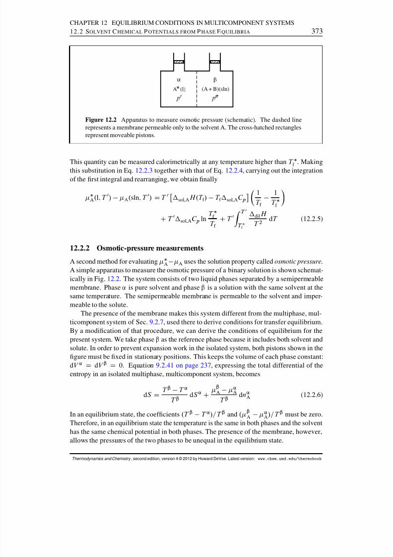
8/12/2019 Howard Devoe Thermodynamic and Chemical
http://slidepdf.com/reader/full/howard-devoe-thermodynamic-and-chemical 373/532
CHAPTER 12 EQUILIBRIUM CONDITIONS IN MULTICOMPONENT SYSTEMS12.2 S OLVENT C HEMICAL P OTENTIALS FROM P HASE E QUILIBRIA 373
A (l)
(A + B)(sln)
Figure 12.2 Apparatus to measure osmotic pressure (schematic). The dashed linerepresents a membrane permeable only to the solvent A. The cross-hatched rectanglesrepresent moveable pistons.
This quantity can be measured calorimetrically at any temperature higher than T f . Makingthis substitution in Eq. 12.2.3 together with that of Eq. 12.2.4 , carrying out the integrationof the rst integral and rearranging, we obtain nally
A . l; T 0/ A . sln ; T 0/ D T 0 sol,A H.T f / T f sol,A C p 1T f
1T f
CT 0 sol,A C p lnT f T f CT 0Z
T 0
T f
dil H T 2
dT (12.2.5)
12.2.2 Osmotic-pressure measurements
A second method for evaluating A A uses the solution property called osmotic pressure .A simple apparatus to measure the osmotic pressure of a binary solution is shown schemat-ically in Fig. 12.2 . The system consists of two liquid phases separated by a semipermeablemembrane. Phase ’ is pure solvent and phase “ is a solution with the same solvent at thesame temperature. The semipermeable membrane is permeable to the solvent and imper-meable to the solute.
The presence of the membrane makes this system different from the multiphase, mul-ticomponent system of Sec. 9.2.7 , used there to derive conditions for transfer equilibrium.By a modication of that procedure, we can derive the conditions of equilibrium for thepresent system. We take phase “ as the reference phase because it includes both solvent andsolute. In order to prevent expansion work in the isolated system, both pistons shown in thegure must be xed in stationary positions. This keeps the volume of each phase constant:dV ’ D dV “ D 0. Equation 9.2.41 on page 237 , expressing the total differential of theentropy in an isolated multiphase, multicomponent system, becomes
dS D T “ T ’T “
dS ’ C “A
’A
T “ dn ’
A (12.2.6)
In an equilibrium state, the coefcients .T “ T ’ /=T “ and . “A ’
A /=T “ must be zero.Therefore, in an equilibrium state the temperature is the same in both phases and the solventhas the same chemical potential in both phases. The presence of the membrane, however,allows the pressures of the two phases to be unequal in the equilibrium state.
Thermodynamics and Chemistry , second edition, version 4 © 2012 by Howard DeVoe. Latest version: www.chem.umd.edu/thermobook
8/12/2019 Howard Devoe Thermodynamic and Chemical
http://slidepdf.com/reader/full/howard-devoe-thermodynamic-and-chemical 374/532
CHAPTER 12 EQUILIBRIUM CONDITIONS IN MULTICOMPONENT SYSTEMS12.2 S OLVENT C HEMICAL P OTENTIALS FROM P HASE E QUILIBRIA 374
Suppose we start with both phases shown in Fig. 12.2 at the same temperature andpressure. Under these conditions, the value of A is less in the solution than in the pureliquid, and a spontaneous ow of solvent will occur through the membrane from the puresolvent to the solution. This phenomenon is called osmosis .4 If we move the right-handpiston down slightly in order to increase the pressure p 00 of the solution in phase “, A
increases in this phase. The osmotic pressure of the solution, ˘ , is dened as the additionalpressure the solution must have, compared to the pressure p 0 of the pure solvent at the sametemperature, to establish an equilibrium state with no ow of solvent in either directionthrough the membrane: p 00D p 0C˘ .
In practice, the membrane may not be completely impermeable to a solute. All that isrequired for the establishment of an equilibrium state with different pressures on eitherside of the membrane is that solvent transfer equilibrium be established on a short timescale compared to the period of observation, and that the amount of solute transferredduring this period be negligible.
The osmotic pressure ˘ is an intensive property of a solution whose value depends on
the solution’s temperature, pressure, and composition. Strictly speaking, ˘ in an equilib-rium state of the system shown in Fig. 12.2 refers to the osmotic pressure of the solutionat pressure p 0, the pressure of the pure solvent. In other words, the osmotic pressure of asolution at temperature T and pressure p 0 is the additional pressure that would have to beexerted on the solution to establish transfer equilibrium with pure solvent that has temper-ature T and pressure p 0. A solution has the property called osmotic pressure regardless of whether this additional pressure is actually present, just as a solution has a freezing pointeven when its actual temperature is different from the freezing point.
Because in an equilibrium state the solvent chemical potential must be the same on bothsides of the semipermeable membrane, there is a relation between chemical potentials andosmotic pressure given by
A .p 00/ D A .p 0C˘ / D A .p 0/ (12.2.7)(equilibrium state)
We can use this relation to derive an expression for A .p 0/ A .p 0/ as a function of ˘ .The dependence of A on pressure is given according to Eq. 9.2.49 by
@ A
@p T; fn igD V A (12.2.8)
where V A is the partial molar volume of the solvent in the solution. Rewriting this equationin the form d A D V A dp and integrating at constant temperature and composition from p 0
to p 0
C˘ , we obtain
A .p 0C˘ / A .p 0/ DZ p 0C ˘
p 0V A dp (12.2.9)
4Greek for push .
Thermodynamics and Chemistry , second edition, version 4 © 2012 by Howard DeVoe. Latest version: www.chem.umd.edu/thermobook
8/12/2019 Howard Devoe Thermodynamic and Chemical
http://slidepdf.com/reader/full/howard-devoe-thermodynamic-and-chemical 375/532
CHAPTER 12 EQUILIBRIUM CONDITIONS IN MULTICOMPONENT SYSTEMS12.3 B INARY M IXTURE IN E QUILIBRIUM WITH A P URE P HASE 375
Substitution from Eq. 12.2.7 changes this to
A .p 0/ A .p 0/ DZ p 0C ˘
p 0V A dp (12.2.10)
(constant T )
which is the desired expression for A A at a single temperature and pressure. To evaluatethe integral, we need an experimental value of the osmotic pressure ˘ of the solution. If we assume V A is constant in the pressure range from p 0 to p 0 C˘ , Eq. 12.2.10 becomessimply
A .p 0/ A .p 0/ D V A˘ (12.2.11)
12.3 BINARY MIXTURE IN EQUILIBRIUM WITH A PURE PHASE
This section considers a binary liquid mixture of components A and B in equilibrium witheither pure solid A or pure gaseous A. The aim is to nd general relations among changes of
temperature, pressure, and mixture composition in the two-phase equilibrium system thatcan be applied to specic situations in later sections.
In this section, A is the chemical potential of component A in the mixture and A isfor the pure solid or gaseous phase. We begin by writing the total differential of A=T with T , p , and xA as the independent variables. These quantities refer to the binary liquidmixture, and we have not yet imposed a condition of equilibrium with another phase. Thegeneral expression for the total differential is
d. A=T / D@. A=T /
@T p;x A
dT C@. A=T /
@p T;x A
dp C@. A=T /
@xA T;pdxA (12.3.1)
With substitutions from Eqs. 9.2.49 and 12.1.3 , this becomes
d. A=T / D H AT 2
dT C V AT
dp C@. A=T /
@xA T;pdxA (12.3.2)
Next we write the total differential of A=T for pure solid or gaseous A. The indepen-dent variables are T and p ; the expression is like Eq. 12.3.2 with the last term missing:
d. A=T / D H AT 2
dT C V A
T dp (12.3.3)
When the two phases are in transfer equilibrium, A and A are equal. If changes occurin T , p , or xA while the phases remain in equilibrium, the condition d . A=T /
D d. A=T /
must be satised. Equating the expressions on the right sides of Eqs. 12.3.2 and 12.3.3 andcombining terms, we obtain the equation
H A H AT 2
dT V A V A
T dp D
@. A=T /@xA T;p
dxA (12.3.4)
Thermodynamics and Chemistry , second edition, version 4 © 2012 by Howard DeVoe. Latest version: www.chem.umd.edu/thermobook
8/12/2019 Howard Devoe Thermodynamic and Chemical
http://slidepdf.com/reader/full/howard-devoe-thermodynamic-and-chemical 376/532
CHAPTER 12 EQUILIBRIUM CONDITIONS IN MULTICOMPONENT SYSTEMS12.4 C OLLIGATIVE P ROPERTIES OF A D ILUTE S OLUTION 376
which we can rewrite as
sol,A H T 2
dT sol,A V T
dp D@. A=T /
@xA T;pdxA (12.3.5)
(phases inequilibrium)
Here sol,A H is the molar differential enthalpy of solution of solid or gaseous A in theliquid mixture, and sol,A V is the molar differential volume of solution. Equation 12.3.5 isa relation between changes in the variables T , p , and xA , only two of which are independentin the equilibrium system.
Suppose we set d p equal to zero in Eq. 12.3.5 and solve for d T = dxA . This gives us therate at which T changes with xA at constant p :
@T @xA p D
T 2
sol,A H @. A=T /
@xA T;p(12.3.6)
(phases inequilibrium)
We can also set d T equal to zero in Eq. 12.3.5 and nd the rate at which p changes with xAat constant T :
@p@xA T D
T
sol,A V @. A=T /
@xA T;p(12.3.7)
(phases inequilibrium)
Equations 12.3.6 and 12.3.7 will be needed in Secs. 12.4 and 12.5 .
12.4 COLLIGATIVE PROPERTIES OF A DILUTE SOLUTION
The colligative properties of a solution are usually considered to be:1. Freezing-point depression : the decrease in the freezing point of the solution, com-
pared to pure solvent at the same pressure.2. Boiling-point elevation : the increase in the boiling point of a solution containing
nonvolatile solutes, compared to pure solvent at the same pressure.3. Vapor-pressure lowering : the decrease in the vapor pressure of a solution containing
nonvolatile solutes, compared to the vapor pressure of the pure solvent at the sametemperature.
4. Osmotic pressure : the increase in the pressure of the solution that places the solventin transfer equilibrium with pure solvent at the same temperature and pressure as theoriginal solution (page 374 ).
Note that all four properties are dened by an equilibrium between the liquid solution and asolid, liquid, or gas phase of the pure solvent. The properties called colligative (Latin: tied together ) have in common a dependence on the concentration of solute particles that affectsthe solvent chemical potential.
Figure 12.3 on the next page illustrates the freezing-point depression and boiling-pointelevation of an aqueous solution. At a xed pressure, pure liquid water is in equilibriumwith ice at the freezing point and with steam at the boiling point. These are the temperatures
Thermodynamics and Chemistry , second edition, version 4 © 2012 by Howard DeVoe. Latest version: www.chem.umd.edu/thermobook
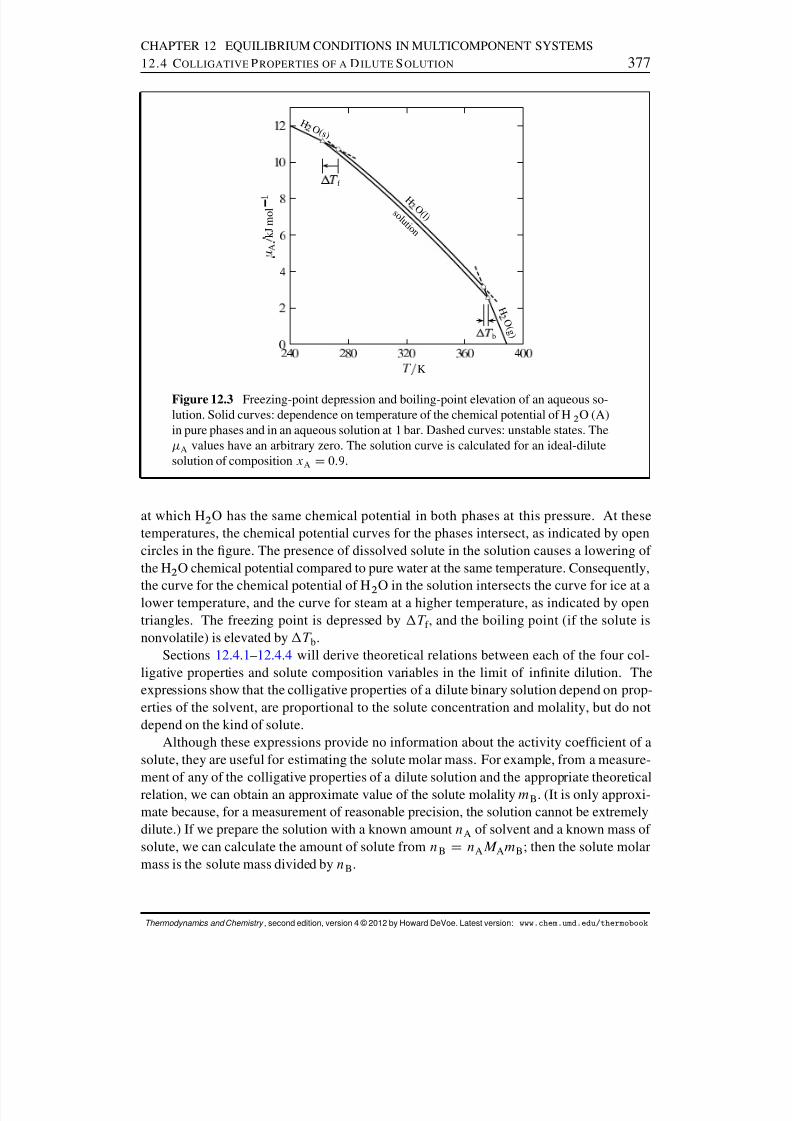
8/12/2019 Howard Devoe Thermodynamic and Chemical
http://slidepdf.com/reader/full/howard-devoe-thermodynamic-and-chemical 377/532
CHAPTER 12 EQUILIBRIUM CONDITIONS IN MULTICOMPONENT SYSTEMS12.4 C OLLIGATIVE P ROPERTIES OF A D ILUTE S OLUTION 377
f
b
H O ( s )
H O ( l ) s o l u t i o n
H
O ( g )
K
A
k J m o l
Figure 12.3 Freezing-point depression and boiling-point elevation of an aqueous so-lution. Solid curves: dependence on temperature of the chemical potential of H 2 O (A)in pure phases and in an aqueous solution at 1 bar. Dashed curves: unstable states. The
A values have an arbitrary zero. The solution curve is calculated for an ideal-dilutesolution of composition xA D 0:9.
at which H 2 O has the same chemical potential in both phases at this pressure. At thesetemperatures, the chemical potential curves for the phases intersect, as indicated by opencircles in the gure. The presence of dissolved solute in the solution causes a lowering of the H 2 O chemical potential compared to pure water at the same temperature. Consequently,
the curve for the chemical potential of H 2 O in the solution intersects the curve for ice at alower temperature, and the curve for steam at a higher temperature, as indicated by opentriangles. The freezing point is depressed by T f , and the boiling point (if the solute isnonvolatile) is elevated by T b .
Sections 12.4.1 –12.4.4 will derive theoretical relations between each of the four col-ligative properties and solute composition variables in the limit of innite dilution. Theexpressions show that the colligative properties of a dilute binary solution depend on prop-erties of the solvent, are proportional to the solute concentration and molality, but do notdepend on the kind of solute.
Although these expressions provide no information about the activity coefcient of asolute, they are useful for estimating the solute molar mass. For example, from a measure-ment of any of the colligative properties of a dilute solution and the appropriate theoreticalrelation, we can obtain an approximate value of the solute molality mB . (It is only approxi-mate because, for a measurement of reasonable precision, the solution cannot be extremelydilute.) If we prepare the solution with a known amount nA of solvent and a known mass of solute, we can calculate the amount of solute from nB D nAM AmB ; then the solute molarmass is the solute mass divided by nB .
Thermodynamics and Chemistry , second edition, version 4 © 2012 by Howard DeVoe. Latest version: www.chem.umd.edu/thermobook
8/12/2019 Howard Devoe Thermodynamic and Chemical
http://slidepdf.com/reader/full/howard-devoe-thermodynamic-and-chemical 378/532
CHAPTER 12 EQUILIBRIUM CONDITIONS IN MULTICOMPONENT SYSTEMS12.4 C OLLIGATIVE P ROPERTIES OF A D ILUTE S OLUTION 378
12.4.1 Freezing-point depression
As in Sec. 12.2.1 , we assume the solid that forms when a dilute solution is cooled to itsfreezing point is pure component A.
Equation 12.3.6 on page 376 gives the general dependence of temperature on the com-position of a binary liquid mixture of A and B that is in equilibrium with pure solid A.
We treat the mixture as a solution. The solvent is component A, the solute is B, and thetemperature is the freezing point T f :
@T f
@xA p D T 2f
sol,A H @. A=T /
@xA T;p(12.4.1)
Consider the expression on the right side of this equation in the limit of innite dilution.In this limit, T f becomes T f , the freezing point of the pure solvent, and sol,A H becomes
fus,A H , the molar enthalpy of fusion of the pure solvent.To deal with the partial derivative on the right side of Eq. 12.4.1 in the limit of innite
dilution, we use the fact that the solvent activity coefcient A approaches 1 in this limit.Then the solvent chemical potential is given by the Raoult’s law relation
A D A CRT ln xA (12.4.2)(solution at innite dilution)
where A is the chemical potential of A in a pure-liquid reference state at the same T andp as the mixture. 5
If the solute is an electrolyte, Eq. 12.4.2 can be derived by the same procedure as de-scribed in Sec. 9.4.6 for an ideal-dilute binary solution of a nonelectrolyte. We must calcu-late xA from the amounts of all species present at innite dilution. In the limit of innitedilution, any electrolyte solute is completely dissociated to its constituent ions: ion pairsand weak electrolytes are completely dissociated in this limit. Thus, for a binary solutionof electrolyte B with ions per formula unit, we should calculate xA from
xA D nAn A C n B
(12.4.3)
where nB is the amount of solute formula unit. (If the solute is a nonelectrolyte, we simplyset equal to 1 in this equation.)
From Eq. 12.4.2 , we can write
@. A=T /@xA T;p ! R as xA ! 1 (12.4.4)
In the limit of innite dilution, then, Eq. 12.4.1 becomes
limx
A! 1
@T f
@xA p D
R.T f /2
fus,AH
(12.4.5)
It is customary to relate freezing-point depression to the solute concentration cB ormolality mB . From Eq. 12.4.3 , we obtain
1 xA D n B
nA C n B(12.4.6)
5At the freezing point of the mixture, the reference state is an unstable supercooled liquid.
Thermodynamics and Chemistry , second edition, version 4 © 2012 by Howard DeVoe. Latest version: www.chem.umd.edu/thermobook
8/12/2019 Howard Devoe Thermodynamic and Chemical
http://slidepdf.com/reader/full/howard-devoe-thermodynamic-and-chemical 379/532
CHAPTER 12 EQUILIBRIUM CONDITIONS IN MULTICOMPONENT SYSTEMS12.4 C OLLIGATIVE P ROPERTIES OF A D ILUTE S OLUTION 379
In the limit of innite dilution, when n B is much smaller than nA , 1 xA approaches thevalue n B=n A . Then, using expressions in Eq. 9.1.14 on page 226 , we obtain the relations
dxA D d.1 xA / D d.n B=n A /
D V A dcB
D M A dmB (12.4.7)(binary solution at
innite dilution)
which transform Eq. 12.4.5 into the following: 6
limcB ! 0
@T f
@cB p D V A R.T f /2
fus,A H
limm B ! 0
@T f
@mB p D M AR.T f /2
fus,A H (12.4.8)
We can apply these equations to a nonelectrolyte solute by setting equal to 1.As cB or mB approaches zero, T f approaches T f . The freezing-point depression (a
negative quantity) is T f D T f T f . In the range of molalities of a dilute solution in which.@T f =@mB / p is given by the expression on the right side of Eq. 12.4.8 , we can write
T f D M AR.T f /2
fus,A H mB (12.4.9)
The molal freezing-point depression constant or cryoscopic constant, K f , is denedfor a binary solution by
K f def
D limm B ! 0
T f
m B(12.4.10)
and, from Eq. 12.4.9 , has a value given by
K f D M AR.T f /2
fus,A H (12.4.11)
The value of K f calculated from this formula depends only on the kind of solvent and thepressure. For H 2 O at 1 bar, the calculated value is K b D 1:860 Kkgmol 1 (Prob. 12. 4).
In the dilute binary solution, we have the relation
T f D K f mB (12.4.12)(dilute binary solution)
This relation is useful for estimating the molality of a dilute nonelectrolyte solution ( D1)from a measurement of the freezing point. The relation is of little utility for an electrolytesolute, because at any electrolyte molality that is high enough to give a measurable depres-sion of the freezing point, the mean ionic activity coefcient deviates greatly from unity andthe relation is not accurate.
6A small dependence of V A on T has been ignored.
Thermodynamics and Chemistry , second edition, version 4 © 2012 by Howard DeVoe. Latest version: www.chem.umd.edu/thermobook
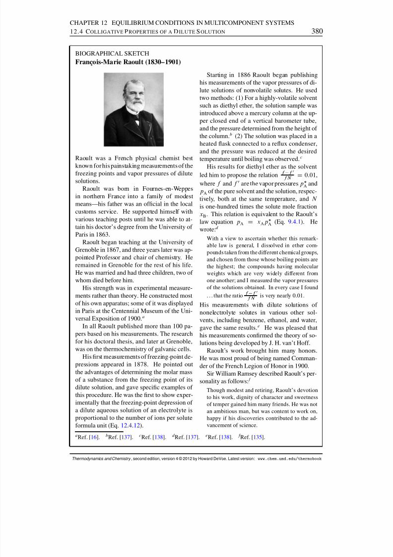
8/12/2019 Howard Devoe Thermodynamic and Chemical
http://slidepdf.com/reader/full/howard-devoe-thermodynamic-and-chemical 380/532
CHAPTER 12 EQUILIBRIUM CONDITIONS IN MULTICOMPONENT SYSTEMS12.4 C OLLIGATIVE P ROPERTIES OF A D ILUTE S OLUTION 380
BIOGRAPHICAL SKETCHFrancois-Marie Raoult (1830–1901)
Raoult was a French physical chemist bestknown forhis painstaking measurements of thefreezing points and vapor pressures of dilutesolutions.
Raoult was born in Fournes-en-Weppesin northern France into a family of modestmeans—his father was an ofcial in the localcustoms service. He supported himself withvarious teaching posts until he was able to at-tain his doctor’s degree from the University of Paris in 1863.
Raoult began teaching at the University of Grenoble in 1867, and three years later was ap-pointed Professor and chair of chemistry. Heremained in Grenoble for the rest of his life.He was married and had three children, two of whom died before him.
His strength was in experimental measure-ments rather than theory. He constructed mostof his own apparatus; some of it was displayedin Paris at the Centennial Museum of the Uni-versal Exposition of 1900. a
In all Raoult published more than 100 pa-pers based on his measurements. The researchfor his doctoral thesis, and later at Grenoble,was on the thermochemistry of galvanic cells.
His rst measurements of freezing-point de-pressions appeared in 1878. He pointed outthe advantages of determining the molar massof a substance from the freezing point of its
dilute solution, and gave specic examples of this procedure. He was the rst to show exper-imentally that the freezing-point depression of a dilute aqueous solution of an electrolyte isproportional to the number of ions per soluteformula unit (Eq. 12.4.12 ).
Starting in 1886 Raoult began publishinghis measurements of the vapor pressures of di-lute solutions of nonvolatile solutes. He used
two methods: (1) For a highly-volatile solventsuch as diethyl ether, the solution sample wasintroduced above a mercury column at the up-per closed end of a vertical barometer tube,and the pressure determined from the height of the column. b (2) The solution was placed in aheated ask connected to a reux condenser,and the pressure was reduced at the desiredtemperature until boiling was observed. c
His results for diethyl ether as the solventled him to propose the relation f f 0
f N D 0:01,where f and f 0 are the vapor pressures p A andp
A of the pure solvent and the solution, respec-
tively, both at the same temperature, and N is one-hundred times the solute mole fractionxB . This relation is equivalent to the Raoult’slaw equation p A D xAp A (Eq. 9.4.1). Hewrote: d
With a view to ascertain whether this remark-able law is general, I dissolved in ether com-pounds taken from the different chemical groups,and chosen from those whose boiling points arethe highest; the compounds having molecularweights which are very widely different fromone another; and I measured the vapor pressuresof the solutions obtained. In every case I found. . . that the ratio f f 0
f N is very nearly 0.01.
His measurements with dilute solutions of nonelectrolyte solutes in various other sol-vents, including benzene, ethanol, and water,gave the same results. e He was pleased thathis measurements conrmed the theory of so-lutions being developed by J. H. van’t Hoff.
Raoult’s work brought him many honors.He was most proud of being named Comman-der of the French Legion of Honor in 1900.
Sir William Ramsey described Raoult’s per-sonality as follows: f
Though modest and retiring, Raoult’s devotionto his work, dignity of character and sweetnessof temper gained him many friends. He was notan ambitious man, but was content to work on,happy if his discoveries contributed to the ad-vancement of science.
a Ref. [ 16]. bRef. [ 137 ]. cRef. [ 138 ]. d Ref. [ 137 ]. eRef. [ 138 ]. f Ref. [ 135 ].
Thermodynamics and Chemistry , second edition, version 4 © 2012 by Howard DeVoe. Latest version: www.chem.umd.edu/thermobook

8/12/2019 Howard Devoe Thermodynamic and Chemical
http://slidepdf.com/reader/full/howard-devoe-thermodynamic-and-chemical 381/532
CHAPTER 12 EQUILIBRIUM CONDITIONS IN MULTICOMPONENT SYSTEMS12.4 C OLLIGATIVE P ROPERTIES OF A D ILUTE S OLUTION 381
12.4.2 Boiling-point elevation
We can apply Eq. 12.3.6 to the boiling point T b of a dilute binary solution. The pure phase of A in equilibrium with the solution is now a gas instead of a solid. 7 Following the procedureof Sec. 12.4.1 , we obtain
limm B ! 0
@T b@mB p D M AR.T b /
2
vap,A H (12.4.13)
where vap,A H is the molar enthalpy of vaporization of pure solvent at its boiling point T b .The molal boiling-point elevation constant or ebullioscopic constant, K b , is dened
for a binary solution by
K bdef
D limm B ! 0
T b
m B(12.4.14)
where T b D T b T b is the boiling-point elevation. Accordingly, K b has a value given by
K b DM AR.T b /2
vap,A H (12.4.15)
For the boiling point of a dilute solution, the analogy of Eq. 12.4.12 is
T b D K b mB (12.4.16)(dilute binary solution)
Since K f has a larger value than K b (because fus,A H is smaller than vap,A H ), the mea-surement of freezing-point depression is more useful than that of boiling-point elevation forestimating the molality of a dilute solution.
12.4.3 Vapor-pressure lowering
In a binary two-phase system in which a solution of volatile solvent A and nonvolatile soluteB is in equilibrium with gaseous A, the vapor pressure of the solution is equal to the systempressure p .
Equation 12.3.7 on page 376 gives the general dependence of p on xA for a binaryliquid mixture in equilibrium with pure gaseous A. In this equation, sol,A V is the molardifferential volume change for the dissolution of the gas in the solution. In the limit of innite dilution, sol,A V becomes vap,A V , the molar volume change for the vaporizationof pure solvent. We also apply the limiting expressions of Eqs. 12.4.4 and 12.4.7 . The resultis
limcB ! 0
@p@cB T D
V A RT
vap,A V lim
m B ! 0
@p@mB T D
M ART
vap,A V (12.4.17)
If we neglect the molar volume of the liquid solvent compared to that of the gas, andassume the gas is ideal, then we can replace vap,A V in the expressions above by V A (g) DRT=p A and obtain
limcB ! 0
@p@cB T V A p A lim
m B ! 0
@p@mB T M Ap A (12.4.18)
7We must assume the solute is nonvolatile or has negligible partial pressure in the gas phase.
Thermodynamics and Chemistry , second edition, version 4 © 2012 by Howard DeVoe. Latest version: www.chem.umd.edu/thermobook
8/12/2019 Howard Devoe Thermodynamic and Chemical
http://slidepdf.com/reader/full/howard-devoe-thermodynamic-and-chemical 382/532

8/12/2019 Howard Devoe Thermodynamic and Chemical
http://slidepdf.com/reader/full/howard-devoe-thermodynamic-and-chemical 383/532
CHAPTER 12 EQUILIBRIUM CONDITIONS IN MULTICOMPONENT SYSTEMS12.4 C OLLIGATIVE P ROPERTIES OF A D ILUTE S OLUTION 383
BIOGRAPHICAL SKETCHJacobus Henricus van’t Hoff (1852–1911)
van’t Hoff was a Dutch chemist who gainedfame from epoch-making publications in sev-eral elds of theoretical chemistry. He was anintrovert who valued nature, philosophy, po-etry, and the power of imagination. a
van’t Hoff was born in Rotterdam, the sonof a physician, and studied at Delft, Leyden,Bonn, and Paris before obtaining his doctor’sdegree at Utrecht in 1874. For 18 years he wasProfessor of Chemistry, Mineralogy, and Geol-ogy at the University of Amsterdam. In 1896,mainly to escape burdensome lecture duties,he accepted an appointment as Professor of Physical Chemistry at the University of Berlin,where he remained for the rest of his life.
In the same year he received his doctor’s de-gree, he published the rst explanation of opti-
cal activity based on the stereoisomerism of anasymmetric carbon atom. Similar ideas werepublished independently two months later bythe French chemist Joseph Le Bel.
In 1884 he entered the eld of physicalchemistry with his book ´ Etudes de DynamiqueChimique , a systematic study of theories of re-action kinetics and chemical equilibrium. Thebook introduced, in the form of Eq. 12.1.12 ,his expression for the temperature dependenceof an equilibrium constant.
van’t Hoff next used thermodynamic cyclesto reason that solutions of equal osmotic pres-
sure should have the same values of freezing-point depression and of vapor-pressure lower-ing. Then, from Raoult’s extensive measure-ments of these values, he found that the os-
motic pressure of a dilute solution is describedby ˘ D icBRT (Eq. 12.4.25 with replacedby i ). The Swedish chemist Svante Arrhenius
later interpreted i as the number of particlesper solute formula unit, helping to validate histheory of ionic dissociation of electrolytes.
In a celebrated 1887 summary of his theoryof osmotic pressure, van’t Hoff wrote: b
. . . the relation found permits of an important ex-tension of the law of Avogadro, which now ndsapplication also to all [nonelectrolyte] solutions,if only osmotic pressure is considered instead of elastic pressure. At equal osmotic pressure andequal temperature, equal volumes of the mostwidely different solutions contain an equal num-ber of molecules, and, indeed, the same number
which, at the same pressure and temperature, iscontained in an equal volume of a gas. . . . theexistence of the so-called normal molecular low-ering of the freezing-point and diminution of thevapor-pressure were not discovered until Raoultemployed the organic compounds. These sub-stances, almost without exception, behave nor-mally. It may, then, have appeared daring to giveAvogadro’s law for solutions such a prominentplace, and I should not have done so had not Ar-rhenius pointed out to me, by letter, the probabil-ity that salts and analogous substances, when insolution, break down into ions.
In 1901 van’t Hoff was awarded the rstNobel Prize in Chemistry “in recognition of the extraordinary services he has rendered bythe discovery of the laws of chemical dynam-ics and osmotic pressure in solutions.”
van’t Hoff was married with two daughtersand two sons. He died of tuberculosis at agefty-eight. In a memorial article, Frederick Donnan c wrote: d
The present writer is one of those whose priv-ilege it is to have worked under van’t Hoff.. . . Every day endeared van’t Hoff to the smallband of workers in his laboratory. His joy in hiswork, the simple and unaffected friendliness of his nature, and the marvellous power of his mindaffected us most deeply. All who worked withvan’t Hoff quickly learned to love and respecthim, and we were no exception to the rule.
a Ref. [ 122 ]. bRef. [ 160 ]. cDonnan was an Irish physical chemist after whom the Donnan membraneequilibrium and Donnan potential (Sec. 12.7.3 ) are named. d Ref. [ 46].
Thermodynamics and Chemistry , second edition, version 4 © 2012 by Howard DeVoe. Latest version: www.chem.umd.edu/thermobook
8/12/2019 Howard Devoe Thermodynamic and Chemical
http://slidepdf.com/reader/full/howard-devoe-thermodynamic-and-chemical 384/532
CHAPTER 12 EQUILIBRIUM CONDITIONS IN MULTICOMPONENT SYSTEMS12.5 S OLID –L IQUID E QUILIBRIA 384
12.5 SOLID–LIQUID EQUILIBRIA
A freezing-point curve (freezing point as a function of liquid composition) and a solubilitycurve (composition of a solution in equilibrium with a pure solid as a function of tempera-ture) are different ways of describing the same physical situation. Thus, strange as it maysound, the composition xA of an aqueous solution at the freezing point is the mole fractionsolubility of ice in the solution.
12.5.1 Freezing points of ideal binary liquid mixtures
Section 12.2.1 described the use of freezing-point measurements to determine the solventchemical potential in a solution of arbitrary composition relative to the chemical potentialof the pure solvent. The way in which freezing point varies with solution composition inthe limit of innite dilution was derived in Sec. 12.4.1 . Now let us consider the freezingbehavior over the entire composition range of an ideal liquid mixture.
The general relation between temperature and the composition of a binary liquid mix-ture, when the mixture is in equilibrium with pure solid A, is given by Eq. 12.3.6 :
@T @xA p D
T 2
sol,A H @. A=T /
@xA T;p(12.5.1)
We can replace T by T f ;A to indicate this is the temperature at which the mixture freezes toform solid A. From the expression for the chemical potential of component A in an idealliquid mixture, A D A CRT ln xA , we have Œ@.A=T /=@xA T;p D R=x A . With thesesubstitutions, Eq. 12.5.1 becomes
@T f ;A
@xA p DRT 2
f ;A
xA sol,A H (12.5.2)
(ideal liquid mixture)
Figure 12.4 on the next page compares the freezing behavior of benzene predicted bythis equation with experimental freezing-point data for mixtures of benzene–toluene andbenzene–cyclohexane. Any constituent that forms an ideal liquid mixture with benzeneshould give freezing points for the formation of solid benzene that fall on the curve in thisgure. The agreement is good over a wide range of compositions for benzene–toluene mix-tures (open circles), which are known to closely approximate ideal liquid mixtures. Theagreement for benzene–cyclohexane mixtures (open triangles), which are not ideal liquidmixtures, is conned to the ideal-dilute region.
If we make the approximation that sol,A H is constant over the entire range of mixturecomposition, we can replace it by fus,A H , the molar enthalpy of fusion of pure solid A atits melting point. This approximation allows us to separate the variables in Eq. 12.5.2 andintegrate as follows from an arbitrary mixture composition x 0A at the freezing point T 0f ;A topure liquid A at its freezing point T f ;A :
Z T f ; A
T 0f ; A
dT T 2 D
R
fus,A H Z 1
x 0A
dxA
xA(12.5.3)
Thermodynamics and Chemistry , second edition, version 4 © 2012 by Howard DeVoe. Latest version: www.chem.umd.edu/thermobook

8/12/2019 Howard Devoe Thermodynamic and Chemical
http://slidepdf.com/reader/full/howard-devoe-thermodynamic-and-chemical 385/532
CHAPTER 12 EQUILIBRIUM CONDITIONS IN MULTICOMPONENT SYSTEMS12.5 S OLID –L IQUID E QUILIBRIA 385
0 0:2 0:4 0:6 0:8 1:0240
250
260
270
280
x B
T f ;
A = K
Figure 12.4 Dependence on composition of the freezing point of binary liquid mix-tures with benzene as component A. a Solid curve: calculated for an ideal liquid mix-ture (Eq. 12.5.2 ), taking the temperature variation of sol,A H into account. Opencircles: B = toluene. Open triangles: B = cyclohexane.
a Experimental data from Ref. [ 121 ].
B
f
A
f
Figure 12.5 Freezing-point curves of ideal binary liquid mixtures. The solid is com-ponent A. Each curve is calculated from Eq. 12.5.4 and is labeled with the value of
fus,A H=RT f ;A .
The result, after some rearrangement, is
ln xA Dfus,A H
R 1T f ;A
1T f ;A! (12.5.4)
(ideal liquid mixture,sol,A H D fus,A H )
This equation was used to generate the curves shown in Fig. 12.5 . Although the shape of thefreezing-point curve ( T f ;A versus xB) shown in Fig. 12.4 is concave downward, Fig. 12.5shows this is not always the case. When fus,A H=RT f ;A is less than 2, the freezing-pointcurve at low xB is concave upward .
Thermodynamics and Chemistry , second edition, version 4 © 2012 by Howard DeVoe. Latest version: www.chem.umd.edu/thermobook

8/12/2019 Howard Devoe Thermodynamic and Chemical
http://slidepdf.com/reader/full/howard-devoe-thermodynamic-and-chemical 386/532
CHAPTER 12 EQUILIBRIUM CONDITIONS IN MULTICOMPONENT SYSTEMS12.5 S OLID –L IQUID E QUILIBRIA 386
12.5.2 Solubility of a solid nonelectrolyte
Suppose we nd that a solution containing solute B at a particular combination of temper-ature, pressure, and composition can exist in transfer equilibrium with pure solid B at thesame temperature and pressure. This solution is said to be saturated with respect to thesolid. We can express the solubility of the solid in the solvent by the value of the mole frac-
tion, concentration, or molality of B in the saturated solution. We can also dene solubilityas the maximum value of the solute mole fraction, concentration, or molality that can existin the solution without the possibility of spontaneous precipitation.
This section considers the solubility of a solid nonelectrolyte. For the solution processB(s) ! B(sln), the general expression for the thermodynamic equilibrium constant is K Da B(sln) =aB(s). 8 The activity of the pure solid is aB(s) D B(s). Let us use a solute standardstate based on mole fraction; then the solute activity is aB(sln) D x; B x; B xB . From theserelations, the solubility expressed as a mole fraction is
xB D B(s) K x; B x; B
(12.5.5)
If we measure the solubility at the standard pressure, the pressure factors B(s) and x; Bare unity and the solubility is given by
xB D K x; B
(12.5.6)(solubility of solid B, p Dp ı )
If the pressure is not exactly equal to p ı , but is not very much greater, the values of thepressure factors are close to unity and Eq. 12.5.6 is a good approximation.
We can nd the standard molar enthalpy of solution of B from the temperature depen-dence of the solubility. Combining Eqs. 12.1.12 and 12.5.6 , we obtain
sol,B H ı D RT 2 d ln . x; B xB /dT
(12.5.7)(p Dp ı )
The solubility may be small enough for us to be able to set the solute activity coefcientequal to 1, in which case Eq. 12.5.7 becomes
sol,B H ı D RT 2 d ln xB
dT (12.5.8)
(p Dp ı , x; BD1)
If the solubility xB increases with increasing temperature, sol,B H ı must be positiveand the solution process is endothermic. A decrease of solubility with increasing tem-
perature implies an exothermic solution process. These statements refer to a solid of lowsolubility; see page 358 for a discussion of the general relation between the temperaturedependence of solubility and the sign of the molar differential enthalpy of solution at satu-ration.
8In this and other expressions for equilibrium constants in this chapter, activities will be assumed to be forequilibrium states, although not indicated by the “eq” subscripts used in Chap. 11 .
Thermodynamics and Chemistry , second edition, version 4 © 2012 by Howard DeVoe. Latest version: www.chem.umd.edu/thermobook
8/12/2019 Howard Devoe Thermodynamic and Chemical
http://slidepdf.com/reader/full/howard-devoe-thermodynamic-and-chemical 387/532
CHAPTER 12 EQUILIBRIUM CONDITIONS IN MULTICOMPONENT SYSTEMS12.5 S OLID –L IQUID E QUILIBRIA 387
For a solute standard state based on molality , we can derive equations like Eqs. 12.5.7and 12.5.8 with x; B replaced by m; B and xB replaced by mB=m ı . If we use a solutestandard state based on concentration , the expressions become slightly more complicated.The solubility in this case is given by
cB D B(s) Kc ı
c; B c; B (12.5.9)
From Eq. 12.1.11 , we obtain, for a nonelectrolyte solid of low solubility, the relation
sol,B H ı D RT 2d ln .c B=cı /
dT C˛ A (12.5.10)
(p Dp ı , c; BD1)
12.5.3 Ideal solubility of a solid
The ideal solubility of a solid at a given temperature and pressure is the solubility calculatedon the assumptions that (1) the liquid is an ideal liquid mixture, and (2) the molar differentialenthalpy of solution equals the molar enthalpy of fusion of the solid ( sol,B H D fus,B H ).These were the assumptions used to derive Eq. 12.5.4 for the freezing-point curve of anideal liquid mixture. In Eq. 12.5.4 , we exchange the constituent labels A and B so that thesolid phase is now component B:
ln xB Dfus,B H
R 1T f ;B
1T ! (12.5.11)
(ideal solubility of solid B)
Here T f ;B is the melting point of solid B.
According to Eq. 12.5.11 , the ideal solubility of a solid is independent of the kind of solvent and increases with increasing temperature. For solids with similar molar enthalpiesof fusion, the ideal solubility is less at a given temperature the higher is the melting point.This behavior is shown in Fig. 12.6 on the next page . In order for the experimental solubilityof a solid to agree even approximately with the ideal value, the solvent and solute must bechemically similar, and the temperature must be close to the melting point of the solid sothat sol,B H is close in value to fus,B H .
From the freezing behavior of benzene–toluene mixtures shown by the open circles inFig. 12.4 on page 385 , we can see that solid benzene has close to ideal solubility inliquid toluene at temperatures not lower than about 20 K below the melting point of benzene.
12.5.4 Solid compound of mixture components
Binary liquid mixtures are known in which the solid that appears when the mixture is cooledis a compound containing both components in a xed proportion. This kind of solid is calleda solid compound , or stoichiometric addition compound. Examples are salt hydrates (saltswith xed numbers of waters of hydration in the formula unit) and certain metal alloys.
Thermodynamics and Chemistry , second edition, version 4 © 2012 by Howard DeVoe. Latest version: www.chem.umd.edu/thermobook
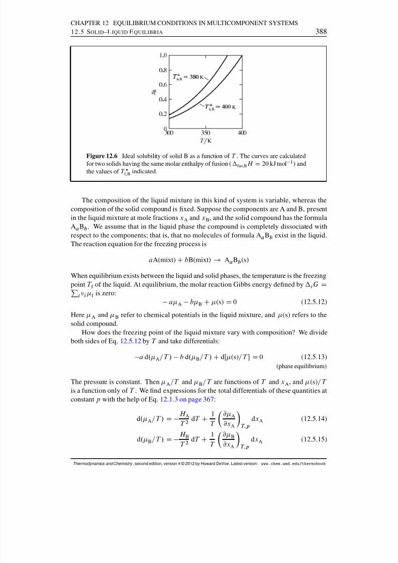
8/12/2019 Howard Devoe Thermodynamic and Chemical
http://slidepdf.com/reader/full/howard-devoe-thermodynamic-and-chemical 388/532
CHAPTER 12 EQUILIBRIUM CONDITIONS IN MULTICOMPONENT SYSTEMS12.5 S OLID –L IQUID E QUILIBRIA 388
f B
K
f B
K
K
B
Figure 12.6 Ideal solubility of solid B as a function of T . The curves are calculatedfor two solids having the same molar enthalpy of fusion ( fus,B H D 20 kJ mol 1 ) andthe values of T f ;B indicated.
The composition of the liquid mixture in this kind of system is variable, whereas thecomposition of the solid compound is xed. Suppose the components are A and B, presentin the liquid mixture at mole fractions xA and xB , and the solid compound has the formulaAa Bb . We assume that in the liquid phase the compound is completely dissociated withrespect to the components; that is, that no molecules of formula A a Bb exist in the liquid.The reaction equation for the freezing process is
a A(mixt) CbB(mixt) ! Aa Bb (s)
When equilibrium exists between the liquid and solid phases, the temperature is the freezingpoint T f of the liquid. At equilibrium, the molar reaction Gibbs energy dened by rG D
Pi i i is zero: a A b B C (s) D 0 (12.5.12)
Here A and B refer to chemical potentials in the liquid mixture, and (s) refers to thesolid compound.
How does the freezing point of the liquid mixture vary with composition? We divideboth sides of Eq. 12.5.12 by T and take differentials:
a d. A=T / b d. B=T / CdΠ(s)=T D 0 (12.5.13)(phase equilibrium)
The pressure is constant. Then A=T and B=T are functions of T and xA , and (s)=T is a function only of T . We nd expressions for the total differentials of these quantities atconstant p with the help of Eq. 12.1.3 on page 367 :
d. A=T / D H AT 2
dT C 1T
@ A
@xA T;pdxA (12.5.14)
d. B=T / D H BT 2
dT C 1T
@ B
@xA T;pdxA (12.5.15)
Thermodynamics and Chemistry , second edition, version 4 © 2012 by Howard DeVoe. Latest version: www.chem.umd.edu/thermobook
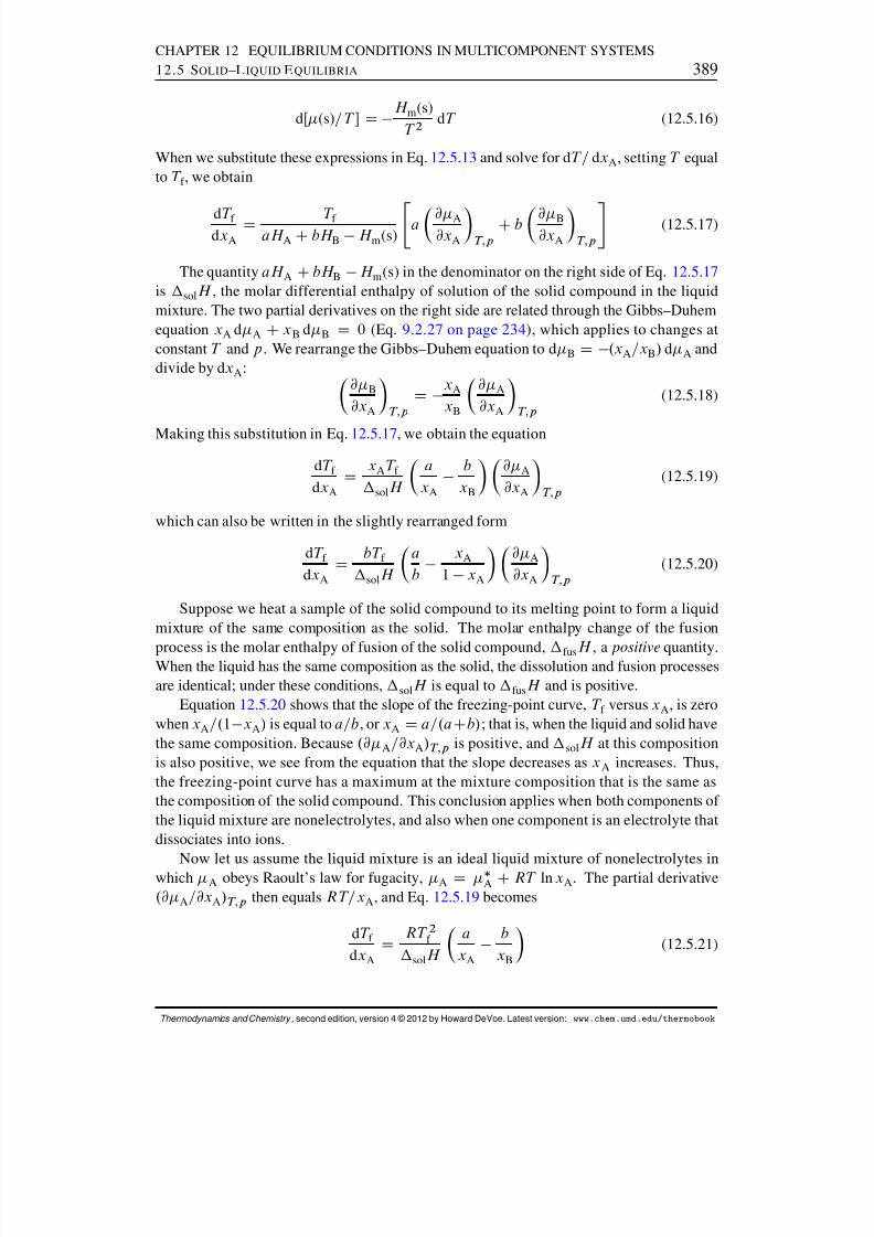
8/12/2019 Howard Devoe Thermodynamic and Chemical
http://slidepdf.com/reader/full/howard-devoe-thermodynamic-and-chemical 389/532

8/12/2019 Howard Devoe Thermodynamic and Chemical
http://slidepdf.com/reader/full/howard-devoe-thermodynamic-and-chemical 390/532
CHAPTER 12 EQUILIBRIUM CONDITIONS IN MULTICOMPONENT SYSTEMS12.5 S OLID –L IQUID E QUILIBRIA 390
Mg mole fraction Zn Zn
f
K
Figure 12.7 Solid curve: freezing-point curve of a liquid melt of Zn and Mg thatsolidies to the solid compound Zn 2 Mg. a The curve maximum (open circle) is atthe compound composition x 00
Zn D 2=3 and the solid compound melting point T 00f D861 K. Dashed curve: calculated using Eq. 12.5.23 with fus H D 15:8 kJmol 1 .
a Ref. [ 50], p. 603.
By making the approximations that sol H is independent of T and xA , and is equal tofus H , we can separate the variables and integrate as follows:
Z T 00
f
T 0f
dT f T 2f D
R
fus H Z x 00
A
x 0A
axA
dxA CZ x 00
B
x 0B
bxB
dxB! (12.5.22)
(The second integral on the right side comes from changing d xA to dxB .) The result of the integration is
1T 0f D
1T 00
f C R
fus H a lnx 00
A
x 0A Cb ln
x 00B
x 0B (12.5.23)
(ideal liquid mixture inequilibrium with solid
compound, sol H D fus H )
Let T 0f be the freezing point of a liquid mixture of composition x 0A and x 0
B D 1 x 0A , and
let T 00f be the melting point of the solid compound of composition x 00
A D a=.a Cb/ and x 00B D
b=.a Cb/ . Figure 12.7 shows an example of a molten metal mixture that solidies to analloy of xed composition. The freezing-point curve of this system is closely approximatedby Eq. 12.5.23 .
12.5.5 Solubility of a solid electrolyte
Consider an equilibrium between a crystalline salt (or other kind of ionic solid) and a solu-tion containing the solvated ions:
MC
X (s) • C Mz C (aq) C Xz (aq)
Here C and are the numbers of cations and anions in the formula unit of the salt, andzC and z are the charge numbers of these ions. The solution in equilibrium with the
Thermodynamics and Chemistry , second edition, version 4 © 2012 by Howard DeVoe. Latest version: www.chem.umd.edu/thermobook
8/12/2019 Howard Devoe Thermodynamic and Chemical
http://slidepdf.com/reader/full/howard-devoe-thermodynamic-and-chemical 391/532
CHAPTER 12 EQUILIBRIUM CONDITIONS IN MULTICOMPONENT SYSTEMS12.5 S OLID –L IQUID E QUILIBRIA 391
solid salt is a saturated solution. The thermodynamic equilibrium constant for this kind of equilibrium is called a solubility product , K s.
We can readily derive a relation between K s and the molalities of the ions in the sat-urated solution by treating the dissolved salt as a single solute substance, B. We write theequilibrium in the form B (s) • B(sln), and write the expression for the solubility product
as a proper quotient of activities:K s D
a m; B
a B(12.5.24)
From Eq. 10.3.16 on page 294 , we have a m; B D m; B ˙ .m C =m ı / C .m =m ı / . Thisexpression is valid whether or not the ions M z C and X z are present in solution in the sameratio as in the solid salt. When we replace a m; B with this expression, and replace a B with B (Table 9.5 ), we obtain
K s D m; B
B ˙
mC
m ı
C
mm ı (12.5.25)
where
D C
C is the total number of ions per formula unit. ˙ is the mean ionic
activity coefcient of the dissolved salt in the saturated solution, and the molalities mC andm refer to the ions M z C and X z in this solution.
The rst factor on the right side of Eq. 12.5.25 , the proper quotient of pressure factorsfor the reaction B (s)! B(sln), will be denoted r (the subscript “r” stands for reaction).The value of r is exactly 1 if the system is at the standard pressure, and is otherwiseapproximately 1 unless the pressure is very high.
If the aqueous solution is produced by allowing the salt to dissolve in pure water, orin a solution of a second solute containing no ions in common with the salt, then the ionmolalities in the saturated solution are mC D C mB and m D mB where mB is thesolubility of the salt expressed as a molality. Under these conditions, Eq. 12.5.25 becomes 9
K s D r ˙C
C mB
m ı (12.5.26)(no common ion)
If the ionic strength of the saturated salt solution is sufciently low (i.e., the solubility issufciently low), it may be practical to evaluate the solubility product with Eq. 12.5.26 andan estimate of ˙ from the Debye–H uckel limiting law (see Prob. 12. 19). The most accuratemethod of measuring a solubility product, however, is through the standard cell potential of an appropriate galvanic cell (Sec. 14.3.3 ).
Since K s is a thermodynamic equilibrium constant that depends only on T , and rdepends only on T and p , Eq. 12.5.26 shows that any change in the solution composition atconstant T and p that decreases ˙ must increase the solubility. For example, the solubilityof a sparingly-soluble salt increases when a second salt, lacking a common ion, is dissolvedin the solution; this is a salting-in effect .
Equation 12.5.25 is a general equation that applies even if the solution saturated withone salt contains a second salt with a common ion. For instance, consider the sparingly-soluble salt M
CX in transfer equilibrium with a solution containing the more soluble
9We could also have obtained this equation by using the expression of Eq. 10.3.10 for am; B .
Thermodynamics and Chemistry , second edition, version 4 © 2012 by Howard DeVoe. Latest version: www.chem.umd.edu/thermobook
8/12/2019 Howard Devoe Thermodynamic and Chemical
http://slidepdf.com/reader/full/howard-devoe-thermodynamic-and-chemical 392/532
CHAPTER 12 EQUILIBRIUM CONDITIONS IN MULTICOMPONENT SYSTEMS12.6 L IQUID –L IQUID E QUILIBRIA 392
salt M 0C
Y 0 at molality mC . The common ion in this example is the cation M z C . Theexpression for the solubility product is now
K s D r ˙ . C mB C 0C mC / C . mB / =.m ı / (12.5.27)
(common cation)
where mB again is the solubility of the sparingly-soluble salt, and mC is the molality of thesecond salt. K s and r are constant if T and p do not change, so any increase in mC atconstant T and p must cause a decrease in the solubility mB . This is called the common ioneffect .
From the measured solubility of a salt in pure solvent, or in an electrolyte solutionwith a common cation, and a known value of K s , we can evaluate the mean ionic activitycoefcient ˙ through Eq. 12.5.26 or 12.5.27 . This procedure has the disadvantage of beinglimited to the value of mB existing in the saturated solution.
We nd the temperature dependence of K s by applying Eq. 12.1.12 :
d ln K sdT D
sol,B H ı
RT 2 (12.5.28)
At the standard pressure, sol,B H ı is the same as the molar enthalpy of solution at innitedilution, sol,B H 1 .
12.6 LIQUID–LIQUID EQUILIBRIA
12.6.1 Miscibility in binary liquid systems
When two different pure liquids are unable to mix in all proportions, they are said to be partially miscible . When these liquids are placed in contact with one another and allowedto come to thermal, mechanical, and transfer equilibrium, the result is two coexisting liquidmixtures of different compositions.
Liquids are never actually completely immiscible . To take an extreme case, liquid mer-cury, when equilibrated with water, has some H 2 O dissolved in it, and some mercury dis-solves in the water, although the amounts may be too small to measure.
The Gibbs phase rule for a multicomponent system to be described in Sec. 13.1 showsthat a two-component, two-phase system at equilibrium has only two independent intensivevariables. Thus at a given temperature and pressure, the mole fraction compositions of bothphases are xed; the compositions depend only on the identity of the substances and thetemperature and pressure.
Figure 13.5 on page 432 shows a phase diagram for a typical binary liquid mixture thatspontaneously separates into two phases when the temperature is lowered. The thermody-namic conditions for phase separation of this kind were discussed in Sec. 11.1.6 . The phaseseparation is usually the result of positive deviations from Raoult’s law. Typically, when
phase separation occurs, one of the substances is polar and the other nonpolar.
12.6.2 Solubility of one liquid in another
Suppose substances A and B are both liquids when pure. In discussing the solubility of liquid B in liquid A, we can treat B as either a solute or as a constituent of a liquid mixture.The difference lies in the choice of the standard state or reference state of B.
Thermodynamics and Chemistry , second edition, version 4 © 2012 by Howard DeVoe. Latest version: www.chem.umd.edu/thermobook

8/12/2019 Howard Devoe Thermodynamic and Chemical
http://slidepdf.com/reader/full/howard-devoe-thermodynamic-and-chemical 393/532
CHAPTER 12 EQUILIBRIUM CONDITIONS IN MULTICOMPONENT SYSTEMS12.6 L IQUID –L IQUID E QUILIBRIA 393
We can dene the solubility of B in A as the maximum amount of B that can dissolvewithout phase separation in a given amount of A at the given temperature and pressure.Treating B as a solute, we can express its solubility as the mole fraction of B in the phaseat the point of phase separation. The addition of any more B to the system will result intwo coexisting liquid phases of xed composition, one of which will have mole fraction xB
equal to its solubility.10
Consider a system with two coexisting liquid phases ’ and “ containing components Aand B. Let ’ be the A-rich phase and “ be the B-rich phase. For example, A could be waterand B could be benzene, a hydrophobic substance. Phase ’ would then be an aqueous phasepolluted with a low concentration of dissolved benzene, and phase “ would be wet benzene.x ’
B would be the solubility of the benzene in water, expressed as a mole fraction.Below, relations are derived for this kind of system using both choices of standard state
or reference state.
Solute standard state
Assume that the two components have low mutual solubilities, so that B has a low mole
fraction in phase ’ and a mole fraction close to 1 in phase “ . It is then appropriate to treatB as a solute in phase ’ and as a constituent of a liquid mixture in phase “ . The value of x ’
Bis the solubility of liquid B in liquid A.
The equilibrium when two liquid phases are present is B( “ ) • B(’ ), and the expressionfor the thermodynamic equilibrium constant, with the solute standard state based on molefraction, is
K Da ’
x; B
a “B
D ’
x; B ’x; B x ’
B
“B “
B x “B
(12.6.1)
The solubility of B is then given by
x’B D
“B “
B x “B
’x; B ’
x; B K (12.6.2)
The values of the pressure factors and activity coefcients are all close to 1, so that thesolubility of B in A is given by x ’
B K . The temperature dependence of the solubility isgiven by
d ln x ’B
dT d ln K
dT Dsol,B H ı
RT 2 (12.6.3)
where sol,B H ı is the molar enthalpy change for the transfer at pressure p ı of pure liquidsolute to the solution at innite dilution.
H2 O and n-butylbenzene are two liquids with very small mutual solubilities. Fig-ure 12.8 on the next page shows that the solubility of n-butylbenzene in water exhibits
a minimum at about 12 ı C. Equation 12.6.3 allows us to deduce from this behavior thatsol,B H ı is negative below this temperature, and positive above.
10 Experimentally, the solubility of B in A can be determined from the cloud point , the point during titration of A with B at which persistent turbidity is observed.
Thermodynamics and Chemistry , second edition, version 4 © 2012 by Howard DeVoe. Latest version: www.chem.umd.edu/thermobook
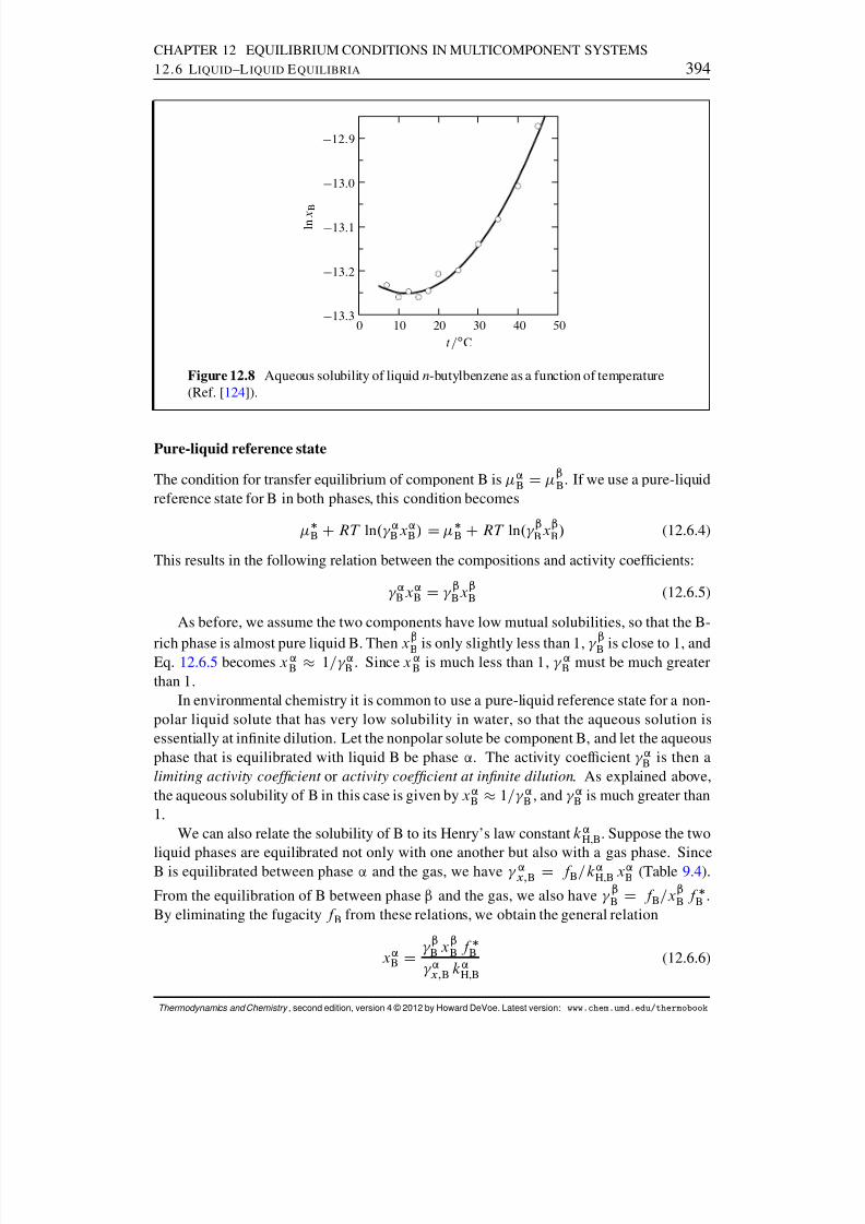
8/12/2019 Howard Devoe Thermodynamic and Chemical
http://slidepdf.com/reader/full/howard-devoe-thermodynamic-and-chemical 394/532
8/12/2019 Howard Devoe Thermodynamic and Chemical
http://slidepdf.com/reader/full/howard-devoe-thermodynamic-and-chemical 395/532
CHAPTER 12 EQUILIBRIUM CONDITIONS IN MULTICOMPONENT SYSTEMS12.7 M EMBRANE E QUILIBRIA 395
If we assume as before that the activity coefcients and x “B are close to 1, and that the gas
phase behaves ideally, the solubility of B is given by x ’B p B=k ’
H,B , where p B is the vaporpressure of the pure solute.
12.6.3 Solute distribution between two partially-miscible solvents
Consider a two-component system of two equilibrated liquid phases, ’ and “ . If we add asmall quantity of a third component, C, it will distribute itself between the two phases. It isappropriate to treat C as a solute in both phases. The thermodynamic equilibrium constantfor the equilibrium C .“/ • C.’/ , with solute standard states based on mole fraction, is
K Da ’
x; C
a “x; C
D ’
x; C ’x; C x ’
C
“x; C “
x; C x “C
(12.6.7)
We dene K 0 as the ratio of the mole fractions of C in the two phases at equilibrium:
K 0 def
Dx ’
C
x “C D “
x; C “x; C
’x; C
’x; C
K (12.6.8)
At a xed T and p , the pressure factors and equilibrium constant are constants. If xC islow enough in both phases for ’
x; C and “x; C to be close to unity, K 0 becomes a constant for
the given T and p . The constancy of K 0 over a range of dilute composition is the Nernstdistribution law .
Since solute molality and concentration are proportional to mole fraction in dilute solu-tions, the ratios m’
C=m “C and c ’
C =c“C also approach constant values at a given T and p . The
ratio of concentrations is called the partition coefcient or distribution coefcient .In the limit of innite dilution of C, the two phases have the compositions that exist
when only components A and B are present. As C is added and x ’C and x “
C increase beyond
the region of dilute solution behavior, the ratios x ’B =x ’A and x“B=x
“A may change. Continued
addition of C may increase the mutual solubilities of A and B, resulting, when enough Chas been added, in a single liquid phase containing all three components. It is easier tounderstand this behavior with the help of a ternary phase diagram such as Fig. 13.17 onpage 444 .
12.7 MEMBRANE EQUILIBRIA
A semipermeable membrane used to separate two liquid phases can, in principle, be per-meable to certain species and impermeable to others. A membrane, however, may not beperfect in this respect over a long time period (see page 374 ). We will assume that during
the period of observation, those species to which the membrane is supposed to be permeablequickly achieve transfer equilibrium, and only negligible amounts of the other species aretransferred across the membrane.
Section 12.2.2 sketched a derivation of the conditions needed for equilibrium in a two-phase system in which a membrane permeable only to solvent separates a solution frompure solvent. We can generalize the results for any system with two liquid phases separatedby a semipermeable membrane: in an equilibrium state, both phases must have the same
Thermodynamics and Chemistry , second edition, version 4 © 2012 by Howard DeVoe. Latest version: www.chem.umd.edu/thermobook

8/12/2019 Howard Devoe Thermodynamic and Chemical
http://slidepdf.com/reader/full/howard-devoe-thermodynamic-and-chemical 396/532
CHAPTER 12 EQUILIBRIUM CONDITIONS IN MULTICOMPONENT SYSTEMS12.7 M EMBRANE E QUILIBRIA 396
temperature, and any species to which the membrane is permeable must have the samechemical potential in both phases. The two phases, however, need not and usually do nothave the same pressure.
12.7.1 Osmotic membrane equilibrium
An equilibrium state in a system with two solutions of the same solvent and different solutecompositions, separated by a membrane permeable only to the solvent, is called an osmoticmembrane equilibrium . We have already seen this kind of equilibrium in an apparatusthat measures osmotic pressure (Fig. 12.2 on page 373 ).
Consider a system with transfer equilibrium of the solvent across a membrane sepa-rating phases ’ and “. The phases have equal solvent chemical potentials but differentpressures:
“A .p “ / D ’
A .p ’ / (12.7.1)
The dependence of A on pressure in a phase of xed temperature and composition is givenby .@ A=@p/T; fn ig D V A (from Eq. 9.2.49 ), where V A is the partial molar volume of A in
the phase. If we apply this relation to the solution of phase “ , treat the partial molar volumeV A as independent of pressure, and integrate at constant temperature and composition fromthe pressure of phase ’ to that of phase “ , we obtain
“A .p “ / D “
A .p ’ / CV “A .p “ p ’ / (12.7.2)
By equating the two expressions for “A .p “ / and rearranging, we obtain the following ex-
pression for the pressure difference needed to achieve transfer equilibrium:
p “ p ’ D ’
A .p ’ / “A .p ’ /
V “A(12.7.3)
The pressure difference can be related to the osmotic pressures of the two phases. FromEq. 12.2.11 on page 375 , the solvent chemical potential in a solution phase can be written
A .p/ D A .p/ V A˘.p/ . Using this to substitute for ’A .p ’ / and “
A .p ’ / in Eq. 12.7.3 ,we obtain
p “ p ’ D ˘ “ .p ’ /V ’AV “A !˘ ’ .p ’ / (12.7.4)
12.7.2 Equilibrium dialysis
Equilibrium dialysis is a useful technique for studying the binding of a small unchargedsolute species (a ligand) to a macromolecule. The macromolecule solution is placed on
one side of a membrane through which it cannot pass, with a solution without the macro-molecule on the other side, and the ligand is allowed to come to transfer equilibrium acrossthe membrane. If the same solute standard state is used for the ligand in both solutions, atequilibrium the unbound ligand must have the same activity in both solutions. Measure-ments of the total ligand molality in the macromolecule solution and the ligand molality inthe other solution, combined with estimated values of the unbound ligand activity coef-cients, allow the amount of ligand bound per macromolecule to be calculated.
Thermodynamics and Chemistry , second edition, version 4 © 2012 by Howard DeVoe. Latest version: www.chem.umd.edu/thermobook

8/12/2019 Howard Devoe Thermodynamic and Chemical
http://slidepdf.com/reader/full/howard-devoe-thermodynamic-and-chemical 397/532
CHAPTER 12 EQUILIBRIUM CONDITIONS IN MULTICOMPONENT SYSTEMS12.7 M EMBRANE E QUILIBRIA 397
12.7.3 Donnan membrane equilibrium
If one of the solutions in a two-phase membrane equilibrium contains certain charged solutespecies that are unable to pass through the membrane, whereas other ions can pass through,the situation is more complicated than the osmotic membrane equilibrium described in Sec.12.7.1 . Usually if the membrane is impermeable to one kind of ion, an ion species to which
it is permeable achieves transfer equilibrium across the membrane only when the phaseshave different pressures and different electric potentials. The equilibrium state in this caseis a Donnan membrane equilibrium , and the resulting electric potential difference acrossthe membrane is called the Donnan potential . This phenomenon is related to the membranepotentials that are important in the functioning of nerve and muscle cells (although the cellsof a living organism are not, of course, in equilibrium states).
A Donnan potential can be measured electrically, with some uncertainty due to unknownliquid junction potentials, by connecting silver-silver chloride electrodes (described in Sec.14.1 ) to both phases through salt bridges.
General expressions
Consider solution phases ’ and “ separated by a semipermeable membrane. Both phasescontain a dissolved salt, designated solute B, that has C cations and anions in eachformula unit. The membrane is permeable to these ions. Phase “ also contains a protein orother polyelectrolyte with a net positive or negative charge, together with counterions of theopposite charge that are the same species as the cation or anion of the salt. The presence of the counterions in phase “ prevents the cation and anion of the salt from being present instoichiometric amounts in this phase. The membrane is impermeable to the polyelectrolyte,perhaps because the membrane pores are too small to allow the polyelectrolyte to passthrough.
The condition for transfer equilibrium of solute B is ’B D “
B , or
. ım; B / ’ CRT ln a ’m; B D . ım; B / “ CRT ln a “m; B (12.7.5)
Solute B has the same standard state in the two phases, so that . ım; B / ’ and . ı
m; B / “ are
equal. The activities a ’m; B and a “
m; B are therefore equal at equilibrium. Using the expressionfor solute activity from Eq. 10.3.16 , which is valid for a multisolute solution, we nd that attransfer equilibrium the following relation must exist between the molalities of the salt ionsin the two phases:
’m; B ’
˙ m’C
C m ’ D “m; B “
˙ m“C
Cm“ (12.7.6)
To nd an expression for the Donnan potential, we can equate the single-ion chemicalpotentials of the salt cation: ’
C . ’ / D “C . “ / . When we use the expression of Eq.
10.1.15 for C . / , we obtain
’ “ D RT zC F
ln “
C “C m“
C
’C ’
C m ’C
(12.7.7)(Donnan potential)
Thermodynamics and Chemistry , second edition, version 4 © 2012 by Howard DeVoe. Latest version: www.chem.umd.edu/thermobook
8/12/2019 Howard Devoe Thermodynamic and Chemical
http://slidepdf.com/reader/full/howard-devoe-thermodynamic-and-chemical 398/532
CHAPTER 12 EQUILIBRIUM CONDITIONS IN MULTICOMPONENT SYSTEMS12.7 M EMBRANE E QUILIBRIA 398
The condition needed for an osmotic membrane equilibrium related to the solvent canbe written
“A .p “ / ’
A .p ’ / D 0 (12.7.8)
The chemical potential of the solvent is A D ıA CRT ln a A D ı
A CRT ln. A A xA / .From Table 9.6 , we have to a good approximation the expression RT ln A D V A .p p ı / .
With these substitutions, Eq. 12.7.8 becomes
RT ln “A x “
A
’A x ’
A CV A p “ p ’ D 0 (12.7.9)
We can use this equation to estimate the pressure difference needed to maintain an equilib-rium state. For dilute solutions, with ’
A and “A set equal to 1, the equation becomes
p “ p ’ RT V A
lnx ’
A
x “A
(12.7.10)
In the limit of innite dilution, ln xA can be replaced by M A
Pi ¤ A m i (Eq. 9.6.12 on
page 267 ), giving the relation
p “ p ’ M ART V A Xi ¤ A
m“i m’
i D ART Xi ¤ A
m“i m’
i (12.7.11)
Example
As a specic example of a Donnan membrane equilibrium, consider a system in which anaqueous solution of a polyelectrolyte with a net negative charge, together with a counterionMC and a salt MX of the counterion, is equilibrated with an aqueous solution of the saltacross a semipermeable membrane. The membrane is permeable to the H 2 O solvent andto the ions M C and X , but is impermeable to the polyelectrolyte. The species in phase’ are H 2 O, M C , and X ; those in phase “ are H 2 O, M C , X , and the polyelectrolyte. Ina equilibrium state, the two phases have the same temperature but different compositions,electric potentials, and pressures.
Because the polyelectrolyte in this example has a negative charge, the system has moreMC ions than X ions. Figure 12.9 (a) on the next page is a schematic representation of an initial state of this kind of system. Phase “ is shown as a solution conned to a closeddialysis bag immersed in phase ’ . The number of cations and anions shown in each phaseindicate the relative amounts of these ions.
For simplicity, let us assume the two phases have equal masses of water, so that themolality of an ion is proportional to its amount by the same ratio in both phases. It is clearthat in the initial state shown in the gure, the chemical potentials of both M C and X aregreater in phase “ (greater amounts) than in phase ’ , and this is a nonequilibrium state. A
certain quantity of salt MX will therefore pass spontaneously through the membrane fromphase “ to phase ’ until equilibrium is attained.
The equilibrium ion molalities must agree with Eq. 12.7.6 . We make the approximationthat the pressure factors and mean ionic activity coefcients are unity. Then for the presentexample, with C D D 1, the equation becomes
m’C m ’ m“
C m“ (12.7.12)
Thermodynamics and Chemistry , second edition, version 4 © 2012 by Howard DeVoe. Latest version: www.chem.umd.edu/thermobook
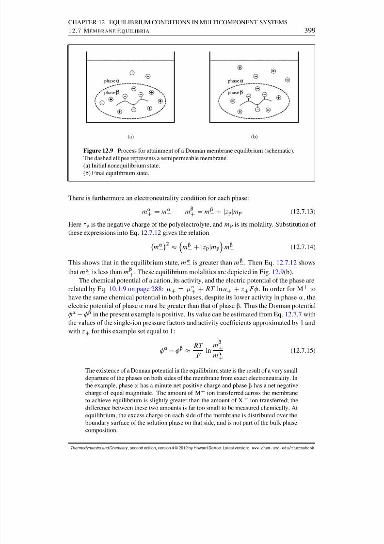
8/12/2019 Howard Devoe Thermodynamic and Chemical
http://slidepdf.com/reader/full/howard-devoe-thermodynamic-and-chemical 399/532
CHAPTER 12 EQUILIBRIUM CONDITIONS IN MULTICOMPONENT SYSTEMS12.7 M EMBRANE E QUILIBRIA 399
phase
phase
(a)
phase
phase
(b)
Figure 12.9 Process for attainment of a Donnan membrane equilibrium (schematic).The dashed ellipse represents a semipermeable membrane.(a) Initial nonequilibrium state.(b) Final equilibrium state.
There is furthermore an electroneutrality condition for each phase:
m’C D m’ m“
C D m“ C jzPjmP (12.7.13)
Here zP is the negative charge of the polyelectrolyte, and mP is its molality. Substitution of these expressions into Eq. 12.7.12 gives the relation
m ’ 2 m“ C jzPjmP m“ (12.7.14)
This shows that in the equilibrium state, m ’ is greater than m“ . Then Eq. 12.7.12 showsthat m’
C is less than m“C . These equilibrium molalities are depicted in Fig. 12.9 (b).
The chemical potential of a cation, its activity, and the electric potential of the phase arerelated by Eq. 10.1.9 on page 288 : C D ı
C CRT ln a C CzC F . In order for M C tohave the same chemical potential in both phases, despite its lower activity in phase ’ , theelectric potential of phase ’ must be greater than that of phase “ . Thus the Donnan potential
’ “ in the present example is positive. Its value can be estimated from Eq. 12.7.7 withthe values of the single-ion pressure factors and activity coefcients approximated by 1 andwith zC for this example set equal to 1:
’ “ RT F
lnm“
C
m ’C
(12.7.15)
The existence of a Donnan potential in the equilibrium state is the result of a very smalldeparture of the phases on both sides of the membrane from exact electroneutrality. Inthe example, phase ’ has a minute net positive charge and phase “ has a net negativecharge of equal magnitude. The amount of M C ion transferred across the membraneto achieve equilibrium is slightly greater than the amount of X ion transferred; thedifference between these two amounts is far too small to be measured chemically. Atequilibrium, the excess charge on each side of the membrane is distributed over theboundary surface of the solution phase on that side, and is not part of the bulk phasecomposition.
Thermodynamics and Chemistry , second edition, version 4 © 2012 by Howard DeVoe. Latest version: www.chem.umd.edu/thermobook

8/12/2019 Howard Devoe Thermodynamic and Chemical
http://slidepdf.com/reader/full/howard-devoe-thermodynamic-and-chemical 400/532
CHAPTER 12 EQUILIBRIUM CONDITIONS IN MULTICOMPONENT SYSTEMS12.8 L IQUID –G AS E QUILIBRIA 400
The pressure difference p “ p ’ at equilibrium can be estimated with Eq. 12.7.11 , andfor the present example is found to be positive. Without this pressure difference, the solutionin phase ’ would move spontaneously through the membrane into phase “ until phase ’completely disappears. With phase ’ open to the atmosphere, as in Fig. 12.9 , the volumeof phase “ must be constrained in order to allow its pressure to differ from atmospheric
pressure. If the volume of phase “ remains practically constant, the transfer of a minutequantity of solvent across the membrane is sufcient to cause the pressure difference.It should be clear that the existence of a Donnan membrane equilibrium introduces
complications that would make it difcult to use a measured pressure difference to estimatethe molar mass of the polyelectrolyte by the method of Sec. 12.4 , or to study the binding of a charged ligand by equilibrium dialysis.
12.8 LIQUID–GAS EQUILIBRIA
This section describes multicomponent systems in which a liquid phase is equilibrated witha gas phase.
12.8.1 Effect of liquid pressure on gas fugacity
If we vary the pressure of a liquid mixture at constant temperature and composition, there isa small effect on the fugacity of each volatile component in an equilibrated gas phase. Oneway to vary the pressure at essentially constant liquid composition is to change the partialpressure of a component of the gas phase that has negligible solubility in the liquid.
At transfer equilibrium, component i has the same chemical potential in both phases:i (l) D i (g). Combining the relations Œ@i (l)=@pT; fn ig D V i (l) and i (g) D ı
i (g) CRT ln.f i =p ı / (Eqs. 9.2.49 and 9.3.12 ), we obtain
d ln .f i =p ı /
dp D
V i (l)
RT
(12.8.1)
(equilibrated liquid andgas mixtures, constant T and liquid composition)
Equation 12.8.1 shows that an increase in pressure, at constant temperature and liquid com-position, causes an increase in the fugacity of each component in the gas phase.
Integration of Eq. 12.8.1 between pressures p 1 and p 2 yields
f i .p 2 / D f i .p 1 / exp "Z p 2
p 1
V i (l)RT
dp# (12.8.2)(equilibrated liquid and
gas mixtures, constant T and liquid composition)
The exponential on the right side is called the Poynting factor .
Thermodynamics and Chemistry , second edition, version 4 © 2012 by Howard DeVoe. Latest version: www.chem.umd.edu/thermobook
8/12/2019 Howard Devoe Thermodynamic and Chemical
http://slidepdf.com/reader/full/howard-devoe-thermodynamic-and-chemical 401/532
CHAPTER 12 EQUILIBRIUM CONDITIONS IN MULTICOMPONENT SYSTEMS12.8 L IQUID –G AS E QUILIBRIA 401
The integral in the Poynting factor is simplied if we make the approximation that V i (l)is independent of pressure. Then we obtain the approximate relation
f i .p 2 / f i .p 1 / expV i (l) .p 2 p 1 /
RT (12.8.3)
(equilibrated liquid and
gas mixtures, constant T and liquid composition)
The effect of pressure on fugacity is usually small, and can often be neglected. Fortypical values of the partial molar volume V i (l), the exponential factor is close to unityunless jp 2 p 1j is very large. For instance, for V i (l)D100 cm 3 mol 1 and T D300 K,we obtain a value for the ratio f i .p 2 /=f i .p 1 / of 1:004 if p 2 p 1 is 1 bar, 1:04 if p 2 p 1is 10 bar, and 1:5 if p 2 p 1 is 100 bar. Thus, unless the pressure change is large, wecan to a good approximation neglect the effect of total pressure on fugacity. Thisstatement applies only to the fugacity of a substance in a gas phase that is equilibratedwith a liquid phase of constant composition containing the same substance. If theliquid phase is absent, the fugacity of i in a gas phase of constant composition is of course approximately proportional to the total gas pressure.
We can apply Eqs. 12.8.2 and 12.8.3 to pure liquid A, in which case V i (l) is the mo-lar volume V A (l). Suppose we have pure liquid A in equilibrium with pure gaseous A ata certain temperature. This is a one-component, two-phase equilibrium system with onedegree of freedom (Sec. 8.1.7 ), so that at the given temperature the value of the pressure isxed. This pressure is the saturation vapor pressure of pure liquid A at this temperature.We can make the pressure p greater than the saturation vapor pressure by adding a secondsubstance to the gas phase that is essentially insoluble in the liquid, without changing thetemperature or volume. The fugacity f A is greater at this higher pressure than it was at thesaturation vapor pressure. The vapor pressure p A , which is approximately equal to f A , hasnow become greater than the saturation vapor pressure. It is, however, safe to say that the
difference is negligible unless the difference between p and p A is much greater than 1 bar.As an application of these relations, consider the effect of the size of a liquid droplet onthe equilibrium vapor pressure. The calculation of Prob. 12. 8(b) shows that the fugacity of H2 O in a gas phase equilibrated with liquid water in a small droplet is slightly greater thanwhen the liquid is in a bulk phase. The smaller the radius of the droplet, the greater is thefugacity and the vapor pressure.
12.8.2 Effect of liquid composition on gas fugacities
Consider system 1 in Fig. 9.5 on page 247 . A binary liquid mixture of two volatile com-ponents, A and B, is equilibrated with a gas mixture containing A, B, and a third gaseouscomponent C of negligible solubility used to control the total pressure. In order for A andB to be in transfer equilibrium, their chemical potentials must be the same in both phases:
A(l) D ıA(g) CRT ln
f Ap ı B(l) D ı
B(g) CRT lnf Bp ı (12.8.4)
Suppose we make an innitesimal change in the liquid composition at constant T and
Thermodynamics and Chemistry , second edition, version 4 © 2012 by Howard DeVoe. Latest version: www.chem.umd.edu/thermobook
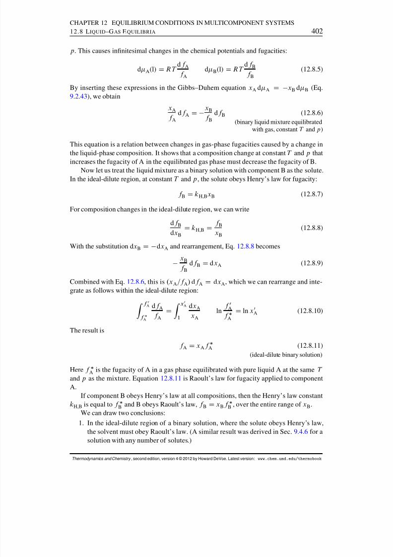
8/12/2019 Howard Devoe Thermodynamic and Chemical
http://slidepdf.com/reader/full/howard-devoe-thermodynamic-and-chemical 402/532
CHAPTER 12 EQUILIBRIUM CONDITIONS IN MULTICOMPONENT SYSTEMS12.8 L IQUID –G AS E QUILIBRIA 402
p . This causes innitesimal changes in the chemical potentials and fugacities:
d A(l) D RT df A
f Ad B(l) D RT
df Bf B
(12.8.5)
By inserting these expressions in the Gibbs–Duhem equation xA d A D xB d B (Eq.
9.2.43 ), we obtainxA
f Adf A D
xB
f Bdf B (12.8.6)
(binary liquid mixture equilibratedwith gas, constant T and p )
This equation is a relation between changes in gas-phase fugacities caused by a change inthe liquid-phase composition. It shows that a composition change at constant T and p thatincreases the fugacity of A in the equilibrated gas phase must decrease the fugacity of B.
Now let us treat the liquid mixture as a binary solution with component B as the solute.In the ideal-dilute region, at constant T and p , the solute obeys Henry’s law for fugacity:
f B D kH,B xB (12.8.7)
For composition changes in the ideal-dilute region, we can write
df BdxB D kH,B D
f BxB
(12.8.8)
With the substitution d xB D dxA and rearrangement, Eq. 12.8.8 becomes
xB
f Bdf B D dxA (12.8.9)
Combined with Eq. 12.8.6 , this is .x A=f A / df A D dxA , which we can rearrange and inte-
grate as follows within the ideal-dilute region:
Z f 0
A
f A
df Af A DZ
x 0A
1
dxA
xAln
f 0A
f A D ln x 0
A (12.8.10)
The result is
f A D xAf A (12.8.11)
(ideal-dilute binary solution)
Here f A is the fugacity of A in a gas phase equilibrated with pure liquid A at the same T
and p as the mixture. Equation 12.8.11 is Raoult’s law for fugacity applied to component
A. If component B obeys Henry’s law at all compositions, then the Henry’s law constantkH,B is equal to f B and B obeys Raoult’s law, f B D xBf
B , over the entire range of xB .We can draw two conclusions:
1. In the ideal-dilute region of a binary solution, where the solute obeys Henry’s law,the solvent must obey Raoult’s law. (A similar result was derived in Sec. 9.4.6 for asolution with any number of solutes.)
Thermodynamics and Chemistry , second edition, version 4 © 2012 by Howard DeVoe. Latest version: www.chem.umd.edu/thermobook
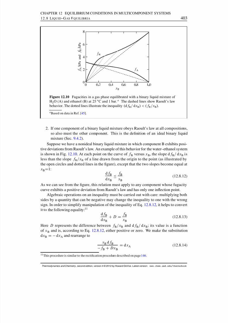
8/12/2019 Howard Devoe Thermodynamic and Chemical
http://slidepdf.com/reader/full/howard-devoe-thermodynamic-and-chemical 403/532
CHAPTER 12 EQUILIBRIUM CONDITIONS IN MULTICOMPONENT SYSTEMS12.8 L IQUID –G AS E QUILIBRIA 403
B
A
B
A
k P a a n d
B
k P a
Figure 12.10 Fugacities in a gas phase equilibrated with a binary liquid mixture of H2 O (A) and ethanol (B) at 25 ı C and 1 bar. a The dashed lines show Raoult’s lawbehavior. The dotted lines illustrate the inequality . df B= dxB / < .f B=xB / .
a Based on data in Ref. [ 45].
2. If one component of a binary liquid mixture obeys Raoult’s law at all compositions,so also must the other component. This is the denition of an ideal binary liquidmixture (Sec. 9.4.2 ).
Suppose we have a nonideal binary liquid mixture in which component B exhibits posi-tive deviations from Raoult’s law. An example of this behavior for the water–ethanol systemis shown in Fig. 12.10 . At each point on the curve of f B versus xB , the slope d f B= dxB isless than the slope f B=xB of a line drawn from the origin to the point (as illustrated bythe open circles and dotted lines in the gure), except that the two slopes become equal at
xBD1: df BdxB
f BxB
(12.8.12)
As we can see from the gure, this relation must apply to any component whose fugacitycurve exhibits a positive deviation from Raoult’s law and has only one inection point.
Algebraic operations on an inequality must be carried out with care: multiplying bothsides by a quantity that can be negative may change the inequality to one with the wrongsign. In order to simplify manipulation of the inequality of Eq. 12.8.12 , it helps to convertit to the following equality: 11
df BdxB CD D
f BxB
(12.8.13)
Here D represents the difference between f B=xB and d f B= dxB ; its value is a functionof xB and is, according to Eq. 12.8.12 , either positive or zero. We make the substitutiondxB D dxA and rearrange to
xB df Bf B CDx B D dxA (12.8.14)
11 This procedure is similar to the rectication procedure described on page 146 .
Thermodynamics and Chemistry , second edition, version 4 © 2012 by Howard DeVoe. Latest version: www.chem.umd.edu/thermobook
8/12/2019 Howard Devoe Thermodynamic and Chemical
http://slidepdf.com/reader/full/howard-devoe-thermodynamic-and-chemical 404/532
CHAPTER 12 EQUILIBRIUM CONDITIONS IN MULTICOMPONENT SYSTEMS12.8 L IQUID –G AS E QUILIBRIA 404
B
A
B
A
k P a a n d
B
k P a
Figure 12.11 Fugacities in a gas phase equilibrated with a binary liquid mixture of chloroform (A) and ethanol (B) at 35 ı C (Ref. [ 147 ]).
When D is zero, this equation becomes xB df B=f B D dxA . When D is positive, theleft side of the equation is less than xB df B=f B and is equal to d xA , so that d xA is lessthan xB df B=f B . Since D cannot be negative, Eq. 12.8.14 is equivalent to the followingrelation: xB
f Bdf B dxA (12.8.15)
A substitution from Eq. 12.8.6 gives us
xA
f Adf A dxA or
df Af A
dxA
xA(12.8.16)
We can integrate both sides of the second relation as follows:12
Z f 0
A
f A
df Af A Z
x 0A
1
dxA
xAln
f 0A
f A
ln x 0A f A xAf
A (12.8.17)
Thus, if the curve of fugacity versus mole fraction for one component of a binary liquid mixture exhibits only positive deviations from Raoult’s law, with only one inection point,so also must the curve of the other component . In the water–ethanol system shown inFig. 12.10 , both curves have positive deviations from Raoult’s law, and both have a singleinection point.
By the same method, we nd that if the fugacity curve of one component has onlynegative deviations from Raoult’s law with a single inection point, the same is true of theother component.
Figure 12.11 illustrates the case of a binary mixture in which component B has onlypositive deviations from Raoult’s law, whereas component A has both positive and negativedeviations ( f A is slightly less than xAf
A for xB less than 0.3). This unusual behavior is
12 The equalities are the same as Eqs. 12.8.10 and 12.8.11 , with the difference that here xA is not restricted tothe ideal-dilute region.
Thermodynamics and Chemistry , second edition, version 4 © 2012 by Howard DeVoe. Latest version: www.chem.umd.edu/thermobook
8/12/2019 Howard Devoe Thermodynamic and Chemical
http://slidepdf.com/reader/full/howard-devoe-thermodynamic-and-chemical 405/532
CHAPTER 12 EQUILIBRIUM CONDITIONS IN MULTICOMPONENT SYSTEMS12.8 L IQUID –G AS E QUILIBRIA 405
possible because both fugacity curves have two inection points instead of the usual one.Other types of unusual nonideal behavior are possible. 13
12.8.3 The Duhem–Margules equation
When we divide both sides of Eq. 12.8.6 by dxA , we obtain the Duhem–Margules equa-tion :
xA
f A
df AdxA D
xB
f B
df BdxA
(12.8.18)(binary liquid mixture equilibrated
with gas, constant T and p )
If we assume the gas mixture is ideal, the fugacities are the same as the partial pressures,and the Duhem–Margules equation then becomes
xA
p A
dp A
dxA D xB
p B
dp B
dxA(12.8.19)
(binary liquid mixture equilibrated
with ideal gas, constant T and p )
Solving Eq. 12.8.19 for dp B= dxA , we obtain
dp B
dxA D xAp B
xBp A
dp A
dxA(12.8.20)
To a good approximation, by assuming an ideal gas mixture and neglecting the effectof total pressure on fugacity, we can apply Eq. 12.8.20 to a liquid–gas system in which thetotal pressure is not constant, but instead is the sum of p A and p B . Under these conditions,we obtain the following expression for the rate at which the total pressure changes with theliquid composition at constant T :
dpdxA D
d.p A Cp B /dxA D
dp A
dxA
xAp B
xBp A
dp A
dxA D dp A
dxA1
xA=xB
p A=p B
D dp A
dxA1
xA=xB
yA=yB (12.8.21)
Here yA and yB are the mole fractions of A and B in the gas phase given by yA D p A=pand yB D p B=p .
We can use Eq. 12.8.21 to make several predictions for a binary liquid–gas system atconstant T .
If the ratio yA=yB is greater than xA=xB (meaning that the mole fraction of A is
greater in the gas than in the liquid), then .x A=xB/=.y A=yB / is less than 1 anddp= dxA must have the same sign as d p A= dxA , which is positive.
Conversely, if yA=yB is less than xA=xB (i.e., the mole fraction of B is greater in thegas than in the liquid), then d p= dxA must be negative.
13 Ref. [ 111 ].
Thermodynamics and Chemistry , second edition, version 4 © 2012 by Howard DeVoe. Latest version: www.chem.umd.edu/thermobook
8/12/2019 Howard Devoe Thermodynamic and Chemical
http://slidepdf.com/reader/full/howard-devoe-thermodynamic-and-chemical 406/532
CHAPTER 12 EQUILIBRIUM CONDITIONS IN MULTICOMPONENT SYSTEMS12.8 L IQUID –G AS E QUILIBRIA 406
Thus compared to the liquid, the gas phase is richer in the component whose addi-tion to the liquid at constant temperature causes the total pressure to increase . Thisstatement is a version of Konowaloff’s rule .
In some binary liquid–gas systems, the total pressure at constant temperature exhibitsa maximum or minimum at a particular liquid composition. At this composition, d p= dxA
is zero but d p A= dxA is positive. From Eq. 12.8.21 , we see that at this composition xA=xBmust equal yA=yB , meaning that the liquid and gas phases have identical mole fractioncompositions. The liquid with this composition is called an azeotrope . The behavior of systems with azeotropes will be discussed in Sec. 13.2.5 .
12.8.4 Gas solubility
For the solution process B(g) ! B(sln), the general expression for the thermodynamic equi-librium constant is K D a B(sln) =aB(g).
The activity of B in the gas phase is given by aB(g) D f B=p ı . If the solute is a nonelec-trolyte and we choose a standard state based on mole fraction, the activity in the solution isa B(sln)
D x; B x; B xB . The equilibrium constant is then given by
K D x; B x; B xB
f B=p ı (12.8.22)
and the solubility, expressed as the equilibrium mole fraction of solute in the solution, isgiven by
xB D Kf B=p ı
x; B x; B(12.8.23)
(nonelectrolyte solute inequilibrium with gas)
At a xed T and p , the values of K and x; B are constant. Therefore any change in thesolution composition that increases the value of the activity coefcient x; B will decreasethe solubility for the same gas fugacity. This solubility decrease is often what happenswhen a salt is dissolved in an aqueous solution, and is known as the salting-out effect (Prob.12.11 ).
Unless the pressure is much greater than p ı , we can with negligible error set the pres-sure factor x; B equal to 1. When the gas solubility is low and the solution contains noother solutes, the activity coefcient x; B is close to 1. If furthermore we assume ideal gasbehavior, then Eq. 12.8.23 becomes
xB D K p B
p ı (12.8.24)(nonelectrolyte solute in equilibrium
with ideal gas, x; BD1, x; BD1)
The solubility is predicted to be proportional to the partial pressure. The solubility of a gasthat dissociates into ions in solution has a quite different dependence on partial pressure.An example is the solubility of gaseous HCl in water to form an electrolyte solution, shownin Fig. 10.1 on page 286 .
Thermodynamics and Chemistry , second edition, version 4 © 2012 by Howard DeVoe. Latest version: www.chem.umd.edu/thermobook

8/12/2019 Howard Devoe Thermodynamic and Chemical
http://slidepdf.com/reader/full/howard-devoe-thermodynamic-and-chemical 407/532
CHAPTER 12 EQUILIBRIUM CONDITIONS IN MULTICOMPONENT SYSTEMS12.8 L IQUID –G AS E QUILIBRIA 407
If the actual conditions are close to those assumed for Eq. 12.8.24 , we can use Eq.12.1.13 to derive an expression for the temperature dependence of the solubility for a xedpartial pressure of the gas:
@ln xB
@T p BD
d ln K dT D
sol,B H ı
RT 2 (12.8.25)
At the standard pressure, sol,B H ı is the same as the molar enthalpy of solution at innitedilution.
Since the dissolution of a gas in a liquid is invariably an exothermic process, sol,B H ı
is negative, and Eq. 12.8.25 predicts the solubility decreases with increasing temperature.Note the similarity of Eq. 12.8.25 and the expressions derived previously for the tem-
perature dependence of the solubilities of solids (Eq. 12.5.8 ) and liquids (Eq. 12.6.3 ). Whenwe substitute the mathematical identity d T D T 2 d.1=T / , Eq. 12.8.25 becomes
@ln xB
@.1=T / p BD
sol,B H ı
R (12.8.26)
We can use this form to evaluate sol,B H ı from a plot of ln xB versus 1=T .
The ideal solubility of a gas is the solubility calculated on the assumption that thedissolved gas obeys Raoult’s law for partial pressure: p B D xBp B . The ideal solubility,expressed as a mole fraction, is then given as a function of partial pressure by
xB D p B
p B(12.8.27)
(ideal solubility of a gas)
Here p B is the vapor pressure of pure liquid solute at the same temperature and total pressureas the solution. If the pressure is too low for pure B to exist as a liquid at this temperature,we can with little error replace p B with the saturation vapor pressure of liquid B at the sametemperature, because the effect of total pressure on the vapor pressure of a liquid is usuallynegligible (Sec. 12.8.1 ). If the temperature is above the critical temperature of pure B, we
can estimate a hypothetical vapor pressure by extrapolating the liquid–vapor coexistencecurve beyond the critical point.We can use Eq. 12.8.27 to make several predictions regarding the ideal solubility of a
gas at a xed value of p B .1. The ideal solubility, expressed as a mole fraction, is independent of the kind of sol-
vent.2. The solubility expressed as a concentration, cB , is lower the greater is the molar
volume of the solvent. This is because at constant xB , cB decreases as the solutionvolume increases.
3. The more volatile is the pure liquid solute at a particular temperature (i.e., the greateris p B ), the lower is the solubility.
4. The solubility decreases with increasing temperature, since pB
increases.Of course, these predictions apply only to solutions that behave approximately as idealliquid mixtures, but even for many nonideal mixtures the predictions are found to havegood agreement with experiment.
As an example of the general validity of prediction 1, Hildebrand and Scott 14 list the
14 Ref. [ 78], Chap. XV.
Thermodynamics and Chemistry , second edition, version 4 © 2012 by Howard DeVoe. Latest version: www.chem.umd.edu/thermobook
8/12/2019 Howard Devoe Thermodynamic and Chemical
http://slidepdf.com/reader/full/howard-devoe-thermodynamic-and-chemical 408/532
CHAPTER 12 EQUILIBRIUM CONDITIONS IN MULTICOMPONENT SYSTEMS12.8 L IQUID –G AS E QUILIBRIA 408
following solubilities of gaseous Cl 2 in several dissimilar solvents at 0 ı C and a partialpressure of 1:01 bar: x B D 0:270 in heptane, xB D 0:288 in SiCl 4 , and xB D 0:298 inCCl 4 . These values are similar to one another and close to the ideal value p B=p B D0:273 .
12.8.5 Effect of temperature and pressure on Henry’s law constants
Consider the solution process B(g) ! B(soln) for a nonelectrolyte solute B. The expressionfor the thermodynamic equilibrium constant, with a solute standard state based on molefraction, is
K D aB(sln)
a B(g) D x; B x; B xB
f B=p ı (12.8.28)
The Henry’s law constant kH,B is related to f B and xB by
kH,B D f B x; B xB
(12.8.29)
(see Table 9.4 ), and is therefore related to K as follows:
kH,B D x; B p ı
K (12.8.30)
(nonelectrolyte solute)
The pressure factor x; B is a function of T and p , and K is a function only of T . The valueof kH,B therefore depends on both T and p .
At the standard pressure p ı D 1 bar, the value of x; B is unity, and Eqs. 12.1.13 and12.1.14 then give the following expressions for the dependence of the dimensionless quan-tity kH,B =p ı on temperature:
d ln .k H,B =p ı /dT D
d ln K dT D
sol,B H ı
RT 2 (12.8.31)
(p Dpı)
d ln .k H,B =p ı /d.1=T / D
d ln K d.1=T / D
sol,B H ı
R (12.8.32)
(p Dp ı )
These expressions can be used with little error at any pressure that is not much greater thanp ı , say up to at least 2 bar, because under these conditions x; B does not differ appreciablyfrom unity (page 275 ).
To nd the dependence of kH,B on pressure, we substitute x; B in Eq. 12.8.30 with theexpression for x; B at pressure p 0 found in Table 9.6 :
kH,B .p0/ D
x; B .p 0/ p ı
K D p ı
K exp Z p 0
p ı
V 1BRT dp! (12.8.33)
We can use Eq. 12.8.33 to compare the values of kH,B at the same temperature and twodifferent pressures, p 1 and p 2 :
kH,B .p 2 / D kH,B .p 1 / exp Z p 2
p 1
V 1BRT
dp! (12.8.34)
Thermodynamics and Chemistry , second edition, version 4 © 2012 by Howard DeVoe. Latest version: www.chem.umd.edu/thermobook

8/12/2019 Howard Devoe Thermodynamic and Chemical
http://slidepdf.com/reader/full/howard-devoe-thermodynamic-and-chemical 409/532
CHAPTER 12 EQUILIBRIUM CONDITIONS IN MULTICOMPONENT SYSTEMS12.9 R EACTION E QUILIBRIA 409
Table 12.2 Expressions for activities (from Table 9.5 and Eqs.10.1.14 and 10.3.16 ).
Species Activity
Pure gas a (g)
D
f
pı
Pure liquid or solid a D
Substance i in a gas mix-ture
a i (g) D f ip ı
Substance i in a liquid orsolid mixture
a i D i i x i
Solvent A of a solution aA D A A xA
Nonelectrolyte solute B,mole fraction basis
a x; B D x; B x; B xB
Nonelectrolyte solute B,concentration basis
a c; B D c; B c; BcB
c ı
Nonelectrolyte solute B,molality basis
a m; B D m; B m; B mBm ı
Electrolyte solute B am; B D m; B ˙mC
m ı
C
mm ı
Ion in solution aC D C CmC
m ı a D mm ı
An approximate version of this relation, found by treating V 1B as independent of pressure,is
kH,B .p 2 / kH,B .p 1 / expV 1B .p 2 p 1 /
RT (12.8.35)
Unless jp 2 p 1j is much greater than 1 bar, the effect of pressure on kH,B is small; seeProb. 12. 12 for an example.
12.9 REACTION EQUILIBRIA
The denition of the thermodynamic equilibrium constant of a reaction or other chemicalprocess is given by Eq. 11.8.9 :
K DYi
.a i / ieq (12.9.1)
The activity a i of each reactant or product species is based on an appropriate standard state.
We can replace each activity on the right side of Eq. 12.9.1 by an expression in Table 12.2 .For example, consider the following heterogeneous equilibrium that is important in the
formation of limestone caverns:
CaCO 3 . cr; calcite / CCO 2 . g/ CH2O. sln / • Ca2C . aq / C2HCO 3 . aq /
Thermodynamics and Chemistry , second edition, version 4 © 2012 by Howard DeVoe. Latest version: www.chem.umd.edu/thermobook
8/12/2019 Howard Devoe Thermodynamic and Chemical
http://slidepdf.com/reader/full/howard-devoe-thermodynamic-and-chemical 410/532
CHAPTER 12 EQUILIBRIUM CONDITIONS IN MULTICOMPONENT SYSTEMS12.9 R EACTION E QUILIBRIA 410
If we treat H 2 O as a solvent and Ca 2C and HCO 3 as the solute species, then we write thethermodynamic equilibrium constant as follows:
K D aC a 2
a CaCO 3 a CO 2
a H2 O D r C 2 mC m2 =.m ı / 3
f CO 2=p ı H2 O xH2 O
(12.9.2)
The subscripts C and refer to the Ca 2C and HCO 3 ions, and all quantities are for thesystem at reaction equilibrium. r is the proper quotient of pressure factors, given for thisreaction by 15
r D C 2
CaCO 3 H2 O
(12.9.3)
Unless the pressure is very high, we can with little error set the value of r equal to unity.Equation 12.9.2 is an example of a “mixed” equilibrium constant—one using more
than one kind of standard state. From the denition of the mean ionic activity coefcient(Eq. 10.3.7 ), we can replace the product C 2 by 3
˙ , where ˙ is the mean ionic activitycoefcient of aqueous Ca(HCO 3 )2 :
K D r 3 mC m2 =.m ı / 3
f CO 2=p ı H2 O xH2 O
(12.9.4)
Instead of treating the aqueous Ca 2C and HCO 3 ions as solute species, we can regard thedissolved Ca(HCO 3 )2 electrolyte as the solute and write
K Da m; B
a CaCO 3 a CO 2
a H2 O(12.9.5)
We then obtain Eq. 12.9.4 by replacing a m; B with the expression in Table 12.2 for an elec-trolyte solute.
The value of K depends only on T , and the value of r depends only on T and p .Suppose we dissolve some NaCl in the aqueous phase while maintaining the system atconstant T and p . The increase in the ionic strength will alter ˙ and necessarily cause acompensating change in the solute molarity in order for the system to remain in reactionequilibrium.
An example of a different kind of reaction equilibrium is the dissociation (ionization)of a weak monoprotic acid such as acetic acid
HA . aq / • HC . aq / CA . aq /
for which the thermodynamic equilibrium constant (the acid dissociation constant ) is
K a D r C mC m
m ,HA mHA m ı D r 2˙ mC m
m ,HA mHA m ı (12.9.6)
Suppose the solution is prepared from water and the acid, and H C from the dissociation of H2 O is negligible compared to H C from the acid dissociation. We may then write mC D15 The product C 2 in the numerator of Eq. 12.9.3 is the pressure factor m; B for the solute Ca(HCO 3 )2 (seeEq. 10.3.11 on page 293 ).
Thermodynamics and Chemistry , second edition, version 4 © 2012 by Howard DeVoe. Latest version: www.chem.umd.edu/thermobook
8/12/2019 Howard Devoe Thermodynamic and Chemical
http://slidepdf.com/reader/full/howard-devoe-thermodynamic-and-chemical 411/532
CHAPTER 12 EQUILIBRIUM CONDITIONS IN MULTICOMPONENT SYSTEMS12.10 E VALUATION OF S TANDARD M OLAR Q UANTITIES 411
m D ˛m B , where ˛ is the degree of dissociation and mB is the overall molality of theacid. The molality of the undissociated acid is mHA D .1 ˛ /m B , and the dissociationconstant can be written
K a D r 2˙ ˛ 2 mB=m ı
m ,HA .1 ˛/ (12.9.7)
From this equation, we see that a change in the ionic strength that decreases ˙ when T , p ,and mB are held constant must increase the degree of dissociation (Prob. 12. 17).
12.10 EVALUATION OF STANDARD MOLAR QUANTITIES
Some of the most useful experimentally-derived data for thermodynamic calculations arevalues of standard molar reaction enthalpies, standard molar reaction Gibbs energies, andstandard molar reaction entropies. The values of these quantities for a given reaction arerelated, as we know (Eq. 11.8.21 ), by
rGı D rH ı T rS ı (12.10.1)
and rS ı can be calculated from the standard molar entropies of the reactants and productsusing Eq. 11.8.22 :
rS ı DXii S ıi (12.10.2)
The standard molar quantities appearing in Eqs. 12.10.1 and 12.10.2 can be evaluatedthrough a variety of experimental techniques. Reaction calorimetry can be used to evaluate
rH ı for a reaction (Sec. 11.5 ). Calorimetric measurements of heat capacity and phase-transition enthalpies can be used to obtain the value of S ıi for a solid or liquid (Sec. 6.2.1 ).For a gas, spectroscopic measurements can be used to evaluate S ıi (Sec. 6.2.2 ). Evaluationof a thermodynamic equilibrium constant and its temperature derivative, for any of thekinds of equilibria discussed in this chapter (vapor pressure, solubility, chemical reaction,etc.), can provide values of rG ı and rH ı through the relations rG ı D RT ln K and
rH ı D R d ln K= d.1=T / .In addition to these methods, measurements of cell potentials are useful for a reaction
that can be carried out reversibly in a galvanic cell. Section 14.3.3 will describe how thestandard cell potential and its temperature derivative allow rH ı , rG
ı , and rS ı to beevaluated for such a reaction.
An efcient way of tabulating the results of experimental measurements is in the formof standard molar enthalpies and Gibbs energies of formation . These values can be used togenerate the values of standard molar reaction quantities for reactions not investigated di-rectly. The relations between standard molar reaction and formation quantities (Sec. 11.3.2 )are
rH ı DXii f H ı .i / rG ı DXi
i f G ı .i / (12.10.3)
and for ions the conventions used are
f H ı (H C , aq) D 0 f Gı (H C ,aq) D 0 S ım(H C ,aq) D 0 (12.10.4)
Appendix H gives an abbreviated set of values of f H ı , S ım , and f Gı at 298:15 K.
Thermodynamics and Chemistry , second edition, version 4 © 2012 by Howard DeVoe. Latest version: www.chem.umd.edu/thermobook

8/12/2019 Howard Devoe Thermodynamic and Chemical
http://slidepdf.com/reader/full/howard-devoe-thermodynamic-and-chemical 412/532
CHAPTER 12 EQUILIBRIUM CONDITIONS IN MULTICOMPONENT SYSTEMS12.10 E VALUATION OF S TANDARD M OLAR Q UANTITIES 412
For examples of the evaluation of standard molar reaction quantities and standard mo-lar formation quantities from measurements made by various experimental techniques, seeProbs. 12. 18–12. 20, 14.3, and 14. 4.
Thermodynamics and Chemistry , second edition, version 4 © 2012 by Howard DeVoe. Latest version: www.chem.umd.edu/thermobook

8/12/2019 Howard Devoe Thermodynamic and Chemical
http://slidepdf.com/reader/full/howard-devoe-thermodynamic-and-chemical 413/532
CHAPTER 12 EQUILIBRIUM CONDITIONS IN MULTICOMPONENT SYSTEMSPROBLEMS 413
PROBLEMS
An underlined problem number or problem-part letter indicates that the numerical answer appearsin Appendix I.
12.1 Consider the heterogeneous equilibrium CaCO 3 . s/ • CaO . s/ C CO 2 . g/ . Table 12.3 listspressures measured over a range of temperatures for this system.
Table 12.3 Pressure of an equilibrium systemcontaining CaCO 3 (s), CaO(s), and CO 2 (g) a
t=ı C p=Torr t=ı C p=Torr
842:3 343:0 904:3 879:0852:9 398:6 906:5 875:0854:5 404:1 937:0 1350868:9 510:9 937:0 1340
a Ref. [ 151 ].
(a) What is the approximate relation between p and K ?
(b) Plot these data in the form ln K versus 1=T , or t ln K to a linear function of 1=T . Then,evaluate the temperature at which the partial pressure of the CO 2 is 1 bar, and the standardmolar reaction enthalpy at this temperature.
12.2 For a homogeneous reaction in which the reactants and products are solutes in a solution,write a rigorous relation between the standard molar reaction enthalpy and the temperaturedependence of the thermodynamic equilibrium constant, with solute standard states based onconcentration.
12.3 Derive an expression for the standard molar reaction entropy of a reaction that can be used tocalculate its value from the thermodynamic equilibrium constant and its temperature derivative.
Assume that no solute standard states are based on concentration.
Table 12.4 Properties of H 2 O at 1 bar
M t f tb fus H vap H
18:0153 gmol 1 0:00 ı C 99:61 ı C 6:010 kJmol 1 40:668 kJmol 1
12.4 Use the data in Table 12.4 to evaluate the molal freezing-point depression constant and themolal boiling-point elevation constant for H 2 O at a pressure of 1 bar.
12.5 An aqueous solution of the protein bovine serum albumin, containing 2:00 10 2 g of proteinper cubic centimeter, has an osmotic pressure of 8:1 10 3 bar at 0 ı C. Estimate the molar
mass of this protein.
12.6 Figure 12.8 on page 394 shows a curve tted to experimental points for the aqueous solubilityof n-butylbenzene. The curve has the equation ln xB D a.t= ı C b/ 2 Cc , where the constantshave the values a D 3:34 10 4 , b D 12:13 , and c D 13:25 . Assume that the saturatedsolution behaves as an ideal-dilute solution, use a solute standard state based on mole frac-tion, and calculate sol,B H ı and sol,B S ı at 5:00 ı C, 12:13 ı C (the temperature of minimumsolubility), and 25:00 ı C.
Thermodynamics and Chemistry , second edition, version 4 © 2012 by Howard DeVoe. Latest version: www.chem.umd.edu/thermobook

8/12/2019 Howard Devoe Thermodynamic and Chemical
http://slidepdf.com/reader/full/howard-devoe-thermodynamic-and-chemical 414/532
CHAPTER 12 EQUILIBRIUM CONDITIONS IN MULTICOMPONENT SYSTEMSPROBLEMS 414
12.7 Consider a hypothetical system in which two aqueous solutions are separated by a semiper-meable membrane. Solution ’ is prepared by dissolving 1:00 10 5 mol KCl in 10:0 g water.Solution “ is prepared from 1:00 10 5 mol KCl and 1:00 10 6 mol of the potassium salt of a polyelectrolyte dissolved in 10:0 g water. All of solution “ is used to ll a dialysis bag, whichis then sealed and placed in solution ’ .Each polyelectrolyte ion has a charge of 10. The membrane of the dialysis bag is permeableto the water molecules and to the K C and Cl ions, but not to the polyelectrolyte. The systemcomes to equilibrium at 25:00 ı C. Assume that the volume of the dialysis bag remains constant.Also make the drastic approximation that both solutions behave as ideal-dilute solutions.
(a) Find the equilibrium molality of each solute species in the two solution phases.
(b) Describe the amounts and directions of any macroscopic transfers of ions across the mem-brane that are required to establish the equilibrium state.
(c) Estimate the Donnan potential, ’ “ .
(d) Estimate the pressure difference across the membrane at equilibrium. (The density of liquid H 2 O at 25:00 ı C is 0:997 g cm 3 .)
12.8 The derivation of Prob. 9. 3 on page 281 shows that the pressure in a liquid droplet of radius r is
greater than the pressure of the surrounding equilibrated gas phase by a quantity 2 =r , where is the surface tension.
(a) Consider a droplet of water of radius 1:00 10 6 m at 25 ı C suspended in air of the sametemperature. The surface tension of water at this temperature is 0:07199 J m 2 . Find thepressure in the droplet if the pressure of the surrounding air is 1:00 bar.
(b) Calculate the difference between the fugacity of H 2 O in the air of pressure 1:00 bar equili-brated with this water droplet, and the fugacity in air equilibrated at the same temperatureand pressure with a pool of liquid water having a at surface. Liquid water at 25 ı C and1 bar has a vapor pressure of 0:032 bar and a molar volume of 1:807 10 5 m3 mol 1 .
12.9 For a solution process in which species B is transferred from a gas phase to a liquid solution,nd the relation between sol G ı (solute standard state based on mole fraction) and the Henry’slaw constant kH,B .
12.10 Crovetto 16 reviewed the published data for the solubility of gaseous CO 2 in water, and ttedthe Henry’s law constant kH,B to a function of temperature. Her recommended values of kH,B atve temperatures are 1233 bar at 15:00 ı C, 1433 bar at 20:00 ı C, 1648 bar at 25:00 ı C, 1874 barat 30:00 ı C, and 2111 bar at 35 ı C.
(a) The partial pressure of CO 2 in the atmosphere is typically about 3 10 4 bar. Assumea fugacity of 3:0 10 4 bar, and calculate the aqueous solubility at 25:00 ı C expressedboth as a mole fraction and as a molality.
(b) Find the standard molar enthalpy of solution at 25:00 ı C.
(c) Dissolved carbon dioxide exists mostly in the form of CO 2 molecules, but a small fractionexists as H 2 CO 3 molecules, and there is also some ionization:
CO 2 . aq/ CH2O. l/ ! HC . aq/ CHCO 3 . aq/
(The equilibrium constant of this reaction is often called the rst ionization constant of carbonic acid.) Combine the kH,B data with data in Appendix H to evaluate K and rH ı
for the ionization reaction at 25:00 ı C. Use solute standard states based on molality, whichare also the solute standard states used for the values in Appendix H.
16 Ref. [ 40].
Thermodynamics and Chemistry , second edition, version 4 © 2012 by Howard DeVoe. Latest version: www.chem.umd.edu/thermobook
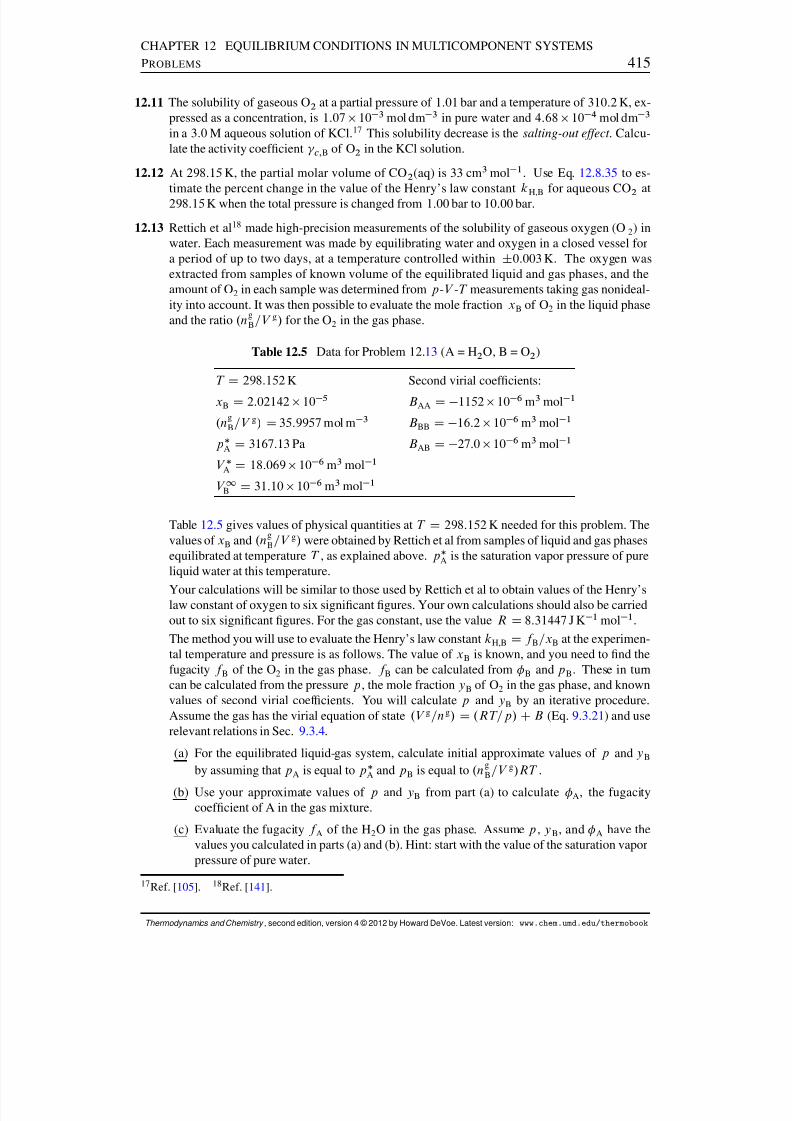
8/12/2019 Howard Devoe Thermodynamic and Chemical
http://slidepdf.com/reader/full/howard-devoe-thermodynamic-and-chemical 415/532
CHAPTER 12 EQUILIBRIUM CONDITIONS IN MULTICOMPONENT SYSTEMSPROBLEMS 415
12.11 The solubility of gaseous O 2 at a partial pressure of 1:01 bar and a temperature of 310:2 K, ex-pressed as a concentration, is 1:07 10 3 mol dm 3 in pure water and 4:68 10 4 mol dm 3
in a 3:0 M aqueous solution of KCl. 17 This solubility decrease is the salting-out effect . Calcu-late the activity coefcient c; B of O2 in the KCl solution.
12.12 At 298:15 K, the partial molar volume of CO 2 (aq) is 33 cm 3 mol 1 . Use Eq. 12.8.35 to es-timate the percent change in the value of the Henry’s law constant k
H,B for aqueous CO
2 at
298:15 K when the total pressure is changed from 1:00 bar to 10:00 bar.
12.13 Rettich et al 18 made high-precision measurements of the solubility of gaseous oxygen (O 2) inwater. Each measurement was made by equilibrating water and oxygen in a closed vessel fora period of up to two days, at a temperature controlled within ˙ 0:003 K. The oxygen wasextracted from samples of known volume of the equilibrated liquid and gas phases, and theamount of O 2 in each sample was determined from p -V -T measurements taking gas nonideal-ity into account. It was then possible to evaluate the mole fraction xB of O2 in the liquid phaseand the ratio .n g
B=V g / for the O 2 in the gas phase.
Table 12.5 Data for Problem 12. 13 (A = H2 O, B = O 2 )
T
D 298:152 K Second virial coefcients:
xB D 2:02142 10 5 BAA D 1152 10 6 m3 mol 1
.n gB=V g/ D 35:9957 mol m 3 BBB D 16:2 10 6 m3 mol 1
p A D 3167:13 Pa BAB D 27:0 10 6 m3 mol 1
V A D 18:069 10 6 m3 mol 1
V 1B D 31:10 10 6 m3 mol 1
Table 12.5 gives values of physical quantities at T D 298:152 K needed for this problem. Thevalues of xB and .n g
B=V g/ were obtained by Rettich et al from samples of liquid and gas phasesequilibrated at temperature T , as explained above. p A is the saturation vapor pressure of pureliquid water at this temperature.
Your calculations will be similar to those used by Rettich et al to obtain values of the Henry’slaw constant of oxygen to six signicant gures. Your own calculations should also be carriedout to six signicant gures. For the gas constant, use the value R D 8:31447 J K 1 mol 1 .The method you will use to evaluate the Henry’s law constant kH,B D f B=xB at the experimen-tal temperature and pressure is as follows. The value of xB is known, and you need to nd thefugacity f B of the O2 in the gas phase. f B can be calculated from B and p B . These in turncan be calculated from the pressure p , the mole fraction yB of O2 in the gas phase, and knownvalues of second virial coefcients. You will calculate p and yB by an iterative procedure.Assume the gas has the virial equation of state .V g=n g/ D .RT=p/ CB (Eq. 9.3.21 ) and userelevant relations in Sec. 9.3.4.
(a) For the equilibrated liquid-gas system, calculate initial approximate values of p and y B
by assuming that p A is equal to p A and p B is equal to .n gB=V g/RT .
(b) Use your approximate values of p and yB from part (a) to calculate A , the fugacitycoefcient of A in the gas mixture.
(c) Evaluate the fugacity f A of the H 2O in the gas phase. Assume p , y B , and A have thevalues you calculated in parts (a) and (b). Hint: start with the value of the saturation vaporpressure of pure water.
17 Ref. [ 105 ]. 18Ref. [ 141 ].
Thermodynamics and Chemistry , second edition, version 4 © 2012 by Howard DeVoe. Latest version: www.chem.umd.edu/thermobook
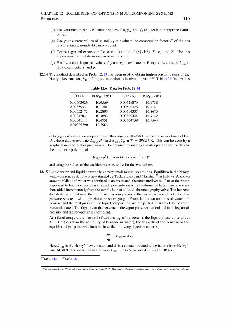
8/12/2019 Howard Devoe Thermodynamic and Chemical
http://slidepdf.com/reader/full/howard-devoe-thermodynamic-and-chemical 416/532
CHAPTER 12 EQUILIBRIUM CONDITIONS IN MULTICOMPONENT SYSTEMSPROBLEMS 416
(d) Use your most recently calculated values of p , A , and f A to calculate an improved valueof yB .
(e) Use your current values of p and yB to evaluate the compression factor Z of the gasmixture, taking nonideality into account.
(f) Derive a general expression for p as a function of .n gB=V g/ , T , yB , and Z . Use this
expression to calculate an improved value of p .(g) Finally, use the improved values of p and yB to evaluate the Henry’s law constant kH,B at
the experimental T and p .
12.14 The method described in Prob. 12. 13 has been used to obtain high-precision values of theHenry’s law constant, kH,B , for gaseous methane dissolved in water. 19 Table 12.6 lists values
Table 12.6 Data for Prob. 12. 14
1=.T=K/ ln .k H,B =p ı / 1=.T = K/ ln .k H,B =p ı /
0:00363029 10:0569 0:00329870 10:67380:00359531 10:1361 0:00319326 10:81410:00352175 10:2895 0:00314307 10:86730:00347041 10:3883 0:00309444 10:91420:00341111 10:4951 0:00304739 10:95640:00335390 10:5906
of ln .k H,B =p ı / at eleven temperatures in the range 275 K–328 K and at pressures close to 1 bar.Use these data to evaluate sol,B H ı and sol,B C ıp at T D 298:15 K. This can be done by agraphical method. Better precision will be obtained by making a least-squares t of the data tothe three-term polynomial
ln .k H,B =p ı / D a Cb.1=T / Cc.1=T / 2
and using the values of the coefcients a , b, and c for the evaluations.
12.15 Liquid water and liquid benzene have very small mutual solubilities. Equilibria in the binarywater–benzene system were investigated by Tucker, Lane, and Christian 20 as follows. A knownamount of distilled water was admitted to an evacuated, thermostatted vessel. Part of the watervaporized to form a vapor phase. Small, precisely measured volumes of liquid benzene werethen added incrementally from the sample loop of a liquid-chromatography valve. The benzenedistributed itself between the liquid and gaseous phases in the vessel. After each addition, thepressure was read with a precision pressure gauge. From the known amounts of water andbenzene and the total pressure, the liquid composition and the partial pressure of the benzenewere calculated. The fugacity of the benzene in the vapor phase was calculated from its partialpressure and the second virial coefcient.
At a xed temperature, for mole fractions xB of benzene in the liquid phase up to about3 10 4 (less than the solubility of benzene in water), the fugacity of the benzene in theequilibrated gas phase was found to have the following dependence on xB :
f BxB D kH,B Ax B
Here kH,B is the Henry’s law constant and A is a constant related to deviations from Henry’slaw. At 30 ı C, the measured values were kH,B D 385:5 bar and A D 2:24 104 bar.
19 Ref. [ 142 ]. 20Ref. [ 157 ].
Thermodynamics and Chemistry , second edition, version 4 © 2012 by Howard DeVoe. Latest version: www.chem.umd.edu/thermobook
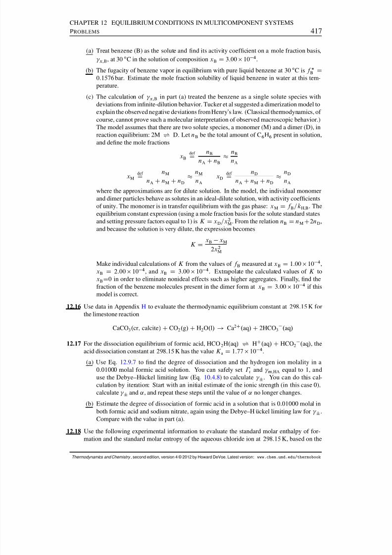
8/12/2019 Howard Devoe Thermodynamic and Chemical
http://slidepdf.com/reader/full/howard-devoe-thermodynamic-and-chemical 417/532
CHAPTER 12 EQUILIBRIUM CONDITIONS IN MULTICOMPONENT SYSTEMSPROBLEMS 417
(a) Treat benzene (B) as the solute and nd its activity coefcient on a mole fraction basis, x; B , at 30 ı C in the solution of composition xB D 3:00 10 4 .
(b) The fugacity of benzene vapor in equilibrium with pure liquid benzene at 30 ı C is f B D0:1576 bar. Estimate the mole fraction solubility of liquid benzene in water at this tem-
perature.
(c) The calculation of x; B in part (a) treated the benzene as a single solute species withdeviations from innite-dilution behavior. Tucker et al suggested a dimerization model toexplain the observed negative deviations fromHenry’s law. (Classical thermodynamics, of course, cannot prove such a molecular interpretation of observed macroscopic behavior.)The model assumes that there are two solute species, a monomer (M) and a dimer (D), inreaction equilibrium: 2M • D. Let nB be the total amount of C 6 H6 present in solution,and dene the mole fractions
xBdef
D nB
nA CnB
nB
nA
xMdef
D nM
nA CnM Cn D
nM
n AxD
def
D nD
nA CnM CnD
nD
nA
where the approximations are for dilute solution. In the model, the individual monomerand dimer particles behave as solutes in an ideal-dilute solution, with activity coefcientsof unity. The monomer is in transfer equilibrium with the gas phase: x M D f B=kH,B . Theequilibrium constant expression (using a mole fraction basis for the solute standard statesand setting pressure factors equal to 1) is K D xD=x 2
M . From the relation nB D nM C2n D ,and because the solution is very dilute, the expression becomes
K D xB xM
2x 2M
Make individual calculations of K from the values of f B measured at xB D 1:00 10 4 ,xB D 2:00 10 4 , and xB D 3:00 10 4 . Extrapolate the calculated values of K toxBD0 in order to eliminate nonideal effects such as higher aggregates. Finally, nd thefraction of the benzene molecules present in the dimer form at xB
D 3:00 10 4 if this
model is correct.
12.16 Use data in Appendix H to evaluate the thermodynamic equilibrium constant at 298:15 K forthe limestone reaction
CaCO 3 . cr; calcite / CCO 2 . g/ CH2O. l/ ! Ca2C . aq / C2HCO 3 . aq/
12.17 For the dissociation equilibrium of formic acid, HCO 2H. aq/ • HC . aq / CHCO 2 . aq/ , theacid dissociation constant at 298:15 K has the value K a D 1:77 10 4 .
(a) Use Eq. 12.9.7 to nd the degree of dissociation and the hydrogen ion molality in a0.01000 molal formic acid solution. You can safely set r and m ,HA equal to 1, anduse the Debye–H uckel limiting law (Eq. 10.4.8 ) to calculate ˙ . You can do this cal-culation by iteration: Start with an initial estimate of the ionic strength (in this case 0),calculate ˙ and ˛ , and repeat these steps until the value of ˛ no longer changes.
(b) Estimate the degree of dissociation of formic acid in a solution that is 0.01000 molal inboth formic acid and sodium nitrate, again using the Debye–H uckel limiting law for ˙ .Compare with the value in part (a).
12.18 Use the following experimental information to evaluate the standard molar enthalpy of for-mation and the standard molar entropy of the aqueous chloride ion at 298:15 K, based on the
Thermodynamics and Chemistry , second edition, version 4 © 2012 by Howard DeVoe. Latest version: www.chem.umd.edu/thermobook

8/12/2019 Howard Devoe Thermodynamic and Chemical
http://slidepdf.com/reader/full/howard-devoe-thermodynamic-and-chemical 418/532
CHAPTER 12 EQUILIBRIUM CONDITIONS IN MULTICOMPONENT SYSTEMSPROBLEMS 418
conventions f H ı . HC , aq / D 0 and S ım . HC , aq / D 0 (Secs. 11.3.2 and 11.8.4 ). (Your calcu-lated values will be close to, but not exactly the same as, those listed in Appendix H, which arebased on the same data combined with data of other workers.)
For the reaction 12 H2 . g/ C 1
2 Cl2 . g/ ! HCl . g/ , the standard molar enthalpy of reactionat 298:15 K measured in a ow calorimeter 21 is rH ı D 92:312 kJ mol 1 .
The standard molar entropy of gaseous HCl at 298:15 K calculated from spectroscopicdata is S ım D 186:902 J K 1 mol 1 . From ve calorimetric runs, 22 the average experimental value of the standard molar en-thalpy of solution of gaseous HCl at 298:15 K is sol,B H ı D 74:84 kJ mol 1 .
From vapor pressure measurements of concentrated aqueous HCl solutions, 23 the valueof the ratio f B=am; B for gaseous HCl in equilibrium with aqueous HCl at 298:15 K is5:032 10 7 bar.
12.19 The solubility of crystalline AgCl in ultrapure water has been determined from the electricalconductivity of the saturated solution. 24 The average of ve measurements at 298:15 K is sB D1:337 10 5 mol dm 3 . The density of water at this temperature is A D 0:9970 kgdm 3 .
(a) From these data and the Debye–H uckel limiting law, calculate the solubility product K sof AgCl at 298:15 K.
(b) Evaluate the standard molar Gibbs energy of formation of aqueous Ag C ion at 298:15 K,using the results of part (a) and the values f G ı . Cl , aq / D 131:22 kJ mol 1 and
f G ı . AgCl, s / D 109:77 kJ mol 1 from Appendix H.
12.20 The following reaction was carried out in an adiabatic solution calorimeter by Wagman andKilday: 25
AgNO 3 (s) CKCl(aq, mB D 0:101 mol kg 1 ) ! AgCl(s) CKNO 3 (aq)
The reaction can be assumed to go to completion, and the amount of KCl was in slight excess,so the amount of AgCl formed was equal to the initial amount of AgNO 3 . After correctionfor the enthalpies of diluting the solutes in the initial and nal solutions to innite dilution,the standard molar reaction enthalpy at 298:15 K was found to be rH ı
D 43:042 kJ mol 1 .
The same workers used solution calorimetry to obtain the molar enthalpy of solution at innitedilution of crystalline AgNO 3 at 298:15 K: sol,B H 1 D 22:727 kJmol 1 .
(a) Show that the difference of these two values is the standard molar reaction enthalpy forthe precipitation reaction
Ag C . aq / CCl . aq / ! AgCl . s/
and evaluate this quantity.
(b) Evaluate the standard molar enthalpy of formation of aqueous Ag C ion at 298:15 K,using the results of part (a) and the values f H ı . Cl , aq / D 167:08 kJmol 1 and
f H ı . AgCl, s / D 127:01 kJmol 1 from Appendix H. (These values come from cal-culations similar to those in Probs. 12. 18 and 14. 4.) The calculated value will be close to,but not exactly the same as, the value listed in Appendix H, which is based on the samedata combined with data of other workers.
21 Ref. [ 144 ]. 22Ref. [ 72]. 23Ref. [ 136 ]. 24Ref. [ 67]. 25Ref. [ 162 ].
Thermodynamics and Chemistry , second edition, version 4 © 2012 by Howard DeVoe. Latest version: www.chem.umd.edu/thermobook
8/12/2019 Howard Devoe Thermodynamic and Chemical
http://slidepdf.com/reader/full/howard-devoe-thermodynamic-and-chemical 419/532
C HAPTER 13
T HE PHASE RULE AND PHASE DIAGRAMS
We encountered the Gibbs phase rule and phase diagrams in Chap. 8 in connection withsingle-substance systems. The present chapter derives the full version of the Gibbs phaserule for multicomponent systems. It then discusses phase diagrams for some representativetypes of multicomponent systems, and shows how they are related to the phase rule and toequilibrium concepts developed in Chaps. 11 and 12.
13.1 THE GIBBS PHASE RULE FOR MULTICOMPONENT SYSTEMS
In Sec. 8.1.7 , the Gibbs phase rule for a pure substance was written F D 3 P . We nowconsider a system of more than one substance and more than one phase in an equilibriumstate. The phase rule assumes the system is at thermal and mechanical equilibrium. Weshall assume furthermore that in addition to the temperature and pressure, the only otherstate functions needed to describe the state are the amounts of the species in each phase;this means for instance that surface effects are ignored.
The derivations to follow will show that phase rule may be written either in the form
F D 2 CC P (13.1.1)
orF D 2 Cs r P (13.1.2)
where the symbols have the following meanings:F = the number of degrees of freedom (or variance)
= the maximum number of intensive variables that can be varied independently whilethe system remains in an equilibrium state;
C = the number of components
= the minimum number of substances (or xed-composition mixtures of substances) thatcould be used to prepare each phase individually;
P = the number of different phases;
s = the number of different species;
r = the number of independent relations among intensive variables of individual phasesother than relations needed for thermal, mechanical, and transfer equilibrium.
419
8/12/2019 Howard Devoe Thermodynamic and Chemical
http://slidepdf.com/reader/full/howard-devoe-thermodynamic-and-chemical 420/532
CHAPTER 13 THE PHASE RULE AND PHASE DIAGRAMS13.1 T HE G IBBS P HASE RULE FOR M ULTICOMPONENT S YSTEMS 420
If we subdivide a phase, that does not change the number of phases P . That is, we treatnoncontiguous regions of the system that have identical intensive properties as parts of thesame phase.
13.1.1 Degrees of freedom
Consider a system in an equilibrium state. In this state, the system has one or more phases;each phase contains one or more species; and intensive properties such as T , p , and themole fraction of a species in a phase have denite values. Starting with the system in thisstate, we can make changes that place the system in a new equilibrium state having thesame kinds of phases and the same species, but different values of some of the intensiveproperties. The number of different independent intensive variables that we may change inthis way is the number of degrees of freedom or variance , F , of the system.
Clearly, the system remains in equilibrium if we change the amount of a phase withoutchanging its temperature, pressure, or composition. This, however, is the change of anextensive variable and is not counted as a degree of freedom.
The phase rule, in the form to be derived, applies to a system that continues to have
complete thermal, mechanical, and transfer equilibrium as intensive variables change. Thismeans different phases are not separated by adiabatic or rigid partitions, or by semiper-meable or impermeable membranes. Furthermore, every conceivable reaction among thespecies is either at reaction equilibrium or else is frozen at a xed advancement during thetime period we observe the system.
The number of degrees of freedom is the maximum number of intensive propertiesof the equilibrium system we may independently vary, or x at arbitrary values, withoutcausing a change in the number and kinds of phases and species. We cannot, of course,change one of these properties to just any value whatever. We are able to vary the valueonly within a certain nite (sometimes quite narrow) range before a phase disappears or anew one appears.
The number of degrees of freedom is also the number of independent intensive vari-ables needed to specify the equilibrium state in all necessary completeness, aside from theamount of each phase. In other words, when we specify values of F different independentintensive variables, then the values of all other intensive variables of the equilibrium statehave denite values determined by the physical nature of the system.
Just as for a one-component system, we can use the terms bivariant , univariant , andinvariant depending on the value of F (Sec. 8.1.7 ).
13.1.2 Species approach to the phase rule
This section derives an expression for the number of degrees of freedom, F , based onspecies . Section 13.1.3 derives an expression based on components . Both approaches yieldequivalent versions of the phase rule.
Recall that a species is an entity, uncharged or charged, distinguished from other speciesby its chemical formula (Sec. 9.1.1 ). Thus, CO 2 and CO 3
2 are different species, butCO 2 (aq) and CO 2 (g) is the same species in different phases.
Consider an equilibrium system of P phases, each of which contains the same set of species. Let the number of different species be s. If we could make changes while the
Thermodynamics and Chemistry , second edition, version 4 © 2012 by Howard DeVoe. Latest version: www.chem.umd.edu/thermobook
8/12/2019 Howard Devoe Thermodynamic and Chemical
http://slidepdf.com/reader/full/howard-devoe-thermodynamic-and-chemical 421/532
CHAPTER 13 THE PHASE RULE AND PHASE DIAGRAMS13.1 T HE G IBBS P HASE RULE FOR M ULTICOMPONENT S YSTEMS 421
system remains in thermal and mechanical equilibrium, but not necessarily in transfer equi-librium, we could independently vary the temperature and pressure of the system as a wholeand the amount of each species in each phase; there would then be 2CP s independent vari-ables.
The equilibrium system is, however, in transfer equilibrium, which requires each species
to have the same chemical potential in each phase: “i D
’i ,
”i D
’i , and so on. Thereare P 1 independent relations like this for each species, and a total of s.P 1/ independent
relations for all species. Each such independent relation introduces a constraint and reducesthe number of independent variables by one. Accordingly, taking transfer equilibrium intoaccount, the number of independent variables is 2 CP s s.P 1/ D 2 Cs .
We obtain the same result if a species present in one phase is totally excluded fromanother. For example, solvent molecules of a solution are not found in a pure perfectly-ordered crystal of the solute, undissociated molecules of a volatile strong acid such as HClcan exist in a gas phase but not in aqueous solution, and ions of an electrolyte solute areusually not found in a gas phase. For each such species absent from a phase, there is onefewer amount variable and also one fewer relation for transfer equilibrium; on balance, thenumber of independent variables is still 2
Cs .
Next, we consider the possibility that further independent relations exist among in-tensive variables in addition to the relations needed for thermal, mechanical, and transferequilibrium. 1 If there are r of these additional relations, the total number of independentvariables is reduced to 2 Cs r . These relations may come from
1. reaction equilibria,2. the requirement of electroneutrality in a phase containing ions, and3. initial conditions determined by the way the system is prepared.
In the case of a reaction equilibrium, the relation is rG DPi i i D 0, or the equivalentrelation K DQi .a i / i for the thermodynamic equilibrium constant. Thus, r is the sum of the number of independent reaction equilibria, the number of phases containing ions, andthe number of independent initial conditions. Several examples will be given in Sec. 13.1.4 .
There is an innite variety of possible choices of the independent variables (both exten-sive and intensive) for the equilibrium system, but the total number of independent variablesis xed at 2 Cs r . Keeping intensive properties xed, we can always vary how much of each phase is present (e.g., its volume, mass, or amount) without destroying the equilib-rium. Thus, at least P of the independent variables, one for each phase, must be extensive.It follows that the maximum number of independent intensive variables is the difference.2 Cs r/ P .
It may be that initial conditions establish relations among the amounts of phases, aswill be illustrated in example 2 on page 424. If present, these are relations amongextensive variables that are not counted in r . Each such independent relation decreases
the total number of independent variables without changing the number of independentintensive variables calculated from .2 Cs r/ P .
Since the maximum number of independent intensive variables is the number of degrees
1Relations such as Pi p i D p for a gas phase or Pi x i D 1 for a phase in general have already been accountedfor in the derivation by the specication of p and the amount of each species.
Thermodynamics and Chemistry , second edition, version 4 © 2012 by Howard DeVoe. Latest version: www.chem.umd.edu/thermobook
8/12/2019 Howard Devoe Thermodynamic and Chemical
http://slidepdf.com/reader/full/howard-devoe-thermodynamic-and-chemical 422/532
CHAPTER 13 THE PHASE RULE AND PHASE DIAGRAMS13.1 T HE G IBBS P HASE RULE FOR M ULTICOMPONENT S YSTEMS 422
of freedom, our expression for F based on species is
F D 2 Cs r P (13.1.3)
13.1.3 Components approach to the phase rule
The derivation of the phase rule in this section uses the concept of components . The numberof components, C , is the minimum number of substances or mixtures of xed compositionfrom which we could in principle prepare each individual phase of an equilibrium state of the system, using methods that may be hypothetical. These methods include the addition orremoval of one or more of the substances or xed-composition mixtures, and the conversionof some of the substances into others by means of a reaction that is at equilibrium in theactual system.
It is not always easy to decide on the number of components of an equilibrium system.The number of components may be less than the number of substances present, on accountof the existence of reaction equilibria that produce some substances from others. When weuse a reaction to prepare a phase, nothing must remain unused. For instance, consider a
system consisting of solid phases of CaCO 3 and CaO and a gas phase of CO 2 . Assume thereaction CaCO 3 (s) ! CaO . s/ C CO 2 . g/ is at equilibrium. We could prepare the CaCO 3phase from CaO and CO 2 by the reverse of this reaction, but we can only prepare the CaOand CO 2 phases from the individual substances. We could not use CaCO 3 to prepare eitherthe CaO phase or the CO 2 phase, because CO 2 or CaO would be left over. Thus this systemhas three substances but only two components, namely CaO and CO 2 .
In deriving the phase rule by the components approach, it is convenient to consideronly intensive variables. Suppose we have a system of P phases in which each substancepresent is a component (i.e., there are no reactions) and each of the C components is presentin each phase. If we make changes to the system while it remains in thermal and mechanicalequilibrium, but not necessarily in transfer equilibrium, we can independently vary the tem-perature and pressure of the whole system, and for each phase we can independently varythe mole fraction of all but one of the substances (the value of the omitted mole fractioncomes from the relation Pi x i D 1). This is a total of 2 CP .C 1/ independent intensivevariables.
When there also exist transfer and reaction equilibria, not all of these variables are in-dependent. Each substance in the system is either a component, or else can be formed fromcomponents by a reaction that is in reaction equilibrium in the system. Transfer equilibriaestablish P 1 independent relations for each component ( “
i D ’i ,
”i D ’
i , etc.) anda total of C .P 1/ relations for all components. Since these are relations among chemicalpotentials, which are intensive properties, each relation reduces the number of independentintensive variables by one. The resulting number of independent intensive variables is
F D Œ2CP .C 1/ C.P 1/ D 2 CC P (13.1.4)
If the equilibrium system lacks a particular component in one phase, there is one fewermole fraction variable and one fewer relation for transfer equilibrium. These changes cancelin the calculation of F , which is still equal to 2 CC P . If a phase contains a substancethat is formed from components by a reaction, there is an additional mole fraction variableand also the additional relation Pi i i D 0 for the reaction; again the changes cancel.
Thermodynamics and Chemistry , second edition, version 4 © 2012 by Howard DeVoe. Latest version: www.chem.umd.edu/thermobook
8/12/2019 Howard Devoe Thermodynamic and Chemical
http://slidepdf.com/reader/full/howard-devoe-thermodynamic-and-chemical 423/532
CHAPTER 13 THE PHASE RULE AND PHASE DIAGRAMS13.1 T HE G IBBS P HASE RULE FOR M ULTICOMPONENT S YSTEMS 423
We may need to remove a component from a phase to achieve the nal composition.Note that it is not necessary to consider additional relations for electroneutrality orinitial conditions; they are implicit in the denitions of the components. For instance,since each component is a substance of zero electric charge, the electrical neutrality of the phase is assured.
We conclude that, regardless of the kind of system, the expression for F based oncomponents is given by F D 2 CC P . By comparing this expression and F D 2 Csr P , we see that the number of components is related to the number of species by
C D s r (13.1.5)
13.1.4 Examples
The ve examples below illustrate various aspects of using the phase rule.
Example 1: liquid water
For a single phase of pure water, P equals 1. If we treat the water as the single speciesH2 O, s is 1 and r is 0. The phase rule then predicts two degrees of freedom:
F D 2 Cs r P
D 2 C1 0 1 D 2 (13.1.6)
Since F is the number of intensive variables that can be varied independently, we could forinstance vary T and p independently, or T and , or any other pair of independent intensivevariables.
Next let us take into account the proton transfer equilibrium
2 H 2O. l/ • H3OC . aq / COH . aq /
and consider the system to contain the three species H 2 O, H 3 OC , and OH . Then for thespecies approach to the phase rule, we have s D 3. We can write two independent relations:
1. for reaction equilibrium, 2 H2 O C H3 OC C OH D 0;
2. for electroneutrality, mH3 OC D mOH .Thus, we have two relations involving intensive variables only. Now s is 3, r is 2, P is 1,and the number of degrees of freedom is given by
F D 2 Cs r P D 2 (13.1.7)
which is the same value of F as before.If we consider water to contain additional cation species (e.g., H 5O2
C ), each such
species would add 1 to s and 1 to r , but F would remain equal to 2. Thus, no matterhow complicated are the equilibria that actually exist in liquid water, the number of degreesof freedom remains 2.
Applying the components approach to water is simple. All species that may exist inpure water are formed, in whatever proportions actually exist, from the single substanceH2 O. Thus, there is only one component: C D 1. The component version of the phaserule, F D 2 CC P , gives the same result as the species version: F D 2.
Thermodynamics and Chemistry , second edition, version 4 © 2012 by Howard DeVoe. Latest version: www.chem.umd.edu/thermobook

8/12/2019 Howard Devoe Thermodynamic and Chemical
http://slidepdf.com/reader/full/howard-devoe-thermodynamic-and-chemical 424/532
CHAPTER 13 THE PHASE RULE AND PHASE DIAGRAMS13.1 T HE G IBBS P HASE RULE FOR M ULTICOMPONENT S YSTEMS 424
Example 2: carbon, oxygen, and carbon oxides
Consider a system containing solid carbon (graphite) and a gaseous mixture of O 2 , CO, andCO 2 . There are four species and two phases. If reaction equilibrium is absent, as might bethe case at low temperature in the absence of a catalyst, we have r D 0 and C D s r D 4.The four components are the four substances. The phase rule tells us the system has four
degrees of freedom. We could, for instance, arbitrarily vary T , p , yO2 , and yCO .Now suppose we raise the temperature or introduce an appropriate catalyst to allow the
following reaction equilibria to exist:1 . 2 C . s/ CO2 . g/ • 2 CO . g/2. C . s/ CO2 . g/ • CO2 . g/
These equilibria introduce two new independent relations among chemical potentials andamong activities. We could also consider the equilibrium 2 CO . g/ CO2 . g/ • 2 CO 2 . g/ ,but it does not contribute an additional independent relation because it depends on the othertwo equilibria: the reaction equation is obtained by subtracting the reaction equation forequilibrium 1 from twice the reaction equation for equilibrium 2. By the species approach,we have s
D 4, r
D 2, and P
D 2; the number of degrees of freedom from these values is
F D 2 Cs r P D 2 (13.1.8)
If we wish to calculate F by the components approach, we must decide on the mini-mum number of substances we could use to prepare each phase separately. (This does notrefer to how we actually prepare the two-phase system, but to a hypothetical preparation of each phase with any of the compositions that can actually exist in the equilibrium system.)Assume equilibria 1 and 2 are present. We prepare the solid phase with carbon, and wecan prepare any possible equilibrium composition of the gas phase from carbon and O 2 byusing the reactions of both equilibria. Thus, there are two components (C and O 2 ) givingthe same result of two degrees of freedom.
What is the signicance of there being two degrees of freedom when the reaction equi-libria are present? There are two ways of viewing the situation:
1. We can arbitrarily vary the two intensive variables T and p . When we do, the molefractions of the three substances in the gas phase change in a way determined byequilibria 1 and 2.
2. If we specify arbitrary values of T and p , each of the mole fractions has only onepossible value that will allow the two phases and four substances to be in equilibrium.
Now to introduce an additional complexity: Suppose we prepare the system by placinga certain amount of O 2 and twice this amount of carbon in an evacuated container, and waitfor the reactions to come to equilibrium. This method of preparation imposes an initialcondition on the system, and we must decide whether the number of degrees of freedom isaffected. Equating the total amount of carbon atoms to the total amount of oxygen atoms inthe equilibrated system gives the relation
nC CnCO CnCO 2 D 2nO2 CnCO C2n CO 2 or nC D 2nO2 CnCO 2
(13.1.9)
Either equation is a relation among extensive variables of the two phases. From them, weare unable to obtain any relation among intensive variables of the phases. Therefore, thisparticular initial condition does not change the value of r , and F remains equal to 2.
Thermodynamics and Chemistry , second edition, version 4 © 2012 by Howard DeVoe. Latest version: www.chem.umd.edu/thermobook
8/12/2019 Howard Devoe Thermodynamic and Chemical
http://slidepdf.com/reader/full/howard-devoe-thermodynamic-and-chemical 425/532
CHAPTER 13 THE PHASE RULE AND PHASE DIAGRAMS13.1 T HE G IBBS P HASE RULE FOR M ULTICOMPONENT S YSTEMS 425
Example 3: a solid salt and saturated aqueous solution
In this example, the equilibrium system consists of crystalline PbCl 2 and an aqueous phasecontaining the species H 2 O, Pb 2C (aq), and Cl (aq).
Applying the components approach to this system is straightforward. The solid phaseis prepared from PbCl 2 and the aqueous phase could be prepared by dissolving solid PbCl 2
in H2 O. Thus, there are two components and two phases:
F D 2 CC P D 2 (13.1.10)
For the species approach, we note that there are four species (PbCl 2 , Pb2C , Cl , andH2 O) and two independent relations among intensive variables:
1. equilibrium for the dissolution process, PbCl 2 C Pb2 C C2 Cl D 0;
2. electroneutrality of the aqueous phase, 2mPb2 C D mCl .We have s D 4, r D 2, and P D 2, giving the same result as the components approach:
F D 2 Cs r P D 2 (13.1.11)
Example 4: liquid water and water-saturated air
For simplicity, let “air” be a gaseous mixture of N 2 and O 2 . The equilibrium system in thisexample has two phases: liquid water saturated with the dissolved constituents of air, andair saturated with gaseous H 2 O.
If there is no special relation among the total amounts of N 2 and O 2 , there are threecomponents and the phase rule gives
F D 2 CC P D 3 (13.1.12)
Since there are three degrees of freedom, we could, for instance, specify arbitrary values 2
of T , p , and yN2 ; then the values of other intensive variables such as the mole fractionsyH2 O and xN2
would have denite values.Now suppose we impose an initial condition by preparing the system with water and
dry air of a xed composition. The mole ratio of N 2 and O 2 in the aqueous solution is notnecessarily the same as in the equilibrated gas phase; consequently, the air does not behavelike a single substance. The number of components is still three: H 2 O, N 2 , and O 2 areall required to prepare each phase individually, just as when there was no initial condition,giving F D 3 as before. 3
We can reach the same conclusion with the species approach. The initial condition canbe expressed by an equation such as
.n l
N2 Cng
N2/
.n lO2 Cng
O2/ D a (13.1.13)
2Arbitrary, that is, within the limits that would allow the two phases to coexist.3The fact that the compositions of both phases depend on the relative amounts of the phases is illustrated inProb. 9. 5.
Thermodynamics and Chemistry , second edition, version 4 © 2012 by Howard DeVoe. Latest version: www.chem.umd.edu/thermobook
8/12/2019 Howard Devoe Thermodynamic and Chemical
http://slidepdf.com/reader/full/howard-devoe-thermodynamic-and-chemical 426/532
CHAPTER 13 THE PHASE RULE AND PHASE DIAGRAMS13.2 P HASE D IAGRAMS : BINARY S YSTEMS 426
where a is a constant equal to the mole ratio of N 2 and O 2 in the dry air. This equationcannot be changed to a relation between intensive variables such as xN2
and xO2, so that r
is zero and there are still three degrees of freedom.Finally, let us assume that we prepare the system with dry air of xed composition, as
before, but consider the solubilities of N 2 and O 2 in water to be negligible. Then n lN2
and
nlO2 are zero and Eq. 13.1.13 becomes n
gN2 =n
gO2 D a , or yN2 D ay O2 , which is a relationbetween intensive variables. In this case, r is 1 and the phase rule becomes
F D 2 Cs r P D 2 (13.1.14)
The reduction in the value of F from 3 to 2 is a consequence of our inability to detect anydissolved N 2 or O2 . According to the components approach, we may prepare the liquidphase with H 2 O and the gas phase with H 2 O and air of xed composition that behaves as asingle substance; thus, there are only two components.
Example 5: equilibrium between two solid phases and a gas phase
Consider the following reaction equilibrium:
3CuO . s/ C2 NH 3 . g/ • 3 Cu . s/ C3 H 2O. g/ CN2 . g/
According to the species approach, there are ve species, one relation (for reaction equilib-rium), and three phases. The phase rule gives
F D 2 Cs r P D 3 (13.1.15)
It is more difcult to apply the components approach to this example. As components,we might choose CuO and Cu (from which we could prepare the solid phases) and also NH 3and H 2 O. Then to obtain the N 2 needed to prepare the gas phase, we could use CuO and
NH 3 as reactants in the reaction 3 CuO C2 NH 3 ! 3 Cu C3 H 2O CN2 and remove theproducts Cu and H 2 O. In the components approach, we are allowed to remove substancesfrom the system provided they are counted as components.
13.2 PHASE DIAGRAMS: BINARY SYSTEMS
As explained in Sec. 8.2, a phase diagram is a kind of two-dimensional map that showswhich phase or phases are stable under a given set of conditions. This section discussessome common kinds of binary systems, and Sec. 13.3 will describe some interesting ternarysystems.
13.2.1 GeneralitiesA binary system has two components; C equals 2, and the number of degrees of freedom isF D 4 P . There must be at least one phase, so the maximum possible value of F is 3.Since F cannot be negative, the equilibrium system can have no more than four phases.
We can independently vary the temperature, pressure, and composition of the system asa whole. Instead of using these variables as the coordinates of a three-dimensional phase
Thermodynamics and Chemistry , second edition, version 4 © 2012 by Howard DeVoe. Latest version: www.chem.umd.edu/thermobook

8/12/2019 Howard Devoe Thermodynamic and Chemical
http://slidepdf.com/reader/full/howard-devoe-thermodynamic-and-chemical 427/532
CHAPTER 13 THE PHASE RULE AND PHASE DIAGRAMS13.2 P HASE D IAGRAMS : BINARY S YSTEMS 427
diagram, we usually draw a two-dimensional phase diagram that is either a temperature–composition diagram at a xed pressure or a pressure–composition diagram at a xed tem-perature. The position of the system point on one of these diagrams then corresponds to adenite temperature, pressure, and overall composition. The composition variable usuallyvaries along the horizontal axis and can be the mole fraction, mass fraction, or mass percent
of one of the components, as will presently be illustrated by various examples.The way in which we interpret a two-dimensional phase diagram to obtain the compo-sitions of individual phases depends on the number of phases present in the system.
If the system point falls within a one-phase area of the phase diagram, the com-position variable is the composition of that single phase. There are three degreesof freedom. On the phase diagram, the value of either T or p has been xed, sothere are two other independent intensive variables. For example, on a temperature–composition phase diagram, the pressure is xed and the temperature and composi-tion can be changed independently within the boundaries of the one-phase area of thediagram.
If the system point is in a two-phase area of the phase diagram, we draw a horizontal
tie line of constant temperature (on a temperature–composition phase diagram) orconstant pressure (on a pressure–composition phase diagram). The lever rule applies.The position of the point at each end of the tie line, at the boundary of the two-phasearea, gives the value of the composition variable of one of the phases and also thephysical state of this phase: either the state of an adjacent one-phase area, or thestate of a phase of xed composition when the boundary is a vertical line. Thus, aboundary that separates a two-phase area for phases ’ and “ from a one-phase areafor phase ’ is a curve that describes the composition of phase ’ as a function of T orp when it is in equilibrium with phase “ . The curve is called a solidus , liquidus , orvaporus depending on whether phase ’ is a solid, liquid, or gas.
A binary system with three phases has only one degree of freedom and cannot be
represented by an area on a two-dimensional phase diagram. Instead, there is a hori-zontal boundary line between areas, with a special point along the line at the junctionof several areas. The compositions of the three phases are given by the positions of this point and the points at the two ends of the line. The position of the system pointon this line does not uniquely specify the relative amounts in the three phases.
The examples that follow show some of the simpler kinds of phase diagrams known forbinary systems.
13.2.2 Solid–liquid systems
Figure 13.1 on the next page is a temperature–composition phase diagram at a xed pres-
sure. The composition variable zB is the mole fraction of component B in the system as awhole. The phases shown are a binary liquid mixture of A and B, pure solid A, and puresolid B.
The one-phase liquid area is bounded by two curves, which we can think of either asfreezing-point curves for the liquid or as solubility curves for the solids. These curves com-prise the liquidus. As the mole fraction of either component in the liquid phase decreasesfrom unity, the freezing point decreases. The curves meet at point a, which is a eutectic
Thermodynamics and Chemistry , second edition, version 4 © 2012 by Howard DeVoe. Latest version: www.chem.umd.edu/thermobook
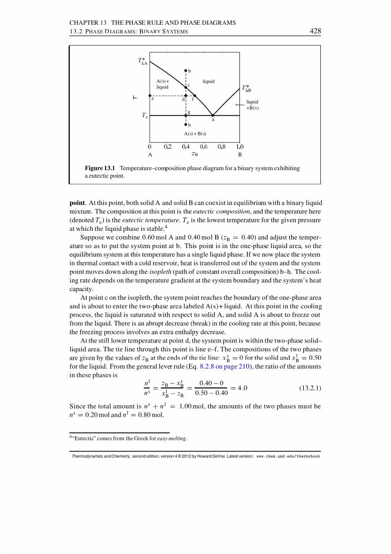
8/12/2019 Howard Devoe Thermodynamic and Chemical
http://slidepdf.com/reader/full/howard-devoe-thermodynamic-and-chemical 428/532
CHAPTER 13 THE PHASE RULE AND PHASE DIAGRAMS13.2 P HASE D IAGRAMS : BINARY S YSTEMS 428
a
b
c
de f
g
h
liquidA(s) +liquid
liquid+B(s)
A(s) + B(s)
A B B
f A
e
f B
Figure 13.1 Temperature–composition phase diagram for a binary system exhibitinga eutectic point.
point . At this point, both solid A and solid B can coexist in equilibrium with a binary liquidmixture. The composition at this point is the eutectic composition , and the temperature here(denoted T e) is the eutectic temperature . T e is the lowest temperature for the given pressureat which the liquid phase is stable. 4
Suppose we combine 0:60 mol A and 0:40 mol B ( zB D 0:40) and adjust the temper-ature so as to put the system point at b. This point is in the one-phase liquid area, so theequilibrium system at this temperature has a single liquid phase. If we now place the systemin thermal contact with a cold reservoir, heat is transferred out of the system and the systempoint moves down along the isopleth (path of constant overall composition) b–h. The cool-ing rate depends on the temperature gradient at the system boundary and the system’s heat
capacity.At point c on the isopleth, the system point reaches the boundary of the one-phase areaand is about to enter the two-phase area labeled A(s)+ liquid. At this point in the coolingprocess, the liquid is saturated with respect to solid A, and solid A is about to freeze outfrom the liquid. There is an abrupt decrease (break) in the cooling rate at this point, becausethe freezing process involves an extra enthalpy decrease.
At the still lower temperature at point d, the system point is within the two-phase solid–liquid area. The tie line through this point is line e–f. The compositions of the two phasesare given by the values of zB at the ends of the tie line: x s
B D 0 for the solid and x lB D 0:50
for the liquid. From the general lever rule (Eq. 8.2.8 on page 210 ), the ratio of the amountsin these phases is
n l
n s D zB x s
Bx lB zB D
0:40 00:50 0:40 D 4 :0 (13.2.1)
Since the total amount is ns C n l D 1:00 mol, the amounts of the two phases must ben s D 0:20 mol and n l D 0:80 mol.
4“Eutectic” comes from the Greek for easy melting .
Thermodynamics and Chemistry , second edition, version 4 © 2012 by Howard DeVoe. Latest version: www.chem.umd.edu/thermobook
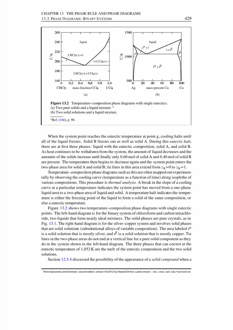
8/12/2019 Howard Devoe Thermodynamic and Chemical
http://slidepdf.com/reader/full/howard-devoe-thermodynamic-and-chemical 429/532
CHAPTER 13 THE PHASE RULE AND PHASE DIAGRAMS13.2 P HASE D IAGRAMS : BINARY S YSTEMS 429
liquid
CHCl
(s )+l
l+CCl
(s)
CHCl
(s) + CCl
(s)
CHCl
mass fraction CCl
CCl
(a)
K
liquid
s + ll + s
s + s
s s
Ag mass percent Cu Cu
(b)
K
Figure 13.2 Temperature–composition phase diagrams with single eutectics.(a) Two pure solids and a liquid mixture. a
(b) Two solid solutions and a liquid mixture.
a Ref. [ 166 ], p. 98.
When the system point reaches the eutectic temperature at point g, cooling halts untilall of the liquid freezes. Solid B freezes out as well as solid A. During this eutectic halt ,there are at rst three phases: liquid with the eutectic composition, solid A, and solid B.As heat continues to be withdrawn from the system, the amount of liquid decreases and theamounts of the solids increase until nally only 0:60 mol of solid A and 0:40 mol of solid Bare present. The temperature then begins to decrease again and the system point enters thetwo-phase area for solid A and solid B; tie lines in this area extend from zBD0 to zBD1.
Temperature–composition phase diagrams such as this are often mapped out experimen-tally by observing the cooling curve (temperature as a function of time) along isopleths of various compositions. This procedure is thermal analysis . A break in the slope of a coolingcurve at a particular temperature indicates the system point has moved from a one-phaseliquid area to a two-phase area of liquid and solid. A temperature halt indicates the temper-ature is either the freezing point of the liquid to form a solid of the same composition, orelse a eutectic temperature.
Figure 13.2 shows two temperature–composition phase diagrams with single eutecticpoints. The left-hand diagram is for the binary system of chloroform and carbon tetrachlo-ride, two liquids that form nearly ideal mixtures. The solid phases are pure crystals, as inFig. 13.1 . The right-hand diagram is for the silver–copper system and involves solid phasesthat are solid solutions (substitutional alloys of variable composition). The area labeled s ’
is a solid solution that is mostly silver, and s “ is a solid solution that is mostly copper. Tielines in the two-phase areas do not end at a vertical line for a pure solid component as theydo in the system shown in the left-hand diagram. The three phases that can coexist at theeutectic temperature of 1,052 K are the melt of the eutectic composition and the two solidsolutions.
Section 12.5.4 discussed the possibility of the appearance of a solid compound when a
Thermodynamics and Chemistry , second edition, version 4 © 2012 by Howard DeVoe. Latest version: www.chem.umd.edu/thermobook
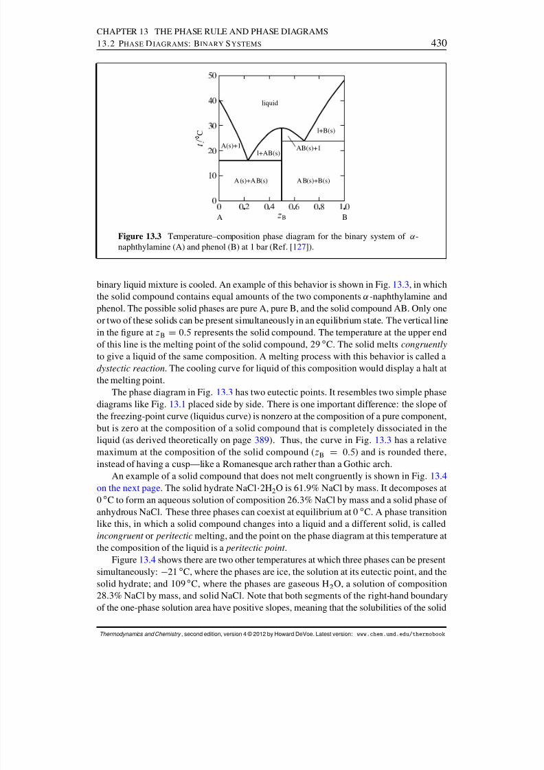
8/12/2019 Howard Devoe Thermodynamic and Chemical
http://slidepdf.com/reader/full/howard-devoe-thermodynamic-and-chemical 430/532
CHAPTER 13 THE PHASE RULE AND PHASE DIAGRAMS13.2 P HASE D IAGRAMS : BINARY S YSTEMS 430
BA B
Æ
C
liquid
A(s)+1l+AB(s)
A(s)+AB(s) AB(s)+B(s)
l+B(s)
AB(s)+1
Figure 13.3 Temperature–composition phase diagram for the binary system of ˛ -naphthylamine (A) and phenol (B) at 1 bar (Ref. [ 127 ]).
binary liquid mixture is cooled. An example of this behavior is shown in Fig. 13.3 , in whichthe solid compound contains equal amounts of the two components ˛ -naphthylamine andphenol. The possible solid phases are pure A, pure B, and the solid compound AB. Only oneor two of these solids can be present simultaneously in an equilibrium state. The vertical linein the gure at zB D 0:5 represents the solid compound. The temperature at the upper endof this line is the melting point of the solid compound, 29 ı C. The solid melts congruentlyto give a liquid of the same composition. A melting process with this behavior is called adystectic reaction . The cooling curve for liquid of this composition would display a halt atthe melting point.
The phase diagram in Fig. 13.3 has two eutectic points. It resembles two simple phase
diagrams like Fig. 13.1 placed side by side. There is one important difference: the slope of the freezing-point curve (liquidus curve) is nonzero at the composition of a pure component,but is zero at the composition of a solid compound that is completely dissociated in theliquid (as derived theoretically on page 389). Thus, the curve in Fig. 13.3 has a relativemaximum at the composition of the solid compound ( zB D 0:5) and is rounded there,instead of having a cusp—like a Romanesque arch rather than a Gothic arch.
An example of a solid compound that does not melt congruently is shown in Fig. 13.4on the next page . The solid hydrate NaCl 2H 2O is 61.9% NaCl by mass. It decomposes at0 ı C to form an aqueous solution of composition 26.3% NaCl by mass and a solid phase of anhydrous NaCl. These three phases can coexist at equilibrium at 0 ı C. A phase transitionlike this, in which a solid compound changes into a liquid and a different solid, is called
incongruent or peritectic melting, and the point on the phase diagram at this temperature atthe composition of the liquid is a peritectic point .Figure 13.4 shows there are two other temperatures at which three phases can be present
simultaneously: 21 ı C, where the phases are ice, the solution at its eutectic point, and thesolid hydrate; and 109 ı C, where the phases are gaseous H 2 O, a solution of composition28.3% NaCl by mass, and solid NaCl. Note that both segments of the right-hand boundaryof the one-phase solution area have positive slopes, meaning that the solubilities of the solid
Thermodynamics and Chemistry , second edition, version 4 © 2012 by Howard DeVoe. Latest version: www.chem.umd.edu/thermobook
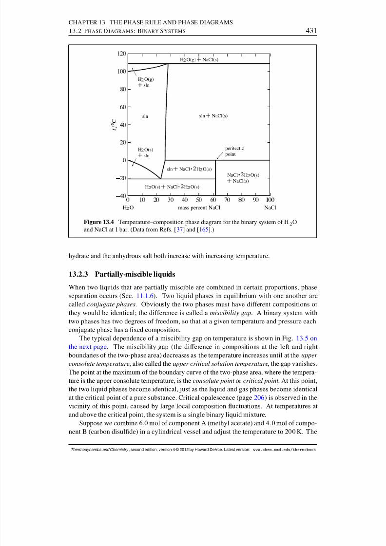
8/12/2019 Howard Devoe Thermodynamic and Chemical
http://slidepdf.com/reader/full/howard-devoe-thermodynamic-and-chemical 431/532
CHAPTER 13 THE PHASE RULE AND PHASE DIAGRAMS13.2 P HASE D IAGRAMS : BINARY S YSTEMS 431
H
O mass percent NaCl NaCl
Æ
C
H
O(g) NaCl(s)
H
O(g) sln
sln sln NaCl(s)
H
O(s) sln
sln NaCl H
O(s)
H
O(s) NaCl H
O(s)
NaCl H
O(s) NaCl(s)
peritecticpoint
Figure 13.4 Temperature–composition phase diagram for the binary system of H 2 Oand NaCl at 1 bar. (Data from Refs. [ 37] and [165 ].)
hydrate and the anhydrous salt both increase with increasing temperature.
13.2.3 Partially-miscible liquids
When two liquids that are partially miscible are combined in certain proportions, phaseseparation occurs (Sec. 11.1.6 ). Two liquid phases in equilibrium with one another arecalled conjugate phases . Obviously the two phases must have different compositions orthey would be identical; the difference is called a miscibility gap . A binary system withtwo phases has two degrees of freedom, so that at a given temperature and pressure eachconjugate phase has a xed composition.
The typical dependence of a miscibility gap on temperature is shown in Fig. 13.5 onthe next page . The miscibility gap (the difference in compositions at the left and rightboundaries of the two-phase area) decreases as the temperature increases until at the upper consolute temperature , also called the upper critical solution temperature , the gap vanishes.The point at the maximum of the boundary curve of the two-phase area, where the tempera-
ture is the upper consolute temperature, is the consolute point or critical point . At this point,the two liquid phases become identical, just as the liquid and gas phases become identicalat the critical point of a pure substance. Critical opalescence (page 206 ) is observed in thevicinity of this point, caused by large local composition uctuations. At temperatures atand above the critical point, the system is a single binary liquid mixture.
Suppose we combine 6:0 mol of component A (methyl acetate) and 4 :0 mol of compo-nent B (carbon disulde) in a cylindrical vessel and adjust the temperature to 200 K. The
Thermodynamics and Chemistry , second edition, version 4 © 2012 by Howard DeVoe. Latest version: www.chem.umd.edu/thermobook

8/12/2019 Howard Devoe Thermodynamic and Chemical
http://slidepdf.com/reader/full/howard-devoe-thermodynamic-and-chemical 432/532
CHAPTER 13 THE PHASE RULE AND PHASE DIAGRAMS13.2 P HASE D IAGRAMS : BINARY S YSTEMS 432
ab c
d
C
H
O
B CS
Kl
l
Figure 13.5 Temperature–composition phase diagram for the binary system of methyl acetate (A) and carbon disulde (B) at 1 bar. a All phases are liquids. Theopen circle indicates the critical point.
a Data from Ref. [ 54].
overall mole fraction of B is zB D 0:40. The system point is at point a in the two-phaseregion. From the positions of points b and c at the ends of the tie line through point a,we nd the two liquid layers have compositions x ’
B D 0:20 and x “B D 0:92. Since carbon
disulde is the more dense of the two pure liquids, the bottom layer is phase “ , the layerthat is richer in carbon disulde. According to the lever rule, the ratio of the amounts in thetwo phases is given by
n“
n ’ D zB x ’
B
x “B zB
D 0:40 0:200:92 0:40 D 0:38 (13.2.2)
Combining this value with n’ Cn“ D 10:0 mol gives us n’ D 7:2 mol and n“ D 2 :8 mol.If we gradually add more carbon disulde to the vessel while gently stirring and keeping
the temperature constant, the system point moves to the right along the tie line. Since theends of this tie line have xed positions, neither phase changes its composition, but theamount of phase “ increases at the expense of phase ’ . The liquid–liquid interface movesup in the vessel toward the top of the liquid column until, at overall composition zB D 0:92(point c), there is only one liquid phase.
Now suppose the system point is back at point a and we raise the temperature whilekeeping the overall composition constant at zB D 0:40. The system point moves up theisopleth a–d. The phase diagram shows that the ratio .z B x ’
B /=.x “B zB / decreases during
this change. As a result, the amount of phase ’ increases, the amount of phase “ decreases,
and the liquid–liquid interface moves down toward the bottom of the vessel until at 217 K(point d) there again is only one liquid phase.
13.2.4 Liquid–gas systems with ideal liquid mixtures
Toluene and benzene form liquid mixtures that are practically ideal and closely obey Raoult’slaw for partial pressure. For the binary system of these components, we can use the
Thermodynamics and Chemistry , second edition, version 4 © 2012 by Howard DeVoe. Latest version: www.chem.umd.edu/thermobook
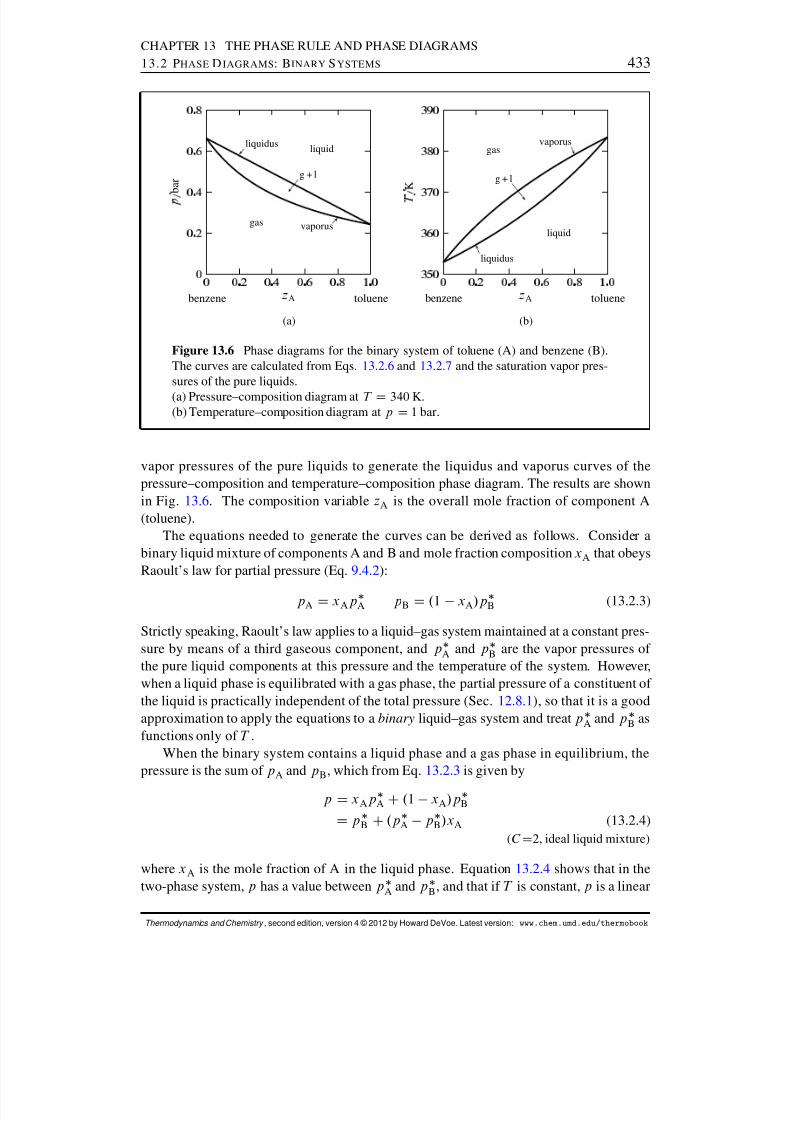
8/12/2019 Howard Devoe Thermodynamic and Chemical
http://slidepdf.com/reader/full/howard-devoe-thermodynamic-and-chemical 433/532
CHAPTER 13 THE PHASE RULE AND PHASE DIAGRAMS13.2 P HASE D IAGRAMS : BINARY S YSTEMS 433
g + l
liquidus
vaporus
liquid
gas
benzene A toluene
(a)
b a r g + l
liquidus
vaporusgas
liquid
benzene A toluene
(b)
K
Figure 13.6 Phase diagrams for the binary system of toluene (A) and benzene (B).The curves are calculated from Eqs. 13.2.6 and 13.2.7 and the saturation vapor pres-sures of the pure liquids.(a) Pressure–composition diagram at T D 340 K.(b) Temperature–composition diagram at p D 1 bar.
vapor pressures of the pure liquids to generate the liquidus and vaporus curves of thepressure–composition and temperature–composition phase diagram. The results are shownin Fig. 13.6 . The composition variable zA is the overall mole fraction of component A(toluene).
The equations needed to generate the curves can be derived as follows. Consider abinary liquid mixture of components A and B and mole fraction composition xA that obeysRaoult’s law for partial pressure (Eq. 9.4.2 ):
p A D xAp A p B D .1 xA /p B (13.2.3)
Strictly speaking, Raoult’s law applies to a liquid–gas system maintained at a constant pres-sure by means of a third gaseous component, and p A and p B are the vapor pressures of the pure liquid components at this pressure and the temperature of the system. However,when a liquid phase is equilibrated with a gas phase, the partial pressure of a constituent of the liquid is practically independent of the total pressure (Sec. 12.8.1 ), so that it is a goodapproximation to apply the equations to a binary liquid–gas system and treat p A and p B asfunctions only of T .
When the binary system contains a liquid phase and a gas phase in equilibrium, thepressure is the sum of p A and p B , which from Eq. 13.2.3 is given by
p D xAp A C.1 xA /p B
D p B C.p A p B /x A (13.2.4)(C D2, ideal liquid mixture)
where xA is the mole fraction of A in the liquid phase. Equation 13.2.4 shows that in thetwo-phase system, p has a value between p A and p B , and that if T is constant, p is a linear
Thermodynamics and Chemistry , second edition, version 4 © 2012 by Howard DeVoe. Latest version: www.chem.umd.edu/thermobook
8/12/2019 Howard Devoe Thermodynamic and Chemical
http://slidepdf.com/reader/full/howard-devoe-thermodynamic-and-chemical 434/532
CHAPTER 13 THE PHASE RULE AND PHASE DIAGRAMS13.2 P HASE D IAGRAMS : BINARY S YSTEMS 434
function of xA . The mole fraction composition of the gas in the two-phase system is givenby
yA D p A
p D xAp A
p B C.p A p B /x A(13.2.5)
A binary two-phase system has two degrees of freedom. At a given T and p , each phase
must have a xed composition. We can calculate the liquid composition by rearranging Eq.13.2.4 :
xA D p p B
p A p B(13.2.6)
(C D2, ideal liquid mixture)
The gas composition is then given by
yA D p A
p D xAp A
p
D
p p B
p A p B
p A
p
(13.2.7)
(C D2, ideal liquid mixture)
If we know p A and p B as functions of T , we can use Eqs. 13.2.6 and 13.2.7 to calculate thecompositions for any combination of T and p at which the liquid and gas phases can coexist,and thus construct a pressure–composition or temperature–composition phase diagram.
In Fig. 13.6 (a), the liquidus curve shows the relation between p and xA for equilibratedliquid and gas phases at constant T , and the vaporus curve shows the relation between pand yA under these conditions. We see that p is a linear function of xA but not of yA .
In a similar fashion, the liquidus curve in Fig. 13.6 (b) shows the relation between T andxA , and the vaporus curve shows the relation between T and yA , for equilibrated liquid andgas phases at constant p . Neither curve is linear.
A liquidus curve is also called a bubble-point
curve or a boiling-point
curve. Othernames for a vaporus curve are dew-point curve and condensation curve. These curves areactually cross-sections of liquidus and vaporus surfaces in a three-dimensional T –p –zAphase diagram, as shown in Fig. 13.7 on the next page . In this gure, the liquidus surface isin view at the front and the vaporus surface is hidden behind it.
13.2.5 Liquid–gas systems with nonideal liquid mixtures
Most binary liquid mixtures do not behave ideally. The most common situation is positivedeviations from Raoult’s law. 5 Some mixtures, however, have specic A–B interactions,such as solvation or molecular association, that prevent random mixing of the moleculesof A and B, and the result is then negative deviations from Raoult’s law. If the deviations
from Raoult’s law, either positive or negative, are large enough, the constant-temperatureliquidus curve exhibits a maximum or minimum and azeotropic behavior results.
Figure 13.8 on page 436 shows the azeotropic behavior of the binary methanol-benzenesystem at constant temperature. In Fig. 13.8 (a), the experimental partial pressures in a
5In the molecular model of Sec. 11.1.5 , positive deviations correspond to a less negative value of kAB than theaverage of kAA and kBB .
Thermodynamics and Chemistry , second edition, version 4 © 2012 by Howard DeVoe. Latest version: www.chem.umd.edu/thermobook

8/12/2019 Howard Devoe Thermodynamic and Chemical
http://slidepdf.com/reader/full/howard-devoe-thermodynamic-and-chemical 435/532
CHAPTER 13 THE PHASE RULE AND PHASE DIAGRAMS13.2 P HASE D IAGRAMS : BINARY S YSTEMS 435
K
b a r
benzene
Atoluene
Figure 13.7 Liquidus and vaporus surfaces for the binary system of toluene (A) andbenzene. Cross-sections through the two-phase region are drawn at constant temper-atures of 340 K and 370 K and at constant pressures of 1 bar and 2 bar. Two of thecross-sections intersect at a tie line at T D 370 K and p D 1 bar, and the other cross-sections are hatched in the direction of the tie lines.
gas phase equilibrated with the nonideal liquid mixture are plotted as a function of the
liquid composition. The partial pressures of both components exhibit positive deviationsfrom Raoult’s law, 6 and the total pressure (equal to the sum of the partial pressures) has amaximum value greater than the vapor pressure of either pure component. The curve of pversus xA becomes the liquidus curve of the pressure–composition phase diagram shown inFig. 13.8 (b). Points on the vaporus curve are calculated from p D p A=yA .
In practice, the data needed to generate the liquidus and vaporus curves of a nonidealbinary system are usually obtained by allowing liquid mixtures of various composi-tions to boil in an equilibrium still at a xed temperature or pressure. When the liquidand gas phases have become equilibrated, samples of each are withdrawn for analy-sis. The partial pressures shown in Fig. 13.8(a) were calculated from the experimentalgas-phase compositions with the relations p A
D yAp and p B
D p p A .
If the constant-temperature liquidus curve has a maximum pressure at a liquid composi-tion not corresponding to one of the pure components, which is the case for the methanol–
6This behavior is consistent with the statement in Sec. 12.8.2 that if one constituent of a binary liquid mixtureexhibits positive deviations from Raoult’s law, with only one inection point in the curve of fugacity versusmole fraction, the other constituent also has positive deviations from Raoult’s law.
Thermodynamics and Chemistry , second edition, version 4 © 2012 by Howard DeVoe. Latest version: www.chem.umd.edu/thermobook
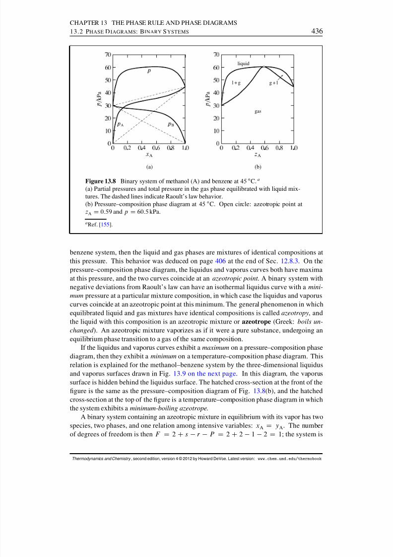
8/12/2019 Howard Devoe Thermodynamic and Chemical
http://slidepdf.com/reader/full/howard-devoe-thermodynamic-and-chemical 436/532
CHAPTER 13 THE PHASE RULE AND PHASE DIAGRAMS13.2 P HASE D IAGRAMS : BINARY S YSTEMS 436
A B
A
(a)
k P a
liquid
gas
l + g g + l
A
(b)
k P a
Figure 13.8 Binary system of methanol (A) and benzene at 45 ı C. a
(a) Partial pressures and total pressure in the gas phase equilibrated with liquid mix-tures. The dashed lines indicate Raoult’s law behavior.(b) Pressure–composition phase diagram at 45 ı C. Open circle: azeotropic point atzA D 0:59 and p D 60:5 kPa.
a Ref. [ 155 ].
benzene system, then the liquid and gas phases are mixtures of identical compositions atthis pressure. This behavior was deduced on page 406 at the end of Sec. 12.8.3 . On thepressure–composition phase diagram, the liquidus and vaporus curves both have maximaat this pressure, and the two curves coincide at an azeotropic point . A binary system withnegative deviations from Raoult’s law can have an isothermal liquidus curve with a mini-mum pressure at a particular mixture composition, in which case the liquidus and vaporuscurves coincide at an azeotropic point at this minimum. The general phenomenon in whichequilibrated liquid and gas mixtures have identical compositions is called azeotropy , andthe liquid with this composition is an azeotropic mixture or azeotrope (Greek: boils un-changed ). An azeotropic mixture vaporizes as if it were a pure substance, undergoing anequilibrium phase transition to a gas of the same composition.
If the liquidus and vaporus curves exhibit a maximum on a pressure–composition phasediagram, then they exhibit a minimum on a temperature–composition phase diagram. Thisrelation is explained for the methanol–benzene system by the three-dimensional liquidusand vaporus surfaces drawn in Fig. 13.9 on the next page . In this diagram, the vaporussurface is hidden behind the liquidus surface. The hatched cross-section at the front of the
gure is the same as the pressure–composition diagram of Fig. 13.8 (b), and the hatchedcross-section at the top of the gure is a temperature–composition phase diagram in whichthe system exhibits a minimum-boiling azeotrope .
A binary system containing an azeotropic mixture in equilibrium with its vapor has twospecies, two phases, and one relation among intensive variables: xA D yA . The numberof degrees of freedom is then F D 2 Cs r P D 2 C2 1 2 D 1; the system is
Thermodynamics and Chemistry , second edition, version 4 © 2012 by Howard DeVoe. Latest version: www.chem.umd.edu/thermobook
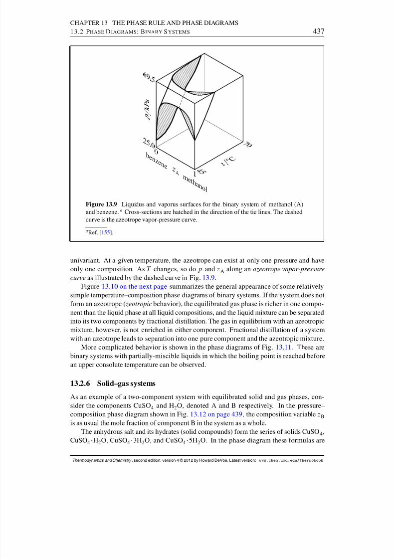
8/12/2019 Howard Devoe Thermodynamic and Chemical
http://slidepdf.com/reader/full/howard-devoe-thermodynamic-and-chemical 437/532
CHAPTER 13 THE PHASE RULE AND PHASE DIAGRAMS13.2 P HASE D IAGRAMS : BINARY S YSTEMS 437
Æ
C
k P a
benzene
Amethanol
Figure 13.9 Liquidus and vaporus surfaces for the binary system of methanol (A)and benzene. a Cross-sections are hatched in the direction of the tie lines. The dashedcurve is the azeotrope vapor-pressure curve.
a Ref. [ 155 ].
univariant. At a given temperature, the azeotrope can exist at only one pressure and haveonly one composition. As T changes, so do p and zA along an azeotrope vapor-pressurecurve as illustrated by the dashed curve in Fig. 13.9 .
Figure 13.10 on the next page summarizes the general appearance of some relativelysimple temperature–composition phase diagrams of binary systems. If the system does notform an azeotrope ( zeotropic behavior), the equilibrated gas phase is richer in one compo-nent than the liquid phase at all liquid compositions, and the liquid mixture can be separatedinto its two components by fractional distillation. The gas in equilibrium with an azeotropicmixture, however, is not enriched in either component. Fractional distillation of a systemwith an azeotrope leads to separation into one pure component and the azeotropic mixture.
More complicated behavior is shown in the phase diagrams of Fig. 13.11 . These arebinary systems with partially-miscible liquids in which the boiling point is reached beforean upper consolute temperature can be observed.
13.2.6 Solid–gas systems
As an example of a two-component system with equilibrated solid and gas phases, con-sider the components CuSO 4 and H 2O, denoted A and B respectively. In the pressure–composition phase diagram shown in Fig. 13.12 on page 439 , the composition variable zBis as usual the mole fraction of component B in the system as a whole.
The anhydrous salt and its hydrates (solid compounds) form the series of solids CuSO 4 ,CuSO 4 H2O, CuSO 4 3H 2O, and CuSO 4 5H 2O. In the phase diagram these formulas are
Thermodynamics and Chemistry , second edition, version 4 © 2012 by Howard DeVoe. Latest version: www.chem.umd.edu/thermobook
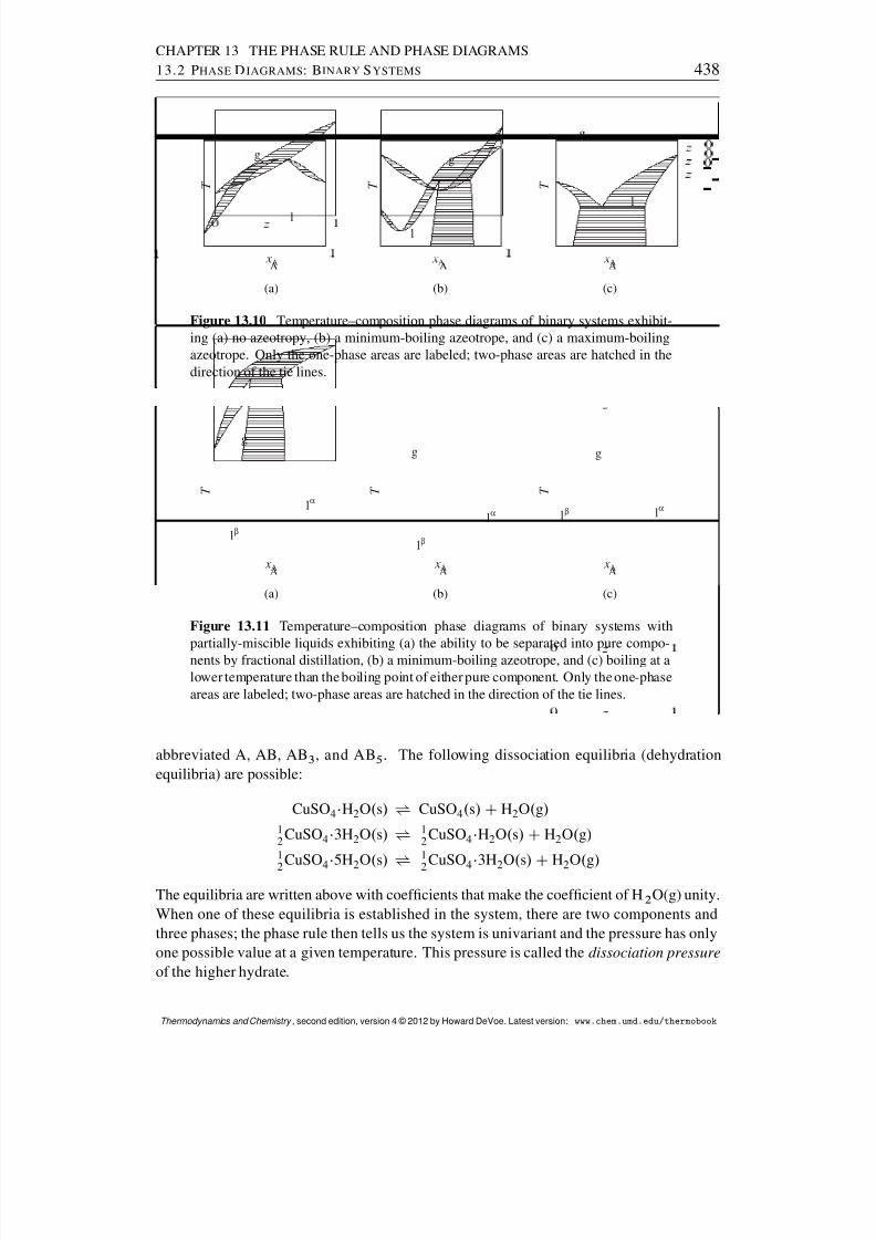
8/12/2019 Howard Devoe Thermodynamic and Chemical
http://slidepdf.com/reader/full/howard-devoe-thermodynamic-and-chemical 438/532
CHAPTER 13 THE PHASE RULE AND PHASE DIAGRAMS13.2 P HASE D IAGRAMS : BINARY S YSTEMS 438
x A
T
g
l
A
(a)
x A
T
g
l
A
(b)
x A
T
g
l
A
(c)
Figure 13.10 Temperature–composition phase diagrams of binary systems exhibit-ing (a) no azeotropy, (b) a minimum-boiling azeotrope, and (c) a maximum-boilingazeotrope. Only the one-phase areas are labeled; two-phase areas are hatched in thedirection of the tie lines.
x A
T
g
l
l
β
α
A
(a)
x A
T
g
l
l
β
α
A
(b)
x A
T
g
l lβ α
A
(c)
Figure 13.11 Temperature–composition phase diagrams of binary systems withpartially-miscible liquids exhibiting (a) the ability to be separated into pure compo-nents by fractional distillation, (b) a minimum-boiling azeotrope, and (c) boiling at alower temperature than the boiling point of either pure component. Only the one-phaseareas are labeled; two-phase areas are hatched in the direction of the tie lines.
abbreviated A, AB, AB 3 , and AB 5 . The following dissociation equilibria (dehydrationequilibria) are possible:
CuSO 4 H2O. s/ • CuSO 4 . s/ CH2O. g/12 CuSO 4 3H 2O. s/ • 1
2 CuSO 4 H2O. s/ CH2O. g/1
2CuSO
45H
2O. s/
• 1
2CuSO
43H
2O. s/
CH
2O. g/
The equilibria are written above with coefcients that make the coefcient of H 2 O(g) unity.When one of these equilibria is established in the system, there are two components andthree phases; the phase rule then tells us the system is univariant and the pressure has onlyone possible value at a given temperature. This pressure is called the dissociation pressureof the higher hydrate.
Thermodynamics and Chemistry , second edition, version 4 © 2012 by Howard DeVoe. Latest version: www.chem.umd.edu/thermobook
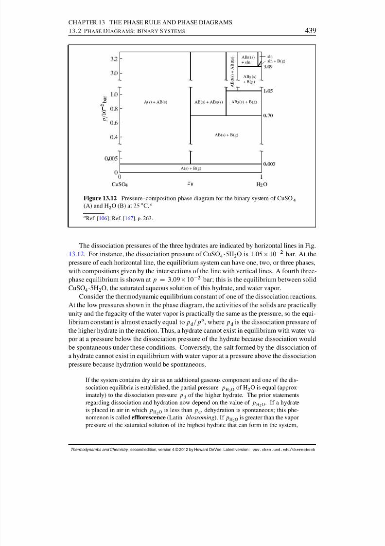
8/12/2019 Howard Devoe Thermodynamic and Chemical
http://slidepdf.com/reader/full/howard-devoe-thermodynamic-and-chemical 439/532
CHAPTER 13 THE PHASE RULE AND PHASE DIAGRAMS13.2 P HASE D IAGRAMS : BINARY S YSTEMS 439
b a r
CuSO
B H
O
A(s) + B(g)
AB(s) + B(g)
A(s) + AB(s)
AB
(s) + B(g)AB(s) + AB
(s)
AB
(s)+ B(g)
A B
( s ) + A B
( s ) AB
(s)+ sln
slnsln + B(g)
Figure 13.12 Pressure–composition phase diagram for the binary system of CuSO 4(A) and H 2 O (B) at 25 ı C. a
a Ref. [ 106 ]; Ref. [ 167 ], p. 263.
The dissociation pressures of the three hydrates are indicated by horizontal lines in Fig.13.12 . For instance, the dissociation pressure of CuSO 4 5H 2O is 1:05 10 2 bar. At thepressure of each horizontal line, the equilibrium system can have one, two, or three phases,with compositions given by the intersections of the line with vertical lines. A fourth three-phase equilibrium is shown at p
D 3:09 10 2 bar; this is the equilibrium between solid
CuSO 4 5H 2O, the saturated aqueous solution of this hydrate, and water vapor.Consider the thermodynamic equilibrium constant of one of the dissociation reactions.
At the low pressures shown in the phase diagram, the activities of the solids are practicallyunity and the fugacity of the water vapor is practically the same as the pressure, so the equi-librium constant is almost exactly equal to p d=p ı , where p d is the dissociation pressure of the higher hydrate in the reaction. Thus, a hydrate cannot exist in equilibrium with water va-por at a pressure below the dissociation pressure of the hydrate because dissociation wouldbe spontaneous under these conditions. Conversely, the salt formed by the dissociation of a hydrate cannot exist in equilibrium with water vapor at a pressure above the dissociationpressure because hydration would be spontaneous.
If the system contains dry air as an additional gaseous component and one of the dis-sociation equilibria is established, the partial pressure p H2 O of H2 O is equal (approx-imately) to the dissociation pressure p d of the higher hydrate. The prior statementsregarding dissociation and hydration now depend on the value of p H2 O . If a hydrateis placed in air in which p H2 O is less than p d , dehydration is spontaneous; this phe-nomenon is called eforescence (Latin: blossoming ). If p H2 O is greater than the vaporpressure of the saturated solution of the highest hydrate that can form in the system,
Thermodynamics and Chemistry , second edition, version 4 © 2012 by Howard DeVoe. Latest version: www.chem.umd.edu/thermobook
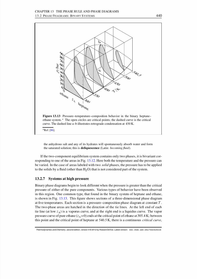
8/12/2019 Howard Devoe Thermodynamic and Chemical
http://slidepdf.com/reader/full/howard-devoe-thermodynamic-and-chemical 440/532
CHAPTER 13 THE PHASE RULE AND PHASE DIAGRAMS13.2 P HASE D IAGRAMS : BINARY S YSTEMS 440
K
a
b
ethane
Aheptane
b a r
Figure 13.13 Pressure–temperature–composition behavior in the binary heptane–ethane system. a The open circles are critical points; the dashed curve is the criticalcurve. The dashed line a–b illustrates retrograde condensation at 450 K.
a Ref. [ 86].
the anhydrous salt and any of its hydrates will spontaneously absorb water and formthe saturated solution; this is deliquescence (Latin: becoming uid ).
If the two-component equilibrium system contains only two phases, it is bivariant cor-responding to one of the areas in Fig. 13.12 . Here both the temperature and the pressure canbe varied. In the case of areas labeled with two solid phases, the pressure has to be appliedto the solids by a uid (other than H 2 O) that is not considered part of the system.
13.2.7 Systems at high pressure
Binary phase diagrams begin to look different when the pressure is greater than the criticalpressure of either of the pure components. Various types of behavior have been observed
in this region. One common type, that found in the binary system of heptane and ethane,is shown in Fig. 13.13 . This gure shows sections of a three-dimensional phase diagramat ve temperatures. Each section is a pressure–composition phase diagram at constant T .The two-phase areas are hatched in the direction of the tie lines. At the left end of eachtie line (at low zA) is a vaporus curve, and at the right end is a liquidus curve. The vaporpressure curve of pure ethane ( zAD0) ends at the critical point of ethane at 305:4 K; betweenthis point and the critical point of heptane at 540:5 K, there is a continuous critical curve ,
Thermodynamics and Chemistry , second edition, version 4 © 2012 by Howard DeVoe. Latest version: www.chem.umd.edu/thermobook

8/12/2019 Howard Devoe Thermodynamic and Chemical
http://slidepdf.com/reader/full/howard-devoe-thermodynamic-and-chemical 441/532
CHAPTER 13 THE PHASE RULE AND PHASE DIAGRAMS13.2 P HASE D IAGRAMS : BINARY S YSTEMS 441
K
He
AXe
b a r
Figure 13.14 Pressure–temperature–composition behavior in the binary xenon–helium system. a The open circles are critical points; the dashed curve is the criticalcurve.a Ref. [ 42].
which is the locus of critical points at which gas and liquid mixtures become identical incomposition and density.
Consider what happens when the system point is at point a in Fig. 13.13 and the pressureis then increased by isothermal compression along line a–b. The system point moves fromthe area for a gas phase into the two-phase gas–liquid area and then out into the gas-phasearea again. This curious phenomenon, condensation followed by vaporization, is calledretrograde condensation .
Under some conditions, an isobaric increase of T can result in vaporization followed bycondensation; this is retrograde vaporization .
A different type of high-pressure behavior, that found in the xenon–helium system, isshown in Fig. 13.14 . Here, the critical curve begins at the critical point of the less volatilecomponent (xenon) and continues to higher temperatures and pressures than the criticaltemperature and pressure of either pure component. The two-phase region at pressuresabove this critical curve is sometimes said to represent gas–gas equilibrium , or gas–gasimmiscibility , because we would not usually consider a liquid to exist beyond the criticalpoints of the pure components. Of course, the coexisting phases in this two-phase regionare not gases in the ordinary sense of being tenuous uids, but are instead high-pressureuids of liquid-like densities. If we want to call both phases gases, then we have to saythat pure gaseous substances at high pressure do not necessarily mix spontaneously in allproportions as they do at ordinary pressures.
Thermodynamics and Chemistry , second edition, version 4 © 2012 by Howard DeVoe. Latest version: www.chem.umd.edu/thermobook
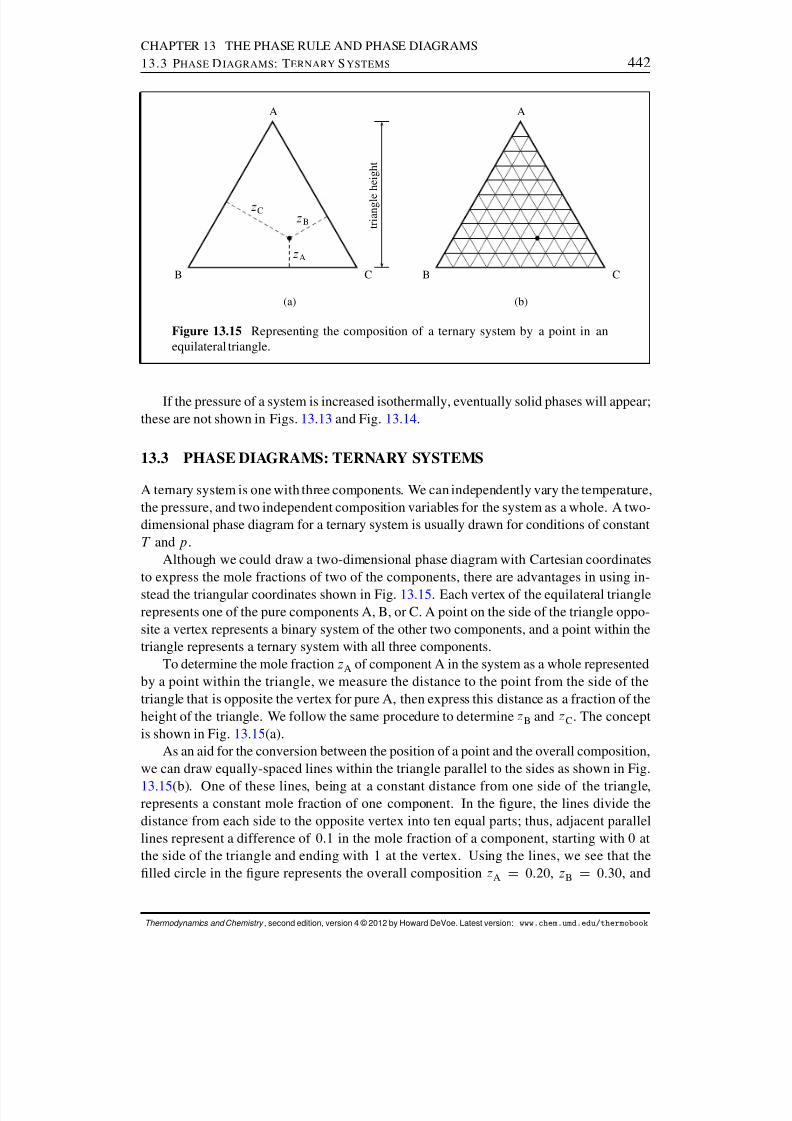
8/12/2019 Howard Devoe Thermodynamic and Chemical
http://slidepdf.com/reader/full/howard-devoe-thermodynamic-and-chemical 442/532
CHAPTER 13 THE PHASE RULE AND PHASE DIAGRAMS13.3 P HASE D IAGRAMS : TERNARY S YSTEMS 442
(a)
A
B
C
A
B C
t r i a
n g
l e
h e
i g h t
(b)
A
B C
Figure 13.15 Representing the composition of a ternary system by a point in anequilateral triangle.
If the pressure of a system is increased isothermally, eventually solid phases will appear;these are not shown in Figs. 13.13 and Fig. 13.14 .
13.3 PHASE DIAGRAMS: TERNARY SYSTEMS
A ternary system is one with three components. We can independently vary the temperature,the pressure, and two independent composition variables for the system as a whole. A two-dimensional phase diagram for a ternary system is usually drawn for conditions of constantT and p .
Although we could draw a two-dimensional phase diagram with Cartesian coordinatesto express the mole fractions of two of the components, there are advantages in using in-stead the triangular coordinates shown in Fig. 13.15 . Each vertex of the equilateral trianglerepresents one of the pure components A, B, or C. A point on the side of the triangle oppo-site a vertex represents a binary system of the other two components, and a point within thetriangle represents a ternary system with all three components.
To determine the mole fraction zA of component A in the system as a whole representedby a point within the triangle, we measure the distance to the point from the side of thetriangle that is opposite the vertex for pure A, then express this distance as a fraction of theheight of the triangle. We follow the same procedure to determine zB and zC . The conceptis shown in Fig. 13.15 (a).
As an aid for the conversion between the position of a point and the overall composition,we can draw equally-spaced lines within the triangle parallel to the sides as shown in Fig.
13.15 (b). One of these lines, being at a constant distance from one side of the triangle,represents a constant mole fraction of one component. In the gure, the lines divide thedistance from each side to the opposite vertex into ten equal parts; thus, adjacent parallellines represent a difference of 0:1 in the mole fraction of a component, starting with 0 atthe side of the triangle and ending with 1 at the vertex. Using the lines, we see that thelled circle in the gure represents the overall composition zA D 0:20, zB D 0:30, and
Thermodynamics and Chemistry , second edition, version 4 © 2012 by Howard DeVoe. Latest version: www.chem.umd.edu/thermobook
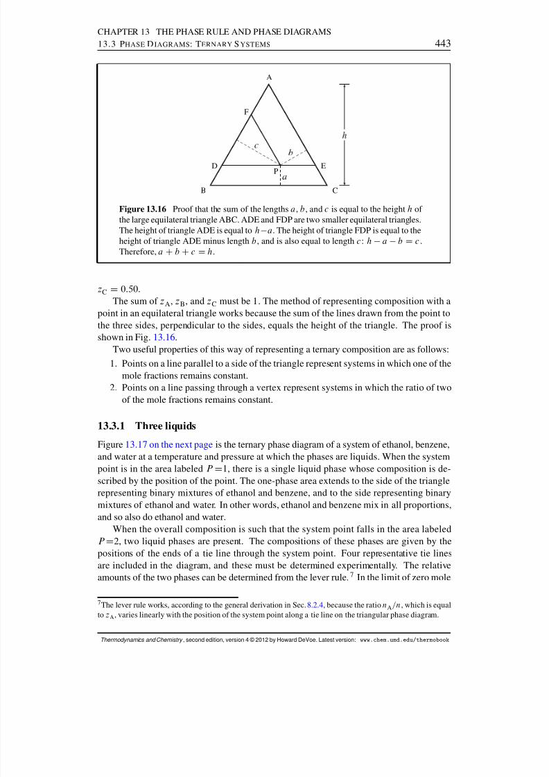
8/12/2019 Howard Devoe Thermodynamic and Chemical
http://slidepdf.com/reader/full/howard-devoe-thermodynamic-and-chemical 443/532
CHAPTER 13 THE PHASE RULE AND PHASE DIAGRAMS13.3 P HASE D IAGRAMS : TERNARY S YSTEMS 443
A
B C
D E
F
P
Figure 13.16 Proof that the sum of the lengths a , b , and c is equal to the height h of the large equilateral triangle ABC. ADE and FDP are two smaller equilateral triangles.The height of triangle ADE is equal to h a . The height of triangle FDP is equal to theheight of triangle ADE minus length b , and is also equal to length c: h a b D c .Therefore, a Cb Cc D h .
zC D 0:50.The sum of zA , zB , and zC must be 1. The method of representing composition with a
point in an equilateral triangle works because the sum of the lines drawn from the point tothe three sides, perpendicular to the sides, equals the height of the triangle. The proof isshown in Fig. 13.16 .
Two useful properties of this way of representing a ternary composition are as follows:1. Points on a line parallel to a side of the triangle represent systems in which one of the
mole fractions remains constant.2. Points on a line passing through a vertex represent systems in which the ratio of two
of the mole fractions remains constant.
13.3.1 Three liquids
Figure 13.17 on the next page is the ternary phase diagram of a system of ethanol, benzene,and water at a temperature and pressure at which the phases are liquids. When the systempoint is in the area labeled P D1, there is a single liquid phase whose composition is de-scribed by the position of the point. The one-phase area extends to the side of the trianglerepresenting binary mixtures of ethanol and benzene, and to the side representing binarymixtures of ethanol and water. In other words, ethanol and benzene mix in all proportions,and so also do ethanol and water.
When the overall composition is such that the system point falls in the area labeled
P D2, two liquid phases are present. The compositions of these phases are given by thepositions of the ends of a tie line through the system point. Four representative tie linesare included in the diagram, and these must be determined experimentally. The relativeamounts of the two phases can be determined from the lever rule. 7 In the limit of zero mole
7The lever rule works, according to the general derivation in Sec. 8.2.4 , because the ratio nA =n , which is equalto zA , varies linearly with the position of the system point along a tie line on the triangular phase diagram.
Thermodynamics and Chemistry , second edition, version 4 © 2012 by Howard DeVoe. Latest version: www.chem.umd.edu/thermobook
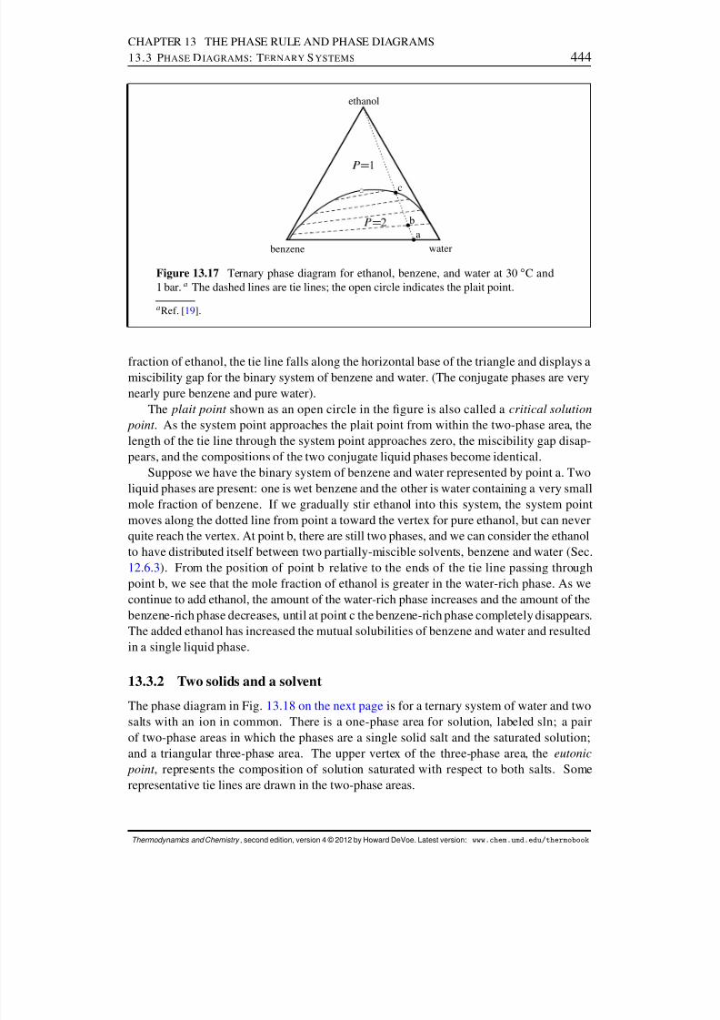
8/12/2019 Howard Devoe Thermodynamic and Chemical
http://slidepdf.com/reader/full/howard-devoe-thermodynamic-and-chemical 444/532
CHAPTER 13 THE PHASE RULE AND PHASE DIAGRAMS13.3 P HASE D IAGRAMS : TERNARY S YSTEMS 444
a
b
c
ethanol
benzene water
Figure 13.17 Ternary phase diagram for ethanol, benzene, and water at 30 ı C and1 bar. a The dashed lines are tie lines; the open circle indicates the plait point.
a Ref. [ 19].
fraction of ethanol, the tie line falls along the horizontal base of the triangle and displays amiscibility gap for the binary system of benzene and water. (The conjugate phases are verynearly pure benzene and pure water).
The plait point shown as an open circle in the gure is also called a critical solution point . As the system point approaches the plait point from within the two-phase area, thelength of the tie line through the system point approaches zero, the miscibility gap disap-pears, and the compositions of the two conjugate liquid phases become identical.
Suppose we have the binary system of benzene and water represented by point a. Twoliquid phases are present: one is wet benzene and the other is water containing a very smallmole fraction of benzene. If we gradually stir ethanol into this system, the system pointmoves along the dotted line from point a toward the vertex for pure ethanol, but can never
quite reach the vertex. At point b, there are still two phases, and we can consider the ethanolto have distributed itself between two partially-miscible solvents, benzene and water (Sec.12.6.3 ). From the position of point b relative to the ends of the tie line passing throughpoint b, we see that the mole fraction of ethanol is greater in the water-rich phase. As wecontinue to add ethanol, the amount of the water-rich phase increases and the amount of thebenzene-rich phase decreases, until at point c the benzene-rich phase completely disappears.The added ethanol has increased the mutual solubilities of benzene and water and resultedin a single liquid phase.
13.3.2 Two solids and a solvent
The phase diagram in Fig. 13.18 on the next page is for a ternary system of water and twosalts with an ion in common. There is a one-phase area for solution, labeled sln; a pairof two-phase areas in which the phases are a single solid salt and the saturated solution;and a triangular three-phase area. The upper vertex of the three-phase area, the eutonic point , represents the composition of solution saturated with respect to both salts. Somerepresentative tie lines are drawn in the two-phase areas.
Thermodynamics and Chemistry , second edition, version 4 © 2012 by Howard DeVoe. Latest version: www.chem.umd.edu/thermobook
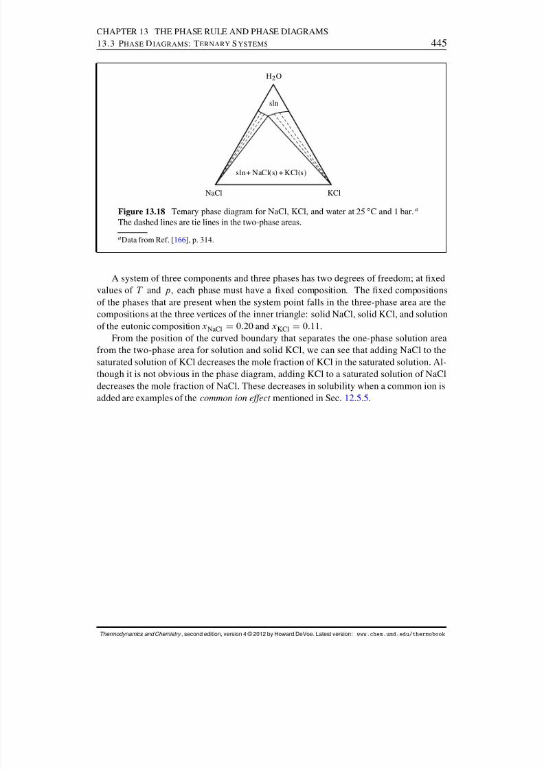
8/12/2019 Howard Devoe Thermodynamic and Chemical
http://slidepdf.com/reader/full/howard-devoe-thermodynamic-and-chemical 445/532
CHAPTER 13 THE PHASE RULE AND PHASE DIAGRAMS13.3 P HASE D IAGRAMS : TERNARY S YSTEMS 445
sln
sln+ NaCl(s) + KCl(s)
H 2 O
NaCl KCl
Figure 13.18 Ternary phase diagram for NaCl, KCl, and water at 25 ı C and 1 bar. a
The dashed lines are tie lines in the two-phase areas.
a Data from Ref. [ 166 ], p. 314.
A system of three components and three phases has two degrees of freedom; at xedvalues of T and p , each phase must have a xed composition. The xed compositionsof the phases that are present when the system point falls in the three-phase area are thecompositions at the three vertices of the inner triangle: solid NaCl, solid KCl, and solutionof the eutonic composition xNaCl D 0:20 and xKCl D 0:11 .
From the position of the curved boundary that separates the one-phase solution areafrom the two-phase area for solution and solid KCl, we can see that adding NaCl to thesaturated solution of KCl decreases the mole fraction of KCl in the saturated solution. Al-though it is not obvious in the phase diagram, adding KCl to a saturated solution of NaCldecreases the mole fraction of NaCl. These decreases in solubility when a common ion isadded are examples of the common ion effect mentioned in Sec. 12.5.5 .
Thermodynamics and Chemistry , second edition, version 4 © 2012 by Howard DeVoe. Latest version: www.chem.umd.edu/thermobook
8/12/2019 Howard Devoe Thermodynamic and Chemical
http://slidepdf.com/reader/full/howard-devoe-thermodynamic-and-chemical 446/532
CHAPTER 13 THE PHASE RULE AND PHASE DIAGRAMSPROBLEMS 446
PROBLEMS
An underlined problem number or problem-part letter indicates that the numerical answer appearsin Appendix I.
13.1 Consider a single-phase system that is a gaseous mixture of N 2 , H2 , and NH 3 . For eachof the following cases, nd the number of degrees of freedom and give an example of theindependent intensive variables that could be used to specify the equilibrium state, apart fromthe total amount of gas.
(a) There is no reaction.
(b) The reaction N 2 . g/ C3 H 2 . g/ ! 2 NH 3 . g/ is at equilibrium.
(c) The reaction is at equilibrium and the system is prepared from NH 3 only.
13.2 How many components has a mixture of water and deuterium oxide in which the equilibriumH2O CD2O • 2 HDO exists?
13.3 Consider a system containing only NH 4 Cl(s), NH 3 (g), and HCl(g). Assume that the equilib-rium NH 4Cl . s/ • NH3 . g/ CHCl . g/ exists.
(a) Suppose you prepare the system by placing solid NH4Cl in an evacuated ask and heating
to 400 K. Use the phase rule to decide whether you can vary the pressure while bothphases remain in equilibrium at 400 K.
(b) According to the phase rule, if the system is not prepared as described in part (a) couldyou vary the pressure while both phases remain in equilibrium at 400 K? Explain.
(c) Rationalize your conclusions for these two cases on the basis of the thermodynamic equi-librium constant. Assume that the gas phase is an ideal gas mixture and use the approxi-mate expression K D p NH 3
p HCl =.p ı / 2 .
13.4 Consider the lime-kiln process CaCO 3 . s/ ! CaO . s/ C CO 2 . g/ . Find the number of inten-sive variables that can be varied independently in the equilibrium system under the followingconditions:
(a) The system is prepared by placing calcium carbonate, calcium oxide, and carbon dioxidein a container.
(b) The system is prepared from calcium carbonate only.
(c) The temperature is xed at 1000 K.
13.5 What are the values of C and F in systems consisting of solid AgCl in equilibrium with anaqueous phase containing H 2 O, Ag C (aq), Cl (aq), Na C (aq), and NO 3 (aq) prepared in thefollowing ways? Give examples of intensive variables that could be varied independently.
(a) The system is prepared by equilibrating excess solid AgCl with an aqueous solution of NaNO 3 .
(b) The system is prepared by mixing aqueous solutions of AgNO 3 and NaCl in arbitraryproportions; some solid AgCl forms by precipitation.
13.6 How many degrees of freedom has a system consisting of solid NaCl in equilibrium withan aqueous phase containing H 2 O, Na C (aq), Cl (aq), H C (aq), and OH (aq)? Would it bepossible to independently vary T , p , and mOH ? If so, explain how you could do this.
13.7 Consult the phase diagram shown in Fig. 13.4 on page 431 . Suppose the system contains 36:0 g(2:00 mol) H 2 O and 58:4 g (1:00 mol) NaCl at 25 ı C and 1 bar.
Thermodynamics and Chemistry , second edition, version 4 © 2012 by Howard DeVoe. Latest version: www.chem.umd.edu/thermobook
8/12/2019 Howard Devoe Thermodynamic and Chemical
http://slidepdf.com/reader/full/howard-devoe-thermodynamic-and-chemical 447/532
CHAPTER 13 THE PHASE RULE AND PHASE DIAGRAMSPROBLEMS 447
(a) Describe the phases present in the equilibrium system and their masses.
(b) Describe the changes that occur at constant pressure if the system is placed in thermalcontact with a heat reservoir at 30 ı C.
(c) Describe the changes that occur if the temperature is raised from 25 ı C to 120 ı C at con-stant pressure.
(d) Describe the system after 200 g H 2 O is added at 25 ı C.
Table 13.1 Aqueous solubilities of sodium sulfate decahydrate and anhy-drous sodium sulfate a
Na 2SO 4 10H 2O Na 2SO 4
t=ı C xB t=ı C xB
10 0:011 40 0:05815 0:016 50 0:05620 0:02425 0:03430 0:048
a Ref. [ 55], p. 179–180.
13.8 Use the following information to draw a temperature–composition phase diagram for the binarysystem of H 2 O (A) and Na 2 SO 4 (B) at p D 1 bar, conning t to the range 20 to 50 ı C andzB to the range 0–0:2. The solid decahydrate, Na 2SO 4 10H 2O, is stable below 32:4 ı C. Theanhydrous salt, Na 2SO 4 , is stable above this temperature. There is a peritectic point for thesetwo solids and the solution at xB D 0:059 and t D 32:4 ı C. There is a eutectic point forice, Na 2SO 4 10H 2O, and the solution at xB D 0:006 and t D 1:3 ı C. Table 13.1 gives thetemperature dependence of the solubilities of the ionic solids.
13.9 Iron(III) chloride forms various solid hydrates, all of which melt congruently. Table 13.2 onthe next page lists the temperatures t of aqueous solutions of various compositions that aresaturated with respect to a solid phase.
(a) Use these data to construct a t –zB phase diagram for the binary system of FeCl 3 (A) andH2O (B). Identify the formula and melting point of each hydrate. Hint: derive a formulafor the mole ratio nB=n A as a function of xA in a binary mixture.
(b) For the following conditions, determine the phase or phases present at equilibrium andthe composition of each.
1. t D 70:0 ı C and zA D 0:1002. t D 50:0 ı C and zA D 0:275
13.10 Figure 13.19 on the next page is a temperature–composition phase diagram for the binarysystem of water (A) and phenol (B) at 1 bar. These liquids are partially miscible below 67 ı C.Phenol is more dense than water, so the layer with the higher mole fraction of phenol is thebottom layer. Suppose you place 4 :0 mol of H 2 O and 1:0 mol of phenol in a beaker at 30 ı Cand gently stir to allow the layers to equilibrate.
(a) What are the compositions of the equilibrated top and bottom layers?
(b) Find the amount of each component in the bottom layer.
Thermodynamics and Chemistry , second edition, version 4 © 2012 by Howard DeVoe. Latest version: www.chem.umd.edu/thermobook

8/12/2019 Howard Devoe Thermodynamic and Chemical
http://slidepdf.com/reader/full/howard-devoe-thermodynamic-and-chemical 448/532
CHAPTER 13 THE PHASE RULE AND PHASE DIAGRAMSPROBLEMS 448
Table 13.2 Data for Problem 13. 9. Temperatures of saturated solutions of aqueous iron(III) chloride at p D1 bar (A = FeCl 3 , B = H2O) a
xA t=ı C xA t=ı C xA t=ı C
0.000 0.0 0.119 35.0 0.286 56.00.020 10:0 0.143 37.0 0.289 55.00.032 20:5 0.157 36.0 0.293 60.00.037 27:5 0.173 33.0 0.301 69.00.045 40:0 0.183 30.0 0.318 72.50.052 55:0 0.195 27.4 0.333 73.50.053 41:0 0.213 32.0 0.343 72.50.056 27:0 0.222 32.5 0.358 70.00.076 0.0 0.232 30.0 0.369 66.00.083 10.0 0.238 35.0 0.369 80.00.093 20.0 0.259 50.0 0.373 100.00.106 30.0 0.277 55.0
a Data from Ref. [ 55], page 193.
B
Æ
C
Figure 13.19 Temperature–composition phase diagram for the binary system of wa-ter (A) and phenol (B) at 1 bar. a Only liquid phases are present.
a Ref. [ 55], p. 95.
(c) As you gradually stir more phenol into the beaker, maintaining the temperature at 30 ı C,what changes occur in the volumes and compositions of the two layers? Assuming thatone layer eventually disappears, what additional amount of phenol is needed to cause thisto happen?
13.11 The standard boiling point of propane is 41:8 ı C and that of n-butane is 0:2 ı C. Table 13.3on the next page lists vapor pressure data for the pure liquids. Assume that the liquid mixturesobey Raoult’s law.
(a) Calculate the compositions, x A , of the liquid mixtures with boiling points of 10:0 ı C,20:0 ı C, and 30:0 ı C at a pressure of 1 bar.
(b) Calculate the compositions, yA , of the equilibrium vapor at these three temperatures.
Thermodynamics and Chemistry , second edition, version 4 © 2012 by Howard DeVoe. Latest version: www.chem.umd.edu/thermobook
8/12/2019 Howard Devoe Thermodynamic and Chemical
http://slidepdf.com/reader/full/howard-devoe-thermodynamic-and-chemical 449/532
CHAPTER 13 THE PHASE RULE AND PHASE DIAGRAMSPROBLEMS 449
Table 13.3 Saturation vapor pressuresof propane (A) and n-butane (B)
t=ı C p A=bar p B =bar
10:0 3:360 0:67820:0 2:380 0:44130:0 1:633 0:275
(c) Plot the temperature–composition phase diagram at p D 1 bar using these data, and labelthe areas appropriately.
(d) Suppose a system containing 10:0 mol propane and 10:0 mol n-butane is brought to apressure of 1 bar and a temperature of 25 ı C. From your phase diagram, estimate thecompositions and amounts of both phases.
Table 13.4 Liquid and gas compositions in the two-phasesystem of 2-propanol (A) and benzene at 45 ı C a
xA yA p= kPa xA yA p= kPa0 0 29:89 0:5504 0:3692 35:320:0472 0:1467 33:66 0:6198 0:3951 34:580:0980 0:2066 35:21 0:7096 0:4378 33:020:2047 0:2663 36:27 0:8073 0:5107 30:280:2960 0:2953 36:45 0:9120 0:6658 25:240:3862 0:3211 36:29 0:9655 0:8252 21:300:4753 0:3463 35:93 1:0000 1:0000 18:14
a Ref. [ 24].
13.12 Use the data in Table 13.4 to draw a pressure–composition phase diagram for the 2-propanol–benzene system at 45 ı C. Label the axes and each area.
Table 13.5 Liquid and gas compositions in the two-phase system of acetone (A) and chloroform at 35:2 ı Ca
xA yA p= kPa xA yA p=kPa
0 0 39:08 0:634 0:727 36:290:083 0:046 37:34 0:703 0:806 38:090:200 0:143 34:92 0:815 0:896 40:970:337 0:317 33:22 0:877 0:936 42:620:413 0:437 33:12 0:941 0:972 44:32
0:486 0:534 33:70 1:000 1:000 45:930:577 0:662 35:09
a Ref. [ 165 ], p. 286.
13.13 Use the data in Table 13.5 to draw a pressure–composition phase diagram for the acetone–chloroform system at 35:2 ı C. Label the axes and each area.
Thermodynamics and Chemistry , second edition, version 4 © 2012 by Howard DeVoe. Latest version: www.chem.umd.edu/thermobook
8/12/2019 Howard Devoe Thermodynamic and Chemical
http://slidepdf.com/reader/full/howard-devoe-thermodynamic-and-chemical 450/532
C HAPTER 14
G ALVANIC CELLS
An electrochemical cell is a system in which passage of an electric current through anelectrical circuit is linked to an internal cell reaction. A galvanic cell , or voltaic cell, isan electrochemical cell that, when isolated, has an electric potential difference between itsterminals; the cell is said to be a seat of electromotive force .
The cell reaction in a galvanic cell differs in a fundamental way from the same reaction(i.e., one with the same reaction equation) taking place in a reaction vessel that is not part of an electrical circuit. In the reaction vessel, the reactants and products are in the same phaseor in phases in contact with one another, and the reaction advances in the spontaneousdirection until reaction equilibrium is reached. This reaction is the direct reaction .
The galvanic cell, in contrast, is arranged with the reactants physically separated fromone another so that the cell reaction can advance only when an electric current passesthrough the cell. If there is no current, the cell reaction is constrained from taking place.When the electrical circuit is open and the cell is isolated from its surroundings, a state of thermal, mechanical, and transfer equilibrium is rapidly reached. In this state of cell equi-librium or electrochemical equilibrium , however, reaction equilibrium is not necessarilypresent—that is, if the reactants and products were moved to a reaction vessel at the sameactivities, there might be spontaneous advancement of the reaction.
As will be shown, measurements of the cell potential of a galvanic cell are capable of yielding precise values of molar reaction quantities of the cell reaction and thermodynamicequilibrium constants, and of mean ionic activity coefcients in electrolyte solutions.
14.1 CELL DIAGRAMS AND CELL REACTIONS
14.1.1 Elements of a galvanic cell
We will treat a galvanic cell as a system . The cell has two metal wires called terminals that
pass through the system boundary. Within the cell are phases that can conduct an electriccurrent and are collectively called electrical conductors . Each terminal is attached to anelectron conductor that is usually a metal, but might also be graphite or a semiconductor.Each electron conductor is in contact with an ionic conductor , usually an electrolyte solu-tion, through which ions but not electrons can move. Both of the electron conductors canbe in contact with the same ionic conductor; or they can be in contact with separate ionicconductors, in which case the ionic conductors contact one another at a liquid junction . The
450
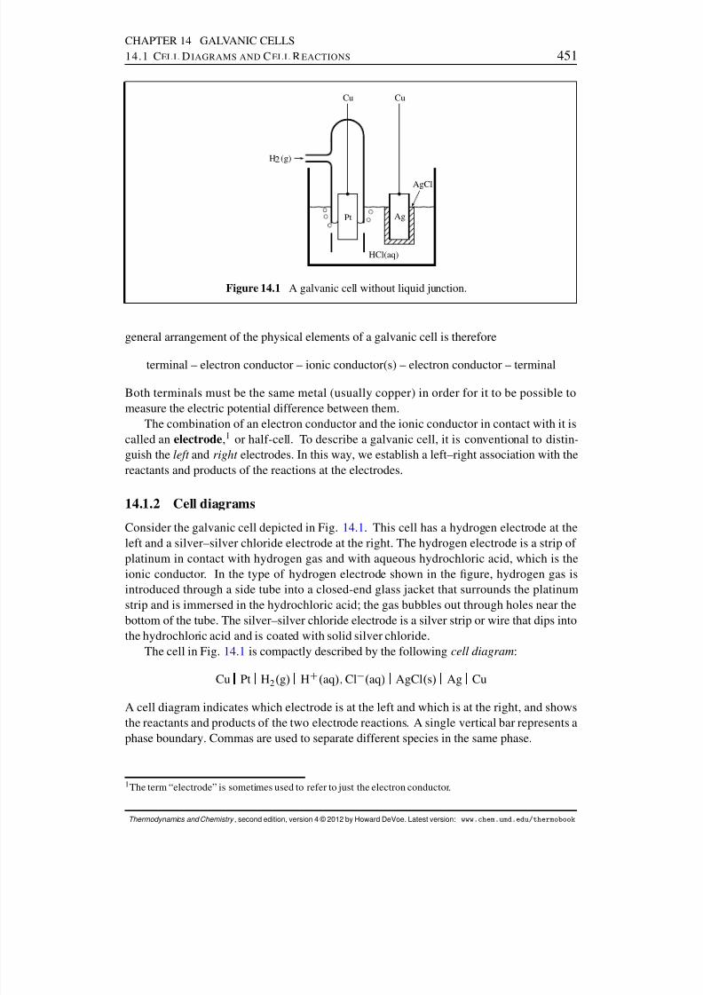
8/12/2019 Howard Devoe Thermodynamic and Chemical
http://slidepdf.com/reader/full/howard-devoe-thermodynamic-and-chemical 451/532
CHAPTER 14 GALVANIC CELLS14.1 C EL L D IAGRAMS AND C EL L R EACTIONS 451
HCl(aq)
Pt Ag
Cu Cu
AgCl
H
(g)
Figure 14.1 A galvanic cell without liquid junction.
general arrangement of the physical elements of a galvanic cell is therefore
terminal – electron conductor – ionic conductor(s) – electron conductor – terminal
Both terminals must be the same metal (usually copper) in order for it to be possible tomeasure the electric potential difference between them.
The combination of an electron conductor and the ionic conductor in contact with it iscalled an electrode ,1 or half-cell. To describe a galvanic cell, it is conventional to distin-guish the left and right electrodes. In this way, we establish a left–right association with thereactants and products of the reactions at the electrodes.
14.1.2 Cell diagrams
Consider the galvanic cell depicted in Fig. 14.1 . This cell has a hydrogen electrode at theleft and a silver–silver chloride electrode at the right. The hydrogen electrode is a strip of platinum in contact with hydrogen gas and with aqueous hydrochloric acid, which is theionic conductor. In the type of hydrogen electrode shown in the gure, hydrogen gas isintroduced through a side tube into a closed-end glass jacket that surrounds the platinumstrip and is immersed in the hydrochloric acid; the gas bubbles out through holes near thebottom of the tube. The silver–silver chloride electrode is a silver strip or wire that dips intothe hydrochloric acid and is coated with solid silver chloride.
The cell in Fig. 14.1 is compactly described by the following cell diagram :
Cu Pt H 2 . g/ HC . aq /; Cl . aq / AgCl . s/ Ag Cu
A cell diagram indicates which electrode is at the left and which is at the right, and showsthe reactants and products of the two electrode reactions. A single vertical bar represents aphase boundary. Commas are used to separate different species in the same phase.
1The term “electrode” is sometimes used to refer to just the electron conductor.
Thermodynamics and Chemistry , second edition, version 4 © 2012 by Howard DeVoe. Latest version: www.chem.umd.edu/thermobook
8/12/2019 Howard Devoe Thermodynamic and Chemical
http://slidepdf.com/reader/full/howard-devoe-thermodynamic-and-chemical 452/532
CHAPTER 14 GALVANIC CELLS14.1 C EL L D IAGRAMS AND C EL L R EACTIONS 452
The same cell can be described by a slightly different cell diagram that omits the copperterminals seen in the gure and shows the electrolyte solute instead of the ion species:
Pt H 2 . g/ HCl . aq / AgCl . s/ Ag
The reason it is not necessary to include the terminals is that the property whose valuewe seek, the zero-current cell potential, is the same regardless of the metal used for theterminals.
14.1.3 Electrode reactions and the cell reaction
A cell diagram, with its designation of the left and right electrodes, allows us to writereaction equations for the cell. These equations are written according to the convention thatelectrons enter at the right terminal and leave at the left terminal.
At each electrode there is an electrode reaction , or half-reaction, one for reduction atthe right electrode and the other for oxidation at the left electrode. The reaction equationsfor the electrode reactions include electrons as either a reactant (at the right terminal) or a
product (at the left terminal). The cell reaction describes the overall chemical change; itsreaction equation is the sum of the equations for the two electrode reactants with cancella-tion of the electrons.
For instance, we can write the electrode reactions of the cell of Fig. 14.1 as follows.
oxidation at left: H 2 . g/ ! 2 HC . aq / C2 e
reduction at right: 2 AgCl . s/ C2 e ! 2 Ag . s/ C2 Cl . aq /
As written here, the stoichiometric numbers of the electrons have the same absolute value(2) in both reaction equations. This allows the electrons to cancel when we add the electrodereactions to form the cell reaction:
H2 . g/ C2 AgCl . s/ ! 2 HC . aq / C2 Cl . aq / C2 Ag . s/
The cell of Fig. 14.1 has a single electrolyte phase with essentially the same composi-tion at both electrodes, and is an example of a cell without liquid junction or cell without transference . As an example of a cell with transference , consider the cell diagram
Zn Zn 2C . aq / Cu2C . aq / Cu
This is the zinc–copper cell depicted in Fig. 14.2 on the next page , sometimes called aDaniell cell. The two electrolyte phases are separated by a liquid junction represented inthe cell diagram by the dashed vertical bar. If the liquid junction potential can be assumedto be negligible, the liquid junction is instead represented by a pair of dashed vertical bars:
Zn Zn 2C . aq / Cu2C . aq / Cu
14.1.4 Advancement and charge
The electron number or charge number, z, of the cell reaction is dened as the amountof electrons entering at the right terminal per unit advancement of the cell reaction. z is a
Thermodynamics and Chemistry , second edition, version 4 © 2012 by Howard DeVoe. Latest version: www.chem.umd.edu/thermobook

8/12/2019 Howard Devoe Thermodynamic and Chemical
http://slidepdf.com/reader/full/howard-devoe-thermodynamic-and-chemical 453/532
CHAPTER 14 GALVANIC CELLS14.2 E LECTRIC P OTENTIALS IN THE C EL L 453
Zn
ZnSO
(aq)
Cu
CuSO
(aq)
L
R
(a)
Zn
ZnSO
(aq)
Cu
CuSO
(aq)
e
(b)
Figure 14.2 Zinc–copper galvanic cell with porous barrier (heavy dashed line) sepa-rating two electrolyte solutions. The dashed rectangle indicates the system boundary.(a) Open circuit with isolated system in equilibrium state.(b) Closed circuit.
positive dimensionless quantity equal to j ej, where e is the stoichiometric number of theelectrons in either of the electrode reactions whose sum is the cell reaction.
Because both electrode reactions are written with the same value of j ej, the advance-ments of these reactions and of the cell reaction are all described by the same advancementvariable . For an innitesimal change d , an amount of electrons equal to z d enters thesystem at the right terminal, an equal amount of electrons leaves at the left terminal, andthere is no buildup of charge in any of the internal phases.
The Faraday constant F is a physical constant dened as the charge per amount of protons, and is equal to the product of the elementary charge (the charge of a proton) and theAvogadro constant: F D eN A . Its value to ve signicant gures is F D 96;485 Cmol 1 .The charge per amount of electrons is
F . Thus, the charge entering the right terminal
during advancement d is¶Q sys D zF d (14.1.1)
14.2 ELECTRIC POTENTIALS IN THE CELL
As explained at the beginning of Sec. 3.8, the electric potential at a point in space isdened as the change in the electrical potential energy of an innitesimal test charge whenit is brought to this point from a position innitely far from other charges, divided by thecharge.
We are concerned with the electric potential within a phase—the inner electric potential,or Galvani potential . We can measure the difference between the values of this electric po-
tential in the two terminals of a galvanic cell, provided the terminals have the same chemicalcomposition. If the terminals were of different metals, at least one of them would have anunknown metal–metal contact potential in its connection to the external measuring circuit.
Since we will be applying the concept of electric potential to macroscopic phases, thevalue of the Galvani potential at a point in a phase should be interpreted as the average valuein a small volume element at this point that is large enough to contain many molecules.
Thermodynamics and Chemistry , second edition, version 4 © 2012 by Howard DeVoe. Latest version: www.chem.umd.edu/thermobook
8/12/2019 Howard Devoe Thermodynamic and Chemical
http://slidepdf.com/reader/full/howard-devoe-thermodynamic-and-chemical 454/532
CHAPTER 14 GALVANIC CELLS14.2 E LECTRIC P OTENTIALS IN THE C EL L 454
14.2.1 Cell potential
The cell potential of a galvanic cell is the electric potential difference between terminals of the same metal, and is dened by Eq. 3.8.6 :
E celldef
D R L (14.2.1)
The subscripts R and L refer to the right and left terminals. The equilibrium cell potential ,E cell, eq , is the cell potential measured under conditions of zero current when the cell isassumed to be in an equilibrium state. 2
Over a relatively long period of time, the state of an isolated galvanic cell is found tochange. Nevertheless, the assumption of an equilibrium state is valid if the changesare very slow compared to the period during which we measure E cell .
The long-term changes can be of two types. If there is a liquid junction betweenelectrolyte solutions of different composition, slow diffusion of ions through the junc-tion is inevitable.
In a cell without a liquid junction, the reactants of the cell reaction can react di-
rectly without the passage of an electric current. For instance, in the cell of Fig. 14.1the electrolyte solution is saturated with respect to gaseous H 2 and solid AgCl, andtherefore contains very small concentrations of dissolved H 2 molecules and Ag C ions.The direct reaction H 2 C2 Ag C ! 2 HC C2 Ag occurs irreversibly and continuouslyin the solution, but is slow on account of the low concentrations.
It is entirely arbitrary whether we show a particular electrode at the left or the rightof the cell diagram, although often there is a preference to place the electrode attached tothe positive terminal at the right. If we exchange the positions of the two electrodes in thediagram, then we must reverse the reaction equations for the electrode reactions and the cellreaction.
For example, it is found that the zinc–copper cell of Fig. 14.2 , with typical electrolyte
molalities, has its positive terminal at the copper electrode. When we write the cell diagramas
Zn Zn 2C . aq / Cu2C . aq / Cu
then E cell and E cell, eq are positive. If we connect the two terminals by an external resistoras depicted in Fig. 14.2 (b), electrons will ow from the left terminal through the externalresistor and wires to the right terminal, and the cell reaction
Zn CCu 2C . aq / ! Zn2C . aq / CCu
will occur spontaneously in the forward direction.If, however, we draw the cell diagram the other way around:
Cu Cu 2C . aq / Zn2C . aq / Zn
then the positive terminal is at the left, E cell and E cell, eq are negative, and electrons willow through an external resistor from the right terminal to the left terminal. Since the cell
2The equilibrium cell potential used to be called the electromotive force, or emf. These names are deprecatedby the IUPAC Green Book (Ref. [ 36], p. 71) because a potential difference is not a force.
Thermodynamics and Chemistry , second edition, version 4 © 2012 by Howard DeVoe. Latest version: www.chem.umd.edu/thermobook

8/12/2019 Howard Devoe Thermodynamic and Chemical
http://slidepdf.com/reader/full/howard-devoe-thermodynamic-and-chemical 455/532
CHAPTER 14 GALVANIC CELLS14.2 E LECTRIC P OTENTIALS IN THE C EL L 455
galvaniccell
L R
(a)
galvaniccell
L R
G
(b)
Figure 14.3 Potentiometer to measure the zero-current cell potential of a galvaniccell.(a) Galvanic cell with zero current.(b) Galvanic cell included in potentiometer circuit; G is a galvanometer.
reaction should show reduction at the right electrode and oxidation at the left, we must nowwrite it as
Cu CZn2C . aq / ! Cu2C . aq / CZn
even though the arrow is not in the direction of the reaction that actually occurs sponta-neously. In other words, the cell reaction is written according to the cell diagram, notaccording to the direction of the spontaneous change.
14.2.2 Measuring the equilibrium cell potential
Figure 14.3 shows how we can use a potentiometer to determine the equilibrium cell poten-tial. Consider Fig. 14.3 (a). Outside the galvanic cell is an external circuit with a battery thatallows an electric current to pass through a slidewire resistor. The cell’s negative terminal isconnected to the negative terminal of the battery. Since the cell is not part of this circuit, nocurrent passes through the cell, and R L is the zero-current cell potential E cell, eq . Theleft end of the slidewire is at the same electric potential as the left terminal of the cell.
In the setup shown in Fig. 14.3 (a), the electric potential within the slidewire is a linearfunction of the distance from the left end. At some position along the slidewire, the electricpotential is equal to R . We can determine this position by connecting the right terminalof the cell to a slidewire contact as shown in Fig. 14.3 (b). When we place the contactat this particular position along the slidewire, there is no electric potential gradient in theconnecting wire, and the galvanometer indicates a condition of zero current in the wire. Itis a straightforward procedure to evaluate R
L from the zero-current position of the
contact; this value is still equal to E cell, eq . When we keep the slidewire contact in thisposition, no current passes through the cell; but if we displace the contact from this positionin either direction along the slidewire, current will pass in one direction or the other throughthe cell.
In practice, it is more convenient to measure the zero-current cell potential with a high-impedance digital voltmeter (a voltmeter that draws negligible current) instead of with a
Thermodynamics and Chemistry , second edition, version 4 © 2012 by Howard DeVoe. Latest version: www.chem.umd.edu/thermobook
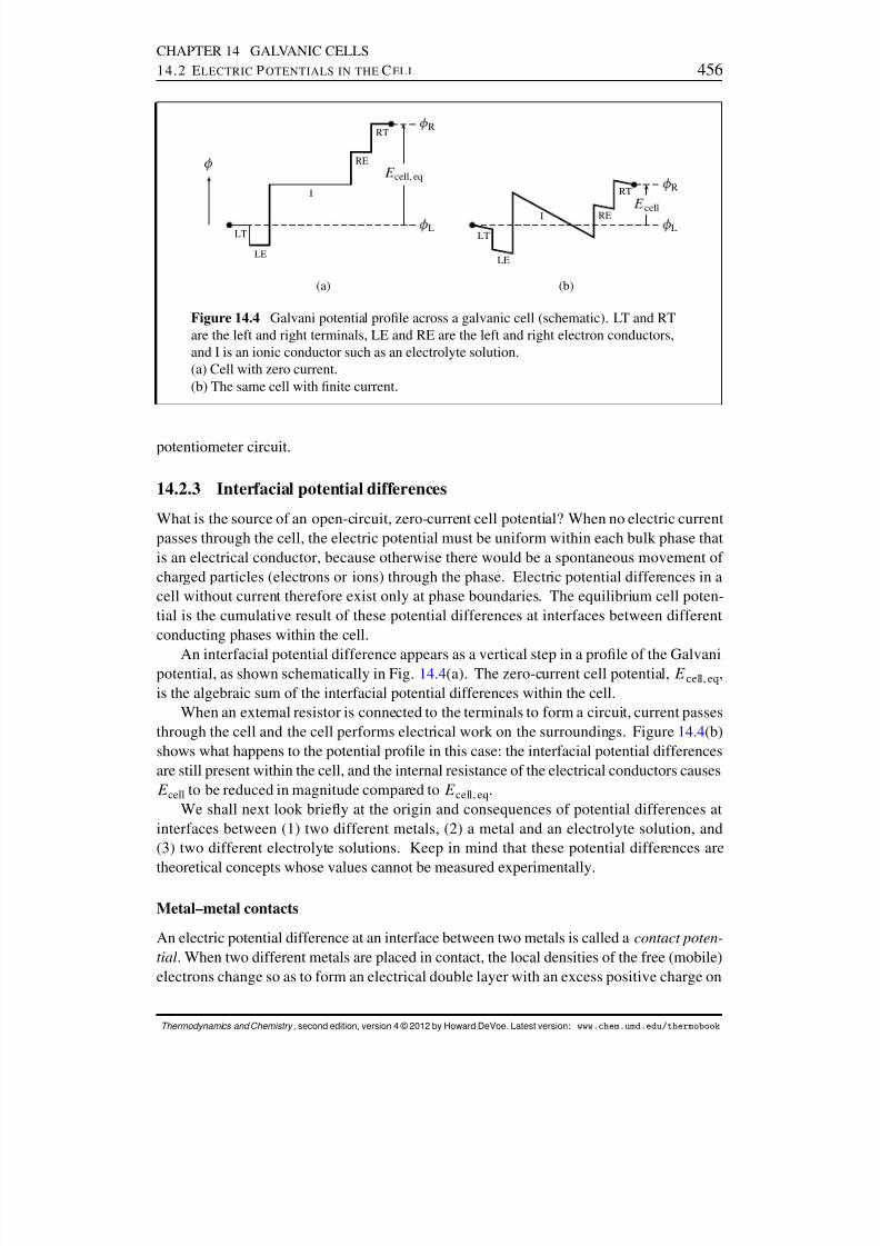
8/12/2019 Howard Devoe Thermodynamic and Chemical
http://slidepdf.com/reader/full/howard-devoe-thermodynamic-and-chemical 456/532
CHAPTER 14 GALVANIC CELLS14.2 E LECTRIC P OTENTIALS IN THE C EL L 456
(a)
LT
LE
I
RE
RT
(b)
LT
LE
I RE
RT
R
L
cell, eq R
L
cell
Figure 14.4 Galvani potential prole across a galvanic cell (schematic). LT and RTare the left and right terminals, LE and RE are the left and right electron conductors,and I is an ionic conductor such as an electrolyte solution.(a) Cell with zero current.(b) The same cell with nite current.
potentiometer circuit.
14.2.3 Interfacial potential differences
What is the source of an open-circuit, zero-current cell potential? When no electric currentpasses through the cell, the electric potential must be uniform within each bulk phase thatis an electrical conductor, because otherwise there would be a spontaneous movement of charged particles (electrons or ions) through the phase. Electric potential differences in acell without current therefore exist only at phase boundaries. The equilibrium cell poten-tial is the cumulative result of these potential differences at interfaces between differentconducting phases within the cell.
An interfacial potential difference appears as a vertical step in a prole of the Galvanipotential, as shown schematically in Fig. 14.4 (a). The zero-current cell potential, E cell, eq ,is the algebraic sum of the interfacial potential differences within the cell.
When an external resistor is connected to the terminals to form a circuit, current passesthrough the cell and the cell performs electrical work on the surroundings. Figure 14.4 (b)shows what happens to the potential prole in this case: the interfacial potential differencesare still present within the cell, and the internal resistance of the electrical conductors causesE cell to be reduced in magnitude compared to E cell, eq .
We shall next look briey at the origin and consequences of potential differences atinterfaces between (1) two different metals, (2) a metal and an electrolyte solution, and(3) two different electrolyte solutions. Keep in mind that these potential differences are
theoretical concepts whose values cannot be measured experimentally.
Metal–metal contacts
An electric potential difference at an interface between two metals is called a contact poten-tial . When two different metals are placed in contact, the local densities of the free (mobile)electrons change so as to form an electrical double layer with an excess positive charge on
Thermodynamics and Chemistry , second edition, version 4 © 2012 by Howard DeVoe. Latest version: www.chem.umd.edu/thermobook
8/12/2019 Howard Devoe Thermodynamic and Chemical
http://slidepdf.com/reader/full/howard-devoe-thermodynamic-and-chemical 457/532
CHAPTER 14 GALVANIC CELLS14.2 E LECTRIC P OTENTIALS IN THE C EL L 457
one side of the interface and an excess negative charge of equal magnitude on the other side.The electrical double layer creates the contact potential.
To understand why a stable equilibrium state of two metals in contact includes a con-tact potential, we can consider the chemical potential of the free electrons. The concept of chemical potential (i.e., partial molar Gibbs energy) applies to the free electrons in a metal
just as it does to other species. The dependence of the chemical potential ’e of free elec-trons in metal phase ’ on the electric potential ’ of the phase is given by the relation of
Eq. 10.1.6 on page 288 , with the charge number zi set equal to 1:
’e . / D ’
e .0/ F ’ (14.2.2)
Here ’e .0/ is the electron chemical potential in a phase with the same intensive properties
as phase ’ but at zero electric potential. ’e .0/ depends only on the temperature and the
composition of phase ’ . (The dependence on pressure is so small for a solid that we willignore it.)
Consider two or more electron conductors that are so arranged that electrons can freelytransfer among them. There is the usual condition for transfer equilibrium in these phases:
the chemical potential (in this case e) is the same in each phase. Thus, electron transferequilibrium between phases ’ and “ requires ’
e and “e to be equal. We equate ’
e and “e ,
substitute from Eq. 14.2.2 to obtain ’e .0/ F ’ D “
e .0/ F “ , and rearrange to
“ ’ D “
e .0/ ’e .0/
F (14.2.3)
(phases in electrontransfer equilibrium)
The quantities on the right side of Eq. 14.2.3 are functions only of the temperature and thecompositions of phases ’ and “ . If the phases have the same temperature and compositionand are in electron transfer equilibrium, ’ and “ are equal.
For an equilibrium state of metals ’ and “ in contact, Eq. 14.2.3 shows that the contactpotential “ ’ depends only on the temperature and the compositions of the two metals. 3
Equation 14.2.3 explainswhy a galvaniccell must have at least one electrical conductorthat is not an electron conductor. If electrons were free to pass from one terminalthrough the system to the other terminal of the same temperature and composition,then in a zero-current equilibrium state e would be the same in both terminals. Inthat case there would be no potential difference between the terminals, and the systemwould not be a galvanic cell.
Metal–electrolyte interfaces
An electrode reaction of a galvanic cell takes place at the interface between a metal electronconductor and an electrolyte solution. In an equilibrium state of the cell, the electrodereaction is at equilibrium. The condition for this equilibrium is Pi i i D 0, where thesum is over the reactants and products of the electrode reaction, including the electrons.The chemical potentials of the ions and electrons in the electrode reaction are functions of
3The temperature dependence of a contact potential between two different metals is the basis of the operationof a thermocouple or thermopile to measure temperature (Sec. 2.3.5 ).
Thermodynamics and Chemistry , second edition, version 4 © 2012 by Howard DeVoe. Latest version: www.chem.umd.edu/thermobook
8/12/2019 Howard Devoe Thermodynamic and Chemical
http://slidepdf.com/reader/full/howard-devoe-thermodynamic-and-chemical 458/532
CHAPTER 14 GALVANIC CELLS14.3 M OLAR R EACTION Q UANTITIES OF THE C EL L R EACTION 458
the electric potentials of their phases. Consequently, in order for the sum to be zero, themetal and solution must in general have different electric potentials.
For example, consider the zinc–copper cell of Fig. 14.2 . The electrode reaction of thecopper electrode at the right is
Cu 2C . aq /
C2 e . Cu /
! Cu
where the metal phase of the electrons is indicated in parentheses. In order for this elec-trode reaction to be at equilibrium, the interfacial potential difference between the copperconductor and the solution containing Cu 2C ions must be such that the following conditionis satised:
. Cu / . Cu 2C / 2 e. Cu / D 0 (14.2.4)
The interfacial potential difference can arise from a combination of charge separationacross the interface, orientation of polar molecules on the solution side of the interface, andspecic adsorption of ions. The thickness of the zones in which properties differ from thosein the bulk phases is probably no greater than 10 11 m on the metal side and 10 7 m on thesolution side.
Liquid junctions
Some galvanic cells contain two electrolyte solutions with different compositions. Thesesolutions must be separated by a porous barrier or some other kind of junction in order toprevent rapid mixing. At this liquid junction in the zero-current cell, there is in generala liquid junction potential caused by diffusion of ions between the two bulk electrolytephases.
To understand this phenomenon, imagine the situation that would exist at the junction if both solution phases had the same electric potential. An ion species with different chemicalpotentials in the two solutions would spontaneously diffuse across the junction in the direc-
tion of lower chemical potential. Different ions would diffuse at different rates, resulting ina net charge transfer across the junction and an electric potential difference. It is this elec-tric potential difference in the equilibrium state of the cell that prevents further net chargetransfer under zero-current conditions.
The liquid junction may consist of a bridging solution in a salt bridge . A commonlyused kind of salt bridge is a glass tube lled with gel made from agar and concentratedaqueous KCl or KNO 3 ; this type of liquid junction is believed to reduce the liquid junctionpotential to several millivolts or less.
14.3 MOLAR REACTION QUANTITIES OF THE CELL REACTION
This book will denote the molar reaction Gibbs energy of a cell reaction by
rG
cell . Thisnotation distinguishes it from the molar reaction Gibbs energy rG of the direct reaction,which may have a different value because in the cell the chemical potential of an ionicspecies is affected by the electric potential of its phase. rGcell is dened by
rG celldef
DXii i (14.3.1)
Thermodynamics and Chemistry , second edition, version 4 © 2012 by Howard DeVoe. Latest version: www.chem.umd.edu/thermobook
8/12/2019 Howard Devoe Thermodynamic and Chemical
http://slidepdf.com/reader/full/howard-devoe-thermodynamic-and-chemical 459/532
CHAPTER 14 GALVANIC CELLS14.3 M OLAR R EACTION Q UANTITIES OF THE C EL L R EACTION 459
where the sum is over the reactants and products of the cell reaction. rGcell is also equalto the partial derivative .@Gcell =@ /T;p , where is the advancement of the cell reaction.
14.3.1 Relation between r G cell and E cell, eq
When a galvanic cell is in a zero-current equilibrium state, both electrode reactions are atreaction equilibrium. In the electrode reaction at the left electrode, electrons are a productwith stoichiometric number equal to z . At the right electrode, electrons are a reactant withstoichiometric number equal to z . We can write the conditions for electrode reactionequilibria as follows:
At the left electrode Xii i Cz e. LE / D 0 (14.3.2)
At the right electrode Xj j j z e . RE / D 0 (14.3.3)
In these equations, the sum over i is for the chemical species (excluding electrons) of theelectrode reaction at the left electrode, and the sum over j is for the chemical species of theelectrode reaction at the right electrode. e . LE / is the chemical potential of electrons in theelectron conductor of the left electrode, and e . RE / is the chemical potential of electronsin the electron conductor of the right electrode.
Adding Eqs. 14.3.2 and 14.3.3 , we obtain
Xii i CXj
j j CzΠe . LE / e. RE / D 0 (14.3.4)
The rst two terms on the left side of Eq. 14.3.4 are sums over all the reactants and productsof the cell reaction. From Eq. 14.3.1 , we recognize the sum of these terms as the molarreaction Gibbs energy of the cell reaction:
Xii i CXj
j j D rG cell (14.3.5)
Substituting from Eq. 14.3.5 into Eq. 14.3.4 and solving for rGcell , we obtain
rGcell D zΠe . LE / e. RE / (14.3.6)
In a zero-current equilibrium state, there is electron transfer equilibrium between the leftelectron conductor and the left terminal, and between the right electron conductor and theright terminal: e . LE / D e . LT / and e . RE / D e . RT / , where e . LT / and e . RT / arethe chemical potentials of electrons in the left terminal and right terminal, respectively.Thus we can rewrite Eq. 14.3.6 as
rGcell D zΠe . LT / e . RT / (14.3.7)
Making substitutions from Eq. 14.2.2 for e . LT / and e . RT / , and recognizing that e .0/is the same in both terminals because they have the same composition, we obtain
rGcell D zF. R L/
D zFE cell, eq (14.3.8)
Thermodynamics and Chemistry , second edition, version 4 © 2012 by Howard DeVoe. Latest version: www.chem.umd.edu/thermobook
8/12/2019 Howard Devoe Thermodynamic and Chemical
http://slidepdf.com/reader/full/howard-devoe-thermodynamic-and-chemical 460/532
CHAPTER 14 GALVANIC CELLS14.3 M OLAR R EACTION Q UANTITIES OF THE C EL L R EACTION 460
We can see from Eq. 14.3.1 that the value of rGcell has nothing to do with the composi-tion of the terminals. The relations of Eq. 14.3.8 were derived for a cell with both terminalsmade of the same metal. We can make the following deductions for such a cell:
1. Neither the potential difference R L nor the equilibrium cell potential E cell, eqdepend on the kind of metal used for the terminals.
2. If we interpose a metal conductor of any composition between the electron conductorand the terminal of one of the electrodes, e will have the same value in all threeconductors and there will be no effect on the value of E cell, eq .
Equation 14.3.8 can be derived by a different route. According to Eq. 5.8.6 on page 146 ,reversible electrical work at constant T and p is equal to the Gibbs energy change:¶w el, rev D dGcell . Making the substitution ¶w el, rev D E cell, eq ¶Q sys (from Eq. 3.8.8),with ¶Q sys set equal to zF d (Eq. 14.1.1 ), followed by division by d , gives
zFE cell, eq D .@Gcell =@ /T;p , or rGcell D zFE cell, eq .Strictly speaking, this derivation applies only to a cell without a liquid junction.
In a cell with a liquid junction, the electric current is carried across the junction bydifferent ions depending on the direction of the current, and the cell is therefore not
reversible.
14.3.2 Relation between r G cell and r G
Suppose we have a galvanic cell in a particular zero-current equilibrium state. Each phaseof the cell has the same temperature and pressure and a well-dened chemical composition.The activity of each reactant and product of the cell reaction therefore has a denite valuein this state.
Now imagine a reaction vessel that has the same temperature and pressure as the gal-vanic cell, and contains the same reactants and products at the same activities as in the cell.This reaction vessel, unlike the cell, is not part of an electrical circuit. In it, the reactantsand products are in direct contact with one another, so there is no constraint preventing aspontaneous direct reaction. For example, the reaction vessel corresponding to the zinc–copper cell of Fig. 14.2 would have zinc and copper strips in contact with a solution of bothZnSO 4 and CuSO 4 . Another example is the slow direct reaction in a cell without liquid junction described on page 454 .
Let the reaction equation of the direct reaction be written with the same stoichiometricnumbers i as in the reaction equation for the cell reaction. The direct reaction in thereaction vessel is described by this equation or its reverse, depending on which direction isspontaneous for the given activities.
The question now arises whether the molar reaction Gibbs energy rGcell of the cellreaction is equal to the molar reaction Gibbs energy rG of the direct reaction. Both rG celland rG are dened by the sum
Pi i i . Both reactions have the same values of i , but
the values of i for charged species are in general different in the two systems because theelectric potentials are different.
Consider rst a cell without a liquid junction. This kind of cell has a single electrolytesolution, and all of the reactant and product ions of the cell reaction are in this solutionphase. The same solution phase is present in the reaction vessel during the direct reaction.When all ions are in the same phase, the value of Pi i i is independent of the electric
Thermodynamics and Chemistry , second edition, version 4 © 2012 by Howard DeVoe. Latest version: www.chem.umd.edu/thermobook
8/12/2019 Howard Devoe Thermodynamic and Chemical
http://slidepdf.com/reader/full/howard-devoe-thermodynamic-and-chemical 461/532
CHAPTER 14 GALVANIC CELLS14.3 M OLAR R EACTION Q UANTITIES OF THE C EL L R EACTION 461
potentials of any of the phases (see the comment following Eq. 11.8.4 on page 351 ), so thatthe molar reaction Gibbs energies are the same for the cell reaction and the direct reaction:
rGcell D rG (14.3.9)(no liquid junction)
Next, consider a cell with two electrolyte solutions separated by a liquid junction. Forthe molar reaction Gibbs energy of the cell reaction, we write
rGcell DXii i . i / CXj
j j . j / (14.3.10)
The sums here include all of the reactants and products appearing in the cell reaction, thosewith index i being at the left electrode and those with index j at the right electrode. Let thesolution at the left electrode be phase ’ and the solution at the right electrode be phase “ .Then making the substitution i . / D i .0/ Czi F (Eq. 10.1.6 ) gives us
rGcell
DXi
i i .0/
CXj
j j .0/
CXi
i zi F ’
CXj
j zj F“ (14.3.11)
The sum of the rst two terms on the right side of Eq. 14.3.11 is the molar reactionGibbs energy of a reaction in which the reactants and products are in phases of zero electricpotential. According to the comment following Eq. 11.8.4 , the molar reaction Gibbs energywould be the same if the ions were in a single phase of any electric potential. Consequentlythe sum Pi i i .0/ CPj j j .0/ is equal to rG for the direct reaction.
The conservation of charge during advancement of the electrode reactions at the leftelectrode and the right electrode is expressed by Pi i zi z D 0 and Pj j zj Cz D 0,respectively. Equation 14.3.11 becomes
rGcell
D rG
zFE j (14.3.12)
(cell with liquid junction)
where E j D “ ’ is the liquid junction potential.Finally, in Eqs. 14.3.9 and 14.3.12 we replace rGcell by zFE cell, eq (Eq. 14.3.8 ) and
solve for E cell, eq :
E cell, eq D rG
zF (14.3.13)
(cell without liquid junction)
E cell, eq D rG
zF CE j (14.3.14)
(cell with liquid junction)
E cell, eq can be measured with great precision. If a reaction can be carried out in a galvaniccell without liquid junction, Eq. 14.3.13 provides a way to evaluate rG under given con-ditions. If the reaction can only be carried out in a cell with a liquid junction, Eq. 14.3.14can be used for this purpose provided that the liquid junction potential E j can be assumedto be negligible or can be estimated from theory.
Thermodynamics and Chemistry , second edition, version 4 © 2012 by Howard DeVoe. Latest version: www.chem.umd.edu/thermobook
8/12/2019 Howard Devoe Thermodynamic and Chemical
http://slidepdf.com/reader/full/howard-devoe-thermodynamic-and-chemical 462/532
CHAPTER 14 GALVANIC CELLS14.3 M OLAR R EACTION Q UANTITIES OF THE C EL L R EACTION 462
Note that the cell has reaction equilibrium only if rG is zero. The cell has thermal,mechanical, and transfer equilibrium when the electric current is zero and the cell potentialis the zero-current cell potential E cell, eq . Equations 14.3.13 and 14.3.14 show that in orderfor the cell to also have reaction equilibrium, E cell, eq must equal the liquid junction potentialif there is a liquid junction, or be zero otherwise. These are the conditions of an exhausted,
“dead” cell that can no longer do electrical work.
14.3.3 Standard molar reaction quantities
Consider a hypothetical galvanic cell in which each reactant and product of the cell reac-tion is in its standard state at unit activity, and in which a liquid junction if present hasa negligible liquid junction potential. The equilibrium cell potential of this cell is calledthe standard cell potential of the cell reaction, E ı
cell, eq . An experimental procedure forevaluating E ı
cell, eq will be described in Sec. 14.5 .In this hypothetical cell, rG cell is equal to the standard molar reaction Gibbs energy
rGı . From Eq. 14.3.13 , or Eq. 14.3.14 with E j assumed equal to zero, we have
rG ı
D zFE ı
cell, eq (14.3.15)
rGı is the molar reaction Gibbs energy when each reactant and product is at unit activity
and, if it is an ion, is in a phase of zero electric potential. Since rGı is equal to RT ln K
(Eq. 11.8.10 ), we can write
ln K D zF RT
E ıcell, eq (14.3.16)
Equation 14.3.16 allows us to evaluate the thermodynamic equilibrium constant K of the cell reaction by a noncalorimetric method. Consider for example the cell
Ag Ag C . aq / Cl . aq / AgCl . s/ Ag
in which the pair of dashed vertical bars indicates a liquid junction of negligible liquid
junction potential. The electrode reactions areAg(s) ! AgC (aq) Ce
AgCl(s) Ce ! Ag(s) CCl (aq)
and the cell reaction isAgCl . s/ ! AgC . aq / CCl . aq /
The equilibrium constant of this reaction is the solubility product K s of silver chloride (Sec.12.5.5 ). At 298:15 K, the standard cell potential is found to be E ı
cell, eq D 0:5770 V. Wecan use this value in Eq. 14.3.16 to evaluate K s at 298:15 K (see Prob. 14. 5).
Equation 14.3.16 also allows us to evaluate the standard molar reaction enthalpy bysubstitution in Eq. 12.1.13 on page 369 :
rH ı D RT 2d ln K
dT
D zF T dE ı
cell, eq
dT E ıcell, eq! (14.3.17)
(no solute standard statesbased on concentration)
Thermodynamics and Chemistry , second edition, version 4 © 2012 by Howard DeVoe. Latest version: www.chem.umd.edu/thermobook

8/12/2019 Howard Devoe Thermodynamic and Chemical
http://slidepdf.com/reader/full/howard-devoe-thermodynamic-and-chemical 463/532
CHAPTER 14 GALVANIC CELLS14.4 T HE N ERNST E QUATION 463
Finally, by combining Eqs. 14.3.15 and 14.3.17 with rGı D rH ı T rS ı , we obtain
an expression for the standard molar reaction entropy:
rS ı D zF dE ı
cell, eq
dT (14.3.18)(no solute standard states
based on concentration)
Because G , H , and S are state functions, the thermodynamic equilibrium constantand the molar reaction quantities evaluated from E ı
cell, eq and d E ıcell, eq = dT are the same
quantities as those for the reaction when it takes place in a reaction vessel instead of in agalvanic cell. However, the heats at constant T and p are not the same (page 319 ). Duringa reversible cell reaction, d S must equal ¶q=T , and ¶q= d is therefore equal to T rS ı
during a cell reaction taking place reversibly under standard state conditions at constant T and p .
14.4 THE NERNST EQUATION
The standard cell potential E ıcell, eq of a cell reaction is the equilibrium cell potential of
the hypothetical galvanic cell in which each reactant and product of the cell reaction isin its standard state and there is no liquid junction potential. The value of E ı
cell, eq for agiven cell reaction with given choices of standard states is a function only of temperature.The measured equilibrium cell potential E cell, eq of an actual cell, however, depends on theactivities of the reactants and products as well as on temperature and the liquid junctionpotential, if present.
To derive a relation between E cell, eq and activities for a cell without liquid junction, orwith a liquid junction of negligible liquid junction potential, we substitute expressions for
rG and for rGı from Eqs. 14.3.13 and Eq. 14.3.15 into rG D rG
ı CRT ln Q rxn(Eq. 11.8.8 on page 352 ) and solve for E cell, eq :
E cell, eq D E ıcell, eq
R T zF
ln Q rxn (14.4.1)(no liquid junction, or E jD0)
Equation 14.4.1 is the Nernst equation for the cell reaction. Here Q rxn is the reactionquotient for the cell reaction dened by Eq. 11.8.6 : Q rxn DQi a
ii .
The rest of this section will assume that the cell reaction takes place in a cell withoutliquid junction, or in one in which E j is negligible.
If each reactant and product of the cell reaction is in its standard state, then each activityis unity and ln Q rxn is zero. We can see from the Nernst equation that the equilibrium cellpotential E cell, eq in this case has its standard value E ı
cell, eq , as expected. A decrease in
product activities or an increase in reactant activities decreases the value of ln Q rxn andincreases E cell, eq , as we would expect since E cell, eq should be greater when the forward cellreaction has a greater tendency for spontaneity.
If the cell reaction comes to reaction equilibrium, as it will if we short-circuit the cell ter-minals with an external wire, the value of Q rxn becomes equal to the thermodynamic equi-librium constant K , and the Nernst equation becomes E cell, eq D E ı
cell, eq .RT=zF/ ln K .
Thermodynamics and Chemistry , second edition, version 4 © 2012 by Howard DeVoe. Latest version: www.chem.umd.edu/thermobook

8/12/2019 Howard Devoe Thermodynamic and Chemical
http://slidepdf.com/reader/full/howard-devoe-thermodynamic-and-chemical 464/532
CHAPTER 14 GALVANIC CELLS14.4 T HE N ERNST E QUATION 464
The term .RT=zF / ln K is equal to E ıcell, eq (Eq. 14.3.16 ), so E cell, eq becomes zero—the
cell is “dead” and is incapable of performing electrical work on the surroundings.At T D298:15 K (25:00 ı C), the value of RT=F is 0:02569 V, and we can write the
Nernst equation in the compact form
E cell, eq D Eıcell, eq
0:02569 V
z ln Q rxn (14.4.2)(T D298:15 K)
As an illustration of an application of the Nernst equation, consider the reaction equation
H2 . g/ C2 AgCl . s/ ! 2 HC . aq / C2 Cl . aq / C2 Ag . s/
This reaction takes place in a cell without liquid junction (Fig. 14.1 ), and the electrolytesolution can be aqueous HCl. The expression for the reaction quotient is
Q rxn Da 2
C a 2 a 2Ag
a H2a 2
AgCl(14.4.3)
We may usually with negligible error approximate the pressure factors of the solids andsolutes by unity. The activities of the solids are then 1, the solute activities are aC D C mC =m ı and a D m =m ı , and the hydrogen activity is a H2 D f H2
=p ı . The ionmolalities mC and m are equal to the HCl molality mB . The expression for Q rxn becomes
Q rxn D 2C 2 .m B=m ı / 4
f H2=p ı D
4˙ .m B=m ı / 4
f H2=p ı (14.4.4)
and the Nernst equation for this cell is
E cell, eq D E ıcell, eq
RT 2F
ln 4˙ .m B=m ı / 4
f H2=p ı
D E ıcell, eq
2RT F
ln ˙ 2RT
F ln
mB
m ı C R T 2F
lnf H2
p ı (14.4.5)
By measuring E cell, eq for a cell with known values of mB and f H2, and with a derived value
of E ıcell, eq , we can use this equation to nd the mean ionic activity coefcient ˙ of the HCl
solute. This is how the experimental curve for aqueous HCl in Fig. 10.3 on page 297 wasobtained.
We can always multiply each of the stoichiometric coefcients of a reaction equationby the same positive constant without changing the meaning of the reaction. How doesthis affect the Nernst equation for the reaction equation above? Suppose we decide tomultiply the stoichiometric coefcients by one-half:
12 H2 . g/ CAgCl . s/ ! HC . aq / CCl . aq / CAg(s)
With this changed reaction equation, the value of z is changed from 2 to 1 and theNernst equation becomes
E cell, eq D E ıcell, eq
R T F
ln 2˙ .m B=m ı / 2
.f H2=p ı / 1=2 (14.4.6)
Thermodynamics and Chemistry , second edition, version 4 © 2012 by Howard DeVoe. Latest version: www.chem.umd.edu/thermobook
8/12/2019 Howard Devoe Thermodynamic and Chemical
http://slidepdf.com/reader/full/howard-devoe-thermodynamic-and-chemical 465/532
CHAPTER 14 GALVANIC CELLS14.5 E VALUATION OF THE S TANDARD C EL L P OTENTIAL 465
which yields the same value of E cell, eq for given cell conditions as Eq. 14.4.5 . Thisvalue must of course be unchanged, because physically the cell is the same no matterhow we write its cell reaction, and measurable physical quantities such as E cell, eq areunaffected. However, molar reaction quantities such as rG and rG ı do depend onhow we write the cell reaction, because they are changes per extent of reaction.
14.5 EVALUATION OF THE STANDARD CELL POTENTIAL
As we have seen, the value of the standard cell potential E ıcell, eq of a cell reaction has useful
thermodynamic applications. The value of E ıcell, eq for a given cell reaction depends only on
temperature. To evaluate it, we can extrapolate an appropriate function to innite dilutionwhere ionic activity coefcients are unity.
To see how this procedure works, consider again the cell reaction H 2 . g/ C2 AgCl . s/ !2 H C . aq / C2 Cl . aq / C2 Ag . s/ . The cell potential depends on the molality mB of the HClsolute according to Eq. 14.4.5 . We can rearrange the equation to
E ıcell, eq
D E cell, eq
C 2RT
F ln ˙
C 2RT
F ln
mB
mı
RT
2F ln
f H2
pı (14.5.1)
For given conditions of the cell, we can measure all quantities on the right side of Eq. 14.5.1except the mean ionic activity coefcient ˙ of the electrolyte. We cannot know the exactvalue of ln ˙ for any given molality until we have evaluated E ı
cell, eq . We do know thatas mB approaches zero, ˙ approaches unity and ln ˙ must approach zero. The Debye–Huckel formula of Eq. 10.4.7 on page 297 is a theoretical expression for ln ˙ that moreclosely approximates the actual value the lower is the ionic strength. Accordingly, we denethe quantity
E 0cell D E cell, eq C
2RT F
Ap mB
1
CBa p mB C
2RT F
lnmB
m ı RT 2F
lnf H2
p ı (14.5.2)
The expression in parentheses is the Debye–H uckel formula for ln ˙ with I m replaced bymB . The constants A and B have known values at any temperature (Sec. 10.4 ), and a is anion-size parameter for which we can choose a reasonable value. At a given temperature, wecan evaluate E 0
cell experimentally as a function of mB .The expression on the right side of Eq. 14.5.1 differs from that of Eq. 14.5.2 by con-
tributions to .2RT =F/ ln ˙ not accounted for by the Debye–H uckel formula. Since thesecontributions approach zero in the limit of innite dilution, the extrapolation of measuredvalues of E 0
cell to mBD0 yields the value of E ıcell, eq .
Figure 14.5 on the next page shows this extrapolation using data from the literature. Theextrapolated value indicated by the lled circle is E ı
cell, eq D 0:2222 V, and the uncertaintyis on the order of only 0:1 mV.
14.6 STANDARD ELECTRODE POTENTIALS
Section 14.5 explained how, by measuring the equilibrium cell potential of a galvanic cellat different electrolyte molalities, we can evaluate the standard cell potential E ı
cell, eq of thecell reaction. It is not necessary to carry out this involved experimental procedure for each
Thermodynamics and Chemistry , second edition, version 4 © 2012 by Howard DeVoe. Latest version: www.chem.umd.edu/thermobook

8/12/2019 Howard Devoe Thermodynamic and Chemical
http://slidepdf.com/reader/full/howard-devoe-thermodynamic-and-chemical 466/532
CHAPTER 14 GALVANIC CELLS14.6 S TANDARD E LECTRODE P OTENTIALS 466
0 0.01 0.02 0.030.2215
0.2220
0.2225
B molkg
c e
l l
V
Figure 14.5 E 0cell (dened by Eq. 14.5.2 ) as a function of HCl molality for the cell of
Fig. 14.1 at 298:15 K. a The dashed line is a least-squares t to a linear relation.
aData from Ref. [ 73] with f H2 set equal to p H2 and the parameter a set equal to 4:3 10
10m.
individual cell reaction of interest. Instead, we can calculate E ıcell, eq from standard electrode
potentials.By convention, standard electrode potentials use a standard hydrogen electrode as a
reference electrode. A standard hydrogen electrode is a hydrogen electrode, such as theelectrode shown at the left in Fig. 14.1 , in which the species H 2 (g) and H C (aq) are in theirstandard states. Since these are hypothetical gas and solute standard states, the standardhydrogen electrode is a hypothetical electrode—not one we can actually construct in thelaboratory.
A standard electrode potential Eı
is dened as the standard cell potential of a cellwith a hydrogen electrode at the left and the electrode of interest at the right. For example,the cell in Fig. 14.1 with cell diagram
Pt H 2 . g/ HCl . aq / AgCl . s/ Ag
has a hydrogen electrode at the left and a silver–silver chloride electrode at the right. Thestandard electrode potential of the silver–silver chloride electrode, therefore, is equal to thestandard cell potential of this cell.
Since a cell with hydrogen electrodes at both the left and right has a standard cell poten-tial of zero, the standard electrode potential of the hydrogen electrode is zero at all temper-atures. The standard electrode potential of any other electrode is nonzero and is a functiononly of temperature.
Consider the following three cells constructed from various combinations of three dif-ferent electrodes: a hydrogen electrode, and two electrodes denoted L and R.
Cell 1 has electrode L at the left and electrode R at the right.
Cell 2 has the hydrogen electrode at the left and electrode L at the right; its standardcell potential is the standard electrode potential E ı
L of electrode L.
Thermodynamics and Chemistry , second edition, version 4 © 2012 by Howard DeVoe. Latest version: www.chem.umd.edu/thermobook
8/12/2019 Howard Devoe Thermodynamic and Chemical
http://slidepdf.com/reader/full/howard-devoe-thermodynamic-and-chemical 467/532
CHAPTER 14 GALVANIC CELLS14.6 S TANDARD E LECTRODE P OTENTIALS 467
Cell 3 has the hydrogen electrode at the left and electrode R at the right; its standardcell potential is the standard electrode potential E ı
R of electrode R.We wish to calculate the standard cell potential E ı
cell, eq of cell 1 from the standard electrodepotentials E ı
L and E ıR .
If we write the cell reactions of cells 1 and 2 using the same value of the electron number
z for both, we nd that their sum is the cell reaction for cell 3 with the same value of z . Callthese reactions 1, 2, and 3, respectively:
(reaction 1) C(reaction 2) D (reaction 3) (14.6.1)
The relation of Eq. 14.6.1 shows that an innitesimal advancement d of reaction 1combined with an equal advancement of reaction 2 causes the same changes in amounts asthe advancement d of reaction 3. Because rG
ı for each reaction is the rate at which Gchanges with at constant T when the reactants and products are in their standard states,the following relation applies when the reactions take place at the same temperature:
rGı (reaction 1) C rG
ı (reaction 2) D rGı (reaction 3) (14.6.2)
Making the substitution rGı D zFE ı
cell, eq (Eq. 14.3.15 ), with the same value of z foreach reaction, gives us E ı
cell, eq CE ıL D E ı
R , or
E ıcell, eq D E ı
R E ıL (14.6.3)
where E ıcell, eq , E ı
R , and E ıL all refer to cell 1.
Equation 14.6.3 is a general relation applicable to any galvanic cell. It should be appar-ent that we can use the relation to calculate the standard electrode potential of an electrodefrom the standard electrode potential of a different electrode and the standard cell potentialof a cell that contains both electrodes. Neither electrode has to be a hydrogen electrode,which is difcult to work with experimentally.
Using Eq. 14.6.3 to calculate standard cell potentials from standard electrode potentialssaves a lot of experimental work. For example, measurement of E ı
cell, eq for ten differentcells, only one of which needs to include a hydrogen electrode, provides values of E ı forten electrodes other than E ı D0 for the hydrogen electrode. From these ten values of E ı ,values of E ı
cell, eq can be calculated for 35 other cells without hydrogen electrodes.
Thermodynamics and Chemistry , second edition, version 4 © 2012 by Howard DeVoe. Latest version: www.chem.umd.edu/thermobook
8/12/2019 Howard Devoe Thermodynamic and Chemical
http://slidepdf.com/reader/full/howard-devoe-thermodynamic-and-chemical 468/532
CHAPTER 14 GALVANIC CELLSPROBLEMS 468
PROBLEMS
An underlined problem number or problem-part letter indicates that the numerical answer appearsin Appendix I.
14.1 The state of a galvanic cell without liquid junction, when its temperature and pressure areuniform, can be fully described by values of the variables T , p , and . Find an expressionfor dG during a reversible advancement of the cell reaction, and use it to derive the relation
rGcell D zFE cell, eq (Eq. 14.3.8 ). (Hint: Eq. 3.8.8 .)
14.2 Before 1982 the standard pressure was usually taken as 1 atm. For the cell shown in Fig.14.1 , what correction is needed, for a value of E ı
cell, eq obtained at 25 ı C and using the olderconvention, to change the value to one corresponding to a standard pressure of 1 bar? Equation14.3.15 can be used for this calculation.
14.3 Careful measurements 4 of the equilibrium cell potential of the cell
Pt H2 . g/ HCl . aq/ AgCl . s/ Ag
yielded, at 298:15 K and using a standard pressure of 1 bar, the values E ıcell, eq D 0:22217 V
and dE ıcell, eq = dT
D 6:462 10 4 V K 1 . (The requested calculated values are close to, but
not exactly the same as, the values listed in Appendix H, which are based on the same datacombined with data of other workers.)
(a) Evaluate rG ı , rS ı , and rH ı at 298:15 K for the reaction
12 H2 . g/ CAgCl . s/ ! HC . aq / CCl . aq / CAg . s/
(b) Problem 12. 18 showed how the standard molar enthalpy of formation of the aqueouschloride ion may be evaluated based on the convention f H ı . HC , aq / D 0. If this value iscombined with the value of rH ı obtained in part (a) of the present problem, the standardmolar enthalpy of formation of crystalline silver chloride can be evaluated. Carry outthis calculation for T
D 298:15 K using the value f H ı . Cl , aq /
D 167:08 kJmol 1
(Appendix H).(c) By a similar procedure, evaluate the standard molar entropy, the standard molar entropy of
formation, and the standard molar Gibbs energy of formation of crystalline silver chlorideat 298:15 K. You need the following standard molar entropies evaluated from spectro-scopic and calorimetric data:
S ım . H2 , g/ D 130:68 J K 1 mol 1 S ım . Cl2 , g/ D 223:08 J K 1 mol 1
S ım . Cl , aq / D 56:60 J K 1 mol 1 S ım . Ag,s / D 42:55 J K 1 mol 1
14.4 The standard cell potential of the cell
Ag AgCl . s/ HCl . aq/ Cl2. g/ Pt
has been determined over a range of temperature. 5 At T D298:15 K, the standard cell poten-tial was found to be E ı
cell, eq D 1:13579 V, and its temperature derivative was found to bedE ı
cell, eq = dT D 5:9863 10 4 V K 1 .
(a) Write the cell reaction for this cell.
4Ref. [ 4]. 5Ref. [ 53].
Thermodynamics and Chemistry , second edition, version 4 © 2012 by Howard DeVoe. Latest version: www.chem.umd.edu/thermobook

8/12/2019 Howard Devoe Thermodynamic and Chemical
http://slidepdf.com/reader/full/howard-devoe-thermodynamic-and-chemical 469/532
CHAPTER 14 GALVANIC CELLSPROBLEMS 469
(b) Use the data to evaluate the standard molar enthalpy of formation and the standard mo-lar Gibbs energy of formation of crystalline silver chloride at 298:15 K. (Note that thiscalculation provides values of quantities also calculated in Prob. 14. 3 using independentdata.)
14.5 Use data in Sec. 14.3.3 to evaluate the solubility product of silver chloride at 298:15 K.
14.6 The equilibrium cell potential of the galvanic cell
Pt H2 (g, f D1 bar) HCl(aq, 0:500 mol kg 1 ) Cl2 (g, f D1 bar) Pt
is found to be E cell, eq D 1:410 V at 298:15 K. The standard cell potential is E ıcell, eq D 1:360 V.
(a) Write the cell reaction and calculate its thermodynamic equilibrium constant at 298:15 K.
(b) Use the cell measurement to calculate the mean ionic activity coefcient of aqueous HClat 298:15 K and a molality of 0:500 mol kg 1 .
14.7 Consider the following galvanic cell, which combines a hydrogen electrode and a calomelelectrode:
Pt H2. g/ HCl . aq/ Hg
2Cl
2. s/ Hg. l/ Pt
(a) Write the cell reaction.
(b) At 298:15 K, the standard cell potential of this cell is E ıcell, eq D 0:2680 V. Using the value
of f G ı for the aqueous chloride ion in Appendix H, calculate the standard molar Gibbsenergy of formation of crystalline mercury(I) chloride (calomel) at 298:15 K.
(c) Calculate the solubility product of mercury(I) chloride at 298:15 K. The dissolution equi-librium is Hg 2Cl2 . s/ • Hg2
2C . aq / C 2 Cl . aq/ . Take values for the standard molarGibbs energies of formation of the aqueous ions from Appendix H.
Table 14.1 Equilibrium cell poten-tial as a function of HBr molality mB .
mB / (molkg 1 ) E cell, eq / V
0.0004042 0.473810.0008444 0.436360.0008680 0.434990.0013554 0.412430.001464 0.408640.001850 0.396670.002396 0.383830.003719 0.36173
14.8 Table 14.1 lists equilibrium cell potentials obtained with the following cell at 298:15 K:6
Pt H2 (g, 1:01 bar) HBr(aq, mB) AgBr(s) Ag
Use these data to evaluate the standard electrode potential of the silver-silver bromide electrodeat this temperature to the nearest millivolt. (Since the electrolyte solutions are quite dilute, youmay ignore the term Ba p mB in Eq. 14.5.2 .)
6Ref. [ 91].
Thermodynamics and Chemistry , second edition, version 4 © 2012 by Howard DeVoe. Latest version: www.chem.umd.edu/thermobook

8/12/2019 Howard Devoe Thermodynamic and Chemical
http://slidepdf.com/reader/full/howard-devoe-thermodynamic-and-chemical 470/532
CHAPTER 14 GALVANIC CELLSPROBLEMS 470
14.9 The cell diagram of a mercury cell can be written
Zn . s/ ZnO . s/ NaOH . aq/ HgO . s/ Hg. l/
(a) Write the electrode reactions and cell reaction with electron number z D 2.
(b) Use data in Appendix H to calculate the standard molar reaction quantities rH ı , rG ı ,and rS ı for the cell reaction at 298:15 K.
(c) Calculate the standard cell potential of the mercury cell at 298:15 K to the nearest 0:01 V.
(d) Evaluate the ratio of heat to advancement, ¶q= d , at a constant temperature of 298:15 Kand a constant pressure of 1 bar, for the cell reaction taking place in two different ways:reversibly in the cell, and spontaneously in a reaction vessel that is not part of an electricalcircuit.
(e) Evaluate d E ıcell, eq = dT , the temperature coefcient of the standard cell potential.
Thermodynamics and Chemistry , second edition, version 4 © 2012 by Howard DeVoe. Latest version: www.chem.umd.edu/thermobook
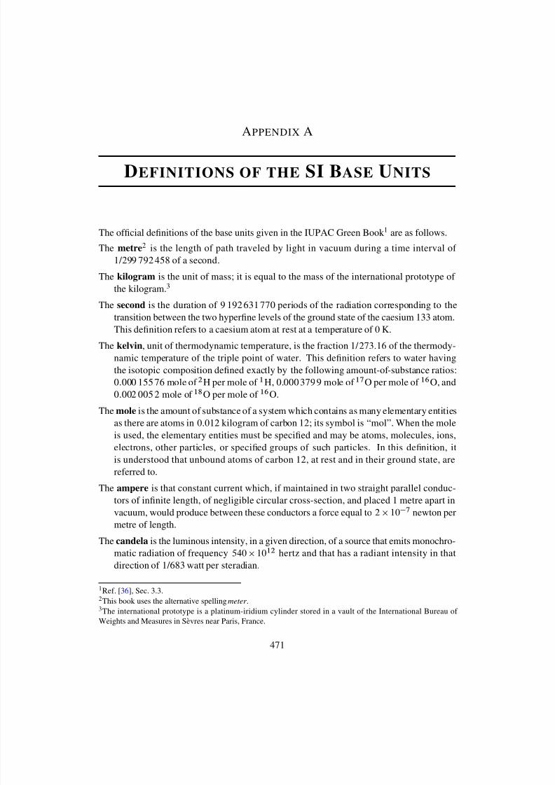
8/12/2019 Howard Devoe Thermodynamic and Chemical
http://slidepdf.com/reader/full/howard-devoe-thermodynamic-and-chemical 471/532
A PPENDIX A
DEFINITIONS OF THE SI BASE UNITS
The ofcial denitions of the base units given in the IUPAC Green Book 1 are as follows.
The metre 2 is the length of path traveled by light in vacuum during a time interval of 1/299 792 458 of a second.
The kilogram is the unit of mass; it is equal to the mass of the international prototype of the kilogram. 3
The second is the duration of 9 192 631 770 periods of the radiation corresponding to thetransition between the two hyperne levels of the ground state of the caesium 133 atom.This denition refers to a caesium atom at rest at a temperature of 0 K.
The kelvin , unit of thermodynamic temperature, is the fraction 1/ 273:16 of the thermody-namic temperature of the triple point of water. This denition refers to water havingthe isotopic composition dened exactly by the following amount-of-substance ratios:0.000 155 76 mole of 2 H per mole of 1 H, 0.000 379 9 mole of 17 O per mole of 16 O, and0.002 005 2 mole of 18 O per mole of 16 O.
The mole is the amount of substance of a system which contains as many elementary entitiesas there are atoms in 0:012 kilogram of carbon 12; its symbol is “mol”. When the moleis used, the elementary entities must be specied and may be atoms, molecules, ions,electrons, other particles, or specied groups of such particles. In this denition, itis understood that unbound atoms of carbon 12, at rest and in their ground state, arereferred to.
The ampere is that constant current which, if maintained in two straight parallel conduc-tors of innite length, of negligible circular cross-section, and placed 1 metre apart invacuum, would produce between these conductors a force equal to 2 10 7 newton permetre of length.
The candela is the luminous intensity, in a given direction, of a source that emits monochro-matic radiation of frequency 540 1012 hertz and that has a radiant intensity in thatdirection of 1/683 watt per steradian.
1Ref. [ 36], Sec. 3.3.2This book uses the alternative spelling meter .3The international prototype is a platinum-iridium cylinder stored in a vault of the International Bureau of Weights and Measures in S evres near Paris, France.
471
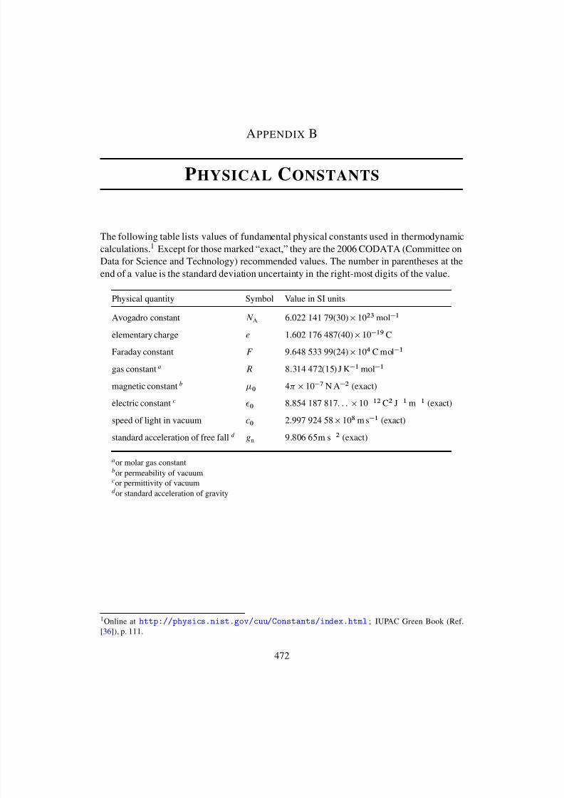
8/12/2019 Howard Devoe Thermodynamic and Chemical
http://slidepdf.com/reader/full/howard-devoe-thermodynamic-and-chemical 472/532
A PPENDIX B
P HYSICAL CONSTANTS
The following table lists values of fundamental physical constants used in thermodynamiccalculations. 1 Except for those marked “exact,” they are the 2006 CODATA (Committee onData for Science and Technology) recommended values. The number in parentheses at theend of a value is the standard deviation uncertainty in the right-most digits of the value.
Physical quantity Symbol Value in SI units
Avogadro constant N A 6.022 141 79(30) 1023 mol 1
elementary charge e 1.602 176 487(40) 10 19 C
Faraday constant F 9.648 533 99(24) 104 C mol 1
gas constant a R 8.314 472(15) J K 1 mol 1
magnetic constant b0 4 10 7 N A 2 (exact)
electric constant c0 8.854 187 817 : : : 10 12 C2 J 1 m 1 (exact)
speed of light in vacuum c0 2.997 924 58 108 m s 1 (exact)
standard acceleration of free fall d gn 9.806 65m s 2 (exact)
a or molar gas constantbor permeability of vacuumcor permittivity of vacuumd or standard acceleration of gravity
1Online at http://physics.nist.gov/cuu/Constants/index.html ; IUPAC Green Book (Ref.[36]), p. 111.
472
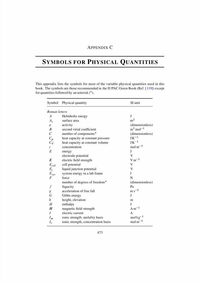
8/12/2019 Howard Devoe Thermodynamic and Chemical
http://slidepdf.com/reader/full/howard-devoe-thermodynamic-and-chemical 473/532
A PPENDIX C
SYMBOLS FOR PHYSICAL QUANTITIES
This appendix lists the symbols for most of the variable physical quantities used in thisbook. The symbols are those recommended in the IUPAC Green Book (Ref. [ 119 ]) exceptfor quantities followed by an asterisk ( ).
Symbol Physical quantity SI unit
Roman lettersA Helmholtz energy JAs surface area m 2
a activity (dimensionless)B second virial coefcient m 3 mol 1
C number of components (dimensionless)C p heat capacity at constant pressure JK 1
C V heat capacity at constant volume JK 1
c concentration mol m
3
E energy Jelectrode potential V
E electric eld strength V m 1
E cell cell potential VE j liquid junction potential VE sys system energy in a lab frame JF force N
number of degrees of freedom (dimensionless)f fugacity Pag acceleration of free fall m s 2
G Gibbs energy Jh height, elevation mH enthalpy JH magnetic eld strength A m 1
I electric current AI m ionic strength, molality basis mol kg 1
I c ionic strength, concentration basis mol m 3
473

8/12/2019 Howard Devoe Thermodynamic and Chemical
http://slidepdf.com/reader/full/howard-devoe-thermodynamic-and-chemical 474/532
A PPENDIX C SYMBOLS FOR P HYSICAL Q UANTITIES 474
(continued from previous page)
Symbol Physical quantity SI unit
K thermodynamic equilibrium constant (dimensionless)K a acid dissociation constant (dimensionless)K p equilibrium constant, pressure basis Pa PK s solubility product (dimensionless)kH;i Henry’s law constant of species i ,
mole fraction basis Pakc;i Henry’s law constant of species i ,
concentration basis Pa m 3 mol 1
km;i Henry’s law constant of species i ,molality basis Pa kg mol 1
l length, distance mL relative partial molar enthalpy Jmol 1
M molar mass kg mol 1
M magnetization A m 1M r relative molecular mass (molecular weight) (dimensionless)m mass kgm i molality of species i mol kg 1
N number of entities (molecules, atoms, ions,formula units, etc.) (dimensionless)
n amount of substance molP number of phases (dimensionless)p pressure Pa
partial pressure PaP dielectric polarization C m 2
Q electric charge CQ sys charge entering system at right conductor CQ rxn reaction quotient (dimensionless)q heat JR el electric resistanceS entropy J K 1
s solubility mol m 3
number of species (dimensionless)T thermodynamic temperature Kt time s
Celsius temperature ı CU internal energy JV volume m 3
v specic volume m 3 kg 1
velocity, speed m s 1
w work Jmass fraction (weight fraction) (dimensionless)
Thermodynamics and Chemistry , second edition, version 4 © 2012 by Howard DeVoe. Latest version: www.chem.umd.edu/thermobook

8/12/2019 Howard Devoe Thermodynamic and Chemical
http://slidepdf.com/reader/full/howard-devoe-thermodynamic-and-chemical 475/532
A PPENDIX C SYMBOLS FOR P HYSICAL Q UANTITIES 475
(continued from previous page)
Symbol Physical quantity SI unit
wel electrical work Jw 0 nonexpansion work Jx mole fraction in a phase (dimensionless)
Cartesian space coordinate my mole fraction in gas phase (dimensionless)
Cartesian space coordinate mZ compression factor (compressibility factor) (dimensionless)z mole fraction in multiphase system (dimensionless)
charge number of an ion (dimensionless)electron number of cell reaction (dimensionless)Cartesian space coordinate m
Greek letters
alpha˛ degree of reaction, dissociation, etc. (dimensionless)
cubic expansion coefcient K 1
gamma surface tension N m 1 , J m 2
i activity coefcient of species i ,pure liquid or solid standard state (dimensionless)
m;i activity coefcient of species i ,molality basis (dimensionless)
c;i activity coefcient of species i ,concentration basis (dimensionless)
x;i activity coefcient of species i ,mole fraction basis (dimensionless) ˙ mean ionic activity coefcient (dimensionless) pressure factor (activity of a reference state) (dimensionless)
epsilon efciency of a heat engine (dimensionless)
energy equivalent of a calorimeter J K 1
theta# angle of rotation (dimensionless)
kappa reciprocal radius of ionic atmosphere m 1
T isothermal compressibility Pa 1
mu chemical potential J mol 1
JT Joule–Thomson coefcient K Pa 1
nu number of ions per formula unit (dimensionless)
Thermodynamics and Chemistry , second edition, version 4 © 2012 by Howard DeVoe. Latest version: www.chem.umd.edu/thermobook
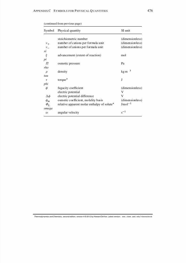
8/12/2019 Howard Devoe Thermodynamic and Chemical
http://slidepdf.com/reader/full/howard-devoe-thermodynamic-and-chemical 476/532
A PPENDIX C SYMBOLS FOR P HYSICAL Q UANTITIES 476
(continued from previous page)
Symbol Physical quantity SI unit
stoichiometric number (dimensionless)C number of cations per formula unit (dimensionless)
number of anions per formula unit (dimensionless) xi
advancement (extent of reaction) mol pi
˘ osmotic pressure Parho
density kg m 3
tau torque J
phi fugacity coefcient (dimensionless)
electric potential V electric potential difference V
m osmotic coefcient, molality basis (dimensionless)˚ L relative apparent molar enthalpy of solute Jmol 1
omega! angular velocity s 1
Thermodynamics and Chemistry , second edition, version 4 © 2012 by Howard DeVoe. Latest version: www.chem.umd.edu/thermobook

8/12/2019 Howard Devoe Thermodynamic and Chemical
http://slidepdf.com/reader/full/howard-devoe-thermodynamic-and-chemical 477/532
A PPENDIX D
M ISCELLANEOUS ABBREVIATIONS AND
SYMBOLS
D.1 PHYSICAL STATES
These abbreviations for physical states (states of aggregation) may be appended in paren-theses to chemical formulas or used as superscripts to symbols for physical quantities. Allbut “mixt” are listed in the IUPAC Green Book (Ref. [ 36], p. 54).
g gas or vaporl liquidf uid (gas or liquid)s solidcd condensed phase (liquid or solid)cr crystallinemixt mixture
sln solutionaq aqueous solutionaq ; 1 aqueous solution at innite dilution
477
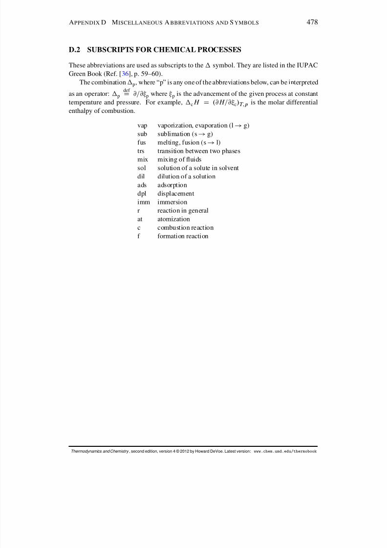
8/12/2019 Howard Devoe Thermodynamic and Chemical
http://slidepdf.com/reader/full/howard-devoe-thermodynamic-and-chemical 478/532
A PPENDIX D M ISCELLANEOUS A BBREVIATIONS AND S YMBOLS 478
D.2 SUBSCRIPTS FOR CHEMICAL PROCESSES
These abbreviations are used as subscripts to the symbol. They are listed in the IUPACGreen Book (Ref. [ 36], p. 59–60).
The combination p , where “p” is any one of the abbreviations below, can be interpreted
as an operator: p
def
D @=@ p where p is the advancement of the given process at constanttemperature and pressure. For example, cH D .@H=@ c/ T;p is the molar differentialenthalpy of combustion.
vap vaporization, evaporation (l ! g)sub sublimation (s ! g)fus melting, fusion (s ! l)trs transition between two phasesmix mixing of uidssol solution of a solute in solventdil dilution of a solutionads adsorptiondpl displacementimm immersionr reaction in generalat atomizationc combustion reactionf formation reaction
Thermodynamics and Chemistry , second edition, version 4 © 2012 by Howard DeVoe. Latest version: www.chem.umd.edu/thermobook
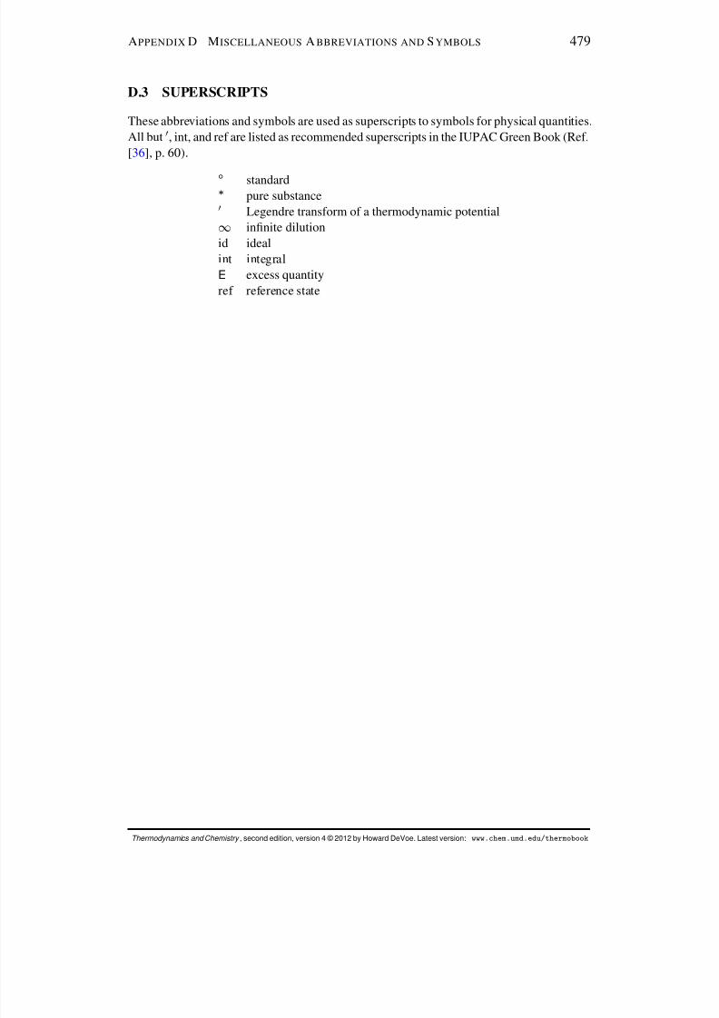
8/12/2019 Howard Devoe Thermodynamic and Chemical
http://slidepdf.com/reader/full/howard-devoe-thermodynamic-and-chemical 479/532
A PPENDIX D M ISCELLANEOUS A BBREVIATIONS AND S YMBOLS 479
D.3 SUPERSCRIPTS
These abbreviations and symbols are used as superscripts to symbols for physical quantities.All but 0, int, and ref are listed as recommended superscripts in the IUPAC Green Book (Ref.[36], p. 60).
ı standardpure substance
0 Legendre transform of a thermodynamic potential
1 innite dilutionid idealint integralE excess quantityref reference state
Thermodynamics and Chemistry , second edition, version 4 © 2012 by Howard DeVoe. Latest version: www.chem.umd.edu/thermobook

8/12/2019 Howard Devoe Thermodynamic and Chemical
http://slidepdf.com/reader/full/howard-devoe-thermodynamic-and-chemical 480/532
A PPENDIX E
C ALCULUS REVIEW
E.1 DERIVATIVES
Let f be a function of the variable x , and let f be the change in f when x changes byx . Then the derivative df = dx is the ratio f = x in the limit as x approaches zero.The derivative d f = dx can also be described as the rate at which f changes with x , and asthe slope of a curve of f plotted as a function of x .
The following is a short list of formulas likely to be needed. In these formulas, u and vare arbitrary functions of x , and a is a constant.
d.u a /dx D au a 1 du
dxd.uv/
dx D udvdx Cv
dudx
d.u=v/dx D
1v2 v
dudx u
dvdx
d ln .ax/dx D 1
xd.e ax /
dx D ae ax
df.u/dx D
df.u/du
dudx
E.2 PARTIAL DERIVATIVES
If f is a function of the independent variables x , y , and z , the partial derivative .@f =@x/y;zis the derivative d f = dx with y and z held constant. It is important in thermodynamics
to indicate the variables that are held constant, as .@f =@x/y;z is not necessarily equal to.@f =@x/a;b where a and b are variables different from y and z .The variables shown at the bottom of a partial derivative should tell you which vari-
ables are being used as the independent variables. For example, if the partial derivative is@f @y a;b
then f is being treated as a function of y , a , and b .
480
8/12/2019 Howard Devoe Thermodynamic and Chemical
http://slidepdf.com/reader/full/howard-devoe-thermodynamic-and-chemical 481/532
A PPENDIX E CALCULUS R EVIEW 481
E.3 INTEGRALS
Let f be a function of the variable x . Imagine the range of x between the limits x 0 and x 00
to be divided into many small increments of size x i .i D 1; 2 ; : : :/ . Let f i be the value of f when x is in the middle of the range of the i th increment. Then the integral
Z x00
x 0f dx
is the sum Pi f i x i in the limit as each x i approaches zero and the number of terms inthe sum approaches innity. The integral is also the area under a curve of f plotted as afunction of x , measured from x D x 0 to x D x 00. The function f is the integrand , whichis integrated over the integration variable x .
This book uses the following integrals:
Z x 00
x 0dx D x 00 x 0
Z x 00
x 0
dxx D ln ˇ
x 00
x 0 ˇZ x 00
x 0x a dx D
1a C1
.x 00/ a C 1 .x 0/ a C 1 (a is a constant other than 1)
Z x 00
x 0
dxax Cb D
1a
ln ˇax 00Cbax 0Cb ˇ (a is a constant)
Here are examples of the use of the expression for the third integral with a set equal to 1and to 2:
Z x 00
x 0x dx D
12
.x 00/ 2 .x 0/ 2
Z x00
x 0
dxx 2 D 1
x 00 1x 0
E.4 LINE INTEGRALS
A line integral is an integral with an implicit single integration variable that constraints theintegration to a path.
The most frequently-seen line integral in this book, R p dV , will serve as an example.The integral can be evaluated in three different ways:
1. The integrand p can be expressed as a function of the integration variable V , so thatthere is only one variable. For example, if p equals c=V where c is a constant, the
line integral is given by R p dV D c R V 2
V 1 .1=V / dV D c ln .V 2 =V 1 / .2. If p and V can be written as functions of another variable, such as time, that coordi-
nates their values so that they follow the desired path, this new variable becomes theintegration variable.
3. The desired path can be drawn as a curve on a plot of p versus V ; then R p dV isequal in value to the area under the curve.
Thermodynamics and Chemistry , second edition, version 4 © 2012 by Howard DeVoe. Latest version: www.chem.umd.edu/thermobook
8/12/2019 Howard Devoe Thermodynamic and Chemical
http://slidepdf.com/reader/full/howard-devoe-thermodynamic-and-chemical 482/532
A PPENDIX F
M ATHEMATICAL PROPERTIES OF STATE
F UNCTIONS
A state function is a property of a thermodynamic system whose value at any given instantdepends only on the state of the system at that instant (Sec. 2.4 ).
F.1 DIFFERENTIALS
The differential df of a state function f is an innitesimal change of f . Since the valueof a state function by denition depends only on the state of the system, integrating d f between an initial state 1 and a nal state 2 yields the change in f , and this change isindependent of the path:
Z f 2
f 1
df D f 2 f 1 D f (F.1.1)
A differential with this property is called an exact differential. The differential of a state
function is always exact.
F.2 TOTAL DIFFERENTIAL
A state function f treated as a dependent variable is a function of a certain number of inde-pendent variables that are also state functions. The total differential of f is df expressedin terms of the differentials of the independent variables and has the form
df D@f @x
dx C@f @y
dy C@f @z
dz C: : : (F.2.1)
There are as many terms in the expression on the right side as there are independent vari-
ables. Each partial derivative in the expression has all independent variables held constantexcept the variable shown in the denominator.Figure F.1 on the next page interprets this expression for a function f of the two in-
dependent variables x and y . The shaded plane represents a small element of the surfacef D f .x ;y/ .
Consider a system with three independent variables. If we choose these independentvariables to be x , y , and z , the total differential of the dependent state function f takes the
482

8/12/2019 Howard Devoe Thermodynamic and Chemical
http://slidepdf.com/reader/full/howard-devoe-thermodynamic-and-chemical 483/532
A PPENDIX F M ATHEMATICAL P ROPERTIES OF S TATE F UNCTIONS 483
o@f @y
x
dy
) @f @x
y
dx9>>=>>;df D
@f @x y dx C
@f @y x dy
x
y
f
d x
d y
slope in f -x plane D@f @x
y
slope in f -y plane D@f @y
x
Figure F.1
formdf D a dx Cb dy Cc dz (F.2.2)
where we can identify the coefcients as
a D@f @x y;z
b D@f @y x;z
c D@f @z x;y
(F.2.3)
These coefcients are themselves, in general, functions of the independent variables andmay be differentiated to give mixed second partial derivatives; for example:
@a@y
x;zD
@2f @y@x
@b@x
y;zD
@2f @x@y
(F.2.4)
The second partial derivative @2f=@y@x, for instance, is the partial derivative with respectto y of the partial derivative of f with respect to x . It is a theorem of calculus that if afunction f is single valued and has continuous derivatives, the order of differentiation in amixed derivative is immaterial. Therefore the mixed derivatives @2f=@y@x and @2f=@x@y,evaluated for the system in any given state, are equal:
@a@y x;z D
@b@x y;z
(F.2.5)
The general relation that applies to a function of any number of independent variables is
@X @y D
@Y @x (F.2.6)
where x and y are any two of the independent variables, X is @f =@x, Y is @f =@y, andeach partial derivative has all independent variables held constant except the variable shownin the denominator. This general relation is the Euler reciprocity relation, or reciprocityrelation for short. A necessary and sufcient condition for d f to be an exact differential isthat the reciprocity relation is satised for each pair of independent variables.
Thermodynamics and Chemistry , second edition, version 4 © 2012 by Howard DeVoe. Latest version: www.chem.umd.edu/thermobook
8/12/2019 Howard Devoe Thermodynamic and Chemical
http://slidepdf.com/reader/full/howard-devoe-thermodynamic-and-chemical 484/532
A PPENDIX F M ATHEMATICAL P ROPERTIES OF S TATE F UNCTIONS 484
F.3 INTEGRATION OF A TOTAL DIFFERENTIAL
If the coefcients of the total differential of a dependent variable are known as functionsof the independent variables, the expression for the total differential may be integrated toobtain an expression for the dependent variable as a function of the independent variables.
For example, suppose the total differential of the state function f .x; y;z/ is given byEq. F.2.2 and the coefcients are known functions a.x;y;z/ , b.x;y;z/ , and c.x;y;z/ .Because f is a state function, its change between f.0;0;0/ and f .x 0; y 0; z 0/ is independentof the integration path taken between these two states. A convenient path would be one withthe following three segments:
1. integration from .0; 0;0/ to .x 0;0;0/ : R x 0
0 a.x;0;0/ dx
2. integration from .x 0;0;0/ to .x 0; y 0; 0/ : R y 0
0 b.x 0;y ;0 / dy
3. integration from .x 0; y 0; 0/ to .x 0; y 0; z 0/ : R z 0
0 c.x 0; y 0; z/ dzThe expression for f .x; y;z/ is then the sum of the three integrals and a constant of inte-gration.
Here is an example of this procedure applied to the total differential
df D .2xy/ dx C.x 2 Cz/ dy C.y 9z 2 / dz (F.3.1)
An expression for the function f in this example is given by the sum
f DZ x 0
0.2x 0/ dx CZ
y 0
0Œ.x0/ 2 C0 dy CZ
z 0
0.y 0 9z 2 / dz CC
D 0 Cx 2 y C.yz 9z 3 =3/ CC
D x 2 y Cyz 3z 3 CC (F.3.2)
where primes are omitted on the second and third lines because the expressions are supposedto apply to any values of x , y , and z . C is an integration constant. You can verify that thethird line of Eq. F.3.2 gives the correct expression for f by taking partial derivatives withrespect to x , y , and z and comparing with Eq. F.3.1 .
In chemical thermodynamics, there is not likely to be occasion to perform this kindof integration. The fact that it can be done, however, shows that if we stick to one set of independent variables, the expression for the total differential of an independent variablecontains the same information as the independent variable itself.
A different kind of integration can be used to express a dependent extensive propertyin terms of independent extensive properties. An extensive property of a thermodynamicsystem is one that is additive, and an intensive property is one that is not additive and hasthe same value everywhere in a homogeneous region (Sec. 2.1.1 ). Suppose we have a state
function f that is an extensive property with the total differential
df D a dx Cb dy Cc dz C: : : (F.3.3)
where the independent variables x; y ; z ; : : : are extensive and the coefcients a; b ; c ; : : :are intensive. If the independent variables include those needed to describe an open system(for example, the amounts of the substances), then it is possible to integrate both sides of
Thermodynamics and Chemistry , second edition, version 4 © 2012 by Howard DeVoe. Latest version: www.chem.umd.edu/thermobook
8/12/2019 Howard Devoe Thermodynamic and Chemical
http://slidepdf.com/reader/full/howard-devoe-thermodynamic-and-chemical 485/532
A PPENDIX F M ATHEMATICAL P ROPERTIES OF S TATE F UNCTIONS 485
the equation from a lower limit of zero for each of the extensive functions while holding theintensive functions constant:
Z f 0
0df D a Z
x 0
0dx Cb Z
y 0
0dy Cc Z
z 0
0dz C: : : (F.3.4)
f 0
D ax0
Cby0
Ccz0
C: : : (F.3.5)Note that a term of the form c du where u is intensive becomes zero when integrated withintensive functions held constant, because d u is this case is zero.
F.4 LEGENDRE TRANSFORMS
A Legendre transform of a state function is a linear change of one or more of the indepen-dent variables made by subtracting products of conjugate variables.
To understand how this works, consider a state function f whose total differential isgiven by
df D a dx Cb dy Cc dz (F.4.1)
In the expression on the right side, x , y , and z are being treated as the independent variables.The pairs a and x , b and y , and c and z are conjugate pairs . That is, a and x are conjugates,b and y are conjugates, and c and z are conjugates.
For the rst example of a Legendre transform, we dene a new state function f 1 bysubtracting the product of the conjugate variables a and x :
f 1def
D f ax (F.4.2)
The function f 1 is a Legendre transform of f . We take the differential of Eq. F.4.2
df 1 D df a dx x da (F.4.3)
and substitute for d f from Eq. F.4.1 :df 1 D .a dx Cb dy Cc dz/ a dx x da
D x da Cb dy Cc dz (F.4.4)
Equation F.4.4 gives the total differential of f 1 with a , y , and z as the independent variables.The functions x and a have switched places as independent variables. What we did in orderto let a replace x as an independent variable was to subtract from f the product of theconjugate variables a and x .
Because the right side of Eq. F.4.4 is an expression for the total differential of the statefunction f 1 , we can use the expression to identify the coefcients as partial derivatives of f 1 with respect to the new set of independent variables:
x D@f 1@a y;z
b D@f 1@y a;z
c D@f 1@z a;y
(F.4.5)
We can also use Eq. F.4.4 to write new reciprocity relations, such as
@x@y a;z D
@b@a y;z
(F.4.6)
Thermodynamics and Chemistry , second edition, version 4 © 2012 by Howard DeVoe. Latest version: www.chem.umd.edu/thermobook
8/12/2019 Howard Devoe Thermodynamic and Chemical
http://slidepdf.com/reader/full/howard-devoe-thermodynamic-and-chemical 486/532
A PPENDIX F M ATHEMATICAL P ROPERTIES OF S TATE F UNCTIONS 486
We can make other Legendre transforms of f by subtracting one or more products of conjugate variables. A second example of a Legendre transform is
f 2def
D f by cz (F.4.7)
whose total differential is
df 2 D df b dy y db c dz z dc
D a dx y db z dc (F.4.8)
Here b has replaced y and c has replaced z as independent variables. Again, we can identifythe coefcients as partial derivatives and write new reciprocity relations.
If we have an algebraic expression for a state function as a function of independent vari-ables, then a Legendre transform preserves all the information contained in that expression.To illustrate this, we can use the state function f and its Legendre transform f 2 describedabove. Suppose we have an expression for f .x; y;z/ —this is f expressed as a function of the independent variables x , y , and z . Then by taking partial derivatives of this expression,
we can nd according to Eq. F.2.3 expressions for the functions a.x; y;z/ , b.x;y; z/ , andc.x;y;z/ .Now we perform the Legendre transform of Eq. F.4.7 : f 2 D f by cz with total
differential d f 2 D a dx y db z dc (Eq. F.4.8 ). The independent variables have beenchanged from x , y , and z to x , b , and c.
We want to nd an expression for f 2 as a function of these new variables, using theinformation available from the original function f .x ;y;z/ . To do this, we eliminate zfrom the known functions b.x; y;z/ and c.x; y;z/ and solve for y as a function of x , b,and c. We also eliminate y from b.x;y;z/ and c.x;y;z/ and solve for z as a functionof x , b , and c . This gives us expressions for y.x; b;c/ and z.x;b; c/ which we substituteinto the expression for f .x ;y;z/ , turning it into the function f .x ;b;c/ . Finally, we usethe functions of the new variables to obtain an expression for f 2 .x;b;c/
D f .x ;b;c/
by.x;b;c/ cz.x;b;c/ .The original expression for f .x ;y;z/ and the new expression for f 2 .x;b;c/ contain
the same information. We could take the expression for f 2 .x;b;c/ and, by following thesame procedure with the Legendre transform f D f 2 Cby Ccz , retrieve the expressionfor f .x; y;z/ . Thus no information is lost during a Legendre transform.
Thermodynamics and Chemistry , second edition, version 4 © 2012 by Howard DeVoe. Latest version: www.chem.umd.edu/thermobook

8/12/2019 Howard Devoe Thermodynamic and Chemical
http://slidepdf.com/reader/full/howard-devoe-thermodynamic-and-chemical 487/532
A PPENDIX G
F ORCES , E NERGY , AND WORK
The aim of this appendix is to describe a simple model that will help to clarify the meaningof energy and mechanical work in macroscopic systems. The appendix applies fundamentalprinciples of classical mechanics to a collection of material particles representing a closedsystem and its surroundings. Although classical mechanics cannot duplicate all features of a chemical system—for instance, quantum properties of atoms are ignored—the behaviorof the particles and their interactions will show us how to evaluate the thermodynamic work in a real system.
In broad outline the derivation is as follows. An inertial reference frame in which New-ton’s laws of motion are valid is used to describe the positions and velocities of the particles.The particles are assumed to exert central forces on one another, such that between any twoparticles the force is a function only of the interparticle distance and is directed along theline between the particles.
We dene the kinetic energy of the collection of particles as the sum for all particlesof 1
2 mv 2 (where m is mass and v is velocity). We dene the potential energy as the sumover pairwise particle–particle interactions of potential functions that depend only on theinterparticle distances. The total energy is the sum of the kinetic and potential energies.With these denitions and Newton’s laws, a series of mathematical operations leads to theprinciple of the conservation of energy: the total energy remains constant over time.
Continuing the derivation, we consider one group of particles to represent a closed ther-modynamic system and the remaining particles to constitute the surroundings. The systemparticles may interact with an external force eld, such as a gravitational eld, created bysome of the particles in the surroundings. The energy of the system is considered to be thesum of the kinetic energy of the system particles, the potential energy of pairwise particle–particle interactions within the system, and the potential energy of the system particles inany external eld or elds. The change in the system energy during a time interval is thenfound to be given by a certain sum of integrals which, in the transition to a macroscopic
model, becomes the sum of heat and thermodynamic work in accord with the rst law of thermodynamics.
A similar derivation, using a slightly different notation, is given in Ref. [ 44].
487
8/12/2019 Howard Devoe Thermodynamic and Chemical
http://slidepdf.com/reader/full/howard-devoe-thermodynamic-and-chemical 488/532
APPENDIX G FORCES, ENERGY, AND WORKG.1 F ORCES BETWEEN PARTICLES 488
G.1 FORCES BETWEEN PARTICLES
A material particle is a body that has mass and is so small that it behaves as a point,without rotational energy or internal structure. We assume each particle has a constant mass,ignoring relativistic effects that are important only when the particle moves at a speed closeto the speed of light.
Consider a collection of an arbitrary number of material particles that have interactionsonly among themselves and with no other particles. Later we will consider some of theparticles to constitute a thermodynamic system and the others to be the surroundings .
Newton’s laws of motion are obeyed only in an inertial reference frame. A referenceframe that is xed or moving at a constant velocity relative to local stars is practically aninertial reference frame. To a good approximation, a reference frame xed relative to theearth’s surface is also an inertial system (the necessary corrections are discussed in Sec.G.10 ). This reference frame will be called simply the lab frame , and treated as an inertialframe in order that we may apply Newton’s laws.
It will be assumed that the Cartesian components of all vector quantities appearing inSections G.1 –G.4 are measured in an inertial lab frame.
Classical mechanics is based on the idea that one material particle acts on another bymeans of a force that is independent of the reference frame. Let the vector F ij denote theforce exerted on particle i by particle j .1 The net force F i acting on particle i is the vectorsum of the individual forces exerted on it by the other particles: 2
F i DXj ¤ i
F ij (G.1.1)
(The term in which j equals i has to be omitted because a particle does not act on itself.)According to Newton’s second law of motion, the net force F i acting on particle i is equalto the product of its mass mi and its acceleration:
F i D m idv
id t (G.1.2)
Here v i is the particle’s velocity in the lab frame and t is time.A nonzero net force causes particle i to accelerate and its velocity and position to
change. The work done by the net force acting on the particle in a given time intervalis dened by the integral 3
W i DZ F i dr i (G.1.3)
where r i is the position vector of the particle—a vector from the origin of the lab frame tothe position of the particle.
1This and the next two footnotes are included for readers who are not familiar with vector notation. The quantity
F ij is printed in boldface to indicate it is a vector having both magnitude and direction.2The rule for adding vectors, as in the summation shown here, is that the sum is a vector whose componentalong each axis of a Cartesian coordinate system is the sum of the components along that axis of the vectorsbeing added. For example, the vector C D A CB has components C x D Ax CBx , C y D Ay CBy , andC z D Az CBz .3The dot between the vectors in the integrand indicates a scalar product or dot product, which is a non vectorquantity. The general denition of the scalar product of two vectors, A and B , is A B D AB cos ˛ where Aand B are the magnitudes of the two vectors and ˛ is the angle between their positive directions.
Thermodynamics and Chemistry , second edition, version 4 © 2012 by Howard DeVoe. Latest version: www.chem.umd.edu/thermobook
8/12/2019 Howard Devoe Thermodynamic and Chemical
http://slidepdf.com/reader/full/howard-devoe-thermodynamic-and-chemical 489/532
APPENDIX G FORCES, ENERGY, AND WORKG.1 F ORCES BETWEEN PARTICLES 489
The integral on the right side of Eq. G.1.3 is an example of a line integral . It indicatesthat the scalar product of the net force acting on the particle and the particle’s displace-ment is to be integrated over time during the time interval. The integral can be writtenwithout vectors in the form R F i cos ˛. ds= d t / d t where F i is the magnitude of the netforce, d s= d t is the magnitude of the velocity of the particle along its path in three-dimensional space, and ˛ is the angle between the force and velocity vectors. The
three quantities F i , cos ˛ , and ds= d t are all functions of time, t , and the integration iscarried out with time as the integration variable.
By substituting the expression for F i (Eq. G.1.2 ) in Eq. G.1.3 , we obtain
W i D m i Z dv i
d tdr i D m i Z dr i
d tdv i D m i Z vi
dv i D m i Z vi dvi
D 12 m i v2
i (G.1.4)
where vi is the magnitude of the velocity.The quantity 1
2 m i v2i is called the kinetic energy of particle i . This kinetic energy de-
pends only on the magnitude of the velocity (i.e., on the speed) and not on the particle’sposition.
The total work W tot done by all forces acting on all particles during the time interval isthe sum of W i for all particles: W tot DPi W i .4 Equation G.1.4 then gives us
W tot DXi
12 m i v2
i D Xi
12 m i v2
i ! (G.1.5)
Equation G.1.5 shows that the total work during a time interval is equal to the change inthe total kinetic energy in this interval. This result is called the “work-energy principle” byphysicists. 5
From Eqs. G.1.1 and G.1.3 we obtain a second expression for W tot :
W tot DXi W i DXi Z Xj ¤ iF ij
dr i DXi Xj ¤ i Z F ij
dr i (G.1.6)
The double sum in the right-most expression can be written as a sum over pairs of particles,the term for the pair i and j being
Z F ij dr i CZ F j i dr j DZ F ij dr i Z F ij dr j
DZ F ij d. r i r j / DZ . F ij e ij / dr ij (G.1.7)
Here we have used the relations F j i D F ij (from Newton’s third law) and . r i r j / De ij r ij , where e ij is a unit vector pointing from j to i and r ij is the distance between the
particles. Equation G.1.6 becomes
W tot DXi Xj ¤ i Z F ij dr i DXi Xj >i Z . F ij e ij / dr ij (G.1.8)
4The work W tot dened here is not the same as the thermodynamic work appearing in the rst law of thermo-dynamics.5Ref. [ 149 ], p. 95.
Thermodynamics and Chemistry , second edition, version 4 © 2012 by Howard DeVoe. Latest version: www.chem.umd.edu/thermobook
8/12/2019 Howard Devoe Thermodynamic and Chemical
http://slidepdf.com/reader/full/howard-devoe-thermodynamic-and-chemical 490/532
APPENDIX G FORCES, ENERGY, AND WORKG.1 F ORCES BETWEEN PARTICLES 490
Next we look in detail at the force that particle j exerts on particle i . This force dependson the nature of the two particles and on the distance between them. For instance, Newton’slaw of universal gravitation gives the magnitude of a gravitational force as Gm i mj =r 2
ij ,where G is the gravitational constant. Coulomb’s law gives the magnitude of an electricalforce between stationary charged particles as Q i Q j =.4 0 r 2
ij / , where Q i and Q j are the
charges and 0 is the electric constant (or permittivity of vacuum). These two kinds of forcesare central forces that obey Newton’s third law of action and reaction, namely, that the forcesexerted by two particles on one another are equal in magnitude and opposite in direction andare directed along the line joining the two particles. (In contrast, the electromagnetic forcebetween charged particles in relative motion does not obey Newton’s third law.)
We will assume the force F ij exerted on particle i by particle j has a magnitude thatdepends only on the interparticle distance r ij and is directed along the line between i andj , as is true of gravitational and electrostatic forces and on intermolecular forces in general.Then we can dene a potential function , ˚ ij , for this force that will be a contribution tothe potential energy. To see how ˚ ij is related to F ij , we look at Eq. G.1.7 . The left-mostexpression,
R F ij dr i C
R F j i
dr j , is the change in the kinetic energies of particles i andj during a time interval (see Eq. G.1.4 ). If these were the only particles, their total energyshould be constant for conservation of energy; thus ˚ ij should have the same magnitudeand the opposite sign of the kinetic energy change:
˚ ij D Z . F ij e ij / dr ij (G.1.9)
The value of ˚ ij at any interparticle distance r ij is fully dened by Eq. G.1.9 and the choiceof an arbitrary zero. The quantity .F ij e ij / is simply the component of the force along theline between the particles, and is negative for an attractive force (one in which F ij pointsfrom i to j ) and positive for a repulsive force. If the force is attractive, the value of ˚ ij increases with increasing rij ; if the force is repulsive, ˚ ij decreases with increasing rij .Since ˚ ij is a function only of r ij , it is independent of the choice of reference frame.
Equations G.1.8 and G.1.9 can be combined to give
W tot D Xi Xj >i
˚ ij D 0@Xi Xj >i
˚ ij 1A (G.1.10)
By equating the expressions for W tot given by Eqs. G.1.5 and G.1.10 and rearranging, weobtain
Xi
12 m i v2
i !C 0@Xi Xj >i
˚ ij 1A D 0 (G.1.11)
This equation shows that the quantity
E tot DXi
12 m i v2
i CXi Xj >i
˚ ij (G.1.12)
is constant over time as the particles move in response to the forces acting on them. Therst term on the right side of Eq. G.1.12 is the total kinetic energy of the particles. Thesecond term is the pairwise sum of particle–particle potential functions; this term is called
Thermodynamics and Chemistry , second edition, version 4 © 2012 by Howard DeVoe. Latest version: www.chem.umd.edu/thermobook

8/12/2019 Howard Devoe Thermodynamic and Chemical
http://slidepdf.com/reader/full/howard-devoe-thermodynamic-and-chemical 491/532
APPENDIX G FORCES, ENERGY, AND WORKG.2 T HE S YSTEM AND S URROUNDINGS 491
(a)
˚ ij
˚ ik
˚ kl
(b)
˚ ij
˚ ik 0˚ ik 00
Figure G.1 Assignment of particles to groups, and some representative particle–particle potential functions (schematic). The closed dashed curve represents the sys-tem boundary.(a) The open circles represent particles in the system, and the lled circles are particlesin the surroundings.(b) The lled triangles are particles in the surroundings that are the source of a con-servative force eld for particles in the system.
the potential energy of the particles. Note that the kinetic energy depends only on particlespeeds and the potential energy depends only on particle positions.
The signicance of Eq. G.1.11 is that the total energy E tot dened by Eq. G.1.12 isconserved . This will be true provided the reference frame used for kinetic energy is inertialand the only forces acting on the particles are those responsible for the particle–particlepotential functions.
G.2 THE SYSTEM AND SURROUNDINGS
Now we are ready to assign the particles to two groups: particles in the system and those in
the surroundings. This section will use the following convention: indices i and j refer toparticles in the system ; indices k and l refer to particles in the surroundings . This divisionof particles is illustrated schematically in Fig. G.1(a). With this change in notation, Eq.G.1.12 becomes
E tot DXi
12 m i v2
i CXi Xj >i
˚ ij CXi Xk
˚ ik CXk
12 mk v2
k CXk Xl>k
˚ kl (G.2.1)
A portion of the surroundings may create a time-independent conservative force eld(an “external” eld) for a particle in the system. In order for such a eld to be present,its contribution to the force exerted on the particle and to the particle’s potential energymust depend only on the particle’s position in the lab frame. The usual gravitational and
electrostatic elds are of this type.In order to clarify the properties of a conservative external eld, the index k0 will be
used for those particles in the surroundings that are not the source of an external eld, andk 00for those that are, as indicated in Fig. G.1 (b). Then the force exerted on system particlei due to the eld is F eld
i DPk 00 F ik 00. If this were the only force acting on particle i ,the change in its kinetic energy during a time interval would be R F eld
i dr i (Eq. G.1.4 ).
Thermodynamics and Chemistry , second edition, version 4 © 2012 by Howard DeVoe. Latest version: www.chem.umd.edu/thermobook
8/12/2019 Howard Devoe Thermodynamic and Chemical
http://slidepdf.com/reader/full/howard-devoe-thermodynamic-and-chemical 492/532
APPENDIX G FORCES, ENERGY, AND WORKG.2 T HE S YSTEM AND S URROUNDINGS 492
For conservation of energy, the potential energy change in the time interval should have thesame magnitude and the opposite sign:
˚ eldi D Z F eld
i dr i (G.2.2)
Only if the integral R F eldi dr i has the same value for all paths between the initial andnal positions of the particle does a conservative force eld exist; otherwise the concept of a potential energy ˚ eld
i is not valid.Taking a gravitational eld as an example of a conservative external eld, we replace
F eldi and ˚ eld
i by F gravi and ˚ grav
i : ˚ gravi D R F grav
i dr i . The gravitational force on
particle i is, from Newton’s rst law, the product of the particle mass and its accelerationg ez in the gravitational eld: F grav
i D m i g ez where g is the acceleration of free falland ez is a unit vector in the vertical (upward) z direction. The change in the gravitationalpotential energy given by Eq. G.2.2 is
˚ gravi D m i g
Z ez
dr i D m i g z i (G.2.3)
(The range of elevations of the system particles is assumed to be small compared with theearth’s radius, so that each system particle experiences essentially the same constant valueof g .) Thus we can dene the gravitational potential energy of particle i , which is a functiononly of the particle’s vertical position in the lab frame, by ˚ grav
i D m i gz i CC i where C i isan arbitrary constant.
Returning to Eq. G.2.1 for the total energy, we can now write the third term on the rightside in the form
Xi Xk
˚ ik DXi Xk 0
˚ ik 0 CXi
˚ eldi (G.2.4)
To divide the expression for the total energy into meaningful parts, we substitute Eq. G.2.4
in Eq. G.2.1 and rearrange in the form
E tot D24Xi
12 m i v2
i CXi Xj >i
˚ ij CXi
˚ eldi 35
C"Xi Xk 0
˚ ik 0#C"Xk
12 mk v2
k CXk Xl>k
˚ kl # (G.2.5)
The terms on the right side of this equation are shown grouped with brackets into threequantities. The rst quantity depends only on the speeds and positions of the particles inthe system , and thus represents the energy of the system:
E sys DXi
12 m i v2
i CXi Xj >i
˚ ij CXi
˚ eldi (G.2.6)
The three terms in this expression for E sys are, respectively, the kinetic energy of the systemparticles relative to the lab frame, the potential energy of interaction among the systemparticles, and the total potential energy of the system in the external eld.
Thermodynamics and Chemistry , second edition, version 4 © 2012 by Howard DeVoe. Latest version: www.chem.umd.edu/thermobook
8/12/2019 Howard Devoe Thermodynamic and Chemical
http://slidepdf.com/reader/full/howard-devoe-thermodynamic-and-chemical 493/532
APPENDIX G FORCES, ENERGY, AND WORKG.3 S YSTEM E NERGY C HANGE 493
The last bracketed quantity on the right side of Eq. G.2.5 depends only on the speedsand positions of all the particles in the surroundings , so that this quantity is the energy of the surroundings, E surr . Thus, an abbreviated form of Eq. G.2.5 is
E tot D E sys C
Xi
Xk 0
˚ ik 0 CE surr (G.2.7)
The quantity Pi Pk 0 ˚ ik 0 represents potential energy shared by both the system and sur-roundings on account of forces acting across the system boundary, other than gravita-tional forces or forces from other external elds. The forces responsible for the quantity
Pi Pk 0 ˚ ik 0 are generally signicant only between particles in the immediate vicinity of the system boundary, and will presently turn out to be the crucial forces for evaluatingthermodynamic work.
G.3 SYSTEM ENERGY CHANGE
This section derives an important relation between the change E sys of the energy of the
system measured in a lab frame, and the forces exerted by the surroundings on the systemparticles. The indices i and j will refer to only the particles in the system .
We write the net force on particle i in the form
F i DXj ¤ i
F ij CF eldi CF sur
i (G.3.1)
where F ij is the force exerted on particle i by particle j , both particles being in the system,and F sur
i DPk 0 F ik 0 is the net force exerted on particle i by the particles in the surround-ings that are not the source of an external eld. During a given period of time, the work done by forces acting on only the system particles is
Xi Z F i dr i DXi Xj ¤ i Z F ij dr i CXi Z F eldi
dr i CXi Z F suri
dr i (G.3.2)
We can replace the rst three sums in this equation with new expressions. Using Eq.G.1.4 , we have
Xi Z F i dr i D Xi
12 m i v2
i ! (G.3.3)
From Eqs. G.1.8 and G.1.9 we obtain
Xi Xj ¤ i Z F ij dr i
D 0@Xi Xj >i
˚ ij
1A (G.3.4)
where the sums are over the system particles. From Eq. G.2.2 we can write
Xi Z F eldi
dr i D Xi
˚ eldi ! (G.3.5)
Thermodynamics and Chemistry , second edition, version 4 © 2012 by Howard DeVoe. Latest version: www.chem.umd.edu/thermobook

8/12/2019 Howard Devoe Thermodynamic and Chemical
http://slidepdf.com/reader/full/howard-devoe-thermodynamic-and-chemical 494/532
APPENDIX G FORCES, ENERGY, AND WORKG.4 M ACROSCOPIC W ORK 494
Combining Eqs. G.3.2 –G.3.5 and rearranging, we obtain
Xi Z F suri
dr i D 0@Xi
12 m i v2
i CXi Xj >i
˚ ij CXi
˚ eldi 1A
(G.3.6)
Comparison of the expression on the right side of this equation with Eq. G.2.6 shows thatthe expression is the same as the change of E sys :
E sys DXi Z F suri
dr i (G.3.7)
Recall that the vector F suri is the force exerted on particle i , in the system, by the particles in
the surroundings other than those responsible for an external eld. Thus E sys is equal tothe total work done on the system by the surroundings, other than work done by an externaleld such as a gravitational eld.
It might seem strange that work done by an external eld is not included in E sys . Thereason it is not included is that ˚ eld
i was dened to be a potential energy belongingonly to the system, and is thus irrelevant to energy transfer from or to the surroundings.
As a simple example of how this works, consider a system consisting of a solidbody in a gravitational eld. If the only force exerted on the body is the downwardgravitational force, then the body is in free fall but E sys in the lab frame is zero; theloss of gravitational potential energy as the body falls is equal to the gain of kineticenergy. On the other hand, work done on the system by an external force that opposesthe gravitational force is included in E sys . For example, if the body is pulled upwardsat a constant speed with a string, its potential energy increases while its kinetic energyremains constant, and E sys increases.
G.4 MACROSCOPIC WORK
In thermodynamics we are interested in the quantity of work done on macroscopic parts of the system during a process, rather than the work done on individual particles. Macroscopicwork is the energy transferred across the system boundary due to concerted motion of manyparticles on which the surroundings exert a force. Macroscopic mechanical work occurswhen there is displacement of a macroscopic portion of the system on which a short-rangecontact force acts across the system boundary. This force could be, for instance, the pressureof an external uid at a surface element of the boundary multiplied by the area of the surfaceelement, or it could be the tension in a cord at the point where the cord passes through theboundary.
The symbol wlab will refer to macroscopic work measured with displacements in the
lab frame.At any given instant, only the system particles that are close to the boundary will havenonnegligible contact forces exerted on them. We can dene an interaction layer , a thinshell-like layer within the system and next to the system boundary that contains all thesystem particles with appreciable contact forces. We imagine the interaction layer to bedivided into volume elements, or segments, each of which either moves as a whole duringthe process or else is stationary. Let R be a position vector from the origin of the lab frame
Thermodynamics and Chemistry , second edition, version 4 © 2012 by Howard DeVoe. Latest version: www.chem.umd.edu/thermobook

8/12/2019 Howard Devoe Thermodynamic and Chemical
http://slidepdf.com/reader/full/howard-devoe-thermodynamic-and-chemical 495/532
APPENDIX G FORCES, ENERGY, AND WORKG.4 M ACROSCOPIC W ORK 495
R
r i
r i
Figure G.2 Position vectors within the system. Segment of the interaction layerlies within the heavy curve (representing the system boundary) and the dashed lines.Open circle: origin of lab frame; open square: point xed in system boundary atsegment ; lled circle: particle i .
to a point xed in the boundary at segment , and let r i be a vector from this point toparticle i (Fig. G.2 ). Then the position vector for particle i can be written r i D R Cr i .Let F sur
be the total contact force exerted by the surroundings on the system particles insegment : F sur
DPi • i F suri , where • i is equal to 1 when particle i is in segment and
is zero otherwise.The change in the system energy during a process is, from Eq. G.3.7 ,
E sys DXi Z F suri
dr i DX Xi Z •i F suri
d . R Cr i /
DX Z F sur
dR CX Xi Z •i F suri
dr i (G.4.1)
We recognize the integral R F sur dR as the macroscopic work at surface element ,because it is the integrated scalar product of the force exerted by the surroundings and thedisplacement. The total macroscopic work during the process is then given by
w lab DX Z F sur
dR (G.4.2)
Heat , qlab , can be dened as energy transfer to or from the system that is not accountedfor by macroscopic work. This transfer occurs by means of chaotic motions and collisionsof individual particles at the boundary. With this understanding, Eq. G.4.1 becomes
E sys
D qlab
Cw lab (G.4.3)
with wlab given by the expression in Eq. G.4.2 and qlab given by
qlab DX Xi Z •i F suri
dr i (G.4.4)
Thermodynamics and Chemistry , second edition, version 4 © 2012 by Howard DeVoe. Latest version: www.chem.umd.edu/thermobook
8/12/2019 Howard Devoe Thermodynamic and Chemical
http://slidepdf.com/reader/full/howard-devoe-thermodynamic-and-chemical 496/532
APPENDIX G FORCES, ENERGY, AND WORKG.5 T HE W ORK D ONE ON THE S YSTEM AND S URROUNDINGS 496
G.5 THE WORK DONE ON THE SYSTEM AND SURROUNDINGS
An additional comment can be made about the transfer of energy between the system andthe surroundings. We may use Eq. G.4.2 , with appropriate redenition of the quantities onthe right side, to evaluate the work done on the surroundings . This work may be equal inmagnitude and opposite in sign to the work wlab done on the system. A necessary conditionfor this equality is that the interacting parts of the system and surroundings have equaldisplacements; that is, that there be continuity of motion at the system boundary. We expectthere to be continuity of motion when a uid contacts a moving piston or paddle.
Suppose, however, that the system is stationary and an interacting part of the surround-ings moves. Then according to Eq. G.4.2 , wlab is zero, whereas the work done on or by thatpart of the surroundings is not zero. How can this be, considering that E tot remains con-stant? One possibility, discussed by Bridgman, 6 is sliding friction at the boundary: energylost by the surroundings in the form of work is gained by the system and surroundings inthe form of thermal energy. Since the effect on the system is the same as a ow of heatfrom the surroundings, the division of energy transfer into heat and work can be ambiguouswhen there is sliding friction at the boundary. 7
Another way work can have different magnitudes for system and surroundings is achange in potential energy shared by the system and surroundings. This shared energyis associated with forces acting across the boundary, other than from a time-independentexternal eld, and is represented in Eq. G.2.7 by the sum Pi Pk 0 ˚ ik 0. In the usual typesof processes this sum is either practically constant, or else each term falls off so rapidlywith distance that the sum is negligible. Since E tot is constant, during such processes thequantity E sys CE surr remains essentially constant.
G.6 THE LOCAL FRAME AND INTERNAL ENERGY
As explained in Sec. 2.6.2 , a lab frame may not be an appropriate reference frame in which
to measure changes in the system’s energy. This is the case when the system as a wholemoves or rotates in the lab frame, so that E sys depends in part on external coordinates thatare not state functions. In this case it may be possible to dene a local frame moving withthe system in which the energy of the system is a state function, the internal energy U .
As before, r i is the position vector of particle i in a lab frame. A prime notation willbe used for quantities measured in the local frame. Thus the position of particle i relativeto the local frame is given by vector r 0
i , which points from the origin of the local frame toparticle i (see Fig. G.3 ). The velocity of the particle in the local frame is v0
i D dr 0i = d t .
We continue to treat the earth-xed lab frame as an inertial frame, although this is notstrictly true (Sec. G.10 ). If the origin of the local frame moves at constant velocity in the labframe, with Cartesian axes that do not rotate with respect to those of the lab frame, then the
6Ref. [ 23], p. 47–56.7The ambiguity can be removed by redening the system boundary so that a thin stationary layer next tothe sliding interface, on the side that was originally part of the system, is considered to be included in thesurroundings instead of the system. The layer removed from the system by this change can be so thin that thevalues of the system’s extensive properties are essentially unaffected. With this redened boundary, the energytransfer across the boundary is entirely by means of heat.
Thermodynamics and Chemistry , second edition, version 4 © 2012 by Howard DeVoe. Latest version: www.chem.umd.edu/thermobook
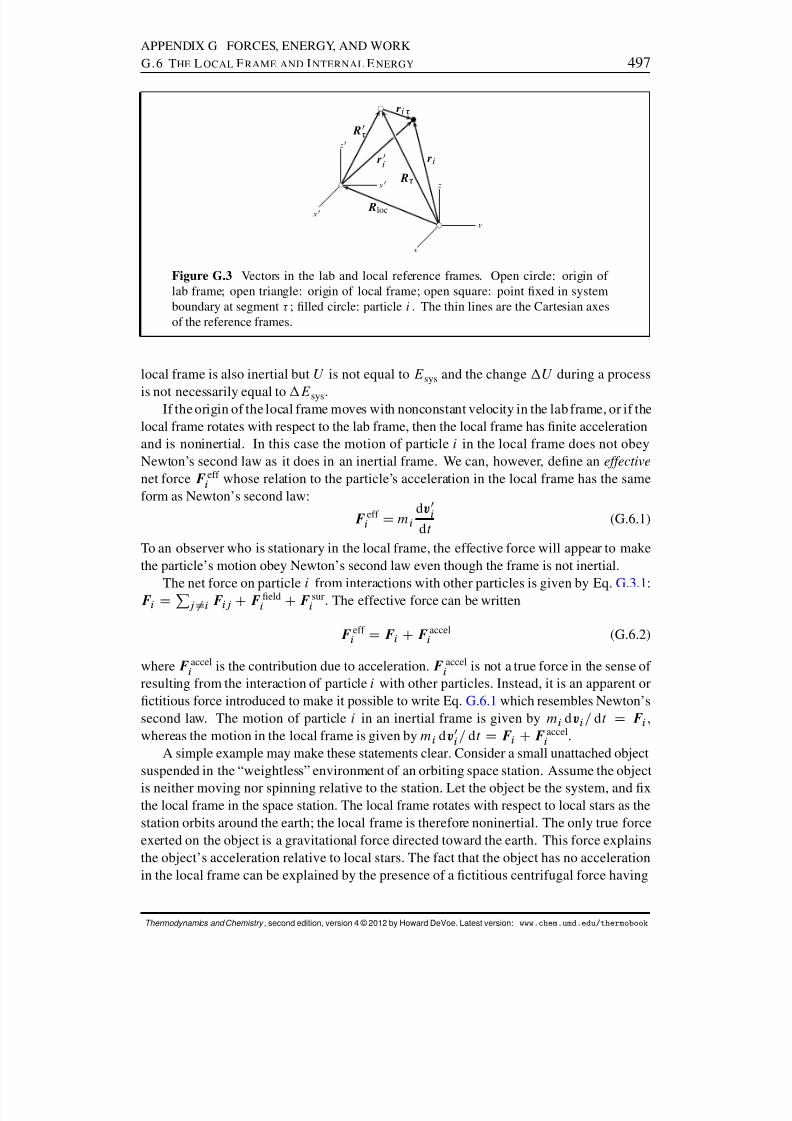
8/12/2019 Howard Devoe Thermodynamic and Chemical
http://slidepdf.com/reader/full/howard-devoe-thermodynamic-and-chemical 497/532
APPENDIX G FORCES, ENERGY, AND WORKG.6 T HE L OCAL F RAME AND INTERNAL E NERGY 497
r i
r 0
i
R
r i
R loc
R 0
x
y
z
x0
y0
z0
Figure G.3 Vectors in the lab and local reference frames. Open circle: origin of lab frame; open triangle: origin of local frame; open square: point xed in systemboundary at segment ; lled circle: particle i . The thin lines are the Cartesian axesof the reference frames.
local frame is also inertial but U is not equal to E sys and the change U during a process
is not necessarily equal to E sys .If the origin of the local frame moves with nonconstant velocity in the lab frame, or if the
local frame rotates with respect to the lab frame, then the local frame has nite accelerationand is noninertial. In this case the motion of particle i in the local frame does not obeyNewton’s second law as it does in an inertial frame. We can, however, dene an effectivenet force F eff
i whose relation to the particle’s acceleration in the local frame has the sameform as Newton’s second law:
F eff i D m i
dv0i
d t (G.6.1)
To an observer who is stationary in the local frame, the effective force will appear to makethe particle’s motion obey Newton’s second law even though the frame is not inertial.
The net force on particle i from interactions with other particles is given by Eq. G.3.1 :F i DPj ¤ i F ij CF eldi CF sur
i . The effective force can be written
F eff i DF i CF accel
i (G.6.2)
where F acceli is the contribution due to acceleration. F accel
i is not a true force in the sense of resulting from the interaction of particle i with other particles. Instead, it is an apparent orctitious force introduced to make it possible to write Eq. G.6.1 which resembles Newton’ssecond law. The motion of particle i in an inertial frame is given by mi dv i = d t D F i ,whereas the motion in the local frame is given by mi dv0
i = d t DF i CF acceli .
A simple example may make these statements clear. Consider a small unattached objectsuspended in the “weightless” environment of an orbiting space station. Assume the objectis neither moving nor spinning relative to the station. Let the object be the system, and xthe local frame in the space station. The local frame rotates with respect to local stars as thestation orbits around the earth; the local frame is therefore noninertial. The only true forceexerted on the object is a gravitational force directed toward the earth. This force explainsthe object’s acceleration relative to local stars. The fact that the object has no accelerationin the local frame can be explained by the presence of a ctitious centrifugal force having
Thermodynamics and Chemistry , second edition, version 4 © 2012 by Howard DeVoe. Latest version: www.chem.umd.edu/thermobook
8/12/2019 Howard Devoe Thermodynamic and Chemical
http://slidepdf.com/reader/full/howard-devoe-thermodynamic-and-chemical 498/532
APPENDIX G FORCES, ENERGY, AND WORKG.6 T HE L OCAL F RAME AND INTERNAL E NERGY 498
the same magnitude as the gravitational force but directed in the opposite direction, so thatthe effective force on the object as a whole is zero.
The reasoning used to derive the equations in Secs. G.1 –G.4 can be applied to an arbi-trary local frame. To carry out the derivations we replace F i by F eff
i , r i by r 0i , and v i by v0
i ,and use the local frame to measure the Cartesian components of all vectors. We need two
new potential energy functions for the local frame, dened by the relations
˚0 eldi
def
D Z F eldi
dr 0i (G.6.3)
˚ acceli
def
D Z F acceli
dr 0i (G.6.4)
Both ˚0 eldi and ˚ accel must be time-independent functions of the position of particle i in
the local frame in order to be valid potential functions. (If the local frame is inertial, F acceli
and ˚ acceli are zero.)
The detailed line of reasoning in Secs. G.1 –G.4 will not be repeated here, but the readercan verify the following results. The total energy of the system and surroundings measuredin the local frame is given by E 0tot D U CPi Pk 0 ˚ ik 0 CE 0surr where the index k 0 is forparticles in the surroundings that are not the source of an external eld for the system. Theenergy of the system (the internal energy) is given by
U DXi
12 m i .v 0
i / 2 CXi Xj >i
˚ ij CXi
˚0 eldi CXi
˚ acceli (G.6.5)
where the indices i and j are for system particles. The energy of the surroundings measuredin the local frame is
E 0surr D
Xk
12 mk .v 0
k / 2 C
Xk
Xl>i
˚ kl C
Xk
˚ accelk (G.6.6)
where k and l are indices for particles in the surroundings. The value of E 0tot is found to
be constant over time, meaning that energy is conserved in the local frame. The internalenergy change during a process is the sum of the heat q measured in the local frame and themacroscopic work w in this frame:
U D q Cw (G.6.7)
The expressions for q and w , analogous to Eqs. G.4.4 and G.4.2 , are found to be
q D
X
Xi Z •i F sur
i dr i (G.6.8)
w DX Z F sur
dR 0 (G.6.9)
In these equations R 0 is a vector from the origin of the local frame to a point xed in the
system boundary at segment , and r i is a vector from this point to particle i (see Fig.G.3 ).
Thermodynamics and Chemistry , second edition, version 4 © 2012 by Howard DeVoe. Latest version: www.chem.umd.edu/thermobook

8/12/2019 Howard Devoe Thermodynamic and Chemical
http://slidepdf.com/reader/full/howard-devoe-thermodynamic-and-chemical 499/532
APPENDIX G FORCES, ENERGY, AND WORKG.6 T HE L OCAL F RAME AND INTERNAL E NERGY 499
We expect that an observer in the local frame will nd the laws of thermodynamicsare obeyed. For instance, the Clausius statement of the second law (Sec. 4.2) is as validin a manned orbiting space laboratory as it is in an earth-xed laboratory: nothing theinvestigator can do will allow energy to be transferred by heat from a colder to a warmerbody through a device operating in a cycle. Equation G.6.7 is a statement of the rst law
of thermodynamics (box on page 56) in the local frame. Accordingly, we may assume thatthe thermodynamic derivations and relations treated in the body of this book are valid inany local frame, whether or not it is inertial, when U and w are dened by Eqs. G.6.5 andG.6.9 .
In the body of the book, w is called the thermodynamic work , or simply the work. Notethe following features brought out by the derivation of the expression for w :
The equation w DP R F sur
dR 0 has been derived for a closed system.
The equation shows how we can evaluate the thermodynamic work w done on thesystem. For each moving surface element of the system boundary at segment of theinteraction layer, we need to know the contact force F sur
exerted by the surroundingsand the displacement d R 0
in the local frame.
We could equally well calculate w from the force exerted by the system on the sur-roundings. According to Newton’s third law, the force F sys
exerted by segment hasthe same magnitude as F sur
and the opposite direction: F sys D F sur
.
During a process, a point xed in the system boundary at segment is either station-ary or traverses a path in three-dimensional space. At each intermediate stage of theprocess, let s be the length of the path that began in the initial state. We can writethe innitesimal quantity F sur
dR 0
in the form F sur cos ˛ ds , where F sur
is themagnitude of the force, d s is an innitesimal change of the path length, and ˛ isthe angle between the directions of the force and the displacement. We then obtainthe following integrated and differential forms of the work:
w DX Z F sur cos ˛ ds ¶w DX
F sur cos ˛ ds (G.6.10)
If only one portion of the boundary moves in the local frame, and this portion haslinear motion parallel to the x 0 axis, we can replace F sur
dR 0
by F surx 0 dx 0, where
F surx 0 is the x0 component of the force exerted by the surroundings on the moving
boundary and d x 0 is an innitesimal displacement of the boundary. In this case wecan write the following integrated and differential forms of the work:
w DZ F surx 0 dx 0 ¶w D F sur
x 0 dx 0 (G.6.11)
The work w does not include work done internally by one part of the system onanother part.
In the calculation of work with Eqs. G.6.9 –G.6.11 , we do not include forces from anexternal eld such as a gravitational eld, or ctitious forces F accel
i if present.
Thermodynamics and Chemistry , second edition, version 4 © 2012 by Howard DeVoe. Latest version: www.chem.umd.edu/thermobook

8/12/2019 Howard Devoe Thermodynamic and Chemical
http://slidepdf.com/reader/full/howard-devoe-thermodynamic-and-chemical 500/532

8/12/2019 Howard Devoe Thermodynamic and Chemical
http://slidepdf.com/reader/full/howard-devoe-thermodynamic-and-chemical 501/532
APPENDIX G FORCES, ENERGY, AND WORKG.8 C ENTER -OF -MASS L OCAL F RAME 501
r 0
i
r i
R cm
Figure G.4 Position vectors in a lab frame and a center-of-mass frame. Open circle:origin of lab frame; open triangle: center of mass; lled circle: particle i . The thinlines represent the Cartesian axes of the two frames.
The center of mass of the system is a point whose position in the lab frame is denedby
R cmdef
DPi m i r i
m (G.8.1)
where m is the system mass: m DPi m i . The position vector of particle i in the lab frameis equal to the sum of the vector R cm from the origin of the lab frame to the center of massand the vector r 0
i from the center of mass to the particle (see Fig. G.4 ):
r i DR cm Cr 0i (G.8.2)
We can use Eqs. G.8.1 and G.8.2 to derive several relations that will be needed presently.Because the Cartesian axes of the lab frame and cm frame are parallel to one another (thatis, the cm frame does not rotate), we can add vectors or form scalar products using the
vector components measured in either frame. The time derivative of Eq. G.8.2 is dr i = d t DdR cm = d t Cdr 0i = d t , or
v i Dvcm Cv0i (G.8.3)
where the vector vcm gives the velocity of the center of mass in the lab frame. Substitutionfrom Eq. G.8.2 into the sum Pi m i r i gives Pi m i r i D mR cm CPi m i r 0
i , and a rear-rangement of Eq. G.8.1 gives Pi m i r i D mR cm . Comparing these two equalities, we seethe sum Pi m i r 0
i must be zero. Therefore the rst and second derivatives of Pi m i r 0i with
respect to time must also be zero:
Xi
m i v0i D 0
Xi
m idv0
i
d t D 0 (G.8.4)
From Eqs. G.1.2 , G.6.1 , G.6.2 , and G.8.3 we obtain
F acceli D m i
d. v0i v i /d t D m i
dvcm
d t (G.8.5)
Equation G.8.5 is valid only for a nonrotating cm frame.
Thermodynamics and Chemistry , second edition, version 4 © 2012 by Howard DeVoe. Latest version: www.chem.umd.edu/thermobook
8/12/2019 Howard Devoe Thermodynamic and Chemical
http://slidepdf.com/reader/full/howard-devoe-thermodynamic-and-chemical 502/532
APPENDIX G FORCES, ENERGY, AND WORKG.8 C ENTER -OF -MASS L OCAL F RAME 502
The difference between the energy changes of the system in the cm frame and the labframe during a process is given, from Eqs. G.2.6 and G.6.5 , by
U E sys D "Xi
12 m i .v 0
i / 2 Xi
12 m i v2
i #C Xi
˚0 eldi Xi
˚ eldi !C Xi
˚ acceli ! (G.8.6)
We will nd new expressions for the three terms on the right side of this equation.The rst term is the difference between the total kinetic energy changes measured in
the cm frame and lab frame. We can derive an important relation, well known in classicalmechanics, for the kinetic energy in the lab frame:
Xi
12 m i v2
i DXi
12 m i . vcm Cv0
i / . vcm Cv0i /
D 12 mv
2cm CXi
12 m i v
0i
2
Cvcm
Xi m i v0i! (G.8.7)
The quantity 12 mv 2
cm is the bulk kinetic energy of the system in the lab frame—that is, thetranslational energy of a body having the same mass as the system and moving with thecenter of mass. The sum Pi m i v0
i is zero (Eq. G.8.4 ). Therefore the rst term on the rightside of Eq. G.8.6 is
"Xi
12 m i .v 0
i / 2 Xi
12 m i v2
i # D 12 mv 2
cm (G.8.8)
Only by using a nonrotating local frame moving with the center of mass is it possible to
derive such a simple relation among these kinetic energy quantities.The second term on the right side of Eq. G.8.6 , with the help of Eqs. G.2.2 , G.6.3 , and
G.8.2 becomes
Xi
˚0 eldi Xi
˚ eldi ! D Xi Z F eld
i d. r 0
i r i /
DZ Xi
F eldi ! dR cm (G.8.9)
Suppose the only external eld is gravitational: F eldi D F grav
i D m i g ez where e z is aunit vector in the vertical (upward)
Cz direction. In this case we obtain
Xi
˚0 eldi Xi
˚ eldi ! D Z Xi
m i!g ez dR cm
D mg Z ez dR cm D mg Z dzcm
D mg z cm (G.8.10)
Thermodynamics and Chemistry , second edition, version 4 © 2012 by Howard DeVoe. Latest version: www.chem.umd.edu/thermobook
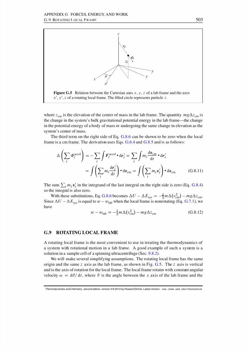
8/12/2019 Howard Devoe Thermodynamic and Chemical
http://slidepdf.com/reader/full/howard-devoe-thermodynamic-and-chemical 503/532
APPENDIX G FORCES, ENERGY, AND WORKG.9 R OTATING L OCAL F RAME 503
Figure G.5 Relation between the Cartesian axes x , y , z of a lab frame and the axesx 0, y 0, z of a rotating local frame. The lled circle represents particle i .
where zcm is the elevation of the center of mass in the lab frame. The quantity mg z cm isthe change in the system’s bulk gravitational potential energy in the lab frame—the changein the potential energy of a body of mass m undergoing the same change in elevation as thesystem’s center of mass.
The third term on the right side of Eq. G.8.6 can be shown to be zero when the localframe is a cm frame. The derivation uses Eqs. G.6.4 and G.8.5 and is as follows:
Xi
˚ acceli ! D Xi Z F accel
i dr 0
i DXi Z midvcm
d tdr 0
i
DZ Xi
m idr 0
i
d t ! dvcm DZ Xi
m i v0i! dvcm (G.8.11)
The sum Pi m i v0i in the integrand of the last integral on the right side is zero (Eq. G.8.4 )so the integral is also zero.
With these substitutions, Eq. G.8.6 becomes U E sys D 12 m v2
cm mg z cm .Since U E sys is equal to w w lab when the local frame is nonrotating (Eq. G.7.1 ), wehave
w w lab D 12 m v2
cm mg z cm (G.8.12)
G.9 ROTATING LOCAL FRAME
A rotating local frame is the most convenient to use in treating the thermodynamics of a system with rotational motion in a lab frame. A good example of such a system is asolution in a sample cell of a spinning ultracentrifuge (Sec. 9.8.2 ).
We will make several simplifying assumptions. The rotating local frame has the sameorigin and the same z axis as the lab frame, as shown in Fig. G.5 . The z axis is verticaland is the axis of rotation for the local frame. The local frame rotates with constant angularvelocity ! D d#= d t , where # is the angle between the x axis of the lab frame and the
Thermodynamics and Chemistry , second edition, version 4 © 2012 by Howard DeVoe. Latest version: www.chem.umd.edu/thermobook

8/12/2019 Howard Devoe Thermodynamic and Chemical
http://slidepdf.com/reader/full/howard-devoe-thermodynamic-and-chemical 504/532
APPENDIX G FORCES, ENERGY, AND WORKG.10 E ARTH -F IXED R EFERENCE F RAME 504
x 0 axis of the local frame. There is a gravitational force in the z direction; this force isresponsible for the only external eld, whose potential energy change in the local frameduring a process is ˚
0 gravi D m i g z i (Eq. G.2.3 ).
The contribution to the effective force acting on particle i due to acceleration when !is constant can be shown to be given by 8
F acceli DF centri CF Cori (G.9.1)
where F centri is the so-called centrifugal force and F Cor
i is called the Coriolis force .The centrifugal force acting on particle i is given by
F centri D m i ! 2 r i e i (G.9.2)
Here r i is the radial distance of the particle from the axis of rotation, and e i is a unit vectorpointing from the particle in the direction away from the axis of rotation (see Fig. G.5 ). Thedirection of e i in the local frame changes as the particle moves in this frame.
The Coriolis force acting on particle i arises only when the particle is moving relativeto the rotating frame, has magnitude 2mi !v 0
i , and is directed perpendicular to both v0i and
the axis of rotation.In a rotating local frame, the work during a process is not the same as that measured in
a lab frame. The heats q and qlab are not equal to one another as they are when the localframe is nonrotating, nor can general expressions using macroscopic quantities be writtenfor U E sys and w w lab .
G.10 EARTH-FIXED REFERENCE FRAME
In the preceding sections of Appendix G, we assumed that a lab frame whose coordinateaxes are xed relative to the earth’s surface is an inertial frame. This is not exactly true, be-cause the earth spins about its axis and circles the sun. Small correction terms, a centrifugalforce and a Coriolis force, are needed to obtain the effective net force acting on particle i
that allows Newton’s second law to be obeyed exactly in the lab frame. 9The earth’s movement around the sun makes only a minor contribution to these correc-
tion terms. The Coriolis force, which occurs only if the particle is moving in the lab frame,is usually so small that it can be neglected.
This leaves as the only signicant correction the centrifugal force on the particle fromthe earth’s spin about its axis. This force is directed perpendicular to the earth’s axis and hasmagnitude m i ! 2 r i , where ! is the earth’s angular velocity, m i is the particle’s mass, andr i is the radial distance of the particle from the earth’s axis. The correction can be treatedas a small modication of the gravitational force acting on the particle that is at most, at theequator, only about 0.3% of the actual gravitational force. Not only is the correction small,but it is completely taken into account in the lab frame when we calculate the effective
gravitational force from F grav
i D m i g ez , where g is the acceleration of free fall and ezis a unit vector in the Cz (upward) direction. The value of g is an experimental quantitythat includes the effect of F centr
i , and thus depends on latitude as well as elevation above theearth’s surface. Since F grav
i depends only on position, we can treat gravity as a conservativeforce eld in the earth-xed lab frame.8The derivation, using a different notation, can be found in Ref. [ 107 ], Chap. 10.9Ref. [ 68], Sec. 4–9.
Thermodynamics and Chemistry , second edition, version 4 © 2012 by Howard DeVoe. Latest version: www.chem.umd.edu/thermobook
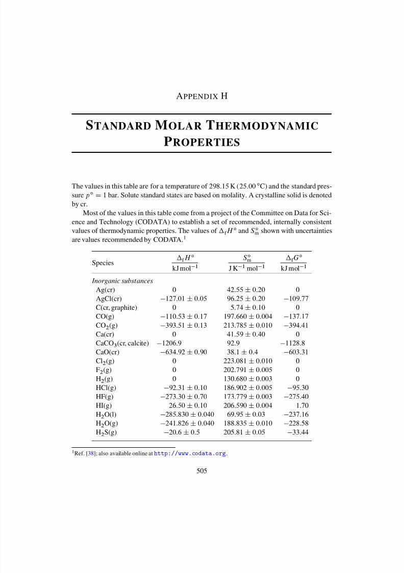
8/12/2019 Howard Devoe Thermodynamic and Chemical
http://slidepdf.com/reader/full/howard-devoe-thermodynamic-and-chemical 505/532
A PPENDIX H
STANDARD M OLAR THERMODYNAMIC
P ROPERTIES
The values in this table are for a temperature of 298:15 K ( 25:00 ı C) and the standard pres-sure p ı
D 1 bar. Solute standard states are based on molality. A crystalline solid is denoted
by cr.Most of the values in this table come from a project of the Committee on Data for Sci-
ence and Technology (CODATA) to establish a set of recommended, internally consistentvalues of thermodynamic properties. The values of f H ı and S ım shown with uncertaintiesare values recommended by CODATA. 1
Species f H ı
kJ mol 1S ım
J K 1 mol 1f G
ı
kJ mol 1
Inorganic substancesAg(cr) 0 42. 55 ˙ 0:20 0
AgCl(cr) 127 .01 ˙ 0:05 96.25 ˙ 0:20 109 .77C(cr, graphite) 0 5. 74 ˙ 0:10 0CO(g) 110 .53 ˙ 0:17 197.660 ˙ 0:004 137 .17CO 2 (g) 393 .51 ˙ 0:13 213.785 ˙ 0:010 394 .41Ca(cr) 0 41. 59 ˙ 0:40 0CaCO 3 (cr, calcite) 1206 .9 92.9 1128 .8CaO(cr) 634 .92 ˙ 0:90 38.1 ˙ 0:4 603 .31Cl2 (g) 0 223. 081 ˙ 0:010 0F2 (g) 0 202. 791 ˙ 0:005 0H2 (g) 0 130. 680 ˙ 0:003 0HCl(g) 92.31 ˙ 0:10 186.902 ˙ 0:005 95 .30HF(g)
273 .30
˙0:70 173.779
˙0:003
275 .40
HI(g) 26. 50 ˙ 0:10 206.590 ˙ 0:004 1.70H2 O(l) 285 .830 ˙ 0:040 69.95 ˙ 0:03 237 .16H2 O(g) 241 .826 ˙ 0:040 188.835 ˙ 0:010 228 .58H2 S(g) 20.6 ˙ 0:5 205.81 ˙ 0:05 33 .44
1Ref. [ 38]; also available online at http://www.codata.org .
505
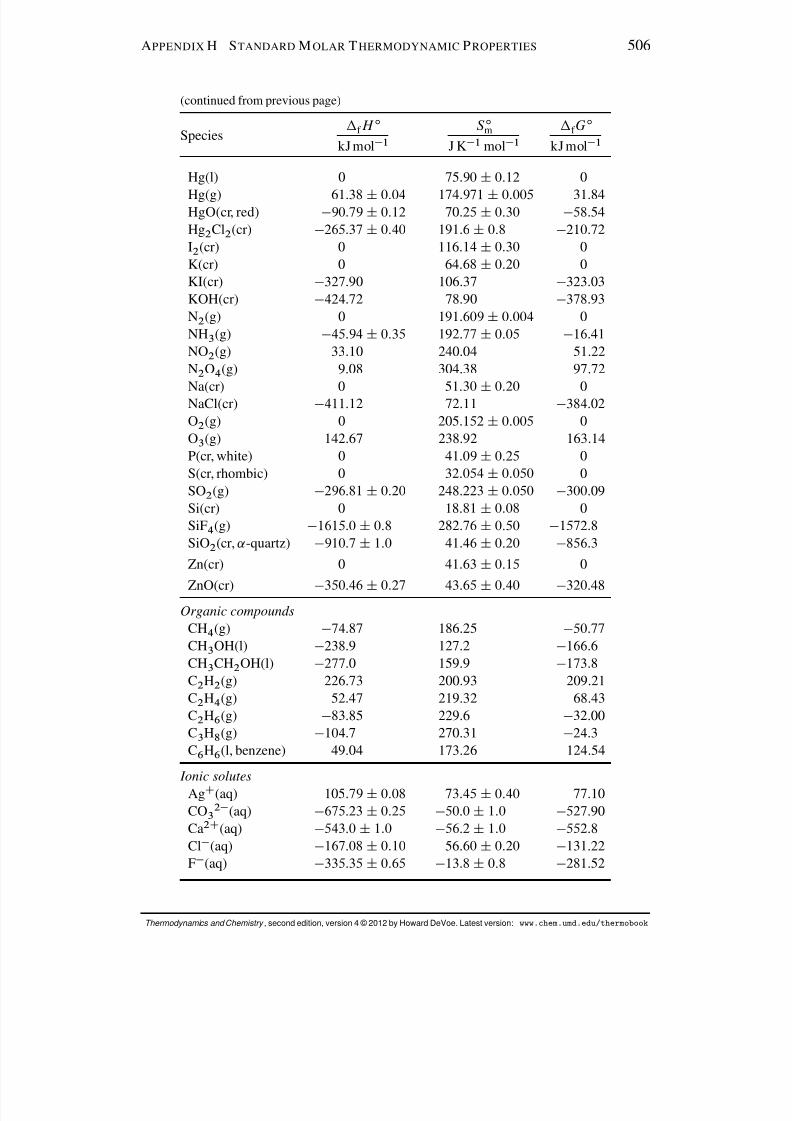
8/12/2019 Howard Devoe Thermodynamic and Chemical
http://slidepdf.com/reader/full/howard-devoe-thermodynamic-and-chemical 506/532
A PPENDIX H STANDARD M OLAR T HERMODYNAMIC P ROPERTIES 506
(continued from previous page)
Species f H ı
kJ mol 1S ım
J K 1 mol 1f G
ı
kJ mol 1
Hg(l) 0 75. 90 ˙ 0:12 0
Hg(g) 61. 38 ˙ 0:04 174.971 ˙ 0:005 31.84HgO(cr, red) 90.79 ˙ 0:12 70.25 ˙ 0:30 58 .54Hg 2 Cl2 (cr) 265 .37 ˙ 0:40 191.6 ˙ 0:8 210 .72I2 (cr) 0 116. 14 ˙ 0:30 0K(cr) 0 64. 68 ˙ 0:20 0KI(cr) 327 .90 106.37 323 .03KOH(cr) 424 .72 78.90 378 .93N2 (g) 0 191. 609 ˙ 0:004 0NH 3 (g) 45.94 ˙ 0:35 192.77 ˙ 0:05 16 .41NO 2 (g) 33.10 240.04 51.22N2 O4 (g) 9.08 304.38 97.72
Na(cr) 0 51. 30 ˙ 0:20 0NaCl(cr) 411 .12 72.11 384 .02O2 (g) 0 205. 152 ˙ 0:005 0O3 (g) 142.67 238.92 163.14P(cr, white) 0 41. 09 ˙ 0:25 0S(cr, rhombic) 0 32. 054 ˙ 0:050 0SO 2 (g) 296 .81 ˙ 0:20 248.223 ˙ 0:050 300 .09Si(cr) 0 18. 81 ˙ 0:08 0SiF 4 (g) 1615 .0 ˙ 0:8 282.76 ˙ 0:50 1572 .8SiO 2 (cr, ˛ -quartz) 910 .7 ˙ 1:0 41.46 ˙ 0:20 856 .3
Zn(cr) 0 41. 63 ˙ 0:15 0
ZnO(cr) 350 .46 ˙ 0:27 43.65 ˙ 0:40 320 .48Organic compounds
CH 4 (g) 74.87 186.25 50 .77CH 3 OH(l) 238 .9 127.2 166 .6CH 3 CH 2 OH(l) 277 .0 159.9 173 .8C2 H2 (g) 226.73 200.93 209.21C2 H4 (g) 52.47 219.32 68.43C2 H6 (g) 83.85 229.6 32 .00C3 H8 (g) 104 .7 270.31 24 .3C6 H6 (l, benzene) 49.04 173.26 124.54
Ionic solutesAg C (aq) 105. 79 ˙ 0:08 73.45 ˙ 0:40 77.10CO 3
2 (aq) 675 .23 ˙ 0:25 50.0 ˙ 1:0 527 .90Ca2C (aq) 543 .0 ˙ 1:0 56.2 ˙ 1:0 552 .8Cl (aq) 167 .08 ˙ 0:10 56.60 ˙ 0:20 131 .22F (aq) 335 .35 ˙ 0:65 13.8 ˙ 0:8 281 .52
Thermodynamics and Chemistry , second edition, version 4 © 2012 by Howard DeVoe. Latest version: www.chem.umd.edu/thermobook

8/12/2019 Howard Devoe Thermodynamic and Chemical
http://slidepdf.com/reader/full/howard-devoe-thermodynamic-and-chemical 507/532
A PPENDIX H STANDARD M OLAR T HERMODYNAMIC P ROPERTIES 507
(continued from previous page)
Species f H ı
kJ mol 1S ım
J K 1 mol 1f G
ı
kJ mol 1
HC (aq) 0 0 0
HCO 3 (aq) 689 .93 ˙ 2:0 98.4 ˙ 0:5 586 .90HS (aq) 16.3 ˙ 1:5 67 ˙ 5 12.2HSO 4 (aq) 886 .9 ˙ 1:0 131.7 ˙ 3:0 755 .4Hg 2
2C (aq) 166. 87 ˙ 0:50 65.74 ˙ 0:80 153.57I (aq) 56.78 ˙ 0:05 106.45 ˙ 0:30 51 .72KC (aq) 252 .14 ˙ 0:08 101.20 ˙ 0:20 282 .52NH 4
C (aq) 133 .26 ˙ 0:25 111. 17 ˙ 0:40 79 .40NO 3 (aq) 206 .85 ˙ 0:40 146.70 ˙ 0:40 110 .84Na C (aq) 240 .34 ˙ 0:06 58.45 ˙ 0:15 261 .90OH (aq) 230 .015 ˙ 0:040 10.90 ˙ 0:20 157 .24S2 (aq) 33.1 14.6 86.0
SO 42
(aq) 909 .34 ˙ 0:40 18.50 ˙ 0:40 744 .00
Thermodynamics and Chemistry , second edition, version 4 © 2012 by Howard DeVoe. Latest version: www.chem.umd.edu/thermobook
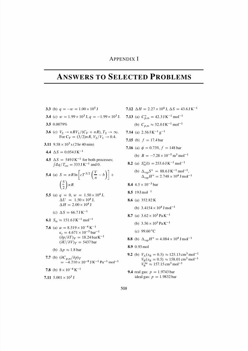
8/12/2019 Howard Devoe Thermodynamic and Chemical
http://slidepdf.com/reader/full/howard-devoe-thermodynamic-and-chemical 508/532
A PPENDIX I
ANSWERS TO SELECTED PROBLEMS
3.3 (b) q D w D 1:00 105 J
3.4 (c) w D 1:99 103 J, q D 1:99 103 J.
3.5 0:0079%
3.6 (c) V 2 ! nRV 1 =.C V CnR/ , T 2 ! 1 .For C V D .3=2/nR , V 2 =V 1 ! 0:4.
3.11 9:58 103 s (2 hr 40 min)
4.4 S D 0:054 J K 1
4.5 S D 549 J K 1 for both processes;
R ¶q=T ext D 333 J K 1 and 0.
5.4 (a) S D nR ln cT 3=2 V n b C
52 nR
5.5 (a) q D 0, w D 1:50 104 J,U D 1:50 104 J,H D 2:00 104 J
(c) S D 66:7 J K 1
6.1 S m 151:6 J K 1 mol 1
7.6 (a) ˛ D 8:519 10 4 K 1
t D 4:671 10 5 bar 1
.@p=@T /V D 18:24 barK 1
.@U=@V /T
D 5437 bar
(b) p 1:8 bar
7.7 (b) .@C p; m =@p/T
D 4:210 10 8 J K 1 Pa 1 mol 1
7.8 (b) 8 10 4 K 1
7.11 5:001 103 J
7.12 H D 2:27 104 J, S D 43:6 J K 1
7.13 (a) C ıp; m D 42:3 J K 1 mol 1
(b) C p; m 52:0 J K 1 mol 1
7.14 (a) 2:56 J K 1 g 1
7.15 (b) f D 17:4 bar
7.16 (a) D 0:739 , f D 148 bar
(b) B D 7:28 10 5 m3 mol 1
8.2 (a) S ım(l) D 253:6 J K 1 mol 1
(b) vap S ı D 88:6 J K 1 mol 1 ,
vap H ı D 2:748 104 J mol 1
8.4 4:5 10 3 bar
8.5 19 J mol 1
8.6 (a) 352:82 K
(b) 3:4154 104 J mol 1
8.7 (a) 3:62 103 Pa K 1
(b) 3:56 103 Pa K 1
(c) 99:60 ı C
8.8 (b) vap H ı D 4:084 104 J mol 1
8.9 0:93 mol
9.2 (b) V A .x B D 0:5/ 125:13 cm 3 mol 1
V B .x B D 0:5/ 158:01 cm 3 mol 1
V 1B 157:15 cm 3 mol 1
9.4 real gas: p D 1:9743 barideal gas: p D 1:9832 bar
508
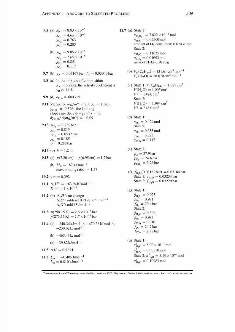
8/12/2019 Howard Devoe Thermodynamic and Chemical
http://slidepdf.com/reader/full/howard-devoe-thermodynamic-and-chemical 509/532
A PPENDIX I ANSWERS TO S ELECTED P ROBLEMS 509
9.5 (a) xN2 D 8:83 10 6
xO2 D 4:65 10 6
yN2 D 0:763yO2 D 0:205
(b) xN2 D 9:85 10 6
xO2 D 2:65 106
yN2 D 0:851yO2 D 0:117
9.7 (b) f A D 0:03167 bar, f A D 0:03040 bar
9.8 (a) In the mixture of compositionxA D 0:9782 , the activity coefcient is B 11:5 .
9.9 (d) kH,A 680 kPa
9.11 Values for mB=m ı D 20: A D 1:026 , m; B D 0:526 ; the limitingslopes are d A= d.m B=m ı /
D 0,
d m; B= d.m B=m ı / D 0:09
9.13 p N2 D 0:235 baryN2 D 0:815p O2 D 0:0532 baryO2 D 0:185p D 0:288 bar
9.14 (b) h D 1:2 m
9.15 (a) p.7:20 cm / p.6:95 cm / D 1:2 bar
(b) M B D 187 kg mol 1
mass binding ratio D 1:37
10.2 ˙ D 0:392
11.1 rH ı D 63:94 kJmol 1
K D 4:41 10 2
11.2 (b) f H ı : no changef S ı : subtract 0:219 J K 1 mol 1
f G ı : add 65 J mol 1
11.3 p.298:15 K/ D 2:6 10 6 barp.273:15 K/ D 2:7 10 7 bar
11.4 (a) 240:34 kJ mol 1 , 470:36 kJmol 1 ,230:02 kJmol 1
(b) 465:43 kJmol 1
(c) 39:82 kJ mol 1
11.5 H D 0:92 kJ
11.6 L A D 0:405 Jmol 1
L B D 0:810 kJmol 1
11.7 (a) State 1:nC6 H14 D 7:822 10 3 molnH2 O D 0:05560 molamount of O 2 consumed: 0:07431 molState 2:nH2 O D 0:11035 mol
nCO 2 D 0:04693 molmass of H 2 O= 1:9880 g
(b) V m (C6 H14 ) D 131:61 cm 3 mol 1
V m (H2 O) D 18:070 cm 3 mol 1
(c) State 1: V (C6 H14 ) D 1:029 cm3
V (H2 O) D 1:005 cm3
V g D 348:0 cm 3
State 2:V (H2 O) D 1:994 cm3
V g D 348:0 cm 3
(d) State 1:nO2 D 0:429 molState 2:nO2 D 0:355 molyO2 D 0:883yCO 2 D 0:117
(e) State 2:p 2 D 27:9 barp O2 D 24:6 barp CO 2 D 3:26 bar
(f) f H2
O .0:03169 bar /
D 0:03164 bar
State 1: f H2 O D 0:03234 barState 2: f H2 O D 0:03229 bar
(g) State 1:H2 O D 0:925O2 D 0:981
f O2 D 29:4 barState 2:
H2 O D 0:896O2 D 0:983CO 2 D 0:910
f O2 D 24:2 bar
f CO 2 D 2:97 bar
(h) State 1:ng
H2 O D 5:00 10 4 moln l
H2 O D 0:05510 molState 2: n g
H2 O D 5:19 10 4 moln l
H2 O D 0:10983 mol
Thermodynamics and Chemistry , second edition, version 4 © 2012 by Howard DeVoe. Latest version: www.chem.umd.edu/thermobook

8/12/2019 Howard Devoe Thermodynamic and Chemical
http://slidepdf.com/reader/full/howard-devoe-thermodynamic-and-chemical 510/532
A PPENDIX I ANSWERS TO S ELECTED P ROBLEMS 510
(i) State 1:km; O2 D 825 bar kg mol 1
nO2 D 3:57 10 5 molState 2:km; O2 D 823 bar kg mol 1
km; CO 2
D 30:8 bar kg mol 1
nO2 D 5:85 10 5 molnCO 2 D 1:92 10 4 mol
(j) H 2 O vaporization: U D C20:8 JH2 O condensation: U D 21:6 J
(k) O 2 dissolution: U D 0:35 JO2 desolution: U D 0:57 JCO 2 desolution: U D 3:32 J
(l) C 6 H14 (l) compression:U D 1:226 Jsolution compression:U
D 0:225 J
solution decompression:U D 0:414 J
(m) O 2 compression: U D 81 Jgas mixture: d B= dT D0:26 10 6 m3 K 1 mol 1
gas mixture expansion: U D 87 J
(n) U D 8 J
(o) cU ı D 4154:4 kJmol 1
(p) cH ı D 4163:1 kJ mol 1
11.8 f H ı
D 198:8 kJmol1
11.9 T 2 D 2272 K
11.10 p (O2 ) D 2:55 10 5 bar
11.11 (a) K D 3:5 1041
(b) p H2 D 2:8 10 42 barN H2 D 6:9 10 17
(c) t D 22 s
11.12 (b) p 1:5 104 bar
11.13 (c) K
D 0:15
12.1 (b) T D 1168 KrH ı D 1:64 105 J mol 1
12.4 K f D 1:860 Kkgmol 1
K b D 0:5118 Kkgmol 1
12.5 M B 5:6 104 g mol 1
12.6 sol,B H ı =kJmol 1 D 3:06; 0; 6:35sol,B S ı =J K 1 mol 1
D 121:0; 110:2; 88:4
12.7 (a) m’C D m ’ D 1:20 10 3 mol kg 1
m“C D 1:80 10 3 mol kg 1
m“
D 0:80 103
mol kg1
mP D 2:00 10 6 mol kg 1
12.8 (a) p l D 2:44 bar
(b) f.2:44 bar / f .1:00 bar /
D 3:4 10 5 bar
12.10 (a) xB D 1:8 10 7
mB D 1:0 10 5 mol kg 1
(b) sol,B H ı D 1:99 104 J mol 1
(c) K D 4:4 10 7
rH ı D 9:3 kJmol 1
12.13 (a) p D 92399:6 Pa, yB D 0:965724(b) A D 0:995801
(c) f A D 3164:47 Pa
(d) yB D 0:965608
(e) Z D 0:999319
(f) p D 92347:7 Pa
(g) kH,B D 4:40890 109 Pa
12.15 (a) x; B D 0:9826
(b) xB
D 4:19 10 4
12.16 K D 1:2 10 6
12.17 (a) ˛ D 0:129mC D 1:29 10 3 mol kg 1
(b) ˛ D 0:140
12.18 f H ı . Cl , aq / D 167:15 kJmol 1
S ım . Cl , aq / D 56:46 J K 1 mol 1
12.19 (a) K s D 1:783 10 10
12.20 (a) rH ı D 65:769 kJ mol 1
(b) f H ı (Ag C ,aq) D 105:84 kJmol 1
13.1 (a) F D 4
(b) F D 3
(c) F D 2
13.10 (a) xB(top) D 0:02, xB(bottom) D 0:31
(b) nA D 2:1 mol, nB D 1:0 mol
Thermodynamics and Chemistry , second edition, version 4 © 2012 by Howard DeVoe. Latest version: www.chem.umd.edu/thermobook
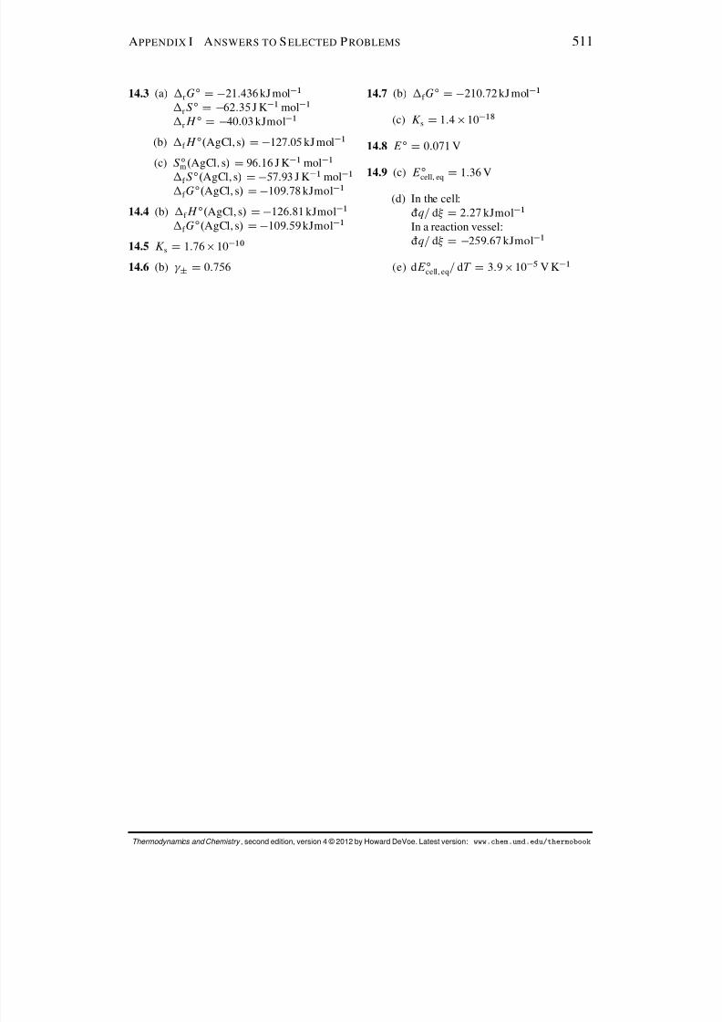
8/12/2019 Howard Devoe Thermodynamic and Chemical
http://slidepdf.com/reader/full/howard-devoe-thermodynamic-and-chemical 511/532
A PPENDIX I ANSWERS TO S ELECTED P ROBLEMS 511
14.3 (a) rG ı D 21:436 kJ mol 1
rS ı D 62:35 J K 1 mol 1
rH ı D 40:03 kJmol 1
(b) f H ı . AgCl, s / D 127:05 kJ mol 1
(c) S ım . AgCl, s / D 96:16 J K 1 mol 1
f S ı. AgCl, s / D 57:93 J K
1mol
1
f G ı . AgCl, s / D 109:78 kJmol 1
14.4 (b) f H ı . AgCl, s / D 126:81 kJmol 1
f G ı . AgCl, s / D 109:59 kJmol 1
14.5 K s D 1:76 10 10
14.6 (b) ˙ D 0:756
14.7 (b) f G ı D 210:72 kJ mol 1
(c) K s D 1:4 10 18
14.8 E ı D 0:071 V
14.9 (c) E ı
cell, eq D 1:36 V
(d) In the cell:¶q= d D 2:27 kJmol 1
In a reaction vessel:¶q= d D 259:67 kJmol 1
(e) dE ıcell, eq = dT D 3:9 10 5 V K 1
Thermodynamics and Chemistry , second edition, version 4 © 2012 by Howard DeVoe. Latest version: www.chem.umd.edu/thermobook
8/12/2019 Howard Devoe Thermodynamic and Chemical
http://slidepdf.com/reader/full/howard-devoe-thermodynamic-and-chemical 512/532
B IBLIOGRAPHY
[1] C. J. Adkins, Equilibrium Thermodynamics , 3rd edition. Cambridge University Press,Cambridge, 1983.
[2] Robert A. Alberty, “Use of Legendre Transforms in Chemical Thermodynamics (IUPACTechnical Report).” Pure Appl. Chem. , 73, 1349–1380 (2001).
[3] S. Angus, B. Armstrong, and K. M. de Reuck, International Thermodynamic Tables of the
Fluid State. Vol. 3. Carbon Dioxide . Pergamon Press, Oxford, 1976.[4] Roger G. Bates and Vincent E. Bower, “Standard Potential of the Silver–Silver-Chloride
Electrode from 0 ı to 95 ı C and the Thermodynamic Properties of Dilute Hydrochloric AcidSolutions.” J. Res. Natl. Bur. Stand. (U.S.) , 53, 283–290 (1954).
[5] Stuart J. Bates and H. Darwin Kirschman, “The Vapor Pressures and Free Energies of theHydrogen Halides in Aqueous Solution; the Free Energy of Formation of HydrogenChloride.” J. Am. Chem. Soc. , 41, 1991–2001 (1919).
[6] Robert P. Bauman, “Work of Compressing an Ideal Gas.” J. Chem. Educ. , 41, 102–104(1964).
[7] Robert P. Bauman, “Maximum Work Revisited (letter).” J. Chem. Educ. , 41, 675 (1964).[8] Robert P. Bauman, “Maximum Work Revisited (letter).” J. Chem. Educ. , 41, 676–677
(1964).[9] Robert P. Bauman and Howard L. Cockerham III, “Pressure of an Ideal Gas on a Moving
Piston.” Am. J. Phys. , 37, 675–679 (1969).[10] Hassan Behnejad, Jan V. Sengers, and Mikhail A. Anisimov, “Thermodynamic Behaviour of
Fluids near Critical Points.” In A. R. H. Goodwin, J. V. Sengers, and C. J. Peters, editors, Applied Thermodynamics of Fluids , pages 321–367. Royal Society of Chemistry,Cambridge, 2010.
[11] Dor Ben-Amotz and J. M. Honig, “Rectication of Thermodynamic Inequalities.” J. Chem.Phys. , 118 , 5932–5936 (2003).
[12] George C. Benson and Osamu Kiyohara, “Thermodynamics of Aqueous Mixtures of Nonelectrolytes. I. Excess Volumes of Water - n-Alcohol Mixtures at Several Temperatures.” J. Solution Chem. , 9, 791–804 (1980).
[13] K. H. Berry, “NPL-75: A Low Temperature Gas Thermometry Scale from 2.6 K to 27.1 K.” Metrologia , 15, 89–115 (1979).
[14] Gary L. Bertrand, “Thermodynamic Calculation of Work for Some Irreversible Processes.” J. Chem. Educ. , 82, 874–877 (2005).
[15] R. W. Blue and W. F. Giauque, “The Heat Capacity and Vapor Pressure of Solid and LiquidNitrous Oxide. The Entropy from its Band Spectrum.” J. Am. Chem. Soc. , 57, 991–997(1935).
[16] M. Boirac, “N ecrologie: Francois Raoult, Discours de M. Boirac, Recteur.” Ann.l’Universit ´ e de Grenoble , 13, i–v (1901).
[17] J. T. Bottomley, “Scientic Worthies. XX.—James Prescott Joule.” Nature , 26, 617–620
512
8/12/2019 Howard Devoe Thermodynamic and Chemical
http://slidepdf.com/reader/full/howard-devoe-thermodynamic-and-chemical 513/532
B IBLIOGRAPHY 513
(1882).[18] Pascale Boulanger, Marc le Maire, M´ elanie Bonhivers, Sandrine Dubois, Michel Desmadril,
and Lucienne Letellier, “Purication and Structural and Functional Characterization of FhuA, a Transporter of the Escherichia coli Outer Membrane.” Biochemistry , 14,14216–14224 (1996).
[19] Vincenzo Brandani, Angelo Chianese, and Maurizio Rossi, “Ternary Liquid-Liquid
Equilibrium Data for the Water-Ethanol-Benzene System.” J. Chem. Eng. Data , 30, 27–29(1985).
[20] L. K. Brice, “Le Chatelier’s Principle: The Effect of Temperature on the Solubility of Solidsin Liquids.” J. Chem. Educ. , 60, 387–389 (1983).
[21] P. W. Bridgman, The Thermodynamics of Electrical Phenomena in Metals and a Condensed Collection of Thermodynamic Formulas . Dover, New York, 1961.
[22] P. W. Bridgman, “A Complete Collection of Thermodynamic Formulas.” Phys. Rev. , 3,273–281 (1914).
[23] P. W. Bridgman, The Nature of Thermodynamics . Harvard University Press, Cambridge,Massachusetts, 1941.
[24] I. Brown, W. Fock, and F. Smith, “Thermodynamic Properties of Alcohol Solutions.” Aust. J.Chem. , 9, 364–372 (1956).
[25] Oliver L. I. Brown and George G. Manov, “The Heat Capacity of Carbon Disulde from 15to 300 ı K. The Entropy and Heat of Fusion of Carbon Disulde.” J. Am. Chem. Soc. , 59,500–502 (1937).
[26] H. L. Callendar, “On a Practical Thermometric Standard.” Phil. Mag. , 48, 519–547 (1899).[27] Sadi Carnot, “Reections on the Motive Power of Fire, and on Machines Fitted to Develop
that Power.” In E. Mendoza, editor, Reections on the Motive Power of Fire: Sadi Carnot and other Papers on the Second Law of Thermodynamics by ´ E. Clapeyron and R. Clausius ,pages 1–59. Dover, Mineola, New York, 1988. Translation by R. H. Thurston of R´ eexionssur la Puissance Motrice du Feu et sur les Machines Propres a D ´ evelopper cette Puissance ,Bachelier, Paris, 1824.
[28] Malcolm W. Chase Jr., NIST-JANAF Thermochemical Tables , Fourth edition. AmericanInstitute of Physics, Woodbury, New York, 1998. Appeared as J. Phys. Chem. Ref. Data ,Monograph 9.
[29] John P. Chesick, “Maximum Work Revisited (letter).” J. Chem. Educ. , 41, 674–675 (1964).[30] E. Clapeyron, “Memoir on the Motive Power of Heat.” In E. Mendoza, editor, Reections on
the Motive Power of Fire: Sadi Carnot and other Papers on the Second Law of Thermodynamics by ´ E. Clapeyron and R. Clausius , pages 71–105. Dover, Mineola, NewYork, 1988. Translation by E. Mendoza of “M´ emoire sur la Puissance Motrice de laChaleur,” J. de l’ ´ Ecole Polytechnique , 14, 153–190 (1834).
[31] E. Colin W. Clarke and David N. Glew, “Evaluation of Thermodynamic Functions forAqueous Sodium Chloride from Equilibrium and Calorimetric Measurements below 154 ı C.” J. Phys. Chem. Ref. Data , 14, 489–610 (1985).
[32] R. Clausius, “Fourth Memoir. On a Modied Form of the Second Fundamental Theorem inthe Mechanical Theory of Heat.” In T. Archer Hirst, editor, The Mechanical Theory of Heat,with its Applications to the Steam-Engine and to the Physical Properties of Bodies , pages11–135. John Van Voorst, London, 1867. Translation of “Ueber eine Ver anderte Form desZweiten Hauptsatzes der Mechanischen W armetheorie,” Ann. Phys. Chem. (Leipzig) , 93,481–506 (1854).
[33] R. Clausius, “Ninth Memoir. On Several Convenient Forms of the Fundamental Equations of the Mechanical Theory of Heat.” In T. Archer Hirst, editor, The Mechanical Theory of Heat,with its Applications to the Steam-Engine and to the Physical Properties of Bodies , pages327–365. John Van Voorst, London, 1867. Translation of “Ueber Verschiedene f ur dieAnwendung Bequeme Formen der Hauptgleichungen der Mechanischen W¨ armetheorie,” Ann. Phys. Chem. (Leipzig) , 125 , 353–400 (1865).
Thermodynamics and Chemistry , second edition, version 4 © 2012 by Howard DeVoe. Latest version: www.chem.umd.edu/thermobook
8/12/2019 Howard Devoe Thermodynamic and Chemical
http://slidepdf.com/reader/full/howard-devoe-thermodynamic-and-chemical 514/532
B IBLIOGRAPHY 514
[34] J. O. Clayton and W. F. Giauque, “The Heat Capacity and Entropy of Carbon Monoxide.Heat of Vaporization. Vapor Pressures of Solid and Liquid. Free Energy to 5000 ı K fromSpectroscopic Data.” J. Am. Chem. Soc. , 54, 2610–2626 (1932).
[35] Patrick Coffey, Cathedrals of Science: The Personalities and Rivalries That Made ModernChemistry . Oxford University Press, New York, 2008.
[36] E. Richard Cohen, Tomislav Cvita s, Jeremy G. Frey, Bertil Holmstr om, Kozo Kuchitsu,
Roberto Marquardt, Ian Mills, Franco Pavese, Martin Quack, J¨ urgen Stohner, Herbert L.Strauss, Michio Takami, and Anders J Thor, Quantities, Units and Symbols in PhysicalChemistry , 3rd edition. RSC Publishing, Cambridge, 2007.
[37] Roger Cohen-Adad and John W. Lorimer, Alkali Metal and Ammonium Chlorides in Water and Heavy Water (Binary Systems) . Solubility Data Series, Vol. 47. Pergamon Press,Oxford, 1991.
[38] J. D. Cox, D. D. Wagman, and V. A. Medvedev, CODATA Key Values for Thermodynamics .Hemisphere Publishing Corp., New York, 1989.
[39] William H. Cropper, “Walther Nernst and the Last Law.” J. Chem. Educ. , 64, 3–8 (1987).[40] Rosa Crovetto, “Evaluation of Solubility Data of the System CO 2 -H2 O from 273 K to the
Critical Point of Water.” J. Phys. Chem. Ref. Data , 20, 575–589 (1991).[41] Thomas W. Davis, “A Common Misunderstanding of Hess’s Law.” J. Chem. Educ. , 28,
584–585 (1951).[42] J. de Swann Arons and G. A. M. Diepen, “Gas-Gas Equilibria.” J. Chem. Phys. , 44,
2322–2330 (1966).[43] Peter Debye. Interviewed by C. Uhlenbeck on 3 May, 1962, Niels Bohr Library & Archives,
American Institute of Physics, College Park, MD USA, online athttp://www.aip.org/history/ohilist/4568_2.html .
[44] Howard DeVoe, “Particle Model for Work, Heat, and the Energy of a ThermodynamicSystem.” J. Chem. Educ. , 84, 504–512 (2007).
[45] Hilyard John Eglinton Dobson, “The Partial Pressures of Aqueous Ethyl Alcohol.” J. Chem.Soc. , 127, 2866–2873 (1925).
[46] Frederick G. Donnan, “Prof. J. H. van’t Hoff.” Nature , 86, 84–86 (1911).[47] J. H. Dymond and E. B. Smith, The Virial Coefcients of Pure Gases and Mixtures, A
Critical Compilation . Clarendon Press, Oxford, 1980.[48] A. E. Edwards and W. E. Roseveare, “The Second Virial Coefcients of Gaseous Mixtures.”
J. Am. Chem. Soc. , 64, 2816–2819 (1942).[49] D. Eisenberg and W. Kauzmann, The Structure and Properties of Water . Oxford University
Press, New York, 1969.[50] Rodney P. Elliot, Constitution of Binary Alloys, First Supplement . McGraw-Hill, New York,
1965.[51] C. W. F. Everitt, “Maxwell’s Scientic Papers.” Applied Optics , 6, 639–646 (1967).[52] M. B. Ewing, T. H. Lilley, G. M. Olofsson, M. T. R atzsch, and G. Somsen, “Standard
Quantities in Chemical Thermodynamics. Fugacities, Activities, and Equilibrium Constantsfor Pure and Mixed Phases (IUPAC Recommendations 1994).” Pure Appl. Chem. , 66,533–552 (1994).
[53] G. Faita, P. Longhi, and T. Mussini, “Standard Potentials of the Cl 2 /Cl Electrode at VariousTemperatures with Related Thermodynamic Functions.” J. Electrochem. Soc. , 114 , 340–343(1967).
[54] P. Ferloni and G. Spinolo, Int. DATA Ser., Sel. Data Mixtures, Ser. A , 70 (1974).[55] Alexander Findlay and A. N. Campbell, The Phase Rule and Its Applications , 8th edition.
Dover, New York, 1945.[56] Kai Fischer and Jurgen Gmehling, “P-x and 1 Data for the Different Binary Butanol-Water
Systems at 50 ı C.” J. Chem. Eng. Data , 39, 309–315 (1994).[57] George Fleck, “Peter Debye.” In Laylin K. James, editor, Nobel Laureates in Chemistry,
1901–1992 , pages 228–235. Chemical Heritage Foundation, 1993.
Thermodynamics and Chemistry , second edition, version 4 © 2012 by Howard DeVoe. Latest version: www.chem.umd.edu/thermobook
8/12/2019 Howard Devoe Thermodynamic and Chemical
http://slidepdf.com/reader/full/howard-devoe-thermodynamic-and-chemical 515/532
B IBLIOGRAPHY 515
[58] W. F. Giauque and D. P. MacDougall, “Attainment of Temperatures Below 1ı Absolute byDemagnetization of Gd 2 . SO 4/ 3 8H 2O.” Phys. Rev. , 43, 768 (1933).
[59] W. F. Giauque and J. W. Stout, “The Entropy of Water and the Third Law of Thermodynamics. The Heat Capacity of Ice from 15 to 273 ı K.” J. Am. Chem. Soc. , 58,1144–1150 (1936).
[60] W. F. Giauque and R. Wiebe, “The Entropy of Hydrogen Chloride. Heat Capacity from
16ıK. to Boiling Point. Heat of Vaporization. Vapor Pressures of Solid and Liquid.” J. Am.
Chem. Soc. , 50, 101–122 (1928).[61] William F. Giauque. “Some Consequences of Low Temperature Research in Chemical
Thermodynamics: Nobel Lecture, December 12, 1949.” Online at http://nobelprize.org/nobel_prizes/chemistry/laureates/1949/giauque-lecture.pdf .
[62] J. Willard Gibbs, “Graphical Methods in the Thermodynamics of Fluids.” In Henry AndrewsBumstead and Ralph Gibbs Van Name, editors, The Scientic Papers of J. Willard Gibbs,Ph.D., LL.D. , Vol. I, Thermodynamics , pages 1–32. Ox Bow Press, Woodbridge,Connecticut, 1993. Reprint of book originally published by Longmans, Green in 1906.
[63] J. Willard Gibbs, “A Method of Geometrical Representation of the ThermodynamicProperties of Substances by Means of Surfaces.” In Henry Andrews Bumstead andRalph Gibbs Van Name, editors, The Scientic Papers of J. Willard Gibbs, Ph.D., LL.D. , Vol.I, Thermodynamics , pages 33–54. Ox Bow Press, Woodbridge, Connecticut, 1993. Reprintof book originally published by Longmans, Green in 1906.
[64] J. Willard Gibbs, “On the Equilibrium of Heterogeneous Substances.” In Henry AndrewsBumstead and Ralph Gibbs Van Name, editors, The Scientic Papers of J. Willard Gibbs,Ph.D., LL.D. , Vol. I, Thermodynamics , pages 55–353. Ox Bow Press, Woodbridge,Connecticut, 1993. Reprint of book originally published by Longmans, Green in 1906.
[65] R. E. Gibson and O. H. Loefer, “Pressure-Volume-Temperature Relations in Solutions. II.The Energy-Volume Coefcients of Aniline, Nitrobenzene, Bromobenzene andChlorobenzene.” J. Am. Chem. Soc. , 61, 2515–2522 (1939).
[66] R. T. Glazebrook, “Joule, James Prescott.” In Sidney Lee, editor, Dictionary of National Biography , Vol. 30, pages 208–214. Macmillan, New York, 1892.
[67] J. A. Gledhill and G. McP. Malan, “The Solubilities of Sparingly Soluble Salts in Water.”Trans. Faraday Soc. , 48, 258–262 (1952).
[68] Herbert Goldstein, Classical Mechanics . Addison-Wesley, Cambridge, Massachusetts, 1950.[69] Sandra C. Greer, M. R. Moldover, and R. Hocken, “A Differential Transformer as a Position
Detector in a Magnetic Densimeter.” Rev. Sci. Instrum. , 45, 1462–1463 (1974).[70] Ulrich Grigull, Johannes Straub, and Peter Schiebener, Steam Tables in SI-Units .
Springer-Verlag, Berlin, 1990.[71] E. A. Guggenheim, Thermodynamics: An Advanced Treatment for Chemists and Physicists ,
8th edition. Elsevier Science, 1985.[72] Stuart R. Gunn and Leroy G. Green, “Heat of Solution of Hydrogen Chloride.” J. Chem.
Eng. Data , 8, 180 (1963).[73] Herbert S. Harned and Russell W. Ehlers, “The Dissociation Constant of Acetic Acid from 0
to 35 ı Centigrade.” J. Am. Chem. Soc. , 54, 1350–1357 (1932).[74] Herbert S. Harned and Benton B. Owen, The Physical Chemistry of Electrolytic Solutions ,
3rd edition. Reinhold, New York, 1958.[75] William Henry, “Experiments on the Quantity of Gases Absorbed by Water, at Different
Temperatures, and under Different Pressures.” Philos. Trans. R. Soc. London , 93, 29–42(1803).
[76] William Henry, “Appendix to Mr. William Henry’s Paper, on the Quantity of GasesAbsorbed by Water, at Different Temperatures, and under Different Pressures.” Philos.Trans. R. Soc. London , 93, 274–276 (1803).
[77] H. Hess, “Thermochemische Untersuchungen.” Ann. Phys. Chem. (Leipzig) , 50, 385–404(1840).
Thermodynamics and Chemistry , second edition, version 4 © 2012 by Howard DeVoe. Latest version: www.chem.umd.edu/thermobook
8/12/2019 Howard Devoe Thermodynamic and Chemical
http://slidepdf.com/reader/full/howard-devoe-thermodynamic-and-chemical 516/532
B IBLIOGRAPHY 516
[78] Joel H. Hildebrand and Robert L. Scott, The Solubility of Nonelectrolytes , 3rd edition.Dover, New York, 1964. Corrected republication of the 3rd (1950) edition.
[79] Joel H. Hildebrand and Robert L. Scott, Regular Solutions . Prentice-Hall, Englewood Cliffs,New Jersey, 1962.
[80] Joseph Hirsch, “Clapeyron.” In ´ Ecole Polytechnique: Livre du Centenaire, 1794–1894 ,Vol. I, pages 194–198. Gauthier-Villars et ls, Paris, 1895. Online at
http://www.annales.org/archives/x/clapeyron.html .[81] J. M. Honig and Dor Ben-Amotz, “The Analysis of Spontaneous Processes Using
Equilibrium Thermodynamics.” J. Chem. Educ. , 83, 132–137 (2006).[82] Irmgard K. Howard, “S Is for Entropy. U is for Energy. What Was Clausius Thinking?” J.
Chem. Educ. , 78, 505–508 (2001).[83] H. L. Johnston and W. F. Giauque, “The Heat Capacity of Nitric Oxide from 14ı K. to the
Boiling Point and the Heat of Vaporization. Vapor Pressures of Solid and Liquid Phases. TheEntropy from Spectroscopic Data.” J. Am. Chem. Soc. , 51, 3194–3214 (1929).
[84] James Prescott Joule, “On the Mechanical Equivalent of Heat.” Philos. Trans. R. Soc. London , 140, 61–82 (1850).
[85] Michael Kasha, “The Triplet State. An Example of G. N. Lewis’ Research Style.” J. Chem. Educ. , 61, 204–215 (1984).
[86] W. B. Kay, “Liquid-Vapor Phase Equilibria Relations in the Ethane–n-Heptane System.” Ind.
Eng. Chem. , 30, 459–465 (1938).[87] Joseph H. Keenan, Frederick G. Keyes, Philip G. Hill, and Joan G. Moore, Steam Tables.
Thermodynamic Properties of Water Including Vapor, Liquid, and Solid Phases . KriegerPublishing Company, Malabar, Florida, 1992.
[88] George S. Kell, “Density, Thermal Expansivity, and Compressibility of Liquid Water from0ı to 150 ı C: Correlations and Tables for Atmospheric Pressure and Saturation Reviewedand Expressed on 1968 Temperature Scale.” J. Chem. Eng. Data , 20, 97–105 (1975).
[89] Lord Kelvin, “On an Absolute Thermometric Scale Founded on Carnot’s Theory of theMotive Power of Heat, and Calculated from Regnault’s Observations.” Philos. Mag. , 33,313–317 (1848). Online at http://zapatopi.net/kelvin/papers/ .
[90] Milton Kerker, “Sadi Carnot and the Steam Engine Engineers.” Isis , 51, 257–270 (1960).[91] Albert S. Keston, “A Silver–Silver Bromide Electrode Suitable for Measurements in Very
Dilute Solutions.” J. Am. Chem. Soc. , 57, 1671–1673 (1935).[92] Daniel Kivelson and Irwin Oppenheim, “Work in Irreversible Expansions.” J. Chem. Educ. ,
43, 233–235 (1966).[93] Angela K ohler-Kr utzfeld and Klaus Christmann. “Hermann Heinrich Hess,” online at
http://www.chemiedidaktik.uni-oldenburg.de/download/Hermann_Heinrich_Hess.pdf (accessed July 2011).
[94] Richard J. Kokes, “Maximum Work Revisited (letter).” J. Chem. Educ. , 41, 675–676 (1964).[95] Frank L. Lambert, “Entropy Is Simple, Qualitatively.” J. Chem. Educ. , 79, 1241–1246
(2002).[96] Frank L. Lambert and Harvey S. Leff, “The Correlation of Standard Entropy with Enthalpy
Supplied from 0 to 298.15 K.” J. Chem. Educ. , 86, 94–98 (2009).[97] Peter T. Landsberg, Thermodynamics and Statistical Mechanics . Dover Publications, Inc.,
New York, 1990.[98] Harvey S. Leff, “Multisystem Temperature Equilibration and the Second Law.” Am. J. Phys. ,
45, 252–254 (1977).[99] Harvey S. Leff, “Thermodynamic Entropy: The Spreading and Sharing of Energy.” Am. J.
Phys. , 64, 1261–1271 (1996).[100] Henry M. Leicester, “Germain Henri Hess and the Foundation of Thermochemistry.” J.
Chem. Educ. , 28, 581–583 (1951).[101] Gilbert N. Lewis and Merle Randall, “The Activity Coefcient of Strong Electrolytes.” J.
Am. Chem. Soc. , 1112–1154 (1921).
Thermodynamics and Chemistry , second edition, version 4 © 2012 by Howard DeVoe. Latest version: www.chem.umd.edu/thermobook

8/12/2019 Howard Devoe Thermodynamic and Chemical
http://slidepdf.com/reader/full/howard-devoe-thermodynamic-and-chemical 517/532
B IBLIOGRAPHY 517
[102] Gilbert Newton Lewis, “A New Conception of Thermal Pressure and a Theory of Solutions.”Proc. Am. Acad. Arts and Sciences , 36, 145–168 (1900).
[103] Gilbert Newton Lewis and Merle Randall, Thermodynamics and the Free Energy of Chemical Substances . McGraw-Hill, New York, 1923.
[104] Gilbert Newton Lewis and Merle Randall, Thermodynamics , 2nd edition. McGraw-Hill,New York, 1961. Revised by Kenneth S. Pitzer and Leo Brewer.
[105] David R. Lide (editor), CRC Handbook of Chemistry and Physics , 73rd edition. CRC Press,Boca Raton, Florida, 1992.
[106] Thomas S. Logan, “Textbook Errors: Guest Column. XVI: The Vapor Pressure of HydratedCupric Sulfate.” J. Chem. Educ. , 35, 148–149 (1958).
[107] Jerry B. Marion and Stephen T. Thornton, Classical Dynamics of Particles and Systems , 4thedition. Harcourt Brace, New York, 1995.
[108] K. N. Marsh, Int. DATA Ser., Sel. Data Mixtures, Ser. A , 2, 73 (1974).[109] T. A. Mary, J. S. O. Evans, T. Vogt, and A. W. Sleight, “Negative Thermal Expansion from
0.3 to 1050 Kelvin in ZrW 2 O8 .” Science , 272, 90–92 (1996).[110] James Clerk Maxwell, Theory of Heat , 9th edition. Longmans, Green and Co., London,
1888.[111] M. L. McGlashan, “Deviations from Raoult’s Law.” J. Chem. Educ. , 40, 516–518 (1963).[112] M. L. McGlashan, Chemical Thermodynamics . Academic Press, London, 1979.[113] M. L. McGlashan, “The International Temperature Scale of 1990 (ITS-90).” J. Chem.
Thermodyn. , 22, 653–663 (1990).[114] E. Mendoza, Reections on the Motive Power of Fire: Sadi Carnot and other Papers on the
Second Law of Thermodynamics . Dover, Mineola, New York, 1988.[115] A. Michels, B. Blaisse, and C. Michels, “The Isotherms of CO 2 in the Neighbourhood of the
Critical Point and Round the Coexistence Line.” Proc. R. Soc. London, Ser. A , 160, 358–375(1937).
[116] Robert A. Millikan, “Walther Nernst, a Great Physicist, Passes.” Scientic Monthly , 54,84–86 (1942). Online at http://www.nernst.de/nernst_millikan1942.htm .
[117] I. M. Mills, “The Choice of Names and Symbols for Quantities in Chemistry.” J. Chem. Educ. , 66, 887–889 (1989).
[118] Ian Mills, Tomislav Cvita s, Klaus Homann, Nikola Kallay, and Kozo Kuchitsu, Quantities,Units and Symbols in Physical Chemistry . Blackwell, Oxford, 1988.
[119] Ian Mills, Tomislav Cvita s, Klaus Homann, Nikola Kallay, and Kozo Kuchitsu, Quantities,Units and Symbols in Physical Chemistry , 2nd edition. Blackwell, Oxford, 1993. Online athttp://www.iupac.org/publications/books/gbook/index.html .
[120] Karol J. Mysels, “Maximum Work Revisited (letter).” J. Chem. Educ. , 41, 677 (1964).[121] R. Negishi, “The Solubility of Solid Benzene in Several Non-Polar Liquids.” Rev. Phys.
Chem. Japan , 15, 98–116 (1941).[122] Nobelprize.org, Jacobus H. van’t Hoff - Biography . 1901. Online at http:
//nobelprize.org/nobel_prizes/chemistry/laureates/1901/hoff-bio.html .[123] National Institute of Standards and Technology, NIST Chemistry WebBook . Online at
http://webbook.nist.gov/chemistry/ .[124] John W. Owens, Stanley P. Wasik, and Howard DeVoe, “Aqueous Solubilities and Enthalpies
of Solution of n-Alkylbenzenes.” J. Chem. Eng. Data , 31, 47–51 (1986).[125] Vivian B. Parker, Thermal Properties of Aqueous Uni-Univalent Electrolytes . National
Standard Data Reference Series. National Bureau of Standards (U.S.), 1965.[126] M. W. Pestak, Raymond E. Goldstein, M. H. W. Chan, J. R. de Bruyn, D. A. Balzarini, and
N. W. Ashcroft, “Three-body Interactions, Scaling Variables, and Singular Diameters in theCoexistence Curves of Fluids.” Phys. Rev. B , 36, 599–614 (1987).
[127] J. C. Philip, “Freezing-Point Curves for some Binary Mixtures of Organic Substances,Chiey Phenols and Amines.” J. Chem. Soc. , 83, 814–834 (1903).
[128] Carl W. F. T. Pistorius, Martha C. Pistorius, J. P. Blakey, and L. J. Admiraal, “Melting Curve
Thermodynamics and Chemistry , second edition, version 4 © 2012 by Howard DeVoe. Latest version: www.chem.umd.edu/thermobook
8/12/2019 Howard Devoe Thermodynamic and Chemical
http://slidepdf.com/reader/full/howard-devoe-thermodynamic-and-chemical 518/532
B IBLIOGRAPHY 518
of Ice VII to 200 kbar.” J. Chem. Phys. , 38, 600–602 (1963).[129] Kenneth S. Pitzer, “Gilbert N. Lewis and the Thermodynamics of Strong Electrolytes.” J.
Chem. Educ. , 61, 104–107 (1984).[130] Kenneth S. Pitzer and David A. Shirley, “William Francis Giauque.” In Biographical
Memoirs , Vol. 69. National Academies Press, Washington, 1996. Online athttp://www.nasonline.org/site/PageServer?pagename=MEMOIRS_A .
[131] Max Planck, Treatise on Thermodynamics , 3rd edition. Dover, Mineola, New York, 1990.Translation by Alexander Ogg of Vorlesungen ¨ uber Thermodynamik , de Gruyter, Berlin,1922.
[132] Max Planck, “A Scientic Autobiography.” In Scientic Autobiography and Other Papers .Williams and Norgate, London, 1950. Translation by Frank Gaynor of WissenschaftlicheSelbstbiographie , Barth, Leipzig, 1948.
[133] R. F. Platford, “Oil-Water Partition Coefcients from Solvent Activities.” J. Solution Chem. ,5, 645–651 (1976).
[134] H. Preston-Thomas, “The International Temperature Scale of 1990 (ITS-90).” Metrologia ,27, 3–10 (1990).
[135] William Ramsey, “Prof. Francois Marie Raoult.” Nature , 64, 17–18 (1901).[136] Merle Randall and Leona Esther Young, “The Calomel and Silver Chloride Electrodes in
Acid and Neutral Solutions. The Activity Coefcient of Aqueous Hydrochloric Acid and theSingle Potential of the Deci-Molal Calomel Electrode.” J. Am. Chem. Soc. , 50, 989–1004(1928).
[137] F. M. Raoult, “On the Vapor-Pressure of Ethereal Solutions.” In Harry C. Jones, editor, The Modern Theory of Solution: Memoirs by Pfeffer, van’t Hoff, Arrhenius, and Raoult , pages95–121. Harper and Brothers, New York, 1899. Translation by Harry C. Jones of “Sur lesTensions de Vapeur des Dissolutions Faites dans l’ Ether,” Ann. Chim. Phys., 6th Ser. , 15,375–407 (1888).
[138] F.-M. Raoult, “Sur les Tensions de Vapeur des Dissolutions.” Ann. Chim. Phys., 6th Ser. , 20,297–371 (1890).
[139] Joseph A. Rard and Donald G. Miller, “Isopiestic Determination of the Osmotic Coefcientsof Aqueous Na 2 SO 4 , MgSO 4 , and Na 2 SO 4 –MgSO 4 at 25ı C.” J. Chem. Eng. Data , 26,33–38 (1981).
[140] Otto Redlich, “The So-Called Zeroth Law of Thermodynamics.” J. Chem. Educ. , 47,740–741 (1970).
[141] T. R. Rettich, Rubin Battino, and Emmerich Wilhelm, “Solubility of Gases in Liquids. 22.High-Precision Determination of Henry’s Law Constants of Oxygen in Liquid Water fromT D 274 K to T D 328 K.” J. Chem. Thermodyn. , 32, 1145–1156 (2000).
[142] Timothy R. Rettich, Y. Paul Handa, Rubin Battino, and Emmerich Wilhelm, “Solubility of Gases in Liquids. 13. High-Precision Determination of Henry’s Constants for Methane andEthane in Liquid Water at 275 to 328 K.” J. Phys. Chem. , 85, 3230–3237 (1981).
[143] R. A. Robinson and R. H. Stokes, Electrolyte Solutions , 2nd edition. Butterworths, London,1959.
[144] Frederick D. Rossini, “Heat of Formation of Hydrogen Chloride and some RelatedThermodynamic Data.” J. Res. Natl. Bur. Stand. (U.S.) , 9, 679–702 (1932).
[145] Benjamin Count of Rumford, “An Inquiry Concerning the Source of the Heat Which isExcited by Friction.” Philos. Trans. R. Soc. London , 88, 80–102 (1798).
[146] James R. Salvador, Fu Guo, Tim Hogan, and Mercouri G. Kanatzidis, “Zero ThermalExpansion in YbGaGe Due to an Electronic Valence Transition.” Nature , 425, 702–705(2003).
[147] George Scatchard and C. L. Raymond, “Vapor–Liquid Equilibrium. II. Chloroform–EthanolMixtures at 35, 45 and 55 ı .” J. Am. Chem. Soc. , 60, 1278–1287 (1938).
[148] George Scatchard, W. J. Hamer, and S. E. Wood, “Isotonic Solutions. I. The ChemicalPotential of Water in Aqueous Solutions of Sodium Chloride, Potassium Chloride, Sulfuric
Thermodynamics and Chemistry , second edition, version 4 © 2012 by Howard DeVoe. Latest version: www.chem.umd.edu/thermobook
8/12/2019 Howard Devoe Thermodynamic and Chemical
http://slidepdf.com/reader/full/howard-devoe-thermodynamic-and-chemical 519/532
B IBLIOGRAPHY 519
Acid, Sucrose, Urea and Glycerol at 25 ı .” J. Am. Chem. Soc. , 60, 3061–3070 (1938).[149] Francis Weston Sears and Mark W. Zemansky, University Physics , 4th edition.
Addison-Wesley, Reading, Massachusetts, 1970.[150] Jan V. Sengers and Anneke Levelt Sengers, “The Critical Region.” Chem. Eng. News , June
10, 104–118 (1968).[151] F. Hastings Smyth and Leason H. Adams, “The system, Calcium Oxide–Carbon Dioxide.” J.
Am. Chem. Soc. , 45, 1167–1184 (1923).[152] Anthony N. Stranges, “William Francis Giauque: An Adventure in Low-Temperature
Research.” J. Chem. Educ. , 67, 187–193 (1990).[153] Julian M. Sturtevant, “The Heat of Dilution of Aqueous Hydrochloric Acid at 25 ı .” J. Am.
Chem. Soc. , 62, 3265–3266 (1940).[154] Craig Thornber, Thomas Henry, FRS and his son, William Henry, MD, FRS, GS . Online at
http://www.thornber.net/cheshire/ideasmen/henry.html .[155] Hossein Toghiani, Rebecca K. Toghiani, and Dabir S. Viswanath, “Vapor-Liquid Equilibria
for the Methanol-Benzene and Methanol-Thiophene Systems.” J. Chem. Eng. Data , 39,63–67 (1994).
[156] Andrzej Treszczanowicz, Teresa Treszczanowicz, Teresa Kasprzycka-Guttman, andTomasz S. Pawlowski, “Excess Molar Volumes for (Binary Mixtures of 1-Alkanol and1-Alkene). I. The System 1-Alkanol and 1-Octene at 25 ı C.” J. Solution Chem. , 31, 455–466(2002).
[157] Edwin E. Tucker, Edwin H. Lane, and Sherril D. Christian, “Vapor Pressure Studies of Hydrophobic Interactions. Formation of Benzene-Benzene and Cyclohexane-CyclohexaneDimers in Dilute Aqueous Solution.” J. Solution Chem. , 10, 1–20 (1981).
[158] Louis A. Turner, “Zeroth Law of Thermodynamics.” Am. J. Phys. , 29, 71–76 (1961).[159] Gijs van Ginkel, Prof. Peter J. W. Debye (1884-1966) in 1935-1945: An Investigation of
Historical Sources , revised edition. RIPCN, The Netherlands, 2006. Online athttp://www.theochem.ru.nl/ ~pwormer/HistoricalsourcesDebye1935-1945.pdf .
[160] J. H. van’t Hoff, “The R ole of Osmotic Pressure in the Analogy between Solutions andGases.” In Harry C. Jones, editor, The Modern Theory of Solution: Memoirs by Pfeffer, van’t Hoff, Arrhenius, and Raoult , pages 13–42. Harper and Brothers, New York, 1899.Translation by Harry C. Jones of “Die Rolle des Osmotischen Druckes in der Analogiezwischen L¨osungen and Gasen,” Z. Phys. Chem. (Leipzig) , 1, 481–508 (1887).
[161] N. B. Vargaftik, B. N. Volkov, and L. D. Voljak, “International Tables of the Surface Tensionof Water.” J. Phys. Chem. Ref. Data , 12, 817–820 (1983).
[162] Donald D. Wagman and Marthada V. Kilday, “Enthalpies of Precipitation of Silver Halides;Entropy of the Aqueous Silver Ion.” J. Res. Natl. Bur. Stand. (U.S.) , 77A , 569–579 (1973).
[163] Donald D. Wagman, William H. Evans, Vivian B. Parker, Richard H. Schumm, Iva Halow,Sylvia M. Bailey, Kenneth L. Churney, and Ralph L. Nuttall, “The NBS Tables of ChemicalThermodynamic Properties. Selected Values for Inorganic and C 1 and C2 OrganicSubstances in SI Units.” J. Phys. Chem. Ref. Data , 11 , Supplement No. 2 (1982).
[164] Jingtao Wang and Mikhail A. Anisimov, “Nature of Vapor-Liquid Asymmetry in FluidCriticality.” Phys. Rev. E , 75, 051107 (2007).
[165] E. W. Washburn, International Critical Tables of Numerical Data, Physics, Chemistry and Technology , Vol. III. McGraw-Hill, New York, 1928.
[166] E. W. Washburn, International Critical Tables of Numerical Data, Physics, Chemistry and Technology , Vol. IV. McGraw-Hill, New York, 1928.
[167] E. W. Washburn, International Critical Tables of Numerical Data, Physics, Chemistry and Technology , Vol. VII. McGraw-Hill, New York, 1930.
[168] Edward W. Washburn, “Standard States for Bomb Calorimetry.” J. Res. Natl. Bur. Stand.(U.S.) , 10, 525–558 (1933).
[169] Lynde Phelps Wheeler, Josiah Willard Gibbs: The History of a Great Mind , revised edition.Yale University Press, New Haven, Connecticut, 1952.
Thermodynamics and Chemistry , second edition, version 4 © 2012 by Howard DeVoe. Latest version: www.chem.umd.edu/thermobook

8/12/2019 Howard Devoe Thermodynamic and Chemical
http://slidepdf.com/reader/full/howard-devoe-thermodynamic-and-chemical 520/532

8/12/2019 Howard Devoe Thermodynamic and Chemical
http://slidepdf.com/reader/full/howard-devoe-thermodynamic-and-chemical 521/532
I NDEX
A boldface page number refers to a denition. A page number followed by “b” is for abiographical sketch, one followed by “n” is for a footnote, and one followed by “p” is for aproblem.
Absolute zero, unattainability of, 162Acid dissociation constant, 410Activity, 270, 409
of an electrolyte solute, 293of a gas, 186 , 273of an ion, 289of a mixture constituent, 273of a pure liquid or solid, 273relative, 270of a solute, 273of a solvent, 273of a symmetrical electrolyte, 291
Activity coefcient, 258 , 259
approach to unity, 261of a gas, 186from the Gibbs–Duhem equation,
265 –266of an ion, 288
from the Debye–H uckel theory, 295mean ionic
from the Debye–H uckel theory, 297of an electrolyte solute, 293from the Nernst equation, 464from the osmotic coefcient, 300from solubility measurement, 392of a symmetrical electrolyte, 290
from the osmotic coefcient, 266–268of a solutein dilute solution, 261from gas fugacity, 262–265
of a solvent, 371nfrom gas fugacity, 262–265
stoichiometric, 294
Activity quotient, 351Additivity rule, 230, 234 , 238 , 243, 290 , 292 ,
294 , 304 , 308 , 329 , 347Adiabat, 77Adiabatic
boundary, 28calorimeter, 169–171 , 334demagnetization, 159, 161ame temperature, 342process, 51, 57, 95, 129
Advancement, 315Afnity of reaction, 343nAmount, 21, 37
Amount of substance, 21, 37, 471Ampere, 471Anisotropic phase, 30, 74Antoine equation, 221pAthermal process, 305Avogadro constant, 21, 472Azeotrope, 406 , 436
minimum-boiling, 436vapor-pressure curve, 437
Azeotropic behavior, 434Azeotropy, 436
Bar, 39Barometric formula, 198, 277Barotropic effect, 33Base units, 19, 471Binary mixture, 224
in equilibrium with a pure phase, 375Binary solution, 225Bivariant system, 200 , 420Body, 28
521
8/12/2019 Howard Devoe Thermodynamic and Chemical
http://slidepdf.com/reader/full/howard-devoe-thermodynamic-and-chemical 522/532
INDEX 522
Boiling point, 204curve, 205, 434elevation in a solution, 376 , 381
Bomb calorimeter, 321 , 334 , 336–341Bomb calorimetry, 362pBoundary, 27
adiabatic, 28diathermal, 28
Boyle temperature, 35Brewer, Leo, 272Bridgman, Percy, 180 , 496Bubble-point curve, 434
Cailletet and Matthias, law of, 206Caloric theory, 62Calorie, 86nCalorimeter, 169
adiabatic, 169–171 , 334bomb, 321 , 334 , 336–341
Bunsen ice, 342combustion, 334constant-pressure, 171 , 214constant-volume, 170continuous-ow, 174ame, 342heat-ow, 342isoperibol, 172 , 334 , 335 , 342isothermal-jacket, 172–174 , 334 , 335 ,
342phase-change, 341reaction, 334–336
Calorimetrybomb, 336 , 362pdrop, 191pto evaluate an equilibrium constant, 355to measure heat capacities, 169to measure transition enthalpies, 214reaction, 323 , 334–342 , 411
Candela, 471Carath eodory’s principle of adiabatic
inaccessibility, 119Carnot
cycle, 106 , 106–109engine, 106, 106–109heat pump, 109
Carnot, Sadi, 107bCell
diagram, 451electrochemical, 450galvanic, 450reaction, 452with transference, 452
without liquid junction, 452without transference, 452
Cell potential, 90, 454equilibrium, 90
Celsius scale, 41Center of mass, 501
Center-of-mass frame, 54, 58, 500–503Centigrade scale, 41Centrifugal force, 504Centrifuge, 275
cell, 277–280Charge
electric, 453number, 295
Chemical amount, 21nChemical equation, 313Chemical potential, 137, 143
of an electrolyte solute, 293of electrons, 457as a function of T and p , 215of a liquid or solid, 186of a pure substance, 182of a solvent
from the freezing point, 371–373from the osmotic coefcient, 370from osmotic pressure, 373–375
of a species in a mixture, 236standard, 258 , 270
of a gas, 183of a gas constituent, 241of an ion, 288of a pure substance, 183
of a symmetrical electrolyte, 290total, 197
Chemical process, 303subscript for, 478
Circuitelectrical, 86–89heater, 169 , 170 , 172 , 173ignition, 337 , 339
Clapeyron equation, 217Clapeyron, Emile, 218bClausius
inequality, 119statement of the second law, 104
Clausius, Rudolf, 103 , 104 , 110 b, 128 , 132Clausius–Clapeyron equation, 219, 370CODATA, 505Coefcient of thermal expansion, 164Coexistence curve, 201, 214
liquid–gas, 33Colligative property, 376
Thermodynamics and Chemistry , second edition, version 4 © 2012 by Howard DeVoe. Latest version: www.chem.umd.edu/thermobook
8/12/2019 Howard Devoe Thermodynamic and Chemical
http://slidepdf.com/reader/full/howard-devoe-thermodynamic-and-chemical 523/532
INDEX 523
to estimate solute molar mass, 377Common ion effect, 392 , 445Component, 422Components, number of, 47, 229nComposition variable, 223, 226
relations at innite dilution, 226
Compressibility factor, 35Compression, 51Compression factor, 35Concentration, 29, 224
standard, 254Condensation curve, 434Conditions of validity, 23nCongruent melting, 430Conjugate
pair, 138phases
in a binary system, 431in a ternary system, 444
variables, 59, 138Consolute point, 431Constants, physical, values of, 472Contact
force, 494potential, 456 , 457
Continuity of states, 33Convergence temperature, 173Conversion factor, 23Coriolis force, 277n, 504Coulomb’s law, 490Critical
curve, 440opalescence, 206point
of partially-miscible liquids, 431of a pure substance, 33, 206
pressure, 206temperature, 206
Cryogenics, 157–162Cryoscopic constant, 379Cubic expansion coefcient, 164, 211 , 219
of an ideal gas, 189pnegative values of, 164n
Curie’s law of magnetization, 161Current, electric, 86, 88, 169 , 170 , 450 , 471Cyclic process, 52
Dalton’s law, 240Debye crystal theory, 153Debye, Peter, 159 , 295 , 296b, 298 , 299Debye–H uckel
equation
for a mean ionic activity coefcient,297 , 298 , 465
for a single-ion activity coefcient,295
limiting law, 297, 331 , 333 , 391theory, 295–300
Deformation, 30elastic, 36plastic, 36work, 69–74
Degree of dissociation, 411Degrees of freedom, 200, 420Deliquescence, 440Density, 29
measurement of, 38Dependent variable, 46Derivative, 480
formulas, 480Dew-point curve, 434Dialysis, equilibrium, 396Diathermal boundary, 28Dieterici equation, 26pDifferential, 24, 482
exact, 52, 482inexact, 52total, 135, 482
of the internal energy, 136–137Dilution process, 325Dimensional analysis, 24–25Disorder, 130Dissipation of energy, 66, 81, 84, 90–95,
114 , 124 , 130 , 171Dissipative work, 84, 89, 92, 95, 136Dissociation pressure of a hydrate, 438Distribution coefcient, 395Donnan
membrane equilibrium, 397, 397–400potential, 397
Duhem–Margules equation, 405
Ebullioscopic constant, 381Efciency
of a Carnot engine, 112 –114of a heat engine, 111
Eforescence, 439Einstein energy relation, 54, 183nElastic deformation, 36Electric
charge, 453current, 86, 88, 169 , 170 , 450 , 471potential, 45, 287 , 298 , 299 , 453
inner, 287 , 453
Thermodynamics and Chemistry , second edition, version 4 © 2012 by Howard DeVoe. Latest version: www.chem.umd.edu/thermobook
8/12/2019 Howard Devoe Thermodynamic and Chemical
http://slidepdf.com/reader/full/howard-devoe-thermodynamic-and-chemical 524/532
INDEX 524
potential difference, 87, 88, 397 , 454power, 174resistance, 44, 89, 170
Electricalcircuit, 86–89conductor of a galvanic cell, 450
force, 490heating, 88–89, 169 , 170 , 174neutrality, 236 , 423resistor, 60, 88–90work, 61, 86–91, 96, 169–171 , 174 ,
214 , 339 , 456Electrochemical
cell, 450potential, 288n
Electrode, 451hydrogen, 451
standard, 466potential, standard, 466reaction, 452
Electrolytesolution, 286–301symmetrical, 289–291
Electromotive force, 454nElectron
chemical potential, 457conductor of a galvanic cell, 450number, 452
Emf, 454nEndothermic reaction, 319Energy, 53, 489–496
dissipation of, 66, 81, 84, 90–95, 114 ,124 , 130 , 171
Gibbs, 138Helmholtz, 138internal, 53, 53–54kinetic, 489potential, 491of the system, 52–54thermal, 62, 496
Energy equivalent, 170, 171 , 173 , 174 , 334,335 , 338 , 339
Enthalpy, 138change at constant pressure, 177of combustion, standard molar, 336 , 341of dilution
integral, 327molar differential, 327molar integral, 328
of formation of a solute, molar, 328of formation, standard molar, 320
of an ion, 323
of a solute, 321of mixing to form an ideal mixture, 305molar reaction, 315molar, effect of temperature on,
324 –325partial molar, 249
in an ideal gas mixture, 242relative, of a solute, 330relative, of the solvent, 329of a solute in an ideal-dilute solution,
257reaction
standard molar, 320, 321 , 369 , 370 ,411
standard molar of a cell reaction, 462relative apparent, of a solute, 331of solution
at innite dilution, 326integral, 326molar differential, 325 , 326 , 386molar integral, 326, 329 , 358
of vaporizationmolar, 212standard molar, 214
Entropy, 103, 120 , 130change
at constant pressure, 177at constant volume, 176
an extensive property, 123as a measure of disorder, 130of mixing
to form an ideal mixture, 305 , 307negative value, 305
molar, 152–157from calorimetry, 153
of a nonequilibrium state, 123partial molar, 249
of a solute in an ideal-dilute solution,257
reactionstandard molar, 411 , 413pstandard molar of a cell reaction, 463
residual, 156–157scale
conventional, 155practical, 155
standard molar, 156 , 411of a gas, 187 , 242
third-law, 152zero of, 150–152
Equationchemical, 313
Thermodynamics and Chemistry , second edition, version 4 © 2012 by Howard DeVoe. Latest version: www.chem.umd.edu/thermobook

8/12/2019 Howard Devoe Thermodynamic and Chemical
http://slidepdf.com/reader/full/howard-devoe-thermodynamic-and-chemical 525/532
INDEX 525
reaction, 313stoichiometric, 314
Equation of state, 46, 47of a uid, 33of a gas at low pressure, 35, 245 , 282p,
363 p
of an ideal gas, 33thermodynamic, 167virial, 34
Equilibriumdialysis, 396gas–gas, 441liquid–gas, 400–409liquid–liquid, 392–395mechanical, 48phase transition, 69, 345position, effect of T and p on, 356–359reaction, 48, 344 , 409–411solid–liquid, 384–392thermal, 48transfer, 48
Equilibrium cell potential, 90, 454Equilibrium conditions
for a gas mixture in a gravitational eld,275 –277
in a gravitational eld, 196in a multiphase multicomponent
system, 236–238in a multiphase one-component system,
194 –195for reaction, 344–350for a solution in a centrifuge cell,
277 –280Equilibrium constant
mixed, 410on a pressure basis, 353thermodynamic, 352
of a cell reaction, 462temperature dependence, 369
Equilibrium state, 48, 48–50Euler reciprocity relation, 483Eutectic
composition, 428halt, 429point, 427, 430temperature, 428 , 429
Eutoniccomposition, 445point, 444
Exact differential, 52, 482Excess
function, 146
quantity, 306work, 91
Exergonic process, 303nExothermic reaction, 319Expansion, 51
free, 79
reversible, of an ideal gas, 127work, 72, 72–79, 96
reversible, 77Expansivity coefcient, 164Extensive property, 28Extent of reaction, 315External eld, 28, 49, 58, 196
Faraday constant, 287 , 453 , 472Field
external, 28, 49, 58, 196gravitational, 28, 36, 49, 54, 196 , 275magnetic, 161
First law of thermodynamics, 56, 136Fluid, 31, 32–33
supercritical, 32, 33, 206, 211 , 212Flux density, magnetic, 159Force, 487–496
apparent, 277n, 497centrifugal, 504contact, 494Coriolis, 277n, 504effective, 497electrical, 490ctitious, 277n, 497 , 499frictional, 70gravitational, 37, 198 , 490 , 504
Formation reaction, 320Frame
center-of-mass, 54, 58, 500–503lab, 53, 58, 59, 80, 275 , 277 , 488 ,
491 –494 , 496 , 497 , 500 , 501local, 53, 57, 58, 69, 80, 277 , 279 , 496 ,
498 , 499nonrotating, 500–503rotating, 277 , 497 , 503–504
reference, 28, 53earth-xed, 504inertial, 53, 487 , 488 , 491
Free expansion, 79, 129Freezing point, 204
curve, 384for a binary solid–liquid system, 427of an ideal binary mixture, 385for solid compound formation, 389
depression in a solution, 376–379
Thermodynamics and Chemistry , second edition, version 4 © 2012 by Howard DeVoe. Latest version: www.chem.umd.edu/thermobook
8/12/2019 Howard Devoe Thermodynamic and Chemical
http://slidepdf.com/reader/full/howard-devoe-thermodynamic-and-chemical 526/532
INDEX 526
to evaluate solvent chemical potential,371 –373
of an ideal binary mixture, 384–385Friction
internal, 91–94sliding, 496
Frictional force, 70Fugacity
effect of liquid composition on,401 –405
effect of liquid pressure on, 400of a gas, 184of a gas mixture constituent, 243
Fugacity coefcientof a gas, 185of a gas mixture constituent, 244, 246
Fundamental equations, Gibbs, 142 , 236, 287
Galvani potential, 287 , 453
Galvanic cell, 89, 450in an equilibrium state, 49
Gas, 32ideal, 75
mixture, 240 , 242perfect, 75nsolubility, 406–408thermometry, 42–44
Gas constant, 472Gas–gas immiscibility, 441Giauque, William, 159 , 160bGibbs
equations, 140, 142fundamental equations, 142, 236 , 287phase rule
for a multicomponent system,419 –426
for a pure substance, 200Gibbs energy, 138
of formation, standard molar, 355of an ion, 355
of mixing, 304to form an ideal mixture, 305molar, 304
molar, 142 , 182molar reaction, 343
of a cell reaction, 458–462reaction, standard molar, 351, 411total differential of, for a mixture, 236
Gibbs, Josiah Willard, 142Gibbs, Willard, 139bGibbs–Duhem equation, 231, 233 , 234 , 255 ,
265 –266 , 268, 301 , 307 , 389 , 402
Gibbs–Helmholtz equation, 368Gravitational
eld, 28, 36, 49, 54, 196 , 275force, 37, 198 , 490 , 504work, 80–82, 96
Gravitochemical potential, 197
Green Book, see IUPAC Green Book
Huckel, Erich, 295 , 298 , 299Heat, 56, 89, 495
ow in an isolated system, 128–129reservoir, 50, 61, 104 , 105 , 108 , 114 ,
116 , 118 , 119 , 121 , 122 , 125, 126 ,129 , 131
technical meaning of, 61transfer, 67–69
Heat capacity, 62, 143–144at constant pressure, 62, 144
molar, 144
partial molar, 249at constant volume, 62, 143
of an ideal gas, 76molar, 143
at constant volume and constantpressure, relation between, 168
measurement of, by calorimetry, 169molar reaction, 323
Heat engine, 104, 106Heater circuit, 169 , 170 , 172 , 173Heating
at constant volume or pressure, 175–177curve, of a calorimeter, 170 , 172 , 174electrical, 88–89, 169 , 170 , 174reversible, 127
Helium, 203nHelmholtz energy, 138Henry’s law, 250
not obeyed by electrolyte solute, 286Henry’s law constant, 250
effect of pressure on, 408effect of temperature on, 408evaluation of, 253
Henry’s law constants, relations betweendifferent, 253
Henry, William, 251bHess’s law, 320 , 321 , 336Hess, Germain, 322bHomogeneous phase, 30Hydrogen electrode, 451
standard, 466
Ice point, 41
Thermodynamics and Chemistry , second edition, version 4 © 2012 by Howard DeVoe. Latest version: www.chem.umd.edu/thermobook
8/12/2019 Howard Devoe Thermodynamic and Chemical
http://slidepdf.com/reader/full/howard-devoe-thermodynamic-and-chemical 527/532
INDEX 527
Ice, high pressure forms, 204Ideal gas, 75
equation, 23, 33, 75internal pressure, 167mixture, 240 , 242
in a gravitational eld, 275–277
and Raoult’s law, 248Ideal mixture, 249, 259
mixing process, 304and Raoult’s law, 248
Ideal solubilityof a gas, 407of a solid, 387
Ideal-dilute solution, 253partial molar quantities in, 256–257solvent behavior in, 255–256 , 402
Ideal-gas temperature, 40, 116Ignition circuit, 337 , 339Impossible process, 66Independent variables, 46, 193
of an equilibrium state, 120number of, 199, 421
Indicator diagram, 77Inertial reference frame, 53, 488 , 491Inexact differential, 52Inner electric potential, 453Integral, 481
formulas, 481line, 72, 481
Integral enthalpy of dilution, 327Integral enthalpy of solution, 326Integrand, 481Integrating factor, 123Intensive property, 29Interface surface, 30Internal
friction, 91–94pressure, 166, 166–167 , 169
of an ideal gas, 167resistance, 456
Internal energy, 53, 53–54of an ideal gas, 75of mixing to form an ideal mixture, 305partial molar, 249
International System of Units, see SIInternational temperature scale, 41Invariant system, 200 , 420Ionic conductor of a galvanic cell, 450Ionic strength, 295 , 297, 299
effect on reaction equilibrium, 410Irreversible process, 66, 102 , 124–126 ,
128 –130
Isobaric process, 51Isochoric process, 51Isolated system, 28, 48
spontaneous changes in, 128Isoperibol calorimeter, 172 , 334 , 335 , 342Isopiestic
process, 51solution, 269vapor pressure technique, 269
Isopleth, 428Isoteniscope, 204Isotherm, 77, 210Isothermal
bomb process, 336, 338–339 , 341compressibility, 164, 211 , 219
of an ideal gas, 189pof a liquid or solid, 181
magnetization, 161pressure changes, 181–182
of a condensed phase, 181of an ideal gas, 181
process, 51Isotropic phase, 30IUPAC, 19IUPAC Green Book, 19, 138 , 182 , 212 ,
260 n, 325 , 352 , 454n, 471
Joulecoefcient, 189pexperiment, 189ppaddle wheel, 84–86, 104
Joule, James Prescott, 58, 62, 84, 85b, 86,100 p, 189p
Joule–Kelvincoefcient, 158experiment, 157
Joule–Thomsoncoefcient, 158, 180experiment, 157
Kelvin (unit), 40, 471Kelvin, Baron of Largs, 103 , 105 , 114 , 115 bKelvin–Planck statement of the second law,
105 , 119Kilogram, 471Kinetic energy, 489Kirchhoff equation, 324, 339Konowaloff’s rule, 406
Lab frame, 53, 58, 59, 80, 275 , 277, 488 ,491 –494 , 496 , 497 , 500 , 501
Laplace equation, 199 , 281p
Thermodynamics and Chemistry , second edition, version 4 © 2012 by Howard DeVoe. Latest version: www.chem.umd.edu/thermobook

8/12/2019 Howard Devoe Thermodynamic and Chemical
http://slidepdf.com/reader/full/howard-devoe-thermodynamic-and-chemical 528/532
INDEX 528
Lawof Cailletet and Matthias, 206of rectilinear diameters, 206scientic, 56
Le Ch atelier’s principle, 358 , 359Legendre transform, 138 , 142 , 161, 485,
485 –486Lever rule, 209, 427
for a binary phase diagram, 428general form, 209for one substance in two phases, 207for partially-miscible liquids, 432for a ternary system, 443
Lewis and Randall rule, 282pLewis, Gilbert Newton, 106 , 150 , 271b, 295Line integral, 72, 481Liquid, 32Liquid junction, 450 , 452 , 458
potential, 452 , 458Liquidus curve, 430
for a binary system, 427for a binary liquid–gas system, 433–436for a binary solid–liquid system, 427at high pressure, 440
Liter, 37Local frame, 53, 57, 58, 69, 80, 277 , 279 ,
496 , 498 , 499nonrotating, 500–503rotating, 497
Magneticenthalpy, 161eld, 161ux density, 159
Magnetization, isothermal, 161Mass, 471
meaurement of, 36–37Mass fraction, 224Maxwell relations, 141Maxwell, James Clerk, 40McMillan–Mayer theory, 262nMean ionic activity coefcient, see Activity
coefcient, mean ionicMean molar volume, 231Melting point, 204
normal, 42Membrane equilibrium
Donnan, 397, 397–400osmotic, 396
Membrane, semipermeable, 49, 373Metastable state, 50Meter, 471
Method of intercepts, 231 , 232Metre, 471Microstate, 131Milliter, 37Minimal work principle, 91Miscibility gap
in a binary system, 313 , 431in a ternary system, 444
Mixing process, 303Mixture
binary, 224of xed composition, 226gas, in a gravitational eld, 275–277ideal, 259
and chemical potential, 249and Raoult’s law, 248
simple, 309Molal boiling-point elevation constant, 381Molal freezing-point depression constant,
379Molality, 224
standard, 254Molar
differential reaction quantity, 317excess quantity, 306integral reaction quantity, 317mass, 37
from a colligative property, 377from sedimentation equilibrium, 280
quantity, 29, 176reaction quantity, 317
standard, 319Mole, 21, 37, 471Mole fraction, 223
standard, 255Mole ratio, 225Molecular mass, relative, 37Molecular weight, 37
Natural variables, 138 , 140–142Nernst
distribution law, 395equation, 463heat theorem, 150
Nernst, Walther, 150n, 151bNeutrality, electrical, 236 , 423Newton’s law of cooling, 172Newton’s law of universal gravitation, 490Newton’s second law of motion, 70, 198 , 488Newton’s third law of action and reaction,
489 , 490 , 499Nonexpansion work, 136, 146
Thermodynamics and Chemistry , second edition, version 4 © 2012 by Howard DeVoe. Latest version: www.chem.umd.edu/thermobook
8/12/2019 Howard Devoe Thermodynamic and Chemical
http://slidepdf.com/reader/full/howard-devoe-thermodynamic-and-chemical 529/532
INDEX 529
Normalboiling point, 205melting point, 42, 205
Optical pyrometer, 45Osmosis, 374
Osmotic coefcient, 266, 382evaluation, 270of a mean ionic activity coefcient,
300Osmotic membrane equilibrium, 396Osmotic pressure, 49, 374, 376 , 382 , 396
to evaluate solvent chemical potential,373 –375
van’t Hoff’s equation for, 382
Paddle wheel, 60Joule, 84–86, 104
Partial
specic quantity, 235specic volume, 235Partial derivative, 480
expressions at constant T , p , and V ,177 –180
Partial molarenthalpy, 249
in an ideal gas mixture, 242relative, of a solute, 330relative, of the solvent, 329of a solute in an ideal-dilute solution,
257entropy, 249
in an ideal gas mixture, 242of a solute in an ideal-dilute solution,
257Gibbs energy, 143heat capacity at constant pressure, 249internal energy, 249quantity, 226
of a gas mixture constituent, 245in general, 234general relations, 238–239in an ideal mixture, 249in an ideal-dilute solution, 256–257
volume, 227–229 , 249in an ideal gas mixture, 242interpretation, 228negative value of, 228
Partial pressure, 240in an ideal gas mixture, 240
Partition coefcient, 395Pascal (unit), 39
Path, 50Path function, 52, 61Peritectic point, 430Perpetual motion of the second kind, 104nPhase, 30
anisotropic, 30, 74
boundary, 201coexistence, 31homogeneous, 30isotropic, 30rule, see Gibbs phase ruleseparation of a liquid mixture, 311 –313 ,
392 , 431transition, 31
equilibrium, 32, 69, 152 , 345Phase diagram
for a binary liquid–gas system, 433for a binary liquid–liquid system, 431for a binary solid–gas system, 437for a binary solid–liquid system, 427for a binary system, 426at high pressure, 440of a pure substance, 200for a ternary system, 442
Physical constants, values of, 472Physical quantities, symbols for, 473–476Physical state, 30
symbols for, 477Pitzer, Kenneth, 272Plait point, 444Planck, Max, 103 , 105 , 117 bPlasma, 32Plastic deformation, 36Plimsoll mark, 182Potential
chemical, 137electric, 453energy, 491function, 490standard cell, 462, 463
evaluation of, 465thermodynamic, 135
Potentiometer to measure equilibrium cellpotential, 455
Poynting factor, 400Prexes, 21Pressure
changes, isothermal, 181–182of a condensed phase, 181of an ideal gas, 181
dissociation, of a hydrate, 438internal, 166 , 166–167 , 169
Thermodynamics and Chemistry , second edition, version 4 © 2012 by Howard DeVoe. Latest version: www.chem.umd.edu/thermobook
8/12/2019 Howard Devoe Thermodynamic and Chemical
http://slidepdf.com/reader/full/howard-devoe-thermodynamic-and-chemical 530/532
INDEX 530
in a liquid droplet, 198measurement of, 38–40negative, 167npartial, 240standard, 39, 182 , 275 , 360p, 468psublimation, 204
vapor, see Vapor pressurePressure factor, 272, 273–275
of an electrolyte solute, 293of an ion, 289of a symmetrical electrolyte, 291
Pressure–volume diagram, 77Process, 50
adiabatic, 51, 57, 95, 129chemical, 303
subscript for, 478compression, 51cyclic, 52dilution, 325expansion, 51impossible, 66, 102, 103–105irreversible, 66, 102 , 124–126 , 128–130isenthalpic, 158isobaric, 51isochoric, 51isopiestic, 51isothermal, 51mechanical, 130mixing, 303purely mechanical, 66quasistatic, 64reverse of a, 64reversible, 64, 64–66, 95, 102 , 103 , 130solution, 325spontaneous, 64, 64–66, 102 , 130 , 343throttling, 157
Product, 314Proper quotient, 351Property
extensive, 28intensive, 29molar, 176
Quantitymolar, 29specic, 29
Quantity calculus, 22Quartz crystal thermometer, 45Quasicrystalline lattice model, 309Quasistatic process, 64
Randall, Merle, 106 , 150 , 295
Raoult’s lawdeviations from, 403–405 , 434for fugacity, 247 , 248
in a binary liquid mixture, 403in an ideal-dilute solution, 256
for partial pressure, 247, 247
in a binary system, 433Raoult, Francois, 246Raoult, Francois-Marie, 380bReactant, 314Reaction
between pure phases, 345cell, 452endothermic, 319equation, 313equilibrium, 409–411exothermic, 319in a gas phase, 353–354in an ideal gas mixture, 347–350in a mixture, 345–347quotient, 351, 463in solution, 354
Reaction quantitymolar, 317molar differential, 317molar integral, 317
Reciprocity relation, 141 , 148p, 483Rectilinear diameters, law of, 206Redlich–Kister series, 311Redlich–Kwong equation, 26p, 34Reduction to standard states, 336Reference frame, 28, 53
earth-xed, 504inertial, 487
Reference state, 258of an element, 320of an ion, 288of a mixture constituent, 260of a solute, 253–254 , 260of a solvent, 260
Regular solution, 310Relative activity, 270Relative apparent molar enthalpy of a solute,
331Relative molecular mass, 37Relative partial molar enthalpy
of a solute, 330of the solvent, 329
Residual entropy, 156–157Resistance
electric, 44, 89, 170internal, 456
Thermodynamics and Chemistry , second edition, version 4 © 2012 by Howard DeVoe. Latest version: www.chem.umd.edu/thermobook
8/12/2019 Howard Devoe Thermodynamic and Chemical
http://slidepdf.com/reader/full/howard-devoe-thermodynamic-and-chemical 531/532
INDEX 531
Resistor, electrical, 60, 88–90Retrograde
condensation, 441vaporization, 441
Reverse of a process, 64Reversible
adiabatic expansion of an ideal gas, 75adiabatic surface, 120expansion and compression, 71expansion of an ideal gas, 127expansion work, 77heating, 127isothermal expansion of an ideal gas, 75phase transition, 69process, 64, 64–66, 95, 102 , 103 , 130work, 95
Rotating local frame, 277 , 503–504Rubber, thermodynamics of, 149pRumford, Count, 62, 63b
Salt bridge, 458Salting-out effect on gas solubility, 406, 415pSaturated solution, 386Saturation
temperature, 204vapor pressure, 204
Second, 471Second law of thermodynamics
Clausius statement, 104equivalence of Clausius and
Kelvin–Planck statements,109 –111
Kelvin–Planck statement, 105 , 119 , 122mathematical statement, 103, 126
derivation, 116 –124Sedimentation equilibrium, 280Shaft work, 82, 82–86Shear stress, 30SI, 19
base units, 20, 471derived units, 20prexes, 21
Simple mixture, 309Solid, 30, 36
viscoelastic, 31Solid compound, 387, 429 , 437
of mixture components, 387–390Solidus curve for a binary system, 427Solubility
curve, 384for a binary solid–liquid system, 427
of a gas, 406–408
ideal, 407of a liquid, relation to Henry’s law
constant, 394of a solid, 386of a solid electrolyte, 390–392of a solid nonelectrolyte, 386–387
Solubility product, 391, 462temperature dependence, 392
Solute, 224reference state, 253–254 , 260
Solution, 224binary, 225in a centrifuge cell, 277–280ideal-dilute, 253multisolute electrolyte, 293process, 325regular, 310saturated, 386solid, 246 , 429
Solvent, 224activity coefcient of, 371nbehavior in an ideal-dilute solution,
255 –256 , 402Species, 223, 420Specic
quantity, 29volume, 29
Spontaneous process, 64, 64–66, 102, 130 ,343
Standardboiling point, 205cell potential, 462 , 463
evaluation, 465chemical potential, see Chemical
potential, standardcomposition, 254concentration, 254electrode potential, 466hydrogen electrode, 466melting point, 205molality, 254mole fraction, 255pressure, 39, 182, 275 , 360p, 468p
Standard molarproperties, values of, 505–507quantity, 186
evaluation of, 411 –412of a gas, 186–188
reaction quantity, 319Standard state
of a gas, 182of a gas mixture constituent, 240
Thermodynamics and Chemistry , second edition, version 4 © 2012 by Howard DeVoe. Latest version: www.chem.umd.edu/thermobook
8/12/2019 Howard Devoe Thermodynamic and Chemical
http://slidepdf.com/reader/full/howard-devoe-thermodynamic-and-chemical 532/532
INDEX 532
of an ion, 288of a mixture component, 270of a pure liquid or solid, 182of a pure substance, 182
Stateof aggregation, 30, 477
equilibrium, 48, 48–50metastable, 50physical, 30, 477standard, see Standard statesteady, 50of a system, 45, 45–50
State function, 45, 45–47change of, 51
Statistical mechanics, 34, 131 , 132Boyle temperature, 35Debye crystal theory 153
closed, 28isolated, 28, 48open, 28, 228 , 229 , 236state of, 45, 45–50
System point, 201Syst eme International d’Unit es, see SI
TemperatureBoyle, 35convergence, 173critical, 206equilibrium systems for xed values, 42ideal-gas, 40, 116 , 167international scale, 41measurement of, 40–45scales, 40–41thermodynamic, 40, 114 , 114 –116 , 167 ,
Related Documents