How to perform statistical analysis? - …workflow4metabolomics.org/.../w4m_HowToPerformStatisticalAnalysis_4...24/09/2015 v 1.0.0 How to perform statistical analysis? PCA analysis

24/09/2015 v 1.0.0

How to perform statistical analysis?

PCA analysis and

(O)PLS(-DA) modelling Etienne Thévenot

The "Multivariate" module

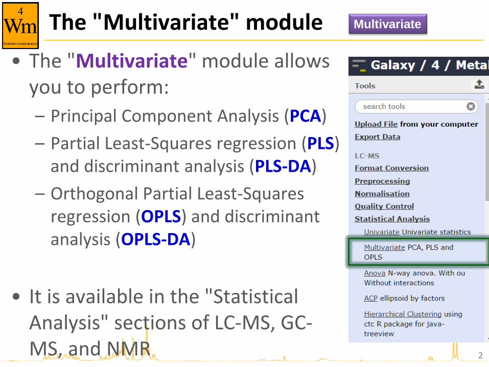
• The "Multivariate" module allows you to perform:

– Principal Component Analysis (PCA)

– Partial Least-Squares regression (PLS) and discriminant analysis (PLS-DA)

– Orthogonal Partial Least-Squares regression (OPLS) and discriminant analysis (OPLS-DA)

• It is available in the "Statistical Analysis" sections of LC-MS, GC-MS, and NMR 2

Multivariate

The "Multivariate" module

• The Multivariate module uses internally the ropls R module from bioconductor

– implements the original, NIPALS based, algorithms for PCA, PLS and OPLS

– diagnostics to detect outliers, overfitting

– graphics (scores, loadings, predictions)

– feature selection (VIP, regression coefficients)

3

http://bioconductor.org/packages/ropls

Thévenot E.A., Roux A., Xu Y., Ezan E. and Junot C. (2015). Analysis of the human adult urinary metabolome

variations with age, body mass index and gender by implementing a comprehensive workflow for univariate and

OPLS statistical analyses. Journal of Proteome Research, 14:3322-3335.

http://dx.doi.org/10.1021/acs.jproteome.5b00354

Multivariate

Objectives

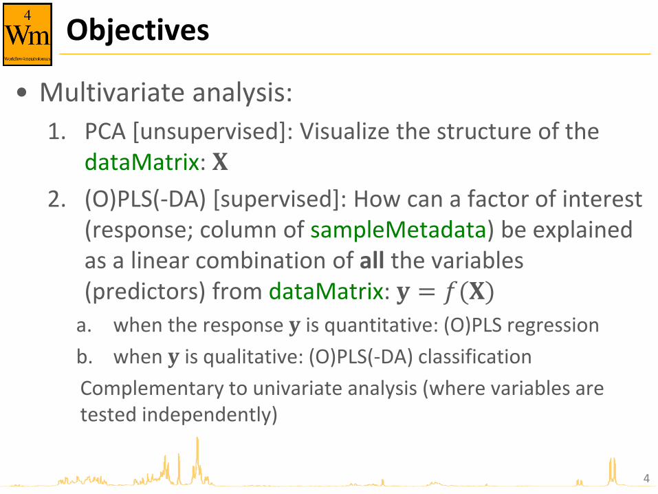
• Multivariate analysis:

1. PCA [unsupervised]: Visualize the structure of the dataMatrix: 𝐗

2. (O)PLS(-DA) [supervised]: How can a factor of interest (response; column of sampleMetadata) be explained as a linear combination of all the variables (predictors) from dataMatrix: 𝐲 = 𝑓(𝐗)

a. when the response 𝐲 is quantitative: (O)PLS regression

b. when 𝐲 is qualitative: (O)PLS(-DA) classification

Complementary to univariate analysis (where variables are tested independently)

4

Latent variable methods

• PCA and (O)PLS(-DA) are latent variable methods: new components are computed as linear combinations of the original variables

• The assumption is that a few components can efficiently represent the whole dataset (PCA) or model the factor of interest (O)PLS(-DA)

• Other powerful multivariate methods exist for regression and classification (Support Vector Machine, Random Forest, etc.)

– soon available on W4M

5

PCA and (O)PLS(-DA) steps in the analysis

6

Discard outliers

(if required)

Exploratory

Data Analysis

Univariate tests

PLS modelling

Select features

also:

ACP,

hierarchical

clustering,

heatmap also:

ANOVA

PC

A

(O)P

LS

(-D

A)

see the shared 'demo_workflow_statistics' workflow

Open the "Multivariate" module

• and select your 3 files of interest:

• you are now ready to start your multivariate analyzes!

7

1

2

3

4

5

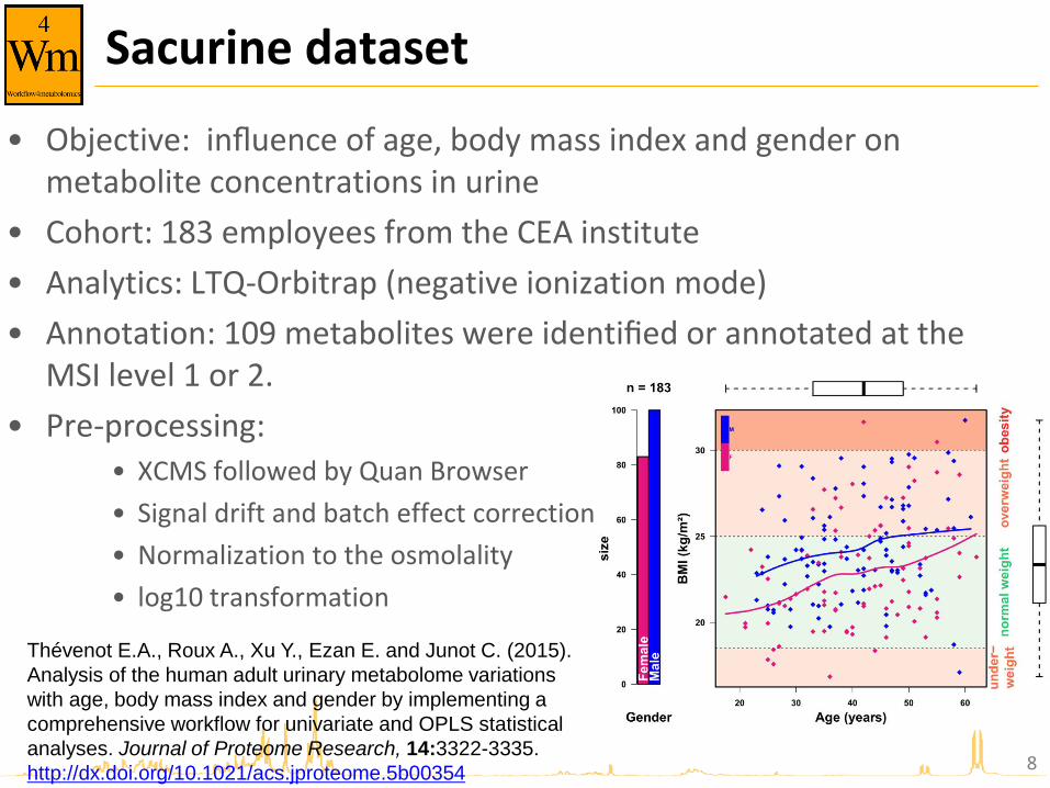
Sacurine dataset

• Objective: influence of age, body mass index and gender on metabolite concentrations in urine

• Cohort: 183 employees from the CEA institute

• Analytics: LTQ-Orbitrap (negative ionization mode)

• Annotation: 109 metabolites were identified or annotated at the MSI level 1 or 2.

• Pre-processing: • XCMS followed by Quan Browser

• Signal drift and batch effect correction

• Normalization to the osmolality

• log10 transformation

8

Thévenot E.A., Roux A., Xu Y., Ezan E. and Junot C. (2015).

Analysis of the human adult urinary metabolome variations

with age, body mass index and gender by implementing a

comprehensive workflow for univariate and OPLS statistical

analyses. Journal of Proteome Research, 14:3322-3335.

http://dx.doi.org/10.1021/acs.jproteome.5b00354

PRINCIPAL COMPONENT ANALYSIS (PCA)

9

Objectives

• Visualize the dataMatrix

– by selecting a few components which capture most of the spread (variance) of the cloud of samples

• Detect outliers

– which may bias the computation of the component

• Detect clusters of samples

– which may suggest an internal structuration of the data

10

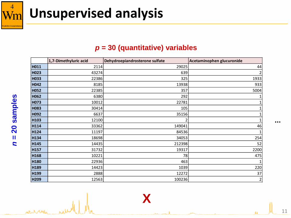
Unsupervised analysis

11

1,7-Dimethyluric acid Dehydroepiandrosterone sulfate Acetaminophen glucuronide

H011 2114 29025 44

H023 43274 639 2

H033 22386 325 1933

H042 8185 13938 933

H052 22385 357 5004

H062 6380 292 1

H073 10012 22781 1

H083 30414 105 1

H092 6637 35156 1

H103 12100 2 1

H114 33362 149041 46

H124 11197 84536 1

H134 18698 34053 254

H145 14435 212398 52

H157 31732 19317 2200

H168 10221 78 475

H180 22936 463 1

H189 14423 1039 220

H199 2888 12272 37

H209 12563 100236 2

n =

20 s

am

ple

s

p = 30 (quantitative) variables

...

X

How to visualize multivariate observations?

12

1 variable 2 variables

3 variables p variables

Projection

• Projected distances as high as possible

13

Husson and Pages (2011). Exploratory

multivariate analysis by example using R.

Chapman & Hall/CRC

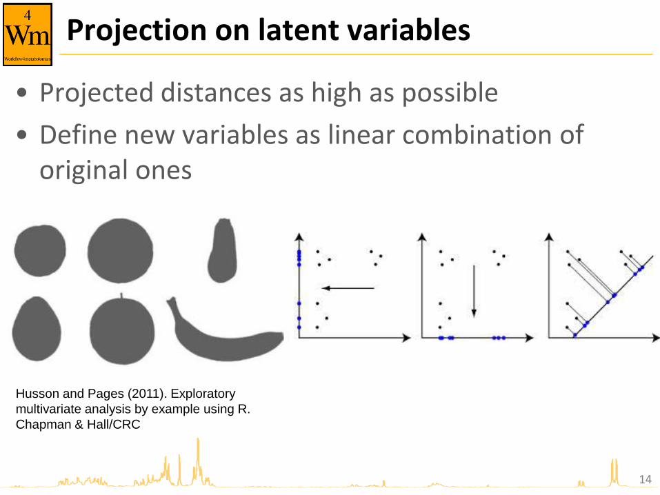
Projection on latent variables

• Projected distances as high as possible

• Define new variables as linear combination of original ones

14

Husson and Pages (2011). Exploratory

multivariate analysis by example using R.

Chapman & Hall/CRC

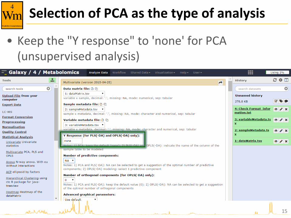
Selection of PCA as the type of analysis

• Keep the "Y response" to 'none' for PCA (unsupervised analysis)

15

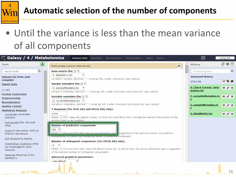
Automatic selection of the number of components

• Until the variance is less than the mean variance of all components

16

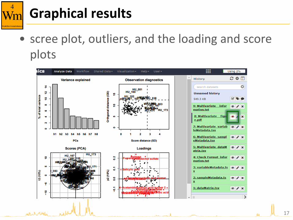
Graphical results

• scree plot, outliers, and the loading and score plots

17

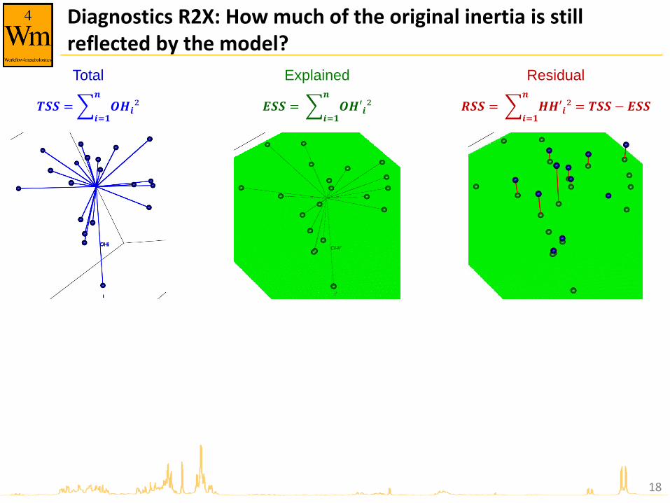
Diagnostics R2X: How much of the original inertia is still reflected by the model?

18

𝑻𝑺𝑺 = 𝑶𝑯𝒊²𝒏

𝒊=𝟏 𝑬𝑺𝑺 = 𝑶𝑯′𝒊²

𝒏

𝒊=𝟏 𝑹𝑺𝑺 = 𝑯𝑯′𝒊²

𝒏

𝒊=𝟏= 𝑻𝑺𝑺 − 𝑬𝑺𝑺

Total Explained Residual

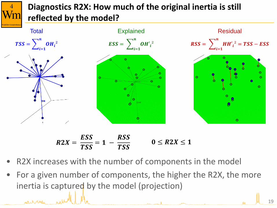
Diagnostics R2X: How much of the original inertia is still reflected by the model?

• R2X increases with the number of components in the model

• For a given number of components, the higher the R2X, the more inertia is captured by the model (projection)

19

𝑹𝟐𝑿 = 𝑬𝑺𝑺

𝑻𝑺𝑺= 𝟏 −

𝑹𝑺𝑺

𝑻𝑺𝑺 𝟎 ≤ 𝑹𝟐𝑿 ≤ 𝟏

𝑻𝑺𝑺 = 𝑶𝑯𝒊²𝒏

𝒊=𝟏 𝑬𝑺𝑺 = 𝑶𝑯′𝒊²

𝒏

𝒊=𝟏 𝑹𝑺𝑺 = 𝑯𝑯′𝒊²

𝒏

𝒊=𝟏= 𝑻𝑺𝑺 − 𝑬𝑺𝑺

Total Explained Residual

Scree plot

• Check that the first components capture most of the variance

20

Mount Yamnuska, Alberta. Wikipedia

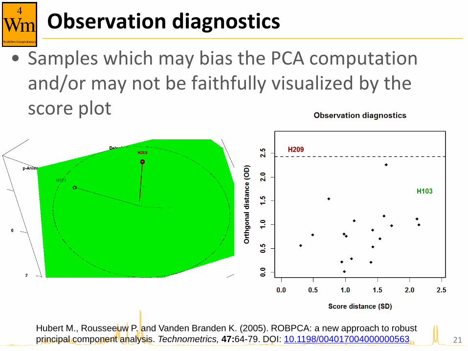
Observation diagnostics

21

• Samples which may bias the PCA computation and/or may not be faithfully visualized by the score plot

Hubert M., Rousseeuw P. and Vanden Branden K. (2005). ROBPCA: a new approach to robust

principal component analysis. Technometrics, 47:64-79. DOI: 10.1198/004017004000000563

Sensitivity to outliers

22

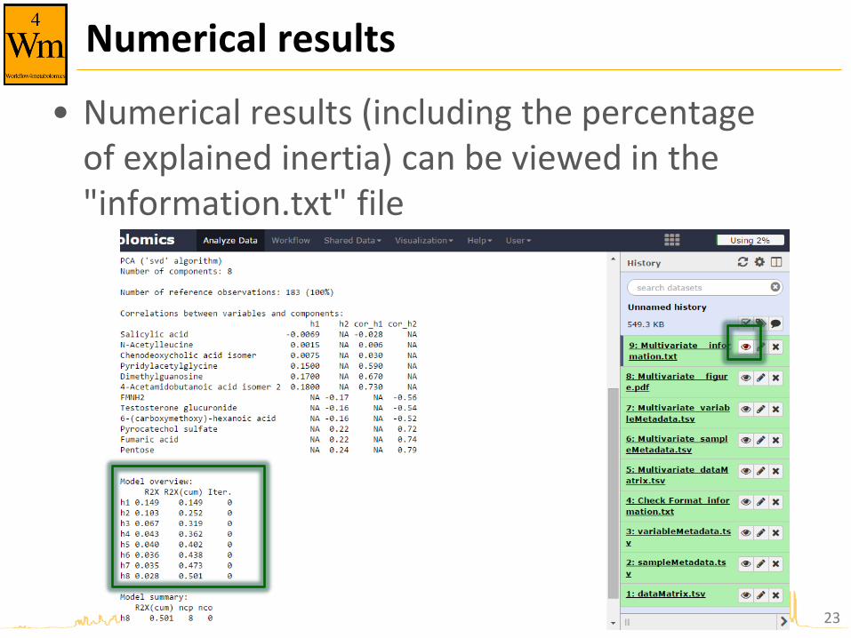
Numerical results

• Numerical results (including the percentage of explained inertia) can be viewed in the "information.txt" file

23

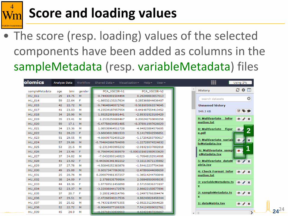
Score and loading values

• The score (resp. loading) values of the selected components have been added as columns in the sampleMetadata (resp. variableMetadata) files

24 24

1

2

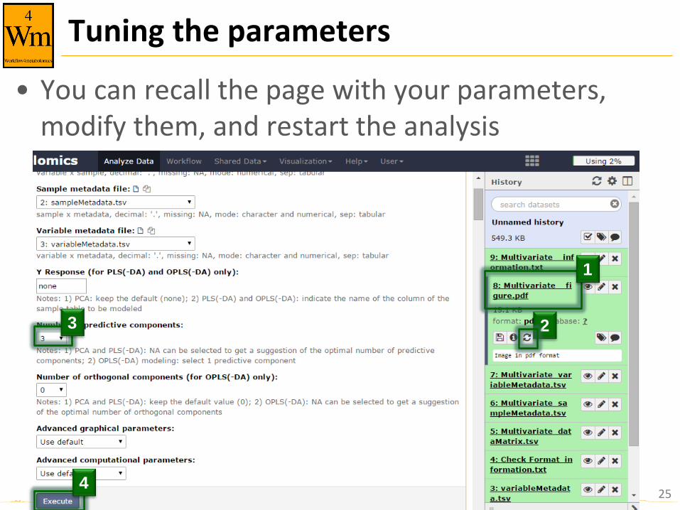
Tuning the parameters

• You can recall the page with your parameters, modify them, and restart the analysis

25

1

2 3

4

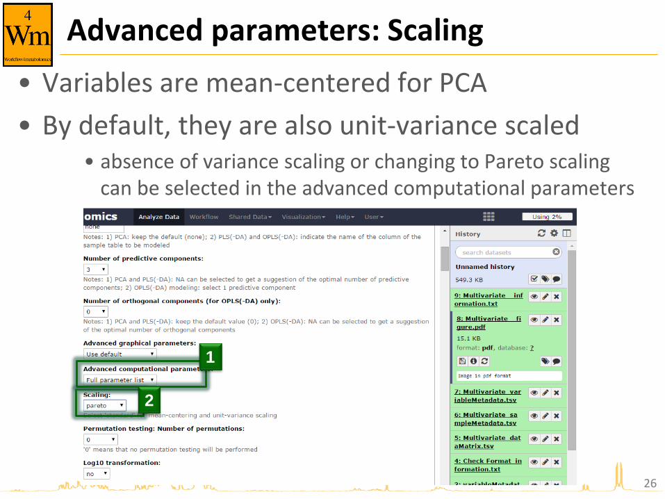
Advanced parameters: Scaling

• Variables are mean-centered for PCA

• By default, they are also unit-variance scaled • absence of variance scaling or changing to Pareto scaling

can be selected in the advanced computational parameters

26

1

2

Advanced parameters: Ellipses

• Indicate the column name of sampleMetadata to be used

27

1

2

References

– Husson F., Le S. and Pages J. (2011). Exploratory multivariate analysis by example using R. Chapman & Hall/CRC

– Ringner M. (2008). What is principal component analysis? Nature Biotechnology, 26:303-304. http://dx.doi.org/10.1038/nbt0308-303

– Baccini A. (2010). Statistique descriptive multidimensionnelle (pour les nuls). www.math.univ-toulouse.fr/~baccini/zpedago/asdm.pdf

28

PARTIAL LEAST SQUARES REGRESSION (PLS) AND DISCRIMINANT ANALYSIS (PLS-DA)

2 9

PLS(-DA) modelling

• Powerful regression method when 𝑛𝑠𝑎𝑚𝑝𝑙𝑒𝑠 < 𝑝𝑣𝑎𝑟𝑖𝑎𝑏𝑙𝑒𝑠

• Complementary to univariate hypothesis testing (where variables are tested independantly)

• Risk of overfitting: i.e., building a model whose (apparently) good performances result from chance only

30

Supervised analysis (i.e. with labels)

31

1,7-Dimethyluric acid Dehydroepiandrosterone sulfate

H011 3.33 4.46

H023 4.64 2.81

H033 4.35 2.51

H042 3.91 4.14

H052 4.35 2.55

H062 3.80 2.47

H073 4.00 4.36

H083 4.48 2.02

H092 3.82 4.55

H103 4.08 0.21

H114 4.52 5.17

H124 4.05 4.93

H134 4.27 4.53

H145 4.16 5.33

H157 4.50 4.29

H168 4.01 1.89

H180 4.36 2.67

H189 4.16 3.02

H199 3.46 4.09

H209 4.10 5.00

p = 30 (quantitative) variables

...

X

n =

20 s

am

ple

s

bmi

H011 19.8

H023 29.6

H033 18.4

H042 19.8

H052 20.1

H062 22.2

H073 25.4

H083 29.8

H092 21.8

H103 26.8

H114 29.4

H124 22.2

H134 22.9

H145 29.1

H157 22.0

H168 20.8

H180 23.7

H189 19.4

H199 21.0

H209 21.5

1 response

y

PLS vs PCA

• PCA finds the directions of maximum variance

32

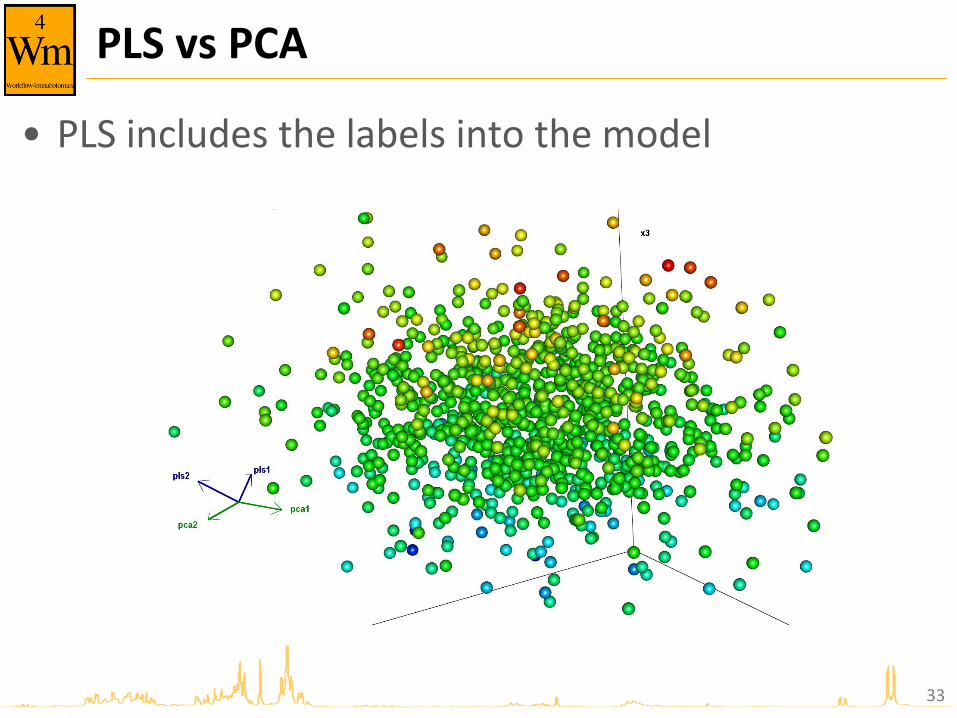
PLS vs PCA

• PLS includes the labels into the model

33

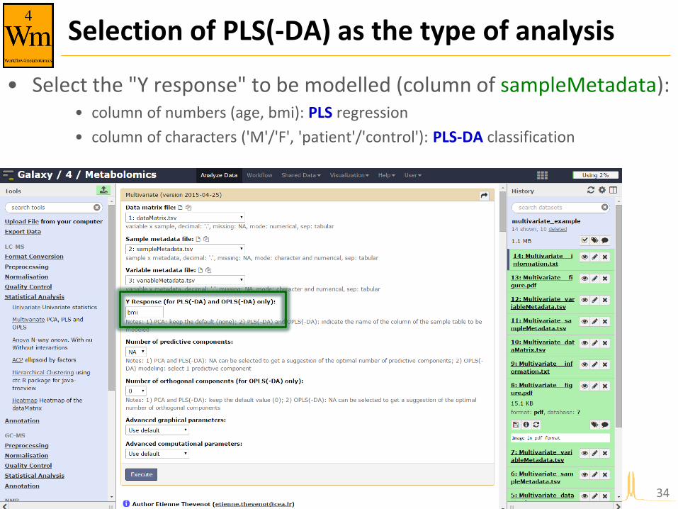
Selection of PLS(-DA) as the type of analysis

• Select the "Y response" to be modelled (column of sampleMetadata): • column of numbers (age, bmi): PLS regression

• column of characters ('M'/'F', 'patient'/'control'): PLS-DA classification

34

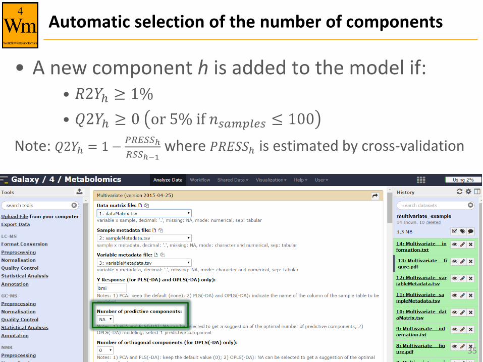
Automatic selection of the number of components

• A new component h is added to the model if: • 𝑅2𝑌ℎ ≥ 1%

• 𝑄2𝑌ℎ ≥ 0 or 5% if 𝑛𝑠𝑎𝑚𝑝𝑙𝑒𝑠 ≤ 100

Note: 𝑄2𝑌ℎ = 1 −𝑃𝑅𝐸𝑆𝑆ℎ

𝑅𝑆𝑆ℎ−1 where 𝑃𝑅𝐸𝑆𝑆ℎ is estimated by cross-validation

35

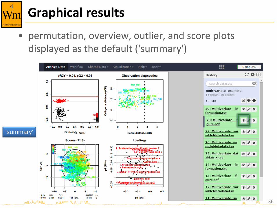
Graphical results

• permutation, overview, outlier, and score plots displayed as the default ('summary')

36

'summary'

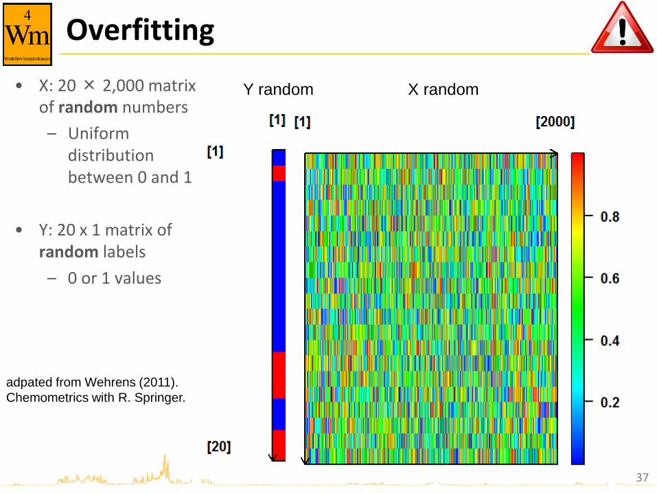
Overfitting

37

Y random X random • X: 20 × 2,000 matrix of random numbers

– Uniform distribution between 0 and 1

• Y: 20 x 1 matrix of random labels

– 0 or 1 values

adpated from Wehrens (2011).

Chemometrics with R. Springer.

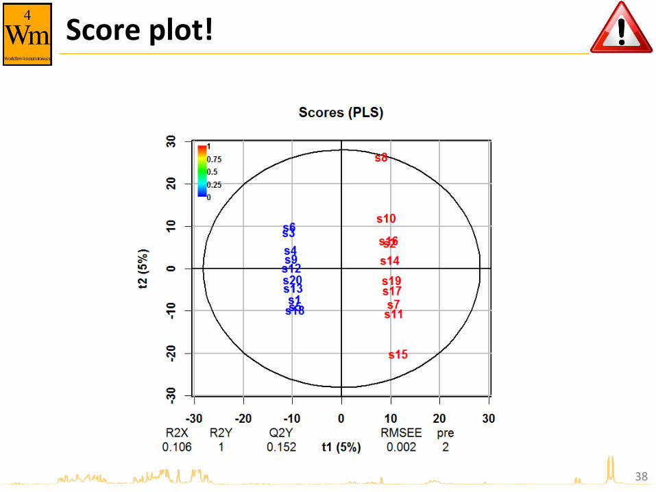
Score plot!

38

Importance of diagnostics

• Permutation testing: comparing the R2Y and Q2Y values of the model built with the true Y labels with 𝒏𝒑𝒆𝒓𝒎 models built with random permutation of Y labels

39

Szymanska E., Saccenti E., Smilde A. and Westerhuis J. (2012). Double-check: validation of diagnostic statistics for PLS-DA models in metabolomics studies. Metabolomics, 8:3-16. DOI: 10.1007/s11306-011-0330-3

Risk of overfitting when n < p

40

0.2 0.5 1 10 100

𝐯𝐚𝐫𝐢𝐚𝐛𝐥𝐞𝐬

𝐬𝐚𝐦𝐩𝐥𝐞𝐬=

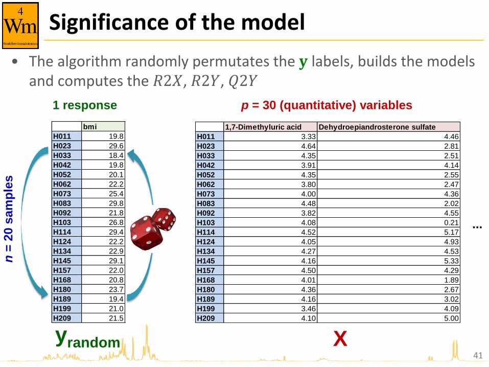
Significance of the model

• The algorithm randomly permutates the 𝐲 labels, builds the models and computes the 𝑅2𝑋, 𝑅2𝑌, 𝑄2𝑌

41

1,7-Dimethyluric acid Dehydroepiandrosterone sulfate

H011 3.33 4.46

H023 4.64 2.81

H033 4.35 2.51

H042 3.91 4.14

H052 4.35 2.55

H062 3.80 2.47

H073 4.00 4.36

H083 4.48 2.02

H092 3.82 4.55

H103 4.08 0.21

H114 4.52 5.17

H124 4.05 4.93

H134 4.27 4.53

H145 4.16 5.33

H157 4.50 4.29

H168 4.01 1.89

H180 4.36 2.67

H189 4.16 3.02

H199 3.46 4.09

H209 4.10 5.00

p = 30 (quantitative) variables

...

X

bmi

H011 19.8

H023 29.6

H033 18.4

H042 19.8

H052 20.1

H062 22.2

H073 25.4

H083 29.8

H092 21.8

H103 26.8

H114 29.4

H124 22.2

H134 22.9

H145 29.1

H157 22.0

H168 20.8

H180 23.7

H189 19.4

H199 21.0

H209 21.5

1 response

n =

20 s

am

ple

s

yrandom

Significance of the model

• Counting the number of 𝑅2𝑌 (and 𝑄2𝑌) metrics from random models which are superior to the values of the true model gives an indication of the significance of the PLS modelling

42

Similarity between 𝐲𝑡𝑟𝑢𝑒 and 𝐲𝑟𝑎𝑛𝑑𝑜𝑚

𝑅2𝑌 and 𝑄2𝑌 of the model

with the true 𝐲 values

'permutation'

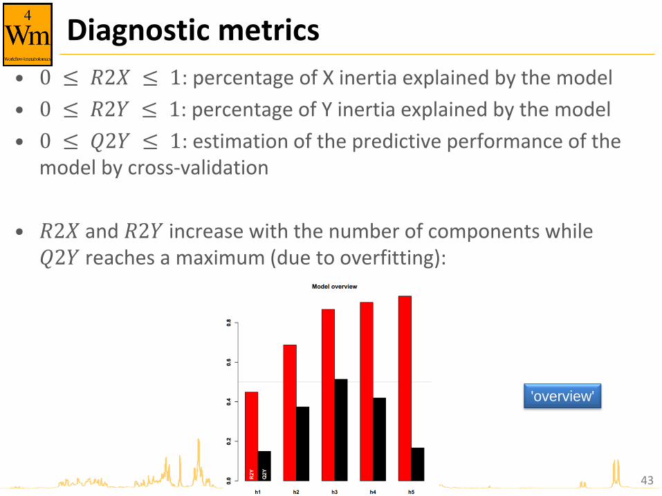
Diagnostic metrics

• 0 ≤ 𝑅2𝑋 ≤ 1: percentage of X inertia explained by the model

• 0 ≤ 𝑅2𝑌 ≤ 1: percentage of Y inertia explained by the model

• 0 ≤ 𝑄2𝑌 ≤ 1: estimation of the predictive performance of the model by cross-validation

• 𝑅2𝑋 and 𝑅2𝑌 increase with the number of components while 𝑄2𝑌 reaches a maximum (due to overfitting):

43

'overview'

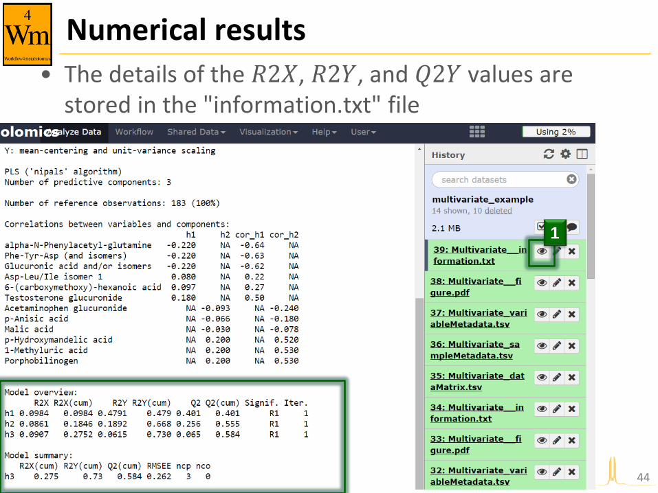
Numerical results

• The details of the 𝑅2𝑋, 𝑅2𝑌, and 𝑄2𝑌 values are stored in the "information.txt" file

44

1

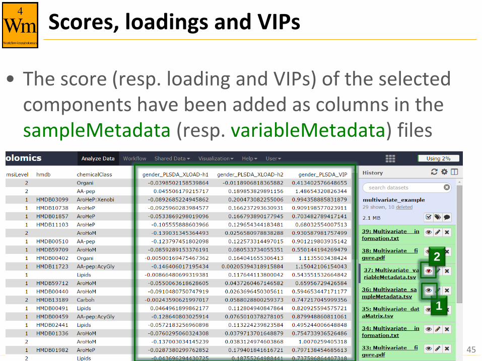
Scores, loadings and VIPs

• The score (resp. loading and VIPs) of the selected components have been added as columns in the sampleMetadata (resp. variableMetadata) files

45

1

2

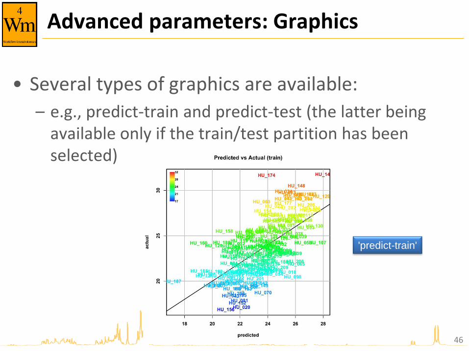
Advanced parameters: Graphics

• Several types of graphics are available:

– e.g., predict-train and predict-test (the latter being available only if the train/test partition has been selected)

46

'predict-train'

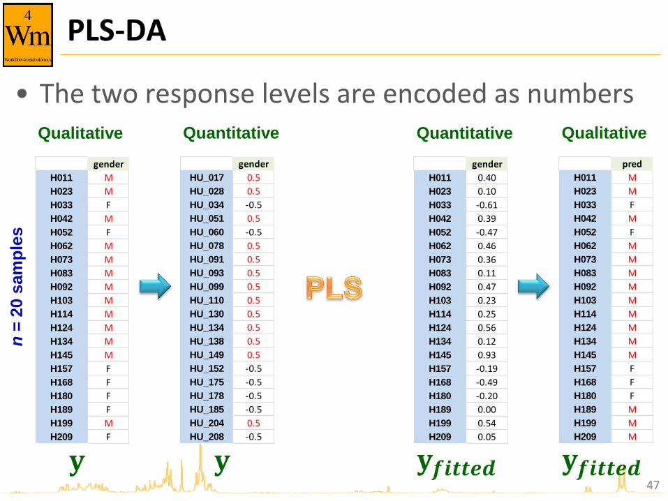
PLS-DA

• The two response levels are encoded as numbers

47

n =

20 s

am

ple

s

gender

H011 M

H023 M

H033 F

H042 M

H052 F

H062 M

H073 M

H083 M

H092 M

H103 M

H114 M

H124 M

H134 M

H145 M

H157 F

H168 F

H180 F

H189 F

H199 M

H209 F

Qualitative

𝐲

gender

HU_017 0.5

HU_028 0.5

HU_034 -0.5

HU_051 0.5

HU_060 -0.5

HU_078 0.5

HU_091 0.5

HU_093 0.5

HU_099 0.5

HU_110 0.5

HU_130 0.5

HU_134 0.5

HU_138 0.5

HU_149 0.5

HU_152 -0.5

HU_175 -0.5

HU_178 -0.5

HU_185 -0.5

HU_204 0.5

HU_208 -0.5

Quantitative

𝐲

gender

H011 0.40

H023 0.10

H033 -0.61

H042 0.39

H052 -0.47

H062 0.46

H073 0.36

H083 0.11

H092 0.47

H103 0.23

H114 0.25

H124 0.56

H134 0.12

H145 0.93

H157 -0.19

H168 -0.49

H180 -0.20

H189 0.00

H199 0.54

H209 0.05

Quantitative

𝐲𝒇𝒊𝒕𝒕𝒆𝒅

pred

H011 M

H023 M

H033 F

H042 M

H052 F

H062 M

H073 M

H083 M

H092 M

H103 M

H114 M

H124 M

H134 M

H145 M

H157 F

H168 F

H180 F

H189 M

H199 M

H209 M

Qualitative

𝐲𝒇𝒊𝒕𝒕𝒆𝒅

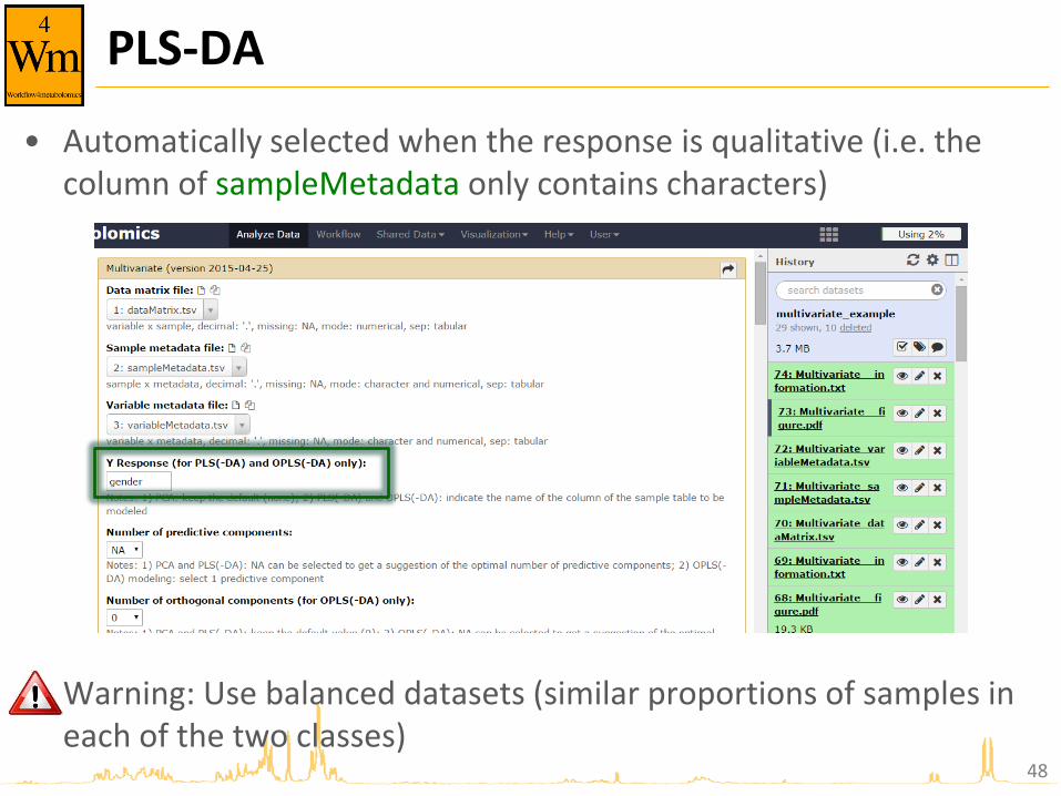
PLS-DA

• Automatically selected when the response is qualitative (i.e. the column of sampleMetadata only contains characters)

• Warning: Use balanced datasets (similar proportions of samples in each of the two classes)

48

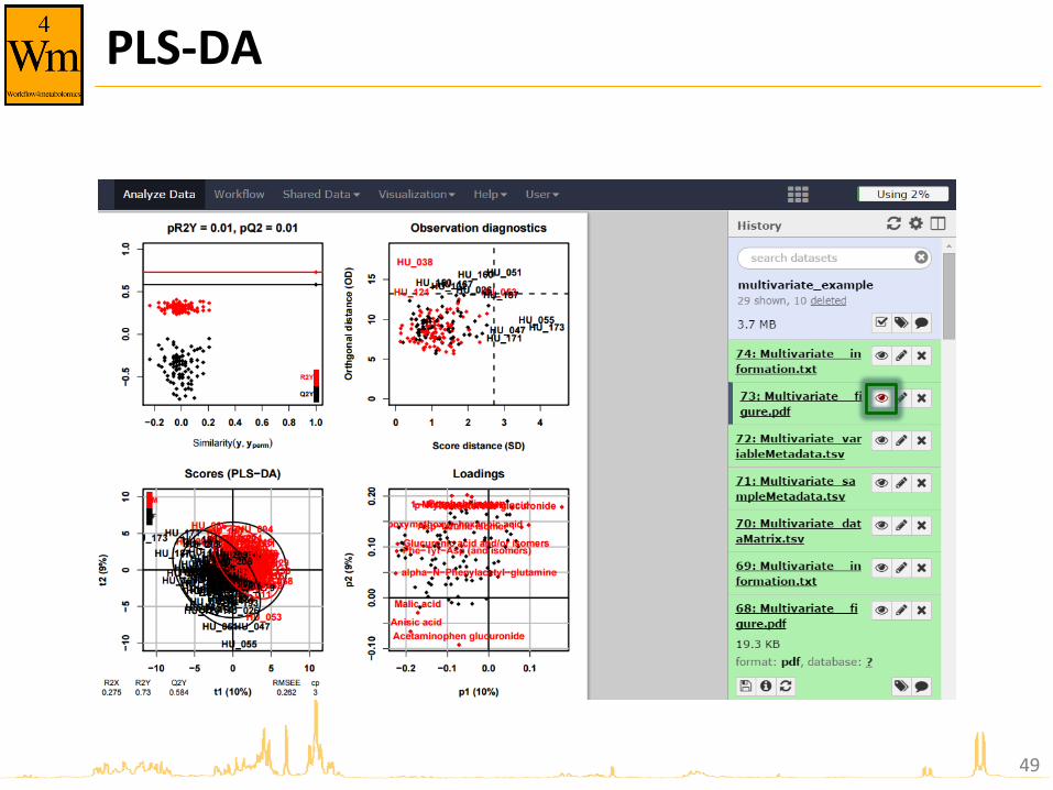
PLS-DA

49

ORTHOGONAL PARTIAL LEAST SQUARES REGRESSION (OPLS) AND DISCRIMINANT ANALYSIS (OPLS-DA)

5 0

Principles

• Separately models the variations of the predictors correlated and orthogonal to the response

• Improves the interpretation of the components but not the overall predictive performance of the model

• Only one predictive component required for single response models

• Note: As with PLS, care should be taken to avoid too many (orthogonal) components (which would result in overfitting)

51

OPLS vs PLS

• Variation not correlated to the response (e.g., technical bias) is modelled separately by the orthogonal component(s)

=> The first predictive component is strongly correlated to the response

52

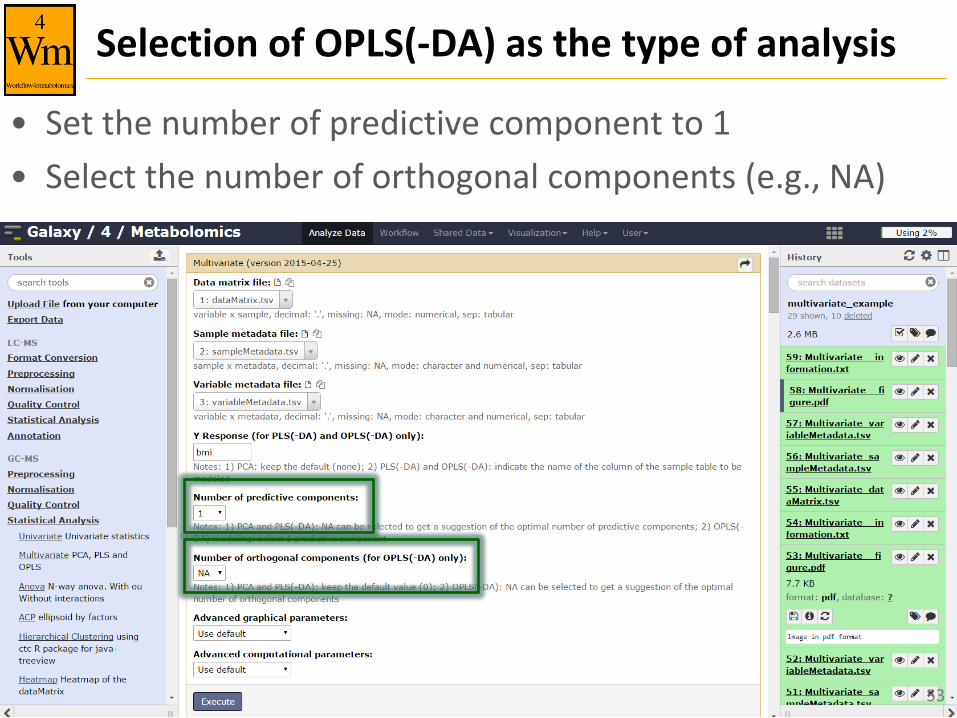
Selection of OPLS(-DA) as the type of analysis

• Set the number of predictive component to 1

• Select the number of orthogonal components (e.g., NA)

53

Graphical results

• permutation, overview, outlier, and score plots displayed as the default ('summary')

54

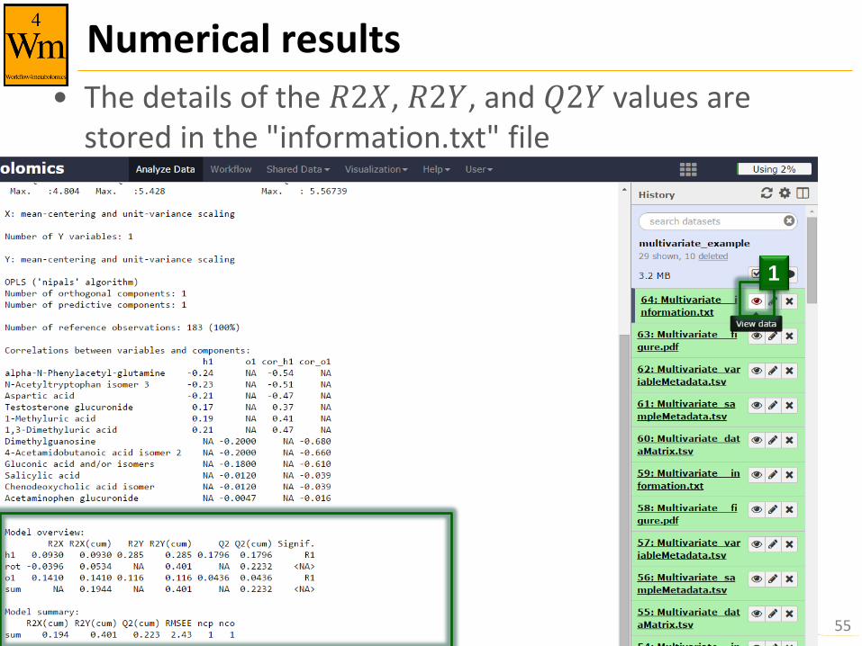
Numerical results

• The details of the 𝑅2𝑋, 𝑅2𝑌, and 𝑄2𝑌 values are stored in the "information.txt" file

55

1

References

– Wold S., Sjöström M. and Eriksson L. (2001). PLS-regression: a basic tool of chemometrics. Chemometrics and Intelligent Laboratory Systems, 58:109-130. http://dx.doi.org/10.1016/S0169-7439(01)00155-1

– Trygg J., Holmes E. and Lundstedt T. (2007). Chemometrics in Metabonomics. Journal of Proteome Research, 6:469-479. http://dx.doi.org/10.1021/pr060594q

– Brereton R.G. and Lloyd G.R. (2014). Partial least squares discriminant analysis: taking the magic away. Journal of Chemometrics, 28:213-225. http://dx.doi.org/10.1002/cem.2609

56