How reliable are meta-analyses for international benefit transfers?

MPRAMunich Personal RePEc Archive

How Reliable are Meta-Analyses forInternational Benefit Transfers?

Henrik Lindhjem and Stale Navrud

Norwegian University of Life Sciences, Econ Poyry

July 2007

Online at http://mpra.ub.uni-muenchen.de/11484/MPRA Paper No. 11484, posted 10. November 2008 00:01 UTC

1

How Reliable are Meta-Analyses for

International Benefit Transfers?

Henrik Lindhjemab∗ and Ståle Navruda

a Department of Economics and Resource Management, Norwegian University of Life Sciences, P.O. Box 5003, N-1432 Ås, Norway

b ECON, P.O. Box 5, N-0051, Oslo, Norway

Draft: 6. July 2007

Published in Ecological Economics 66(2-3): 425-435, 2008.

∗ Corresponding author. E-mail: [email protected]. Phone: +4798263957, Fax: +4764965701

2

How Reliable are Meta-Analyses for

International Benefit Transfers?1

Abstract

Meta-analysis has increasingly been used to synthesise the environmental valuation

literature, but only a few test the use of these analyses for benefit transfer. These are

typically based on national studies only. However, meta-analyses of valuation studies

across countries are a potentially powerful tool for benefit transfer, especially for

environmental goods where the domestic literature is scarce. We test the reliability of

such international meta-analytic transfers, and find that even under conditions of

homogeneity in valuation methods, cultural and institutional conditions across

countries, and a meta-analysis with large explanatory power, the transfer errors could

still be large. Further, international meta-analytic transfers do not on average perform

better than simple value transfers averaging over domestic studies. Thus, we question

whether the use of meta-analysis for practical benefit transfer achieves reliability gains

justifying the increased effort. However, more meta-analytic benefit transfer tests

should be performed for other environmental goods and other countries before

discarding international meta-analysis as a tool for benefit transfer.

Keywords: benefit transfer, environmental valuation, meta-analysis, forest. JEL Classification: Q51, H41.

1 A previous version of this paper was presented at the annual conferences of the US Society of Ecological

Economics (New York 26. June 2007) and the European Association of Environmental and Resource Economists

(Thessaloniki, Greece 30. June 2007).

3

Introduction

Meta-analysis (MA), “the study of studies”, is now common in environmental

economics and non-market valuation (Smith and Pattanayak, 2002). Since Smith and

Karou’s (1990) seminal study of recreational benefits, MA has been conducted for a

wide range of environmental goods, from wetlands (Woodward and Wui, 2001) to

visibility (Smith and Osborne, 1996). Common to all of these studies is the focus on

research synthesis and hypothesis testing, rather than on the more interesting policy

question of how MA can be used to improve benefit transfer (BT) practices. Meta-

analytic benefit transfer (MA-BT) to unstudied sites (“policy sites”) has only been

cursory treated in the literature, typically a few pages add-ons at the end of lengthy MA

papers, although authors emphasise its potential importance for future research and

applications, for example in cost-benefit analysis (CBA) (see the special issue on

benefit transfer in Ecological Economics 2006). While there is some knowledge of how

unit value and value function-based BT from single studies perform (Rosenberger and

Phipps, 2007), Bergstrom and Taylor (2006:359) point out that “before widespread

application of MA-BT models, there is a need for additional MA-BT convergent

validity tests across different types of natural resources and environmental

commodities.” Only a few studies have, to our knowledge, investigated the validity and

reliability of MA-BT (Santos, 1998; Rosenberger and Loomis, 2000b; Shrestha and

Loomis, 2001; 2003; Santos, 2007; Shrestha et al., 2007). Four of the studies, however,

are based on the same large dataset of use values for different recreational activities in

the USA2, and are unable to cover the breadth of issues involved in more typical MA-

2 A recreational database originally assembled for the US Forest Service maintained over 20-30 years, supplemented

with additional data collected for the purpose of validity testing (see e.g. Rosenberger and Loomis (2001)).

4

BT exercises, i.e. limited datasets, complex goods with significant non-use values,

different level of methodological heterogeneity and mix of international studies to

mention a few. Santos (2007) is the only study attempting a comprehensive comparison

of two versions of a domestic MA-BT with simple BT techniques often used in practice.

Further, all the above studies can be said to under-appreciate the potential impacts on

the MA-BT performance of model specifications, values of methodological variables

(Johnston et al., 2006) and other choices the meta-analyst needs to make (Hoehn,

2006)3.

This paper aims to investigate the validity and reliability of international MA-BT of

Non-timber benefits (NTBs) based on a recently published MA of contingent valuation

(CV) research in Fennoscandia (a term for Norway, Sweden and Finland) (Lindhjem,

2007). Compared to previous research on MA-BT, our paper adds several new and

interesting dimensions: (i) a more systematic and diverse testing of different MA-BT

models, including comparisons with simple BT techniques, (ii) the good we investigate

is complex and has substantial non-use values related to biodiversity (rather than mainly

use values), (iv) data from three European countries, which are similar culturally,

economically, institutionally (e.g. everyman´s right to walk in private forests), and in

the way the good is perceived and used, and (v) data are generally more homogenous

methodologically since only CV studies are included. We investigate the transfer error

(TE) of four different meta-regression model specifications, and use the best two

models to compare MA-BT with simple unit value transfer techniques. A key question

is whether the use of MA-BT achieves reliability gains justifying the increased effort.

3 A alternative to the classical MA approach, not considered here, uses Bayesian modeling techniques to address

some of these challenges, for example treatment of methodological variables and difference in availability of

regressors across source studies (Moeltner et al., 2007)

5

As pointed out by Navrud and Ready (2007a:288): “Simple approaches should not be

cast aside until we are confident that more complex approaches do perform better”.

Validity and reliability of meta-analytic benefit transfer

Underlying theory of MA-BT

The simple underlying indirect utility function for a change from Q0 to Q1 in the

quality/quantity vector describing an environmental good available for individual i is:

Vi (pi, Ii, Q0) = Vi (pi, Ii-WTP, Q1) (1)

where Pi, Ii are a market price vector and income, respectively, and WTP is

Willingness-to-Pay. Since indirect utility functions are homogenous of degree 0,

identical individuals from two countries using different currencies will have the same

real WTP only if they have the same real income and faces the same real prices. Thus

the appropriate exchange rate to use for conversion is the purchasing power parity (PPP)

(Ready and Navrud, 2006). Equation (1) solved for WTP, yields the bid-function that

forms the (often implicit) basis for any MA-BT exercise. Following Bergstrom and

Taylor (2006), we further assume what they call a “Weak structural utility theoretic”

approach4, i.e. that the underlying variables in the WTP-function is assumed to be

derivable from some unknown utility function, but that flexibility is maintained to

introduce explanatory variables, such as study characteristics, into the WTP model that

do not necessarily follow from (1). This is the approach used in most previous MA-BT

exercises (for example Rosenberger and Loomis 2000b, Shresta and Loomis 2003). We

4 Bergstrom and Taylor (2006) suggest three main approaches (of which only the first two are recommended); (1)

Strong structural utility theoretic approach; (2) Weak structural utility theoretic approach; (3) Non-structural

utility theoretic approach.

6

specify a meta-model that captures j site characteristics X, k study or methodological

characteristics M, l program characteristics P, and q socio-economic characteristics S.

Mean WTP estimate (long term, per household in Norwegian Kroner 2005) m from

study s, WTPms, can then be defined as:

smsqmsS

lmsP

kmsM

jmsX0ms ueSPMXWTP ++β+β+β+β+β= (2)

Where, β0, β are constant term and parameter vectors for the explanatory variables, and

ems and us are random error terms for the measurement and study levels, respectively.

MA-BT involves estimating (2) based on previous studies, and inserting values for X, P

and S for the policy site under investigation, and choosing values for M (typically

average of the meta-data, “best-practice” values or sample from a distribution – see e.g.

Johnston et al (2006)). The meta-model has several potential advantages for BT,

compared to unit value transfer or function transfer based on a single study5. MA

utilizes information from several studies providing more rigorous measures of central

tendency that are sensitive to the underlying distribution of the study values

(Rosenberger and Loomis 2000b). Further, as specified in the model above, MA can

control for study-specific choices of methodology, and finally it is possible to account

for differences in site and programme characteristics between the policy site and the

study sites in the meta-data, by setting these variable values equal to the policy site6.

Convergent validity and reliability

5 The benefit transfer function from a single study is often specified as WTPi=a + bXij +cYik + ei, where WTPi is

willingness-to-pay of respondent i, X site/good characteristics (j), Y respondent characteristics (k), ej random

error, and the number of observations is equal to the number of respondents (Brouwer, 2000).

6 This is provided that the policy site characteristics are represented in the meta-data. Otherwise the meta-model

would be unsuitable for BT to that particular policy site.

7

If the process of BT is accurate, it can be used to inform decisions at a policy site, for

example in a CBA framework. The focus to date has primarily been on the concept of

validity, which requires that the values, or the value functions generated from the study

site(s), be statistically identical to those estimated at the policy site (Navrud and Ready,

2007b). Further, the transferred estimate should be relatively invariant to various

judgements by the analyst, for example choice of model specification (Rosenberger and

Loomis 2000b). Most of the studies testing BT validity have used the same

questionnaire for similar goods for different populations nationally and internationally,

often resulting in high levels of TE (up to several hundred percent; see Rosenberger and

Phipps (2007, table 1) for an overview of results). For MA-BT, such tests are scarce.

For one thing, it is harder to define a yardstick value suitable for comparison with the

transferred estimate. Rosenberger and Loomis (2000b) compare raw values from studies

within their sample of recreation activities with the predictions from their national and

regional MA-BT models, and calculate TE. Shresta and Loomis (2003; 2001) and

Shresta et al (2007) follow a similar convergent validity approach, comparing their

meta-model predictions based on the same dataset with the recreational values from a

number of additional domestic and international studies, respectively (i.e. out-of-sample

comparisons). More recently the BT validity testing has shifted focus somewhat to the

concept of reliability, which requires that TE is small (but not necessarily zero). Santos

(2007) compares the performance of MA-BT of landscape values to a site for which

there exists a CV study to investigate convergent validity but also to assess the practical

importance of TE for policy. Equivalence tests, which combine the concepts of

statistical significance and policy significance into one test by defining an acceptable

TE prior to the validity test, have been suggested (Kristofersson and Navrud, 2005).

However, there is still no agreement on what the acceptable transfer errors should be for

8

different policy applications, though levels of 20 and 40 percent have been suggested

(Kristofersson and Navrud, 2007). Thus, the focus here is on measuring reliability in

terms of TE and compare across model specifications and restrictions, and between

alternative ways of conducting BT based on the same data. We define TE as

T

TE

WTP|WTPWTP|

TE−

= , (3)

where E = Estimated (predicted) value, T = True (observed) value7. Our procedure for

measuring TE and checking reliability of BT is summarised in Table 1 below, and

explained in the following. A first check of the transfer error for our meta-model

specified in (2) is to compare the in-sample model prediction or forecast with the WTP

observation and calculate TE for each observation and the overall Mean Absolute

Percentage Error (MAPE) in our sample (Objective 1 in Table 1). Second, we estimate

N-1 different MA-BT models, where for each run the WTP observation we shall predict

is taken out, and calculate TE and MAPE again8. The TE can be expected to be larger

than for the within-sample error above. We also characterize TE for different

observations to discern patterns in the data. Brander et al (2006; In press) have

suggested the within- and out-of sample TE calculation procedure for each observation

as a first step to check reliability of the MA-BT model. Third, to more closely resemble

an actual BT situation, we draw (randomly) a single WTP observation from each survey

to represent a benchmark, unknown policy site value (Objective 2 in Table 1)9. We then

7 It is important to note that this value, the benchmark value for comparison, for example as estimated by a single

study, is only an estimate of the assumed, true underlying value and has its own measurement error.

8 As pointed out by Brander et al (2006) this is similar to a jacknife resampling technique.

9 This procedure, i.e. using internal WTP estimates as benchmark for “true” values, resembles how convergent

validity considerations often are carried out in the (MA-)BT literature, e.g. starting with Loomis (1992).

9

use the other studies to transfer a best estimate to that “policy site” based on different

BT techniques that are often used in practice10. Such techniques include a simple

transfer of the mean WTP estimate from one study that has similar site and program

characteristics, or the mean WTP averaged over several similar domestic or

international study sites. We compare TE from these methods with the use of the two

most promising MA-BT models, judged on the basis of lowest TE from the initial

MAPE assessment above. Finally, in previous MA-BT convergent validity studies no

systematic check on the impact of the choice of model specifications and model

restrictions on TE have been carried out (Objective 3 in Table 1). There are many

different types of meta-model specifications in use, and there is little guidance as to

which to choose (linear, semi-log, double-log etc) (Johnston et al., 2005). Regarding

restricted model versions, a model frequently used (though rarely convincingly

justified11) in MA-BT is one where variables that are not significant at the 20 percent

level are left out of the MA-BT model. To investigate the implications of this choice,

we decided to test both a fully specified meta-model and a restricted version, like the

one used for example in Rosenberger and Loomis (2000b).

10 In this case, all observations from the same survey from which a WTP estimate has been drawn to represent the

policy site, are left out of the MA-BT model used for transfer.

11 A principal reason put forward for this choice is that it is easier to use for practitioners, a reason that may not be

valid today as a spread-sheet based BT tool would easily accommodate more variables without complicating the

operation.

10

Table 1 Objectives and transfer error calculation procedures for validity and

reliability check of MA-BT

Objective Transfer error estimation procedure

1. Convergent validity of transfer estimates

Analyse within-sample TE Compare model predictions with observed WTP on the individual measurement level for all observations, and calculate Mean Absolute Percentage Error (MAPE).

Analyse out-of-sample TE Compare N meta-model predictions and observed WTP for N-1of the meta-data for each prediction, and calculate Mean Absolute Percentage Error (MAPE).

2. Reliability comparison of different benefit transfer procedures

Compare reliability of simple unit transfer techniques with MA-BT

Simple unit transfer techniques based on the most similar study, mean of similar domestic and international studies, are compared with MA-BT transfer. Single WTP observations from each study are drawn randomly as a benchmark, unknown true policy site value for TE calculation.

3. Robustness of transfer errors to methodological choices and meta-analysis scope

Analyse TE across model specifications & restrictions

Two different model specifications (linear, and double-log) and two restricted models are used for transfer error calculations under 1. The two specifications with the lowest TE are used in 2.

Based on the Objectives 1.-.3 in Table 1, we will get a good check on convergent

validity, reliability and robustness of MA-BT, and a comparison with other BT

techniques. If the MA-BT approach through these procedures is found (or can be made)

to be reliable enough for certain applications, specific WTP forecasts for different site

and programme characteristics (for example a national forest protection plan for

Norway) may be calculated for policy use (for example as attempted by Van Houtven et

al (2006) for water quality policy).

Meta-data sources and regression results

A substantial stated preference literature of around 50 studies reporting from 30 surveys

valuing NTBs has developed in Fennoscandia over the last 20 years. The studies

typically ask for respondents’ WTP for either full forest protection plans or for

programmes introducing more environmentally and/or recreationally sensitive forestry

practices – called multiple use forestry (MUF) (for example leaving old trees of

11

importance for biodiversity, limiting clear-cutting, leaving broadleaf trees etc). The

values from these studies can be interpreted as the WTP to obtain a positive change in at

least one element in an attribute vector describing the forest environment, Q in the

utility function (1), i.e. level of biodiversity, forest density, forest size, scenic beauty

etc. A substantial portion of the stated WTP can be assumed to be non-use values.

Based on a broad search for studies in the three countries we compiled a meta-dataset

consisting of 72 observations, where 1-7 WTP estimates were gleaned from each study.

All but one use the CV approach, and the number of studies is about evenly distributed

between countries. To make WTP from different countries comparable, estimates from

Sweden and Finland were converted to NOK at the year of the survey using annual

average OECD PPP rates, and then adjusted to 2005 by use of the Norwegian consumer

price index (CPI). For each WTP observation from a study, we coded explanatory

variables according to the meta-model specified in (2) (see first column of Table 2). Of

the variables, only the year is a continuous variable. The base format (all dummies equal

to zero), is an in-person survey of a Norwegian national level forest protection program

increasing Q, asking a dichotomous choice question in the spring/summer season, using

a non-voluntary payment vehicle (e.g. tax), reporting long-term annual WTP per

household. We chose long-term average annual WTP per household as the base format,

coding other formats (such as per month, per year for a limited period etc) using

dummies, since respondents’ discount rates are not known. Preliminary analysis showed

that the socio-economic variables, S (income, age and education level), did not have a

significant effect on WTP, and were therefore excluded from the subsequent analysis.

This is a very common result in MA (Rosenberger and Loomis, 2000b; Johnston et al.,

2003; Johnston et al., 2005).

12

Programme (P) and site (X) characteristics variables try to capture the variation in the

forest good valued and are of particular relevance for MA-BT. The size of the forest can

a priori be assumed to capture an important dimension of the good. In preliminary

analyses we used different measures of the size of the forest in hectares, as percentage

of productive forestland in the country or as part of the whole land area, to capture this

scope dimension. This analysis is conceptually difficult for several reasons. Some

surveys ask WTP for national changes in forest practices, which basically would

involve all forest areas in the country. Further, the dataset included both surveys of local

and national protection or MUF plans, with high non-use values at the national level and

higher degree of resource conflicts at the local level12. We did not find any significant

increase in WTP with simple measures of forest size, which in our opinion is not

evidence against valid stated preference research. The complexity of the good, the high

share of non-use values, the relatively small changes proposed, the geographical

dimensions, may just mean that the area of the forest is too crude a measure to capture

people’s sense of scope in a MA13. It may also be that two forest plans that only differ

marginally in size, may be seen as no different in substance as long as people know for

instance that a minimum of biodiversity is protected with both plans. The existing MA

literature, with a few exceptions such as Smith and Osborne (1996), can be said to have

under appreciated the potential conceptual and practical problems involved in capturing

scope sensitivity across very heterogeneous international studies of complex goods such

as wetlands – where WTP/hectare often is used uncritically as the variable explained

12 Although there may also be a distance decay effect, i.e. that people value forests closer to where they live, higher.

13 It is also fair to say that some of the studies had unclear and fuzzy scenario descriptions making it harder for people

to judge differences between plans.

13

(Woodward and Wui, 2001; Brander et al., 2006)14. Instead, we included other

dimensions of the good that may be important to people; geography (local, regional,

national levels, country), primarily use, and type of plan (forest protection, multiple use

forestry or a mix, urban forests). We also included a dummy for the season of the

survey, checking if people display “season illusion”.

14 Recent CV studies have moved beyond the relatively simplistic (“bird count”) scope debate following the Exxon

Valdez disaster in the early 1990s, trying to probe deeper into the issue. See for example Bateman et al (2004)

and Heberlein et al (2005).

14

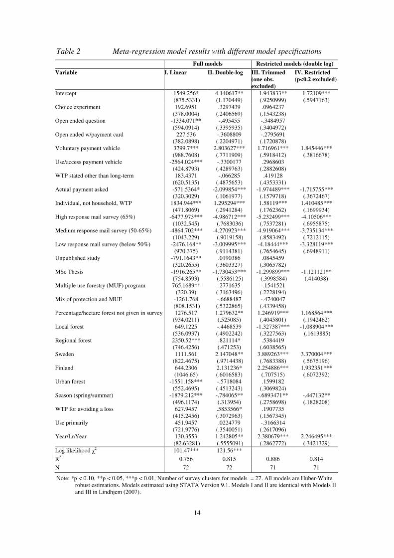
Table 2 Meta-regression model results with different model specifications

Full models Restricted models (double log)

Variable I. Linear II. Double-log III. Trimmed

(one obs.

excluded)

IV. Restricted

(p<0.2 excluded)

Intercept 1549.256* (875.5331)

4.140617** (1.170449)

1.943833** (.9250999)

1.72109*** (.5947163)

Choice experiment 192.6951 (378.0004)

.3297439 (.2406569)

.0964237 (.1543238)

Open ended question

-1334.071** (594.0914)

-.495455 (.3395935)

-.3484957 (.3404972)

Open ended w/payment card 227.536 (382.0898)

-.3608809 (.2204971)

-.2795691 (.1720878)

Voluntary payment vehicle 3799.7*** (988.7608)

2.803627*** (.7711909)

1.716961*** (.5918412)

1.845446*** (.3816678)

Use/access payment vehicle -2564.024*** (424.8793)

-.3300177 (.4289763)

.2968603 (.2882608)

WTP stated other than long-term 183.4371 (620.5135)

-.066285 (.4875653)

.419128 (.4353331)

Actual payment asked -571.5364* (320.3029)

-2.099854*** (.1061977)

-1.974489*** (.1579718)

-1.715755*** (.3672467)

Individual, not household, WTP 1834.944*** (471.8069)

1.295294*** (.2941284)

1.58119*** (.1762362)

1.410485*** (.1699934)

High response mail survey (65%) -6477.973*** (1032.545)

-4.986712*** (.7683036)

-5.232499*** (.7537281)

-4.10506*** (.6955875)

Medium response mail survey (50-65%) -4864.702*** (1043.229)

-4.270923*** (.9019158)

-4.919064*** (.8583492)

-3.735134*** (.7212115)

Low response mail survey (below 50%) -2476.168** (970.375)

-3.009995*** (.9114381)

-4.18444*** (.7654645)

-3.328119*** (.6948911)

Unpublished study -791.1643** (320.2655)

.0190386 (.3603327)

.0845459 (.3065782)

MSc Thesis -1916.265** (754.8593)

-1.730453*** (.5586125)

-1.299899*** (.3998584)

-1.121121** (.414038)

Multiple use forestry (MUF) program 765.1689** (320.39)

.2771635 (.3163496)

-.1541521 (.2228194)

Mix of protection and MUF -1261.768 (808.1531)

-.6688487 (.5322865)

-.4740047 (.4339458)

Percentage/hectare forest not given in survey 1276.517 (934.0211)

1.279632** (.525085)

1.246919*** (.4045801)

1.168564*** (.1942462)

Local forest 649.1225 (536.0937)

-.4468539 (.4902242)

-1.327387*** (.3227563)

-1.088904*** (.1613885)

Regional forest 2350.52*** (746.4256)

.821114* (.471253)

.5384419 (.6038565)

Sweden 1111.561 (822.4675)

2.147048** (.9714438)

3.889263*** (.7683388)

3.370004*** (.5675196)

Finland 644.2306 (1046.65)

2.131236* (.6016583)

2.254886*** (.707515)

1.932351*** (.6072392)

Urban forest -1551.158*** (552.4695)

-.5718084 (.4513243)

.1599182 (.3069824)

Season (spring/summer) -1879.212*** (496.1174)

-.784065** (.313954)

-.6893471** (.2758698)

-.447132** (.1828208)

WTP for avoiding a loss 627.9457 (415.2456)

.5853566* (.3072963)

.1907735 (.1567345)

Use primarily 451.9457 (721.9776)

.0224779 (.3540051)

-.3166314 (.2617096)

Year/LnYear 130.3553 (82.63281)

1.242805** (.5555091)

2.380679*** (.2862772)

2.246495*** (.3421329)

Log likelihood χ2 101.47*** 121.56*** R2 0.756 0.815 0.886 0.814

N 72 72 71 71

Note: *p < 0.10, **p < 0.05, ***p < 0.01, Number of survey clusters for models = 27. All models are Huber-White robust estimations. Models estimated using STATA Version 9.1. Models I and II are identical with Models II and III in Lindhjem (2007).

15

The simplest approach to estimating the meta-model in (2), which has been used in

several MA studies (Loomis and White, 1996; Rosenberger and Loomis, 2000b), is to

treat all WTP observations as independent replications and hence assume that study

level error is zero. A more advanced approach, and our preferred choice here, is to apply

a Huber-White robust variance estimation procedure to adjust for potential

heteroskedasticity and intercluster correlation15 (Smith and Osborne 1996). Given this

empirical framework, we choose four different models. The first two are linear and

double-log specifications, while the third model is restricted in that one observation,

which gave very high TE was left out16. The fourth model is a version of the third where

we following Rosenberger and Loomis (2000b), retain only those variables that are

significant at an 80 per cent level or better based on t-statistics. The regression results

displayed in the second to fifth columns of Table 2 show that the models fit the data

well, with adjusted R2 between 75 and 90 percent. The models confirm several of our

expectations about the methodological variables, for example related to open ended

question formats, response rates of mail surveys, voluntary payment vehicles, actual

payment etc (see Lindhjem (2007) for discussion). It is clear that methodological

variables show a higher degree of significance than site and programme variables for

explaining the variation in the data. This is a potential problem when using the meta-

regressions for BT, and is common in the literature. Regarding the site and programme

variables, the geographical variables in the model show that regional forests are valued

15 Some MA studies use multilevel models, but often find little improvement on the standard models applied here (for

example Bateman and Jones (2003), Rosenberger and Loomis (2000b)). We therefore do not pursue this approach

here.

16 In preliminary analysis we also ran several alternative models, e.g. following Shresta and Loomis (2001), testing a

trimming procedure of the data, leaving out WTP estimates larger or smaller than two standard deviations from

the mean. This procedure did only marginally reduce the TE.

16

higher than national (the base case) though not statistically significant, while local

forests have lower WTP. The resource use conflicts at local levels may explain the latter

difference. Further, Sweden and Finland have significantly higher WTP in the last three

models than observed in Norway, suggesting that even if economic, cultural and

institutional conditions are similar across these countries, WTP can still be different.

Urban forests are valued lower than other forests, which may indicate that non-use

values of non-urban forests are important. WTP to avoid a loss is higher (though not

significantly so) than WTP for a gain. WTP from users or related primarily to use is not

statistically different than from a mixed group. Regarding type of programme, our

results are somewhat puzzling. It seems that respondents value full protection lower

than MUF, but higher than a mix between the two (though not significant through the

four models). It is worth noting that in Model IV, the only site/programme description

variables left are the local and country dimensions. Further, it also seems to be

important to the stated WTP whether forest area and percentage have been explicitly

mentioned in the survey. These results are of an exploratory kind, but shows at least that

it is not immaterial to people whether it is question of full protection or just a change in

existing forestry practices. Finally, the models show that the season variable is negative

and highly significant, while the year of the survey influence WTP positively. The

discussion of meta-regression results is not elaborated further here since our intention is

to use the estimated equations for BT analysis (see Lindhjem (2007) for details).

Transfer error results and comparison of benefit transfer techniques

Within and out-of-sample Mean Average Percentage Error (MAPE)

The first step in our assessment of the suitability of MA-BT involves checking the Mean

Average Percentage Error (MAPE) comparing the forecasts of our four regression

17

models in Table 2 with WTP observations. This is first carried out within-sample (i.e.

the models predict single observations in the sample) and then out-of-sample (i.e. N

versions of each of the four models are run using N-1 of the data to predict the single

out-of-sample observations). For each run, TE is calculated and averaged over all the

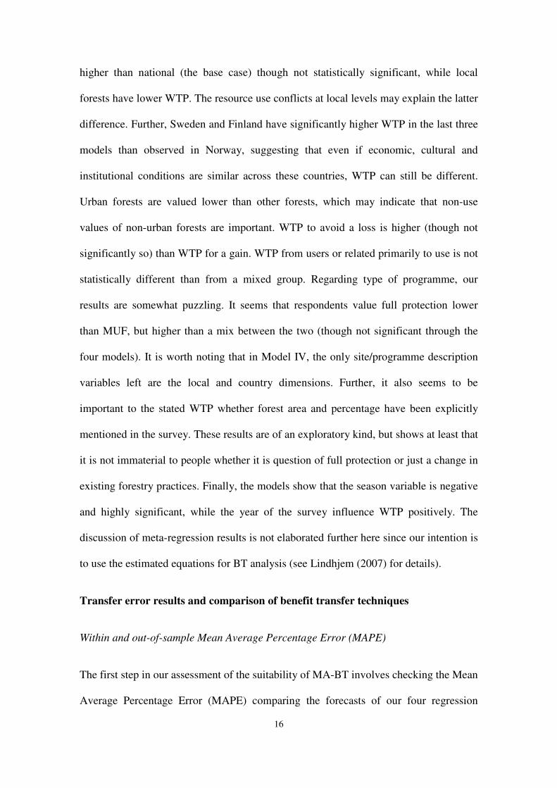
observations into MAPE17. The results from these two exercises are given in Table 3.

Table 3 Mean Average Percentage Error for within-sample and out-of-sample runs

of four MA-BT models

Mean Average Percentage Error (MAPE) for

different model specifications

Model I:

Linear

Model II:

Dbl log

Model III:

1 obs. excl.

Model IV:

p>0.2 excl.

Within-sample

Mean TE 135 52 39 52

Median TE 37 26 25 30

0 -25th percentile (obs 1-18)* 390 71 77 76

25 - 50th percentile (obs 19-36) 105 92 57 72

50 - 75th percentile (obs 37-54) 24 17 25 24

75 – 100th percentile (obs 55-71/2) 24 26 26 37

N-1 out of sample functions

Mean and Median TE 266 222 62 63

Median TE 51 40 34 31

0 -25th percentile (obs 1-18) 770 202 110 109

25 - 50th percentile (obs 19-36) 213 592 70 53

50 - 75th percentile (obs 37-54) 38 27 20 35

75 – 100th percentile (obs 55-71/2) 42 67 50 54

Notes: *Percentiles calculates the transfer errors in four different segments of the data, when WTP is sorted in ascending order.

17 The MA results for the double-log models allow one to calculate ln(WTP) for each observation, transformed into

WTP using antilog. To account for econometric error we add standard deviation (s2/2), which estimate varies

when the sample changes, prior to transfomation of ln(WTP) (Johnston et al., 2006). An alternative, or

supplement, for brevity not considered here would be to replace s2 with the variance of the prediction

(Goldberger, 1968).

18

The first point to note is the relatively low median MAPE for all models, varying from

25-51 percent. Further, it is expected that MAPE goes up when the observation we

predict are left out of the data. When considering means, the linear models perform

much worse than the double-log models having transfer errors between 135 and 266

percent. The double-log model II also has high MAPE, which is considerably reduced

when leaving out an extreme observation and retained at the same level when the model

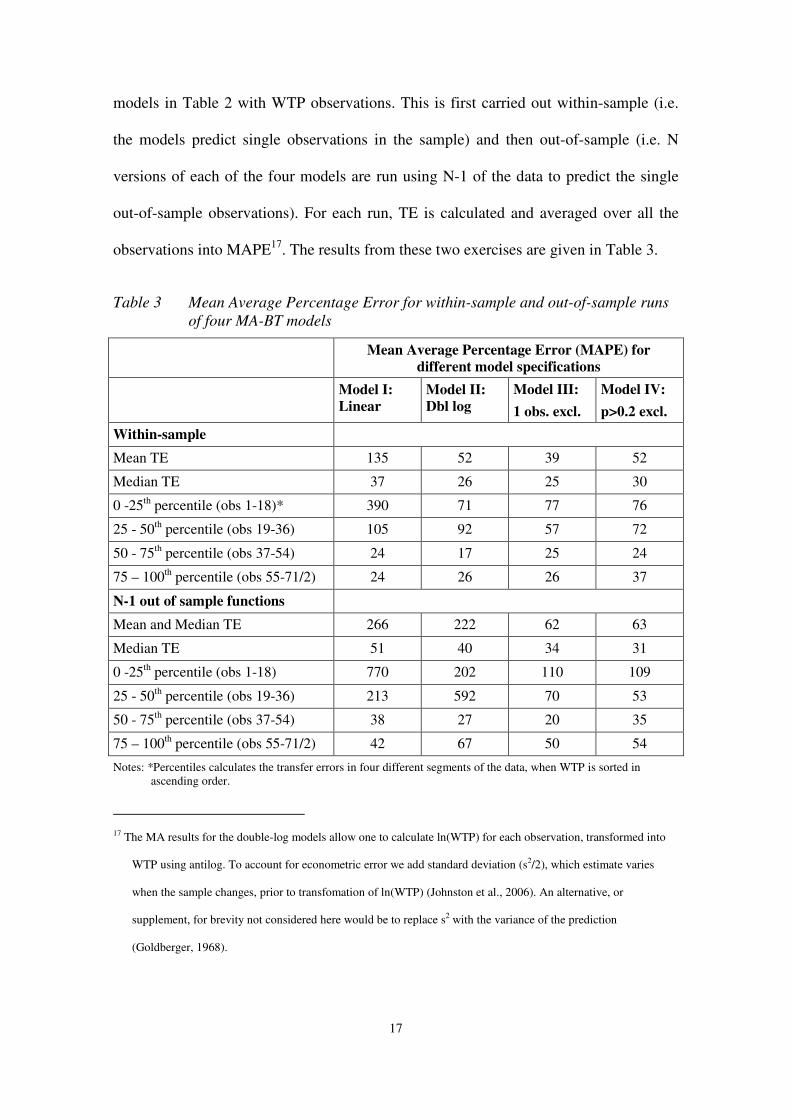
is further restricted in that variables with p>0.2 are taken out. The predicted and

observed values are plotted for out-of-sample Models II and IV for ascending order of

WTP in Figures 1 and 2.

Figure 1 Plot of observed log WTP (lnwtp05) and predicted/transferred values

(wtp_p) for Model II of out-of-sample

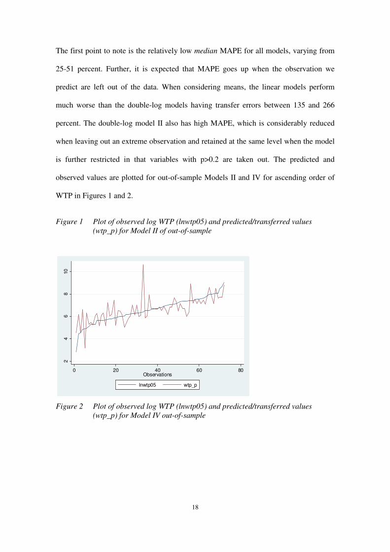
Figure 2 Plot of observed log WTP (lnwtp05) and predicted/transferred values

(wtp_p) for Model IV out-of-sample

24

68

10

0 20 40 60 80Observations

lnwtp05 wtp_p

19

It can be seen from the figures firstly that the precision increases considerably using

Model specification IV (or III) rather than II. Further, the figures show that TE is higher

for lower values of WTP, a similar result to Brander (2006). Calculating MAPE for

different percentiles of the data, as shown in Table 3, when WTP is sorted in ascending

order, also clearly shows the error going down for higher WTP (though TE goes up

again for the highest percentile)18. The predictions also seem to overshoot more often

for lower WTP than for the ones above the median, which is an important consideration

in making MA-BT conservative and err on the low side. The interpretation of TE for

different levels of WTP is important also in terms of calculating a total welfare measure,

i.e. summing WTP over the relevant population. For practical CBA it is the TE of the

total welfare estimate that is important. If WTP per household from a local survey of a

local protection plan is lower than a nationwide survey of a national plan (which is the

case in our data), the overall TE for the welfare measures of both plans may “even out”

in the aggregate.

The MAPE of around 60 percent we find for Models III and IV is comparable or

somewhat lower than the only two studies we have seen conducting this exercise

18 This is partly a result of the definition of TE, as the same absolute prediction error is higher in relative terms for

low WTP values than for high.

24

68

10

0 20 40 60 80Observations

lnwtp05 wtp_p

20

(Brander et al 2006, 2007)19. Their meta-analyses have 72 and 201 observations, are

based on more heterogeneous data, and use regression models with lower explanatory

power. In their convergent validity tests of MA-BT Shresta and Loomis (2001; 2003)

find average TE ranging from a low 28 percent to 88 percent, respectively. The within-

sample test results of Rosenberger and Loomis (2000b) show mean TE ranging from 54

to 71 percent depending on whether a national or a region/activity specific model is

used. The MAPE would be not directly comparable to TE from BT exercises based on

single study situations.

TE for different BT techniques

Based on the first assessment above, we compare the two models with the lowest TE

(i.e. Models III and IV) with simple BT techniques using a more realistic simulation of

actual BT. If we were faced with a policy site without sufficient time and resources to

do a primary study, we could use a study from the most similar site, use a mean from

studies of similar domestic or international sites, or conduct an international MA-BT20.

We compare these techniques in the following way. First we randomly draw one

estimate from each of the 26 surveys included in the data, to represent a benchmark,

“true” value for a policy site. All observations from this survey are then excluded when

the remaining data is used for BT. We then calculate TE for each site, and calculate the

overall mean and median TE for each BT technique21. The benchmark value has of

19 Brander et al (2006) also exclude an extreme observation from their model, so the most relevant model for

comparison would be our model III.

20 Most countries will not have enough domestic studies conduct an MA, and would have to base their MA-BT on a

mix of domestic and international studies, like in the present study.

21 We realise that a fuller test could include a bootstrap to calculate TE for many random draws of single “policy site”

estimates, and not just one draw.

21

course its own error in measurement and is influenced by the survey methodology

chosen. Nevertheless, a comparison of BT techniques for all sites represented by the

data gives a valuable indication of the reliability and level of error that can be expected.

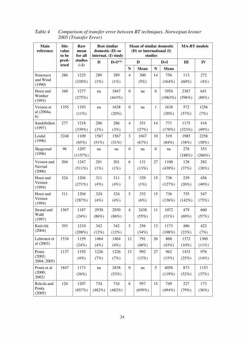
Table 6 displays results. The second column is the value in Norwegian Kroner (2005)

representing the unknown benchmark value for a site to be predicted. This value can be

seen as a rough estimate of long-term household WTP for a forest protection or MUF

plan at a policy site, defined by certain site and programme characteristics22. Column

three displays the raw mean of WTP, regardless of site characteristics, for all

observations in the data (except the benchmark study), representing an upper TE ceiling

(“the worst you could do”). Column six displays the mean WTP for domestic surveys in

the data that have the same site characteristics (the variables defining MUF, forest

protection or a mix of the two, and local or national forests were used to assemble

relevant value estimates).23 Column seven is the mean WTP when observations with the

same site characteristics from the other two countries were also included. For both these

mean value transfers study characteristics are ignored. Expanding to include

international studies would typically be done if there are no similar domestic studies or

because the analyst believes a larger dataset will improve precision in BT. In contrast

with the raw mean in column three, we picked the two values closest to the policy site

value from the set of domestic or international studies that have the same site

22 We do not distinguish between different formats of WTP in terms of long-term vs lump-sum and individual vs

household etc, but assume that the value at the site and the simple transfer estimates roughly represent long-term

household WTP (and as the meta-regression results show many of these dummies were also insignificant in the

analysis).

23 Using the whole set of site characteristics, i.e. also urban, regional and primarily use value etc have the

disadvantage that there often are no observations in the data with exact matching characteristics. A subset was

therefore chosen.

22

characteristics (see columns four and five). This would not be possible in practice, but is

a useful indication of the lower bound TE from choosing estimates from single, similar

site studies (“the best you could do”)24. Finally, the last two columns give the results

from the use of the MA-BT models III and IV. Instead of setting the methodological

dummy variables at average values, at 0.5 or at some best practice value as would have

to be done in practical MA-BT (for example as investigated by Johnston et al (2006)),

we set the values of these dummies to the same as for the benchmark study. This

represents the lower bound TE for the MA-BT models. It would be unnecessary to

introduce in our comparison the additional TE implied by the choice of methodological

dummy values if the MA-BT models in our “best case” perform only marginally better

than the simple BT techniques.

The last four rows in Table 4 sum up the mean and median TE for all BT techniques.

First we ignore that some studies with matching policy site characteristics are not

available (marked “na” in Table 4). Using the simplest of all techniques, just

transferring raw mean WTP from the dataset of forest valuation studies would yield a

mean TE of 217 percent. If it were possible to choose the closest value estimate with

similar site characteristics, mean TE would be 62 percent if chosen from domestic

studies and 71 percent if the set were expanded to include international studies. Taking

means from domestic and the whole set of studies with similar site characteristics yields

mean TE of 86 percent and 166 percent, respectively. Thus, expanding the dataset to

include international studies in this case increases the TE substantially – close to “max”

24 We first tried to use an objective rule to choose a study or site estimate that would most closely resemble the policy

site to mimic situation of simple BT . However, this is not straightforward as the set of studies with the full range

of site and programme characteristics matching the policy site is often empty. In this case, secondary rules using a

subset of the site characteristics need to be applied to end up with a unique, best estimate.

23

TE of 216 percent. In comparison, the two MA-BT models yield mean TE of 126 and

47 percent, a range that includes the TE from using mean from domestic studies. One

reason why the MA-BT model IV gives a lower TE than model III is that simplified

models often tend to give better predictions compared to fully specified models. Our BT

testing procedure yields a lower number of observations for each model run, hence

reinforcing his feature compared to the within and out-of-sample tests in the previous

section. From comparing mean TE for all 26 sites, international MA-BT does not

perform better on average than transferring mean WTP from domestic studies, though

the best meta-model has lower TE. Considering the medians this conclusion is

strengthened. It is clear from the data that the TE from using the simple BT techniques

is pushed up by a number of high values compared with MA-BT. Medians of the best

simple BT technique and MA-BT models are 41 percent and 37 per cent, respectively.

Comparing TE from all 26 sites is not entirely satisfactory as there are missing values

for some of the simple techniques, while the MA-BT predicts values for all sites.

Limiting the set for comparison to the sites where transferred estimates are available

across all BT techniques does not change the general picture, though MA-BT comes out

a little more favourably in this case (see last two rows of Table 4).

24

Table 4 Comparison of transfer error between BT techniques. Norwegian kroner

2005 (Transfer Error)

Best similar

domestic (D) or

internat. (I) study

Mean of similar domestic

(D) or international (I)

studies

MA-BT models

D D+I

Main

reference

Site

value

to be

pred-

icted

Raw

mean

for all

studies

(-1) D D+I**

N Mean N Mean

III IV

Simensen and Wind (1990)

286 1225

(328%)

289

(1%)

289

(1%)

4 300

(5%)

14

756

(164%)

113

(60%)

272

(4%)

Hoen and Winther (1993)

340 1277

(275%)

na 1847

(443%)

0 na 6 3954

(1063%)

2367

(596%)

641

(88%)

Veisten et al (2004a; b)

1355 1193

(11%)

na 1638

(20%)

0 na 1 1638

(20%)

572

(57%)

1256

(7%)

Sandsbråten (1997)

277 1218

(339%)

286

(3%)

286

(3%)

4 351

(27%)

14 771

(178%)

1175

(323%)

416

(49%)

Leidal (1996)

3248 1109

(65%)

1567

(51%)

1567

(51%)

3 1047

(67%)

10 519

(84%)

1985

(38%)

2258

(30%)

Skagestad (1996)

96 1207

(1157%)

na na 0 na 0 na 278

(188%)

353

(266%)

Veisten and Navrud (2006)

204 1247

(511%)

201

(1%)

201

(1%)

6 131

(13%)

27 1100

(439%)

128

(37%)

282

(38%)

Hoen and Veisten (1994)

324 1204

(271%)

311

(4%)

311

(4%)

5 329

(1%)

15 736

(127%)

239

(26%)

456

(40%)

Hoen and Veisten (1994)

311 1204

(287%)

324

(4%)

324

(4%)

5 332

(6%)

15 736

(136%)

755

(142%)

547

(75%)

Strand and Wahl (1997)

1567 1187

(24%)

2930

(86%)

2930

(86%)

4 2438

(55%)

11 1072

(31%)

479

(69%)

660

(57%)

Kniivilä (2004)

393 1210

(208%)

342

(12%)

342

(12%)

5 256

(34%)

12 1173

(198%)

486

(23%)

422

(7%)

Lehtonen et al (2003)

1534 1159

(24%)

1464

(4%)

1464

(4%)

12 791

(48%)

26 868

(43%)

1372

(10%)

1360

(11%)

Pouta (2003; 2004; 2005)

1137 1192

(4%)

1226

(7%)

1226

(7%)

13 992

(12%)

27 962

(15%)

1433

(25%)

976

(14%)

Pouta et al (2000; 2002)

1847 1173

(36%)

na 2838

(53%)

0 na 5 4058

(119%)

873

(52%)

1153

(37%)

Rekola and Pouta (2005)

126 1207

(857%)

734

(482%)

734

(482%)

6 957

(659%)

15 749

(494%)

227

(79%)

173

(36%)

25

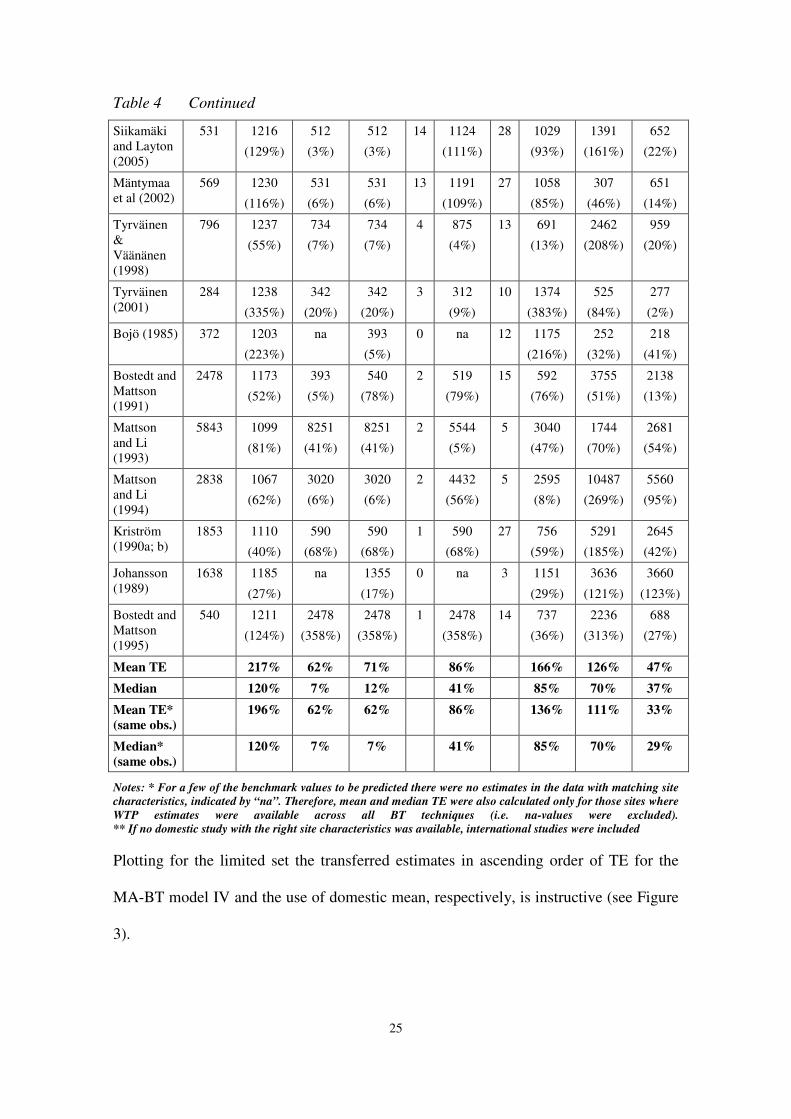
Table 4 Continued

Siikamäki and Layton (2005)

531 1216

(129%)

512

(3%)

512

(3%)

14 1124

(111%)

28 1029

(93%)

1391

(161%)

652

(22%)

Mäntymaa et al (2002)

569 1230

(116%)

531

(6%)

531

(6%)

13 1191

(109%)

27 1058

(85%)

307

(46%)

651

(14%)

Tyrväinen & Väänänen (1998)

796 1237

(55%)

734

(7%)

734

(7%)

4 875

(4%)

13 691

(13%)

2462

(208%)

959

(20%)

Tyrväinen (2001)

284 1238

(335%)

342

(20%)

342

(20%)

3 312

(9%)

10 1374

(383%)

525

(84%)

277

(2%)

Bojö (1985) 372 1203

(223%)

na 393

(5%)

0 na 12 1175

(216%)

252

(32%)

218

(41%)

Bostedt and Mattson (1991)

2478 1173

(52%)

393

(5%)

540

(78%)

2 519

(79%)

15 592

(76%)

3755

(51%)

2138

(13%)

Mattson and Li (1993)

5843 1099

(81%)

8251

(41%)

8251

(41%)

2 5544

(5%)

5 3040

(47%)

1744

(70%)

2681

(54%)

Mattson and Li (1994)

2838 1067

(62%)

3020

(6%)

3020

(6%)

2 4432

(56%)

5 2595

(8%)

10487

(269%)

5560

(95%)

Kriström (1990a; b)

1853 1110

(40%)

590

(68%)

590

(68%)

1 590

(68%)

27 756

(59%)

5291

(185%)

2645

(42%)

Johansson (1989)

1638 1185

(27%)

na 1355

(17%)

0 na 3 1151

(29%)

3636

(121%)

3660

(123%)

Bostedt and Mattson (1995)

540 1211

(124%)

2478

(358%)

2478

(358%)

1 2478

(358%)

14 737

(36%)

2236

(313%)

688

(27%)

Mean TE 217% 62% 71% 86% 166% 126% 47%

Median 120% 7% 12% 41% 85% 70% 37%

Mean TE*

(same obs.)

196% 62% 62% 86% 136% 111% 33%

Median*

(same obs.)

120% 7% 7% 41% 85% 70% 29%

Notes: * For a few of the benchmark values to be predicted there were no estimates in the data with matching site

characteristics, indicated by “na”. Therefore, mean and median TE were also calculated only for those sites where

WTP estimates were available across all BT techniques (i.e. na-values were excluded).

** If no domestic study with the right site characteristics was available, international studies were included

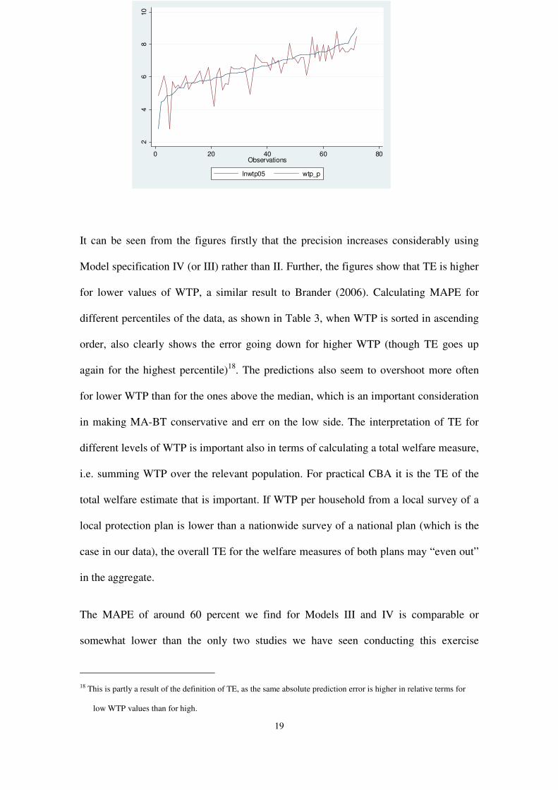
Plotting for the limited set the transferred estimates in ascending order of TE for the

MA-BT model IV and the use of domestic mean, respectively, is instructive (see Figure

3).

26

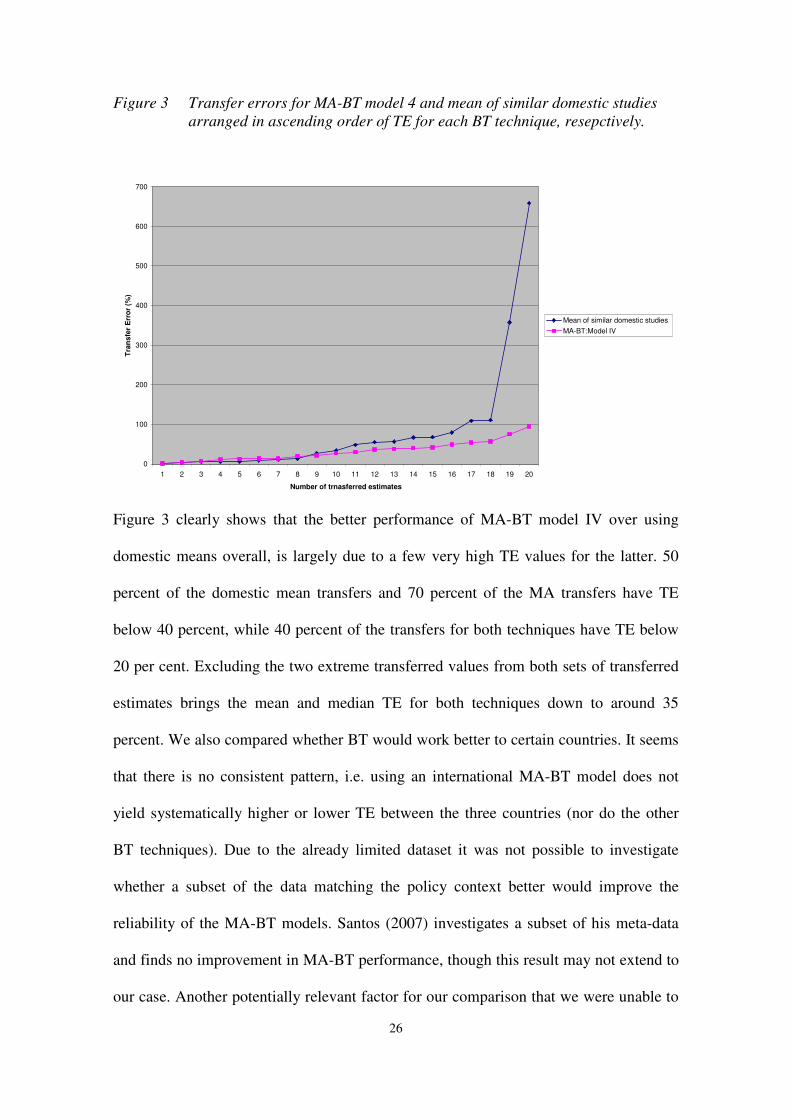
Figure 3 Transfer errors for MA-BT model 4 and mean of similar domestic studies

arranged in ascending order of TE for each BT technique, resepctively.

0

100

200

300

400

500

600

700

1 2 3 4 5 6 7 8 9 10 11 12 13 14 15 16 17 18 19 20

Number of trnasferred estimates

Tra

nsfe

r E

rro

r (%

)

Mean of similar domestic studies

MA-BT:Model IV

Figure 3 clearly shows that the better performance of MA-BT model IV over using

domestic means overall, is largely due to a few very high TE values for the latter. 50

percent of the domestic mean transfers and 70 percent of the MA transfers have TE

below 40 percent, while 40 percent of the transfers for both techniques have TE below

20 per cent. Excluding the two extreme transferred values from both sets of transferred

estimates brings the mean and median TE for both techniques down to around 35

percent. We also compared whether BT would work better to certain countries. It seems

that there is no consistent pattern, i.e. using an international MA-BT model does not

yield systematically higher or lower TE between the three countries (nor do the other

BT techniques). Due to the already limited dataset it was not possible to investigate

whether a subset of the data matching the policy context better would improve the

reliability of the MA-BT models. Santos (2007) investigates a subset of his meta-data

and finds no improvement in MA-BT performance, though this result may not extend to

our case. Another potentially relevant factor for our comparison that we were unable to

27

investigate due to limited reporting in source studies, is the different level of uncertainty

in WTP estimates. A richer BT test could use confidence intervals for the “true value” at

the policy site as benchmark, as done by Santos (2007).

Concluding remarks

This paper has investigated the validity and reliability of international meta-analytic

benefit transfer (MA-BT) based on a data set of stated preference surveys of forest

protection and multiple use forestry plans from Norway, Sweden and Finland. The

studies included in the meta-analysis (MA) are relatively homogenous in terms of

valuation methodology and all three countries have similar cultural, institutional and

economic conditions. We assess convergent validity of transfer estimates for within-

sample and out-of-sample individual estimates, compare reliability of MA-BT with

simpler transfer techniques frequently in use, and investigate the impact on transfer

errors (TE) of different meta-regression specifications. The initial check of the

convergent validity of within and out-of sample predictions of four meta-models show

substantial variation in performance. The best models give median and mean TE of

between 25-34 percent and 39-62 percent. The TE is lower for higher WTP estimates.

Moving to the comparison of transfer techniques, MA-BT shows mean TE of between

47-126 percent (median 37-70 percent) depending on the model. A simple transfer

based on the mean of domestic studies with similar site characteristics to the policy site

yields a mean TE of 86 percent (median 41 per cent), as compared with 62 percent

(median 7 percent) if a best study estimate could be chosen from a domestic study.

Including also international studies in the simple mean transfer increases the TE

substantially to 166 percent (median 85 percent). Finally, the meta-model specification

and observations included have substantial impact on the TE. Despite the simple flavour

of the BT exercise and the challenges of any convergent validity and reliability test

28

based on the same dataset, our comparison of simple BT techniques with more

advanced international MA-BT nevertheless shows interesting results. The best simple

BT technique yields TE in the middle of the range of the two international MA-BT

models. It is worth emphasising that in practical BT applications, the TE for the MA-BT

models would increase since values of methodological characteristics would have to be

set. Our results suggest that MA-BT may not always yield reliability gains over simple

unit value techniques, as often claimed in the MA literature. However, more MA-BT

tests should be performed for other environmental goods and other countries before

discarding international MA as a tool for BT.

Acknowledgements

We would like to thank Olvar Bergland, Norwegian University of Life Sciences, Shelby

Gerking, University of Central Florida, and John A. List, University of Chicago, for

constructive comments.

References

Bateman, I., Cole, M., Cooper, P., Georgiou, S., Hadley, D. and Poe, G. L., 2004. On visible choice sets and scope sensitivity. Journal of Environmental Economics and Management, 47; 71-93.

Bateman, I. J. and Jones, A. P., 2003. Contrasting conventional with multi-level modeling approaches to meta-analysis: Expectation consistency in UK woodland recreation values. Land Economics, 79(2); 235-258.

Bergstrom, J. C. and Taylor, L. O., 2006. Using meta-analysis for benefits transfer: Theory and practice. Ecological Economics, 60; 351-360.

Bojö, J., 1985. Cost-benefit analysis of mountainous forests: the Vala Valley Case (In Swedish). Research Report, The Economic Research Institute, Stockholm School of Economics.,

Bostedt, G. and Mattson, L., 1991. The importance of forests for tourism: A pilot cost-benefit analysis (In Swedish). Arbetsrapport 141, Department of Forest Economics, Swedish University of Agricultural Sciences, Umeå,

Bostedt, G. and Mattsson, L., 1995. The value of forests for tourism in Sweden. Annals of Tourism Research, 22(3); 671-680.

29

Brander, L. M., Florax, R. J. G. M. and Verrmaat, J. E., 2006. The Empirics of Wetland Valuation: A Comprehensive Summary and a Meta-Analysis of the Literature. Environmental & Resource economics, 33; 223-250.

Brander, L. M., van Beukering, P. and Cesar, H., In press. The recreational value of coral reefs: a meta-analysis. Ecological Economics.

Brouwer, R., 2000. Environmental value transfer: state of the art and future prospects. Ecol. Econ., 32(1); 137-152.

Goldberger, A. S., 1968. The interpretation and estimation of Cobb-Douglas functions. Econometrica, 36; 464-472.

Heberlein, T. A., Wilson, M. A., Bishop, R. C. and Schaeffer, N. C., 2005. Rethinking the scope test as a criterion for validity in contingent valuation. Journal of Environmental Economics and Management, 50; 1–22.

Hoehn, J. P., 2006. Methods to address selection effects in the meta regression and transfer of ecosystem values. Ecological Economics, 60(2); 389-398.

Hoen, H. F. and Veisten, K., 1994. A survey of the users of Oslomarka: attitudes towards forest scenary and forestry practices (In Norwegian). Skogforsk 6/94,

Hoen, H. F. and Winther, G., 1993. Multiple-use forestry and preservation of coniferous forests in Norway: A study of attitudes and Willingness-to-pay. Scandinavian Journal of Forest Research, 8(2); 266-280.

Johansson, P. O., 1989. Valuing public goods in a risky world: an experiment, in H. Folmer and E. C. van Ierland, Eds, Evaluation methods and policy making in environmental economics. North Holland, Amsterdam, 39-48.

Johnston, R. J., Besedin, E. Y., Iovanna, R., Miller, C. J., Wardwell, R. F. and Ranson, M. H., 2005. Systematic variation in willingness to pay for aquatic resource improvements and implications for benefit transfer: a meta-analysis. Canadian Journal of Agricultural Economics, 53(2-3); 221-248.

Johnston, R. J., Besedin, E. Y. and Ranson, M. H., 2006. Characterizing the effects of valuation methodology in function-based benefits transfer. Ecological Economics, 60(2); 407-419.

Johnston, R. J., Besedin, E. Y. and Wardwell, R. F., 2003. Modeling relationships between use and nonuse values for surface water quality: A meta-analysis. Water Resoures Research, 39(12).

Kniivilä, M., 2004. Contingent valuation and cost-benefit analysis of nature conservation: a case study in North Karelia, Finland. D.Sc. (Agr. and For.) thesis, Faculty of Forestry, University of Joensuu: pp.

Kristofersson, D. and Navrud, S., 2005. Validity Tests of Benefit Transfer – Are We Performing the Wrong Tests? Environmental and Resource Economics, 30; 279-286.

Kristofersson, D. and Navrud, S., 2007. Can Use and Non-Use Values be Transferred Across Countries? in S. Navrud and R. Ready, Eds, Environmental Value Transfer: Issues and Methods. Kluwer Academic Publishers.

30

Kriström, B., 1990. A Nonparametric Approach To The Estimation Of Welfare Measures In Discrete Response Valuation Studies. Land Economics, 66(2); 135-139.

Kriström, B., 1990. Valuing Environmental Benefits Using the Contingent Valuation Method – An Econometric Analysis. PhD thesis, Doctoral thesis, Umeå Economic Studies No 219, Umeå University.: pp.

Lehtonen, E., Kuuluvainen, J., Pouta, E., Rekola, M. and Li, C. Z., 2003. Non-market benefits of forest conservation in southern Finland. Environmental Science and Policy, 6(3); 195-204.

Leidal, K., 1996. Valuation of an urban recreation area: a contingent valuation study of the Eige Lake area in Kristiansand municipality (In Norwegian). Master Thesis, Department of Economics and Resource Management, Norwegian University of Life Sciences: pp.

Lindhjem, H., 2007. 20 Years of stated preference valuation of non-timber benefits from Fennoscandian forests: A meta-analysis. Journal of Forest Economics, 12; 251-277.

Loomis, J. B., 1992. The Evolution Of A More Rigorous Approach To Benefit Transfer - Benefit Function Transfer. Water Resour. Res, 28(3); 701-705.

Loomis, J. B. and White, D. S., 1996. Economic benefits of rare and endangered species: Summary and meta-analysis. Ecological Economics, 18(3); 197-206.

Mattsson, L. and Li, C. Z., 1993. The Non-Timber Value Of Northern Swedish Forests - An Economic-Analysis. Scandinavian Journal of Forest Research, 8(3); 426-434.

Mattsson, L. and Li, C. Z., 1994. How Do Different Forest Management-Practices Affect The Non-Timber Value Of Forests - An Economic-Analysis. Journal of Environmental Management, 41(1); 79-88.

Moeltner, K., Boyle, K. and Paterson, R. W., 2007. Meta-analysis and benefit transfer for resource valuation - addressing classical challenges with Bayesian modeling. Journal of Environmental Economics and Management, 53; 250-269.

Mäntymaa, E., Mönkkönen, M., Siikamäki, J. and Svento, R., 2002. Estimating the Demand for Biodiversity - Vagueness Band and Open-Ended Questions, in E. C. van Ierland, H. P. Weikard and J. Wesseler, Eds, Proceedings: Risk and Uncertainty in Environmental and Resource Economics.

Navrud, S. and Ready, R., 2007. Lessons learned for environmental value transfer, in S. Navrud and R. Ready, Eds, Environmental Value Transfer: Issues and Methods. Springer.

Navrud, S. and Ready, R., 2007. Review of methods for value transfer, in S. Navrud and R. Ready, Eds, Environmental value transfer: Issues and methods. Springer.

Pouta, E., 2003. Attitude-behavior framework in contingent valuation of forest conservation. PhD, Faculty of Agriculture and Forestry, University of Helsinki: 100 pp.

Pouta, E., 2004. Attitude and belief questions as a source of context effect in a contingent valuation survey. Journal of Economic Psychology, 25; 229-242.

31

Pouta, E., 2005. Sensitivity to scope of environmental regulation in contingent valuation of forest cutting practices in Finland. Forest Policy and Economics, 7; 539– 550.

Pouta, E., Rekola, M., Kuuluvainen, J., Li, C. Z. and Tahvonen, I., 2002. Willingness to pay in different policy-planning methods: insights into respondents' decision-making processes. Ecological Economics, 40(2); 295-311.

Pouta, E., Rekola, M., Kuuluvainen, J., Tahvonen, O. and Li, C. Z., 2000. Contingent valuation of the Natura 2000 nature conservation programme in Finland. Forestry, 73(2); 119-128.

Ready, R. and Navrud, S., 2006. International benefit transfer: Methods and validity tests. Ecological Economics, 60; 429-434.

Rekola, M. and Pouta, E., 2005. Public preferences for uncertain regeneration cuttings: a contingent valuation experiment involving Finnish private forests. Forest Policy and Economics, 7; 635-649.

Rosenberger, R. and Loomis, J., 2000a. Panel stratification in meta-analysis of economic studies: an investigation of its effects in the recreation valuation literature. Journal of Agricultural and Applied Economics, 32(1); 131-149.

Rosenberger, R. and Phipps, T. T., 2007. Correspondence and convergence in benefit transfer accuracy: Meta-analytic review of the literature, in S. Navrud and R. Ready, Eds, Environmental Value Transfer: Issues and Methods. Springer.

Rosenberger, R. S. and Loomis, J. B., 2000b. Using meta-analysis for benefit transfer: In-sample convergent validity tests of an outdoor recreation database. Water Resources Research, 36(4); 1097-1107.

Rosenberger, R. S. and Loomis, J. B., 2001. Benefit transfer of outdoor use values. U.S. Department of Agriculture & Forest Service,

Sandsbråten, L., 1997. Valuation of environmental goods in Oslomarka: a contingent valuation survey of private and municipality owned forest in inner Oslomarka (In Norwegian). Master Thesis, Department of Forestry, Norwegian University of Life Sciences: pp.

Santos, J. M. L., 1998. The Economic Valuation of Landscape Change. Theory and Policies for Land Use and Conservation. Edward Elgar, Cheltenham, pp.

Santos, J. M. L., 2007. Transferring landscape values: How and how accurately? in S. Navrud and R. Ready, Eds, Environmental Value Transfer: Issues and Methods. Springer.

Shrestha, R. K. and Loomis, J. B., 2001. Testing a meta-analysis model for benefit transfer in international outdoor recreation. Ecological Economics, 39(1); 67-83.

Shrestha, R. K. and Loomis, J. B., 2003. Meta-Analytic Benefit Transfer of Outdoor Recreation Economic Values: Testing Out-of-Sample Convergent Validity. Environmental & Resource economics, 25; 79-100.

Shrestha, R. K., Rosenberger, R. and Loomis, J., 2007. Benefit transfer using meta-analysis in recreation economic valuation, in S. Navrud and R. Ready, Eds, Environmental Value Transfer: Issues and Methods. Springer.

32

Siikamäki, J. and Layton, D., 2005. Discrete Choice Survey Experiments: A Comparison Using Flexible Methods. Resources for the Future Discussion Paper,

Simensen, K. and Wind, M., 1990. Attitudes and WTP for different forestry practices in mountainous forests: a survey of the Hirkjolen common (In Norwegian). Master Thesis, Department of Forestry, Norwegian University of Life Sciences: pp.

Skagestad, E., 1996. Recreation and Forestry - A survey of hikers in the outer Oslomarka, Romeriksåsen, in the winter time (In Norwegian). Master thesis, Department of Forestry, Norwegian University of Life Sciences: pp.

Smith, V. K. and Kaoru, Y., 1990. Signals Or Noise - Explaining The Variation In Recreation Benefit Estimates. American Journal of Agricultural Economics, 72(2); 419-433.

Smith, V. K. and Osborne, L. L., 1996. Do contingent valuation estimates pass a ''scope'' test? A meta-analysis. Journal of Environmental Economics and Management, 31(3); 287-301.

Smith, V. K. and Pattanayak, S. K., 2002. Is Meta-Analysis a Noah’s Ark for Non-Market Valuation? Environmental and Resource Economics, 22; 271-296.

Strand, J. and Wahl, T. S., 1997. Valuation of municipality recreation areas in Oslo: A contingent valuation study (In Norwegian). SNF Report 82/97,

Tyrväinen, L., 2001. Economic valuation of urban forest benefits in Finland. Journal of Environmental Management, 62(1); 75-92.

Tyrväinen, L. and Väänänen, H., 1998. The economic value of urban forest amenities: an application of the contingent valuation method. Landscape and Urban Planning, 43(1-3); 105-118.

Van Houtven, G., Powers, J. and Pattanayak, S. K., 2006. Valuing water quality improvements using meta-analysis: Is the glass half-full or half-empty for national policy analysis? Kyoto, Japan

Veisten, K., Hoen, H. F., Navrud, S. and Strand, J., 2004. Scope insensitivity in contingent valuation of complex environmental amenities. Journal of Environmental Management, 73(4); 317-331.

Veisten, K., Hoen, H. F. and Strand, J., 2004. Sequencing and the adding-up property in contingent valuation of endangered species: Are contingent non-use values economic values? Environmental and Resource Economics, 29(4); 419-433.

Veisten, K. and Navrud, S., 2006. Contingent valuation and actual payment for for voluntarily provided passive-use values: assessing the effect of an induced truth-telling mechanism and elicitation formats. Applied Economics, 38(7); 735-756.

Woodward, R. T. and Wui, Y.-S., 2001. The economic value of wetland services: a meta-analysis. Ecological Economics, 37; 257-270.