How much is built? Quantifying and interpreting patterns of built space from different data sources

How much is built? Quantifying and interpreting patterns of built space

from different data sources

DANIEL E. ORENSTEIN*†‡, BETHANY A. BRADLEY**§, JEFF ALBERT¶,

JOHN F. MUSTARDj and STEVEN P. HAMBURG***¤

†Faculty of Architecture and Town Planning, Technion – Israel Institute of Technology,

Technion City, Haifa 32000, Israel

‡Watson Institute for International Studies, BrownUniversity, Providence, RI 02912, USA

§WoodrowWilson School, 410A Robertson Hall, Princeton University, Princeton, NJ

08544, USA

¶The Aquaya Institute, 37 Graham Street, Suite 100A, The Presidio, San Francisco, CA94129, USA

jDepartment of Geological Sciences, Brown University, Providence, RI 02912, USA¤Center for Environmental Studies, Brown University, Providence, RI 02912, USA

(Received 24 July 2008; in final form 17 January 2010)

Land-use/cover change (LUCC) has emerged as a crucial component of applied

research in remote sensing. This work compares two methodologies, based on two

data sources, for assessing amounts of land transformed from open to built space in

three regions in Israel. We use a decision-tree methodology to define open and built

space from remotely sensed (RS) Landsat data and a geographic information systems

(GIS) platform for analysing 1:50 000 scale survey maps. The methodologies are

developed independently, used to quantify and characterize the spatial pattern of

built space, and then analysed for their strengths and weaknesses. We then develop a

method for combining the built area maps derived from eachmethodology, capitaliz-

ing on the strengths of each. TheRSmethodology hadhigher omission errors for built

space in areas with high vegetation levels and low-density exurban development, but

high commission errors in the arid region.TheGISanalysis generally had fewer errors,

although systematically missed built surfaces that were not specifically buildings or

roads, aswell as structures intentionally omitted from themaps.We recommendusing

maps for baseline estimates whenever possible and then complementing the estimates

with clusters of built areas identified with the RS methodology. The results of this

comparative study are relevant to both researchers and practitioners who need to

understand the strengths and weaknesses of mapping techniques they are using.

1. Introduction

1.1 The importance of quantifying growth of built space

Land-use/cover change (LUCC) is central to the most profound global and local

environmental challenges facing humanity (Vitousek et al. 1997, Rindfuss et al. 2004,

*Corresponding author. Email: [email protected]

**Current address: Department of Environmental Conservation, University of

Massachusetts, Amherst, MA, 01003, USA.

***Current address: Environmental Defense Fund, 257 Park Avenue South, New

York, NY 10010, USA

International Journal of Remote SensingISSN 0143-1161 print/ISSN 1366-5901 online# 2011 Taylor & Francis

http://www.tandf.co.uk/journalsDOI: 10.1080/01431161003713036

International Journal of Remote Sensing

Vol. 32, No. 9, 10 May 2011, 2621–2644

Downloaded By: [Orenstein, Daniel Eli] At: 04:11 30 April 2011

Lambin and Veldkamp 2005), including preservation of biodiversity (Velazquez et al.

2003, Defries et al. 2004), mitigation and adaptation to climate change (Feddema

et al. 2005) and sustainable management of natural resources (Kummer and Turner

1994, Jiang et al. 2005). Among the most intense and permanent forms of LUCC is

urbanization, defined in this work as the transformation of open land to built land

(covered with a human structure, including buildings and roads).

Urbanization and the concurrent loss of open space is implicated in the decline of

species richness in general (Ehrlich and Ehrlich 1981, Meffe and Carroll 1994), and in

particular the loss of local species (Perry and Dmi’el 1995, Cam et al. 2000, Hennings

and Edge 2003), habitat loss and fragmentation (Marzluff and Ewing 2001,

McKinney 2002), and in the alteration of ecosystem function (Kemp and Spotila

1997). Within cities, higher human population densities have been found to correlate

with areas of impoverished biodiversity (Turner et al. 2004) and the proliferation of

built space may be linked to a decline in the value of ecosystem services at the

watershed scale (Kreuter et al. 2001). Ecosystem services lost when land is trans-

formed from open to built include carbon sequestration, air and water filtration,

groundwater recharge and lost aesthetic and recreational use (Christensen et al. 1996,

Costanza et al. 1997). Urbanization is inevitable and desirable to some degree, but

without good information on patterns of change it is difficult to quantify andmitigate

the effects and improve planning.

In Israel, rapid urbanization may be the country’s foremost environmental chal-

lenge (Frankenberg 1999, Tal 2002). Rapid urbanization has characterized Israel’s

development since the country’s inception in the middle of the 20th century, and

suburbanization accompanied by increased motorization has characterized Israeli

development over the past two decades of the 20th century (Shoshany and

Goldshleger 2002, Tal 2002, Ayalon 2003, Frenkel 2004b). Israel is a relatively small

country (22 000 km2) with a disproportionately high amount of biological diversity due

to its steep climate gradient, diverse topography and position as the only land-bridge

linking three continents (Yom Tov and Mendelsohn 1988, Frankenberg 1999, Dolev

and Perevolotsky 2004). Thus, knowledge of the rate and pattern of human develop-

ment is essential to the establishment of policies that increase the probability of ensuring

long-term ecological sustainability of the region’s diverse ecosystems.

Since the early 1990s, Israel’s planning authorities have prioritized the importance

of protecting open land. This priority gained prominence during a period of massive

immigration from the former Soviet Union, when there was significant pressure to

convert large tracks of agricultural land to residential development (Alterman 2002).

Concurrently, economic and demographic growth trends coupled with changing

tastes in residential living encouraged out-migration from cities into suburban and

exurban communities (Shoshany and Goldshleger 2002, Frenkel 2004a). Recognizing

this process as deleterious, Israeli planners and policy makers adopted national

development plans that emphasized the protection of open spaces. This process

culminated in National Outline Plan 35, which explicitly aims to protect open spaces

and limit inefficient (e.g. low density) land development (Shachar 1998, Golan 2005).

In this research, we estimate the amount and geographic distribution of open space

transformation to built areas using two methodologies: one based on remote sensing,

and one based on geographic information systems (GIS). Reliable estimates of built

and open space are crucial for assessing the efficacy of open-space preservation

policies. Our definition of open space is intentionally broad to include every land-

cover type that qualifies as a non-built, non-paved surface (e.g. agriculture, sand

2622 D. E. Orenstein et al.


dunes, forests, shrubland and other vegetation). Likewise, our definition of built land

is broad, including any land covered by human infrastructure (e.g. buildings and

roads). The distinction is drawn based on the ease with which land could be protected

for the ecosystem services it provides or could provide. By limiting our investigation

to two land-cover classes, we can focus more intensively on our objective of compar-

ing results arising from the analysis of two different data sources.

1.2 Quantifying built space: two approaches

We derive independent estimates of built and open space from two distinct data sets:

Landsat Thematic Mapper (TM) and survey maps. For each data source, we develop

a separatemethodology to generate quantitative estimates of built area for three study

regions, conduct accuracy assessments for each and then compare the results of each

methodology. We analyse the results for spatial and aggregate agreement and dis-

agreement, and integrate the results into a final estimate of changes in the amount of

built area. Through this process we can assess the strengths and weaknesses of each

approach, analysing how the spatial characteristics of the built environment might be

interpreted differently according to the methodology used to generate the data.

Integration of multiple data sources allows for better estimates of rates and types of

land-cover change. Remotely sensed (RS) data obtained from satellite sensors have

been the most popular starting point for information in this regard. Indeed, the

growing understanding of the scale of LUCC is largely due to systematic monitoring

of the Earth’s surface using satellite data. Satellite data allow for monitoring of large

areas of the Earth’s surface at various scales of spatial resolution and at high temporal

frequencies, and can thus be used to identify spatial and temporal change.

The Landsat TM sensor has been among the most popular resources for monitor-

ing land cover (Cohen and Goward 2004) and has been used widely in assessing

growth of built space (e.g. Ward et al. 2000, Yang and Lo 2002, Zhang et al. 2002,

Yuan et al. 2005) and associated ecological impacts (Kreuter et al. 2001). The TM

sensor and its Landsat predecessor, the Multispectral Scanner (MSS), provide a

relatively long data record due to their length of continuous operation, their fre-

quency of data capture over a given area, and a relatively high spatial resolution and a

large area in each image. Furthermore, TM records reflectance data in seven spectral

bands, including three in the visible spectrum and four infrared bands. The combina-

tion of visible and infrared wavelengths allows for distinction among land-cover

types, including vegetation, soil and built space, through the use of semi-automated

analyses over large geographic areas.

However, satellite data interpretation presents challenges (Rogan and Chen 2004).

The source of remotely sensed data and the choice of methodology with which to

interpret the data can influence the estimates of land-cover change; for example, the

rates and extents of urbanization (Herold et al. 2003, Irwin and Bockstael 2008). It is

often difficult, for example, to distinguish among land-cover types when relying

exclusively on the seven TM bands (for reviews, see Cihlar (2000), Foody (2002)).

Further challenges come in the form of mixed pixels, land surface variability and

atmospheric interference of the satellite signal.

Accurately quantifying proliferation of built space in agricultural and semi-arid

environments has proven particularly difficult. In heterogeneous environments like

these, detecting urbanization is complicated by concurrent LUCCs, including differ-

ential vegetative response to rainfall patterns, spatially heterogeneous distribution of

Quantifying built space from different data sources 2623


soil moisture, differential reflectance responses between fallow land and vigorously

growing crops, and land manipulation in anticipation of development. Diverse and

sometimes complex algorithms (Le Hegarat-Mascle et al. 2000, Duda and Canty

2002), spectral unmixing analyses (Elmore et al. 2000, Pu et al. 2008), decision trees

(Martinez-Casasnovas 2000, Ward et al. 2000) and ancillary data sources (Le

Hegarat-Mascle et al. 2000, Stefanov et al. 2001, Yang and Lo 2002) have been

used to increase the accuracy of land-cover classifications. Digitized maps and GIS

layers are commonly used to supplement initial TM-derived land-cover classifications

in post-classification analyses.

As routine collection of satellite data only began in 1972, an analysis of longer-term

LUCC requires use of older non-sensor-based survey maps (Petit and Lambin 2001,

2002). Maps, such as the 1:50 000 scale thematic survey maps used in this research,

have been routinely produced through national surveys for almost a century. In many

cases, maps are more accessible to researchers than are satellite data, and GIS

methods of analysis of urbanization patterns are simpler and more intuitive to use.

At the same time, reliance on survey maps has drawbacks in estimating LUCC. Maps

are generalized and subjective representations of information surveyed or extracted

from aerial photographs. In Mandate Palestine prior to 1948, British survey maps

were produced through standard cartographic techniques, after which Israel used

aerial photography to complement ground surveys (Gavish 1976). At low scales of

resolution, cartographers may have to exclude information, for example when there

may not be room for all the structures that exist in a given area (Weibel and Jones

1998, Petit and Lambin 2002). We compared the number of structures in randomly

chosen sites within the 1:50 000 scale maps used in this research to those found in

aerial photographs for the same areas and found that the maps graphically repre-

sented between one-half and one-quarter of the structures that appeared in the aerial

photographs, with low-density areas being generally more accurate than high-density

areas. Furthermore, maps often do not display actual land cover, but rather land use.

In these cases, the physical characteristics of the land cover can only be assumed based

on the land-use designation (e.g. agriculture, open space, sand dunes, or buildings).

Another limitation of using survey map data to examine LUCC is that they take

time to produce and thus there is usually a delay between the specific point in time

when the aerial photographs are captured, and when the map becomes available. In

Israel, maps are generally ‘partially’ updated every 4 years (though more frequently

for some areas of the country) and are published with a several-month lag. A further

drawback is that the spatial extent of individual maps (e.g. 1:50 000 scale) is much

smaller than, for example, a Landsat scene. This necessitates the collection of multiple

maps to cover broad areas.

We set out here to produce built area maps using two data sources. In doing so, we

aimed to (1) produce reliable estimates of the increase of built space between two

periods, (2) assess the strengths and weaknesses of the methodologies used for inter-

preting each data source and (3) suggest a simple and intuitive way to combine data

sets to increase the accuracy of the estimates, building on the strengths of each

methodology and the predictability of the common built area types that may be

overlooked by one methodology or the other. This methodological comparison,

highlighting the strengths and weaknesses of the RS and GIS sources and analytical

techniques, provides important information useful to both researchers and practi-

tioners seeking to better understand patterns of urban growth.



2. Data and methods

2.1 Study regions

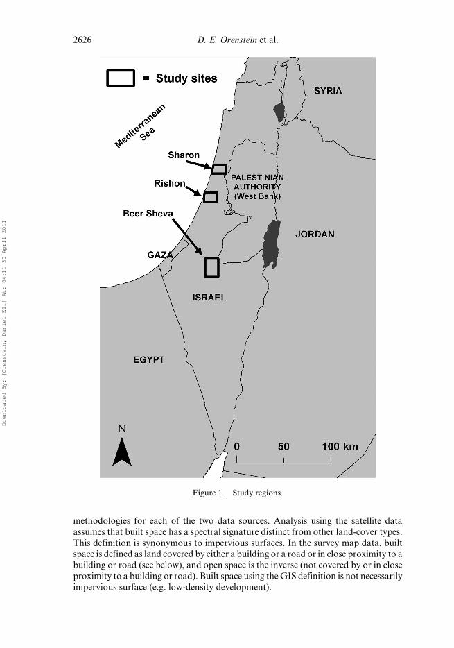
In this study, we analyse three geographically distinct regions in Israel: 130 km2 of

Mediterranean coast north of Tel Aviv (‘Sharon’, after the name of the geographic

region), 140 km2 ofMediterranean coast south of Tel Aviv (‘Rishon’, named after the

city located at the centre of the study site), and 270 km2 of northern semi-arid Negev

Desert (‘Beer Sheva’, after the city at the southern edge of the site; figure 1). The study

regions display both intra- and inter-region ecological, demographic and land-use

heterogeneity. Communities in each region range from high-density cities to low-

density rural communities within an agricultural matrix. These regions were chosen

because: they are included within a single Landsat scene, path 174, row 38; they

embody the conflict between farmland and/or open space preservation versus

demands for increased housing and industrial development; and they form both a

demographic (most of Israel’s population is concentrated in the country’s geographic

centre) and an ecological gradient from Mediterranean ecosystems in the north to

semi-arid desert in the south.

The Sharon study region is situated along the Mediterranean coast. The soils are

primarily sandy-loam, with coastal sand dunes. The topography is generally flat, with

elevations rising from sea level to approximately 80 m inland. Land use is dominated

by irrigated agriculture and low- to medium-density rural and exurban communities

(approximately 30% of land use). The 1983 population was 73 000 (560 persons/km2),

which rose to 110 000 (850 persons/km2) by 1995.

The Rishon study region also lies in the Mediterranean coastal plain, approxi-

mately 20 km south of the Sharon region, and has similar topography and soils, with a

higher predominance of bright sand dunes. Land use here is characterized by agri-

culture and high-density urban development. The western third of the study region

consists of sand dunes and the southern edges of urban Tel-Aviv/Jaffa. The eastern

portion of this region is dominated by rural communities and irrigated agriculture.

Topography and soil types are similar to those of the previous region. The population

of the area was 410 000 (2900 persons/km2) in 1983 and 520 000 (3700 persons/km2) in

1995.

The Beer Sheva study region lies in the northern Negev desert. The region includes

one high-density urban community (Beer Sheva), several medium-density suburbs

and towns, and dispersed rural settlements. The area is primarily open semi-arid

shrubland, although much of the open space is used for rainfed grain production

and some of the land has been forested with pine plantations and fruit trees, and some

has been terraced and planted with dryland tree species at low densities (‘savannaza-

tion’). Soils are loess and regosols, and the topography consists of moderately sloped

foothills, wadis and plains with elevation ranging from 100 to 500 m above sea level.

The population, predominantly in Beer Sheva, was 120 000 (440 persons/km2) in 1983,

rising to 180 000 (670 persons/km2) in 1995.

2.2 Definition of built space

The primary objective of the data analysis was to assess changes in the area and

geographic distribution of built space between two points in time. We define built

space as land covered with a physical, anthropogenic structure: primarily buildings

and roads. However, the interpretation of built space required different



methodologies for each of the two data sources. Analysis using the satellite data

assumes that built space has a spectral signature distinct from other land-cover types.

This definition is synonymous to impervious surfaces. In the survey map data, built

space is defined as land covered by either a building or a road or in close proximity to a

building or road (see below), and open space is the inverse (not covered by or in close

proximity to a building or road). Built space using theGIS definition is not necessarily

impervious surface (e.g. low-density development).

Figure 1. Study regions.



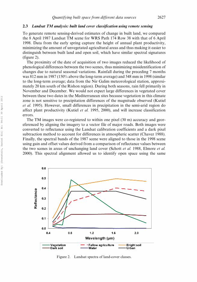
2.3 Landsat TM analysis: built land cover classification using remote sensing

To generate remote sensing-derived estimates of change in built land, we compared

the 8 April 1987 Landsat TM scene for WRS Path 174 Row 38 with that of 6 April

1998. Data from the early spring capture the height of annual plant productivity,

minimizing the amount of unvegetated agricultural areas and thus making it easier to

distinguish between built land and open soil, which have similar spectral signatures

(figure 2).

The proximity of the date of acquisition of two images reduced the likelihood of

phenological differences between the two scenes, thus minimizing misidentification of

changes due to natural seasonal variations. Rainfall during the preceding 7 months

was 812 mm in 1987 (150% above the long-term average) and 548 mm in 1998 (similar

to the long-term average; data from the Nir Galim meteorological station, approxi-

mately 20 km south of the Rishon region). During both seasons, rain fell primarily in

November and December. We would not expect large differences in vegetated cover

between these two dates in the Mediterranean sites because vegetation in this climate

zone is not sensitive to precipitation differences of the magnitude observed (Kutiel

et al. 1995). However, small differences in precipitation in the semi-arid region do

affect plant productivity (Kutiel et al. 1995, 2000), and will increase classification

errors.

The TM images were co-registered to within one pixel (30 m) accuracy and geor-

eferenced by aligning the imagery to a vector file of major roads. Both images were

converted to reflectance using the Landsat calibration coefficients and a dark pixel

subtraction method to account for differences in atmospheric scatter (Chavez 1988).

Finally, the spectral bands of the 1987 scene were aligned to those in the 1998 scene

using gain and offset values derived from a comparison of reflectance values between

the two scenes in areas of unchanging land cover (Schott et al. 1988, Elmore et al.

2000). This spectral alignment allowed us to identify open space using the same

Figure 2. Landsat spectra of land-cover classes.



methodology for both time periods. Both images were clipped to encompass only the

Sharon, Rishon and Beer Sheva study regions, corresponding to theGIS surveymaps.

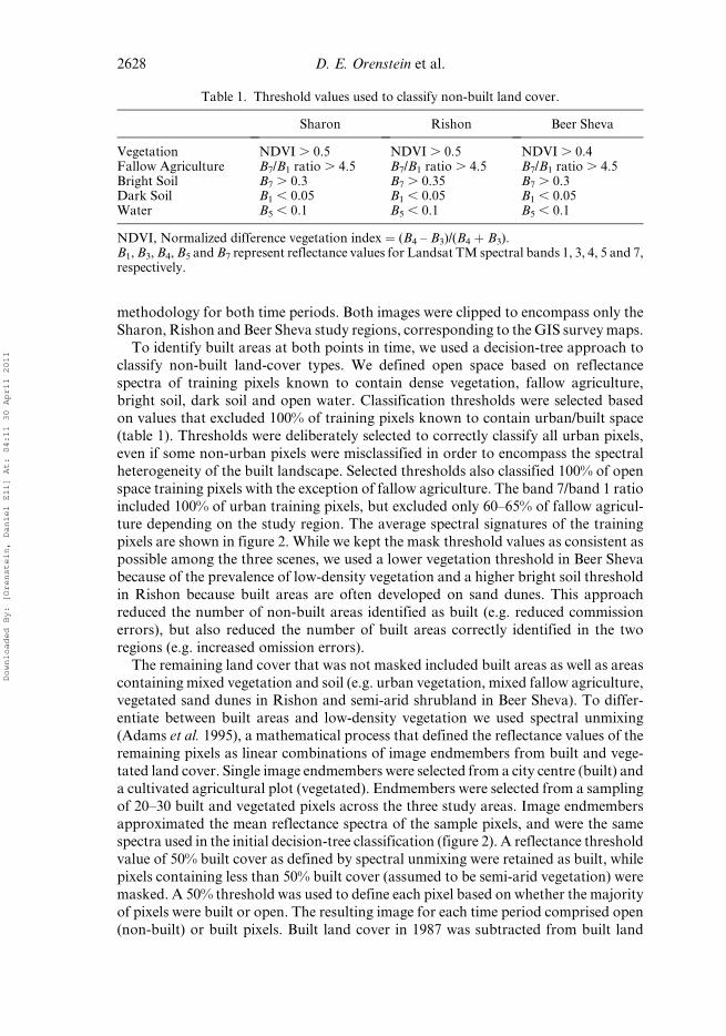
To identify built areas at both points in time, we used a decision-tree approach to

classify non-built land-cover types. We defined open space based on reflectance

spectra of training pixels known to contain dense vegetation, fallow agriculture,

bright soil, dark soil and open water. Classification thresholds were selected based

on values that excluded 100% of training pixels known to contain urban/built space

(table 1). Thresholds were deliberately selected to correctly classify all urban pixels,

even if some non-urban pixels were misclassified in order to encompass the spectral

heterogeneity of the built landscape. Selected thresholds also classified 100% of open

space training pixels with the exception of fallow agriculture. The band 7/band 1 ratio

included 100% of urban training pixels, but excluded only 60–65% of fallow agricul-

ture depending on the study region. The average spectral signatures of the training

pixels are shown in figure 2. While we kept the mask threshold values as consistent as

possible among the three scenes, we used a lower vegetation threshold in Beer Sheva

because of the prevalence of low-density vegetation and a higher bright soil threshold

in Rishon because built areas are often developed on sand dunes. This approach

reduced the number of non-built areas identified as built (e.g. reduced commission

errors), but also reduced the number of built areas correctly identified in the two

regions (e.g. increased omission errors).

The remaining land cover that was not masked included built areas as well as areas

containing mixed vegetation and soil (e.g. urban vegetation, mixed fallow agriculture,

vegetated sand dunes in Rishon and semi-arid shrubland in Beer Sheva). To differ-

entiate between built areas and low-density vegetation we used spectral unmixing

(Adams et al. 1995), a mathematical process that defined the reflectance values of the

remaining pixels as linear combinations of image endmembers from built and vege-

tated land cover. Single image endmembers were selected from a city centre (built) and

a cultivated agricultural plot (vegetated). Endmembers were selected from a sampling

of 20–30 built and vegetated pixels across the three study areas. Image endmembers

approximated the mean reflectance spectra of the sample pixels, and were the same

spectra used in the initial decision-tree classification (figure 2). A reflectance threshold

value of 50% built cover as defined by spectral unmixing were retained as built, while

pixels containing less than 50% built cover (assumed to be semi-arid vegetation) were

masked. A 50% threshold was used to define each pixel based on whether the majority

of pixels were built or open. The resulting image for each time period comprised open

(non-built) or built pixels. Built land cover in 1987 was subtracted from built land

Table 1. Threshold values used to classify non-built land cover.

Sharon Rishon Beer Sheva

Vegetation NDVI . 0.5 NDVI . 0.5 NDVI . 0.4Fallow Agriculture B7/B1 ratio . 4.5 B7/B1 ratio . 4.5 B7/B1 ratio . 4.5Bright Soil B7 . 0.3 B7 . 0.35 B7 . 0.3Dark Soil B1 , 0.05 B1 , 0.05 B1 , 0.05Water B5 , 0.1 B5 , 0.1 B5 , 0.1

NDVI, Normalized difference vegetation index ¼ (B4 – B3)/(B4 þ B3).B1,B3,B4,B5 andB7 represent reflectance values for Landsat TM spectral bands 1, 3, 4, 5 and 7,respectively.



cover in 1998 to produce a change map identifying areas of expansion of built space

between the two time periods.

To further address the difficulty in identifying open pixels with spectral signatures

similar to built cover, we applied a smoothing filter (Yang and Lo 2002) using a 3� 3

pixel moving window to reclassify pixels according to the majority pixel value within

the window. This removed stray change pixels associated with spectrally similar semi-

arid land cover as well as those associated with scene offsets along roads.

2.4 GIS map analysis: defining open and built land and quantifying the transition

between land-cover classes

Survey maps, at 1:50 000 scale, produced by the Survey of Israel (collected from the

cartography library of Hebrew University) were scanned and digitized. The maps

analysed were those closest in date to the Landsat TM data (1987 and 1998). For the

Sharon area, maps were from 1989 and 1999, for Rishon they were from 1985 and

1999, and for Beer Sheva, from 1984 and 1999.

Built structures on the maps were digitized as points, and paved roads were

digitized as lines. Digitized maps from the 1980s were used as a baseline, and new

structures were added based on the 1990s maps. Single points rather than polygons

were used to describe structures to reduce the time required to digitize the survey

maps, and because structure density was easier to measure with point data.

The built vector files for each location and time period were converted into

structure density raster grids with 30 m resolution using a 30 m search radius and a

kernel density function, which weights the centre of the search radius more heavily

than the edges, producing a smoother density distribution. A 30 m resolution was

chosen to correspond with TM spatial resolution, and because a 30 m radius was wide

enough to ensure that the spatial footprint of large buildings would be included as

built. A pixel was defined as built if it contained at least one structure or was within

30m of a structure (thus with a pixel threshold value of� 1) was defined as ‘built’. The

road files were converted into raster grids using the same methods. Note that because

of the binary open-built definition, most pixels are likely to be a fraction of each cover

type (see section 3.1). The road and structure layers were aggregated for each of the

two time periods to create a raster grid of ‘built’ area.

2.5 Combining RS/GIS maps for comparison

To compare the results from both the RS andGIS analyses, we created raster maps of

either no change (remain open or built) or change (open to built) for both methodol-

ogies. We assumed that no transitions from built to open occurred during this time

period because of the high development rates in these parts of Israel. The two maps

were combined to identify four distinct classes: (1) open space according to both

methods; (2) built space according to RS only; (3) built space according to GIS only

and (4) built space according to both methods. The result was a single change map for

each study region that displayed the amount and spatial configuration of agreement

and disagreement between the RS and GIS methodologies in assessing land-cover

change between open and built.

Our final task was to create a built area map that exploited the advantages of both

methodologies to maximize accuracy of our final estimates. Our aim was to use the

most accurate map (in our case, the GIS-derived map) as a base map, and add

supplementary information regarding built spaces from the auxiliary map (here, the



RS-derived map). After comparing the RS and GIS results quantitatively, we ana-

lysed the qualitative land-cover types that were defined as built by the RS methodol-

ogy but not by the GIS methodology.

2.6 Accuracy assessment

We separately conducted an accuracy assessment of the individual and combined

methodologies using a 2001 orthophoto to check the accuracy of approximately 750

randomly selected pixels for each study region in the 1990s RS and GIS maps. These

pixels provided us with an estimate of the proportion of built to open space (true

cover) and were also used to assess the accuracy of our maps. Although a stratified

sampling may have been preferred to increase precision over the simple random

sampling and to ensure adequate representation of the rarer land cover class

(Stehman and Czaplewski 1998), we chose random sampling because we had a large

enough sample size to ensure adequate representation of the rarer class (Foody 2002).

For example, in Beer Sheva, where built area was the rarest of the three study sites,

over 100 points fell in built areas. Our large sample size also suggested that precision

gains through stratified sampling would have been minimal. Had we been working

with more land-cover classes, including rarer types, a stratified sampling technique

may have been more appropriate.

When determining land-cover class in the orthophoto, we considered both the

dominant land cover within each pixel and the dominant land cover in a nine-pixel

matrix with the selected pixel at the centre (Stehman andCzaplewski 1998). This latter

step helped us to differentiate between registration errors and errors arising for other

reasons. For both methodologies we investigated the nature of omission and commis-

sion errors for each of the pixels that were erroneously defined as either built or open

in order to reveal underlying patterns in the errors observed. Overall accuracy is

defined as the total probability that a pixel was classified correctly (Stehman and

Czaplewski 1998) and is the sum of the correctly classified pixels in each category

divided by the size of the sample.

We did not conduct an accuracy assessment for the 1980s map because the only

spatial data we could access were the survey maps and the satellite imagery, which

were both used in the research. Orthophotos were not available for this time period,

and aerial photographs were not suitable for accuracy assessment because they were

used to produce the survey maps and thus would introduce a favourable bias towards

the GIS maps.

3. Results

3.1 Accuracy assessment

The error matrices and overall accuracy of the maps produced by the twomethods are

shown in table 2. For the RSmethod, the overall accuracy was approximately 85% for

each of the study regions. For the GIS method, the overall accuracy was 87, 79 and

92% for the Sharon, Rishon and Beer Sheva regions, respectively. While the overall

accuracy of both methods was about 85%, the source of errors differed greatly.

For the RS methodology, commission errors (false positives, or the proportion of

all land defined as built that was, in reality, open) were highest in the Beer Sheva

region, with 52% commission errors as compared to 21% and 8% in Sharon and

Rishon, respectively. A majority (56%) of the commission errors in the Beer Sheva



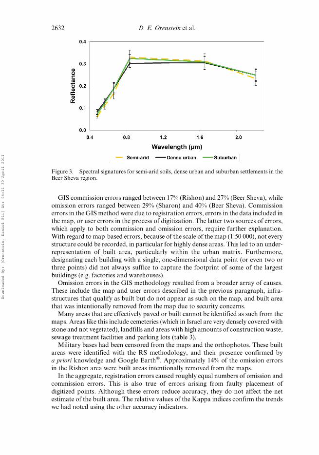
region occurred on semi-arid pixels with similar spectral signatures to built pixels

(figure 3). These areas included terraced hillsides, dry river beds, hill slopes with

patchy shrub vegetation and outcroppings of bedrock. The remaining RS commission

errors were primarily due to registration errors.

At 55%, the Sharon region had the highest number of RS omission errors (land that

was built, but which was erroneously defined as open), with Rishon and Beer Sheva at

26% and 27%, respectively. In all three regions, these errors occurred primarily in

suburban built areas with high vegetation cover. This type of development was most

prevalent at the Sharon region. Additional omission errors in the three regions were

caused by registration errors and new construction that occurred between the time the

satellite data were captured and the date of the orthophoto (D. Orenstein, personal

observation).

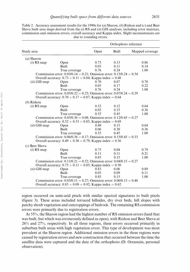
Table 2. Accuracy assessment results for the 1990s for (a) Sharon, (b) Rishon and (c) and BeerSheva built area maps derived from the (i) RS and (ii) GIS analyses, including error matrices,commission and omission errors, overall accuracy and Kappa index. Slight inconsistencies are

due to rounding errors.

Orthophoto reference

Study area Open Built Mapped coverage

(a) Sharon(i) RS map Open 0.73 0.13 0.86

Built 0.03 0.11 0.14True coverage 0.76 0.24 1.00

Commission error: 0.03/0.14 ¼ 0.21; Omission error: 0.13/0.24 ¼ 0.54Overall accuracy: 0.73 þ 0.11 ¼ 0.84; Kappa index ¼ 0.48

(ii) GIS map Open 0.70 0.07 0.78Built 0.05 0.17 0.22True coverage 0.76 0.24 1.00


(b) Rishon(i) RS map Open 0.52 0.12 0.64





(c) Beer Sheva(i) RS map Open 0.75 0.04 0.79







GIS commission errors ranged between 17% (Rishon) and 27% (Beer Sheva), while

omission errors ranged between 29% (Sharon) and 40% (Beer Sheva). Commission

errors in the GIS method were due to registration errors, errors in the data included in

the map, or user errors in the process of digitization. The latter two sources of errors,

which apply to both commission and omission errors, require further explanation.

With regard to map-based errors, because of the scale of the map (1:50 000), not every

structure could be recorded, in particular for highly dense areas. This led to an under-

representation of built area, particularly within the urban matrix. Furthermore,

designating each building with a single, one-dimensional data point (or even two or

three points) did not always suffice to capture the footprint of some of the largest

buildings (e.g. factories and warehouses).

Omission errors in the GIS methodology resulted from a broader array of causes.

These include the map and user errors described in the previous paragraph, infra-

structures that qualify as built but do not appear as such on the map, and built area

that was intentionally removed from the map due to security concerns.

Many areas that are effectively paved or built cannot be identified as such from the

maps. Areas like this include cemeteries (which in Israel are very densely covered with

stone and not vegetated), landfills and areas with high amounts of construction waste,

sewage treatment facilities and parking lots (table 3).

Military bases had been censored from the maps and the orthophotos. These built

areas were identified with the RS methodology, and their presence confirmed by

a priori knowledge and Google Earth�. Approximately 14% of the omission errors

in the Rishon area were built areas intentionally removed from the maps.

In the aggregate, registration errors caused roughly equal numbers of omission and

commission errors. This is also true of errors arising from faulty placement of

digitized points. Although these errors reduce accuracy, they do not affect the net

estimate of the built area. The relative values of the Kappa indices confirm the trends

we had noted using the other accuracy indicators.

Figure 3. Spectral signatures for semi-arid soils, dense urban and suburban settlements in theBeer Sheva region.



3.2 RS classification

The decision-tree classifications of non-built land cover successfully identified a

majority of open space in each time period and study area. However, the additional

spectral mixture analysis was necessary to further refine the classification of built

pixels (table 4). This was particularly true in the semi-arid Beer Sheva site. For

example, in 1987 the decision tree alone classified 96 901, or 25% of pixels in Beer

Sheva as built. The addition of the spectral mixture analysis reclassified the number of

built pixels to 16 279, or 4% of pixels.

Table 3. Strengths and weaknesses of using either GIS or RS methods and data sources fordefining built area.

GIS map-based approach RS satellite data-based approach

Correctly identifies: Correctly identifies:l High-density development l High-density developmentl Rural and low-density development l Large structures (factories, warehouses) that

cover more land surface than the single datapoint in the GIS study would account for

l Roads l Impervious surfaces such as parking lots,cemeteries

l Small stand-alone structures

Misidentifies: Misidentifies:l Impervious surfaces such as parking lots,cemeteries

lRural and low-density development includingnarrow or unpaved roads

lLarge structures (factories, warehouses) thatcover more land surface than the single datapoint in the GIS study would account for

lOpen space with similar spectral properties tobuilt areas (e.g. sand dunes, semi-aridscrubland)

l Structures intentionally or unintentionallyomitted from maps

Table 4. Number of pixels in the (a) Sharon, (b) Rishon and (c) Beer Sheva study regionsdefined as open and built by RS using a decision tree alone, and a decision tree plus spectral

mixture analysis (SMA).

1987 1998

Decisiontree Decision treeþ SMA

Decisiontree Decision treeþ SMA

(a) SharonClassified asopen

187 662 188 172 174 162 178 036

Classified as built 7129 6919 20 929 17 055(b) Rishon

Classified asopen

119 723 155 750 131 528 142 928

Classified as built 75 478 39 451 63 673 52 273(c) Beer Sheva

Classified asopen

296 030 376 656 243 215 321 027

Classified as built 96 901 16 275 149 716 71 904



3.3 Comparison of RS/GIS built estimates

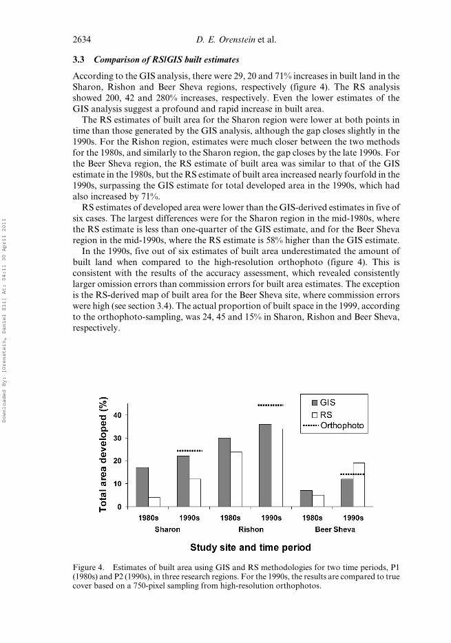
According to the GIS analysis, there were 29, 20 and 71% increases in built land in the

Sharon, Rishon and Beer Sheva regions, respectively (figure 4). The RS analysis

showed 200, 42 and 280% increases, respectively. Even the lower estimates of the

GIS analysis suggest a profound and rapid increase in built area.

The RS estimates of built area for the Sharon region were lower at both points in

time than those generated by the GIS analysis, although the gap closes slightly in the

1990s. For the Rishon region, estimates were much closer between the two methods

for the 1980s, and similarly to the Sharon region, the gap closes by the late 1990s. For

the Beer Sheva region, the RS estimate of built area was similar to that of the GIS

estimate in the 1980s, but the RS estimate of built area increased nearly fourfold in the

1990s, surpassing the GIS estimate for total developed area in the 1990s, which had

also increased by 71%.

RS estimates of developed area were lower than the GIS-derived estimates in five of

six cases. The largest differences were for the Sharon region in the mid-1980s, where

the RS estimate is less than one-quarter of the GIS estimate, and for the Beer Sheva

region in the mid-1990s, where the RS estimate is 58% higher than the GIS estimate.

In the 1990s, five out of six estimates of built area underestimated the amount of

built land when compared to the high-resolution orthophoto (figure 4). This is

consistent with the results of the accuracy assessment, which revealed consistently

larger omission errors than commission errors for built area estimates. The exception

is the RS-derived map of built area for the Beer Sheva site, where commission errors

were high (see section 3.4). The actual proportion of built space in the 1999, according

to the orthophoto-sampling, was 24, 45 and 15% in Sharon, Rishon and Beer Sheva,

respectively.

Figure 4. Estimates of built area using GIS and RS methodologies for two time periods, P1(1980s) and P2 (1990s), in three research regions. For the 1990s, the results are compared to truecover based on a 750-pixel sampling from high-resolution orthophotos.



3.4 Spatial agreement/disagreement between the RS and GIS methodologies

Avisual comparison of the results of theGIS andRS analyses (figures 5–7) shows that

clusters of densely built area are detected similarly by both methods. However, fine-

scale differences in the spatial patterns of built space are also visible. The RS assess-

ments of built area contain considerable noise, in particular in the western portion of

the Rishon region (figure 6), which corresponds to the presence of sand dunes, and in

the centre of the Beer Sheva region (figure 7), corresponding to semi-vegetated hills. In

the RS analysis, only the largest roads were defined as built. Smaller roads are too

narrow to be defined as built by the RS methodology.

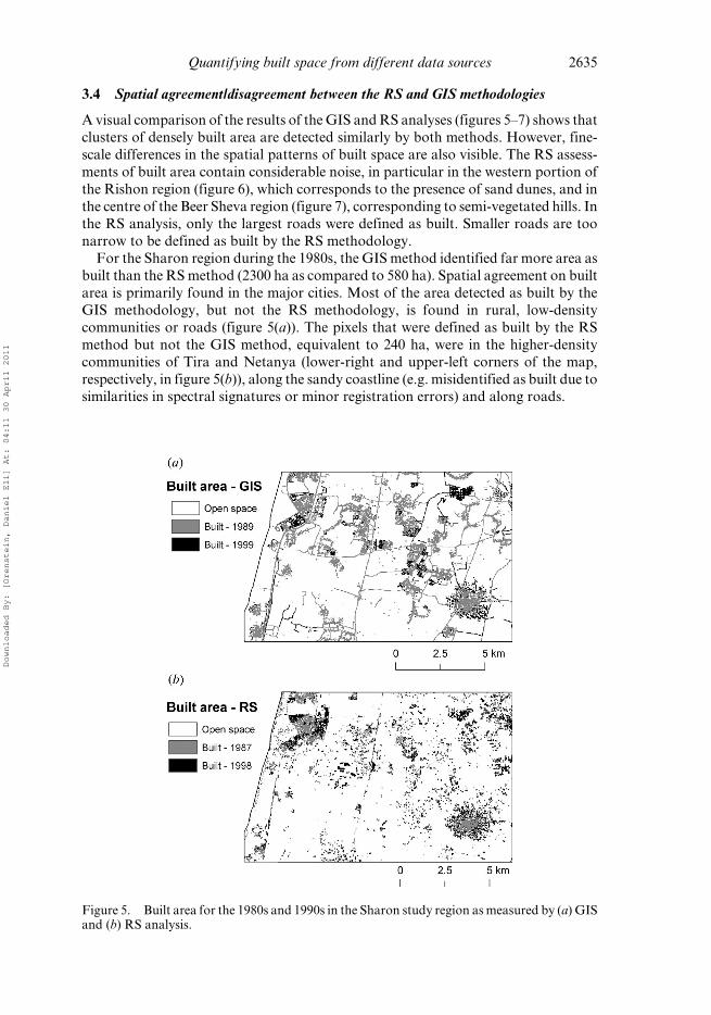
For the Sharon region during the 1980s, the GIS method identified far more area as

built than the RSmethod (2300 ha as compared to 580 ha). Spatial agreement on built

area is primarily found in the major cities. Most of the area detected as built by the

GIS methodology, but not the RS methodology, is found in rural, low-density

communities or roads (figure 5(a)). The pixels that were defined as built by the RS

method but not the GIS method, equivalent to 240 ha, were in the higher-density

communities of Tira and Netanya (lower-right and upper-left corners of the map,

respectively, in figure 5(b)), along the sandy coastline (e.g. misidentified as built due to

similarities in spectral signatures or minor registration errors) and along roads.

Figure 5. Built area for the 1980s and 1990s in the Sharon study region asmeasured by (a) GISand (b) RS analysis.



Similar relationships are found in the Sharon 1990s analysis. However, the differ-

ence in total built area between the two methods is smaller. We attribute this to

intensive development in the region that occurred during the interim period, including

intensification of development in rural areas. As noted, a major fraction of the built

areas detected with the GIS method but not with the RS method consisted of low-

density rural areas. In the Sharon, the development of low-density rural areas into

higher-density built areas was common during the study period, thus these areas

became detectable by the RS methodology.

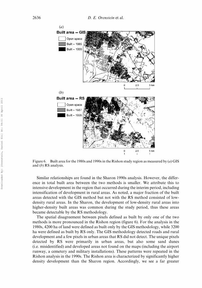
The spatial disagreement between pixels defined as built by only one of the two

methods is more pronounced in the Rishon region (figure 6). For the analysis in the

1980s, 4200 ha of land were defined as built only by the GIS methodology, while 3200

ha were defined as built by RS only. The GIS methodology detected roads and rural

development and a few pixels in urban areas that RS did not detect. The unique pixels

detected by RS were primarily in urban areas, but also some sand dunes

(i.e. misidentified) and developed areas not found on the maps (including the airport

runway, a cemetery and military installations). These patterns were repeated in the

Rishon analysis in the 1990s. The Rishon area is characterized by significantly higher

density development than the Sharon region. Accordingly, we see a far greater

Figure 6. Built area for the 1980s and 1990s in the Rishon study region asmeasured by (a) GISand (b) RS analysis.



proportion of the area defined as built during both periods (15–20%) in Rishon than

in the other study regions.

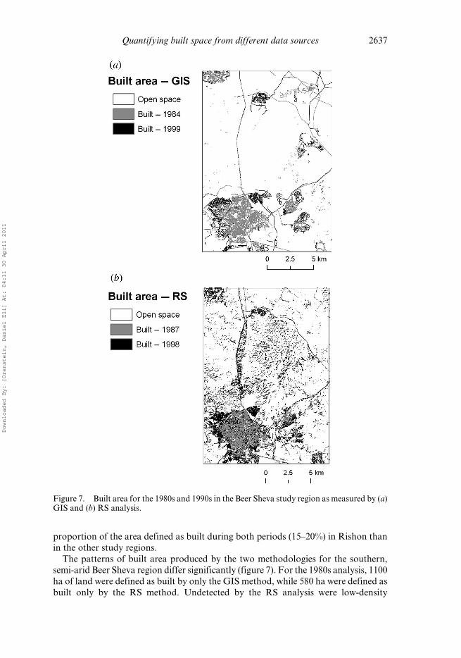
The patterns of built area produced by the two methodologies for the southern,

semi-arid Beer Sheva region differ significantly (figure 7). For the 1980s analysis, 1100

ha of land were defined as built by only the GIS method, while 580 ha were defined as

built only by the RS method. Undetected by the RS analysis were low-density

Figure 7. Built area for the 1980s and 1990s in the Beer Sheva study region as measured by (a)GIS and (b) RS analysis.



settlements and roads, as well as scattered pixels within urban centres. Approximately

two-thirds of the land defined as built by the RSmethodology, but open by GIS, were

also in dense urban areas or along roads, while the rest was found in open shrubland

areas or in built areas excluded from the maps. For the 1990s analysis, there is more

land defined as built exclusively by the RSmethod than defined as such exclusively by

the GIS method. Again, built areas defined as such only by the GIS method were split

between rural settlements and roads, and by built land in urban areas. As observed in

the accuracy assessment, approximately one-third of the land defined as built only by

the RS method was in shrubland areas or areas used for low-density tree planting.

These were misidentified as built due to their spectral signature similarities to urban

areas. The remaining RS-only built pixels were in urban areas and approximately 10%

in built areas intentionally or unintentionally excluded from the maps.

3.5 Constructing a best-estimate built area map

We defined three main types of built area that were misclassified in the GIS base map

but correctly identified in the RS auxiliary map: (1) infill in urban residential and

industrial areas, (2) built areas that had been purposely or inadvertently excluded

from the maps, including newly built areas and (3) infrastructures that are not

structures per se, but are paved surfaces (including sewage treatment plants, waste

disposal facilities and agricultural installations). These land-cover types were added

to the GIS map from a filtered RS built map for the Rishon site (figure 8). The

estimate of total built area for the GISþRSmap rose from 5100 to 6600 ha, omission

errors were reduced from 34 to 9%, while commission errors were statistically

unchanged. The overall accuracy of the final map was 87%, as compared to 78% for

the original GIS estimate, and the Kappa index is accordingly larger. The combined

map is shown in figure 8(c), and table 5 displays the confusionmatrix for the improved

map.

Combining the GIS and RS maps was less effective for the semi-arid Beer Sheva

region, which was characterized by large blocs of open soil misidentified as built space

in the RS analysis. The filtering was less effective at removing the pixels responsible

for commission errors, so the combinedmap had 49% commission errors (nearly twice

the number as the GIS map alone), although omission errors were significantly

reduced (to 12%) relative to the original GIS map. Overall accuracy was 86%,

which was lower than the accuracy of the GIS map alone.

Our best estimates of increases in total built area in the three research regions

between the mid-1980s and the mid-1990s are: 15–22% in the Sharon region, 35–45%

in the Rishon region and 8–20% in the Beer Sheva region. Supplementing the GIS

estimates with RS estimates of built area resulted in an upward adjustment of between

1 and 15% of built land, depending on the region. The addition of RS data had the

least effect in the rural area of Sharon, and the greatest in the densely built Rishon

region.

4. Discussion

Much of the recent literature on methodological approaches to land-cover classifica-

tion treat GIS maps as a secondary, or ancillary, data set with an RS product as the

primary source (Vogelmann et al. 1998, Yang and Lo 2002). While both approaches

have unique strengths and weaknesses, we argue that a GIS-based analysis of built

areas yields more predictable errors that can be largely resolved with the addition of a



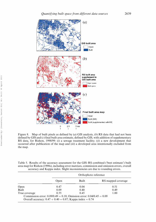
Figure 8. Map of built pixels as defined by (a) GIS analysis, (b) RS data that had not beendefined byGIS and (c) final built area estimate, defined byGIS, with addition of supplementaryRS data, for Rishon, 1998/99: (i) a sewage treatment facility; (ii) a new development thatoccurred after publication of the map and (iii) a developed area intentionally excluded fromthe map.

Table 5. Results of the accuracy assessment for the GIS–RS combined (‘best estimate’) builtarea map for Rishon (1990s), including error matrices, commission and omission errors, overall

accuracy and Kappa index. Slight inconsistencies are due to rounding errors.

Orthophoto reference

Open Built RS mapped coverage

Open 0.47 0.04 0.51Built 0.09 0.40 0.49True coverage 0.55 0.45 1.00




relatively simple RS methodology using a decision-tree approach. The GIS metho-

dology had consistently higher overall accuracy, most notably in semi-arid regions.

Where possible, the use of survey maps as a primary data source, supplemented by

remote sensing, may lead to more accurate identification of built areas and improved

quantification of urban expansion.

The use of each data set has distinct advantages and disadvantages, and we concur

with other researchers that combining data sources holds the greatest potential for

accurate assessments of land development (Foresman et al. 1997, Stefanov et al. 2001,

Yang and Lo 2002, Mundia and Aniya 2005). The GIS approach described here is

labour intensive, requiring substantial georeferencing, and digitizing of maps and/or

primary source aerial photographs. Furthermore, the maps may be subject to human

error and the comprehensiveness of updates may be compromised by limited funding

(E. Shlomi, Survey of Israel, personal communication). Another important limitation

of the survey maps is that land use, as defined by survey maps, may not adequately

describe the actual land cover, as in the case where agricultural land lies fallow, or is

covered with construction waste, greenhouses or plastic sheeting, or ‘open’ spaces are

in fact parking lots.

However, the maps typically provide more historical depth, having been produced

over much of the 20th century for many parts of the world. Furthermore, because

maps are based on aerial photographs, there is little risk of confusing urban areas with

sand or soils. Finally, the proportion of omission and commission errors in the GIS

methodology was consistently between 25 and 35% and, importantly, the causes of the

errors were predictable.

The RS analysis can be less work intensive than theGIS approach depending on the

methodology used to differentiate among land-cover types (this process itself can be

challenging and time-consuming). The decision tree used in the RS analysis is a

straightforward method for characterizing land cover and illustrates limitations likely

to be found regardless of classification methodology. Although higher accuracy may

be possible with more involved techniques (e.g. textural analysis or temporal unmix-

ing), the simpler method is more likely to be used by planners and resource managers

with limited experience with remote sensing. Advantages of using the RS techniques

include more readily accessible data, which are also available in real time. When

defining built area, the RS analysis may be more reliable in urban settings, primarily

due to being able to detect large impervious surfaces such as parking lots.

However, in rural settings Landsat TMdata-basedmaps fail to identify low-density

communities as built areas because pixels are often a mixture of built and vegetated

land cover. Past efforts to discriminate between low-density residential areas using RS

data have had mixed success (McCauley and Goetz 2004, Irwin and Bockstael 2008).

Underestimation of built area in rural and suburban settings should be expected with

RS analysis given existing approaches. RS identification of built areas is also subject

to error when spectral properties of open space are similar to built space, for example,

semi-arid regions (figure 7). Overestimation of built area (commission errors) in semi-

arid regions with low vegetated cover should be expected with RS analysis.

Combining maps based on GIS and RS data compensates for the weaknesses of

each data source individually. Researchers who rely on a Landsat-based RS analysis

should pay particular attention to the types of developed land cover that are apt to be

missed or underestimated by the analysis. This is a particular concern for suburban

and rural development, which is fast growing in many areas (Irwin and Bockstael

2008). The RS data supplemented the GIS data by identifying three built land-cover



types. First, the RS method detected areas that were functionally ‘built’ but were not

structures, including cemeteries, airport runways, large structures (e.g. warehouses,

hangars and shopping centres) and parking lots. An example of this is a sewage

treatment plant (figure 8(c), (i)). Second, the RS method detected areas that had

been built between successive publications of updated maps (figure 8(c), (ii)). Third,

the RSmethod detected areas that were built but were unintentionally or intentionally

excluded from maps (figure 8(c), (iii)).

Landsat data have been shown to be effective for urban change detection in several

analyses (Ward et al. 2000, Stefanov et al. 2001, Zhang et al. 2002, Xian and Crane

2005, Yuan et al. 2005). To control for some of the heterogeneity in determining

amounts and patterns of change using large satellite data sets, researchers can focus

on smaller areas immediately around built areas, thereby eliminating some landscape

variability. However, as spatial scales of analysis becomes more focused, survey maps

become increasingly attractive as a primary data source.

Our GIS method identifies a greater amount of built area undetected by the RS

method than the reverse, and so we advocate beginning an analysis of urban LUCC

with thematic maps whenever available at the desired spatial scales. In this compar-

ison, the RS method underestimated the amount of built land cover in rural areas

(e.g. the Sharon region) by up to 75% as compared to the GIS method (figure 5).

Researchers and practitioners can avoid systematic underestimations of built area

by combining data sources and exploiting the strengths of each data source to offset

the weaknesses of the other. Our combined map provides a more realistic estimate of

built area in that it includes rural and suburban development, censured data and

impermeable surfaces that may have been overlooked by relying on a single data

source. As suburban and exurban sprawl becomes more pervasive, the need for

increasing accuracy by combining data sources grows.

Ultimately, the choice in data sources for the detection of patterns of expansion of

built space depends on the desired temporal and spatial resolution and the scale of the

analysis, as well as the technical limitations of the researchers or practitioners. This

research draws attention to specific land-cover types that may be misclassified when

using either survey maps or satellite data. It is important that researchers be aware of

the potential differences in results that can be generated from different sources and

even more importantly, circumstances in which we may be over- or underestimating

built space using only RS data.

Acknowledgements

The GIS units of the central and southern units of the Keren Kayemeth L’Israel

(KKL), the Cartography Library of the Hebrew University of Jerusalem, and Yale

University’s Center for EarthObservation graciously provided spatial data.We thank

E. Shlomi and B. Peretzman of the Survey of Israel for explaining the process of

producing and updating survey maps, Alon Tal, Adi Ben-Nun and Benjamin Kedar

for assistance in procuring data, Ayala Cohen for her insights regarding sampling

methods and Lior Asaf for providing precipitation data. Jeremy Fisher, Lynn

Carlson, Matt Vadeboncoeur and two anonymous reviewers provided excellent feed-

back and advice. Funding was provided through a Luce Graduate Environmental

Fellowship to Daniel Orenstein.



References

ADAMS, J.B., SABOL, D.E., KAPOS, V., ALMEIDA, R., ROBERTS, D.A., SMITH, M.O. andGILLESPIE,

A.R., 1995, Classification of multispectral images based on fractions of endmembers:

application to land-cover change in the Brazilian Amazon. Remote Sensing of

Environment, 52, pp. 137–154.

ALTERMAN, R., 2002, Planning in the Face of Crisis: Land Use, Housing, and Mass Immigration

in Israel. The Cities and Regions Series (London: Routledge).

AYALON, O. (Ed.), 2003, National Priorities for Environment in Israel (Haifa: The Economic

Forum for the Environment in Israel, Samuel Ne’eman Institute).

CAM, E., NICHOLS, J.D., SAUER, J.R., HINES, J.E. and FLATHER, C.H., 2000, Relative species

richness and community completeness: birds and urbanization in the Mid-Atlantic

States. Ecological Applications, 10, pp. 1196–1210.

CHAVEZ, P.S., 1988, An improved dark-object subtraction technique for atmospheric scattering

correction of multispectral data. Remote Sensing of Environment, 24, pp. 459–479.

CHRISTENSEN, N.L., BARTUSKA, A.M., BROWN, J.H., CARPENTER, S., D’ANTONIO, C., FRANCIS,

R., FRANKLIN, J.F., MACMAHON, J.A., NOSS, R.F., PARSONS, D.J., PETERSON, C.H.,

TURNER, M.G. and WOODMANSEE, R.G., 1996, The report of the Ecological Society of

America Committee on the scientific basis for ecosystem management. Ecological

Applications, 6, pp. 665–691.

CIHLAR, J., 2000, Land cover mapping of large areas from satellites: status and research

priorities. International Journal of Remote Sensing, 21, pp. 1093–1114.

COHEN, W.B. and GOWARD, S.N., 2004, Landsat’s role in ecological applications of remote

sensing. BioScience, 54, pp. 535–545.

COSTANZA, R., D’ARGE, R., DE GROOT, R., FARBER, S., GRASSO, M., HANNON, B., LIMBURG, K.,

NAEEM, S., O’NEILL, R.V., PARUELO, J., RASKIN, R.G., SUTTON, P. and VAN DEN BELT,

M., 1997, The value of the world’s ecosystem services and natural capital. Nature, 387,

pp. 253–260.

DEFRIES, R., ASNER, G.P. and HOUGHTON, R. (Eds.), 2004, Effects of Land-Use Change on

Ecosystems (Washington, DC: American Geophysical Union).

DOLEV, A. andPEREVOLOTSKY, A. (Eds.), 2004,TheRedBook: Vertebrates in Israel (Jerusalem: The

Israel Nature and Parks Authority and The Society for the Protection ofNature in Israel).

DUDA, T. and CANTY, M., 2002, Unsupervised classification of satellite imagery: choosing a

good algorithm. International Journal of Remote Sensing, 23, pp. 2193–2212.

EHRLICH, P.R. and EHRLICH, A., 1981, Extinction (New York, NY: Random House).

ELMORE, A.J., MUSTARD, J.F., MANNING, S.J. and LOBELL, D.B., 2000, Quantifying vegetation

change in semiarid environments: precision and accuracy of spectral mixture analysis

and the normalized difference vegetation index.Remote Sensing of Environment, 73, pp.

87–102.

FEDDEMA, J.J., OLESON, K.W., BONAN, G.B., MEARNS, L.O., BUJA, L.E., MEEHL, G.A. and

WASHINGTON, W.M., 2005, The importance of land-cover change in simulating future

climates. Science, 310, pp. 1674–1678.

FOODY, G.M., 2002, Status of land cover classification accuracy assessment. Remote Sensing of

Environment, 80, pp. 185–201.

FORESMAN, T.W., PICKETT, S.T.A. and ZIPPERER, W.C., 1997, Methods for spatial and temporal

land use and land cover assessment for urban ecosystems and application in the greater

Baltimore-Chesapeake region. Urban Ecosystems, 1, pp. 201–216.

FRANKENBERG, E., 1999, Will the biogeographical bridge continue to exist? Israel Journal of

Zoology, 45, pp. 65–74.

FRENKEL, A., 2004a, A land-consumption model: its application to Israel’s future spatial

development. Journal of the American Planning Association, 70, pp. 454–470.

FRENKEL, A., 2004b, The potential effect of national growth-management policy on urban

sprawl and the depletion of open spaces and farmland. Land Use Policy, 21, pp.

357–369.



GAVISH, D., 1976, Changes in rural land-use on the urban fringe of Tel Aviv. In Geography in

Israel, D.H.K.Amiram andY. Ben-Arieh (Eds.), pp. 218–238 (Jerusalem: International

Geographical Union).

GOLAN, A., 2005, The Era of the Conquest of Land has Ended [in Hebrew]. Ha’aretz On-Line, Tel

Aviv. Available online at: www.haaretz.co.il (accessed).

HENNINGS, L.A. and EDGE, W.D., 2003, Riparian bird community structure in Portland,

Oregon: habitat, urbanization, and spatial pattern. The Condor, 105, pp. 288–302.

HEROLD,M., GOLDSTEIN, N.C. andCLARKE, K.C., 2003, The spatiotemporal form of urban growth:

measurement, analysis and modeling. Remote Sensing of Environment, 86, pp. 286–302.

IRWIN, E.G. and BOCKSTAEL, N.E., 2008, The evolution of urban sprawl: evidence of spatial

heterogeneity and increasing land fragmentation. Proceedings of the National Academy

of Sciences of the USA, 104, pp. 20672–20677.

JIANG, L., YUFEN, T., ZHIJIE, Z., TIANHONG, L. and JIANHUA, L., 2005, Water resources, land

exploration and population dynamics in arid areas: the case of the TarimRiver Basin in

Xinjiang of China. Population and Environment, 26, pp. 471–503.

KEMP, S.J. and SPOTILA, J.R., 1997, Effects of urbanization on brown trout Salmo trutta, other

fishes and macroinvertebrates in Valley Creek, Valley Forge, Pennsylvania. American

Midland Naturalist, 138, pp. 55–68.

KREUTER, U.P., HARRIS, H.G., MATLOCK, M.D. and LACEY, R.E., 2001, Change in ecosystem

service values in the San Antonio area, Texas. Ecological Economics, 39, pp. 333–346.

KUMMER, D.M. and TURNER, B.L., 1994, The human causes of deforestation in Southeast-Asia.

Bioscience, 44, pp. 323–328.

KUTIEL, P., KUTIEL, H. and LAVEE, H., 2000, Vegetation response to possible scenarios of

rainfall variations along a Mediterranean-extreme arid climatic transect. Journal of

Arid Environments, 44, pp. 277–290.

KUTIEL, P., LAVEE, H. and SHOSHANY, M., 1995, Influence of a climatic gradient upon vegetation

dynamics along aMediterranean-arid transect. Journal of Biogeography, 22, pp. 1065–1071.

LAMBIN, E. and VELDKAMP, A., 2005, Key findings of LUCC on its research questions. Global

Change Newsletter, 63, pp. 12–14.

LE HEGARAT-MASCLE, S., QUESNEY, A., VIDAL-MADJAR, D., NORMAND, M. and LOUMAGNE, C.,

2000, Land cover discrimination from multitemporal ERS images and multispectral

Landsat images: a study case in an agricultural area in France. International Journal of

Remote Sensing, 21, pp. 435–456.

MARTINEZ-CASASNOVAS, J.A., 2000, A cartographic and database approach for land cover/use

mapping and generalization from remotely sensed data. International Journal of Remote

Sensing, 21, pp. 1825–1842.

MARZLUFF, J.M. and EWING, K., 2001, Restoration of fragmented landscapes for the conserva-

tion of birds: a general framework and specific recommendations for urbanizing land-

scapes. Restoration Ecology, 9, pp. 280–292.

MCCAULEY, S. and GOETZ, S.J., 2004, Mapping residential density patterns using multi-

temporal Landsat data and a decision-tree classifier. International Journal of Remote

Sensing, 25, pp. 1077–1094.

MCKINNEY, M.L., 2002, Urbanization, biodiversity, and conservation.Bioscience, 52, pp. 883–890.

MEFFE, G.K. and CARROLL, C.R., 1994, Principles of Conservation Biology (Sunderland, MA:

Sinauer Associates, Inc.).

MUNDIA, C.N. andANIYA,M., 2005, Analysis of land use/cover changes and urban expansion of

Nairobi city using remotes sensing and GIS. International Journal of Remote Sensing,

26, pp. 2831–2849.

PERRY, G. and DMI’EL, R., 1995, Urbanization and sand dunes in Israel: direct and indirect

effects. Israel Journal of Zoology, 41, pp. 33–41.

PETIT, C.C. and LAMBIN, E.F., 2001, Integration of multi-source remote sensing data for land

cover change detection. International Journal of Geographical Information Science, 15,

pp. 785–803.



PETIT, C.C. and LAMBIN, E.F., 2002, Impact of data integration technique on historical land-

use/land-cover change: comparing historical maps with remote sensing data in the

Belgian Ardennes. Landscape Ecology, 17, pp. 117–132.

PU, R., GONG, P., MICHISHITA, R. and SASAGAWA, T., 2008, Spectral mixture analysis for

mapping abundance of urban surface components from the Terra/ASTER data.

Remote Sensing of Environment, 112, pp. 939–954.

RINDFUSS, R.R., WALSH, S.J., TURNER, II, B.L., FOX, J. and MISHRA, V., 2004, Developing a

science of land change: challenges and methodological issues. Proceedings of the

National Academy of Sciences of the USA, 101, pp. 13976–13981.

ROGAN, J. and CHEN, D., 2004, Remote sensing technology for mapping and monitoring land-

cover and land-use change. Progress in Planning, 61, pp. 301–325.

SCHOTT, J.R., SALVAGGIO, C. and VOLCHOK, W.J., 1988, Radiometric scene normalization using

pseudoinvariant features. Remote Sensing of Environment, 26, pp. 1–16.

SHACHAR, A., 1998, Reshaping the map of Israel: a new national planning doctrine. Annals of

the American Academy of Political and Social Science, 555, pp. 209–218.

SHOSHANY, M. and GOLDSHLEGER, N., 2002, Land-use and population density changes in Israel

– 1950 to 1990: analysis of regional and local trends. Land Use Policy, 19, pp. 123–133.

STEFANOV, W.L., RAMSEY, M.S. and CHRISTENSEN, P.R., 2001, Monitoring urban land cover

change: an expert system approach to land cover classification of semiarid to arid urban

centers. Remote Sensing of Environment, 77, pp. 173–185.

STEHMAN, S.V. and CZAPLEWSKI, R.L., 1998, Design and analysis for thematic map accuracy

assessment. Remote Sensing of Environment, 64, pp. 331–344.

TAL, A., 2002, Pollution in a Promised Land (Berkeley, CA: University of California Press).

TURNER, W.R., NAKAMURA, T. and DINETTI, M., 2004, Global urbanization and the separation

of humans from nature. BioScience, 54, pp. 585–590.

VELAZQUEZ, A., DURAN, E., RAMIREZ, I., MAS, J.F., BOCCO, G., RAMIREZ, G. and PALACIO, J.L.,

2003, Land use-cover change processes in highly biodiverse areas: the case of Oaxaca,

Mexico.Global Environmental Change: Human and Policy Dimensions, 13, pp. 175–184.

VITOUSEK, P.M.,MOONEY, H.A., LUBCHENCO, J. andMELILO, J.M., 1997, Human domination of

Earth’s ecosystems. Science, 277, pp. 494–499.

VOGELMANN, J.E., SOHL, T.L., CAMBELL, P.V. and SHAW, D.M., 1998, Regional land cover

characterization using Landsat Thematic Mapper data and ancillary data sources.

Environmental Monitoring and Assessment, 51, pp. 415–428.

WARD, D., PHINN, S.R. and MURRAY, A.T., 2000, Monitoring growth in rapidly urbanizing

areas using remotely sensed data. Professional Geographer, 52, pp. 371–386.

WEIBEL, R. and JONES, C.B., 1998, Computational perspectives on map generalization.

GeoInformatica, 2, pp. 307–314.

XIAN, G. and CRANE, M., 2005, Assessments of urban growth in the Tampa Bay watershed

using remote sensing data. Remote Sensing of Environment, 97, pp. 203–215.

YANG, X. and LO, C.P., 2002, Using a time series of satellite imagery to detect land use and land

cover changes in the Atlanta, Georgia metropolitan area. International Journal of

Remote Sensing, 23, pp. 1775–1798.

YOM TOV, Y. and MENDELSOHN, H., 1988, Changes in the distribution and abundance of

vertebrates in Israel. In The Zoogeography of Israel: the Distribution and Abundance

of a Zoogeographical Crossroad, Y. Yom Tov and E. Tchernov (Eds.), pp. 515–548

(Dordrecht: DRW Junk).

YUAN, F., SAWAYA, K.E., LOEFFELHOLZ, B.C. and BAUER, M.E., 2005, Land cover classification

and change analysis of the Twin Cities (Minnesota) Metropolitan Area by multitem-

poral Landsat remote sensing. Remote Sensing of Environment, 98, pp. 317–328.

ZHANG, Q., WANG, J., PENG, X., GONG, P. and SHI, P., 2002, Urban built-up land change

detection with road density and spectral information frommulti-temporal Landsat TM

data. International Journal of Remote Sensing, 23, pp. 3057–3078.



How much is built? Quantifying and interpreting patterns of built space from different data sources

Documents