1 How many species of mammals are there? CONNOR J. BURGIN, 1 JOCELYN P. COLELLA, 1 PHILIP L. KAHN, AND NATHAN S. UPHAM* Department of Biological Sciences, Boise State University, 1910 University Drive, Boise, ID 83725, USA (CJB) Department of Biology and Museum of Southwestern Biology, University of New Mexico, MSC03-2020, Albuquerque, NM 87131, USA (JPC) Museum of Vertebrate Zoology, University of California, Berkeley, CA 94720, USA (PLK) Department of Ecology and Evolutionary Biology, Yale University, New Haven, CT 06511, USA (NSU) Integrative Research Center, Field Museum of Natural History, Chicago, IL 60605, USA (NSU) 1 Co-first authors. * Correspondent: [email protected] Accurate taxonomy is central to the study of biological diversity, as it provides the needed evolutionary framework for taxon sampling and interpreting results. While the number of recognized species in the class Mammalia has increased through time, tabulation of those increases has relied on the sporadic release of revisionary compendia like the Mammal Species of the World (MSW) series. Here, we present the Mammal Diversity Database (MDD), a digital, publically accessible, and updateable list of all mammalian species, now available online: https://mammaldiversity.org. The MDD will continue to be updated as manuscripts describing new species and higher taxonomic changes are released. Starting from the baseline of the 3rd edition of MSW (MSW3), we performed a review of taxonomic changes published since 2004 and digitally linked species names to their original descriptions and subsequent revisionary articles in an interactive, hierarchical database. We found 6,495 species of currently recognized mammals (96 recently extinct, 6,399 extant), compared to 5,416 in MSW3 (75 extinct, 5,341 extant)—an increase of 1,079 species in about 13 years, including 11 species newly described as having gone extinct in the last 500 years. We tabulate 1,251 new species recognitions, at least 172 unions, and multiple major, higher-level changes, including an additional 88 genera (1,314 now, compared to 1,226 in MSW3) and 14 newly recognized families (167 compared to 153). Analyses of the description of new species through time and across biogeographic regions show a long-term global rate of ~25 species recognized per year, with the Neotropics as the overall most species-dense biogeographic region for mammals, followed closely by the Afrotropics. The MDD provides the mammalogical community with an updateable online database of taxonomic changes, joining digital efforts already established for amphibians (AmphibiaWeb, AMNH’s Amphibian Species of the World), birds (e.g., Avibase, IOC World Bird List, HBW Alive), non-avian reptiles (The Reptile Database), and fish (e.g., FishBase, Catalog of Fishes). Una taxonomía que precisamente refleje la realidad biológica es fundamental para el estudio de la diversidad de la vida, ya que proporciona el armazón evolutivo necesario para el muestreo de taxones e interpretación de resultados del mismo. Si bien el número de especies reconocidas en la clase Mammalia ha aumentado con el tiempo, la tabulación de esos aumentos se ha basado en las esporádicas publicaciones de compendios de revisiones taxonómicas, tales como la serie Especies de mamíferos del mundo (MSW por sus siglas en inglés). En este trabajo presentamos la Base de Datos de Diversidad de Mamíferos (MDD por sus siglas en inglés): una lista digital de todas las especies de mamíferos, actualizable y accesible públicamente, disponible en la dirección URL https://mammaldiversity.org/. El MDD se actualizará con regularidad a medida que se publiquen artículos que describan nuevas especies o que introduzcan cambios de diferentes categorías taxonómicas. Con la tercera edición de MSW (MSW3) como punto de partida, realizamos una revisión en profundidad de los cambios taxonómicos publicados a partir del 2004. Los nombres de las especies nuevamente descriptas (o ascendidas a partir de subespecies) fueron conectadas digitalmente en una base de datos interactiva y jerárquica con sus Journal of Mammalogy, 99(1):1–14, 2018 DOI:10.1093/jmammal/gyx147 INVITED PAPER © 2018 American Society of Mammalogists, www.mammalogy.org Downloaded from https://academic.oup.com/jmammal/article-abstract/99/1/1/4834091 by University of Wyoming Libraries user on 21 August 2018

Welcome message from author
This document is posted to help you gain knowledge. Please leave a comment to let me know what you think about it! Share it to your friends and learn new things together.
Transcript
1
How many species of mammals are there?
Connor J. Burgin,1 JoCelyn P. Colella,1 PhiliP l. Kahn, and nathan S. uPham*
Department of Biological Sciences, Boise State University, 1910 University Drive, Boise, ID 83725, USA (CJB)Department of Biology and Museum of Southwestern Biology, University of New Mexico, MSC03-2020, Albuquerque, NM 87131, USA (JPC)Museum of Vertebrate Zoology, University of California, Berkeley, CA 94720, USA (PLK)Department of Ecology and Evolutionary Biology, Yale University, New Haven, CT 06511, USA (NSU)Integrative Research Center, Field Museum of Natural History, Chicago, IL 60605, USA (NSU)1Co-first authors.
* Correspondent: [email protected]
Accurate taxonomy is central to the study of biological diversity, as it provides the needed evolutionary framework for taxon sampling and interpreting results. While the number of recognized species in the class Mammalia has increased through time, tabulation of those increases has relied on the sporadic release of revisionary compendia like the Mammal Species of the World (MSW) series. Here, we present the Mammal Diversity Database (MDD), a digital, publically accessible, and updateable list of all mammalian species, now available online: https://mammaldiversity.org. The MDD will continue to be updated as manuscripts describing new species and higher taxonomic changes are released. Starting from the baseline of the 3rd edition of MSW (MSW3), we performed a review of taxonomic changes published since 2004 and digitally linked species names to their original descriptions and subsequent revisionary articles in an interactive, hierarchical database. We found 6,495 species of currently recognized mammals (96 recently extinct, 6,399 extant), compared to 5,416 in MSW3 (75 extinct, 5,341 extant)—an increase of 1,079 species in about 13 years, including 11 species newly described as having gone extinct in the last 500 years. We tabulate 1,251 new species recognitions, at least 172 unions, and multiple major, higher-level changes, including an additional 88 genera (1,314 now, compared to 1,226 in MSW3) and 14 newly recognized families (167 compared to 153). Analyses of the description of new species through time and across biogeographic regions show a long-term global rate of ~25 species recognized per year, with the Neotropics as the overall most species-dense biogeographic region for mammals, followed closely by the Afrotropics. The MDD provides the mammalogical community with an updateable online database of taxonomic changes, joining digital efforts already established for amphibians (AmphibiaWeb, AMNH’s Amphibian Species of the World), birds (e.g., Avibase, IOC World Bird List, HBW Alive), non-avian reptiles (The Reptile Database), and fish (e.g., FishBase, Catalog of Fishes).
Una taxonomía que precisamente refleje la realidad biológica es fundamental para el estudio de la diversidad de la vida, ya que proporciona el armazón evolutivo necesario para el muestreo de taxones e interpretación de resultados del mismo. Si bien el número de especies reconocidas en la clase Mammalia ha aumentado con el tiempo, la tabulación de esos aumentos se ha basado en las esporádicas publicaciones de compendios de revisiones taxonómicas, tales como la serie Especies de mamíferos del mundo (MSW por sus siglas en inglés). En este trabajo presentamos la Base de Datos de Diversidad de Mamíferos (MDD por sus siglas en inglés): una lista digital de todas las especies de mamíferos, actualizable y accesible públicamente, disponible en la dirección URL https://mammaldiversity.org/. El MDD se actualizará con regularidad a medida que se publiquen artículos que describan nuevas especies o que introduzcan cambios de diferentes categorías taxonómicas. Con la tercera edición de MSW (MSW3) como punto de partida, realizamos una revisión en profundidad de los cambios taxonómicos publicados a partir del 2004. Los nombres de las especies nuevamente descriptas (o ascendidas a partir de subespecies) fueron conectadas digitalmente en una base de datos interactiva y jerárquica con sus
Journal of Mammalogy, 99(1):1–14, 2018DOI:10.1093/jmammal/gyx147
invited PaPer
© 2018 American Society of Mammalogists, www.mammalogy.org
Downloaded from https://academic.oup.com/jmammal/article-abstract/99/1/1/4834091by University of Wyoming Libraries useron 21 August 2018
2 JOURNAL OF MAMMALOGY
descripciones originales y con artículos de revisión posteriores. Los datos indican que existen actualmente 6,495 especies de mamíferos (96 extintas, 6,399 vivientes), en comparación con las 5,416 reconocidas en MSW3 (75 extintas, 5,341 vivientes): un aumento de 1,079 especies en aproximadamente 13 años, incluyendo 11 nuevas especies consideradas extintas en los últimos 500 años. Señalamos 1,251 nuevos reconocimientos de especies, al menos 172 uniones y varios cambios a mayor nivel taxonómico, incluyendo 88 géneros adicionales (1,314 reconocidos, comparados con 1,226 en MSW3) y 14 familias recién reconocidas (167 en comparación con 153 en MSW3). Los análisis témporo-geográficos de descripciones de nuevas especies (en las principales regiones del mundo) sugieren un promedio mundial de descripciones a largo plazo de aproximadamente 25 especies reconocidas por año, siendo el Neotrópico la región con mayor densidad de especies de mamíferos en el mundo, seguida de cerca por la region Afrotrópical. El MDD proporciona a la comunidad de mastozoólogos una base de datos de cambios taxonómicos conectada y actualizable, que se suma a los esfuerzos digitales ya establecidos para anfibios (AmphibiaWeb, Amphibian Species of the World), aves (p. ej., Avibase, IOC World Bird List, HBW Alive), reptiles “no voladores” (The Reptile Database), y peces (p. ej., FishBase, Catalog of Fishes).
Key words: biodiversity, conservation, extinction, taxonomy
Species are a fundamental unit of study in mammalogy. Yet spe-cies limits are subject to change with improved understanding of geographic distributions, field behaviors, and genetic relation-ships, among other advances. These changes are recorded in a vast taxonomic literature of monographs, books, and periodi-cals, many of which are difficult to access. As a consequence, a unified tabulation of changes to species and higher taxa has become essential to mammalogical research and conservation efforts in mammalogy. Wilson and Reeder’s 3rd edition of Mammal Species of the World (MSW3), published in November 2005, represents the most comprehensive and up-to-date list of mammalian species, with 5,416 species (75 recently extinct, 5,341 extant), 1,229 genera, 153 families, and 29 orders. That edition relied on expertise solicited from 21 authors to deliver the most comprehensive list of extant mammals then availa-ble. However, the episodic release of these massive anthologies (MSW1—Honacki et al. 1982; MSW2—Wilson and Reeder 1993; MSW3—Wilson and Reeder 2005) means that taxo-nomic changes occurring during or soon after the release of a new edition may not be easily accessible for over a decade. For example, MSW3, compared to MSW2, resulted in the addition of 787 species, 94 genera, and 17 families compared to MSW2 (Solari and Baker 2007). Since the publication of MSW3, there has been a steady flow of taxonomic changes proposed in peer-reviewed journals and books; however, changes proposed more than a decade ago (e.g., Carleton et al. 2006; Woodman et al. 2006) have yet to be incorporated into a Mammalia-wide refer-ence taxonomy. This lag between the publication of taxonomic changes and their integration into the larger field of mammal-ogy inhibits taxonomic consistency and accuracy in mam-malogical research, and—at worst—it can impede the effective conservation of mammals in instances where management deci-sions depend upon the species-level designation of distinctive evolutionary units.
The genetic era has catalyzed the discovery of morphologi-cally cryptic species and led to myriad intra- and interspecific revisions, either dividing species (splits) or uniting them (lumps). Many groups of mammals are taxonomically complex and in need of further revision, especially those that have received relatively little systematic attention or are morphologically or
behaviorally cryptic (e.g., shrews, burrowing mammals). For example, the phylogenetic placement of tenrecs and golden moles (families: Tenrecidae and Chrysochloridae) has long been a point of taxonomic contention, having variously been included within Insectivora, Eulipotyphla, and Lipotyphla. Taxonomic assignment of this group was only conclusively resolved when genetic data (Madsen et al. 2001; Murphy et al. 2001), as corrob-orated by morphology (Asher et al. 2003), aligned Tenrecidae and Chrysochloridae in the order Afrosoricida and found it allied to other African radiations in the superorder Afrotheria (Macroscelidea, Tubulidentata, Hyracoidea, Proboscidea, Sirenia). As analytical methods evolve and techniques become more refined, mammalian taxonomy will continue to change, making it desirable to create an adjustable list of accepted spe-cies-level designations and their hierarchical placement that can be updated on a regular basis. Such a list is needed to promote consistency and accuracy of communication among mammalo-gists and other researchers.
Here, using MSW3 as a foundation, we provide an up-to-date list of mammal species and introduce access to this spe-cies list as an amendable digital archive: the Mammal Diversity Database (MDD), available online at http://mammaldiversity.org. We compare our list to that of MSW3 to quantify changes in mammalian taxonomy that have occurred over the last 13 years and evaluate the distribution of species diversity and new species descriptions across both geography and time. We intend the MDD as a community resource for compiling and disseminating published changes to mammalian taxonomy in real time, rather than as a subjective arbiter for the relative strength of revisionary evidence, and hence defer to the peer-reviewed literature for such debates.
Materials and Methods
Starting from those species recognized in MSW3, we reviewed > 1,200 additional taxonomic publications appearing after MSW3’s end-2003 cutoff date in order to compile a list of every recognized mammal species. In addition to evaluating peer-reviewed manuscripts, other major references included the Handbook of the Mammals of the World volumes 1–6 (Wilson
Downloaded from https://academic.oup.com/jmammal/article-abstract/99/1/1/4834091by University of Wyoming Libraries useron 21 August 2018
INVITED PAPER—MAMMALIAN SPECIES DIVERSITY 3
and Mittermeier 2009, 2011, 2014, 2015; Mittermeier et al. 2013; Wilson et al. 2016), Mammals of South America volumes 1 and 2 (Gardner 2007; Patton et al. 2015), Mammals of Africa volumes 1–6 (Kingdon et al. 2013), Rodents of Sub-Saharan Africa (Monadjem et al. 2015), Taxonomy of Australian Mammals (Jackson and Groves 2015), and Ungulate Taxonomy (Groves and Grubb 2011). We linked each species to its pri-mary, descriptive publication and if a species was taxonomi-cally revised since 2004, the associated revisionary publications also were linked. The list was curated for spelling errors and compared to the species recognized in MSW3 to determine the total change in the number of recognized species over the inter-val 1 January 2004 to 15 August 2017; the latter date was our cutoff for reviewing literature. As with MSW3 and the IUCN (2017) RedList, species totals for the MDD include mamma-lian species that have gone extinct during the last 500 years, an arbitrary period of time used to delimit species “recently extinct”. The IUCN taxonomy was downloaded on 28 June 2017.
We considered “de novo” species descriptions to be those species recognized since MSW3 and named with novel spe-cies epithets (post-MSW3 proposal date), whereas “splits” are species established by resurrecting an existing name (i.e., ele-vated subspecies or synonym, and pre-MSW3 proposal). We based these 2 bins of new species on the epithet authority year to enable downstream analyses of species discovery trends. However, we acknowledge that this categorization is not precise regarding the more complex (and biologically interesting) issue of how many species were derived from new field discover-ies of distinctive populations versus the recognition of multiple species within named forms (Patterson 1996). Nevertheless, we expected the de novo category to encompass those field dis-coveries along with other types of species descriptions, and the splits category to encompass instances where existing names are elevated or validated, both of which are categories warrant-ing future investigation.
In addition to taxonomic ranks (order, family, genus, species) and primary data links, MDD species information includes the year of description, scientific authority, and geographic occurrence by biogeographic region. Here, we approximate the biogeographic realms defined by the World Wildlife Fund (Olson and Dinerstein 1998; Olson et al. 2001), with the excep-tion that we classified countries split across multiple biogeo-graphic realms as belonging exclusively to the realm covering the majority of that country. We defined the Nearctic realm as all of North America, including Florida, Bermuda, and all of Mexico. The Neotropical realm included all of South America, Central America, and the insular Caribbean. The Palearctic realm included all of Europe, northern Asia (including all of China), Japan, and northern Africa (Egypt, Algeria, Tunisia, Morocco, Western Sahara, Canary Islands, and the Azores). The Indomalayan realm included southern and southeastern Asia (Pakistan, India, Nepal, Bhutan, Vietnam, Laos, Myanmar) and all islands west of Sulawesi including the Greater Sundas and Philippines. The Afrotropical realm included all of sub-Saharan Africa and the Arabian Peninsula, plus Madagascar and the nearby Indian Ocean islands (e.g., Comoros, Mauritius,
Seychelles). We grouped the Australasian and Oceanian realms to include a single category for Australia, New Zealand, Sulawesi, and the islands east of Sulawesi, including Melanesia, Polynesia, Micronesia, Hawaii, and Easter Island, but excluding the Palearctic Japanese Bonin Islands. There are no terrestrial mammal species native to Antarctica. Open-water and coastal marine species, including the few Antarctic breed-ing species (e.g., leopard seals, Hydrurga), were grouped sep-arately. Freshwater species (e.g., river dolphins, river otters) were sorted by their resident landmass.
Based on our newly curated list, we calculated the number of new species described each decade since the origin of bi-nomial nomenclature (Linnaeus 1758) to determine the major eras of species discovery and taxonomic description. The year 1758 includes all the species described by Linnaeus that are still currently recognized. For each biogeographic realm, we calculated the total number of mammalian species recognized and the number of new species recognized since 2004. Note that the recognition of new species in a particular region can re-flect greater research efforts per region or taxon and thus cannot be extrapolated to the expected number of undiscovered species in that region. We scaled the number of species by regional land area (km2—World Atlas 2017) to determine the most species-dense region.
results
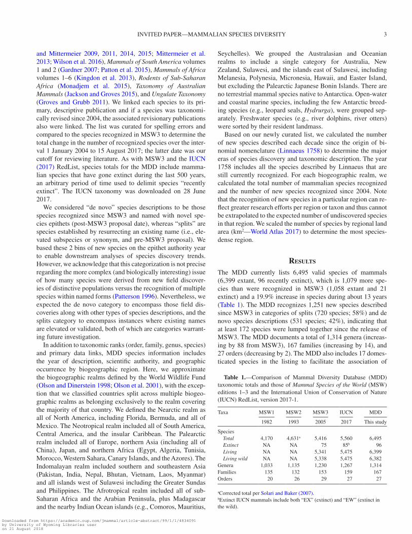
The MDD currently lists 6,495 valid species of mammals (6,399 extant, 96 recently extinct), which is 1,079 more spe-cies than were recognized in MSW3 (1,058 extant and 21 extinct) and a 19.9% increase in species during about 13 years (Table 1). The MDD recognizes 1,251 new species described since MSW3 in categories of splits (720 species; 58%) and de novo species descriptions (531 species; 42%), indicating that at least 172 species were lumped together since the release of MSW3. The MDD documents a total of 1,314 genera (increas-ing by 88 from MSW3), 167 families (increasing by 14), and 27 orders (decreasing by 2). The MDD also includes 17 domes-ticated species in the listing to facilitate the association of
Table 1.—Comparison of Mammal Diversity Database (MDD) taxonomic totals and those of Mammal Species of the World (MSW) editions 1–3 and the International Union of Conservation of Nature (IUCN) RedList, version 2017-1.
Taxa MSW1 MSW2 MSW3 IUCN MDD
1982 1993 2005 2017 This study
Species Total 4,170 4,631a 5,416 5,560 6,495 Extinct NA NA 75 85b 96 Living NA NA 5,341 5,475 6,399 Living wild NA NA 5,338 5,475 6,382Genera 1,033 1,135 1,230 1,267 1,314Families 135 132 153 159 167Orders 20 26 29 27 27
aCorrected total per Solari and Baker (2007).bExtinct IUCN mammals include both “EX” (extinct) and “EW” (extinct in the wild).
Downloaded from https://academic.oup.com/jmammal/article-abstract/99/1/1/4834091by University of Wyoming Libraries useron 21 August 2018
4 JOURNAL OF MAMMALOGY
these derivatives of wild populations with their often abundant trait data (e.g., DNA sequences, reproductive data). Details of the full MDD version 1 taxonomy, including associated citations and geographic region assignments, are provided in Supplementary Data S1.
The largest mammalian families are in the order Rodentia—Muridae (834 species versus 730 in MSW3) and Cricetidae (792 species versus 681 in MSW3)—followed by the chi-ropteran family Vespertilionidae (493 species versus 407 in MSW3) and the eulipotyphlan family Soricidae (440 species versus 376 in MSW3). Unsurprisingly, the 2 most speciose orders (Rodentia and Chiroptera) witnessed the most species additions: 371 and 304 species, respectively. The most speciose rodent family besides Muridae and Cricetidae is Sciuridae (298 species) and 6 rodent families are monotypic: Aplodontiidae, Diatomyidae, Dinomyidae, Heterocephalidae, Petromuridae, and Zenkerellidae. The most speciose chiropteran families along with Vespertilionidae are Phyllostomidae (214 species) and Pteropodidae (197 species), whereas there is only 1 mono-typic bat family: Craseonycteridae.
The increased number of recognized genera to 1,314 (from 1,230 in MSW3) results from the demonstrated paraphyly of several speciose and widely distributed former genera. This includes Spermophilus, which was split into 8 dis-tinct genera (Spermophilus, Urocitellus, Callospermophilus, Otospermophilus, Xerospermophilus, Ictidomys, Poliocitellus, and Notocitellus—Helgen et al. 2009) and Oryzomys, which was split into 11 genera (Oryzomys, Aegialomys, Cerradomys, Eremoryzomys, Euryoryzomys, Hylaeamys, Mindomys, Nephelomys, Oreoryzomys, Sooretamys, and Transandinomys—Weksler et al. 2006). Many smaller generic splits broke 1 genus into 2 or more genera and often involved the naming of a new genus, such as with Castoria (formerly Akodon—Pardiñas et al. 2016), Paynomys (formerly Chelemys—Teta et al. 2016), and Petrosaltator (formerly Elephantulus—Dumbacher 2016). Other genera were described on the basis of newly discovered taxa, such as Laonastes (Jenkins et al. 2005), Xeronycteris (Gregorin and Ditchfield 2005), Rungwecebus (Davenport et al. 2006), Drymoreomys (Percequillo et al. 2011), and Paucidentomys (Esselstyn et al. 2012). The most speciose cur-rently recognized genera are Crocidura (197 species), Myotis (126 species), and Rhinolophus (102 species). These also are the only genera of mammals that currently exceed 100 recog-nized and living species, with Rhinolophus reaching this level only recently.
Higher-level taxonomy also was significantly altered since 2004, with the recognition of 14 additional families and 2 fewer orders than MSW3. In the MDD, we included 3 families (†Megaladapidae, †Palaeopropithecidae, †Archaeolemuridae) that were not in MSW3 but that may have gone extinct in the last 500 years (McKenna and Bell 1997; Montagnon et al. 2001; Gaudin 2004; Muldoon 2010). The net addition of 11 other families in the MDD are the result of taxonomic splits and new taxon discoveries, as well as families lumped since MSW3. For example, Dipodidae was split into 3 families (Dipodidae, Zapodidae, Sminthidae—Lebedev et al. 2013), Hipposideridae
into 2 (Hipposideridae, Rhinonycteridae—Foley et al. 2015), and Bathyergidae into 2 (Bathyergidae, Heterocephalidae—Patterson and Upham 2014). One family, Diatomyidae, was added based on a species discovery (Laonastes aenigmamus—Jenkins et al. 2005), although it was already known as a prehistorically extinct family (Dawson et al. 2006). Additional newly recognized families are Chlamyphoridae, Cistugidae, Kogiidae, Lipotidae, Miniopteridae, Pontoporiidae, Potamogalidae, Prionodontidae, and Zenkerellidae. Three families recognized in MSW3 have since been subsumed: Myocastoridae and Heptaxodontidae inside Echimyidae (Emmons et al. 2015), and Aotidae inside Cebidae (Schneider and Sampaio 2015; Dumas and Mazzoleni 2017). Note that Capromyidae is still recognized at the family level (Fabre et al. 2017). The order Cetacea also experienced major revi-sions, and is now included within the order Artiodactyla based on genetic and morphological data (Gatesy et al. 1999; Adams 2001; Asher and Helgen 2010). Soricomorpha and Erinaceomorpha also are grouped together in the order Eulipotyphla, given their shared evolutionary history demonstrated by genetic analyses (Douady et al. 2002; Meredith et al. 2011).
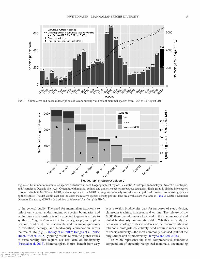
On average, since 1758, 24.95 species have been described per decade, including 3 major spikes in species recognition in the 1820–1840s, 1890–1920s, and 2000–2010s (Fig. 1). These bursts of systematic and taxonomic development were followed by 2 major troughs from about 1850–1880 and 1930–1990 (Fig. 1). Currently, we detect an accelerating rate of species description per decade, increasing from the 1990s (207 species), 2000s (341 species), and 2010s so far (298 species). A linear regression on these data suggests that if trends in mammalian species discov-ery continue, 120.46 species are yet to be discovered this decade, potentially resulting in a total of 418 new species to be recog-nized between 2010 and 2020 (R2 = 0.97, P < 0.000; Fig. 1).
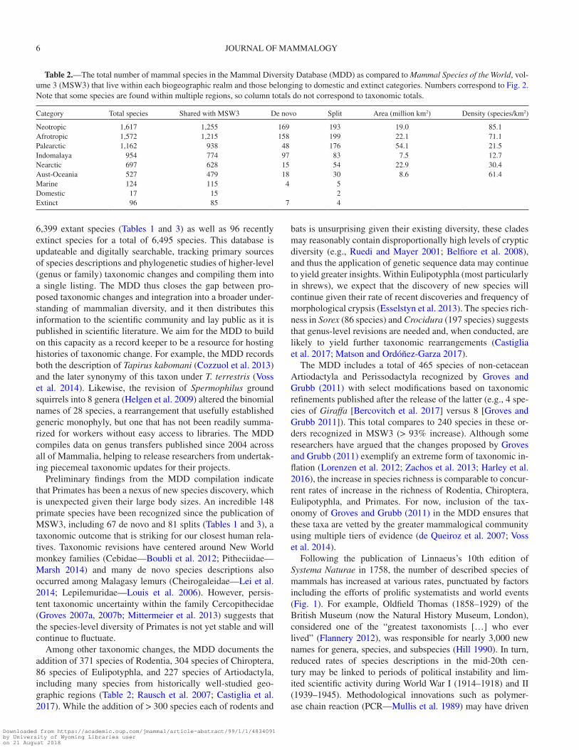
Across biogeographic regions, the Neotropics harbors the greatest number of currently recognized mammalian species (1,617 species), followed by the Afrotropics (1,572 species), and the Palearctic (1,162 species), whereas Australasia-Oceania has the least (527 species) (Fig. 2). The Neotropics also has the most newly recognized species (362 species—169 de novo and 193 split), again followed by the Afrotropics (357 spe-cies—158 de novo and 199 split), and with the fewest new spe-cies described from Australasia-Oceania (48 species—18 de novo and 30 split). Other categories included the marine (124 total species—4 de novo and 5 split), domesticated (17 total spe-cies—0 de novo and 2 split), and extinct (96 total species—7 de novo and 4 split; Fig. 2; Table 2) categories. When weighting the biogeographic realms by land area, we find the Neotropics and Afrotropics are also the most species-dense biogeographic regions (85.1 and 71.1 species per km2, respectively), followed closely by Australasia-Oceania (61.4 species per km2; Table 2). In all realms except the Indomalayan, more species were recog-nized via taxonomic splits than by de novo descriptions.
discussion
Mammalogists have a collective responsibility to serve the most current taxonomic information about mammalian biodiversity
Downloaded from https://academic.oup.com/jmammal/article-abstract/99/1/1/4834091by University of Wyoming Libraries useron 21 August 2018
INVITED PAPER—MAMMALIAN SPECIES DIVERSITY 5
to the general public. The need for mammalian taxonomy to reflect our current understanding of species boundaries and evolutionary relationships is only expected to grow as efforts to synthesize “big data” increase in frequency, scope, and sophis-tication. Studies at this macroscale address major questions in evolution, ecology, and biodiversity conservation across the tree of life (e.g., Rabosky et al. 2012; Hedges et al. 2015; Hinchliff et al. 2015), yielding results relevant to global issues of sustainability that require our best data on biodiversity (Pascual et al. 2017). Mammalogists, in turn, benefit from easy
access to this biodiversity data for purposes of study design, classroom teaching, analyses, and writing. The release of the MDD therefore addresses a key need in the mammalogical and global biodiversity communities alike. Whether we study the behavioral ecology of desert rodents or the macroevolution of tetrapods, biologists collectively need accurate measurements of species diversity—the most commonly assessed (but not the only) dimension of biodiversity (Jarzyna and Jetz 2016).
The MDD represents the most comprehensive taxonomic compendium of currently recognized mammals, documenting
Fig. 1.—Cumulative and decadal descriptions of taxonomically valid extant mammal species from 1758 to 15 August 2017.
Fig. 2.—The number of mammalian species distributed in each biogeographical region: Palearctic, Afrotropic, Indomalayan, Nearctic, Neotropic, and Australasia-Oceania (i.e., Aust-Oceania), with marine, extinct, and domestic species in separate categories. Each group is divided into species recognized in both MSW3 and MDD, and new species in the MDD in categories of newly coined species epithet (de novo) versus existing species epithet (splits). The dot within each bar indicates the relative species density per km2 land area, values are available in Table 2. MDD = Mammal Diversity Database; MSW3 = 3rd edition of Mammal Species of the World.
Downloaded from https://academic.oup.com/jmammal/article-abstract/99/1/1/4834091by University of Wyoming Libraries useron 21 August 2018
6 JOURNAL OF MAMMALOGY
6,399 extant species (Tables 1 and 3) as well as 96 recently extinct species for a total of 6,495 species. This database is updateable and digitally searchable, tracking primary sources of species descriptions and phylogenetic studies of higher-level (genus or family) taxonomic changes and compiling them into a single listing. The MDD thus closes the gap between pro-posed taxonomic changes and integration into a broader under-standing of mammalian diversity, and it then distributes this information to the scientific community and lay public as it is published in scientific literature. We aim for the MDD to build on this capacity as a record keeper to be a resource for hosting histories of taxonomic change. For example, the MDD records both the description of Tapirus kabomani (Cozzuol et al. 2013) and the later synonymy of this taxon under T. terrestris (Voss et al. 2014). Likewise, the revision of Spermophilus ground squirrels into 8 genera (Helgen et al. 2009) altered the binomial names of 28 species, a rearrangement that usefully established generic monophyly, but one that has not been readily summa-rized for workers without easy access to libraries. The MDD compiles data on genus transfers published since 2004 across all of Mammalia, helping to release researchers from undertak-ing piecemeal taxonomic updates for their projects.
Preliminary findings from the MDD compilation indicate that Primates has been a nexus of new species discovery, which is unexpected given their large body sizes. An incredible 148 primate species have been recognized since the publication of MSW3, including 67 de novo and 81 splits (Tables 1 and 3), a taxonomic outcome that is striking for our closest human rela-tives. Taxonomic revisions have centered around New World monkey families (Cebidae—Boubli et al. 2012; Pitheciidae—Marsh 2014) and many de novo species descriptions also occurred among Malagasy lemurs (Cheirogaleidae—Lei et al. 2014; Lepilemuridae—Louis et al. 2006). However, persis-tent taxonomic uncertainty within the family Cercopithecidae (Groves 2007a, 2007b; Mittermeier et al. 2013) suggests that the species-level diversity of Primates is not yet stable and will continue to fluctuate.
Among other taxonomic changes, the MDD documents the addition of 371 species of Rodentia, 304 species of Chiroptera, 86 species of Eulipotyphla, and 227 species of Artiodactyla, including many species from historically well-studied geo-graphic regions (Table 2; Rausch et al. 2007; Castiglia et al. 2017). While the addition of > 300 species each of rodents and
bats is unsurprising given their existing diversity, these clades may reasonably contain disproportionally high levels of cryptic diversity (e.g., Ruedi and Mayer 2001; Belfiore et al. 2008), and thus the application of genetic sequence data may continue to yield greater insights. Within Eulipotyphla (most particularly in shrews), we expect that the discovery of new species will continue given their rate of recent discoveries and frequency of morphological crypsis (Esselstyn et al. 2013). The species rich-ness in Sorex (86 species) and Crocidura (197 species) suggests that genus-level revisions are needed and, when conducted, are likely to yield further taxonomic rearrangements (Castiglia et al. 2017; Matson and Ordóñez-Garza 2017).
The MDD includes a total of 465 species of non-cetacean Artiodactyla and Perissodactyla recognized by Groves and Grubb (2011) with select modifications based on taxonomic refinements published after the release of the latter (e.g., 4 spe-cies of Giraffa [Bercovitch et al. 2017] versus 8 [Groves and Grubb 2011]). This total compares to 240 species in these or-ders recognized in MSW3 (> 93% increase). Although some researchers have argued that the changes proposed by Groves and Grubb (2011) exemplify an extreme form of taxonomic in-flation (Lorenzen et al. 2012; Zachos et al. 2013; Harley et al. 2016), the increase in species richness is comparable to concur-rent rates of increase in the richness of Rodentia, Chiroptera, Eulipotyphla, and Primates. For now, inclusion of the tax-onomy of Groves and Grubb (2011) in the MDD ensures that these taxa are vetted by the greater mammalogical community using multiple tiers of evidence (de Queiroz et al. 2007; Voss et al. 2014).
Following the publication of Linnaeus’s 10th edition of Systema Naturae in 1758, the number of described species of mammals has increased at various rates, punctuated by factors including the efforts of prolific systematists and world events (Fig. 1). For example, Oldfield Thomas (1858–1929) of the British Museum (now the Natural History Museum, London), considered one of the “greatest taxonomists […] who ever lived” (Flannery 2012), was responsible for nearly 3,000 new names for genera, species, and subspecies (Hill 1990). In turn, reduced rates of species descriptions in the mid-20th cen-tury may be linked to periods of political instability and lim-ited scientific activity during World War I (1914–1918) and II (1939–1945). Methodological innovations such as polymer-ase chain reaction (PCR—Mullis et al. 1989) may have driven
Table 2.—The total number of mammal species in the Mammal Diversity Database (MDD) as compared to Mammal Species of the World, vol-ume 3 (MSW3) that live within each biogeographic realm and those belonging to domestic and extinct categories. Numbers correspond to Fig. 2. Note that some species are found within multiple regions, so column totals do not correspond to taxonomic totals.
Category Total species Shared with MSW3 De novo Split Area (million km2) Density (species/km2)
Neotropic 1,617 1,255 169 193 19.0 85.1Afrotropic 1,572 1,215 158 199 22.1 71.1Palearctic 1,162 938 48 176 54.1 21.5Indomalaya 954 774 97 83 7.5 12.7Nearctic 697 628 15 54 22.9 30.4Aust-Oceania 527 479 18 30 8.6 61.4Marine 124 115 4 5Domestic 17 15 2Extinct 96 85 7 4
Downloaded from https://academic.oup.com/jmammal/article-abstract/99/1/1/4834091by University of Wyoming Libraries useron 21 August 2018
INVITED PAPER—MAMMALIAN SPECIES DIVERSITY 7
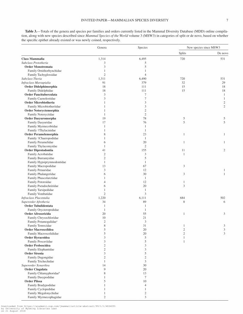
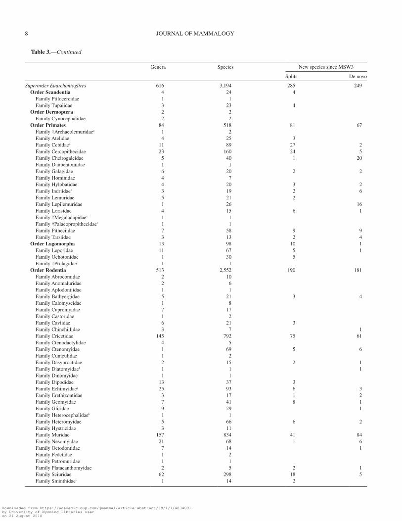
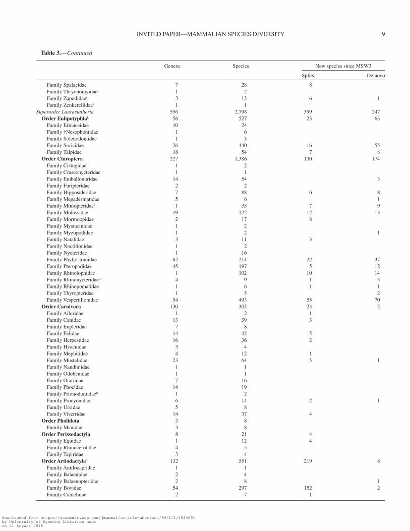
Table 3.—Totals of the genera and species per families and orders currently listed in the Mammal Diversity Database (MDD) online compila-tion, along with new species described since Mammal Species of the World volume 3 (MSW3) in categories of split or de novo, based on whether the specific epithet already existed or was newly coined, respectively.
Genera Species New species since MSW3
Splits De novo
Class Mammalia 1,314 6,495 720 531Subclass Prototheria 3 5 Order Monotremata 3 5 Family Ornithorhynchidae 1 1 Family Tachyglossidae 2 4Subclass Theria 1,311 6,490 720 531Infraclass Marsupialia 91 379 32 29 Order Didelphimorphia 18 111 15 18 Family Didelphidae 18 111 15 18 Order Paucituberculata 3 7 1 Family Caenolestidae 3 7 1 Order Microbiotheria 1 3 2 Family Microbiotheriidae 1 3 2 Order Notoryctemorphia 1 2 Family Notoryctidae 1 2 Order Dasyuromorpha 19 78 5 5 Family Dasyuridae 17 76 5 5 Family Myrmecobiidae 1 1 Family †Thylacinidae 1 1 Order Peramelemorphia 8 23 1 1 Family †Chaeropodidae 1 1 Family Peramelidae 6 20 1 1 Family Thylacomyidae 1 2 Order Diprotodontia 41 155 11 2 Family Acrobatidae 2 3 1 Family Burramyidae 2 5 Family Hypsiprymnodontidae 1 1 Family Macropodidae 13 67 3 Family Petauridae 3 12 1 Family Phalangeridae 6 30 3 1 Family Phascolarctidae 1 1 Family Potoroidae 4 12 1 Family Pseudocheiridae 6 20 3 Family Tarsipedidae 1 1 Family Vombatidae 2 3Infraclass Placentalia 1,220 6,111 684 502Superorder Afrotheria 34 89 8 6 Order Tubulidentata 1 1 Family Orycteropodidae 1 1 Order Afrosoricida 20 55 1 3 Family Chrysochloridae 10 21 Family Potamogalidaea 2 3 Family Tenrecidae 8 31 1 3 Order Macroscelidea 5 20 2 3 Family Macroscelididae 5 20 2 3 Order Hyracoidea 3 5 1 Family Procaviidae 3 5 1 Order Proboscidea 2 3 Family Elephantidae 2 3 Order Sirenia 3 5 Family Dugongidae 2 2 Family Trichechidae 1 3Superorder Xenarthra 14 30 Order Cingulata 9 20 Family Chlamyphoridaeb 8 13 Family Dasypodidae 1 7 Order Pilosa 5 10 Family Bradypodidae 1 4 Family Cyclopedidae 1 1 Family Megalonychidae 1 2 Family Myrmecophagidae 2 3
Downloaded from https://academic.oup.com/jmammal/article-abstract/99/1/1/4834091by University of Wyoming Libraries useron 21 August 2018
8 JOURNAL OF MAMMALOGY
Genera Species New species since MSW3
Splits De novo
Superorder Euarchontoglires 616 3,194 285 249 Order Scandentia 4 24 4 Family Ptilocercidae 1 1 Family Tupaiidae 3 23 4 Order Dermoptera 2 2 Family Cynocephalidae 2 2 Order Primates 84 518 81 67 Family †Archaeolemuridaec 1 2 Family Atelidae 4 25 3 Family Cebidaed 11 89 27 2 Family Cercopithecidae 23 160 24 5 Family Cheirogaleidae 5 40 1 20 Family Daubentoniidae 1 1 Family Galagidae 6 20 2 2 Family Hominidae 4 7 Family Hylobatidae 4 20 3 2 Family Indriidaee 3 19 2 6 Family Lemuridae 5 21 2 Family Lepilemuridae 1 26 16 Family Lorisidae 4 15 6 1 Family †Megaladapidaec 1 1 Family †Palaeopropithecidaec 1 1 Family Pitheciidae 7 58 9 9 Family Tarsiidae 3 13 2 4 Order Lagomorpha 13 98 10 1 Family Leporidae 11 67 5 1 Family Ochotonidae 1 30 5 Family †Prolagidae 1 1 Order Rodentia 513 2,552 190 181 Family Abrocomidae 2 10 Family Anomaluridae 2 6 Family Aplodontiidae 1 1 Family Bathyergidae 5 21 3 4 Family Calomyscidae 1 8 Family Capromyidae 7 17 Family Castoridae 1 2 Family Caviidae 6 21 3 Family Chinchillidae 3 7 1 Family Cricetidae 145 792 75 61 Family Ctenodactylidae 4 5 Family Ctenomyidae 1 69 5 6 Family Cuniculidae 1 2 Family Dasyproctidae 2 15 2 1 Family Diatomyidaef 1 1 1 Family Dinomyidae 1 1 Family Dipodidae 13 37 3 Family Echimyidaeg 25 93 6 3 Family Erethizontidae 3 17 1 2 Family Geomyidae 7 41 8 1 Family Gliridae 9 29 1 Family Heterocephalidaeh 1 1 Family Heteromyidae 5 66 6 2 Family Hystricidae 3 11 Family Muridae 157 834 41 84 Family Nesomyidae 21 68 1 6 Family Octodontidae 7 14 1 Family Pedetidae 1 2 Family Petromuridae 1 1 Family Platacanthomyidae 2 5 2 1 Family Sciuridae 62 298 18 5 Family Sminthidaei 1 14 2
Table 3.—Continued
Downloaded from https://academic.oup.com/jmammal/article-abstract/99/1/1/4834091by University of Wyoming Libraries useron 21 August 2018
INVITED PAPER—MAMMALIAN SPECIES DIVERSITY 9
Genera Species New species since MSW3
Splits De novo
Family Spalacidae 7 28 8 Family Thryonomyidae 1 2 Family Zapodidaei 3 12 6 1 Family Zenkerellidaej 1 1Superorder Laurasiatheria 556 2,798 399 247 Order Eulipotyphlak 56 527 23 63 Family Erinaceidae 10 24 Family †Nesophontidae 1 6 Family Solenodontidae 1 3 Family Soricidae 26 440 16 55 Family Talpidae 18 54 7 8 Order Chiroptera 227 1,386 130 174 Family Cistugidael 1 2 Family Craseonycteridae 1 1 Family Emballonuridae 14 54 3 Family Furipteridae 2 2 Family Hipposideridae 7 88 6 8 Family Megadermatidae 5 6 1 Family Miniopteridael 1 35 7 9 Family Molossidae 19 122 12 13 Family Mormoopidae 2 17 8 Family Mystacinidae 1 2 Family Myzopodidae 1 2 1 Family Natalidae 3 11 3 Family Noctilionidae 1 2 Family Nycteridae 1 16 Family Phyllostomidae 62 214 22 37 Family Pteropodidae 45 197 5 12 Family Rhinolophidae 1 102 10 14 Family Rhinonycteridaem 4 9 1 3 Family Rhinopomatidae 1 6 1 1 Family Thyropteridae 1 5 2 Family Vespertilionidae 54 493 55 70 Order Carnivora 130 305 23 2 Family Ailuridae 1 2 1 Family Canidae 13 39 3 Family Eupleridae 7 8 Family Felidae 14 42 5 Family Herpestidae 16 36 2 Family Hyaenidae 3 4 Family Mephitidae 4 12 1 Family Mustelidae 23 64 5 1 Family Nandiniidae 1 1 Family Odobenidae 1 1 Family Otariidae 7 16 Family Phocidae 14 19 Family Prionodontidaen 1 2 Family Procyonidae 6 14 2 1 Family Ursidae 5 8 Family Viverridae 14 37 4 Order Pholidota 3 8 Family Manidae 3 8 Order Perissodactyla 8 21 4 Family Equidae 1 12 4 Family Rhinocerotidae 4 5 Family Tapiridae 3 4 Order Artiodactylao 132 551 219 8 Family Antilocapridae 1 1 Family Balaenidae 2 4 Family Balaenopteridae 2 8 1 Family Bovidae 54 297 152 2 Family Camelidae 2 7 1
Table 3.—Continued
Downloaded from https://academic.oup.com/jmammal/article-abstract/99/1/1/4834091by University of Wyoming Libraries useron 21 August 2018
10 JOURNAL OF MAMMALOGY
later bursts of species descriptions by allowing morphologically cryptic but genetically divergent evolutionary lineages to be recognized as species. For example, over one-half of the spe-cies described since 2004 appear to have stemmed from taxo-nomic splits (~58%), many based in part or whole on genetic data, to go with at least 172 species unions (lumps) during the same period. As we continue to progress within the genomic era, where data on millions of independent genetic loci can be read-ily generated for taxonomic studies, there is a growing under-standing that hybridization and introgression commonly occur among mammalian species that may otherwise maintain genetic integrity (e.g., Larsen et al. 2010; Miller et al. 2012; vonHoldt et al. 2016). Characterizing species and their boundaries using multiple tiers of evidence will continue to be essential given the profound impact of species delimitation on legislative decisions (e.g., U.S. Endangered Species Act of 1973—Department of the Interior, U.S. Fish and Wildlife Service 1973).
At the current rate of taxonomic description of mammals (~25 species/year from 1750 to 2017), we predict that 7,342 mammalian species will be recognized by 2050 and 8,590 by 2100. Alternatively, if we consider the increased rate of taxo-nomic descriptions since the advent of PCR (~30 species/year from 1990 to 2017), our estimates increase to 7,509 species recognized by 2050 and 9,009 by 2100. These estimates sur-pass Reeder and Helgen’s (2007) prediction of > 7,000 total mammalian species, but echo their observation that mammals
contain considerably greater species diversity than is com-monly recognized. Remarkably, the same estimate of ~25 spe-cies/year was derived somewhat independently from tracking 14 estimates of global diversity (1961–1999—Patterson 2001) and from species-level changes between MSW2 and MSW3 (Reeder and Helgen 2007), thereby affirming the robustness of that estimate across both data sources and eras.
Assumed in all taxonomic forecasts is the stability of global ecosystems, scientific institutions, and natural history collections. With mammals being disproportionately impacted by human-induced extinctions (Ceballos et al. 2017), especially in insular regions like the Caribbean (Cooke et al. in press), efforts to protect threatened habitats and their resident mammalian species are key to the continued persistence, existence, and discovery of mammals. The Neotropics is the most species-dense biogeographic region in the world, followed closely by the Afrotropics and Australasia-Oceania, the latter of which is one of the least explored terrestrial regions on Earth, with the second fewest de novo species descrip-tions (18 species; Table 2). Inventory efforts may thus be fruitfully prioritized in northern Australia, Melanesia, Sulawesi, and other oceanic islands east of Wallace’s Line. However, we note that obtaining collecting permissions is a barrier to species description in any region. The continued description and discovery of mamma-lian species diversity hinges on investment in both natural history collecting and in the physical collections that house the specimens essential for taxonomic research. Natural history collections are
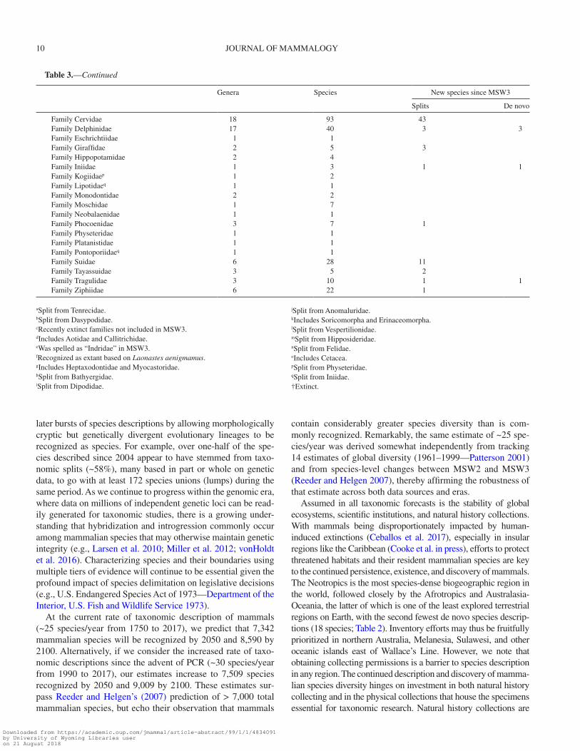
Table 3.—Continued
Genera Species New species since MSW3
Splits De novo
Family Cervidae 18 93 43 Family Delphinidae 17 40 3 3 Family Eschrichtiidae 1 1 Family Giraffidae 2 5 3 Family Hippopotamidae 2 4 Family Iniidae 1 3 1 1 Family Kogiidaep 1 2 Family Lipotidaeq 1 1 Family Monodontidae 2 2 Family Moschidae 1 7 Family Neobalaenidae 1 1 Family Phocoenidae 3 7 1 Family Physeteridae 1 1 Family Platanistidae 1 1 Family Pontoporiidaeq 1 1 Family Suidae 6 28 11 Family Tayassuidae 3 5 2 Family Tragulidae 3 10 1 1 Family Ziphiidae 6 22 1
aSplit from Tenrecidae.bSplit from Dasypodidae.cRecently extinct families not included in MSW3.dIncludes Aotidae and Callitrichidae.eWas spelled as “Indridae” in MSW3.fRecognized as extant based on Laonastes aenigmamus.gIncludes Heptaxodontidae and Myocastoridae.hSplit from Bathyergidae.iSplit from Dipodidae.
jSplit from Anomaluridae.kIncludes Soricomorpha and Erinaceomorpha.lSplit from Vespertilionidae.mSplit from Hipposideridae.nSplit from Felidae.oIncludes Cetacea.pSplit from Physeteridae.qSplit from Iniidae.†Extinct.
Downloaded from https://academic.oup.com/jmammal/article-abstract/99/1/1/4834091by University of Wyoming Libraries useron 21 August 2018
INVITED PAPER—MAMMALIAN SPECIES DIVERSITY 11
repositories for the genetic and morphological vouchers used to describe every new species listed in the MDD, a fact that high-lights the indispensable role of museums and universities in under-standing species and the ecosystems in which they live (McLean et al. 2015). As our planet changes, the need to support geographi-cally broad and site-intensive biological archives only grows in rel-evance. Collections represent time series of change in biodiversity and often harbor undiscovered species (e.g., Helgen et al. 2013), including those vulnerable or already extinct.
Acting under the supervision of the American Society of Mammalogists’ Biodiversity Committee, the MDD has a 2018–2020 plan to further integrate synonym data, track Holocene-extinct taxa, and add links to outside data sources. While full synonymies are not feasible, inclusion of common synonyms will facilitate tracking taxonomic changes through time, especially within controversial groups (e.g., Artiodactyla and Perissodactyla—Groves and Grubb 2011). Controversial taxonomic assignments also will be “flagged” as tentative or pending further scientific investigation. The MDD aims to link taxon entries to a variety of relevant per-species and per-higher taxon data pages on other web platforms, includ-ing geographic range maps, trait database entries, museum records, genetic resources, and other ecological information. Mammalian Species accounts, published by the American Society of Mammalogists since 1969 and consisting of over 950 species-level treatments, will be linked to relevant MDD species pages, including synonym-based links. In this manner, the MDD’s efforts parallel initiatives in other vertebrate taxa to digitize taxonomic resources (amphibians—AmphibiaWeb 2017; Amphibian Species of the World—Frost 2017; birds: Avibase—LePage et al. 2014; IOC World Bird List—Gill and Donsker 2017; the Handbook of the Birds of the World Alive—del Hoyo et al. 2017; non-avian reptiles, turtles, croco-diles, and tuatara—Uetz et al. 2016; and bony fish: FishBase—Froese and Pauly 2017; Catalog of Fishes—Eschmeyer et al. 2017). The new mammalian taxonomic database summarized herein aims to advance the study of mammals while bringing it to par with the digital resources available in other tetrapod clades, to the benefit of future mammalogists and non-mam-malogists alike.
acknowledgMents
We are grateful to the American Society of Mammalogists for funding this project, and as well as for logistical support from the NSF VertLife Terrestrial grant (#1441737). We thank J. Cook, D. Wilson, B. Patterson, W. Jetz, M. Koo, J. Esselstyn, E. Lacey, D. Huckaby, L. Ruedas, R. Norris, D. Reeder, R. Guralnick, J. Patton, E. Heske, and other members of the ASM Biodiversity Committee for advice, support, and input about this initiative.
suppleMentary data
Supplementary data are available at Journal of Mammalogy online. Supplementary Data SD1.— Details of the full Mammal Diversity Database (MDD) version 1 taxonomy, including associated citations and geographic regions.
literature cited
adamS, D. C. 2001. Are the fossil data really at odds with the molec-ular data? Systematic Biology 50:444–453.
amPhiBiaWeB. 2017. AmphibiaWeb. University of California, Berkeley. http://amphibiaweb.org. Accessed 12 May 2017.
aSher, R. J., and K. M. helgen. 2010. Nomenclature and placental mammal phylogeny. BMC Evolutionary Biology 10:102.
aSher, R. J., M. J. novaCeK, and J. H. geiSler. 2003. Relationships of endemic African mammals and their fossil relatives based on morphological and molecular evidence. Journal of Mammalian Evolution 10:131–194.
Belfiore, N. M., L. liu, and C. moritz. 2008. Multilocus phylo-genetics of a rapid radiation in the genus Thomomys (Rodentia: Geomyidae). Systematic Biology 57:294–310.
BerCovitCh, F. B., et al. 2017. How many species of giraffe are there? Current Biology 27:R136–R137.
BouBli, J. P., A. B. rylandS, I. P. fariaS, M. E. alfaro, and J. L. alfaro. 2012. Cebus phylogenetic relationships: a preliminary reassessment of the diversity of the untufted capuchin monkeys. American Journal of Primatology 74:381–393.
Carleton, M. D., J. C. KerBiS PeterhanS, and W. T. Stanley. 2006. Review of the Hylomyscus denniae group (Rodentia: Muridae) in Eastern Africa, with comments on the generic allocation of Epimys endorobae Heller. Proceedings of the Biological Society of Washington 119:293–325.
CaStiglia, R., F. anneSi, G. amori, E. Solano, and G. aloiSe. 2017. The phylogeography of Crocidura suaveolens from southern Italy reveals the absence of an endemic lineage and supports a Trans-Adriatic connection with the Balkanic refugium. Hystrix, the Italian Journal of Mammalogy 28:1–3.
CeBalloS, G., P. R. ehrliCh, and R. dirzo. 2017. Biological anni-hilation via the ongoing sixth mass extinction signaled by verte-brate population losses and declines. Proceedings of the National Academy of Sciences 114: E6089–E6096.
CooKe, S. B., L. M. dávaloS, A. M. myChaJliW, S. T. turvey, and N. S. uPham. 2017. Anthropogenic extinction dominates Holocene declines of West Indian mammals. Annual Review of Ecology, Evolution, and Systematics 48:301–327.
Cozzuol, M. A., et al. 2013. A new species of tapir from the Amazon. Journal of Mammalogy 94:1331–1345.
davenPort, T. R., et al. 2006. A new genus of African monkey, Rungwecebus: morphology, ecology, and molecular phylogenetics. Science 312:1378–1381.
daWSon, M., C. marivaux, C.-K. li, K. C. Beard, and G. metaiS. 2006. Laonastes and the “Lazarus effect” in recent mammals. Science 311:1456–1458.
de Queiroz, K. 2007. Species concepts and species delimitation. Systematic Biology 56:879–886.
del hoyo, J., A. elliott, J. Sargatal, D. A. ChriStie, and E. de Juana. 2017. Handbook of the birds of the world alive. Lynx Edicions, Barcelona, Spain. http://www.hbw.com/. Accessed 12 May 2017.
dePartment of the interior, u.S. fiSh and Wildlife ServiCe. 1973. U.S. Endangered Species Act of 1973. http://www.nmfs.noaa.gov/pr/laws/esa/text.htm. Accessed 12 May 2017.
douady, C. J., et al. 2002. Molecular phylogenetic evidence con-firming the Eulipotyphla concept and in support of hedgehogs as the sister group to shrews. Molecular Phylogenetics and Evolution 25:200–209.
dumaS, F., and S. mazzoleni. 2017. Neotropical primate evolution and phylogenetic reconstruction using chromosomal data. The European Zoological Journal 84:1–18.
Downloaded from https://academic.oup.com/jmammal/article-abstract/99/1/1/4834091by University of Wyoming Libraries useron 21 August 2018
12 JOURNAL OF MAMMALOGY
dumBaCher, J. P. 2016. Petrosaltator gen. nov., a new genus replacement for the North African sengi Elephantulus rozeti (Macroscelidea; Macroscelididae). Zootaxa 4136:567–579.
emmonS, L. H., Y. L. R. leite, and J. L. Patton. 2015. Family Echimyidae. Mammals of South America. Vol. 2 (J. L. Patton, U. F. J. Pardiñas, and G. D’Elía, eds.). University of Chicago Press, Chicago, Illinois; 877–1022.
eSChmeyer, W. N., R. friCKe, and R. van der laan. 2017. Catalog of fishes: genera, species, references. https://www.calacademy.org/scientists/projects/catalog-of-fishes. Accessed 12 May 2017.
eSSelStyn, J. A., A. S. aChmadi, and K. C. roWe. 2012. Evolutionary novelty in a rat with no molars. Biology Letters 8:990–993.
eSSelStyn, J. A., maharadatunKamSi, A. S. aChmadi, C. D. Siler, and B. J. evanS. 2013. Carving out turf in a biodiversity hotspot: multiple, previously unrecognized shrew species co-occur on Java Island, Indonesia. Molecular Ecology 22:4972–4987.
faBre, P. H., et al. 2017. Mitogenomic phylogeny, diversifica-tion, and biogeography of South American spiny rats. Molecular Biology and Evolution 34:613–633.
flannery, T. 2012. Among the islands: adventures in the Pacific. Grove/Atlantic, Inc., New York City, New York.
foley, N. M., et al. 2015. How and why overcome the impediments to resolution: lessons from rhinolophid and hipposiderid bats. Molecular Biology and Evolution 32:313–333.
froeSe, R., and D. Pauly. 2017. FishBase. www.FishBase.org. Accessed 12 May 2017.
froSt, D. R. 2017. Amphibian species of the world: an online ref-erence. Version 6.0. American Museum of Natural History, New York. http://research.amnh.org/vz/herpetology/amphibia/. Accessed 28 June 2017.
gardner, A. L. 2007. Mammals of South America: volume 1: marsu-pials, xenarthrans, shrews, and bats. University of Chicago Press, Chicago, Illinois.
gateSy, J., P. o’grady, and R. H. BaKer. 1999. Corroboration among data sets in simultaneous analysis: hidden support for phyloge-netic relationships among higher level artiodactyl taxa. Cladistics 15:271–313.
gaudin, T. J. 2004. Phylogenetic relationships among sloths (Mammalia, Xenarthra, Tardigrada): the craniodental evidence. Zoological Journal of the Linnean Society 140:255–305.
gill, F., and D. donSKer. 2017. IOC World Bird List (v 7.3). www.worldbirdnames.org. Accessed 12 May 2017.
gregorin, R., and A. D. ditChfield. 2005. New genus and species of nectar-feeding bat in the tribe Lonchophyllini (Phyllostomidae: Glossophaginae) from northeastern Brazil. Journal of Mammalogy 86:403–414.
groveS, C. P. 2007a. Speciation and biogeography of Vietnam’s pri-mates. Vietnamese Journal of Primatology 1:27–40.
groveS, C. P. 2007b. The endemic Uganda mangabey, Lophocebus ugandae, and other members of the albigena-group (Lophocebus). Primate Conservation 22:123–128.
groveS, C., and P. gruBB. 2011. Ungulate taxonomy. Johns Hopkins University Press/Bucknell University, Baltimore, Maryland.
harley, E. H., M. de Waal, S. murray, and C. o’ryan. 2016. Comparison of whole mitochondrial genome sequences of north-ern and southern white rhinoceroses (Ceratotherium simum): the conservation consequences of species definitions. Conservation Genetics 17:1285–1291.
hedgeS, S. B., J. marin, M. SuleSKi, M. Paymer, and S. Kumar. 2015. Tree of life reveals clock-like speciation and diversification. Molecular Biology and Evolution 32:835–845.
helgen, K. M., et al. 2013. Taxonomic revision of the olingos (Bassaricyon), with description of a new species, the Olinguito. ZooKeys 324:1–83.
helgen, K. M., F. R. Cole, L. E. helgen, and D. E. WilSon. 2009. Generic revision in the holarctic ground squirrel genus Spermophilus. Journal of Mammalogy 90:270–305.
hill, J. E. 1990. A memoir and bibliography of Michael Rogers Oldfield Thomas, F.R.S. Bulletin of the British Museum (Natural History). Historical Series 18:25–113.
hinChliff, C. E., et al. 2015. Synthesis of phylogeny and taxon-omy into a comprehensive tree of life. Proceedings of the National Academy of Sciences 112:12764–12769.
honaCKi, J. H., K. E. Kinman, and J. W. KoePPl. 1982. Mammal species of the world: a taxonomic and geographic reference. 1st ed. Allen Press and the Association of Systematics Collections, Lawrence, Kansas.
iuCn. 2017. The IUCN Red List of Threatened Species. Version 2017-1. www.iucnredlist.org. Accessed 28 June 2017.
JaCKSon, S. M., and C. groveS. 2015. Taxonomy of Australian mam-mals. CSIRO Publishing, Clayton South, Victoria, Australia.
Jarzyna, M. A., and W. Jetz. 2016. Detecting the multiple facets of biodiversity. Trends in Ecology & Evolution 31:527–538.
JenKinS, P. D., C. W. KilPatriCK, M. F. roBinSon, and R. J. timminS. 2005. Morphological and molecular investigations of a new family, genus and species of rodent (Mammalia: Rodentia: Hystricognatha) from Lao PDR. Systematics and Biodiversity 2:419–454.
Kingdon, J., D. haPPold, T. ButynSKi, M. hoffmann, M. haPPold, and J. Kalina. 2013. Mammals of Africa (Vol. 1–6). A&C Black, New York.
larSen, P. A., M. R. marChán-rivadeneira, and R. J. BaKer. 2010. Natural hybridization generates mammalian lineage with species characteristics. Proceedings of the National Academy of Sciences 107:11447–11452.
leBedev, V. S., A. A. BanniKova, J. PiSano, J. R. miChaux, and G. I. ShenBrot. 2013. Molecular phylogeny and systematics of Dipodoidea: a test of morphology‐based hypotheses. Zoologica Scripta 42:231–249.
lei, R., et al. 2014. Revision of Madagascar’s dwarf lemurs (Cheirogaleidae: Cheirogaleus): designation of species, candidate species status and geographic boundaries based on molecular and morphological data. Primate Conservation:9–35.
lePage, D., G. vaidya, and R. guralniCK. 2014. Avibase - a database system for managing and organizing taxonomic concepts. ZooKeys 420:117–135.
linnaeuS, C. 1758. Systema naturae per regna tria naturae: secundum classes, ordines, genera, species, cum characteribus, differentiis, synonymis, locis. Laurentius Salvius, Stockholm, Sweeden.
lorenzen, E. D., R. heller, and H. R. SiegiSmund. 2012. Comparative phylogeography of African savannah ungulates. Molecular Ecology 21:3656–3670.
louiS, E. E., Jr., et al. 2006. Molecular and morphological analyses of the sportive lemurs (Family Megaladapidae: Genus Lepilemur) reveals 11 previously unrecognized species. Special Publications of the Museum of Texas Tech University 49:1–47.
madSen, O., M. SCally, C. J. douady, and D. J. Kao. 2001. Parallel adaptive radiations in two major clades of placental mammals. Nature 409:610.
marSh, L. K. 2014. A taxonomic revision of the saki monkeys, Pithecia Desmarest, 1804. Neotropical Primates 21:1–165.
matSon, J. O., and N. ordóñez-garza. 2017. The taxonomic sta-tus of long-tailed shrews (Mammalia: genus Sorex) from Nuclear Central America. Zootaxa 4236:461–483.
Downloaded from https://academic.oup.com/jmammal/article-abstract/99/1/1/4834091by University of Wyoming Libraries useron 21 August 2018
INVITED PAPER—MAMMALIAN SPECIES DIVERSITY 13
mCKenna, M. C., and S. K. Bell. 1997. Classification of mammals: above the species level. Columbia University Press, New York City, New York.
mClean, B. S., et al. 2015. Natural history collections-based research: progress, promise, and best practices. Journal of Mammalogy 97:287–297.
meredith, R. W., et al. 2011. Impacts of the Cretaceous terrestrial revolution and KPg extinction on mammal diversification. Science 334:521–524.
miller, W., et al. 2012. Polar and brown bear genomes reveal ancient admixture and demographic footprints of past cli-mate change. Proceedings of the National Academy of Sciences 109:E2382–E2390.
mittermeier, R. A., A. B. rylandS, and D. E. WilSon. 2013. Handbook of the mammals of the world, volume 3: Primates. Lynx Edicions, Barcelona, Spain.
monadJem, A., P. J. taylor, C. denyS, and F. P. Cotterill. 2015. Rodents of sub-Saharan Africa: a biogeographic and taxonomic synthesis. Walter de Gruyter GmbH & Co. KG, Berlin, Germany.
montagnon, D., B. ravaoarimanana, B. raKotoSamimanana, and Y. rumPler. 2001. Ancient DNA from Megaladapis edwardsi (Malagasy subfossil): preliminary results using partial cytochrome b sequence. Folia Primatologica 72:30–32.
muldoon, K. M. 2010. Paleoenvironment of Ankilitelo Cave (late Holocene, southwestern Madagascar): implications for the extinction of giant lemurs. Journal of Human Evolution 58: 338–352.
mulliS, K. B., H. A. erliCh, N. arnheim, G. T. horn, R. K. SaiKi, and S. J. SCharf. 1989. Process for amplifying, detecting, and/or clon-ing nucleic acid sequences. Patent US4683195 A.
murPhy, W. J., E. eiziriK, W. E. JohnSon, and Y. P. zhang. 2001. Molecular phylogenetics and the origins of placental mammals. Nature 409:614–618.
olSon, D. M., et al. 2001. Terrestrial ecoregions of the world: a new map of life on Earth. Bioscience 51:933–938.
olSon, D. M., and E. dinerStein. 1998. The Global 200: a representa-tion approach to conserving the Earth’s most biologically valuable ecoregions. Conservation Biology 12:502–515.
oSterholz, M., L. Walter, and C. rooS. 2008. Phylogenetic po-sition of the langur genera Semnopithecus and Trachypithecus among Asian colobines, and genus affiliations of their species groups. BMC Evolutionary Biology 8:58.
PardiñaS, U. F., L. geiSe, K. ventura, and G. leSSa. 2016. A new genus for Habrothrix angustidens and Akodon serrensis (Rodentia, Cricetidae): again paleontology meets neontology in the legacy of Lund. Mastozoología Neotropical 23:93–115.
PaSCual, U., et al. 2017. Valuing nature’s contributions to people: the IPBES approach. Current Opinion in Environmental Sustainability 26:7–16.
PatterSon, B. D. 1996. The “species alias” problem. Nature 380:588–589.
PatterSon, B. D. 2001. Fathoming tropical biodiversity: the continu-ing discovery of Neotropical mammals. Diversity and Distributions 7:191–196.
PatterSon, B. D., and N. S. uPham. 2014. A newly recognized fam-ily from the Horn of Africa, the Heterocephalidae (Rodentia: Ctenohystrica). Zoological Journal of the Linnean Society 172:942–963.
Patton, J. L., U. F. J. PardiñaS, and G. d’elíaS. 2015. Mammals of South America, volume 2: rodents. University of Chicago Press, Chicago, Illinois.
PerCeQuillo, A. R., M. WeKSler, and L. P. CoSta. 2011. A new genus and species of rodent from the Brazilian Atlantic Forest (Rodentia: Cricetidae: Sigmodontinae: Oryzomyini), with comments on ory-zomyine biogeography. Zoological Journal of the Linnean Society 161:357–390.
raBoSKy, D. L., G. J. Slater, and M. E. alfaro. 2012. Clade age and species richness are decoupled across the eukaryotic tree of life. PLoS Biology 10:e1001381.
rauSCh, R. L., J. E. feagin, and V. R. rauSCh. 2007. Sorex rohweri sp. nov. (Mammalia, Soricidae) from northwestern North America. Mammalian Biology-Zeitschrift für Säugetierkunde 72:93–105.
reeder, D. M., and K. M. helgen. 2007. Global trends and biases in new mammal species discoveries. Occasional Papers of the Museum of Texas Tech University 269:1–35.
roWe, K. C., A. S. aChmadi, and J. A. eSSelStyn. 2016. A new genus and species of omnivorous rodent (Muridae: Murinae) from Sulawesi, nested within a clade of endemic carnivores. Journal of Mammalogy 97:978–991.
ruedi, M., and F. mayer. 2001. Molecular systematics of bats of the genus Myotis (Vespertilionidae) suggests deterministic ecomorphologi-cal convergences. Molecular Phylogenetics and Evolution 21:436–448.
SChneider, H., and I. SamPaio. 2015. The systematics and evolution of new world primates - a review. Molecular Phylogenetics and Evolution 82:348–357.
Solari, S., and R. J. BaKer. 2007. Mammal species of the world: a taxonomic reference by D. E. Wilson; D. M. Reeder. Journal of Mammalogy 88:824–839.
teta, P., C. Cañón, B. D. PatterSon, and U. F. PardiñaS. 2016. Phylogeny of the tribe Abrotrichini (Cricetidae, Sigmodontinae): integrating morphological and molecular evidence into a new clas-sification. Cladistics 33:153–182.
uetz, P., P. freed, and J. hošeK. 2016. The reptile database. http://reptile-database.org. Accessed 12 May 2017.
vonholdt, B. M., et al. 2016. Whole-genome sequence analysis shows that two endemic species of North American wolf are admix-tures of the coyote and gray wolf. Science Advances 2:e1501714.
voSS, R. S., K. M. helgen, and S. A. JanSa. 2014. Extraordinary claims require extraordinary evidence: a comment on Cozzuol et al. (2013). Journal of Mammalogy 95:893–898.
WeKSler, M., A. R. PerCeQuillo, and R. S. voSS. 2006. Ten new gen-era of oryzomyine rodents (Cricetidae: Sigmodontinae). American Museum Novitates 3537:1–29.
WilSon, D. E., T. E. laCher, Jr., and R. A. mittermeier. 2016. Handbook of the mammals of the world, volume 6: lagomorphs and rodents I. Lynx Edicions, Barcelona, Spain.
WilSon, D. E., and R. A. mittermeier. 2009. Handbook of the mammals of the world, volume 1: carnivores. Lynx Edicions, Barcelona, Spain.
WilSon, D. E., and R. A. mittermeier. 2011. Handbook of the mam-mals of the world, volume 2: hoofed mammals. Lynx Edicions, Barcelona, Spain.
WilSon, D. E., and R. A. mittermeier. 2014. Handbook of the mammals of the world, volume 4: sea mammals. Lynx Edicions, Barcelona, Spain.
WilSon, D. E., and R. A. mittermeier. 2015. Handbook of the mam-mals of the world, volume 5: monotremes and marsupials. Lynx Edicions, Barcelona, Spain.
WilSon, D. E., and D. M. reeder. 1993. Mammal species of the world: a taxonomic and geographic reference. 2nd ed. Smithsonian Institution Press, Washington, D.C.
WilSon, D. E., and D. M. reeder. 2005. Mammal species of the world: a taxonomic and geographic reference. 3rd ed. Johns Hopkins University Press/Bucknell University, Baltimore, Maryland.
Downloaded from https://academic.oup.com/jmammal/article-abstract/99/1/1/4834091by University of Wyoming Libraries useron 21 August 2018

14 JOURNAL OF MAMMALOGY
Woodman, N., R. M. timm, and G. R. graveS. 2006. Characters and phylogenetic relationships of nectar-feeding bats, with descriptions of new Lonchophylla from western South America (Mammalia: Chiroptera; Phyllostomidae: Lonchophyllini). Proceedings of the Biological Society of Washington 119: 437–476.
World atlaS. 2017. Map and details of all 7 continents. www.worl-datlas.com. Accessed 12 May 2017.
zaChoS, F. E., et al. 2013. Species inflation and taxonomic artefacts—a critical comment on recent trends in mammalian classification. Mammalian Biology-Zeitschrift für Säugetierkunde 78:1–6.
Submitted 21 September 2017. Accepted 12 October 2017.
Associate Editor was Edward Heske.
Downloaded from https://academic.oup.com/jmammal/article-abstract/99/1/1/4834091by University of Wyoming Libraries useron 21 August 2018
70 S C I E N T I F I C A M E R I C A N
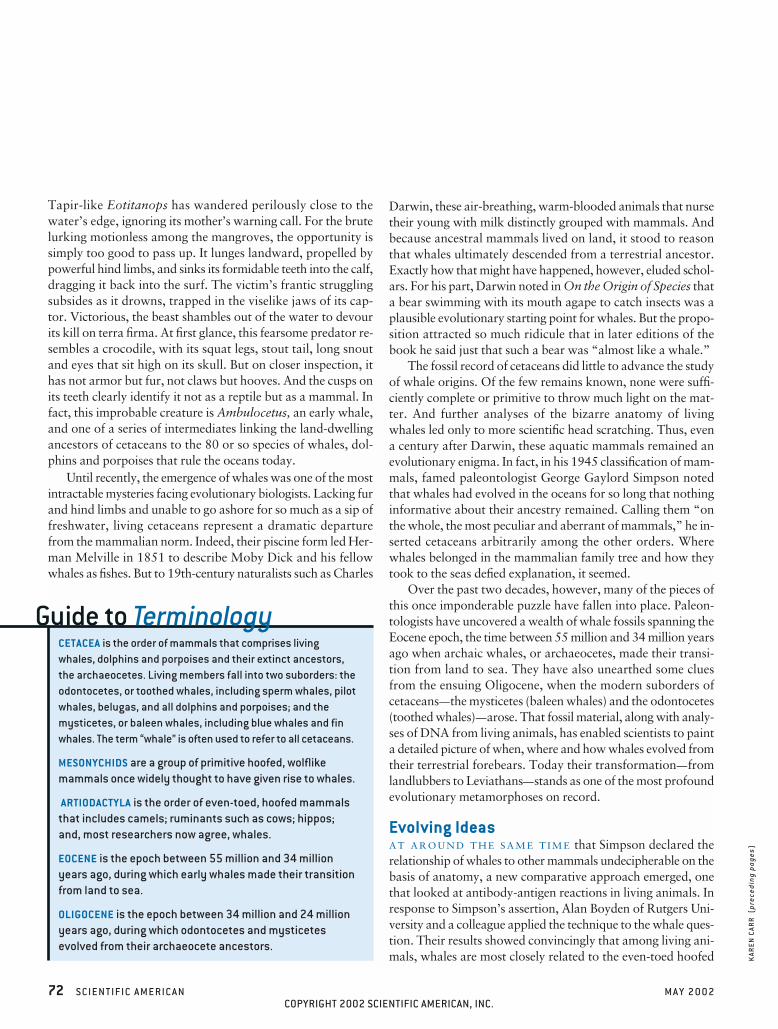
Mammals ThatConquered the The
New fossils and DNA analyses elucidate the remarkable
COPYRIGHT 2002 SCIENTIFIC AMERICAN, INC.
S C I E N T I F I C A M E R I C A N 71
Seas By Kate WongBy Kate Wongevolutionary history of whales
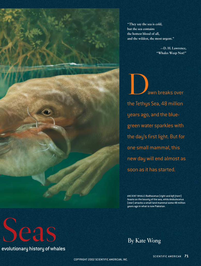
“They say the sea is cold, but the sea contains the hottest blood of all, and the wildest, the most urgent.”
—D. H. Lawrence, “Whales Weep Not!”
Dawn breaks over
the Tethys Sea, 48 million
years ago, and the blue-
green water sparkles with
the day’s first light. But for
one small mammal, this
new day will end almost as
soon as it has started.
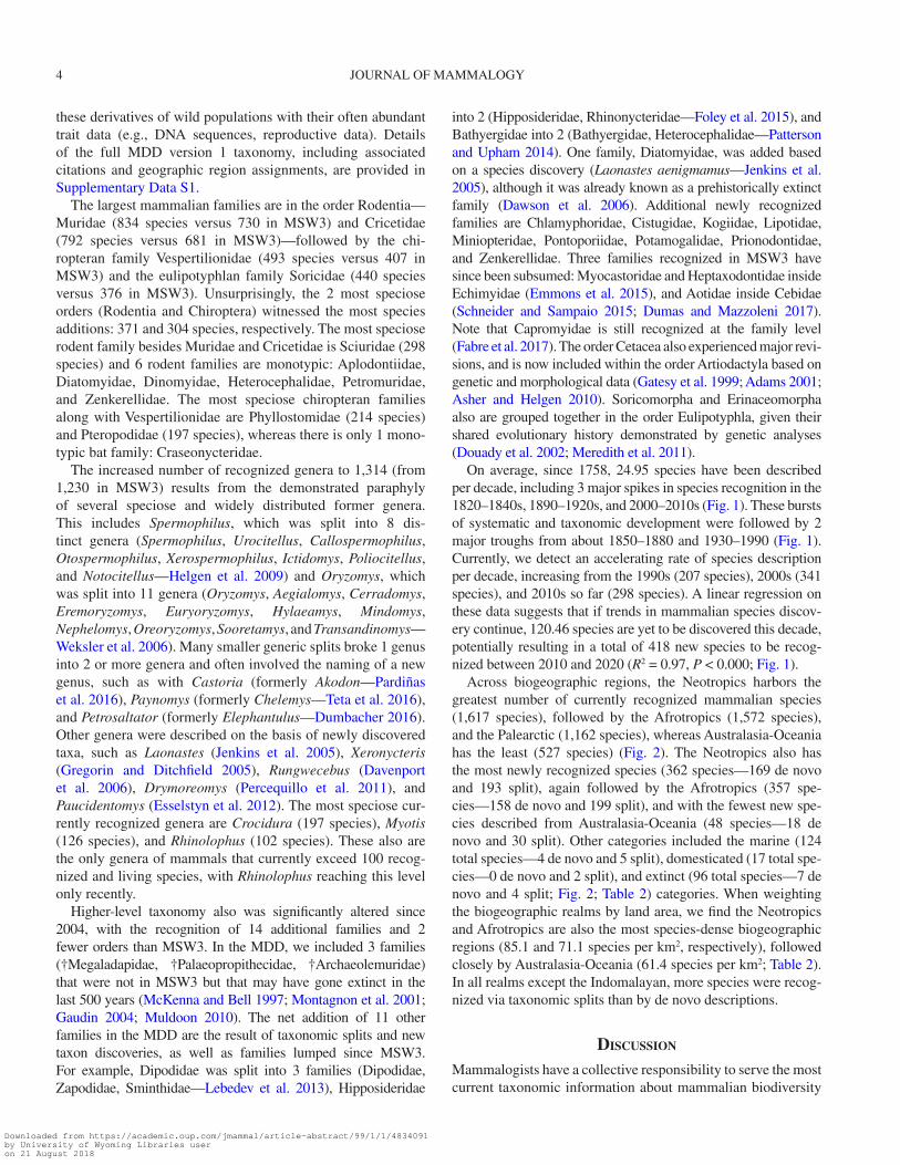
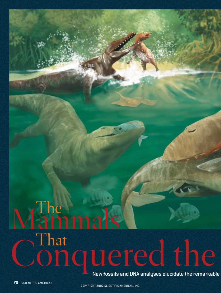
ANCIENT WHALE Rodhocetus (right and left front)feasts on the bounty of the sea, while Ambulocetus(rear) attacks a small land mammal some 48 millionyears ago in what is now Pakistan.
COPYRIGHT 2002 SCIENTIFIC AMERICAN, INC.
Tapir-like Eotitanops has wandered perilously close to thewater’s edge, ignoring its mother’s warning call. For the brutelurking motionless among the mangroves, the opportunity issimply too good to pass up. It lunges landward, propelled bypowerful hind limbs, and sinks its formidable teeth into the calf,dragging it back into the surf. The victim’s frantic strugglingsubsides as it drowns, trapped in the viselike jaws of its cap-tor. Victorious, the beast shambles out of the water to devourits kill on terra firma. At first glance, this fearsome predator re-sembles a crocodile, with its squat legs, stout tail, long snoutand eyes that sit high on its skull. But on closer inspection, ithas not armor but fur, not claws but hooves. And the cusps onits teeth clearly identify it not as a reptile but as a mammal. Infact, this improbable creature is Ambulocetus, an early whale,and one of a series of intermediates linking the land-dwellingancestors of cetaceans to the 80 or so species of whales, dol-phins and porpoises that rule the oceans today.
Until recently, the emergence of whales was one of the mostintractable mysteries facing evolutionary biologists. Lacking furand hind limbs and unable to go ashore for so much as a sip offreshwater, living cetaceans represent a dramatic departurefrom the mammalian norm. Indeed, their piscine form led Her-man Melville in 1851 to describe Moby Dick and his fellowwhales as fishes. But to 19th-century naturalists such as Charles
Darwin, these air-breathing, warm-blooded animals that nursetheir young with milk distinctly grouped with mammals. Andbecause ancestral mammals lived on land, it stood to reasonthat whales ultimately descended from a terrestrial ancestor.Exactly how that might have happened, however, eluded schol-ars. For his part, Darwin noted in On the Origin of Species thata bear swimming with its mouth agape to catch insects was aplausible evolutionary starting point for whales. But the propo-sition attracted so much ridicule that in later editions of thebook he said just that such a bear was “almost like a whale.”
The fossil record of cetaceans did little to advance the studyof whale origins. Of the few remains known, none were suffi-ciently complete or primitive to throw much light on the mat-ter. And further analyses of the bizarre anatomy of livingwhales led only to more scientific head scratching. Thus, evena century after Darwin, these aquatic mammals remained anevolutionary enigma. In fact, in his 1945 classification of mam-mals, famed paleontologist George Gaylord Simpson notedthat whales had evolved in the oceans for so long that nothinginformative about their ancestry remained. Calling them “onthe whole, the most peculiar and aberrant of mammals,” he in-serted cetaceans arbitrarily among the other orders. Wherewhales belonged in the mammalian family tree and how theytook to the seas defied explanation, it seemed.
Over the past two decades, however, many of the pieces ofthis once imponderable puzzle have fallen into place. Paleon-tologists have uncovered a wealth of whale fossils spanning theEocene epoch, the time between 55 million and 34 million yearsago when archaic whales, or archaeocetes, made their transi-tion from land to sea. They have also unearthed some cluesfrom the ensuing Oligocene, when the modern suborders ofcetaceans—the mysticetes (baleen whales) and the odontocetes(toothed whales)—arose. That fossil material, along with analy-ses of DNA from living animals, has enabled scientists to painta detailed picture of when, where and how whales evolved fromtheir terrestrial forebears. Today their transformation—fromlandlubbers to Leviathans—stands as one of the most profoundevolutionary metamorphoses on record.
Evolving IdeasAT AROUND THE SAME TIME that Simpson declared therelationship of whales to other mammals undecipherable on thebasis of anatomy, a new comparative approach emerged, onethat looked at antibody-antigen reactions in living animals. Inresponse to Simpson’s assertion, Alan Boyden of Rutgers Uni-versity and a colleague applied the technique to the whale ques-tion. Their results showed convincingly that among living ani-mals, whales are most closely related to the even-toed hoofed
72 S C I E N T I F I C A M E R I C A N M A Y 2 0 0 2
KAR
EN
CAR
R (
pre
ced
ing
pa
ges
)
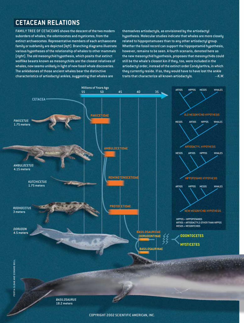
CETACEA is the order of mammals that comprises livingwhales, dolphins and porpoises and their extinct ancestors,the archaeocetes. Living members fall into two suborders: theodontocetes, or toothed whales, including sperm whales, pilotwhales, belugas, and all dolphins and porpoises; and themysticetes, or baleen whales, including blue whales and finwhales. The term “whale” is often used to refer to all cetaceans.
MESONYCHIDS are a group of primitive hoofed, wolflikemammals once widely thought to have given rise to whales.
ARTIODACTYLA is the order of even-toed, hoofed mammalsthat includes camels; ruminants such as cows; hippos;and, most researchers now agree, whales.
EOCENE is the epoch between 55 million and 34 millionyears ago, during which early whales made their transitionfrom land to sea.
OLIGOCENE is the epoch between 34 million and 24 millionyears ago, during which odontocetes and mysticetesevolved from their archaeocete ancestors.
Guide to Terminology
COPYRIGHT 2002 SCIENTIFIC AMERICAN, INC.
mammals, or artiodactyls, a group whose members includecamels, hippopotamuses, pigs and ruminants such as cows.Still, the exact nature of that relationship remained unclear.Were whales themselves artiodactyls? Or did they occupy theirown branch of the mammalian family tree, linked to the artio-dactyl branch via an ancient common ancestor?
Support for the latter interpretation came in the 1960s,from studies of primitive hoofed mammals known as condy-larths that had not yet evolved the specialized characteristics ofartiodactyls or the other mammalian orders. Paleontologist
Leigh Van Valen, then at the American Museum of NaturalHistory in New York City, discovered striking resemblancesbetween the three-cusped teeth of the few known fossil whalesand those of a group of meat-eating condylarths called mesony-chids. Likewise, he found shared dental characteristics betweenartiodactyls and another group of condylarths, the arctocy-onids, close relatives of the mesonychids. Van Valen conclud-ed that whales descended from the carnivorous, wolflikemesonychids and thus were linked to artiodactyls through thecondylarths.
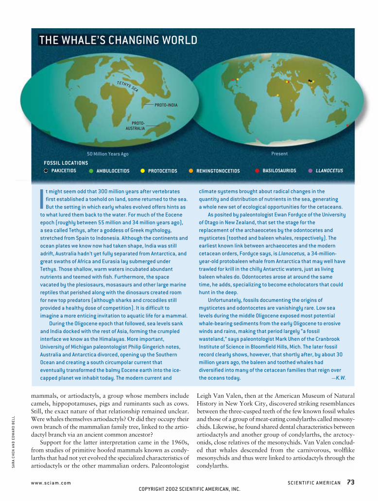
climate systems brought about radical changes in thequantity and distribution of nutrients in the sea, generating a whole new set of ecological opportunities for the cetaceans.
As posited by paleontologist Ewan Fordyce of the Universityof Otago in New Zealand, that set the stage for thereplacement of the archaeocetes by the odontocetes andmysticetes (toothed and baleen whales, respectively). Theearliest known link between archaeocetes and the moderncetacean orders, Fordyce says, is Llanocetus, a 34-million-year-old protobaleen whale from Antarctica that may well havetrawled for krill in the chilly Antarctic waters, just as livingbaleen whales do. Odontocetes arose at around the same time, he adds, specializing to become echolocators that couldhunt in the deep.
Unfortunately, fossils documenting the origins ofmysticetes and odontocetes are vanishingly rare. Low sealevels during the middle Oligocene exposed most potentialwhale-bearing sediments from the early Oligocene to erosivewinds and rains, making that period largely “a fossilwasteland,” says paleontologist Mark Uhen of the CranbrookInstitute of Science in Bloomfield Hills, Mich. The later fossilrecord clearly shows, however, that shortly after, by about 30million years ago, the baleen and toothed whales haddiversified into many of the cetacean families that reign overthe oceans today. —K.W.
It might seem odd that 300 million years after vertebratesfirst established a toehold on land, some returned to the sea.But the setting in which early whales evolved offers hints as
to what lured them back to the water. For much of the Eoceneepoch (roughly between 55 million and 34 million years ago), a sea called Tethys, after a goddess of Greek mythology,stretched from Spain to Indonesia. Although the continents andocean plates we know now had taken shape, India was stilladrift, Australia hadn’t yet fully separated from Antarctica, andgreat swaths of Africa and Eurasia lay submerged underTethys. Those shallow, warm waters incubated abundantnutrients and teemed with fish. Furthermore, the spacevacated by the plesiosaurs, mosasaurs and other large marinereptiles that perished along with the dinosaurs created roomfor new top predators (although sharks and crocodiles stillprovided a healthy dose of competition). It is difficult toimagine a more enticing invitation to aquatic life for a mammal.
During the Oligocene epoch that followed, sea levels sankand India docked with the rest of Asia, forming the crumpledinterface we know as the Himalayas. More important,University of Michigan paleontologist Philip Gingerich notes,Australia and Antarctica divorced, opening up the SouthernOcean and creating a south circumpolar current thateventually transformed the balmy Eocene earth into the ice-capped planet we inhabit today. The modern current and
w w w . s c i a m . c o m S C I E N T I F I C A M E R I C A N 73
SAR
A C
HE
N A
ND
ED
WAR
D B
ELL
50 Million Years Ago Present
PROTO-INDIA
PROTO-AUSTRALIA
BASILOSAURIDSFOSSIL LOCATIONS
PROTOCETIDS
THE WHALE’S CHANGING WORLD
LLANOCETUSPAKICETIDS AMBULOCETIDS REMINGTONOCETIDS
TETHYS SEA
COPYRIGHT 2002 SCIENTIFIC AMERICAN, INC.
PO
RTI
A SL
OAN
AN
D E
DW
ARD
BE
LL
HIPPOS = HIPPOPOTAMIDSARTIOS = ARTIODACTYLS OTHER THAN HIPPOS MESOS = MESONYCHIDS
OLD MESONYCHID HYPOTHESIS
MESOS ARTIOS HIPPOS WHALES
ARTIOS HIPPOS MESOS WHALES
HIPPOPOTAMID HYPOTHESIS
ARTIOS HIPPOS MESOS WHALES
NEW MESONYCHID HYPOTHESIS
MESOS ARTIOS HIPPOS WHALES
ARTIODACTYL HYPOTHESIS
FAMILY TREE OF CETACEANS shows the descent of the two modernsuborders of whales, the odontocetes and mysticetes, from theextinct archaeocetes. Representative members of each archaeocetefamily or subfamily are depicted (left). Branching diagrams illustratevarious hypotheses of the relationship of whales to other mammals(right). The old mesonychid hypothesis, which posits that extinctwolflike beasts known as mesonychids are the closest relatives ofwhales, now seems unlikely in light of new fossil whale discoveries.The anklebones of those ancient whales bear the distinctivecharacteristics of artiodactyl ankles, suggesting that whales are
themselves artiodactyls, as envisioned by the artiodactylhypothesis. Molecular studies indicate that whales are more closelyrelated to hippopotamuses than to any other artiodactyl group.Whether the fossil record can support the hippopotamid hypothesis,however, remains to be seen. A fourth scenario, denoted here asthe new mesonychid hypothesis, proposes that mesonychids couldstill be the whale’s closest kin if they, too, were included in theartiodactyl order, instead of the extinct order Condylarthra, in whichthey currently reside. If so, they would have to have lost the ankletraits that characterize all known artiodactyls. —K.W.
CETACEAN RELATIONS
BASILOSAURUS18.2 meters
DORUDON4.5 meters
RODHOCETUS3 meters
KUTCHICETUS1.75 meters
AMBULOCETUS4.15 meters
PAKICETUS1.75 meters
Millions of Years Ago55 50 45 40 35
PAKICETIDAE
AMBULOCETIDAE
PROTOCETIDAE
BASILOSAURIDAEODONTOCETES
MYSTICETES
CETACEA
DORUDONTINAE
BASILOSAURINAE
REMINGTONOCETIDAE
COPYRIGHT 2002 SCIENTIFIC AMERICAN, INC.
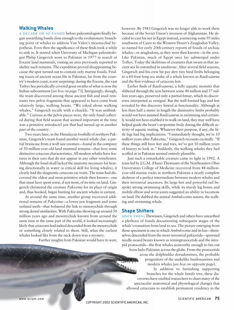
Walking WhalesA DECADE OR SO PASSED before paleontologists finally be-gan unearthing fossils close enough to the evolutionary branch-ing point of whales to address Van Valen’s mesonychid hy-pothesis. Even then the significance of these finds took a whileto sink in. It started when University of Michigan paleontolo-gist Philip Gingerich went to Pakistan in 1977 in search ofEocene land mammals, visiting an area previously reported toshelter such remains. The expedition proved disappointing be-cause the spot turned out to contain only marine fossils. Find-ing traces of ancient ocean life in Pakistan, far from the coun-try’s modern coast, is not surprising: during the Eocene, the vastTethys Sea periodically covered great swaths of what is now theIndian subcontinent [see box on page 73]. Intriguingly, though,the team discovered among those ancient fish and snail rem-nants two pelvis fragments that appeared to have come fromrelatively large, walking beasts. “We joked about walkingwhales,” Gingerich recalls with a chuckle. “It was unthink-able.” Curious as the pelvis pieces were, the only fossil collect-ed during that field season that seemed important at the timewas a primitive artiodactyl jaw that had turned up in anotherpart of the country.
Two years later, in the Himalayan foothills of northern Pak-istan, Gingerich’s team found another weird whale clue: a par-tial braincase from a wolf-size creature—found in the companyof 50-million-year-old land mammal remains—that bore somedistinctive cetacean characteristics. All modern whales have fea-tures in their ears that do not appear in any other vertebrates.Although the fossil skull lacked the anatomy necessary for hear-ing directionally in water (a critical skill for living whales), itclearly had the diagnostic cetacean ear traits. The team had dis-covered the oldest and most primitive whale then known—onethat must have spent some, if not most, of its time on land. Gin-gerich christened the creature Pakicetus for its place of originand, thus hooked, began hunting for ancient whales in earnest.
At around the same time, another group recovered addi-tional remains of Pakicetus—a lower jaw fragment and someisolated teeth—that bolstered the link to mesonychids throughstrong dental similarities. With Pakicetus showing up around 50million years ago and mesonychids known from around thesame time in the same part of the world, it looked increasinglylikely that cetaceans had indeed descended from the mesonychidsor something closely related to them. Still, what the earliestwhales looked like from the neck down was a mystery.
Further insights from Pakistan would have to wait,
however. By 1983 Gingerich was no longer able to work therebecause of the Soviet Union’s invasion of Afghanistan. He de-cided to cast his net in Egypt instead, journeying some 95 milessouthwest of Cairo to the Western Desert’s Zeuglodon Valley,so named for early 20th-century reports of fossils of archaicwhales—or zeuglodons, as they were then known—in the area.Like Pakistan, much of Egypt once lay submerged underTethys. Today the skeletons of creatures that swam in that an-cient sea lie entombed in sandstone. After several field seasons,Gingerich and his crew hit pay dirt: tiny hind limbs belongingto a 60-foot-long sea snake of a whale known as Basilosaurusand the first evidence of cetacean feet.
Earlier finds of Basilosaurus, a fully aquatic monster thatslithered through the seas between some 40 million and 37 mil-lion years ago, preserved only a partial femur, which its discov-erers interpreted as vestigial. But the well-formed legs and feetrevealed by this discovery hinted at functionality. Although atless than half a meter in length the diminutive limbs probablywould not have assisted Basilosaurus in swimming and certain-ly would not have enabled it to walk on land, they may well havehelped guide the beast’s serpentine body during the difficult ac-tivity of aquatic mating. Whatever their purpose, if any, the lit-tle legs had big implications. “I immediately thought, we’re 10million years after Pakicetus,” Gingerich recounts excitedly. “Ifthese things still have feet and toes, we’ve got 10 million yearsof history to look at.” Suddenly, the walking whales they hadscoffed at in Pakistan seemed entirely plausible.
Just such a remarkable creature came to light in 1992. Ateam led by J.G.M. (Hans) Thewissen of the Northeastern OhioUniversities College of Medicine recovered from 48-million-year-old marine rocks in northern Pakistan a nearly completeskeleton of a perfect intermediate between modern whales andtheir terrestrial ancestors. Its large feet and powerful tail be-spoke strong swimming skills, while its sturdy leg bones andmobile elbow and wrist joints suggested an ability to locomoteon land. He dubbed the animal Ambulocetus natans, the walk-ing and swimming whale.
Shape ShiftersSINCE THEN, Thewissen, Gingerich and others have uneartheda plethora of fossils documenting subsequent stages of thewhale’s transition from land to sea. The picture emerging fromthose specimens is one in which Ambulocetus and its kin—them-selves descended from the more terrestrial pakicetids—spawnedneedle-nosed beasts known as remingtonocetids and the intre-pid protocetids—the first whales seaworthy enough to fan out
from Indo-Pakistan across the globe. From the protocetidsarose the dolphinlike dorudontines, the probable
progenitors of the snakelike basilosaurines andmodern whales [see box on opposite page].
In addition to furnishing supportingbranches for the whale family tree, these dis-
coveries have enabled researchers to chart many of thespectacular anatomical and physiological changes that
allowed cetaceans to establish permanent residency in the
w w w . s c i a m . c o m S C I E N T I F I C A M E R I C A N 75COPYRIGHT 2002 SCIENTIFIC AMERICAN, INC.
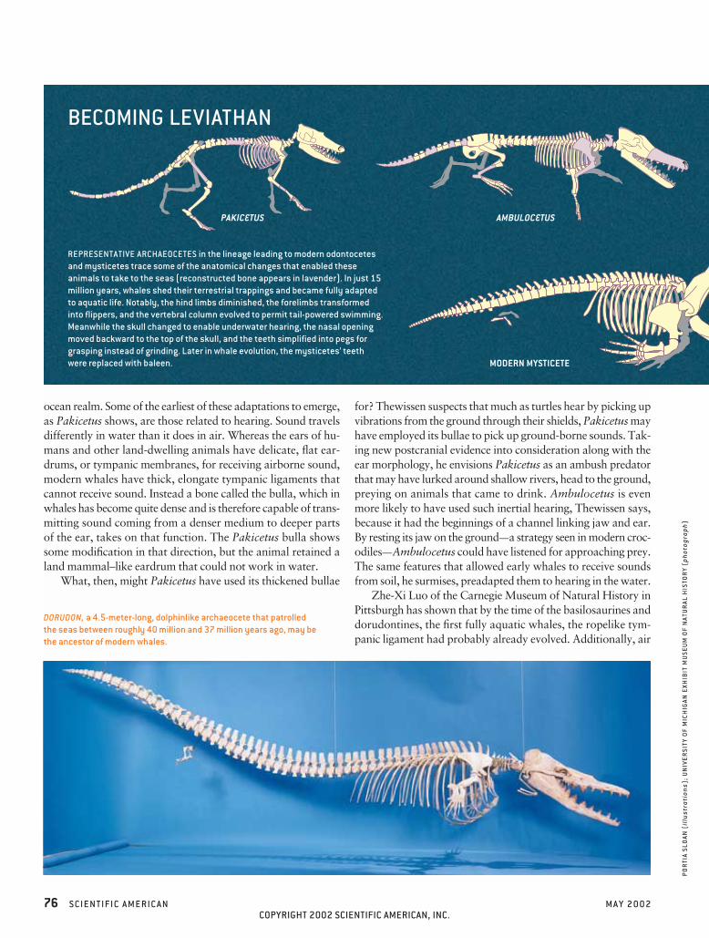
ocean realm. Some of the earliest of these adaptations to emerge,as Pakicetus shows, are those related to hearing. Sound travelsdifferently in water than it does in air. Whereas the ears of hu-mans and other land-dwelling animals have delicate, flat ear-drums, or tympanic membranes, for receiving airborne sound,modern whales have thick, elongate tympanic ligaments thatcannot receive sound. Instead a bone called the bulla, which inwhales has become quite dense and is therefore capable of trans-mitting sound coming from a denser medium to deeper partsof the ear, takes on that function. The Pakicetus bulla showssome modification in that direction, but the animal retained aland mammal–like eardrum that could not work in water.
What, then, might Pakicetus have used its thickened bullae
for? Thewissen suspects that much as turtles hear by picking upvibrations from the ground through their shields, Pakicetus mayhave employed its bullae to pick up ground-borne sounds. Tak-ing new postcranial evidence into consideration along with theear morphology, he envisions Pakicetus as an ambush predatorthat may have lurked around shallow rivers, head to the ground,preying on animals that came to drink. Ambulocetus is evenmore likely to have used such inertial hearing, Thewissen says,because it had the beginnings of a channel linking jaw and ear.By resting its jaw on the ground—a strategy seen in modern croc-odiles—Ambulocetus could have listened for approaching prey.The same features that allowed early whales to receive soundsfrom soil, he surmises, preadapted them to hearing in the water.
Zhe-Xi Luo of the Carnegie Museum of Natural History inPittsburgh has shown that by the time of the basilosaurines anddorudontines, the first fully aquatic whales, the ropelike tym-panic ligament had probably already evolved. Additionally, air
76 S C I E N T I F I C A M E R I C A N M A Y 2 0 0 2
PO
RTI
A SL
OAN
(il
lust
rati
ons)
; U
NIV
ER
SITY
OF
MIC
HIG
AN E
XHIB
IT M
USE
UM
OF
NAT
UR
AL H
ISTO
RY
(ph
otog
rap
h)
BECOMING LEVIATHAN
REPRESENTATIVE ARCHAEOCETES in the lineage leading to modern odontocetesand mysticetes trace some of the anatomical changes that enabled theseanimals to take to the seas (reconstructed bone appears in lavender). In just 15million years, whales shed their terrestrial trappings and became fully adaptedto aquatic life. Notably, the hind limbs diminished, the forelimbs transformedinto flippers, and the vertebral column evolved to permit tail-powered swimming.Meanwhile the skull changed to enable underwater hearing, the nasal openingmoved backward to the top of the skull, and the teeth simplified into pegs forgrasping instead of grinding. Later in whale evolution, the mysticetes’ teethwere replaced with baleen.
PAKICETUS AMBULOCETUS
MODERN MYSTICETE
DORUDON, a 4.5-meter-long, dolphinlike archaeocete that patrolled the seas between roughly 40 million and 37 million years ago, may be the ancestor of modern whales.
COPYRIGHT 2002 SCIENTIFIC AMERICAN, INC.
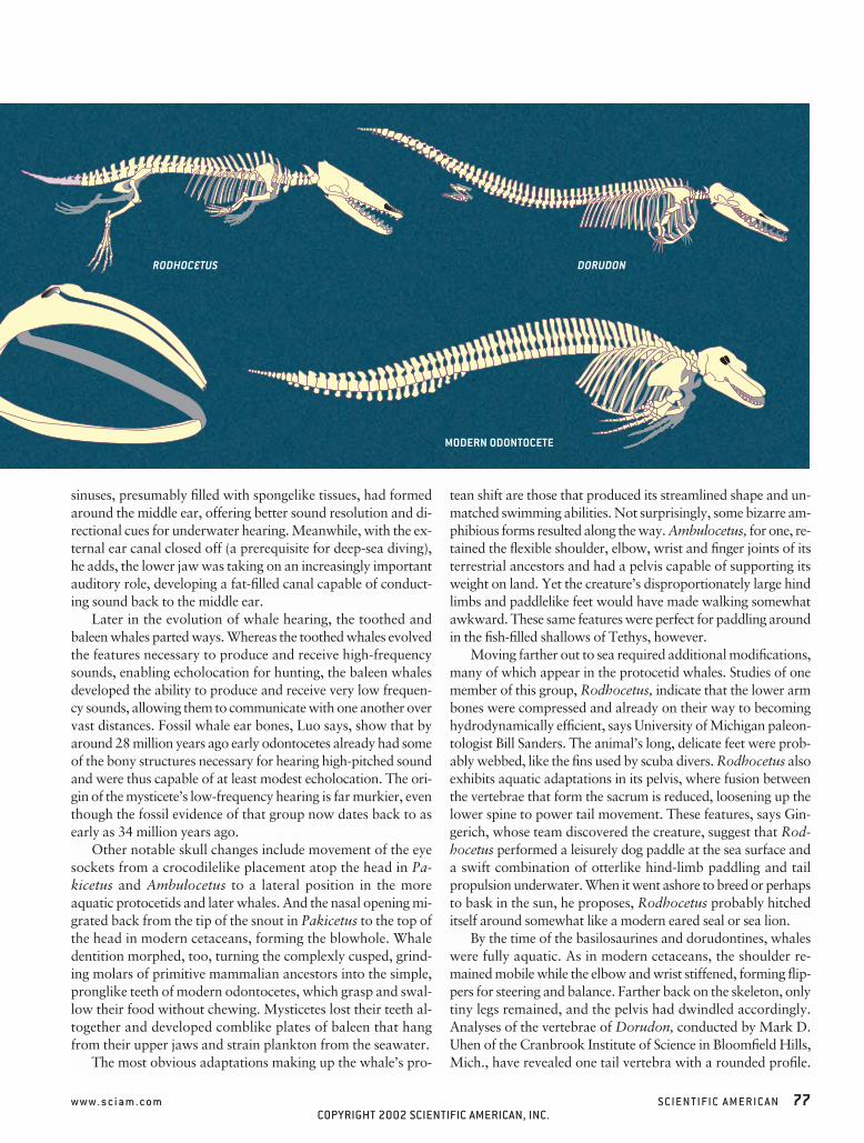
sinuses, presumably filled with spongelike tissues, had formedaround the middle ear, offering better sound resolution and di-rectional cues for underwater hearing. Meanwhile, with the ex-ternal ear canal closed off (a prerequisite for deep-sea diving),he adds, the lower jaw was taking on an increasingly importantauditory role, developing a fat-filled canal capable of conduct-ing sound back to the middle ear.
Later in the evolution of whale hearing, the toothed andbaleen whales parted ways. Whereas the toothed whales evolvedthe features necessary to produce and receive high-frequencysounds, enabling echolocation for hunting, the baleen whalesdeveloped the ability to produce and receive very low frequen-cy sounds, allowing them to communicate with one another overvast distances. Fossil whale ear bones, Luo says, show that byaround 28 million years ago early odontocetes already had someof the bony structures necessary for hearing high-pitched soundand were thus capable of at least modest echolocation. The ori-gin of the mysticete’s low-frequency hearing is far murkier, eventhough the fossil evidence of that group now dates back to asearly as 34 million years ago.
Other notable skull changes include movement of the eyesockets from a crocodilelike placement atop the head in Pa-kicetus and Ambulocetus to a lateral position in the moreaquatic protocetids and later whales. And the nasal opening mi-grated back from the tip of the snout in Pakicetus to the top ofthe head in modern cetaceans, forming the blowhole. Whaledentition morphed, too, turning the complexly cusped, grind-ing molars of primitive mammalian ancestors into the simple,pronglike teeth of modern odontocetes, which grasp and swal-low their food without chewing. Mysticetes lost their teeth al-together and developed comblike plates of baleen that hangfrom their upper jaws and strain plankton from the seawater.
The most obvious adaptations making up the whale’s pro-
tean shift are those that produced its streamlined shape and un-matched swimming abilities. Not surprisingly, some bizarre am-phibious forms resulted along the way. Ambulocetus, for one, re-tained the flexible shoulder, elbow, wrist and finger joints of itsterrestrial ancestors and had a pelvis capable of supporting itsweight on land. Yet the creature’s disproportionately large hindlimbs and paddlelike feet would have made walking somewhatawkward. These same features were perfect for paddling aroundin the fish-filled shallows of Tethys, however.
Moving farther out to sea required additional modifications,many of which appear in the protocetid whales. Studies of onemember of this group, Rodhocetus, indicate that the lower armbones were compressed and already on their way to becominghydrodynamically efficient, says University of Michigan paleon-tologist Bill Sanders. The animal’s long, delicate feet were prob-ably webbed, like the fins used by scuba divers. Rodhocetus alsoexhibits aquatic adaptations in its pelvis, where fusion betweenthe vertebrae that form the sacrum is reduced, loosening up thelower spine to power tail movement. These features, says Gin-gerich, whose team discovered the creature, suggest that Rod-hocetus performed a leisurely dog paddle at the sea surface anda swift combination of otterlike hind-limb paddling and tailpropulsion underwater. When it went ashore to breed or perhapsto bask in the sun, he proposes, Rodhocetus probably hitcheditself around somewhat like a modern eared seal or sea lion.
By the time of the basilosaurines and dorudontines, whaleswere fully aquatic. As in modern cetaceans, the shoulder re-mained mobile while the elbow and wrist stiffened, forming flip-pers for steering and balance. Farther back on the skeleton, onlytiny legs remained, and the pelvis had dwindled accordingly.Analyses of the vertebrae of Dorudon, conducted by Mark D.Uhen of the Cranbrook Institute of Science in Bloomfield Hills,Mich., have revealed one tail vertebra with a rounded profile.
w w w . s c i a m . c o m S C I E N T I F I C A M E R I C A N 77
MODERN ODONTOCETE
RODHOCETUS DORUDON
COPYRIGHT 2002 SCIENTIFIC AMERICAN, INC.
Modern whales have a similarly shaped bone, the ball vertebra,at the base of their fluke, the flat, horizontal structure capping thetail. Uhen thus suspects that basilosaurines and dorudontineshad tail flukes and swam much as modern whales do, using so-called caudal oscillation. In this energetically efficient mode oflocomotion, motion generated at a single point in the vertebralcolumn powers the tail’s vertical movement through the water,and the fluke generates lift.
Exactly when whales lost their legs altogether remains un-
known. In fact, a recent discovery made by Lawrence G. Barnesof the Natural History Museum of Los Angeles County hints atsurprisingly well developed hind limbs in a 27-million-year-oldbaleen whale from Washington State, suggesting that whale legspersisted far longer than originally thought. Today, however,some 50 million years after their quadrupedal ancestors first wad-ed into the warm waters of Tethys, whales are singularly sleek.Their hind limbs have shrunk to externally invisible vestiges, andthe pelvis has diminished to the point of serving merely as an an-chor for a few tiny muscles unrelated to locomotion.
Making WavesTHE FOSSILS UNCOVERED during the 1980s and 1990s ad-vanced researchers’ understanding of whale evolution by leapsand bounds, but all morphological signs still pointed to amesonychid origin. An alternative view of cetacean roots wastaking wing in genetics laboratories in the U.S., Belgium andJapan, however. Molecular biologists, having developed so-phisticated techniques for analyzing the DNA of living creatures,took Boyden’s 1960s immunology-based conclusions a step fur-ther. Not only were whales more closely related to artiodactylsthan to any other living mammals, they asserted, but in factwhales were themselves artiodactyls, one of many twigs on thatbranch of the mammalian family tree. Moreover, a number ofthese studies pointed to an especially close relationship betweenwhales and hippopotamuses. Particularly strong evidence forthis idea came in 1999 from analyses of snippets of noncodingDNA called SINES (short interspersed elements), conducted byNorihiro Okada and his colleagues at the Tokyo Institute ofTechnology.
The whale-hippo connection did not sit well with paleontol-ogists. “I thought they were nuts,” Gingerich recollects. “Every-thing we’d found was consistent with a mesonychid origin. I washappy with that and happy with a connection through mesony-chids to artiodactyls.” Whereas mesonychids appeared at theright time, in the right place and in the right form to be consid-ered whale progenitors, the fossil record did not seem to containa temporally, geographically and morphologically plausible ar-tiodactyl ancestor for whales, never mind one linking whalesand hippos specifically. Thewissen, too, had largely dismissedthe DNA findings. But “I stopped rejecting it when Okada’sSINE work came out,” he says.
It seemed the only way to resolve the controversy was to find,of all things, an ancient whale anklebone. Morphologists havetraditionally defined artiodactyls on the basis of certain featuresin one of their anklebones, the astragalus, that enhance mobili-ty. Specifically, the unique artiodactyl astragalus has twogrooved, pulleylike joint surfaces. One connects to the tibia, orshinbone; the other articulates with more distal anklebones. Ifwhales descended from artiodactyls, researchers reasoned, thosethat had not yet fully adapted to life in the seas should exhibitthis double-pulleyed astragalus.
That piece of the puzzle fell into place last fall, when Gin-gerich and Thewissen both announced discoveries of new prim-itive whale fossils. In the eastern part of Baluchistan Province,
78 S C I E N T I F I C A M E R I C A N M A Y 2 0 0 2
WATER, WATER EVERYWHEREMOST MAMMALS—big ones in particular—cannot live withoutfreshwater. For marine mammals, however, freshwater isdifficult to come by. Seals and sea lions obtain most of theirwater from the fish they eat (some will eat snow to getfreshwater), and manatees routinely seek out freshwater fromrivers. For their part, cetaceans obtain water both from theirfood and from sips of the briny deep.
When did whales, which evolved from a fairly large (andtherefore freshwater-dependent) terrestrial mammal, develop asystem capable of handling the excess salt load associated withingesting seawater? Evidence from so-called stable oxygenisotopes has provided some clues. In nature, oxygen mainlyoccurs in two forms, or isotopes: 16O and 18O. The ratios of theseisotopes in freshwater and seawater differ, with seawatercontaining more 18O. Because mammals incorporate oxygenfrom drinking water into their developing teeth and bones, theremains of those that imbibe seawater can be distinguishedfrom those that take in freshwater.
J.G.M. (Hans) Thewissen of the Northeastern OhioUniversities College of Medicine and his colleagues thusanalyzed the oxygen isotope ratios in ancient whale teeth togain insight into when these animals might have moved from afreshwater-based osmoregulatory system to a seawater-basedone. Oxygen isotope values for pakicetids, the most primitivewhales, indicate that they drank freshwater, as would bepredicted from other indications that these animals spent muchof their time on land. Isotope measurements from amphibiousAmbulocetus, on the other hand, vary widely, and somespecimens show no evidence of seawater intake. Inexplanation, the researchers note that although Ambulocetus isknown to have spent time in the sea (based on the marinenature of the rocks in which its fossils occur), it may still havehad to go ashore to drink. Alternatively, it may have spent theearly part of its life (when its teeth mineralized) in freshwaterand only later entered the sea.
The protocetids, however, which show more skeletaladaptations to aquatic life, exhibit exclusively marine isotopevalues, indicating that they drank only seawater. Thus, just afew million years after the first whales evolved, theirdescendants had adapted to increased salt loads. Thisphysiological innovation no doubt played an important role infacilitating the protocetids’ dispersal across the globe. —K.W.
COPYRIGHT 2002 SCIENTIFIC AMERICAN, INC.
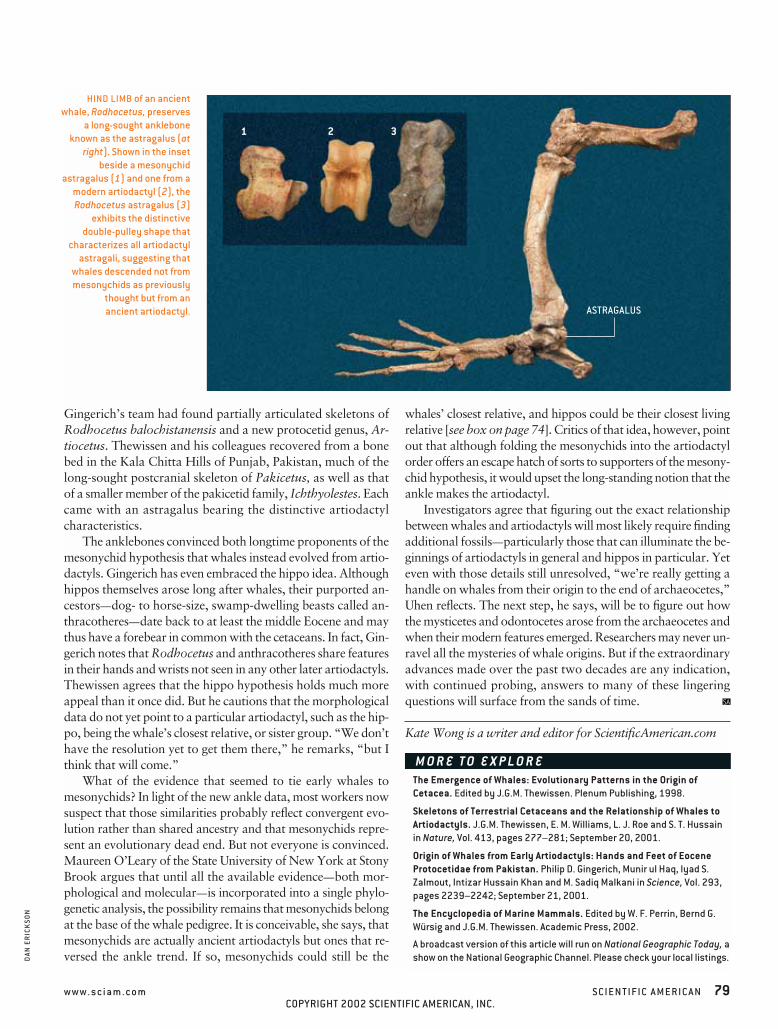
Gingerich’s team had found partially articulated skeletons ofRodhocetus balochistanensis and a new protocetid genus, Ar-tiocetus. Thewissen and his colleagues recovered from a bonebed in the Kala Chitta Hills of Punjab, Pakistan, much of thelong-sought postcranial skeleton of Pakicetus, as well as thatof a smaller member of the pakicetid family, Ichthyolestes. Eachcame with an astragalus bearing the distinctive artiodactylcharacteristics.
The anklebones convinced both longtime proponents of themesonychid hypothesis that whales instead evolved from artio-dactyls. Gingerich has even embraced the hippo idea. Althoughhippos themselves arose long after whales, their purported an-cestors—dog- to horse-size, swamp-dwelling beasts called an-thracotheres—date back to at least the middle Eocene and maythus have a forebear in common with the cetaceans. In fact, Gin-gerich notes that Rodhocetus and anthracotheres share featuresin their hands and wrists not seen in any other later artiodactyls.Thewissen agrees that the hippo hypothesis holds much moreappeal than it once did. But he cautions that the morphologicaldata do not yet point to a particular artiodactyl, such as the hip-po, being the whale’s closest relative, or sister group. “We don’thave the resolution yet to get them there,” he remarks, “but Ithink that will come.”
What of the evidence that seemed to tie early whales tomesonychids? In light of the new ankle data, most workers nowsuspect that those similarities probably reflect convergent evo-lution rather than shared ancestry and that mesonychids repre-sent an evolutionary dead end. But not everyone is convinced.Maureen O’Leary of the State University of New York at StonyBrook argues that until all the available evidence—both mor-phological and molecular—is incorporated into a single phylo-genetic analysis, the possibility remains that mesonychids belongat the base of the whale pedigree. It is conceivable, she says, thatmesonychids are actually ancient artiodactyls but ones that re-versed the ankle trend. If so, mesonychids could still be the
whales’ closest relative, and hippos could be their closest livingrelative [see box on page 74]. Critics of that idea, however, pointout that although folding the mesonychids into the artiodactylorder offers an escape hatch of sorts to supporters of the mesony-chid hypothesis, it would upset the long-standing notion that theankle makes the artiodactyl.
Investigators agree that figuring out the exact relationshipbetween whales and artiodactyls will most likely require findingadditional fossils—particularly those that can illuminate the be-ginnings of artiodactyls in general and hippos in particular. Yeteven with those details still unresolved, “we’re really getting ahandle on whales from their origin to the end of archaeocetes,”Uhen reflects. The next step, he says, will be to figure out howthe mysticetes and odontocetes arose from the archaeocetes andwhen their modern features emerged. Researchers may never un-ravel all the mysteries of whale origins. But if the extraordinaryadvances made over the past two decades are any indication,with continued probing, answers to many of these lingeringquestions will surface from the sands of time.
Kate Wong is a writer and editor for ScientificAmerican.com
w w w . s c i a m . c o m S C I E N T I F I C A M E R I C A N 79
DAN
ER
ICK
SON
The Emergence of Whales: Evolutionary Patterns in the Origin ofCetacea. Edited by J.G.M. Thewissen. Plenum Publishing, 1998.
Skeletons of Terrestrial Cetaceans and the Relationship of Whales toArtiodactyls. J.G.M. Thewissen, E. M. Williams, L. J. Roe and S. T. Hussainin Nature, Vol. 413, pages 277–281; September 20, 2001.
Origin of Whales from Early Artiodactyls: Hands and Feet of EoceneProtocetidae from Pakistan. Philip D. Gingerich, Munir ul Haq, Iyad S.Zalmout, Intizar Hussain Khan and M. Sadiq Malkani in Science, Vol. 293,pages 2239–2242; September 21, 2001.
The Encyclopedia of Marine Mammals. Edited by W. F. Perrin, Bernd G.Würsig and J.G.M. Thewissen. Academic Press, 2002.
A broadcast version of this article will run on National Geographic Today, ashow on the National Geographic Channel. Please check your local listings.
M O R E T O E X P L O R E
SA
HIND LIMB of an ancientwhale, Rodhocetus, preserves
a long-sought ankleboneknown as the astragalus (at
right). Shown in the insetbeside a mesonychid
astragalus (1) and one from amodern artiodactyl (2), theRodhocetus astragalus (3)
exhibits the distinctivedouble-pulley shape that
characterizes all artiodactylastragali, suggesting that
whales descended not frommesonychids as previously
thought but from an ancient artiodactyl. ASTRAGALUS
1 2 3
COPYRIGHT 2002 SCIENTIFIC AMERICAN, INC.
, 20140161, published 2 July 2014281 2014 Proc. R. Soc. B Bryan C. Sykes, Rhettman A. Mullis, Christophe Hagenmuller, Terry W. Melton and Michel Sartori other anomalous primatesGenetic analysis of hair samples attributed to yeti, bigfoot and
References
http://rspb.royalsocietypublishing.org/content/281/1789/20140161.full.html#related-urls Article cited in:
http://rspb.royalsocietypublishing.org/content/281/1789/20140161.full.html#ref-list-1
This article cites 11 articles, 3 of which can be accessed free
This article is free to access
Subject collections
(198 articles)taxonomy and systematics � (145 articles)genetics � (1869 articles)evolution �
Articles on similar topics can be found in the following collections
Email alerting service hereright-hand corner of the article or click Receive free email alerts when new articles cite this article - sign up in the box at the top
http://rspb.royalsocietypublishing.org/subscriptions go to: Proc. R. Soc. BTo subscribe to
on August 28, 2014rspb.royalsocietypublishing.orgDownloaded from on August 28, 2014rspb.royalsocietypublishing.orgDownloaded from
on August 28, 2014rspb.royalsocietypublishing.orgDownloaded from
rspb.royalsocietypublishing.org
ResearchCite this article: Sykes BC, Mullis RA,
Hagenmuller C, Melton TW, Sartori M. 2014
Genetic analysis of hair samples attributed to
yeti, bigfoot and other anomalous primates.
Proc. R. Soc. B 281: 20140161.
http://dx.doi.org/10.1098/rspb.2014.0161
Received: 21 January 2014
Accepted: 27 March 2014
Subject Areas:genetics, taxonomy and systematics, evolution
Keywords:yeti, almasty, bigfoot, sasquatch,
mitochondrial DNA
Author for correspondence:Bryan C. Sykes
e-mail: [email protected]
& 2014 The Authors. Published by the Royal Society under the terms of the Creative Commons AttributionLicense http://creativecommons.org/licenses/by/3.0/, which permits unrestricted use, provided the originalauthor and source are credited.
Genetic analysis of hair samplesattributed to yeti, bigfoot and otheranomalous primates
Bryan C. Sykes1, Rhettman A. Mullis2, Christophe Hagenmuller3,Terry W. Melton4 and Michel Sartori5,6
1Institute of Human Genetics, Wolfson College, University of Oxford, Oxford OX2 6UD, UK2PO Box 40143, Bellevue, WA 98005, USA3NaturAlpes, Annecy-Le-Vieux 74940, France4Mitotyping Technologies, 2565 Park Center Boulevard, State College, PA 16801, USA5Museum of Zoology, Palais de Rumine, Lausanne 1014, Switzerland6Museum of Zoology and Grindel Biocentre, Hamburg 20146, Germany
In the first ever systematic genetic survey, we have used rigorous decontami-
nation followed by mitochondrial 12S RNA sequencing to identify the species
origin of 30 hair samples attributed to anomalous primates. Two Himalayan
samples, one from Ladakh, India, the other from Bhutan, had their closest
genetic affinity with a Palaeolithic polar bear, Ursus maritimus. Otherwise
the hairs were from a range of known extant mammals.
1. IntroductionDespite several decades of research, mystery still surrounds the species identity
of so-called anomalous primates such as the yeti in the Himalaya, almasty in
central Asia and sasquatch/bigfoot in North America. On the one hand, numer-
ous reports including eye-witness and footprint evidence, point to the existence
of large unidentified primates in many regions of the world. On the other hand,
no bodies or recent fossils of such creatures have ever been authenticated. There
is no shortage of theories about what these animals may be, ranging from sur-
viving populations of collateral hominids such as Homo neanderthalensis, Homofloresiensis [1] or Denisovans [2], extinct apes such as Gigantopithecus [3] or even
unlikely hybrids between Homo sapiens and other mammals [4]. Modern science
has largely avoided this field and advocates frequently complain that they have
been ‘rejected by science’ [5]. This conflicts with the basic tenet that science
neither rejects nor accepts anything without examining the evidence. To
apply this philosophy to the study of anomalous primates and to introduce
some clarity into this often murky field, we have carried out a systematic genetic
survey of hair samples attributed to these creatures. Only two ‘tongue-in-cheek’
scientific publications report DNA sequence data from anomalous primates.
Milinkovitch et al. [6], after analysis of a Nepalese sample, confirmed Captain
Haddock’s suspicions that the yeti was an ungulate [7]. The same conclusion
was reached by Coltman et al. [8] after analysis of sasquatch hair from Alaska.
2. Material and methodsHair samples submissions were solicited from museum and individual collections in
a joint press release issued on 14 May 2012 by the Museum of Zoology, Lausanne
and the University of Oxford. A total of 57 samples were received and subjected
to macroscopic, microscopic and infrared fluorescence examination to eliminate
obvious non-hairs. This excluded one sample of plant material and one of glass
fibre. Of the screened samples, 37 were selected for genetic analysis based on
their provenance or historic interest. Lengths (2–4 cm) of individual hair shaft
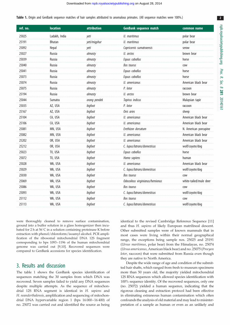
Table 1. Origin and GenBank sequence matches of hair samples attributed to anomalous primates. (All sequence matches were 100%.)
ref. no. location attribution GenBank sequence match common name
25025 Ladakh, India yeti U. maritimus polar bear
25191 Bhutan yeti/migyhur U. maritimus polar bear
25092 Nepal yeti Capricornis sumatraensis serow
25027 Russia almasty U. arctos brown bear
25039 Russia almasty Equus caballus horse
25040 Russia almasty Bos taurus cow
25041 Russia almasty Equus caballus horse
25073 Russia almasty Equus caballus horse
25074 Russia almasty U. americanus American black bear
25075 Russia almasty P. lotor raccoon
25194 Russia almasty U. arctos brown bear
25044 Sumatra orang pendek Tapirus indicus Malaysian tapir
25035 AZ, USA bigfoot P. lotor raccoon
25167 AZ, USA bigfoot Ovis aries sheep
25104 CA, USA bigfoot U. americanus American black bear
25106 CA, USA bigfoot U. americanus American black bear
25081 MN, USA bigfoot Erethizon dorsatum N. American porcupine
25082 MN, USA bigfoot U. americanus American black bear
25202 OR, USA bigfoot U. americanus American black bear
25212 OR, USA bigfoot C. lupus/latrans/domesticus wolf/coyote/dog
25023 TX, USA bigfoot Equus caballus horse
25072 TX, USA bigfoot Homo sapiens human
25028 WA, USA bigfoot U. americanus American black bear
25029 WA, USA bigfoot C. lupus/latrans/domesticus wolf/coyote/dog
25030 WA, USA bigfoot Bos taurus cow
25069 WA, USA bigfoot Odocoileus virginianus/hemionus white-tailed/mule deer
25086 WA, USA bigfoot Bos taurus cow
25093 WA, USA bigfoot C. lupus/latrans/domesticus wolf/coyote/dog
25112 WA, USA bigfoot Bos taurus cow
25113 WA, USA bigfoot C. lupus/latrans/domesticus wolf/coyote/dog
rspb.royalsocietypublishing.orgProc.R.Soc.B
281:20140161
2
on August 28, 2014rspb.royalsocietypublishing.orgDownloaded from
were thoroughly cleaned to remove surface contamination,
ground into a buffer solution in a glass homogenizer then incu-
bated for 2 h at 568C in a solution containing proteinase K before
extraction with phenol/chloroform/isoamyl alcohol. PCR ampli-
fication of the ribosomal mitochondrial DNA 12S fragment
corresponding to bps 1093–1196 of the human mitochondrial
genome was carried out [9,10]. Recovered sequences were
compared to GenBank accessions for species identification.
3. Results and discussionThe table 1 shows the GenBank species identification of
sequences matching the 30 samples from which DNA was
recovered. Seven samples failed to yield any DNA sequences
despite multiple attempts. As the sequence of mitochon-
drial 12S RNA segment is identical in H. sapiens and
H. neanderthalensis, amplification and sequencing of mitochon-
drial DNA hypervariable region 1 (bps 16 000–16 400) of
no. 25072 was carried out and identified the source as being
identical to the revised Cambridge Reference Sequence [11]
and thus H. sapiens of likely European matrilineal descent.
Other submitted samples were of known mammals that in
most cases were living within their normal geographical
range, the exceptions being sample nos. 25025 and 25191
(Ursus maritimus, polar bear) from the Himalayas, no. 25074
(Ursus americanus, American black bear) and no. 25075 (Procyonlotor, raccoon) that were submitted from Russia even though
they are native to North America.
Despite the wide range of age and condition of the submit-
ted hair shafts, which ranged from fresh to museum specimens
more than 50 years old, the majority yielded mitochondrial
12S RNA sequences which allowed species identification with
100% sequence identity. Of the recovered sequences, only one
(no. 25072) yielded a human sequence, indicating that the
rigorous cleaning and extraction protocol had been effective
in eliminating extraneous human contamination which often
confounds the analysis of old material and may lead to misinter-
pretation of a sample as human or even as an unlikely and
rspb.royalsocietypublishing.orgProc.R.Soc.B
281:20140161
3
on August 28, 2014rspb.royalsocietypublishing.orgDownloaded from
unknown human x mammalian hybrid [4]. The deliberately
permissive primer combination used here allowed a wide
range of mammalian DNA to be amplified within a single reac-
tion, although this meant that some identification did not go
beyond the level of genus. For example, no. 25029 was identified
as Canis but did not distinguish between Canis lupus (wolf),
Canis latrans (coyote) and Canis domesticus (domestic dog).
Sequences derived from hair sample nos. 25025 and 25191
had a 100% match with DNA recovered from a Pleistocene
fossil more than 40 000 BP of U. maritimus (polar bear) [12]
but not to modern examples of the species. Hair sample no.
25025 came from an animal shot by an experienced hunter in
Ladakh, India ca 40 years ago who reported that its behaviour
was very different from a brown bear Ursus arctos with which
he was very familiar. Hair sample no. 25191 was recovered
from a high altitude (ca 3500 m) bamboo forest in Bhutan
and was identified as a nest of a migyhur, the Bhutanese
equivalent of the yeti. The Ladakh hairs (no. 25025) were
golden-brown, whereas the hair from Bhutan (no. 25191) was
reddish-brown in appearance. As the match is to a segment
only 104 bp long, albeit in the very conserved 12S RNA gene,
this result should be regarded as preliminary. Other than
these data, nothing is currently known about the genetic affi-
nity of Himalayan bears and although there are anecdotal
reports of white bears in Central Asia and the Himalayas
[13,14], it seems more likely that the two hairs reported here
are from either a previously unrecognized bear species,
colour variants of U. maritimus, or U. arctos/U. maritimushybrids. Viable U. arctos/U. maritimus hybrids are known
from the Admiralty, Barayanov and Chicagov (ABC) islands
off the coast of Alaska though in the ABC hybrids the mito-
chondrial sequence homology is with modern rather than
ancient polar bears [15]. If they are hybrids, the Ladakh and
Bhutan specimens are probably descended from a different
hybridization event during the early stages of species diver-
gence between U. arctos and U. maritimus. Genomic sequence
data are needed to decide between these alternatives. If these
bears are widely distributed in the Himalayas, they may well
contribute to the biological foundation of the yeti legend,
especially if, as reported by the hunter who shot the Ladakh
specimen, they behave more aggressively towards humans
than known indigenous bear species.
With the exception of these two samples, none of the sub-
mitted and analysed hairs samples returned a sequence that
could not be matched with an extant mammalian species,
often a domesticate. While it is important to bear in mind
that absence of evidence is not evidence of absence and this
survey cannot refute the existence of anomalous primates,
neither has it found any evidence in support. Rather than per-
sisting in the view that they have been ‘rejected by science’,
advocates in the cryptozoology community have more work
to do in order to produce convincing evidence for anomalous
primates and now have the means to do so. The techniques
described here put an end to decades of ambiguity about
species identification of anomalous primate samples and set
a rigorous standard against which to judge any future claims.
Acknowledgements. We thank Reinhold Messner, Peter Byrne, JustinSmeja, Bart Cutino, Derek Randles, Dan Shirley, Garland Fields,Loren Coleman, Betty Klopp, Marcel Cagey, Sam Cagey, LoriSimmons, Adam Davies, Dr Mike Amaranthus, Mike Long, PatrickSpell, Maxwell David, Mark McClurkan, Rob Kryder, Jack Barnes,Jeff Anderson, David Ellis, Steve Mattice, Brenda Harris, StuartFleming, Igor Burtsev, Dmitri Pirkulov, Michael Trachtengerts andDmitri Bayanov for submitting samples and for their progressivestance in doing so. Thanks also to, Ray Crowe, Ronnie Roseman,Greg Roberts and Tom Graham for discussing their experiencesand to Jeff Meldrum and Anna Nekaris for advice and guidance.We are very grateful to Ken Goddard, Ed Espinoza, Mike Tucker,Barry Baker, Bonnie Yates, Cookie Smith and Dyan Straughan ofthe US Fish and Wildlife Service Forensic Laboratory, Ashland, OR,USA, for help with forensic methods of trace evidence analysis andto Charity Holland, Bonnie Higgins, Gloria Dimick and MicheleYon for technical assistance.
Data accessibility. DNA sequences: GenBank accession nos. KJ155696–KJ155724 and KJ607607. Voucher samples of the research materialshave been deposited in the Heuvelmans Archive at the Museum ofZoology, Lausanne, Switzerland.
Funding statement. We also thank Harry Marshall and Icon Films fortheir contribution to the costs of analysis.
References
1. Brown P, Sutikna T, Morwood M, Soejono R, Jatmiko E,Saptomo E, Awa Due R. 2004 A new small-bodiedhominin from the Late Pleistocene of Flores, Indonesia.Nature 431, 1055 – 1061. (doi:10.1038/nature02999)
2. Reich D et al. 2010 Genetic history of an archaichominin group in Denisova Cave in Siberia. Nature468, 1053 – 1060. (doi:10.1038/nature09710)
3. Strauss W. 1957 Jaw of Gigantopithecus. Science125, 685. (doi:10.1126/science.125.3250.685)
4. Ketchum M et al. 2013 North American hominins.De Novo 1, 1 – 15.
5. Regal B. 2011 Searching for Sasquatch, p. 5.New York, NY: Palgrave Macmillan.
6. Milinkovitch MC et al. 2004 Molecular phylogeneticanalyses indicate extensive morphologicalconvergence between the ‘yeti’ and primates. Mol.
Phylogenet. Evol. 31, 1 – 3. (doi:10.1016/j.ympev.2004.01.009)
7. Herge. 1960 Tintin au Tibet. Tournai, Belgium:Casterman.
8. Coltman D, Davis C. 2005 Molecular cryptozoologymeets the Sasquatch. Trends Ecol. Evol. 21, 60 – 61.(doi:10.1016/j.tree.2005.11.010)
9. Melton T, Dimick G, Higgins B, Lindstrom Nelson K.2005 Forensic mitochondrial DNA analysis of 691casework hairs. J. Forensic Sci. 50, 73 – 80. (doi:10.1520/JFS2004230)
10. Melton T, Holland C. 2007 Routine forensic use of themitochondrial 12S ribosomal RNA genes for speciesidentification. J. Forensic Sci. 52, 1305 – 1307.
11. Andrews R, Kubacka I, Chinnery C, Lightowlers RN,Turnbull DM, Howell N. 1999 Reanalysis and
revision of the Cambridge reference sequence forhuman mitochondrial DNA. Nat. Genet. 23, 147.(doi:10.1038/13779)
12. Linqvist C et al. 2010 Complete mitochondrialgenome of a Pleistocene jawbone unveils the originof polar bear. Proc. Natl Acad. Sci. USA 107,5053 – 5057. (doi:10.1073/pnas.0914266107)
13. Brunner B. 2007 Bears: a brief history, p. 64. NewHaven, CT: Yale University Press.
14. Smythe F. 1936 The valley of flowers, p. 144.London, UK: Hodder and Stoughton.
15. Hailer F, Kutschera V, Hallstron B, Klassert D, Fain S,Leonard J, Arnasojn U, Janke A. 2012 Nucleargenomic sequences reveal that polar bears are anold and distinct bear lineage. Science 336,344 – 347. (doi:10.1126/science.1216424)

DOI: 10.1126/science.1194442, 1503 (2010);330 Science
et al.Michael HoffmannThe Impact of Conservation on the Status of the World's Vertebrates
This copy is for your personal, non-commercial use only.
clicking here.colleagues, clients, or customers by , you can order high-quality copies for yourIf you wish to distribute this article to others
here.following the guidelines
can be obtained byPermission to republish or repurpose articles or portions of articles
): August 25, 2012 www.sciencemag.org (this information is current as of
The following resources related to this article are available online at
http://www.sciencemag.org/content/330/6010/1503.full.htmlversion of this article at:
including high-resolution figures, can be found in the onlineUpdated information and services,
http://www.sciencemag.org/content/suppl/2010/10/27/science.1194442.DC1.html can be found at: Supporting Online Material
http://www.sciencemag.org/content/330/6010/1503.full.html#relatedfound at:
can berelated to this article A list of selected additional articles on the Science Web sites
http://www.sciencemag.org/content/330/6010/1503.full.html#ref-list-1, 13 of which can be accessed free:cites 36 articlesThis article
http://www.sciencemag.org/content/330/6010/1503.full.html#related-urls21 articles hosted by HighWire Press; see:cited by This article has been
http://www.sciencemag.org/cgi/collection/ecologyEcology
subject collections:This article appears in the following
registered trademark of AAAS. is aScience2010 by the American Association for the Advancement of Science; all rights reserved. The title
CopyrightAmerican Association for the Advancement of Science, 1200 New York Avenue NW, Washington, DC 20005. (print ISSN 0036-8075; online ISSN 1095-9203) is published weekly, except the last week in December, by theScience
on
Aug
ust 2
5, 2
012
ww
w.s
cien
cem
ag.o
rgD
ownl
oade
d fr
om
The Impact of Conservation on theStatus of the World’s VertebratesMichael Hoffmann,1,2* Craig Hilton-Taylor,3 Ariadne Angulo,4,5 Monika Böhm,6
Thomas M. Brooks,7,8,9 Stuart H. M. Butchart,10 Kent E. Carpenter,2,5,11 Janice Chanson,5,12
Ben Collen,6 Neil A. Cox,5,13 William R. T. Darwall,3 Nicholas K. Dulvy,14 Lucy R. Harrison,14
Vineet Katariya,3 Caroline M. Pollock,3 Suhel Quader,15 Nadia I. Richman,6 Ana S. L. Rodrigues,16
Marcelo F. Tognelli,5,13,17 Jean-Christophe Vié,5 John M. Aguiar,18 David J. Allen,3
Gerald R. Allen,19 Giovanni Amori,20 Natalia B. Ananjeva,21 Franco Andreone,22 Paul Andrew,23
Aida Luz Aquino Ortiz,24 Jonathan E. M. Baillie,25 Ricardo Baldi,26,27 Ben D. Bell,28
S. D. Biju,29 Jeremy P. Bird,30 Patricia Black-Decima,31 J. Julian Blanc,32 Federico Bolaños,33
Wilmar Bolivar-G.,34 Ian J. Burfield,10 James A. Burton,35,36 David R. Capper,37
Fernando Castro,38 Gianluca Catullo,39 Rachel D. Cavanagh,40 Alan Channing,41
Ning Labbish Chao,42,43,44 Anna M. Chenery,45 Federica Chiozza,46 Viola Clausnitzer,47
Nigel J. Collar,10 Leah C. Collett,3 Bruce B. Collette,48 Claudia F. Cortez Fernandez,49
Matthew T. Craig,50 Michael J. Crosby,10 Neil Cumberlidge,51 Annabelle Cuttelod,3
Andrew E. Derocher,52 Arvin C. Diesmos,53 John S. Donaldson,54 J. W. Duckworth,55 Guy Dutson,56
S. K. Dutta,57 Richard H. Emslie,58 Aljos Farjon,59 Sarah Fowler,60 Jorg Freyhof,61
David L. Garshelis,62 Justin Gerlach,63 David J. Gower,64 Tandora D. Grant,65
Geoffrey A. Hammerson,66 Richard B. Harris,67 Lawrence R. Heaney,68 S. Blair Hedges,69
Jean-Marc Hero,70 Baz Hughes,71 Syed Ainul Hussain,72 Javier Icochea M.,73 Robert F. Inger,68
Nobuo Ishii,74 Djoko T. Iskandar,75 Richard K. B. Jenkins,76,77,78 Yoshio Kaneko,79
Maurice Kottelat,80,81 Kit M. Kovacs,82 Sergius L. Kuzmin,83 Enrique La Marca,84
John F. Lamoreux,5,85 Michael W. N. Lau,86 Esteban O. Lavilla,87 Kristin Leus,88
Rebecca L. Lewison,89 Gabriela Lichtenstein,90 Suzanne R. Livingstone,91
Vimoksalehi Lukoschek,92,93 David P. Mallon,94 Philip J. K. McGowan,95 Anna McIvor,96
Patricia D. Moehlman,97 Sanjay Molur,98 Antonio Muñoz Alonso,99 John A. Musick,100
Kristin Nowell,101 Ronald A. Nussbaum,102 Wanda Olech,103 Nikolay L. Orlov,21
Theodore J. Papenfuss,104 Gabriela Parra-Olea,105 William F. Perrin,106 Beth A. Polidoro,5,11
Mohammad Pourkazemi,107 Paul A. Racey,108 James S. Ragle,5 Mala Ram,6 Galen Rathbun,109
Robert P. Reynolds,110 Anders G. J. Rhodin,111 Stephen J. Richards,112,113 Lily O. Rodríguez,114
Santiago R. Ron,115 Carlo Rondinini,46 Anthony B. Rylands,2 Yvonne Sadovy de Mitcheson,116,117
Jonnell C. Sanciangco,5,11 Kate L. Sanders,118 Georgina Santos-Barrera,119 Jan Schipper,120
Caryn Self-Sullivan,121,122 Yichuan Shi,3 Alan Shoemaker,123 Frederick T. Short,124
Claudio Sillero-Zubiri,125 Débora L. Silvano,126 Kevin G. Smith,3 Andrew T. Smith,127
Jos Snoeks,128,129 Alison J. Stattersfield,10 Andrew J. Symes,10 Andrew B. Taber,130
Bibhab K. Talukdar,131 Helen J. Temple,132 Rob Timmins,133 Joseph A. Tobias,134
Katerina Tsytsulina,135 Denis Tweddle,136 Carmen Ubeda,137 Sarah V. Valenti,60
Peter Paul van Dijk,2 Liza M. Veiga,138,139 Alberto Veloso,140 David C. Wege,10 Mark Wilkinson,64
Elizabeth A. Williamson,141 Feng Xie,142 Bruce E. Young,7 H. Resit Akçakaya,143 Leon Bennun,10
Tim M. Blackburn,6 Luigi Boitani,46 Holly T. Dublin,144,145 Gustavo A. B. da Fonseca,146,147
Claude Gascon,2 Thomas E. Lacher Jr.,18 Georgina M. Mace,148 Susan A. Mainka,149
Jeffery A. McNeely,149 Russell A. Mittermeier,2,149 Gordon McGregor Reid,150
Jon Paul Rodriguez,151 Andrew A. Rosenberg,2 Michael J. Samways,152 Jane Smart,149
Bruce A. Stein,153 Simon N. Stuart1,2,154,155
Using data for 25,780 species categorized on the International Union for Conservation of NatureRed List, we present an assessment of the status of the world’s vertebrates. One-fifth of species areclassified as Threatened, and we show that this figure is increasing: On average, 52 species ofmammals, birds, and amphibians move one category closer to extinction each year. However, thisoverall pattern conceals the impact of conservation successes, and we show that the rate ofdeterioration would have been at least one-fifth again as much in the absence of these.Nonetheless, current conservation efforts remain insufficient to offset the main drivers ofbiodiversity loss in these groups: agricultural expansion, logging, overexploitation, andinvasive alien species.
In the past four decades, individual popula-tions ofmany species have undergone declinesand many habitats have suffered losses of
original cover (1, 2) through anthropogenic ac-tivity. These losses are manifested in species ex-tinction rates that exceed normal background rates
by two to three orders of magnitude (3), withsubstantial detrimental societal and economicconsequences (4). In response to this crisis, 193parties to the Convention on Biological Diversity(CBD; adopted 1992) agreed “to achieve by2010 a significant reduction of the current rate ofbiodiversity loss at the global, regional, and na-tional level as a contribution to poverty alle-viation and to the benefit of all life on Earth” (5).That the target has not been met was borne outby empirical testing against 31 cross-disciplinaryindicators developed within the CBD frameworkitself (1). However, this does not mean that con-servation efforts have been ineffective. Conser-vation actions have helped to prevent extinctions(6, 7) and improve population trajectories (8),but there has been limited assessment of theoverall impact of ongoing efforts in reducinglosses in biodiversity (9, 10). Here, we assess theoverall status of the world’s vertebrates, deter-mine temporal trajectories of extinction risk forthree vertebrate classes, and estimate the degree towhich conservation actions have reduced bio-diversity loss.
Described vertebrates include 5498 mam-mals, 10,027 birds, 9084 reptiles, 6638 amphib-ians, and 31,327 fishes (table S1). Vertebratesare found at nearly all elevations and depths,occupy most major habitat types, and displayremarkable variation in body size and life his-tory. Although they constitute just 3% of knownspecies, vertebrates play vital roles in ecosystems(11) and have great cultural importance (12).Under the auspices of the International Union forConservation of Nature (IUCN) Species SurvivalCommission, we compiled data on the taxonomy,distribution, population trend, major threats, con-servation measures, and threat status for 25,780vertebrate species, including all mammals, birds,amphibians, cartilaginous fishes, and statistically
RESEARCHARTICLE
1IUCN SSC Species Survival Commission, c/o United NationsEnvironment ProgrammeWorld Conservation Monitoring Centre,219 Huntingdon Road, Cambridge CB3 0DL, UK. 2ConservationInternational, 2011 Crystal Drive, Arlington, VA 22202, USA.3Species Programme, IUCN, 219c Huntingdon Road, CambridgeCB3 0DL, UK. 4IUCN–CI Biodiversity Assessment Unit, c/o P.O.Box 19004, 360 A Bloor Street W., Toronto, Ontario M5S 1X1,Canada. 5Species Programme, IUCN, Rue Mauverney 28, 1196,Gland, Switzerland. 6Institute of Zoology, Zoological Society ofLondon, Regent’s Park, London NW1 4RY, UK. 7NatureServe,1101 Wilson Boulevard, Arlington, VA 22209, USA. 8WorldAgroforestry Center (ICRAF), University of the Philippines LosBaños, Laguna 4031, Philippines. 9School of Geography andEnvironmental Studies, University of Tasmania, Hobart, Tasmania7001, Australia. 10BirdLife International, Wellbrook Court, GirtonRoad, Cambridge CB3 0NA, UK. 11Department of BiologicalSciences, Old Dominion University, Norfolk, VA 23529, USA.12IUCN–CI Biodiversity Assessment Unit, c/o 130 WeatherallRoad, Cheltenham 3192, Victoria, Australia. 13IUCN–CI Biodi-versity Assessment Unit, Conservation International, 2011 CrystalDrive Ste 500, Arlington, VA 22202,USA. 14IUCNShark SpecialistGroup, Department of Biological Sciences, Simon FraserUniversity, Burnaby, British Columbia V5A 1S6, Canada.15National Centre for Biological Sciences, Tata Institute ofFundamental Research, GKVK Campus, Bellary Road, Bangalore560 065, India. 16Centre d’Ecologie Fonctionnelle et Evolutive,CNRS UMR5175, 1919 Route de Mende, 34293 Montpellier,
www.sciencemag.org SCIENCE VOL 330 10 DECEMBER 2010 1503
on
Aug
ust 2
5, 2
012
ww
w.s
cien
cem
ag.o
rgD
ownl
oade
d fr
om
France. 17IADIZA-CONICET, CCT-Mendoza, CC 507, 5500Mendoza,Argentina. 18Department of Wildlife and Fisheries Sciences,Texas A&M University, College Station, TX 77843, USA.19Western Australian Museum, Locked Bag 49, Welshpool DC,Perth, Western Australia 6986, Australia. 20CNR–Institute forEcosystem Studies, Viale dell’Università 32, 00185 Rome, Italy.21Zoological Institute, Russian Academy of Sciences, 199034 St.Petersburg, Universitetskaya nab.1, Russia. 22Museo Regionaledi Scienze Naturali, Via G. Giolitti, 36, I-10123 Torino, Italy.23Taronga Conservation Society Australia, Taronga Zoo, P.O. Box20, Mosman 2088, Sydney, Australia. 24Martin Barrios 2230 c/Pizarro; Barrio Republicano, Asunción, Paraguay. 25ZoologicalSociety of London, Regent’s Park, London, NW1 4RY, UK.26Unidad de Investigación Ecología Terrestre, Centro NacionalPatagónico–CONICET, Boulevard Brown 2915, 9120 PuertoMadryn, Argentina. 27Patagonian and Andean Steppe Program,Wildlife Conservation Society, Boulevard Brown 2915, 9120Puerto Madryn, Argentina. 28Centre for Biodiversity & Restora-tion Ecology, School of Biological Sciences, Victoria Universityof Wellington, P.O. Box 600, Wellington 6140, New Zealand.29Systematics Lab, School of Environmental Studies, Universityof Delhi, Delhi 110 007, India. 30Center for Biodiversity andBiosecurity Studies, Pacific Institute for Sustainable Develop-ment, Jalan Bumi Nyiur 101, Manado, North Sulawesi,Indonesia. 31Facultad de Ciencias Naturales e Instituto MiguelLillo, Universidad Nacional de Tucuman, Miguel Lillo 205,4000 SM de Tucumán, Tucumán, Argentina. 32P.O. Box 47074,Nairobi 00100, Kenya. 33Escuela de Biología, Universidad deCosta Rica, San Pedro, 11501-2060 San José, Costa Rica.34Sección de Zoología, Departamento de Biología, Facultad deCiencias Naturales y Exactas, Universidad del Valle, Calle 13, No.100-00, Cali, Colombia. 35Earthwatch Institute, 256 BanburyRoad, Oxford OX2 7DE, UK. 36Veterinary Biomedical Sciences,Royal (Dick) School of Veterinary Studies, University ofEdinburgh, Summerhall, Edinburgh EH9 1QH, Scotland, UK.3747B Lewisham Hill, London SE13 7PL, UK. 38Laboratorio deHerpetologia, Universidad del Valle, Carrera 51, No. 8H-15, Cali,Colombia. 39WWF Italy–SpeciesOffice, Via Po 25/c 00198Rome,Italy. 40British Antarctic Survey, High Cross, Madingley Road,Cambridge CB30ET,UK. 41Biodiversity and ConservationBiologyDepartment, University of the Western Cape, Private Bag X17,Bellville 7535, South Africa. 42Bio-Amazonia ConservationInternational, 1295 William Street, Baltimore, MD 21230, USA.43Universidade Federal doAmazonas, DeptoCiências Pesqueiras,Manaus, AM 60700, Brazil. 44National Museum of Marine Bi-ology and aquarium, 2 Houwan Road, Checheng, Pingtung 944,Taiwan, R.O.C. 45United Nations Environment ProgrammeWorldConservation Monitoring Centre, 219 Huntingdon Road, Cam-bridge CB3 0DL, UK. 46Department of Animal and HumanBiology, Sapienza Università di Roma, Viale dell’Università 32,00185 Roma, Italy. 47Senckenberg Museum of Natural HistoryGoerlitz, PF 300 154, 02806 Goerlitz, Germany. 48NationalMarine Fisheries Service Systematics Laboratory, NationalMuseum of Natural History, MRC-0153, Smithsonian Institution,Washington, DC 20013, USA. 49Av. Busch, Edificio Girasoles 2,Piso 5, Depto 7, La Paz, Bolivia. 50Department of MarineSciences, University of Puerto Rico, P.O. Box 9000, Mayagüez,PR 00681, USA. 51Department of Biology, Northern MichiganUniversity, Marquette, MI 49855, USA. 52Department ofBiological Sciences, University of Alberta, Edmonton, AlbertaT6G 2E9, Canada. 53Herpetology Section, Zoology Division,National Museum of the Philippines, Padre Burgos Avenue,Ermita 1000, Manila, Philippines. 54South African NationalBiodiversity Institute, KRC, Private Bag X7, Claremont 7735,South Africa. 55P.O. Box 5573, Vientiane, Lao PDR. 56c/o BirdsAustralia, 60 Leicester Street, Carlton, Victoria 3053, Australia.57North Orissa University, Sriram Chandra Vihar, Takatpur,Baripada 757003, Dist: Mayurbhanj, Orissa, India. 58IUCN SSCAfrican Rhino Specialist Group, Box 1212, Hilton 3245, SouthAfrica. 59Herbarium, Library, Art & Archives, Royal Botanic Gar-dens, Kew, Richmond, Surrey TW9 3AB, UK. 60NatureBureau,36 Kingfisher Court, Hambridge Road, Newbury RG14 5SJ, UK.61Leibniz-Institute of Freshwater Ecology and Inland Fisheries,Müggelseedamm 310, 12587 Berlin, Germany. 62MinnesotaDepartment of Natural Resources, Grand Rapids, MN 55744,USA. 63Nature Protection Trust of Seychelles, 133 Cherry HintonRoad, Cambridge CB1 7BX, UK. 64Department of Zoology,Natural History Museum, London SW7 5BD, UK. 65San DiegoZoo Institute for Conservation Research, 15600 San Pasqual
Valley Road, Escondido, CA 92027, USA. 66NatureServe, 746Middlepoint Road, Port Townsend, WA 98368, USA. 67Depart-ment of Ecosystem and Conservation Science, University ofMontana, Missoula, MT 59812, USA. 68Field Museum of Nat-ural History, Chicago, IL 60605, USA. 69Department of Biol-ogy, Pennsylvania State University, University Park, PA 16802,USA. 70Environmental Futures Centre, School of Environment,Griffith University, Gold Coast campus, Queensland, 4222,Australia. 71Wildfowl & Wetlands Trust, Slimbridge, Glos GL27BT,UK. 72Wildlife Institute of India, Post Box #18,Dehra Dun,248001 Uttarakhand, India. 73Calle Arica 371, Dpto U-2,Miraflores, Lima 18, Perú. 74School of Arts and Sciences, TokyoWoman’s Christian University, Zempukuji 2-6-1, Suginami-ku,Tokyo 167-8585, Japan. 75School of Life Sciences andTechnologi, Institut Teknologi Bandung, 10, Jalan Ganesa,Bandung 40132, Indonesia. 76Durrell Institute of Conservationand Ecology, School of Anthropology and Conservation,University of Kent, Canterbury, Kent CT2 7NR, UK. 77Schoolof the Environment and Natural Resources, Bangor University,Bangor LL57 2UW, UK. 78Madagasikara Voakajy, B.P. 5181,Antananarivo (101), Madagascar. 79Iwate Prefectural Uni-versity, Sugo 152-52, Takizawa, Iwate 020-0193, Japan.80Route de la Baroche 12, 2952 Cornol, Switzerland. 81RafflesMuseum of Biodiversity Research, National University ofSingapore, Department of Biological Sciences, 6 Science Drive2, #03-01, 117546, Singapore. 82Norwegian Polar Institute,9296 Tromsø, Norway. 83Institute of Ecology and Evolution,Russian Academy of Sciences, Leninsky Prospect, 33, Moscow119071, Russia. 84Laboratorio de Biogeografía, Escuela deGeografía, Universidad de Los Andes, Mérida 5101, Vene-zuela. 85IUCN Species Programme, c/o 406 Randolph HillRoad, Randolph, NH 03593, USA. 86Kadoorie Farm & BotanicGarden, Lam Kam Road, Tai Po, New Territories, Hong KongSAR. 87Instituto de Herpetología, Fundación Miguel Lillo–CONICET, Miguel Lillo 251, 4000 SM de Tucumán, Tucumán,Argentina. 88Conservation Breeding Specialist Group–EuropeanRegional Office, p/a Annuntiatenstraat 6, 2170 Merksem,Belgium. 89Biology Department, San Diego State University,San Diego, CA 92182, USA. 90Instituto Nacional de Antropologiay Pensamiento Latinoamericano, 3 de Febrero 1378, 1426Buenos Aires, Argentina. 91Ecology and Evolutionary Biology,Faculty of Biomedical & Life Sciences, Graham Kerr Building,University of Glasgow, Glasgow G12 8QQ, Scotland, UK.92Department of Ecology and Evolutionary Biology, Universityof California, Irvine, CA 92697, USA. 93ARC Centre of Excel-lence for Coral Reef Studies, James Cook University, Townsville,Queensland, 4811, Australia. 94Department of Biology, Chem-istry and Health Science, Manchester Metropolitan University,Manchester M1 5GD, UK. 95World Pheasant Association, New-castle University Biology Field Station, Close House Estate,Heddon on the Wall, Newcastle upon Tyne NE15 0HT, UK.96115 Suez Road, Cambridge CB1 3QD, UK. 97Wildlife TrustAlliance, Box 2031, Arusha, Tanzania. 98Zoo Outreach Or-ganisation, 9A Lal Bahadur Colony, Peelamedu, Coimbatore,Tamil Nadu 641004, India. 99El Colegio de la Frontera Sur,Apartado postal 63, Carretera Panamericana y Periférico surs/n Col. María Auxiliadora, 29290, San Cristóbal de las Casas,Chiapas, México. 100Virginia Institute of Marine Science,Gloucester Point, VA 23062, USA. 101CAT, P.O. Box 332,Cape Neddick, ME 03902, USA. 102Division of Reptiles andAmphibians, Museum of Zoology, University of Michigan,Ann Arbor, MI 48109, USA. 103Warsaw University of LifeSciences, Ciszewskiego 8, 02-786 Warsaw, Poland. 104Museumof Vertebrate Zoology, University of California, Berkeley, CA94720, USA. 105Departamento de Zoologia, Instituto deBiologia, Universidad Nacional Autónoma de México, 04510Ciudad Universitaria, México. 106Southwest Fisheries ScienceCenter, National Marine Fisheries Service, NOAA, 3333 NorthTorrey Pines Court, La Jolla, CA 92037, USA. 107InternationalSturgeon Research Institute, P.O. Box 41635-3464, Rasht, Iran.108Centre for Ecology and Conservation, University of Exeter inCornwall, Penryn TR10 9EZ, UK. 109Department of Ornithologyand Mammalogy, California Academy of Sciences (San Fran-cisco), c/o P.O. Box 202, Cambria, CA 93428, USA. 110USGSPatuxent Wildlife Research Center, MRC 111, National Museumof Natural History, Smithsonian Institution, P.O. Box 37012,Washington, DC 20013, USA. 111Chelonian Research Founda-tion, 168 Goodrich Street, Lunenburg, MA 01462, USA.112Herpetology Department, South Australian Museum, North
Terrace, Adelaide, South Australia 5000, Australia. 113RapidAssessment Program, Conservation International, P.O. Box 1024,Atherton, Queensland 4883, Australia. 114German TechnicalCooperation (GTZ) GmbH, Pasaje Bernardo Alcedo N° 150, piso4, El Olivar, San Isidro, Lima 27, Perú. 115Museo de Zoología,Escuela de Biología, Pontificia Universidad Católica del Ecuador,Av. 12 de Octubre y Veintimilla, Quito, Ecuador. 116School ofBiological Sciences, University of Hong Kong, Pok Fu Lam Road,Hong Kong SAR. 117Society for the Conservation of Reef FishAggregations, 9888 Caroll Centre Road, Suite 102, San Diego,CA 92126, USA. 118School of Earth and Environmental Sciences,Darling Building, University of Adelaide, North Terrace, Adelaide5005, Australia. 119Departamento de Biología Evolutiva, Facultadde Ciencias, Universidad Nacional Autónoma de México, CircuitoExterior S/N, 04510, Ciudad Universitaria, México. 120Big IslandInvasive Species Committee, Pacific Cooperative Studies Unit,University of Hawai’i, 23 East Kawili Street, Hilo, HI 96720, USA.121Sirenian International, 200 Stonewall Drive, Fredericksburg,VA 22401, USA. 122Department of Biology, P.O. Box 8042,Georgia Southern University, Statesboro, GA 30460, USA.123IUCN SSC Tapir Specialist Group, 330 Shareditch Road,Columbia, SC 29210, USA. 124Department of Natural Resourcesand the Environment, University of New Hampshire, JacksonEstuarine Laboratory, Durham, NH 03824, USA. 125WildlifeConservation ResearchUnit, Department of Zoology, University ofOxford, Recanati-Kaplan Centre, Tubney House, Tubney OX135QL, UK. 126Laboratório de Zoologia, Universidade Católica deBrasília, Campus I-Q.S. 07 Lote 01 EPCT-Taguatinga-DF, 71966-700, Brazil. 127School of Life Sciences, Arizona State University,Tempe, AZ 85287, USA. 128Royal Museum for Central Africa,Ichthyology, Leuvensesteenweg 13, B-3080 Tervuren, Belgium.129Katholieke Universiteit Leuven, Laboratory of Animal Diversityand Systematics, Charles Deberiotstraat 32, B-3000 Leuven,Belgium. 130Center for International Forestry Research, JalanCIFOR, Situ Gede, Bogor Barat 16115, Indonesia. 131Aaranyakand International Rhino Foundation, 50 SamanwoyPath (Survey),Post Office Beltola, Guwahati-781 028, Assam, India. 132TheBiodiversity Consultancy Ltd., 4 Woodend, Trumpington, Cam-bridge CB2 9LJ, UK. 1332313 Willard Avenue, Madison, WI53704, USA. 134Edward Grey Institute, Department of Zoology,University ofOxford,OxfordOX13PS,UK. 135VertebrateResearchDivision,National Institute of Biological Resources, EnvironmentalResearch Complex, Gyoungseo-dong, Seo-gu, Incheon 404-708,South Korea. 136South African Institute for Aquatic Biodiversity,P/Bag1015,Grahamstown,6140, SouthAfrica. 137Departamentode Zoologia, Centro Regional Universitario Bariloche, UniversidadNacional del Comahue, Quintral 1250, 8400 Bariloche,Argentina. 138Emilio Goeldi Museum, Av. Perimetral, 1901,Belém, Pará 66017-970, Brazil. 139Federal University of Pará,Rua Augusto Corrêa, 01, Belém, Pará 66075-110, Brazil. 140De-partamento de Ciencias Ecológicas, Facultad de Ciencias,Universidad de Chile, Las Palmeras 3425, Casilla 6553, Santiago,Chile. 141Department of Psychology, University of Stirling, StirlingFK9 4LA, Scotland, UK. 142Chengdu Institute of Biology, theChinese Academy of Sciences, Chengdu, 610041, P.R. China.143Department of Ecology and Evolution, Stony Brook University,Stony Brook, NY 11794, USA. 144IUCN SSC, African ElephantSpecialist Group, c/o IUCN ESARO, P.O. Box 68200, Nairobi00200, Kenya. 145Wildlife Conservation Society, 2300 SouthernBoulevard, Bronx, NY 10460, USA. 146Global EnvironmentFacility, 1818 H Street NW, G 6-602, Washington, DC 20433,USA. 147Department of Zoology, Federal University of MinasGerais, 31270-901, Belo Horizonte, Brazil. 148Centre forPopulation Biology, Imperial College London, Silwood Park,Ascot, Berks SL5 7PY, UK. 149IUCN, 28 Rue Mauverney, CH-1196Gland, Switzerland. 150North of England Zoological Society,Chester Zoo, Upton-by-Chester, Chester CH2 1LH, UK. 151Centrode Ecología, Instituto Venezolano de Investigaciones Científicas,Apartado 20632, Caracas 1020-A, Venezuela, and Provita,Apartado 47552, Caracas 1041-A, Venezuela. 152Department ofConservation Ecology and Entomology, Stellenbosch University,P/Bag X1, Matieland 7602, South Africa. 153National WildlifeFederation, 901 E Street NW, Suite 400, Washington, DC 20004,USA. 154Department of Biology and Biochemistry, University ofBath, Bath BA2 7AY, UK. 155Al Ain Wildlife Park & Resort, P.O.Box 45553, Abu Dhabi, United Arab Emirates.
*To whom correspondence should be addressed. E-mail:[email protected]
10 DECEMBER 2010 VOL 330 SCIENCE www.sciencemag.org1504
RESEARCH ARTICLE
on
Aug
ust 2
5, 2
012
ww
w.s
cien
cem
ag.o
rgD
ownl
oade
d fr
om
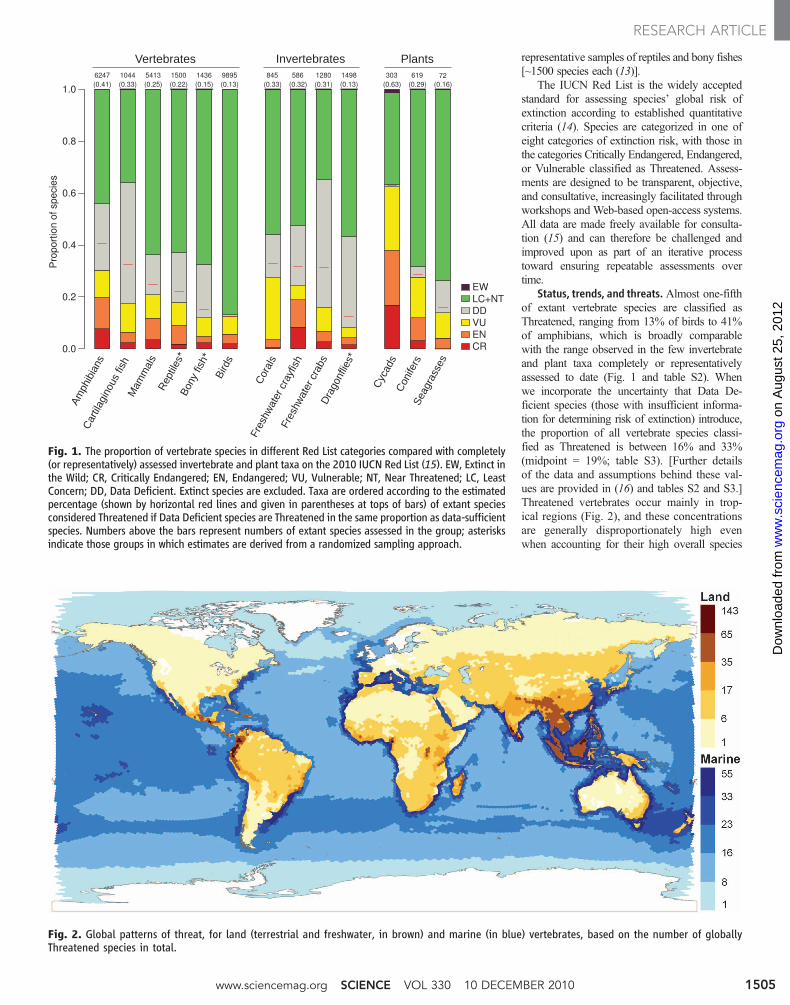
representative samples of reptiles and bony fishes[~1500 species each (13)].
The IUCN Red List is the widely acceptedstandard for assessing species’ global risk ofextinction according to established quantitativecriteria (14). Species are categorized in one ofeight categories of extinction risk, with those inthe categories Critically Endangered, Endangered,or Vulnerable classified as Threatened. Assess-ments are designed to be transparent, objective,and consultative, increasingly facilitated throughworkshops and Web-based open-access systems.All data are made freely available for consulta-tion (15) and can therefore be challenged andimproved upon as part of an iterative processtoward ensuring repeatable assessments overtime.
Status, trends, and threats. Almost one-fifthof extant vertebrate species are classified asThreatened, ranging from 13% of birds to 41%of amphibians, which is broadly comparablewith the range observed in the few invertebrateand plant taxa completely or representativelyassessed to date (Fig. 1 and table S2). Whenwe incorporate the uncertainty that Data De-ficient species (those with insufficient informa-tion for determining risk of extinction) introduce,the proportion of all vertebrate species classi-fied as Threatened is between 16% and 33%(midpoint = 19%; table S3). [Further detailsof the data and assumptions behind these val-ues are provided in (16) and tables S2 and S3.]Threatened vertebrates occur mainly in trop-ical regions (Fig. 2), and these concentrationsare generally disproportionately high evenwhen accounting for their high overall species
Fig. 1. The proportion of vertebrate species in different Red List categories compared with completely(or representatively) assessed invertebrate and plant taxa on the 2010 IUCN Red List (15). EW, Extinct inthe Wild; CR, Critically Endangered; EN, Endangered; VU, Vulnerable; NT, Near Threatened; LC, LeastConcern; DD, Data Deficient. Extinct species are excluded. Taxa are ordered according to the estimatedpercentage (shown by horizontal red lines and given in parentheses at tops of bars) of extant speciesconsidered Threatened if Data Deficient species are Threatened in the same proportion as data-sufficientspecies. Numbers above the bars represent numbers of extant species assessed in the group; asterisksindicate those groups in which estimates are derived from a randomized sampling approach.
Fig. 2. Global patterns of threat, for land (terrestrial and freshwater, in brown) and marine (in blue) vertebrates, based on the number of globallyThreatened species in total.
www.sciencemag.org SCIENCE VOL 330 10 DECEMBER 2010 1505
RESEARCH ARTICLE
on
Aug
ust 2
5, 2
012
ww
w.s
cien
cem
ag.o
rgD
ownl
oade
d fr
om
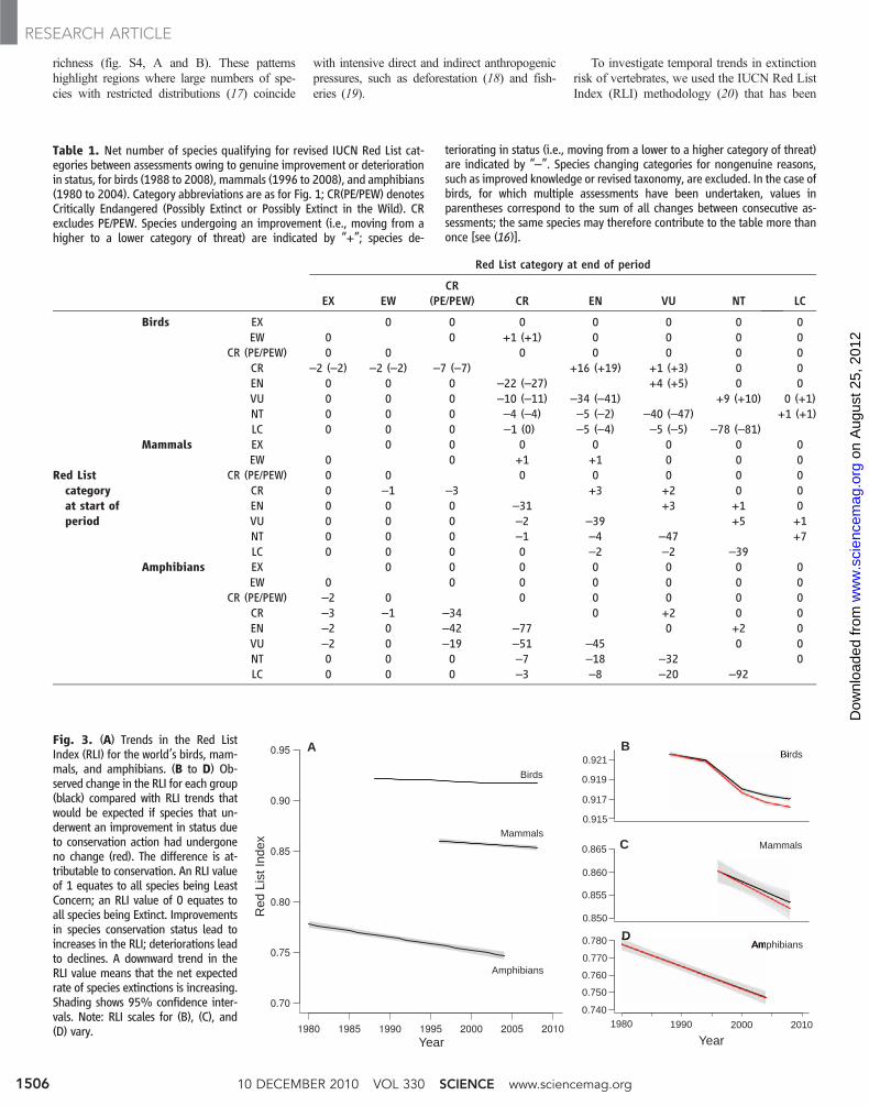
richness (fig. S4, A and B). These patternshighlight regions where large numbers of spe-cies with restricted distributions (17) coincide
with intensive direct and indirect anthropogenicpressures, such as deforestation (18) and fish-eries (19).
To investigate temporal trends in extinctionrisk of vertebrates, we used the IUCN Red ListIndex (RLI) methodology (20) that has been
Fig. 3. (A) Trends in the Red ListIndex (RLI) for the world’s birds, mam-mals, and amphibians. (B to D) Ob-served change in the RLI for each group(black) compared with RLI trends thatwould be expected if species that un-derwent an improvement in status dueto conservation action had undergoneno change (red). The difference is at-tributable to conservation. An RLI valueof 1 equates to all species being LeastConcern; an RLI value of 0 equates toall species being Extinct. Improvementsin species conservation status lead toincreases in the RLI; deteriorations leadto declines. A downward trend in theRLI value means that the net expectedrate of species extinctions is increasing.Shading shows 95% confidence inter-vals. Note: RLI scales for (B), (C), and(D) vary.
Table 1. Net number of species qualifying for revised IUCN Red List cat-egories between assessments owing to genuine improvement or deteriorationin status, for birds (1988 to 2008), mammals (1996 to 2008), and amphibians(1980 to 2004). Category abbreviations are as for Fig. 1; CR(PE/PEW) denotesCritically Endangered (Possibly Extinct or Possibly Extinct in the Wild). CRexcludes PE/PEW. Species undergoing an improvement (i.e., moving from ahigher to a lower category of threat) are indicated by “+”; species de-
teriorating in status (i.e., moving from a lower to a higher category of threat)are indicated by “–”. Species changing categories for nongenuine reasons,such as improved knowledge or revised taxonomy, are excluded. In the case ofbirds, for which multiple assessments have been undertaken, values inparentheses correspond to the sum of all changes between consecutive as-sessments; the same species may therefore contribute to the table more thanonce [see (16)].
Red List category at end of period
EX EWCR
(PE/PEW) CR EN VU NT LC
Red Listcategoryat start ofperiod
Birds EX 0 0 0 0 0 0 0EW 0 0 +1 (+1) 0 0 0 0
CR (PE/PEW) 0 0 0 0 0 0 0CR –2 (–2) –2 (–2) –7 (–7) +16 (+19) +1 (+3) 0 0EN 0 0 0 –22 (–27) +4 (+5) 0 0VU 0 0 0 –10 (–11) –34 (–41) +9 (+10) 0 (+1)NT 0 0 0 –4 (–4) –5 (–2) –40 (–47) +1 (+1)LC 0 0 0 –1 (0) –5 (–4) –5 (–5) –78 (–81)
Mammals EX 0 0 0 0 0 0 0EW 0 0 +1 +1 0 0 0
CR (PE/PEW) 0 0 0 0 0 0 0CR 0 –1 –3 +3 +2 0 0EN 0 0 0 –31 +3 +1 0VU 0 0 0 –2 –39 +5 +1NT 0 0 0 –1 –4 –47 +7LC 0 0 0 0 –2 –2 –39
Amphibians EX 0 0 0 0 0 0 0EW 0 0 0 0 0 0 0
CR (PE/PEW) –2 0 0 0 0 0 0CR –3 –1 –34 0 +2 0 0EN –2 0 –42 –77 0 +2 0VU –2 0 –19 –51 –45 0 0NT 0 0 0 –7 –18 –32 0LC 0 0 0 –3 –8 –20 –92
10 DECEMBER 2010 VOL 330 SCIENCE www.sciencemag.org1506
RESEARCH ARTICLE
on
Aug
ust 2
5, 2
012
ww
w.s
cien
cem
ag.o
rgD
ownl
oade
d fr
om
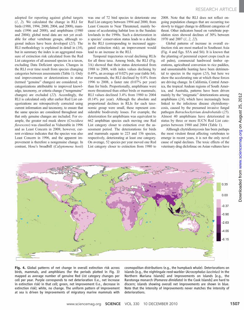
adopted for reporting against global targets(1, 2). We calculated the change in RLI forbirds (1988, 1994, 2000, 2004, and 2008), mam-mals (1996 and 2008), and amphibians (1980and 2004); global trend data are not yet avail-able for other vertebrate groups, although re-gional indices have been developed (21). TheRLI methodology is explained in detail in (16),but in summary the index is an aggregated mea-sure of extinction risk calculated from the RedList categories of all assessed species in a taxon,excluding Data Deficient species. Changes inthe RLI over time result from species changingcategories between assessments (Table 1). Onlyreal improvements or deteriorations in status(termed “genuine” changes) are considered; re-categorizations attributable to improved knowl-edge, taxonomy, or criteria change (“nongenuine”changes) are excluded (22). Accordingly, theRLI is calculated only after earlier Red List cat-egorizations are retrospectively corrected usingcurrent information and taxonomy, to ensure thatthe same species are considered throughout andthat only genuine changes are included. For ex-ample, the greater red musk shrew (Crociduraflavescens) was classified as Vulnerable in 1996and as Least Concern in 2008; however, cur-rent evidence indicates that the species was alsoLeast Concern in 1996, and the apparent im-provement is therefore a nongenuine change. Incontrast, Hose’s broadbill (Calyptomena hosii)
was one of 72 bird species to deteriorate oneRed List category between 1994 and 2000, fromLeast Concern to Near Threatened, mainly be-cause of accelerating habitat loss in the Sundaiclowlands in the 1990s. Such a deterioration ina species’ conservation status leads to a declinein the RLI (corresponding to increased aggre-gated extinction risk); an improvement wouldlead to an increase in the RLI.
Temporal trajectories reveal declining RLIsfor all three taxa. Among birds, the RLI (Fig.3A) showed that their status deteriorated from1988 to 2008, with index values declining by0.49%, an average of 0.02% per year (table S4).For mammals, the RLI declined by 0.8% from1996 to 2008, a faster rate (0.07% per year)than for birds. Proportionally, amphibians weremore threatened than either birds or mammals;RLI values declined 3.4% from 1980 to 2004(0.14% per year). Although the absolute andproportional declines in RLIs for each taxo-nomic group were small, these represent con-siderable biodiversity losses. For example, thedeterioration for amphibians was equivalent to662 amphibian species each moving one RedList category closer to extinction over the as-sessment period. The deteriorations for birdsand mammals equate to 223 and 156 species,respectively, deteriorating at least one category.On average, 52 species per year moved one RedList category closer to extinction from 1980 to
2008. Note that the RLI does not reflect on-going population changes that are occurring tooslowly to trigger change to different categories ofthreat. Other indicators based on vertebrate pop-ulation sizes showed declines of 30% between1970 and 2007 (1, 2, 22).
Global patterns of increase in overall ex-tinction risk are most marked in Southeast Asia(Fig. 4 and figs. S5A and S6). It is known thatthe planting of perennial export crops (such asoil palm), commercial hardwood timber op-erations, agricultural conversion to rice paddies,and unsustainable hunting have been detrimen-tal to species in the region (23), but here weshow the accelerating rate at which these forcesare driving change. In California, Central Amer-ica, the tropical Andean regions of South Amer-ica, and Australia, patterns have been drivenmainly by the “enigmatic” deteriorations amongamphibians (24), which have increasingly beenlinked to the infectious disease chytridiomy-cosis, caused by the presumed invasive fungalpathogen Batrachochytrium dendrobatidis (25).Almost 40 amphibians have deteriorated instatus by three or more IUCN Red List cate-gories between 1980 and 2004 (Table 1).
Although chytridiomycosis has been perhapsthe most virulent threat affecting vertebrates toemerge in recent years, it is not the only novelcause of rapid declines. The toxic effects of theveterinary drug diclofenac on Asian vultures have
Fig. 4. Global patterns of net change in overall extinction risk acrossbirds, mammals, and amphibians (for the periods plotted in Fig. 3)mapped as average number of genuine Red List category changes percell per year. Purple corresponds to net deterioration (i.e., net increasein extinction risk) in that cell; green, net improvement (i.e., decrease inextinction risk); white, no change. The uniform pattern of improvementat sea is driven by improvements of migratory marine mammals with
cosmopolitan distributions (e.g., the humpback whale). Deteriorations onislands [e.g., the nightingale reed-warbler (Acrocephalus luscinius) in theNorthern Mariana Islands] and improvements on islands [e.g., theRarotonga monarch (Pomarea dimidiata) in the Cook Islands] are hard todiscern; islands showing overall net improvements are shown in blue.Note that the intensity of improvements never matches the intensity ofdeteriorations.
www.sciencemag.org SCIENCE VOL 330 10 DECEMBER 2010 1507
RESEARCH ARTICLE
on
Aug
ust 2
5, 2
012
ww
w.s
cien
cem
ag.o
rgD
ownl
oade
d fr
om
caused estimated population declines exceeding99% over the past two decades in certain Gypsspecies, and have resulted in three species movingfrom Near Threatened to Critically Endangeredbetween 1994 and 2000. Numbers of Tasmaniandevils (Sarcophilus harrisii) have fallen by morethan 60% in the past 10 years because of theemergence of devil facial tumor disease (result-ing in three step changes from Least Concern toEndangered). Climate change is not yet ade-quately captured by the IUCN Red List (26, 27)but has been directly implicated in the deterio-rating status of several vertebrates and may in-teract with other threats to hasten extinction (28).However, there is no evidence of a parallel to thesystemwide deteriorations documented for reef-building corals affected by bleaching eventsrelated to El Niño–Southern Oscillation occur-rences (29).
Most deteriorations in status are reversible,but in 13% of cases they have resulted in extinc-tion. Two bird species—the kamao (Myadestesmyadestinus) from Hawaii and the Alaotra grebe(Tachybaptus rufolavatus) from Madagascar—became extinct between 1988 and 2008, and afurther six Critically Endangered species havebeen flagged as “possibly extinct” during thisperiod (Table 1 and table S5). At least nine am-phibian species vanished during the two decadesafter 1980, including the golden toad (Inciliusperiglenes) from Costa Rica and both of Austra-lia’s unique gastric-brooding frog species (genusRheobatrachus); a further 95 became possiblyextinct, 18 of them harlequin toads in the Neo-tropical genus Atelopus (23% of species). Nomammals are listed as Extinct for the period1996 to 2008, although the possible extinctionof the Yangtze River dolphin (Lipotes vexillifer)would be the first megafauna vertebrate speciesextinction since the Caribbean monk seal in the1950s (30).
Estimates of conservation success. Theseresults support previous findings that the stateof biodiversity continues to decline, despite in-creasing trends in responses such as protectedareas coverage and adoption of national legislation(1, 2). Next, we asked whether conservationefforts have made any measurable contributionto reducing declines or improving the status ofbiodiversity.
The RLI trends reported here are derivedfrom 928 cases of recategorization on the IUCNRed List (Table 1 and table S6), but not all ofthese refer to deteriorations. In 7% of cases(68/928), species underwent an improvement instatus, all but four due to conservation action.For example, the Asian crested ibis (Nipponianippon) changed from Critically Endangeredin 1994 to Endangered in 2000 owing to pro-tection of nesting trees, control of agrochem-icals in rice fields, and prohibition of firearms;the four exceptions were improvements result-ing from natural processes, such as unassistedhabitat regeneration (tables S7 and S8). Nearlyall of these improvements involved mammals
and birds, where the history of conservation ex-tends farther back and where the bulk of species-focused conservation funding and attention isdirected (31). Only four amphibian species un-derwent improvements, because the amphib-ian extinction crisis is such a new phenomenonand a plan for action has only recently beendeveloped (32).
To estimate the impact of conservation suc-cesses, we compared the observed changes inthe RLI with the RLI trends expected if all 64species that underwent an improvement instatus due to conservation action had not doneso (16). Our explicit assumption is that in theabsence of conservation, these species wouldhave remained unchanged in their original cat-egory, although we note that this approach isconservative because it is likely that some wouldhave deteriorated [in the sense of (6)]. The re-sulting difference between the two RLIs can beattributed to conservation. We show that the in-dex would have declined by an additional 18%for both birds and mammals in the absence ofconservation (Fig. 3, B andC, and table S4). Therewas little difference for amphibians (+1.4%; Fig.3D) given the paucity of species improvements.For birds, conservation action reduced the de-cline in the RLI from 0.58% to 0.49%, equivalentto preventing 39 species each moving one RedList category closer to extinction between 1988and 2008. For mammals, conservation actionreduced the RLI decline from 0.94% to 0.8%,equivalent to preventing 29 species moving onecategory closer to extinction between 1996 and2008.
These results grossly underestimate the im-pact of conservation, because they do not ac-count for species that either (i) would havedeteriorated further in the absence of conser-vation actions, or (ii) improved numerically, al-though not enough to change Red List status.As an example among the former, the blackstilt (Himantopus novaezelandiae) would havegone extinct were it not for reintroduction andpredator control efforts, and its Critically En-dangered listing has thus remained unchanged(6). Among the latter, conservation efforts im-proved the total population numbers of 33 Crit-ically Endangered birds during the period 1994to 2004, but not sufficiently for any species tobe moved to a lower category of threat (33). Asmany as 9% of mammals, birds, and amphib-ians classified as Threatened or Near Threat-ened have stable or increasing populations (15)largely due to conservation efforts, but it willtake time for these successes to translate intoimprovements in status. Conservation effortshave also helped to avoid the deterioration instatus of Least Concern species. Finally, con-servation actions have benefited many otherThreatened species besides birds, mammals, andamphibians, but this cannot yet be quantifiedthrough the RLI for groups that have beenassessed only once [e.g., salmon shark (Lamnaditropis) numbers have improved as the result
of a 1992 U.N. moratorium on large-scale pe-lagic driftnet fisheries].
Confronting threats. Species recovery iscomplex and case-specific, but threat mitigationis always required. We investigated the maindrivers of increased extinction risk by identify-ing, for each species that deteriorated in status,the primary threat responsible for that change. Tounderstand which drivers of increased extinctionrisk are being mitigated most successfully, weidentified, for each species that improved in sta-tus, the primary threat offset by successful con-servation (table S6).
We found that for any single threat, re-gardless of the taxa involved, deteriorationsoutnumber improvements; conservation actionshave not yet succeeded in offsetting any ma-jor driver of increased extinction risk (fig. S7).On a per-species basis, amphibians are in anespecially dire situation, suffering the doublejeopardy of exceptionally high levels of threatcoupled with low levels of conservation effort.Still, there are conservation successes amongbirds and mammals, and here we investigatethe degree to which particular threats have beenaddressed.
Conservation actions have been relativelysuccessful at offsetting the threat of invasivealien species for birds and mammals: For everyfive species that deteriorated in status becauseof this threat, two improved through its mit-igation. These successes have resulted from theimplementation of targeted control or eradica-tion programs [e.g., introduced cats have beeneradicated from 37 islands since the mid-1980s(34)] coupled with reintroduction initiatives [e.g.,the Seychelles magpie-robin (Copsychus sechel-larum) population was 12 to 15 birds in 1965but had increased to 150 birds by 2005 (fig.S8)]. Many of these improvements have oc-curred on small islands but also in Australia,owing in part to control of the red fox (Vulpesvulpes) (Fig. 4 and fig. S5B). However, amongamphibians, only a single species—the Mallor-can midwife toad (Alytes muletensis)—improvedin status as a result of mitigation of the threatposed by invasive alien species, compared with208 species that deteriorated. This is becausethere is still a lack of understanding of the path-ways by which chytridiomycosis is spread andmay be controlled, and in situ conservation man-agement options are only just beginning to beidentified [e.g., (35)]. Meanwhile, the establish-ment of select, targeted captive populations withthe goal of reintroducing species in the wildmay offer valuable opportunities once impactsin their native habitat are brought under control[e.g., the Kihansi spray toad (Nectophrynoidesasperginis), categorized as Extinct in the Wildbecause of drastic alteration of its spray zonehabitat].
For mammals and birds, the threats lead-ing to habitat loss have been less effectivelyaddressed relative to that of invasive alien spe-cies: For every 10 species deteriorating as a
10 DECEMBER 2010 VOL 330 SCIENCE www.sciencemag.org1508
RESEARCH ARTICLE
on
Aug
ust 2
5, 2
012
ww
w.s
cien
cem
ag.o
rgD
ownl
oade
d fr
om
result of agricultural expansion, fewer than 1improved because of mitigation of this threat.Protected areas are an essential tool to safe-guard biodiversity from habitat loss, but theprotected areas network remains incompleteand nonstrategic relative to Threatened species(17), and reserve management can be ineffec-tive (36). Numerous Threatened species are re-stricted to single sites, many still unprotected(37), and these present key opportunities toslow rates of extinction. In the broader matrix ofunprotected land, agri-environmental schemescould offer important biodiversity benefits, pro-vided that management policies are sufficientto enhance populations of Threatened species(38).
Hunting has been relatively poorly addressedin mammals (62 deteriorations, 6 improve-ments) when compared with birds (31 deteriora-tions, 9 improvements). In birds, successes haveresulted mainly from targeted protection [e.g.,Lear’s macaw (Anodorhynchus leari) changedfrom Critically Endangered to Endangered asa result of active protection of the Toca Velha/Serra Branca cliffs in Brazil], but also from en-forcement of legislation (e.g., hunting bans) andharvest management measures. Many mammalssubject to hunting occur at low densities, havelarge home ranges, and/or are large-bodied. Al-though active site-based protection has contrib-uted to an improvement in the status of someof these species, site protection alone is ofteninsufficient if not complemented by appropriatelegislation, biological management, and effec-tive enforcement (39). For example, a combina-tion of the Convention on International Tradein Endangered Species of Wild Flora and Fauna(CITES) and enactment of the Vicuña Conven-tion, which prohibited domestic exploitation andmandated the establishment of protected areas,has helped to improve the status of the vicuña(Vicugna vicugna) from Near Threatened to LeastConcern.
The threat of fisheries has been mitigatedrelatively more effectively for marine mammals(4 deteriorations, 2 improvements) than for birds(10 deteriorations, 0 improvements), reflectingboth the time when drivers first emerged and thepast influence of supranational conservationpolicy. Among historically exploited, long-livedmammals, for example, the humpback whale(Megaptera novaeangliae) has benefited fromprotection from commercial whaling (since1955) and has improved from Vulnerable toLeast Concern. Declines among slow-breedingseabirds (particularly albatrosses and petrels; fig.S9) are mainly a consequence of increasingincidental by-catch resulting from the growth ofcommercial fisheries, primarily those that uselong-line and trawling methods. Legislativetools, such as the recently enacted multilateralAgreement on the Conservation of Albatrossesand Petrels (40), may yet deliver dividends bycoordinating international action to reduce fish-eries mortality of these highly migratory species.
Binding legislation and harvest managementstrategies also are urgently needed to addressthe disproportionate impact of fisheries oncartilaginous fishes (fig. S10).
We have no data on the relationship betweenexpenditure on biodiversity and conservation suc-cess. A disproportionate percentage of annualconservation funding is spent in economicallywealthy countries (41), where there are generallyfewer Threatened species (Fig. 2 and fig. S4B)and the disparity between success and failureappears less evident (Fig. 4). Southeast Asia, bycontrast, has the greatest imbalance betweenimproving and deteriorating trends, emphasizingthe need there for greater investment of resourcesand effort.
Conclusions. Our study confirms previousreports of continued biodiversity losses. Wealso find evidence of notable conservation suc-cesses illustrating that targeted, strategic con-servation action can reduce the rate of lossrelative to that anticipated without such ef-forts. Nonetheless, the current level of action isoutweighed by the magnitude of threat, andconservation responses will need to be sub-stantially scaled up to combat the extinction cri-sis. Even with recoveries, many species remainconservation-dependent, requiring sustained,long-term investment (42); for example, actionshave been under way for 30 years for the goldenlion tamarin (Leontopithecus rosalia), 70 yearsfor the whooping crane (Grus americana), and115 years for the white rhinoceros (Ceratothe-rium simum).
Halting biodiversity loss will require coordi-nated efforts to safeguard and effectively man-age critical sites, complemented by broad-scaleaction to minimize further destruction, degra-dation, and fragmentation of habitats (37, 39)and to promote sustainable use of productivelands and waters in a way that is supportive tobiodiversity. Effective implementation and en-forcement of appropriate legislation could deliverquick successes; for example, by-catch mitiga-tion measures, shark-finning bans, and mean-ingful catch limits have considerable potentialto reduce declines in marine species (19). The2010 biodiversity target may not have been met,but conservation efforts have not been a failure.The challenge is to remedy the current shortfallin conservation action to halt the attrition ofglobal biodiversity.
References and Notes1. S. H. M. Butchart et al., Science 328, 1164 (2010);
10.1126/science.1187512.2. Secretariat of the Convention on Biological Diversity,
Global Biodiversity Outlook 3 (Convention on BiologicalDiversity, Montréal, 2010).
3. S. L. Pimm, G. J. Russell, J. L. Gittleman, T. M. Brooks,Science 269, 347 (1995).
4. TEEB, The Economics and Ecosystems of Biodiversity:An Interim Report (European Communities, Cambridge,2008).
5. UNEP, Report of the Sixth Meeting of the Conference ofthe Parties to the Convention on Biological Diversity(UNEP/CBD/COP/20/Part 2) Strategic Plan Decision VI/26
in CBD (UNEP, Nairobi, 2002); www.cbd.int/doc/meetings/cop/cop-06/official/cop-06-20-en.pdf.
6. S. H. M. Butchart, A. J. Stattersfield, N. J. Collar, Oryx 40,266 (2006).
7. A. S. L. Rodrigues, Science 313, 1051 (2006).8. P. F. Donald et al., Science 317, 810 (2007).9. T. M. Brooks, S. J. Wright, D. Sheil, Conserv. Biol. 23,
1448 (2009).10. P. J. Ferraro, S. K. Pattanayak, PLoS Biol. 4, e105
(2006).11. J. W. Terborgh, Conserv. Biol. 2, 402 (1988).12. B. Clucas, K. Mchugh, T. Caro, Biodivers. Conserv. 17,
1517 (2008).13. J. E. M. Baillie et al., Cons. Lett. 1, 18 (2008).14. G. M. Mace et al., Conserv. Biol. 22, 1424
(2008).15. IUCN Red List of Threatened Species. Version 2010.3
(IUCN, 2010; www.iucnredlist.org).16. See supporting material on Science Online.17. A. S. L. Rodrigues et al., Bioscience 54, 1092
(2004).18. M. C. Hansen et al., Proc. Natl. Acad. Sci. U.S.A. 105,
9439 (2008).19. B. Worm et al., Science 325, 578 (2009).20. S. H. M. Butchart et al., PLoS One 2, e140 (2007).21. N. K. Dulvy, S. Jennings, S. I. Rogers, D. L. Maxwell,
Can. J. Fish. Aquat. Sci. 63, 1267 (2006).22. B. Collen et al., Conserv. Biol. 23, 317 (2009).23. N. S. Sodhi, L. P. Koh, B. W. Brook, P. K. Ng, Trends Ecol.
Evol. 19, 654 (2004).24. S. N. Stuart et al., Science 306, 1783 (2004);
10.1126/science.1103538.25. D. B. Wake, V. T. Vredenburg, Proc. Natl. Acad. Sci. U.S.A.
105 (suppl. 1), 11466 (2008).26. H. R. Akçakaya, S. H. M. Butchart, G. M. Mace,
S. N. Stuart, C. Hilton-Taylor, Glob. Change Biol. 12,2037 (2006).
27. B. W. Brook et al., Biol. Lett. 5, 723 (2009).28. W. F. Laurance, D. C. Useche, Conserv. Biol. 23, 1427
(2009).29. K. E. Carpenter et al., Science 321, 560 (2008);
10.1126/science.1159196.30. S. T. Turvey et al., Biol. Lett. 3, 537 (2007).31. N. Sitas, J. E. M. Baillie, N. J. B. Isaac, Anim. Conserv. 12,
231 (2009).32. C. Gascon et al., Eds., Amphibian Conservation Action
Plan (IUCN/SSC Amphibian Specialist Group, Gland,Switzerland, 2007).
33. M. de L. Brooke et al., Conserv. Biol. 22, 417(2008).
34. M. Nogales et al., Conserv. Biol. 18, 310 (2004).35. R. N. Harris et al., ISME J. 3, 818 (2009).36. L. M. Curran et al., Science 303, 1000 (2004).37. T. H. Ricketts et al., Proc. Natl. Acad. Sci. U.S.A. 102,
18497 (2005).38. D. Kleijn et al., Ecol. Lett. 9, 243 (2006).39. C. Boyd et al., Cons. Lett. 1, 37 (2008).40. J. Cooper et al., Mar. Ornithol. 34, 1 (2006).41. A. N. James, K. J. Gaston, A. Balmford, Nature 401,
323 (1999).42. J. M. Scott, D. D. Goble, A. M. Haines, J. A. Wiens,
M. C. Neel, Cons. Lett. 3, 91 (2010).43. We are indebted to the more than 3000 species
experts who devoted their knowledge, intellect, and timeto the compilation of vertebrate data on the IUCN RedList. Full acknowledgments are provided in the supportingonline material.
Supporting Online Materialwww.sciencemag.org/cgi/content/full/science.1194442/DC1Materials and MethodsFigs. S1 to S10Tables S1 to S9ReferencesAcknowledgments
29 June 2010; accepted 11 October 2010Published online 26 October 2010;10.1126/science.1194442
www.sciencemag.org SCIENCE VOL 330 10 DECEMBER 2010 1509
RESEARCH ARTICLE
on
Aug
ust 2
5, 2
012
ww
w.s
cien
cem
ag.o
rgD
ownl
oade
d fr
om
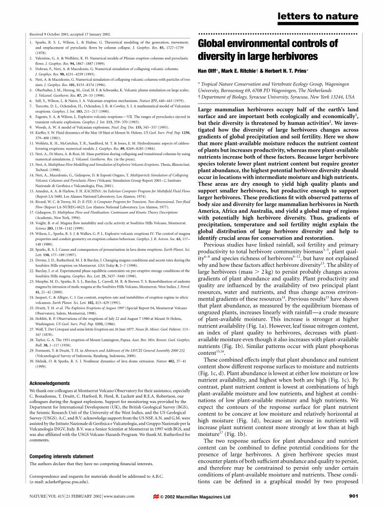
letters to nature
NATURE | VOL 415 | 21 FEBRUARY 2002 | www.nature.com 901
Received 9 October 2001; accepted 17 January 2002.
1. Sparks, R. S. J., Wilson, L. & Hulme, G. Theoretical modeling of the generation, movement,
and emplacement of pyroclastic ¯ows by column collapse. J. Geophys. Res. 83, 1727±1739
(1978).
2. Valentine, G. A. & Wolhletz, K. H. Numerical models of Plinian eruption columns and pyroclastic
¯ows. J. Geophys. Res. 94, 1867±1887 (1989).
3. Dobran, F., Neri, A. & Macedonio, G. Numerical simulation of collapsing volcanic columns.
J. Geophys. Res. 98, 4231±4259 (1993).
4. Neri, A. & Macedonio, G. Numerical simulation of collapsing volcanic columns with particles of two
sizes. J. Geophys. Res. 101, 8153±8174 (1996).
5. Oberhuber, J. M., Herzog, M., Graf, H. F. & Schwanke, K. Volcanic plume simulation on large scales.
J. Volcanol. Geotherm. Res. 87, 29±53 (1998).
6. Self, S., Wilson, L. & Nairn, I. A. Vulcanian eruption mechanisms. Nature 277, 440±443 (1979).
7. Turcotte, D. L., Ockendon, H., Ockendon, J. R. & Cowley, S. J. A mathematical model of Vulcanian
eruptions. Geophys. J. Int. 103, 211±217 (1990).
8. Fagents, S. A. & Wilson, L. Explosive volcanic eruptionsÐVII. The ranges of pyroclastics ejected in
transient volcanic explosions. Geophys. J. Int. 113, 359±370 (1993).
9. Woods, A. W. A model of Vulcanian explosions. Nucl. Eng. Des. 155, 345±357 (1995).
10. Kieffer, S. W. Fluid dynamics of the May 18 blast at Mount St. Helens. US Geol. Surv. Prof. Pap. 1250,
379±400 (1981).
11. Wohletz, K. H., McGetchin, T. R., Sandford, M. T. & Jones, E. M. Hydrodynamic aspects of caldera-
forming eruptions: numerical models. J. Geophys. Res. 89, 8269±8285 (1984).
12. Neri, A., Di Muro, A. & Rosi, M. Mass partition during collapsing and transitional columns by using
numerical simulations. J. Volcanol. Geotherm. Res. (in the press).
13. Neri, A. Multiphase Flow Modelling and Simulation of Explosive Volcanic Eruptions. Thesis, Illinois Inst.
Technol. (1998).
14. Neri, A., Macedonio, G., Gidaspow, D. & Esposti Ongaro, T. Multiparticle Simulation of Collapsing
Volcanic Columns and Pyroclastic Flows (Volcanic Simulation Group Report 2001±2, Instituto
Nazionale di Geo®sica e Vulcanologia, Pisa, 2001).
15. Amsden, A. A. & Harlow, F. H. KACHINA: An Eulerian Computer Program for Multi®eld Fluid Flows
(Report LA-5680, Los Alamos National Laboratory, Los Alamos, 1974).
16. Rivard, W. C. & Torrey, M. D. K-FIX: A Computer Program for Transient, Two-dimensional, Two-¯uid
Flow (Report LA-NUREG-6623, Los Alamos National Laboratory, Los Alamos, 1977).
17. Gidaspow, D. Multiphase Flow and Fluidization: Continuum and Kinetic Theory Descriptions
(Academic, New York, 1994).
18. Voight, B. et al. Magma ¯ow instability and cyclic activity at SoufrieÁre Hills Volcano, Montserrat.
Science 283, 1138±1142 (1999).
19. Wilson, L., Sparks, R. S. J. & Walker, G. P. L. Explosive volcanic eruptions IV. The control of magma
properties and conduit geometry on eruption column behaviour. Geophys. J. R. Astron. Soc. 63, 117±
148 (1980).
20. Sparks, R. S. J. Causes and consequences of pressurisation in lava dome eruptions. Earth Planet. Sci.
Lett. 150, 177±189 (1997).
21. Devine, J. D., Rutherford, M. J. & Barclay, J. Changing magma conditions and ascent rates during the
SoufrieÁre Hills eruption on Montserrat. GSA Today 8, 2±7 (1998).
22. Barclay, J. et al. Experimental phase equilibria constraints on pre-eruptive storage conditions of the
SoufrieÁre Hills magma. Geophys. Res. Lett. 25, 3437±3440 (1998).
23. Murphy, M. D., Sparks, R. S. J., Barclay, J., Carroll, M. R. & Brewer, T. S. Remobilization of andesite
magma by intrusion of ma®c magma at the SoufrieÁre Hills Volcano, Montserrat, West Indies. J. Petrol.
41, 21±42 (2000).
24. Jaupart, C. & AlleÁgre, C. J. Gas content, eruption rate and instabilities of eruption regime in silicic
volcanoes. Earth Planet. Sci. Lett. 102, 413±429 (1991).
25. Druitt, T. H. et al. The Explosive Eruptions of August 1997 (Special Report 04, Montserrat Volcano
Observatory, Salem, Montserrat, 1998).
26. Hoblitt, R. P. Observations of the eruptions of July 22 and August 7 1980 at Mount St Helens,
Washington. US Geol. Surv. Prof. Pap. 1335, (1986).
27. Wolf, T. Der Cotopaxi und seine letzte Eruption am 26 Juni 1877. Neues Jb. Miner. Geol. PalaÈont. 113±
167 (1878).
28. Taylor, G. A. The 1951 eruption of Mount Lamington, Papua. Aust. Bur. Min. Resour. Geol. Geophys.
Bull. 38, 1±117 (1958).
29. Formenti, Y. & Druitt, T. H. in Abstracts and Addresses of the IAVCEI General Assembly 2000 232
(Volcanological Survey of Indonesia, Bandung, Indonesia, 2000).
30. Melnik, O. & Sparks, R. S. J. Nonlinear dynamics of lava dome extrusion. Nature 402, 37±41
(1999).
Acknowledgements
We thank our colleagues at Montserrat Volcano Observatory for their assistance, especiallyC. Bonadonna, T. Druitt, C. Harford, R. Herd, R. Luckett and R.E.A. Robertson, ourcolleagues during the August explosions. Support for monitoring was provided by theDepartment for International Development (UK), the British Geological Survey (BGS),the Seismic Research Unit of the University of the West Indies, and the US GeologicalSurvey (USGS). A.C. and B.V. acknowledge support from the US NSF. A.N. and G.M. wereassisted by the Istituto Nazionale di Geo®sica e Vulcanologia, and Gruppo Nazionale per laVulcanologia INGV, Italy. B.V. was a Senior Scientist at Montserrat in 1997 with BGS, andwas also af®liated with the USGS Volcano Hazards Program. We thank M. Rutherford forcomments.
Competing interests statement
The authors declare that they have no competing ®nancial interests.
Correspondence and requests for materials should be addressed to A.B.C.(e-mail: [email protected]).
.................................................................Global environmental controls ofdiversity in large herbivoresHan Olff*, Mark E. Ritchie² & Herbert H. T. Prins*
* Tropical Nature Conservation and Vertebrate Ecology Group, WageningenUniversity, Bornsesteeg 69, 6708 PD Wageningen, The Netherlands² Department of Biology, Syracuse University, Syracuse, New York 13244, USA..............................................................................................................................................
Large mammalian herbivores occupy half of the earth's landsurface and are important both ecologically and economically1,but their diversity is threatened by human activities2. We inves-tigated how the diversity of large herbivores changes acrossgradients of global precipitation and soil fertility. Here we showthat more plant-available moisture reduces the nutrient contentof plants but increases productivity, whereas more plant-availablenutrients increase both of these factors. Because larger herbivorespecies tolerate lower plant nutrient content but require greaterplant abundance, the highest potential herbivore diversity shouldoccur in locations with intermediate moisture and high nutrients.These areas are dry enough to yield high quality plants andsupport smaller herbivores, but productive enough to supportlarger herbivores. These predictions ®t with observed patterns ofbody size and diversity for large mammalian herbivores in NorthAmerica, Africa and Australia, and yield a global map of regionswith potentially high herbivore diversity. Thus, gradients ofprecipitation, temperature and soil fertility might explain theglobal distribution of large herbivore diversity and help toidentify crucial areas for conservation and restoration.
Previous studies have linked rainfall, soil fertility and primaryproductivity to total herbivore community biomass3±5, plant qual-ity6±8 and species richness of herbivores9±12, but have not explainedwhy and how these factors affect herbivore diversity13. The ability oflarge herbivores (mass . 2 kg) to persist probably changes acrossgradients of plant abundance and quality. Plant productivity andquality are in¯uenced by the availability of two principal plantresources, water and nutrients, and thus change across environ-mental gradients of these resources14. Previous results15 have shownthat plant abundance, as measured by the equilibrium biomass ofungrazed plants, increases linearly with rainfallÐa crude measureof plant-available moisture. This increase is stronger at highernutrient availability (Fig. 1a). However, leaf tissue nitrogen content,an index of plant quality to herbivores, decreases with plant-available moisture even though it also increases with plant-availablenutrients (Fig. 1b). Similar patterns occur with plant phosphoruscontent15,16.
These combined effects imply that plant abundance and nutrientcontent show different response surfaces to moisture and nutrients(Fig. 1c, d). Plant abundance is lowest at either low moisture or lownutrient availability, and highest when both are high (Fig. 1c). Bycontrast, plant nutrient content is lowest at combinations of highplant-available moisture and low nutrients, and highest at combi-nations of low plant-available moisture and high nutrients. Weexpect the contours of the response surface for plant nutrientcontent to be concave at low moisture and relatively horizontal athigh moisture (Fig. 1d), because an increase in nutrients willincrease plant nutrient content more strongly at low than at highmoisture17 (Fig. 1b).
The two response surfaces for plant abundance and nutrientcontent can be combined to de®ne potential conditions for thepresence of large herbivores. A given herbivore species mustencounter plants of both suf®cient abundance and quality to persist,and therefore may be constrained to persist only under certainconditions of plant-available moisture and nutrients. These condi-tions can be de®ned in a graphical model by two proposed
© 2002 Macmillan Magazines Ltd
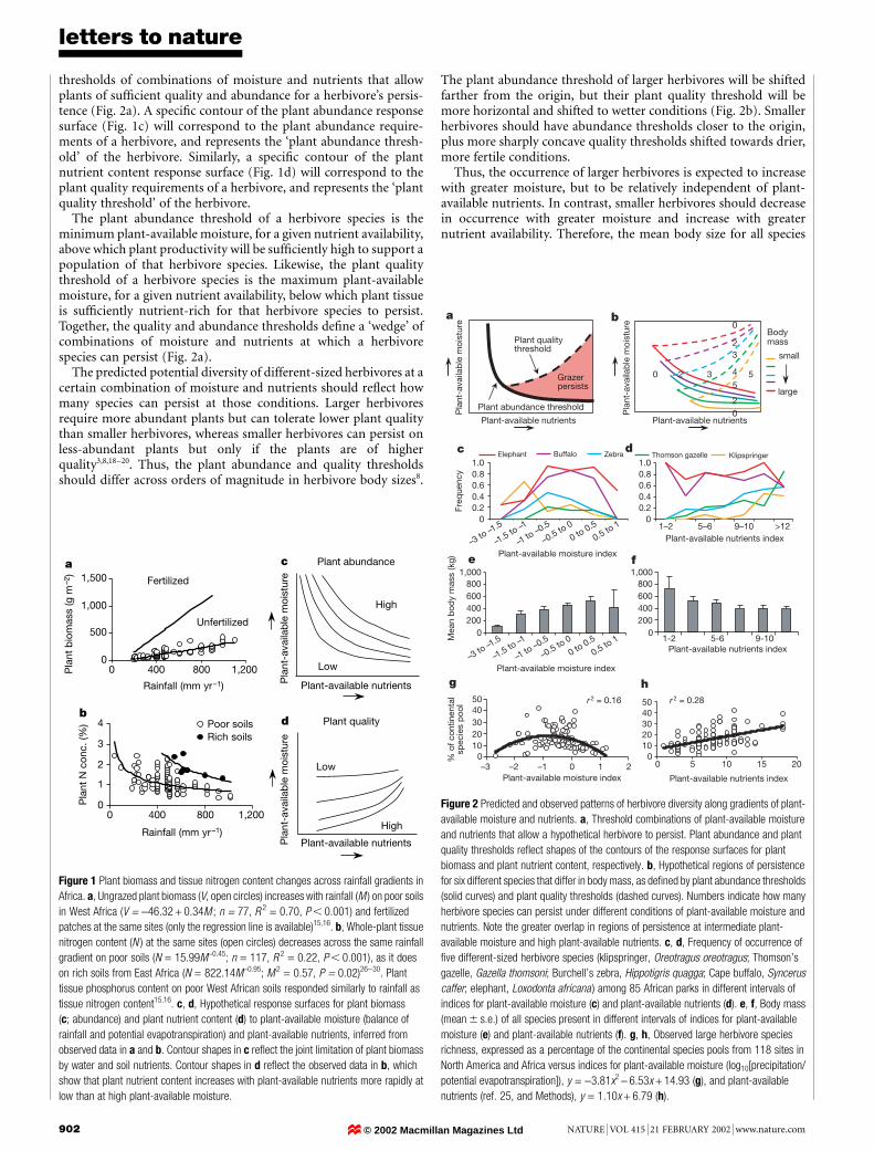
letters to nature
902 NATURE | VOL 415 | 21 FEBRUARY 2002 | www.nature.com
thresholds of combinations of moisture and nutrients that allowplants of suf®cient quality and abundance for a herbivore's persis-tence (Fig. 2a). A speci®c contour of the plant abundance responsesurface (Fig. 1c) will correspond to the plant abundance require-ments of a herbivore, and represents the `plant abundance thresh-old' of the herbivore. Similarly, a speci®c contour of the plantnutrient content response surface (Fig. 1d) will correspond to theplant quality requirements of a herbivore, and represents the `plantquality threshold' of the herbivore.
The plant abundance threshold of a herbivore species is theminimum plant-available moisture, for a given nutrient availability,above which plant productivity will be suf®ciently high to support apopulation of that herbivore species. Likewise, the plant qualitythreshold of a herbivore species is the maximum plant-availablemoisture, for a given nutrient availability, below which plant tissueis suf®ciently nutrient-rich for that herbivore species to persist.Together, the quality and abundance thresholds de®ne a `wedge' ofcombinations of moisture and nutrients at which a herbivorespecies can persist (Fig. 2a).
The predicted potential diversity of different-sized herbivores at acertain combination of moisture and nutrients should re¯ect howmany species can persist at those conditions. Larger herbivoresrequire more abundant plants but can tolerate lower plant qualitythan smaller herbivores, whereas smaller herbivores can persist onless-abundant plants but only if the plants are of higherquality3,8,18±20. Thus, the plant abundance and quality thresholdsshould differ across orders of magnitude in herbivore body sizes8.
The plant abundance threshold of larger herbivores will be shiftedfarther from the origin, but their plant quality threshold will bemore horizontal and shifted to wetter conditions (Fig. 2b). Smallerherbivores should have abundance thresholds closer to the origin,plus more sharply concave quality thresholds shifted towards drier,more fertile conditions.
Thus, the occurrence of larger herbivores is expected to increasewith greater moisture, but to be relatively independent of plant-available nutrients. In contrast, smaller herbivores should decreasein occurrence with greater moisture and increase with greaternutrient availability. Therefore, the mean body size for all species
0
1
2
3
4
0 400 800 1,200
Pla
nt N
con
c. (%
) Poor soilsRich soils
0
500
1,000
1,500
0 400 800 1,200
Rainfall (mm yr–1)
Rainfall (mm yr–1)
Pla
nt b
iom
ass
(g m
–2)
Fertilized
Unfertilized
a
b
High
Low
c Plant abundance
Plant-available nutrients
Plant-available nutrients
High
Low
Pla
nt-a
vaila
ble
moi
stur
eP
lant
-ava
ilab
le m
oist
ure
d Plant quality
Figure 1 Plant biomass and tissue nitrogen content changes across rainfall gradients in
Africa. a, Ungrazed plant biomass (V, open circles) increases with rainfall (M ) on poor soils
in West Africa (V = -46.32 + 0.34M ; n = 77, R 2 = 0.70, P , 0.001) and fertilized
patches at the same sites (only the regression line is available)15,16. b, Whole-plant tissue
nitrogen content (N ) at the same sites (open circles) decreases across the same rainfall
gradient on poor soils (N = 15.99M-0.45; n = 117, R 2 = 0.22, P , 0.001), as it does
on rich soils from East Africa (N = 822.14M-0.95; M 2 = 0.57, P = 0.02)26±30. Plant
tissue phosphorus content on poor West African soils responded similarly to rainfall as
tissue nitrogen content15,16. c, d, Hypothetical response surfaces for plant biomass
(c; abundance) and plant nutrient content (d) to plant-available moisture (balance of
rainfall and potential evapotranspiration) and plant-available nutrients, inferred from
observed data in a and b. Contour shapes in c re¯ect the joint limitation of plant biomass
by water and soil nutrients. Contour shapes in d re¯ect the observed data in b, which
show that plant nutrient content increases with plant-available nutrients more rapidly at
low than at high plant-available moisture.
–3 to –1
.5
–1.5 to –1
–1 to –0.5
–0.5 to 0
0 to 0.5
0.5 to 1
Plant-available moisture index
–3 to –1
.5
–1.5 to –1
–1 to –0.5
–0.5 to 0
0 to 0.5
0.5 to 1
Plant-available moisture index
Freq
uenc
y
small
2
4
0
2
205
3 5
0
3
Plant-available nutrients
Bodymass
b
large
Pla
nt-a
vaila
ble
moi
stur
e
Elephant Buffalo Zebra Thomson gazelle Klipspringer
Plant-available nutrients
Plant abundance threshold
Plant qualitythreshold
a
Grazer persists
00.20.40.60.81.0
00.20.40.60.81.0
1–2 5–6 9–10 >12Plant-available nutrients index
0200400600800
1,000
0200400600800
1,000
Mea
n b
ody
mas
s (k
g)
1-2 5-6 9-10Plant-available nutrients index
r2 = 0.16 r2 = 0.28
–3 –2 –1 0 1 2Plant-available moisture index
% o
f con
tinen
tal
spec
ies
poo
l
01020304050
01020304050
0 5 10 15 20
Plant-available nutrients index
g h
fe
c dP
lant
-ava
ilab
le m
oist
ure
Figure 2 Predicted and observed patterns of herbivore diversity along gradients of plant-
available moisture and nutrients. a, Threshold combinations of plant-available moisture
and nutrients that allow a hypothetical herbivore to persist. Plant abundance and plant
quality thresholds re¯ect shapes of the contours of the response surfaces for plant
biomass and plant nutrient content, respectively. b, Hypothetical regions of persistence
for six different species that differ in body mass, as de®ned by plant abundance thresholds
(solid curves) and plant quality thresholds (dashed curves). Numbers indicate how many
herbivore species can persist under different conditions of plant-available moisture and
nutrients. Note the greater overlap in regions of persistence at intermediate plant-
available moisture and high plant-available nutrients. c, d, Frequency of occurrence of
®ve different-sized herbivore species (klipspringer, Oreotragus oreotragus; Thomson's
gazelle, Gazella thomsoni; Burchell's zebra, Hippotigris quagga; Cape buffalo, Syncerus
caffer; elephant, Loxodonta africana ) among 85 African parks in different intervals of
indices for plant-available moisture (c) and plant-available nutrients (d). e, f, Body mass
(mean 6 s.e.) of all species present in different intervals of indices for plant-available
moisture (e) and plant-available nutrients (f). g, h, Observed large herbivore species
richness, expressed as a percentage of the continental species pools from 118 sites in
North America and Africa versus indices for plant-available moisture (log10[precipitation/
potential evapotranspiration]), y = -3.81x2 - 6.53x + 14.93 (g), and plant-available
nutrients (ref. 25, and Methods), y = 1.10x + 6.79 (h).
© 2002 Macmillan Magazines Ltd
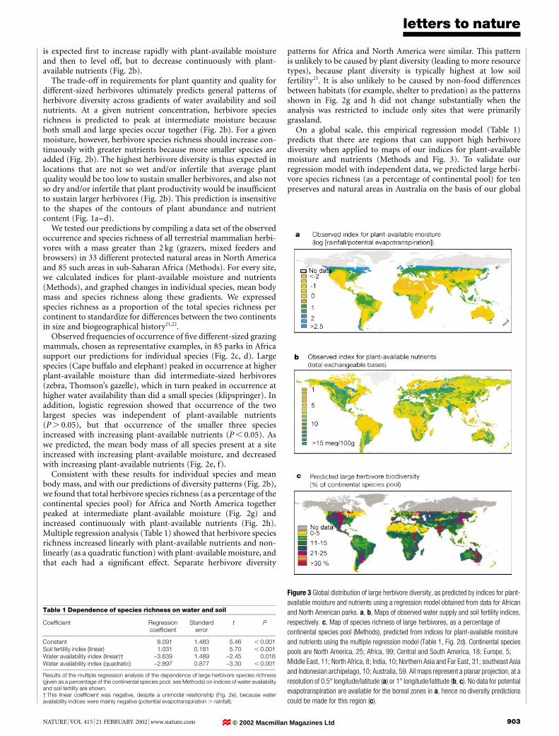
letters to nature
NATURE | VOL 415 | 21 FEBRUARY 2002 | www.nature.com 903
is expected ®rst to increase rapidly with plant-available moistureand then to level off, but to decrease continuously with plant-available nutrients (Fig. 2b).
The trade-off in requirements for plant quantity and quality fordifferent-sized herbivores ultimately predicts general patterns ofherbivore diversity across gradients of water availability and soilnutrients. At a given nutrient concentration, herbivore speciesrichness is predicted to peak at intermediate moisture becauseboth small and large species occur together (Fig. 2b). For a givenmoisture, however, herbivore species richness should increase con-tinuously with greater nutrients because more smaller species areadded (Fig. 2b). The highest herbivore diversity is thus expected inlocations that are not so wet and/or infertile that average plantquality would be too low to sustain smaller herbivores, and also notso dry and/or infertile that plant productivity would be insuf®cientto sustain larger herbivores (Fig. 2b). This prediction is insensitiveto the shapes of the contours of plant abundance and nutrientcontent (Fig. 1a±d).
We tested our predictions by compiling a data set of the observedoccurrence and species richness of all terrestrial mammalian herbi-vores with a mass greater than 2 kg (grazers, mixed feeders andbrowsers) in 33 different protected natural areas in North Americaand 85 such areas in sub-Saharan Africa (Methods). For every site,we calculated indices for plant-available moisture and nutrients(Methods), and graphed changes in individual species, mean bodymass and species richness along these gradients. We expressedspecies richness as a proportion of the total species richness percontinent to standardize for differences between the two continentsin size and biogeographical history21,22.
Observed frequencies of occurrence of ®ve different-sized grazingmammals, chosen as representative examples, in 85 parks in Africasupport our predictions for individual species (Fig. 2c, d). Largespecies (Cape buffalo and elephant) peaked in occurrence at higherplant-available moisture than did intermediate-sized herbivores(zebra, Thomson's gazelle), which in turn peaked in occurrence athigher water availability than did a small species (klipspringer). Inaddition, logistic regression showed that occurrence of the twolargest species was independent of plant-available nutrients(P . 0.05), but that occurrence of the smaller three speciesincreased with increasing plant-available nutrients (P , 0.05). Aswe predicted, the mean body mass of all species present at a siteincreased with increasing plant-available moisture, and decreasedwith increasing plant-available nutrients (Fig. 2e, f).
Consistent with these results for individual species and meanbody mass, and with our predictions of diversity patterns (Fig. 2b),we found that total herbivore species richness (as a percentage of thecontinental species pool) for Africa and North America togetherpeaked at intermediate plant-available moisture (Fig. 2g) andincreased continuously with plant-available nutrients (Fig. 2h).Multiple regression analysis (Table 1) showed that herbivore speciesrichness increased linearly with plant-available nutrients and non-linearly (as a quadratic function) with plant-available moisture, andthat each had a signi®cant effect. Separate herbivore diversity
patterns for Africa and North America were similar. This patternis unlikely to be caused by plant diversity (leading to more resourcetypes), because plant diversity is typically highest at low soilfertility23. It is also unlikely to be caused by non-food differencesbetween habitats (for example, shelter to predation) as the patternsshown in Fig. 2g and h did not change substantially when theanalysis was restricted to include only sites that were primarilygrassland.
On a global scale, this empirical regression model (Table 1)predicts that there are regions that can support high herbivorediversity when applied to maps of our indices for plant-availablemoisture and nutrients (Methods and Fig. 3). To validate ourregression model with independent data, we predicted large herbi-vore species richness (as a percentage of continental pool) for tenpreserves and natural areas in Australia on the basis of our global
Figure 3 Global distribution of large herbivore diversity, as predicted by indices for plant-
available moisture and nutrients using a regression model obtained from data for African
and North American parks. a, b, Maps of observed water supply and soil fertility indices,
respectively. c, Map of species richness of large herbivores, as a percentage of
continental species pool (Methods), predicted from indices for plant-available moisture
and nutrients using the multiple regression model (Table 1, Fig. 2d). Continental species
pools are North America, 25; Africa, 99; Central and South America, 18; Europe, 5;
Middle East, 11; North Africa, 8; India, 10; Northern Asia and Far East, 31; southeast Asia
and Indonesian archipelago, 10; Australia, 59. All maps represent a planar projection, at a
resolution of 0.58 longitude/latitude (a) or 18 longitude/latitude (b, c). No data for potential
evapotranspiration are available for the boreal zones in a, hence no diversity predictions
could be made for this region (c).
Table 1 Dependence of species richness on water and soil
Coef®cient Regressioncoef®cient
Standarderror
t P
.............................................................................................................................................................................
Constant 8.091 1.483 5.46 , 0.001Soil fertility index (linear) 1.031 0.181 5.70 , 0.001Water availability index (linear)² -3.639 1.489 -2.45 0.016Water availability index (quadratic) -2.897 0.877 -3.30 , 0.001.............................................................................................................................................................................
Results of the multiple regression analysis of the dependence of large herbivore species richness(given as a percentage of the continental species pool; see Methods) on indices of water availabilityand soil fertility are shown.² This linear coef®cient was negative, despite a unimodal relationship (Fig. 2e), because wateravailability indices were mainly negative (potential evapotranspiration . rainfall).
© 2002 Macmillan Magazines Ltd
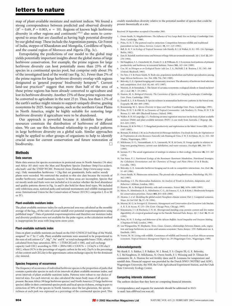
letters to nature
904 NATURE | VOL 415 | 21 FEBRUARY 2002 | www.nature.com
map of plant-available moisture and nutrient indices. We found astrong correspondence between predicted and observed diversity(R2 = 0.69, P = 0.003, n = 10). Regions of known high herbivorediversity in other regions and continents1,10,22 also seem to corre-spond to areas that are classi®ed as having high potential diversityby our global map. These include the Argentinian pampa, Gir Forestof India, steppes of Khazakstan and Mongolia, Cordillera of Spain,and the coastal region of Morocco and Algeria (Fig. 3c).
Extrapolating the predictions of our model to the global mapyields potentially important insights about the global status of largeherbivore conservation. For example, the prime regions for largeherbivore diversity can host potentially more than 25% of thespecies in a continental species pool, but comprise only about 5%of the investigated land of the world (see Fig. 3c). Fewer than 2% ofthe prime regions for large herbivore diversity overlap with regionsdesignated as `general purpose' biodiversity hotspots24. Currentland-use practices25 suggest that more than half of the area ofthese prime regions has been already converted to agriculture andlost its herbivore diversity. Another 25% of these prime regions maybe converted to agriculture in the next 25 yr. Thus, less than 1.2% ofthe earth's surface might remain to support uniquely diverse, grazingecosystems by 2025. Some regions, such as the northern Great Plainsin North America, might be highly suitable for restoring largeherbivore diversity if agriculture were to be abandoned.
Our approach is powerful because it identi®es how plantresources constrain the distribution of herbivores of differentsizes. We can use this functional relationship to predict patternsin large herbivore diversity on a global scale. Similar approachesmight be applied to other groups of organisms to help to identifycrucial areas for current conservation and future restoration ofbiodiversity. M
MethodsData sources
Main data sources for species occurrences in protected areas in North America (34 sites)and Africa (85 sites) were the Man and Biosphere Species Database (http://ice.ucdavis.edu/mab) and the UNEP-WCMC Protected Areas Database (http://www.unep-wcmc.org). Only mammalian herbivores . 2 kg that eat graminoids, forbs and/or woodyplants were recorded. We restricted the analysis to this size class because the records ofsmaller herbivores (small mammals, insects) in these areas are incomplete. Species thateat mostly seeds and fruits were not included as it is unclear whether the food abundanceand quality patterns shown in Fig. 1a and b also hold for these food types. We includedonly wilderness areas, national parks and national monuments and wildlife managementareas (International Union for the Conservation of Nature (IUCN)) categories I, II or IIIor IV).
Plant-available moisture index
The plant-available moisture index for each protected area was calculated as the monthlyaverage of the log10 of the ratio of actual rainfall over potential evapotranspiration usingpublished maps26. Data of potential evapotranspiration and therefore our moisture indexand diversity prediction were not available for the polar region, as the calculation methodis inappropriate for areas with long-term snow cover.
Plant-available nutrients index
Data on plant-available nutrients are based on the FAO-UNESCO Soil Map of the World,assigned25 to 18 by 18 cells. Plant-available nutrients were assumed to be proportional tothe sum of soil cations Ca2+, Mg2+, Na+ and K+ or total exchangeable bases (TEB), which iscalculated from base saturation, BS% = [(TEB/CECsoil) ´ 100], and soil exchangecapacity (soil CEC) according to TEB = (BS%/100) ´ 3.5OC% + [(Clay% x CECclay)/100)], where OC% is the percentage of organic carbon in the soil, Clay% is the percentageof clay content and CECclay is the approximate cation exchange capacity for the dominantclay mineral.
Species frequency of occurrence
The frequency of occurrence of individual herbivore species is the proportion of parks thatcontain a particular species in each of six intervals of plant-available moisture index, andseven intervals of plant-available nutrients index. Patterns were robust to our choice ofinterval sizes. For each interval, we also calculated the mean body mass of all speciespresent. Because Africa (99 large herbivore species) and North America (25 large herbivorespecies) differ in their continental species pools and local species richness, owing in part toextinction of 50% of the species in North America since the last glaciation, the speciesrichness at each park was expressed as a percentage of the continental species pool. This
crudely standardizes diversity relative to the potential number of species that could bepresent theoretically at a site.
Received 28 September; accepted 6 December 2001.
1. Owen-Smith, N. Megaherbivores. The In¯uence of Very Large Body Size on Ecology (Cambridge Univ.
Press, Cambridge, 1988).
2. Prins, H. H. T. The pastoral road to extinction: Competition between wildlife and traditional
pastoralism in East Africa. Environ. Conserv. 19, 117±123 (1992).
3. Bell, R. H. V. in Ecology of Tropical Savannas (eds Huntly, B. J. & Walker, B. H.) 193±216 (Springer,
Berlin, 1982).
4. East, R. Rainfall, nutrient status and biomass of large African savannah mammals. Afr. J. Ecol. 22, 245±
270 (1984).
5. McNaughton, S. J., Oesterheld, M., Frank, D. A. & Williams, K. J. Ecosystem-level patterns of primary
productivity and herbivory in terrestrial habitats. Nature 341, 142±144 (1989).
6. Coe, M. in Nitrogen as an Ecological Factor (eds Lee, J. A., McNeill, J. & Rorison, I. H.) 345±368
(Oxford, Blackwell, 1983).
7. Du Toit, J. T. & Owen-Smith, N. Body size, population metabolism and habitat specialization among
large African herbivores. Am. Nat. 133, 736±740 (1989).
8. Belovsky, G. E. Optimal foraging and community structure: The allometry of herbivore food selection
and competition. Evol. Ecol. 11, 641±672 (1997).
9. Western, D. & Ssemakula, J. The future of savanna ecosystems: ecological islands or faunal enclaves?
Afr. J. Ecol. 19, 7±19 (1981).
10. Huston, M. A. Biological Diversity. The Coexistence of Species on Changing Landscapes (Cambridge
Univ. Press, Cambridge, 1994).
11. Danell, K. L. P. & Niemela, P. Species richness in mammalian herbivores: patterns in the boreal zone.
Ecography 19, 404±409 (1996).
12. Rosenzweig, M. L. Species Diversity in Space and Time (Cambridge Univ. Press, Cambridge, 1995).
13. Prins, H. H. T. & Olff, H. in Dynamics of Tropical Communities (eds Newbery, D., Prins, H. H. T. &
Brown, G.) 449±489 (Blackwell Science, Oxford, 1998).
14. Walker, B. H. & Langridge, J. L. Predicting savanna vegetation structure on the basis of plant available
moisture (PAM) and plant available nutrients (PAN): A case study from Australia. J. Biogeogr. 24,
813±825 (1997).
15. Breman, H. & De Wit, C. T. Rangeland productivity and exploitation in the Sahel. Science 221, 1341±
1347 (1983).
16. Breman, H. & Krul, J. M. in La Productivite de PaÃturages SaheÂliens. Une Etude des Sols, des VeÂgeÂtations et
de l'Explotation de cette Ressource Naturelle (eds Penning de Vries, F. W. T. & Djiteye, M. A.) 322±345
(Pudoc, Wageningen, 1991).
17. Milchunas, D. G., Varnamkhasti, A. S., Lauenroth, W. K. & Goetz, H. Forage quality in relation to
long-term grazing history, current-year defoliation, and water resource. Oecologia 101, 366±374
(1995).
18. Jarman, P. J. The social organization of antelope in relation to their ecology. Behaviour 48, 215±267
(1974).
19. Van Soest, P. J. Nutritional Ecology of the Ruminant: Ruminant Metabolism, Nutritional Strategies,
the Cellulolytic Fermentation and the Chemistry of Forages and Plant Fibres (O & B Books,
Corvallis, 1982).
20. Belovsky, G. E. Generalist herbivore foraging and its role in competitive interactions. Am. Zool. 26,
51±69 (1986).
21. Owen-Smith, N. Pleistocene extinctions: The pivotal role of megaherbivores. Paleobiology 13, 351±
362 (1987).
22. Eisenberg, J. F. The Mammalian Radiations. An Analysis of Trends in Evolution, Adaptation, and
Behaviour (Athlone, London, 1981).
23. Huston, M. A. Biological diversity, soils and economics. Science 262, 1676±1680 (1993).
24. Myers, N., Mittelmeier, R. A., Mittelmeier, C. G., da Fonseca, G. A. B. & Kent, J. Biodiversity hotspots
for conservation priorities. Nature 403, 853±858 (2000).
25. Alcamo, J. et al. Modeling the global society-biosphere-climate system: Part 2. Computed scenarios.
Water Air Soil Poll. 76, 37±78 (1994).
26. Murray, M. G. in Serengeti II. Dynamics, Management and Conservation of an Ecosystem (eds Sinclair,
A. R. E. & Arcese, P.) 231±256 (Univ. Chicago Press, Chicago, 1995).
27. Kinyamario, J. I. & Macharia, J.-N. M. Aboveground standing crop, protein content and dry matter
digestibility of a tropical grassland range in the Nairobi National Park, Kenya. Afr. J. Ecol. 30, 33±41
(1992).
28. Prins, H. H. T. Ecology and Behaviour of the African Buffalo. Social Inequality and Decision Making
(Chapman & Hall, London, 1996).
29. van Wijngaarden, W. Elephants±Trees±Grass±Grazers, relationships between climate, soils, vegeta-
tion and large herbivores in a semi-arid savanna ecosystem (Tsavo, Kenya). (ITC Publication no. 4,
Enschede, 1985).
30. Voeten, M. M. Living with wildlife. Coexistence of wildlife and livestock in an East African savanna
ecosystem. Tropical Resource Management Papers no. 29 (Wageningen Univ., Wageningen, 1999).
Acknowledgements
We thank E. S. Bakker, J. P. Bakker, W. J. Bond, F. S. Chapin III, G. E. Belovsky,S. J. McNaughton, D. Milchunas, N. Owen-Smith, F. J. Weissing and D. Tilman forcomments; M. A. Huston for soil fertility data; and R. Leemans for temperature andrainfall data. Financial support was provided by the Dutch NWO (WOTRO and ALW),Wageningen University, the NSF, the Utah Agricultural Experiment Station, and the UtahState University Ecology Center.
Competing interests statement
The authors declare that they have no competing ®nancial interests.
Correspondence and requests for materials should be addressed to H.O.(e-mail: [email protected]).
© 2002 Macmillan Magazines Ltd
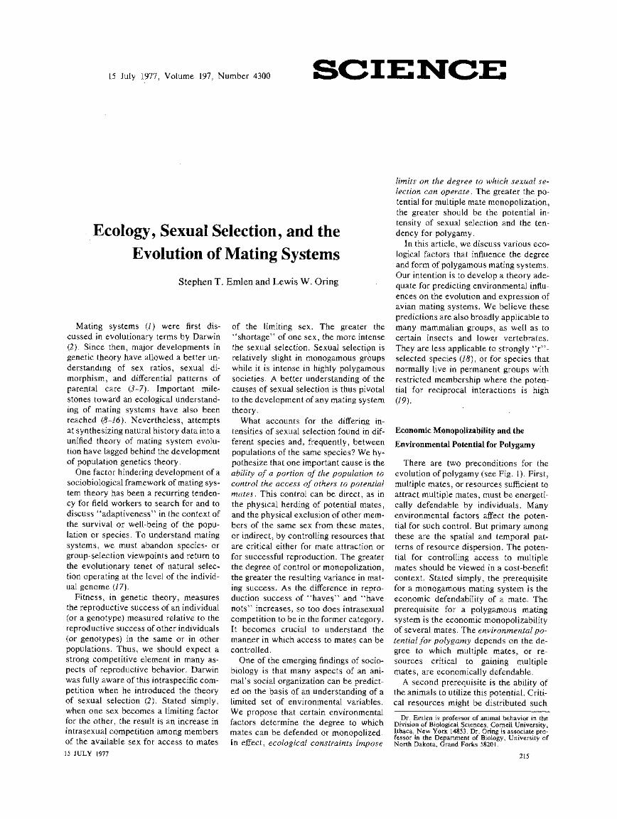
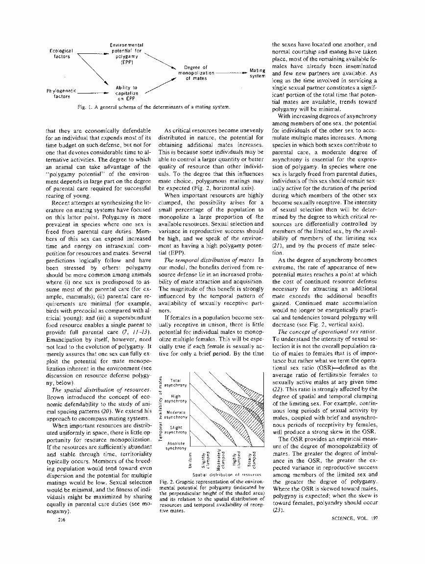
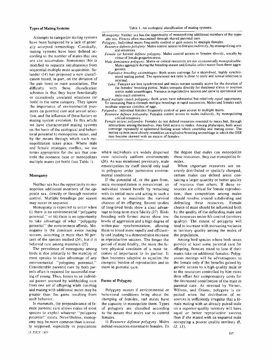

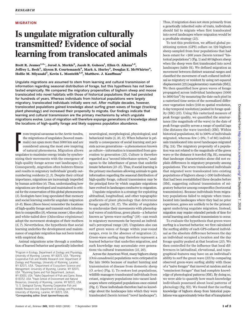
MIGRATION
Is ungulate migration culturallytransmitted? Evidence of sociallearning from translocated animalsBrett R. Jesmer1,2*, Jerod A. Merkle2, Jacob R. Goheen1, Ellen O. Aikens1,2,Jeffrey L. Beck3, Alyson B. Courtemanch4, Mark A. Hurley5, Douglas E. McWhirter4,Hollie M. Miyasaki5, Kevin L. Monteith2,6, Matthew. J. Kauffman7
Ungulate migrations are assumed to stem from learning and cultural transmission ofinformation regarding seasonal distribution of forage, but this hypothesis has not beentested empirically. We compared the migratory propensities of bighorn sheep and moosetranslocated into novel habitats with those of historical populations that had persistedfor hundreds of years. Whereas individuals from historical populations were largelymigratory, translocated individuals initially were not. After multiple decades, however,translocated populations gained knowledge about surfing green waves of forage (trackingplant phenology) and increased their propensity to migrate. Our findings indicate thatlearning and cultural transmission are the primary mechanisms by which ungulatemigrations evolve. Loss of migration will therefore expunge generations of knowledge aboutthe locations of high-quality forage and likely suppress population abundance.
From tropical savannas to the Arctic tundra,the migrations of ungulates (hoovedmam-mals) can spanmore than 1000 km and areconsidered among the most awe inspiringof natural phenomena. Migration allows
ungulates tomaximize energy intake by synchro-nizing their movements with the emergence ofhigh-quality forage across vast landscapes (1).Consequently, migration often bolsters fitnessand results inmigratory individuals’ greatly out-numbering residents (2, 3). Despite their criticalimportance,migrations are increasingly imperiledby human activities (4). Thus, understanding howmigrations are developed andmaintained is criti-cal for the conservationof this global phenomenon(5). Ecologists have long speculated that memoryand social learning underlie ungulate migration(6–8). Bison (Bison bison) remember the locationsof high-quality forage and transmit such informa-tion to conspecifics (9),whereasmoose (Alces alces)and white-tailed deer (Odocoileus virginianus)adopt the movement strategies of their mothers(6, 7). Nevertheless, the hypothesis that sociallearning underlies the development and mainte-nance of ungulatemigration has not been testedwith empirical data.Animal migrations arise through a combina-
tion of learned behavior and genetically inherited
neurological, morphological, physiological, andbehavioral traits (5, 10, 11). When behavior is pri-marily a consequence of social learning and per-sists across generations—a phenomenon knownas culture—information is transmitted from gen-eration to generation (12). Culture is thereforeregarded as a “second inheritance system,” anal-ogous to the inheritance of genes that underlieinnate behaviors (13–15). Thus, if social learning isthe primarymechanism allowing animals to gaininformation regarding the seasonal distribution ofhigh-quality forage, cultural transmission may bethe principal force by which ungulate migrationshave evolved in landscapes conducive tomigration.Ungulatemigration is a strategy for exploiting
altitudinal, longitudinal, and other topographicgradients of plant phenology that determineforage quality (16, 17). The ability of ungulatesto synchronize their movements with phenolog-ical waves of nutritious, green plants—a behaviorknown as “green-wave surfing” (18)—can resultin migratory movements far beyond an individ-ual’s perceptual range (19). Ungulates also cansurf green waves of forage within year-roundranges, even in the absence of migration (1).Green-wave surfing may therefore represent alearned behavior that underlies migration, andsuch knowledge may accumulate over genera-tions via cultural transmission (15, 20).Across theAmericanWest,manybighorn sheep
(Ovis canadensis) populationswere extirpated inthe late 1800s because of market hunting andtransmission of disease from domestic sheep(O. aries) (Fig. 1). To restore lost populations,wildlifemanagers translocated individuals fromextant, migratory populations into vacant land-scapeswhere extirpated populations once existed(Fig. 1). These individuals therefore hadno knowl-edge about the landscapes into which they weretranslocated (herein termed “novel landscapes”).
Thus, if migration does not stem primarily froma genetically inherited suite of traits, individualsshould fail to migrate when first translocatedinto novel landscapeswheremigrationwould bea profitable strategy (21).To test this prediction, we affixed global po-
sitioning system (GPS) collars on 129 bighornsheep sampled from four populations that hadbeen extant for >200 years (herein termed “his-torical populations”) (Fig. 1) and 80 bighorn sheepwhen the sheep were first translocated into novellandscapes (table S1). We defined migration asmovement between distinct seasonal ranges andclassified the movement of each collared individ-ual asmigratory or resident by using net-squareddisplacement (22) [supplementarymaterials (SM)].We then quantified how green waves of foragepropagated across individual landscapes (1000to 3600 km2) bymeasuring the date each pixel ina rasterized time series of the normalized differ-ence vegetation index (250-m spatial resolution,8-day temporal resolution) peaked in forage qual-ity (SM) (23). Using this rasterized measure ofpeak forage quality, we quantified the semivar-iance (the magnitude of the wave) in the date ofpeak forage quality across a range of spatial lags(the distance the wave traveled) (SM). Withinhistorical populations, 65 to 100% of individualsmigrated, whereas few (<9%; 7 of 80) individ-uals translocated into novel landscapesmigrated(Fig. 2A). The migratory propensity of a popula-tionwas not related to themagnitude of the greenwave or the distance it traveled (fig. S1), meaningthat landscape characteristics alone did not ex-plain differences in migratory propensity amongpopulations. The seven translocated individualsthat migrated were translocated into existingpopulations of bighorn sheep (<200 individuals)that had been reestablished three decades before(SM), suggesting cultural transmission of mi-gratory behavior among conspecifics (horizontaltransmission). Because individuals frommigra-tory populations failed to migrate when trans-located into landscapes where they had no priorexperience, genes are unlikely to be the primaryagent underlying ungulate migration. Instead,migrationmay require extended periods of time forsocial learning and cultural transmission to occur.To evaluate the hypothesis that green-wave
surfing is a learned behavior, we first calculatedthe surfing ability of each GPS-collared individ-ual as the absolute difference between the dayan individual occupied a location and the dayforage quality peaked at that location (23). Wethen controlled for the influence that local dif-ferences in latitudinal, elevational, and topo-graphical features may have on an individual’sability to surf the green wave (23) by comparingobserved green-wave surfing ability with thoseof a “naïve forager” thatmoved at randomand an“omniscient forager” that had complete knowl-edge of phenological patterns (SM). By doing so,we were able to quantify how much knowledgeindividuals possessed about local patterns ofphenology (fig. S2). We found that the surfingknowledge of bighorn sheep from historical popu-lationswasapproximately twice thatof transplanted
RESEARCH
Jesmer et al., Science 361, 1023–1025 (2018) 7 September 2018 1 of 3
1Program in Ecology, Department of Zoology and Physiology,University of Wyoming, Laramie, WY 82071, USA. 2WyomingCooperative Fish and Wildlife Research Unit, Department ofZoology and Physiology, University of Wyoming, Laramie,WY 82071, USA. 3Department of Ecosystem Science andManagement, University of Wyoming, Laramie, WY 82071,USA. 4Wyoming Game and Fish Department, Jackson,WY 83001, USA. 5Idaho Department of Fish and Game, Boise,ID 83712, USA. 6Haub School of Environment and NaturalResources, University of Wyoming, Laramie, WY 82072, USA.7U. S. Geological Survey, Wyoming Cooperative Fish andWildlife Research Unit, Department of Zoology and Physiology,University of Wyoming, Laramie, WY 82071, USA.*Corresponding author. Email: [email protected]
on Septem
ber 7, 2018
http://science.sciencemag.org/
Dow
nloaded from
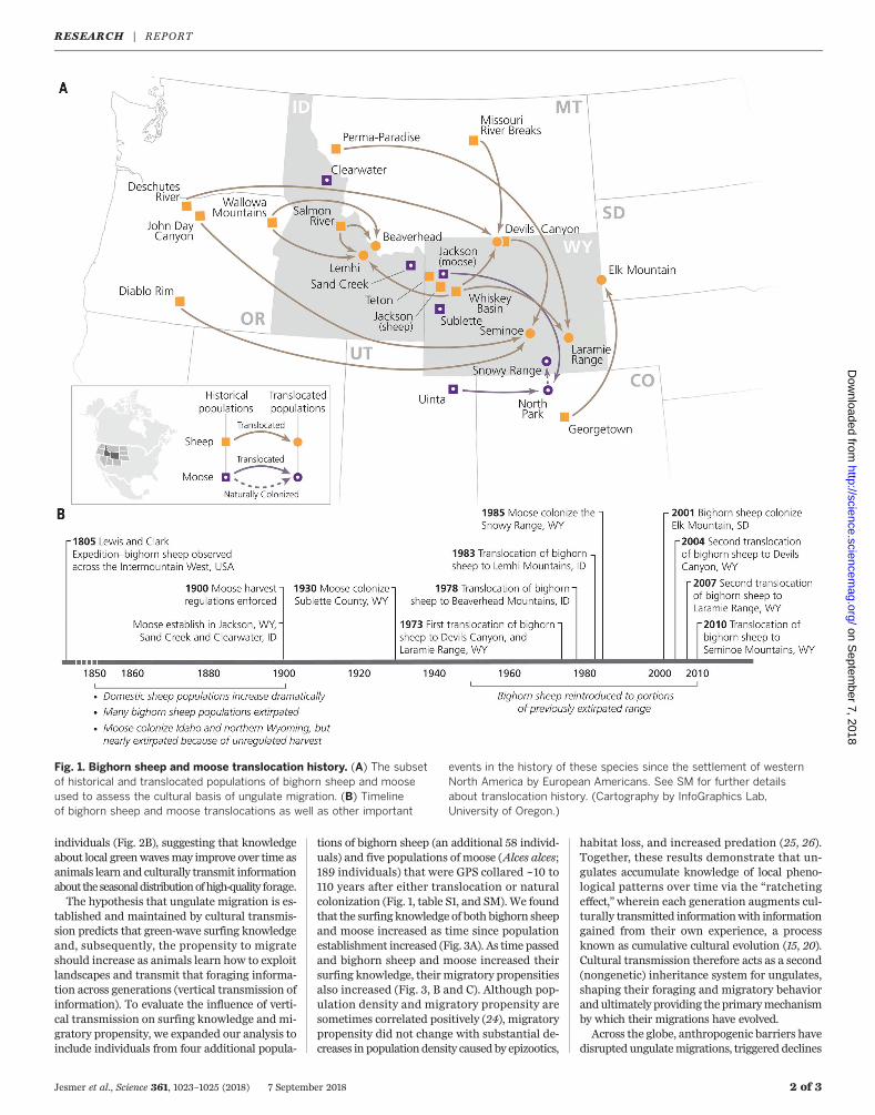
individuals (Fig. 2B), suggesting that knowledgeabout local greenwavesmay improve over time asanimals learn and culturally transmit informationabout theseasonaldistributionofhigh-quality forage.The hypothesis that ungulate migration is es-
tablished and maintained by cultural transmis-sion predicts that green-wave surfing knowledgeand, subsequently, the propensity to migrateshould increase as animals learn how to exploitlandscapes and transmit that foraging informa-tion across generations (vertical transmission ofinformation). To evaluate the influence of verti-cal transmission on surfing knowledge and mi-gratory propensity, we expanded our analysis toinclude individuals from four additional popula-
tions of bighorn sheep (an additional 58 individ-uals) and five populations of moose (Alces alces;189 individuals) that were GPS collared ~10 to110 years after either translocation or naturalcolonization (Fig. 1, table S1, and SM). We foundthat the surfing knowledge of both bighorn sheepand moose increased as time since populationestablishment increased (Fig. 3A). As time passedand bighorn sheep and moose increased theirsurfing knowledge, their migratory propensitiesalso increased (Fig. 3, B and C). Although pop-ulation density and migratory propensity aresometimes correlated positively (24), migratorypropensity did not change with substantial de-creases in populationdensity causedby epizootics,
habitat loss, and increased predation (25, 26).Together, these results demonstrate that un-gulates accumulate knowledge of local pheno-logical patterns over time via the “ratchetingeffect,”wherein each generation augments cul-turally transmitted informationwith informationgained from their own experience, a processknown as cumulative cultural evolution (15, 20).Cultural transmission therefore acts as a second(nongenetic) inheritance system for ungulates,shaping their foraging and migratory behaviorandultimately providing the primarymechanismby which their migrations have evolved.Across the globe, anthropogenic barriers have
disrupted ungulatemigrations, triggered declines
Jesmer et al., Science 361, 1023–1025 (2018) 7 September 2018 2 of 3
Fig. 1. Bighorn sheep and moose translocation history. (A) The subsetof historical and translocated populations of bighorn sheep and mooseused to assess the cultural basis of ungulate migration. (B) Timelineof bighorn sheep and moose translocations as well as other important
events in the history of these species since the settlement of westernNorth America by European Americans. See SM for further detailsabout translocation history. (Cartography by InfoGraphics Lab,University of Oregon.)
RESEARCH | REPORTon S
eptember 7, 2018
http://science.sciencem
ag.org/D
ownloaded from
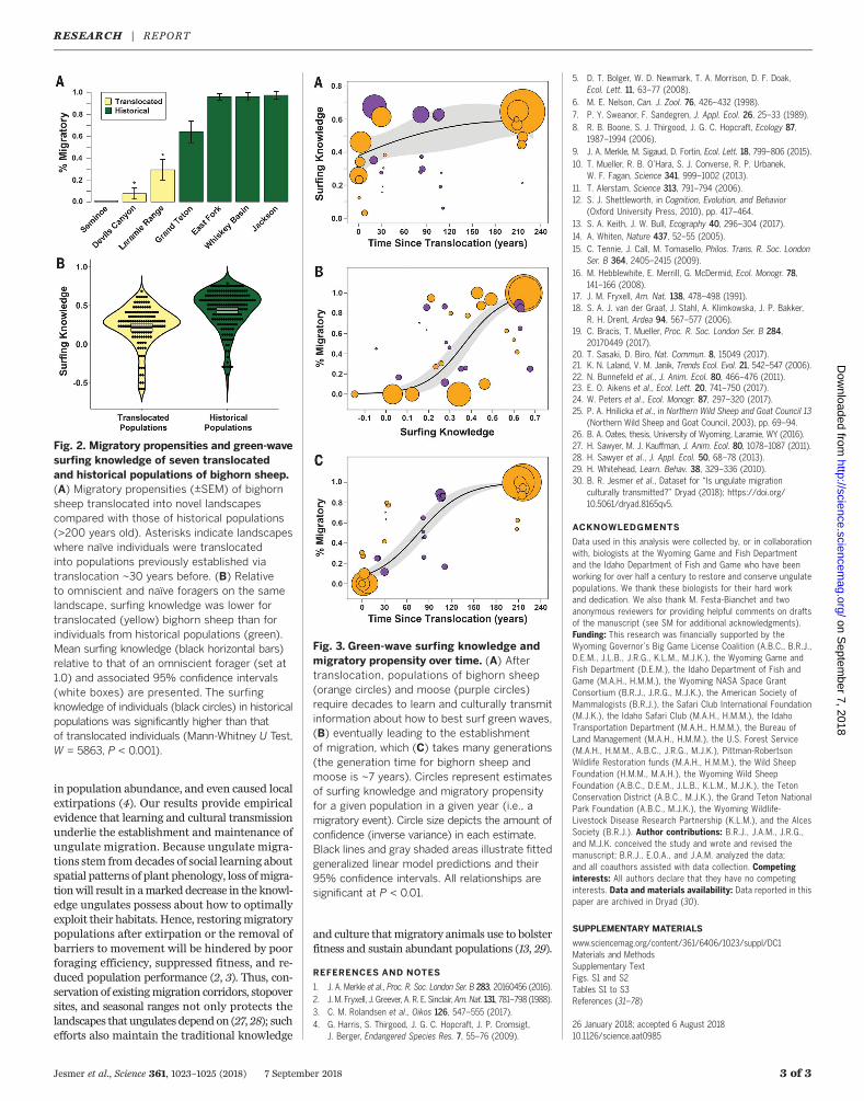
in population abundance, and even caused localextirpations (4). Our results provide empiricalevidence that learning and cultural transmissionunderlie the establishment and maintenance ofungulate migration. Because ungulate migra-tions stem fromdecades of social learning aboutspatial patterns of plant phenology, loss ofmigra-tionwill result in amarked decrease in the knowl-edge ungulates possess about how to optimallyexploit their habitats. Hence, restoringmigratorypopulations after extirpation or the removal ofbarriers to movement will be hindered by poorforaging efficiency, suppressed fitness, and re-duced population performance (2, 3). Thus, con-servation of existingmigration corridors, stopoversites, and seasonal ranges not only protects thelandscapes that ungulates depend on (27, 28); suchefforts also maintain the traditional knowledge
and culture thatmigratory animals use to bolsterfitness and sustain abundant populations (13, 29).
REFERENCES AND NOTES
1. J. A. Merkle et al., Proc. R. Soc. London Ser. B 283, 20160456 (2016).2. J. M. Fryxell, J. Greever, A. R. E. Sinclair,Am.Nat. 131, 781–798 (1988).3. C. M. Rolandsen et al., Oikos 126, 547–555 (2017).4. G. Harris, S. Thirgood, J. G. C. Hopcraft, J. P. Cromsigt,
J. Berger, Endangered Species Res. 7, 55–76 (2009).
5. D. T. Bolger, W. D. Newmark, T. A. Morrison, D. F. Doak,Ecol. Lett. 11, 63–77 (2008).
6. M. E. Nelson, Can. J. Zool. 76, 426–432 (1998).7. P. Y. Sweanor, F. Sandegren, J. Appl. Ecol. 26, 25–33 (1989).8. R. B. Boone, S. J. Thirgood, J. G. C. Hopcraft, Ecology 87,
1987–1994 (2006).9. J. A. Merkle, M. Sigaud, D. Fortin, Ecol. Lett. 18, 799–806 (2015).10. T. Mueller, R. B. O’Hara, S. J. Converse, R. P. Urbanek,
W. F. Fagan, Science 341, 999–1002 (2013).11. T. Alerstam, Science 313, 791–794 (2006).12. S. J. Shettleworth, in Cognition, Evolution, and Behavior
(Oxford University Press, 2010), pp. 417–464.13. S. A. Keith, J. W. Bull, Ecography 40, 296–304 (2017).14. A. Whiten, Nature 437, 52–55 (2005).15. C. Tennie, J. Call, M. Tomasello, Philos. Trans. R. Soc. London
Ser. B 364, 2405–2415 (2009).16. M. Hebblewhite, E. Merrill, G. McDermid, Ecol. Monogr. 78,
141–166 (2008).17. J. M. Fryxell, Am. Nat. 138, 478–498 (1991).18. S. A. J. van der Graaf, J. Stahl, A. Klimkowska, J. P. Bakker,
R. H. Drent, Ardea 94, 567–577 (2006).19. C. Bracis, T. Mueller, Proc. R. Soc. London Ser. B 284,
20170449 (2017).20. T. Sasaki, D. Biro, Nat. Commun. 8, 15049 (2017).21. K. N. Laland, V. M. Janik, Trends Ecol. Evol. 21, 542–547 (2006).22. N. Bunnefeld et al., J. Anim. Ecol. 80, 466–476 (2011).23. E. O. Aikens et al., Ecol. Lett. 20, 741–750 (2017).24. W. Peters et al., Ecol. Monogr. 87, 297–320 (2017).25. P. A. Hnilicka et al., in Northern Wild Sheep and Goat Council 13
(Northern Wild Sheep and Goat Council, 2003), pp. 69–94.26. B. A. Oates, thesis, University of Wyoming, Laramie, WY (2016).27. H. Sawyer, M. J. Kauffman, J. Anim. Ecol. 80, 1078–1087 (2011).28. H. Sawyer et al., J. Appl. Ecol. 50, 68–78 (2013).29. H. Whitehead, Learn. Behav. 38, 329–336 (2010).30. B. R. Jesmer et al., Dataset for “Is ungulate migration
culturally transmitted?” Dryad (2018); https://doi.org/10.5061/dryad.8165qv5.
ACKNOWLEDGMENTS
Data used in this analysis were collected by, or in collaborationwith, biologists at the Wyoming Game and Fish Departmentand the Idaho Department of Fish and Game who have beenworking for over half a century to restore and conserve ungulatepopulations. We thank these biologists for their hard workand dedication. We also thank M. Festa-Bianchet and twoanonymous reviewers for providing helpful comments on draftsof the manuscript (see SM for additional acknowledgments).Funding: This research was financially supported by theWyoming Governor’s Big Game License Coalition (A.B.C., B.R.J.,D.E.M., J.L.B., J.R.G., K.L.M., M.J.K.), the Wyoming Game andFish Department (D.E.M.), the Idaho Department of Fish andGame (M.A.H., H.M.M.), the Wyoming NASA Space GrantConsortium (B.R.J., J.R.G., M.J.K.), the American Society ofMammalogists (B.R.J.), the Safari Club International Foundation(M.J.K.), the Idaho Safari Club (M.A.H., H.M.M.), the IdahoTransportation Department (M.A.H., H.M.M.), the Bureau ofLand Management (M.A.H., H.M.M.), the U.S. Forest Service(M.A.H., H.M.M., A.B.C., J.R.G., M.J.K.), Pittman-RobertsonWildlife Restoration funds (M.A.H., H.M.M.), the Wild SheepFoundation (H.M.M., M.A.H.), the Wyoming Wild SheepFoundation (A.B.C., D.E.M., J.L.B., K.L.M., M.J.K.), the TetonConservation District (A.B.C., M.J.K.), the Grand Teton NationalPark Foundation (A.B.C., M.J.K.), the Wyoming Wildlife-Livestock Disease Research Partnership (K.L.M.), and the AlcesSociety (B.R.J.). Author contributions: B.R.J., J.A.M., J.R.G.,and M.J.K. conceived the study and wrote and revised themanuscript; B.R.J., E.O.A., and J.A.M. analyzed the data;and all coauthors assisted with data collection. Competinginterests: All authors declare that they have no competinginterests. Data and materials availability: Data reported in thispaper are archived in Dryad (30).
SUPPLEMENTARY MATERIALS
www.sciencemag.org/content/361/6406/1023/suppl/DC1Materials and MethodsSupplementary TextFigs. S1 and S2Tables S1 to S3References (31–78)
26 January 2018; accepted 6 August 201810.1126/science.aat0985
Jesmer et al., Science 361, 1023–1025 (2018) 7 September 2018 3 of 3
Fig. 3. Green-wave surfing knowledge andmigratory propensity over time. (A) Aftertranslocation, populations of bighorn sheep(orange circles) and moose (purple circles)require decades to learn and culturally transmitinformation about how to best surf green waves,(B) eventually leading to the establishmentof migration, which (C) takes many generations(the generation time for bighorn sheep andmoose is ~7 years). Circles represent estimatesof surfing knowledge and migratory propensityfor a given population in a given year (i.e., amigratory event). Circle size depicts the amount ofconfidence (inverse variance) in each estimate.Black lines and gray shaded areas illustrate fittedgeneralized linear model predictions and their95% confidence intervals. All relationships aresignificant at P < 0.01.
Fig. 2. Migratory propensities and green-wavesurfing knowledge of seven translocatedand historical populations of bighorn sheep.(A) Migratory propensities (±SEM) of bighornsheep translocated into novel landscapescompared with those of historical populations(>200 years old). Asterisks indicate landscapeswhere naïve individuals were translocatedinto populations previously established viatranslocation ~30 years before. (B) Relativeto omniscient and naïve foragers on the samelandscape, surfing knowledge was lower fortranslocated (yellow) bighorn sheep than forindividuals from historical populations (green).Mean surfing knowledge (black horizontal bars)relative to that of an omniscient forager (set at1.0) and associated 95% confidence intervals(white boxes) are presented. The surfingknowledge of individuals (black circles) in historicalpopulations was significantly higher than thatof translocated individuals (Mann-Whitney U Test,W = 5863, P < 0.001).
RESEARCH | REPORTon S
eptember 7, 2018
http://science.sciencem
ag.org/D
ownloaded from
animalsIs ungulate migration culturally transmitted? Evidence of social learning from translocated
Douglas E. McWhirter, Hollie M. Miyasaki, Kevin L. Monteith and Matthew. J. KauffmanBrett R. Jesmer, Jerod A. Merkle, Jacob R. Goheen, Ellen O. Aikens, Jeffrey L. Beck, Alyson B. Courtemanch, Mark A. Hurley,
DOI: 10.1126/science.aat0985 (6406), 1023-1025.361Science
, this issue p. 1023; see also p. 972Sciencethrough social exchange.increasingly migratory. Thus, newly introduced animals learned about their environment and shared the informationdecades, newly established herds were better able to track the emergence of vegetation in the environment and were Reintroduced populations of bighorn sheep and moose did not migrate as historical herds had. However, after severalAmerican ungulate species to determine the role of learning in migrations (see the Perspective by Festa-Bianchet).
took advantage of regional extinctions and reintroductions of several Northet al.leave and where to go. Jesmer Large ungulate migrations occur across continents and inspire curiosity about how these animals know when to
Learning where and when
ARTICLE TOOLS http://science.sciencemag.org/content/361/6406/1023
MATERIALSSUPPLEMENTARY http://science.sciencemag.org/content/suppl/2018/09/05/361.6406.1023.DC1
CONTENTRELATED http://science.sciencemag.org/content/sci/361/6406/972.full
REFERENCES
http://science.sciencemag.org/content/361/6406/1023#BIBLThis article cites 51 articles, 6 of which you can access for free
PERMISSIONS http://www.sciencemag.org/help/reprints-and-permissions
Terms of ServiceUse of this article is subject to the
is a registered trademark of AAAS.Sciencelicensee American Association for the Advancement of Science. No claim to original U.S. Government Works. The title Science, 1200 New York Avenue NW, Washington, DC 20005. 2017 © The Authors, some rights reserved; exclusive
(print ISSN 0036-8075; online ISSN 1095-9203) is published by the American Association for the Advancement ofScience
on Septem
ber 7, 2018
http://science.sciencemag.org/
Dow
nloaded from
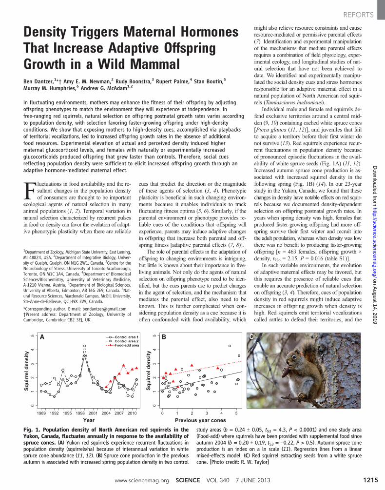
Density Triggers Maternal HormonesThat Increase Adaptive OffspringGrowth in a Wild MammalBen Dantzer,1*† Amy E. M. Newman,2 Rudy Boonstra,3 Rupert Palme,4 Stan Boutin,5
Murray M. Humphries,6 Andrew G. McAdam1,2
In fluctuating environments, mothers may enhance the fitness of their offspring by adjustingoffspring phenotypes to match the environment they will experience at independence. Infree-ranging red squirrels, natural selection on offspring postnatal growth rates varies accordingto population density, with selection favoring faster-growing offspring under high-densityconditions. We show that exposing mothers to high-density cues, accomplished via playbacksof territorial vocalizations, led to increased offspring growth rates in the absence of additionalfood resources. Experimental elevation of actual and perceived density induced highermaternal glucocorticoid levels, and females with naturally or experimentally increasedglucocorticoids produced offspring that grew faster than controls. Therefore, social cuesreflecting population density were sufficient to elicit increased offspring growth through anadaptive hormone-mediated maternal effect.
Fluctuations in food availability and the re-sultant changes in the population densityof consumers are thought to be important
ecological agents of natural selection in manyanimal populations (1, 2). Temporal variation innatural selection characterized by recurrent pulsesin food or density can favor the evolution of adapt-ive phenotypic plasticity when there are reliable
cues that predict the direction or the magnitudeof these agents of selection (3, 4). Phenotypicplasticity is beneficial in such changing environ-ments because it enables individuals to trackfluctuating fitness optima (5, 6). Similarly, if theparental environment or phenotype provides re-liable cues of the conditions that offspring willexperience, parents may induce adaptive changesin offspring that increase both parental and off-spring fitness [adaptive parental effects (7, 8)].
The role of parental effects in the adaptation ofoffspring to changing environments is intriguing,but little is known about their importance in free-living animals. Not only do the agents of naturalselection on offspring phenotype need to be iden-tified, but the cues parents use to predict changesin the agent of selection, and the mechanism thatmediates the parental effect, also need to beknown. This is further complicated when con-sidering population density as a cue because it isoften confounded with food availability, which
might also relieve resource constraints and causeresource-mediated or permissive parental effects(7). Identification and experimental manipulationof the mechanisms that mediate parental effectsrequires a combination of field physiology, exper-imental ecology, and longitudinal studies of nat-ural selection that have not been achieved todate. We identified and experimentally manipu-lated the social density cues and stress hormonesresponsible for an adaptive maternal effect in anatural population of North American red squir-rels (Tamiasciurus hudsonicus).
Individual male and female red squirrels de-fend exclusive territories around a central mid-den (9, 10) containing cached white spruce cones[Picea glauca (11, 12)], and juveniles that failto acquire a territory before their first winter donot survive (13). Red squirrels experience recur-rent fluctuations in population density becauseof pronounced episodic fluctuations in the avail-ability of white spruce seeds (Fig. 1A) (11, 12).Increased autumn spruce cone production is as-sociated with increased squirrel density in thefollowing spring (Fig. 1B) (14). In our 23-yearstudy in the Yukon, Canada, we found that thesechanges in density have notable effects on red squir-rels because we documented density-dependentselection on offspring postnatal growth rates. Inyears when spring density was high, females thatproduced faster-growing offspring had more off-spring survive their first winter and recruit intothe adult population, whereas when density was lowthere was no benefit to producing faster-growingoffspring [n = 463 females, offspring growth ×density, t726 = 2.15, P = 0.016 (table S1)].
In such variable environments, the evolutionof adaptive maternal effects may be favored, butthis requires the presence of reliable cues thatenable an accurate prediction of natural selectionon offspring (3, 4). Therefore, cues of populationdensity in red squirrels might induce adaptiveincreases in offspring growth when density ishigh. Red squirrels emit territorial vocalizationscalled rattles to defend their territories, and the
1Department of Zoology, Michigan State University, East Lansing,MI 48824, USA. 2Department of Integrative Biology, Univer-sity of Guelph, Guelph, ON N1G 2W1, Canada. 3Centre for theNeurobiology of Stress, University of Toronto Scarborough,Toronto, ON M1C 1A4, Canada. 4Department of BiomedicalSciences/Biochemistry, University of Veterinary Medicine,A-1210 Vienna, Austria. 5Department of Biological Sciences,University of Alberta, Edmonton, AB T6G 2E9, Canada. 6Nat-ural Resource Sciences, Macdonald Campus, McGill University,Ste-Anne-de-Bellevue, QC H9X 3V9, Canada.
*Corresponding author. E-mail: [email protected]†Present address: Department of Zoology, University ofCambridge, Cambridge CB2 3EJ, UK.
Fig. 1. Population density of North American red squirrels in theYukon, Canada, fluctuates annually in response to the availability ofspruce cones. (A) Yukon red squirrels experience recurrent fluctuations inpopulation density (squirrels/ha) because of interannual variation in whitespruce cone abundance (11, 12). (B) Spruce cone production in the previousautumn is associated with increased spring population density in two control
study areas (b = 0.24 T 0.05, t53 = 4.3, P < 0.0001) and one study area(Food-add) where squirrels have been provided with supplemental food sinceautumn 2004 (b = 0.20 T 0.19, t53 = –0.22, P > 0.5). Autumn spruce coneproduction is an index on a ln scale (11). Regression lines from a linearmixed-effects model. (C) Red squirrel extracting seeds from a white sprucecone. [Photo credit: R. W. Taylor]
www.sciencemag.org SCIENCE VOL 340 7 JUNE 2013 1215
REPORTSon A
ugust 14, 2019
http://science.sciencemag.org/
Dow
nloaded from
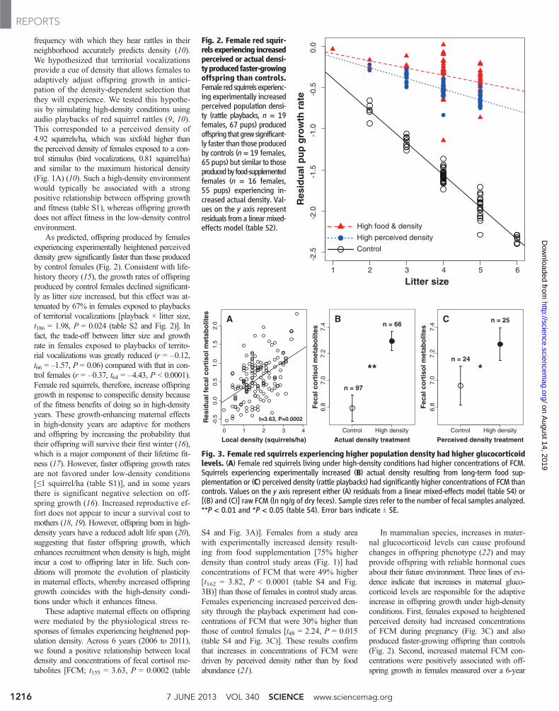
frequency with which they hear rattles in theirneighborhood accurately predicts density (10).We hypothesized that territorial vocalizationsprovide a cue of density that allows females toadaptively adjust offspring growth in antici-pation of the density-dependent selection thatthey will experience. We tested this hypothe-sis by simulating high-density conditions usingaudio playbacks of red squirrel rattles (9, 10).This corresponded to a perceived density of4.92 squirrels/ha, which was sixfold higher thanthe perceived density of females exposed to a con-trol stimulus (bird vocalizations, 0.81 squirrel/ha)and similar to the maximum historical density(Fig. 1A) (10). Such a high-density environmentwould typically be associated with a strongpositive relationship between offspring growthand fitness (table S1), whereas offspring growthdoes not affect fitness in the low-density controlenvironment.
As predicted, offspring produced by femalesexperiencing experimentally heightened perceiveddensity grew significantly faster than those producedby control females (Fig. 2). Consistent with life-history theory (15), the growth rates of offspringproduced by control females declined significant-ly as litter size increased, but this effect was at-tenuated by 67% in females exposed to playbacksof territorial vocalizations [playback × litter size,t186 = 1.98, P = 0.024 (table S2 and Fig. 2)]. Infact, the trade-off between litter size and growthrate in females exposed to playbacks of territo-rial vocalizations was greatly reduced (r = –0.12,t66 = –1.57, P = 0.06) compared with that in con-trol females (r = –0.37, t64 = –4.43, P < 0.0001).Female red squirrels, therefore, increase offspringgrowth in response to conspecific density becauseof the fitness benefits of doing so in high-densityyears. These growth-enhancing maternal effectsin high-density years are adaptive for mothersand offspring by increasing the probability thattheir offspring will survive their first winter (16),which is a major component of their lifetime fit-ness (17). However, faster offspring growth ratesare not favored under low-density conditions[≤1 squirrel/ha (table S1)], and in some yearsthere is significant negative selection on off-spring growth (16). Increased reproductive ef-fort does not appear to incur a survival cost tomothers (18, 19). However, offspring born in high-density years have a reduced adult life span (20),suggesting that faster offspring growth, whichenhances recruitment when density is high, mightincur a cost to offspring later in life. Such con-ditions will promote the evolution of plasticityin maternal effects, whereby increased offspringgrowth coincides with the high-density condi-tions under which it enhances fitness.
These adaptive maternal effects on offspringwere mediated by the physiological stress re-sponses of females experiencing heightened pop-ulation density. Across 6 years (2006 to 2011),we found a positive relationship between localdensity and concentrations of fecal cortisol me-tabolites [FCM; t155 = 3.63, P = 0.0002 (table
S4 and Fig. 3A)]. Females from a study areawith experimentally increased density result-ing from food supplementation [75% higherdensity than control study areas (Fig. 1)] hadconcentrations of FCM that were 49% higher[t162 = 3.82, P < 0.0001 (table S4 and Fig.3B)] than those of females in control study areas.Females experiencing increased perceived den-sity through the playback experiment had con-centrations of FCM that were 30% higher thanthose of control females [t48 = 2.24, P = 0.015(table S4 and Fig. 3C)]. These results confirmthat increases in concentrations of FCM weredriven by perceived density rather than by foodabundance (21).
In mammalian species, increases in mater-nal glucocorticoid levels can cause profoundchanges in offspring phenotype (22) and mayprovide offspring with reliable hormonal cuesabout their future environment. Three lines of evi-dence indicate that increases in maternal gluco-corticoid levels are responsible for the adaptiveincrease in offspring growth under high-densityconditions. First, females exposed to heightenedperceived density had increased concentrationsof FCM during pregnancy (Fig. 3C) and alsoproduced faster-growing offspring than controls(Fig. 2). Second, increased maternal FCM con-centrations were positively associated with off-spring growth in females measured over a 6-year
Fig. 2. Female red squir-rels experiencing increasedperceived or actual densi-typroducedfaster-growingoffspring than controls.Female redsquirrels experienc-ing experimentally increasedperceived population densi-ty (rattle playbacks, n = 19females, 67 pups) producedoffspring thatgrewsignificant-ly faster than those producedby controls (n = 19 females,65 pups) but similar to thoseproducedby food-supplementedfemales (n = 16 females,55 pups) experiencing in-creased actual density. Val-ues on the y axis representresiduals from a linearmixed-effects model (table S2).
1 2 3 4 5 6
-2.5
-2.0
-1.5
-1.0
-0.5
0.0
Res
idu
al p
up
gro
wth
rat
e
High food & density
High perceived density
Control
Litter size
-0.5
0.0
0.5
1.0
1.5
2.0
Res
idu
al f
ecal
co
rtis
ol m
etab
olit
es A
t=3.63, P=0.0002
Local density (squirrels/ha)0 1 2 3 4
6.8
7.0
7.2
7.4
Fec
al c
ort
iso
l met
abo
lites
**n = 97
n = 66B
Control High density
Actual density treatment6.
87.
07.
27.
4F
ecal
co
rtis
ol m
etab
olit
es
*n = 24
n = 25C
Control High density
Perceived density treatment
Fig. 3. Female red squirrels experiencing higher population density had higher glucocorticoidlevels. (A) Female red squirrels living under high-density conditions had higher concentrations of FCM.Squirrels experiencing experimentally increased (B) actual density resulting from long-term food sup-plementation or (C) perceived density (rattle playbacks) had significantly higher concentrations of FCM thancontrols. Values on the y axis represent either (A) residuals from a linear mixed-effects model (table S4) or[(B) and (C)] raw FCM (ln ng/g of dry feces). Sample sizes refer to the number of fecal samples analyzed.**P < 0.01 and *P < 0.05 (table S4). Error bars indicate T SE.
7 JUNE 2013 VOL 340 SCIENCE www.sciencemag.org1216
REPORTSon A
ugust 14, 2019
http://science.sciencemag.org/
Dow
nloaded from
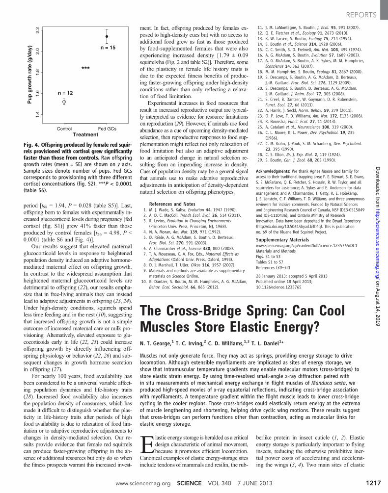
period [t98 = 1.94, P = 0.028 (table S5)]. Last,offspring born to females with experimentally in-creased glucocorticoid levels during pregnancy [fedcortisol (fig. S1)] grew 41% faster than thoseproduced by control females [t26 = 4.98, P <0.0001 (table S6 and Fig. 4)].
Our results suggest that elevated maternalglucocorticoid levels in response to heightenedpopulation density induced an adaptive hormone-mediated maternal effect on offspring growth.In contrast to the widespread assumption thatheightened maternal glucocorticoid levels aredetrimental to offspring (22), our results empha-size that in free-living animals they can insteadlead to adaptive adjustments in offspring (23, 24).Under high-density conditions, squirrels spendless time feeding and in the nest (10), suggestingthat increased offspring growth is not a simpleoutcome of increased maternal care or milk pro-visioning. Alternatively, elevated exposure to glu-cocorticoids early in life (22, 25) could increaseoffspring growth by directly influencing off-spring physiology or behavior (22, 26) and sub-sequent changes in growth hormone secretionin offspring (27).
For nearly 100 years, food availability hasbeen considered to be a universal variable affect-ing population dynamics and life-history traits(28). Increased food availability also increasesthe population density of consumers, which hasmade it difficult to distinguish whether the plas-ticity in life-history traits after periods of highfood availability is due to relaxation of food lim-itation or to adaptive reproductive adjustments tochanges in density-mediated selection. Our re-sults provide evidence that female red squirrelscan produce faster-growing offspring in the ab-sence of additional resources but only do so whenthe fitness prospects warrant this increased invest-
ment. In fact, offspring produced by females ex-posed to high-density cues but with no access toadditional food grew as fast as those producedby food-supplemented females that were alsoexperiencing increased density [1.79 T 0.09squirrels/ha (Fig. 2 and table S2)]. Therefore, someof the plasticity in female life history traits isdue to the expected fitness benefits of produc-ing faster-growing offspring under high-densityconditions rather than only reflecting a relaxa-tion of food limitation.
Experimental increases in food resources thatresult in increased reproductive output are typical-ly interpreted as evidence for resource limitationson reproduction (29). However, if animals use foodabundance as a cue of upcoming density-mediatedselection, then reproductive responses to food sup-plementation might reflect not only relaxation offood limitation but also an adaptive adjustmentto an anticipated change in natural selection re-sulting from an impending increase in density.Cues of population density may be a general signalthat animals use to make adaptive reproductiveadjustments in anticipation of density-dependentnatural selection on offspring phenotypes.
References and Notes1. M. J. Wade, S. Kalisz, Evolution 44, 1947 (1990).2. A. D. C. MacColl, Trends Ecol. Evol. 26, 514 (2011).3. R. Levins, Evolution in Changing Environments
(Princeton Univ. Press, Princeton, NJ, 1968).4. N. A. Moran, Am. Nat. 139, 971 (1992).5. D. Réale, A. G. McAdam, S. Boutin, D. Berteaux,
Proc. Biol. Sci. 270, 591 (2003).6. A. Charmantier et al., Science 320, 800 (2008).7. T. A. Mousseau, C. A. Fox, Eds., Maternal Effects as
Adaptations (Oxford Univ. Press, Oxford, 1998).8. D. J. Marshall, T. Uller, Oikos 116, 1957 (2007).9. Materials and methods are available as supplementary
materials on Science Online.10. B. Dantzer, S. Boutin, M. M. Humphries, A. G. McAdam,
Behav. Ecol. Sociobiol. 66, 865 (2012).
11. J. M. LaMontagne, S. Boutin, J. Ecol. 95, 991 (2007).12. Q. E. Fletcher et al., Ecology 91, 2673 (2010).13. K. W. Larsen, S. Boutin, Ecology 75, 214 (1994).14. S. Boutin et al., Science 314, 1928 (2006).15. C. C. Smith, S. D. Fretwell, Am. Nat. 108, 499 (1974).16. A. G. McAdam, S. Boutin, Evolution 57, 1689 (2003).17. A. G. McAdam, S. Boutin, A. K. Sykes, M. M. Humphries,
Écoscience 14, 362 (2007).18. M. M. Humphries, S. Boutin, Ecology 81, 2867 (2000).19. S. Descamps, S. Boutin, A. G. McAdam, D. Berteaux,
J.-M. Gaillard, Proc. Biol. Sci. 276, 1129 (2009).20. S. Descamps, S. Boutin, D. Berteaux, A. G. McAdam,
J.-M. Gaillard, J. Anim. Ecol. 77, 305 (2008).21. S. Creel, B. Dantzer, W. Goymann, D. R. Rubenstein,
Funct. Ecol. 27, 66 (2013).22. A. Harris, J. Seckl, Horm. Behav. 59, 279 (2011).23. O. P. Love, T. D. Williams, Am. Nat. 172, E135 (2008).24. R. Boonstra, Funct. Ecol. 27, 11 (2013).25. A. Catalani et al., Neuroscience 100, 319 (2000).26. C. L. Moore, K. L. Power, Dev. Psychobiol. 19, 235
(1986).27. C. M. Kuhn, J. Pauk, S. M. Schanberg, Dev. Psychobiol.
23, 395 (1990).28. C. S. Elton, Br. J. Exp. Biol. 2, 119 (1924).29. S. Boutin, Can. J. Zool. 68, 203 (1990).
Acknowledgments: We thank Agnes Moose and family foraccess to their traditional trapping area; F. E. Stewart, S. E. Evans,S. E. McFarlane, Q. E. Fletcher, S. Hossain, R. W. Taylor, and allsquirrelers for assistance; A. Sykes and E. Anderson for datamanagement; and A. Charmantier, T. Getty, K. E. Holekamp,J. S. Lonstein, C. T. Williams, T. D. Williams, and three anonymousreviewers for incisive comments. Funded by Natural Sciencesand Engineering Research Council of Canada, NSF (DEB-0515849and IOS-1110436), and Ontario Ministry of ResearchInnovation. Data have been deposited in the Dryad Repository(http://dx.doi.org/10.5061/dryad.b3h4q). This is publicationno. 69 of the Kluane Red Squirrel Project.
Supplementary Materialswww.sciencemag.org/cgi/content/full/science.1235765/DC1Materials and MethodsFigs. S1 to S3Tables S1 to S7References (30–54)
28 January 2013; accepted 5 April 2013Published online 18 April 2013;10.1126/science.1235765
The Cross-Bridge Spring: Can CoolMuscles Store Elastic Energy?N. T. George,1 T. C. Irving,2 C. D. Williams,1,3 T. L. Daniel1*
Muscles not only generate force. They may act as springs, providing energy storage to drivelocomotion. Although extensible myofilaments are implicated as sites of energy storage, weshow that intramuscular temperature gradients may enable molecular motors (cross-bridges) tostore elastic strain energy. By using time-resolved small-angle x-ray diffraction paired within situ measurements of mechanical energy exchange in flight muscles of Manduca sexta, weproduced high-speed movies of x-ray equatorial reflections, indicating cross-bridge associationwith myofilaments. A temperature gradient within the flight muscle leads to lower cross-bridgecycling in the cooler regions. Those cross-bridges could elastically return energy at the extremaof muscle lengthening and shortening, helping drive cyclic wing motions. These results suggestthat cross-bridges can perform functions other than contraction, acting as molecular links forelastic energy storage.
Elastic energy storage is heralded as a criticaldesign characteristic of animal movement,because it promotes efficient locomotion.
Canonical examples of elastic energy-storage sitesinclude tendons of mammals and resilin, the rub-
berlike protein in insect cuticle (1, 2). Elasticenergy storage is particularly important to flyinginsects, reducing the otherwise prohibitive iner-tial power costs of accelerating and decelerat-ing the wings (3, 4). Two main sites of elastic
1.4
1.6
1.8
2.0
2.2
Pu
p g
row
th r
ate
(g/d
ay)
***
n = 12
n = 15
Control Fed GCsTreatment
Fig. 4. Offspring produced by female red squir-rels provisioned with cortisol grew significantlyfaster than those from controls. Raw offspringgrowth rates (mean T SE) are shown on y axis.Sample sizes denote number of pups. Fed GCscorresponds to provisioning with three differentcortisol concentrations (fig. S2). ***P < 0.0001(table S6).
www.sciencemag.org SCIENCE VOL 340 7 JUNE 2013 1217
REPORTSon A
ugust 14, 2019
http://science.sciencemag.org/
Dow
nloaded from
MammalDensity Triggers Maternal Hormones That Increase Adaptive Offspring Growth in a Wild
Ben Dantzer, Amy E. M. Newman, Rudy Boonstra, Rupert Palme, Stan Boutin, Murray M. Humphries and Andrew G. McAdam
originally published online April 18, 2013DOI: 10.1126/science.1235765 (6137), 1215-1217.340Science
produced in the dense population.stimulate them to produce pups that will grow faster and hopefully outcompete the many other pups expected to be because of increased glucocorticoid levels in the mother. The density stress experienced by mothers thus appears toboth natural and artificially induced increases in the number of conspecific calls increased the growth rate of pups
(p. 1215, published online 18 April) monitored a population of red squirrels and found thatet al.Dantzer they may face. Maternal effects and influence can sometimes prepare unborn offspring for some of the environmental conditions
Thank Your Mother
ARTICLE TOOLS http://science.sciencemag.org/content/340/6137/1215
MATERIALSSUPPLEMENTARY http://science.sciencemag.org/content/suppl/2013/04/17/science.1235765.DC1
CONTENTRELATED http://stke.sciencemag.org/content/sigtrans/6/279/ec134.abstract
REFERENCES
http://science.sciencemag.org/content/340/6137/1215#BIBLThis article cites 47 articles, 3 of which you can access for free
PERMISSIONS http://www.sciencemag.org/help/reprints-and-permissions
Terms of ServiceUse of this article is subject to the
is a registered trademark of AAAS.Sciencelicensee American Association for the Advancement of Science. No claim to original U.S. Government Works. The title Science, 1200 New York Avenue NW, Washington, DC 20005. 2017 © The Authors, some rights reserved; exclusive
(print ISSN 0036-8075; online ISSN 1095-9203) is published by the American Association for the Advancement ofScience
on August 14, 2019
http://science.sciencem
ag.org/D
ownloaded from
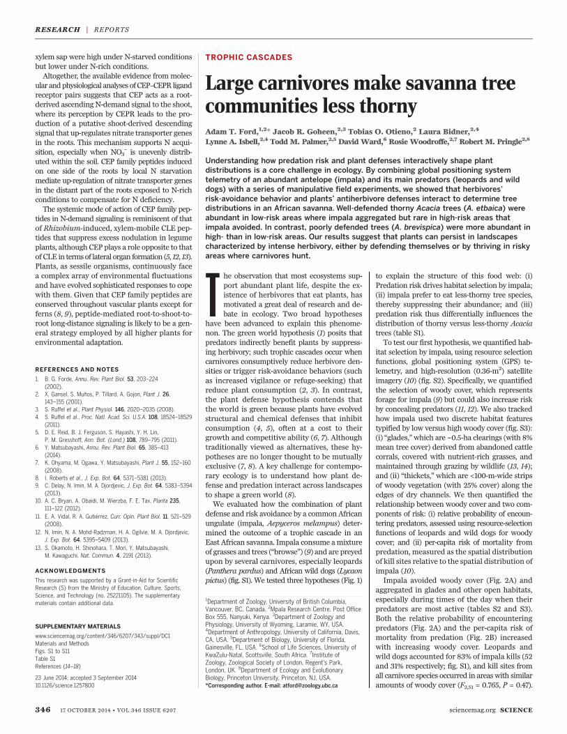
xylem sap were high under N-starved conditionsbut lower under N-rich conditions.Altogether, the available evidence frommolec-
ular andphysiological analyses of CEP–CEPR ligandreceptor pairs suggests that CEP acts as a root-derived ascending N-demand signal to the shoot,where its perception by CEPR leads to the pro-duction of a putative shoot-derived descendingsignal that up-regulates nitrate transporter genesin the roots. This mechanism supports N acqui-sition, especially when NO3
– is unevenly distrib-uted within the soil. CEP family peptides inducedon one side of the roots by local N starvationmediate up-regulation of nitrate transporter genesin the distant part of the roots exposed to N-richconditions to compensate for N deficiency.The systemic mode of action of CEP family pep-
tides in N-demand signaling is reminiscent of thatof Rhizobium-induced, xylem-mobile CLE pep-tides that suppress excess nodulation in legumeplants, although CEP plays a role opposite to thatof CLE in termsof lateral organ formation (5, 12, 13).Plants, as sessile organisms, continuously facea complex array of environmental fluctuationsand have evolved sophisticated responses to copewith them. Given that CEP family peptides areconserved throughout vascular plants except forferns (8, 9), peptide-mediated root-to-shoot-to-root long-distance signaling is likely to be a gen-eral strategy employed by all higher plants forenvironmental adaptation.
REFERENCES AND NOTES
1. B. G. Forde, Annu. Rev. Plant Biol. 53, 203–224(2002).
2. X. Gansel, S. Muños, P. Tillard, A. Gojon, Plant J. 26,143–155 (2001).
3. S. Ruffel et al., Plant Physiol. 146, 2020–2035 (2008).4. S. Ruffel et al., Proc. Natl. Acad. Sci. U.S.A. 108, 18524–18529
(2011).5. D. E. Reid, B. J. Ferguson, S. Hayashi, Y. H. Lin,
P. M. Gresshoff, Ann. Bot. (Lond.) 108, 789–795 (2011).6. Y. Matsubayashi, Annu. Rev. Plant Biol. 65, 385–413
(2014).7. K. Ohyama, M. Ogawa, Y. Matsubayashi, Plant J. 55, 152–160
(2008).8. I. Roberts et al., J. Exp. Bot. 64, 5371–5381 (2013).9. C. Delay, N. Imin, M. A. Djordjevic, J. Exp. Bot. 64, 5383–5394
(2013).10. A. C. Bryan, A. Obaidi, M. Wierzba, F. E. Tax, Planta 235,
111–122 (2012).11. E. A. Vidal, R. A. Gutiérrez, Curr. Opin. Plant Biol. 11, 521–529
(2008).12. N. Imin, N. A. Mohd-Radzman, H. A. Ogilvie, M. A. Djordjevic,
J. Exp. Bot. 64, 5395–5409 (2013).13. S. Okamoto, H. Shinohara, T. Mori, Y. Matsubayashi,
M. Kawaguchi, Nat. Commun. 4, 2191 (2013).
ACKNOWLEDGMENTS
This research was supported by a Grant-in-Aid for ScientificResearch (S) from the Ministry of Education, Culture, Sports,Science, and Technology (no. 25221105). The supplementarymaterials contain additional data.
SUPPLEMENTARY MATERIALS
www.sciencemag.org/content/346/6207/343/suppl/DC1Materials and MethodsFigs. S1 to S11Table S1References (14–18)
23 June 2014; accepted 3 September 201410.1126/science.1257800
TROPHIC CASCADES
Large carnivores make savanna treecommunities less thornyAdam T. Ford,1,2* Jacob R. Goheen,2,3 Tobias O. Otieno,2 Laura Bidner,2,4
Lynne A. Isbell,2,4 Todd M. Palmer,2,5 David Ward,6 Rosie Woodroffe,2,7 Robert M. Pringle2,8
Understanding how predation risk and plant defenses interactively shape plantdistributions is a core challenge in ecology. By combining global positioning systemtelemetry of an abundant antelope (impala) and its main predators (leopards and wilddogs) with a series of manipulative field experiments, we showed that herbivores’risk-avoidance behavior and plants’ antiherbivore defenses interact to determine treedistributions in an African savanna. Well-defended thorny Acacia trees (A. etbaica) wereabundant in low-risk areas where impala aggregated but rare in high-risk areas thatimpala avoided. In contrast, poorly defended trees (A. brevispica) were more abundant inhigh- than in low-risk areas. Our results suggest that plants can persist in landscapescharacterized by intense herbivory, either by defending themselves or by thriving in riskyareas where carnivores hunt.
The observation that most ecosystems sup-port abundant plant life, despite the ex-istence of herbivores that eat plants, hasmotivated a great deal of research and de-bate in ecology. Two broad hypotheses
have been advanced to explain this phenome-non. The green world hypothesis (1) posits thatpredators indirectly benefit plants by suppress-ing herbivory; such trophic cascades occur whencarnivores consumptively reduce herbivore den-sities or trigger risk-avoidance behaviors (suchas increased vigilance or refuge-seeking) thatreduce plant consumption (2, 3). In contrast,the plant defense hypothesis contends thatthe world is green because plants have evolvedstructural and chemical defenses that inhibitconsumption (4, 5), often at a cost to theirgrowth and competitive ability (6, 7). Althoughtraditionally viewed as alternatives, these hy-potheses are no longer thought to be mutuallyexclusive (7, 8). A key challenge for contempo-rary ecology is to understand how plant de-fense and predation interact across landscapesto shape a green world (8).We evaluated how the combination of plant
defense and risk avoidance by a common Africanungulate (impala, Aepyceros melampus) deter-mined the outcome of a trophic cascade in anEast African savanna. Impala consume amixtureof grasses and trees (“browse”) (9) and are preyedupon by several carnivores, especially leopards(Panthera pardus) and African wild dogs (Lycaonpictus) (fig. S1). We tested three hypotheses (Fig. 1)
to explain the structure of this food web: (i)Predation risk drives habitat selection by impala;(ii) impala prefer to eat less-thorny tree species,thereby suppressing their abundance; and (iii)predation risk thus differentially influences thedistribution of thorny versus less-thorny Acaciatrees (table S1).To test our first hypothesis, we quantified hab-
itat selection by impala, using resource selectionfunctions, global positioning system (GPS) te-lemetry, and high-resolution (0.36-m2) satelliteimagery (10) (fig. S2). Specifically, we quantifiedthe selection of woody cover, which representsforage for impala (9) but could also increase riskby concealing predators (11, 12). We also trackedhow impala used two discrete habitat featurestypified by low versus high woody cover (fig. S3):(i) “glades,”which are ~0.5-ha clearings (with 8%mean tree cover) derived from abandoned cattlecorrals, covered with nutrient-rich grasses, andmaintained through grazing by wildlife (13, 14);and (ii) “thickets,” which are <100-m-wide stripsof woody vegetation (with 25% cover) along theedges of dry channels. We then quantified therelationship between woody cover and two com-ponents of risk: (i) relative probability of encoun-tering predators, assessed using resource-selectionfunctions of leopards and wild dogs for woodycover; and (ii) per-capita risk of mortality frompredation, measured as the spatial distributionof kill sites relative to the spatial distribution ofimpala (10).Impala avoided woody cover (Fig. 2A) and
aggregated in glades and other open habitats,especially during times of the day when theirpredators are most active (tables S2 and S3).Both the relative probability of encounteringpredators (Fig. 2A) and the per-capita risk ofmortality from predation (Fig. 2B) increasedwith increasing woody cover. Leopards andwild dogs accounted for 83% of impala kills (52and 31% respectively; fig. S1), and kill sites fromall carnivore species occurred in areas with similaramounts of woody cover (F2,51 = 0.765, P = 0.47).
346 17 OCTOBER 2014 • VOL 346 ISSUE 6207 sciencemag.org SCIENCE
1Department of Zoology, University of British Columbia,Vancouver, BC, Canada. 2Mpala Research Centre, Post OfficeBox 555, Nanyuki, Kenya. 3Department of Zoology andPhysiology, University of Wyoming, Laramie, WY, USA.4Department of Anthropology, University of California, Davis,CA, USA. 5Department of Biology, University of Florida,Gainesville, FL, USA. 6School of Life Sciences, University ofKwaZulu-Natal, Scottsville, South Africa. 7Institute ofZoology, Zoological Society of London, Regent's Park,London, UK. 8Department of Ecology and EvolutionaryBiology, Princeton University, Princeton, NJ, USA.*Corresponding author. E-mail: [email protected]
RESEARCH | REPORTS
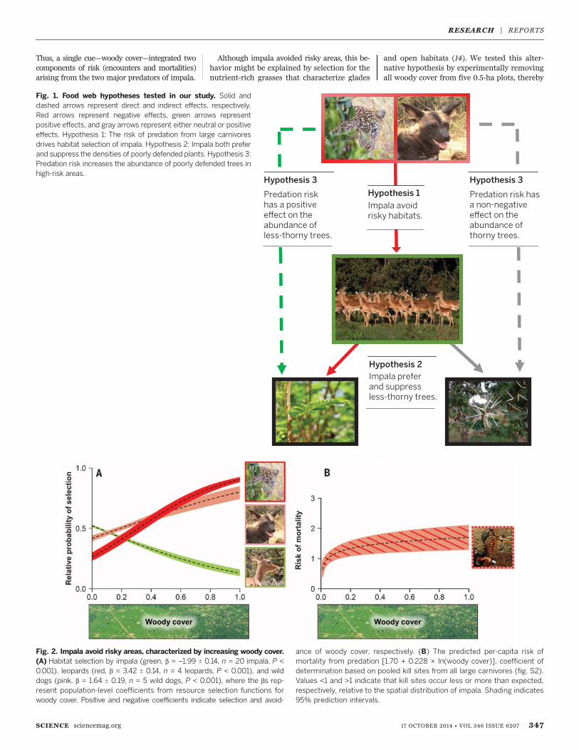
Thus, a single cue—woody cover—integrated twocomponents of risk (encounters and mortalities)arising from the two major predators of impala.
Although impala avoided risky areas, this be-havior might be explained by selection for thenutrient-rich grasses that characterize glades
and open habitats (14). We tested this alter-native hypothesis by experimentally removingall woody cover from five 0.5-ha plots, thereby
SCIENCE sciencemag.org 17 OCTOBER 2014 • VOL 346 ISSUE 6207 347
RESEARCH | REPORTS
Fig. 2. Impala avoid risky areas, characterized by increasing woody cover.(A) Habitat selection by impala (green, b = –1.99 T 0.14, n = 20 impala, P <0.001), leopards (red, b = 3.42 T 0.14, n = 4 leopards, P < 0.001), and wilddogs (pink, b = 1.64 T 0.19, n = 5 wild dogs, P < 0.001), where the bs rep-resent population-level coefficients from resource selection functions forwoody cover. Positive and negative coefficients indicate selection and avoid-
ance of woody cover, respectively. (B) The predicted per-capita risk ofmortality from predation [1.70 + 0.228 × ln(woody cover)], coefficient ofdetermination based on pooled kill sites from all large carnivores (fig. S2).Values <1 and >1 indicate that kill sites occur less or more than expected,respectively, relative to the spatial distribution of impala. Shading indicates95% prediction intervals.
Fig. 1. Food web hypotheses tested in our study. Solid anddashed arrows represent direct and indirect effects, respectively.Red arrows represent negative effects, green arrows representpositive effects, and gray arrows represent either neutral or positiveeffects. Hypothesis 1: The risk of predation from large carnivoresdrives habitat selection of impala. Hypothesis 2: Impala both preferand suppress the densities of poorly defended plants. Hypothesis 3:Predation risk increases the abundance of poorly defended trees inhigh-risk areas.
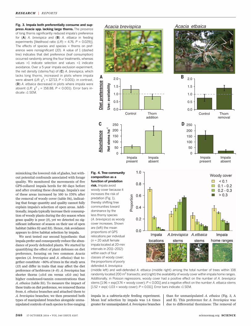
mimicking the lowered risk of glades, but with-out potential confounds associated with foragequality. We monitored the movements of fiveGPS-collared impala herds for 60 days beforeand after creating these clearings. Impala’s useof these areas increased by 160 to 576% afterthe removal of woody cover (table S4), indicat-ing that forage quantity and quality cannot fullyexplain impala’s selection of open areas. Addi-tionally, impala typically increase their consump-tion of woody plants during the dry season whengrass quality is poor (9), yet we detected no sig-nificant influence of season on their use of openhabitat (tables S2 and S3). Hence, risk avoidanceappears to drive habitat selection by impala.We next tested our second hypothesis: that
impala prefer and consequently reduce the abun-dance of poorly defended plants. We started byquantifying the effect of plant defenses on dietpreference, focusing on two common Acaciaspecies (A. brevispica and A. etbaica) that to-gether constitute ~80% of trees in the study area(13) and differ in traits that may affect the dietpreference of herbivores (4–8): A. brevispica hasshorter thorns (≤0.6 cm versus ≤6.0 cm) buthigher condensed-tannin concentrations thanA. etbaica (table S5). To measure the impact ofthese traits on diet preference, we removed thornsfrom A. etbaica branches and attached them toA. brevispica branches; we then presented bothtypes of manipulated branches alongside unma-nipulated controls of each species to free-ranging
impala in a cafeteria-style feeding experiment.Mean leaf selection by impala was 1.4 timesgreater for unmanipulatedA. brevispica branches
than for unmanipulated A. etbaica (Fig. 3, Aand B). This preference for A. brevispica wasdue to differential thorniness: The removal of
348 17 OCTOBER 2014 • VOL 346 ISSUE 6207 sciencemag.org SCIENCE
Fig. 3. Impala both preferentially consume and sup-press Acacia spp. lacking large thorns. The presenceof long thorns significantly reduced impala’s preferencefor (A) A. brevispica and (B) A. etbaica in feedingexperiments [likelihood ratio (LR) = 4.76, P = 0.029)].The effects of species and species × thorns on pref-erence were nonsignificant (10). A value of 1 (dashedline) indicates that diet preference (leaf consumption)occurred randomly among the four treatments, whereasvalues >1 indicate selection and values <1 indicateavoidance. Over a 5-year impala exclusion experiment,the net density (stems/ha) of (C) A. brevispica, whichlacks long thorns, increased in plots where impalawere absent (LR: c21 = 127.13, P < 0.001); in contrast,(D) A. etbaica decreased in plots where impala wereabsent (LR: c2 1 = 158.88, P < 0.001). Error bars in-dicate T1 SEM.
0.0
0.5
1.0
1.5
2.0
Control Thornaddition
Acacia etbaica
Ab
un
dan
ceD
iet
pre
fere
nce
Use
: av
aila
bili
ty0.0
0.5
1.0
1.5
2.0
Control Thornremoval
Net
ste
ms
ha-1
0
50
100
150
200
250
Impalapresent
Impalaabsent
0
50
100
150
200
250
Impalapresent
Impalaabsent
Acacia brevispica
Fig. 4. Tree-communitycomposition as afunction of predationrisk. Impala avoidwoody cover because itincreases the risk ofpredation (Fig. 1),thereby shifting treecommunities towarddominance by theless thorny species(A. brevispica) as woodycover increases. Shownare (left) the meanproportions of GPSrelocations per individual(n = 20 adult femaleimpala located at 20-minintervals in 2011–2012)within each of fourclasses of woody cover;the proportions of poorlydefended A. brevispica(middle left) and well-defended A. etbaica (middle right) among the total number of trees within 108randomly located 200m2 transects; and (right) the availability of woody cover within impala home ranges.Additionally, in Poisson regressions, woody cover had a positive effect on the number of A. brevispicastems [1.96 + exp(3.74 × woody cover); P < 0.001] and a negative effect on the number A. etbaica stems[1.52 + exp(–1.03 × woody cover); P = 0.011]. Error bars indicate T1 SEM.
RESEARCH | REPORTS
A. etbaica’s long thorns increased leaf selectionto levels commensurate with that of unmanipu-lated A. brevispica, whereas selection for thorn-addition A. brevispica was roughly equal to thatof unmanipulated A. etbaica (Fig. 3, A and B).Thus, we conclude that A. brevispica is preferredrelative to A. etbaica and that this preference isdetermined by thorns rather than tannins orother species-specific attributes.Next, we considered whether the diet pref-
erence of impala could alter the abundanceof Acacia species. We therefore measured thenet change in the density of tree stems from2009–2014 within nine replicate sets of 1-ha herbi-vore exclosures that independently manipu-lated megaherbivores [elephants (Loxodontaafricana) and giraffes (Giraffa camelopardalis)],mesoherbivores [impala and eland (Taurotragusoryx)], and small browsers [dik-dik (Madoquaguentheri)], using electrified wires at differentheights (15). We isolated the effects of impala onAcacia species by comparing the megaherbivoreand mesoherbivore-exclusion treatments; we at-tributed mesoherbivore-driven effects on treedensity to impala because they account for ~87%of browser biomass in this size class (9). The ex-clusion of impala increased the net stem densityof the preferred and poorly defendedA. brevispicaby 233% (Fig. 3C). Conversely, net stem densityof well-defended A. etbaica increased by 692%in plots accessible to impala as compared toimpala-exclusion plots (Fig. 3D). This increasein A. etbaica in plots where impala were presentis perhaps due to reduced competition withA. brevispica (15, 16). Thus, although impalaconsumed leaves from bothAcacia species (Fig. 3,A and B), the long thorns of A. etbaica enabledthem to avoid suppression by impala.To evaluate our third and final hypothesis,
we related spatial patterns in the abundance ofthese two Acacia species to satellite-derived esti-mates of woody cover. We counted all trees in 108transects (200 m2) located near randomly se-lected glades and thickets throughout our 140-km2
study area. The abundance of A. brevispica in-creased monotonically with satellite-derived es-timates of woody cover (i.e., risk) across thesetransects, whereas A. etbaica became scarcer aswoody cover increased (Fig. 4 and fig. S4). Riskavoidance by impala (Fig. 2) was functionallyanalogous to impala exclusion by electrifiedfences (Fig. 3, C and D): Our results consistentlyshowed that the absence of impala herbivoryincreased the prevalence of poorly defended treesbut not the prevalence ofwell-defended trees. Thus,tree communities became less thorny as preda-tion risk arising from large carnivores increased(Fig. 4).Collectively, our results show that the nature
of trophic control is contingent on biotic context:namely predation risk and plant defenses (Fig. 1).Both mechanisms enable plants to thrive in dif-ferent parts of the landscape: Where risk is high,poorly defended trees are released from brows-ing, resulting in a trophic cascade; where risk islow, intense herbivory increases the benefit ofdefenses, creating communities dominated by
thorny trees. Consequently, the thorniness of treecommunities decreased across the landscape be-cause of the way in which impala responded tospatial variation in predation risk, and also be-cause of the way plant defenses affected impala’sdiet preference.Human activities—both past and present—
exert a major influence on the interactions be-tween carnivores, impala, and the tree community.Glades represent the legacy of traditional live-stock production (17), generating a constellationof refugia that has shaped the spatial distributionof impala herbivory. However, the loss of largecarnivores will make landscapes less risky (18),decoupling the spatial interplay of risk avoidanceand herbivory. The loss of carnivores will alsorender obsolete the need for pastoralists to corraltheir cattle nightly, eliminating the formation ofglades. Consequently, human-driven extirpationof large carnivores fromAfrican savannas (2) willreduce spatial variation in plant communities,leading to a world that is thornier, but still green.As large-carnivore populations continue to de-cline globally, understanding the context in whichpredators shape key ecosystem processes is anurgent priority (19). Studies integrating risk ofpredation and plant defenses will constitute amajor step toward this goal.
REFERENCES AND NOTES
1. N. G. Hairston, F. E. Smith, L. B. Slobodkin, Am. Nat. 94, 421(1960).
2. J. A. Estes et al., Science 333, 301–306 (2011).3. E. L. Preisser, D. I. Bolnick, M. F. Benard, Ecology 86, 501–509
(2005).4. W. W. Murdoch, Am. Nat. 100, 219 (1966).5. S. L. Pimm, The Balance of Nature?: Ecological Issues in the
Conservation of Species and Communities (Univ. of ChicagoPress, Chicago, 1991).
6. O. J. Schmitz, Proc. Natl. Acad. Sci. U.S.A. 91, 5364–5367(1994).
7. K. A. Mooney, R. Halitschke, A. Kessler, A. A. Agrawal, Science327, 1642–1644 (2010).
8. O. J. Schmitz, Resolving Ecosystem Complexity, vol. 47of Monographs in Population Biology, S. A. Levin,H. S. Horn, Eds. (Princeton Univ. Press, Princeton,NJ, 2010).
9. D. J. Augustine, Afr. J. Ecol. 48, 1009–1020 (2010).10. Materials and methods are available as supplementary
materials on Science Online.11. R. Underwood, Behaviour 79, 81–107 1982).12. M. Thaker et al., Ecology 92, 398–407 (2011).13. T. P. Young, N. Patridge, A. Macrae, Ecol. Appl. 5, 97
(1995).14. D. J. Augustine, J. Wildl. Manage. 68, 916–923 (2004).15. J. R. Goheen et al., PLOS ONE 8, e55192 (2013).16. J. L. Orrock, R. D. Holt, M. L. Baskett, Ecol. Lett. 13, 11–20
(2010).17. K. E. Veblen, J. Arid Environ. 78, 119–127 (2012).18. J. Berger, J. E. Swenson, I.-L. Persson, Science 291, 1036–1039
(2001).19. W. J. Ripple et al., Science 343, 1241484 (2014).
ACKNOWLEDGMENTS
This research was supported by grants from Canada’s NaturalSciences and Engineering Research Council (A.T.F., J.R.G.), theUniversity of British Columbia (A.T.F.), the University of Wyoming(J.R.G.), the American Society of Mammalogists (A.T.F.),Keren Keyemet I’Israel (D.W.), the U.S. National Science Foundation(L.A.I.), and the Wenner-Gren Foundation (L.B.). We thank S. Lima,M. Kinnaird, M. Littlewood, B. Agwanda, C. Forbes, J. Estes,M. Kauffman, R. Ostfeld, S. Buskirk, C. Martinez del Rio, C. Riginos,and the Kenya Wildlife Service. Comments from threeanonymous reviewers greatly improved the manuscript.
SUPPLEMENTARY MATERIALS
www.sciencemag.org/content/346/6207/346/suppl/DC1Materials and MethodsFigs. S1 to S4Tables S1 to S5References
28 February 2014; accepted 15 September 201410.1126/science.1252753
CLIMATE CHANGE
Increased variability of tornadooccurrence in the United StatesHarold E. Brooks,1* Gregory W. Carbin,2 Patrick T. Marsh2
Whether or not climate change has had an impact on the occurrence of tornadoes in theUnited States has become a question of high public and scientific interest, but changesin how tornadoes are reported have made it difficult to answer it convincingly. We showthat, excluding the weakest tornadoes, the mean annual number of tornadoes has remainedrelatively constant, but their variability of occurrence has increased since the 1970s.This isdue to a decrease in the number of days per year with tornadoes combined with anincrease in days with many tornadoes, leading to greater variability on annual and monthlytime scales and changes in the timing of the start of the tornado season.
Separating nonmeteorological effects in theofficial database of tornadoes in the UnitedStates from actual meteorological oneshas made interpreting the existence andcauses of long-term physical changes in tor-
nado occurrence extremely difficult (1). Non-meteorological effects in the database result fromchanges in the emphasis on, and methodology of,
collecting reports, and from how tornadoes areobserved. The mean occurrence of well-reportedaspects of the database, such as the mean annual
SCIENCE sciencemag.org 17 OCTOBER 2014 • VOL 346 ISSUE 6207 349
RESEARCH | REPORTS
1National Oceanic and Atmospheric Administration(NOAA)/National Severe Storms Laboratory, Norman, OK73072, USA. 2NOAA/National Weather Service Storm PredictionCenter, Norman, OK 73072, USA.*Corresponding author. E-mail: [email protected]
rspb.royalsocietypublishing.org
ResearchCite this article: Pauli JN, Mendoza JE,
Steffan SA, Carey CC, Weimer PJ, Peery MZ.
2014 A syndrome of mutualism reinforces the
lifestyle of a sloth. Proc. R. Soc. B 281:
20133006.
http://dx.doi.org/10.1098/rspb.2013.3006
Received: 16 November 2013
Accepted: 20 December 2013
Subject Areas:ecology, evolution
Keywords:commensalism, Costa Rica, Cryptoses,
Trichophilus
Author for correspondence:Jonathan N. Pauli
e-mail: [email protected]
Electronic supplementary material is available
at http://dx.doi.org/10.1098/rspb.2013.3006 or
via http://rspb.royalsocietypublishing.org.
& 2014 The Author(s) Published by the Royal Society. All rights reserved.
A syndrome of mutualism reinforces thelifestyle of a sloth
Jonathan N. Pauli1, Jorge E. Mendoza1, Shawn A. Steffan2, Cayelan C. Carey3,5,Paul J. Weimer4 and M. Zachariah Peery1
1Department of Forest and Wildlife Ecology, 2USDA-ARS, Department of Entomology, 3Center for Limnology,and 4USDA-ARS, Department of Bacteriology, University of Wisconsin – Madison, Madison, WI 53706, USA5Department of Biological Sciences, Virginia Tech, Blacksburg, VA 24061, USA
Arboreal herbivory is rare among mammals. The few species with this lifestyle
possess unique adaptions to overcome size-related constraints on nutritional
energetics. Sloths are folivores that spend most of their time resting or eating
in the forest canopy. A three-toed sloth will, however, descend its tree
weekly to defecate, which is risky, energetically costly and, until now, inexplic-
able. We hypothesized that this behaviour sustains an ecosystem in the fur of
sloths, which confers cryptic nutritional benefits to sloths. We found that the
more specialized three-toed sloths harboured more phoretic moths, greater
concentrations of inorganic nitrogen and higher algal biomass than the gener-
alist two-toed sloths. Moth density was positively related to inorganic nitrogen
concentration and algal biomass in the fur. We discovered that sloths con-
sumed algae from their fur, which was highly digestible and lipid-rich. By
descending a tree to defecate, sloths transport moths to their oviposition
sites in sloth dung, which facilitates moth colonization of sloth fur. Moths
are portals for nutrients, increasing nitrogen levels in sloth fur, which fuels
algal growth. Sloths consume these algae-gardens, presumably to augment
their limited diet. These linked mutualisms between moths, sloths and algae
appear to aid the sloth in overcoming a highly constrained lifestyle.
1. IntroductionWhile herbivory is the predominant foraging strategy among mammals, arboreal
herbivores are exceedingly rare. Indeed, less than 4% of all mammalian genera con-
tain species that are, to some extent, arboreal and herbivorous, and only 10 species
of mammals (or less than 0.2% of mammalian diversity) are considered specialized
arboreal herbivores [1]. Species that forage on plant matter in trees possess a highly
constrained lifestyle. On one hand, they must be small and light to be supported in
the canopy; on the other hand, small body size limits digestive capacity, especially
for processing plant matter, which is rich in fibre but low in digestible nutrients.
So, although the evolution towards arboreal herbivory is found in taxonomically
disparate mammalian groups, including primates, tree sloths and marsupials,
all weigh between 1 and 14 kg [2]. Thus, the rarity of this lifestyle and convergence
of body size among herbivorous and arboreal mammals appears to reflect con-
straints of nutritional energetics on body size [3]. To overcome such constraints,
arboreal herbivores have evolved dramatic anatomical (e.g. ruminant-like pre-
gastric digestive organs), physiological (e.g. depressed metabolic rates) and
behavioural (e.g. strict dietary preferences) adaptations.
Sloths, or los perezosos (‘the lazies’) in Spanish, are slow-moving Neotropical
mammals. The two phylogenetic groups, two- (Choloepus spp.) and three-toed
(Bradypus spp.) sloths (figure 1a,b), diverged around 40 Ma [4] and are ecologi-
cally quite different. Although both are mid-sized foregut fermenting arboreal
mammals [2], two-toed sloths possess relatively large home-ranges (�x ¼ 18:7 ha,
but up to 140 ha) [5] and a comparatively diverse diet of animal matter, fruits
and leaves, whereas three-toed sloths have highly restricted home-ranges
(�x ¼ 5:4 ha, range ¼ 0.3–15.0 ha) [6] and are regarded as strict folivores [7]. Fur-
thermore, individual three-toed sloths are specialists, roosting and consuming
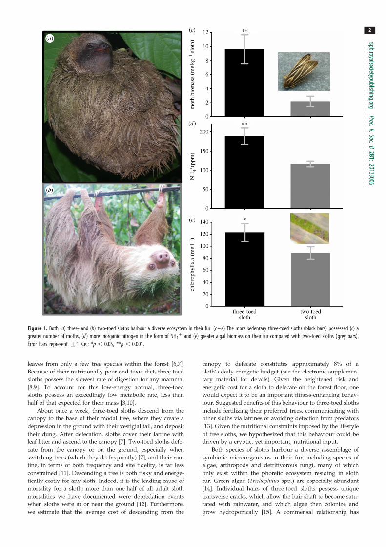
(b)
(a)12
10
8
6
4
2
0
200
150
100
50
0
140
120
100
80
60
40
20
0three-toed
slothtwo-toed
sloth
mot
h bi
omas
s (m
gkg
–1 s
loth
)ch
loro
phyl
la a
(m
gl–1
)N
H4+
(ppm
)
**
**
*
(c)
(d )
(e)
Figure 1. Both (a) three- and (b) two-toed sloths harbour a diverse ecosystem in their fur. (c – e) The more sedentary three-toed sloths (black bars) possessed (c) agreater number of moths, (d ) more inorganic nitrogen in the form of NH4
þ and (e) greater algal biomass on their fur compared with two-toed sloths (grey bars).Error bars represent +1 s.e.; *p , 0.05, **p , 0.001.
rspb.royalsocietypublishing.orgProc.R.Soc.B
281:20133006
2
leaves from only a few tree species within the forest [6,7].
Because of their nutritionally poor and toxic diet, three-toed
sloths possess the slowest rate of digestion for any mammal
[8,9]. To account for this low-energy accrual, three-toed
sloths possess an exceedingly low metabolic rate, less than
half of that expected for their mass [3,10].
About once a week, three-toed sloths descend from the
canopy to the base of their modal tree, where they create a
depression in the ground with their vestigial tail, and deposit
their dung. After defecation, sloths cover their latrine with
leaf litter and ascend to the canopy [7]. Two-toed sloths defe-
cate from the canopy or on the ground, especially when
switching trees (which they do frequently) [7], and their rou-
tine, in terms of both frequency and site fidelity, is far less
constrained [11]. Descending a tree is both risky and energe-
tically costly for any sloth. Indeed, it is the leading cause of
mortality for a sloth; more than one-half of all adult sloth
mortalities we have documented were depredation events
when sloths were at or near the ground [12]. Furthermore,
we estimate that the average cost of descending from the
canopy to defecate constitutes approximately 8% of a
sloth’s daily energetic budget (see the electronic supplemen-
tary material for details). Given the heightened risk and
energetic cost for a sloth to defecate on the forest floor, one
would expect it to be an important fitness-enhancing behav-
iour. Suggested benefits of this behaviour to three-toed sloths
include fertilizing their preferred trees, communicating with
other sloths via latrines or avoiding detection from predators
[13]. Given the nutritional constraints imposed by the lifestyle
of tree sloths, we hypothesized that this behaviour could be
driven by a cryptic, yet important, nutritional input.
Both species of sloths harbour a diverse assemblage of
symbiotic microorganisms in their fur, including species of
algae, arthropods and detritivorous fungi, many of which
only exist within the phoretic ecosystem residing in sloth
fur. Green algae (Trichophilus spp.) are especially abundant
[14]. Individual hairs of three-toed sloths possess unique
transverse cracks, which allow the hair shaft to become satu-
rated with rainwater, and which algae then colonize and
grow hydroponically [15]. A commensal relationship has
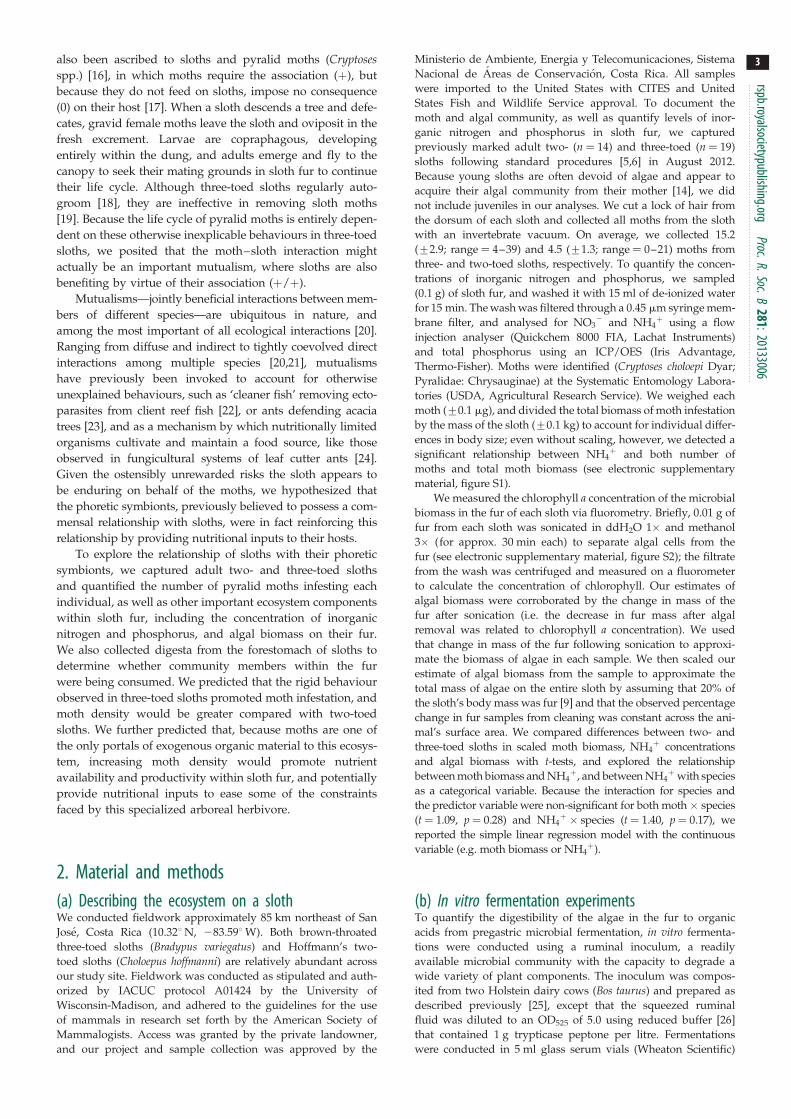
rspb.royalsocietypublishing.orgProc.R.Soc.B
281:20133006
3
also been ascribed to sloths and pyralid moths (Cryptosesspp.) [16], in which moths require the association (þ), butbecause they do not feed on sloths, impose no consequence
(0) on their host [17]. When a sloth descends a tree and defe-
cates, gravid female moths leave the sloth and oviposit in the
fresh excrement. Larvae are copraphagous, developing
entirely within the dung, and adults emerge and fly to the
canopy to seek their mating grounds in sloth fur to continue
their life cycle. Although three-toed sloths regularly auto-
groom [18], they are ineffective in removing sloth moths
[19]. Because the life cycle of pyralid moths is entirely depen-
dent on these otherwise inexplicable behaviours in three-toed
sloths, we posited that the moth–sloth interaction might
actually be an important mutualism, where sloths are also
benefiting by virtue of their association (þ/þ).
Mutualisms—jointly beneficial interactions between mem-
bers of different species—are ubiquitous in nature, and
among the most important of all ecological interactions [20].
Ranging from diffuse and indirect to tightly coevolved direct
interactions among multiple species [20,21], mutualisms
have previously been invoked to account for otherwise
unexplained behaviours, such as ‘cleaner fish’ removing ecto-
parasites from client reef fish [22], or ants defending acacia
trees [23], and as a mechanism by which nutritionally limited
organisms cultivate and maintain a food source, like those
observed in fungicultural systems of leaf cutter ants [24].
Given the ostensibly unrewarded risks the sloth appears to
be enduring on behalf of the moths, we hypothesized that
the phoretic symbionts, previously believed to possess a com-
mensal relationship with sloths, were in fact reinforcing this
relationship by providing nutritional inputs to their hosts.
To explore the relationship of sloths with their phoretic
symbionts, we captured adult two- and three-toed sloths
and quantified the number of pyralid moths infesting each
individual, as well as other important ecosystem components
within sloth fur, including the concentration of inorganic
nitrogen and phosphorus, and algal biomass on their fur.
We also collected digesta from the forestomach of sloths to
determine whether community members within the fur
were being consumed. We predicted that the rigid behaviour
observed in three-toed sloths promoted moth infestation, and
moth density would be greater compared with two-toed
sloths. We further predicted that, because moths are one of
the only portals of exogenous organic material to this ecosys-
tem, increasing moth density would promote nutrient
availability and productivity within sloth fur, and potentially
provide nutritional inputs to ease some of the constraints
faced by this specialized arboreal herbivore.
2. Material and methods(a) Describing the ecosystem on a slothWe conducted fieldwork approximately 85 km northeast of San
Jose, Costa Rica (10.328 N, 283.598 W). Both brown-throated
three-toed sloths (Bradypus variegatus) and Hoffmann’s two-
toed sloths (Choloepus hoffmanni) are relatively abundant across
our study site. Fieldwork was conducted as stipulated and auth-
orized by IACUC protocol A01424 by the University of
Wisconsin-Madison, and adhered to the guidelines for the use
of mammals in research set forth by the American Society of
Mammalogists. Access was granted by the private landowner,
and our project and sample collection was approved by the
Ministerio de Ambiente, Energia y Telecomunicaciones, Sistema
Nacional de Areas de Conservacion, Costa Rica. All samples
were imported to the United States with CITES and United
States Fish and Wildlife Service approval. To document the
moth and algal community, as well as quantify levels of inor-
ganic nitrogen and phosphorus in sloth fur, we captured
previously marked adult two- (n ¼ 14) and three-toed (n ¼ 19)
sloths following standard procedures [5,6] in August 2012.
Because young sloths are often devoid of algae and appear to
acquire their algal community from their mother [14], we did
not include juveniles in our analyses. We cut a lock of hair from
the dorsum of each sloth and collected all moths from the sloth
with an invertebrate vacuum. On average, we collected 15.2
(+2.9; range ¼ 4–39) and 4.5 (+1.3; range ¼ 0–21) moths from
three- and two-toed sloths, respectively. To quantify the concen-
trations of inorganic nitrogen and phosphorus, we sampled
(0.1 g) of sloth fur, and washed it with 15 ml of de-ionized water
for 15 min. The wash was filtered through a 0.45 mm syringe mem-
brane filter, and analysed for NO3� and NH4
þ using a flow
injection analyser (Quickchem 8000 FIA, Lachat Instruments)
and total phosphorus using an ICP/OES (Iris Advantage,
Thermo-Fisher). Moths were identified (Cryptoses choloepi Dyar;
Pyralidae: Chrysauginae) at the Systematic Entomology Labora-
tories (USDA, Agricultural Research Service). We weighed each
moth (+0.1 mg), and divided the total biomass of moth infestation
by the mass of the sloth (+0.1 kg) to account for individual differ-
ences in body size; even without scaling, however, we detected a
significant relationship between NH4þ and both number of
moths and total moth biomass (see electronic supplementary
material, figure S1).
We measured the chlorophyll a concentration of the microbial
biomass in the fur of each sloth via fluorometry. Briefly, 0.01 g of
fur from each sloth was sonicated in ddH2O 1� and methanol
3� (for approx. 30 min each) to separate algal cells from the
fur (see electronic supplementary material, figure S2); the filtrate
from the wash was centrifuged and measured on a fluorometer
to calculate the concentration of chlorophyll. Our estimates of
algal biomass were corroborated by the change in mass of the
fur after sonication (i.e. the decrease in fur mass after algal
removal was related to chlorophyll a concentration). We used
that change in mass of the fur following sonication to approxi-
mate the biomass of algae in each sample. We then scaled our
estimate of algal biomass from the sample to approximate the
total mass of algae on the entire sloth by assuming that 20% of
the sloth’s body mass was fur [9] and that the observed percentage
change in fur samples from cleaning was constant across the ani-
mal’s surface area. We compared differences between two- and
three-toed sloths in scaled moth biomass, NH4þ concentrations
and algal biomass with t-tests, and explored the relationship
between moth biomass and NH4þ, and between NH4
þ with species
as a categorical variable. Because the interaction for species and
the predictor variable were non-significant for both moth � species
(t ¼ 1.09, p¼ 0.28) and NH4þ � species (t ¼ 1.40, p ¼ 0.17), we
reported the simple linear regression model with the continuous
variable (e.g. moth biomass or NH4þ).
(b) In vitro fermentation experimentsTo quantify the digestibility of the algae in the fur to organic
acids from pregastric microbial fermentation, in vitro fermenta-
tions were conducted using a ruminal inoculum, a readily
available microbial community with the capacity to degrade a
wide variety of plant components. The inoculum was compos-
ited from two Holstein dairy cows (Bos taurus) and prepared as
described previously [25], except that the squeezed ruminal
fluid was diluted to an OD525 of 5.0 using reduced buffer [26]
that contained 1 g trypticase peptone per litre. Fermentations
were conducted in 5 ml glass serum vials (Wheaton Scientific)
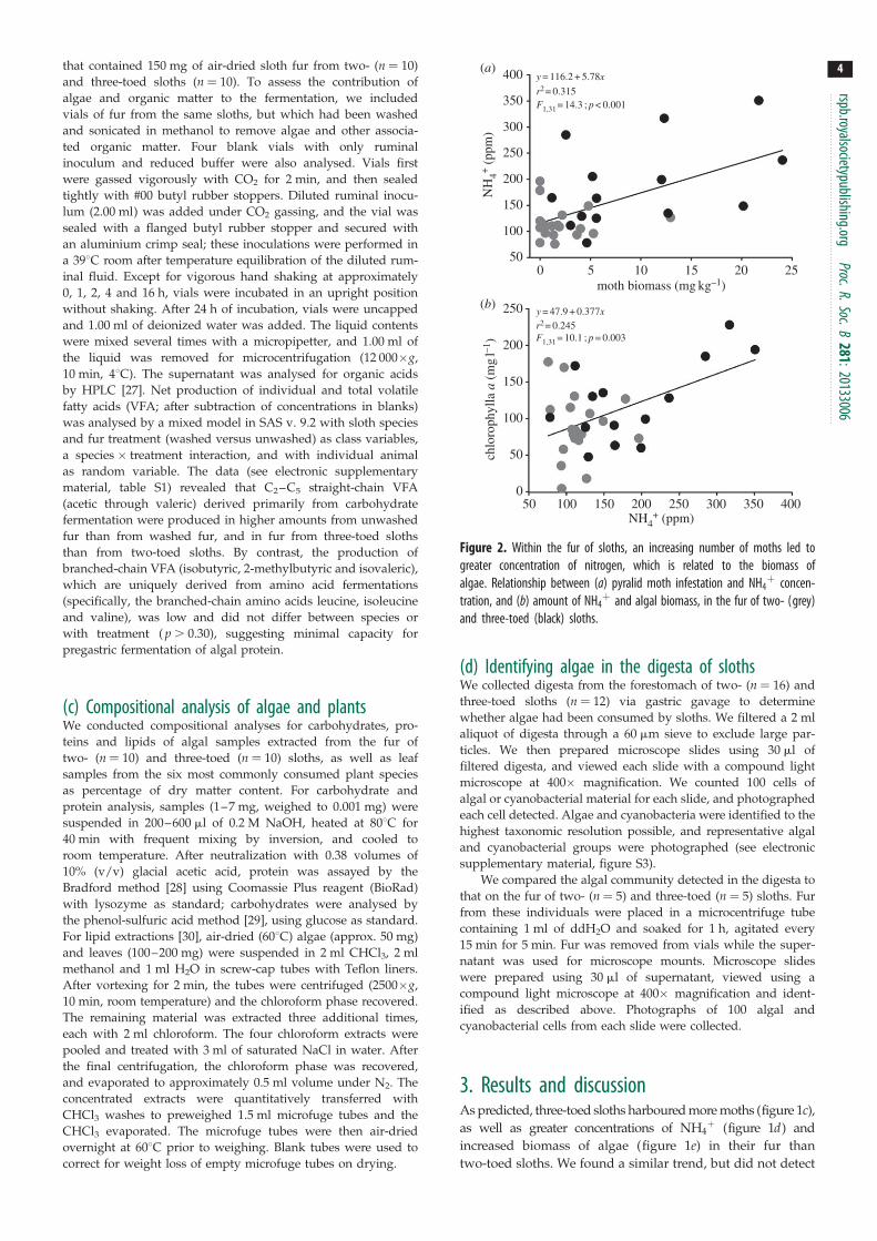
400
350
300
250
200
150
100
50
250
200
150
100
50
0
y = 116.2 + 5.78x
r2 = 0.315F1,31 = 14.3 ; p < 0.001
y = 47.9 + 0.377xr2 = 0.245F1,31 = 10.1 ; p = 0.003
chlo
roph
ylla
a (
mg
l–1)
moth biomass (mg kg–1)
NH
4+ (
ppm
)
NH4+ (ppm)
0
50 100 150 200 250 300 350 400
5 10 15 20 25
(b)
(a)
Figure 2. Within the fur of sloths, an increasing number of moths led togreater concentration of nitrogen, which is related to the biomass ofalgae. Relationship between (a) pyralid moth infestation and NH4
þ concen-tration, and (b) amount of NH4
þ and algal biomass, in the fur of two- (grey)and three-toed (black) sloths.
rspb.royalsocietypublishing.orgProc.R.Soc.B
281:20133006
4
that contained 150 mg of air-dried sloth fur from two- (n ¼ 10)and three-toed sloths (n ¼ 10). To assess the contribution of
algae and organic matter to the fermentation, we included
vials of fur from the same sloths, but which had been washed
and sonicated in methanol to remove algae and other associa-
ted organic matter. Four blank vials with only ruminal
inoculum and reduced buffer were also analysed. Vials first
were gassed vigorously with CO2 for 2 min, and then sealed
tightly with #00 butyl rubber stoppers. Diluted ruminal inocu-
lum (2.00 ml) was added under CO2 gassing, and the vial was
sealed with a flanged butyl rubber stopper and secured with
an aluminium crimp seal; these inoculations were performed in
a 398C room after temperature equilibration of the diluted rum-
inal fluid. Except for vigorous hand shaking at approximately
0, 1, 2, 4 and 16 h, vials were incubated in an upright position
without shaking. After 24 h of incubation, vials were uncapped
and 1.00 ml of deionized water was added. The liquid contents
were mixed several times with a micropipetter, and 1.00 ml of
the liquid was removed for microcentrifugation (12 000�g,
10 min, 48C). The supernatant was analysed for organic acids
by HPLC [27]. Net production of individual and total volatile
fatty acids (VFA; after subtraction of concentrations in blanks)
was analysed by a mixed model in SAS v. 9.2 with sloth species
and fur treatment (washed versus unwashed) as class variables,
a species � treatment interaction, and with individual animal
as random variable. The data (see electronic supplementary
material, table S1) revealed that C2–C5 straight-chain VFA
(acetic through valeric) derived primarily from carbohydrate
fermentation were produced in higher amounts from unwashed
fur than from washed fur, and in fur from three-toed sloths
than from two-toed sloths. By contrast, the production of
branched-chain VFA (isobutyric, 2-methylbutyric and isovaleric),
which are uniquely derived from amino acid fermentations
(specifically, the branched-chain amino acids leucine, isoleucine
and valine), was low and did not differ between species or
with treatment ( p . 0.30), suggesting minimal capacity for
pregastric fermentation of algal protein.
(c) Compositional analysis of algae and plantsWe conducted compositional analyses for carbohydrates, pro-
teins and lipids of algal samples extracted from the fur of
two- (n ¼ 10) and three-toed (n ¼ 10) sloths, as well as leaf
samples from the six most commonly consumed plant species
as percentage of dry matter content. For carbohydrate and
protein analysis, samples (1–7 mg, weighed to 0.001 mg) were
suspended in 200–600 ml of 0.2 M NaOH, heated at 808C for
40 min with frequent mixing by inversion, and cooled to
room temperature. After neutralization with 0.38 volumes of
10% (v/v) glacial acetic acid, protein was assayed by the
Bradford method [28] using Coomassie Plus reagent (BioRad)
with lysozyme as standard; carbohydrates were analysed by
the phenol-sulfuric acid method [29], using glucose as standard.
For lipid extractions [30], air-dried (608C) algae (approx. 50 mg)
and leaves (100–200 mg) were suspended in 2 ml CHCl3, 2 ml
methanol and 1 ml H2O in screw-cap tubes with Teflon liners.
After vortexing for 2 min, the tubes were centrifuged (2500�g,
10 min, room temperature) and the chloroform phase recovered.
The remaining material was extracted three additional times,
each with 2 ml chloroform. The four chloroform extracts were
pooled and treated with 3 ml of saturated NaCl in water. After
the final centrifugation, the chloroform phase was recovered,
and evaporated to approximately 0.5 ml volume under N2. The
concentrated extracts were quantitatively transferred with
CHCl3 washes to preweighed 1.5 ml microfuge tubes and the
CHCl3 evaporated. The microfuge tubes were then air-dried
overnight at 608C prior to weighing. Blank tubes were used to
correct for weight loss of empty microfuge tubes on drying.
(d) Identifying algae in the digesta of slothsWe collected digesta from the forestomach of two- (n ¼ 16) and
three-toed sloths (n ¼ 12) via gastric gavage to determine
whether algae had been consumed by sloths. We filtered a 2 ml
aliquot of digesta through a 60 mm sieve to exclude large par-
ticles. We then prepared microscope slides using 30 ml of
filtered digesta, and viewed each slide with a compound light
microscope at 400� magnification. We counted 100 cells of
algal or cyanobacterial material for each slide, and photographed
each cell detected. Algae and cyanobacteria were identified to the
highest taxonomic resolution possible, and representative algal
and cyanobacterial groups were photographed (see electronic
supplementary material, figure S3).
We compared the algal community detected in the digesta to
that on the fur of two- (n ¼ 5) and three-toed (n ¼ 5) sloths. Fur
from these individuals were placed in a microcentrifuge tube
containing 1 ml of ddH2O and soaked for 1 h, agitated every
15 min for 5 min. Fur was removed from vials while the super-
natant was used for microscope mounts. Microscope slides
were prepared using 30 ml of supernatant, viewed using a
compound light microscope at 400� magnification and ident-
ified as described above. Photographs of 100 algal and
cyanobacterial cells from each slide were collected.
3. Results and discussionAs predicted, three-toed sloths harboured more moths (figure 1c),
as well as greater concentrations of NH4þ (figure 1d) and
increased biomass of algae (figure 1e) in their fur than
two-toed sloths. We found a similar trend, but did not detect
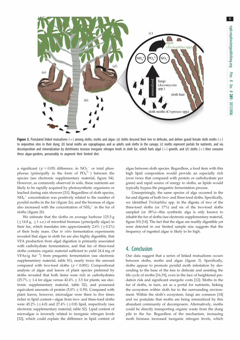
sloth moths (Cryptoses spp.)
sloth hair
fungi
NH4+ PO4
3– NO3–
algae(Trichophilus spp.)
(Ascomycotaspp.)
min
eral
ized
(b)
(a)
(c)
(d )
Figure 3. Postulated linked mutualisms (þ) among sloths, moths and algae: (a) sloths descend their tree to defecate, and deliver gravid female sloth moths (þ)to oviposition sites in their dung; (b) larval moths are copraphagous and as adults seek sloths in the canopy; (c) moths represent portals for nutrients, and viadecomposition and mineralization by detritivores increase inorganic nitrogen levels in sloth fur, which fuels algal (þ) growth, and (d ) sloths (þ) then consumethese algae-gardens, presumably to augment their limited diet.
rspb.royalsocietypublishing.orgProc.R.Soc.B
281:20133006
5
a significant ( p . 0.05) difference, in NO3� or total phos-
phorus (principally in the form of PO43� ) between the
species (see electronic supplementary material, figure S4).
However, as commonly observed in soils, these nutrients are
likely to be rapidly acquired by photosynthetic organisms or
leached during rain showers [31]. Regardless of sloth species,
NH4þ concentration was positively related to the number of
pyralid moths in the fur (figure 2a), and the biomass of algae
also increased with the concentration of NH4þ in the fur of
sloths (figure 2b).
We estimate that the sloths on average harbour 125.5 g
(+14.8 g, +1 s.e.) of microbial biomass (principally algae) in
their fur, which translates into approximately 2.6% (+0.2%)
of their body mass. Our in vitro fermentation experiments
revealed that algae in sloth fur are also highly digestible, that
VFA production from algal digestion is primarily associated
with carbohydrate fermentation, and that fur of three-toed
sloths contains organic material sufficient to yield 24.4 mg of
VFAs.(g fur21) from pregastric fermentation (see electronic
supplementary material, table S1), nearly twice the amount
compared with two-toed sloths ( p , 0.001). Compositional
analysis of algae and leaves of plant species preferred by
sloths revealed that both items were rich in carbohydrates
(25.7%+1.4 for algae versus 42.4%+3.5 for plants; see elec-
tronic supplementary material, table S2), and possessed
equivalent amounts of protein (5.0%+0.39). Compared with
plant leaves, however, microalgae were three to five times
richer in lipid content—algae from two- and three-toed sloths
were 45.2% (+4.0) and 27.4% (+0.8) lipid, respectively (see
electronic supplementary material, table S2). Lipid content of
microalgae is inversely related to inorganic nitrogen levels
[32], which could explain the difference in lipid content of
algae between sloth species. Regardless, a food item with this
high lipid composition would provide an especially rich
(over twice that compared with protein or carbohydrate per
gram) and rapid source of energy to sloths, as lipids would
typically bypass the pregastric fermentation process.
Unsurprisingly, the same species of alga occurred in the
fur and digesta of both two- and three-toed sloths. Specifically,
we identified Trichophilus spp. in the digesta of two of the
three-toed sloths (or 17%) and six of the two-toed sloths
sampled (or 38%)—this symbiotic alga is only known to
inhabit the fur of sloths (see electronic supplementary material,
figure S3) [14]. The fact that the algae are readily digestible yet
were detected in our limited sample size suggests that the
frequency of ingested algae is likely to be high.
4. ConclusionOur data suggest that a series of linked mutualisms occurs
between sloths, moths and algae (figure 3). Specifically,
sloths appear to promote pyralid moth infestation by des-
cending to the base of the tree to defecate and assisting the
life cycle of moths [16,19], even in the face of heightened pre-
dation risk and significant energetic costs [12]. Moths in the
fur of sloths, in turn, act as a portal for nutrients, linking
the ecosystem within sloth fur to the surrounding environ-
ment. Within the sloth’s ecosystem, fungi are common [14]
and we postulate that moths are being mineralized by this
abundant community of decomposers. Alternatively, moths
could be directly transporting organic waste from the dung
pile to the fur. Regardless of the mechanism, increasing
moth biomass increased inorganic nitrogen levels, which
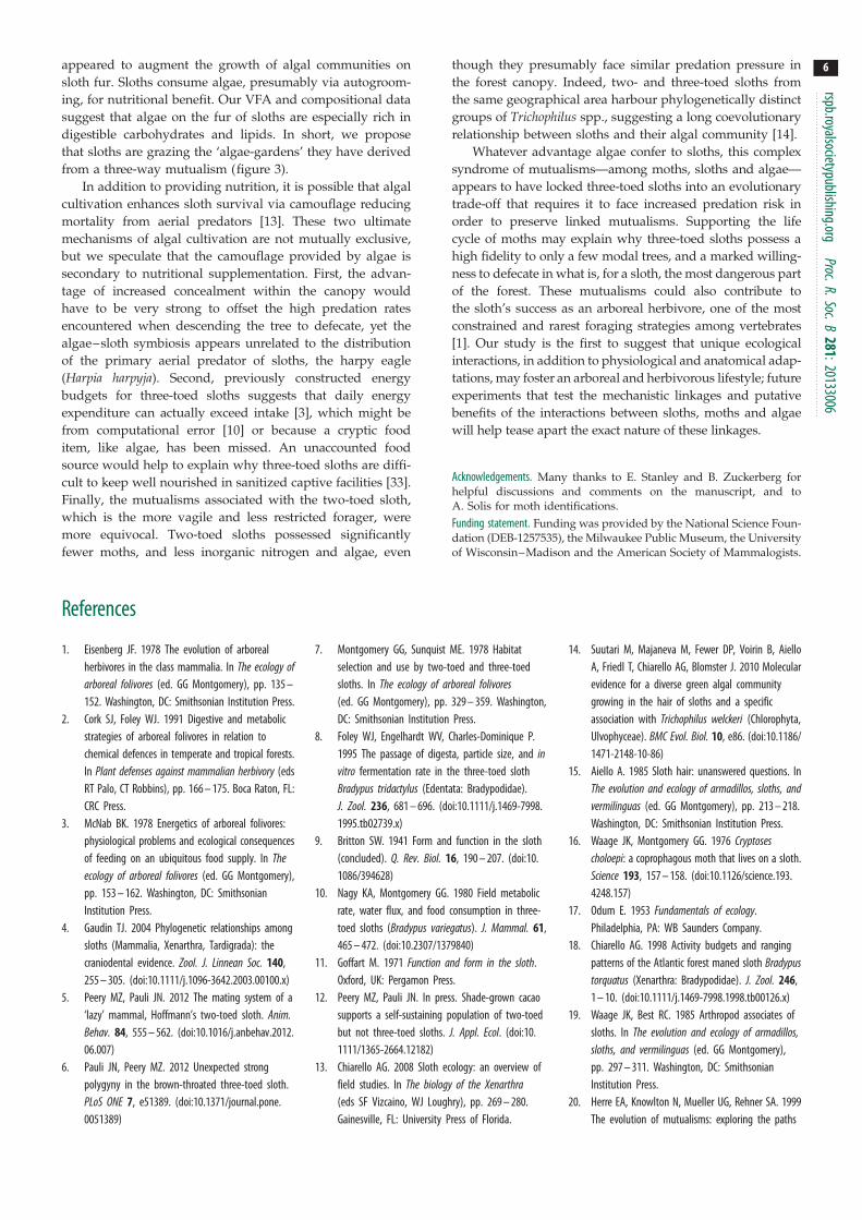
rspb.royalsocietypublishing.orgProc.R.Soc.B
281:20133006
6
appeared to augment the growth of algal communities onsloth fur. Sloths consume algae, presumably via autogroom-
ing, for nutritional benefit. Our VFA and compositional data
suggest that algae on the fur of sloths are especially rich in
digestible carbohydrates and lipids. In short, we propose
that sloths are grazing the ‘algae-gardens’ they have derived
from a three-way mutualism (figure 3).
In addition to providing nutrition, it is possible that algal
cultivation enhances sloth survival via camouflage reducing
mortality from aerial predators [13]. These two ultimate
mechanisms of algal cultivation are not mutually exclusive,
but we speculate that the camouflage provided by algae is
secondary to nutritional supplementation. First, the advan-
tage of increased concealment within the canopy would
have to be very strong to offset the high predation rates
encountered when descending the tree to defecate, yet the
algae–sloth symbiosis appears unrelated to the distribution
of the primary aerial predator of sloths, the harpy eagle
(Harpia harpyja). Second, previously constructed energy
budgets for three-toed sloths suggests that daily energy
expenditure can actually exceed intake [3], which might be
from computational error [10] or because a cryptic food
item, like algae, has been missed. An unaccounted food
source would help to explain why three-toed sloths are diffi-
cult to keep well nourished in sanitized captive facilities [33].
Finally, the mutualisms associated with the two-toed sloth,
which is the more vagile and less restricted forager, were
more equivocal. Two-toed sloths possessed significantly
fewer moths, and less inorganic nitrogen and algae, even
though they presumably face similar predation pressure in
the forest canopy. Indeed, two- and three-toed sloths from
the same geographical area harbour phylogenetically distinct
groups of Trichophilus spp., suggesting a long coevolutionary
relationship between sloths and their algal community [14].
Whatever advantage algae confer to sloths, this complex
syndrome of mutualisms—among moths, sloths and algae—
appears to have locked three-toed sloths into an evolutionary
trade-off that requires it to face increased predation risk in
order to preserve linked mutualisms. Supporting the life
cycle of moths may explain why three-toed sloths possess a
high fidelity to only a few modal trees, and a marked willing-
ness to defecate in what is, for a sloth, the most dangerous part
of the forest. These mutualisms could also contribute to
the sloth’s success as an arboreal herbivore, one of the most
constrained and rarest foraging strategies among vertebrates
[1]. Our study is the first to suggest that unique ecological
interactions, in addition to physiological and anatomical adap-
tations, may foster an arboreal and herbivorous lifestyle; future
experiments that test the mechanistic linkages and putative
benefits of the interactions between sloths, moths and algae
will help tease apart the exact nature of these linkages.
Acknowledgements. Many thanks to E. Stanley and B. Zuckerberg forhelpful discussions and comments on the manuscript, and toA. Solis for moth identifications.
Funding statement. Funding was provided by the National Science Foun-dation (DEB-1257535), the Milwaukee Public Museum, the Universityof Wisconsin–Madison and the American Society of Mammalogists.
References
1. Eisenberg JF. 1978 The evolution of arborealherbivores in the class mammalia. In The ecology ofarboreal folivores (ed. GG Montgomery), pp. 135 –152. Washington, DC: Smithsonian Institution Press.
2. Cork SJ, Foley WJ. 1991 Digestive and metabolicstrategies of arboreal folivores in relation tochemical defences in temperate and tropical forests.In Plant defenses against mammalian herbivory (edsRT Palo, CT Robbins), pp. 166 – 175. Boca Raton, FL:CRC Press.
3. McNab BK. 1978 Energetics of arboreal folivores:physiological problems and ecological consequencesof feeding on an ubiquitous food supply. In Theecology of arboreal folivores (ed. GG Montgomery),pp. 153 – 162. Washington, DC: SmithsonianInstitution Press.
4. Gaudin TJ. 2004 Phylogenetic relationships amongsloths (Mammalia, Xenarthra, Tardigrada): thecraniodental evidence. Zool. J. Linnean Soc. 140,255 – 305. (doi:10.1111/j.1096-3642.2003.00100.x)
5. Peery MZ, Pauli JN. 2012 The mating system of a‘lazy’ mammal, Hoffmann’s two-toed sloth. Anim.Behav. 84, 555 – 562. (doi:10.1016/j.anbehav.2012.06.007)
6. Pauli JN, Peery MZ. 2012 Unexpected strongpolygyny in the brown-throated three-toed sloth.PLoS ONE 7, e51389. (doi:10.1371/journal.pone.0051389)
7. Montgomery GG, Sunquist ME. 1978 Habitatselection and use by two-toed and three-toedsloths. In The ecology of arboreal folivores(ed. GG Montgomery), pp. 329 – 359. Washington,DC: Smithsonian Institution Press.
8. Foley WJ, Engelhardt WV, Charles-Dominique P.1995 The passage of digesta, particle size, and invitro fermentation rate in the three-toed slothBradypus tridactylus (Edentata: Bradypodidae).J. Zool. 236, 681 – 696. (doi:10.1111/j.1469-7998.1995.tb02739.x)
9. Britton SW. 1941 Form and function in the sloth(concluded). Q. Rev. Biol. 16, 190 – 207. (doi:10.1086/394628)
10. Nagy KA, Montgomery GG. 1980 Field metabolicrate, water flux, and food consumption in three-toed sloths (Bradypus variegatus). J. Mammal. 61,465 – 472. (doi:10.2307/1379840)
11. Goffart M. 1971 Function and form in the sloth.Oxford, UK: Pergamon Press.
12. Peery MZ, Pauli JN. In press. Shade-grown cacaosupports a self-sustaining population of two-toedbut not three-toed sloths. J. Appl. Ecol. (doi:10.1111/1365-2664.12182)
13. Chiarello AG. 2008 Sloth ecology: an overview offield studies. In The biology of the Xenarthra(eds SF Vizcaino, WJ Loughry), pp. 269 – 280.Gainesville, FL: University Press of Florida.
14. Suutari M, Majaneva M, Fewer DP, Voirin B, AielloA, Friedl T, Chiarello AG, Blomster J. 2010 Molecularevidence for a diverse green algal communitygrowing in the hair of sloths and a specificassociation with Trichophilus welckeri (Chlorophyta,Ulvophyceae). BMC Evol. Biol. 10, e86. (doi:10.1186/1471-2148-10-86)
15. Aiello A. 1985 Sloth hair: unanswered questions. InThe evolution and ecology of armadillos, sloths, andvermilinguas (ed. GG Montgomery), pp. 213 – 218.Washington, DC: Smithsonian Institution Press.
16. Waage JK, Montgomery GG. 1976 Cryptosescholoepi: a coprophagous moth that lives on a sloth.Science 193, 157 – 158. (doi:10.1126/science.193.4248.157)
17. Odum E. 1953 Fundamentals of ecology.Philadelphia, PA: WB Saunders Company.
18. Chiarello AG. 1998 Activity budgets and rangingpatterns of the Atlantic forest maned sloth Bradypustorquatus (Xenarthra: Bradypodidae). J. Zool. 246,1 – 10. (doi:10.1111/j.1469-7998.1998.tb00126.x)
19. Waage JK, Best RC. 1985 Arthropod associates ofsloths. In The evolution and ecology of armadillos,sloths, and vermilinguas (ed. GG Montgomery),pp. 297 – 311. Washington, DC: SmithsonianInstitution Press.
20. Herre EA, Knowlton N, Mueller UG, Rehner SA. 1999The evolution of mutualisms: exploring the paths
rspb.royalsocietypublishing.orgProc.R.Soc.B
281:20133
7
between conflict and cooperation. Trends Ecol. Evol.14, 49 – 53. (doi:10.1016/S0169-5347(98)01529-8)21. Kiers ET, Palmer TD, Ives AR, Bruno JF, Bronstein JL.2010 Mutualisms in a changing world: anevolutionary perspective. Ecol. Lett. 13, 1459 – 1474.(doi:10.1111/j.1461-0248.2010.01538.x)
22. Bshary R, Grutter AS, Willener AST, Leimar O. 2008Pairs of cooperating cleaner fish provide betterservice quality than singletons. Nature 455,964 – 966. (doi:10.1038/nature07184)
23. Janzen DH. 1966 Coevolution of mutualism betweenants and acacias in Central America. Evolution 20,249 – 275. (doi:10.2307/2406628)
24. Currie CR, Mueller UG, Malloch D. 1999 Theagricultural pathology of ant fungus gardens. Proc.Natl Acad. Sci. USA 96, 7998 – 8002. (doi:10.1073/pnas.96.14.7998)
25. Weimer PJ, Dien BS, Springer TL, Vogel KP. 2005 Invitro gas production as a surrogate measurement of
the fermentability of cellulosic biomass to ethanol.Appl. Microbiol. Biotechnol. 67, 52 – 58. (doi:10.1007/s00253-004-1844-7)
26. Goering HK, Van Soest PJ. 1970 Foragefiber analysis: apparatus, reagents, procedures,and some applications. Agricultural HandbookNo. 379. Washington, DC: US Department ofAgriculture.
27. Weimer PJ, Shi Y, Odt CL. 1991 A segmented gas/liquid delivery system for continuous culture ofmicroorganisms on insoluble substrates and its usefor growth of Ruminococcus flavefaciens oncellulose. Appl. Microbiol. Biotechnol. 36, 178 – 183.(doi:10.1007/BF00164416)
28. Bradford MM. 1976 A rapid and sensitivemethod for quantitation of microgram quantitiesof protein utilizing the principle of protein-dyebinding. Anal. Biochem. 72, 248 – 254. (doi:10.1016/0003-2697(76)90527-3)
29. Dubois M, Gilles KE, Hamilton JK, Rebers PA, SmithF. 1956 Colorimetric method for determination ofsugars and related substances. Anal. Chem. 28,350 – 356. (doi:10.1021/ac60111a017)
30. Huang G-H, Chen G, Chen F. 2009 Rapid screeningmethod for lipid production in alga based on Nilered fluorescence. Biomass Bioenergy 33, 1386 –1392. (doi:10.1016/j.biombioe.2009.05.022)
31. Nadelhoffer KJ, Aber JD, Melillo JM. 1984 Seasonalpatterns of ammonium and nitrate uptake in ninetemperate forest ecosystems. Plant Soil 80,321 – 335. (doi:10.1007/BF02140039)
32. Williams PJ le B, Laurens LML. 2010 Microalgae asbiodiesel and biomass feedstocks: review and analysisof the biochemistry, energetics and economics. EnergyEnviron. Sci. 3, 554 – 590. (doi:10.1039/b924978h)
33. Diniz LS, Oliveira PM. 1999 Clinical problems ofsloths (Bradypus sp. and Choloepus sp.) in captivity.J. Zoo Wildl. Med. 30, 76 – 80.
0
06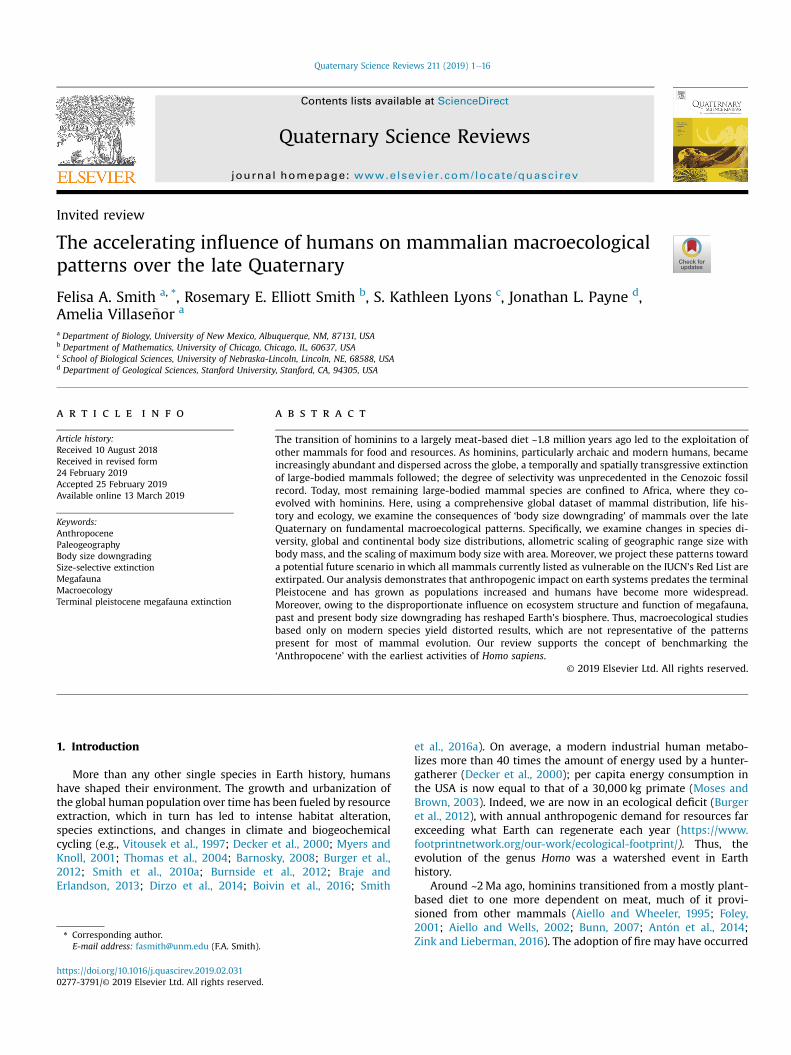
lable at ScienceDirect
Quaternary Science Reviews 211 (2019) 1e16
Contents lists avai
Quaternary Science Reviews
journal homepage: www.elsevier .com/locate/quascirev
Invited review
The accelerating influence of humans on mammalian macroecologicalpatterns over the late Quaternary
Felisa A. Smith a, *, Rosemary E. Elliott Smith b, S. Kathleen Lyons c, Jonathan L. Payne d,Amelia Villase~nor a
a Department of Biology, University of New Mexico, Albuquerque, NM, 87131, USAb Department of Mathematics, University of Chicago, Chicago, IL, 60637, USAc School of Biological Sciences, University of Nebraska-Lincoln, Lincoln, NE, 68588, USAd Department of Geological Sciences, Stanford University, Stanford, CA, 94305, USA
a r t i c l e i n f o
Article history:Received 10 August 2018Received in revised form24 February 2019Accepted 25 February 2019Available online 13 March 2019
Keywords:AnthropocenePaleogeographyBody size downgradingSize-selective extinctionMegafaunaMacroecologyTerminal pleistocene megafauna extinction
* Corresponding author.E-mail address: [email protected] (F.A. Smith).
https://doi.org/10.1016/j.quascirev.2019.02.0310277-3791/© 2019 Elsevier Ltd. All rights reserved.
a b s t r a c t
The transition of hominins to a largely meat-based diet ~1.8 million years ago led to the exploitation ofother mammals for food and resources. As hominins, particularly archaic and modern humans, becameincreasingly abundant and dispersed across the globe, a temporally and spatially transgressive extinctionof large-bodied mammals followed; the degree of selectivity was unprecedented in the Cenozoic fossilrecord. Today, most remaining large-bodied mammal species are confined to Africa, where they co-evolved with hominins. Here, using a comprehensive global dataset of mammal distribution, life his-tory and ecology, we examine the consequences of ‘body size downgrading’ of mammals over the lateQuaternary on fundamental macroecological patterns. Specifically, we examine changes in species di-versity, global and continental body size distributions, allometric scaling of geographic range size withbody mass, and the scaling of maximum body size with area. Moreover, we project these patterns towarda potential future scenario in which all mammals currently listed as vulnerable on the IUCN's Red List areextirpated. Our analysis demonstrates that anthropogenic impact on earth systems predates the terminalPleistocene and has grown as populations increased and humans have become more widespread.Moreover, owing to the disproportionate influence on ecosystem structure and function of megafauna,past and present body size downgrading has reshaped Earth's biosphere. Thus, macroecological studiesbased only on modern species yield distorted results, which are not representative of the patternspresent for most of mammal evolution. Our review supports the concept of benchmarking the‘Anthropocene’ with the earliest activities of Homo sapiens.
© 2019 Elsevier Ltd. All rights reserved.
1. Introduction
More than any other single species in Earth history, humanshave shaped their environment. The growth and urbanization ofthe global human population over time has been fueled by resourceextraction, which in turn has led to intense habitat alteration,species extinctions, and changes in climate and biogeochemicalcycling (e.g., Vitousek et al., 1997; Decker et al., 2000; Myers andKnoll, 2001; Thomas et al., 2004; Barnosky, 2008; Burger et al.,2012; Smith et al., 2010a; Burnside et al., 2012; Braje andErlandson, 2013; Dirzo et al., 2014; Boivin et al., 2016; Smith
et al., 2016a). On average, a modern industrial human metabo-lizes more than 40 times the amount of energy used by a hunter-gatherer (Decker et al., 2000); per capita energy consumption inthe USA is now equal to that of a 30,000 kg primate (Moses andBrown, 2003). Indeed, we are now in an ecological deficit (Burgeret al., 2012), with annual anthropogenic demand for resources farexceeding what Earth can regenerate each year (https://www.footprintnetwork.org/our-work/ecological-footprint/). Thus, theevolution of the genus Homo was a watershed event in Earthhistory.
Around ~2Ma ago, hominins transitioned from a mostly plant-based diet to one more dependent on meat, much of it provi-sioned from other mammals (Aiello and Wheeler, 1995; Foley,2001; Aiello and Wells, 2002; Bunn, 2007; Ant�on et al., 2014;Zink and Lieberman, 2016). The adoption of fire may have occurred
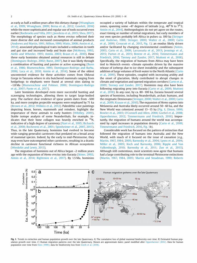
F.A. Smith et al. / Quaternary Science Reviews 211 (2019) 1e162
as early as half a million years after this dietary change (Wranghamet al., 1999; Wrangham, 2009; Berna et al., 2012; Gowlett, 2016)while themore sophisticated and regular use of tools occurred evenearlier (Roebroeks and Villa, 2011; Joordens et al., 2015; Shea, 2017).The morphology of species such as Homo erectus reflected theirmore diverse diet and increased consumption of animal products(Andrews andMartin, 1991; Milton, 1999;Watts, 2008; Ant�on et al.,2014); associated physiological traits included a reduction in toothand gut size and increased body and brain size (McHenry, 1992;Aiello and Wheeler, 1995; Ant�on, 2003; Braun et al., 2010). Howthese early hominins obtained animal resources is still in debate(Domínguez-Rodrigo, 2002; Bunn, 2007), but it was likely througha combination of hunting and passive or active scavenging (Bunnet al., 1986; Blumenschine, 1995; Domínguez-Rodrigo and Barba,2006; Luca et al., 2010; Ant�on et al., 2014). Some of the oldestuncontested evidence for these activities comes from OlduvaiGorge in Tanzania where in situ butchered mammals ranging fromhedgehogs to elephants were found at several sites dating to~1.8Ma (Blumenschine and Pobiner, 2006; Domínguez-Rodrigoet al., 2007; Pante et al., 2017).
Later hominins developed even more successful hunting andscavenging technologies, allowing them to target large-bodiedprey. The earliest clear evidence of spear points dates from ~500ka, and more complex projectile weapons were employed by 71 ka(Brown et al., 2012; Wilkins et al., 2012). Paleolithic cave paintingsdepicting bison, horses, mammoth and reindeer, highlight theimportance of these animals to early hunters (Whitley, 2009).Stable isotope analysis of some Neanderthals, for example, in-dicates that their bone collagen was heavily enriched in 15N,indicative of a high degree of carnivory (Fizet et al., 1995; Richardset al., 2000; Bocherens et al., 2001; Sponheimer et al., 2007, 2013).Thus, in the late Quaternary, hominins had evolved to becomewide-ranging generalist carnivores that predated on a broad arrayof mammal species. Indeed, by the early to mid-Pleistocene, theymay even have outcompeted other carnivores, resulting in a drasticdecline in carnivore functional richness in African ecosystems(Werdelin and Lewis, 2013).
The migration of hominins out of Africa began ~2 million yearsago with the expansion of Homo erectus into Eurasia (Stiner, 2002;Ant�on et al., 2014; Rightmire et al., 2017). By 1.5Ma, hominins
Fig. 1. Trends in extinction and human population growth over the late Quaternary. A) Thulation growth over time. C) Human migration patterns over the late Quaternary. Shownpopulation over time from Hern (1999); data for biodiversity loss from Smith et al. (2018).
occupied a variety of habitats within the temperate and tropicalzones, spanning some ~47 degrees of latitude (e.g., 400 N to 70 S;Ant�on et al., 2014). Anthropologists do not yet agree on the routes,exact timing or number of initial migrations, but early members ofour own species probably left Africa in pulses ca. 100 ka (Stringerand Andrews, 1988; Stringer, 2000; Walter et al., 2000; Cartoet al., 2009; Groucutt et al., 2015, Fig. 1); an exodus likely drivenand/or facilitated by changing environmental conditions (Ant�on,2003; Carto et al., 2009; Larrasoa~na et al., 2013; Jennings et al.,2015; Parton et al., 2015; Breeze et al., 2016; Timmermann andFriedrich, 2016; Tierney and Zander, 2017; Muttoni et al., 2018).Specifically, the migration of humans from Africa may have beentied to Heinrich events -climate episodes driven by the massiverelease of icebergs due to ice sheet instability and the subsequentaddition of large volumes of freshwater to the North Atlantic (Cartoet al., 2009). These episodes, coupled with increasing aridity andthe onset of glaciation, likely contributed to abrupt changes inclimate and vegetation and openedmigration corridors (Carto et al.,2009; Tierney and Zander, 2017). Hominins may also have beenfollowing migrating prey into Eurasia (Carto et al., 2009; Muttoniet al., 2018). In any case, by ca. 80e100 ka, Eurasia housed severalspecies of hominins, including Neanderthals, archaic humans, andthe enigmatic Denisovans (Stringer, 2000;Walter et al., 2000; Cartoet al., 2009; Krause et al., 2010). The expansion of Homo sapiens intoMelanesia and Australia likely occurred around 50e60 ka, and theNew World was colonized around 13e15 ka (Fig. 1; Dixon, 1999;Bowler et al., 2003; O’Connell and Allen, 2004; Goebel et al., 2008;Oppenheimer, 2012; Timmermann and Friedrich, 2016). Impor-tantly, the migration of humans around the world was accompa-nied by rapid increases in population density (Carto et al., 2009;Timmermann and Friedrich, 2016, Fig. 1b).
Considerable work has focused on the pattern of extinction thatfollowed the migration of humans into Australia and the NewWorld, with much of it focused on the issue of causation (e.g.,Martin, 1967, 1984; 2005; Barnosky et al., 2004; Lyons et al., 2004;Miller et al., 2005; Koch and Barnosky, 2006; Ripple and VanValkenburgh, 2010; Barnosky et al., 2011; Zuo et al., 2013).Although still contentious, most scientists now agree that humanshad a large contributing role to the terminal Pleistocene extinctions(Martin, 1967, 1984, 2005; Martin and Steadman, 1999; Roberts
e cumulative loss of global mammal biodiversity over time. B) Estimated human pop-are approximate dates; panel modified after Oppenheimer (2012). Data for human
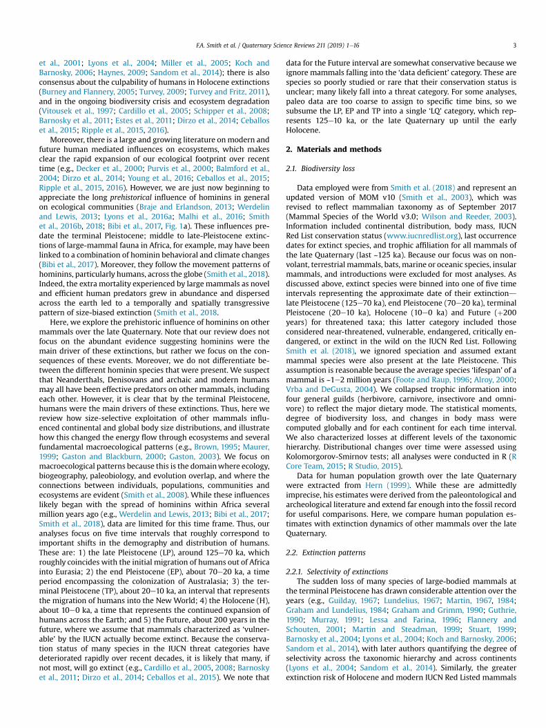
F.A. Smith et al. / Quaternary Science Reviews 211 (2019) 1e16 3
et al., 2001; Lyons et al., 2004; Miller et al., 2005; Koch andBarnosky, 2006; Haynes, 2009; Sandom et al., 2014); there is alsoconsensus about the culpability of humans in Holocene extinctions(Burney and Flannery, 2005; Turvey, 2009; Turvey and Fritz, 2011),and in the ongoing biodiversity crisis and ecosystem degradation(Vitousek et al., 1997; Cardillo et al., 2005; Schipper et al., 2008;Barnosky et al., 2011; Estes et al., 2011; Dirzo et al., 2014; Ceballoset al., 2015; Ripple et al., 2015, 2016).
Moreover, there is a large and growing literature onmodern andfuture human mediated influences on ecosystems, which makesclear the rapid expansion of our ecological footprint over recenttime (e.g., Decker et al., 2000; Purvis et al., 2000; Balmford et al.,2004; Dirzo et al., 2014; Young et al., 2016; Ceballos et al., 2015;Ripple et al., 2015, 2016). However, we are just now beginning toappreciate the long prehistorical influence of hominins in generalon ecological communities (Braje and Erlandson, 2013; Werdelinand Lewis, 2013; Lyons et al., 2016a; Malhi et al., 2016; Smithet al., 2016b, 2018; Bibi et al., 2017, Fig. 1a). These influences pre-date the terminal Pleistocene; middle to late-Pleistocene extinc-tions of large-mammal fauna in Africa, for example, may have beenlinked to a combination of hominin behavioral and climate changes(Bibi et al., 2017). Moreover, they follow the movement patterns ofhominins, particularly humans, across the globe (Smith et al., 2018).Indeed, the extra mortality experienced by large mammals as noveland efficient human predators grew in abundance and dispersedacross the earth led to a temporally and spatially transgressivepattern of size-biased extinction (Smith et al., 2018.
Here, we explore the prehistoric influence of hominins on othermammals over the late Quaternary. Note that our review does notfocus on the abundant evidence suggesting hominins were themain driver of these extinctions, but rather we focus on the con-sequences of these events. Moreover, we do not differentiate be-tween the different hominin species that were present. We suspectthat Neanderthals, Denisovans and archaic and modern humansmay all have been effective predators on other mammals, includingeach other. However, it is clear that by the terminal Pleistocene,humans were the main drivers of these extinctions. Thus, here wereview how size-selective exploitation of other mammals influ-enced continental and global body size distributions, and illustratehow this changed the energy flow through ecosystems and severalfundamental macroecological patterns (e.g., Brown, 1995; Maurer,1999; Gaston and Blackburn, 2000; Gaston, 2003). We focus onmacroecological patterns because this is the domainwhere ecology,biogeography, paleobiology, and evolution overlap, and where theconnections between individuals, populations, communities andecosystems are evident (Smith et al., 2008). While these influenceslikely began with the spread of hominins within Africa severalmillion years ago (e.g., Werdelin and Lewis, 2013; Bibi et al., 2017;Smith et al., 2018), data are limited for this time frame. Thus, ouranalyses focus on five time intervals that roughly correspond toimportant shifts in the demography and distribution of humans.These are: 1) the late Pleistocene (LP), around 125e70 ka, whichroughly coincides with the initial migration of humans out of Africainto Eurasia; 2) the end Pleistocene (EP), about 70e20 ka, a timeperiod encompassing the colonization of Australasia; 3) the ter-minal Pleistocene (TP), about 20e10 ka, an interval that representsthe migration of humans into the New World; 4) the Holocene (H),about 10e0 ka, a time that represents the continued expansion ofhumans across the Earth; and 5) the Future, about 200 years in thefuture, where we assume that mammals characterized as ‘vulner-able’ by the IUCN actually become extinct. Because the conserva-tion status of many species in the IUCN threat categories havedeteriorated rapidly over recent decades, it is likely that many, ifnot most, will go extinct (e.g., Cardillo et al., 2005, 2008; Barnoskyet al., 2011; Dirzo et al., 2014; Ceballos et al., 2015). We note that
data for the Future interval are somewhat conservative because weignore mammals falling into the ‘data deficient’ category. These arespecies so poorly studied or rare that their conservation status isunclear; many likely fall into a threat category. For some analyses,paleo data are too coarse to assign to specific time bins, so wesubsume the LP, EP and TP into a single ‘LQ’ category, which rep-resents 125e10 ka, or the late Quaternary up until the earlyHolocene.
2. Materials and methods
2.1. Biodiversity loss
Data employed were from Smith et al. (2018) and represent anupdated version of MOM v10 (Smith et al., 2003), which wasrevised to reflect mammalian taxonomy as of September 2017(Mammal Species of the World v3.0; Wilson and Reeder, 2003).Information included continental distribution, body mass, IUCNRed List conservation status (www.iucnredlist.org), last occurrencedates for extinct species, and trophic affiliation for all mammals ofthe late Quaternary (last ~125 ka). Because our focus was on non-volant, terrestrial mammals, bats, marine or oceanic species, insularmammals, and introductions were excluded for most analyses. Asdiscussed above, extinct species were binned into one of five timeintervals representing the approximate date of their extinctiondlate Pleistocene (125e70 ka), end Pleistocene (70e20 ka), terminalPleistocene (20e10 ka), Holocene (10e0 ka) and Future (þ200years) for threatened taxa; this latter category included thoseconsidered near-threatened, vulnerable, endangered, critically en-dangered, or extinct in the wild on the IUCN Red List. FollowingSmith et al. (2018), we ignored speciation and assumed extantmammal species were also present at the late Pleistocene. Thisassumption is reasonable because the average species ‘lifespan’ of amammal is ~1e2 million years (Foote and Raup, 1996; Alroy, 2000;Vrba and DeGusta, 2004). We collapsed trophic information intofour general guilds (herbivore, carnivore, insectivore and omni-vore) to reflect the major dietary mode. The statistical moments,degree of biodiversity loss, and changes in body mass werecomputed globally and for each continent for each time interval.We also characterized losses at different levels of the taxonomichierarchy. Distributional changes over time were assessed usingKolomorgorov-Smirnov tests; all analyses were conducted in R (RCore Team, 2015; R Studio, 2015).
Data for human population growth over the late Quaternarywere extracted from Hern (1999). While these are admittedlyimprecise, his estimates were derived from the paleontological andarcheological literature and extend far enough into the fossil recordfor useful comparisons. Here, we compare human population es-timates with extinction dynamics of other mammals over the lateQuaternary.
2.2. Extinction patterns
2.2.1. Selectivity of extinctionsThe sudden loss of many species of large-bodied mammals at
the terminal Pleistocene has drawn considerable attention over theyears (e.g., Guilday, 1967; Lundelius, 1967; Martin, 1967, 1984;Graham and Lundelius, 1984; Graham and Grimm, 1990; Guthrie,1990; Murray, 1991; Lessa and Farina, 1996; Flannery andSchouten, 2001; Martin and Steadman, 1999; Stuart, 1999;Barnosky et al., 2004; Lyons et al., 2004; Koch and Barnosky, 2006;Sandom et al., 2014), with later authors quantifying the degree ofselectivity across the taxonomic hierarchy and across continents(Lyons et al., 2004; Sandom et al., 2014). Similarly, the greaterextinction risk of Holocene and modern IUCN Red Listed mammals
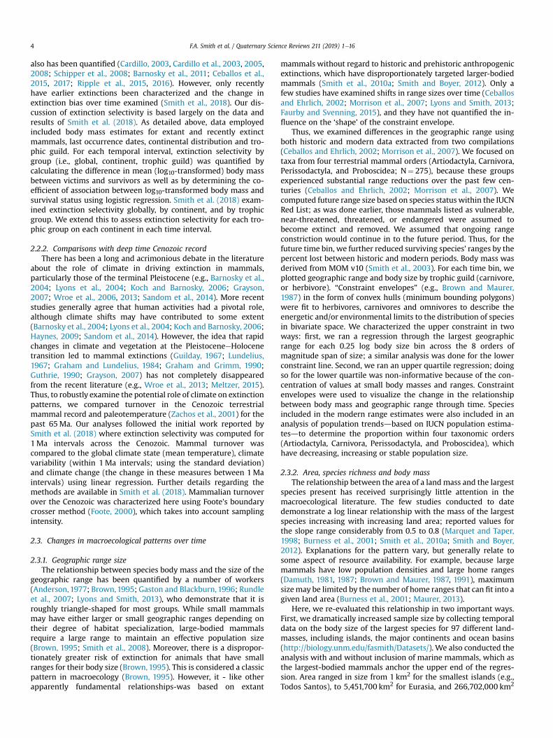
F.A. Smith et al. / Quaternary Science Reviews 211 (2019) 1e164
also has been quantified (Cardillo, 2003, Cardillo et al., 2003, 2005,2008; Schipper et al., 2008; Barnosky et al., 2011; Ceballos et al.,2015, 2017; Ripple et al., 2015, 2016). However, only recentlyhave earlier extinctions been characterized and the change inextinction bias over time examined (Smith et al., 2018). Our dis-cussion of extinction selectivity is based largely on the data andresults of Smith et al. (2018). As detailed above, data employedincluded body mass estimates for extant and recently extinctmammals, last occurrence dates, continental distribution and tro-phic guild. For each temporal interval, extinction selectivity bygroup (i.e., global, continent, trophic guild) was quantified bycalculating the difference in mean (log10-transformed) body massbetween victims and survivors as well as by determining the co-efficient of association between log10-transformed body mass andsurvival status using logistic regression. Smith et al. (2018) exam-ined extinction selectivity globally, by continent, and by trophicgroup. We extend this to assess extinction selectivity for each tro-phic group on each continent in each time interval.
2.2.2. Comparisons with deep time Cenozoic recordThere has been a long and acrimonious debate in the literature
about the role of climate in driving extinction in mammals,particularly those of the terminal Pleistocene (e.g., Barnosky et al.,2004; Lyons et al., 2004; Koch and Barnosky, 2006; Grayson,2007; Wroe et al., 2006, 2013; Sandom et al., 2014). More recentstudies generally agree that human activities had a pivotal role,although climate shifts may have contributed to some extent(Barnosky et al., 2004; Lyons et al., 2004; Koch and Barnosky, 2006;Haynes, 2009; Sandom et al., 2014). However, the idea that rapidchanges in climate and vegetation at the PleistoceneeHolocenetransition led to mammal extinctions (Guilday, 1967; Lundelius,1967; Graham and Lundelius, 1984; Graham and Grimm, 1990;Guthrie, 1990; Grayson, 2007) has not completely disappearedfrom the recent literature (e.g., Wroe et al., 2013; Meltzer, 2015).Thus, to robustly examine the potential role of climate on extinctionpatterns, we compared turnover in the Cenozoic terrestrialmammal record and paleotemperature (Zachos et al., 2001) for thepast 65Ma. Our analyses followed the initial work reported bySmith et al. (2018) where extinction selectivity was computed for1Ma intervals across the Cenozoic. Mammal turnover wascompared to the global climate state (mean temperature), climatevariability (within 1Ma intervals; using the standard deviation)and climate change (the change in these measures between 1Maintervals) using linear regression. Further details regarding themethods are available in Smith et al. (2018). Mammalian turnoverover the Cenozoic was characterized here using Foote's boundarycrosser method (Foote, 2000), which takes into account samplingintensity.
2.3. Changes in macroecological patterns over time
2.3.1. Geographic range sizeThe relationship between species body mass and the size of the
geographic range has been quantified by a number of workers(Anderson,1977; Brown,1995; Gaston and Blackburn, 1996; Rundleet al., 2007; Lyons and Smith, 2013), who demonstrate that it isroughly triangle-shaped for most groups. While small mammalsmay have either larger or small geographic ranges depending ontheir degree of habitat specialization, large-bodied mammalsrequire a large range to maintain an effective population size(Brown, 1995; Smith et al., 2008). Moreover, there is a dispropor-tionately greater risk of extinction for animals that have smallranges for their body size (Brown, 1995). This is considered a classicpattern in macroecology (Brown, 1995). However, it - like otherapparently fundamental relationships-was based on extant
mammals without regard to historic and prehistoric anthropogenicextinctions, which have disproportionately targeted larger-bodiedmammals (Smith et al., 2010a; Smith and Boyer, 2012). Only afew studies have examined shifts in range sizes over time (Ceballosand Ehrlich, 2002; Morrison et al., 2007; Lyons and Smith, 2013;Faurby and Svenning, 2015), and they have not quantified the in-fluence on the ‘shape’ of the constraint envelope.
Thus, we examined differences in the geographic range usingboth historic and modern data extracted from two compilations(Ceballos and Ehrlich, 2002; Morrison et al., 2007). We focused ontaxa from four terrestrial mammal orders (Artiodactyla, Carnivora,Perissodactyla, and Proboscidea; N¼ 275), because these groupsexperienced substantial range reductions over the past few cen-turies (Ceballos and Ehrlich, 2002; Morrison et al., 2007). Wecomputed future range size based on species status within the IUCNRed List; as was done earlier, those mammals listed as vulnerable,near-threatened, threatened, or endangered were assumed tobecome extinct and removed. We assumed that ongoing rangeconstriction would continue in to the future period. Thus, for thefuture time bin, we further reduced surviving species’ ranges by thepercent lost between historic and modern periods. Body mass wasderived from MOM v10 (Smith et al., 2003). For each time bin, weplotted geographic range and body size by trophic guild (carnivore,or herbivore). “Constraint envelopes” (e.g., Brown and Maurer,1987) in the form of convex hulls (minimum bounding polygons)were fit to herbivores, carnivores and omnivores to describe theenergetic and/or environmental limits to the distribution of speciesin bivariate space. We characterized the upper constraint in twoways: first, we ran a regression through the largest geographicrange for each 0.25 log body size bin across the 8 orders ofmagnitude span of size; a similar analysis was done for the lowerconstraint line. Second, we ran an upper quartile regression; doingso for the lower quartile was non-informative because of the con-centration of values at small body masses and ranges. Constraintenvelopes were used to visualize the change in the relationshipbetween body mass and geographic range through time. Speciesincluded in the modern range estimates were also included in ananalysis of population trendsdbased on IUCN population estima-tesdto determine the proportion within four taxonomic orders(Artiodactyla, Carnivora, Perissodactyla, and Proboscidea), whichhave decreasing, increasing or stable population size.
2.3.2. Area, species richness and body massThe relationship between the area of a landmass and the largest
species present has received surprisingly little attention in themacroecological literature. The few studies conducted to datedemonstrate a log linear relationship with the mass of the largestspecies increasing with increasing land area; reported values forthe slope range considerably from 0.5 to 0.8 (Marquet and Taper,1998; Burness et al., 2001; Smith et al., 2010a; Smith and Boyer,2012). Explanations for the pattern vary, but generally relate tosome aspect of resource availability. For example, because largemammals have low population densities and large home ranges(Damuth, 1981, 1987; Brown and Maurer, 1987, 1991), maximumsizemay be limited by the number of home ranges that can fit into agiven land area (Burness et al., 2001; Maurer, 2013).
Here, we re-evaluated this relationship in two important ways.First, we dramatically increased sample size by collecting temporaldata on the body size of the largest species for 97 different land-masses, including islands, the major continents and ocean basins(http://biology.unm.edu/fasmith/Datasets/). We also conducted theanalysis with and without inclusion of marine mammals, which asthe largest-bodied mammals anchor the upper end of the regres-sion. Area ranged in size from 1 km2 for the smallest islands (e.g.,Todos Santos), to 5,451,700 km2 for Eurasia, and 266,702,000 km2
F.A. Smith et al. / Quaternary Science Reviews 211 (2019) 1e16 5
for the Atlantic, Pacific, Artic, and Southern ocean basins combined.Second, we investigated the influence of size-selective extinctionon this relationship. Here, data limitations led us to focus on fourtime periods: LQ (125e10 ka), Holocene (10e0 ka), Modern (0 ka)and the Future (þ200 yrs). Note that our sample size of landmassesis not completely consistent over time. For example, we had fewerlandmasses for the LQ because some were landbridge islands thatonly formed in with the rising of sea levels at the terminal Pleis-tocene. Both body mass and land areawere logged prior to analysesand then evaluated using ordinary least squares regression.
Fig. 2. The taxonomic sensitivity of extinction over time. A) Cumulative degree ofextinction within each level of the taxonomic hierarchy. B) The distribution ofextinction over various taxonomic levels. Note the sharp increase in both the extentand the breadth of extinction in the future time bin; while extinctions were onceconfined to particular clades, they are nowwidespread across the taxonomic hierarchy.
2.3.3. Trophic structureTrophic downgrading of modern ecosystems is ongoing (Estes
et al., 2011). The loss of the apex consumers in ecosystems hasmany direct and indirect consequences, including the potential tochange vegetation structure and composition, unravel food webs,and change processes such as fire regimes (Estes et al., 2011; Rippleet al., 2014). We are just beginning to develop an appreciation forthe integral role of large consumers in Earth systems (Smith et al.,2016a,b). Here, we examine the influence of the size-selectivetrophic downgrading across the Quaternary within two majorterrestrial trophic groups, carnivores and herbivores. These are thegroups that have suffered the greatest biodiversity losses over thelate Quaternary (Smith et al., 2018).
As with the biodiversity analyses, we employed body mass, theIUCN Red List conservation status (www.iucnredlist.org), lastoccurrence dates for extinct species, and trophic affiliation for allmammals of the late Quaternary from Smith et al. (2018). Allmembers of the order Carnivora were classified as carnivores,regardless of the degree or source of meat consumption. Wegrouped species identified as being predominately browsers orgrazers as herbivores. We then characterized the distributions ofthese two trophic groups for the six time bins: prior (>125 ka), latePleistocene (125-70ka), end Pleistocene (70e20 ka), terminalPleistocene (20e10 ka), Holocene (10e0 ka), Modern (0 ka), andFuture (þ200 years), where all species listed as threatened,vulnerable, and extinct by the IUCN Red List were removed.Changes in the range of body size and in the shapes of the distri-butions over time were tested using Kolomorgorov-Smirnov tests;all analyses were conducted in R.
3. Results and discussion
3.1. Biodiversity loss
The extinction rate of mammals has increased dramatically overthe last ~125,000 years (Fig. 1a), concomitant with the growth andspread of human populations (Fig. 1b and c). To date, we have lostapproximately 8% of the world's mammals; without interventionthe cumulative biodiversity loss could reach ~30% within a few
Table 1Global alpha diversity of terrestrial nonvolant mammals by taxonomic level and time in
Interval Time Interval Cumulative Biodiversity loss (%) Ex
Sp
Before 125 ka unknown 3Late Pleistocene 125-70 ka 0.5 3End Pleistocene 70-20 ka 2.1 3Terminal Pleistocene 20-10 ka 6.8 3Holocene 10e0 8.0 3Future �200 yrs 29.6 2Change from LP to Future 29.6 �
Higher level taxonomic information provided for extinct species showing the extent ofobtained by subtracting between temporal intervals.
hundred years (Table 1; Fig. 2). This value may be conservativebecause we ignored ‘data deficient’ mammals in the future pro-jections. However, our cumulative estimate is in line with manyrecent projections, which focus on the change in biodiversity fromthemodern to the future (Cardillo et al., 2005; Schipper et al., 2008;Hoffmann et al., 2010; Barnosky et al., 2011; Dirzo et al., 2014;Ceballos et al., 2015; Ripple et al., 2015, 2016, 2017). Moreover,while past extinctions were concentrated in particular taxonomicgroups (e.g., the Holocene and late Pleistocene extinctions wereconfined to 7 and 11 orders, respectively; Table 1), suggesting thatconserved biological traits made some clades more susceptible toextinction (Purvis et al., 2000; Turvey and Fritz, 2011), the magni-tude of future extinctionsmeans theywill necessarily becomemorewidespread across the taxonomic hierarchy (Fig. 2). Our computa-tions suggest that in the Future, for example, more than 88% oforders could experience at least one extinction (Fig. 2). Moreover,extinctions could lead to considerable loss of phylogenetic andfunctional diversity with as many as ~27% of terrestrial nonvolantfamilies and 25% of mammalian orders lost (Table 1).
Interestingly, these past and future extinction events have notchanged the canonical ‘hollow curve’ pattern of species among
terval.
tant at end of interval Species extinctions during interval
ecies Genus Family Order Species Genus Family Order
305 891 126 32292 889 126 32 13 10 8 5241 869 124 32 51 33 16 6084 792 115 30 157 101 33 11043 785 112 29 41 28 12 7328 604 92 24 711 349 82 21973 �287 �34 �8
loss; it does not represent the actual generic, family or ordinal losses. Those can be
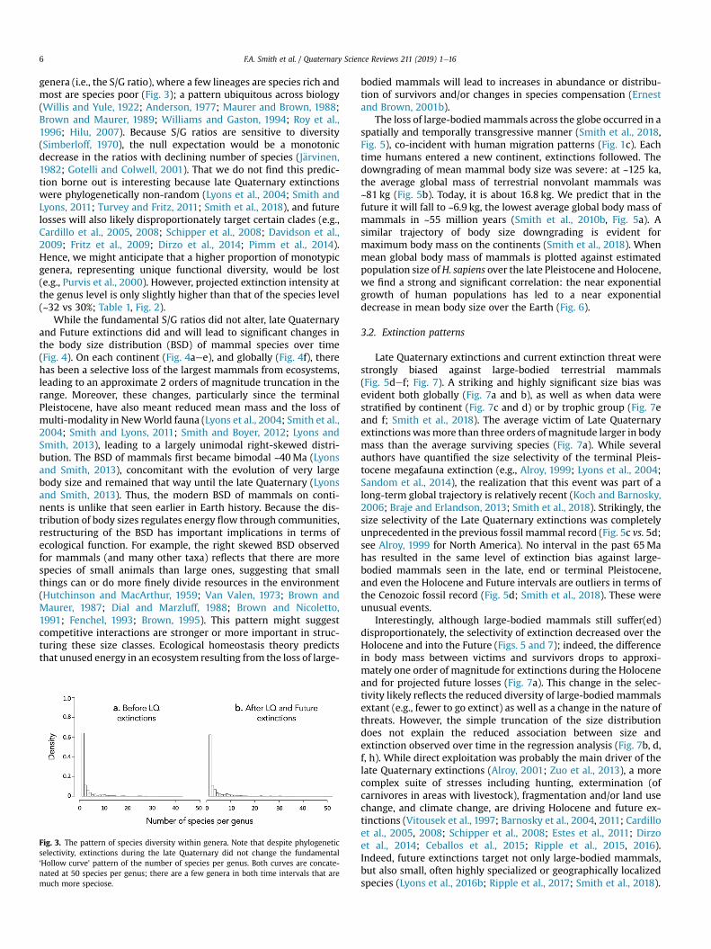
F.A. Smith et al. / Quaternary Science Reviews 211 (2019) 1e166
genera (i.e., the S/G ratio), where a few lineages are species rich andmost are species poor (Fig. 3); a pattern ubiquitous across biology(Willis and Yule, 1922; Anderson, 1977; Maurer and Brown, 1988;Brown and Maurer, 1989; Williams and Gaston, 1994; Roy et al.,1996; Hilu, 2007). Because S/G ratios are sensitive to diversity(Simberloff, 1970), the null expectation would be a monotonicdecrease in the ratios with declining number of species (J€arvinen,1982; Gotelli and Colwell, 2001). That we do not find this predic-tion borne out is interesting because late Quaternary extinctionswere phylogenetically non-random (Lyons et al., 2004; Smith andLyons, 2011; Turvey and Fritz, 2011; Smith et al., 2018), and futurelosses will also likely disproportionately target certain clades (e.g.,Cardillo et al., 2005, 2008; Schipper et al., 2008; Davidson et al.,2009; Fritz et al., 2009; Dirzo et al., 2014; Pimm et al., 2014).Hence, we might anticipate that a higher proportion of monotypicgenera, representing unique functional diversity, would be lost(e.g., Purvis et al., 2000). However, projected extinction intensity atthe genus level is only slightly higher than that of the species level(~32 vs 30%; Table 1, Fig. 2).
While the fundamental S/G ratios did not alter, late Quaternaryand Future extinctions did and will lead to significant changes inthe body size distribution (BSD) of mammal species over time(Fig. 4). On each continent (Fig. 4aee), and globally (Fig. 4f), therehas been a selective loss of the largest mammals from ecosystems,leading to an approximate 2 orders of magnitude truncation in therange. Moreover, these changes, particularly since the terminalPleistocene, have also meant reduced mean mass and the loss ofmulti-modality in NewWorld fauna (Lyons et al., 2004; Smith et al.,2004; Smith and Lyons, 2011; Smith and Boyer, 2012; Lyons andSmith, 2013), leading to a largely unimodal right-skewed distri-bution. The BSD of mammals first became bimodal ~40Ma (Lyonsand Smith, 2013), concomitant with the evolution of very largebody size and remained that way until the late Quaternary (Lyonsand Smith, 2013). Thus, the modern BSD of mammals on conti-nents is unlike that seen earlier in Earth history. Because the dis-tribution of body sizes regulates energy flow through communities,restructuring of the BSD has important implications in terms ofecological function. For example, the right skewed BSD observedfor mammals (and many other taxa) reflects that there are morespecies of small animals than large ones, suggesting that smallthings can or do more finely divide resources in the environment(Hutchinson and MacArthur, 1959; Van Valen, 1973; Brown andMaurer, 1987; Dial and Marzluff, 1988; Brown and Nicoletto,1991; Fenchel, 1993; Brown, 1995). This pattern might suggestcompetitive interactions are stronger or more important in struc-turing these size classes. Ecological homeostasis theory predictsthat unused energy in an ecosystem resulting from the loss of large-
Fig. 3. The pattern of species diversity within genera. Note that despite phylogeneticselectivity, extinctions during the late Quaternary did not change the fundamental‘Hollow curve’ pattern of the number of species per genus. Both curves are concate-nated at 50 species per genus; there are a few genera in both time intervals that aremuch more speciose.
bodied mammals will lead to increases in abundance or distribu-tion of survivors and/or changes in species compensation (Ernestand Brown, 2001b).
The loss of large-bodiedmammals across the globe occurred in aspatially and temporally transgressive manner (Smith et al., 2018,Fig. 5), co-incident with human migration patterns (Fig. 1c). Eachtime humans entered a new continent, extinctions followed. Thedowngrading of mean mammal body size was severe: at ~125 ka,the average global mass of terrestrial nonvolant mammals was~81 kg (Fig. 5b). Today, it is about 16.8 kg. We predict that in thefuture it will fall to ~6.9 kg, the lowest average global body mass ofmammals in ~55 million years (Smith et al., 2010b, Fig. 5a). Asimilar trajectory of body size downgrading is evident formaximum body mass on the continents (Smith et al., 2018). Whenmean global body mass of mammals is plotted against estimatedpopulation size ofH. sapiens over the late Pleistocene and Holocene,we find a strong and significant correlation: the near exponentialgrowth of human populations has led to a near exponentialdecrease in mean body size over the Earth (Fig. 6).
3.2. Extinction patterns
Late Quaternary extinctions and current extinction threat werestrongly biased against large-bodied terrestrial mammals(Fig. 5def; Fig. 7). A striking and highly significant size bias wasevident both globally (Fig. 7a and b), as well as when data werestratified by continent (Fig. 7c and d) or by trophic group (Fig. 7eand f; Smith et al., 2018). The average victim of Late Quaternaryextinctions wasmore than three orders of magnitude larger in bodymass than the average surviving species (Fig. 7a). While severalauthors have quantified the size selectivity of the terminal Pleis-tocene megafauna extinction (e.g., Alroy, 1999; Lyons et al., 2004;Sandom et al., 2014), the realization that this event was part of along-term global trajectory is relatively recent (Koch and Barnosky,2006; Braje and Erlandson, 2013; Smith et al., 2018). Strikingly, thesize selectivity of the Late Quaternary extinctions was completelyunprecedented in the previous fossil mammal record (Fig. 5c vs. 5d;see Alroy, 1999 for North America). No interval in the past 65Mahas resulted in the same level of extinction bias against large-bodied mammals seen in the late, end or terminal Pleistocene,and even the Holocene and Future intervals are outliers in terms ofthe Cenozoic fossil record (Fig. 5d; Smith et al., 2018). These wereunusual events.
Interestingly, although large-bodied mammals still suffer(ed)disproportionately, the selectivity of extinction decreased over theHolocene and into the Future (Figs. 5 and 7); indeed, the differencein body mass between victims and survivors drops to approxi-mately one order of magnitude for extinctions during the Holoceneand for projected future losses (Fig. 7a). This change in the selec-tivity likely reflects the reduced diversity of large-bodied mammalsextant (e.g., fewer to go extinct) as well as a change in the nature ofthreats. However, the simple truncation of the size distributiondoes not explain the reduced association between size andextinction observed over time in the regression analysis (Fig. 7b, d,f, h). While direct exploitation was probably the main driver of thelate Quaternary extinctions (Alroy, 2001; Zuo et al., 2013), a morecomplex suite of stresses including hunting, extermination (ofcarnivores in areas with livestock), fragmentation and/or land usechange, and climate change, are driving Holocene and future ex-tinctions (Vitousek et al., 1997; Barnosky et al., 2004, 2011; Cardilloet al., 2005, 2008; Schipper et al., 2008; Estes et al., 2011; Dirzoet al., 2014; Ceballos et al., 2015; Ripple et al., 2015, 2016).Indeed, future extinctions target not only large-bodied mammals,but also small, often highly specialized or geographically localizedspecies (Lyons et al., 2016b; Ripple et al., 2017; Smith et al., 2018).
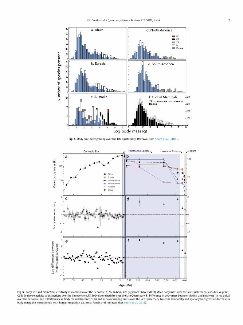
Fig. 4. Body size downgrading over the late Quaternary. Redrawn from Smith et al. (2018)..
Fig. 5. Body size and extinction selectivity of mammals over the Cenozoic. A) Mean body size (kg) from 66 to 1Ma. B) Mean body mass over the late Quaternary (last ~125 ka years).C) Body size selectivity of extinctions over the Cenozoic era, D) Body size selectivity over the late Quaternary, E) Difference in body mass between victims and survivors (in log units)over the Cenozoic, and, F) Difference in body mass between victims and survivors (in log units) over the late Quaternary. Note the temporally and spatially transgressive decrease inbody mass; this corresponds with human migration patterns (Panels aed redrawn after Smith et al., 2018).
F.A. Smith et al. / Quaternary Science Reviews 211 (2019) 1e16 7
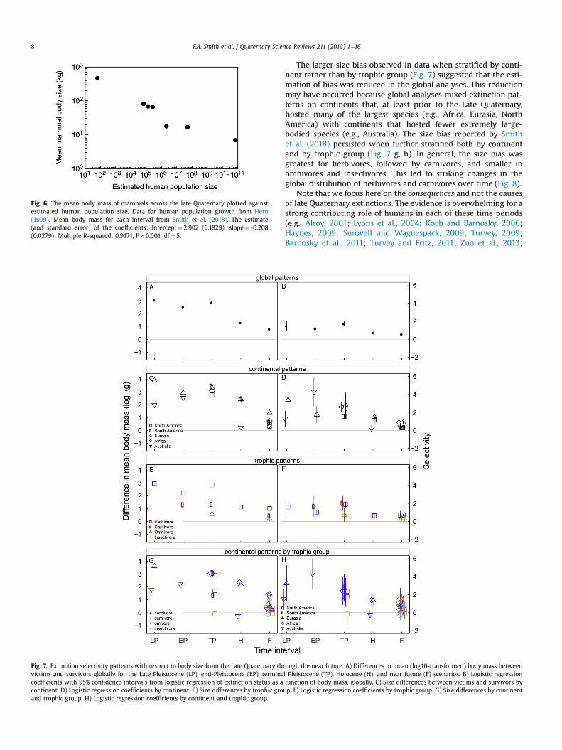
Fig. 6. The mean body mass of mammals across the late Quaternary plotted againstestimated human population size. Data for human population growth from Hern(1999). Mean body mass for each interval from Smith et al. (2018). The estimate(and standard error) of the coefficients: Intercept¼ 2.902 (0.1829), slope¼ -0.208(0.0279); Multiple R-squared: 0.9171, P< 0.001, df¼ 5.
Fig. 7. Extinction selectivity patterns with respect to body size from the Late Quaternary thvictims and survivors globally for the Late Pleistocene (LP), end-Pleistocene (EP), terminacoefficients with 95% confidence intervals from logistic regression of extinction status as acontinent. D) Logistic regression coefficients by continent. E) Size differences by trophic groand trophic group. H) Logistic regression coefficients by continent and trophic group.
F.A. Smith et al. / Quaternary Science Reviews 211 (2019) 1e168
The larger size bias observed in data when stratified by conti-nent rather than by trophic group (Fig. 7) suggested that the esti-mation of bias was reduced in the global analyses. This reductionmay have occurred because global analyses mixed extinction pat-terns on continents that, at least prior to the Late Quaternary,hosted many of the largest species (e.g., Africa, Eurasia, NorthAmerica) with continents that hosted fewer extremely large-bodied species (e.g., Australia). The size bias reported by Smithet al. (2018) persisted when further stratified both by continentand by trophic group (Fig. 7 g, h). In general, the size bias wasgreatest for herbivores, followed by carnivores, and smaller inomnivores and insectivores. This led to striking changes in theglobal distribution of herbivores and carnivores over time (Fig. 8).
Note that we focus here on the consequences and not the causesof late Quaternary extinctions. The evidence is overwhelming for astrong contributing role of humans in each of these time periods(e.g., Alroy, 2001; Lyons et al., 2004; Koch and Barnosky, 2006;Haynes, 2009; Surovell and Waguespack, 2009; Turvey, 2009;Barnosky et al., 2011; Turvey and Fritz, 2011; Zuo et al., 2013;
rough the near future. A) Differences in mean (log10-transformed) body mass betweenl Pleistocene (TP), Holocene (H), and near future (F) scenarios. B) Logistic regressionfunction of body mass, globally. C) Size differences between victims and survivors byup. F) Logistic regression coefficients by trophic group. G) Size differences by continent
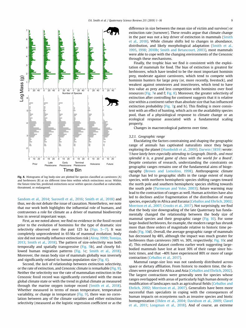
Fig. 8. Histograms of log body-size are plotted for species classified as carnivores (A)and herbivores (B) at six different time-bins within which extinctions occur. Withinthe future time bin, predicted extinctions occur within species classified as vulnerable,threatened, or endangered.
F.A. Smith et al. / Quaternary Science Reviews 211 (2019) 1e16 9
Sandom et al., 2014; Surovell et al., 2016; Smith et al., 2018) andthus, we do not debate the issue of causation. Nonetheless, we notethat our work both highlights the influential role of humans, andcontravenes a role for climate as a driver of mammal biodiversityloss in several important ways.
First, as we noted above, we find no evidence in the fossil recordprior to the evolution of hominins for the type of dramatic sizeselectivity observed over the past 125 ka (Figs. 5e7). It wascompletely unprecedented in 65Ma of mammal evolution; bodysize did not normally influence extinction risk (Alroy, 1999; Tomiya,2013; Smith et al., 2018). The pattern of size-selectivity was bothtemporally and spatially transgressive (Fig. 5b), and closely fol-lowed human migration patterns (Fig. 1c; Smith et al., 2018).Moreover, the mean body size of mammals globally was inverselyand significantly related to human population size (Fig. 6).
Second, the lack of relationship between extinction selectivity,or the rate of extinction, and Cenozoic climate is remarkable (Fig. 9).Neither the selectivity nor the rate of mammalian extinction in theCenozoic fossil record was significantly correlated with the meanglobal climate state or with the trend in global climate as measuredthrough the marine oxygen isotope record (Smith et al., 2018).Whether measured in terms of mean temperature, temperaturevariability, or change in temperature (Fig. 9), there was no corre-lation between any of the climate variables and either extinctionselectivity (measured as the logistic regression coefficient or as the
difference in size between the mean size of victim and survivor) orextinction rate (turnover). These results argue that climate changein the past was not a key driver of extinction in mammals (Smithet al., 2018). While climate shifts led to changes in abundance,distribution, and likely morphological adaptation (Smith et al.,1995, 1998; 2010b; Smith and Betancourt, 2003), most mammalswere able to cope with the changing environments of the Cenozoicthrough these mechanisms.
Finally, the trophic bias we find is consistent with the exploi-tation of mammals for food. The bias of extinction is greatest forherbivores, which have tended to be the most important homininprey, moderate against carnivores, which tend to compete withhominin hunters for large prey (or, more recently, livestock), andweakest against omnivores and insectivores, which tend to haveless value as prey and less competition with hominins over foodresources (Fig. 7e and f; Fig. 8). Moreover, the greater selectivity ofextinction after controlling for continent suggests that it is relativesizewithin a continent rather than absolute size that has influencedextinction probability (Fig. 7g and h). This finding is more consis-tent with an effect of hunting, which acts on the availability speciespool, than of a physiological response to climate change or anecological response associated with a fundamental scalingproperty.
Changes in macroecological patterns over time.
3.2.1. Geographic rangeElucidating the factors constraining and shaping the geographic
range of animals has captivated naturalists since they beganexploring the planet (Humboldt et al., 2009). Darwin (1859) wrote:‘I have lately been especially attending to Geograph. Distrib., and mostsplendid it is, a grand game of chess with the world for a Board’.Despite centuries of research, understanding the constraints ongeographic ranges remains one of the fundamental aims of bioge-ography (Brown and Lomolino, 1998). Anthropogenic climatechange has led to geographic shifts in the range extent of manyspecies, with northern hemispheric species shifting ranges towardthe north pole and southern hemispheric species shifting towardsthe south pole (Parmesan and Yohe, 2003); future warming maylead to the contraction of ranges as well. Human activities have alsoled to declines and/or fragmentation of the distribution of manyspecies, especially in Africa and Eurasia (Ceballos and Ehrlich, 2002;Morrison et al., 2007; Crooks et al., 2017). Not surprisingly, we findthat the body size downgrading of the late Quaternary has funda-mentally changed the relationship between the body size ofmammal species and their geographic range (Fig. 10). For somelarge-bodied herbivores, for example, themodern range has shrunkmore than three orders of magnitude relative to historic time pe-riods (Fig. 10d). Overall, the average geographic range of mammalshas decreased by 48%, although the impact was much greater forherbivores than carnivores (60% vs. 30%, respectively; Fig. 10c andd). This enhanced dataset confirms earlier work suggesting large-bodied mammals have lost at least 30% of their range since his-toric times, and that ~40% have experienced 80% or more of rangecontraction (Ceballos et al., 2017).
Mammal range-size loss was not randomly distributed acrossspace or dietary affiliation. From historic to modern time, the de-clines were greatest for Africa and Asia (Ceballos and Ehrlich, 2002).The largest contractions were generally seen for species whoseranges overlapped with areas of particularly high human density ormodification of landscapes such as agricultural fields (Ceballos andEhrlich, 2002; Morrison et al., 2007). Generalists have been moresuccessful than specialists in coping with the consequences ofhuman impacts on ecosystems such as invasive species and biotichomogenization (Olden et al., 2004; Davidson et al., 2009; Clavelet al., 2011; Longman et al., 2018). And of course, an extreme
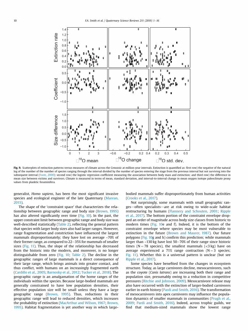
Fig. 9. Scatterplots of extinction patterns versus measures of climate across the Cenozoic at million-year intervals. Extinction is quantified as: first row) the negative of the naturallog of the number of the number of species ranging through the interval divided by the number of species entering the stage from the previous interval but not surviving into thesubsequent interval (Foote, 2000); second row) the logistic regression coefficient measuring the association between body mass and extinction; and third row) the difference inmean size between victims and survivors. Climate is measured in terms of mean, standard deviation, and interval-to-interval change in mean oxygen isotope paleoclimate proxyvalues from planktic foraminifera.
F.A. Smith et al. / Quaternary Science Reviews 211 (2019) 1e1610
generalist, Homo sapiens, has been the most significant invasivespecies and ecological engineer of the late Quaternary (Marean,2015).
The shape of the ‘constraint space’ that characterizes the rela-tionship between geographic range and body size (Brown, 1995)has also altered significantly over time (Fig. 10). In the past, theupper constraint limit between geographic range and body sizewaswell-described statistically (Table 2), reflecting the general patternthat species with larger body sizes also had larger ranges. However,range fragmentation and constriction have influenced the largestmammals disproportionately; they have lost on average ~70% oftheir former range, as compared to 22e35% for mammals of smallersizes (Fig. 11). Thus, the slope of the relationship has decreasedfrom the historic into the modern, and moreover, is no longerdistinguishable from zero (Fig. 10; Table 2). The decline in thegeographic ranges of large mammals is a direct consequence oftheir large range, which brings animals into greater contact, andthus conflict, with humans on an increasingly fragmented earth(Cardillo et al., 2005; Barnosky et al., 2012; Tucker et al., 2018). Thegeographic range is an amalgamation of the home ranges of theindividuals within the species. Because large-bodied mammals aregenerally constrained to have low population densities, theireffective population size will be small unless they have a largegeographic range (Brown, 1995). Thus, reductions in theirgeographic range will lead to reduced densities, which increasesthe probability of extinction (MacArthur and Wilson, 1967; Brown,1995). Habitat fragmentation is yet another way in which large-
bodied mammals suffer disproportionately from human activities(Crooks et al., 2017).
Not surprisingly, some mammals with small geographic ran-gesdoften specialistsdare at risk owing to wide-scale habitatrestructuring by humans (Flannery and Schouten, 2001; Rippleet al., 2017). The bottom portion of the constraint envelope drop-ped an order of magnitude across body size classes from historic tomodern times (Fig. 10e and f). Indeed, it is the bottom of theconstraint envelope where species may be most vulnerable toextinction in the future (Brown and Maurer, 1987). Our futurepolygons (Fig. 10g and h) confirm this prediction; while mammalslarger than ~130 kg have lost 50e70% of their range since historictimes (N¼ 78 species), the smallest mammals (<3 kg) have onaverage experienced a 71% range contraction (N¼ 3 species;Fig. 11). Whether this is a universal pattern is unclear (but seeRipple et al., 2017).
Some species have benefited from the changes in ecosystemstructure. Today, as large carnivores decline, mesocarnivores, suchas the coyote (Canis latrans) are increasing both their range andpopulation size, presumably owing to a reduction in competitivepressures (Ritchie and Johnson, 2009). Mesocarnivore release mayalso have occurred with the extinction of larger-bodied carnivoresearlier in earth history (Pardi and Smith, 2016). The transformationof mesocarnivores into apex carnivores may influence the popula-tion dynamics of smaller mammals in communities (Prugh et al.,2009; Pardi and Smith, 2016). Indeed, across trophic guilds, wefind that medium-sized mammals show the lowest range
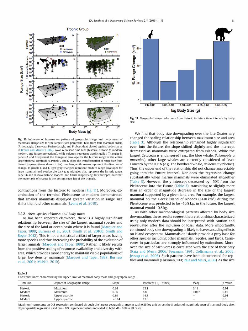
Fig. 10. Influence of humans on pattern of geographic range and body mass ofmammals. Range size for the largest (50% percentile) taxa from four mammal orders(Artiodactyla, Carnivora, Perissodactyla, and Proboscidea) plotted against body size asin Brown and Maurer (1987). Rows represent time bins (historic, historic to modern,modern, and future projections), while columns represent trophic guilds. Triangles inpanels A and B represent the triangular envelope for the historic range of the entirelarge mammal community. Panels C and D show the transformation of range size fromhistoric (squares) to modern (circles) time bins, while arrows represent the direction ofchange. In panels E and F, light gray triangles represent modern range envelopes forlarge mammals and overlay the dark gray triangles that represent the historic range.Panels G and H show historic, modern, and future range triangular envelopes, note thatthe major axis of change is the bottom right leg of the triangle.
Fig. 11. Geographic range reductions from historic to future time intervals by bodysize.
F.A. Smith et al. / Quaternary Science Reviews 211 (2019) 1e16 11
contractions from the historic to modern (Fig. 11). Moreover, ex-amination of the terminal Pleistocene to modern demonstratedthat smaller mammals displayed greater variation in range sizeshifts than did other mammals (Lyons et al., 2010).
3.2.2. Area, species richness and body massAs has been reported elsewhere, there is a highly significant
relationship between the size of the largest mammal species andthe size of the land or ocean basin where it is found (Marquet andTaper, 1998; Burness et al., 2001; Smith et al., 2010b; Smith andBoyer, 2012). This is not a statistical artifact of larger areas havingmore species and thus increasing the probability of the evolution oflarger animals (Marquet and Taper, 1998). Rather, it likely resultsfrom the positive scaling of resource availability and diversity witharea, which provides more energy tomaintain viable populations oflarge, low density, mammals (Marquet and Taper, 1998; Burnesset al., 2001; McNab, 2010).
Table 2‘Constraint lines’ characterizing the upper limit of mammal body mass and geographic r
Time Bin Aspect of Geographic Range Slope
Historic Maximum 0.24Modern Maximum 0.36Historic Upper quartile 0.19Modern Upper quartile �0.14
‘Maximum’ represents an OLS regression conducted through the largest geographic rangUpper quartile regression used tau¼ 0.9; significant values indicated in bold. df¼ 168 in
We find that body size downgrading over the late Quaternarychanged the scaling relationship between maximum size and area(Table 3). Although the relationship remained highly significanteven into the future, the slope shifted slightly and the interceptdecreased as mammals were extirpated from islands. While thelargest Cetacean is endangered (e.g., the blue whale, Balaenopteramusculus), other large whales are currently considered of LeastConcern by the IUCN (e.g., the bowhead whale, Balaena mysticetus).Thus, the upper end of the relationship did not change appreciablygoing into the Future interval. Nor does the regression changesubstantially when marine mammals were eliminated altogether(Table 3). However, the y-intercept decreased by ~50% from thePleistocene into the Future (Table 3), translating to slightly morethan an order of magnitude decrease in the size of the largestmammal supported by a given land area. For example, the largestmammal on the Greek island of Rhodes (1410 km2) during thePleistocene was predicted to be ~10.8 kg; in the future, the largestmammal would ~0.8 kg.
As with other macroecological patterns affected by body sizedowngrading, these results suggest that relationships characterizedusing only modern data should be interpreted with caution andreevaluated after the inclusion of fossil data. More importantly,continued body size downgrading is likely to have cascading effectson island ecosystems. Mammals on islands provide a prey base forother species including other mammals, reptiles, and birds. Carni-vores in particular, are strongly influenced by extinctions. More-over, the size of carnivores is correlated with the size of their prey(Raia and Meiri, 2006; Forsman, 1991; Goltsmann et al., 2005;Jessop et al., 2006). Such patterns have been documented for rep-tiles andmammals (Forsman,199; Raia andMeiri, 2006). As the size
ange.
Intercept (þ/� stdev) r2adj p-value
12.1 0.11 0.048.8 0.037 0.1614.8 e 0.0417.5 e 0.5
e in each 0.25 log unit across the 8 orders of magnitude span of mammal body size;all cases.
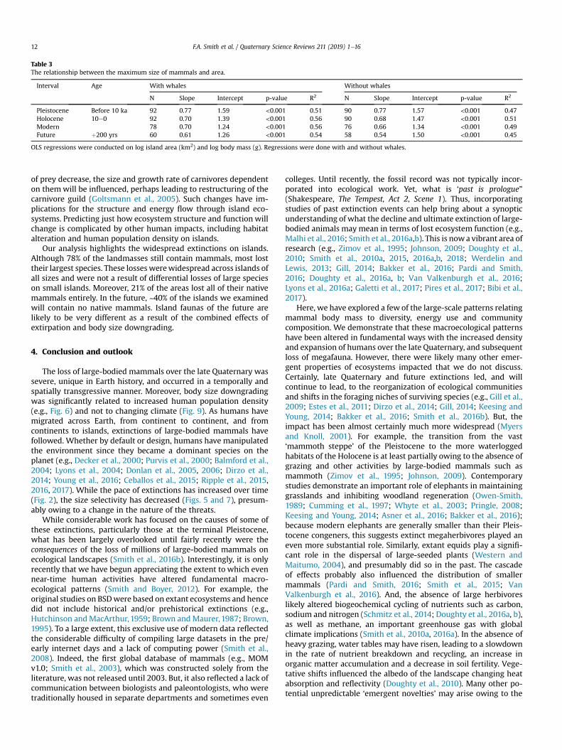
Table 3The relationship between the maximum size of mammals and area.
Interval Age With whales Without whales
N Slope Intercept p-value R2 N Slope Intercept p-value R2
Pleistocene Before 10 ka 92 0.77 1.59 <0.001 0.51 90 0.77 1.57 <0.001 0.47Holocene 10e0 92 0.70 1.39 <0.001 0.56 90 0.68 1.47 <0.001 0.51Modern 78 0.70 1.24 <0.001 0.56 76 0.66 1.34 <0.001 0.49Future þ200 yrs 60 0.61 1.26 <0.001 0.54 58 0.54 1.50 <0.001 0.45
OLS regressions were conducted on log island area (km2) and log body mass (g). Regressions were done with and without whales.
F.A. Smith et al. / Quaternary Science Reviews 211 (2019) 1e1612
of prey decrease, the size and growth rate of carnivores dependenton themwill be influenced, perhaps leading to restructuring of thecarnivore guild (Goltsmann et al., 2005). Such changes have im-plications for the structure and energy flow through island eco-systems. Predicting just how ecosystem structure and function willchange is complicated by other human impacts, including habitatalteration and human population density on islands.
Our analysis highlights the widespread extinctions on islands.Although 78% of the landmasses still contain mammals, most losttheir largest species. These losses werewidespread across islands ofall sizes and were not a result of differential losses of large specieson small islands. Moreover, 21% of the areas lost all of their nativemammals entirely. In the future, ~40% of the islands we examinedwill contain no native mammals. Island faunas of the future arelikely to be very different as a result of the combined effects ofextirpation and body size downgrading.
4. Conclusion and outlook
The loss of large-bodied mammals over the late Quaternary wassevere, unique in Earth history, and occurred in a temporally andspatially transgressive manner. Moreover, body size downgradingwas significantly related to increased human population density(e.g., Fig. 6) and not to changing climate (Fig. 9). As humans havemigrated across Earth, from continent to continent, and fromcontinents to islands, extinctions of large-bodied mammals havefollowed. Whether by default or design, humans have manipulatedthe environment since they became a dominant species on theplanet (e.g., Decker et al., 2000; Purvis et al., 2000; Balmford et al.,2004; Lyons et al., 2004; Donlan et al., 2005, 2006; Dirzo et al.,2014; Young et al., 2016; Ceballos et al., 2015; Ripple et al., 2015,2016, 2017). While the pace of extinctions has increased over time(Fig. 2), the size selectivity has decreased (Figs. 5 and 7), presum-ably owing to a change in the nature of the threats.
While considerable work has focused on the causes of some ofthese extinctions, particularly those at the terminal Pleistocene,what has been largely overlooked until fairly recently were theconsequences of the loss of millions of large-bodied mammals onecological landscapes (Smith et al., 2016b). Interestingly, it is onlyrecently that we have begun appreciating the extent to which evennear-time human activities have altered fundamental macro-ecological patterns (Smith and Boyer, 2012). For example, theoriginal studies on BSDwere based on extant ecosystems and hencedid not include historical and/or prehistorical extinctions (e.g.,Hutchinson andMacArthur, 1959; Brown andMaurer, 1987; Brown,1995). To a large extent, this exclusive use of modern data reflectedthe considerable difficulty of compiling large datasets in the pre/early internet days and a lack of computing power (Smith et al.,2008). Indeed, the first global database of mammals (e.g., MOMv1.0; Smith et al., 2003), which was constructed solely from theliterature, was not released until 2003. But, it also reflected a lack ofcommunication between biologists and paleontologists, who weretraditionally housed in separate departments and sometimes even
colleges. Until recently, the fossil record was not typically incor-porated into ecological work. Yet, what is ‘past is prologue”(Shakespeare, The Tempest, Act 2, Scene 1). Thus, incorporatingstudies of past extinction events can help bring about a synopticunderstanding of what the decline and ultimate extinction of large-bodied animals may mean in terms of lost ecosystem function (e.g.,Malhi et al., 2016; Smith et al., 2016a,b). This is nowa vibrant area ofresearch (e.g., Zimov et al., 1995; Johnson, 2009; Doughty et al.,2010; Smith et al., 2010a, 2015, 2016a,b, 2018; Werdelin andLewis, 2013; Gill, 2014; Bakker et al., 2016; Pardi and Smith,2016; Doughty et al., 2016a, b; Van Valkenburgh et al., 2016;Lyons et al., 2016a; Galetti et al., 2017; Pires et al., 2017; Bibi et al.,2017).
Here, we have explored a few of the large-scale patterns relatingmammal body mass to diversity, energy use and communitycomposition. We demonstrate that these macroecological patternshave been altered in fundamental ways with the increased densityand expansion of humans over the late Quaternary, and subsequentloss of megafauna. However, there were likely many other emer-gent properties of ecosystems impacted that we do not discuss.Certainly, late Quaternary and future extinctions led, and willcontinue to lead, to the reorganization of ecological communitiesand shifts in the foraging niches of surviving species (e.g., Gill et al.,2009; Estes et al., 2011; Dirzo et al., 2014; Gill, 2014; Keesing andYoung, 2014; Bakker et al., 2016; Smith et al., 2016b). But, theimpact has been almost certainly much more widespread (Myersand Knoll, 2001). For example, the transition from the vast‘mammoth steppe’ of the Pleistocene to the more waterloggedhabitats of the Holocene is at least partially owing to the absence ofgrazing and other activities by large-bodied mammals such asmammoth (Zimov et al., 1995; Johnson, 2009). Contemporarystudies demonstrate an important role of elephants in maintaininggrasslands and inhibiting woodland regeneration (Owen-Smith,1989; Cumming et al., 1997; Whyte et al., 2003; Pringle, 2008;Keesing and Young, 2014; Asner et al., 2016; Bakker et al., 2016);because modern elephants are generally smaller than their Pleis-tocene congeners, this suggests extinct megaherbivores played aneven more substantial role. Similarly, extant equids play a signifi-cant role in the dispersal of large-seeded plants (Western andMaitumo, 2004), and presumably did so in the past. The cascadeof effects probably also influenced the distribution of smallermammals (Pardi and Smith, 2016; Smith et al., 2015; VanValkenburgh et al., 2016). And, the absence of large herbivoreslikely altered biogeochemical cycling of nutrients such as carbon,sodium and nitrogen (Schmitz et al., 2014; Doughty et al., 2016a, b),as well as methane, an important greenhouse gas with globalclimate implications (Smith et al., 2010a, 2016a). In the absence ofheavy grazing, water tables may have risen, leading to a slowdownin the rate of nutrient breakdown and recycling, an increase inorganic matter accumulation and a decrease in soil fertility. Vege-tative shifts influenced the albedo of the landscape changing heatabsorption and reflectivity (Doughty et al., 2010). Many other po-tential unpredictable ‘emergent novelties’ may arise owing to the
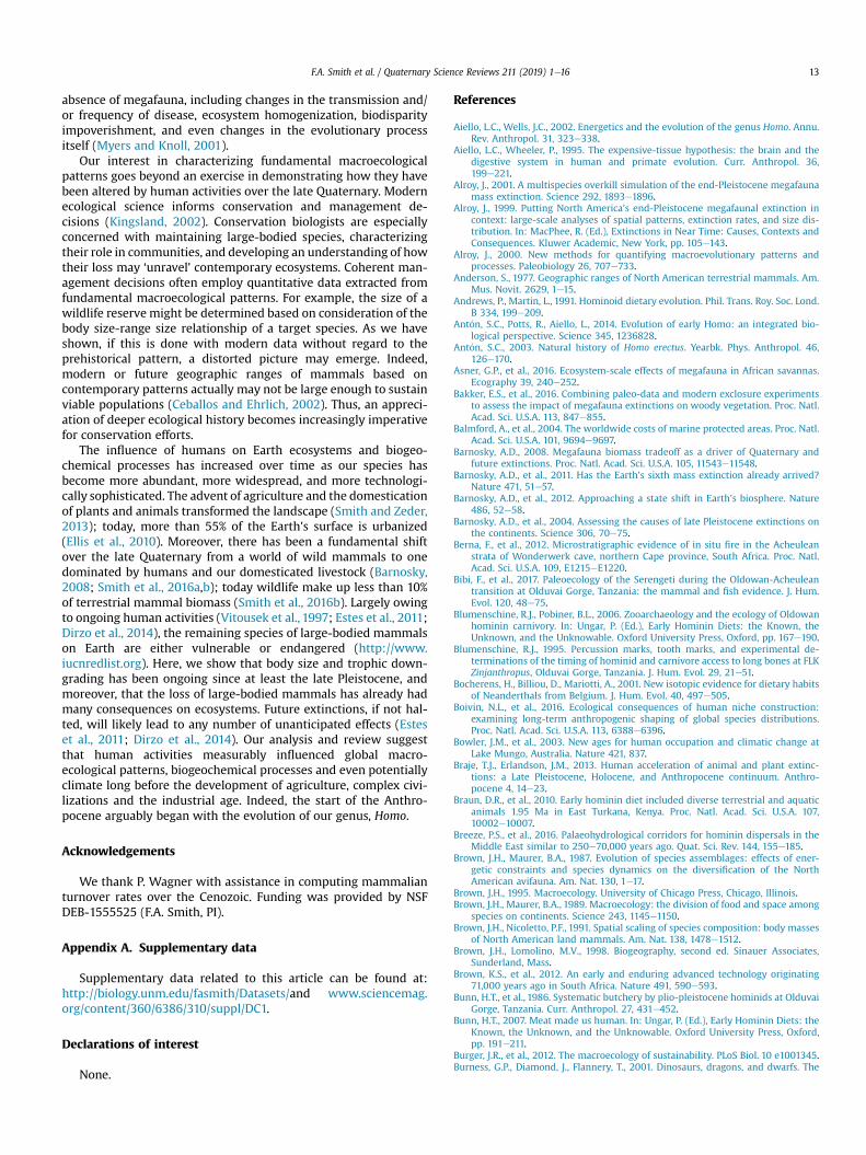
F.A. Smith et al. / Quaternary Science Reviews 211 (2019) 1e16 13
absence of megafauna, including changes in the transmission and/or frequency of disease, ecosystem homogenization, biodisparityimpoverishment, and even changes in the evolutionary processitself (Myers and Knoll, 2001).
Our interest in characterizing fundamental macroecologicalpatterns goes beyond an exercise in demonstrating how they havebeen altered by human activities over the late Quaternary. Modernecological science informs conservation and management de-cisions (Kingsland, 2002). Conservation biologists are especiallyconcerned with maintaining large-bodied species, characterizingtheir role in communities, and developing an understanding of howtheir loss may ‘unravel’ contemporary ecosystems. Coherent man-agement decisions often employ quantitative data extracted fromfundamental macroecological patterns. For example, the size of awildlife reserve might be determined based on consideration of thebody size-range size relationship of a target species. As we haveshown, if this is done with modern data without regard to theprehistorical pattern, a distorted picture may emerge. Indeed,modern or future geographic ranges of mammals based oncontemporary patterns actually may not be large enough to sustainviable populations (Ceballos and Ehrlich, 2002). Thus, an appreci-ation of deeper ecological history becomes increasingly imperativefor conservation efforts.
The influence of humans on Earth ecosystems and biogeo-chemical processes has increased over time as our species hasbecome more abundant, more widespread, and more technologi-cally sophisticated. The advent of agriculture and the domesticationof plants and animals transformed the landscape (Smith and Zeder,2013); today, more than 55% of the Earth's surface is urbanized(Ellis et al., 2010). Moreover, there has been a fundamental shiftover the late Quaternary from a world of wild mammals to onedominated by humans and our domesticated livestock (Barnosky,2008; Smith et al., 2016a,b); today wildlife make up less than 10%of terrestrial mammal biomass (Smith et al., 2016b). Largely owingto ongoing human activities (Vitousek et al., 1997; Estes et al., 2011;Dirzo et al., 2014), the remaining species of large-bodied mammalson Earth are either vulnerable or endangered (http://www.iucnredlist.org). Here, we show that body size and trophic down-grading has been ongoing since at least the late Pleistocene, andmoreover, that the loss of large-bodied mammals has already hadmany consequences on ecosystems. Future extinctions, if not hal-ted, will likely lead to any number of unanticipated effects (Esteset al., 2011; Dirzo et al., 2014). Our analysis and review suggestthat human activities measurably influenced global macro-ecological patterns, biogeochemical processes and even potentiallyclimate long before the development of agriculture, complex civi-lizations and the industrial age. Indeed, the start of the Anthro-pocene arguably began with the evolution of our genus, Homo.
Acknowledgements
We thank P. Wagner with assistance in computing mammalianturnover rates over the Cenozoic. Funding was provided by NSFDEB-1555525 (F.A. Smith, PI).
Appendix A. Supplementary data
Supplementary data related to this article can be found at:http://biology.unm.edu/fasmith/Datasets/and www.sciencemag.org/content/360/6386/310/suppl/DC1.
Declarations of interest
None.
References
Aiello, L.C., Wells, J.C., 2002. Energetics and the evolution of the genus Homo. Annu.Rev. Anthropol. 31, 323e338.
Aiello, L.C., Wheeler, P., 1995. The expensive-tissue hypothesis: the brain and thedigestive system in human and primate evolution. Curr. Anthropol. 36,199e221.
Alroy, J., 2001. A multispecies overkill simulation of the end-Pleistocene megafaunamass extinction. Science 292, 1893e1896.
Alroy, J., 1999. Putting North America's end-Pleistocene megafaunal extinction incontext: large-scale analyses of spatial patterns, extinction rates, and size dis-tribution. In: MacPhee, R. (Ed.), Extinctions in Near Time: Causes, Contexts andConsequences. Kluwer Academic, New York, pp. 105e143.
Alroy, J., 2000. New methods for quantifying macroevolutionary patterns andprocesses. Paleobiology 26, 707e733.
Anderson, S., 1977. Geographic ranges of North American terrestrial mammals. Am.Mus. Novit. 2629, 1e15.
Andrews, P., Martin, L., 1991. Hominoid dietary evolution. Phil. Trans. Roy. Soc. Lond.B 334, 199e209.
Ant�on, S.C., Potts, R., Aiello, L., 2014. Evolution of early Homo: an integrated bio-logical perspective. Science 345, 1236828.
Ant�on, S.C., 2003. Natural history of Homo erectus. Yearbk. Phys. Anthropol. 46,126e170.
Asner, G.P., et al., 2016. Ecosystem-scale effects of megafauna in African savannas.Ecography 39, 240e252.
Bakker, E.S., et al., 2016. Combining paleo-data and modern exclosure experimentsto assess the impact of megafauna extinctions on woody vegetation. Proc. Natl.Acad. Sci. U.S.A. 113, 847e855.
Balmford, A., et al., 2004. The worldwide costs of marine protected areas. Proc. Natl.Acad. Sci. U.S.A. 101, 9694e9697.
Barnosky, A.D., 2008. Megafauna biomass tradeoff as a driver of Quaternary andfuture extinctions. Proc. Natl. Acad. Sci. U.S.A. 105, 11543e11548.
Barnosky, A.D., et al., 2011. Has the Earth's sixth mass extinction already arrived?Nature 471, 51e57.
Barnosky, A.D., et al., 2012. Approaching a state shift in Earth's biosphere. Nature486, 52e58.
Barnosky, A.D., et al., 2004. Assessing the causes of late Pleistocene extinctions onthe continents. Science 306, 70e75.
Berna, F., et al., 2012. Microstratigraphic evidence of in situ fire in the Acheuleanstrata of Wonderwerk cave, northern Cape province, South Africa. Proc. Natl.Acad. Sci. U.S.A. 109, E1215eE1220.
Bibi, F., et al., 2017. Paleoecology of the Serengeti during the Oldowan-Acheuleantransition at Olduvai Gorge, Tanzania: the mammal and fish evidence. J. Hum.Evol. 120, 48e75.
Blumenschine, R.J., Pobiner, B.L., 2006. Zooarchaeology and the ecology of Oldowanhominin carnivory. In: Ungar, P. (Ed.), Early Hominin Diets: the Known, theUnknown, and the Unknowable. Oxford University Press, Oxford, pp. 167e190.
Blumenschine, R.J., 1995. Percussion marks, tooth marks, and experimental de-terminations of the timing of hominid and carnivore access to long bones at FLKZinjanthropus, Olduvai Gorge, Tanzania. J. Hum. Evol. 29, 21e51.
Bocherens, H., Billiou, D., Mariotti, A., 2001. New isotopic evidence for dietary habitsof Neanderthals from Belgium. J. Hum. Evol. 40, 497e505.
Boivin, N.L., et al., 2016. Ecological consequences of human niche construction:examining long-term anthropogenic shaping of global species distributions.Proc. Natl. Acad. Sci. U.S.A. 113, 6388e6396.
Bowler, J.M., et al., 2003. New ages for human occupation and climatic change atLake Mungo, Australia. Nature 421, 837.
Braje, T.J., Erlandson, J.M., 2013. Human acceleration of animal and plant extinc-tions: a Late Pleistocene, Holocene, and Anthropocene continuum. Anthro-pocene 4, 14e23.
Braun, D.R., et al., 2010. Early hominin diet included diverse terrestrial and aquaticanimals 1.95 Ma in East Turkana, Kenya. Proc. Natl. Acad. Sci. U.S.A. 107,10002e10007.
Breeze, P.S., et al., 2016. Palaeohydrological corridors for hominin dispersals in theMiddle East similar to 250e70,000 years ago. Quat. Sci. Rev. 144, 155e185.
Brown, J.H., Maurer, B.A., 1987. Evolution of species assemblages: effects of ener-getic constraints and species dynamics on the diversification of the NorthAmerican avifauna. Am. Nat. 130, 1e17.
Brown, J.H., 1995. Macroecology. University of Chicago Press, Chicago, Illinois.Brown, J.H., Maurer, B.A., 1989. Macroecology: the division of food and space among
species on continents. Science 243, 1145e1150.Brown, J.H., Nicoletto, P.F., 1991. Spatial scaling of species composition: body masses
of North American land mammals. Am. Nat. 138, 1478e1512.Brown, J.H., Lomolino, M.V., 1998. Biogeography, second ed. Sinauer Associates,
Sunderland, Mass.Brown, K.S., et al., 2012. An early and enduring advanced technology originating
71,000 years ago in South Africa. Nature 491, 590e593.Bunn, H.T., et al., 1986. Systematic butchery by plio-pleistocene hominids at Olduvai
Gorge, Tanzania. Curr. Anthropol. 27, 431e452.Bunn, H.T., 2007. Meat made us human. In: Ungar, P. (Ed.), Early Hominin Diets: the
Known, the Unknown, and the Unknowable. Oxford University Press, Oxford,pp. 191e211.
Burger, J.R., et al., 2012. The macroecology of sustainability. PLoS Biol. 10 e1001345.Burness, G.P., Diamond, J., Flannery, T., 2001. Dinosaurs, dragons, and dwarfs. The
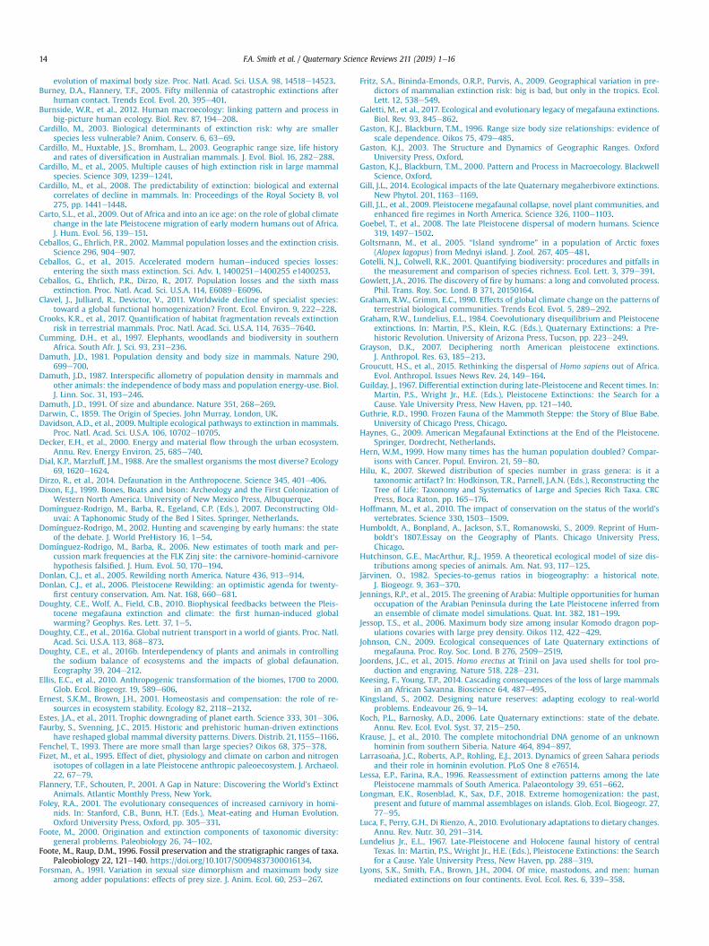
F.A. Smith et al. / Quaternary Science Reviews 211 (2019) 1e1614
evolution of maximal body size. Proc. Natl. Acad. Sci. U.S.A. 98, 14518e14523.Burney, D.A., Flannery, T.F., 2005. Fifty millennia of catastrophic extinctions after
human contact. Trends Ecol. Evol. 20, 395e401.Burnside, W.R., et al., 2012. Human macroecology: linking pattern and process in
big-picture human ecology. Biol. Rev. 87, 194e208.Cardillo, M., 2003. Biological determinants of extinction risk: why are smaller
species less vulnerable? Anim. Conserv. 6, 63e69.Cardillo, M., Huxtable, J.S., Bromham, L., 2003. Geographic range size, life history
and rates of diversification in Australian mammals. J. Evol. Biol. 16, 282e288.Cardillo, M., et al., 2005. Multiple causes of high extinction risk in large mammal
species. Science 309, 1239e1241.Cardillo, M., et al., 2008. The predictability of extinction: biological and external
correlates of decline in mammals. In: Proceedings of the Royal Society B, vol275, pp. 1441e1448.
Carto, S.L., et al., 2009. Out of Africa and into an ice age: on the role of global climatechange in the late Pleistocene migration of early modern humans out of Africa.J. Hum. Evol. 56, 139e151.
Ceballos, G., Ehrlich, P.R., 2002. Mammal population losses and the extinction crisis.Science 296, 904e907.
Ceballos, G., et al., 2015. Accelerated modern humaneinduced species losses:entering the sixth mass extinction. Sci. Adv. 1, 1400251e1400255 e1400253.
Ceballos, G., Ehrlich, P.R., Dirzo, R., 2017. Population losses and the sixth massextinction. Proc. Natl. Acad. Sci. U.S.A. 114, E6089eE6096.
Clavel, J., Julliard, R., Devictor, V., 2011. Worldwide decline of specialist species:toward a global functional homogenization? Front. Ecol. Environ. 9, 222e228.
Crooks, K.R., et al., 2017. Quantification of habitat fragmentation reveals extinctionrisk in terrestrial mammals. Proc. Natl. Acad. Sci. U.S.A. 114, 7635e7640.
Cumming, D.H., et al., 1997. Elephants, woodlands and biodiversity in southernAfrica. South Afr. J. Sci. 93, 231e236.
Damuth, J.D., 1981. Population density and body size in mammals. Nature 290,699e700.
Damuth, J.D., 1987. Interspecific allometry of population density in mammals andother animals: the independence of body mass and population energy-use. Biol.J. Linn. Soc. 31, 193e246.
Damuth, J.D., 1991. Of size and abundance. Nature 351, 268e269.Darwin, C., 1859. The Origin of Species. John Murray, London, UK.Davidson, A.D., et al., 2009. Multiple ecological pathways to extinction in mammals.
Proc. Natl. Acad. Sci. U.S.A. 106, 10702e10705.Decker, E.H., et al., 2000. Energy and material flow through the urban ecosystem.
Annu. Rev. Energy Environ. 25, 685e740.Dial, K.P., Marzluff, J.M., 1988. Are the smallest organisms the most diverse? Ecology
69, 1620e1624.Dirzo, R., et al., 2014. Defaunation in the Anthropocene. Science 345, 401e406.Dixon, E.J., 1999. Bones, Boats and bison: Archeology and the First Colonization of
Western North America. University of New Mexico Press, Albuquerque.Domínguez-Rodrigo, M., Barba, R., Egeland, C.P. (Eds.), 2007. Deconstructing Old-
uvai: A Taphonomic Study of the Bed I Sites. Springer, Netherlands.Domínguez-Rodrigo, M., 2002. Hunting and scavenging by early humans: the state
of the debate. J. World PreHistory 16, 1e54.Domínguez-Rodrigo, M., Barba, R., 2006. New estimates of tooth mark and per-
cussion mark frequencies at the FLK Zinj site: the carnivore-hominid-carnivorehypothesis falsified. J. Hum. Evol. 50, 170e194.
Donlan, C.J., et al., 2005. Rewilding north America. Nature 436, 913e914.Donlan, C.J., et al., 2006. Pleistocene Rewilding: an optimistic agenda for twenty-
first century conservation. Am. Nat. 168, 660e681.Doughty, C.E., Wolf, A., Field, C.B., 2010. Biophysical feedbacks between the Pleis-
tocene megafauna extinction and climate: the first human-induced globalwarming? Geophys. Res. Lett. 37, 1e5.
Doughty, C.E., et al., 2016a. Global nutrient transport in a world of giants. Proc. Natl.Acad. Sci. U.S.A. 113, 868e873.
Doughty, C.E., et al., 2016b. Interdependency of plants and animals in controllingthe sodium balance of ecosystems and the impacts of global defaunation.Ecography 39, 204e212.
Ellis, E.C., et al., 2010. Anthropogenic transformation of the biomes, 1700 to 2000.Glob. Ecol. Biogeogr. 19, 589e606.
Ernest, S.K.M., Brown, J.H., 2001. Homeostasis and compensation: the role of re-sources in ecosystem stability. Ecology 82, 2118e2132.
Estes, J.A., et al., 2011. Trophic downgrading of planet earth. Science 333, 301e306.Faurby, S., Svenning, J.C., 2015. Historic and prehistoric human-driven extinctions
have reshaped global mammal diversity patterns. Divers. Distrib. 21, 1155e1166.Fenchel, T., 1993. There are more small than large species? Oikos 68, 375e378.Fizet, M., et al., 1995. Effect of diet, physiology and climate on carbon and nitrogen
isotopes of collagen in a late Pleistocene anthropic paleoecosystem. J. Archaeol.22, 67e79.
Flannery, T.F., Schouten, P., 2001. A Gap in Nature: Discovering the World's ExtinctAnimals. Atlantic Monthly Press, New York.
Foley, R.A., 2001. The evolutionary consequences of increased carnivory in homi-nids. In: Stanford, C.B., Bunn, H.T. (Eds.), Meat-eating and Human Evolution.Oxford University Press, Oxford, pp. 305e331.
Foote, M., 2000. Origination and extinction components of taxonomic diversity:general problems. Paleobiology 26, 74e102.
Foote, M., Raup, D.M., 1996. Fossil preservation and the stratigraphic ranges of taxa.Paleobiology 22, 121e140. https://doi.org/10.1017/S0094837300016134.
Forsman, A., 1991. Variation in sexual size dimorphism and maximum body sizeamong adder populations: effects of prey size. J. Anim. Ecol. 60, 253e267.
Fritz, S.A., Bininda-Emonds, O.R.P., Purvis, A., 2009. Geographical variation in pre-dictors of mammalian extinction risk: big is bad, but only in the tropics. Ecol.Lett. 12, 538e549.
Galetti, M., et al., 2017. Ecological and evolutionary legacy of megafauna extinctions.Biol. Rev. 93, 845e862.
Gaston, K.J., Blackburn, T.M., 1996. Range size body size relationships: evidence ofscale dependence. Oikos 75, 479e485.
Gaston, K.J., 2003. The Structure and Dynamics of Geographic Ranges. OxfordUniversity Press, Oxford.
Gaston, K.J., Blackburn, T.M., 2000. Pattern and Process in Macroecology. BlackwellScience, Oxford.
Gill, J.L., 2014. Ecological impacts of the late Quaternary megaherbivore extinctions.New Phytol. 201, 1163e1169.
Gill, J.L., et al., 2009. Pleistocene megafaunal collapse, novel plant communities, andenhanced fire regimes in North America. Science 326, 1100e1103.
Goebel, T., et al., 2008. The late Pleistocene dispersal of modern humans. Science319, 1497e1502.
Goltsmann, M., et al., 2005. “Island syndrome” in a population of Arctic foxes(Alopex lagopus) from Mednyi island. J. Zool. 267, 405e481.
Gotelli, N.J., Colwell, R.K., 2001. Quantifying biodiversity: procedures and pitfalls inthe measurement and comparison of species richness. Ecol. Lett. 3, 379e391.
Gowlett, J.A., 2016. The discovery of fire by humans: a long and convoluted process.Phil. Trans. Roy. Soc. Lond. B 371, 20150164.
Graham, R.W., Grimm, E.C., 1990. Effects of global climate change on the patterns ofterrestrial biological communities. Trends Ecol. Evol. 5, 289e292.
Graham, R.W., Lundelius, E.L., 1984. Coevolutionary disequilibrium and Pleistoceneextinctions. In: Martin, P.S., Klein, R.G. (Eds.), Quaternary Extinctions: a Pre-historic Revolution. University of Arizona Press, Tucson, pp. 223e249.
Grayson, D.K., 2007. Deciphering north American pleistocene extinctions.J. Anthropol. Res. 63, 185e213.
Groucutt, H.S., et al., 2015. Rethinking the dispersal of Homo sapiens out of Africa.Evol. Anthropol. Issues News Rev. 24, 149e164.
Guilday, J., 1967. Differential extinction during late-Pleistocene and Recent times. In:Martin, P.S., Wright Jr., H.E. (Eds.), Pleistocene Extinctions: the Search for aCause. Yale University Press, New Haven, pp. 121e140.
Guthrie, R.D., 1990. Frozen Fauna of the Mammoth Steppe: the Story of Blue Babe.University of Chicago Press, Chicago.
Haynes, G., 2009. American Megafaunal Extinctions at the End of the Pleistocene.Springer, Dordrecht, Netherlands.
Hern, W.M., 1999. How many times has the human population doubled? Compar-isons with Cancer. Popul. Environ. 21, 59e80.
Hilu, K., 2007. Skewed distribution of species number in grass genera: is it ataxonomic artifact? In: Hodkinson, T.R., Parnell, J.A.N. (Eds.), Reconstructing theTree of Life: Taxonomy and Systematics of Large and Species Rich Taxa. CRCPress, Boca Raton, pp. 165e176.
Hoffmann, M., et al., 2010. The impact of conservation on the status of the world'svertebrates. Science 330, 1503e1509.
Humboldt, A., Bonpland, A., Jackson, S.T., Romanowski, S., 2009. Reprint of Hum-boldt's 1807.Essay on the Geography of Plants. Chicago University Press,Chicago.
Hutchinson, G.E., MacArthur, R.J., 1959. A theoretical ecological model of size dis-tributions among species of animals. Am. Nat. 93, 117e125.
J€arvinen, O., 1982. Species-to-genus ratios in biogeography: a historical note.J. Biogeogr. 9, 363e370.
Jennings, R.P., et al., 2015. The greening of Arabia: Multiple opportunities for humanoccupation of the Arabian Peninsula during the Late Pleistocene inferred froman ensemble of climate model simulations. Quat. Int. 382, 181e199.
Jessop, T.S., et al., 2006. Maximum body size among insular Komodo dragon pop-ulations covaries with large prey density. Oikos 112, 422e429.
Johnson, C.N., 2009. Ecological consequences of Late Quaternary extinctions ofmegafauna. Proc. Roy. Soc. Lond. B 276, 2509e2519.
Joordens, J.C., et al., 2015. Homo erectus at Trinil on Java used shells for tool pro-duction and engraving. Nature 518, 228e231.
Keesing, F., Young, T.P., 2014. Cascading consequences of the loss of large mammalsin an African Savanna. Bioscience 64, 487e495.
Kingsland, S., 2002. Designing nature reserves: adapting ecology to real-worldproblems. Endeavour 26, 9e14.
Koch, P.L., Barnosky, A.D., 2006. Late Quaternary extinctions: state of the debate.Annu. Rev. Ecol. Evol. Syst. 37, 215e250.
Krause, J., et al., 2010. The complete mitochondrial DNA genome of an unknownhominin from southern Siberia. Nature 464, 894e897.
Larrasoa~na, J.C., Roberts, A.P., Rohling, E.J., 2013. Dynamics of green Sahara periodsand their role in hominin evolution. PLoS One 8 e76514.
Lessa, E.P., Farina, R.A., 1996. Reassessment of extinction patterns among the latePleistocene mammals of South America. Palaeontology 39, 651e662.
Longman, E.K., Rosenblad, K., Sax, D.F., 2018. Extreme homogenization: the past,present and future of mammal assemblages on islands. Glob. Ecol. Biogeogr. 27,77e95.
Luca, F., Perry, G.H., Di Rienzo, A., 2010. Evolutionary adaptations to dietary changes.Annu. Rev. Nutr. 30, 291e314.
Lundelius Jr., E.L., 1967. Late-Pleistocene and Holocene faunal history of centralTexas. In: Martin, P.S., Wright Jr., H.E. (Eds.), Pleistocene Extinctions: the Searchfor a Cause. Yale University Press, New Haven, pp. 288e319.
Lyons, S.K., Smith, F.A., Brown, J.H., 2004. Of mice, mastodons, and men: humanmediated extinctions on four continents. Evol. Ecol. Res. 6, 339e358.
F.A. Smith et al. / Quaternary Science Reviews 211 (2019) 1e16 15
Lyons, S.K., Wagner, P.J., Dzikiewicz, K., 2010. Ecological correlates of range shifts ofLate Pleistocene mammals. Phil. Trans. Biol. Sci. 365, 3681e3693.
Lyons, S.K., Smith, F.A., 2013. Macroecological patterns of body size in mammalsacross time and space. In: Smith, F.A., Lyons, S.K. (Eds.), Body Size: LinkingPattern and Process across Space, Time and Taxonomy. University of ChicagoPress, Chicago, pp. 114e142.
Lyons, S.K., et al., 2016a. Holocene shifts in the assembly of plant and animalcommunities implicate human impacts. Nature 529, 80eU183.
Lyons, S.K., et al., 2016b. The changing role of mammal life histories in late Qua-ternary extinction vulnerability on continents and islands. Biol. Lett. 12,20160342.
MacArthur, R.H., Wilson, E.O., 1967. z Theory of Island Biogeography. PrincetonUniversity Press, Princeton.
Malhi, Y., et al., 2016. Megafauna and ecosystem function from the pleistocene tothe Anthropocene. Proc. Natl. Acad. Sci. U.S.A. 113, 838e846.
Marean, C.W., 2015. The most invasive species of all. Sci. Am. 313, 33e39.Marquet, P.A., Taper, M.L., 1998. On size and area: patterns of mammalian body size
extremes across landmasses. Evol. Ecol. 12, 127e139.Martin, P.S., 1967. Prehistoric overkill. In: Martin, P.S., Wright Jr., H.E. (Eds.), Pleis-
tocene Extinctions: the Search for a Cause. Yale University Press, New Haven,pp. 75e120.
Martin, P.S., 1984. Prehistoric overkill: the global model. In: Martin, P.S., Klein, R.G.(Eds.), Quaternary Extinctions: A Prehistoric Revolution. University of ArizonaPress, Tucson, pp. 354e403.
Martin, P.S., 2005. Twilight of the Mammoths: Ice Age Extinctions and RewildingAmerica. University of California Press, Berkley.
Martin, P.S., Steadman, D.W., 1999. Prehistoric extinctions on islands and conti-nents. In: MacPhee, R.D.E. (Ed.), Extinctions in Near Time: Causes, Contexts, andConsequences. Kluwer Academic/Plenum Press, New York, pp. 17e55.
Maurer, B.A., Brown, J.H., 1988. Distribution of energy use and biomass amongspecies of North American terrestrial birds. Ecology 69, 1923e1932.
Maurer, B.A., 1999. Untangling Ecological Complexity: the Macroscopic Perspective.University of Chicago Press, Chicago.
Maurer, B.A., 2013. Geographic variation in body size distributions of continentalavifauna. In: Smith, F.A., Lyons, S.K. (Eds.), Body Size: Linking Pattern andProcess across Space, Time and Taxonomy. University of Chicago Press, Chicago,pp. 83e94.
McHenry, H.M., 1992. Body size and proportions in early hominids. Am. J. Phys.Anthropol. 87, 407e431.
McNab, B.K., 2010. Geographic and temporal correlations of mammalian sizereconsidered: a resource rule. Oecologica 164, 13e23.
Meltzer, D.J., 2015. Pleistocene overkill and North American mammal extinctions.Annu. Rev. Anthropol. 44, 33e53.
Miller, G.H., et al., 2005. Ecosystem collapse in Pleistocene Australia and a humanrole in megafaunal extinction. Science 309, 287e290.
Milton, K., 1999. A hypothesis to explain the role of meat-eating in human evolu-tion. Evol. Anthropol. 8, 11e21.
Morrison, J.C., et al., 2007. Persistence of large mammal faunas as indicators ofglobal human impacts. J. Mammal. 88, 1363e1380.
Moses, M.E., Brown, J.H., 2003. Allometry of human fertility and energy use. Ecol.Lett. 6, 295e300.
Murray, P., 1991. The Pleistocene megafauna of Australia. In: Vickers-Rich, P.,Mongahan, J.M., Baird, R.F., Rich, T.H. (Eds.), Vertebrate Palaeontology of Aus-tralasia. Pioneer Design Studio, Melbourne, pp. 1070e1164.
Muttoni, G., Scardia, G., Kent, D.V., 2018. Early hominins in Europe: the Galerianmigration hypothesis. Quat. Sci. Rev. 180, 1e29.
Myers, N., Knoll, A.H., 2001. The biotic crisis and the future of evolution. Proc. Natl.Acad. Sci. U.S.A. 98, 5389e5392.
O'Connell, J., Allen, J., 2004. Dating the colonization of Sahul (Pleistocene Australia-New Guinea): A review of recent research. J. Archaeol. Sci. 31 (6), 835e853.
Olden, J.D., et al., 2004. Ecological and evolutionary consequences of biotic ho-mogenization. Trends Ecol. Evol. 19, 18e24.
Oppenheimer, S., 2012. Out-of-Africa, the peopling of continents and islands:tracing uniparental gene trees across the map. Phil. Trans. Biol. Sci. 367,770e784.
Owen-Smith, N., 1989. Megafaunal extinctions: the conservation message from11,000 years B.P. Conserv. Biol. 3, 405e412.
Pante, M.C., et al., 2017. The carnivorous feeding behavior of early Homo at HWK EE,Bed II, Olduvai Gorge, Tanzania. J. Hum. Evol. 120, 215e235.
Pardi, M.I., Smith, F.A., 2016. Biotic responses of canids to the terminal Pleistocenemegafauna extinction. Ecography 39, 141e151.
Parmesan, C., Yohe, G., 2003. A globally coherent fingerprint of climate changeimpacts across natural systems. Nature 421, 37e42.
Parton, A., et al., 2015. Orbital-scale climate variability in Arabia as a potential motorfor human dispersals. Quat. Int. 382, 82e97.
Pimm, S.L., et al., 2014. The biodiversity of species and their rates of extinction,distribution, and protection. Science 344, 1246752.
Pires, M.M., et al., 2017. Pleistocene megafaunal extinctions and the functional lossof long-distance seed-dispersal services. Ecography 41, 153e163.
Pringle, R.M., 2008. Elephants as agents of habitat creation for small vertebrates atthe patch scale. Ecology 89, 26e33.
Prugh, L.R., et al., 2009. The rise of the mesopredator. Bioscience 59, 779e791.Purvis, A., et al., 2000. Nonrandom extinction and the loss of evolutionary history.
Science 288, 328e330.R Core Team, 2015. R: A Language and Environment for Statistical Computing. R
Foundation Statistical Company.R Studio Team, 2015. R Studio. Integrated Development for R. R Foundation Sta-
tistical Company.Raia, P., Meiri, S., 2006. The island rule in large mammals: paleontology meets
ecology. Evolution 60, 1731e1742.Richards, M.P., et al., 2000. Neanderthal diet at Vindija and Neatherthal predation:
the evidence from stable isotopes. Proc. Natl. Acad. Sci. U.S.A. 97, 7663e7666.Rightmire, G.P., et al., 2017. Skull 5 from Dmanisi: descriptive anatomy, comparative
studies, and evolutionary significance. J. Hum. Evol. 104, 50e79.Ripple, W.J., Van Valkenburgh, B., 2010. Linking top-down forces to the Pleistocene
megafaunal extinctions. Bioscience 60, 516e526.Ripple, W.J., et al., 2014. Status and ecological effects of the world's largest carni-
vores. Science 343 (6167), 1241484.Ripple, W.J., et al., 2015. Collapse of the world's largest herbivores. Sci. Adv. 1,
31400103.Ripple, W.J., et al., 2016. Saving the world's terrestrial megafauna. Bioscience 66,
807e812.Ripple, W.J., et al., 2017. Extinction risk is most acute for the world's largest and
smallest vertebrates. Proc. Natl. Acad. Sci. Unit. States Am. 114, 10678e10683.Ritchie, E.G., Johnson, C.N., 2009. Predator interactions, mesopredator release and
biodiversity conservation. Ecol. Lett. 12, 982e998.Roberts, R.G., et al., 2001. New ages for the last Australian megafauna: continent-
wide extinction about 46,000 years ago. Science 292, 1888e1892.Roebroeks, W., Villa, P., 2011. On the earliest evidence for habitual use of fire in
Europe. Proc. Natl. Acad. Sci. U.S.A. 108, 5209e5214.Roy, K., Jablonski, D., Valentine, J.W., 1996. Higher taxa in biodiversity studies:
patterns from eastern Pacific marine molluscs. Phil. Trans. Biol. Sci. 351,1605e1613.
Rundle, S.D., Bilton, D.T., Abbott, J.C., Foggo, A., 2007. Range size in North AmericanEnallagma damselflies correlates with wing size. Freshw. Biol. 52, 471e477.
Sandom, C., et al., 2014. Global late Quaternary megafauna extinctions linked tohumans, not climate change. Proc. Roy. Soc. Lond. B 281, 20133254.
Schipper, J., et al., 2008. The status of the world's land and marine mammals: di-versity, threat, and knowledge. Science 322, 225e230.
Schmitz, O.J., et al., 2014. Animating the carbon cycle. Ecosystems 17, 344e359.Shea, J.J., 2017. Occasional, obligatory, and habitual stone tool use in hominin
evolution. Evol. Anthropol. Issues News Rev. 26, 200e217.Simberloff, D., 1970. Taxonomic diversity of island biotas. Evolution 24, 23e47.Smith, B.D., Zeder, M.A., 2013. The onset of the Anthropocene. Anthropocene 4,
8e13.Smith, F.A., Boyer, A.G., 2012. Losing time? Incorporating a deeper temporal
perspective into modern ecology. Front. Biogeogr. 4, 27e39.Smith, F.A., Betancourt, J.L., 2003. The effect of late Holocene temperature fluctu-
ations on the evolution and ecology of woodrats (Neotoma) in Idaho andnorthwestern Utah. Quat. Res. 59, 160e171.
Smith, F.A., Betancourt, J.L., Brown, J.H., 1995. Evolution of woodrat body size tracks20,000 years of climate change. Science 270, 2012e2014.
Smith, F.A., Browning, H., Shepherd, U.L., 1998. The influence of climatic change onthe body mass of woodrats (Neotoma albigula) in an arid region of New Mexico,USA. Ecography 21, 140e148.
Smith, F.A., Elliott, S.M., Lyons, S.K., 2010a. Methane emissions from extinctmegafauna. Nat. Geosci. 3, 374e375.
Smith, F.A., Lyons, S.K., 2011. How big should a mammal be? A macroecological lookat mammalian body size over space and time. Proc. R. Soc. Ser. B 366,2364e2378.
Smith, F.A., et al., 2003. Body mass of late Quaternary mammals. Ecology 84, 3402.Smith, F.A., et al., 2004. Similarity of mammalian body size across the taxonomic
hierarchy and across space and time. Am. Nat. 163, 672e691.Smith, F.A., et al., 2008. Macroecology: more than the division of food and space
among species on continents. Prog. Phys. Geogr. 32, 115e138.Smith, F.A., et al., 2010b. The evolution of maximum body size of terrestrial
mammals. Science 330, 1216e1219.Smith, F.A., et al., 2015. Unraveling the consequences of the terminal Pleistocene
megafauna extinction on mammal community assembly. Ecography 39,223e239.
Smith, F.A., et al., 2016a. Exploring the influence of ancient and historic mega-herbivore extirpations on the global methane budget. Proc. Natl. Acad. Sci.U.S.A. 113, 874e879.
Smith, F.A., et al., 2016b. Megafauna in the earth system. Ecography 39, 99e108.Smith, F.A., et al., 2018. Body size downgrading of mammals over the late Quater-
nary. Science 360, 310e313.Sponheimer, et al., 2013. Isotopic evidence of early hominin diets. Proc. Natl. Acad.
Sci. U.S.A. 110, 10513e10518.Sponheimer, M.J., Lee-Thorp, de Ruiter, D., 2007. Icarus, isotopes and australopith
diets. In: Ungar, P.S. (Ed.), Evolution of the Human Diet: the Known, the Un-known and the Unknowable. Oxford University Press, Oxford, pp. 132e149.
Stiner, M., 2002. Carnivory, coevolution, and the geographic spread of the genusHomo. J. Archaeol. Res. 10, 1e63.
Stringer, C., 2000. Paleoanthropology: coasting out of Africa. Nature 405, 24e27.Stringer, C., Andrews, P., 1988. Genetic and fossil evidence for the origins of modern
humans. Science 239, 1263e1268.Stuart, A.J., 1999. Late Pleistocene megafaunal extinctions: a European perspective.
In: MacPhee, R.D.E. (Ed.), Extinctions in Near Time: Causes, Contexts, andConsequences. Kluwer Academic/Plenum, New York, pp. 257e270.
Surovell, T.A., et al., 2016. Test of Martin's overkill hypothesis using radiocarbon
F.A. Smith et al. / Quaternary Science Reviews 211 (2019) 1e1616
dates on extinct megafauna. Proc. Natl. Acad. Sci. U.S.A. 113, 886e891.Surovell, T.A., Waguespack, N.M., 2009. Human prey choice in the late Pleistocene
and its relation to megafaunal extinctions. In: Haynes, G. (Ed.), AmericanMegafaunal Extinctions at the End of the Pleistocene. Springer-Verlag, NewYork, pp. 77e105.
Thomas, C.D., et al., 2004. Extinction risk from climate change. Nature 427, 145e148.Tierney, J.E., Zander, P.D., 2017. A climatic context for the out-of-Africa migration.
Geology 45, 1023e1026.Timmermann, A., Friedrich, T., 2016. Late Pleistocene climate drivers of early human
migration. Nature 538, 92e95.Tomiya, S., 2013. Body size and extinction risk in terrestrial mammals above the
species level. Am. Nat. 182, 196eE214.Tucker, M.A., et al., 2018. Moving in the Anthropocene: global reductions in
terrestrial mammalian movements. Science 359, 466e469.Turvey, S.T., 2009. Holocene Extinctions. Oxford University Press, Oxford.Turvey, S.T., Fritz, S.A., 2011. The ghosts of mammals past: biological and
geographical patterns of global mammalian extinction across the Holocene.Phil. Trans. Biol. Sci. 366, 2564.
Van Valen, L., 1973. A new evolutionary law. Evol. Theory 1, 1e30.Van Valkenburgh, B., et al., 2016. The impact of large terrestrial carnivores on
Pleistocene ecosystems. Proc. Natl. Acad. Sci. U.S.A. 113, 862e867.Vitousek, P.M., et al., 1997. Human domination of earth's ecosystems. Science 277,
494e499.Vrba, E.S., DeGusta, D., 2004. Do species populations really start small? New per-
spectives from the Late Neogene fossil record of African mammals. Phil. Trans.Biol. Sci. 359, 285e292.
Walter, R.C., et al., 2000. Early human occupation of the Red sea coast of Eritreaduring the last interglacial. Nature 405, 65e69.
Watts, D.P., 2008. Scavenging by chimpanzees at Ngogo and the relevance of chim-panzee scavenging to early hominin behavioral ecology. J. Hum. Evol. 54,125e133.
Werdelin, L., Lewis, M.E., 2013. Temporal change in functional richness and even-ness in the eastern African plio-Pleistocene carnivoran guild. PLoS One 8e57944.
Western, D., Maitumo, D., 2004. Woodland loss and restoration in a savanna park: a
20-year experiment. Afr. J. Ecol. 42, 111e121.Whitley, D.S., 2009. Cave Paintings and the Human Spirit: the Origin of Creativity
and Belief. Prometheus, Amherst.Whyte, I.J., et al., 2003. Kruger's elephant population: its size and consequences for
ecosystem heterogeneity. In: Du Toit, J.T., Rogers, K.H., Biggs, H.C. (Eds.), TheKruger Experience: Ecology and Management of Savanna Heterogeneity. IslandPress, Washington, D.C, pp. 332e348.
Wilkins, J., et al., 2012. Evidence for early hafted hunting technology. Science 338,942e946.
Williams, P.H., Gaston, K.J., 1994. Measuring more of biodiversity: can higher-taxonrichness predict wholesale species richness? Biol. Conserv. 67, 211e217.
Willis, J.C., Yule, G.U., 1922. Some statistics of evolution and geographical distri-bution in plants and animals, and their significance. Nature 109, 177e179.
Wilson, D.E., Reeder, D.M., 2003. Mammal Species of the World. A Taxonomic andGeographic Reference. John Hopkins University Press, Baltimore.
Wrangham, R.W., et al., 1999. The raw and the stolend cooking and the ecology ofhuman origins. Curr. Anthropol. 40, 567e594.
Wrangham, R.W., 2009. Catching Fire: How Cooking Made Us Human. Basic Books,New York.
Wroe, S., et al., 2013. Climate change frames debate over the extinction of mega-fauna in Sahul (Pleistocene Australia-New Guinea). Proc. Natl. Acad. Sci. U.S.A.110, 8777e8781.
Wroe, S., Field, J., Grayson, D.K., 2006. Megafaunal extinction: climate, humans, andassumptions. Trends Ecol. Evol. 21, 61e62.
Young, H.S., et al., 2016. Patterns, causes, and consequences of Anthropocenedefaunation. Annu. Rev. Ecol. Evol. Syst. 47, 333e358.
Zachos, J., et al., 2001. Trends, rhythms, and aberrations in global climate 65 Ma topresent. Science 292, 686e693.
Zimov, S.A., et al., 1995. Steppe-tundra transition: a herbivore- driven biome shift atthe end of the Pleistocene. Am. Nat. 146, 765e794.
Zink, K.D., Lieberman, D.E., 2016. Impact of meat and Lower Palaeolithic food pro-cessing techniques on chewing in humans. Nature 531, 500e503.
Zuo, W., et al., 2013. A life-history approach to the Late Pleistocene megafaunalextinction. Am. Nat. 182, 524e531.
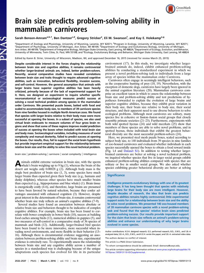
Brain size predicts problem-solving ability inmammalian carnivoresSarah Benson-Amrama,b,1, Ben Dantzerc,d, Gregory Strickere, Eli M. Swansonf, and Kay E. Holekampe,g
aDepartment of Zoology and Physiology, University of Wyoming, Laramie, WY 82071; bProgram in Ecology, University of Wyoming, Laramie, WY 82071;cDepartment of Psychology, University of Michigan, Ann Arbor, MI 48109; dDepartment of Ecology and Evolutionary Biology, University of Michigan,Ann Arbor, MI 48109; eDepartment of Integrative Biology, Michigan State University, East Lansing, MI 48824; fDepartment of Ecology, Evolution, and Behavior,University of Minnesota, Twin Cities, St. Paul, MN 55108; and gEcology, Evolutionary Biology and Behavior, Michigan State University, East Lansing, MI 48824
Edited by Karen B. Strier, University of Wisconsin, Madison, WI, and approved December 16, 2015 (received for review March 25, 2015)
Despite considerable interest in the forces shaping the relationshipbetween brain size and cognitive abilities, it remains controversialwhether larger-brained animals are, indeed, better problem-solvers.Recently, several comparative studies have revealed correlationsbetween brain size and traits thought to require advanced cognitiveabilities, such as innovation, behavioral flexibility, invasion success,and self-control. However, the general assumption that animals withlarger brains have superior cognitive abilities has been heavilycriticized, primarily because of the lack of experimental support forit. Here, we designed an experiment to inquire whether specificneuroanatomical or socioecological measures predict success atsolving a novel technical problem among species in the mammalianorder Carnivora. We presented puzzle boxes, baited with food andscaled to accommodate body size, to members of 39 carnivore speciesfrom nine families housed in multiple North American zoos. We foundthat species with larger brains relative to their body mass were moresuccessful at opening the boxes. In a subset of species, we also usedvirtual brain endocasts to measure volumes of four gross brain re-gions and show that some of these regions improve model predictionof success at opening the boxes when included with total brain sizeand bodymass. Socioecological variables, including measures of socialcomplexity and manual dexterity, failed to predict success at openingthe boxes. Our results, thus, fail to support the social brain hypothesisbut provide important empirical support for the relationship betweenrelative brain size and the ability to solve this novel technical problem.
brain size | problem-solving | carnivore | social complexity | intelligence
Animals exhibit extreme variation in brain size, with the spermwhale’s brain weighing up to 9 kg (1), whereas the brain of the
desert ant weighs only 0.00028 g (2). Although body mass is thesingle best predictor of brain size (1, 3), some species have muchlarger brains than expected given their body size (e.g., humans anddusky dolphins), whereas other species have much smaller brainsthan expected (e.g., hippopotamus and blue whale) (1). Brain tissueis energetically costly (4–6), and therefore, large brains are presumedto have been favored by natural selection, because they confer ad-vantages associated with enhanced cognition (3). However, despitegreat interest in the determinants of brain size, it remains controversialwhether brain size truly reflects an animal’s cognitive abilities (7–9).Several studies have found an association between absolute or
relative brain size and behaviors thought to be indicative of complexcognitive abilities. For example, brain size has been found to cor-relate with bower complexity in bower birds (10), success at buildingfood caches among birds (11), numerical abilities in guppies (5), andtwo measures of self-control in a comparative study of 36 species ofmammals and birds (12). Additionally, larger-brained bird specieshave been found to be more innovative, more successful when in-vading novel environments, and more flexible in their behavior (13–16). Although there is circumstantial evidence suggesting an asso-ciation between problem-solving ability and brain size, experimentalevidence is extremely rare. To experimentally assess the relationshipbetween brain size and any cognitive ability across a number ofspecies in a standardized way is challenging because of the uniqueadaptations each species has evolved for life in its particular
environment (17). In this study, we investigate whether larger-brained animals do, indeed, exhibit enhanced problem-solvingabilities by conducting a standardized experiment in which wepresent a novel problem-solving task to individuals from a largearray of species within the mammalian order Carnivora.Carnivores often engage in seemingly intelligent behaviors, such
as the cooperative hunting of prey (18, 19). Nevertheless, with theexception of domestic dogs, carnivores have largely been ignored inthe animal cognition literature (20). Mammalian carnivores com-prise an excellent taxon in which to assess the relationship betweenbrain size and problem-solving ability and test predictions of hy-potheses forwarded to explain the evolution of large brains andsuperior cognitive abilities, because they exhibit great variation intheir body size, their brain size relative to body size, their socialstructure, and their apparent need to use diverse behaviors to solveecological problems. Although most carnivores are solitary, manyspecies live in cohesive or fission–fusion social groups that closelyresemble primate societies (21–23). Furthermore, experiments withboth wild spotted hyenas (24) and wild meerkats (25) show thatmembers of these species are able to solve novel problems, and inspotted hyenas, those individuals that exhibit the greatest behav-ioral diversity are the most successful problem-solvers (24).Here, we presented steel mesh puzzle boxes, scaled according to
subject body size, to 140 individuals from 39 species in nine familiesof zoo-housed carnivores and evaluated whether individuals in eachspecies successfully opened the boxes to obtain a food reward inside(Fig. 1A and Dataset S1). In addition to testing whether larger-brained carnivores are better at solving a novel technical problem,we inquired whether species that live in larger social groups exhibitenhanced problem-solving abilities compared with species that aresolitary or live in smaller social groups. We also asked whetherspecies exhibiting greater behavioral diversity are better at solving
Significance
Intelligence presents evolutionary biology with one of its greatestchallenges. It has long been thought that species with relativelylarge brains for their body size are more intelligent. However,despite decades of research, the idea that brain size predictscognitive abilities remains highly controversial; little experimentalsupport exists for a relationship between brain size and the abilityto solve novel problems. We presented 140 zoo-housed membersof 39 mammalian carnivore species with a novel problem-solvingtask and found that the species’ relative brain sizes predictedproblem-solving success. Our results provide important supportfor the claim that brain size reflects an animal’s problem-solvingabilities and enhance our understanding of why larger brainsevolved in some species.
Author contributions: K.E.H. designed research; G.S. performed research; B.D., E.M.S., and S.B.-Aanalyzed data; S.B.-A., B.D., E.M.S., and K.E.H. wrote the paper; and S.B.-A. extracted video data.
The authors declare no conflict of interest.
This article is a PNAS Direct Submission.1To whom correspondence should be addressed. Email: [email protected].
This article contains supporting information online at www.pnas.org/lookup/suppl/doi:10.1073/pnas.1505913113/-/DCSupplemental.
2532–2537 | PNAS | March 1, 2016 | vol. 113 | no. 9 www.pnas.org/cgi/doi/10.1073/pnas.1505913113
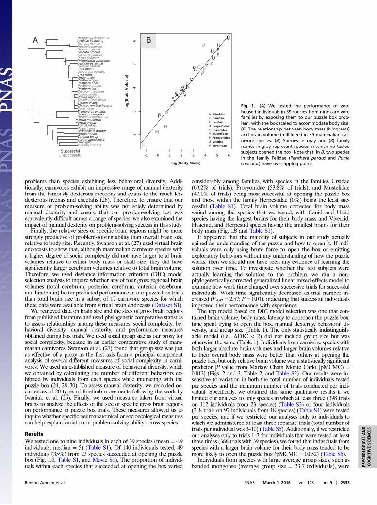
problems than species exhibiting less behavioral diversity. Addi-tionally, carnivores exhibit an impressive range of manual dexterityfrom the famously dexterous raccoons and coatis to the much lessdexterous hyenas and cheetahs (26). Therefore, to ensure that ourmeasure of problem-solving ability was not solely determined bymanual dexterity and ensure that our problem-solving test wasequivalently difficult across a range of species, we also examined theimpact of manual dexterity on problem-solving success in this study.Finally, the relative sizes of specific brain regions might be more
strongly predictive of problem-solving ability than overall brain sizerelative to body size. Recently, Swanson et al. (27) used virtual brainendocasts to show that, although mammalian carnivore species witha higher degree of social complexity did not have larger total brainvolumes relative to either body mass or skull size, they did havesignificantly larger cerebrum volumes relative to total brain volume.Therefore, we used deviance information criterion (DIC) modelselection analysis to inquire whether any of four gross regional brainvolumes (total cerebrum, posterior cerebrum, anterior cerebrum,and hindbrain) better predicted performance in our puzzle box trialsthan total brain size in a subset of 17 carnivore species for whichthese data were available from virtual brain endocasts (Dataset S1).We retrieved data on brain size and the sizes of gross brain regions
from published literature and used phylogenetic comparative statisticsto assess relationships among these measures, social complexity, be-havioral diversity, manual dexterity, and performance measuresobtained during box trials. We used social group size as our proxy forsocial complexity, because in an earlier comparative study of mam-malian carnivores, Swanson et al. (27) found that group size was justas effective of a proxy as the first axis from a principal componentanalysis of several different measures of social complexity in carni-vores. We used an established measure of behavioral diversity, whichwe obtained by calculating the number of different behaviors ex-hibited by individuals from each species while interacting with thepuzzle box (24, 28–30). To assess manual dexterity, we recorded oc-currences of 20 types of forelimb movements following the work byIwaniuk et al. (26). Finally, we used measures taken from virtualbrains to analyze the effects of the size of specific gross brain regionson performance in puzzle box trials. These measures allowed us toinquire whether specific neuroanatomical or socioecological measurescan help explain variation in problem-solving ability across species.
ResultsWe tested one to nine individuals in each of 39 species (mean = 4.9individuals; median = 5) (Table S1). Of 140 individuals tested, 49individuals (35%) from 23 species succeeded at opening the puzzlebox (Fig. 1A, Table S1, and Movie S1). The proportion of individ-uals within each species that succeeded at opening the box varied
considerably among families, with species in the families Ursidae(69.2% of trials), Procyonidae (53.8% of trials), and Mustelidae(47.1% of trials) being most successful at opening the puzzle boxand those within the family Herpestidae (0%) being the least suc-cessful (Table S1). Total brain volume corrected for body massvaried among the species that we tested, with Canid and Ursidspecies having the largest brains for their body mass and Viverrid,Hyaenid, and Herpestid species having the smallest brains for theirbody mass (Fig. 1B and Table S1).It appeared that the majority of subjects in our study actually
gained an understanding of the puzzle and how to open it. If indi-viduals were only using brute force to open the box or emittingexploratory behaviors without any understanding of how the puzzleworks, then we should not have seen any evidence of learning thesolution over time. To investigate whether the test subjects wereactually learning the solution to the problem, we ran a non-phylogenetically corrected generalized linear mixed-effects model toexamine how work time changed over successive trials for successfulindividuals. Work time significantly decreased as trial number in-creased (F9,97 = 2.57; P = 0.01), indicating that successful individualsimproved their performance with experience.The top model based on DIC model selection was one that con-
tained brain volume, body mass, latency to approach the puzzle box,time spent trying to open the box, manual dexterity, behavioral di-versity, and group size (Table 1). The only statistically indistinguish-able model (i.e., ΔDIC < 2) did not include group size but wasotherwise the same (Table 1). Individuals from carnivore species withboth larger absolute brain volumes and larger brain volumes relativeto their overall body mass were better than others at opening thepuzzle box, but only relative brain volume was a statistically significantpredictor [P value from Markov Chain Monte Carlo (pMCMC) =0.013] (Figs. 2 and 3, Table 2, and Table S2). Our results were in-sensitive to variation in both the total number of individuals testedper species and the minimum number of trials conducted per indi-vidual. Specifically, we obtained the same qualitative results if welimited our analyses to only species in which at least three (398 trialson 112 individuals from 23 species) (Table S3) or four individuals(348 trials on 97 individuals from 18 species) (Table S4) were testedper species, and if we restricted our analyses only to individuals towhich we administered at least three separate trials (total number oftrials per individual was 3–10) (Table S5). Additionally, if we restrictedour analyses only to trials 1–3 for individuals that were tested at leastthree times (388 trials with 39 species), we found that individuals fromspecies with a larger brain volume for their body mass tended to bemore likely to open the puzzle box (pMCMC = 0.052) (Table S6).Individuals from species with large average group sizes, such as
banded mongoose (average group size = 23.7 individuals), were
A B
Fig. 1. (A) We tested the performance of zoo-housed individuals in 39 species from nine carnivorefamilies by exposing them to our puzzle box prob-lem, with the box scaled to accommodate body size.(B) The relationship between body mass (kilograms)and brain volume (milliliters) in 39 mammalian car-nivore species. (A) Species in gray and (B) familynames in gray represent species in which no testedsubjects opened the box. Note that, in B, two speciesin the family Felidae (Panthera pardus and Pumaconcolor) have overlapping points.
Benson-Amram et al. PNAS | March 1, 2016 | vol. 113 | no. 9 | 2533
PSYC
HOLO
GICALAND
COGNITIVESC
IENCE
S
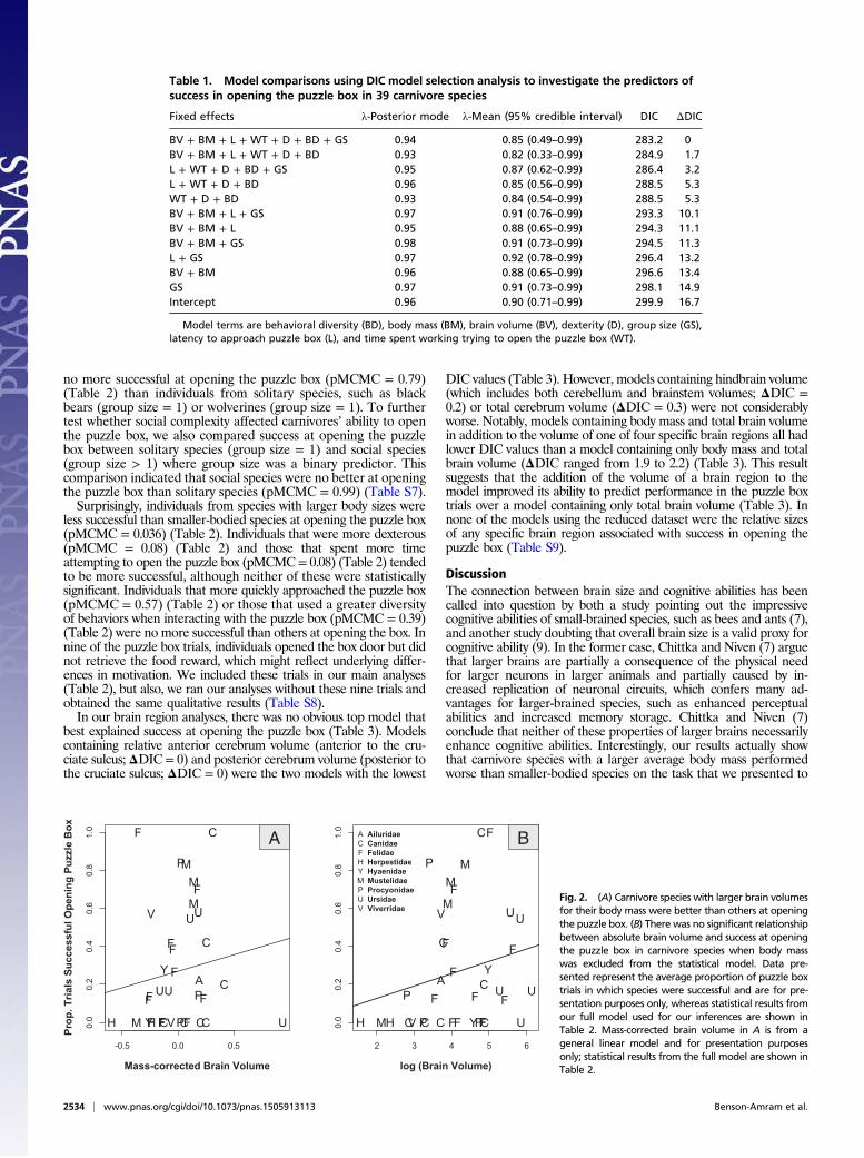
no more successful at opening the puzzle box (pMCMC = 0.79)(Table 2) than individuals from solitary species, such as blackbears (group size = 1) or wolverines (group size = 1). To furthertest whether social complexity affected carnivores’ ability to openthe puzzle box, we also compared success at opening the puzzlebox between solitary species (group size = 1) and social species(group size > 1) where group size was a binary predictor. Thiscomparison indicated that social species were no better at openingthe puzzle box than solitary species (pMCMC = 0.99) (Table S7).Surprisingly, individuals from species with larger body sizes were
less successful than smaller-bodied species at opening the puzzle box(pMCMC = 0.036) (Table 2). Individuals that were more dexterous(pMCMC = 0.08) (Table 2) and those that spent more timeattempting to open the puzzle box (pMCMC = 0.08) (Table 2) tendedto be more successful, although neither of these were statisticallysignificant. Individuals that more quickly approached the puzzle box(pMCMC = 0.57) (Table 2) or those that used a greater diversityof behaviors when interacting with the puzzle box (pMCMC = 0.39)(Table 2) were no more successful than others at opening the box. Innine of the puzzle box trials, individuals opened the box door but didnot retrieve the food reward, which might reflect underlying differ-ences in motivation. We included these trials in our main analyses(Table 2), but also, we ran our analyses without these nine trials andobtained the same qualitative results (Table S8).In our brain region analyses, there was no obvious top model that
best explained success at opening the puzzle box (Table 3). Modelscontaining relative anterior cerebrum volume (anterior to the cru-ciate sulcus;ΔDIC = 0) and posterior cerebrum volume (posterior tothe cruciate sulcus; ΔDIC = 0) were the two models with the lowest
DIC values (Table 3). However, models containing hindbrain volume(which includes both cerebellum and brainstem volumes; ΔDIC =0.2) or total cerebrum volume (ΔDIC = 0.3) were not considerablyworse. Notably, models containing body mass and total brain volumein addition to the volume of one of four specific brain regions all hadlower DIC values than a model containing only body mass and totalbrain volume (ΔDIC ranged from 1.9 to 2.2) (Table 3). This resultsuggests that the addition of the volume of a brain region to themodel improved its ability to predict performance in the puzzle boxtrials over a model containing only total brain volume (Table 3). Innone of the models using the reduced dataset were the relative sizesof any specific brain region associated with success in opening thepuzzle box (Table S9).
DiscussionThe connection between brain size and cognitive abilities has beencalled into question by both a study pointing out the impressivecognitive abilities of small-brained species, such as bees and ants (7),and another study doubting that overall brain size is a valid proxy forcognitive ability (9). In the former case, Chittka and Niven (7) arguethat larger brains are partially a consequence of the physical needfor larger neurons in larger animals and partially caused by in-creased replication of neuronal circuits, which confers many ad-vantages for larger-brained species, such as enhanced perceptualabilities and increased memory storage. Chittka and Niven (7)conclude that neither of these properties of larger brains necessarilyenhance cognitive abilities. Interestingly, our results actually showthat carnivore species with a larger average body mass performedworse than smaller-bodied species on the task that we presented to
Table 1. Model comparisons using DIC model selection analysis to investigate the predictors ofsuccess in opening the puzzle box in 39 carnivore species
Fixed effects λ-Posterior mode λ-Mean (95% credible interval) DIC ΔDIC
BV + BM + L + WT + D + BD + GS 0.94 0.85 (0.49–0.99) 283.2 0BV + BM + L + WT + D + BD 0.93 0.82 (0.33–0.99) 284.9 1.7L + WT + D + BD + GS 0.95 0.87 (0.62–0.99) 286.4 3.2L + WT + D + BD 0.96 0.85 (0.56–0.99) 288.5 5.3WT + D + BD 0.93 0.84 (0.54–0.99) 288.5 5.3BV + BM + L + GS 0.97 0.91 (0.76–0.99) 293.3 10.1BV + BM + L 0.95 0.88 (0.65–0.99) 294.3 11.1BV + BM + GS 0.98 0.91 (0.73–0.99) 294.5 11.3L + GS 0.97 0.92 (0.78–0.99) 296.4 13.2BV + BM 0.96 0.88 (0.65–0.99) 296.6 13.4GS 0.97 0.91 (0.73–0.99) 298.1 14.9Intercept 0.96 0.90 (0.71–0.99) 299.9 16.7
Model terms are behavioral diversity (BD), body mass (BM), brain volume (BV), dexterity (D), group size (GS),latency to approach puzzle box (L), and time spent working trying to open the puzzle box (WT).
Y FC F UM PH FHF C CCVF
FF
Y
UA C
C
U
MM
F
M
PF
U
P
F
F
U
F
V
C
F
-0.5 0.0 0.5
0.0
0.2
0.4
0.6
0.8
1.0
Mass-corrected Brain Volume
Prop
. Tria
ls S
ucce
ssfu
l Ope
ning
Puz
zle
Box
A
YFC F UM PH FH FC CCV F
F F
Y
UA C
C
U
MM
F
M
P F
U
P
F
F
U
F
V
C
F
2 3 4 5 6
0.0
0.2
0.4
0.6
0.8
1.0
log (Brain Volume)
ACFHYMPUV
AiluridaeCanidaeFelidaeHerpestidaeHyaenidaeMustelidaeProcyonidaeUrsidaeViverridae
B
Fig. 2. (A) Carnivore species with larger brain volumesfor their body mass were better than others at openingthe puzzle box. (B) There was no significant relationshipbetween absolute brain volume and success at openingthe puzzle box in carnivore species when body masswas excluded from the statistical model. Data pre-sented represent the average proportion of puzzle boxtrials in which species were successful and are for pre-sentation purposes only, whereas statistical results fromour full model used for our inferences are shown inTable 2. Mass-corrected brain volume in A is from ageneral linear model and for presentation purposesonly; statistical results from the full model are shown inTable 2.
2534 | www.pnas.org/cgi/doi/10.1073/pnas.1505913113 Benson-Amram et al.
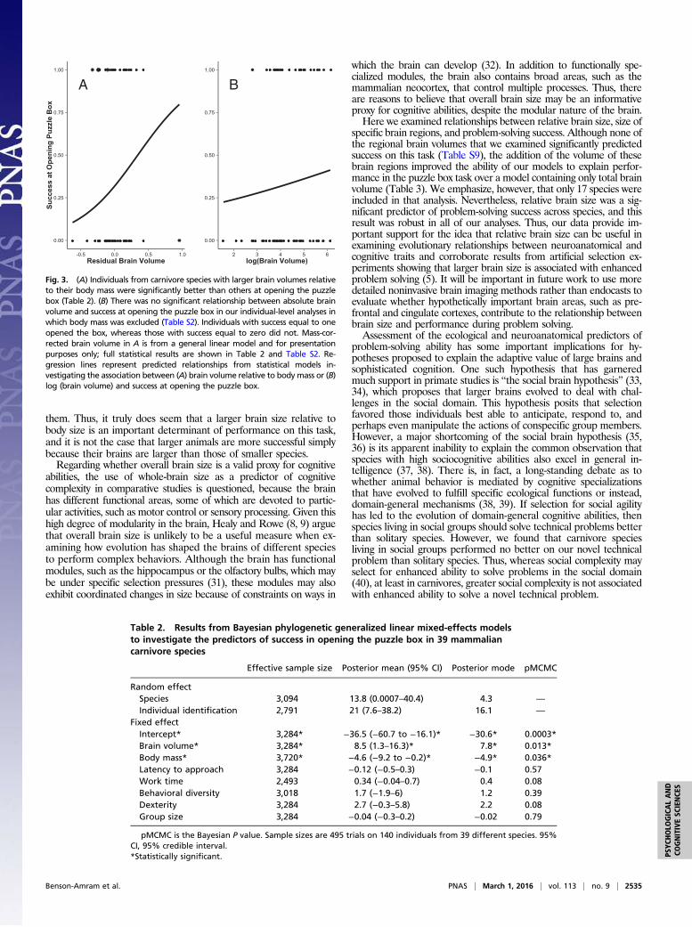
them. Thus, it truly does seem that a larger brain size relative tobody size is an important determinant of performance on this task,and it is not the case that larger animals are more successful simplybecause their brains are larger than those of smaller species.Regarding whether overall brain size is a valid proxy for cognitive
abilities, the use of whole-brain size as a predictor of cognitivecomplexity in comparative studies is questioned, because the brainhas different functional areas, some of which are devoted to partic-ular activities, such as motor control or sensory processing. Given thishigh degree of modularity in the brain, Healy and Rowe (8, 9) arguethat overall brain size is unlikely to be a useful measure when ex-amining how evolution has shaped the brains of different speciesto perform complex behaviors. Although the brain has functionalmodules, such as the hippocampus or the olfactory bulbs, which maybe under specific selection pressures (31), these modules may alsoexhibit coordinated changes in size because of constraints on ways in
which the brain can develop (32). In addition to functionally spe-cialized modules, the brain also contains broad areas, such as themammalian neocortex, that control multiple processes. Thus, thereare reasons to believe that overall brain size may be an informativeproxy for cognitive abilities, despite the modular nature of the brain.Here we examined relationships between relative brain size, size of
specific brain regions, and problem-solving success. Although none ofthe regional brain volumes that we examined significantly predictedsuccess on this task (Table S9), the addition of the volume of thesebrain regions improved the ability of our models to explain perfor-mance in the puzzle box task over a model containing only total brainvolume (Table 3). We emphasize, however, that only 17 species wereincluded in that analysis. Nevertheless, relative brain size was a sig-nificant predictor of problem-solving success across species, and thisresult was robust in all of our analyses. Thus, our data provide im-portant support for the idea that relative brain size can be useful inexamining evolutionary relationships between neuroanatomical andcognitive traits and corroborate results from artificial selection ex-periments showing that larger brain size is associated with enhancedproblem solving (5). It will be important in future work to use moredetailed noninvasive brain imaging methods rather than endocasts toevaluate whether hypothetically important brain areas, such as pre-frontal and cingulate cortexes, contribute to the relationship betweenbrain size and performance during problem solving.Assessment of the ecological and neuroanatomical predictors of
problem-solving ability has some important implications for hy-potheses proposed to explain the adaptive value of large brains andsophisticated cognition. One such hypothesis that has garneredmuch support in primate studies is “the social brain hypothesis” (33,34), which proposes that larger brains evolved to deal with chal-lenges in the social domain. This hypothesis posits that selectionfavored those individuals best able to anticipate, respond to, andperhaps even manipulate the actions of conspecific group members.However, a major shortcoming of the social brain hypothesis (35,36) is its apparent inability to explain the common observation thatspecies with high sociocognitive abilities also excel in general in-telligence (37, 38). There is, in fact, a long-standing debate as towhether animal behavior is mediated by cognitive specializationsthat have evolved to fulfill specific ecological functions or instead,domain-general mechanisms (38, 39). If selection for social agilityhas led to the evolution of domain-general cognitive abilities, thenspecies living in social groups should solve technical problems betterthan solitary species. However, we found that carnivore speciesliving in social groups performed no better on our novel technicalproblem than solitary species. Thus, whereas social complexity mayselect for enhanced ability to solve problems in the social domain(40), at least in carnivores, greater social complexity is not associatedwith enhanced ability to solve a novel technical problem.
A
0.00
0.25
0.50
0.75
1.00
-0.5 0.0 0.5 1.0Residual Brain Volume
Succ
ess
at O
peni
ng P
uzzl
e B
ox
B
0.00
0.25
0.50
0.75
1.00
2 3 4 5 6log(Brain Volume)
Fig. 3. (A) Individuals from carnivore species with larger brain volumes relativeto their body mass were significantly better than others at opening the puzzlebox (Table 2). (B) There was no significant relationship between absolute brainvolume and success at opening the puzzle box in our individual-level analyses inwhich body mass was excluded (Table S2). Individuals with success equal to oneopened the box, whereas those with success equal to zero did not. Mass-cor-rected brain volume in A is from a general linear model and for presentationpurposes only; full statistical results are shown in Table 2 and Table S2. Re-gression lines represent predicted relationships from statistical models in-vestigating the association between (A) brain volume relative to body mass or (B)log (brain volume) and success at opening the puzzle box.
Table 2. Results from Bayesian phylogenetic generalized linear mixed-effects modelsto investigate the predictors of success in opening the puzzle box in 39 mammaliancarnivore species
Effective sample size Posterior mean (95% CI) Posterior mode pMCMC
Random effectSpecies 3,094 13.8 (0.0007–40.4) 4.3 —
Individual identification 2,791 21 (7.6–38.2) 16.1 —
Fixed effectIntercept* 3,284* −36.5 (−60.7 to −16.1)* −30.6* 0.0003*Brain volume* 3,284* 8.5 (1.3–16.3)* 7.8* 0.013*Body mass* 3,720* −4.6 (−9.2 to −0.2)* −4.9* 0.036*Latency to approach 3,284 −0.12 (−0.5–0.3) −0.1 0.57Work time 2,493 0.34 (−0.04–0.7) 0.4 0.08Behavioral diversity 3,018 1.7 (−1.9–6) 1.2 0.39Dexterity 3,284 2.7 (−0.3–5.8) 2.2 0.08Group size 3,284 −0.04 (−0.3–0.2) −0.02 0.79
pMCMC is the Bayesian P value. Sample sizes are 495 trials on 140 individuals from 39 different species. 95%CI, 95% credible interval.*Statistically significant.
Benson-Amram et al. PNAS | March 1, 2016 | vol. 113 | no. 9 | 2535
PSYC
HOLO
GICALAND
COGNITIVESC
IENCE
S
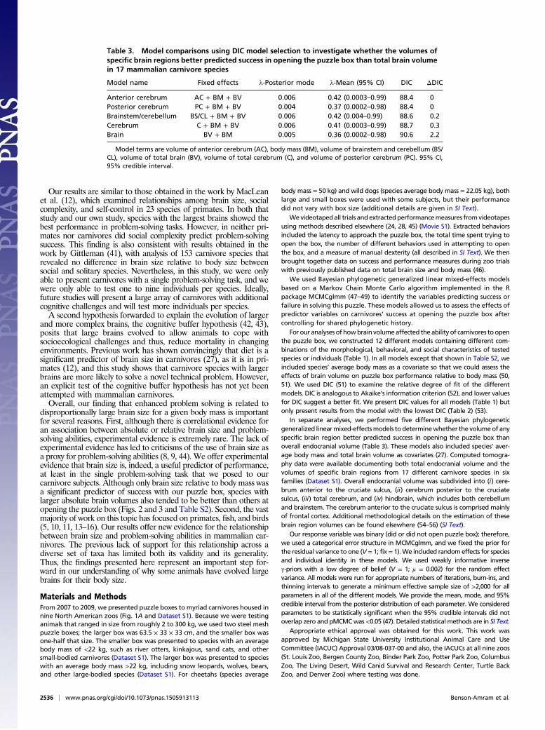
Our results are similar to those obtained in the work by MacLeanet al. (12), which examined relationships among brain size, socialcomplexity, and self-control in 23 species of primates. In both thatstudy and our own study, species with the largest brains showed thebest performance in problem-solving tasks. However, in neither pri-mates nor carnivores did social complexity predict problem-solvingsuccess. This finding is also consistent with results obtained in thework by Gittleman (41), with analysis of 153 carnivore species thatrevealed no difference in brain size relative to body size betweensocial and solitary species. Nevertheless, in this study, we were onlyable to present carnivores with a single problem-solving task, and wewere only able to test one to nine individuals per species. Ideally,future studies will present a large array of carnivores with additionalcognitive challenges and will test more individuals per species.A second hypothesis forwarded to explain the evolution of larger
and more complex brains, the cognitive buffer hypothesis (42, 43),posits that large brains evolved to allow animals to cope withsocioecological challenges and thus, reduce mortality in changingenvironments. Previous work has shown convincingly that diet is asignificant predictor of brain size in carnivores (27), as it is in pri-mates (12), and this study shows that carnivore species with largerbrains are more likely to solve a novel technical problem. However,an explicit test of the cognitive buffer hypothesis has not yet beenattempted with mammalian carnivores.Overall, our finding that enhanced problem solving is related to
disproportionally large brain size for a given body mass is importantfor several reasons. First, although there is correlational evidence foran association between absolute or relative brain size and problem-solving abilities, experimental evidence is extremely rare. The lack ofexperimental evidence has led to criticisms of the use of brain size asa proxy for problem-solving abilities (8, 9, 44). We offer experimentalevidence that brain size is, indeed, a useful predictor of performance,at least in the single problem-solving task that we posed to ourcarnivore subjects. Although only brain size relative to body mass wasa significant predictor of success with our puzzle box, species withlarger absolute brain volumes also tended to be better than others atopening the puzzle box (Figs. 2 and 3 and Table S2). Second, the vastmajority of work on this topic has focused on primates, fish, and birds(5, 10, 11, 13–16). Our results offer new evidence for the relationshipbetween brain size and problem-solving abilities in mammalian car-nivores. The previous lack of support for this relationship across adiverse set of taxa has limited both its validity and its generality.Thus, the findings presented here represent an important step for-ward in our understanding of why some animals have evolved largebrains for their body size.
Materials and MethodsFrom 2007 to 2009, we presented puzzle boxes to myriad carnivores housed innine North American zoos (Fig. 1A and Dataset S1). Because we were testinganimals that ranged in size from roughly 2 to 300 kg, we used two steel meshpuzzle boxes; the larger box was 63.5 × 33 × 33 cm, and the smaller box wasone-half that size. The smaller box was presented to species with an averagebody mass of <22 kg, such as river otters, kinkajous, sand cats, and othersmall-bodied carnivores (Dataset S1). The larger box was presented to specieswith an average body mass >22 kg, including snow leopards, wolves, bears,and other large-bodied species (Dataset S1). For cheetahs (species average
body mass = 50 kg) and wild dogs (species average body mass = 22.05 kg), bothlarge and small boxes were used with some subjects, but their performancedid not vary with box size (additional details are given in SI Text).
Wevideotapedall trials and extractedperformancemeasures fromvideotapesusing methods described elsewhere (24, 28, 45) (Movie S1). Extracted behaviorsincluded the latency to approach the puzzle box, the total time spent trying toopen the box, the number of different behaviors used in attempting to openthe box, and a measure of manual dexterity (all described in SI Text). We thenbrought together data on success and performance measures during zoo trialswith previously published data on total brain size and body mass (46).
We used Bayesian phylogenetic generalized linear mixed-effects modelsbased on a Markov Chain Monte Carlo algorithm implemented in the Rpackage MCMCglmm (47–49) to identify the variables predicting success orfailure in solving this puzzle. These models allowed us to assess the effects ofpredictor variables on carnivores’ success at opening the puzzle box aftercontrolling for shared phylogenetic history.
For our analyses of howbrain volumeaffected theability of carnivores to openthe puzzle box, we constructed 12 different models containing different com-binations of the morphological, behavioral, and social characteristics of testedspecies or individuals (Table 1). In all models except that shown in Table S2, weincluded species’ average body mass as a covariate so that we could assess theeffects of brain volume on puzzle box performance relative to body mass (50,51). We used DIC (51) to examine the relative degree of fit of the differentmodels. DIC is analogous to Akaike’s information criterion (52), and lower valuesfor DIC suggest a better fit. We present DIC values for all models (Table 1) butonly present results from the model with the lowest DIC (Table 2) (53).
In separate analyses, we performed five different Bayesian phylogeneticgeneralized linearmixed-effectsmodels to determinewhether the volumeof anyspecific brain region better predicted success in opening the puzzle box thanoverall endocranial volume (Table 3). These models also included species’ aver-age body mass and total brain volume as covariates (27). Computed tomogra-phy data were available documenting both total endocranial volume and thevolumes of specific brain regions from 17 different carnivore species in sixfamilies (Dataset S1). Overall endocranial volume was subdivided into (i) cere-brum anterior to the cruciate sulcus, (ii) cerebrum posterior to the cruciatesulcus, (iii) total cerebrum, and (iv) hindbrain, which includes both cerebellumand brainstem. The cerebrum anterior to the cruciate sulcus is comprised mainlyof frontal cortex. Additional methodological details on the estimation of thesebrain region volumes can be found elsewhere (54–56) (SI Text).
Our response variable was binary (did or did not open puzzle box); therefore,we used a categorical error structure in MCMCglmm, and we fixed the prior forthe residual variance to one (V= 1; fix= 1).We included randomeffects for speciesand individual identity in these models. We used weakly informative inverseγ-priors with a low degree of belief (V = 1; μ = 0.002) for the random effectvariance. All models were run for appropriate numbers of iterations, burn-ins, andthinning intervals to generate a minimum effective sample size of >2,000 for allparameters in all of the different models. We provide the mean, mode, and 95%credible interval from the posterior distribution of each parameter. We consideredparameters to be statistically significant when the 95% credible intervals did notoverlap zero and pMCMCwas<0.05 (47). Detailed statistical methods are in SI Text.
Appropriate ethical approval was obtained for this work. This work wasapproved by Michigan State University Institutional Animal Care and UseCommittee (IACUC) Approval 03/08-037-00 and also, the IACUCs at all nine zoos(St. Louis Zoo, Bergen County Zoo, Binder Park Zoo, Potter Park Zoo, ColumbusZoo, The Living Desert, Wild Canid Survival and Research Center, Turtle BackZoo, and Denver Zoo) where testing was done.
Table 3. Model comparisons using DIC model selection to investigate whether the volumes ofspecific brain regions better predicted success in opening the puzzle box than total brain volumein 17 mammalian carnivore species
Model name Fixed effects λ-Posterior mode λ-Mean (95% CI) DIC ΔDIC
Anterior cerebrum AC + BM + BV 0.006 0.42 (0.0003–0.99) 88.4 0Posterior cerebrum PC + BM + BV 0.004 0.37 (0.0002–0.98) 88.4 0Brainstem/cerebellum BS/CL + BM + BV 0.006 0.42 (0.004–0.99) 88.6 0.2Cerebrum C + BM + BV 0.006 0.41 (0.0003–0.99) 88.7 0.3Brain BV + BM 0.005 0.36 (0.0002–0.98) 90.6 2.2
Model terms are volume of anterior cerebrum (AC), body mass (BM), volume of brainstem and cerebellum (BS/CL), volume of total brain (BV), volume of total cerebrum (C), and volume of posterior cerebrum (PC). 95% CI,95% credible interval.
2536 | www.pnas.org/cgi/doi/10.1073/pnas.1505913113 Benson-Amram et al.
ACKNOWLEDGMENTS. We thank Steve Glickman for inspiring this work andAdam Overstreet for help with data extraction. We thank Dorothy Cheney,Robert Seyfarth, Jeff Clune, and three anonymous reviewers for manyhelpful suggestions and discussions. This work was supported by National
Science Foundation (NSF) Grants IOS 1121474 (to K.E.H.) and DEB 1353110(to K.E.H.) and NSF Cooperative Agreement DBI 0939454 supporting theBEACON Center for the Study of Evolution in Action. E.M.S. was supportedby NSF Postdoctoral Fellowship 1306627.
1. Roth G, Dicke U (2005) Evolution of the brain and intelligence. Trends Cogn Sci 9(5):250–257.
2. Wehner R, Fukushi T, Isler K (2007) On being small: Brain allometry in ants. BrainBehav Evol 69(3):220–228.
3. Striedter GF (2005) Principles of Brain Evolution (Sinauer, Sunderland, MA).4. Aiello LC, Wheeler P (1995) The expensive-tissue hypothesis: The brain and the di-
gestive system in human and primate evolution. Curr Anthropol 36(2):199–221.5. Kotrschal A, et al. (2013) Artificial selection on relative brain size in the guppy reveals
costs and benefits of evolving a larger brain. Curr Biol 23(2):168–171.6. Isler K, van Schaik CP (2009) The expensive brain: A framework for explaining evo-
lutionary changes in brain size. J Hum Evol 57(4):392–400.7. Chittka L, Niven J (2009) Are bigger brains better? Curr Biol 19(21):R995–R1008.8. Healy SD, Rowe C (2013) Costs and benefits of evolving a larger brain: Doubts over the
evidence that large brains lead to better cognition. Anim Behav 86(4):e1–e3.9. Healy SD, Rowe C (2007) A critique of comparative studies of brain size. Proc Biol Sci
274(1609):453–464.10. Madden J (2001) Sex, bowers and brains. Proc Biol Sci 268(1469):833–838.11. Garamszegi LZ, Eens M (2004) The evolution of hippocampus volume and brain size in
relation to food hoarding in birds. Ecol Lett 7(12):1216–1224.12. MacLean EL, et al. (2014) The evolution of self-control. Proc Natl Acad Sci USA 111(20):
E2140–E2148.13. Sol D, Duncan RP, Blackburn TM, Cassey P, Lefebvre L (2005) Big brains, enhanced
cognition, and response of birds to novel environments. Proc Natl Acad Sci USA102(15):5460–5465.
14. Sol D, Timmermans S, Lefebvre L (2002) Behavioural flexibility and invasion success inbirds. Anim Behav 63(3):495–502.
15. Sol D, Lefebvre L, Rodríguez-Teijeiro JD (2005) Brain size, innovative propensity andmigratory behaviour in temperate Palaearctic birds. Proc Biol Sci 272(1571):1433–1441.
16. Sol D, Lefebvre L (2000) Behavioural flexibility predicts invasion success in birds in-troduced to New Zealand. Oikos 90(3):599–605.
17. Kotrschal A, Corral-Lopez A, Amcoff M, Kolm N (2015) A larger brain confers a benefitin a spatial mate search learning task in male guppies. Behav Ecol 26(2):527–532.
18. Mech LD (2007) Possible use of foresight, understanding, and planning by wolveshunting muskoxen. Arctic 60(2):145–149.
19. Bailey I, Myatt JP, Wilson AM (2013) Group hunting within the Carnivora: Physio-logical, cognitive and environmental influences on strategy and cooperation. BehavEcol Sociobiol 67(1):1–17.
20. Vonk J, Jett SE, Mosteller KW (2012) Concept formation in American black bears,Ursus americanus. Anim Behav 84(4):953–964.
21. Gittleman JL (1989) Carnivore group living: Comparative trends. Carnivore Behaviour,Ecology and Evolution, ed Gittleman JL (Cornell Univ Press, Ithaca, NY), pp 183–208.
22. Stankowich T, Haverkamp PJ, Caro T (2014) Ecological drivers of antipredator de-fenses in carnivores. Evolution 68(5):1415–1425.
23. Holekamp KE, Dantzer B, Stricker G, Shaw Yoshida KC, Benson-Amram S (2015)Brains, brawn and sociality: A hyaena’s tale. Anim Behav 103:237–248.
24. Benson-Amram S, Holekamp KE (2012) Innovative problem solving by wild spottedhyenas. Proc R Soc Lond B Biol Sci 279(1744):4087–4095.
25. Thornton A, Samson J (2012) Innovative problem solving in wild meerkats. AnimBehav 83(6):1459–1468.
26. Iwaniuk AN, Pellis SM, Whishaw IQ (1999) Brain size is not correlated with forelimbdexterity in fissiped carnivores (Carnivora): A comparative test of the principle ofproper mass. Brain Behav Evol 54(3):167–180.
27. Swanson EM, Holekamp KE, Lundrigan BL, Arsznov BM, Sakai ST (2012) Multipledeterminants of whole and regional brain volume among terrestrial carnivorans.PLoS One 7(6):e38447.
28. Benson-Amram S, Weldele ML, Holekamp KE (2013) A comparison of innovativeproblem-solving abilities between wild and captive spotted hyaenas, Crocuta crocuta.Anim Behav 85(2):349–356.
29. Griffin AS, Guez D (2014) Innovation and problem solving: A review of commonmechanisms. Behav Processes 109(Pt B):121–134.
30. Griffin AS, Diquelou M, Perea M (2014) Innovative problem solving in birds: A key roleof motor diversity. Anim Behav 92:221–227.
31. Barton RA, Harvey PH (2000) Mosaic evolution of brain structure in mammals. Nature405(6790):1055–1058.
32. Finlay BL, Darlington RB (1995) Linked regularities in the development and evolutionof mammalian brains. Science 268(5217):1578–1584.
33. Brothers L (1990) The social brain: A project for integrating primate behaviour andneurophysiology in a new domain. Concepts Neurosci 1:27–51.
34. Barton RA, Dunbar RIM (1997) Evolution of the social brain. Machiavellian Intelligence II:Extensions and Evaluations, eds Whiten A, Byrne RW (Cambridge Univ Press, Cambridge,United Kingdom), pp 240–263.
35. Holekamp KE (2007) Questioning the social intelligence hypothesis. Trends Cogn Sci11(2):65–69.
36. van Schaik CP, Isler K, Burkart JM (2012) Explaining brain size variation: From social tocultural brain. Trends Cogn Sci 16(5):277–284.
37. Byrne RW (1997) The technical intelligence hypothesis: An additional evolutionarystimulus to intelligence? Machiavellian Intelligence II: Extensions and Evaluations, edsWhiten A, Byrne RW (Cambridge Univ Press, Cambridge, United Kingdom), pp 289–311.
38. Reader SM, Hager Y, Laland KN (2011) The evolution of primate general and culturalintelligence. Philos Trans R Soc Lond B Biol Sci 366(1567):1017–1027.
39. Thornton A, Clayton NS, Grodzinski U (2012) Animal minds: From computation toevolution. Philos Trans R Soc Lond B Biol Sci 367(1603):2670–2676.
40. Maclean EL, et al. (2013) Group size predicts social but not nonsocial cognition inlemurs. PLoS One 8(6):e66359.
41. Gittleman JL (1986) Carnivore brain size, behavioral ecology, and phylogeny.J Mammal 67(1):23–36.
42. Sol D (2009) Revisiting the cognitive buffer hypothesis for the evolution of largebrains. Biol Lett 5(1):130–133.
43. Sol D (2009) The cognitive-buffer hypothesis for the evolution of large brains. CognitiveEcology II, eds Dukas R, Ratcliffe RM (Chicago Univ Press, Chicago), pp 111–136.
44. Rowe C, Healy SD (2014) Measuring variation in cognition. Behav Ecol 25(6):1287–1292.45. Benson-Amram S, Heinen VK, Gessner A, Weldele ML, Holekamp KE (2014) Limited social
learning of a novel technical problem by spotted hyenas. Behav Processes 109(Pt B):111–120.46. Finarelli JA, Flynn JJ (2009) Brain-size evolution and sociality in Carnivora. Proc Natl
Acad Sci USA 106(23):9345–9349.47. Hadfield JD (2010) MCMC methods for multi-response generalized linear mixed
models: The MCMCglmm R package. J Stat Softw 33(2):1–22.48. Hadfield JD, Nakagawa S (2010) General quantitative genetic methods for compar-
ative biology: Phylogenies, taxonomies and multi-trait models for continuous andcategorical characters. J Evol Biol 23(3):494–508.
49. Garamszegi LZ (2014) Modern Phylogenetic Comparative Methods and TheirApplication in Evolutionary Biology (Springer, Berlin).
50. Freckleton RP (2009) The seven deadly sins of comparative analysis. J Evol Biol 22(7):1367–1375.
51. Freckleton RP, Harvey PH, Pagel M (2002) Phylogenetic analysis and comparative data:A test and review of evidence. Am Nat 160(6):712–726.
52. Spiegelhalter DJ, Best NG, Carlin BP, van der Linde A (2002) Bayesian measures ofmodel complexity and fit. J R Stat Soc Series B Stat Methodol 64(4):583–639.
53. Burnham KP, Anderson DR (2002) Model Selection and Multimodel Inference:A Practical Information-Theoretic Approach (Springer Science and Business Media, Berlin).
54. Sakai ST, Arsznov BM, Lundrigan BL, Holekamp KE (2011) Brain size and social com-plexity: A computed tomography study in Hyaenidae. Brain Behav Evol 77(2):91–104.
55. Sakai ST, Arsznov BM, Lundrigan BL, Holekamp KE (2011) Virtual endocasts: An ap-plication of computed tomography in the study of brain variation among hyenas.Ann N Y Acad Sci 1225(Suppl 1):E160–E170.
56. Arsznov BM, Lundrigan BL, Holekamp KE, Sakai ST (2010) Sex and the frontal cortex:A developmental CT study in the spotted hyena. Brain Behav Evol 76(3-4):185–197.
57. Barrett L (2014) What counts as (non) cognitive?: A comment on Rowe and Healy.Behav Ecol 25(6):1293–1294.
58. Shettleworth SJ (2010) Cognition, Evolution, and Behavior (Oxford Univ Press, New York).59. Cole EF, Morand-Ferron J, Hinks AE, Quinn JL (2012) Cognitive ability influences re-
productive life history variation in the wild. Curr Biol 22(19):1808–1812.60. Isden J, Panayi C, Dingle C, Madden J (2013) Performance in cognitive and problem-
solving tasks in male spotted bowerbirds does not correlate with mating success.Anim Behav 86(4):829–838.
61. Bergman TJ, Beehner JC (2015) Measuring social complexity. Anim Behav 103:203–209.62. Dunbar RIM (1992) Neocortex size as a constraint on group size in primates. J Hum
Evol 22(6):469–493.63. White DJ, Gersick AS, Snyder-Mackler N (2012) Social networks and the development
of social skills in cowbirds. Philos Trans R Soc Lond B Biol Sci 367(1597):1892–1900.64. Bininda-Emonds ORP, et al. (2007) The delayed rise of present-day mammals. Nature
446(7135):507–512.65. Fritz SA, Bininda-Emonds ORP, Purvis A (2009) Geographical variation in predictors of
mammalian extinction risk: Big is bad, but only in the tropics. Ecol Lett 12(6):538–549.66. R Development Core Team (2014) R: A Language and Environment for Statistical
Computing (R Found Stat Comput). Available at https://www.r-project.org. AccessedJune 1, 2015.
67. Harmon LJ, Weir JT, Brock CD, Glor RE, Challenger W (2008) GEIGER: Investigatingevolutionary radiations. Bioinformatics 24(1):129–131.
68. Pagel M (1999) Inferring the historical patterns of biological evolution. Nature401(6756):877–884.
69. Housworth EA, Martins EP, Lynch M (2004) The phylogenetic mixed model. Am Nat163(1):84–96.
70. Plummer M, Best N, Cowles K, Vines K (2006) CODA: Convergence diagnosis andoutput analysis for MCMC. R News 6(1):7–11.
71. Geweke J (1992) Evaluating the accuracy of sampling-based approaches to calculatingposterior moments. Bayesian Statistics, ed Jm B (Clarendon, Oxford).
72. Gelman A, Rubin D (1992) Inference from iterative simulation using multiple se-quences. Stat Sci 7(4):457–511.
73. Brooks SPB, Gelman AG (1998) General methods for monitoring convergence of it-erative simulations. J Comput Graph Stat 7(4):434–455.
74. Gelman AG (2006) Prior distributions for variance parameters in hierarchical models.Bayesian Anal 1(3):515–533.
75. Hadfield J (2015) MCMCglmm Course Notes. Available at cran.us.r-project.org/web/packages/MCMCglmm/vignettes/CourseNotes.pdf. Accessed October 13, 2014.
Benson-Amram et al. PNAS | March 1, 2016 | vol. 113 | no. 9 | 2537
PSYC
HOLO
GICALAND
COGNITIVESC
IENCE
S
Related Documents