2 How Magnetic Particle Imaging Works Contents 2.1 Introduction .................................................................................. 11 2.2 Magnetic Particles ........................................................................... 12 2.3 Signal Generation and Acquisition .......................................................... 25 2.4 Spatial Encoding: Selection Field ........................................................... 36 2.5 Performance Upgrade: Drive Field .......................................................... 40 2.6 Performance Upgrade: Focus Field ......................................................... 58 2.7 Limitations of MPI ........................................................................... 61 2.1 Introduction In this chapter, the basic concepts of MPI are introduced. In order to get MPI to work, two basic ingredients are needed: First, one has to find a way to get the particles to emit some kind of characteristic signal that reveals their existence. To end up at a quantitative method, this signal should also carry information about the amount of magnetic material, i.e., the particle concentration. How this signal encoding is done in MPI is explained in Sect. 2.3. As a second component, one needs a way to determine where the signal comes from in relation to the object under examination. This usually is called spatial encoding and is achieved by making the emitted characteristic particle signal spatially dependent. In Sect. 2.4, the basic principle of spatial encoding is introduced. As it turns out, the simplest method for spatial encoding is rather slow and cannot fulfill the real-time requirements that potential applications have. Therefore, the subject of Sect. 2.5 is a way to improve the MPI performance with respect to acquisition time. Still, this performance upgrade is only capable of imaging small volumes of few centimeters in length. To circumvent this size limitation, in Sect. 2.6 a way to handle large imaging volumes is introduced. Finally in Sect. 2.7, limitations of MPI in spatial resolution and sensitivity are discussed. T. Knopp, T.M. Buzug, Magnetic Particle Imaging, DOI 10.1007/978-3-642-04199-0 2, © Springer-Verlag Berlin Heidelberg 2012 11

Welcome message from author
This document is posted to help you gain knowledge. Please leave a comment to let me know what you think about it! Share it to your friends and learn new things together.
Transcript

2How Magnetic Particle Imaging Works
Contents
2.1 Introduction . . . . . . . . . . . . . . . . . . . . . . . . . . . . . . . . . . . . . . . . . . . . . . . . . . . . . . . . . . . . . . . . . . . . . . . . . . . . . . . . . . 112.2 Magnetic Particles . . . . . . . . . . . . . . . . . . . . . . . . . . . . . . . . . . . . . . . . . . . . . . . . . . . . . . . . . . . . . . . . . . . . . . . . . . . 122.3 Signal Generation and Acquisition . . . . . . . . . . . . . . . . . . . . . . . . . . . . . . . . . . . . . . . . . . . . . . . . . . . . . . . . . . 252.4 Spatial Encoding: Selection Field . . . . . . . . . . . . . . . . . . . . . . . . . . . . . . . . . . . . . . . . . . . . . . . . . . . . . . . . . . . 362.5 Performance Upgrade: Drive Field . . . . . . . . . . . . . . . . . . . . . . . . . . . . . . . . . . . . . . . . . . . . . . . . . . . . . . . . . . 402.6 Performance Upgrade: Focus Field . . . . . . . . . . . . . . . . . . . . . . . . . . . . . . . . . . . . . . . . . . . . . . . . . . . . . . . . . 582.7 Limitations of MPI . . . . . . . . . . . . . . . . . . . . . . . . . . . . . . . . . . . . . . . . . . . . . . . . . . . . . . . . . . . . . . . . . . . . . . . . . . . 61
2.1 Introduction
In this chapter, the basic concepts of MPI are introduced. In order to get MPI towork, two basic ingredients are needed: First, one has to find a way to get theparticles to emit some kind of characteristic signal that reveals their existence. Toend up at a quantitative method, this signal should also carry information aboutthe amount of magnetic material, i.e., the particle concentration. How this signalencoding is done in MPI is explained in Sect. 2.3. As a second component, oneneeds a way to determine where the signal comes from in relation to the object underexamination. This usually is called spatial encoding and is achieved by makingthe emitted characteristic particle signal spatially dependent. In Sect. 2.4, the basicprinciple of spatial encoding is introduced. As it turns out, the simplest method forspatial encoding is rather slow and cannot fulfill the real-time requirements thatpotential applications have. Therefore, the subject of Sect. 2.5 is a way to improvethe MPI performance with respect to acquisition time. Still, this performanceupgrade is only capable of imaging small volumes of few centimeters in length. Tocircumvent this size limitation, in Sect. 2.6 a way to handle large imaging volumesis introduced. Finally in Sect. 2.7, limitations of MPI in spatial resolution andsensitivity are discussed.
T. Knopp, T.M. Buzug, Magnetic Particle Imaging,DOI 10.1007/978-3-642-04199-0 2, © Springer-Verlag Berlin Heidelberg 2012
11
12 2 How Magnetic Particle Imaging Works
2.2 Magnetic Particles
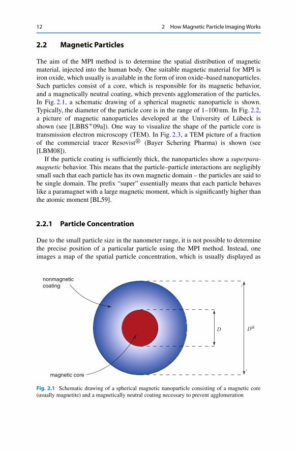
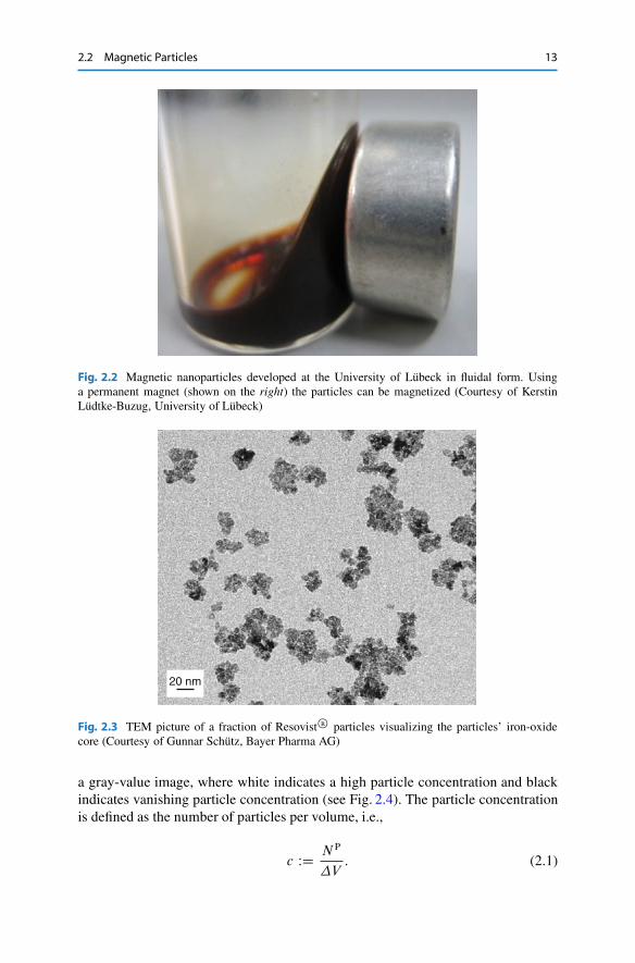
The aim of the MPI method is to determine the spatial distribution of magneticmaterial, injected into the human body. One suitable magnetic material for MPI isiron oxide, which usually is available in the form of iron oxide–based nanoparticles.Such particles consist of a core, which is responsible for its magnetic behavior,and a magnetically neutral coating, which prevents agglomeration of the particles.In Fig. 2.1, a schematic drawing of a spherical magnetic nanoparticle is shown.Typically, the diameter of the particle core is in the range of 1–100 nm. In Fig. 2.2,a picture of magnetic nanoparticles developed at the University of Lubeck isshown (see [LBBSC09a]). One way to visualize the shape of the particle core istransmission electron microscopy (TEM). In Fig. 2.3, a TEM picture of a fractionof the commercial tracer Resovist R� (Bayer Schering Pharma) is shown (see[LBM08]).
If the particle coating is sufficiently thick, the nanoparticles show a superpara-magnetic behavior. This means that the particle–particle interactions are negligiblysmall such that each particle has its own magnetic domain – the particles are said tobe single domain. The prefix “super” essentially means that each particle behaveslike a paramagnet with a large magnetic moment, which is significantly higher thanthe atomic moment [BL59].
2.2.1 Particle Concentration
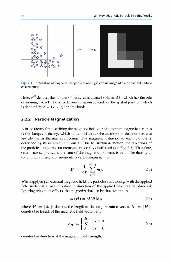
Due to the small particle size in the nanometer range, it is not possible to determinethe precise position of a particular particle using the MPI method. Instead, oneimages a map of the spatial particle concentration, which is usually displayed as
nonmagneticcoating
magnetic core
DHD
Fig. 2.1 Schematic drawing of a spherical magnetic nanoparticle consisting of a magnetic core(usually magnetite) and a magnetically neutral coating necessary to prevent agglomeration
2.2 Magnetic Particles 13
Fig. 2.2 Magnetic nanoparticles developed at the University of Lubeck in fluidal form. Usinga permanent magnet (shown on the right) the particles can be magnetized (Courtesy of KerstinLudtke-Buzug, University of Lubeck)
20 nm
Fig. 2.3 TEM picture of a fraction of Resovist R� particles visualizing the particles’ iron-oxidecore (Courtesy of Gunnar Schutz, Bayer Pharma AG)
a gray-value image, where white indicates a high particle concentration and blackindicates vanishing particle concentration (see Fig. 2.4). The particle concentrationis defined as the number of particles per volume, i.e.,
c WD N P
�V: (2.1)
14 2 How Magnetic Particle Imaging Works
Fig. 2.4 Distribution of magnetic nanoparticles and a gray-value image of the discretized particleconcentration
Here,N P denotes the number of particles in a small volume�V , which has the roleof an image voxel. The particle concentration depends on the spatial position, whichis denoted by r D .x; y; z/T in this book.
2.2.2 Particle Magnetization
A basic theory for describing the magnetic behavior of superparamagnetic particlesis the Langevin theory, which is defined under the assumption that the particlesare always in thermal equilibrium. The magnetic behavior of each particle isdescribed by its magnetic moment m. Due to Brownian motion, the directions ofthe particles’ magnetic moments are randomly distributed (see Fig. 2.5). Therefore,on a macroscopic scale, the sum of the magnetic moments is zero. The density ofthe sum of all magnetic moments is called magnetization:
M WD 1
�V
N P�1X
jD0mj : (2.2)
When applying an external magnetic field, the particles start to align with the appliedfield such that a magnetization in direction of the applied field can be observed.Ignoring relaxation effects, the magnetization can be thus written as
M .H / D M.H/eH ; (2.3)
where M WD kMk2 denotes the length of the magnetization vector, H WD kH k2denotes the length of the magnetic field vector, and
eH WD8<
:
H
HH > 0
0 H D 0(2.4)
denotes the direction of the magnetic field strength.
2.2 Magnetic Particles 15
H M
H M
H M
H M
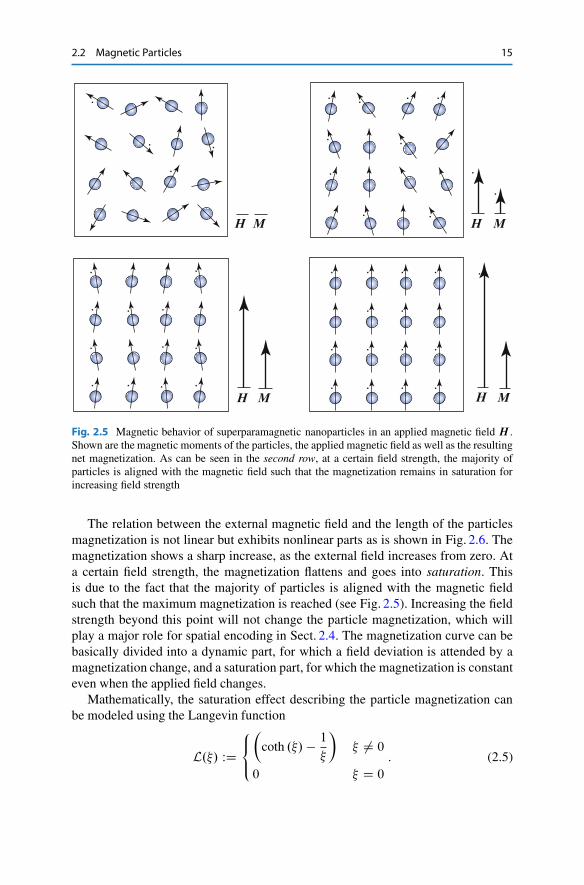
Fig. 2.5 Magnetic behavior of superparamagnetic nanoparticles in an applied magnetic field H .Shown are the magnetic moments of the particles, the applied magnetic field as well as the resultingnet magnetization. As can be seen in the second row, at a certain field strength, the majority ofparticles is aligned with the magnetic field such that the magnetization remains in saturation forincreasing field strength
The relation between the external magnetic field and the length of the particlesmagnetization is not linear but exhibits nonlinear parts as is shown in Fig. 2.6. Themagnetization shows a sharp increase, as the external field increases from zero. Ata certain field strength, the magnetization flattens and goes into saturation. Thisis due to the fact that the majority of particles is aligned with the magnetic fieldsuch that the maximum magnetization is reached (see Fig. 2.5). Increasing the fieldstrength beyond this point will not change the particle magnetization, which willplay a major role for spatial encoding in Sect. 2.4. The magnetization curve can bebasically divided into a dynamic part, for which a field deviation is attended by amagnetization change, and a saturation part, for which the magnetization is constanteven when the applied field changes.
Mathematically, the saturation effect describing the particle magnetization canbe modeled using the Langevin function
L.�/ WD8<
:
�coth .�/ � 1
�
�� ¤ 0
0 � D 0
: (2.5)

16 2 How Magnetic Particle Imaging Works
−20 −15 −10 −5 0 5 10 15 20H/(mTm0
−1)
−5
0
5
M/(
kAm
−1)
dynamic regionsaturation region saturation region
Fig. 2.6 The relation between the external magnetic field (usually measured in A/m or mT��10 )1
and the magnetization of the particles forD D 30 nm particle diameter and unit iron concentration.If the external field is small, the particles are not yet in saturation, and the magnetization shows asharp increase. For larger external fields, the particle goes into saturation, and the magnetizationhardly changes with the external field
The dependency of the particles’ magnetization length M on the magnetic field isthen described by
M.H/ D c mL .ˇH/ (2.6)
with
ˇ WD �0m
kBT P: (2.7)
Here, kB denotes the Boltzmann constant, T P denotes the particle temperature, �0denotes permeability of free space and m WD kmk2 denotes the modulus of themagnetic moment of a single particle.
1Field strengths are reported in units of T��10 D 4� Am�1 in this book. This convention has
been introduced in the first MPI publication [GW05] and since that time consistently used in mostMPI-related publications. The aim of this convention is to report the numbers on a Tesla scale,which most readers with a background in MRI are familiar with, but, on the other hand still use thecorrect unit for the magnetic field strength.

2.2 Magnetic Particles 17
In (2.6), the Langevin function is multiplied with the particle concentration c andthe particle magnetic momentm. The latter can be calculated as follows:
m D VM Score: (2.8)
Here, M Score is the saturation magnetization of the material the particle core is made
of and V is the particle core volume. The volume of a spherical particle with corediameterD is given by
V D 1
6�D3: (2.9)
To discuss the impact of c and m on the magnetization, one has to take intoaccount that in practice the iron concentration and not the particle concentrationis the limiting factor for the application of particles in vivo. For constant ironconcentration, the particle concentration scales inversely with the particle volume,i.e., c / V �1. Consequently, for constant iron concentration, the scaling factor c min front of the Langevin function in (2.6) and in turn the saturation magnetization ofthe suspension
M S D c m (2.10)
is independent of the particle size. This is graphically supported in Fig. 2.7,where the magnetization characteristic is shown for different particle diameters butconstant (unit) iron concentration.
Besides the scaling of the Langevin function, an important property of themagnetization characteristic is the field strength at which the saturation region of themagnetization is reached. This is named the saturation field strength. It is, however,not uniquely defined as actually full saturation is only achieved when applying aninfinite field strength. One possible way is to define the saturation field strengthH S as that field strength for which the magnetization reaches 80% of the saturationmagnetization. The Langevin function reaches a value of 0.8 at about �S D 5. Dueto the scaling of the field strength with the factor ˇ in (2.6), the saturation fieldstrength varies in dependence of ˇ, i.e.,
H S D �S
ˇD 5kBT
P
�0m: (2.11)
In Fig. 2.7, magnetization characteristics for different particle diameters are plotted.As the magnetic moment m scales with the third power of the particle diameter,the saturation field strength scales with the reciprocal of D3. This means thatlarge particles have a low saturation field strength while small particles have highsaturation field strength. Therefore, smaller particles need a higher field strengthto get into the state of saturation than larger particles. As it will be discussed in
18 2 How Magnetic Particle Imaging Works
10 nm
15 nm
20 nm
30 nm
40 nm
100 nm
−20 −15 −10 −5 0 5 10 15 20H/(mTm0
−1)
−5
0
5
M/(
kAm
−1)
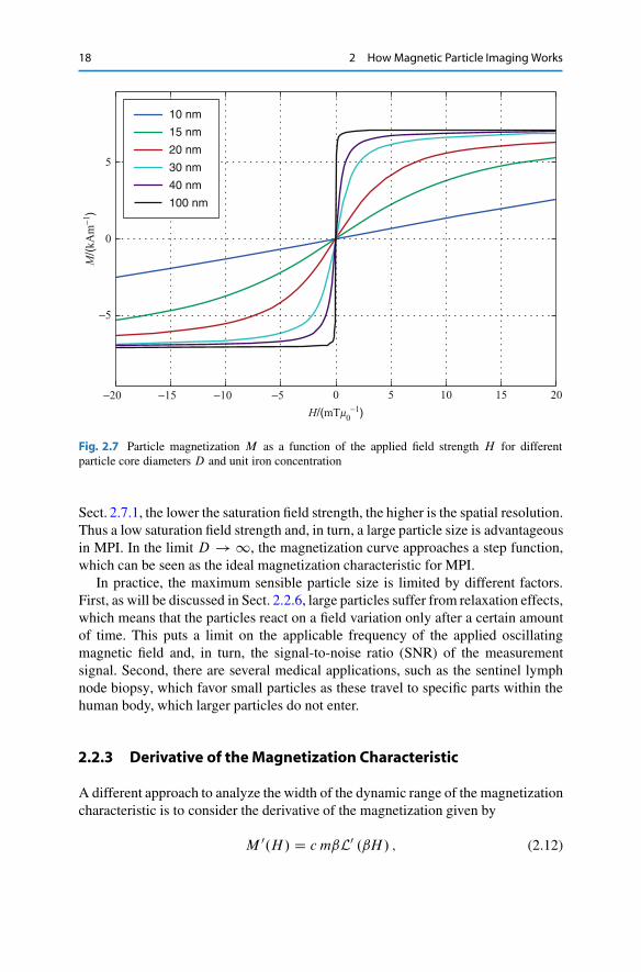
Fig. 2.7 Particle magnetization M as a function of the applied field strength H for differentparticle core diameters D and unit iron concentration
Sect. 2.7.1, the lower the saturation field strength, the higher is the spatial resolution.Thus a low saturation field strength and, in turn, a large particle size is advantageousin MPI. In the limit D ! 1, the magnetization curve approaches a step function,which can be seen as the ideal magnetization characteristic for MPI.
In practice, the maximum sensible particle size is limited by different factors.First, as will be discussed in Sect. 2.2.6, large particles suffer from relaxation effects,which means that the particles react on a field variation only after a certain amountof time. This puts a limit on the applicable frequency of the applied oscillatingmagnetic field and, in turn, the signal-to-noise ratio (SNR) of the measurementsignal. Second, there are several medical applications, such as the sentinel lymphnode biopsy, which favor small particles as these travel to specific parts within thehuman body, which larger particles do not enter.
2.2.3 Derivative of the Magnetization Characteristic
A different approach to analyze the width of the dynamic range of the magnetizationcharacteristic is to consider the derivative of the magnetization given by
M 0.H/ D c mˇL0 .ˇH/ ; (2.12)

2.2 Magnetic Particles 19
−20 −15 −10 −5 0 5 10 15 20−0.05
0.00
0.05
0.10
0.15
0.20
0.25
0.30
0.35 FWHM
´
Fig. 2.8 Derivative of the Langevin function L0. The vertical dashed red lines indicate the FWHMof L0
where
L0.�/ D
8<
:
�1
�2� 1
sinh2 .�/
�� ¤ 0
1
3� D 0
(2.13)
is the derivative of the Langevin function. In Fig. 2.8, the derivative of the Langevinfunction is shown. As can be seen, the derivative has a maximum at � D 0 and thendecreases rapidly to zero for increasing �. In the saturation region, obviously, thederivative of the Langevin function is almost zero.
The width of the dynamic range of the magnetization characteristic can bealternatively reported using the full width at half maximum (FWHM) of itsderivativeM 0. The FWHM is defined as the width at which a kernel function decaysto 50% of its maximum. For the derivative of the Langevin function, the FWHM isapproximately given by
��FWHM D 4:16: (2.14)
The FWHM of the derivative of the magnetization characteristic is in turn given by
�H FWHM D ��FWHM
ˇD 4:16 kBT
P
�0m: (2.15)
20 2 How Magnetic Particle Imaging Works
1.0
0.8
0.6
0.4
0.2
0.0
dM/d
H107×
−20 −15 −10 −5 0 5 10 15 20H/(mTm0
−1)
40 nm30 nm20 nm15 nm
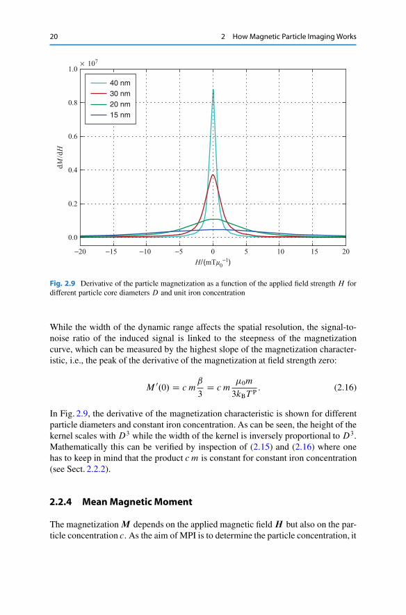
Fig. 2.9 Derivative of the particle magnetization as a function of the applied field strength H fordifferent particle core diameters D and unit iron concentration
While the width of the dynamic range affects the spatial resolution, the signal-to-noise ratio of the induced signal is linked to the steepness of the magnetizationcurve, which can be measured by the highest slope of the magnetization character-istic, i.e., the peak of the derivative of the magnetization at field strength zero:
M 0.0/ D c mˇ
3D c m
�0m
3kBT P: (2.16)
In Fig. 2.9, the derivative of the magnetization characteristic is shown for differentparticle diameters and constant iron concentration. As can be seen, the height of thekernel scales with D3 while the width of the kernel is inversely proportional to D3.Mathematically this can be verified by inspection of (2.15) and (2.16) where onehas to keep in mind that the product c m is constant for constant iron concentration(see Sect. 2.2.2).
2.2.4 Mean Magnetic Moment
The magnetizationM depends on the applied magnetic fieldH but also on the par-ticle concentration c. As the aim of MPI is to determine the particle concentration, it
2.2 Magnetic Particles 21
is convenient to separate the concentration c from the magnetizationM in the form
M D cm: (2.17)
Here,m denotes the mean magnetic moment that is defined as
m WD 1
N P
N P�1X
jD0mj : (2.18)
The linear dependency of the magnetization on the particle concentration c can bederived by inserting (2.1) into (2.2). As it is discussed in Chap. 4, the reconstructionprinciple applied in MPI is based on the linear relationship between the particlemagnetization and the particle concentration.
2.2.5 Particle Size Distribution
Until now it has been assumed that all particles within the particle suspension are ofthe same size. In practice, it is a challenging task to develop a tracer, which consistsof monosized particles. Instead, there are particles of different size in the suspension.The size distribution of the nanoparticles can be described by the probability densityfunction (PDF) �.D/. For a monodisperse particle distribution with a particle sizeD0, the PDF is given by
�.D/ D ı.D �D0/; (2.19)
where ı is the Dirac delta distribution. In theory, the PDF of a polydisperse sizedistribution can have an arbitrary shape with the restriction that
�.D/ D 0 for D � 0: (2.20)
This is obviously necessary as particles with a negative particle diameter cannotexist. Assuming a natural growth process, the PDF follows a log-normal distribution[KSNG99]
�.D/ D
8<
:
1
Q�Dp2�
exp
�12
�ln .D/� Q�
Q��2!
D > 0
0 D � 0
: (2.21)
Here, the parameters Q� and Q� are related to the expectation value E.D/ and thestandard deviation
pVar.D/:
Q� D ln .E.D// � 1
2ln
�Var.D/
E2.D/C 1
�; (2.22)
Q� Ds
ln
�Var.D/
E2.D/C 1
�: (2.23)
22 2 How Magnetic Particle Imaging Works
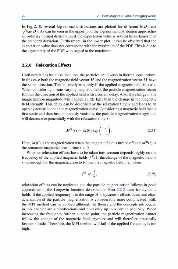
In Fig. 2.10, several log-normal distributions are plotted for different E.D/ andpVar.D/. As can be seen in the upper plot, the log-normal distribution approaches
an ordinary normal distribution if the expectation value is several times larger thanthe standard deviation. Furthermore, in the lower plot, it can be observed that theexpectation value does not correspond with the maximum of the PDF. This is due tothe asymmetry of the PDF with regard to the maximum.
2.2.6 Relaxation Effects
Until now it has been assumed that the particles are always in thermal equilibrium.In this case both the magnetic field vectorH and the magnetization vectorM havethe same direction. This is strictly true only if the applied magnetic field is static.When considering a time-varying magnetic field, the particle magnetization vectorfollows the direction of the applied field with a certain delay. Also, the change in themagnetization magnitude will happen a little later than the change in the magneticfield strength. This delay can be described by the relaxation time � and leads to anopen hysteresis loop in the magnetization curve. Considering a magnetic field that isfirst static and then instantaneously vanishes, the particle magnetization magnitudewill decrease exponentially with the relaxation time � :
M R.t/ D M.0/ exp
�� t�
�: (2.24)
Here,M.0/ is the magnetization when the magnetic field is turned off andM R.t/ isthe remanent magnetization at time t > 0.
Whether relaxation effects have to be taken into account depends highly on thefrequency of the applied magnetic fields f E. If the change of the magnetic field isslow enough for the magnetization to follow the magnetic field, i.e., when
f E � 1
�; (2.25)
relaxation effects can be neglected and the particle magnetization follows in goodapproximation the Langevin function described in Sect. 2.2.2 even for dynamicfields. If the applied frequency is in the range of 1
�, hysteresis effects occur and char-
acterization of the particle magnetization is considerably more complicated. Still,the MPI method can be applied although the theory and the concepts introducedin this chapter are simplifications and hold only up to a certain accuracy. Whenincreasing the frequency further, at some point, the particle magnetization cannotfollow the change of the magnetic field anymore and will therefore drasticallylose amplitude. Therefore, the MPI method will fail if the applied frequency is toohigh.

2.2 Magnetic Particles 23
0 5 10 15 20 25 30 35 40D/nm
D/nm
2.5
2.0
1.5
1.0
0.5
0.0
108
0 5 10 15 20 25 30 35 40
2.5
2.0
1.5
1.0
0.5
0.0
108
r(D
)r(
D)
2 nm4 nm6 nm8 nm10 nm
4 nm8 nm12 nm16 nm20 nm
Fig. 2.10 Several log-normal distributions for different expectation values and standard devia-tions. In the upper plot, the standard deviation is 4 nm and the expectation value is varied. In thelower plot, the expectation value is 16 nm and the standard deviation is varied

24 2 How Magnetic Particle Imaging Works
Bro
wni
an r
otat
ion
Née
l rot
atio
nm
H
m
H
m
H
mm
m
Fig. 2.11 Comparison of Neel and Brownian rotation. While Neel rotation describes a rotationof the particles’ magnetic moment for a fixed particle, Brownian rotation describes a mechanicalrotation of the entire particle
The concepts and theories developed and discussed in this book are restricted toapplied frequencies, which are lower than the reciprocal particle relaxation times.Although in some MPI-related publications, simple models including relaxationeffects have been considered [FMK09, FKMK11], the Langevin theory is still thestandard model used to date.
There are, in general, two ways a magnetic nanoparticle can change its directionwhen the applied field changes temporarily. Either the particle itself performs aphysical rotation, which is named Brownian rotation, or the magnetic moment inthe particle can rotate in a fixed particle, which is named Neel rotation. In a viscosemedium, a combination of both rotations is performed and it depends on the appliedfrequency, which process is the dominant one. In Fig. 2.11, Neel and Brownianrotation are compared.
The relaxation time of the Neel rotation can be computed by
�N D �0 exp
�KAV
kBT P
�; (2.26)

2.3 Signal Generation and Acquisition 25
where KA is the anisotropy constant [N49, N55] and V is the particle core volume.The relaxation time of Brownian rotation can be computed by
�B D 3V H
kBT P: (2.27)
Here, is the viscosity of the fluid and V H is the hydrodynamical volume[Bro63]. In contrast to the Neel relaxation time, which depends exponentiallyon the (core) particle volume, the Brownian relaxation time linearly depends onthe (hydrodynamical) particle volume. Hence, in the lower frequency range, theBrownian relaxation will dominate if the suspension is sufficiently viscose, while inthe higher frequency range Neel relaxation will be dominant. The total relaxationtime is a combination of the Neel and the Brownian relaxation times and can beapproximated by
� D �B�N
�B C �N: (2.28)
Hence, the shorter of both relaxation times determines the total relaxation time. Thetransition frequency between Neel and Brownian depends on the particle size, theparticle anisotropy, and the viscosity of the particle suspension.
2.3 Signal Generation and Acquisition
Following the discussion of the magnetization behavior of magnetic nanoparticles,this section will discuss, how the particles can be excited such that they respondwith a characteristic signal. Beforehand, the reception of the particle magnetizationusing the induction principle is investigated.
2.3.1 Signal Reception
In its very basic form, MPI applies a time-dependent external magnetic field tochange the magnetization of the magnetic material using send coils. In order todetect the change of the magnetization, one needs a method to measure the magneticflux density. In MPI this is done by measuring the voltage induced in receivecoils. The inductive measurement is mainly used due its ability to measure verysmall magnetization changes at high frequencies in the kHz–MHz range, which aretypically used in MPI.
2.3.1.1 Induction PrincipleThe induction principle is, as the name indicates, linked to Faraday’s law ofinduction, which is given in differential form by
r �E D �@B@t: (2.29)
26 2 How Magnetic Particle Imaging Works
E
− ∂B∂t
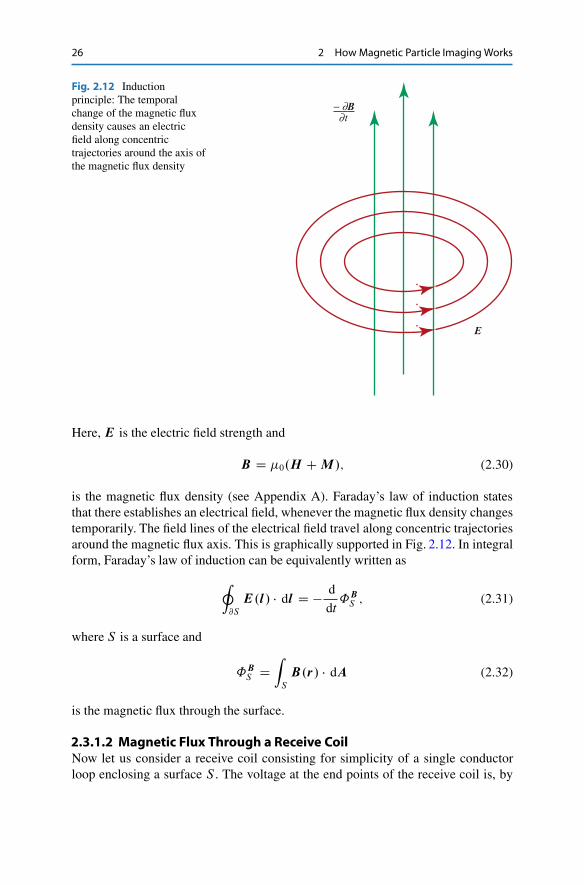
Fig. 2.12 Inductionprinciple: The temporalchange of the magnetic fluxdensity causes an electricfield along concentrictrajectories around the axis ofthe magnetic flux density
Here, E is the electric field strength and
B D �0.H CM /; (2.30)
is the magnetic flux density (see Appendix A). Faraday’s law of induction statesthat there establishes an electrical field, whenever the magnetic flux density changestemporarily. The field lines of the electrical field travel along concentric trajectoriesaround the magnetic flux axis. This is graphically supported in Fig. 2.12. In integralform, Faraday’s law of induction can be equivalently written as
I
@S
E.l / � dl D � d
dt˚BS ; (2.31)
where S is a surface and
˚BS DZ
S
B.r/ � dA (2.32)
is the magnetic flux through the surface.
2.3.1.2 Magnetic Flux Through a Receive CoilNow let us consider a receive coil consisting for simplicity of a single conductorloop enclosing a surface S . The voltage at the end points of the receive coil is, by
2.3 Signal Generation and Acquisition 27
x
y
z
receive coil
E
dAu
∂S
S
∂B−∂t
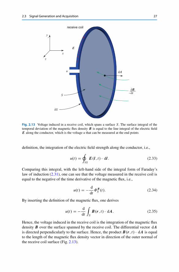
Fig. 2.13 Voltage induced in a receive coil, which spans a surface S . The surface integral of thetemporal deviation of the magnetic flux density B is equal to the line integral of the electric fieldE along the conductor, which is the voltage u that can be measured at the end points
definition, the integration of the electric field strength along the conductor, i.e.,
u.t/ DI
@S
E.l ; t/ � dl : (2.33)
Comparing this integral, with the left-hand side of the integral form of Faraday’slaw of induction (2.31), one can see that the voltage measured in the receive coil isequal to the negative of the time derivative of the magnetic flux, i.e.,
u.t/ D � d
dt˚BS .t/: (2.34)
By inserting the definition of the magnetic flux, one derives
u.t/ D � d
dt
Z
S
B.r ; t/ � dA: (2.35)
Hence, the voltage induced in the receive coil is the integration of the magnetic fluxdensity B over the surface spanned by the receive coil. The differential vector dAis directed perpendicularly to the surface. Hence, the productB.r ; t/ � dA is equalto the length of the magnetic flux density vector in direction of the outer normal ofthe receive coil surface (Fig. 2.13).

28 2 How Magnetic Particle Imaging Works
Due to the time derivative on the right-hand side of (2.35), it is only the variationof the magnetization @M
@tthat can be detected using electromagnetic induction.
This is, however, not a drawback of the induction method as it is not the particledynamics, which MPI aims to image but the particle concentration. The latter can befactored out of the magnetization change @M
@tdue to the linear dependency described
in Sect. 2.2.2.
2.3.1.3 Detection of the Particle MagnetizationTo determine the voltage induced by the superparamagnetic nanoparticles in areceive coil one has to compute the magnetization within the enclosed surface of thereceive coil (2.35). As it is derived in Appendix A.4.3, there is an alternative wayto express the induced voltage using the law of reciprocity [HR76], which leads toan integration over the volume, where the particles are located, i.e. the object to beimaged. The induced voltage is then given by
uP.t/ D ��0 d
dt
Z
objectpR.r/ �M .r; t/d3r
D ��0Z
objectpR.r/ � @M .r ; t/
@td3r; (2.36)
where pR.r/ denotes the receive coil sensitivity, which contains all geometricalparameters of the coil, for instance, the path of the wire determining the size of theenclosed surface S . The coil sensitivity is essentially the magnetic field that wouldbe generated by the coil if driven by unit current, i.e.,
pR.r/ WD H R.r/
IR: (2.37)
The law of reciprocity states that the receiving properties of a coil are the sameas the field generating properties. This knowledge is essential when designing thecoils of an MPI scanner. Both the send and the receive coils should be designed tohave a high sensitivity: the send coils to minimize the power loss of the setup, thereceive coils to maximize the SNR of the measured signal. To pick up the particlemagnetization at all positions in the FOV, ideally, the receive coil sensitivity shouldbe homogeneous in space.
2.3.2 Direct Coupling of Excitation Field
In order to get the particles to induce a voltage signal in the receive coils, a dynamicfield excitation is needed. The dynamic magnetic field directly couples into thereceive coil and induces according to (2.35) a respective excitation signal:
uE.t/ D ��0 d
dt
I
@S
H .r; t/ � dA: (2.38)

2.3 Signal Generation and Acquisition 29
The voltage measured in the receive coil is the superposition of the particle signaluP induced by the time-varying magnetization and the excitation signal uE inducedby the time-varying magnetic field, i.e.,
u.t/ D uP.t/C uE.t/: (2.39)
To determine the particle distribution c one needs a way to access the particle signaluP.t/. From a mathematical perspective, this seems to be feasible and could besolved by performing the following steps:1. Measure the signal induced by the excitation field in an empty scanner:
uempty.t/ D uE.t/ (2.40)
2. Perform the regular MPI measurement:
u.t/ D uE.t/C uP.t/ (2.41)
3. Extract the particle signal by subtracting the empty measurement:
uP.t/ D u.t/ � uempty.t/ (2.42)
Unfortunately, this obvious procedure is only feasible in theory when all signalsare available at infinite precision. In practice, the particle signal uP is very smallcompared to the induced excitation signal uE. For typical particle concentrationsand coil sensitivities, the particle signal is more than six orders of magnitudelower than the induced excitation signal. On top of that, as is discussed inSect. 2.3.4, the particle signal itself has a high dynamic range of several decadessuch that there are frequency components, which have an amplitude 1010 timeslower than the excitation signal.
To convert the analog signal into a digital signal, one uses an analog-to-digitalconverter (ADC). Even advanced ADCs have a finite input range of about 16 bits atthe frequency range used in MPI. Hence, the ADC can only resolve a range of about105 V.
Now, what would happen if one tries to digitize the voltage u.t/ and remove theexcitation signal uE.t/? One would obtain a signal containing no particle signal butonly quantization noise. This shows that one cannot get rid of the excitation signalby simple post-processing of the data. Instead, one has to choose the excitationsignal in a special way such that it can be filtered prior to digitization. Therefore,the signals uE and uP have to be distinguishable.
2.3.3 Signal Generation
Now that we know that it requires a time-varying magnetization to detect themagnetization change using receive coils, we have to choose the dynamic magneticfield that is used to excite the particles. As we have seen in the last section, the

30 2 How Magnetic Particle Imaging Works
t
H
M
H
M
t
uP
t
signal of linear material
uE
t
excitation signal
Fig. 2.14 Magnetization progression and induced signals for a linear material and sinusoidal fieldexcitation. As the magnetization characteristic is linear, both the induced magnetization signal andthe induced excitation signal resemble a sinusoidal function and cannot be distinguished
temporal progression of the magnetic field has to be chosen such that both theinduced particle signal and the induced excitation signal can be distinguished.Actually, this can be achieved by selecting an excitation field of a very smallbandwidth, for instance, a sinusoidal excitation field2
H E.t/ D �AE cos.2�f Et/; (2.43)
where AE denotes the amplitude and f E denotes the frequency of the field. Therepetition time for one field cycle is given by T R D 1
f E . The excitation field isusually homogeneous in space such that all particles within the volume of interestexperience the same field. The field is, however, not required to be as homogeneousas the B0 field in MRI.
Assuming for a moment that the relation between the external field and themagnetization of the particles would be linear, the magnetization progression wouldresemble the waveform of the external field and would be purely sinusoidal. Hence,there would be no way to distinguish the voltage induced by the external field andthe voltage induced by the particle magnetization (see Fig. 2.14).
2Note that the cosine excitation is considered to simplify later calculations.

2.3 Signal Generation and Acquisition 31
t
H
M
H
M
t
uP
t
particle signal
uE
t
excitation signal
Fig. 2.15 Signal generation in MPI: The magnetic nanoparticles are excited with a sinusoidalmagnetic field causing a magnetization progression, which resembles a rectangular function. Theinduced voltage contains two sharp peaks and can be distinguished from the sinusoidal excitationsignal directly coupling into the receive coil
But, as the relationship between the external field and the particle magnetizationis nonlinear, both signals can be discriminated. As it is shown in Fig. 2.15, themagnetization progression resembles that of the external field only for small fieldstrength and approaches a constant function when the external field proceeds tohigher field strengths. One might say that the sinusoidal progression is cut off whenthe magnetization reaches its maximum value. Actually, the magnetization progres-sion has more similarities with a rectangular function than with a sinusoidal one.In fact, for a step-like magnetization characteristic, the magnetization progressionwould be exactly rectangular as the magnetization would only flip its direction,when the external field changes in sign.
Considering the induced voltage, one can see in Fig. 2.15 that there are two peaksin the signal. These occur whenever the magnetization rapidly changes, which is thecase when the particle flips its direction. In Sect. 2.4, it is shown that this behavioris the key to achieve spatial encoding in MPI. The more pronounced the differencebetween the applied sinusoidal excitation field and the magnetization progressionis, the steeper is the magnetization curve. Later in this book, it is shown that alow saturation field strength ensures a high spatial resolution. Hence, a step-likemagnetization curve is indeed the ideal situation for imaging with MPI. In this idealcase, the induced voltage signal would contain exactly two Dirac delta peaks perperiod and would be zero elsewhere.

32 2 How Magnetic Particle Imaging Works
2.3.4 Signal Spectrum
To study the differences between the excitation signal and the particle signal, it isinstructive to consider both signals in frequency space. Due to the periodicity ofthe field excitation, the induced excitation signal and the induced particle signal areperiodic as well. Hence, these signals can be expanded into a Fourier series
u.t/ D1X
kD�1Ouke2� ikf Et (2.44)
and the spectrum consists of discrete lines at multiples of the frequency f E, whichis also called the fundamental or base frequency. These multiples,
fk D kf E; k 2 Z; (2.45)
are usually called harmonic frequencies or just harmonics. The Fourier coefficientscan be computed by
Ouk D 1
T R
Z T R
0
u.t/e�2� ikf Et dt; k 2 Z: (2.46)
As the induced voltage is real, the Fourier coefficients obey the relation
Ouk D 1
T R
Z T R
0
u.t/e�2� ikf Et dt
D 1
T R
Z T R
0
�u.t/e2� ikf Et
��dt
D .Ou�k/� : (2.47)
Therefore, one usually neglects the negative frequencies in MPI as they do not carryany additional information.
Being a purely sinusoidal function, the excitation signal shows up as a single peakat the frequency f E. Due to the nonlinear relationship between magnetization andexternal field, the particle signal has not only a peak at the fundamental frequencybut rather at all higher harmonics. This is shown in Fig. 2.16, where the periodicparticle signal and its Fourier transform are shown.
The generation of higher harmonics for a nonlinear magnetization curve can bemathematically described by expanding the Langevin function into a Taylor series
L.�/ D 1
3� � 1
45�3 C 2
954�5 � 1
4;725�7 C : : : : (2.48)
2.3 Signal Generation and Acquisition 33
t
uP ûP
1 3 5 7 9 11 13 15 17 19f/f0
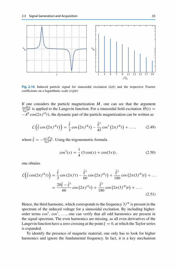
Fig. 2.16 Induced particle signal for sinusoidal excitation (left) and the respective Fouriercoefficients on a logarithmic scale (right)
If one considers the particle magnetization M , one can see that the argument�0Hm
kBT P is applied to the Langevin function. For a sinusoidal field excitation H.t/ D�AE cos.2�f Et/, the dynamic part of the particle magnetization can be written as
L� Q� cos
�2�f Et
�� DQ�3
cos�2�f Et
� �Q�345
cos3�2�f Et
�C : : : ; (2.49)
where Q� D ��0AEm
kBT P . Using the trigonometric formula
cos3.x/ D 1
4.3 cos.x/C cos.3x// ; (2.50)
one obtains
L� Q� cos.2�f Et/
�D
Q�3
cos .2�f t/ �Q�360
cos�2�f Et
�CQ�3180
cos�2�.3f E/t
�C : : :
D 20 Q� � Q�360
cos�2�f Et
�CQ�3180
cos�2�.3f E/t
�C : : : :
(2.51)
Hence, the third harmonic, which corresponds to the frequency 3f E is present in thespectrum of the induced voltage for a sinusoidal excitation. By including higher-order terms cos5, cos7, : : : , one can verify that all odd harmonics are present inthe signal spectrum. The even harmonics are missing, as all even derivatives of theLangevin function have a zero-crossing at the point � D 0, at which the Taylor seriesis expanded.
To identify the presence of magnetic material, one only has to look for higherharmonics and ignore the fundamental frequency. In fact, it is a key mechanism
34 2 How Magnetic Particle Imaging Works
t
uHuP
t
t
1 3 5 7 9 11 13 15 17 19
1 3 5 7 9 11 13 15 17 19f /f 0
f /f 0
f /f 0
ûHûP
u û
1 3 5 7 9 11 13 15 17 19
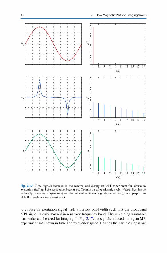
Fig. 2.17 Time signals induced in the receive coil during an MPI experiment for sinusoidalexcitation (left) and the respective Fourier coefficients on a logarithmic scale (right). Besides theinduced particle signal (first row) and the induced excitation signal (second row), the superpositionof both signals is shown (last row)
to choose an excitation signal with a narrow bandwidth such that the broadbandMPI signal is only masked in a narrow frequency band. The remaining unmaskedharmonics can be used for imaging. In Fig. 2.17, the signals induced during an MPIexperiment are shown in time and frequency space. Besides the particle signal and

2.3 Signal Generation and Acquisition 35
the excitation signal, the superposition of both signals is illustrated. As can be seen,the particle signal can hardly be detected in time space. This is due to the lowamplitude of the particle signal in comparison to the excitation signal. In contrast,all higher harmonics of the particle signal can be clearly seen in the signal spectrumwhile only the fundamental frequency is covered by the excitation signal.
Ignoring the fundamental frequency does not only remove the excitation signalbut has the additional advantage that it removes any background signal potentiallyinduced by the iron in the human body. As this iron is present in atomic ormolecular form and thus substantially smaller than the magnetic nanoparticles, itsmagnetization characteristic is linear in the considered field range. Hence, the irononly affects the signal at the fundamental frequency (see Fig. 2.14) such that allhigher harmonics are background free.
2.3.5 Excitation Frequency and Field Strength
The time-dependent external field that periodically changes the magnetization ofthe magnetic material usually has a frequency in the range of several tens toover hundreds of kilohertz, with the first results published using a frequency of25 kHz [GW05]. These frequencies normally are not detectable for the human earand scanner operation is thus scarcely audible. Using higher frequencies can bebeneficial, as the noise in the receiver electronics is in many cases dominated by a 1
f
behavior. On the contrary, certain physiological limitations apply for the exposureof human bodies to electromagnetic waves, one of those being energy deposition(specific absorption rate, SAR). It is proportional to the square of the field amplitudeand frequency [LBFC97], thus posing limitations to the use of higher excitationfrequencies. One further limitation is caused by the particles themselves. Due totheir finite relaxation times, the particles can only follow a field variation up to acertain frequency. If the excitation frequency is higher, the change of the particlemagnetization is suppressed, leading to a loss of intensity of the induced signal.
To be effective, the amplitude of the excitation field should be high enough toensure that the change in magnetization goes well into the nonlinear areas of themagnetization curve, preferably nearly into saturation. The higher the amplitude,the more pronounced the higher harmonics in the received spectrum of the MPIsignal will be. Feasible amplitudes are in the range of several mT��1
0 up to about20 mT��1
0 . Although technically higher amplitudes can be achieved, the SARlimitation leads to a restriction of the excitation field amplitude.
To gain information on the exact amount of magnetic material, i.e., to makea quantitative measurement, it is sufficient to read the amplitude of one selectedharmonic from the spectrum. Given a suitable calibration measurement with a well-known amount of magnetic material, the amplitude of the selected harmonic inrelation to its value during the calibration measurement will be proportional to theamount of iron. It is, of course, mandatory to keep all parameters, for instance, thefield strength of the excitation field, constant between measurements.
36 2 How Magnetic Particle Imaging Works
2.4 Spatial Encoding: Selection Field
Using a setup as outlined in the last section, i.e., an excitation field with sufficientamplitude that penetrates the volume of interest, one can easily reveal if magneticmaterial is present or not. However, it is not possible to determine where exactly themagnetic material is and how much material is present at a particular location. Whatis missing in the explanation up to now is a way to determine the spatial distributionof the magnetic material. This is usually called spatial encoding and the subject ofthe current section.
2.4.1 Particle Selection
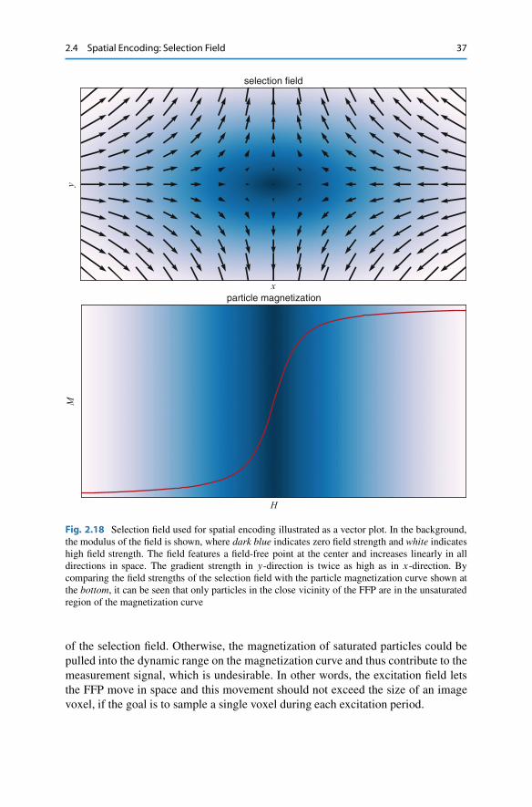
The basic problem of achieving spatial encoding in MPI can be formulated asfinding a solution for the task to associate the emitted particle signal to a particularlocation at a certain time point. In this way, the signal can be directly assignedto the spatial particle concentration. In order to manage that particles at differentlocations in space generate distinct signals, MPI uses a static magnetic field, whichis highly inhomogeneous in space. As is shown in Fig. 2.18, the field in fact hasa distinct field vector at each position in space. Furthermore, the field containsone special location named field-free point (FFP), which is simply characterizedby the field magnitude or field vector being zero. While veering away from thisFFP, the field strength quickly increases in a linear fashion. Such a field is usuallycalled a constant-gradient or, simply, gradient field in the context of magneticresonance imaging. This name is derived from the gradient being constant for alinear increasing magnetic field.
When applying a gradient field with a strong gradient strength to a volumecontaining magnetic nanoparticles, the resulting particle magnetization will be insaturation in most positions in space. Only in a small region around the FFP, theparticle magnetization will be in the dynamic range of the magnetization curve withzero magnetization at the exact location of the FFP.
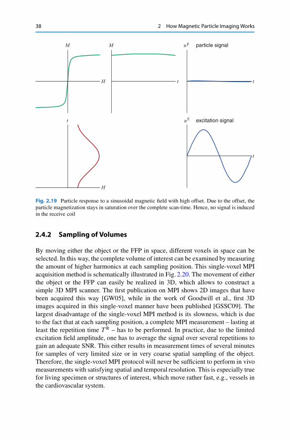
When superimposing the excitation field on top of the gradient field, the particleswith sufficient distance to the FFP do not react on the change of the total magneticfield (see Fig. 2.19). In turn, almost no MPI signal is induced in the receive coil.In contrast, the particles in close vicinity experience a strong magnetization changewith the particles directly located at the FFP flipping back and forth. Actually, atthe FFP the particles are only affected by the excitation field and thus behave asdescribed in Sect. 2.3. The magnetization change results in a measurable voltagesignal in the receive coil. As this induced signal stems only from the magneticmaterial in a certain vicinity of the FFP, a direct relation between the signal andthe FFP location is established, i.e., spatial encoding is achieved. As the appliedgradient field selects the position at which the particles are free to react on a fieldexcitation, it is called selection field in the context of MPI.
One thing one has to consider when using the form of spatial encoding outlinedabove is that the excitation field amplitude should be small compared to the gradient
2.4 Spatial Encoding: Selection Field 37
selection field
xparticle magnetization
H
My
Fig. 2.18 Selection field used for spatial encoding illustrated as a vector plot. In the background,the modulus of the field is shown, where dark blue indicates zero field strength and white indicateshigh field strength. The field features a field-free point at the center and increases linearly in alldirections in space. The gradient strength in y-direction is twice as high as in x-direction. Bycomparing the field strengths of the selection field with the particle magnetization curve shown atthe bottom, it can be seen that only particles in the close vicinity of the FFP are in the unsaturatedregion of the magnetization curve
of the selection field. Otherwise, the magnetization of saturated particles could bepulled into the dynamic range on the magnetization curve and thus contribute to themeasurement signal, which is undesirable. In other words, the excitation field letsthe FFP move in space and this movement should not exceed the size of an imagevoxel, if the goal is to sample a single voxel during each excitation period.
38 2 How Magnetic Particle Imaging Works
t
H
M
H
M
t
uP
t
particle signal
uE
t
excitation signal
Fig. 2.19 Particle response to a sinusoidal magnetic field with high offset. Due to the offset, theparticle magnetization stays in saturation over the complete scan-time. Hence, no signal is inducedin the receive coil
2.4.2 Sampling of Volumes
By moving either the object or the FFP in space, different voxels in space can beselected. In this way, the complete volume of interest can be examined by measuringthe amount of higher harmonics at each sampling position. This single-voxel MPIacquisition method is schematically illustrated in Fig. 2.20. The movement of eitherthe object or the FFP can easily be realized in 3D, which allows to construct asimple 3D MPI scanner. The first publication on MPI shows 2D images that havebeen acquired this way [GW05], while in the work of Goodwill et al., first 3Dimages acquired in this single-voxel manner have been published [GSSC09]. Thelargest disadvantage of the single-voxel MPI method is its slowness, which is dueto the fact that at each sampling position, a complete MPI measurement – lasting atleast the repetition time T R – has to be performed. In practice, due to the limitedexcitation field amplitude, one has to average the signal over several repetitions togain an adequate SNR. This either results in measurement times of several minutesfor samples of very limited size or in very coarse spatial sampling of the object.Therefore, the single-voxel MPI protocol will never be sufficient to perform in vivomeasurements with satisfying spatial and temporal resolution. This is especially truefor living specimen or structures of interest, which move rather fast, e.g., vessels inthe cardiovascular system.

2.4 Spatial Encoding: Selection Field 39
FFP
image voxel
objectFig. 2.20 Sampling animage volume using thesingle-voxel method. TheFFP is moved to eachposition at which the particledistribution is to be imaged.After each positioning, theexcitation field is applied andthe spectral componentsstemming from particles inthe close vicinity of the FFPare recorded using the receivecoil
2.4.3 Properties of the Selection Field
As can be observed in Fig. 2.18, the gradient strength of the selection field varies indifferent directions. More precisely, the gradient strength in y-direction Gy WD @Hy
@y
is twice the value of that in x-direction Gx WD @Hx@x
but has a different sign. If onewould look at the field within the yz-plane, one would find that the gradient inz-direction Gz WD @Hz
@z has the same value as the gradient in x-direction. Hence, therelation between the three gradient strengths is given by
Gy D �2Gx D �2Gz: (2.52)
This asymmetry is not a coincidence but due to the very nature of the Maxwellequations (see Appendix A). Gauß’s law of magnetism states that the divergenceof the magnetic field, which is the sum of the spatial derivatives in x-, y- andz-directions, has to be zero, i.e.,
r �H D @Hx
@xC @Hy
@yC @Hz
@zD 0: (2.53)
One way to fulfill this relation is to chose the gradients in the way outlined in (2.52).Certainly, Maxwell’s equations allow other field shapes such as
Gy D �Gx and Gz D 0; (2.54)
which generates a field-free line along the z-direction (see Sect. 6.3). What is,however, not possible is that the gradient strength along the three principle axeshave the same absolute value. This asymmetry of the selection field has impact onthe spatial resolution of MPI, which is in y-direction twice as high as in x- andz-directions.
40 2 How Magnetic Particle Imaging Works
2.4.3.1 Gradient MatrixUsing the observations outlined above, the selection field shown in Fig. 2.19 can bewritten as
H S.r/ D0
@Gx 0 0
0 Gy 0
0 0 Gz
1
A r D G
0
@� 120 0
0 1 0
0 0 � 12
1
A r : (2.55)
where G D Gy is the steepest gradient of the field. By defining the gradient matrix
G WD0
@Gx 0 0
0 Gy 0
0 0 Gz
1
A ; (2.56)
the selection field can be compactly written as
H S.r/ D Gr: (2.57)
Note that the matrix G is the Jacobian matrix or vector gradient of the vectorialfunctionH S.r/.
In order for the area around the FFP where the particles are unsaturated tobe sufficiently small, the gradient strength G, measured in units of Tm�1��1
0 ,has to be sufficiently high. For small scanner devices gradient strengths of morethan 10 Tm�1��1
0 are feasible. For a human scanner, the highest feasible gradientstrength is about 3 Tm�1��1
0 for a system realized by resistive coils or perma-nent magnets, while superconductors would allow for up to 6 Tm�1��1
0 gradientstrength.
2.5 Performance Upgrade: Drive Field
The basic MPI setup described in the last section relies on the movement of thesample in relation to the FFP, while the MPI signal is generated by an excitationfield. This results in a very slow image acquisition. Furthermore, as the excitationfield is limited in amplitude to ensure that the FFP stays within a voxel at eachmeasurement, the method is not optimal regarding the SNR of the measurementsignal. In this section, an improved MPI acquisition method is introduced, whichsubstantially shortens the acquisition time enabling real-time MPI as has beenexperimentally proven in [GWB08] and [WGRC09].
2.5.1 Moving the Field-Free Point
In order to speed up the imaging process, one just has to break the rule that the FFPhas to stay within an image voxel during one measurement. Instead, by increasing
2.5 Performance Upgrade: Drive Field 41
FFP
image voxelobject
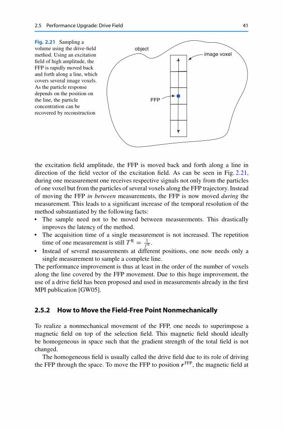
Fig. 2.21 Sampling avolume using the drive-fieldmethod. Using an excitationfield of high amplitude, theFFP is rapidly moved backand forth along a line, whichcovers several image voxels.As the particle responsedepends on the position onthe line, the particleconcentration can berecovered by reconstruction
the excitation field amplitude, the FFP is moved back and forth along a line indirection of the field vector of the excitation field. As can be seen in Fig. 2.21,during one measurement one receives respective signals not only from the particlesof one voxel but from the particles of several voxels along the FFP trajectory. Insteadof moving the FFP in between measurements, the FFP is now moved during themeasurement. This leads to a significant increase of the temporal resolution of themethod substantiated by the following facts:• The sample need not to be moved between measurements. This drastically
improves the latency of the method.• The acquisition time of a single measurement is not increased. The repetition
time of one measurement is still T R D 1f E .
• Instead of several measurements at different positions, one now needs only asingle measurement to sample a complete line.
The performance improvement is thus at least in the order of the number of voxelsalong the line covered by the FFP movement. Due to this huge improvement, theuse of a drive field has been proposed and used in measurements already in the firstMPI publication [GW05].
2.5.2 How to Move the Field-Free Point Nonmechanically
To realize a nonmechanical movement of the FFP, one needs to superimpose amagnetic field on top of the selection field. This magnetic field should ideallybe homogeneous in space such that the gradient strength of the total field is notchanged.
The homogeneous field is usually called the drive field due to its role of drivingthe FFP through the space. To move the FFP to position rFFP, the magnetic field at

42 2 How Magnetic Particle Imaging Works
this very position has to be canceled out. The superposition of the selection fieldH S
and the drive fieldH D thus has to fulfill
H�rFFP� D H S �rFFP�CH D D 0: (2.58)
Hence, to move the FFP to position rFFP, the drive field has to be chosen as
H D D �H S �rFFP� D �GrFFP: (2.59)
To determine the position of the FFP for the given drive fieldH D one can solve forrFFP yielding
rFFP D �G�1H D: (2.60)
The inverse of the gradient matrix is given by
G�1 D
0
B@
1Gx
0 0
0 1Gy
0
0 0 1Gz
1
CA : (2.61)
Hence, the change of the drive field linearly translates to a movement of the FFP. InFig. 2.22, it is illustrated how the superposition of the drive field translates the FFPin 1D, while in Fig. 2.23 a 2D FFP translation is shown.
2.5.3 Drive-Field Waveform
Now that we know how to adjust the drive field to move the FFP to a certain position,we have to chose how the field strength changes temporarily to cover a certain FOV.For now an 1D FOV is considered.
When choosing the drive-field waveform, one has to keep in mind that a changeof the magnetic field induces a voltage in the receive coil, which masks the inducedparticle signal. As introduced in Sect. 2.5.1, the drive field is actually the excitationfield with a high amplitude. Hence, the same method can be applied to distinguishbetween the induced particle signal from the induced drive-field signal. As it hasbeen discussed in Sect. 2.3.3, the excitation field and in turn the drive field shouldhave a sinusoidal temporal progression, so that the masking of the excitation signalis limited to the excitation frequency, while all higher harmonics of the particlesignal can be easily detected.
For a sinusoidal drive field directed in x-direction
H D.t/ D �ADx cos
�2�f Et
�ex; (2.62)
2.5 Performance Upgrade: Drive Field 43
H
x
H S
H D
HFFP
H
x
H
x
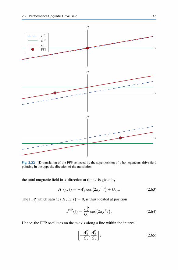
Fig. 2.22 1D translation of the FFP achieved by the superposition of a homogeneous drive fieldpointing in the opposite direction of the translation
the total magnetic field in x-direction at time t is given by
Hx.x; t/ D �ADx cos
�2�f Et
�CGxx: (2.63)
The FFP, which satisfies Hx.x; t/ D 0, is thus located at position
xFFP.t/ D ADx
Gxcos
�2�f Et
�: (2.64)
Hence, the FFP oscillates on the x-axis along a line within the interval
��A
Dx
Gx;ADx
Gx
: (2.65)

44 2 How Magnetic Particle Imaging Works
selection field drive field superposition
Fig. 2.23 2D translation of the FFP achieved by the superposition of a homogeneous drive field
The FFP has its highest speed at the center and its lowest speed at the edges ofthe FOV. This has impact on the image quality, which can be slightly higher in thecenter.
2.5.4 Individual Signals
In contrast to the mechanical way of spatial encoding, the drive field method yieldsa measurement signal containing contributions of particles at different positions.One obvious question is whether it is possible to separate the individual signals ofparticles located at different positions.

2.5 Performance Upgrade: Drive Field 45
H
t
M
t t
H
t
M
t t
H
t
M
t
u P
u P
u P
t
Fig. 2.24 Effect of applying a constant offset to the sinusoidal drive field. As can be seen, thelocations of the peaks in the induced particle signal are shifted by the applied offset
Without the selection field all particles in space behave the same as the drive fieldis homogeneous in space. By applying the selection field, a spatially dependentoffset is superimposed onto the drive field. Consequently, the time at which thetotal field crosses zero is shifted by the offset such that the zero-crossings at twodifferent positions happen at different time points. This conclusion has already beenformulated in (2.64), which implies that the FFP (zero-crossing of the gradient field)is unique in space during the complete scanning period.
Now recall that the induced particle signal is maximum when the magnetizationflips its direction. When moving the FFP through the FOV, the particle magnetiza-tion flips only at a single position in space, which is the FFP. Hence, at time t , thehighest contribution to the induced signal is of particles located at position xFFP.t/.In Fig. 2.24, the signals induced by a small object located at different positions areshown. As can be seen, each signal contains one positive and one negative peak andhas a rotational symmetry. This is due to the symmetry of the sinusoidal excitationfunction and the derivative applied to the particle magnetization. The two timepoints at which the peaks occur are shifted according to the object position xdelta

46 2 How Magnetic Particle Imaging Works
magnetic field magnetization magn. derivativese
cond
tim
e po
int
first
tim
e po
int
Fig. 2.25 FFP moving from the left to the right in x-direction acting as a sensitiv spot on theparticle distribution. On the left, the FFP field is shown at two subsequent time points. In themiddle, the particle magnetization of a homogeneous particle distribution is illustrated at both timepoints. On the right, the time derivative of the magnetization is shown. For better illustration, theinterval between the considered time points is finite, whereas for the calculation of the derivativean infinitisimal small time interval is used
and can be computed by
t1 D 1
2�f Earccos
�Gx
ADx
xdelta�; (2.66)
t2 D T R � 1
2�f Earccos
�Gx
ADx
xdelta
�: (2.67)
The peaks have a finite width even for infinitesimal small objects. This is due to thefinite steepness of the magnetization curve, which induces this blurring. The heightof the peaks varies with the position xdelta and is maximum at the origin. Goingto the edges of the FOV, the height decreases. In fact, the envelope of the signalsat different positions resembles the sinusoidal excitation pattern. This variation inthe signal intensity is induced by the speed of the FFP, which is slow at the edgesand maximum at the origin. The time derivative in (2.36) is responsible for thisdependency of the signal intensity on speed of the field change. A mathematicalexplanation for the sinusoidal envelope is given in the next section.
In Fig. 2.25, the signal contribution of different particles in space is illustratedwhen the FFP moves along a certain direction (here, the x-direction). This intensity
2.5 Performance Upgrade: Drive Field 47
map can be seen as the sensitivity around the FFP. When sweeping the FFP throughthe space, the sensitive spot in the center of the sensitivity map directly followsthe FFP. What is not directly obvious is that the FFP sensitivity map seems to bewider in the orthogonal direction to the FFP movement, although the FFP gradientis, in the considered case, by a factor of 2 smaller in x-direction than in y-direction.The reason for this is that in orthogonal direction to the FFP movement even thesaturated particles rotate and therefore change their magnetization.
In summary, the spatially dependent selection field leads to a time shift in theparticle response, which gives each position in space a unique profile of the voltagebeing induced in the receive coil. Thus, it is possible to compute the particledistribution given the known signal profiles for all positions in the FOV.
2.5.5 Convolution with the FFP Kernel
As we have seen in the last section, the signals induced by different particles inspace are shifted according to their position. Hence, the question arises, whetherthe imaging equation can be mathematically described by a convolution, which is aproperty of linear shift-invariant systems. As it is shown next, for 1D imaging thesystem can indeed be formulated as a convolution.
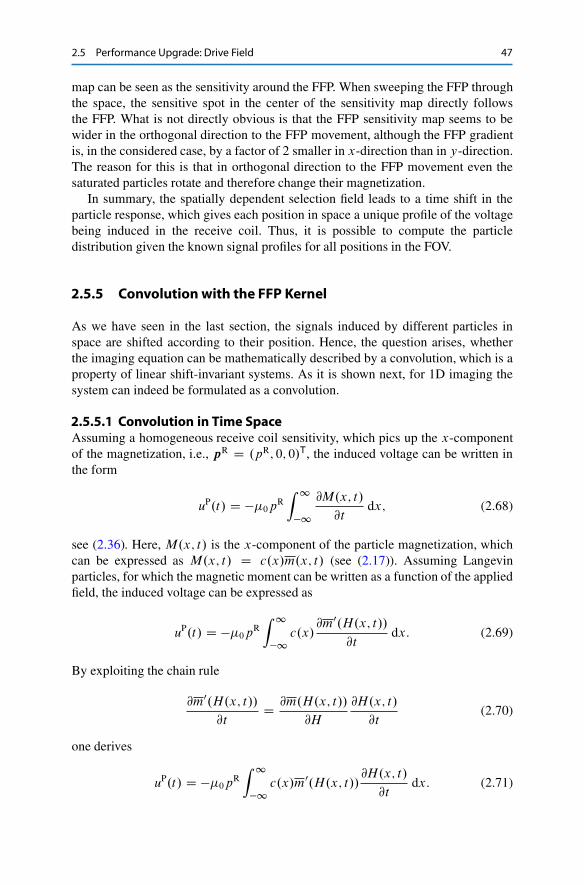
2.5.5.1 Convolution in Time SpaceAssuming a homogeneous receive coil sensitivity, which pics up the x-componentof the magnetization, i.e., pR D .pR; 0; 0/T, the induced voltage can be written inthe form
uP.t/ D ��0pRZ 1
�[email protected]; t/
@tdx; (2.68)
see (2.36). Here, M.x; t/ is the x-component of the particle magnetization, whichcan be expressed as M.x; t/ D c.x/m.x; t/ (see (2.17)). Assuming Langevinparticles, for which the magnetic moment can be written as a function of the appliedfield, the induced voltage can be expressed as
uP.t/ D ��0pRZ 1
�1c.x/
@m0.H.x; t//@t
dx: (2.69)
By exploiting the chain rule
@m0.H.x; t//@t
D @m.H.x; t//
@H
@H.x; t/
@t(2.70)
one derives
uP.t/ D ��0pRZ 1
�1c.x/m0.H.x; t//
@H.x; t/
@tdx: (2.71)
48 2 How Magnetic Particle Imaging Works
wherem0.H/ D @m.H/
@His the derivative of the mean magnetic moment. The shape of
the derivative has already been discussed in Sect. 2.2.3. Inserting the total magneticfield H.x; t/ D HD.t/CGxx yields
uP.t/ D ��0pR.HD/0.t/Z 1
�1c.x/m0.HD.t/CGxx/ dx: (2.72)
By defining the kernel
Qm.x/ WD ��0pRm0.Gxx/ (2.73)
and using the reflectional symmetry Qm.x/ D Qm.�x/ one derives
uP.t/ D .HD/0.t/Z 1
�1c.x/ Qm.�G�1
x HD.t/ � x/ dx; (2.74)
which can be written as a convolution:
Theorem 2.1. For a 1D imaging sequence, the relation between the particleconcentration c and the induced voltage uP can be described as
uP.t/ D .HD/0.t/ .c � Qm/ ��G�1x HD.t/
�; (2.75)
which consists of a convolution weighted with the time derivative of the drivefield.
One can identify in (2.75) that the convolved particle distribution is weightedwith the factor .HD/0.t/, which is the change of the magnetic drive field that isproportional to the speed of the FFP. As the FFP speed is slow at the edges and fastat the center of the FOV, it is clear that the signal amplitude is damped at the edgesof the FOV (see Fig. 2.24).
2.5.5.2 FFP Speed NormalizationBy dividing the signal through the derivative of the excitation function
uN.t/ WD uP.t/
.HD/0.t/D .c � Qm/ ��G�1
x HD.t/�; (2.76)
the signal is compensated for the varying speed of the FFP movement. Here, onehas to drop the signal at those time points where .HD/0.t/ D 0, which is the casewhen the FFP reaches the edges of the FOV and, therefore, no signal is induced inthe receive coil. In the following, the signal is neglected at these time points.

2.5 Performance Upgrade: Drive Field 49
2.5.5.3 Gridding on Spatial IntervalFor equidistantly sampled time points, the convolution on the right-hand side of(2.76) is evaluated at non-equidistant values. By applying the coordinate transform
xFFP.t/ D �HD.t/
GxD AD
x
Gxcos.2�f Et/; (2.77)
the time signal can be mapped onto a spatial interval and described by an ordinaryconvolution:
Theorem 2.2. By normalizing the induced signal for the FFP speed (2.76) andapplying the coordinate transform (2.77), the relation between the particleconcentration c and the transformed signal ux can be described as
ux.xFFP/ D uN
�1
2�f Earccos
�Gx
ADx
xFFP
��D .c � Qm/ .xFFP/; (2.78)
which consists of an ordinary convolution.
It should be noted that only the first half of the time interval Œ0; T R/ is used in(2.78). This is due to the fact that the mapping between the time and the FFP is notbijective when considering the complete time period Œ0; T R/. However, in the firsthalf of the this interval, i.e., for one sweep of the FFP through the FOV, the mappingis bijective.
2.5.6 2D/3D Imaging
Until now, only 1D movement of the FFP has been considered. By applying asinusoidal field excitation along a certain direction, the FFP moves along a line.The path of the FFP represents the sampling trajectory in MPI. In order to image avolume, the FFP has to be steered along a 3D trajectory. In contrast to 1D imaging,where the path of the FFP movement is fixed to be a line, in 3D one has the freedomto use several different trajectories to sample the volume of interest. Let the desiredimaging volume be a cuboid
˝ WD�� lx2;lx
2
��� ly2;ly
2
��� lz2;lz
2
; (2.79)
where lx , ly , and lz are the side lengths. The path
.t/ D0
@ x.t/
y.t/
z.t/
1
A ; (2.80)
50 2 How Magnetic Particle Imaging Works
along which the FFP travels can be implicitly defined as
H . .t/; t/ D 0; t 2 Œ0; T R/: (2.81)
For ideal magnetic fields, i.e., a linear selection field and a homogeneous drive field,the trajectory can be explicitly expressed as
.t/ D �G�1H D.t/; (2.82)
see (2.60). Hence, there is a direct linear dependency between the drive field and theFFP position. To move the FFP at arbitrary positions in 3D space, the drive field, thusneeds to be freely adjustable. This can be accomplished by using the superpositionof three homogeneous drive fields, which are orientated along the three main axesof the coordinate system, i.e.,
H Dx .t/ D HD
x .t/ex;
H Dy .t/ D HD
y .t/ey;
H Dz .t/ D HD
z .t/ez: (2.83)
In practice, the fields are generated by three different coil units, which are drivenby independent currents ID
x .t/, IDy .t/, and ID
z .t/. The magnetic drive fields are thengiven by
H Dx .t/ D ID
x .t/pDx ex;
H Dy .t/ D ID
y .t/pDy ey;
H Dz .t/ D ID
z .t/pDz ez; (2.84)
where pDx , pD
y , and pDz denote the sensitivities of the three drive-field coil units. The
superposition of the three drive fields leads to
H D.t/ D H Dx .t/CH D
y .t/CH Dz .t/ D
0
B@IDx .t/p
Dx
IDy .t/p
Dy
IDz .t/p
Dz
1
CA : (2.85)
Hence, the field vector of the total drive field indeed can be adjusted in any directionin space when superimposing three orthogonal drive fields. Inserting (2.85) in (2.82)yields the FFP position at time t :
x.t/ D � 1
GxIDx .t/p
Dx ;
y.t/ D � 1
GyIDy .t/p
Dy ;
z.t/ D � 1
GzID
z .t/pDz : (2.86)
2.5 Performance Upgrade: Drive Field 51
Hence, by varying the currents in the three drive-field coil units, the FFP is moved inspace with a linear dependency on the drive-field current. The currents are maximumwhen moving the FFP to corners of the FOV ˝ . For instance, to move the FFP to
the FOV corner�lx2;ly2;lz2
�T, the currents have to be set to
IDx D �Gxlx
pDx
; IDy D �Gyly
pDy
; IDz D �Gzlz
pDz
:
If the selection field has its highest gradient strength in y-direction, i.e., Gy D� Gx
2D �Gx
2and if the side lengths of the FOV are equal, i.e., if the FOV is a
cube, the currents in the x- and z-directions will be by a factor of 2 smaller thanin the y-direction. In practice, the currents are chosen to be as high as possible toincrease the SNR of the measurement signal yielding a cuboid with one short andtwo long axes, i.e.,
ly D lx
2D lz
2: (2.87)
To steer the FFP through the FOV, the current waveform has to be appropriatelychosen. In the following sections, the most important MPI trajectories are discussed,namely, the Cartesian trajectory and the Lissajous trajectory. For alternative trajec-tories, for instance, the spiral and the radial sampling pattern, we refer the readerto [KBSC09].
2.5.6.1 Cartesian TrajectoryBefore discussing 3D trajectories, the sampling of a 2D plane is discussed. Withoutloss of generality, the xy-plane is considered. In this case only the two drive fieldsin the x- and y-directions are used for moving the FFP. The most obvious choice tosample a rectangular 2D FOV is to use a Cartesian sampling pattern as is shownin Fig. 2.26. This can be accomplished by using sinusoidal currents of differentfrequency in the two drive-field channels, i.e.,
IDx .t/ D I 0x sin.2�fxt/; (2.88)
IDy .t/ D I 0y sin.2�fyt/: (2.89)
Here, I 0x and I 0y are the amplitudes of the drive-field currents. By choosing twofrequencies differing substantially in magnitude, i.e.,
fx � fy; (2.90)
the FFP rapidly moves back and forth in x-direction, while slowly moving iny-direction. Hence, the FOV is scanned line by line until the complete slice issampled. The total acquisition time for one sampling period depends on the density

52 2 How Magnetic Particle Imaging Works
x
y t
I xDI yD
t
Cartesian trajectory drive-field currents
Fig. 2.26 2D Cartesian trajectory generated by sinusoidal currents. The drive-field frequency inx-direction is 12-times higher than the drive-field frequency in y-direction
of the trajectory, which is controlled by the ratio of the excitation frequencies. Whenusing the commensurable frequency ratio
fy
fxD 1
ND; (2.91)
the repetition time is given by
T R D ND
fx; (2.92)
whereND is the density parameter. IncreasingND leads to a higher sampling densitywith the downside of a longer repetition time.
As the FFP motion is mainly aligned along the x-direction for the Cartesiantrajectory, only a single receive coil aligned in x-direction is required. A secondorthogonal receive coil aligned in y-direction would only receive a signal of poorSNR. As it has been shown in a simulation study in [KBSC09], the resolution ofthe Cartesian trajectory is better in the fast direction of the FFP movement than inthe slow direction. This is due to the fact that the FFP kernel shown in Fig. 2.25is wider in the transversal direction of FFP movement than in the direction ofFFP movement. One way to mitigate this problem of the Cartesian trajectory isto take two measurements, where the frequencies in the perpendicular coil units areswitched in such a way that in each measurement the fast FFP movement is aligned

2.5 Performance Upgrade: Drive Field 53
−0.5
−0.5
0.50.0−0.5
0.5
0.5
−0.0
0.0
x
y
z
Fig. 2.27 3D Cartesian trajectory generated by three sinusoidal drive-field currents with frequen-cies fx D NDfy D N2
Dfz for ND D 6
along a different direction. Although this can increase the resolution in y-direction,it has the drawback that the sampling density is decreased, when considering aconstant acquisition time.
3D ImagingIn order to sample a 3D volume, one has to use also the third drive field
IDz .t/ D I 0z sin.2�fzt/; (2.93)
which has a frequency even lower than fy , i.e.,
fx � fy � fz: (2.94)
In this way the volume is scanned slice by slice, where the selection of the slice isdone by the drive field orientated in z-direction (see Fig. 2.27). Using
fx D NDfy D N2Dfz; (2.95)
the density of the trajectory can be uniformly changed by adjusting the densityparameterND. The repetition time is then given by
T R D N2D
fx: (2.96)
54 2 How Magnetic Particle Imaging Works
Hence, for 3D imaging an increase of the density by a certain factor increases therepetition time in a squared fashion. Similar to the 2D Cartesian trajectory, it makessense to change the direction of the fast FFP movement, when measuring the samevolume several times.
2.5.6.2 Lissajous TrajectoryAlthough the Cartesian trajectory is the most obvious sampling scheme to covera multidimensional FOV, it has not been used in practical implementations so far.Instead, the first 2D [GWB08] and the first 3D [WGRC09] images were obtainedusing an alternative sampling scheme named Lissajous trajectory.
The Lissajous trajectory also uses sinusoidal currents in each drive-field coil unit(see (2.88) and (2.89)). But instead of using two very different frequencies in the x-and the y-directions, the frequencies are chosen to be similar, i.e.,
fx fy: (2.97)
One way to chose the frequencies in a way that the repetition time T R remains finiteis to use commensurable frequencies, which are characterized by the frequencyratios being finite, i.e.,
fy
fxD Kx
Ky
: (2.98)
Here, Kx and Ky are natural numbers, which determine the frequency ratio. Toobtain similar frequencies, the frequency ratio can be chosen as
fy
fxD ND
ND C 1: (2.99)
IncreasingND leads to more similar frequencies and a longer repetition time
T R D ND C 1
fxD ND
fy: (2.100)
In Fig. 2.28, an exemplary Lissajous trajectory and the respective current waveformsare illustrated for ND D 11. A segmentation of the 2D Lissajous trajectory intoperiods of frequency fx is shown in Fig. 2.29. As can be seen, the FFP travels alongellipsoidal paths and continuously changes the shape of the ellipse. Taking a closerlook at the current waveforms by inserting (2.99) into (2.88) and (2.89) leads to
IDx .t/ D I 0x sin.2�fxt/; (2.101)
IDy .t/ D I 0y sin.2�fxt � .t//; (2.102)
where .t/ D 2�fxNDC1 t is a time-varying phase drift. Depending on the phase, the FFP
travels along a different ellipsoidal path. As for each oscillation with frequency fx

2.5 Performance Upgrade: Drive Field 55
x
yLissajous trajectory
t
drive-field currents
tI yD
I xD
Fig. 2.28 2D Lissajous trajectory generated by sinusoidal drive-field currents. Both excitationfrequencies are similar with a frequency ratio of 11
12
the phase slightly changes (by 2�NDC1 ), the ellipsoidal path is not closed but slightly
open. At t D 0 and t D NDC12fx
, the FFP moves mainly along the bisecting lines. Inbetween these time points, the area covered by the ellipse increases.
3D ImagingTo extend the 2D Lissajous trajectory to 3D, a third sinusoidal excitation is used,which is directed in z-direction. The frequency of this excitation is chosen to besimilar to both excitation frequencies in x- and y-directions, i.e.,
fx fy fz: (2.103)
As for the 2D Lissajous trajectory, the frequencies are chosen to be commensurableto ensure a finite repetition time T R:
fy
fxD Kx
Ky
andfz
fxD Kx
Kz: (2.104)
In this way, the products fxKx, fyKy , and fzKz equal such that one can define abase frequency
f B D fxKx D fyKy D fzKz; (2.105)
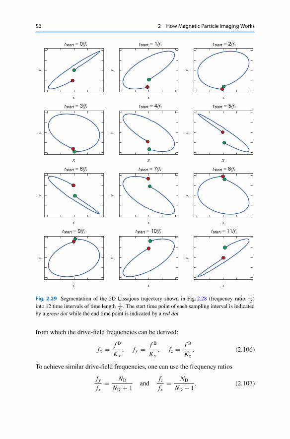
56 2 How Magnetic Particle Imaging Works
y y y
y y y
y y y
y y y
x
tstart = 9/fx tstart = 10/fx tstart = 11/fx
tstart = 8/fxtstart = 7/fxtstart = 6/fx
tstart = 3/fx tstart = 4/fx tstart = 5/fx
tstart = 0/fx tstart = 1/fx tstart = 2/fx
x x
x x x
x x x
x x x
Fig. 2.29 Segmentation of the 2D Lissajous trajectory shown in Fig. 2.28 (frequency ratio 1112
)into 12 time intervals of time length 1
fx. The start time point of each sampling interval is indicated
by a green dot while the end time point is indicated by a red dot
from which the drive-field frequencies can be derived:
fx D f B
Kx
; fy D f B
Ky
; fz D f B
Kz: (2.106)
To achieve similar drive-field frequencies, one can use the frequency ratios
fy
fxD ND
ND C 1and
fz
fxD ND
ND � 1: (2.107)
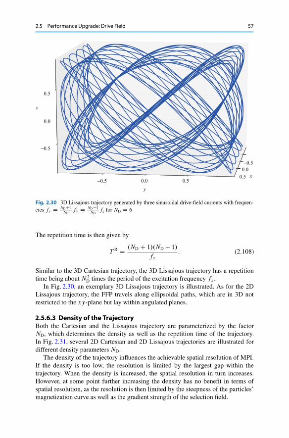
2.5 Performance Upgrade: Drive Field 57
−0.50.0
0.5−0.5
0.5
0.0
−0.5
0.0 0.5x
y
z
Fig. 2.30 3D Lissajous trajectory generated by three sinusoidal drive-field currents with frequen-cies fx D NDC1
NDfy D ND�1
NDfz for ND D 6
The repetition time is then given by
T R D .ND C 1/.ND � 1/fx
: (2.108)
Similar to the 3D Cartesian trajectory, the 3D Lissajous trajectory has a repetitiontime being about N2
D times the period of the excitation frequency fx .In Fig. 2.30, an exemplary 3D Lissajous trajectory is illustrated. As for the 2D
Lissajous trajectory, the FFP travels along ellipsoidal paths, which are in 3D notrestricted to the xy-plane but lay within angulated planes.
2.5.6.3 Density of the TrajectoryBoth the Cartesian and the Lissajous trajectory are parameterized by the factorND, which determines the density as well as the repetition time of the trajectory.In Fig. 2.31, several 2D Cartesian and 2D Lissajous trajectories are illustrated fordifferent density parametersND.
The density of the trajectory influences the achievable spatial resolution of MPI.If the density is too low, the resolution is limited by the largest gap within thetrajectory. When the density is increased, the spatial resolution in turn increases.However, at some point further increasing the density has no benefit in terms ofspatial resolution, as the resolution is then limited by the steepness of the particles’magnetization curve as well as the gradient strength of the selection field.

58 2 How Magnetic Particle Imaging Works
ND
= 3
0N
D =
20
ND
= 1
0
x
yCartesian trajectory
x
x x
x x
y
Lissajous trajectoryy y
y y
Fig. 2.31 Cartesian and Lissajous trajectories for different density parameters ND 2 f10; 20; 30g
2.6 Performance Upgrade: Focus Field
In this section, it is shown that the scanning volume that can be covered by the drivefield is limited to few centimeters in length. To overcome this limitation, a methodfor scanning large scanning volumes is introduced, which utilizes a so-calledfocus field.
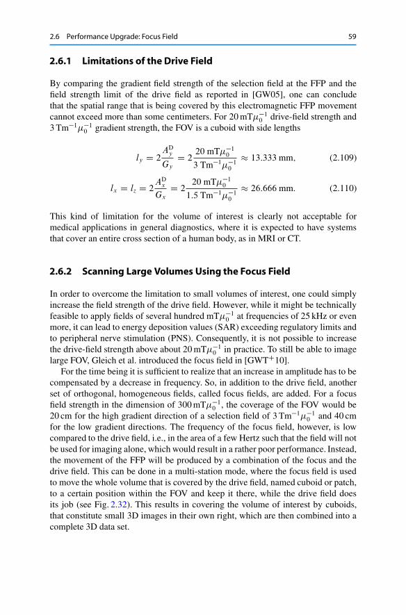
2.6 Performance Upgrade: Focus Field 59
2.6.1 Limitations of the Drive Field
By comparing the gradient field strength of the selection field at the FFP and thefield strength limit of the drive field as reported in [GW05], one can concludethat the spatial range that is being covered by this electromagnetic FFP movementcannot exceed more than some centimeters. For 20 mT��1
0 drive-field strength and3 Tm�1��1
0 gradient strength, the FOV is a cuboid with side lengths
ly D 2ADy
GyD 2
20 mT��10
3 Tm�1��10
13:333mm; (2.109)
lx D lz D 2ADx
GxD 2
20 mT��10
1:5 Tm�1��10
26:666 mm: (2.110)
This kind of limitation for the volume of interest is clearly not acceptable formedical applications in general diagnostics, where it is expected to have systemsthat cover an entire cross section of a human body, as in MRI or CT.
2.6.2 Scanning Large Volumes Using the Focus Field
In order to overcome the limitation to small volumes of interest, one could simplyincrease the field strength of the drive field. However, while it might be technicallyfeasible to apply fields of several hundred mT��1
0 at frequencies of 25 kHz or evenmore, it can lead to energy deposition values (SAR) exceeding regulatory limits andto peripheral nerve stimulation (PNS). Consequently, it is not possible to increasethe drive-field strength above about 20 mT��1
0 in practice. To still be able to imagelarge FOV, Gleich et al. introduced the focus field in [GWTC10].
For the time being it is sufficient to realize that an increase in amplitude has to becompensated by a decrease in frequency. So, in addition to the drive field, anotherset of orthogonal, homogeneous fields, called focus fields, are added. For a focusfield strength in the dimension of 300 mT��1
0 , the coverage of the FOV would be20 cm for the high gradient direction of a selection field of 3 Tm�1��1
0 and 40 cmfor the low gradient directions. The frequency of the focus field, however, is lowcompared to the drive field, i.e., in the area of a few Hertz such that the field will notbe used for imaging alone, which would result in a rather poor performance. Instead,the movement of the FFP will be produced by a combination of the focus and thedrive field. This can be done in a multi-station mode, where the focus field is usedto move the whole volume that is covered by the drive field, named cuboid or patch,to a certain position within the FOV and keep it there, while the drive field doesits job (see Fig. 2.32). This results in covering the volume of interest by cuboids,that constitute small 3D images in their own right, which are then combined into acomplete 3D data set.
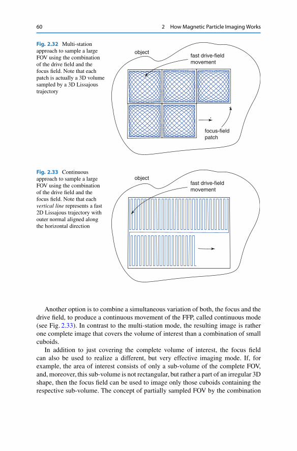
60 2 How Magnetic Particle Imaging Works
fast drive-fieldmovement
object
focus-fieldpatch
Fig. 2.32 Multi-stationapproach to sample a largeFOV using the combinationof the drive field and thefocus field. Note that eachpatch is actually a 3D volumesampled by a 3D Lissajoustrajectory
fast drive-fieldmovement
objectFig. 2.33 Continuousapproach to sample a largeFOV using the combinationof the drive field and thefocus field. Note that eachvertical line represents a fast2D Lissajous trajectory withouter normal aligned alongthe horizontal direction
Another option is to combine a simultaneous variation of both, the focus and thedrive field, to produce a continuous movement of the FFP, called continuous mode(see Fig. 2.33). In contrast to the multi-station mode, the resulting image is ratherone complete image that covers the volume of interest than a combination of smallcuboids.
In addition to just covering the complete volume of interest, the focus fieldcan also be used to realize a different, but very effective imaging mode. If, forexample, the area of interest consists of only a sub-volume of the complete FOV,and, moreover, this sub-volume is not rectangular, but rather a part of an irregular 3Dshape, then the focus field can be used to image only those cuboids containing therespective sub-volume. The concept of partially sampled FOV by the combination
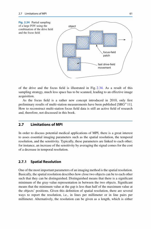
2.7 Limitations of MPI 61
fast drive-fieldmovement
object
focus-fieldpatch
Fig. 2.34 Partial samplingof a large FOV using thecombination of the drive fieldand the focus field
of the drive and the focus field is illustrated in Fig. 2.34. As a result of thissampling strategy, much less space has to be scanned, leading to an effective imageacquisition.
As the focus field is a rather new concept introduced in 2010, only firstpreliminary results of multi-station measurements have been published [SRGC11].How to reconstruct multi-station focus field data is still an active field of researchand, therefore, not discussed in this book.
2.7 Limitations of MPI
In order to discuss potential medical applications of MPI, there is a great interestto asses essential imaging parameters such as the spatial resolution, the temporalresolution, and the sensitivity. Typically, these parameters are linked to each other;for instance, an increase of the sensitivity by averaging the signal comes for the costof a decrease in temporal resolution.
2.7.1 Spatial Resolution
One of the most important parameters of an imaging method is the spatial resolution.Basically, the spatial resolution describes how close two objects can be to each othersuch that they can be distinguished. Distinguished means that there is a significantminimum of the gray-value representation in between the two objects. Significantmeans that the minimum value at the gap is less than half of the maximum value atthe objects’ positions. Given this definition of spatial resolution, there are severalways to report the resolution, i.e., in lines per millimeter or in line pairs permillimeter. Alternatively, the resolution can be given as a length, which is either

62 2 How Magnetic Particle Imaging Works
the width in millimeter of the smallest line that can be resolved or the width of thesmallest line pair (i.e., the width of the line plus the gap).
In this book, the resolution is given as the size of the smallest line, which can beresolved. This measure has been proposed in the context of MPI in [WBG07] andmatches that given by the FWHM of the convolution kernel, which has been used in[RWGB09, GC10].
As the magnetic particle imaging process can in 1D be formulated as a convolu-tion, one can use well-known tools to analyze the spatial resolution [BM03]. In thefollowing, two important resolution measures are discussed: the FWHM resolutionand the modulation transfer function (MTF) resolution.
2.7.1.1 Full Width at Half Maximum of the Convolution KernelWhen applying a convolution, sharp structures in a signal are blurred, which leadsto a loss of resolution. The actual resolution loss depends on the shape of theconvolution kernel. One way to estimate the resolution based on the shape of theconvolution kernel is to consider its full width half maximum, which was alreadyintroduced in Sect. 2.2.3.
In Fig. 2.35, three different signals resulting from a convolution of line pairphantoms with the MPI convolution kernel Qm for 1 mm FWHM are shown. As canbe seen, the spatial resolution according to the definition outlined above is about1 mm, which matches the FWHM of the convolution kernel. However, for differentkernels both values can differ slightly, for instance for, the Gaussian kernel, whichcan resolve 0.82 mm structures for 1 mm FWHM.
In Sect. 2.2.3, the FWHM of the derivative of the magnetization characteristicM 0.H/ was calculated to be �H FWHM D 4:16 ˇ�1. Consequently, the convolutionkernel Qm as defined in (2.73) has an FWHM of
RFWHM D 4:161
ˇG: (2.111)
In Fig. 2.36, the FWHM resolution is plotted versus the gradient strength of theselection field for different particle diameters. As can be seen, the resolutionincreases inversely proportional with the applied gradient strength. Furthermore,as the factor ˇ depends on the third power of the particle diameter, the resolutionincrease in a cubic fashion when increasing the particle diameter. In practice,gradient strengths up to 6 Tm�1��1
0 and particle diameters of 30 nm are feasiblesuch that the resolution can potentially be better than 0.5 mm.
While the FWHM criterion is a simple way to analyze the resolution of animaging system, it is not the most accurate one, as it does not take into accountthat the resolution can be increased by performing a deconvolution. It further doesnot consider the SNR of the measured signal. Hence, in practice, the real resolutioncan be both higher and lower than (2.111) would suggest.

2.7 Limitations of MPI 63
convolution kernel: 1 mm FWHM˜
1.0 mm gap
˜m
/m (
0)
1.0
0.5
0.0
1.0
0.5
0.0
1.0
0.5
0.0
1.0
0.5
0.0
line-pair phantoms and convolved signals
norm
aliz
ed v
alue
s/ar
bitr
ary
unit
1.5 mm gap
−3 −2 −1 0 1 2 3
−3 −2 −1 0 1 2 3
−3 −2 −1 0 1 2 3
−3 −2 −1 0 1 2 3
x/mm
x/mm
0.5 mm gap
Fig. 2.35 Normalized convolution kernel Qm= Qm.0/ for 1 mm FWHM (top) and normalizedconvolved signals (blue) for several line-pair phantoms consisting of two rectangular dots of thesame size and gap (1.5, 1.0, and 0.5 mm). In green the original line-pair phantoms are illustrated
2.7.1.2 Modulation Transfer FunctionA more sophisticated way to analyze the spatial resolution of an imaging systemis to consider the modulation transfer function [Buz08], which allows to relate thespatial resolution to the SNR of the measured signal. The MTF describes how thecontrast of an image structure is damped by the convolution of the imaging process.The MTF is a function of the spatial frequency and can be defined in Fourier spacewhere the convolution corresponds to a multiplication of the Fourier transform ofthe particle concentration
Oc.�/ WD F.c.x// (2.112)
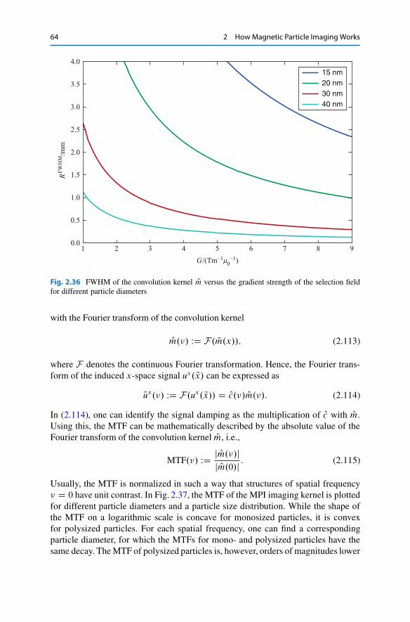
64 2 How Magnetic Particle Imaging Works
1 2 3 4 5 6 7 8 9G/(Tm−1m0
−1)
4.0
3.5
3.0
2.5
2.0
1.5
1.0
0.5
0.0
RFW
HM
/mm
15 nm20 nm30 nm40 nm
Fig. 2.36 FWHM of the convolution kernel Qm versus the gradient strength of the selection fieldfor different particle diameters
with the Fourier transform of the convolution kernel
Om.�/ WD F. Qm.x//; (2.113)
where F denotes the continuous Fourier transformation. Hence, the Fourier trans-form of the induced x-space signal ux. Qx/ can be expressed as
Oux.�/ WD F.ux. Qx// D Oc.�/ Om.�/: (2.114)
In (2.114), one can identify the signal damping as the multiplication of Oc with Om.Using this, the MTF can be mathematically described by the absolute value of theFourier transform of the convolution kernel Om, i.e.,
MTF.�/ WD j Om.�/jj Om.0/j : (2.115)
Usually, the MTF is normalized in such a way that structures of spatial frequency� D 0 have unit contrast. In Fig. 2.37, the MTF of the MPI imaging kernel is plottedfor different particle diameters and a particle size distribution. While the shape ofthe MTF on a logarithmic scale is concave for monosized particles, it is convexfor polysized particles. For each spatial frequency, one can find a correspondingparticle diameter, for which the MTFs for mono- and polysized particles have thesame decay. The MTF of polysized particles is, however, orders of magnitudes lower
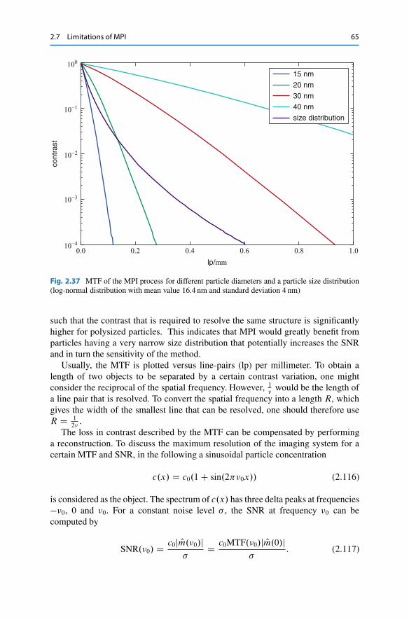
2.7 Limitations of MPI 65
0.40.20.0 0.6 0.8 1.0lp/mm
10−2
10−3
10−4
10−1
100co
ntra
st
15 nm
20 nm
30 nm
40 nm
size distribution
Fig. 2.37 MTF of the MPI process for different particle diameters and a particle size distribution(log-normal distribution with mean value 16.4 nm and standard deviation 4 nm)
such that the contrast that is required to resolve the same structure is significantlyhigher for polysized particles. This indicates that MPI would greatly benefit fromparticles having a very narrow size distribution that potentially increases the SNRand in turn the sensitivity of the method.
Usually, the MTF is plotted versus line-pairs (lp) per millimeter. To obtain alength of two objects to be separated by a certain contrast variation, one mightconsider the reciprocal of the spatial frequency. However, 1
�would be the length of
a line pair that is resolved. To convert the spatial frequency into a length R, whichgives the width of the smallest line that can be resolved, one should therefore useR D 1
2�.
The loss in contrast described by the MTF can be compensated by performinga reconstruction. To discuss the maximum resolution of the imaging system for acertain MTF and SNR, in the following a sinusoidal particle concentration
c.x/ D c0.1C sin.2��0x// (2.116)
is considered as the object. The spectrum of c.x/ has three delta peaks at frequencies��0, 0 and �0. For a constant noise level � , the SNR at frequency �0 can becomputed by
SNR.�0/ D c0j Om.�0/j�
D c0MTF.�0/j Om.0/j�
: (2.117)
66 2 How Magnetic Particle Imaging Works
As the MTF of the MPI process is monotonically decreasing for increasingfrequency (see Fig. 2.37), the SNR decreases for increasing frequency as well.Hence, one can find for a certain SNR a corresponding frequency �0. If the SNRdrops below 1, the signal cannot be recovered. Hence, to compute the maximumfrequency �max, one can insert SNR.�max/ D 1 and solve for the frequency �max
yielding
�max D MTF �1�
�
c0j Om.0/j�: (2.118)
Note, that MTF�1 is the inverse of the MTF, which gives the resolution for a certaincontrast. It should not be mixed up with the inverse of the Fourier transformationF�1. The argument in (2.118) is actually the inverse of the SNR for frequencyzero, i.e., for constant signal. Thus, the maximum frequency that can be resolvedis given by
�max D MTF�1�
1
SNR.0/
�: (2.119)
By taking the half of the reciprocal of the spatial frequency, the maximum resolutioncan be expressed as
RMTF D 1
2�maxD 1
2MTF�1�
1SNR.0/
� : (2.120)
For a graphical representation of this resolution expression, one can draw ahorizontal line at the contrast level 1
SNR.0/ in the MTF plot (Fig. 2.37) and look forthe intersection point with the MTF. The resulting spatial frequency on the x-axisrepresents the maximum that can be resolved for the given noise level.
Monosized ParticlesTo derive an explicit expression for the maximum resolution, we focus onmonosized particles next. Unfortunately, no analytic expression for the Fouriertransform of the Langevin function and in turn the MTF of the MPI process isknown. To arrive at an analytical expression, one can approximate the derivative ofthe Langevin function by the Lorentzian
�.�/ D 2
�
2
4C �2; (2.121)
for which the Fourier transform is well known to be
O�.�/ D 2 exp .�4�j�j/ : (2.122)
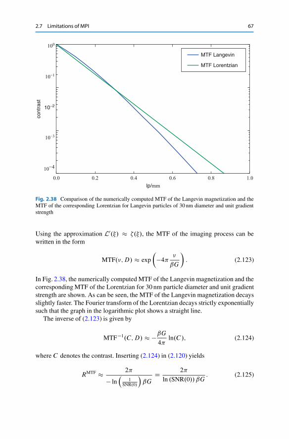
2.7 Limitations of MPI 67
MTF Langevin
MTF Lorentzian
0.40.20.0 0.6 0.8 1.0lp/mm
10−2
10−3
10−4
10−1
100co
ntra
st
Fig. 2.38 Comparison of the numerically computed MTF of the Langevin magnetization and theMTF of the corresponding Lorentzian for Langevin particles of 30 nm diameter and unit gradientstrength
Using the approximation L0.�/ �.�/, the MTF of the imaging process can bewritten in the form
MTF.�;D/ exp
��4� �
ˇG
�: (2.123)
In Fig. 2.38, the numerically computed MTF of the Langevin magnetization and thecorresponding MTF of the Lorentzian for 30 nm particle diameter and unit gradientstrength are shown. As can be seen, the MTF of the Langevin magnetization decaysslightly faster. The Fourier transform of the Lorentzian decays strictly exponentiallysuch that the graph in the logarithmic plot shows a straight line.
The inverse of (2.123) is given by
MTF�1.C;D/ �ˇG4�
ln.C /; (2.124)
where C denotes the contrast. Inserting (2.124) in (2.120) yields
RMTF 2�
� ln�
1SNR.0/
�ˇG
D 2�
ln .SNR.0// ˇG: (2.125)

68 2 How Magnetic Particle Imaging Works
Comparing this resolution with that derived by the FWHM of the convolutionkernel, one can see that both expressions depend on the reciprocal of ˇ and G.However, the expression (2.125) additionally takes into account the SNR of thesignal. For an SNR of about 4.6 the MTF resolution gives the same value as theFWHM resolution. An SNR of 4.6 indeed seems to be a reasonable value, for whichone can identify a structure, but one is not able to increase its resolution using adeconvolution technique.
Polysized ParticlesFor polysized particles, the dependency of the spatial resolution on the SNR cannotbe written in a simple form like (2.125). The Fourier transform of the convolutionkernel for polysized particles can be written as
Om.�/ DZ 1
0
�.D/ Om.�;D/ dD: (2.126)
Hence, the MTF can be formulated as
MTF.�/ D
Z 1
0
�.D/MTF.�;D/ Om.0;D/ dDZ 1
0
�.D/ Om.0;D/ dD; (2.127)
i.e., the MTF of polysized particles is the superposition of the MTFs of monosizedparticles weighted with the probability density function �.D/. The superpositionof several MTFs of monosized particles justifies the concave shape of the MTF ofpolysized particles illustrated in Fig. 2.37.
2.7.2 Sensitivity and Temporal Resolution
Besides the spatial resolution, the sensitivity is an essential parameter of an imagingmethod. Basically, the sensitivity describes the minimal amount of magneticmaterial that can be detected using MPI. As it has been derived in Sect. 2.7.1, thesensitivity does also influence the spatial resolution in a logarithmic fashion.
In [WBG07], the sensitivity of MPI has been investigated and the scaling law
SNR / pT measc0G
�3 pRf E
pRP
(2.128)
has been derived. Here, T meas denotes the total measurement time , c0 denotes themean particle concentration within a considered voxel, pR is the sensitivity of thereceive coil, f E is the excitation frequency and RP is the noise resistance of thereceive coil.

2.7 Limitations of MPI 69
In the ideal case, the noise present in the receive coil does not stem fromthe instrumentation itself but from eddy currents induced by the patient. As ithas been shown in [Ros87], the equivalent noise resistance of a patient increasesquadratically with the excitation frequency. Consequently, considering patient noise,the sensitivity of MPI is independent of the excitation frequency as the frequencyand the noise resistance cancel out each other in (2.128).
Obviously, the particle concentration influences the SNR of the measured signalin a linear fashion. Furthermore, the sensitivity of the receive coil should be as highas possible to improve the SNR. In the scaling law (2.128), the sensitivity dependson the third power of the reciprocal of the gradient strength. This is based on theassumption that a change of the gradient strength is attended by a change of thevoxel size that can be resolved. As MPI using the FFP encoding scheme basicallymeasures a single voxel at a time point, the sensitivity decreases for increasinggradient strength. However, as it has been discussed in Sect. 2.7.1, the sensitivityand the spatial resolution are linked to each other such that an increase of thegradient strength does not necessarily improve the spatial resolution if the SNRof the measured signal becomes too small.
By repeating the MPI experiment several times and averaging the signals, theSNR can be improved in a square root sense. Alternatively, as it has been discussedin [KBSC09], one can increase the density of the FFP trajectory, which doesimprove the SNR in the same way but leads to a more independent informationduring a fixed acquisition time. However, an increase of sensitivity by averagingobviously comes for the cost of a decrease in temporal resolution. Therefore, inpractice, the number of averages is limited by the frame rate required by the medicalapplication.
2.7.3 Detection Limit
In order to determine the detection limit of MPI, the signal that is being generatedby a definite test sample of magnetic material has to be compared to a noise signal.The lowest possible noise level is the patient noise. To determine the signal and thenoise, a square-shaped single loop coil of 10 cm edge length is considered. Placingsuch a coil on the chest of an adult human yields an increase of the resistance of thecoil of approximately 100 mT��1
0 at 20 MHz, equating to a noise voltage of RP D40 pV/
pHz root-mean-square, calculated from
unoise Dp4kBT Pf SRP; (2.129)
where f S is the frequency bandwidth (see [Joh28]). To determine the signalstrength, it is assumed that in a finite volume V sample, a given total magnetizationoscillates with a given frequency, leading to
usignal D 2�pRf EMV sample cos.2�f Et/; (2.130)

70 2 How Magnetic Particle Imaging Works
where f E is the excitation frequency,M is the magnetization and pR D 10�6 TA�1is the coil sensitivity of the test coil. The product of the magnetization M and thevolume V sample is a dipole moment, the value of which is 92 fAm2, assuming thatthe test sample consists of 1 pg of iron oxide available in a finite volume. Using(2.130), this results in a signal strength of 12 pV peak and about 8 pV root-mean-square. To ensure the detectability of the signal, the arbitrary choice is made, that thesignal strength has to be five times higher than the noise, which would be 200 pV.This corresponds to 25 pg of iron in a given, finite volume. This derivation assumesa frequency bandwidth of 1 Hz, which corresponds to a measurement time of 1 s.Prolonging the measurement to, e.g., 625 s – a little more than 10 min – leads to afrequency bandwidth of 1/625 and, following (2.129), to a decrease in the noise bya factor of 25. This, in turn, would also lower the demand on the signal by a factorof 25 and thus lower the detection limit to 1 pg iron oxide.
To convert these amounts of material into concentrations, usually expressed bythe number of iron atoms per liter of solvent/dispersion, the magnetic materialcontained in one voxel has to be considered. As the molar mass of iron oxide(Fe3O4) is 231.5 g mol�1, 1 g of iron oxide contains about 4.32 mmol iron oxide andthus about 13 mmol iron and, therefore, 1 pg of iron oxide contains about 13 fmoliron. Assuming that this number of iron atoms is contained in a voxel of 1 mm3,the concentration in this voxel will be about 13 fmol(Fe)mm�3, corresponding to adetectable concentration of about 13 nmol(Fe)l�1.
Starting from 25 pg instead of 1 pg, implying a measurement time of 1 s instead ofabout 10 min, yields a detection limit of 324 nmol(Fe)l�1 for a voxel size of 1 mm3.Resovist R� has an undiluted concentration of 500 mmol(Fe)l�1. Applied accordingto prescription, 1.4 ml of undiluted Resovist R� is administered for one examinationduring an MRI scan. Assuming an adult human’s blood volume to be 6 l, this resultsin a steady state concentration of 116 mol(Fe)l�1, about 360 times the detection limitfor a voxel size of 1 mm3 and a measurement time of 1 s.
All these estimations imply that MPI is being used as a single voxel method,i.e., the concentration of the magnetic material is measured one voxel at a time.Using more effective coding schemes, as exemplified in Sect. 6.3, can increase thedetection limit by about one order of magnitude.

http://www.springer.com/978-3-642-04198-3
Related Documents