1 How Increased Crude Oil Demand by China and India Affects the International Market By Amanda Niklaus a and Julian Inchauspe b (a) Department of Economics, Curtin University, Perth, Australia. Presenting author. (b) Department of Economics, Curtin University, Perth, Australia. Corresponding author. Abstract The global crude oil market is characterised by complex interactions between demand and supply. The question that we address in this paper is how increased demand for crude oil by China and India affects the world crude oil market. More specifically, we study the implications for pricing, OPEC production and non-OPEC production in a VAR setting. An interesting hypothesis tested in this paper is whether or not oil demand by China and India is different to the oil demand by other countries. Theoretical aspects of the crude oil market are considered in the analysis. 1. Introduction This paper investigates the implications of increased crude oil demand from China and India for the world crude oil market. Before addressing this question, it is necessary to carefully study the structure of the international crude oil market. In particular, it is also necessary to understand the characteristics of supply and the interactions between OPEC and non-OPEC suppliers. All these considerations will be taken into account in the empirical model that is presented later. The balance of this paper is organised as follows. Section 2 presents a non-technical overview of trends in demand and supply. Section 3 performs a literature review using a theoretical model as a benchmark. Section 4 provides some empirical analysis based on considerations laid out in Sections 2 and 3. Conclusions are presented in Section 5.

Welcome message from author
This document is posted to help you gain knowledge. Please leave a comment to let me know what you think about it! Share it to your friends and learn new things together.
Transcript

1
How Increased Crude Oil Demand by China
and India Affects the International Market
By Amanda Niklausa and Julian Inchauspeb
(a) Department of Economics, Curtin University, Perth, Australia. Presenting author.
(b) Department of Economics, Curtin University, Perth, Australia. Corresponding author.
Abstract
The global crude oil market is characterised by complex interactions between demand and supply. The question that we address in this paper is how increased demand for crude oil by China and India affects the world crude oil market. More specifically, we study the implications for pricing, OPEC production and non-OPEC production in a VAR setting. An interesting hypothesis tested in this paper is whether or not oil demand by China and India is different to the oil demand by other countries. Theoretical aspects of the crude oil market are considered in the analysis.
1. Introduction
This paper investigates the implications of increased crude oil demand from China and
India for the world crude oil market. Before addressing this question, it is necessary to
carefully study the structure of the international crude oil market. In particular, it is also
necessary to understand the characteristics of supply and the interactions between OPEC
and non-OPEC suppliers. All these considerations will be taken into account in the
empirical model that is presented later.
The balance of this paper is organised as follows. Section 2 presents a non-technical
overview of trends in demand and supply. Section 3 performs a literature review using a
theoretical model as a benchmark. Section 4 provides some empirical analysis based on
considerations laid out in Sections 2 and 3. Conclusions are presented in Section 5.

2
2. An Overview of the Crude Oil Market
The global crude oil market can be analysed by considering how quantity and price are
affected by the complex interactions between demand and supply. Before emerging into a
more detailed analysis, it is worth noting that the crude oil market can be described as a
“global” market, as Smith (2009, 162) and other researchers in the area have pointed out.
Figure 1 shows that the most important crude oil prices in the world move together (the
price differences are due to different oil quality and specific shocks).
Figure 1- Crude Oil Prices. Source: DataStream.
It is relevant to mention that Brent and Western Texas Intermediate (WTI) crude oil
prices have been moving apart from late 2010 as can be seen in Figure 2.1. Typically,
WTI from Cushing Oklahoma holds a higher price than Brent crude oil. This has been
the case until recently as WTI is a lighter and sweeter type of oil, holding only about
0.24% of sulphur, making it easier to refine into gasoline. Whereas Brent crude contains
about 0.37% of sulphur but is still considered as a sweet crude oil. It is interesting to
compare them with heavier types of oil such as the heavy crude oil produced from
Venezuela’s Orinoco Belt which contains approximately 4.5% of sulphur (Energy &
Capital 2012). Even OPEC supplying about 40% of the world’s crude oil does not have
such a sweet type of crude oil; hence this is why WTI has had higher prices over the
years until recently. The concern is that WTI is losing its connection to the global
0
20
40
60
80
100
120
140
160
1992
1993
1994
1995
1996
1997
1998
1999
2000
2001
2002
2003
2004
2005
2006
2007
2008
2009
2010
2011
WTI Crude Oil-WTI Spot Cushing US$/BBLBrent Crude Oil-Brent Dated FOB US$/BBLDubai Crude Oil-Arab Gulf Dubai FOB US$/BBLTapis Crude Oil-Malaysia Tapis FOB US$/BBLUrals Crude Oil-Urals FOB US$/BBLBonny Crude Oil-Africa FOB Bonny Lght US$/BBL

3
markets particularly the demand-supply issue. There were Enbridge’s recent pipelines
troubles where the company was forced to shut down one of its pipelines after a leak was
discovered. The Midwest is oversupplied because of the import from Canada and due to
the inadequate pipeline capacity to the Gulf Coast; the crude oil cannot reach this area
(Tverberg 2011). On top of that, a year ago, Saudi Aramco decided to change their oil
benchmark from WTI to Argus Sour Crude Index stating that Argus is closer to the
heavier, more sour crude that the country exports.
Next, some analysis of the most important trends in the global oil market is presented.
2.2 Trends in Oil Supply
2.2.1 Historical Trends in Oil Supply: The Establishment of the International Market
It is relevant to consider some historical facts affecting oil production. In the nineteenth
century, the oil industry expanded fast in the US thanks to the “law of capture”. Effective
since 1840, this law gives property rights to the owner of a well to extract unlimited
amount of oil, even if it comes from someone else’s property. This very competitive
search for oil pushed the prices down in the 1860s (Dahl 2011). Later on, Rockefeller
founded the Standard Oil Company in 1870 which dominated and revolutionized the oil
industry by stabilizing the US market (Dahl 2011). Other important developments
include the merge of Royal Dutch (which had been drilling in Indonesia since 1890) as
well as Shell Transport and Trading (which started transporting Kerosene from Russia to
the Far East in 1892) to form the Shell Group in 1907 (Dahl 2011).
Standard Oil and Shell were the major producers by the end of the nineteenth century,
but Standard Oil was broken up by antitrust laws in 1911 (Dahl 2011). In Britain,
Churchill bought a controlling share in Anglo-Persian Oil Company, the first company to
extract petroleum from the South Asian country of Iran, which later became British
Petroleum (BP). BP played a fundamental role in supplying oil to the British fleet during
the First World War. After the War, oil prices fell down. The major producers tried to
increase prices but were prevented by the arrival of new entrants, namely Gulf, Texaco,
Chevron and Mobil. These seven companies, referred pejoratively as the “Seven Sisters”,
formed the Iran cartel and became the dominant firms in the oil industry between the
mid-1940s to the 1970s. In parallel, during the 1950s, new rivals entered the oil market

4
such as Getty and Occidental oil producing in North Africa. Taxes for the companies
increased to substantial levels over major producing countries following the initiative of
Venezuela (Dahl 2011). Oil companies paying taxes did not immediately cut their prices,
but falling demand from European recession and increased competition would later push
prices down. This led to reduce taxes for producing countries giving incentive to
Venezuela, Iran, Iraq, Kuwait, and Saudi Arabia to form a cartel in 1960 which was
named Organisation of the Petroleum Exporting Countries (OPEC). They were later
joined by Qatar, Libya, Indonesia, United Arab Emirates, Algeria and Nigeria (Dahl
2011). Up to the oil crisis of 1973, the Seven Sisters controlled the majority of the
world’s petroleum resources. From 1973, the Seven Sisters have become less influential,
but overall OPEC and state-owned oil companies in emerging-market economies have
become more dominant (Dahl 2011).
2.2.2 Current Supply Trends: Facts and Forecasts
Global oil supply has increased by 2.2% in 2010, this gain in production has been shared
almost equally between OPEC and non-OPEC producers (BP 2011). Indeed, non-OPEC
countries accounted for 58.2% of global oil production in 2010 which has not changed
much since 2000 (BP 2011). This process was led by China which recorded its biggest
increase in production ever, and by the US and Russia; in fact, non-OPEC production
grew by 1.8% which is the largest increase since 2002 (BP 2011). Meanwhile, Norway
and the UK have seen a decline in their oil production. OPEC countries have seen their
production amplify by 2.5% in 2010, where the largest increase in production came from
Nigeria and Qatar (BP 2011). Additional capacity in 2010 came mainly from non-OECD
countries making almost 90% of the global total (BP 2011). Therefore, installed refining
capacity is now greater in non-OECD countries than in OECD (BP 2011).
An interesting report with projections for energy consumption and production until 2030
is provided by BP (BP Energy Outlook 2030 2012), which is one of the most respectable
sources of data, analysis and projections for energy. This report is based on a consensus
on the evolution of the world economy, policy, and technology. According to this report,
OPEC will continue to be the leading supplier with major contributions from Iraq and
Saudi Arabia. Concurrently, non-OPEC supply is also expected to increase.

5
Even though Iraq has great uncertainty regarding its capacity expansion, due to limited
project development capacity, infrastructure constraints, security challenges as well as
political instability, BP expect Iraq to account for 20% of global oil supply for the next
20 years (BP 2012). This is important as the ability and willingness of OPEC members to
expand capacity and production is one of the main factors determining the future path of
oil market.
It is important to note that shale oil has been developing quickly in the last decade. Shale
oil has long been set aside because of high extraction costs. It is only recently that
producers from the US and Canada have shown that the extraction of shale gas can be
facilitated by new technology that combines horizontal drilling with hydraulic fracturing
which made it economically viable. The same technology is being applied to the
extraction of shale oil in some countries, although shale oil resources are not as
developed as shale gas. Most of the development of shale oil resources occurs in western
United States around the Green River Formation, which is estimated to contain about 1.5
trillion barrels of shale oil (USGS 2006). Due to different quality of shale oil found in
various countries, not all of it is extractable with today’s technology. The total resources
of shale oil deposits of a selected group of 33 countries are estimated to be about 2.8
trillion U.S. barrels of shale oil according to USGS (2006). More recently, China
National Petroleum Corp (CNPC) started to cooperate with foreign companies such as
Shell and Hess corp. to explore shale oil in the country’s Santanghu Basin (Bai and
Aizhu 2012). If these projects go ahead in the future, it is likely to bring further
advancement in technology in the extraction and production of shale oil. This again
shows the constant interest and importance of China in the energy market.
In summary, the global oil supply has increased, an increase coming from both OPEC
and non-OPEC countries. The main increase in supply comes notably from China, the
US, Russia, Nigeria and Qatar. Accordingly, we will now analyse the demand side of the
oil market.
2.3 Trends in Demand
The demand for all types of energy has grown substantially due to the fact that GDP
growth in non-OECD has been above the world average, while to the mature energy

6
consumption by OECD countries has been steady. Non-OECD oil consumption growth
rate reached 5.5% in 2010, which contrasts with the 0.9% steady growth from OECD
(BP 2011). Indeed, among the large increase in the consumption of all types of energy,
oil remains the world’s leading fuel satisfying 33.6% of global energy consumption, even
though it has been losing market share since 2000 (Figure 2).
Figure 2- Trends in Oil Consumption.
Source: BP (2011), Statistical Review of World Energy.
The increase in oil consumption in 2010 (Figure 2) has not been matched by the global
production of oil, leading to a consequent decrease in inventories. Global oil
consumption grew by 3.1% while production increased by only 2.2% (BP 2011). This
could be attributed to the OPEC production interruptions implemented since late 2008.
As other energy sources may be substitutes for oil, it is important to consider trends in oil
demand compared to global trends for combined energy sources. To analyse this, we
consider an energy demand forecast provided by BP (2012), which is based on
consensual assumptions on key variables. Population and income will remain the key
determinants of energy demand. Assuming a population growth of 1.4 billion until 2030
and a global GDP growth of 3.7% p.a.1, overall growth of primary energy consumption is
1The average between 1990 and 2010 was 3.2% p.a. (BP 2012).
Energy Consumption by Source (Million Tonnes Oil Equivalent)

7
forecasted to grow by 1.6% over this period, primarily pushed by fast-growing non-
OECD countries (BP 2012). Non-OECD countries are expected to increase their
consumption by 69% in 2030 (above the 2010 level), which contrasts OECD energy
consumption forecasted to be just 4% higher than in 2010 (BP 2012).
The economic development of non-OECD countries creates an appetite for energy that
can only be met by expanded consumption of all types of fuel. Gas and non-fossil fuels
will gain share at the expense of coal and oil. The fastest growing fuels are renewable
about 8.2% p.a., whereas oil will be the slowest at 0.7% p.a., according to BP (2012).
These projections are explained by an expected shift from oil in transportation to gas and
renewables by 2030, and by a combination of relative fuel prices, technological
innovation and policy interventions.
Most of the growth in oil demand will be attributable to China and India, both of which
are expected to increase their net oil imports. According to BP (2012), China and India
will become the world’s largest and third largest economies and energy consumers,
respectively by 2030, accounting for much of the consumption increase in liquid fuels
(Figure 3). The increase in global liquids (oil, biofuels and other liquids) demand by
China (8 Mb/d2), India (3.5 Mb/d) and Middle-East countries (4 Mb/d) will account for
nearly all the net global increase by 2030. Furthermore, China and India will account for
35% of the global population and are likely to represent 94% of the net oil demand
growth (BP 2012).
Figure 3- Liquid Fuels Demand Growth. Source: BP (2012), Energy Outlook. 2Millions of Barrels per day (MB/d).

8
Chinese energy consumption grew by 11.2% in 2010 giving China the world largest
share of global energy consumption at 20.3% (BP 2011). In fact, more than half of global
liquids demand growth is in China, and its refinery expansion plans will affect product
balances globally.
3. Theoretical Considerations and Literature Review
There is an extensive literature on the behaviour of OPEC, the structure of the world
crude oil market and price decisions. This Section examines some of this literature, with
particular focus on the interactions among the OPEC members as well as the increased
demand from China and India. Section 3.1 discusses a popular baseline model used to
analyse the global crude oil market. Section 3.2 addresses literature that deals with the
deviations from this baseline model, and in doing so, it addresses the imperative
question: Is there a necessity for a reassessment of the market structure? Section 3.3
layouts the studies that concentrate on the structure of the crude oil demand. Section 3.4
comments on alternative theories such as the speculative behaviour in the crude oil
market.
3.1 The Baseline Model and Related Empirical Studies
Since the formation of OPEC in the 1970s, many theoretical models have been developed
to study its behaviour. The consensus economic model that has been used as a baseline to
study the global oil market is described in Dahl (2011), and is attributable to many
authors that have worked on modelling the global oil market. According to this model,
the key feature of the global oil market is its dominant firm-competitive fringe structure.
The “dominant firm” in that model represents OPEC, which behaves as a cartel and
restricts its output in order to maximize its profit subject to the supply by non-OPEC
countries. The “competitive fringe” represents the non-OPEC countries that satisfy the
residual demand of the global market, i.e. the demand that is not satisfied by OPEC. Due
to the natural endowments of oil and other economic restrictions, OPEC countries satisfy
a great part of the global demand. This gives enough market power to OPEC to influence
the price and obtain economic profits by restricting output, while firms from the
competitive fringe act as price-takers.

9
There is no agreement on a specific model to describe the oil market behaviour and it
seems that different strategies have been used over different periods of time. However,
there has been a consensus model that has been used as a baseline to study the global oil
market. We will introduce this baseline model as presented in Dahl (2011); this model is
attributable to many authors that have worked on modelling the global oil market.
According to this model, the key feature of the global oil market is its dominant firm-
competitive fringe structure.
The conception of this model has been dominated by historical facts. The oil world
market behaviour seems to be constantly changing. Dahl (2011) observed that oil is a
market where historically monopolies (such as Rockefeller’s) have risen and then faded
away, and that OPEC has been subject to cartel instability. In fact, monopolies have
emerged but have not been sustained. Not surprisingly, there is a variety of models that
can be found in the literature. According to Adelman (1982, quoted in Griffin 1985, 955),
OPEC’s actual behaviour has fluctuated between the dominant firm and market-sharing
models depending on market conditions. OPEC has often been studied as an individual
market and repeatedly referred to as a cartel, a monopoly and sometimes an oligopoly,
but this view has been greatly challenged. This led Griffin (1985) to study an alternative
hypothesis for explaining OPEC countries’ oil production. Similarly, Jones (1990)
conducted a study on OPEC and its behaviour under falling prices and in the same way
concluded that OPEC’s production behaviour could be best explained by a partial
market-sharing cartel model. Although this idea has been partially rejected by Dahl and
Yücel (1991), who found no formal evidence of coordination across OPEC producers to
support a strict market-sharing cartel, it seems that in terms of the ability of the various
models to explain production, the partial-sharing cartel model dominates for OPEC
producers.
Assumptions- There is a “dominant firm” representing OPEC which supplies the amount
of crude oil. OPEC can be represented as a single firm in this model because it is
assumed that it behaves as a cartel (we discuss deviations from this assumption later on).
There is a “competitive fringe” which represents the non-OPEC countries that satisfy the
residual demand of the global market , i.e. the demand that is not satisfied
by OPEC. Conversely, we can say that OPEC satisfies the residual demand which is not
satisfied by the competitive fringe, i.e. . It is assumed that the competitive
firm is formed by a large number of small firms, so each firm in the competitive fringe is

10
a price-taker. This market structure has correspondence with the actual structure.
Countries with large endowments of crude oil created OPEC; nowadays these large
players satisfy about 40% of global demand. The non-OPEC suppliers typically lack
enough market power to individually affect the global price of crude oil; hence they act
as price-taker when making economic decisions.
In this structure, OPEC has enough market power to influence the price of oil to obtain
economic (i.e. abnormal) profits. The dominant firm restricts its output in order to
maximize its profit subject to the supply by the competitive fringe. More specifically, the
dominant firm acts as a monopolist on the residual demand that cannot be satisfied by the
competitive fringe. This problem is represented by the following set of equations:
Global demand for crude oil: . (3.1)
Competitive fringe supply: . (3.2)
Demand facing OPEC: . (3.3)
OPEC cost function: . (3.4)
Where are constants and
OPEC’s profit maximization problem:
, . (3.5)
Or, written as an unconstrained optimisation problem:
(3.6)
Equilibrium- To obtain the equilibrium we assume that the dominant firm maximizes its
profit after making the correct predictions about the quantity to be supplied by the
competitive fringe, i.e. . In the real world, it is possible to make error
predictions. However, by trial-and-error the dominant firm should “find” the level of
output that provides the maximum profit.
. (3.7)

11
The first-order necessary condition for OPEC profit maximization is:
∗ . (3.8)
Solution (OPEC profit-maximising level of output):
∗ . (3.9)
Equation (3.8) states that the marginal revenue has to be equal to the marginal cost at the
optimum. From this condition, we can estimate ∗ and then the equilibrium values of the
rest of the variables in the model.
We have represented our solution in Figure 4 (as in Dahl, 2011). The competitive fringe
supply curve, as it is competitive, is equal to its marginal cost curve: . The
world demand is also represented in Figure 4, and OPEC’s demand is determined by
the difference between the world demand and the production of the fringe . As a
result OPEC faces a kinked demand curve (Dahl 2011).
The marginal revenue from OPEC is determined by the marginal revenue of the flatter
part of the demand curve to the left of the kink, that is, the difference between the world
demand and the supply of the competitive fringe (Dahl 2011). The marginal
revenue of the steeper part of the demand on the right of the kink is determined by the
total world demand, . This gives the non-linear marginal revenue for OPEC, as
depicted in Figure 4. The optimum quantity for OPEC, is found where the marginal
cost of OPEC, is equal to its marginal revenue, and the price, is the one on
the demand for OPEC, the red kinked demand. When the price is below , the fringe
will not supply any oil and OPEC faces the entire demand. When the price is above ,
the producers outside OPEC are able to supply the whole demand and OPEC faces none.
The fringe would therefore produce so that .

12
Figure 4- Dominant Firm-Competitive Fringe Model.
In the next section we will consider deviations from this baseline model. Before
presenting these special cases, it is convenient to summarize the results of our model as
follows:
It is worth remarking that similar results would arise if the control variable for OPEC was
the price level, or a combination of price and quantity3.
Various studies have analysed the empirical relevance of the dominant firm-competitive
fringe model. Griffin (1985) used multi-step simultaneous-equation OLS regression
techniques to compare four different hypotheses for explaining oil production in OPEC
countries: cartel, competitive, target revenue and property rights. Griffin (1985)
concluded that the hypothesis of the partial market-sharing cartel for OPEC and the
competitive fringe hypothesis for non-OPEC countries could not be rejected,
respectively.
A similar study based on more recent data is provided in Alhajji and Huettner (2000a),
who used a multi-equation econometric model to test the hypotheses of dominant firm,
Cournot’s equilibrium and competition for the world crude oil market. The authors
concluded that the dominant firm-competitive fringe model is valid, however the
dominant firm is not OPEC but Saudi Arabia alone, and the competitive fringe is formed
by countries other than Saudi Arabia. The authors explain that this result is natural as
there is no mechanism for punishing OPEC members from cheating within an implicit 3 Price-setting by the dominant firm (which is possible in this model) should not be confused with price competition between the dominant firm and the competitive fringe.

13
cartel agreement. This follows from an old belief by Moran (1981), a political scientist,
who argued that Saudi Arabia has taken decisions based on its own market power.
Overall, Griffin (1985) and Alhajji and Huettner (2000a) found some evidence in favour
of the dominant firm-competitive fringe model, but their results are far from perfect.
First, important factors are ignored, meaning that alternative modelling approaches could
lead to different results. Second, these models might be subject to econometric
disadvantages that were not clearly identified at the time. For instance, Griffin (1985)
used non-stationary data meaning that his results may be subject to spurious regression
biasedness. Third, even if we concede some validity for their results, their datasets do not
include observations for the last decade. Consequently, an interesting research question is
whether or not the dominant firm-competitive fringe model is relevant to describe the
current oil market, after all the important factors are taken into account.
3.2 Extensions and Deviations from the Baseline Model
There are many critical studies that can be seen as extensions or deviations of the
dominant firm-competitive fringe model. These studies are classified in three groups in
this section.
First, some authors have questioned whether OPEC is actually a cartel. For instance,
Gülen (1996) used cointegration analysis and causality testing to determine whether
OPEC is a cartel with members coordinating their output and cutting production to
increase the oil prices for the time period 1965-1993. Only three members were found to
be moving together in setting production according to the cartels’ hypothesis. This study
repeated the first test conducted by Dahl and Yücel (1991) but for a longer time span.
Similarly, Alhaji and Huettner (2000a) found no proof that some OPEC countries have
cut production voluntarily in 1999 after an OPEC’s meeting, apart from Saudi Arabia.
More recently Brémond, Hache and Mignon (2012), tested if OPEC’s production
decisions of the different members were coordinated and if they had any influence on the
price. Their results indicated that OPEC acts mainly as a price taker, and that by further
dividing OPEC between savers and spenders; it acts as a cartel principally with a
subgroup of its members. OPEC countries face “quotas”, that is, restrictions on the
amount of oil that they can produce over some period. Game theory suggests that in a
collusive agreement such as OPEC cartel, individual countries may have incentive to

14
“cheat,” i.e. to produce in excess of the agreed quota. There is evidence showing that the
production quotas have been often violated. At some point in the early 1980s, the
difference between actual production and quotas widened significantly. Analysts in the
1980s thought OPEC was moving from a cartel (where all firms agree to collude) to
competition resulting from each country “cheating” on the initial agreement. Aguiar-
Conraria and Wen (2012) explain the decline in economic volatility in the mid-1980s in
oil importing countries, when OPEC changed its market strategies from setting price to
setting quantities in an interesting way. By combining their finding with the fact that
OPEC changed its market strategy in the 1980s, the authors found an alternative to the
Great Moderation in that it could be explained by the US economy moving from a state
of equilibrium indeterminacy to a state of equilibrium determinacy. Indeed, they
concluded that the stronger the dependence on foreign oil, the larger the likelihood of
indeterminacy provided that oil exporters act as a cartel fixing the price of oil. On the
other hand, if oil exporters fix the quantity then the theory of indeterminacy becomes
unlikely. Later evidence suggests that in the following two decades the gap between
actual and quota production closed down again. The OPEC may be far from being a
perfect cartel, but the evidences suggest that overall there is room for collusive
behaviour.
Second, some models have focused on the political issues that provoke interruptions of
supply in the Middle East. For instance, Barsky and Lutz (2004) found that there is a link
between political events in the Middle East and the changes in the price of oil. However,
according to the authors, this is one of many factors driving oil prices. In another paper,
Matthies (2003) explains the increase in oil prices a few days before the US led military
attacks against Iraq actually began, by the expectations of shorter oil supplies due to the
war in the Middle East.
Third, some authors have suggested that some OPEC countries follow a revenue-
maximising strategy as opposed to the profit-sharing maximisation strategy that is
described in the dominant firm-competitive fringe model. Alhajji and Huettner (2000b)
found evidence supporting the target revenue hypothesis for non-OPEC countries in
which governments own and control oil production; these countries include Mexico,
China, Egypt, former USSR and India. The authors also found that the behaviour of Iran,
Libya and Nigeria have similarities with the target revenue model. Non-OPEC countries,
where the oil is privately owned and produced such as the US and Canada or publicly
owned and privately produced such as the UK, Norway and Australia, are suspected to be

15
price-takers and behave competitively. This result is in conflict with other findings. For
instance, Dahl and Yücel (1991) rejected the idea that non-OPEC producers dynamically
optimize and follow the target revenue model for their production decisions; they also
found no evidence of any behaviour in a competitive fringe or any coordination of their
output with OPEC or any other free-world production. One crucial difference in all the
studies reviewed above is that they consider data for different time samples, which
suggests that there is a need of a re-assessment of the current oil market situation.
3.3 Studies Focusing on the Structure of Crude Oil Demand
From the demand side, interesting studies have recently contributed to explaining the
current oil market situation. Kriechene (2002) examines the world market for crude oil
by estimating the elasticities. It was found that the demand elasticity was highly price
inelastic in the short-run and this was explained by a structural change in 1973-1999 with
high taxation on oil consumption in oil-importing countries. According to the author, this
contributed to the decrease in the demand elasticity, through energy saving and
substitution, by compressing long-run demand for oil to a non-elastic region. An
interesting question for today’s oil market is how the high growth in China and India is
affecting the price-elasticity of crude oil demand.
Some recent literature has focused on the issues related to the demand changes driven by
the rapid economic growth of China and India. Kilian (2009) argues that the recent oil
price run-up until mid-2008 is primarily due to a strong global demand driven by a
booming world economy and an increase in precautionary demand. After reviewing
several strands of theories about oil prices, Hamilton (2009a) concludes that the scarcity
rent may have started to become an important factor in the price of crude oil owing to the
strong demand growth from China and other emerging countries. Similarly and in
another paper, Hamilton (2009b) finds that the causes of price shocks in 2007-2008 were
due to a strong demand growth and stagnating production. In a similar way, Smith (2009)
analyses the global demand shift, non-OPEC and OPEC supply shifts relative to 1973-
1975 levels and concludes that a main part of the oil price rise since 2004 is due to a
combination of unexpected demand growth from China and other developing nations as
well as a negative shift in oil supply. An interesting study by Skeer and Wang (2007)
analyses different scenarios for China’s oil demand through 2020 and to find that new

16
demand from China’s transport sector would raise world oil prices by 1-3% in reference
scenarios or by 3-10% if oil supply investment is constrained in 2020.
Adding to the above studies, a recent econometric study by Li and Lin (2011) supports
the idea that increased oil imports by China and India are a major driving force for the oil
prices. The authors use an error correction model to analyse the impact of the quantity of
crude oil imported by China and India on the oil pricing system, also incorporating the
strategic production decisions by OPEC members. Through their empirical work, using
monthly data from 2002 to 2010, they find evidence to support the hypotheses that
increased oil imports by China and India act as a demand shock, driving world oil prices
upwards.
A study by Mu and Ye (2011) looks at the impact of China and India high economic
growth on the oil market from a different angle. They analyse China’s net import from
1997 to 2010 and its impact on the crude oil prices. Mu and Ye (2011) base their analysis
on a vector autoregression (VAR) analysis employing monthly data on China’s net oil
import. Contrasting with Li and Lin (2011), the paper from Mu and Ye (2011) finds no
significance between growth of China’s net import and the monthly oil price changes,
with no Granger causality between the two variables. However, in a second part of their
analysis, calculating the price changes implied by increases in China’s oil demand from a
longer-term supply and demand shift perspective, they find that about 17% of the
historical price changes between 2002 and 2010 are due to increased demand for
imported oil from China, which the authors found minor. This paper casts a doubt on the
popular belief that the predominant demand growth from China has a significant impact
on oil price changes between 2002 and 2008.
3.4 Speculation in the Oil Market
Finally, it is worth making some remarks in regards to the role of speculation in oil
markets, a topic that has been largely discussed in the media and the literature. The
popular belief that financial speculators play a significant role in driving oil prices is
wide-spread, but this belief has been discarded by studies conducted by specialists in the
area. We refer to the work by Ripple (2008, 2009) and Smith (2009) to explain why the
role of financial speculators will not be considered here.

17
Ripple (2008, 2009) has explained that the data for futures contracts is often
misunderstood. Futures contracts provide valuable price discovery and are frequently
used as the basis for analysing energy price volatility, but might be misinterpreted. Based
on the price series for WTI over the period 2000-2008, the price volatility seems to be
increasing and this is typically attributed to speculators. By using the correct data
definitions, Ripple (2009) has shown that the data indicating a general increase in price
volatility and the swings in crude-oil prices from 2000 to 2008 are not attributable to a
rising role of outside speculators in the oil market. It has been demonstrated in this work
that the volatility on daily returns on futures prices (what really matters to speculators)
indicated no particular positive or negative slope over the period 2000-2008. Ripple
(2009) emphasizes his point with another equivalent method of evaluating the volatility:
plotting a rolling measure of the coefficient of variation over the same period. He found a
clear downward sloping trend line and the volatility of the coefficient of variation
appears to decline over the period. Ripple (2009) also found that the price volatility is
likely to have attracted the non-commercials rather than the other way around and the
market may have been even more volatile without them. This is concluded after an
analysis of the share of open interest held by non-commercial traders, along with an
analysis of the relations between trading volumes and open interest. Finally, Ripple
(2009) concluded his analysis into the role of traders, by examining the relations between
trading activity and open interest. Indeed, he used the trading volumes for crude oil on
the NYMEX4 and compared it with the average weekly open interest positions, as
reported by the CFTC5. The common beliefs state that if non-commercials were
operating like the bad version of speculators is expected to, we would see an increase in
the amount of trading volume for a given level of open interest. Contrastingly, the author
found little evidence of either increased price volatility or an increase in the relative role
of non-commercial traders.
On the other hand, Smith (2009) suggests that rapid changes and much of volatility in
crude oil prices are attributable to the inelasticity of demand and supply in the short run.
Indeed, empirical estimates of price elasticity of demand for crude oil average are -0.05
in the short run and -0.30 in the long-run. The price elasticity of supply is more difficult
4New York Mercantile Exchange is a commodity futures exchange owned and operated by Chicago Mercantile Exchange (CME) Group.
5The U.S. Commodity Futures Trading Commission is an independent agency of the United States government that regulates futures and option markets.

18
to determine but according to OECD reports, it is about 0.04 in the short-run and 0.35 in
the long-run. Smith (2009) justifies part of the sharp increase in oil price in 2004-2008,
to shifts in demand and supply curves that are highly inelastic in the short-run. Demand
is inelastic due to the time it takes to change the stock of fuel-consuming equipment and
supply is inelastic in the short-run owing to the time it takes to increase production
capacity of oil fields. Price volatility encourages producers to hold inventories but those
are costly. Hence, they might not be sufficient to offset the inelasticity of demand and
supply and this could explain that shocks to demand or supply lead to high levels of
volatility in oil prices. Furthermore, to understand why the price of oil kept increasing
between January and July 2008, even though a high demand should have been predicted,
Smith (2009) suggests that, when demand and supply are both highly rigid, low
elasticities combine to create a large multiplier and each physical shock could trigger a
short-run price adjustment about ten times as large. This way, Smith’s (2009) research
provides solid foundations to explain how small shocks in production or consumption
lead to large changes in the world oil price. However, while those above mentioned
theories are interesting approaches, the analysis of high frequency data6 and the role of
speculation go beyond the scope of this paper.
4. Empirical Analysis: The Role of China and India
4.1 Methodology
The proposed methodology adopts a general-to-specific approach. We start by proposing
research questions followed by an analysis on how these questions can be accessed in a
general model, given the data limitations and the econometric tools available for the
purposes of our research. Naturally, from all the questions that economic theory may
suggest, only few can be tested against data and, more often than not, these tests are
imperfect. The general approach will be narrowed later to address specific research
questions.
6 Among the variables included in our methodology, only oil (spot and futures) prices are available on high-frequency (daily). Quantities traded are available on quarterly or annual data.

19
4.1.1 Research Questions
There are two main research questions. First, we want to analyse the implications of
increased demand from China and India for the global crude oil market. In particular, we
want to see if changes in demand from China and India have implications for the crude
oil market share of OPEC and non-OPEC economies. Second, we would like to know the
dynamic relationships between the increases in crude demand due to China and India, the
crude price as well as the market share of OPEC and non-OPEC countries.
4.1.2 Data Sources
To approach and isolate our research questions, a set of relevant variables have been
selected. In addition, during the research process we will have to control the econometric
working environment for exogenous effects on the oil market, or at least the most
important of them. Table 1 summarizes the sources of the variables that are relevant and
available to address our research questions.
Variables Frequency Source
Brent Crude Oil Price (in US$/barrel) Available for all main markets. Crude Oil Production/Supply (number of barrels) Available for each OECD country, main non-OECD countries (including China) and for each OPEC country. Crude Oil Demand (number of barrels) Source 1: Monthly demand for OECD countries and quarterly for non-OECD countries.
Quarterly
Quarterly
Quarterly
DataStream®
International Energy Agency (IEA), Monthly Oil Data Services.
International Energy Agency (IEA), Monthly Oil Data Services.
Table 1- Variables and Sources.
4.1.3 Econometric Modelling
The structure of our econometric framework is underpinned by our theoretical
considerations in Sections 2 and 3 on the market structure. In addition, we will propose
improvements on Mu and Ye (2011) approach to address similar questions. These
considerations motivate a set of various time series of interest. The econometric
methodology is based on vector autoregressive (VAR) analysis.
Keeping the theoretical structure in mind, the initial step in our empirical research will be
to define a relevant set of variables to address our questions. There are several aspects

20
that need to be considered. First and as was explained earlier, the data should be grouped
in a convenient way that will be consistent with theoretical hypotheses. Second, some
variables may be used in natural logarithm whereas some variables may need to be
differenced. Time series that are trended are typically used in their logarithmic form; unit
root and cointegration tests need to be used to decide whether the variables in a VAR
should appear in levels or first difference. A unit root test tells us whether a time series is
stationary or non-stationary (trended). Econometric models that use non-stationary time
series may be subject to spurious-regression effects7. Variables that shared a common
trend are said to be cointegrated and may be modelled in an error correction term.
The second step specifies and identifies a VAR structure that will allow us to confront
our hypotheses against data. Our VAR will be used to capture the linear
interdependencies among multiple time series and can be restricted to form a set of
specific equations that correspond with economic theory. Within the VAR structure, we
consider specifying an error correction term, in which case the VAR becomes a VECM
(Vector Error Correction Model). In this setup, cointegration means that some non-
stationary variables may share a linear relationship that is stationary and usually
interpreted as a long-run equilibrium relationship.
The previous study by Mu and Ye (2011) is used as a baseline for shaping our VAR
model. The latter study employs VAR methodology to analyse the role of China in the
global crude oil market, but their results suffer from several disadvantages. In particular,
their three-variable VAR, using monthly data from 1997 to 2010, is sensitive to the
definitions of the variables. First, the log of real oil price is transformed into a stationary
variable by subtracting a linear trend which does not seem to be consistent with the
transformations made to the other two variables. For instance, the authors convert the log
of China’s net imports, a stationary process by calculating the month-over-month change,
i.e. the difference between its value in a given month and its value in the same month the
previous year. Second, the log of oil production is transformed into a stationary variable
by taking the first difference with respect to the value in the previous month. At the very
least, Mu and Ye (2011) results are difficult to interpret due to these inconsistent variable
definitions. More precise variable definitions would have aided in the data analysis which
motivated the proposed research in this document. Furthermore, the ordering in the
7 Spurious regressions yield biased estimators, a high coefficient of determination and highly significant t-values.

21
Cholesky variance decomposition used in Mu and Ye (2011) is somehow ad hoc, so
improving it is another one of the motivations for this paper.
For setting up our VAR model, we will also use some econometric tools. To choose
between competing models and identify lag structures, we will use information criterion
tools. Increasing the number of lags in a VAR model leads to a trade-off between a better
log-likelihood value and increased number of parameter estimates affecting the statistical
efficiency of the model. For selecting a parsimonious model, the literature has proposed
different information criterion indicators. First, we will consider the Akaike criterion,
which accounts for both the goodness of fit and the numbers of parameters that have to
be estimated to achieve this particular degree of fit, by imposing a penalty for increasing
the number of parameters. A second tool for model selection is the Hannan-Quinn
information criterion, which considers not only the value of the log-likelihood objective
function but also the sum of square residuals and the number of observations. Lastly,
Schwartz criterion works in a similar way as the above mentioned criterions, but
punishes more severely for the number of parameters in the model than the other criteria.
In our VAR setup, we use Cholesky and other variance decompositions to obtain impulse
reactions of interest. Impulse-reaction functions allow for evaluating the response in each
variable in a system to a shock to one of the variables, provided that a structure for the
relations among the variables’ shocks can be identified.
Adding to the above VAR-oriented tools, the Granger causality test can provide
information on whether one variable x can “Granger-cause” another variable y. To carry
out this test, we would perform a statistical test using the null hypothesis that all the
lagged values of x in the equation for y are equal to zero at the same time; if the null
cannot be rejected, we conclude that x Granger-causes y. Causality of tests of this type
may face certain short-comings. For instance, one could find causality from x to y and
also from y to x; in this case, it may be of interest to know which of the two effects is
stronger. In addition, if there is a third variable z Granger-causing x and y, the results
obtained from a model including x and y only may be misleading. This is meant to
emphasize, once again, that theory should provide the background for the relationships
that can be tested for causality (Lütkepohl and Krätzig 2007).

22
4.2 The Model and the Hypotheses
We start by introducing some previous theoretical considerations, which are reflected in
the set of equations (4.1). In a second step we will explain how these theoretical identities
could be re-expressed in a reduced form. The first equation in set (4.1) states that the
optimal crude oil production by OPEC, depends on the quantity demanded at a
particular price level and the amount of demand that is satisfied by non-OPEC
producers . The second equation describes the decisions by the competitive
fringe formed by non-OPEC countries: their long run oil output level depends on the
global crude oil demand and the production by OPEC. The third equation simply states
that the equilibrium price in the global crude oil market is a function of demand and
supply (by OPEC and non-OPEC economies). Finally, the last equation in the system
simply disaggregates demand to distinguish between the demand from China and India
and the demand from the rest of the world, which is of interest for our research.
(4.1)
Further assumptions need to be made to obtain a reduced form of system (4.1). As it is,
equations set (4.1) cannot be introduced in a VAR system, for two reasons. First,
is an accounting definition, so it does not make sense to
introduce and in a same VAR model. This means that at least one
of the variables will have to be dropped and that we should device an alternative
mechanism for measuring OPEC crude production relative to non-OPEC production. To
circumvent this problem, we propose using the variables and the share of OPEC
production to total production, i.e. , instead of
and . The second problem is that
should, again, hold by definition, so one of the variables is redundant.
To solve this issue, we will consider (which we already decided to include in the
model) and only. These two considerations leave us with two concrete
testable hypotheses:

23
Hypothesis I- For the determination of a global crude oil market equilibrium ( ∗ ∗), it
does not matter whether the crude oil is supplied by OPEC or non-OPEC producers. In
other words, the ratio of OPEC crude oil production to total crude oil production
does not have any significant impact on the other variables of the VAR system.
Hypothesis II- For the determination of a global crude oil market equilibrium ( ∗ ∗),
it does not matter whether the demand for crude oil comes from China and India or some
other part of the world. All the variation in price and oil production (and possibly the
distribution of market shares between OPEC and non-OPEC countries) in the VAR
system should be explained solely by the world demand , and should not
have any additional impact on the other VAR variables.
Of course, we are interested in testing whether these two hypotheses are violated in the
real world and, if they are, we would like to know what would be the implications for the
other variables in the VAR model. A similar methodology was employed by Mu and Ye
(2011) to assess Hypothesis II, although the authors did not state it this way. Mu and Ye
(2011) used price, total crude oil world demand and net imports by China and India.
They wanted to assess if the net imports from China and India have a significant effect of
equilibrium price and quantity (which already included consumption by China and
India). In our model we use total consumption by China and India instead of net imports
because we think that they are more relevant in a model that uses data for total
consumption and total production. In addition, we added the ratio variable , which
we think could be relevant for our analysis. Hopefully, our analysis carried out using
methodology ad absurdum (by contradiction), will shed some light on the implications of
OPEC production and the increased demand from China and India for the global crude
market.
To analyse the dynamic relationship between OPEC’s production, the total world
demand as well as the impact on oil prices of the increased demand from China and
India, we estimate a four variable vector autoregression (VAR) model over the entire
sample period as follows:
, (4.2)
Where is a vector of stationary endogenous variables, and includes seasonal and
interventional dummy variables. In order to identify a more specific structure, we
proceed as follows:
24
(i) Preparation of variables (Taking logs, calculating ratios, calculating real crude
oil price).
(ii) Unit-root tests: These tests will tell us whether variables are stationary in
levels I(0), stationary in first difference I(1) or stationary in second difference
I(2).
(iii) Cointegration test (Johansen’s test). This test will give us information about
the number of cointegrating relationships that cannot be rejected.
(iv) Identifying weakly exogenous variables in the cointegrating relationship by
imposing restrictions on parameters.
(v) Assessment short-run Granger-causality among the variables.
(vi) Forecast variance decomposition will help obtain impulse-reaction functions.
To start, it is relevant to analyse the time series properties of the variables used before
estimating the VAR. The data has been collected from 1991Q1-2012Q2 with quarterly
frequencies. The total and combined consumption of oil by China and India is expressed
in natural logarithms of quantity consumed in thousands of barrels per day. Similarly, the
world total production and the production by OPEC are expressed in natural logarithms
of physical quantity. Both consumption and production data are sourced from the
International Energy Agency. As for the crude oil price, we use the Brent dated spot price
available from DataStream. We choose Brent prices as the benchmark for world crude oil
prices since it represents a large proportion of world crude trades and because the WTI
price (a long established benchmark) has recently been exposed to domestic US shocks
related to transportation capacity constraints. The Brent price is first deflated using the
US production price index (PPI) and expressed in 1990Q4 US dollars; in a second step
we take the lateral logarithm of this real price. When analysing the dynamics, it should be
taken into account that natural log differences are approximately equal to the percentage
growth rate. A summary of the variables is provided in Table 2.
25
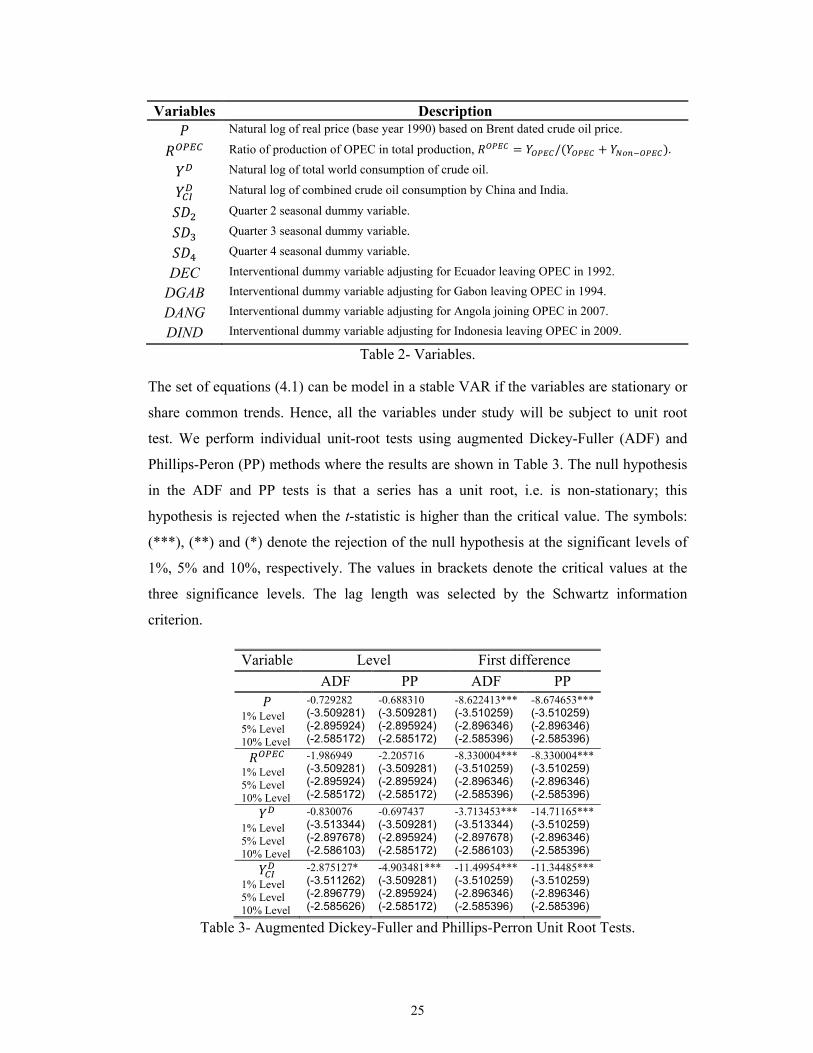
Variables Description Natural log of real price (base year 1990) based on Brent dated crude oil price.
Ratio of production of OPEC in total production,
Natural log of total world consumption of crude oil.
Natural log of combined crude oil consumption by China and India.
Quarter 2 seasonal dummy variable.
Quarter 3 seasonal dummy variable.
Quarter 4 seasonal dummy variable.
DEC Interventional dummy variable adjusting for Ecuador leaving OPEC in 1992.
DGAB Interventional dummy variable adjusting for Gabon leaving OPEC in 1994.
DANG Interventional dummy variable adjusting for Angola joining OPEC in 2007.
DIND Interventional dummy variable adjusting for Indonesia leaving OPEC in 2009.
Table 2- Variables.
The set of equations (4.1) can be model in a stable VAR if the variables are stationary or
share common trends. Hence, all the variables under study will be subject to unit root
test. We perform individual unit-root tests using augmented Dickey-Fuller (ADF) and
Phillips-Peron (PP) methods where the results are shown in Table 3. The null hypothesis
in the ADF and PP tests is that a series has a unit root, i.e. is non-stationary; this
hypothesis is rejected when the t-statistic is higher than the critical value. The symbols:
(***), (**) and (*) denote the rejection of the null hypothesis at the significant levels of
1%, 5% and 10%, respectively. The values in brackets denote the critical values at the
three significance levels. The lag length was selected by the Schwartz information
criterion.
Variable Level First difference
ADF PP ADF PP
1% Level 5% Level 10% Level
-0.729282 (-3.509281) (-2.895924) (-2.585172)
-0.688310 (-3.509281) (-2.895924) (-2.585172)
-8.622413*** (-3.510259) (-2.896346) (-2.585396)
-8.674653*** (-3.510259) (-2.896346) (-2.585396)
1% Level 5% Level 10% Level
-1.986949 (-3.509281) (-2.895924) (-2.585172)
-2.205716 (-3.509281) (-2.895924) (-2.585172)
-8.330004*** (-3.510259) (-2.896346) (-2.585396)
-8.330004*** (-3.510259) (-2.896346) (-2.585396)
1% Level 5% Level 10% Level
-0.830076 (-3.513344) (-2.897678) (-2.586103)
-0.697437 (-3.509281) (-2.895924) (-2.585172)
-3.713453*** (-3.513344) (-2.897678) (-2.586103)
-14.71165*** (-3.510259) (-2.896346) (-2.585396)
1% Level 5% Level 10% Level
-2.875127* (-3.511262) (-2.896779) (-2.585626)
-4.903481*** (-3.509281) (-2.895924) (-2.585172)
-11.49954*** (-3.510259) (-2.896346) (-2.585396)
-11.34485*** (-3.510259) (-2.896346) (-2.585396)
Table 3- Augmented Dickey-Fuller and Phillips-Perron Unit Root Tests.

26
The results show that all variables are non-stationary in levels but become stationary in
first difference. The variable appears stationary under the ADF test and stationary
under the PP test, this is due to higher order autocorrelation not fully captured in the PP
test. The results indicate that we could use a VAR with all the variables in log deviations
from trend in first difference; however, omitting long-run cointegrating relationships if
they exist would be misleading. Thus, we need to perform contegration tests before
deciding how to model our data.
4.2.1 Identifying Long-Run Cointegrating Relationships
Based on the oil price theory, there exists a long run relationship between the crude oil
price and the quantity supplied by OPEC where the other variables may have a role to
play in this relationship as well. Cointegration techniques may be used for modelling this
long-run relationship between non-stationary variables. In the presence of cointegration,
the VAR model becomes a vector error correction model (VECM). The latter can capture
both the short-term and long-term dynamics.
In order to identify long run relationship between variables of interest Johansen’s VAR-
based cointegrating will be used, assuming that all the variables are first-order integrated.
Johansen’s test assumes a linear deterministic trend and the critical values assume no
exogenous series, it includes three seasonal dummy variables SD2, SD3, SD4 as well as
four dummy variables to adjust for the changes in the composition of OPEC, namely,
DANG, DEC, DGAB and DIND. The test uses two lags in first differences (three lags in
levels).
If there are k variables, there could be up to cointegrating relationships. In this
approach, the null hypothesis is tested using a trace statistic against the
alternative hypothesis . Rejecting implies that there is at least one
cointegrating vector. The next step is to test against , and so on.
Table 4 reports results for testing the number of cointegration relations. Note that two
types of test statistics are reported; first, the trace statistics and second, the maximum
eigenvalue statistics. For each block, the first column is the number of cointegrating
relations under the null hypothesis, the second column is the ordered eigenvalues of the
matrix, the third column is the test statistic, and the last two columns are the 5% and 1%
critical values. The trace statistic, reported in the first block, tests the null hypothesis of

27
the cointegrating relations against the alternative of cointegrating relations, where
is the number of endogenous variables, for . The alternative of
cointegrating relations corresponds to the case where none of the series have a unit root
and stationary VAR may be specified in terms of the levels of all of the series. The test
suggests the presence of one cointegrating vector at the 5% significance level. This
means that some variables have one common stochastic trend. The second panel in Table
4, reporting maximum eigenvalue statistics, tests the null hypothesis of the cointegrating
relations against the alternative of cointegrating relations and also shows one
cointegration at the 5% significance level.
Unrestricted Cointegration Rank Test (Trace)
Hypothesized Trace 0.05 No. of CE(s) Eigenvalue Statistic Critical Value Prob.**
None * 0.369889 64.64745 47.85613 0.0006 At most 1 0.147411 26.31310 29.79707 0.1196 At most 2 0.131277 13.07646 15.49471 0.1120 At most 3 0.016677 1.395834 3.841466 0.2374
Notes: Trace test indicates 1 cointegratingeqn(s) at the 0.05 level * denotes rejection of the hypothesis at the 0.05 level **MacKinnon-Haug-Michelis (1999) p-values Unrestricted Cointegration Rank Test (Maximum Eigenvalue)
Hypothesized Max-Eigen 0.05 No. of CE(s) Eigenvalue Statistic Critical Value Prob.**
None * 0.369889 38.33435 27.58434 0.0014 At most 1 0.147411 13.23664 21.13162 0.4307 At most 2 0.131277 11.68062 14.26460 0.1232 At most 3 0.016677 1.395834 3.841466 0.2374
Notes: Max-eigenvalue test indicates 1 cointegratingeqn(s) at the 0.05 level * denotes rejection of the hypothesis at the 0.05 level **MacKinnon-Haug-Michelis (1999) p-values
Table 4- Johansen Cointegration Test Results.
As cointergrating relationship exists among the variables, we will use the vector error
correction model (VECM) that will support the analysis of the cointegration structure.
4.2.2 Exogenous variables
Before presenting the results, it is convenient to explain that some coefficients in the
VECM will be set to zero if variables are weakly exogenous. A set of variables is said

28
to be weakly exogenous for a parameter vector of interest for example , if estimating
within a conditional model does not lead to a loss of information relative to estimating
the vector in a full model that does not condition on . In addition, is said to be
strongly exogenous if it is weakly exogenous for the parameters of the conditional model
and forecasts of can be made conditional on without loss of forecast precision
(Lütkepohl and Krätzig 2007). Performing this kind of tests, we set some parameters to
zero, as is shown in Table 5. We estimated our VECM model twice, with and without
restrictions, and no significant changes were found in the parameter estimates, causality
tests and impulse-reaction analysis. The economic interpretation of these restrictions will
be analysed later.
4.2.3 The Full Model
To gain some clarity in our exposition, we will now proceed to write the full set of
equations in our final VECM specification:
(4.4)
(4.5)
(4.6)
Where (4.7)

29
The lag order was selected by minimized AIC statistics for our dynamic VAR
specification. The parameter estimates and other relevant results are reported below in
Table 5. We are assuming normal distribution of each error term with mean zero and
constant variance , , .
The first thing to note from the results is that a long-run relationship has been
established. The error-correction term suggests that total demand, the demand from
China and India and the ratio of production by OPEC converge to a long-run equilibrium
relationship. The consumption from China and India are obviously related to total
demand as the latter includes the former. What is interesting is that the ratio of
production by OPEC is part of the long run relationship. This gives support to the idea
that the dominant firm-competitive fringe model is relevant in the long run. It also gives
evidence against the hypothesis that it does not matter where the production comes from.
It is also interesting that the price level plays no role in this long-run relationship which
is defined in terms of quantities (tests carried on the coefficient associated with P
suggests that the variable is weakly exogenous, so this coefficient has been set to zero,
which produces no major changes in the model). Essentially, what the results predict is
that the quantities converge to fixed proportions between demand from China and India,
demand from the rest of the world and production by OPEC and non-OPEC countries.
The significance of consumption by China and India gives some evidence to reject
Hypothesis II, whereas the significance of the OPEC ratio provides some evidence
against Hypothesis I.

30
Cointegrating Vector (Eq. 7) (-1) (-1)
P(-1) (-1)
7.419946 -52.43008 0.00000* -8.168689 535.2608
*Cointegration Restrictions: 0, 0, 0; LR test for binding restrictions (rank = 1): Chi-square(3)12.37072 Probability0.00622
Short-Run Parameter Estimates ∆ (Eq. 3) ∆ (Eq. 4) ∆P(Eq. 5) ∆ (Eq. 6)
0.112374 [ 2.87559]
0.014068 [ 2.87845]
-0.020621 [-0.25159]
0.002945 [ 0.93846]
ECM -0.043111 [-4.80494]
0.000289 [ 0.25340]
0.00000* [ NA]
0.00000* [ NA]
∆ (-1) -0.224249 [-2.19741]
0.011190 [ 0.87671]
0.070074 [ 0.32738]
0.017123 [ 2.08977]
∆ (-2) -0.117246 [-1.25108]
0.010633 [ 0.90722]
-0.152064 [-0.77363]
0.002442 [ 0.32450]
∆ (-1) -1.776277 [-2.01091]
-0.172575 [-1.56214]
2.244623 [ 1.21155]
-0.074731 [-1.05370]
∆ (-2) -1.668465 [-1.93785]
-0.605208 [-5.62042]
0.082799 [ 0.04585]
0.027922 [ 0.40392]
∆P(-1) -0.098320 [-1.58065]
-0.004482 [-0.57611]
-0.055805 [-0.42775]
0.008025 [ 1.60691]
∆P(-2) 0.026743 [ 0.41782]
0.001335 [ 0.16683]
-0.032223 [-0.24003]
0.003611 [ 0.70276]
∆ (-1) 0.491068 [ 0.31232]
0.143364 [ 0.72906]
0.490503 [ 0.14874]
0.001617 [ 0.01281]
∆ (-2) -2.439893 [-1.66042]
-0.071256 [-0.38773]
1.098999 [ 0.35658]
-0.022492 [-0.19064]
SD2 0.007614 [ 0.21678]
-0.021944 [-4.99528]
0.171650 [ 2.32999]
-0.002312 [-0.81983]
SD3 -0.056199 [-1.12996]
-0.000833 [-0.13392]
0.209610 [ 2.00937]
0.000688 [ 0.17229]
SD4 0.023574 [ 0.51445]
-0.002522 [-0.44009]
0.042425 [ 0.44142]
-0.000170 [-0.04616]
DEC 0.083479 [ 1.81929]
0.012614 [ 2.19813]
0.141830 [ 1.47369]
0.007406 [ 2.01024]
DGAB -0.099456 [-2.29194]
-0.004508 [-0.83060]
-0.056574 [-0.62160]
-0.005662 [-1.62497]
DANG 0.029524 [ 0.81421]
0.004151 [ 0.91525]
-0.010817 [-0.14223]
-0.003684 [-1.26541]
DIND -0.127258 [-2.59589]
-0.016942 [-2.76336]
-0.190411 [-1.85187]
-0.005968 [-1.51625]
R-squared Adj. R-squared Sum sq. resids. S.E. equation F-statistic Log likelihood Akaike AIC Schwarz SC Mean dependent S.D. dependent
0.564579 0.459022 0.434893 0.081174 5.348589 100.1652 -2.003981 -1.508556 0.038809 0.110364
0.805760 0.758671 0.006802 0.010152 17.11157 272.7150 -6.161807 -5.666382 0.003517 0.020666
0.189806 -0.006605 1.913152 0.170256 0.966372 38.68678 -0.522573 -0.027148 0.017130 0.169697
0.237370 0.052490 0.002804 0.006517 1.283914 309.5005 -7.048204 -6.552779 0.000383 0.006696
Determinant resid. covariance (dof adj.) Determinant resid covariance Log likelihood Akaike information criterion Schwarz criterion
5.40E-13 2.16E-13 736.9036 -16.02177 -13.92350
Table 5- Vector Error Correction Estimates (t-statistics in [ ]).

31
The dynamic adjustment towards the long-run equilibrium is defined by the estimates
vector . The speed of adjustment in equation (4.3) is which
suggests that each quarter the consumption by China and India make an adjustment of
4.311% towards the equilibrium relationship (recall that the variables are expressed in
natural logarithms). The speed of adjustment in equation (4.4) is much slower: total
demand adjusts towards the long-run equilibrium at the average rate of 0.0289% per
quarter. The speeds of adjustment for equations (4.5) and (4.6) explaining and
, respectively were negligible, meaning that the adjustment towards the long-run
equilibrium is not driven by these two variables. These results suggest that the
consumption by China and India have to adjust quickly to the market conditions that
change at a much slower pace over time. This preliminary result will be enriched and
better analysed with the aim of short-run responses in the sections to come.
The R-squared statistics for and are high and hence indicate the success of the
model in predicting the values of these dependent variables within the sample. However,
for the two last variables it seems to be indicating a poorly fitting of the model as one of
the values is even negative. On the other hand, the coefficients of correlation for
and are not high, meaning that these two variables are subject to large shocks
which cannot be fully explained by the model. This is expected, for instance, short-run
price shocks associated with political events in the Middle-East have not been modelled
through dummy variables, but assessing their impact is not the main purpose of the
model. We choose to keep all the variables in the VAR to provide a dynamic analysis of
the relationships between the variables. Further analysis of the shocks is carried through
impulse-reaction functions later.
The F-statistic reported in Table 5 tests the hypothesis that all of the slope coefficients
(excluding the constant, or intercept) are equal to zero at the same time in a given
equation of the VAR model. The p-values reported in Table 5 are essentially zero, so we
reject the null hypothesis that all of the regression coefficients are zero.
4.2.4 Granger Causality: Block Exogeneity Wald Test in VAR
The Granger causality tests are an important vehicle for understanding the dynamics
behind the short-run coefficient estimates in Table 5. In each equation (4.3)-(4.6), the

32
null hypothesis of this test states that all the coefficients associated with a particular
variable are equal to zero; rejection of this hypothesis implies causality. With this test, it
is possible to find well-defined unidirectional causality, bidirectional causality or no
causality.
The results are summarized in Table 6 Unfortunately, the results indicate no clear
causality explaining , which was of interest in our research. According to
economic theory, in the long-run, we would expect the ratio of OPEC’s production to
affect total consumption as well as the prices of oil but we could not find such a causal
link. The results only suggest causality from total consumption and consumption by
China and India. This means that past values of total consumption will improve the
accuracy of the forecast of the combined consumption of China and India. When
interpreting these results, it is important to consider the limitations of short-run Granger
causality tests. For instance, a variable not included in the model (such as income by
different group of countries) may be Granger-causing total consumption, consumption by
China and India and the ratio of production by OPEC. The absence of Granger-causality
tests carried in this model does not imply that there is no causality at all between the
variables. Extensive literature has covered causality between income and different types
of energy consumption, but this question was not pursued here. If we had found
significant Granger-causality in this section, we could have extracted some information
from it, but its absence suggests that further research needs to be done to investigate
casual links.
LOG( ) LOG( ) LOG(P) DLOG( )
LOG( ) - No No No
LOG( ) Yes - No No
LOG(P) No No - No
DLOG( ) No No No -
Table 6- Summary of Causality Test Results. (‘Yes’ indicates a statistically significant causation running from
a row variable to a column variable at 5% significance level.)

33
4.2.5 Restricted Variance Decomposition
The variance decomposition analyses the impact of an exogenous shock to one of the
variables by analysing how the n-period ahead forecast innovations are explained. When
the elements of the covariance matrix off the main diagonal are zero, the dynamic
response to the shock is simply driven by the autoregressive parameters. The variance
decomposition in this sections analyses the possibility of contemporaneous shocks (for
example, if there is a shock to oil demand, it would seem reasonable to assume a
contemporaneous shock to oil production will accompany it). In Table 7, we report the
percentage contributions of the four identified shocks to the forecast error variance of the
four variables at various horizons in the variance decomposition based on the estimated
VAR(2).
The Cholesky decomposition is applied to the reduced form residuals with the following
variable ordering , , and . The forecast error for is determined by
shocks to at the next period but not to the other variables, that is only
shocks today affect the forecast error. According to section I of Table 7, at two quarters
forecast, about 2.52% and 1.69% of the forecast error variance of the changes in
can be accounted for by and shocks, respectively. This does not increase by more
than that over the twenty quarters horizon.
Section II of Table 7 analyses shocks that are contemporaneous to and ,
following the order of the Cholesky variance decomposition. At one quarter forecast,
about 7.74% of the forecast error variance in can be accounted for by shock.
This increases to 9.28% for a two quarters horizon and to 15.67% at twenty quarters
horizon. Interestingly, explains 9.18% of the forecast error variance of the changes in
at five quarters horizon and this increase to 46.06% at twenty quarters horizon.
Whereas does not expain more than 3% over the twenty quarters horizon and the rest
of the changes is explained by itself. We conclude that demand shocks coming from
China and India provoke a later reaction in OPEC production and have little influence on
oil price.
With a similar analysis technique, we arrive at the conclusion that Section III of Table 7
indicates that is an important factor for ’s fluctuations.

34
Finally, section IV of Table 7 indicates that shocks to oil price are on average more
correlated to shocks in demand that lead to increased production than changes in the
production of OPEC relative to total consumption.
I. Variance Decomposition of ∆ :
Period S.E. ∆ ∆ ∆ ∆
1 0.081174 0.000000 0.000000 0.000000 100.0000
2 0.089832 2.517385 0.194015 1.689863 95.59874
3 0.093816 2.797492 0.174290 2.753945 94.27427
4 0.101388 2.687978 0.382809 3.362629 93.56658
5 0.108992 2.633144 0.426195 3.683207 93.25745
… … … … … …
20 0.199152 1.816226 1.132068 4.808487 92.24322
II. Variance Decomposition of ∆ :
Period S.E. ∆ ∆ ∆ ∆
1 0.010152 92.25559 0.000000 0.000000 7.744405
2 0.013433 87.76563 0.018882 2.940034 9.275454
3 0.013777 88.53064 0.179766 2.713430 8.576159
4 0.014508 84.52785 4.654393 2.514393 8.303366
5 0.016593 79.22335 9.178521 2.487652 9.110478
… … … … … …
20 0.028634 37.45038 46.05621 0.824107 15.66930
III. Variance Decomposition of ∆ :
Period S.E. ∆ ∆ ∆ ∆
1 0.170256 10.53841 82.74272 0.000000 6.718869
2 0.241891 12.68436 77.23046 0.273208 9.811965
3 0.289757 14.20036 75.30217 0.324262 10.17321
4 0.332419 13.98999 76.18584 0.292668 9.531497
5 0.370522 12.95406 77.89136 0.244847 8.909738
… … … … … …
20 0.734792 13.15491 77.27902 0.212168 9.353907
IV. Variance Decomposition of ∆ :
Period S.E. ∆ ∆ ∆ ∆
1 0.006517 10.64313 3.736481 84.66783 0.952560
2 0.009671 12.56162 6.437379 79.34009 1.660915
3 0.011997 11.64703 7.018212 79.07894 2.255811
4 0.013894 11.57433 6.333815 79.78799 2.303868
5 0.015609 11.48792 6.302312 79.77993 2.429840
… … … … … …
20 0.032160 11.49308 6.202312 79.48522 2.819393
Cholesky Ordering: , , ,
Table 7- Forecast Error Variance Decomposition for the Four Variables.

35
4.2.6 Impulse Responses
In this section, we introduce impulse-response analysis to provide a more graphical
interpretation of the variance decompositions. Impulse responses trace out the
responsiveness of the dependent variables in the VAR to shocks to each of the variables
as represented in Figure 5. The shocks do not converge to zero as the restrictions
imposed imply that the shocks are permanent.
Figure 5- Impulse Response Analysis.
response to a shock in and is just below 0.02 in the first period, this shows
that OPEC is quick in responding to demand or price shocks. However, it only responds
to a shock in in the second period. This makes sense as shocks in world consumption
are likely to be more significant, hence OPEC is expected to take some time to increase
oil production.
Not surprisingly, does not absorb price shocks as negative values are obtained for all
the periods observed, this can be explained by the fact that the price elasticity of demand
of China and India is more elastic than total demand: large changes in oil prices have
more influence on the combined consumption by China and India. The same pattern can
be observed from the response of to a shock in .
Res
pons
e of
:
To a shock in:
-.002
.000
.002
.004
.006
.008
2 4 6 8 10 12 14 16 18 20
Response of R_P_OPEC to L_TC_P_CHINA_P_INDIA
-.002
.000
.002
.004
.006
.008
2 4 6 8 10 12 14 16 18 20
Response of R_P_OPEC to L_T_C
-.002
.000
.002
.004
.006
.008
2 4 6 8 10 12 14 16 18 20
Response of R_P_OPEC to L_R_PRICE
-.002
.000
.002
.004
.006
.008
2 4 6 8 10 12 14 16 18 20
Response of R_P_OPEC to R_P_OPEC
-.02
.00
.02
.04
.06
.08
2 4 6 8 10 12 14 16 18 20
Response of L_TC_P_CHINA_P_INDIA to L_TC_P_CHINA_P_INDIA
-.02
.00
.02
.04
.06
.08
2 4 6 8 10 12 14 16 18 20
Response of L_TC_P_CHINA_P_INDIA to L_T_C
-.02
.00
.02
.04
.06
.08
2 4 6 8 10 12 14 16 18 20
Response of L_TC_P_CHINA_P_INDIA to L_R_PRICE
-.02
.00
.02
.04
.06
.08
2 4 6 8 10 12 14 16 18 20
Response of L_TC_P_CHINA_P_INDIA to R_P_OPEC
-.002
.000
.002
.004
.006
.008
.010
2 4 6 8 10 12 14 16 18 20
Response of L_T_C to L_TC_P_CHINA_P_INDIA
-.002
.000
.002
.004
.006
.008
.010
2 4 6 8 10 12 14 16 18 20
Response of L_T_C to L_T_C
-.002
.000
.002
.004
.006
.008
.010
2 4 6 8 10 12 14 16 18 20
Response of L_T_C to L_R_PRICE
-.002
.000
.002
.004
.006
.008
.010
2 4 6 8 10 12 14 16 18 20
Response of L_T_C to R_P_OPEC
.00
.04
.08
.12
.16
2 4 6 8 10 12 14 16 18 20
Response of L_R_PRICE to L_TC_P_CHINA_P_INDIA
.00
.04
.08
.12
.16
2 4 6 8 10 12 14 16 18 20
Response of L_R_PRICE to L_T_C
.00
.04
.08
.12
.16
2 4 6 8 10 12 14 16 18 20
Response of L_R_PRICE to L_R_PRICE
.00
.04
.08
.12
.16
2 4 6 8 10 12 14 16 18 20
Response of L_R_PRICE to R_P_OPEC
Response to Cholesky One S.D. Innovations

36
It can also be seen from the estimations that responds with no lags to a shock in
showing the significant impact of OPEC’s production decisions on price.
Some information can also be drawn from the contemporaneous correlation of the error
term as represented in Table 8.
LOG( ) LOG( ) LOG( )
1 0.6668733 0.5746587 0.5100631
LOG( )
0.6668733 1 0.8398973 0.7267639
LOG( )
0.5746587 0.8398973 1 0.9488617
LOG( )
0.5100631 0.7267639 0.9488617 1
Table 8- Correlation Matrix.
It reflects the degree to which new information producing an abnormal change in one
variable is shared by other variables in the same quarter. The world consumption and the
combined consumption of China and India exhibit the highest correlation. Whereas the
correlation for OPEC’s production and the world consumption as well as the combined
consumption of China and India is relatively lower. This pattern of contemporaneous
correlations is consistent with what we expect from the structure between pairs of
variables. In line with the general observations made above, the contemporaneous
correlations of the real price and the combined consumption of China and India are quite
strong. However, the correlation between the real price and the total consumption is
higher. This is not quite consistent with what we have observed in the impulse responses
as the price responded less strongly to a shock in total consumption than to a shock in the
combined consumption of China and India. The strong correlation between the world
consumption and the combined consumption of China and India is probably due to the
fact that the consumption of China and India is included in the total world consumption.

37
5. Conclusions
Our research questions focused on the role of OPEC and non-OPEC production and
implications of increased demand in China and India. The research was conducted in
several steps. We proposed a reduced set of equations to test two specific hypotheses (for
which we expected rejection). Hypothesis I stated that OPEC producers are not different
to non-OPEC producers. Hypothesis II stated that demand from China and India is not
different than demand from the rest of the world, i.e. it does not matter where demand
comes from. Both hypotheses were rejected by the estimation results. This gives support
to the following ideas: (i) the (modified) dominant firm-competitive fringe model is
relevant in the short- and long-run, and (ii) the combined demand from China and India
is found to exhibit different characteristics than total demand. The most significant
contribution in our VAR model can be found in the long-term cointegrating relationship.
Through the estimation of a vector error-correction term, the data suggest that the
consumption by China and India shares a long-term relationship with total demand and
the ratio of OPEC production to total production. Interestingly, prices do not play a role
in this long-term relationship between proportional quantities of supply and demand. We
would naturally expect a long-run relationship between total demand and demand from
China and India as the former includes the latter (in the similar way as macroeconomists
include GDP and consumption in an error-correction term). The finding that the ratio or
production by OPEC to total production is a contributor to this long-term relationship is
also an interesting result.
In our empirical VAR model, we concentrated our efforts in trying to improve the setup
in Mu and Ye (2011). Despite using a different setup, our findings on Granger causality
are consistent with Mu and Ye (2011): no economically significant causality was found
between the variables (the absence of Granger-Causality tests does not suggest that there
is no causality between the variables, and further research needs to be done in order to
investigate potential causal links). In the impulse-reaction analysis conducted later we
have found some interesting results, although these results may be subject to the setting
of our Cholesky variance decomposition. The combined demand from China and India
was found to be more price elastic than the total demand. In other words, crude oil
demand by developed or low-growth countries are more price-inelastic. This result sets
the basis for further future research.

38
This result was, somehow, surprising. However, a careful re-consideration of the issue
leads us to think that this finding can be explained, although there are confronting
factors. China and India’s infrastructure constraints could deprive them from fast
adaption to pacey economic growth, which would suggest that the demand in these
countries should be relatively inelastic. On the other hand, microeconomic theory
suggests that lower income economies such as China and India would be more sensitive
to changes in the prices of the goods they consume compared to higher income countries.
The overall econometric results suggest that the second argument prevails. Figure 5 also
suggests that China and India have high price-elasticity in the short-run but relatively
inelastic in the medium-run. We also found that an increase in OPEC production relative
to the total production produces a significant increase in consumption in China and India
during the first two quarters (increased OPEC production decreases the oil price which in
turn leads to higher consumption). As later pointed out, the main contribution of was not
measuring elasticities but identifying a long-run equilibrium structure. The identification
of the error-correction term was independent from the variance decomposition that was
applied later.
Overall, this paper has contributed by, at least, partially answering some of the most
important questions for today’s global crude oil market.
References
Aguiar-Conraria, Luís, and Yi Wen. 2012. “OPEC’s Oil Exporting Strategy and
Macroeconomic (In)Stability.” Energy Economics 34 (1): 132-136.
Alhajji, Anas, and David Huettner. 2000a. “OPEC and World Crude Oil Markets from
1973 to 1994: Cartel, Oligopoly, or Competitive?” The Energy Journal 21 (3): 31-
60.
Alhajji, Anas, and David Huettner. 2000b. “The Target Revenue Model and the World
Oil Market: Empirical Evidence from 1971 to 1994.” The Energy Journal 21 (2):
121-144.
Bai, Jim, and Chen Aizhu. 2012. “PetroChina in Talks with Shell, Hess to Explore Shale
Oil.” Reuters. http://in.reuters.com/article/2012/04/05/us-china-oil-shale-
idINBRE83405920120405

39
Barsky, Robert B., and Lutz Kilian. 2004. “Oil and the Macroeconomy Since the 1970s.”
The Journal Economic Perspectives 18 (4): 115-134.
Bhattacharyya, Subhes C. 2011. Energy Economics: Concepts, Issues, Markets and
Governance. London: Springer-Verlag.
BP (British Petroleum). 2012. BP Energy Outlook 2030. January.
http://www.bp.com/liveassets/bp_internet/globalbp/globalbp_uk_english/reports_a
nd_publications/statistical_energy_review_2011/STAGING/local_assets/pdf/2030_
energy_outlook_booklet.pdf
BP (British Petroleum). 2011. BP Statistical Review of World Energy. June.
bp.com/statistical review
Brémond, Vincent, Emmanuel Hache, and Valérie Mignon. 2012. “Does OPEC still
Exist as a Cartel? An Empirical Investigation. ”Energy Economics 34 (1): 125-131.
Burns, Stuart. 2012. OilPrice.com. “Oil Prices Could Follow Gas Prices Down as
Demand Decreases.” http://oilprice.com/Energy/Oil-Prices/Oil-Prices-could-
Follow-Gas-Prices-as-Demand-Decreases-and-Production-Increases.html
Dahl, Carol A. 2011. International Energy Markets: Understanding Pricing, Policies,
and Profits. Tulsa: Penn Well.
Dahl, Carol, and Mine Yücel. 1991. “Testing Alternative Hypotheses of Oil Producer
Behaviour.” The Energy Journal 12 (4): 117-137.
Energy & Capital. 2012. “Brent vs. WTI.”
http://www.energyandcapital.com/resources/brent-vs-wti
Griffin, James M. 1985. “OPEC Behaviour: A Test of Alternative Hypotheses.” The
American Economic Review 75 (5): 954-963.
Gülen, Gürcan. 1996. “Is OPEC a Cartel? Evidence from Cointegration and Causality
Tests.” Energy Journal 17 (2): 43-57.
Hamilton, James. 2009a. “Understanding Crude Oil Prices.” The Energy Journal 30 (2):
179-206.
Hamilton, James. 2009b. “Causes and Consequences of the Oil Shock of 2007-08”
Brookings Papers on Economic Activity, Spring: 215-261.

40
Hershey Jr., Robert D. 1989. “Worrying A New Over Oil Imports.” The New York Times.
http://www.nytimes.com/1989/12/30/business/worrying-anew-over-oil-
imports.html?pagewanted=all&src=pm
(IEA) International Energy Agency. 2012. “Iraq Energy Outlook.” November.
http://iea.org/publications/freepublications/publication/WEO_2012_Iraq_Energy_
OutlookFINAL.pdf
Jones, Clifton. 1990. “OPEC Behaviour under Falling Prices: Implications for Cartel
Stability.” The Energy Journal 11 (3): 117-129.
Kilian, Lutz. 2009. “Not All Oil Price Shocks Are Alike: Disentangling Demand and
Supply Shocks in the Crude Oil Market.” American Economic Review 99 (3):
1053-1069.
Koepp, Stephen. 1986. “Cheap Oil!” Time Magazine.
http://www.time.com/time/printout/0,8816,961087,00.html
Kriechene, Noureddine. 2002. “World Crude Oil and Natural Gas: A Demand and
Supply Model.” Energy Economics 24 (6): 557-576.
Li, Hong, and Sharon Xiaowen Lin. 2011. “Do Emerging Markets Matter in the World
Oil Pricing System? Evidence of imported crude oil by China and India.” Energy
Policy 39: 4624-4630.
Lütkepohl, Helmut and Markus Krätzig. 2007. Applied Time Series Econometrics. New
York: Cambridge University Press.
Matthies, Klaus. 2003. “Oil Prices Decline as Concerns about Supply Lessens.”
Intereconomics 38 (2): 109-112.
Moran, Theodore. 1981. “Modelling OPEC Behaviour: Economic and Political
Alternatives.” International Organization 35 (2): 241-272.
Mu, Xiaoyi, and Haichun Ye. 2011. “Understanding the Crude Oil Price: How Important
Is the China Factor?” The Energy Journal 32 (4): 71-94.
OPEC (Organization of the Petroleum Exporting Countries). 2012. “Brief History.”
http://www.opec.org/opec_web/en/about_us/24.htm

41
Powell, Stephen G. 1990. “The Target Capacity Utilization Model of OPEC and the
Dynamics of the World Oil Market.” Energy Journal 11(1): 27-63.
Ripple, Ronald. 2009. “International Energy Derivatives Markets,” in International
Handbook on the Economics of Energy, edited by Joanne Evans and Lester C.
Hunt, 705-739. Northampton: Edward Elgar.
Ripple, Ronald. 2008. “Have Oil Futures Traders Driven up the Market?” Oil and Gas
Journal 106 (37): 24-26.
Rousseau, David L. 2008. History of OPEC. Liberty Park USA Foundation.
http://www.libertyparkusafd.org/Hale/reports%5CHistory%20of%20OPEC.pdf
Shone, Ronald. 2002. Economic Dynamics: Phase Diagrams and their Economic
Application. 2nd ed. New York: Cambridge University Press.
Skeer, Jeffrey, and Yanjia Wang. 2007. “China on the Move: Oil Price Explosion?”
Energy Policy 35 (1): 678-691.
Smith, James L. 2009. “World Oil: Market or Mayhem?” Journal of Economic
Perspectives 23 (3): 145-164.
Tvergerg, Gail. 2011. “Why are WTI and Brent Prices so Different?”
http://ourfiniteworld.com/2011/02/19/why-are-wti-and-brent-prices-so-different/
EIA (US Energy Information Administration.) 2012. “Countries.”
http://www.eia.gov/countries/
USGS (United States Geological Survey). 2006. Geology and Resources of Some World
Oil-Shale Deposits Scientific Investigations Report 2005–5294. Reston, Virginia:
U.S. Geological Survey. http://www.usgs.gov/sir/2006/5294
Varian, Hal R. 1992. Macroeconomic Analysis. 3rd ed. New York: W. W. Norton &
Company, Inc.
Williams, James L. 2011. “Oil Price History and Analysis.”
http://www.wtrg.com/prices.htm
Related Documents