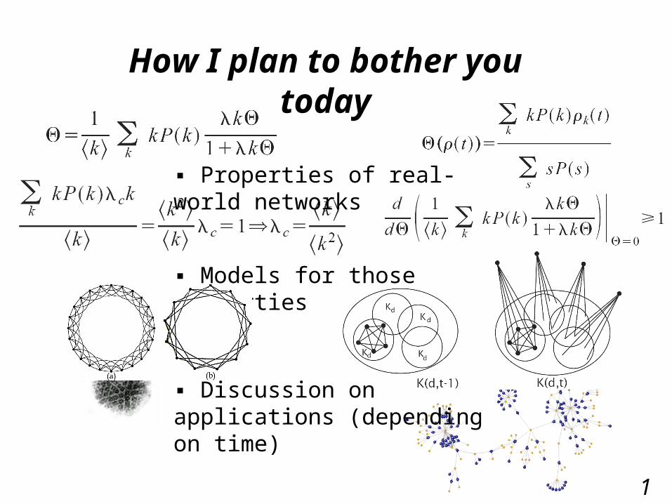
How I plan to bother you today ▪ Discussion on applications (depending on time) 1 ▪ Properties of real-world networks ▪ Models for those properties.

How I plan to bother you today

▪ Discussion on applications (depending on time)

1

▪ Properties of real-world networks

▪ Models for those properties

Basic Properties – Small World – Scale Free – Static models – Dynamics

2

• We analyze the structure of (big) networks from the real-world to understand which properties are underlying them.

• If a general class of network has a given property then we can use it to reason about any unknown network of this class.

What do we do in complex network?

Social Network

Biological network

Blogs Facebook Population

Property: some individuals are very social compared to other ones.

Goal: spread a saucy rumor!

Idea: whatever the network as long as it’s a social network, try to target the

social individuals.

• There is a tremendous number of applications and since the main two properties were discovered in 1998, there has been hundreds if not thousands of papers on complex networks.

How strong is the connection from A to C?

What is the influence of A over C in the social network?

How likely is it that if A is infected by a virus then C will get infected?


3

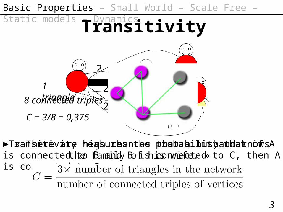
Transitivity

« There are high chances that a husband knows the family of his wife. »

11

11

2

2

2

►Transitivity measures the probability that if A is connected to B and B is connected to C, then A is connected to C.

1 triangle

8 connected triples

C = 3/8 = 0,375


4

Network Motifs• When we looked for transitivity, we basically counted the number of subgraphs of a particular type (triangles and triples).

• We can generalize this approach to see which patterns are ‘very frequent’ in the network. Those patterns are called network motifs.

• To measure the frequency, we compare with how expected it is to see such patterns in a random network.

• The significance profile (SP) of the network is a vector of those frequencies.

• For each subgraph, we measure its relative frequency in the network.

• As we are measuring for the 13 possible directed connected graphs of 3 vertices, it is called a triad significance profile (TSP).

• 4 networks of different micro-organisms are shown to have very similar TSPs, and in particular the triad 7 called « feed-forward loop ».


5

Let’s play the Kevin Bacon Game.

Think of an actor or an actress…

→ If they’ve been in a film with him, they have Bacon Number one.

→ Otherwise, if they have been in a film with somebody who has Bacon Number one, then they have Bacon Number two, etc.

Hollywood’s world is pretty large. What do you think is the average Bacon Number an american actor will get?

Only 4 !

Laurence Fishburne (alias Morpheus in Matrix)

Played with Kevin Bacon in Mystic Rivers !

Mos Def (in The Italian Job) played with Kevin Bacon in The

Woodsman


6

The Small-World property• Through this Kevin Bacon’s experiment, we know that although the network of actors is quite big, the average distance is very small.

• A network is said to have the small-world property if the average shortest path L is at most logarithmically on the network size N.

→ An e-mail network of 59 812 nodes… L = 4.95 !

→ Actor network or 225 226 actors… L = 3.65 !

• It tells you that transmitting information in small-world networks will be very fast. And so, transmitting viruses will be fast too…

• Some authors defined the small-world property with an additional constraint with the presence of a high clustering. It’s a choice…

At a local level, we have strongly connected communities.

Efficient to exchange information at a local scale.

Efficient to exchange information at a global scale.

Global efficiency of small-world networks.

This value is the typical size.


Many of the things we measure are centered

around a particular value.

However, there are things that have an enormous variation in the distribution.

If we plot this histogram with logarithmic horizontal and vertical axis, a pattern will clearly emerge: a line.

In a normal histogram, this line is p(x) = -αx + c. Here it’s log-log, so:

ln p(x) = -α ln x + c

apply exponent e

p(x) = ecxc -α

We say that this distribution follows a power-law, with exponent α.

7

The Scale-Free property

A power law is the only distribution that is the same whatever scale we look at it on, i.e. p(bx) = g(b)p(x). So, it’s also called scale-free.


8

We found that the population has the scale-free property!

In 1955, Herbert Simon already showed that many systems follow a power law distribution, so that’s neither new nor unique.

• Sizes of earthquakes

• Moon craters

• Solar flares

• Computer files

• Wars

• Number of citations received / paper

• Number of hits on web pages

• People’s annual incomes


It has been found that the distribution of the degree of nodes follows a power-law in many networks, i.e. many networks are scale-free…

What is important is not so much to find a power-law as it’s common, but to understand why and which other structural parameters can be there.


9


Myth and reality• Scaling distributions are a subset of a larger family of heavy-tailed distributions that exhibit high variability.

• One important claim of the litterature for scale-free networks was the presence of highly connected central hubs.

• However, it only requires high variability and not strict scaling…

• It was said that « the most highly connected nodes represent an Achilles’ heel »: delete them and the graph breaks into pieces.

• Recent research have shown that complex networks that claimed to be scale-free have a power-law but not this Achilles’ heel.

• One mechanism was used to build scale-free networks, called preferential attachment, or « the rich get richer ».

• It is only one of several, and not less than 7 other mechanisms give the same result, so preferential attachment gives little or no insight in the process.


10

Other measurements• We have the clustering, distribution of degree, etc. Are there other global characteristics relevant to the performances of the network, in term of searchability or stability?

• Rozenfeld has proposed in his PhD thesis to study the cycles, with algorithms to approximate their counting (as it’s exponential otherwise).

• Using cycles as a measure for complex networks has received attention:Inhomogeneous evolution of subgraphs and cycles in complex

networks (Vazquez, Oliveira, Barabasi. Phys. Rev E71, 2005).

Degree-dependent intervertex separation in complex networks (Dorogovtsev, Mendes, Oliveira. Phys Rev. E73 2006)

• See also studies on the correlation of degree (i.e. assortativity).


11

Random graphs• The earliest model was made formal by Erdos and Rényi (although discovered independly by Rapoport 10 years before).

• We have N vertices, and two vertices are connected with probability P.

• The goal was not to study properties such as small-world or scale-free (it wasn’t even known). This theory is interested in the properties that happen for large graph size, i.e. for n → ∞.

• To illustrate the main property of those graphs, let’s go through an example…

Suppose that a porous stone is immerged in a bucket of water.

What is the probability that the centre of the stone is moistened?

Let’s model it!A fluid can flow through channels if they are wide enough.

A channel has a probability p of being wide enough, and 1 – p too small.If we model this in two dimensions, we have some grids (square lattice).

Is there a path from the center to the side?

Above a threshold pc, a cluster containing vertices in the center and having path to

the side will appear!The system behaves very differently for p < pc and p > pc : it’s sharp!

For a sharp transition, think of water in a glass and the pc = 0 degree.


12

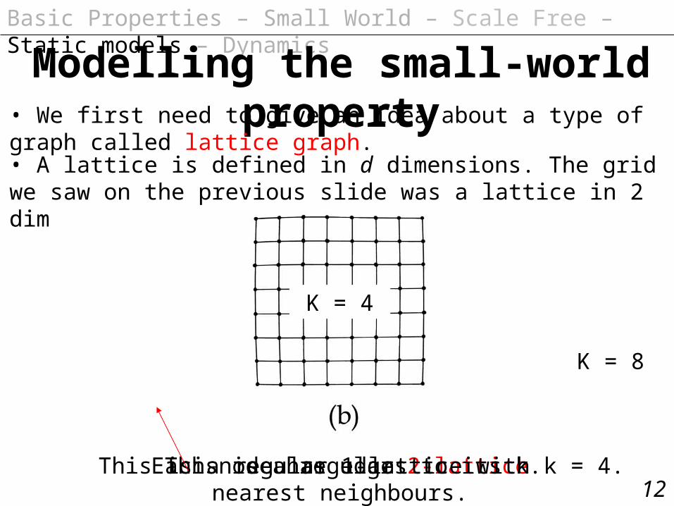
Modelling the small-world property• We first need to give an idea about a type of graph called lattice graph.

• A lattice is defined in d dimensions. The grid we saw on the previous slide was a lattice in 2 dimensions, i.e. a 2-lattice.

This is a regular 2-lattice.Each node has edges to its k nearest neighbours.

K = 4

K = 8

This is a regular 1-lattice with k = 4.


12

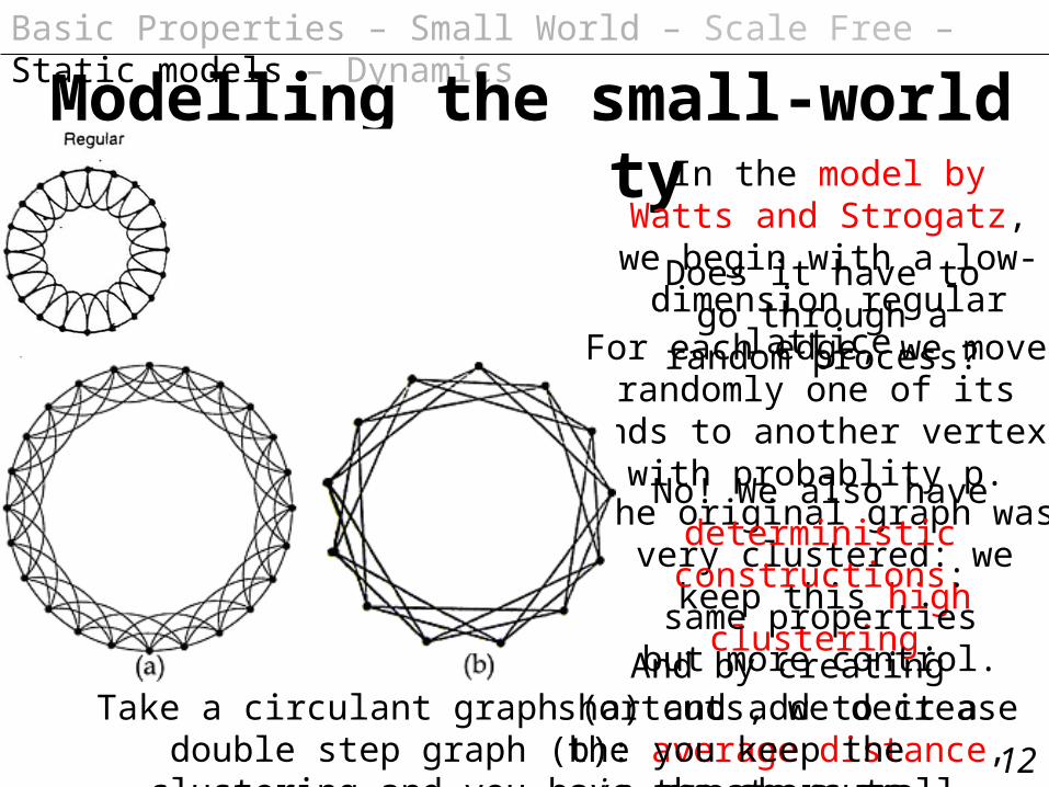
Modelling the small-world propertyIn the model by Watts and Strogatz, we begin with a

low-dimension regular lattice.

For each edge, we move randomly one of its ends to

another vertex with probablity p.

The original graph was very clustered: we keep this high

clustering.

And by creating shortcuts, we decrease the average distance, i.e. create a small-world effect.

Does it have to go through a random

process?

No! We also have deterministic constructions: same properties but more

control.

Take a circulant graph (a) and add to it a double step graph (b): you keep the clustering and you have the shorcuts.


13

Scale-free networksStart with a complete graph of N vertices (a

dense group).

Make N – 1 copies.

Link the root (red) to all vertices but the copies of the root.

Repeat the process.

This construction was generalized in

the family of graphs Hn,k.

Start with a group of n nodes and iterate k

steps (i.e. build k levels).

• It has a scale-free distribution of degrees.

• It has a high clustering: for a node with k links, its clustering is C(k) ~ 1/k.

• Its diameter is 2k – 1 (this network is not small-world).


14

Scale-free and small-world• This family Kn,k is defined in a similar way than the previous one:

∙ Start at k = 0 with a complete graph Kn.

∙ Do k times the following:

Add one vertex for each of the existing Kn and connect it to all vertices of this Kn.

same

change

Let’s start our example with K3.There is one K3 so we add one

node.

No other K3 in the graph: next level.

For each of the 4 possible K3, we add one node.


15

Preferences of newcomers• Another very popular way to model networks is to reproduce the growth processes taking place in the real world: new nodes come in!

• So, the most common way of generating a scale-free network is to use preferential attachment.

→ When a new node arrives, it prefers to link to the most popular nodes.

• Herbert Simon showed in 1955 that power laws are encountered when the rich get richer: the more we already have, the more we get.

• In 1965, Derek de Solla Price set up a model where the probability that a new node links to another one is proportional to kin + 1, where kin is the incoming degree of the node.

I’m new! Who should I get in

touch with?

Only one person knows Tracy,

it’s unlikely that we get in touch...

Bob and Ted are really cool guys, everybody knows

them so we’ll meet


16

The Barabasi-Albert (BA) model• Price’s model created a directed graph with variables number of edges added at each node. It gives the degree distribution pk ~ k .

-(2+1/m)

• Thirty years after, in 1999, Barabasi and Albert came with their model: undirected, constant number of edges, always gives pk ~ k .

-3

∙ The BA model is the most famous and ‘started’ the field. Why?

They gave an important situation where this model has a strong potential: the Web.

• You decided to start your website, and it’s time to create a ‘link’ section.

∙ Most likely, you will link to popular websites, making them even more popular (i.e. it creates a feedback loop system → rich get richer).


17

Including assortativity in a model• Krapivsky and Redner have considered a directed version of the BA model with degree-degree correlations (which we don’t have in BA).

• In general, Sokolov and Xulvi-Brunet have proposed a simple algorithm to make a network assortative with a parameter p:

1. Choose randomly two links.

2. Order their four end-nodes with respect to their degree.

1

2

3

4

3. Rewire with probability p to connect small vertices and high ones together, or 1 – p for random.

If you repeat, you make the network assortative and you keep the degree distribution.


18

Generalization of the BA model• The Dorogovtsev-Mendes-Samukhin (DMS) model adds a parameter k0 to the equations of preferential attachment. If k0 = 0, we have the BA.

• Krapivsky has shown that if we have a nonlinear attachment probability, then we don’t have a power law but an exponential: a single nodes take all the newcomers.

• The Albert and Barabasi (AB) model uses two more parameters p and q to rewire changes on the connections after a node has been attached.

• Solé-Pastor Satorras-Smith-Kepler (SPSK) model uses 3 mechanisms.

∙ Duplicate (copy a randomly selected node with its connection)

∙ Divergence (some connections of a duplicate are removed)

∙ Mutate (connections are added to the duplicate)

It produces power-law but unrealistic assortativity and clustering.

• A more realistic one with duplication and divergence is the Vazquez – Flammini – Maritan – Vespignani (VFMV) model.


19

Triangle-generating protocol• In the same way that many sets of rules can guide a dynamic process toward to be scale-free, how can it guide it to be small-world?

• Remember the example: when you marry somebody, it’s quite likely that you will get to know his/her family (whether you want it or not).

• Nodes are dynamically introduced to each other by a common node:

∙ One random node chooses randomly two of its neighbours and link them. If the node has less than 2 neighbours, it links to a random node.

∙ With probability p, a random node is removed with its links, and replaced by a new node with a randomly chosen neighbour.

References

For Network Motifs, see Superfamilies of evolved and designed networks by Ron Milo et al., Science 303 1538 (2004).

For a number of mechanisms to get a power-law, see Power laws, Pareto distributions and Zipf’s law, M. E. J. Newman (2006)

The story of the porous stone in the bucket of water is called percolation theory. See Harry Kesten, What is percolation?, Notices of the American

Mathematical Society Vol. 53 No. 5 (2006)

Francesc Comellas, Complex Networks: Deterministic Models, Physics and Theoretical Computer Science, IOS Press (2007)

Three fundamental reviews on Complex Networks

Towards a theory of Scale-Free Graphs: Definition, Properties and Implications, Lun Li, David Alderson, Reiko Tanaka, John C. Doyle,

Walter Willinger, Technical Report CIT-CDS-04-006, California Tech., Pasadena, 2005.

The structure and function of complex networks, M. E. J. Newman, SIAM Review, Vol. 45, No. 2. , pp. 167-256. , 2003.

Complex networks: Structure and dynamics, S. Boccaletti, V. Latora, Y. Moreno, M. Chavez, D.-U. Hwang, Physics Reports 424, pp. 175-308,

2006.

Complement used for specific parts of this presentation

How I plan to bother you today ▪ Discussion on applications (depending on time) 1 ▪ Properties of real-world networks ▪ Models for those properties.

Documents

network motifs

unknown network

network of actors

random network

smallworld property

general class of network

average bacon number

hollywoods world