How Does Your Kindergarten Classroom Affect Your Earnings ...

How Does Your Kindergarten Classroom Affect Your Earnings? Evidence from Project Star

CitationChetty, Raj, John N. Friedman, Nathaniel Hilger, Emmanuel Saez, Diane Whitmore Schanzenbach, and Danny Yagan. 2011. How Does Your Kindergarten Classroom Affect Your Earnings? Evidence from Project Star. Quarterly Journal of Economics 126(4): 1593-1660.

Published Versionhttp://dx.doi.org/10.1093/qje/qjr041

Permanent linkhttp://nrs.harvard.edu/urn-3:HUL.InstRepos:9639983

Terms of UseThis article was downloaded from Harvard University’s DASH repository, and is made available under the terms and conditions applicable to Open Access Policy Articles, as set forth at http://nrs.harvard.edu/urn-3:HUL.InstRepos:dash.current.terms-of-use#OAP

Share Your StoryThe Harvard community has made this article openly available.Please share how this access benefits you. Submit a story .

Accessibility

NBER WORKING PAPER SERIES

HOW DOES YOUR KINDERGARTEN CLASSROOM AFFECT YOUR EARNINGS?EVIDENCE FROM PROJECT STAR

Raj ChettyJohn N. FriedmanNathaniel HilgerEmmanuel Saez

Diane Whitmore SchanzenbachDanny Yagan

Working Paper 16381http://www.nber.org/papers/w16381

NATIONAL BUREAU OF ECONOMIC RESEARCH1050 Massachusetts Avenue

Cambridge, MA 02138September 2010

We thank Lisa Barrow, David Card, Gary Chamberlain, Elizabeth Cascio, Janet Currie, Jeremy Finn,Edward Glaeser, Bryan Graham, James Heckman, Caroline Hoxby, Guido Imbens, Thomas Kane,Lawrence Katz, Alan Krueger, Derek Neal, Jonah Rockoff, Douglas Staiger, numerous seminar participants,and anonymous referees for helpful discussions and comments. We thank Helen Bain and Jayne Zahariasat HEROS for access to the Project STAR data. The tax data were accessed through contract TIRNO-09-R-00007with the Statistics of Income (SOI) Division at the US Internal Revenue Service. Gregory Bruich,Jane Choi, Jessica Laird, Keli Liu, Laszlo Sandor, and Patrick Turley provided outstanding researchassistance. Financial support from the Lab for Economic Applications and Policy at Harvard, the Centerfor Equitable Growth at UC Berkeley, and the National Science Foundation is gratefully acknowledged.The views expressed herein are those of the authors and do not necessarily reflect the views of theNational Bureau of Economic Research.

NBER working papers are circulated for discussion and comment purposes. They have not been peer-reviewed or been subject to the review by the NBER Board of Directors that accompanies officialNBER publications.

© 2010 by Raj Chetty, John N. Friedman, Nathaniel Hilger, Emmanuel Saez, Diane Whitmore Schanzenbach,and Danny Yagan. All rights reserved. Short sections of text, not to exceed two paragraphs, may bequoted without explicit permission provided that full credit, including © notice, is given to the source.

How Does Your Kindergarten Classroom Affect Your Earnings? Evidence From Project STARRaj Chetty, John N. Friedman, Nathaniel Hilger, Emmanuel Saez, Diane Whitmore Schanzenbach,and Danny YaganNBER Working Paper No. 16381September 2010, Revised August 2011JEL No. H0,J0

ABSTRACT

In Project STAR, 11,571 students in Tennessee and their teachers were randomly assigned to classroomswithin their schools from kindergarten to third grade. This paper evaluates the long-term impacts ofSTAR by linking the experimental data to administrative records. We first demonstrate that kindergartentest scores are highly correlated with outcomes such as earnings at age 27, college attendance, homeownership, and retirement savings. We then document four sets of experimental impacts. First, studentsin small classes are significantly more likely to attend college and exhibit improvements on other outcomes.Class size does not have a significant effect on earnings at age 27, but this effect is imprecisely estimated.Second, students who had a more experienced teacher in kindergarten have higher earnings. Third,an analysis of variance reveals significant classroom effects on earnings. Students who were randomlyassigned to higher quality classrooms in grades K-3 – as measured by classmates' end-of-class testscores – have higher earnings, college attendance rates, and other outcomes. Finally, the effects ofclass quality fade out on test scores in later grades but gains in non-cognitive measures persist.

Raj ChettyDepartment of EconomicsHarvard University1805 Cambridge St.Cambridge, MA 02138and [email protected]

John N. FriedmanHarvard Kennedy SchoolTaubman 35679 JFK St.Cambridge, MA 02138and [email protected]

Nathaniel HilgerDepartment of EconomicsHarvard University1805 Cambridge St.Cambridge, MA [email protected]

Emmanuel SaezDepartment of EconomicsUniversity of California, Berkeley549 Evans Hall #3880Berkeley, CA 94720and [email protected]

Diane Whitmore SchanzenbachSchool of Education and Social PolicyNorthwestern UniversityAnnenberg Hall, Room 2052120 Campus DriveEvanston, IL 60208and [email protected]

Danny YaganDepartment of EconomicsLittauer 200, North YardHarvard UniversityCambridge, MA [email protected]

I. Introduction

What are the long-term impacts of early childhood education? Evidence on this important policy

question remains scarce because of a lack of data linking childhood education and outcomes in

adulthood. This paper analyzes the long-term impacts of Project STAR, one of the most widely

studied education experiments in the United States. The Student/Teacher Achievement Ratio

(STAR) experiment randomly assigned one cohort of 11,571 students and their teachers to different

classrooms within their schools in grades K-3. Some students were assigned to small classes (15

students on average) in grades K-3, while others were assigned to large classes (22 students on

average). The experiment was implemented across 79 schools in Tennessee from 1985 to 1989.

Numerous studies have used the STAR experiment to show that class size, teacher quality, and

peers have significant causal impacts on test scores (see Schanzenbach 2006 for a review). Whether

these gains in achievement on standardized tests translate into improvements in adult outcomes

such as earnings remains an open question.

We link the original STAR data to administrative data from tax returns, allowing us to follow

95% of the STAR participants into adulthood.1 We use these data to analyze the impacts of STAR

on outcomes ranging from college attendance and earnings to retirement savings, home ownership,

and marriage. We begin by documenting the strong correlation between kindergarten test scores

and adult outcomes. A one percentile increase in end-of-kindergarten (KG) test scores is associated

with a $132 increase in wage earnings at age 27 in the raw data, and a $94 increase after controlling

for parental characteristics. Several other adult outcomes — such as college attendance rates,

quality of college attended, home ownership, and 401(k) savings — are also all highly correlated

with kindergarten test scores. These strong correlations motivate the main question of the paper:

do classroom environments that raise test scores — such as smaller classes and better teachers —

cause analogous improvements in adult outcomes?

Our analysis of the experimental impacts combines two empirical strategies. First, we study the

impacts of observable classroom characteristics. We analyze the impacts of class size using the same

intent-to-treat specifications as Krueger (1999), who showed that students in small classes scored

higher on standardized tests. We find that students assigned to small classes are 1.8 percentage

points more likely to be enrolled in college at age 20, a significant improvement relative to the mean

1The data for this project were analyzed through a program developed by the Statistics of Income (SOI) Divisionat the U.S. Internal Revenue Service to support research into the effects of tax policy on economic and social outcomesand improve the administration of the tax system.

college attendance rate of 26.4% at age 20 in the sample. We do not find significant differences in

earnings at age 27 between students who were in small and large classes, although these earnings

impacts are imprecisely estimated. Students in small classes also exhibit statistically significant

improvements on a summary index of the other outcomes we examine (home ownership, 401(k)

savings, mobility rates, percent college graduate in ZIP code, and marital status).

We study variation across classrooms along other observable dimensions, such as teacher and

peer characteristics, using a similar approach. Prior studies (e.g. Krueger 1999) have shown that

STAR students with more experienced teachers score higher on tests. We find similar impacts

on earnings. Students randomly assigned to a KG teacher with more than 10 years of experience

earn an extra $1, 093 (6.9% of mean income) on average at age 27 relative to students with less

experienced teachers.2 We also test whether observable peer characteristics have long-term impacts

by regressing earnings on the fraction of low-income, female, and black peers in KG. These peer

impacts are not significant, but are very imprecisely estimated because of the limited variation in

peer characteristics across classrooms.

Because we have few measures of observable classroom characteristics, we turn to a second

empirical strategy that captures both observed and unobserved aspects of classrooms. We use an

analysis of variance approach analogous to that in the teacher effects literature to test whether

earnings are clustered by kindergarten classroom. Because we observe each teacher only once

in our data, we can only estimate “class effects” — the combined effect of teachers, peers, and

any class-level shock —by exploiting random assignment to KG classrooms of both students and

teachers. Intuitively, we test whether earnings vary across KG classes by more than what would

be predicted by random variation in student abilities. An F test rejects the null hypothesis that

KG classroom assignment has no effect on earnings. The standard deviation of class effects on

annual earnings is approximately 10% of mean earnings, highlighting the large stakes at play in

early childhood education.

The analysis of variance shows that kindergarten classroom assignment has significant impacts

on earnings, but it does not tell us whether classrooms that improve scores also generate earnings

gains. That is, are class effects on earnings correlated with class effects on scores? To analyze

this question, we proxy for each student’s KG “class quality” by the average test scores of his

classmates at the end of kindergarten. We show that end-of-class peer test scores are an omnibus

2Because teacher experience is correlated with many other unobserved attributes — such as attachment to theteaching profession —we cannot conclude that increasing teacher experience would improve student outcomes. Thisevidence simply establishes that a student’s KG teacher has effects on his or her earnings as an adult.

2

measure of class quality because they capture peer effects, teacher effects, and all other classroom

characteristics that affect test scores. Using this measure, we find that kindergarten class quality

has significant impacts on both test scores and earnings. Students randomly assigned to a classroom

that is one standard deviation higher in quality earn 3% more at age 27. Students assigned to

higher quality classes are also significantly more likely to attend college, enroll in higher quality

colleges, and exhibit improvements in the summary index of other outcomes. The class quality

impacts are similar for students who entered the experiment in grades 1-3 and were randomized

into classes at that point. Hence, the findings of this paper should be viewed as evidence on the

long-term impacts of early childhood education rather than kindergarten in particular.

Our analysis of “class quality”must be interpreted very carefully. The purpose of this analysis

is to detect clustering in outcomes at the classroom level: are a child’s outcomes correlated with

his peers’outcomes? Although we test for such clustering by regressing own scores and earnings

on peer test scores, we emphasize that such regressions are not intended to detect peer effects.

Because we use post-intervention peer scores as the regressor, these scores incorporate the impacts

of peer quality, teacher quality, and any random class-level shock (such as noise from construction

outside the classroom). The correlation between own outcomes and peer scores could be due to

any of these factors. Our analysis shows that the classroom a student was assigned to in early

childhood matters for outcomes 20 years later, but does not shed light on which specific factors

should be manipulated to improve adult outcomes. Further research on which factors contribute

to high “class quality”would be extremely valuable in light of the results reported here.

The impacts of early childhood class assignment on adult outcomes may be particularly surpris-

ing because the impacts on test scores “fade out”rapidly. The impacts of class size on test scores

become statistically insignificant by grade 8 (Krueger and Whitmore 2001), as do the impacts of

class quality on test scores. Why do the impacts of early childhood education fade out on test

scores but re-emerge in adulthood? We find some suggestive evidence that part of the explanation

may be non-cognitive skills. We find that KG class quality has significant impacts on non-cognitive

measures in 4th and 8th grade such as effort, initiative, and lack of disruptive behavior. These

non-cognitive measures are highly correlated with earnings even conditional on test scores but are

not significant predictors of future standardized test scores. These results suggest that high quality

KG classrooms may build non-cognitive skills that have returns in the labor market but do not

improve performance on standardized tests. While this evidence is far from conclusive, it highlights

the value of further empirical research on non-cognitive skills.

3

In addition to the extensive literature on the impacts of STAR on test scores, our study builds

on and contributes to a recent literature investigating selected long-term impacts of class size in

the STAR experiment. These studies have shown that students assigned to small classes are more

likely to complete high school (Finn, Gerber, and Boyd-Zaharias 2005) and take the SAT or ACT

college entrance exams (Krueger and Whitmore 2001) and are less likely to be arrested for crime

(Krueger and Whitmore 2001). Most recently, Muennig et al. (2010) report that students in small

classes have higher mortality rates, a finding that we do not obtain in our data as we discuss below.

We contribute to this literature by providing a unified evaluation of several outcomes, including

the first analysis of earnings, and by examining the impacts of teachers, peers, and other attributes

of the classroom in addition to class size.

Our results also complement the findings of studies on the long-term impacts of other early

childhood interventions, such as the Perry and Abecederian preschool demonstrations and the

Head Start program, which also find lasting impacts on adult outcomes despite fade-out on test

scores (see Almond and Currie 2010 for a review). We show that a better classroom environment

from ages 5-8 can have substantial long-term benefits even without intervention at earlier ages.

The paper is organized as follows. In Section II, we review the STAR experimental design

and address potential threats to the validity of the experiment. Section III documents the cross-

sectional correlation between test scores and adult outcomes. Section IV analyzes the impacts of

observable characteristics of classrooms — size, teacher characteristics, and peer characteristics —

on adult outcomes. In Section V, we study class effects more broadly, incorporating unobservable

aspects of class quality. Section VI documents the fade-out and re-emergence effects and the

potential role of non-cognitive skills in explaining this pattern. Section VI concludes.

II. Experimental Design and Data

II.A. Background on Project STAR

Word et al. (1990), Krueger (1999), and Finn et al. (2007) provide a comprehensive summary of

Project STAR; here, we briefly review the features of the STAR experiment most relevant for our

analysis. The STAR experiment was conducted at 79 schools across the state of Tennessee over

four years. The program oversampled lower-income schools, and thus the STAR sample exhibits

lower socioeconomic characteristics than the state of Tennessee and the U.S. population as a whole.

In the 1985-86 school year, 6,323 kindergarten students in participating schools were randomly

assigned to a small (target size 13-17 students) or regular-sized (20-25 students) class within their

4

schools.3 Students were intended to remain in the same class type (small vs. large) through 3rd

grade, at which point all students would return to regular classes for 4th grade and subsequent years.

As the initial cohort of kindergarten students advanced across grade levels, there was substantial

attrition because students who moved away from a participating school or were retained in grade

no longer received treatment. In addition, because kindergarten was not mandatory and due to

normal residential mobility, many children joined the initial cohort at the participating schools after

kindergarten. A total of 5,248 students entered the participating schools in grades 1-3. These new

entrants were randomly assigned to classrooms within school upon entry. Thus all students were

randomized to classrooms within school upon entry, regardless of the entry grade. As a result, the

randomization pool is school-by-entry-grade, and we include school-by-entry-grade fixed effects in

all experimental analyzes below.

Upon entry into one of the 79 schools, the study design randomly assigned students not only

to class type (small vs. large) but also to a classroom within each type (if there were multiple

classrooms per type, as was the case in 50 of the 79 schools). Teachers were also randomly assigned

to classrooms. Unfortunately, the exact protocol of randomization into specific classrooms was

not clearly documented in any of the offi cial STAR reports, where the emphasis was instead the

random assignment into class type rather than classroom (Word et al. 1990). We present statistical

evidence confirming that both students and teachers indeed appear to be randomly assigned directly

to classrooms upon entry into the STAR project, as the original designers attest.

As in any field experiment, there were some deviations from the experimental protocol. In

particular, some students moved from large to small classes and vice versa. To account for such

potentially non-random sorting, we adopt the standard approach taken in the literature and assign

treatment status based on initial random assignment (intent-to-treat).

In each year, students were administered the grade-appropriate Stanford Achievement Test, a

multiple choice test that measures performance in math and reading. These tests were given only

to students participating in STAR, as the regular statewide testing program did not extend to the

early grades.4 Following Krueger (1999), we standardize the math and reading scale scores in each

grade by computing the scale score’s corresponding percentile rank in the distribution for students

3There was also a third treatment group: regular sized class with a full-time teacher’s aide. This was a relativelyminor intervention, since all regular classes were already assigned a 1/3 time teacher’s aide. Prior studies of STARfind no impact of a full-time teacher’s aide on test scores. We follow the convention in the literature and group theregular and regular plus aide class treatments together.

4These K-3 test scores contain considerable predictive content. As reported in Krueger Whitmore (2001), thecorrelation between test scores in grades g and g+1 is 0.65 for KG and 0.80 for each grade 1-3. The values for grades4-7 lie between 0.83 and 0.88, suggesting that the K-3 test scores contain similar predictive content.

5

in large classes. We then assign the appropriate percentile rank to students in small classes and

take the average across math and reading percentile ranks. Note that this percentile measure is a

ranking of students within the STAR sample.

II.B. Variable Definitions and Summary Statistics

We measure adult outcomes of Project STAR participants using administrative data from United

States tax records. 95.0% of STAR records were linked to the tax data using an algorithm based on

standard identifiers (SSN, date of birth, gender, and names) that is described in Online Appendix

A.5

We obtain data on students and their parents from federal tax forms such as 1040 individual

income tax returns. Information from 1040’s is available from 1996-2008. Approximately 10%

of adults do not file individual income tax returns in a given year. We use third-party reports

to obtain information such as wage earnings (form W-2) and college attendance (form 1098-T) for

all individuals, including those who do not file 1040s. Data from these third-party reports are

available since 1999. The year always refers to the tax year (i.e., the calendar year in which the

income is earned or the college expense incurred). In most cases, tax returns for tax year t are filed

during the calendar year t+1. The analysis dataset combines selected variables from individual tax

returns, third party reports, and information from the STAR database, with individual identifiers

removed to protect confidentiality.

We now describe how each of the adult outcome measures and control variables used in the

empirical analysis is constructed. Table I reports summary statistics for these variables for the

STAR sample as well as a random 0.25% sample of the US population born in the same years

(1979-1980).

Earnings. The individual earnings data come from W-2 forms, yielding information on earnings

for both filers and non-filers.6 We define earnings in each year as the sum of earnings on all W-2

forms filed on an individual’s behalf. We express all monetary variables in 2009 dollars, adjusting

for inflation using the Consumer Price Index. We cap earnings in each year at $100,000 to reduce

the influence of outliers; fewer than 1% of individuals in the STAR sample report earnings above

5All appendix material is available as an on-line appendix posted as supplementary material to the article. Notethat the matching algorithm was suffi ciently precise that it uncovered 28 cases in the original STAR dataset that werea single split observation or duplicate records. After consolidating these records, we are left with 11,571 students.

6We obtain similar results using household adjusted gross income reported on individual tax returns. We focus onthe W-2 measure because it provides a consistent definition of individual wage earnings for both filers and non-filers.One limitation of the W-2 easure is that it does not include self-employment income.

6

$100,000 in a given year. To increase precision, we typically use average (inflation indexed) earnings

from year 2005 to 2007 as an outcome measure. The mean individual earnings for the STAR sample

in 2005-2007 (when the STAR students are 25-27 years old) is $15,912. This earnings measure

includes zeros for the 13.9% of STAR students who report no income 2005-2007. The mean level of

earnings in the STAR sample is lower than in the same cohort in the U.S. population, as expected

given that Project STAR targeted more disadvantaged schools.

College Attendance. Higher education institutions eligible for federal financial aid —Title IV

institutions —are required to file 1098-T forms that report tuition payments or scholarships received

for every student.7 Title IV institutions include all colleges and universities as well as vocational

schools and other postsecondary institutions. Comparisons to other data sources indicate that

1098-T forms accurately capture US college enrollment.8 We have data on college attendance from

1098-T forms for all students in our sample since 1999, when the STAR students were 19 years

old. We define college attendance as an indicator for having one or more 1098-T forms filed on

one’s behalf in a given year. In the STAR sample, 26.4% of students are enrolled in college at age

20 (year 2000). 45.5% of students are enrolled in college at some point between 1999 and 2007,

compared with 57.1% in the same cohort of the U.S. population. Because the data are based purely

on tuition payments, we have no information about college completion or degree attainment.

College Quality. Using the institutional identifiers on the 1098-T forms, we construct an

earnings-based index of college quality as follows. First, using the full population of all individuals

in the United States aged 20 on 12/31/1999 and all 1098-T forms for year 1999, we group individuals

by the higher education institution they attended in 1999. This sample contains over 1.4 million

individuals.9 We take a 1% sample of those not attending a higher education institution in 1999,

comprising another 27,733 individuals, and pool them together in a separate “no college”category.

Next, we compute average earnings of the students in 2007 when they are aged 28 by grouping

students according to the educational institution they attended in 1999. This earnings-based

index of college quality is highly correlated with the US News ranking of the best 125 colleges and7These forms are used to administer the Hope and Lifetime Learning education tax credits created by the Taxpayer

Relief Act of 1997. Colleges are not required to file 1098-T forms for students whose qualified tuition and relatedexpenses are waived or paid entirely with scholarships or grants; however, in many instances the forms are availableeven for such cases, perhaps because of automation at the university level.

8 In 2009, 27.4 million 1098-T forms were issued (Internal Revenue Service, 2010). According to the CurrentPopulation Survey (US Census Bureau, 2010, Tables V and VI), in October 2008, there were 22.6 million students inthe U.S. (13.2 million full time, 5.4 million part-time, and 4 million vocational). As an individual can be a studentat some point during the year but not in October and can receive a 1098-T form from more than one institution, thenumber of 1098-T forms for the calendar year should indeed be higher than the number of students as of October.

9 Individuals who attended more than one institution in 1999 are counted as students at all institutions theyattended.

7

universities: the correlation coeffi cient of our measure and the log US news rank is 0.75. The

advantages of our index are that while the US News ranking only covers the top 125 institutions,

ours covers all higher education institutions in the U.S. and provides a simple cardinal metric for

college quality. Among colleges attended by STAR students, the average value of our earnings

index is $35,080 for four-year colleges and $26,920 for two-year colleges.10 For students who did

not attend college, the imputed mean wage is $16,475.

Other Outcomes. We identify spouses using information from 1040 forms. For individuals

who file tax returns, we define an indicator for marriage based on whether the tax return is filed

jointly. We code non-filers as single because most non-filers in the U.S. who are not receiving

Social Security benefits are single (Cilke 1998, Table I). We define a measure of ever being married

by age 27 as an indicator for ever filing a joint tax return in any year between 1999 and 2007. By

this measure, 43.2% of individuals are married at some point before age 27.

We measure retirement savings using contributions to 401(k) accounts reported on W-2 forms

from 1999-2007. 28.2% of individuals in the sample make a 401(k) contribution at some point

during this period. We measure home ownership using data from the 1098 form, a third party

report filed by lenders to report mortgage interest payments. We include the few individuals who

report a mortgage deduction on their 1040 forms but do not have 1098’s as homeowners. We define

any individual who has a mortgage interest deduction at any point between 1999 and 2007 as a

homeowner. Note that this measure of home ownership does not cover individuals who own homes

without a mortgage, which is rare among individuals younger than 27. By our measure, 30.8% of

individuals own a home by age 27. We use data from 1040 forms to identify each household’s ZIP

code of residence in each year. For non-filers, we use the ZIP code of the address to which the W-2

form was mailed. If an individual did not file and has no W-2 in a given year, we impute current

ZIP code as the last observed ZIP code. We define a measure of cross-state mobility by an indicator

for whether the individual ever lived outside Tennessee between 1999 and 2007. 27.5% of STAR

students lived outside Tennessee at some point between age 19 and 27. We construct a measure

of neighborhood quality using data on the percentage of college graduates in the individual’s 2007

ZIP code from the 2000 Census. On average, STAR students lived in 2007 in neighborhoods with

17.6% college graduates.

We observe dates of birth and death until the end of 2009 as recorded by the Social Security

10For the small fraction of STAR students who attend more than one college in a single year, we define collegequality based on the college that received the largest tuition payments on behalf of the student.

8

Administration. We define each STAR participant’s age at kindergarten entry as the student’s age

(in days divided by 365.25) as of September 1, 1985. Virtually all students in STAR were born in

the years 1979-1980. To simplify the exposition, we say that the cohort of STAR children is aged

a in year 1980 + a (e.g., STAR children are 27 in 2007). Approximately 1.7% of the STAR sample

is deceased by 2009.

Parent Characteristics. We link STAR children to their parents by finding the earliest 1040

form from 1996-2008 on which the STAR student was claimed as dependents. Most matches were

found on 1040 forms for the tax year 1996, when the STAR children were 16. We identify parents

for 86% of the STAR students in our linked dataset. The remaining students are likely to have

parents who did not file tax returns in the early years of the sample when they could have claimed

their child as a dependent, making it impossible to link the children to their parents. Note that

this definition of parents is based on who claims the child as a dependent, and thus may not reflect

the biological parent of the child.

We define parental household income as average Adjusted Gross Income (capped at $252,000,

the 99th percentile in our sample) from 1996-1998, when the children were 16-18 years old. For

years in which parents did not file, we define parental household income as zero. For divorced

parents, this income measure captures the total resources available to the household claiming the

child as a dependent (including any alimony payments), rather than the sum of the individual

incomes of the two parents. By this measure, mean parent income is $48,010 (in 2009 dollars) for

STAR students whom we are able to link to parents. We define marital status, home ownership,

and 401(k) saving as indicators for whether the parent who claims the STAR child ever files a joint

tax return, has a mortgage interest payment, or makes a 401(k) contribution over the period for

which relevant data are available. We define mother’s age at child’s birth using data from Social

Security Administration records on birth dates for parents and children. For single parents, we

define the mother’s age at child’s birth using the age of the filer who claimed the child, who is

typically the mother but is sometimes the father or another relative.11 By this measure, mothers

are on average 25.0 years old when they give birth to a child in the STAR sample. When a child

cannot be matched to a parent, we define all parental characteristics as zero, and we always include

10Alternative definitions of income for non-filers —such as income reported on W-2’s starting in 1999 —yield very

similar results to those reported below.11We define the mother’s age at child’s birth as missing for 471 observations in which the implied mother’s age

at birth based on the claiming parent’s date of birth is below 13 or above 65. These are typically cases where theparent does not have an accurate birth date recorded in the SSA file.

9

a dummy for missing parents in regressions that include parent characteristics.

Background Variables from STAR. In addition to classroom assignment and test score variables,

we use some demographic information from the STAR database in our analysis. This includes

gender, race (an indicator for being black), and whether the student ever received free or reduced

price lunch during the experiment. 36% of the STAR sample are black and 60% are eligible for

free or reduced-price lunches. Finally, we use data on teacher characteristics —experience, race,

and highest degree —from the STAR database. The average student has a teacher with 10.8 years

of experience. 19.5% of kindergarten students have a black teacher, and 35.9% have a teacher with

a master’s degree or higher.

Our analysis dataset contains one observation for each of the 10,992 STAR students we link

to the tax data. Each observation contains information on the student’s adult outcomes, parent

characteristics, and classroom characteristics in the grade the student entered the STAR project

and was randomly assigned to a classroom. Hence, when we pool students across grades, we include

test score and classroom data only from the entry grade.

II.C. Validity of the Experimental Design

The validity of the causal inferences that follow rests on two assumptions: successful randomization

of students into classrooms and no differences in attrition (match rates) across classrooms. We

now evaluate each of these issues.

Randomization into Classrooms. To evaluate whether the randomization protocol was imple-

mented as designed, we test for balance in pre-determined variables across classrooms. The original

STAR dataset contains only a few pre-determined variables: age, gender, race, and free-lunch status.

Although the data are balanced on these characteristics, some skepticism naturally has remained

because of the coarseness of the variables (Hanushek 2003).

The tax data allow us to improve upon the prior evidence on the validity of randomization

by investigating a wider variety of family background characteristics. In particular, we check

for balance in the following five parental characteristics: household income, 401(k) savings, home

ownership, marital status, and mother’s age at child’s birth. Although most of these characteristics

are not measured prior to random assignment in 1985, they are measured prior to the STAR cohort’s

expected graduation from high school and are unlikely to be impacted by the child’s classroom

assignment in grades K-3. We first establish that these parental characteristics are in fact strong

predictors of student outcomes. In column 1 of Table II, we regress the child’s earnings on the

10

five parent characteristics, the student’s age, gender, race, and free-lunch status, and school-by-

entry-grade fixed effects. We also include indicators for missing data on certain variables (parents’

characteristics, mother’s age, student’s free lunch status, and student’s race). The student and

parent demographic characteristics are highly significant predictors of earnings.

Having identified a set of pre-determined characteristics that predict children’s future earnings,

we test for balance in these covariates across classrooms. We first evaluate randomization into the

small class treatment by regressing an indicator for being assigned to a small class upon entry on

the same variables as in column 1. As shown in column 2 of Table II, none of the demographic

characteristics predict the likelihood that a child is assigned to a small class. An F test for the joint

significance of all the pre-determined demographic variables is insignificant (p = 0.26), showing that

students in small and large classes have similar demographic characteristics.

Columns 3-5 of Table II evaluate the random assignment of teachers to classes by regressing

teacher characteristics —experience, bachelor’s degree, and race —on the same student and parent

characteristics. Again, none of the pre-determined variables predict the type of teacher a student

is assigned, consistent with random assignment of teachers to classrooms.

Finally, we evaluate whether students were randomly assigned into classrooms within small or

large class types. If students were randomly assigned to classrooms, then conditional on school

fixed effects, classroom indicator variables should not predict any pre-determined characteristics of

the students. Column 6 of Table II reports p values from F tests for the significance of kindergarten

classroom indicators in regressions of each pre-determined characteristic on class and school fixed

effects. None of the F tests is significant, showing that each of the parental and child character-

istics is balanced across classrooms. To test whether the pre-determined variables jointly predict

classroom assignment, we predict earnings using the specification in column 1 of Table II. We then

regress predicted earnings on KG classroom indicators and school fixed effects and run an F test

for the significance of the classroom indicators. The p value of this F test is 0.92, confirming that

one would not predict clustering of earnings by KG classroom based on pre-determined variables.

We use only kindergarten entrants for the F tests in column 6 because F tests for class effects

are not powerful in grades 1-3 as only a few students enter each class in those grades. In Online

Appendix Table II, we extend these randomization tests to include students who entered in grades

1-3 using the technique developed in Section V below and show that covariates are balanced across

classrooms in later entry grades as well.

Selective Attrition. Another threat to the experimental design is differential attrition across

11

classrooms (Hanushek 2003). Attrition is a much less serious concern in the present study than

in past evaluations of STAR because we are able to locate 95% of the students in the tax data.

Nevertheless, we investigate whether the likelihood of being matched to the tax data varies by

classroom assignment within schools. In columns 1 and 2 of Table III, we test whether the match

rate varies significantly with class size by regressing an indicator for being matched on the small

class dummy. Column 1 includes no controls other than school-by-entry-grade fixed effects. It

shows that, eliminating the between-school variation, the match rate in small and large classes

differs by less than 0.02 percentage points. Column 2 shows that controlling for the full set of

demographic characteristics used in Table II does not uncover any significant difference in the

match rate across class types. The p values reported at the bottom of columns 1 and 2 are for F

tests of the significance of classroom indicators in predicting match rates in regression specifications

analogous to those in column 6 of Table II. The p values are approximately 0.9, showing that there

are no significant differences in match rates across classrooms within schools.

Another potential source of attrition from the sample is through death. Columns 3 and 4

replicate the first two columns, replacing the dependent variable in the regressions with an indicator

for death before January 1, 2010. We find no evidence that mortality rates vary with class size or

across classrooms. The difference in death rates between small and large classes is approximately

0.01 percentage points. This finding is inconsistent with recent results reported by Muennig et

al. (2010), who find that students in small classes and regular classes with a certified teaching

assistant are slightly more likely to die using data from the National Death Index. We find that

154 STAR students have died by 2007 while Muennig et al. (2010) find 141 deaths in their data.

The discrepancy between the findings might be due to differences in match quality.12

III. Test Scores and Adult Outcomes in the Cross-Section

We begin by documenting the correlations between test scores and adult outcomes in the cross-

section to provide a benchmark for assessing the impacts of the randomized interventions. Figure

Ia documents the association between end-of-kindergarten test scores and mean earnings from age

25-27.13 To construct this figure, we bin individuals into twenty equal-width bins (vingtiles) and

12As 95% of STAR students are matched to the our data and have a valid Social Security Number, we believethat deaths are recorded accurately in our sample. It is unclear why a lower match rate would lead to a systematicdifference in death rates by class size. However, given the small number of deaths, slight imbalances might generatemarginally significant differences in death rates across class types.13Although individuals’earnings trajectories remain quite steep at age 27, earnings levels from ages 25-27 are highly

correlated with earnings at later ages (Haider and Solon 2006), a finding we have confirmed with our population wide

12

plot mean earnings in each bin. A one percentile point increase in KG test score is associated

with a $132 (0.83%) increase in earnings twenty years later. If one codes the x-axis using national

percentiles on the standardized KG tests instead of within-sample percentiles, the earnings increase

is $154 per percentile. The correlation between KG test score percentiles and earnings is linear

and remains significant even in the tails of the distribution of test scores. However, KG test scores

explain only a small share of the variation in adult earnings: the adjusted R2 of the regression of

earnings on scores is 5%.14

Figures Ib and Ic show that KG test scores are highly predictive of college attendance rates and

the quality of the college the student attends, as measured by our earnings-based index of college

quality. To analyze the other adult outcomes in a compact manner, we construct a summary index

of five outcomes: ever owning a home by 2007, 401(k) savings by 2007, ever married by 2007, ever

living outside Tennessee by 2007, and living in a higher SES neighborhood in 2007 as measured

by the percent of college graduates living in the ZIP code. Following Kling, Liebman, and Katz

(2007), we first standardize each outcome by subtracting its mean and dividing it by its standard

deviation. We then sum the five standardized outcomes and divide by the standard deviation

of the sum to obtain an index that has a standard deviation of 1. A higher value of the index

represents more desirable outcomes. Students with higher entry-year test scores have stronger

adult outcomes as measured by the summary index, as shown in Figure Id.

The summary index should be interpreted as a broader measure of success in young adulthood.

Some of its elements proxy for future earnings conditional on current income. For example, having

401(k) savings reflects holding a good job that offers such benefits. Living outside Tennessee is

a proxy for cross-state mobility, which is typically associated with higher socio-economic status.

While none of these outcomes are unambiguously positive —for instance, marriage or homeownership

by age 27 could in principle reflect imprudence — existing evidence suggests that, on net, these

measures are associated with better outcomes. In our sample, each of the five outcomes is highly

positively correlated with test scores on its own, as shown in Online Appendix Table III.

Table IV quantifies the correlations between test scores and adult outcomes. We report standard

errors clustered by school in this and all subsequent tables. Column 1 replicates Figure Ia by

regressing earnings on KG test scores without any additional controls. Column 2 controls for

classroom fixed effects and a vector of parent and student demographic characteristics. The

longitudinal data (see Online Appendix Table I).14These cross-sectional estimates are consistent with those obtained by Currie and Thomas (2001) using the British

National Child Development Survey and Currie (2010) using the National Longitudinal Survey of Youth.

13

parent characteristics are a quartic in parent’s household income interacted with an indicator for

whether the filing parent is ever married between 1996 and 2008, mother’s age at child’s birth,

and indicators for parent’s 401(k) savings and home ownership. The student characteristics are

gender, race, age at entry-year entry, and free lunch status.15 We use this vector of demographic

characteristics in most specifications below. When the class fixed effects and demographic controls

are included, the coeffi cient on kindergarten percentile scores falls to $94, showing that part of

the raw correlation in Figure Ia is driven by these characteristics. Equivalently, a one standard

deviation (SD) increase in test scores is associated with an 18% increase in earnings conditional on

demographic characteristics.

Columns 1 and 2 use only kindergarten entrants. 55% of students entered STAR in Kinder-

garten, with 20%, 14% and 11% entering in grades 1 through 3, respectively. In column 3, we also

include students who entered in grades 1-3 in order to obtain estimates consistent with the exper-

imental analysis below, which pools all entrants. To do so, we define a student’s “entry-grade”

test score as her score at the end of the grade in which she entered the experiment. Column 3

shows that a 1 percentile increase in entry-grade scores is associated with a $90 increase in earnings

conditional on demographic controls. This $90 coeffi cient is a weighted average of the correlations

between grade K-3 test scores and earnings, with the weights given by the entry rates in each grade.

In column 4, we include both 8th grade scores (the last point at which data from standardized

tests are available for most students in the STAR sample) and entry-grade scores in the regression.

The entire effect of entry-grade test score is absorbed by the 8th grade score, but the adjusted R2 is

essentially unchanged. In column 5, we compare the relative importance of parent characteristics

and cognitive ability as measured by test scores. We calculate the parent’s income percentile rank

using the tax data for the U.S. population. We regress earnings on test scores, parents’income

percentile, and controls for the student’s race, gender, age, and class fixed effects. A one percentile

point increase in parental income is associated with approximately a $148 increase in earnings,

suggesting that parental background affects earnings as much as or more than cognitive ability in

the cross section.16

Columns 6-9 of Table IV show the correlations between entry-grade test scores and the other

outcomes we study. Conditional on demographic characteristics, a one percentile point increase in

15We code all parental characteristics as 0 for students whose parents are missing, and include an indicator formissing parents as a control. We also include indicators for missing data on certain variables (mother’s age, student’sfree lunch status, and student’s race) and code these variables as zero when missing.16Moreover, this $148 coeffi cient is an underestimate if parental income directly affects entry-grade test scores.

14

entry-grade score is associated with a 0.36 percentage point increase in the probability of attending

college at age 20 and a 0.51 percentage point increase in the probability of attending college at

some point before age 27. A one percentile point increase in score is associated with $32 higher

predicted earnings based on the college the student attends and a 0.5% of a standard deviation

improvement in the summary index of other outcomes.

We report additional cross-sectional correlations in the online appendix. Online Appendix

Table IV replicates Table IV for each entry grade separately. Online Appendix Table V documents

the correlation between test scores and earnings from grades K-8 for a fixed sample of students,

while Online Appendix Table VI reports the heterogeneity of the correlations by race, gender, and

free lunch status. Throughout, we find very strong correlations between test scores and adult

outcomes, which motivates the central question of the paper: do classroom environments that raise

early childhood test scores also yield improvements in adult outcomes?

IV. Impacts of Observable Classroom Characteristics

In this section, we analyze the impacts of three features of classrooms that we can observe in our

data —class size, teacher characteristics, and peer characteristics.

IV.A. Class Size

We estimate the effects of class size on adult outcomes using an intent-to-treat regression specifi-

cation analogous to Krueger (1999):

(1) yicnw = αnw + βSMALLcnw +Xicnwδ + εicnw

where yicnw is an outcome such as earnings for student i randomly assigned to classroom c at

school n in entry grade (wave) w. The variable SMALLcnw is an indicator for whether the

student was assigned to a small class upon entry. Because children were randomly assigned to

classrooms within schools in the first year they joined the STAR cohort, we include school-by-

entry-grade fixed effects (αnw) in all specifications. The vector Xicnw includes the student and

parent demographic characteristics described above: a quartic in household income interacted with

an indicator for whether the parents are ever married, 401(k) savings, home ownership, mother’s

age at child’s birth, and the student’s gender, race, age (in days), and free lunch status (along with

indicators for missing data). To examine the robustness of our results, we report the coeffi cient

both with and without this vector of controls. The inclusion of these controls does not significantly

15

affect the estimates, as expected given that the covariates are balanced across classrooms. In all

specifications, we cluster standard errors by school. Although treatment occurred at the classroom

level, clustering by school provides a conservative estimate of standard errors that accounts for any

cross-classroom correlations in errors within schools, including across students in different entry

grades. These standard errors are in nearly all cases larger than those from clustering on only

classroom.17

We report estimates of equation (1) for various outcomes in Table V using the full sample of

STAR students; we show in Online Appendix Table VIII that similar results are obtained for the

subsample of students who entered in kindergarten. As a reference, in column 1 of Table V, we

estimate equation (1) with the entry grade test score as the outcome. Consistent with Krueger

(1999), we find that students assigned to small classes score 4.8 percentile points higher on tests in

the year they enter a participating school. Note that the average student assigned to a small class

spent 2.27 years in a small class, while those assigned to a large class spent 0.13 years in a small

class. On average, large classes had 22.6 students while small classes had 15.1 students. Hence,

the impacts on adult outcomes below should be interpreted as effects of attending a class that is

33% smaller for 2.14 years.

College Attendance. We begin by analyzing the impacts of class size on college attendance.

Figure IIa plots the fraction of students who attend college in each year from 1999 to 2007 by class

size. In this and all subsequent figures, we adjust for school-by-entry-grade effects to isolate the

random variation of interest. To do so, we regress the outcome variable on school-by-entry-grade

dummies and the small class indicator in each tax year. We then construct the two series shown

in the figure by setting the difference between the two lines equal to the regression coeffi cient on

the small class indicator in the corresponding year and the weighted average of the lines equal to

the sample average in that year.

Figure IIa shows that students assigned to a small class are more likely to attend college,

particularly before age 25. As the cohort ages from 19 (in 1999) to 27 (in 2007), the attendance

rate of both treatment and control students declines, consistent with patterns in the broader U.S.

population. Because our measure of college attendance is based on tuition payments, it includes

students who attend higher education institutions both part-time and full-time. Measures of college

attendance around age 20 (two years after the expected date of high school graduation) are most

likely to pick up full-time attendance to two-year and four-year colleges, while college attendance

17Online Appendix Table VII compares standard errors when clustering at different levels for key specifications.

16

in later years may be more likely to reflect part-time enrollment. This could explain why the effect

of class size becomes much smaller after age 25. We therefore analyze two measures of college

attendance below: college attendance at age 20 and attendance at any point before age 27.

The regression estimates reported in Column 2 of Table V are consistent with the results in

Figure IIa. Controlling for demographic characteristics, students assigned to a small class are 1.8

percentage points (6.7%) more likely to attend college in 2000. This effect is marginally significant

with p = 0.06. Column 3 shows that students in small classes are 1.6 percentage points more likely

to attend college at some point before age 27.

Next, we investigate how class size affects the quality of colleges that students attend. Using the

earnings-based college quality measure described above, we plot the distribution of college quality

attended in 2000 by small and large class assignment in Figure IIb. We compute residual college

mean earnings from a regression on school-by-entry-grade effects and plot the distribution of the

residuals within small and large classes, adding back the sample mean to facilitate interpretation

of units. To show where the excess density in the small class group lies, the densities are scaled to

integrate to the total college attendance rates for small and large classes. The excess density in

the small class group lies primarily among the lower quality colleges, suggesting that the marginal

students who were induced to attend college because of reduced class size enrolled in relatively low

quality colleges.

Column 4 of Table V shows that students assigned to a small class attend colleges whose students

have mean earnings that are $109 higher. That is, based on the cross-sectional relationship between

earnings and attendance at each college, we predict that students in small classes will be earning

approximately $109 more per year at age 28. This earnings increase incorporates the extensive-

margin of higher college attendance rates, because students who do not attend college are assigned

the mean earnings of individuals who do not attend college in our index.18 Conditional on attending

college, students in small classes attend lower quality colleges on average because of the selection

effect shown in Figure IIb.19

Earnings. Figure IIc shows the analog of Figure IIa for wage earnings. Earnings rise rapidly

over time because many students are in college in the early years of the sample. Individuals in

18Alternative earnings imputation procedures for those who do not attend college yield similar results. For example,assigning these students the mean earnings of Tennessee residents or STAR participants who do not attend collegegenerates larger estimates.19Because of the selection effect, we are unable to determine whether there was an intensive-margin improvement

in quality of college attended. Quantifying the effect of reduced class size on college quality for those who werealready planning to attend college would require additional assumptions such as rank preservation.

17

small classes have slightly higher earnings than those in large classes in most years. Column 5 of

Table V shows that without controls, students who were assigned to small classes are estimated

to earn $4 more per year on average between 2005 and 2007. With controls for demographic

characteristics, the point estimate of the earnings impact becomes -$124 (with a standard error of

$336). Though the point estimate is negative, the upper bound of the 95% confidence interval is

an earnings gain of $535 (3.4%) gain per year. If we were to predict the expected earnings gain

from being assigned to a small class from the cross-sectional correlation between test scores and

earnings reported in column 4 of Table IV, we obtain an expected earnings effect of 4.8 percentiles

× $90 = $432. This prediction lies within the 95% confidence interval for the impact of class size

on earnings. In Online Appendix Table IX, we consider several alternative measures of earnings,

such as total household income and an indicator for positive wage earnings. We find qualitatively

similar impacts —point estimates close to zero with confidence intervals that include the predicted

value from cross-sectional estimates —for all of these measures. We conclude that the class size

intervention, which raises test scores by 4.8 percentiles, is unfortunately not powerful enough to

detect earnings increases of a plausible magnitude as of age 27. Because class size has impacts

on college attendance, earnings effects might emerge in subsequent years, especially since college

graduates have much steeper earnings profiles than non college graduates.

Other Outcomes. Column 6 of Table V shows that students assigned to small classes score 4.6

percent of a standard deviation higher in the summary outcome index defined in Section III, an

effect that is statistically significant with p < 0.05. This index combines information on savings

behavior, home ownership, marriage rates, mobility rates, and residential neighborhood quality.

In Online Appendix Table X, we analyze the impacts of class size on each of the five outcomes

separately. We find particularly large and significant impacts on the probability of having a

401(k), which can be thought of as a proxy for having a good job. This result is consistent with

the view that students in small classes may have higher permanent income that could emerge in

wage earnings measures later in their lifecycles. We also find positive effects on all the other

components of the summary index, though these effects are not individually significant.20

In Online Appendix Table XI, we document the heterogeneity of class size impacts across

subgroups. We replicate the analysis of class size impacts in Table V for six groups: black and

20 In Online Appendix Table X, we also analyze an alternative summary index that weights each of the five compo-nents by their impacts on wage earnings. We construct this index by regressing wage earnings on the five componentsin the cross-section and predicting wage earnings for each individual. We find significant impacts of class size onthis predicted-earnings summary index, confirming that our results are robust to the way in which the componentsof the summary index are weighted.

18

white students, males and females, and lower- and higher-income students (based on free lunch

status). The point estimates of the impacts of class size are positive for most of the groups and

outcomes. The impacts on adult outcomes are somewhat larger for groups that exhibit larger

test scores increases. For instance, black students assigned to small classes score 6.9 percentile

points higher on their entry-grade test, are 5.3 percentage points more likely to ever attend college,

and have an earnings increase of $250 (with a standard error of $540). There is some evidence

that reductions in class size may have more positive effects for men than women and for higher

income than lower income (free-lunch eligible) students. Overall, however, the STAR experiment

is not powerful enough to detect heterogeneity in the impacts of class size on adult outcomes with

precision.

IV.B. Observable Teacher and Peer Effects

We estimate the impacts of observable characteristics of teachers and peers using specifications

analogous to equation (1):

(2) yicnw = αnw + β1SMALLcnw + β2zcnw +Xicnwδ + εicnw

where zcnw denotes a vector of teacher or peer characteristics for student i assigned to classroom c

at school n in entry grade w. Because students and teachers were randomly assigned to classrooms,

β2 can be interpreted as the effect of the relevant teacher or peer characteristics on the outcome

y. Note that we control for class size in these regressions, so the variation identifying teacher and

peer effects is orthogonal to that used above.

Teachers. We begin by examining the impacts of teacher experience on scores and earnings.

Figure IIIa plots KG scores vs. the numbers of years of experience that the student’s KG teacher

had at the time she taught his class. We exclude students who entered the experiment in grades

1 to 3 in these graphs for reasons we discuss below. We adjust for school effects by regressing the

outcome and dependent variables on these fixed effects and computing residuals. The figure is a

scatter plot of the residuals, with the sample means added back in to facilitate interpretation of

the axes. Figure IIIa shows that students randomly assigned to more experienced KG teachers

have higher test scores. The effect of experience on KG scores is roughly linear in the STAR

experimental data, in contrast with other studies which find that the returns to experience drop

sharply after the first few years.

Figure IIIb replicates IIIa for the earnings outcome. It shows that students who were randomly

19

assigned to more experienced KG teachers have higher earnings at age 27. As with scores, the

impact of experience on earnings in these data appear roughly linear. Figure IIIc characterizes the

time path of the earnings impact. We divide teachers in two groups —those with experience above

and below 10 years (since mean years of experience is 9.3 years). We then plot mean earnings

for the students in the low- and high-experience groups by year, adjusting for school fixed effects

as in Figure IIIb. From 2000 to 2004 (when students are aged 20 to 24), there is little difference

in earnings between the two curves. A gap opens starting in 2005; by 2007, students who had

high-experience teachers in kindergarten are earning $1,104 more on average.

Columns 1-2 of Table VI quantify the impacts of teacher experience on scores and earnings,

conditioning on the standard vector of student and parent demographic characteristics as well as

whether the teacher has a master’s degree or higher and the small class indicator. Column 1 shows

that students assigned to a teacher with more than 10 years of experience score 3.2 percentile

points higher on KG tests. Column 2 shows that these same students earn $1,093 more on average

between ages 25 and 27 (p < 0.05).21

Columns 3-4 show that teacher experience has a much reduced effect for children entering the

experiment in grades 1 to 3 on both test scores and earnings. The effect of teacher experience

on test scores is no longer statistically significant in grades 1-3. Consistent with this result,

teacher experience in grades 1-3 also does not have a statistically significant effect on wage earnings.

Unfortunately, the STAR dataset includes very few teacher characteristics, so we are unable to

provide definitive evidence on why the effect of teacher experience varies across grades.

The impact of kindergarten teacher experience on earnings must be interpreted very carefully.

Our results show that placing a child in a kindergarten class taught by a more experienced teacher

yields improved outcomes. This finding does not imply that increasing a given teacher’s experi-

ence will improve student outcomes. The reason is that while teachers were randomly assigned to

classrooms, experience was not randomly assigned to teachers. The difference in earnings of stu-

dents with experienced teachers could be due to the intrinsic characteristics of experienced teachers

rather than experience of teachers per se. For instance, teachers with more experience have selected

to stay in the profession and may be more passionate or more skilled at teaching. Alternatively,

teachers from older cohorts may have been more skilled (Corcoran, Evans, and Schwab 2004, Hoxby

21 In Online Appendix Table XII, we replicate columns 1 and 2 for small and large classes separately to evaluatewhether teacher experience is more important in managing classrooms with many students. We find some evidencethat teacher experience has a larger impact on earnings in large classes, but the difference in impacts is not statisticallysignificant.

20

and Leigh 2004, Bacolod 2007). These factors may explain the difference between the effect of

teacher experience in Kindergarten and later grades. For instance, the selection of teachers may

vary across grades or cohort effects may differ for Kindergarten teachers.

The linear relationship between kindergarten teacher experience and scores in the STAR data

stands in contrast to earlier studies that track teachers over time in a panel and find that teacher

performance improves with the first few years of experience and then plateaus. This further

suggests that other factors correlated with experience may drive the observed impacts on scores

and earnings. We therefore conclude that early childhood teaching has a causal impact on long

term outcomes but we cannot isolate the characteristics of teachers responsible for this effect.

The few other observable teacher characteristics in the STAR data (degrees, race, and progress

on a career ladder) have no significant impact on scores or earnings. For instance, columns 1-4 of

Table VI show that the effect of teachers’degrees on scores and earnings is statistically insignificant.

The finding that experience is the only observable measure that predicts teacher quality matches

earlier studies of teacher effects (Hanushek 2010, Rockoff and Staiger 2010).22

Peers. Better classmates could create an environment more conducive to learning, leading to

improvements in adult outcomes. To test for such peer effects, we follow the standard approach in

the recent literature by using linear-in-means regressions specifications. We include students who

enter in all grades and measure peer characteristics in their first, randomly assigned classroom, and

condition on school-by-entry-grade effects. We proxy for peer abilities (z) in equation (2) with the

following exogenous peer characteristics: fraction black, fraction female, fraction eligible for free or

reduced-price lunch (a proxy for low income), and mean age. Replicating previous studies, we show

in column 5 of Table VI that the fraction of female and low-income peers significantly predict test

scores. Column 6 replicates column 5 with earnings as the dependent variable. The estimates on

all four peer characteristics are very imprecise. For instance, the estimated effect of increasing the

fraction of low-income peers by 10 percentage points is an earnings loss of $28, but with a standard

error of $173. In an attempt to obtain more power, we construct a single index of peer abilities by

first regressing scores on the full set of parent and student demographic characteristics described

above and then predicting peers’scores using this regression. However, as column 7 shows, even

the predicted peer score measure does not yield a precise estimate of peer effects on earnings; the

95% confidence interval for a 1 percentile point improvement in peers’predicted test scores ranges

22Dee (2004) shows that being assigned to a teacher of the same race raises test scores. We find a positive butstatistically insignificant impact of having a teacher of the same race on earnings.

21

from -$207 to $160.23

The STAR experiment lacks the power to measure the effects of observable peer characteristics

on earnings precisely because the experimental design randomized students across classrooms. As a

result, it does not generate significant variation in mean peer abilities across classes. The standard

deviation of mean predicted peer test scores (removing variation across schools and waves) is less

than two percentile points. This small degree of variation in peer abilities is adequate to identify

some contemporaneous effects on test scores but proves to be insuffi cient to identify effects on

outcomes twenty years later, which are subject to much higher levels of idiosyncratic noise.

V. Impacts of Unobservable Classroom Characteristics

Many unobserved aspects of teachers and peers could impact student achievement and adult out-

comes. For instance, some teachers may generate greater enthusiasm among students or some

peers might be particularly disruptive. To test whether such unobservable aspects of class quality

have long-term impacts, we estimate the parameters of a correlated random effects model. In

particular, we test for “class effects” on scores and earnings by exploiting random assignment to

classrooms. These class effects include the effects of teachers, peers, and any class-level shocks.

We formalize our estimation strategy using a simple empirical model.

V.A. A Model of Class Effects

For simplicity, we analyze a model in which all students enter in the same grade and suppress the

entry grade index (w); we discuss below how our estimator can be applied to the case with multiple

entry grades. We first consider a case without peer effects and then show how peer effects affect

our analysis below.

Consider the following model of test scores (sicn) at the end of the class and earnings or other

adult outcomes (yicn) for student i in class c at school n:

sicn = dn +∑k

µSkZkcn + aicn(3)

yicn = δn +∑k

µYk Zkcn + ρaicn + νicn,(4)

where the error term aicn can be interpreted as intrinsic academic ability. The error term νicn

represents the component of intrinsic earnings ability that is uncorrelated with academic ability.

23We find positive but insignificant impacts of teacher and peer characteristics on the other outcomes above,consistent with a general lack of power in observable characteristics (not reported).

22

The parameter ρ controls the correlation between intrinsic academic and earnings ability. The

school fixed effects dn and δn capture school-level differences in achievement on tests and earnings

outcomes, e.g. due to variation in socioeconomic characteristics across school areas. Zcn =

(Z1cn, .., ZKcn) denotes a vector of classroom characteristics such as class size, teacher experience, or

other teacher attributes. The coeffi cients µSk and µYk are the effects of class characteristic k on test

scores and earnings respectively. Note that the ratios of µYk /µSk may vary across characteristics.

For example, teaching to the test could improve test scores but not earnings, while an inspiring

teacher who does not teach to the test might raise earnings without improving test scores.

Denote by zcn =∑

k µSkZ

kcn the total impact of the bundle of class characteristics offered

in classroom c on scores. The total impact of classrooms on earnings can be decomposed as∑k µ

Yk Z

kcn = βzcn + zYcn, where z

Ycn is by construction orthogonal to zcn. Hence, we can rewrite

equations (3) and (4) as

sicn = dn + zcn + aicn(5)

yicn = δn + βzcn + zYcn + ρaicn + νicn.(6)

In this correlated random effects model, zcn represents the component of classrooms that affects

test scores (and earnings if β > 0), while zYcn represents the component of classrooms that affects

only earnings without affecting test scores. Class effects on earnings are determined by both β and

var(zYcn). The parameter β measures the correlation of class effects on scores and class effects on

earnings. Importantly, β only measures the impact of the bundle of classroom-level characteristics

that varied in the STAR experiment rather than the impact of any single characteristic. Because

β is not a structural parameter, not all educational interventions that improve test scores will have

the same effect on earnings.24 Moreover, we could find β > 0 even if no single characteristic affects

both test scores and earnings.25

Because of random assignment to classrooms, students’ intrinsic abilities aicn and νicn are

orthogonal to zcn and zYcn. Exploiting this orthogonality condition, one can estimate equations (3)

and (4) directly using OLS for characteristics that are directly observable, as we did using equations

(1) and (2) to analyze the impacts of class size and observable teacher and peer attributes. To

analyze unobservable attributes of classrooms, we use two techniques: an analysis of variance to

24As an extreme example, teachers who help students raise test scores by cheating may have zero impact onearnings. The β estimated below applies to the set of classroom characteristics that affected test scores in the STARexperiment.25Suppose teaching to the test affects only test scores while teaching discipline affects only earnings. If the decisions

of teachers to teach to the test and teach discipline are correlated, then we would still obtain β > 0 in (6).

23

test for class effects on earnings (βvar(zcn) + var(zYcn) > 0) and a regression-based method to test

for covariance of class effects on scores and earnings (β > 0).

Analysis of Variance: class effects on scores and earnings. We decompose the variation in yicn

into individual and class-level components and test for the significance of class-level variation using

an ANOVA. Intuitively, the ANOVA tests whether the outcome y varies across classes by more

than what would be predicted by random variation in students across classrooms. We measure the

magnitude of the class effects on earnings using a random class effects specification for equation

(6) to estimate the standard deviation of class effects under the assumption that they are normally

distributed.

Although the ANOVA is useful for estimating the magnitude of class effects on earnings, it has

two limitations. First, it does not tell us whether class effects on scores are correlated with class

effects on earnings (i.e., whether β > 0). Hence, it does not answer a key question: do classroom

environments that raise test scores also improve adult outcomes? This is an important question

because the impacts of most educational policies can be measured only by test scores in the short

run. Second, in the STAR data, roughly half the students enter in grades 1-3 and are randomly

assigned to classrooms at that point. Because only a small number of students enter each school

in each of these later grades, we do not have the power to detect class effects in later grades and

therefore do not include these students in the ANOVA.

Covariance between class effects on scores and earnings. Motivated by these limitations, our

second strategy measures the covariance between class effects on scores and class effects on earnings

(β). As the class effect on scores zcn is unobserved, we proxy for it using end-of-class peer test

scores. Let scn denote the mean test score in class c (in school n) and sn denote the mean test

score in school n. Let I denote the number of students per class, C the number of classes per

school, and N the number of schools.26 The mean test score in class c is

scn =1

I

I∑i=1

sicn = dn + zcn +1

I

I∑i=1

aicn

To simplify notation, assume that the mean value of zcn across classes within a school is 0 (zn = 0).

26We assume that I and C do not vary across classes and schools for presentational simplicity. Our empiricalanalysis accounts for variation in I and C across classrooms and schools, and the analytical results below are unaffectedby such variation.

24

Then the difference between mean test scores in class c and mean scores in the school is

(7) ∆scn = scn − sn = zcn +

1

I

I∑j=1

ajcn −1

IC

C∑c=1

I∑j=1

ajcn

.Equation (7) shows that ∆scn is a (noisy) observable measure of class quality zcn. The noise arises

from variation in student abilities across classes. As the number of students grows large (I →∞),

∆scn converges to the true underlying class quality zcn if all students are randomly assigned to

classrooms.

Equation (7) motivates substituting ∆scn for zcn in equation (6) and estimating a regression of

the form:

(8) yicn = αn + bM∆scn + εicn.

The OLS estimate b̂M is a consistent estimate of β as the number of students I → ∞, but it is

upward-biased with finite class size because a high ability student raises the average class score

and also has high earnings himself. Because of this own-observation problem, plim N−→∞ b̂M > 0

even when β = 0 (see Online Appendix B). An intuitive solution to eliminate the upward bias due

to the own-observation problem is to omit the own score sicn from the measure of class quality for

individual i. Hence, we proxy for class quality using a leave-out mean (or jackknife) peer score

measure

(9) ∆s−icn = s−icn − s−in ,

where

s−icn =1

I − 1

I∑j=1,j 6=i

sjcn

is classmates’mean test scores and

s−in =1

IC − 1

C∑k=1

I∑j=1,j 6=i

sjkn

is schoolmates’mean scores. Intuitively, the measure ∆s−icn answers the question: “How good are

your classmates’ scores compared with those of classmates you could have had in your school?”

Replacing ∆scn by ∆s−icn , we estimate regressions of the following form:

(10) yicn = αn + bLM∆s−icn + εicn.

25

We show in Online Appendix B that the coeffi cient on class quality converges to a positive value as

the number of schools N grows large if and only if class quality has an impact on adult outcomes:

plim N−→∞ b̂LM > 0 iff β > 0.27 However, bLM is biased toward zero relative to β because ∆s−icn is

a noisy measure of class quality. In Online Appendix B, we use the sample variance of test scores

to estimate the degree of this attenuation bias at 23%.

Our preceding analysis ignores variation in class quality due to peer effects. With peer effects, a

high ability student may raise his peers’scores, violating the assumption made above that zcn ⊥ aicn.

Such peer effects bias bLM upward (generating plim N−→∞ b̂LM > β) because of the reflection

problem (Manski 1993). Even if there is no effect of class quality on earnings, that student’s

higher earnings (due solely to her own ability) will generate a positive correlation between peer

scores and own earnings. While we cannot purge our leave-out-mean estimator of this bias, we

show below that we can tightly bound the degree of reflection bias in a linear-in-means model. The

reflection bias turns out to be relatively small in our application because it is of order 1I and classes

have 20 students on average.

We refer to peer-score measure ∆s−icn as “class quality”and the coeffi cient bLM as the effect of

class quality on earnings (or other outcomes). Although we regress outcomes on peer scores in

equation (10), the coeffi cient bLM should not be interpreted as an estimate of peer effects. Because

class quality ∆s−icn is defined based on end-of-class peer scores, it captures teacher quality, peer

quality, and any other class-level shocks that may have affected students systematically. End-

of-class peer scores are a single index that captures all classroom characteristics that affect test

scores. Equation (10) simply provides a regression-based method of estimating the correlation

between random classroom effects on scores and earnings.

We include students who enter STAR in later grades when estimating equation (10) by defining

∆s−icn as the difference between mean end-of-year test scores for classmates and schoolmates in the

student’s grade in the year she entered a STAR school. To maximize precision, we include all

peers (including those who had entered in earlier grades) when defining ∆s−icn for new entrants.

Importantly, ∆s−icn varies randomly within schools for new entrants —who are randomly assigned

to their first classroom —as it does for kindergarten entrants.28 With this definition of ∆s−icn , bLM

measures the extent to which class quality in the initial class of entry (weighted by the entry rates

27We use the difference between peer scores in the class and the school (rather than simply using classmates’scores)to address the finite-sample bias in small peer groups identified by Guryan, Kroft, and Notowidigdo (2009).28For entrants in grades 1-3, there can be additional noise in the class quality measure because students who had

entered in earlier grades were not in general re-randomized across classrooms. Because such noise is orthogonal toentering student ability, it generates only additional attenuation bias.

26

across the four grades) affects outcomes.

An alternative approach to measuring the covariance between class effects on scores and earnings

is to use an instrumental variables strategy, regressing earnings on test scores and instrumenting

for scores with classroom fixed effects. Because the fitted values from the first stage regression are

just mean test scores by classroom, the coeffi cient obtained from this TSLS regression coincides

with bM when we run equation (8). The TSLS estimate of β is upward biased because the own

observation is included in both mean scores and mean earnings, which is the well known weak

instruments problem. The weak instruments literature has developed various techniques to deal

with this bias, including (a) jackknife IV (Angrist, Imbens, and Krueger 1999), which solves the

problem by omitting the own observation when forming the instrument; (b) split-sample IV (Angrist

and Krueger 1995), which randomly splits classes into two and only uses mean scores in the other

half of the class as an instrument; and (c) limited information maximum likelihood (LIML), which

collapses the parameter space and uses maximum likelihood to obtain a consistent estimate of β.

The estimator for bLM in equation (10) is essentially the reduced-form of the first technique, the

jackknife IV regression. We present estimates using the instrumental variable strategies in Online

Appendix Table XIII to evaluate the robustness of our results.

V.B. Analysis of Variance

We implement the analysis of variance using regression specifications of the following form for

students who enter the experiment in kindergarten:

(11) yicn = αn + γcn +Xicnδ + εicn

where yicn is an outcome for student i who enters class c in school n in kindergarten and γcn

is the class effect on the outcome, and Xicn a vector of pre-determined individual background

characteristics.29

We first estimate equation (11) using a fixed-effects specification for the class effects γcn. Under

the null hypothesis of no class effects, the class dummies should not be significant because of random

assignment of students to classrooms. We test this null hypothesis using an F test for whether

γcn = 0 for all c, n. To quantify the magnitude of the class effects, we compute the variance of γcn

by estimating equation (11) using a random-effects specification. In particular, we assume that

γcn ∼ N(0, σ2c) and estimate the standard deviation of class effects σc.

29We omit γcn for one class in each school to avoid collinearity with the school effects αn.

27

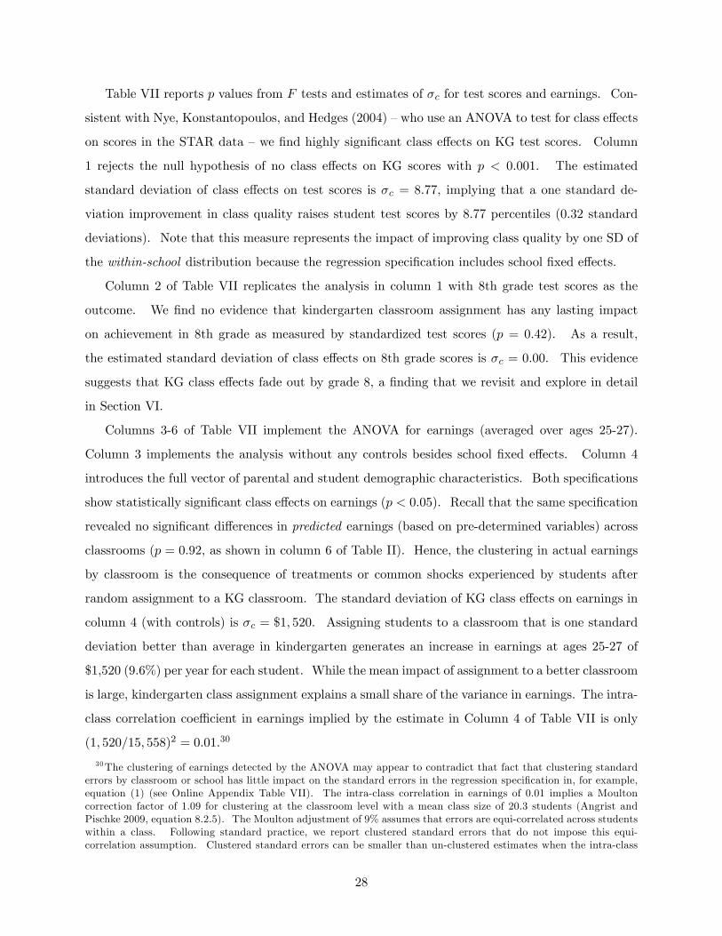
Table VII reports p values from F tests and estimates of σc for test scores and earnings. Con-

sistent with Nye, Konstantopoulos, and Hedges (2004) —who use an ANOVA to test for class effects

on scores in the STAR data —we find highly significant class effects on KG test scores. Column

1 rejects the null hypothesis of no class effects on KG scores with p < 0.001. The estimated

standard deviation of class effects on test scores is σc = 8.77, implying that a one standard de-

viation improvement in class quality raises student test scores by 8.77 percentiles (0.32 standard

deviations). Note that this measure represents the impact of improving class quality by one SD of

the within-school distribution because the regression specification includes school fixed effects.

Column 2 of Table VII replicates the analysis in column 1 with 8th grade test scores as the

outcome. We find no evidence that kindergarten classroom assignment has any lasting impact

on achievement in 8th grade as measured by standardized test scores (p = 0.42). As a result,

the estimated standard deviation of class effects on 8th grade scores is σc = 0.00. This evidence

suggests that KG class effects fade out by grade 8, a finding that we revisit and explore in detail

in Section VI.

Columns 3-6 of Table VII implement the ANOVA for earnings (averaged over ages 25-27).

Column 3 implements the analysis without any controls besides school fixed effects. Column 4

introduces the full vector of parental and student demographic characteristics. Both specifications

show statistically significant class effects on earnings (p < 0.05). Recall that the same specification

revealed no significant differences in predicted earnings (based on pre-determined variables) across

classrooms (p = 0.92, as shown in column 6 of Table II). Hence, the clustering in actual earnings

by classroom is the consequence of treatments or common shocks experienced by students after

random assignment to a KG classroom. The standard deviation of KG class effects on earnings in

column 4 (with controls) is σc = $1, 520. Assigning students to a classroom that is one standard

deviation better than average in kindergarten generates an increase in earnings at ages 25-27 of

$1,520 (9.6%) per year for each student. While the mean impact of assignment to a better classroom

is large, kindergarten class assignment explains a small share of the variance in earnings. The intra-

class correlation coeffi cient in earnings implied by the estimate in Column 4 of Table VII is only

(1, 520/15, 558)2 = 0.01.30

30The clustering of earnings detected by the ANOVA may appear to contradict that fact that clustering standarderrors by classroom or school has little impact on the standard errors in the regression specification in, for example,equation (1) (see Online Appendix Table VII). The intra-class correlation in earnings of 0.01 implies a Moultoncorrection factor of 1.09 for clustering at the classroom level with a mean class size of 20.3 students (Angrist andPischke 2009, equation 8.2.5). The Moulton adjustment of 9% assumes that errors are equi-correlated across studentswithin a class. Following standard practice, we report clustered standard errors that do not impose this equi-correlation assumption. Clustered standard errors can be smaller than un-clustered estimates when the intra-class

28

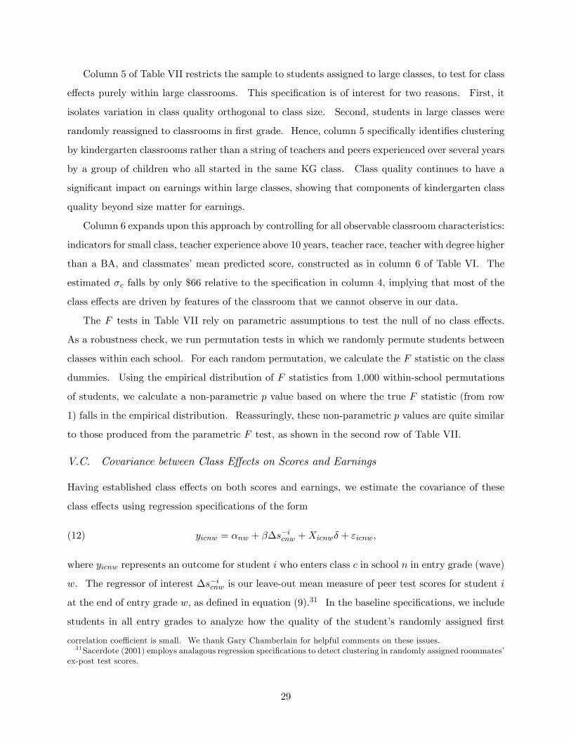
Column 5 of Table VII restricts the sample to students assigned to large classes, to test for class

effects purely within large classrooms. This specification is of interest for two reasons. First, it

isolates variation in class quality orthogonal to class size. Second, students in large classes were

randomly reassigned to classrooms in first grade. Hence, column 5 specifically identifies clustering

by kindergarten classrooms rather than a string of teachers and peers experienced over several years

by a group of children who all started in the same KG class. Class quality continues to have a

significant impact on earnings within large classes, showing that components of kindergarten class

quality beyond size matter for earnings.

Column 6 expands upon this approach by controlling for all observable classroom characteristics:

indicators for small class, teacher experience above 10 years, teacher race, teacher with degree higher

than a BA, and classmates’mean predicted score, constructed as in column 6 of Table VI. The

estimated σc falls by only $66 relative to the specification in column 4, implying that most of the

class effects are driven by features of the classroom that we cannot observe in our data.

The F tests in Table VII rely on parametric assumptions to test the null of no class effects.

As a robustness check, we run permutation tests in which we randomly permute students between

classes within each school. For each random permutation, we calculate the F statistic on the class

dummies. Using the empirical distribution of F statistics from 1,000 within-school permutations

of students, we calculate a non-parametric p value based on where the true F statistic (from row

1) falls in the empirical distribution. Reassuringly, these non-parametric p values are quite similar

to those produced from the parametric F test, as shown in the second row of Table VII.

V.C. Covariance between Class Effects on Scores and Earnings

Having established class effects on both scores and earnings, we estimate the covariance of these

class effects using regression specifications of the form

(12) yicnw = αnw + β∆s−icnw +Xicnwδ + εicnw,

where yicnw represents an outcome for student i who enters class c in school n in entry grade (wave)

w. The regressor of interest ∆s−icnw is our leave-out mean measure of peer test scores for student i

at the end of entry grade w, as defined in equation (9).31 In the baseline specifications, we include

students in all entry grades to analyze how the quality of the student’s randomly assigned first

correlation coeffi cient is small. We thank Gary Chamberlain for helpful comments on these issues.31Sacerdote (2001) employs analagous regression specifications to detect clustering in randomly assigned roommates’

ex-post test scores.

29

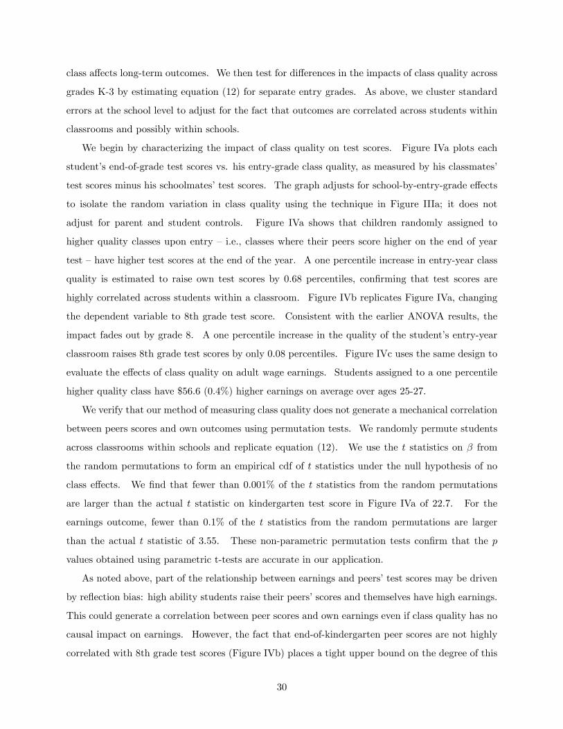
class affects long-term outcomes. We then test for differences in the impacts of class quality across

grades K-3 by estimating equation (12) for separate entry grades. As above, we cluster standard

errors at the school level to adjust for the fact that outcomes are correlated across students within

classrooms and possibly within schools.

We begin by characterizing the impact of class quality on test scores. Figure IVa plots each

student’s end-of-grade test scores vs. his entry-grade class quality, as measured by his classmates’

test scores minus his schoolmates’test scores. The graph adjusts for school-by-entry-grade effects

to isolate the random variation in class quality using the technique in Figure IIIa; it does not

adjust for parent and student controls. Figure IVa shows that children randomly assigned to

higher quality classes upon entry —i.e., classes where their peers score higher on the end of year

test —have higher test scores at the end of the year. A one percentile increase in entry-year class

quality is estimated to raise own test scores by 0.68 percentiles, confirming that test scores are

highly correlated across students within a classroom. Figure IVb replicates Figure IVa, changing

the dependent variable to 8th grade test score. Consistent with the earlier ANOVA results, the

impact fades out by grade 8. A one percentile increase in the quality of the student’s entry-year

classroom raises 8th grade test scores by only 0.08 percentiles. Figure IVc uses the same design to

evaluate the effects of class quality on adult wage earnings. Students assigned to a one percentile

higher quality class have $56.6 (0.4%) higher earnings on average over ages 25-27.

We verify that our method of measuring class quality does not generate a mechanical correlation

between peers scores and own outcomes using permutation tests. We randomly permute students

across classrooms within schools and replicate equation (12). We use the t statistics on β from

the random permutations to form an empirical cdf of t statistics under the null hypothesis of no

class effects. We find that fewer than 0.001% of the t statistics from the random permutations

are larger than the actual t statistic on kindergarten test score in Figure IVa of 22.7. For the

earnings outcome, fewer than 0.1% of the t statistics from the random permutations are larger

than the actual t statistic of 3.55. These non-parametric permutation tests confirm that the p

values obtained using parametric t-tests are accurate in our application.

As noted above, part of the relationship between earnings and peers’test scores may be driven

by reflection bias: high ability students raise their peers’scores and themselves have high earnings.

This could generate a correlation between peer scores and own earnings even if class quality has no

causal impact on earnings. However, the fact that end-of-kindergarten peer scores are not highly

correlated with 8th grade test scores (Figure IVb) places a tight upper bound on the degree of this

30

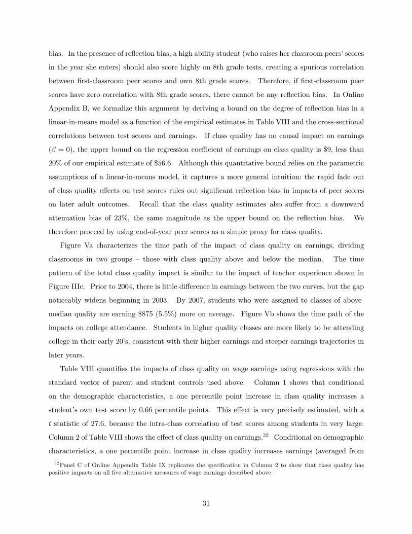
bias. In the presence of reflection bias, a high ability student (who raises her classroom peers’scores

in the year she enters) should also score highly on 8th grade tests, creating a spurious correlation

between first-classroom peer scores and own 8th grade scores. Therefore, if first-classroom peer

scores have zero correlation with 8th grade scores, there cannot be any reflection bias. In Online

Appendix B, we formalize this argument by deriving a bound on the degree of reflection bias in a

linear-in-means model as a function of the empirical estimates in Table VIII and the cross-sectional

correlations between test scores and earnings. If class quality has no causal impact on earnings

(β = 0), the upper bound on the regression coeffi cient of earnings on class quality is $9, less than

20% of our empirical estimate of $56.6. Although this quantitative bound relies on the parametric

assumptions of a linear-in-means model, it captures a more general intuition: the rapid fade out

of class quality effects on test scores rules out significant reflection bias in impacts of peer scores

on later adult outcomes. Recall that the class quality estimates also suffer from a downward

attenuation bias of 23%, the same magnitude as the upper bound on the reflection bias. We

therefore proceed by using end-of-year peer scores as a simple proxy for class quality.

Figure Va characterizes the time path of the impact of class quality on earnings, dividing

classrooms in two groups — those with class quality above and below the median. The time

pattern of the total class quality impact is similar to the impact of teacher experience shown in

Figure IIIc. Prior to 2004, there is little difference in earnings between the two curves, but the gap

noticeably widens beginning in 2003. By 2007, students who were assigned to classes of above-

median quality are earning $875 (5.5%) more on average. Figure Vb shows the time path of the

impacts on college attendance. Students in higher quality classes are more likely to be attending

college in their early 20’s, consistent with their higher earnings and steeper earnings trajectories in

later years.

Table VIII quantifies the impacts of class quality on wage earnings using regressions with the

standard vector of parent and student controls used above. Column 1 shows that conditional

on the demographic characteristics, a one percentile point increase in class quality increases a

student’s own test score by 0.66 percentile points. This effect is very precisely estimated, with a

t statistic of 27.6, because the intra-class correlation of test scores among students in very large.

Column 2 of Table VIII shows the effect of class quality on earnings.32 Conditional on demographic

characteristics, a one percentile point increase in class quality increases earnings (averaged from

32Panel C of Online Appendix Table IX replicates the specification in Column 2 to show that class quality haspositive impacts on all five alternative measures of wage earnings described above.

31

2005 to 2007) by $50.6 per year, with a t statistic of 2.9 (p < 0.01). To interpret the magnitude of

this effect, note that a one standard deviation increase in class quality as measured by peer scores

leads to a $455 (2.9%) increase in earnings at age 27.33

The impact of class quality on earnings is estimated much more precisely than the impacts of

observable characteristics on earnings because class quality varies substantially across classrooms.

Recall from Table V that students assigned to small classes scored 4.8 percentile points higher on

end-of-year tests. If class quality varied only from -2.4 to 2.4, we would be unable to determine

whether the relationship between class quality and earnings is significant, as can be seen in Figure

IVc. By pooling all observable and unobservable sources of variation across classrooms, we obtain

more precise (though less policy relevant) estimates of the impact of classroom environments on

adult outcomes.

Column 3 of Table VIII isolates the variation in class quality that is orthogonal to observable

classroom characteristics by controlling for class size, teacher characteristics, and peer characteris-

tics as in column 6 of Table VII. Class quality continues to have a significant impact on earnings

conditional on these observables, confirming that components of class quality orthogonal to observ-

ables matter for earnings.

The preceding specifications pool grades K-3. Column 4 restricts the sample to kindergarten

entrants and shows that a one percentile increase in KG class quality raises earnings by $53.4.

Column 5 includes only those who entered STAR after kindergarten. This point estimate is similar

to that in column 4, showing that class quality in grades 1-3 matters as much for earnings as class

quality in kindergarten.

Columns 6-9 show the impacts of class quality on other adult outcomes. These columns

replicate the baseline specification for the full sample in column 2. Columns 6 and 7 show that a

1 percentile improvement in class quality raises college attendance rates by 0.1 percentage points,

both at age 20 and before age 27 (p < 0.05). Column 8 shows that a one percentile increase in

class quality generates an $9.3 increase in the college quality index (p < 0.05). Finally, column 9

shows that a one percentile point improvement in class quality leads to an improvement of 0.25%

of a standard deviation in our outcome summary index (p < 0.05). Online Appendix Table X

reports the impacts of class quality on each of the five outcomes separately and shows that the

33Part of the impact of being randomly assigned to a higher quality class in grade w may come from being placedin higher quality classes in subsequent grades. A 1 percentile increase in KG class quality (peer scores) is associatedwith a 0.15 percentile increase in class quality (peer scores) in grade 1. The analogous effect of grade 1 class qualityon grade 2 class quality is 0.37 percentiles.

32

point estimates of the impacts are positive for all of the outcomes. Online Appendix Table XI

documents the heterogeneity of class quality impacts across subgroups. The point estimates of the

impacts of class quality are positive for all the groups and outcomes.

Finally, we check the robustness of our results by implementing instrumental-variable methods

of detecting covariance between class effects on scores and earnings. The effects of class quality on

test scores and earnings in columns 1 and 2 of Table VIII can be combined to produce a jackknife

IV estimate of the earnings gain associated with an increase in test scores: $50.61/0.662 = $76.48.

That is, class-level factors that raise test scores by one percentile point raise earnings by $76.48

on average. In Online Appendix Table XIII, we show that other IV estimators yield very similar

estimates.

While class effects on scores and earnings are highly correlated, a substantial portion of class

effects on earnings is orthogonal to our measure of class quality. Using a random effects estimator

as in Column 4 of Table VII, we find that the standard deviation of class effects on earnings falls

from $1520 to $1372 after we control for our peer-score class quality measure ∆s−icnw. Hence,

roughly 1− (13721520)2 ≈ 1/5 of the variance of the class effect on earnings comes through class effects

on test scores.

VI. Fade-Out, Re-Emergence, and Non-Cognitive Skills

In this section, we explore why the impacts of class size and class quality in early childhood fade

out on tests administered in later grades but re-emerge in adulthood. In order to have a fixed

benchmark to document fade-out, we use only kindergarten entrants throughout this section and

analyze the impacts of KG class quality on test scores and other outcomes in later grades.

We first document the fade-out effect using the class quality measure by estimating equation

(12) with test scores in each grade as the dependent variable and with the standard vector of parent

and student controls as well as school fixed effects. Figure VIa plots the estimated impacts on

test scores in grades K-8 of increasing KG class quality by one (within-school) standard deviation.

A one (within school) SD increase in KG class quality increases end-of-kindergarten test scores by

6.27 percentiles, consistent with our findings above. In grade 1, students who were in a 1 SD better

KG class score approximately 1.50 percentile points higher on end-of-year tests, an effect that is

significant with p < 0.001. The effect gradually fades over time, and by grade 4 students who were

in a better KG class no longer score significantly higher on tests.34

34This fade-out effect is consistent with the rapid fade-out of teacher effects documented by Jacob, Lefgren, and

33

If a one percentile increase in 8th grade test scores is more valuable than a one percentile

increase in KG test scores, then the evidence in Figure VIa would not necessarily imply that the

effects of early childhood education fade out. To evaluate this possibility, we convert the test score

impacts to predicted earnings gains. We run separate OLS regressions of earnings on the test

scores for each grade from K-8 to estimate the cross-sectional relationship between each grade’s

test score and earnings (see Online Appendix Table V, Column 1 for these coeffi cients). We then

multiply the class quality effect on scores shown in Figure VIa by the corresponding coeffi cient on

scores from the OLS earnings regression. Figure VIb plots the earnings impacts predicted by the

test score gains in each grade that arise from attending a better KG class. The pattern in Figure

VIb looks very similar to that in Figure VIa, showing that there is indeed substantial fade-out of

the KG class quality effect on predicted earnings. By 4th grade, one would predict less than a $50

per year gain in earnings from a better KG class based on observed test score impacts.

The final point in Figure VIb shows the actual observed earnings impact of a one SD improve-

ment in KG class quality. The actual impact of $483 is similar to what one would have predicted

based on the improvement in KG test scores ($588). The impacts of early childhood education

re-emerge in adulthood despite fading out on test scores in later grades.

Non-Cognitive Skills. One potential explanation for fade-out and re-emergence is the acquisition

of non-cognitive skills (e.g. Heckman 2000, Heckman, Stixrud, and Urzua 2006, Lindqvist and

Vestman 2011). We evaluate whether non-cognitive skills could explain our findings using data on

non-cognitive measures collected for a subset of STAR students in grades 4 and 8.35

Finn et al. (2007) and Dee and West (2008) describe the non-cognitive measures in the STAR

data in detail; we provide a brief summary here. In grade 4, teachers in the STAR schools were asked

to evaluate a random subset of their students on a scale of 1-5 on several behavioral measures, such

as whether the student “annoys others.” These responses were consolidated into four standardized

scales measuring each student’s effort, initiative, nonparticipatory behavior, and how the student

is seen to “value” the class. In grade 8, math and English teachers were asked to rate a subset

of their students on a similar set of questions, which were again consolidated into the same four

standardized scales. To obtain a measure analogous to our percentile measure of test scores, we

construct percentile measures for these four scales and compute the average percentile score for

Sims (2008), Kane and Staiger (2008), and others.35Previous studies have used the STAR data to investigate whether class size affects non-cognitive skills (Finn et al.

1989, Dee and West 2008). They find mixed evidence on the impact of class size on non-cognitive skills: statisticallysignificant impacts are detected in grade 4, but not in grade 8. Here, we analyze the impacts of our broader classquality measure.

34

each student. For 8th grade, we then take the average of the math and English teacher ratings.

Among the 6,025 students who entered Project STAR in KG and whom we match in the IRS

data, we have data on non-cognitive skills for 1,671 (28%) in grade 4 and 1,780 (30%) in grade

8. The availability of non-cognitive measures for only a subset of the students who could be

tracked until grade 8 naturally raises concerns about selective attrition. Dee and West (2008)

investigate this issue in detail, and we replicate their findings with our expanded set of parental

characteristics. In grade 8, we find no significant differences in the probability of having non-

cognitive data by KG classrooms or class types (small vs. large), and confirm that in this sample

the observable background characteristics are balanced across classrooms and class types. In

grade 4, non-cognitive data are significantly more likely to be available for students assigned to

small classes, but among the sample with non-cognitive data there are no significant differences in

background characteristics across classrooms or class types. Hence, the sample for whom we have

non-cognitive data appear to be balanced across classrooms at least on observable characteristics.

We begin by estimating the cross-sectional correlation between non-cognitive outcomes and

earnings. Column 1 of Table IX shows that a 1 percentile improvement in non-cognitive measures in

grade 4 is associated with a $106 gain in earnings conditional on the standard vector of demographic

characteristics used above and school-by-entry-grade fixed effects. Column 2 shows that controlling

for math and reading test scores in grade 4 reduces the predictive power of non-cognitive scores

only slightly, to $88 per percentile. In contrast, column 3 shows that non-cognitive skills in grade

4 are relatively weak predictors of 8th grade test scores when compared with math and reading

scores in 4th grade. Because non-cognitive skills appear to be correlated with earnings through

channels that are not picked up by subsequent standardized tests, they could explain fade-out and

re-emergence.

To further evaluate this mechanism, we investigate the effects of KG class quality on non-

cognitive skills in grade 4 and 8. As a reference, column 4 shows that a 1 percentile improvement

in KG class quality increases a student’s test scores in grade 4 by a statistically insignificant 0.05

percentiles. In contrast, column 5 shows that the same improvement in KG class quality generates

a statistically significant increase of 0.15 percentiles in the index of non-cognitive measures in grade

4. Columns 6 and 7 replicate columns 4 and 5 for grade 8.36 Again, KG class quality does not have

a significant impact on 8th grade test scores but has a significant impact on non-cognitive measures.

36We use all KG entrants for whom test scores are available in columns 4 and 6 to increase precision. The pointestimates on test score impacts are similar for the subsample of students for whom non-cognitive data are available.

35

Finally, columns 8 and 9 show that the experience of the student’s teacher in kindergarten —which

we showed above also impacts earnings —has a small and statistically insignificant impact on test

scores but a substantially larger impact on non-cognitive measures in 8th grade (p = 0.07).37

We can translate the impacts on non-cognitive skills into predicted impacts on earnings fol-

lowing the method in Figure VIb. We regress earnings on the non-cognitive measure in grade 4,

conditioning on demographic characteristics, and obtain an OLS coeffi cient of $101 per percentile.

Multiplying this OLS coeffi cient by the estimated impact of class quality on non-cognitive skills

in grade 4, we predict that a 1 SD improvement in KG class quality will increase earnings by

$139. The same exercise for 4th grade math+reading test scores yields a predicted earnings gain

of $40. These results suggest that improvements in non-cognitive skills explain a larger share

of actual earnings gains than improvements in cognitive performance, consistent with Heckman

et al.’s (2010) findings for the Perry Preschool program. In contrast, a one standard deviation

increase in class quality is predicted to raise 8th grade test scores by only 0.47 percentiles based on

its observed impacts on non-cognitive skills in grade 4 and the cross-sectional correlation between

grade 4 non-cognitive skills and grade 8 test scores. This predicted impact is quite close to the

actual impact of class quality on 8th grade scores of 0.57 percentiles. Hence, the impacts of class

quality on non-cognitive skills is consistent with both fade-out on scores and re-emergence on adult

outcomes.

Intuitively, a better kindergarten classroom might simultaneously increase performance on end-

of-year tests and improve untested non-cognitive skills. For instance, a KG teacher who is able to

make her students memorize vocabulary words may instill social skills in the process of managing

her classroom successfully. These non-cognitive skills may not be well measured by standardized

tests, leading to very rapid fade-out immediately after KG. However, these skills could still have

returns in the labor market.

Although non-cognitive skills provide one plausible explanation of the data, our analysis is far

from definitive proof of the importance of non-cognitive skills. The estimates of non-cognitive

impacts could suffer from attrition bias and are somewhat imprecisely estimated. Moreover, our

analysis does not show that manipulating non-cognitive skills directly has causal impacts on adult

outcomes. We have shown that high quality KG classes improve both non-cognitive skills and

adult outcomes, but the mechanism through which adult outcomes are improved could run through

37Online Appendix Table XIV decomposes the relationships described in Table IX into the four constituent com-ponents of non-cognitive skill.

36

another channel that is correlated with the acquisition of non-cognitive skills. It would be valuable

to analyze interventions that target non-cognitive skills directly in future work.

VII. Conclusion

The impacts of education have traditionally been measured by achievement on standardized tests.

This paper has shown that the classroom environments that raise test scores also improve long-term

outcomes. Students who were randomly assigned to higher quality classrooms in grades K-3 earn

more, are more likely to attend college, save more for retirement, and live in better neighborhoods.

Yet the same students do not do much better on standardized tests in later grades. These results

suggest that policy makers may wish to rethink the objective of raising test scores and evaluating

interventions via long-term test score gains. Researchers who had examined only the impacts of

STAR on test scores would have incorrectly concluded that early childhood education does not

have long-lasting impacts. While the quality of education is best judged by directly measuring its

impacts on adult outcomes, our analysis suggests that contemporaneous (end-of-year) test scores

are a reasonably good short-run measure of the quality of a classroom.

We conclude by using our empirical estimates to provide rough calculations of the benefits of

various policy interventions (see Online Appendix C for details). These cost-benefit calculations

rely on several strong assumptions. We assume that the percentage gain in earnings observed at

age 27 remains constant over the lifecycle. We ignore non-monetary returns to education (such as

reduced crime) as well as general equilibrium effects. We discount earnings gains at a 3% annual

rate back to age 6, the point of the intervention.

(1) Class Quality. The random-effects estimate reported in column 4 of Table VII implies that

increasing class quality by one standard deviation of the distribution within schools raises earnings

by $1,520 (9.6%) at age 27. Under the preceding assumptions, this translates into a lifetime

earnings gain of approximately $39,100 for the average individual. For a classroom of twenty

students, this implies a present-value benefit of $782,000 for improving class quality for a single

year by one (within-school) standard deviation. This large figure includes all potential benefits

from an improved classroom environment, including better peers, teachers, and random shocks,

and hence is useful primarily for understanding the stakes at play in early childhood education. It

is less helpful from a policy perspective because one cannot implement interventions that directly

improve classroom quality. This motivates the analysis of class size and better teachers, two factors

that contribute to classroom quality.

37

(2) Class Size. We calculate the benefits of reducing class size by 33% in two ways. The first

method uses the estimated earnings gain from being assigned to a small class reported in column

5 of Table V. The point estimate of $4 in Table V translates into a lifetime earnings gain from

reducing class size by 33% for one year of $103 in present value per student, or $2,057 for a class that

originally had twenty students. But this estimate is imprecise: the 95% confidence interval for the

lifetime earnings gain of reducing class size by 33% for one year ranges from -$17,500 to $17,700 per

child. To obtain more precision, we predict the benefits of class size reduction using the estimated

impact of classroom quality on scores and earnings. We estimate that a 1 percentile increase in

class quality raises test scores by 0.66 percentiles and earnings by $50.6, implying an earnings gain

of $76.7 per percentile increase in test scores. Next, we make the strong assumption that the ratio

of earnings gains to test score gains is the same for changes in class size as it is for improvements

in class quality more generally. Under this assumption, a 33% class size reduction in grades K-3

(which raised test scores by 4.8 percentiles) is predicted to raise earnings by 4.8 × $76.7 = $368

(2.3%) at age 27. This calculation implies a present value earnings gain from class size reduction

of $9,460 per student and $189,000 for the classroom.38

(3) Teachers. We cannot directly estimate the total impacts of teachers on earnings in this study

because we observe each teacher in only one classroom, making it impossible to separate teacher

effects from peer effects and classroom-level shocks. However, we can predict the magnitudes of

teacher effects as measured by value-added on test scores by drawing upon prior work. Rockoff

(2004), Rivkin, Hanushek, and Kain (2005), and Kane and Staiger (2008) use datasets with multiple

classrooms per teacher to estimate that a one standard deviation increase in teacher quality raises

test scores by between 0.1 and 0.2 standard deviations (2.7-5.4 percentiles).39 Under the strong

assumption that the ratio of earnings gains to test score gains is the same for changes in teacher

quality and class quality more broadly, this test score gain implies an earnings gain of $208-$416

(1.3%-2.6%) at age 27 and a present-value earnings gain ranging from $5,350-$10,700 per student.

Hence, we predict that a one standard deviation improvement in teacher quality in a single year

would generate earnings gains between $107,000 and $214,000 for a classroom of twenty students.

These predictions are roughly consistent with the findings of Chetty, Friedman, and Rockoff (2011),

38Krueger (1999) projects a gain from small-class attendence of $9, 603 for men and $7, 851 for women. Neitherof our estimates are statistically distinguishable from these predictions.39We use estimates of the impacts of teacher quality on scores from other studies to predict earnings gains because

we do not have repeat observations on teachers in our data. In future work, it would be extremely valuable tolink datasets with repeat observations on teachers to administrative data on students in order to measure teachers’impacts on earnings directly.

38

who directly estimate the impacts of teacher value-added on earnings using a dataset that contains

information on multiple classrooms per teacher.

Our results suggest that good teachers could potentially create great social value, perhaps

several times larger than current teacher salaries.40 However, our findings do not have direct

implications for optimal teacher salaries or merit pay policies as we do not know whether higher

salaries or merit pay would improve teacher quality.41 Relative to efforts that seek to improve the

quality of teachers, class size reductions have the important advantage of being more well-defined

and straightforward to implement. However, reductions in class size must be implemented carefully

to generate improvements in outcomes. If schools are forced to reduce teacher and class quality

along other dimensions when reducing class size, the net gains from class size reduction may be

diminished (Jepsen and Rivkin 2009, Sims 2009).

Finally, our analysis raises the possibility that differences in school quality perpetuate income

inequality. In the U.S., higher income families have access to better public schools on average

because of property-tax finance. Using the class quality impacts reported above, Chetty and

Friedman (2011) estimate that the intergenerational correlation of income would fall by roughly

1/3 if all children attended schools of the same quality. Improving early childhood education in

disadvantaged areas — e.g. through federal tax credits or tax policy reforms — could potentially

reduce inequality in the long run.

40According to calculations from the 2006-2008 American Community Survey, the mean salary for elementary andmiddle school teachers in the U.S. was $39,164 (in 2009 dollars).41An analogy with executive compensation might be helpful in understanding this point. CEOs’decisions have

large impacts on the firms they run, and hence can create or destroy large amounts of economic value. But this doesnot necessarily imply that increasing CEO compensation or pay-for-performance would improve CEO decisions.

39

References

Aaronson, Daniel, Lisa Barrow, and William Sander, “Teachers and Student Achievement inChicago Public High Schools,”Journal of Labor Economics 24:1 (2007), 95-135.

Almond, Douglas, and Janet Currie, “Human Capital Development Before Age Five,”forthcoming,Handbook of Labor Economics, Volume 4 (2010).

American Community Survey, (http://www.census.gov, U.S. Census Bureau), 2006-2008 ACS 3-year data.

Angrist, Joshua D., Guido W. Imbens, and Alan B. Krueger. “Jackknife Instrumental VariablesEstimation,”Journal of Applied Econometrics 14:1 (1999), 57—67.

Angrist, Joshua D. and Alan B. Krueger, “Split-Sample Instrumental Variables Estimates of the Re-turn to Schooling,”Journal of Business and Economic Statistics, American Statistical Association,13:2 (1995), 225-235.

Angrist, Joshua D. and Jorn-Steffen Pischke. Mostly Harmless Econometrics: An Empiricist’sCompansion. Princeton: Princeton University Press (2009).

Bacolod, Marigee P, “Do Alternative Opportunities Matter? The Role of Female Labor Marketsin the Decline of Teacher Quality,”Review of Economics and Statistics, 89:4 (2007), 737-751.

Chetty, Raj and John N. Friedman. “Does Local Tax Financing of Public Schools PerpetuateInequality?”Forthcoming, National Tax Association Proceedings (2011).

Chetty, Raj, John N. Friedman, and Jonah Rockoff. “The Impact of Teacher Value Added onStudent Outcomes in Adulthood”Harvard Univ. mimeo (2011).

Cilke, James “A Profile of Non-Filers,”U.S. Department of the Treasury, Offi ce of Tax AnalysisWorking Paper No. 78, July, 1998.

Corcoran, Sean P., William N. Evans, Robert M. Schwab, “Changing Labor-market Opportunitiesfor Women and the Quality of Teachers, 1957-2000,”American Economic Review, 94 (2004), 230-235.

Currie, Janet. “Inequality at Birth: Some Causes and Consequences.” NBER Working Paper No.16798, 2011.

Currie, Janet, and Duncan Thomas, “Early Test Scores, School Quality and SES: Longrun Effectsof Wage and Employment Outcomes,”Worker Wellbeing in a Changing Labor Market, 20 (2001),103—132.

Dee, Thomas S., “Teachers, Race, and Student Achievement in a Randomized Experiment,”Reviewof Economics and Statistics, 86 (2004), 195-210.

Dee, Thomas S., and Martin West, “The Non-Cognitive Returns to Class Size,”Educational Eval-uation and Policy Analysis, 33 (2011), 23-46.

Finn, Jeremy D., DeWayne Fulton, Jayne Zaharias, and Barbara A. Nye, “Carry-Over Effects ofSmall Classes,”Peabody Journal of Education, 67 (1989) 75-84.

Finn, Jeremy D., Jayne Boyd-Zaharias, Reva M. Fish, and Susan B. Gerber, “Project STAR andBeyond: Database User’s Guide,”Lebanon: Heros, inc., 2007.

Guryan, Jonathan, Kory Kroft and Matthew J. Notowidigdo, “Peer Effects in the Workplace: Ev-idence from Random Groupings in Professional Golf Tournaments,”American Economic Journal:Applied Economics, 1 (2009), 34-68.

40

Haider, Steven, and Gary Solon, “Life-cycle variation in the Association Between Current andLifetime Earnings,”The American Economic Review, 96 (2006), 1308-1320.

Hanushek, Eric A., “The Failure of Input-Based Schooling Policies.” Economic Journal 113(1):F64-F98, 2003.

Hanushek, Eric A., “Economic Aspects of the Demand for Teacher Quality,” prepared for theEconomics of Education Review, 2010.

Heckman, James J., “Policies to Foster Human Capital,”Research in Economics, 54:1 (2000), 3-56.

Heckman, James J., Jora Stixrud, and Sergio Urzua, “The Effects of Cognitive and Non-cognitiveAbilities on Labor Market Outcomes and Social Behaviors.” Journal of Labor Economics 24:3(2006), 411-482.

Heckman, James J., Lena Malofeeva, Rodrigo Pinto, and Peter A. Savelyev, “Understanding theMechanisms Through Which an Influential Early Childhood Program Boosted Adult Outcomes,”unpublished manuscript, University of Chicago (2010).

Holland, Paul W. “Statistics and Causal Inference,”Journal of the American Statistical Association,81 (1986), 945-960.

Hoxby, Caroline M. and Andrew Leigh, “Pulled away or pushed out? Explaining the decline ofteacher aptitude in the United States,”American Economic Review, 94 (2004) 236-240.

Internal Revenue Service. Document 6961: Calendar Year Projections of Information and With-holding Documents for the United States and IRS Campuses 2010-2018, IRS Offi ce of Research,Analysis, and Statistics, Washington, D.C, 2010.

Jacob, Brian A., Lars Lefgren and David Sims, “The Persistence of Teacher-Induced LearningGains,”Forthcoming, Journal of Human Resources (2011).

Jepsen, Christopher and Steven Rivkin, “Class Size Reduction and Student Achievement: ThePotential Tradeoff between Teacher Quality and Class Size,” Journal of Human Resources, 44:1(2009) 223-250.

Kane, Thomas, and Douglas O. Staiger, “Estimating Teacher Impacts on Student Achievement:An Experimental Evaluation,”NBER Working Paper No. 14607, 2008.

Kling, Jeffrey R., Jeffrey B. Liebman, and Lawrence F. Katz, “Experimental Analysis of Neighbor-hood Effects,”Econometrica, 75 (2007), 83-119.

Krueger, Alan B, “Experimental Estimates of Education Production Functions,”Quarterly Journalof Economics, 114 (1999), 497-532.

Krueger, Alan B., and Diane M. Whitmore, “The Effect of Attending a Small Class in the EarlyGrades on College-Test Taking and Middle School Test Results: Evidence from Project STAR,”The Economic Journal, 111 (2001), 1-28.

Lindqvist, Erik and Roine Vestman. “The Labor Market Returns to Cognitive and NoncognitiveAbility: Evidence from the Swedish Enlistment.”American Economic Journal: Applied Economics,3 (2011), 101-28.

Manski, Charles, “Identification of Exogenous Social Effects: The Reflection Problem,”Review ofEconomic Studies, 60 (1993), 531-542.

Muennig, Peter, Gretchen Johnson, Jeremy Finn, and Elizabeth Ty Wilde, The Effect of SmallClass Sizes on Mortality Through Age 29: Evidence From a Multi-Center Randomized ControlledTrial, unpublished mimeo, 2010.

41

Nye, Barbara, Spyros Konstantopoulos, and Larry V. Hedges, “How Large are Teacher Effects?”Educational Evaluation and Policy Analysis, 26 (2004), 237-257.

Rivkin, Steven. G., Eric. A. Hanushek, and John F. Kain, “Teachers, Schools and AcademicAchievement,”Econometrica, 73 (2005), 417—458.

Rockoff, Jonah E., “The Impact of Individual Teachers on Student Achievement: Evidence fromPanel Data,”American Economics Review, 94 (2004), 247-252.

Rockoff, Jonah E., and Douglas Staiger, “Searching for Effective Teachers with Imperfect Informa-tion,”Journal of Economic Perspectives, 24 (2010), 97-117.

Sacerdote, Bruce, “Peer Effects with Random Assignment: Results for Dartmouth Roommates,”Quarterly Journal of Economics, 116 (2001), 681-704.

Schanzenbach, Diane W., “What Have Researchers Learned From Project STAR?”Brookings Pa-pers on Education Policy, (2006), 205-228.

Sims, David, “Crowding Peter to Educate Paul: Lessons From a Class Size Reduction Externality,”Economics of Education Review 28:4 (2009), 465-473.

US Census Bureau. “School Enrollment—Social and Economic Characteristics of Students: October2008, Detailed Tables,”Washington, D.C., 2010.

(http://www.census.gov/population/www/socdemo/school.html).

Word, Elizabeth., John. Johnston, Helen. P. Bain, B. Dewayne Fulton, Charles M. Achilles,Martha N. Lintz, John Folger, and Carolyn Breda, “The State of Tennessee’s Student/TeacherAchievement Ratio (STAR) Project: Technical Report 1985—1990,”Tennessee State Departmentof Education, 1990.

42

Appendix A: Algorithm for Matching STAR Records to Tax Data

The tax data were accessed through contract TIRNO-09-R-00007 with the Statistics of Income(SOI) Division at the US Internal Revenue Service. Requests for research contracts by SOI areposted online at the Federal Business Opportunities https://www.fbo.gov/. SOI also welcomesresearch partnerships between outside academics and internal researchers at SOI.

STAR records were matched to tax data using social security number (SSN), date of birth,gender, name, and STAR elementary school ZIP code. Note that STAR records do not contain allthe same information. Almost every STAR record contains date of birth, gender, and last name.Some records contain no SSN while others contain multiple possible SSNs. Some records containno first name. A missing field yielded a non-match unless otherwise specified.

We first discuss the general logic of the match algorithm and then document the routines indetail. The match algorithm was designed to match as many records as possible using variablesthat are not contingent on ex post outcomes. SSN, date of birth, gender, and last name in the taxdata are populated by the Social Security Administration using information that is not contingenton ex post outcomes. First name and ZIP code in tax data are contingent on observing some expost outcome. First name data derive from information returns, which are typically generated afteran adult outcome like employment (W-2 forms), college attendance (1098-T forms), and mortgageinterest payment (1098 forms). The ZIP code on the claiming parent’s 1040 return is typically from1996 and is thus contingent on the ex post outcome of the STAR subject not having moved farfrom her elementary school by age 16.

89.8% of STAR records were matched using only ex ante information. The algorithm firstmatched as many records as possible using only SSN, date of birth, gender, and last name. It thenused first name only to exclude candidate matches based on date of birth, gender, and last name,often leaving only one candidate record remaining. Because that exclusion did not condition on aninformation return having been filed on behalf of that remaining candidate, these matches also didnot condition on ex post outcomes.

The match algorithm proceeded as follows, generating seven match types denoted A throughG. The matches generated purely through ex-ante information are denoted A through E belowand account for 89.8% of STAR records. Matches based on ex-post-information are denoted F andG below and constitute an additional 5.4% of STAR records. The paper reports results using thefull 95.0% matched sample, but all the qualitative results hold in the 89.8% sample matched usingonly ex ante information.

1. Match STAR records to tax records by SSN. For STAR records with multiple possible SSNs,match on all of these SSNs to obtain a set of candidate tax record matches for each STARrecord with SSN information. Each candidate tax record contains date of birth, gender, andfirst four letters of every last name ever assigned to the SSN.

• Match Type A. Keep unique matches after matching on first four letters of last name,date of birth, and gender.

• Match Type B. Refine non-unique matches by matching on either first four letters oflast name or on “fuzzy”date of birth. Then keep unique matches. Fuzzy date of birthrequires the absolute value of the difference between STAR record and tax record datesof birth to be in the set {0,1,2,3,4,5,9,10,18,27} in days, in the set {1,2} in months, orin the set {1} in years. These sets were chosen to reflect common mistakes in recordeddates of birth, such as being off by one day (e.g. 12 vs. 13) or inversion of digits (e.g.12 vs. 21).

43

2. Match residual unmatched STAR records to tax records by first four letters of last name,date of birth, and gender.

• Match Type C. Keep unique matches.• Match Type D. Refine non-unique matches by excluding candidates who have a firstname issued on information returns (e.g. W-2 forms, 1098-T forms, and various 1099forms) that does not match the STAR first name on first four letters when the STARfirst name is available. Then keep unique matches.

• Match Type E. Refine residual non-unique matches by excluding candidates who haveSSNs that, based on SSN area number, were issued from outside the STAR region(Tennessee and neighboring environs). Then keep unique matches.

• Match Type F. Refine residual non-unique matches by keeping unique matches after eachof the following additional criteria is applied: require a first name match when STARfirst name is available, require the candidate tax record’s SSN to have been issued fromthe STAR region, and require the first three digits of the STAR elementary school ZIPcode to match the first three digits of the ZIP code on the earliest 1040 return on whichthe candidate tax record was claimed as a dependent.

3. Match residual unmatched STAR records to tax records by first four letters of last name andfuzzy date of birth.

• Match Type G. Keep unique matches after each of several criteria is sequentially applied.These criteria include matches on first name, last name, and middle initial using thecandidate tax record’s information returns; on STAR region using the candidate taxrecord’s SSN area number; and between STAR elementary school ZIP code and ZIPcode on the earliest 1040 return on which the candidate tax record was claimed as adependent.

The seven match types cumulatively yielded a 95.0% match rate:

Match type Frequency Percent Cumulative percentA 7036 60.8% 60.8%B 271 2.3% 63.1%C 699 6.0% 69.2%D 1391 12.0% 81.2%E 992 8.6% 89.8%F 299 2.6% 92.4%G 304 2.6% 95.0%

Identifiers such as names and SSN’s were used solely for the matching procedure. After thematch was completed, the data were de-identified (i.e., individual identifiers such as names andSSNs were stripped) and the statistical analysis was conducted using the de-identified dataset.

Appendix B: Derivations for Measurement of Unobserved Class Quality

This appendix derives the estimators discussed in the empirical model in Section V and quan-tifies the degree of attenuation and reflection bias. We first use equations (5) and (6) to define

44

average of test scores and earnings within each class c and school n:

scn = dn + zcn + acn

ycn = δn + βzcn + zYcn + ρacn + νcn

sn = dn + zn + an

yn = δn + βzn + zYn + ρan + νn.

We define variables demeaned within schools as

sicn − sn = zcn − zn + aicn − an∆scn ≡ scn − sn = zcn − zn + acn − an,

yicn − yn = β(zcn − zn) + (zYicn − zYn ) + ρ(aicn − an) + νicn − νnycn − yn = β(zcn − zn) + (zYcn − zYn ) + ρ(acn − an) + νcn − νn.

Recall that aicn and νicn are independent of each other and zcn. Let σ2 = var(aicn). Weassume in parts 1 and 2 below that zcn, zYcn ⊥ aicn, ruling out peer effects. Note also that, aszcn ⊥ zYcn, the component of classroom environments that affects only test scores drops out entirelyof the covariance analysis below. In what follows, we take the number of students per class I andthe number of classrooms per school C as fixed and analyze the asymptotic properties of variousestimators as the number of schools N →∞.

1. Mean score estimator. The simplest proxy for class quality is the average test scorewithin a class. Since we include school fixed effects in all specifications, scn is equivalent to ∆scnas defined above. Therefore, consider the following (school) fixed effects OLS regression:

(13) yicn = αn + bM∆scn + εicn.

As the number of schools N →∞, the coeffi cient estimate b̂M converges to

plim N−→∞ b̂M =cov(yicn − yn, scn − sn)

var(scn − sn),

which we can rewrite as

plim N−→∞ b̂M =cov

(β(zcn − zn) + ρ(aicn −

∑k

∑j ajkn

I·C ), zcn − zn +∑j ajcnI −

∑k

∑j ajkn

I·C

)var

(zcn − zn +

∑j ajcnI −

∑k

∑j ajkn

I·C

)=

βvar(zcn − zn) + ρσ2C−1IC

var(zcn − zn) + σ2C−1IC

.

Even absent class effects (β = 0), we obtain plim N−→∞ b̂M > 0 if I is finite and ρ > 0. Withfinite class size, bM is upward-biased due to the correlation between wages and own-score, which isincluded within the class quality measure.

2. Leave-out mean estimator. We address the upward bias due to the own observationproblem using a leave-out mean estimator. Consider the OLS regression with school fixed effects

(14) yicn = αn + bLM∆s−icn + εicn.

45

where ∆s−icn = s−icn − s−in is defined as in equation (9). The coeffi cient bLM converges to

plim N−→∞ b̂LM =cov(yicn − yn, s−icn − s−in )

var(s−icn − s−in ),

which we can rewrite as

plim N−→∞ b̂LM =cov

(β(zcn − zn) + ρ(aicn − an), IC

IC−1(zcn − zn) + 1I−1

∑j 6=i ajcn − 1

IC−1∑

k

∑j 6=i ajkn

)var

(ICIC−1(zcn − zn) + 1

I−1∑

j 6=i ajcn − 1IC−1

∑k

∑j 6=i ajkn

)= β ×

ICIC−1var(zcn − zn)

(IC)2

(IC−1)2 var(zcn − zn) + σ2

I−1 −σ2

I·C−1

Hence, plim N−→∞ b̂LM = 0 if and only if βvar(zcn− zn) = 0 (no class effects) even when I and Care finite.42 However, bLM is attenuated relative to β because peer scores are a noisy measure ofclass quality.

Quantifying the degree of attenuation bias. We can quantify the degree of attenuation bias byusing the within-class variance of test scores as an estimate of σ2 = var(aicn). First, note that:

v̂ar(zcn − zn) =(IC − 1)2

(IC)2

[v̂ar

(s−icn − s−in

)−(

σ̂2

I − 1− σ̂2

I · C − 1

)]=

(83.63)2

(84.73)2

[81.75−

(437.4

19.07− 437.4

83.63

)]= 62.39

where we use the sample harmonic means for IC, IC−1, and I−1 because the number of studentsin each class and school varies across the sample. This implies an estimate of bias of

83.6384.7362.39

(83.63)2

(84.73)262.39 + 437.4

19.07 −437.483.63

= 0.773.

That is, bLM is attenuated relative to β by 22.7%. Note that this bias calculation assumes that allstudents in the class were randomly assigned, which is true only in KG. In later grades, the degreeof attenuation in bLM when equation (14) is estimated using new entrants is larger than 22.7%,because existing students were not necessarily re-randomized at the start of subsequent grades.

3. Peer effects and reflection bias. With peer effects, the assumption zcn ⊥ aicn doesnot hold. We expect zcn and aicn to be positively correlated with peer effects as a higher abilitystudent has a positive impact on the class. This leads to an upward bias in both bLM and bSS

due to the reflection problem. To characterize the magnitude of this bias, consider a standard

42The leave-out mean estimator bLM is consistent as the number of schools grows large, but is downward biased insmall samples because own scores sicn and peer scores ∆s−icn are mechanically negatively correlated within classrooms.Monte Carlo simulations suggest that this finite sample bias is negligible in practice with the number of schools andclassrooms in the STAR data.

46

linear-in-the-means model of peer effects, in which

zcn = tcn +θ

I

∑j

ajcn

with tcn ⊥ ajcn for all j. Here tcn represents the component of class effects independent of peereffects (e.g., a pure teacher effect). The parameter θ > 0 captures the strength of peer effects.Averaging across classrooms within a school implies that

zn = tn +θ

IC

∑k

∑j

ajkn.

In this model, the leave-out mean proxy of class quality is

∆s−icn = s−icn − sin =IC

IC − 1(tcn − tn) + θ

IC

IC − 1(acn − an) +

1

I − 1

∑j 6=i

ajcn −1

IC − 1

∑k

∑j 6=i

ajkn

and as N grows large b̂LM converges to

plim N−→∞ b̂LM =cov(yicn − yn, s−icn − s−in )

var(s−icn − s−in )

=β ·[

ICIC−1var(tcn − tn) + (θ + θ2)σ2 C−1IC−1

]+ ρθσ2 C−1IC−1

(IC)2

(IC−1)2 var(tcn − tn) + (2θ + θ2)σ2 IC(C−1)(IC−1)2 + σ2

I−1 −σ2

I·C−1

The last term in the numerator is the reflection bias that arises because a high ability student hasboth high earnings (through ρ) and a positive impact on peers’scores (through θ). Because of thisterm, we can again obtain plim N−→∞ b̂LM > 0 even when β = 0. This bias occurs iff θ > 0 (i.e.,we estimate bLM > 0 only if there are peer effects on test scores). This bias is of order 1I since anygiven student is only one of I students in a class that affects class quality.

Bounding the degree of reflection bias. We use the estimated impact of KG class quality on 8thgrade test scores to bound the degree of reflection bias in our estimate of the impact of class qualityon earnings. Recall that the reflection bias arises because a high ability student has better long-term outcomes and also has a positive impact on peers’kindergarten test scores. Therefore, thesame reflection bias is present when estimating b̂LM using eighth grade test scores as the outcomeinstead of earnings.

Denote by b̂LMe the estimated coeffi cient on ∆s−icn when the outcome y is earnings and b̂LMs the

same coeffi cient when the outcome y is grade 8 test scores.43 Similarly, denote by ρe and ρs the(within class) correlation between individual kindergarten test score and earnings or eighth gradetest score. Under our parametric assumptions, these two parameters can be estimated by an OLSregression yicn = αcn + ρsicn + εicn that includes class fixed effects.

To obtain an upper bound on the degree of reflection bias, we make the extreme assumptionthat the effect of kindergarten class quality on eighth grade test scores (b̂LMs ) is due entirely to thereflection bias. If there are no pure class effects (var(tcn− tn) = 0) and peers do not affect earnings

43The latest test score we have in our data is in grade 8. We find similar results if we use other grades, such asfourth grade test scores.

47

(β = 0),

(15) plim b̂LM =ρθ

11− 1

I

+ 2θ+θ2

1− 1IC

' ρθ

(1 + θ)2

Using equation (15) for b̂LMs and the estimate of ρ̂s, we obtain an estimate of the reflection biasparameter θ

(1+θ)2= b̂LMs /ρ̂s. Combining this estimate and the estimate ρ̂e, we can then use equation

(15) for b̂LMe to obtain an upper bound on the b̂LMe that could arise solely from reflection bias.We implement the bound empirically by estimating the relevant parameters conditional on

the vector of parent and student demographics, using regression specifications that parallel thoseused in column 3 of Table IV and column 2 of Table VIII. For eighth grade scores, we estimateb̂LMs = 0.057 (SE = 0.036) and ρs = 0.597 (SE = 0.016), and hence

θ

(1 + θ)2=

0.057

0.597= 0.0955.

For earnings, we estimate ρe = $90.04 (SE = $8.65) in Table IV. Hence, if the entire effect of classquality on earnings were due to reflection bias, we would obtain

b̂LMe =ρeθ

(1 + θ)2= $90.04 · 0955 = $8.60 (SE = $5.49)

where the standard error is computed using the delta method under the assumption that theestimates of b̂LMs , ρs, and ρe are uncorrelated. This upper bound of $8.60 due to reflection bias isonly 17% of the estimate of b̂LMe = $50.61 (SE = $17.45) in Table VIII. Note that the degree ofreflection bias would be smaller in the presence of class quality effects (β > 0); hence, 17% is anupper bound on the degree of reflection bias in a linear-in-means model of peer effects.

Appendix C: Cost-Benefit Analysis

We make the following assumptions to calculate the benefits of the policies considered in theconclusion. First, following Krueger (1999), we assume a 3% annual discount rate and discountall earnings streams back to age 6, the point of the intervention. Second, we use the mean wageearnings of a random sample of the U.S. population in 2007 as a baseline earnings profile over thelifecycle. Third, because we can observe earnings impacts only up to age 27, we must make anassumption about the impacts after that point. We assume that the percentage gain observedat age 27 remains constant over the lifecycle. This assumption may understate the total benefitsbecause the earnings impacts appear to grow over time, for example as college graduates havesteeper earnings profiles. Finally, our calculations ignore non-monetary returns to education suchas reduced crime. They also ignore general equilibrium effects: increasing the education of thepopulation at large would increase the supply of skilled labor and may depress wage rates for moreeducated individuals, reducing total social benefits. Under these assumptions, we calculate thepresent-value earnings gains for a classroom of 20 students from three interventions: improvementsin classroom quality, reductions in class size, and improvements in teacher quality.

(1) Class Quality. The random-effects estimate reported in column 4 of Table VII implies thatincreasing class quality by one standard deviation of the distribution within schools raises earningsby $1,520 (9.6%) at age 27. Under the preceding assumptions, this translates into a lifetimeearnings gain of approximately $39,100 for the average individual. This implies a present-valuebenefit of $782,000 for improving class quality by one within-school standard deviation.

48

(2) Class Size. We calculate the benefits of reducing class size by 33% in two ways. The firstmethod uses the estimated earnings gain from being assigned to a small class reported in column5 of Table V. The point estimate of $4 in Table V translates into a lifetime earnings gain fromreducing class size by 33% for one year of $103 in present value per student, or $2,057 for a classthat originally had twenty students. But this estimate is imprecise: the 95% confidence intervalfor the lifetime earnings gain of reducing class size by 33% for one year ranges from -$17,500 to$17,700 per child. Moreover, the results for other measures such as college attendance suggest thatthe earnings impact may be larger in the long run.

To obtain more precise estimates, we predict the gains from class size reduction using theestimated impact of classroom quality on scores and earnings. We estimate that a 1 percentileincrease in class quality raises test scores by 0.66 percentiles and earnings by $50.6. This impliesan earnings gain of $76.67 per percentile (or 13.1% per standard deviation) increase in test scores.We make the strong assumption that the ratio of earnings gains to test score gains is the samefor changes in class size as it is for improvements in class quality more generally.44 Under thisassumption, smaller classes (which raised test scores by 4.8 percentiles) are predicted to raiseearnings by 4.8× $76.7 = $368 (2.3%) at age 27. This calculation implies a present value earningsgain from class size reduction of $9,460 per student and $189,000 for the classroom.

Calculations analogous to those in Krueger (1999) imply that the average cost per child ofreducing class size by 33% for 2.14 years (the mean treatment duration for STAR students) is$9,355 in 2009 dollars.45 Our second calculation suggests that the benefit of reducing class sizemight outweigh the costs. However, we must wait for more time to elapse before we can determinewhether the predicted earnings gains based on the class quality estimates are in fact realized bythose who attended smaller classes.

(3) Teachers. We calculate the benefits of improving teacher quality in two ways. The firstmethod uses the estimated earnings gain of $57 from being assigned to a kindergarten teacher withone year of extra experience, reported in Figure IIIb. The standard deviation of teacher experiencein our sample is 5.8 years. Hence, a one standard deviation increase in teacher experience raisesearnings by $331 (2.1%) at age 27. This translates into a lifetime earnings gain of $8,500 in presentvalue, or $170,000 for a class of twenty students.

The limitation of the preceding calculation is that it is based upon only one observable aspect ofteacher quality. To incorporate other aspects of teacher quality, we again develop a prediction basedon the impacts of class quality on scores and earnings. Rockoff (2004), Rivkin, Hanushek, and Kain(2005), and Kane and Staiger (2008) use datasets with repeated teacher observations to estimatethat a one standard deviation increase in teacher quality raises test scores by approximately 0.2standard deviations (5.4 percentiles). Under the strong assumption that the ratio of earnings gainsto test score gains is the same for changes in teacher quality and class quality more broadly, thistranslates into an earnings gain of 5.4×$76.7 = $416 (2.6%) at age 27. This implies a present-valueearnings gain of $10,700 per student. A one standard deviation improvement in teacher quality ina single year generates earnings gains of $214,000 for a class of twenty students.

44This assumption clearly does not hold for all types of interventions. As an extreme example, raising test scoresby cheating would be unlikely to yield an earnings gain of $77 per percentile improvement in test scores. The $77per percentile measure should be viewed as a prior estimate of the expected gain when evaluating interventions suchas class size or teacher quality for which precise estimates of earnings impacts are not yet available.45This cost is obtained as follows. The annual cost of school for a child is $8,848 per year. Small classes had 15.1

students on average, while large classes had 22.56 students on average. The average small class treatment lasted 2.14years. Hence, the cost per student of reducing class size is (22.56/15.1-1)*2.14*8848= $9,355.

49

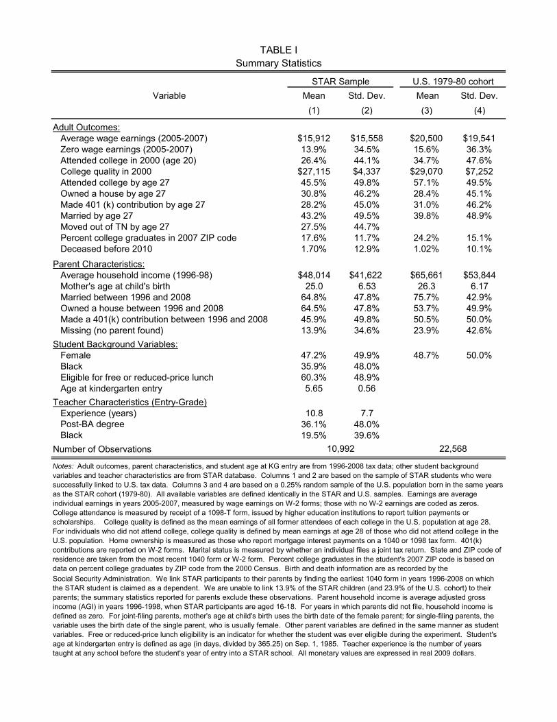
Variable Mean Std. Dev. Mean Std. Dev.(1) (2) (3) (4)

Adult Outcomes: Average wage earnings (2005-2007) $15,912 $15,558 $20,500 $19,541 Zero wage earnings (2005-2007) 13.9% 34.5% 15.6% 36.3% Attended college in 2000 (age 20) 26.4% 44.1% 34.7% 47.6% College quality in 2000 $27,115 $4,337 $29,070 $7,252 Attended college by age 27 45.5% 49.8% 57.1% 49.5% Owned a house by age 27 30.8% 46.2% 28.4% 45.1% Made 401 (k) contribution by age 27 28.2% 45.0% 31.0% 46.2% Married by age 27 43.2% 49.5% 39.8% 48.9% Moved out of TN by age 27 27.5% 44.7% Percent college graduates in 2007 ZIP code 17.6% 11.7% 24.2% 15.1% Deceased before 2010 1.70% 12.9% 1.02% 10.1%

Parent Characteristics: Average household income (1996-98) $48,014 $41,622 $65,661 $53,844 Mother's age at child's birth 25.0 6.53 26.3 6.17 Married between 1996 and 2008 64.8% 47.8% 75.7% 42.9% Owned a house between 1996 and 2008 64.5% 47.8% 53.7% 49.9% Made a 401(k) contribution between 1996 and 2008 45.9% 49.8% 50.5% 50.0% Missing (no parent found) 13.9% 34.6% 23.9% 42.6%Student Background Variables: Female 47.2% 49.9% 48.7% 50.0% Black 35.9% 48.0% Eligible for free or reduced-price lunch 60.3% 48.9% Age at kindergarten entry 5.65 0.56Teacher Characteristics (Entry-Grade) Experience (years) 10.8 7.7 Post-BA degree 36.1% 48.0% Black 19.5% 39.6%Number of Observations

TABLE ISummary Statistics

STAR Sample U.S. 1979-80 cohort

Social Security Administration. We link STAR participants to their parents by finding the earliest 1040 form in years 1996-2008 on which the STAR student is claimed as a dependent. We are unable to link 13.9% of the STAR children (and 23.9% of the U.S. cohort) to their parents; the summary statistics reported for parents exclude these observations. Parent household income is average adjusted gross income (AGI) in years 1996-1998, when STAR participants are aged 16-18. For years in which parents did not file, household income is defined as zero. For joint-filing parents, mother's age at child's birth uses the birth date of the female parent; for single-filing parents, the variable uses the birth date of the single parent, who is usually female. Other parent variables are defined in the same manner as student variables. Free or reduced-price lunch eligibility is an indicator for whether the student was ever eligible during the experiment. Student's age at kindergarten entry is defined as age (in days, divided by 365.25) on Sep. 1, 1985. Teacher experience is the number of years taught at any school before the student's year of entry into a STAR school. All monetary values are expressed in real 2009 dollars.

Notes: Adult outcomes, parent characteristics, and student age at KG entry are from 1996-2008 tax data; other student background variables and teacher characteristics are from STAR database. Columns 1 and 2 are based on the sample of STAR students who were successfully linked to U.S. tax data. Columns 3 and 4 are based on a 0.25% random sample of the U.S. population born in the same years as the STAR cohort (1979-80). All available variables are defined identically in the STAR and U.S. samples. Earnings are average individual earnings in years 2005-2007, measured by wage earnings on W-2 forms; those with no W-2 earnings are coded as zeros. College attendance is measured by receipt of a 1098-T form, issued by higher education institutions to report tuition payments or scholarships. College quality is defined as the mean earnings of all former attendees of each college in the U.S. population at age 28. For individuals who did not attend college, college quality is defined by mean earnings at age 28 of those who did not attend college in the U.S. population. Home ownership is measured as those who report mortgage interest payments on a 1040 or 1098 tax form. 401(k) contributions are reported on W-2 forms. Marital status is measured by whether an individual files a joint tax return. State and ZIP code of residence are taken from the most recent 1040 form or W-2 form. Percent college graduates in the student's 2007 ZIP code is based on data on percent college graduates by ZIP code from the 2000 Census. Birth and death information are as recorded by the

22,56810,992

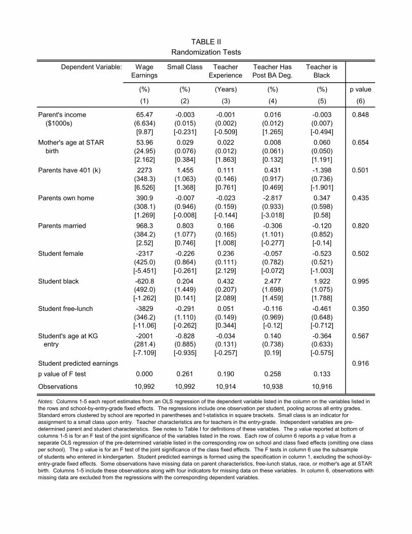
Dependent Variable: Wage Earnings

Small Class Teacher Experience

Teacher Has Post BA Deg.

Teacher is Black

(%) (%) (Years) (%) (%) p value

(1) (2) (3) (4) (5) (6)

Parent's income 65.47 -0.003 -0.001 0.016 -0.003 0.848 ($1000s) (6.634) (0.015) (0.002) (0.012) (0.007)

[9.87] [-0.231] [-0.509] [1.265] [-0.494]Mother's age at STAR 53.96 0.029 0.022 0.008 0.060 0.654 birth (24.95) (0.076) (0.012) (0.061) (0.050)

[2.162] [0.384] [1.863] [0.132] [1.191]Parents have 401 (k) 2273 1.455 0.111 0.431 -1.398 0.501

(348.3) (1.063) (0.146) (0.917) (0.736)[6.526] [1.368] [0.761] [0.469] [-1.901]

Parents own home 390.9 -0.007 -0.023 -2.817 0.347 0.435(308.1) (0.946) (0.159) (0.933) (0.598)[1.269] [-0.008] [-0.144] [-3.018] [0.58]

Parents married 968.3 0.803 0.166 -0.306 -0.120 0.820(384.2) (1.077) (0.165) (1.101) (0.852)[2.52] [0.746] [1.008] [-0.277] [-0.14]

Student female -2317 -0.226 0.236 -0.057 -0.523 0.502(425.0) (0.864) (0.111) (0.782) (0.521)[-5.451] [-0.261] [2.129] [-0.072] [-1.003]

Student black -620.8 0.204 0.432 2.477 1.922 0.995(492.0) (1.449) (0.207) (1.698) (1.075)[-1.262] [0.141] [2.089] [1.459] [1.788]

Student free-lunch -3829 -0.291 0.051 -0.116 -0.461 0.350(346.2) (1.110) (0.149) (0.969) (0.648)[-11.06] [-0.262] [0.344] [-0.12] [-0.712]

Student's age at KG -2001 -0.828 -0.034 0.140 -0.364 0.567 entry (281.4) (0.885) (0.131) (0.738) (0.633)

[-7.109] [-0.935] [-0.257] [0.19] [-0.575]Student predicted earnings 0.916p value of F test 0.000 0.261 0.190 0.258 0.133

Observations 10,992 10,992 10,914 10,938 10,916

TABLE IIRandomization Tests

Notes: Columns 1-5 each report estimates from an OLS regression of the dependent variable listed in the column on the variables listed in the rows and school-by-entry-grade fixed effects. The regressions include one observation per student, pooling across all entry grades. Standard errors clustered by school are reported in parentheses and t-statistics in square brackets. Small class is an indicator for assignment to a small class upon entry. Teacher characteristics are for teachers in the entry-grade. Independent variables are pre-determined parent and student characteristics. See notes to Table I for definitions of these variables. The p value reported at bottom of columns 1-5 is for an F test of the joint significance of the variables listed in the rows. Each row of column 6 reports a p value from a separate OLS regression of the pre-determined variable listed in the corresponding row on school and class fixed effects (omitting one class per school). The p value is for an F test of the joint significance of the class fixed effects. The F tests in column 6 use the subsampleof students who entered in kindergarten. Student predicted earnings is formed using the specification in column 1, excluding the school-by-entry-grade fixed effects. Some observations have missing data on parent characteristics, free-lunch status, race, or mother's age at STAR birth. Columns 1-5 include these observations along with four indicators for missing data on these variables. In column 6, observations with missing data are excluded from the regressions with the corresponding dependent variables.

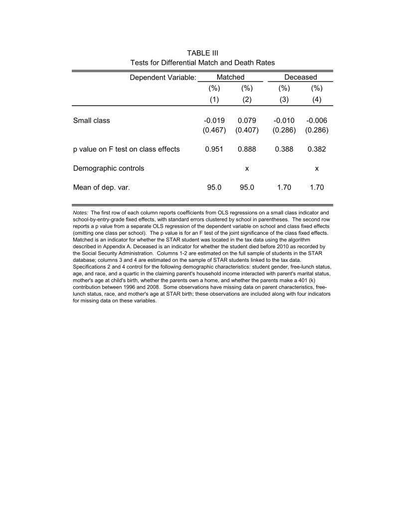
Dependent Variable:(%) (%) (%) (%)(1) (2) (3) (4)

Small class -0.019 0.079 -0.010 -0.006(0.467) (0.407) (0.286) (0.286)

p value on F test on class effects 0.951 0.888 0.388 0.382

Demographic controls x x

Mean of dep. var. 95.0 95.0 1.70 1.70

Notes: The first row of each column reports coefficients from OLS regressions on a small class indicator and school-by-entry-grade fixed effects, with standard errors clustered by school in parentheses. The second row reports a p value from a separate OLS regression of the dependent variable on school and class fixed effects (omitting one class per school). The p value is for an F test of the joint significance of the class fixed effects. Matched is an indicator for whether the STAR student was located in the tax data using the algorithm described in Appendix A. Deceased is an indicator for whether the student died before 2010 as recorded by the Social Security Administration. Columns 1-2 are estimated on the full sample of students in the STAR database; columns 3 and 4 are estimated on the sample of STAR students linked to the tax data. Specifications 2 and 4 control for the following demographic characteristics: student gender, free-lunch status, age, and race, and a quartic in the claiming parent's household income interacted with parent's marital status, mother's age at child's birth, whether the parents own a home, and whether the parents make a 401 (k) contribution between 1996 and 2008. Some observations have missing data on parent characteristics, free-lunch status, race, and mother's age at STAR birth; these observations are included along with four indicators for missing data on these variables.

TABLE IIITests for Differential Match and Death Rates

Matched Deceased

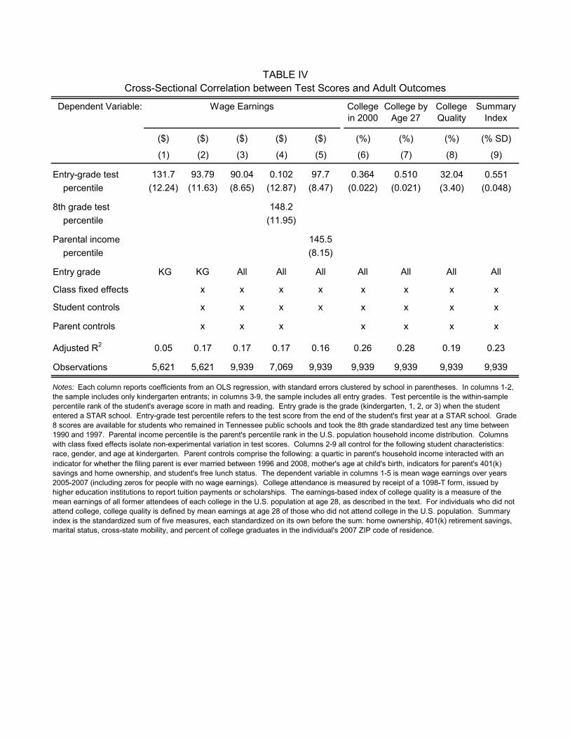
Dependent Variable: Collegein 2000

College by Age 27

College Quality

Summary Index

($) ($) ($) ($) ($) (%) (%) (%) (% SD)

(1) (2) (3) (4) (5) (6) (7) (8) (9)

Entry-grade test 131.7 93.79 90.04 0.102 97.7 0.364 0.510 32.04 0.551 percentile (12.24) (11.63) (8.65) (12.87) (8.47) (0.022) (0.021) (3.40) (0.048)

8th grade test 148.2 percentile (11.95)

Parental income 145.5 percentile (8.15)

Entry grade KG KG All All All All All All All

Class fixed effects x x x x x x x x

Student controls x x x x x x x x

Parent controls x x x x x x x

Adjusted R2 0.05 0.17 0.17 0.17 0.16 0.26 0.28 0.19 0.23

Observations 5,621 5,621 9,939 7,069 9,939 9,939 9,939 9,939 9,939

indicator for whether the filing parent is ever married between 1996 and 2008, mother's age at child's birth, indicators for parent's 401(k) savings and home ownership, and student's free lunch status. The dependent variable in columns 1-5 is mean wage earnings over years 2005-2007 (including zeros for people with no wage earnings). College attendance is measured by receipt of a 1098-T form, issued by higher education institutions to report tuition payments or scholarships. The earnings-based index of college quality is a measure of the mean earnings of all former attendees of each college in the U.S. population at age 28, as described in the text. For individuals who did not attend college, college quality is defined by mean earnings at age 28 of those who did not attend college in the U.S. population. Summary index is the standardized sum of five measures, each standardized on its own before the sum: home ownership, 401(k) retirement savings, marital status, cross-state mobility, and percent of college graduates in the individual's 2007 ZIP code of residence.

Notes: Each column reports coefficients from an OLS regression, with standard errors clustered by school in parentheses. In columns 1-2, the sample includes only kindergarten entrants; in columns 3-9, the sample includes all entry grades. Test percentile is the within-sample percentile rank of the student's average score in math and reading. Entry grade is the grade (kindergarten, 1, 2, or 3) when the student entered a STAR school. Entry-grade test percentile refers to the test score from the end of the student's first year at a STAR school. Grade 8 scores are available for students who remained in Tennessee public schools and took the 8th grade standardized test any time between 1990 and 1997. Parental income percentile is the parent's percentile rank in the U.S. population household income distribution. Columns with class fixed effects isolate non-experimental variation in test scores. Columns 2-9 all control for the following student characteristics: race, gender, and age at kindergarten. Parent controls comprise the following: a quartic in parent's household income interacted with an

TABLE IVCross-Sectional Correlation between Test Scores and Adult Outcomes

Wage Earnings

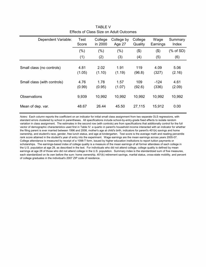
Dependent Variable: Test Score

College in 2000

College by Age 27

College Quality

Wage Earnings

Summary Index

(%) (%) (%) ($) ($) (% of SD)(1) (2) (3) (4) (5) (6)

Small class (no controls) 4.81 2.02 1.91 119 4.09 5.06(1.05) (1.10) (1.19) (96.8) (327) (2.16)

Small class (with controls) 4.76 1.78 1.57 109 -124 4.61(0.99) (0.95) (1.07) (92.6) (336) (2.09)

Observations 9,939 10,992 10,992 10,992 10,992 10,992

Mean of dep. var. 48.67 26.44 45.50 27,115 15,912 0.00

Notes: Each column reports the coefficient on an indicator for initial small class assignment from two separate OLS regressions, with standard errors clustered by school in parentheses. All specifications include school-by-entry-grade fixed effects to isolate random variation in class assignment. The estimates in the second row (with controls) are from specifications that additionally control for the full vector of demographic characteristics used first in Table IV: a quartic in parent's household income interacted with an indicator for whether the filing parent is ever married between 1996 and 2008, mother's age at child's birth, indicators for parent's 401(k) savings and home ownership, and student's race, gender, free lunch status, and age at kindergarten. Test score is the average math and reading percentile rank score attained in the student's year of entry into the experiment. Wage earnings are the mean earnings across years 2005-07. College attendance is measured by receipt of a 1098-T form, issued by higher education institutions to report tuition payments or scholarships. The earnings-based index of college quality is a measure of the mean earnings of all former attendees of each college in the U.S. population at age 28, as described in the text. For individuals who did not attend college, college quality is defined by mean earnings at age 28 of those who did not attend college in the U.S. population. Summary index is the standardized sum of five measures,

TABLE VEffects of Class Size on Adult Outcomes

each standardized on its own before the sum: home ownership, 401(k) retirement savings, marital status, cross-state mobility, and percentof college graduates in the individual's 2007 ZIP code of residence.

Dependent Variable: Test Score

Wage Earnings

Test Score

Wage Earnings

Test Score

(%) ($) (%) ($) (%) ($) ($)(1) (2) (3) (4) (5) (6) (7)

Teacher with >10 years 3.18 1093 1.61 -536.1 of experience (1.26) (545.5) (1.21) (619.3)

Teacher has post-BA deg. -0.848 -261.1 0.95 -359.4(1.15) (449.4) (0.90) (500.1)

Fraction black classmates -6.97 -1,757(9.92) (2692)

Fraction female classmates 9.74 -67.53(4.26) (1539)

Fraction free-lunch -7.53 -284.6 classmates (4.40) (1731)

Classmates' mean age -3.24 -25.78(3.33) (1359)

Classmates' mean -23.06 predicted score (94.07)

Small class 5.19 -8.158 3.77 -284.2 4.63 -132.2 -119.2(1.19) (448.4) (1.17) (536.4) (0.99) (342.3) (330.9)

Entry grade KG KG Grade ≥1 Grade ≥1 All All All

Observations 5,601 6,005 4,270 4,909 9,939 10,992 10,992

TABLE VI

and omit the own student. Classmates' mean predicted score is constructed by regressing test scores on school-by-entry-grade fixed effects and the demographic characteristics listed above and then taking the mean of the predicted scores. Variables labeled "fraction" are in units between zero and one. Free-lunch status is a proxy for having low household income.

Wage Earnings

Notes: Each column reports coefficients from an OLS regression, with standard errors clustered by school in parentheses. All specifications control for school-by-entry-grade fixed effects, an indicator for initial assignment to a small class, and the vector of demographic characteristics used first in Table IV: a quartic in parent's household income interacted with an indicator for whether the filing parent is ever married between 1996 and 2008, mother's age at child's birth, indicators for parent's 401(k) savings and home ownership, and student's race, gender, free lunch status, and age at kindergarten. Columns 1-2 include only students who entered a STAR school in kindergarten. Columns 3-4 include only students who enter STAR after kindergarten. Columns 5-7 pool all students, regardless of their entry grade. Test score is the average math and reading test score at the end of the year in which the student enters a STAR school (measured in percentiles). Wage earnings is the individual's mean wage earnings over years 2005-2007 (including zeros for people with no wage earnings). Teacher experience is the number of years the teacher taught at any school before the student's year of entry into a STAR school. Classmates' characteristics are defined based on the classroom that the student enters in the first year he is in a STAR school

Observable Teacher and Peer Effects

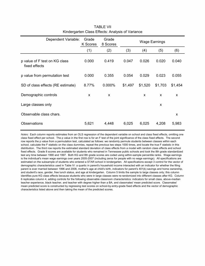
Grade Grade K Scores 8 Scores

(1) (2) (3) (4) (5) (6)

p value of F test on KG class 0.000 0.419 0.047 0.026 0.020 0.040 fixed effects

p value from permutation test 0.000 0.355 0.054 0.029 0.023 0.055

SD of class effects (RE estimate) 8.77% 0.000% $1,497 $1,520 $1,703 $1,454

Demographic controls x x x x x

Large classes only x

Observable class chars. x

Observations 5,621 4,448 6,025 6,025 4,208 5,983

demographic characteristics used in Table IV: a quartic in parent's household income interacted with an indicator for whether the filing parent is ever married between 1996 and 2008, mother's age at child's birth, indicators for parent's 401(k) savings and home ownership, and student's race, gender, free lunch status, and age at kindergarten. Column 5 limits the sample to large classes only; this column identifies pure KG class effects because students who were in large classes were re-randomized into different classes after KG. Column 6 replicates column 4, adding controls for the following observable classroom characteristics: indicators for small class, above-median teacher experience, black teacher, and teacher with degree higher than a BA, and classmates' mean predicted score. Classmates' mean predicted score is constructed by regressing test scores on school-by-entry-grade fixed effects and the vector of demographic characteristics listed above and then taking the mean of the predicted scores.

Dependent Variable: Wage Earnings

TABLE VIIKindergarten Class Effects: Analysis of Variance

Notes: Each column reports estimates from an OLS regression of the dependent variable on school and class fixed effects, omitting one class fixed effect per school. The p value in the first row is for an F test of the joint significance of the class fixed effects. The second row reports the p value from a permutation test, calculated as follows: we randomly permute students between classes within each school, calculate the F statistic on the class dummies, repeat the previous two steps 1000 times, and locate the true F statistic in this distribution. The third row reports the estimated standard deviation of class effects from a model with random class effects and school fixed effects. Grade 8 scores are available for students who remained in Tennessee public schools and took the 8th grade standardized test any time between 1990 and 1997. Both KG and 8th grade scores are coded using within-sample percentile ranks. Wage earnings is the individual's mean wage earnings over years 2005-2007 (including zeros for people with no wage earnings). All specifications are estimated on the subsample of students who entered a STAR school in kindergarten. All specifications except 3 control for the vector of

Dependent Variable: Test Score

College in 2000

College by Age 27

College Quality

Summary Index

(%) ($) ($) ($) ($) (%) (%) ($) (% of SD)(1) (2) (3) (4) (5) (6) (7) (8) (9)

Class Quality (peer 0.662 50.61 61.31 53.44 47.70 0.096 0.108 9.328 0.250 scores) (0.024) (17.45) (20.21) (24.84) (18.63) (0.046) (0.053) (4.573) (0.098)

Entry grade All All All KG Grade ≥1 All All All All

Observable class x chars.

Observations 9,939 10,959 10,859 6,025 4,934 10,959 10,959 10,959 10,959

College attendance is measured by receipt of a 1098-T form, issued by higher education institutions to report tuition payments or scholarships. The earnings-based index of college quality is a measure of the mean earnings of all former attendees of each college in the U.S. population at age 28, as described in the text. For individuals who did not attend college, college quality is defined by mean earnings at age 28 of those who did not attend college in the U.S. population. Summary index is the standardized sum of five measures, each standardized on its own before the sum: home ownership, 401(k) retirement savings, marital status, cross-state mobility, and percent of college graduates in the individual's 2007 ZIP code of residence.

Wage Earnings

TABLE VIIIEffects of Class Quality on Wage Earnings

Notes: Each column reports coefficients from an OLS regression, with standard errors clustered by school in parentheses. Class quality is measured as the difference (in percentiles) between mean end-of-year test scores of the student's classmates and (grade-specific) schoolmates. Class quality is defined based on the first, randomly assigned STAR classroom (i.e. KG class for KG entrants, 1st grade class for 1st grade entrants, etc.). All specifications control for school-by-entry-grade fixed effects and the vector of demographic characteristics used first in Table IV: a quartic in parent's household income interacted with an indicator for whether the filing parent is ever married between 1996 and 2008, mother's age at child's birth, indicators for parent's 401(k) savings and home ownership, and student's race, gender, free-lunch status, and age at kindergarten. Column 3 includes controls for observable classroom characteristics as in Column 6 of Table VII. Column 4 restricts the sample to kindergarten entrants; Column 5 includes only those who enter in grades 1-3. Test score is the average math and reading test score at the end of the year in which the student enters STAR (measured in percentiles). Wage earnings is the individual's mean wage earnings over years 2005-2007 (including zeros for people with no wage earnings).

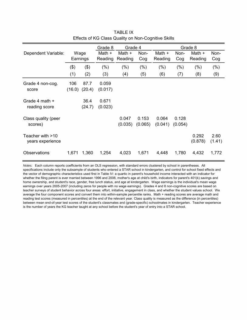
Grade 8Dependent Variable: Math +

ReadingMath +

ReadingNon-Cog

Math + Reading

Non-Cog

Math + Reading

Non-Cog

($) ($) (%) (%) (%) (%) (%) (%) (%)(1) (2) (3) (4) (5) (6) (7) (8) (9)

Grade 4 non-cog. 106 87.7 0.059 score (16.0) (20.4) (0.017)

Grade 4 math + 36.4 0.671 reading score (24.7) (0.023)

Class quality (peer 0.047 0.153 0.064 0.128 scores) (0.035) (0.065) (0.041) (0.054)

Teacher with >10 0.292 2.60 years experience (0.878) (1.41)

Observations 1,671 1,360 1,254 4,023 1,671 4,448 1,780 4,432 1,772

TABLE IXEffects of KG Class Quality on Non-Cognitive Skills

Wage Earnings

Grade 4 Grade 8

Notes: Each column reports coefficients from an OLS regression, with standard errors clustered by school in parentheses. All specifications include only the subsample of students who entered a STAR school in kindergarten, and control for school fixed effects and the vector of demographic characteristics used first in Table IV: a quartic in parent's household income interacted with an indicator for whether the filing parent is ever married between 1996 and 2008, mother's age at child's birth, indicators for parent's 401(k) savings and home ownership, and student's race, gender, free lunch status, and age at kindergarten. Wage earnings is the individual's mean wage earnings over years 2005-2007 (including zeros for people with no wage earnings). Grades 4 and 8 non-cognitive scores are based on teacher surveys of student behavior across four areas: effort, initiative, engagement in class, and whether the student values school. We average the four component scores and convert them into within-sample percentile ranks. Math + reading scores are average math and reading test scores (measured in percentiles) at the end of the relevant year. Class quality is measured as the difference (in percentiles) between mean end-of-year test scores of the student's classmates and (grade-specific) schoolmates in kindergarten. Teacher experience is the number of years the KG teacher taught at any school before the student's year of entry into a STAR school.

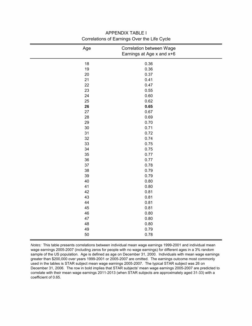
Age Correlation between Wage Earnings at Age x and x+6

18 0.3619 0.3620 0.3721 0.4122 0.4723 0.5524 0.6025 0.6226 0.65

27 0.6728 0.6929 0.7030 0.7131 0.7232 0.7433 0.7534 0.7535 0.7736 0.7737 0.7838 0.7939 0.7940 0.8041 0.8042 0.8143 0.8144 0.8145 0.8146 0.8047 0.8048 0.8049 0.7950 0.78

APPENDIX TABLE ICorrelations of Earnings Over the Life Cycle

Notes: This table presents correlations between individual mean wage earnings 1999-2001 and individual mean wage earnings 2005-2007 (including zeros for people with no wage earnings) for different ages in a 3% random sample of the US population. Age is defined as age on December 31, 2000. Individuals with mean wage earnings greater than $200,000 over years 1999-2001 or 2005-2007 are omitted. The earnings outcome most commonly used in the tables is STAR subject mean wage earnings 2005-2007. The typical STAR subject was 26 on December 31, 2006. The row in bold implies that STAR subjects' mean wage earnings 2005-2007 are predicted to correlate with their mean wage earnings 2011-2013 (when STAR subjects are approximately aged 31-33) with a coefficient of 0.65.

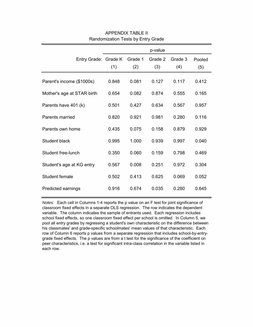
Entry Grade: Grade K Grade 1 Grade 2 Grade 3 Pooled(1) (2) (3) (4) (5)

Parent's income ($1000s) 0.848 0.081 0.127 0.117 0.412

Mother's age at STAR birth 0.654 0.082 0.874 0.555 0.165

Parents have 401 (k) 0.501 0.427 0.634 0.567 0.957

Parents married 0.820 0.921 0.981 0.280 0.116

Parents own home 0.435 0.075 0.158 0.879 0.929

Student black 0.995 1.000 0.939 0.997 0.040

Student free-lunch 0.350 0.060 0.159 0.798 0.469

Student's age at KG entry 0.567 0.008 0.251 0.972 0.304

Student female 0.502 0.413 0.625 0.069 0.052

Predicted earnings 0.916 0.674 0.035 0.280 0.645

p-value

APPENDIX TABLE IIRandomization Tests by Entry Grade

Notes: Each cell in Columns 1-4 reports the p value on an F test for joint significance of classroom fixed effects in a separate OLS regression. The row indicates the dependent variable. The column indicates the sample of entrants used. Each regression includes school fixed effects, so one classroom fixed effect per school is omitted. In Column 5, we pool all entry grades by regressing a student's own characteristic on the difference between his classmates' and grade-specific schoolmates' mean values of that characteristic. Each row of Column 6 reports p values from a separate regression that includes school-by-entry-grade fixed effects. The p values are from a t test for the significance of the coefficient on peer characteristics, i.e. a test for significant intra-class correlation in the variable listed in each row.

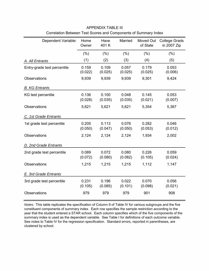
Dependent Variable: Home Owner

Have401 K

Married Moved Out of State

College Grads in 2007 Zip

(%) (%) (%) (%) (%)

(1) (2) (3) (4) (5)

Entry-grade test percentile 0.159 0.109 0.057 0.179 0.053(0.022) (0.025) (0.025) (0.025) (0.006)

Observations 9,939 9,939 9,939 9,301 9,424

B. KG Entrants

KG test percentile 0.136 0.100 0.048 0.145 0.053(0.028) (0.035) (0.035) (0.021) (0.007)

Observations 5,621 5,621 5,621 5,354 5,367

C. 1st Grade Entrants

1st grade test percentile 0.205 0.113 0.076 0.282 0.046(0.050) (0.047) (0.050) (0.053) (0.012)

Observations 2,124 2,124 2,124 1,934 2,002

D. 2nd Grade Entrants

2nd grade test percentile 0.089 0.072 0.080 0.226 0.059(0.072) (0.080) (0.082) (0.105) (0.024)

Observations 1,215 1,215 1,215 1,112 1,147

E. 3rd Grade Entrants

3rd grade test percentile 0.231 0.196 0.022 0.070 0.056(0.105) (0.085) (0.101) (0.098) (0.021)

Observations 979 979 979 901 908

Notes: This table replicates the specification of Column 9 of Table IV for various subgroups and the five constituent components of summary index. Each row specifies the sample restriction according to the year that the student entered a STAR school. Each column specifies which of the five components of the summary index is used as the dependent variable. See Table I for definitions of each outcome variable. See notes to Table IV for the regression specification. Standard errors, reported in parentheses, are clustered by school.

APPENDIX TABLE IIICorrelation Between Test Scores and Components of Summary Index

A. All Entrants

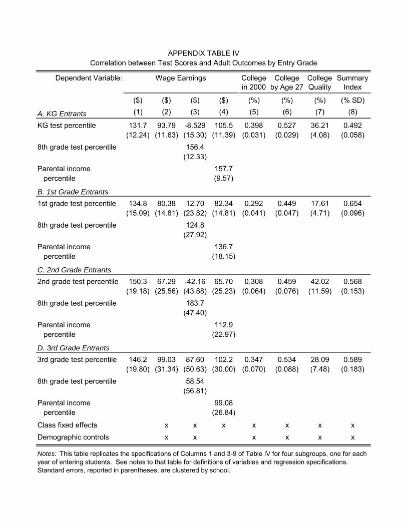
Dependent Variable: Collegein 2000

College by Age 27

College Quality

Summary Index

($) ($) ($) ($) (%) (%) (%) (% SD)(1) (2) (3) (4) (5) (6) (7) (8)

KG test percentile 131.7 93.79 -8.529 105.5 0.398 0.527 36.21 0.492(12.24) (11.63) (15.30) (11.39) (0.031) (0.029) (4.08) (0.058)

8th grade test percentile 156.4(12.33)

Parental income 157.7 percentile (9.57)

B. 1st Grade Entrants

1st grade test percentile 134.8 80.38 12.70 82.34 0.292 0.449 17.61 0.654(15.09) (14.81) (23.82) (14.81) (0.041) (0.047) (4.71) (0.096)

8th grade test percentile 124.8(27.92)

Parental income 136.7 percentile (18.15)

C. 2nd Grade Entrants

2nd grade test percentile 150.3 67.29 -42.16 65.70 0.308 0.459 42.02 0.568(19.18) (25.56) (43.88) (25.23) (0.064) (0.076) (11.59) (0.153)

8th grade test percentile 183.7(47.40)

Parental income 112.9 percentile (22.97)

D. 3rd Grade Entrants

3rd grade test percentile 146.2 99.03 87.60 102.2 0.347 0.534 28.09 0.589(19.80) (31.34) (50.63) (30.00) (0.070) (0.088) (7.48) (0.183)

8th grade test percentile 58.54(56.81)

Parental income 99.08 percentile (26.84)

Class fixed effects x x x x x x xDemographic controls x x x x x x

APPENDIX TABLE IVCorrelation between Test Scores and Adult Outcomes by Entry Grade

Wage Earnings

Notes: This table replicates the specifications of Columns 1 and 3-9 of Table IV for four subgroups, one for each year of entering students. See notes to that table for definitions of variables and regression specifications. Standard errors, reported in parentheses, are clustered by school.

A. KG Entrants

Dependent Variable:(1) (2)

Grade K scores 93.79 39.46(11.63) (30.08)

Grade 1 scores 98.40 71.21(11.83) (23.53)

Grade 2 scores 88.72 83.32(14.15) (24.66)

Grade 3 scores 97.43 103.5(12.78) (20.08)

Grade 4 scores 94.71 91.40(12.40) (20.69)

Grade 5 scores 110.8 113.2(10.81) (19.24)

Grade 6 scores 121.6 139.5(11.37) (21.53)

Grade 7 scores 138.2 158.7(11.53) (21.82)

Grade 8 scores 148.9 155.2(11.11) (21.47)

Sample All KG Entrants Constant Sample of KG Entrants

Wage Earnings ($)

APPENDIX TABLE VCorrelation Between Test Scores and Earnings by Grade

Notes: Each row of this table reports the coefficient on test score from a separate regression that replicates Column 2 of Table IV, replacing KG test score with the test score from the listed grade. The STAR data do not contain test scores for all students in all grades. Regressions underlying Column 1 use all students who entered a STAR school in kindergarten and who have a test score for the listed grade. Regressions underlying Column 2 use only these KG entrants who have a test score for every grade. The coefficients in Column 1 are used to construct Figure VIb. See notes to Table IV for other variable definitions and the regression specification. Standard errors, reported in parentheses, are clustered by school.

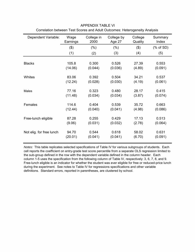
Dependent Variable: Wage Earnings

College in 2000

College by Age 27

College Quality

Summary Index

($) (%) (%) ($) (% of SD)(1) (2) (3) (4) (5)

Blacks 105.8 0.300 0.526 27.39 0.553(14.06) (0.044) (0.036) (4.89) (0.091)

Whites 83.06 0.392 0.504 34.21 0.537(12.24) (0.028) (0.030) (4.19) (0.061)

Males 77.16 0.323 0.480 28.17 0.415(11.48) (0.034) (0.034) (3.87) (0.074)

Females 114.6 0.404 0.539 35.72 0.663(12.44) (0.040) (0.041) (4.98) (0.086)

Free-lunch eligible 87.28 0.255 0.429 17.13 0.513(9.06) (0.031) (0.032) (2.78) (0.064)

Not elig. for free lunch 94.70 0.544 0.618 58.02 0.631(20.01) (0.041) (0.041) (6.70) (0.091)

APPENDIX TABLE VICorrelation between Test Scores and Adult Outcomes: Heterogeneity Analysis

Notes: This table replicates selected specifications of Table IV for various subgroups of students. Each cell reports the coefficient on entry-grade test score percentile from a separate OLS regression limited to the sub-group defined in the row with the dependent variable defined in the column header. Each column 1-5 uses the specification from the following column of Table IV, respectively: 3, 6, 7, 8, and 9. Free-lunch eligible is an indicator for whether the student was ever eligible for free or reduced-price lunch during the experiment. See notes to Table IV for regressions specifications and other variable definitions. Standard errors, reported in parentheses, are clustered by school.

Dependent Var:Krueger

(1999), Table V col 6

Linked STAR-

IRS

Linked STAR-IRS

Linked STAR-

IRS

Linked STAR-IRS

(1) (2) (3) (4) (5)

Small Class Dummy 5.37 5.40 -124SE w/o clustering (0.78) (325)SE cluster by class (1.25) (1.29) (299)SE cluster by school (1.45) (336)

High Teacher Exp. 1093SE w/o clustering (453)SE cluster by class (437)SE cluster by school (545)

Class Quality 50.61SE w/o clustering (15.35)SE cluster by class (14.76)SE cluster by school (17.45)

Demographic controls x x x

Observations 5,861 5,869 10,992 6,005 10,959

Grade K Test Score Earnings ($)

APPENDIX TABLE VIIEffect of Clustering on Standard Errors

Notes: Table shows estimates from regressions with standard errors calculated in three ways: no clustering, clustering by entry classroom, and clustering by school. In Columns 1-2, independent variables include indicators for assignment to small class as well as assignment to regular class with aide (coefficient not shown) to replicate the specification in Krueger (1999). Columns 3-5 replicate the key earnings specifications from Table V (Col. 5), Table VI (Col. 1) and Table VII (Col. 2). Columns 1-2 use grade K entrants, while Columns 3-5 use all matched students regardless of entry grade. All columns include school by entry wave fixed effects.

Dependent Variable: Test Score College in 2000

College by Age 27

College Quality

Wage Earnings

Summary Index

(%) (%) (%) ($) ($) (% of SD)(1) (2) (3) (4) (5) (6)

Small class (no controls) 5.37 1.56 1.57 165 -3.23 6.07(1.26) (1.50) (1.29) (145) (431) (2.63)

Small class (with controls) 5.16 1.70 1.64 185 -57.6 5.64(1.21) (1.35) (1.22) (143) (440) (2.60)

Observations 5,621 6,025 6,025 6,025 6,025 6,025

Mean of dep. var. 51.44 31.47 51.45 27,422 17,111 4.88

APPENDIX TABLE VIIIEffects of Class Size on Adult Outcomes: Kindergarten Entrants Only

Notes: This table replicates Table V, restricting the sample to students who entered a STAR school in kindergarten. See notes to Table V for regression specifications and variable definitions. Standard errors, reported in parentheses, are clustered by school.

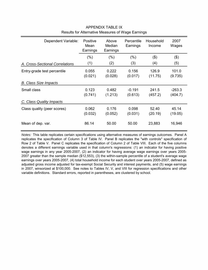
Dependent Variable: Positive Mean

Earnings

Above Median

Earnings

Percentile Earnings

Household Income

2007 Wages

(%) (%) (%) ($) ($)(1) (2) (3) (4) (5)

Entry-grade test percentile 0.055 0.222 0.156 126.9 101.0(0.021) (0.028) (0.017) (11.75) (9.735)

B. Class Size Impacts

Small class 0.123 0.482 -0.191 241.5 -263.3(0.741) (1.213) (0.613) (457.2) (404.7)

C. Class Quality Impacts

Class quality (peer scores) 0.062 0.176 0.098 52.40 45.14(0.032) (0.052) (0.031) (20.19) (19.05)

Mean of dep. var. 86.14 50.00 50.00 23,883 16,946

APPENDIX TABLE IXResults for Alternative Measures of Wage Earnings

Notes: This table replicates certain specifications using alternative measures of earnings outcomes. Panel Areplicates the specification of Column 3 of Table IV. Panel B replicates the "with controls" specification ofRow 2 of Table V. Panel C replicates the specification of Column 2 of Table VIII. Each of the five columnsdenotes a different earnings variable used in that column's regressions: (1) an indicator for having positivewage earnings in any year 2005-2007, (2) an indicator for having average wage earnings over years 2005-2007 greater than the sample median ($12,553), (3) the within-sample percentile of a student's average wageearnings over years 2005-2007, (4) total household income for each student over years 2005-2007, defined as adjusted gross income adjusted for tax-exempt Social Security and interest payments, and (5) wage earningsin 2007, winsorized at $100,000. See notes to Tables IV, V, and VIII for regression specifications and othervariable definitions. Standard errors, reported in parentheses, are clustered by school.

A. Cross-Sectional Correlations

Dependent Variable: Home Owner

Have 401 K

Married Moved Out of State

College Grads in 2007 Zip

Predicted Earnings

Summary Index

(%) (%) (%) (%) (%) ($)(1) (2) (3) (4) (5) (6)

Small class 0.712 2.888 1.872 1.105 -0.038 438.9(1.039) (1.042) (1.082) (0.930) (0.223) (209.8)

Observations 10,992 10,992 10,404 10,268 10,404 10,992

B. Class Quality

Class quality (peer scores) 0.080 0.053 0.056 0.029 0.019 16.48(0.047) (0.058) (0.051) (0.045) (0.012) (12.16)

Observations 10,959 10,959 10,375 10,238 10,375 10,959

Mean of dep. var. 30.80 28.18 44.83 27.53 17.60 15,912

APPENDIX TABLE XImpacts of Class Size and Quality on Components of Summary Outcome Index

Notes: Columns 1-5 decompose the impacts of class size and quality on the summary index into impacts on each of the summary index's five constituent components. Panel A replicates the "with controls" specification of Row 2 of Table V for each component. Panel B replicates Column 9 of Table VIII for each component. See notes to those tables for regression specifications and sample definitions. See Table I for definitions of the dependent variables used in Columns 1-5, each of which is a component of summary index. Column 6 reports impacts on an alternative "predicted earnings" summary index. This index is constructed by predicting earnings from a regression of mean wage earnings over years 2005-2007 on the five dependent variables in Columns 1-5. Standard errors, reported in parentheses, are clustered by school.

A. Class Size

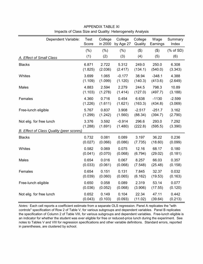
Dependent Variable: Test Score

College in 2000

College by Age 27

College Quality

Wage Earnings

Summary Index

(%) (%) (%) ($) ($) (% of SD)(1) (2) (3) (4) (5) (6)

Blacks 6.871 2.722 5.312 249.0 250.0 6.308(1.825) (2.036) (2.417) (134.1) (540.0) (3.343)

Whites 3.699 1.065 -0.177 38.94 -348.1 4.388(1.109) (1.099) (1.120) (140.3) (413.6) (2.649)

Males 4.883 2.594 2.279 244.5 798.3 10.89(1.103) (1.278) (1.414) (127.0) (497.7) (3.188)

Females 4.360 0.716 0.454 6.638 -1130 -2.599(1.226) (1.611) (1.621) (163.3) (434.8) (3.069)

Free-lunch eligible 5.767 0.837 3.908 -2.517 -251.7 3.162(1.299) (1.242) (1.560) (88.34) (394.7) (2.790)

Not elig. for free lunch 3.376 3.592 -0.914 296.6 293.0 7.292(1.288) (1.691) (1.480) (222.8) (595.5) (3.390)

B. Effect of Class Quality (peer scores)

Blacks 0.732 0.081 0.089 3.197 36.22 0.236(0.027) (0.066) (0.086) (7.735) (18.60) (0.099)

Whites 0.582 0.069 0.075 12.16 68.17 0.180(0.041) (0.070) (0.068) (6.794) (29.02) (0.181)

Males 0.654 0.016 0.067 8.257 66.03 0.357(0.033) (0.061) (0.068) (7.548) (25.48) (0.158)

Females 0.654 0.151 0.131 7.845 32.37 0.032(0.039) (0.060) (0.065) (6.162) (19.53) (0.163)

Free-lunch eligible 0.650 0.058 0.089 2.319 53.14 0.077(0.036) (0.052) (0.068) (3.906) (17.55) (0.120)

Not elig. for free lunch 0.652 0.149 0.104 22.34 47.11 0.442(0.043) (0.103) (0.093) (11.02) (39.64) (0.213)

APPENDIX TABLE XIImpacts of Class Size and Quality: Heterogeneity Analysis

Notes: Each cell reports a coefficient estimate from a separate OLS regression. Panel A replicates the "with controls" specification of Row 2 of Table V, for various subgroups and dependent variables. Panel B replicates the specification of Column 2 of Table VIII, for various subgroups and dependent variables. Free-lunch eligible is an indicator for whether the student was ever eligible for free or reduced-price lunch during the experiment. See notes to Tables V and VIII for regression specifications and other variable definitions. Standard errors, reported in parentheses, are clustered by school.

A. Effect of Small Class

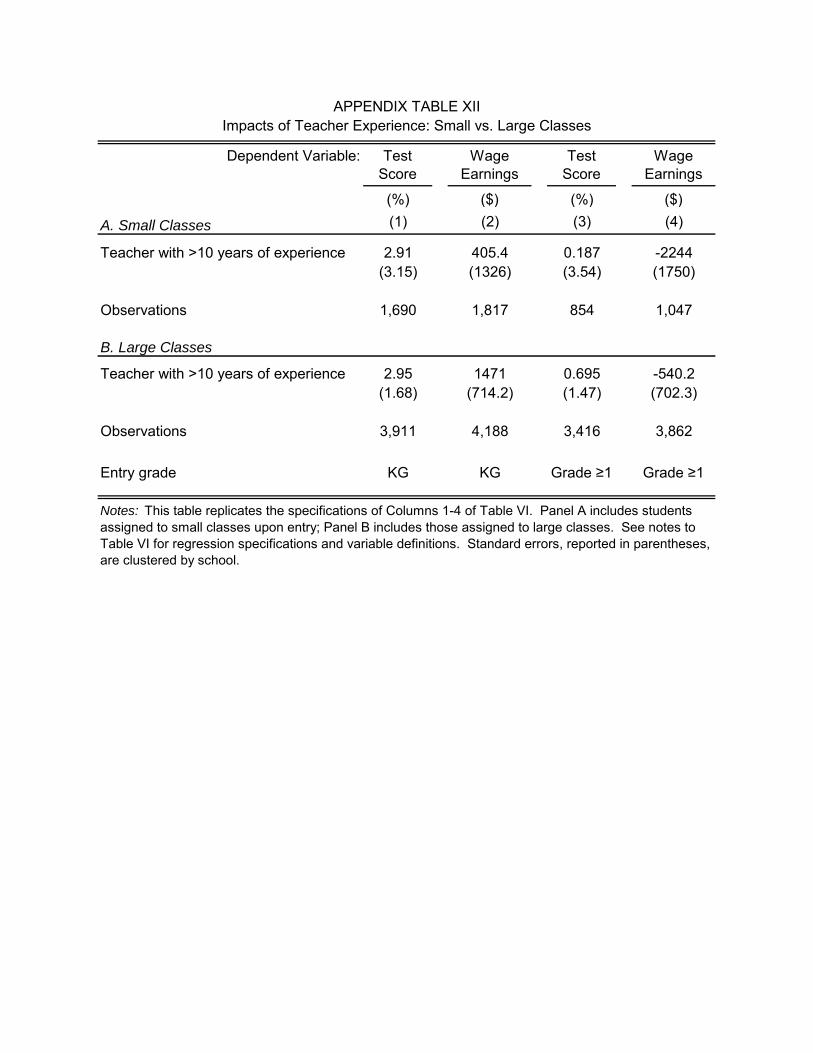
Dependent Variable: Test Score

Wage Earnings

Test Score

Wage Earnings

(%) ($) (%) ($)(1) (2) (3) (4)

Teacher with >10 years of experience 2.91 405.4 0.187 -2244(3.15) (1326) (3.54) (1750)

Observations 1,690 1,817 854 1,047

B. Large Classes

Teacher with >10 years of experience 2.95 1471 0.695 -540.2(1.68) (714.2) (1.47) (702.3)

Observations 3,911 4,188 3,416 3,862

Entry grade KG KG Grade ≥1 Grade ≥1

APPENDIX TABLE XIIImpacts of Teacher Experience: Small vs. Large Classes

Notes: This table replicates the specifications of Columns 1-4 of Table VI. Panel A includes students assigned to small classes upon entry; Panel B includes those assigned to large classes. See notes to Table VI for regression specifications and variable definitions. Standard errors, reported in parentheses, are clustered by school.

A. Small Classes

Dependent Variable:

(1) (2) (3) (4) (5)

Entry-grade test percentile 82.21 96.39 90.04 (23.63) (31.16) (8.65)

B. KG Entrants

KG test percentile 78.71 89.28 74.85 80.33 93.79 (35.09) (39.70) (26.50) (26.40) (9.56)

Estimation method Leave-Out Mean

Split-Sample

LIML 2SLS OLS

estimates for three of the specifications. Instrumenting with entry class dummies is ill defined in later grades as it would require defining class quality based purely on the new entrants, who constitute a small fraction of each class. Panel B replicates the specifications in A using the subsample of kindergarten entrants. The leave-out mean IV estimator in Panel B Column 1 coincides with the jackknife IV of Angrist, Imbens, and Krueger (1995), when we use only KG entrants. When we pool entry grades, our leave-out mean estimator differs from jackknife IV because we form the leave-out mean measure of class quality using all peers (including previous entrants), not just those who entered in the current entry grade. Standard errors, reported in parentheses, are clustered by school in all columns except 3.

APPENDIX TABLE XIIIEffects of Class Quality on Earnings: Instrumental Variable Estimates

Wage Earnings ($)

Notes: The effects of class quality on test scores and earnings reported in Columns 1 and 2 of Table VIII can be combined to produce a reduced-form IV estimate of the earnings effect associated with an increase in test scores: $50.61/0.662=$76.48. Including only those observations with both test score and wages in the data changes the coefficient slightly to $82.21 in Column 1. To test the robustness of our leave-out mean estimator, we report three alternative IV estimates of the impact of test scores on earnings, controlling for school-by-entry-grade fixed effects and the demographic controls used in Column 2 of Table VIII. Column 2 instead uses a split-sample definition of peer scores, in which we randomly split classes into two groups and proxy for class quality using peer scores in the other group. Column 3 estimates the model using limited information maximum likelihood, using kindergarten class dummies as instruments. Column 4 instruments for test score with classroom dummies using two-stage least squares. Column 5 reports an OLS estimate of the correlation between test scores and earnings as a reference. Panel A pools all entry grades and reports

A. All Entrants

A. Cross-Sectional Correlations

Dependent Variable:

($) ($) ($) ($) ($) ($) ($) ($)(1) (2) (3) (4) (5) (6) (7) (8)

Effort 79.91 127.8(16.52) (15.43)

Initiative 57.06 92.29(18.08) (16.86)

Value 61.47 115.5(16.97) (19.68)

Participation 37.26 66.34(18.68) (16.38)

B. Class Quality Impacts

Dependent Variable: Effort Initiative Value Particip Effort Initiative Value Particip

(%) (%) (%) (%) (%) (%) (%) (%)(1) (2) (3) (4) (5) (6) (7) (8)

Class quality 0.151 0.165 0.095 0.120 0.141 0.070 0.124 0.178 (peer scores) (0.066) (0.070) (0.071) (0.082) (0.071) (0.056) (0.069) (0.066)

APPENDIX TABLE XIVEffects of Class Quality on Components of Non-Cognitive Measures

Notes: This table decomposes relationships described in Table IX into the four constituent components of non-cognitive skill. These four non-cognitive measures are constructed from a series of questions asked of the student’s teacher(s) and are intended to measure, respectively: student effort in class, initiative, whether a student perceives school/class as "valuable", and participatory behavior. The measures were reported twice, once by the student’s regular 4th grade teacher (Columns 1-4) and the second time the scores are the average of the reports by the 8th grade math and English teachers (Columns 5-8). Each of the four variables is scaled as a within-sample percentile rank. Panel A replicates Column 1 of Table IX, using only one of the four non-cognitive measures as a covariate in each regression. Panel B replicates Column 5 of Table IX, using one of the four non-cognitive measures as the dependent variable in each regression. See notes to Table IX for regression specifications and other variable definitions. Standard errors, reported in parentheses, are clustered by school.

Grade 4 Non-Cognitive Measure Grade 8 Non-Cognitive Measure

Wage EarningsGrade 4 Non-Cognitive Measure Grade 8 Non-Cognitive Measure

FIGURE ICorrelation between Kindergarten Test Scores and Adult Outcomes

(a) Wage Earnings

Mea

n W

age

Ear

nin

gs f

rom

Age

25-

27

$10K

0 20 40 60 80 100

$15K

$20K

$25K

KG Test Score Percentile

R²=0.05

(b) College Attendance

KG Test Score Percentile

Att

ende

d C

olle

ge b

efor

e A

ge

27

0.0

20%

40%

60%

80%

0 20 40 60 80 100

Attended in 2000 Ever Attended

Ever Attended: R²=0.11Attended in 2000: R²=0.10

(c) College Quality

KG Test Score Percentile

Ear

nin

gs-B

ase

d C

olle

ge Q

ualit

y In

dex

$18K

$20K

$22K

$24K

$26K

$28K

0 20 40 60 80 100

R²=0.05

(d) Outcome Summary Index

KG Test Score Percentile

Out

com

e S

umm

ary

Ind

ex

0 20 40 60 80 100

-.4

-.2

0

.2

.4

R²=0.05

These figures plot the raw correlations between adult outcomes and kindergarten average test scores in math and reading(measured by within-sample percentile ranks). To construct these figures, we bin test scores into twenty equal sized (5percentile point) bins and plot the mean of the adult outcome within each bin. The solid or dashed line shows the bestlinear fit estimated on the underlying student-level data using OLS. The R2 from this regression, listed in each panel,shows how much of the variance in the outcome is explained by KG test scores. Earnings are mean annual earnings overyears 2005-2007, measured by wage earnings on W-2 forms; those with no W-2 earnings are coded as zeros. Collegeattendance is measured by receipt of a 1098-T form, issued by higher education institutions to report tuition payments orscholarships, at some point between 1999 and 2007. The earnings-based index of college quality is a measure of the meanearnings of all former attendees of each college in the U.S. population at age 28, as described in the text. For individualswho did not attend college, college quality is defined by mean earnings at age 28 of those who did not attend college in theU.S. population. The summary index is the standardized sum of five measures, each standardized on its own before thesum: home ownership, 401(k) retirement savings, marital status, cross-state mobility, and percent of college graduates inthe individual’s 2007 ZIP code of residence. Thus the summary index has mean 0 and standard deviation of 1. Allmonetary values are expressed in real 2009 dollars.

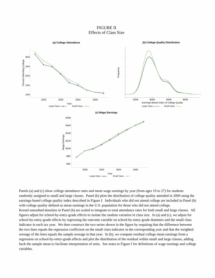
FIGURE IIEffects of Class Size

Year

Per

cent

Atte

ndin

g C

olle

ge

10%

15%

20%

25%

30%

2000 2002 2004 2006

Large Class Small Class

(a) College Attendance (b) College Quality Distribution

Earnings-Based Index of College Quality

Fre

quen

cy

Large Class Small Class

$20K $30K $40K $50K

Wag

e E

arni

ngs

$6K

$8K

$10K

$12K

$14K

$16K

$18K

2000 2002 2004 2006

(c) Wage Earnings

YearLarge Class Small Class

Panels (a) and (c) show college attendance rates and mean wage earnings by year (from ages 19 to 27) for studentsrandomly assigned to small and large classes. Panel (b) plots the distribution of college quality attended in 2000 using theearnings-based college quality index described in Figure I. Individuals who did not attend college are included in Panel (b)with college quality defined as mean earnings in the U.S. population for those who did not attend college.Kernel-smoothed densities in Panel (b) are scaled to integrate to total attendance rates for both small and large classes. Allfigures adjust for school-by-entry-grade effects to isolate the random variation in class size. In (a) and (c), we adjust forschool-by-entry-grade effects by regressing the outcome variable on school-by-entry-grade dummies and the small classindicator in each tax year. We then construct the two series shown in the figure by requiring that the difference betweenthe two lines equals the regression coefficient on the small class indicator in the corresponding year and that the weightedaverage of the lines equals the sample average in that year. In (b), we compute residual college mean earnings from aregression on school-by-entry-grade effects and plot the distribution of the residual within small and large classes, addingback the sample mean to facilitate interpretation of units. See notes to Figure I for definitions of wage earnings and collegevariables.

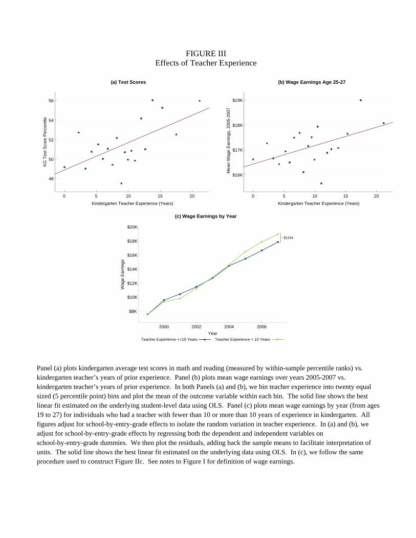
FIGURE IIIEffects of Teacher Experience

48

50

52

54

56

0 5 10 15 20

(a) Test Scores

Kindergarten Teacher Experience (Years)

KG

Tes

t Sco

re P

erce

ntile

$16K

$17K

$18K

$19K

0 5 10 15 20

(b) Wage Earnings Age 25-27

Kindergarten Teacher Experience (Years)

Mea

n W

age

Ear

nin

gs,

2005

-200

7

$8K

$10K

$12K

$14K

$16K

$18K

$20K

Teacher Experience <=10 Years Teacher Experience > 10 Years

Year

2000 2002 2004 2006

Wag

e E

arni

ngs

(c) Wage Earnings by Year

$1104

Panel (a) plots kindergarten average test scores in math and reading (measured by within-sample percentile ranks) vs.kindergarten teacher’s years of prior experience. Panel (b) plots mean wage earnings over years 2005-2007 vs.kindergarten teacher’s years of prior experience. In both Panels (a) and (b), we bin teacher experience into twenty equalsized (5 percentile point) bins and plot the mean of the outcome variable within each bin. The solid line shows the bestlinear fit estimated on the underlying student-level data using OLS. Panel (c) plots mean wage earnings by year (from ages19 to 27) for individuals who had a teacher with fewer than 10 or more than 10 years of experience in kindergarten. Allfigures adjust for school-by-entry-grade effects to isolate the random variation in teacher experience. In (a) and (b), weadjust for school-by-entry-grade effects by regressing both the dependent and independent variables onschool-by-entry-grade dummies. We then plot the residuals, adding back the sample means to facilitate interpretation ofunits. The solid line shows the best linear fit estimated on the underlying data using OLS. In (c), we follow the sameprocedure used to construct Figure IIc. See notes to Figure I for definition of wage earnings.

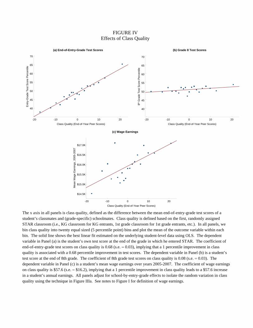
FIGURE IVEffects of Class Quality

40

45

50

55

60

65

70

-10 0 10 20

(a) End-of-Entry-Grade Test Scores

Class Quality (End-of-Year Peer Scores)

Ent

ry-G

rad

e T

est S

core

Per

cent

ile

-20

8th

Gra

de T

est S

core

Per

cent

ile

40

45

50

55

60

65

70

-20 -10 0 10 20

(b) Grade 8 Test Scores

Class Quality (End-of-Year Peer Scores)

Mea

n W

age

Ear

ning

s, 2

005-

2007

$14.5K

$15.0K

$15.5K

$16.0K

$16.5K

$17.0K

-20 -10 0 10 20

Class Quality (End-of-Year Peer Scores)

(c) Wage Earnings

The x axis in all panels is class quality, defined as the difference between the mean end-of-entry-grade test scores of astudent’s classmates and (grade-specific) schoolmates. Class quality is defined based on the first, randomly assignedSTAR classroom (i.e., KG classroom for KG entrants, 1st grade classroom for 1st grade entrants, etc.). In all panels, webin class quality into twenty equal sized (5 percentile point) bins and plot the mean of the outcome variable within eachbin. The solid line shows the best linear fit estimated on the underlying student-level data using OLS. The dependentvariable in Panel (a) is the student’s own test score at the end of the grade in which he entered STAR. The coefficient ofend-of-entry-grade test scores on class quality is 0.68 (s.e. 0.03), implying that a 1 percentile improvement in classquality is associated with a 0.68 percentile improvement in test scores. The dependent variable in Panel (b) is a student’stest score at the end of 8th grade. The coefficient of 8th grade test scores on class quality is 0.08 (s.e. 0.03). Thedependent variable in Panel (c) is a student’s mean wage earnings over years 2005-2007. The coefficient of wage earningson class quality is $57.6 (s.e. $16.2), implying that a 1 percentile improvement in class quality leads to a $57.6 increasein a student’s annual earnings. All panels adjust for school-by-entry-grade effects to isolate the random variation in classquality using the technique in Figure IIIa. See notes to Figure I for definition of wage earnings.

FIGURE VEffects of Class Quality by Year

$8K

$10K

$12K

$14K

$16K

$18KW

age

Ear

ning

s

2000 2002 2004 2006Year

Below-Average Class Quality Above-Average Class Quality

(a) Wage Earnings

10%

15%

20%

25%

30%

35%

2000 2002 2004 2006

(b) College Attendance

Per

cen

t A

tten

ding

Col

lege

Below-Average Class Quality Above-Average Class Quality

Year

These figures show college attendance rates and mean wage earnings by year (from ages 19 to 27) for students in twogroups of classes: those that were above the class quality median and those that were below. Class quality is defined as thedifference between the mean end-of-entry-grade test scores of a student’s classmates and (grade-specific) schoolmates.Class quality is defined based on the first, randomly assigned STAR classroom (i.e., KG classroom for KG entrants, 1stgrade classroom for 1st grade entrants, etc.). Both panels adjust for school-by-entry-grade effects to isolate the randomvariation in class quality using the procedure in Figure IIc. See notes to Figure I for definitions of wage earnings andcollege attendance.

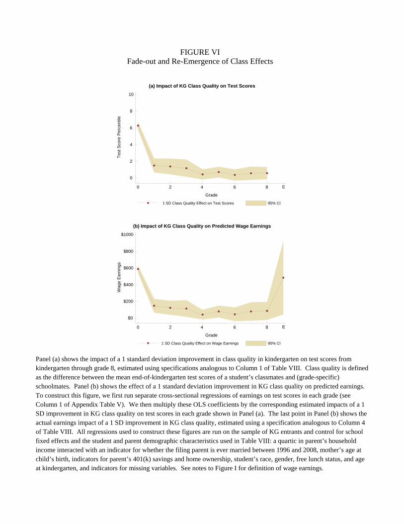
FIGURE VIFade-out and Re-Emergence of Class Effects

Te

st S

core

Per

cent

ile

(a) Impact of KG Class Quality on Test Scores

1 SD Class Quality Effect on Test Scores

0

2

4

6

8

10

Grade

95% CI

0 2 4 6 8 E

$0

$200

$400

$600

$800

$1000

(b) Impact of KG Class Quality on Predicted Wage Earnings

Grade

95% CI1 SD Class Quality Effect on Wage Earnings

0 2 4 6 8 E

Wa

ge E

arn

ing

s

Panel (a) shows the impact of a 1 standard deviation improvement in class quality in kindergarten on test scores fromkindergarten through grade 8, estimated using specifications analogous to Column 1 of Table VIII. Class quality is definedas the difference between the mean end-of-kindergarten test scores of a student’s classmates and (grade-specific)schoolmates. Panel (b) shows the effect of a 1 standard deviation improvement in KG class quality on predicted earnings.To construct this figure, we first run separate cross-sectional regressions of earnings on test scores in each grade (seeColumn 1 of Appendix Table V). We then multiply these OLS coefficients by the corresponding estimated impacts of a 1SD improvement in KG class quality on test scores in each grade shown in Panel (a). The last point in Panel (b) shows theactual earnings impact of a 1 SD improvement in KG class quality, estimated using a specification analogous to Column 4of Table VIII. All regressions used to construct these figures are run on the sample of KG entrants and control for schoolfixed effects and the student and parent demographic characteristics used in Table VIII: a quartic in parent’s householdincome interacted with an indicator for whether the filing parent is ever married between 1996 and 2008, mother’s age atchild’s birth, indicators for parent’s 401(k) savings and home ownership, student’s race, gender, free lunch status, and ageat kindergarten, and indicators for missing variables. See notes to Figure I for definition of wage earnings.