How does economic theory explain the Hubbert peak oil model?

How does economic theory explain the Hubbert

peak oil model?

Frédéric Reynès a, b, *

, Samuel Okullo a, Marjan Hofkes

a

a Institute for Environmental Studies - Instituut voor Milieuvraagstukken (IVM), Faculty of Earth and Life

Sciences (FALW), VU University Amsterdam, De Boelelaan 1085, 1081 HV Amsterdam, The Netherlands

b OFCE - Sciences Po Research Centre, 69 Quai d’Orsay, 75007 Paris, France

Abstract

The aim of this paper is to provide an economic foundation for bell shaped oil

extraction trajectories, consistent with Hubbert’s peak oil model. There are several

reasons why it is important to get insight into the economic foundations of peak oil.

As production decisions are expected to depend on economic factors, a better

comprehension of the economic foundations of oil extraction behaviour is

fundamental to predict production and price over the coming years. The investigation

made in this paper helps us to get a better understanding of the different mechanisms

that may be at work in the case of OPEC and non-OPEC producers. We show that

profitability is the main driver behind production plans. Changes in profitability due

to divergent trajectories between costs and oil price may give rise to a Hubbert

production curve. For this result we do not need to introduce a demand or an

exploration effect as is generally assumed in the literature.

IVM Working Paper: IVM 10/01

Keywords: Hubbert peak, Hotelling, shadow price, depletion effect

Date: January 2010

Acknowledgements

The authors acknowledge the financial support of the NWO’s ACTS Sustainable

Hydrogen research program.

About IVM

Institute for Environmental Studies Vrije Universiteit

De Boelelaan 1087 1081 HV AMSTERDAM

The Netherlands Tel. +31 (0)20-5989 555 Fax. +31 (0)20-5989 553

Web: http://www.vu.nl/ivm

The Institute for Environmental Studies (Instituut voor Milieuvraagstukken, IVM) is the oldest academic environmental research institute in the Netherlands. Since its creation in 1971, IVM has built up considerable experience in dealing with the complexities of environmental problems. Its purpose is to contribute to sustainable development and the rehabilitation and preservation of the environment through academic research and training. The institute has repeatedly been evaluated as the best Dutch research group in this field.

1

How does economic theory explain the Hubbert peak

oil model?

Equation Chapter 1 Section 1

Frédéric Reynès a, b, *, Samuel Okullo a, Marjan Hofkes a

a Institute for Environmental Studies - Instituut voor Milieuvraagstukken (IVM), Faculty of Earth and Life

Sciences (FALW), VU University Amsterdam, De Boelelaan 1085, 1081 HV Amsterdam, The Netherlands

b OFCE - Sciences Po Research Centre, 69 Quai d’Orsay, 75007 Paris, France

Abstract:

The aim of this paper is to provide an economic foundation for bell shaped oil

extraction trajectories, consistent with Hubbert’s peak oil model. There are several reasons

why it is important to get insight into the economic foundations of peak oil. As production

decisions are expected to depend on economic factors, a better comprehension of the

economic foundations of oil extraction behaviour is fundamental to predict production and

price over the coming years. The investigation made in this paper helps us to get a better

understanding of the different mechanisms that may be at work in the case of OPEC and

non-OPEC producers. We show that profitability is the main driver behind production

plans. Changes in profitability due to divergent trajectories between costs and oil price may

give rise to a Hubbert production curve. For this result we do not need to introduce a

demand or an exploration effect as is generally assumed in the literature.

Keywords: Hubbert peak, Hotelling, shadow price, depletion effect

JEL Classification: Q30, Q41

* Corresponding author. Tel.: + 31 (0)20 59 85934. Fax : + 31 (0)20 59 89553. E-mail addresses:

[email protected], [email protected], [email protected].

Acknowledgments: The authors acknowledge the financial support of the NWO’s ACTS Sustainable

Hydrogen research program.

2

1. Introduction

Calibrating a logistic function on historical oil production data and two estimates of

ultimate recoverable reserves, Hubbert (1956; 1962) predicted that oil production in the

lower 48 US states would peak either in 1965 or in 1970. His 1970 prediction came to pass

and Hubbert’s methodology to predict oil production subsequently became renowned1.

Hubbert found that oil production often exhibits a bell shaped extraction trajectory. His

model is often defined as a technical approach to oil production because it is supposed to

provide a kind of proxy of the technical limit to production.

The accuracy of Hubbert’s prediction combined with the relative simplicity of his

method had a huge influence on the modelling of oil production in particular among oil peak

theorists such as Campbell and Laherrère (1998) and Deffeyes (2001). Nonetheless, the

approach has often been criticised both empirically and theoretically2. Theoretically,

Hubbert’s approach has been criticised for lacking economic foundation. The bell-shaped

trend followed by production is rather ad hoc. It is not deduced from economic

maximisation behaviour and thus does not take into account any economic factors such as

prices. From an empirical point of view, the Hubbert model generally fails in predicting

production for the Organisation of the Petroleum Exporting Countries (OPEC), whose

production has widely diverged from the Hubbert curve since the 1970s (see Rehrl and

Friedrich, 2006, p. 2416). This discrepancy casts doubt on the ability of the Hubbert model

to accurately predict global oil production in the coming years especially in an era where

OPEC will be dominating in terms of reserve and production share3.

Economic theory has been able to provide a comprehensive explanation for the

divergence of OPEC production from the Hubbert curve. With a non negligible share in the

world production (about 30%), OPEC production has been observed to affect price (see

Salant, 1975; 1976; 1982; Hnyilicza and Pindyck, 1976; Pindyck, 1978; Yang, 2008b): a

1 Since then, the Hubbert curve has been applied to modelling depletion of several exhaustible resources such

as oil, coal, natural gas and uranium by Hubbert himself (Hubbert, 1956; 1962; 1967) and by other proponents

of the Hubbert peaking theory who are reviewed in Section 2.

2 For an early critic see Ryan (1965). For more recent views see Rehrl & Friedrich (2006) or Watkins (2006).

3 In 2007, OPEC possessed nearly 80% of the proved reserves for conventional oil (BP, 2008)

3

coordinated reduction (resp. increase) in production generally leads to a negative (resp.

positive) gap between supply and demand, which is reabsorbed by an increase (resp.

decrease) in price. OPEC as a cartel has rationally an interest to produce below what the best

technology allows since a higher price provides to its members a higher intertemporal profit

(i.e. a higher profit during a longer period of time). Consequently, it is common practice to

model non-OPEC production via Hubbert curves while modelling OPEC production by

solving a profit maximisation program (e.g. Rehrl and Friedrich, 2006).

On the contrary, economic theory has more trouble to justify why the Hubbert curve is

exhibited by many non-OPEC producers such as UK North Sea fields, the lower 48 US

states or Mexico [for a review of regional Hubbert curves see Brandt (2007)]. In fact, the

Hubbert modelling framework could be said to have challenged the basics of neoclassical

economic theory on exhaustible resources as influenced by the seminal works of Gray

(1914), Fisher (1930) and Hotelling (1931)4. According to these neo-classical economic

approaches, the optimal level of extraction of a non-renewable resource maximises an

intertemporal objective function, in general the profit function in case of an industry or an

individual producer, and, alternatively the social welfare function in case of a social planner5.

Most of the time, these models do not generate a peak in production but reproduce the

famous result of the basic Hotelling model where the resource price rises at the rate of

discount and production decreases monotonically via the sensitivity of demand to price. This

property was sometimes interpreted as a failure of the neoclassical approach in modelling the

oil market. However, several studies have shown that the neoclassical approach is able to

generate an oil peak, in particular via changes in cost and/or demand or by introducing an

exploration effect (see Uhler, 1976; Pindyck, 1978; Holland, 2008).

The primary aim of this article is to provide economic foundations for bell shaped

extraction trajectories. The rationale of economic research on this question is threefold.

Firstly, as production decisions are expected to depend on economic factors, the robustness

of Hubbert model may, in the future, be strongly affected by the recent important changes in

the oil market environment such as the strong increases in demand and price. Secondly, this

4 See Devarajan & Fisher (1981) for a historical survey.

5 The cases that involve a social utility function are treated in Dasgupta & Heal (1974), Withagen (1999);

Perman et al. (2003, Chap. 15).

4

investigation may be helpful for understanding the different mechanisms that are at work in

the case of OPEC and non-OPEC producers. Thirdly, a better comprehension of the oil

extraction behaviour is fundamental to predict production and price in the coming years

where there is a high uncertainty on the capacity of the supply to satisfy the demand.

In this article, we provide a direct economic interpretation to Hubbert peak model that

encompasses the technical interpretation. This interpretation seems more realistic than

previous attempts to provide an economic foundation to the Hubbert peak model. Here the

Hubbert curve reflects changes in profitability which depends partly on the technical

characteristic of the resource via costs. Section 2 discusses the limits of a purely technical

approach of the Hubbert model. Section 3 reviews the literature that proposes economic

foundations to Hubbert model. Section 4 develops a basic intertemporal economic

maximisation model where the resource owner operates in a competitive market, taking

prices as given. We show that this model reproduces a Hubbert production curve if the level

of profitability follows a bell-shaped curve, for instance by simply assuming that costs follow

a U-shaped trajectory. No further assumptions are necessary as is generally the case in

previous attempts to provide economic foundations for the Hubbert peak oil model. In

particular, there is no need to introduce a demand effect (where demand and thus

production increases because cost and thus price decreases) or an exploration effect (where

new discoveries allow for a period of increase in production). Moreover, an intertemporal

maximisation behaviour is not a fundamental hypothesis either. Indeed, the link between the

levels of production and profitability is a fundamental result of economic theory that holds

in a static framework that is in the case of a producer who maximises the level of production

of a renewable resource.

Section 5 extends the basic model by assuming that the cost of production increases

with depletion and shows that it is possible to reproduce a bell curve without assuming a U-

shaped cost trajectory. Here intertemporality is fundamental: if the producer expects a period

where the discounted marginal cost decreases, her production may increase along with

profitability over time until the depletion effect is strong enough to decrease profitability and

production. Section 6 discusses the limits of our approach in modelling oil production.

Section 7 concludes.

5

2. The technical interpretation of Hubbert model

Many oil experts and studies interpret the Hubbert model as a technical constraint on

oil production. One reason may be that the Hubbert curve matches fairly well the traditional

techniques used for the extraction of conventional oil from an oil field: a well is drilled, the

downhole pressure pushes up the oil; in order to increase production a second well is drilled,

and then a third, a fourth, etc; production hence increases until no more wells can be drilled

because the margins of the field are reached and/or the underground pressure becomes too

low to push out any more oil, leading to production declines. According to this technical

interpretation, which Hubbert himself largely shares6, the bell shape would mirror the

physical characteristics of the resource (Cleveland and Kaufmann, 1991; Kaufmann, 1991;

Kaufmann, 1995; Moroney and Berg, 1999) and the geological factors that influence its

extraction (Pesaran and Samiei, 1995)7.

This view implicitly assumes that exogenous technical constraints limit production

below a level that would be the optimum production (in terms of profit) if there were no

technological restriction. A typical example would be the case where the extraction is

profitable (because the price is high and costs are low) and where the demand is higher given

prices than the technical constraint. The production would then follow the technical limit

and would not depend on any economic factors such as prices. In this situation, one might

argue that production depends on geophysical constraints and should be modelled as

petroleum engineers do. For conventional oil, production capacity may depend on the size

and the deepness of the field, the underground pressure and the size of the pipes. For

another type of oil, the technical mechanisms that determine extraction trajectories over time

are different but for some reasons (that may look mysterious to the economist) the Hubbert

model appears to give a fairly good approximation of the technical limit to production over

6 According to Hubbert, production at any particular point in time will be determined by the resources’ own

physical limits: “[…] although production rates tend to initially increase, physical limits prevent their continuing

to do so.” (Hubbert, 1956, p. 8).

7 “The basic idea behind Hubbert’s model of production (and discovery) is very simple, and is derived from the

observation that under the influence of geological factors, there are three distinct phases to the production of

an exhaustible resource” (Pesaran and Samiei, 1995, p. 545).

6

time. Many economic studies on oil production adopt implicitly this point of view by

modelling non-OPEC production as a logistic function (e.g. Kaufmann, 1995; Rehrl and

Friedrich, 2006)8. If the Hubbert logistic model is the most popular approach, numerous

variants and extensions sometimes involving economic variables adopt this technical view of

oil production (reviewed in Table 1)

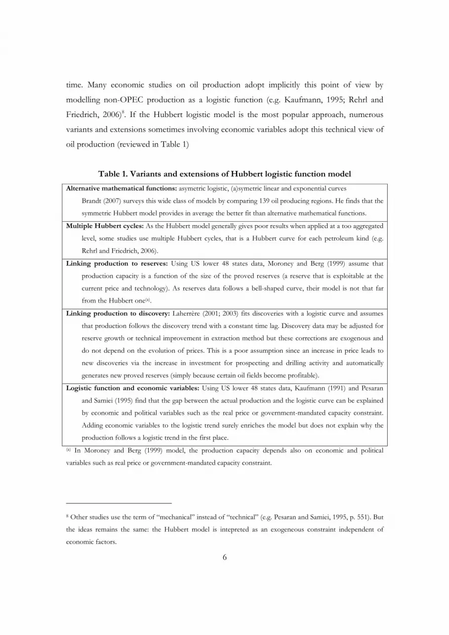
Table 1. Variants and extensions of Hubbert logistic function model

Alternative mathematical functions: asymetric logistic, (a)symetric linear and exponential curves

Brandt (2007) surveys this wide class of models by comparing 139 oil producing regions. He finds that the

symmetric Hubbert model provides in average the better fit than alternative mathematical functions.

Multiple Hubbert cycles: As the Hubbert model generally gives poor results when applied at a too aggregated

level, some studies use multiple Hubbert cycles, that is a Hubbert curve for each petroleum kind (e.g.

Rehrl and Friedrich, 2006).

Linking production to reserves: Using US lower 48 states data, Moroney and Berg (1999) assume that

production capacity is a function of the size of the proved reserves (a reserve that is exploitable at the

current price and technology). As reserves data follows a bell-shaped curve, their model is not that far

from the Hubbert one(a).

Linking production to discovery: Laherrère (2001; 2003) fits discoveries with a logistic curve and assumes

that production follows the discovery trend with a constant time lag. Discovery data may be adjusted for

reserve growth or technical improvement in extraction method but these corrections are exogenous and

do not depend on the evolution of prices. This is a poor assumption since an increase in price leads to

new discoveries via the increase in investment for prospecting and drilling activity and automatically

generates new proved reserves (simply because certain oil fields become profitable).

Logistic function and economic variables: Using US lower 48 states data, Kaufmann (1991) and Pesaran

and Samiei (1995) find that the gap between the actual production and the logistic curve can be explained

by economic and political variables such as the real price or government-mandated capacity constraint.

Adding economic variables to the logistic trend surely enriches the model but does not explain why the

production follows a logistic trend in the first place.

(a) In Moroney and Berg (1999) model, the production capacity depends also on economic and political

variables such as real price or government-mandated capacity constraint.

8 Other studies use the term of “mechanical” instead of “technical” (e.g. Pesaran and Samiei, 1995, p. 551). But

the ideas remains the same: the Hubbert model is intepreted as an exogeneous constraint independent of

economic factors.

7

A purely technical representation of the Hubbert model is unsatisfactory because the

level of production is not directly determined by the technical characteristic of the resource

but by profitability which depends mainly on three economic factors: the oil price, the

extraction costs and the interest rate9. Costs reflect the prices of all the inputs entering into

the production process such as the intermediary material inputs, labour and capital. The unit

cost of the installed production capacity depends (amongst other) on the physical or

geological characteristics of the resource. It is higher, the more difficult the extraction in a

given oil field. Thus the technical constraints have a direct economic interpretation: they

increase the cost of investment and decrease profitability and thus production (for a given oil

price). Taking the example of conventional oil, the producer would have to install more wells

or use enhanced oil recovery technology if she wishes to stabilise the production when the

underground pressure drops. Because of its cost, this additional investment may not be

profitable and consequently production decreases.

A technical constraint limits production because the cost of circumventing it is too high.

This cost may grow exponentially if the desired level of production is increasingly difficult to

reach (e.g. when the resource is nearing depletion). If the desired level of production is

impossible to reach because the resource stock is too low, this cost can be viewed as infinite.

In oil peak regions, reserves are big enough to allow for an increase in production after the

peak. Yet production decreases because the cost of producing one extra unit of oil is too

high, that is because the marginal cost (of a higher level of production) is too high.

Producing more would lead to a suboptimal profit since the marginal cost would become

higher than the oil production price (in the case of a competitive market).

9 The interest rate reflects the trade off the resource owner has to make in choosing to invest in the oil sector

with respect to investing in the other sectors. This term could also describe the trade off of choosing to invest

today or tomorrow, which is referred to as the discount rate.

8

3. The economic interpretation of the Hubbert model

The fact that the Hubbert model works remarkably well for most non-OPEC regions is

somehow a mystery for the economist since this model does not involve any maximisation

strategy from the agent exploiting the resource. The empirical success is no doubt a puzzle

for economic theory. Several authors have tried to solve it by proposing an economic

foundation for the Hubbert peak model and interpreting peaks in production as the result of

an economic maximisation program. They have identified several theoretical situations

which lead to a peak in production.

In the first one, the production follows a bell-shaped curve because the production

costs follow an U-shaped curve over time. The fact that production increases (resp.

decreases) when cost decreases (resp. increases) comes generally from a demand effect: when

the price decreases, the demand increases, and so does the production. Several studies follow

this reasoning although their modelling strategies or the reasons leading to a U-shaped cost

diverge:

Reynolds (1999) reinterprets the Hubbert curve as a cost function that combines the

information and depletion effects proposed by Uhler (1976). The information effect reduces

costs: the more experience in oil prospecting and extraction, the cheaper the related costs. It

reflects a learning curve in oil exploration and exploitation. On the contrary, the depletion

effect increases costs: the less oil, the more difficult to find and the more expensive to

extract. The author uses an elegant metaphor according to which Robinson Crusoe has to

search for a buried resource in order to survive. The probability of success in finding the

hidden resource is interpreted as the inverse of the cost function: the higher this probability,

the less costly it is to find more of the resource. As this probability increases with the

research experience but decreases with the number of discoveries, the model predicts a

period of fall in price and then a sudden increase. The price equals the marginal cost which

follows a U-curve (more precisely a logistic function) since the depletion effect becomes at

some point bigger than the information effect. As a consequence of the adjustment of

demand to prices, the production follows a logistic function.

In Reynolds (1999), the marginal cost function is not directly derived from the

theoretical model based on probabilities but is assumed to follow an exogenous Hubbert

9

curve. This weakness is overcome by Bardi (2005) who specifies explicitly Reynolds

probabilistic model and simulates it using Monte Carlo techniques. He shows that the model

reproduces a bell-shaped production curve whose symmetry depends on the main

hypotheses of the model: e.g. the taking into account or not of technical changes.

Holland (2008, Model 2) brings a related argument within a standard neoclassical

approach of exhaustible resources where the producer maximises her intertemporal profit.

Similarly to the previous information effect, the technological change has a decreasing effect

on cost and thus price. But the increase in price comes from an increase in the scarcity rent

(i.e. the shadow price) and not directly from costs. The result is the same: the peak arises

when the scarcity effect offsets the technical change effect.

The same authors propose other models based on intertemporal maximisation that

reproduce also a peak. Holland (2008, Model 1) assumes that price increases with the scarcity

rent. Via the demand function this leads to an endogeneous decrease in demand. In the case

of an exogeneous increase in demand (due for instance to the increase of the standard of

living of the population), production increases as long as the exogeneous increase in demand

is higher that the endogeneous decrease in demand. At a certain point in time, “the demand

increase will eventually be less than the full marginal cost increase, and equilibrium

production will decrease” (Holland, 2008, p.65). Holland (2008, Model 4) proposes also a

site development model where the peak is driven by an increase in production capacity due

to the production at newly developed sites, the decrease in production still resulting from a

decrease in demand (that follows the increase in price due to the increase in scarcity).

Holland’s Model 3 is based on Pindyck (1978) who assumes that the cost of production

increases as the reserve base depletes and that new discoveries depend positively on the

exploratory effort and negativelly on the cumulative discovery. This model shows a different

production pattern depending on the size of the initial reserve. If the initial reserve is large,

the production (resp. the price) decrease (resp. increase) monotoneously as in the basic

Hotteling model. But if the initial reserve is low, “price will start high, fall as rerserves

increases (as a result of exploratory activity), and then rise slowly as reserves decline”

(Pindyck, 1978, p. 11). Production is close to a Hubbert model with a possible asymetry in

the bell-shaped curve.

10

4. An intertemporal model reproducing Hubbert via cost

Previous attempts to provide economic foundation to Hubbert peak oil model often

rely on a demand effect to explain the decrease in production after the peak: the increase in

cost causes the increase in price which causes the decrease in demand and thus in

production. Unfortunately, this theoretical explanation is not supported by the empirical

facts. The producers who experienced a decrease in production in the past were not

constrained by the demand: despite the oil price increases, demand never stopped increasing

because of the increases in the world population and in its standard of living. Consequently,

the decrease in production comes more likely from the producer’s rational choice than from

an external demand constraint. In this section and in the following one, we provide

economic foundations for this argument by developing a model where a competitive

producer chooses her level of production such as that she maximises her intertemporal

profit. This model shows that Hubbert production curve may arise from changes in

profitability due to divergent trajectories between costs and the oil price. We believe that the

profitability argument is more realistic that the demand effect proposed by previous authors.

Let us suppose that the oil producer takes price as given (since she operates in a

competitive market and therefore does not affect price) and faces the following technology,

cost and profit functions:

θ= ( )nput

t tY I with θ > 0 [1]

1Input nput Input

t t t t tC P I P Y θ −

= =

[2]

1Input

t t t t t t t tPY C PY P Y θ −

Π = − = −

[3]

Where Y is the quantity of oil produced (or the extraction level), P is the oil price (or the

output price), C the cost of production, and t is the time operator10. nputI is an index of all

the possible input quantities used in the production process (labour, capital, energy, etc.).

Consequently, the input price index ( InputP ) is a function of the prices of these inputs. If it

depends on the oil price, the algebraic resolution of the maximisation program is more

arduous. One way to circumvent this complication is to consider that Y is the net production

10 Variables in growth rate are referred to as 1/ 1t t tX X X −= −& and all coefficients are positive.

11

that is the quantity of oil actually extracted minus the quantity of oil used as an input. This

way, the oil price is excluded from the input price index and does not intervene as a cost in

the profit function11.

In order to have general results, we do not assume any particular function for the input

index such as a Constant Elasticity of Substitution (CES), Cobb-Douglas or Translog

function. In other words, we do not impose any constraint on the elasticity of substitution

between production factors. The only constraint is that the production function is

homogeneous of degree θ which corresponds to the level of returns to scale: if θ < 1 (resp.

= 1, > 1), there is decreasing (resp. constant, increasing) returns to scale. In case of

increasing (resp. decreasing) returns to scale, a 1%-increase in the production factors

generates more (resp. less) than 1%-increase in the production.

The producer determines the optimal production trajectory by maximising its

intertemporal profit subject to the constraint (s.t.) of a limited resource stock12:

ρ= =

Π + ≤∑ ∑ 0

1 1

/(1 ) s.t. t

n nt es

t tY

t t

Max Y R

[4]

Where es

tR is the size of the reserve (or the resource stock) at the instant t, and ρ the

discount rate.

11 Note, however, that in our particular case of perfect competition, the optimal production resulting from the

maximisation program presented below would be unchanged if we assumed that the input price index was a

function of the oil price: because prices are taken as given, their first derivative with respect to production is

zero.

12 In order to ease the resolution, we assume further that the profit at each period is non-negative (Π ≥ 0t ).

This means that (1) the price is high enough to cover the average cost and that (2) the production is never

negative ( ≥ 0tY ) because the producer is assumed not to buy oil in order to store it and sell it at a more

profitable period.

12

4.1. Analytical solution

Following the Karush-Kuhn-Tucker approach, we introduce the slack variable es

nv R=

in order to rewrite this maximisation program under inequality constraint as a maximisation

program under equality constraint13. Applying the Karush-Kuhn-Tucker theorem the

Lagrangian to this model problem is:

ρ λ= =

= Π + + − −

∑ ∑2

01 1

/(1 )n n

t es

t t

t t

L R v Y

[5]

As the Lagrange multiplier λ is unique and constant over time in this simple model, its

time subscript t is dropped. The optimum must satisfy the following necessary first order

conditions:

Pθλ ρ θ

−− −′∂ ∂ = ⇔ + = ∂Π ∂ = − = −11 ( 1)/ 0 (1 ) / ( )t Input

t t t t t t t tL Y Y P C Y P Y

[6]

λ=

∂ ∂ = ⇔ − − =∑20

1

/ 0 0n

es

t

t

L R v Y

[7]

λ∂ ∂ = ⇔ =/ 0 2 0L v v

[8]

These conditions are sufficient for optimality if the objective function (Π t ) is a

continuously differentiable concave function. This is only the case for decreasing returns to

scale (θ < 1). In case of constant or increasing returns to scale (θ ≥ 1), it is possible to

increase indefinitely the profit by increasing the level of production. If there were no stock

limit, the optimal production would be infinite. By increasing indefinitely production, price

would be affected at some stage. This violates the hypothesis where producers take price as

given because their production is too small to affect price. This is the well-known result

according to which perfect competition is only possible if we assume decreasing returns to

scale technology (θ < 1).

If there is a stock limit and constant or increasing returns to scale optimum (θ ≥ 1), the

optimum of the maximisation program [4] is not defined by the set of equations [6] to [8].

13 See for instance Dixit (1990, Chap. 3), Simon & Blume (1994, Chap. 18 & 19) or Yang (2008a, Chap. 7) for

more details on the resolution of nonlinear optimisation problems under inequality constraint.

13

Instead, it is characterised by several solutions or by one “corner” solution where the

producer exhausts her full resource. In case of constant returns to scale (θ = 1), the average

cost of production is constant. As a consequence, there is infinity of possible optima if the

prices of input and output both grow at the same rate as the discount factor. There is one

“corner” solution if the prices of input and output do not grow at the same rate as the

discount factor: the producer exhausts all her resource at the last (resp. first) period if the

growth rate of prices of input and output is higher (resp. lower) than the discount factor

because it is (resp. not) more profitable to wait. Increasing returns to scale (θ > 1) is always

characterised by one corner solution because the average cost of production decreases when

production increases. It is thus more profitable to produce everything at one period. The

choice of the optimum period will depend on the trajectories of prices and on the discount

factor.

As the cases of constant or increasing returns to scale are more relevant in an imperfect

competition framework where production plans affect the price, we shall assume from now

on decreasing returns to scale (θ < 1). In this case, the first order necessary conditions [6],

[7] and [8] are sufficient for optimality and solving the maximisation program with inequality

constraint is equivalent to comparing two optima (because of condition [8]):

• The optimum where the inequality constraint is inactive: λ = 0 and v ≠ 0 (⇔ ≠ 0es

nR )

This optimum is equivalent to maximising the profit without constraint, that is to

maximise profit in every period. Condition [6] becomes identical to the first order condition

in case of a competitive producer of a conventional (renewable) commodity: price equal

marginal cost. The optimum does not depend on the discount factor and the level of

production depends positively on the ratio between the price of output and the price of the

input:

( )Pθ

θ− −

=11/( 1)

/ Input

t t tY P

[9]

An increase in the output price or a decrease in the input price leads to an increase in

production. This result is not surprising since the ratio between the oil and the input prices

( / Input

t tP P ) is an indicator of the profitability of the firm. This ratio is in fact the “real” oil

price faced by the producer since the deflator considered by the latter is the input price.

14

When the real oil price increases, the producer’s revenue ( t tPY ) increases more than its costs

(Equation [2]). The producer has thus an incentive to increase its production.

Combining [9] and [7] allows for the calculation of the reserve stock at the end of the

maximising period ( es

nR ). If 0es

nR ≥ , we can conclude that the initial reserve is large enough

to be not constraining over the maximisation period. In other words, the decreasing returns

to scale hypothesis acts as a cost constraint that is more constraining than the stock

constraint. The alternative case where < 0es

nR is impossible since the reserve stock should

always be positive. This indicates that the initial stock is not large enough to allow the

producer to reach the unconstrained optimum. Of course this case always arises if the time

horizon is large enough. We must then look at the optimum where the inequality constraint

is active:

• The optimum where the inequality constraint is active: λ ≠ 0 and v = 0 (⇔ = 0es

nR )

In this case, the producer cannot produce as much as she wishes every period because

of the stock limit. The optimal production is thus lower than the one defined at [9]:

P

θλ ρ

θ

− − − +

=

11/( 1)

(1 )ttt Input

t

PY

[10]

Assuming input and output price stability, the optimal production decreases over time if the

discount factor is above 0 because future profit is considered less important relatively to the

present profit. However, if the prices of the input and the output are growing at the rate of

discount (i.e. ρ= +0(1 )ttP P and P P ρ= +0 (1 )Input Input t

t ), the optimal level of extraction does

not depend on the value of the discount rate and is constant up to the point where the final

exhaustion of the resource occurs. Under these assumptions, production is stable over time

because the discounted marginal profit λ is stable over time. This result is a consequence of

the so-called “Hotelling rule”. As Hotelling (1931) assumes no extraction costs, the original

Hotelling rule states that at the optimum the price of a non-renewable resource should grow

at the same rate as the discount factor in order to maximize the present value of the resource

15

capital over the extraction period14. As the price is negatively related to the aggregate level of

production via the demand function, the basic Hotelling model expects the optimal level of

production to decrease steadily over time (all other things being equal). Taking production

costs into consideration, the Hotelling rule becomes the first necessary condition [6] which

states that the optimum level of extraction is such that the marginal profit ( / Y∂Π ∂ ) grows

at the rate of discount. Unlike the original Hotelling rule, condition [6] can be satisfied when

the oil price does not increase at the rate of discount. For instance, if the oil price is constant

and if the marginal cost decreases at the rate of discount, the marginal profit ( / Y∂Π ∂ )

grows at the rate of discount. Consequenly, unlike the basic Hotelling model, the optimum

level of production is not necessary decreasing over time when one accounts for production

costs. This more general framework allows variety of extraction trajectories that depends on

the trajectories followed by the input and oil prices.

Moreover Equation [10] shows that the level of production is lower, the lower the value

of λ. From Equation [6], we see that λ is the discounted (or present) value of the marginal

profit (at the optimum level of production) and is stable across time in this simple model.

From a mathematical point of view, this parameter is the Lagrange multiplier. It measures

how much profit increases if production increases by relaxing the constraint (that is by

increasing the initial reserve). From an economic point of view, λ can be interpreted as the

maximum price a producer is willing to pay for acquiring one extra unit of the resource. It is

sometimes viewed as a kind of rent for the producer because it implies that the price is

above marginal cost (Equation [6]). Alternatively, it could be seen as a kind of extra cost

reflecting the loss in profit compared to a situation where the producer would have an

unlimited resource. For these reasons, λ takes on several names in the economic literature:

(the discounted value of) the shadow price the resource, the scarcity rent, the opportunity

cost, the economic rent or the user cost.

Combining [10] and [7], we show that λ is a negative function of the initial reserve ( 0esR ),

i.e. the higher the initial reserve, the closer the solution is to the unconstrained optimum and

14 Assuming a discount factor γ, Hotelling (1931, p. 140) gives the following justification: “Since it is a matter of

indifference to the owner of a mine whether he receives for a unit of his product a price p0 now or a price p0.eγt

after time t, it is not unreasonable to expect that the price p will be a function of the time of the form p = p0.eγt.

[…] The various units of the mineral are then to be thought of as being at any time all equally valuable […]”.

16

the smaller is the shadow price (because the opportunity of profit increases become smaller).

The limit case of λ = 0 arises when the initial reserve is high enough to allow the producer to

reach the unconstrained optimum. This is the previous case where the constraint is inactive

and some petrol is left at the end of the maximisation period.

The close link between the size of the initial reserve and λ may be more

comprehensively understood by considering the static case of one single maximisation

period (n = 1). Figure 1 depicts the evolution of profit (as defined in Equation [3]) when

production increases. Although the values chosen for the calibration are arbitrary and not

fundamental in terms of interpretation, we set values that replicate the situation of the

competitive producer in the real world. This may give a better intuition of the economic

reasoning. The oil price is set at 100 US dollar ($) and the input price at $10. As a direct

consequence of the decreasing returns to scale hypothesis (θ = 0.5 < 1), profit increases until

the optimal level of production, 5 million barrels (mbls) (C in Figure 1), and then decreases.

If the producer could produce as much as she wanted, she would produce 5. At this point,

the tangent to the profit curve (the marginal profit) is zero

(λ = ∂Π ∂ = − × =/ 100 20 5 0C Y ) as stated by the first order condition [6]. Moreover, the

average cost of production ( / 10 * 5InputC Y P Y= = ) is $50.

If the initial reserve is 1 mbls, the producer cannot reach the unconstrained optimal

production level, and produces 1 which is the constrained optimal production level (A in

Figure 1). The marginal profit at the constrained optimum (the parameter λ) is positive and equal to

80. Increasing the size of the resource stock, let us say to 3 (B in Figure 1), decreases the

value of λ to 40. The closer to the unconstrained optimum (C), the flatter the tangent to the

profit curve since at that point λ = 0. λ is higher at A than at B because A is further from the

unconstrained optimum C. Hence the producer will gain more from an increase of reserve at

A that at B. At C, λ = 0 because the producer cannot increase its profit by increasing its

production. Although the graphic representation may not be possible anymore, the

interpretation of the value of the shadow price remains the same with a higher number of

periods (n > 1).

17

Figure 1. Link between the shadow price and the initial reserve

Profit (Π)

Production level (Y)

Key: The profit function is Equation [3] with 100P = , 10InputP = and θ = 0.5, that is Π = − 2100 10Y Y . Thus

the shadow price (marginal profit) is λ = ∂Π ∂ = −/ 100 20Y Y ; authors’ calculation.

From Equation [6], we see also that λ is a positive (resp. negative) function of the oil

price (resp. the input price). The economic interpretation is similar to the one about the link

between the initial reserve and the shadow price: the lower the oil price (or the higher the

input price), the lower the profitability, the lower the optimal level of production, the closer

the constraint to the unconstrained optimum and thus the lower the shadow price λ.

Here as well, the production evolves according to profitability. But the indicator of

profitability is not the same as when the resource constraint is inactive. Instead of being

simply the real oil price ( / Input

t tP P ), the indicator of profitability is the gap between the real

oil price and the real shadow price ( (1 )t Input

tλ ρ+ / P ). As shown in Equation [10],

production increases when the real oil price increases faster than the real shadow price.

18

4.2. Numerical simulations

Although the system [6], [7] (and [8] with λ ≠ 0 and v = 0) constitutes a system of n + 1

equations with n + 1 unknowns ( λ;tY ), it cannot be easily solved analytically because of

strong non-linearity. The model is linear only if we assume a specific level of returns to scale:

θ = 0.5. Even in that case, the explicit analytical solution is arduous to find, leading to very

complicated formulas for each of the endogenous variables ( λ;tY ) in terms of the

exogenous variables. As this does not bring much insight for the problem we are studying

here, we look now at numerical solutions. In this article, all the simulations were performed

with the GAMS program15.

First, consider the case in which both input and output prices are growing at the rate of

discount (i.e. ρ= +0(1 )ttP P and P P ρ= +0 (1 )Input Input t

t ). We know from the discussions above

that tY will be constant for each period and that λ is higher, the lower the quantities of the

initial resource stock and the lower the input price. Table 2 provides an illustration of this

link assuming that the number of periods is n = 200, level of the returns to scale is θ = 0.5

and the initial oil price is P0 = $100. The discount rate is set at ρ = 0.05, although, changing

the value of the discount rate does not have any impact on the numerical simulation:

production does not depend on the discount rate when the input and output prices are

growing at the rate of discount (see Equation [10]).

But changing the initial reserve stock or the initial input price will affect the level of

extraction as the four similations of Table 2 show. In the first three simulations, the initial

input price is fixed at $10, whereas the initial oil reserves stock takes decreasing values: 1000,

850 and 750 mbls. In the fourth case, the initial reserves are kept at the level of case 3 (750

mbls), whereas the initial input price drop to $5.

15 The scripts used are available upon request.

19

The values chosen for the exogenous variables present an extraction pattern close to the

case of a competitive producer that could be observed in the real world. The world proved

reserve of crude oil was 1 213 billion barrels in 2007 (OPEC, 2008, Table 33) whereas the

level of 2008 world crude oil production was 73.8 million barrels (mbls) per day (EIA, 2009,

Table 11.1b). In case (1) of Table 2, the initial reserves are set to 1000 mbls and the resulting

level of production is 5 mbls annually (i.e. 0.014 mbls per day) until depletion occurs at the

horizon of the simulation. This simulation corresponds to an oil producer that would

possess in the real world 0.08% of the total proved reserve and extract nearly 0.02% of the

total production. This producer can be considered taking the oil price as given because the

level of production is too small to affect prices16.

In this first simulation, the resource depletion constraint is found to be inactive, i.e. the

shadow price is null (λ = 0); this implies that the producer receives no scarcity rent and will

therefore extract as though the resource were non-exhaustible. The producer will not

increase production in the event of an increase in initial reserve level (λ can not be negative)

and any additional reserves would remain un-extracted at the end of the time horizon.

Moreover the optimal production tY is such that the resource constraint is just inactive.

Consequently depletion occurs but only in the last period. Case 1 is nothing else but case C

in Figure 1 in the situation of multiple periods. The level of extraction is constant because

the initial input price is the same and because all prices grow at the rate of discount.

The resource constraint becomes active if we increase the simulation horizon or if we

decrease the initial reserves. The latter is simulated in Cases 2 and 3 in Table 2. With smaller

initial reserves of 850 and 750 mbls of oil, the shadow value of the resource λ jumps from 0

to 15 and 25 respectively because a smaller resource stock prevents the producer from

maintaining extraction at the level of Case 1 over the selected time horizon (200 periods). As

a consequence, production ( tY ) has to drop or alternatively extraction has to take place over

a shorter period. As we do not change the time horizon, annual production falls instead.

16 The fact the producer will extract her reserve over 200 years may be seen unrealistic: in the real world, the

lifetime of a field is approximately 30 years whereas the world ratio between reserve and production is close to

40 years (BP, 2008). A more realistic figure in this respect can easily be obtained by changing the time unit:

assuming that the time unit is 2 months, the extraction lasts 33 years. With 0.11% of the total production, this

is still the case of a competitive producer.

20

This fall in production can be viewed as a loss in revenues for which the producer asks

compensation through an increase in the scarcity rent λ. Without this increase, the first order

condition [6] would be violated and the solution would not be optimal. Making the initial

reserves even smaller increases the shadow price λ even more (Case 3). This is an illustration

of the economic principle that the scarcer a resource, the higher the rate of return asked by

the producers because they cannot exploit indefinitely their resource.

Table 2. Effect on the shadow price of changes in reserves and input price

Cases

(1) (2) (3) (4)

Results

Shadow price: λ 0 15 25 62.5

Production: tY 5 4.25 3.75 3.75

Assumptions

Initial reserve: 0

esR 1000 850 750 750

Initial input price: P0Input 10 10 10 5

Key: numerical simulation of Equation [4] with 0.05Inputt tP P ρ= = =& & , n = 200, 0 100P = and θ = 0.5;

production and reserve expressed in mbls and prices in $; authors’ calculation.

Let us suppose now that the initial input price decreases from $10 (Case 3 in Table 2) to

$5 (Case 4 in Table 2) keeping the initial reserves of Case 3 (750 mbls of oil). The discounted

shadow value is observed to increase from 25 to 62.5 whereas the level of production

remains unchanged. A decrease in the input price corresponds to an increase in profitability.

If the resource were un-exhaustible, the producer would increase its production as we can

see from Equation [9]. As the limited size of the reserve does not allow it, the stability in

production is compensated with an increase in the scarcity rent λ. This is the only way for

shadow value λ plus the marginal cost to equate to the output price, that is for the first order

condition [6] to remain satisfied. An increase in the initial oil price (P0) would give a similar

result whereas an increase of the initial input price (P0Input ) would logically have the opposite

effect.

21

Because both input and output prices grow at the rate of discount, the optimal level of

extraction chosen by the producer is constant over time irrespective of the size of reserves.

This is true both for the unconstrained and constrained optima (Equations [9]) and [10]).

This result comes from the Hotelling rule and from the fact that the profitability is stable

over time. In contrast, when output and input prices are growing at different rates,

producers may shift production from one period to another in response to how the

discounted net profits evolve.

In particular, it can be readily observed from Equations [9] (the unconstrained

optimum) and [10] (the constrained optimum) that our simple model is capable of

reproducing Hubbert model via costs: if the price of the inputs follows a U trajectory (via for

instance the interaction between information and depletion effects), the production will

follow a bell shaped curve. This happens without having to introduce a demand effect as in

Reynolds (1999), Bardi (2005) and Holland (2008) or an exploration effect as in Pindyck

(1978). Here the Hubbert peak model arises out of changes in profitability due to a U

trajectory followed by the input prices, rather than because of the physical characteristics of

the resource. An graphic illustration is given in Figure 2 in the case of the unconstrained

optimum (Equation [9]). The oil price is assumed constant while the input price follows U

trajectory based on a simple quadratic function. As the input price falls, production increases

up to the point where it reaches a maximum where costs are at their minimum (the 100th

period). Then the input price starts to rise forcing production to decline. Because the

quadratic function is symmetric, the extraction pattern is also symmetric. If the path for the

input price was not symmetric, but still U-shaped, the trajectory for extraction would

become non-symmetric but still bell-shaped. More generally, if the ratio between the output

and input prices (i.e. the real oil price) follows a bell shaped curve, production will follow a

Hubbert curve.

Although intertemporal maximisation is not a fundamental assumption to reproduce a

Hubbert peak model, it seems more realistic in the case of non-renewable resources because

it is more rational to take into account the stock constraint. The fact that Hubbert peak

model can be reproduced in a static maximisation framework (the unconstrained model

Equation [9]) is nonetheless interesting in at least two respects. Firstly, it shows that the link

between the levels of production and profitability is a general result of economic rationality.

Secondly, one may argue that some oil producers have actually a very short intertemporal

22

horizon for several reasons: for example, (1) if the producer is highly uncertain about the

future and thinks that at any moment new technologies will come up and lead to a drop in

demand for his resource; (2) due to political pressure, some oil country producers have to

achieve a minimum revenue. In these cases, the producer may behave as one of a renewable

resource: by maximising only its current profit, she sets her production according to her cost

constraint but not according to her resource stock constraint (embodied here in the shadow

price).

Figure 2: Peak in production when the input price exhibits a U-shaped trajectory.

0

1

2

3

4

5

0 50 100 150 200 0

20

40

60

80

100

Extr

action in m

illions

of

bar

rels

Input pri

ces

in $

s

ExtractionInput prices

Key: simulation of Equation [9] with 2( 100)

100

Inputt

tP

−= , n = 200, =0 100P , θ = 0.5; authors’ calculation.

5. Introducing stock depletion effects in costs

Noteworthy are the two shortcomings of the simple model discussed above. First, it

does not reproduce the Hubbert production curve endogeneously but only via specific

exogeneous trajectories for prices. Second, the shadow price is constant over time because

the profit function [3] does not depend on the resource stock. Increasing the initial resources

stock therefore affects uniformally profit across time. Assuming that cost depends on the

23

stock via a depletion effect, we show both analytically and numerically that these two

shortcomings can be removed. A common way to do this is to assume that the price of input

is a negative function of the reserve (e.g. as in Holland, 2008)17:

α−−= 1( )Input Input es

t t tP P R with α ≥ 0

[11]

Where InputP is the exogenous component of the input price referred to from now on as the

exogenous input price. α is the elasticity of costs to reserves.

For the algebraic resolution, it is convenient to reformulate the maximisation program

[4] and the Lagrangian [5] as follows:

1

;1

/ (1 ) s.t. 0

est t

es esnt t tt

t esY Rt n

R R YMax

Rρ

−

=

= −Π +

≥∑

[12]

( ) ( )211

/(1 )n

t es es es

t t t t t n n

t

L R R Y R vρ λ λ−=

= Π + − − + − − ∑

[13]

The necessary and sufficient conditions for optimality are:

11/( 1)

1

(1 )/ 0 (1 ) ( ) ( )

tt est t

t t t t t tInput

t

PL Y P C Y Y R

P

θ

αλ ρλ ρ θ

− −

−

− +′∂ ∂ = ⇔ + = − ⇔ =

[14]

λ −∂ ∂ = ⇔ − + =1/ 0 0es es

t t t tL R R Y

[15]

1 1

1 1/ 0 ( )(1 )

Inputes estt t t t tt

PL R Y Rθ αλ λ α

ρ

− − −− −∂ ∂ = ⇔ − = −

+ [16]

/ 0 2 0nL v vλ∂ ∂ = ⇔ =

[17]

This model presents strong similarities with the one of Section 4. Condition [14] which

determines the optimal level of production is similar to Equation [10] except that λ is not

constant anymore (and thus has a time subscript) and that the optimal level of production is

positively related to the resource stock. Equation [15] is nothing else but a reformulation of

17 This link between the input price and the size of the reserve is determined by geophysical and engineering

aspects.

24

[7]18. Moreover we can see that the previous model correspond to the case of α = 0 which

implies that λ is constant (Equation [16]) and that the optimal level of production is

independent of the resource stock (Equation [14]).

If α > 0 , λ decreases over time. Increasing the initial resources stock does not affect

uniformally profit across time anymore. Such an increase now generates more gain at the

beginning than at the end of the maximisation period. In other words, the oil producer has

more incentive to find new reserves at the start of extraction. Assuming that the output price

and the exogenous input price grow at the rate of discount (i.e. ρ= +0(1 )ttP P and

P P ρ= +0 (1 )Input Input t

t ), the evolution of the optimal production depends on the dynamic of

the reserve and of the discounted shadow price λ (Equation [14]). As the resource stock

decreases over time, production decreases over time. This result has a direct economic

explanation. Because of the depletion effect, the input price increases and thus the

profitability and the optimal level of production decreases over time. Since profitability is

lower at the end of the maximisation period, increasing the initial resource stock generates

less (discounted) profit than at the begining of the sample. Consequently the discounted

18 Indeed summing conditions [15] one to another for all t collapses into [7] since =2 esnv R .

25

marginal profit (λ) decreases over time (as stated by the optimal condition [16]) but this

decrease is too slow to offset the depletion effect and increase production. This result is

simulated in Figure 3 where in addition a strong correlation between production (see panel

(ii)) and the discounted net profit (see panel (i)) appears.

It is notable from the figure that unlike the model presented in Section 4, output and

the discounted shadow price are not constant anymore: they decrease over time. The

discounted marginal cost on the other hand increases over time at an increasing rate (see

panel (i) of Figure 3) because of the depletion effect. Consequently, as less and less of the

resource remains, it becomes increasingly expensive and less profitable to extract. As

evidenced in panel (ii) of Figure 3, this results into a steady fall in production.

Figure 3. Trajectories when prices grow at the rate of discount

0

10

20

30

40

50

60

70

80

90

100

0 20 40 60 80 100 120 140 160 180 200 0

0.1

0.2

0.3

0.4

0.5

0.6

0.7

0.8

0.9

1

Mar

gin

al c

ost

/Shad

ow

pri

ce, both

in $

s

Net

pro

fits

in thousa

nds

of

$s

panel (i)

Discounted marginal costDiscounted shadow price

Discounted net profit

0

1

2

3

4

5

6

7

8

9

10

0 20 40 60 80 100 120 140 160 180 200 0

0.1

0.2

0.3

0.4

0.5

0.6

0.7

0.8

0.9

1

Extr

action in m

illions

of

bar

rels

Res

erves

in b

illions

of

barr

els

panel (ii)

Resource extractionResource stock

Key: simulation of Model [12] with ρ= = =&& 0.05Input

t tP P , n = 200, =0 100P , 0 250InputP = , 0 1000esR = ,

1.978esnR = , 0.591nY = , θ = 0.5, �� = 1, and Φ = 0 ; authors’ calculation.

If we relax the assumption that the output and exogenous input prices grow at the

discount rate, the extraction rate may not decrease as steadily as observed in Figure 3 (where

the output and input prices grow at the same rate). When prices (both output and exogenous

26

input prices) grow at the same rate, which is smaller than the discount rate ( ρ= <&& Input

t tP P ),

production still decreases through the combination of two effects that decrease profitability.

This first is the depletion effect that increases the input price and decreases production (via

the decrease in the ratio 1( ) /es Input

t tR Pα− in Equation [14]). The second is the decrease at the

beginning in the gap between the actual and shadow oil prices ( (1 )tt tP λ ρ− + ) because the

oil price grows at a smaller rate than the discount rate ( tP ρ<& ). At the end of extraction

however, the discounted shadow price (λ) is small enough for the gap between the actual and

shadow oil price to increase. This has a positive effect on production but too small

compared to the depletion effect to lead to an increase in production. Moreover, the fall in

production is non linear at an increasing rate: as the present value of the oil price decreases

while the input price increases through the depletion effect, the producer has a tendency to

shift the most production to the first period.

Consider now the case where the growth rate of the output price is higher than that of

exogenous input prices, but lower than the discount rate ( ρ< <& &Input

t tP P ). Equation [14]

shows that production may increase over time for some periods depending on the dynamic

of the gap between the actual and shadow oil price (which is nothing else but the marginal

cost): ( )0(1 ) (1 ) (1 ) /(1 )t t t t

t t t tP P Pλ ρ ρ ρ λ− + = + + + −& . Indeed, we see that this gap

increases when the (discounted) oil price, 0(1 ) /(1 )t t

tP P ρ+ +& , is higher than the

(discounted) shadow price λ. This has an increasing effect on production that may offset the

depletion effect. Consequently, 3 scenarios for oil production could be observed (1)

production decreases, (2) production increases and then decreases, (3) production increases

monotonically.

The first scenario (decreasing production) is reproduced in Figure 4 by assuming that

the initial exogenous input price 0 $500Input =P . In addition, we assume that the exogenous

27

input price is time invariant ( 0Input

tP =& ) and that the growth rate of the oil price is lower than

the discount rate i.e. 0.04tP =& and ρ = 0.05.

With those hypotheses, production decreases over time, although it is relatively stable

during the first ten periods before it starts falling at more or less exponential rates. It is also

noticeable that the discounted net profit exhibits the same shape as the production curve

(see panel (i)). Production falls slowly in the initial periods because the discounted oil price is

higher than the discounted shadow price. This acts as a driving force that increases

production. This force is not strong enough to offset the depletion effect but limits for some

time the decrease in production.

Figure 4. Decreasing production curve with depletion effect

0

10

20

30

40

50

60

70

80

0 10 20 30 40 50 60 0

0.5

1

1.5

2

2.5

Marg

inal cost

/Shad

ow

pri

ce,

both

in $

s

Net pro

fits

in thousa

nd o

f $s

panel (i)

Discounted marginal costDiscounted shadow price

Discounted net profit

0

5

10

15

20

25

30

0 10 20 30 40 50 60 0

0.1

0.2

0.3

0.4

0.5

0.6

0.7

0.8

0.9

1

Extr

action in m

illions

of

barr

els

Res

erves

in b

illions

of

barr

els

panel (ii)

Resource extractionResource stock

Key: simulation of Model [12] with =& 0.04tP , =&

0InputtP , ρ = 0.05 , n = 200, =0 100P , P =0 500Input ,

0 1000esR = , 0 0.5Input =P , 72.7 *10esnR −= , θ = 0.5, �� = 1, and Φ = 0 ; authors’ calculation.

If the oil price is sufficiently higher than the shadow price, production may increase for

a certain period of time. This can be done here by increasing the initial input price as we

have shown previously the negative correlation between the input price and the shadow

28

price (see Table 2): the higher the input price, the less profitable the extraction, the less gain

from an increase in production, the lower the shadow price. Multiplying the initial

exogenous input price (P0Input ) by 100 compared to the previous case, the initial input price

(computed from [11]) jumps from $0.5 to $50 and the initial shadow price drops from $72 to

$32. All other parameters remain the same as those in Figure 4. Extraction in panel (ii)

Figure 5 rises from initially low levels (about 0.7 mbls) reaches a peak at about 11 mbls in the

117th period and then steeply declines to zero in the 195th when the resource is physically

exhausted. Here as well, the discounted net profit mirrors exactly production by following a

bell-shaped curve (see panel (i)).

Here, the exogenous initial input price is substantially high leading to initially high

marginal costs with low profitability and thus low production. However, the discounted

input price initially decreases over time, which reflects into the sharp decline of the

discounted marginal costs. This leads to an increase in profitability and thus in production.

Because the growth rate of the oil price is lower than the discount rate, the gap between

discounted oil price and the discounted shadow price (the discounted marginal cost in panel

(i) of Figure 5) decreases. This leads to smaller and smaller increase in production until the

depletion effect, due to increasingly lower stock levels, becomes stronger. At this point

profitability, and hence production, peak and start to decline.

Note that the Hubbert curve in Figure 5 is generated by simply making the gap between

oil price and the shadow price (i.e. the marginal costs) substantially high in the initial periods.

No period of decreasing cost is introduced as previously proposed in the literature via the

information effect or the technological change effect. Here the key element reproducing a

Hubbert curve is that the oil price grows at a lower rate than the rate of discount so that the

gap between the discounted oil price and the discounted shadow price (i.e. the discounted

marginal costs) decreases for a certain period of time. This allows for extraction to be less

profitable in the initial periods and incites the producer to delay extraction.

29

Figure 5. Hubbert production curve with depletion effect

0

10

20

30

40

50

60

70

0 20 40 60 80 100 120 140 160 180 200 0

0.05

0.1

0.15

0.2

0.25

0.3

0.35

Mar

gin

al c

ost

/Shadow

pri

ce, both

in $

s

Net pro

fits

in thousa

nds

of

$s

panel (i)

Discounted marginal costDiscounted shadow price

Discounted net profit

0

2

4

6

8

10

12

0 20 40 60 80 100 120 140 160 180 200 0

0.1

0.2

0.3

0.4

0.5

0.6

0.7

0.8

0.9

1

Extr

act

ion in m

illions

of

bar

rels

Res

erves

in b

illion o

f barr

els

panel (ii)

Resource extractionResource stock

Key: simulation of Model [12] with =& 0.04tP , =& 0InputtP , ρ = 0.05 , n = 200, =0 100P , P =0 50000Input ,

0 1000esR = , 78.3 *10esnR −= , 0 1000esR = , θ = 0.5, �� = 1, and Φ = 0 ; authors’ calculation.

A fourth sub-scenario is not presented here since we find it trivial. It corresponds to the

case where extraction increases monotonically. This scenario is actually a special case of the

scenario in Figure 5 with the phase of decreasing production truncated before it occurs. If

the optimisation period was sufficiently extended, it would be possible to observe the

decreasing production phase as well.

As a conclusion, the last two sections have shown that production could exhibit a

Hubbert curve depending on the dynamics of the oil price and costs. Higher profitability at

the start (resp. middle, end) of the mining period leads to more extraction in the initial (resp.

middle, last) periods. In this respect, the close correlation between the discounted net profit

and production exhibited in Figure 3 to Figure 5 is quite striking. Moreover our

investigations show that the Hubbert curve is just one of the many trajectories a production

path could follow. They provide evidence for the thesis that profitability, reflected here by

the trajectory of the discounted net profit, is important in determining whether a Hubbert

curve is reproduced.

30

6. Limits to the approach and possible extensions

The two previous sections have identified several conditions that generate the Hubbert

peak model in the case of a small competitive producer. The evolution of costs and more

generally of profitability appeared to be a key element to provide an economic foundation to

a peak in oil production. We shall however recognise that the analytical framework retained

is rather restrictive since we only looked at the case of a competitive producer facing no

uncertainty about the future and a simple cost function. We made this choice for mainly two

reasons.

Firstly, at first approximation, the case of a small competitive producer seems quite

realistic for most non-OPEC producers since their production is small enough not to

influence the oil price. Although in reality, the future is not perfectly known, the production

plans depend on anticipation of prices and cost. The simple model presented here can be

viewed as providing the optimal extraction pattern based on these anticipations.

Anticipations on the oil price depend on anticipations on aggregate demand and the other

producers’ supply whereas anticipations on costs depend mainly on anticipations on

technical changes and the depletion effect.

Secondly, this simple framework allows showing easily the impact of profitability in

production decisions. However, this link remains in any more general framework that

assumes that the producer sets her production plan in order to maximise her profit. Under

this hypothesis, the incentive to increase (or decrease) the level of production comes from

the expected increase (decrease) in benefit of doing so. Except in countries where

production decisions are purely based on political discretionary measures, oil producers

choose their level of production according to economic factors. A more complex model will

certainly change the determinants of profitability but not the fact that profitability is the

main driver of production plans.

For instance, the case of imperfect competition would modify the first order condition

[6] as follows:

1/ 0 (1 ) (1 ) ( )t

t t t tL Y P C Yλ ρ η − ′∂ ∂ = ⇔ + = + −

[18]

Because the price is now affected by the production level, the level of production will

depend also on the elasticity of the demand (addressed to the producer) with respect to the

31

price: t tt

t t

Y P

P Yη

∂=

∂. Assuming a specific demand function, this more realistic model with

several producers would also have the advantage to determine endogenously the price level.

But this is a more arduous optimisation problem since several objectives have to be

maximised simultaneously. This can be dealt with using iterative non linear programming

(e.g. Salant, 1982) or mixed complementary approaches (e.g. Yang, 2008). This increase in

complexity would not change the main argument presented here: oil production trajectories

and thus the eventuality of a Hubbert peak is primary the reflection of changes in

profitability.

Our study suggests that further research, investigating how the link between profitability

and production behaves when the model is extended to reflect more realistically the actual

functioning of the oil market, may prove promising. In addition to the case of imperfect

competition, other possible extensions could take account of the uncertainty on demand, of

prospection activity and of a more general cost function. It would also be more realistic to

distinguish between investment plans and production plans. The former determines the

optimum level of production capacity to be installed whereas the latter determines the

optimum level of production under the constraints of a fixed production capacity for a

certain period of time. Once again, this would make the model more realistic but this would

not change our main conclusion: changes in the level of extraction chosen by an oil producer

reflect primarily changes she faces in profitability.

7. Conclusion

The aim of the paper was to provide economic mechanisms leading to oil supply curves

consistent with the Hubbert oil peak model. We find that there are two main ways to

reproduce a Hubbert peak via costs: (1) as already proposed in the literature, production

follows a bell-shaped curve when costs are assumed to follow a U-shaped curve. One

important difference with the literature is that our result does not come from the effect of

costs on demand via the oil price. It comes from the effect of costs on profitability, which

seems to be more realistic regarding empirical facts and has the advantage to encompass the

purely technical interpretation of the Hubbert model. Because of the hypothesis of

32

decreasing returns to scale, a decrease (increase) in cost increases (decreases) profitability and

thus production. This result is quite general in the sense that it holds in the absence of

intertemporal constraints (that is if the oil production did not have any quantitative limit). It

can thus be reproduced in a static framework in which the producer sets the level of

production by maximising its profit without constraint on the level of production. (2) The

second way only assumes that cost increases over time due to a depletion effect by relating

negatively costs to reserve. It does not need a period where costs decrease but is reproduced

in an intertemporal framework. When the discounted marginal cost decreases over time,

profitability and thus production may increase until a peak where the depletion effect is high

enough to decrease profitability and thus production.

8. References

Bardi, U., 2005. The mineral economy: a model for the shape of oil production curves. Energy Policy 33 (1), 53-61.

BP, 2008. Statistical Review of World Energy. www.bp.com. Available at http://www.bp.com/productlanding.do?categoryId=6929&contentId=7044622.

Brandt, A. R., 2007. Testing Hubbert. Energy Policy 35 (5), 3074-3088.

Campbell, C. J., Laherrère, J. H., 1998. The end of cheap oil. Scientific American 278 (6).

Cleveland, C. J., Kaufmann, R. K., 1991. Forecasting Ultimate Oil Recovery and Its Rate of Production: Incorporating Economic Forces into the Models of M. King Hubbert. The Energy Journal 12 (2), 17-47.

Dasgupta, P., Heal, G., 1974. The Optimal Depletion of Exhaustible Resources. The Review of Economic Studies 41, 3-28.

Deffeyes, K. S., 2001. Hubbert's Peak: The Impending World Oil. Princeton: Princeton University Press.

Devarajan, S., Fisher, A. C., 1981. Hotelling's "Economics of Exhaustible Resources": Fifty Years Later. Journal of Economic Literature 19 (1), 65-73.

Dixit, A. K., 1990. Optimization in Economic Theory. (2nd ed.) Oxford: Oxford University Press.

EIA, 2009. Monthly Energy Review. Energy Information Administration. Available at http://www.eia.doe.gov/emeu/mer/inter.html.

Fisher, I., 1930. The theory of Interest. New York: Macmillan.

33

Gray, L. C., 1914. Rent Under the Assumption of Exhaustibility. The Quarterly Journal of Economics 28 (3), 466-489.

Hnyilicza, E., Pindyck, R. S., 1976. Pricing policies for a two-part exhaustible resource cartel: The case of OPEC. European Economic Review 8 (2), 139-154.

Holland, S. P., 2008. Modeling Peak Oil. The Energy Journal 29 (2), 61-79.

Hotelling, H., 1931. The Economics of Exhaustible Resources. The Journal of Political Economy 39 (2), 137-175.

Hubbert, M. K., 1956. Nuclear Energy and Fossil Fuels. Drilling and production practice 23, 7-25.

Hubbert, M. K., 1962. Energy Resources. Council, National Research.

Hubbert, M. K., 1967. Degree of Advancement of Petroluem Exploration in the United States. In A.A.of Petroluem Geologists (Ed.), American Association of Petroluem Geologists (Bulletin 511) (pp. 2207-2227).

Kaufmann, R. K., 1991. Oil production in the lower 48 states : Reconciling curve fitting and econometric models. Resources and Energy 13 (1), 111-127.

Kaufmann, R. K., 1995. A model of the world oil market for project LINK Integrating economics, geology and politics. Economic Modelling 12 (2), 165-178.

Laherrère, J., 2001. Forecasting future production from past discoveries. www.hubbertpeak.com. Available at http://www.hubbertpeak.com/laherrere/opec2001.pdf.

Laherrère, J., 2003. Future of oil supplies. www.oilcrisis.com. Available at http://www.oilcrisis.com/laherrere/zurich.pdf.

Moroney, J. R., Berg, M. D., 1999. An integrated model of oil production. The Energy Journal 20 (1), 105.

OPEC, 2008. Annual Statistical Bulletin 2007. Organization of the Petroleum Exporting Countries. Available at http://www.opec.org/library/Annual%20Statistical%20Bulletin/ASB2007.htm.

Perman, R., Ma, Y., McGilvray, J., Common, M., 2003. Natural Resource and Environmental Economics. (3rd ed.) Addison Wesley.

Pesaran, M. H., Samiei, H., 1995. Forecasting ultimate resource recovery. International Journal of Forecasting 11 (4), 543-555.

Pindyck, R. S., 1978. The Optimal Exploration and Production of Nonrenewable Resources. The Journal of Political Economy 86 (5), 841-861.

34

Rehrl, T., Friedrich, R., 2006. Modelling long-term oil price and extraction with a Hubbert approach: The LOPEX model. Energy Policy 34 (15), 2413-2428.

Reynolds, D. B., 1999. The mineral economy: how prices and costs can falsely signal decreasing scarcity. Ecological Economics 31 (1), 155-166.

Ryan, J. M., 1965. Discussion. Bulletin of the American Association of Petroleum Geologists 49 (10), 1713-1727.

Salant, S. W., 1975. Nash-Cournot equilibrium for an exhaustible resource like oil. International Finance Discussion Papers 63, Board of Governors of the Federal Reserve System. Available at http://www.federalreserve.gov/pubs/ifdp/1975/63/ifdp63.pdf.

Salant, S. W., 1976. Exhaustible Resources and Industrial Structure: A Nash-Cournot Approach to the World Oil Market. Journal of Political Economy 84 (5), 1079-1093.

Salant, S. W., 1982. Imperfect competition in the international energy market: a computerized Nash-Cournot model. MPRA Paper 12021, University Library of Munich. Available at http://mpra.ub.uni-muenchen.de/12021/.

Simon, C. P., Blume, L. E., 1994. Mathematics for Economists. W W Norton.

Uhler, R. S., 1976. Costs and Supply in Petroleum Exploration: The Case of Alberta. The Canadian Journal of Economics / Revue canadienne d'Economique 9 (1), 72-90.

Watkins, G. C., 2006. Oil scarcity: What have the past three decades revealed? Energy Policy 34 (5), 508-514.

Withagen, C., 1999. Optimal extraction of non-renewable resources. In J.v.Bergh (Ed.), Handbook of Environmental and Resource Economics (pp. 49-58). Edward Elgar Publishing.

Yang, X.-S., 2008a. Introduction to Mathematical Optimization: From Linear Programming to Metaheuristics. Cambridge International Science Publishing.

Yang, Z., 2008b. How Does ANWR Exploration Affect OPEC Behavior? --A Simulation Study of an Open-loop Cournot-Nash Game. Energy Economics 30 (2), 321-332.

IVM Working Papers Series

IVM Working Papers present some cutting edge results of IVM’s scientific research in a concise

format to the international research community, policy makers and other interested people. The

papers are available as PDF files from IVM’s website www.vu.nl/ivm. Up to now, the following

papers have been published in this series:

06/01 Buitenhuis, C.J.K., Cenijn P.C., van Velzen, M., Lilienthal, H., Malmberg, T., Bergman, Å.,

Gutleb, A.C., Legler, J., Brouwer, A. Prenatal exposure of rats to hydroxylated PCBs and some

brominated flame retardants.

06/02 Hisschemöller, M., Bode, R., van de Kerkhof, M. What governs the transition to a sustainable

hydrogen economy?

06/03 Hofkes, M.W., Dellink, R.B. Towads more efficient national climate policy: a dynamic CGE

analysis.

06/04 Vermaat, J.E., Thampanya, U. Mangroves reduce coastal erosion.

06/05 Goosen, H., Janssen, R., Vermaat, J.E. Spatial evaluation and design tools for participatory

wetland planning.

06/06 de Boer, J., Hoogland, C.T., Boersema, J.J. Sustainable food choices: main values and goal

orientations.

06/07 Brander, L.M., van Beukering, P., Cesar, H.S.J. The recreational value of coral reefs: a meta-

analysis.

06/08 Botzen, W.J.W., van den Bergh, J.C.J.M. Bounded Rationality, Climate Risks and Insurance: Is

There a Market for Natural Disasters?

06/09 Botzen, W.J.W., Van den Bergh, J.C.J.M. Insurance against climate change and flooding in the

Netherlands: present, future and comparison with other countries.

07/01 Brouwer, R., Brander, L., Beukering, P. van. “A convenient truth”: air travel passengers’

willingness to pay to offset their CO2

emissions

07/02 Boer, Joop de, Boersema, Jan J., Aiking, Harry. Consumers' motivation for eating free-range meat

or less meat.

07/03 Brander, Luke M., Koetse, Mark J. The Value of Urban Open Space: Meta-Analyses of Contingent

Valuation and Hedonic Pricing Results.

08/01 Berkhout, Frans, Angel, David, Wieczorek, Anna. Asian development pathways and sustainable

socio-technical regimes.

08/02 Cuppen, Eefje, Breukers, Sylvia, Hisschemöller, Matthijs, Bergsma, Emmy. Articulating

Divergent Perspectives: Q Methodology in a Participatory Integrated Assessment on Energy

Options from Biomass in The Netherlands.

09/01 Botzen, W.J.W., Aerts, J.C.J.H., Van den Bergh, J.C.J.M. Willingness of Homeowners to Mitigate

Climate Risk through Insurance.

09/02 Brouwer, Roy. Stated preference uncertainty: signal or noise?

09/03 Dellink, Rob, Den Elzen, Michel, Aiking, Harry, Bergsma, Emmy, Berkhout, Frans, Dekker, Thijs,

Gupta, Joyeeta. Common-but differentiated-Responsibilities for adaptation financing: an

assessment of the contributions of countries.

09/04 Gordon Mackerron, Frans Berkhout. Learning to listen: institutional change and legitimation in

UK radioactive waste policy

09/05 M. Schaafsma, P.J.H. van Beukering, O. Davies, I.Oskolokaite. Do qualitative methods validate

choice experiment-results? A case study on the economic valuation of peatland restoration in

Central Kalimantan, Indonesia.

09/06 Jetske Bouma, Onno Kuik, Arnold Dekker. The Value of Earth Observation for Managing the

Great Barrier Reef.

10/01 Frédéric Reynès, Samuel Okullo, Marjan Hofkes. How does economic theory explain the Hubbert

peak oil model?